Influence of Parameters Setting on Calculating Water-entry Flow Field at High Speed

Zhu Zhu College of Mechanics, Civil and

Architecture Northwestern Polytechnical University

Xi’an, China，(86)15349222635

Xulong Yuan College of Marine

Northwestern Polytechnical University Xi’an, China，(86)18691859360

Yadong Wang College of Marine

Northwestern Polytechnical University Xi’an, China.

Abstract—Water-entry is a very difficult problem whether in theoretical analysis, in experiment analysis or in numerical simulation. In this paper, the high-speed water-entry of an axisymmetric body with six-DOF flow field was studied. The flow field was simulated by dynamic gird and user defined function (UDF), based the software Fluent. The influence of the parameters setting on the simulation results are analyzed by changing time step and turbulent model.

Keywords-dynamic grid; turbulent model; time step; high-speed; water-entry

I. INTRODUCTION Water-entry is a complicated problem. A lot of works have

done in theoretical analysis and in numerical simulation, and have many accomplishment, based on the von Karman[1] and Wagner[2] theories. There are much more headway in low speed water-entry, however, the high speed water-entry problem has not been plenty studied because of the limit of the experimenting and the calculating condition. [3,4]

In order to calculate the high speed water-entry flow field of an axisymmetric body with six-DOF, the calculating model was adopted to a three-phase flow field that can solve the cavitation model with liquid, gas and vapour. The calculating model compute and control the movement of the axisymmetric body through the UDF. Dynamic grid was updated by Layering, Smoothing and Remeshing method of FLUENT 6.3. The embedded in UDF could export the movement parameters and forces real time.

In the calculating model used in this paper, it should pay especially attention to the parameters setting, otherwise, the convergence is bad, or even divergent directly. So it is required to research the influence of the calculating setting.

II. MATHEMATICAL MODEL

A. Dynamic grid method Dynamic grid method can be used to solve the problems of

fluid field changed with time as a result of the moving boundaries. The motorial form of the boundary can be defined or not in advance. Fluent software can automaticly update the grid according to the movement of boundary in each time step.

In an arbitrary control volume, the integral conservation equation of Generalized scalar Ф is:

( )gV V V V

d dV u u dA dA S dVdt

ρ ρ Φ∂ ∂Φ + Φ − ⋅ = Γ∇Φ⋅ +∫ ∫ ∫ ∫ (1)

where, ρ is fluid density, is velocity,u gu is the velocity of the

dynamic mesh, Γ is diffusion coefficient, SΦ is source item,

V∂ is the boundary of the control volume V.

The time derivative term using first-order backward difference format can be written as:

1( ) ( )n n

V

d VdVdt t

ρ ρρ+Φ − Φ

Φ =Δ∫

V (2)

where andn 1n + are different time layer, the 1nV + of 1n + layer can calculate as follows:

1n n dVV Vdt

+ = + Δt (3)

where, dVdt is the time derivative of the control volume,

which can be calculated by equation (4) to meet the grid

conservation law.

,

fn

g g f jVj

dV u dA u Adt ∂

= ⋅ = ⋅∑∫ (4)

where fn is the number of the surface mesh of the control

volume, and jA is the area vector of surface j . The

,g fu Aj⋅ can be calculated be the follow equation:

,j

g f j

Vu A

tδ

⋅ =Δ

(5)

where jVδ is the spatial volumes swept by control

volume surface j in the time interval . tΔ

B. Multi-phase model The MIXTURE model is used as the basic multi-phase

model.

The continuity equation of MIXTURE is:

sponsored by National Science Foundation（11172241）and school basic research foundation (NPU-FFR-1015)

Proceedings of 2012 International Conference on Mechanical Engineering and Material Science (MEMS 2012)

© 2012. The authors - Published by Atlantis Press 724

( ) ( ) 0m m mvtρ ρ∂

+∇ =∂

i (6)

where, mρ is the density of the mixture, mv is the velocity in the sense of mass average. The Momentum equation of MIXTURE is:

( )3

, ,1

( ) ( )m m m m m

Tm m m m i i dr

i

v v vt

F g p v v v v

ρ ρ

ρ μ α ρ=

∂+ ∇

∂⎛ ⎞⎡ ⎤= + − ∇ + ∇ ∇ + ∇ + ∇ ⎜ ⎟⎣ ⎦ ⎝ ⎠∑

i

i i dr i

(7)

where, mμ is the viscosity, is the slip velocity of the

secondary phase . ,dr iv

iThe energy equation of the MIXTURE is :

( )3 3

1 1( ) ( ( ))i i i i i i i ef E

i iE v E p k T

tα ρ α ρ

= =

∂+∇ + = ∇ ∇ +

∂ ∑ ∑i i S

)k

(8)

where， ，and is the heat exchange

coefficient,

( ( )ef i i tk kα= +∑ tk

ES include other source of volume heat. The volume fraction equation of the secondary phase is :

( ) ( )

( ) (d ,1

p p p p m

n

)p p r p qp pqq

vt

v m

α ρ α ρ

α ρ=

∂+∇

∂

= −∇ + −∑

i

i m (9)

In this paper ,the primary phase is water-liquid, and the secondary phase are water-vapor and air.

III. SIMULATION EXAMPLE

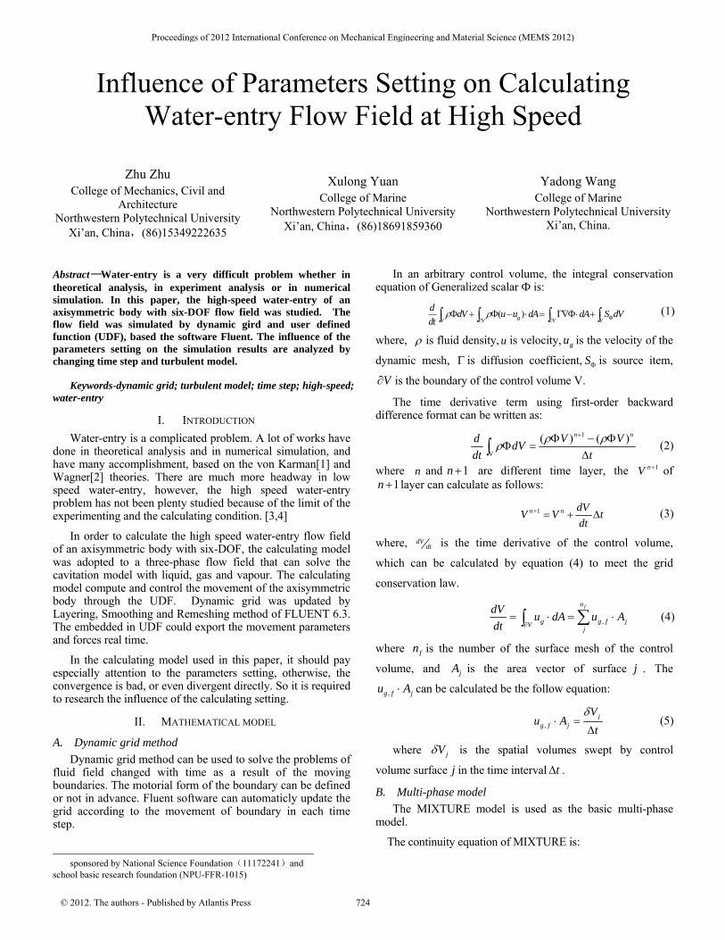
A. Calculating zones and grid dividing The calculating zones are shown in Fig.1.

Fig. 1 Calculated zones

Fig.2 Grid dividing

The far-field of whole computational domain is defined as pressure boundary. The vertical pressure boundary is assigned in accordance with the actual situation, that is, the pressure below the water surface is given according the gravity gradient, and that on the water surface is determined as the atmospheric pressure. The media of the boundary backflow is specified by actual situation.

The setting of fluid zone depends on the dynamic mesh mode. According to the fluid zone in Fig.1, the fluid zone 1 has the degree of freedom in y-direction and the fluid zone 2 has the degree of freedom in x-direction. The missile can freely rotate in the wrapped volume.

The calculated zone is divided into grids according to Fig.1. The updating of the overall dynamic grid of the fluid zone 1 and 2 all are the Layering , so the generation and extinction of its grid all use the hexahedral grid. Thus, it is helpful to the grid updating as well as improves the precision of the numerical solution. In order to adapt to the rotation of the missile, the local volume enwrapped missile use Smoothing and Re-meshing, so the grid of this region is divided using Tet method, and the quality of the body-fitted grid is controlled by the size function.

In this kind of grid, the movement of fluid zone 1 and 2 are determined according to the projection of the real velocity of the missile velocity in the given direction. The grid aberrance caused by the missile rotation can be eliminated using Smoothing and Remeshing. Thus, the whole grid net can coordinately operate to ensure the calculation precision as well as possible.

B. Model setting and result influence In the simulation, flow field is solved by FLUENT solver,

and the trajectory is solved by UDF, which was implanted self-program. The program could export a data file include motion parameters and forces in terms of time sequence.

1) Basic setting In this paper, MIXTURE model and RNG k-e model are

used to the multi-phase model and turbulence model respectively as the basic setting, and the SIMPLEC and the PRESTO! are chose to the Pressure-Velocity Coupling and discretization respectively.

2) Tim step influence Time step is the most important factor of the calculating

cost. The aim of analyzing the time step influence is to get the biggest time step satisfied the calculating stability to economize the calculating cost and shortening the develop periods.

Adopting the basic setting, 1e-6 and 5e-7 were separately used to calculate the high-speed water-entry flow field. The calculated results are shown in Fig.3.

725

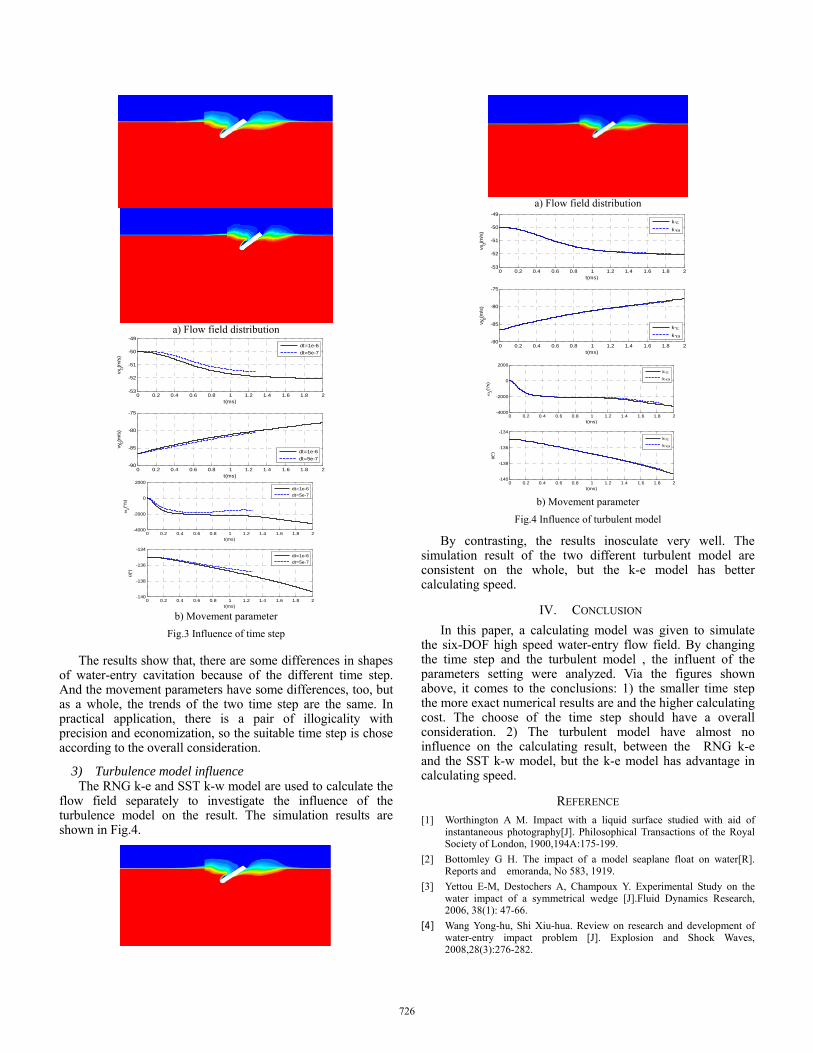
a) Flow field distribution

0 0.2 0.4 0.6 0.8 1 1.2 1.4 1.6 1.8 2-53

-52

-51

-50

-49

t(ms)

vx0(m

/s)

dt=1e-6dt=5e-7

0 0.2 0.4 0.6 0.8 1 1.2 1.4 1.6 1.8 2-90

-85

-80

-75

t(ms)

vy0(m

/s)

dt=1e-6dt=5e-7

0 0.2 0.4 0.6 0.8 1 1.2 1.4 1.6 1.8 2-4000

-2000

0

2000

t(ms)

ωz( °

/s)

dt=1e-6dt=5e-7

0 0.2 0.4 0.6 0.8 1 1.2 1.4 1.6 1.8 2-140

-138

-136

-134

t(ms)

θ(°)

dt=1e-6dt=5e-7

b) Movement parameter

Fig.3 Influence of time step

The results show that, there are some differences in shapes of water-entry cavitation because of the different time step. And the movement parameters have some differences, too, but as a whole, the trends of the two time step are the same. In practical application, there is a pair of illogicality with precision and economization, so the suitable time step is chose according to the overall consideration.

3) Turbulence model influence The RNG k-e and SST k-w model are used to calculate the

flow field separately to investigate the influence of the turbulence model on the result. The simulation results are shown in Fig.4.

a) Flow field distribution

0 0.2 0.4 0.6 0.8 1 1.2 1.4 1.6 1.8 2-53

-52

-51

-50

-49

t(ms)

vx0(m

/s)

k-εk-ω

0 0.2 0.4 0.6 0.8 1 1.2 1.4 1.6 1.8 2-90

-85

-80

-75

t(ms)

vy0(m

/s)

k-εk-ω

0 0.2 0.4 0.6 0.8 1 1.2 1.4 1.6 1.8 2-4000

-2000

0

2000

t(ms)

ωz( °

/s)

k-εk-ω

0 0.2 0.4 0.6 0.8 1 1.2 1.4 1.6 1.8 2-140

-138

-136

-134

t(ms)θ(°)

k-εk-ω

b) Movement parameter

Fig.4 Influence of turbulent model

By contrasting, the results inosculate very well. The simulation result of the two different turbulent model are consistent on the whole, but the k-e model has better calculating speed.

IV. CONCLUSION In this paper, a calculating model was given to simulate

the six-DOF high speed water-entry flow field. By changing the time step and the turbulent model , the influent of the parameters setting were analyzed. Via the figures shown above, it comes to the conclusions: 1) the smaller time step the more exact numerical results are and the higher calculating cost. The choose of the time step should have a overall consideration. 2) The turbulent model have almost no influence on the calculating result, between the RNG k-e and the SST k-w model, but the k-e model has advantage in calculating speed.

REFERENCE [1] Worthington A M. Impact with a liquid surface studied with aid of

instantaneous photography[J]. Philosophical Transactions of the Royal Society of London, 1900,194A:175-199.

[2] Bottomley G H. The impact of a model seaplane float on water[R]. Reports and emoranda, No 583, 1919.

[3] Yettou E-M, Destochers A, Champoux Y. Experimental Study on the water impact of a symmetrical wedge [J].Fluid Dynamics Research, 2006, 38(1): 47-66.

[4] Wang Yong-hu, Shi Xiu-hua. Review on research and development of water-entry impact problem [J]. Explosion and Shock Waves, 2008,28(3):276-282.

726