influence of swell on shear strength of expansive...
TRANSCRIPT
INFLUENCE OF SWELL ON SHEAR STRENGTH OF EXPANSIVE
SOILS
A THESIS SUBMITTED TO
THE GRADUATE SCHOOL OF NATURAL AND APPLIED
SCIENCES
OF
MIDDLE EAST TECHNICAL UNIVERSITY
BY
CEREN DELİKTAŞ
IN PARTIAL FULFILMENT OF THE REQUIREMENTS
FOR
THE DEGREE OF MASTER OF SCIENCE
IN
CIVIL ENGINEERING
MARCH 2016
iii
Approval of the thesis:
INFLUENCE OF SWELL ON SHEAR STRENGTH OF EXPANSIVE SOILS
submitted by CEREN DELİKTAŞ in partial fulfillment of the requirements for the
degree of Master of Science in Civil Engineering Department, Middle East
Technical University by,
Prof. Dr. Gülbin Dural Ünver
Dean, Graduate School of Natural and Applied Sciences
Prof. Dr. İsmail Özgür Yaman
Head of Department, Civil Engineering
Prof. Dr. Erdal Çokça
Supervisor, Civil Engineering Dept., METU
Examining Committee Members:
Assoc. Prof. Dr. Zeynep Gülerce
Civil Engineering Dept., METU
Prof. Dr. Erdal Çokça
Civil Engineering Dept., METU
Assoc. Prof. Dr. Cem Akgüner
Civil Engineering Dept., TEDU
Assist. Prof. Dr. Nejan Huvaj Sarıhan
Civil Engineering Dept., METU
Assist. Prof. Dr. Nabi Kartal Toker
Civil Engineering Dept., METU
Date: 9.3.2016
iv
I hereby declare that all information in this document has been obtained and
presented in accordance with academic rules and ethical conduct. I also declare
that, as required by these rules and conduct, I have fully cited and referenced
all material and results that are not original to this work.
Name, Last Name: CEREN DELİKTAŞ
Signature:
v
ABSTRACT
INFLUENCE OF SWELL ON SHEAR STRENGTH OF
EXPANSIVE SOILS
Deliktaş, Ceren
M.S., Department of Civil Engineering
Supervisor: Prof. Dr. Erdal Çokça
March 2016, 161 pages
Behavior of swelling soils is thoroughly investigated since they cause significant
hazard to structures all around the world, especially in the regions with climate of
arid or semi-arid. These types of soils expand upon wetting and shrink when water is
removed. Existence of water significantly alters the shear strength of swelling soils.
Therefore, the objective of this study is to examine the influence of swell on the
shear strength of expansive soils. For the first series of tests, an artificial expansive
soil was prepared in the laboratory by mixing 15% bentonite and 85% kaolinite.
Grain size distribution, specific gravity, Atterberg limits and dry density versus
moisture content curve were determined. Then, to obtain swell percent and rate of
swell, swell tests were conducted in special molds and unconfined compression tests
were made. For the first series of tests, soil samples were sheared without allowing
expansion to take place. This test was considered as the reference test. Then,
specimens were sheared after they were allowed to swell in specially designed molds
until vertical swell stopped, which were referred to 100% swell. In the mid-steps,
vi
shear strength was obtained when soil sample reached to 10%, 15%, 20%, 25%, 50%
and 75% of ultimate vertical swell. These eight swell and shear tests were repeated
for three expansive Ankara clays having different swelling potentials since natural
soil samples could be found just in Ankara. As the result of shearing tests, it was
seen that when the specimen reached to ultimate swell, shear strength was reduced to
approximately 90% of its initial value. Free swell index test and methylene blue test
were performed to estimate the swelling potential. Besides, tests showed that a
frictional stress equal to about 17-25% of swell pressure developed between the mold
and specimen.
Key Words: Expansive Soil, Swelling Potential, Shear Strength, Rate of Swell
vii
ÖZ
ŞİŞEN ZEMİNLERDE ŞİŞMENİN KAYMA
MUKAVEMETİ ÜZERİNDEKİ ETKİSİ
Deliktaş, Ceren
Yüksek Lisans, İnşaat Mühendisliği Bölümü
Tez Yöneticisi: Prof. Dr. Erdal Çokça
Mart 2016, 161 sayfa
Dünyanın her yerinde, özellikle kurak ya da yarı kurak iklimlerin yaşandığı
bölgelerde, yapılarda ciddi hasarlara neden olduğu için şişen zeminlerin davranışı
derinlemesine araştırılmıştır. Bu tip zeminler ıslanmaya bağlı olarak şişer ve su
kaybettiklerinde büzülürler. Suyun varlığı, şişen zeminlerin kayma mukavemetlerini
önemli miktarda değiştirirler. Bundan dolayı, bu çalışmanın amacı, şişmenin şişen
zeminlerin kayma mukavemeti üzerindeki etkisini sorgulamaktır: İlk seri deneyler
için, %15 bentonit ve %85 kaolin, laboratuvarda karıştırılarak, yapay bir şişen zemin
hazırlanmıştır. Numunenin dane çapı dağılımı, özgül ağırlığı, kıvam limitleri ve kuru
yoğunluk-su muhtevası eğrileri belirlenmiştir. Daha sonra, şişme yüzdesi ve şişme
hızını tespit etmek amacıyla, şişme deneyleri özel tasarlanan kalıplar ile ve kesme
deneyleri serbest basınç aleti ile yapılmıştır. İlk seri deney olarak, zemin
numunelerine, şişmenin gerçekleşmesine izin verilmeden, serbest basınç test
düzeneği ile kesme kuvveti uygulanmıştır. Bu deney referans deney olarak
düşünülmüştür. Daha sonra, özel tasarlanmış kalıplarda, düşey şişme duruncaya
viii
kadar şişmesine izin verilen numunelere kesme kuvveti uygulanmıştır ve bu deney
%100 şişme olarak isimlendirilmiştir. Ara basamaklarda, zemin örneği maksimum
düşey şişme miktarının %10, %15, %20, %25, %50 ve %75’ine ulaştığında kayma
mukavemeti elde edilmiştir. Bu sekiz şişme ve kesme deneyleri, farklı şişme
potansiyellerine sahip, üç Ankara kili için tekrar edilmiştir çünkü doğal zemin
numuneleri sadece Ankara’dan bulunabilmiştir. Kesme deneylerinin sonucunda,
örneklerin nihai şişmeye ulaştığında, kayma mukavemetlerinin ilk değerlerinin
yaklaşık %90’ına düştüğü görülmüştür. Şişme potansiyelini tahmin etmek için,
serbest şişme indis deneyi ve metilen mavisi testi uygulanmıştır. Ayrıca, testler,
numune ile kalıplar arasında şişme basıncının yaklaşık %17-25’ine eşit bir sürtünme
gerilmesi oluştuğunu göstermiştir.
Anahtar Kelimeler: Şişen Zemin, Şişme Potansiyeli, Kayma Mukavemeti, Şişme
Hızı

ix
To my mum
x
ACKNOWLEDGEMENTS
Immeasurable appreciation and deepest gratitude for the help and support are
extended to the following people without whom the completion of this thesis could
not be possible:
Firstly, I would like to express my sincere appreciation to my supervisor,
Prof. Dr. Erdal Çokça for his trust in me, continuous patience, endless support and
invaluable guidance throughout this study.
I also would like to thank to geological engineer Mr. Ulaş Nacar and
technicians Mr. Kamber Bilgen for their valuable advices and help as well as friendly
attitude during laboratory works.
Moreover, my sincere thankfulness goes to my friends Berkan Söylemez,
Yılmaz Emre Sarıçiçek, Yiğit Değer and Bengü Elcik for their suggestions, help and
encouragement. Especially, help received from Yılmaz and Berkan about
experimental measurements within working hours was really invaluable. In addition,
I would like to express my special thanks to Amir Jalehforouzan who shares all
experience, knowledge and advices about the experiments and process.
Finally, my endless thanks go to my parents, Işık and Mehmet Nedim
Deliktaş and my sister Seren Deliktaş for their patience, support and encouragement
throughout my life. Also, I would like to thank to my fiancé Okan Demirel for his
limitless love.
xi
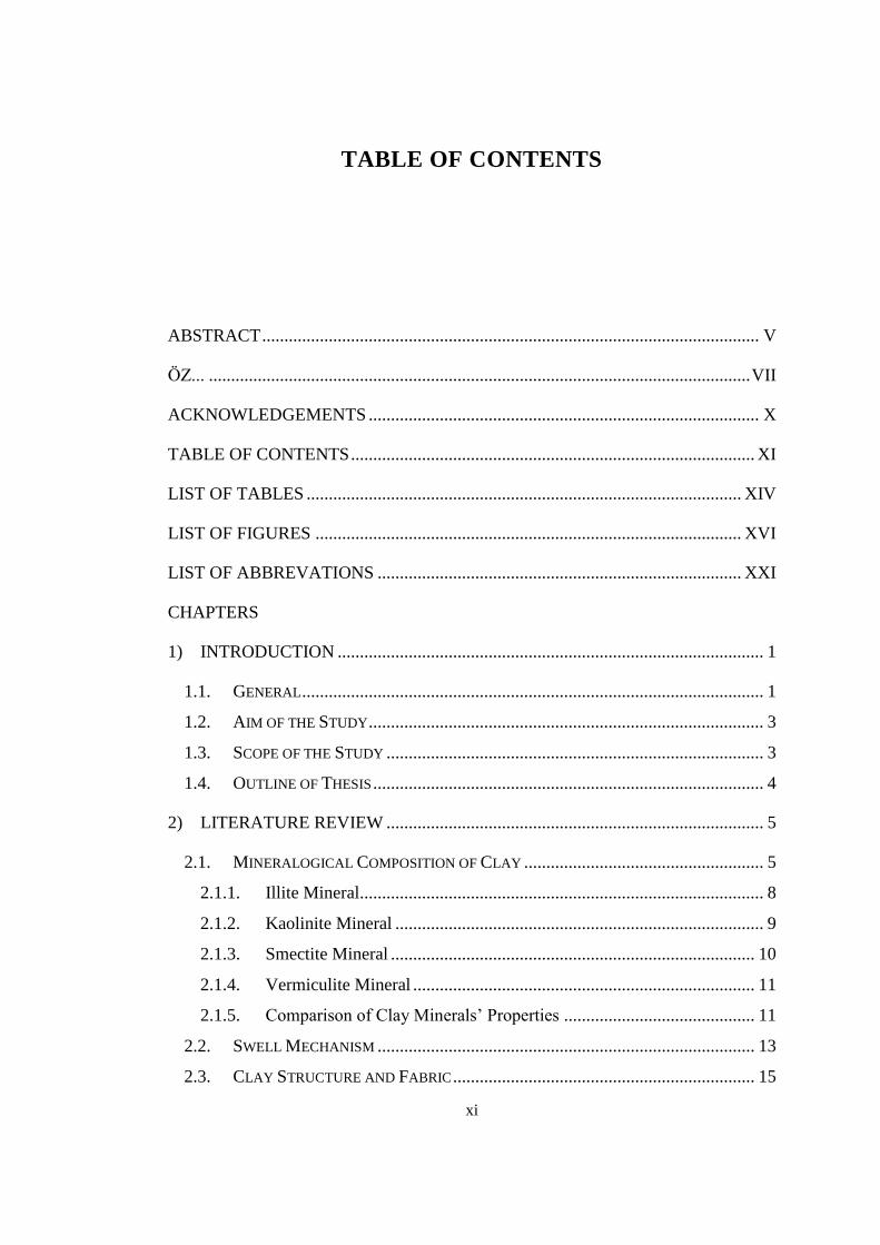
TABLE OF CONTENTS
ABSTRACT ................................................................................................................ V
ÖZ... .......................................................................................................................... VII
ACKNOWLEDGEMENTS ........................................................................................ X
TABLE OF CONTENTS ........................................................................................... XI
LIST OF TABLES .................................................................................................. XIV
LIST OF FIGURES ................................................................................................ XVI
LIST OF ABBREVATIONS .................................................................................. XXI
CHAPTERS
1) INTRODUCTION ................................................................................................ 1
1.1. GENERAL ........................................................................................................ 1
1.2. AIM OF THE STUDY ......................................................................................... 3
1.3. SCOPE OF THE STUDY ..................................................................................... 3
1.4. OUTLINE OF THESIS ........................................................................................ 4
2) LITERATURE REVIEW ..................................................................................... 5
2.1. MINERALOGICAL COMPOSITION OF CLAY ...................................................... 5
2.1.1. Illite Mineral........................................................................................... 8
2.1.2. Kaolinite Mineral ................................................................................... 9
2.1.3. Smectite Mineral .................................................................................. 10
2.1.4. Vermiculite Mineral ............................................................................. 11
2.1.5. Comparison of Clay Minerals’ Properties ........................................... 11
2.2. SWELL MECHANISM ..................................................................................... 13
2.3. CLAY STRUCTURE AND FABRIC .................................................................... 15
xii
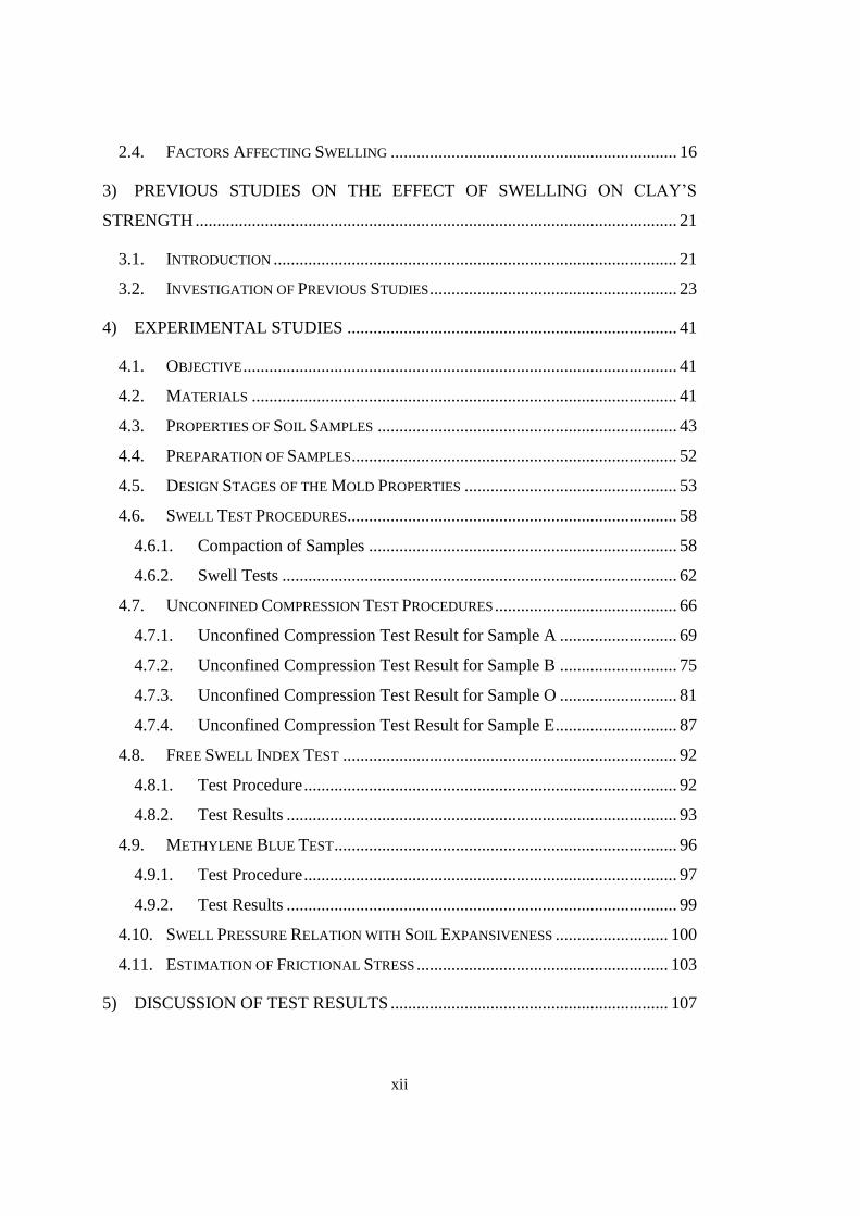
2.4. FACTORS AFFECTING SWELLING .................................................................. 16
3) PREVIOUS STUDIES ON THE EFFECT OF SWELLING ON CLAY’S
STRENGTH ............................................................................................................... 21
3.1. INTRODUCTION ............................................................................................. 21
3.2. INVESTIGATION OF PREVIOUS STUDIES ......................................................... 23
4) EXPERIMENTAL STUDIES ............................................................................ 41
4.1. OBJECTIVE .................................................................................................... 41
4.2. MATERIALS .................................................................................................. 41
4.3. PROPERTIES OF SOIL SAMPLES ..................................................................... 43
4.4. PREPARATION OF SAMPLES ........................................................................... 52
4.5. DESIGN STAGES OF THE MOLD PROPERTIES ................................................. 53
4.6. SWELL TEST PROCEDURES............................................................................ 58
4.6.1. Compaction of Samples ....................................................................... 58
4.6.2. Swell Tests ........................................................................................... 62
4.7. UNCONFINED COMPRESSION TEST PROCEDURES .......................................... 66
4.7.1. Unconfined Compression Test Result for Sample A ........................... 69
4.7.2. Unconfined Compression Test Result for Sample B ........................... 75
4.7.3. Unconfined Compression Test Result for Sample O ........................... 81
4.7.4. Unconfined Compression Test Result for Sample E ............................ 87
4.8. FREE SWELL INDEX TEST ............................................................................. 92
4.8.1. Test Procedure ...................................................................................... 92
4.8.2. Test Results .......................................................................................... 93
4.9. METHYLENE BLUE TEST ............................................................................... 96
4.9.1. Test Procedure ...................................................................................... 97
4.9.2. Test Results .......................................................................................... 99
4.10. SWELL PRESSURE RELATION WITH SOIL EXPANSIVENESS .......................... 100
4.11. ESTIMATION OF FRICTIONAL STRESS .......................................................... 103
5) DISCUSSION OF TEST RESULTS ................................................................ 107
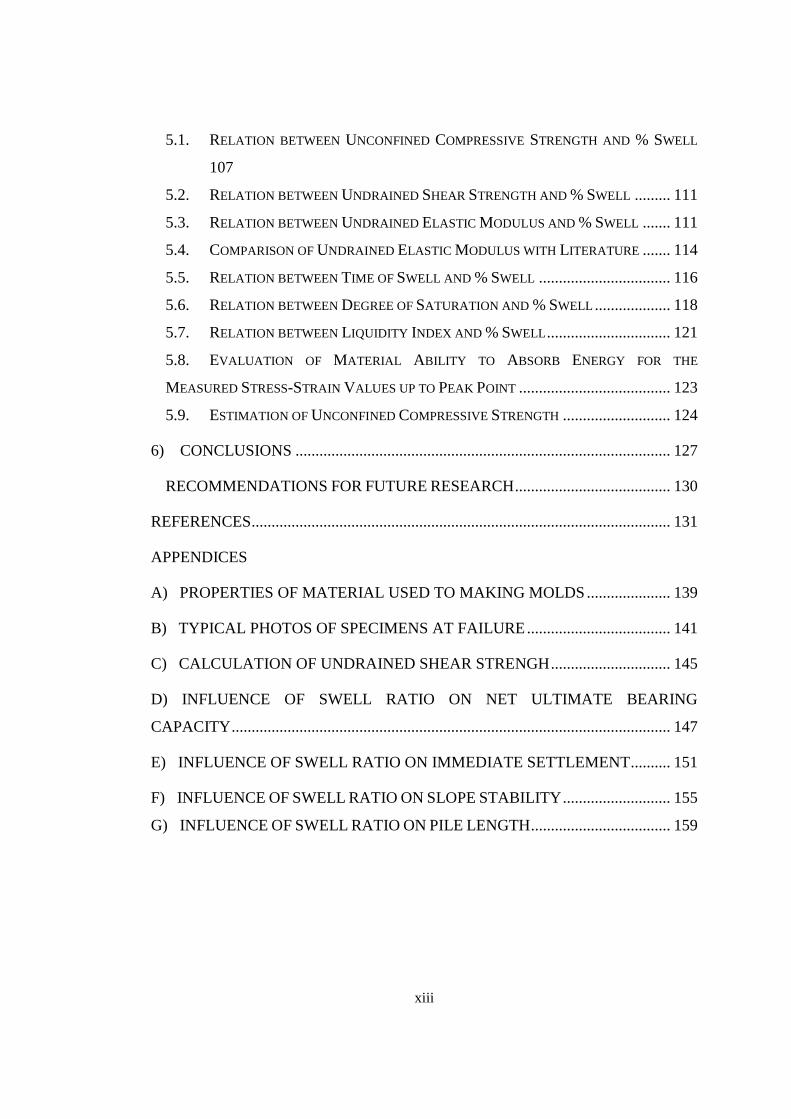
xiii
5.1. RELATION BETWEEN UNCONFINED COMPRESSIVE STRENGTH AND % SWELL
107
5.2. RELATION BETWEEN UNDRAINED SHEAR STRENGTH AND % SWELL ......... 111
5.3. RELATION BETWEEN UNDRAINED ELASTIC MODULUS AND % SWELL ....... 111
5.4. COMPARISON OF UNDRAINED ELASTIC MODULUS WITH LITERATURE ....... 114
5.5. RELATION BETWEEN TIME OF SWELL AND % SWELL ................................. 116
5.6. RELATION BETWEEN DEGREE OF SATURATION AND % SWELL ................... 118
5.7. RELATION BETWEEN LIQUIDITY INDEX AND % SWELL ............................... 121
5.8. EVALUATION OF MATERIAL ABILITY TO ABSORB ENERGY FOR THE
MEASURED STRESS-STRAIN VALUES UP TO PEAK POINT ...................................... 123
5.9. ESTIMATION OF UNCONFINED COMPRESSIVE STRENGTH ........................... 124
6) CONCLUSIONS .............................................................................................. 127
RECOMMENDATIONS FOR FUTURE RESEARCH ....................................... 130
REFERENCES ......................................................................................................... 131
APPENDICES
A) PROPERTIES OF MATERIAL USED TO MAKING MOLDS ..................... 139
B) TYPICAL PHOTOS OF SPECIMENS AT FAILURE .................................... 141
C) CALCULATION OF UNDRAINED SHEAR STRENGH .............................. 145
D) INFLUENCE OF SWELL RATIO ON NET ULTIMATE BEARING
CAPACITY .............................................................................................................. 147
E) INFLUENCE OF SWELL RATIO ON IMMEDIATE SETTLEMENT .......... 151
F) INFLUENCE OF SWELL RATIO ON SLOPE STABILITY ........................... 155
G) INFLUENCE OF SWELL RATIO ON PILE LENGTH ................................... 159
xiv
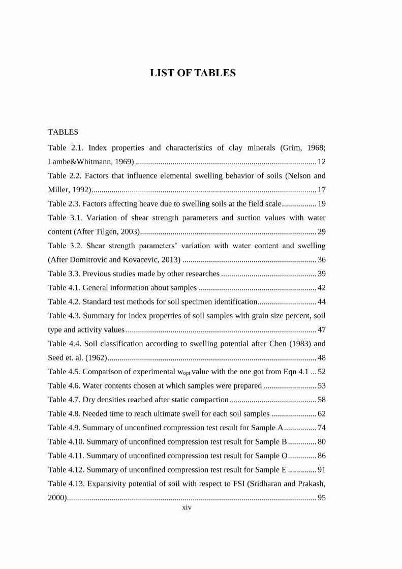
LIST OF TABLES
TABLES
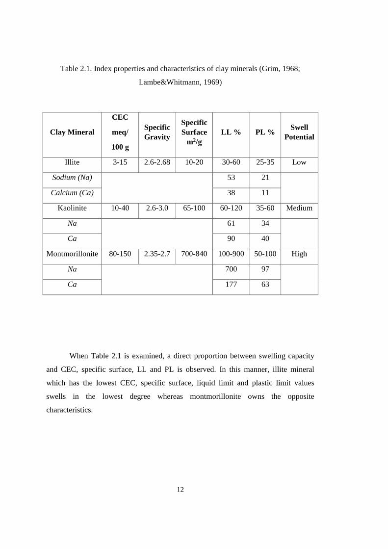
Table 2.1. Index properties and characteristics of clay minerals (Grim, 1968;
Lambe&Whitmann, 1969) ......................................................................................... 12
Table 2.2. Factors that influence elemental swelling behavior of soils (Nelson and
Miller, 1992) ............................................................................................................... 17
Table 2.3. Factors affecting heave due to swelling soils at the field scale ................. 19
Table 3.1. Variation of shear strength parameters and suction values with water
content (After Tilgen, 2003) ....................................................................................... 29
Table 3.2. Shear strength parameters’ variation with water content and swelling
(After Domitrovic and Kovacevic, 2013) .................................................................. 36
Table 3.3. Previous studies made by other researches ............................................... 39
Table 4.1. General information about samples .......................................................... 42
Table 4.2. Standard test methods for soil specimen identification ............................. 44
Table 4.3. Summary for index properties of soil samples with grain size percent, soil
type and activity values .............................................................................................. 47
Table 4.4. Soil classification according to swelling potential after Chen (1983) and
Seed et. al. (1962) ....................................................................................................... 48
Table 4.5. Comparison of experimental wopt value with the one got from Eqn 4.1 ... 52
Table 4.6. Water contents chosen at which samples were prepared .......................... 53
Table 4.7. Dry densities reached after static compaction ........................................... 58
Table 4.8. Needed time to reach ultimate swell for each soil samples ...................... 62
Table 4.9. Summary of unconfined compression test result for Sample A ................ 74
Table 4.10. Summary of unconfined compression test result for Sample B .............. 80
Table 4.11. Summary of unconfined compression test result for Sample O .............. 86
Table 4.12. Summary of unconfined compression test result for Sample E .............. 91
Table 4.13. Expansivity potential of soil with respect to FSI (Sridharan and Prakash,
2000) ........................................................................................................................... 95
xv
Table 4.14. Classification of soil swelling according to MFSI (Sridharan and
Prakash, 2000) ............................................................................................................ 96
Table 4.15. Calculation steps of frictional stress and comparison of frictional stress
with swell pressure at 0% and 100% of swell .......................................................... 105
Table 5.1. Typical Young’s Modulus values of soils in MPa (Kezdi, 1974 and Prat et
al., 1995)................................................................................................................... 115
Table 5.2. Undrained elastic modulus with respect to % swell ............................... 116
Table 5.3. Liquidity index values of samples with respect to % swell .................... 121
Table 5.4. Consistency of cohesive soils according to liquidity index (Ranjan and
Rao, 2005) ................................................................................................................ 122
Table 5.5. Absorbed energy values of soil samples up to peak points, which were
obtained from stress-strain curves ............................................................................ 124
Table A.1. Material properties of molds………………..……...…….…………….139
Table C.1. Calculation steps of undrained shear strength for Sample B at 0% of swell
…………………………………………………..….…….…………….....…….….146
Table D.1. Change in net foundation pressure with variation of swell ratio for Sample
A……………...……………………………………………………………..……...149
Table E.1. Values of Is (Birand et al., 2011) ……………...………………..……...152
Table E.2. Change in immediate settlement with variation of swell ratio for Sample
A……………………………………...……………...……………………………..153
Table F.1. Change in FS against sliding with variation of swell ratio for Sample
A…………………………………………………………...………………..……...156
Table G.1. Change in L with variation of swell ratio for Sample A…….…............161
xvi
LIST OF FIGURES
FIGURES
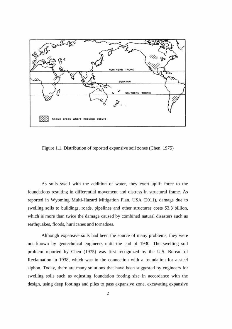
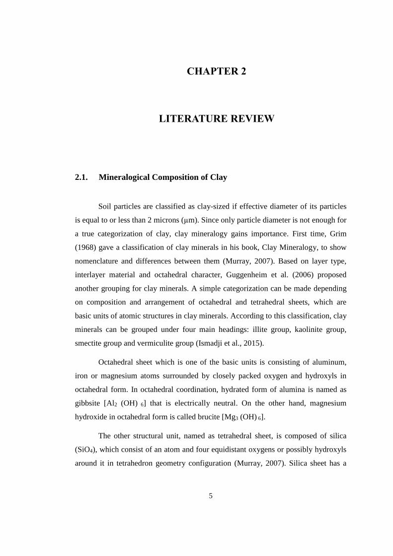
Figure 1.1. Distribution of reported expansive soil zones (Chen, 1975) ..................... 2
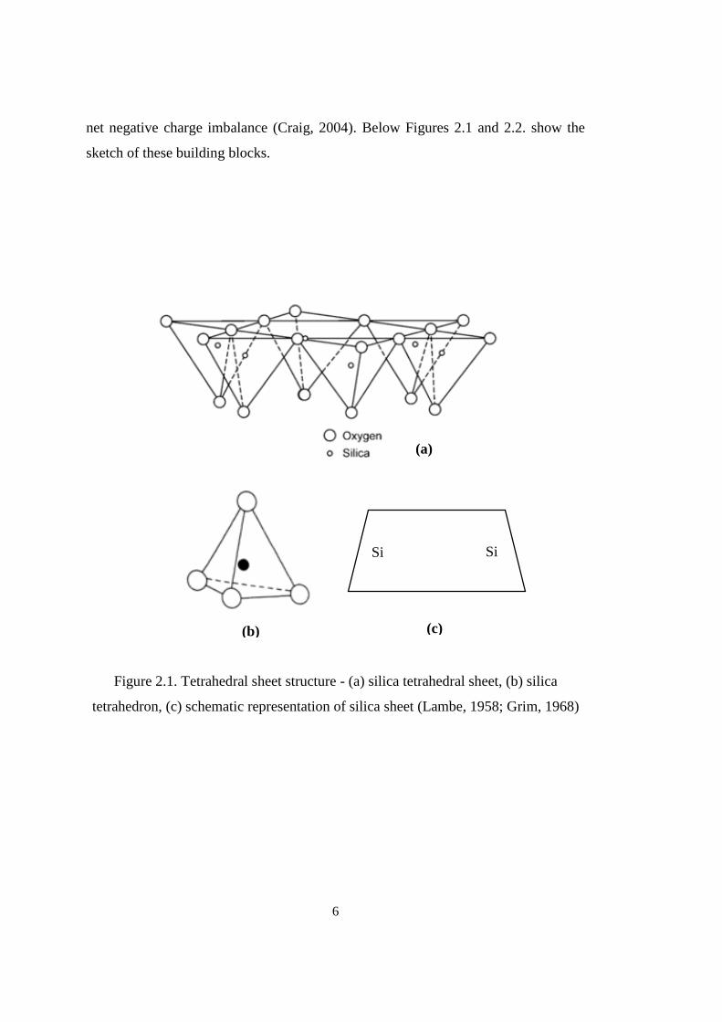
Figure 2.1. Tetrahedral sheet structure - (a) silica tetrahedral sheet, (b) silica
tetrahedron, (c) schematic representation of silica sheet (Lambe, 1958; Grim, 1968) 6
Figure 2.2. Octahedral sheet structure - (a) octahedral sheet, (b) octahedron, (c)
schematic representation of gibbsite octahedral sheet (Lambe, 1958; Grim, 1968) .... 7
Figure 2.3. (a)1:1 clay mineral structure (b) 2:1 clay mineral structure (Mitchell,
1993) ............................................................................................................................. 8
Figure 2.4. Structure of illite group (Source: http://soils.ag.uidaho.edu/soil205-
90/index.htm) ............................................................................................................... 9
Figure 2.5. Kaolinite group structure (Source: http://soils.ag.uidaho.edu/soil205-
90/index.htm) ............................................................................................................. 10
Figure 2.6. Smectite mineral structure (Source: http://soils.ag.uidaho.edu/soil205-
90/index.htm) ............................................................................................................. 11
Figure 2.7. Presentation of diffuse double layer and force of attraction (Ammam,
2011) ........................................................................................................................... 14
Figure 2.8. Types of clay structure (Ishibashi and Hazarika, 2015) .......................... 16
Figure 3.1. Results of a series of semi confined swell test made on Georgian Bay
Shale for the design of shafts and tunnels (After Lo et al., 1987) .............................. 23
Figure 3.2. Typical arrangement of modified semi confined swell test (After Lo and
Lee, 1990) ................................................................................................................... 25
Figure 3.3. Section view of modified semi confined swell test setup (After Lo and
Lee, 1990) ................................................................................................................... 26
Figure 3.4. Linear pressure and horizontal swell potential relation of Queenston
Shale (After Lo and Lee, 1990) .................................................................................. 27
Figure 3.5. Schematic drawing of hydraulic triaxial stress path setup (After Al-
Mhaidib and Al-Shamrani, 2006) ............................................................................... 21
xvii
Figure 3.6. Schematic drawing of hydraulic triaxial stress path setup (After Al-
Mhaidib and Al-Shamrani, 2006) .............................................................................. 32
Figure 3.7. Deviator stress versus axial strain graph for the sample that is at 14% of
initial water content and under 100 kPa confining pressure (After Al-Mhaidib and
Al-Shamrani, 2006) .................................................................................................... 33
Figure 3.8. Vertical displacement versus time graph for betonite samples under
changing normal stresses (After Domitrovic and Kovacevic, 2013) ......................... 34
Figure 3.9. Peak strength versus normal stress and hydration times graphs (After
Domitrovic and Kovacevic, 2013) ............................................................................. 35
Figure 3.10. Apparatus for sample compaction (After Wang et al., 2014) ................ 37
Figure 3.11. Relation between w-c and w-ɸ (After Wang et al., 2014) ..................... 38
Figure 3.12. Relation between e-c and e-ɸ (After Wang et al., 2014) ....................... 38
Figure 4.1. View of samples (1-Sample A, 2-Sample B, 3-Sample O, 4-Sample E). 43
Figure 4.2. Grain size distribution curves for all samples.......................................... 45
Figure 4.3. Plasticity chart in order to determine soil type ........................................ 46
Figure 4.4. Swelling potential chart proposed by Williams (1957) ........................... 49
Figure 4.5. Harvard miniature compaction test apparatus (a- Sample extruder, b-
tamper, c-mould, d- collar of the mould, e- base of the mold) .................................. 50
Figure 4.6. Dry denstiy versus water content curves for all soil samples .................. 51
Figure 4.7. 3-D view and photo of the mold with its parts ........................................ 55
Figure 4.8. Drawing and sections of final molds with rod having rigid circular plates
.................................................................................................................................... 56
Figure 4.9. Schematic drawing of the mold after sample preparation ....................... 57
Figure 4.10. Sample preparation process ................................................................... 59
Figure 4.11. Submerged specimen in perforated mold .............................................. 63
Figure 4.12. 100 % of swell versus time graph for Sample A ................................... 64
Figure 4.13. 100 % of swell versus time graph for Sample B ................................... 65
Figure 4.14. 100 % Swell versus time graph for Sample O ....................................... 65
Figure 4.15. 100 % Swell versus time graph for Sample E ....................................... 66
Figure 4.16. Unconfined compression test machine view during shearing of a
specimen ..................................................................................................................... 67
xviii
Figure 4.17. Cutting of a swelled specimen to be fitted to the height to diameter ratio
in ASTM D2166 ......................................................................................................... 68
Figure 4.18. Unconfined compression test result for 0% of swell on Sample A ....... 70
Figure 4.19. Unconfined compression test result for 10% of swell on Sample A ..... 70
Figure 4.20. Unconfined compression test result for 15% of swell on Sample A ..... 71
Figure 4.21. Unconfined compression test result for 20% of swell on Sample A ..... 71
Figure 4.22. Unconfined compression test result for 25% of swell on Sample A ..... 72
Figure 4.23. Unconfined compression test result for 50% of swell on Sample A ..... 72
Figure 4.24. Unconfined compression test result for 75% of swell on Sample A ..... 73
Figure 4.25. Unconfined compression test result for 100% of swell on Sample A ... 73
Figure 4.26. Unconfined compression test result for 0% of swell on Sample B ....... 75
Figure 4.27. Unconfined compression test result for 10% of swell on Sample B ..... 76
Figure 4.28. Unconfined compression test result for 15% of swell on Sample B ..... 76
Figure 4.29. Unconfined compression test result for 20% of swell on Sample B ..... 77
Figure 4.30. Unconfined compression test result for 25% of swell on Sample B ..... 77
Figure 4.31. Unconfined compression test result for 50% of swell on Sample B ..... 78
Figure 4.32. Unconfined compression test result for 75% of swell on Sample B ..... 78
Figure 4.33. Unconfined compression test result for 100% of swell on Sample B ... 79
Figure 4.34. Unconfined compression test result for 0% of swell on Sample O ....... 81
Figure 4.35. Unconfined compression test result for 10% of swell on Sample O ..... 82
Figure 4.36. Unconfined compression test result for 15% of swell on Sample O ..... 82
Figure 4.37. Unconfined compression test result for 20% of swell on Sample O ..... 83
Figure 4.38. Unconfined compression test result for 25% of swell on Sample O ..... 83
Figure 4.39. Unconfined compression test result for 50% of swell on Sample O ..... 84
Figure 4.40. Unconfined compression test result for 75% of swell on Sample O ..... 84
Figure 4.41. Unconfined compression test result for 100% of swell on Sample O ... 85
Figure 4.42. Unconfined compression test result for 0% of swell on Sample E ........ 87
Figure 4.43. Unconfined compression test result for 15% of swell on Sample E ...... 88
Figure 4.44. Unconfined compression test result for 20% of swell on Sample E ...... 88
Figure 4.45. Unconfined compression test result for 25% of swell on Sample E ...... 89
Figure 4.46. Unconfined compression test result for 50% of swell on Sample E ...... 89
xix
Figure 4.47. Unconfined compression test result for 75% swell ............................... 90
Figure 4.48. Unconfined compression test result for 100% swell ............................. 90
Figure 4.49. Free swell index test at resting stage ..................................................... 93
Figure 4.50. Comparison of free swell index values of samples ............................... 94
Figure 4.51. Summary of methylene blue test procedure .......................................... 98
Figure 4.52. Comparison of methylene blue values of samples ................................ 99
Figure 4.53. Swell pressure test setup ...................................................................... 101
Figure 4.54. Plastic rods used for specimen compaction in swell pressure test....... 101
Figure 4.55. Comparison of swell pressure values of samples ................................ 102
Figure 4.56. (a) Sketch of test setup to determine frictional force, (b) Photo of test
setup to find frictional force ..................................................................................... 104
Figure 5.1. Unconfined compressive strength versus % swell for Sample A .......... 108
Figure 5.2. Unconfined compressive strength versus % swell for Sample B .......... 108
Figure 5.3. Unconfined compressive strength versus % swell for Sample O .......... 109
Figure 5.4. Unconfined compressive strength versus % swell for Sample E .......... 109
Figure 5.5. Experimental normalized logqu values with regression equation .......... 110
Figure 5.6. Comparison of experimental and predicted normalized logqu values ... 111
Figure 5.7. Undrained elastic modulus versus % swell for Sample A ..................... 112
Figure 5.8. Undrained elastic modulus versus % swell for Sample B ..................... 112
Figure 5.9. Undrained elastic modulus versus % swell for Sample O ..................... 113
Figure 5.10. Undrained elastic modulus versus % swell for Sample E ................... 113
Figure 5.11: Time of swell versus % swell for all samples ..................................... 117
Figure 5.12. Degree of saturation versus % swell for Sample A ............................. 119
Figure 5.13. Degree of saturation versus % swell for Sample B ............................. 119
Figure 5.14. Degree of saturation versus % swell for Sample O ............................. 120
Figure 5.15. Degree of saturation versus % swell for Sample E .............................. 120
Figure 5.16. Comparison of normalized qu values obtained from experiments and
regression analysis ................................................................................................... 125
Figure B.1. Photo of 15% of swell test for Specimen A at the failure…..................141
Figure B.2. Photo of reference test for Specimen B at the failure……….…...…....142
Figure B.3. Photo of reference test for Specimen O at the failure…….……..…….142
xx
Figure B.4. Photo of 20% of swell test for Specimen E at the failure….………….143
Figure D.1. Bearing capacity factors for foundations in clay (Ф=0) (After Skempton,
1951)……………………………………………….………....……...…………….148
Figure D.2. Relation between qnf and % swell for Sample A……..……........…….149
Figure E.1. Relation between Si and % swell for Sample A………………………153
Figure F.1. Change in FS aganist sliding with variation of swell ratio for
Sample A ……………...………………………….………....……...…………….156
Figure F.2. Relation between FS and % swell for Sample A ………….………….157
Figure G.1. Forces acting on a pile in swelling soi……...……..….………………159
xxi
LIST OF ABBREVATIONS
Al Aluminum
ASTM American Society for Testing and Materials
A Corrected area
Anet,side Net lateral surface area
aw Normalized water area
A0 Initial cross sectional area
Al2 (OH) 6 Aluminium hydroxide
Br Width of the foundation
BS British Standards
c’ Cohesion
Ca Calcium
CEC Cation exchange capacity
CH Clay with high plasticity
CL Clays with low-medium plasticity
Cp Proving ring constant
cu Undrained shear strength
d Diameter of perforation in the mold
D Initial sample diameter
dp Pile diameter
e Void ratio
ef Final void ratio
ec Unit electronic charge
Eu Undrained elastic modulus
Eqn. Equation
f’ Sample dry weight in MB test
Fapplied Applied force
xxii
Ff Friction force equal to the applied force
FS Factor of safety
FSI Free swell index
Fu Uplift force on pile
Gs Specific gravity
H Slope height
H0 Initial sample height
H2O Water molecule
IS Indian Standard Methods of Tests for Soils
Is Shape factor
k Boltzmann’s constant
L Depth to foundation level
LL Liquid limit
LI Liquidity index
MB Methylene blue
MBV Methylene blue value
meq Miliequivalent
Mg Magnesium
Mg3 (OH) 6 Magnesium hydroxide
ML Silt with slight plasticity
MSFI Modified free swell index
Na Sodium
Nc Dimensionless bearing capacity factor
Ns Stability coefficient depending on slope angle
NF The Association Française de Normalization (AFNOR)
OH Organic clays of medium to high plasticity
OL Organic silts of low plasticity
OMC Optimum moisture content
P Axial load
PI Plasticity index
PL Plastic limit
xxiii
PS Swell pressure
qn Net foundation pressure
Qd Allowable load from the superstructure
qnf Net ultimate bearing capacity
qu Unconfined compressive strength
R2 Coefficient of determination
SL Shrinkage limit
Si Silicon
Si Immediate settlement determined using Elastic Theory
SiO4 Silicon tetraoxide
%S Swell potential
Sr Degree of saturation
t Diffuse double layer thickness
T Absolute temperature
txx Time of swell corresponding to given swell percent
ua Air pressure
uw Pore water pressure
v Cation valence
Vcc Volume of methylene blue solution injected to
the sample solution
Vd Soil specimen volume read from the graduated cylinder
filled with distilled water in free swell test Vk Soil specimen volume read from the graduated cylinder
filled with kerosene in free swell test w Water content
Wf Resisting forces
wopt Optimum moisture content
Za Depth of active zone
α Adhesion factor
β Uplift factor
ɣ Unit weight of soil
xxiv
δ1 Strain dial gauge reading
δ2 Proving ring dial gauge reading
ΔH Height difference in the sample length
ε Strain
εc Dielectric constant of medium
εp Swelling potential
η Electrolyte concentration
ν Poisson's ratio
ρd Dry density
ρdmax Maximum dry density
σ Compressive stress
σf Frictional stress
σt Total normal stress
σ’n Effective normal stress
τ Shear strength
Ф’ Internal friction angle
Φb Angle of shearing resistance with respect to matric suction
χ Effective stress parameter
1
CHAPTER 1
1) INTRODUCTION
1.1. General
Soils that swell when moisture content is increased and shrink when moisture
content is decreased are called “expansive soils”. Donaldson (1969) categorized
swelling soils into two groups according to their parent materials. Basic igneous
rocks with the feldspar and pyroxene minerals, which have chemically broken down
in order to form swelling clay minerals, constitute one of the groups (e.g. the basalts
of the Deccan Plateau in India). The other group is the sedimentary rocks containing
montmorillonite (e.g. limestone and marls in Israel). Figure 1.1 shows the spatial
distribution of reported expansive soils (Chen, 1975). When Figure 1.1 is examined,
it is realized that expansive soils mostly exist in the regions where annual
precipitation is less than evapotranspiration. The common trait of these zones is their
arid or semi-arid climate.
2
Figure 1.1. Distribution of reported expansive soil zones (Chen, 1975)
As soils swell with the addition of water, they exert uplift force to the
foundations resulting in differential movement and distress in structural frame. As
reported in Wyoming Multi-Hazard Mitigation Plan, USA (2011), damage due to
swelling soils to buildings, roads, pipelines and other structures costs $2.3 billion,
which is more than twice the damage caused by combined natural disasters such as
earthquakes, floods, hurricanes and tornadoes.
Although expansive soils had been the source of many problems, they were
not known by geotechnical engineers until the end of 1930. The swelling soil
problem reported by Chen (1975) was first recognized by the U.S. Bureau of
Reclamation in 1938, which was in the connection with a foundation for a steel
siphon. Today, there are many solutions that have been suggested by engineers for
swelling soils such as adjusting foundation footing size in accordance with the
design, using deep footings and piles to pass expansive zone, excavating expansive
3
soil, stabilization of swelling soil with lime, fly ash or cement, waterproofing (Al-
Rawas and Goosen, 2006).
1.2. Aim of the Study
Influence of swelling on undrained shear strength of an expansive soil is an
important subject in geotechnical engineering in the sense of foundation design,
slope stability prediction and calculation of earth pressure against retaining structure,
(e.g. pile in expansive clay, slope stability of expansive clay, bearing capacity of
foundations on expansive clay etc., which was given in Appendix D, E, F and G).
There are studies about the change in shear strength and shear strength parameters of
expansive soils with the water content, swelling and suction in the available
literature. However, decrease in shear strength at swell ratios below 25% of ultimate
swell was not presented in previous studies. Additionally, unconfined compression
test was not chosen as the way for the determination of shear strength of clay.
Therefore, this study aims to investigate the influence of 0%, 10%, 15%, 20%, 25%,
50%, 75% and 100% of ultimate swell on expansive soils’ undrained shear strength
by using unconfined compression test.
1.3. Scope of the Study
This study involves the change in undrained shear strength of swelling soils
with the amount of swell. For this aim, one artificial and three natural soil samples
were used. Artificial soil sample was obtained by mixing 15% bentonite and 85%
kaolinite in the laboratory while three representative Ankara clays were selected as
natural soil samples. Firstly, grain size distribution, specific gravity, Atterberg limits
and dry density versus moisture content curves were determined for each sample
separately. Then, statically compacted samples were let to swell in specially designed
molds and sheared with the unconfined compression test setup to define swell
4
percent and rate of swell. As the first test for each material, soil samples were
sheared without allowing any swell to take place. This test was accepted as the
reference test. After this test, when soil samples that are allowed to swell freely,
reached ultimate vertical swelling, unconfined compression test was conducted on
them. This was called 100% of swell. Next, undrained shear strength of soil samples
at 10%, 15%, 20%, 25%, 50% and 75% of ultimate vertical swell could be measured.
After determination of swelling capacities of the samples in the specially designed
molds, free swell index test and Methylene Blue test were made to verify the
obtained results. In addition, swell pressures of each soil sample were determined
and compared with the frictional stresses which developed between the mold and the
specimen.
1.4. Outline of Thesis
This study includes literature review part, previous studies made on shear
strength of expansive soils, experimental works, discussion of test results and
conclusions. In Chapter 2 including literature review part, mineralogy of clay
particles, clay fabric and structure, swell mechanism and factors affecting swelling
are mentioned. Chapter 3 consists of previous works on shear strength of swelling
soils. Experimental works like soil sample preparation, soil properties determination,
swell and shear tests, free swell index test, Methylene Blue test, swell pressure and
frictional stress determination are shared in Chapter 4. Tests results are given in
Chapter 5. Finally, in Chapter 6 conclusions attained at the end of testing are
summarized.
5
CHAPTER 2
2) LITERATURE REVIEW
2.1. Mineralogical Composition of Clay
Soil particles are classified as clay-sized if effective diameter of its particles
is equal to or less than 2 microns (µm). Since only particle diameter is not enough for
a true categorization of clay, clay mineralogy gains importance. First time, Grim
(1968) gave a classification of clay minerals in his book, Clay Mineralogy, to show
nomenclature and differences between them (Murray, 2007). Based on layer type,
interlayer material and octahedral character, Guggenheim et al. (2006) proposed
another grouping for clay minerals. A simple categorization can be made depending
on composition and arrangement of octahedral and tetrahedral sheets, which are
basic units of atomic structures in clay minerals. According to this classification, clay
minerals can be grouped under four main headings: illite group, kaolinite group,
smectite group and vermiculite group (Ismadji et al., 2015).
Octahedral sheet which is one of the basic units is consisting of aluminum,
iron or magnesium atoms surrounded by closely packed oxygen and hydroxyls in
octahedral form. In octahedral coordination, hydrated form of alumina is named as
gibbsite [Al2 (OH) 6] that is electrically neutral. On the other hand, magnesium
hydroxide in octahedral form is called brucite [Mg3 (OH) 6].
The other structural unit, named as tetrahedral sheet, is composed of silica
(SiO4), which consist of an atom and four equidistant oxygens or possibly hydroxyls
around it in tetrahedron geometry configuration (Murray, 2007). Silica sheet has a
6
net negative charge imbalance (Craig, 2004). Below Figures 2.1 and 2.2. show the
sketch of these building blocks.
Figure 2.1. Tetrahedral sheet structure - (a) silica tetrahedral sheet, (b) silica
tetrahedron, (c) schematic representation of silica sheet (Lambe, 1958; Grim, 1968)
Si Si
(b) (c)
(a)
7
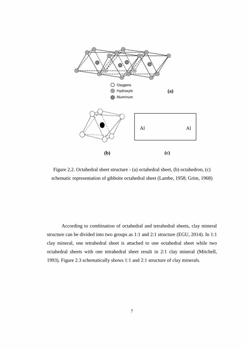
Figure 2.2. Octahedral sheet structure - (a) octahedral sheet, (b) octahedron, (c)
schematic representation of gibbsite octahedral sheet (Lambe, 1958; Grim, 1968)
According to combination of octahedral and tetrahedral sheets, clay mineral
structure can be divided into two groups as 1:1 and 2:1 structure (EGU, 2014). In 1:1
clay mineral, one tetrahedral sheet is attached to one octahedral sheet while two
octahedral sheets with one tetrahedral sheet result in 2:1 clay mineral (Mitchell,
1993). Figure 2.3 schematically shows 1:1 and 2:1 structure of clay minerals.
Al Al
(b) (c)
(a)
8
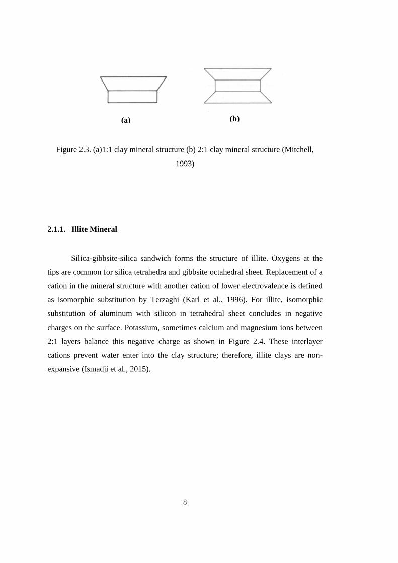
Figure 2.3. (a)1:1 clay mineral structure (b) 2:1 clay mineral structure (Mitchell,
1993)
2.1.1. Illite Mineral
Silica-gibbsite-silica sandwich forms the structure of illite. Oxygens at the
tips are common for silica tetrahedra and gibbsite octahedral sheet. Replacement of a
cation in the mineral structure with another cation of lower electrovalence is defined
as isomorphic substitution by Terzaghi (Karl et al., 1996). For illite, isomorphic
substitution of aluminum with silicon in tetrahedral sheet concludes in negative
charges on the surface. Potassium, sometimes calcium and magnesium ions between
2:1 layers balance this negative charge as shown in Figure 2.4. These interlayer
cations prevent water enter into the clay structure; therefore, illite clays are non-
expansive (Ismadji et al., 2015).
(a) (b)

9
Figure 2.4. Structure of illite group (Source: http://soils.ag.uidaho.edu/soil205-
90/index.htm)
2.1.2. Kaolinite Mineral
Basic structure of kaolinite mineral consists of a single sheet of gibbsite and a
single sheet of tetrahedral silica. It is a 1:1 clay mineral. Oxygens existed in the tip of
tetrahedron are shared by two structural blocks, gibbsite and silica. Unit layers of
kaolinite are stacked one above the other with hydrogen bonding (Murray, 2007) as
shown in Figure 2.5. Hydrogen bonding leads to very low expansion capacity of
kaolinite.
10
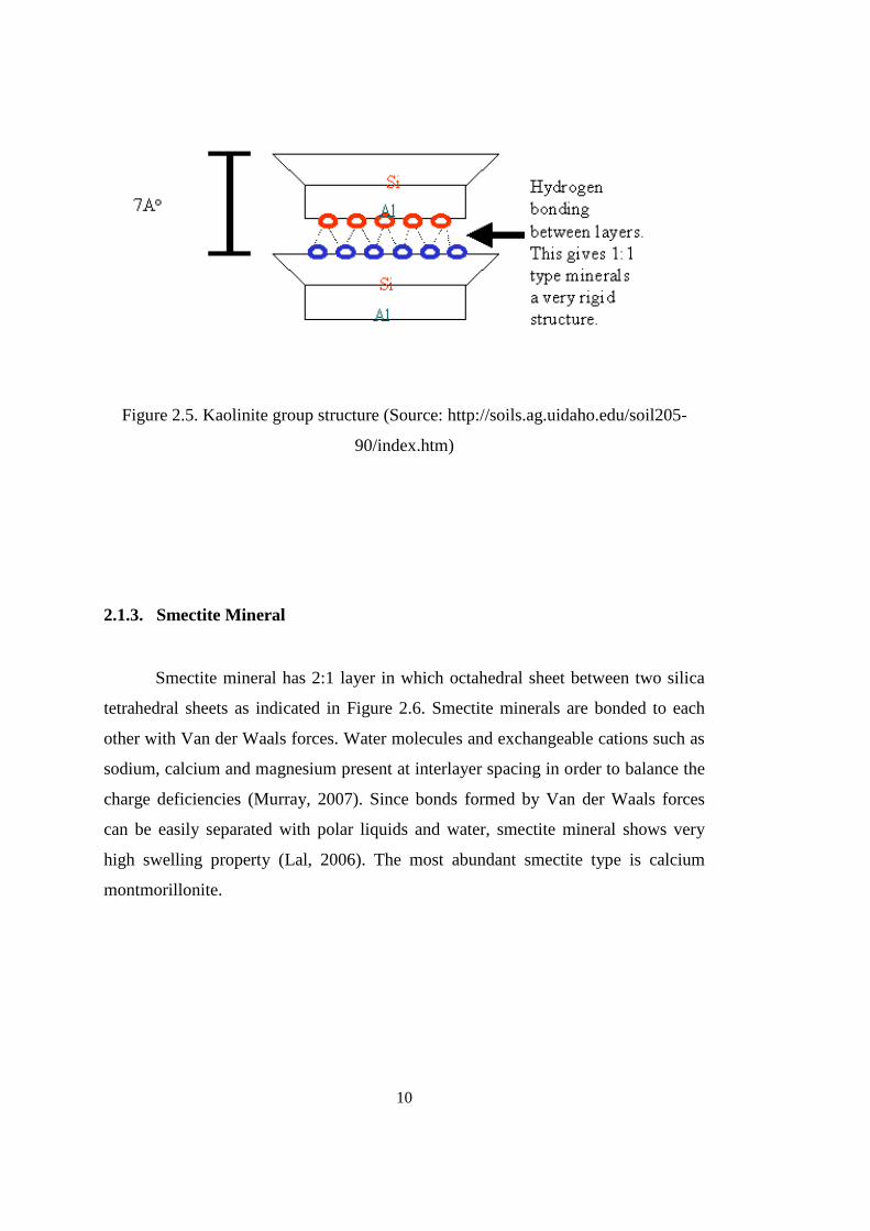
Figure 2.5. Kaolinite group structure (Source: http://soils.ag.uidaho.edu/soil205-
90/index.htm)
2.1.3. Smectite Mineral
Smectite mineral has 2:1 layer in which octahedral sheet between two silica
tetrahedral sheets as indicated in Figure 2.6. Smectite minerals are bonded to each
other with Van der Waals forces. Water molecules and exchangeable cations such as
sodium, calcium and magnesium present at interlayer spacing in order to balance the
charge deficiencies (Murray, 2007). Since bonds formed by Van der Waals forces
can be easily separated with polar liquids and water, smectite mineral shows very
high swelling property (Lal, 2006). The most abundant smectite type is calcium
montmorillonite.
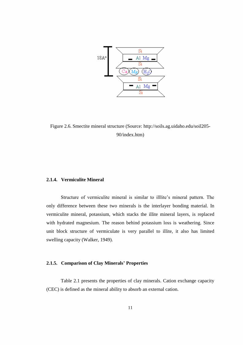
11
Figure 2.6. Smectite mineral structure (Source: http://soils.ag.uidaho.edu/soil205-
90/index.htm)
2.1.4. Vermiculite Mineral
Structure of vermiculite mineral is similar to illlite’s mineral pattern. The
only difference between these two minerals is the interlayer bonding material. In
vermiculite mineral, potassium, which stacks the illite mineral layers, is replaced
with hydrated magnesium. The reason behind potassium loss is weathering. Since
unit block structure of vermiculate is very parallel to illite, it also has limited
swelling capacity (Walker, 1949).
2.1.5. Comparison of Clay Minerals’ Properties
Table 2.1 presents the properties of clay minerals. Cation exchange capacity
(CEC) is defined as the mineral ability to absorb an external cation.
12
Table 2.1. Index properties and characteristics of clay minerals (Grim, 1968;
Lambe&Whitmann, 1969)
Clay Mineral
CEC
meq/
100 g
Specific
Gravity
Specific
Surface
m2/g
LL % PL % Swell
Potential
Illite 3-15 2.6-2.68 10-20 30-60 25-35 Low
Sodium (Na)
53 21
Calcium (Ca) 38 11
Kaolinite 10-40 2.6-3.0 65-100 60-120 35-60 Medium
Na
61 34
Ca 90 40
Montmorillonite 80-150 2.35-2.7 700-840 100-900 50-100 High
Na
700 97
Ca 177 63
When Table 2.1 is examined, a direct proportion between swelling capacity
and CEC, specific surface, LL and PL is observed. In this manner, illite mineral
which has the lowest CEC, specific surface, liquid limit and plastic limit values
swells in the lowest degree whereas montmorillonite owns the opposite
characteristics.

13
2.2. Swell Mechanism
When the clay particle interacts with water, high concentration of cations
develops near the negatively charged clay particle surface due to bipolar water
molecules, release of adsorbed cations existing on the surface and release of
hydrogen from the hydroxyl group (Oweis and Khera, 1998). As a result, an
electrostatic force forms between negative surface and exchangeable cations (Das,
2008). The electrical interparticle force field depends on the variabilities in negative
surface charges, electrochemistry of the soil-water, van der Waals forces and
adsorptive forces between clay surface and water molecules. If one of these variables
change, interparticle force field will also be altered. Since there is no externally
applied stress to balance this change, particle spacing will change to get the system in
equilibrium. This change in particle spacing as the result of disturbance of internal
stress equilibrium is known as shrink/swell (Nelson and Miller, 1992).
The region of negative charges on the clay surface and balancing cations in
the solution that surround clay surface is called as diffuse double (stern) layer (Das,
2008). Figure 2.7 schematically shows water molecule layers and attraction force.
Water molecule layers can be divided into two parts as solid (adsorbed) water and
double layer. Solid water is strongly held by particle as a very thin layer around it,
which is marked as “b “in Figure 2.7. Less attractive forces and liquid water form
double layer, which is responsible for the plasticity of clay (Al-Rawas and Goosen,
2006). Double layer is indicated in Figure 2.7 by “c”. The region is termed as diffuse
because the further from the surface, attractive forces decreases with the inverse
square of distance as stating in Figure 2.7.
14
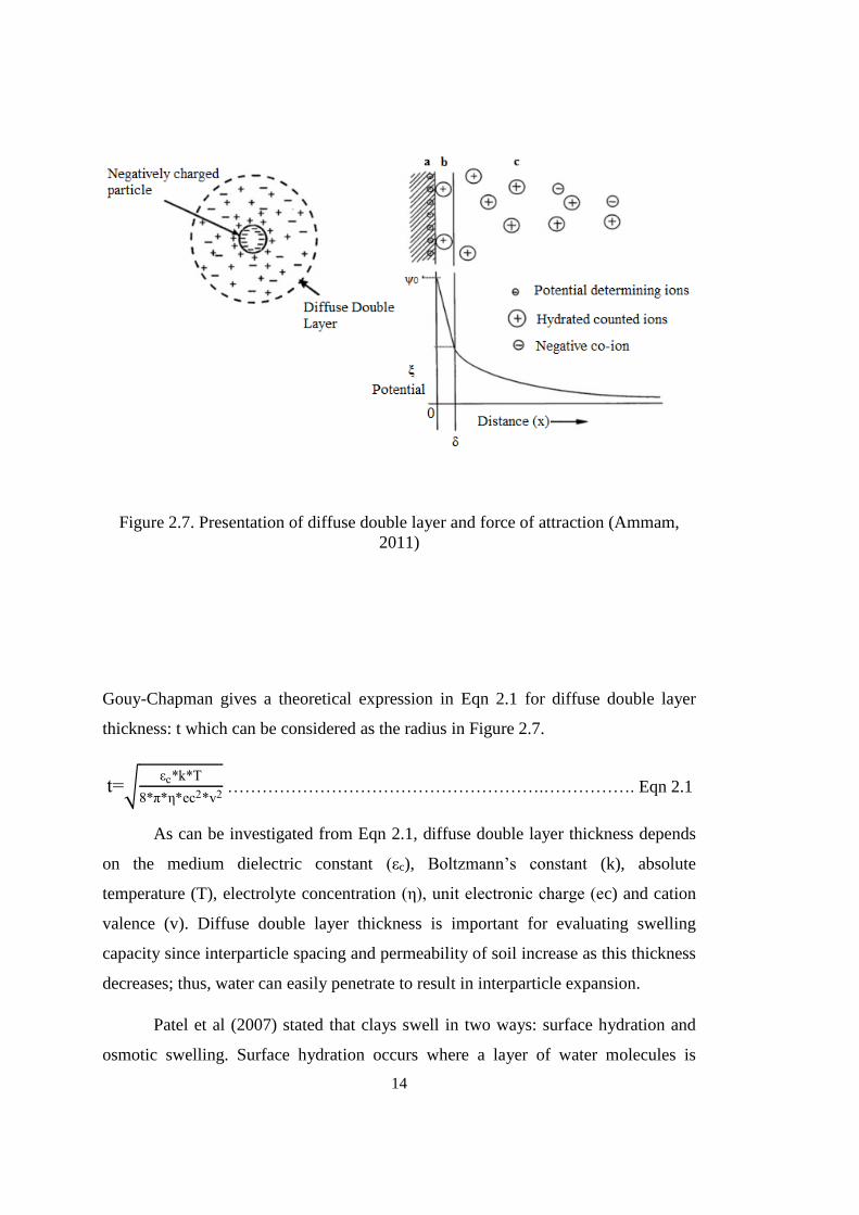
Figure 2.7. Presentation of diffuse double layer and force of attraction (Ammam,
2011)
Gouy-Chapman gives a theoretical expression in Eqn 2.1 for diffuse double layer
thickness: t which can be considered as the radius in Figure 2.7.
t=√εc*k*T
8*π*η*ec2*v2 ……………………………………………….……………. Eqn 2.1
As can be investigated from Eqn 2.1, diffuse double layer thickness depends
on the medium dielectric constant (εc), Boltzmann’s constant (k), absolute
temperature (T), electrolyte concentration (η), unit electronic charge (ec) and cation
valence (v). Diffuse double layer thickness is important for evaluating swelling
capacity since interparticle spacing and permeability of soil increase as this thickness
decreases; thus, water can easily penetrate to result in interparticle expansion.
Patel et al (2007) stated that clays swell in two ways: surface hydration and
osmotic swelling. Surface hydration occurs where a layer of water molecules is
15
adsorbed on crystal surfaces by hydrogen bonding. Successive layers of these water
molecules increase spacing with a quasi-crystalline alignment. On the other hand,
when water osmotically moves between the unit layers in the clay mineral from
higher concentration to the lower side in the surrounding water, overall volume
increases. This phenomenon is called osmotic swelling. Volume increase due to
osmotic swelling is larger than that is caused by surface hydration. A few clays such
as sodium montmorillonite, a kind of smectite, undergo osmotic swell whereas
surface hydration occurs in all types of clays.
2.3. Clay Structure and Fabric
Holtz and Kovacs (1981) stated that only geometrical arrangement of
particles is referred as soil fabric. The structure of soil means combined effect of
fabrics and interparticle forces.
When clay particles interact with water, they will repel each other and form
an interparticle spacing due to negatively charged clay surface and cations existing in
double layer of adjacent particles. Thickness of diffuse double layer leads to increase
in magnitude of repulsive forces; therefore, parameters changing diffuse double layer
thickness also alter repulsive forces.
In addition to repulsive forces, there are Van der Waals forces between
approaching clay particles, regardless of the fluid between the particles.
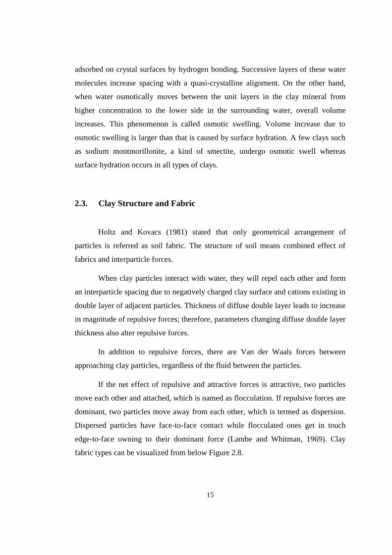
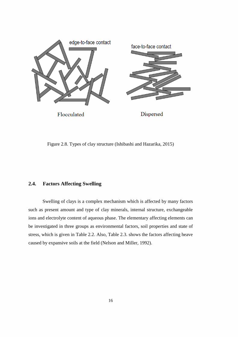
If the net effect of repulsive and attractive forces is attractive, two particles
move each other and attached, which is named as flocculation. If repulsive forces are
dominant, two particles move away from each other, which is termed as dispersion.
Dispersed particles have face-to-face contact while flocculated ones get in touch
edge-to-face owning to their dominant force (Lambe and Whitman, 1969). Clay
fabric types can be visualized from below Figure 2.8.
16
Figure 2.8. Types of clay structure (Ishibashi and Hazarika, 2015)
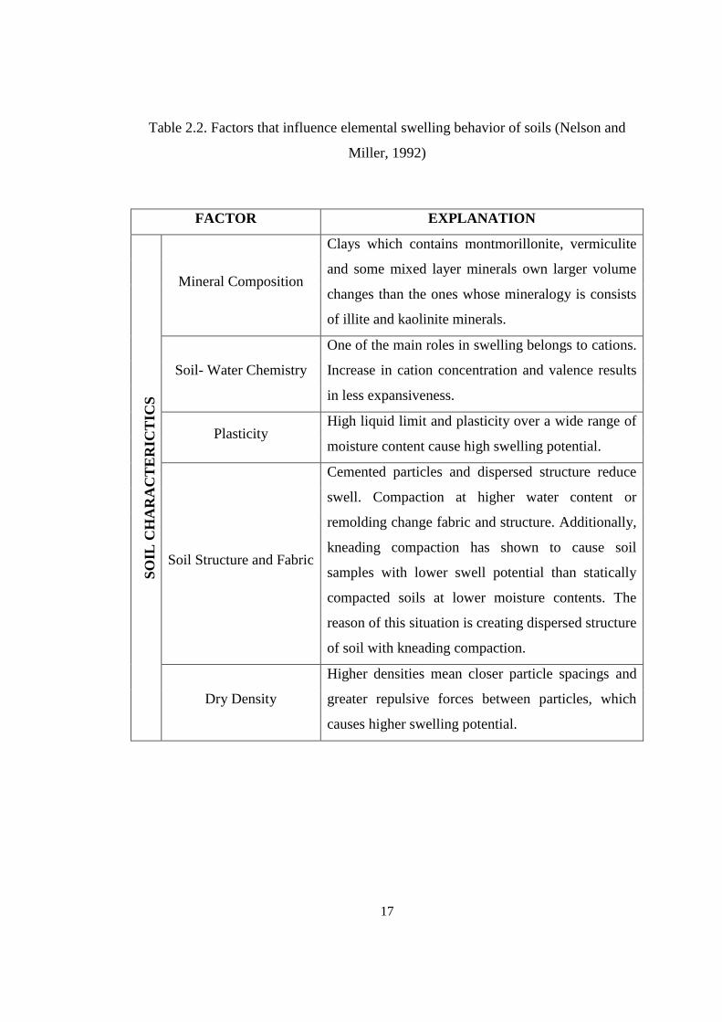
2.4. Factors Affecting Swelling
Swelling of clays is a complex mechanism which is affected by many factors
such as present amount and type of clay minerals, internal structure, exchangeable
ions and electrolyte content of aqueous phase. The elementary affecting elements can
be investigated in three groups as environmental factors, soil properties and state of
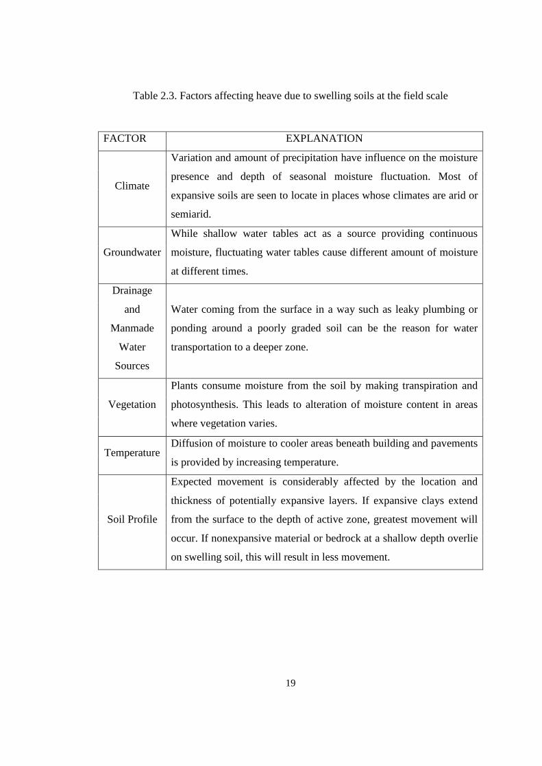
stress, which is given in Table 2.2. Also, Table 2.3. shows the factors affecting heave
caused by expansive soils at the field (Nelson and Miller, 1992).
17
Table 2.2. Factors that influence elemental swelling behavior of soils (Nelson and
Miller, 1992)
FACTOR EXPLANATION
SO
IL C
HA
RA
CT
ER
ICT
ICS
Mineral Composition
Clays which contains montmorillonite, vermiculite
and some mixed layer minerals own larger volume
changes than the ones whose mineralogy is consists
of illite and kaolinite minerals.
Soil- Water Chemistry
One of the main roles in swelling belongs to cations.
Increase in cation concentration and valence results
in less expansiveness.
Plasticity High liquid limit and plasticity over a wide range of
moisture content cause high swelling potential.
Soil Structure and Fabric
Cemented particles and dispersed structure reduce
swell. Compaction at higher water content or
remolding change fabric and structure. Additionally,
kneading compaction has shown to cause soil
samples with lower swell potential than statically
compacted soils at lower moisture contents. The
reason of this situation is creating dispersed structure
of soil with kneading compaction.
Dry Density
Higher densities mean closer particle spacings and
greater repulsive forces between particles, which
causes higher swelling potential.
18
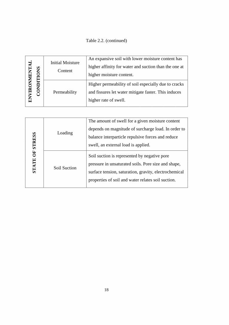
Table 2.2. (continued)
EN
VIR
ON
ME
NT
AL
CO
ND
ITIO
NS
Initial Moisture
Content
An expansive soil with lower moisture content has
higher affinity for water and suction than the one at
higher moisture content.
Permeability
Higher permeability of soil especially due to cracks
and fissures let water mitigate faster. This induces
higher rate of swell.
ST
AT
E O
F S
TR
ES
S
Loading
The amount of swell for a given moisture content
depends on magnitude of surcharge load. In order to
balance interparticle repulsive forces and reduce
swell, an external load is applied.
Soil Suction
Soil suction is represented by negative pore
pressure in unsaturated soils. Pore size and shape,
surface tension, saturation, gravity, electrochemical
properties of soil and water relates soil suction.
19
Table 2.3. Factors affecting heave due to swelling soils at the field scale
FACTOR EXPLANATION
Climate
Variation and amount of precipitation have influence on the moisture
presence and depth of seasonal moisture fluctuation. Most of
expansive soils are seen to locate in places whose climates are arid or
semiarid.
Groundwater
While shallow water tables act as a source providing continuous
moisture, fluctuating water tables cause different amount of moisture
at different times.
Drainage
and
Manmade
Water
Sources
Water coming from the surface in a way such as leaky plumbing or
ponding around a poorly graded soil can be the reason for water
transportation to a deeper zone.
Vegetation
Plants consume moisture from the soil by making transpiration and
photosynthesis. This leads to alteration of moisture content in areas
where vegetation varies.
Temperature Diffusion of moisture to cooler areas beneath building and pavements
is provided by increasing temperature.
Soil Profile
Expected movement is considerably affected by the location and
thickness of potentially expansive layers. If expansive clays extend
from the surface to the depth of active zone, greatest movement will
occur. If nonexpansive material or bedrock at a shallow depth overlie
on swelling soil, this will result in less movement.

20
21
CHAPTER 3
3) PREVIOUS STUDIES ON THE EFFECT OF
SWELLING ON CLAY’S STRENGTH
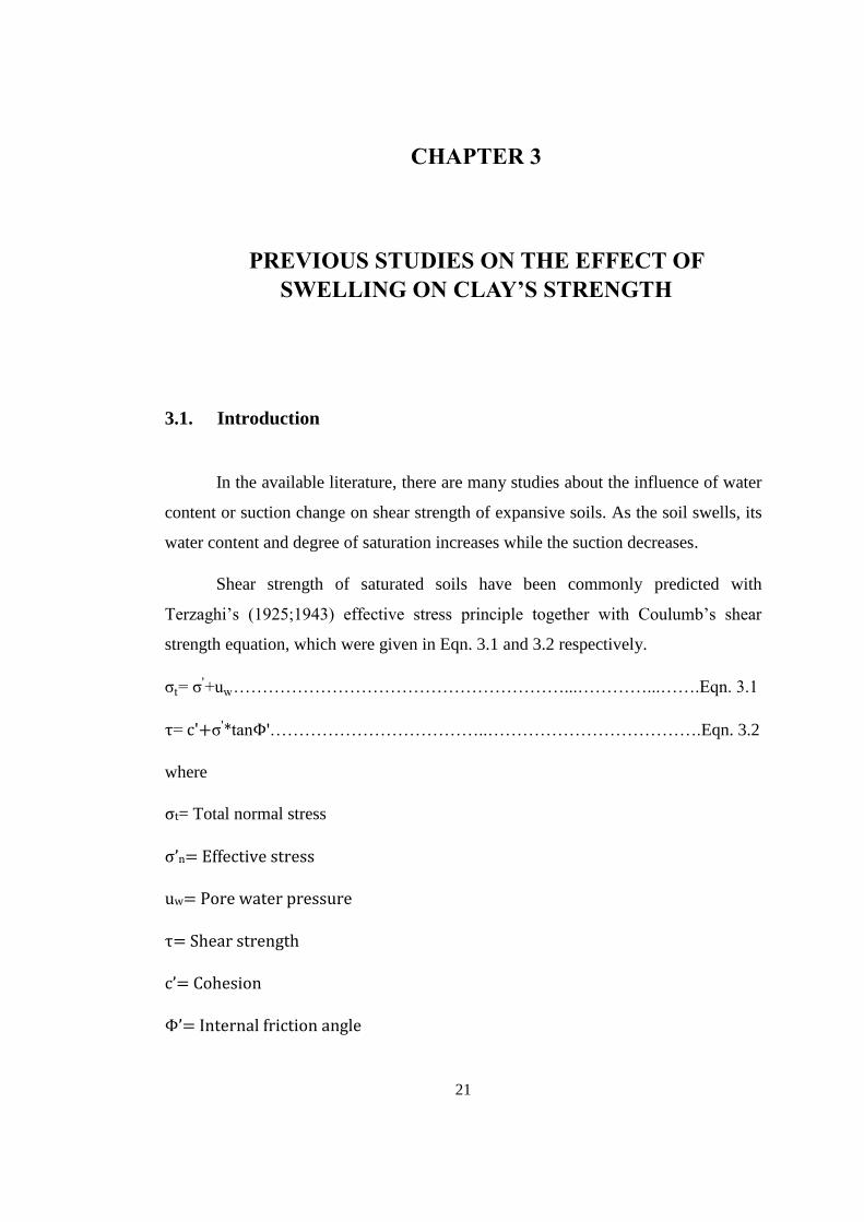
3.1. Introduction
In the available literature, there are many studies about the influence of water
content or suction change on shear strength of expansive soils. As the soil swells, its
water content and degree of saturation increases while the suction decreases.
Shear strength of saturated soils have been commonly predicted with
Terzaghi’s (1925;1943) effective stress principle together with Coulumb’s shear
strength equation, which were given in Eqn. 3.1 and 3.2 respectively.
σt= σ'+uw…………………………………………………...…………...…….Eqn. 3.1
τ= c'+σ'*tanΦ'………………………………..……………………………….Eqn. 3.2
where
σt= Total normal stress
σ’n= Effective stress
uw= Pore water pressure
τ= Shear strength
c’= Cohesion
Φ’= Internal friction angle
22
In order to estimate the shear strength of partially saturated soils, Bishop
(1959) proposed effective stress approach, which is given in Eqn. 3.3, while
Fredlund and Morgenstern (1977) used independent stress state variables, whose
expression is presented in Eqn. 3.4, by developing Coulumb’s strength equation.
τ= c'+( σt- ua)* tan Φ''- χ*(ua- uw)* tan Φ'
''………..........……………………Eqn. 3.3
τ= c'+( σt- ua)* tan Φ''''- (uw- ua)* tan Φ'
'b'………..…………………………Eqn. 3.4
where
ua= Air pressure
χ= Effective stress parameter
Φ''b= Angle of shearing resistance with respect to matric suction
tanΦ''b= aw*tanΦ'
' where aw is the normalized water area
Many researches have focused on the ways determining χ or tanΦ'b as the
function of degree of saturation or suction. Karube et al. (1996) introduced a linear
relationship of degree of saturation to determine χ value. Again, Öberg and Sӓllfors
(1997) proposed an equation showing the degree of saturation and χ relationship.
Khalili and Khabbaz (1998) presented an empirical correlation between soil suction
and χ by analyzing the shear strength data in the available literature. Bao et al.
proposed a relation involving the air entry and residual suction value for χ. In
addition to the studies to obtain χ or aw value, Tekinsoy et al. (2004) introduced an
empirical equation showing the relation between shear strength and soil- water
characteristic curve through air entry value.
In other respects, previous strength values were mostly found with the help of
triaxial or direct shear test. Studies were mostly associated with the stress- swell
relations instead of change in shear strength at different swell ratio.
23
3.2. Investigation of Previous Studies
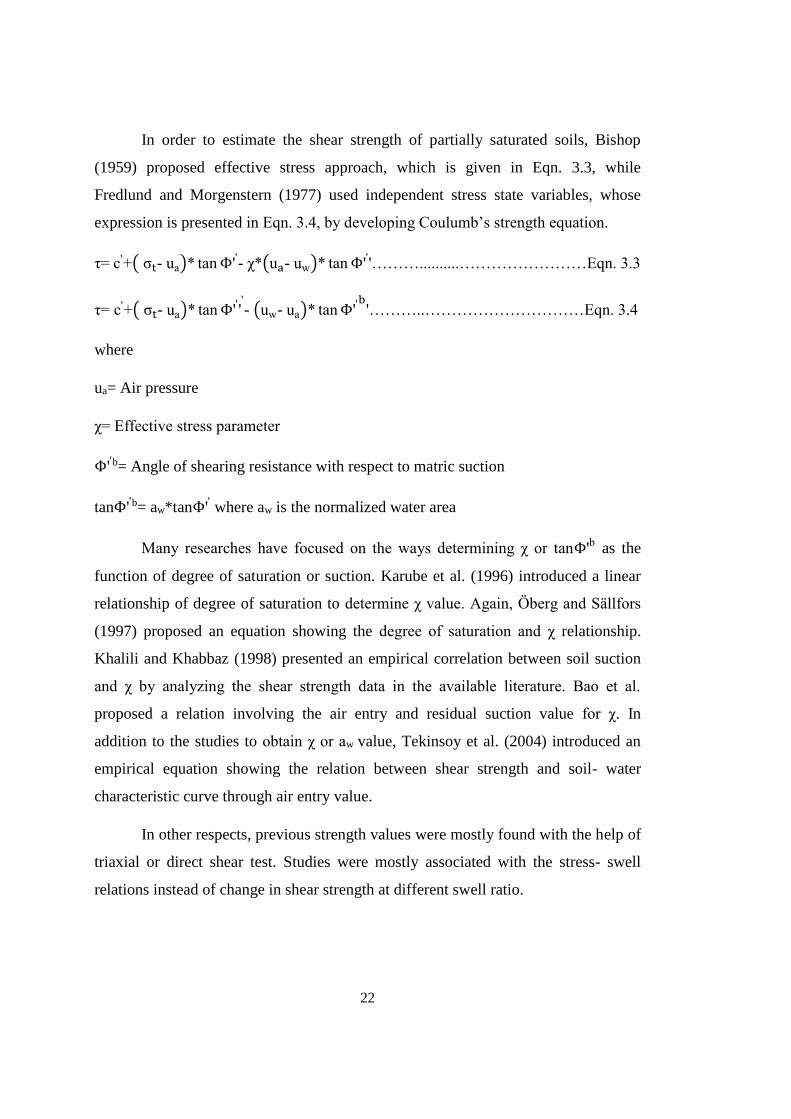
Lo et al. (1987) performed semi confined swell tests on Georgian Bay Shale
whose results are presented in Figure 3.1. These results show that swelling strains
increase as applied vertical stresses decrease.
Figure 3.1. Results of a series of semi confined swell test made on Georgian Bay
Shale for the design of shafts and tunnels (After Lo et al., 1987)
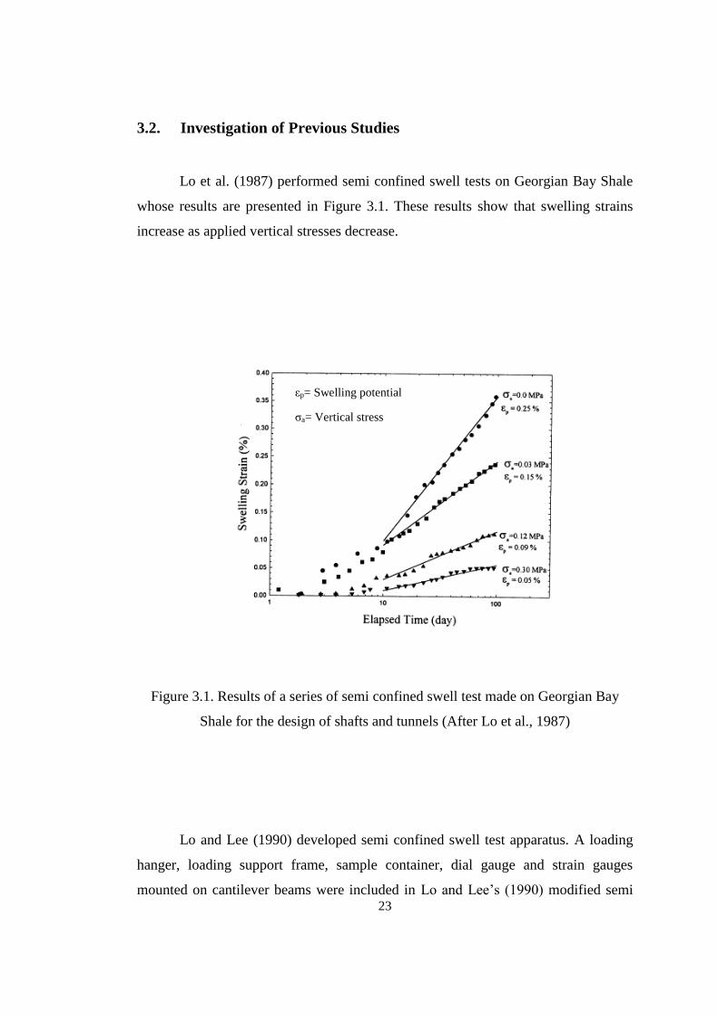
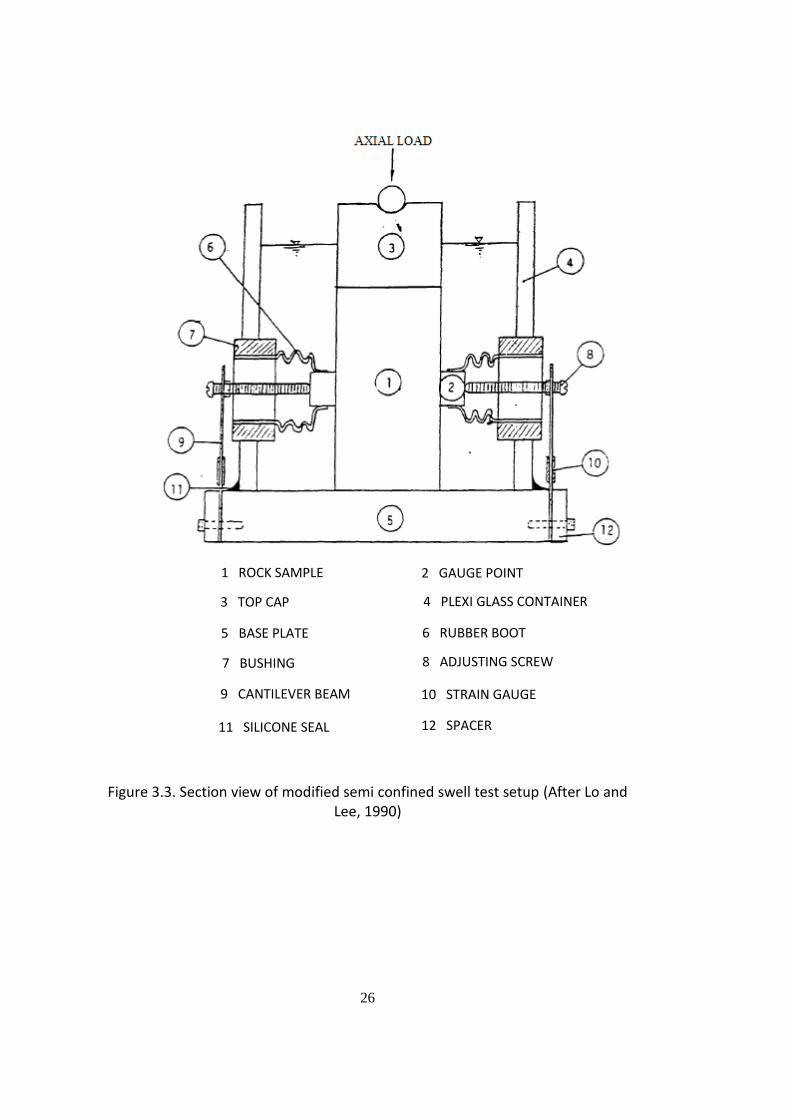
Lo and Lee (1990) developed semi confined swell test apparatus. A loading
hanger, loading support frame, sample container, dial gauge and strain gauges
mounted on cantilever beams were included in Lo and Lee’s (1990) modified semi
εp= Swelling potential
σa= Vertical stress
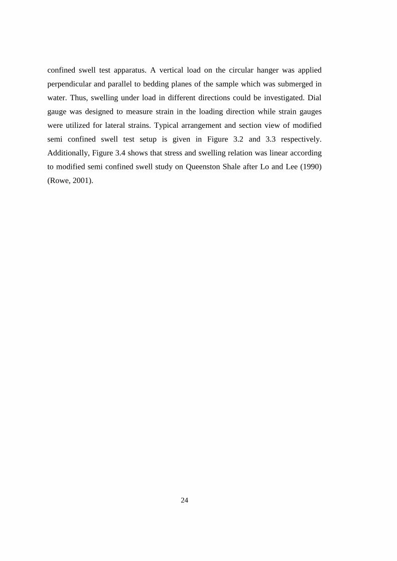
24
confined swell test apparatus. A vertical load on the circular hanger was applied
perpendicular and parallel to bedding planes of the sample which was submerged in
water. Thus, swelling under load in different directions could be investigated. Dial
gauge was designed to measure strain in the loading direction while strain gauges
were utilized for lateral strains. Typical arrangement and section view of modified
semi confined swell test setup is given in Figure 3.2 and 3.3 respectively.
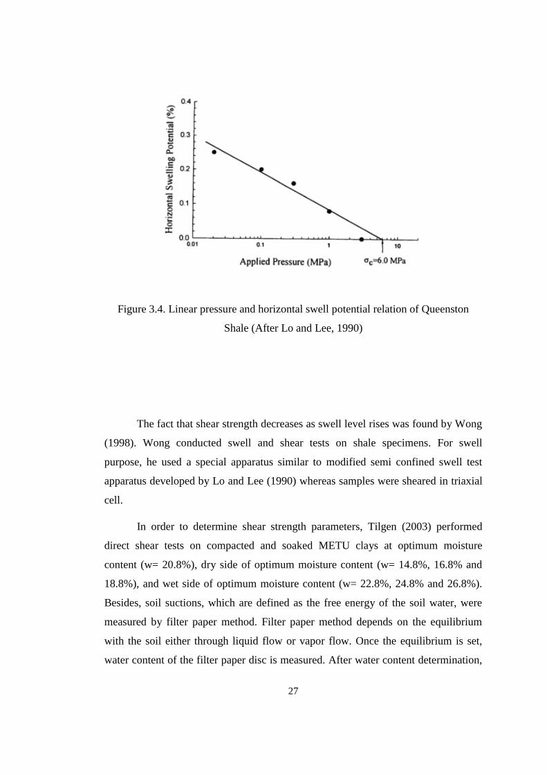
Additionally, Figure 3.4 shows that stress and swelling relation was linear according
to modified semi confined swell study on Queenston Shale after Lo and Lee (1990)
(Rowe, 2001).
25
Figure 3.2. Typical arrangement of modified semi confined swell test (After Lo and
Lee, 1990)
26
Figure 3.3. Section view of modified semi confined swell test setup (After Lo and Lee, 1990)
1 ROCK SAMPLE
3 TOP CAP
5 BASE PLATE
7 BUSHING
9 CANTILEVER BEAM
11 SILICONE SEAL
2 GAUGE POINT
4 PLEXI GLASS CONTAINER
6 RUBBER BOOT
8 ADJUSTING SCREW
10 STRAIN GAUGE
12 SPACER
27
Figure 3.4. Linear pressure and horizontal swell potential relation of Queenston
Shale (After Lo and Lee, 1990)
The fact that shear strength decreases as swell level rises was found by Wong
(1998). Wong conducted swell and shear tests on shale specimens. For swell
purpose, he used a special apparatus similar to modified semi confined swell test
apparatus developed by Lo and Lee (1990) whereas samples were sheared in triaxial
cell.
In order to determine shear strength parameters, Tilgen (2003) performed
direct shear tests on compacted and soaked METU clays at optimum moisture
content (w= 20.8%), dry side of optimum moisture content (w= 14.8%, 16.8% and
18.8%), and wet side of optimum moisture content (w= 22.8%, 24.8% and 26.8%).
Besides, soil suctions, which are defined as the free energy of the soil water, were
measured by filter paper method. Filter paper method depends on the equilibrium
with the soil either through liquid flow or vapor flow. Once the equilibrium is set,
water content of the filter paper disc is measured. After water content determination,
28
filter paper calibration curve is constructed or adopted to find the suction value
corresponding to the water content.
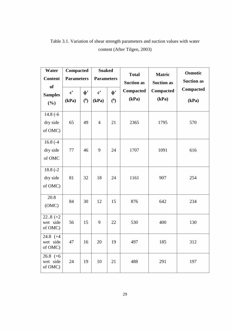
Relation between water content and shear strength parameters as well as the
water content and suction correlation of both compacted and soaked samples is
summarized in Table 3.1. As can be seen from Table 3.1, as moisture content
increased, cohesion values also increased up to OMC while angle of friction values
decreased because of gained granular soil fabric. After the OMC, cohesion and angle
of friction values exhibited a decreasing trend. When the results for compacted and
soaked samples were compared, it was seen that cohesion and friction angle values
of soaked samples were smaller than the ones obtained from compacted samples. In
addition, soaked samples’ cohesion and angle of friction values were almost constant
at 12 kPa and 220 respectively. Another experimental result was the fact that total
soil suction, matric soil suction and osmotic soil suction decreased with increasing
water content at the dry side of OMC, which verified the direct relation between
suction and shear strength.
29
Table 3.1. Variation of shear strength parameters and suction values with water
content (After Tilgen, 2003)
Water
Content
of
Samples
(%)
Compacted
Parameters
Soaked
Parameters Total
Suction as
Compacted
(kPa)
Matric
Suction as
Compacted
(kPa)
Osmotic
Suction as
Compacted
(kPa)
c’
(kPa)
ɸ’
(0)
c’
(kPa)
ɸ’
(0)
14.8 (-6
dry side
of OMC)
65 49 4 21 2365 1795 570
16.8 (-4
dry side
of OMC
77 46 9 24 1707 1091 616
18.8 (-2
dry side
of OMC)
81 32 18 24 1161 907 254
20.8
(OMC) 84 30 12 15 876 642 234
22..8 (+2
wet side
of OMC)
56 15 9 22 530 400 130
24.8 (+4
wet side
of OMC)
47 16 20 19 497 185 312
26.8 (+6
wet side
of OMC)
24 19 10 21 488 291 197
30
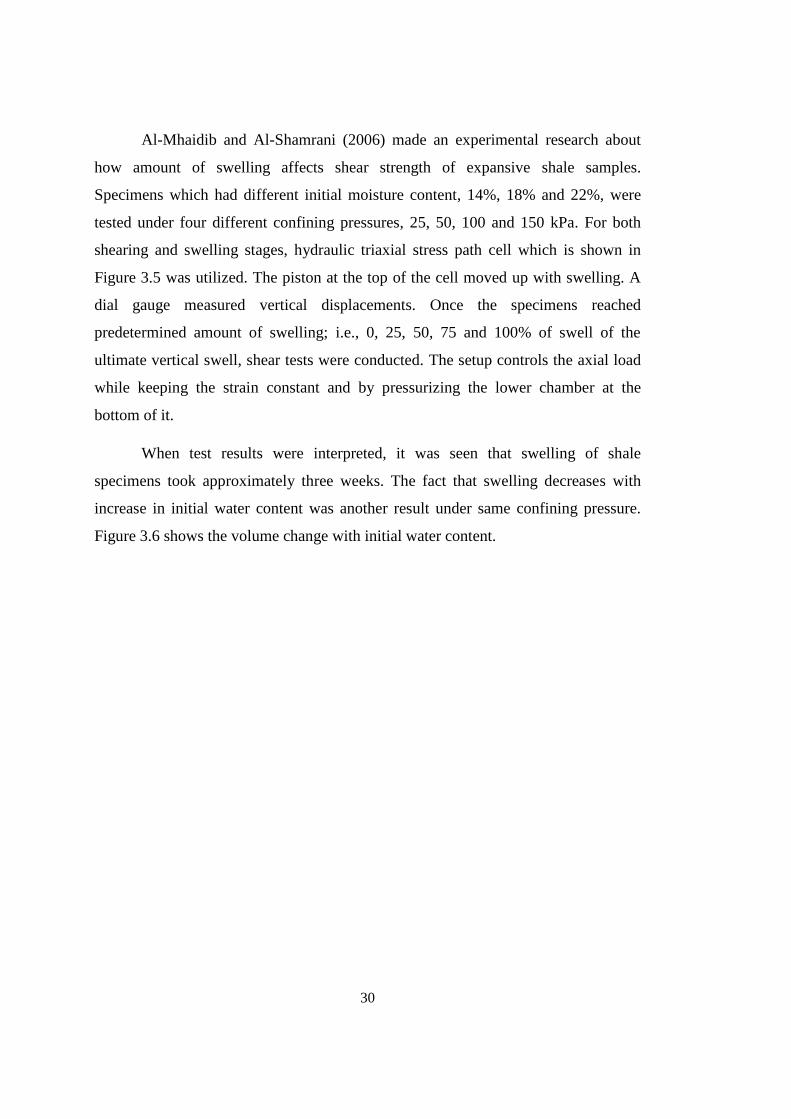
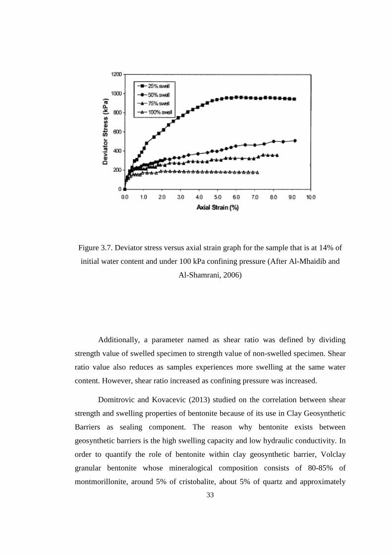
Al-Mhaidib and Al-Shamrani (2006) made an experimental research about
how amount of swelling affects shear strength of expansive shale samples.
Specimens which had different initial moisture content, 14%, 18% and 22%, were
tested under four different confining pressures, 25, 50, 100 and 150 kPa. For both
shearing and swelling stages, hydraulic triaxial stress path cell which is shown in
Figure 3.5 was utilized. The piston at the top of the cell moved up with swelling. A
dial gauge measured vertical displacements. Once the specimens reached
predetermined amount of swelling; i.e., 0, 25, 50, 75 and 100% of swell of the
ultimate vertical swell, shear tests were conducted. The setup controls the axial load
while keeping the strain constant and by pressurizing the lower chamber at the
bottom of it.
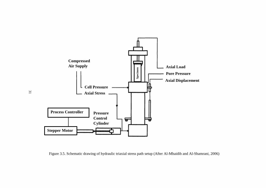
When test results were interpreted, it was seen that swelling of shale
specimens took approximately three weeks. The fact that swelling decreases with
increase in initial water content was another result under same confining pressure.
Figure 3.6 shows the volume change with initial water content.
22
Figure 3.5. Schematic drawing of hydraulic triaxial stress path setup (After Al-Mhaidib and Al-Shamrani, 2006)
Axial Load
Pore Pressure
Axial Displacement
Sp
ecim
en
31
Pressure
Control
Cylinder
Compressed
Air Supply
Cell Pressure
Axial Stress
Process Controller
Stepper Motor
32
Figure 3.6. Schematic drawing of hydraulic triaxial stress path setup (After
Al-Mhaidib and Al-Shamrani, 2006)
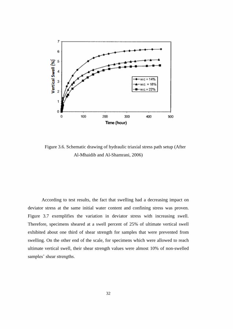
According to test results, the fact that swelling had a decreasing impact on
deviator stress at the same initial water content and confining stress was proven.
Figure 3.7 exemplifies the variation in deviator stress with increasing swell.
Therefore, specimens sheared at a swell percent of 25% of ultimate vertical swell
exhibited about one third of shear strength for samples that were prevented from
swelling. On the other end of the scale, for specimens which were allowed to reach
ultimate vertical swell, their shear strength values were almost 10% of non-swelled
samples’ shear strengths.
33
Figure 3.7. Deviator stress versus axial strain graph for the sample that is at 14% of
initial water content and under 100 kPa confining pressure (After Al-Mhaidib and
Al-Shamrani, 2006)
Additionally, a parameter named as shear ratio was defined by dividing
strength value of swelled specimen to strength value of non-swelled specimen. Shear
ratio value also reduces as samples experiences more swelling at the same water
content. However, shear ratio increased as confining pressure was increased.
Domitrovic and Kovacevic (2013) studied on the correlation between shear
strength and swelling properties of bentonite because of its use in Clay Geosynthetic
Barriers as sealing component. The reason why bentonite exists between
geosynthetic barriers is the high swelling capacity and low hydraulic conductivity. In
order to quantify the role of bentonite within clay geosynthetic barrier, Volclay
granular bentonite whose mineralogical composition consists of 80-85% of
montmorillonite, around 5% of cristobalite, about 5% of quartz and approximately
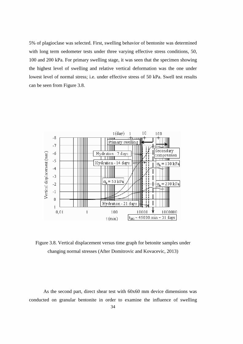
34
5% of plagioclase was selected. First, swelling behavior of bentonite was determined
with long term oedometer tests under three varying effective stress conditions, 50,
100 and 200 kPa. For primary swelling stage, it was seen that the specimen showing
the highest level of swelling and relative vertical deformation was the one under
lowest level of normal stress; i.e. under effective stress of 50 kPa. Swell test results
can be seen from Figure 3.8.
Figure 3.8. Vertical displacement versus time graph for betonite samples under
changing normal stresses (After Domitrovic and Kovacevic, 2013)
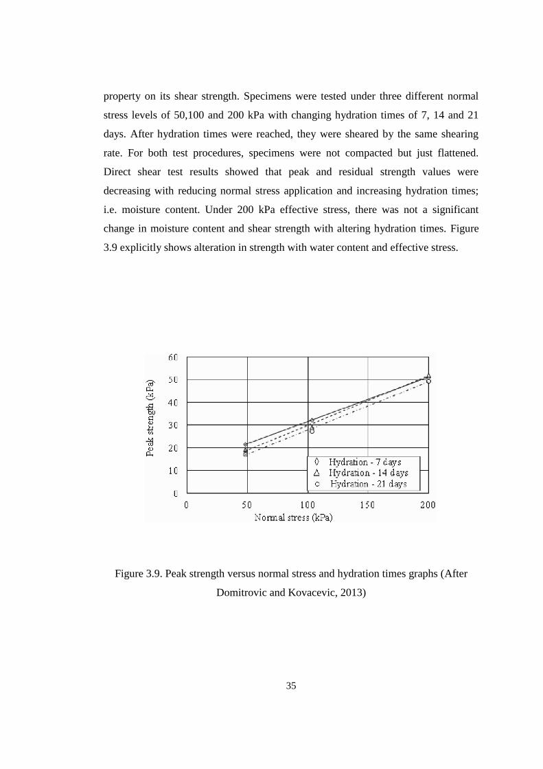
As the second part, direct shear test with 60x60 mm device dimensions was
conducted on granular bentonite in order to examine the influence of swelling
35
property on its shear strength. Specimens were tested under three different normal
stress levels of 50,100 and 200 kPa with changing hydration times of 7, 14 and 21
days. After hydration times were reached, they were sheared by the same shearing
rate. For both test procedures, specimens were not compacted but just flattened.
Direct shear test results showed that peak and residual strength values were
decreasing with reducing normal stress application and increasing hydration times;
i.e. moisture content. Under 200 kPa effective stress, there was not a significant
change in moisture content and shear strength with altering hydration times. Figure
3.9 explicitly shows alteration in strength with water content and effective stress.
Figure 3.9. Peak strength versus normal stress and hydration times graphs (After
Domitrovic and Kovacevic, 2013)
36
Moreover, when shear strength parameters were evaluated, peak and residual
cohesion values were observed to decrease with longer hydration times while peak
and residual friction angle values increased in the same moisture content change. The
most dramatic variation in friction angle was visible up to 14 days of hydration.
Results are given in Table 3.2.
Table 3.2. Shear strength parameters’ variation with water content and swelling
(After Domitrovic and Kovacevic, 2013)
Hydration
Time
Peak Parameters Residual Parameters
c (kPa) Ф (0) c (kPa) Ф (0)
7 days 11.99 11.23 11.05 7.80
14 days 8.04 12.47 4.79 9.38
21 days 6.32 12.27 3.63 9.31
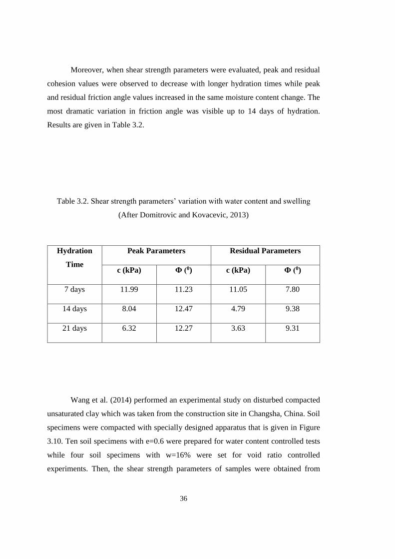
Wang et al. (2014) performed an experimental study on disturbed compacted
unsaturated clay which was taken from the construction site in Changsha, China. Soil
specimens were compacted with specially designed apparatus that is given in Figure
3.10. Ten soil specimens with e=0.6 were prepared for water content controlled tests
while four soil specimens with w=16% were set for void ratio controlled
experiments. Then, the shear strength parameters of samples were obtained from
37
strain controlled multistage direct shear test under 100, 200, 300 and 400 kPa vertical
loading.
Figure 3.10. Apparatus for sample compaction (After Wang et al., 2014)
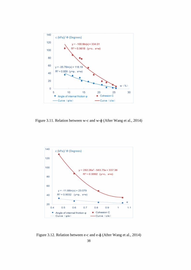
According to direct shear test results, correlation between water content and
cohesion as well as the relation between water content and internal friction angle at
mean void ratio of 0.6 can be examined from Figure 3.11. On the other side, Figure
3.12 shows the void ratio versus cohesion and void ratio versus angle of internal
friction relations at mean water content of 15.52%. As the result, it can be said that
increase in water content or void ratio had an decreasing effect on both for cohesion
and internal friction angle. The reason of decrease in the cohesion could be explained
as the fact that attached water caused increase in the distance between clay particles
and water molecules and so thickened the hydration membrane, which resulted in the
weakening of the intermolecular and electrostatic attraction forces. Moreover, due to
same reasons enhancing of lubricity between clay particles induced decrease in
internal friction angle.
All mentioned studies were listed below in Table 3.3:
38
Figure 3.11. Relation between w-c and w-ɸ (After Wang et al., 2014)
Figure 3.12. Relation between e-c and e-ɸ (After Wang et al., 2014)
c (kPa)/ Ф (Degrees)
c (kPa)/ Ф (Degrees)
39
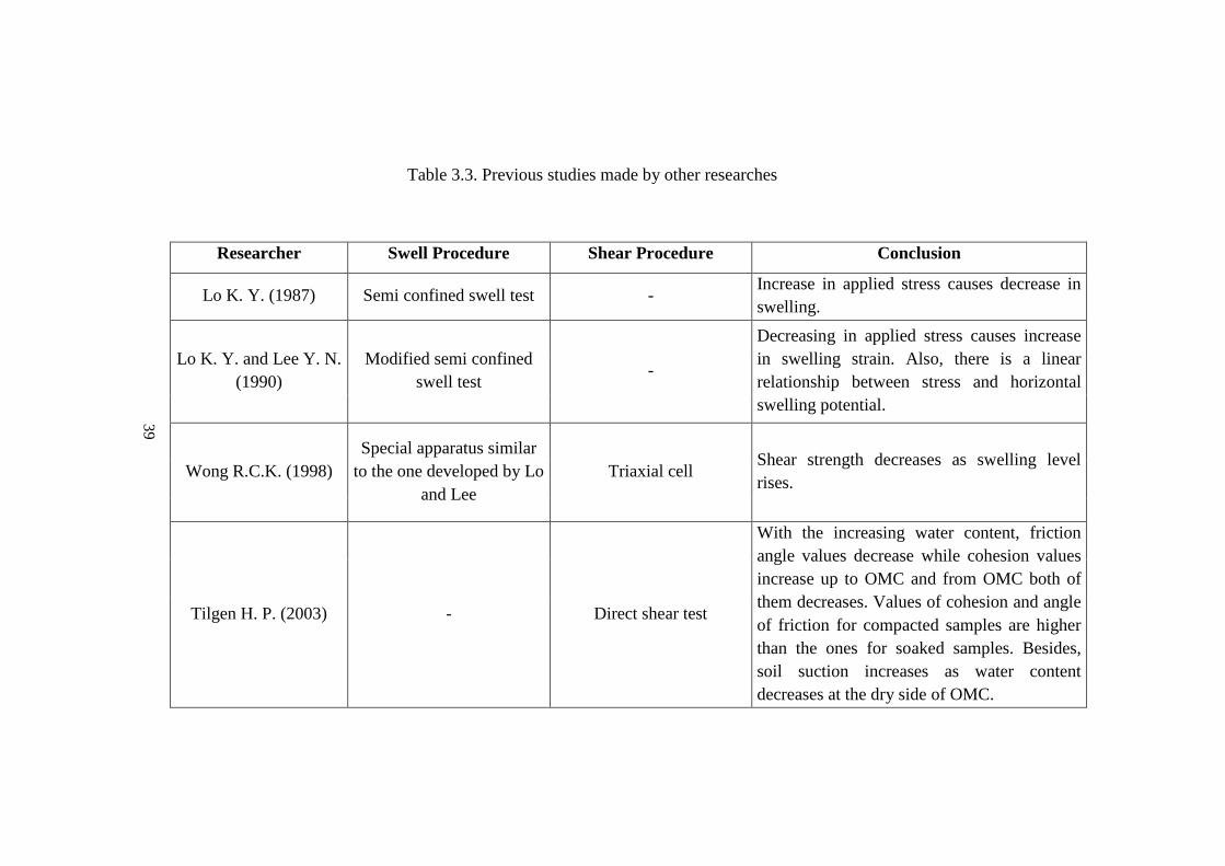
Table 3.3. Previous studies made by other researches
Researcher Swell Procedure Shear Procedure Conclusion
Lo K. Y. (1987) Semi confined swell test - Increase in applied stress causes decrease in
swelling.
Lo K. Y. and Lee Y. N.
(1990)
Modified semi confined
swell test -
Decreasing in applied stress causes increase
in swelling strain. Also, there is a linear
relationship between stress and horizontal
swelling potential.
Wong R.C.K. (1998)
Special apparatus similar
to the one developed by Lo
and Lee
Triaxial cell Shear strength decreases as swelling level
rises.
Tilgen H. P. (2003) - Direct shear test
With the increasing water content, friction
angle values decrease while cohesion values
increase up to OMC and from OMC both of
them decreases. Values of cohesion and angle
of friction for compacted samples are higher
than the ones for soaked samples. Besides,
soil suction increases as water content
decreases at the dry side of OMC.
40
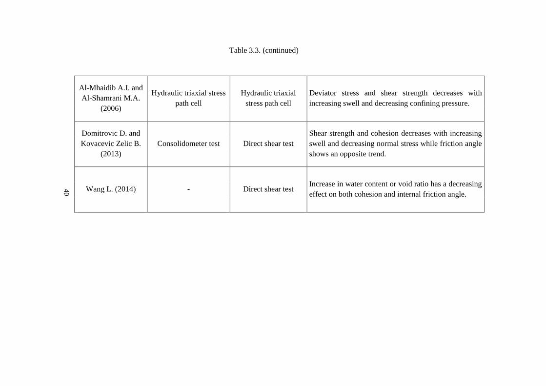
Table 3.3. (continued)
Al-Mhaidib A.I. and
Al-Shamrani M.A.
(2006)
Hydraulic triaxial stress
path cell
Hydraulic triaxial
stress path cell
Deviator stress and shear strength decreases with
increasing swell and decreasing confining pressure.
Domitrovic D. and
Kovacevic Zelic B.
(2013)
Consolidometer test Direct shear test
Shear strength and cohesion decreases with increasing
swell and decreasing normal stress while friction angle
shows an opposite trend.
Wang L. (2014) - Direct shear test Increase in water content or void ratio has a decreasing
effect on both cohesion and internal friction angle.
41
CHAPTER 4
4) EXPERIMENTAL STUDIES
4.1. Objective
The objective of this study was to investigate the change in unconfined
compressive strength, undrained shear strength, undrained elastic modulus, void
ratio, liquidity index and energy absorption capacity of expansive clays at swelling
0%, 10%, 15%, 20%, 25%, 50%, 75% and 100% of ultimate swell. In addition,
swelling strain relation with time, swell pressure and frictional stress developed
between mold and sample were determined. Expansion capacity of soil samples was
also estimated with Free Swell Index Test and Methylene Blue Test.
4.2. Materials
Four samples were selected including one artificial and three natural ones in
order to conduct the tests. They are listed with sampling information in Table 4.1.
42
Table 4.1. General information about samples
Soil
Designation Sample Type Sampling Location
Sampling
Depth (m)
Sample A Artificial
Obtained by mixing 15%
bentonite and 85% kaolinite.
Bentonite bought from Karakaya
Bentonite Inc. in Ankara and
kaolinite from Kalemaden
Company in Çanakkale.
-
Sample B Natural Bilkent Integrated Health
Campus, Ankara 3-4
Sample O Natural Middle East Technical
University Campus, Ankara 1-3
Sample E Natural Ege Plaza, Ankara 20-25
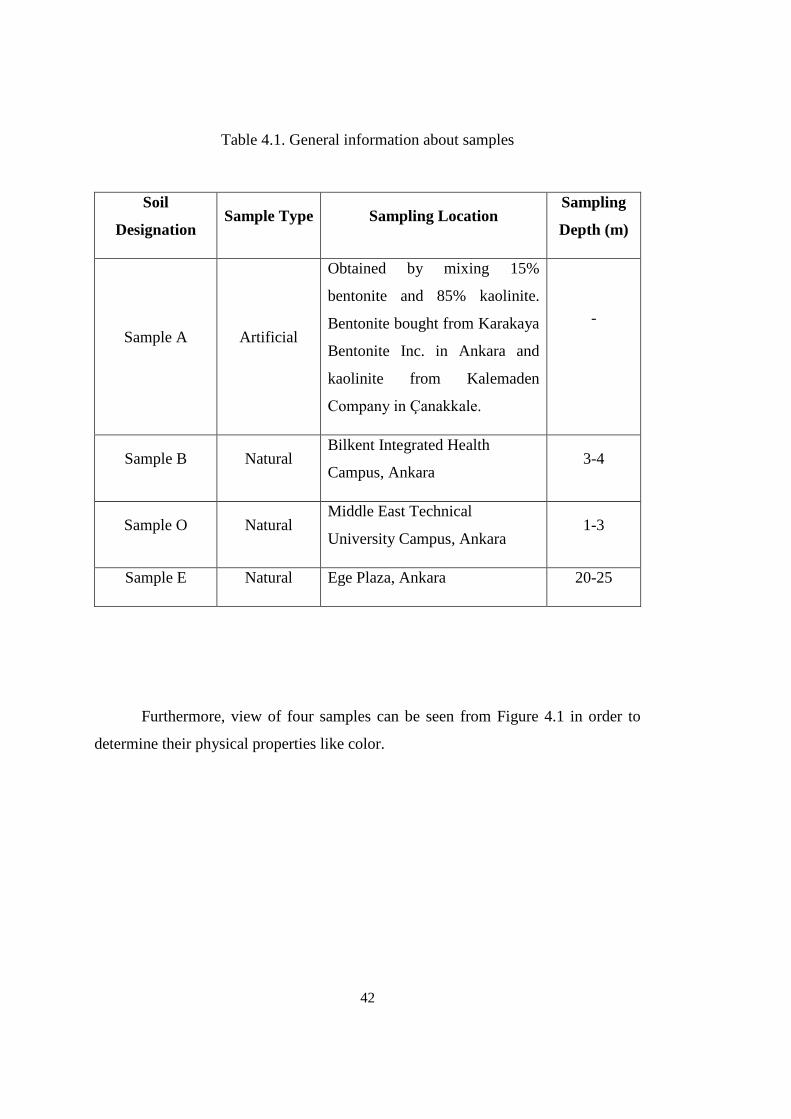
Furthermore, view of four samples can be seen from Figure 4.1 in order to
determine their physical properties like color.
43
Figure 4.1. View of samples (1-Sample A, 2-Sample B, 3-Sample O, 4-Sample E)
4.3. Properties of Soil Samples
Maximum dry density, optimum water content, specific gravity, Atterberg
limits; liquid limit (LL), plastic limit (PL), plasticity index (PI) and shrinkage limit
(SL) values were determined in order to obtain the index properties of each sample.
Additionally, hydrometer test and sieve analysis were performed for each sample.
Standard test methods that were used to identify the soil samples are presented in
Table 4.2.
1 2 3 4
44
Table 4.2. Standard test methods for soil specimen identification
Index Properties Utilized Test Method
Optimum water content and
maximum dry density
Harvard Miniature Compaction (for Sample A)
Test Methods for Laboratory Compaction
Characteristics of Soil Using Standard Effort (for
Samples B, O and E)---ASTM D698
Specific Gravity
Test Methods for Specific Gravity of Soil Solids
by Water Pycnometer (for all samples)--- ASTM
D854
Sieve Analysis
Test Methods for Particle Size Distribution
(Gradation) of Soils Using Sieve Analysis (for
Samples B, O and E)--- ASTM D6913
Particle Sedimentation Test Methods for Particle-Size Analysis of Soils
(for all samples)--- ASTM D422
Liquid Limit, Plastic Limit
and Plasticity Index
Test Methods for Liquid Limit, Plastic Limit and
Plasticity Index of Soils (for all samples)--- ASTM
D4318
Shrinkage Limit Test Methods for Shrinkage Factors of Soils by the
Mercury Method (for all samples)--- ASTM D427
Grain size distribution curves for all soil samples are given in Figure 4.2.
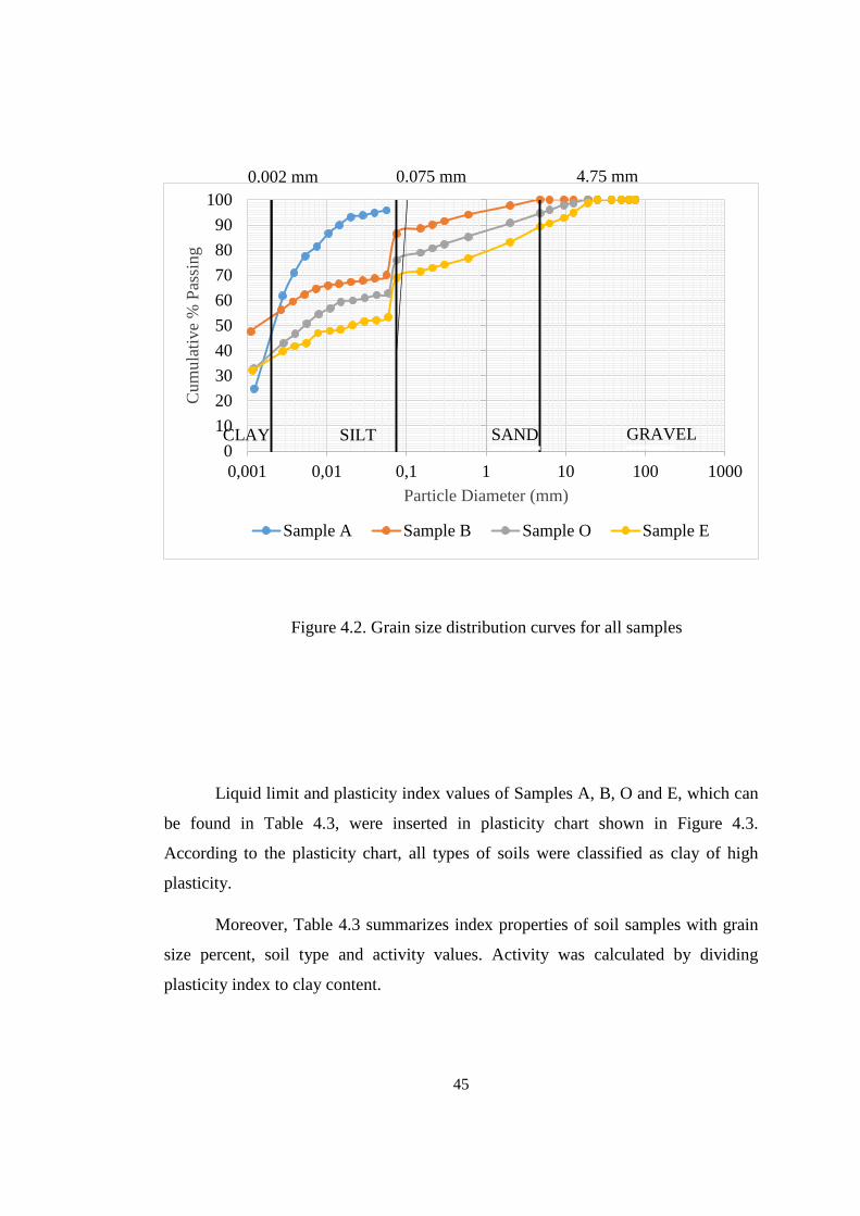
45
Figure 4.2. Grain size distribution curves for all samples
Liquid limit and plasticity index values of Samples A, B, O and E, which can
be found in Table 4.3, were inserted in plasticity chart shown in Figure 4.3.
According to the plasticity chart, all types of soils were classified as clay of high
plasticity.
Moreover, Table 4.3 summarizes index properties of soil samples with grain
size percent, soil type and activity values. Activity was calculated by dividing
plasticity index to clay content.
0
10
20
30
40
50
60
70
80
90
100
0,001 0,01 0,1 1 10 100 1000
Cum
ula
tive
% P
assi
ng
Particle Diameter (mm)
Sample A Sample B Sample O Sample E
0.002 mm 0.075 mm 4.75 mm
CLAY SILT
CLAY
SAND
CLAY
GRAVEL
CLAY
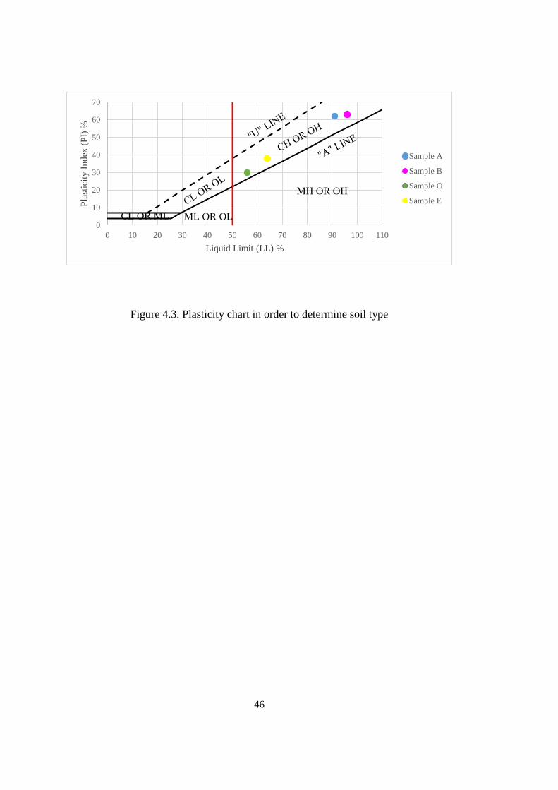
46
Figure 4.3. Plasticity chart in order to determine soil type
0
10
20
30
40
50
60
70
0 10 20 30 40 50 60 70 80 90 100 110
Pla
stic
ity I
nd
ex (
PI)
%
Liquid Limit (LL) %
Sample A
Sample B
Sample O
Sample E
CL OR ML
MH OR OH
ML OR OL
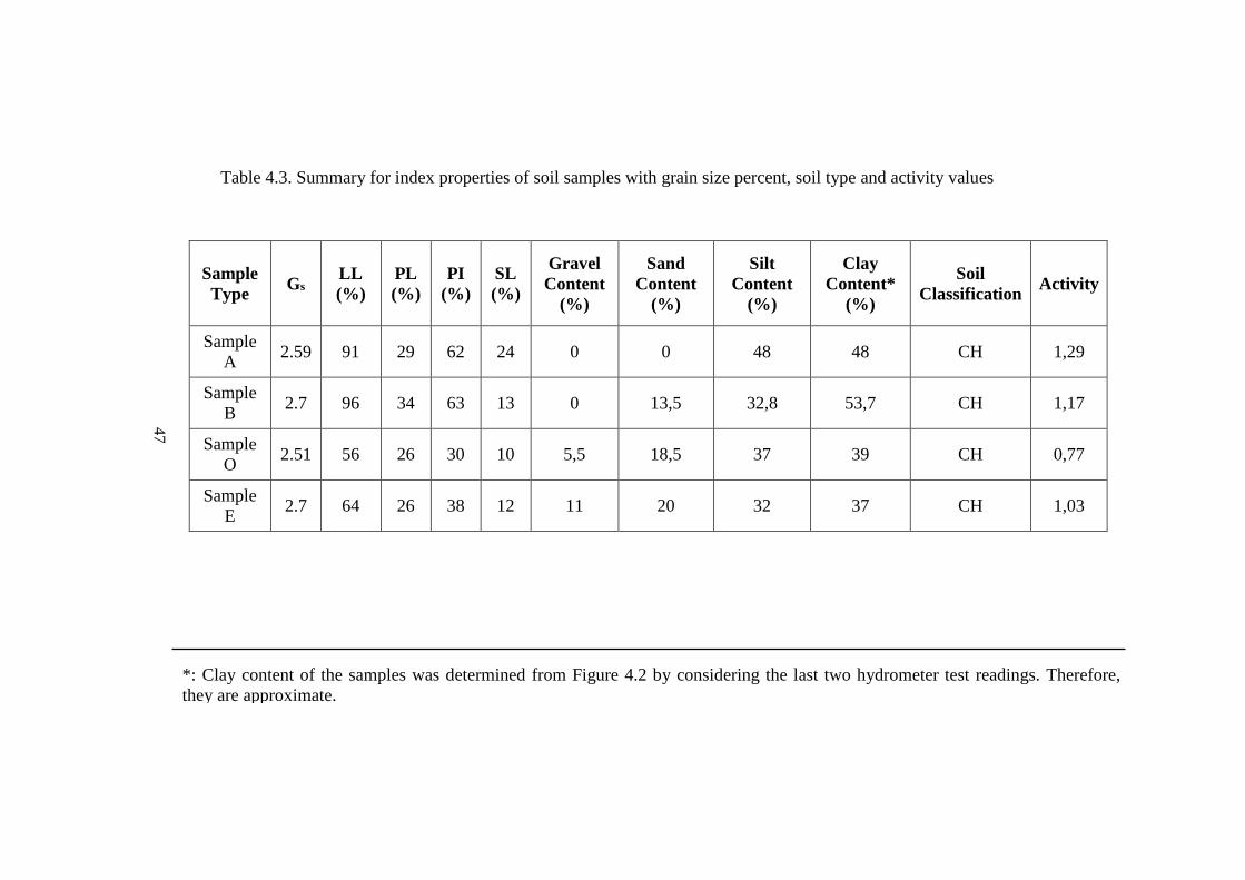
47
Table 4.3. Summary for index properties of soil samples with grain size percent, soil type and activity values
Sample
Type Gs
LL
(%)
PL
(%)
PI
(%)
SL
(%)
Gravel
Content
(%)
Sand
Content
(%)
Silt
Content
(%)
Clay
Content*
(%)
Soil
Classification Activity
Sample
A 2.59 91 29 62 24 0 0 48 48 CH 1,29
Sample
B 2.7 96 34 63 13 0 13,5 32,8 53,7 CH 1,17
Sample
O 2.51 56 26 30 10 5,5 18,5 37 39 CH 0,77
Sample
E 2.7 64 26 38 12 11 20 32 37 CH 1,03
*: Clay content of the samples was determined from Figure 4.2 by considering the last two hydrometer test readings. Therefore,
they are approximate.
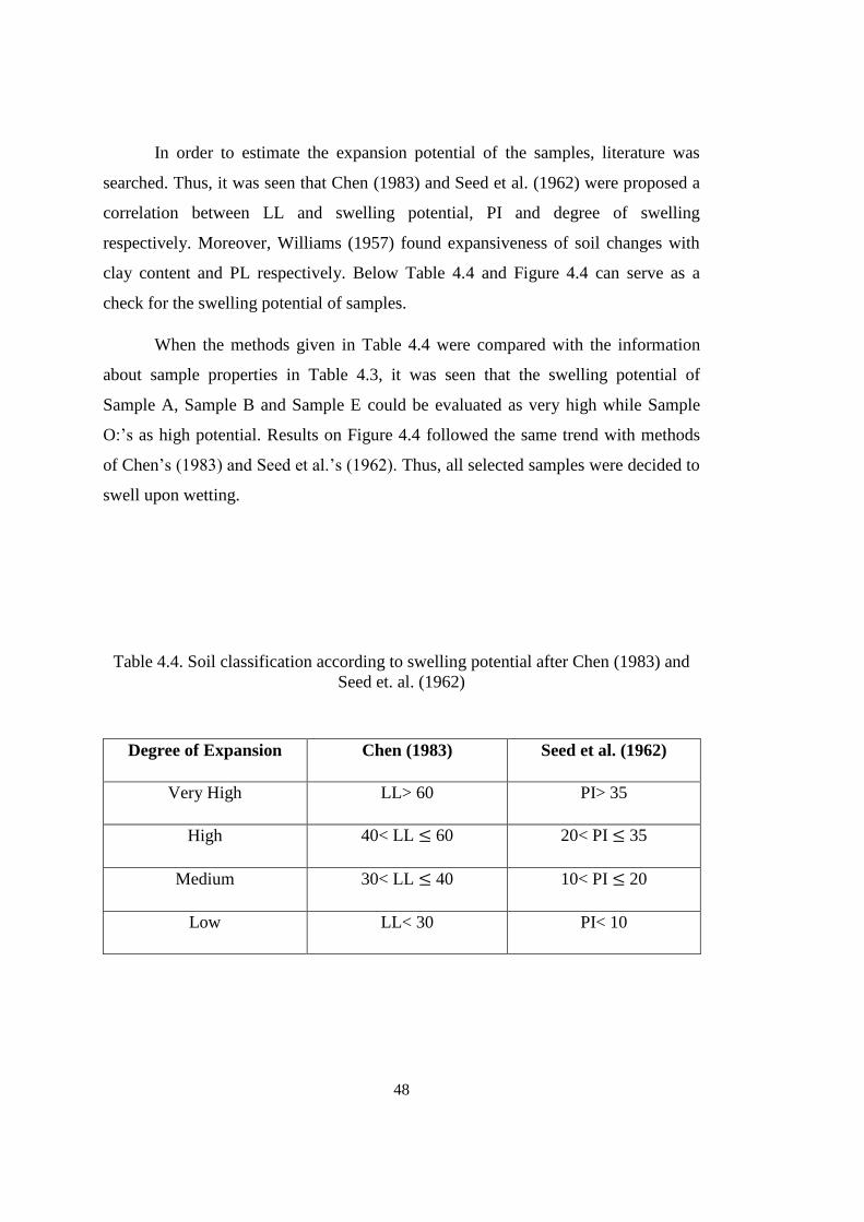
48
In order to estimate the expansion potential of the samples, literature was
searched. Thus, it was seen that Chen (1983) and Seed et al. (1962) were proposed a
correlation between LL and swelling potential, PI and degree of swelling
respectively. Moreover, Williams (1957) found expansiveness of soil changes with
clay content and PL respectively. Below Table 4.4 and Figure 4.4 can serve as a
check for the swelling potential of samples.
When the methods given in Table 4.4 were compared with the information
about sample properties in Table 4.3, it was seen that the swelling potential of
Sample A, Sample B and Sample E could be evaluated as very high while Sample
O:’s as high potential. Results on Figure 4.4 followed the same trend with methods
of Chen’s (1983) and Seed et al.’s (1962). Thus, all selected samples were decided to
swell upon wetting.
Table 4.4. Soil classification according to swelling potential after Chen (1983) and
Seed et. al. (1962)
Degree of Expansion Chen (1983) Seed et al. (1962)
Very High LL> 60 PI> 35
High 40< LL ≤ 60 20< PI ≤ 35
Medium 30< LL ≤ 40 10< PI ≤ 20
Low LL< 30 PI< 10
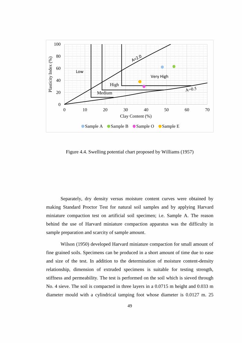
49
Figure 4.4. Swelling potential chart proposed by Williams (1957)
Separately, dry density versus moisture content curves were obtained by
making Standard Proctor Test for natural soil samples and by applying Harvard
miniature compaction test on artificial soil specimen; i.e. Sample A. The reason
behind the use of Harvard miniature compaction apparatus was the difficulty in
sample preparation and scarcity of sample amount.
Wilson (1950) developed Harvard miniature compaction for small amount of
fine grained soils. Specimens can be produced in a short amount of time due to ease
and size of the test. In addition to the determination of moisture content-density
relationship, dimension of extruded specimens is suitable for testing strength,
stiffness and permeability. The test is performed on the soil which is sieved through
No. 4 sieve. The soil is compacted in three layers in a 0.0715 m height and 0.033 m
diameter mould with a cylindrical tamping foot whose diameter is 0.0127 m. 25
0
20
40
60
80
100
0 10 20 30 40 50 60 70
Pla
stic
ity I
nd
ex (
%)
Clay Content (%)
Sample A Sample B Sample O Sample E
LowVery High
High
Medium
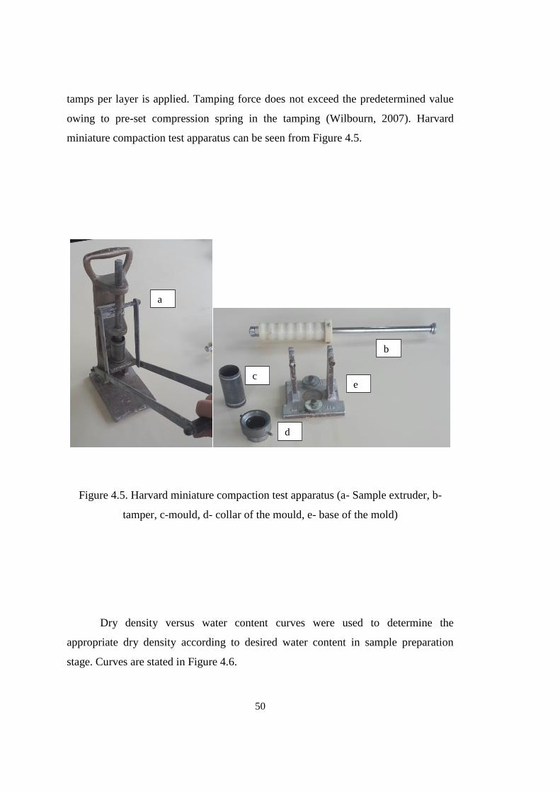
50
tamps per layer is applied. Tamping force does not exceed the predetermined value
owing to pre-set compression spring in the tamping (Wilbourn, 2007). Harvard
miniature compaction test apparatus can be seen from Figure 4.5.
Figure 4.5. Harvard miniature compaction test apparatus (a- Sample extruder, b-
tamper, c-mould, d- collar of the mould, e- base of the mold)
Dry density versus water content curves were used to determine the
appropriate dry density according to desired water content in sample preparation
stage. Curves are stated in Figure 4.6.
a
b
c
b e
b
d
b
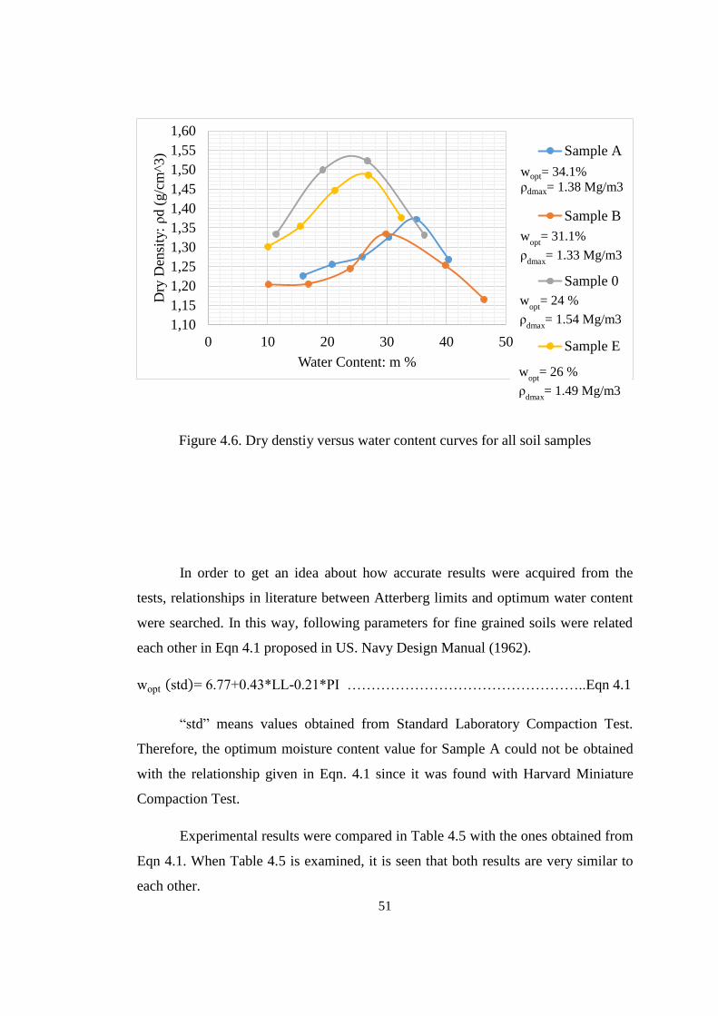
51
Figure 4.6. Dry denstiy versus water content curves for all soil samples
In order to get an idea about how accurate results were acquired from the
tests, relationships in literature between Atterberg limits and optimum water content
were searched. In this way, following parameters for fine grained soils were related
each other in Eqn 4.1 proposed in US. Navy Design Manual (1962).
wopt (std)= 6.77+0.43*LL-0.21*PI …………………………………………..Eqn 4.1
“std” means values obtained from Standard Laboratory Compaction Test.
Therefore, the optimum moisture content value for Sample A could not be obtained
with the relationship given in Eqn. 4.1 since it was found with Harvard Miniature
Compaction Test.
Experimental results were compared in Table 4.5 with the ones obtained from
Eqn 4.1. When Table 4.5 is examined, it is seen that both results are very similar to
each other.
1,10
1,15
1,20
1,25
1,30
1,35
1,40
1,45
1,50
1,55
1,60
0 10 20 30 40 50
Dry
Den
sity
: ρd (
g/c
m^3)
Water Content: m %
Sample A
Sample B
Sample 0
Sample E
wopt= 34.1%
ρdmax= 1.38 Mg/m3
wopt
= 26 %
ρdmax
= 1.49 Mg/m3
wopt
= 31.1%
ρdmax
= 1.33 Mg/m3
wopt
= 24 %
ρdmax
= 1.54 Mg/m3
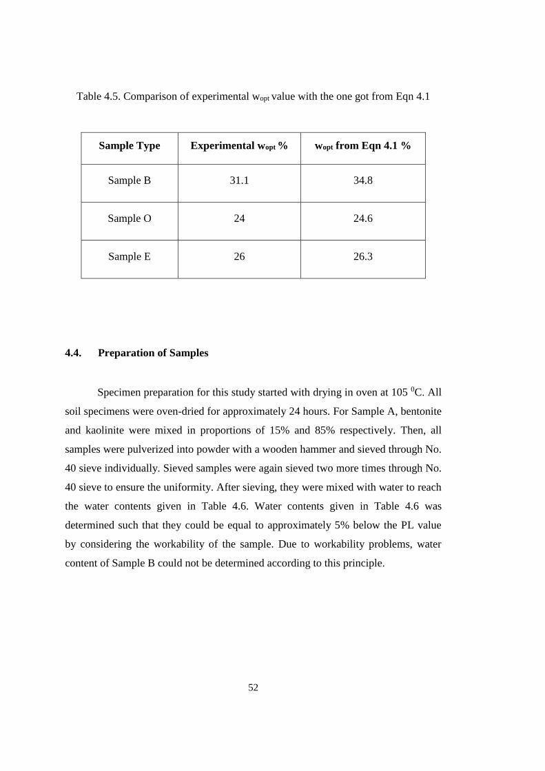
52
Table 4.5. Comparison of experimental wopt value with the one got from Eqn 4.1
Sample Type Experimental wopt % wopt from Eqn 4.1 %
Sample B 31.1 34.8
Sample O 24 24.6
Sample E 26 26.3
4.4. Preparation of Samples
Specimen preparation for this study started with drying in oven at 105 0C. All
soil specimens were oven-dried for approximately 24 hours. For Sample A, bentonite
and kaolinite were mixed in proportions of 15% and 85% respectively. Then, all
samples were pulverized into powder with a wooden hammer and sieved through No.
40 sieve individually. Sieved samples were again sieved two more times through No.
40 sieve to ensure the uniformity. After sieving, they were mixed with water to reach
the water contents given in Table 4.6. Water contents given in Table 4.6 was
determined such that they could be equal to approximately 5% below the PL value
by considering the workability of the sample. Due to workability problems, water
content of Sample B could not be determined according to this principle.
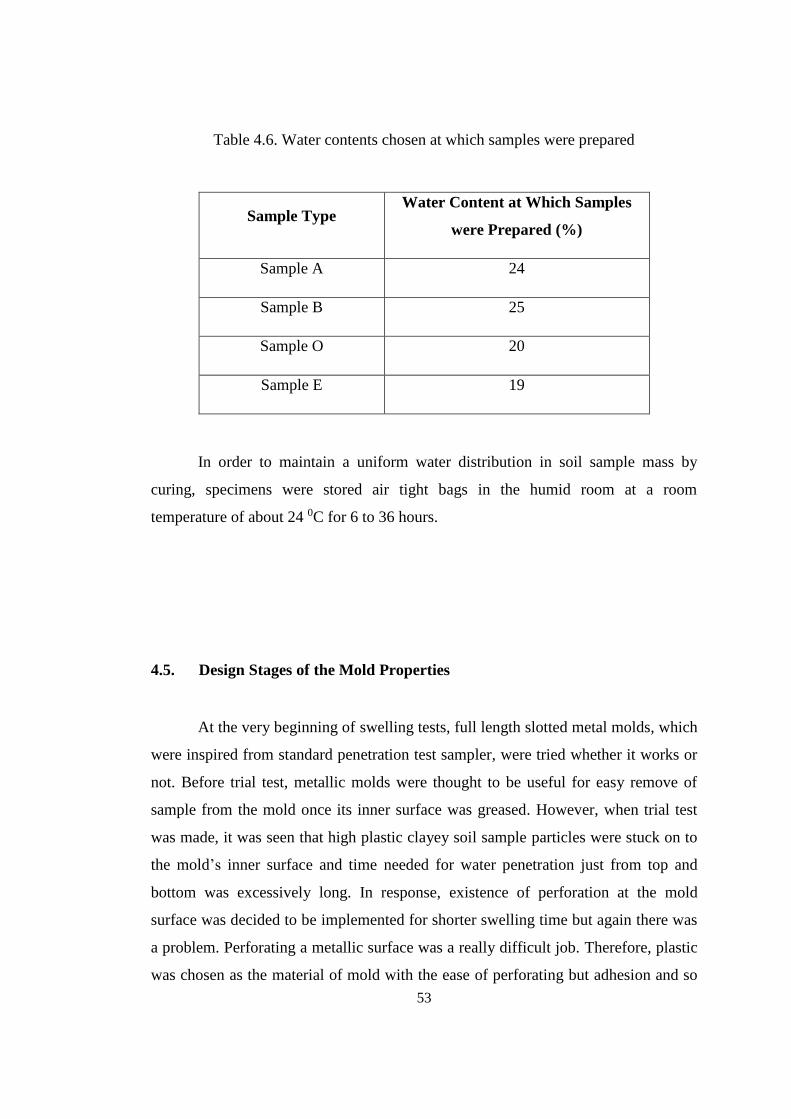
53
Table 4.6. Water contents chosen at which samples were prepared
Sample Type Water Content at Which Samples
were Prepared (%)
Sample A 24
Sample B 25
Sample O 20
Sample E 19
In order to maintain a uniform water distribution in soil sample mass by
curing, specimens were stored air tight bags in the humid room at a room
temperature of about 24 0C for 6 to 36 hours.
4.5. Design Stages of the Mold Properties
At the very beginning of swelling tests, full length slotted metal molds, which
were inspired from standard penetration test sampler, were tried whether it works or
not. Before trial test, metallic molds were thought to be useful for easy remove of
sample from the mold once its inner surface was greased. However, when trial test
was made, it was seen that high plastic clayey soil sample particles were stuck on to
the mold’s inner surface and time needed for water penetration just from top and
bottom was excessively long. In response, existence of perforation at the mold
surface was decided to be implemented for shorter swelling time but again there was
a problem. Perforating a metallic surface was a really difficult job. Therefore, plastic
was chosen as the material of mold with the ease of perforating but adhesion and so
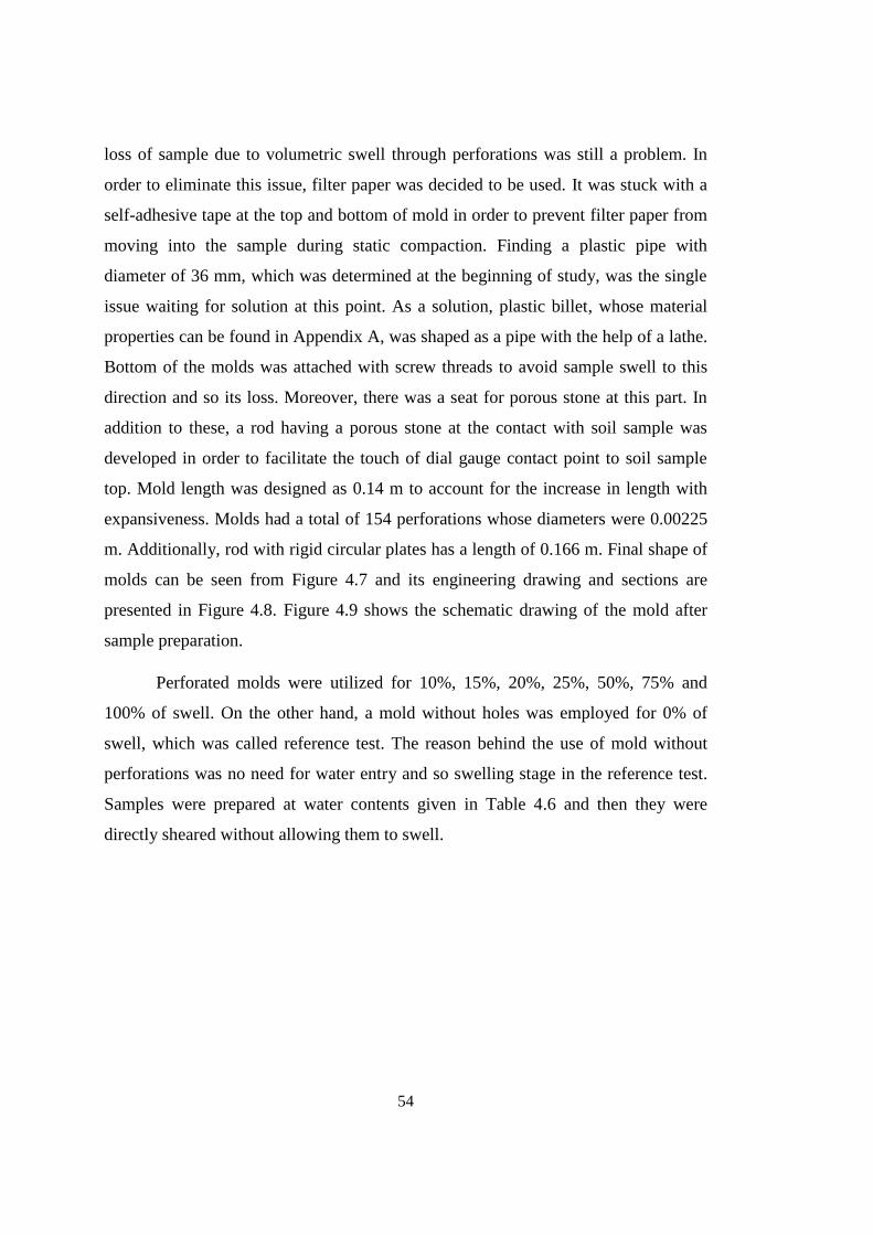
54
loss of sample due to volumetric swell through perforations was still a problem. In
order to eliminate this issue, filter paper was decided to be used. It was stuck with a
self-adhesive tape at the top and bottom of mold in order to prevent filter paper from
moving into the sample during static compaction. Finding a plastic pipe with
diameter of 36 mm, which was determined at the beginning of study, was the single
issue waiting for solution at this point. As a solution, plastic billet, whose material
properties can be found in Appendix A, was shaped as a pipe with the help of a lathe.
Bottom of the molds was attached with screw threads to avoid sample swell to this
direction and so its loss. Moreover, there was a seat for porous stone at this part. In
addition to these, a rod having a porous stone at the contact with soil sample was
developed in order to facilitate the touch of dial gauge contact point to soil sample
top. Mold length was designed as 0.14 m to account for the increase in length with
expansiveness. Molds had a total of 154 perforations whose diameters were 0.00225
m. Additionally, rod with rigid circular plates has a length of 0.166 m. Final shape of
molds can be seen from Figure 4.7 and its engineering drawing and sections are
presented in Figure 4.8. Figure 4.9 shows the schematic drawing of the mold after
sample preparation.
Perforated molds were utilized for 10%, 15%, 20%, 25%, 50%, 75% and
100% of swell. On the other hand, a mold without holes was employed for 0% of
swell, which was called reference test. The reason behind the use of mold without
perforations was no need for water entry and so swelling stage in the reference test.
Samples were prepared at water contents given in Table 4.6 and then they were
directly sheared without allowing them to swell.
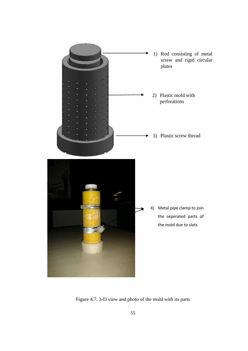
55
Figure 4.7. 3-D view and photo of the mold with its parts
1) Rod consisting of metal
screw and rigid circular
plates
2) Plastic mold with
perforations
3) Plastic screw thread
4) Metal pipe clamp to join
the seperated parts of
the mold due to slots
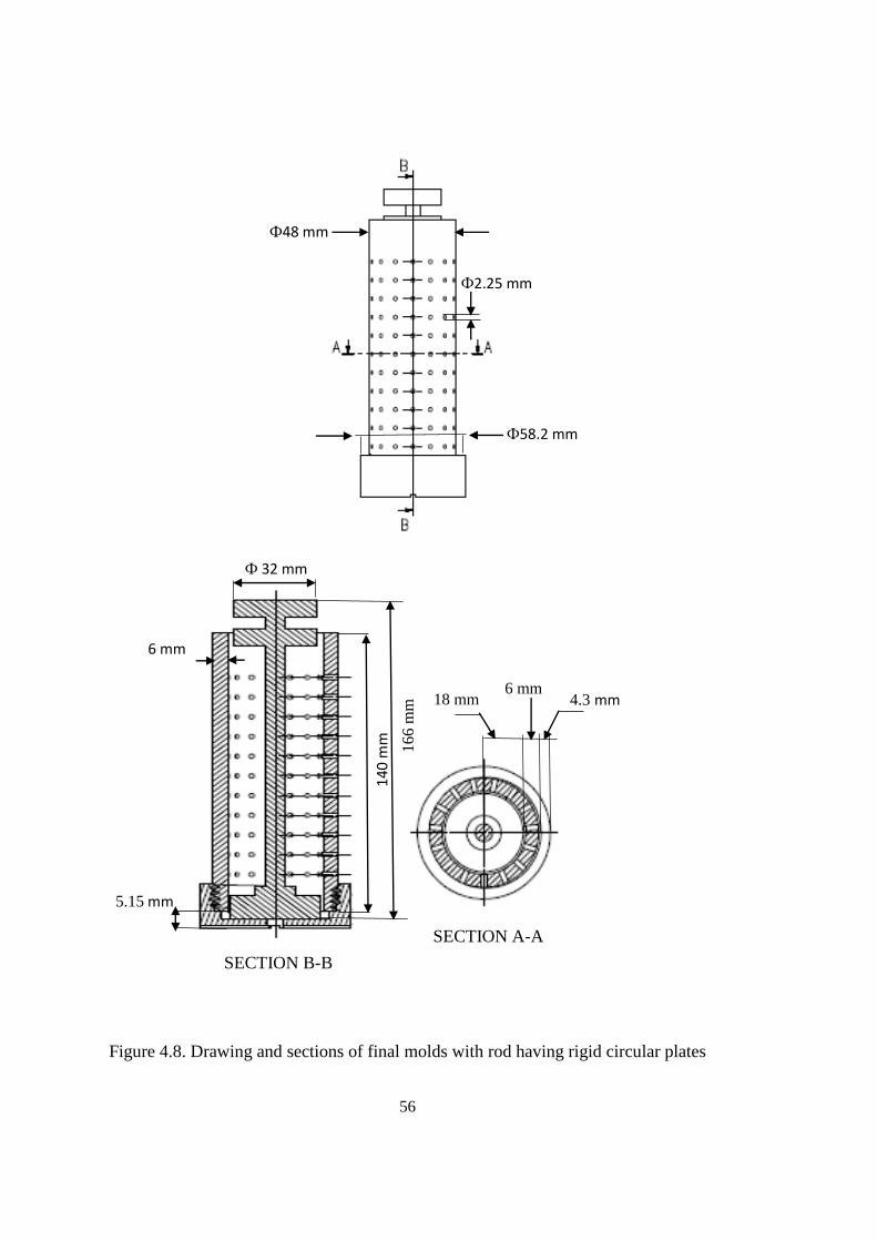
56
Figure 4.8. Drawing and sections of final molds with rod having rigid circular plates
4.3 mm 6 mm
18 mm
SECTION B-B
5.15 mm
SECTION A-A
Ф58.2 mm
Ф48 mm
Ф2.25 mm
Ф 32 mm
140
mm
166 m
m
6 mm
57
Figure 4.9. Schematic drawing of the mold after sample preparation
Rod consisting of metal screw and
rigid circular plates to facilitate the
touch of dial gauge contant point to
the top of the soil
v Self adhesive tape to prevent the
filter paper from moving into the
sample during static compaction
Filter paper that was stuck with
self adhesive tape to prevent soil
swell through the holes
Porous stone
Plastic screw thread
Plastic mold
Perforation that water
infiltrated
Hole for water penetration
from the bottom
Self adhesive tape
Filter paper
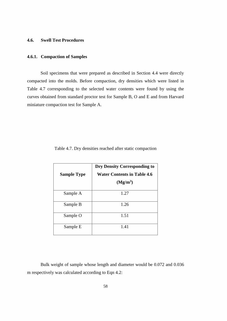
58
4.6. Swell Test Procedures
4.6.1. Compaction of Samples
Soil specimens that were prepared as described in Section 4.4 were directly
compacted into the molds. Before compaction, dry densities which were listed in
Table 4.7 corresponding to the selected water contents were found by using the
curves obtained from standard proctor test for Sample B, O and E and from Harvard
miniature compaction test for Sample A.
Table 4.7. Dry densities reached after static compaction
Sample Type
Dry Density Corresponding to
Water Contents in Table 4.6
(Mg/m3)
Sample A 1.27
Sample B 1.26
Sample O 1.51
Sample E 1.41
Bulk weight of sample whose length and diameter would be 0.072 and 0.036
m respectively was calculated according to Eqn 4.2:
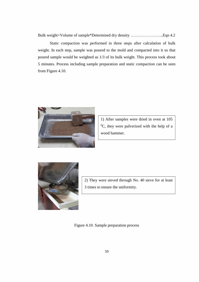
59
Bulk weight=Volume of sample*Determined dry density ……….…………...Eqn 4.2
Static compaction was performed in three steps after calculation of bulk
weight. In each step, sample was poured to the mold and compacted into it so that
poured sample would be weighted as 1/3 of its bulk weight. This process took about
5 minutes. Process including sample preparation and static compaction can be seen
from Figure 4.10.
Figure 4.10. Sample preparation process
1) After samples were dried in oven at 105
0C, they were pulverized with the help of a
wood hammer.
2) They were sieved through No. 40 sieve for at least
3 times to ensure the uniformity.
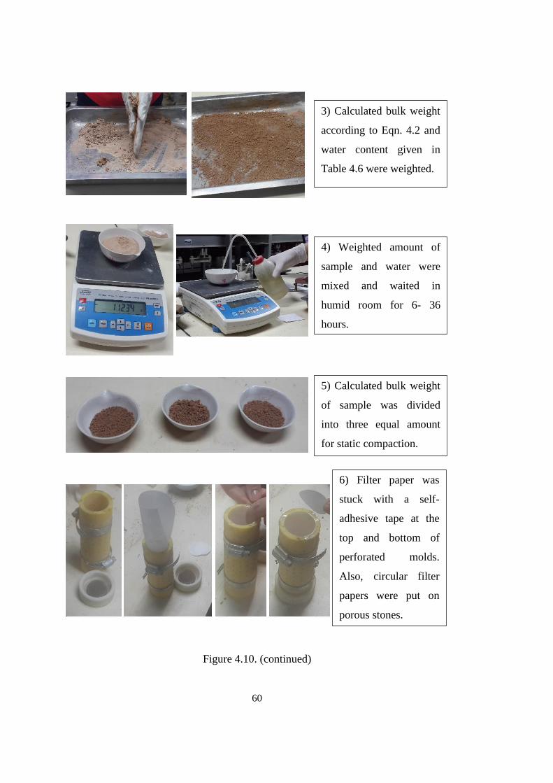
60
Figure 4.10. (continued)
3) Calculated bulk weight
according to Eqn. 4.2 and
water content given in
Table 4.6 were weighted.
4) Weighted amount of
sample and water were
mixed and waited in
humid room for 6- 36
hours.
5) Calculated bulk weight
of sample was divided
into three equal amount
for static compaction.
6) Filter paper was
stuck with a self-
adhesive tape at the
top and bottom of
perforated molds.
Also, circular filter
papers were put on
porous stones.
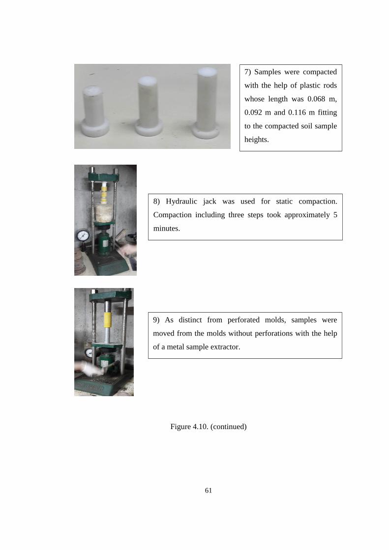
61
Figure 4.10. (continued)
7) Samples were compacted
with the help of plastic rods
whose length was 0.068 m,
0.092 m and 0.116 m fitting
to the compacted soil sample
heights.
8) Hydraulic jack was used for static compaction.
Compaction including three steps took approximately 5
minutes.
9) As distinct from perforated molds, samples were
moved from the molds without perforations with the help
of a metal sample extractor.
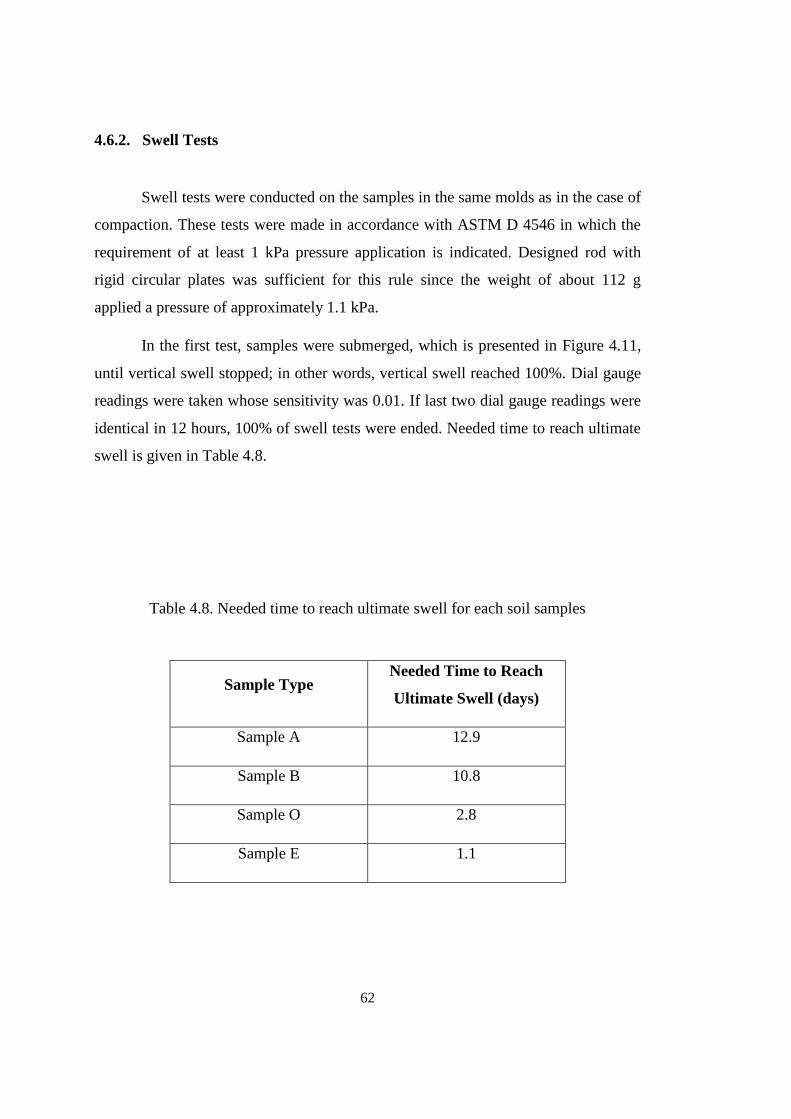
62
4.6.2. Swell Tests
Swell tests were conducted on the samples in the same molds as in the case of
compaction. These tests were made in accordance with ASTM D 4546 in which the
requirement of at least 1 kPa pressure application is indicated. Designed rod with
rigid circular plates was sufficient for this rule since the weight of about 112 g
applied a pressure of approximately 1.1 kPa.
In the first test, samples were submerged, which is presented in Figure 4.11,
until vertical swell stopped; in other words, vertical swell reached 100%. Dial gauge
readings were taken whose sensitivity was 0.01. If last two dial gauge readings were
identical in 12 hours, 100% of swell tests were ended. Needed time to reach ultimate
swell is given in Table 4.8.
Table 4.8. Needed time to reach ultimate swell for each soil samples
Sample Type Needed Time to Reach
Ultimate Swell (days)
Sample A 12.9
Sample B 10.8
Sample O 2.8
Sample E 1.1
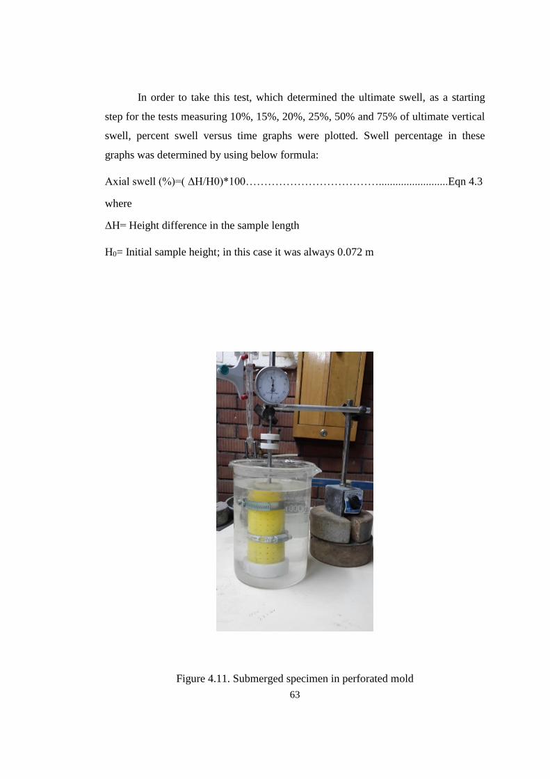
63
In order to take this test, which determined the ultimate swell, as a starting
step for the tests measuring 10%, 15%, 20%, 25%, 50% and 75% of ultimate vertical
swell, percent swell versus time graphs were plotted. Swell percentage in these
graphs was determined by using below formula:
Axial swell (%)=( ΔH/H0)*100……………………………….........................Eqn 4.3
where
ΔH= Height difference in the sample length
H0= Initial sample height; in this case it was always 0.072 m
Figure 4.11. Submerged specimen in perforated mold
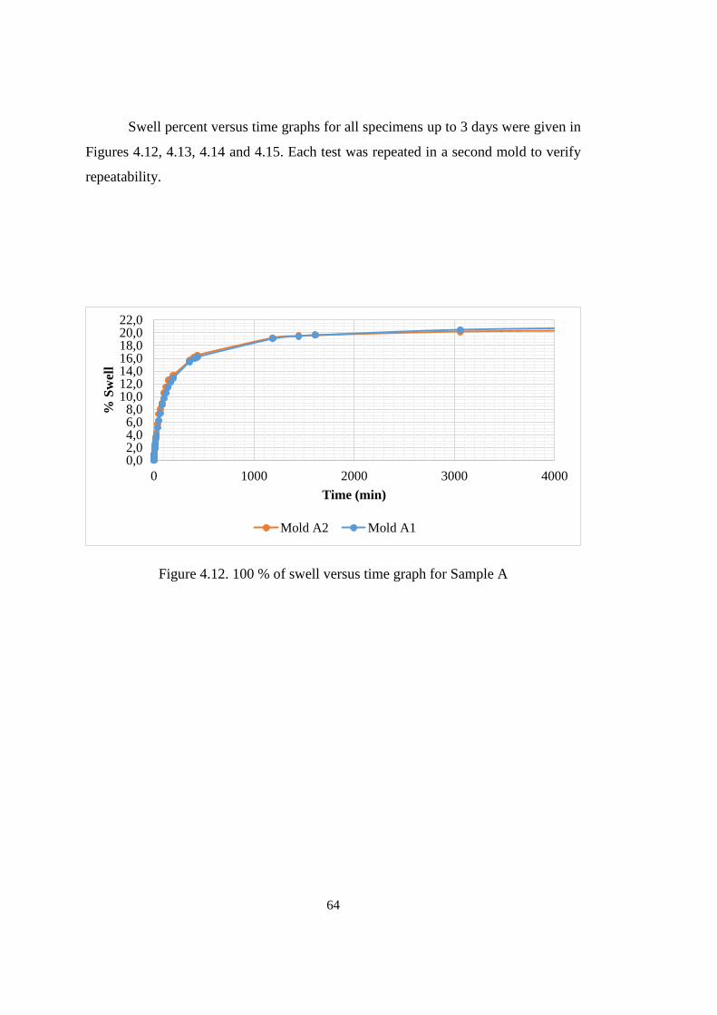
64
Swell percent versus time graphs for all specimens up to 3 days were given in
Figures 4.12, 4.13, 4.14 and 4.15. Each test was repeated in a second mold to verify
repeatability.
Figure 4.12. 100 % of swell versus time graph for Sample A
0,02,04,06,08,0
10,012,014,016,018,020,022,0
0 1000 2000 3000 4000
% S
wel
l
Time (min)
Mold A2 Mold A1
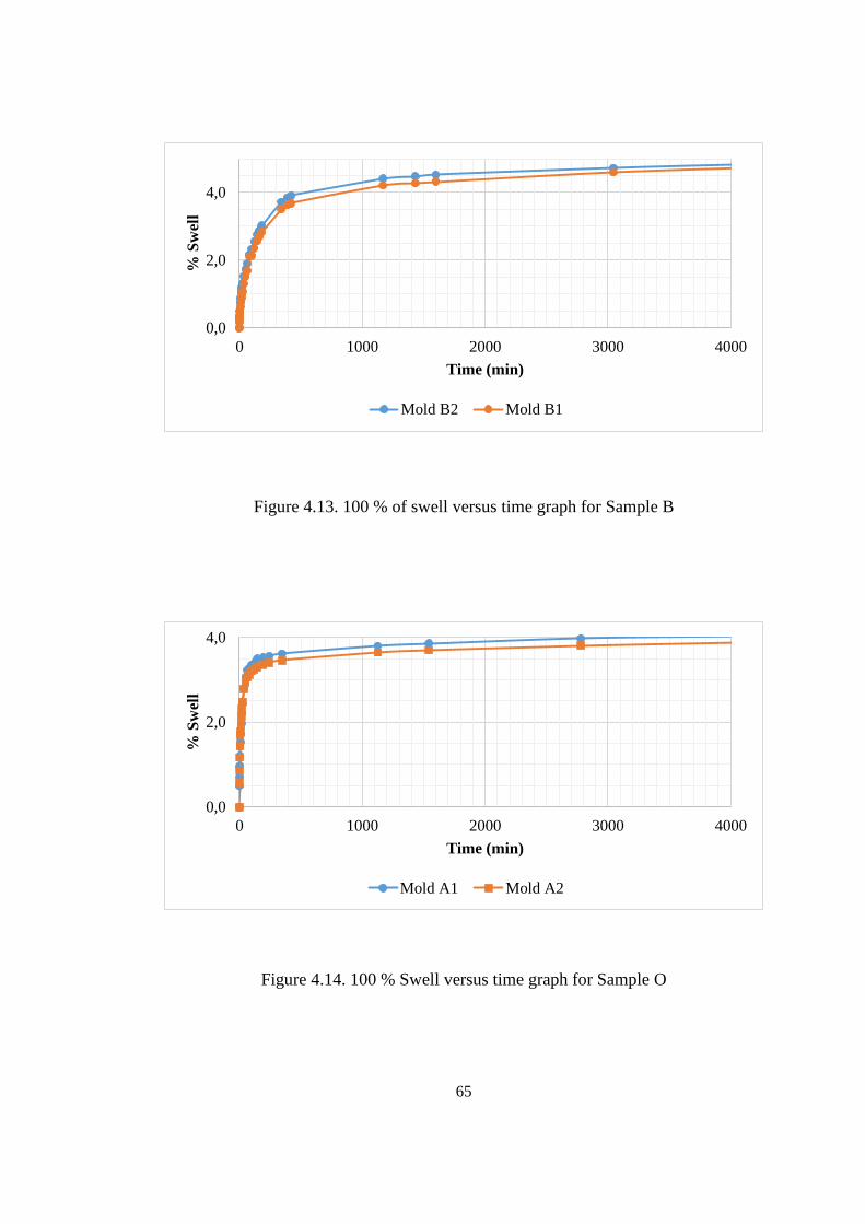
65
Figure 4.13. 100 % of swell versus time graph for Sample B
Figure 4.14. 100 % Swell versus time graph for Sample O
0,0
2,0
4,0
0 1000 2000 3000 4000
% S
wel
l
Time (min)
Mold B2 Mold B1
0,0
2,0
4,0
0 1000 2000 3000 4000
% S
wel
l
Time (min)
Mold A1 Mold A2
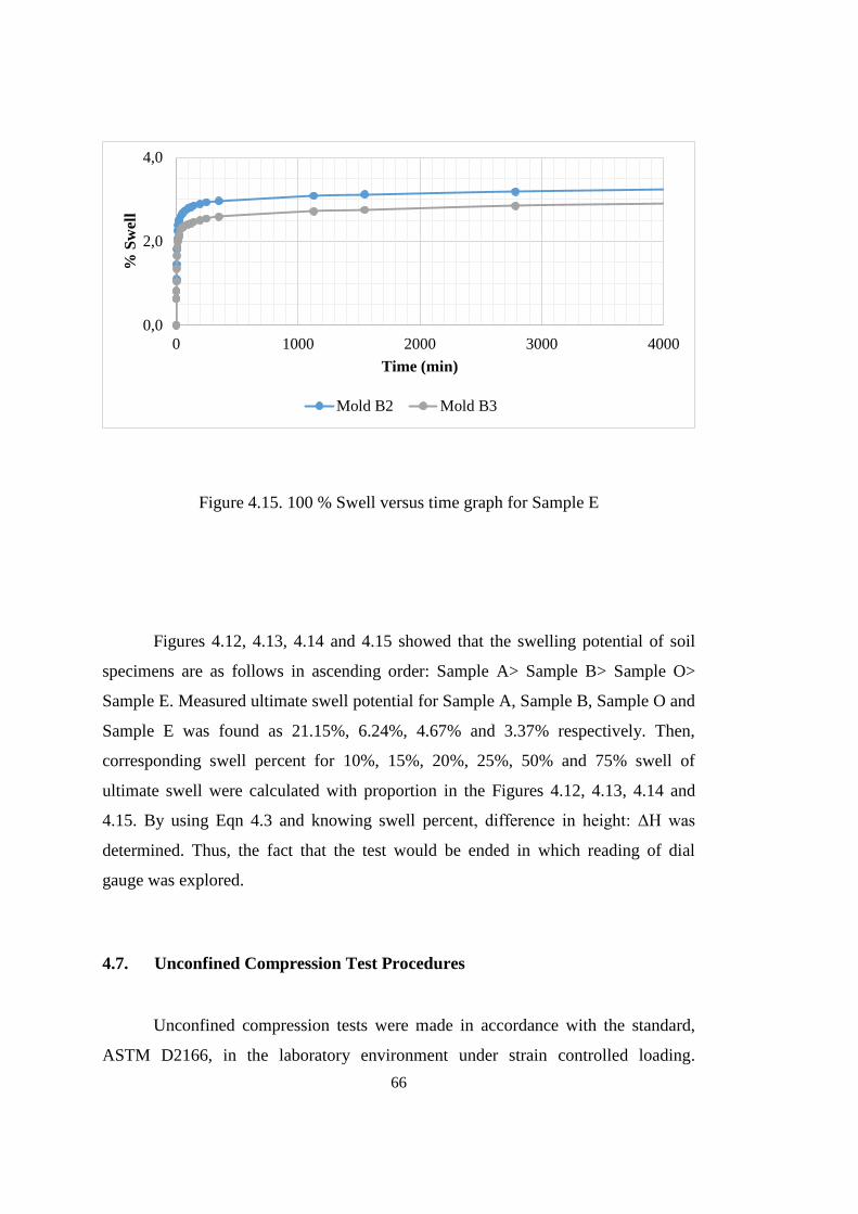
66
Figure 4.15. 100 % Swell versus time graph for Sample E
Figures 4.12, 4.13, 4.14 and 4.15 showed that the swelling potential of soil
specimens are as follows in ascending order: Sample A> Sample B> Sample O>
Sample E. Measured ultimate swell potential for Sample A, Sample B, Sample O and
Sample E was found as 21.15%, 6.24%, 4.67% and 3.37% respectively. Then,
corresponding swell percent for 10%, 15%, 20%, 25%, 50% and 75% swell of
ultimate swell were calculated with proportion in the Figures 4.12, 4.13, 4.14 and
4.15. By using Eqn 4.3 and knowing swell percent, difference in height: ΔH was
determined. Thus, the fact that the test would be ended in which reading of dial
gauge was explored.
4.7. Unconfined Compression Test Procedures
Unconfined compression tests were made in accordance with the standard,
ASTM D2166, in the laboratory environment under strain controlled loading.
0,0
2,0
4,0
0 1000 2000 3000 4000
% S
wel
l
Time (min)
Mold B2 Mold B3
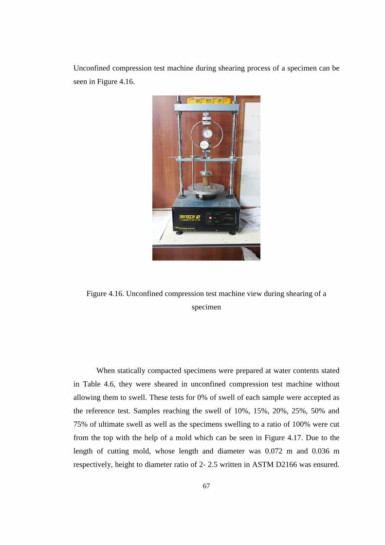
67
Unconfined compression test machine during shearing process of a specimen can be
seen in Figure 4.16.
Figure 4.16. Unconfined compression test machine view during shearing of a
specimen
When statically compacted specimens were prepared at water contents stated
in Table 4.6, they were sheared in unconfined compression test machine without
allowing them to swell. These tests for 0% of swell of each sample were accepted as
the reference test. Samples reaching the swell of 10%, 15%, 20%, 25%, 50% and
75% of ultimate swell as well as the specimens swelling to a ratio of 100% were cut
from the top with the help of a mold which can be seen in Figure 4.17. Due to the
length of cutting mold, whose length and diameter was 0.072 m and 0.036 m
respectively, height to diameter ratio of 2- 2.5 written in ASTM D2166 was ensured.
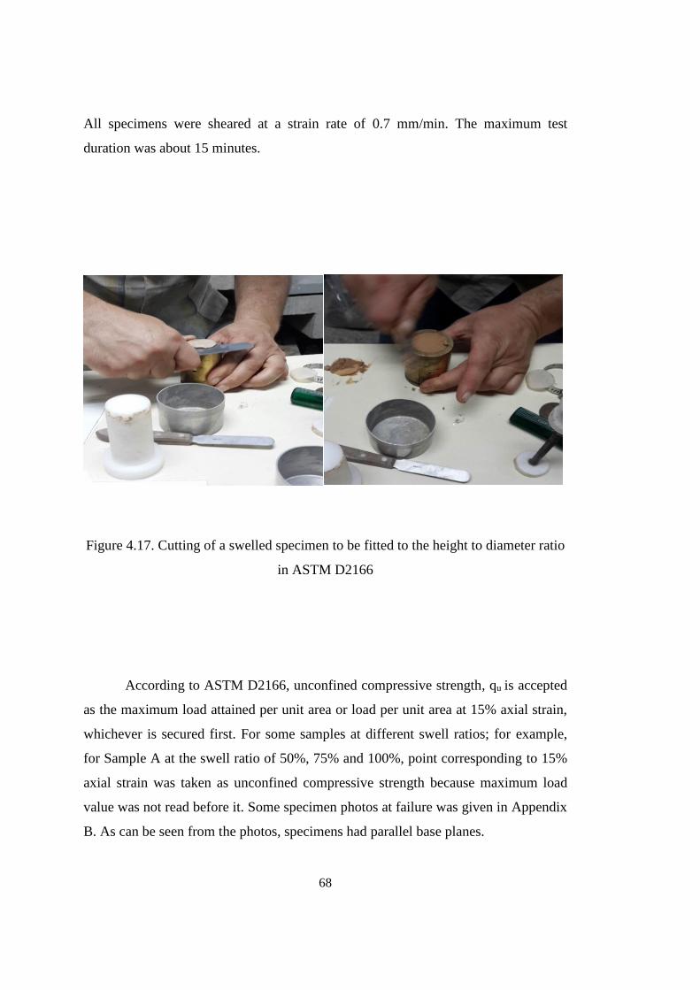
68
All specimens were sheared at a strain rate of 0.7 mm/min. The maximum test
duration was about 15 minutes.
Figure 4.17. Cutting of a swelled specimen to be fitted to the height to diameter ratio
in ASTM D2166
According to ASTM D2166, unconfined compressive strength, qu is accepted
as the maximum load attained per unit area or load per unit area at 15% axial strain,
whichever is secured first. For some samples at different swell ratios; for example,
for Sample A at the swell ratio of 50%, 75% and 100%, point corresponding to 15%
axial strain was taken as unconfined compressive strength because maximum load
value was not read before it. Some specimen photos at failure was given in Appendix
B. As can be seen from the photos, specimens had parallel base planes.
69
For each sample type and swell step; i.e. 0%, 10%, 15%, 20%, 25%, 50%,
75%, 100% of swell, stress-strain curves were obtained from unconfined
compression test. In addition to these curves, undrained shear strength, unconfined
compressive stress and undrained elastic modulus were stated in the following
Sections 4.7.1, 4.7.2., 4.7.3. and 4.7.4. Briaud (2001) stated that one can obtain a
modulus from a stress-strain curve for the case where confining pressure is zero such
as unconfined compression test on clay or typical concrete cylinder test. Based on
this statement, undrained elastic modulus was calculated with secant method by
drawing a line from the origin to the point at 1/2 of unconfined compressive strength.
4.7.1. Unconfined Compression Test Result for Sample A
Stress- strain curves with undrained elastic modulus lines were given in
Figures 4.18, 4.19, 4.20, 4.21, 4.22, 4.23, 4.24 and 4.25. Table 4.9 also shows clearly
the results of curves; in other words, undrained shear strength, water content and
undrained elastic modulus at 0%, 10%, 15%, 20%, 25%, 50%, 75% and 100% swell
ratios.
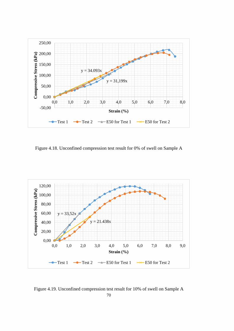
70
Figure 4.18. Unconfined compression test result for 0% of swell on Sample A
Figure 4.19. Unconfined compression test result for 10% of swell on Sample A
y = 31,199x
y = 34.093x
-50,00
0,00
50,00
100,00
150,00
200,00
250,00
0,0 1,0 2,0 3,0 4,0 5,0 6,0 7,0 8,0
Co
mp
ress
ive
Str
ess
(kP
a)
Strain (%)
Test 1 Test 2 E50 for Test 1 E50 for Test 2
y = 33,52x
y = 21.438x
0,00
20,00
40,00
60,00
80,00
100,00
120,00
0,0 1,0 2,0 3,0 4,0 5,0 6,0 7,0 8,0 9,0
Co
mp
ress
ive
Str
ess
(kP
a)
Strain (%)
Test 1 Test 2 E50 for Test 1 E50 for Test 2
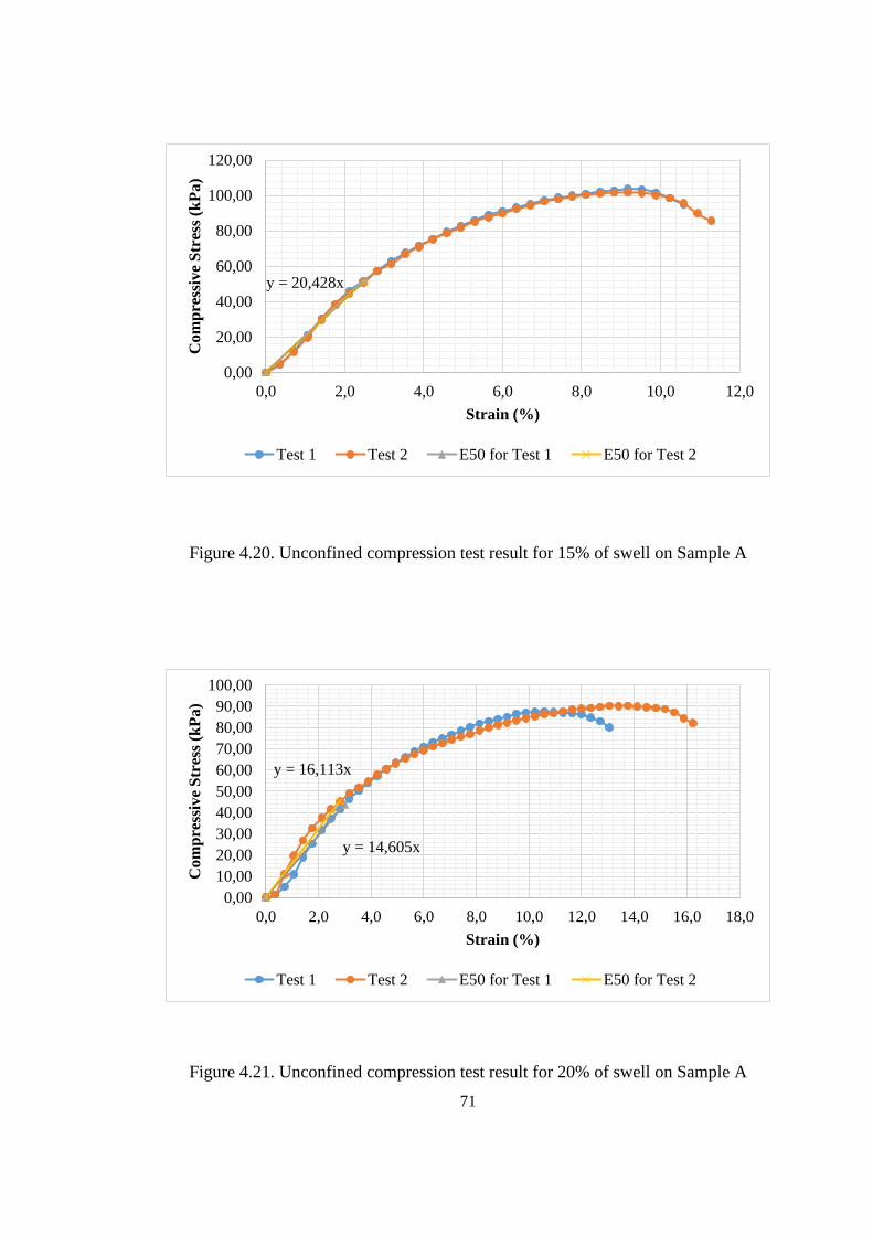
71
Figure 4.20. Unconfined compression test result for 15% of swell on Sample A
Figure 4.21. Unconfined compression test result for 20% of swell on Sample A
y = 20,428x
0,00
20,00
40,00
60,00
80,00
100,00
120,00
0,0 2,0 4,0 6,0 8,0 10,0 12,0
Co
mp
ress
ive
Str
ess
(kP
a)
Strain (%)
Test 1 Test 2 E50 for Test 1 E50 for Test 2
y = 14,605x
y = 16,113x
0,00
10,00
20,00
30,00
40,00
50,00
60,00
70,00
80,00
90,00
100,00
0,0 2,0 4,0 6,0 8,0 10,0 12,0 14,0 16,0 18,0
Co
mp
ress
ive
Str
ess
(kP
a)
Strain (%)
Test 1 Test 2 E50 for Test 1 E50 for Test 2
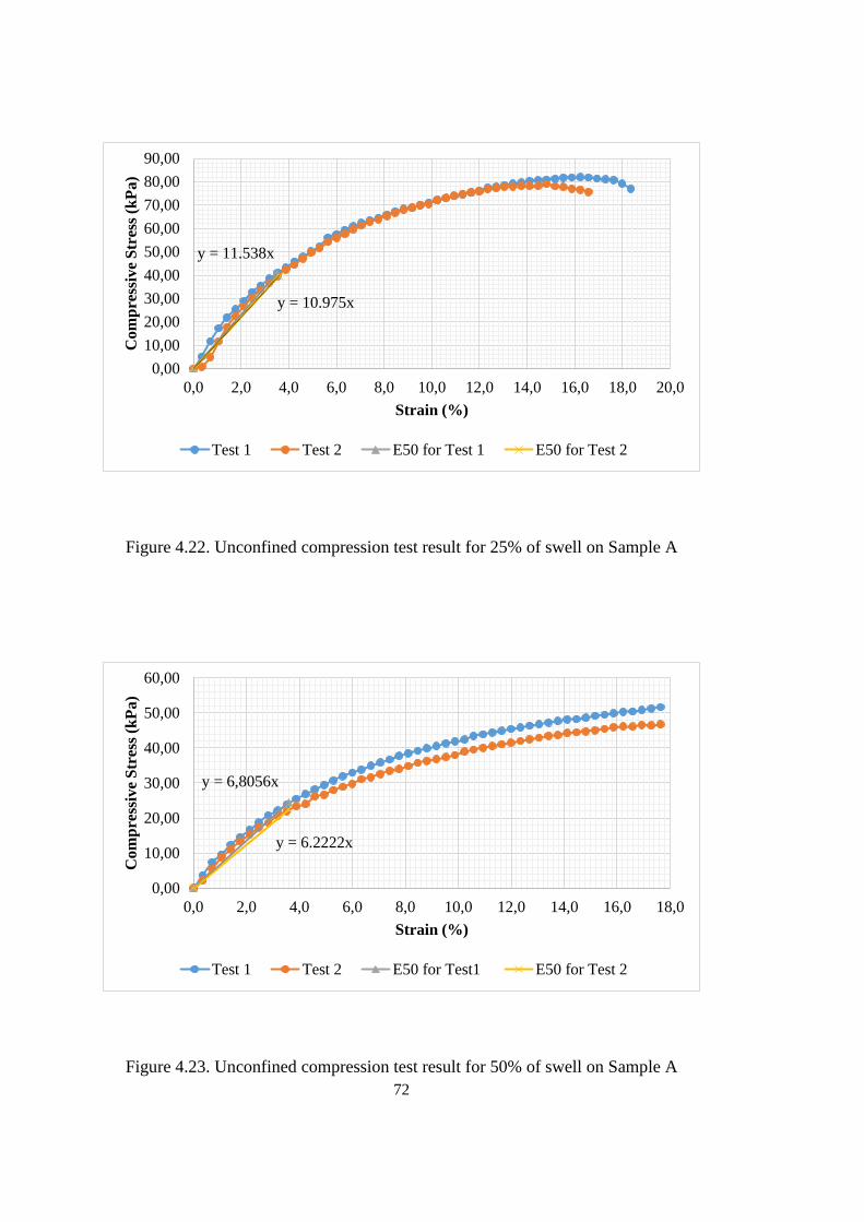
72
Figure 4.22. Unconfined compression test result for 25% of swell on Sample A
Figure 4.23. Unconfined compression test result for 50% of swell on Sample A
y = 11.538x
y = 10.975x
0,00
10,00
20,00
30,00
40,00
50,00
60,00
70,00
80,00
90,00
0,0 2,0 4,0 6,0 8,0 10,0 12,0 14,0 16,0 18,0 20,0
Co
mp
ress
ive
Str
ess
(kP
a)
Strain (%)
Test 1 Test 2 E50 for Test 1 E50 for Test 2
y = 6,8056x
y = 6.2222x
0,00
10,00
20,00
30,00
40,00
50,00
60,00
0,0 2,0 4,0 6,0 8,0 10,0 12,0 14,0 16,0 18,0
Co
mp
ress
ive
Str
ess
(kP
a)
Strain (%)
Test 1 Test 2 E50 for Test1 E50 for Test 2
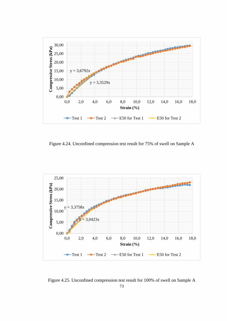
73
Figure 4.24. Unconfined compression test result for 75% of swell on Sample A
Figure 4.25. Unconfined compression test result for 100% of swell on Sample A
y = 3,3529x
y = 3,6792x
0,00
5,00
10,00
15,00
20,00
25,00
30,00
0,0 2,0 4,0 6,0 8,0 10,0 12,0 14,0 16,0 18,0
Co
mp
ress
ive
Str
ess
(kP
a)
Strain (%)
Test 1 Test 2 E50 for Test 1 E50 for Test 2
y = 3,3758x
y = 3,0423x
0,00
5,00
10,00
15,00
20,00
25,00
0,0 2,0 4,0 6,0 8,0 10,0 12,0 14,0 16,0 18,0
Co
mp
ress
ive
Str
ess
(kP
a)
Strain (%)
Test 1 Test 2 E50 for Test 1 E50 for Test 2
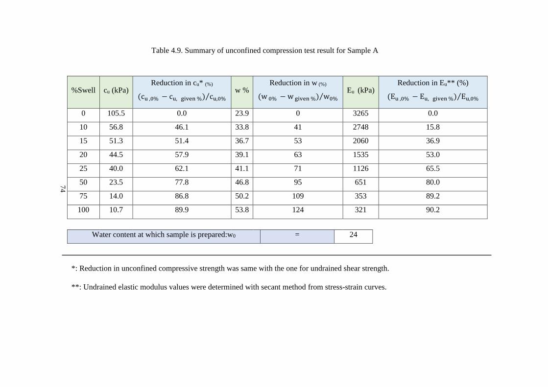
74
Table 4.9. Summary of unconfined compression test result for Sample A
%Swell cu (kPa) Reduction in cu* (%)
(cu ,0% − cu, given %) cu,0%⁄ w %
Reduction in w (%)
(w 0% − w given %) w0%⁄ Eu (kPa)
Reduction in Eu** (%)
(Eu ,0% − Eu, given %) Eu,0%⁄
0 105.5 0.0 23.9 0 3265 0.0
10 56.8 46.1 33.8 41 2748 15.8
15 51.3 51.4 36.7 53 2060 36.9
20 44.5 57.9 39.1 63 1535 53.0
25 40.0 62.1 41.1 71 1126 65.5
50 23.5 77.8 46.8 95 651 80.0
75 14.0 86.8 50.2 109 353 89.2
100 10.7 89.9 53.8 124 321 90.2
Water content at which sample is prepared:w0 = 24
*: Reduction in unconfined compressive strength was same with the one for undrained shear strength.
**: Undrained elastic modulus values were determined with secant method from stress-strain curves.
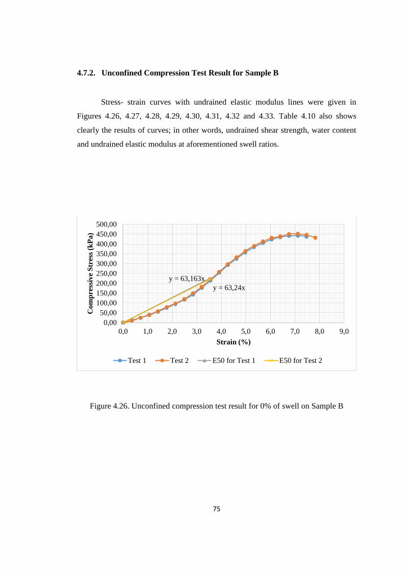
75
4.7.2. Unconfined Compression Test Result for Sample B
Stress- strain curves with undrained elastic modulus lines were given in
Figures 4.26, 4.27, 4.28, 4.29, 4.30, 4.31, 4.32 and 4.33. Table 4.10 also shows
clearly the results of curves; in other words, undrained shear strength, water content
and undrained elastic modulus at aforementioned swell ratios.
Figure 4.26. Unconfined compression test result for 0% of swell on Sample B
y = 63,24x
y = 63,163x
0,00
50,00
100,00
150,00
200,00
250,00
300,00
350,00
400,00
450,00
500,00
0,0 1,0 2,0 3,0 4,0 5,0 6,0 7,0 8,0 9,0
Com
pre
ssiv
e S
tres
s (k
Pa)
Strain (%)
Test 1 Test 2 E50 for Test 1 E50 for Test 2
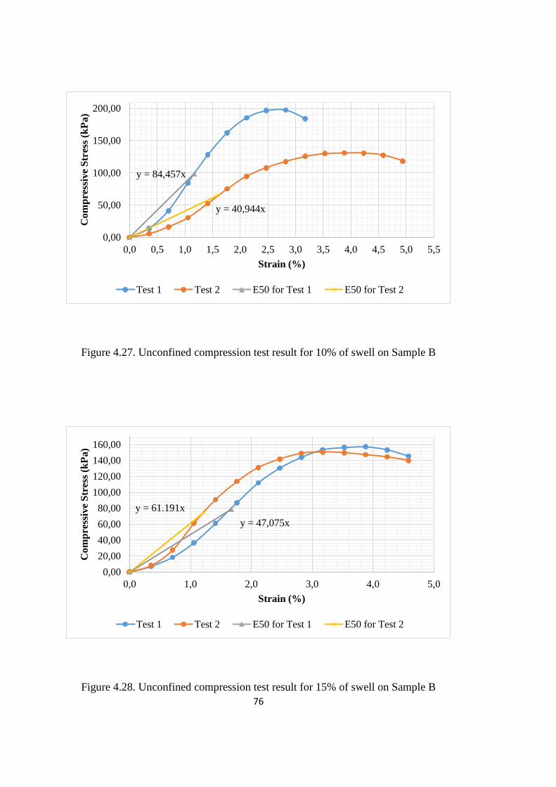
76
Figure 4.27. Unconfined compression test result for 10% of swell on Sample B
Figure 4.28. Unconfined compression test result for 15% of swell on Sample B
y = 84,457x
y = 40,944x
0,00
50,00
100,00
150,00
200,00
0,0 0,5 1,0 1,5 2,0 2,5 3,0 3,5 4,0 4,5 5,0 5,5
Co
mp
ress
ive
Str
ess
(kP
a)
Strain (%)
Test 1 Test 2 E50 for Test 1 E50 for Test 2
y = 47,075x
y = 61.191x
0,00
20,00
40,00
60,00
80,00
100,00
120,00
140,00
160,00
0,0 1,0 2,0 3,0 4,0 5,0
Co
mp
ress
ive
Str
ess
(kP
a)
Strain (%)
Test 1 Test 2 E50 for Test 1 E50 for Test 2
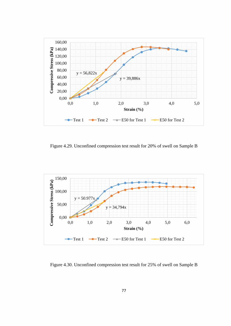
77
Figure 4.29. Unconfined compression test result for 20% of swell on Sample B
Figure 4.30. Unconfined compression test result for 25% of swell on Sample B
y = 39,886x
y = 56,822x
0,00
20,00
40,00
60,00
80,00
100,00
120,00
140,00
160,00
0,0 1,0 2,0 3,0 4,0 5,0
Co
mp
ress
ive
Str
ess
(kP
a)
Strain (%)
Test 1 Test 2 E50 for Test 1 E50 for Test 2
y = 50.977x
y = 34,794x
0,00
50,00
100,00
150,00
0,0 1,0 2,0 3,0 4,0 5,0 6,0
Com
pre
ssiv
e S
tres
s (k
Pa)
Strain (%)
Test 1 Test 2 E50 for Test 1 E50 for Test 2
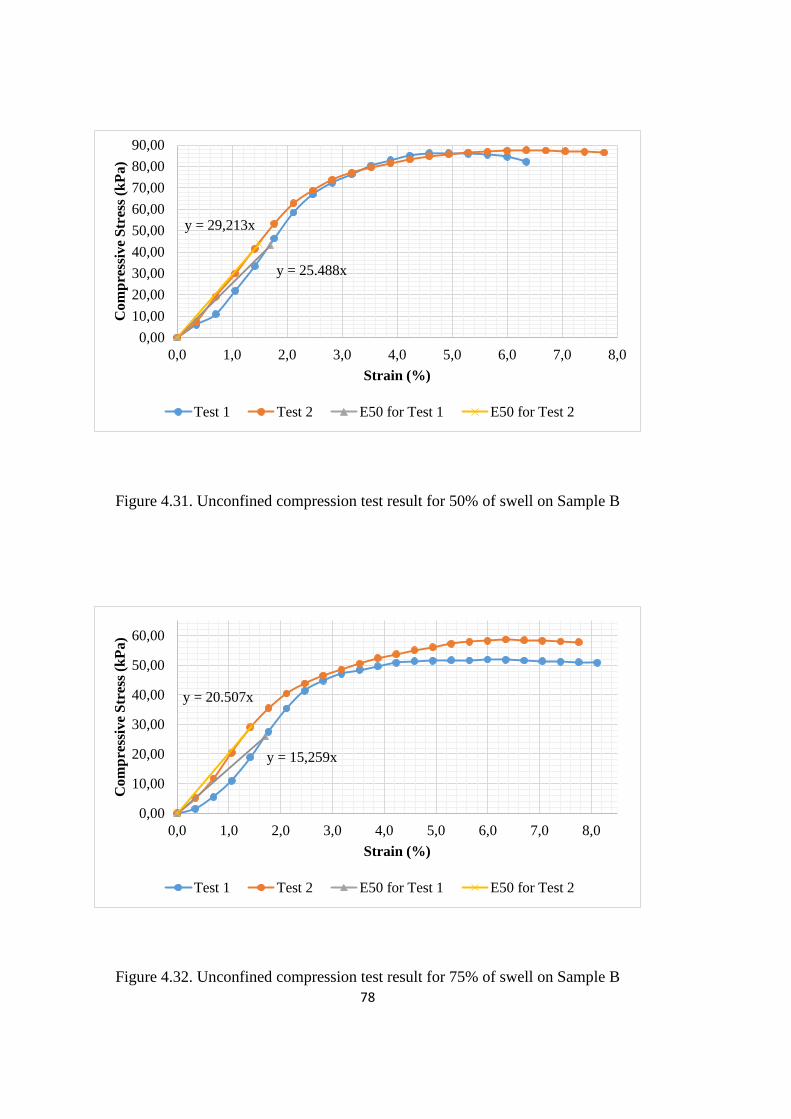
78
Figure 4.31. Unconfined compression test result for 50% of swell on Sample B
Figure 4.32. Unconfined compression test result for 75% of swell on Sample B
y = 25.488x
y = 29,213x
0,00
10,00
20,00
30,00
40,00
50,00
60,00
70,00
80,00
90,00
0,0 1,0 2,0 3,0 4,0 5,0 6,0 7,0 8,0
Co
mp
ress
ive
Str
ess
(kP
a)
Strain (%)
Test 1 Test 2 E50 for Test 1 E50 for Test 2
y = 15,259x
y = 20.507x
0,00
10,00
20,00
30,00
40,00
50,00
60,00
0,0 1,0 2,0 3,0 4,0 5,0 6,0 7,0 8,0
Co
mp
ress
ive
Str
ess
(kP
a)
Strain (%)
Test 1 Test 2 E50 for Test 1 E50 for Test 2
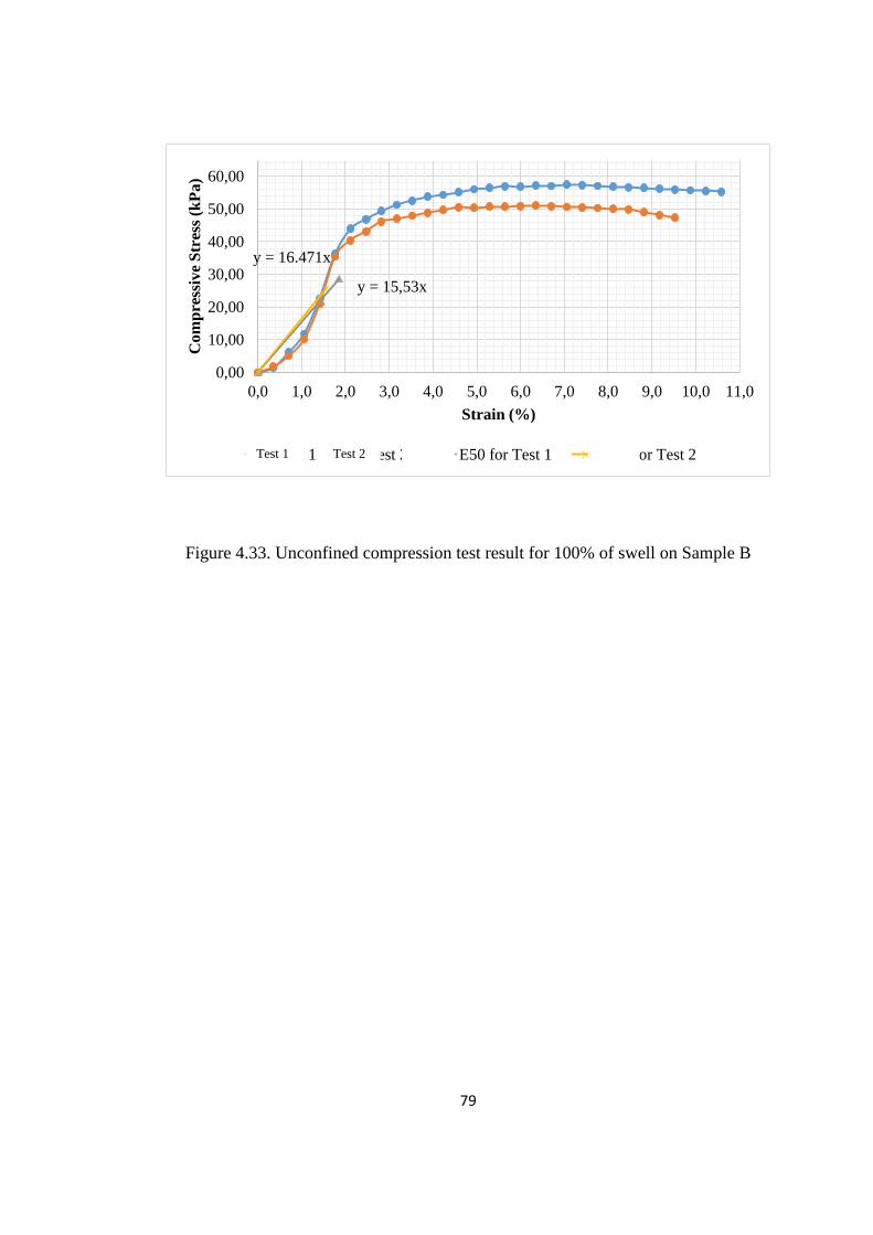
79
Figure 4.33. Unconfined compression test result for 100% of swell on Sample B
y = 15,53x
y = 16.471x
0,00
10,00
20,00
30,00
40,00
50,00
60,00
0,0 1,0 2,0 3,0 4,0 5,0 6,0 7,0 8,0 9,0 10,0 11,0
Co
mp
ress
ive
Str
ess
(kP
a)
Strain (%)
Test 1 Test 2 E50 for Test 1 E50 for Test 2
3
Test 2 Test 1

80
Table 4.10. Summary of unconfined compression test result for Sample B
%Swel
l
cu
(kPa)
Reduction in cu* (%)
(cu ,0% − cu, given %) cu,0%⁄ w %
Reduction in w (%)
(w 0% − w given %) w0%⁄ Eu (kPa)
Reduction in Eu** (%)
(Eu ,0% − Eu, given %) Eu,0%⁄
0 223.7 0.0 25.3 1 6320 0.0
10 82.2 63.3 33.8 35 6269 0.8
15 76.9 65.6 36.2 45 5414 14.3
20 72.5 67.6 36.9 48 4836 23.5
25 63.5 71.6 37.1 49 4290 32.1
50 43.4 80.6 40.5 62 2732 56.8
75 27.6 87.6 48.3 93 1786 71.7
100 27.1 87.9 48.7 95 1598 74.7
Water content at which sample is prepared:w0 = 25
80
*: Reduction in unconfined compressive strength was same with the one for undrained shear strength.
**: Undrained elastic modulus values were determined with secant method from stress-strain curves.
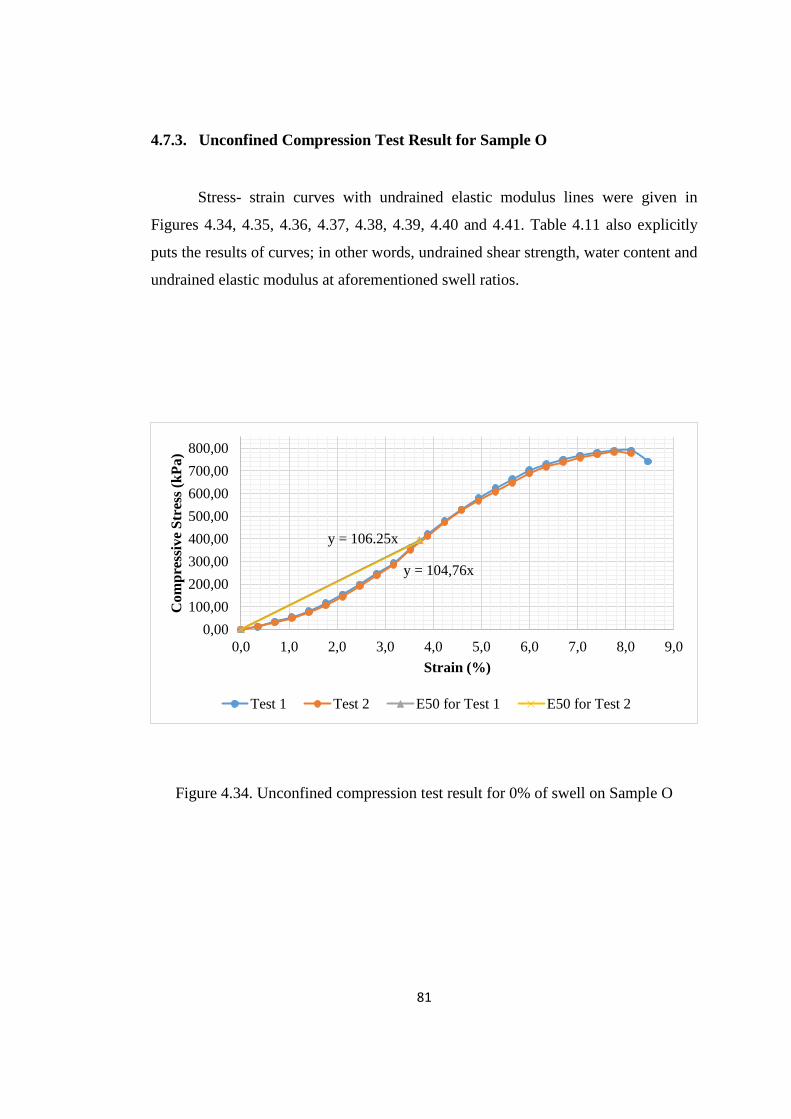
81
4.7.3. Unconfined Compression Test Result for Sample O
Stress- strain curves with undrained elastic modulus lines were given in
Figures 4.34, 4.35, 4.36, 4.37, 4.38, 4.39, 4.40 and 4.41. Table 4.11 also explicitly
puts the results of curves; in other words, undrained shear strength, water content and
undrained elastic modulus at aforementioned swell ratios.
Figure 4.34. Unconfined compression test result for 0% of swell on Sample O
y = 106.25x
y = 104,76x
0,00
100,00
200,00
300,00
400,00
500,00
600,00
700,00
800,00
0,0 1,0 2,0 3,0 4,0 5,0 6,0 7,0 8,0 9,0
Com
pre
ssiv
e S
tres
s (k
Pa)
Strain (%)
Test 1 Test 2 E50 for Test 1 E50 for Test 2
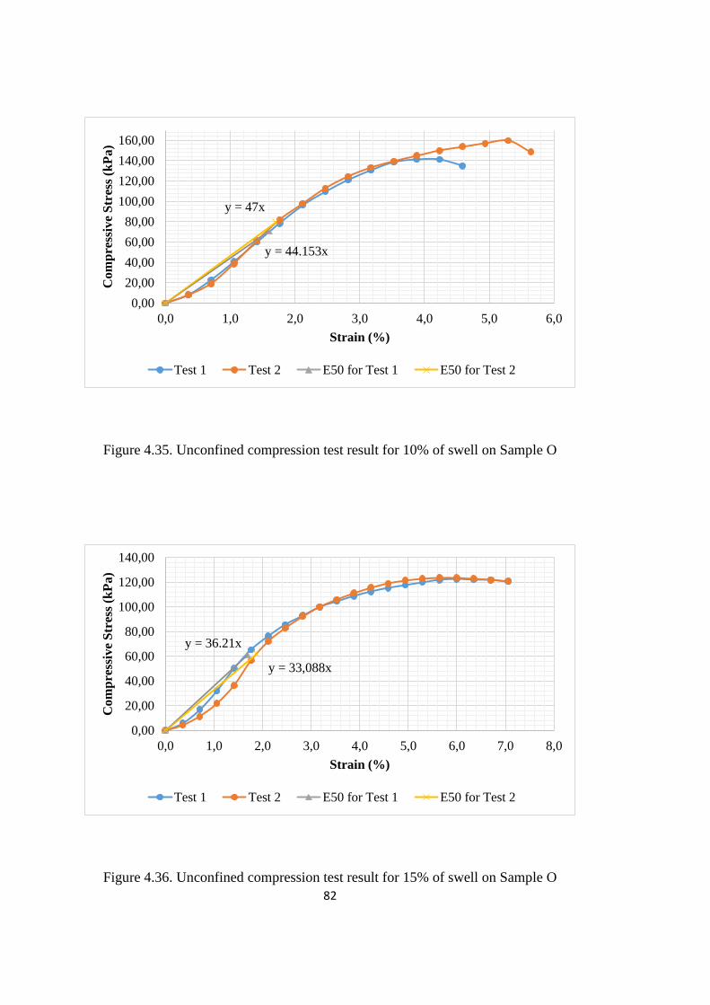
82
Figure 4.35. Unconfined compression test result for 10% of swell on Sample O
Figure 4.36. Unconfined compression test result for 15% of swell on Sample O
y = 44.153x
y = 47x
0,00
20,00
40,00
60,00
80,00
100,00
120,00
140,00
160,00
0,0 1,0 2,0 3,0 4,0 5,0 6,0
Co
mp
ress
ive
Str
ess
(kP
a)
Strain (%)
Test 1 Test 2 E50 for Test 1 E50 for Test 2
y = 36.21x
y = 33,088x
0,00
20,00
40,00
60,00
80,00
100,00
120,00
140,00
0,0 1,0 2,0 3,0 4,0 5,0 6,0 7,0 8,0
Co
mp
ress
ive
Str
ess
(kP
a)
Strain (%)
Test 1 Test 2 E50 for Test 1 E50 for Test 2
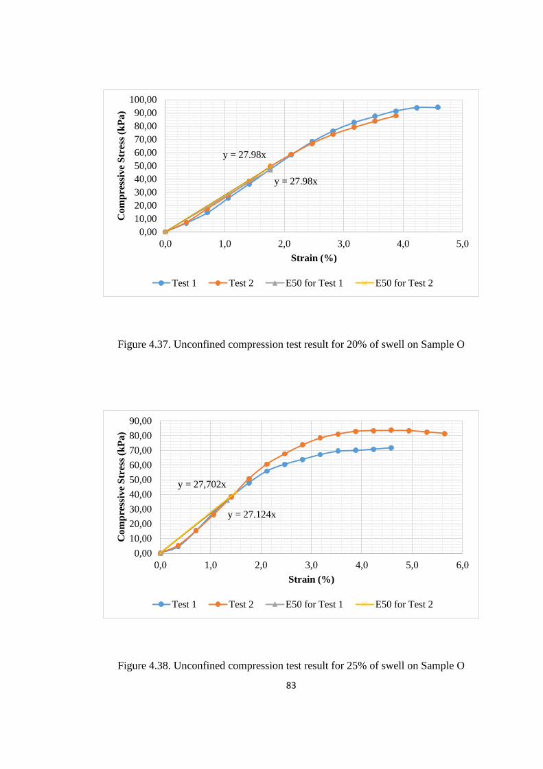
83
Figure 4.37. Unconfined compression test result for 20% of swell on Sample O
Figure 4.38. Unconfined compression test result for 25% of swell on Sample O
y = 27.98x
y = 27.98x
0,00
10,00
20,00
30,00
40,00
50,00
60,00
70,00
80,00
90,00
100,00
0,0 1,0 2,0 3,0 4,0 5,0
Co
mp
ress
ive
Str
ess
(kP
a)
Strain (%)
Test 1 Test 2 E50 for Test 1 E50 for Test 2
y = 27.124x
y = 27,702x
0,00
10,00
20,00
30,00
40,00
50,00
60,00
70,00
80,00
90,00
0,0 1,0 2,0 3,0 4,0 5,0 6,0
Com
press
ive S
tress
(k
Pa)
Strain (%)
Test 1 Test 2 E50 for Test 1 E50 for Test 2
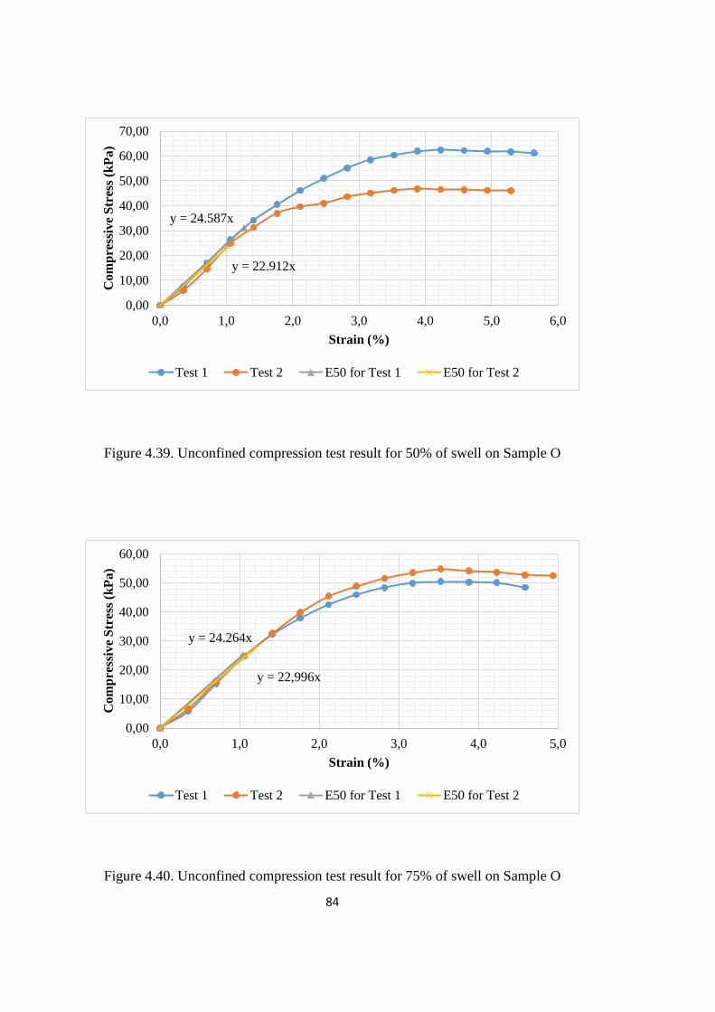
84
Figure 4.39. Unconfined compression test result for 50% of swell on Sample O
Figure 4.40. Unconfined compression test result for 75% of swell on Sample O
y = 24.587x
y = 22.912x
0,00
10,00
20,00
30,00
40,00
50,00
60,00
70,00
0,0 1,0 2,0 3,0 4,0 5,0 6,0
Co
mp
ress
ive
Str
ess
(kP
a)
Strain (%)
Test 1 Test 2 E50 for Test 1 E50 for Test 2
y = 24.264x
y = 22,996x
0,00
10,00
20,00
30,00
40,00
50,00
60,00
0,0 1,0 2,0 3,0 4,0 5,0
Com
press
ive S
tress
(k
Pa)
Strain (%)
Test 1 Test 2 E50 for Test 1 E50 for Test 2
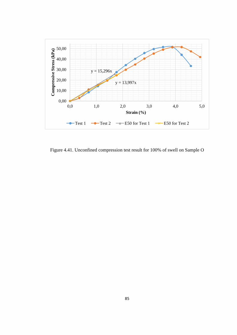
85
Figure 4.41. Unconfined compression test result for 100% of swell on Sample O
y = 15,296x
y = 13,997x
0,00
10,00
20,00
30,00
40,00
50,00
0,0 1,0 2,0 3,0 4,0 5,0
Co
mp
ress
ive
Str
ess
(kP
a)
Strain (%)
Test 1 Test 2 E50 for Test 1 E50 for Test 2
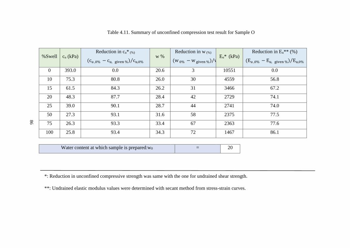
86
Table 4.11. Summary of unconfined compression test result for Sample O
%Swell cu (kPa) Reduction in cu* (%)
(cu ,0% − cu, given %) cu,0%⁄ w %
Reduction in w (%)
(w 0% − w given %) w0%⁄ Eu* (kPa)
Reduction in Eu** (%)
(Eu ,0% − Eu, given %) Eu,0%⁄
0 393.0 0.0 20.6 3 10551 0.0
10 75.3 80.8 26.0 30 4559 56.8
15 61.5 84.3 26.2 31 3466 67.2
20 48.3 87.7 28.4 42 2729 74.1
25 39.0 90.1 28.7 44 2741 74.0
50 27.3 93.1 31.6 58 2375 77.5
75 26.3 93.3 33.4 67 2363 77.6
100 25.8 93.4 34.3 72 1467 86.1
Water content at which sample is prepared:w0 = 20
86
*: Reduction in unconfined compressive strength was same with the one for undrained shear strength.
**: Undrained elastic modulus values were determined with secant method from stress-strain curves.
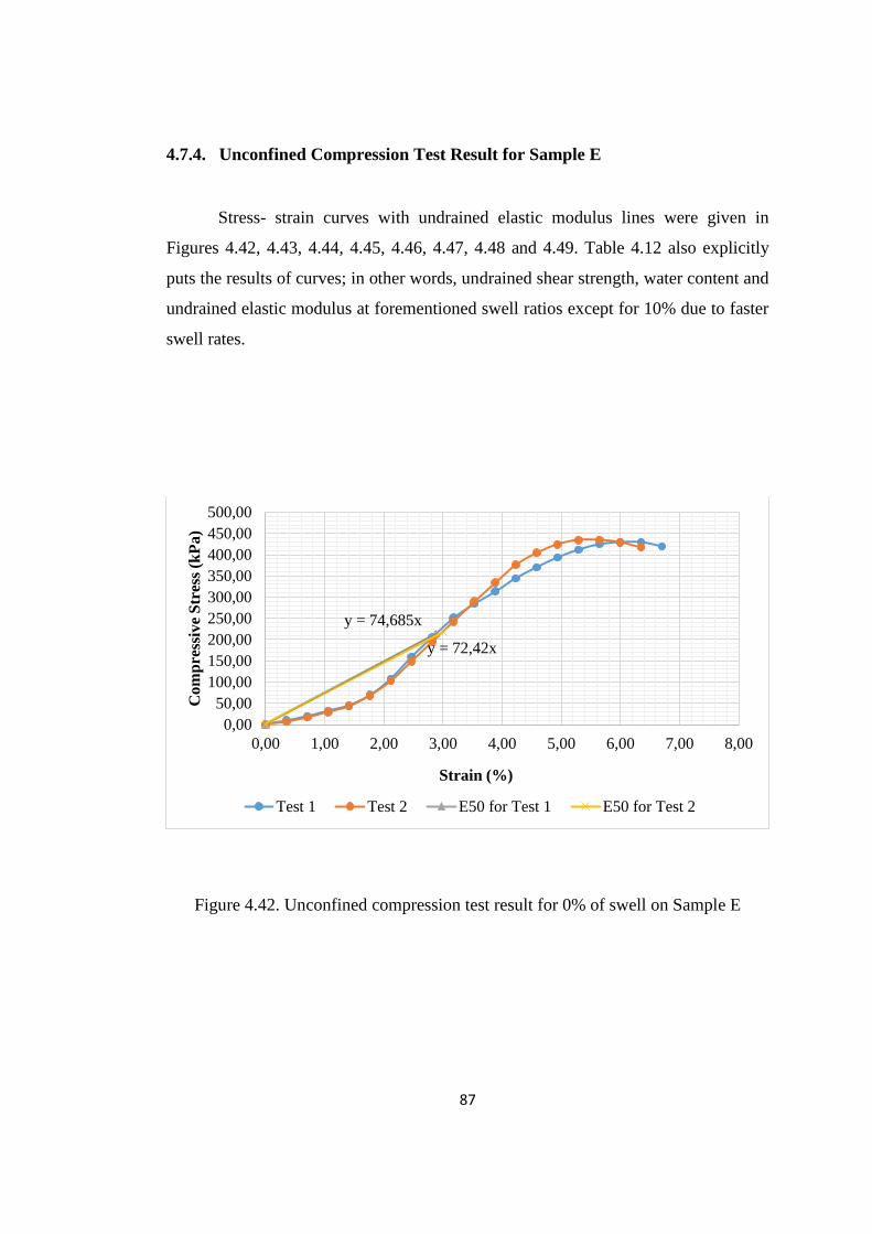
87
4.7.4. Unconfined Compression Test Result for Sample E
Stress- strain curves with undrained elastic modulus lines were given in
Figures 4.42, 4.43, 4.44, 4.45, 4.46, 4.47, 4.48 and 4.49. Table 4.12 also explicitly
puts the results of curves; in other words, undrained shear strength, water content and
undrained elastic modulus at forementioned swell ratios except for 10% due to faster
swell rates.
Figure 4.42. Unconfined compression test result for 0% of swell on Sample E
y = 74,685x
y = 72,42x
0,00
50,00
100,00
150,00
200,00
250,00
300,00
350,00
400,00
450,00
500,00
0,00 1,00 2,00 3,00 4,00 5,00 6,00 7,00 8,00
Com
pre
ssiv
e S
tres
s (k
Pa)
Strain (%)
Test 1 Test 2 E50 for Test 1 E50 for Test 2
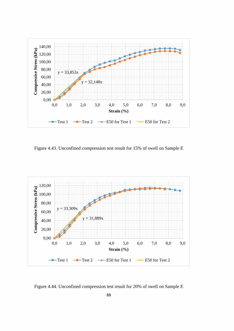
88
Figure 4.43. Unconfined compression test result for 15% of swell on Sample E
Figure 4.44. Unconfined compression test result for 20% of swell on Sample E
y = 33,853x
y = 32,148x
0,00
20,00
40,00
60,00
80,00
100,00
120,00
140,00
0,0 1,0 2,0 3,0 4,0 5,0 6,0 7,0 8,0 9,0
Co
mp
ress
ive
Str
ess
(kP
a)
Strain (%)
Test 1 Test 2 E50 for Test 1 E50 for Test 2
y = 33.309x
y = 31,889x
0,00
20,00
40,00
60,00
80,00
100,00
120,00
0,0 1,0 2,0 3,0 4,0 5,0 6,0 7,0 8,0 9,0
Com
press
ive S
tress
(k
Pa)
Strain (%)
Test 1 Test 2 E50 for Test 1 E50 for Test 2
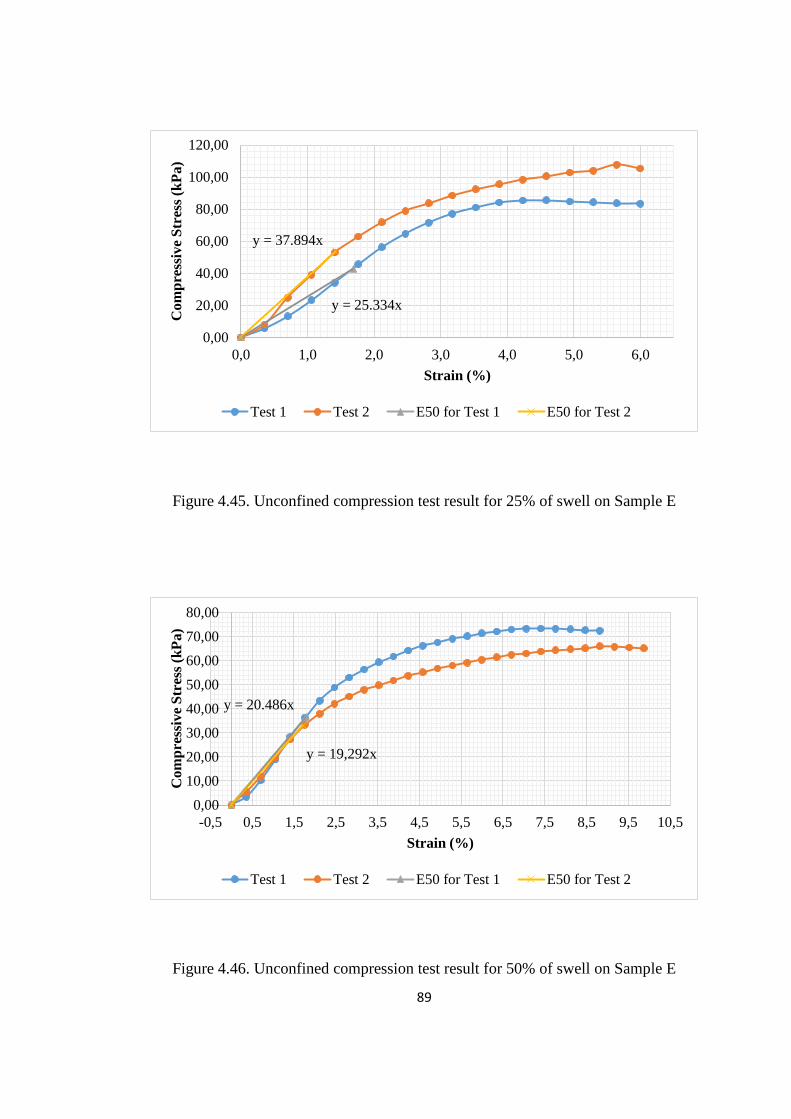
89
Figure 4.45. Unconfined compression test result for 25% of swell on Sample E
Figure 4.46. Unconfined compression test result for 50% of swell on Sample E
y = 25.334x
y = 37.894x
0,00
20,00
40,00
60,00
80,00
100,00
120,00
0,0 1,0 2,0 3,0 4,0 5,0 6,0
Co
mp
ress
ive
Str
ess
(kP
a)
Strain (%)
Test 1 Test 2 E50 for Test 1 E50 for Test 2
y = 20.486x
y = 19,292x
0,00
10,00
20,00
30,00
40,00
50,00
60,00
70,00
80,00
-0,5 0,5 1,5 2,5 3,5 4,5 5,5 6,5 7,5 8,5 9,5 10,5
Com
press
ive S
tress
(k
Pa)
Strain (%)
Test 1 Test 2 E50 for Test 1 E50 for Test 2
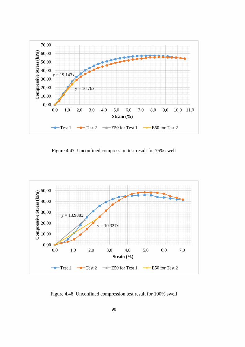
90
Figure 4.47. Unconfined compression test result for 75% swell
Figure 4.48. Unconfined compression test result for 100% swell
y = 19,143x
y = 16,76x
0,00
10,00
20,00
30,00
40,00
50,00
60,00
70,00
0,0 1,0 2,0 3,0 4,0 5,0 6,0 7,0 8,0 9,0 10,0 11,0
Co
mp
ress
ive
Str
ess
(kP
a)
Strain (%)
Test 1 Test 2 E50 for Test 1 E50 for Test 2
y = 13.988x
y = 10.327x
0,00
10,00
20,00
30,00
40,00
50,00
0,0 1,0 2,0 3,0 4,0 5,0 6,0 7,0
Com
pre
ssiv
e S
tres
s (k
Pa)
Strain (%)
Test 1 Test 2 E50 for Test 1 E50 for Test 2
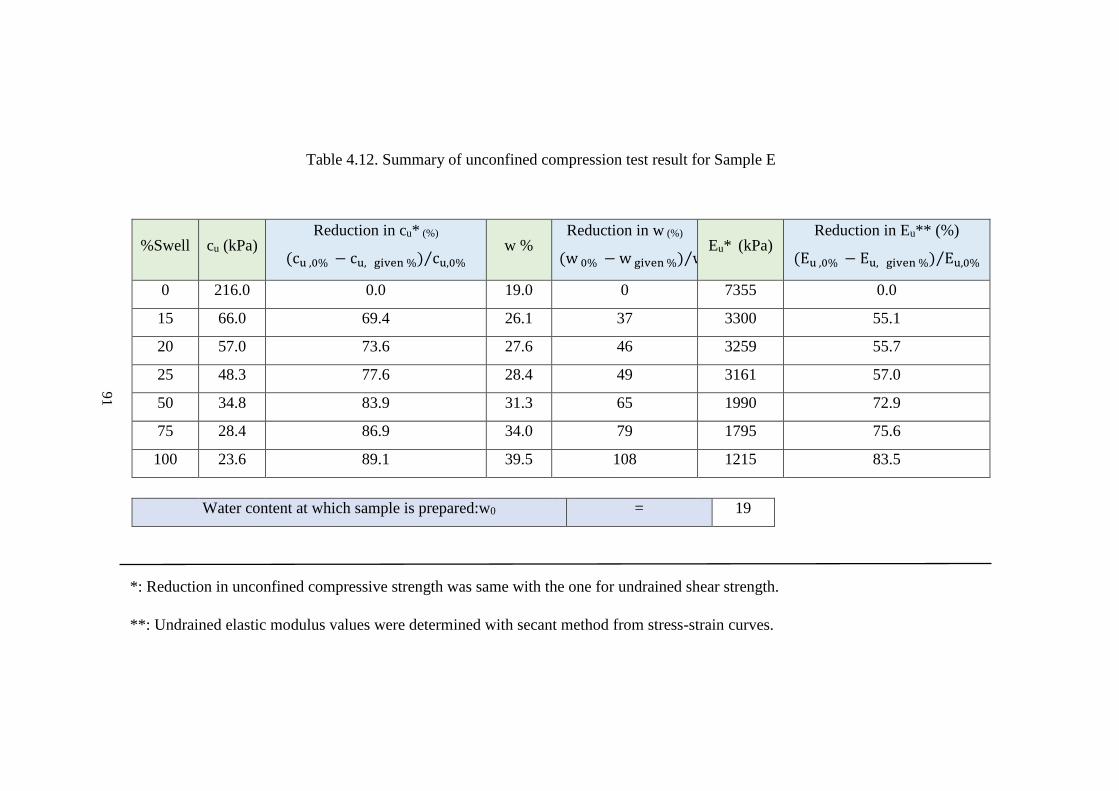
91
Table 4.12. Summary of unconfined compression test result for Sample E
%Swell cu (kPa) Reduction in cu* (%)
(cu ,0% − cu, given %) cu,0%⁄ w %
Reduction in w (%)
(w 0% − w given %) w0%⁄ Eu* (kPa)
Reduction in Eu** (%)
(Eu ,0% − Eu, given %) Eu,0%⁄
0 216.0 0.0 19.0 0 7355 0.0
15 66.0 69.4 26.1 37 3300 55.1
20 57.0 73.6 27.6 46 3259 55.7
25 48.3 77.6 28.4 49 3161 57.0
50 34.8 83.9 31.3 65 1990 72.9
75 28.4 86.9 34.0 79 1795 75.6
100 23.6 89.1 39.5 108 1215 83.5
Water content at which sample is prepared:w0 = 19
91
*: Reduction in unconfined compressive strength was same with the one for undrained shear strength.
**: Undrained elastic modulus values were determined with secant method from stress-strain curves.
92
4.8. Free Swell Index Test
Free swell index test is used for determination of soil expansiveness potential.
It is a quick test and so it is preferred for preliminary site investigation. In order to
get an idea about expansiveness of soil samples, Free swell index test is performed in
compliance with Indian Standard Methods of Test for Soils (IS:2720).
4.8.1. Test Procedure
Oven dried two samples which pass from No.40 Sieve are weighted as 10
grams (g). Then, they are poured into two glass graduated cylinder with 100 ml
capacity separately. One of the cylinders is filled with distilled water while the other
with kerosene up to 100 ml. After filling the cylinders, entrapped air is removed by
stirring with a glass rod and slowly shaking. It is left to rest for at least 24 hours and
soil specimen volume is measured. Figure 4.49 shows the resting stage. Thus,
percent Free Swell Index: FSI is computed from below correlation given in Eqn 4.4:
FSI %= Vd-Vk
Vk*100…………………………………………………................. Eqn 4.4
where
Vd= Soil specimen volume read from the graduated cylinder filled with distilled
water
Vk= Soil specimen volume read from the graduated cylinder filled with kerosene/ gas
oil.
As stated in the standard, in the case of existence of highly expansive soil,
Sample A in this case, graduated cylinder with 250 ml capacity was used instead of
100 mm capacity cylinder.

93
Figure 4.49. Free swell index test at resting stage
4.8.2. Test Results
Free swell index test results were summarized and compared with each other
in Figure 4.50.
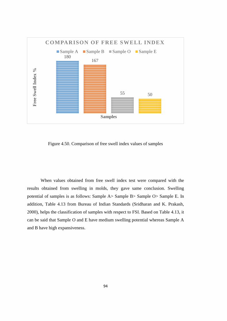
94
Figure 4.50. Comparison of free swell index values of samples
When values obtained from free swell index test were compared with the
results obtained from swelling in molds, they gave same conclusion. Swelling
potential of samples is as follows: Sample A> Sample B> Sample O> Sample E. In
addition, Table 4.13 from Bureau of Indian Standards (Sridharan and K. Prakash,
2000), helps the classification of samples with respect to FSI. Based on Table 4.13, it
can be said that Sample O and E have medium swelling potential whereas Sample A
and B have high expansiveness.
180167
55 50
Fre
e S
wel
l In
dex
%
Samples
COMPARISON OF FREE SWELL INDEX
Sample A Sample B Sample O Sample E
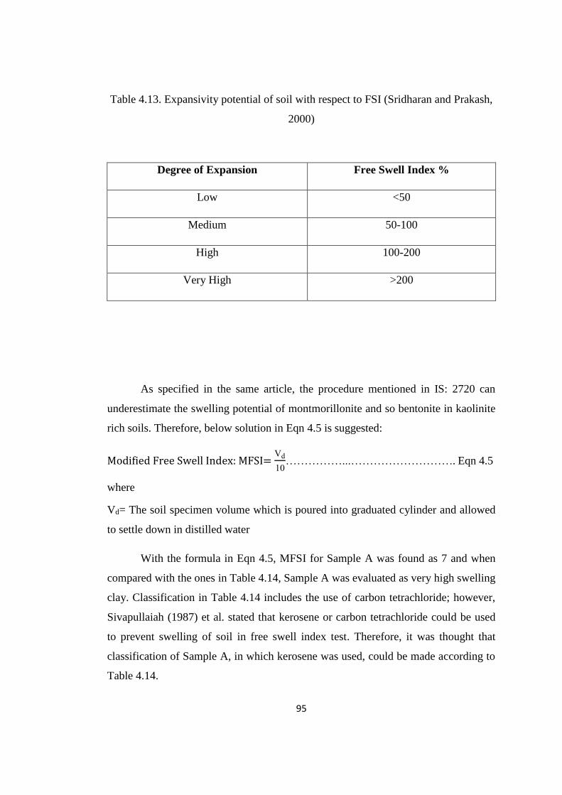
95
Table 4.13. Expansivity potential of soil with respect to FSI (Sridharan and Prakash,
2000)
Degree of Expansion Free Swell Index %
Low <50
Medium 50-100
High 100-200
Very High >200
As specified in the same article, the procedure mentioned in IS: 2720 can
underestimate the swelling potential of montmorillonite and so bentonite in kaolinite
rich soils. Therefore, below solution in Eqn 4.5 is suggested:
Modified Free Swell Index: MFSI= Vd
10……………...………………………. Eqn 4.5
where
Vd= The soil specimen volume which is poured into graduated cylinder and allowed
to settle down in distilled water
With the formula in Eqn 4.5, MFSI for Sample A was found as 7 and when
compared with the ones in Table 4.14, Sample A was evaluated as very high swelling
clay. Classification in Table 4.14 includes the use of carbon tetrachloride; however,
Sivapullaiah (1987) et al. stated that kerosene or carbon tetrachloride could be used
to prevent swelling of soil in free swell index test. Therefore, it was thought that
classification of Sample A, in which kerosene was used, could be made according to
Table 4.14.
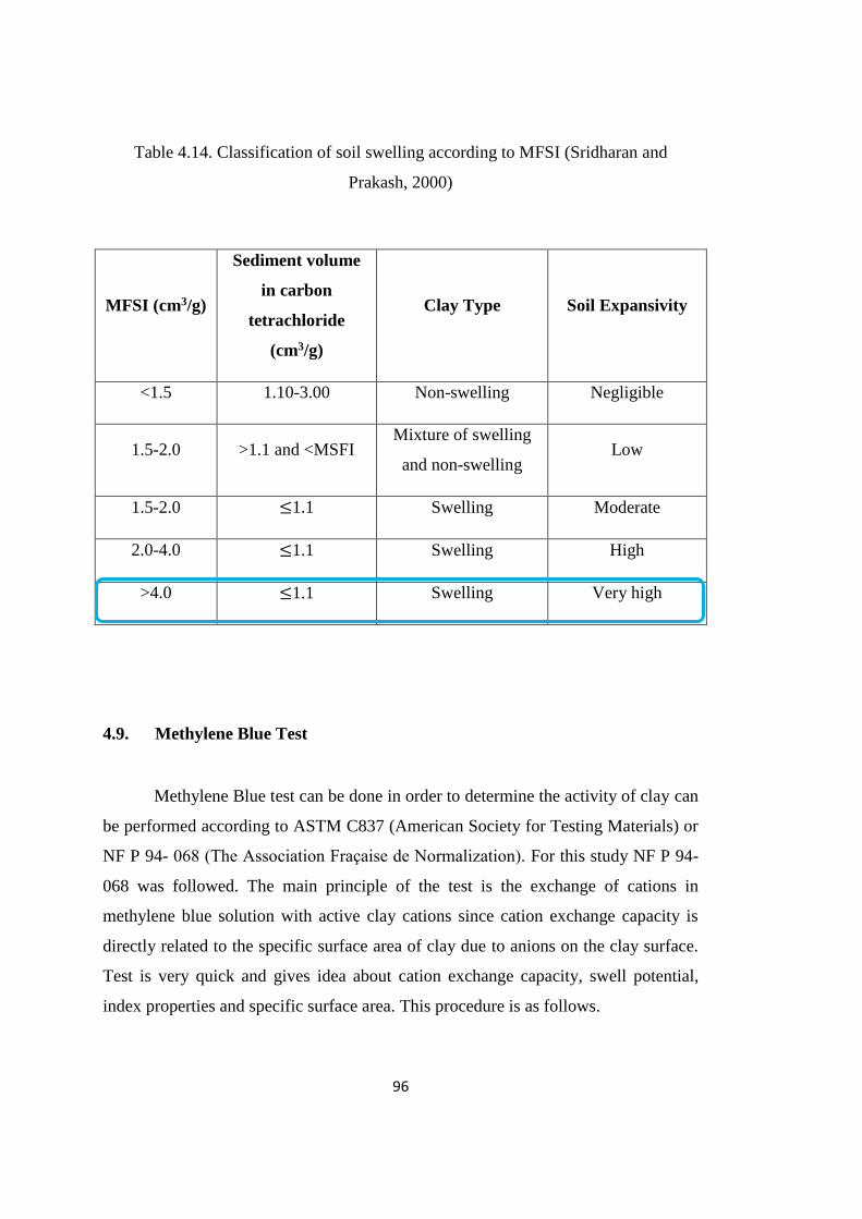
96
Table 4.14. Classification of soil swelling according to MFSI (Sridharan and
Prakash, 2000)
MFSI (cm3/g)
Sediment volume
in carbon
tetrachloride
(cm3/g)
Clay Type Soil Expansivity
<1.5 1.10-3.00 Non-swelling Negligible
1.5-2.0 >1.1 and <MSFI Mixture of swelling
and non-swelling Low
1.5-2.0 ≤1.1 Swelling Moderate
2.0-4.0 ≤1.1 Swelling High
>4.0 ≤1.1 Swelling Very high
4.9. Methylene Blue Test
Methylene Blue test can be done in order to determine the activity of clay can
be performed according to ASTM C837 (American Society for Testing Materials) or
NF P 94- 068 (The Association Fraçaise de Normalization). For this study NF P 94-
068 was followed. The main principle of the test is the exchange of cations in
methylene blue solution with active clay cations since cation exchange capacity is
directly related to the specific surface area of clay due to anions on the clay surface.
Test is very quick and gives idea about cation exchange capacity, swell potential,
index properties and specific surface area. This procedure is as follows.
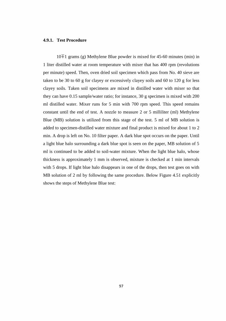
97
4.9.1. Test Procedure
10∓1 grams (g) Methylene Blue powder is mixed for 45-60 minutes (min) in
1 liter distilled water at room temperature with mixer that has 400 rpm (revolutions
per minute) speed. Then, oven dried soil specimen which pass from No. 40 sieve are
taken to be 30 to 60 g for clayey or excessively clayey soils and 60 to 120 g for less
clayey soils. Taken soil specimens are mixed in distilled water with mixer so that
they can have 0.15 sample/water ratio; for instance, 30 g specimen is mixed with 200
ml distilled water. Mixer runs for 5 min with 700 rpm speed. This speed remains
constant until the end of test. A nozzle to measure 2 or 5 milliliter (ml) Methylene
Blue (MB) solution is utilized from this stage of the test. 5 ml of MB solution is
added to specimen-distilled water mixture and final product is mixed for about 1 to 2
min. A drop is left on No. 10 filter paper. A dark blue spot occurs on the paper. Until
a light blue halo surrounding a dark blue spot is seen on the paper, MB solution of 5
ml is continued to be added to soil-water mixture. When the light blue halo, whose
thickness is approximately 1 mm is observed, mixture is checked at 1 min intervals
with 5 drops. If light blue halo disappears in one of the drops, then test goes on with
MB solution of 2 ml by following the same procedure. Below Figure 4.51 explicitly
shows the steps of Methylene Blue test:
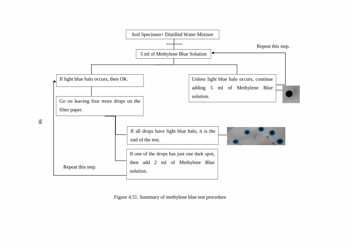
98
Figure 4.51. Summary of methylene blue test procedure
98
Soil Specimen+ Distilled Water Mixture
5 ml of Methylene Blue Solution
If light blue halo occurs, then OK.
Repeat this step.
Unless light blue halo occurs, continue
adding 5 ml of Methylene Blue
solution.
Repeat this step.
If one of the drops has just one dark spot,
then add 2 ml of Methylene Blue
solution.
Go on leaving four more drops on the
filter paper.
If all drops have light blue halo, it is the
end of the test.
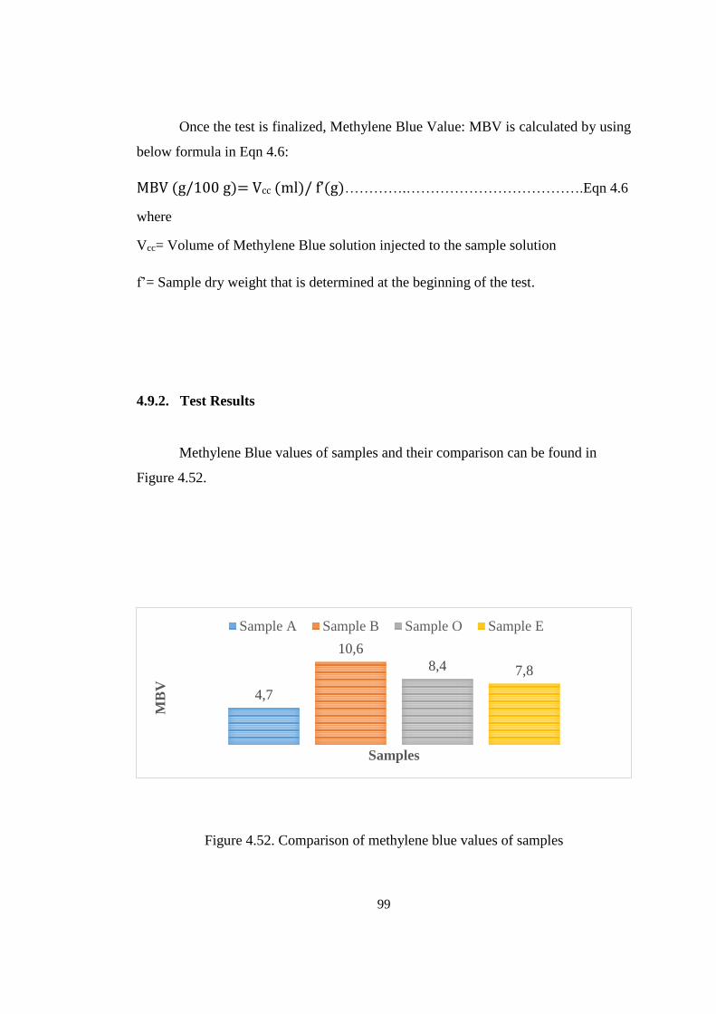
99
Once the test is finalized, Methylene Blue Value: MBV is calculated by using
below formula in Eqn 4.6:
MBV (g/100 g)= Vcc (ml)/ f’(g)………….……………………………….Eqn 4.6
where
Vcc= Volume of Methylene Blue solution injected to the sample solution
f’= Sample dry weight that is determined at the beginning of the test.
4.9.2. Test Results
Methylene Blue values of samples and their comparison can be found in
Figure 4.52.
Figure 4.52. Comparison of methylene blue values of samples
4,7
10,6
8,4 7,8
MB
V
Samples
Sample A Sample B Sample O Sample E

100
According to MBV of samples, expansiveness ascending sequence is as
follows: Sample B> Sample O> Sample E> Sample A. Sample A has the lowest
MBV although it has the highest swelling potential according to free swell index test
and tests made with molds. The reason behind this result may be due to existence of
some chemicals, variability in clay minerals and fast downfall of natural soil
particles. Therefore, comparison between natural and artificial soil samples does not
give a realistic result.
4.10. Swell Pressure Relation with Soil Expansiveness
Swell pressure tests were performed on compacted soil specimens at water
contents given in Table 4.6. Tests were made in accordance with ASTM D4546.
Figure 4.53 shows the test setup. Soil specimen preparation was nearly same with the
one which was explained in Figure 4.10. The differences between them was the
aimed height and volume as well as the molds where specimens were compacted.
Therefore, bulk weight calculations, which was given in Eqn. 4.2, were revised
according to 0.0019 m height and 6.02x10⁻⁵ m3 volume of consolidometer ring.
Plastic rods that were used for specimen compaction in consolidometer rings are
given in Figure 4.54. In addition, specimens were compacted directly into
consolidometer rings.
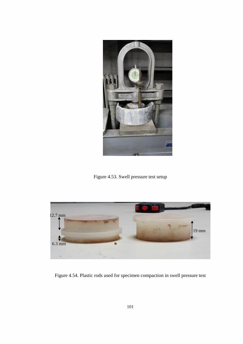
101
Figure 4.53. Swell pressure test setup
Figure 4.54. Plastic rods used for specimen compaction in swell pressure test
19 mm
6.3 mm
12.7 mm
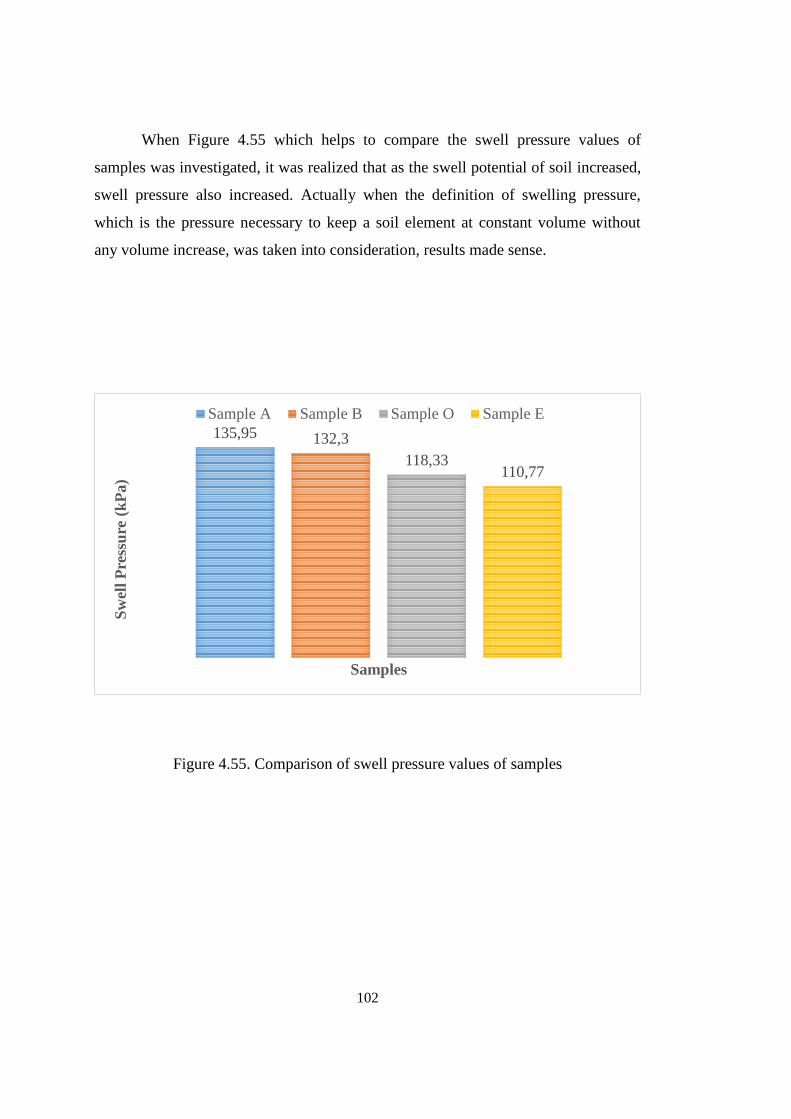
102
When Figure 4.55 which helps to compare the swell pressure values of
samples was investigated, it was realized that as the swell potential of soil increased,
swell pressure also increased. Actually when the definition of swelling pressure,
which is the pressure necessary to keep a soil element at constant volume without
any volume increase, was taken into consideration, results made sense.
Figure 4.55. Comparison of swell pressure values of samples
135,95 132,3
118,33110,77
Sw
ell
Pre
ssu
re (
kP
a)
Samples
Sample A Sample B Sample O Sample E
103
4.11. Estimation of Frictional Stress
A frictional force develops between soil specimen and plastic mold during
swelling in the volume constraint molds. In order to compute this frictional force and
so frictional stress, it was assumed that at the time of sample movement, frictional
force would be equal to the applied force to give this movement since soil specimen
particles would directly transmit applied force to the lateral surface. Therefore, soil
specimens were prepared as mentioned in Figure 4.10 as the first step. For the
specimens that were allowed to swell to ultimate level, specimens were submerged in
water and waited. When the swelling stopped, porous stones were removed.
Meanwhile, this step was skipped for the specimens which would be tested for 0% of
swell. Then, needed force was determined with unconfined compression test setup by
applying the load to the plastic rod which was mentioned in Step 7 of Figure 4.10. At
the force that gave this rod a movement was accepted as the frictional force. Figure
4.56 shows the sketch and photo of the test setup.
After frictional force was determined with this method, frictional stress: σf on
net lateral surface area: Anet,side due to developed frictional force: Ff was calculated
by using Eqn. 4.7.
σf=Ff
Anet,side………………………………………………………………....…..Eqn 4.7
where
Ff= Frictional force which is equal to the applied force
Anet,side= (Lateral surface area corresponding to the swelled sample height)- (Area of
perforations*154)
Area of perforation= Π*d2/ 4= Π*0.0022/ 4= 3.142x10⁻⁶ m2
Thus, total perforation area for 154 ones was found as 4.838x10⁻⁴ m2. Table
4.15 presents calculation steps and comparison of swell pressure with formed
frictional stress between mold and soil specimen at 0% and 100% of swell. As can be
seen from Table 4.15, a frictional stress aroused between soil samples and mold
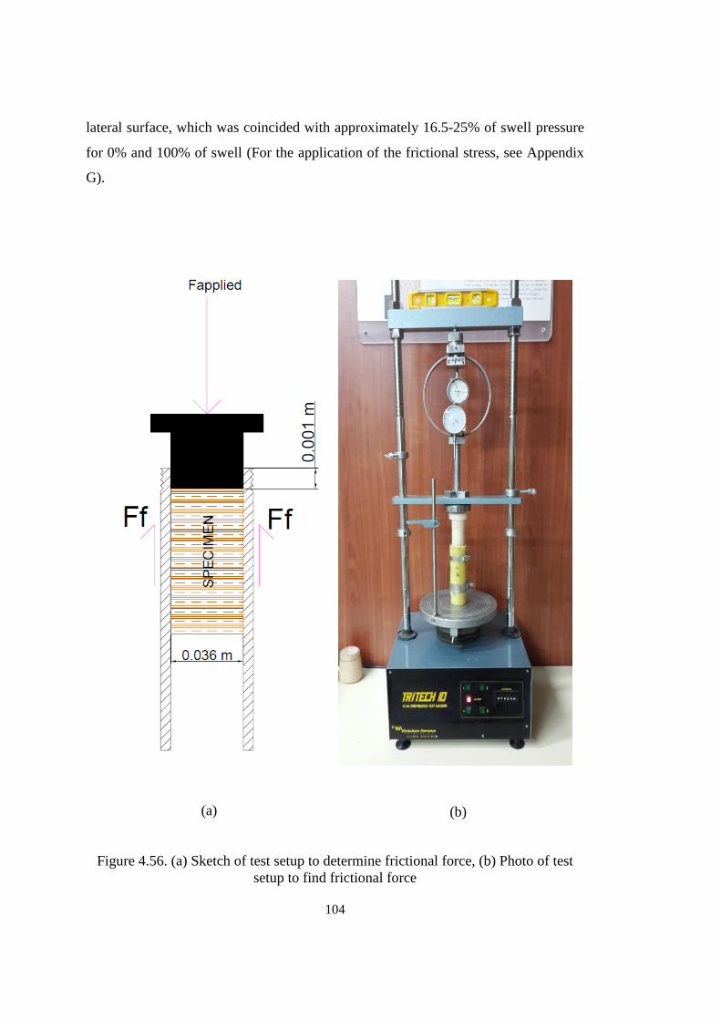
104
lateral surface, which was coincided with approximately 16.5-25% of swell pressure
for 0% and 100% of swell (For the application of the frictional stress, see Appendix
G).
Figure 4.56. (a) Sketch of test setup to determine frictional force, (b) Photo of test
setup to find frictional force
(a) (b)
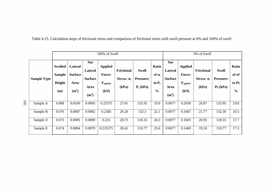
105
Table 4.15. Calculation steps of frictional stress and comparison of frictional stress with swell pressure at 0% and 100% of swell
100% of Swell 0% of Swell
Sample Type
Swelled
Sample
Height
(m)
Lateral
Surface
Area
(m2)
Net
Lateral
Surface
Area
(m2)
Applied
Force:
Fapplied
(kN)
Frictional
Stress: σf
(kPa)
Swell
Pressure:
Ps (kPa)
Ratio
of σf
to Ps
%
Net
Lateral
Surface
Area
(m2)
Applied
Force:
Fapplied
(kN)
Frictional
Stress: σf
(kPa)
Swell
Pressure:
Ps (kPa)
Ratio
of σf
to Ps
%
Sample A 0.088 0.0100 0.0095 0.25575 27.01 135.95 19.9 0.0077 0.2058 26.87 135.95 19.8
Sample B 0.076 0.0087 0.0082 0.2385 29.20 132.3 22.1 0.0077 0.1667 21.77 132.30 16.5
Sample O 0.075 0.0085 0.0080 0.231 28.73 118.33 24.3 0.0077 0.1603 20.93 118.33 17.7
Sample E 0.074 0.0084 0.0079 0.225375 28.41 110.77 25.6 0.0077 0.1469 19.18 110.77 17.3
105

106
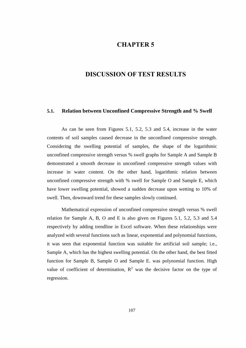
107
CHAPTER 5
5) DISCUSSION OF TEST RESULTS
5.1. Relation between Unconfined Compressive Strength and % Swell
As can be seen from Figures 5.1, 5.2, 5.3 and 5.4, increase in the water
contents of soil samples caused decrease in the unconfined compressive strength.
Considering the swelling potential of samples, the shape of the logarithmic
unconfined compressive strength versus % swell graphs for Sample A and Sample B
demonstrated a smooth decrease in unconfined compressive strength values with
increase in water content. On the other hand, logarithmic relation between
unconfined compressive strength with % swell for Sample O and Sample E, which
have lower swelling potential, showed a sudden decrease upon wetting to 10% of
swell. Then, downward trend for these samples slowly continued.
Mathematical expression of unconfined compressive strength versus % swell
relation for Sample A, B, O and E is also given on Figures 5.1, 5.2, 5.3 and 5.4
respectively by adding trendline in Excel software. When these relationships were
analyzed with several functions such as linear, exponential and polynomial functions,
it was seen that exponential function was suitable for artificial soil sample; i.e.,
Sample A, which has the highest swelling potential. On the other hand, the best fitted
function for Sample B, Sample O and Sample E. was polynomial function. High
value of coefficient of determination, R2 was the decisive factor on the type of
regression.
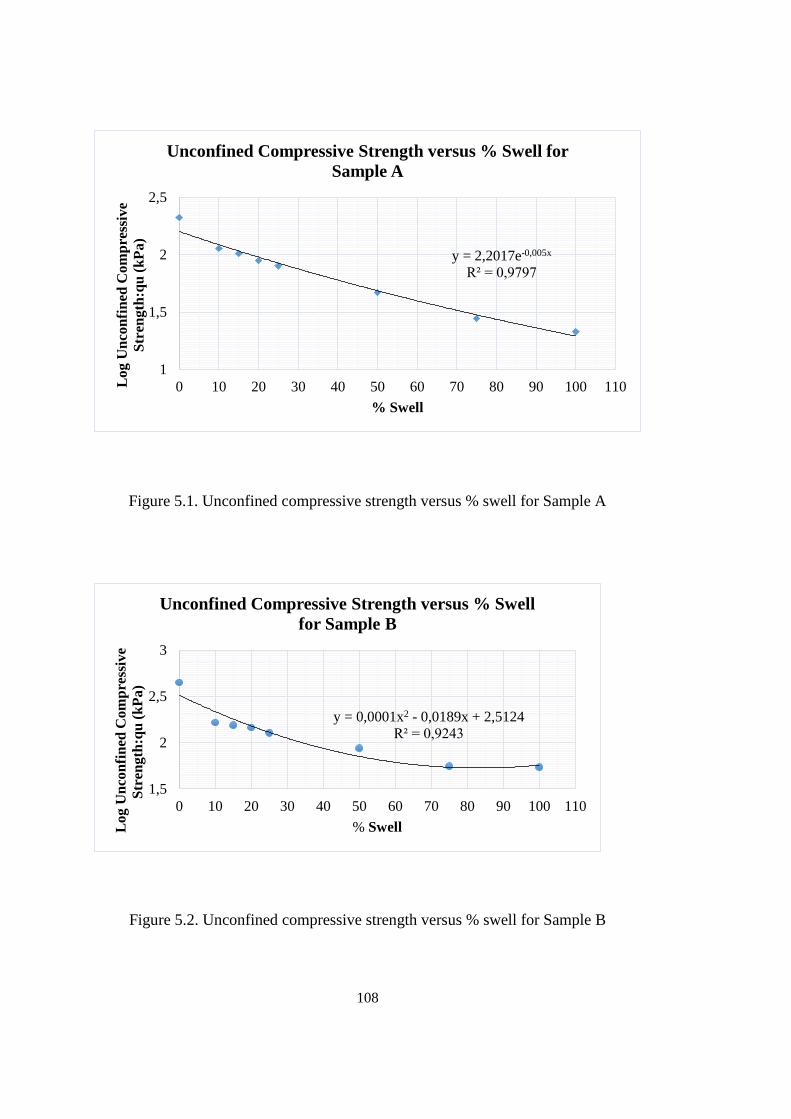
108
Figure 5.1. Unconfined compressive strength versus % swell for Sample A
Figure 5.2. Unconfined compressive strength versus % swell for Sample B
y = 2,2017e-0,005x
R² = 0,9797
1
1,5
2
2,5
0 10 20 30 40 50 60 70 80 90 100 110Lo
g U
nco
nfi
ned
Co
mp
ress
ive
Str
eng
th:q
u (
kP
a)
% Swell
Unconfined Compressive Strength versus % Swell for
Sample A
y = 0,0001x2 - 0,0189x + 2,5124
R² = 0,9243
1,5
2
2,5
3
0 10 20 30 40 50 60 70 80 90 100 110
Lo
g U
nco
nfi
ned
Com
pre
ssiv
e
Str
eng
th:q
u (
kP
a)
% Swell
Unconfined Compressive Strength versus % Swell
for Sample B
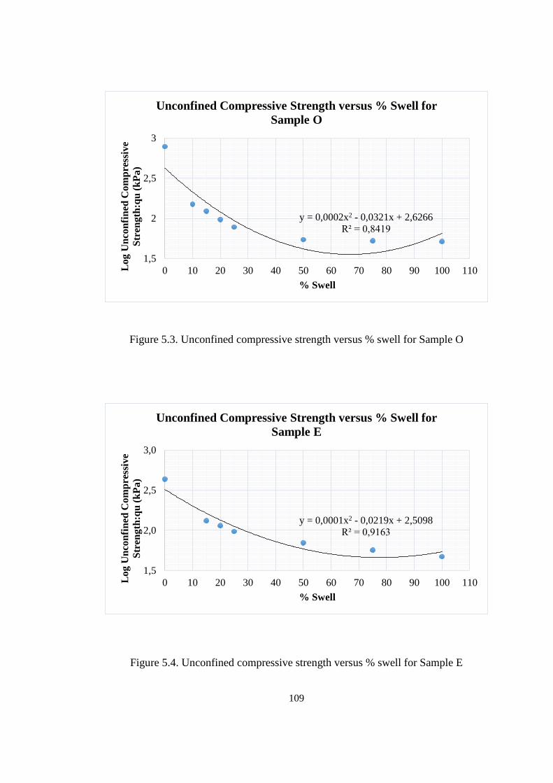
109
Figure 5.3. Unconfined compressive strength versus % swell for Sample O
Figure 5.4. Unconfined compressive strength versus % swell for Sample E
y = 0,0002x2 - 0,0321x + 2,6266
R² = 0,8419
1,5
2
2,5
3
0 10 20 30 40 50 60 70 80 90 100 110Lo
g U
nco
nfi
ned
Co
mp
ress
ive
Str
eng
th:q
u (
kP
a)
% Swell
Unconfined Compressive Strength versus % Swell for
Sample O
y = 0,0001x2 - 0,0219x + 2,5098
R² = 0,9163
1,5
2,0
2,5
3,0
0 10 20 30 40 50 60 70 80 90 100 110Lo
g U
nco
nfi
ned
Com
pre
ssiv
e
Str
ength
:qu
(k
Pa)
% Swell
Unconfined Compressive Strength versus % Swell for
Sample E
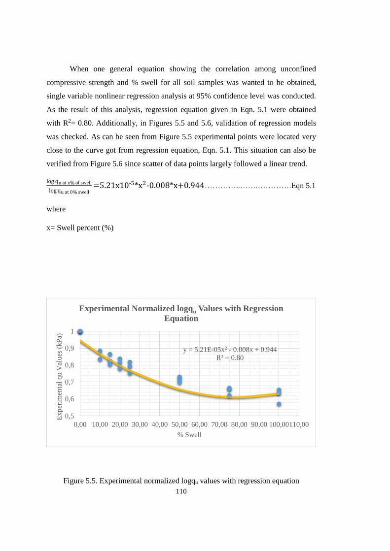
110
When one general equation showing the correlation among unconfined
compressive strength and % swell for all soil samples was wanted to be obtained,
single variable nonlinear regression analysis at 95% confidence level was conducted.
As the result of this analysis, regression equation given in Eqn. 5.1 were obtained
with R2= 0.80. Additionally, in Figures 5.5 and 5.6, validation of regression models
was checked. As can be seen from Figure 5.5 experimental points were located very
close to the curve got from regression equation, Eqn. 5.1. This situation can also be
verified from Figure 5.6 since scatter of data points largely followed a linear trend.
log qu at x% of swell
log qu at 0% swell=5.21x10⁻⁵*x2-0.008*x+0.944…………..…….………….Eqn 5.1
where
x= Swell percent (%)
Figure 5.5. Experimental normalized logqu values with regression equation
y = 5.21E-05x2 - 0.008x + 0.944
R² = 0.80
0,5
0,6
0,7
0,8
0,9
1
0,00 10,00 20,00 30,00 40,00 50,00 60,00 70,00 80,00 90,00 100,00110,00
Ex
per
imen
tal
qu V
alues
(kP
a)
% Swell
Experimental Normalized logqu Values with Regression
Equation
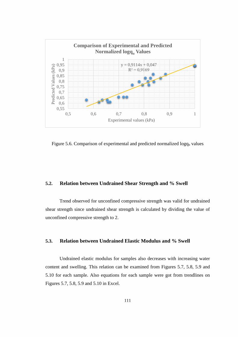
111
Figure 5.6. Comparison of experimental and predicted normalized logqu values
5.2. Relation between Undrained Shear Strength and % Swell
Trend observed for unconfined compressive strength was valid for undrained
shear strength since undrained shear strength is calculated by dividing the value of
unconfined compressive strength to 2.
5.3. Relation between Undrained Elastic Modulus and % Swell
Undrained elastic modulus for samples also decreases with increasing water
content and swelling. This relation can be examined from Figures 5.7, 5.8, 5.9 and
5.10 for each sample. Also equations for each sample were got from trendlines on
Figures 5.7, 5.8, 5.9 and 5.10 in Excel.
y = 0,9114x + 0,047
R² = 0,9169
0,55
0,6
0,65
0,7
0,75
0,8
0,85
0,9
0,95
1
0,5 0,6 0,7 0,8 0,9 1
Pre
dic
ted
Val
ues
(kP
a)
Experimental values (kPa)
Comparison of Experimental and Predicted
Normalized logqu Values
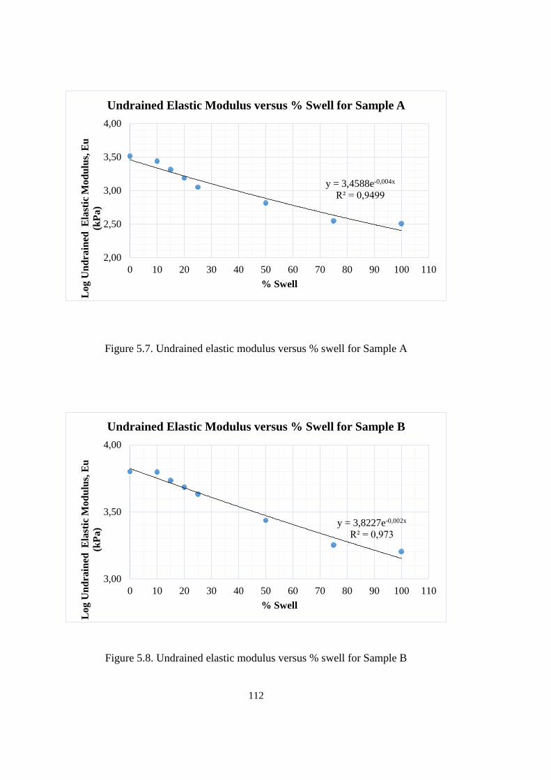
112
Figure 5.7. Undrained elastic modulus versus % swell for Sample A
Figure 5.8. Undrained elastic modulus versus % swell for Sample B
y = 3,4588e-0,004x
R² = 0,9499
2,00
2,50
3,00
3,50
4,00
0 10 20 30 40 50 60 70 80 90 100 110
Lo
g U
nd
rain
ed E
last
ic M
od
ulu
s, E
u
(kP
a)
% Swell
Undrained Elastic Modulus versus % Swell for Sample A
y = 3,8227e-0,002x
R² = 0,973
3,00
3,50
4,00
0 10 20 30 40 50 60 70 80 90 100 110
Lo
g U
nd
rain
ed E
last
ic M
od
ulu
s, E
u
(kP
a)
% Swell
Undrained Elastic Modulus versus % Swell for Sample B
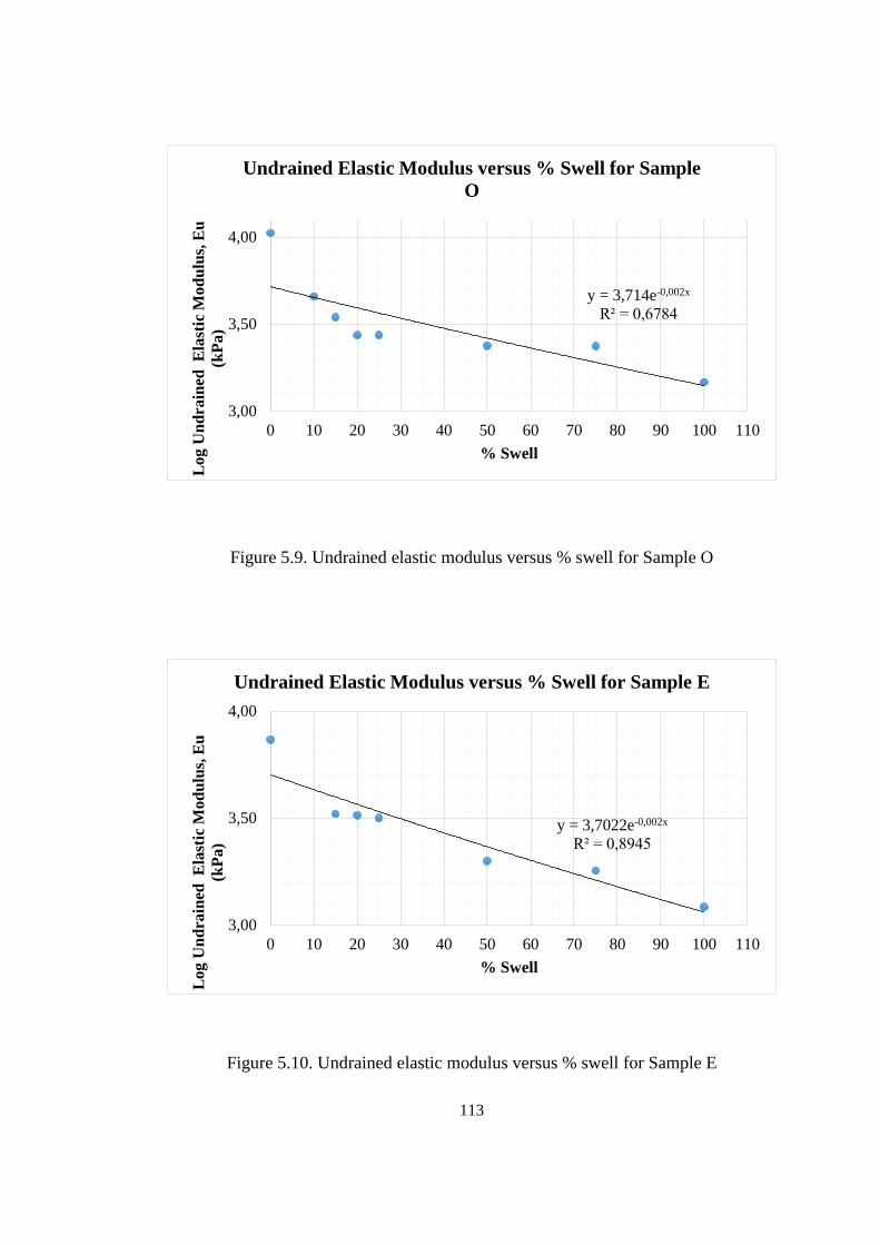
113
Figure 5.9. Undrained elastic modulus versus % swell for Sample O
Figure 5.10. Undrained elastic modulus versus % swell for Sample E
y = 3,714e-0,002x
R² = 0,6784
3,00
3,50
4,00
0 10 20 30 40 50 60 70 80 90 100 110
Lo
g U
nd
rain
ed E
last
ic M
od
ulu
s, E
u
(kP
a)
% Swell
Undrained Elastic Modulus versus % Swell for Sample
O
y = 3,7022e-0,002x
R² = 0,8945
3,00
3,50
4,00
0 10 20 30 40 50 60 70 80 90 100 110
Lo
g U
nd
rain
ed E
last
ic M
od
ulu
s, E
u
(kP
a)
% Swell
Undrained Elastic Modulus versus % Swell for Sample E
114
5.4. Comparison of Undrained Elastic Modulus with Literature
Typical Young’s Modulus values in MPa were summarized in Table 5.1
compiled from Kezdi (1974) and Prat et al. (1995). On the other hand, Table 5.2
shows the obtained undrained elastic modulus values with respect to swell ratio. All
soil samples were evaluated as CH soil (clay of high plasticity) as the result of soil
classification in Chapter 4. When Tables 5.1 and 5.2 matched each other, it was seen
that all soil samples had soft to very soft modulus when vertical displacement
stopped and they reached to ultimate swell. The only difference between the
undrained elastic modulus values of samples was the initial states and decreases.
Initial modulus of Sample A and Sample B at 0% of swell were evaluated as very
soft to soft and medium respectively. However, undrained elastic modulus values of
Sample O and Sample E, which have lower swelling potential, were in the range of
stiff to very stiff. When Sample O and E got water and reached to 10% and 15% of
swell respectively, their modulus showed a sudden decrease. From these points for
Sample O and E, there was a gradual decrease.
At the end, when total decline in undrained elastic modulus values were
explored, it was realized that Sample A had the most change as 90.2% with the
highest swelling potential. Samples B, O and E possessed nearly the same trend with
74.7%, 86.1% and 83.5% respectively.
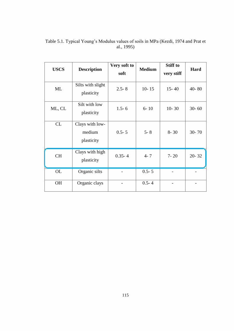
115
Table 5.1. Typical Young’s Modulus values of soils in MPa (Kezdi, 1974 and Prat et
al., 1995)
USCS Description Very soft to
soft Medium
Stiff to
very stiff Hard
ML Silts with slight
plasticity 2.5- 8 10- 15 15- 40 40- 80
ML, CL Silt with low
plasticity 1.5- 6 6- 10 10- 30 30- 60
CL Clays with low-
medium
plasticity
0.5- 5 5- 8 8- 30 30- 70
CH Clays with high
plasticity 0.35- 4 4- 7 7- 20 20- 32
OL Organic silts - 0.5- 5 - -
OH Organic clays - 0.5- 4 - -
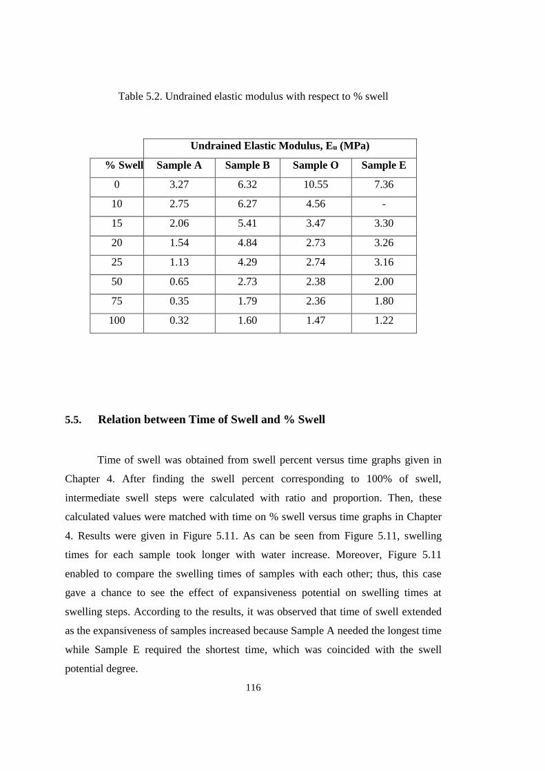
116
Table 5.2. Undrained elastic modulus with respect to % swell
Undrained Elastic Modulus, Eu (MPa)
% Swell Sample A Sample B Sample O Sample E
0 3.27 6.32 10.55 7.36
10 2.75 6.27 4.56 -
15 2.06 5.41 3.47 3.30
20 1.54 4.84 2.73 3.26
25 1.13 4.29 2.74 3.16
50 0.65 2.73 2.38 2.00
75 0.35 1.79 2.36 1.80
100 0.32 1.60 1.47 1.22
5.5. Relation between Time of Swell and % Swell
Time of swell was obtained from swell percent versus time graphs given in
Chapter 4. After finding the swell percent corresponding to 100% of swell,
intermediate swell steps were calculated with ratio and proportion. Then, these
calculated values were matched with time on % swell versus time graphs in Chapter
4. Results were given in Figure 5.11. As can be seen from Figure 5.11, swelling
times for each sample took longer with water increase. Moreover, Figure 5.11
enabled to compare the swelling times of samples with each other; thus, this case
gave a chance to see the effect of expansiveness potential on swelling times at
swelling steps. According to the results, it was observed that time of swell extended
as the expansiveness of samples increased because Sample A needed the longest time
while Sample E required the shortest time, which was coincided with the swell
potential degree.
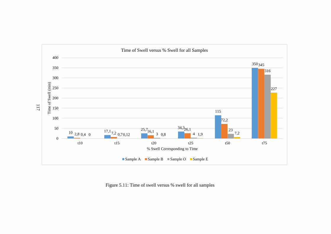
117
Figure 5.11: Time of swell versus % swell for all samples
10 17,1 25,7 34,3
115
350
2,8 7,216,1
26,1
72,2
345
0,4 0,7 3 423
316
0 0,12 0,8 1,9 7,2
227
0
50
100
150
200
250
300
350
400
t10 t15 t20 t25 t50 t75
Tim
e o
f S
wel
l (m
in)
% Swell Corresponding to Time
Time of Swell versus % Swell for all Samples
Sample A Sample B Sample O Sample E
117
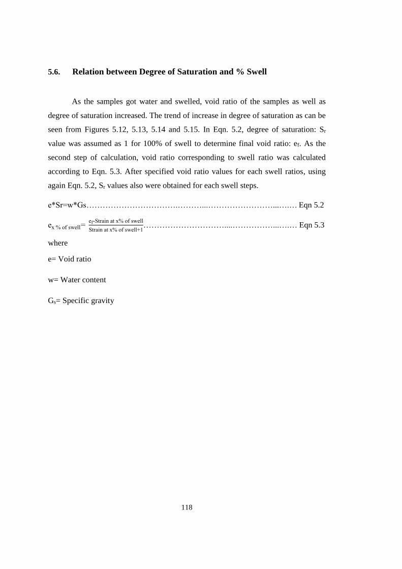
118
5.6. Relation between Degree of Saturation and % Swell
As the samples got water and swelled, void ratio of the samples as well as
degree of saturation increased. The trend of increase in degree of saturation as can be
seen from Figures 5.12, 5.13, 5.14 and 5.15. In Eqn. 5.2, degree of saturation: Sr
value was assumed as 1 for 100% of swell to determine final void ratio: ef. As the
second step of calculation, void ratio corresponding to swell ratio was calculated
according to Eqn. 5.3. After specified void ratio values for each swell ratios, using
again Eqn. 5.2, Sr values also were obtained for each swell steps.
e*Sr=w*Gs…………………………….………...……………………...….… Eqn 5.2
ex % of swell= ef-Strain at x% of swell
Strain at x% of swell+1…………………………....……………...….… Eqn 5.3
where
e= Void ratio
w= Water content
Gs= Specific gravity
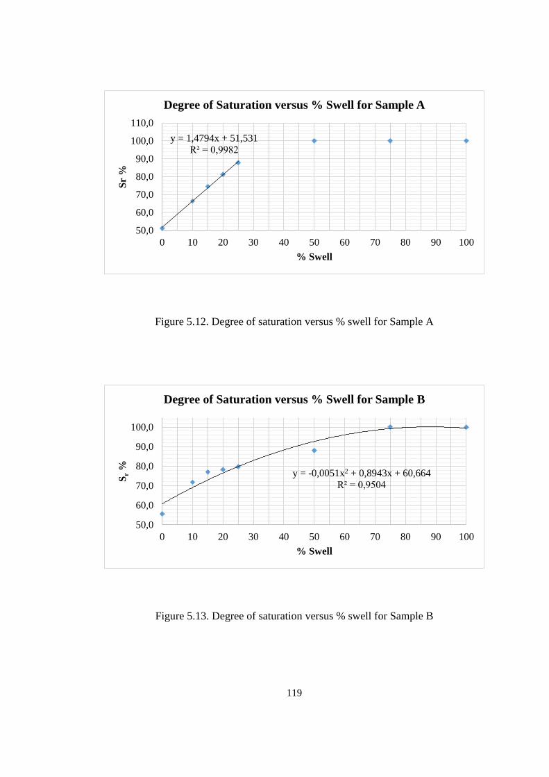
119
Figure 5.12. Degree of saturation versus % swell for Sample A
Figure 5.13. Degree of saturation versus % swell for Sample B
y = 1,4794x + 51,531
R² = 0,9982
50,0
60,0
70,0
80,0
90,0
100,0
110,0
0 10 20 30 40 50 60 70 80 90 100
Sr
%
% Swell
Degree of Saturation versus % Swell for Sample A
y = -0,0051x2 + 0,8943x + 60,664
R² = 0,9504
50,0
60,0
70,0
80,0
90,0
100,0
0 10 20 30 40 50 60 70 80 90 100
Sr
%
% Swell
Degree of Saturation versus % Swell for Sample B
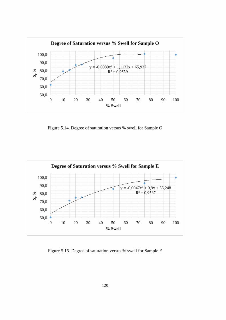
120
Figure 5.14. Degree of saturation versus % swell for Sample O
Figure 5.15. Degree of saturation versus % swell for Sample E
y = -0,0089x2 + 1,1132x + 65,937
R² = 0,9539
50,0
60,0
70,0
80,0
90,0
100,0
0 10 20 30 40 50 60 70 80 90 100
Sr
%
% Swell
Degree of Saturation versus % Swell for Sample O
y = -0,0047x2 + 0,9x + 55,248
R² = 0,9567
50,0
60,0
70,0
80,0
90,0
100,0
0 10 20 30 40 50 60 70 80 90 100
Sr
%
% Swell
Degree of Saturation versus % Swell for Sample E
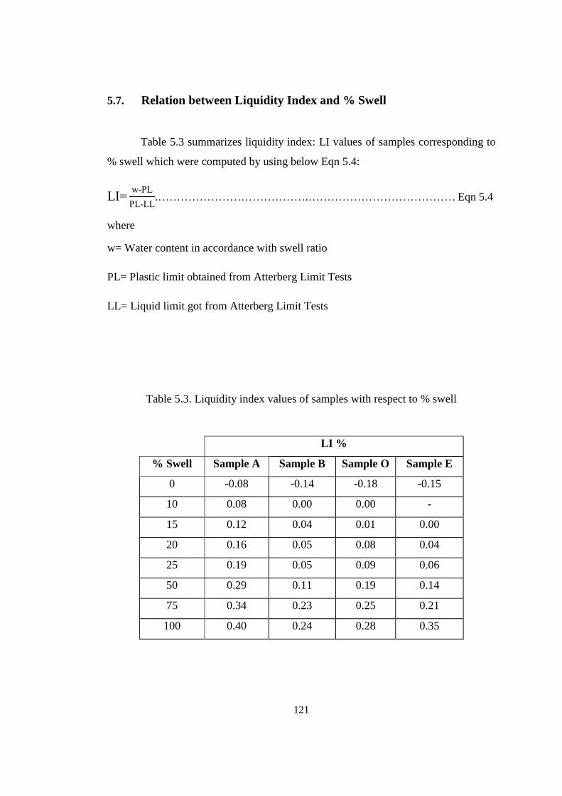
121
5.7. Relation between Liquidity Index and % Swell
Table 5.3 summarizes liquidity index: LI values of samples corresponding to
% swell which were computed by using below Eqn 5.4:
LI=w-PL
PL-LL.………………………………….………………………………… Eqn 5.4
where
w= Water content in accordance with swell ratio
PL= Plastic limit obtained from Atterberg Limit Tests
LL= Liquid limit got from Atterberg Limit Tests
Table 5.3. Liquidity index values of samples with respect to % swell
LI %
% Swell Sample A Sample B Sample O Sample E
0 -0.08 -0.14 -0.18 -0.15
10 0.08 0.00 0.00 -
15 0.12 0.04 0.01 0.00
20 0.16 0.05 0.08 0.04
25 0.19 0.05 0.09 0.06
50 0.29 0.11 0.19 0.14
75 0.34 0.23 0.25 0.21
100 0.40 0.24 0.28 0.35
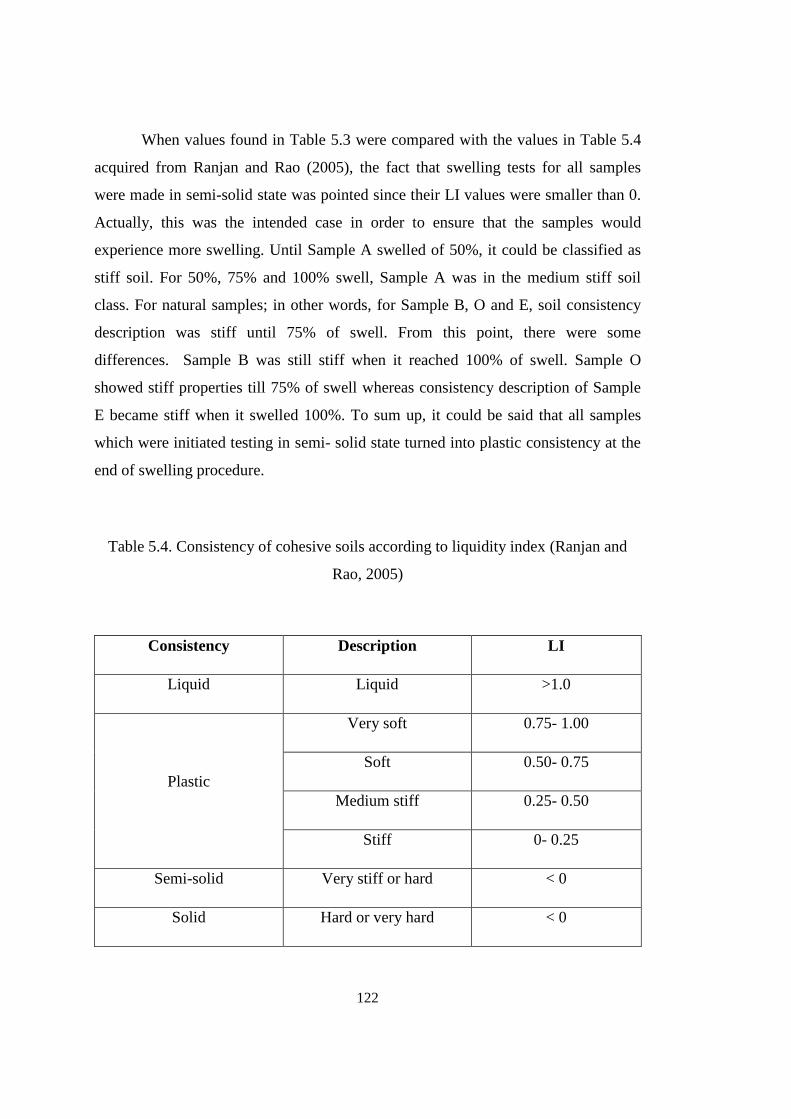
122
When values found in Table 5.3 were compared with the values in Table 5.4
acquired from Ranjan and Rao (2005), the fact that swelling tests for all samples
were made in semi-solid state was pointed since their LI values were smaller than 0.
Actually, this was the intended case in order to ensure that the samples would
experience more swelling. Until Sample A swelled of 50%, it could be classified as
stiff soil. For 50%, 75% and 100% swell, Sample A was in the medium stiff soil
class. For natural samples; in other words, for Sample B, O and E, soil consistency
description was stiff until 75% of swell. From this point, there were some
differences. Sample B was still stiff when it reached 100% of swell. Sample O
showed stiff properties till 75% of swell whereas consistency description of Sample
E became stiff when it swelled 100%. To sum up, it could be said that all samples
which were initiated testing in semi- solid state turned into plastic consistency at the
end of swelling procedure.
Table 5.4. Consistency of cohesive soils according to liquidity index (Ranjan and
Rao, 2005)
Consistency Description LI
Liquid Liquid >1.0
Plastic
Very soft 0.75- 1.00
Soft 0.50- 0.75
Medium stiff 0.25- 0.50
Stiff 0- 0.25
Semi-solid Very stiff or hard < 0
Solid Hard or very hard < 0
123
5.8. Evaluation of Material Ability to Absorb Energy for the Measured
Stress-Strain Values up to Peak Point
Material ability to absorb energy defines toughness. Since residual strength
values were not measured for some samples in some swell steps, energy absorption
ability of soil specimens was calculated from the area below the measured stress-
strain curve at the ultimate peak stress and corresponding strain points. In the
calculation, Trapezoidal Rule was used for measured strain and stress values up to
peak point in the curves obtained from unconfined compression test. Then, absorbed
energy values up to peak point were obtained by taking averages of two test results
and summarized in Table 5.5 for each sample.
The fact that as the stored energy increases, material becomes ductile, is
known. When Table 5.5 was examined, it was seen that all samples were ductile up
to a certain swell percent, which can be 25% swell for Sample A or 15% swell for
Sample O to give an example. After that swell percent, they started to become brittle.
In general, it can be said that absorbed energy increases up to a point. After that
point, soil specimens show brittle behavior.
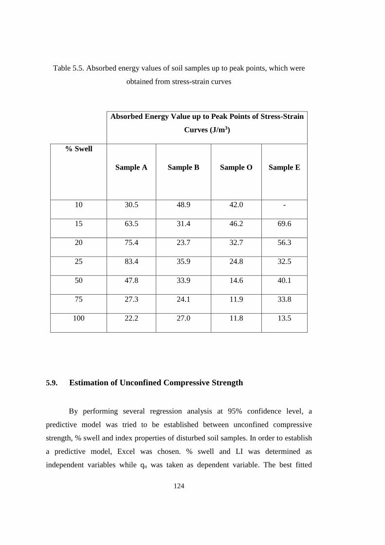
124
Table 5.5. Absorbed energy values of soil samples up to peak points, which were
obtained from stress-strain curves
Absorbed Energy Value up to Peak Points of Stress-Strain
Curves (J/m3)
% Swell
Sample A Sample B Sample O Sample E
10 30.5 48.9 42.0 -
15 63.5 31.4 46.2 69.6
20 75.4 23.7 32.7 56.3
25 83.4 35.9 24.8 32.5
50 47.8 33.9 14.6 40.1
75 27.3 24.1 11.9 33.8
100 22.2 27.0 11.8 13.5
5.9. Estimation of Unconfined Compressive Strength
By performing several regression analysis at 95% confidence level, a
predictive model was tried to be established between unconfined compressive
strength, % swell and index properties of disturbed soil samples. In order to establish
a predictive model, Excel was chosen. % swell and LI was determined as
independent variables while qu was taken as dependent variable. The best fitted
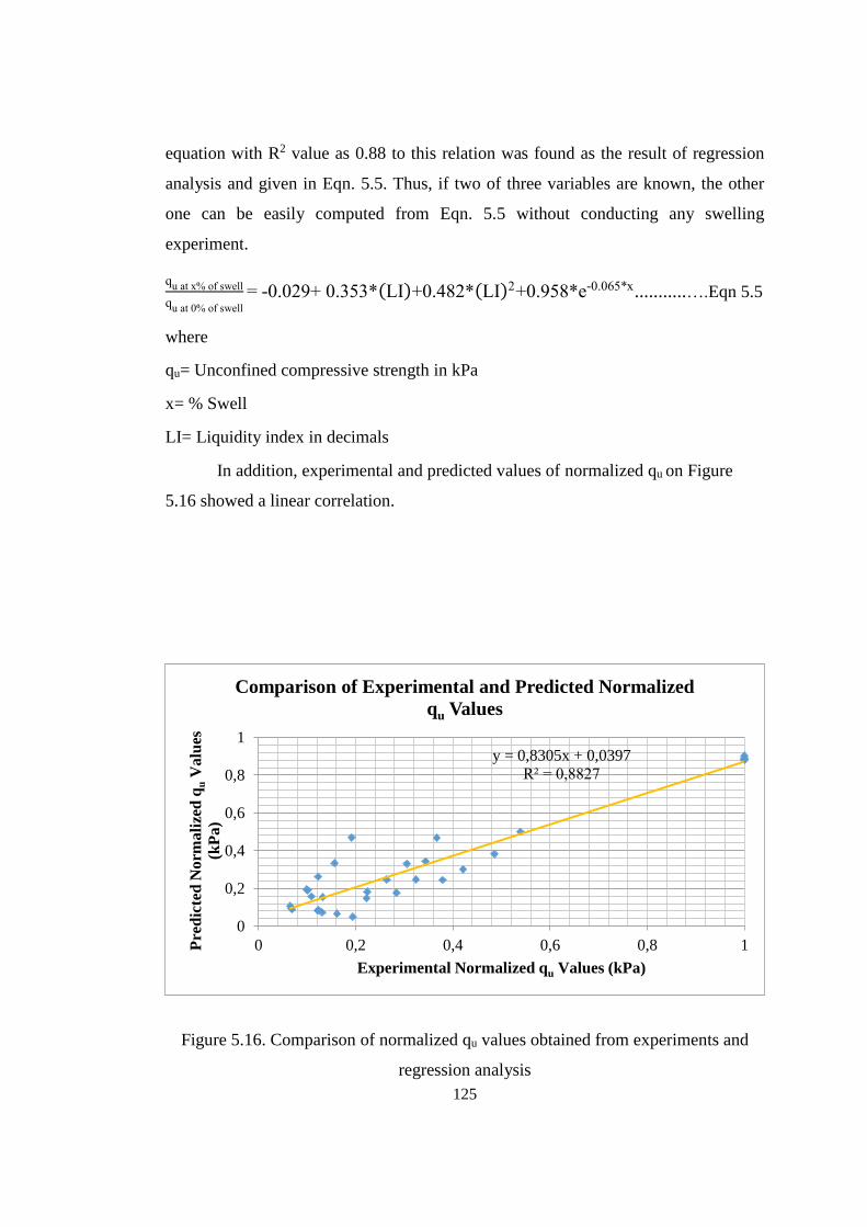
125
equation with R2 value as 0.88 to this relation was found as the result of regression
analysis and given in Eqn. 5.5. Thus, if two of three variables are known, the other
one can be easily computed from Eqn. 5.5 without conducting any swelling
experiment.
qu at x% of swell
qu at 0% of swell
= -0.029+ 0.353*(LI)+0.482*(LI)2+0.958*e-0.065*x...........….Eqn 5.5
where
qu= Unconfined compressive strength in kPa
x= % Swell
LI= Liquidity index in decimals
In addition, experimental and predicted values of normalized qu on Figure
5.16 showed a linear correlation.
Figure 5.16. Comparison of normalized qu values obtained from experiments and
regression analysis
y = 0,8305x + 0,0397
R² = 0,8827
0
0,2
0,4
0,6
0,8
1
0 0,2 0,4 0,6 0,8 1Pre
dic
ted
No
rmali
zed
qu
Valu
es
(kP
a)
Experimental Normalized qu Values (kPa)
Comparison of Experimental and Predicted Normalized
qu Values

126
127
CHAPTER 6
6) CONCLUSIONS
The objective of this study was to search the effect of swelling on undrained
shear strength and unconfined compressive strength of expansive soils. Three natural
and one artificial samples were prepared and then swelled in designed plastic molds
and sheared with unconfined compression test setup. Shearing of specimens prepared
at the intended water contents without swelling was accepted as reference test. Then,
they were allowed to reach ultimate swell in the molds and sheared. Thus, undrained
shear strength in the intermediate steps which included 10%, 15%, 20%, 25%, 50%
and 75% of ultimate swell was found. To verify the swelling potentials determined
from the swell tests made in the specially designed molds, free swell index and
Methylene Blue test were performed on the samples. Moreover, swell pressure and
frictional stress between the specimen and the mold were determined. By taking into
consideration of these experimental test results, following conclusions can be drawn:
As expansive soil sample got water and so swelled, it lost unconfined
compressive strength and undrained shear strength to a degree of about 90-%
of its initial value. Decrease in unconfined compressive strength and
undrained shear strength was same since undrained shear strength was found
by dividing unconfined compressive strength by 2.
Water suction capacity of soil samples was quite variable due to change in
their mineral composition, existence of some chemicals or salts, variability in
temperature etc. When samples reached to ultimate swell, difference in water
contents with respect to initial water content became 124%, 95%, 72% and
108% for Samples A, B, O and E respectively.
128
Undrained elastic modulus values were also decreased with increasing swell
ratio. At 100% swell, soil samples possessed undrained elastic modulus
values which were less than approximately 75-90% of their initial values.
When Free Swell Index Test was used for quick estimation of swelling
potential of soils, it was seen that FSI value was increased with increasing
swelling potential.
When Methylene Blue Test was decided to be utilized for determination of
clay activity, it was observed that the obtained results of artificial and natural
soil samples cannot be compared with each other. However, by taking into
consideration the test results for just natural soil samples; i.e. Sample B, O
and E, the fact that MBV increased as soil swelling potential got higher, was
realized.
More swelling of a sample meant larger force would be needed in order to get
the vertical displacement to zero. Therefore, increase in swell potential
resulted in higher swell pressure values.
Since plastic molds prevented volumetric swelling, a frictional force and so
stress developed between soil specimen and mold, which was equal to about
16.5-25% of swell pressure for 0% and 100% of swell respectively.
It was seen that as expansiveness potential of the specimen increased, it took
more time to complete the swell procedure.
The main reason behind the swell mechanism was the water existence in
interlayer spacing. Therefore, as soil took water, degree of saturation of it
also increased. When Sample A reached 50% of swell, it became fully
saturated. On the other hand, Sample B and O had full saturation at 75% of
swell. For Sample E, which has the lowest swelling potential, fully saturation
case was accomplished at the ultimate swell.
When the results obtained from liquidity index and undrained elastic modulus
were examined, existence of differences were observed. The reason of this
129
could be explained with the method used to calculate undrained elastic
modulus and liquidity index. Undrained elastic modulus was computed by
drawing secant line from the initial point to 50% of peak stress at the stress-
strain curve while liquidity index was obtained from the relation between
water content, liquid limit and plastic limit.
Calculation of absorbed energy from the area under stress-strain curves up to
peak point showed that soil specimens became ductile to a point as they got
water. After that point, their behavior against little stress increase turned out
to be brittle.
When the relation between net bearing capacity and swell % was examined
by an example in Appendix D, it was seen that once Sample A swelled until
vertical displacement stopped, its net bearing capacity value decreased to
approximately 90% of values at 0% swell.
In an example problem in Appendix E, the calculation of immediate
settlement values for 0% and 100% swell showed that immediate settlement
values for artificial soil sample increased about 917 % of its initial value
when their vertical displacement ceased.
Factor of safety of an example slope with the expansive soil in Appendix F
decreased below 1 after the soil reached 20% of swell.
Pile length in an example swelling soil increased about 422% of its initial
value when the ultimate swelling reached (Appendix G).
130
RECOMMENDATIONS FOR FUTURE RESEARCH
This study includes influence of swell amount on shear strength of expansive
soils. For this aim, specially designed molds were used in swell procedure and
swelled samples were sheared in unconfined compression test machine. These tests
may be repeated on swelling clay samples from different regions of Turkey and on
samples with different proportions of bentonite and kaolinite. Furthermore,
mineralogy by x-ray diffraction test and chemical analysis of the test samples may be
determined and correlated with MBV test.
131
7) REFERENCES
AFNOR, Mesure de la Capacite D’adsorption de Bleu de Methylene d’un sol ou d’un
Materiau Rocheux, l’Association Française de Normalisation, NF P 94-068,
1998
Al-Rawas, A. and Goosen, M.F.A., Eds., Expansive Soils Recent Advances in
Characterization and Treatment, Taylor and Francis Group, London, pp. 25-27,
pp.375-384, 2006
Al- Mhaidib, A. and Al- Shamrani, M., Influence of Swell on Shear Strength of
Expansive Soils, Advances in Unsaturated Soil, Seepage, and Environmental
Geotechnics,pp. 160-165, 2006
ASTM, Standard Practice for Classification of Soils for Engineering Purposes (
Unified Soil Classification System), Annual Book of ASTM Standards, D 2487-
06, Vol. 04. 08, 2011
ASTM, Standard Test Methods for Laboratory Compaction Characteristics of Soil
Using Standard Effort (12400 ft- lbf/ft3 (600 kN- m/ m3)), Annual Book of ASTM
Standards, D698- 07, 2007
ASTM, Standard Test Methods for Liquid Limit, Plastic Limit, and Plasticity Index
of Soils, Annual Book of ASTM Standards, D4318- 10e1, 2010
ASTM, Standard Test Methods for One- Dimensional Swell or Settlement Potential
of Cohesive Soils, Annual Book of ASTM Standards, D4546- 96, Vol. 04. 08,
1996
ASTM, Standard Test Method for Particle- Size Analysis of Soils, Annual Book of
ASTM Standards, D 422- 63, 2007
132
ASTM, Standard Test Method for Particle- Size Distribution (Gradation) of Soils
Using Sieve Analysis, Annual Book of ASTM Standards, D6913- 04, 2009
ASTM, Standard Test Method for Shrinkage Factors of Soils by the Mercury
Method, Annual Book of ASTM Standards, D- 427- 98, Vol. 04.02, 1998
ASTM, Standard Test Methods for Specific Gravity of Soil Solids by Water
Pycnometer, Annual Book of ASTM Standards, D854- 14, 2014
ASTM, Standard Test Methods for Unconfined Compressive Strength of Cohesive
Soils, Annual Book of ASTM Standards, D2166/ D2166M- 13, 2013
Bao, C., Gong, B., & Zhan, L., Properties of Unsaturated Soils and Slope Stability of
Expansive Soils. In Proc., 2nd Int. Conf. on Unsaturated Soils (UNSAT 98), pp.
71–98, 1998
Barshad, I., Adsorptive and Swelling Properties of Clay- Water System, Clays and
Clay Minerals, Vol. 1, Issue. 1, pp. 70-77, 1949
Bergaya, F., Theng, B. K. G. and Lagaly, G., Eds., Developments in Clay Science:
Handbook of Clay Science, 1st Ed., Elsevier, Amsterdam, pp. 1-16, 2006
Birand, A., Ergun, U. and Erol, O., CE366 Foundation Engineering 1, METU Press,
Ankara, 2011
Bishop, A. W. The Principle of Effective Stress, Teknisk Ukeblad, Vol.106, No.39,
pp.859-863,1959
Blogs of the European Geosciences Union, http://blogs.egu.eu/, last visited on
November 2015
133
Briaud, J. L., Introduction to Soil Moduli, Geotechnical News, BiTech Publisherd
Ltd., Richmond, Canada, 2001
Chen, F. H., Foundations on Expansive Soils Developments in Geotechnical
Engineering, 12th Ed., Elsevier Scientific Publishing Company, Amsterdam, pp.
1-10, 1975
Chen, Y. J., Lin, S. S., Chang, H. W. and Marcos, M. C., Evaulation of Side
Resistance Capacity for Drilled Shafts, Journal of Marine Science and
Technology, Vol. 19, No. 2, pp. 201-221, 2011
Craig, R. F., Craig’s Soil Mechanics, 7th Ed., Spon Press, London, pp. 4-5, 2004
Das, B. M., Advanced Soil Mechanics, 3rd Ed., Taylor and Francis Group, New
York, USA, pp. 7-17, 2008
Domitrovic, D. and Kovacevic, Z.B., The Relationship between Swelling and Shear
Strength Properties of Bentonites, Proceedings of the 18th International
Conference on Soil Mechanics and Geotechnical Engineering, Paris, 2013
Eslharief, E. M., Foundations in Expansive Soils, Sudan Experience, Conference of
Graduate Studies and Scientific Research, University of Khartoum, 2010
Fredlund, D. G. and Morgenstern, N. R., Stress State Variables for Unsaturated
Soils, Journal of Geotechnical Division, ASCE, Vol.103, No. GT5, pp.447-466,
1977
Gardiner, D. T. and Miller, R. W., Soils in our Environment, 8th Ed., Prentice- Hall
Publishers, Upper Saddle River, NY, 1998
Grim, R.E., Clay Mineralogy, 2nd Ed., McGraw Hill, New York, pp.596, 1968
134
Grim, R. E., Properties of Clay, Authority of the State of Illinois, Urbana, 1939
Guggenheim, S., Adams, J.M., Bain, D.C., Bergaya, F., Brigatti, F., Brigatti, M.F.,
Drits, V.A., Formoso, M.L.L., Galan, E., Kogure, T. and Stanjek, H., Summary
of Recommendations of Nomenclature Committees Relevant to Clay
Mineralogy, Report of the Association Internationale Pour L’etude des Argiles
(AIPEA)
Holtz, R. D. and Kovacs, W. D, Introduction to Geotechnical Engineering, Prentice-
Hall, 1981
Inter- Organization Programme for the Sound Management of Chemicals,
Environmental Health Criteria 231: Bentonite, Kaolin and Selected Clay
Minerals, World Health Organization, Geneva, 2005
IS, Method of Test for Soils Part XL Determination of Free Swell Index of Soils,
Bureau of Indian Standards, 2720, Part XL, 2002
Ishibashi, E. I. and Hazarika, H., Soil Mechanics Fundamentals and Applications,
2nd Ed., CRC Press, 2015
Khalili, N. and Khabbaz, M. H., A Unique Relationship for the Determination of
Shear Strength of Unsaturated Soils, Geotechnique, Vol. 48, No. 5, pp.681-687,
1998
Karube, D., Kato, S., Hamada, K. and Honda, M., The Relationship between the
Mechanical Behavior and the State of Pore Water in Soil”, Journal of JSCE,
Vol.535, pp.83-92, 1996
Lambe, T. W. and Whitman, R. V., Soil Mechanics, John Wiley and Sons, USA, pp.
40-51, 1969
135
Lal, R., Ed., Encyclopedia of Soil Science, Vol.1., Taylor and Francis Group, USA,
pp. 277-278, 2006
Lee, Y., Stress- Strain- Time Relationship of Queenston Shale, Doctor of Philosophy
Thesis, The University of Western Ontario, Canada, 554 pages, 1988
Mitchell, J.K., Fundamentals of Soil Behavior, 2nd Ed., John Wiley and Sons, 1993
Murray, H.H., Applied Clay Mineralogy Occurences, Processing and Application of
Kaolins, Bentonites, Palygorskite- Sepiılite and Common Clays, 1st Ed.,
Elsevier, Amsterdam, pp. 1-19, 2007
Nelson, J. D. and Miller, J. M., Expansive Soils Problems and Practice in
Foundation and Pavement Engineering, John Wiley and Sons Inc., USA, pp. 8-
12, 1992
New Mexico Tech Institute of Mining and Technology, www.nmt.edu, last visited
on May 2015
Nicholson, P. G., Soil Improvement and Ground Modification Methods, Elsevier,
USA, pp. 77-78, 2015
Nomenclature Committee 2006, Clays and Clay Minerals, Vol. 54, pp. 761-772,
2006
NovoPILE User’s Manual, http://help.novotechsoftware.com, last visited on
February 2016
Öberg, A. L. and Sällfors, G. A Rational Approach to the Determination of the Shear
Strength Parameters of Unsaturated Soils, Proceedings of First International
Conference on Unsaturated Soils, Paris, Vol.1, pp.151-158, 1995
136
Patel, A. D., Stamatakis, E., Davis, E. and Friedheim, J., High Performance Water
Based Drilling Fluids and Method of Used, Houston, 2007
Ranjan, G. and Rao, A.S.R., Basic and Applied Soil Mechanics, 2nd Ed., New Age
International Ltd., New Delhi, pp. 41, 2005
Reeves, G. M., Sims, I. and Cripps, Eds., J. C., Clay Materials Used in Construction,
The Geological Society, London, pp. 20-23, 2006
Rowe, R. K., Ed., Geotechnical and Geoenvironmental Engineering Handbook, Vol.
1, Springer Science+ Business Media, New York, pp. 162-163, 2001
Sivapullaiah, P., Sitharam, T. and Subba, R. K., Modified Free Swell Index for
Clays, Geotechnical Testing Journal, Vol. 10, Issue 2, pp. 80-85, 1987
Skempton, A. W. and Macdonald, D. H., The Allowable Settlement of Buildings,
Proceedings of the Institution of Civil Engineers, Vol. 5, No. 6, pp. 727- 768,
1956
Sridharan, A. and Prakash, K., Classification Procedures for Expansive Soils,
Proceedings of the Institution of Civil Engineers- Geotechnical Engineering,
Vol. 143, pp. 235-240, 2000
Soil Expedition, http://soilnews.feedsynews.com, last visited on October 2015
Tekinsoy, M. ., Kayadelen, C., Keskin, M., and Söylemez, M., An Equation for
Predicting Shear Strength Envelope with respect to Matric Suction. Computers
and Geotechnics, 31(7), 589–593, 2004
Terzaghi, K., Erdbaumechanik auf Bodenphsikalischer Grundlage, 1925
137
Terzaghi, K., Peck, R.B. and Mesri, G., Soil Mechanics in Engineering Practice, 3rd
Ed., John Wiley and Sons Inc., USA, pp. 9-10, 1996
Tilgen, H. P., Relationship between Suction and Shear Strength Parameters of
Compacted METU Campus Clay, M.S. Thesis, METU, Turkey, 120 pages, 2003
The European Geosciences Union Blogs, http://blogs.egu.eu/, last visited on
October 2015
Türköz, M. and Tosun, H., The Use of Methylene Blue Test for Predicting Swell
Parameters of Natural Clay Soils, Scientific Research and Essays, Vol. 6, No. 8,
pp.1780-1792, 2011
University of Idaho Soil 205-90, General Soils for Distance Students Lecture Notes,
http://www.uidaho.edu/, last visited on October 2015
University of Pennsylvania, http://calculus.seas.upenn.edu/, last visited on November
2015
NAVDOCKS DM-7, Soil Mechanics, Foundation and Earth Structures, U.S.
Department of the Navy Design Manual, 1962
Wang, L., Long, W. and Gao, S., Effect of Moisture Content, Void Ratio and
Compacted Sand Content on the Shear Strength of Remolded Unsaturated Clay,
The Electronic Journal of Geotechnical Engineering, Vol. 19, Bundle Q, pp.
4413-4426, 2014
Weaver, C. E. and Pollard, L. D., Developments in Sedimentology 15: The Chemistry
of Clay Minerals, Amsterdam, pp. 1-106, 1973
Wilbourn, K., Index Properties and Strength of Artificial Soil Using the Harvard
Miniature Method, Report, University of Houston, USA, 2007
138
Wyoming Multi-Hazard Mitigation Plan, http://hls.wyo.gov/, last visited on
December 2015
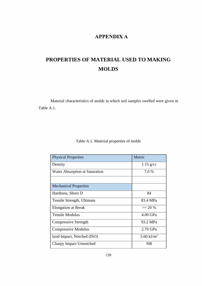
139
8) APPENDIX A
PROPERTIES OF MATERIAL USED TO MAKING
MOLDS
Material characteristics of molds in which soil samples swelled were given in
Table A.1.
Table A.1. Material properties of molds
Physical Properties Metric
Density 1.15 g/cc
Water Absorption at Saturation 7.0 %
Mechanical Properties
Hardness, Shore D 84
Tensile Strength, Ultimate 83.4 MPa
Elongation at Break >= 20 %
Tensile Modulus 4.00 GPa
Compressive Strength 93.2 MPa
Compressive Modulus 2.70 GPa
Izod Impact, Notched (ISO) 5.60 kJ/m2
Charpy Impact Unnotched NB
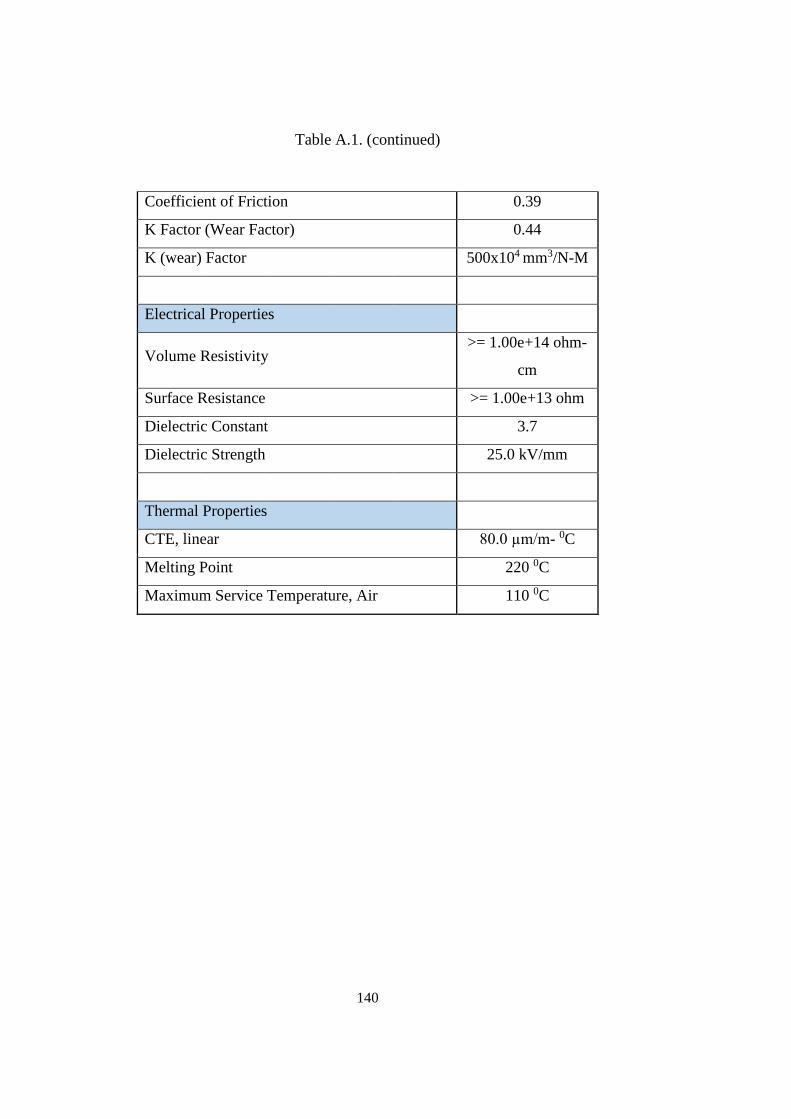
140
Table A.1. (continued)
Coefficient of Friction 0.39
K Factor (Wear Factor) 0.44
K (wear) Factor 500x104 mm3/N-M
Electrical Properties
Volume Resistivity >= 1.00e+14 ohm-
cm
Surface Resistance >= 1.00e+13 ohm
Dielectric Constant 3.7
Dielectric Strength 25.0 kV/mm
Thermal Properties
CTE, linear 80.0 µm/m- 0C
Melting Point 220 0C
Maximum Service Temperature, Air 110 0C
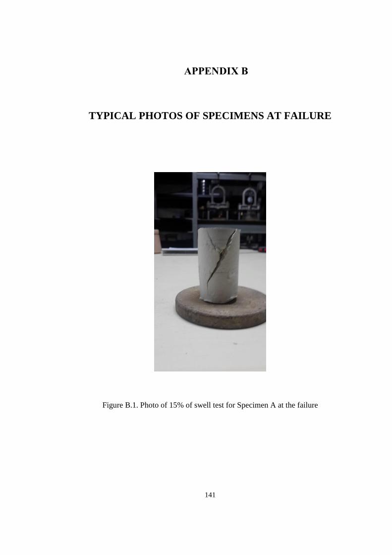
141
9) APPENDIX B
TYPICAL PHOTOS OF SPECIMENS AT FAILURE
Figure B.1. Photo of 15% of swell test for Specimen A at the failure
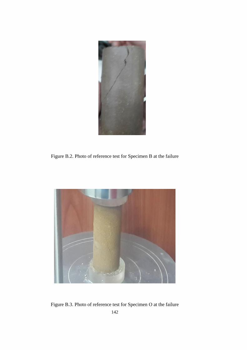
142
Figure B.2. Photo of reference test for Specimen B at the failure
Figure B.3. Photo of reference test for Specimen O at the failure
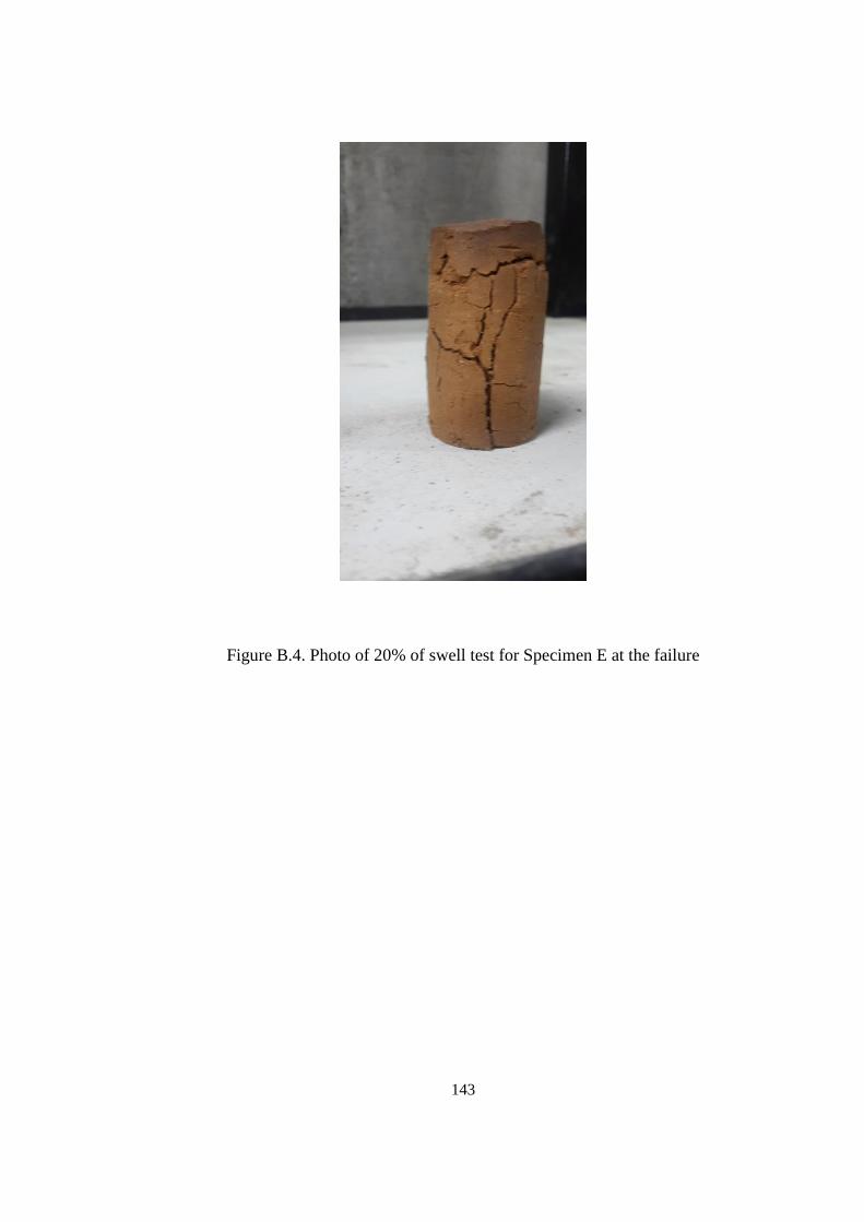
143
Figure B.4. Photo of 20% of swell test for Specimen E at the failure
10)

144
145
11) APPENDIX C
CALCULATION OF UNDRAINED SHEAR STRENGTH
Calculation of undrained shear strength for Sample B at 0 % swell; i.e., at
reference test, was given below as an example:
After strain and load dial gauge readings were recorded during unconfined
compression test, initial cross sectional area: A0 was calculated as 0.001092 m2 using
Eqn. C.1 for all tests at all steps.
A0=π*D2
4 ……………..…………………………...……..…………………….Eqn. C.1
where
D= Initial sample diameter
Proving ring constant: Cp and initial sample height: H0 were taken as 0.075
and 0.072 m respectively at the computations. Used proving ring determined Cp
value. Table C.1 summarized the calculation steps from this point. After strain and
compressive stress values were obtained, which were marked in Table C.1 with blue
color, peak point was determined. Half of this peak point gave undrained shear
strength value. Meanwhile, necessary unit conversions were made.
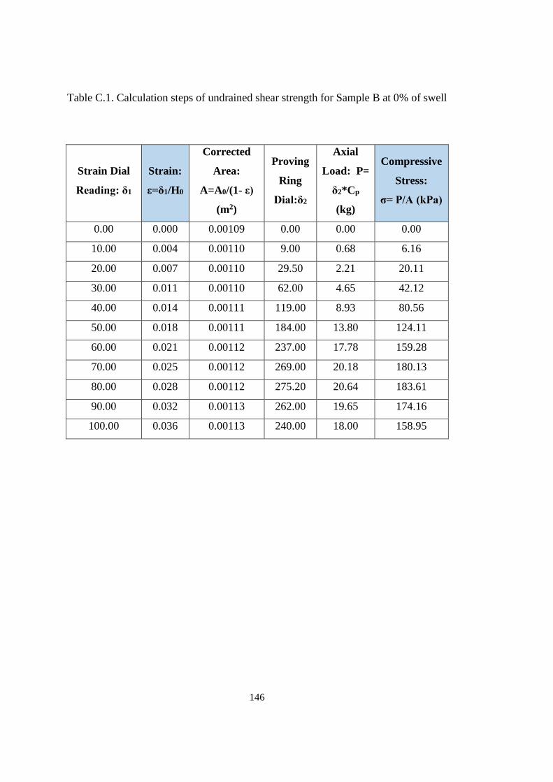
146
Table C.1. Calculation steps of undrained shear strength for Sample B at 0% of swell
Strain Dial
Reading: δ1
Strain:
ε=δ1/H0
Corrected
Area:
A=A0/(1- ε)
(m2)
Proving
Ring
Dial:δ2
Axial
Load: P=
δ2*Cp
(kg)
Compressive
Stress:
σ= P/A (kPa)
0.00 0.000 0.00109 0.00 0.00 0.00
10.00 0.004 0.00110 9.00 0.68 6.16
20.00 0.007 0.00110 29.50 2.21 20.11
30.00 0.011 0.00110 62.00 4.65 42.12
40.00 0.014 0.00111 119.00 8.93 80.56
50.00 0.018 0.00111 184.00 13.80 124.11
60.00 0.021 0.00112 237.00 17.78 159.28
70.00 0.025 0.00112 269.00 20.18 180.13
80.00 0.028 0.00112 275.20 20.64 183.61
90.00 0.032 0.00113 262.00 19.65 174.16
100.00 0.036 0.00113 240.00 18.00 158.95
147
12) APPENDIX D
INFLUENCE OF SWELL RATIO ON NET ULTIMATE
BEARING CAPACITY
In order to see the effect of swelling at different ratios on bearing capacity, a
square foundation whose depth was 1 m and dimensions were 1x1 m were taken into
consideration. Foundation existence was assumed on soil from which Sample A was
taken.
Skempton (1951) stated that net ultimate bearing capacity of clays: qnf is
computed by using below Eqn D.1 ( Birand et al., 2011).
qnf=cu*Nc…………………...………………………….………………….... Eqn D.1
where
cu= Undrained shear strength of soil
Nc= Dimensionless bearing capacity factor taken from Skempton’s Chart given in
Figure D.1.
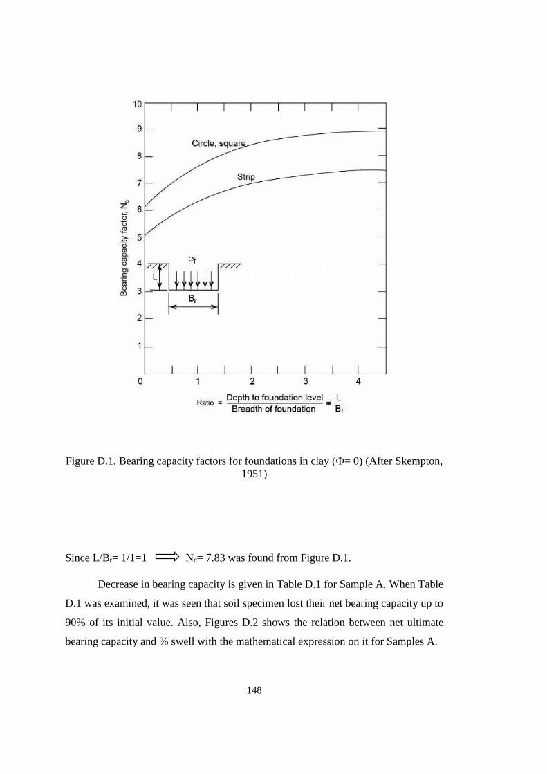
148
Figure D.1. Bearing capacity factors for foundations in clay (Ф= 0) (After Skempton,
1951)
Since L/Br= 1/1=1 Nc= 7.83 was found from Figure D.1.
Decrease in bearing capacity is given in Table D.1 for Sample A. When Table
D.1 was examined, it was seen that soil specimen lost their net bearing capacity up to
90% of its initial value. Also, Figures D.2 shows the relation between net ultimate
bearing capacity and % swell with the mathematical expression on it for Samples A.
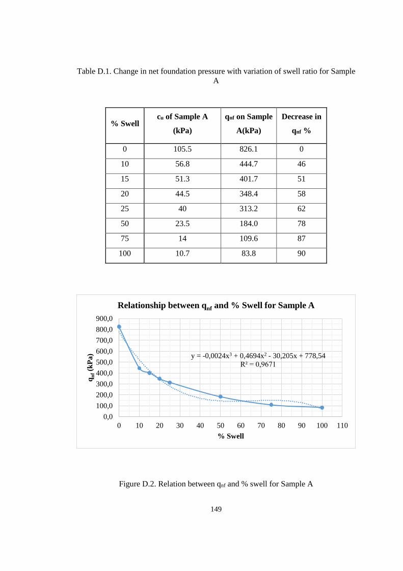
149
Table D.1. Change in net foundation pressure with variation of swell ratio for Sample
A
% Swell cu of Sample A
(kPa)
qnf on Sample
A(kPa)
Decrease in
qnf %
0 105.5 826.1 0
10 56.8 444.7 46
15 51.3 401.7 51
20 44.5 348.4 58
25 40 313.2 62
50 23.5 184.0 78
75 14 109.6 87
100 10.7 83.8 90
Figure D.2. Relation between qnf and % swell for Sample A
y = -0,0024x3 + 0,4694x2 - 30,205x + 778,54
R² = 0,9671
0,0
100,0
200,0
300,0
400,0
500,0
600,0
700,0
800,0
900,0
0 10 20 30 40 50 60 70 80 90 100 110
qn
f(k
Pa)
% Swell
Relationship between qnf and % Swell for Sample A

150
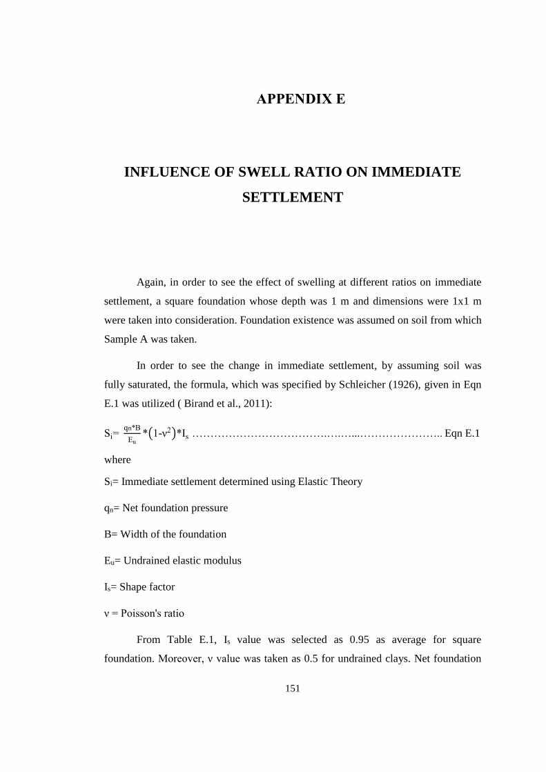
151
13) APPENDIX E
INFLUENCE OF SWELL RATIO ON IMMEDIATE
SETTLEMENT
Again, in order to see the effect of swelling at different ratios on immediate
settlement, a square foundation whose depth was 1 m and dimensions were 1x1 m
were taken into consideration. Foundation existence was assumed on soil from which
Sample A was taken.
In order to see the change in immediate settlement, by assuming soil was
fully saturated, the formula, which was specified by Schleicher (1926), given in Eqn
E.1 was utilized ( Birand et al., 2011):
Si= qn*B
Eu*(1-ν2)*Is ……………………………….….…...………………….. Eqn E.1
where
Si= Immediate settlement determined using Elastic Theory
qn= Net foundation pressure
B= Width of the foundation
Eu= Undrained elastic modulus
Is= Shape factor
ν = Poisson's ratio
From Table E.1, Is value was selected as 0.95 as average for square
foundation. Moreover, ν value was taken as 0.5 for undrained clays. Net foundation
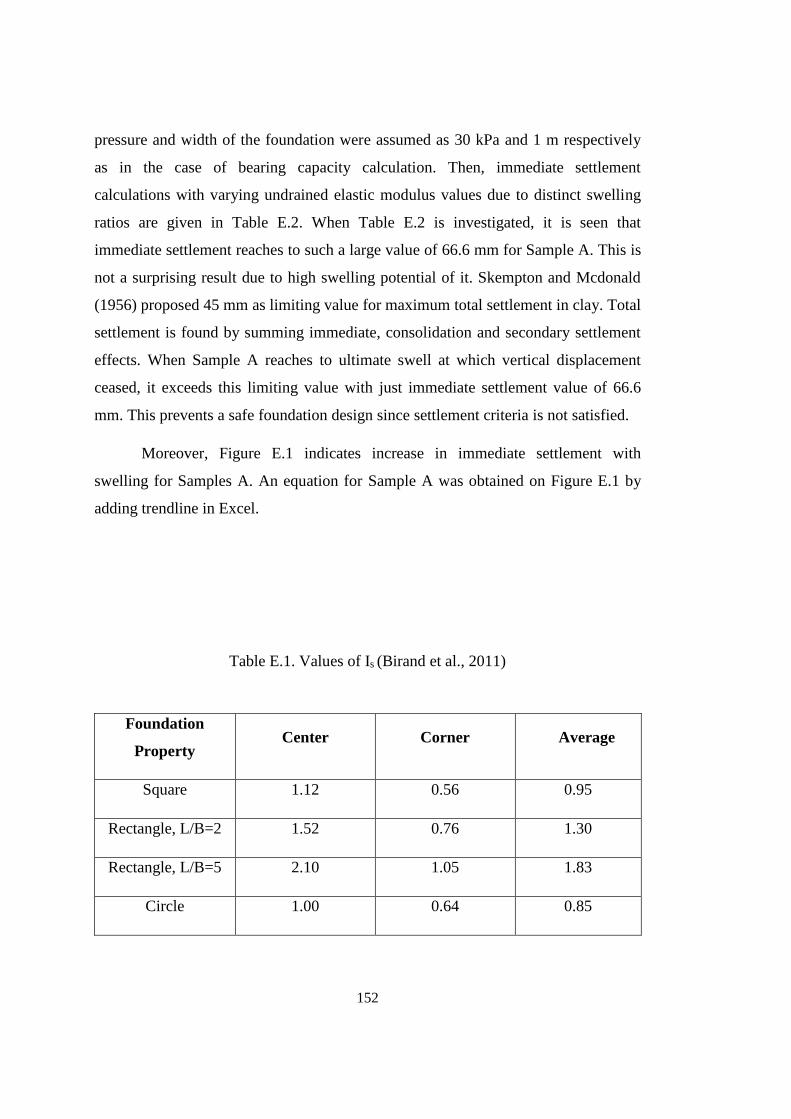
152
pressure and width of the foundation were assumed as 30 kPa and 1 m respectively
as in the case of bearing capacity calculation. Then, immediate settlement
calculations with varying undrained elastic modulus values due to distinct swelling
ratios are given in Table E.2. When Table E.2 is investigated, it is seen that
immediate settlement reaches to such a large value of 66.6 mm for Sample A. This is
not a surprising result due to high swelling potential of it. Skempton and Mcdonald
(1956) proposed 45 mm as limiting value for maximum total settlement in clay. Total
settlement is found by summing immediate, consolidation and secondary settlement
effects. When Sample A reaches to ultimate swell at which vertical displacement
ceased, it exceeds this limiting value with just immediate settlement value of 66.6
mm. This prevents a safe foundation design since settlement criteria is not satisfied.
Moreover, Figure E.1 indicates increase in immediate settlement with
swelling for Samples A. An equation for Sample A was obtained on Figure E.1 by
adding trendline in Excel.
Table E.1. Values of Is (Birand et al., 2011)
Foundation
Property Center Corner Average
Square 1.12 0.56 0.95
Rectangle, L/B=2 1.52 0.76 1.30
Rectangle, L/B=5 2.10 1.05 1.83
Circle 1.00 0.64 0.85
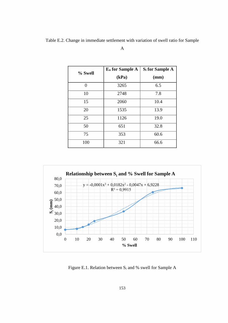
153
Table E.2. Change in immediate settlement with variation of swell ratio for Sample
A
% Swell Eu for Sample A
(kPa)
Si for Sample A
(mm)
0 3265 6.5
10 2748 7.8
15 2060 10.4
20 1535 13.9
25 1126 19.0
50 651 32.8
75 353 60.6
100 321 66.6
Figure E.1. Relation between Si and % swell for Sample A
y = -0,0001x3 + 0,0182x2 - 0,0047x + 6,9228
R² = 0,9915
0,0
10,0
20,0
30,0
40,0
50,0
60,0
70,0
80,0
0 10 20 30 40 50 60 70 80 90 100 110
Si(m
m)
% Swell
Relationship between Si and % Swell for Sample A

154
14)
155
APPENDIX F
INFLUENCE OF SWELL RATIO ON SLOPE
STABILITY
In order to see the effects of swelling on slope stability of expansive clay,
slope whose height and angle was assumed as 10 m and 540 respectively. Slope of a
soil was considered from which Sample A was taken.
Change in factor of safety against sliding was search according to Eqn. F.1
(Taylor, 1948):
FS= cu
Ns*ɣ*H…………………………………...……………………………….Eqn. F.1
where
cu= Undrained shear strength
Ns= Stability coefficient depending on slope angle
ɣ= Unit weight of soil sample
H= Slope height
Unit weight of soil sample was computed from Gs in Table 4.3 as 25.9 kN/m3.
Additionally, Ns value was determined as 0.183 from Figure E.1 for Фu= 0 and slope
angle as 540. Table F.1 shows the calculation steps. Figure F.2 presents the change in
FS versus % swell with the mathematical correlation on it. As can be seen from
Table F.1, after 20% of swell, FS value is even under 1.
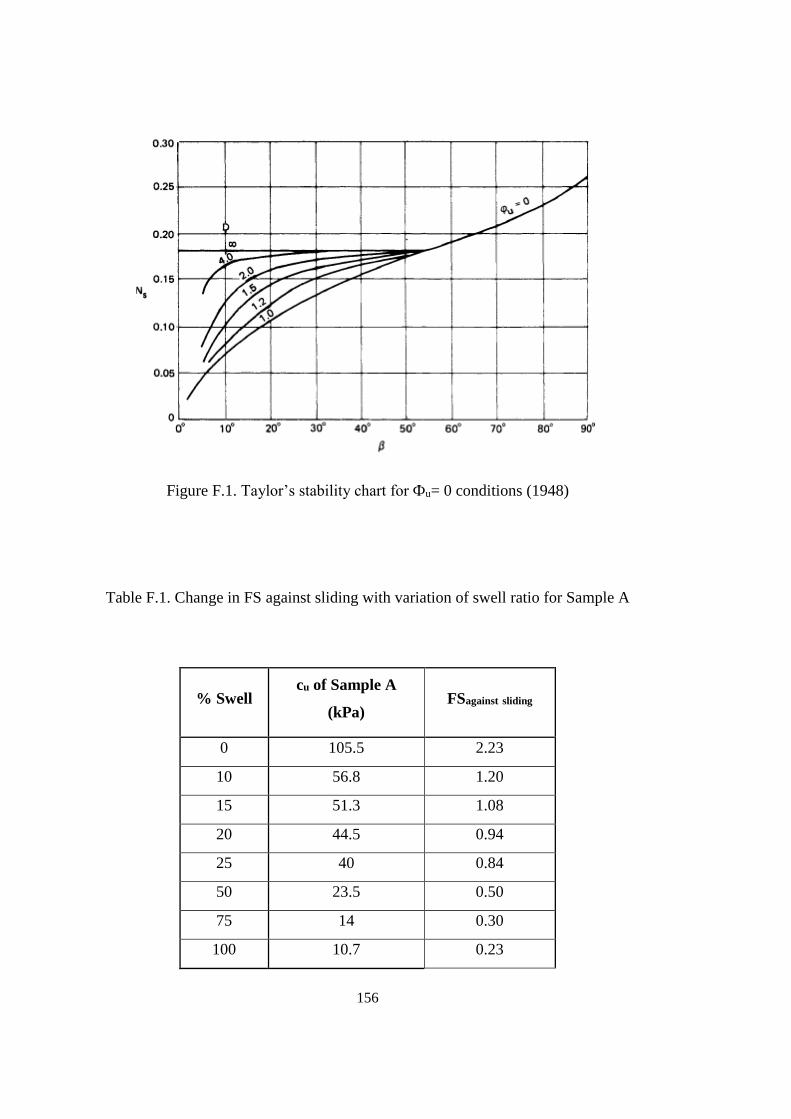
156
Figure F.1. Taylor’s stability chart for Фu= 0 conditions (1948)
Table F.1. Change in FS against sliding with variation of swell ratio for Sample A
% Swell cu of Sample A
(kPa) FSagainst sliding
0 105.5 2.23
10 56.8 1.20
15 51.3 1.08
20 44.5 0.94
25 40 0.84
50 23.5 0.50
75 14 0.30
100 10.7 0.23
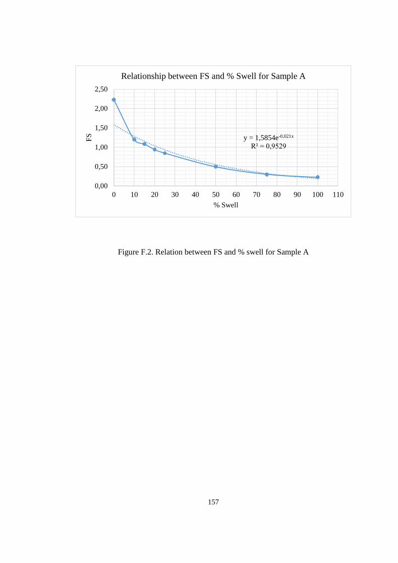
157
Figure F.2. Relation between FS and % swell for Sample A
y = 1,5854e-0,021x
R² = 0,9529
0,00
0,50
1,00
1,50
2,00
2,50
0 10 20 30 40 50 60 70 80 90 100 110
FS
% Swell
Relationship between FS and % Swell for Sample A

158
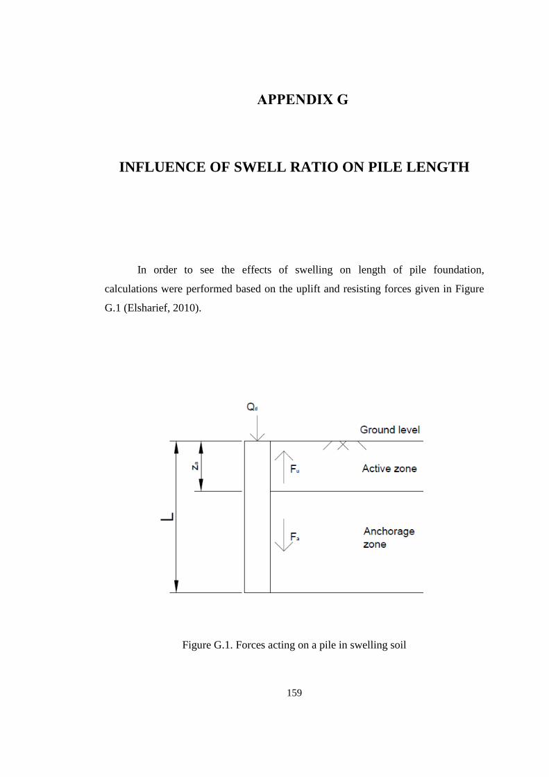
159
15) APPENDIX G
INFLUENCE OF SWELL RATIO ON PILE LENGTH
In order to see the effects of swelling on length of pile foundation,
calculations were performed based on the uplift and resisting forces given in Figure
G.1 (Elsharief, 2010).
Figure G.1. Forces acting on a pile in swelling soil
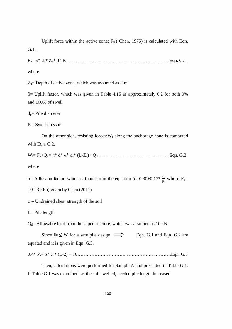
160
Uplift force within the active zone: Fu ( Chen, 1975) is calculated with Eqn.
G.1.
Fu= π* dp* Za* β* Ps…………………….…………………………………….…………..………………Eqn. G.1
where
Za= Depth of active zone, which was assumed as 2 m
β= Uplift factor, which was given in Table 4.15 as approximately 0.2 for both 0%
and 100% of swell
dp= Pile diameter
Ps= Swell pressure
On the other side, resisting forces:Wf along the anchorage zone is computed
with Eqn. G.2.
Wf= Fa+Qd= π* d* α* cu* (L-Za)+ Qd…………………………...…………….…………………Eqn. G.2
where
α= Adhesion factor, which is found from the equation (α=0.30+0.17* cu
Pa where Pa=
101.3 kPa) given by Chen (2011)
cu= Undrained shear strength of the soil
L= Pile length
Qd= Allowable load from the superstructure, which was assumed as 10 kN
Since Fu≤ W for a safe pile design Eqn. G.1 and Eqn. G.2 are
equated and it is given in Eqn. G.3.
0.4* Ps= α* cu* (L-2) + 10………………………….………………..……….Eqn. G.3
Then, calculations were performed for Sample A and presented in Table G.1.
If Table G.1 was examined, as the soil swelled, needed pile length increased.
161
Table G.1. Change in L with variation of swell ratio for Sample A
%
Swell
cu of Sample A
(kPa)
Water
Content:w
(%)
Adhesion
factor: α
Α* cu
(kPa)
L from Eqn.
G.3 (m)
0 105.5 23.9 0.477 50.329 2.88
10 56.8 33.8 0.395 22.454 3.98
15 51.3 36.7 0.386 19.806 4.24
20 44.5 39.1 0.375 16.673 4.66
25 40 41.1 0.367 14.685 5.02
50 23.5 46.8 0.339 7.977 7.56
75 14 50.2 0.323 4.529 11.80
100 10.7 53.8 0.318 3.402 15.04