Information Acquisition and Consumer Choice*

Preliminary Draft – INCOMPLETE – Comments sought!

T. Bresnahan, T. Landvoigt, and P.-L. Yin†

ABSTRACT

We specify and estimate a model of demand for new goods implementing Simon’s idea

that consumers may not know their entire choice set. The model is identified in data, like ours,

in which there is information about both what consumers say about their choices and about their

actual choices. Learning what consumers do not know about their choice set from what they say

about their choices is difficult, but solvable. We apply our model to software upgrade demand in

the era before automatic upgrading. We find that much of the consumer inertia in electronic

markets around default changes arises from incomplete information about choice sets, not from

high adjustment costs.

1. INTRODUCTION

We study the sources of consumer inertia around initial product choices in online

markets. We build a model which lets us distinguish between two sources of inertia, adjustment

costs net of the value of switching to a new product and incomplete information about the choice

set. Measuring those demand forces is part of understanding the emergence of a number of

modern market institutions, notably pay-for-referral institutions such as advertising-supported

search and demander-choice-replacing institutions such as automatic upgrades.1 Our approach

* This version of the paper is preliminary in a number of senses. There are few citations, and we do not yet

thank the many colleagues who have given us valuable comments. † Stanford University, Stanford University, and MIT, respectively. 1 There is a wide variety of such institutions. One dramatic change on the supply side is the emergence of

a number of institutions by which sellers obtain product placement and/or consumer referrals. Advertising auctions

2

relies on having data on both what consumers do – actual demand – and what they say – self-

reported demand. More importantly, we build a model that permits us to draw an inference

about the demand role of what consumers know without assuming a close relationship between

what they say and what they know.

In particular, we examine individual choice and information gathering by demanders in a

technologically dynamic market. Technologically dynamic markets, in which newly-invented

product varieties expand the choice set, present demanders with a Simon (1955) problem of

learning their full choice set as well as a choice problem. We model this as a simple repeated

two-stage problem for a rational consumer. In stage I of each period, the consumer either learns,

or does not, the characteristics of any new products in the choice set. In stage II, the consumer

decides on a product, with an adjustment cost if there is a product change.2 The pace at which

consumers take up a new version will be slower if either the arrival rate of information about the

full choice set is slower or if more consumers, once informed, choose not to adopt the newest

version. Our empirical goal is to tell those two sources of inertia apart.

More narrowly, we study upgrading to new versions of software in a context where the

upgrades are free: Microsoft web browsers in the late 1990s. Studying upgrades in this early era,

before software started insisting on upgrading itself, brings us a number of analytical advantages.

First, the problem of knowing whether a new version has been introduced is a search problem

are the most studied of these institutions: in them, advertisers typically pay for a referral, i.e., pay only if a consumer

clicks on a link to their website (online) or runs her thumb over their ad (mobile). Other related institutions include

“nagware,” in which an old version of product asks to be updated, “soft” bundling in which a default choice of

product B is presented to a consumer who has chosen product A, and collaborative filters which suggest products a

consumer might like. These new institutions are (1) clearly intended to overcome frictions of some kind, despite the

much-predicted explosion of “frictionless commerce” and (2) drive the private returns to technical progress online

and in the rapidly growing mobile markets. Many high-tech industries have active corollary markets for “product

placement” as a default choice. For example, consumers who buy a new computer typically are offered a number of

products and services bundled with it, including try-to-buy software from antiviral to word processing, “free”

software such as a browser or advertising-supported games, and internet service provider signups. The product

placement is valuable; no economist will be surprised that software and services firms pay operating system (OS)

suppliers or computer manufacturers for placement. Other industries have similar corollary markets. A consumer

who buys an iPhone finds some apps on it and more made default through the app store (which you can be sure

charges app developers for placement). These arrangements do not bind consumers to a particular choice in each of

the related categories, but they do create a default choice. Many consumers take the default choice, and even

continue to choose the same brand long after. A default choice lies somewhere in between having already chosen a

particular product (so that search would be needed to find an alternative) and receiving an advertising message (so

that search is cheaper for a particular product). 2 While consumers have rational expectations about the rate of improvement of new varieties, limited

attention means they do not necessarily know the realization of the improvement to their own utility from

characteristics of a new variety. The consumers’ initial choice before information acquisition may be determined

either by a past choice or through a default or “opt out” choice being set for the consumer.

3

with a very simple structure, and we can hope to learn about consumers knowledge of their

choice set from their answer to a simple and objective question, such as “are you using the

newest version?” Second, studying free upgrades brings the problem of inertia to the

foreground. These consumers were very slow to adopt the latest version, though quality was

improving, rapidly at first, and the upgrade was free.3 Our goal in this paper is to learn why

consumers were so slow to adopt.

Empirically, we model consumers as heterogeneous both in the rate of information

acquisition and in the net-of-cost benefits of new versions. We exploit a dataset that lets us

distinguish between a Simon-esque interpretation – users who don’t know their choice set – and

a richly specified set of ordinary demand forces. The dataset is of a familiar and not all that

uncommon form. Internet users filled out a survey questionnaire, and one of the questions they

answered was “Are you using the newest version of your browser?” Because we linked the

survey answers to the survey web log, we know the correct answer to that question. Like many

papers in information economics, the key to our identifying assumptions is that we know

something that the consumer may or may not know. In this case, we know it from something

like an administrative record, i.e., the web log.

Another advantage of our particular context is that we have a great deal of information

about consumer initial conditions and choice sets even though our sample is a repeated cross

section. This advantage derives mostly from the well-documented distribution of Microsoft

browsers with new personal computers (PCs) and by internet service providers (ISPs). Because

of the importance of product placement in this “browser war” era, our problem has remarkably

simple and clean initial conditions (IC). Our consumers were given an early version of Internet

Explorer (IE) – the default version of the product – under conditions we can state precisely. We

can then study their decision to opt-in to new, better versions. Because backward-looking

3 In earlier work, we showed that demand was inertial in two directions. Consumers were slow to upgrade

to new versions, and tended to use the brand of browser that was given to them rather than to switch. Indeed, users

tended to stay with both the brand of browser and the version of the brand that came with their computer or that was

offered to them by their internet service provider (ISP). See Bresnahan and Yin (2005) and sources cited therein

(both other scholarly studies and the business assessments of both browser firms of the era), which attribute inertia

around defaults to “distribution convenience” but offer no deep insight into the reason consumers do the convenient

thing of staying with the default. In this paper we drop the brand choice and go into the “why” of version choice

inertia. The quantifications we undertook in the earlier paper suggest about the same degree of inertia in both the

brand and version dimensions, but from the estimates in this paper we can’t learn – yet – if the role if information is

the same in both dimensions.

4

information about dates is incomplete, we will need to aggregate our model across multiple

possible IC dates, but for each date we know with what product a consumer began, when they

first had the opportunity to opt-in to the newest browser, and thus how long they have been at

risk of learning about and possibly choosing to adopt the newest.

The core ideas behind our model can be seen in a simple diagram. The relationship

between our model and a standard choice model can be seen in Figure 1. The (strongly Simon-

esque) diagram shows the actual and known choice set of a hypothetical consumer. In fact,

versions 1 through 3 have all been introduced into the market, but this consumer does not yet

know of version 3, so we grey it out. This particular consumer, i, demands version 1, i.e. xi=x1.

The product quality of version 3, x3, might be high enough to induce this consumer to upgrade if

she knew about it, but she doesn’t.

Figure 1

Version 1

x1

Version 2

x2

Version 3

x3

xi=x1

We endow each consumer, i, with two demand parameters, θi and Δi, where θi is the

hazard that the consumer will learn of the true choice set.4 By this we simply mean that each

period (month in our application) the consumer in Figure 1 has probability θi of transitioning to

knowing that version 3 exists, i.e., to redrawing Figure 1 with the third column no longer grayed

out. In that eventuality, the consumer would consider adopting version 3, and Δi is the net cost

of adoption.

We assume consumers have a dynamically optimum adoption policy and use the

optimum in our estimates of demand. The main purpose of the demand model is to organize the

comparative statics of the decision to adopt – which depend not only on θi and Δi, but also on the

4 In one version of our model, we had consumers choose their rate of “search”, i.e. the hazard function for

learning the true state of the market, based on their cost of “search” effort. While this model is not literally identical

to the one reported below, since the hazard function for learning would be higher if consumers expected a faster rate

of improvement (as they should have in the early stages of our sample) it is practically identical and we don’t report

estimates of it.

5

consumer’s IC, on the timing of when we observe the consumer, on the timing of browser

releases, and on the improvements in product quality from one version to the next.

We make a more complex assumption about what consumers say. In our preferred

specification, we assume a mixture model in which some consumers act as rational statisticians

and try to answer the question “are you using the newest browser” the way a very dutiful

economics graduate student would. Others answer in a more emotive, less rigorous way.

Either adjustment costs or consumer learning add dynamic elements to demand. New

varieties may have lower demand (than they would have if both new and old varieties were

presented to consumers on the same basis) either because consumers do not yet know about

them, or because switching to them is costly. This raises the demand for product varieties which

have already been chosen, creating an inertial effect. This will impact the rate of diffusion when

a subset of consumers with high information-gathering and product-testing costs may optimally

decide to become informed only slowly or when the adjustment costs to new versions are

particularly high for them. That behavior will further slow the movement of demand to new

options and away from existing ones.5

Both motives are plausible in technically dynamic markets, and we had no particular

anticipation of what answer we would find. Technologically dynamic markets, in which newly-

invented product varieties rapidly expand the choice set, clearly present demanders with an

information acquisition problem as well as a choice problem. A consumer who has not recently

investigated available product varieties will not know what choices are available; there may be

(time) costs of investigating new product varieties to learn how much utility each will yield.

Similarly, rapid change can increase the adjustment costs directly – e.g., by making new varieties

larger and harder to download – or increase the salience of adjustment costs by limiting the

period in which any particular new product will be used, shortening the payback period for a new

variety.

We find that poor information about user choice sets explained most of the slow diffusion

of new browsers in the late 1990s. We offer a present-tense interpretation of that result at the

end.

5 This possibility is well recognized in the literature on diffusion, which has long recognized the importance

of information-spreading institutions such as agricultural extension services. See Griliches (1988), Hall (2004).

6

2. DATA

We employ individual level data on browser use from Georgia Institute of Technology's

Graphics Visualization and Usability (GVU) Center’s online surveys of web usage. These

surveys were conducted biannually in April and October. We employ data from 7 waves of the

survey (indexed by the variable SURVEYS as surveys 4-10) from October 1995 through October

1998.6 The survey asked questions about the respondent’s web browsing activity and

demographics. Since the surveys were conducted online, web server logs recorded the operating

system (OS) and browser used by the survey respondent. Detailed information about the survey

and definitions for all variables from the survey and web server logs are listed in Appendix Table

1 and 2.

There are several reasons why this data set is useful for studying the role of information

about choice sets in the slow diffusion of new technologies. We observe several rounds of

introduction of improved technologies, new versions of a browser. Automatic upgrading

software was not yet in use at the time of our sample, so we observe the individual consumer’s

decision to opt-in to an upgrade. The survey gathers information about demand both by asking

the consumer and by recording their employed choices directly to the web server logs, so we

have data related to the consumer’s knowledge state.

The respondents were sophisticated enough to have been on the Internet in the late 1990’s,

but we will limit our attention to the mainstream consumers within that population. Our sample

consists of users running any version of the Internet Explorer (IE) browser and any version of

Windows OS.7 For these users, we have very good information about what browser was initially

distributed to them before they faced the choice of opting-in to a new version. The restriction

results in 5556 observations.

2.1. Web Server Log Dataset

Web servers record the “user-agent field,” a code sent by a respondent’s browser when the

user goes to a web page. This field identifies the browser and OS of the user’s computer so that

6 While the surveys are not a panel, in a small number of cases the same individual responded to more than

one wave. Since the incidence of repetition is small, we do not attempt to exploit the limited panel data structure. 7 Extending our results to include browser brand choice awaits future work. By restricting the sample to

one brand of browser, we avoid having to compare the quality of, or make assumptions about the rate of introduction

of, competing brands. The treatment of initial conditions also grows more complicated. However, in earlier work

we saw that the degree of overall consumer inertia in brand choice and in upgrading to new versions was similar, so

we are optimistic that we can learn about the sources of the inertia in both dimensions.

7

web pages can be rendered in the appropriate way. We define dummies for the (major) OS being

used: Windows 3.1 (including earlier versions), Windows 95, and Windows 98. Statistics on

these variables are reported in Table 1. Similarly, we define dummies for the (major) version of

IE being used and report on their prevalence in our sample in Table 2. Because of the timing of

the surveys, our sample is dominated by IE 3 and 4 and by Windows 95.

Since we know the browser the user is running and the history of browser version

introductions (see Appendix Table 2), we can define the dummy NEWEST = 1 if the user is

running the newest (major) version of her browser on the date when she responds to the survey.

We consider a “beta” version of the browser to be newest, rather than defining NEWEST

according to which version is being distributed with a new computer. We adopt this definition

because (1) we are studying opt-in and (2) half of total upgrades in our sample can occur before

the distribution release date.8 Only 27% of the sample updated to the newest version (Table 4).

2.2. Survey Responses Dataset

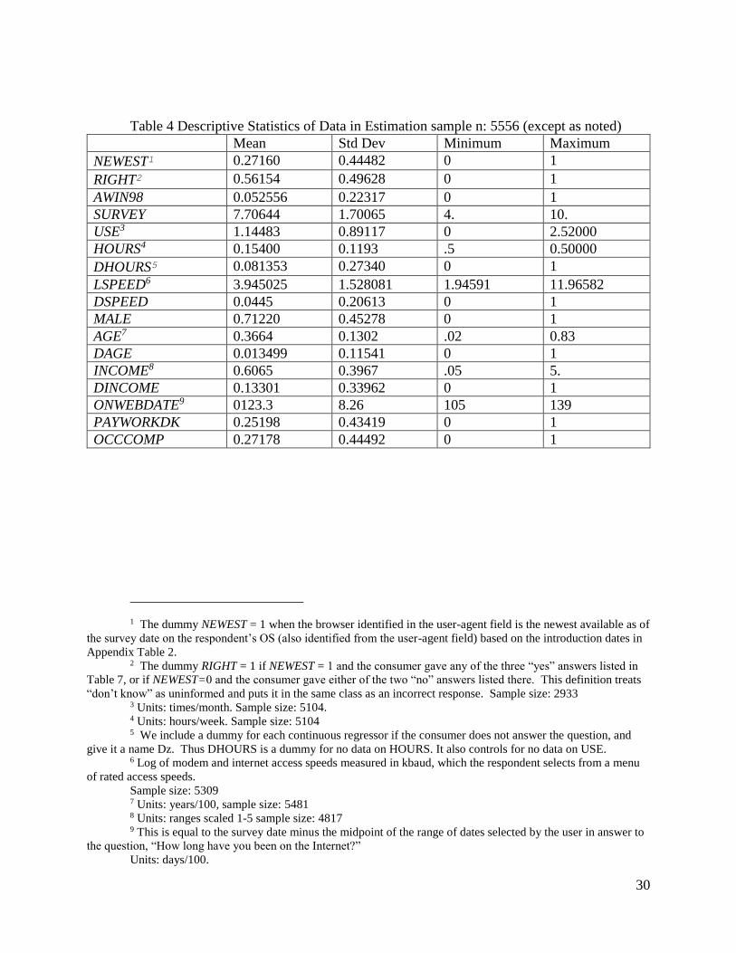
We employ a number of ordinary, self-described demographic or economic survey

responses (MALE, AGE, INCOME) from the GVU survey. We also select regressors that capture

cross-sectional variation in (1) users’ interest and ability to process information about new

technologies and (2) their demand (in the usual sense) for the newest technology. Their

definitions and summary statistics are given in Table 4.

To control for particular expertise about browser technology, we include the dummy

OCCCOMP=1 if the occupation involves computers. Conversely, the date a respondent first got

on the Internet (ONWEBDATE) controls for less knowledgeable “newbies” (people who just

entered the market), while PAYWORKDK=1 if the user does not know who pays for internet

access or work pays.

USE and HOURS measure time spent on the web, reflecting the benefit of downloading

the newest technology. The time costs of obtaining the newest browser version is measured by

the log of internet access speed, LSPEED. We do not interpret these variables as exogenous

determinants of technology demand, but rather as measures of cross-sectional variation in web

demand and, therefore, demand for the newest web technology.

8 We have also estimated a version of the model using official “release to manufacturing” dates to define

NEWEST and found little qualitative difference from our main results. The biggest difference quantitatively is that

this model has a higher predicted probability of upgrading, not that it has a distinct breakdown between information

and other causes.

8

2.3. Combined Web Server Log and Survey Datasets

In addition to the automatic recording of survey respondents’ browser and OS by the web

server logs, the survey redundantly asks the users whether their browser is the newest available

of its brand and what OS they use. The survey also asks the respondents to indicate how

confident they are in their answer (whether they are “certain” or “uncertain”). These answers

give us the dependent variable SAY, which takes on the five values “yes, certain,” “yes,

uncertain,” “don’t know,” “no, uncertain,” and “no, certain.”9 See Appendix Table 3 for the

specific wording and choices. See Table 7 for statistics on consumers’ responses.

We compare the human to web server log answers to construct the dummy RIGHT = 1 if the

human and web server log answers agree regarding whether the user is running the newest

version of the browser. We code human/computer disagreements or the answer “don’t know” as

RIGHT = 0. Only 56% of the sample is right (Table 4) – the average user in our sample is doing

only slightly better than flipping a coin.

A standard econometric approach would be to use the distinction between human and

computer answers to “validate” survey responses, that is, to learn how much measurement error

there is in the human responses compared to the computer responses.10 Our approach is, in many

ways, the reverse. We are instead going to use consumers’ statements to draw an inference about

what they don’t know about demand. We emphasize that the consumer’s statement and the

administrative record correspond to distinct concepts: the consumer may not know the true state

of the market.

The last column of Table 7, “Percent actually RIGHT,” indicates that those who responded

“Yes” are considerably less likely to be right than those who responded “No,” suggesting the

possibility of an “optimistic bias.” 11 Table 7 also reveals that consumers who say they are

“certain” are more likely to be RIGHT, regardless of their answer. This suggests some elements

of accurate self-assessment in consumer’s answers. The lessons we draw from this quick and

descriptive examination of what consumers say are that (1) our model should provide for the

9 We treat the rare response “yes, and it is a beta version” as “yes, certain.” 10 A large literature in econometrics uses both survey research data and administrative records data, as we

do, but for somewhat different purposes than ours. In this literature, “validation” is the label for learning how much

measurement error there is in the survey data in order to design an econometric solution to the measurement error

problem. See Bound et al. (2001) section 3. 11 Indeed, users who answer that they are using the newest browser “and it is a pre-release/beta version” are

less likely to be right than even uncertain users who answer no.

9

possibility of optimistic bias in attempting to isolate the part of consumers’ answers which

reveals their true mental state and (2) we should utilize not only the consumers’ yes/no answers

but also their degree of certainty in our model of what they say.

2.4. Missing Data

Survey respondents sometimes skip a question or answer “rather not say” in response to a

specific question when the option is offered.12 We include observations with missing regressors

by adding a dummy for missing data. For example, DAGE is a dummy for the individuals for

whom we do not know their age. The specific names of the dummies and the regressors for

which these dummies are relevant are described in Appendix Table 3.

Some questions are not asked in some waves of the survey, so data may be missing for an

entire year on a particular variable. We exclude such variables from consideration as regressors.

One of our key dependent variables, what the users SAY about their demand behavior, is also

missing because the question was not asked in a number of surveys. For those surveys, we do

not predict SAY, and the likelihood contribution of an observation is the marginal probability of

NEWEST.

3. FRAMEWORK

Assume there is a technology that is evolving over time. Consequently, new and better

versions of the technology are released into the market over time. Consumers have

heterogeneous demand for the technology, i.e., the utility of the technology net of cost varies

across consumers. However, consumers are not perfectly informed about the release date of the

new versions. Without observing the state of the world, they do not know for certain if the new

version exists yet, nor how much more utility they would receive from the new version.

Consumers thus face both an information acquisition problem and a product choice problem.

Consumers are heterogeneous in their probability of observing the state of the world.

Some observe quite frequently, while others do not. This heterogeneity is driven, for example, by

differences in consumers’ occupations (some work daily with the technology and so are more

likely to become informed about the existence of a new version).

12 Even for the same question, the ability to respond with “rather not say” can change from survey to

survey. See Appendix Table 3.

10

If the consumer observes the state of the world AND observes that a newer version of the

technology exists, the consumer can then chose to upgrade to the newest version of the

technology. Otherwise, the consumer stays with her current version of the technology. Although

the new version is assumed to provide greater utility than the previous versions, the consumer

may choose to remain with her current version if the disutility from adoption costs associated

with the new version is too large.

In this setting, there are two potential reasons why a consumer may not adopt the newest

version of a technology. First, if the consumer is informed of their full choice set, the utility of

the newest version may not exceed the adoption costs. Second, a consumer simply may not be

informed of the existence of a new version of the technology. These two reasons have different

implications for how policy and market institutions would affect consumer welfare.

The shape of the aggregate diffusion path for a new technology is thus determined by the

distribution in the consumer population of the (net) costs of adopting the new technology, which

we will call Δ and the rate at which consumers become informed, which we will call θ. An

econometrician seeking to distinguish between these two reasons cannot simply look at the

pattern of diffusion of the newest technology: there could be considerable delay before adoption

either because many consumers, i, have high Δi (low net benefits of adoption) or, alternatively,

because many consumers have low θi (low information arrival rates).13 The econometrician

needs some information that reveals the consumer’s knowledge of her choice set in order to

compare adoption rates by informed and uninformed consumers. This will identify the

importance of information about the state of the world (specifically, the existence of a new

version of a technology) relative to adoption costs for the diffusion of the technology.

3.1. Model Overview

We propose a model and a corresponding dataset which allows us to separately identify

and quantify the role of information and adoption costs on delayed diffusion of a new

technology. The center of our estimation strategy is that we employ two dependent variables to

measure adoption costs (the consumer’s demand for elements in the choice set) and information

(the consumer’s knowledge of her choice set). The first dependent variable is a traditional

13 This is a familiar observation in the economics of diffusion of new technologies. See, e.g. “Innovation

and Diffusion,” by Bronwyn H. Hall, in Fagerberg, J., D. Mowery, and R. R. Nelson (eds.), Handbook of

Innovation, Oxford University Press, 2004.

11

diffusion variable called NEWEST, and it is an indicator of whether a consumer has upgraded to

the newest version at time t (NEWESTit=1 if consumer i has the newest version at time t). The

second dependent variable is called SAYit, and it is a statement by the consumer about whether

she has the newest version at time t. Like our dataset, many modern computer generated datasets

create a variable like NEWEST automatically; constructing a variable like SAY requires

administering a survey to consumers by researchers or business people.

To use these two dependent variables, we need a working model both of what people do,

i.e. a dynamic demand model, and of what people say. To understand the key modeling steps in

our approach, first consider a dream dataset in which (a) consumers’ actual choices are

automatically recorded over time, (b) consumers are asked every period whether they are using

the newest version of the technology, and (c) all consumers answer that question in a way which

reveals their exact knowledge state.

As long as the econometrician can observe what version of technology the consumer is

using at each time t and can observe the release dates of each new version, NEWESTt is easy to

construct for all periods. As a result, we could identify exactly when a consumer adopted a new

version. But how do we know whether a non-adopter did not know about the new version or,

instead, knew about it and decided against adopting? In our dream dataset, each consumer’s

answer to the question “Are you using the newest version of the technology?” is easy to

interpret. A consumer answers “yes” only if she means “I observed the state of the world this

period, and then I chose to adopt the newest version,” or “I saw that I already have the newest

version.” She says “no” only to mean “I observed the state of the world this period, and although

I saw that a newer version existed, I chose not to adopt, because the net utility did not exceed

that of my current version.” Finally, she says “I don’t know” only if (recall, this is a dream) she

didn’t observe this period. With this information, one could divide non-adopters into the

uninformed and the unwilling-to-adopt, and then pin down the distribution of Δi and θi. That is,

diffusion could be divided into its learning and choosing elements.

Our data differs from this ideal panel data in two ways. First, we do not observe

consumers at each time t. We observe several cross-sections of consumers at survey times t=S.

This means that we cannot observe exactly when a consumer upgraded to a newer version. We

only know that it occurred sometime between S and the release date of the newer version, time

t=R. Similarly, a consumer may have observed the state of the market at any time between her

12

initial period t0 and S. We build a dynamic programming model of the consumer’s path of

observation and upgrades and accumulating hazard for NEWEST from R to S.

Second, no survey can hope, realistically, to direct all consumers to answer a question

(especially one to which they do not know the answer) in a way which reveals their exact

knowledge state (see the literature on surveys and elicitation of consumer preferences and

beliefs).14 We construct a model in which a consumer who gives a better answer, e.g. a

consumer who answers the question correctly, is more likely to be a well-informed consumer.

However, our model is much more cautious than the one that would work in our dream dataset;

in particular, we do not make the assumption that any consumer answers in a way which fully

reveals their information. Instead, we assume that a subset of consumers answers the question as

a rational statistician while another subset of consumers answers in a way which is not related to

their information type. Our rational statistician (RS) model is very restrictive, and we draw

information about consumers’ information types only to the extent that their answers correspond

to the RS model.

Our empirical model addresses our data constraints so that we can identify the difference

between information and transaction cost reasons for delayed diffusion of new browser versions.

3.2. Dynamic Model of Technology Demand

14 The experimental economics literature since Becker, DeGroot and Marschak (1964) has emphasized the

importance of incentive-compatible elicitation of preferences and probabilities. Many experiments have linked

consumer statements in surveys to incentive-compatible actions in the surveys. Glaeser et al. (2000) has shown that

there can be a complex relationship among (1) self-reported beliefs, (2) self-reported past actions, (3) tastes (as

revealed by actual behavior) and beliefs (as revealed by actual behavior).

A large number of studies, most in cognitive psychology but some in other social sciences, illuminate the

problem of modeling the relationship between what a consumer knows and says. This is a complex area, but some

knowledge decays with time, and consumers are particularly bad at remembering the precise date of long ago events.

Consumers are better at recall of major events than of minor ones. These empirical regularities are relevant to our

estimation because the question of whether a consumer has the newest browser involves recalling when they got

their browser, typically not an important event, after different amounts of time have elapsed.

A considerable literature, almost all outside economics, considers consumers’ tendency to report, in some

circumstances, what they would like to be true or what they would like to be perceived as true by others. In our

context, this could plausibly lead to a tendency to say “newest” or even “certain newest” without regard to their

actual knowledge.

“Measuring utility by a single‐response sequential method,” GM Becker, MH DeGroot, J Marschak -

Behavioral Science, 1964, pp. 226-232.

Edward L. Glaeser, David I. Laibson, José A. Scheinkman, and Christine L. Soutter, “Measuring Trust,”

The Quarterly Journal of Economics (2000) 115(3): 811-846.

Cite Khaneman

13

We model a consumer’s optimal demand decision over time in this section. Step 1 is the

consumer’s environment. Step 2 is the consumer’s information and her optimizing decision over

whether to opt-in to new versions of the technology she observes.

The evolution of technology over time is characterized by a scalar time-series process

Xt= Xt-1+stεt, (1)

where st∈{0,1}, the version-introduction dummy, follows a Markov chain and εt >0, the product

quality improvement, has an i.i.d. distribution with positive support.

Each consumer i is infinitely-lived and discounts utility from future periods by factor ρ.

At the beginning of period t, consumer i is using technology xit, acquired at some earlier time

period. Since the consumer may not have the latest technology, xit< Xt. Consumer i begins at

time t0i with technology xit0. Consumers are heterogeneous in initial conditions (IC), varying in

t0i, in xit0, and by not always having xit0= Xt.

Consumers are heterogeneous in their ability to observe realizations of the aggregate

technology process Xt. Specifically, consumer i observes the current level Xt only with

probability θi in period t. All consumers, however, form statistically correct expectations about

unobserved Xt. Consumers are also heterogeneous in their cost of adopting the newest

technology. If the consumer observes, she can decide to pay an adoption cost Δi > 0 and

download the newest version, setting xit+1= Xt. Otherwise, if the consumer does not observe, or if

the consumer observes but decides not to adopt, the consumer's technology does not change, i.e.

xit+1= xit. Consumers are not heterogeneous in flow utility, u( ), i.e. a consumer with technology

x receives flow utility u(x).

Denote the outcome of the probabilistic observation opportunity in period t by

Θit∈{0,1},with Pr(Θit = 1| Θit-1 = 0) = θi for all t. The consumer's only decision each period is

whether or not to download the newest version conditional on Θit = 1. Let this decision be

dit ∈{0,1}. We can thus write the complete life-time optimization problem of consumer i as

)()1())(()()1(Emax0

0}{

itititititititt

t

td

xudXudxuit

(2)

subject to the transition constraint for the individual consumer

,)1()1(1 itittititititit xdXdxx (3)

and to the aggregate (market) technology transition (1) and IC (t0i, xit0).

To calculate the expectation operator in (2), we assume that all consumers know their

own type θi, Δi, and the distributions of st and εt. Hence the expectation operator in equation 2

14

implies a rational expectation over the evolution of future technology levels and own observation

and adoption opportunities, given time t0 information.

We assume the per-period utility function u( ) has u’(x)>0 and u”(x)<0. This is important

for the long-run stationarity of the problem. Note that the average level of technology

improvements E(εt) is constant based on the specification in Equation 1.15 For our

implementation, however, the relevant range of the state space is an intermediate stage in which

adopting the next version is most likely beneficial to consumers.

We use dynamic programming to solve for the optimal adoption behavior conditional on

consumer type (θi. Δi) and IC (t0i, xit0).

Our first dependent variable is NEWEST at the time we observe the consumer, S. If

Xs > xti0, the consumer can only have the newest technology by opting-in. In that case, the

newest technology must have been introduced at a time R such that S> R >t0i and the consumer’s

opt-in interval is [R, S]. This means that if the user becomes informed at any time in that

interval, she may choose to obtain the newest version. NEWEST is a compound event whenever

R<S because the choice may occur at any point in the opt-in interval.

The full (numerical) solution to the demand model lets us calculate the probability that a

user whom we observe at time S demands the newest version of the technology. To do this, we

condition on the realization of X.16 Let R<S be the earliest date at which XR = XS. We calculate

the pdf of the event that i’s most recent observation was at time t, mit={Θit = 1 & Θitʹ = 0 for

t<tʹ<S}, and call it fm(t, θ).17 We calculate

Pr(NEWESTi| θi, Δi,S,R,t0, xit0) = Σt=R…S Pr(dit| θi. Δi, t0i, xit0) fm(t, θi). (1)

We will often use a survivor (cumulative hazard) interpretation of this probability in

which θi is the hazard for consumer i becoming informed and Pr(dit| θi. Δi, t0i, xit0) is the hazard

for adopting an available technology conditional on becoming informed. Note that this depends

on θi as well as Δi because we derive it from a consumers’ dynamic optimum, so that the

15 Decreasing marginal utility, in combination with a strictly positive and constant cost of adoption Δi > 0,

then implies that after a certain date the expected utility gain from adopting the next version will be less than the

adoption cost. This is realistic when applied to a narrow category of technology such as web browsers. 16 We must condition on the realization of X even to define the dependent variable NEWEST. More

importantly, as with any serious study in the economics of information, it is essential that we know something the

consumers do not, i.e. the realization of the X process. 17 By a recursion, we see fm(S)= θ, fm(S-1)= (1- θ) θ and so on.

15

likelihood of becoming informed again in the future affects the consumers’ decision to download

conditional on observing today.

An example may illustrate how we use the model to calculate the probability that

NEWESTi=1. Suppose a user gets her computer at time 1, with version X1 installed as the

default. A new version of the technology, X2, is introduced at time 5, and we observe the user at

time 6. So this example has S=6 > R =5 > ti0=1. The opt-in interval is [R, S]=[5,6]. To

calculate the probability, we condition on the event that the opt-in interval begins at time 5 and

that the technological level of the newest technology is X2. Consumers whose latest observation

occurs before the opt-in interval cannot have the latest technology, so we can calculate the

Pr(NEWEST) as follows:

Figure 2

Period Hazard for

Getting

Informed

Hazard for

Obtaining | Informed

Probability of Obtaining

NEWEST

5 θi D5=Pr(d5=1) θi D5

6 θi D6=Pr(d6=1) (1- D5θi)θi D6

Pr(NEWEST) θi D5+(1- D5θi)θi D6

In the example, calculating the probability that a user has adopted by time S is simply a matter of

accumulating the hazard for adoption at each of the two dates in the opt-in interval. Of course, to

calculate D5=Pr(di5| θi. Δi, t0i, xit0) we need to solve the consumer’s dynamic optimum.

In short, we use the solution to the optimizing model to calculate the probability of the

event xiS=Xs.18 We create a function that yields this probability; it depends on the date and the

initial conditions and the user’s type.19 We call this function Pr(NEWESTi | (θi. Δi, t0i, xit0).

18 Each of these events in which a user obtains the latest technology at time t can also be a compound event

when the history is longer than in our example. In particular, the user can have obtained a version of the technology

in between xi0 and Xn. It is also possible that the user has observed at earlier times than she downloads (either before

or after t1N) but this does not create a compound event as earlier observations are superseded by the latest

observation under our information assumptions. 19 The solution to the optimization problem for the user depends on the realizations of the dates of

introductions of all improvements before S and also on the extent of those improvements. We calculate the

probability conditioning on those introductions. Since the date S and the IC determine the history of introductions,

we do not include it as a separate conditioning event in Pr(xiS =XS|events).

16

3.3. Model of Survey Responses

We as econometricians know whether each consumer has the newest version of the

technology. Given the information-processing problem just described, a consumer need not

know the correct answer. We now model a consumer’s answer to the question “Do you have the

newest version of the technology?” to sharpen our inference about their information-processing

type, θi.

An obvious intuition is that consumers who know their choice set are more likely to

answer this question correctly than consumers who do not know their choice set. One simple

model – not obviously correct, but easy to interpret – thus posits that consumers with higher θ are

better informed and thus more likely to answer the question correctly. We estimate a version of

this model, specifying a simple descriptive model of RIGHT as a function of θ and other causes.

To be specific, we model

Pr(RIGHTi |NEWESTi)=logit(ZRβR) (2)

where ZR includes θi and NEWESTi. The benefit of this model is that the inclusion of θi in the

model for RIGHT imposes a cross-equation restriction which permits separate identification of

econometric models of θi and of Δi.

That simple and obvious model has two kinds of problems. First, it assumes that all

consumers answer the question as best they can using an economist’s rational-statistician frame

of reference. The empirical literature on consumer information reporting is not encouraging for

making this assumption about all consumers. Second, it does not adequately account for the

possibility that a well- but not perfectly-informed consumer could give the wrong answer. For

example, if R=S, thoughtful consumers who observed last period might answer “yes.” Such

consumers are wrong, but, conditional on their information set, have given a very good answer.

Our solution to these two problems is to construct a model (1) with heterogeneity in how

consumers answer and (2) that carefully specifies the relationship between what a rational-

statistician consumer knows and what she says.

3.3.1. Rational-statistician (RS) consumer types

Let Q be the set of responses a consumer can choose in response to “Are you using the

latest version?” In our application, Q={“yes, certain,” “yes, uncertain,” “no, certain,” “no,

uncertain,” “don’t know”}.

17

An RS consumer gives the best possible answer to the question given her information at

the time of the survey, S. Denote the consumer's information set at time t as Ίit. What the

consumer says at time S, ήiS Q, is the outcome of a decision rule that maps her information

into the answer set, ήiS=ή(Ίit). The RS-consumer bases her answer on the objective probability

that her technology is the newest version at the time of survey, i.e. πis =Pr(xiS=Xs | ΊiS). We use a

simple model based on two thresholds, q2<q1<.5.

We assume that the RS consumer uses the same model in calculating Pr(xiS=Xs | Ίit) as in

the demand model but permit consumers to be uncertain in their recall of dates.20 Begin with a

consumer who most recently observed at time m. If a consumer observed and did not adopt, i.e.

if m>t0i & Xm>xiS, then πis =Pr(xiS=Xs | ΊiS)=0. (3)

This is a restriction between the RS model and the demand model based on the assumption that a

consumer who has decided not to adopt (knowing their choice set at that time) recalls the

decision. If a consumer observed and has the newest version (whether adopting at time m or

earlier), then they use the Markov chain model with introduction probability pi to calculate the

probability. The consumer calculates if m>t0i & Xm=xim+1, then πis =Pr(xiS=Xs | ΊiS)=pi(S-m) where

we assume that pi is distributed BETA(αq, βq). Thus we calculate

πis(m,αq, βq) =E[Pr(xiS=Xs | ΊiS)=pi(S-m)| αq, βq ] (4)

Figure 3

Consumer Response ήiS Thresholds Partition Probability

Yes, certain πis>1-q2

Yes, uncertain 1-q2>πis>1-q1

Don’t know 1-q1>πis>q1

No, uncertain q2< πis <q1

No, certain πis <q2

Finally, we need to make an assumption about the information set of a consumer who has

never observed, i.e., make an assumption about the information set at t0i. Neither economic

theory nor anything else is helpful here, so we consider a variety of assumptions about

πit0=Pr(xit0=Xt0 | Ίito), including (a) the consumer is informed of the state of the market at t0i and

20 {Cite to survey research literature on date recall.}

18

(b) the consumer is certain that they have the newest version at t0i. These differ importantly

when consumers IC involve getting an older version at t0i.

The econometrician does not know when the consumer last observed, but the consumer

does (i.e. ΊiS contains miS). Recall that fm(m, θ) is the pdf of m, We calculate

Pr(ήiS | θi, αq, βq, q2, S,R,t0i) = (1- fm(t0i, θi) )πit0 + Σt=R…S fm(m, θi) πis(m,αq, βq) (5)

Thus we see that the same distribution over time, driven by θ, mixes the model for

adoption (1) and the RS model for what consumers say (7). These restrictions are what lead the

joint estimation of the demand model and the RS model to identify θ.

3.3.2. Descriptive (DE) consumer types

Some consumers may answer the question without attempting to remember when they

last observed and working out the statistics. We construct a simple model of what (in Q) these

descriptive (DE) consumers say. Scholars in other disciplines have determined that many

consumers have a bias toward positive answers, particularly men, and that many consumers have

a bias toward certainty, particularly men. So we model Q for these consumers as a bivariate

logit:

PrY=Pr(Yes)=logit( α0+ αMMALE),

PrC=Pr(Certain)= logit( αc0+ αc1+αcMMALE); (6)

PrD=Pr(Don’t Know)=1- logit( αc0+αcMMALE)

Finally, we model the probability that a particular user is an RS or a DE. Our simplest

model is an independent mixture model, in which Pr(DE)=λ.

4. ECONOMETRIC ESTIMATION

We now turn to econometric estimation of our models. The structure of our estimation is

presented in Figure 5. First, we specify which deep parameters we assume fixed and which ones

are functions of observables. Second, we solve the problems raised by incomplete sample

information about IC.

4.1.1. Deep parameters as function of observables

We do not actually observe θi or Δi but instead have an econometric model of them that

depends on covariates, z, and parameters β=(βθ, βΔ). Let the observable data about consumer i be

zi and assume an econometric model such that the distribution of θi, Δi is G(θi, Δi | zi, β).

The per-period observation hazard θi is naturally bounded on the interval [0,1], and, from

both the perspective of a user and the econometrician, future observation events are random as

19

long as θi is in the interior. Accordingly, we model θi as a deterministic function of user

characteristics:

θi =[1+exp(-zi βθ)]⁻¹ (7)

We include regressors, listed in Table 8, which we suspect might be particularly likely to capture

consumer heterogeneity in information about software.

Demand in the ordinary sense in our model consists both of the flow utility u(x) and the

one-time adjustment cost. Since u(x) does not depend on i, we model Δi as capturing variety in

the taste for new technology as well as literal download cost. Thus we include not only user

characteristics that predict download cost (such as modem speed) but also characteristics that

predict value in use (such as hours spent on the web.) These are listed in Table 8. We let the

range of Δi be [0, Δmax] so that at one extreme it is always optimal to download, never optimal at

the other. Finally, we reverse signs so that β∆ will have the sign of demand, not of cost, and

write

Δi =Δmax [1+exp(zi β∆)]⁻¹+εi, (8)

where εi is distributed type 1 extreme value. While the agent knows Δi, we can observe only zi,

not εi.

A number of elements of the demand model are assigned constants rather than estimated.

Details are in Appendix Table 4. We assign values to the utility Xt of each new version, and a

function for u( ). To some degree, this is a normalization, since we permit consumers to be

heterogeneous in the costs of adopting. However, it does impose a restriction on the demand

behavior of consumers considering IE3 vs. IE2 because we only let Δi vary across individuals,

not across individuals and versions.

We treat the level of technology Xt as an index, and rather than estimate it, assign a

separate value for each version of each brand of browser using data and a variation on

regressions in Bresnahan & Yin (2005).21

4.1.2. Ranges of Initial Conditions (IC)

We only observe consumers on their survey date, but have three kinds of information

about their IC: (1) respondents answer a question about when they first used the Internet, (2) the

21 Essentially, using a different, aggregate dataset, that paper regresses the logit of the market share of the

newest version of a browser within its brand on a version dummy, the time since introduction of the newest version,

and various controls for the distribution of browsers. The coefficients on the version dummy dummies form our

estimate of Xt.

20

respondent’s OS gives us some information about when they got their current computer, and (3)

IE was not available for every OS at the same date. This information gives us a range of possible

IC dates and states for each user. We sum the likelihood over this range using a weighting

scheme that reflects outside information about the relative likelihood of different dates and, in

specifications estimated but not reported in this version, also reflects concerns about the relative

quality of different IC information. We call the range of dates T0i, with t0i T0i, and the initial

demand states xit0. We first discuss how we determine T0i and then discuss how we deal with the

uncertainty within the range and how we determine IC demand states.

Our model is a model of opt-in to the newest version of application software. The user

opts-in by upgrading to the newest version from whatever earlier version was running on their

computer. Accordingly, the conceptually correct IC are the first use of any version – that is, the

date and version of that first use -- of the software on the user’s current computer. The

applications software IC occur when the user buys a new computer with the software on it or

gets on the web and receives a copy of the software from their ISP. We make a fundamental

assumption that those events are exogenous. Perhaps more to the point, we do not treat the

consumer’s as “choosing” the browser that came with their computer or from their ISP; we

model only their decision to opt-in to newer versions.

4.1.2.1. Definition of IC dates

Respondents were asked, “How long have you been on the Internet?” and given several

time intervals from which to choose (see Table 3). We subtract the beginning and end of this

range from the survey date to get a range of dates, 𝑇𝑅𝑖. In our study period of rapid Internet

growth, these first-use times are typically quite recent. We also know the range of dates, TAi,

when some version of the software was available for user i’s OS up to and including S.22 The

early bound on T0i is defined as (1) the earliest date in 𝑇𝑅𝑖 or (2) the earliest date in 𝑇𝐴𝑖 ⊇ 𝑇0𝑖,

whichever is latest.

With those details in place we can say that the early bound on T0 is defined as (1) the

earliest date in 𝑇𝑅𝑖 OR (2) the earliest date in 𝑇𝐴𝑖, whichever is latest. The later bound on T0i is

more complex. Even if a user first got on the Internet long ago, they may have bought a

22 To avoid the proliferation of notation, we end TAi at the survey date S: this is just the assumption that all

IC are at or before S. If the user is running Win95, TAi begins with the introduction date of IE1 (also the introduction

date of Win95); if Win3.1, with the introduction date of IE2 for Win3.1, if Win98, with the introduction date of

Win98.

21

computer more recently and thus have new IC. We infer a range of dates at which i might have

bought their computer, 𝑇𝐶𝑖, from the range of dates when i’s current OS was the newest OS.

Then 𝑇𝐴𝑖⋂𝑇𝐶𝑖 is the range of dates at which buying a new computer would have led to getting a

new browser version. We consider only the subset of these dates which are after max(𝑇𝑅𝑖).

Taking this into account, our definition of the range of dates which might be IC is

𝑇0𝑖 = 𝑇𝐴𝑖⋂ {𝑇𝑅𝑖⋃[𝑇𝐶𝑖⋂{t>max(𝑇𝑅𝑖)]}.

The logic can be easily seen in this example drawn from our data. We observe a user at S

running the newest OS, which has been in the marketplace and has had the software available for

at least a year. The user’s 𝑇𝑅𝑖 is [S-12, S-7], i.e., they report they got on the web between six

months and a year ago. However, since they might have bought a new computer in the last six

months, the information available to us does not rule out IC in [S-6, S]. Thus 𝑇0𝑖 is, as shown in

Figure 4, the union of these two ranges of date, [S-12, S]. It is obvious in the example and easy

to show generally that this leads to a contiguous list of dates.

The example shows the caution in our definition of 𝑇0𝑖. It includes all the different IC

times that are not explicitly ruled out by a fact in the data. The mean length of the IC interval

(i.e., max(𝑇0𝑖)- min(𝑇0𝑖)) is reported in Table 5.

Figure 4

We show, in a specification reported in Table 9, that even if the only information about

IC we use is 𝑡0𝑖 ∈ 𝑇0𝑖, we can estimate the parameters of our model with considerable precision.

That is because even though there are many users for whom we have only an IC date range, there

is still tremendous variation across individuals in IC. We have some individuals where we know

their IC are in the last few months (for example, those who are surveyed early on) and others

𝑇0𝑖

𝑇𝑅𝑖 {𝑡 ∈ 𝑇𝐶𝑖 & 𝑡 >max(𝑇𝑅𝑖)}

S-12 S-6 S

S

22

where we know their IC are long ago; for others we are certain that they did not get the newest

version of the software at their IC. Statistics on the IC are reported in Table 5

4.1.2.2.Weighting within IC date range

We consider two weighting schemes that assign different probabilities, wt, to dates 𝑡 ∈

𝑇0𝑖. These let us construct the predicted probability that the user has the newest browser as

∑ 𝑤𝑡𝑡∈𝑇0𝑖∑ 𝑤𝑡𝑡∈𝑇0𝑖

Pr (𝑁|𝑡 = 𝑡0𝑁𝐸𝑊𝐸𝑆𝑇𝑖|𝑡 = 𝑡0𝑖. (9)

The first weighting scheme is used in all of our specifications. It assigns higher weights

to more recent dates, using information on the growth rate of PC demand and of Internet usage.23

This is a nontrivial element of our main specification, as both PC demand and Internet usage

grew at about 1% per month in our period.

Our second weighting scheme arises only in cases like that shown in Figure 4 above,

where the range of IC dates includes both the user’s self-reported Internet start time and a

possible later computer purchase time. In specifications not yet reported in this version, we add

a parameter, 𝛾𝑟𝑡, which is the probability that the user has correctly reported their IC dates. We

put 𝛾𝑟𝑡 weight on the subset of 𝑇0𝑖 which is in 𝑇𝑅𝑖 and 1-𝛾𝑟𝑡 on the rest.

4.1.2.1.IC demand states

Once we have defined the list of times at which the IC could have occurred, we associate

the browser version that would have been given to the user with a new computer or a new ISP

signup at each date. This is based on the distribution release dates shown in Table 2. We also

associate each date with an initial expectation about the state of the market.

Figure 5 Model Structure

23 [Cite sources]

λi

Say Newest

Pr(NEWESTi| θi, Δi, S, R, t0i)

DE:

Pr(ήiS )=DE(MALE, α)

RS:

Pr(ήiS | θi, αq, βq, q2, S, R, t0i)

IC: T0i

Weights: Growth rate, γIC

23

4.1.3. The special case of Pr(NEWEST=1)

In some cases, a consumer will have gotten the newest technology at their IC and need

not opt-in to adopt it. In our application, these are a subset of the cases in which R<ti0, since the

dates at which OEMs and ISPs could distribute the newest browser to consumers typically came

after the dates at which consumers could download it. We include such cases, assigning

Pr(NEWESTi | (θi. Δi, t0i, xit0) =1. These cases do not influence our estimates via prediction of

NEWEST because for them Pr(Pr( NEWESTi | …) is a trivial function of parameters. However,

these users may be well or badly informed about their choice set, contributing to our estimates of

information parameters.

5. RESULTS

5.1. Descriptive Results

As a threshold matter, we note that the rate of diffusion in our sample is low. Table 6

shows the mean of NEWEST to be .27, so a considerable majority of browser users have not

downloaded the newest version. PCTCOVER also shows that just over 10% of our users would

have NEWEST without downloading (i.e., at their IC), so the actual rate of opting in is even

lower. Finally, the table shows that users whose IC is before R, have, on average, about 5.8

months to opt-in. If under 20% of consumers are opting-in after just less than 6 months on

average after release of a new browser version, then there is some inertia around IC.

Can the inertia be explained by information? The same table shows that only just over

half of users, 56%, are RIGHT. This encourages the view that consumers are badly informed.

The last two rows of the table show that consumers who are RIGHT are much more likely (66%)

to have downloaded NEWEST than those who are not RIGHT (7%). Many economists would

conclude at this point, saying that consumer ignorance must provide much of the answer.

However, what if many consumers answer “yes” to this question without deep thought? The

dependence between RIGHT and NEWEST would follow mechanically. This cautionary

interpretation is consistent with Table 7, which shows that those who say they have the newest

are significantly less likely to be RIGHT than those who say they do not.

5.2. Structural Results

In Table 10 we present estimates of a model using the structure in equations (9), (8), and

(6). The estimates for the two models of what consumers say (RS and DE) are shown in the right

S

24

panel of Table 10. The DE model estimates are as one would expect from the bias literature.

The average user tends to say “yes” (men do so more) and the average user tends to be certain

(men, more so).

The RS estimates have the structure we have imposed. The threshold for certainty,

q2=0.0046 is quite close to πis=1 or 0, suggesting that RS types would not casually indicate any

response with certainty. The threshold for “don’t know,” q1=0.46, is also close to πis=.5. The

average consumer responds as if the hazard for version introductions is .58, somewhat slower

than the true hazard.

At the bottom of Table 10 we compare predicted values from the RS and DE models to

the actual data from Table 7. It is easy to see here where the restricted RS model has trouble

predicting. It particularly underpredicts “yes, certain” and overpredicts “no, certain,” a response

we impose if a consumer has observed the state of the market and not downloaded. Imposing

symmetry and orderedness is clearly not consistent with the behavior of most consumers. It is

not surprising that the estimated mixture weight on the DE model is 0.85.

We next consider the relative importance of information vs. ordinary demand in

determining the pace of diffusion. The hazard for adopting in a particular period is θiPr(dit| θi. Δi,

t0i, xit0) which we abbreviate as θiHit( ), the product of two hazards. While there are a number of

different ways to decide which of these is “more important” in explaining the low rate of

diffusion, a simple calculations seems to work for our estimates. We first note that if θiHit( )

were a constant, h, then h=.130 would predict the sample mean of NEWEST. The estimated

mean of θi is .295, and the estimated mean of Hit( ) is .571, suggesting that any calculation is

going to assign more of the slow diffusion to information.

Since θi enters not only as the hazard for becoming informed, but as one determinant of

Hit( ), the (dynamically-optimal) probability of downloading, several different definitions of the

relative importance of information are possible. These do not differ much.24

24 Those two estimates of the relative importance of information diverge because θi and Hit( ) covary. So

we examine changes in the predicted mean of newest, (NEWEST) ̅(θ,Δ)≡ ΣiPr(NEWESTi| θi, Δi,S,R,t0i, xit0) that

would arise if (a) θi=1 and (b) Δi=-∞ so that Hit( )=1. (NEWEST) ̅(1,Δ ̂ )-(NEWEST) ̅(θ ̂,Δ ̂ ) measures how much

faster users would adopt if information were immediately available, and (NEWEST) ̅(θ ̂,-∞)-(NEWEST) ̅(θ ̂,Δ ̂ ) measures how much faster they would adopt if they always select the newest they know of. If we were to instead

define a marginal “contribution of information” we would consider letting Hit( ) vary with θi, in computing the

predicted values. In general, Pr(dit| θi. Δi, t0i, xit0) is decreasing in θi, because a low-θi consumer considering

skipping a version expects to wait a long time for the next version. This would tend to reduce the marginal

25

5.3. A model in which RIGHT reflects better information

In Table 9 we present joint estimates of equation (9), our demand model, and (2), the

simple descriptive model in which those who have higher θi are more likely to be RIGHT. This

model is semi-structural in that it continues to use our demand model but identifies information

vs. ordinary demand without any requirement that consumers be rational statisticians.

Identification follows from the idea that consumers who are better information processors are

more likely to be RIGHT. In this table, all regressors that were included above in either θi, Δi

are included in both – no exclusion restrictions. The point of this table, then, is to show that

demand in the ordinary sense can be separately identified from information without any

exclusion restrictions.

Looking first at demand in the ordinary sense (Δi), we note that few coefficients are

estimated precisely. The consumer’s modem speed variables (DSPEED and LSPEED) are the

exception, and these coefficients tells us that, as we would expect, a consumer who has a faster

modem, or who does not know the modem speed (for example, because they get Internet

connection services at work or at a university) has a lower download cost.

Now looking at the consumers’ hazard for observing the state of the market, θi, we note

that most of the coefficients are estimated reasonably precisely. Looking at the precisely-

estimated coefficients, we see that consumers tend to become informed about new versions if

they use the Internet more, if they work in the computer industry, if they are men, if they are

younger, or if they manage their own internet connection instead of having it done for them at

work. This looks like a model of information processing. The same was true in the structural

model in Table 10, but there we imposed exclusion restrictions on which z’s predict Δi vs θi.

The model does a good job of predicting NEWEST, and a less good job of predicting

RIGHT. The equation for RIGHT is reported to the right of the table. The model appears to be

doing what we asked, as the coefficient on θi suggests that those users with higher θi tend to be

more RIGHT. So, too, are users who have the NEWEST, which we interpret as this model’s

treatment of excess optimism.

Looking now at information/ordinary demand breakdown at the bottom of the table, we

see that this model, too, reports information as the key determinant of demand. The mean of θi is

contribution of better information to more rapid diffusion. As we can see in Table 7, however, these effects are

small. They also do not impact the “total” calculations reported in text.

26

far smaller than the mean of Hit( ), meaning once again that most of the slow diffusion is

attributed to poor information. Why? This model has no restrictive treatment of who is an

informed person, nor does it restrict the regressors permitted to predict Δi vs θi. The finding that

information about the choice set is more important seems robust.

Indeed, information is much more important in this model than in the structural model

just reported.25 This difference in results is easy to understand. The structural model restricts

the role of θi (in what consumers say) to only RS consumers. Since this restriction binds quite

tightly, and since there is no comparable restriction on Δi, maximum likelihood on the demand

model substitutes out of using θi into Δi to predict NEWEST. In the present model, we relax the

restriction played by θi in what consumers say and it thus ends up predicting a larger portion of

what they do.

We find that, in both a restricted model and a less restricted one, information about the

choice set is the primary explanation of slow diffusion. To be sure, a few variables which

predict demand in the usual sense (the speed of a consumer’s modem, which is the main cost

variable, and the hours of internet use) have statistically significant effects, but demand in the

usual sense comes in as a distant second economically to information about the choice set.

When we do not restrict the specification, consumer characteristic (z) appear to enter demand not

through the ordinary channel of trading off the costs and benefits of downloading and installing

the latest browser, but rather through variation in the consumer’s information gathering.

6. CONCLUSION

We have reported two broad empirical findings about the sources of consumer inertia in

the browser market. The first is methodological: we were able to distinguish between

consumers’ not knowing their full choice set and other sources of inertia by combining

information about what consumers say and what they do. Perhaps surprisingly, this works only

because a subset of consumers are rational in what they say. Alternative models, designed to be

less than rigorous about discounting the irrational statements of consumers, provide a higher

estimate of the importance of incomplete consumer information. We are encouraged by our

success in a simple problem – product upgrades without brand choice – to consider more

25 The result that the variation in NEWEST explained by variation in θi is far larger than that explained by

variation in Δi also provides an intuitive explanation of why we are better able to estimate the coefficients in θi.

27

difficult consumer problems with potentially incomplete choice set information. The ability to

discern when information processing is central to the distinction between opt-in and opt-out is

more generally important, and we will continue to investigate it.

Our second finding is substantive. The consumers we study, browser users in the late

1990s, exhibit considerable inertia in their software demand. The primary cause of the inertia,

larger than all other causes together, is consumers’ incomplete information about their choice

sets.

We think this finding about demand partly explains two large changes in supply in

electronic markets since the early days studied here. In our study era, consumers opt-in to the

upgrade. Today, consumers of most software packages are confronted with an automatic

upgrading system. They may either opt-in or opt-out of this system. Most use the system and

thus do not have an opportunity to choose any particular product upgrade. Automatic upgrades

economize on consumers’ costs of becoming informed. However, there is no presumption of

efficiency: suppliers will select the same policy about upgrades as that which would have been

chosen by consumers only if consumers’ and suppliers’ interests in upgrades are aligned.

Second, large scale electronic markets have emerged to “nudge” particular products into

consumers’ choice sets. These take on a number of very different forms. Amazon, a retailer,

recommends that consumers consider products similar to ones they have searched for or bought,

increasing sales for itself and product suppliers. Google and Bing auction off the right to be

presented for consideration to consumers who have searched for particular terms. Applications

running on mobile phones or tablets similarly sell the attention of consumers. Markets to

“nudge” can only emerge when consumers will react to learning that something is in their choice

set. Much of the private return to technical progress in the 21st century has been created in these

“nudge” markets. Here, too, any efficiency conclusion turns not on the motivations of the

nudged (incomplete information) but on the motivations of the nudger (making a profitable or an

efficient sale).

Whether efficient or not, these two sets of efforts -- to get in consumers’ choice sets and

to become the incumbent product and manage customers’ demand for future versions – are here

to stay. Efforts to sell consumers’ attention have made it scarcer by crowding it not only with

electronic products, but with media, games, and ordinary products.

28

It is worth pointing out that this growth is consistent only with our finding about

information, not with the alternative explanations that, say, the browsers we study were hard to

download or install. Today’s consumers face many more choices on the online world and in the

mobile world than the users we study. If the important blockage to rapid and widespread

adoption of new technologies were technological, we should expect technical progress to

improve it. In our example, if the important reason for the slow diffusion of new browsers was

time-consuming downloads (slow modems) or difficult installations we should expect technical

resources to speed up downloads and/or to make installations easier, as, indeed, occurred. So if

that were the blockage, the problem we examine in this paper should be, by now, going away. If,

however, the important blockage is that mass market users are incompletely informed, we should

expect the problem to continue to get worse. There are more and more applications, and

consumer attention is drawn to more and more diverse topics, as the online world moves to being

the mobile world. Despite efforts to give consumers better and better opportunities to become

informed through search or through social networks, the problem of incomplete information is

growing secularly. We forecast that the importance of a wide variety of novel supply

institutions, many with a default or demand-steering flavor, will grow. Such institutions today

are providing much of the mechanism for “monetizing” consumer-oriented technical progress in

the online and mobile worlds today; understanding them is one part of understanding the

extremely rapid technical progress seen in consumer-oriented networks today.

29

Table 1 Observed OS and their market periods (n=5556)

OS Windows 3.1 Windows 95 Windows 98

Market Period Through 7/95 8/95—7/98 after 8/98

% of Sample .045 .902 .052

Table 2 Major Microsoft browser versions in our analysis (n=5556)

Version IE1 IE2 IE3 IE4 IE5

Definition includes 1.x includes 2.x includes 3.x includes 4.x includes 5.x

% of Sample .062 .051 .536 .346 .004

Table 3 Ynet: User-recalled time on the internet (n=5556)

Time Percent

0 - 6 months 12.31%

6 months - 1 year 14.58%

1 – 3 years 44.06%

4 – 6 years 22.03%

Over 7 years 7.02%

Total 100.00%

30

Table 4 Descriptive Statistics of Data in Estimation sample n: 5556 (except as noted)

Mean Std Dev Minimum Maximum

NEWEST1 0.27160 0.44482 0 1

RIGHT2 0.56154 0.49628 0 1

AWIN98 0.052556 0.22317 0 1

SURVEY 7.70644 1.70065 4. 10.

USE3 1.14483 0.89117 0 2.52000

HOURS4 0.15400 0.1193 .5 0.50000

DHOURS5 0.081353 0.27340 0 1

LSPEED6 3.945025 1.528081 1.94591 11.96582

DSPEED 0.0445 0.20613 0 1

MALE 0.71220 0.45278 0 1

AGE7 0.3664 0.1302 .02 0.83

DAGE 0.013499 0.11541 0 1

INCOME8 0.6065 0.3967 .05 5.

DINCOME 0.13301 0.33962 0 1

ONWEBDATE9 0123.3 8.26 105 139

PAYWORKDK 0.25198 0.43419 0 1

OCCCOMP 0.27178 0.44492 0 1

1 The dummy NEWEST = 1 when the browser identified in the user-agent field is the newest available as of

the survey date on the respondent’s OS (also identified from the user-agent field) based on the introduction dates in

Appendix Table 2. 2 The dummy RIGHT = 1 if NEWEST = 1 and the consumer gave any of the three “yes” answers listed in

Table 7, or if NEWEST=0 and the consumer gave either of the two “no” answers listed there. This definition treats

“don’t know” as uninformed and puts it in the same class as an incorrect response. Sample size: 2933 3 Units: times/month. Sample size: 5104. 4 Units: hours/week. Sample size: 5104 5 We include a dummy for each continuous regressor if the consumer does not answer the question, and

give it a name Dz. Thus DHOURS is a dummy for no data on HOURS. It also controls for no data on USE. 6 Log of modem and internet access speeds measured in kbaud, which the respondent selects from a menu

of rated access speeds.

Sample size: 5309 7 Units: years/100, sample size: 5481 8 Units: ranges scaled 1-5 sample size: 4817 9 This is equal to the survey date minus the midpoint of the range of dates selected by the user in answer to

the question, “How long have you been on the Internet?”

Units: days/100.

31

Table 5 Initial Conditions (IC) Statistics (n=5556)

Variable Mean Std. Dev. Min Max

S (Survey date) Aug 1997 310.47* Oct 1995 Oct 1998

Lag from t0i to S1 9.49 5.91 0.00 30.43

On web before t0i2 0.361 0.480 0.000 1.000

IC Interval

min(T0i) Feb 1996 302.72* Sep1995 Sep 1998

max(T0i) Jul 1997 308.29* Oct1995 Oct 1998

T0i length3 17.66 11.29 0 36

*Standard Deviations are measured in days

Table 6 Dependent Variables Statistics for Descriptive Statistics Analysis

Variable Mean

NEWEST4 0.272

RIGHT5 0.562

PCTCOVER6 0.106

Opt-in period7 5.83

NEWEST | RIGHT 0.660

NEWEST | not RIGHT 0.074

1 In months, measured from center of T0i to S. 2 Dummy: = 1 if last reported on web date is (weakly) before earliest date in T0i. 3 Max(T0i) - min(T0i), in months. 4 NEWEST is a dummy that is one when the browser identified in the user-agent field is the newest one

available as of the survey date on the user’s OS (also identified from the user-agent field) based on the introduction

dates in Appendix Table 2. 5 RIGHT is 1 if NEWEST=1 and the consumer gave any of the three “yes” answers listed in Table 7 or if

NEWEST=0 and the consumer gave either of the two “no” answers listed there. Note this definition treats “don’t

know” as uninformed, and puts in the same class as an incorrect response. 6 PCTCOVER is the likelihood that a user got NEWEST at their initial conditions. Calculated as the

(unweighted) mean across the months in T0i of the dummy t0>Rʹ. 7 The opt-in period is the number of months S-Rʹ .

32

Table 7 Consumer Statements (SAY) and RIGHT (2,933 respondents)

Possible response to “Do you think you are using the most up-to-date version of your

browser?”

Frequency Percent Actually RIGHT

Yes, I am quite certain .5742 .5540

Yes, and it is a pre-release/beta version .0147 .5349

Yes, but I am not so certain .1643 .2697

No, I think I am using an older version .0603 .8079

No, I am definitely using an older version .1558 .9147

Don’t know .0307 (NA)

All 1.00 .5615

Table 8 Included Regressors (Preferred Specification)

βθ βΔ

CONSTANT CONSTANT

ONWEBP1 DSPEED

OCCOMP LSPEED

PAYWKDK DHOURS

HOURS

DAGE

AGE

INCNS

INC

MALE

1 See Appendix Table 3 for survey questions underlying these variables. ONWEBP is (days on the web

since the beginning of the self-reported interval in Ynet)/10,000. OCCOMP is OccComp, self-reported profession is

computers or computer consulting. PAYWDK is the sum of PayWork and PayDK, i.e. a dummy for people

uninformed about their internet costs either because their employer pays or because they say they don’t know who

pays.

33

Table 9 Estimates of Model with RIGHT

Δi θi RIGHT

Est SE Est SE Est SE

CONST -0.906 0.629 -1.855 0.402 CONST 7.074 0.723

DHOURS 0.521 0.307 -0.142 0.236 AWIN98 -1.354 0.233

HOURS 0.743 0.728 0.491 0.642 SURVEY -0.811 0.078

USE 0.120 0.106 0.225 0.109 θi 0.669 0.192

PAYWORK 0.097 0.199 -0.713 0.212 NEWESTi 2.719 0.124

DSPEED 1.965 0.709 -1.242 0.500

LSPEED 0.459 0.190 -0.102 0.043

OCCCOMP 0.247 0.171 0.265 0.174

MALE 0.023 0.185 0.827 0.266

DAGE 1.613 1.217 -1.329 0.654

AGE -0.360 0.541 -1.290 0.600

DINC -0.031 0.217 0.122 0.230

INC 0.184 0.228 -0.206 0.201

# Obs=5556 for NEWEST, 2933 for RIGHT

Ln(likelihood)=- 5222.969

For the columns headed Δi, and θi, what is presented are the estimates of β and their estimated

standard errors. For RIGHT, which has a new set of row labels, the columns are the probit

estimates and their standard errors.

Predictions:

avg. Pr(NEWEST) 0.543 for users who have NEWEST

avg. Pr(NEWEST) 0.329 for users who don't have NEWEST

avg. Pr(RIGHT) 0.753 for users with RIGHT=1

avg. Pr(RIGHT) 0.681 for users with RIGHT=0

Demand Breakdown:

Mean of Hit() .963 Mean of Hit()*θi .130

34

Table 10 Estimates of Structural Model

Parameters Est SE Est SE

βθ RS Model

CONSTANT 3.45575 0.1725 q1 .46 .0116

ONWEBP -3.52681 0.1348 q2/q1 .01 .6513

OCCOMP 0.42981 0.1320 mean(p) .58 .9982

PAYWKDK -0.36118 0.1273

DE Model

Mean(θi) .295 Yes

Constant 1.79669

βΔ Male -0.02599

CONSTANT -1.29077 0.5406 Certain

DSPEED 0.47005 0.5605 Constant -2.87040

LSPEED -0.10657 0.1016 C2 -1.13045

DHOURS 0.58107 0.2677 Male 2.37841

HOURS -3.50724 0.9882

DAGE -0.47825 0.7159 Pr(DE) .85249

AGE 2.01000 0.4915

INCNS 0.96495 0.2200

INC 0.32595 0.2507

MALE -1.24024 0.6483

# Obs=5556 for NEWEST, 2933 for RIGHT.

Ln(likelihood)= -3240.35

Actual and Predicted SAY

yc yu nu nc dk

Actual data 0.589 0.164 0.060 0.156 0.031

RS 0.208 0.103 0.251 0.410 0.029

DE 0.652 0.176 0.030 0.112 0.030

35

Table 11 Probability Derivatives for Hazard (based on model in Table 9)

Person ∂θi H(∆i, θ i) /∂z ∂H((∆i, θi)/ ∂z

Unconditional

Hazard for NEWEST

Conditional adoption

hazard

DHOURS 0.009 -0.013

HOURS -0.050 0.049

USE -0.019 0.021

PAYWORK 0.029 -0.054

DSPEED 0.035 -0.079

LSPEED 0.007 -0.009

OCCCOMP -0.023 0.025

MALE -0.102 0.083

DAGE 0.035 -0.082

AGE 0.035 -0.081

DINC -0.009 0.011

INC 0.012 -0.018

36

7. Appendix

Appendix Table 1 Variable Definitions from Web Server Log

Variable Definition

who unique identifier

IE Dummy for choice of Internet Explorer

v Numerical value (1-5) of version of browser used

Amac Dummy for operating system (OS) used, according to agent file: Mac = 1

Awin31 Dummy for OS used, according to agent file: Windows 3.1 = 1

Awin95 Dummy for OS used, according to agent file: Windows 95 = 1

Awin98 Dummy for OS used, according to agent file: Windows 98 = 1

Appendix Table 2 Introduction (beta) date for each browser on each OS

Windows 3.1 Windows 95 Windows 98

IE1 Aug. 1995

IE2 April 1996 Dec. 1995

IE3 Dec. 1996 Aug. 1996

IE4 Feb. 1998 Oct. 1997 Aug. 1998

IE5 March 1999 March 1999 March 1999

37

Appendix Table 3 Variable Definitions from GVU Survey

Superscripts on variable names indicate survey numbers in which question was asked. No

superscript indicates that the question was asked in surveys 4-10.

Variable Definition

who unique identifier

Survey Survey number

S Date of survey

Age4-8 “What is your age?” Numerical value entered by respondent or “Rather not say”

(not an option in survey 4)

Age9-10 “What is your age?” Checkboxes for 5 year intervals and “Rather not say”

Dage Dummy=1 for “Rather not say” age

Male “What is your sex?” Dummy for sex: male = 1

White “How would you classify your race?” Dummy for race: white = 1

Asian “How would you classify your race?” Dummy for race: asian = 1

Black “How would you classify your race?” Dummy for race: black = 1

Raceot “How would you classify your race?” Dummy for race: hispanic, latino, indigenous,

native, multi, spanish, other = 1

Racens “How would you classify your race?” Dummy for race: not say, na = 1

Educ11 “Please indicate the highest level of education achieved.” Dummy for education:

grammar = 1

EducHS “Please indicate the highest level of education achieved.” Dummy for education:

HS, special, abitur, voctech = 1

EducSC “Please indicate the highest level of education achieved.” Dummy for education:

some college, some = 1

EducC “Please indicate the highest level of education achieved.” Dummy for education:

college = 1

EducPG “Please indicate the highest level of education achieved.” Dummy for education:

masters, professional, doctoral = 1

EducOT “Please indicate the highest level of education achieved.” Dummy for education:

other = 1

Income “Please indicate your current household income.” (in thousands of dollars)

Checkboxes for $10-$15 intervals and “Rather not say”

Dincome Dummy for “Rather not say” income

Ynet “How long have you been using the internet?” Checkboxes for intervals

USA “Where are you located?” Dummy for location: USA=1

EUR “Where are you located?” Dummy for location: Europe=1

LocOT “Where are you located?” Dummy for location: Africa, Antarctica, Asia, Canada,

Central America, Mexico, Middle East, Oceania, South America, West Indies = 1

38

Dos “What is your primary computing platform?” Dummy for platform: dos = 1

NT “What is your primary computing platform?” Dummy for platform: nt = 1

Win “What is your primary computing platform?” Dummy for platform: Windows = 1

Win95 “What is your primary computing platform?” Dummy for platform: Windows 95 =

1

Mac “What is your primary computing platform?” Dummy for platform: Mac = 1

Win9810 “What is your primary computing platform?” Dummy for platform: Windows 98 =

1

PlatDK “What is your primary computing platform?” Dummy for platform: don’t know = 1

PlatOT “What is your primary computing platform?” Dummy for platform: unix, pc_unix,

os2, vt100, next step, vms, t, webtv, other = 1

OccComp10 “Which of the following categories best describes your primary occupation?”

Dummy for occupation: support, consultant = 1

OccComp4-9 “Which of the following categories best describes your primary occupation?”

Dummy for occupation: computer = 1

OccProf10 “Which of the following categories best describes your primary occupation?”

Dummy for occupation: trained professional = 1

OccProf4-9 “Which of the following categories best describes your primary occupation?”

Dummy for occupation: professional = 1

OccMgmt10 “Which of the following categories best describes your primary occupation?”

Dummy for occupation: upper management, middle management, junior

management = 1

OccMgmt4-9 “Which of the following categories best describes your primary occupation?”

Dummy for occupation: management = 1

OccOT10 “Which of the following categories best describes your primary occupation?”

Dummy for occupation: student, researcher, skilled labor, self employed,

administrator, temporary, other = 1

OccOT4-9 “Which of the following categories best describes your primary occupation?”

Dummy for occupation: education, other = 1

AccessW5-10 “What is the primary place you access the WWW from?” Dummy for place of

access: work, primarily work = 1

AccessH5-10 “What is the primary place you access the WWW from?” Dummy for place of

access: home, primarily home, friend = 1

AccessP8-10 “What is the primary place you access the WWW from?” Dummy for place of

access: public = 1

AccessOT5-10 “What is the primary place you access the WWW from?” Dummy for place of

access: distributed, school, other, na = 1

PaySelf4-8,10 “Who pays for your internet access?” Dummy for payer: self, parents = 1

PayWork4-8,10 “Who pays for your internet access?” Dummy for payer: work, school, other = 1

PayDK4-8,10 “Who pays for your internet access?” Dummy for payer: don’t know = 1

Eng5-10 “What is your native/first language?” Dummy for language: English = 1

LangOT5-10 “What is your native/first language?” Dummy for language: all other languages = 1

Marr “What is your current marital status?” Dummy for marital status: married = 1

Single “What is your current marital status?” Dummy for marital status: single = 1

39

Marrot “What is your current marital status?” Dummy for marital status: divorced,

separated, widowed, other, not say = 1

IEPref4-6,8-10 “What online service do you currently subscribe to?” Dummy for online services:

aol, att, compuserve, delphi, ibm, mindspring, msn, netcom, prodigy = 1

OnlineOT4-6,8-10 “What online service do you currently subscribe to?” Dummy for online services:

ambert, europeonline, genie, pipeline, t-online, other, other_local, other_national,

web-based e-mail = 1

OnlineDK4-6,8-10 “What online service do you currently subscribe to?” Dummy for online services:

don’t know, none = 1

Netsc5-10 “Which browser do you expect to be your primary browser in 12 months?” Dummy

for browser: netscape communicator, netscape navigator = 1

Micro5-10 “Which browser do you expect to be your primary browser in 12 months?” Dummy

for browser: aol, Microsoft = 1

BrowseOT5-10 “Which browser do you expect to be your primary browser in 12 months?” Dummy

for browser: hotjava, lotus, lynx, netcom, netcruiser, psi, spry, other = 1

Speed “Which of the following connection speeds do you primarily use to connect to the

internet?” (in kbaud) Checkboxes for finite speeds and unsure

Dspeed Dummy for speed unsure

Use “On average, how often do you use your WWW browser?” Checkboxes for varying

time intervals

Duse Dummy for missing answer to Use

Hours “On average, how many hours a week do you use your WWW browser?”

Checkboxes for varying time intervals

Dhours Dummy for missing answer to hours

Say8-9 “Do you think you are using the most up-to-date version of your browser?”

Checkboxes for responses (“Yes, I am quite certain,” “Yes, and it is a pre-

release/beta version,” “Yes, but I am not so certain,” “No, I think I am using an

older version,” “No, I am definitely using an older version,” “Don’t know”)

Say10 “For your primary browser, do you think you are using the most up-to-date

version?” Checkboxes for responses (“Yes, I am quite certain,” “Yes, and it is a pre-

release/beta version,” “Yes, but I am not so certain,” “No, I think I am using an

older version,” “No, I am definitely using an older version,” “Don’t know”)

40

Appendix Table 4 Assumed Constants

Constant or

Parameter

Definition Value Source

ρ Consumer discount .95 standard

Δ max Maximum

Adoption cost

10 Upper Bound. Calculated using

optimization model.

xt, Xt Quality of new version 2*v Estimates of Bresnahan & Yin

(2005)

u( ) Consumer flow utility Assumed

p Transition matrix for s

(product introduction) .9 .1

1 0

Assumed structure, estimates from

historical new version

introductions

41

7.1. Appendix 2: Consumer’s Decision Problem.

The consumer’s problem can be characterized by dynamic programming. In this

appendix, we show how we solve it, dropping all subscripts i for clarity.

At each date t, there are two phases to the consumer’s decision problem. First, the

consumer gets to observe the current technology level with probability θ. A consumer who

observes can additionally decide to choose the current version by paying a cost of Δ. This cost Δ

can be spread out over several periods of usage, so the condition for choosing the new

technology is not the same as u(Xt)- Δ> u(xt) but instead depends on the dynamic program.

We begin by defining all of the state variables of the problem. At time t, the consumer is

using version xt. The consumer most recently observed at time τt, and we record the

observations they made at that time as �̃�t, �̃�t.

Let the value function at the beginning of the period (before potentially observing) be

given by W(xt, �̃�t, �̃�t, τt). It is easiest to work backwards by defining two value functions, called

VO(xt, st, Xt) for the case of observation, and VN(xt, �̃�t, �̃�t, τt) for the case of non-observation.

The arguments of VO(xt, st, Xt) are the technological level of the consumer’s existing choice and

the release status and technological level as of time t – which have been observed by the

consumer. The arguments of VN(xt, �̃�t, �̃�t, τt) are the same as of W() because the consumer’s

information set does not change.

The case of non-observation is simple. The consumer’s information state does not

change and the consumer keeps using the same product as before. Thus

VN(xt, �̃�t, �̃�t, τt)=u(xt)+ρW(xt, �̃�t, �̃�t, τt+1) (A10)

where ρ is the consumer’s discount factor.

The case of observation involves choice by the consumer and, whether the choice is of

the newest technology or not, an updated information state. That is, �̃� = Xt because the

consumer has observed it (and similarly for �̃�t). In particular, we have

VO(xt, st, Xt)=max{u(xt)+ρW(xt, Xt, st, 0), u(Xt)-Δ +ρW(Xt, Xt, st, 0)} (A11)

The consumer’s decision to chose Xt is called dt and is given by

dt=1 iff u(xt)+ρW(xt, Xt, st, 0) < u(Xt)-Δ +ρW(Xt, Xt, st, 0) (A12)

We can now write out W() based on the likelihood that the consumer becomes informed

and the distribution of the information should she get it, which is

W(xt, �̃�t, �̃�t, τt)=(1- θ) VN(xt, �̃�t, �̃�t, τt)+ θE[VO(xt, st, Xt)| �̃�t, �̃�t, τt] (A13)

42

Bibliography

Becker, G.M., M.H. DeGroot and J. Marschak (1964) “Measuring utility by a single‐response

sequential method,” Behavioral Science, 1964, pp. 226-232.

Bound, John, C. Brown, and N. Mathiowitz, (2001) “ Measurement Error in Survey Data”

Handbook of Econometrics Volume 5, 2001, Pages 3705–3843.

Timothy F. Bresnahan & Pai-Lin Yin, 2005. "Economic and Technical Drivers of Technology

Choices: Browsers," Annales d'Economie et de Statistique, ENSAE, issue 79-80, pages

629-670

Cusumano, Michael A. and David B. Yoffie. (1998) Competing on Internet Time: Lessons from

Netscape and Its Battle with Microsoft. New York: Free Press, 1998.

Davis, Steven J. and Kevin M. Murphy. (2000) “A Competitive Perspective on Internet

Explorer.” The American Economic Review 90 (2): 184-187, May 2000.

Ellison, Glenn (2006) “Bounded Rationality in Industrial Organization”

Fisher, Franklin, (1999) Testimony in Microsoft case,

http://www.usdoj.gov/atr/cases/f2000/2057.htm

Glaeser, Edward L. , David I. Laibson, José A. Scheinkman, and Christine L. Soutter,

“Measuring Trust,” The Quarterly Journal of Economics (2000) 115(3): 811-846

Goolsbee, Austan and Peter J. Klenow. (2002) “Evidence on Learning and Network Externalities

in the Diffusion of Home Computers.” Journal of Law and Economics 45: 317-343.

Griliches, Z. (1957), “Hybrid Corn: An Exploration in the Economics of Technical Change”

Econometrica, 25(4) pp.501-522.

Griliches, Z. (1988), “Postscript on Diffusion”, Chapter 3 in Technology, Education, and

Productivity, Basil Blackwell, New York.

Hall, Bronwyn H. (2004) “Innovation and Diffusion,” in Fagerberg, J., D. Mowery, and R. R.

Nelson (eds.), Handbook of Innovation, Oxford University Press, 2004.

Meier, S and C. Sprenger “Time Discounting Predicts Creditworthiness.”

Nielsen, Jakob (1998) “Alertbox: The Increasing Conservatism of Web Users: March 22, 1998

http://www.useit.com/alertbox/980322.html

Schmalensee, R. (1999) Testimony in Microsoft case.

---. (2000) “Antitrust Issues in Schumpeterian Industries.” The American Economic Review 90

(2): 192-196, May 2000.

Simon (1955), “A Behavioral Model of Rational Choice”, The Quarterly Journal of Economics

(1955) 69 (1): 99-118.

Trajtenberg, M. (1990), Economic Analysis of Product Innovation – The Case of CT Scanners,

Harvard University Press, Cambridge.

Trajtenberg, M. (1989), “The Welfare Analysis of Product Innovations, with an Application to

Computed Tomograghy Scanners”, Journal of Political Economy, April, 97(2), pp. 444-

479.

Trajtenberg, M., and Helpman, E. (1998), “Diffusion of General Purpose Technologies”, In

Helpman, E., (ed.) General Purpose and Economic Growth, MIT Press, Cambridge.

U.S. Department of Commerce. (2002) Economics and Statistics Administration. National

Telecommunications and Information Administration. A Nation Online: How Americans

are Expanding Their Use of the Internet, February 2002.