information bounds for cox regression models with missing data

The Annals of Statistics2004, Vol. 32, No. 2, 723–753© Institute of Mathematical Statistics, 2004

INFORMATION BOUNDS FOR COX REGRESSION MODELSWITH MISSING DATA

BY BIN NAN, MARY J. EMOND1 AND JON A. WELLNER2

University of Michigan and University of Washington

We derive information bounds for the regression parameters in Coxmodels when data are missing at random. These calculations are of interestfor understanding the behavior of efficient estimation in case-cohort designs,a type of two-phase design often used in cohort studies. The derivations makeuse of key lemmas appearing in Robins, Rotnitzky and Zhao [J. Amer. Statist.Assoc. 89 (1994) 846–866] and Robins, Hsieh and Newey [J. Roy. Statist.Soc. Ser. B 57 (1995) 409–424], but in a form suited for our purposes here.We begin by summarizing the results of Robins, Rotnitzky and Zhao in aform that leads directly to the projection method which will be of use forour model of interest. We then proceed to derive new information bounds forthe regression parameters of the Cox model with data Missing At Random(MAR). In the final section we exemplify our calculations with severalmodels of interest in cohort studies, including an i.i.d. version of the classicalcase-cohort design of Prentice [Biometrika 73 (1986) 1–11] and Self andPrentice [Ann. Statist. 16 (1988) 64–81].

1. Introduction. Models for missing data have been the subject of intenseresearch over the past decade. In particular, the landmark paper of Robins,Rotnitzky and Zhao (1994) (hereafter RRZ) provides theoretical results forinformation bounds in semiparametric regression models with some covariatesmissing at random. RRZ studied extensively the special case where the model forthe complete data is restricted only by specification of its mean, conditional on thecovariates. They provided a brief treatment of the case where the full data modelis the Cox regression model. In related work, Robins, Hsieh and Newey (1995)(hereafter RHN) provided information bounds for classical regression models withmissing covariate data.

Meanwhile, case-cohort and stratified case-cohort designs have become increas-ingly important and popular in epidemiology since the basic work of Prentice(1986) and Self and Prentice (1988). For reports of studies using these designs, see,

Received June 2002; revised January 2003.1Supported in part by NIH Grant R29CA77607.2Supported in part by NSF Grant DMS-9532039 and NIAID Grant 2R01 AI291968-04.AMS 2000 subject classifications. Primary 62E17; secondary 65D20.Key words and phrases. Case-cohort design, Cox model, efficient score, efficient influence

function, information bound, integral equation, least favorable direction, martingale operators, meanresidual life operators, missing at random, regression models, scores, stratification, survival analysis,tangent set, tangent space.

723

724 B. NAN, M. J. EMOND AND J. A. WELLNER

for example, Bell, Hertz-Picciotto and Beaumont (2001), Dome, Chung, Berge-mann, Umbricht, Saji, Carey, Grundy, Perlman, Breslow and Sukumar (1999),Margolis, Knauss and Bilker (2002), Mark, Qiao, Dawsey, Wu, Katki, Guntere,Fraumeni, Blot, Dong and Taylor (2000), Rasmussen, Folsom, Catellier, Tsai, Gargand Eckfeldt (2001), Zeegers, Goldbohm and van den Brandt (2001) and Zeegers,Swaen, Kant, Goldbohm and van den Brandt (2001). These study designs corre-spond to missing data models, since complete data are collected only on a subsam-ple of the study cohort. The currently used estimators for the Cox model with thesedesigns are not known to be efficient, being based on pseudo-likelihoods or variousad hoc estimating equations. Because of the sheer volume of studies using thesedesigns, it is becoming increasingly important to better understand the following:

(1) What are the information bounds for these types of designs and models?(2) How much information is being lost by use of ad hoc estimators?(3) Is it possible to construct reasonable, easily computable estimators which

achieve the information bounds?

Our goal here is to begin to address the first two of these issues.We begin by reorganizing and summarizing some results appearing in

RRZ and RHN. Our summary (in Section 2) is formulated in a way which will leadquickly to information bounds for the models of primary concern here, namely Coxregression models with missing data. Our new information bounds for the Cox re-gression model with missing data are presented in Section 3. The efficient scoresare characterized in terms of the solution of an integral equation.

In Section 4 the information bounds arecalculated explicitly for particularsubmodels in several special cases, including case-cohort and exposure-stratifiedcase-cohort versions of the Cox model. Although it has been known for some timethat pseudo-likelihood estimators are not semiparametrically efficient, our explicitcalculations quantify the loss of efficiency, and also show that two-phase designswith stratified subsampling can partially recover the information that is lost due tomissing data.

Although we will not address question (3) in this paper, we note that forcomplex models such as those under study in Sections 3 and 4 of this paper, itis not uncommon for the calculation of information bounds to precede and aidin the development of efficient estimators. For example, the information boundsobtained by Sasieni (1992a, b) came seven or eight years before the developmentof efficient estimators for “partly linear” extensions of the Cox model in Huang(1999). Construction of efficient estimators for case-cohort designs, with andwithout stratification, will be treated by the first author. For preliminary work inthis direction, see Nan (2001).

While our focus here is on information bounds rather than on constructionof estimators, we comment briefly here on work on the estimation side of theproblem. Most of the recent work on estimators for missing data in the Cox modelfocuses on improvements of the pseudo-likelihood estimators of Self and Prentice

INFORMATION BOUNDS FOR COX MODELS WITH MISSING DATA 725

(1988); see, for example, Borgan, Langholz, Samuelsen, Goldstein and Pogoda(2000), Chen and Lo (1999) and the methods developed for related missing datamodels in Chatterjee, Chen and Breslow (2003).

2. Information bounds for models with missing data. We first give a briefreview of the general setting for information bound calculations with missingdata. This material is a reworking of important results in Robins, Rotnitzky andZhao (1994) in a form suitable for our present calculations. Readers new to thesecalculations may also be interested in van der Vaart [(1998), pages 379–383] andEmond and Wellner (1995).

The general setup in this article is as follows: we suppose thatU0 is a randomvector with distributionQ in the modelQ: U0 represents the “full” or “completedata.” The complete or “full data” modelQ may be parametric, semiparametricor nonparametric, but in our examples it will be semiparametric:Q = {Qθ,η : θ ∈� ⊂ R

d , η ∈ H} whereθ is the parameter of primary interest andη is an infinite-dimensional “nuisance parameter.” The “observed data” isU , where typicallyU0 = (U0

1 ,U02 ), and thenU = (U0,R) = (U0,1) when the indicator variable

R = 1, andU = (U01 ,R) = (U0

1 ,0) when R = 0. The distribution ofU is P ,an element of the (induced) “observed data” modelP . In our examplesP issemiparametric, parametrized by(θ, η), whereθ ∈ � ⊂ R

d is the parameter ofinterest andη is a nuisance parameter. The goal is to find the information boundfor estimation ofθ whenη is unknown based on observation ofU1, . . . ,Un i.i.d.asU ∼ Pθ,η ∈ P .

Here is the primary model of interest for which the information bound is derivedin Sections 3–5.

EXAMPLE (The Cox model with missing covariates). LetT be a failure time,C be a censoring time andZ = (X,V ) ∈ R

d be a covariate vector which is not timedependent. The dataX are missing at random, whileY ≡ T ∧ C, � ≡ 1[T ≤C] andV andR are always observed, whereR is an indicator of missingness as above. Thefull data areU0 = (Y,�,X,V ) and the observed data areU = (Y,�,RX,V,R)

in the general notation introduced above. Note thatX may be missing by design,as in two-phase studies. In a two-phase study(Y,�,V ) is observed for all subjectsin phase 1 of the study. [In some “classical” case-cohort designs, only(�,V ) isobserved in phase 1. We will treat this case briefly in Section 3.3.] In phase 2X isobtained on a subsample of the subjects. The probability of being included in thissubsample may depend on what was observed in phase 1. We are interested inestimating the effect onT of the covariateZ = (X,V ). Let (T |Z) ∼ F(·|Z) withdensityf = fθ,λ, where

1− Fθ,λ(t|z) = exp(−eθ ′z�(t)

)so

fθ,λ(t|z)1− Fθ,λ(t|z) = eθ ′zλ(t),


whereλ is the (Lebesgue) density of�. Also, let(C|Z) ∼ G(·|Z) with densityg,where

g(c|z)1− G(c|z) = λG(c|z) and �G(c|z) =

∫ c

0λG(t|z) dt.

We assume thatT andC are conditionally independent givenZ (noninformativecensoring). LetZ ∼ H with densityh. ThenQ is the set of all densities of theform

qθ,λ,λG,h(y, δ, z)

= q(y, δ, x, v)

=[f (y|z)

∫(y,∞)

g(t|z) dt

]δ[g(y|z)

∫(y,∞)

f (t|z) dt

]1−δ

h(z)(2.1)

= (eθ ′zλ(y)

)δ exp(−eθ ′z�(y)

)(λG(y|z))1−δ exp

(−�G(y|z))h(z).

The regression parameterθ is the parameter of interest, and the nuisanceparameterη is (λ,λG,h). This is basically the model introduced by Cox (1972).The modelP for the observed data is the set of all distributions with densities ofthe form

p(r, y, δ, (r · x), v

) = (π(y, δ, v)q(y, δ, x, v)

)r×

((1− π(y, δ, v)

) ∫q(y, δ, x, v) dµ(x)

)1−r

,(2.2)

where π(Y,�,V ) = P (R = 1|U01 ), with π(Y,�,V ) ≥ σ > 0, and µ is a

dominating measure onX.

Now we give a brief introduction to efficiency calculations in general; for moredetails see Bickel, Klaassen, Ritov and Wellner (1993) or van der Vaart [(1998),pages 362–371].

2.1. Introduction to information bounds for semiparametric models. Theinformation bound for estimation ofθ in the modelP is equal toI ∗−1

θ . Here,I ∗θ is the efficient information matrix forθ in P , given by

I ∗θ = EP

(l∗θ l∗T

θ

) ≡ EP

(l∗⊗2θ

),(2.3)

where l∗θ is the efficient score forθ . The efficient score forθ in a modelP ={Pθ,η : θ ∈ �,η ∈ H} with nuisance parametersη is the (componentwise) projec-tion of the vector of scoreslθ ∈ (L0

2(P ))d for θ onto the orthogonal complementof the (closure of the linear span) of all scores for the nuisance parameters,Pη.Intuitively, whenη is unknown information aboutθ can only come from that com-ponent oflθ that is statistically independent of variability in the data controlled


by the nuisance parameter. This component isl∗θ . Formally, each component ofthe efficient score forθ is orthogonal to all scores for nuisance parameters, whereorthogonality is relative to the inner product〈b(U), a(U)〉L0

2(P ) ≡ EP {ba} in thespaceL0

2(P ), the space of all mean-zero square-integrable functions ofU . Let Pbe the tangent space forP . P is the closure of the linear span of the scores of allsubmodels ofP passing throughP (see BKRW). The tangent space for a modelcan be thought of as the space of all components of its score, and the “size” ofPcorresponds to the amount of unknown information aboutP . For example, whenP is completely nonparametric,P is all of L0

2(P ). Now let Pθ and Pη be thetangent spaces for the submodels ofP whereη andθ are assumed known, respec-tively. Analogous definitions hold forQθ andQη. ThenPθ + Pη ⊂ P and we mayassume for our purposes thatPθ + Pη = P ; see BKRW (page 76) for a discussion.The orthogonality condition described above forl∗θ ∈ (P ⊥

η )d is

l∗θ ⊥ Pη in L02(P );(2.4)

that is,EP (l∗θ b) = 0 for all b ∈ Pη, where the orgonality is componentwise (i.e., itholds for each component of the vector of functionsl∗θ ). Thus, our approachto calculatingl∗θ and the resulting efficiency bound is to projectlθ onto theorthocomplementP ⊥

η of Pη in L02(P ):

l∗θ = �(lθ |P ⊥

η

),(2.5)

where � denotes the projection operator; see, for example, Bickel, Klaassen,Ritov and Wellner [(1993), Appendix A.2]. [Here the⊥ (orthogonal complement)denotes the ortho-complement inL0

2(P ) or L02(Q), depending on the context.] The

spaceP ⊥η is of further importance, because it contains all influence functions for

all regular estimators ofθ in P . Note thatl∗θ = �(lθ |P ⊥η ) = b∗ if and only if

〈b, lθ − b∗〉 = 0 for all b ∈ P ⊥η .(2.6)

This implies that we can find the desired projection by proposing a guessb∗ forl∗θ and then showing that (2.6) holds. This requires some understanding ofP ⊥

η .

However, this last requirement can be relaxed somewhat. Sincelθ ∈ P = Pθ + Pη,we have

�(lθ |P ⊥

η

) = �(lθ |P ∩ P ⊥

η

) = �(lθ |M ∩ P ⊥

η

)for any (closed) subspaceM such thatP ⊂ M ⊂ L0

2(P ). So it is sufficient to beable to identify allb in some setM ∩ P ⊥

η , which might not be all ofP ⊥η . Note that

P ∩ P ⊥η ⊂ M ∩ P ⊥

η ⊂ P ⊥η . This is essentially the approach of Robins, Rotnitzky

and Zhao (1994); see also the discussion in van der Vaart [(1998), pages 379–383].The approach proceeds by identifying an “intermediate” setK = M ∩ P ⊥

η , andthen knowingl∗θ ∈ (K)d provides a general form forl∗θ . An expression forl∗θ


will be obtained by finding the specific element ofK that is the projection oflθontoK . The next subsection provides the formal results necessary to carry out thisapproach.

2.2. Information bounds with missing data. The following material is essen-tially a special case of results appearing in Robins, Rotnitzky and Zhao (1994).Throughout this subsection we take the complete data to beU0 = (U0

1 ,U02 ) ∼

Q ∈ Q, with U02 Missing At Random (MAR) in the observed data: thusR is an

indicator of whetherU02 is observed withP (R = 1|U0) = P (R = 1|U0

1) ≡ π(U01)

with π(U01) ≥ σ > 0. If π = πγ is allowed to be unknown via parametersγ ∈ �,

then we letR = {πγ :γ ∈ �} denote the model for the “missingness probabili-ties” π . The observed data areU ≡ (U0

1 ,U02 ,R)R(U0

1 ,R)1−R ≡ (U01 ,RU0

2 ,R).

Because there is a measurable map from(U0,R) to U , the tangent space forQ×Rcan be mapped toP via an operatorA that we call thescore operator. The tangentspaceQ × R for Q × R is justQ under our assumption thatπ(U0

1) is known, andwe indeed impose this assumption throughout the rest of this paper.

REMARK. We have not includedR in U0 because the functions inQ donot depend onR. However, if π were partially unknown, then the parametersof π would be additional nuisance parameters,R would be included inU0, andQ would be replaced byQ + R in Lemmas 2.1 and 2.2.

Fora ∈ L02(Q) define the (score) operatorA :L0

2(Q) → L02(P ) by

Aa(U) ≡ (Aa)(U) ≡ E{a(U0)|U } = Ra(U0) + (1− R)E(a(U0)|U0

1).

LEMMA 2.1.

A. {Aa(U) :a ∈ Q} ⊂ P .B. The adjoint AT :L0

2(P ) → L02(Q) of A is given by AT b(U0) ≡ E{b(U)|U0}

for b ∈ L02(P ).

C. AT Aa = π(U01)a(U0) + (1− π(U0

1))E[a|U01 ] for a ∈ L0

2(Q).D. The operator (AT A)−1 is given by

(AT A)−1a = a(U0)

π(U01)

− 1− π(U01)

π(U01 )

E[a|U01 ].

Robins, Rotnitzky and Zhao (1994) denote the operatorAT A by m. ThenC and D are special cases of their Propositions 8.2a2 and 8.2e. The next lemmais key since it identifiesP ⊥

η onceQ⊥η is known.

LEMMA 2.2. Suppose that π(U01) ≥ σ > 0. Then:


A. Range(A) is closed [and so is Range(A|Q) or the range of A restricted toany other closed subspace of L0

2(Q)].B. Let b ∈ L0

2(P ). Then b ∈ P ⊥η if and only if AT b ∈ Q⊥

η .

Part B of Lemma 2.2 is Lemma A.6 of Robins, Rotnitzky and Zhao (1994),while part A of Lemma 2.2 is proved in Robins and Rotnitzky [(1992), proof ofTheorem 4.1, page 326]. It is also in the proof of Lemma A.4 in Robins, Rotnitzkyand Zhao [(1994), page 862]. Note that the condition of Lemma 2.2 is used byRobins, Rotnitzky and Zhao (1994) in the proofs of both parts A and B sinceRRZ’s proof of Lemma A.6 uses their Lemma A.2 which in turn has their (36) asa hypothesis.

Now suppose thatQ⊥η is known. Then for the subspaceM in the discussion

earlier in this section we will takePη + K , whereK consists of the closedsubspace of all functionsk(U) of the form

k(U) = R

πζ(U0) − R − π

πE[ζ(U0)|U0

1 ],

whereζ(U0) ∈ Q⊥η . Moreover, letJ be the set of allj (U) such that

j (U) = R

πζ(U0) − R − π

πφ(U0

1),

whereζ(U0) ∈ Q⊥η andφ(U0

1 ) is any function inL2(PU01). The setJ is discussed

by Robins, Rotnitzky and Zhao (1994) and by van der Vaart [(1998), page 383].As noted by RRZ, the particular functionφ(U0

1 ) in the definition ofk yields thesmallest variance for a given functionζ .

The next three lemmas and two propositions characterizeJ andK in terms ofP andP ⊥

η and show thatK has the desired properties. These propositions formthe basis for our specific information bound calculations for the Cox model in thesections to follow.

The next lemma shows that everyb = Aa ∈ L02(P ) for a ∈ L0

2(Q) can bedecomposed into the form(R/π)(AT A)a − �((R/π)(AT A)a|J(2)), whereJ(2)

is the subspace ofL02(P ) with form of the second term in the definition of the

classJ. The following Lemma 2.3 is a special case of Lemma A.3 of Robins,Rotnitzky and Zhao (1994).

LEMMA 2.3. Suppose a(U0) ∈ L02(Q). Then Aa ⊥ R−π

πφ(U0

1 ) for all a ∈L0

2(Q), φ ∈ L2(Q); equivalently

Aa = R

π(AT A)(a) − �

(R

π(AT A)(a)

∣∣∣J(2)

),(2.7)

where J(2) ≡ {(R/π − 1)φ(U01 ) :φ(U0

1) ∈ L2(Q)}.


PROPOSITION2.1. K ⊂ J ⊂ P ⊥η and P ⊥

η ∩ P ⊂ K .

REMARK. Any function b ∈ (P ⊥η )d with 〈b, l∗θ 〉 = J , the d × d identity

matrix, is an influence function for estimation ofθ ∈ � ⊂ Rd in the modelP

for the observed data (see, e.g., BKRW, page 73, Proposition 3.4.2), and thedecomposition ofb = Aa given in (2.7) shows howb = Aa ∈ (P ⊥

η )d is related tothe influence functionAT Aa for estimation ofθ in the modelQ for the completedata. Note that(R/π)(AT A)a is then the influence function of an inverse-weightedestimator ofθ in P of the basic type proposed by Horvitz and Thompson (1952).

LEMMA 2.4. Given a subspace M of L02(P ) there is a unique projection map

�(·|M) from L02(P ) onto M. In particular:

A. For a∗ ∈ Pη, h ∈ L02(P ) we have a∗ = �(h|Pη) if and only if 〈h − a∗,

a〉 = 0 for all a ∈ Pη.B. For b∗ ∈ P ⊥

η , h ∈ L02(P ) we have b∗ = �(h|P ⊥

η ) if and only if 〈b,

h − b∗〉 = 0 for all b ∈ P ⊥η .

C. For b∗ ∈ P ⊥η ∩ P , h ∈ P , we have b∗ = �(h|P ⊥

η ∩ P ) if and only if

〈b,h − b∗〉 = 0 for all b ∈ P ⊥η ∩ P .

D. Suppose that h ∈ M with P ⊂ M ⊂ L02(P ), M a closed subspace. Then

for b∗ ∈ P ⊥η ∩ M, b∗ = �(h|P ⊥

η ∩ M) if and only if 〈b,h − b∗〉 = 0 for all

b ∈ P ⊥η ∩ M.

E. For h ∈ P , the projection �(h|P ⊥η ∩ M) = �(h|P ⊥

η ∩ P ) ∈ P .

The following proposition is an immediate consequence of Proposition 2.1 andLemma 2.4, part E. It is a special case of Proposition 8.1e1 of Robins, Rotnitzkyand Zhao (1994).

PROPOSITION 2.2. l∗θ = �[lθ |K] = Rπζ ∗ − R−π

πE[ζ ∗|U0

1 ], where l∗θ is theefficient score for θ in model P and ζ ∗ is the unique element of (Q⊥

η )d satisfying

�

(1

πζ ∗ − 1− π

πE[ζ ∗|U0

1 ]∣∣∣Q⊥

η

)= l∗0

θ ,(2.8)

where l∗0θ is the efficient score for θ in the complete data model Q.

3. The Cox model with missing covariate data. In this section we discussthe efficient score and information calculations for Cox regression models withmissing covariates as introduced in the example in Section 2. This model isvery useful in epidemiology studies, especially in two-stage designs (also calledtwo-phase designs) where the probabilitiesπ are determined by the investigator.Equation (2.1) gives the joint density of the complete data(Y,�,X,V ) ≡


(Y,�,Z) and (2.2) gives the joint density of the observed data(Y,�,RX,V,R).The finite-dimensional parameterθ is the parameter of interest and the nuisanceparameterη = (λ,λG,h) is a vector of three infinite-dimensional nuisanceparameters. We will use Proposition 2.2 to obtain the efficient scorel∗θ in theobserved modelP for Cox regression. The efficient score function in the fullmodelQ, l∗0

θ , has been studied by many authors, such as Efron (1977), Andersenand Gill (1982), Begun, Hall, Huang and Wellner (1983) and Bickel, Klaassen,Ritov and Wellner (1993). Hence our main job will be to characterize thespaceQ⊥

η .

3.1. The nuisance parameter tangent space Q⊥η of the full data model Q. The

scores for the parameter of interestθ and the score operators for the nuisanceparametersλ, λG andh in the “full” model Q given in (2.1) are the following:

l01(Y,�,Z) ≡ l0θ (Y,�,Z) = �Z − Z�(Y )eθ ′Z =∫

Z dM(t),(3.1)

l02(Y,�,Z) ≡ l0λa(Y,�,Z)(3.2)

= �a(Y ) − eθ ′Z∫ Y

0a(t) d�(t) =

∫a(t) dM(t),

l03(Y,�,Z) ≡ l0λGb(Y,�,Z)

= (1− �)b(Y,Z) −∫ Y

0b(t,Z)d�G(t|Z)

(3.3)=

∫b(t,Z)dMG(t),

l04(Y,�,Z) ≡ l0hc(Y,�,Z) = c(Z),(3.4)

whereM andMG are martingales, conditional onZ, for the failure and censoringcounting processes, respectively;

M(t) = �1(Y ≤ t) −∫ t

01(Y ≥ s) d�(s|Z),

MG(t) = (1− �)1(Y ≤ t) −∫ t

01(Y ≥ s) d�G(s|Z),

(3.5)a(t) = ∂

∂χlogλχ(t),

b(t,Z) = ∂

∂ψlogλGψ(t|Z), c(Z) = ∂

∂κloghκ(Z),

for regular parametric submodels{λχ }, {λGψ} and{hκ} passing through the trueparametersλ, λG and h when χ = 0, ψ = 0 and κ = 0, respectively. Herewe abuse notation slightly by writing�(·) for the baseline cumulative hazard


function and�(·|Z) for the cumulative hazard function conditional onZ. Underthe proportional hazards assumption�(·|Z) = �(·)eθ ′Z .

Then the scores in the observed model (2.2) are the following:

li (Y,�,RX,V,R) = Rl0i (Y,�,Z) + (1− R)E{l0i (Y,�,Z)

∣∣Y,�,V},

i = 1, . . . ,4.

Hence the tangent spaces for the parameters in the two models are

Qi ≡ [l0i ], Pi ≡ [li], i = 1, . . . ,4.(3.6)

Here[α] denotes the closed linear span of the setα in L02(Q) orL0

2(P ) as in Bickel,Klaassen, Ritov and Wellner [(1993), page 49]. By definition all the elementsin Qi andPi , i = 1, . . . ,4, are square integrable. It is easy to see thatQ2, Q3 andQ4 are mutually orthogonal. Since they are closed (by definition), the nuisancetangent space isQη = Q2 + Q3 + Q4.

Let W1 andW2 be subdistributions onRd+1 defined by

W1(y, z) ≡ Q(Y ≤ y,Z ≤ z,� = 1)

=∫(−∞,z]

∫(0,y]

(1− G(t|z′)

)dF (t|z′) dH(z′),

W2(y, z) ≡ Q(Y ≤ y,Z ≤ z,� = 0)

=∫(−∞,z]

∫(0,y]

(1− F(t|z′)

)dG(t|z′) dH(z′),

corresponding to the uncensored and censored data. HenceW = W1 + W2 is themarginal distribution of(Y,Z). Then we can defineL2 spaces corresponding tothe subprobability measures

L2(Wi) ={u(Y,Z) :

∫ ∫u2(y, z) dWi(y, z) < ∞

}, i = 1,2.

These spaces will be used in characterizingQ2, Q3 and thusQ⊥η . It is easy

to see thatL2(W) ≡ L2(QY,Z) = L2(W1) ∩ L2(W2), L2(QT,Z) ⊂ L2(W1)

and L2(QC,Z) ⊂ L2(W2). Here QY,Z , QT,Z and QC,Z denote the marginaldistributions of(Y,Z), (T ,Z) and(C,Z) underQ ∈ Q.

Then the conditional distribution and conditional subdistributions ofY givenZ,W(y|z), W1(y|z) andW2(y|z) have the following forms:

W(y|z) =∫ y

0

(1− G(t|z))dF (t|z) +

∫ y

0

(1− F(t|z))dG(t|z)

= 1− (1− F(y|z))(1− G(y|z)),

W1(y|z) =∫ y

0

(1− G(t|z))dF (t|z),

W2(y|z) =∫ y

0

(1− F(t|z))dG(t|z).


Now we define two operatorsR1 andR2 as follows:

R1b(y, z) = b(y,1, z) −∫ ∞y b(t,1, z) dW1(t|z) + b(t,0, z) dW2(t|z)

1− W(y|z) ,(3.7)

R2b(y, z) = b(y,0, z) −∫ ∞y b(t,1, z) dW1(t|z) + b(t,0, z) dW2(t|z)

1− W(y|z) .(3.8)

They can be rewritten as

R1b(y, z) = b(y,1, z) − E[b(Y,�,Z)|Y > y,Z = z],(3.9)

R2b(y, z) = b(y,0, z) − E[b(Y,�,Z)|Y > y,Z = z].(3.10)

We will show later in Proposition 3.1 thatR1 andR2 mapL02(Q) to L2(W1) and

L2(W2), respectively. These operators are similar to theR operator discussed byRitov and Wellner (1988), Efron and Johnstone (1990) and Bickel, Klaassen, Ritovand Wellner (1993).

The following Proposition 3.1 plays a key role in characterizing the spaceQ⊥η

which will be used to derive the efficient scorel∗θ for θ in the modelP in the nextsubsection.

PROPOSITION3.1. Any function b ∈ L02(Q) can be decomposed as follows:

b(Y,�,Z) =∫

R1b(t,Z)dM(t) +∫

R2b(t,Z)dMG(t) + E(b|Z),(3.11)

where

R1b(Y,Z) ∈ L2(W1), R2b(Y,Z) ∈ L2(W2).(3.12)

The decomposition is unique in the sense that R1b is unique a.e. W1 and R2b isunique a.e. W2.

To prove Proposition 3.1, we will use the following two lemmas.

LEMMA 3.1. For the failure counting process martingale {M(t) : t ≥ 0}defined by (3.5),we have∫

h1(t,Z) dM(t) ∈ L02(Q) if and only if h1(Y,Z) ∈ L2(W1),(3.13)

and similarly for the censoring counting process martingale,∫h2(t,Z) dMG(t) ∈ L0

2(Q) if and only if h2(Y,Z) ∈ L2(W2).(3.14)


PROOF. By using the methods of Chapter 6 of Shorack and Wellner (1986)we can easily show that

E

(∫h1(t,Z) dM(t)

)2

=∫∫

h21(t, s) dW1(t, s),

E

(∫h2(t,Z) dMG(t)

)2

=∫∫

h22(t, s) dW2(t, s).

The zero means are trivial.�

LEMMA 3.2. For any functions hj :R+ × Rd → R

q in L2(W1), j = 1,2,

E

[∫h1(t,Z) dM(t)

∫h2(t,Z) dM(t)

]= E[�h1(Y,Z)h2(Y,Z)].

Similarly, for any functions hj :R+ × Rd → R

q in L2(W2), j = 1,2,

E

[∫h1(t,Z) dMG(t)

∫h2(t,Z) dMG(t)

]= E[(1− �)h1(Y,Z)h2(Y,Z)].

PROOF. This follows from Lemma 1 of Sasieni (1992a).�

PROOF OFPROPOSITION3.1. Equation (3.11) can be verified directly by thedefinitions ofR1 andR2 operators in (3.7) and (3.8). See Nan (2001) for details.By Lemma 3.1 we know that the right-hand side of (3.11) is inL0

2(Q) if (3.12) istrue. Now we show (3.12). Let

m(y, z) =∫ ∞y b(t,1, z) dW1(t|z) + b(t,0, z) dW2(t|z)

1− W(y|z) .

Obviously,b(Y,1,Z) ∈ L2(W1) andb(Y,0,Z) ∈ L2(W2) since

E[b2(Y,�,Z)] = E[�b2(Y,1,Z) + (1− �)b2(Y,0,Z)

]=

∫∫b2(y,1, z) dW1(y, z) +

∫∫b2(y,0, z) dW2(y, z) < ∞.

Thus we only need to show thatm(Y,Z) ∈ L2(W). We rewritem(Y,Z) as

m(Y,Z) = 1

1− W(Y |Z)

∫ ∞Y

{b(t,1,Z)α(t,Z) + b(t,0,Z)β(t,Z)

}dW(t|Z),

where

α(t,Z) = dW1(t|Z)

dW(t|Z), β(t,Z) = dW2(t|Z)

dW(t|Z).


It is obvious that 0≤ α ≤ 1 and 0≤ β ≤ 1. Then by the same argument as that onpage 423 of Bickel, Klaassen, Ritov and Wellner (1993), we have

E[m2(Y,Z)|Z]

≤ 4∫ {

b(t,1,Z)dW1(t|Z)

dW(t|Z)+ b(t,0,Z)

dW2(t|Z)

dW(t|Z)

}2

dW(t|Z)

≤ 8{∫

b2(t,1,Z)α(t,Z)dW1(t|Z) +∫

b2(t,0,Z)β(t,Z)dW2(t|Z)

}

≤ 8{∫

b2(t,1,Z)dW1(t|Z) +∫

b2(t,0,Z)dW2(t|Z)

}.

Then by Fubini’s theorem we have

E[m2(Y,Z)] ≤ 8{∫∫

b2(t,1, s) dW1(t, s) +∫∫

b2(t,0, s) dW2(t, s)

}< ∞.

Actually, from the above proof we have also shown that

L02(Q) ≡

{h0(Z) +

∫h1(t,Z) dM(t)

+∫

h2(t,Z) dMG(t) :h0 ∈ L02(H),h1 ∈ L2(W1), h2 ∈ L2(W2)

}.

The uniqueness can be proved by showing that any two decompositions of anelement inL0

2(Q) are identical. Suppose we have

b =∫

h1(t,Z) dM(t) +∫

h2(t,Z) dMG(t) + h0(Z);

b =∫

h′1(t,Z) dM(t) +

∫h′

2(t,Z) dMG(t) + h′0(Z).

Taking the expectation of the square of the difference of the right-hand sides of thetwo equalities and using the orthogonality ofM , MG, and any function ofZ, byLemma 3.2 we have

0 =∫

(h1 − h′1)

2 dW1 +∫

(h2 − h′2)

2 dW2 +∫

(h0 − h′0)

2dH.

Thush′0 = h0 a.s.H , h′

1 = h1 a.e.W1 andh′2 = h2 a.e.W2. �

Now we are ready to discuss the spaceQ⊥η .

PROPOSITION3.2. For any function s(Y,Z) ∈ L2(W1) define the operator Bby

Bs =∫ {

s(t,Z) − E[s(Y,Z)|Y = t,� = 1]}dM(t).(3.15)

Then:


(i) Bs ⊥ Qη in L02(Q).

(ii) For any b ∈ L02(Q) we have �(b|Q⊥

η ) = B ◦ R1b.(iii) Q⊥

η = (Q2 + Q3 + Q4)⊥ = {Bs : s ∈ L2(W1)}.

PROOF. (i) SinceQ2, Q3 andQ4 are mutually orthogonal andM ⊥ MG, wehave

�(Bs|Q2 + Q3 + Q4) = �(Bs|Q2) + �(Bs|Q3) + �(Bs|Q4) = �(Bs|Q2).

Let m(Y,�,Z) = ∫s(t,Z) dM(t). Then �(m|Q2) = ∫

a∗(t) dM(t) for somea∗(Y ) ∈ L2(W1) satisfying

E

[∫{s(t,Z) − a∗(t)}dM(t)

∫a(t) dM(t)

]= 0

for any a(Y ) ∈ L2(W1). Now by Lemma 3.2 the left-hand side of the aboveequation is equal to

E[�{s(Y,Z) − a∗(Y )}a(Y )

] = E[{E[�s(Y,Z)|Y ] − a∗(Y )E[�|Y ]}a(Y )

]and hence

a∗(Y ) = E[�s(Y,Z)|Y ]E[�|Y ] = E[s(Y,Z)|Y,� = 1].

SoBs ⊥ Q2, and this yieldsBs ⊥ Q2 + Q3 + Q4 ≡ Qη.(ii) From Proposition 3.1 we know that for anyb ∈ L0

2(Q) we have thedecomposition (3.11). Hence, from the proof of part (i) we know that

�(b|Q2 + Q3 + Q4)

= �(b|Q2) + �(b|Q3) + �(b|Q4)

=∫

E[R1b(Y,Z)|Y = t,� = 1]dM(t)

+∫

R2b(t,Z)dMG(t) + E(b|Z).

Thus,

�(b|(Q2 + Q3 + Q4)

⊥) = b − �(b|Q2 + Q3 + Q4) = B ◦ R1b.

(iii) This is an immediate consequence of (i) and (ii).�

If we chooses(t,Z) = Z, thenBs is the efficient score forθ in the (“full” or“complete” data) modelQ.


3.2. Efficient score for θ in observed model P . In this subsection we will usethe results in Section 2 and the previous subsection to derive the efficient scorel∗θof P . Since from Proposition 3.2 we know thatQ⊥

η = {Bs, s ∈ L2(W1)}, for themodelP , with P ∈ P , we define the classK of all functions with the form

k(Y,�,RX,V,R) = R

πB

(s(Y,X,V )

) − R − π

πE

[B

(s(Y,X,V )

)∣∣Y,�,V],

wheres ∈ L2(W1). Note that we can rewrite the functionsk in terms of the operatorD :L2(W1) → L0

2(Q) defined by

Du(Y,�,Z) =∫

u(t,Z)dM(t).(3.16)

ThusBs = D ◦ �1s = Du, where

u(Y,Z) ≡ �1s ≡ s(Y,Z) − E[s(Y,Z)|Y,� = 1].(3.17)

Then we have the following proposition:

PROPOSITION3.3. The efficient score l∗θ for θ in the model P for the observeddata is given by

l∗θ (R,Y,�,R · X,V )

= k∗ ≡ R

πDu∗(Y,�,Z) − R − π

πE[Du∗(Y,�,Z)|Y,�,V ],

where u∗ ∈ (L2(W1))d is the unique a.e. W1 solution of the equation

�1Z = �1 ◦ R1

{Du∗ +

(1− π

π

)[Du∗ − E(Du∗|Y,�,V )]

}

= u∗ + Tu∗,(3.18)

where

T ≡ �1 ◦ R1 ◦ H(3.19)

and

Hu∗ =(

1− π

π

)[Du∗ − E(Du∗|Y,�,V )].(3.20)

COROLLARY 3.1. The function u∗ in Proposition 3.3 also satisfies, equiva-lently,

u∗(Y,Z) −{

Ku∗(Y,Z)

− π(Y,1,V )

E[π(Y,1,V )|Y,� = 1]E[Ku∗(Y,Z)|T Y,� = 1]}

= π(Y,1,V ){Z − E[Z|Y,R� = 1]},

(3.21)


where the operator K is a linear operator defined by

Ku∗(Y,Z)

= −E[Du∗(Y ′,�,Z)|Y ′ > Y,Z]+ π(Y,1,V )E

(Du∗(Y ′,�,Z)

π(Y ′,�,V )

∣∣∣Y ′ > Y,Z

)(3.22) + (

1− π(Y,1,V ))E[Du∗|Y,�,V ]|�=1

− π(Y,1,V )E

(1− π(Y ′,�,V )

π(Y ′,�,V )

× E[Du∗(Y ′,�,Z)|Y ′,�,V ]∣∣∣Y ′ > Y,Z

).

Our proof of Proposition 3.3 will use the following lemma.

LEMMA 3.3. Denote the adjoint of D by DT :L02(Q) → L2(W1). Let �1 be

defined as in (3.17).Then:

(i) DT = R1.(ii) R1 ◦ D = I.(iii) �1 is a projection operator on L2(W1).

PROOF. (i) Let a ∈ L2(W1), b ∈ L02(Q). Then we have〈a,DT b〉L2(W1) =

〈Da, b〉L02(Q). By Proposition 3.1,

b(Y,�,Z) =∫

R1b(t,Z)dM(t) +∫

R2b(t,Z)dMG(t) + E[b(Y,�,Z)|Z].

Then we have

〈Da, b〉L02(Q) = EQ

{∫a(t,Z)dM(t)

∫R1b(t,Z)dM(t)

}

= EQ

{�a(Y,Z)R1b(Y,Z)

}=

∫∫a(t, z)R1b(t, z) dW1(t, z) = 〈a,R1b〉L2(W1).

(ii) For all h ∈ L2(W1), by Proposition 3.1 we haveDh = ∫hdM = ∫

R1 ◦DhdM and thush = R1 ◦ Dh a.e.W1.

(iii) That �2(·) = E(·|Y,� = 1) is a projection operator onL2(W1) can beshown by checking the three properties in Proposition A.2.2 of Bickel, Klaassen,Ritov and Wellner (1993). So is�1 = I − �2. �


PROOF OF PROPOSITION 3.3. We use Proposition 2.2 directly to proveProposition 3.3. For the Cox regression model we havel∗0

θ = BZ = D ◦ �1Z andζ ∗ = Du∗. Let

b(Y,�,Z) = BZ − 1

πDu∗ + 1− π

πE[Du∗|Y,�,V ].

Then by Proposition 2.2 and Proposition 3.2(ii) we have�(b|Q⊥η ) = B ◦ R1b = 0.

Since by Lemma 3.3 we haveB ◦ R1b = D ◦ �1 ◦ R1b = D ◦ �1DT b = D ◦(D ◦ �1)

T b = D ◦ BT b and R1 ◦ D = I, B ◦ R1b = 0 implies R1 ◦ B ◦ R1b =R1 ◦ D ◦ BT b = BT b = 0 which is

BT

(BZ − 1

πDu∗ + 1− π

πE[Du∗|Y,�,V ]

)= 0.(3.23)

Sinceu∗(Y,Z) ≡ s∗(Y,Z) − E[s∗(Y,Z)|Y,� = 1] ∈ L2(W1) satisfies

E[u∗(Y,Z)|Y,� = 1] = 0,(3.24)

we must solve the pair of equations (3.23) and (3.24) for the functionu∗. Note that�1 is a projection operator and thus we have

BT ◦ BZ = �T1 ◦ DT ◦ BZ

= �1 ◦ R1 ◦ D ◦ �1Z = �21Z = �1Z = Z − E(Z|Y,� = 1).

Hence (3.23) can be rewritten, using Lemma 3.3 (ii) and (iii), as

Z − E[Z|Y,� = 1]= �1 ◦ R1

{Du∗

π− 1− π

πE(Du∗|Y,�,V )

}(3.25)

= �1 ◦ R1

{Du∗ + 1− π

π

(Du∗ − E(Du∗|Y,�,V )

)}

= u∗ + Tu∗,

whereT = �1 ◦ R1 ◦ H andH is given by (3.20). Thus (3.18) holds.To see that the solution is unique, we argue as follows: letζ ∗ = Du∗. Then from

Proposition 2.2 we know thatζ ∗ ∈ (Q⊥η )d is the unique solution of the operator

equation

�

(1

πζ ∗ − 1− π

πE[ζ ∗|Y,�,V ]

∣∣∣Q⊥η

)= l∗0

θ .

Suppose we have

ζ ∗ = Du∗1 =

∫u∗

1(t,Z) dM(t) and ζ ∗ = Du∗2 =

∫u∗

2(t,Z) dM(t).


Then taking the expectation of the square of the difference of the two equalitiescomponentwise and using Lemma 3.2 (componentwise), we have

0=∫

|u∗1 − u∗

2|2dW1.

It follows thatu∗1 = u∗

2 a.e.W1. �

PROOF OFCOROLLARY 3.1. It also follows from (3.25) that

Z − E[Z|Y,� = 1](3.26)

= �1 ◦ R1

{Du∗

π− 1− π

πE(Du∗|Y,�,V )

}

= R1

{Du∗

π− 1− π

πE(Du∗|Y,�,V )

}

− E

{R1

{Du∗

π− 1− π

πE(Du∗|Y,�,V )

}∣∣∣Y,� = 1}

≡ R1

{Du∗

π− 1− π

πE(Du∗|Y,�,V )

}− fu∗(Y ).(3.27)

Now

R1

(Du∗

π

)= Du∗|�=1

π(Y,1,V )− E

(Du∗(Y ′,�,Z)

π(Y ′,�,V )

∣∣∣Y ′ > Y,Z

)(3.28)

and

R1

(1− π

πE[Du∗|Y,�,V ]

)

= 1− π(Y,1,V )

π(Y,1,V )E[Du∗|Y,�,V ]|�=1(3.29)

− E

(1− π(Y ′,�,Z)

π(Y ′,�,V )E[Du∗(Y ′,�,Z)|Y ′,�,V ]

∣∣∣Y ′ > Y,Z

).

Substituting (3.28) and (3.29) into (3.27) yields

Z − E[Z|Y,� = 1] + fu∗(Y )

= Du∗|�=1

π(Y,1,V )− E

(Du∗(Y ′,�,Z)

π(Y ′,�,V )

∣∣∣Y ′ > Y,Z

)

− 1− π(Y,1,V )

π(Y,1,V )E[Du∗|Y,�,V ]|�=1(3.30)

+ E

(1− π(Y ′,�,V )

π(Y ′,�,V )E[Du∗|Y ′,�,V ]

∣∣∣Y ′ > Y,Z

)

≡ 1

π(Y,1,V )

(u∗(Y,Z) − Ku∗(Y,Z)

).


Here we use

Du∗|�=1 = R1 ◦ Du∗(Y,Z) + E[Du∗(Y ′,�,Z)|Y ′ > Y,Z],and the operatorK is defined as (3.22). Then we have

u∗(Y,Z) − Ku∗(Y,Z) = π(Y,1,V ){Z − E(Z|Y,� = 1) + fu∗(Y )

}.(3.31)

Thus, taking conditional expectations givenY,� = 1 and usingE(u∗|Y,� =1) = 0 as required by (3.24),

−E[Ku∗|Y,� = 1] = E[π(Y,1,V )|Y,� = 1]fu∗(Y )

+ E[π(Y,1,V )

(Z − E(Z|Y,� = 1)

)∣∣Y,� = 1].

Solving this forfu∗(Y ) yields

fu∗(Y ) = − E[Ku∗|Y,� = 1]E[π(Y,1,V )|Y,� = 1]

(3.32)− E[π(Y,1,V )(Z − E(Z|Y,� = 1))|Y,� = 1]

E[π(Y,1,V )|Y,� = 1] .

Note thatE[π(Y,1,V )(Z − E(Z|Y,� = 1))|Y,� = 1]

E[π(Y,1,V )|Y,� = 1]= E[π(Y,1,V )Z|Y,� = 1]

E[π(Y,1,V )|Y,� = 1] − E[Z|Y,� = 1](3.33)

= E[Z|Y,� = 1,R = 1] − E[Z|Y,� = 1].Combining (3.32) and (3.33) with (3.31), we obtain (3.21).�

The reason that we solve foru∗ instead ofs∗ is that there is no uniquesolution if we solve fors∗: if s∗(Y,Z) satisfies (3.23) withu∗ replaced bys∗ − E[s∗|Y,� = 1], then s∗(Y,Z) + f (Y ) will satisfy (3.23) for any func-tion f (Y ). From the form ofk ∈ K we know thatk is determined byu(Y,Z) ≡s(Y,Z) − E[s(Y,Z)|Y,� = 1]. So we only need to solve foru∗(Y,Z) ≡s∗(Y,Z) − E[s∗(Y,Z)|Y,� = 1] and then computel∗θ ≡ k∗.

The parts of (3.18) and (3.21) involvingT andK, respectively, can be viewedas integral operators on the unknown functionu∗. But these equations are notstandard Fredholm integral equations of the second kind [see, e.g., Kress (1999)and Rudin (1973), Chapter 4]. Note that the terms ofK involving conditionalexpectation givenY ′ > Y correspond to noncompact operators [see, e.g., Rudin(1973), Problem 17, page 107] in general.

REMARK. The equation corresponding to our (3.18) given by Robins,Rotnitzky and Zhao [(1994) Section 8.3, page 862, column 1] is incorrect.According to personal communications with Robins, their incorrect result is dueto algebraic errors.


3.3. Alternative models. The survival model we have discussed so far assumesthat Y is always observable andV is also a vector of covariates of interest. Wenow consider some alternative scenarios for the models involved in the two-phasedesigns.

When Z = (X,V ) but the Cox model only involves X. WhenZ = (X,V ), butthe Cox model for the conditional distribution ofT givenZ includes onlyX, thenθ ′z is replaced byθ ′x in the model (2.1). After going through the same procedureas deriving equation (3.18), we obtain

u∗(Y,Z) −{

Ku∗(Y,Z)

− π(Y,1,V )

E[π(Y,1,V )|Y,� = 1]E[Ku∗(Y,Z)|Y,� = 1]}

(3.34)

= π(Y,1,V ){X − E[X|Y,R� = 1]},

where the operatorK is as defined in (3.22).

When Y is not observed at phase 1. If we are not able to observeY in the firstphase, we will observe the data

(Y,�,X,V )R(�,V )1−R

≡ (RY,�,RX,V,R) ≡{

(Y,�,X,V ), R = 1

(�,V ), R = 0 ,

and the efficient score will have the form

k∗ = R

πDu∗(Y,X,V ) − R − π

πE[Du∗(Y,X,V )|�,V ].

By the same method used to derive (3.18), we find, for estimation of the coefficientof Z, thatu∗ satisfies

u∗(Y,Z) −{

Ku∗(Y,Z) − π(1,V )

E[π(1,V )|Y,� = 1]E[Ku∗(Y,Z)|Y,� = 1]}

= π(1,V ){Z − E[Z|Y,R� = 1]},

(3.35)

where

Ku∗(Y,Z) = −E[Du∗(Y ′,�,Z)|Y ′ > Y,Z]+ π(1,V )E

(Du∗(Y ′,�,Z)

π(�,V )

∣∣∣Y ′ > Y,Z

)(3.36) + (

1− π(1,V ))E[Du∗|�,V ]|�=1

− π(1,V )E

(1− π(�,V )

π(�,V )E[Du∗(Y ′,�,Z)|�,V ]

∣∣∣Y ′ > Y,Z

).


When Y is not observed at phase 1, Z = (X,V ), and the Cox model onlyinvolves X. When the Cox model involves onlyθ ′X and just(�,V ) is observedin the first phase,u∗ must satisfy

u∗(Y,Z) −{

Ku∗(Y,Z) − π(1,V )

E[π(1,V )|Y,� = 1]E[Ku∗(Y,Z)|Y,� = 1]}

= π(1,V ){X − E[X|Y,R� = 1]},

(3.37)

with K defined in (3.36).

When Z = (X,V ), V = (V1,V2) and the Cox model only involves (X,V1).Suppose thatV = (V1,V2) and thatT andV2 are conditionally independent given(X,V1), that is, the Cox model for the conditional distribution ofT involves only(X,V1). This is a generalization of the previous models. In order to avoid repeatingcalculation of the efficient score function, we can reduce the general model tothe model either in Section 3.1 or in Section 3.3 and apply those existing results.Let X = (X,V1) and assume thatX is missing at random. ThusX andV would,respectively, play the role ofX andV in our Sections 3.1 and 3.2. AlthoughV1 canbe missing inX, it is fully recovered fromV . Then we can directly use the resultsof alternative models in Sections 3.1 and 3.3 for the general model.

4. Examples of information bound calculations. The case-cohort design,studied by Prentice (1986) and Self and Prentice (1988), and the exposurestratified case-cohort design, studied by Borgan, Langholz, Samuelsen, Goldsteinand Pogoda (2000), are two special cases in the class of two-phase designs. Inthe case-cohort design the complete information is essentially observed for allthe failures and a simple random subsample of the nonfailures. The exposurestratified case-cohort design is a modification of the classical case-cohort designin which complete covariate data is observed for all failures and for a stratifiedrandom subsample of the nonfailures. The stratification is based upon a correlate(or surrogate variable, available for everyone) of the true exposure (or prognosticfactor) of interest. In this section we treat the simplified i.i.d. versions of thesesampling designs.

Pseudo-likelihood type (inefficient) estimators have been proposed by Prentice(1986) for case-cohort designs, and by Borgan, Langholz, Samuelsen, Goldsteinand Pogoda (2000) for exposure stratified case-cohort designs. For discussionsof efficient estimators for these designs we refer to Nan (2001). But informationbound calculations can tell us how much information we could potentially gainfrom fully efficient estimators and which design methods use the observed datamore efficiently, if efficient estimators were available. Here we give two examplesin which the information bound calculations can be carried out analytically.Although these two hypothetical examples are rather special cases involvingevaluation of the information for a simple parametric subfamily, the calculations


in this section may tell us the fundamental properties of the designs and potentialestimators. The results may give some guidance for designing and analyzing realstudies.

4.1. A case-cohort study. We assume that the true distribution has expo-nentially distributed failure times and a single binary covariateZ taking values0 and 1. Leth(z) = P (Z = z) be the probability that a subject has covariate valuez ∈ {0,1}; thus h(0) + h(1) = 1. The censoring time is distributed with pointmass 1 att = 1, which means that all subjects in the cohort are followed fromtime zero to either failure or to the end of the study att = 1. This is discussed asan example by Self and Prentice (1988). The density of the complete data can bewritten as

qY,�,Z(y, δ, z) ={

w1(y|z)h(z) = λeθz−λyeθzh(z), δ = 1, 0≤ y ≤ 1,

w2(y|z)h(z) = e−λeθzh(z), δ = 0, y = 1.

(4.1)

In the i.i.d. version of the case-cohort study, a simple random subsample is takenfrom the nonfailures with sampling (inclusion) probabilityπ0. The values of thecovariateZ are measured for all the failures and only the sampled nonfailures.Hence it is a special case of the two-phase design discussed in the previous sectionwith π(Y,�) ≡ P (R = 1|Y,�) = π(�) only, and whereπ(1) = 1, π(0) = π0 ∈(0,1). Note that we do not have a surrogate covariateV in this example. In aclassical case-cohort design,Y may not be observed if the subject is not a failureand not in the subcohort. But for this special example� = 0 impliesY = 1. So forinformation bound calculations it does not matter whether we treatY as known ornot. Detailed calculation is omitted here and can be found in Nan (2001).

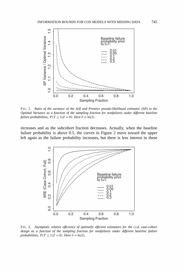
Figure 1 displays the ratios of asymptotic variance of the Self and Prentice(1988) pseudo-likelihood estimator (SP Variance) to the information lower boundfor θ as a function of the sampling fraction for nonfailures in the i.i.d. case-cohort model shown above. Figure 1 shows that when the disease is rare, thatis, the baseline failure probability is very low, the pseudo-likelihood estimator isclose to fully efficient. As the failure probability increases, the pseudo-likelihoodestimator loses more efficiency, especially when the subcohort fraction is small.Hence development of more efficient estimators may be worthwhile for case-cohort designs where increasing the subcohort fraction is costly and the failureprobability is moderate.

Figure 2 displays the ratio of the information lower bound for estimation ofθ

based on the “observed data” (1/I ∗θ whereI ∗

θ is the information forθ ) and theasymptotic variance of the partial-likelihood estimator forθ based on “complete”(or “full”) data. This ratio is shown as a function of the sampling fraction for thenonfailures under different baseline failure probabilities wheneθ = 2. Figure 2shows that the case-cohort design loses more information (supposing that anefficient estimator is available), relative to complete data, as the failure probability


FIG. 1. Ratio of the variance of the Self and Prentice pseudo-likelihood estimator (SP) to theOptimal Variance as a function of the sampling fraction for nonfailures under different baselinefailure probabilities, P(T ≤ 1|Z = 0). Here θ = ln(2).

increases and as the subcohort fraction decreases. Actually, when the baselinefailure probability is above 0.5, the curves in Figure 2 move toward the upperleft again as the failure probability increases, but there is less interest in these

FIG. 2. Asymptotic relative efficiency of optimally efficient estimators for the i.i.d. case-cohortdesign as a function of the sampling fraction for nonfailures under different baseline failureprobabilities, P(T ≤ 1|Z = 0). Here θ = ln(2).


high failure probability cases in practice. From Figure 2 we can see that a greatdeal of precision may be lost by using a case-cohort design as opposed to datacollection on the full cohort, even when a fully efficient estimator is used forthe case-cohort study. With this knowledge investigators can weigh the trade-offbetween precision and study cost. Further work is needed to explore presumablymore efficient designs: for example, an alternative design might be an “exposurestratified case-cohort design” as in our second example.

Perhaps the more interesting phenomena appear in Figure 3 and Figure 4. InFigure 3 we look at the asymptotic relative efficiency of the pseudo-likelihoodestimator as a function ofθ . Figure 4 shows the relative efficiency of the optimalvariances for the i.i.d. case-cohort design versus the full data design as a functionof θ . Whenθ is near zero Figure 3 shows that the pseudo-likelihood estimator doesnot lose much efficiency compared to the optimal estimator for the case-cohortdesign. However, Figure 4 shows that the case-cohort design (with an optimalestimator) loses considerable information compared to the full data design. Theminimum ARE (as a function ofθ ) depends on the baseline failure probability;the minimum increases and it moves away fromθ = 0 as the baseline failureprobability decreases. Whenθ is away from zero, that is, the effect of the covariateZ is large, the pseudo-likelihood estimator loses significant efficiency, especiallywhenθ is positive and the baseline failure probability is high. However, away fromzero the design itself starts to gain information and is very close to the full datadesign when the absolute value ofθ is large. The conclusion is that if we expect

FIG. 3. Ratio of the variance for the Self and Prentice pseudo-likelihood estimator (SP) to theOptimal Variance as a function of θ (log of relative risk) for different baseline failure probabilitiesP(T ≤ 1|Z = 0) in the i.i.d. case-cohort design. Here the sampling fraction for nonfailures is 0.1.


FIG. 4. Asymptotic relative efficiency of the optimally efficient estimator in the case-cohort designrelative to the optimally efficient estimator in the full cohort design as a function of θ (log of relativerisk) for different baseline failure probabilities P(T ≤ 1|Z = 0). Here the sampling fraction fornonfailures is 0.1.

intermediate to large covariate effects, it may be very worthwhile to find efficientestimators forθ . Certainly, developing more efficient designs is also valuable, ascan be seen from Figures 2 and 4.

4.2. An exposure stratified case-cohort study. Assume thatX is the variableof interest and thatV is a surrogate variable forX, or measurement ofX witherror, andV is conditionally independent ofT givenX. We suppose thatV can beobserved for everyone in the entire cohort, butX is only observed for subjectsin the subcohort and failures. Then the model for this type of data is the firstalternative model discussed in the previous section. The i.i.d. version of theexposure stratified case-cohort design studied by Borgan, Langholz, Samuelsen,Goldstein and Pogoda (2000) is a special case of this model. Here we discussan example with a binary covariateX ∈ {0,1} and a binary surrogate variableV ∈ {0,1}. The distribution forX andV has the form of a 2× 2 table. Let

P (V = 1|X = 1) = 1− α, P (V = 0|X = 0) = 1− β.

If we considerV = 1 as a “positive” test forX, then 1− α is the sensitivityand 1−β is the specificity of the test. We assume exponentially distributed failuretimes. All subjects in the cohort are followed from time zero to either failure orto the end of the study at timet = 1. For our calculations the exponential failurerate parameterλ will be set to achieve a specified baseline failure probability as


in Section 4.1. Let the joint mass function of(X,V ) beh(x, v). Thus we have thejoint density for the underlying complete data,

qY,�,X,V (y, δ, x, v) ={

λeθx−λyeθxh(x, v), δ = 1, 0≤ y ≤ 1,

e−λeθxh(x, v), δ = 0, y = 1.

(4.2)

By the same argument as in the previous example, we may assume thatY always isobserved. The cohort is then categorized into three strata:{� = 1}, {� = 0,V = 0}and{� = 0,V = 1}. We observe complete information for all the subjects in thefirst stratum, and ofπ0, π1 fractions (constants) of the subjects in the secondand third strata, respectively. We only observe(Y,�,V ) for other subjects. Inprobability language we haveP (R = 1|� = 1, Y,V ) ≡ π(Y,1,V ) = 1, P (R =1|� = 0, Y,V ) ≡ π(Y,0,V ) ≡ π0 if V = 0 andπ1 if V = 1. Again, we omit thedetailed calculations here and refer to Nan (2001).

We calculateI ∗θ for different α, β, P (X = 0), π0, π1, θ and λ by using

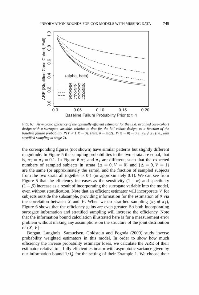
numerical integration. Whenα = β = 0.5, the exposure stratified case-cohortdesign is equivalent to the classical case-cohort design (previous example)sinceV is not correlated withX under this condition. Figures 5 and 6 showthe comparisons of the asymptotic relative efficiency (ARE) of fully efficientestimators (if they exist) for the exposure stratified (atπ0 = π1 and π0 �= π1)and classical case-cohort designs ateθ = 2 andP (X = 0) = 0.9. Whenθ = 0,

FIG. 5. Asymptotic efficiency of the optimally efficient estimator for the case-cohort design with asurrogate variable, relative to that for the full cohort design, as a function of the baseline failureprobability, P(T ≤ 1|X = 0). Here θ = ln(2), P (X = 0) = 0.9, π0 = π1 = 0.1 (i.e., stage 2sampling is not stratified).


FIG. 6. Asymptotic efficiency of the optimally efficient estimator for the i.i.d. stratified case-cohortdesign with a surrogate variable, relative to that for the full cohort design, as a function of thebaseline failure probability P(T ≤ 1|X = 0). Here, θ = ln(2), P (X = 0) = 0.9, π0 �= π1 (i.e., withstratified sampling at stage 2).

the corresponding figures (not shown) have similar patterns but slightly differentmagnitude. In Figure 5 the sampling probabilities in the two strata are equal, thatis, π0 = π1 = 0.1. In Figure 6π0 and π1 are different, such that the expectednumbers of sampled subjects in strata{� = 0,V = 0} and {� = 0,V = 1}are the same (or approximately the same), and the fraction of sampled subjectsfrom the two strata all together is 0.1 (or approximately 0.1). We can see fromFigure 5 that the efficiency increases as the sensitivity (1− α) and specificity(1− β) increase as a result of incorporating the surrogate variable into the model,even without stratification. Note that an efficient estimator will incorporateV forsubjects outside the subsample, providing information for the estimation ofθ viathe correlation betweenX and V . When we do stratified sampling (π0 �= π1),Figure 6 shows that the efficiency gains are even greater. So both incorporatingsurrogate information and stratified sampling will increase the efficiency. Notethat the information bound calculation illustrated here is for a measurement errorproblem without making any assumptions on the structure of the joint distributionof (X,V ).

Borgan, Langholz, Samuelsen, Goldstein and Pogoda (2000) study inverseprobability weighted estimators in this model. In order to show how muchefficiency the inverse probability estimator loses, we calculate the ARE of theirestimator relative to a fully efficient estimator with asymptotic variance given byour information bound 1/I ∗

θ for the setting of their Example 1. We choose their


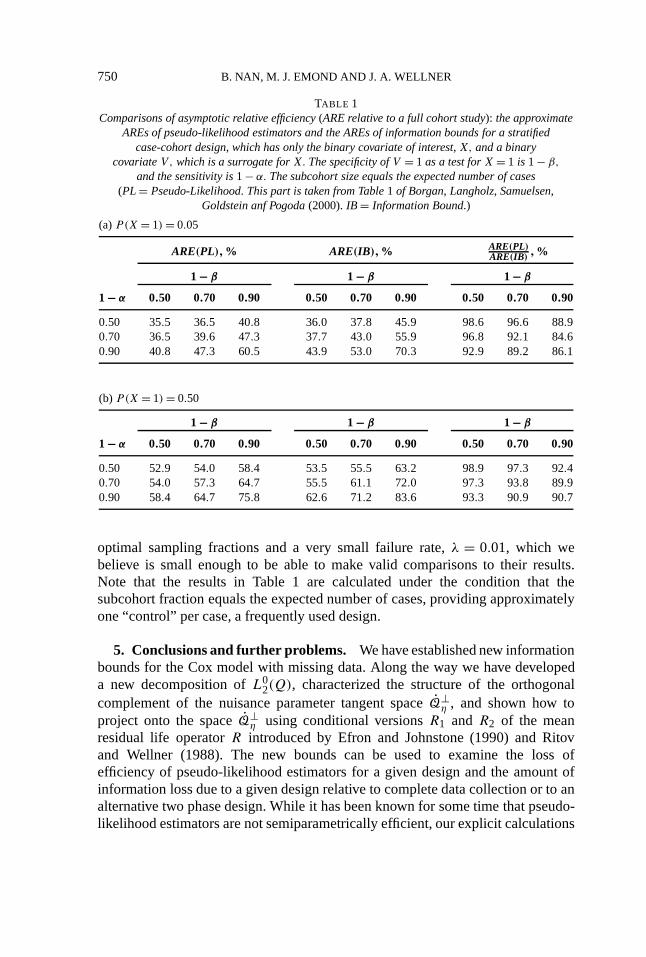
TABLE 1Comparisons of asymptotic relative efficiency (ARE relative to a full cohort study): the approximate

AREs of pseudo-likelihood estimators and the AREs of information bounds for a stratifiedcase-cohort design, which has only the binary covariate of interest, X, and a binary

covariate V, which is a surrogate for X. The specificity of V = 1 as a test for X = 1 is 1− β,

and the sensitivity is 1− α. The subcohort size equals the expected number of cases(PL = Pseudo-Likelihood. This part is taken from Table 1 of Borgan, Langholz, Samuelsen,

Goldstein anf Pogoda (2000).IB = Information Bound.)

(a)P(X = 1) = 0.05

ARE(PL),% ARE(IB),% ARE(PL)ARE(IB) ,%

1 − β 1 − β 1 − β

1 − α 0.50 0.70 0.90 0.50 0.70 0.90 0.50 0.70 0.90

0.50 35.5 36.5 40.8 36.0 37.8 45.9 98.6 96.6 88.90.70 36.5 39.6 47.3 37.7 43.0 55.9 96.8 92.1 84.60.90 40.8 47.3 60.5 43.9 53.0 70.3 92.9 89.2 86.1

(b) P(X = 1) = 0.50

1 − β 1 − β 1 − β

1 − α 0.50 0.70 0.90 0.50 0.70 0.90 0.50 0.70 0.90

0.50 52.9 54.0 58.4 53.5 55.5 63.2 98.9 97.3 92.40.70 54.0 57.3 64.7 55.5 61.1 72.0 97.3 93.8 89.90.90 58.4 64.7 75.8 62.6 71.2 83.6 93.3 90.9 90.7

optimal sampling fractions and a very small failure rate,λ = 0.01, which webelieve is small enough to be able to make valid comparisons to their results.Note that the results in Table 1 are calculated under the condition that thesubcohort fraction equals the expected number of cases, providing approximatelyone “control” per case, a frequently used design.

5. Conclusions and further problems. We have established new informationbounds for the Cox model with missing data. Along the way we have developeda new decomposition ofL0

2(Q), characterized the structure of the orthogonalcomplement of the nuisance parameter tangent spaceQ⊥

η , and shown how toproject onto the spaceQ⊥

η using conditional versionsR1 and R2 of the meanresidual life operatorR introduced by Efron and Johnstone (1990) and Ritovand Wellner (1988). The new bounds can be used to examine the loss ofefficiency of pseudo-likelihood estimators for a given design and the amount ofinformation loss due to a given design relative to complete data collection or to analternative two phase design. While it has been known for some time that pseudo-likelihood estimators are not semiparametrically efficient, our explicit calculations


quantify the loss of efficiency and also show that two-phase designs with stratifiedsubsampling can partially recover the information that is lost due to missing data.

Further problems.

1. Construction of efficient estimators when covariates are discrete. Efficientestimators can be constructed explicitly using one-step methods when thecovariates are discrete. For a preliminary study of such estimators, seeNan (2001).

2. Construction of efficient estimators in general. This will depend crucially onunderstanding the properties of the integral equation defining the efficient scoreand influence function. A major difficulty in constructing efficient estimators isthe fact that the conditional cumulative hazard function�G(y|z) enters intothe key equation (3.18) which determinesu∗ and hence the efficient scorefunction l∗θ . This function is typically completely unknown and is a functionof d + 1 variables which must be estimated nonparametrically. This is, ofcourse, a difficult task for even moderately larged . However, our goal is notto estimate�G well, but instead to estimateθ well, and it is not yet clearhow crucial the difficulty in estimating�G will be for construction of (nearly)efficient estimates ofθ . We remain optimistic about this at least for moderatevalues ofd , and regard this as an important question for future work.

3. How can we “optimize” the sampling design for a particular study? If we focuson the variance of the estimator of a particular regression coefficient (e.g., thecoefficient corresponding to a binary treatment-control covariate), then it wouldbe very interesting to know how to allocate the sampling effort in the secondphase to minimize the (asymptotic) variance. Our results provide the tools tographically address this extremely important question.

4. Are there better compromise estimators based on pseudo-likelihood? Here theapproaches of Chatterjee, Chen and Breslow (2003) and Chatterjee (1999) maybe useful.

Acknowledgments. We owe thanks to Norman Breslow, Nilanjan Chatterjeeand the other participants in theMissing Data Working Group at the Universityof Washington during the period 1995–1998, for many useful discussions aboutmissing data and the subject of this paper. We also owe thanks to J. Robinsfor helpful discussions and to a referee for suggesting the current form given inProposition 3.3 for the equation characterizingu∗.

REFERENCES

ANDERSEN, P. K. and GILL , R. D. (1982). Cox’s regression model for counting processes: A largesample study.Ann. Statist. 10 1100–1120.

BEGUN, J. M., HALL , W. J., HUANG, W. M. and WELLNER, J. A. (1983). Information andasymptotic efficiency in parametric-nonparametric models.Ann. Statist. 11 432–452.


BELL, E. M., HERTZ-PICCIOTTO, I. and BEAUMONT, J. J. (2001). Case-cohort analysis ofagricultural pesticide applications near maternal residence and selected causes of fetaldeath.Amer. J. Epidemiology 154 702–710.

BICKEL, P. J., KLAASSEN, C. A. J., RITOV, Y. and WELLNER, J. A. (1993).Efficient and AdaptiveEstimation for Semiparametric Models. Johns Hopkins Univ. Press, Baltimore, MD.

BORGAN, O., LANGHOLZ, B., SAMUELSEN, S. O., GOLDSTEIN, L. and POGODA, J. (2000).Exposure stratified case-cohort designs.Lifetime Data Analysis 6 39–58.

CHATTERJEE, N. (1999). Semiparametric inference based on estimating equations in regressionmodels for two phase outcome dependent sampling. Ph.D. dissertation, Dept. Statistics,Univ. Washington.

CHATTERJEE, N., CHEN, Y.-H. and BRESLOW, N. E. (2003). A pseudoscore estimator for regressionproblems with two-phase sampling.J. Amer. Statist. Assoc. 98. 158–168.

CHEN, K. and LO, S.-H. (1999). Case-cohort and case-control analysis with Cox’s model.Biometrika86 755–764.

COX, D. R. (1972). Regression models and life tables (with discussion).J. Roy. Statist. Soc. Ser. B34 187–220.

DOME, J. S., CHUNG, S., BERGEMANN, T., UMBRICHT, C. B., SAJI, M., CAREY, L. A., GRUNDY,P. E., PERLMAN, E. J., BRESLOW, N. E. and SUKUMAR, S. (1999). High telomerasereverse transcriptase (hTERT) messenger RNA level correlates with tumor recurrence inpartients with favorable histology Wilms’ tumor.Cancer Res. 59 4301–4307.

EFRON, B. (1977). The efficiency of Cox’s likelihood function for censored data.J. Amer. Statist.Assoc. 72 557–565.

EFRON, B. and JOHNSTONE, I. (1990). Fisher’s information in terms of the hazard rate.Ann. Statist.18 38–62.

EMOND, M. and WELLNER, J. A. (1995). Missing data: Expansion on BKRW (1993) and commentson/computations for Robins, Rotnitzky and Zhao. Technical report, Univ. Washington.

HORVITZ, D. G. and THOMPSON, D. J. (1952). A generalization of sampling without replacementfrom a finite universe.J. Amer. Statist. Assoc. 47 663–685.

HUANG, J. (1999). Efficient estimation of the partly linear additive Cox model.Ann. Statist. 271536–1563.

KRESS, R. (1999).Linear Integral Equations, 2nd ed. Springer, New York.MARGOLIS, D. J., KNAUSS, J. and BILKER, W. (2002). Hormone replacement therapy and

prevention of pressure ulcers and venous leg ulcers.Lancet 359 675–677.MARK, S. D., QIAO, Y. L., DAWSEY, S. M., WU, Y. P., KATKI , H., GUNTER, E. W., FRAUMENI,

J. F., JR., BLOT, W. J., DONG, Z. W. and TAYLOR, P. R. (2000). Prospective study ofserum selenium levels and incident esophageal and gastric cancers.J. Natl. Cancer Inst.92 1753–1763.

NAN, B. (2001). Information bounds and efficient estimation for two-phase designs with lifetimedata. Ph.D. dissertation, Dept. Biostatistics, Univ. Washington.

NAN, B., EMOND, M. and WELLNER, J. A. (2000). Information bounds for regression models withmissing data. Technical Report 378, Dept. Statistics, Univ. Washington.

PRENTICE, R. L. (1986). A case-cohort design for epidemiologic cohort studies and diseaseprevention trials.Biometrika 73 1–11.

RASMUSSEN, M. L., FOLSOM, A. R., CATELLIER, D. J., TSAI, M. Y., GARG, U. andECKFELDT, J. H. (2001). A prospective study of coronary heart disease and thehemochromatosis gene (HFE) C282Y mutation: The Atherosclerosis Risk in Commu-nities (ARIC) study.Atherosclerosis 154 739–746.

RITOV, Y. and WELLNER, J. A. (1988). Censoring, martingales, and the Cox model. InStatistical In-ference from Stochastic Processes (N. U. Prabhu, ed.) 191–219. American MathematicalSociety, Providence, RI.


ROBINS, J. M., HSIEH, F. and NEWEY, W. (1995). Semiparametric efficient estimation of aconditional density with missing or mismeasured covariates.J. Roy. Statist. Soc. Ser. B57 409–424.

ROBINS, J. M. and ROTNITZKY, A. (1992). Recovery of information and adjustment for dependentcensoring using surrogate markers. InAIDS Epidemilology: Methodological Issues(N. P. Jewell, K. Dietz and V. T. Farewell, eds.) 297–331. Birkhäuser, Boston.

ROBINS, J. M., ROTNITZKY, A. and ZHAO, L. P. (1994). Estimation of regression coefficients whensome regressors are not always observed.J. Amer. Statist. Assoc. 89 846–866.

RUDIN, W. (1966).Real and Complex Analysis. McGraw-Hill, New York.RUDIN, W. (1973).Functional Analysis. McGraw-Hill, New York.SASIENI, P. (1992a). Information bounds for the conditional hazard ratio in a nested family of

regression models.J. Roy. Statist. Soc. Ser. B 54 617–635.SASIENI, P. (1992b). Nonorthogonal projections and their application to calculating the information

in a partly linear Cox model.Scand. J. Statist. 19 215–233.SELF, S. G. and PRENTICE, R. L. (1988). Asymptotic distribution theory and efficiency results for

case-cohort studies.Ann. Statist. 16 64–81.SHORACK, G. R. and WELLNER, J. A. (1986).Empirical Processes with Applications to Statistics.

Wiley, New York.TERRY, P., JAIN , M., MILLER, A. B., HOWE, G. R. and ROHAN, T. E. (2002). Dietary intake of folic

acid and colorectal cancer risk in a cohort of women.Internat. J. Cancer 97 864–867.VAN DER VAART, A. W. (1998).Asymptotic Statistics. Cambridge Univ. Press.ZEEGERS, M. P., GOLDBOHM, R. A. andVAN DEN BRANDT, P. A. (2001). Are retinol, vitamin C,

vitamin E, folate and carotenoids intake associated with bladder cancer risk? Results fromthe Netherlands cohort study.British J. Cancer 85 977–983.

ZEEGERS, M. P., SWAEN, G. M., KANT, I., GOLDBOHM, R. A. andVAN DEN BRANDT, P. A. (2001).Occupational risk factors for male bladder cancer: Results from a population based casecohort study in the Netherlands.Occupational and Environmental Medicine 58 590–596.

B. NAN

DEPARTMENT OFBIOSTATISTICS

UNIVERSITY OF MICHIGAN

1420 WASHINGTONHEIGHTS

ANN ARBOR, MICHIGAN 48109-2029USAE-MAIL : [email protected]

M. EMOND

DEPARTMENT OFBIOSTATISTICS

UNIVERSITY OF WASHINGTON

P.O. BOX 357232SEATTLE, WASHINGTON 98195-7232USAE-MAIL : [email protected]

J. A. WELLNER

DEPARTMENT OFSTATISTICS

UNIVERSITY OF WASHINGTON

P.O. BOX 354322SEATTLE, WASHINGTON 98195-4322USAE-MAIL : [email protected]

information bounds for cox regression models with missing data

Documents