INFORMATION CRITERION AND CHANGE POINT

PROBLEM FOR REGULAR MODELS1

Jiahua Chen A. K. Gupta

Department of Statistics & Actuarial Science Department of Mathematics and Statistics

University of Waterloo Bowling Green State University

Waterloo, Ontario, Canada N2L 3G1 Bowling Green, OH 43403-0221 U.S.A.

Jianmin Pan

Department of Statistics & Actuarial Science

University of Waterloo

Waterloo, Ontario, Canada N2L 3G1

ABSTRACT

Information criteria are commonly used for selecting competing statistical models. They

do not favor the model which gives the best fit to the data and little interpretive value,

but simpler models with good fit. Thus, model complexity is an important factor in in-

formation criteria for model selection. Existing results often equate the model complexity

to the dimension of the parameter space. Although this notion is well founded in regular

parametric models, it lacks some desirable properties when applied to irregular statistical

models. We refine the notion of model complexity in the context of change point problems,

and modify the existing information criteria. The modified criterion is found consistent in

selecting the correct model and has simple limiting behavior. The resulting estimator τ of

the location of the change point achieves the best convergence rate Op(1), and its limiting

distribution is obtained. Simulation results indicate that the modified criterion has better

power in detecting changes compared to other methods.

Key words: consistency; irregular parametric model; limiting distribution; location; model

complexity; regular parametric model; convergence rate.

1991 AMS Subject Classification: Primary 62H15; Secondary 62H10.

1Running title: Change point problem

1

1 Introduction

Out of several competing statistical models, we do not always use the one with the best fit

to the data. Such models may simply interpolate the data and have little interpretive value.

Information criteria, such as the Akaike information criterion and the Schwarz information

criterion, are designed to select models with simple structure and good interpretive value,

see Akaike (1973) and Schwarz (1978). The model complexity is often measured in terms of

the dimensionality of the parameter space.

Consider the problem of making inference on whether a process has undergone some

changes. In the context of model selection, we want to choose between a model with a single

set of parameters, or a model with two sets of parameters plus the location of change. The

Akaike and the Schwarz information criteria can be readily adopted to this kind of change

point problems. There have been many fruitful research done in this respect such as Hirotsu,

Kuriki and Hayter (1992) and Chen and Gupta (1997), to name a few.

Compared to usual model selection problems, the change point problem contains a special

parameter: the location of the change. When it approaches the beginning or the end of the

process, one of the two sets of the parameter becomes completely redundant. Hence, the

model is un-necessarily complex. This observation motivates the notion that the model

complexity also depends on the location of the change point. Consequently, we propose to

generalize the Akaike and Schwarz information criteria by making the model complexity also

a function of the location of the change point. The new method is shown to have a simple

limiting behavior, and favourable power properties in many situations via simulation.

The change point problem has been extensively discussed in the literature in recent years.

The study of the change point problem dates back to Page (1954, 1955 and 1957) which tested

the existence of a change point. Parametric approaches to this problem have been studied

by a number of researchers, see Chernoff and Zacks (1964), Hinkley (1970), Hinkley et. al.

(1980), Siegmund (1986) and Worsley (1979, 1986). Nonparametric tests and estimations

have also been proposed (Brodsky and Darkhovsky, 1993; Lombard, 1987; Gombay and

Huskova, 1998). Extensive discussions on the large sample behavior of likelihood ratio test

statistics can be found in Gombay and Horvath (1996) and Csorgo and Horvath (1997).

2

The detail can be found in some survey literatures such as Bhattacharya (1994), Basseville

and Nikiforov (1993), Zacks (1983), and Lai (1985). The present study deviates from other

studies by refining the traditional measure of the model complexity, and by determining

the limiting distribution of the resulting test statistic under very general parametric model

settings.

In Section 2, we define and motivate the new information criterion in detail. In Section

3, we give the conditions under which the resulting test statistic has chi-square limiting

distribution and the estimator τ of change point attains the best convergence rate. An

application example and some simulation results are given in Section 4. The new method is

compared to three existing methods and found to have good finite sample properties. The

proofs are given in the Appendix.

2 Main Results

Let X1, X2, . . . , Xn be a sequence of independent random variables. It is suspected that Xi

has density function f(x, θ1) when i ≤ k and density f(x, θ2) for i > k. We assume that

f(x, θ1) and f(x, θ2) belong to the same parametric distribution family {f(x, θ) : θ ∈ Rd}.The problem is to test whether this change has indeed occurred and if so, find the location of

the change k. The null hypothesis is H0 : θ1 = θ2 and the alternative is H1 : θ1 6= θ2 and 1 ≤k < n.

Equivalently, we are asked to choose a model from H0 or a model from H1 for the data.

For regular parametric (not change point) models with log likelihood function `n(θ),

Akaike and Schwarz information criteria are defined as

AIC = −2`n(θ) + 2dim(θ);

SIC = −2`n(θ) + dim(θ) log(n)

where θ is the maximum point of `n(θ). The best model according to these criteria is the one

which minimizes AIC or SIC. The Schwarz information criterion is asymptotically optimal

according to certain Bayes formulation.

3

The log likelihood function for the change point problem has the form

`n(θ1, θ2, k) =k∑

i=1

log f(Xi, θ1) +n∑

i=k+1

log f(Xi, θ2). (1)

The Schwarz information criterion for the change point problem becomes

SIC(k) = −2`n(θ1k, θ2k, k) + [2dim(θ1k) + 1] log(n)

and similarly for Akaike information criterion, where θ1k, θ2k maximize `n(θ1, θ2, k) for given

k. See, for example, Chen and Gupta (1997). When the model complexity is the focus, we

may also write it as

SIC(k) = −2`n(θ1k, θ2k, k) + complexity(θ1k, θ2k, k) log(n).

We suggest that the notion of complexity(θ1k, θ2k, k) = 2dim(θ1k) + 1 needs re-examination

in the context of change point problem. When k takes values in the middle of 1 and n, both

θ1 and θ2 are effective parameters. When k is near 1 or n, either θ1 or θ2 becomes redundant.

Hence, k is an increasingly undesirable parameter as k getting close to 1 or n. We hence

propose a modified information criterion with

complexity(θ1k, θ2k, k) = 2dim(θ1k) + (2k

n− 1)2 + constant. (2)

For 1 ≤ k < n, let

MIC(k) = −2`n(θ1k, θ2k, k) + [2dim(θ1k) + (2k

n− 1)2] log(n). (3)

Under the null model, we define

MIC(n) = −2`n(θ, θ, n) + dim(θ) log(n) (4)

where θ maximizes `n(θ, θ, n). If MIC(n) > min1≤k<n MIC(k), we select the model with a

change point and estimate the change point by τ such that

MIC(τ) = min1≤k<n

MIC(k).

Clearly, this procedure can be repeated when a second change point is suspected.

4

The size of model complexity can be motivated as follows. If the change point is at k, the

variance of θ1k would be proportional to k−1 and the variance of θ2k would be proportional

to (n− k)−1. Thus, the total variance is

1

k+

1

n− k= n−1

[1

4− (

k

n− 1

2)2

]−1

.

The specific form in (2) reflects this important fact. Thus, if a change at an early stage is

suspected, relatively stronger evidence is needed to justify the change. Hence, we should

place larger penalty when k is near 1 or n. This notion is shared by many researchers.

The method in Inclan and Tiao (1994) scales down the statistics heavier when the suspected

change point is near 1 or n. The U-statistic method in Gombay and Horvath (1995) is scaled

down by multiplying the factor k(n− k).

To assess the error rates of the method, we can simulate the finite sample distribution, or

find the asymptotic distribution of the related statistics. For Schwarz information criterion,

the related statistic is found to have type I extreme value distribution asymptotically (Chen

and Gupta, 1997; Csorgo and Horvath 1997). We show that the MIC statistic has chi-square

limiting distribution for any regular distribution family, the estimator τ achieves the best

convergence rate Op(1) and has a limiting distribution expressed via a random walk.

Our asymptotic results under alternative model is obtained under the assumption that the

location of the change point, k, evolves with n as n → ∞. Thus, {Xin : 1 ≤ i ≤ n, n ≥ 2}form a triangle array. The classical results on almost sure convergence for independent

and identically distributed (iid) random variables cannot be directly applied. However, the

conclusions on weak convergence will not be affected as the related probability statements

are not affected by how one sequence is related to the other. Precautions will be taken on

this issue but details will be omitted.

Let

Sn = MIC(n)− min1≤k<n

MIC(k) + dim(θ) log n (5)

where MIC(k) and MIC(n) are defined in (3) and (4). Note that this standardization

removes the constant term dim(θ) log n in the difference of MIC(k) and MIC(n).

Theorem 1 Under Wald conditions W1-W7 and the regularity conditions R1-R3, to be

5

specified in Section 3, as n →∞,

Sn → χ2d (6)

in distribution under H0, where d is the dimension of θ and Sn is defined in (5).

In addition, if there has been a change at τ such that as n →∞, τ/n has a limit in (0,

1), then

Sn →∞ (7)

in probability.

Theorem 1 implies that the new information criterion is consistent in the sense that when

there is indeed a fixed amount of change in θ at τ such that τ/n has a limit in (0, 1), the

model with a change point will be selected with probability approaching 1.

Our next result claims that the estimator τ achieves the best convergence rate and obtains

its limiting distribution.

Theorem 2 Assume that the Wald conditions W1-W7 and the regularity conditions R1-R3

are satisfied by the parametric distribution family {f(x; θ), θ ∈ Θ}. As n goes to infinity, the

change point satisfies τ = [nλ] with 0 < λ < 1. Then, the change point estimator

τ − τ = Op(1).

Theorem 2 shows that the estimator τ of the change point attains the best convergence

rate.

We further show that the asymptotic distribution of the estimator τ can be characterized

by the minimizer of a random walk. Let {Yi, i = −1,−2, . . .} be a sequence of iid random

variables with common density function f(x, θ10). Similarly, let {Yi, i = 1, 2, . . .} be iid

random variables with the common density function f(x, θ20), and the two sequences are

independent. Let Y0 be a number such that f(Y0, θ10) = f(Y0, θ20).

Define Wk =∑k

j=0 sgn(k)[log f(Yj, θ20)− log f(Yj, θ10)] for k = 0,±1,±2, . . ..

Theorem 3 Assume the Wald conditions W1-W7, and the regularity conditions R1-R3.

Assume that there exists a change point at τ = [nλ] where 0 < λ < 1. As n →∞, we have

τ − τ → ξ

6

in distribution, where ξ = arg min−∞<k<∞{Wk}, and (θ10, θ20) are the true value of (θ1, θ2)

under the alternative.

We spell out the conditions in the next Section and give a few examples when these

conditions are satisfied. The proof of Theorems 1-3 will be given in the Appendix.

3 Conditions and Examples

The first crucial step in proving Theorem 1 is to establish the consistency of θ1k, θ2k and θ

for estimating the single true value θ0 under the null hypothesis H0. Our approach is similar

to that of Wald (1949). Consequently, the following conditions look similar to the conditions

there.

W1. The distribution of X1 is either discrete for all θ or is absolutely continuous for all θ.

W2. For sufficiently small ρ and for sufficiently large r, the expected values E[log f(X; θ, ρ)]2 <

∞ and E[log ϕ(X, r)]2 < ∞ for all θ, where

f(x, θ, ρ) = sup‖θ′−θ‖≤ρ

f(x, θ′); ϕ(x, r) = sup‖θ′−θ0‖>r

f(x, θ′).

W3. The density function f(x, θ) is continuous in θ for every x.

W4. If θ1 6= θ2, then F (x, θ1) 6= F (x, θ2) for at least one x, where F (x, θ) is the cumulative

distribution function corresponding to the density function f(x, θ).

W5. lim‖θ‖→∞ f(x, θ) = 0 for all x.

W6. The parameter space Θ is a closed subset of the d-dimensional Cartesian space.

W7. f(x, θ, ρ) is a measurable function of x for any fixed θ and ρ.

The notation E will be understood as expectation under the true distribution which has

parameter value θ0 unless otherwise specified.

7

Lemma 1 Under Wald conditions W1-W7 and the null model,

θ1k, θ2k → θ0 (8)

in probability uniformly for all k such that min(k, n− k)/√

n →∞ as n →∞.

Under Wald conditions W1-W7 and the alternative model with the change point at τ =

[nλ] for some 0 < λ < 1,

(θ1k, θ2k) → (θ10, θ20) (9)

in probability uniformly for all k such that |k − τ | < n(log n)−1 as n →∞.

Lemma 1 allows us to focus on a small neighborhood of θ0 or a small neighborhood of

(θ10, θ20) under appropriate model assumptions. The precise asymptotic behavior of Sn is

determined by the properties of the likelihood when θ is close to θ0. This is where the

regularity conditions are needed. The following conditions can be compared to those given

in Serfling (1980).

R1. For each θ ∈ Θ, the derivatives

∂ log f(x, θ)

∂θ,

∂2 log f(x, θ)

∂θ2,

∂3 log f(x, θ)

∂θ3

exist for all x.

R2. For each θ0 ∈ Θ, there exist functions g(x) and H(x) (possibly depending on θ0) such

that for θ in a neighborhood N(θ0) the relations

∣∣∣∣∣∂f(x, θ)

∂θ

∣∣∣∣∣ ≤ g(x) ,

∣∣∣∣∣∂2f(x, θ)

∂θ2

∣∣∣∣∣ ≤ g(x) ,

∣∣∣∣∣∂2 log f(x, θ)

∂θ2

∣∣∣∣∣2

≤ H(x) ,

∣∣∣∣∣∂3 log f(x, θ)

∂θ3

∣∣∣∣∣ ≤ H(x)

hold for all x, and

∫g(x)dx < ∞, Eθ[H(X)] < ∞ for θ ∈ N(θ0).

R3. For each θ ∈ Θ,

0 < Eθ

(∂ log f(X, θ)

∂θ

)2 < ∞, Eθ

∣∣∣∣∣∂ log f(X, θ)

∂θ

∣∣∣∣∣3 < ∞.

8

Some of the Wald conditions are implied by regularity conditions. For clarity, we do not

combine the two sets of conditions into a concise set of conditions. When θ is a vector, the

above conditions are true for all components

Let an be a sequence of positive numbers and An be a sequence of random variables,

n = 1, 2, . . .. If P (An ≤ εan) → 1, for each ε > 0, we say that An ≤ op(an). This convention

will be used throughout the paper.

Lemma 2 Under the null hypothesis and assuming the Wald conditions W1-W7 and the

regularity conditions R1-R3, we have

max1≤k<n

[supθ1,θ2

`n(θ1, θ2, k)− `n(θ0, θ0, n)] ≤ op(log log n).

Lemma 2 indicates that random fluctuation in MIC(k) is less than the penalty (2k/n−1)2 log n under the null model. Hence, the minimum of MIC(k) is attained in the middle of

1 and n in probability under the null model. Lemmas 1 and 2 together imply that the MIC

value is mainly determined by the likelihood function when θ and k are close to θ0 and n/2.

Lemma 3 Under the null hypothesis and assuming Wald conditions W1-W7 and the regu-

larity conditions R1-R3, tτ = τn→ 1

2in probability as n →∞.

The conditions required for these Theorems are not restrictive. In the following we use

two examples to illustrate.

Example 1: Assume

f(x, θ) =θx

x!e−θ, θ ∈ (0,∞)

and x = 0, 1, 2, . . .. To prove that the Poisson model satisfies conditions W2, it is sufficient

to show that E[X log(X)I(X > 1)]2 < ∞. This is obvious by using the Sterling’s Formula.

Example 2: Assume that for all x ≥ 0, f(x, θ) = θe−θx with Θ = (0,∞). Note that

E[log f(X, θ, ρ)]2 < ∞ for small ρ. On the other hand, for all r > 0, ϕ(x, r) = sup‖θ−θ0‖>r f(x, θ)

≤ x−1. Hence, E[log ϕ(X, r)]2 ≤ E[log X]2 < ∞.

Some models do not satisfy these conditions directly. The most interesting case is the

normal model with unknown mean and variance. Its likelihood function is unbounded at

9

1880 1900 1920 1940 1960 1980 2000

4060

8010

012

0

Year

Rain

Figure 1: Yearly Data for Argentina Rainfall

k = 1, σ2 = 0 and µ = X1. This obscure phenomenon quickly disappears by requiring 2 ≤k ≤ n− 2. Other methods such as Schwarz information criterion also require 2 ≤ k ≤ n− 2.

It can be shown that all other conditions are satisfied by models in Examples 1 and 2.

Most commonly used models satisfy the conditions of Theorems.

4 Application and Simulation Study

4.1 Example: Argentina Rainfall Data

In this section, we apply both our MIC and SIC criteria to a real data set, the Argentina

rainfall data, which has been investigated by many researchers.

Argentina rainfall data set is a classical example where the change point analysis is

used. The data set was provided by Eng Cesar Lamelas, a meteorologist in the Agricultural

Experimental Station Obispo Colombres, Tucuman and contained yearly rainfall records

collected from 1884 to 1996, with 113 observations in all. Lamelas believed that there was

a change in the mean of the annual rain, caused by the construction of a dam in Tucuman

between 1952 and 1962. Wu, Woodroofe and Mentz (2001) studied the data using the

isotonic regression method and pointed out that there is an apparent increase in the mean.

10

0 5 10 15 20

−0.2

0.00.2

0.40.6

0.81.0

Lag

Autoc

orrela

tion

Rainfall

Frequ

ency

40 60 80 100 120 140

05

1015

2025

Figure 2: Autocorrelation Plot and Histogram for Argentina Rainfall Data

−2 −1 0 1 2

4060

8010

012

0

Theoretical Quantiles

Rai

n Q

uant

iles

Figure 3: Normal Q-Q Plot for Argentina Rainfall Data

11

The rainfall data plot of {Yt}, t = 1, . . . , 113, is shown in Figure 1.

According to the autocorrelation and histogram plots in time series (see Figure 2) and the

Normal Q-Q plot (see Figure 3), although there appears to be some autocorrelation in the

sequence, it is not large enough to be of big concern. At this stage, we ignore the possibility

of the autocorrelation. The normality seems to be reasonable. We use both the MIC and

SIC based on the normal model to analyze the rainfall data, and examine the possibility

of changes in mean and variance in the sequence. That is, we test the following hypothesis

based on {Yt} series:

H0 : µ1 = µ2 = µ and σ21 = σ2

2 = σ2 (µ, σ2 unknown)

against the alternative

H1 : µ1 6= µ2 or σ21 6= σ2

2 and 1 < τ < n.

Our analysis shows that min2<k<112 MIC(k) = MIC(71), Sn = 17.97 and the p-value is

1.3 × 10−4. Hence τ = 71 is suggested as a significant change point in mean and variance

for the Yt series, which corresponds to 1954. Not surprisingly, our conclusion fits very well

with the fact that there was a dam constructed in Tucuman between 1952 and 1962.

If the Schwarz criterion is used, then we have min2<k<112 SIC(k) = SIC(71), Tn =

SIC(n) − mink SIC(k) + (d + 1) log n = 18.32 and the p-value is 3.6 × 10−2. Hence, two

methods give similar conclusions.

For reference, we computed the means and standard deviations for the whole data set,

the first subset (before the suggested change point 1954) and the second subset (after 1954)

as follows: µ = 81.33, µ1 = 76.50 and µ2 = 89.50; σ = 17.59, σ1 = 15.46 and σ2 = 17.96.

From these values, we find that there is a substantial difference between µ1 and µ2, but not

so apparent change in standard deviation. Hence the change point 1954 suggested by both

the MIC and SIC methods is mainly due to the change in the mean precipitation.

12

4.2 Simulation Study

4.2.1 The Power Comparison between MIC and Other Methods

In this section, we use simulation to investigate finite sample properties of several methods.

In addition to the modified information criterion, we also consider the Schwartz information

criterion, the U-statistic method by Gombay and Horvath (1995) and the method given

by Inclan and Tiao (1994). The U-statistics method computes the values of the U-statistics

based on the first k observations, and based on the rest n−k observations. If there is a change

at k, the difference between these values will be stochastically larger than the difference when

there is no change. They choose to standardize the difference by k(n − k). The method in

Inclan and Tiao (1994) computes the ratio of the sum of squares of the first k observations to

the sum of squares of all observations. If the variance of the first k observations is different

from the variance of the rest observations, this ratio likely deviates from k/n significantly.

The test statistic is defined as the maximum absolute difference between the ratio and k/n.

We considered three models in our simulation: normal distribution with a change in the

mean, normal distribution with a change in the variance, and exponential distribution with

a change in the scale. For the U-statistics, we choose kernel function h(x) = x for the first

model, and h(x, y) = (x− y)2 for the second and third models. Since the sample mean and

variance are complete and sufficient statistics in the first two models respectively, the choices

of the kernel function are very sensible.

The sample sizes are chosen to be n = 100 and 200. Under alternative model, we placed

the change at 25%, 50% and 75% points. The amount of change in normal mean was a

difference of 0.5, in normal variance was a factor of 2, and in exponential mean is a factor of√

2. The simulation was repeated 5000 times for all combinations of sample size, location of

change and the model. In Table 1, we report the null rejection rates (in percentage) of the

Schwarz and Modified information criteria in the rows of SIC and MIC. Because two criteria

have rather different null rejection rates, direct power comparison is not possible. In the

row called SIC∗, we calculated the powers of the Schwarz information criterion after its null

rejection rates were made the same as the corresponding MIC (by increasing/decreasing its

critical values). The row called U∗, T∗ are obtained from two other methods similarly.

13

Table 1: Comparison between SIC and MIC

n=100 n=200

normal model: change in the mean(c = 0.5)

k 0 25 50 75 0 50 100 150

MIC 14.7 58.3 78.8 58.4 10.2 79.1 94.4 78.0

SIC 4.94 37.2 49.1 36.4 3.06 61.0 75.7 59.7

SIC* 56.3 67.1 56.4 76.8 87.8 76.2

U* 59.7 78.3 60.0 80.5 94.3 79.5

normal model: change in the variance (c = 2)

k 0 25 50 75 0 50 100 150

MIC 13.6 53.3 75.3 54.3 9.2 74.9 94.3 77.0

SIC 5.70 31.8 45.7 37.4 4.58 51.5 72.9 60.1

SIC* 46.9 61.0 50.9 67.9 84.3 73.5

U* 21.1 50.5 49.1 28.1 70.9 66.6

T* 24.6 65.5 54.1 33.9 86.2 77.2

Exponential model, change in the mean (c=√

2)

k 0 25 50 75 0 50 100 150

MIC 14.1 36.9 53.3 35.7 10.2 48.7 71.4 49.5

SIC 6.46 18.7 24.8 18.9 3.72 26.5 37.8 28.9

SIC* 33.9 40.8 34.6 43.4 56.3 45.2

U* 20.8 36.0 32.1 21.8 46.2 38.3

T* 22.7 44.2 38.8 29.9 62.5 51.1

14

We can make several conclusions from the simulation results. First, both information

criteria are consistent. When the sample size increases from n = 100 to n = 200, the

probabilities of type I errors decrease and the powers increase. Second, after the probabilities

of type I errors have been lined up, the powers of the modified information criterion are higher

than the corresponding Schwarz information criterion in all cases, higher than U∗ and T ∗ in

most cases. There is only one case when the power of the MIC is more than 2% lower than

another method. Third, the MIC is most powerful when the change point is in the middle of

the sequence. The differences of 2% or more are considered significant with 5000 repetitions.

4.2.2 The Comparison of τ and its Limiting Distribution

The limiting distributions of the estimators of the location of the change point based on

the MIC and SIC methods are the same. To investigate their finite sample properties, we

simulated the limiting distribution given in Theorem 3, and the distributions of τ − τ under

the MIC and SIC criteria. We considered four models. The first three models are the same

as the models in the last subsection. The additional model is a normal model with changes

in both mean and variance with mean difference 0.5 and variance ratio 2. To save space, we

only report results when sample sizes are 100 and 1000, and placed the change at τ = n/4

and n/2 in the simulation.

We conducted simulation with 5000 repetitions for each combination and obtained the

rates of ξ, τMIC − τ and τSIC − τ belong to specified intervals. The results are presented in

Tables 2 and 3. It is seen that the limiting distribution (that of ξ) is a good approximation

for both τ when n is in the range of 1000.

When n is as small as 100, P{|τMIC − τ | ≤ δ} ≥ P{|τSIC − τ | ≤ δ} in all cases; The

difference narrows when n increases. At n = 1000, two estimators are almost the same.

5 Appendix: Proofs

We split the proof of Lemmas 1 and 2 into several steps.

Lemma 1A. Let f(x, θ, ρ) and ϕ(x, r) be the functions defined in W2 such that 0 < ρ <

‖θ − θ0‖ and E log[f ∗(X, θ, ρ)] < ∞. Then, for some ρ > 0 small enough (may depend on

15

Table 2: The Comparison of the Distributions τ − τ and ξ for τ = n/2

Pξ = P{|ξ| ≤ δ}, PM = P{|τMIC − τ | ≤ δ} and PS = P{|τSIC − τ | ≤ δ}Models Prob δ = 5 δ = 10 δ = 20 δ = 30 δ = 40

n=100

Model 1 Pξ 0.4698 0.6488 0.8288 0.9048 0.9426

PM 0.5156 0.7016 0.8692 0.9416 0.9796

PS 0.4100 0.5632 0.7250 0.8154 0.8952

Model 2 Pξ 0.4562 0.6248 0.7922 0.8820 0.9344

PM 0.4846 0.6670 0.8502 0.9308 0.9712

PS 0.3644 0.5036 0.6688 0.7780 0.8672

Model 3 Pξ 0.3066 0.4590 0.6432 0.7538 0.8298

PM 0.3852 0.5682 0.7856 0.8888 0.9502

PS 0.2486 0.3704 0.5360 0.6582 0.7864

Model 4 Pξ 0.5820 0.7632 0.9096 0.9636 0.9856

PM 0.5406 0.7040 0.8356 0.8924 0.9218

PS 0.4470 0.5806 0.7006 0.7676 0.8196

n=1000

Model 1 Pξ 0.4804 0.6492 0.8152 0.8966 0.9384

PM 0.4580 0.6498 0.8150 0.8896 0.9322

PS 0.4562 0.6472 0.8122 0.8876 0.9304

Model 2 Pξ 0.4456 0.6216 0.8002 0.8878 0.9332

PM 0.4524 0.6190 0.7926 0.8750 0.9228

PS 0.4510 0.6172 0.7910 0.8732 0.9212

Model 3 Pξ 0.3062 0.4584 0.6288 0.7324 0.8000

PM 0.2972 0.4478 0.6180 0.7190 0.7920

PS 0.2912 0.4376 0.6034 0.7024 0.7738

Model 4 Pξ 0.6000 0.7706 0.9058 0.9578 0.9782

PM 0.5882 0.7660 0.8978 0.9528 0.9744

PS 0.5878 0.7652 0.8970 0.9518 0.9736

16

Table 3: The Comparison of the Distributions τ − τ and ξ for τ = n/4

Pξ = P{|ξ| ≤ δ}, PM = P{|τMIC − τ | ≤ δ} and PS = P{|τSIC − τ | ≤ δ}Models Prob δ = 5 δ = 10 δ = 20 δ = 30 δ = 40

n=100

Model 1 Pξ 0.4698 0.6488 0.8288 0.9048 0.9426

PM 0.4048 0.5614 0.7422 0.8516 0.9114

PS 0.3812 0.5284 0.7068 0.8072 0.8402

Model 2 Pξ 0.4562 0.6248 0.7922 0.8820 0.9344

PM 0.3724 0.5334 0.7234 0.8358 0.9028

PS 0.3552 0.5050 0.6884 0.7940 0.8304

Model 3 Pξ 0.3066 0.4590 0.6432 0.7538 0.8298

PM 0.2642 0.3992 0.5980 0.7570 0.8564

PS 0.2336 0.3566 0.5428 0.6902 0.7406

Model 4 Pξ 0.5820 0.7632 0.9096 0.9636 0.9856

PM 0.4332 0.5674 0.7262 0.8454 0.8842

PS 0.3754 0.5002 0.6488 0.7988 0.8204

n=1000

Model 1 Pξ 0.4804 0.6492 0.8152 0.8966 0.9384

PM 0.4644 0.6456 0.8082 0.8826 0.9226

PS 0.4652 0.6498 0.8124 0.8870 0.9274

Model 2 Pξ 0.4456 0.6216 0.8002 0.8878 0.9332

PM 0.4394 0.5978 0.7742 0.8596 0.9052

PS 0.4420 0.6048 0.7832 0.8686 0.9136

Model 3 Pξ 0.3062 0.4584 0.6288 0.7324 0.8000

PM 0.2760 0.4142 0.5778 0.6804 0.7516

PS 0.2796 0.4194 0.5886 0.6918 0.7596

Model 4 Pξ 0.6000 0.7706 0.9058 0.9578 0.9782

PM 0.5982 0.7602 0.9020 0.9546 0.9768

PS 0.5966 0.7584 0.9028 0.9548 0.9764

17

θ 6= θ0),

maxk

[k∑

i=1

log f(Xi, θ, ρ)−k∑

i=1

log f(Xi, θ0)

]≤ op(log log n).

Similarly, for some r > 0 large enough,

maxk

[k∑

i=1

log ϕ(Xi, r)−k∑

i=1

log f(Xi, θ0)

]≤ op(log log n).

Proof: From the regularity conditions,

limρ→0+

E[log f(X, θ, ρ)− log f(X, θ0)] = E[log f(X, θ)− log f(X, θ0)] = −K(θ, θ0) < 0,

where K is the Kullback Leibler Information. Hence, we can find ρ small enough such that

EYi < 0 for Yi = log f(Xi, θ, ρ)− log f(Xi, θ0).

By the Levy-Skorohod inequality (Shokack and Wellner, 1986, pp. 844), we have for any

ε > 0 and 0 < c < 1,

P

{max

k

k∑

i=1

[log f(Xi, θ, ρ)−k∑

i=1

log f(Xi, θ0)] ≥ ε log log n

}

≤ P [∑n

i=1 Yi ≥ cε log log n]

min1≤i≤n P[∑n

j=i+1 Yj ≤ (1− c)ε log log n] . (10)

By Chebyshev’s inequality and noting EY1 < 0,

P

[n∑

i=1

Yi ≥ cε log log n

]= P

[1√n

n∑

i=1

(Yi − EYi) ≥ −√nEY1 +cε√n

log log n

]

→ 0, (11)

and, for all i, P[∑n

j=i+1 Yj ≤ (1− c)ε log log n]→ 1. Hence, the probability in (10) goes to

0. The result for ϕ(x, r) can be proved in the same way.

Lemma 1B. Let N(θ0) be an open neighborhood of θ0 and define

A = {θ : ‖θ − θ0‖ ≤ r, θ 6∈ N(θ0)}.

Then,

maxk

supθ∈A

[k∑

i=1

log f(Xi, θ)−k∑

i=1

log f(Xi, θ0)

]≤ op(log log n).

Proof: Note that A is a bounded, closed subset of Rd and hence is compact. By finite

coverage theorem, we can find {θj : j = 1, . . . , N} and their corresponding {ρj, j = 1, . . . , N}

18

such that⋃N

j=1{θ : ‖θ − θj‖ < ρj} ⊃ A. Thus,

max1≤k<n

supθ∈A

[k∑

i=1

log f(Xi, θ)−k∑

i=1

log f(Xi, θ0)

]

≤ max1≤k<n

max1≤j≤N

[k∑

i=1

log f(Xi, θj, ρj)−k∑

i=1

log f(Xi, θ0)

]

≤ op(log log n) (12)

by Lemma 1A and the finiteness of N .

To finish the job, we further consider θ in N(θ0).

Lemma 1C. For N(θ0) small enough,

maxk

supθ∈N(θ0)

[k∑

i=1

log f(Xi, θ)−k∑

i=1

log f(Xi, θ0)

]≤ op(log log n).

Proof: Without loss of generality, we will proceed with the proof as if θ is one-dimensional.

Let Cn = (log log n)1/2 and consider the maximum over the range of k ≤ Cn. The quantity

is less than maxk≤Cn

∑ki=1 [log f(Xi, θ0, ρ0)− log f(Xi, θ0)] for some small ρ0 > 0 when N(θ0)

is small enough. Further, for all k in this range,

k∑

i=1

[log f(Xi, θ0, ρ0)− log f(Xi, θ0)]

=k∑

i=1

{[log f(Xi, θ0, ρ0)− log f(Xi, θ0)]− E[log f(Xi, θ0, ρ0)− log f(Xi, θ0)]}

+kE |log f(Xi, θ0, ρ0)− log f(Xi, θ0)| .

The maximum of the first term is Op(Cn) by the Kolmogorov Maximal Inequality for mar-

tingales. The second term is uniformly smaller than Cn times the expectation.

For k > Cn, we will use Taylor’s expansion and the usual law of large numbers. Define

g(x, θ0) = supθ∈N(θ0)

∂2 log f(x, θ)

∂θ2.

Under regularity conditions, E[g(X, θ0)] converges to E[∂2 log f(X, θ)/∂θ2]|θ=θ0 which is neg-

ative (of Fisher information) as N(θ0) shrinking to θ0. Hence, E[g(X, θ0)] < 0 for sufficiently

small N(θ0). Let t =√

k(θ − θ0). Then we get, for some ζ between θ and θ0,

k∑

i=1

[log f(Xi, θ)− log f(Xi, θ0)]

19

=k∑

i=1

∂ log f(Xi, θ0)

∂θ(θ − θ0) +

1

2

k∑

i=1

∂2 log f(Xi, ζ)

∂θ2(θ − θ0)

2

≤ 1√k

k∑

i=1

∂ log f(Xi, θ0)

∂θ· t +

1

2k

k∑

i=1

g(Xi, θ0) · t2. (13)

From Kolmogorov Maximum Inequality for reversed martingales under R2 (Sen and Singer,

1993, pp. 81)

maxk>Cn

∣∣∣∣∣1

k

k∑

i=1

g(Xi, θ0)− Eg(X, θ0)

∣∣∣∣∣ = op(1).

Recall that E[g(X, θ0)] < 0. Thus, the quadratic function of t in (13) is bounded by a

constant times

maxk>Cn

[1√k

k∑

i=1

∂ log f(Xi, θ0)

∂θ

]2

/

∣∣∣∣∣1

k

k∑

i=1

g(Xi, θ0)

∣∣∣∣∣

. (14)

Note that ∂ log f(Xi,θ0)∂θ

has mean zero, and condition R3 implies that it has finite third mo-

ment. By Theorem 1 in Darling and Erdos (1956) on the maximum of normalized sums of

independent random variables under finite third moment, we can easily get

maxk>Cn

1√k

k∑

i=1

∂ log f(Xi, θ0)

∂θ= op((log log n)1/2).

Hence, (14) has order op(log log n). The proof is similar for d ≥ 2. This completes the proof

of Lemma 1C.

Proof of Lemmas 1 and 2: Note that

maxk

[`n(θ1, θ2, k)− `n(θ0, θ0, n)] = maxk

{[k∑

i=1

log f(Xi, θ1)−k∑

i=1

log f(Xi, θ0)

]

+

n∑

i=k+1

log f(Xi, θ2)−n∑

i=k+1

log f(Xi, θ0)

.(15)

Lemmas 1A, 1B, 1C conclude that the first term in (15) is less than op(log log n) when θ1

is close to θ0 i.e., in N(θ0); far away from θ0, i.e. ‖θ − θ0‖ > r; or in between (θ ∈ A).

The second term is symmetric to the first term in k, hence the same conclusion holds. This

proves Lemma 2.

Now we prove the first part of Lemma 1. Similar to the proof in Wald (1949), we need

only show that when (θ1, θ2) is not in an open neighborhood of (θ0, θ0),

sup[`n(θ1, θ2, k)− `n(θ0, θ0, n)] < 0 (16)

20

in probability uniformly for all k such that min(k, n− k)/√

n →∞, where the sup is taken

over a very small neighborhood of (θ1, θ2). After this, we use the compactness to conclude

that (θ1k, θ2k) has diminishing probability to be outside of any open neighborhood of (θ0, θ0).

Let the range of sup in (16) be defined by (θ1 − θ1)2 + (θ2 − θ2)

2 < ρ2. Let Yi =

log f(Xi, θ1, ρ)− log f(X, θ0) and Zi = log f(Xi, θ2, ρ)− log f(X, θ0) and ρ be small enough

such that EY1 + EZ1 < 0, EY1 ≤ 0 and EZ1 ≤ 0.

By Kolomgorov Maximal Inequality again,

sup[`n(θ1, θ2, k)− `n(θ0, θ0, n)] ≤ 2k∑

i=1

(Yi − EYi) + 2n∑

i=k+1

(Zi − EZi)

+2kEY1 + 2(n− k)EZ1

≤ 2 min(k, n− k)(EY1 + EZ1) + Op(n1/2).

Since EY1 + EZ1 < 0 and min(k, n − k)/√

n → ∞, we have shown (16). The proof of the

second part of Lemma 1 is similar. Thus we complete the proof of Lemma 1.

Before we start proving Lemma 3, define

MIC(θ1, θ2; k) = −2ln(θ1, θ2; k) + [2 dim(θ1) + (2k

n− 1)2] log n.

Obviously, MIC(k) = MIC(θ1k, θ2k; k) ≤ MIC(θ1, θ2, k), for any θ1, θ2 ∈ Θ.

Proof of Lemma 3: For any ε > 0, define ∆ = {k : | kn− 1

2| < ε}. Since the penalty term on

the location of change point in MIC disappears if τ = n/2 and ln(θ0, θ0, n/2) = ln(θ0, θ0, n),

it is seen that

P{τ /∈ ∆} ≤ P{mink/∈∆

MIC(k) ≤ MIC(θ0, θ0, n/2)}= P{2 max

k/∈∆[ln(θ1k, θ2k, k)− (2k/n− 1)2 log n] ≥ 2ln(θ0, θ0, n/2)}

≤ P{maxk/∈∆

[ln(θ1k, θ2k, k)− ln(θ0, θ0, n)] ≥ Cε2 log n}→ 0

by noting that

maxk/∈∆

[ln(θ1k, θ2k, k)− ln(θ0, θ0, n)] ≤ op(log log n).

This proves Lemma 3.

21

Proof of Theorem 1: We first prove the result when d = 1.

Lemma 3 implies that the range of k/n can be restricted to an arbitrarily small neighbor-

hood of value 12. If k is in such a neighborhood, we have min(k, n− k)/

√n →∞. Lemma 1

then enables us to consider only θ1, θ2 and θ an arbitrarily small neighborhood of true value

θ0. Mathematically, it means that for any ε > 0, δ > 0,

Sn = 2 max| kn− 1

2|<ε

sup|θ1−θ0|<δ

k∑

i=1

log f(Xi, θ1) + sup|θ2−θ0|<δ

n∑

i=k+1

log f(Xi, θ2)

− sup|θ−θ0|<δ

n∑

i=1

log f(Xi, θ)

]− 1

2

(2k

n− 1

)2

log n

+ op(1)

≤ 2 max| kn− 1

2|<ε

sup|θ1−θ0|<δ

k∑

i=1

log f(Xi, θ1) + sup|θ2−θ0|<δ

n∑

i=k+1

log f(Xi, θ2)

− sup|θ−θ0|<δ

n∑

i=1

log f(Xi, θ)

]}+ op(1). (17)

Let θ1k, θ2k and θ be the maximum points ofk∑

i=1

log f(Xi, θ),n∑

i=k+1

log f(X, θ) andn∑

i=1

log f(Xi, θ)

in the range (θ0− δ, θ0 + δ) respectively. Whenever θ equals one of θ1k, θ2k or θ, there exists

ζ such that |ζ − θ0| < δ and

∑log f(Xi, θ) =

∑log f(Xi, θ0) +

∑ ∂ log f(Xi, θ0)

∂θ(θ − θ0)

+1

2

∑ ∂2 log f(Xi, θ0)

∂θ2(θ − θ0)

2

+1

6

∑ ∂3 log f(Xi, ζ)

∂θ3(θ − θ0)

3 (18)

where the range of summation is from i = 1 to k when θ = θ1k; from i = k + 1 to n when

θ = θ2k; or from i = 1 to n when θ = θ. The regularity condition R2 on the third derivative

implies that∑ ∂3 log f(Xi, ζ)

∂θ3(θ − θ0)

3 = Op(n(θ − θ0)3).

This term is negligible compared to

∑ ∂2 log f(Xi, θ0)

∂θ2(θ − θ0)

2

which is of order n(θ − θ0)2 in each case, as δ is arbitrarily small.

22

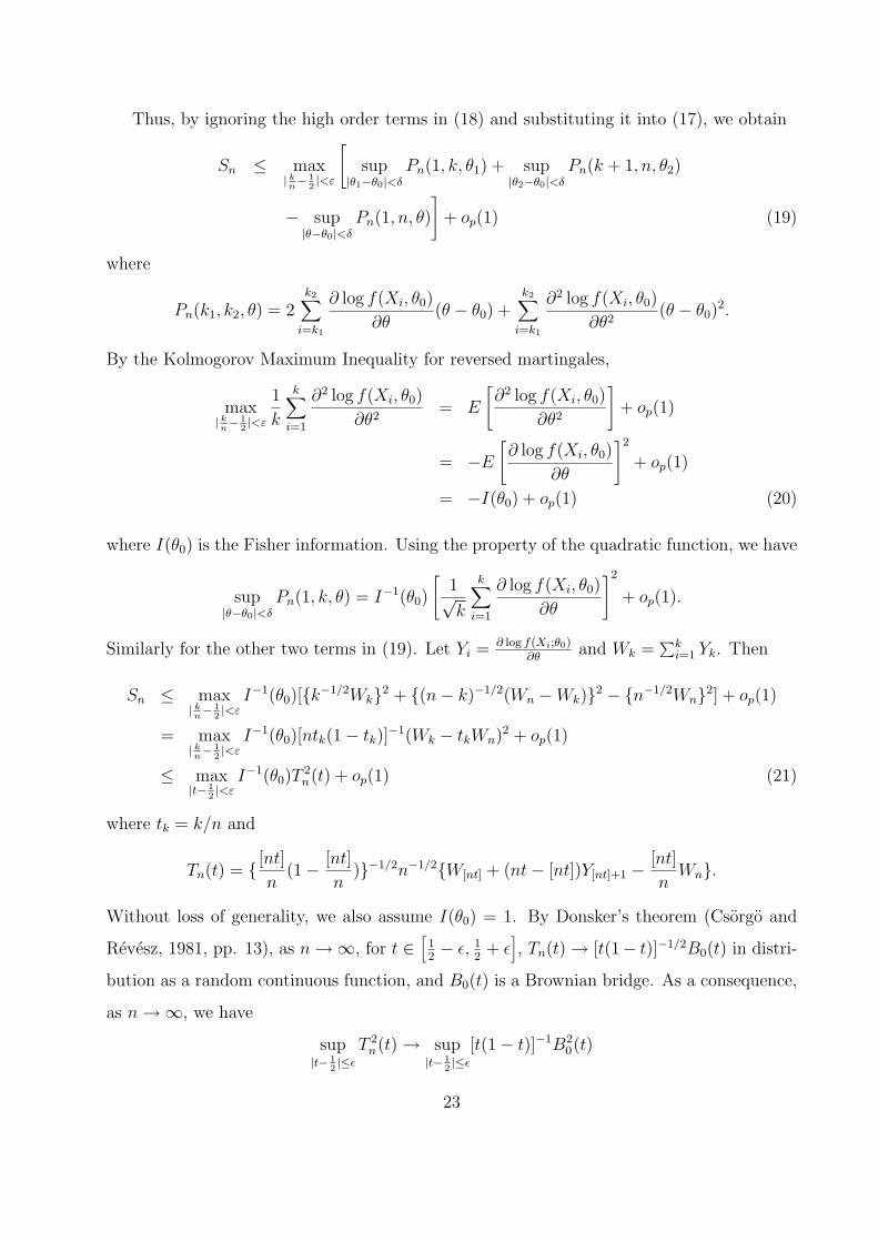
Thus, by ignoring the high order terms in (18) and substituting it into (17), we obtain

Sn ≤ max| kn− 1

2|<ε

[sup

|θ1−θ0|<δPn(1, k, θ1) + sup

|θ2−θ0|<δPn(k + 1, n, θ2)

− sup|θ−θ0|<δ

Pn(1, n, θ)

]+ op(1) (19)

where

Pn(k1, k2, θ) = 2k2∑

i=k1

∂ log f(Xi, θ0)

∂θ(θ − θ0) +

k2∑

i=k1

∂2 log f(Xi, θ0)

∂θ2(θ − θ0)

2.

By the Kolmogorov Maximum Inequality for reversed martingales,

max| kn− 1

2|<ε

1

k

k∑

i=1

∂2 log f(Xi, θ0)

∂θ2= E

[∂2 log f(Xi, θ0)

∂θ2

]+ op(1)

= −E

[∂ log f(Xi, θ0)

∂θ

]2

+ op(1)

= −I(θ0) + op(1) (20)

where I(θ0) is the Fisher information. Using the property of the quadratic function, we have

sup|θ−θ0|<δ

Pn(1, k, θ) = I−1(θ0)

[1√k

k∑

i=1

∂ log f(Xi, θ0)

∂θ

]2

+ op(1).

Similarly for the other two terms in (19). Let Yi = ∂ log f(Xi;θ0)∂θ

and Wk =∑k

i=1 Yk. Then

Sn ≤ max| kn− 1

2|<ε

I−1(θ0)[{k−1/2Wk}2 + {(n− k)−1/2(Wn −Wk)}2 − {n−1/2Wn}2] + op(1)

= max| kn− 1

2|<ε

I−1(θ0)[ntk(1− tk)]−1(Wk − tkWn)2 + op(1)

≤ max|t− 1

2|<ε

I−1(θ0)T2n(t) + op(1) (21)

where tk = k/n and

Tn(t) = { [nt]

n(1− [nt]

n)}−1/2n−1/2{W[nt] + (nt− [nt])Y[nt]+1 − [nt]

nWn}.

Without loss of generality, we also assume I(θ0) = 1. By Donsker’s theorem (Csorgo and

Revesz, 1981, pp. 13), as n →∞, for t ∈[

12− ε, 1

2+ ε

], Tn(t) → [t(1− t)]−1/2B0(t) in distri-

bution as a random continuous function, and B0(t) is a Brownian bridge. As a consequence,

as n →∞, we have

sup|t− 1

2|≤ε

T 2n(t) → sup

|t− 12|≤ε

[t(1− t)]−1B20(t)

23

in distribution.

Consequently, from (21) we have shown that

Sn ≤ sup|t− 1

2|<ε

T 2n(t) + op(1) → sup

|t− 12|<ε

[t(1− t)]−1B20(t). (22)

As ε → 0, the P. Levy modulus of continuity of the Wiener process implies,

sup|t− 1

2|≤ε

|B0(t)−B0(1

2)| → 0

almost surely. Since ε > 0 can be chosen arbitrarily small, and

[1

2

(1− 1

2

)]−1

B20(

1

2) ∼ χ2

1,

(22) implies

limn→∞

P{Sn ≤ s} ≥ P{χ21 ≤ s}

for all s > 0. It is straightforward to show that Sn ≥ MIC(n)−MIC(n/2)+d log(n) → χ21.

Thus,

limn→∞P{Sn ≤ s} ≤ P{χ2

1 ≤ s}.

Hence, Sn → χ21 in distribution as n →∞.

Consider the situation when θ has dimension d ≥ 2. The current proof is valid up to

(18). All we need after this point is to introduce vector notation. The subsequent order

comparison remains the same as the Fisher Information is positive definite by the regularity

conditions. This strategy also works for (21). Note that Yk is now a vector. Reparameterizing

the model so that the Fisher information is an identity matrix under the null hypothesis, and

consequently the components of Yk are un-correlated. We remark here that the test statistic

remains unchanged as the likelihood method is invariant to re-parameterization. The term

I−1(θ0)T2n(t) in (21) becomes T 2

n1(t) + T 2n2(t) + · · ·+ T 2

nd(t).

Note that that finite dimensional distribution of Tn1(t), Tn2(t), · · · , Tnd(t) converge to

that of independent Brownian motions B1(t), B2(t), . . . , Bd(t). By Condition R3 and the

inequality in Chow and Teicher (1978, pp 357), it is easy to verify

d∑

j=1

E|Tnj(s)− Tnj(t)|3 ≤ C|s− t|3/2

24

for some constant C. Thus, Tn1(t), Tn2(t), · · · , Tnd(t) is tight. In conclusion, the multidimen-

sional process Tn1(t), Tn2(t), · · · , Tnd(t) with continuous sample path (after some harmless

smoothing) converges to B1(t), B2(t), . . . , Bd(t) in distribution according to Revuz and Yor

(1999, pp 448-449). Hence, we have Sn → χ2d in distribution as n → ∞. This proves the

conclusion of Theorem 1 for the null hypothesis.

To prove the conclusion of Theorem 1 under the alternative hypothesis, note that

Sn ≥ MIC(n)−MIC(τ) + dim(θ) log n

≥ 2[`n(θ10, θ20, τ)− `n(θ, θ, n)] + O(log n)

where τ is the change point and θ10 and θ20 be true values of the parameters. Hence |θ10 −θ20| > 0. It is well known (Serfling, 1980)

2 supθ

τ∑

i=1

log{f(Xi, θ)/f(Xi, θ10)} → χ2d (23)

in distribution when τ →∞. Also, by Wald (1949),

infθ:|θ−θ10|≥δ

τ∑

i=1

log{f(Xi, θ10)/f(Xi, θ)} ≥ C1τ + op(τ) (24)

for any δ > 0 with some positive constant C1. Similarly for the sum from τ + 1 to n.

Let δ = |θ10−θ20|/3. Divide the parameter space into three regions: A1 = {θ : |θ−θ10| ≤δ}, A2 = {θ : |θ − θ20| ≤ δ}, and A3 be the complement of A1 ∪ A2. We have

infθ∈Aj

[`n(θ10, θ20, τ)− `n(θ, θ, n)] ≥ C2 min{τ, n− τ}

for j = 1, 2, 3 with some positive constant C2. For example, when j = 1, (24) implies part

of `n is larger than C1τ , and (23) implies the other part is of order 1. Hence, when both τ

and n− τ go to infinity at a rate faster than log n, MIC(n)−MIC(τ) + dim(θ) log n go to

infinity. This completes the proof.

Remark: Even though {Xin, 1 ≤ i ≤ τ, n ≥ 2} under the alternative model becomes a

triangle array with two sets of iid random variables, classical weak convergence results for a

single sequence of iid random variables such as in Serfling (1980) and Wald (1949) can be

applied to each set for the reasons discussed earlier.

Proof of Theorem 2: The proof will be done in two steps.

25

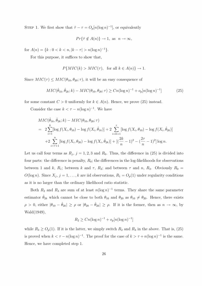
Step 1. We first show that τ − τ = Op[n(log n)−1], or equivalently

Pr{τ /∈ A(n)} → 1, as n →∞,

for A(n) = {k : 0 < k < n, |k − τ | > n(log n)−1}.For this purpose, it suffices to show that,

P{MIC(k) > MIC(τ), for all k ∈ A(n)} → 1.

Since MIC(τ) ≤ MIC(θ10, θ20; τ), it will be an easy consequence of

MIC(θ1k, θ2k; k)−MIC(θ10, θ20; τ) ≥ Cn(log n)−1 + op[n(log n)−1] (25)

for some constant C > 0 uniformly for k ∈ A(n). Hence, we prove (25) instead.

Consider the case k < τ − n(log n)−1. We have

MIC(θ1k, θ2k; k)−MIC(θ10, θ20; τ)

= 2k∑

i=1

[log f(Xi, θ10)− log f(Xi, θ1k)] + 2τ∑

i=k+1

[log f(Xi, θ10)− log f(Xi, θ2k)]

+2n∑

i=τ+1

[log f(Xi, θ20)− log f(Xi, θ2k)] + [(2k

n− 1)2 − (

2τ

n− 1)2] log n.

Let us call four terms as Rj, j = 1, 2, 3 and R0. Thus, the difference in (25) is divided into

four parts: the difference in penalty, R0; the differences in the log-likelihoods for observations

between 1 and k, R1; between k and τ , R2; and between τ and n, R3. Obviously R0 =

O(log n). Since Xj, j = 1, . . . , k are iid observations, R1 = Op(1) under regularity conditions

as it is no larger than the ordinary likelihood ratio statistic.

Both R2 and R3 are sum of at least n(log n)−1 terms. They share the same parameter

estimator θ2k which cannot be close to both θ10 and θ20 as θ10 6= θ20. Hence, there exists

ρ > 0, either |θ10 − θ2k| ≥ ρ or |θ20 − θ2k| ≥ ρ. If it is the former, then as n → ∞, by

Wald(1949),

R2 ≥ Cn(log n)−1 + op[n(log n)−1]

while R3 ≥ Op(1). If it is the latter, we simply switch R2 and R3 in the above. That is, (25)

is proved when k < τ − n(log n)−1. The proof for the case of k > τ + n(log n)−1 is the same.

Hence, we have completed step 1.

26

Step 2. We show τ − τ = Op(1).

According to Step 1, the convergence rate of τ is at least Op[n(log n)−1]. We need only

tighten this rate to obtain the result of the theorem. For this purpose, it suffices to show

MIC(θ1k, θ2k; k) > MIC(θ10, θ20; τ)

with probability tending to 1 uniformly for τ − n(log n)−1 ≤ k ≤ τ −M , and for τ + M ≤k ≤ τ + n(log n)−1. We only give the proof for the first case.

We use the same strategy as in Step 1. Due to the narrower range of k under consideration,

we have R0 = O(1) in the current case. Since Xj, j = 1, . . . , k are iid observations, R1 =

Op(1) under regularity conditions as it is no larger than the ordinary likelihood ratio statistic.

Similarly, R3 = Op(1).

The focus is now on R2. We intend to show that R2 > CM + M · op(1) for some

constant C > 0 uniformly in the range of consideration. If so, we could choose large enough

M and claim that the probability of MIC(θ1k, θ2k; k) > MIC(θ10, θ20; τ) in the range of

consideration is larger than 1− ε for any pre-given ε > 0.

By Lemma 1 since |k−τ | < n(log n)−1, θ2k → θ20 6= θ10. Thus, we may assume that it falls

outside a small neighborhood of θ10. According to Wald(1949), this implies, as τ − k ≥ M ,

R2 =τ∑

i=k+1

[log f(Xi; θ10)− log f(Xi; θ2k)] ≥ CM

for some C > 0 in probability as M →∞. Consequently, the theorem is proved.

Proof of Theorem 3: It suffices to show that for any given M > 0,

MIC(τ + k)−MIC(τ) → Wk (26)

in probability uniformly for all k such that |k| ≤ M .

Keep in mind that M is finite, for −M ≤ k ≤ 0,

MIC(τ + k)−MIC(τ)

= 2τ∑

i=1

log f(Xi, θ1τ ) + 2n∑

i=τ+1

log f(Xi, θ2τ )− 2τ+k∑

i=1

log f(Xi, θ1(τ+k))

−2n∑

i=τ+k+1

log f(Xi, θ2(τ+k)) + [(2(τ + k)

n− 1)2 − (

2τ

n− 1)2] log n

27

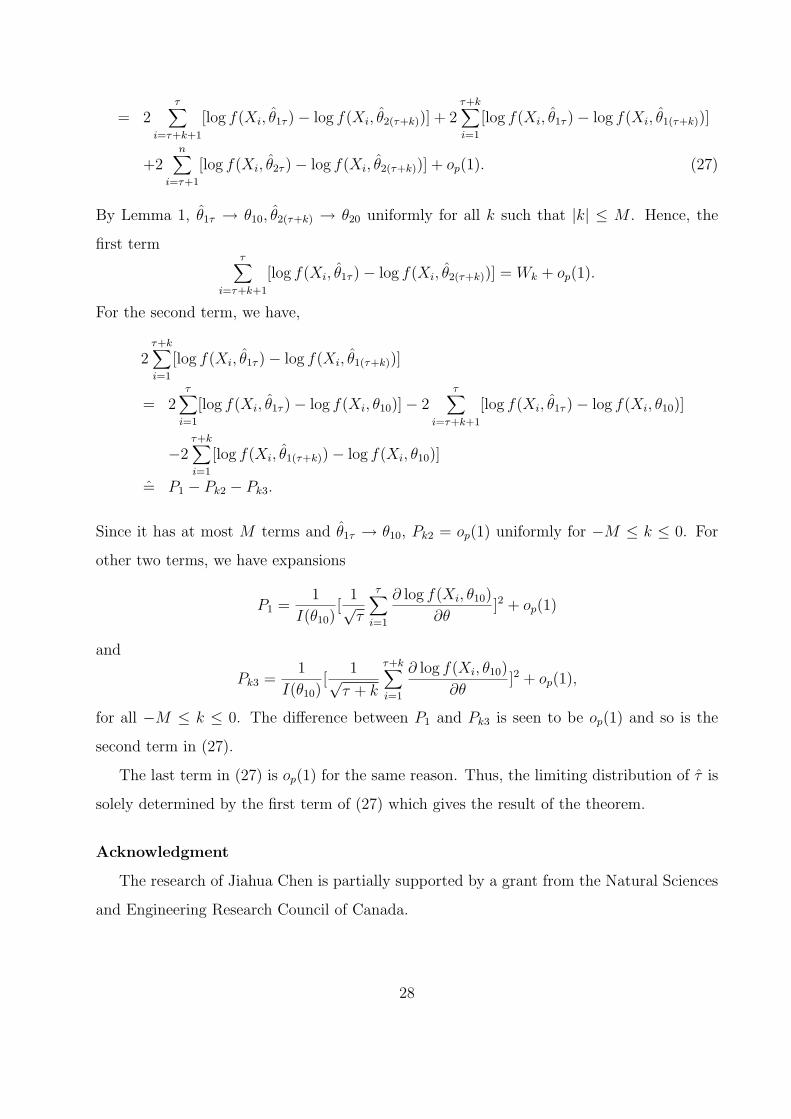
= 2τ∑

i=τ+k+1

[log f(Xi, θ1τ )− log f(Xi, θ2(τ+k))] + 2τ+k∑

i=1

[log f(Xi, θ1τ )− log f(Xi, θ1(τ+k))]

+2n∑

i=τ+1

[log f(Xi, θ2τ )− log f(Xi, θ2(τ+k))] + op(1). (27)

By Lemma 1, θ1τ → θ10, θ2(τ+k) → θ20 uniformly for all k such that |k| ≤ M . Hence, the

first termτ∑

i=τ+k+1

[log f(Xi, θ1τ )− log f(Xi, θ2(τ+k))] = Wk + op(1).

For the second term, we have,

2τ+k∑

i=1

[log f(Xi, θ1τ )− log f(Xi, θ1(τ+k))]

= 2τ∑

i=1

[log f(Xi, θ1τ )− log f(Xi, θ10)]− 2τ∑

i=τ+k+1

[log f(Xi, θ1τ )− log f(Xi, θ10)]

−2τ+k∑

i=1

[log f(Xi, θ1(τ+k))− log f(Xi, θ10)]

= P1 − Pk2 − Pk3.

Since it has at most M terms and θ1τ → θ10, Pk2 = op(1) uniformly for −M ≤ k ≤ 0. For

other two terms, we have expansions

P1 =1

I(θ10)[

1√τ

τ∑

i=1

∂ log f(Xi, θ10)

∂θ]2 + op(1)

and

Pk3 =1

I(θ10)[

1√τ + k

τ+k∑

i=1

∂ log f(Xi, θ10)

∂θ]2 + op(1),

for all −M ≤ k ≤ 0. The difference between P1 and Pk3 is seen to be op(1) and so is the

second term in (27).

The last term in (27) is op(1) for the same reason. Thus, the limiting distribution of τ is

solely determined by the first term of (27) which gives the result of the theorem.

Acknowledgment

The research of Jiahua Chen is partially supported by a grant from the Natural Sciences

and Engineering Research Council of Canada.

28

References

Akaike, H. (1973). Information Theory and an Extension of the Maximum Likelihood Prin-ciple, 2nd Int. Symp. Inf. Theory (B. N. Petrov and E. Csaki, Eds.). Budapest:Akademiai Kiado, 267-281.

Basseville, M. and Nikiforov, I. V. (1993). Detection of Abrupt Changes: Theory andApplication, PTR Prentice-Hall.

Bhattacharya, P. K. (1994). Some Aspects of Change-Point Analysis, In Change-PointProblems, 23, 28-56.

Brodsky, B. E. and Darkhovsky, B. S. (1993). Nonparametric Methods in Change-PointProblems. Kluwer Academic Publishers, The Netherlands.

Chen, Jie and Gupta, A. K. (1997). Testing and locating variance change points withapplication to stock prices, J. Amer. Statist. Assoc., 92, 739-747.

Chernoff, H. and Zacks, S. (1964). Estimating the current mean of a normal distributionwhich is subjected to change in time, Ann. Math. Statist., 35, 999-1018.

Chow, Y. and Teicher, H. (1978). Probability theory, independence, interchangeability, Mar-tingales. New York: Springer-Verily.

Csorgo, M. and Horvath, L. (1997). Limit Theorems in Change-Point Analysis. John Wiley& Sons, New York.

Csorgo, M. and Revesz, P. (1981). Strong approximations in probability and statistics. Aca-demic Press, New York.

Darling, D. A. and Erdos, P. (1956). A limit theorem for the maximum of normalized sumsof independent random variables, Duke Math. J. 23 143-155.

Gombay, E. and Horvath, L. (1996). On the rate of approximations for maximum likelihoodtests in change-point models, J. Multi. Analy. 56 120-152.

Gombay, E. and Horvath, L. (1995). An application of U-statistics to change-point analysisActa. Sci. Math. 60 345-357.

Gombay, E. and Huskova, M. (1998). Rank based estimators of the change-point, J. Statist.Plann. Inf. 67 137-154.

Hinkley, D. V. (1970). Inference about the change point in a sequence of random variables,Biometrika, 57, 1-7.

Hinkley, D. V., Chapman, P., and Rungel, G. (1980). Changepoint problems, TechnicalReport 382. University of Minnesota, Minneapolis, MN.

Hirotsu, C., Kuriki, S., and Hayter, A. J. (1992). Multiple comparison procedures basedon the maximal component of the cumulative chi-squared statistic, Biometrika, 79,381-392.

Inclan, C., and Tiao, G. C. (1994), Use of sums of squares for retrospective detection ofchanges of variance, J. Amer. Statist. Assoc., 89, 913-923.

Lai, T. L. (1995). Sequential Changepoint detection in Quality Control and DynamicalSystems, J. R. Statist. Soc. B., 57, 613-658.

Lombard, F. (1987). Rank tests for change point problems, Biometrika, 74, 615-624.

29

Page, E. S. (1954). Continuous Inspection Schemes, Biometrika, bf 41, 100-115.

Page, E. S. (1955). A test for a change in a parameter occurring at an unknown point,Biometrika, bf 42, 523-527.

Page, E. S. (1957). On problems in which a change in a parameter occurs at an unknownpoint, Biometrika, bf 44, 248-252.

Revuz, D. and Yor, M. (1999). Continuous Martingales and Brownian Motion. SecondEdition. Springer-Verlag. New York.

Schwarz, G. (1978). Estimating the dimension of a model, Ann. Statist., 6, 461-464.

Sen, P. K. and , Singer, J. M. (1993). Large Sample Methods in Statistics: An Introductionwith Applications. Chapman & Hall, New York.

Serfling, R. J. (1980). Approximation Theorems of Mathematical Statistics. John Wiley &Sons, New York.

Serfling, R. J. (1980). Approximation Theorems of Mathematical Statistics. John Wiley &Sons, New York.

Shorack, G. R. and Wellner (1986). Empirical Processes with Applications to Statistics. JohnWiley & Sons, New York.

Wald, A. (1949). Note on the consistency of the maximum likelihood estimate, Ann. Math.Statist., 20, 595-601.

Worsley, K. J. (1979). On the likelihood ratio test for a shift in location of normal popula-tions, J. Amer. Statist. Assoc., 74, 365-367.

Worsley, K. J. (1986). Confidence regions and tests for a change point in a sequence ofexponential family random variables, Biometrika, 73, 91-104.

Wu, W. B,, Woodroofe, M., and Mentz, G. (2001), Isotonic regression: Another look at thechangepoint problem, Biometrika, 88(3), 793-804.

Zacks, S. (1983). Survey of classical and bayesian approaches to the change-point problem:Fixed sample and sequential procedures in testing and estimation, In Recent Advancesin Statistics, Academic Press, 245-269.

30