information retrieval to recommender systems

From Information Retrievalto Recommender Systems

Maria Mateva

Sofia UniversityFaculty of Mathematics and Informatics

Data Science SocietyFebruary 25, 2015

whoami

Maria Mateva:

I BSc of FMI, “Computer Science”

I MSc of FMI, “Artificial Intelligence”

I 2.5 years software developer in Ontotext

I 1 year software developer in Experian

I 3 semesters - teaching assistant in “Informarion Retrieval”

I now joining Data Science Society

http://www.ontotext.com/

http://www.experian.com/

http://www.datasciencesociety.net/

Acknowledgements

This lecture is a mixture from knowledge I gained as a teachingassistant in Information Retrieval in FMI, Sofia University and fromknowledge I gained during research in Ontotext.Special thanks to:

I FMI - in general, always

I Doc. Ivan Koychev for letting me be part of his teamI Ontotext, especially

I PhD Konstantin Kutzkov for our work on recommendationsI PhD Laura Tolosi for her guidance

I Prof. Christopher Manning of Stanford for opening“Introduction to Information Retrieval” for all of us

I Jure Leskovec, Anand Rajaraman, Jeff Ullman for “MiningMassive Datasets” book and course

Today we discuss...

Introduction

Information Retrieval Basics

Introduction to Recommender Systems

A Common Solution to a Common Problem

Q and A

What is Information Retrieval?

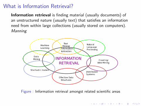
Information retrieval is finding material (usually documents) ofan unstructured nature (usually text) that satisfies an informationneed from within large collections (usually stored on computers).Manning

Figure : Information retrieval amongst related scientific areas

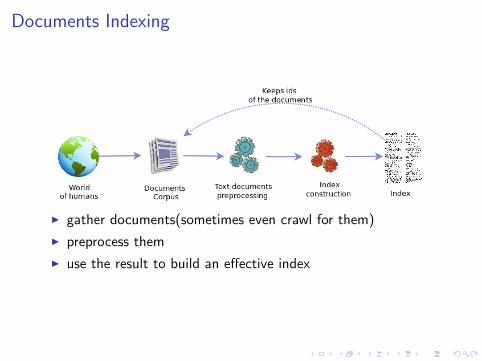
Documents Indexing

I gather documents(sometimes even crawl for them)

I preprocess them

I use the result to build an effective index

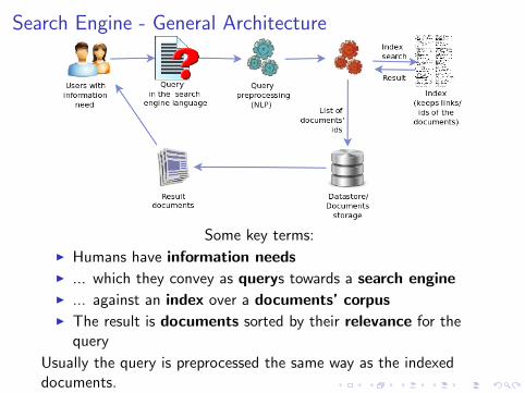
Search Engine - General Architecture

Some key terms:

I Humans have information needsI ... which they convey as querys towards a search engineI ... against an index over a documents’ corpusI The result is documents sorted by their relevance for the

query

Usually the query is preprocessed the same way as the indexeddocuments.

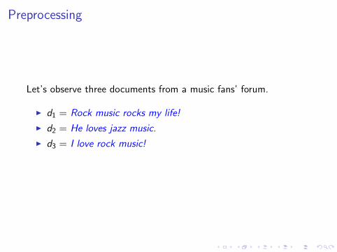
Preprocessing

Let’s observe three documents from a music fans’ forum.

I d1 = Rock music rocks my life!

I d2 = He loves jazz music.

I d3 = I love rock music!

Preprocessing

After some language NLP-processing, we get:

I d1 = Rock music rocks my life! → { life, music, rock ×2 }I d2 = He loves jazz music. → { jazz, love, music }I d3 = I love rock music! → { love, music, rock }

Preprocessing

After some language NLP-processing, we get:


Here we have most probably applied language-dependent:

I tokenizer

I stopwords

I lemmatizer

I etc.

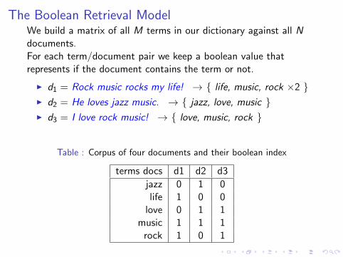
The Boolean Retrieval ModelWe build a matrix of all M terms in our dictionary against all Ndocuments.For each term/document pair we keep a boolean value thatrepresents if the document contains the term or not.


Table : Corpus of four documents and their boolean index

terms docs d1 d2 d3

jazz 0 1 0life 1 0 0

love 0 1 1music 1 1 1

rock 1 0 1

The Boolean Retrieval Model

A query, q=“love”




Table : Corpus of three documents and its inverted index

terms docs d1 d2 d3 q

jazz 0 1 0 0life 1 0 0 0

love 0 1 1 1music 1 1 1 0

rock 1 0 0 0

Advantages: high recall, fastProblem: retrieved documents are not rakned

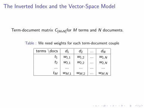
The Inverted Index and the Vector-Space Model

Term-document matrix C[MxN]for M terms and N documents.

Table : We need weights for each term-document couple

terms \docs d1 d2 ... dN

t1 w1,1 w1,2 ... w1,N

t2 w2,1 w2,2 ... w2,N

... ... ... ... ...tM wM,1 wM,2 ... wM,N

TF-IDF

We need a metric for how specific each term for each document is.Term frequency - inverted document frequency very wellserves the purpose.

TF − IDFt,doc = TFt,doc × IDFt

TF − IDFt,doc = tft,doc × logN

dft

wheretft,doc - number of occurrences of t in doc

dft - number of documents in the corpus, which contains tN - total number of documents in the corpus

TF-IDF Example: The Scores




Table : Corpus of three documents and its inverted index

terms d1 d2 d3

jazz TF − IDF(jazz,d1) TF − IDF(jazz,d2) TF − IDF(jazz,d3)

life TF − IDF(life,d1) TF − IDF(life,d2) TF − IDF(life,d3)

love TF − IDF(love,d1) TF − IDF(love,d2) TF − IDF(love,d3)

music TF − IDF(music,d1) TF − IDF(music,d2) TF − IDF(music,d3)

rock TF − IDF(rock,d1) TF − IDF(rock,d2) TF − IDF(rock,d3)

TF-IDF The Scores




Table : TF-IDF score of the documents

terms \docs d1 d2 d3

jazz 0.0 0.477 0.0life 0.477 0.0 0.0

love 0.0 0.176 0.176music 0.0 0.0 0.0

rock 0.352 0.0 0.176

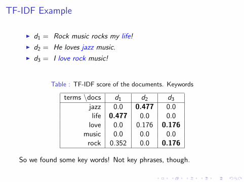
TF-IDF Example




Table : TF-IDF score of the documents. Keywords


jazz 0.0 0.477 0.0life 0.477 0.0 0.0

love 0.0 0.176 0.176music 0.0 0.0 0.0

rock 0.352 0.0 0.176

So we found some key words! Not key phrases, though.

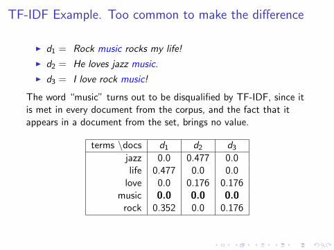
TF-IDF Example. Too common to make the difference




The word “music” turns out to be disqualified by TF-IDF, since itis met in every document from the corpus, and the fact that itappears in a document from the set, brings no value.


jazz 0.0 0.477 0.0life 0.477 0.0 0.0

love 0.0 0.176 0.176music 0.0 0.0 0.0

rock 0.352 0.0 0.176

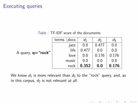
Executing queries


A query, q=“rock”


jazz 0.0 0.477 0.0life 0.477 0.0 0.0

love 0.0 0.176 0.176music 0.0 0.0 0.0

rock 0.352 0.0 0.176

We know d1 is more relevant than d3 to the “rock” query, and, asin this corpus, d2 is not relevant at all.

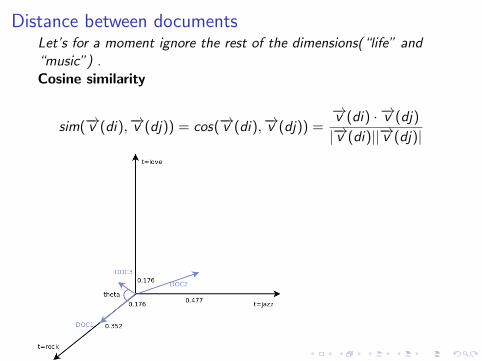
Distance between documentsLet’s for a moment ignore the rest of the dimensions(“life” and“music”) .Cosine similarity

sim(−→v (di),−→v (dj)) = cos(−→v (di),−→v (dj)) =−→v (di) · −→v (dj)

|−→v (di)||−→v (dj)|

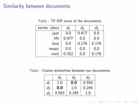
Similarity between documents



jazz 0.0 0.477 0.0life 0.477 0.0 0.0

love 0.0 0.176 0.176music 0.0 0.0 0.0

rock 0.352 0.0 0.176

Table : Cosine similarities between our documents

d1 d2 d3

d1 1.0 0.0 0.593d2 0.0 1.0 0.245d3 0.593 0.245 1.0

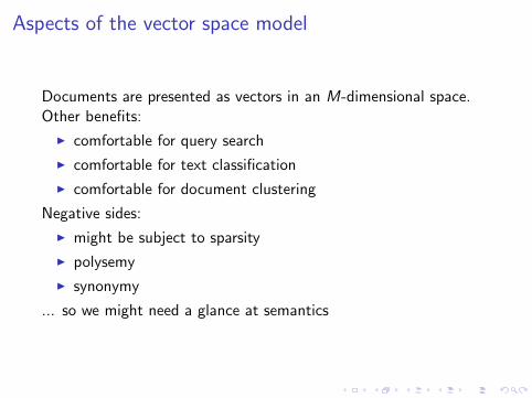
Aspects of the vector space model

Documents are presented as vectors in an M-dimensional space.Other benefits:

I comfortable for query search

I comfortable for text classification

I comfortable for document clustering

Negative sides:

I might be subject to sparsity

I polysemy

I synonymy

... so we might need a glance at semantics

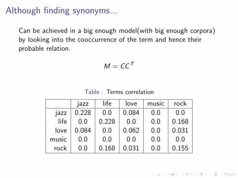
Although finding synonyms...

Can be achieved in a big enough model(with big enough corpora)by looking into the cooccurrence of the term and hence theirprobable relation.

M = CCT

Table : Terms correlation

jazz life love music rock

jazz 0.228 0.0 0.084 0.0 0.0life 0.0 0.228 0.0 0.0 0.168

love 0.084 0.0 0.062 0.0 0.031music 0.0 0.0 0.0 0.0 0.0

rock 0.0 0.168 0.031 0.0 0.155

Related Software

I Apache Lucene

I Apache Solr

I ElasticSearch

I Apache Nutch

What are Recommender Systems?

Software systems that suggests to users items of interest byanticipating their rating/likeness/relevance to the items. The lattermight be for example:

I friends to follow

I products to buy

I music videos to watch online

I new books to read

I etc, etc, etc

Let’s see some examples.

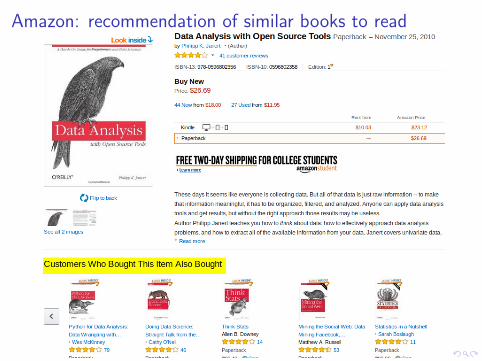
Amazon: recommendation of similar books to read

YouTube: personalized videos recommendation

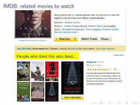
IMDB: related movies to watch

Types of recommender systems

Recommender system approaches

I Collaborative filtering

I Content-based approach

I Hybrid approaches

Collaborative filtering

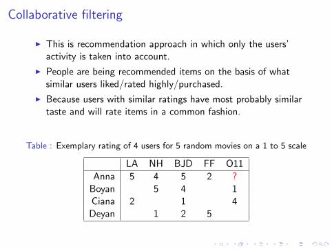
I This is recommendation approach in which only the users’activity is taken into account.

I People are being recommended items on the basis of whatsimilar users liked/rated highly/purchased.

I Because users with similar ratings have most probably similartaste and will rate items in a common fashion.

Table : Exemplary rating of 4 users for 5 random movies on a 1 to 5 scale

LA NH BJD FF O11

Anna 5 4 5 2 ?Boyan 5 4 1Ciana 2 1 4

Deyan 1 2 5

Centered user ratingsSubtract from each user’s ratings the average of his/her rating.

Table : Initial ratings

LA NH BJD FF O11

Anna 5 4 5 2Boyan 5 4 1Ciana 2 1 4

Deyan 1 2 5

Table : Centered ratings. The sum at each row is 0.

LA NH BJD FF O11

Anna 1 0 1 -2 0Boyan 0 5

323 0 - 7

3Ciana −1

3 0 −43 0 5

3Deyan 0 −5

3 −23 0 7

3

Centered cosine similarity/Pearson Correlation

Applied to find similar users for user-to-user collaborative filtering.

Table : Initial ratings

LA NH BJD FF O11

Anna 1 0 1 -2 0Boyan 0 5

323 0 - 7

3Ciana −1

3 0 −43 0 5

3Deyan 0 −5

3 −23 0 7

3

sim(−→v (“Anna′′),−→v (“Boyan′′) = cos(−→v (“Anna′′),−→v (“Boyan′′) = 0.092

sim(−→v (“Anna′′),−→v (“Ciana′′) = cos(−→v (“Anna′′),−→v (“Ciana′′) = −0.315

sim(−→v (“Anna′′),−→v (“Deyan′′) = cos(−→v (“Anna′′),−→v (“Deyan′′) = −0.092

sim(−→v (“Boyan′′),−→v (“Deyan′′) = cos(−→v (“Boyan′′),−→v (“Deyan′′) = −1.0

Collaborative filtering. User-to-User Approach

Take the most similar users to user X and predict X’s taste on the base of theirratings. The rating of user i for movie j , where SU(i) are user i ’s most closest user isthen given by:

rij =

∑m∈SU(i) sim(m, j) ∗ rmj∑

m∈SU(i) sim(m, j)

Example:SU(Anna) = {Boyan}

rBoyan,O11 = −7

3

Our prediction for

rAnna,O11 =0.092 ∗ (− 7

3)

0.092= −

7

3

RAnna,O11 = avg(RAnna,j ) + rAnna,O11 = 4−7

3= 1.67

I For each user we need to first screen out the best similar users, then rate eachelement separately

I Then we suggest the items with highest predicted ratings to the user

Collaborative filtering. Item-to-Item Approach

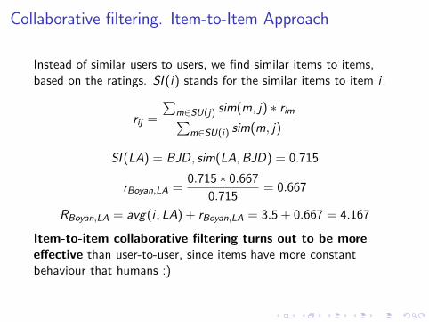
Instead of similar users to users, we find similar items to items,based on the ratings. SI (i) stands for the similar items to item i .

rij =

∑m∈SU(j) sim(m, j) ∗ rim∑

m∈SU(i) sim(m, j)

SI (LA) = BJD, sim(LA,BJD) = 0.715

rBoyan,LA =0.715 ∗ 0.667

0.715= 0.667

RBoyan,LA = avg(i , LA) + rBoyan,LA = 3.5 + 0.667 = 4.167

Item-to-item collaborative filtering turns out to be moreeffective than user-to-user, since items have more constantbehaviour that humans :)

Collaborative filtering. Results

Table : Our new results

LA NH BJD FF O11

Anna 5 4 5 2 1.67Boyan 4.167 5 4 1Ciana 2 1 4

Deyan 1 2 5

The “Cold start” problem

I New user. We have no information about a new user, hencewe cannot find similar users and recommend based on theiractivity

I workaround: offer the newest or highest ranking items ro thisuser

I New item. We have no information about new item and hencecannot relate it to other(rated) item

I workaround: the newest items for at least several times arerecommended to the most active users

Content-based approach

I Items’ content is observed. No cold start for new item :) Stillhave the cold start on new user, though.

I Users are generated a profile on the basis of the contentof the items they liked

I This profile can be represented by a vector of weights in thecontent representation space

I Then, the user’s profile can be examined for proximity toitems in this space

I Back to the vector-space model and the documents space...The user profile can be viewed as a dynamic document!

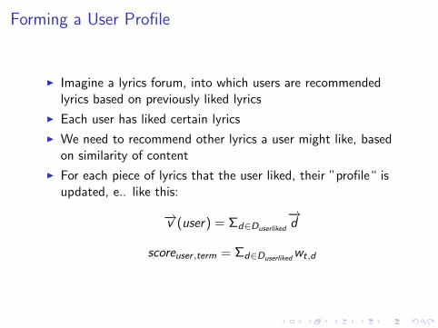
Forming a User Profile

I Imagine a lyrics forum, into which users are recommendedlyrics based on previously liked lyrics

I Each user has liked certain lyrics

I We need to recommend other lyrics a user might like, basedon similarity of content

I For each piece of lyrics that the user liked, their ”profile“ isupdated, e.. like this:

−→v (user) = Σd∈Duserliked

−→d

scoreuser ,term = Σd∈Duserlikedwt,d

Users become documents!

Table : TF-IDF score of the documents/user profiles

terms \docs d1 d2 d3 ... Anna Boyan... ... ... ... ... ... ...

jazz 0.0 0.477 0.0 ... 0.073 0.0life 0.477 0.0 0.0 ... 0.211 0.023

love 0.0 0.176 0.176 ... 0.812 0.345music 0.0 0.0 0.0 ... 0.0 0.0

rock 0.352 0.0 0.176 ... 0.001 0.654... ... ... ... ... ... ...

We can add document classes, extracted topics, extracted namedentities, locations, etc. to the model. Also, e.g. actors or directorsfor IMDB, musicians or vlogger for YouTube, and so forth.Anything that is related to the user and is found in thedocuments(or their metadata).

Some time-related insights

I Use time decay factorI some user interests or inclinations are temporaryI e.g. ”curling“ during the Winter Olympics or ”wedding“

around a person’s weddingI so it is nice idea to periodically decrease the score of a user’s

topics, so that the old-favourite topics declineI hint: don’t actualize data for non-active users

I Use only active usersI it might be good idea to (temporarily) reduce the data size by

ignoring ancient users

The problem with dimensionality and sparsity

Imagine...

I N = 10,000,000 users

I 200, 000 items

I in a vector-space of M = 1,000,000 terms

I how do we use our sparse matrix C[NxM]?

The problem with dimensionality and sparsity

Imagine...

I N = 10,000,000 users

I 200, 000 items

I in a vector-space of M = 1,000,000 terms

I how do we use our sparse matrix C[NxM]?

I OMG!!! This is big data!!!

I ;)

Latent Semantic Indexing

a.k.a Latent Semantic Analysis to te rescue.We use SVD as a low-rank approximation of the orginal space. Wereduce both memory needed and noise. Also, we find semanticnotions in the data.

Singular Value Decomposition

Theorem. (Manning) Let r be the rank of the M x M matrix C.Then, there is a singular value decomposition(SVD) of C of theform:

C = UΣV T

where

I The eigenvalues λ1, ..., λr of CCT are the same as theeigenvalues of CTC

I For 1 ≤ i ≤ r , letσi =√λi , with λi ≥ λi+1. Then the M x N

matrix Σ is composed by setting Σii = σi for 1 ≤ i ≤ r , andzero otherwise.

I σi are called singular values of C

I the columns of U - left-singular vectors of C

I the columns of V - right-singular vectors of C

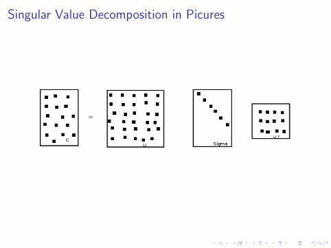
Singular Value Decomposition in Picures

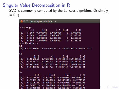
Singular Value Decomposition in RSVD is commonly computed by the Lanczos algorithm. Or simplyin R :)

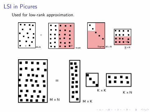
LSI in Picures

Used for low-rank approximation.

LSI in Recommedations

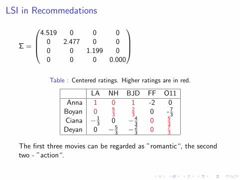
Σ =

4.519 0 0 0

0 2.477 0 00 0 1.199 00 0 0 0.000

Table : Centered ratings. Higher ratings are in red.

LA NH BJD FF O11

Anna 1 0 1 -2 0Boyan 0 5

323 0 - 7

3Ciana −1

3 0 −43 0 5

3Deyan 0 −5

3 −23 0 7

3

The first three movies can be regarded as ”romantic“, the secondtwo - ”action“.

LSI in IR

I the query is adapted to use the low-rank approximation

I noise is cleared and the model is improved

I synonyms and better handles

I other values are still subject of investigation

Discussion time!

QUESTIONS!

Thanks

Thank You for Your Time!Now it’s beer time! :)

information retrieval to recommender systems

Data & Analytics