Information Science and StatisticsSeries Editors

M. JordanR. NowakB. Scholkopf

Information Science and Statistics

For further volumes:http://www.springer.com/series/3816

Uffe B. Kjærulff • Anders L. Madsen

Bayesian Networksand Influence Diagrams:A Guide to Constructionand Analysis

123

Second Edition

Uffe B. KjærulffDepartment of Computer ScienceAalborg UniversityAalborg, Denmark

Anders L. MadsenHUGIN EXPERT A/SAalborg, Denmark

Department of Computer ScienceAalborg UniversityAalborg, Denmark

ISSN 1613-9011ISBN 978-1-4614-5103-7 ISBN 978-1-4614-5104-4 (eBook)DOI 10.1007/978-1-4614-5104-4Springer New York Heidelberg Dordrecht London

Library of Congress Control Number: 2012945936

© Springer Science+Business Media New York 2013This work is subject to copyright. All rights are reserved by the Publisher, whether the whole or part ofthe material is concerned, specifically the rights of translation, reprinting, reuse of illustrations, recitation,broadcasting, reproduction on microfilms or in any other physical way, and transmission or informationstorage and retrieval, electronic adaptation, computer software, or by similar or dissimilar methodologynow known or hereafter developed. Exempted from this legal reservation are brief excerpts in connectionwith reviews or scholarly analysis or material supplied specifically for the purpose of being enteredand executed on a computer system, for exclusive use by the purchaser of the work. Duplication ofthis publication or parts thereof is permitted only under the provisions of the Copyright Law of thePublisher’s location, in its current version, and permission for use must always be obtained from Springer.Permissions for use may be obtained through RightsLink at the Copyright Clearance Center. Violationsare liable to prosecution under the respective Copyright Law.The use of general descriptive names, registered names, trademarks, service marks, etc. in this publicationdoes not imply, even in the absence of a specific statement, that such names are exempt from the relevantprotective laws and regulations and therefore free for general use.While the advice and information in this book are believed to be true and accurate at the date ofpublication, neither the authors nor the editors nor the publisher can accept any legal responsibility forany errors or omissions that may be made. The publisher makes no warranty, express or implied, withrespect to the material contained herein.

Printed on acid-free paper

Springer is part of Springer Science+Business Media (www.springer.com)

To our wives and children

Preface

This book is a monograph on practical aspects of probabilistic networks (a.k.a.probabilistic graphical models) and is intended to provide a comprehensive guidefor practitioners who wish to understand, construct, and analyze decision supportsystems based on probabilistic networks, including a number of different variants ofBayesian networks and influence diagrams. This book consists of three parts:

• Part I: Fundamentals of probabilistic networks, including Chaps. 1–5, coveringa brief introduction to probabilistic graphical models, the basic graph-theoreticterminology, the basic (Bayesian) probability theory, the key concepts of (con-ditional) dependence and independence, the different varieties of probabilisticnetworks, and the methods for making inference in these kinds of models. Thispart can be skipped by readers with fundamental knowledge about probabilisticnetworks.

• Part II: Model construction, including Chaps. 6–8, covering methods and tech-niques for elicitation of model structure and parameters, a large number ofuseful techniques and tricks to solve commonly recurring modeling problems,and methods for constructing probabilistic networks automatically from data,possibly through fusion of data and expert knowledge. Chapters 6 and 7 offerconcrete advice and techniques on issues related to model construction, andChap. 8 explains the theory and methods behind learning of Bayesian networksfrom data.

• Part III: Model analysis, including Chaps. 9–11, covering conflict analysis fordetecting conflicting pieces of evidence (observations) or evidence that conflictswith the model, sensitivity analysis of a model with respect to both variationsof evidence and model parameters, and value of information analysis. This partexplains the theory and methods underlying the three different kinds of analyses.

Probabilistic networks have become an increasingly popular paradigm for prob-abilistic inference, addressing such tasks as diagnosis, prediction, decision making,classification, and data mining. From its infancy in the mid-1980s till today there hasbeen a rapid development of algorithms for construction, inference, learning, andanalysis of probabilistic networks, and since the turn of the millennium there has

vii

viii Preface

been a steep increase in the number of new applications of probabilistic networks.Its popularity stems from a number of factors:

• The graphical-based language for probabilistic networks is a powerful tool forexpressing causal interactions while at the same time expressing dependence andindependence relations among entities of a problem domain. Being graphicaland compact the language furthermore provides an excellent intuitive means ofcommunicating ideas among knowledge engineers and problem-domain experts.

• Although inference in complex probabilistic networks can be quite demanding(or even intractable), inference can often be performed efficiently in models ofhundreds or even thousands of variables.

• Inference in probabilistic networks is based on a well-established theoreticalfoundation of probability calculus and decision theory and hence providesmathematically coherent methods for deriving conclusions under uncertaintywhere multiple sources of information and complex interaction patterns areinvolved.

• There exist efficient algorithms for learning and adaptation of probabilisticnetworks from data and it is possible to fuse data and expert knowledge.

• Probabilistic networks are “white boxes” in the sense that the model components(variables, links, probability and utility parameters) are open to interpretation,which makes it possible to perform a whole range of different analyses of thenetworks (e.g., conflict analysis, (in)dependence analyses, sensitivity analysis,and value of information analysis).

• There exist a number of powerful software tools that make it easy to constructand make inference in probabilistic networks.

As mentioned above, this book takes a practical point of departure and is intendedprimarily for those who wish to construct and analyze probabilistic networks with-out necessarily having a deep understanding neither of their underlying theory andmethods nor of alternative paradigms supporting belief updating under uncertainty.Hence, the scope of this book is narrow, focusing almost exclusively on issuesrelevant for understanding, constructing, and analyzing the different variants ofBayesian networks and influence diagrams. Other methods for inference and supportfor decision making under uncertainty, therefore, get limited attention.

The intended audience of this book is practitioners as well as students of artificialintelligence, however, with a primary focus on the former. The theory behindprobabilistic networks is explained to quite some depth, enabling the dedicatedpractitioner as well as the student to gain a solid theoretical understanding to alevel sufficient to further develop and implement methods for model construction,inference, and analysis. Therefore, to support this understanding, exercises havebeen included in all chapters (except Chap. 1) for the reader to check his/herlevel of understanding. Answers to selected exercises and more can be found athugin.com/developer/publications/bnid.

For a quick overview, the different kinds of probabilistic network modelsconsidered in this book can be characterized very briefly as follows:

Preface ix

• Discrete Bayesian networks represent factorizations of joint probability distribu-tions over finite sets of discrete random variables. The variables are representedby the nodes of the network, and the links of the network represent theproperties of (conditional) dependences and independences among the variables.A set of local probability distributions conditional on the configuration of theconditioning (parent) variables is specified for each variable.

• Conditional linear Gaussian (CLG) Bayesian networks represent factorizationsof joint probability distributions over finite sets of random variables where someare discrete and some continuous. Each continuous variable is assumed to followa linear Gaussian distribution conditional on the configuration of its discreteparent variables.

• Discrete influence diagrams are (discrete) Bayesian networks augmented with(discrete) decision variables and (discrete) utility functions. An influence dia-gram is capable of computing expected utilities of various decision options giventhe information known at the time of the decision.

• Conditional linear-quadratic Gaussian (CLQG) influence diagrams combineCLG Bayesian networks, discrete influence diagrams, and quadratic utilityfunctions into a single framework supporting decision making under uncertaintywith both continuous and discrete variables.

• Limited-memory influence diagrams (LIMIDs) relax two fundamental assump-tions of influence diagrams: the no-forgetting assumption implying perfect recallof past observations and decisions and the assumption of a total order on thedecisions. LIMIDs allow us to model more types of decision problems than theordinary influence diagrams.

• Object-oriented probabilistic networks are hierarchically specified probabilisticnetworks (i.e., one of the above), allowing the knowledge engineer (modelbuilder) to work on different levels of abstraction, as well as exploiting theusual concepts of encapsulation and inheritance known from object-orientedprogramming paradigms.

The book provides numerous examples, hopefully helping the reader to gain agood understanding of the various concepts, some of which are known to be hard tounderstand at a first encounter.

Even though probabilistic networks provide an intuitive language for con-structing knowledge-based models for probabilistic inference, knowledge engineerscan often benefit from a deeper understanding of the principles underlying thesemodels. For example, knowing the rules for reading statements of dependence andindependence encoded in the structure of a network may prove very valuable inevaluating whether the network correctly models the dependence and independenceproperties of the target problem. This, in turn, may be crucial to achieving, forexample, correct posterior probability distributions from the model. Also, havinga basic understanding of the relations between the structure of a network and thecomplexity of inference may prove useful in the model construction phase, avoidingstructures that are likely to result in problems of poor performance of the finaldecision support system.

x Preface

We present such basic concepts, principles, and methods underlying probabilisticmodels that practitioners need to acquaint themselves with.

In Chap. 1, we provide a bit of background and contextual introduction toBayesian networks and influence diagrams. To give the reader a first understandingof probabilistic networks, we present a very simple Bayesian network and show howit can be augmented with explicit representation of decision options and a utilityfunction, turning it into an influence diagram. Also, we discuss briefly the notionsof causality, construction of probabilistic networks, and applicability (i.e., when touse probabilistic networks).

In Chap. 2, we describe the fundamental concepts of the graphical languageused to construct probabilistic networks as well as the rules for reading statementsof (conditional) dependence and independence encoded in network structures. Wepresent two equivalent criteria for reading these statements, namely Pearl’s d-separation criterion (Pearl 1988) and the criterion of directed Markov property byLauritzen, Dawid, Larsen & Leimer (1990a).

In Chap. 3, we present the uncertainty calculus used in probabilistic networksto represent the numerical counterpart of the graphical structure, namely classical(Bayesian) probability calculus. We shall see how a basic axiom of probabilitycalculus leads to recursive factorizations of joint probability distributions intoproducts of conditional probability distributions and how such factorizations alongwith local statements of conditional independence can be expressed naturally ingraphical terms.

In Chap. 4, we see how putting the basic notions of Chaps. 2 and 3 together weget the notion of discrete Bayesian networks. Also, we present a range of derivedtypes of network models, including conditional Gaussian models where discreteand continuous variables coexist, influence diagrams that are Bayesian networksaugmented with decision variables and utility functions, limited-memory influencediagrams that allow the knowledge engineer to reduce model complexity throughassumptions about limited memory of past events, object-oriented models that allowthe knowledge engineer to construct hierarchical models consisting of reusablesubmodels, and dynamic Bayesian networks that provide a framework for modelingphenomena evolving over time.

In Chap. 5, we explain the principles underlying inference in these different kindsof probabilistic networks.

In Chap. 6, we discuss the art of constructing a probabilistic network andthe characteristics of problem domains that can be successfully modeled byprobabilistic networks. The different phases of model construction are discussed,including design (how to identify the right set of variables, how to elicit thestructure of a probabilistic network, and how to verify a network structure),implementation (elicitation of probability and utility parameters), test, and analysis(i.e., troubleshooting the model).

In Chap. 7, we present a large number of techniques and tricks for solvingcommonly occurring modeling problems in probabilistic networks. The set of tech-niques and tricks includes various structure-related techniques (parent divorcing,temporal transformation of causal relations, modeling of structural and functional

Preface xi

uncertainty, modeling of undirected dependence relations, bidirectional relations,and naive Bayes models), probability distribution-related techniques (modeling ofmeasurement error, (different) expert opinions, node absorption, value set by inter-vention, independence of causal influence, and mixture of Gaussian distributions),and decision-related techniques (modeling of test decisions, missing informationallinks, missing observations, hypothesis of highest probability, and constraints ondecisions).

In Chap. 8, we describe how probabilistic networks can be constructed automat-ically from data or from a combination of data and problem domain expertise. Theunderlying theory of structure learning is explained, and different constraint-basedlearning algorithms, search and score-based algortihms, and structure restricted al-gorithms are presented. The expectation-maximization (EM) algorithm is describedfor learning the values of probability parameters from data as well as from data andproblem domain expertise (penalized EM). Finally, we describe how the values ofthe probability parameters of a probabilistic network can be learned sequentially(adaptation).

In Chap. 9, we describe a method for performing conflict analysis in a proba-bilistic network, which aims at detecting pieces of evidence that might be in conflictwith one another (i.e., pointing in different directions with respect to output fromthe network) or in conflict with the network model. Also, the topics of tracing andresolution of conflicts are discussed.

In Chap. 10, we describe how to analyze the sensitivity of the output of aprobabilistic network (e.g., diagnosis and classification) to changes in the values ofobserved variables (evidence) as well as probability parameters. Also, we describehow parameters can be adjusted to make a probabilistic network produce requiredposterior probabilities.

Finally, in Chap. 11, we describe methods for performing value-of-informationanalysis in Bayesian networks and influence diagrams.

Compared to the first edition, this second edition of the book contains additionalmaterial: Sections 6.3.3 and 6.3.4 elaborate on model construction, Section 8.3describes search and score-based structure learning, Section 8.4 presents a workedexample on structure learning, Section 10.3 describes two-way parameter sensitivityanalysis, Section 10.4 describes parameter tuning, and an appendix provides a quickreference to model construction with lists of recommendations and pitfalls for themodel builder. Finally, lists of examples, figures, and tables have been added.

Uffe B. KjærulffAnders L. Madsen

Contents

Part I Fundamentals

1 Introduction . . . . . . . . . . . . . . . . . . . . . . . . . . . . . . . . . . . . . . . . . . . . . . . . . . . . . . . . . . . . . . . . . 31.1 Expert Systems . . . . . . . . . . . . . . . . . . . . . . . . . . . . . . . . . . . . . . . . . . . . . . . . . . . . . . . 3

1.1.1 Representation of Uncertainty . . . . . . . . . . . . . . . . . . . . . . . . . . . . . 41.1.2 Normative Expert Systems . . . . . . . . . . . . . . . . . . . . . . . . . . . . . . . . . 5

1.2 Rule-Based Systems . . . . . . . . . . . . . . . . . . . . . . . . . . . . . . . . . . . . . . . . . . . . . . . . . 51.2.1 Causality . . . . . . . . . . . . . . . . . . . . . . . . . . . . . . . . . . . . . . . . . . . . . . . . . . . . 61.2.2 Uncertainty in Rule-Based Systems . . . . . . . . . . . . . . . . . . . . . . . 71.2.3 Explaining Away . . . . . . . . . . . . . . . . . . . . . . . . . . . . . . . . . . . . . . . . . . . 8

1.3 Bayesian Networks . . . . . . . . . . . . . . . . . . . . . . . . . . . . . . . . . . . . . . . . . . . . . . . . . . . 81.3.1 Inference in Bayesian Networks . . . . . . . . . . . . . . . . . . . . . . . . . . . 91.3.2 Construction of Bayesian Networks . . . . . . . . . . . . . . . . . . . . . . . 101.3.3 An Example .. . . . . . . . . . . . . . . . . . . . . . . . . . . . . . . . . . . . . . . . . . . . . . . . 11

1.4 Bayesian Decision Problems. . . . . . . . . . . . . . . . . . . . . . . . . . . . . . . . . . . . . . . . . 131.5 When to Use Probabilistic Nets . . . . . . . . . . . . . . . . . . . . . . . . . . . . . . . . . . . . . 141.6 Concluding Remarks . . . . . . . . . . . . . . . . . . . . . . . . . . . . . . . . . . . . . . . . . . . . . . . . . 15

2 Networks . . . . . . . . . . . . . . . . . . . . . . . . . . . . . . . . . . . . . . . . . . . . . . . . . . . . . . . . . . . . . . . . . . . . . 172.1 Graphs . . . . . . . . . . . . . . . . . . . . . . . . . . . . . . . . . . . . . . . . . . . . . . . . . . . . . . . . . . . . . . . . 182.2 Graphical Models . . . . . . . . . . . . . . . . . . . . . . . . . . . . . . . . . . . . . . . . . . . . . . . . . . . . 20

2.2.1 Variables . . . . . . . . . . . . . . . . . . . . . . . . . . . . . . . . . . . . . . . . . . . . . . . . . . . . 202.2.2 Vertices Vs. Variables . . . . . . . . . . . . . . . . . . . . . . . . . . . . . . . . . . . . . . 212.2.3 Taxonomy of Vertices/Variables . . . . . . . . . . . . . . . . . . . . . . . . . . . 222.2.4 Vertex Symbols . . . . . . . . . . . . . . . . . . . . . . . . . . . . . . . . . . . . . . . . . . . . . 232.2.5 Summary of Notation. . . . . . . . . . . . . . . . . . . . . . . . . . . . . . . . . . . . . . . 23

2.3 Evidence . . . . . . . . . . . . . . . . . . . . . . . . . . . . . . . . . . . . . . . . . . . . . . . . . . . . . . . . . . . . . . 242.4 Causality . . . . . . . . . . . . . . . . . . . . . . . . . . . . . . . . . . . . . . . . . . . . . . . . . . . . . . . . . . . . . . 242.5 Flow of Information in Causal Networks . . . . . . . . . . . . . . . . . . . . . . . . . . . 25

2.5.1 Serial Connections .. . . . . . . . . . . . . . . . . . . . . . . . . . . . . . . . . . . . . . . . . 262.5.2 Diverging Connections . . . . . . . . . . . . . . . . . . . . . . . . . . . . . . . . . . . . . 28

xiii

xiv Contents

2.5.3 Converging Connections . . . . . . . . . . . . . . . . . . . . . . . . . . . . . . . . . . . 292.5.4 Intercausal Inference (Explaining Away) . . . . . . . . . . . . . . . . . . 302.5.5 The Importance of Correct Modeling of Causality . . . . . . . 31

2.6 Two Equivalent Irrelevance Criteria . . . . . . . . . . . . . . . . . . . . . . . . . . . . . . . . . 322.6.1 d-Separation Criterion . . . . . . . . . . . . . . . . . . . . . . . . . . . . . . . . . . . . . . 332.6.2 Directed Global Markov Criterion . . . . . . . . . . . . . . . . . . . . . . . . . 35

2.7 Summary.. . . . . . . . . . . . . . . . . . . . . . . . . . . . . . . . . . . . . . . . . . . . . . . . . . . . . . . . . . . . . 36

3 Probabilities . . . . . . . . . . . . . . . . . . . . . . . . . . . . . . . . . . . . . . . . . . . . . . . . . . . . . . . . . . . . . . . . . 393.1 Basics . . . . . . . . . . . . . . . . . . . . . . . . . . . . . . . . . . . . . . . . . . . . . . . . . . . . . . . . . . . . . . . . . 40

3.1.1 Events . . . . . . . . . . . . . . . . . . . . . . . . . . . . . . . . . . . . . . . . . . . . . . . . . . . . . . . 403.1.2 Axioms . . . . . . . . . . . . . . . . . . . . . . . . . . . . . . . . . . . . . . . . . . . . . . . . . . . . . . 403.1.3 Conditional Probability. . . . . . . . . . . . . . . . . . . . . . . . . . . . . . . . . . . . . 41

3.2 Probability Distributions for Variables . . . . . . . . . . . . . . . . . . . . . . . . . . . . . . 433.2.1 Rule of Total Probability . . . . . . . . . . . . . . . . . . . . . . . . . . . . . . . . . . . 443.2.2 Graphical Representation . . . . . . . . . . . . . . . . . . . . . . . . . . . . . . . . . . 46

3.3 Probability Potentials . . . . . . . . . . . . . . . . . . . . . . . . . . . . . . . . . . . . . . . . . . . . . . . . 463.3.1 Normalization .. . . . . . . . . . . . . . . . . . . . . . . . . . . . . . . . . . . . . . . . . . . . . . 473.3.2 Evidence Potentials . . . . . . . . . . . . . . . . . . . . . . . . . . . . . . . . . . . . . . . . . 493.3.3 Potential Calculus . . . . . . . . . . . . . . . . . . . . . . . . . . . . . . . . . . . . . . . . . . 503.3.4 Barren Variables . . . . . . . . . . . . . . . . . . . . . . . . . . . . . . . . . . . . . . . . . . . . 53

3.4 Fundamental Rule and Bayes’ Rule . . . . . . . . . . . . . . . . . . . . . . . . . . . . . . . . . 543.4.1 Interpretation of Bayes’ Rule . . . . . . . . . . . . . . . . . . . . . . . . . . . . . . 55

3.5 Bayes’ Factor . . . . . . . . . . . . . . . . . . . . . . . . . . . . . . . . . . . . . . . . . . . . . . . . . . . . . . . . . 583.6 Independence . . . . . . . . . . . . . . . . . . . . . . . . . . . . . . . . . . . . . . . . . . . . . . . . . . . . . . . . . 59

3.6.1 Independence and DAGs . . . . . . . . . . . . . . . . . . . . . . . . . . . . . . . . . . . 603.7 Chain Rule . . . . . . . . . . . . . . . . . . . . . . . . . . . . . . . . . . . . . . . . . . . . . . . . . . . . . . . . . . . . 623.8 Summary.. . . . . . . . . . . . . . . . . . . . . . . . . . . . . . . . . . . . . . . . . . . . . . . . . . . . . . . . . . . . . 64

4 Probabilistic Networks . . . . . . . . . . . . . . . . . . . . . . . . . . . . . . . . . . . . . . . . . . . . . . . . . . . . . 694.1 Belief Update . . . . . . . . . . . . . . . . . . . . . . . . . . . . . . . . . . . . . . . . . . . . . . . . . . . . . . . . . 70

4.1.1 Discrete Bayesian Networks . . . . . . . . . . . . . . . . . . . . . . . . . . . . . . . 714.1.2 Conditional Linear Gaussian Bayesian Networks. . . . . . . . . 75

4.2 Decision Making Under Uncertainty . . . . . . . . . . . . . . . . . . . . . . . . . . . . . . . . 794.2.1 Discrete Influence Diagrams . . . . . . . . . . . . . . . . . . . . . . . . . . . . . . . 804.2.2 Conditional LQG Influence Diagrams .. . . . . . . . . . . . . . . . . . . . 894.2.3 Limited Memory Influence Diagrams . . . . . . . . . . . . . . . . . . . . . 93

4.3 Object-Oriented Probabilistic Networks . . . . . . . . . . . . . . . . . . . . . . . . . . . . 954.3.1 Chain Rule . . . . . . . . . . . . . . . . . . . . . . . . . . . . . . . . . . . . . . . . . . . . . . . . . . 1004.3.2 Unfolded OOPNs . . . . . . . . . . . . . . . . . . . . . . . . . . . . . . . . . . . . . . . . . . . 1004.3.3 Instance Trees . . . . . . . . . . . . . . . . . . . . . . . . . . . . . . . . . . . . . . . . . . . . . . . 1004.3.4 Inheritance . . . . . . . . . . . . . . . . . . . . . . . . . . . . . . . . . . . . . . . . . . . . . . . . . . 101

4.4 Dynamic Models . . . . . . . . . . . . . . . . . . . . . . . . . . . . . . . . . . . . . . . . . . . . . . . . . . . . . 1024.4.1 Time-Sliced Networks Represented as OOPNs . . . . . . . . . . . 104

4.5 Summary.. . . . . . . . . . . . . . . . . . . . . . . . . . . . . . . . . . . . . . . . . . . . . . . . . . . . . . . . . . . . . 105

Contents xv

5 Solving Probabilistic Networks . . . . . . . . . . . . . . . . . . . . . . . . . . . . . . . . . . . . . . . . . . . 1115.1 Probabilistic Inference . . . . . . . . . . . . . . . . . . . . . . . . . . . . . . . . . . . . . . . . . . . . . . . 112

5.1.1 Inference in Discrete Bayesian Networks . . . . . . . . . . . . . . . . . 1125.1.2 Inference in CLG Bayesian Networks . . . . . . . . . . . . . . . . . . . . . 125

5.2 Solving Decision Models . . . . . . . . . . . . . . . . . . . . . . . . . . . . . . . . . . . . . . . . . . . . 1285.2.1 Solving Discrete Influence Diagrams . . . . . . . . . . . . . . . . . . . . . . 1285.2.2 Solving CLQG Influence Diagrams . . . . . . . . . . . . . . . . . . . . . . . 1325.2.3 Relevance Reasoning . . . . . . . . . . . . . . . . . . . . . . . . . . . . . . . . . . . . . . . 1345.2.4 Solving LIMIDs . . . . . . . . . . . . . . . . . . . . . . . . . . . . . . . . . . . . . . . . . . . . 136

5.3 Solving OOPNs . . . . . . . . . . . . . . . . . . . . . . . . . . . . . . . . . . . . . . . . . . . . . . . . . . . . . . 1405.4 Summary.. . . . . . . . . . . . . . . . . . . . . . . . . . . . . . . . . . . . . . . . . . . . . . . . . . . . . . . . . . . . . 140

Part II Model Construction

6 Eliciting the Model . . . . . . . . . . . . . . . . . . . . . . . . . . . . . . . . . . . . . . . . . . . . . . . . . . . . . . . . . 1456.1 When to Use Probabilistic Networks . . . . . . . . . . . . . . . . . . . . . . . . . . . . . . . . 146

6.1.1 Characteristics of Probabilistic Networks . . . . . . . . . . . . . . . . . 1476.1.2 Some Criteria for Using Probabilistic Networks . . . . . . . . . . 148

6.2 Identifying the Variables of a Model . . . . . . . . . . . . . . . . . . . . . . . . . . . . . . . . 1496.2.1 Well-Defined Variables . . . . . . . . . . . . . . . . . . . . . . . . . . . . . . . . . . . . . 1496.2.2 Types of Variables . . . . . . . . . . . . . . . . . . . . . . . . . . . . . . . . . . . . . . . . . . 152

6.3 Eliciting the Structure . . . . . . . . . . . . . . . . . . . . . . . . . . . . . . . . . . . . . . . . . . . . . . . . 1546.3.1 A Basic Approach . . . . . . . . . . . . . . . . . . . . . . . . . . . . . . . . . . . . . . . . . . 1546.3.2 Idioms .. . . . . . . . . . . . . . . . . . . . . . . . . . . . . . . . . . . . . . . . . . . . . . . . . . . . . . 1566.3.3 An Example: Extended Chest Clinic Model . . . . . . . . . . . . . . 1636.3.4 The Generic Structure of Probabilistic Networks .. . . . . . . . 173

6.4 Model Verification.. . . . . . . . . . . . . . . . . . . . . . . . . . . . . . . . . . . . . . . . . . . . . . . . . . . 1746.5 Eliciting the Numbers . . . . . . . . . . . . . . . . . . . . . . . . . . . . . . . . . . . . . . . . . . . . . . . . 176

6.5.1 Eliciting Subjective Conditional Probabilities . . . . . . . . . . . . 1776.5.2 Eliciting Subjective Utilities . . . . . . . . . . . . . . . . . . . . . . . . . . . . . . . 1796.5.3 Specifying CPTs and UTs Through Expressions . . . . . . . . . 180

6.6 Concluding Remarks . . . . . . . . . . . . . . . . . . . . . . . . . . . . . . . . . . . . . . . . . . . . . . . . . 1836.7 Summary.. . . . . . . . . . . . . . . . . . . . . . . . . . . . . . . . . . . . . . . . . . . . . . . . . . . . . . . . . . . . . 185

7 Modeling Techniques . . . . . . . . . . . . . . . . . . . . . . . . . . . . . . . . . . . . . . . . . . . . . . . . . . . . . . . 1917.1 Structure-Related Techniques.. . . . . . . . . . . . . . . . . . . . . . . . . . . . . . . . . . . . . . . 191

7.1.1 Parent Divorcing .. . . . . . . . . . . . . . . . . . . . . . . . . . . . . . . . . . . . . . . . . . . 1927.1.2 Temporal Transformation . . . . . . . . . . . . . . . . . . . . . . . . . . . . . . . . . . 1967.1.3 Structural and Functional Uncertainty .. . . . . . . . . . . . . . . . . . . . 1977.1.4 Undirected Dependence Relations . . . . . . . . . . . . . . . . . . . . . . . . . 2017.1.5 Bidirectional Relations . . . . . . . . . . . . . . . . . . . . . . . . . . . . . . . . . . . . . 2047.1.6 Naive Bayes Model . . . . . . . . . . . . . . . . . . . . . . . . . . . . . . . . . . . . . . . . . 206

7.2 Probability Distribution-Related Techniques . . . . . . . . . . . . . . . . . . . . . . . 2087.2.1 Measurement Uncertainty . . . . . . . . . . . . . . . . . . . . . . . . . . . . . . . . . . 2097.2.2 Expert Opinions . . . . . . . . . . . . . . . . . . . . . . . . . . . . . . . . . . . . . . . . . . . . 211

xvi Contents

7.2.3 Node Absorption.. . . . . . . . . . . . . . . . . . . . . . . . . . . . . . . . . . . . . . . . . . . 2137.2.4 Set Value by Intervention . . . . . . . . . . . . . . . . . . . . . . . . . . . . . . . . . . 2147.2.5 Independence of Causal Influence . . . . . . . . . . . . . . . . . . . . . . . . . 2167.2.6 Mixture of Gaussian Distributions . . . . . . . . . . . . . . . . . . . . . . . . . 221

7.3 Decision-Related Techniques .. . . . . . . . . . . . . . . . . . . . . . . . . . . . . . . . . . . . . . . 2247.3.1 Test Decisions . . . . . . . . . . . . . . . . . . . . . . . . . . . . . . . . . . . . . . . . . . . . . . 2247.3.2 Missing Informational Links . . . . . . . . . . . . . . . . . . . . . . . . . . . . . . . 2277.3.3 Missing Observations . . . . . . . . . . . . . . . . . . . . . . . . . . . . . . . . . . . . . . 2297.3.4 Hypothesis of Highest Probability . . . . . . . . . . . . . . . . . . . . . . . . . 2317.3.5 Constraints on Decisions . . . . . . . . . . . . . . . . . . . . . . . . . . . . . . . . . . . 233

7.4 Summary.. . . . . . . . . . . . . . . . . . . . . . . . . . . . . . . . . . . . . . . . . . . . . . . . . . . . . . . . . . . . . 235

8 Data-Driven Modeling . . . . . . . . . . . . . . . . . . . . . . . . . . . . . . . . . . . . . . . . . . . . . . . . . . . . . 2378.1 The Task and Basic Assumptions . . . . . . . . . . . . . . . . . . . . . . . . . . . . . . . . . . . 238

8.1.1 Basic Assumptions . . . . . . . . . . . . . . . . . . . . . . . . . . . . . . . . . . . . . . . . . 2408.1.2 Equivalent Models . . . . . . . . . . . . . . . . . . . . . . . . . . . . . . . . . . . . . . . . . . 240

8.2 Constraint-Based Structure Learning.. . . . . . . . . . . . . . . . . . . . . . . . . . . . . . . 2428.2.1 Statistical Hypothesis Tests . . . . . . . . . . . . . . . . . . . . . . . . . . . . . . . . 2428.2.2 Structure Constraints . . . . . . . . . . . . . . . . . . . . . . . . . . . . . . . . . . . . . . . 2458.2.3 PC Algorithm . . . . . . . . . . . . . . . . . . . . . . . . . . . . . . . . . . . . . . . . . . . . . . . 2468.2.4 PC� Algorithm.. . . . . . . . . . . . . . . . . . . . . . . . . . . . . . . . . . . . . . . . . . . . . 2518.2.5 NPC Algorithm . . . . . . . . . . . . . . . . . . . . . . . . . . . . . . . . . . . . . . . . . . . . . 251

8.3 Search and Score-Based Structure Learning .. . . . . . . . . . . . . . . . . . . . . . . 2568.3.1 Space of Structures . . . . . . . . . . . . . . . . . . . . . . . . . . . . . . . . . . . . . . . . . 2568.3.2 Search Procedures . . . . . . . . . . . . . . . . . . . . . . . . . . . . . . . . . . . . . . . . . . 2578.3.3 Score Functions .. . . . . . . . . . . . . . . . . . . . . . . . . . . . . . . . . . . . . . . . . . . . 2588.3.4 Learning Structure Restricted Models . . . . . . . . . . . . . . . . . . . . . 265

8.4 Worked Example on Structure Learning . . . . . . . . . . . . . . . . . . . . . . . . . . . . 2718.4.1 PC Algorithm . . . . . . . . . . . . . . . . . . . . . . . . . . . . . . . . . . . . . . . . . . . . . . . 2728.4.2 NPC Algorithm . . . . . . . . . . . . . . . . . . . . . . . . . . . . . . . . . . . . . . . . . . . . . 2738.4.3 Search and Score-Based Algorithm.. . . . . . . . . . . . . . . . . . . . . . . 2758.4.4 Chow–Liu Tree . . . . . . . . . . . . . . . . . . . . . . . . . . . . . . . . . . . . . . . . . . . . . 2768.4.5 Comparison . . . . . . . . . . . . . . . . . . . . . . . . . . . . . . . . . . . . . . . . . . . . . . . . . 277

8.5 Batch Parameter Learning . . . . . . . . . . . . . . . . . . . . . . . . . . . . . . . . . . . . . . . . . . . 2788.5.1 Expectation–Maximization Algorithm . . . . . . . . . . . . . . . . . . . . 2798.5.2 Penalized EM Algorithm .. . . . . . . . . . . . . . . . . . . . . . . . . . . . . . . . . . 281

8.6 Sequential Parameter Learning . . . . . . . . . . . . . . . . . . . . . . . . . . . . . . . . . . . . . . 2838.7 Summary.. . . . . . . . . . . . . . . . . . . . . . . . . . . . . . . . . . . . . . . . . . . . . . . . . . . . . . . . . . . . . 285

Part III Model Analysis

9 Conflict Analysis . . . . . . . . . . . . . . . . . . . . . . . . . . . . . . . . . . . . . . . . . . . . . . . . . . . . . . . . . . . . 2919.1 Evidence-Driven Conflict Analysis. . . . . . . . . . . . . . . . . . . . . . . . . . . . . . . . . . 292

9.1.1 Conflict Measure. . . . . . . . . . . . . . . . . . . . . . . . . . . . . . . . . . . . . . . . . . . . 292

Contents xvii

9.1.2 Tracing Conflicts . . . . . . . . . . . . . . . . . . . . . . . . . . . . . . . . . . . . . . . . . . . 2949.1.3 Conflict Resolution . . . . . . . . . . . . . . . . . . . . . . . . . . . . . . . . . . . . . . . . . 295

9.2 Hypothesis-Driven Conflict Analysis . . . . . . . . . . . . . . . . . . . . . . . . . . . . . . . 2979.2.1 Cost-of-Omission Measure. . . . . . . . . . . . . . . . . . . . . . . . . . . . . . . . . 2979.2.2 Evidence with Conflict Impact . . . . . . . . . . . . . . . . . . . . . . . . . . . . . 297

9.3 Summary.. . . . . . . . . . . . . . . . . . . . . . . . . . . . . . . . . . . . . . . . . . . . . . . . . . . . . . . . . . . . . 299

10 Sensitivity Analysis . . . . . . . . . . . . . . . . . . . . . . . . . . . . . . . . . . . . . . . . . . . . . . . . . . . . . . . . . 30310.1 Evidence Sensitivity Analysis . . . . . . . . . . . . . . . . . . . . . . . . . . . . . . . . . . . . . . . 304

10.1.1 Distance and Cost-of-Omission Measures . . . . . . . . . . . . . . . . 30510.1.2 Identify Minimum and Maximum Beliefs . . . . . . . . . . . . . . . . . 30610.1.3 Impact of Evidence Subsets . . . . . . . . . . . . . . . . . . . . . . . . . . . . . . . . 30710.1.4 Discrimination of Competing Hypotheses . . . . . . . . . . . . . . . . 30810.1.5 What-If Analysis. . . . . . . . . . . . . . . . . . . . . . . . . . . . . . . . . . . . . . . . . . . . 30910.1.6 Impact of Findings. . . . . . . . . . . . . . . . . . . . . . . . . . . . . . . . . . . . . . . . . . 309

10.2 Parameter Sensitivity Analysis . . . . . . . . . . . . . . . . . . . . . . . . . . . . . . . . . . . . . . 31110.2.1 Sensitivity Function . . . . . . . . . . . . . . . . . . . . . . . . . . . . . . . . . . . . . . . . 31210.2.2 Sensitivity Value . . . . . . . . . . . . . . . . . . . . . . . . . . . . . . . . . . . . . . . . . . . . 31410.2.3 Admissible Deviation . . . . . . . . . . . . . . . . . . . . . . . . . . . . . . . . . . . . . . 316

10.3 Two-Way Parameter Sensitivity Analysis . . . . . . . . . . . . . . . . . . . . . . . . . . . 31710.3.1 Sensitivity Function . . . . . . . . . . . . . . . . . . . . . . . . . . . . . . . . . . . . . . . . 317

10.4 Parameter Tuning.. . . . . . . . . . . . . . . . . . . . . . . . . . . . . . . . . . . . . . . . . . . . . . . . . . . . 32010.5 Summary.. . . . . . . . . . . . . . . . . . . . . . . . . . . . . . . . . . . . . . . . . . . . . . . . . . . . . . . . . . . . . 323

11 Value of Information Analysis. . . . . . . . . . . . . . . . . . . . . . . . . . . . . . . . . . . . . . . . . . . . . 32711.1 VOI Analysis in Bayesian Networks . . . . . . . . . . . . . . . . . . . . . . . . . . . . . . . . 328

11.1.1 Entropy and Mutual Information . . . . . . . . . . . . . . . . . . . . . . . . . . 32811.1.2 Hypothesis-Driven Value of Information Analysis . . . . . . . 329

11.2 VOI Analysis in Influence Diagrams . . . . . . . . . . . . . . . . . . . . . . . . . . . . . . . . 33311.3 Summary.. . . . . . . . . . . . . . . . . . . . . . . . . . . . . . . . . . . . . . . . . . . . . . . . . . . . . . . . . . . . . 336

Quick Reference to Model Construction . . . . . . . . . . . . . . . . . . . . . . . . . . . . . . . . . . . . . . 341

List of Examples . . . . . . . . . . . . . . . . . . . . . . . . . . . . . . . . . . . . . . . . . . . . . . . . . . . . . . . . . . . . . . . . . . 351

List of Figures . . . . . . . . . . . . . . . . . . . . . . . . . . . . . . . . . . . . . . . . . . . . . . . . . . . . . . . . . . . . . . . . . . . . 355

List of Tables . . . . . . . . . . . . . . . . . . . . . . . . . . . . . . . . . . . . . . . . . . . . . . . . . . . . . . . . . . . . . . . . . . . . . . 365

List of Symbols . . . . . . . . . . . . . . . . . . . . . . . . . . . . . . . . . . . . . . . . . . . . . . . . . . . . . . . . . . . . . . . . . . . 369

Reference . . . . . . . . . . . . . . . . . . . . . . . . . . . . . . . . . . . . . . . . . . . . . . . . . . . . . . . . . . . . . . . . . . . . . . . . . . 371

Index . . . . . . . . . . . . . . . . . . . . . . . . . . . . . . . . . . . . . . . . . . . . . . . . . . . . . . . . . . . . . . . . . . . . . . . . . . . . . . . 377

Part IFundamentals

Chapter 1Introduction

The desire to have computers perform intellectually challenging tasks has existedever since the invention of the general-purpose computer that could be programmedto execute an arbitrary set of manipulations on numbers and symbols. Solving anintellectually challenging task can be characterized as a process of deriving con-clusions (new pieces of knowledge) by manipulating a (large) body of knowledge,typically including definitions of entities (objects, concepts, events, phenomena,etc.), relations among them, and observations of states (values) of some of theentities.

As a prototypical example of a decision problem, imagine a physician who isconsulted by a patient complaining about stomach pain. The physician then conductsan interview of the patient and possibly makes some investigations to localizethe origin of the pain, to find other symptoms of the disorder, etc. Based on herknowledge about pathophysiological cause–effect mechanisms involving stomachpain as well as on the information revealed from the patient’s medical records, fromthe interview, from the symptoms observed, etc., the physician makes a diagnosisand a treatment plan.

By formulating the physician’s knowledge in an appropriate formal (computer)language for which there exist methods for making inferences to manipulate piecesof knowledge formulated in this language, the reasoning conducted by the physiciancan be automated and carried out by a computer. Probabilistic network is an exampleof such a language that has gained a lot of popularity over the last couple of decades.

This chapter provides brief accounts on the context of probabilistic networks,what they are, and when to use them.

1.1 Expert Systems

A system that is able to perform tasks that are supposed to be intellectually demand-ing is often said to exhibit artificial intelligence (AI) or to be an expert system ifthe system’s problem-solving ability is restricted to a particular area of expertise.

U.B. Kjærulff and A.L. Madsen, Bayesian Networks and Influence Diagrams: A Guideto Construction and Analysis, ISS 22, DOI 10.1007/978-1-4614-5104-4 1,© Springer Science+Business Media New York 2013

3

4 1 Introduction

Many definitions of artificial intelligence have been proposed. In this book, weshall consider techniques that enable us to construct devices and services that areable to:

• Perform probabilistic inference to support belief updating and decision makingunder uncertainty

• Acquire knowledge from data/experience• Solve problems efficiently and respond to new situations

We shall refrain from discussing whether or not this makes the devices or servicesexhibit AI and leave this decision to the reader.

In any case, a probabilistic network is always constructed to solve a particularproblem within a given problem domain (area of expertise). Therefore, the label“expert system” can often be attached to systems that perform reasoning anddecision making by means of probabilistic networks.

The motivation for constructing an expert system is typically to automate somerecurring task involving belief updating and decision making under uncertainty,possibly involving extraction of information/knowledge from data.

Several other expert system paradigms have been suggested. This book is notintended to provide accounts on such competing paradigms, but for the sake ofhistorical context of probabilistic networks, we shall briefly mention some of theimportant and well-known alternatives to probabilistic networks.

1.1.1 Representation of Uncertainty

Randomness and uncertain judgment is inherent in most real-world decisionproblems. We therefore need a method (paradigm) that supports representation ofquantitative measures of uncertain statements as well as evidence about states of“the world” and a method for combining the statements and the evidence in such away that consistent posterior probabilities and expected utilities can be provided tosupport belief updating and decision making under uncertainty.

Probability theory is the prevailing method for dealing with uncertainty, and itis the one in focus in this book. However, other methods have been proposed, assome researchers find probability theory inappropriate for presenting some forms ofquantitative uncertainty. Probability theory deals with uncertainty of well-definedoccurrences; that is, the source of ambiguity is occurrence. Situations involvingambiguously and/or vaguely defined occurrences might be better represented byother methods. Let us very briefly mention the two most prominent alternativemethods for dealing with uncertainty. Readers interested in more detailed accountsare referred to the literature.

Dempster and Shafer (Dempster 1968, Shafer 1976) developed belief theory to beable to assign measures of uncertainty to sets of events without necessarily having toassign or assess uncertainty for single events. For example, if you receive a messagethat your golf partner is free for a match of golf “next Sunday,” you might be willing

1.2 Rule-Based Systems 5

to assign a measure of uncertainty to the pair of (mutually exclusive) events that youand your partner will be playing this Sunday or Sunday next week, but unwilling toassign measures to the two individual possibilities. Rather than focusing on events,belief theory focuses on evidence (on sets of events).1

Fuzzy methods (Zadeh 1965, Zadeh & Kacprzyk 1992) address situationswhere the ambiguity lies in the nature of events rather than in their occurrence.Typical examples of ambiguous concepts include everyday concepts like beauty,intelligence, size, and speed. For example, both the statement “Paul is tall” (S ) andthe statement “Paul is not tall” (¬S ) might be plausible, and we therefore wish toassign some degree of plausibility to S∧¬S , which is in contrast with ordinary logicwhere S ∧ ¬S is always false. Expert systems based on fuzzy logic have achievedsome popularity, maybe especially so in applications involving control loops (fuzzycontrol).

1.1.2 Normative Expert Systems

The objective in some early attempts to construct expert systems was to create amodel of the decision making performed by some (human) expert and let a systemcontaining such a model perform tasks that previously needed human expertise.Today, a more realistic approach is normally taken where a model of the problemdomain is created rather than a model of the expert such that systems containingsuch a model support experts in performing their tasks rather than substituting them.

Systems containing models of problem domains that use classical probabilitycalculus and decision theory as their basis for supporting belief updating anddecision making under uncertainty are often referred to as normative expert systems,as their behavior is governed by a set of fundamental rules (or axioms).

In some sense, Bayesian networks can be seen as an extension of one of theearliest methods for knowledge representation and manipulation, namely, logicalrules. Let us therefore dwell a little on rule-based systems.

1.2 Rule-Based Systems

One of the earliest methods for knowledge representation and manipulation waslogical rules of the form

R1: if s1 then s2,

where statement s2 (the consequence) can be concluded with certainty wheneverstatement s1 (the condition) is observed to hold. If another rule states that

R2: if s2 then s3,

1Adapted from example by Bender (1996).

6 1 Introduction

then s3 can be concluded through forward chaining involving rules R1 and R2 onces1 is known to hold.

Notice that such rules are asymmetric in the sense that the condition and con-sequence statements are not interchangeable; observing the consequence statementdoes not allow us to conclude that the condition statement holds.

1.2.1 Causality

Assume that the occurrence of some event c is known to cause the effect e andthat the relationship between c and e is known to be deterministic (logical). Then,obviously, observing c, we can conclude e. Observing e, on the other hand, does notmake us able to conclude c, unless c is known to be the only cause of e. Thus, informulating the causal relationship between c and e as a rule, we would obviouslywant to formulate it as “if c then e” rather than “if e then c.”

From this insight, we conclude that rules like R1 and R2 express causalrelationships, where s1, say, plays the role of the cause and s2 the role of the effect,the only possible exception being if s1, as an effect, only can be caused by s2.

A rule-based system, like any other knowledge representation scheme, representsa certain part of the world (the problem domain) only up to some precision. Thisimplies that certain (causal) mechanisms might be ignored as being unimportant forthe precision (or level of detail) at which conclusions need to be drawn. For example,in a medical expert system, a disorder causing some symptom, s, might be ignoredif it only appears in, say, less than one out of a million cases. If ignoring such a rareexplanation for s leaves only one possible cause (disorder), say d , for the symptom,it might at a first consideration seem reasonable to state a rule like “if s then d .”

Violating the “causal direction” in formulating rules is, however, not advisable.For example, in a medical expert system, consider the causal chain

Smoking→ Bronchitis→ Dyspnoea,

denoting the concatenation of rules

R3: if Smoking then Bronchitis,

and

R4: if Bronchitis then Dyspnoea,

Here Bronchitis is a disorder, Dyspnoea (a medical term for shortness of breath) asymptom of Bronchitis, and Smoking a cause of Bronchitis, sometimes referred to asa piece of background information. Assume that instead of R4, we formulated therule

R 04: if Dyspnoea then Bronchitis,

1.2 Rule-Based Systems 7

which would make Smoking and Dyspnoea be competing explanations forBronchitis. Then upon observing that the patient smokes, we would be able toconclude only that the patient might suffer from bronchitis, but would not be able toconclude anything about the patient’s breathing characteristics. In effect, rules R3and R 0

4 collectively express independence between Smoking and Dyspnoea, whichis obviously wrong.

1.2.2 Uncertainty in Rule-Based Systems

As clearly demonstrated by rules R3 and R4, crisp logic is inappropriate forrepresenting the nature of the causal relations among Smoking, Bronchitis, andDyspnoea. Only a certain proportion of the smoking patients entering a chest clinicsuffer from bronchitis. Similarly, dyspnoea appears as a symptom only for someof the patients suffering from bronchitis. In terms of having uncertainty associatedwith the (cause–effect) rules, these examples are by no means exceptional. The vastmajority of cause–effect mechanisms of interest in our attempts to model parts ofthe world in expert (or AI) systems are uncertain.

In order to make up for this fact, a method for rule-based systems with uncer-tainty was developed in the 1970s by the team behind the medical expert systemMYCIN (Shortliffe & Buchanan 1975). Associated with each rule in MYCIN is anumerical value in the interval Œ−1;C1� called a certainty factor (CF).

This factor indicates the strength of the conclusion of the rule whenever itscondition is satisfied. In particular, given the evidence available,

CF D⎧

⎨

⎩

C1 when the conclusion is certainly true−1 when the conclusion is certainly false0 when no information about the conclusion can be derived

Certainty factors are, however, nothing but an ad hoc device for dealing withuncertainty. Heckerman (1986) proved that certainty factors cannot be definedconsistently if the domains of the variables have more than two elements. Moreprecisely, certain factors can be proved to be consistent only for binary variables,where the rules induce a singly connected tree in which there is exactly one variablewith no parents.2

2The variables in the condition of a rule are often referred to as the “parents” of the consequencevariable, which is often referred to as the “child” variable. For example, variables temperature andhumidity in rule “if temperature D high and humidity D high then comfort D low” are parents ofcomfort. A parent–child relation is depicted by two nodes in a graph (or tree) interconnected by adirected link from the parent to the child.

8 1 Introduction

C1 C2

E1 E2

Fig. 1.1 Graphicalrepresentation of rules “if C1then E1” and “if C1 and C2then E2”

1.2.3 Explaining Away

Consider the small rule-based system depicted in Fig. 1.1, where C1 can cause E1and E2 and C2 can cause E2. The CF method provides a formula for combiningevidence from E1 and E2 and applying it to C1. Unfortunately, however, theCF method provides no mechanism for applying E1 to C2, which is needed toimplement the “explaining-away” mechanism, where evidence on E1 makes C1more probable, in turn, making the competing explanation C2 for E2 less probable.

1.3 Bayesian Networks

Having realized that rule-based systems with certainty factors have serious limita-tions as a method for knowledge representation and support for reasoning underuncertainty, researchers turned their attention towards a probabilistic interpretationof certainty factors, leading to the definition of Bayesian networks (Kim &Pearl 1983, Pearl 1988). A Bayesian network can be described briefly as anacyclic directed graph (DAG) which defines a factorization of a joint probabilitydistribution over the variables that are represented by the nodes of the DAG, wherethe factorization is given by the directed links of the DAG. More precisely, for aDAG, G D .V;E/, where V denotes a set of nodes (or vertices) and E a set ofdirected links (or edges) between pairs of the nodes, a joint probability distribution,P.XV /, over the set of (typically discrete) variables XV indexed by V can befactorized as

P.XV / DY

v2VP.Xv |Xpa.v//; (1.1)

where Xpa.v/ denotes the (preferably small) set of parent variables of variable Xv

for each node v 2 V . The factorization in (1.1) expresses a set of independenceassumptions, which are represented by the DAG in terms of pairs of nodes that arenot directly connected to one another by a directed link. It is the existence of suchindependence assumptions and the small set of parents for each node that makes itpossible to specify the conditional probabilities and to perform inference efficientlyin a Bayesian network.

1.3 Bayesian Networks 9

Each conditional probability distribution, P.Xv |Xpa.v//, represents a set of“rules,” where each “rule” (conditional probability) takes the form

R5: if Xpa.v/ D xpa.v/ then Xv D xv with probability z,

where xv and xpa.v/ denote, respectively, a value assigned toXv and a vector of valuesassigned to the parent variables of Xv. For example, if one of five possible valuescan be assigned to Xv and it has four parents each of which can be assigned one ofthree possible values, then P.Xv |Xpa.v// represents a collection of 5 � 34 D 405

rules of the kind shown in rule R5.Actually, the notion of rules is only implicitly apparent in Bayesian networks.

The explicit notion is that of conditional probability distributions, P.Xv |Xpa.v//,where, rather than as in rule R5, each term is formulated as a conditional probability(parameter) of the form

P.Xv D xv |Xpa.v/ D xpa.v// D z

or even simpler as

P.xv |xpa.v// D z:

1.3.1 Inference in Bayesian Networks

Contrary to rule-based systems with certainty factors, inference in Bayesiannetworks is always consistent, and the ability to handle the explaining-away problemis embedded naturally in the way in which inference is performed in Bayesian net-works. However, in general, it is an NP-hard task to solve the inference problem inBayesian networks (Cooper 1990); even approximate inference is NP-hard (Dagum& Luby 1993). Fortunately, efficient inference algorithms have been developed suchthat inference in Bayesian networks can be done in fractions of a second evenfor large networks containing hundreds or even thousands of variables (Lauritzen& Spiegelhalter 1988, Jensen, Lauritzen & Olesen 1990). Efficiency of inference,however, is highly dependent on the structure of the DAG, so networks with arelatively small number of variables sometimes resist exact inference, in which caseapproximate methods must be applied.

As Bayesian networks most often represent causal statements of the kindX → Y , where X is a cause of Y and where Y often takes the role of an observableeffect of X , which typically cannot be observed itself, we need to derive theposterior probability distribution P.X |Y D y/ given the observation Y D y usingthe prior distribution P.X/ and the conditional probability distribution P.Y |X/

specified in the model. Reverend Thomas Bayes (1702–1761) provided the famousBayes’ rule for performing this calculation:

P.X |Y D y/ D P.Y D y |X/P.X/

P.Y D y/;

10 1 Introduction

where P.Y D y/ D Px P.Y D y |X D x/P.X D x/. This rule (or theorem)

plays a central role in statistical inference because the probability of a cause canbe inferred when its effect has been observed. Olmsted (1983) and Shachter (1986)developed a method for inference in Bayesian networks, which involved multipleapplications of Bayes’ rule. Lauritzen & Spiegelhalter (1988) and Jensen et al.(1990) developed inference methods for Bayesian networks based on messagepassing in a tree structure (junction tree) derived from the structure of the Bayesiannetwork. The latter approach is the prevailing inference method used in modernsoftware packages for inference in probabilistic networks.

1.3.2 Construction of Bayesian Networks

As described above, a Bayesian network can be described in terms of a qualitativecomponent, consisting of a DAG, and a quantitative component, consisting of ajoint probability distribution that factorizes into a set of conditional probabilitydistributions governed by the structure of the DAG.

The construction of a Bayesian network thus runs in two phases. First, giventhe problem at hand, one identifies the relevant variables and the (causal) relationsamong them. The resulting DAG specifies a set of dependence and independenceassumptions that will be enforced on the joint probability distribution, which isnext to be specified in terms of a set of conditional probability distributions,P.Xv |Xpa.v//, one for each “family,” {v} [ pa.v/, of the DAG.

A Bayesian network can be constructed manually, (semi-)automatically fromdata, or through a combination of a manual and a data-driven process, where partialknowledge about structure, as well as parameters (i.e., conditional probabilities),blends with statistical information extracted from databases of cases (i.e., previousjoint observations of values of the variables).

Manual construction of a Bayesian network can be a labor-intensive task,requiring a great deal of skill and creativity as well as close communicationwith problem-domain experts. Extensive guidance on how to manually constructa probabilistic network is the core of this book. This includes methods and hints onhow to elicit the network structure (with emphasis on the importance of maintaininga causal perspective), methods for eliciting and specifying the parameter valuesof the network, and numerous tricks that can be applied for solving prototypicalmodeling problems.

Once constructed (be it manually or automatically), the parameters of a Bayesiannetwork may be continuously updated as new information arrives. Thus, a model forwhich rough guesses on the parameter values are provided initially will graduallyimprove itself as it gets presented with more and more cases.

1.3 Bayesian Networks 11

1.3.3 An Example

As a simple example, let us consider a problem concerning reasoning about startingproblems for a car. Assume for simplicity that we only consider two competingcauses for starting problems, namely, no fuel and dirty spark plugs. Also assumethat, apart from starting problems, the only observation we can make is readingthe fuel gauge. Now, if the car will not start and the fuel gauge reads “empty,” thenwe conclude that “no fuel” is probably the cause of the problem, and we stronglyreduce our suspicion that dirty spark plugs might be causing the problem.

Let us see how to automate that reasoning process in a Bayesian network. First,we identify four variables and the possible values (states) that they may attain(in this case, no more than two states for each variable is necessary). The variablesand their possible states are shown in Table 1.1.

Figure 1.2 shows the structure of the Bayesian network for this simple problem,where Fuel‹ and Spark plugs have causal influences on Start‹ and Fuel‹ has a causalinfluence on Fuel gauge.

A (conditional) probability table needs to be specified for each variable. Assumethat when knowing nothing about the states of the other variables, we would expectthat there is fuel on the car (i.e., Fuel‹ D yes) in 999 out of 1; 000 cases. Therefore,respecting the order of states in Table 1.1, we specify the probability distribution forFuel‹ as

P.Fuel‹/ D .0:001; 0:999/.

Similarly, expecting that the spark plugs are clean in 95 out of 100 cases, we specify

P.Spark plugs/ D .0:05; 0:95/.

For Fuel gauge, we need to specify two conditional probability distributions, onefor each possible state of Fuel‹. For Start‹, we need to specify four conditionalprobability distributions, one for each combination of possible states of Fuel‹

Table 1.1 The four variablesand their possible states forthe “car would not start”problem

Variable Possible states

Start‹ {no; yes}

Spark plugs {dirty; clean}Fuel‹ {no; yes}Fuel gauge {empty; not empty}

Fuel gauge Start‹

Fuel‹ Spark plugs

Fig. 1.2 Bayesian networkfor the “car would not start”problem

12 1 Introduction

Table 1.2 Conditionalprobability distributions forFuel gauge given Fuel‹,P.Fuel gauge |Fuel‹/

Fuel‹Fuel gauge no yes

empty 0:995 0:001

not empty 0:005 0:999

Table 1.3 Conditionalprobability distributions forStart‹ given Fuel‹ andSpark plugs,P.Start‹ |Fuel‹;Spark plugs/

Start‹Fuel‹ Spark plugs no yes

no dirty 1 0

no clean 1 0

yes dirty 0:1 0:9

yes clean 0:01 0:99

and Spark plugs. These probability distributions appear in the conditional proba-bility tables shown in Tables 1.2 and 1.3, respectively, where we expect the fuelgauge to read empty with probability 0:995 if there is no fuel, the car to startwith probability 0:99 when there is fuel on the car and the spark plugs are clean,etc. In Table 1.3, the probability of 0:01 for Start‹ D no when Fuel‹ D yes andSpark plugs D clean captures other causes not explicitly considered in our simplemodel.

From the probabilities specified, we can compute that

P.Start‹ D no/ D 0:016,

that is, we expect the car to start in 984 out of 1;000 cases (or with probability0:984). Now, if we fix the value of Start‹ to no, then, using Bayes’ rule, we get

P.Fuel‹ D no |Start‹ D no/ D 0:065

andP.Spark plugs D dirty |Start‹ D no/ D 0:326.

Thus, our best guess is that dirty spark plugs are causing the problem, although theprobability of dirty spark plugs might not be high enough and the probability of “nofuel” not low enough to settle with the conclusion that dirty spark plugs are causingour problem. Making the observation that Fuel gauge D empty and repeating thecomputations, we find that

P.Fuel‹ D no |Start‹ D no; Fuel gauge D empty/ D 0:986

and

P.Spark plugs D dirty |Start‹ D no; Fuel gauge D empty/ D 0:054.

The observation Fuel gauge D Empty thus makes us strongly believe that “nofuel” is the cause of the problem, as we see a dramatic increase in the probabilityof Fuel‹ D no and a (somewhat less dramatic) decrease in the probability ofSpark plugs D dirty. The decrease in the probability of Spark plugs D dirtyillustrates the explaining-away effect.

1.4 Bayesian Decision Problems 13

1.4 Bayesian Decision Problems

Most often, the outputs of interest of a Bayesian network are the posteriorprobabilities of the variables representing the problem that we wish to reason about(e.g., possible diagnoses). These probabilities are often combined with costs andbenefits (utilities) of performing one or more actions to solve the problem. That is,from the posterior probabilities and the utilities, we compute expected utilities foreach possible decision option (e.g., different treatment alternatives). The decisionoption with the highest expected utility should then be selected. Based on a numberof studies, Tversky & Kahneman (1981) have shown that people usually do notmake decisions that maximize their expected utility, so supporting human decisionsby recommendations from decision support systems can often improve the qualityof decisions.

A Bayesian network can be augmented with decision variables, representingdecision options, and utility functions, representing preferences, that may depend onboth random (or chance) variables and decision variables. Networks so augmentedare called influence diagrams and can be used to compute expected utilities for thevarious decision options given the observations (and decisions) made.

Assume that we wish to augment our Bayesian network in Fig. 1.2 with adecision variable, say Action, with states {no action; add fuel; clean spark plugs}and a utility function, say U , that depends on the states of chance variables Fuel‹and Spark plugs and on our decision variable. Figure 1.3 shows the structure of theaugmented network, where the links from Fuel gauge and Start‹ to Action indicatethat the states of Fuel gauge and Start‹ are known prior to making the decision onwhich action to perform. Table 1.4 shows our utility function, where we assign autility value of 1 to combinations of states of Action, Fuel‹, and Spark plugs wherethe action is supposed to solve a problem; otherwise, we assign a value of 0 to theutility function.

With the evidence that Start‹ D no and Fuel gauge D empty, we find that

EU.Action/ D .0:009; 0:986; 0:054/;

Fuel gauge Start‹

Fuel‹ Spark plugs

U

Action

Fig. 1.3 Influence diagramfor the “car would not start”problem

14 1 Introduction

Table 1.4 Utility function for the “car would not start” decision problem

ActionFuel‹ Spark plugs no action add fuel clean spark plugs

no dirty 0 1 1

no clean 0 1 0

yes dirty 0 0 1

yes clean 1 0 0

that is, the expected utilities (EU) of decision options no action, add fuel, andclean spark plugs are 0:009, 0:986, and 0:054, respectively. Since EU.add fuel/is greater than both EU.no action/ and EU.clean spark plugs/, we select decisionoption add fuel.

Note that, coincidentally, P.Fuel‹ D no/ D EU.add fuel/ because of the wayin which we have defined the utility function. In general, the domain of a utilityfunction is the set of real numbers. If one defines the utility values on, say, amonetary scale, the expected utilities of one’s decision options can be interpreteddirectly as expected gains or losses on the chosen scale, say dollars.

1.5 When to Use Probabilistic Nets

There are many good reasons to choose probabilistic networks as the framework forsupporting belief updating and decision problems under uncertainty. As indicatedabove, these include (among others):

• Coherent and mathematically sound handling of uncertainty• Normative decision making• Automated construction and adaptation of models based on data• Intuitive and compact representation of cause–effect relations and (conditional)

dependence and independence relations• Efficient solution of queries given evidence

There are, however, some requirements to the nature of the problem that should befulfilled for probabilistic networks to be an appropriate choice of method. Here, weshall just briefly mention some key requirements:

• The variables and events (i.e., possible values of the variables) of the problemdomain must be well-defined.

• Knowledge should be available about the (causal) relations among the vari-ables, the conditional probabilities quantifying the relations, and the utilities(preferences) associated with the various decision options.

• Uncertainty should be associated with at least some of the relations among thevariables.

• The problem at hand should most probably contain an element of decisionmaking involving a desire to maximize the expected utility of a decision.

1.6 Concluding Remarks 15

Data are often available in the form of joint observations of a subset of thevariables pertaining to the problem domain. Each set of joint observations pertainsto a particular instance (case) of the problem domain. For example, data can beextracted from a database of customers, where a lot of features (e.g., gender, age,marital status, and income) are recorded for each customer (case), and analyzedstatistically to derive both structure and parameters of a probabilistic network. Suchautomatically generated models can reveal a lot of information about dependenceand independence relations (and sometimes even causal mechanisms) among thevariables and thus provide new knowledge about the problem domain. Sometimes,however, the available data do not originate from variables with clearly understoodsemantics, or the patterns of interactions among variables are complex. In suchcases, a neural network model might be better suited, where the model consists of afunction that attempts to match each input case with a desired output by iterativelytweaking a large number of coefficients (weights) until convergence (i.e., until thedistance between the desired and the actual outputs is sufficiently small).

1.6 Concluding Remarks

In this brief introduction, we have only touched superficially upon a few keycharacteristics of probabilistic networks. These and many more will be presentedin much greater detail in the chapters to come.

Careful introductions to the fundamental concepts, theories, and methods under-lying probabilistic networks as well as definitions of Bayesian networks, influencediagrams, and their variants are provided in the remaining chapters of Part I, thatis, Chaps. 2–5. These chapters can be skipped if you already know enough aboutthe basics of probabilistic networks and wish to dive directly into Part II coveringtopics on model elicitation, modeling techniques, and learning models from data orPart III covering topics on model analysis.

Chapter 2Networks

Probabilistic networks are graphical models of (causal) interactions among a set ofvariables, where the variables are represented as vertices (nodes) of a graph andthe interactions (direct dependences) as directed edges (links or arcs) between thevertices. Any pair of unconnected vertices of such a graph indicates (conditional)independence between the variables represented by these vertices under particularcircumstances that can easily be read from the graph. Hence, probabilistic networkscapture a set of (conditional) dependence and independence properties associatedwith the variables represented in the network.

Graphs have proven themselves an intuitive language for representing suchdependence and independence statements and thus provide an excellent languagefor communicating and discussing dependence and independence relations amongproblem-domain variables. A large and important class of assumptions aboutdependence and independence relations expressed in factorized representations ofjoint probability distributions can be represented compactly in a class of graphsknown as acyclic, directed graphs (DAGs).

Chain graphs are a generalization of DAGs capable of representing a broaderclass of dependence and independence assumptions (Frydenberg 1989, Wermuth& Lauritzen 1990). The added expressive power comes, however, with the costof a significant increase in the semantic complexity, making specification of jointprobability factors much less intuitive. Thus, despite their expressive power, chaingraph models have gained little popularity as practical models for decision supportsystems, and we shall therefore focus exclusively on models that factorize accordingto DAGs.

As indicated above, probabilistic network is a class of probabilistic modelsthat have gotten their name from the fact that the joint probability distributionsrepresented by these models can be naturally described in graphical terms, where thevertices of a graph (or network) represent variables over which a joint probabilitydistribution is defined and the presence and absence of edges represent dependenceand independence properties among the variables.

U.B. Kjærulff and A.L. Madsen, Bayesian Networks and Influence Diagrams: A Guideto Construction and Analysis, ISS 22, DOI 10.1007/978-1-4614-5104-4 2,© Springer Science+Business Media New York 2013

17

18 2 Networks

Probabilistic networks can be seen as compact representations of “fuzzy” cause–effect rules that, contrary to ordinary (logical) rule-based systems, is capable ofperforming deductive and abductive reasoning as well as intercausal reasoning.Deductive reasoning (sometimes referred to as causal reasoning) follows thedirection of the causal links between variables of a model; for example, knowingthat a patient suffers from angina, we can conclude (with high probability) thepatient has fever and a sore throat. Abductive reasoning (sometimes referred to asdiagnostic reasoning) goes against the direction of the causal links; for example,observing that a patient has a sore throat provides supporting evidence for anginabeing the correct diagnosis.

The property, however, that sets inference in probabilistic networks apart fromother automatic reasoning paradigms is its ability to make intercausal reasoning:Getting evidence that supports solely a single hypothesis (or a subset of hypotheses)automatically leads to decreasing belief in the unsupported, competing hypotheses.This property is often referred to as the explaining away effect. For example, thereare a large number of possible causes that a car will not start, one being lackof fuel. Observing that the fuel gauge indicates no fuel provides strong evidencethat lack of fuel is the cause of the problem, while the beliefs in other possiblecauses decrease substantially (i.e., they are explained away by the observation;see Sect. 1.3.3 on page 11). The ability of probabilistic networks to automaticallyperform such intercausal inference is a key contribution to their reasoning power.

Often the graphical aspect of a probabilistic network is referred to as itsqualitative aspect and the probabilistic, numerical part as its quantitative aspect.This chapter is devoted to the qualitative aspect of probabilistic networks. InSect. 2.1, we introduce some basic graph notation that will be used throughoutthe book. Section 2.2 discusses the notion of variables, which is the key entity ofprobabilistic networks. Another key concept is that of “evidence,” which we shalltouch upon in Sect. 2.3. Maintaining a causal perspective in the model, constructionprocess can prove valuable, as mentioned briefly in Sect. 2.4. Sections 2.5 and2.6 are devoted to an in-depth treatment on the principles and rules for flow ofinformation in DAGs. We carefully explain the properties of the three basic types ofconnections in a DAG (i.e., serial, diverging, and converging connections) throughexamples and show how these combine directly into the d-separation criterionand how they support intercausal (explaining away) reasoning. We also presentan alternative to the d-separation criterion known as the directed global Markovcriterion, which in many cases proves to be a more efficient method for reading offdependence and independence statements of a DAG.

2.1 Graphs

A graph is a pair G D .V;E/, where V is a finite set of distinct vertices and E �V � V is a set of edges. An ordered pair .u; v/ 2 E denotes a directed edge fromvertex u to vertex v, and u is said to be a parent of v and v a child of u. The set ofparents and children of a vertex v shall be denoted by pa.v/ and ch.v/, respectively.

2.1 Graphs 19

X D

SA

T L B

E

(a)

X D

SA

T L B

E

(b)

Fig. 2.1 (a) An acyclic,directed graph (DAG). (b)Moralized graph

As we shall see later, depending on what they represent, vertices are displayed aslabeled circles, ovals, or polygons, directed edges as arrows, and undirected edgesas lines. Figure 2.1a shows a graph with eight vertices and eight edges (all directed),where, for example, the vertex labeled E has two parents labeled T and L. Thelabels of the vertices are referring to (1) the names of the vertices, (2) the namesof the variables represented by the vertices, or (3) descriptive labels associated withthe variables represented by the vertices.1

We often use the intuitive notation uG→ v to denote .u; v/ 2 E (or just u → v

if G is understood). If .u; v/ 2 E and .v; u/ 2 E, the edge between u and v is anundirected edge denoted by {u; v} 2 E or u G v (or just u v). We shall use thenotation u ∼ v to denote that u → v, v → u, or u v. Vertices u and v are said to

be connected in G if uG∼ v. If u → v and w → v, then these edges are said to meet

head-to-head at v.If E does not contain undirected edges, then G is a directed graph, and if E does

not contain directed edges, then it is an undirected graph. As mentioned above, weshall not deal with mixed cases of both directed and undirected edges.

A path hv1; : : : ; vni is a sequence of distinct vertices such that vi ∼ viC1 foreach i D 1; : : : ; n− 1; the length of the path is n− 1. The path is a directed path ifvi → viC1 for each i D 1; : : : ; n−1; vi is then an ancestor of vj and vj a descendantof vi for each j > i . The set of ancestors and descendants of v are denoted an.v/ andde.v/, respectively. The set nd.v/ D V \ de.v/[ {v} are called the non-descendantsof v. The ancestral set An.U / � V of a set U � V of a graph G D .V;E/ is the setof vertices U [S

u2U an.u/.A path hv1; : : : ; vni from v1 to vn of an undirected graph, G D .V;E/, is

blocked by a set S � V if {v2; : : : ; vn−1} \ S ¤ ;. There is a similar concept forpaths of acyclic, directed graphs (see below), but the definition is somewhat morecomplicated (see Proposition 2.4 on page 33).

1See Sect. 2.2 for the naming conventions used for vertices and variables.

20 2 Networks

A graph G D .V;E/ is connected if for any pair {u; v} � V , there is a pathhu; : : : ; vi in G. A connected graph G D .V;E/ is a tree if for any pair {u; v} � V ,there is a unique path hu; : : : ; vi in G.

A cycle is a path, hv1; : : : ; vni, of length greater than two with the exception thatv1 D vn; a directed cycle is defined in the obvious way. A directed graph with nodirected cycles is called an acyclic, directed graph or simply a DAG; see Fig. 2.1afor an example. The undirected graph obtained from a DAG, G, by replacing all itsdirected edges with undirected ones is known as the skeleton of G.

Let G D .V;E/ be a DAG. The undirected graph, Gm D .V;Em/, where

Em D {{u; v} | u and v are connected or have a common child in G} ;

is called the moral graph of G. That is, Gm is obtained from G by first addingundirected edges between pairs of unconnected vertices that share a common childand then replacing all directed edges with undirected edges; see Fig. 2.1b for anexample.

The set of vertices connected to a vertex v 2 V in the moral graph of a DAGG D .V;E/ (i.e., the set of vertices pa.v/ [ ch.v/ [ S

u2ch.v/ pa.u/) is denoted theMarkov blanket of v.

2.2 Graphical Models

On a structural (or qualitative) level, probabilistic network models are graphs withthe vertices representing variables and utility functions and the edges representingdifferent kinds of relations among the variables and utility functions.

2.2.1 Variables

A chance variable represents an exhaustive set of mutually exclusive events,referred to as the domain of the variable. These events are also often called states,levels, values, choices, options, etc. The domain of a variable can be discrete orcontinuous; discrete domains are always finite.

Example 2.1 (Sample Variable Domains). Some sample variable domains can be

{false; true}{red; green; blue}{1; 3; 5; 7}

{−1:7; 0; 2:32; 5}{< 0; 0− 5;> 5}�−∞I∞Œ{�−∞I 0Œ; Œ0I 5Œ; Œ5I 10Œ}

2.2 Graphical Models 21

The penultimate domain in the above list represents a domain for a continuousvariable; the remaining ones represent domains for discrete variables. �

Throughout this book, we shall use capital letters (possibly indexed) to denotevariables or sets of variables and lowercase letters (possibly indexed) to denoteparticular values of variables. Thus, X D x may either denote the fact thatvariableX attains the value x or the fact that the set of variablesX D .X1; : : : ; Xn/

attains the (vector) of values x D .x1; : : : ; xn/. By dom.X/ D .x1; : : : ; x||X ||/, weshall denote the domain of X , where ||X || D |dom.X/| is the number of possibledistinct values of X . If X D .X1; : : : ; Xn/, then dom.X/ is the Cartesian product(or product space) over the domains of the variables in X . Formally,

dom.X/ D dom.X1/ � � � � � dom.Xn/;

and thus, ||X || D Qi ||Xi ||. For two (sets of) variablesX and Y , we shall write either

dom.X [ Y / or dom.X; Y / to denote dom.X/ � dom.Y /. If z 2 dom.Z/, then byzX , we shall denote the projection of z to dom.X/, where X \Z ¤ ;.

Example 2.2 (Cartesian Product and Projecting Variable Domains). Assume thatdom.X/ D .false; true/ and dom.Y / D .red; green; blue/. Then dom.X; Y / D..false; red/; .false; green/; .false; blue/; .true; red/; .true; green/; .true; blue/}. Forz D .true; blue/, we get zX D true and zY D blue. �

Chance Variables and Decision Variables

There are basically two categories of variables, namely, variables representingrandom events and variables representing choices under the control of some,typically human, agent. Consequently, the first category of variables is often referredto as chance variables (or random variables) and the second category as decisionvariables. Note that a random variable can depend functionally on other variablesin which case it is sometimes referred to as a deterministic (random) variable.Sometimes, it is important to distinguish between truly random variables anddeterministic variables, but unless this distinction is important, we shall treat themuniformly and refer to them simply as “random variables,” or just “variables.”

The problem of identifying those entities of a domain that qualify as variables isnot necessarily trivial. Also, identifying the “right” set of variables can be nontrivial.These questions, however, will not be further touched upon in this chapter but willbe discussed in detail in Chap. 6.

2.2.2 Vertices Vs. Variables

The notions of variables and vertices (or nodes) are often used interchangeablyfor models containing no decision variables and utility functions (e.g., Bayesiannetworks). For models that contain decision variables and utility Functions, it is

22 2 Networks

Table 2.1 The taxonomy forvariables/vertices

Category Kind Subtype

Chance Discrete LabeledDecision Continuous BooleanUtility Numbered

Interval

Note that the subtype dimension only applies fordiscrete chance and decision variables

convenient to distinguish between variables and vertices, as a vertex does notnecessarily represent a variable. In this book, we shall therefore maintain thatdistinction.

As indicated above, we shall use lowercase letters like u; v;w (or sometimes˛; ˇ; � , etc.) to denote vertices and uppercase letters like U; V;W to denote sets ofvertices. Vertex names will sometimes be used in the subscripts of variable namesto identify the variables corresponding to vertices. For example, if v is a vertexrepresenting a variable, then we denote that variable by Xv. If v represents a utilityfunction, then Xpa.v/ denotes the domain of the function, which is a set of chanceand/or decision variables.

2.2.3 Taxonomy of Vertices/Variables

For convenience, we shall use the following terminology for classifying variablesand/or vertices of probabilistic networks.

First, as discussed above, there are three main classes of vertices in probabilisticnetworks, namely, vertices representing chance variables, vertices representing de-cision variables, and vertices representing utility functions. We define the categoryof a vertex to represent this dimension of the taxonomy.

Second, chance and decision variables as well as utility functions can be discreteor continuous. This dimension of the taxonomy will be characterized by the kind ofthe variable or vertex.

Finally, for discrete chance and decision variables, we shall distinguish betweenlabeled, Boolean, numbered, and interval variables. For example, referring toExample 2.1 on page 20, the first domain is the domain of a Boolean variable, thesecond and the fifth are domains of labeled variables, the third and the fourth aredomains of numbered variables, and the last is the domain of an interval variable.This dimension of the taxonomy is referred to by the subtype of discrete variablesand is useful for providing mathematical expressions of specifications of conditionalprobability tables and utility tables, as discussed in Chap. 6.

Table 2.1 summarizes the variable/vertex taxonomy.

2.2 Graphical Models 23

Table 2.2 Vertex symbols Category Kind Symbol

Chance DiscreteContinuous

Decision DiscreteContinuous

Utility DiscreteContinuous

Table 2.3 Notation used for vertices, variables, and utility functions

S; U; V;W Sets of verticesV Set of vertices of a modelV� The subset of V that represent discrete variablesV� The subset of V that represent continuous variablesu; v;w; : : : Vertices˛; ˇ; �; : : : Vertices

X; Yi ; Zk Variables or sets of variablesXW Subset of variables corresponding to set of vertices WX The set of variables of a model; note that X D XVXW Subset of X, where W � V

Xu; X˛ Variables corresponding to vertices u and ˛, respectivelyx; yi ; zk Configurations/states of (sets of) variablesxY Projection of configuration x to dom.Y /, X \ Y ¤ ;XC The set of chance variables of a modelXD The set of decision variables of a modelX� The subset of discrete variables of XX� The subset of continuous variables of X

U The set of utility functions of a modelVU The subset of V representing utility functionsu.X/ Utility function u 2 U with the set of variables X as domain

2.2.4 Vertex Symbols

Throughout this book, we shall be using ovals to indicate discrete chance variables,rectangles to indicate discrete decision variables, and diamonds to indicate discreteutility functions. Continuous variables and utility functions are indicated withdouble borders. See Table 2.2 for an overview.

2.2.5 Summary of Notation

Table 2.3 summarizes the notation used for vertices (upper part), variables (middlepart), and utility functions (lower part).

24 2 Networks

X"

(a)

X"

(b)Fig. 2.2 (a) Hard evidenceon X . (b) Soft (or hard)evidence on X

2.3 Evidence

A key inference task with a probabilistic network is computation of posteriorprobabilities of the form P.x |"/, where, in general, " is evidence (i.e., information)received from external sources in the form of a likelihood distribution over the statesof a set of variables, X , of the network, also often called an evidence function(or potential2) for X . An evidence function, EX , for a set, X , of variables is afunction EX W dom.X/→ R

C.

Example 2.3 (Evidence Function). If dom.X/ D .x1; x2; x3/, then EX D .1; 0; 0/

is an evidence function indicating that X D x1 with certainty. If EX D .1; 2; 0/,then with certainty X ¤ x3 and X D x2 is twice as likely as X D x1. �

An evidence function that assigns a zero probability to all but one state is oftensaid to provide hard evidence; otherwise, it is said to provide soft evidence.3 Weshall often leave out the “hard” or “soft” qualifier and simply talk about evidence ifthe distinction is immaterial. Hard evidence on a variableX is also often referred toas instantiation of X , or we say that X has been observed.

We shall attach the label " to vertices representing variables with hard evidenceand the label " to vertices representing variables with either soft or hard evidence.For example, hard evidence on variable X (like EX D .1; 0; 0/ in Example 2.3)is indicated as shown in Fig. 2.2a, and soft evidence (like EX D .1; 2; 0/ inExample 2.3) is indicated as shown in Fig. 2.2b.

2.4 Causality

Causality plays an important role in the process of constructing probabilisticnetwork models. There are a number of reasons why proper modeling of causalrelations is important or helpful, although, in a Bayesian network model, it is notstrictly necessary to have the directed links of the model follow a causal interpre-tation. In models with explicit representation of decisions (influence diagrams), thedirected links into chance variables must represent causal relations. We shall only

2See Sect. 3.3 on page 46.3In the literature, soft evidence is often called virtual evidence.

2.5 Flow of Information in Causal Networks 25

briefly touch upon the issue of causality and stress a few important points aboutcausal modeling. The reader is referred to Pearl’s work for an in-depth treatment ofthe subject (Pearl 2000).

A variable X is said to be a direct cause of Y if setting the value of X by force,the value of Y may change and there is no other variable Z that is a direct cause ofY such that X is a direct cause of Z; see Pearl (2000) for details.

As an example, consider the variables Flu and Fever. Common sense tells us thatflu is a cause of fever, not the other way around. This fact can be verified fromthe thought experiment of forcefully setting the states of Flu and Fever: Killingfever with an aspirin or by taking a cold shower will have no effect on the state ofFlu, whereas eliminating a flu would make the body temperature go back to normal(assuming flu is the only effective cause of fever).

To correctly represent the dependence and independence relations that existamong a set of variables of a problem domain, it is useful to have the causal relationsamong the variables represented in terms of directed links from causes to effects.That is, if X is a direct cause of Y , we should make sure to add a directed linkfrom X to Y . If done the other way around (i.e., Y → X ), we may end up with amodel that does not properly represent the dependence and independence relationsof the problem domain. In subsequent sections, we shall see several examples of theimportance of respecting the causal relations in this sense.

That said, however, in a Bayesian network, one does not have to constructa model where the links can be interpreted as causal relations; it just makesthe model much more intuitive, eases the process of getting the dependence andindependence relations right, and significantly eases the process of eliciting theconditional probabilities of the model. In Sect. 2.5.5 on page 31, we shall brieflyreturn to the issue of the importance of correctly modeling the causal relationshipsin probabilistic networks.

2.5 Flow of Information in Causal Networks

As mentioned above, the DAG of a probabilistic network model is a graphical rep-resentation of the dependence and independence properties of the joint probabilitydistribution of the model. In this section, we shall see how to read these propertiesfrom a DAG. In doing this, it is convenient to consider each possible basic kind ofconnection that can exist in a DAG.

To illustrate the different kinds of connections, consider the example in Fig. 2.3on the following page, which shows the structure of a probabilistic network for thefollowing small fictitious example, where each variable has two possible states, noand yes.

Example 2.4 (Burglary or Earthquake (Pearl 1988)). Mr. Holmes is working in hisoffice when he receives a phone call from his neighbor Dr. Watson, who tells himthat Holmes’ burglar alarm has gone off. Convinced that a burglar has broken into

26 2 Networks

B E

A R

W

• W : Phone call from Watson• A: Burglary alarm• B: Burglary• R: Radio news• E: Earthquake

Fig. 2.3 Structure of a probabilistic network model for the “Burglary or Earthquake” story ofExample 2.4 on the previous page.

his house, Holmes rushes to his car and heads for home. On his way, he listens tothe radio, and in the news, it is reported that there has been a small earthquake inthe area. Knowing that earthquakes have a tendency to make burglar alarms go off,he returns to his work. �

Notice that all of the links in the network of Fig. 2.3 are causal: Burglaryor earthquake can cause the alarm to go off, earthquake can cause a report onearthquake in the radio news, and the alarm can cause Dr. Watson to call Mr.Holmes.

We see three different kinds of connections in the network of Fig. 2.3:

• Two serial connectionsB → A→ W and E → A→ W

• One diverging connection A← E → R

• One converging connection B → A← E

In the following subsections, we discuss each of these three possible kinds ofconnections in terms of their ability to transmit information given evidence andgiven no evidence on the middle variable, and we shall see that it is the convergingconnection that provides the ability of probabilistic networks to perform intercausalreasoning (explaining away).

2.5.1 Serial Connections

Let us consider the serial connection (causal chain) depicted in Fig. 2.4 on the facingpage, referring to Example 2.4 on the previous page.

We need to consider two cases, namely, with and without hard evidence (seeSect. 2.3 on page 24) on the middle variable (Alarm).

First, assume we do not have definite knowledge about the state of Alarm. Thenevidence about Burglary will make us update our belief about the state of Alarm,which in turn will make us update our belief about the state of Watson calls. Theopposite is also true: If we receive information about the state of Watson calls, thatwill influence our belief about the state of Alarm, which in turn will influence ourbelief about Burglary.

2.5 Flow of Information in Causal Networks 27

Burglary Alarm Watson calls

Fig. 2.4 Serial connection (causal chain) with no hard evidence on Alarm. Evidence on Burglarywill affect our belief about the state of Watson calls and vice versa

Burglary Alarm"

Watson calls

Fig. 2.5 Serial connection (causal chain) with hard evidence on Alarm. Evidence on Burglary willhave no affect on our belief about the state of Watson calls and vice versa

So, in conclusion, as long as we do not know the state of Alarm for sure,information about either Burglary or Watson calls will influence our belief on thestate of the other variable. This is illustrated in Fig. 2.4 by the two dashed arrows,signifying that evidence may be transmitted through a serial connection as long aswe do not have definite knowledge about the state of the middle variable.

Now, assume we do have definite knowledge about the state of Alarm (seeFig. 2.5). Then a change in our belief about the state of Burglary (Watson calls)given a change in our belief about Watson calls (Burglary) can only happen througha change in our belief on Alarm which then in turn will make us change our beliefabout Burglary (Watson calls). But, since our belief on the state of Alarm cannotbe changed, as we have observed its state with certainty, any information about thestate of Watson calls (Burglary) will not make us change our belief about Burglary(Watson calls).

In conclusion, when the state of the middle variable of a serial connection isknown for sure (i.e., we have hard evidence on it), then transmission of evidencebetween the other two variables cannot take place through this connection. This isillustrated in Fig. 2.5 by the two dashed arrows ending at the observed variable,indicating that transmission of evidence is blocked.

The general rule for transmission of evidence in serial connections can thus bestated as follows:

Proposition 2.1 (Serial Connection). Information may be transmitted througha serial connectionX → Y → Z unless the state of Y is known.

28 2 Networks

Alarm Earthquake Radio news

Fig. 2.6 Diverging connection with no evidence on Earthquake. Evidence on Alarm will affect ourbelief about the state of Radio news and vice versa

Alarm Earthquake"

Radio news

Fig. 2.7 Diverging connection with hard evidence on Earthquake. Evidence on Alarm will notaffect our belief about the state of Radio news and vice versa

2.5.2 Diverging Connections

Consider the diverging connection depicted in Fig. 2.6, referring to Example 2.4 onpage 25.

Again, we consider the cases with and without hard evidence on the middlevariable (Earthquake).

First, assume we do not know the state of Earthquake for sure. Then receivinginformation about Alarm will of course influence our belief about Earthquake, asearthquake is a possible explanation for alarm. The updated belief about the stateof Earthquake will in turn make us update our belief about the state of Radio news.The opposite case (i.e., receiving information about Radio news) will, of course,lead to a similar conclusion. So, we get a result that is similar to the result forserial connections, namely, that evidence can be transmitted through a divergingconnection if we do not have definite knowledge about the state of the middlevariable. This result is illustrated in Fig. 2.6.

Next, assume the state of Earthquake is known for sure (i.e., we have receivedhard evidence on that variable). Now, if information is received about the state ofeither Alarm or Radio news, then this information is not going to change our beliefabout the state of Earthquake, and consequently, we are not going to update ourbelief about the other, yet unobserved, variable. Again, this result is similar to thecase for serial connections and is illustrated in Fig. 2.7.

The general rule for transmission of evidence in diverging connections can bestated as follows:

Proposition 2.2 (Diverging Connection). Information may be transmitted througha diverging connectionX ← Y → Z unless the state of Y is known.

2.5 Flow of Information in Causal Networks 29

Burglary Alarm Earthquake

Fig. 2.8 Converging connection with no evidence on Alarm or any of its descendants. Informationabout Burglary will not affect our belief about the state of Earthquake and vice versa

Burglary Alarm"

Earthquake

Fig. 2.9 Converging connection with (possibly soft) evidence on Alarm or any of its descendants.Information about Burglary will affect our belief about the state of Earthquake and vice versa

2.5.3 Converging Connections

Consider the converging connection depicted in Fig. 2.8, referring to Example 2.4on page 25.

First, if no evidence is available about the state of Alarm, then information aboutthe state of Burglary will not provide any derived information about the state ofEarthquake. In other words, burglary is not an indicator of earthquake and viceversa (again, of course, assuming correctness of the model). Thus, contrary to serialand diverging connections, a converging connection will not transmit information ifno evidence is available for the middle variable. This fact is illustrated in Fig. 2.8.

Second, if evidence is available on Alarm, then information about the state ofBurglary will provide an explanation for the evidence that was received about thestate of Alarm and thus either confirm or disconfirm Earthquake as the cause of theevidence received for Alarm. The opposite, of course, also holds true. Again, con-trary to serial and diverging connections, converging connections allow transmissionof information whenever evidence about the middle variable is available. This factis illustrated in Fig. 2.9.

The rule illustrated in Fig. 2.8 tells us that if nothing is known about a commoneffect of two (or more) causes, then the causes are independent; that is, receivinginformation about one of them will have no impact on the belief about theother(s). However, as soon as some evidence is available on a common effect, thecauses become dependent. If, for example, Mr. Holmes receives a phone call fromDr. Watson, telling him that his burglar alarm has gone off, burglary and earthquakebecome competing explanations for this effect, and receiving information aboutthe possible state of one of them obviously either confirms or disconfirms the otherone as the cause of the (possible) alarm. Note that even if the information received

30 2 Networks

Watson

Alarm Radio

Burglary Earthquake

"

Fig. 2.10 Flow ofinformation in the “Burglaryor Earthquake” network withevidence on Alarm

from Dr. Watson might not be totally reliable (amounting to receiving soft evidenceon Alarm), Burglary and Earthquake still become dependent.

The general rule for transmission of evidence in converging connections can thenbe stated as follows:

Proposition 2.3 (Converging Connection). Information may only be trans-mitted through a converging connection X → Y ← Z if evidence on Y or one ofits descendants is available.

2.5.4 Intercausal Inference (Explaining Away)

Before we conclude this section by discussing the importance of correct modelingof causality, let us dwell a bit on what we have learned so far concerning flow ofinformation in DAGs.

Example 2.5 (The Power of DAGs). Consider the “Burglary or Earthquake” modelin Example 2.4 on page 25 and assume that the burglar alarm goes off (i.e., we haveevidence on variable Alarm); see Fig. 2.10.

Using Propositions 2.1 and 2.2, we find that information flows to all theremaining variables of the network, indicated by the dashed arrows in Fig. 2.10.The information flowing opposite the direction of the causal links (indicated bythe dashed arrows pointing upwards) represent abductive (or diagnostic) reasoning,whereas information flowing in the direction of the causal links (indicated by thedashed arrows pointing downwards) represent deductive (or causal) reasoning.

Now, assume that we receive an additional piece of evidence, namely, a radioreport on a recent earthquake, which provides strong evidence that the earthquakeis responsible for the burglar alarm. Thus, we have now also evidence on variableRadio; see Fig. 2.11 on the facing page.

2.5 Flow of Information in Causal Networks 31

Watson

Alarm Radio

Burglary Earthquake

" "

Fig. 2.11 Flow ofinformation in the “Burglaryor Earthquake” network withadditional evidence on Radioafter evidence on Alarm

Using Propositions 2.2 and 2.3, we find that information flows to variablesEarthquake and Burglary, indicated by the dashed arrows in Fig. 2.11. The (hard)evidence on variable Alarm prevents information from flowing down to vari-able Watson.

The property of converging connections, X → Y ← Z, that information aboutthe state of X (Z) provides an explanation for an observed effect on Y , and henceconfirms or disconfirms Z (X ) as the cause of the effect, is often referred to as theexplaining-away effect or as intercausal inference.

The flow of information from Radio to Burglary is an example of the explaining-away effect. The bidirected dashed arrow in Fig. 2.11 indicates the intercausalinference taking place between Earthquake and Burglary, in this case explainingaway burglary as the cause of the alarm. �

As shown by the example, representing causal interactions between domainvariables by way of a DAG provides a compact yet powerful means of performingdeductive, abductive, and intercausal reasoning.

The ability to perform intercausal inference is unique for graphical modelsand is one of the key differences between automatic reasoning systems based onprobabilistic networks and systems based on, for example, production rules. In arule-based system, we would need dedicated rules for taking care of intercausalreasoning.

2.5.5 The Importance of Correct Modeling of Causality

It is a common modeling mistake to let arrows point from effect to cause, leading tofaulty statements of (conditional) dependence and independence and, consequently,faulty inference. For example, in the “Burglary or Earthquake” example on page 25one might put a directed link from W (Watson calls) to A (Alarm) because thefact that Dr. Watson makes a phone call to Mr. Holmes “points to” the fact that

32 2 Networks

B E

A R

W

• W : Watson calls• A: Alarm• B: Burglary• R: Radio news• E: Earthquake

Fig. 2.12 Wrong model for the “Burglary or Earthquake” story of Example 2.4 on page 25,where the links are directed from effects to causes, leading to faulty statements of (conditional)dependence and independence

Mr. Holmes’ alarm has gone off. Experience shows that this kind of reasoning iscommon when people are building their first probabilistic networks and is probablydue to a mental flow of information model, where evidence acts as the “input” andthe derived conclusions as the “output.”

Using this faulty modeling approach, the “Burglary or Earthquake” model inFig. 2.3 on page 26 would have all its links reversed (see Fig. 2.12). UsingProposition 2.2 on page 28 on the model in Fig. 2.12, we find that B and E aredependent when nothing is known about A, and, using Proposition 2.3 on page 30,we find thatA andR are dependent whenever evidence aboutE is available. Neitherof these conclusions are, of course, true and will make the model make wronginferences.

Having the causal relations among domain variables be mapped to directed linksX → Y , where X is a cause of Y , is thus (at least) helpful, if not crucial, to havingthe model correctly represent the dependence and independence properties of theproblem domain.

Another reason why respecting a causal modeling approach is important stemsfrom the potential difficulties in specifying the conditional probability of X D x

given that Y D y when Y → X does not reflect a causal relationship. For example,it might be difficult for Mr. Holmes to specify the probability that a burglar hasbroken into his house given that he knows the alarm has gone off, as the alarm mighthave gone off for other reasons. Thus, specifying the probability that the alarm goesoff given its possible causes might be easier and more natural, providing a sort ofcomplete description of a local phenomenon. We shall leave the discussion of thisimportant issue for now and resume in Chaps. 4 and 6.

2.6 Two Equivalent Irrelevance Criteria

Propositions 2.1–2.3 comprise the components needed to formulate a general rulefor reading off the statements of relevance and irrelevance relations for two (sets of)variables, possibly given a third variable (or set of variables). This general rule is

2.6 Two Equivalent Irrelevance Criteria 33

known as the d-separation criterion (where d stands for directional) and is due toPearl (1988).

In Chap. 3, we show that for any joint probability distribution that factorizesaccording to a DAG, G (see Chap. 3 for a definition), independence statementsinvolving variablesXu and Xv (again, see Chap. 3 for a definition) are equivalent tosimilar statements about d-separation of vertices u and v in G.

Thus, the d-separation criterion may be used to answer queries of the kind “areX and Y independent givenZ” (in a probabilistic sense) or, more generally, queriesof the kind “is information about X irrelevant for our belief about the state of Ygiven information aboutZ,” whereX and Y are individual variables andZ is eitherthe empty set of variables or an individual variable.

The d-separation criterion may also be used with sets of variables, although thismay be cumbersome. On the other hand, answering such queries is efficient usingthe directed global Markov criterion (Lauritzen, Dawid, Larsen & Leimer 1990b),which is a criterion that is equivalent to the d-separation criterion.

As statements of (conditional) d-separation play a key role in probabilisticnetworks, some shorthand notation is convenient. We shall use the standard notationu ?G v to denote that vertices u and v are d-separated in DAG G, or simply u ? v ifG is obvious from the context. By u ? v |w, we denote the statement that u and v ared-separated given (hard) evidence on w. By U ? V , we denote the fact that u ? vfor each u 2 U and each v 2 V . If vertices u and v are not d-separated, we shalloften say that they are d-connected. We shall use 6? to denote d-connection.

Example 2.6 (Burglary or Earthquake, page 25). Some of the d-separation/d-connection properties observed in the “Burglary or Earthquake” example are:

(1) Burglary ? Earthquake(2) Burglary 6? Earthquake | Alarm(3) Burglary ? Radio report(4) Burglary ? Watson calls | Alarm

�

Also, notice that d-separation and d-connection depend on the informationavailable; that is, it depends on what you know (and do not know). Also, note that d-separation and d-connection relations are always symmetric; that is, u ? v � v ? u.

2.6.1 d-Separation Criterion

Propositions 2.1–2.3 can be summarized into a rule known as d-separation (Pearl1988):

Proposition 2.4 (d-Separation). A path � D hu; : : : ; vi in a DAG, G D .V;E/, issaid to be blocked by S � V if � contains a vertex w such that either

• w 2 S and the edges of � do not meet head-to-head at w, or

34 2 Networks

H

F G

C D E

A B

(1) C and G are d-connected

(2) C and E are d-separated

(3) C and E are d-connected given evidence on G

(4) A and G are d-separated given evidence on D and E

(5) A and G are d-connected given evidence on D

Fig. 2.13 Sample DAG with a few sample dependence (d-connected) and independence (d-separated) statements

• w 62 S , de.w/ \ S D ;, and the edges of � meet head-to-head at w.

For three disjoint subsets A;B; S of V , A and B are said to be d-separated if allpaths between A and B are blocked by S .

Proposition 2.4 on the previous page says, for example, that two vertices u andv are d-separated if for each path between u and v, there is a vertex w such that theedges of the path meet head-to-head at w.

Example 2.7 (d-Separation). We may use Proposition 2.4 to determine if, forexample, variables C and G are d-separated in the DAG in Fig. 2.13; that is, are Cand G independent when no evidence about any of the variables is available? First,we find that there is a diverging connection C ← A→ D allowing transmission ofinformation from C to D via A. Second, there is a serial connection A → D → G

allowing transmission of information from A to G via D. So, information can thusbe transmitted from C toG via A andD, meaning that C andG are not d-separated(i.e., they are d-connected).C andE , on the other hand, are d-separated since each path fromC toE contains

a converging connection, and since no evidence is available, each such connectionwill not allow transmission of information. Given evidence on one or more of thevariables in the set {D;F;G;H }, C and E will, however, become d-connected. Forexample, evidence on H will allow the converging connection D → G ← E totransmit information from D to E via G, as H is a child of G. Then informationmay be transmitted from C to E via the diverging connection C ← A → D andthe converging connectionD → G ← E. �

2.6 Two Equivalent Irrelevance Criteria 35

(a): G

A

S B

(b): G

(c): GAn.A[B[S/ (d):�GAn.A[B[S/

�m

Fig. 2.14 (a) A DAG, G. (b) G with subsets A, B , and S indicated, where the variables in S areassumed to be observed. (c) The subgraph induced by the ancestral set of A [ B [ S . (d) Themoral graph of the DAG of part (c)

2.6.2 Directed Global Markov Criterion

The directed global Markov criterion (Lauritzen et al. 1990b) provides a criterionthat is equivalent to that of the d-separation criterion but which in some cases mayprove more efficient in terms of requiring less inspections of possible paths betweenthe involved vertices of the graphs.

Proposition 2.5 (Directed Global Markov Criterion). Let G D .V;E/ be a DAGand A;B; S be disjoint sets of V . Then each pair of vertices .˛ 2 A;ˇ 2 B/ ared-separated by S whenever each path from ˛ to ˇ is blocked by vertices in S in thegraph �

GAn.A[B[S/�m

.

Although the criterion might look somewhat complicated at a first glance, it isactually quite easy to apply. The criterion says that A ?G B |S if all paths from A

to B passes at least one vertex in S in the moral graph of the sub-DAG induced bythe ancestral set of A[ B [ S .

Example 2.8 (Directed Global Markov Criterion). Let us consider the DAG, G D.V;E/, in Fig. 2.14a, and let the subsets A;B; S � V be given as shown inFig. 2.14b. That is, we ask if A ?G B |S . Using Proposition 2.5, we first remove

36 2 Networks

each vertex not belonging to the ancestral set An.A [ B [ S/. This gives us theDAG in Fig. 2.14c. Second, we moralize the resulting sub-DAG, which gives us theundirected graph in Fig. 2.14d. Then, to answer the query, we consult this graph tosee if there is a path from a vertex in A to a vertex in B that do not contain a vertexin S . Since this is indeed the case, we conclude that A 6?G B |S . �

2.7 Summary

In this chapter, we first defined some key concepts used to describe the qualitativepart (i.e., the graphical structure) of probabilistic networks that are given by DAGs.We defined the notion of the moral graph of a DAG, which plays an important role inunderstanding the independence properties represented by a DAG and in generatinga junction tree for making inference in a probabilistic network (cf. Chap. 5).

We introduced the taxonomy of variables and vertices (the nodes of the DAGof a probabilistic network that represent the chance and decision variables and theutility functions of the network) and discussed the notions of product spaces overthe domains of variables and projections down to smaller-dimensional spaces, whichplay a crucial role in inference processes (in Chap. 3, we shall see how the operationof projection is defined for probability functions). Also, the notion of evidence wasbriefly touched upon, including the distinction between hard and soft evidence.

To understand the notion of (conditional) independence in probabilistic networks,we discussed the three fundamental constructs (serial, diverging, and convergingconnections) in terms of which any path X ∼ Y ∼ Z of a DAG can be described.When the directed links of a DAG can be interpreted as causal links, the threefundamental constructs have clear relevance properties, which can be describedcollectively by means of the d-separation criterion that can be used to determine ifinformation about one set of variables is relevant to another set of variables, possiblygiven information about the states of a third set of variables (i.e., can informationflow from the first set to the second set given the third set). An equivalent criterion(the directed, global Markov criterion), which uses the notion of moral graphs, wasalso presented.

In Chap. 3, we shall see that if a joint probability distribution factorizes accordingto the structure of a DAG, then the DAG is a graphical representation of theindependence properties of the distribution. We briefly discussed the importanceof having the directed edges of a DAG of a probabilistic network represent causalrelations (i.e., the directed links should point from cause to effect). Otherwise,problems might arise both in terms of getting the right (conditional) independenceproperties of the network and in terms of ease of specification of the conditionalprobabilities (parameters) of the network. This important issue will be furtherdiscussed in Chaps. 4 and 6.

Exercises 37

Exercises

Exercise 2.1. For the discrete variablesX , Y , andZ assume that dom.X/ D .0; 1/,dom.Y / D .good; bad/, and dom.Z/ D .low; average; high/.

(a) What is ||.X; Y;Z/||?(b) Specify dom.X; Y D good; Z/.(c) Let w D .1; good; high/. Specify w{X;Z} and wY .(d) Specify evidence functions for Z that indicate:

(i) Z D low with certainty(ii) Z ¤ low and Z D high is three times as likely as Z ¤ average

Exercise 2.2. Direct the links below such that the parent nodes represent the causesand the child nodes represent the effects.

(a) Flu Fever(b) State of battery Age of battery(c) Living standard Education(d) Age Number of children(e) Occupation Education(f) Fake die Number of 6s

Exercise 2.3. Consider the DAG in Fig. 2.13 on page 34. Use the d-separationcriterion to test which of the following statements are true.

(a) A ? B

(b) A ? B |C

(c) A ? B | {C;D}

(d) B 6? F

(e) B ? F |E

(f) B ? F | {D;E}

(g) F ? G

(h) F ? G |E

(i) F ? G | {A;E}

Exercise 2.4. Draw the graphs�GAn.A[B[S/

�mwith G given by the DAG in

Fig. 2.13 on page 34 and A;B; S given in Exercise 2.3(a)–(i) and verify youranswers in Exercise 2.3 using the directed global Markov criterion.

Chapter 3Probabilities

As mentioned in Chap. 2, probabilistic networks have a qualitative aspect and acorresponding quantitative aspect, where the qualitative aspect is given by a graph-ical structure in the form of a DAG that represents the (conditional) dependenceand independence properties of a joint probability distribution defined over a set ofvariables that are indexed by the vertices of the DAG.

The fact that the structure of a probabilistic network can be characterized asa DAG derives from basic axioms of probability calculus leading to recursivefactorization of a joint probability distribution into a product of lower-dimensionalconditional probability distributions. First, any joint probability distribution can bedecomposed (or factorized) into a product of conditional distributions of differentdimensionality, where the dimensionality of the largest distribution is identical tothe dimensionality of the joint distribution.1 This gives rise to a densely connectedDAG. Second, statements of local conditional independences manifest themselvesas reductions of dimensionalities of some of the conditional probability distribu-tions. Most often, these independence statements give rise to dramatic reductions ofcomplexity of the DAG such that the resulting DAG appears to be quite sparse.

In fact, a joint probability distribution, P , can be decomposed recursively inthis fashion if and only if there is a DAG that correctly represents the (conditional)dependence and independence properties of P . This means that a set of conditionalprobability distributions specified according to a DAG, G D .V;E/, (i.e., adistribution P.A |pa.A// for each A 2 V ) define a joint probability distribution.

Therefore, a probabilistic network model can be specified either through directspecification of a joint probability distribution or through a DAG (typically)expressing cause–effect relations and a set of corresponding conditional probabilitydistributions. Obviously, a model is almost always specified in the latter fashion.

1The dimensionality of a function is defined as the number of variables over which the function isdefined.

U.B. Kjærulff and A.L. Madsen, Bayesian Networks and Influence Diagrams: A Guideto Construction and Analysis, ISS 22, DOI 10.1007/978-1-4614-5104-4 3,© Springer Science+Business Media New York 2013

39

40 3 Probabilities

This chapter presents some basic axioms of probability calculus from whichthe famous Bayes’ rule follows as well as the chain rule for decomposing a jointprobability distribution into a product of conditional distributions. We shall alsopresent the fundamental operations needed to perform inference in probabilisticnetworks.

3.1 Basics

This section introduces some axioms of probability theory and the fundamentalconcept of conditional probability, which provides the basis for probability calculusin discrete Bayesian networks.

3.1.1 Events

The language of probability consists of statements (propositions) about probabilitiesof events. The probability of an event a is denotedP.a/. An event can be consideredas an outcome of an experiment (e.g., a coin flip), a particular observation of a valueof a variable (or set of variables), an assignment of a value to a variable (or set ofvariables), etc. As a probabilistic network define a probability distribution over aset of variables, V , in our context, an event is a configuration, x 2 dom.X/, (i.e., avector of values) of a subset of variables X � V . dom.X/ is sometimes called anevent space.

Example 3.1 (Burglary or Earthquake, page 25). Assume we observe W D yesand R D yes. This evidence is given by the event " D .W D yes; R D yes/ 2dom.W / � dom.R/, where dom.W / � dom.R/ is the event space. The probabilityP."/ denotes the probability of this event, namely, the probability that both W Dyes and R D yes have been observed. �

Let S denote an event space and let A;B � S . Even though A and B are subsetsof S (i.e., subsets of events), we might sometimes refer to them simply as events.Elementary events are denoted by lowercase letters; for example, a 2 A � S . By¬A, we denote S \ A.

3.1.2 Axioms

The following three axioms, known as Kolmogorov’s axioms or the axioms ofprobability, provide the basis for (Bayesian) probability calculus.

Axiom 3.1. P.A/ 2 R∧ P.A/ � 0 for any event A � S .

3.1 Basics 41

Axiom 3.2. P.S/ D 1.

Axiom 3.3. For any two mutually exclusive events A and B , the probability thateither A or B occur is

P.A or B/ � P.A [ B/ D P.A/C P.B/.

In general, if events A1; : : : ; An are pairwise mutually exclusive, then

P

n[

i

Ai

!D P.A1/C � � � C P.An/ D

nX

i

P.Ai /.

Axiom 3.1 simply says that a probability is a nonnegative real number.Axiom 3.2 says that the probability that some elementary event in the event space

will occur is 1. For example, the probability that the flip of a coin will result in eitherheads or tails is P.{heads; tails}/ D 1 (assuming that {heads; tails} is an exhaustiveset of possible states of a coin).

Axiom 3.3 says that if two events cannot co-occur (i.e., they are mutuallyexclusive), then the probability that either one of them occurs equals the sum ofthe probabilities of their individual occurrences.

Example 3.2 (Probability of Mutually Exclusive Events). Consider the events “Theroll of the die yields a 1” and “The roll of the die yields a 6.” Obviously, these eventsare mutually exclusive, and the probability that one of them is true equals the sumof the probabilities that the first event is true and that the second event is true. Thus,intuitively, Axiom 3.3 makes sense. �

Note that if a set of events, {a1; : : : ; an}, is an exhaustive set of outcomes of someexperiment (e.g., rolling a die), then

Pi P.ai / D 1.

Some consequences of the axioms are that P.¬A/ D 1−P.A/ and that P.A/ �P.B/ ifA � B . The latter is called the monotonicity property, from which it followsthat P.A/ � 1 for allA � S . In the general case withA andB not necessarily beingmutually exclusive, it furthermore follows that P.A[B/ D P.A/CP.B/−P.A\B/. For proofs, see, for example, Grinstead & Snell (1997).

3.1.3 Conditional Probability

The basic concept in the Bayesian treatment of uncertainty is that of conditionalprobability: Given event B , the conditional probability of event A is x, written as

P.A |B/ D x.

This means that if B has occurred and everything else known is irrelevant for A,then the probability that A occurs is x.

42 3 Probabilities

Example 3.3 (Burglary or Earthquake, page 25). Let us assume that the alarmsounds in eight of every ten cases when there is an earthquake but no burglary.This fact would then be expressed as the conditional probability P.A D yes |B Dno; E D yes/ D 0:8. �

Definition 3.1 (Fundamental Rule). For any two events A and B , the probabilitythat both A and B occur is

P.A and B/ � P.A;B/ D P.B |A/P.A/ D P.A |B/P.B/.

P.A;B/ is called the joint probability of the events A and B .

Definition 3.1 says that the probability of the co-occurrence of two events, Aand B , can be computed as the product of the probability of event A (B) occurringconditional on the fact that event B (A) has already occurred and the probability ofevent B (A) occurring.

Example 3.4 (Balls in An Urn). Assume we have an urn with 2 red, 3 green, and 5blue balls. The probabilities of picking a red, a green, or a blue ball are

P.red/ D 2

10D 0:2, P.green/ D 3

10D 0:3, P.blue/ D 5

10D 0:5.

By Axiom 3.3 on the previous page, we get the probability of picking either a greenor a blue ball:

P.green or blue/ D P.green/C P.blue/ D 0:8.

Similarly, the probability of picking either a red, a green, or a blue is 1. Withoutreplacement, the color of the second ball depends on the color of the first ball. If wefirst pick a red ball (and keep it), then the probabilities of picking a red, a green, ora blue ball as the next one are, respectively,

P.2nd-is-red |1st-was-red/ D 2− 1

10− 1D 1

9,

P.2nd-is-green |1st-was-red/ D 3

10− 1D 3

9,

P.2nd-is-blue |1st-was-red/ D 5

10− 1D 5

9.

By Definition 3.1, we get the probability that the 1st ball is red and the 2nd is red:

P.1st-was-red; 2nd-is-red/ D P.2nd-is-red |1st-was-red/P.1st-was-red/

D 1

9� 15

D 1

45

3.2 Probability Distributions for Variables 43

Similarly, the probabilities that the 1st ball is red and the 2nd is green/blue are

P.1st-was-red; 2nd-is-green/ D P.2nd-is-green |1st-was-red/P.1st-was-red/

D 1

3� 15

D 1

15,

P.1st-was-red; 2nd-is-blue/ D P.2nd-is-blue |1st-was-red/P.1st-was-red/

D 5

9� 15

D 1

9,

respectively. �

3.2 Probability Distributions for Variables

Discrete probabilistic networks are defined over a (finite) set of variables, each ofwhich represents a finite set of exhaustive and mutually exclusive states (or events);see Sect. 2.2 on page 20. Thus, (conditional) probability distributions for variables(i.e., over exhaustive sets of mutually exclusive events) play a very central role inprobabilistic networks.

If X is a (random) variable with domain dom.X/ D .x1; : : : ; x||X ||/, then P.X/denotes a probability distribution (i.e., a vector of probabilities summing to 1),where

P.X/ D �P.X D x1/; : : : ; P.X D x||X ||/

�.

If no confusion is possible, we shall often use P.x/ as short for P.X D x/,P.y/ as short for P.Y D y/, etc. If the probability distribution for a variable Yis given conditional on a variable (or set of variables) X , then we shall use thenotation P.Y |X/. That is, for each possible value (state), x 2 dom.X/, we have aprobability distribution P.Y |X D x/; again, if no confusion is possible, we shalloften write P.Y |x/.

Example 3.5 (Balls in An Urn, page 42). Let X1 represent the following exhaustiveset of mutually exclusive events:

dom.X1/ D .“1st ball is red,”“1st ball is green,”“1st ball is blue”/.

If we defineX1 to denote the random variable “The color of the 1st ball drawn fromthe urn,” then we may define dom.X1/ D .red; green; blue/. Similarly, if we defineX2 to denote the random variable “The color of the 2nd ball drawn from the urn,”then dom.X2/ D dom.X1/. From Example 3.4 on the preceding page, we get

P.X1/ D�2

10;3

10;5

10

�,

44 3 Probabilities

P.X2 |X1 D red/ D�1

9;3

9;5

9

�.

P.X2 |X1/ can be described in terms of a table of three (conditional) distributions:

P.X2 |X1/ D

X1 D red X1 D green X1 D blue

X2 D red1

9

2

9

2

9

X2 D green3

9

2

9

3

9

X2 D blue5

9

5

9

4

9

Note that the probabilities in each column sum to 1. �

3.2.1 Rule of Total Probability

Let P.X; Y / be a joint probability distribution for two variables X and Y withdom.X/ D .x1; : : : ; xm/ and dom.Y / D .y1; : : : ; yn/. Using the fact thatdom.X/ and dom.Y / are exhaustive sets of mutually exclusive states of X and Y ,respectively, Axiom 3.3 on page 41 gives us the rule of total probability:

8i W P.xi / D P.xi ; y1/C � � � C P.xi ; yn/ DnX

jD1P.xi ; yj /. (3.1)

Using (3.1), we can calculate P.X/ from P.X; Y /:

P.X/ D0

@nX

jD1P.x1; yj /; : : : ;

nX

jD1P.xm; yj /

1

A .

In a more compact notation, we may write P.X/ as

P.X/ DnX

jD1P.X; yj /,

or even shorter as

P.X/ DX

Y

P.X; Y /; (3.2)

3.2 Probability Distributions for Variables 45

denoting the fact that we sum over all indices of Y . We shall henceforth refer to theoperation in (3.2) as marginalization or projection.2 Also, we sometimes refer tothis operation as “marginalizing out Y ” of P.X; Y /.

Example 3.6 (Balls in An Urn, page 42). Using Definition 3.1 on page 42 for eachcombination of states of X1 and X2 of Example 3.5 on page 43, we can compute

P.X1 D red; X2 D red/ D P.X1 D red/P.X2 D red |X1 D red/

D 2

10� 19

D 1

45,

etc. That is, we get P.X1;X2/ by combining P.X1/ and P.X2 |X1/:

P.X1;X2/ D

X1 D red X1 D green X1 D blue

X2 D red1

45

1

15

1

9

X2 D green1

15

1

15

1

6

X2 D blue1

9

1

6

2

9

(Note that the numbers in the table sum to 1.) Now, through marginalization, we get

P.X2/ D P.X1 D red; X2/C P.X1 D green; X2/C P.X1 D blue; X2/

D

0

BBBBBB@

1

451

151

9

1

CCCCCCAC

0

BBBBBB@

1

151

151

6

1

CCCCCCAC

0

BBBBBB@

1

91

62

9

1

CCCCCCAD

0

BBBBBB@

1

53

101

2

1

CCCCCCA.

That is, the probabilities of getting a red, a green, and a blue ball in the second draware, respectively, 0:2, 0:3, and 0:5, given that we know nothing about the color ofthe first ball. That is, P.X2/ D P.X1/ D .0:2; 0:3; 0:5/, whereas, for example,P.X2 |X1 D red/ D .0:1111; 0:3333; 0:5556/; that is, once the color of the first ballis known, our belief about the color of the second changes. �

2See Sect. 3.3.3 on page 50 for more on marginalization.

46 3 Probabilities

X

Y1 YnFig. 3.1 Graphicalrepresentation ofP.X |Y1; : : : ; Yn/

3.2.2 Graphical Representation

The conditional probability distributions of probabilistic networks are of the form

P.X |Y /,

where X is a single variable and Y is a (possibly empty) set of variables. X andY are sometimes called the head and the tail, respectively, of P.X |Y /. If Y D ;(i.e., the empty set), P.X |Y / is often called a marginal probability distribution andis then written as P.X/. This relation between X and Y D {Y1; : : : ; Yn} can berepresented graphically as the DAG illustrated in Fig. 3.1, where the child vertex islabeled X and the parent vertices are labeled Y1, Y2, etc.

Example 3.7 (Burglary or Earthquake, page 25). Consider variables B (Burglary),E (Earthquake), and A (Alarm), where B andE are possible causes of A. A naturalway of specifying the probabilistic relations between these three variables wouldbe through a conditional probability distribution for A given B and E. Thus, foreach combination of outcomes (states) of B andE, we need to specify a probabilitydistribution over the states of A:

P.A |B;E/ DB D no B D yes

A E D no E D yes E D no E D yes

no 0:99 0:1 0:1 0:01

yes 0:01 0:9 0:9 0:99

This conditional probability table expresses the probability (whether obtained as anobjective frequency or a subjective belief) of an alarm if either a burglary or anearthquake has taken place (but not both) to be 0:9. �

3.3 Probability Potentials

In working with probabilistic networks, the notion of “potentials” often appears tobe convenient. Formally, a probability potential is a nonnegative function definedover the product space over the domains of a set of variables. We shall use Greek

3.3 Probability Potentials 47

letters (�, , etc.) to denote potentials and sometimes use subscripts to identifytheir domain (e.g., �X denotes a potential defined on dom.X/) or to indicate that apotential �X is a marginal potential of �.3

3.3.1 Normalization

A (probability) potential, �X defined on dom.X/, is turned into a probabilitydistribution, P.X/, through the operation known as normalization. We shall usethe notation �.�X/ to denote normalization of �X , where �.�X/ is defined as

�.�X/4D �XP

X �X(3.3)

Hence, P.X/ D �.�X/. The conditional probability distribution P.Y |X/ can beobtained from the joint distribution P.X; Y / through conditional normalizationwith respect to X :

�X.P.X; Y //4D P.X; Y /P

Y P.X; Y /D P.Y |X/.

In general,

�X 0.P.X//4D P.X/P

X\X 0 P.X/D P.X \X 0 |X 0/, (3.4)

where X 0 is a subset of the set of variablesX . In particular,

�.P.X// D �;.P.X// D P.X/,

whenever P.X/ is a probability distribution over X . This also holds true forconditional distributions:

�Y .P.X |Y // D P.X |Y /,

sinceX

X

P.X |Y / D 1Y ; (3.5)

3Note that the two interpretations are consistent. See Sect. 3.3.3 on page 50 for details onmarginalization.

48 3 Probabilities

where 1Y denotes a vector of 1s over dom.Y /. A uniform potential, for example,1Y , is called a vacuous potential. Intuitively, a vacuous potential can be thought ofas a non-informative (or superfluous) potential.

We shall be using the notion of potentials extensively in Chaps. 4 and 5, but fornow, we will just give a couple of simple examples illustrating the usefulness of thisnotion.

Example 3.8 (Normalization). Let P.A;B/ D P.A/P.B |A/ be a factorization ofthe joint distribution for the Boolean variables A and B and assume that P.A/ andP.B |A/ are given by the potentials � and , respectively, where

� D .1; 2/ and DB A D false A D true

false 5 7

true 3 1

Then

P.A/ D �.�/ D�1

3;2

3

�

and

P.B |A/ D �A. / D PB

DB A D false A D true

false 58

78

true 38

18

Coincidentally, because the normalization vectorP

B D .8; 8/ is uniform, weget4

P.A;B/ D �.� � / DB A D false A D true

false 524

1424

true 324

224

In general, with a nonuniform vector (or matrix) of normalization constantsP

B

in �A. / D =P

B , we have P.A;B/ ¤ �.� � /. If, for example, had instead been defined as

DB A D false A D true

false 5 7

true 3 2

4See Sect. 3.3.3 for a definition of combination of potentials.

3.3 Probability Potentials 49

we would haveP

B D .8; 9/ and

P.A;B/ DB A D false A D true

false 524

1427

true 324

427

whereas

�.� � / DB A D false A D true

false 526

1426

true 326

426

�

3.3.2 Evidence Potentials

As indicated in Sect. 2.3 on page 24, evidence functions are actually potentials.To compute the joint posterior distribution resulting from incorporating a set ofobservations in the form of evidence functions, we simply extend the set of proba-bility function constituents (possibly in the form of potentials) with correspondingevidence potentials, multiply, and normalize the product.

Before any evidence has been taken into account, the probability distributionP.X 0/ for a subset X 0 � X of variables is referred to as the prior probabilitydistribution for X 0. The conditional probability distribution P.X 0 |"/, where "denotes evidence, is referred to as the posterior probability distribution for X 0given ". Given an evidence potential EE on a subset E � X \X 0 (expressing "), theposterior conditional distribution is obtained as

P.X 0 |"/ D �.P.X 0; "//,

whereP.X 0; "/ D

X

X\X 0

P.X/ � EE .

We define P.X/�EE to have dimensionality |X \E |. Thus, multiplication of P.X/with EE gives rise to a dimensionality decrease by |E |.

Example 3.9 (Example 3.8, cont.). Assume that we observe B D true, representedby the evidence potential EB D .0; 1/. Then the posterior marginal distribution,P.A |"/, is given by

P.A |"/ D �.� � � EB/ D

�

�.1; 2/ �

�5 7

3 1

���0

1

��D �.3; 2/ D

�3

5;2

5

�,

50 3 Probabilities

where the two-dimensional potential � � on A and B reduces to the one-dimensional potential .3; 2/ on A when multiplied by the evidence potential EB .

�

3.3.3 Potential Calculus

To perform inference in probabilistic networks, we only need a few simple opera-tions, namely, multiplication (combination), division, addition, and marginalization(projection). These are all defined very straightforwardly as follows.

Let � and be potentials defined on dom.X/ and dom.Y /, respectively, and letz 2 dom.X [ Y / be an arbitrary element (configuration).

We then define � � as

.� � /.z/ 4D �.zX/ .zY /, (3.6)

where zX and zY are projections of z onto dom.X/ and dom.Y /, respectively.5

Addition is defined analogously. We need to take special care to avoid division byzero, but otherwise, division is defined in the obvious way:

.�= /.z/4D⎧

⎨

⎩

0 if �.zX/ D 0

�.zX/= .zY / if .zY / ¤ 0

undefined otherwise.(3.7)

As we shall see later, for all relevant operations involved in inference in probabilisticnetworks,�.zX/ D 0 implies .zY / D 0 upon division of � by , and thus, defining0=0 D 0, the division operator is always defined.

Let X 0 � X and let � be a potential defined on dom.X/. Then �X 0 D PX\X 0 �

denotes the marginalization (or projection) of � to dom.X 0/ and is defined as

�X 0.x 0/ 4DX

z2dom.X\X 0/

�.z:x 0/, (3.8)

where z:x 0 is the element in dom.X/ for which .z:x 0/X\X 0 D z and .z:x 0/X 0 D x 0.In other words, if, say,X D .X1; : : : ; Xn/ andX 0 D .Xk; : : : ; Xn/, 1 < k < n, thenz D .x1; : : : ; xk−1/ and x 0 D .xk; : : : ; xn/ are the projections of z:x 0 D .x1; : : : ; xn/

onto dom.X \X 0/ and dom.X 0/, respectively.

Example 3.10 (Combination and Marginalization). Let X D {A;B} and Y D{B;C;D}, where A;B;C;D are all binary variables with dom.A/ D .a1; a2/, etc.Let �X and �Y be potentials defined over dom.X/ and dom.Y /, respectively, where

5As defined in Sect. 2.2 on page 20.

3.3 Probability Potentials 51

�X Da1 a2

b1 0:1 0:9

b2 0:4 0:6

and �Y Dc1 c2

d1 d2 d1 d2

b1 0:11 0:14 0:06 0:09

b2 0:23 0:07 0:18 0:12

From (3.6), we get D �X � �Y to be

Dc1 c2

d1 d2 d1 d2

b1 .0:011; 0:099/ .0:014; 0:126/ .0:006; 0:054/ .0:009; 0:081/

b2 .0:092; 0:138/ .0:028; 0:042/ .0:072; 0:108/ .0:048; 0:072/

where .�X � �Y /.a1; b1; c1; d1/ D �X.a1; b1/�Y .b1; c1; d1/ D 0:1 � 0:11 D 0:011,.�X � �Y /.a2; b1; c1; d1/ D �X.a2; b1/�Y .b1; c1; d1/ D 0:9 � 0:11 D 0:099, etc.

Now, if Z D {A;D}, then from (3.8), we get the marginal of with respect toZ to be

Z Dd1 d2

a1 0:011C 0:092C 0:006C 0:072 0:014C 0:028C 0:009C 0:048

a2 0:099C 0:138C 0:054C 0:108 0:126C 0:042C 0:081C 0:072

Dd1 d2

a1 0:181 0:099

a2 0:399 0:321

where, for example, Z.a1; d1/ D ..b1; c1/:.a1; d1// C ..b2; c1/:.a1; d1// C ..b1; c2/:.a1; d1// C ..b2; c2/:.a1; d1// D 0:011 C 0:092 C 0:006 C 0:072 D0:181. Note that (and hence also Z) is a probability distribution (i.e.,P

x .x/ D 1), since �X is a conditional probability distribution for A given Band �Y is a joint probability distribution for {B;C;D}. �

Distributive Law

Let � and be potentials defined on dom.X/ D .x1; : : : ; xm/ and dom.Y / D.y1; : : : ; yn/. Assume that we wish to compute the marginal potential

.� � /X 0[Y 0 DX

X\X 0

X

Y \Y 0

.� � /,

where X 0 � X and Y 0 � Y such that X \ X 0 \ Y D ; and Y \ Y 0 \ X D ; (i.e.,the two subsets of variables to be marginalized out, namely,X \X 0 and Y \ Y 0, donot intersect with the sets of variables on which and �, respectively, are defined).

52 3 Probabilities

Using the distributive law, we then get

X

X\X 0

X

Y \Y 0

.� � / DX

x2dom.X\X 0/

X

y2dom.Y \Y 0/

�.x/ .y/

D �.x1/ .y1/C � � � C �.x1/ .yn/C � � � C�.xm/ .y1/C � � � C �.xm/ .yn/

D �.x1/ Œ .y1/C � � � C .yn/�C � � � C�.xm/ Œ .y1/C � � � C .yn/�

DX

x2dom.X\X 0/

�.x/X

y2dom.Y \Y 0/

.y/

DX

X\X 0

�X

Y \Y 0

, (3.9)

whereP

X �P

Y is short forP

X.� � .PY //. Thus, if we wish to compute themarginal distribution .� � /X 0[Y 0 , where X \ X 0 \ Y D ; and Y \ Y 0 \ X D;, then using the distributive law may help significantly in terms of reducing thecomputational complexity.

Example 3.11 (Distributive Law). Let �, , and be potentials defined on dom.A;B; C /, dom.B; D/, and dom.C;D;E/, respectively, and let EE be an evi-dence potential defined on dom.E/, where the variables A; : : : ; E are all binary.Assume that we wish to compute P.A |"/, where " denotes the evidence providedthrough EE . A brute-force approach would be simply to combine all potentials,marginalize out variables B; : : : ; E, and normalize

P.A |"/ D �

X

B

X

C

X

D

X

E

.� � � � EE/

!.

Combining potentials and EE requires 8 multiplications. Next, combining and �EE requires 16multiplications, and, finally, combining � and � �EE requires32 multiplications. Marginalizing out E, D, C , and B , respectively, requires 16, 8,4, and 2 additions.

Alternatively, we could take advantage of the distributive law to compute thesame thing:

P.A |"/ D �

X

B

X

C

�X

D

X

E

. � EE/

!.

First, combining and EE requires 8 multiplications. Then, marginalizing out Erequires 4 additions. Multiplying the resulting potential by requires 8 multiplica-tions, and marginalizing outD requires 4 additions. Next, multiplying the resulting

3.3 Probability Potentials 53

potential by � requires 8 multiplications, and finally, marginalizing out C and Brequires 4 and 2 additions, respectively.

Summing up the number of arithmetic operations used in the two computations,we find that the brute-force approach takes 56 multiplications and 30 additions,whereas the one exploiting the distributive law takes only 24 multiplications and 14additions, less than half of what the brute-force approach requires. (On top of thesenumbers, we should also count the number of operations needed to normalize thefinal marginal, but that is the same in both cases.)

Note that the ordering .B; C;D;E/ is just one out of 4Š D 24 different sequencesin which we might marginalize out these four variables, and to each ordering isassociated a certain number of arithmetic operations required to compute P.A |"/.

�

The single most important key to efficient inference in probabilistic networks isthe ability to take advantage of the distributive law (i.e., to find optimal (or nearoptimal) sequences in which the variables are marginalized out). We shall return tothis issue in Chap. 5.

3.3.4 Barren Variables

If a variable,X , of a probabilistic network is never observed,P.X/ is of no interest,and the same holds true for each of X ’s descendants (if any), then X is calleda barren variable (Shachter 1986), as it provides no information relevant for theinference process. In fact, a barren variable provides “information” in the form of avacuous potential (cf. (3.5)) and may hence be removed from the network.

Example 3.12 (Barren Variables). ConsiderP.X; Y;Z/ D P.X/P.Y |X/P.Z |Y /

as a model over the variables X , Y , and Z. Following the discussion in Sect. 3.2.2on page 46, this model can be represented graphically as indicated in Fig. 3.2a. LetEY and EZ be evidence potentials for Y andZ, respectively, but where EZ is alwaysvacuous. Then the posterior probability distribution for X can be calculated as

P.X |"/ D �

P.X/

X

Y

P.Y |X/ � EYX

Z

P.Z |Y / � EZ

!

D �

P.X/

X

Y

P.Y |X/ � EYX

Z

P.Z |Y /

!

D �

P.X/

X

Y

P.Y |X/ � EY � 1Y!

D �

P.X/

X

Y

P.Y |X/ � EY

!,

54 3 Probabilities

Z

Y

X

(a)

Y

X

(b)

Fig. 3.2 (a) Model forP.X; Y;Z/. (b) Equivalentmodel when Z is barren

whereP

Z P.Z |Y / D 1Y follows from (3.5) and " denotes the evidence. If neitherP.Z/ nor P.Z |"/ are of any interest, then Z is barren, and the term P.Z |Y / canbe neglected in the inference process, and the model can be simplified to the oneshown in Fig. 3.2b. �

We shall return to the issue of barren variables in more detail in Sect. 5.1.1.

3.4 Fundamental Rule and Bayes’ Rule

Generalizing Definition 3.1 on page 42 to arbitrary (random) variablesX and Y , weget the fundamental rule of probability calculus:

P.X; Y / D P.X |Y /P.Y / D P.Y |X/P.X/: (3.10)

Bayes’ rule follows immediately from (3.10):

P.Y |X/ D P.X |Y /P.Y /

P.X/. (3.11)

Using Definition 3.1 on page 42 and the rule of total probability, (3.11) can berewritten as

P.Y |X/ D P.X |Y /P.Y /

P.X |Y D y1/P.Y D y1/C � � � C P.X |Y D y||Y ||/P.Y D y||Y ||/.

That is, the denominator in (3.11) can be derived from the numerator in (3.11).Since, furthermore, the denominator is obviously the same for all states of Y , weoften write Bayes’ rule as

P.Y |X/ / P.X |Y /P.Y /, (3.12)

read as “P.Y |X/ is proportional to P.X |Y /P.Y /.” Note that the proportionalityfactor P.X/−1 is in fact a vector of proportionality constants, one for each stateof X , determined in a normalization operation.

3.4 Fundamental Rule and Bayes’ Rule 55

Division by zero in (3.11) is not a problem if we define 0=0 D 0 as in (3.7), sincefor

P.xi / DX

j

P.xi |yj /P.yj /

to be zero at least one of P.xi |yj / and P.yj /must be zero for each j , and if this isthe case, then both the numerator term, P.xi |yj /P.yj /, and the denominator term,P.xi /, of (3.11) will be zero.

Example 3.13 (Burglary or Earthquake, page 25). Given P.E/ D .0:01; 0:99/,P.B/ D .0:1; 0:9/, and the conditional probability table (CPT) for P.A |B;E/

from Example 3.7 on page 46, we can use Bayes’ rule to compute P.B |A/, theconditional probability distribution for burglary (B) given alarm (A):

P.B |A/ /X

E

P.A |B;E/P.B/P.E/ D P.A;B/:

First, we compute the joint distribution for A, B , and E:

P.A;B;E/ D P.A |B;E/P.B/P.E/

DB D no B D yes

A E D no E D yes E D no E D yes

no 0:88209 0:0009 0:0099 0:00001

yes 0:00891 0:0081 0:0891 0:00099

Next, we marginalize out E of P.A;B;E/ to obtain

P.A;B/ DX

E

P.A;B;E/ DA B D no B D yes

no 0:88299 0:00991

yes 0:00991 0:09009

Finally, we normalize P.A;B/ with respect to A, and get

P.B |A/ D �A.P.A;B// DB A D no A D yes

no 0:9889 0:1588

yes 0:0111 0:8412

�

3.4.1 Interpretation of Bayes’ Rule

Since Bayes’ rule is so central to inference in Bayesian probability calculus, let usdwell a little on how Bayes’ rule can be used and understood. Assume that we have

56 3 Probabilities

B

A

P.A;B/ D P.A/P.B |A/

(a)

B

A

P.A;B/ D P.B/P.A |B/

(b)

Fig. 3.3 Two equivalent models that can be obtained from each other through arc reversal

two (possibly, sets of) variables X and Y , a model P.X; Y / given in the factorizedform P.X |Y /P.Y /, and that we observe X D x. We would then typically want tocompute P.Y |x/.

The prior distribution, P.Y /, expresses our initial belief about Y , and theposterior distribution, P.Y |x/, expresses our revised belief about Y in light of theobservation X D x. Bayes’ rule tells us how to obtain the posterior distribution bymultiplying the prior P.Y / by the ratio P.x |Y /=P.x/, known as the normalizedlikelihood of Y given x. Again, since P.x/ is a constant for each y 2 dom.Y /, weget

P.Y |x/ / P.Y /P.x |Y /.

The quantity P.x |Y /4D L.Y |x/ is called the likelihood of Y given x. Hence, we

haveP.Y |x/ / P.Y /L.Y |x/. (3.13)

In general,posterior / prior � likelihood.

In a machine learning context, Bayes’ rule plays an important role. For example,consider a prior distribution, P.M/, for a random variable M , expressing a setof possible models. For any value d of another variable D, expressing data, thequantity P.d |M/—considered as a function of M—is the likelihood function forM given data d . The posterior distribution forM given the data is then

P.M |d/ / P.M/P.d |M/,

which provides a set of goodness-of-fit measures for models M (i.e., we obtain aconditional probability P.m |d/ for each m 2 dom.M/).

3.4.1.1 Arc Reversal

Application of Bayes’ rule can also be given a graphical interpretation. Consider,for example, two variablesA and B and a model P.A;B/ D P.A/P.B |A/. Again,following the discussion in Sect. 3.2.2 on page 46, this model can be representedgraphically as indicated in Fig. 3.3a. Applying Bayes’ rule on this model

3.4 Fundamental Rule and Bayes’ Rule 57

Z

Y

X

(a)

Z

Y

X

(b)

Z

X

(c)

Z

X

(d)

Fig. 3.4 (a) Model for P.X; Y;Z/. (b) Equivalent model obtained by reversing Y → Z. (c)Equivalent model provided Y is barren. (d) Equivalent model obtained by reversing X → Z

P.A |B/ D P.A/P.B |A/PA P.A/P.B |A/

D P.A;B/

P.B/;

we obtain an equivalent model shown in Fig. 3.3b. Thus, one way of interpreting theapplication of Bayes’ rule is through so-called arc reversal. As the typical inferencetask in probabilistic networks can be described as computing P.X |"/, inference inprobabilistic networks can be thought of as (repetitive) application of Bayes’ rule or,in other words, as a sequence of arc reversals. Olmsted (1983) and Shachter (1990)have exploited this view of inference in an arc reversal algorithm for inference inprobabilistic networks.

Example 3.14 (Arc Reversal). Consider the model in Fig. 3.4a, and assume thatwe wish to calculate the posterior marginal distribution for X given evidence, EZ ,onZ. Using Shachter’s arc reversal procedure (Shachter 1990) (not described in thisbook), we may proceed as follows:

P.X |"/ D �

X

Y

X

Z

P.X/P.Y |X/P.Z |Y /EZ

!

D �

X

Y

X

Z

P.X/P.Y;Z |X/EZ

!(3.14)

D �

X

Y

X

Z

P.X/P.Y;Z |X/PY P.Y;Z |X/

X

Y

P.Y;Z |X/EZ

!(3.15)

D �

X

Y

X

Z

P.X/P.Y |X;Z/P.Z |X/EZ

!(3.16)

58 3 Probabilities

D �

X

Z

P.X/P.Z |X/EZX

Y

P.Y |X;Z/

!(3.17)

D �

X

Z

P.X/P.Z |X/EZ

!(3.18)

D �

X

Z

P.X/P.Z |X/PX P.X/P.Z |X/

X

X

P.X/P.Z |X/EZ

!(3.19)

D �

X

Z

P.X |Z/P.Z/EZ

!, (3.20)

where we combine P.Y |X/ and P.Z |Y / into P.Y;Z |X/ (3.14), use Bayes’ ruleto reverse Y → Z (3.15), which induces a new edge X → Z (3.16), use thedistributive law (3.17), eliminate barren variable Y (3.18), and finally use Bayes’rule to reverse X → Z (3.19). Now, if EZ represent hard evidence (i.e., Z D z),(3.20) reduces to

P.X |"/ D P.X |Z D z/,

that is, a simple lookup. �We shall return to the arc reversal approach in more detail in Sect. 5.1.1 on

page 116.

3.5 Bayes’ Factor

To calculate the relative support provided by an observation, Y D y, for twocompeting hypotheses, H0 W X D x0 and H1 W X D x1, the notion of Bayes’factor is useful:

B D posterior odds

prior oddsD P.x0 |y/=P.x1 |y/

P.x0/=P.x1/D P.y |x0/

P.y |x1/D L.x0 |y/

L.x1 |y/; (3.21)

that is, the ratio of the likelihoods of the two hypotheses given the observation.Bayes’ factor is also known as the Bayesian likelihood ratio.

From (3.21), we see that

B > 1 if the observation provides more support for H0 than forH1,B < 1 if the observation provides less support forH0 than for H1, andB D 1 if the observation does not provide useful information for differentiating

between H0 and H1.

3.6 Independence 59

Example 3.15 (Balls in An Urn, page 42). Let hypothesesH0 andH1 be given as

H0 W The second ball drawn will be green:X2 D green

H1 W The second ball drawn will be blue: X2 D blue,

and assume we observe that the first ball drawn is blue (i.e.,X1 D blue). Now, usingthe numbers calculated in Example 3.5 on page 43, we get the Bayes’ factor

B D P.X2 D green |X1 D blue/=P.X2 D blue |X1 D blue/

P.X2 D green/=P.X2 D blue/D

39= 49

310= 510

D 5

4.

That is, since the posterior odds (3=4) is greater than the prior odds (3=5),the observation provides more support for H0 than for H1. Still, however, theprobability that H1 is going to be true is greater than the probability that H0 isgoing to be true, as P.H0 |X1 D blue/ D 3=9 and P.H1 |X1 D blue/ D 4=9. �

3.6 Independence

A variable X is independent of another variable Y with respect to a probabilitydistribution P if

P.x |y/ D P.x/, 8x 2 dom.X/, 8y 2 dom.Y /. (3.22)

Using standard notation, we express this property symbolically as X ??P Y orsimply as X ?? Y when P is obvious from the context. Symmetry of independence(i.e., X ?? Y � Y ?? X ) can be verified from Bayes’ rule:

P.x |y/ D P.x/ D P.y |x/P.x/

P.y/⇔ P.y |x/ D P.y/.

The statement X ?? Y is often referred to as marginal independence between Xand Y .

A variable X is conditionally independent of Y given Z (with respect to aprobability distribution P ) if

P.x |y; z/ D P.x |z/, 8x 2 dom.X/, 8y 2 dom.Y /, 8z 2 dom.Z/. (3.23)

The conditional independence statement expressed in (3.23) is indicated as X ??Y |Z in the standard notation. With a slight misuse of notation, we shall also expressthis as P.X |Y;Z/ D P.X |Z/.6

6The misuse is concerned with differences in dimensionalities of P.X |Y;Z/ and P.X |Z/.

60 3 Probabilities

Example 3.16 (Conditional Independence). Consider the Burglary or Earthquakeexample from page 25. With P.R |E/ given as

P.R |E/ DR E D no E D yes

no 0:999 0:01

yes 0:001 0:99

and

P.A;E;R/ DX

B

P.A |B;E/P.B/P.E/P.R |E/

DX

B

P.A;B;E/P.R |E/

D P.A;E/P.R |E/,

(see Example 3.13 on page 55), using the fundamental rule, we get

P.A |E;R/ D P.A;E;R/PA P.A;E;R/

D P.A;E/P.R |E/PA P.A;E/P.R |E/

DR D no R D yes

A E D no E D yes E D no E D yes

no 0:901 0:091 0:901 0:091

yes 0:099 0:909 0:099 0:909

and

P.A |E/ DP

R P.A;E/P.R |E/PA;R P.A;E/P.R |E/

DA E D no E D yes

no 0:901 0:091

yes 0:099 0:909

Obviously, P.A |E;R/ D P.A |E/. Thus, we conclude that A ??P R |E. �

3.6.1 Independence and DAGs

Let P be a probability distribution over a set of variables V and let G D .V;E/ be aDAG. Then G is said to be an independency map (or I-map) of P ifXA ??P XB |XSwhenever A ?G B |S for subsets A;B; S of V . In other words, if for each pair of

unconnected variables u; v 2 V in G (i.e., uG

6∼ v) it holds true that there is a setS � V such that Xu ??P Xv |XS , then G is a representation of the independenceproperties of P . For brevity, we shall then say that “G is an I-map of P .”

Note that a DAG that is an I-map of P does not necessarily represent allindependence properties of P . In fact, the complete graph is an I-map of anydistribution.

3.6 Independence 61

X Y

Z

(a)

X Y

Z

(b)

X Y

Z

(c)

Fig. 3.5 Graphicalrepresentations ofX ??P Y |Z, representing,respectively, (3.24)–(3.26)

Definition 3.2 (I-map and D-map (Pearl 1988)). Let P be a probability distribu-tion over a set of variables XV , where G D .V;E/ is a DAG over the vertices thatindexes these variables. As defined by Pearl:

G is a D-map of P if A ?G B |S ⇐H XA ??P XB |XS .G is an I-map of P if A ?G B |S H⇒ XA ??P XB |XS .

If G is both a D-map (or dependency map) and an I-map of P , then G is said to be aperfect map of P .

If G is an I-map of P , then P is said to be Markov with respect to G, and if G is aD-map of P , then P is said to be faithful to G (Chickering & Meek 2003). We shallreturn to the issue of DAG faithfulness in Sect. 8.1.

Example 3.17 (Independence and DAGs). Let X , Y , and Z be three variables forwhich X ??P Y |Z. Following the ordering .X; Y;Z/ and using the fundamentalrule (3.10) twice yields

P.X; Y;Z/ D P.X |Y;Z/P.Y |Z/P.Z/.

Since X ??P Y |Z, this can be simplified to

P.X; Y;Z/ D P.X |Z/P.Y |Z/P.Z/. (3.24)

Similarly, following the orderings .X;Z; Y / and .Y;Z;X/, we get, respectively,

P.X; Y;Z/ D P.X |Z/P.Z |Y /P.Y / (3.25)

andP.X; Y;Z/ D P.Y |Z/P.Z |X/P.X/. (3.26)

Equations (3.24)–(3.26) have graphical representations as shown in Fig. 3.5a–c,respectively (see Sect. 3.2.2 on page 46). �

Only a subset of the independence properties that can exist in a probabilitydistribution can be represented by a DAG. That is, the DAG language is not richenough to simultaneously capture all sets of independence statements.

Example 3.18 (No D-maps). Consider the following set of independence state-ments for a probability distribution P :

62 3 Probabilities

˛ ˇ

� ı

(a)

˛ ˇ

� ı

(b)

˛ ˇ

� ı

(c)

Fig. 3.6 (a) Preliminary skeleton for the independence statements of Example 3.18. (b) DAGrepresenting CID1 and CID3. (c) DAG representing CID1 and CID2

CID1 W X˛ ??P Xˇ

CID2 W X˛ ??P Xı | {Xˇ;X� }

CID3 W Xˇ ??P X� | {X˛;Xı}.

From these statements, we can conclude that a DAG, G, over {˛; ˇ; �; ı} mustinclude edges between each pair of vertices except .˛; ˇ/, .˛; ı/, and .ˇ; �/, asat least one independence statement has been specified for each of the variablepairs {X˛;Xˇ}, {X˛;Xı}, and {Xˇ;X� }, respectively. A preliminary skeleton of thepossible DAGs therefore appears as shown in Fig. 3.6a.

Recalling the d-separation criterion or the directed global Markov criterion (seeSect. 2.6 on page 32), we see that for CID1 to hold true, there must be a convergingconnection at � or ı. However, a converging connection at, for example, � implies˛ ?G ı, making G not being an I-map of P . To remedy that, we will have to includean edge between ˛ and ı. Now, to ensure ˛ ?G ˇ, the edges ˛ ı and ˇ ı mustmeet head-to-head at ı (i.e., must converge at ı). The resulting DAG in Fig. 3.6b isan I-map of P but not a D-map as CID2 is not represented. Similarly, the DAG inFig. 3.6c represents CID1 and CID2 but not CID3.

Each DAG in Fig. 3.6b, c is an I-map of P , but neither of them are D-maps of P ,as they both fail to represent all three independence statements. �

3.7 Chain Rule

For a probability distribution, P.X/, over a set of variables X D {X1; : : : ; Xn},we can use the fundamental rule repetitively to decompose it into a product ofconditional probability distributions:

P.X/ D P.X1 |X2; : : : ; Xn/P.X2; : : : ; Xn/

D P.X1 |X2; : : : ; Xn/P.X2 |X3; : : : ; Xn/ � � �P.Xn−1 |Pn/P.Xn/

3.7 Chain Rule 63

ı

ˇ �

˛

(a)

ı

ˇ �

˛

(b)

Fig. 3.7 (a) DAG corresponding to (3.28). (b) DAG corresponding to (3.29)

DnY

iD1P.Xi |XiC1; : : : ; Xn/. (3.27)

Notice that the actual conditional distributions that comprise the factors of thedecomposition are determined by the order in which we select the head variables ofthe conditional distributions. Thus, there are n factorial different factorizations ofP.X/, and to each factorization corresponds a unique DAG, but all of these DAGsare equivalent in terms of dependence and independence properties, as they are allcomplete graphs, and hence represent no independence statements.7

Example 3.19 (Chain Decomposition and DAGs). Let V D {˛; ˇ; �; ı}. ThenP.XV / factorizes as

P.XV / D P.X˛;Xˇ;X� ;Xı/ D P.X˛ |Xˇ;X� ;Xı/P.Xˇ;X�;Xı/

D P.X˛ |Xˇ;X� ;Xı/P.Xˇ |X�;Xı/P.X� ;Xı/

D P.X˛ |Xˇ;X� ;Xı/P.Xˇ |X�;Xı/P.X� |Xı/P.Xı/ (3.28)

D P.Xˇ |X˛;X� ;Xı/P.Xı |X˛;X�/P.X� |X˛/P.X˛/ (3.29)

D � � �The DAGs corresponding to (3.28) and (3.29) appear in Fig. 3.7a, b, respectively.

�Assume that DAG G is a perfect map of P and that the order in which we select

the head variables of the conditional distributions respect a topological ordering.Xv1 ; : : : ; Xvn/

8 with respect to G: pa.vi / � {v1; : : : ; vi−1} for all i D 1; : : : ; n (i.e.,the parents of each variable are selected before the variable itself). That is, the tailvariables always include the parents.

7See (8.1) for the number of possible DAGs on n vertices.8For notational convenience, we assume (without loss of generality) that v1; : : : ; vn is a topologicalordering.

64 3 Probabilities

ı

ˇ �

˛

Fig. 3.8 A perfect map of adistribution P ; seeExample 3.20

It follows easily from the d-separation criterion or the directed Markov criterion(Sect. 2.6) that for any vertex v of a DAG, G, v ?G nd.v/ |pa.v/.9 Since G isa perfect map of P , it follows that Xv ??P Xnd.v/ |Xpa.v/. Therefore, each termP.Xvi |Xv1 ; : : : ; Xvi / can be reduced to P.Xvi |Xpa.vi //. The product in (3.27) thensimplifies to the chain rule:

P.XV / DnY

iD1P.Xvi |Xpa.vi //. (3.30)

Example 3.20 (Example 3.19, cont.). Assume that the complete set of indepen-dence properties thatP satisfies comprises {Xˇ ??P X� |X˛;X˛ ??P Xı | {Xˇ;X� }}.Then the DAG in Fig. 3.8 is a perfect map of P . From the chain rule, we cantherefore write the joint distribution as

P.XV / D P.X˛/P.Xˇ |X˛/P.X� |X˛/P.Xı |Xˇ;X�/,

where the tail variables are exactly the set of parents for each head variable. �

3.8 Summary

Bayesian probability calculus is based on a few very simple and intuitive axiomsthat express ground statements of probability about the occurrence of a singleevent, the occurrence of mutually exclusive events, and the co-occurrence of events.Being defined, basically, as exhaustive lists of mutually exclusive events, (discrete)variables hence provide an excellent concept on which to base a calculus ofdistributions of probabilities. For example, we saw how the axiom on mutuallyexclusive events implies the rule of total probability, which is the basis forcomputing a (lower-dimensional) marginal probability distribution through projec-tion from a (higher-dimensional) distribution. Together with the straightforwardoperations of multiplication (combination), division, and addition, the projection

9This result is probably easiest to acknowledge from the directed Markov criterion: The graph.GAn.{v}[nd.v/[pa.v///

m obviously excludes all descendants of v forcing all paths to v to gothrough pa.v/.

3.8 Summary 65

(or marginalization) operation provide a complete set of operations for probabilisticinference.

As a matter of convenience, the notion of probability potentials was introducedas a generalization of probability distributions in the sense that the elements ofa probability potential do not necessarily sum to 1. Probability distributions arerestored through the operation of normalization, where the normalization constantexpresses the reciprocal value of the probability of the evidence.

The fundamental trick in making efficient probabilistic inference with a jointprobability distribution over a (possibly large) collection of discrete random vari-ables lies in the ability to exploit the (conditional) independence properties of thedistribution. The extent to which these properties allow a factorization of the dis-tribution into lower-dimensional distributions (i.e., distributions defined on subsetsof the variables) determines how efficiently inference can be performed. Basically,this gain in efficiency is realized through the exploitation of the distributive law,which implies interleaving of the operations of combination and marginalization.Allowing a marginalization operation (dimensionality decrease) to be performedbefore a combination operation (dimensionality increase) reduces the total amountof arithmetic operations needed.

The ability to perform abductive reasoning in probabilistic inference (e.g., tocompute P.X |Y D y/ given P.Y |X/ and P.X/) follows from Bayes’ rule,which in turn follows from the fundamental rule of probability calculus that isa generalization of the axiom on the co-occurrence of events. An often-usedinterpretation of Bayes’ rule states that the posterior probability of an event givensome observation, say P.X D x |Y D y/ (i.e., our belief about the probabilityof the occurrence of the event X D x after the event Y D y has been observed),is proportional to the prior probability of the event, P.X D x/ (i.e., our beliefabout the probability of the occurrence of the event X D x before observingY D y), times the likelihood of the event given the observation, defined asL.X D x |Y D y/ D P.Y D y |X D x/.

We saw how to establish the important connection between the notion of d-separation (and the equivalent directed, global Markov property) defined on a DAG,G D .V;E/, as discussed in Chap. 2, and the independence properties of a jointprobability distribution, P , defined over variables represented by V , where thedirected edges, E , lead from nodes representing tail variables to nodes representinghead variables of conditional probability distributions constituting a factorizationof P . In fact, with G so defined, there is a one-to-one correspondence between thestatements of d-separation in G and the (conditional) independence statements ofP (i.e., G is a perfect map of P ). This correspondence between d-separation and(conditional) independence is expressed in the chain rule on page 64.10

10Special cases in which variables are independent only for particular values of some other vari-able(s) might exist. Such context-specific independence properties obviously cannot be captured bya DAG. Thus, the one-to-one correspondence should be understood with respect to independencestatements on the “level of variables.”

66 3 Probabilities

On the basis of the fundamental concepts introduced in Chaps. 2 and 3, we shallsee in Chaps. 4 and 5, respectively, how different kinds of probabilistic networkscan be defined and how inference in these can be performed.

Exercises

Exercise 3.1. Assume that a non-red ball is removed from the urn in Example 3.4on page 42. What is then the probability of picking a blue ball from the urn?

Exercise 3.2. Assume that smoking (S D true) causes lung cancer (L D true) inone out every ten cases and that nonsmokers (S D false) get lung cancer in one outof 500 cases.

(a) Specify the probability table for P.L |S/.(b) Assuming that smoking is the only cause of lung cancer, what is then the

frequency of lung cancer in a population, where one third of the populationare smokers?

Exercise 3.3. Suppose we have the simple model X → Y and are given P.X/,P.Y |X/, and evidence Y D y.

(a) Indicate a minimal-cost procedure for computing P.X |Y D y/.(b) Use the procedure to compute P.S |L D true/ in Exercise 3.2.

Exercise 3.4. Normally, John arrives on time at his office. If, however, the roads areicy, there is a chance that he will be late. Let I D icy denote the event that the roadsare icy, and let L D late denote the event that John is late. Assume that our priorknowledge about road conditions (i.e., without knowing when John arrives) is givenby P.I / D P.I D icy; I D ¬icy/ D .0:01; 0:99/. Also, assume our experiencetells us that P.L D late | icy/ D 0:9 and P.L D late |¬icy/ D 0:2.

(a) What is the likelihood for icy roads given that John arrives late?(b) What is the probability of icy roads given that John arrives late?

Exercise 3.5. Assume that the complete list of conditional independence state-ments satisfied by a probability distribution P.A;B;C;D;E/ is given by:

A ?? D | {B;C } B ?? C |A D ?? E |C

A ?? D | {B;C;E} B ?? C | {A;E} D ?? E | {B;C }

A ?? E |C B ?? E |A D ?? E | {A;C }

A ?? E | {B;C } B ?? E |C D ?? E | {A;B;C }

A ?? E | {C;D} B ?? E | {A;C }

A ?? E | {B;C;D} B ?? E | {C;D}

B ?? E | {A;C;D}

Exercises 67

(a) Draw a DAG fulfilling the assumptions.(b) How many DAGs fulfill the assumptions?(c) Make factorizations of P corresponding to the DAGs.

Exercise 3.6. Let W � U , and let � � �U be a potential defined on dom.U /,where U D {A;B;C;D}, W D {A;C }, and all four variables are binary, wheredom.A/ D .a1; a2/; dom.B/ D .b1; b2/, etc. Let �U be given by the followingtable:

c1 c1 c2 c2

d1 d2 d1 d2

a1 b1 0:0957 0:0672 0:0341 0:0513

a1 b2 0:1021 0:0162 0:0634 0:1287

a2 b1 0:0174 0:1297 0:0040 0:1089

a2 b2 0:0624 0:0776 0:0307 0:0107

(a) Compute �W .(b) Indicate the table for the evidence function ED (defined on dom.D/), represent-

ing the evidence “D is in state d1.”(c) Compute �U � ED .(d) Compute the normalization constant, , in P.U |e/ D � �U � ED .

Chapter 4Probabilistic Networks

In this chapter we introduce probabilistic networks for belief update and decisionmaking under uncertainty.

Many real-life situations can be modeled as a domain of entities representedas random variables in a probabilistic network. A probabilistic network is a clevergraphical representation of dependence and independence relations between randomvariables. A domain of random variables can, for instance, form the basis ofa decision support system to help decision makers identify the most beneficialdecision in a given situation.

A probabilistic network represents and processes probabilistic knowledge. Therepresentational components of a probabilistic network are a qualitative and aquantitative component. The qualitative component encodes a set of (conditional)dependence and independence statements among a set of random variables, in-formational precedence, and preference relations. The statements of (conditional)dependence and independence, information precedence, and preference relationsare visually encoded using a graphical language. The quantitative component, onthe other hand, specifies the strengths of dependence relations using probabilitytheory and preference relations using utility theory.

The graphical representation of a probabilistic network describes knowledge ofa problem domain in a precise manner. The graphical representation is intuitiveand easy to comprehend, making it an ideal tool for communication of domainknowledge between experts, users, and systems. For these reasons, the formalismof probabilistic networks is becoming an increasingly popular knowledge represen-tation for belief update and decision making under uncertainty.

Since a probabilistic network consists of two components, it is customary toconsider its construction as a two-phase process: the construction of the qualitativecomponent and subsequently the construction of the quantitative component. Thequalitative component defines the structure of the quantitative component. Asthe first step, the qualitative structure of the model is constructed using a graphicallanguage. This step consists of identifying variables and relations between variables.As the second step, the parameters of the quantitative part as defined by thequalitative part are assessed.

U.B. Kjærulff and A.L. Madsen, Bayesian Networks and Influence Diagrams: A Guideto Construction and Analysis, ISS 22, DOI 10.1007/978-1-4614-5104-4 4,© Springer Science+Business Media New York 2013

69

70 4 Probabilistic Networks

In this book, we consider the subclass of probabilistic networks known asBayesian networks and influence diagrams. Bayesian networks and influencediagrams are ideal knowledge representations for use in many situations in-volving belief update and decision making under uncertainty. These models areoften characterized as normative expert systems as they provide model-baseddomain descriptions, where the model is reflecting properties of the problem domain(rather than the domain expert) and probability calculus is used as the calculus foruncertainty.

A Bayesian network model representation of a problem domain can be usedas the basis for performing inference and analysis about the domain. Decisionoptions and utilities associated with these options can be incorporated explicitlyinto the model, in which case the model becomes an influence diagram, capable ofcomputing expected utilities of all decision options given the information known atthe time of decision. Bayesian networks and influence diagrams are applicable for alarge range of domain areas with inherent uncertainty.

Section 4.1 considers Bayesian networks as probabilistic models for beliefupdate. We consider Bayesian network models containing discrete variables onlyand models containing a mixture of continuous and discrete variables. Section 4.2considers influence diagrams as probabilistic networks for decision making underuncertainty. The influence diagram is a Bayesian network augmented with decisionvariables, informational precedence relations, and preference relations. We considerinfluence diagram models containing discrete variables only and models contain-ing a mixture of continuous and discrete variables. In Sect. 4.3 object-orientedprobabilistic networks are considered. An object-oriented probabilistic network isa flexible framework for building hierarchical knowledge representations using thenotions of classes and instances. In Sect. 4.4 dynamic probabilistic networks areconsidered. A dynamic probabilistic network is a method for representing dynamicsystems that are changing over time.

4.1 Belief Update

A probabilistic interaction model between a set of random variables may berepresented as a joint probability distribution. Considering the case where randomvariables are discrete, it is obvious that the size of the joint probability distributionwill grow exponentially with the number of variables as the joint distribution mustcontain one probability for each configuration of the random variables. Therefore,we need a more compact representation for reasoning about the state of large andcomplex systems involving a large number of variables.

To facilitate an efficient representation of a large and complex domain with manyrandom variables, the framework of Bayesian networks uses a graphical representa-tion to encode dependence and independence relations among the random variables.The dependence and independence relations induce a compact representation of thejoint probability distribution.

4.1 Belief Update 71

4.1.1 Discrete Bayesian Networks

A (discrete) Bayesian network, N D .X;G;P/, over variables, X, consists of aDAG G D .V;E/ and a set of conditional probability distributions P. Each node vinG corresponds one-to-one with a discrete random variableXv 2 X with a finite setof mutually exclusive states. The directed linksE � V �V of G specify assumptionsof conditional dependence and independence between random variables accordingto the d-separation criterion (see Proposition 2.4 on page 33).

There is a conditional probability distribution, P.Xv |Xpa.v// 2 P, for eachvariable Xv 2 X. The set of variables represented by the parents, pa.v/, of v 2 V

in G D .V;E/ is sometimes called the conditioning variables of Xv — theconditioned variable.

Definition 4.1 (Jensen 2001). A (discrete) Bayesian network N D .X;G;P/

consists of:

• A DAG G D .V;E/ with nodes V D {v1; : : : ; vn} and directed links E• A set of discrete random variables, X, represented by the nodes of G• A set of conditional probability distributions, P, containing one distribution,P.Xv |Xpa.v//, for each random variable Xv 2 X

A Bayesian network encodes a joint probability distribution over a set ofrandom variables, X, of a problem domain. The set of conditional probabilitydistributions, P, specifies a multiplicative factorization of the joint probabilitydistribution over X as represented by the chain rule of Bayesian networks (seeSect. 3.7 on page 62):

P.X/ DY

v2VP.Xv |Xpa.v//. (4.1)

Even though the joint probability distribution specified by a Bayesian networkis defined in terms of conditional independence, a Bayesian network is most oftenconstructed using the notion of cause–effect relations, see Sect. 2.4. In practice,cause–effect relations between entities of a problem domain can be represented in aBayesian network using a graph of nodes representing random variables and linksrepresenting cause–effect relations between the entities. Usually, the constructionof a Bayesian network (or any probabilistic network for that matter) proceedsaccording to an iterative procedure where the set of nodes and their states and theset of links are updated iteratively as the model becomes more and more refined.In Chaps. 6 and 7, we consider in detail the art of building efficient probabilisticnetwork representations of a problem domain.

To solve a Bayesian network N D .X;G;P/ is to compute all posterior marginalsgiven a set of evidence ", that is, P.X |"/ for allX 2 X. If the evidence set is empty,that is, " D ;, then the task is to compute all prior marginals, that is, P.X/ forall X 2 X.

Example 4.1 (Apple Jack (Madsen, Nielsen & Jensen 1998)). Let us consider thesmall orchard belonging to Jack Fletcher (also called Apple Jack). One day, Apple

72 4 Probabilistic Networks

Sick Dry

Loses

Fig. 4.1 The Apple Jacknetwork

Jack discovers that his finest apple tree is losing its leaves. Apple Jack wants toknow why this is happening. He knows that if the tree is dry (for instance, causedby a drought), there is no mystery as it is common for trees to lose their leaves duringa drought. On the other hand, the loss of leaves can be an indication of a disease.

The qualitative knowledge about the cause–effect relations of this situationcan be modeled by the DAG G shown in Fig. 4.1. The graph consists of threenodes: Sick, Dry, and Loses that represent variables of the same names. Eachvariable may be in one of two states: no and yes, that is, dom.Dry/ D dom.Loses/ Ddom.Sick/ D .no; yes/. The variable Sick tells us that the apple tree is sick bybeing in state yes. Otherwise, it will be in state no. The variables Dry and Losestell us whether or not the tree is dry and whether or not the tree is losing its leaves,respectively.

The graph, G, shown in Fig. 4.1 models the cause–effect relations betweenvariables Sick and Loses as well as between Dry and Loses. This is representedby the two (causal) links .Sick; Loses/ and .Dry; Loses/. In this way, Sick and Dryare common causes of the effect Loses.

Let us return to the discussion of causality considered previously in Sect. 2.4.When there is a causal dependence relation going from a variable A to anothervariable B , we expect that when A is in a certain state, this has an impact on thestate of B . One should be careful when modeling causal dependence relations in aBayesian network. Sometimes it is not quite obvious in which direction a link shouldpoint. In the Apple Jack example, we say that there is a causal impact from Sickon Loses, because when a tree is sick, this might cause the tree to lose its leaves.Why can we not say that when the tree loses its leaves, it might be sick and turn thelink in the other direction? The reason is that it is the sickness that causes the tree tolose its leaves and not the lost leaves that causes the sickness.

Figure 4.1 shows the graphical representation of the Bayesian network model.This is referred to as the qualitative representation. To have a complete Bayesiannetwork, we need to specify the quantitative representation. Recall that each variablehas two states, no and yes.

The quantitative representation of a Bayesian network is the set of condi-tional probability distributions, P, defined by the structure of G. Table 4.1 showsthe conditional probability distribution of Loses given Sick and Dry, that is,P.Loses |Dry;Sick/. For variables Sick and Dry, we assume thatP.S/ D .0:9; 0:1/ and P.D/ D .0:9; 0:1/ (we use D as short for Dry, S as shortfor Sick, and L as short for Loses).

4.1 Belief Update 73

Table 4.1 The conditionalprobabilitydistribution P.L |D;S/

L

D S no yes

no no 0:98 0:02

no yes 0:1 0:9

yes no 0:15 0:85

yes yes 0:05 0:95

Note that all distributions specify the probability of a variable being in a specificstate depending on the configuration of its parent variables, but since Sick and Drydo not have any parent variables, their distributions are marginal distributions.

The model may be used to compute all prior marginals and the posteriordistribution of each nonevidence variable given evidence in the form of observationson a subset of the variables in the model. The priors for D and S equal thespecified marginal distributions, that is, P.D/ D P.S/ D .0:9; 0:1/, while the priordistribution for L is computed through combination of the distributions specifiedfor the three variables, followed by marginalization, where variables D and S aremarginalized out. This yields P.L/ D .0:82; 0:18/ (see Example 3.10 on page 50for details on combination and marginalization). Following a similar procedure, theposteriors of D and S given L D yes can be computed to be P.D |L D yes/ D.0:53; 0:47/ and P.S |L D yes/ D .0:51; 0:49/. Thus, according to the model, thetree being sick is the most likely cause of the loss of leaves. �

The specification of a conditional probability distribution P.Xv |Xpa.v// can bea labor-intensive knowledge acquisition task as the number of parameters growsexponentially with the size of dom.Xfa.v//, where fa.v/ D pa.v/ [ {v}. Differenttechniques can be used to simplify the knowledge acquisition task, assumptions canbe made, or the parameters can be estimated from data.

The complexity of a Bayesian network is defined in terms of the family fa.v/

with the largest state space size kXfa.v/k 4D |dom.Xfa.v//|. As the state space sizeof a family of variables grows exponentially with the size of the family, we seekto reduce the size of the parent sets to a minimum. Another useful measure of thecomplexity of a Bayesian network is the number of cycles and the length of cyclesin its graph.

Definition 4.2. A Bayesian network N D .X;G;P/ is minimal if and only if forevery variable Xv 2 X and for every parent Y 2 Xpa.v/, Xv is not independent of Ygiven Xpa.v/ \ {Y }.

Definition 4.2 says that the parent set Xpa.v/ of Xv should be limited to the set ofvariables with a direct impact on Xv.

Example 4.2 (Chest Clinic (Lauritzen & Spiegelhalter 1988)). A physician at achest clinic wants to diagnose her patients with respect to three diseases basedon observations of symptoms and possible causes of the diseases. The fictitiousqualitative medical knowledge is the following.

74 4 Probabilistic Networks

Asia Smoker

Tuberculosis Cancer Bronchitis

Tub or cancer

X ray Dyspnoea

Fig. 4.2 A graph specifying the independence and dependence relations of the Asia example

The physician is trying to diagnose a patient who may be suffering from oneor more of tuberculosis, lung cancer, or bronchitis. Shortness of breath (dyspnoea)may be due to tuberculosis, lung cancer, bronchitis, none of them, or more than oneof them. A recent visit to Asia increases the chances of tuberculosis, while smokingis known to be a risk factor for both lung cancer and bronchitis. The results of asingle chest X-ray do not discriminate between lung cancer and tuberculosis, asneither does the presence nor absence of dyspnoea.

From the description of the situation, it is clear that there are three possiblediseases to consider (lung cancer, tuberculosis, and bronchitis). The three diseasesproduce three variables Tuberculosis .T /, Cancer .L/, and Bronchitis .B/ withstates no and yes. These variables are the targets of the reasoning and may, for thisreason, be referred to as hypothesis variables.The diseases may be manifested in twosymptoms (results of the X-ray and shortness of breath). The two symptoms producetwo variables X ray .X/, and Dyspnoea .D/ with states no and yes. In addition,there are two causes or risk factors (smoking and a visit to Asia) to consider. Thetwo risk factors produce variables Asia .A/ and Smoker .S/ with states no and yes.

An acyclic, directed graph, G, encoding the above medical qualitative knowledgeis shown in Fig. 4.2, where the variable Tub or cancer .E/ is a mediating variable(modeling trick, see Sect. 6.2.2 on page 152) specifying whether or not the patienthas tuberculosis or lung cancer (or both).

Using the structure of G, we may perform an analysis of dependence andindependence properties between variables in order to ensure that the qualitativestructure encodes the domain knowledge correctly. This analysis would be based onan application of the d-separation criterion.

Figure 4.2 only presents the qualitative structure G (and the variables) of N D.X;G;P/. In order to have a fully specified Bayesian network, it is necessary tospecify the quantitative part, P, too.

The quantitative domain knowledge is specified in the following set of (condi-tional) probability distributions P.A/ D .0:99; 0:01/, P.S/ D .0:5; 0:5/, and theremaining conditional probability distributions, except P.E |L; T /, are shown inTables 4.2 and 4.3.

4.1 Belief Update 75

Table 4.2 The conditional probability distributions P.L |S/, P.B |S/, P.T |A/,and P.X |E/

P.L |S/ S D no S D yes P.B |S/ S D no S D yesL D no 0:99 0:9 B D no 0:7 0:4

L D yes 0:01 0:1 B D yes 0:3 0:6

P.T |A/ A D no A D yes P.X |E/ E D no E D yes

T D no 0:99 0:95 X D no 0:95 0:02

T D yes 0:01 0:05 X D yes 0:05 0:98

Table 4.3 The conditionalprobabilitydistribution P.D |B;E/

B D no B D yes

E D no E D yes E D no E D yes

D D no 0:9 0:3 0:2 0:1

D D yes 0:3 0:7 0:8 0:9

Table 4.4 Posterior distributions of the disease variables given various evidence scenarios

" P.B D yes |"/ P.L D yes |"/ P.T D yes |"/

; 0:45 0:055 0:01

{S D yes} 0:6 0:1 0:01

{S D yes; D D yes} 0:88 0:15 0:015

{S D yes; D D yes; X D yes} 0:71 0:72 0:08

The conditional probability table of the random variable E can be generatedfrom a mathematical expression. From our domain knowledge of the diagnosisproblem, we know that E represents the disjunction of L and T . That is, Erepresents whether or not the patient has tuberculosis or lung cancer. From this,we can express E as E D T ∨ L. This produces the conditional probabilityP.E D yes |L D l; T D t/ D 1 whenever l or t is yes and 0 otherwise.

We will, in a later section, consider in more detail how to build mathematical ex-pressions for the generation of conditional probability distributions (see Sect. 6.5.3on page 180).

Using the Bayesian network model just developed, we may compute the posteriorprobability of the three diseases given various subsets of evidence on the causes andsymptoms as shown in Table 4.4. �

4.1.2 Conditional Linear Gaussian Bayesian Networks

Up until now, we have considered Bayesian networks over discrete random variablesonly. However, there are many reasons for extending our considerations to includecontinuous variables. In this section we will consider Bayesian networks consistingof both continuous and discrete variables. For reasons to become clear later, werestrict our attention to the case of conditional linear Gaussian (also known as

76 4 Probabilistic Networks

normal) distributions and the case of conditional linear Gaussian Bayesian networks.We refer to a conditional linear Gaussian Bayesian network as a CLG Bayesiannetwork.

A CLG Bayesian network N D .X;G;P;F/ consists of an acyclic, directedgraph G D .V;E/, a set of conditional probability distributions P, and a set ofdensity functions F. There will be one conditional probability distribution for eachdiscrete random variable X of X and one density function for each continuousrandom variable Y of X.

A CLG Bayesian network specifies a distribution over a mixture of discrete andcontinuous variables (Lauritzen 1992b, Lauritzen & Jensen 2001). The variables, X,are partitioned into the set of continuous variables, X� , and the set of discrete vari-ables, X�. Each node of G represents either a discrete random variable with a finiteset of mutually exclusive and exhaustive states or a continuous random variablewith a conditional linear Gaussian distribution conditional on the configuration ofits discrete parent variables. This implies an important constraint on the structureof G, namely, that a discrete random variable Xv may only have discrete parents,that is, Xpa.v/ � X� for any Xv 2 X�.

Any Gaussian distribution function can be specified by its mean and varianceparameter. As mentioned above, we consider the case where a continuous randomvariable can have a single Gaussian distribution function for each configuration ofits discrete parent variables. If a continuous variable has one or more continuousvariables as parents, the mean may depend linearly on the state of the continuousparent variables. Continuous parent variables of discrete variables are disallowed.

A random variable,X , has a continuous distribution if there exists a nonnegativefunction p, defined on the real line, such that for any interval J ,

P.X 2 J / D∫

J

p.x/dx,

where the function p is the probability density function of X (DeGroot 1986). Theprobability density function of a Gaussian (or normal)- distributed variable, X ,with a mean value, , and a positive variance, �2, is (i.e.,X ∼ N.; �2/ or L.X/ DN.; �2/)

p.xI; �2/ D N.; �2/ D 1p.2��2/

exp

�−.x − /2

2�2

�,

where x 2 R.1

A continuous random variable,X , has a conditional linear Gaussian distribution(or CLG distribution), conditional on the configuration of the parent variables .Z �X� ; I � X�/ if

L.X |Z D z; I D i/ D N.A.i/C B.i/T z; C.i//, (4.2)

1L.X/ should be read as “the law of X .”

4.1 Belief Update 77

X1 X2

X3

Fig. 4.3 CLG Bayesiannetwork with X1 discreteand X2 and X3 continuous

where A is a table of mean values (one value for each configuration i of the discreteparent variables I ), B is a table of regression coefficient vectors (one vector foreach configuration i of I with one regression coefficient for each continuous parentvariable), and C is a table of variances (one for each configuration i of I ). Noticethat the mean value A.i/ C B.i/T z of X depends linearly on the values of thecontinuous parent variables Z, while the variance is independent of Z. We allowfor the situation where the variance is zero such that deterministic relations betweencontinuous variables can be represented.

The quantitative part of a CLG Bayesian network consists of a conditionalprobability distribution for each X 2 X� and a conditional Gaussian distributionfor each X 2 X� . For each X 2 X� with discrete parents, I , and continuousparents, Z, we need to specify a one-dimensional Gaussian probability distributionfor each configuration i of I as shown in (4.2).

Definition 4.3. A CLG Bayesian network N D .X;G;P;F/ consists of:

• A DAG G D .V;E/ with nodes V and directed links E• A set of random variables, X, represented by the nodes of G• A set of conditional probability distributions, P, containing one distribution,P.Xv |Xpa.v//, for each discrete random variable Xv

• A set of conditional linear Gaussian probability density functions, F, containingone density function, p.Yv |Xpa.v//, for each continuous random variable Yv

The joint distribution over all the variables in a CLG Bayesian network has theform P.X� D i/ � N|X� |..i/; �

2.i//, where Nk.; �2/ denotes a k-dimensional

Gaussian distribution. The chain rule of CLG Bayesian networks is

P.X� D i/ � N|X� |..i/; �2.i// D

Y

v2V�P.iv | ipa.v// �

Y

w2V�p.yw |Xpa.w//,

for each configuration i of X�.Recall from Table 2.2 that in the graphical representation of a CLG Bayesian

network, continuous variables are represented by double ovals.

Example 4.3 (CLG Bayesian Network). Figure 4.3 shows an example of the qual-itative specification of a CLG Bayesian network, N, with three variables, that is,X D {X1;X2;X3}, where X� D {X1} and X� D {X2;X3}. Hence, N consists ofa continuous random variable X3 having one discrete random variable X1 (binarywith states false and true) and one continuous random variable X2 as parents.

78 4 Probabilistic Networks

Housing

MaritalStatus

WillToPay

Profession Employment

CreditLimit Income

Loss

Fig. 4.4 CLG Bayesian network for credit account management

To complete the model, we need to specify the relevant conditional probabilitydistribution and density functions. The quantitative specification could, for instance,consist of the following conditional linear Gaussian distribution functions for X3:

L.X3 | false; x2/ D N.−5C .−2 � x2/; 1:1/L.X3 | true; x2/ D N.5C .2 � x2/; 1:2/.

The quantitative specification is completed by letting X2 have a standard normaldistribution (i.e., X2 ∼ N.0; 1/) and P.X1/ D .0:75; 0:25/.

The qualitative and quantitative specifications complete the specification of N.The joint distribution induced by N is

P.X1 D false/ � p.X2;X3/ D 0:75 � N

��0

−5

�;

�1 10

10 5:1

��,

P.X1 D true/ � p.X2;X3/ D 0:25 � N

��0

5

�;

�1 10

10 5:2

��.

�Determining the joint distribution induced by N requires a series of nontrivial

computations. We refer the reader to the next chapter for a brief treatment ofinference in CLG Bayesian networks. A detailed treatment of these computationsis beyond the scope of this book.

Example 4.4 (Adapted from Lauritzen (1992a)). Consider a banker monitoringher clients in order to limit future loss from each client account. The task ofthe banker is to identify clients who may have problems repaying their loans bypredicting potential future loss originating from each individual customer based ondemographic information and credit limit.

Figure 4.4 shows a simple CLG Bayesian network model for this scenario.Loss is a linear function of variables Income (I ) given variable WillToPay (W ).

4.2 Decision Making Under Uncertainty 79

CreditLimit (C ) is a linear function of Income given Housing (H ) and Marital Status(M ). In addition MaritalStatus is also a causal factor of Housing and WillToPay,while Profession and Employment are causal factors of Income.

With the model, the banker may enter observations on each client and computean expected loss for that client. The model may be extended to include variousrisk indicators and controls in order to facilitate a scenario-based analysis on eachclient. �

The reason for restricting our attention to the case of conditional linear Gaussiandistributions is that only for this case is exact probabilistic inference feasible bylocal computations. For most other cases, it is necessary to resort to approximatealgorithms.

4.2 Decision Making Under Uncertainty

The framework of influence diagrams (Howard & Matheson 1981) is an effectivemodeling framework for representation and analysis of (Bayesian) decision makingunder uncertainty. Influence diagrams provide a natural representation for capturingthe semantics of decision making with a minimum of clutter and confusion for thedecision maker (Shachter & Peot 1992). Solving a decision problem amounts to(1) determining an (optimal) strategy that maximizes the expected utility for thedecision maker and (2) computing the expected utility of adhering to this strategy.

An influence diagram is a type of causal model that differs from a Bayesiannetwork. A Bayesian network is a probabilistic network for belief update, whereasan influence diagram is a probabilistic network for reasoning about decision makingunder uncertainty. An influence diagram is a graphical representation of a decisionproblem involving a sequence of interleaved decisions and observations. Similar toBayesian networks, an influence diagram is a compact and intuitive probabilisticknowledge representation (a probabilistic network). It consists of a graphical rep-resentation describing dependence relations between entities of a problem domain,points in time where decisions are to be made, and a precedence ordering specifyingthe order on decisions and observations. It also consists of a quantification of thestrengths of the dependence relations and the preferences of the decision maker. Assuch, an influence diagram can be considered as a Bayesian network augmentedwith decision variables, utility functions specifying the preferences of the decisionmaker, and a precedence ordering.

As decision makers we are interested in making the best possible decisionsgiven our model of the problem domain. Therefore, we associate utilities with stateconfigurations of the network. These utilities are represented by utility functions(also known as value functions ). Each utility function associates a utility value witheach configuration of its domain variables. The objective of decision analysis is toidentify the decision options that produce the highest expected utility.

80 4 Probabilistic Networks

By making decisions, we influence the probabilities of the configurations ofthe network. To identify the decision option with the highest expected utility, wecompute the expected utility of each decision alternative. If A is a decision variablewith options a1; : : : ; am, H is a hypothesis with states h1; : : : ; hn, and " is a setof observations in the form of evidence, then we can compute the utility of eachoutcome of the hypothesis and the expected utility of each action. The utility of anoutcome .ai ; hj / is U.ai ; hj / whereU.�/ is our utility function. The expected utilityof performing action ai is

EU.ai / DX

j

U.ai ; hj /P.hj |"/,

where P.�/ represents our belief inH given ". The utility function U.�/ encodes thepreferences of the decision maker on a numerical scale.

We shall choose the alternative with the highest expected utility; this is knownas the (maximum) expected utility principle. Choosing the action, which maximizesthe expected utility, amounts to selecting an option a� such that

a� D arg maxa2A EU.a/.

There is an important difference between observations and actions. An observa-tion of an event is passive in the sense that we assume that an observation does notaffect the state of the world, whereas the decision on an action is active in the sensethat an action enforces a certain event. The event enforced by a decision may or maynot be included in the model depending on whether or not the event is relevant for thereasoning. If the event enforced by an action A is represented in our model, then Ais referred to as an intervening action, otherwise it is referred to as a noninterveningaction.

4.2.1 Discrete Influence Diagrams

An (discrete) influence diagram N D .X;G;P;U/ is a four-tuple consisting ofa set, X, of discrete random variables and discrete decision variables, an acyclic,directed graph G, a set of conditional probability distributions P, and a set of utilityfunctions U. The acyclic, directed graph, G D .V;E/, contains nodes representingrandom variables, decision variables, and utility functions (also known as value orutility nodes).

Each decision variable,D, represents a specific point in time under the model ofthe problem domain where the decision maker has to make a decision. The decisionoptions or alternatives are the states .d1; : : : ; dn/ of D where n D kDk. The use-fulness of each decision option is measured by the local utility functions associatedwith D or one of its descendants in G. Each local utility function u.Xpa.v// 2 U,

4.2 Decision Making Under Uncertainty 81

where v 2 VU is a utility node, represents an additive contribution to the totalutility function u.X/ in N. Thus, the total utility function is the sum of all the utilityfunctions in the influence diagram, that is, u.X/ D P

v2VU u.Xpa.v//.

Definition 4.4. A (discrete) influence diagram N D .X;G;P;U/ consists of:

• A DAG G D .V;E/ with nodes, V , and directed links, E, encoding dependencerelations and information precedence including a total order on decisions

• A set of discrete random variables, XC , and discrete decision variables, XD, suchthat X D XC [ XD represented by nodes of G

• A set of conditional probability distributions, P, containing one distribution,P.Xv |Xpa.v//, for each discrete random variable Xv

• A set of utility functions, U, containing one utility function, u.Xpa.v//, for eachnode v in the subset VU V of utility nodes

An influence diagram supports the representation and solution of sequentialdecision problems with multiple local utility functions under the no-forgettingassumption (Howard & Matheson 1981), that is, perfect recall is assumed of allobservations and decisions made in the past.

An influence diagram, N D .X;G;P;U/, should be constructed such that onecan determine exactly which variables are known prior to making each decision.If the state of a variable Xv 2 XC will be known at the time of making adecision Dw 2 XD , this will (probably) have an impact on the choice of alternativeat D. An observation on Xv made prior to decision Dw is represented in N bymaking v a parent of w in G. If v is a parent of w in G D .V;E/ (i.e., .v;w/ 2 E,implying Xv 2 Xpa.w/), then it is assumed that Xv is observed prior to making thedecision represented by Dw. The link .v;w/ is then referred to as an informationallink.

In an (perfect recall) influence diagram, there must also be a total order on thedecision variables XD D {D1; : : : ;Dn} � X. This is referred to as the regularityconstraint. That is, there can be only one sequence in which the decisions aremade. We add informational links to specify a total order .D1; : : : ;Dn/ on XD D{D1; : : : ;Dn}. There need only be a directed path from one decision variable to thenext one in the decision sequence in order to enforce a total order on the decisions.

In short, a link, .w; v/, into a node representing a random variable, Xv, denotesa possible probabilistic dependence relation of Xv on Yw, while a link from a noderepresenting a variable, X , into a node representing a decision variable,D, denotesthat the state of X is known when decision D is to be made. A link, .w; v/, intoa node representing a local utility function, u, denotes functional dependence of uon Xv 2 X.

The chain rule of influence diagrams is

EU.X/ DY

Xv2XC

P.Xv |Xpa.v//X

w2VUu.Xpa.w//.

An influence diagram is a compact representation of a joint expected utility function.

82 4 Probabilistic Networks

Oil

Seismic

Test

DrillU1

U2

Fig. 4.5 The oil wildcatternetwork

Table 4.5 The conditionalprobability distribu-tionP.Seismic |Oil; Test D yes/

Seismic

Oil diffuse open closed

dry 0:6 0:3 0:1

wet 0:3 0:4 0:3

soaking 0:1 0:4 0:5

In the graphical representation of an influence diagram, utility functions arerepresented by rhombuses (diamond-shaped nodes), whereas decision variables arerepresented as rectangles, see Table 2.2.

Example 4.5 (Oil Wildcatter (Raiffa 1968)). Consider the fictitious example of anoil wildcatter about to decide whether or not to drill for oil at a specific site.

The situation of the oil wildcatter is the following. The oil wildcatter must decideeither to drill or not to drill. He is uncertain whether the hole will be dry, wet,or soaking with oil. The wildcatter could take seismic soundings that will helpdetermine the geological structure of the site. The soundings will give a closedreflection pattern (indication of much oil), an open pattern (indication of some oil),or a diffuse pattern (almost no hope of oil).

The qualitative domain knowledge extracted from the above description can beformulated as the DAG shown in Fig. 4.5. The state spaces of the variables are asfollows dom.Drill/ D .no; yes/, dom.Oil/ D .dry;wet; soaking/, dom.Seismic/ D.closed; open; diffuse/, and dom.Test/ D .no; yes/.

Figure 4.5 shows how the qualitative knowledge of the example can be compactlyspecified in the structure of an influence diagram N D .X;G;P;U/.

The quantitative probabilistic knowledge as defined by the structure of G consistsofP.Oil/ andP.Seismic |Oil; Test/, while the quantitative utility knowledge consistsof U1.Test/ and U2.Drill;Oil/.

The cost of testing is 10k, whereas the cost of drilling is 70k. The utilityof drilling is 0k, 120k, and 270k for a dry, wet, and soaking hole, respectively.Hence, U1.Test/ D .0;−10/ and U2.Drill D yes;Oil/ D .−70; 50; 200/. The testresult Seismic depends on the amount of oil represented by variable Oil as specifiedin Table 4.5. The prior belief of the oil wildcatter on the amount of oil at the siteis P.Oil/ D .0:5; 0:3; 0:2/.

4.2 Decision Making Under Uncertainty 83

This produces a completely specified influence diagram representation of theoil wildcatter decision problem. The decision strategy of the oil wildcatter will beconsidered in Example 4.7 on the following page. �

As a consequence of the total order on decisions and the set of informationallinks, the set of discrete random variables and decision variables is subjected to apartial ordering. The random variables are partitioned into disjoint information setsI0; : : : ; In (i.e., Ii \ Ij D ; for i 6D j ) relative to the decision variables specifyingthe precedence order. The information set Ii is the set of variables observed afterdecision Di and before decision DiC1. The partition induces a partial ordering, ,on the variables X. The set of variables observed between decisions Di and DiC1precedesDiC1 and succeedsDi in the ordering

I0 D1 I1 � � � Dn In,

where I0 is the set of discrete random variables observed before the first decision, Iiis the set of discrete random variables observed after making decisionDi and beforemaking decisionDiC1, for all i D 1; : : : ; n− 1, and In is the set of discrete randomvariables never observed or observed after the last decision Dn has been made.If the influence diagram is not constructed or used according to this constraint, thecomputed expected utilities will (of course) not be correct.

Example 4.6 (Partial Order of Information Set). The total order on decisions andthe informational links of Example 4.5 on the preceding page induce the followingpartial order:

{} Test {Seismic} Drill {Oil}.

This partial order turns out to be a total order. In general, this is not the case.The total order specifies the flow of information in the decision problem. Noobservations are made prior to the decision on whether or not to Test. After testingand before deciding on whether or not to Drill, the oil wildcatter will make anobservation on Seismic, that is, the test result is available before the Drill decision.After drilling Oil is observed. �

To solve an influence diagram N D .X;G;P;U/ with decision variables, XD ,is to identify an optimal strategy, O�, over XD maximizing the expected utility forthe decision maker and to compute the (maximum) expected utility EU. O�/ of O�.A strategy, �, is an ordered set of decision policies� D .ı1; : : : ; ın/ including onedecision policy for each decision D 2 XD. An optimal strategy O� D . Oı1; : : : ; Oın/,maximizes the expected utility over all possible strategies, that is, it satisfies

EU. O�/ � EU.�/,

for all strategies �.

84 4 Probabilistic Networks

The decision history of Di , denoted H.Di /, is the set of previous decisions andtheir parent variables

H.Di / Di−1[

jD1.{Dj } [ Xpa.vj // D {D1; : : : ;Di−1} [

i−2[

jD0Ij ,

where vj denotes the node that representsDj .The decision past of Dj , denoted I.Di /, is the set of its parent variables and the

decision history H.Di /

I.Di / D Xpa.vi / [ H.Di /

D Xpa.vi / [i−1[

jD1.{Dj } [Xpa.vj //

D {D1; : : : ;Di−1} [i−1[

jD1Ij .

Hence, I.Di / \H.Di / D Ii−1 are the variables observed betweenDi−1 andDi .The decision future of Di , denoted F.Di / is the set of its descendant variables

F.Di / D Ii [0

@n[

jDiC1.{Dj } [ Xpa.vj //

1

A

D {DiC1; : : : ;Dn} [n[

jDiIj .

A policy ıi is a mapping from the information set I.Di / of Di to the statespace dom.Di / of Di such that ıi W I.Di / → dom.Di /. A policy for decision Dspecifies the (optimal) action for the decision maker for all possible observationsmade prior to making decisionD.

It is only necessary to consider ıi as a function from relevant observationson I.Di / to dom.Di /, that is, observations with an unblocked path to a utilitydescendant of Di . Relevance of an observation with respect to a decision is definedin Sect. 4.2.3 on page 93.

Example 4.7 (Oil Wildcatter Strategy). After solving the influence diagram, weobtain an optimal strategy O� D { OıTest; OıDrill}. Hence, the optimal strategy O� (we showhow to identify the optimal strategy for this example in Example 5.11 on page 129)consists of a policy OıTest for Test and a policy OıDrill for Drill given Test and Seismic

OıTest D yes

4.2 Decision Making Under Uncertainty 85

OıDrill.Seismic; Test/ D

⎧

⎪⎪⎪⎪⎪⎪⎪⎪⎪⎨

⎪⎪⎪⎪⎪⎪⎪⎪⎪⎩

yes Seismic D closed; Test D no

yes Seismic D open; Test D no

yes Seismic D diffuse; Test D no

yes Seismic D closed; Test D yes

yes Seismic D open; Test D yes

no Seismic D diffuse; Test D yes

The policy for Test says that we should always test, while the policy for Drill saysthat we should drill except when the test produces a diffuse pattern indicating almostno hope of oil. �

An intervening decisionD of an influence diagram is a decision that may impactthe state or value of another variable X represented in the model. In order for Dto potentially impact the value of X , X must be a descendant of D in G. Thiscan be realized by considering the d-separation criterion (consider the informationblocking properties of the converging connection) and the set of evidence availablewhen making the decision D. Consider, for instance, the influence diagram shownin Fig. 4.5. The decision Test is an intervening decision as it impacts the valueof Seismic. It cannot, however, impact the value of Oil as Oil is a non-descendantof Test, and we have no down-stream evidence when making the decision on Test.Since decision D may only have a potential impact on its descendants, theusefulness of D can only be measured by the utility descendants of D.

A total ordering on the decision variables is usually assumed. This assumptioncan, however, be relaxed. Nielsen & Jensen (1999) describe when decision problemswith only a partial ordering on the decision variables are well defined. In addition,the limited memory influence diagram (Lauritzen & Nilsson 2001), see Sect. 4.2.3,and the unconstrained influence diagram (Vomlelova & Jensen 2002) support theuse of unordered decision variables.

Example 4.8 (Apple Jack). We consider once again the problems of Apple Jackfrom Example 4.1 on page 71. A Bayesian network for reasoning about the causesof the apple tree losing its leaves was shown in Fig. 4.1 on page 72.

We continue the example by assuming that Apple Jack wants to decide whetheror not to invest resources in giving the tree some treatment against a possibledisease. Since this involves a decision through time, we have to extend the Bayesiannetwork to capture the impact of the treatment on the development of the disease.We first add three variables similar to those already in the network. The newvariables Sick�, Dry�, and Loses� correspond to the original variables, except thatthey represent the situation at the time of harvest, that is, after the treatment decision.These variables have been added in Fig. 4.6.

The additional variables have the same states as the original variables: Sick�,Dry�, and Loses� all have states no and yes. In the extended model, we expecta causal influence from the original Sick variable on the Sick� variable and fromthe original Dry variable on the Dry� variable. The reason is the following. If, for

86 4 Probabilistic Networks

Sick

Loses

dry

Sick�

Loses�

dry�Fig. 4.6 We model thesystem at two different pointsin time (before and after adecision) by replicating thestructure

Sick

Loses

Ddry

Sick�

Loses�

Dry�

Treat

Fig. 4.7 Addition of adecision variable fortreatment to the Bayesiannetwork in Fig. 4.6

example, we expect the tree to be sick now, then this is also likely to be the casein the future and especially at the time of harvest. Of course, the strength of theinfluence depends on how far out in the future we look. Perhaps one could also havea causal influence from Loses on Loses�, but we have chosen not to model such apossible dependence relation in this model.

Apple Jack may try to heal the tree with a treatment to get rid of the possibledisease. If he expects that the loss of leaves is caused by drought, he might savehis money and just wait for rain. The action of giving the tree a treatment is nowadded as a decision variable to the Bayesian network, which will then no longer bea Bayesian network. Instead, it becomes the influence diagram shown in Fig. 4.7.

The treat decision variable has the states no and yes. There is a causallink .Treat;Sick�/ from the decision Treat to Sick� as we expect the treatment tohave a causal impact on the future health of the tree. There is an informational linkfrom Loses to Treat as we expect Apple Jack to observe whether or not the appletree is losing its leaves prior to making the decision on treatment.

We need to specify the utility functions enabling us to compute the expectedutility of the decision options. This is done by adding utility functions to theinfluence diagram. Each utility function will represent a term of an additivelydecomposing utility function, and each term will contribute to the total utility. Theutility functions are shown in Fig. 4.8.

The utility functionC specifies the cost of the treatment, while utility functionHspecifies the reward of the harvest. The latter depends on the state of Sick�,indicating that the production of apples depends on the health of the tree.

4.2 Decision Making Under Uncertainty 87

Sick

Loses

Dry

Sick�

Loses�

Dry�

Treat C

H

Fig. 4.8 A completequalitative representation ofthe influence diagram usedfor decision making in AppleJack’s orchard

Table 4.6 The conditionalprobability distributionP.Sick� |Treat;Sick/

Sick�

Treat Sick no yes

no no 0:98 0:02

no yes 0:01 0:99

yes no 0:99 0:01

yes yes 0:8 0:2

Table 4.7 The conditionalprobability distributionP.Dry� |Dry/

Dry�

Dry no yes

no 0:95 0:05

yes 0:4 0:6

Table 4.8 The conditionalprobability distribu-tion P.Loses� |Dry�;Sick�/

Loses�

Dry� Sick� no yes

no no 0:98 0:02

no yes 0:1 0:9

yes no 0:15 0:85

yes yes 0:05 0:95

Figure 4.8 shows the complete qualitative representation of the influence dia-gram N D .X;G;P;U/. To complete the quantitative representation as well, weneed to specify the conditional probability distributions, P, and utility functions, U,of N. Recall that a decision variable does not have any distribution. The appropriateprobability distributions are specified in Tables 4.6–4.8.

If we have a healthy tree (Sick� is in state no), then Apple Jack will get an incomeof e 200, while if the tree is sick (Sick� is in state yes), his income is only e 30, thatis,H.Sick�/ D .200; 30/. To treat the tree, he has to spende 80, that is, C.Treat/ D.0;−80/.

Since Dry� and Loses� are not relevant for the decision on whether or not to treatand since we do not care about their distribution, we remove them from our modelproducing the final model shown in Fig. 4.9. Variables Dry� and Loses� are in fact

88 4 Probabilistic Networks

Sick

Loses

Dry

Sick�

Treat C

H

Fig. 4.9 A simplifiedinfluence diagram for thedecision problem of AppleJack

barren variables, see Sect. 3.3.4 on page 53. In an influence diagram, a variable isa barren variable when none of its descendants are utility nodes, and none of itsdescendants are ever observed.

The purpose of our influence diagram is to be able to determine the optimalstrategy for Apple Jack. After solving N, we obtain the following policy (ıTreat WLoses→ dom.Treat/) for Treat:

ıTreat.Loses/ D{

no Loses D no

yes Loses D yes

Hence, we should only treat the tree when it loses its leaves. In Sect. 5.2, we describehow to solve an influence diagram. �

Notice that since a policy is a mapping from all possible observations to decisionoptions, it is sufficient to solve an influence diagram once. Hence, the computedstrategy can be used by the decision maker each time she or he is faced with thedecision problem.

Implications of Perfect Recall

As mentioned above, when using influence diagrams to represent decision problems,we assume perfect recall. This assumption states that at the time of any decision, thedecision maker remembers all past decisions and all previously known information(as enforced by the informational links). This implies that a decision variable and allof its parent variables are informational parents of all subsequent decision variables.Due to this assumption, it is not necessary to include no-forgetting links in the DAGof the influence diagram as they—if missing—will implicitly be assumed present.

Example 4.9 (Jensen, Jensen & Dittmer (1994)). Let N be the influence diagram inFig. 4.10 on the facing page. This influence diagram represents a decision probleminvolving four decisions D1, D2, D3, andD4 in that order.

From the structure of N, the following partial ordering on the random anddecision variables can be read:

{B} D1 {E;F } D2 {} D3 {G} D4 {A;C;D;H; I; J;K;L}.

4.2 Decision Making Under Uncertainty 89

U1

A

B

D1

C

D

E

F

D2

G

D4

I

H

D3

L

J

K

U3

U4

U2

Fig. 4.10 An influence diagram representing the sequence of decisions D1;D2;D3;D4

This partial ordering specifies the flow of information in the decision problemrepresented by N. Thus, the initial (relevant) information available to the decisionmaker is an observation of B . After making a decision on D1, the decision makerobserves E and F . After the observations of E and F , a decision on D2 is made,and so on.

Notice that no-forgetting links have been left out, for example, there are no linksfrom B to D2, D3, or D4. These links are included in Fig. 4.11. The difference incomplexity of reading the graph is apparent.

As this example shows, a rather informative analysis can be performed by readingonly the structure of the graph of N. �

4.2.2 Conditional LQG Influence Diagrams

Conditional linear–quadratic Gaussian influence diagrams combine conditional lin-ear Gaussian Bayesian networks, discrete influence diagrams, and quadratic utilityfunctions into a single framework supporting decision making under uncertaintywith both continuous and discrete variables (Madsen & Jensen 2005).

Definition 4.5. A CLQG influence diagram N D .X;G;P;F;U/ consists of:

• A DAG G D .V;E/ with nodes, V , and directed links, E, encoding dependencerelations and information precedence including a total order on decisions

90 4 Probabilistic Networks

U1

A

B

D1

C

D

E

F

D2

G

D4

I

H

D3

L

J

K

U3

U4

U2

Fig. 4.11 The influence diagram of Fig. 4.10 with no-forgetting links

• A set of random variables, XC , and decision variables, XD, such that X D XC [XD represented by nodes of G

• A set of conditional probability distributions, P, containing one distribution,P.Xv |Xpa.v//, for each discrete random variable Xv

• A set of conditional linear Gaussian probability density functions, F, containingone density function, p.Yw |Xpa.w//, for each continuous random variable Yw

• A set of linear–quadratic utility functions, U, containing one utility func-tion, u.Xpa.v//, for each node v in the subset VU V of utility nodes

We refer to a conditional linear–quadratic Gaussian influence diagram as aCLQG influence diagram. The chain rule of CLQG influence diagrams is

EU.X� D i;X� / D P.X� D i/ � N|X� |

�.i/; �2.i/

� �X

z2VUu.Xpa.z//

DY

v2V�P.iv | ipa.v// �

Y

w2V�p.yw |Xpa.w// �

X

z2VUu.Xpa.z//

for each configuration i of X�.

4.2 Decision Making Under Uncertainty 91

Play Guess Sex Height

U

Fig. 4.12 A CLQG influencediagram for a simple guessinggame

Recall that in the graphical representation of a CLQG influence diagram,continuous utility functions are represented by double rhombuses and continuousdecision variables as double rectangles, see Table 2.2 on page 23 for an overview ofvertex symbols.

A CLQG influence diagram is a compact representation of a joint expectedutility function over continuous and discrete variables, where continuous variablesare assumed to follow a linear Gaussian distribution conditional on a subset ofdiscrete variables, while utility functions are assumed to be linear–quadratic inthe continuous variables (and constant in the discrete). This may seem a severeassumption which could be limiting to the usefulness of the CLQG influencediagram. The assumption seems to indicate that all local utility functions specified ina CLQG influence diagram should be linear–quadratic in the continuous variables.This is not the case, however, as the following examples show. We will consider theassumption in more detail in Sect. 5.2 on solving decision models.

Example 4.10 (Guessing Game (Madsen & Jensen 2005)). Figure 4.12 illustratesa CLQG influence diagram, N, representation of a simple guessing game with twodecisions.

The first decision, represented by the discrete decision variable Play withstates reward and Play, is to either accept an immediate reward or to play a gamewhere you will receive a payoff determined by how good you are at guessing theheight of a person, represented by the continuous random variable Height, basedon knowledge about the sex of the person, represented by the discrete randomvariable Sex with states female and male. The second decision, represented by thereal-valued decision variable Guess, is your guess on the height of the person givenknowledge about the sex of the person.

The payoff is a constant (higher than the reward) minus the distance of your guessfrom the true height of the person measured as height minus guess squared.

To quantify N, we need to specify a prior probability distribution for Sex, aconditional Gaussian distribution for Height and a utility function over Play, Guess,and Height. Assume the prior distribution on Sex is P.Sex/ D .0:5; 0:5/, whereasthe distribution for Height is

L.Height | female/ D N.170; 400/

L.Height |male/ D N.180; 100/.

92 4 Probabilistic Networks

Test

U1

Seismic

Oil

U2

Drill

Volume

Cost

U3

Price

Fig. 4.13 A revised versionof the oil wildcatter problem

We assume the average height of a female to be 170 cm with a standard deviationof 20 cm and average height of a male to be 180 cm with a standard deviationof 10 cm. The utility function over Play;Guess; andHeight is

u.play; d2; h/ D 150− .h− d2/2

u.reward; d2; h/ D 100.

We assume the immediate reward is 100. After solving N, we obtain an optimalstrategy� D {ıPlay; ıGuess}

ıPlay D play

ıGuess.play; female/ D 170

ıGuess.play;male/ D 180:

The optimal strategy is to guess that the height of a female person is 170 cm and theheight of a male person is 180 cm.

In this example the policy for Guess reduces to a constant for each configurationof its parent variables. In the general case, the policy for a continuous decisionvariable is a multilinear function in its continuous parent variables given the discreteparent variables. �

As another example of a CLQG influence diagram, consider a revised extensionof the oil wildcatter problem of Raiffa (1968) (Example 4.5 on page 82). The revisedOil Wildcatter problem, which is further revised here, is due to Cobb & Shenoy(2004).

Example 4.11 (Oil Wildcatter (Madsen & Jensen 2005)). The network of therevised version of the Oil Wildcatter problem is shown in Fig. 4.13. First, thedecision maker makes a decision on whether or not to perform a test Test of thegeological structure of the site under consideration. When performed, this testwill produce a test result, Seismic depending on the amount of oil Oil. Next, adecision Drill on whether or not to drill is made. There is a cost Cost associated withdrilling, while the revenue is a function of oil volume Volume and oil price Price.

4.2 Decision Making Under Uncertainty 93

We assume the continuous random variables (i.e., cost of drilling, oil price, andoil volume) to follow (conditional) Gaussian distributions. The utility function canbe stated in thousands of euros as U1.Test D yes/ D −10, U2.Cost D c;Drill Dyes/ D −c, U3.Volume D v;Price D p;Drill D yes/ D v � p, and zero for the nodrill and no test situations.

If the hole is dry, then no oil is extracted: L.Volume |Oil D dry/ D N.0; 0/. Ifthe hole is wet, then some oil is extracted: L.Volume |Oil D wet/ D N.6; 1/. If thehole is soaking with oil, then a lot of oil is extracted: L.Volume |Oil D soaking/ DN.13:5; 4/. The unit is a thousand barrels. The cost of drilling follows a Gaussiandistribution L.Cost |Drill D yes/ D N.70; 100/. We assume that the price ofoil Price also follows a Gaussian distribution L.Price/ D N.20; 4/.

Notice that the continuous utility functionsU2 and U3 are not linear–quadratic intheir continuous domain variables. �

4.2.3 Limited Memory Influence Diagrams

The framework of influence diagrams offers compact and intuitive models forreasoning about decision making under uncertainty. Two of the fundamental as-sumptions of the influence diagram representation are the no-forgetting assumptionimplying perfect recall of the past and the assumption of a total order on thedecisions. The limited memory influence diagram framework (LIMID) (Lauritzen& Nilsson 2001) relaxes both of these fundamental assumptions.

Relaxing the no-forgetting and the total order (on decisions) assumptions largelyincreases the class of multistage decision problems that can be modeled. LIMIDsallow us to model more types of decision problems than the ordinary influencediagrams.

The graphical difference between the LIMID representation and the ordinaryinfluence diagram representation is that the latter representation (as presented inthis book) assumes some informational links to be implicitly present in the graph.This assumption is not made in the LIMID representation. For this reason, it isnecessary to explicitly represent all information available to the decision maker ateach decision.

The definition of a limited memory influence diagram is as follows.

Definition 4.6. A LIMID N D .X;G;P;U/ consists of:

• A DAG G D .V;E/ with nodes V and directed links E encoding dependencerelations and information precedence.

• A set of random variables, XC , and discrete decision variables, XD, suchthat X D XC [ XD represented by nodes of G.

• A set of conditional probability distributions, P, containing one distribution,P.Xv |Xpa.v//, for each discrete random variable Xv.

• A set of utility functions, U, containing one utility function, u.Xpa.v//, for eachnode v in the subset VU V of utility nodes.

94 4 Probabilistic Networks

Di

Ui

Dj

Uj

A B

C D

E F

Fig. 4.14 A LIMIDrepresentation of a decisionscenario with two unordereddecisions

Using the LIMID representation, it is possible to model multistage decisionproblems with unordered sequences of decisions and decision problems in whichperfect recall cannot be assumed or may not be appropriate. This makes the LIMIDframework a good candidate for modeling large and complex domains using anappropriate assumption of forgetfulness of the decision maker. Notice that alldecision problems that can be represented as an ordinary influence diagram canalso be represented as a LIMID.

Example 4.12 (LIMID). Figure 4.14 shows an example of a LIMID representa-tion N D .X;G;P;U/ of a decision scenario with two unordered decisions. Priorto decision Di , observations on the values of A and C are made, while prior todecisionDj , an observation on the value of E is made. Notice that the observationson A and C made prior to decision Di are not available at decision Dj and viceversa for the observation on E. �

Example 4.13 (Breeding Pigs (Lauritzen & Nilsson 2001)). A farmer is growingpigs for a period of four months and subsequently selling them. During this period,the pigs may or may not develop a certain disease. If a pig has the disease at thetime, it must be sold for slaughtering; its expected market price is e 40. If it isdisease free, its expected market price as a breeding animal is e 135.

Once a month, a veterinarian inspects each pig and makes a test for presence ofthe disease. If a pig is ill, the test will indicate this with probability 0:80, and if thepig is healthy, the test will indicate this with probability 0:90. At each monthly visit,the doctor may or may not treat a pig for the disease by injecting a certain drug. Thecost of an injection is e 13.

A pig has the disease in the first month with probability 0:10. A healthy pigdevelops the disease in the following month with probability 0:20 without injection,whereas a healthy and treated pig develops the disease with probability 0:10, so theinjection has some preventive effect. An untreated pig that is unhealthy will remainso in the following month with probability 0:90, whereas the similar probabilityis 0:50 for an unhealthy pig that is treated. Thus, spontaneous cure is possible, buttreatment is beneficial on average.

4.3 Object-Oriented Probabilistic Networks 95

C1 C2 C3

D1 D2 D3

R1 R2 R3

H1 H2 H3 H4

P

Fig. 4.15 Threetest-and-treat cycles areperformed prior to selling apig

The qualitative structure of the LIMID representation of this decision problemis shown in Fig. 4.15. Notice that we make the assumption that the test result Riis only available for decision Di . This implies that the test result is not taken intoaccount for future decisions as it is either forgotten or ignored. �

The above example could be modeled as a standard influence diagram (assumingperfect recall), but if more test-and-treat cycles must be performed, the state spacesize of the past renders decision making intractable. Therefore, it is appropriate tomake the decision on whether or not to treat based on the current test result (andnot considering past test results and possible treatments)—in this case, individualrecords for the pigs need not be kept. In short, the example illustrates a situationwhere instead of keeping track of all past observations and decisions, some of theseare deliberately ignored (in order to maintain tractability of the task of computingpolicies).

4.3 Object-Oriented Probabilistic Networks

As large and complex systems are often composed of collections of identicalor similar components, models of such systems will naturally contain repetitivepatterns. A complex system will typically be composed of a large number ofsimilar or even identical components. This composition of the system should bereflected in models of the system to support model construction, maintenance, andreconfiguration. For instance, a diagnosis model for diagnosing car start problemscould reflect the natural decomposition of a car into its engine, electrical system,fuel system, etc.

To support this approach to model development, the framework of object-oriented probabilistic networks has been developed, see, for example, (Koller &Pfeffer 1997, Laskey & Mahoney 1997, Neil, Fenton & Nielsen 2000). Object-orientation may be defined in the following way

96 4 Probabilistic Networks

C1

C3

C2

MC1 C2

C3

Fig. 4.16 M is an instance ofa network class CM withinanother network class CN

object-orientation = objects + inheritance,

where objects are instances of classes and inheritance defines a relationship betweenclasses. Thus, we need to introduce the notion of objects and classes. In this section,we introduce the notion of object-oriented probabilistic networks (OOPNs).

The basic OOPN mechanisms described below support a type of object-orientedspecification of probabilistic networks, which makes it simple to reuse models, toencapsulate submodels (providing a means for hierarchical model specification),and to perform model construction in a top-down fashion, a bottom-up fashion, or amixture of the two (allowing repeated changes of level of abstraction).

An object-oriented modeling paradigm provides support for working withdifferent levels of abstraction in constructing network models. Repeated changes offocus are partly due to the fact that humans naturally think about systems in termsof hierarchies of abstractions and partly due to lack of ability to mentally captureall details of a complex system simultaneously. Specifying a model in a hierarchicalfashion often makes the model less cluttered and thus provides a better means ofcommunicating ideas among knowledge engineers, domain experts, and users.

In the OOPN paradigm we present, an instance or object has a set of variablesand related functions (i.e., probability distributions, probability densities, utilityfunctions, and precedence constraints). This implies that in addition to the usualtypes of nodes, the graph of an OOPN model may contain nodes representinginstances of other networks encapsulated in the model. A node that does notrepresent an instance of a network class is said to represent a basic variable.

An instance represents an instantiation of a network class within another networkclass. A network class is a blueprint for an instance. As such, a network class is anamed and self-contained description of a probabilistic network, characterized byits name, interface, and hidden part. As instances can be nested, an object-orientednetwork can be viewed as a hierarchical description of a problem domain. In thisway, an instance M is the instantiation (or realization) of a network class CM withinanother network class CN, see Fig. 4.16.

An instance connects to other variables via some of its (basic) variables. Thesevariables are known as its interface variables. As we wish to support informationhiding, the interface variables usually only constitute a subset of the variables in thenetwork class.

4.3 Object-Oriented Probabilistic Networks 97

Let us be more precise. A network class C is a DAG over three pairwise disjointsets of nodes I.C /, H.C /, and O.C /, where I.C / are the input nodes, H.C / arethe hidden nodes, and O.C / are the output nodes of C . The set I.C /[O.C / is theinterface of C . Interface nodes may represent either decision or random variables,whereas hidden nodes may be instances of network classes, decision variables,random variables, and utility functions.

Definition 4.7. An OOPN network class C D .N; I;O/ consists of:

• A probabilistic network N over variables X with DAG G

• A set of basic variables I � X specified as input variables and a set of basicvariables O � X specified as output variables such that I \ O D ; and H DX \ .I [ O/In the graphical representation of an OOPN instances are represented as rect-

angles with arc-shaped corners, whereas input variables are represented as dashedovals, and output variables are represented as bold ovals. If the interface variablesof a network instance are not shown, then the instance is collapsed. Otherwise, it isexpanded.

Since an OOPN implements information hiding through encapsulation, we needto be clear on scope rules. First, we define the notations of simple and qualifiednames. If X is a variable of a network instance N, then X is the simple name of thevariable, whereas N:X is the qualified name (also known as the long name) of thevariable. The scope S.X/ of a variable X (i.e., a basic variable or an instance) isdefined as the part of a model in which the declaration ofX can be referred to by itssimple name.

The (internal) scope S.C / of a network class C is the set of variables andinstances which can be referred to by their simple names inside C . For instance,the internal scope of the network CN in Fig. 4.16 on the facing page is S.CN/ D{C1; C3; C2;M}. The scope of an instance M of a network class CM, that is,class.M/ D CM, is defined in a similar manner.

The interface variables I.C / [ O.C / of C are used to enlarge the visibilityof basic variables in the instantiations of C . The visibility of a variable X can beenlarged by specifying it as either an input or an output variable of its class.

An input variable X of an instance M is a placeholder for a variable (the parentof X ) in the encapsulating class of M. Therefore, an input variable has at mostone parent. An output variable X of an instance M, on the other hand, enlarges thevisibility of X to include the encapsulating network class of M.

Notice that the scope of a variable is distinct from visibility of the variable.In Fig. 4.16, the scope of output variable C3 is M, whereas its visibility is enlargedto include N by defining it as an output variable of M.

An input variable I of an instance M of network class C is bound if it has aparent X in the network class encapsulating M. Each input random variable I of aclass C is assigned a default prior probability distribution P.I /, which becomes theprobability distribution of the variable I in all instances of C where I is an unboundinput variable. A link into a node representing an input variable may be referred toas a binding link.

98 4 Probabilistic Networks

Let M be an instance of network class C . Each input variable I 2 I.C / hasno parent in C , no children outside C , and the corresponding variable of M has atmost one parent in the encapsulating class of M. Each output variable O 2 O.C /may only have parents in I.C / [ H.C /. The children and parents of H 2 H.C /are subsets of the variables of C .

Example 4.14 (Object-Oriented Probabilistic Network). Figure 4.16 shows aninstance M of a network class CM instantiated within another network class CN.Network class CN has input variable C1, hidden variables C3 and M, and outputvariable C2. The network class CM has input variables C1 and C2, output vari-able C3, and unknown hidden variables. The input variable C1 of instance M isbound to C1 of CN , whereas C2 is unbound.

Since C1 2 I.CN/ is bound to C1 2 I.M/, the visibility of C1 2 I.CN/ isextended to include the internal scope of M. Hence, when we refer to C1 2 I.CM/

inside CM, we are in fact referring to C1 2 I.CN/ as C1 2 I.CM/ in instance Mis a placeholder for C1 2 I.CN/ (i.e., you may think of C1 2 I.CM/ as the formalparameter of CM and C1 2 I.CN/ as the actual parameter of M). �

Since an input variable I 2 I.M/ of an instance M is a placeholder for avariable Y in the internal scope of the encapsulating instance of M, type checkingbecomes important when the variable Y is bound to I . The variable I enlargesthe visibility of Y to include the internal scope of M, and it should therefore beequivalent to Y . We define two variables Y and X to be equivalent as follows:

Definition 4.8. Two variablesX and Y are equivalent if and only if they are of thesame kind, category, and subtype with the same state labels in the case of discretevariables.

This approach to type checking is referred as strong type checking.If a model contains a lot of repetitive structure, its construction may be tiresome,

and the resulting model may even be rather cluttered. Both issues are solved whenusing object-oriented models. Another key feature of object-oriented models ismodularity. Modularity allows knowledge engineers to work on different parts of themodel independently once an appropriate interface has been defined. The followingexample will illustrate this point.

Example 4.15 (Apple Jack’s Garden). Let us assume that Apple Jack fromExample 4.1 on page 71 has a garden of three apple trees (including his finest appletree). He may want to reason about the sickness of each tree given observations onwhether or not some of the trees in the garden are losing their leaves.

Figure 4.17 shows the apple tree network class. The prior of each tree being sickwill be the same, while the dryness of a tree is caused by a drought. The droughtis an input variable of the apple tree network class. If there is a drought, this willimpact the dryness of all trees. The prior on drought is P.Drought/ D .0:9; 0:1/,while the conditional distribution of Dry conditional on Drought is shown inTable 4.9.

4.3 Object-Oriented Probabilistic Networks 99

Drought

Sick Dry

Loses

Fig. 4.17 The apple treenetwork class

Table 4.9 The conditionalprobabilitydistribution P.Drought |Dry/

Dry

Drought no yes

no 0:85 0:15

yes 0:35 0:65

Drought

Tree1 Tree2

Tree3

Drought

Fig. 4.18 The apple gardennetwork consisting of threeinstantiations of the apple treenetwork

Figure 4.18 shows the network class of the apple garden. The input vari-able Drought of each of the instances of the apple tree network class is bound tothe Drought variable in the apple garden network class. This enlarges the visibilityof the Drought variable (in the apple garden network class) to the internal scopedefined by each instance.

The two instances Tree1 and Tree2 are collapsed (i.e., not showing the interfacevariables), while the instance Tree3 is expanded (i.e., not collapsed) illustrating theinterface of the network class.

The Drought variable could be an input variable of the apple garden network classas well as it is determined by other complex factors. For the sake of simplicity ofthe example, we have made it a hidden variable of the apple garden network class.

�

As mentioned above, a default prior distribution P.X/ is assigned to each inputvariable X 2 I.C / of the class C D .N;O; I/. Assigning a default potential toeach input variableX implies that any network class is a valid probabilistic networkmodel.

100 4 Probabilistic Networks

4.3.1 Chain Rule

It should be clear from the above discussion that each OOPN encodes either aprobability distribution or an expected utility function. For simplicity, we willdiscuss only the chain rule for object-oriented (discrete) Bayesian networks. Thechain rule of an object-oriented Bayesian network reflects the hierarchical structureof the model.

An instance M of network class C encapsulates a conditional probabilitydistribution over its random variables given its unbound input nodes. For furthersimplicity, let C D .N; I;O/ be a network class over basic discrete randomvariables only (i.e., no instances, no decisions, and no utilities) with N D .X;G;P/

where X 2 X is the only input variable, that is, X 2 I and |I | D 1. Since Xhas a default prior distribution, N is a valid model representing the joint probabilitydistribution

P.X/ D P.X/Y

Yv 6DXP.Yv |Xpa.v//.

In general, an instance M is a representation of the conditional probabilitydistribution P.O |I 0/ where I 0 � I is the subset of bound input variables of M

P.O |I 0/ DY

X2I\I0

P.X/Y

Yv 62IP.Yv |Xpa.v//.

4.3.2 Unfolded OOPNs

An object-oriented network N has an equivalent flat or unfolded network modelrepresentation M. The unfolded network model of an object-oriented network N isobtained by recursively unfolding the instance nodes of N. The unfolded networkrepresentation of a network class is important as it is the structure used for inference.

The joint distribution of an object-oriented Bayesian network model is equivalentto the joint distribution of its unfolded network model

P.X/ DY

Xv2XM

P.Xv |Xpa.v//,

where M D .X;G;P/ is the unfolded network.

4.3.3 Instance Trees

An object-oriented model is a hierarchical model representation. The instance tree Tof an object-oriented model N is a tree over the set of instances of classes in N. Two

4.3 Object-Oriented Probabilistic Networks 101

v

Fig. 4.19 An instance tree

nodes vi and vj in T (with vi closer to the root of T than vj ) are connected by anundirected link if and only if the instance represented by vi contains the instancerepresented by vj . The root of an instance tree is the top-level network class notinstantiated in any other network class within the model. Notice that an instancetree is unique.

In addition to the notion of default potentials, there is the notion of the defaultinstance. Let C be a network class with instance tree T . Each non-root node v of Trepresents an instance of a class Cv, whereas the root node r of T represents aninstance of the unique class Cr , which has not been instantiated in any class. Thisinstance is referred to as the default instance of Cr .

Example 4.16 (Instance Tree). Figure 4.19 shows the instance tree of a networkclass N where the root is the default instance of N.

Each node v of T represents an instance M, and the children of v in T representinstances in M. �

4.3.4 Inheritance

Another important concept of the OOPN framework is inheritance. For simplicity,we define inheritance as the ability of an instance to take its interface definition fromanother instance. Let C1 be a network class with input variables I.C1/ and outputvariables O.C1/, that is, C1 D .N1; I1;O1/. A network class C2 D .N2; I2;O2/

may be specified as a subclass of C1 if and only if I1 � I2 and O1 � O2. Hence,subclasses may enlarge the interface.

Inheritance is not to the knowledge of the authors implemented in any widelyavailable software supporting OOPN.

102 4 Probabilistic Networks

4.4 Dynamic Models

The graph of a probabilistic network is restricted to be a finite acyclic directed graph,see Sect. 2.1. This seems to imply that probabilistic networks as such do not supportmodels with feedback loops or models of dynamic systems changing over time. Thisis not the case. A common approach to representing and solving dynamic models ormodels with feedback loops is to unroll the dynamic model for the desired number oftime steps and treat the resulting network as a static network. Similarly, a feedbackloop can be unrolled and represented using a desired number of time steps. Theunrolled static network is then solved using a standard algorithm applying evidenceat the appropriate time steps.

As an example of a dynamic model, consider the problem of monitoring the stateof a dynamic process over a specific period of time. Assume the network of Fig. 4.20is an appropriate model of the causal relations between variables representing thesystem at any point in time. The structure of this network is static in the sensethat it represents the state of the system at a certain point in time. In the processof monitoring the state of the system over a specific period of time, we will makeobservations on a subset of the variables in the network and make inference aboutthe remaining unobserved variables. In addition to reasoning about the current stateof the system, we may want to reason about the state of the system at previousand future points in time. For this usage, the network in Fig. 4.20 is inadequate.Furthermore, the state of the system at the current point in time will impact the stateof the system in the future and be impacted by the state of the system in the past.

What is needed is a time-sliced model covering the period of time over which thesystem should be monitored. Figure 4.21 indicates a time-sliced model constructedbased on the static network shown in Fig. 4.20. Each time-slice consists of thestructure shown in Fig. 4.20, while the development of the system is specified bylinks between variables of different time-slices.

The temporal links of a time-slice ti are the set of links from variables of time-slice ti−1 into variables of time-slice ti . The temporal links of time-slice ti define theconditional distribution of the variables of time-slice ti given the variables of time-

X1 X2

X3

X4Fig. 4.20 The structure of astatic network model

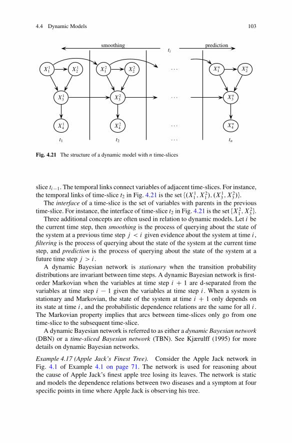
4.4 Dynamic Models 103

X11 X1

2

X13

X14

X21 X2

2

X23

X24

Xn1 Xn

2

Xn3

Xn4

smoothingti

prediction

t1 t2 : : : tn

: : :

: : :

: : :

Fig. 4.21 The structure of a dynamic model with n time-slices

slice ti−1. The temporal links connect variables of adjacent time-slices. For instance,the temporal links of time-slice t2 in Fig. 4.21 is the set {.X1

1 ; X21 /; .X

13 ; X

23 /}.

The interface of a time-slice is the set of variables with parents in the previoustime-slice. For instance, the interface of time-slice t2 in Fig. 4.21 is the set {X2

1 ;X23 }.

Three additional concepts are often used in relation to dynamic models. Let i bethe current time step, then smoothing is the process of querying about the state ofthe system at a previous time step j < i given evidence about the system at time i ,filtering is the process of querying about the state of the system at the current timestep, and prediction is the process of querying about the state of the system at afuture time step j > i .

A dynamic Bayesian network is stationary when the transition probabilitydistributions are invariant between time steps. A dynamic Bayesian network is first-order Markovian when the variables at time step i C 1 are d-separated from thevariables at time step i − 1 given the variables at time step i . When a system isstationary and Markovian, the state of the system at time i C 1 only depends onits state at time i , and the probabilistic dependence relations are the same for all i .The Markovian property implies that arcs between time-slices only go from onetime-slice to the subsequent time-slice.

A dynamic Bayesian network is referred to as either a dynamic Bayesian network(DBN) or a time-sliced Bayesian network (TBN). See Kjærulff (1995) for moredetails on dynamic Bayesian networks.

Example 4.17 (Apple Jack’s Finest Tree). Consider the Apple Jack network inFig. 4.1 of Example 4.1 on page 71. The network is used for reasoning aboutthe cause of Apple Jack’s finest apple tree losing its leaves. The network is staticand models the dependence relations between two diseases and a symptom at fourspecific points in time where Apple Jack is observing his tree.

104 4 Probabilistic Networks

Sick1

Loses1

dry1

Sick2

Loses2

dry2

Sick3

Loses3

dry3

Sick4

Loses4

dry4

Fig. 4.22 A model with four time-slices

Consider the case where Apple Jack is monitoring the development of the diseaseover a period of time by observing the tree each day in the morning. In this case, thelevel of dryness of the tree on a specific day will depend on the level of dryness onthe previous day and impact the level of dryness on the next day, similarly for thelevel of sickness. The levels of dryness and sickness on the next day are independentof the levels of dryness and sickness on the previous day given the levels of drynessand sickness on the current day. This can be captured by a dynamic model.

Figure 4.22 shows a dynamic model with four time-slices. Each time stepmodels the state of the apple tree at a specific point in time (the dashed linesillustrate the separation of the model into time-slices). The conditional probabilitydistributions P.Dryi |Dryi−1/ and P.Sicki |Sicki−1/ are the transition probabilitydistributions. The interface between time-slices i − 1 and i consists of Dryi andSicki .

Assume that it is the second day when Apple Jack is observing his tree. Theobservations on Loses of the first and second day are entered as evidence onthe corresponding variables. Filtering is the task of computing the probability of thetree being sick on the second day, smoothing is the task of computing the probabilityof sickness on the first day, and prediction is the task of computing the probabilityof the tree being sick on the third or fourth day. �

Dynamic models are not restricted to be Bayesian networks. Influence diagramsand LIMIDs can also be represented as dynamic models.

4.4.1 Time-Sliced Networks Represented as OOPNs

Time-sliced networks are often represented using object-oriented networks as thefollowing example illustrates.

Example 4.18 (Breeding Pigs). Example 4.13 shows a LIMID representation of adecision problem related to breeding pigs, see Fig. 4.15 on page 95. The decisionproblem is in fact modeled as a time-sliced model where the structure of each time-slice representing a test-and-treat cycle is shown in Fig. 4.23.

4.5 Summary 105

Ci

Di

Ri

Hi HiC1

Fig. 4.23 The test-and-treatcycle of the breeding pigsnetwork in Fig. 4.15

Cycle1 Cycle2 Cycle3 C4

Fig. 4.24 The breeding pigs network as a time-sliced OOPN

Three instances of the network class in Fig. 4.23 are constructed to create thenetwork in Fig. 4.24. The use of object-oriented modeling has simplified the networkconstruction.

The network in Fig. 4.24 is equivalent to the network in Fig. 4.15 on page 95. �

Kjærulff (1995) has described a computational system for dynamic time-slicedBayesian networks. The system implemented is referred to as dHugin. Boyen& Koller (1998) have described an approximate inference algorithm for solvingdynamic Bayesian networks with bounds on the approximation error.

4.5 Summary

In this chapter we have introduced probabilistic networks for belief update and de-cision making under uncertainty. A probabilistic network represents and processesprobabilistic knowledge. The qualitative component of a probabilistic networkencodes a set of (conditional) dependence and independence statements amonga set of random variables, informational precedence, and preference relations.The quantitative component specifies the strengths of dependence relations usingprobability theory and preference relations using utility theory.

We have introduced discrete Bayesian network models and CLG Bayesiannetwork models for belief update. A discrete Bayesian network supports the useof discrete random variables, whereas a CLG Bayesian network supports the useof a mixture of continuous and discrete random variables. The continuous variablesare constrained to be conditional linear Gaussian variables. This chapter contains anumber of examples that illustrate the use of Bayesian networks for belief update.

106 4 Probabilistic Networks

Discrete influence diagrams, CLQG influence diagrams, and limited memoryinfluence diagrams were introduced as models for belief update and decision makingunder uncertainty. An influence diagram is a Bayesian network augmented withdecision variables, informational precedence relations, and preference relations.A discrete influence diagram supports the use of discrete random and decisionvariables with an additively decomposing utility function. A CLQG influencediagram supports the use of a mixture of continuous and discrete variables. Thecontinuous random variables are constrained to be conditional linear Gaussianvariables, while the utility function is constrained to be linear–quadratic. A limitedmemory influence diagram is an extension of the discrete influence diagram wherethe assumptions of no-forgetting and regularity (i.e., a total order on the decisions)are relaxed. This allows us to model a large set of decision problems that cannotbe modeled using the traditional influence diagram representation. This chaptercontains a number of examples that illustrate the use of influence diagrams fordecision making under uncertainty.

Finally, we have introduced OOPNs. The basic OOPN mechanisms introducedsupport a type of object-oriented specification of probabilistic networks, whichmakes it simple to reuse models, to encapsulate submodels, and to perform modelconstruction at different levels of abstraction. This chapter contains a number ofexamples that illustrate the use of the basic OOPN mechanisms in the modeldevelopment process. OOPNs are well suited for constructing time-sliced networks.Time-sliced networks are used to represent dynamic models.

In Chap. 5, we discuss techniques for solving probabilistic networks.

Exercises

Exercise 4.1. Peter and Eric are chefs at Restaurant Bayes. Peter works 6 daysa week, while Eric works one day a week. In 90% of the cases, Peter’s food ishigh quality, while Eric’s food is high quality in 50% of the cases. One eveningRestaurant Bayes serves an awful meal.

Is it fair to conclude that Eric prepared the food that evening?

Exercise 4.2. One in a thousand people has a prevalence for a particular heartdisease. There is a test to detect this disease. The test is 100% accurate for peoplewho have the disease and is 95% accurate for those who do not (this means that 5%of people who do not have the disease will be wrongly diagnosed as having it).

(1) If a randomly selected person tests positive, what is the probability that theperson actually has the heart disease?

Exercise 4.3. Assume a math class is offered once every semester, while an AIclass is offered twice. The number of students taking a class depends on the subject.On average, 120 students take AI (�2 D 500), while 180 students take math (�2 D1; 000). Assume that on average 25% pass the AI exam (�2 D 400) while 50% passthe math exam (�2 D 500).

Exercises 107

(a) What is the average number of students passing either a math or AI exam?(b) What is the average number of students passing a math exam?(c) What is the average number of students taking a math class when 80 students

pass the exam?

Exercise 4.4. Frank goes to the doctor because he believes that he has got the flu.At this particular time of the year, the doctor estimates that one out of 1; 000 peoplesuffers from the flu. The first thing the doctor checks is whether Frank appears tohave the standard symptoms of the flu; if Frank suffers from the flu, then he willexhibit these symptoms with probability 0:9, but if he does not have the flu, hemay still have these symptoms with probability 0:05. After checking whether or notFrank has the symptoms, the doctor can decide to have a test performed which mayreveal more information about whether or not Frank suffers from the flu; the cost ofperforming the test is e 40. The test can either give a positive or a negative result,and the frequency of false-positives and false-negatives is 0:05 and 0:1, respectively.After observing the test result (if any), the doctor can decide to administer a drugthat with probability 0:6 may shorten the sickness period if Frank suffers from theflu (if he has not got the flu, then the drug has no effect). The cost of administeringthe drug is e 100, and if the sickness period is shortened, the doctor estimates thatthis is worth e 1; 000.

(a) Construct an influence diagram for the doctor from the description above.(b) Specify the probability distributions and the utility functions for the influence

diagram.

Exercise 4.5. Assume that Frank is thinking about buying a used car for e 20; 000,and the market price for similar cars with no defects is e 23; 000. The car may,however, have defects which can be repaired at the cost of e 5; 000; the probabilitythat the car has defects is 0:3. Frank has the option of asking a mechanic to perform(exactly) one out of two different tests on the car. Test1 has three possible outcomes,namely, no defects, defects, and inconclusive. For Test2 there are only two possibleoutcomes (no defects and defects). If Frank chooses to have a test performed on thecar, the mechanic will report the result back to Frank who then decides whether ornot to buy the car; the cost of Test1 is e 300, and the cost of Test2 is e 1; 000.

(a) Construct an influence diagram for Frank’s decision problem.(b) Calculate the expected utility and the optimal strategy for the influence

diagram; calculate the required probabilities from the joint probability table (overthe variables Test1, Test2, and StateOfCar) specified below.

Test1no defects defects inconclusive

Test2no defects .0:448; 0:00375/ .0:028; 0:05625/ .0:084; 0:015/

defects .0:112; 0:01125/ .0:007; 0:16875/ .0:021; 0:045/

Exercise 4.6. An environmental agency visits a site where a chemical productionfacility has previously been situated. Based on the agency’s knowledge about the

108 4 Probabilistic Networks

facility, they estimate that there is a 0:6 risk that chemicals from the facility havecontaminated the soil. If the soil is contaminated (and nothing is done about it),all people in the surrounding area will have to undergo a medical examinationdue to the possible exposure; there are 1; 000 people in the area, and the cost ofexamining/treating one person is $100. To avoid exposure, the agency can decideto remove the top layer of the soil which, in case the ground is contaminated, willcompletely remove the risk of exposure; the cost of removing the soil is $30; 000.Before making the decision of whether or not to remove the top layer of soil, theagency can perform a test which will give a positive result (with probability 0:9) ifthe ground is contaminated; if the ground is not contaminated, the test will give apositive result with probability 0:01. The cost of performing the test is $1; 000.

(a) Construct an influence diagram for the environmental agency from the descrip-tion above.

(b) Specify the probability distributions and the utility functions for the influencediagram.

Exercise 4.7. A company has observed that one of their software systems isunstable, and they have identified a component which they suspect is the cause ofthe instability. The company estimates that the prior probability for the componentbeing faulty is 0:01, and if the component is faulty, then it causes the systemto become unstable with probability 0:99; if the component is not faulty, thenthe system may still be unstable (due to some other unspecified element) withprobability 0:001.

To try to solve the problem, the company must first decide whether to patch thecomponent at a cost e 10; 000 : if the component is faulty, then the patch will solvethe fault with probability 0:95 (there may be several things wrong, not all of whichmay be covered by the patch), but if the component is not faulty, then the patchwill have no effect. The company also knows that in the near future the vendor ofthe component will make another patch available at the cost of e 20; 000; the twopatches focus on different parts of the component. This new patch will solve theproblem with probability 0:99, and (as for the first patch) if the component is notfaulty, then the patch will have no effect. Thus, after deciding on the first patch, thecompany observes whether or not the patch solved the problem (i.e., is the systemstill unstable?) and it then has to decide on the second patch. The company estimatesthat (after the final decision has been made) the value of having a fully functioningcomponent is worth e 100; 000.

(a) Construct an influence diagram for the company from the description above.(b) Specify the probability distributions and the utility functions for the influence

diagram.

Exercise 4.8. Consider a stud farm with ten horses where Cecily has unknown mareand sire, John has mare Irene and sire Henry, Henry has mare Dorothy and sireFred, Irene has mare Gwenn and sire Eric, Gwenn has mare Ann and unknown sire,Eric has mare Cecily and sire Brian, Fred has mare Ann and unknown sire, Brian

Exercises 109

Cecily Ann Brian

Eric Gwenn Fred Dorothy

Irene Henry

John

Fig. 4.25 The stud farmpedigree

has unknown mare and sire, Dorothy has mare Ann and sire Brian, and Ann hasunknown mare and sire, see Fig. 4.25.

A sick horse has genotype aa, a carrier of the disease has genotype aA, and anoncarrier has genotype AA. P.aa; aA;AA/ D .0:04; 0:32; 0:64/.

(a) Construct an object-oriented network representation of the stud farm problem.(b) What is the probability of each horse being sick/a carrier/a noncarrier once we

learn that John is sick?

Chapter 5Solving Probabilistic Networks

We build knowledge bases in order to formulate our knowledge about a certainproblem domain in a structured way. The purpose of the knowledge base isto support our reasoning about events and decisions in a domain with inherentuncertainty. The fundamental idea of solving a probabilistic network is to exploit thestructure of the knowledge base to reason efficiently about the events and decisionsof the domain taking the inherent uncertainty into account.

An expert system consists of a knowledge base and an inference engine. Theinference engine is used to solve queries against the knowledge base. In the case ofprobabilistic networks, we have a clear distinction between the knowledge base andthe inference engine. The knowledge base is the Bayesian network or influencediagram, whereas the inference engine consists of a set of generic methods thatapplies the knowledge formulated in the knowledge base on task-specific data sets,known as evidence, to compute solutions to queries against the knowledge base. Theknowledge base alone is of limited use if it cannot be applied to update our beliefabout the state of the world or to identify (optimal) decisions in the light of newknowledge.

As we saw in the previous chapter, the knowledge bases we consider areprobabilistic networks. A probabilistic network may be an efficient representation ofa joint probability distribution or a joint expected utility function. In the former casethe model is a Bayesian network, while in the latter case it is an influence diagram.

In this chapter we consider the process of solving probabilistic networks. Asthe exact nature of solving a query against a probabilistic network depends on thetype of model, the solution process of Bayesian networks and influence diagrams isconsidered separately in the following sections.

Section 5.1 considers probabilistic inference in Bayesian networks as the taskof computing posterior beliefs in the light of evidence. A number of differentapproaches to inference are considered. We consider variable elimination, query-based inference, arc reversal, and message passing in junction trees. The inferenceprocess in discrete Bayesian networks is treated in detail, while the inferenceprocess in CLG Bayesian networks and CLQG influence diagrams is outlined.

U.B. Kjærulff and A.L. Madsen, Bayesian Networks and Influence Diagrams: A Guideto Construction and Analysis, ISS 22, DOI 10.1007/978-1-4614-5104-4 5,© Springer Science+Business Media New York 2013

111

112 5 Solving Probabilistic Networks

In Sect. 5.2, we consider the task of solving decision models. Solving a decisionmodel amounts to computing (maximum) expected utilities. We derive a genericmethod for solving influence diagrams and LIMIDs.

Parts of this chapter have appeared in Madsen, Jensen, Kjærulff & Lang (2005).

5.1 Probabilistic Inference

We build Bayesian network models in order to support efficient belief update ina given domain. Belief update is the task of computing our updated beliefs in(unobserved) events given observations on other events, that is, evidence.

5.1.1 Inference in Discrete Bayesian Networks

One particular type of probabilistic inference task in Bayesian networks is the taskof computing the posterior marginal of an unobserved variable Y given a (possiblyempty) set of evidence ", that is, P.Y |"/. Let N D .X;G;P/ be a Bayesian networkover the set of discrete random variables X D {X1; : : : ; Xn}, and assume that " D ;.Exploiting the chain rule for Bayesian networks [see, e.g., (4.1) on page 71], forvariable Y 2 X, we may compute

P.Y / DX

X2X\{Y }

P.X/

DX

X2X\{Y }

Y

Xv2XP.Xv |Xpa.v//: (5.1)

This is the prior marginal distributionP.Y / of Y . The prior marginal of all variablesmay be computed by repetition for each variable.

Example 5.1 (Prior Probability (Apple Jack)). Given the example of Apple Jack(Example 4.1 on page 71), we may consider the task of computing the prior marginaldistribution P.L/ over the events that the tree does lose its leaves and that the treedoes not lose its leaves. The distribution P.L/ may be computed as

P.L/ DX

S

X

D

P.S/P.L |S;D/P.D/:

Using the quantification of the model specified as part of Example 4.1, we arriveat the prior distribution P.L/ D .0:82; 0:18/. Hence, a priori, there is an 18%probability that the tree will lose its leaves. �

5.1 Probabilistic Inference 113

The above approach does not incorporate evidence into the inference task.In addition, it is a very inefficient approach for nontrivial Bayesian networks becausethe joint distributionP.X/ overX is constructed as an intermediate step and becausea lot of calculations are repeated.

As we will see, it is possible to develop a more efficient approach to probabilisticinference by exploiting the independence relations induced by the structure of theDAG and the evidence and by minimizing the repetition of calculations. Having saidthat, let us turn to the general case of computing the posterior marginal P.X |"/ ofa variable, X , given evidence ".

Let " D {"1; : : : ; "m} be a nonempty set of evidence over variables X."/. Fora (non-observed) variable Xvj 2 X of N, the task is to compute the posteriorprobability distribution P.Xvj |"/. This can be done by exploiting the chain rulefactorization of the joint probability distribution induced by N:

P.Xvj |"/ D �.P." |Xvj /P.Xvj //

D P." |Xvj /P.Xvj /

P."/D P.Xvj ; "/

P."/

/ P.Xvj ; "/

DX

Y2X\{Xvj }

P.X; "/

DX

Y2X\{Xvj }

Y

Xvi 2XP.Xvi |Xpa.vi //E"

DX

Y2X\{Xvj }

Y

Xvi 2XP.Xvi |Xpa.vi //

Y

X2X."/EX

for each Xvj 62 X."/, where EX is the evidence function for X 2 X."/ and vi is thenode representingXvi . Notice that

L.Xvj |"/ D P." |Xvj / DX

Y2X\{Xvj }

Y

i 6DjP.Xvi |Xpa.vi //

Y

X2X."/EX (5.2)

is the likelihood function ofXvj given ". SinceP.Xvj /may be obtained by inferenceover the empty set of evidence, we can—using Bayes’ rule—compute

P.Xvj |"/ / L.Xvj |"/P.Xvj /:

The proportionality factor is the normalization constant ˛ D �.P.X; "// D P."/,which is easily computed from P.X; "/ by summation over X as ˛ D �.P.X; "// DP

X P.X; "/; see 3.3 on page 47.

114 5 Solving Probabilistic Networks

Example 5.2 (Posterior Probability (Apple Jack)). One evening when Apple Jackis taking his usual after-dinner walk in the garden, he observes his finest apple treeto be losing its leaves. Given that he knows that this may be an indication of the treebeing sick, he starts wondering whether or not the tree is sick.

Apple Jack is interested in the probability of the tree being sick given theobservation on the tree losing its leaves

P.S |"/ D P.S; "/

P."/

DP

S

PD P.S/P.L |S;D/P.D/EL

P."/

/ .0:0927; 0:0905/;

where EL D .0; 1/ is the evidence function reflecting the tree losing its leaves.The normalization constant is ˛ D P."/ D P.S D no |"/ C P.S D yes |"/ D0:0927 C 0:0905 D 0:1832. This produces the posterior distribution P.S |"/ D.0:506; 0:494/ over the tree losing its leaves. Hence, there is an increased probabilitythat the tree is sick when it has been observed to lose its leaves. The prior distributionon the tree being sick is P.S/ D .0:9; 0:1/. �

In general, probabilistic inference is an NP-hard task (Cooper 1990). Evenapproximate probabilistic inference is NP-hard (Dagum & Luby 1993). For certainclasses of Bayesian network models, the complexity of probabilistic inference ispolynomial or even linear in the number of variables in the network. The complexityis polynomial when the graph of the Bayesian network is a poly-tree (Kim &Pearl 1983, Pearl 1988) (a directed graph G is called a poly-tree, if its underlyingundirected graph is singly connected), while it is linear when the graph of theBayesian network is a tree.

The most critical problem related to the efficiency of the inference processis that of finding the optimal order in which to perform the computations. Theinference task is, in principle, solved by performing a sequence of multiplicationsand additions.

Query-Based Inference

One approach to inference is to consider the inference task as the task of computingthe posterior distribution of a set of variables. This is referred to as query-basedinference. We define the notion of a query,Q, against a Bayesian network model Nas follows.

Definition 5.1 (Query). Let N D .X;G;P/ be a Bayesian network model. Aquery Q is a three-tuple Q D .N;T; "/ where T � X is the target set and " isthe evidence set.

5.1 Probabilistic Inference 115

The solution of a query, Q, is the posterior distribution over the target, that is,P.T |"/. A variable X is a target variable if X 2 T. Notice that computing allposterior marginals of a Bayesian network N D .X;G;P/ corresponds to solving |X|

queries, that is, Q D .N; {X }; "/ for each X 2 X.Prior to solving the query Q, the graph G of N may be pruned to include only

variables relevant for the query. One class of variables which may be pruned fromthe graph without any computation is the class of barren variables; see Sect. 3.3.4on page 53 for an example. Here, we give a formal definition of a barren variable.

Definition 5.2 (Barren Variable). Let N D .X;G;P/ be a Bayesian network andletQ D .N;T � X; "/ be a query against N. A variableX is a barren variable withrespect to Q, if X 62 T, X 62 ", and all descendants, if any, de.X/, of X are barren.

When a variable X is classified as a barren variable, it is always relative to atarget and given a set of evidence. A barren variable does not add any informationto the inference process. It is computationally irrelevant to Q.

Once all barren variables with respect to Q have been pruned from the graph G,the inference task can be solved by variable elimination as described in the previoussection.

In addition to the concept of a barren variable, there is the concept of a nuisancevariable.

Definition 5.3 (Nuisance Variable). Let N D .X;G;P/ be a Bayesian networkand let Q D .N;T � X; "/ be a query against N. A non-barren variable X is anuisance variable with respect to Q, if X 62 T, X 62 ", and X is not on a pathbetween any pair of variables Y 2 T and Z 2 ".

Notice that a nuisance variable is computationally relevant for a queryQ, but it isnot on a path between any pair of evidence and query variables. Given a query and aset of evidence variables, the contribution from a nuisance variable does not dependon the observed values of the evidence variables. Hence, if a query is to be solvedwith respect to multiple instantiations over the evidence variables, then the nuisancevariables (and barren variables) may be eliminated in a preprocessing step to obtainthe relevant network (Lin & Druzdzel 1997). The relevant network consists of targetvariables, evidence variables, and variables on paths between target and evidencevariables only.

Example 5.3 (Barren Variables and Nuisance Variables). Let us return to the chestclinic example (Example 4.2 on page 73) and consider the task of computing theprobability of each disease given the observations that the patient is a smoker andhas a positive X-ray result. That is, we need to compute P.Y |"/ for Y 2 {T;L;B}

and " D {S D yes; X D yes}.The variables {A; T } are nuisance variables with respect to posteriors for B

and L. The variable D is a barren variable with respect to the posteriors for B , T ,and L, whereas B is a barren variable with respect to the posteriors for T and L.Figure 5.1 shows the relevant networks for (a) computing P.T |"/ and P.L |"/ andfor (b) computing P.B |"/. �

116 5 Solving Probabilistic Networks

S

T L

E

X

(a)S

L B

E

X

(b)

Fig. 5.1 The relevant networks for computing (a) P.T |"/ and P.L |"/ and (b) P.B |"/

The approach to inference outlined above may be referred to as a direct approach.Arc reversal is a specific type of direct approach to inference (Olmsted 1983,Shachter 1986).

Arc Reversal

In Sect. 3.4.1.1 on page 56, we illustrated how application of Bayes’ rule can begiven a graphical interpretation as arc reversal. We mentioned that Olmsted (1983)and Shachter (1986) have exploited this view of inference in their arc reversalalgorithms for inference in probabilistic networks. Here, we consider the processin more detail.

Let G be the DAG of a Bayesian networkN D .X;G;P/ and assume a queryQ D.N; {Z};;/ against N. The inference task is to compute P.Z/ by eliminating allvariables X \ {Z}.

The inference process on G has a natural graphical interpretation as a sequenceof arc reversals and barren variable eliminations. The fundamental idea is to adjustthe structure of G such that all variables except Z are pruned as barren variableswhile maintaining the underlying properties of the joint probability distributionsover the remaining variables. The structure of G is adjusted through a sequence ofarc reversal operations.

Assume Xw is the next variable to be eliminated as a barren variable. Let Xw

have parents Xpa.w/ D Xi [ Xj and Xv have parents Xpa.v/ D {Xw} [ Xj [ Xkwhere Xi \ Xj D Xi \ Xk D Xj \ Xk D ; such that Xi D Xpa.w/ \ Xpa.v/

are the parents specific for Xw, Xj D Xpa.w/ \ Xpa.v/ are the common parents,and Xk D Xpa.v/ \Xfa.w/ are the parents specific for Xv.

The reversal of arc .w; v/ proceeds by setting Xpa.w/ D Xi [ Xj [ Xk [ {Xv}

andXpa.v/ D Xi [Xj [Xk as well as performing the computations specified below;see Fig. 5.2 for a graphical representation

5.1 Probabilistic Inference 117

i j k

w v

⇒

i j k

w v

Fig. 5.2 An illustration of reversal of the arc .w; v/

S

L

D

.a/

S

L

D

.b/

S

L

.c/

S

L

.d/

L

.e/

Fig. 5.3 Computing P.L/ by arc reversal

P.Xv |Xi ;Xj ;Xk/ DX

Xw

P.Xw |Xi ;Xj /P.Xv |Xw; Xj ;Xk/ (5.3)

P.Xw |Xv; Xi ; Xj ;Xk/ D P.Xw |Xi;Xj /P.Xv |Xw; Xj ;Xk/

P.Xv |Xi;Xj ;Xk/: (5.4)

The operation of reversing an arc changes the structure of G without changingthe underlying joint probability distribution over X induced by N.

Once the arc .w; v/ has been reversed, the variableXw is a barren variable relativeto the other variables (given the empty set of evidence) and can be pruned from G

without further computations.The basic idea of the inference process known as arc reversal is to perform a

sequence of arc reversals and barren variable eliminations on the DAG G until adesired marginal or conditional is obtained. In this process a valid Bayesian networkstructure is maintained throughout the inference process.

Example 5.4 (Arc Reversal). We may compute the prior probability distributionP.L/in the Apple Jack example (see Example 4.1 on page 71) using a sequence of arcreversals and barren variable eliminations as indicated in Fig. 5.3.

Notice that the arc reversal method does not have worse complexity than variableelimination. �

Arc reversal is not a local computation algorithm in the sense that when reversingan arc .w; v/, it is necessary to test for existence of a directed path from w to v notcontaining .w; v/. If such a path exists, then the arc .w; v/ cannot be reversed untilone or more other arcs have been reversed as reversing .w; v/would otherwise createa directed path.

118 5 Solving Probabilistic Networks

Graphical Representation of Inference

We may define the task of solving a Bayesian network model N D .X;G;P/ as theproblem of computing the posterior marginal P.X |"/ given a set of evidence " forall variablesX 2 X.

When defining the task of probabilistic inference as the task of computingthe posterior marginals P.X |"/ for all X given evidence ", the most commonapproach is to use a secondary computational structure. Performing inference ina secondary computational structure aims at reusing calculations solving all queriessimultaneously.

From (5.1) on page 112, we should notice the direct correspondence betweenthe acyclic, directed graph G and the factorization of the joint probability distribu-tion P.X/ over X. The domain of each factor in the factorization corresponds toa node and its parents. The head of the factor is the child node, whereas the tailconsists of the parents. Furthermore, if we drop the distinction between head andtail, we see that the domain of each factor corresponds to a clique (a clique is amaximal complete subgraph) of Gm—the moralization of G. This is exploited tobuild a secondary structure for performing inference.

Assume we are in the process of computing P.Xi /. Let Y be the first randomvariable to eliminate. The elimination process proceeds by local computation inorder to maintain efficiency (i.e., we exploit the distributive law to maintain thefactorization of the joint probability distribution—see Sect. 3.3.3 on page 51). Theset of probability potentials P can be divided into two disjoint subsets with respectto Y . Let PY � P be the subset of probability potentials including Y in the domain

PY D {P 2 P|Y 2 dom.P /};

where dom.P / denotes the domain of P (i.e., the set of variables over which itis defined). Then P \ PY is the set of probability potentials not including Y intheir domain. Let �Y be the probability potential obtained by eliminating Y (bysummation) from the combination of all probability potentials in PY . Using �Yas well as a generalized version of the distributive law, we may rewrite 5.1 onpage 112 as

P.Xi / DX

X2X\{Xi }

Y

Xv2XP.Xv |Xpa.v//

DX

X2X\{Xi }

Y

�2P\PY

�Y

�02PY�0

DX

X2X\{Xi ;Y }

Y

�2P\PY

�X

Y

Y

�02PY�0

DX

X2X\{Xi ;Y }

�YY

�2P\PY

�: (5.5)

5.1 Probabilistic Inference 119

X1X2Y X1X2 X1X2X3X4 X2X3X4 � � �

Fig. 5.4 A graphical illustration of the process of eliminating Y from �.X1; X2; Y / and X1from �.X1; X2; X3; X4/, where the ovals represent the domain of a potential before eliminationand rectangles represent the domain of a potential after elimination

B E

A R

W

Fig. 5.5 The Burglary orEarthquake network

Equation 5.5 on the preceding page specifies a decomposition of the jointprobability distribution over X \ {Y }. The decomposition has the form of (5.1). Thedecomposition is the product over the elements of P\PY [{�Y }. In addition, we haveperformed the elimination over Y by local computations only involving potentialsof which Y is a domain variable. We say that the set

P \ PY [ {�Y }

is a reduction of P where Y has been eliminated. The elimination of the next variablemay proceed in the same manner on P \ PY [ {�Y }. The order in which variablesare eliminated is the elimination order. An example of this process may be depictedgraphically as shown in Fig. 5.4 where we assume dom.�Y / D .X1;X2/. The arrowsin the figure are used to illustrate the flow of computations.

The elimination of Y from �.X1;X2; Y / creates a potential over �.X1;X2/which is included in the elimination of the next variableX1 to be eliminated. In thisway the process continues until the desired marginals are obtained. Let us consideran even more concrete example.

Example 5.5 (Burglary or Earthquake, page 25). Consider the Bayesian networkin Fig. 2.3 on page 26, which is repeated in Fig. 5.5.

The prior marginal on A may be computed by elimination of {B;E;R;W } asfollows:

P.A/ DX

E

P.E/X

B

P.B/P.A |B;E/X

R

P.R |E/X

W

P.W |A/: (5.6)

120 5 Solving Probabilistic Networks

A A AE AE ABE

A AW

E ER

Fig. 5.6 A graphical illustration of the process of computing P.A/ in (5.6), where the ovalsrepresent the domain of a potential before elimination and rectangles represent the domain of apotential after elimination

W W AW A AE

AE ABE

E ER

Fig. 5.7 A graphical illustration of the process of computing P.W / in (5.7), where the ovalsrepresent the domain of a potential before elimination and rectangles represent the domain of apotential after elimination

Figure 5.6 shows a graphical representation of the computations and potentialscreated the during process of computing P.A/.

Similarly, the prior marginal distribution over W may be computed by elimina-tion of {A;B;E;R} as follows:

P.W / DX

A

P.W |A/X

E

P.E/X

B

P.B/P.A |B;E/X

R

P.R |E/: (5.7)

Figure 5.7 shows a graphical representation of the computations and potentialscreated during the process of computing of P.W /.

Notice the similarity between the potentials created in the process of comput-ing P.A/ and P.W /. There is a significant overlap between the potentials createdand therefore the calculations performed. This is no coincidence. �

Junction Trees

The task of probabilistic inference may be solved efficiently by local proceduresoperating on a secondary computational structure known as the junction tree(also known as a join tree and a Markov tree) representation of a Bayesiannetwork (Jensen & Jensen 1994, Jensen et al. 1994).

5.1 Probabilistic Inference 121

BDE BLS

EX BEL AT

ELT

ELE T

BE BL

Fig. 5.8 A junction treerepresentation T for the chestclinic network

The junction tree representation is efficient when solving the inference task formultiple sets of different evidence and target variables. A junction tree represen-tation T of a Bayesian network N D .X;G;P/ is a pair T D .C; S/ where C isthe set of cliques and S is the set of separators. The cliques C are the nodes of T,whereas the separators S annotate the links of the tree. Each clique C 2 C representsa maximal complete subset of pairwise connected variables of X, that is, C � X,of an undirected graph.1 The link between two neighboring cliques Ci and Cj isannotated with the intersection S D Ci \ Cj , where S 2 S.

Example 5.6 (Chest Clinic). Figure 4.2 on page 74 shows the DAG G of the chestclinic network N D .X;G;P/; see Example 4.2 on page 73.

Figure 5.8 shows a junction tree representation T D .C; S/ of the chest clinicnetwork. The junction tree consists of cliques

C D {{A; T }; {B;D;E}; {B;E;L}; {B;L; S }; {E;L; T }; {E;X }}

and separatorsS D {{B;E}; {B;L}; {E}; {E;L}; {T }

}

:

The structure of T is determined from the structure of G. �

The process of creating a junction tree representation of a DAG is beyond thescope of this book. Instead, we refer the interested reader to the literature; see, forexample, Cowell, Dawid, Lauritzen & Spiegelhalter (1999).

The junction tree serves as an excellent control structure for organizing the com-putations performed during probabilistic inference. Messages are passed betweencliques of the junction tree in two sweeps such that a single message is passedbetween each pair of neighboring cliques in each sweep. This process is referred toas a propagation of information.

1The undirected graph is constructed from the moral graph Gm of G by adding undirected edgesuntil the graph is triangulated. A graph is triangulated if every cycle of length greater than threehas a chord.

122 5 Solving Probabilistic Networks

R � � � Ci S Cj

C 0

C 00

S 0

S 00

Fig. 5.9 When Cj has absorbed information from its other neighbors, Ci can absorb from Cj

Once the junction tree T D .C; S/ has been constructed, a probability potential isassociated with each clique C 2 C and each separator S 2 S between two adjacentcliques Ci and Cj where S D Ci \ Cj ; see Fig. 5.9.

Inference involves the following steps:

1. Each item of evidence must be incorporated into the junction tree potentials. Foreach item of evidence, an evidence function is multiplied onto an appropriateclique potential.

2. Some clique R 2 C of T is selected. This clique is referred to as the root of thepropagation.

3. Then messages are passed toward the selected root. The messages are passedthrough the separators of the junction tree (i.e., along the links of the tree).These messages cause the potentials of the receiving cliques and separators tobe updated. This phase is known as COLLECTINFORMATION.

4. Now messages are passed in the opposite direction (i.e., from the root toward theleaves of the junction tree). This phase is known as DISTRIBUTEINFORMATION.

5. At this point, the junction tree is said to be in equilibrium: the probabilityP.X |"/

can be computed from any clique or separator containing X—the result will beindependent of the chosen clique or separator.

Prior to the initial round of message passing, for each variable Xv 2 X, weassign the conditional probability distribution P.Xv |Xpa.v// to a clique C suchthat Xfa.v/ � C . Once all conditional probability distributions have been assignedto cliques, the distributions assigned to each clique are combined to form the initialclique potential.

Example 5.7 (Association of CPTs to Cliques). Consider again the junction tree ofthe chest clinic network shown in Fig. 5.8. Each conditional probability distribu-tion P 2 P is associated with a clique of T such that dom.P /�C for C2C. Noticethat the association of distributions with cliques is unique in this example. �

The basic inference algorithm is as follows. Each separator holds a singlepotential over the separator variables, which initially is a unity potential. Duringpropagation of information, the separator and clique potentials are updated. Con-sider two adjacent cliques Ci and Cj as shown in Fig. 5.9. When a message is

5.1 Probabilistic Inference 123

ABE

A

AW

E

ER

Fig. 5.10 A junction treerepresentation T of theBayesian network depicted inFig. 5.5 on page 119

passed from Cj to Ci either during COLLECTINFORMATION or DISTRIBUTEIN-FORMATION, Ci absorbs information from Cj . Absorption of information involvesperforming the following calculations:

1. Calculate the updated separator potential:

��S D

X

Cj \S

�Cj :

2. Update the clique potential of Ci :

�Ci WD �Ci��S

�S:

3. Associate the updated potential with the separator:

�S D ��S :

After a full round of message passing, the potential associated with any clique(separator) is the joint probability distribution (up to the same normalizationconstant) of the variables in the clique (separator) and the evidence. This algorithmis known as the HUGIN algorithm. Details on the inference process can be foundin the literature (Lauritzen & Spiegelhalter 1988, Andersen, Olesen, Jensen &Jensen 1989, Jensen et al. 1990, Dawid 1992, Jensen et al. 1994, Lauritzen &Jensen 2001).

Example 5.8 (Cluster Trees Vs. Junction Trees). Figure 5.10 shows a junction treerepresentation T D .C; S/ of the Bayesian network depicted in Fig. 5.5 on page 119with cliques:

C D {{A;B;E}; {E;R}; {A;W }}

and separators:S D {{E}; {A}}:

Notice the similarity between Fig. 5.10 and Figs. 5.6 and 5.7. The nodesof Figs. 5.6 and 5.7 are clusters (i.e., subsets of variables), whereas the nodes ofFig. 5.10 are cliques (i.e., maximal subsets of pairwise connected variables) ofundirected graphs.

124 5 Solving Probabilistic Networks

B E

A R

W

Fig. 5.11 The undirectedgraph corresponding toFigs. 5.6, 5.7, and 5.10

ABE

A

AW

E

ER

→

3

←

1

←

2

→

4

Fig. 5.12 Message passingin T

The undirected graph corresponding to a junction tree is obtained by addingundirected edges between each pair of variables contained in the same clique orcluster. Figure 5.11 is the undirected graph corresponding to Figs. 5.6, 5.7, and 5.10.

Figure 5.12 shows how messages are passed over T relative to the root ABE.Underlying any approach to inference is the junction tree representation, al-

though its presence may be implicit. Figure 5.6 shows the cluster tree representationunderlying the computation of P.A/, whereas Fig. 5.7 shows the cluster treerepresentation underlying the computation of P.W /. Figures 5.6 and 5.7 are notjunction trees, but cluster trees. The cliques of a junction tree are maximal completesubsets of pairwise connected variables, whereas clusters are not necessarilymaximal. �

The quality of the junction tree T D .C; S/ determines the efficiency of inference.A common score or criterion to use when considering the optimality of a junctiontree is the maximum state space size over all cliques in T, that is, maxC2C kCk.Another similar score is the sum over all cliques in T, that is,

PC2C kCk.

If the maximum state space size of a clique C is very large, for example,kCk D 1;000;000;000, then exact inference may become intractable on standarddesktop computers. A very large state space size of a clique may be due to a poortriangulation of the underlying DAG of the Bayesian network, for instance. Thus,the first option should be to search for a better triangulation reducing (significantly)the state space size of the largest clique. If the triangulation, on the other hand, isknown to be optimal (or near optimal), then options to change the structure of thegraph should be considered, for instance, using the modeling techniques described

5.1 Probabilistic Inference 125

in Chap. 7. An alternative to changing the structure is to use approximate algorithmsfor performing inference in the model.

All types of probabilistic networks considered in this book may be solvedby message passing in a junction tree representation. However, we will restrictourselves from a detailed treatment of this topic for all models presented as it isbeyond the scope of this book.

The approach to inference outlined above may be referred to as an indirectapproach.

5.1.2 Inference in CLG Bayesian Networks

Let N D .X;G;P;F/ be a CLG Bayesian network with continuous randomvariables, X� , and discrete random variables, X�, such that X D X� [X�. To solvethe probabilistic inference task on N is to compute the marginal for each X 2 X.Since N is a CLG Bayesian network, the task of performing inference becomesmore subtle than in the case of a pure discrete Bayesian network.

The prior distribution, P.X/, of a discrete variable X 2 X� is equal to thedistribution of X in the discrete network N0 D .X�;P/ obtained by removing allcontinuous variables from the model (all continuous variables are barren variableswith respect to the joint over the discrete variables). The prior density of acontinuous variable Y , on the other hand, will, in general, be a mixture of Gaussiandistributions where the mixing factors are joint probabilities over configurations ofdiscrete variables I � X�. For each configuration i of I with nonzero probability,that is, p.i/ > 0, the joint distribution of I and X has the form

P.I D i/ � N..i/; �2.i//:

This implies that the marginal of X 2 X� is

L.X/ DX

i WP.IDi />0P.i/ � N..i/; �2.i//:

For each configuration i of I with P.i/ D 0, the mean .i/ and variance �2.i/may be random numbers. Hence, the marginal density function for a continuousvariable X 2 X� is, in general, a mixture of Gaussian distributions

f .x/ DnX

iD0˛ifi .x/;

where each component fi is a one-dimensional Gaussian density function in Xand each coefficient ˛i is the probability of a configuration of discrete variables.This implies that the marginal density function of X 2 X� is not necessarily aCLG distribution with the indicated mean and variance �2. That is, the resultof a marginalization of a CLG distribution over continuous variables is a CLGdistribution, whereas the result of a marginalization of a CLG distribution over

126 5 Solving Probabilistic Networks

discrete variables, in general, is not. The marginalization is performed using theoperations defined by Lauritzen & Jensen (2001). The result of the first type ofmarginal is referred to as a strong marginal, whereas the latter is referred to asa weak marginal. The marginal is strong as we compute the mean and thevariance �2, and we know the distribution is a CLG distribution; whereas in thecase of a weak marginal, only and � are computed; the exact density is usuallynot computed as part of belief update. It is computed separately.

Probabilistic inference is the task of updating our belief about the state of theworld in light of evidence. Evidence on discrete variables, be it hard or soft evidence,is treated as in the case of discrete Bayesian networks. Evidence on a continuousvariable, on the other hand, is restricted to be hard evidence, that is, instantiations.

In the general case where evidence " is available, the marginal for a discretevariableX 2 X� is a probability distribution P.X |"/ conditional on the evidence ",whereas the marginal for a continuous variableX 2 X� is a density function f .x |"/conditional on " with a mean and a variance �2.

Example 5.9 (Density Function). Example 4.3 on page 77 shows an example ofa simple CLG Bayesian network. Computing the prior probability density in X3amounts to eliminating the variablesX1 andX2. With the quantification specified inExample 4.3, this produces the following mixture:

L.X3/ D 0:75 � N .−5; 5:1/C 0:25 � N .5; 5:2/

with mean D −2:5 and variance �2 D 23:88. Notice that the density forX3 is notthe density for the Gaussian distribution with mean D −2:5 and variance �2 D23:88. The density function is shown in Fig. 5.13 on the next page.

The prior probability density for X2 and the prior probability distribution for X1are trivial to compute as {X2;X3} are barren with respect to the prior for X1 andsimilarly {X1;X3} are barren with respect to the prior for X2. �

The above examples illustrates that the class of CLG distributions is notclosed under the operation of discrete variable elimination. The marginal distribu-tion N.; �2/may, however, be used as an approximation of the true marginal. Thismarginal is the closest non-mixture to the true marginal in terms of the Kullback–Leibler distance (Lauritzen 1996).

Example 5.10 (Density Function vs. Weak Marginal). Again, let us consider theCLG Bayesian network N from Example 4.3 on page 77. Figure 5.13 on thenext page shows the density function for X3. Figure 5.14 shows both the densityfunction f .X3/ and the weak marginal g.X3/ for X3. It is obvious that the weakmarginal is only an approximation of the exact density function. �

Since the CLG distribution is not closed under the operation of discrete variableelimination and since the operation of discrete variable elimination is not definedwhen continuous variables are in the domain of the potential to be marginalized, itis required that continuous variables are eliminated before discrete variables. Forthis reason, when marginalizing over both continuous and discrete variables,

5.1 Probabilistic Inference 127

0

0.02

0.04

0.06

0.08

0.1

0.12

0.14

-15 -10 -5 0 5 10 15

f.X3/

Fig. 5.13 The density function for X3

0

0.02

0.04

0.06

0.08

0.1

0.12

0.14

-15 -10 -5 0 5 10 15

g(X3)f(X3)

Fig. 5.14 The density function f .X3/ for X3 and its weak marginal g.X3/

we first marginalize over the continuous variables and then over the discretevariables (Lauritzen 1992b).

This implies that the (exact) solution method for inference in CLG Bayesiannetworks induces the partial order X� X� on the elimination order. Hence,the continuous variables X� should be eliminated before the discrete variables X�.A variable elimination order, which is restricted to induce a certain (partial) order, isreferred to as a strong elimination order. Hence, we use a strong elimination order tosolve a CLG Bayesian network by variable elimination. For this reason, inferencein a CLG Bayesian network may be more resource intensive than inference in acorresponding Bayesian network with the same structure, but consisting only of

128 5 Solving Probabilistic Networks

continuous random variables. Notice that due to independence relations induced bythe structure of G D .V;E/ of a CLG Bayesian network and the structure of theevidence ", it may in some situations be possible to eliminate discrete variablesbefore continuous variables.

In the special case where the ancestors of v 2 V are all representing continuousvariables (i.e., an.v/ � V� ) for Xv 2 X, the posterior marginal for Xv is astrong marginal. Otherwise, it is a weak marginal. If the posterior for Xv is a weakmarginal, the density function of Xv is an unknown mixture of Gaussians, whichneeds to be computed as part of probabilistic inference.

The normalization constant ˛ computed as part of probabilistic inference isproportional to the density at the observed values of the continuous variables.The proportionality constant is P.".�/ |".� //, where ".�/ is the evidence ondiscrete variables and ".� / is the evidence on continuous variables. In general, ˛ isscale dependent and does not make much sense. For instance, the value of ˛ will bedependent on whether height is measured in meters or centimeters. If " only containsdiscrete variables, then ˛ is the probability of ".

The presence of both continuous and discrete variables makes the operationsrequired for performing probabilistic inference in CLG Bayesian networks morecomplicated than those required for performing probabilistic inference in discreteBayesian networks. For a detailed treatment on inference in CLG Bayesian net-works, see, for example, Lauritzen (1992b) and Lauritzen & Jensen (2001).

5.2 Solving Decision Models

We build decision models in order to support efficient belief update and decisionmaking under uncertainty in a given problem domain. Belief update is the task ofcomputing our updated beliefs in (unobserved) events given observations on otherevents, whereas decision making under uncertainty is the task of identifying the(optimal) decision strategy for the decision-maker-given observations.

The construction of influence diagrams and limited memory influence diagrams,as well as the notion of expected utility, is described in detail in Sect. 4.2.

5.2.1 Solving Discrete Influence Diagrams

Inference in an (perfect recall) influence diagram N D .X;G;P;U/ is to determinean optimal strategy O� D { Oı1; : : : ; Oın} for the decision maker and compute theexpected utility of adhering to O�.

The influence diagram is a compact representation of a joint expected utilityfunction due to the chain rule

EU.X/ DY

Xv2XC

P.Xv |Xpa.v//X

w2VUu.Xpa.w//:

Applying theP

-max-P

-rule (Jensen 1996) on the joint expected utility function,we may solve N by eliminating variables in the reverse order of the information

5.2 Solving Decision Models 129

precedence order . That is, the precedence relation induces a partial order on theelimination of variables in X. This implies that we use a strong variable eliminationorder to solve an influence diagram by variable elimination.

Starting with the last decision Dn, theP

-max-P

-rule says that we shouldaverage over the unknown random variables In, maximize over the decision Dn,average over the random variables In−1 known to the decision maker at Dn (butnot known to the analyst), maximize over Dn−1, and so on. The principle is toaverage over the unknown random variables, maximize over the decision variable,and finally average over the observed random variables.

The intuition behind the application of theP

-max-P

-rule in reverse order ofdecisions is as follows. When we consider the last decision Dn, its past is fullyobserved, and the only unobserved variables are the variables never observed orobserved after Dn, that is, In. Hence, after averaging over In, we can select amaximizing argument of the utility function u.I.Dn/;Dn/ for each configurationof I.Dn/ as an optimal decision atDn. Notice that we select a maximizing argumentfor each configuration of the past. In principle, this eliminates In and Dn from thedecision problem, and we may considerDn−1 as the last decision. This implies thatwhen we solve forDn−1, we assume the decision maker to act optimally forDn.

Notice that the variables are observed at the time of decision, but not (necessarily)at the time of analysis. Whether a random variable is known or unknown is definedfrom the point of view of the decision maker, and not the analyst. In this way wemay solve N by computing the expected utility EU. O�/ of the optimal strategy� as

EU. O�/ DX

I0

maxD1

X

I1

maxD2

� � �X

In−1

maxDn

X

In

EU.X/

DX

I0

maxD1

X

I1

maxD2

� � �X

In−1

maxDn

Y

Xv2XC

P.Xv |Xpa.v//X

Uw2XU

u.Xpa.w//: (5.8)

As part of the process, prior to the elimination of each decisionD, we record themaximizing arguments of D over the utility potential .D; I.D// from which Dis eliminated for each configuration of I.D/. From .D; I.D//, we define the(probabilistic) policy function ı.D | I.D// forD as

ı.d | I.D/ D i/ D{

1 if d D arg maxd 0 .d 0; i /;0 otherwise;

where we assume the maximizing argument arg maxd 0 .d 0; i / to be unique. If it isnot unique, then any maximizing argument may be chosen.2

Example 5.11 (Oil Wildcatter). To solve the decision problem of the oil wildcatterof Example 4.5 on page 82 is to identify the optimal decision policies for the

2As we shall see in Sect. 5.2.4, the policy function need not be deterministic.

130 5 Solving Probabilistic Networks

Table 5.1 The joint expectedutility function EU.D; S; T /

D S T

no cl no 0

yes cl no 7

no op no 0

yes op no 7

no di no 0

yes di no 7

no cl yes −2:4

yes cl yes 18:6

no op yes −3:5

yes op yes 8

no di yes −4:1

yes di yes −16:6

Table 5.2 The expectedutility function EU.T /

T

no 21

yes 22:5

test and drill decisions. From the joint expected utility function, EU.X/, overvariables X of N D .X;G;P;U/, we may compute the expected utility, EU. O�/,of the optimal strategy, O� D

{ OıD.S; T /; OıT ./}

, and in the process determine the

optimal strategy as

EU. O�/ D maxT

X

S

maxD

X

O

P.O/P.S |O;T /.U1.T /C U2.D;O//:

Table 5.1 shows the expected utility function over D, S , T from which thedecision policy OıD.S; T / is identified as the maximizing argument of D for eachconfiguration of S and T . The oil wildcatter should drill for oil unless he performedthe test and obtained a diffuse pattern.

Table 5.2 shows the expected utility function over T from which the decisionpolicy OıT ./ is identified as the maximizing argument of T . Hence, the test shouldalways be performed.

The decision policies OıT ./ and OıD.S; T / are already known from Example 4.7on page 84. The expected utility for the decision problem is 22:5. �

Solving an influence diagram by performing the variable eliminations accordingto (5.8) will be highly inefficient even for simple influence diagrams. Instead, wewill—as in the case of Bayesian networks—apply a generalized version of thedistributive law to increase computational efficiency.

For notational convenience, the generalized marginalization operator

∑

wasintroduced by Jensen et al. (1994). The marginalization operator works differentlyfor marginalization of random variables and decision variables:

5.2 Solving Decision Models 131

∑

X

� ,X

X

� and

∑

D

� , maxD�;

where X is a random variable while D is a decision variable. We will use thegeneralized marginalization operator to explain the process of solving an influencediagram; see Madsen & Jensen (1999) for details.

Using a generalized version of the distributive law, the solution of an influencediagram may proceed as follows. Let Y be the first random variable to eliminate.The set of utility potentials U can be divided into two disjoint subsets with respectto Y . Let UY � U be the subset of utility potentials including Y in the domain

UY D {u 2 U|Y 2 dom.u/}:

Then U \ UY is the set of utility potentials not including Y in the domain.Similarly, let PY � P be the subset of probability distributions including Y in thedomain

PY D {P 2 P|Y 2 dom.P /}:

Then P \ PY is the set of probability potentials not including Y in the domain.The elimination process proceeds by local computation in order to maintainefficiency (i.e., we exploit the distributive law to maintain the factorization of thejoint expected utility function). Let �Y be the probability potential obtained byeliminating Y from the combination of all probability potentials in PY and let Ybe the utility potential obtained by eliminating Y from the combination of allprobability and utility potentials in PY [ UY such that

�Y D

∑

Y

Y

�2PY�;

Y D

∑

Y

�YX

2UY

: (5.9)

The two potentials �Y and Y will be used to enforce the factorization of thejoint expected utility function over X \ {Y }. The factorization may be achieved byrewriting (5.8) using �Y and Y as well as applying the distributive law

EU. O�/ D

∑

X2X

� Y

�2P�X

2U

D

∑

X2X

�� Y

�2P\PY

�Y

�02PY�0�� X

2U\UY

CX

02UY

0��

D

∑

X2X\{Y }

�� Y

�2P\PY

�

�

∑

Y

� Y

�02PY�0�� X

2U\UY

CX

02UY

0��

132 5 Solving Probabilistic Networks

D

∑

X2X\{Y }

�� Y

�2P\PY

�

��� X

2U\UY

��Y C Y

��(5.10)

D

∑

X2X\{Y }

�� Y

�2P\PY

�

��Y

� X

2U\UY

C Y

�Y

��: (5.11)

Equation (5.11) specifies a decomposition of the joint expected utility functionover X \ {Y }, and decomposition has the form of (5.8). The decomposition is theproduct of the summation over the elements of U \ UY [ {

Y�Y

} and the product overthe elements of P\PY [ {�Y }. In addition, we have performed the elimination of Yby local computations only involving potentials with Y as a domain variable. Wesay that the sets

P \ PY [ {�Y } and U \ UY [{

Y

�Y

}

are a value preserving reduction of P and U where Y has been eliminated. Theelimination of the next variable may proceed in the same manner on U\UY [{ Y

�Y

}

and P \ PY [ {�Y }.The division operation in (5.11) is introduced because the combination of

probability potentials and utility potentials is nonassociative. Thus, either thedivision should be performed or the probability potentials have to be distributedover the terms of the utility function as in (5.10).

Example 5.12 (Oil Wildcatter). Utilizing the local computation approach explainedabove, we may solve the oil wildcatter problem as follows:

EU. O�/ D maxT

X

S

maxD

X

O

P.O/P.S |O;T /.C.T /C U.D;O//

D maxT.C.T /C

X

S

P.S/maxD

X

O

P.O/P.S |O; T /

P.S/U.D;O//:

The division byP.S/ is necessary in order to obtain the correct conditional expectedutility for D. This division does not effect the policy.

The benefit of the local computation approach is more profound on large andmore complex influence diagrams. �

5.2.2 Solving CLQG Influence Diagrams

Inference in a CLQG influence diagram N D .X;G;P;F;U/ is similar to inferencein a discrete influence diagram. The task is to determine an optimal strategy, O� D{ Oı1; : : : ; Oın}, for the decision maker and compute the expected utility of adheringto O�.

5.2 Solving Decision Models 133

U1

U2

Budget

Units CostPrice

Fig. 5.15 Optimization ofprice given marketing budgetsize

The influence diagram is a compact representation of a joint expected utilityfunction due to the chain rule

EU.X� D i;X� / DY

v2V�P.iv | ipa.v// �

Y

w2V�p.yw |Xpa.w// �

X

z2VUu.Xpa.z//:

The solution process for CLQG influence diagrams follows the same approach asthe solution process for discrete influence diagrams. The solution process proceedsby applying an extension of the

P-max-

P-rule (Madsen & Jensen 2005).The

extension is that we need to eliminate the continuous random variables X� byintegration as opposed to summation. We refer the interested reader to the literaturefor details on the solution process (Kenley 1986, Shachter & Kenley 1989, Poland1994, Madsen & Jensen 2005).

The optimal strategy O� D { Oı1; : : : ; Oın} will consist of decision policies forboth discrete and continuous decision variables. The decision policy for a discretedecision variable Di 2 X� \ XD is a mapping from the configuration of itspast I.Di / to dom.Di /, whereas the decision policy for a continuous decisionvariableDj 2 X� \XD is a multilinear function in its continuous past I.Di /\X�conditional on its discrete past I.Di /\ X�.

Example 5.13 (Marketing Budget (Madsen & Jensen 2005)). Consider a companymanager has to decide on a unit price, Price, to charge for a certain item he/she wantsto sell. The number of items sold, Units, is a function of the price and marketingbudget, Budget, whereas the cost of production, Cost, is a function of the numberof items sold. This scenario can be modeled using the CLQG influence diagramshown in Fig. 5.15. Prior to making the decision on price, he/she will be allocated amarketing budget.

The decision problem may be quantified as follows where the unit of utility isthousands of euros. The distributions of items sold and production cost are

L.Units |Budget D b;Price D p/ D N.20C 0:2 � b − 0:1 � p; 25/L.Cost |Units D u/ D N.400C 10 � u; 2500/

The distribution of marketing budget is

L.Budget/ D N.100; 400/:

134 5 Solving Probabilistic Networks

050

100150

200250Marketing Budget

0

100

200

300

400

Price

−10000

−5000

0

5000

10000

15000

Fig. 5.16 Expected utility as a function of price and marketing budget

The cost function is

U2.Cost D c/ D −c

and the revenue function is

U1.Price D p;Units D u/ D u � p:

Figure 5.16 shows the expected utility function as a function of M and P . Theoptimal decision policy ıP .m/ for P is a linear function in M : ıP .m/ D 105Cm.

�

5.2.3 Relevance Reasoning

As mentioned in the previous section, a policy ı for D is a mapping from pastobservations and decisions to the possible decision options at D. When modelinga large and complex decision problem involving a sequence of decisions, the pastobservations and decisions of a decision may involve a large set of variables. Atthe same time, it may be that only a small subset of these are essential for thedecision. Informally speaking, an observation (or decision) is essential (also knownas requisite) for a decision, if the outcome of the observation may impact the choiceof decision option.

Assume we are able to identify and remove non-requisite parents of eachdecision. This makes a policy for decision D a function from the requisite

5.2 Solving Decision Models 135

past RP.D/ to the decision options such that ı W RP.D/ → dom.D/. It is not atrivial task to determine the requisite past of a decision D, that is, the variablesobserved prior to D, whose values have an impact on the choice of decision optionforD (Shachter 1998, Lauritzen & Nilsson 2001, Nielsen 2001).

Definition 5.4 (Requisite Observation). Let N D .X;G D .V;E/;P;U/ bean influence diagram. The observation on variable Yv 2 I.Di / is requisite fordecision Di in N if and only if v 6?G VU \ de.vi / | .VI.Di / \ {v}/, where vi is thenode representingDi .

The solution algorithm will identify some of the non-requisite parents for eachdecision, but there is no guarantee that all non-requisite parents will be identifiedand ignored. The implicit identification of non-requisite parents is due to conditionalindependence properties of the graph.

Similar to the concept of a requisite observation is the concept of a relevantvariable. The set of variables relevant for a decision, D, is the set of variablesobserved and the set of decisions made after decision D, which may impact theexpected utility ofD.

Definition 5.5 (Relevant Variable). Let N D .X;G D .V;E/;P;U/ be aninfluence diagram. A variable Yv 2 F.Di / is relevant for decision Di if and onlyif v 6?G VU \ de.vi / | .VI.Di / \ {v}/, where vi is the node representingDi .

Using the concepts of relevant variables and requisite observations, it is possibleto decompose the structure of an influence diagram N D .X;G D .V;E/;P;U/

into a submodels consisting only of requisite parents and relevant variables for eachdecision in N.

Example 5.14 (Decomposition of Influence Diagrams (Nielsen 2001)). Let us con-sider the influence diagram shown in Fig. 4.10 on page 89. Traversing the decisionvariables in reverse order, we may for each decision variable construct the submodelconsisting of relevant variables and requisite parents only.

We consider the decisions in reverse order starting with D4. The reasoningproceeds by searching for non-requisite parents ofD4. By inspection of the diagram,it becomes clear that G blocks the flow of information from observations madeprior to D4 to the only utility descendant U3 of D4. Hence, all other parents arenon-requisite. Similarly, we identify the set of relevant variables. Figure 5.17 on thefollowing page shows the DAG induced by the subset of requisite observations andrelevant variables for D4.

Similarly, Figs. 5.18 and 5.19 show the DAGs induced by the subsets of requisiteobservations and relevant variables for D3 and D2, respectively.

The DAG induced by the subset of requisite observations and relevant variablesforD1 is equal to the DAG shown in Fig. 4.10 on page 89. �

Decomposing an influence diagram into its submodels of requisite observationsand relevant variables for each decision is very useful for model validation.

136 5 Solving Probabilistic Networks

D2

G

D4

I

L U3

Fig. 5.17 The DAG inducedby the subset of requisiteobservations and relevantvariables for D4

F H

D3

J

K

U4

U2

Fig. 5.18 The DAG inducedby the subset of requisiteobservations and relevantvariables for D3

E

D2

G

D4

I

L U3

Fig. 5.19 The DAG inducedby the subset of requisiteobservations and relevantvariables for D2

5.2.4 Solving LIMIDs

The LIMID representation relaxes the two fundamental assumptions of the influencediagram representation. The assumptions are the total order on decisions andthe perfect recall of past decisions and observations. These two assumptions arefundamental to the solution algorithm for influence diagrams described above. Dueto the relaxation of these two assumptions, the solution process of LIMIDs becomesmore complex than the solution process of influence diagrams.

5.2 Solving Decision Models 137

Let N D .X;G;P;U/ be a LIMID representation of a decision problem. TheSingle Policy Updating (SPU) algorithm is an iterative procedure for identifying(locally) optimal decision policies for the decisions of N. The basic idea is to startan iterative process from some initial strategy where the policy at each decision isupdated while keeping the remaining policies fixed until convergence. The startingpoint can be the uniform strategy where all options are equally likely to be chosenby the decision maker.

As mentioned in Chap. 4, a decision policy ıDi is a mapping from the decisionpast of Di to the state space dom.Di / of Di such that ıDi W I.Di / → dom.Di /.This implies that we may use the probabilistic policy function ı0

i .Di | I.Di //

of ıDi .I.Di// introduced in Sect. 5.2.1

ı0i .di | I.Di/ D j / D

{

1 if di D ıDi .j /;

0 otherwise:

This encoding will play a central role in the process of solving a LIMID.Let N D .X;G;P;U/ be a LIMID model with chance and decision variables XC

and XD, respectively. A strategy � D {ıD W D 2 XD} for N induces a jointprobability distribution P�.X/ over X as it specifies a probability distribution foreach decision variable:

P�.X/ DY

Xv2XC

P.Xv |Xpa.v//Y

Di2XD

ı0i : (5.12)

The aim of solving N is to identify a strategy,�, maximizing the expected utility

EU.�/ DX

X2XP�.X/U.X/ D

Y

Xv2XC

P.Xv |Xpa.v//Y

Di2XD

ı0i

X

u2Uu:

The SPU algorithm starts with some initial strategy and iteratively updates asingle policy until convergence has occurred. Convergence has occurred whenno single policy modification can increase the expected utility of the strategy.As mentioned above, a common initial strategy is the uniform strategy � D{ı1

0; : : : ; ın

0} consisting of uniform policies ı1

0; : : : ; ın

0where ı0

i .d / D 1kDik for

each d 2 dom.Di / and each Di 2 XD .Assume� is the current strategy andDi is the next decision to be considered for

a policy update, then SPU proceeds by performing the following steps:

Retract Retract the policy ı0i from � to obtain �−i D � \ {ı0

i } (i.e., �−i is astrategy for all decisions exceptDi ).

Update Identify a new policy Oı0i forDi by computing

Oı0i D arg max

ı0

i

EU.�−i [ {ı0i }/:

Replace Set � D �−i [ { Oı0i }.

138 5 Solving Probabilistic Networks

SPU may consider the decisions in an arbitrary order. However, if the graph G

specifies a partial order on a subset of decisionsDi1 � � � Dij � � � Dim , thenthese decisions are processed in reverse order, cf. the solution process of ordinaryinfluence diagrams.

Example 5.15 (Solving LIMID: Breeding Pigs). To solve the breeding pigs deci-sion problem of Example 4.13 on page 94 is to identify a strategy consisting of onepolicy for each decision on whether or not to treat each pig for the disease. Using theSPU algorithm described above, we may solve the decision problem by iterativelyupdating each single policy until convergence has occurred.

The uniform strategy will serve as the initial strategy. Hence, we assign a uniformpolicy ıi to each decisionDi . As there is a total temporal order on the decisions, weconsider them in reverse temporal order.

The SPU algorithm updates the policy of each decision iteratively until con-vergence. Once convergence has occurred, we have obtained the strategy � D{ıD1; ıD2 ; ıD3 }, where

ıD1.R1/ D{

no R1 D unhealthy

no R1 D healthy

ıD2.R2/ D{

yes R2 D unhealthy

no R2 D healthy

ıD3.R3/ D{

yes R3 D unhealthy

no R3 D healthy

For R2 and R3, the strategy is to treat a pig when the test indicates that the pigis unhealthy. For R1, no treatment should be performed. Notice that each policy isonly a function of the most recent test result. This implies that previous results anddecisions are ignored. �

Probability of Future Decisions

Equation (5.12) specifies a factorization of the joint probability distribution P�over X encoded by a strategy�. This factorization may be interpreted as a Bayesiannetwork model. With this interpretation, we are able to compute the probability offuture events under the assumption that the decision maker adheres to the strategy�.This property also holds for ordinary influence diagrams.

Example 5.16 (Probability of Future Decisions). In Example 5.15, we identified astrategy � D {ıD1; ıD2; ıD3 } for the breeding pigs problem. Having identified a

5.2 Solving Decision Models 139

strategy, the farmer may be interested in knowing the probability of a pig beinghealthy when it is sold for slaughtering. This probability may be computed using(5.12).

The probability of a pig being healthy under strategy � is P�.H4 D true/ D67:58, whereas the probability of a pig being healthy under the uniform strategy �is P�.H4 D true/ D 70:55. The uniform strategy has a lower expected utilitythough. �

Minimal LIMIDs

LIMIDs relax the assumption of perfect recall of the decision maker. This impliesthat the structure of a LIMID defines what information is available to the decisionmaker at each decision. In addition to specifying what information is available tothe decision maker, we may perform an analysis of which information is relevant toeach decision.

It is not always obvious which informational links to include in a LIMID withgraph G D .V;E/. Sometimes a link .v;w/ 2 E from Xv 2 XC to Dw 2 XD maybe removed from the graph G without affecting the policies and the expected utilityof the computed policies. When this is the case, we say that the link .v;w/ (and theparentXv given by the link) is non-requisite forDw.

Removing all non-requisite informational links from a LIMID N D .X;G D.V;E/;P;U/ produces the minimal reduction Nmin D .X;G D .V;E�/;P;U/of N.Any LIMID N has a unique minimal reduction Nmin obtained by iterativeremoval of informational links from non-requisite parents into decisions.

Since removing a non-requisite parent X from decision Di may make anotherpreviously requisite parent Y 2 Xpa.vi / a non-requisite parent, it is necessary toiteratively process the parent set of each decision until no non-requisite parents areidentified. If N is an ordinary influence diagram, it is sufficient to perform a singlepass over the decisions starting with the last decision first. The reason is that wehave a total order on the decisions and all decisions are extremal (see Definition 5.6below).

Optimal Strategies

In order to characterize the conditions under which SPU is guaranteed to find anoptimal solution, we need to define the notion of an extremal decision.

Definition 5.6 (Extremal Decision). Let N D .X;G;P;U/ be a LIMID. Adecision variableDi is extremal if and only if

.VU \ de.Di // ?G

[

j 6Difa.Dj / | fa.Di /:

140 5 Solving Probabilistic Networks

That is, a decision variable is extremal if all other decisions and their parents ared-separated from the utility descendants of Di given the family of Di .

A LIMID is soluble if all decisions are extremal. If Di is extremal in N, then ithas an optimal policy. If all policies in � are optimal, then � is an optimal strategy.

Example 5.17 (Unsoluble LIMID: Breeding Pigs). The breeding pigs network inFig. 4.15 on page 95 is not soluble as all decisions are non-extremal. This impliesthat the local optimal strategy identified is not necessarily a globally optimalstrategy.

Similarly, Fig. 4.14 of Example 4.12 on page 94 shows an example of a non-soluble LIMID N D .X;G D .V;E/;P;U/. On the other hand, the LIMID N D.X;G D .V;E \ {.Di ;D/}/;P;U/ is soluble as bothDi and Dj are extremal. �

Notice that since any ordinary influence diagram may be represented as a limitedmemory influence diagram, the SPU solution process may be used to solve influencediagrams; see, for example, Madsen & Nilsson (2001). Any ordinary influencediagram is a special case of a limited memory influence diagram. The LIMIDrepresentation of an ordinary influence diagram will produce an optimal strategy.

See Lauritzen & Nilsson (2001) for more details on the solution process.

5.3 Solving OOPNs

For the purpose of inference, an object-oriented model is unfolded. The unfoldednetwork is subsequently transformed into the computational structure used forinference. This implies that to solve an object-oriented model is equivalent tosolving its unfolded network. Hence, from the point of view of inference, thereis no difference between an object-oriented network and a flat network.

5.4 Summary

In this chapter we have considered the process of solving probabilistic networks. Asthe exact nature of solving a query against a probabilistic network depends on thetype of model, the solution processes of Bayesian networks and influence diagramshave been considered separately.

We build Bayesian network models in order to support efficient belief updatein a given domain. Belief update is the task of computing our updated beliefs in(unobserved) events given observations on other events, that is, evidence.

We have considered the task of computing the posterior marginal of eachunobserved variable, Y , given a (possibly empty) set of evidence ", that is, P.Y |"/.We have focused on the solution process that computes the posterior marginal forall unobserved variables using a two-phase message passing process on a junctiontree structure.

Exercises 141

We build decision models in order to support efficient belief update and decisionmaking under uncertainty in a given problem domain. Belief update is the task ofcomputing our updated beliefs in (unobserved) events given observations on otherevents, whereas decision making under uncertainty is the task of identifying the(optimal) decision strategy for the decision maker given observations.

We have derived a method for solving influence diagrams by variable elimina-tion. In the process of eliminating variables, we are able to identify the decisionpolicy for each decision. The resulting set of policies is the optimal strategy for theinfluence diagram.

The LIMID representation relaxes the two fundamental assumptions of theinfluence diagram representation. The assumptions are the total order on decisionsand the perfect recall of past decisions and observations. These two assumptions arefundamental to the solution algorithm for influence diagrams described above. Dueto the relaxation of these two assumptions, the solution process of LIMIDs becomesmore complex than the solution process of influence diagrams.

We have described how the single policy updating algorithm iteratively identifiesa set of locally optimal decision policies. A decision policy is globally optimal whenthe decision is extremal.

Finally, an OOPN is solved by solving its equivalent unfolded network.

Exercises

Exercise 5.1. You are confronted with three doors, A, B, and C. Behind exactlyone of the doors, there is a big prize. The money is yours if you choose the correctdoor. After you have made your first choice of door but still not opened it, an officialopens another one with nothing behind it, and you are allowed to alter your choice.

(a) Construct a model for reasoning about the location of the prize.(b) Compute by hand the probability distribution over the location of the prize given

you select door A and the official opens door B.

Exercise 5.2. Consider the Asia network shown in Fig. 5.20 (see Example 4.2 onpage 73 for more details).

(a) Determine the set of barren variables for queries:

Q1 D .N; {Bronchitis}; {}/,Q2 D .N; {Bronchitis}; {Dyspnoea D yes}/,Q3 D .N; {Bronchitis}; {Dyspnoea D no;X ray D yes}/,

where Qi D .N;T; "/ with N denoting the model, T the target, and " theevidence set.

(b) Determine the set of nuisance variables for the same queries.

Exercise 5.3. Consider again the Asia network shown in Fig. 5.20.

142 5 Solving Probabilistic Networks

Asia Smoker

Tuberculosis Cancer Bronchitis

Tub or cancer

X ray Dyspnoea

Fig. 5.20 A graphspecifying theindependence anddependence relationsof the Asia example

(a) Identify the domain of potentials created by the elimination sequence � D.Tub or cancer;Asia;Smoker;Bronchitis;Cancer;X ray;Dyspnoea; Tub-erculosis/.

(b) Construct a junction tree representation using the elimination order � .(c) Compare the answer to (a) with Fig. 5.8 on page 121.

Exercise 5.4. Consider the influence diagram in Fig. 4.10 on page 89.

(a) Which variables are relevant for each decision node?(b) Which observed variables are requisite for each decision node?(c) Identify the partial order of the chance nodes relative to the decision nodes.(d) Identify the domains of each decision policy.

Exercise 5.5. Interpret the graph in Fig. 4.10 on page 89 as a LIMID.

(a) Identify the domains of decision policies and compare the results with thepolicies identified in Exercise 5.4(d).

(b) Are any of the decision nodes extreme?

Exercise 5.6. Consider the decision problem in Exercise 5.1.

(a) Calculate the EU for the first choice/decision.(b) Explain the results of your calculations.(c) Construct an influence diagram for this problem, and check if the results are

consistent with your calculations.(d) What is the optimal policy?

Part IIModel Construction

Chapter 6Eliciting the Model

This chapter, focusing on fundamental issues of manual construction of probabilisticnetworks, and Chap. 7, focusing on techniques and tricks to attack commonlyrecurring modeling problems, jointly comprise the complete account on manualmodel construction offered in this book.

A probabilistic network can be constructed manually, (semi-)automatically fromdata, or through a combination of a manual and a data-driven process. In this chapterwe will focus exclusively on the manual approach. See Chap. 8 for approachesinvolving data.

Faced with a new problem, one first has to figure out whether or not probabilisticnetworks are the right choice of “tool” for solving the problem. Depending onthe nature of the problem, probabilistic networks might or might not be a naturalchoice of modeling methodology. In Sect. 6.1, we consider criteria to be fulfilled forprobabilistic networks to be a suitable modeling methodology.

A probabilistic network consists of two components: structure and parameters[i.e., conditional probabilities and utilities (statements of preference)]. The structureof a probabilistic network is often referred to as the qualitative part of thenetwork, whereas the parameters are often referred to as its quantitative part. Asthe parameters of a model are determined by its structure, the model elicitationprocess always proceeds in two consecutive stages: First, the variables and thecausal, functional or informational relations among the variables are identified,providing the qualitative part of the model. Second, once the model structure hasbeen determined through an iterative process involving testing of variables andconditional independences, and verification of the directionality of the links, thevalues of the parameters are elicited.

Manual construction of probabilistic networks can be a labor-intensive task,requiring close communication with problem-domain experts. Two key problemsneed to be addressed in the process of establishing the model structure: identificationof the relevant variables and identification of the links between the variables.

The notion of variables (be they discrete chance or decision variables orcontinuous chance or decision variables) plays a key role in probabilistic networks.

U.B. Kjærulff and A.L. Madsen, Bayesian Networks and Influence Diagrams: A Guideto Construction and Analysis, ISS 22, DOI 10.1007/978-1-4614-5104-4 6,© Springer Science+Business Media New York 2013

145

146 6 Eliciting the Model

At a first glance, it might seem like a relatively simple task to identify the variablesof a probabilistic network, but experience shows that in some cases, it can be adifficult task. In Sect. 6.2, we carefully introduce the notion of variables, discussthe various types of variables and their roles, and provide a test that each variableshould be able to pass.

In Sect. 6.3, we discuss the process of eliciting the structure of a probabilisticnetwork for a problem domain, discussing both a basic approach, utilizing variableclassification and typical causal relations among these, and a more elaborateapproach based on identification of archetypical semantical substructures.

Although the use of structured approaches to elicitation of model structure mightdrastically reduce the risk of misplacing and/or reversing links, model verificationought to be performed before elicitation of model parameters is initiated. InSect. 6.4, we discuss the importance of inspecting the model structure to verifythat the dependence and independence properties encoded in the structure arereasonable.

Having the structure of the probabilistic network in place, the parameters[conditional probabilities and the utilities (if any)] of the network are identified.Quite often, this is the most labor-intensive task, as the number of parameters canbe counted in hundreds or even thousands, possibly each requiring consultation of adomain expert. In Sect. 6.5, we consider ways in which the elicitation of the numbers(parameters) can be eased.

In Sect. 6.6 we make some concluding remarks about the art of constructingprobabilistic networks by hand and point out the importance of being aware ofthe limitations of models and the conditions and assumptions under which they aresupposed to work. We also stress that an object-oriented approach, which facilitatesa modular model construction approach, should preferably be used for large modelsor models with repetitive structures (e.g., dynamic models). Finally, we point outthat manual model construction is an iterative process that can be quite laborintensive.

6.1 When to Use Probabilistic Networks

Following up on the discussion in Sect. 1.5, let us discuss in greater detail theprerequisites to be fulfilled for probabilistic networks to be a suitable framework formodeling problem domain knowledge and supporting belief updating and decisionmaking under uncertainty.

A probabilistic network is a compact and intuitive representation of causalrelations among entities of a problem domain, where these entities are representedas discrete variables over either finite sets of mutually exclusive and exhaustive setsof possible values or as continuous variables defined over a space ranging fromminus infinity to plus infinity.

There are many good reasons to choose probabilistic networks as the mod-eling framework, including the coherent and mathematically sound handling of

6.1 When to Use Probabilistic Networks 147

uncertainty and normative decision making; the automated construction andadaptation of models based on data; the intuitive and compact representation ofcause–effect relations and (conditional) dependence and independence relations; theefficient solution of queries given evidence; and the ability to support a whole rangeof analyses of the results produced, including conflict analysis, sensitivity analysis(with respect to both parameters and evidence), and value of information analysis.There are, however, some requirements to the nature of the problem that have to befulfilled for probabilistic networks to be the right choice of paradigm for solving theproblem.

6.1.1 Characteristics of Probabilistic Networks

To understand the power as well as the limitations of the framework of probabilisticnetworks, let us briefly discuss the main characteristics of probabilistic networks.Probabilistic networks are normative, meaning that they provide answers to queriesthat are mathematically coherent and in agreement with a set of fundamentalprinciples (axioms) of probability calculus and decision theory. There are fourground characteristics that constitute the foundation of (normative) probabilisticmodels:

• Graphical representation of causal relations among domain entities (variables).The notion of causality is central in probabilistic networks, meaning that adirected link from one variable to another (usually) signifies a causal relationamong the two. For example, in the chest clinic model (see Example 4.2 onpage 73), the directed link from Smoker to Bronchitis indicates that Smoker isa (possible) cause of Bronchitis.

• Strengths of probabilistic relations are represented by (conditional) probabilities.Causal relations among variables are seldomly deterministic in the sense that ifthe cause is present, then the effect can be concluded by certainty. For example,P.Bronchitis D yes |Smoker D yes/ D 0:6 indicates that among smokersentering the chest clinic, 60% suffer from bronchitis.

• Preferences are represented as utilities on a numerical scale. All sorts ofpreferences that are relevant in a decision scenario must be expressed on anumerical scale. In a medical scenario, for example, some relevant factors mightbe medicine expenses and patient comfort.

• Recommendations are based on the principle of maximal expected utility. Asthe reasoning performed by a probabilistic network is normative, the outcome(e.g., most likely diagnosis or suggested decision) is guaranteed to provide arecommended course of action that maximizes the expected utility to the extentthat the model is a “true” representation of problem domain.

In addition, it is important to realize the fact that real-world problem domainsexist in an open world, whereas any model is based on a closed-world assumption,that is, that it is valid only in a particular context and thus only works correctly undercertain assumptions and conditions.

148 6 Eliciting the Model

6.1.2 Some Criteria for Using Probabilistic Networks

Given the characteristics of probabilistic networks, there are obviously someproblems that can be modeled nicely with probabilistic networks and others thatcannot.

For probabilistic networks to be a good choice of modeling paradigm, thereshould normally be an element of uncertainty associated with the problem definition,implying a desire to maximize some sort of expected utility.

There are a few problem domains where probabilistic networks might not bethe ideal choice of modeling paradigm. For example, some problems concerningpattern recognition (e.g., recognition of fingerprints), where there are no well-understood mechanisms underlying the layout of the pattern, probabilistic networksmost probably would not be the ideal choice. Also, if the cause–effect relationschange over time (i.e., there is no fixed structure of the corresponding probabilisticnetwork), other modeling paradigms might be considered.

So, we might set up the following criteria to be met for probabilistic networks topotentially be a good candidate technology for solving the problem at hand:

• Well-defined variables. The variables and events (i.e., possible values of thevariables) of the problem domain need to be well defined. For example, in manymedical problems, the set of relevant factors (e.g., headache, fever, fatigue, andabdominal pain) are well defined. On the other hand, the variables that determinewhether or not a person likes a painting may not be well defined.

• Highly structured problem domain with identifiable cause–effect relations. Well-established and detailed knowledge should be available concerning structure(variables and (causal) links), conditional probabilities, and utilities (preferences).In general, the structure needs to be static (i.e., not changing over time), althoughre-estimation of structure (often through the usage of learning tools; see Chap. 8)can be performed. The values of the probability parameters of a probabilisticnetwork might be drifting, in which case, adaptation techniques can be used toupdate the parameter values (see Chap. 8).

• Uncertainty associated with the cause–effect relations. If all cause–effect rela-tions are deterministic (i.e., all conditional probabilities either take the value0 or the value 1), more efficient technologies probably exist. In almost allreal-world problem domains, there are, however, various kinds of uncertaintyassociated with cause–effect mechanisms, be it incomplete knowledge aboutthe mechanisms, noisy observations (measurement error), or abstraction ofinformation (e.g., discretization of real-valued observations).

• Repetitive problem solving. Often, for the (sometimes large) effort invested inconstructing a probabilistic network to pay off, the problem solved should beof repetitive nature. A physician diagnosing respiratory diseases, an Internetcompany profiling its customers, and a bank deciding to grant loans to itscustomers are all examples of problems that need to be solved over and overagain, where the involved variables and causal mechanisms are invariant over

6.2 Identifying the Variables of a Model 149

time, and only the values observed for (some of) the variables differ. Althoughthe repetitiveness criterion is characteristic of many real-world decision problemsfor which model-based decision support is well suited in terms of payoff ofinvestment, there are important exceptions. Non-repetitive decision problemswith high stakes comprise an important exception to this criterion. Examplesinclude decisions on whether or not to establish an offshore oil rig, build ahighway bridge, launch a Mars exploration mission, go to war, etc.

• Maximization of expected utility. For the probabilistic network framework to bea natural choice, the problem at hand should most probably involve an elementof maximization of an expected utility, typically, to support decision making.

6.2 Identifying the Variables of a Model

The set of variables of a probabilistic network comprises the cornerstone of themodel. Basically, there are two kinds of variables in probabilistic networks, namely,chance and decision variables. Chance variables model events of the problemdomain, which are not under control of the decision maker, whereas decisionvariables represent precisely the decisions taken by the decision maker.

Variables can be discrete or continuous. Discrete variables take values from afinite set of possible values, whereas continuous variables take values from the setof real numbers. We refer the reader to Sect. 4.1.2 for details regarding networkswith continuous variables.

6.2.1 Well-Defined Variables

A discrete chance variable of a probabilistic network must represent an exhaustiveset of mutually exclusive events. That is, all possible values of the variable must berepresented in its state space (exhaustiveness), and no pair of values from the setmust exclude each other (mutual exclusiveness).

Example 6.1 (Set of States of a Variable). Let us consider the following sets ofevents:

1. {heads; tails},2. {1; 2; 3}, and3. {black or white; black;white}.

Assume that the first set is meant to describe the set of possible outcomes of a flipwith a coin. Thus, assuming that the coin cannot end up in an upright position,the set constitutes an exhaustive set of mutually exclusive events describing theoutcomes and is thus a positive example of a set of possible states of a variable of aprobabilistic network.

150 6 Eliciting the Model

Assume that the second set is meant to describe the outcomes of a roll with anordinary die. The events of the set are mutually exclusive, but being non-exhaustive,the second set is a negative example of a set of possible states of a variable of aprobabilistic network.

Assume that the third set is meant to describe the colors of the keys of a piano.The set of events is exhaustive, but not mutually exclusive, and is thus anothernegative example of a set of possible states of a variable of a probabilistic network.�

In addition to representing an exhaustive set of mutually exclusive events, avariable of a probabilistic network typically must represent a unique set of events.This means that, usually, a state of a variable should not be mutually exclusive witha state of a single other variable. In other words, the state of a variable should notbe given deterministically by the state of a single other variable. If there are statesof two variables, say A and B , that are mutually exclusive, it most probably meansthat the two variables should be merged into one variable having {A;B} as part of itsset of states. We shall refer to a test of a variable for fulfillment of this uniquenessproperty as the uniqueness test.

Although we usually require variables to pass the uniqueness test, we do allow(the state of) a variable to be deterministically given by the states of two (ormore) other variables. Consider, for example, the chest clinic example (see Exam-ple 4.2), where Tub or Cancer depends deterministically on variables Tuberculosisand Cancer through a logical OR relation. Constraint variables (see Chap. 7) alsodepend deterministically on its parent variables. Such “artificial” variables can behandy in many modeling situations, for example, reducing the number of conditionalprobabilities needed to be specified or enforcing constraints on the combinations ofstates among a subset of the variables.

Example 6.2 (Variables of a Probabilistic Network). Consider some candidatevariables of a probabilistic network:

1. High temperature2. Low temperature3. Error occurred4. No error

all having state space {no; yes}. Assume that the variables pairwise refer to the stateof the same phenomenon (e.g., temperature of cooling water of a power plant andstate of operation of a particular device of the plant, respectively). Then there areobviously states of variables High temperature and Low temperature that are mutu-ally exclusive (i.e., High temperature D no implies that Low temperature D yesand vice versa). Obviously, the same problem pertains to variables error occurredand no error.

New variables, say Temperature and Error, with sets of states {high; low} and{error occured; no error}, respectively, should be defined, and the variables listedabove should be eliminated. �

6.2 Identifying the Variables of a Model 151

Finally, a candidate variable of a problem domain needs to be clearly definedso that everyone involved in the construction or application of the model (i.e.,knowledge engineers, domain experts, and decision makers) knows the exact se-mantics of each variable of the model. For example, the variable It will rain tomorrowmight not be clearly defined, as there could be open questions regarding the locationof the rain, the amount of rain, the time of observation of rain, etc.

To test if a candidate variable, say V , is indeed a proper and useful variable ofthe problem domain, it should be able to pass the clarity test:

1. The state space of V must consist of an exhaustive set of mutually exclusivevalues that V can take.

2. Usually, V should represent a unique set of events (i.e., there should be no othercandidate variable of the problem domain a state of which is mutually exclusivewith a state of V ). If this principle is violated, the model most probably shouldinclude one or more “constraint” variables (see Sect. 7.1.4) to enforce mutualexclusivity.

3. V should be clearly defined, leaving no doubts about its semantics. In general, avariable is well defined if a clairvoyant can answer questions about the variablewithout asking further clarifying questions.

Identifying the variables of a problem domain is not always an easy task andrequires some practicing. Defining variables corresponding to the (physical) objectsof a problem domain is a common mistake made by most novices. Instead offocusing on objects of the problem domain, one needs to focus on the problem(possible diagnoses, classifications, predictions, decisions, etc., to be made) and therelevant pieces of information for solving the problem.

Example 6.3 (Clarity Test: Doors). Consider the task of constructing a probabilisticnetwork for the following decision problem (cf. Exercise 5.1 on page 141):

You are confronted with three doors, A, B, and C. Behind exactly one of the doors thereis a big prize. The prize is yours if you choose the correct door. After you have made yourfirst choice of door but still not opened it, an official opens another one with nothing behindit, and you are allowed to alter your choice. Now, the question is: Should you alter yourchoice?

A small probabilistic network can be constructed for solving the problem and whichprovides exact odds of winning given the two options. By experience, though,most novices construct models with one variable for each door, instead of variablesmodeling the information available and the problem to be solved.

By defining a variable for each door (with each variable having state space{Prize;No prize}, say), one violates the principle that variables should representunique sets of events (unless constraint variables are included) and thus do not passthe clarity test.

Instead, one needs to take a different perspective, focusing on the problem andthe available information:

1. Problem: Where is the prize? This gives rise to a variable, Prize location, withstate space {A;B;C}, corresponding to doors A, B, and C, respectively.

152 6 Eliciting the Model

2. Information 1: Which door did you choose originally? This gives rise to avariable, say First choice, with state space {A;B;C}.

3. Information 2: Which door were opened by the host? This gives rise to a variable,say Host choice, with state space {A;B;C}.

These variables pass the clarity test. �

6.2.2 Types of Variables

In the process of identifying the variables, it can be useful to distinguish betweendifferent types of variables:

• Problem variables: These are the variables of interest, that is, those for whichwe want to compute their posterior probability given observations of values forinformation variables (see next item). Usually, the values of problem variablescannot be observed; otherwise, there would not be any point in constructing aprobabilistic network in the first place. Problem variables (also sometimes calledhypothesis variables) relate to diagnoses, classifications, predictions, decisions,etc., to be made.

• Information variables: These are the variables for which observations may beavailable and which can provide information relevant for solving the problem.Two subcategories of information variables can be distinguished:

– Background information: Background information for solving a problem(represented by one or more problem variables) is information that wasavailable before the occurrence of the problem and that has a causal influenceon problem variables and symptom variables (see next item) and is thususually among the “root” variables of a probabilistic network. For example, ina medical setting, relevant background information could include patient age,smoking habits, blood type, gender, etc.

– Symptom information: Symptom information, on the other hand, can beobserved as a consequence of the presence of the problem and hence willbe available after the occurrence of the problem. In other words, problemvariables have causal influences on its symptoms. Hence, symptom variablesare usually descendants of background and problem variables. Again, in amedical setting, relevant symptom information could include various out-comes of clinical tests and patient interviews, for example, blood pressure,fever, headache, and weight.

• Mediating variables: These are unobservable variables for which posteriorprobabilities are not of immediate interest but which play important roles forachieving correct conditional independence and dependence properties and/orefficient inference. Mediating variables often have problem and backgroundvariables as parents and symptom variables as children.

6.2 Identifying the Variables of a Model 153

Table 6.1 Typical causal dependence relations for different variable classes

Type Causally influenced by

Background variables NoneProblem variables Background variablesMediating variables Background and problem variablesSymptom variables Background, problem, and mediating variables

Table 6.1 summarizes the typical causal dependence relations for the fourdifferent variable classes.

In Example 6.3, there are one problem variable (Prize location) and two informa-tion variables (First choice and Host choice), where First choice represents a pieceof background information, as it was available before the problem occurred, andHost choice represents a piece of symptom information that became available onlyafter the occurrence of the problem and as a consequence of it.

Example 6.4 (Classification). Assume that we wish to construct a probabilisticnetwork for classifying scientific papers into the two classes of:

(1) Books referring to real-world applications of Bayesian networks(2) Other books

We identify a problem variable, say Class, with two states, say bn appl books andother books. Assume that the classification is going to be based on detection ofkeywords, where keywords like “Bayesian network,” “Bayes net,” “application,”“industrial,” “decision support,” etc., found in a book might indicate reference toreal-world applications of Bayesian networks. Then we might define an information(symptom) variable for each keyword (or phrase). Each information variable couldbe binary, for example, Boolean, with states 0 (“false”) and 1 (“true”) indicating ifthe keyword is absent or present, respectively, in a particular book. In a more refinedversion, each information variable could represent the number of occurrencesof the associated keyword, in which case the variable needs several states, say{Œ0I 1Œ; Œ1I 5Œ; Œ5I 15Œ; Œ15I∞Œ}. �

Example 6.5 provides a simple example in which the need for a mediating variableis crucial for achieving correct dependence and independence properties of a model(and, consequently, to get reliable answers from the model).

Example 6.5 (Insemination (Jensen 2001)). Six weeks after insemination of a cow,two tests can be performed to investigate the pregnancy state of the cow: bloodtest and urine test. We identify pregnancy state as the problem variable (PS) andthe results of the blood and urine tests as information (symptom) variables (BT andUT, respectively), where PS has states {pregnant; not pregnant} and variables (BTand UT have states {positive; negative}). As the state of pregnancy has a causalinfluence on the outcome of the tests, we identify an initial model as shown inFig. 6.1. Using d-separation, we find that this model assumes BT and UT to be

154 6 Eliciting the Model

PS

BT UT

Fig. 6.1 A model fordetermining pregnancy state

PS

HS

BT UT

Fig. 6.2 A refined model fordetermining the pregnancystate, reflecting the fact thatboth tests are indications ofthe hormonal state, which inturn is an indication ofpregnancy state

independent given information about the state of PS (i.e., P.PS D pregnant/ D 0

or P.PS D pregnant/ D 1). Assume now that a domain expert (e.g., a veterinarian)informs us that this independence statement is false, that is, the expert expects theoutcome of one of the tests to be informative about the outcome of the other test evenif the pregnancy state of the cow is known for sure. As there are no natural causalmechanisms linking BT and UT that could counter for the dependence between thesetwo variables, we need to solve the problem by introducing a fourth (mediating)variable (HS) describing the hormonal state of the cow, which determines theoutcomes of both tests (i.e., HS has a causal influence on BT and UT). The resultingmodel is shown in Fig. 6.2, where BT and UT are dependent (as they should be) evenif the state of pregnancy is known. �

6.3 Eliciting the Structure

We shall consider two structured ways of eliciting the model structure. A basicapproach relies on the natural causal ordering that exists among the four categoriesof variables that were discussed in Sect. 6.2.2. A more refined approach has beendeveloped by Neil et al. (2000) where model fragments are identified by recognizingarchetypical relations (known as idioms) among groups of variables.

6.3.1 A Basic Approach

Given an initial set of variables identified for a given problem domain, the nextstep in the model construction process concerns the identification and verificationof (causal) links of the model. As discussed in Sect. 2.4, maintaining a causal

6.3 Eliciting the Structure 155

Background variables

Problem variables

Mediating variables

Symptom variables

Fig. 6.3 Typical overall causal structure of a probabilistic network

perspective in the model construction process may prove valuable in terms ofcorrectly representing the dependence and independence relations as well as interms of ease of elicitation of the conditional probabilities of the model. Notice thatmaintaining a causal perspective is crucial when constructing influence diagrams(see Chap. 4).

As discussed in Sect. 6.2.2, there are four categories of variables of a probabilisticnetwork: (1) background (information) variables, (2) problem variables, (3) medi-ating variables, and (4) symptom (information) variables. Also, as discussed above,background variables have a causal influence on problem variables and symptomvariables, and problem variables have a causal influence on symptom variables.Mediating variables, if present, are most often causally influenced by problemvariables and background variables, and they causally influence symptom variables.This gives us a typical overall causal structure of a probabilistic network as shownin Fig. 6.3.

Notice that the structure of the chest clinic example on page 73 fits nicelywith this overall structure of a probabilistic network, where Asia and Smoker arebackground variables; Tuberculosis, Cancer, and Bronchitis are problem variables;Tub or cancer is a mediating variable; and X ray and Dyspnoea are symptomvariables.

Example 6.6 (Doors, cont.). For the problem of Example 6.3 on page 151, weidentified First choice as a background variable, Prize location as a problem variable,and Host choice as a symptom variable. Obviously, First choice has no influenceon Prize location (i.e., no cheating by the host). Also, clearly, the choice of thehost depends on your initial choice (First choice) as well as on the host’s privateinformation about the location of the prize (Prize location). Thus, following theoverall structure in Fig. 6.3, we arrive at a structure for the problem as shown inFig. 6.4. �

156 6 Eliciting the Model

First choice

Prize location

Host choice

Fig. 6.4 Causal structure forthe prize problem

Class

Bayesian network Bayes net Application . . .

Fig. 6.5 Structure of the model for the classification problem of Example 6.4

Example 6.7 (Classification, cont.). In Example 6.4 on page 153, we have oneproblem variable Class and a number of symptom variables, Bayesian network,Bayes net, Application, Industrial, Decision support, etc. According to the overallstructure in Fig. 6.3, we get a network structure as shown in Fig. 6.5. �

6.3.2 Idioms

Neil et al. (2000) have developed an approach to elicitation of model structure,which is based on describing the semantics and syntax of five commonly occurringsubstructures (called idioms), representing different modes of uncertain reasoning.These five idioms are believed to cover the vast majority, if not all, substructuresthat can occur in a Bayesian network. Each idiom can be considered an archetypicalset of relations among a set of variables. Thus, the use of idioms encourages theknowledge engineer to think in terms of semantical relations among a (small) groupof variables rather than in terms of nodes and links. The modeling paradigm is thusmoved to a higher level of abstraction, leaving details about which links to includeand their directionality to be handled automatically through the predefined structuresof the idioms.

The five idioms are:

1. Definitional/synthesis: Models the combination of variables into a single vari-able, including deterministic or uncertain definition/function of a variable interms of other variables.

2. Cause–consequence: Models cause–effect mechanisms (causal processes).3. Measurement: Models the uncertainty associated with an observation or mea-

surement.

6.3 Eliciting the Structure 157

Experience Effort Coverage

Quality

Fig. 6.6 Sample instantiationof the definitional/synthesisidiom (Neil et al. 2000)

Difficulty Supplier

Failures

Fig. 6.7 Sample instantiationof the cause–consequenceidiom (Neil et al. 2000)

4. Induction: Models inductive reasoning based on observations from similarentities to infer something about an unobserved entity.

5. Reconciliation: Models the reconciliation of results from competing statementsthat arise from different sources of information.

Let us consider some examples on the use of the idioms, all taken fromthe problem domain of risk assessment in software development processes (Neilet al. 2000).

Example 6.8 (Definitional/Synthesis Idiom (Neil et al. 2000)). The quality of soft-ware testing is defined in terms of the experience of the tester, the effort put into thetesting process, and the coverage of the test (i.e., how many modules of the softwaresystem is tested). A submodel implementing this definition of testing quality as aninstance of the definitional/synthesis idiom is shown in Fig. 6.6. �

Example 6.9 (Cause–Consequence Idiom (Neil et al. 2000)). Supplier quality andproblem difficulty have causal impacts on the number of failures in a softwareproduct. The three variables, Difficulty, Supplier, and Failures, comprise a submodelimplemented as a join of two instantiations of the cause–consequence idiom, asillustrated in Fig. 6.7. �

One might argue that in Example 6.8, Experience, Effort, and Coverage are allcauses of Quality, and hence, these four variables comprise a submodel imple-mented as a join of three instantiations of the cause–consequence idiom. Also, inExample 6.9, one might argue that variable Failures is defined in terms of (or isa synthesis of) variables Difficulty and Supplier and hence should give rise to asubmodel implemented as an instance of the definitional/synthesis idiom. Whichof the two idioms is chosen, however, is immaterial, and depends on how the modelconstructor perceives the relations among the variables.

158 6 Eliciting the Model

Inserted defects Accuracy

Detected defects

Fig. 6.8 Sample instantiationof the measurementidiom (Neil et al. 2000)

Comp 1 Comp 2 Competence

Hist Comp SimilarityFig. 6.9 Sample instantiationof the induction idiom (Neilet al. 2000)

Example 6.10 (Measurement Idiom (Neil et al. 2000)). The number of defects in asoftware system can only be estimated up to a certain accuracy. Still, however, thetrue number of defects is the important variable in assessing the risk of employingthe system. Hence, based on the observed number of defects (Detected defects),we need to estimate the true number (Inserted defects). In doing that, we need toknow the accuracy of the testing procedure applied. This is a classical example ofan instantiation of the measurement idiom, as illustrated in Fig. 6.8. �

Example 6.11 (Induction Idiom (Neil et al. 2000)). Assume that information isavailable on the competence of a software testing organization on two previousoccasions, where the organization tested noncritical software products. Given thisinformation and a measure on the similarity of these previous software productswith a safety-critical software product, we wish to estimate the competence ofthe organization in testing the safety-critical product. In other words, we wish toinduce the competence from previous competencies on similar tasks. This inductionproblem is implemented as an instantiation of the induction idiom, as illustrated inFig. 6.9. �

Example 6.12 (Reconciliation Idiom (Neil et al. 2000)). Statements on fault tol-erance of a software system can be derived either through a cause–consequencerelation, where the quality of the software development process has a causalinfluence on the fault tolerance of the system or through a definitional relationinvolving the contributions of various fault tolerance strategies such as errorchecking and error recovery mechanisms. Thus, if two such competing submodelsprovide statements about fault tolerance, we need to reconcile the two statements.Figure 6.10 shows how this problem can be solved through an instantiation ofthe reconciliation idiom, where Reconciliation is a binary variable with states onand off that forces P.Fault tol 1 |"/ and P.Fault tol 2 |"/ to be identical wheneverReconciliation D on, that is,

6.3 Eliciting the Structure 159

Process quality Err checking Err recovery

Fault tol 1 Fault tol 2

Reconciliation

Fig. 6.10 Sample instantiation of the reconciliation idiom (Neil et al. 2000)

P.R D on |F1; F2/ D{

1 whenever F1 D F20 otherwise;

where F1, F2, and R are abbreviations for, respectively, Fault tol 1, Fault tol 2, andReconciliation. Assume that dom.F1/ D dom.F2/ D .low; high/ and that beforereconciliation has taken place (i.e., R has not been instantiated), we have

P.F1 D high |"/ D 0:7

P.F2 D high |"/ D 0:8:

Using Bayes’ rule (3.11), we then get

P.F1 D high |R D on; "/

D P.F1 D high; R D on |"/

P.R D on |"/

D P.R D on |F1 D high; F2 D high/P.F1 D high |"/P.F2 D high |"/

P.R D on |"/

CP.R D on |F1 D high; F2 D low/P.F1 D high |"/P.F2 D low |"/

P.R D on |"/

D 1 � P.F1 D high |"/P.F2 D high |"/C 0 � P.F1 D high |"/P.F2 D low |"/PF1;F2

P.R D on |F1; F2/P.F1 |"/P.F2 |"/

D P.F1 D high |"/P.F2 D high |"/

P.F1 D high |"/P.F2 D high |"/C P.F1 D low |"/P.F2 D low |"/:

160 6 Eliciting the Model

(Note that with the last expression being symmetrical in F1 and F2, we get (asexpected) P.F1 D high |R D no; "/ D P.F2 D high |R D no; "/.) Now, withP.F1 D high |"/ D 0:7 and P.F2 D high |"/ D 0:8, we get

P.F1 D high |R D no; "/ D P.F2 D high |R D no; "/ D 0:903:

That is, the reconciliation model reinforces both statements whenever the statementssupport each other, that is, if P.F1 D high |"/ > 1

2and P.F2 D high |"/ > 1

2, then

P.Fi D high |R D no; "/ > max{P.F1 D high |"/; P.F2 D high |"/}

for i D 1; 2. Similarly, with the above sample values for P.F1 D high |"/ andP.F2 D high |"/,

P.Fi D low |R D no; "/ < min{P.F1 D low |"/; P.F2 D low |"/}

for i D 1; 2. �

Some remarks concerning the feasibility of the reconciliation idiom are in order.As shown in Example 6.12 on page 158, the model reinforces statements supportingeach other. That is, the posterior probability (i.e., after reconciliation) of a statementis greater (less) than the prior probability of the statement if the prior probabilityof each of the contributing statements is greater (less) than 1

2. In applications like

the one sketched in Example 6.12, this might make perfect sense, as two differentsources of information form the bases of the two statements about fault tolerance,that is, one is based on an assessment of process quality and another on the extentto which errors have been checked for and the ability of the system to recover fromerrors. Thus, whenever two such independent statements about the fault toleranceof a system both point in the same direction, there is reason to believe that thecombined statement is stronger than each individual statement.

Care should be taken, however, not to apply the reconciliation model in caseswhere the contributing/competing statements are based on the same source of in-formation. Consider, for example, the statements from two, otherwise independent,astronomers about the risk of an asteroid hitting the Earth. If each of them statesthat the risk of collision is 10%, it would definitely be a mistake to concludethat the risk then would be only 1:2%, which would be the result of applying thereconciliation model in this case! In Sect. 7.2.2, we shall present a model for dealingwith competing statements that are based on the same source of information.

The basic structures of the idioms are illustrated in Fig. 6.11. Notice that thesebasic structures can be combined into more complex structures. For example, par-ents in a definitional/synthesis idiom can be a child in another definitional/synthesisidiom etc., breaking down a definitional/synthesis idiom with many parents intoa hierarchy through a parent divorcing process (see Chap. 7). Also, basic cause–consequence idioms are typically combined into more complex structures wherecauses have common effects and effects have common causes.

6.3 Eliciting the Structure 161

Definitional/synthesis Cause–consequence

Measurement Reconciliation

Induction

Term1 Term2 � � � Termn

Synthesis

Cause

Consequence

True value Accuracy

Obs value

Statement1 Statement2

Reconciliation

Pop parameter Context diff

Attribute1 Attribute2 � � � Attributen

Fig. 6.11 The five basic kinds of idioms defined by Neil et al. (2000)

Also notice that depending on whether or not a root variable of an idiom is a rootvariable of the overall model structure, it may be categorized as either a backgroundvariable, a problem variable, or a mediating variable. Similarly, a non-root variableof an idiom may be a problem variable, a mediating variable, or a symptom variableof the overall model. For example, in the induction idiom of Fig. 6.9 on page 158,variables Hist comp and Similarity could typically be characterized as backgroundvariables, Comp 1 and Comp 2 as symptom variables, and Competence as a problemvariable.

Probably the most frequent idiom used is the cause–consequence idiom. Thus,in determining the “right” idiom to use, it might be advisable to start considering

162 6 Eliciting the Model

Focus oncausingsome-thing?

Cause–consequenceidiom

Focus ondefiningsome-thing?

Definition/ Syn-thesis idiom

Focus onassess-ment?

Usingpast ex-

peri-ence?

Think again

Induction idiom

Reconciliat-ing differentpredictions/

views?

Reconciliationidiom

Measurementidiom

yes no

yes no

yes no

yes no

yes no

Fig. 6.12 Choosing the right idiom (Neil et al. 2000)

whether the relations among the subset of variables under consideration are bestdescribed using one or more cause–consequence relations. Also, the measurement,induction, and reconciliation idioms all deal with assessments of some sort.Therefore, another relevant question to ask is whether the relations among thevariables under consideration describe some sort of assessment. As a guide tochoosing the right idiom, one might consult the flowchart in Fig. 6.12.

6.3 Eliciting the Structure 163

6.3.3 An Example: Extended Chest Clinic Model

To get a better understanding of the structure elicitation process, let us consider alarger, more realistic version of the chest clinic problem introduced in Example 4.2on page 73. Although this extended version of the model is closer to a realistic,useful model, it still is only a layman’s rough interpretation of medical texts.However, whether or not the model is correct is irrelevant to the points discussedin this section.

We wish to construct a model for diagnosing four diseases related to therespiratory system: bronchitis, lung cancer, pneumonia, and tuberculosis. Thediagnostic task can be formulated as computing posterior probabilities for thesefour diseases given observations about a particular patient.

Problem Variables

Therefore, our problem variables are variables whose posterior probabilities provideinformation about which of the four diseases the patient suffers from. As thediseases can coexist (i.e., they are not mutually exclusive), we need one problemvariable per disease.

Since each problem variable is supposed to express presence (possibly in variousforms or degrees) or absence of the disease it represents, the variable can assumea limited number of (mutually exclusive) discrete states. To decide on the set ofpossible states, we need to closely define our problem:

Bronchitis is an inflammation in the bronchi that can be classified as either acuteor chronic. Since we need to be able to distinguish between the two for treatmentpurposes, the problem variable Bronchitis then has three possible states: No,Acute, and Chronic.

Lung cancer is characterized by uncontrolled cell growth in lung tissue. Thedisease can be categorized in terms of three main types: small cell lung carcinoma(SCLC), non-small cell lung carcinoma (NSCLC), and other (less common) lungcancers. Again, the distinction between the different types is important becauseof different treatment regimes. The problem variable Lung cancer then has fourpossible states: no, sclc, nsclc, and other.

Pneumonia is an inflammation in the lungs, which can be classified in severalways. In our model, we shall restrict the problem variable Pneumonia to beBoolean, as we shall assume that pneumonia in any case is treated using a broad-spectrum antibiotic.

Tuberculosis is an infectious disease, which usually attacks the lungs but can alsoattack other parts of the body. We shall assume that tuberculosis can be classifiedas primary pulmonary tuberculosis (initial infection form), tuberculosis pleuritis(variant of the former, where the disease is located between the lungs and theabdomen), miliary tuberculosis (the disease has spread to other parts of the body),and reactivated tuberculosis (return of a previous outbreak of the disease). Thus,

164 6 Eliciting the Model

we shall define a problem variable Tuberculosis, which can assume one of thefollowing states: no, primary, pleuritis, miliary, and reactivated.

Having the problem variables defined, we next need to identify the informationvariables, that is, the background (information) variables, describing risk factors(causes) of the diseases, and the symptom (information) variables. A variablequalifies as a relevant information variable for the model if a value observed forthe variable provides information about a patient that can potentially influence thediagnosis. That is, the value can affect the posterior probability distributions of theproblem variables.

Background Variables

To identify background variables, let us consider the risk factors (causes) of thediseases:

Bronchitis: We distinguish between acute and chronic forms of the disease:

Acute bronchitis is most often caused by viruses but can also be causedby bacteria. As other inflammatory diseases, bronchitis is more likely tohit people with weak immune systems, such as old people and peoplesuffering from HIV and other diseases weakening the immune system. Theinflammation can be caused by irritation of the airways by tobacco smoke orother forms of polluted or dusty air. The disease often occurs during the courseof a common cold or influenza. Lung cancer can cause repeated outbreak ofbronchitis.

Chronic bronchitis is most commonly caused by long-term smoking, but alsolong-term inhalation of dust and fume can cause chronic bronchitis.

Lung cancer is most often caused by carcinogens of tobacco smoke that leadto cumulative changes in the DNA of the lung tissue. Long-term exposure toair polluted by asbestos, radon, or chemicals are other potential causes of lungcancer.

Pneumonia is most often caused by viruses and bacteria and is frequently seenin conjunction with a preceding common cold or influenza. Again, as for otherinflammatory diseases, people with weak immune system are more likely toacquire pneumonia. Exposure to polluted air (including tobacco smoke) can alsocause pneumonia. Lung cancer can cause repeated outbreak of pneumonia.

Tuberculosis, being an infectious disease spread through the air when people whohave the disease cough, sneeze, or spit, is acquired by health-care workers, peoplewho live (or have lived) in countries or regions with high intensity of tuberculosis,people exposed to crowded living conditions, or people of low socioeconomicstatus who abuse alcohol (typically homeless). Weak immune system is anotherrisk factor of tuberculosis.

Remembering that background variables represent information that was availablebefore occurrence of the problem and that they causally influence the problem, the

6.3 Eliciting the Structure 165

Fig. 6.13 Structure of potential causes of bronchitis

immediate background variables identified for the Bronchitis problem variable arethen the following:

• Acute bronchitis: As the disease is caused by viruses or bacteria, it would seemnatural to define background variables directly representing these causes. First,however, to detect viruses and bacteria, costly and time-consuming laboratorytests must be conducted, which are not cost-effective enough for a relatively milddisease like bronchitis. Second, even if presence of viruses or bacteria was to bedetected indirectly through observations of some other immediately observablebackground variables, we would not be better off, as the causal mechanismslinking these other variables to the viruses and bacteria variables are not wellknown. Therefore, we shall exclude background variables representing virusesand bacteria altogether and instead rely on immediately observable backgroundvariables.

Weak immune system appears to be an important piece of backgroundinformation, although it is observable only indirectly through the observablebackground variables Elderly, HIV, and ODWIS (i.e., “other diseases weakeningthe immune system”). We could choose to model these three variables as directcauses of Bronchitis, but since they all cause bronchitis only indirectly byweakening the immune system, we choose to introduce Weak immune systemas an intermediate background variable (see Fig. 6.13). Apart from matchingbetter with our conceptual understanding of the causal mechanisms underlyingthe relationship between Elderly, HIV, and ODWIS on the one side and Bronchitison the other, we also obtain a model in which the specification of the quantitativeknowledge, specifically the conditional probability table of Bronchitis given itsparents (i.e., causes), is significantly less complicated (cf. Occam’s razor; seepage 184).

166 6 Eliciting the Model

From the above description of risk factors, we get that Cold or flu mustbe another background variables of Bronchitis. Although common cold andinfluenza are two separate conditions, in terms of causing bronchitis, we assumethat they are indistinguishable and hence can be modeled in a single (Boolean)variable that assumes the value true if either one of the conditions are present.

As unclean air (whether caused by smoking or other forms of polluted or dustyair) in the patients living or working environment can cause acute bronchitis,we introduce background variables Airborne particles and Smoking severity. Seebelow for a more elaborate description of these variables.

Although the problem variable Lung cancer can cause repeated outbreak ofacute bronchitis, we do not consider it an (observable) background variable ofbronchitis per se; rather, there is an internal structure in the group of problemvariables, with Lung cancer being a potential cause of Bronchitis.

Similarly, as we have just seen, there might be an internal structure in thegroup of background variables. Later, we shall see that this might also be thecase in the group of symptom variables.

• Chronic bronchitis: From the description of the risk factors of chronic bronchitis,we infer that the extent to which the patient smokes and has been smoking (i.e.,smoking history) provides an important piece of background information. Thus,Smoking severity, introduced above, (obviously) depends on whether or not thepatient is still smoking. We shall further assume that it depends on how manyyears the patient has been smoking and on the age at which the smoking started.Hence, we introduce the three causal variables Smoking, Smoking years, andStarted Smoking of Smoking severity.

Being another possible cause of chronic bronchitis, long-term exposure todust, fume, or polluted air should be modeled through background variablesDusty working environment (assuming that the exposure has been induced bythe patient’s working environment) and Air pollution. For simplicity, we shallassume that Air pollution and Dusty working environment can be synthesizedinto an intermediate background variable Airborne particles (introduced above),which will hence be a cause of both acute and chronic bronchitis and which,as Smoking severity, will not be directly observed. (Consequently, we do notdistinguish between short-term and long-term exposure to airborne particles,which (of course) is an approximation that could lead to model inaccuracies.)

Figure 6.13 shows the resulting causal structure of Bronchitis and its risk factors(background variables), where the immediately observable “root causes” are shownas white ovals, the indirectly observable intermediate causes are shown as grayovals, and the unobservable problem variables as black ovals.

NB: Some of the background variables (e.g., Smoking, Smoking years, andStarted smoking) obviously are not marginally independent (e.g., knowing that thepatient started smoking at the age of 16 has a significant influence on the probabilityof the patient currently being a smoker). Thus, there ought to be links betweensome of the background variables to model such direct dependences. However,we shall ignore such dependences for all background variables, partly to simplify

6.3 Eliciting the Structure 167

the exposition and partly because they are unimportant, since the values of allbackground variables are supposed to be known for any given patient prior tomaking diagnostic inference.

Continuing along the same lines, we identify the immediate background variablesfor the Lung cancer problem variable as follows:

• Lung cancer: The above description of the risk factors tells us that Lung cancerand Bronchitis share Smoking severity as a risk factor.

In addition, Lung cancer can be caused by airborne carcinogenic substances,including asbestos, chemicals (typically related to working conditions), andradon. Hence, we define the background variables Asbestos, Work chemicals,and Radon, representing exposure (possibly in various degrees) to asbestos,chemicals in the working environment, and the radioactive gas radon.

Assuming that public polluted air, represented by the background variableAir pollution discussed above, can cause lung cancer, this variable will also be ashared as background variable for Bronchitis and Lung cancer. Analogous to theabove discussion in the case of factors contributing to a weak immune system, thefour variables Asbestos, Work chemicals, Radon, and Air pollution all contributeas risk factors of Lung cancer by releasing carcinogenic substances to air inhaledby the patient. In other words, there is a joint causal mechanism involved whichcan be described as inhalation of air containing carcinogenic substances. Thus,we introduce an intermediate background variable Carcinogenic air which joinsthe contributions from the four root-cause variables.

The resulting structure of Lung cancer and Bronchitis and their potential causesare shown in Fig. 6.14.

We observe that the causes of Pneumonia are a subset of the causes of Bronchitis,so the structure of the causes of Pneumonia is a substructure of the one shown inFig. 6.13.

Continuing in the same fashion with Tuberculosis, we arrive at the structureshown in Fig. 6.15.

There are, however, a couple of aspects of the structure in Fig. 6.15 that are worthdwelling a bit on.

Although it is not a root cause, the variable Homeless is indeed immediatelyobservable (indicated by the white coloring of the oval). Conditional independencerules (e.g., d-separation analysis) readily tell us that information about the states ofvariables Alcohol Aause and Low socioeconomic status is irrelevant once the stateof Homeless is observed. Thus, other than communicating the causal relationshipsbetween the three variables, there is no reason to include Alcohol abuse andLow socioeconomic status in the model.

Another interesting aspect of the structure in Fig. 6.15 is the complex ofintermediate background variables Exposed to TB, Bad living conditions, and TBenvironment which collectively reduce the maximum number of parent variablesto two in the part of the model containing these variables and their ancestors. Inthe alternative model (see Fig. 6.16) without these three intermediate backgroundvariables, we would have the root causes of the complex be parents of the

168 6 Eliciting the Model

Fig. 6.14 Structure of potential causes of bronchitis and lung cancer

Fig. 6.15 Structure of potential causes of tuberculosis

problem variable. Assuming that |dom.Tuberculosis/| D 5 (as discussed above),|dom.TB environment/| D 3 (say, low, medium, or high), and that all other variablesin our complex are Boolean, the size of the conditional probability table forTuberculosis given its parent variables is going to be 5 � 3 � 2 � 2 D 60 in our

6.3 Eliciting the Structure 169

Fig. 6.16 Alternative structure of potential causes of tuberculosis

original model and 5 � 26 D 320 in our alternative model, assuming that variablesPrevious TB outbreak and Weak immune system are both Boolean. Counting in alsothe conditional probability tables of the three intermediate background variables, wearrive at a total of 60 C 8 C 8 C 12 D 88 numbers in the conditional probabilitytables of Tuberculosis and the three intermediate background variables.

So our three intermediate background variables play a very important role, notonly in interpreting and communicating how the root causes affect the problemvariable but also in significantly reducing the task of eliciting the probabilityparameters of the model.

It should be emphasized, however, that this trick of “divorcing” the parents ofTuberculosis is not universally applicable. Some requirements must be fulfilledfor applying this trick without reducing the expressiveness of the model. We shalldiscuss these requirements in Sect. 7.1.1 on page 192.

Symptom Variables

To identify variables representing symptoms of the four diseases, let us consider thevarious effects that can be observed when a patient suffers from one or more of thediseases:

Bronchitis: As before, we distinguish between acute and chronic forms of thedisease:

Acute bronchitis most often causes coughing (with or without production ofsputum), shortness of breath, and wheezing. Other symptoms occasionally

170 6 Eliciting the Model

seen include chest pain, fever, sore throat, nasal congestion, and achingmuscles.

Chronic bronchitis can be characterized by the presence of a productive coughthat lasts for 3 months or more, and it causes shortness of breath and wheezing.Chest pains may also occasionally be observed.

Lung cancer potentially causes a variety of symptoms, including shortness ofbreath, chest pain, persistent fatigue, poor appetite, weight loss, hoarseness,wheezing, coughing, a new coughing pattern, worsening cough, blood in sputum,and repeated outbreak of bronchitis and/or pneumonia. Indications of lung cancercan also be found by performing a chest X-ray or a CT scan.

Pneumonia is often associated with a productive cough, high fever, shortness ofbreath, and chest pain. The disease produces a distinct pattern on a chest X-ray.

Tuberculosis causes chest pain, night sweats, fever, persistent fatigue, poor ap-petite, weight loss, and a productive, prolonged cough. Diagnosis relies (amongother things) on chest X-rays and sputum examination. Chest X-rays can be usedto distinguish between pulmonary tuberculosis and miliary (i.e., disseminated)tuberculosis.

Considering the symptoms of (acute and chronic) bronchitis, we observe a needto distinguish between “cough” and “old cough” (i.e., a cough that has lasted forat least 3 months), as the latter is characteristic of the chronic form of bronchitis.We could assume that “old cough” is a specific variant of coughing, and hencemodel all patterns of coughing in a single variable with “old cough” being oneof several mutually exclusive variants (i.e., states) of coughing. However, forat least two reasons, we choose to model “old cough” as a separate (Boolean)variable. First, a cough can be dry, productive, productive with blood, etc., irre-spective of the cough being “old” or not. Thus, the state space of the variablerepresenting coughing would span the Cartesian product of, say, {old;¬old} and{dry; productive .sputum/; productive .sputum and blood/; : : :}. Second, coughing isa symptom shared by all four diseases, but “old cough” is relevant only for (chronic)bronchitis.

The variables Coughing and Old cough are clearly related. For example, ifOld cough is observed to be true, we would clearly expect P.Coughing D no/ D0. This cannot necessarily be guaranteed by a diverging connection through theproblem variables, since the observation that the patient suffers from an old coughmight not be sufficient for diagnosing chronic bronchitis with certainty, and hence,P.Coughing D no/ > 0. Therefore, we need a direct connection between Coughingand Old cough. Since an old cough is defined as a cough that has lasted for acertain amount of time, we make the connection Coughing → Old cough (cf.the definitional/synthesis idiom) and specify P.Old cough D true |Bronchitis D�;Coughing D no/ D 0, that is, no matter the state of Bronchitis, wheneverCoughing D no, P.Old cough D true/ D 0 (and vice versa).

Apart from this (causal) relationship between “cough” and “old cough,” assumethat the symptoms of bronchitis and pneumonia are conditionally independent givenbronchitis and pneumonia (i.e., given that we know whether or not a patient suffers

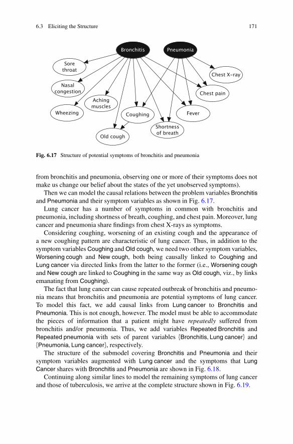
6.3 Eliciting the Structure 171

Fig. 6.17 Structure of potential symptoms of bronchitis and pneumonia

from bronchitis and pneumonia, observing one or more of their symptoms does notmake us change our belief about the states of the yet unobserved symptoms).

Then we can model the causal relations between the problem variables Bronchitisand Pneumonia and their symptom variables as shown in Fig. 6.17.

Lung cancer has a number of symptoms in common with bronchitis andpneumonia, including shortness of breath, coughing, and chest pain. Moreover, lungcancer and pneumonia share findings from chest X-rays as symptoms.

Considering coughing, worsening of an existing cough and the appearance ofa new coughing pattern are characteristic of lung cancer. Thus, in addition to thesymptom variables Coughing and Old cough, we need two other symptom variables,Worsening cough and New cough, both being causally linked to Coughing andLung cancer via directed links from the latter to the former (i.e., Worsening coughand New cough are linked to Coughing in the same way as Old cough, viz., by linksemanating from Coughing).

The fact that lung cancer can cause repeated outbreak of bronchitis and pneumo-nia means that bronchitis and pneumonia are potential symptoms of lung cancer.To model this fact, we add causal links from Lung cancer to Bronchitis andPneumonia. This is not enough, however. The model must be able to accommodatethe pieces of information that a patient might have repeatedly suffered frombronchitis and/or pneumonia. Thus, we add variables Repeated Bronchitis andRepeated pneumonia with sets of parent variables {Bronchitis; Lung cancer} and{Pneumonia; Lung cancer}, respectively.

The structure of the submodel covering Bronchitis and Pneumonia and theirsymptom variables augmented with Lung cancer and the symptoms that LungCancer shares with Bronchitis and Pneumonia are shown in Fig. 6.18.

Continuing along similar lines to model the remaining symptoms of lung cancerand those of tuberculosis, we arrive at the complete structure shown in Fig. 6.19.

172 6 Eliciting the Model

Fig. 6.18 Structure of potential symptoms shared by bronchitis, pneumonia, and lung cancer

Fig. 6.19 Complete structure of the extended chest clinic model

6.3 Eliciting the Structure 173

Notice the intermediate symptom variable Blockage or inflammation, which playsthe same role as variable HS in Example 6.5 on page 153 because hoarseness andwheezing are both symptoms of a blockage or an inflammation in the lungs causedby the lung cancer. Thus, without this intermediate variable, the (ground) symptomvariables Hoarseness and Wheezing would be direct symptoms of Lung cancer andhence conditionally independent whenever the state of Lung cancer is known. Thiswould be incorrect, as Hoarseness and Wheezing are conditionally independentonly if the state of their true common cause, namely, Blockage or inflammation, isknown. The gray coloring of the node in Fig. 6.19 on the facing page representingBlockage or inflammation indicates the (maybe not quite true) assumption that ablockage or an inflammation can be observed only indirectly through observationof Hoarseness and Wheezing.

Conclusion

This completes the (first iteration of) elicitation of a structure of the extended chestclinic model. The next phase of the model elicitation process consists of defining thedomains of the variables not already determined as part of the structure elicitationprocess.

In general, we wish variable domains to be as small as possible to minimize thecomplexity of eliciting the probability parameters of the model and to minimizethe complexity of inference. On the other hand, the number of states needs tobe big enough to achieve sufficient expressive power to adequately representthe relationships between the domain variables and thereby give the model thenecessary reasoning power and precision.

As a simple example, let us consider the task of defining the domain of variableSmoking severity, which is a potential cause of Bronchitis (in its chronic form) andLung cancer. Assuming that lung cancer can be caused by even small doses oftobacco smoke and that chronic bronchitis only occurs in cases where the patienthas been smoking intensely for many years, we can assume that Smoking severityneeds to have states none, mild, medium, and heavy. To keep the presentation ofthe elicitation process for the extended chest clinic example as simple as possible,we have deliberately avoided discussing how the idioms approach could have beenused. However, one of the exercises of this chapter addresses this issue.

6.3.4 The Generic Structure of Probabilistic Networks

From the elicitation of the structure of the extended chest clinic model, we haveexperienced that the typical overall structure of a probabilistic network shown inFig. 6.3 on page 155 can be elaborated a bit, as mediating variables can appear also

174 6 Eliciting the Model

Background variables

Root causes

Intermediate causes

Problem variables

Mediating variables

Symptom variables

Intermediate symptoms

Ground symptoms

Fig. 6.20 Typical expanded overall causal structure of a probabilistic network

as intermediate causes and intermediate symptoms. Figure 6.20 shows an elaborated(or expanded) version of the typical overall causal structure of a probabilisticnetwork.

A directed link between two dotted areas in Fig. 6.20 indicates that a directedlink from anyone of the two node categories in the “source area” to anyone of thetwo node categories in the “destination area.”

6.4 Model Verification

Proper use of idioms or identification and categorization of variables as backgroundvariables, problem variables, symptom variables, and mediating variables andadhering to the overall causal structure in Fig. 6.3 reduces the typical error of lettinglinks (arrows) point from symptom variables to problem variables. If, however, amodel contains links that point from effects to causes, inspection of the dependenceand independence properties represented by the model will often reveal a problemcaused by the reversed links.

Example 6.13 (Model Verification). Consider the following three Boolean variables(i.e., having state space {false; true}):

6.4 Model Verification 175

Two PCs Card copied

Fraud

(a)

Two PCs Card copied

Fraud

(b)

Fig. 6.21 Two competing models for Example 6.13

• Two PCs: Two or more PCs have been bought within a few days using the samecredit card.

• Card copied: The credit card has been used at almost the same time at differentlocations.

• Fraud: The credit card has been subject to fraud.

Now, the question is if model A in Fig. 6.21a is correct or model B in Fig. 6.21b iscorrect. Experience shows that most novices tend to prefer model A, probablybased on the notion that “input” leads to “output” (i.e., observations imply ahypothesis). That is, given the two pieces of information that the credit card hasbeen used to buy two or more PCs within a few days and that the card has beenused almost at the same time at different locations (the input), we can conclude thatthe card has been subject to fraud (the output). According to model A, however,information about Two PCs (Card copied) does not provide us with any informationabout Card copied (Two PCs) when no information is available about Fraud. This isobviously incorrect, as one piece of evidence confirming (or disconfirming) fraudwould obviously make us believe more (or less) in observing the other symptom offraud. Based on model A, we would thus get wrong posterior probabilities. Noticealso that model A does not have the typical causal structure as displayed in Fig. 6.3,as we identify Fraud as the problem variable and Two PCs and Card copied asinformation (symptom) variables.

Model B, on the other hand, rightfully tells us that:

• Two PCs and Card copied are dependent when we have no hard evidence onFraud: Observing Two PCs (Card copied) will increase our belief that we willalso observe Card copied (Two PCs).

• Two PCs and Card copied are independent when the state of Fraud is known:If we know that we are considering a case of fraud, then observing Two PCs(Card copied) will not change our belief about whether or not we are going toobserve Card copied (Two PCs).

As this example shows, close inspection of the dependence and independencerelations of a model may reveal links pointing in the wrong direction. However,adherence to the overall causal structure of Fig. 6.3 would eliminate the possibilityof arriving at model A.

176 6 Eliciting the Model

Using the idiom approach to structure elicitation in this case, one would have todecide whether to use the definitional/synthesis idiom or the cause–consequenceidiom (the measurement, reconciliation, and induction idioms would be readilyrejected). The definitional/synthesis idiom would make Fraud be defined in termsof Card copied and Two PCs, which would be awkward. For one thing, such adefinition would be open-ended, as there are an unlimited number of ways inwhich a credit card can be abused. Another, more convincing, argument why thedefinitional/synthesis idiom is the wrong choice is that it violates the overall causalstructure of Fig. 6.3. �

Despite its simplicity, Example 6.13 shows that it might be beneficial to combinethe idiom approach and the basic approach to structure elicitation. In other words,keeping in mind the overall causal structure of Fig. 6.3 might be helpful when achoice of idiom has to be made.

As illustrated in Example 6.5 on page 153, model verification may reveal aneed to introduce additional (mediating) variables. The mediating variable, HS, ofFig. 6.2 is a common cause of variables BT and UT. Identification of such commoncauses most often requires a close collaboration between a problem-domain expertand a knowledge engineer, as the domain expert often lacks the ability to read thedependence and independence properties displayed by a network structure and theknowledge engineer lacks insight into the causal mechanisms among the variablesof problem domain. As illustrated in the pregnancy example, failure to identifysuch hidden common causes (i.e., causes for which we have neither any immediateinterest in their probability distributions nor any (easy) way of observing their states)may lead to models that provide wrong answers. In the case of the pregnancymodel, exclusion of the variable HS would make the model exaggerate the influencefrom BT and UT when both are observed, as they are both indicative of the samephenomenon, namely, a possible change in the hormonal state of the cow.

6.5 Eliciting the Numbers

Once the structure of the probabilistic network has been established—probablythrough an iterative process involving model verification and model revisions,including identification of new variables; deletion and redefinition of existingvariables; and addition, deletion, and reversal of links—the next and usually themost difficult phase of constructing a probabilistic network concerns the elicitationof the quantitative information, including (conditional) probability distributions andutilities (jointly referred to as the “numbers” or the “parameters”).

Due to the (most often) quite demanding effort involved in eliciting the numbers,it is important to carefully verify the structure of the model before proceeding to thequantitative part of the model construction. Otherwise, one runs the risk of having toreject or alter already elicited numbers, as the kind of numbers required is dictatedby the model structure. Also, eliciting conditional probabilities with causal links

6.5 Eliciting the Numbers 177

reversed may be difficult and prone to errors. In practice, however, minor modelstructure adjustments are often made during the number elicitation process (e.g., toreduce the number of parameters).

The quantitative information of a probabilistic network (often referred to as theparameters of the model) is represented as real numbers in conditional probabilitytables (CPTs) and utility tables (UTs). CPTs represent (conditional) probabilitydistributions with domains spanning the interval Œ0I 1�, whereas UTs represent utilityfunctions with domains spanning �−∞I∞Œ.

The parameters of a probabilistic network can be retrieved from databases,elicited from (subjective) domain expert knowledge (e.g., from literature or inter-views of domain experts), or established through a mathematical model (e.g., basedon assumptions that a given probabilistic distribution can be approximated througha mixture of normal distributions). In this section, we shall focus only on the lattertwo approaches; see Chap. 8 for learning probability parameters from data.

6.5.1 Eliciting Subjective Conditional Probabilities

Part of the reason why elicitation of values of probability parameters can be ratherdemanding is that human reasoning is seldomly based on probabilities. In otherwords, a domain expert might find it awkward to express her/his domain-specificknowledge in terms of conditional probabilities and utility values. Thus, differentindirect ways of eliciting the quantitative knowledge may be used.

The fact that small differences in the values of probability (or utility) parametersoften make no difference in the recommendations provided by a model allowsfor parameter elicitation methods based on qualitative approaches. A qualitativeapproach often makes the domain expert more comfortable specifying her/hisknowledge about strengths of causal relations and relative preferences associatedwith decision problems. An example of a qualitative approach for assessing subjec-tive probabilities includes the usage of a so-called probability wheel. A probabilitywheel is a circle subdivided into n pie wedges, where n equals the number ofpossible states of the variable for which a (conditional) probability distribution isrequested. The domain expert then estimates a probability for a particular stateby sizing the corresponding pie wedge to match her/his best assessment of thatprobability.

Example 6.14 (Probability Wheel). A climate researcher asked to provide an esti-mate of the increase in the average global temperature over the next 100 years mightuse a probability wheel as shown in Fig. 6.22, working with a granularity of< 2 ıC,2–5 ıC, and > 5 ıC. �

Another example of a qualitative approach is the use of verbal statementslike “very unlikely” or “almost certain” that are then mapped to probabilities(see Fig. 6.23) (Renooij & Witteman 1999, van der Gaag, Renooij, Witteman &Taal 2002). The use of such a limited set of verbal statements often makes it quite alot easier for the domain expert to provide assessments of (conditional) probabilities.

178 6 Eliciting the Model

< 2ıC2–5ıC

> 5ıC

0:220:33

0:44

Fig. 6.22 Probability wheel with three pie wedges corresponding to three states of a variablerepresenting the increase in the average global temperature over the next 100 years. The relativearea occupied by a particular pie wedge represents the (conditional) probability for the associatedstate (indicated by the numbers next to the pie wedges)

0 Impossible0:05 Very unlikely0:1 Unlikely

0:2 Not probable

0:5 Fifty-fifty

0:8 Probable

0:9 Very probable0:95 Almost certain1 CertainFig. 6.23 Mapping of verbal

statements of probability toprobabilities

The reason why the scale in Fig. 6.23 is more fine-grained close to 0 and 1 is thatsmall and large probabilities usually have greater influence on the outcome thanthose closer to 0:5.

A simple gamble-based approach can be used for assessing the value of a prob-ability parameter. Assume that a domain expert is asked to assess the conditionalprobability that X D x when Y D y, that is, P.X D x |Y D y/. An indirect wayof making the expert assess this quantity would be to ask the expert to choose ann, where 0 � n � 100, such that he/she finds the following two gambles equallyattractive:

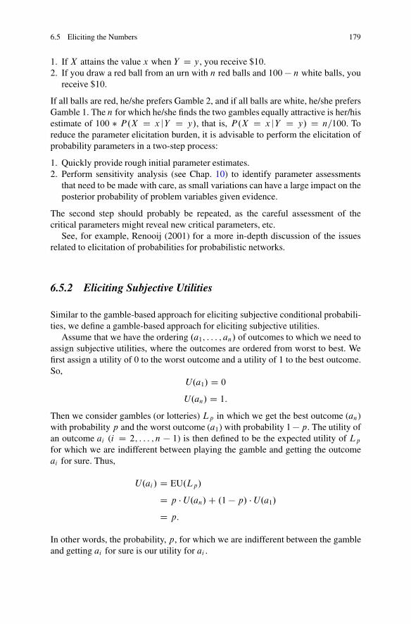
6.5 Eliciting the Numbers 179

1. If X attains the value x when Y D y, you receive $10.2. If you draw a red ball from an urn with n red balls and 100− n white balls, you

receive $10.

If all balls are red, he/she prefers Gamble 2, and if all balls are white, he/she prefersGamble 1. The n for which he/she finds the two gambles equally attractive is her/hisestimate of 100 � P.X D x |Y D y/, that is, P.X D x |Y D y/ D n=100. Toreduce the parameter elicitation burden, it is advisable to perform the elicitation ofprobability parameters in a two-step process:

1. Quickly provide rough initial parameter estimates.2. Perform sensitivity analysis (see Chap. 10) to identify parameter assessments

that need to be made with care, as small variations can have a large impact on theposterior probability of problem variables given evidence.

The second step should probably be repeated, as the careful assessment of thecritical parameters might reveal new critical parameters, etc.

See, for example, Renooij (2001) for a more in-depth discussion of the issuesrelated to elicitation of probabilities for probabilistic networks.

6.5.2 Eliciting Subjective Utilities

Similar to the gamble-based approach for eliciting subjective conditional probabili-ties, we define a gamble-based approach for eliciting subjective utilities.

Assume that we have the ordering .a1; : : : ; an/ of outcomes to which we need toassign subjective utilities, where the outcomes are ordered from worst to best. Wefirst assign a utility of 0 to the worst outcome and a utility of 1 to the best outcome.So,

U.a1/ D 0

U.an/ D 1:

Then we consider gambles (or lotteries) Lp in which we get the best outcome (an)with probability p and the worst outcome (a1) with probability 1−p. The utility ofan outcome ai (i D 2; : : : ; n − 1) is then defined to be the expected utility of Lpfor which we are indifferent between playing the gamble and getting the outcomeai for sure. Thus,

U.ai / D EU.Lp/

D p � U.an/C .1− p/ � U.a1/D p:

In other words, the probability, p, for which we are indifferent between the gambleand getting ai for sure is our utility for ai .

180 6 Eliciting the Model

6.5.3 Specifying CPTs and UTs Through Expressions

Probability distributions and utility functions in probabilistic networks often follow(at least approximately) certain functional or distributional forms. In such cases,the CPTs/UTs can be described compactly through mathematical expressions.Apart from ease of specification, specification through expressions also makesmaintenance and reuse much easier.

An expression may be built using standard statistical distributions (e.g., normal,binomial, beta, gamma), arithmetic operators, standard mathematical functions(e.g., logarithmic, exponential, trigonometric, and hyperbolic functions), logicaloperators (e.g., and, or, if-then-else), and relations (e.g., less than, equals).

The different operators used in an expression have different return types anddifferent type requirements for arguments. Thus, in order to provide a rich languagefor specifying expressions, it is convenient to have a classification of the discretechance and decision variables into different groups:

• Labeled variables have state spaces of arbitrary qualitative descriptors providedin the form of character strings. Labeled variables can be used in equalitycomparisons and to express deterministic relationships. For example, a labeledvariable C1 with states state 1 and state 2 can appear in an expression likeif.C1 D state 1;Distribution.0:2;0:8/;Distribution .0:4; 0:6// forP.C2 |C1/, where C2 is another discrete chance variable with two possible statesand where if.p; a; b/ is read as if predicate p is true, then a else b.

• Boolean variables represent the truth values “false” and “true” (in that order) andcan be used in logical operators. For example, for a Boolean variable, B0, beingthe logical OR of its (Boolean) parents, B1, B2, and B3, P.B0 |B1;B2; B3/ canbe specified simply as or.B1;B2;B3/.

• Numbered variables represent increasing sequences of numbers (integers orreals) and can be used in arithmetic operators, mathematical functions, etc. Forexample, a numbered variable with state space {1; 2; 3; 4; 5; 6} can represent theoutcome of the roll of a die.

• Interval variables represent disjoint intervals on the real line and can be usedin the same way as numbered variables. In addition, they can be used whenspecifying the intervals over which a continuous quantity is to be discretized. Forexample, an interval variable with state space {Œ0I 2Œ; Œ2I 5Œ; Œ5I 10Œ} may representthe increase in the average global temperature over the next 100 years (cf.Example 6.14 on page 177).

Table 6.2 shows some examples of possible states of the various subtypes ofdiscrete chance variables.

Based on the semantics of discrete chance nodes provided by the above subtyp-ing, an algorithm for automatic generation of CPTs and UTs can be implemented.The functionality of such a table generator will be dependent on the subtypes ofthe variables involved. Table 6.3 shows how the functionality of a table generatoralgorithm might be dependent on variable subtypes.

6.5 Eliciting the Numbers 181

Table 6.2 Examples ofpossible states of the varioussubtypes of discrete chancevariables

Subtype Sample states

Labeled red, blue, lowBoolean false, true

Numbered −∞; : : : ;−2:2;−1:5; 0; 1; 2; 3; : : : ;∞

Interval �−∞I−10Œ; Œ−10I−5Œ; Œ−5I−1Œ

Table 6.3 The functionality of a table generator algorithm is dependent on thesubtype of the involved variables

Operation Labeled Boolean Numbered Interval Utility

If-then-else + + + + +Arithmetic operators + + +Boolean operators +Boolean comparison +Boolean distributions +Continuous distributions +Discrete distributions +Custom distribution +

Example 6.15 (Number of People (HUGIN 2006)). Assume that in some appli-cation, we have probability distributions over the number of males and females,where the distributions are defined over intervals Œ0I 100Œ, Œ100I 500Œ, Œ500I 1000Œand that we wish to compute the distribution over the total number of individualsgiven the two former distributions. (Note that this is an obvious sample usageof the definitional/synthesis idiom presented in Sect. 6.3.2 on page 157.) It is asimple but tedious task to specify P.NI |NM;NF /, where NI , NM , and NF standfor the number of individuals, the number of males, and the number of females,respectively. A much more expedient way of specifying this conditional probabilitydistribution would be to let NM and NF be interpreted as interval variables withstates Œ0I 100Œ, Œ100I 500Œ, and Œ500I 1000Œ and to let NI be interpreted as an intervalvariable with states Œ0I 200Œ, Œ200I 1000Œ, and Œ1000I 2000Œ, for example, and thendefine P.NI |NM;NF / through the simple expression NI D NM C NF . Thealternative would require specification (including computation) of 27 probabilityparameters; see Table 6.4. �

Example 6.16 (Fair or Fake Die (HUGIN 2006)). Consider the problem of com-puting the probabilities of getting n sixes in n rolls with a fair die and a fake die,respectively. A random variable, X , denoting the number of sixes obtained in nrolls with a fair die is binomially distributed with parameters .n; 1=6/. Thus, theprobability of getting k sixes in n rolls with a fair die is Pfair.X D k/, where Pfair isa Binomial.n; 1=6/. Assuming that for a fake die the probability of six pips facingup is 1=5, the probability of getting k sixes in n rolls with a fake die isPfake.X D k/,where Pfake is a Binomial.n; 1=5/.

A model of this problem is shown in Fig. 6.24, where #6 0s depends on #rollsand Fake die‹. Now, if we let #rolls be interpreted as a numbered variable withstate space {1; 2; 3; 4; 5}, let Fake die‹ be interpreted as a Boolean variable, and

182 6 Eliciting the Model

Table 6.4 The CPT for P.NI |NM;NF / in Example 6.15 generated fromthe expression NI D NM CNF

NI

NF NM Œ0I 200Œ Œ200I 1000Œ Œ1;000I 2;000ŒŒ0I 100Œ Œ0I 100Œ 1 0 0

Œ0I 100Œ Œ100I 500Œ 0:1248 0:8752 0

Œ0I 100Œ Œ500I 1000Œ 0 0:8960 0:1040

Œ100I 500Œ Œ0I 100Œ 0:1248 0:8752 0

Œ100I 500Œ Œ100I 500Œ 0 1 0

Œ100I 500Œ Œ500I 1000Œ 0 0:4 0:6

Œ500I 1000Œ Œ0I 100Œ 0 0:8960 0:1040

Œ500I 1000Œ Œ100I 500Œ 0 0:4 0:6

Œ500I 1000Œ Œ500I 1000Œ 0 0 1

#rolls Fake die‹

#60s

Fig. 6.24 A model for thefake die problem

Table 6.5 The CPT for P.#60s |#rolls; Fake die‹/ in the fake die problem of Example6.16 generated from the expression Binomial.#rolls;if.Fake die‹; 1=5; 1=6//

#60s

Fake die‹ #rolls 0 1 2 3 4 5

false 1 0:8333 0:1666 0 0 0 0

false 2 0:6944 0:2777 0:0277 0 0 0

false 3 0:5787 0:3472 0:0694 0:0046 0 0

false 4 0:4822 0:3858 0:1157 0:0154 0:0007 0

false 5 0:4018 0:4018 0:1607 0:0321 0:0032 0:0001

true 1 0:8 0:2 0 0 0 0

true 2 0:6400 0:3200 0:0400 0 0 0

true 3 0:5120 0:3840 0:0960 0:0080 0 0

true 4 0:4096 0:4096 0:1536 0:0256 0:0016 0

true 5 0:3276 0:4096 0:2048 0:0512 0:0064 0:0003

let #6 0s be interpreted as a numbered variable with state space {0; 1; 2; 3; 4; 5}, thenP.#6 0s |#rolls; Fake die‹/ can be specified elegantly using the expression

P.#6 0s |#rolls; Fake die‹/ D Binomial.#rolls;if.Fake die‹; 1=5; 1=6//:

Filling in the probabilities by hand would require computation of 60 values of thebinomial function with different parameters; see Table 6.5. �

Example 6.17 (Discretizing a Variable (HUGIN 2006)). Assume that P.C1 |C2/can be approximated by a normal distribution with mean given by C2 and with

6.6 Concluding Remarks 183

Table 6.6 The CPT for P.C1 |C2/ in the discretization problem of Example 6.17generated from the expression Normal.C2; 1/

C1

C2 � −∞I−5Œ Œ−5I−2Œ Œ−2I 0Œ Œ0I 2Œ Œ2I 5Œ Œ5I∞Œ

Œ−5I−1Œ 0:0996 0:6297 0:2499 0:0207 9:4E−5 3:8E−11

Œ−1I 0Œ 7:1E−6 0:0748 0:6096 0:3075 0:0081 5:3E−8

Œ0I 1Œ 5:3E−8 0:0081 0:3075 0:6096 0:0748 7:1E−6

Œ1I 5Œ 3:8E−11 9:4E−5 0:0207 0:2499 0:6297 0:0996

variance 1, where C2 is an interval variable with states Œ−5I−1Œ, Œ−1I 0Œ, Œ0I 1Œ,Œ1I 5Œ. If the discretization of C1 given by the intervals �−∞I−5Œ, Œ−5I−2Œ, Œ−2I 0Œ,Œ0I 2Œ, Œ2I 5Œ, Œ5;∞Œ is found to be suitable, then we can specify P.C1 |C2/ simply asNormal.C2; 1/. The probability distribution P.C1 |C2 D c2/ (i.e., the conditionaldistribution for C1 given that the value of C2 belongs to interval c2) is generated bycomputing a large number of probability distributions forC2, each distribution beingobtained by instantiating C1 to a value in the interval, c2, under consideration. Theaverage of these distributions (based on, e.g., the midpoints of 25 subintervals) isused as P.C1 |C2 D c2/. Hence, for expressions involving several interval variablesas parents, the generation of the CPT may be computationally intensive. Table 6.6shows P.C1 |C2/. �

6.6 Concluding Remarks

In this chapter we have tried to convey a set of good practices, routines, and hintsthat can be helpful for novices wanting to construct a probabilistic network modelfor a problem domain.

When constructing a model (probabilistic or not), it is crucial to realize thatreal-world problem domains are usually embedded in a complex reality involvinginteraction with numerous different aspects of the real world in a way that can neverbe fully captured in a model. Also, the internal causal mechanisms of a problemdomain can almost always only be approximately described in a model. Thus, it isimportant to bear in mind that all models are wrong, but that some might be useful.

Based on this insight, it is important to clearly state the context of the model aswell as the assumptions and conditions under which it is supposed to work. Real-world problem domains exist in an open world, whereas models for the problemdomains are based on a (most often, erroneous) closed-world assumption.

The construction of a probabilistic network typically runs through four mainphases:

Design of the network structure, covering identification of variables and (causal)relations among the variables. In addition, verification of the network structure isan essential activity of the design phase, where the dependence and independencerelations represented in the model are stated and verified.

184 6 Eliciting the Model

Implementation of the network, covering the process of populating the CPTs andUTs with (conditional) probabilities and utilities. This phase is often the mostlabor intensive of the four phases.

Test of the network to check if it provides sensible outputs to a carefullyselected set of inputs. In a medical setting, for example, testing may amount toentering patient data and comparing network recommendations (e.g., diagnosesor treatment plans) with recommendations provided by medical experts. If thetest phase does not reveal any flaws of the network, construction of the networkis considered successfully completed.

Analysis of the network is performed to pinpoint problematic aspects of thenetwork revealed in the test phase. Various tools may be brought into play,including conflict analysis (see Chap. 9), sensitivity analyses (see Chap. 10), andvalue of information analysis (see Chap. 11).

In the design phase, it is crucial to clearly define the problem that is going tobe addressed by the model and to pay close attention to this problem definitionwhen identifying the variables of the model. It is strongly recommended to keep thenumber of variables and (causal) relations among them to a minimum; only thosevariables and relations that are thought to have significant influences on the problemvariable(s) should be included.

In his writings, William of Occam (or Ockham) (1284–1347) stressed theAristotelian principle that entities must not be multiplied beyond what is necessary.This principle became known as Occam’s razor or the law of parsimony; a problemshould be stated in its basic and simplest terms. In science, the simplest theory thatfits the facts of a problem is the one that should be selected. This rule is interpretedto mean that the simplest of two or more competing theories is preferable and thatan explanation for unknown phenomena should first be attempted in terms of whatis already known.1

One argument why one should go for simpler rather than complex solutions toa problem lies in the fact that simpler solutions impose less assumptions about theproblem (e.g., about dependences and independences) and hence postulate fewerhypothetical solutions. The underlying idea is thus that simpler solutions are morelikely to be “correct.”

A key design principle applied in the construction of virtually any complexsystem is the principle of a modular top-down design in which the level ofabstraction changes from the more abstract to the more concrete. To support amodular design approach, clear descriptions of the interface mechanisms of themodules must be provided. Also, given clear interface descriptions, cooperationamong sub-teams, reuse modules (submodels), and support for bottom-up design aremade possible. There are several reasons why an object-oriented modeling approach(see Sect. 4.3), which facilitates exactly a modular model construction approach that

1This paragraph is taken from http://www.2think.org/occams razor.shtml.

6.7 Summary 185

allows for both top-down and bottom-up design, is recommended for constructinglarge models:

• Large and complex systems are often composed of collections of identical orsimilar components. Therefore, models of such systems will naturally containrepetitive submodels. Object orientation allows such components to be instanti-ated from a generic class. Both construction and maintenance become a wholelot easier in this way: Each component is generated simply through instantiation,and changes that apply to all instances should be made only in the class fromwhich the components have been instantiated.

• Many complex real-world systems (e.g., mechanical and biological systems)are naturally described in terms of hierarchies of components (i.e., the systemconsists of components, which consist of subcomponents, etc.). Thus, oftenan object-oriented probabilistic network (OOPN) more naturally describes thestructure of the system modeled.

• Object-oriented model construction supports both top-down and bottom-upmodes of construction, which are often used, respectively, to maintain a goodoverview of the model by abstracting away irrelevant details and to focuson subcomponents with a well-defined interfaces to their surroundings. Thus,the OOPN framework provides support for working with different levels ofabstraction in the model constructing process.

• Object-oriented model construction provides a natural means to reuse of existingsubmodels. That is, the methodology provides a means to maintain a library ofsubmodels that can be instantiated in many different OOPNs.

• Specifying a model in a hierarchical fashion often makes the model less clutteredand thus provides a better means of communicating ideas among knowledgeengineers, domain experts, and users.

• The composition of a model by a number of components with well-definedinterfaces supports a collaborative model construction process, where differentmodel constructors work on different parts of the model.

Finally, it is important to realize that construction of a probabilistic network isan iterative process in the sense that if model testing reveals flaws of the model,another cycle through the model construction phases mentioned above is necessary.In most practical model construction projects, many iterations are needed before aworkable model is found. This iterative or spiral process, which is well known fromalmost all areas of engineering, is illustrated in Fig. 6.25.

6.7 Summary

Manual construction of a probabilistic network for a complex decision or diagnosisproblem is usually a demanding task, involving different sources of expertise thatprovide model engineering skills as well as deep understanding of the problemdomain. The model elicitation process requires careful problem definition, careful

186 6 Eliciting the Model

Fig. 6.25 Modeldevelopment is an activitythat iteratively passes throughdesign, implementation, test,and analysis phases untilmodel tests no longer uncoverundesired behavior of themodel

identification of the relevant variables and dependences/independences among thevariables, and elicitation of many (conditional) probabilities and utilities.

However, appealing a probabilistic network might seem in terms of compactnessof representation and in terms of serving as an intuitive means for communicationof problem-domain characteristics, there exist problems for which probabilisticnetworks are not the ideal tool to use. In Sect. 6.1, we discussed some characteristicsof probabilistic networks and some criteria for using them. Briefly, and most impor-tantly, the variables of the problem domain should be well defined, causal relationsamong the variables should be identifiable, uncertainty should be associated withthe causal relations, and the problem should contain an element of decision makingwith a desire to maximize the expected utility of a decision.

In Sect. 6.2, we discussed how to identify the right set of variables of aprobabilistic network and what it takes for a variable to be well defined. A simpletaxonomy of variables was introduced, which includes three basic types of variablesand their causal relations. Problem variables (or hypothesis variables) representthe diagnoses, classifications, predictions, decisions, etc., to be made. Informationvariables represent the available information (evidence) that can provide infor-mation relevant for solving the problem. Finally, mediating variables representunobservable entities of the problem domain for which posterior probabilities areof no immediate interest but which play an important role for achieving the rightdependence and independence properties of the network or for making efficientinference.

In Sect. 6.3, we first described a basic approach to structure elicitation, showinghow the variable taxonomy can be used in the attempt to elicit the model structure.Next, we described how the notion of idioms can be helpful in identifying fractionsof a network structure, depending on the nature of the semantic relations that existamong a small set of variables. Five idioms, thought to cover the vast majority ofcommonly occurring semantic relationships, were presented. The five idioms can

Exercises 187

be thought of as five archetypical modes of uncertain reasoning, and thus, using theidioms approach to elicitation of model structure, one is encouraged to think at ahigher level of abstraction, leaving behind details about which links to include andtheir directionality.

Although the basic approach to structure elicitation can be quite feasible for someproblems, for most (large) real-world problems, the use of idioms is preferable, asthe idioms approach splits the problem into smaller and more manageable chunks.

In Sect. 6.4, we briefly touched upon the issue of model verification, an importantactivity immediately following the structure elicitation effort. In the model verifica-tion process, one checks if the dependence and independence statements imposedby the structure are consistent with the knowledge of problem-domain experts.

In Sect. 6.5, we presented some techniques that might be considered in theattempt to elicit the (subjective) values of the parameters (i.e., (conditional)probabilities and utilities) dictated by the structure of the model. Also, we presenteda lower-level taxonomy for variables, distinguishing among them in terms of theirtypes of domains. Knowledge about the types of domains of variables allowsfor automatic generation of CPTs and UTs through a language of mathematicaloperations, including if-then-else statements, arithmetic and Boolean operations,and a variety of discrete and continuous distributions. The ability to define CPTsand UTs in terms of compact mathematical expressions might greatly reduce theburden of eliciting the numbers (parameter values) of a probabilistic network.

We concluded the discussion on model elicitation in Sect. 6.6 by pointing outsome typical main phases of the model construction process, and how these phasesare repeated iteratively until model tests no longer uncover undesired behavior ofthe model. Also, we pointed to the fact that the best models are usually constructedthrough deliberate use of the law of parsimony (or Occam’s razor). Finally, wetouched upon the potential benefits of applying an objected-oriented modelingapproach, which facilitates modular model construction with the freedom to usea top-down or a bottom-up approach. The use of an object-oriented approach isespecially beneficial for construction of large models.

Exercises

Exercise 6.1. There are three condemned prisoners A, B, and C. The governor hasannounced that one of the three, chosen at random, has been pardoned, but doesnot say which. Prisoner A, realizing that he only has a 1=3 chance of having beenpardoned, reasons with the warden as follows: “Please tell me the name of oneof the other prisoners B or C who will be executed. I already know that at leastone of them will be executed so you will not be divulging any information.” Thewarden then asks how he should choose between B or C in case both are to beexecuted. “In that case,” A tells him, “simply flip a coin (when I’m not around)to choose randomly between the two.” The warden agrees and later tells A that B

188 6 Eliciting the Model

will be executed. On hearing this news, A smiles and thinks to himself, “Now mychances of having been pardoned have increased from 1=3 to 1=2.”

(a) Identify the variables of a Bayesian network model of the reasoning made byprisoner A.

(b) Specify the domains of the variables.(c) Are your variables well defined? Why or why not?(d) Characterize the variables in terms of the taxonomy presented in Sect. 6.2.2

on page 152 and specify the causal links of your model using the prototypicalcausal structure shown in Fig. 6.3.

(e) Specify the (conditional) probabilities of your model and check if your modelagrees with the conclusion drawn by prisoner A.

Exercise 6.2. In Exercise 6.1, consider the suggestion to define three variables A,B , and C to represent the three prisoners. Are these variables well defined? If so,why? If not, why not?

Exercise 6.3. In the morning, when Mr. Holmes leaves his house, he realizes thathis grass is wet. He wonders whether it has rained during the night or whether hehas forgotten to turn off his sprinkler. He looks at the grass of his neighbors, Dr.Watson and Mrs. Gibbon. Both lawns are dry, and he concludes that he must haveforgotten to turn off his sprinkler.

(a) Identify the relevant variables a probabilistic network representing Mr. Holmes’reasoning problem. Also, identify the domains of the variables.

(b) Characterize the variables in terms of the taxonomy presented in Sect. 6.2.2on page 152 and specify the causal links of your model using the prototypicalcausal structure shown in Fig. 6.3.

(c) If you were to construct the model using the idioms approach, which idiom(s)would you use?

(d) Verify that your model is consistent with the following dependence andindependence statements:

1. Information about the states of the lawns (i.e., wet or dry) is independent ifwe know that it has rained; otherwise, they are dependent.

2. Information about the state of rain and information about the state ofHolmes’ sprinkler are dependent if the state of Holmes’ lawn is known;otherwise, they are independent.

Exercise 6.4. Consider the inference problem in Example 2.4 on page 25, which isstated as follows:

Mr Holmes is working in his office when he receives a phone call from his neighbor Dr.Watson, who tells him that Holmes’ burglar alarm has gone off. Convinced that a burglarhas broken into his house, Holmes rushes to his car and heads for home. On his way, helistens to the radio, and in the news, it is reported that there has been a small earthquake inthe area. Knowing that earthquakes have a tendency to turn burglar alarms on, he returns tohis work.

Exercises 189

B E

A R

W

• W : Phone call from Watson• A: Burglary alarm• B: Burglary• R: Radio news• E: Earthquake

Fig. 6.26 Structure of a Bayesian network for the “burglary or earthquake” inference problem

The structure of a Bayesian network for this inference problem is shown inFig. 6.26:

(a) Classify the variables in Fig. 6.26 according to the taxonomy in Sect. 6.2.2 onpage 152.

(b) Verify that the structure in Fig. 6.26 is consistent with the prototypical causalstructure shown in Fig. 6.3 on page 155.

Exercise 6.5. Consider the structure of the extended chest clinic model in Fig. 6.19on page 172:

(a) Which kinds of idioms could have been applied in eliciting the structure?(b) Give examples of substructures of the structure that could have been derived

using the kinds of idioms suggested in part (a).

Exercise 6.6. Consider the task of providing your subjective probabilities of whois going to win the next World Cup in soccer:

(a) Provide your probability that Brazil wins.(b) Consider the following gambles:

1. If Brazil wins, you receive $10.2. If you draw a red ball from an urn with n red balls and 100− n white balls,

you receive $10.

For which value of n are the two gambles equally attractive to you?(c) Compare your original subjective probability that Brazil wins with n=100

from (b).

Chapter 7Modeling Techniques

In this chapter we introduce a set of modeling methods and techniques forsimplifying the specification of a probabilistic network.

The construction of a probabilistic network may be a labor-intensive task toperform. The construction involves a sequence of steps such as identifying variables,identifying states of variables, encoding dependence and independence relations asan acyclic, directed graph, and eliciting (conditional) probabilities and utilities asrequired by the structure of the acyclic, directed graph.

There are many reasons for considering the utilization of modeling techniques inthe model development process. Modeling techniques may be applied in order, forinstance, to simplify knowledge elicitation and model specification, capture certainproperties of the problem domain that are not easily captured by an acyclic, directedgraph, to reduce model complexity and improve efficiency of inference in the model,and so on.

Section 7.1 considers modeling techniques for adjusting the structure of a prob-abilistic network. This includes, in particular, modeling techniques that capturescertain structural properties of the problem domain that help reduce the complexityof a model. Section 7.2 considers modeling techniques for the specification ofconditional probability distributions. This includes modeling techniques for cap-turing uncertain information and for reducing the number of parameters to specify.Finally, Sect. 7.3 considers modeling techniques for influence diagram models. Thisincludes modeling techniques of capturing properties of a problem domain thatseemingly do not fulfill the underlying assumptions of influence diagrams.

7.1 Structure-Related Techniques

In this section we consider modeling techniques related to the structure of a proba-bilistic network. In particular, we consider parent divorcing, temporaltransformation, the representation of structural and functional uncertainty, undi-rected dependence links, bidirectional relations, and the naive Bayes model.

U.B. Kjærulff and A.L. Madsen, Bayesian Networks and Influence Diagrams: A Guideto Construction and Analysis, ISS 22, DOI 10.1007/978-1-4614-5104-4 7,© Springer Science+Business Media New York 2013

191

192 7 Modeling Techniques

X1 X2 X3

Y

(a)

X1 X2 X3

I

Y

(b)

Fig. 7.1 (a) X1, X2, and X3 are direct parents of Y . (b) X3 is a direct parent of Y , while thecombined influence of X1 and X2 is mediated through I

7.1.1 Parent Divorcing

The modeling techniques referred to as parent divorcing (Olesen, Kjærulff, Jensen,Jensen, Falck, Andreassen & Andersen 1989) is a commonly used modelingtechnique for reducing the complexity of a model by adjusting the structure ofthe graph of a probabilistic network. The technique of parent divorcing can beapplied to reduce the complexity of specifying and representing the direct impact ofa relatively large number of variablesX1; : : : ; Xn, referred to as the cause variables,on a single variable Y , referred to as the effect variable.

The basic idea of parent divorcing is to introduce layers of intermediate variablesbetween the effect variable Y and its direct causes X1; : : : ; Xn such that eachintermediate variable I captures the impact of its parents on the child variable. Theparents of I may consists of a subset of intermediate variables and cause variables.

Figure 7.1a illustrates a model structure where the variable Y has three direct par-ent causesX1;X2;X3. Parent divorcing applied to Y and its direct causesX1;X2;X3amounts to introducing a mediating variable I between Y and a subset of itsparents X1;X2;X3. Let the subset of parents be X1 and X2 such that Y after parentdivorcing has parentsX3 and I while X1 and X2 are parents of I . The result of thisprocess is as illustrated in Fig. 7.1b. Notice that X1 and X2 are divorced from theremaining parents of Y .

The following example illustrates how the use of parent divorcing may reducethe size of a conditional probability distribution significantly by exploiting structurewithin conditional probability distributions.

Example 7.1 (Parent Divorcing). Consider Fig. 7.1 and assume Y is defined asthe disjunction (denoted ∨) of its three parents X1, X2, and X3. This implies thatthe conditional probability distribution P.Y |X1;X2;X3/ is defined as shown inTable 7.1.

7.1 Structure-Related Techniques 193

Table 7.1 The conditionalprobabilitydistribution P.Y |X1;X2; X3/

Y

X1 X2 X3 false true

false false false 1 0

false false true 0 1

false true false 0 1

false true true 0 1

true false false 0 1

true false true 0 1

true true false 0 1

true true true 0 1

X1 X2 X3

X1 ∨X2

Y

Fig. 7.2 Parent divorcingapplied to the distribution forY D X1 ∨ X3 ∨X3

Table 7.2 The conditionalprobabilitydistribution P.X1 ∨X2 |X1;X2/

X1 ∨X2

X1 X2 false true

false false 1 0

false true 0 1

true false 0 1

true true 0 1

By inspection of Table 7.1, it is clear that the conditional probability distri-bution P.Y |X1;X2;X3/ has a lot of structure. This structure can be exploitedto reduce the size of the largest conditional probability distribution using parentdivorcing.

The structure in Fig. 7.1a defines Y as Y D X1 ∨X2 ∨X3 disregarding the factthat disjunction (∨) is a binary operator. On the other hand, the structure shown inFig. 7.2 defines Y as Y D .X1 ∨ X2/ ∨ X3 by introducing a mediating variableTable 7.2 (the distribution P.Y |X1 ∨X2;X3/ is equivalent).

Thus, instead of having one distribution of size 16 we have two tables ofsize 8. The reduction in size of the largest conditional probability table may seeminsignificant. However, if there is a large number of parents, the reduction issignificant. The reduction may make an otherwise intractable task tractable. �

The fundamental idea of parent divorcing is that through the utilization ofmediating variables, it may be possible to divorce subsets of parents of the effect

194 7 Modeling Techniques

Table 7.3 The conditionalprobability distribu-tion P.Y |X1; : : : ; Xm/

Y

X1 X2 X3 � � � Xm y1 � � � yn

x1 x2 x3 � � � xm z1 � � � zn:::

:::

x1 x0

2 x3 � � � xm z0

1 � � � z0

n

:::

:::

x0

1 x2 x3 � � � xm z0

1 � � � z0

n

:::

:::

x0

1 x0

2 x3 � � � xm z1 � � � zn

X1 X2 X3 � � � Xm

I

Y

Fig. 7.3 Parent divorcing ingeneral

variable in order to limit the size of parent sets. Parent divorcing is almost only usedwhen the relation among parent variables can be expressed as a chain of associativebinary operations such as ∨;∧;min;max;C;−; : : :.

In general, the underlying assumption of parent divorcing is that the configura-tions of .X1;X2/, that is, pairs of instantiations ofX1 andX2, can be partitioned intosets i1; : : : ; im such that different configurations .x1; x2/; .x0

1; x02/ 2 ii if and only if

for all y:

P.y |x1; x2; x3; : : : ; xn/ D P.y |x01; x

02; x3; : : : ; xn/:

Table 7.3 shows how the conditional distribution P.Y |X1; : : : ; Xm/may supportthe use of parent divorcing. For different configurations of X1 and X2, the childvariable Y has the same distribution, for example, for configurations .x1; x2/and .x0

1; x02/, the distribution of Y is z1; : : : ; zn.

An intermediate variable I may be introduced in order to exploit of the structureof P.Y |X1; : : : ; Xm/. Figure 7.3 illustrates how the intermediate variable I isintroduced as a parent of Y and a child of X1 and X2.

The conditional probability distribution of the intermediate variable I is oftena deterministic function in configurations of its parents. Table 7.4 shows theconditional probability distribution P.I |X1;X2/.

Since I replaces X1 and X2 as parents of Y , the conditional probabilitydistribution of Y changes. Table 7.5 shows the conditional probability distribu-tion P.Y |I;X3; : : : ; Xm/.

7.1 Structure-Related Techniques 195

Table 7.4 The conditionalprobabilitydistribution P.I |X1;X2/

I

X1 X2 i1 i2

x1 x2 1 0

x1 x0

2 0 1

x0

1 x2 0 1

x0

1 x0

2 1 0

Table 7.5 The conditionalprobability distribu-tion P.Y |I; X3; : : : ; Xm/

Y

I X3 � � � Xm y1 � � � yn

i1 x3 � � � xm z1 � � � zn:::

:::

i2 x3 � � � xm z0

1 � � � z0

n

The above property is captured by introducing a mediating variable I as parentof Y with X1 and X2 as parents. Parent divorcing is particularly useful in situationswhere the state space size of the intermediate variable is (significantly) smallerthan the combined state space of its parents. Example 7.1 on page 192 shows onesituation where parent divorcing improves the efficiency of a model. That is, parentdivorcing is (representationally) efficient if ||I || < ||X1|| � ||X2||, that is, if the numberof subsets is less than the combined state space size of X1 and X2.

Parent divorcing may be considered as a relevant modeling technique when spec-ifying P.Y |X1; : : : ; Xn/ is a significant or even intractable knowledge acquisitiontask or when the size of n makes probabilistic inference intractable.

Notice that parent divorcing can always be applied to a variable and its parents.If the intermediate variable I in Fig. 7.1b has one state for each configuration of itsparents, then the conditional probability distribution P.Y |X3; I / can be consideredas equivalent to P.Y |X1;X2;X3/. In this case, nothing has been gained fromapplying parent divorcing with respect to reducing the complexity of the model orimproving efficiency of the model.

How to Implement This Technique

The parent divorcing modeling technique is implemented as follows:

1. Let XW pa.Y / be the subset of parents of Y to be divorced from pa.Y / \ XW .2. Create an intermediate node I as a common child of XW and a new parent of Y

replacing XW as parents of Y .3. Let I have one state for each subset of XW mapping to the same distribution

on Y .4. Define the distribution of I given XW such that each subset of XW mapping to

the same distribution on Y maps to the same state of I .5. Repeat the above steps for each subset XW pa.Y / to be divorced from

pa.Y / \ XW .

196 7 Modeling Techniques

X1

X2 X3 X4

Y1 Y2 Y

Fig. 7.4 Modeling atemporal order of the impactsof X1; : : : ; X4 on Y

7.1.2 Temporal Transformation

In this section we focus on applying the temporal transformation to adjust thenetwork structure to capture structure within a conditional probability distributionof an effect variable Y given a set of causes X1; : : : ; Xn expressing a temporal (orcausal) order on the impact of the cause variables on the effect variable Y . Insteadof combining causes pairwise as in parent divorcing, the influence of causes on theeffect variable is taken into account one cause at a time in their causal or temporalorder.

The method of temporal transformation is best illustrated by an example.Figure 7.4 shows the result of applying the temporal order method on the conditionalprobability distribution of a variable Y given cause variables X1, X2, X3, and X4.Notice the temporal order on the causal impacts of the cause variables on the effectvariable. The intermediate variables Y1 and Y2 have the same state spaces as Y .

The variables in Fig. 7.4 may represent causesX1,X2, andX3 of a disease Y anda medicamentX4 for curing the disease. The causes X1, X2, and X3 add to the levelof the disease Y independently, while the medicament cures the disease no matterthe level of the disease. In this example, it is important that X4 is the last variable inthe temporal order of the causes. The example could be extended such that X1, X2,and X3 represent different risk factors of the disease that have a temporal order.

The temporal transformation method was introduced by Heckerman (1993)and refined by Heckerman & Breese (1994). A temporal order of the causalimpacts of X1; : : : ; Xn on Y is not necessary for applying the method of temporaltransformation. In addition to representing a temporal order of causal influence, thetemporal transformation method can be used as an alternative to parent divorcing.The parent divorcing method described in the previous section also captures internalstructure of a conditional probability distribution of an effect variable given a set ofcause variables. The parent divorcing method often constructs a (balanced) binarytree combining causes pairwise recursively, while the temporal transformationmethod constructs an unbalanced binary tree as illustrated in Fig. 7.4.

The temporal transformation was introduced by Heckerman (1993) as a methodfor representing causal independence between a set of cause variables X1; : : : ; Xnwith a common effect E. The model structure in Fig. 7.1a on page 192 does notcapture the property that cause variables X1; : : : ; Xn impact the effect variable Eindependently. Temporal transformation can be used to implement independence ofcausal influence as defined in Sect. 7.2.5.

7.1 Structure-Related Techniques 197

A B X1 X2

Y

? ?

a

A B S

P X1 X2

Y

b

Fig. 7.5 (a) Should A or B be the parent of Y ? (b) Modeling structure and functionalityuncertainty

How to Implement This Technique

The temporal transformation modeling technique is implemented as follows.

1. Let .X1; : : : ; Xn/ be an ordering of the parents pa.Y / of Y .2. For i D 2; : : : ; n − 1 create an intermediate node Yi with the same state space

as Y as a child of Xi and a parent of YiC1 where Yn D Y .3. Add X1 as a parent of Y2.4. Define the distribution of Yi for i D 2; : : : ; n such that it captures the combined

impact of its parents on Y .

7.1.3 Structural and Functional Uncertainty

When modeling certain domains as a probabilistic network, it may be difficultor even seem impossible to specify the set of independence and dependenceassumptions using a DAG. It may seem impossible to specify a static DAG for aproblem domain where dependence relations change or are uncertain in the sensethat they are not known at the time of model development. Similarly, it may be thatthe functional dependence relation between a variable and (a subset of) its parentsis uncertain.

Figure 7.5a shows an example where A and B may both be considered as parentof Y . However, due to the nature of the problem domain, only one of the twois parent of Y at any given time. This is an example of what we term structureuncertainty. Figure 7.5b shows how this behavior may be represented as a DAGwhere S is a selector variable specifying P as taking on the value of A or B .The nodes A, B , and P are assumed to have the same domain, that is,

dom.A/ D dom.B/ D dom.P / D .z1; : : : ; zn/:

198 7 Modeling Techniques

Table 7.6 The conditionalprobability distributionP.P |A;B; S/

P

S A B z1 z2 � � � znA z1 z1 1 0 � � � 0

A z1 z2 1 0 � � � 0:::

:::

A z2 z1 0 1 � � � 0

A z2 z2 0 1 � � � 0:::

:::

B z1 z1 1 0 � � � 0

B z1 z2 0 1 � � � 0:::

:::

B z2 z1 1 0 � � � 0

B z2 z2 0 1 � � � 0:::

:::

The prior distribution P.S D A/ D 1 − P.S D B/ specifies the priorbelief in A being the true parent of Y . Table 7.6 shows the conditional probabilitydistribution P.P |A;B; S/. We can define P.P |A;B; S/ compactly through

P D{

A if S D A

B if S D B

The following example illustrates how structure uncertainty between a vari-able Ann and two causes George and Henry may be represented.

Example 7.2 (Paternity). In addition to maintaining his orchard, Jack Fletcherbreeds horses. Assume Jack—by mistake—placed a group of mares with twostallions (instead of a single stallion) for breeding. After some time, the foal Annis born. It is clear that the sire of Ann is one the stallions. The question is which one.

The two stallions are Henry and George. Soon after birth, it is discovered that Annis suffering from a disease caused by a certain genotype aa.

This implies that one of the stallions is a carrier of the gene making its offspringunsuitable for breeding. A carrier of the disease has genotype aA, while a pure horsehas genotype AA. A stallion with the disease or carrying the disease should not beused in future breeding. For this reason, it is important to determine the paternityof Ann. The graph shown in Fig. 7.6 captures the properties of the problem. Eachvariable (except S ) species the genotype of a horse where Sire denotes the truefather of Ann.

The selector variable S specifies either Henry or George as the true father,and its domain is dom.S/ D .Henry;George/. Thus, the conditional probabilitydistribution P.Sire |George;Henry; S/ is defined as

Sire D{

Henry if S D Henry

George if S D George

7.1 Structure-Related Techniques 199

George Henry S

Sire Mare

Ann

Fig. 7.6 Either Georgeor Henry is the true sireof Ann

Table 7.7 The conditionalprobability distributionP.Sire |Henry;George; S/

Sire

S Henry George aa AA aA

Henry aa aa 1 0 0

Henry aa AA 1 0 0

Henry aa aA 1 0 0:::

:::

George aa aa 1 0 0

George aa AA 0 1 0

George aa aA 0 0 1:::

:::

F X1 X2

Y

Fig. 7.7 EitherY D X1 ∨ X2or Y D X1 ∧X2

This construction can be generalized for more complex pedigrees with multiplegenerations and offspring of the stallion. Table 7.7 shows the conditional probabilitydistributionP.Sire |Henry;George; S/where aa, aA, andAA are the three differentgenotypes. �

The situation where a variable Y is a function of a subset of its parents such thatthe state of Y is either one or another (known) function of its parents is termedfunctional uncertainty. Functional uncertainty is similar to structure uncertainty.The following example illustrates how functional uncertainty between a variable Yand two causes X1 an X2 may be represented.

Example 7.3 (Functional Uncertainty). Consider two Boolean variablesX1 andX2.Assume we know that there is a direct impact of configurations of X1 and X2 onthe Boolean variable Y . Assume further that we know that either Y D X1 ∨ X2or Y D X1∧X2 and that the first case is known to appear twice as frequently as theother.

This situation can be captured by a simplified version of the structure shown inFig. 7.5b as illustrated in Fig. 7.7.

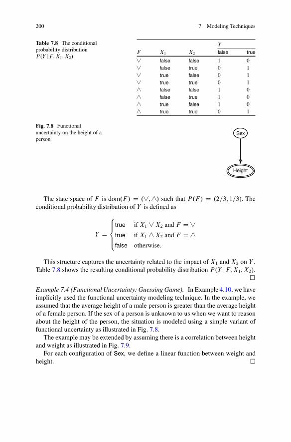
200 7 Modeling Techniques

Table 7.8 The conditionalprobability distributionP.Y |F;X1; X2/

Y

F X1 X2 false true

∨ false false 1 0

∨ false true 0 1

∨ true false 0 1

∨ true true 0 1

∧ false false 1 0

∧ false true 1 0

∧ true false 1 0

∧ true true 0 1

Sex

Height

Fig. 7.8 Functionaluncertainty on the height of aperson

The state space of F is dom.F / D .∨;∧/ such that P.F / D .2=3; 1=3/. Theconditional probability distribution of Y is defined as

Y D

⎧

⎪⎪⎨

⎪⎪⎩

true if X1 ∨X2 and F D ∨

true if X1 ∧X2 and F D ∧

false otherwise.

This structure captures the uncertainty related to the impact of X1 and X2 on Y .Table 7.8 shows the resulting conditional probability distribution P.Y |F;X1;X2/.

�Example 7.4 (Functional Uncertainty: Guessing Game). In Example 4.10, we haveimplicitly used the functional uncertainty modeling technique. In the example, weassumed that the average height of a male person is greater than the average heightof a female person. If the sex of a person is unknown to us when we want to reasonabout the height of the person, the situation is modeled using a simple variant offunctional uncertainty as illustrated in Fig. 7.8.

The example may be extended by assuming there is a correlation between heightand weight as illustrated in Fig. 7.9.

For each configuration of Sex, we define a linear function between weight andheight. �

7.1 Structure-Related Techniques 201

SexWeight

Height

Fig. 7.9 Functionaluncertainty on the height of aperson

How to Implement This Technique

The functional uncertainty modeling technique is implemented as follows.

1. Let Y be a random variable with parents pa.Y / D {X1; : : : ; Xn} such that Y is afunction of pa.Y /.

2. Assume the functional dependence relation between Y and pa.Y / is uncertainsuch that the alternatives and their relative frequencies are known.

3. Create a discrete random variable F with one state for each possible functionaldependence relation between Y and pa.Y /.

4. Define the prior probability distribution P.F / such that it encodes the relativefrequency of the possible functional dependence relations.

The structure uncertainty modeling technique is implemented similarly to the wayfunctional uncertainty is implemented.

7.1.4 Undirected Dependence Relations

The DAG structure of a probabilistic network specifies a set of dependence andindependence relations between variables. These dependence and independencerelations are specified using directed links between pairs of variables only. Whencapturing a set of dependence relations between variables using a DAG, it isnot unusual to encounter the problem of how (most efficiently) to represent adependence relation which by nature is undirected.

Let X1, X2, and X3 be discrete variables with the same set of states. Assumeconfigurations where all variables are in the same state are illegal. This is a typicalexample of an undirected dependence relation over a set of variables. This type ofundirected relation is referred to as a constraint.

A constraint over a subset of variables may be enforced by introducing anauxiliary variable referred to as the constraint variable with an appropriate numberof states as a child of the variables to be constrained. Often the constraint variable isBoolean, but it may have more than two states. Configurations of the parent variablesare mapped to states of the child, and the constraint is enforced using evidenceon the constraint variable. For instance, assume that we want to enforce a prior

202 7 Modeling Techniques

X1

X2

X3

a

X1 X2 X3

C"

b

Fig. 7.10 (a) A functional relation f .X1; X2; X3/ is to be enforced. (b) A constraint over X1, X2,and X3 is enforced by instantiating C to on

joint probability potential f .X1;X2;X3/ over variables X1, X2, and X3. The jointprobability can be enforced using a Boolean constraint node C with a conditionalprobability distribution defined as

P.C D on |X1;X2;X3/ D f .X1;X2;X3/; (7.1)

P.C D off |X1;X2;X3/ D 1− f .X1;X2;X3/: (7.2)

The constraint is enforced by instantiating C to on.Figure 7.10 illustrates how constraints over configurations of variables X1, X2,

and X3 are enforced by introducing an auxiliary variable C with two states. Onestate reflects legal configurations of variables X1, X2, and X3, while the otherstate reflects illegal configurations of variables X1, X2, and X3. In the example,all configurations where the three variables are not in the same state are legal, whilethe remaining configurations where all variables are in the same state are illegal.The constraint is enforced by instantiating the variable C to the state correspondingto legal configurations.

The following example illustrates the application of the modeling techniquedescribed above to an everyday problem.

Example 7.5 (Washing Socks (Jensen 1996)). Two pairs of socks have been washedin the washing machine. The washing has been rather hard on the colors and patternsof the socks. One pair of socks is the pair of socks usually worn to play golf,while the other is the pair of socks usually worn during long airplane trips. Theairplane socks help to improve blood circulation, while the golf socks have improvedrespiration. For this reason, it is important to pair the socks correctly.

The airplane socks are blue, while the golf socks are black. The patterns of twopairs of socks are also similar (at least after the washing).

A model for distinguishing the socks of different types has to capture theundirected relation over the four socks. The relation enforces the fact that thereare exactly two airplane socks and two golf socks.

The model has four variables S1; : : : ; S4. Each Si represents a sock and hasdomain dom.Si / D .airplane; golf/. The undirected relation R.S1; : : : ; S4/ is aconstraint over configurations of the S1; : : : ; S4. Figure 7.11 illustrates the model

7.1 Structure-Related Techniques 203

S1 S2 S3 S4

C

Fig. 7.11 The constraintover S1; : : : ; S4 is enforcedby instantiating C to on

Table 7.9 The conditionalprobability distributionP.C |S1; : : : ; S4/

C

S1 S2 S3 S4 off on

airplane airplane airplane airplane 1 0

airplane airplane airplane golf 1 0

airplane airplane golf airplane 1 0

airplane airplane golf golf 0 1

airplane golf airplane airplane 1 0

airplane golf airplane golf 0 1

airplane golf golf airplane 0 1

airplane golf golf golf 1 0

golf airplane airplane airplane 1 0

golf airplane airplane golf 0 1

golf airplane golf airplane 0 1

golf airplane golf golf 1 0

golf golf airplane airplane 0 1

golf golf airplane golf 1 0

golf golf golf airplane 1 0

golf golf golf golf 1 0

structure, while Table 7.9 shows the conditional probability distribution P.C |S1;

: : : ; S4/. The conditional probability distribution P.C |S1; : : : ; S4/ may bedefined as

P.C D on |s1; s2; s3; s4/ D{

1 if |{si D airplane}| D 2

0 otherwise.

The constraint is enforced by instantiating C to on. �

In the description above we have focused on binary constraint variables. Inthe general case the constraint variable may have more than two states. In thiscase multiple states of the constraint variable specifying legal configurationscan be enforced using likelihood evidence assigning the value zero to all statesspecifying illegal configurations and one to all states specifying legal configurations.

Notice that enforcing a constraint may change the marginal distribution on parentvariables. One approach to avoid this is described by Fenton, Neil & Lagnado(2011).

204 7 Modeling Techniques

X1 X2

a

?

?

X1 X2

Y

bFig. 7.12 (a) How should thebidirectional correlationbetween X1 and X2 becaptured? (b) A mediatingvariable Y between X1 andX2 captures the bidirectionalrelation

How to Implement This Technique

The undirected directions modeling technique is implemented as follows:

1. Let {X1; : : : ; Xn} be the set of variables over which the prior joint probabilitydistribution f .X1; : : : ; Xn/ is to be enforced.

2. Create a binary constraint node C with states off and on.3. Add each X 2 {X1; : : : ; Xn} as a parent of C .4. Define the conditional probability distribution P.C |X1; : : : ; Xn/ as specified in

(7.1) and (7.2).5. Instantiate C to state on enforcing the constraint.

7.1.5 Bidirectional Relations

Section 7.1.4 describes how an undirected dependence relation over a subsetof variables can be enforced using a constraint variable. The introduction of aconstraint variable is necessary in order to represent the undirected relation as aDAG. In this section we consider the similar problem of representing what seemsto be a bidirectional relation between a pair of variables. That is, when a pair ofvariables is dependent, it is not always evident which direction the connecting linkshould have.

Figure 7.12a illustrates the situation where a pair of variables X1 and X2 shouldbe connected by a link as there seems to be a direct dependence relation betweenX1and X2, but it is not possible to identify the direction of the link. Should the link bedirected from X1 to X2 or vice versa? An insufficient set of variables for capturingthe dependence and independence properties of a problem domain as a DAG isa common cause of this type of difficulty in identifying the direction of a link.Figure 7.12b illustrates how a mediating variable Y may be used to capture thebidirectional relation. The mediating variable Y is introduced as a common causeof X1 and X2.

The following example illustrates how an insufficient set of variables forcapturing the dependence properties of the problem domain can imply difficultiesin determining the direction of links.

7.1 Structure-Related Techniques 205

Pr

BT UT

?

?

(a)

Pr

BT UT

HS

(b)

Fig. 7.13 (a) How should the bidirectional correlation between BT and UT be captured? (b) Thebidirectional correlation between BT and UT is captured by the mediating variable HS

Example 7.6 (Insemination (Jensen 1996)). Consider the task of monitoringthe pregnancy state of a cow (also considered in Example 6.5 on page 153).Assume we have the options to perform a blood test and a urine test to determinethe pregnancy state of the cow. Both the blood test and the urine test are indicatorsfor the pregnancy state of the cow. Furthermore, we argue that there is a dependencerelation between the results of the two tests (if either is positive (negative), we wouldexpect the other test to be positive (negative) as well).

We know there is a correlation between blood test and urine test, but we cannotidentify one test as a cause of the other test. This is indicated in Fig. 7.13a where Prspecifies the pregnancy state of the cow, while BT and UT specify the results of theblood and urine tests, respectively. We assume the blood test is not independent ofthe urine test given the pregnancy state of the cow.

Looking deeper into the properties of the problem domain, we identify someadditional structure that alleviates the problem of a bidirectional relation between BTand UT. The two tests do not identify the pregnancy state of the cow directly. Insteadthe two tests identify the hormonal state of the cow. The resulting structure is shownin Fig. 7.13b where HS represents the hormonal state of the cow.

Notice that the structure shown in Fig. 7.13b correctly captures the conditionaldependency of BT and UT given Pr. �

How to Implement This Technique

The bidirectional relations modeling technique is implemented as follows.

1. Let X1 and X2 be a pair of variables which seems to have a bidirectionalinteraction.

2. Create a mediating variable Y such that it is the intermediate variable in a serialconnection with X1 and X2.

3. The identification of the states of Y and the probability distribution of Y isdomain dependent.

206 7 Modeling Techniques

I1 � � � In

CFig. 7.14 The structure ofthe naive Bayes model

7.1.6 Naive Bayes Model

Restricted probabilistic graphical models are used or considered when low modelcomplexity and high computational power are required. Low model complexity andhigh computational power are often required in classification-related problems. Ina classification problem, the task is to assign a class label to an instance based onobservations on properties of the instance.

The naive Bayes model is one of the simplest restricted probabilistic graphicalmodels; see Friedman, Geiger & Goldszmidt (1997) who cite Duda & Hart (1973)and Langley, Iba & Thompson (1992). The naive Bayes model is a popular modeldue to its high representational and computational simplicity while maintaining animpressive performance on classification tasks.

Since the naive Bayes model is most commonly used for classification problems,we will describe the model from this point of view. We consider the task ofclassifying a set of instances into a predefined set of classes based on observationson properties of the instances. Let C be the class variable with one state for eachpossible class and let I D {I1; : : : ; In} be the set of variables (also known asattributes, indicators, and features) where each variable represents a property thatwe can possibly observe and have decided to include in our model.

The structure of the naive Bayes model is the reason for the simplicity andefficiency of the model. The structure of the naive Bayes model is illustrated inFig. 7.14 where the class variable C is the only parent of each attribute and noother structure is present in the graph. The naive Bayes model assumes conditionalpairwise independence of the attributes given the class. This is a rather strong butoften useful assumption.

The set of (conditional) probability distributions induced by the naive Bayesmodel consists of the prior distribution P.C / on the class variable and theconditional probability distribution P.Ii |C/ on the attribute Ii given the class forall i D 1; : : : ; n. The naive Bayes model induces a joint probability distribution overthe class and attributes as

P.X/ D P.C; I1; : : : ; In/ D P.C /

nY

iD1P.Ii |C/:

Notice that this implies that the representational complexity of the model is linearin the number of attributes.

7.1 Structure-Related Techniques 207

Shape Color Odor

ClassFig. 7.15 A naive Bayesmodel for classifyingmushrooms

Probabilistic inference in a naive Bayes model consists of computing theconditional probability distribution P.C |"/ where " consists of observations on asubset of the attributes of the instance to be classified. For any set of observations" D {i1; : : : ; im}, we may calculate the likelihood of the class as

L.C |"/ D P." |C/ DY

i2"P.i |C/:

The posterior of the class is computed from the product of the prior and thelikelihood by normalization P.C |"/ D ˛L.C |"/P.C /, where ˛ D P."/−1 D.P

C L.C |"/P.C //−1, or expressed via Bayes’ rule as

P.C |"/ D �.P." |C/P.C // D P." |C/P.C /

P."/:

Despite its simplicity and strong assumption of pairwise independence of theattributes given the class, the naive Bayes model has in practice been shown to haveexcellent performance on (many) classification tasks. This makes the naive Bayesmodel popular. The following example illustrates the most common application ofthe naive Bayes model.

Example 7.7 (Classification of Mushrooms). Consider the task of classifying amushroom as either edible or poisonous based on observations on the shape, color,and odor of the mushroom. This is a classic classification problem. We makeobservations on the mushroom to identify it as either edible or poisonous.

Figure 7.15 shows a naive Bayes model for this classification task. The modelhas class variable Class and feature variables Color, Odor, and Shape. The classvariable is the direct parent of each feature variable, and no other structure is present.

The class variable has states dom.Class/ D .Edible; poisonous/, while thefeature variables have states dom.Odor/ D .none; almond; spicy/, dom.shape/ D.flat; bell; convex/, and dom.Color/ D .brown;white; black/.

The prior distribution on Class specifies the frequency of edible and poisonousmushrooms, while the conditional distribution of each feature variable specifiesthe distribution of the feature given the mushroom class. Table 7.10 shows thedistribution P.Odor |Class/. The distribution of each of the other feature variablesis similar.

208 7 Modeling Techniques

Table 7.10 The conditionalprobabilitydistribution P.Odor |C/

Odor

C none almond spicy

edible 0:902 0:0979 0:0001

poisonous 0:173 0:001 0:826

Each time a mushroom is picked up, the features of the mushroom are observedand entered into the model as evidence. After inference, the model returns theprobability that the mushroom is edible. �

There exist other classes of restricted probabilistic graphical models than thenaive Bayes model. For instance, the tree-augmented naive Bayes model (Friedmanet al. 1997) appears as a natural extension of the naive Bayes model, while thehierarchical naive Bayes model (Zhang 2004) is another extension of the naiveBayes model.

In Sect. 8.3.4, the task for learning structure restricted probabilistic graphicalmodels such as the naive Bayes model and the tree-augmented naive Bayes modelare described in detail.

How to Implement This Technique

The naive Bayes modeling technique is implemented as follows:

1. Let C be the class variable with one state for each possible class.2. Let I D {I1; : : : ; In} be the set of feature variables.3. Let C have no parents and let it be the only parent of each feature variable Ii . In

this way, C becomes the intermediate variable in a serial connection with eachpair of feature variables.

4. Define the prior probability distribution P.C / such that it encodes the relativefrequency of each class.

5. For each Ii 2 I, define the conditional probability distributionP.Ii |C/ such thatit encodes the relative frequency of each state of the feature given each state ofthe class variable.

If data are available, then it may be an advantage to estimate the prior andconditional probability distributions P.C / and P.I1 |C/; : : : ; P.In |C/ from data.

7.2 Probability Distribution-Related Techniques

In this section we consider modeling techniques related to the specification ofprobability distributions of a probabilistic network. In particular we consider mea-surement error, expert opinions, node absorption, setting a value by intervention,independence of causal influence, and mixture of Gaussian distributions.

7.2 Probability Distribution-Related Techniques 209

Accuracy Value

Observed

Fig. 7.16 The observed value of a phenomenon is a function of the accuracy of the measurementand the actual value of the measured phenomenon

Quality Temperature

Obs Temperature

Fig. 7.17 The measuredtemperature is a function ofthe quality of thethermometer and the actualtemperature

7.2.1 Measurement Uncertainty

Probabilistic networks are well-suited models for reflecting properties of problemdomains with some kind of uncertainty. The sources of uncertainty may be manyand diverse. In this section we consider a modeling technique for representinguncertainty related to measurements. Measurements and observations on the stateof the problem domain such as, for instance, sensor readings and noisy observationsare subject to uncertainty. In some situations it may be important to capture andrepresent the uncertainty explicitly in a probabilistic model.

Figure 7.16 illustrates a modeling technique that captures measurement uncer-tainty. The variable Value represents the actual value of the phenomenon beingmeasured, the variables Observed and Accuracy represent the observed value ofthe phenomenon and the accuracy with which observations are made, respectively.

Example 7.8 (Explicit Representation of Uncertainty). Assume we would like tomeasure the temperature in a room. The true temperature is unknown, but we mayuse a thermometer to get an estimate of the temperature in the room. Assume wehave two different thermometers to choose from: one thermometer of low qualityand another thermometer of high quality. The high-quality thermometer offers moreaccurate estimates of the temperature.

Figure 7.17 shows the structure of a model with variables Obs Temperature,Quality, and Temperature. Assume that the three variables have domainsdom.Obs Temperature/ D .low;medium; high/, dom.Quality/ D .low; high/, anddom.Temperature/ D .low;medium; high/. Table 7.11 shows the conditional proba-bility distribution P.Obs Temperature |Quality; Temperature/.

Notice how the distribution over Obs Temperature depends on the quality of thethermometer used to measure the temperature. This reflects the accuracy of eachthermometer. �

210 7 Modeling Techniques

Table 7.11 The conditionalprobability distributionP.Obs Temperature |Quality; Temperature/

Obs Temperature

Quality Temperature low medium high

low low 0:6 0:3 0:1

low medium 0:2 0:6 0:2

low high 0:1 0:3 0:6

high low 0:9 0:1 0

high medium 0:05 0:9 0:05

high high 0 0:1 0:9

Sock

Color

Obs Color

Pattern

Obs Pattern

Fig. 7.18 The observationson color and pattern areimperfect

Table 7.12 The conditionalprobability distribu-tion P.Obs Color |Color/

Obs Color

Color blue black

blue 0:9 0:1

black 0:05 0:95

An explicit representation of the accuracy with which observations are made isnot always necessary.

Example 7.9 (Implicit Representation of Uncertainty). Example 7.5 on page 202illustrates how to enforce the fact that there are two socks of each type (airplane andgolf). To classify the four socks, we make observations on the color and pattern ofeach sock. Color and pattern are indicator variables for the type of sock.

The observations on color and pattern are imperfect due to the washing.Figure 7.18 shows the model structure for classifying a single sock based on(imperfect) observations on color and pattern.

The conditional probability distribution P.Obs Color |Color/ is shown inTable 7.12. Notice that blue is observed as black in 10% of the cases and blackis observed as blue in 5% of the cases. �

The measure uncertainty modeling technique is closely related to the measure-ment idiom, see Sect. 6.3.2 on page 156.

7.2 Probability Distribution-Related Techniques 211

How to Implement This Technique

The measurement uncertainty modeling technique is implemented as follows.

1. Let variable Value represent the actual value of the phenomenon being measured.2. Create variables Observed and Accuracy representing the observed value of the

phenomenon and the accuracy with which observations are made, respectively.3. Let Value and Accuracy be the parents of Observed.4. Let Observed have one state for each possible observation of Value.5. Let Accuracy have one state for each possible level of accuracy of the observation

on Value.6. Define the prior probability distribution P.Accuracy/ such that it encodes the

relative frequency of each possible level of accuracy.7. Define the conditional probability distribution P.Observation |Accuracy;

Value/ such that it encodes the relative frequency of each possible observationgiven the level of accuracy and the actual value.

7.2.2 Expert Opinions

The specification of the parameters of a probabilistic network is often basedon knowledge elicitation from problem domain experts. Typically, a knowledgeengineer interviews one or more experts in order to assess the values of model pa-rameters. In some cases, when the elicitation of parameters is based on assessmentsfrom a group of experts, it is advantageous that any differences in the assessed valuesare represented explicitly in the model. This is, for instance, useful when the groupof experts are distributed physically and when the model is developed iteratively.

A conditioning (or auxiliary) variable can select among the opinions of differentexperts expressed in the probability assessments of a single variable. The condition-ing variable is a parent of the variable of interest and has one state correspondingto each expert. The prior distribution of the auxiliary value will assign a weight tothe experts represented in the auxiliary variable. Different auxiliary variables neednot have the same set of states. The following example illustrates the modelingtechnique on a simple example.

Example 7.10 (Expert Opinions: Chest Clinic). Consider the quantification of thechest clinic example (Example 4.2 on page 73). Assume the model is constructedby elicitation of knowledge from two experts Bill and John. Consider the elicitationof conditional probability distribution P.Bronchitis |Smoker/, and assume that Billand John have different opinions on this distribution.

To reflect the different opinions of the experts, we construct the model structureshown in Fig. 7.19 where dom.Experts/ D .Bill; John/ representing the two experts.

Table 7.13 shows the distribution P.Bronchitis |Smoker;Experts/. The distribu-tion encodes the different opinions of the experts on the conditional probabilitydistribution, whereas the prior distribution P.Experts/ encodes the reliability of theexperts.

212 7 Modeling Techniques

Bronchitis

Smoker ExpertsFig. 7.19 The variableExperts has one state for eachexpert

Table 7.13 The specificationof the conditional probabilitydistributionP.Bronchitis |Smoker;Experts/

Bronchitis

Experts Smoker false true

bill false 0:7 0:3

bill true 0:4 0:6

john false 0:8 0:2

john true 0:3 0:7

Asia Smoker

Tuberculosis Cancer Bronchitis

Tub or cancer

X ray Dyspnoea

Experts1 Experts2

Fig. 7.20 A graph specifying the independence and dependence relations of the Asia example

The model captures the opinions of experts Bill and John using the Expertsvariable to condition the conditional probability distribution they have differentopinions on.

One expert node is introduced for each conditional probability distributionelicited from domain expert knowledge. Figure 7.20 illustrates how two groupsof experts have been consulted to elicit the conditional probability distributionsof Bronchitis and Cancer. By introducing multiple expert nodes, we assume theelicitation of different conditional probability distributions to be independent. �

The model in Example 7.10 has an explicit representation of the opinions of thetwo experts. In some situations, it is desirable not to have an explicit representationof expert opinions in the model. This can be achieved by eliminating the variablesrepresenting different experts from the model. This is described in Sect. 7.2.3.

How to Implement This Technique

The expert opinions modeling technique is implemented as follows:

1. Let P.X |pa.X// be the conditional probability distribution assessed from agroup of experts (one instance of P.X |pa.X// is assessed from each expert).

2. Create a discrete random variable Experts with one state for each expert.

7.2 Probability Distribution-Related Techniques 213

3. Let Experts be a parent of X .4. Define the prior probability distribution P.Experts/ such that it encodes the

reliability of the experts.5. Define the conditional probability distribution P.X |pa.X/;Experts/ such that

for each state of Experts it encodes the assessment of P.X |pa.X// given by thecorresponding expert.

7.2.3 Node Absorption

Node absorption is the process of eliminating a variable from a model by arcreversals and barren variable eliminations. Recall that in Sect. 3.4.1.1 on page 56,we illustrated the application of Bayes’ rule as an arc reversal operation, while inSect. 5.1.1 on page 116, we considered repeated applications of arc reversal as aninference process.

The node absorption method may also be a useful tool in the model developmentprocess. Node absorption may be used to eliminate variables from a model whichfor one reason or another should not be included in the final model. If efficiencyof probabilistic inference in a probabilistic network is of high priority, it maybe worthwhile to eliminate variables that are neither observed nor the target ofinference. In Sect. 5.1.1, we denoted a variable that is neither an evidence variablenor a target variable as a nuisance variable.

Example 7.11 (Node Absorption: Expert Opinions). Consider Example 7.10 onpage 211 where P.Bronchitis |Smoker/ has been elicited from the two experts Billand John. From the example, we know that Bill and John disagree slightly on thestrength of the dependence relation between Bronchitis and Smoker. This is capturedby the graph of Fig. 7.19.

For different reasons (e.g., political), we would like to eliminate the intermediatevariable Experts from the model while maintaining the underlying dependencerelations between the remaining variables. This can be achieved using nodeabsorption.

Since Experts has Bronchitis as its only child, a single arc reversal operation issufficient to absorb Experts. Once the arc .Experts;Bronchitis/ is reversed, Expertsis barren and can therefore be removed from the graph without changing thedependence relations between the remaining variables in the graph.

If we assume that we have equal trust in the two experts, then Table 7.14shows the conditional probability distribution P.Bronchitis |Smoker/ after absorb-ing Experts from the distribution shown in Table 7.13.

The prior distribution P.Experts/ can be interpreted as specifying our relativetrust in the two experts. In the example, we have used a uniform distribution. �

The order in which arcs are reversed may be constrained by the structure ofthe graph. That is, the sequence of arc reversals should be performed such thatall intermediate graphs are acyclic. In addition, the order in which variables are

214 7 Modeling Techniques

Table 7.14 The conditional probabilitydistribution P.Bronchitis |Smoker/ afterabsorbing Experts from the distributionshown in Table 7.13

Bronchitis

Smoker false true

false 0:75 0:25

true 0:35 0:65

absorbed and arcs are reversed may impact the size of the parent sets in the resultinggraph.

How to Implement This Technique

The node absorption modeling technique is implemented as follows:

1. Let X be the variable to be eliminated by node absorption.2. Let ch.X/ be the direct successors of X , that is, the children of X .3. For each Y 2 ch.X/ reverse the link .X; Y / according to the arc reversal

operation. Traverse ch.X/ in topological order.4. Eliminated X as a barren variable, that is, simply remove X and incoming links

from the model.

Node absorption may be implemented as a single step operation in probabilisticnetwork editor software.

7.2.4 Set Value by Intervention

An important distinction should be made between a passive observation of the stateof a variable and an active action forcing a variable to be in a certain state. A passiveobservation of a variable impacts the beliefs of the ancestors of the variable, whereasan active action enforcing a certain state on a variable does not under the assumptionof a causal ordering (see Sect. 4.2 on decision making under uncertainty). Werefer to this type of active action as an intervention. When we make a passiveobservation on a variable, this produces a likelihood on the parents of the variable.This should not be the case when the value of a variable is set by intervention. Theinstantiation of a decision variable in an influence diagram is an example of thistype of intervention.

In some situations it is undesirable to model active actions forcing a variable tobe in a certain state as a decision in an influence diagram. Instead of modeling thesituation using decision variables, a simple modeling technique may be used. Themodeling technique is illustrated in Fig. 7.21.

7.2 Probability Distribution-Related Techniques 215

I

A B C

Fig. 7.21 Modeling theoption of setting a value of Bby intervention

Table 7.15 (a) Theconditional probabilitydistribution P.B |A/. (b) Theconditional probabilitydistribution P.B | I; A/

aB

A false true

false 0:9 0:1

true 0:2 0:8

b

B

I A false true

no intervention false 0:9 0:1

no intervention true 0:2 0:8

false false 1 0

false true 1 0

true false 0 1

true true 0 1

In Fig. 7.21, we illustrate a situation where the value of the random variable Bmay be set by intervention. The causal properties of the example are such thatthe variable A has a causal impact on B which in turn has a causal impacton C . The variable I captures the property that the state of variable B maybe set by intervention. Assuming Table 7.15(a) shows the conditional probabilitydistribution P.B |A/, then Table 7.15(b) shows the distribution P.B |A; I /.

This construction of P.B |I; A/ implies that C ?? A |I D i where i 6Dno intervention, that is, setting I to a value different from no intervention makes Aand C independent. Thus, if we enforce a certain state on B by selecting a state of I(different from no intervention), then observing C subsequently will not change thebelief in A. In general, the conditional probability distribution P.B | I; A/ may bedefined as

P.B D b |A; I D i/ D

⎧

⎪⎪⎨

⎪⎪⎩

P.b |A/ if i D no intervention

1 if b D i

0 otherwise

(7.3)

where dom.I / D dom.B/ [ {no intervention}.It is important to notice that when the state of B is observed, the observation is

enforced by setting the state of B , whereas if the state of B is set by intervention,then I is instantiated to the corresponding state. When B is not observed, I is in thestate no intervention.

216 7 Modeling Techniques

Flu Fever Sleepy

Aspirin

Fig. 7.22 Taking an aspirin forces the fever to a certain level. Subsequent observations on Sleepyshould not change our belief in Flu

Example 7.12 (Set Value by Intervention). Figure 7.22 depicts a simple model forreasoning about a common medical situation. The model captures the direct causalinfluence of flu on fever and the direct causal impact of fever on sleepiness. Theseevents are represented by the variables Flu, Fever, and Sleepy, respectively.

In addition to the aforementioned variables, the model has the variable Aspirin.This variable represents the event that the patient takes an aspirin to reduce feverto a certain level. Once an aspirin has been taken, an observation on Sleepy willbe uninformative with respect to Flu. This behavior may be enforced as describedabove. �

How to Implement This Technique

The set value by intervention modeling technique is implemented as follows.

1. Let X be the random variable that may be set by intervention.2. Create a random variable I with dom.I / D dom.B/[ {no intervention}.3. Let I be a parent of X .4. Define the prior probability distribution P.I / such that it encodes the relative

frequency of setting each state of X and no intervention.(5) Define the conditional probability distribution P.X |pa.X/; I / according

to (7.3).

7.2.5 Independence of Causal Influence

In this section we consider how a special kind of structure within a conditionalprobability distribution may be exploited to reduce the complexity of knowledgeelicitation from exponential in the number of parents to linear in the number ofparents. The property we consider is known as independence of causal influence(Heckerman 1993).

In an independence of causal influence model, the parent variables of a commonchild variable interact independently on the child. With a slight abuse of terms,the parents are sometimes said to be causally independent. All variables inan independence of causal influence model are assumed to be discrete random

7.2 Probability Distribution-Related Techniques 217

C1 C2 C3

E

Fig. 7.23 The causalinfluence of Ci on E isindependent of the causalinfluence of Cj on E (fori 6D j )

C1 C2 C3

E1 E2 E3

E

C1 C2 C3

E1 E2 E3

E 0 E 00 E

Fig. 7.24 Two model structures for capturing independence of causal influence

variables. The common child variable is denotedE, and it is referred to as the effectvariable. The parent variables are denoted C1; : : : ; Cn, and they are referred to ascause variables or causes, see Fig. 7.23.

The cause variables C1; : : : ; Cn may cause an abnormality modeled as the effectvariableE to be present at a certain level. The states of the effect variableE specifydifferent levels of the abnormality. The states ofE are ordered in the sense that theyrepresent different levels of abnormality and such that a designated state indicatesthat the abnormality is absent. Similarly, each of the causes have an absence statecorresponding to no impact on the effect variable. The principle of an independenceof causal influence model is that the causal impact of each cause is independent ofthe causal impact of all other causes.

In this section we consider the Boolean independence of causal influence modelknown as the Noisy-OR model (Pearl 1988). The Noisy-OR model is a commonlyused example of a model for local conditional probability distributions that dependson fewer parameters than the total number of combinations of fa.E/ (Laskey 1993).

In the Noisy-OR model, the effect variable E and the variables C1; : : : ; Cn areBoolean variables (i.e., binary discrete random variables with states false and true).The designated state is false. The causal impact of each cause Ci is independentof the causal impact of any other cause Cj for i 6D j . Figure 7.24 illustratestwo different ways in which this independence may be modeled explicitly. Eachvariable Ei has the same state space as E, and it captures the contribution fromcause Ci to the value of E. Each variableEi is referred to as a contribution variableand P.Ei |Ci/ captures the causal impact of Ci on E. In the left part of the figure,the total impact on the effect variable is the disjunction of all causes, whereas inthe right part of the figure, the temporal transformation modeling technique has

218 7 Modeling Techniques

C1 C2

E1 E2

E

q1 q2

Fig. 7.25 One inhibitorprobability for each parent Ciof the effect E

been applied such the total impact is determined based on a pairwise combinationof causes. The conditional probability distribution P.E |E1; : : : ; En/ is defined asdisjunction and so are P.E 00 |E 0; E2/ and P.E |E 00; E3/. The effect variableE is instate true when at least one contribution variable is in state true.

The causal impact of a cause Ci is the probability P.E D yes |Ci D yes/whereas P.E D yes |Ci D no/ D 0. We denote P.E D yes |Ci D yes/ D 1 − qiwhere qi is referred to as the inhibitor probability, see Fig. 7.25.

In some domains there may be a need to have a leak probability 1 − q0representing the probability of E D true when all causes C1; : : : ; Cn are absentwhere q0 is known as the default inhibitor. A leak probability may be implementedby introducing as a separate Boolean cause variable C0 instantiated to state true.The leak variable C0 represents the set of causes not modeled explicitly in thenetwork. In this way, the leak variable can be used to enforce the closed-worldassumption. The leak probability is assigned as the probability that the effect willoccur in the absence of any of the causes C1; : : : ; Cn that are explicitly representedin the network (Pradhan, Provan, Middleton & Henrion 1994).

Let us consider how the reduction from exponential to linear in the numberof parents is achieved. We may consider the conditional probability distribu-tion P.Xi |pa.Xi // as parameterized over a vector i of parameters �ijk with onecomponent for each possible value of Xi and combination of pa.Xi / such that

P.xijk |�ij ; i / D �ijkPk �ijk

;

where �ij is the j th configuration of pa.Xi/. The above formula is an unrestrictedlocal conditional probability distribution. The distribution depends on |Xfa.Xi /|

parameters.In an independence of causal influence model, the conditional probability

distribution P.Xi |pa.Xi// can be specified using a parameter vector i that growsin size only linearly in the number of parents, |pa.Xi /|, rather than linearly in thenumber of configurations of the parents, |Xpa.Xi /|; that is, exponential in |pa.Xi/|.

For the Noisy-OR model, it is straightforward to determine the conditionalprobability distribution P.E |pa.E/; E/ given a specific parameter vector E forthe model. In that case P.E |C1; : : : ; Cn/ can be specified as

7.2 Probability Distribution-Related Techniques 219

Angina Cold

SoreThroat

Fig. 7.26 Sore throat may becaused by both angina andcold

P.E D true |C1 D c1; : : : ; Cn D cn; E/ D 1− �0Y

CiDtrue

�i ;

where �0 is the default inhibitor, �i is the inhibitor forCi , and E D {�0; �1; : : : ; �n}.From this, it follows that

P.E D false |C1 D c1; : : : ; Cn D cn; E/ D �0Y

CiDtrue

�i :

The following example illustrates how independence of causal influence may beexploited to simplify the knowledge elicitation process.

Example 7.13 (Noisy-OR: Sore Throat). A physician wants to diagnose her patientswith respect to diseases causing a sore throat. For simplicity of the example, weassume the physician is mainly interested in modeling the causal effect of cold andangina on sore throat. In addition to cold and angina, there are other potential causesof a sore throat. These other causes are not to be represented explicitly in the modelthough.

Thus, initially the model consists of three variables: SoreThroat, Angina, andCold. All variables are Boolean with states false and true. Figure 7.26 shows thestructure of the model.

The synergy between Angina and Cold with respect to their combined effecton SoreThroat is assumed to be minimal. Thus, we may use the Noisy-OR modelto specify and represent the conditional probability distribution of SoreThroat givenAngina and Cold where all other implicit causes of sore throat are captured by thebackground event.

First, assume the inhibitor probabilities are qAngina D 0:1 and qCold D 0:2,while the default inhibitor is one (i.e., there are no other causes of sore throat).The combined impact of Angina and Cold on SoreThroat is computed as

P.SoreThroat D false |Angina D false;Cold D false; E/ D 1;

P.SoreThroat D false |Angina D false;Cold D true; E/ D 0:2;

P.SoreThroat D false |Angina D true;Cold D false; E/ D 0:1;

P.SoreThroat D false |Angina D true;Cold D true; E/ D 0:1 � 0:2:

220 7 Modeling Techniques

Table 7.16 The conditionalprobability distribu-tionP.SoreThroat |Angina;Cold/with a zero background eventprobability

SoreThroat

Angina Cold false true

false false 1 0

false true 0:2 0:8

true false 0:1 0:9

true true 0:02 0:98

Table 7.17 The conditionalprobability distribu-tionP.SoreThroat |Angina;Cold/with a nonzero backgroundevent probability

SoreThroat

Angina Cold false true

false false 0:95 0:05

false true 0:19 0:81

true false 0:095 0:905

true true 0:019 0:981

Table 7.16 shows the distribution P.SoreThroat |Angina;Cold/.Next, assume the background inhibitor is 0:95 (i.e., the probability that sore

throat is caused by the background event (other causes not represented in the model)is 0:05 such that q0 D 0:95). The combined impact of Angina, Cold, and thebackground event on SoreThroat given is computed as

P.SoreThroat D false |Angina D false;Cold D false; E/ D 0:95;

P.SoreThroat D false |Angina D false;Cold D true; E/ D 0:95 � 0:2;P.SoreThroat D false |Angina D true;Cold D false; E/ D 0:95 � 0:1;P.SoreThroat D false |Angina D true;Cold D true; E/ D 0:95 � 0:1 � 0:2:

Table 7.17 shows the distribution P.SoreThroat |Angina;Cold/.By exploiting the independence of causal influence between Cold and Angina, the

number of parameters to elicit has decreased from four to two. This may seem tobe an insignificant reduction. However, if we consider the case where ten differentcauses of SoreThroat are to be represented explicitly in the model, then the numberof parameters to elicit is reduced from 1;024 to 10. �

The benefit of independence of causal influence becomes even more apparentwhen the effect has a large number of causes as the number of parameters growslinearly with the number of causes. The advantage of independence of causalinfluence is an exponential decrease in the number of parameters to elicit. Thedisadvantage of independence of causal influence is that any synergy betweencauses (with respect to their combined impact on the effect variable) is ignored.

Using independence of causal influence in conjunction with parent divorcing mayreduce the complexity of inference exponentially.

Srinivas (1993) discusses a generalization of the Noisy-OR model to nonbinaryvariables. Pradhan et al. (1994) and Diez (1993) have considered in detail the Noisy-MAX model as a generalization of the Noisy-OR model to the case in which each

7.2 Probability Distribution-Related Techniques 221

variable is allowed to have a finite discrete state space. In the Noisy-MAX model,the max operator specifies the combination of the cause variables. In the Noisy-MAX model, the probability distribution of the effect variable E given its parentcauses can be expressed as

P.E |C1; : : : ; Cn/ DX

max.E1;:::;En/

nY

iD1P.Ei |Ci/:

One prerequisite for using the Noisy-MAX model is that the variable state spaces areordered as, for example, .absent;mild;moderate; severe/. In addition, each causevariable must have a distinguished (or absent) state designating an influence of thecause on the effect variable.

How to Implement This Technique

The independence of causal influence modeling technique is implemented asfollows:

1. Let {C1; : : : ; Cn} be the set of causes of effect variable E.2. Assume the impact of C1; : : : ; Cn on E can be modeled as a Noisy-OR model.

Hence, C1; : : : ; Cn and E are Boolean variables.3. Create one Boolean contribution variable Ei for each Ci 2 {C1; : : : ; Cn}.4. Let each Ei be a child of Ci and a parent of E.5. For each Ci , define the conditional probability distribution P.Ei |Ci/ such

that P.Ei D true |Ci D true/ is the probability of E D true given Ci D trueand Cj D false for i 6D j and P.Ei D false |Ci D false/ D 1.

6. Define the conditional probability distribution P.E |E1; : : : ; En/ as disjunction(i.e., or).

Once the independence of causal influence modeling technique has been applied,it may be an advantage to use the parent divorcing modeling technique (seeSect. 7.1.1) to reduce the number of parents of the effect variable.

7.2.6 Mixture of Gaussian Distributions

When modeling problem domains with continuous entities, a decision on how torepresent the continuous entities in a network has to be made. One option is torepresent a continuous entity as a discrete variable with states representing intervalsfor the continuous entity. For instance, we may choose to represent temperature asa discrete variable with three states: low, medium, and high. In other cases, we maychoose to approximate the distribution of a continuous entity using the conditionallinear Gaussian distribution.

222 7 Modeling Techniques

S

X

Fig. 7.27 Approximation ofa continuous distributionusing the MoGs modelingtechnique

A third option is presented in this section. The third option is to approximatethe continuous distribution of a variable using a mixture of Gaussian distributions(MoGs). This option is interesting as it is well known that mixtures of Gaussiandistributions can approximate any probability distribution; see Shenoy (2006) whocites Titterington, Smith & Makov (1995).

An MoGs is a sum of Gaussian distributions where each component is weightedby a number between zero and one such that the sum of the weights is one, that is,the weights are probabilities. Assume X is a continuous variable with a probabilitydistribution that can be approximated using the MoGs:

f .x/ DnX

iD1pi � N.˛i ; �i /; (7.4)

where ˛i ; �i 2 R and 0 � pi � 1 such thatP

i pi D 1 are the mean, variance, andweight of the i ’th component in the mixture.

To approximate the probability distribution on X using (7.4), a selector vari-able S with n states is introduced as a parent of X . The variable X becomes acontinuous variable with a conditional linear Gaussian distribution, see Sect. 4.1.2.Each state si of S corresponds to one component pi � N.˛i ; �i / in the mixture. Theprior distribution on S is P.S D si / D pi while X |si ∼ N.˛i ; �i /. Figure 7.27illustrates the use of the MoGs modeling technique on the distribution for X .

Using MoGs, the network becomes either a CLG Bayesian network or a CLQGinfluence diagram.

Example 7.14 (Mixture of Gaussian Distributions). A Gamma.2; 2/ distributioncan, for instance, be approximated using a two-component mixture of MoGs such as

f .x/ D 0:609 � N.4:57; 2:37/C 0:391 � N.1:93; 1:12/: (7.5)

Figure 7.28 shows the result of approximating the Gamma.2; 2/ distribution withthe above two-component mixture of Gaussian distributions.

The two-component approximation in (7.5) produces a reasonable fit to theGamma.2; 2/ distribution. Whether or not the fit is of sufficient quality dependson the problem domain and application. �

The MoGs modeling technique introduces a discrete random variable with onestate for each component in the mixture. Approximating continuous distributionsusing the MoGs modeling technique is not necessarily simple and may producenetworks where belief updating is computationally intensive.

7.2 Probability Distribution-Related Techniques 223

0

0.02

0.04

0.06

0.08

0.1

0.12

0.14

0.16

0.18

0.2

0 2 4 6 8 10 12 14

Two-component MoGGamma(2, 2)

Fig. 7.28 A two-component mixture approximation of the Gamma.2; 2/ distribution

How to Implement This Technique

The mixture of Gaussian distributions modeling technique is implemented asfollows:

1. Let X be the variable of the probability distribution to approximate.2. Assume the probability distribution of X can be approximated using the MoGs

f .x/ DnX

iD1pi � N.˛i ; �i /:

3. Create a discrete variable S with n states.4. Let S be the parent of X in the network with P.S D si / D pi .5. For each state, si of S set X |si ∼ N.˛i ; �i /.

The process of identifying the number of components as well as the parameteri-zation and weight of each component is not trivial.

In this section we have considered the case of approximating the prior distribu-tion of a continuous variable with no parents. Shenoy (2006) presents a methodologyfor belief updating in hybrid Bayesian networks (i.e., Bayesian networks with bothcontinuous and discrete variables and with no restrictions on the model structure)based on approximating distributions using MoGs. Shenoy (2006) gives exampleson how to approximate different types of distributions using MoGs. This includesapproximating the distribution of a discrete child of a continuous variable. Poland(1994) has presented an algorithm for identifying MoGs using the EM algorithm(see Sect. 8.5.1).

224 7 Modeling Techniques

7.3 Decision-Related Techniques

In this section we consider modeling techniques related to the specification of adecision problem as an influence diagram. In particular, we consider how to modeltest decisions, how to exploit missing informational links, how to model variableswhich may or may not be observed prior to a decision, how to force a decisionvariable to be in a state corresponding to a hypothesis of maximum probability, andhow to enforce constraints on decision options.

7.3.1 Test Decisions

As part of a decision problem, a decision maker may be faced with the optionto perform some kind of test. Performing the test produces a test result which ismodeled as a random variable with states corresponding to the possible test resultsin an influence diagram. In addition to the random variable representing the testresult, the influence diagram has a decision variable with states representing whetheror not the test is performed. If the test is performed, then the result of the test(usually) becomes available to the decision maker. If the test, on the other hand,is not performed, then no test result becomes available. The influence diagram mayalso have a utility function associated with the test specifying the cost of the test.Solving the influence diagram will produce a policy for when to perform the test.

The random variable representing the test result may be an informational parentof another decision variable in the influence diagram. If the test result variable is aninformational parent of another decision in the influence diagram, then the variablemust be observed prior to this decision. This, however, contradicts the fact that thetest result is available only when the test is performed. In this section, we considertwo examples that illustrate different approaches to alleviating this contradiction.

Example 7.15 (Oil Wildcatter (Raiffa 1968)). Example 4.5 on page 82 considers anoil wildcatter about to decide whether or not to drill for oil at a specific site. Priorto her decision on whether or not to drill for oil, the oil wildcatter has the option totake seismic soundings to better understand the geological structure of the site. Thestructure of the oil wildcatter model (Fig. 4.5 on page 82) is repeated in Fig. 7.29for convenience.

Oil

Seismic

Test

DrillU1

U2

Fig. 7.29 The test result isonly available after a test isperformed

7.3 Decision-Related Techniques 225

Table 7.18 The conditionalprobability distributionP.Seismic |Test;Oil/

Seismic

Test Oil closed open diffuse

no dry 0:1 0:3 0:6

no wet 0:3 0:4 0:3

no soaking 0:5 0:4 0:1

yes dry 1=3 1=3 1=3

yes wet 1=3 1=3 1=3

yes soaking 1=3 1=3 1=3

Table 7.19 The conditionalprobability distributionP.Seismic |Test;Oil/where Seismic has a no resultstate

Seismic

Test Oil closed open diffuse no result

no dry 0:1 0:3 0:6 0

no wet 0:3 0:4 0:3 0

no soaking 0:5 0:4 0:1 0

yes dry 0 0 0 1

yes wet 0 0 0 1

yes soaking 0 0 0 1

There are two informational links in the graph of Fig. 7.29. The link .Test;Drill/from Test to Drill and the link .Seismic;Drill/ from Seismic to Drill are bothinformational links. The former link specifies whether or not the oil wildcatterdecided to take seismic soundings prior to the drill decision. On the other hand,the latter link specifies that the value of Seismic is also known when making thedrill decision. This cannot, however, be the case when the test is not performed.

We consider two alternative options to correct this problem. Both optionsconsider the specification of the conditional probability distribution P.Seismic |Oil; Test/.

One option is to specifyP.Seismic |Oil; Test D no/ as a uniform distribution. Thecorresponding distribution is shown in Table 7.18. If the oil wildcatter decides notto perform the test, then any observation on Seismic will not affect the belief in Oil(the likelihood potential over Oil induced by the observation on Seismic assignsequal likelihood to all states of Oil due to the uniform distribution).

The other option is to introduce an additional no result state in Seismic. Thedistribution P.Seismic |Oil; Test D no/ is specified such that not performing thetest instantiates Seismic to no result. The corresponding distribution is shown inTable 7.19. If the oil wildcatter decides not to perform the test, then Seismic isinstantiated to no result.

The latter option is semantically more clear than the former option in the sensethat it is easily understood that Seismic should be instantiated to no result when thetest is not performed. On the other hand, the latter option increases the complexityof the model by introducing the additional no result state in the Seismic variable. �

Example 7.16 (Aspirin (Jensen 1996)). Example 7.12 on page 216 describes asimple model for reasoning about the effect of flu on fever and the effect of fever onsleepiness. Here we consider this example as a decision problem where the decisionmaker has to decide on whether or not to take an aspirin.

226 7 Modeling Techniques

Flu Fever Sleepy

A

T

Fig. 7.30 Prior to decidingon whether or not to take anaspirin, we may measure thetemperature

Flu Fever Fever� Sleepy

ATempT

Fig. 7.31 The test fortemperature is modeled as adecision value with a randomvariable as a child specifyingthe result of the test

The level of fever may be reduced by taking an aspirin. This is represented by thedecision variable A. Notice that decision variable A is an intervening decision andrecall from the discussion on causality in Sect. 2.4 the important difference betweensetting the state of a variable, that is, selecting an option for a decision variable,and observing the state of a variable. Prior to taking an aspirin, there is the optionto measure temperature. This option is indicated using the triangular-shaped nodewith label T in Fig. 7.30.

The test option indicated in Fig. 7.30 by the triangular-shaped node may berepresented using three nodes as indicated in Fig. 7.31. The three nodes representdecision variable T and random variables Temp and Fever�. The decision variable Trepresents whether or not the temperature is measured. The random variable Tempspecifies the temperature measured, and the random variable Fever� represents thelevel of fever after taking an aspirin, while the random variable Fever represents thelevel of fever prior to taking an aspirin. �

How to Implement This Technique

The test decisions modeling technique is implemented as follows:

1. Let P be a discrete random variable representing the phenomenon that may bemeasured by a test.

2. Create a decision variable T with two states no test and test corresponding to notperforming and performing the test, respectively.

3. Create a discrete random variable R representing the result of the test as a childof T and P .

4. Let R have one state for each possible test result and the state no resultrepresenting the event that the test is not performed, that is, T D no test.

7.3 Decision-Related Techniques 227

5. Define the conditional probability distribution P.R |P; T / such that P.R Dno result |P; T D no test/ D 1 and P.R |P; T D test/ encodes the probabilityof each possible test result given the actual value of phenomenonP .

Instead of using the state no result to specify no test result, a uniform distributionmay be used. Furthermore, the modeling technique may be used in combinationwith the measurement uncertainty modeling technique described in Sect. 7.2.1.

7.3.2 Missing Informational Links

Informational links of an influence diagram define the points at which information isassumed to become available to the decision maker. An informational link .X;D/from a random variable X to a decision variable D specifies that the value of Xis known to the decision maker when the decision corresponding to decisionvariableD is made. The informational links of an influence diagram induce a partialorder over the random variables relative to the decision variables. The partial orderover random variables is important for the solution of an influence diagram. Inessence, the partial order over random variables induces a constraint on the order inwhich variables may be eliminated when solving the decision model; see Sect. 5.2for details on solving decision models. Thus, correct specification of informationallinks is imperative.

When the influence diagram has only a single decision, then informational linkscan be ignored if the influence diagram is solved for each set of evidence. That is,the influence diagram is solved prior to making the decision each time the influencediagram is used. This implies that the optimal strategy is only implicitly available tothe decision maker as the optimal decision is determined for each evidence scenarioprior to making the decision. This can be particularly useful if the optimal policyfor the decision has a large state space.

Example 7.17 (Missing Informational Links). In Example 7.6 on page 205, weconsidered the task of monitoring the pregnancy state of a cow. Assume that inaddition to the blood and urine tests, we have the option to make a scanning ofthe cow. A scanning of the cow will produce a more accurate estimation of thepregnancy of the cow. The option to scan the cow introduces the variable Sc withstates false and true as a child of Pr.

The pregnancy state of the cow is estimated 6 weeks after the initial inseminationof the cow. Based on the observations and the probability distribution of thepregnancy state of the cow, we need to make a decision on whether or not to repeatthe insemination of the cow or to wait for another 6 weeks before estimating thepregnancy state of the cow. This decision introduces the decision variable D withstates Wait and repeat.

The cost of repeating the insemination is 65 no matter the pregnancy state of thecow. If the cow is pregnant, and we wait, it will cost us nothing, but if the cow is

228 7 Modeling Techniques

Table 7.20 The utilityfunction U.Pr;D/

Pr D

false wait −95

false repeat −65

true wait 0

true repeat −65

BT UT

HS

Pr

Sc

D

U

(a)

BT UT

HS

Pr

Sc

D

U

(b)

Fig. 7.32 (a) Informational links are unnecessary in influence diagrams with a single decision.(b) Informational links only clutter up the graph

not pregnant, and we wait, it will cost us another 30 units plus the eventual repeatedinsemination (that makes a total of 95 for waiting). A blood test has the cost 1 and aurine test has the cost 2. This defines a utility function over variables Pr and D, seeTable 7.20.

Figure 7.32a shows the resulting structure of the model. Notice that there are noinformational links in the structure.

Since the structure in Fig. 7.32a does not contain any informational links, it doesnot properly reflect the test options available prior to deciding on whether or not torepeat the insemination.

To capture the three test options, we may introduce an additional no test state ineach of the test result variables (BT, UT, and Sc). This would produce the structureshown in Fig. 7.32b.

Alternatively, we may use the fact that the decision problem contains a singledecision variable. This allows us to leave out informational links and instantiate therandom variables observed prior to the decision as the observations are made. Thisleaves us with Fig. 7.32a instead of the more cluttered Fig. 7.32b. �

When informational links are included in the influence diagram, the solutionwill identify a decision policy specifying an optimal decision option for eachconfiguration of the parents of the decision. Thus, the influence diagram is solvedonce and off-line in the sense that the influence diagram is solved before the decisionmaker has to make a decision and before any observations are made. On the otherhand, it is necessary to resolve the influence diagram each time the decision makerhas to make the decision when informational links are not included in the network.The solution process identifies an optimal decision option for the specific set ofobservations made prior to the decision. The influence diagram is solved on-line in

7.3 Decision-Related Techniques 229

X D

X D

X O D

(a) (b)

Fig. 7.33 (a) In some situations X is observed prior to D, while in others it is not. (b) Byintroducing an additional variable, we capture the situation where an observation on X may ormay not be available

the sense that the influence diagram is solved when the decision maker has to makethe decision and after observations have been made. Solving the influence diagramon-line is often a significantly simpler task than solving it off-line and may be theonly option when the influence diagram is complex.

How to Implement This Technique

The missing informational links modeling technique is implemented as follows.

1. Let D be the decision under consideration.2. Assume observations " have been made prior to making decision D where

pa.D/ � X."/.3. Insert " as evidence and solve the influence diagram.4. The expected utility associated with each state d of D is EU.d |"/, that is, the

expected utility of decision option d given observations ".

The above steps should be repeated each time observations are made prior todeciding onD.

7.3.3 Missing Observations

The structure of an influence diagram induces a partial order on the random variablesof the model relative to the decision variables of the model. The partial orderis induced by the informational links of the graph of the influence diagram. Aninformational link .X;D/ from a node representing a random variable X to a noderepresenting a decision variable D specifies that the value of X is observed whendecision D is to be made. That is, the value of X is always observed prior todecisionD.

Figure 7.33a illustrates a typical dilemma a knowledge engineer may be facedwith when representing a decision problem as an influence diagram. In somesituations, the random variable X is observed prior to the decision representedas D, and in other situations, it is not observed prior to making decision D. In this

230 7 Modeling Techniques

Oil

Seismic

Test

DrillU1

U2

Fig. 7.34 The observationon Seismic is missing whenthe test is not performed

ObsSeismic Drill

Fig. 7.35 This graph captures the situation where the result of seismic soundings may not beavailable

section we describe a modeling technique for solving the dilemma where a randomvariable X may or may not be observed prior to a decision D. This is a typicaland frequently occurring situation when considering decision problems with sensorreadings or other similar types of observations, which may, for some reason, bemissing or lost.

Figure 7.33b illustrates the solution to the dilemma. An auxiliary variable Ois introduced as a child of X and a parent of D. The random variable O has thestate space ofX extended with one additional state, for example, named none. Eachstate o 2 dom.O/ corresponding to state x 2 dom.X/ represents an observationof X to the state x, while the additional state none represents the event that X isnot observed. The conditional probability distribution P.O |X/ is constructed suchthat P.O D o |X D x/ D p and P.O D none |X D x/ D 1 − p where pspecifies the probability that the observation on X is made when X is in state x.The following example illustrates the use of this modeling technique.

Example 7.18 (Missing Observations: Oil Wildcatter). In Example 4.5 on page 82,the oil wildcatter has the option to take seismic soundings prior to the drill decision.In this example we will assume that the oil wildcatter is not in full control of thetest option. This implies that the test event should be modeled as a random variable.Figure 7.34 shows the resulting structure.

The dashed link from Seismic to Drill indicates that Seismic is only observedwhen the test is performed. This property can be captured by the approach describedabove. Figure 7.35 shows the structure which captures the situation where the resultof seismic soundings may not be available.

The conditional probability distribution of Obs is shown in Table 7.21. Thevariable Obs has one state for each state of Seismic and one additional state nonerepresenting the event that no result is available. The table specifies the probabilitythat the result of seismic soundings is available to be 0:9.

The variable Obs is always observed. Either it instantiates Seismic to the staterepresenting the seismic soundings result or it carries no information on the testresult. �

7.3 Decision-Related Techniques 231

Table 7.21 The conditionalprobabilitydistribution P.Obs |Seismic/

Obs

Seismic closed open diffuse none

closed 0:9 0 0 0:1

open 0 0:9 0 0:1

diffuse 0 0 0:9 0:1

H

U

DFig. 7.36 Decision D selectsa hypothesis of maximumprobability

How to Implement This Technique

The missing observations modeling technique is implemented as follows:

1. Let X be the discrete random variable that may or may not be observed prior todecision D.

2. Create a discrete random variable O with state space dom.O/ D dom.X/ [{none} representing the observation on X when it is observed and none when itis not.

3. Let X be the parent of O and let O be a parent of D.4. Define the prior probability distribution P.O |X/ such that P.O D o |X Dx/ D p and P.O D none |X D x/ D 1 − p where p specifies the probabilitythat the observation on X is made when X is in state x.

5. Instantiate O to the state of X when X is observed and instantiate O to thestate none when X is not observed.

7.3.4 Hypothesis of Highest Probability

An influence diagram is useful for solving problems of decision making underuncertainty. The variables of an influence diagram consist of a mixture of randomvariables and decision variables. The random variables are used for representinguncertainty, while the decision variables represent entities under the full control ofthe decision maker. The state of a random variable may be observable or hidden,while the state of a decision variable is under the full control of the decision maker.

As indicated above there is a fundamental difference between random variablesand decision variables. Situations exist, however, where it is useful to have thedecision maker select a decision option corresponding to the state of a randomvariable. In a medical diagnosis situation, for instance, it may be necessary tohave the model suggest the most likely diagnosis as the disease with the maximumprobability where the presence or absence of diseases are modeled as randomvariables. Figure 7.36 illustrates a simple modeling technique for representing this

232 7 Modeling Techniques

H1 H2 H3

U D

Fig. 7.37 Decision D selectsa hypothesis of maximumprobability

situation. Let D be the discrete decision variable under the full control of thedecision maker and let H be the hypothesis variable such that D and H have thesame (or equivalent) state spaces, that is, dom.D/ D dom.H/. The goal is to assignthe maximum expected utility to the decision option d of D corresponding to thehypothesis h of H with maximum probability. This is achieved by adding a utilityfunction U with domain dom.U / D {D;H }, assigning utilities to configurationsof H andD as

U.h; d/ D{

1 if h D d

0 otherwise.

That is, all configurations where the decision variable D and the hypothesisvariable H are in the same state are assigned the value one, while all remainingconfigurations are assigned the value zero. In effect, each state of D has expectedutility corresponding to (a linear transformation of) the probability of the hypothesis.Since influence diagrams are solved by selecting the decision option with maximumexpected utility, the optimal decision policy for D will select a hypothesis withmaximum probability.

In the general case, each hypothesis h may be a configuration over a set ofvariables such that the utility function has more than one hypothesis variable asparent. Figure 7.37 illustrates this situation.

Example 7.19 (Hypothesis of Highest Probability). In the chest clinic example(Example 4.2 on page 73) a physician is diagnosing her patients with respect tolung cancer, tuberculosis, and bronchitis based on observations of symptoms andpossible causes of the diseases.

Assume the physician would like to select the single diagnosis with highest prob-ability. Figure 7.38 shows the structure of a model where the decision variable Dselects the disease hypothesis with highest probability. The decision variableD hasstates Bronchitis, cancer, and tuberculosis.

The utility function U.T;L;B;D/ encodes the behavior of the model, and it isspecified as

U.T;L;B;D/ D

⎧

⎪⎪⎪⎪⎨

⎪⎪⎪⎪⎩

1 if B D yes; L D no; T D no and D D bronchitis

1 if B D no; L D yes; T D no and D D cancer

1 if B D no; L D no; T D yes and D D tuberculosis

0 otherwise.

7.3 Decision-Related Techniques 233

Asia Smoker

Tuberculosis Cancer Bronchitis

Tub or cancer

X ray Dyspnoea U D

Fig. 7.38 Selecting a disease hypothesis with highest probability

This model will enforce the expected utility function over D to assign thehypothesis with the highest probability with the maximum expected utility. �

How to Implement This Technique

The hypothesis of highest probability modeling technique is implemented asfollows:

1. Let H be the random variable for which the hypothesis (i.e., state) of highestprobability is to be selected.

2. Create a decision variable D with the same state space as H , that is, suchthat dom.D/ D dom.H/.

3. Create a utility function U with D and H as its parents.4. Define the utility function U.H;D/ such that

U.h; d/ D{

1 if h D d

0 otherwise;

where h and d are states of H and D, respectively.

7.3.5 Constraints on Decisions

One of the underlying assumptions of representing and solving a decision makingproblem with uncertainty using influence diagrams is that the decision maker is infull control of her decision options. It is, however, common that a decision makingproblem is subject to certain constraints on the decision (and random) variables. Weconsider the situation where certain configurations of decision variables are illegalin the sense that such configurations should never be optimal.

234 7 Modeling Techniques

U

D1 D2

Fig. 7.39 A constraint onconfigurations ofdecisions D1 and D2

Table 7.22 The utility tableU.D1;D2/

D1 D2

don0 t sell don0 t sell −100

don0 t sell sell −100

sell don0 t sell −100

sell sell 0

The basic idea of the approach considered here is to assign an infinitely largenegative value to configurations of decision options that are illegal. Since influencediagrams are solved by maximizing the expected utility, decision options withinfinitely large negative expected utilities will not be chosen.

It is, however, not possible to specify that a configuration of variables hasinfinitely large negative expected utility. Instead of using an infinitely large negativevalue, we may use zero (or a very large negative value). This implies that it maybe necessary to make a linear utility transformation to avoid zero expected utilitiesfor any configuration which is not illegal. This transformation of the utility functionwill preserve the optimal policy.

Example 7.20 (Constraints on Decisions). Assume that two decisions D1 and D2

specify two different points in time where the decision maker can choose to sell anold car that needs repair. If both decisions are to keep the car (i.e., don’t sell), thena repair cost is induced. If the car is sold at decision D1, then it is not an option tosell the car at decisionD2.

This implies that options available for the decision maker at decision D2 areconstrained by the decision made at decisionD1. This property can be encoded as aconstraint overD1 andD2 as illustrated in Fig. 7.39 with utility functionU.D1;D2/

as specified in Table 7.22.In order to avoid problems related to decision options having zero expected utility

due to illegal events, a linear transformation of the utility function can be made. Inthe example, we may add a constant greater than the numerical value of the cost ofrepairing the car to all utilities. This will force all utilities to be positive and zeroexpected utility to be assigned to illegal configurations only. �

In the example we assume thatD1 andD2 are temporally ordered in the enclosingmodel, that is, decision D1 is made prior to decision D2. This assumption has noimpact on the model.

Exercises 235

How to Implement This Technique

The constraints on decisions modeling technique is implemented as follows.

1. Let {D1; : : : ;Dn} be the set of decisions to be constrained.2. Create a utility node U .3. Add each D 2 {D1; : : : ;Dn} as a parent of U .4. Define the utility function U.D1; : : : ;Dn/ such that all illegal configurations

of {D1; : : : ;Dn} are assigned a large negative value.

If a linear transformation of the utility function is required, this should beperformed subsequently.

7.4 Summary

In this chapter we have introduced modeling methods and techniques for adjustingthe structure of a probabilistic network, for the specification of conditional proba-bility distributions, and for influence diagram models.

The construction of a probabilistic network may be a labor-intensive task toperform. A sequence of steps related to knowledge acquisition and representation isperformed in the process of constructing a probabilistic network. The steps includeidentifying variables, identifying states of variables, identifying and encodingdependence and independence relations among variables as an acyclic, directedgraph, and eliciting the quantification of the model as required by the structure.

In Chap. 8 we discuss methods for data-driven modeling.

Exercises

Exercise 7.1. Assume that the causal influences of Angina, Cold, and Flu onSoreThroat can be assumed to be independent. Furthermore, assume that there isa background event that can cause the throat to be sore.

The probability of a sore throat being caused by other causes is 0:05, whereas theinhibitor probabilities for Angina, Cold, and Flu are 0:3, 0:4, and 0:25, respectively.The prior probabilities for Angina, Cold, and Flu are 0:4, 0:1, and 0:25, respectively.

(a) Construct a Bayesian network model representing the causal impact on SoreThroat.

(b) Compute the prior probability of SoreThroat.(c) Apply the parent divorcing modeling technique to simplify the model.

236 7 Modeling Techniques

Table 7.23 The utility func-tion U.Surgery;Appendicitis/

¬surgery surgery

¬appendicitis 5 −5

appendicitis −10 10

Exercise 7.2. Consider the Asia network in Fig. 7.20 on page 212.

(a) Perform a sequence of node absorption operations to remove the variablesExperts1 and Experts2.

(b) Assume bronchitis can be cured by taking a certain type of medicine. Extendthe network accordingly.

Exercise 7.3. Consider the naive Bayes network for classifying mushrooms inFig. 7.15 on page 207. Assume no odor is perfectly observed, whereas almondis mistakenly observed as spicy in 10% of the cases, while spicy is mistakenlyobserved as almond in 5% of the cases. Extend the network accordingly.

Exercise 7.4. Consider the Asia network in Fig. 4.2 on page 74, see Example 4.2on page 73.

(a) Perform a node absorption operation to remove the variable Tub or cancer.(b) Apply the parent divorcing technique on the resulting network.

Exercise 7.5. Assume appendicitis may cause fever, pain, or both. If a patient hasappendicitis, then the patient will have an increased white blood cells count. Whena patient potentially has appendicitis, the physician may choose to carry out surgeryright away or wait for a blood test result. Fever and pain are observed.

The prevalence of appendicitis is 0:15. The true positive rates are 0:98, 0:95, and0:99 for fever, pain, and white cells count, respectively. The true negative rates are0:5, 0:4, and 0:95 for fever, pain, and white cells count, respectively. The utilities ofoperating are shown in Table 7.23.

(a) Build a model for the diagnosis problem.(b) Compute the expected utility of the scenario where the physician does not wait

for the blood test result.(c) Compute the expected utility of the scenario where the physician waits for the

blood test result.(d) Prior to deciding on whether or not to carry out surgery, the physician has the

option to carry out a test for the white blood cell count.Extend the model to include a representation of the test decision.

Chapter 8Data-Driven Modeling

In this chapter we introduce data-driven modeling as the task of inducing a Bayesiannetwork by fusion of (observed) data and domain expert knowledge.

The data-driven modeling is illustrated in Fig. 8.1. The assumption is that someunderlying process has generated a database of observed cases as well as domainexpert experience and knowledge. The task of data-driven modeling is to fuse theseinformation sources in order to induce a representative model of the underlyingprocess. If the model is a good approximation of the underlying process, then it canbe used to answer questions about properties of the underlying process.

In this book we consider the use of Bayesian networks to model the underlyingprocess. The process of inducing a Bayesian network from a database of casesand expert knowledge consists of two main steps. The first step is to induce thestructure of the model, that is, the DAG, while the second step is to estimate theparameters of the model as defined by the structure. In this chapter we consider onlydiscrete Bayesian networks. Thus, the task of data-driven modeling is to constructa Bayesian network N D .X;G;P/ from the available information sources. Ingeneral, the problem of inducing the structure of a Bayesian network is NP-complete(Chickering 1996). Thus, heuristic methods are appropriate.

Section 8.1 gives some background on data-driven modeling and presents aset of assumptions underlying the presented approach to data-driven modeling.Sections 8.2 and 8.3 consider two different approaches to structure learning ofBayesian networks. In Sect. 8.2, a number of different constraint-based algorithmsfor structure learning are considered. We consider the PC, PC�, and NPC algo-rithms. In Sect. 8.3, a number of different search and score-based algorithms forstructure learning are considered. This includes algorithms for learning structurerestricted models from data. Section 8.4 provides a complete example on structurelearning using (some of) the algorithms described in this chapter. In Sect. 8.5,we consider the expectation–maximization algorithm for parameter estimation. Inaddition to the two main steps of data-driven modeling, there is the step of sequentialparameter learning. Structure learning and parameter estimation are performedduring the model construction phase, whereas sequential parameter learning is

U.B. Kjærulff and A.L. Madsen, Bayesian Networks and Influence Diagrams: A Guideto Construction and Analysis, ISS 22, DOI 10.1007/978-1-4614-5104-4 8,© Springer Science+Business Media New York 2013

237

238 8 Data-Driven Modeling

Underlying process

Database of cases

Experience & knowledge

Induced model

Fig. 8.1 We assume the underlying process generates a database of cases as well as experienceand knowledge that can be fused for learning a model of the process

performed during model usage. In Sect. 8.6, we consider sequential parameterlearning, which is the task of adjusting parameters of the model as the model isused, that is, as new cases occur.

Parts of this chapter have appeared in Madsen et al. (2005).

8.1 The Task and Basic Assumptions

Data-driven modeling is the task of identifying a Bayesian network model from asource of data. We assume the underlying process follows a probability distribu-tion P0 (referred to as the underlying probability distribution of the process). Thatis, we assume the data source can be adequately represented by sampling from P0.The goal of data-driven modeling is to identify a model representation of P0.

To simplify the task, the probability distribution P0 is assumed to be a DAG-faithful probability distribution with underlying DAG G0. That is, we assume thedistribution P0 can be represented as a Bayesian network (if P0 is not DAG-faithful,a Bayesian network may still be an excellent approximation).

The faithfulness assumption (also known as the stability assumption) says thatthe distribution P induced by N D .X;G;P/ satisfies no independence relationsbeyond those implied by the structure of G (Spirtes, Glymour & Scheines 2000,Pearl 2000). A Bayesian network is faithful if and only if for every d-connectionthere is a corresponding conditional dependence, that is,

X 6?G Y | ⇒ X 6??p Y |Z:

We assume the underlying probability distribution P0 to be DAG-faithful withDAG G0.

The database of cases generated by the underlying and unknown process (i.e.,the data source for learning) is denoted D D {c1; : : : ; cN }, where N is the numberof cases in the database. We assume D consists of independent and identicallydistributed data cases drawn at random from the probability distribution P0, that is,we assume cases are drawn at random and independently from the same probabilitydistribution P0.

8.1 The Task and Basic Assumptions 239

Table 8.1 A database ofcases

X1 X2 : : : Xn

c1 blue yes : : : lowc2 green no : : : low

c3 red N=A : : : high: : : : : : : : : : : : : : :

cN red no : : : high

Each case ci D {xi1; : : : ; xin} in D specifies an assignment of a value xij to each

variableXj 2 X. Some values in D may be missing, but missing values are assumedto be missing at random (MAR) or missing completely at random (MCAR), that is,the missing data mechanism is uninformative and can be ignored (Cowell et al.1999). A variable never observed is called a hidden or a latent variable.

Example 8.1 (Data Cases). Table 8.1 shows a database ofN cases DD{c1; : : : ; cN }

over n variables XD{X1; : : : ; Xn}.In case c2, for instance, variableX2 is observed to have value no, that is, x22 D no,

while its value is missing in case c3 (missing values are indicated using N=A). �We consider learning a Bayesian network as the task of identifying a DAG

structure G and a set of conditional probability distributions P with parameters on the basis of D D {c1; : : : ; cN } and possibly some domain expert backgroundknowledge.

Applying Occam’s Razor (the law of parsimony), see Sect. 6.6, to the problemof learning the structure of a Bayesian network from a database of cases suggeststhat the simplest model of a set of competing models is preferable. Why shouldwe adhere to the Occam’s Razor principle, that is, adhere to one specific selectionbias? One argument is that we want models that generalize correctly with respect tosubsequent data and it is unlikely that we by coincidence will find a simple modelwhich fits the data as well as a very complex model.

Learning the structure of a sparse graph is computationally less involved thanlearning the structure of a dense graph where the number of edges is used as ameasure of the density of the graph. Inducing a graph from a sample of cases thatrequires the induced graph to be dense is computationally more expensive thaninducing a graph from a sample of cases that requires the induced graph to be sparse.In addition, domains that require the induced graph to be dense may be difficult torepresent as a Bayesian network as inducing the graph is computationally expensive,representing a dense graph requires a lot of storage, and inference in dense graphsmay be intractable.

The size of the space of possible DAGs grows super-exponentially with thenumber of vertices in the graph. Robinson (1977) gives the following recursiveformula for calculating the number f .n/ of DAGs on n vertices:

f .n/ DnX

iD1.−1/iC1

n

i

!2i.n−i /f .n − i/: (8.1)

240 8 Data-Driven Modeling

Table 8.2 The number ofpossible DAGs for values of nfrom one to ten as calculatedusing f .n/

Number of vertices (n) Number of possible DAGs (f .n/)

1 1

2 3

3 25

4 543

5 29;281

6 3;781;503

7 1;138;779;265

8 783;702;329;343

9 1;213;442;454;842;881

10 4;175;098;976;430;598;143

Table 8.2 shows the number of possible DAGs for values of n from one toten (OEIS 2010). For example, f .10/ � 4:2 � 1018.

8.1.1 Basic Assumptions

Under the following conditions, the structure learning algorithm considered will dis-cover a DAG structure equivalent to the DAG structure ofP0 (Spirtes et al. 2000):

• The independence relationships have a perfect representation as a DAG. This isthe DAG faithfulness assumption.

• The database consists of a set of independent and identically distributed cases.• The database of cases is infinitely large.• No hidden (latent) variables are involved.• In the case of structure learning, data is complete.• In the case of constraint-based learning algorithms, the statistical tests have

no error.

Even though the basic assumptions may not in practice be satisfied for a specificdatabase of cases or it may not be known if a database of cases satisfies thebasic assumptions, the structure learning algorithms considered in this chaptercan be applied to construct a knowledge representation of the data. A commonapproach to handle missing values in structure learning, for instance, is to ignorethe missing values.

8.1.2 Equivalent Models

Two DAGs representing the same set of conditional dependence and independencerelations (CDIRs) are equivalent in the sense that they can capture the same set ofprobability distributions. That is, two modelsM1 andM2 are statistically equivalent

8.1 The Task and Basic Assumptions 241

A

B C

D

(a)

A

B C

D

(b)

A

B C

D

(c)

Fig. 8.2 Three equivalent DAGs

if and only if they contain the same set of variables and joint samples over themprovide no statistical grounds for preferring one over the other.

The equivalence class of a DAG G is the set of DAGs with the same setof d-separation relations as G. A PDAG—an acyclic, partially directed graph,that is, an acyclic graph with some edges undirected (also known as a patternor essential graph)—can be used to represent the equivalence class of a set ofDAG structures, that is, a maximal set of DAGs with the same set of d-separationrelations (Pearl 2000).

Any two models M1 and M2 over the same set of variables, whose graphs G1and G2, respectively, have the same skeleton GS (i.e., undirected graph obtainedby replacing directed edges with undirected edges) and the same v-structuresare equivalent. That is, two DAGs G1 and G2 are equivalent if they have thesame skeleton and the same set of uncovered colliders (i.e., X → Y ← Z-structures where X and Z are not connected by a link, which are also known asv-structures) (Pearl 2000).

Example 8.2 (Equivalent Models). The models A → B → C and A ← B ← C

and A← B → C are equivalent, as they share the skeleton A−B −C and have nov-structures.

Hence, based on observational data alone, we cannot distinguish A → B → C

and A ← B ← C and A ← B → C . These models can, however, be distinguishedfrom A→ B ← C . �

An equivalence class is a maximal set of DAGs with the same set of indepen-dence properties.

Example 8.3 (Equivalence Class). The three DAGs in Fig. 8.2 all represent thesame set of conditional independence and dependence relations.

Figure 8.3 shows the equivalence class of the three equivalent DAGs of Fig. 8.2.�

If structure is identified from data, then two DAGs Gi and Gj from the sameequivalence class cannot be distinguished. Based on observational data alone, wecan at most hope to identify a PDAG representing the equivalence class of thegenerating distribution P0.

242 8 Data-Driven Modeling

A

B C

D

Fig. 8.3 The equivalenceclass of the DAGs in Fig. 8.2

Structure learning from data is the task of inducing the structure, that is, thegraph, of a Bayesian network from data. There exist different classes of algorithmsfor learning the structure of a Bayesian network such as constraint-based algorithmsand search and score-based algorithms as well as combinations of the two. In thenext section, we consider structure learning algorithms based on the constraint-based approach (Wermuth & Lauritzen 1983, Verma & Pearl 1992, Spirtes et al.2000).

8.2 Constraint-Based Structure Learning

In the constraint-based approach, the DAG G of a Bayesian network N D .X;G;P/

is considered as an encoding of a set of CDIRs MG, which can be read off G usingthe d-separation criterion (Lauritzen et al. 1990b, Geiger, Verma & Pearl 1990).Structure learning is then the task of identifying a DAG structure that (best) encodesa set of CDIRs. The set of CDIRs may, for instance, be derived from the data sourceby statistical tests. Based on observational data D alone, we can at most hopeto identify an equivalence class of graphs encoding the CDIRs of the generatingdistribution P0.

A constraint-based structure learning algorithm proceeds by determining thevalidity of independence relations of the form I.X; Y |SXY / (i.e., X is independentof Y given subset SXY where X; Y 2 X and SXY � X). The structure learningalgorithm will work with any information source able to provide such information.We will consider the case where the validity of independence relations is determinedby statistical hypothesis tests of independence based on a database of cases.

8.2.1 Statistical Hypothesis Tests

A set of CDIRs may be generated by statistical tests on the database of cases. Ineach test, the hypothesis tested is that of independence between a pair of variables.

Let X and Y be a pair of variables for which we would like to determinedependence by statistical hypothesis testing. First, we test for marginal indepen-dence, and subsequently we test for conditional independence given subsets of

8.2 Constraint-Based Structure Learning 243

other variables. In the case of marginal independence testing between X and Y ,the hypothesisH0 (and alternative hypothesisH1) to be tested is

H0 W P.X; Y / D P.X/P.Y /; that is, X ??P Y

H1 W P.X; Y / 6D P.X/P.Y /:

Hence, the null hypothesis H0 is X ??P Y , while the alternative hypothesis H1

is X 6??P Y .In order to test the hypothesis, we may use the likelihood G2 test statistic.

Under the null hypothesis H0, the likelihood G2 test statistic has an asymptotic �2

distribution with the appropriate degrees of freedom denoted df. The likelihood G2

test statistic is computed as

G2 D 2X

x;y

Nxy log

�Nxy

Exy

�;

where Exy D NxNyN

and Nxy specifies the number of cases in D where X D x

and Y D y.In the case of conditional independence testing between X and Y given a

subset SXY , the hypothesisH0 (and alternative hypothesisH1)to be tested is

H0 W P.X; Y |SXY / D P.X |SXY /P.Y |SXY /; that is, X ??P Y |SXY

H1 W P.X; Y |SXY / 6D P.X |SXY /P.Y |SXY /:

The null hypothesis H0 is X ??P Y |SXY , while the alternative hypothesis H1

isX 6??P Y |SXY . In the case of conditional independence testing, the likelihoodG2

test statistic is computed as

G2 D 2X

x;y;z

Nxyz log

�Nxyz

Exyz

�;

where Exyz D NxzNyz

Nzand z is a configuration of SXY .

If the test statistic G2 is sufficiently small, that is, G2 < c, then the nullhypothesis H0 is not rejected. Since the value of c is unknown, the probabilitydistribution of G2 under H0 and a significance level ˛ are used. The significancelevel ˛ is the probability of rejecting a true hypothesis and is typically set to 0:05(or 0:01 or 0:001). Not rejecting a hypothesis does not imply that data supportindependence. A hypothesis is not rejected when there is no evidence in the dataagainst the hypothesis.

Under the null hypothesisH0 (i.e., (conditional) independence of X and Y ), thelikelihood G2 test statistic has, as mentioned above, an asymptotic �2 distribution

244 8 Data-Driven Modeling

Fig. 8.4 The �2 density function for different degrees of freedom

with an appropriate number of degrees of freedom denoted df. The value of df isdefined as

df D .||X ||− 1/.||Y ||− 1/Y

Z2SXY||Z||;

where ||X ||, ||Y ||, and ||Z|| are the number of distinct values of X , Y , and Z,respectively, in D.

If the tail probability of the �2 distribution at G2 is less than ˛, then H0 isrejected. Otherwise, it is not rejected. Thus, the hypothesis H0 is rejected in favorof the alternative hypothesis H1 when P�2.df/.x � G2/ < ˛, see Fig. 8.4 for anillustration.

In the figure f .x; 5/ and f .x; 10/ are �2 density functions with five and tendegrees of freedom, respectively. The solid line specifies the density function withten degrees of freedom, while G2 specifies the value of the likelihood G2 teststatistic. The tail of the distribution P�2.df /.x � G2/ is the area indicated in thefigure and is often referred to as the p-value. If the tail is less than the significancelevel, then the independence hypothesis is rejected. It is clear from the figure that itis important to use the correct value of df when considering the tail probability ofthe distribution.

Example 8.4 (Statistical Test). Consider the statistical test for (marginal) indepen-dence between a pair of variablesX and Y with states n and y given the contingencytable shown in Table 8.3.

The hypothesis to be tested is H0 W X ??P Y under the distribution induced bythe contingency table. Computing the test statistic G2 proceeds as

8.2 Constraint-Based Structure Learning 245

Table 8.3 Contingency tablefor testing marginalindependence of X and Y

Y

X n y

n 12 1 13

y 84 3 87

96 4 100

G2 D 2X

x;y

Nxy log

�Nxy

Exy

�

D 2

12 log

1213�96100

!C 1 log

113�4100

!C 84 log

8487�96100

!C

3 log

387�4100

!!

D 0:2194:

Since G2 ∼ �2.1/ under H0, we obtain a p-value of 0:64 (i.e., PH0.X �G2/ D 0:64). At a significance level ˛ D 0:01, we cannot reject the hypothesisH0.Hence, X and Y are assumed to be independent. �

The value of df is computed as the sum of .||X || − 1/.||Y || − 1/ over allconfigurations of SXY correcting for marginal zero counts (i.e.,Nx D 0 orNy D 0).The value of ||X || (or ||Y ||) is decreased by one for each marginal count equal tozero. This means that the degrees of freedom are reduced when a variable is neverobserved to be in a specific state.

It is common to perform tests X ?? Y |SXY for |SXY | D 0; 1; 2; 3 as the testsbecome unreliable (for finite data sets) when the size of SXY exceeds three as thenumber of counts Nxyz become too small.

If we reject H0 when it is true, we incur a Type I error. On the other hand, ifwe do not reject H0 when it is false, we incur a Type II error. In the constraint-based approach to structure learning, the relative frequency of Type I and Type IIerrors can (to some extent) be controlled by varying the significance level used inthe statistical tests for conditional independence. The lower the significance level,the lower the probability of incurring a Type I error.

8.2.2 Structure Constraints

Prior to the testing phase, background knowledge of domain experts in the form ofconstraints on the structure of the DAG can be specified. It is possible to specify thepresence and absence of edges, the orientation of edges, and a combination.

246 8 Data-Driven Modeling

If the background knowledge is assumed to be consistent with the underlyingDAG G0 of the generating distribution P0, then it is not necessary to test thevalidity of the background knowledge. Hence, specifying background knowledgemay reduce the number of statistical tests. Unfortunately, this may, in practice,produce unwanted behavior of the edge-orientation algorithm (as described later).This means that background knowledge should often be used with caution.

Domain expert knowledge can be used to guide and speed up the structurelearning process. If the database of cases contains a large number variables, then thespace of possible DAG structures is huge (as indicated in Table 8.2). In this case,the use of domain expert knowledge to define a set of constraints on the networkstructure may increase the time efficiency significantly. Domain expert knowledgemay also be used in combination with structure restricted algorithms and the edge-orientation algorithm.

8.2.3 PC Algorithm

The PC algorithm (Spirtes & Glymour 1991, Spirtes et al. 2000) (which is similarto the IC algorithm (Verma & Pearl 1992, Pearl 2000)) is a constraint-basedalgorithm for learning the structure of a Bayesian network. The main steps of thePC algorithm are:

(1) Test for (conditional) independence between each pair of variables representedin D to derive MD, the set of CDIRs

(2) Identify the skeleton of the graph induced by MD

(3) Identify colliders(4) Identify derived directions

The PC algorithm produces a PDAG representing an equivalence class. Eachstep of the PC algorithm is described in the following sections where the task is toidentify a graph G representing the independence model of the underlying processgenerating the database of cases.

Step 1: Test for (Conditional) Independence

We try to determine the validity of the conditional independence statement X ??Y |SXY by a statistical hypothesis test as explained in Sect. 8.2.1.

The independence hypothesis is tested for conditioning sets SXY of cardinal-ity 0; 1; 2; 3 in that order. If the hypothesisX ?? Y |SXY cannot be rejected based onsome preselected significance level ˛, then the search for an independence relationbetween X and Y is terminated.

Example 8.5 (Independence Tests). Assume D is a database of cases generatedfrom the Burglary or Earthquake network in Fig. 5.5 on page 119. If the sample is

8.2 Constraint-Based Structure Learning 247

B E

A R

W

Fig. 8.5 Skeletonrepresenting the CDIRs MD

of (8.2) and (8.3)

sufficiently large, the conditional independence tests will generate the set MD DM 6?? [ M?? of CDIRs where

M?? D {B ?? E;B ?? R;B ?? W |A;A ?? R |E;E ?? W |A;

R ?? W |A} (8.2)

M 6?? D {B 6?? A;B 6?? A | {E}; B 6?? A | {R}; B 6?? A | {W }; B 6?? A | {E;R};

B 6?? A | {E;W }; B 6?? A | {R;W }; B 6?? A | {E;R;W }; A 6?? E; : : : ;

A 6?? W; : : : ; E 6?? R; : : :}: (8.3)

We will continue this example in the following subsections describing the stepsof the PC algorithm. �

Step 2: Identify the Skeleton

The skeleton of an acyclic, directed, or partially directed graph G is the undirectedgraph G0 obtained from G by removing the direction on all directed edges. Theskeleton of the graph induced from MD is constructed from the conditionaldependence and independence statements of MD generated by the statistical testin Step (1) of the PC algorithm.

For each pair of variables X and Y where no independence statements X ??Y |SXY exist, the undirected edge {X; Y } is created in the skeleton.

Example 8.6 (Example 8.5, cont.). From MD, the skeleton of G is generated. Theskeleton of G generated from MD is shown in Fig. 8.5.

Comparing the skeleton of Fig. 8.5 with the skeleton of the graph of Fig. 5.5 onpage 119, we see a perfect match.

In addition, it is obvious that the graph of Fig. 8.5 is a more intuitive andcompact representation of the dependence and independence model than that of(8.2) and (8.3). �

248 8 Data-Driven Modeling

B E

A R

W

Fig. 8.6 Colliders identifiedfrom MD and the skeleton ofFig. 8.5

X Y Z ⇒ X Y Z

Fig. 8.7 Rule R1 for identifying derived directions

Step 3: Identify Colliders

Once the skeleton has been identified, colliders in the skeleton are identified. Basedon the skeleton, we search for subsets of variables {X; Y;Z} such that X and Y areneighbors,Z and Y are neighbors, while X and Z are not neighbors. For each suchsubset, a collider X → Y ← Z is created when Y 62 SXZ for any SXZ satisfyingX ?? Z |SXZ in MD. This is referred to as rule R0.

Example 8.7 (Example 8.6, cont.). From the skeleton GS D .VS ;ES/ (see Fig. 8.5)and MD (see (8.2) and (8.3)), a single collider B → A ← E is identified, seeFig. 8.6. This collider is identified as {B;A}; {E;A} 2 ES , {B;E} 62 ES , and A 62SBE for any B ?? E |SBE .

Notice that the collider B → A ← W is not identified as A 2 SBWfor B ?? W |SBW where SBW D {A}. A similar argument holds for the potentialcollider E → A← W . �

Step 4: Identify Derived Directions

After identifying the skeleton and the colliders of G, derived directions are identified.The direction of an edge is said to be derived when it is a logical consequence of(the lack of) previous actions (i.e., since the edge was not directed in a previous stepand it should have been in order to have a certain direction, then the edge must bedirected in the opposite direction).

Starting with any PDAG including all valid colliders, a maximally directedPDAG can be obtained following four necessary and sufficient rules (Verma &Pearl 1992, Meek 1995). That is, by repeated application of these four rules, alledges common to the equivalence class of G are identified. The four rules R1 to R4are illustrated in Figs. 8.7–8.10.

8.2 Constraint-Based Structure Learning 249

X Y Z ⇒ X Y Z

Fig. 8.8 Rule R2 foridentifying derived directions

V X Z

Y

⇒

V X Z

Y

Fig. 8.9 Rule R3 foridentifying derived directions

VX

Z

Y

⇒ VX

Z

Y

Fig. 8.10 Rule R4 foridentifying derived directions.(The dashed line between Xand V indicates that X and Vare adjacent, i.e., connectedby an edge.)

Rules R1 to R4 direct edges under the assumption that G is a valid DAG, that is,they ensure that no directed cycle is created in the graph and no additional collidersare created.

Rule R1 as illustrated in Fig. 8.7 follows from the fact that the collider X →Y ← Z was not identified as a valid collider. Since the edge between Y and Z isnot part of the aforementioned collider, it must be directed from Y to Z.

Rule R2 as illustrated in Fig. 8.8 follows from the fact that directing the edgebetween X and Z from Z to X will induce a directed cycle in the graph. Thus, theedge must be directed from X to Z.

Rule R3 as illustrated in Fig. 8.9 follows from the fact that directing the edgebetween X and Y from Y to X will inevitable produce an additional collider V →X ← Z or a directed cycle. Hence, the edge must be directed from X to Y .

Rule R4 as illustrated in Fig. 8.10 follows from the fact that directing the edgebetween X and Y from Y to X will inevitable produce an additional collider Y →X ← Z or a directed cycle. Hence, the edge must be directed from X to Y . Thedashed lines used to illustrate the fourth rule indicate that X and V are connectedby an edge (either directed or not).

The fourth rule is not necessary if the orientation of the initial PDAG is limited tocontaining colliders only. The initial PDAG may contain non-colliders when expertknowledge on edge directions is included in the graph.

Example 8.8 (Example 8.7, cont.). As neither the collider B → A ← W nor thecolliderE → A← W were identified as a collider of G, the edge betweenA andWmust be directed from A to W . This is an application of rule R1.

250 8 Data-Driven Modeling

B E

A R

W

Fig. 8.11 Derived directionsidentified from the skeletonand the colliders identified inExample 8.7

Figure 8.11 shows the equivalence class of MD. The equivalence class containstwo DAGs differing only with respect to the orientation of the edge between Eand R. �

The four rules R1 to R4 are necessary and sufficient for achieving maximalorientation (up to equivalence) of the PDAG returned by the PC algorithm.

We use these four rules repeatedly until no edge can be given an orientation.Notice that the result of closing edge directions under rules R1 to R4 is notnecessarily a DAG. If the graph is not a DAG, then expert knowledge may beappropriate in order to direct an edge. Once an edge has been directed by use ofexpert knowledge, derived directions should be identified. This process may berepeated until a DAG structure is obtained. Experience shows that most edges aredirected using R1 and that R3 is only rarely used.

Since the goal of structure learning is to induce a DAG structure over thevariables in the data, a decision has to be made on how to handle directed cycles andadditional colliders induced by rules R1 to R4. In a practical implementation of thealgorithm as part of a tool, we suggest to give the user a warning and to enforce theconstraint that the induced graph must be acyclic with the possible implication thatedges may be reversed after the application of a rule in order to enforce acyclicity.

Example 8.9 (Example 8.8, cont.). There are two possible completions of thePDAG shown in Fig. 8.11 into a DAG. Either the edge betweenE and R is directedfrom E to R or vice versa. The two DAGs induce the same set of CDIRs.

Since, based on observational data alone, we cannot determine the direction ofthe edge between E and R, the direction can either be selected at random or we canexploit expert knowledge, if available. From our knowledge of the problem domainand the underlying process, we may argue that if there is an edge betweenE andR,then it should be directed from E to R. An earthquake may cause a report on theradio reporting the earthquake. A report on the radio definitely cannot cause anearthquake. Figure 8.12 shows the result.

Once the edge betweenE andR has been given a direction, the resulting graph isa DAG. This completes the structure learning process. The next step in the learningprocess is to determine or estimate the parameters of the model in order to obtain afully specified Bayesian network. �

8.2 Constraint-Based Structure Learning 251

B E

A R

W

Fig. 8.12 The result ofstructure learning

8.2.4 PC� Algorithm

To speed up the structure learning process, various heuristic improvements of thestraightforward incremental testing scheme have been developed (Spirtes et al.2000).

One of the main improvements is to identify the conditioning set SXY usingan undirected graph specifying pairs of variables that have been identified as(conditional) independent, given previous test results. Thus, an undirected graphdescribing the current set of neighbors of each variable is maintained.

This neighbor graph may be updated each time an independence statementis identified (or after the completion of the sequence of tests performed for afixed cardinality of the conditioning set), that is, each independence test notrejecting the hypothesis. Hence, the conditional independence of X and Y isonly tested conditional on subsets of the neighbors of X and Y in the undirectedgraph. This can significantly reduce the number of independence tests performed.With the improvement described above, the algorithm is referred to as the PC�algorithm (Spirtes et al. 2000).

Similarly, the order in which we try out the possible conditioning sets of a fixedcardinality may be selected according to how likely they are to cause independencefor the edge under consideration. For instance, the heuristic rule that the variables ofthe conditioning set should be strongly correlated with both endpoints of the edgebeing tested may be used.

Due to the nature of the testing scheme, the conditioning set SXY for an identifiedindependence relation X ?? Y |SXY is minimal in the sense that no proper subsetof SXY makes X and Y independent. This is an important property that is exploitedby the NPC algorithm.

8.2.5 NPC Algorithm

The NPC algorithm (Steck & Tresp 1999) is an extension of the PC algorithm. Theadditional feature of the NPC algorithm over the PC algorithm is the introductionof the notion of a necessary path condition (Steck & Tresp 1999) for the absence ofan edge.

252 8 Data-Driven Modeling

X Y

Z1

Zn

:::

Fig. 8.13 The necessary pathcondition says that in orderfor X ?? Y | {Z1; : : : ; Zn} tobe valid, there should for eachZi ; i D 1; : : : ; n exist a pathbetween X and Zi notcrossing Y and vice versa

Necessary Path Condition

Informally, the necessary path condition for the absence of an edge says that in orderfor two variablesX and Y to be independent (in a DAG faithful data set) conditionalon a minimal set SXY , there must exist a path between X and every Z 2 SXY (notcrossing Y ) and between Y and every Z 2 SXY (not crossing X ), see Fig. 8.13.Otherwise, the inclusion of each Z in SXY is unexplained. Thus, in order for anindependence relation to be valid, a number of edges (or paths) are required to bepresent in the graph. This is the necessary path condition.

The necessary path condition introduces the concept of an ambiguous edge. Anedge {X; Y } is ambiguous if the absence of {X; Y } depends on the presence of anedge {X 0; Y 0} and vice versa. In that case, {X; Y } and {X 0; Y 0} are said to be inter-dependent. An ambiguous edge indicates inconsistency in the set of independencerelations derived by the statistical tests. A maximal set of interdependent ambiguousedges is denoted an ambiguous region. The necessary path condition is probablybetter explained by the following example.

Example 8.10 (Necessary Path Condition). Assume we are given the set ofindependence relations M?? over {Tub or cancer; Tuberculosis;Cancer;X ray} fromthe Asia example (Example 4.2 on page 73) where

M?? D{

X ray ?? Tub or cancer | {Cancer; Tuberculosis};

X ray ?? Tuberculosis |Tub or cancer;

X ray ?? Cancer |Tub or cancer

}

: (8.4)

The set M?? specifies the independence relations induced by the quantificationof the model (i.e., by the conditional probability distributions on the variables of themodel given their parents). The CDIR

X ray ?? Tub or cancer | {Cancer; Tuberculosis}

8.2 Constraint-Based Structure Learning 253

{L;X }

{E;X}

{T;X }

{E;L} {E; T }

Fig. 8.14 The conditiongraph over M??

follows from the fact that Tub or cancer is a deterministic function of the variablesTuberculosis and Cancer. That is, whenever the states of Tuberculosis and Cancerare given, the state of Tub or cancer is known and hence independent of the stateof X ray. Assume further that the collider

Tuberculosis→ Tub or cancer← Cancer

is known to be present, see, for example, Fig. 8.16.The set M?? consists of three independence statements, which are inconsistent

(in the rest of this section we useE as short for Tub or cancer,L as short for Cancer,and T as short for Tuberculosis). The absence of the edge betweenE andX dependson the presence of the edges {E;L}, {E; T }, {X;L}, and {X; T } according to thenecessary path condition. Contrary to this, the absence of the edge betweenX and Tdepends on the presence of the edges {E;X } and {E; T }. Similarly, the absence ofthe edge betweenX and L depends on the presence of the edges {E;X } and {E;L}.�

The interdependencies between edges induced by the set of conditional inde-pendence statements M?? may be displayed as a directed graph GM??

D .V;E/,where each vertex v 2 V corresponds to an edge {X; Y } in G and each directededge .u; v/ 2 E specifies that the absence of v in G depends on the presence of uin G. The graph GM??

is referred to as the condition graph.

Example 8.11 (Condition Graph). Figure 8.14 shows the condition graph overM?? in (8.4). Notice that vertices {L;X } and {E;X } as well as {T;X } and {E;X }

are connected by two directed edges.The condition graph shows how the absence of each edge depends on the

presence of other edges. �

When a vertex v in GM??does not have a parent, it means that the absence of

the edge represented by v does not depend on the presence of any other edges.Hence, the independence statement related to the absence of the edge representedby v satisfies the necessary path condition.

The set of ambiguous regions can be identified as the strongly connectedcomponents of GM??

, where a strongly connected component is a maximal subgraphin which every vertex is connected to every other vertex by a directed path.

254 8 Data-Driven Modeling

{L;X }

{E;X}

{T;X }

Fig. 8.15 The stronglyconnected component of thecondition graph in Fig. 8.14

Tuberculosis.T/ Cancer.L/

Tub or cancer.E/

X ray.X/

Fig. 8.16 Ambiguous edges in the skeleton due to the deterministic relationbetween Cancer, Tuberculosis, and Tub or cancer

T L

E

E

T L

E

E

Fig. 8.17 The two possibleresolutions of the ambiguousregion

Example 8.12 (Strongly Connected Component). The strongly connected compo-nent of the condition graph of Fig. 8.14 is shown in Fig. 8.15. The componentconsists of vertices {L;X }, {E;X }, and {T;X }. This set of vertices represents anambiguous region over the corresponding edges.

The graph of Fig. 8.16 illustrates an alternative graphical representation of theambiguous region consisting of three edges. The graph does not, however, illustratehow the absence of an edge depends on the presence of another set of edges.

The two possible resolutions of the ambiguous region are shown in Fig. 8.17. Theambiguous region may be resolved by including either edge {E;X } or edges {L;X }

and {T;X } in the graph. The minimal resolution is {E;X }. �An ambiguous region is resolved by including a minimal number of ambiguous

edges in order to satisfy a maximal number of independence relations. In agraphical representation, ambiguous regions should, for instance, have differentcolors as they consist of independent sets of ambiguous edges. A resolution of anambiguous region is a minimal set of edges which will remove all ambiguous edges.

8.2 Constraint-Based Structure Learning 255

Asia.A/ Smoker.S/

Tuberculosis.T/ Cancer.L/ Bronchitis.B/

Tub or cancer.E/

X ray.X/ Dyspnoea.D/

Fig. 8.18 Skeleton representing the CDIRs MD generated from D by the PC algorithm

Asia.A/ Smoker.S/

Tuberculosis.T/ Cancer.L/ Bronchitis.B/

Tub or cancer.E/

X ray.X/ Dyspnoea.D/

Fig. 8.19 Skeleton representing the CDIRs MD generated from D by the NPC algorithm afterselecting minimal resolutions

A resolution is to include some of the ambiguous edges in the graph in order to beable to make as many independence relations as possible fulfill the necessary pathcondition.

Example 8.13 (Skeleton (PC Algorithm)). Figure 8.18 shows the skeleton of thegraph identified by the PC algorithm based on a (sufficiently large) sample D

generated from the Asia network (Fig. 4.2 on page 74).Comparing the skeleton of Fig. 8.18 with the skeleton of the acyclic, di-

rected graph of Fig. 4.2, we notice that three edges seem to be missing inFig. 8.18. These are the edges {Asia; Tuberculosis}, {X ray; Tub or cancer}, and{Dyspnoea; Tub or cancer}. The edge {Asia; Tuberculosis} is too weak not to berejected by the hypothesis test, whereas the edges {X ray; Tub or cancer} and{Dyspnoea; Tub or cancer} are absent due to the (deterministic) relation betweenTub or cancer, Tuberculosis, and Cancer as explained in Example 8.10.

Figure 8.19 shows the skeleton of the graph identified by the NPC algorithmbased on the same data set D. The edge {Asia; Tuberculosis} is missing for thereasons explained above, whereas the (deterministic) relation between Tuber orcancer, Tuberculosis, and Cancer has induced two ambiguous regions; oneambiguous region with ambiguous edges {Cancer;X ray}, {Tuber or cancer; X ray},

256 8 Data-Driven Modeling

and {Tuberculosis;X ray} and another ambiguous region with ambiguous edges{Cancer;Dyspnoea}, {Tuber or cancer;Dyspnoea}, and {Tuberculosis;Dyspnoea}.

The ambiguous regions can be resolved by selecting the minimal resolution ineach region. �

In the above presentation we have assumed that at most a single conditionalindependence statement is generated for each pair of variables. If multiple condi-tional independence statements are generated, it is necessary to introduce a morecomplicated graphical notion where it is possible to represent the fact that an edgemay depend on different subsets of edges (one subset of edges corresponding toeach independence statement).

In order to increase reliability and stability of the NPC algorithm, multipleindependence statements may be generated for each pair of variables. This can, forinstance, be achieved by completing the iteration step for a fixed cardinality of theconditioning set even if an independence statement is found.

If one of the independence relations satisfies the necessary path condition, thenthe independence hypothesis is not rejected. Otherwise, an ambiguous edge iscreated.

The PC and NPC structure learning algorithms can be considered as extensionsof the WL (Wermuth & Lauritzen 1983) and SGS (Spirtes et al. 2000) algorithms.

8.3 Search and Score-Based Structure Learning

Search and score-based algorithms are a different approach to learning structure.It is an optimization-based search approach requiring a scoring function and a searchstrategy. In this section, we consider structure learning algorithms based on thesearch and score-based approach (Cooper & Herskovits 1992, Heckerman 1998,Chickering 2002).

In the search and score-based approach, each DAG G D .V;E/ of a Bayesiannetwork N D .X;G;P/ has a score that is computed from the data D using a scorefunction s.G W D/. Structure learning is then the task of identifying a DAG structurethat has an optimal score. The score is a selection criterion that measures goodnessof the model as a representation of the data D. The task is solved by searchingthrough the space of possible structures computing a score for each candidate andselecting the structure with the highest score of all structures visited in the search.

8.3.1 Space of Structures

In search and score-based learning, the structure search space can, for instance,be the space of DAGs or the space of equivalence classes. Here, we consider only thespace of DAGs as the structure search space. This means that we search through the

8.3 Search and Score-Based Structure Learning 257

set of all possible DAGs over the observed variables X in the complete data D, thatis, we assume no hidden variables.

One method to identifying a DAG structure with an optimal quality score is touse brute-force search where we systematically generate each candidate structureand compute the score of the structure, that is, an exhaustive search in the spaceof structures. An optimal scoring DAG is selected as a structure with the highestscore computed. This approach is, however, infeasible in practice as the number ofpossible DAGs grows super-exponentially with the number of vertices in the graphas illustrated in Table 8.2. Even for DAGs with as few as ten vertices, an exhaustivesearch would be infeasible as the number of DAGs is approximately 4:2 � 1018.

As a result of the super-exponential growth in the number of possible DAGs, weneed to use a different method for navigating the space of possible DAGs structures,that is, a transition function between neighboring network structures.

8.3.2 Search Procedures

There are a number of different search procedures that can be used to navigate in thespace of structures. An exhaustive search is one (infeasible) option. Another optionis to use a local search strategy based on greedy hill climbing where we in eachstep select as the next candidate the neighboring structure of the current candidatewith the highest score. Given a candidate DAG structure G D .V;E/, the searchprocedure makes incremental changes to G aimed at improving the quality of thestructure as determined by the quality score. Each modification to G changes thescore of the structure.

The incremental changes considered are to add a directed edge, to reverse adirected edge, or to delete a directed edge under the constraint that the structureremains a DAG. This means that the operator is not allowed to make the structurecyclic, that is, after performing the operation, the structure should remain a DAG.

Figure 8.20 illustrates the three operations of incremental change consideredwhere (a) is the current candidate G, (b) is the candidate obtained by adding theedge .X1;X4/ to G, (c) is the candidate obtained by removing the edge .X1;X2/from G and (d) is the candidate obtained by reversing the edge .X1;X2/ in G.

The search procedure for navigating the space of DAG structures can bedescribed as a hill climbing algorithm:

(1) Start with an initial structure G.(2) Repeat.

(a) Generate a set G of candidate structures from G using the search operatorsfor modifying a structure.

(b) Compute the score of each candidate structure in G.

258 8 Data-Driven Modeling

X1

X2

X3

X4

(a) Current graph

X1

X2

X3

X4

(b) Add edge

X1

X2

X3

X4

(c) Remove edge

X1

X2

X3

X4

(d) Reverse edge

Fig. 8.20 Three operations of incremental change

(c) Select G� 2 G with highest score.(d) Use G� as the candidate G in the next iteration.

Until the score cannot be improved.(3) Return G.

The search procedure moves between neighboring candidate structures usingthe score function to select the next structure. As described above, the searchmoves deterministically in the search space by greedily selecting the highest scoringneighbor to the current candidate where the neighborhood is defined with respect tothe incremental change operators, that is, adding, removing, or reversing an edge.The greedy search procedure can move to neighbors stochastically, and it can berestarted several times with different initial structures in an attempt to improve thequality score and avoid local maxima of the score function.

The search procedure may be invoked with different initial structures, forexample, a DAG with no edges, a DAG constructed from domain knowledge, arandom DAG, or a Chow–Liu tree (see Sect. 8.3.4). A variety of different heuristicscan be applied to the search space in addition to the greedy hill climbing heuristic.This includes randomized walks with multiple restarts.

8.3.3 Score Functions

The objective in the search and score-based approach to structure learning is toidentify the network structure with the highest quality score as a representation of

8.3 Search and Score-Based Structure Learning 259

Table 8.4 A set ofvalues .xi ; yi / for variablesX and Y

X Y

1 38

2 52

3 140

4 150

data D. Let s.G W D/ be the score function where G is the DAG and D is data.The score function s.G W D/ is a measure of the quality or goodness of G as arepresentation of D. The task is to find a structure G with the optimal score.

There are a number of possible candidates to choose from when selecting thescore function to be used by the search procedure, see, for example, Darwiche(2009). One option would be to use the likelihood function. In this case, the scorefunction s.G W D/ is based on the best guess of the associated conditional probabilitydistributions given the structure G and the data D. That is, to compute the score, weneed to estimate the parameters of the conditional probability distributions definedby G. This is done by maximum likelihood estimation as described below.

The log-likelihood function l.G W D/ of data D D {c1; : : : ; cN } given structure Gis computed as

l.G W D/ DNX

lD1logP.cl / D

NX

lD1

|V |X

iD1logP.Xi D xli |pa.Xi/ D xlpa.Xi /; c

l /;

where .xli ; xlpa.Xi /

/ are the values of .Xi ; pa.Xi // in the l th case cl of D. The log-likelihood l.G W D/ of the data D given structure G is the sum of the contributionsfrom each variable for each case. Notice that the log-likelihood function l.G W D/grows linearly with N .

The log-likelihood function l.G W D/ is, however, not an appropriate scorefunction to use as it often leads to overfitting the model to the data D. Overfittingrefers to the use of a representation that is too complex, that is, has too manyparameters compared to the available data. The result of data overfitting will bea complete DAG as adding a parent always increases the log-likelihood score.

To cope with overfitting, we use a score function that takes the complexity of therepresentation into account. The more complex the structure, the higher the gain inmodel quality as measured by the log-likelihood l.G W D/ is required. This means atrade-off between model quality and complexity.

Example 8.14 (Overfitting). A classical example for illustrating the problem ofoverfitting a model to a data set is that of finding a polynomial that fits perfectlya set of value pairs .x1; y1/; .x2; y2/; : : : ; .xn; yn/ (Darwiche 2009).

Assume we are given the set of value pairs shown in Table 8.4. The data suggestsa positive linear relationship between X and Y where values of X close to zeroproduce values of Y close to zero. Figure 8.21 shows a plot of the data .x; y/, alinear function fl .x/, and a polynomial fp.x/ of degree three fitted to the data.

The plot suggests that the relationship between X and Y is linear, that is, y D˛ � x C ˇ. The fit between the linear function and the data is not perfect in the

260 8 Data-Driven Modeling

Fig. 8.21 Four data points and a linear function and a three-degree polynomial fitted to the datato illustrate overfitting

sense that the line does not pass through each data point. We can, on the otherhand, achieve a perfect fit by using a polynomial of degree three. A polynomial ofdegree three will guarantee a perfect fit to the data, but it will also overfit the data asillustrated in Fig. 8.21. The problem is that the model does not generalize the datavery well. For instance, for values of x close to zero, fp.x/ goes to infinity.

In this example, we could use Occam’s Razor (the law of parsimony) to selectthe simple model (a linear function) based on the argument that it is unlikely thatwe by coincidence have found a simple model that fits the data (almost) as good asa more complex model. �

The Jeffreys–Schwarz criterion, also called the Bayesian Information Criterion(BIC), is an example of a score function that penalizes the log-likelihood scorewith a term defined by the structure of the network. The BIC score is computedas l.G W D/ − �

2logN , where � is the number of free parameters in the network

(also known as degrees of freedom) and N is the number of cases in the database.The first term measures how well the parameterized model predicts the data, whilethe second term penalizes complexity of the model. Notice that the second termgrows logarithmically with N , while the first term grows linearly with N . Thismeans that the complexity penalty decreases as the size of the database increases.The log-likelihood term will dominate the penalty score when the size growssufficiently large.

The Akaike’s Information Criterion (AIC) is another example of a functionscore that penalizes the log-likelihood score with a term defined by the structure of

8.3 Search and Score-Based Structure Learning 261

the network. The AIC score is computed as l.G W D/− �. Notice that the BIC scorepenalizes model complexity more than the AIC score. In the following paragraphs,we will use BIC as the score function.

We may say that a function is decomposable if it decomposes into the combi-nation of a set of simpler functions, for example, a function may decompose intothe sum over a set of simpler functions. A decomposable score function leads toa significant gain in the computational efficiency over a non-decomposable scorefunction as it enables us to compute the score s.G W D/ of G given D as a functionof local scores s.X |pa.X/ W D/, that is,

s.G W D/ DX

X2Xs.X |pa.Xi/ W D/:

When the scoring function decomposes according to the structure of the DAG, wecan maximize the contribution to the score of each variable independently under theassumption of parameter independence, that is, the parameters for each variable areassumed to be independent of the parameters of other variables.

The BIC score is an example of a decomposable score. This simplifies thecalculation of the score of a neighbor of the current candidate DAG for which thescore is known. If the change operation (i.e., add or reverse) for an edge .X; Y / isvalid, then it is necessary only to consider the families ofX and Y . For instance, foraddition of edge .X; Y /, we can compute the difference as

�.X; Y / D s.Y |pa.Y /[ {X } W D/− s.Y |pa.Y / W D/:This reduces the number of calculations significantly. The BIC score BIC.G|D/ ofstructure G given complete data D is computed as

BIC.G|D/ D l.G W D/− �

2logN

DNX

lD1

|V |X

iD1logP.Xi D xli |pa.Xi / D xlpa.Xi /; c

l /−�

2logN

DX

i

X

k

X

j

Nijk logNijk

Nik−�

2logN

where Nijk is the number of cases in D where Xi D xk and pa.Xi/ is inconfiguration j and Nik=Nijk is the maximum likelihood estimate for P.Xi Dxk |pa.Xi/ D j;D/. The number of free parameters � is defined as

� DX

X2V�.Xi/ D

X

X2V.||X ||− 1/

Y

Y2pa.X/

||Y ||:

The BIC decomposes into one term for each variable. The local family BICscore is

BIC.fa.Xi/ |D/ DX

k

X

j

Nijk logNijk

Nik−�.Xi/

2logN:

262 8 Data-Driven Modeling

Table 8.5 Joint probabilitydistributions over X , Y ,and Z

X Y Z P.x; y; z/

x0 y0 z0 0:02

x0 y0 z1 0:005

x0 y1 z0 0:0075

x0 y1 z1 0:0675

x1 y0 z0 0:576

x1 y0 z1 0:144

x1 y1 z0 0:018

x1 y1 z1 0:162

Table 8.6 Data D over X , Y , and Z

cl X Y Z PG1 .cl / PG2 .c

l / PG3 .cl /

c1 x0 y0 z0 0:02 0:0155 0:02

c2 x0 y1 z0 0:075 0:0466 0:075

c3 x1 y0 z1 0:144 0:2725 0:144

c4 x1 y1 z1 0:162 0:0681 0:162

c5 x1 y0 z0 0:576 0:4478 0:576

c6 x0 y1 z1 0:0675 0:0284 0:0675

X

Y

Z

(a) G1

X

Y

Z

(b) G2

X

Y

Z

(c) G3

Fig. 8.22 Three different network structures for encoding the joint probability distribution inTable 8.5

If data is incomplete, then the calculation of the log-likelihood is considerablymore complicated, and it is necessary to perform parameter estimation, for instance,using the expectation–maximization (EM) algorithm (Lauritzen 1995). Parameterestimation using the EM algorithm is described in Sect. 8.5.

Example 8.15 (Log-Likelihood vs. BIC). LetX , Y , andZ be three binary variableswith state spaces {x0; x1}, {y0; y1}, and {z0; z1}, respectively. Assume we know theunderlying probability distribution over X , Y , and Z and that we can use thisprobability distribution to identify a parameterization of possible DAG structurerepresentations of a sample overX , Y , and Z. Table 8.5 shows the joint probabilitydistribution over X , Y , and Z. The aim then is to identify the DAG structure thatbest represents a small random sample D of six cases over X , Y , and Z shown inTable 8.6.

Figure 8.22 shows three different DAG structures G1, G2, and G3 over X , Y ,and Z. We want to evaluate how well each of these structures (when quantified

8.3 Search and Score-Based Structure Learning 263

Table 8.7 The conditional probability distributions P.Y |X/

and P.Z |Y /

P.Y |X/ X D x0 X D x1 P.Z |Y / Y D y0 Y D y1

Y D y0 0:25 0:8 Z D z0 0:8 0:1

Y D y1 0:75 0:2 Z D z1 0:2 0:9

Table 8.8 The conditionalprobabilitydistribution P.Z |X; Y /

Z

X Y z0 z1x0 y0 0:8 0:2

x0 y1 0:1 0:9

x1 y0 0:8 0:2

x1 y1 0:1 0:9

using the joint probability distribution in Table 8.5) represents the sample D.From the distribution in Table 8.5, the content of the conditional probabilitydistributionsP.X/, P.Y |X/, P.Z |Y /, P.Z/, and P.Z |X; Y / associated with G1,G2, and G3 can be computed to be P.X/ D .0:1; 0:9/, P.Z/ D .0:6215; 0:3785/

and as shown in Tables 8.7 and 8.8.We want to evaluate the quality of G1, G2 and G3 as representations of D using

log-likelihood and BIC as the quality scores. For candidate G1, we compute thelog-likelihood score sl .G1 W D/ and BIC score s.G1 W D/ as

sl .G1 W D/ D6X

iD1logPG1 .c

i /

D log.0:02/C log.0:075/C log.0:144/C log.0:162/

C log.0:576/C log.0:0675/ D −13:51;

s.G1 W D/ D sl .G1 W D/ − 5

2log.6/ D −13:51− 4:48 D −17:99:

For candidate G2, we compute scores

sl .G2 W D/ D −15:59;

s.G2 W D/ D sl .G2 W D/− 4

2log.6/ D −15:59− 3:58 D −19:17:

For candidate G3, we compute scores

sl .G3 W D/ D sl .G1 W D/ D −13:51;

s.G3 W D/ D sl .G1 W D/ − 7

2log.6/ D −13:51− 6:27 D −19:78:

264 8 Data-Driven Modeling

X

Y

Z

(a)

X

Y

Z

(b)

X

Y

Z

(c)

X

Y

Z

(d)

X

Y

Z

(e)

Fig. 8.23 Five different neighbors of the DAG in Fig. 8.22b

Table 8.9 BIC scores forneighbors of G in Fig. 8.22b

Gi BIC.Gi W D/G1 (Fig. 8.22a) −17:99

G2 (Fig. 8.23a) −19:17

G3 (Fig. 8.23b) −19:23

G4 (Fig. 8.23c) −21:19

G5 (Fig. 8.23d) −21:19

G6 (Fig. 8.23e) −20:05

Thus, s.G1 W D/ > s.G2 W D/ > s.G3 W D/. Therefore, the best structure(of the ones considered) to represent D based on the BIC score is G1. Basedon the log-likelihood, score structures G1 and G3 are equally good, but G3 has ahigher complexity penalty than G1 caused by the (unnecessary) edge .X;Z/. Theedge .X;Z/ is unnecessary as X is independent of Z given Y which is clear fromTable 8.8. �Example 8.16 (Hill Climbing). Assume the graph in Fig. 8.22b is the currentcandidate structure G in the hill climbing algorithm described above. The BIC scorewas computed as s.G W D/ D −19:16 in Example 8.15.

In the second step of the hill climbing algorithm, the setG of candidate structuresis generated using the incremental change operators of adding, reversing, anddeleting a single edge in the current candidate. Figure 8.22a shows the candidateobtained by adding the edge .Y;Z/ to G, while Fig. 8.23 shows the remainingneighbors of G obtained by adding, deleting, or reversing a single edge.

The greedy hill climbing algorithm selects as the next candidate structure theDAG with the highest score. The scores of neighboring DAGs are shown inTable 8.9.

Recall from Example 8.15 that BIC.G W D/ D −19:17. This means that theonly neighbor with a strictly higher score is G1. Notice that G4 and G5 have thesame score as they are equivalent models. The remaining neighbors have lower BICscores than G. Hence, G1 is selected as the candidate in the next iteration of the hillclimbing algorithm. �

8.3 Search and Score-Based Structure Learning 265

8.3.4 Learning Structure Restricted Models

The complexity of a Bayesian network learned from data may become infeasibledue to too large conditional probability distributions caused by high density of thelearned graph or by high complexity of the junction tree representation used forbelief update. Some score functions such as BIC aim at reducing the complexityof the model by including a model complexity penalty. This may be insufficientin some cases, for example, when building probabilistic graphical models forclassification involving a large number of variables or when data are sparse. Asan alternative, it may be useful to consider learning probabilistic graphical modelswith restricted structure. In this section, we consider three simple approximations ofa joint probability distribution, namely, naive Bayes models, Chow–Liu trees, andtree-augmented naive Bayes models.

Naive Bayes Model

The naive Bayes model introduced in Sect. 7.1.6 is one of the simplest restrictedprobabilistic graphical models there is. As mentioned in the aforementioned section,the naive Bayes model is popular due to its high representational and computationalsimplicity while maintaining an impressive performance on classification tasks.The structure of the naive Bayes model is fixed with one variable R defined asroot (or target variable) and the remaining variables X 2 X \ {R} defined aschildren of R. The children of R are referred to as feature variables. In this way thenaive Bayes model encodes conditional independence between each pair of featurevariables X; Y 2 X \ {R} given R and therefore ignores any correlation between Xand Y when R is known.

Learning a naive Bayes model N D .X;G;P/ from data D is simple. Let R 2 X

be the selected root variable. Construct the DAG G of N such that there is oneedge from R to each feature variable X 2 X and define the conditional probabilitydistributions of P as the frequencies in D in the case of complete data or estimatethe distributions using the EM algorithm (see Sect. 8.5.1) in case of incomplete data.

Example 8.17 (Naive Bayes Model). Assume we need to construct a naive Bayesmodel for classifying patients as suffering or not suffering from lung cancer,represented by the variable L with states no and yes. To perform the classification,we have four indicator variables (or attributes) where A represents whether or notthe patient has recently been to Asia, D represents whether or not the patient hasdyspnoea,S represents whether or not the patient smokes, andX represents whetheror not the patient has a positive X-ray. The structure of the corresponding naiveBayes model is shown in Fig. 8.24.

To complete the model specification, we need to quantify the links in thegraph, that is, the conditional probability distribution of each attribute given the

266 8 Data-Driven Modeling

A D S X

LFig. 8.24 A naive Bayesmodel for classifying patients

Table 8.10 Contingencytable for L and A

A

L yes no

yes 3 510 513no 81 9,406 9,487

84 9,916 10,000

Table 8.11 The conditionalprobabilitydistribution P.A |L/

A

L yes no

yes 3=513 510=513

no 81=9;487 9;406=9;487

class variable L. We assume a complete database of cases is available. Let D D{c1; : : : ; cN } be the complete database with N D 10; 000. Each case is assumed tocontain a value for the class variable L and each attribute.

The data frequencies for L are NLDyes D 513 and NLDno D 9; 487 with N DNLDyes CNLDno. This produces the prior probability distribution

P.L/ D�

513

10;000;9;487

10;000

�D .0:0513; 0:9487/:

Let Table 8.10 be the contingency table computed from D for the pair A and L.From Table 8.10, we can compute the conditional probability distribution P.A |L/

as specified in Table 8.11.The remaining conditional probability distributions of the model can be com-

puted in the same way using contingency tables computed from D. �Example 7.7 on page 207 describes another example of a naive Bayes model.

Chow–Liu Trees

A Chow–Liu tree is the best possible tree-shaped Bayesian network approxima-tion N D .X;G;P/ to a probability distribution P.X/ such that all edges aredirected away from the root of the tree. The quality of the approximation is measuredusing the Kullback–Leibler distance between the true distribution P.X/ and thedistribution defined by the Chow–Liu tree represented as N. When we learn fromdata, the true distribution is defined by the frequencies of the observations.

8.3 Search and Score-Based Structure Learning 267

Table 8.12 Contingencytable for D and S

D

S yes no

yes 2;744 2;295 5;039

no 1;539 3;422 4;961

4;283 5;717 10;000

Chow & Liu (1968) showed that the optimum tree can be found as the maximum-weight spanning tree over all variables, where the weight of each edge is defined asthe mutual information I.X; Y / between the variables X and Y connected by theedge. A Chow–Liu tree can be constructed as follows:

(1) Calculate the mutual information I.X; Y / (a measure of marginal dependence)

I.X; Y / DX

X

P.X/X

Y

P.Y |X/ logP.Y;X/

P.Y /P.X/

for each pair X and Y in X.(2) Build a maximal-weight spanning tree G for the complete I-weighted graph.(3) Direct edges by selecting a root R 2 X and direct edges away from R.

In the second step, the complete I-weighted graph is a complete graph where theedge between any pair X and Y is annotated with the mutual information I.X; Y /.

The result of the procedure above is a maximum-weight spanning tree G withrootR. To complete the process, conditional probability distributions defined by thestructure of G should be estimated, in our case, from data D.

The maximal-weight spanning tree can be constructed efficiently using Prim’sgreedy algorithm. Prim’s algorithm constructs the spanning tree by greedily addingvertices to the tree. It starts with a tree over one vertex and at each step greedilyselects the next edge to include as an edge with maximal weight such that it connectsa node in the current tree to a node not in the current tree. The initial vertex can bechosen arbitrarily, and the algorithm terminates when all vertices are connected ina tree structure. A node is selected as root at random, and edges are directed awayfrom the root.

When constructing a Chow–Liu tree from data, the probability distributions P

involved in the calculation of the mutual information I.X; Y / are computed asfrequencies in the data D. In order to complete the specification of N D .X;G;P/,the conditional probability distributions P are estimated from D.

Example 8.18 (Chow–Liu Tree). Assume we are interested in determining themaximal-weight spanning tree over the attributes listed in Example 8.17 in orderto better understand the dependence relations between the four attributes. That is,we want to construct a Chow–Liu tree over the four variables A, D, S , and X .

The first step of the algorithm is to compute the mutual information I.X; Y / foreach pair of variables. Let us consider the computation of I.D; S/. The contingencytable for D and S are shown in Table 8.12.

268 8 Data-Driven Modeling

Table 8.13 Mutualinformation I.X; Y / for eachpair

A D S

D 0:0001

S 0:0 0:0283

X 0:0 0:3628 0:0089

A D

S

XFig. 8.25 A maximal-weightspanning tree

From Table 8.12, the mutual information I.D; S/ is computed as

I.D; S/ DX

D;S

P.D; S/ logP.D; S/

P.D/P.S/

D 3;422

10;000� log

3;422=10;000

5;717=10;000 � 4;961=10;000

C 2;295

10;000� log

2;295=10;000

5;717=10;000 � 5;039=10;000

C 1;539

10;000� log

1;539=10;000

4;283=10;000 � 4;961=10;000

C 2;744

10;000� log

2;744=10;000

4;283=10;000 � 5;039=10;000D 0:0283:

The mutual information I.X; Y / for each pair of variables is shown in Table 8.13.The algorithm needs to select three edges to construct a maximal-weight spanningtree. The first two edges selected are {X;D} and {S;D} as they are the twohighest scoring edges. The pair with the third highest mutual information scoreis {S;X }. However, selecting this edge would cause a cycle in the graph. Instead, theedge {A;D} is selected. A maximal-weight spanning tree has now been constructed.

To complete the model construction, we need to select a root vertex and directedges away from it. Assume we select (at random)S as root. The resulting maximal-weight spanning tree is shown in Fig. 8.25.

The conditional probability distributions of the model can be determined asfrequency counts as illustrated in Example 8.17. �

Notice that the mutual information I.X; Y / is related to the likelihood teststatistic G2 used for constraint-based structure learning considered in Sect. 8.2. Therelation is I.X; Y / D G2

X;Y

ı.2N / where N is the number of cases in the database.

8.3 Search and Score-Based Structure Learning 269

Tree-Augmented Naive Bayes

The simplicity and strong independence assumptions of the naive Bayes model maynot be desirable in all cases. In this section, we consider the tree-augmented naiveBayes model as an alternative to the naive Bayes model that supports conditionaldependence relations between feature variables.

The tree-augmented naive Bayes model is a naive Bayes model augmented witha spanning tree over the feature variables. The algorithm for constructing a tree-augmented naive Bayes considered here is based on the Chow–Liu algorithm. Wemay refer to the learned probabilistic graphical model as a conditional Chow–Liutree. A conditional Chow–Liu tree can be constructed as follows:

(1) Let R 2 X be the root vertex.(2) Calculate the conditional mutual information I.X; Y |R/ (a measure of

conditional marginal dependence)

I.X; Y |R/ DX

R

P.R/X

X

P.X |R/X

Y

P.Y |X;R/ logP.Y;X |R/

P.Y |R/P.X |R/

for each pair X; Y 2 X \ {R}.(3) Build a maximal-weight spanning tree T for the complete I-weighted graph

over X \ {R}.(4) Direct edges in T by selecting a root in X \ {R} and direct edges away from it.(5) Construct the graph corresponding to a Naive Bayes model over X with R as

root and add the edges of T to it.

In the third step, the complete I-weighted graph is a complete graph wherethe edge between any pair X and Y is annotated with the mutual informa-tion I.X; Y |R/.

The tree-augmented naive Bayes model is useful for solving classification taskswhere a specific variable of the model is the target of the reasoning. The targetvariable is used to construct a conditional Chow–Liu tree (i.e., a Chow–Liu treeoverall variables except the selected target) with the target as root. Notice that allfeature variables except one have two parents in the graph, that is, the root and oneother feature variable.

When constructing a conditional Chow–Liu tree from data, the probabilitydistributions P involved in the calculation of the conditional mutual informa-tion I.X; Y |R/ are computed as frequencies in the data D. In order to completethe specification of N D .X;G;P/, the conditional probability distributions P areestimated from D.

Example 8.19 (Tree-Augmented Naive Bayes). Continuing Example 8.17, assumewe want to construct a tree-augmented naive Bayes model for classifying patients assuffering or not suffering from lung cancer (L) based on observations on smoking(S ), recent visit to Asia (A), dyspnoea (D), and a X-ray result (X ). That is, we wantto construct a tree-augmented naive Bayes model over the set of five variables X D{A;D;L; S;X } with L as the target vertex of the tree.

270 8 Data-Driven Modeling

Table 8.14 Data frequenciesfor D, L, and S

L D S

yes yes yes 393

yes yes no 24

yes no yes 85

yes no no 11

no yes yes 2;351

no yes no 1;515

no no yes 2;210

no no no 3;411

10;000

The first step of the algorithm is to compute the conditional mutual informa-tion I.X; Y |L/ for each pair of variables conditional on target L. Let us considerthe computation of I.D; S |L/. The data frequencies for L, D, and S are shown inTable 8.14.

From Table 8.14, the conditional mutual information I.D; S |L/ is computed as

I.D; S |L/ DX

L;D;S

P.L;D; S/ logP.D; S |L/

P.D |L/P.S |L/

D 3;411

10;000� log

3;411=9;487

5;621=9;487 � 4;926=9;487

C 2;210

10;000� log

2;210=9;487

5;621=9;487 � 4;561=9;487

C 1;515

10;000� log

1;515=9;487

3;866=9;487 � 4;926=9;487

C 2;351

10;000� log

2;351=9;487

3;866=9;487 � 4;561=9;487

C 11

10;000� log

11=513

96=513 � 35=513

C 85

10;000� log

85=513

96=513 � 478=513

C 24

10;000� log

24=513

417=513 � 35=513

C 393

10;000� log

393=513

417=513 � 478=513D 0:0259:

Notice that the conditional mutual information I.D; S |L/ is slightly lower thanthe mutual information I.D; S/ computed in Example 8.18.

8.4 Worked Example on Structure Learning 271

Table 8.15 Conditionalmutual informationI.X; Y |L/ for each pair

A D S

D 0:0002

S 0:0004 0:0259

X 0:0002 0:449 0:0015

A D

S

X

LFig. 8.26 A tree-augmentednaive Bayes model

The conditional mutual information I.X; Y |L/ for each pair of variables isshown in Table 8.15. The algorithm needs to select three edges to construct amaximal-weight spanning tree over X\ {L}. The first two edges selected are {X;D}

and {S;D} as they are the two highest scoring edges. The pair with the third highestconditional mutual information score is {S;X }. However, selecting this edge wouldcause a cycle in the graph. Instead, the edge {A; S } is selected. A maximal-weightspanning tree T has now been constructed over X \ {L}.

To complete the model construction, we need to select a root vertex and directedges away from it in the maximal-weight spanning tree T . Assume we select(at random) S as root. The resulting tree-augmented naive Bayes model is shown inFig. 8.26.

The conditional probability distributions of the model can be determined asfrequency counts as illustrated in Example 8.17.

Notice the difference in structure over X \ {L} between Figs. 8.26 and 8.25.By conditioning on L, the pairwise mutual information scores change, and the twostructures are not identical. �

8.4 Worked Example on Structure Learning

This section provides a worked example on learning the structure of a (discrete)Bayesian network from a database of cases. The example illustrates the use ofdifferent algorithms and discusses the difference between the algorithms.

For the example, a (sufficiently large) database of cases D is generated fromthe Asia network (Fig. 4.2 on page 74) by sampling. We assume the sample D D{c1; : : : ; cN } is a complete database with N D 10; 000, that is, there are no missingvalues in the data. Notice that the sample D satisfies the basic assumptions ofSect. 8.1.1 related to the data.

If D would have contained missing values, then the learning algorithms wouldhave ignored the (parts of the) cases where values would have been missing. Sincethe database is complete, the parameters of each learned Bayesian network can

272 8 Data-Driven Modeling

Asia.A/ Smoker.S/

Tuberculosis.T/ Cancer.L/ Bronchitis.B/

Tub or cancer.E/

X ray.X/ Dyspnoea.D/

Fig. 8.27 The PDAG produced by the PC algorithm

be determined using maximum likelihood estimation. Had D been incomplete,the parameter estimation could have been performed using the EM algorithm (seeSect. 8.5.1).

In the example, we assume the goal is to construct an efficient Bayesian networkknowledge representation of D. For each learned Bayesian network N D .X;G;P/,the quality of the model as a representation of D is assessed using different scorefunctions on the form s.G W D/.

For ease of presentation, we use abbreviations to represent the variables.Each variable in the data is represented by the first letter, for example, vari-able Tuberculosis is represented by letter T , except variables Tub or cancer and Cancerthat are represented by letters E and L, respectively.

In the example, we assume no prior knowledge on the structure, that is, noconstraints are placed on the structure learning algorithms, and no prior knowledgeon the parameter values.

8.4.1 PC Algorithm

When using the constraint-based PC algorithm for learning the structure of aBayesian network, see Sect. 8.2.3, we need to decide on a significance level ˛ touse in the statistical tests. A significance level ˛ D 0:05 is not uncommon and willbe used in this example.

The PC algorithm performs a sequence of statistical tests for pairwise(conditional) independence. Based on the test results, a skeleton is identified, seeFig. 8.27 (and ignore the direction of edges).

The skeleton produced by the statistical tests has a subset set of variables {T;L;E}

such that T and E are neighbors, L and E are neighbors, while T and L are notneighbors. For this subset, the collider T → E ← L is created as E 62 SLT D ;for any SLT , where SLT is a conditioning set for conditional independence betweenL and T , satisfying T ?? L |SLT as T and L are assumed marginally independentbased on the test results, see Sect. 8.2.3 for a description of rule R0 for identifyingcolliders. The resulting PDAG is shown in Fig. 8.27.

8.4 Worked Example on Structure Learning 273

Asia.A/ Smoker.S/

Tuberculosis.T/ Cancer.L/ Bronchitis.B/

Tub or cancer.E/

X ray.X/ Dyspnoea.D/

Fig. 8.28 The DAG GPC produced using the PC algorithm

The direction of undirected edges {{S;L}; {S;B}; {B;D}} can either be set atrandom under the constraint that no new v-structures are created in the process orset based on domain expert knowledge.

Based on experience and knowledge of the problem domain, we may arguethat the undirected edge {S;B} should be directed as .S; B/ and the undirectededge {S;L} should be directed as .S;L/.

Once the undirected edge {S;B} is directed as .S; B/, the undirected edge {D;B}is directed as .B;D/ using rule R1, see Sect. 8.2.3 on page 248 for a description ofthe four rules identifying derived directions.

The resulting DAG GPC is shown in Fig. 8.28. Since data is complete, theparameters of the conditional probability distributions defined by the DAG GPCcan be determined using maximum likelihood estimation. Using the score functionsdefined in Sect. 8.3.3, the model quality is computed as sl l .GPC W D/ D −24; 034:3,sAIC .GPC W D/ D −24; 098:8, and sBIC .GPC W D/ D −24; 048:3.

The PC algorithm can be characterized as aggressive as it does not perform fur-ther tests for a pair of variables when a single conditional independence hypothesishas not been rejected. The algorithm focuses on not rejecting the independenceassumption as soon as possible, that is, the aim is to find an independence hypothesisthat is not rejected by the statistical tests as soon as possible in order to reduce theconnectivity of the graph. Since the results are used to guide the tests, the resultingskeleton may be sensitive to errors in the tests for pairwise independence. Thismeans that the PC algorithm is usually fast in producing sparsely connected DAGs,that is, DAGs with few edges.

8.4.2 NPC Algorithm

When using the constraint-based NPC algorithm for learning the structure of aBayesian network, see Sect. 8.2.5, we need to decide on a significance level ˛ touse in the statistical tests. A significance level ˛ D 0:05 is not uncommon and willbe used in this example.

274 8 Data-Driven Modeling

Asia.A/ Smoker.S/

Tuberculosis.T/ Cancer.L/ Bronchitis.B/

Tub or cancer.E/

X ray.X/ Dyspnoea.D/

Fig. 8.29 The PDAG produced by the NPC algorithm after resolving ambiguous regions

Asia.A/ Smoker.S/

Tuberculosis.T/ Cancer.L/ Bronchitis.B/

Tub or cancer.E/

X ray.X/ Dyspnoea.D/

Fig. 8.30 The DAG GNPC produced using the NPC algorithm

As the PC algorithm, the NPC algorithm performs a sequence of statistical testsfor pairwise (conditional) independence. The necessary path condition ensures that(some) inconsistencies in the test results are presented to the user as ambiguousregions.

Based on the test results, a skeleton is identified, see Fig. 8.29 (and ignore thedirection of edges), where ambiguous regions have been resolved as explained inExample 8.13.

Once the ambiguous regions have been resolved by including edges {E;D}

and {E;X }, the collider with edges .E;D/ and .B;D/ is created and rule R1 isapplied to direct {E;X } as .E;X/, respectively.

The undirected edges {{S;L}; {S;B}} are directed at random under the constraintthat no new colliders are created in the process or by using domain expertknowledge.

The resulting DAG GNPC is shown in Fig. 8.30. Since data is complete, theparameters of the conditional probability distributions defined by GNPC can bedetermined using maximum likelihood estimation. Using the score functions definedin Sect. 8.3.3, the model quality is computed as sl l .GNPC W D/ D −22;309:4,sAIC .GNPC W D/ D −22;326:4, and sBIC .GNPC W D/ D −22;387:7.

8.4 Worked Example on Structure Learning 275

Asia.A/ Smoker.S/

Tuberculosis.T/ Cancer.L/ Bronchitis.B/

Tub or cancer.E/

X ray.X/ Dyspnoea.D/

Fig. 8.31 The DAG GGSS produced using the greedy search and score-based algorithm

The NPC algorithm is less efficient than the PC algorithm as a larger number ofconditional independence tests are performed. On the other hand, the NPC algorithmis more robust. The necessary path condition ensures that some inconsistencies inthe test results can be reported to the user. The user has the option to make decisionson the edges to include in the skeleton in order to resolve ambiguous regions.

8.4.3 Search and Score-Based Algorithm

When using the greedy search and score algorithm (GSS) for learning the structureof a Bayesian network, see Sect. 8.3, we need to decide on a score function to usein the search procedure for the optimal structure and an upper limit on the numberof parents in the resulting DAG. In the example, we use the BIC score and no upperlimit on the number of parents.

The search procedure is started from an initial structure. In the example, we startthe search from the empty graph, but other graphs can be used, for instance, a Chow–Liu tree may be a possible candidate for an initial structure.

The GSS algorithm performs a sequence of local greedy hill climbing operationsto improve the quality score. At each step, the next neighboring candidate with thehighest score is selected. The incremental changes considered are to add a directededge, to reverse a directed edge, or to delete a directed edge under the constraint thatthe structure remains a DAG.

The resulting DAG GGSS produced by the GSS algorithm is shown in Fig. 8.31.Notice that GGSS is equivalent to the true DAG G0 except for the edge {A; T }.

Since data are complete, the parameters of the conditional probability distri-butions defined by the DAG GGSS can be determined using maximum likelihoodestimation. Using the score functions defined in Sect. 8.3.3, the model quality iscomputed as sl l .GGSS W D/ D −22; 309:4, sAIC .GGSS W D/ D −22; 326:4, andsBIC .GGSS W D/ D −22; 387:7.

276 8 Data-Driven Modeling

Asia.A/

Smoker.S/

Tuberculosis.T/ Cancer.L/ Bronchitis.B/

Tub or cancer.E/

X ray.X/ Dyspnoea.D/

Fig. 8.32 The DAG GCL produced using the Chow–Liu algorithm

In practice, the GSS algorithm is often slower than the PC and NPC algorithmsand more sensitive to missing values in the data. It is possible to launch the GSSalgorithm with an initial structure to guide the search procedure. The initial structurecould be a Chow–Liu tree.

8.4.4 Chow–Liu Tree

The Chow–Liu algorithm is in principle a search and score-based algorithmfor learning the structure of a Bayesian network as described in Sect. 8.3.4. Itdetermines the best possible tree-shaped Bayesian network approximation N D.X;G;P/ to a probability distribution P.X/ such that all edges are directed awayfrom the root of the tree where in the case of learning from data D, the probabilitydistribution P.X/ is defined by the frequencies of the observations in D.

When using the Chow–Liu algorithm to learn the structure of a Bayesiannetwork, we need to select a root variable. In the example, we will use variable S asroot. This means that edges are directed away from S .

The Chow–Liu algorithm determines the skeleton of the DAG as a maximal-weight spanning tree G for the complete I-weighted graph, that is, each edge betweenany pairX and Y is annotated with the mutual information I.X; Y / computed usingfrequency distributions of D. Once the skeleton of the DAG has been identified,edges are directed away from the selected root S . The resulting DAG GCL is shownin Fig. 8.32. Notice that the skeleton is missing the edge {E;D} as this would createa cycle in the graph and that the edge {T;A} is replaced by the edge {A;D}.

Since data is complete, the parameters of the conditional probability distributionsdefined by the DAG GCL can be determined using maximum likelihood estimation.Using the score functions defined in Sect. 8.3.3, the model quality is computed assl l .GCL W D/ D −22;830:9, sAIC .GCL W D/ D −22;845:9, and sBIC .GCL W D/ D−22900.

The Chow–Liu algorithm is based on computing the mutual information scoreI.X; Y / between each pair of variables X and Y . This operation can be performed

8.4 Worked Example on Structure Learning 277

Table 8.16 Different model quality scores for the five DAGs consideredin the example

Graph (G) sl l .G;D/ �.G/ sAIC .G;D/ sBIC .G;D/

GPC −24;034:3 14 −24;048:3 −24;098:8

GCL −22;830:9 15 −22;845:9 −22;900

G0 −22;318:5 18 −22;338:5 −22;401:4

GNPC −22;309:4 17 −22;326:4 −22;387:7

GGSS −22;309:4 17 −22;326:4 −22;387:7

fast compared to the operations performed by other structure learning algorithms.Using the Chow–Liu algorithm, it is efficient to create a maximum-weight spanningtree of the variables represented in the data D. A maximum-weight spanning treecould, for instance, be used as the initial starting point for the GSS structure learningalgorithm.

8.4.5 Comparison

The above subsections have illustrated how four different structure learningalgorithms can be applied to induce a Bayesian network from data D. It is clearfrom the descriptions above that there are differences in the DAGs produced bythe algorithms. The PC and Chow–Liu algorithms produce the most sparse graphs,while the NPC and GSS algorithms produce DAGs that are equivalent to theunderlying DAG G0 of the Bayesian network from which D is sampled except forthe missing edge {A; T }.

Table 8.16 compares the log-likelihood (ll), degrees of freedom (�), and AIC andBIC scores produced by the DAG candidates produced by the four different structurelearning algorithms and G0 the underlying DAG structure used to generate the data.The rows are organized in increasing order from the top.

Notice that GSS and GNPC are equivalent. Therefore, the scores for the two DAGsare the identical. In practice, the NPC and the search and score-based algorithms willsometimes produce different results. This is due to the data not satisfying the basicassumptions described in Sect. 8.1.1.

The structure produced by the NPC and GSS algorithms has only slightly largerscores than the underlying DAG G0 (the difference originates from sampling noisedue to the weak dependence relation between A and T specified on the edge .A; T /in G0 and not in GNPC and GNPC ). In practice, the underlying DAG G0 will notbe known. In fact, the goal of structure learning is to uncover a DAG equivalent toDAG G0.

Notice that the quality scores are relatively robust with respect to different DAGstructures, and since logN

2> 1, the BIC score is greater than the AIC score for each

candidate DAG structure.In the example, D is assumed to have no missing values. If values are missing in

the data, these data values are usually ignored in the structure learning algorithms

278 8 Data-Driven Modeling

described here, but other approaches to handling missing values in structure learningdo exist (e.g., completion of data or using the structure EM algorithm (Friedman1998)).

Cowell (2001) describes the conditions under which conditional independenceand scoring methods lead to identical selection of Bayesian network models.He argues that under the conditions of a given vertex ordering and complete data, thedistinction between conditional independence tests and searching the model spaceusing a score metric is largely a myth. In practice, however, the algorithms mayproduce different results, and using both to find the best structure is advised.

8.5 Batch Parameter Learning

Parameter estimation in a Bayesian network N D .X;G;P/ is the task of estimatingthe values of parameters corresponding to DAG structure G and distributions Pfrom a database of cases D D {c1; : : : ; cN }.

Let N D .X;G;P/ be a Bayesian network with parameters D { i }

where i D { ij } and ij D {�ijk} such that �ijk D P.Xi D k |pa.Xi / D j /

for each i; j; k. Batch parameter learning from data is to estimate the value of �ijkfrom D.

When each case ci 2 D is complete, maximum likelihood parameter estimationis simple (a case ci is complete when ci assigns a value to each variable Xi 2 X).The basic idea of parameter learning is illustrated in the following example.

Example 8.20 (Maximum Likelihood Estimate). Table 8.3 on page 245 shows thecontingency table for testing marginal independence of X and Y in Example 8.4.From this example, we may determine a maximum likelihood estimate OP.X Dy |Y D y/ of the conditional probability of X D y given Y D y as follows:

OP .X D y |Y D y/ DOP.X D y; Y D y/

OP .Y D y/

Dn.XDy;YDy/

N

n.YDy/N

D n.X D y; Y D y/

n.Y D y/:

From Table 8.3, we have n.X D y/ D 87 and n.X D y; Y D y/ D 3. Estimatingthe conditional probability parameter O�YDy |XDy D OP .Y D y |X D y/ proceeds as

OP .Y D y |X D y/ D n.Y D y;X D y/

n.X D y/D 3

87D 0:034:

The remaining parameters of P.Y |X/ are estimated in a similar way. �

8.5 Batch Parameter Learning 279

8.5.1 Expectation–Maximization Algorithm

Parameter estimation in the case of missing values may be performed using theexpectation–maximization (EM) algorithm (Lauritzen 1995). The EM algorithm iswell suited for calculating maximum likelihood (ML) and maximum a posterior(MAP), that is, an estimate incorporating prior knowledge on the parameters,estimates in the case of missing data. The EM algorithm proceeds by iterating twosteps: the expectation step (E-step) and the maximization step (M-step).

Let N D .X;G;P/ be a Bayesian network for which we would like to estimate theparameters of P from a database of cases D. The estimation of the parameters from D proceeds, as mentioned above, by iterating the E-step and the M-step. Givenan initial assignment to the parameters , the E-step is to compute the expecteddata frequencies under , while the subsequent M-step is to maximize the log-likelihood of the parameters under the expected data frequencies. These two stepsare alternated iteratively until a stopping criterion is satisfied.

In the case of missing data, the log-likelihood function of the parameters isa linear function in the sufficient marginals (Lauritzen 1995). The log-likelihoodfunction l. / of the parameters given the data D D {c1; : : : ; cN } and DAG G is

l. / DNX

lD1logP.cl | /

DNX

lD1

|V |X

iD1logP.Xi D xli |pa.Xi/ D xlpa.Xi /; i ; c

l /

D|V |X

iD1l. i /;

where l. i / D PNlD1 logP.Xi D xli |pa.Xi/ D xlpa.Xi /

; i ; cl / assuming the

parameters i to be independent and .xli ; xlpa.Xi /

/ are the values of .Xi ; pa.Xi //

in the l th (possibly incomplete) case cl of D.For Bayesian networks, the E-step of the EM algorithm is to compute expected

counts (expected data frequencies for a complete database), where expectation istaken with respect to the joint distribution over V under the current parametervalues and observed data D:

E .Nijk/ DNX

lD1P.Xi D k; pa.Xi/ D j |cl ; i ; G/;

where Nijk is the count for .Xi ; pa.Xi // D .k; j / and cl is the l th case of D.Next, the M-step computes new estimates ��

ijk of �ijk interpreting the expected datafrequencies as actual data frequencies from a complete database of cases:

280 8 Data-Driven Modeling

��ijk D E .Nijk/

P||Xi ||

kD1 E .Nijk/:

The E-step and M-step are iterated until convergence of l. / (or until a limit onthe number of iterations is reached).

We say convergence is achieved when the difference between the log-likelihoodsof two consecutive iterations is less than or equal to a log-likelihood threshold, ı,times the numerical value of the log-likelihood, that is,

li . / − liC1. / � ı|liC1. /|

where li . / is the log-likelihood of after the i th iteration and liC1. / is thelog-likelihood of after the .i C 1/st iteration.

Alternatively, an upper limit on the number of iterations can be specified in orderto ensure that the procedure terminates.

Example 8.21 (Toss of a Coin). Consider the task of predicting the toss of a coin.Having no additional knowledge of the coin, we would assume it to be fair. Hence,we assume heads and tails to be equally likely as the result of tossing the coin.LetX be a discrete random variable with two states tails and heads representing theoutcome of a toss of the coin.

If we have observed the result of ten tosses of the coin, we can use this data topredict the result of a subsequent toss of the coin. Assume we make the followingsequence of observations on previous tosses of the coin:

tails; tails; heads; tails; heads; tails; ; tails; tails; heads;

where the observation on the outcome of the seventh throw is missing, that is, weknow the coin was tossed, but for some (random and uninformative) reason, wedo not have access to the result. From this sequence of observations, we want toestimate the distribution of X .

Since we have no extra knowledge about the coin, we assume a uniform priordistribution on X . Hence, the initial parameter assignment is set to P.X/ D.0:5; 0:5/, that is, D {�tails D 0:5; �heads D 0:5}.

The estimated distribution after running the EM algorithm with the data and pa-rameter setting described above is P.X/ D .0:74992; 0:25008/with an experiencecount ˛ D 10. This distribution is the result of five iterations of the EM algorithmwith ı D 0:0001 and

l1. / D −5:54518

l2. / D −4:548

l3. / D −4:50078

l4. / D −4:49877

l5. / D −4:49868:

8.5 Batch Parameter Learning 281

The parameter estimation is completed after five iterations of the EM algorithm asdescribed above.

Taking the observations on the coin into account, we predict tails to be approxi-mately three times as likely as heads. �

In the EM algorithm, the log-likelihood function l. / of the model given datais used as a quality measure to compare different parameterizations of the samenetwork structure. When the increase in quality of the parameterization betweensubsequent iteration steps is below a threshold, the EM algorithm terminates. Thelog-likelihood function is well suited for this purpose. However, the log-likelihoodquality measure does not take network complexity into account. Thus, the log-likelihood measure is not well suited for model selection due to overfitting fromusing a too-complex network structure. The log-likelihood measure will take itsmaximum value for a complete graph.

Instead of using log-likelihood for model selection, the AIC or BIC score maybe used. The scores are described in Sect. 8.3.3.

8.5.2 Penalized EM Algorithm

When both data and domain expert knowledge are available, both of these twosources of knowledge should be taken into consideration by the parameter estima-tion algorithm. This can be achieved using the penalized EM algorithm to achieve aMAP estimate.

Domain expert knowledge on the parameters of a conditional probability dis-tribution is specified in the form of a Dirichlet probability distribution and anexperience table. For each variable Xi , the distribution P.Xi |pa.Xi// D {P.Xi Dk |pa.Xi/ D j /} and the experience counts ˛i1; : : : ; ˛im, where m D kpa.Xi /k,associated with Xi are used to specify the prior expert knowledge associatedwith P.Xi |pa.Xi//. The size of the experience count ˛ij indicates the weight ofthe domain expert knowledge compared to the size of the observed data set D. Theexperience count may be considered as a case count for virtual cases. For instance, if˛ij D N , then D, and the expert knowledge carry the same weight in the estimation.The experience table over a variableXi and its parent variables pa.Xi/ indicates theexperience related to the child distribution for each possible configuration of pa.Xi /.

In the case of expert knowledge, the E-step does not change, whereas the M-stepbecomes

��ijk D ˛ijk C E .Nijk/

||Xi ||PkD1

�˛ijk C E .Nijk/

�;

where ˛ijk D P.Xi D k |pa.Xi/ D j /˛ij is the initial count for .Xi ; pa.Xi// D.k; j /. Thus, the M-step is changed to take the expert knowledge into account.

282 8 Data-Driven Modeling

X Y

a b

X Y

Fig. 8.33 Two equivalentDAGs over X and Y

Table 8.17 Data frequenciesfor estimating thedistributions of X and Y

X

Y x0 x1

y0 0 2 2

y1 4 2 6

y2 6 3 9

10 7 17

Example 8.22 (Penalized EM: Coin Tossing). Consider again the problem ofpredicting the result of a coin toss. Assume we have reason to believe that the coin isnot fair. Instead of assuming a uniform prior distribution on the parameters, we willassume a nonuniform prior onX , for example, we assume the parameter assignmentis P.X/ D .0:75; 0:25/ with an experience count of ˛ D 5. This will serve as theinitial parameter assignment.

The estimated distribution is P.X/ D .0:75; 0:25/ with an experience count˛ D 15. This distribution is the result of only two iterations of the EM algorithmwith ı D 0:0001 and

l1. / D l2. / D −4:49868:

The parameter estimation is completed after only two iterations of the EM algorithmas described above.

Taking the observations on the coin and the additional knowledge of the coin intoaccount, we predict tails to be three times as likely as heads. �

The penalized EM algorithm is useful for combining expert domain knowledgeand data in parameter estimation. It is, however, important to be careful when usingthe penalized EM algorithm as illustrated by the following example.

Example 8.23 (Penalized EM: Experience Counts). Assume we need to estimatethe conditional probability distributions of a network with two dependent vari-ables X and Y , where ||X D 2|| and ||Y || D 3. To model the dependency betweenvariables X and Y , we have either the network in Fig. 8.33a or the network inFig. 8.33b.

From the point of view of modeling the joint probability distribution overvariables X and Y , the choice of network does not matter as the two models areequivalent. Assume the complete database of cases to be used in the parameterestimation has data frequencies as shown in Table 8.17. The database consists of 17complete cases, that is, no missing values. Notice that the configuration .x0; y0/does not appear in the database.

The probability of the configuration .x0; y0/ will be zero in both networks if theEM algorithm is used for the estimation. The penalized EM algorithm may be used

8.6 Sequential Parameter Learning 283

Table 8.18 Joint probabilitydistributions over X and Y

X Y

x0 y0 0:0177 0:0216 0:0093

x0 y1 0:2298 0:2262 0:2315

x0 y2 0:3359 0:3370 0:3426

x1 y0 0:1215 0:1080 0:1204

x1 y1 0:1215 0:1257 0:1204

x1 y2 0:1736 0:1815 0:1759

to avoid zero probabilities in the joint probability distribution. The trick is to assigna positive probability distribution to the initial parameter values and a nonzero valueto the experience counts. The values of the experience counts should be chosen withcare, though.

Assume we decide to assign a uniform probability distribution to the param-eters,for example, P.X/ D .1=2; 1=2/, P.Y |X D x0/ D .1=3; 1=3; 1=3/, andP.Y |X D x1/ D .1=3; 1=3; 1=3/ for the network in Fig. 8.33a. To avoid a zeroprobability for the configuration .x0; y0/, we assign experience counts as ˛X D 1,˛Y 0 D 1 and ˛Y1 D 1. The resulting joint probability distribution over X and Y isshown in the second column of Table 8.18.

If we use the same approach on the network in Fig. 8.33b, then the resulting jointprobability distribution over X and Y is shown in the third column of Table 8.18.

It is clear from Table 8.18 that the approach taken does not produce thesame results for two equivalent models given complete data and a uniform prior.The problem is the value assigned to the experience counts.

Instead of assigning the value 1 to all experience counts, we assign thevalue 1=||pa.X/|| to each parent configuration of X and value 1=||pa.Y /|| to eachparent configuration of Y . This approach will ensure that the two equivalentnetworks in Fig. 8.33 represent the same joint probability distribution overX and Yafter EM learning. With this approach, the result is the same for both models, and itis shown in the last column of Table 8.18. �

8.6 Sequential Parameter Learning

Sequential parameter learning or parameter adaptation is the task of sequentiallyupdating the parameters of the conditional probability distributions of a Bayesiannetwork when the structure and an initial specification of the conditional probabilitydistributions are given in advance. We consider a Bayesian approach to sequentialparameter learning (Spiegelhalter & Lauritzen 1990, Cowell et al. 1999).

In sequential learning, experience is extended to include both quantitative expertknowledge and past cases (e.g. from EM learning). Thus, the result of EM learningmay be considered as input for sequential learning.

Let Xi be a variable with n states. Then, the prior belief in the parametervector ij D .�ij1; : : : ; �ijn/, that is, the conditional probability distribution

284 8 Data-Driven Modeling

Experience

Evidence ci Model M

Dissem

ination

Ret

riev

al

Fig. 8.34 Retrieval anddissemination of experience

of Xi given its parents pa.Xi / D j , is specified as an n-dimensional Dirich-let distribution D.˛ij1; : : : ; ˛ijn/. This distribution is represented using a singleexperience count ˛ij D 1=||pa.Xi /|| (equivalent sample size)and the initial distri-bution P.Xi |pa.Xi / D j /. The experience count ˛ijk for a particular state k of Xigiven pa.Xi/ D j is ˛ijk D ˛ij P.Xi D k |pa.Xi / D j /. This setting is similar tothe setting of the EM algorithm.

Parameter adaptation proceeds by updating the experience associated with theparameters and subsequently updating the parameters to reflect the new experience.The process of updating the experience associated with a distribution is referred toas retrieval of experience. Dissemination of experience is the process of calculatingprior conditional probability distributions for the variables in the Bayesian networkgiven the experience, and it proceeds by setting each parameter equal to the mean ofthe corresponding updated Dirichlet distribution, that is, ��

ijk , as shown below. SeeFig. 8.34 for a graphical representation of dissemination and retrieval of experience.

After a complete observation .Xi ; pa.Xi// D .k; j /, the posterior belief in thedistribution is updated as ˛�

ijk D ˛ijk C 1 and ˛�ij l D ˛ijl for l 6D k. After an

incomplete observation, the resulting weighted sum of Dirichlet distributions overthe parameters is approximated with a single Dirichlet distribution with the samemeans and sum of variances as the mixture. The approximation is used in order toavoid the combinatorial explosion, which would otherwise occur when subsequentincomplete observations are made. For each i; j; k, the updated value ��

ijk of eachparameter �ijk is

��ijk D ˛ijk C P.Xi D k; pa.Xi / D j | "/C �ijk.1− P.pa.Xi/ D j |"//

˛ij C 1:

The updated equivalent sample size ˛�ij is a function of the means and the sum

of variances, see, for example, Cowell et al. (1999) for details on computing theupdated ˛�

ij . Notice that P.Xi D k; pa.Xi/ D j | "/ and P.pa.Xi / D j |"/ arereadily available after a propagation of evidence.

In order to reduce the influence of past and possibly outdated information, anoptional feature of fading is provided. Fading proceeds by reducing the experiencecount before the retrieval of experience takes place. The experience count ˛ij isfaded by a factor of 0 < �ij � 1 typically close to one according to pij D

8.7 Summary 285

Table 8.19 Experience counts for B , L, and S before and after adaptation

˛S ˛L|SDno ˛L|SDyes ˛B |SDno ˛B |SDyes

Before 10;000 4;970:88 5;029:12 4;970:88 5;029:12

After 9;001 4;472:71 5;029:12 4;473:73 5;029:12

P.pa.Xi / D j / such that ˛�ij D ˛ij ..1 − pij / C �ij pij /. Notice that experience

counts corresponding to parent configurations, which are inconsistent with theevidence, are unchanged. The fading factors of a variable Xi are specified in aseparate table including one fading factor for each configuration of pa.Xi/.

Example 8.24 (Sequential Parameter Learning). Consider again the Asia example(Example 4.2 on page 73). Assume we have evidence " D {S D no; A D yes;D Dyes} on a patient, that is, a nonsmoking patient with dyspnoea who has recentlybeen to Asia. The evidence is entered and propagated followed by an adaptation ofparameters. Table 8.19 shows the experience counts for L, B , and S before (i.e.,after EM learning using 10; 000 randomly generated cases) and after the adaptationwith fading factor of � D 0:999 for each distribution.

Note that since S is an observed variable without parents, the experiencecount ˛S for P.S/ will converge to 1

�D 1;001 if S D no is observed multiple

times. �

Sequential updating may be applied to the parameters of conditional probabilitydistributions in mixed Bayesian networks and in influence diagrams when alldecisions have been instantiated.

8.7 Summary

In this chapter, we have considered data-driven modeling as the process of inducinga Bayesian network from data and domain expert knowledge. We have consideredthis as a two-step learning process where the first step is to induce the structure of thegraph of the Bayesian network, whereas the second step is to estimate the parametersof the conditional probability distributions induced by the graphical structure of theBayesian network.

We have considered both a constraint-based and a search and score-basedapproach to learning the structure of a Bayesian network from data. For theconstraint-based approach, we have described in some detail the steps of the PCalgorithm. The PC algorithm is based on performing a sequence of statisticalhypothesis tests for (conditional) independence. Based on the set of CDIRs derivedby the test, the skeleton, the colliders, and derived directions of the graph areidentified. For the search and score-based approach, we have described in somedetail the steps of a hill climbing algorithm using the BIC score to measure thegoodness of a candidate structure. We have also in detail described search andscore-based approaches for learning structure restricted models such as the naive

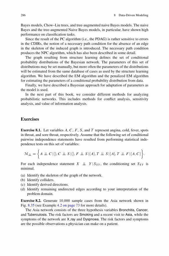
286 8 Data-Driven Modeling

Bayes models, Chow–Liu trees, and tree-augmented naive Bayes models. The naiveBayes and the tree-augmented Naive Bayes models, in particular, have shown highperformance on classification tasks.

Since the result of the PC algorithm (i.e., the PDAG) is rather sensitive to errorsin the CDIRs, the notion of a necessary path condition for the absence of an edgein the skeleton of the induced graph is introduced. The necessary path conditionproduces the NPC algorithm, which has also been described in some detail.

The graph resulting from structure learning defines the set of conditionalprobability distributions of the Bayesian network. The parameters of this set ofdistributions may be set manually, but more often the parameters of the distributionswill be estimated from the same database of cases as used by the structure learningalgorithm. We have described the EM algorithm and the penalized EM algorithmfor estimating the parameters of a conditional probability distribution from data.

Finally, we have described a Bayesian approach for adaptation of parameters asthe model is used.

In the next part of this book, we consider different methods for analyzingprobabilistic networks. This includes methods for conflict analysis, sensitivityanalysis, and value of information analysis.

Exercises

Exercise 8.1. Let variables A, C , F , S , and T represent angina, cold, fever, spotsin throat, and sore throat, respectively. Assume that the following set of conditionalpairwise independence statements have resulted from performing statistical inde-pendence tests on this set of variables:

M?? D{

A ?? C | {}; C ?? S | {}; F ?? S | {A}; T ?? S | {A}; T ?? F | {A;C }

}

:

For each independence statement X ?? Y |SXY , the conditioning set SXY isminimal.

(a) Identify the skeleton of the graph of the network.(b) Identify colliders.(c) Identify derived directions.(d) Identify remaining undirected edges according to your interpretation of the

problem domain.

Exercise 8.2. Generate 10;000 sample cases from the Asia network shown inFig. 8.35 (see Example 4.2 on page 73 for more details).

The Asia network consists of the three hypothesis variables Bronchitis, Cancer,and Tuberculosis. The risk factors are Smoking and a recent visit to Asia, while thesymptoms of the network are X ray and Dyspnoea. The risk factors and symptomsare the possible observations a physician can make on a patient.

Exercises 287

Asia.A/ Smoker.S/

Tuberculosis.T/ Cancer.L/ Bronchitis.B/

Tub or cancer.E/

X ray.X/ Dyspnoea.D/

Fig. 8.35 A graph specifying the independence and dependence relations of the Asia example

Cold Angina

Fever SoreThroat SeeSpots

Fig. 8.36 The anginanetwork

Table 8.20 Data frequenciesfor the class variable

Class n

edible 5;333

poisonous 4;667

(a) Use a software package for learning the equivalence class of DAGs representingthe data generated. Specify expert knowledge on the structure of the DAG asconstraints.

(b) Resolve ambiguous regions.(c) Complete orientation of the DAG.(d) Specify expert knowledge on the distributions of the model and estimate the

parameters from the data generated.

Exercise 8.3. Consider the network in Fig. 8.36. Assume tat the variables are allbinary and that the network is the result of learning from a complete databasewith 1; 000 cases and let l. / D −964.

(a) Compute the AIC score.(b) Compute the BIC score.(c) Compare the AIC and BIC scores. Explain the difference.

Exercise 8.4. Assume we plan to pick up mushrooms to prepare for a nice dinner.In the process, we want to classify each mushroom as either edible or poisonous.We want to construct a network for classifying each mushroom based on a databaseof mushrooms. Assume Tables 8.20–8.23 specify the data frequencies of a databasewe found on the Internet.

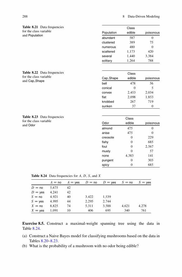
288 8 Data-Driven Modeling

Table 8.21 Data frequenciesfor the class variableand Population

Class

Population edible poisonous

abundant 587 0

clustered 389 75

numerous 480 0

scattered 1;173 420

several 1;440 3;384

solitary 1;264 788

Table 8.22 Data frequenciesfor the class variableand Cap Shape

ClassCap Shape edible poisonous

bell 478 56

conical 0 5

convex 2;453 2;034

flat 2;098 1;853

knobbed 267 719

sunken 37 0

Table 8.23 Data frequenciesfor the class variableand Odor

ClassOdor edible poisonous

almond 475 0

anise 475 0

creosote 0 229

fishy 0 685

foul 0 2;567

musty 0 57

none 4;383 141

pungent 0 303

spicy 0 685

Table 8.24 Data frequencies for A, D, S , and X

A D no A D yes D D no D D yes S D no S D yes

D D no 5;675 42

D D yes 4;241 42

S D no 4;921 40 3;422 1;539

S D yes 4;995 44 2;295 2;744

X D no 8;825 74 5;311 3;588 4;621 4;278

X D yes 1;091 10 406 695 340 761

Exercise 8.5. Construct a maximal-weight spanning tree using the data inTable 8.24.

(a) Construct a Naive Bayes model for classifying mushrooms based on the data inTables 8.20–8.23.

(b) What is the probability of a mushroom with no odor being edible?

Part IIIModel Analysis

Chapter 9Conflict Analysis

It is difficult or even impossible to construct models covering all aspects of(complex) problem domains of interest. A model is therefore most often anapproximation of a problem domain that is designed to be applied according to theassumptions as determined by the background condition or context of the model. Ifa model is used under circumstances not consistent with the background condition,the results will in general be unreliable. The evidence need not be inconsistent withthe model in order for the results to be unreliable. It may be that evidence is simplyin conflict with the model. This implies that the model in relation to the evidencemay be weak, and therefore the results may be unreliable.

Evidence-driven conflict analysis is used to detect possible conflicts in theevidence or between the evidence and the model. If a possible conflict is detected,we should alert the user that the model given the evidence may be weak or evenmisleading. In this way, conflict analysis can also be used for model revision.

Hypothesis-driven conflict analysis is used to identify findings acting in favor ofor against a hypothesis. If the evidence set consists of a large number of findings,it may be crucial to identify which individual findings act in favor of or against ahypothesis.

In this chapter we use the Asia example to illustrate the concepts of evidence andhypothesis-driven conflict analysis in Bayesian networks.

Example 9.1 (Conflict Analysis). As an example, we apply conflict analysis to theAsia example shown in Fig. 9.1 (see Example 4.2 on page 73 for more details).

Assume we see a smoking patient with no shortness of breath and a negativeX-ray result, that is, the initial set of evidence is " D {Dyspnoea D no;Smoker Dyes;X ray D no}. In the remainder of this section, we write " D {"D; "S ; "X } forshort.

From our knowledge about the problem domain and the assumptions of themodel, we would say that the findings are in conflict. The patient visited the chestclinic, but she does not have any of the symptoms even though she is a smoker.A propagation of the evidence produces posterior probability distributions over the

U.B. Kjærulff and A.L. Madsen, Bayesian Networks and Influence Diagrams: A Guideto Construction and Analysis, ISS 22, DOI 10.1007/978-1-4614-5104-4 9,© Springer Science+Business Media New York 2013

291

292 9 Conflict Analysis

Asia.A/ Smoker.S/

Tuberculosis.T/ Cancer.L/ Bronchitis.B/

Tub or cancer.E/

X ray.X/ Dyspnoea.D/

Fig. 9.1 A graph specifying the independence and dependence relations of the Asia example

diseases P.B D yes |"/ D 0:25, P.L D yes |"/ D 0:089, and P.T D yes |"/ D0:009. This does not disclose a possible conflict, but only indicates that the mostlikely disease the patient is suffering from is bronchitis. Using the model only, wecannot distinguish between flawed evidence, a case not covered by the model, or arare case. �

In Sect. 9.1, we describe evidence-driven conflict analysis. A conflict measuredesigned to be efficient to compute and to give indications of possible conflicts inevidence is introduced. Possible conflicts should be detected and traced or explainedas rare cases that the model may not cover well. In Sect. 9.2, we describe hypothesis-driven conflict analysis. A cost-of-omission measure is introduced. This measure isuseful for relating the impact of findings on a hypothesis variable. In addition, wedescribe how to investigate the impact of a finding on the probability of a hypothesis.

9.1 Evidence-Driven Conflict Analysis

The objective in evidence-driven conflict analysis is to detect possible conflicts in aset of evidence. As a tool for detecting possible conflicts, we want a conflict measurewhich is easy to calculate and which gives a reliable indication of a possible conflict.

9.1.1 Conflict Measure

In order to detect a possible conflict, we need to compare the results obtained fromour best model with the results obtained from an alternative model. This model isreferred to as a straw model. A straw model is a simple and computationally efficientmodel used as an alternative model in the detection of possible conflicts.

In the design of the conflict measure, we make the assumption that for the nor-mally (according to the model) behaving evidence, it is the case thatP."i |"j />P."i /

9.1 Evidence-Driven Conflict Analysis 293

where "i and "j are two pieces of evidence. Based on this assumption andsince P."i ; "j / D P."i |"j /P."j /, the conflict measure is designed to indicate apossible conflict when the joint probability of the evidence is less than the productof the probabilities of the individual pieces of evidence given the model. We thusassume that there is a possible conflict between two pieces of evidence "i and "j , if

P."i /P."j /

P."i ; "j /> 1⇔ log

P."i /P."j /

P."i ; "j /> 0;

that is, "i and "j are negatively correlated. Thus, we define the conflict measure as

conf."/ D logP."i /P."j /

p."/;

where " D {"i ; "j }. Notice that we are comparing the joint probability of theevidence with a model where the observed variables are independent (the strawmodel).

The main assumption is that pieces of evidence are positively correlated suchthat P."/ >

QniD1 P."i /. With this assumption, the general conflict measure is

defined as

conf."/ D conf.{"1; : : : ; "n}/ D log

QniD1 P."i /p."/

:

This implies that a positive value of the conflict measure conf."/ indicates a possibleconflict. Notice that the conflict measure is easy to calculate once the evidence "has been propagated in a junction tree representation of the model. The marginalprobabilities P."i / are available once the junction tree has been initialized, and theprobability of the evidence P."/ is available as a by-product of message passing,see Sect. 5.1 for details on propagation of evidence.

Another way to look at the definition of the conflict measure is the following. Inthe general case, two pieces of evidence "i and "j are either:

• Positively correlated, that is, P."i |"j / > P."i /• Negatively correlated, that is, P."i |"j / < P."i /• Independent, that is, P."i |"j / D P."i /

Given these three options, we choose to assume that two pieces of evidence "i and "jare positively correlated.

Example 9.2 (Conflict Detection). Returning to Example 9.1, the evidence is" D {"D; "S ; "X }. We compute the conflict measure to be

conf."/ D conf.{D D no; S D yes; X D no}/

D logP.D D no/P.S D yes/P.X D no/

P."/

294 9 Conflict Analysis

D log0:56 � 0:5 � 0:89

0:2D 0:22

> 0:

Thus, conf."/ indicates a possible conflict in ". �

9.1.2 Tracing Conflicts

Once a possible conflict has been detected, the origin of the conflict should bedetermined such that it can be presented to the analyst or user. Tracing the sourceof a conflict amounts to computing the conflict measure conf."0/ for (all) subsets"0 � ".

Tracing the conflict to all subsets of the evidence is a computationally complexproblem as the number of subsets increases exponentially with the size of theevidence set. It is not always possible or meaningful to assume monotonicity withrespect to conflict in subsets, that is, no subset "00 � "0 with conf."00/ > 0 existsfor "0 with conf."0/ � 0. That is, the monotonicity assumption states that if "0 is notin conflict, then no subset of "0 is in conflict.

Example 9.3 (Conflict Traced). In Example 9.2, a possible conflict was identified,but not traced, that is, located. That is, after the conflict measure has been foundto indicate a possible conflict, the source of the conflict should be traced. This isachieved by computing the conflict measure for different subsets "0 of ".

With three pieces of evidence, there are three pairs of evidence to consider.The pair "DS D {"D; "S } has conflict measure

conf."D; "S / D logP.D D no/P.S D yes/

P.D D no; S D yes/

D log0:56 � 0:50:22

D 0:24;

the pair "DX D {"D; "X } has conflict measure

conf."D; "X/ D logP.D D no/P.X D no/

P.D D no; X D no/

D log0:56 � 0:890:52

D −0:04;

and the pair "SX D {"S ; "X } has conflict measure

conf."S ; "X/ D logP.S D yes/P.X D no/

P.S D yes; X D no/

D log0:5 � 0:890:47

D −0:06:

9.1 Evidence-Driven Conflict Analysis 295

The (partial) conflicts show that there is a conflict in the pair "DS D {"D; "S } whilethere are no conflicts in the pairs "DX D {"D; "X } and "SX D {"S; "X }. Hence,the source of the global conflict in conf."/ can be traced to the partial conflictbetween "D and "S . The finding that the patient is a smoker is in conflict with thefinding that the patient is not suffering from dyspnoea (under the assumptions ofthe model). �

Let "i and "j be a partitioning of the evidence " into two disjoint subsets suchthat " D "i ["j is the evidence under consideration. The global conflict conf."/ canbe computed from local conf.{"i ; "j }/ and partial conflicts conf."i / and conf."j /

conf."/ D conf.{"i ; "j }/C conf."i /C conf."j /:

This property holds in general, and it may be used as a tool for tracing conflicts.

Example 9.4 (Partial Conflicts). In the example, we have three subsets with par-tial conflicts computed in Example 9.3 conf."D; "S/ D 0:24, conf."DX/ Dconf.{"D; "X }/ D −0:04, and conf."DS/ D conf.{"S; "X }/ D −0:06. The localconflict between {"D; "S } and "X is

conf.{"D; "S }; "X/ D logP.D D no; S D yes/P.X D no/

P."/

D log0:22 � 0:89

0:2D −0:02:

The global conflict can be computed from local and partial conflicts as

conf.{"D; "S ; "X }/ D conf.{"D; "S }/C conf.{{"D; "S }; "X }/

D 0:24C .−0:02/ D 0:22:

We notice that the finding "X reduces the global conflict slightly. �

9.1.3 Conflict Resolution

Typical evidence from a rare case may indicate a possible conflict (a rare case isidentified as a finding or set of evidence with low (prior) probability). Let " D{"1; : : : ; "n} be findings for which the conflict measure indicates a possible conflict,that is, conf."/ > 0. Also, let h be a hypothesis which could explain the findings(i.e., conf." [ {h}/ � 0). That is, if we also know the hypothesis h to be true, thenwe will not expect a conflict. We compute

conf." [ {h}/ D conf."/C logP.h/

P.h |"/:

If conf."/ � log P.h |"/

P.h/, then h can explain away the conflict where P.h |"/

P.h/is the

normalized likelihood.

296 9 Conflict Analysis

Table 9.1 Thelog-normalized likelihood ofeach possible instantiation ofeach variable in Example 9.1

Hypothesis P.h/ P.h |"/ log P.h|"/

P.h/

Asia D no 0:99 0:99 0

Asia D yes 0:01 0:01 0

Bronchitis D no 0:55 0:75 0:31

Bronchitis D yes 0:45 0:25 −0:59

Cancer D no 0:545 0:1 1:7

Cancer D yes 0:455 0:9 0:68

Tuberculosis D no 0:99 0:999 0:01

Tuberculosis D yes 0:01 0:001 −2:3

Tub or cancer D no 0:995 0:9999 0:005

Tub or cancer D yes 0:005 0:0001 −3:9

Example 9.5 (Conflict Resolution). Table 9.1 shows the log-normalized likelihoodof each possible instantiation of each variable in Example 9.1. From this table, it isclear that there are five possible explanations of the conflict (some of which have alow log-normalized likelihood).

For instance, the posterior probability of the patient not having bronchitisis P.B D no |"/ D 0:75 while the prior probability is P.B D no/ D 0:55. Wecompute the logarithm of the normalized likelihood

logP.h |"/

P.h/D log

0:75

0:55D 0:31:

From this, we compute the conflict measure under the hypothesis of the patient nothaving bronchitis

conf." [ {h}/ D conf."/C logP.h/

P.h |"/

D 0:22− 0:31 < 0:

Thus, the conflict may be explained away as the rare case where the patientis not suffering from bronchitis given the symptoms and risk factors (similarlyfor Cancer). In general, if the normalized likelihood is greater than the conflict,then we may have a rare case. �

The above method for detecting conflicts may fail. This will happen if theassumption of positively correlated pieces of evidence does not hold. The aboveapproach can be combined with other methods such as those reported in Kim &Valtorta (1995) and Laskey (1991). These methods are based on using a morecomplex straw model for the comparison (i.e., evidence variables are not assumedindependent) and a different measure to detect conflicts. The advantage of the aboveapproach is that it is computationally efficient.

The above method for detecting conflicts was introduced by Andersen et al.(1989), and the method is described in Jensen (1996) and Jensen (2001).

9.2 Hypothesis-Driven Conflict Analysis 297

9.2 Hypothesis-Driven Conflict Analysis

In hypothesis-driven conflict analysis, the impact of a finding on the probability ofa hypothesis is investigated. In order to be able to relate the impacts of differentfindings on the probability of the hypothesis given evidence, a measure is needed.This will allow us to identify pieces of evidence that conflict with the impact of theentire set of evidence.

9.2.1 Cost-of-Omission Measure

The main purpose of hypothesis-driven conflict analysis is to identify pieces ofevidence with an impact on the evidence that conflicts with the impact of theentire set of evidence. In order to perform this investigation, a measure providinga numerical value specifying the cost of omitting a single piece of evidence isrequired. Suermondt (1992) defines the cost-of-omission c.P.X |"/; P.X |" \ {"i }//

of "i as

c.P.X |"/; P.X |" \ {"i }// DX

x2dom.X/

P.x |"/ logP.x |"/

P.x |" \ {"i }/: (9.1)

The above equation is undefined for values P.x |"/ D 0 and P.x |" \ {"i }/ D 0. Forthese two cases, we define cost-of-omission to be 0 and infinity, respectively.

9.2.2 Evidence with Conflict Impact

Let H be a hypothesis variable with states dom.H/ D .h1; : : : ; hn/ and let " D{"1; : : : ; "m} be the set of evidence. The impact of a finding "i 2 " on ahypothesis h 2 dom.H/ is determined by computing and comparing the priorprobability of the hypothesis P.h/, the posterior probability of the hypothesisgiven all evidence P.h |"/, and the posterior probability of the hypothesis given allevidence except the finding under consideration P.h |" \ "i /. By comparing thesethree probabilities, we can identify findings that have a conflicting impact on theprobability of the hypothesis compared with the impact of the entire set of evidence.

Example 9.6 (Evidence with Conflict Impact). In the Asia example, we assumeevidence " D {Dyspnoea D no;Smoker D yes;X ray D no} D {"D; "S ; "X }.Assume further that B D Bronchitis is the hypothesis variable under consideration.

Figure 9.2 shows the impact of the finding "S on the hypothesis B D nowhile Fig. 9.3 shows the impact of the finding "S on the hypothesis B D yes.From Fig. 9.2, it is clear that the finding "S acts against the hypothesis B D no.

298 9 Conflict Analysis

0

0.2

0.4

0.6

0.8

1

P.h |"/P.h |" \ "S /P.h/

Impact of evidence

Fig. 9.2 The impact of finding "S on the hypothesis h W B D no

0

0.2

0.4

0.6

0.8

1

P.h |"/P.h |" \ "S /P.h/

Impact of evidence

Fig. 9.3 The impact of finding "S on the hypothesis h W B D yes

The probability of the hypothesis is higher when the finding "S is excluded thanwhen it is included. The posterior is higher than the prior. This implies that thecombined effect of the evidence acts in favor of the hypothesis.

Similarly, from Fig. 9.3, it is clear that the finding "S acts in favor of thehypothesisB D yes. The probability of the hypothesis is higher when the finding "Sis included than when it is excluded, but not as high as the prior though. Theposterior is lower than the prior. This implies that the combined effect of theevidence acts against the hypothesis.

The numbers in the two graphs are pairwise complementary since B is binary.�

When considering the impact of findings given a large set of evidence, it maybe an advantage to use a cost-of-omission threshold to focus on findings with acost-of-omission greater than the threshold.

Example 9.7 (Example 9.6, cont.). In Example 9.6 the cost-of-omission of find-ing "S is 0:03, that is,

c.P.B |"/; P.B |" \ {"S }// D 0:03:

�

Exercises 299

Further information on hypothesis-driven conflict analysis can be found in Suer-mondt (1992).

9.3 Summary

In this chapter we have considered evidence and hypothesis-driven conflict analysisin Bayesian networks.

The objective of evidence-driven conflict analysis is to detect possible conflictsin the evidence. To support this analysis, we have defined a conflict measure that issimple to compute. The conflict measure is computed based on an alternative andmuch simpler model (the straw model). The conflict measure is defined such that apositive value is an indication that a conflict may be present in the evidence. Oncea possible conflict is detected, we try to trace and resolve the conflict. We say thata hypothesis may resolve the conflict if the log of the normalized likelihood of thehypothesis is greater than the conflict. Furthermore, a positive conflict measure mayoriginate from a rare case.

The objective of hypothesis-driven conflict analysis is to investigate the impactof a single piece of evidence on the probability of a hypothesis compared with theimpact of all the evidence. To support this investigation, we have defined a cost-of-omission measure. The cost-of-omission measure is used to measure the differencebetween including and excluding the selected piece of evidence on the probabilityof the hypothesis given evidence. In hypothesis-driven conflict analysis, we relatethe prior probability of the hypothesis to the probability of the hypothesis given theentire set of evidence and the probability of the hypothesis given the entire set ofevidence except the selected piece of evidence. This enables us to determine whetheror not a single piece of evidence conflicts with the remaining set of evidence withrespect to the probability of the hypothesis.

In Chap. 10, we consider sensitivity analysis. Evidence sensitivity analysis isto determine the sensitivity of the posterior probability of a hypothesis relativeto observations made. Parameter sensitivity is to determine the sensitivity of theposterior probability of a hypothesis relative to parameters of the model.

Exercises

Exercise 9.1. From Example 2.4 on page 25, we know that Dr Watson makesfrequent calls to Mr. Holmes regarding the burglar alarm; however, till now thecause of activation of the alarm has been small earthquakes or a big truck passingby near the house. Every time Mr. Holmes rushes home just to find that everythingis in order; so now Mr. Holmes is installing a seismometer in his house with a directline to his office. In this exercise, we assume P.B/ D P.E/ D .0:1; 0:9/.

300 9 Conflict Analysis

A

B E

R

W

S

Fig. 9.4 Mr. Holmes installsa seismometer with a directline to his office

Table 9.2 The conditional probability distributions P.W |A/ and P.S |B;E/

S

W A D no A D yes B E no some large

no 0:99 0:65 no no 0:97 0:02 0:01

yes 0:01 0:35 no yes 0:01 0:97 0:02

yes no 0:01 0:02 0:97

yes yes 0 0:03 0:97

Table 9.3 The conditionalprobability distributionP.A |B;E; F /

A

E B F no yes

no no no 0:99 0:01

no no yes 0:01 0:99

no yes no 0:01 0:99

no yes yes 0 1

yes no no 0:01 0:99

yes no yes 0 1

yes yes no 0 1

yes yes yes 0 1

The revised model in Fig. 9.4 captures the situation where Mr. Holmes hasinstalled a seismometer in his house with a direct line to the office. Assume Shas states reflecting no, some, and large vibrations in the house. The conditionalprobability distributions P.W |A/ and P.S |B;E/ are shown in Table 9.2.

(a) One afternoon, Dr. Watson calls again and announces that Mr. Holmes’ alarmhas gone off. Mr. Holmes checks the seismometer; it is in state no.

Are the two observations in conflict?(b) Mr. Holmes looks out his window. It rains heavily. When it rains heavily, a

flood is likely to occur. Extend the model in Fig. 9.4 to capture these eventswhen the prior of rain is 0:01 and rain causes a flood in one out of ten cases.The conditional probability table P.A |B;E; F / where F represents flood isshown in Table 9.3.

Are the observations in conflict in this model and what is the value of theconflict measure?

(c) Is there a potential explanation of the value of the conflict measure?

Exercises 301

(d) What is the partial conflict of each subset of the observations and whatconclusion can be derived from the partial conflicts?

Exercise 9.2. Consider again the model with a seismometer of Mr. Holmes inExercise 9.1.

(a) Perform hypothesis-driven conflict analyses with respect to both Burglar D yesand Earthquake D yes.

(b) What is the cost-of-omission for "R with respect to Burglar and Earthquake?

Chapter 10Sensitivity Analysis

We construct probabilistic networks to support and solve problems of belief updateand decision making under uncertainty. In problems of belief update the posteriorprobability of a single hypothesis variable is sometimes of interest. When theevidence set consists of a large number of findings or even when it consists of only asmall number of findings questions concerning the impact of subsets of the evidenceon the hypothesis or a competing hypothesis emerge.

Evidence sensitivity analysis may, for instance, give answers to questions likewhat are the minimum and maximum beliefs produced by observing a variable?,which evidence acts in favor of or against a hypothesis?, which evidence discrimi-nates one hypothesis from an alternative hypothesis?, and what if a certain observedvariable had been observed to a value different from the actual value? Knowingthe answers to these and similar questions may help to explain and understand theconclusions reached by the model as a result of probabilistic inference. It will alsohelp to understand the impact of subsets of the evidence on a certain hypothesis andalternative hypotheses.

Evidence sensitivity analysis is not the only possible kind of sensitivity analysisthat can be performed on a probabilistic network. Parameter sensitivity analysisis another type of sensitivity analysis that is supported by probabilistic networks.We focus on parameter sensitivity analysis in discrete Bayesian networks. Theparameters considered in parameter sensitivity analysis are the entries of theconditional probability distributions specified in the Bayesian network. The analysisis performed relative to a hypothesis and a given set of evidence. It has been shownthat there is a (surprisingly) simple correlation between the probability of a set ofevidence and an entry of a conditional probability distribution. The probability ofthe evidence is a linear function of the parameter. This knowledge can be exploitedto determine the functional relation between the probability of a hypothesis given asubset of evidence and a parameter of a conditional probability distribution.

Parameter sensitivity analysis is particularly useful for identifying parametersof a probabilistic network that have a large or small impact on the probability ofa hypothesis given evidence. When knowledge elicitation resources are limited,

U.B. Kjærulff and A.L. Madsen, Bayesian Networks and Influence Diagrams: A Guideto Construction and Analysis, ISS 22, DOI 10.1007/978-1-4614-5104-4 10,© Springer Science+Business Media New York 2013

303

304 10 Sensitivity Analysis

parameter sensitivity analysis is a useful tool for identifying and focusing resourceson the parameters that are most influential on the posterior probability of ahypothesis given evidence. That is, parameter sensitivity analysis can be used in anattempt to focus knowledge elicitation resources in the model construction process.

In Sect. 10.1, we introduce evidence sensitivity analysis. A distance measuredesigned to measure the impact of evidence on the probability of a hypothesisis introduced. In the following subsections, we consider identifying minimumand maximum beliefs in a hypothesis given various subsets of the evidence, theimpact of different evidence subsets on a hypothesis, how subsets of the evidencediscriminates between a pair of competing hypotheses, what-if analysis, and theimpact of findings on a hypothesis variable. In Sect. 10.2 (one-way), parametersensitivity analysis is introduced, and in Sect. 10.3, two-way parameter sensitivityanalysis is considered while Sect. 10.4 introduces parameter tuning.

10.1 Evidence Sensitivity Analysis

Evidence sensitivity analysis (SE analysis) is the analysis of how sensitive theresults of a belief update (propagation of evidence) is to variations in the set ofevidence (observations, likelihood, etc.).

Consider the situation where a decision maker has to make a decision basedon the probability distribution of a hypothesis variable. It could, for instance, be aphysician deciding on a treatment of a patient given the probability distribution of adisease variable. Prior to deciding on a treatment, the physician may have the optionto investigate the impact of the collected information on the posterior distributionof the hypothesis variable, that is, given a set of findings and a hypothesis, whichsets of findings are in favor of, against, or irrelevant for the hypothesis, whichsets of findings discriminate the hypothesis from an alternative hypothesis, whatif a variable had been observed to a different value than the one observed, etc.These questions can be answered by SE analysis. Given a Bayesian network modeland a hypothesis variable, the task is to determine how sensitive the belief in thehypothesis variable is to variations in the evidence. We consider one-step look-aheadhypothesis-driven SE analysis on discrete random variables.

Example 10.1 (Evidence Sensitivity Analysis). As an example, we consider SEanalysis on the Asia example shown in Fig. 10.1 (see Example 4.2 on page 74for more details). The hypothesis variable is Bronchitis (B), and the initial set ofevidence is " D {"S ; "D} D {S D no;D D yes}. That is, we are considering whetheror not the patient is suffering from bronchitis after observing that the patient doesnot smoke (Smoker D no) and has shortness of breath (Dyspnoea D yes).

This example is used in the following sections to illustrate concepts of SEanalysis. �

10.1 Evidence Sensitivity Analysis 305

Asia.A/ Smoker.S/

Tuberculosis.T/ Cancer.L/ Bronchitis.B/

Tub or cancer.E/

X ray.X/ Dyspnoea.D/

Fig. 10.1 A graph specifying the independence and dependence relations of the Asia example

10.1.1 Distance and Cost-of-Omission Measures

The main purpose of hypothesis-driven SE analysis is to investigate how changesin the set of evidence impact the probability of a hypothesis. In order to performthis investigation, two distance measures are required. Each distance measure willprovide a numerical value specifying the distance between either two probabilitiesor two probability distributions.

Let X be a hypothesis variable with state space dom.X/ D .x1; : : : ; xn/ andlet " D {"1; : : : ; "m} be a set of evidence (findings). We let "Y 2 " denote the findingon variable Y 2 X."/.

The distance d.p; q/ between two probabilities p and q is defined, for p 6D 0, as

d.p; q/ Dˇˇ qp− 1

ˇˇ :

This measure is, for instance, useful for measuring the distance between theprobability P.x |"/ of hypothesis x given evidence " and the probability P.x |" \{"i }/ of hypothesis x given evidence " \ {"i }, that is, the set of evidence where "i isexcluded from ".

A pair of probabilities p and q are said to be almost equal when theirdistance d.p; q/ is below a predefined threshold ı, that is, d.p; q/ < ı.

The cost-of-omission c.P.X |"/; P.X |" \ {"i }// of "i was defined in Sect. 9.2.1on page 297 as

c.P.X |"/; P.X |" \ {"i }// DX

x2dom.X/

P.x |"/ log

�P.x |"/

P.x |" \ {"i }/

�:

Notice the difference between the distance measure and the cost-of-omissionmeasure. The distance measure evaluates the distance between probability valueswhereas the cost-of-omission measure evaluates the distance between two posterior

306 10 Sensitivity Analysis

Table 10.1 Sensitivity of the posterior probability distribution of the hypothe-sis variable B to findings on A

b mina P.B D b |"; a/ P.B D b |"/ maxa P.B D b |"; a/

no 0:228 0:228 0:236

yes 0:764 0:772 0:772

probability distributions relative to omitting a certain finding "i from the evidence ".The cost-of-omission measure is a special case of the more general cross entropydistance (or Kullback–Leibler distance) measure between a probability distribu-tion P and an approximation P 0 of P :

DKL.P;P0/ D

X

x2dom.X/

P.x/ log

�P.x/

P 0.x/

�:

The cost-of-omission measure is, for instance, useful for measuring the distancebetween the posterior probability distribution P.X |"/ of hypothesis variable Xgiven evidence " and the posterior probability distribution P.X |" \ {"i }/ ofhypothesis variableX given evidence " \ {"i }, that is, the set of evidence where "i isexcluded from ".

In the following sections, the distance measures defined above are used tointroduce different concepts related to SE analysis.

10.1.2 Identify Minimum and Maximum Beliefs

As part of performing SE analysis, we may be interested in knowing the minimumand maximum values of the posterior belief for each possible state x 2 dom.X/ ofthe hypothesis variable X given all possible observations on a given variable Y 62X."/, that is, what are the minimum and maximum values ofP.x |"; y/ as a functionof y 2 dom.Y /.

The minimum miny2dom.Y / P.x |"; y/ and maximum maxy2dom.Y / P.x |"; y/

values of the posterior belief are determined by entering and propagating eachstate y of the information variable Y . This analysis requires one belief update foreach state of variable Y .

This analysis identifies the range of the posterior belief in a hypothesis as afunction of possible observations on an unobserved variable. This may help todetermine the impact of a possible observation on the probability of the hypothesis.

Example 10.2 (Example 10.1, cont.). Table 10.1 shows the sensitivity of theposterior probability distribution P.B |"; a/ of the hypothesis variable B relativeto instantiations of the unobserved variable Asia (A).

For each state b 2 dom.B/ of B , the minimum posterior belief mina P.B Db |"; a/, the current belief P.B D b |"/, and the maximum posterior belief

10.1 Evidence Sensitivity Analysis 307

Table 10.2 Normalizedlikelihood of hypothesis hBgiven all subsets of theevidence "

"0 NL

"S "X "D 1:256

"S "X − 0:667

"S − "D 1:675

"S − − 0:667

− "X "D 1:515

− "X − 1:125

− − "D 1:853

− − − 1

mina P.B D b |"; a/ are shown. From the table, it is clear that an observation on Awould produce insignificant variations in the posterior belief in any state of B . �

10.1.3 Impact of Evidence Subsets

Investigation of the impact of different subsets of the evidence " on each state x 2dom.X/ of the hypothesis variable X is a useful part of SE analysis. Investigatingthe impact of different subsets of the evidence on states of the hypothesis may helpto determine subsets of the evidence acting in favor of or against each possiblehypothesis.

The impact of a subset of the evidence "0 � " on a state x of the hypothesisvariable X is determined by computing the normalized likelihood NL of thehypothesis x given evidence "0, that is,

NL D P."0 |x/P."0/

D P."0; x/=P.x/P."0/

D P.x |"0/P."0/=P.x/P."0/

D P.x |"0/P.x/

;

where we assume P."0/ > 0 and P.x/ > 0. This fraction is computed by enteringand propagating "0. Therefore, this analysis requires one belief update for eachsubset "0 of the evidence ".

Each normalized likelihood is a measure of the impact of a subset of evidence onthe hypothesis. By comparing the normalized likelihoods of different subsets of theevidence, we compare the impacts of the subsets of evidence on the hypothesis.

Example 10.3 (Example 10.2, cont.). Assume that we observe the patient to havea positive X-ray result X D yes, such that the set of evidence is " D {"S ; "D; "X } D{S D no;D D yes; X D yes}. Table 10.2 shows the normalized likelihood of thehypothesis hB W B D yes given the evidence " D {"S ; "D; "X }.

From Table 10.2, it is clear that the finding "D on D acts in favor of thehypothesis hB . On the other hand, the evidence "S acts slightly against thehypothesis hB while "X is irrelevant, against, and in favor of hB depending on theremaining evidence. �

308 10 Sensitivity Analysis

Table 10.3 Discriminationbetween hypothesis hB andthe alternative hypothesis hL

"0 B

"S "X "D 0:281

"S "X − 0:258

"S − "D 3:869

"S − − 3:667

− "X "D 0:134

− "X − 0:127

− − "D 0:992

− − − 1

10.1.4 Discrimination of Competing Hypotheses

A central question considered by SE analysis is how different subsets of theevidence discriminate between competing hypotheses. The challenge is to comparethe impact of subsets of the evidence on competing hypotheses.

We consider the discrimination between two different hypotheses represented asstates of two different variables. Thus, let X be the hypothesis variable of interestand let Y be an alternative hypothesis variable where X 6D Y .

In Sect. 3.5, we describe how the discrimination of a pair of competinghypotheses x 2 dom.X/ and y 2 dom.Y / may be based on the calculation ofBayes’ factor B (or Bayesian likelihood ratio)for all subsets "0 � " of a set ofevidence ":

B D posterior odds ratio

prior odds ratioD P.x |"0/=P.y |"0/

P.x/=P.y/D P."0 |x/P."0 |y/

D L.x |"0/L.y |"0/

; (10.1)

where we assume P.x/ > 0, P.y/ > 0, and P."0/ > 0. Bayes’ factor is the ratio ofthe likelihoods of hypothesis x and y given the evidence "0.

From (10.1), we see that:

B > 1 if the evidence "0 provides more support for x than for y.B < 1 if the evidence "0 provides less support for x than for y.B D 1 if the evidence "0 does not provide useful information for differentiatingbetween x and y.

This analysis requires one belief update for each subset "0 � ".

Example 10.4 (Example 10.3, cont.). Assume that hL W Cancer D yes is analternative hypothesis to the hypothesis hB . Table 10.3 shows Bayes’ factor for thehypothesis hB and the alternative hypothesis hL.

From Table 10.3, it is clear that subsets {"S } and {"S ; "D} act in favor of thehypothesis hB when compared with the alternative hypothesis hL. On the otherhand, the remaining subsets act slightly against the hypothesis hB when comparedwith the alternative hypothesis hL. �

10.1 Evidence Sensitivity Analysis 309

Table 10.4 What-if analysison findings Y y0

P.B D yes |" \{"Y }; y

0/

D no 0:092

D yes 0:565

S no 0:565

S yes 0:714

X no 0:774

X yes 0:565

10.1.5 What-If Analysis

In what-if analysis, the type of question considered is the following. What if thefinding on a discrete random variable Y 2 X."/ had been the observation Y D y0instead of Y D y (represented by the finding "Y 2 ", where " is the set of evidence)?We consider a hypothesis-driven approach to what-if SE analysis.

Hypothesis-driven what-if analysis is performed by computing the posteriorprobability distribution P.X |" \ {"Y }; y

0/ of the hypothesis variable X for eachpossible state y0 6D y of the observed variable Y .

The posterior probability distribution P.X |" \ {"Y }; y0/ specifies the impact

of each possible instantiation of Y on the posterior distribution of the hypothesisvariable X . The analysis requires one belief update for each y0 2 dom.Y /. Noticethat "Y need not be an instantiation of Y , that is, "Y may be soft evidence.

Example 10.5 (Example 10.4, cont.). For each finding variable Y , we may considerthe impact of each possible observation Y D y. Table 10.4 shows the posteriorbelief in the hypothesis B D yes given the evidence where the finding y issubstituted with each possible state y0 2 dom.Y /.

From Table 10.4, it is clear that changing the observation on D from yes to nohas a significant impact of the posterior belief in the hypothesis B D yes. On theother hand, the posterior belief in the hypothesisB D yes has a lower sensitivity toobservations on S and X .

Since each finding (i.e., "S , "X , or "D) is an instantiation, one row for eachobserved variable Y corresponds to the posterior belief in the hypothesis B D yes.That is, P.B D yes |"/ D 0:565 is represented three times in the table. �

10.1.6 Impact of Findings

Let X D x be the hypothesis of interest where X is the hypothesis variable andlet " be the entire set of evidence. The impact of each finding "Y 2 " on theprobability of x is determined by computing and comparing the prior probabilityof the hypothesis, P.x/, the posterior probability of the hypothesis given the entireset of evidence, P.x |"/, and the posterior probability of the hypothesis given theentire set of evidence except the finding "Y , P.x |" \ {"Y }/.

310 10 Sensitivity Analysis

Table 10.5 Findings impactanalysis

"Y P.B D yes/ P.B D yes |" \ {"Y }/ P.B D yes |"/

"S 0:45 0:682 0:565

"X 0:45 0:754 0:565

"D 0:45 0:3 0:565

To relate the impact of individual findings on the probability of the hypothesis,we define the notions of an important finding, a redundant finding, and an irrelevantfinding:

• A finding "Y 2 " is important when the difference between the probability q DP.x |" \ {"Y }/ of the hypothesis given the entire set of evidence except "Y andthe probability p D P.x |"/ of the hypothesis given the entire set of evidence istoo large; that is, the probabilities p and q are not almost equal (d.p; q/ � ı).

• A finding "Y 2 " is redundant when q D P.x |" \ {"Y }/ is almost equal to p DP.x |"/; that is, d.p; q/ < ı.

• A finding "Y 2 " is irrelevant when q D P.x |"0 \ {"Y }/ is almost equal to p DP.x |"0/ for all subsets "0; that is, d.p; q/ < ı for all subsets "0. That is, thefinding "Y is redundant for all subsets of the evidence.

The term almost equal is defined based on the distance measure introduced inSect. 10.1.1. Similarly, a sufficient set of evidence is defined as:

• A subset of evidence "0 � ", for example, the entire set of evidence " excepta certain finding "Y , is sufficient when q D P.x |"0/ is almost equal to p DP.x |"/; that is, d.p; q/ < ı.

The impact of each finding "Y may be considered for each state or a certain stateof the hypothesis variableX . Sufficiency ıs and importance ıi thresholds should bespecified by the user.

Example 10.6 (Example 10.5, cont.). We may be interested in considering theimpact of each finding "Y 2 " on the probability of the hypothesis B D yes bycomparing P.B D yes/, P.B D yes |"/, and P.B D yes |" \ {"Y }/. Table 10.5shows the prior belief in the hypothesis B D yes, the posterior belief given allevidence P.B D yes |"/, and the posterior belief given all evidence except a singlefinding P.B D yes |" \ {"Y }/.

From Table 10.5, we make the following observations:

• The finding "S is important. At sufficiency threshold ıs D 0:02, the finding "S isredundant, and "\ {"S } is sufficient. At cost-of-omission threshold ıo D 0:03, theevidence "S would not be included in the analysis.

• The finding "X is important.• The finding "D is important.

The subset "0 D {"S ; "X ; "D} D " is, of course, also sufficient. The analysis isperformed using threshold values ıo D 0:0001, ıs D 0:02, and ıi D 0:05.

Table 10.6 shows the cost-of-omission c.P.B |"/; P.B |" \ {"Y }// and thedistance d.P.B D yes |"/; P.B D yes |" \ {"Y }// for each finding "Y . �

10.2 Parameter Sensitivity Analysis 311

Table 10.6 Cost-of-omission and distance inposterior beliefs of thehypothesis for each finding

"Y

c.P.B |"/; P.B |"\

{"Y }//

d.P.B D yes |"/; P.B Dyes |" \ {"Y }//

"S 0:03 0:171

"X 0:085 0:25

"D 0:151 0:884

10.2 Parameter Sensitivity Analysis

Parameter sensitivity analysis (SP analysis) is the analysis of how sensitive theresults of a belief update (propagation of evidence) is to variations in the value of aparameter of the model. The parameters of a model are the entries of the conditionalprobability distributions.

Consider the situation where company management allocates resources toresearch and development projects based on an estimation of projects’ successes.The success of a project depends on the ability of the project management to obtaincertain environmental permissions from the authorities. This and other properties ofthe domain are modeled as a Bayesian network. As part of the model construction,the knowledge engineers (and the management of the company) would like toassess how sensitive the conclusion of the model (i.e., the probability of projectsuccess) is to the prior probability of a specific environmental permission beingobtained. Parameter sensitivity analysis is designed to answer such questions. Givena Bayesian network model, a hypothesis, and a set of evidence, the task is todetermine the sensitivity of the posterior belief in the hypothesis to variations inthe value of an assessed parameter.

We consider scenario-based SP analysis on discrete random variables withrespect to changes in a single parameter value where a scenario S is defined as avector consisting of a hypothesis variable H , a state of the hypothesis variable h,and a set of evidence ", that is, S D .H; h; "/.

Example 10.7 (Parameter Sensitivity Analysis). Apple Jack, see Example 4.1 onpage 71, is interested in computing the probability of his finest apple tree beingsick. His hypothesis is that the tree is sick, that is, the hypothesis is Sick D yes. Theevidence available to support the reasoning of Apple Jack is that the tree is losing itsleaves. Thus, the scenario under consideration is S D .Sick; yes; {Loses D yes}/.Given the Bayesian network shown in Fig. 4.1 on page 72 and the conditionalprobability distributions P.Sick/ D .0:95; 0:05/, P.dry/ D .0:9; 0:1/, andP.Loses |Sick;Dry/ as specified in Table 4.1 on page 73, the posterior distributionof the hypothesis given the observation, P.Sick D yes |"/, is 31:62%.

How sensitive is this posterior probability to small variations in the quantificationof the model? For instance, how would the posterior probability of the hypothesischange if the prior probability of Dry D yes decreases from 0:1 to 0:075? Setting theprior probability of Dry D yes to 0:075, the posterior distribution of the hypothesisgiven the observation, P.Sick D yes |"/, is 36:64%.

312 10 Sensitivity Analysis

This shows that the posterior probability of the hypothesis Sick D yes (and otherevents) changes when the prior on Dry D yes is changed to 0:075 (from 0:1).The posterior probability of Sick D yes increases from 31:52% to 36:64%. Thisseems intuitive as the prior of one cause decreases and the posterior of another causeincreases given the observed effect. However, what if the prior had been changed to adifferent value? Is it necessary to compute the posterior probability of the hypothesisfor all possible values of P.Dry D yes/, that is, the parameter we are investigating?

The aforementioned questions may be answered more efficiently using parametersensitivity analysis. �

10.2.1 Sensitivity Function

Parameter sensitivity analysis is based on the observation that the probabilityof the evidence is a linear function of any single parameter in the model, thatis, any entry of any conditional probability distribution (Castillo, Gutierrez &Hadi 1997, Coupe & van der Gaag 1998). That is, y D P."/ as a function of aconditional probability t D P.X D x |pa.X/ D z/ has the simple form y D ˛ �tCˇwhere ˛; ˇ 2 R. This implies that the conditional probability of a hypothesish givenevidence " as a function of a parameter t has the form

f .t/ D P.h |"/.t/ D P.h; "/.t/

P."/.t/D ˛ � t C ˇ

� � t C ı;

where ˛; ˇ; �; ı 2 R. Hence, the posterior probability P.h |"/ is a quotient of twolinear functions of the parameter t .

The function f .t/ is known as the sensitivity function. The coefficients of thesensitivity function are determined separately for its numerator and denominatorfunctions. The coefficients of a linear function can be determined from two valuesof the function for two different values of the parameter. We can compute thevalue of the function for two different values of the parameter by propagating theevidence twice (once for each of the two parameter values). When determiningthe coefficients of the sensitivity function, we use proportional scaling to changethe remaining related parameters such that they keep the original proportion. Thisimplies that when we change the parameter value for t , the remaining probabilityvalues for the corresponding parent configuration (i.e., P.X D x0 |pa.X/ D z/for all x 6D x0) are scaled proportionally (Chan & Darwiche 2002a). We needto scale the values such that the values sum to one; that is,

Px P.x |pa.X//D1.

Assume P.X |pa.X/ D z/ D .p1; : : : ; pn/ is the initial assessment of theprobability ofX given pa.X/ D z andpi is the parameter value under consideration.Proportional scaling on pj for j 6D i when changing pi to pi� amounts tocomputing

p�j D pj .1− p

�i /P

j 6Di pj;

where .p�1 ; : : : ; p

�n / is the updated probability of X given pa.X/ D z.

10.2 Parameter Sensitivity Analysis 313

We assume that each parameter can be varied independently of other parametersand that each parameter is non-extreme, that is, it can be varied in an open intervalaround its initial assessment.

Example 10.8 (Proportional Scaling). Assume that the variable Dry has threestates, no, dry, and Very dry, with a prior distribution P.Dry/ D .0:9; 0:08; 0:02/.Let S D .Dry; no; {Loses D yes}/ be the scenario under consideration. If we wantto investigate the impact of adjusting the parameter P.Dry D no/ D 0:9 to 0:875,then it is necessary to adjust the values of the other two parameters such that allthree adjusted parameters sum to one. This is achieved by proportional scaling suchthat the adjusted prior distribution becomes

P.Dry/ D�0:875;

0:08 � .1− 0:875/0:08C 0:02

;0:02 � .1− 0:875/0:08C 0:02

�

D .0:875; 0:1; 0:025/:

When a variable has only two states, a change in the value of one parameter mustinduce a similar (but opposite) change in the other parameter. �

Example 10.9 (Sensitivity Function). Let S D .Sick; yes; " D {Loses D yes}/be the scenario under consideration. Hence, the hypothesis under investigationis Sick D yes while the parameter in focus is t D P.Dry D yes/. The sensitivityfunction f .t/ where t is the parameter for P.Dry D yes/ is

f .t/ D P.Sick D yes |Loses D yes/

D P.Sick D yes; Loses D yes/

P.Loses D yes/

D ˛ � t C ˇ

� � t C ı

D 0:0025 � t C 0:045

0:791 � t C 0:064

The coefficients of denominator and numerator functions are determined separately.Both functions are linear in the parameter t . Thus, the coefficients of each functioncan be determined by propagating evidence for two different parameter values. Forinstance, the coefficients � and ı of the denominator can be determined as

� D P.Loses D yes/.t1/− P.Loses D yes/.t0/

t1 − t0D 0:2222− 0:1431

0:2− 0:1D 0:791

ı D P.Loses D yes/.t0/− � � t0 D 0:1431− 0:791 � 0:1 D 0:064;

where t0 D 0:1 and t1 D 0:2 are two different values of the parameter t .

314 10 Sensitivity Analysis

0

0.2

0.4

0.6

0.8

1

0 0.1 0.2 0.3 0.4 0.5 0.6 0.7 0.8 0.9 1

.t0; f .t0//

P.Sick D yes |"/

Fig. 10.2 The graph of the sensitivity function f .t/ D P.Sick D yes |Loses D yes/ as a functionof t D P.Dry D yes/

The graph of the sensitivity function f .t/ for all possible values of t , that is,values of t between zero and one, is plotted in Fig. 10.2.

Figure 10.2 shows that the minimum value of the probability of the hypothesisis 0:0556 for t D 1 while the maximum value of the probability of the hypothesisis 0:7031 for t D 0. Thus, no matter what value of t is specified P.Sick D yes |"/ isbetween 0:0556 and 0:7031. In addition, it is clear from Fig. 10.2 that the posteriorprobability of the hypothesis is more sensitive to small variations in the parametervalue when the initial parameter value is in the range from 0 to, say, 0:25 than whenthe initial parameter is in the range from 0:25 to 1. �

Performing two full propagations of the evidence for each parameter valuemay be inefficient if the number of parameters is large. Jensen (2001) describesa modeling technique for computing the coefficients of the linear function based onintroducing an auxiliary variable (for each parameter inspected). By introducing anauxiliary variable, it is possible to reduce the number of messages to be passed in thejunction tree representation. Kjærulff & van der Gaag (2000) describe an approachfor making sensitivity analysis computationally efficient while Madsen (2005)describes a propagation method that makes it possible to compute the coefficientsfor all parameters from a single propagation in a junction tree representation.

10.2.2 Sensitivity Value

The partial derivative f 0.t/ D @P.h |"/=@t of the sensitivity function f .t/ withrespect to t expresses how much P.h |"/.t/ changes as a function of t given small

10.2 Parameter Sensitivity Analysis 315

variations in the initial assessment. The partial derivative f 0.t/ of the sensitivityfunction on t is

f 0.t/ D ˛ � ı − ˇ � �.� � t C ı/2

:

The partial derivative reflects how the posterior probability of the hypothesis hchanges with changes in the parameter t under evidence scenario ". Wang, Rish& Ma (2002) define parameter sensitivity S.t |h; "/ as f 0.t/ D @P.h |"/=@t .The sensitivity value of a parameter is defined as |S.t |h; "/|, that is, the absolutevalue of the derivative of the sensitivity function at the initial assessment of theparameter (Laskey 1993). The sign of S.t |h; "/ indicates whether the probability ofthe hypothesis is increasing or decreasing in t .

The sensitivity value can be used as a guide to identify parameter assessmentswhere small variations in the value may have the largest impact on the posteriorprobability of the hypothesis given the evidence. In general, a parameter is of interestwhen the sensitivity value is greater than zero. Parameter sensitivity analysis enablesus to identify the most important parameter assessments in the Bayesian network.Let t 0 and t 00 be two parameters. If t 0 has a higher sensitivity value than t 00, then t 0will intuitively induce a larger change on the probability of interest than t 00 giventhe same variation in the parameter assessments.

When considering sensitivity analysis with respect to multiple evidence sets,we may choose to weigh the parameter sensitivity with the probability of theevidence, that is, P."/ �S.t |h; "/ as different evidence scenarios may have differentprobabilities. Parameter importance defines the importance of a parameter acrossmultiple evidence scenarios " and multiple hypotheses h. Wang et al. (2002) defineparameter importance I.t/ as

I.t/ D 1

mn

X

h;"

S.t |h; "/ D 1

mn

X

h;"

@P.h |"/

@t;

where m is the number of hypotheses and n is the number of evidence scenarios.The importance value of a parameter is defined as |I.t0/|, that is, the absolute valueof the parameter importance function at the initial assessment of the parameter.

Example 10.10 (Sensitivity Value). Let S D .Dry; yes; {Loses D yes}/ be thescenario under consideration. The initial value of the parameter of interest t DP.Dry D yes/ is t0 D 0:1. This implies that the sensitivity value of the parameter tis f 0.t0/ D 17.

On the other hand, the conditional probabilityP.Loses D yes |Dry D yes;Sick Dyes/ has sensitivity function

f .t/ D 0:005 � t C 0:13835

0:005 � t C 0:0405:

The initial parameter assessment is t0 D 0:95, and the sensitivity value is 0:24. �

316 10 Sensitivity Analysis

10.2.3 Admissible Deviation

Parameter sensitivity values may be used to focus the knowledge elicitationresources in the model construction process. The sensitivity function, its derivative,and the sensitivity value are not sufficient tools for analyzing how the change in aparameter t may change the most likely state of a hypothesis variableH .

We extend the basic sensitivity analysis method with the calculation of an intervalwithin which the parameter under investigation can be varied without changing themost likely value of the hypothesis variable of interest. Let H be the hypothesisvariable of interest, " the evidence scenario under consideration, and t the parameterunder investigation with initial assessment t0. The admissible deviation of t from t0is a pair of real numbers .r; s/ such that t can be varied from max.0; t0 − r/

to min.1; t0Cs/without changing the most likely state ofH , that is, arg maxP.h |"/is unchanged by the deviation of t from t0. The values of .r; s/ should be the largestsuch numbers for which the property is satisfied (van der Gaag & Renooij 2001).The admissible deviation interval is Œmin.0; t0 − r/I max.1; t0 C s/�. Notice that theinterval specifying the admissible deviation is in general not symmetric around thevalue t0, that is, in general r is not equal to s.

Some parameters may take any value without changing the most likely stateof H . This implies that the value of the parameter can be varied over the entirerange Œ0I 1� without changing the most likely state of the hypothesis. In this case theadmissible deviation interval is specified as .∞;∞/.

Example 10.11 (Admissible Deviation). Assume that Apple Jack is interested indetermining whether or not his apple tree is sick. The hypothesis variable of interestis Sick, the evidence scenario is Loses D yes, and the parameter under investigationis t D P.Dry D yes/. How much can the parameter t be varied without inducinga change in the most likely state of Sick? Apple Jack wants to know the admissibledeviation of t .

The sensitivity function f .t) for Sick D no is

f .t/ D 0:7885 � t C 0:019

0:791 � t C 0:064:

The sensitivity functions for Sick D no and Sick D yes are shown in Fig. 10.3.For t D 0:033, we have P.Sick D yes |"/ D P.Sick D no |"/ D 0:5. Since

the hypothesis variable Sick is binary, the two states have equal probability whenthey both have probability 0:5. Assuming that t0 D 0:1, the admissible deviationof t is the pair .−0:0967;∞/, that is, the value of the parameter t can be variedfrom 0:033 D 0:1 − 0:0967 to 1 without changing the hypothesis with highestprobability. �

10.3 Two-Way Parameter Sensitivity Analysis 317

0

0.1

0.2

0.3

0.4

0.5

0.6

0.7

0.8

0.9

1

0 0.1 0.2 0.3 0.4 0.5 0.6 0.7 0.8 0.9 1

P (Sick = yes | ε )P (Sick = no | ε )

(0.033, 0.5)

admissible deviation

(t0, f(t0))

Fig. 10.3 The graph of the sensitivity functions for Sick D yes and Sick D no

10.3 Two-Way Parameter Sensitivity Analysis

In Sect. 10.2, we considered one-way parameter sensitivity analysis, that is, howsensitive the results of a belief update are to variations in the value of a singleparameter of the model. In this section, we consider the case of two-way parametersensitivity analysis where the values of two parameters of the model are variedjointly.

Two-way parameter sensitivity analysis is considered under the same assump-tions as the one-way parameter sensitivity analysis considered in Sect. 10.2.

10.3.1 Sensitivity Function

As mentioned in Sect. 10.2, one-way parameter sensitivity analysis is based on theobservation that the probability of the evidence is a linear function of any singleparameter in the model, that is, any entry of any conditional probability distribution.In the case of two-way parameter sensitivity analysis, the probability of the evidenceis a multilinear function of any two parameters in the model, i.e., any two entriesof any one or two conditional probability distributions. That is, y D P."/ as afunction of two conditional probabilities t1 D P.X1 D x1 |pa.X1/ D z1/ and t2 DP.X2 D x2 |pa.X2/ D z2/ has the slightly more complex form of a multilinearfunction y D ˛ � t1 � t2 C ˇ � t1 C � � t2 C ı where ˛; ˇ; �; ı 2 R. This implies thatthe conditional probability of a hypothesis h given evidence " as a function of twoparameters t1 and t2 has the form

318 10 Sensitivity Analysis

f .t1; t2/ D P.h |"/.t1; t2/ D P.h; "/.t1; t2/

P."/.t1; t2/

D ˛1 � t1 � t2 C ˇ1 � t1 C �1 � t2 C ı1

˛2 � t1 � t2 C ˇ2 � t1 C �2 � t2 C ı2;

where ˛1; ˛2; ˇ1; ˇ2; �1; �2; ı1; ı2 2 R. Hence, the posterior probability P.h |"/ is aquotient of two multilinear functions of the parameters t1 and t2.

If the parameters t1 and t2 are independent, then y D ˛ � t1 � t2 Cˇ � t1 C � � t2 C ı

simplifies to y D ˇ � t1 C � � t2 C ı as ˛ D 0. This is, for instance, the case for twoparameters in the same conditional probability distribution for two different parentconfigurations. In this case, the sensitivity function simplifies to

f .t1; t2/ D ˇ1 � t1 C �1 � t2 C ı1

ˇ2 � t1 C �2 � t2 C ı2;

where ˇ1; ˇ2; �1; �2; ı1; ı2 2 R. Hence, the posterior probability P.h |"/ is aquotient of two multilinear functions of the parameters t1 and t2.

Example 10.12 (Two-Way Sensitivity Analysis). As mentioned in Sect. 10.2, AppleJack, see Example 4.1 on page 71, is interested in computing the probability ofhis finest apple tree being sick. His hypothesis is that the tree is sick, that is, thehypothesis is Sick D yes. The evidence available to support the reasoning of AppleJack is that the tree is losing its leaves. Thus, the scenario under considerationis S D .Sick; yes; {Loses D yes}/. Given the Bayesian network shown in Fig. 4.1on page 72 and the conditional probability distributions P.Sick/ D .0:95; 0:05/,P.Dry/ D .0:9; 0:1/, and P.Loses |Sick;Dry/ as specified in Table 4.1 on page 73,the posterior distribution of the hypothesis given the observation, P.Sick D yes |"/,is 31:62%.

In Sect. 10.2, we considered how sensitive this posterior probability is to smallvariations in a single parameter of the model. The sensitivity function f .t/ forparameter t D P.Dry D yes/ was computed as

f .t/ D 0:0025 � t C 0:045

0:791 � t C 0:064:

Here we consider how sensitive this posterior probability is to small variations in apair of parameters of the model. Let t1 D P.Dry D yes/ and t2 D P.Loses Dyes |Dry D yes;Sick D yes/ be the two parameters in focus. The sensitivityfunction f .t1; t2/ is computed as

f .t1; t2/ D 0:05 � t1 � t2 − 0:045 � t1 C 0 � t2 C 0:045

0:05 � t1 � t2 C 0:7435 � t1 C 0 � t2 C 0:064:

For each multilinear function, the coefficients can be calculated by entering andpropagating two different (non-extreme) values for each parameter (resulting in

10.3 Two-Way Parameter Sensitivity Analysis 319

00.2

0.40.6

0.81 0

0.20.4

0.60.8

1

0

0.2

0.4

0.6

0.8

1

.t10; t20; f .t10; t20//.t10; t20; f .t10; t20//.t10; t20; f .t10; t20//

P.Sick D yes |"/

t1

t2

Fig. 10.4 The graph of the sensitivity function f .t1; t2/ D P.Sick D yes |Loses D yes/ as afunction of t1 D P.Dry D yes/ and t2 D P.Loses D yes |Dry D yes;Sick D yes/, wheret0 D .t10 D 0:1; t20 D 0:95/ are the initial values of the two parameters in focus

four propagations) and solving the resulting four linear equations. That is, thesecalculations are performed for both the numerator and the denominator.

The graph of the sensitivity function f .t1; t2/ for all possible values of t1 and t2,that is, values of t1 and t2 between zero and one, is plotted in Fig. 10.4.

Figure 10.4 shows that the minimum value of the probability of the hypothesisis 0 for t1 D 1 and t2 D 0 while the maximum value of the probability of thehypothesis is 0:7031 for t1 D 0 and t2 D 1 (t2 can take any value for t1 D 0).Thus, no matter what values of t1 and t2 are specified P.Sick D yes |"/ is between0 and 0:7031. In addition, it is clear from Fig. 10.4 that the posterior probabilityof the hypothesis is sensitive to small variations in the initial parameter values of t1and t2. Given the initial parameter assessments, the posterior probability seems mostsensitive to variations in t1. �

Notice that the parameters under consideration must not be 0 or 1 because themethod used to compute the constants in the sensitivity function will fail in thesecases.

In principle, it is possible to perform an n-way sensitivity parameter analysison any n parameters of the model. The computations involved in determiningthe coefficients of the sensitivity function become more and more complex as nincreases. For practical purposes, it is recommended to consider one-way or at mosttwo-way parameter sensitivity analysis only.

320 10 Sensitivity Analysis

10.4 Parameter Tuning

In some cases, we may want to tune the parameters of a Bayesian network modelby imposing constraints on the posterior probabilities computed. For instance, itmay be that we would like to impose a constraint of the posterior probability of ahypothesis under a specific evidence scenario. This can be achieved using propertiesof parameter sensitivity analysis. Here we consider how the results related to one-way parameter sensitivity analysis can be used to tune the parameters of a Bayesiannetwork model. Major parts of this section are taken from Jensen (2010).

Recall the equation for the sensitivity function in the case of one-way parametersensitivity analysis

f .t/ D P.h |"/.t/ D ˛ � t C ˇ

� � t C ı:

The sensitivity function describes how the posterior probability P.h |"/.t/ of thehypothesis h given " changes as a function of the parameter t . Using this function,we can compute the values of t that satisfy a given constraint on the posteriorprobability. Chan & Darwiche (2002b) consider three different types of constraints

P.h |"/ � � .Simple/

P.h1 |"/− P.h2 |"/ � � .Difference/

P.h1 |"/=P.h2 |"/ � � .Ratio/

where � is a constant and P.h1 |"/ and P.h2 |"/ are posterior probabilities fordifferent hypotheses h1 and h2 given the same evidence ". The hypotheses h1 and h2may or may not be states of the same variable. Hence, we assume two sensitivityfunctions fh1.t/ and fh2.t/ such that

fh1.t/ D ˛1 � t C ˇ1

� � t C ı

fh2 .t/ D ˛2 � t C ˇ2

� � t C ı:

Since the evidence scenario is the same, the denominators of fh1.t/ and fh2.t/ areidentical. For the Simple constraint P.h |"/ � � , we can write

P.h |"/ D ˛ � t C ˇ

� � t C ı� �

” .˛ − � � �/ � t � −ˇ C ı � �:

10.4 Parameter Tuning 321

This means that

t � −ˇ C ı � �˛ − � � � ; if ˛ − � � � > 0;

t � −ˇ C ı � �˛ − � � � ; if ˛ − � � � < 0:

That is, if the value of ˛ − � � � is positive, then a lower bound for t is obtainedwhereas an upper bound is obtained if the value is negative. For the Differenceconstraint P.h1 |"/− P.h2 |"/ � � , we can write

P.h1 |"/− P.h2 |"/ D ˛1 � t C ˇ1

� � t C ı−˛2 � t C ˇ2

� � t C ı� �

” .˛1 − ˛2 − � � �/ � t � −ˇ1 C ˇ2 C � � �:

This means that

t � −ˇ1 C ˇ2 C � � �˛1 − ˛2 − �

; if ˛1 − ˛2 − � � � > 0;

t � −ˇ1 C ˇ2 C � � �˛1 − ˛2 − �

; if ˛1 − ˛2 − � � � < 0:

That is, if the value of ˛1 − ˛2 − � � � is positive, then a lower bound for t isobtained whereas an upper bound is obtained if the value is negative. For the Ratioconstraint P.h1 |"/=P.h2 |"/ � � , we can write

P.h1 |"/=P.h2 |"/ D ˛1 � t C ˇ1

� � t C ı=˛2 � t C ˇ2

� � t C ı� �

” .˛1 − ˛2 � �/ � t � −ˇ1 C ˇ2 � �:

This means that

t � −ˇ1 C ˇ2 � �˛1 − ˛2 � � ; if ˛1 − ˛2 � � > 0;

t � −ˇ1 C ˇ2 � �˛1 − ˛2 � � ; if ˛1 − ˛2 � � < 0:

That is, if the value of ˛1 − ˛2 � � is positive, then a lower bound for t is obtainedwhereas an upper bound is obtained if the value is negative.

In each case we assume that the parameter t under consideration has an impacton both h1 and h2. If this is not the case, then the equations above will simplifyaccordingly. The equations can be used to find the parameter value of t that satisfythe chosen constraint. The next example illustrates how the equations for the Simple

322 10 Sensitivity Analysis

Table 10.7 Parameter valuesthat satisfy theconstraint P.Sick Dyes |"/ � 0:35

Parameter Current value Suggested value

P.Dry D no/ 0:9 � 0:9177

P.Dry D yes/ 0:1 � 0:0823

P.Sick D no/ 0:95 � 0:9422

P.Sick D yes/ 0:05 � 0:0578

constraint can be used to adjust the value of a parameter of the model in order tosatisfy the constraint.

Example 10.13 (Parameter Tuning). Consider again Apple Jack from Example 4.1on page 71, and assume as in Example 10.12 that the scenario under considerationis S D .Sick; yes; {Loses D yes}/. Apple Jack is interested in computing theprobability of his finest apple tree being sick. His hypothesis is that the tree issick, that is, the hypothesis is Sick D yes. Given the initial parameterizationof the Bayesian network, the posterior distribution of the hypothesis given theobservation,P.Sick D yes |"/, is 0:3162. Assume we want to adjust the model suchthat P.Sick D yes |"/ � 0:35. The question is how can we adjust the parameters ofthe model such that this constraint is satisfied.

Let t be the parameter under consideration for adjustment in order to satisfythe constraint. In Example 10.9, the sensitivity function f .t/ for parameter t DP.Dry D yes/ was computed as

f .t/ D 0:0025 � t C 0:045

0:791 � t C 0:064:

Using the equation above, we can compute the value for each parameter where theconstraint is satisfied. For the parameter t D P.Dry D yes/, we may compute

f .t/ D 0:0025 � t C 0:045

0:791 � t C 0:064� 0:35

” .0:0025− 0:791 � 0:35/ � t � −0:045C 0:064 � 0:35” t � 0:0823:

Hence, if t � 0:0823, then the constraint is satisfied. A similar computation can beperformed for each of the other parameters that can be adjusted.

Table 10.7 shows examples of parameter values that satisfy the constraintP.Sick D yes |"/ � 0:35. Which parameter to adjust will depend on thecircumstances, but in the example, it is clear that the adjustment producingthe smallest absolute change in a parameter value is to change the prior onP.Sick/. �

Exercises 323

10.5 Summary

In this chapter we have considered evidence and parameter sensitivity analysis inBayesian networks.

The objective of evidence sensitivity analysis is to investigate how sensitive theresult of a belief update is to variations in the set of evidence. To support thisanalysis, we have defined two distance measures designed to provide a numericalvalue specifying the distance between either two probabilities or two probabilitydistributions. Based on the distance measures, we have described five different typesof evidence sensitivity analysis: identifying minimum and maximum beliefs, impactof evidence subsets, discrimination of competing hypotheses, what-if analysis, andimpact of findings. We described how parameter sensitivity analysis can be used forparameter tuning and how to perform two-way parameter sensitivity analysis.

The objective of parameter sensitivity analysis is to investigate how sensitive theresult of a belief update is to variations in a parameter of the model. It has beenshown that there is a simple functional relation between the probability of a set ofevidence and an entry of a conditional probability table, that is, a parameter. Theprobability of the evidence is a simple linear function of the parameter. This insightmay be used to perform parameter sensitivity analysis on the posterior probabilityof a hypothesis given a set of evidence. Parameter sensitivity values may be used tofocus the knowledge elicitation resources in the model construction process.

In Chap. 11, we consider value of information analysis. Value of informationanalysis is to compute the value of potential new observations.

Exercises

Exercise 10.1. In the morning when Mr. Holmes leaves his house, he realizes thathis grass is wet. He wonders whether it has rained during the night or whetherhe has forgotten to turn off his sprinkler. He looks at the grass of his neighbors,Dr. Watson and Mrs. Gibbon. Both lawns are dry, and he concludes that he must haveforgotten to turn off his sprinkler. (This problem was also discussed in Exercise 6.3on page 188.)

The structure of a network for modeling the above scenario is shown in Fig. 10.5.The prior probabilities are P.Rain D no/ D P.Sprinkler D no/ D 0:9 while the

conditional probability distributions are shown in Tables 10.8–10.10.The hypothesis under consideration is Sprinkler D yes.

(a) Identify the set of evidence.(b) What is the impact of subsets of the evidence on the hypothesis?(c) What subsets of the evidence discriminate the hypothesis from the alternative

hypothesis Rain D yes?(d) How does the posterior distribution of the hypothesis change with changes in

the observed state for each evidence variable?

324 10 Sensitivity Analysis

Rain Sprinkler

Gibbon0s lawn Watson0s lawn Holmes0 lawn

Fig. 10.5 The wet grass network

Table 10.8 The conditionalprobability distributionP.Holmes0 lawn |Rain;Sprinkler/

Holmes0 lawn

Rain Sprinkler dry wet

no no 1 0

no yes 0:1 0:9

yes no 0:01 0:99

yes yes 0 1

Table 10.9 The conditionalprobability distributionP.Gibbon0s lawn |Rain/

Gibbon0s lawn

Rain dry wet

no 0:9 0:1

yes 0:01 0:99

Table 10.10 The conditionalprobability distributionP.Watson0s lawn |Rain/

Watson0s lawn

Rain dry wet

no 0:9 0:1

yes 0:01 0:99

(e) What is the impact of each individual piece of evidence on the posteriordistribution of the hypothesis?

Exercise 10.2. Consider the Asia network shown in Fig. 10.6 (see Example 4.2 onpage 73 for more details).

The Asia network consists of the three hypothesis variables Bronchitis, Cancer,and Tuberculosis. The risk factors are Smoking and a recent visit to Asia while thesymptoms of the network are X ray and Dyspnoea. The risk factors and symptomsare the possible observations a physician can make on a patient.

Assume the physician is diagnosing a smoking patient with dyspnea who hasrecently been to Asia. The hypothesis under consideration is Bronchitis D yes.

(a) Identify the set of evidence.(b) What is the impact of subsets of the evidence on the hypothesis?(c) What subsets of the evidence discriminate the hypothesis from the alternative

hypothesis Cancer D yes?(d) How does the posterior distribution of the hypothesis change with changes in

the observed state for each evidence variable?(e) What is the impact of each individual piece of evidence on the posterior

distribution of the hypothesis?

Exercises 325

Asia Smoker

Tuberculosis Cancer Bronchitis

Tub or cancer

X ray Dyspnoea

Fig. 10.6 A graph specifying the independence and dependence relations of the Asia example

Exercise 10.3. One in a thousand people has a prevalence for a particular heartdisease. There is a test to detect this disease. The test is 100% accurate for peoplewho have the disease and is 95% accurate for those who do not (this means that 5%of people who do not have the disease will be wrongly diagnosed as having it).

(a) If a randomly selected person tests positive, what is the probability that theperson actually has the heart disease?

(b) Compute the sensitivity function f .t/ D P.Heart Disease D yes |Test Dyes/.t/ where t D P.Heart Disease D yes/.

(c) Compute the sensitivity value for t0 D 0:001.(d) Identify the admissible deviation of t .

Exercise 10.4. Let us consider parameter sensitivity analysis in the wet grassnetwork (cf. Exercise 10.1).

(a) Compute the sensitivity function f .t/ D P.Sprinkler D yes |Holmes 0 lawn Dwet;Watson 0s lawn D dry/.t/ where t D P.Rain D yes/.

(b) Compute the sensitivity value for t0 D 0:2.(c) Compute the sensitivity function f .t/ D P.Rain D yes |Holmes 0 lawn D

wet;Watson 0s lawn D dry/.t/ where t D P.Rain D yes/.(d) Identify the admissible deviation of t when the hypothesis is Sprinkler D yes

and the alternative hypothesis is Rain D yes.

Chapter 11Value of Information Analysis

Probabilistic networks are constructed to support belief update and decision makingunder uncertainty. A common solution to a belief update problem is the posteriorprobability distribution over a hypothesis variable given a set of evidence. Similarly,the solution to a decision-making problem is an optimal decision given a set ofevidence. When faced with a belief update or decision-making problem, we mayhave the option to consult additional information sources for further informationthat may improve the solution. Value of information analysis is a tool for analyzingthe potential usefulness of additional information before the information source isconsulted.

We consider a greedy hypothesis-driven approach to value of information (VOI)analysis. At any time, at most one additional information source may be consultedin the search for additional information. In the case of a belief update problem, weassume that the posterior probability distribution of a certain hypothesis variable isof interest and that a set of evidence is available. The task of value of informationanalysis is to determine the value of information from different information sources,that is, the value of making additional observations before accepting the posteriordistribution of the hypothesis as the solution to belief update. On the other hand,in the case of a decision-making problem, we assume that we are about to makea certain decision based on a set of observations on its relevant past. Again, thetask of value of information analysis is to consider the value of information fromdifferent information sources, that is, the value of making additional observationsbefore making a decision based on the current expected utility function over thedecision options available.

In Sect. 11.1, we describe value of information analysis in Bayesian networks.The value of information analysis in Bayesian networks is based on an informa-tion theoretic approach using concepts such as entropy, mutual information, andinformation gain. Entropy and mutual information are introduced as informationmeasures specifying the information gain by observing a variable. These informa-tion measures are easy to compute using probabilistic inference. In Sect. 11.2, wedescribe value of information analysis in influence diagrams where the change inexpected utility is used as the information measure. In both sections, we consider

U.B. Kjærulff and A.L. Madsen, Bayesian Networks and Influence Diagrams: A Guideto Construction and Analysis, ISS 22, DOI 10.1007/978-1-4614-5104-4 11,© Springer Science+Business Media New York 2013

327

328 11 Value of Information Analysis

a greedy hypothesis-driven approach to value of information analysis where weassume at most a single information source may be consulted in a quest foradditional information.

11.1 VOI Analysis in Bayesian Networks

Consider the situation where a decision maker has to make a decision based on theprobability distribution of a hypothesis variable. It could, for instance, be a physiciandeciding on a treatment of a patient given the probability distribution of a diseasevariable. For instance, if the probability of the patient suffering from the diseaseis above a certain threshold, then the patient should be treated immediately. Priorto deciding on a treatment, the physician may have the option to gather additionalinformation about the patient such as performing a test or asking a certain question.Given a range of options, what option should the physician choose next? That is,which of the given options will (on average) produce the most information? Thesequestions can be answered by a value of information analysis.

Given a Bayesian network model and a hypothesis variable, the task is to identifythe variable which is most informative with respect to the hypothesis variable.Hence, we consider a greedy hypothesis-driven value of information analysis inBayesian networks.

11.1.1 Entropy and Mutual Information

The main reason for acquiring additional information is to decrease the uncertaintyabout the hypothesis under consideration. The selection of the variable to observenext (e.g., the question to ask next) can be based on the notion of entropy. Entropy isa measure of how much the probability mass is scattered over the states of a variable(the degree of chaos in the distribution of the variable), see Cover & Thomas (1991).As such, entropy is a measure of randomness. The more random a variable is, thehigher its entropy will be.

Let X be a discrete random variable with n states x1; : : : ; xn and probabilitydistribution P.X/; then the entropy of X is defined as

H.X/ D −EP.X/ŒlogP.X/�

D −X

X

P.X/ logP.X/

� 0:

The maximum entropy, log.n/, is achieved when the probability distribution,P.X/, is uniform while the minimum entropy, 0, is achieved when all the probabilitymass is located on a single state. Thus, H.X/ 2 Œ0; log.n/�.

11.1 VOI Analysis in Bayesian Networks 329

Since entropy can be used as a measure of the uncertainty in the distribution ofa variable, we can determine how the entropy of a variable changes as observationsare made. In particular, we can identify the most informative observation.

If Y is a random variable, then the entropy of X given an observation on Y is

H.X |Y / D −EP.X;Y /ŒlogP.X |Y /�

D −X

Y

P.Y /X

X

P.X |Y / logP.X |Y /

D H.X/− I.X; Y /;

where I.X; Y / is the mutual information (also known as cross entropy )ofX and Y .The conditional entropy H.X |Y / is a measure of the uncertainty of X givenan observation on Y , while the mutual information I.X; Y / is a measure of theinformation shared by X and Y (i.e., the reduction in entropy from observing Y ).IfX is the variable of interest, then I.X; Y / is a measure of the value of observing Y .The mutual information is computed as

I.X; Y / D H.X/−H.X |Y /

D H.Y /−H.Y |X/

DX

Y

P.Y /X

X

P.X |Y / logP.X; Y /

P.X/P.Y /:

In principle, I.X; Y / is a measure of the distance between P.X/P.Y / andP.X; Y /. The conditional mutual information given a set of evidence " is computedby conditioning the probability distributions on the available evidence ":

I.X; Y |"/ DX

Y

P.Y |"/X

X

P.X |Y; "/ logP.X; Y |"/

P.X |"/P.Y |"/:

We compute I.X; Y |"/ for each possible observation Y . The next variable toobserve is the variable Y that has the highest nonzero mutual information with X(i.e., I.X; Y |"/), if any.

The probabilities needed for the computation of mutual information are readilycomputed by message passing in a junction tree representation of the model.

11.1.2 Hypothesis-Driven Value of Information Analysis

Value of information analysis is the task of estimating the value of additionalinformation. When considering hypothesis-driven value of information analysis inBayesian networks, we need to define a value function in order to determine thevalue of an information scenario. Entropy can be used as a value function.

330 11 Value of Information Analysis

0

0.1

0.2

0.3

0.4

0.5

0.6

0.7

0 0.1 0.2 0.3 0.4 0.5 0.6 0.7 0.8 0.9 1

Entropy for the binary case

H.T /

Fig. 11.1 The entropy of T

In a hypothesis-driven value of information analysis, the value of an informationscenario is defined in terms of the probability distribution of the hypothesis variable.If T is the hypothesis variable and entropy is used as the value function, then thevalue function is defined as

V.T / D −H.T / DX

T

P.T / log.P.T //:

The reason for using the negation of the entropy is best illustrated using anexample. Consider a binary hypothesis variable T with states false and true. Hence,the distribution of T is fully specified by a single parameter p; that is, P.T Dfalse; T D true/ D .p; 1− p/. Figure 11.1 illustrates the entropy as a function of pwhile Fig. 11.2 illustrates the negation of the entropy as a function of p.

As can be seen from Fig. 11.1, the entropy takes on its maximum value for theuniform distribution and its minimum value for the extreme cases (p D 0 and pD1).Since the value function should take on its maximum value at the extreme cases andthe minimum value in the uniform case, the negation of the entropy is used as thevalue function as illustrated in Fig. 11.2.

The value of the information scenario after observing a variableX is

V.T |X/ D −.H.T /− I.X; T //:

Thus, greedy hypothesis-driven value of information analysis in Bayesian net-works amounts to computing the value of the initial information scenario V.T / andthe value of information scenarios where a variableX is observed, that is, V.T |X/.The task is to identify the variable that increases the value of information the most.The most informative variable to observe is the variable with the highest mutualinformation with the hypothesis variable.

11.1 VOI Analysis in Bayesian Networks 331

-0.7

-0.6

-0.5

-0.4

-0.3

-0.2

-0.1

0

0 0.1 0.2 0.3 0.4 0.5 0.6 0.7 0.8 0.9 1

Negative entropy for the binary case

−H.T /

Fig. 11.2 The negation of the entropy of T

Asia.A/ Smoker.S/

Tuberculosis.T/ Cancer.L/ Bronchitis.B/

Tub or cancer.E/

X ray.X/ Dyspnoea.D/

Fig. 11.3 A graph specifying the independence and dependence relations of the Asia example

Example 11.1 (VOI Analysis in a Bayesian Network). As an example we consider agreedy hypothesis-driven value of information analysis on the Asia example shownin Fig. 11.3. The hypothesis variable is Bronchitis (B), and the initial set of evidenceis " D ;. That is, we are considering whether or not the patient is suffering frombronchitis.

Given the network of Fig. 11.3, the hypothesis variable Bronchitis, and the initialset of evidence " D {"D} D {D D yes}, we want to determine the most valuableobservation. We may compute the value of the initial information scenario as

V.Bronchitis/ D −H.Bronchitis/

D −X

x2{no;yes}

P.Bronchitis D x/ logP.Bronchitis D x/

D −0:69;

332 11 Value of Information Analysis

Table 11.1 Mutualinformationbetween Bronchitis and othervariables given noobservations

Variable name (X) I.Bronchitis; X/

Dyspnoea 0:25

Smoker 0:05

X ray 0:0008

Asia 0

Table 11.2 Mutualinformationbetween Bronchitis and othervariablesgiven Dyspnoea D yes

Variable name (X) I.Bronchitis; X/

X ray 0:014

Smoker 0:0129

Asia 0:0002

where

P.Bronchitis D yes/ D 1− P.Bronchitis D no/

D 0:45I

that is, P.Bronchitis/ D .yes; no/ D .0:55; 0:45/.To identify the most informative observation, we compute the mutual information

between the hypothesis variable and each of the other variables in the model.Table 11.1 specifies the mutual information between Bronchitis and each of the other(unobserved) variables.

Notice that one of the variables has a mutual information measure of valuezero. A mutual information measure of zero specifies that the two variables areindependent (this can be easily verified applying d-separation).

From Table 11.1, it is clear that the most informative variable is Dyspnoea. Thus,we choose to observe this variable. Assume we observe the patient to suffer fromdyspnoea; that is, Dyspnoea D yes. The value of the new information scenario canbe computed as described above:

V.Bronchitis |Dyspnoea D yes/ D −H.Bronchitis |Dyspnoea D yes/

D −0:45;

where P.Bronchitis |Dyspnoea D yes/ D .yes; no/ D .0:834; 0:166/. Oncethe Dyspnoea variable has been observed to be in state yes, we may be satisfiedwith the certainty in the hypothesis or we may search for the next observation tomake.

Table 11.2 shows the mutual information between Bronchitis and each of theremaining unobserved variables when Dyspnoea is observed to be in state yes. Thevariable with the highest mutual information score is X ray.

If the variable with the highest mutual information score is unobservable, thenwe proceed to the variable with the second highest score. Notice that the mutualinformation scores change as observations are made. Often both the score and theorder of the variables will change with observations.

11.2 VOI Analysis in Influence Diagrams 333

Variables with a score of zero should not be observed as they will not add anyinformation to the analysis. Notice that additional information cannot decrease thevalue of an information scenario. �

11.2 VOI Analysis in Influence Diagrams

The value of information is a core element of decision analysis. We perform decisionanalysis using influence diagram representations of decision problems. The structureof an influence diagram N D .X;G;P;U/ specifies a partial order on observationsrelative to the order of decisions

I0 D1 I1 � � � Dn In:

Value of information analysis in influence diagrams considers the impact ofchanging the partial order of observations relative to decisions.

Assume Dj is the next decision to be made and let " be the set of observationsand decisions made up to decision Dj . Initially, the basis for making decision Dj

is the expected utility function EU.Dj |"/ over the options encoded by Dj .Let Xi 2 Ik where k � j such that Xj 62 F.Dj / be a discrete random variable

with n states x1; : : : ; xn; that is,Xi is a variable observed afterDj or never observedsuch that Xi is not a descendant of Dj . Assume Xi D x is observed prior tomaking decision Dj . The revised basis for making decision Dj is the expectedutility function EU.Dj |"; x/. Prior to observing the state of Xi , the probabilitydistribution of Xi is P.Xi |"/. Thus, we can compute the expected utility of theoptimal decision atDj after Xi is observed EUO.Xi ;Dj |"/ to be

EUO.Xi ;Dj |"/ DX

Xi

P.Xi |"/maxDj

EU.Dj |";Xi/:

This value should be compared with the expected utility maxDj EU.Dj |"/ of theoptimal decision atDj without the observation onXi . The value VOI.Xi ;Dj |"/ ofobservingXi before decisionDj is

VOI.Xi ;Dj |"/ D EUO.Xi ;Dj |"/− maxDj

EU.Dj |"/:

Example 11.2 (VOI Analysis in Influence Diagrams). Appendicitis may causefever, pain, or both. If a patient has appendicitis, then the patient will have anincreased count of white blood cells in addition to fever and pain. Assume thatfever and pain are observed.

When a patient potentially has appendicitis, the physician may choose to operateright away or wait for the result of a blood test. The question considered is whetheror not the result of the blood test provides sufficient value.

334 11 Value of Information Analysis

Appendicitis

FeverPainWhite Blood Cells

Operate

U

Fig. 11.4 A graph representing the appendicitis example

Table 11.3 The conditional probability distribution P.Fever |Appendicitis/

Appendicitis D no Appendicitis D yes

Fever D no 0:5 0:02

Fever D yes 0:5 0:98

Table 11.4 The conditionalprobability distribu-tion P.Pain |Appendicitis/

Appendicitis D no Appendicitis D yes

Pain D no 0:4 0:05

Pain D yes 0:6 0:95

Table 11.5 The conditional probability distribution P.White Blood Cells |Appendicitis/

Appendicitis D no Appendicitis D yes

White Blood Cells D no 0:95 0:01

White Blood Cells D yes 0:05 0:99

Table 11.6 The utility func-tion U.Appendicitis;Operate/

Appendicitis Operate

no now 5

no wait −5

yes now −10

yes wait 10

Figure 11.4 shows a graphical representation of the decision problem where weassume fever and pain are observed while the blood test result is not (yet) observed.

To compute the value of information on White Blood Cells, the model has to bequantified. Let P.Appendicitis D no;Appendicitis D yes/ D .0:85; 0:15/ and theremaining conditional probability distributions be given as specified in Tables 11.3–11.5. Table 11.6 shows the utility function U.Appendicitis; Operate/.

11.2 VOI Analysis in Influence Diagrams 335

Assume that the physician observes the patient to suffer from pain and fever;that is, " D {Fever D yes;Pain D yes}. With the above quantification we computethe expected utility function over Operate to be EU.Operate |Fever D yes;Pain Dyes/ D .0:31;−0:31/. We compute the expected utility of the optimal decisionat Operate after White Blood Cells is observed to be

EUO.White Blood Cells;Operate |"/

DX

White Blood Cells

P.White Blood Cells |"/

maxOperate

EU.Operate |";White Blood Cells/

D 6:375:

The value of observing White Blood Cells before decision Operate is

VOI.White Blood Cells;Operate |"/

D EUO.White Blood Cells;Operate |"/− maxOperate

EU.Operate |"/

D 6:375− 0:31 D 6:065:

Thus, the physician should wait for the result of the blood test. �

Instead of considering which observation to make next, if any, at a decisionin the middle of the decision process, we may consider how the expected utilityof the optimal strategy O� changes as the partial order of observations is altered.Let EU. O�/ be the expected utility of the original formulation of the decisionproblem N and let EU. O��/ be the expected utility of the revised formulation ofthe decision problem N� where a variable X 2 Ij in N and X 2 Ik in N� suchthat j > k and X 62 F.Dk−1/. The value of observing X before decision k − 1

instead of before decision j − 1 is EU. O��/ − EU. O�/.Example 11.3 (Reconsidering the Decision Problem in Example 11.2). Let uscompute the expected utility EU. O�/ of the optimal strategy O� for the informationscenario where White Blood Cells is not observed before making any observation tobe (where we use the first letter of each variable name to shorten the presentation)

EU. O�/ DX

P

X

F

maxO

X

W

X

A

P.A/P.F |A/P.P |A/P.W |A/U.O;A/

D 2:99:

Similarly, we compute the expected utility EU�. O��/ of the optimal strategy O�� forthe information scenario where White Blood Cells is observed to be

336 11 Value of Information Analysis

EU�. O��/ DX

W

X

P

X

F

maxO

X

A

P.A/P.F |A/P.P |A/P.W |A/U.O;A/

D 5:45:

Based on the above analysis, the physician should wait for the result of the bloodtest. The value of observing White Blood Cells prior to the decision is

VOI.White Blood Cells;Operate |"/ D EU�. O��/− EU. O�/D 5:45− 2:99

D 2:46;

where " is the set of observations on Fever and Pain. �

11.3 Summary

In this chapter we have considered value of information analysis in Bayesiannetworks and influence diagrams in two separate sections. In both cases, wehave described a greedy approach to value of information analysis, that is, valueof information analysis performed under the assumption that we may at mostconsult one additional information source in the search for further informationbefore accepting the posterior distribution of the hypothesis variable or making thedecision. In order to perform value of information analysis in Bayesian networks,we have defined entropy and mutual information as information measures. Entropyis a measure of how much the probability mass is scattered over the states of thehypothesis variable. In the evaluation of possible information sources, we identifythe possible observation that reduces the entropy of the hypothesis variable the most.This will be the variable with the highest mutual information with the hypothesisvariable.

In the case of value of information analysis in influence diagrams, expectedutility is used as the information measure. In the evaluation of possible informationsources, we identify the possible observation that increases the expected utility ofthe decision the most. This variable is identified by computing the expected utility ofthe decision given that the variable is observed prior to the decision. This expectedutility is computed for each possible observation and compared with the expectedutility of the decision given no additional information.

Exercises 337

Exercises

Exercise 11.1. Consider the Asia network shown in Fig. 11.5 (see Example 4.2 onpage 73 for more details).

The Asia network consists of the three hypothesis variables Bronchitis, Cancer,and Tuberculosis. The risk factors are Smoking and a recent visit to Asia while thesymptoms of the network are X ray and Dyspnoea. The risk factors and symptomsare the possible observations a physician can make on a patient.

(a) What is the entropy of the prior distribution on each of the diseases?(b) What is the most informative observation with respect to each of the diseases?(c) What is the most informative observation with respect to each of the diseases if

the patient is a smoker suffering from dyspnoea?

Exercise 11.2. A used car salesman offers all potential customers a test performedon the car they are interested in buying. The test should reveal whether the car haseither no defects or one (or more) defect; the prior probability that a car has one ormore defects is 0:3. There are two possible tests: Test1 has three possible outcomes,namely, no defects, defects, and inconclusive. If the car does not have any defects,then the probabilities for these test results are 0:8, 0:05, and 0:15, respectively.On the other hand, if the car has defects, then the probabilities for the test resultsare 0:05, 0:75, and 0:2. For Test2, there are only two possible outcomes (no defectsand defects). If the car does not have any defects, then the probabilities for the testresults are 0:8 and 0:2, respectively, and if the car has defects, then the probabilitiesare 0:25 and 0:75.

(a) Construct a Bayesian network (both structure and probabilities) representingthe relations between the two tests and the state of the car.

(b) Calculate the probabilities P.StateOfCar |Test1/ and P.Test1/.(c) Perform a value of information analysis on both Test1 and Test2 with respect to

StateOfCar.

Asia Smoker

Tuberculosis Cancer Bronchitis

Tub or cancer

X ray Dyspnoea

Fig. 11.5 A graph specifying the independence and dependence relations of the Asia example

338 11 Value of Information Analysis

A B

C

T

D1

D2U1 U2

Fig. 11.6 An influence diagram with two decisions

Exercise 11.3. Assume we are given the influence diagram in Fig. 11.6.

P.A |D1/ d11 d12

a1 0:3 0:6

a2 0:7 0:4

P.B |A/ a1 a2

b1 0:1 0:8

b2 0:9 0:2

P.T |A;B/ a1 a2

b1 .0; 1/ .0:2; 0:8/

b2 .0:6; 0:4/ .0:8; 0:2/

P.C |B;D2/ b1 b2

d21 .0:9; 0:1/ .0:5; 0:5/

d22 .0:5; 0:5/ .0:9; 0:1/

U1.A;D2/ a1 a2

d21 10 0

d22 0 −6

U2.C / D .20; 0/

(a) Compute the solution to this decision problem (i.e., compute the strategymaximizing the expected utility).

(b) Describe the impact of the information on variable T .(c) Repeat parts (a) and (b) when P.A |D1 D d12/ D .0:4; 0:6/ and U2.C / D

.20; 100/.(d) Assume the informational link between T andD2 is not present in the influence

diagram. Compute VOI.T / whenD1 D d12 for both quantifications.

Exercise 11.4. Assume that Frank wakes up one morning feeling ill. Frank thinksthat he may have caught the flu, and he now has to decide whether to go to thepharmacy to buy some medicine (at the cost of e 150). If Frank has the flu, then themedicine will relieve his discomfort during the sickness period; if he does not havethe flu, then the medicine will have no effect. Assuming that Frank does not sufferfrom the discomfort caused by a flu, then he can take some additional overtime workwhich will be worth e 2000.

Before Frank decides to go to the pharmacy, he can try to get more informationby buying a thermometer (at a cost of e 10.) and test whether he has a fever; thethermometer is very precise and will indicate a fever if and only if Frank actuallyhas a fever.

Exercises 339

Table 11.7 The jointprobabilitydistribution P.Fever; Flu/

Flu

no yes

Fever no 0:89298 0:00095

yes 0:09702 0:00905

(a) Perform a myopic value of information analysis for the decision problemabove and calculate the expected profit of performing the test (i.e., buyingthe thermometer at a cost of e 10 and taking the temperature). Calculate therequired probabilities from the joint probability table (over the variables Fluand Fever) specified in Table 11.7.

Quick Reference to Model Construction

In this quick reference, we have listed those modeling methods, recommendations,and tricks that appear in Chaps. 6 and 7. For each item, we give reference to thepage in the book, where the item is described in greater detail, as well as listingsome associated “dos” and “don’ts.”

Identifying the Variables (page 149). There are two kinds of variables: Chancevariables model events of the problem domain, which are not under control ofthe decision maker. Decision variables represent decisions taken by the decisionmaker. Variables can be discrete or continuous. Discrete variables take valuesfrom a finite set of possible values. Continuous variables (page 75) take valuesfrom the set of real numbers. For discrete variables:

Do:

• Make sure that the variables are well defined (page 149) such that itcan pass the clarity test (page 151); that is, each variable consists of anexhaustive and mutually exclusive set of states, can pass the uniquenesstest, and each state is semantically absolutely clear.

• Categorize the variables as problem variables, background informationvariables, symptom variables or mediating variables (page 152).

Don’t:

• Define states of a variable that are not mutually exclusive.• Define a set of states that is not complete (i.e., the set does not exhaustively

define the space of possible values of the variable).• (Normally) define a state of a variable that is mutually exclusive with a

state of a single other variable.• Define a state of a variable that is not semantically absolutely clear.

Identifying the Links (page 154). It is the links of a probabilistic network thatdetermine the factorization of the joint probability distribution defined over thevariables represented in the network; that is, they determine the conditional

U.B. Kjærulff and A.L. Madsen, Bayesian Networks and Influence Diagrams: A Guideto Construction and Analysis, ISS 22, DOI 10.1007/978-1-4614-5104-4,© Springer Science+Business Media New York 2013

341

342 Quick Reference to Model Construction

independence properties of the network and hence the complexity of inference.Thus, if the links give rise to independence properties that only approximatelyor not at all match reality, erroneous inferences can be made, or if there areindependences among the domain variables that are not represented in the model,inference may become unnecessarily complex or even intractable.Therefore, identifying a “correct” set of links is important for obtaining a goodbalance between correctness and speed of the inference process.

Do:

• Make sure links are directed from cause to effect, for example, from abackground variable to a problem variable or from a problem variable to asymptom variable (see Figs. 6.3 and 6.20).

• If the relations among a (sub)set of variables can be appropriately charac-terized through one of the five idioms on page 156, use the appropriateidiom to define the links between the variables. See the flow chart onpage 162 for a guide on how to select the right idiom.

• Try to keep the number of parents of each (discrete) variable as low aspossible. If the number of parents of a variable exceeds two, consider usingparent divorcing, temporal transformation, or an independence of causalinfluence model to reduce the burden of eliciting the conditional probabilitydistributions and (potentially) the complexity of inference (see below).

• If the relation between a pair of variables is not naturally described usinga directed link, consider using the trick described below to specify anundirected dependence relation.

Don’t:

• Add a directed link from effect to cause, for example, from a symptomvariable to a problem variable. This is a typical error, probably resultingfrom thinking in terms of “input” and “output” (i.e., from observationto “consequence”). Not only does adding a link opposite the causaldirection typically lead to erroneous inference and wrong (conditional)independence assumptions, but it also makes elicitation of conditionalprobabilities awkward.

• Generally, a variable shouldn’t have many parent variables. As mentionedabove, this can make the inference and the burden of eliciting the condi-tional probability distributions unnecessarily heavy.

• Add a direct edge .X; Y / between two variablesX and Y whenX has onlyan indirect impact on Y , for example, there is a third variable Z such thatX → Z → Y .

Eliciting the numbers (page 176). The task of eliciting the (conditional) prob-abilities of a probabilistic network can be quite huge and may involve severaldomain experts. Therefore, as the structure of the network dictates the factor-ization of the joint probability distribution of the model and hence the structure

Quick Reference to Model Construction 343

and the domain of each factor [i.e., (conditional) probability distribution] to bespecified, care must be taken to ensure that the network structure (i.e., variablesand links) is as correct as possible.

Do:

• Make sure the structure of the network has been carefully verified beforeelicitation of (conditional) probabilities commences.

• Consider making assumptions to allow use of, for example, parent divorc-ing, independence of causal influence, or Noisy-OR to ease the elicitationprocess.

• Consider using a qualitative approach to assess subjective Probabilities,for example, the probability wheel (Section page 178) or verbal statements(page 178).

• Consider using indirect assessment of a subjective probability (i.e., pa-rameter value) or a subjective utility value through a simple gamble-basedapproach (Sect. 6.5.1, page 177 and Sect. 6.5.2, page 179, respectively).

• Consider performing elicitation of (conditional) probabilities in a three-step process, where only rough estimates of the probabilities are providedin the first step. In the second step, perform sensitivity analysis (seeChap. 10) to identify probabilities that need to be specified with care. Then,in the third step, provide more precise estimates of those probabilities.Probably, the second and the third steps need to be repeated a number oftimes, as the careful assessment of the critical probabilities in the third stepmight reveal new critical probabilities in the reiterated second step.

• Use algorithmic/mathematical expressions to specify (conditional) proba-bility tables (CPTs) and utility tables (UTs) whenever possible, as this maygreatly simplify the elicitation task (Sect. 6.5.3, page 180).

Don’t:

• Start eliciting probabilities and utilities before the structure of the modelhas been properly verified.

• Elicit conditional probabilities of a variable with many parents, unlessparent divorcing, temporal transformation, or independence of causalinfluence model are not applicable.

• Elicit parameter values [i.e., (conditional) probabilities or utilities] manu-ally if the CPT or UT can be specified using an algorithmic/mathematicalexpression. Specification as well as maintenance becomes much easier ifthe table has been specified via an expression.

Parent divorcing (page 192). An effect (e.g., a symptom) can have many causes.In a probabilistic network representation, this can be modeled with a node, sayv, (representing the effect) with one parent node for each cause. As the numberof entries in the CPT representing P.Xv |Xpa.v// grows exponentially with thenumber of parents, one should try to exploit or make assumptions about indepen-dences that allow a factorization ofP.Xv |Xpa.v// so as to minimize the parameter

344 Quick Reference to Model Construction

elicitation effort. Such independences are represented in a probabilistic networkby introducing additional (mediating) variables representing contributions to theeffect from a subset of the cause variables. The process of introducing suchmediating variables is called parent divorcing.

Do:

• Whenever a node has more than two parents, consider using parentdivorcing to reduce the number of parents per node to two, potentially byrecursive application of the technique.

• Be sure not to violate crucial dependences among the parent variables.• If parent divorcing does not apply, consider using some other technique like

temporal transformation or independence of causal influence (see below).

Don’t:

• Assume that parent divorcing is a universally applicable trick to reduce thesize of the CPTs of a probabilistic network.

• Let the number of states of an added mediating variable be greater than orequal to the product of the number of states of its parent variables.

Temporal Transformation (page 196). Instead of combining causes pairwise asin parent divorcing, the influence of causes on the effect variable is taken intoaccount one cause at a time in their causal or temporal order.Temporal transformation can be used to implement independence of causalinfluence (see below).

Do:

• Consider using this technique if the impacts from a number of causevariables act cumulatively on a common effect variable.

• Make sure that the “temporal” ordering of the cause variables is respected.• Make sure the states of the effect variable are ordered and represent dif-

ferent levels of abnormality and that there is a designated state indicatingabsence of abnormality.

• Similarly, make sure that each of the causes has a state corresponding to“no impact” on the effect variable.

Don’t:

• Make a cause variable representing the impact of an act seeking toeliminate the effect appear before the end of the “temporal” ordering, thatis, the variable must appear as the last in the ordering.

Structural and Functional Uncertainty (page 197). If it is difficult or impossi-ble to specify a set of independence and dependence assumptions, maybe becausethey change or are unknown, a trick can be applied to model this structural un-certainty. Similarly, uncertain functional dependence relation between a variableand (a subset of) its parents can be modeled structurally.

Quick Reference to Model Construction 345

Do:

• Consider using this technique if you are uncertain if one or the other of twovariables should be parent of a third variable (e.g., in paternity models).

• Consider using this technique if the functional relationship that governsthe conditional probability distribution of a variable given its parents canassume different forms depending on circumstances.

Don’t:

• Assume the two competing parent variables in structural uncertainty mod-eling to have different domains or even states that are ordered differently.

Undirected dependence relations (page 201). When capturing a set of depen-dence relations between variables using a DAG, it is not unusual to encounter theproblem of how to (most efficiently) represent a dependence relation which bynature is undirected.

Do:

• Use this technique to implement constraints among variables, for example,a value of one variable prohibits another variable from assuming a certainvalue.

Don’t:

• Generally, use this technique to implement joint probability distributions.

Bidirectional Relations (page 204). A problem similar to implementing undi-rected dependence relations is the problem of representing bidirectional relations,that is, when a pair of variables, sayXu andXv, are dependent and it is not evidentwhich direction the link between them should have.

Do:

• If neither u → v nor u ← v is obvious, consider adding a common causevariable, say Xw, such that w→ u and w→ v.

• If u and v already have a common parent, say w, and Xu 6?? Xv |Xw, thenconsider introducing a new common cause, sayXz, such thatXu ?? Xv |Xz,and let w be a parent of z (see Example 7.6 on page 205).

Don’t:

• Implement a bidirectional relation using the undirected dependence rela-tions technique (see above).

Naive Bayes Model (page 206). A naive Bayes model is characterized by astructure where all variables but one are children (attribute variables) of a singleclass variable and the attribute variables are conditionally independent given theclass variable. This makes the model construction very easy and the inferencevery efficient. The model is popular for solving classification problems.

346 Quick Reference to Model Construction

Do:

• Consider using the naive Bayes model if you are faced with a classificationproblem or (equivalently) a diagnostic problem with a single variablerepresenting a set of mutually exclusive diagnoses with symptoms that areconditionally independent given the diagnosis.

Don’t:

• Use the naive Bayes model if two or more problems (e.g., classes in aclassification problem or diagnoses in a diagnostic problem) can coexist(i.e., are not mutually exclusive).

• Use the naive Bayes model if the attribute variables (e.g., features in aclassification problem or symptoms in a diagnostic problem) are (strongly)conditionally dependent given the class or diagnosis variable.

• Use the naive Bayes model if the probability model is supposed to beaccurate, as the joint probability distribution of the naive Bayes modeltends to sometimes not be well calibrated.

Measurement Uncertainty (page 209). The value observed for variables in aprobabilistic network is often subject to uncertainty, for example, because ofnoise or inaccuracies of sensors. Then an extra node should be added tothe network, representing the actual observed value. In addition, it should beconsidered to add a node representing the source of the uncertainty.

Do:

• Consider using this technique if the observed value of some observablevariable is subject to uncertainty.

• If known, consider explicitly modeling the source of the uncertainty byadding a variable representing the uncertainty mechanism (e.g., knownaccuracy specifications of a sensor).

Don’t:

• Use explicit representation of measurement/observation accuracy if themeasurement uncertainty can be naturally encoded in the conditionalprobability distribution of the observation given the true value.

Expert opinions (page 211). Domain experts might sometimes disagree on thevalues of the probability parameters (i.e., the (conditional) probabilities) of amodel. Such disagreement may profitably be represented explicitly in the modelstructure.

Do:

• If experts disagree on the (conditional) probability distribution of somevariable, add an extra variable with states representing the disagreeingexperts, and let the variable be a parent of the variable for which thereis disagreement on its (conditional) probability distribution.

Quick Reference to Model Construction 347

• Encode the relative trust in the experts in the probability distribution of thenew variable.

Don’t:

• Let one “experts” node be parent of many CPTs. Use separate “experts”nodes, that is, one for each relevant CPT.

• Leave “experts” nodes in the final model. That is, avoid explicit distribu-tions on experts; instead, use node absorption to eliminate “experts” nodes(see below).

Node Absorption (page 213). An unobserved variable with no children has noimpact on the probability distributions of the other variables in the network.Hence, such (barren) variables can simply be removed from the network. Anunobserved variable with children can be turned into a barren variable througharc reversal(s) and subsequently removed. Such an operation is called nodeabsorption and can be useful for removing nuisance variables.

Do:

• Use this technique to remove nuisance variables (Definition 5.3, page 115),for example, intermediate auxiliary variables like “experts” nodes, toimprove efficiency of inference.

Don’t:

• Absorb a node unless there is no chance it will be observed and its presencein the model is unimportant to understand the model and capture the(conditional) independence properties of the model.

Set Value by Intervention (page 214). An important distinction should be madebetween a passive observation of the state of a variable and an active actionforcing a variable to be in a certain state. Under the assumption of a causalordering (see Sect. 4.2), a passive observation of a variable impacts the beliefs ofthe ancestors of the variable, whereas an active action enforcing a certain stateon a variable does not. We refer to this type of active action as intervention.

Do:

• Use this technique if you wish to model an active action forcing a variableto be in a certain state.

Don’t:

• Use this technique if the assumption of a causal ordering is not fulfilled.

Independence of causal influence (page 216). Parent variables interacting inde-pendently on a common child variable (called the effect variable) are said toexhibit independence of causal influence. This can be modeled structurally insuch a way that the complexity of eliciting the probability parameters reducesfrom exponential to linear in the number of parents.

348 Quick Reference to Model Construction

Do:

• See temporal transformation above.• If the variables involved are Boolean, consider using the noisy-OR model.

Don’t:

• Use on variables with states that cannot be ordered.• Use when there is high synergy among causes.

Mixture of Gaussian Distributions (page 221). An arbitrary continuous distri-bution of a variable can be approximated by a mixture of Gaussian distributions.

Do:

• Add a discrete parent variable of the continuous variable, let the number ofstates of the discrete variable determine the number of components of themixture distribution, and let the probabilities of the states of the discretevariable determine the weights of the individual components.

Don’t:

• Overdo it. Mixtures of Gaussian distributions are expensive in terms ofcomplexity of inference.

• Use a mixture of Gaussian distributions if a discrete/interval variable issufficient.

• Use mixture of Gaussian distributions if the variable is supposed to havechild variables.

Test Decisions (page 224). A decision maker may be faced with the option toperform a test. This option is represented by a binary decision variable with statesrepresenting whether or not the test is performed. If the test is not performed,the random variable representing the test outcome will remain unobserved, andhence, the informational link to a subsequent decision variable will be violated,unless special modeling tricks are employed.

Do:

• Use this technique if you are faced with the problem of modeling a testdecision (i.e., a decision that determines whether or not the value of aparticular random variable (potentially) becomes known, where this valuehas an impact on subsequent decisions).

• Consider introducing a utility function associated with the test decision ifthere is a cost associated with performing the test.

Don’t:

• Consider a test decision as any other decision.

Missing Informational Links (page 227). Correct specification of informationallinks in influence diagrams is crucial for making correct inferences (i.e., solution

Quick Reference to Model Construction 349

of the decision problem). However, if the decision problem involves only a singledecision, informational links can be avoided provided the influence diagramis solved (i.e., propagation of evidence is performed) each time new evidencebecomes available. Using this kind of “on-line” solution (as opposed to “off-line” solution, where the decision policy specifies an optimal decision once andfor all for each configuration of the parents of the decision) may substantiallyincrease the efficiency of inference. Moreover, the influence diagram may appearless cluttered.

Do:

• Consider using this trick if your influence diagram includes only a singledecision variable.

• If informational links are excluded, solve the decision problem (i.e.,propagate evidence) after entering the evidence

Don’t:

• Avoid informational links if your influence diagram contains more than onedecision variable.

• Rely on the decision policy after entering evidence if the influence diagramcontains no informational link.

Missing Observations (page 229). An informational link .X;D/ from a randomvariableX to a decision variableD of an influence diagram signifies that a valueof X is observed before decision D is made. Sometimes, however, the value ofX may be unavailable, in which case .X;D/ should be absent. This modelingdilemma can be solved by introducing an auxiliary variable between X andD.

Do:

• Use this technique if an observation of a random variable of an influencediagram may be missing.

Don’t:

• Use this technique unless you have to.• Use this technique if there is only a single decision variable.

Hypothesis of highest probability (page 231). In some decision scenarios, itcan be useful to define a decision variable that represents a decision to selecta decision option corresponding to the state of a random variable with highestprobability (e.g., in medical diagnosis).

Do:

• Consider using this technique if a decision variable is supposed to representa decision option to select a state of a random variable or a set of randomvariables with highest probability.

350 Quick Reference to Model Construction

• If there is only one decision variable, consider leaving out informationallinks (see missing informational links above).

Don’t:

• Possibly, use this technique if the influence diagram already contains oneor more decision variables, and the addition of the new decision variableeither makes solution of the decision problem very complex or makes themodel very cluttered.

Constraints on Decisions (page 233). There may be constraints on the configu-rations of two or more decision variables, that is, not all combinations of decisionoptions across the variables make sense or are legal. In such cases, a randomvariable must be included, which contains the space of acceptable combinations.

Do:

• If an influence diagram contains decision variables where not all combina-tions of decision options are legal, introduce a constraining binary randomvariable as a child of the decision variables.

Don’t:

• Use this technique unless you have to — use large negative utility instead.

List of Examples

2.1 Sample Variable Domains . . . . . . . . . . . . . . . . . . . . . . . . . . . . . . . . . . . . . . . . . . . . . . . . . 202.2 Cartesian Product and Projecting Variable Domains .. . . . . . . . . . . . . . . . . . . . 212.3 Evidence Function . . . . . . . . . . . . . . . . . . . . . . . . . . . . . . . . . . . . . . . . . . . . . . . . . . . . . . . . . 242.4 Burglary or Earthquake (Pearl 1988) . . . . . . . . . . . . . . . . . . . . . . . . . . . . . . . . . . . . . 252.5 The Power of DAGs . . . . . . . . . . . . . . . . . . . . . . . . . . . . . . . . . . . . . . . . . . . . . . . . . . . . . . . 302.6 Burglary or Earthquake, page 25 . . . . . . . . . . . . . . . . . . . . . . . . . . . . . . . . . . . . . . . . . . 332.7 d-Separation .. . . . . . . . . . . . . . . . . . . . . . . . . . . . . . . . . . . . . . . . . . . . . . . . . . . . . . . . . . . . . . . 342.8 Directed Global Markov Criterion . . . . . . . . . . . . . . . . . . . . . . . . . . . . . . . . . . . . . . . . 353.1 Burglary or Earthquake, page 25 . . . . . . . . . . . . . . . . . . . . . . . . . . . . . . . . . . . . . . . . . . 403.2 Probability of Mutually Exclusive Events . . . . . . . . . . . . . . . . . . . . . . . . . . . . . . . . 413.3 Burglary or Earthquake, page 25 . . . . . . . . . . . . . . . . . . . . . . . . . . . . . . . . . . . . . . . . . . 423.4 Balls in An Urn . . . . . . . . . . . . . . . . . . . . . . . . . . . . . . . . . . . . . . . . . . . . . . . . . . . . . . . . . . . . 423.5 Balls in An Urn, page 42 . . . . . . . . . . . . . . . . . . . . . . . . . . . . . . . . . . . . . . . . . . . . . . . . . . 433.6 Balls in An Urn, page 42 . . . . . . . . . . . . . . . . . . . . . . . . . . . . . . . . . . . . . . . . . . . . . . . . . . 453.7 Burglary or Earthquake, page 25 . . . . . . . . . . . . . . . . . . . . . . . . . . . . . . . . . . . . . . . . . . 463.8 Normalization .. . . . . . . . . . . . . . . . . . . . . . . . . . . . . . . . . . . . . . . . . . . . . . . . . . . . . . . . . . . . . 483.9 Example 3.8, cont. . . . . . . . . . . . . . . . . . . . . . . . . . . . . . . . . . . . . . . . . . . . . . . . . . . . . . . . . . 493.10 Combination and Marginalization . . . . . . . . . . . . . . . . . . . . . . . . . . . . . . . . . . . . . . . . 503.11 Distributive Law . . . . . . . . . . . . . . . . . . . . . . . . . . . . . . . . . . . . . . . . . . . . . . . . . . . . . . . . . . . 523.12 Barren Variables . . . . . . . . . . . . . . . . . . . . . . . . . . . . . . . . . . . . . . . . . . . . . . . . . . . . . . . . . . . 533.13 Burglary or Earthquake, page 25 . . . . . . . . . . . . . . . . . . . . . . . . . . . . . . . . . . . . . . . . . . 553.14 Arc Reversal . . . . . . . . . . . . . . . . . . . . . . . . . . . . . . . . . . . . . . . . . . . . . . . . . . . . . . . . . . . . . . . 573.15 Balls in An Urn, page 42 . . . . . . . . . . . . . . . . . . . . . . . . . . . . . . . . . . . . . . . . . . . . . . . . . . 593.16 Conditional Independence .. . . . . . . . . . . . . . . . . . . . . . . . . . . . . . . . . . . . . . . . . . . . . . . . 603.17 Independence and DAGs . . . . . . . . . . . . . . . . . . . . . . . . . . . . . . . . . . . . . . . . . . . . . . . . . . 613.18 No D-maps . . . . . . . . . . . . . . . . . . . . . . . . . . . . . . . . . . . . . . . . . . . . . . . . . . . . . . . . . . . . . . . . . 613.19 Chain Decomposition and DAGs . . . . . . . . . . . . . . . . . . . . . . . . . . . . . . . . . . . . . . . . . 633.20 Example 3.19, cont. . . . . . . . . . . . . . . . . . . . . . . . . . . . . . . . . . . . . . . . . . . . . . . . . . . . . . . . . 644.1 Apple Jack (Madsen et al. 1998) . . . . . . . . . . . . . . . . . . . . . . . . . . . . . . . . . . . . . . . . . . 714.2 Chest Clinic (Lauritzen & Spiegelhalter 1988) . . . . . . . . . . . . . . . . . . . . . . . . . . . 734.3 CLG Bayesian Network . . . . . . . . . . . . . . . . . . . . . . . . . . . . . . . . . . . . . . . . . . . . . . . . . . . 77

U.B. Kjærulff and A.L. Madsen, Bayesian Networks and Influence Diagrams: A Guideto Construction and Analysis, ISS 22, DOI 10.1007/978-1-4614-5104-4,© Springer Science+Business Media New York 2013

351

352 List of Examples

4.4 Adapted from Lauritzen (1992a) .. . . . . . . . . . . . . . . . . . . . . . . . . . . . . . . . . . . . . . . . . 784.5 Oil Wildcatter (Raiffa 1968) . . . . . . . . . . . . . . . . . . . . . . . . . . . . . . . . . . . . . . . . . . . . . . 824.6 Partial Order of Information Set . . . . . . . . . . . . . . . . . . . . . . . . . . . . . . . . . . . . . . . . . . 834.7 Oil Wildcatter Strategy . . . . . . . . . . . . . . . . . . . . . . . . . . . . . . . . . . . . . . . . . . . . . . . . . . . . 844.8 Apple Jack . . . . . . . . . . . . . . . . . . . . . . . . . . . . . . . . . . . . . . . . . . . . . . . . . . . . . . . . . . . . . . . . . 854.9 Jensen et al. (1994) . . . . . . . . . . . . . . . . . . . . . . . . . . . . . . . . . . . . . . . . . . . . . . . . . . . . . . . . 884.10 Guessing Game (Madsen & Jensen 2005) .. . . . . . . . . . . . . . . . . . . . . . . . . . . . . . . 914.11 Oil Wildcatter (Madsen & Jensen 2005).. . . . . . . . . . . . . . . . . . . . . . . . . . . . . . . . . 924.12 LIMID .. . . . . . . . . . . . . . . . . . . . . . . . . . . . . . . . . . . . . . . . . . . . . . . . . . . . . . . . . . . . . . . . . . . . . 944.13 Breeding Pigs (Lauritzen & Nilsson 2001) .. . . . . . . . . . . . . . . . . . . . . . . . . . . . . . 944.14 Object-Oriented Probabilistic Network . . . . . . . . . . . . . . . . . . . . . . . . . . . . . . . . . . . 984.15 Apple Jack’s Garden .. . . . . . . . . . . . . . . . . . . . . . . . . . . . . . . . . . . . . . . . . . . . . . . . . . . . . . 984.16 Instance Tree . . . . . . . . . . . . . . . . . . . . . . . . . . . . . . . . . . . . . . . . . . . . . . . . . . . . . . . . . . . . . . . 1014.17 Apple Jack’s Finest Tree. . . . . . . . . . . . . . . . . . . . . . . . . . . . . . . . . . . . . . . . . . . . . . . . . . . 1034.18 Breeding Pigs . . . . . . . . . . . . . . . . . . . . . . . . . . . . . . . . . . . . . . . . . . . . . . . . . . . . . . . . . . . . . . 1045.1 Prior Probability (Apple Jack) . . . . . . . . . . . . . . . . . . . . . . . . . . . . . . . . . . . . . . . . . . . . 1125.2 Posterior Probability (Apple Jack) . . . . . . . . . . . . . . . . . . . . . . . . . . . . . . . . . . . . . . . . 1145.3 Barren Variables and Nuisance Variables . . . . . . . . . . . . . . . . . . . . . . . . . . . . . . . . . 1155.4 Arc Reversal . . . . . . . . . . . . . . . . . . . . . . . . . . . . . . . . . . . . . . . . . . . . . . . . . . . . . . . . . . . . . . . 1175.5 Burglary or Earthquake, page 25 . . . . . . . . . . . . . . . . . . . . . . . . . . . . . . . . . . . . . . . . . . 1195.6 Chest Clinic . . . . . . . . . . . . . . . . . . . . . . . . . . . . . . . . . . . . . . . . . . . . . . . . . . . . . . . . . . . . . . . . 1215.7 Association of CPTs to Cliques . . . . . . . . . . . . . . . . . . . . . . . . . . . . . . . . . . . . . . . . . . . 1225.8 Cluster Trees Vs. Junction Trees . . . . . . . . . . . . . . . . . . . . . . . . . . . . . . . . . . . . . . . . . . 1235.9 Density Function .. . . . . . . . . . . . . . . . . . . . . . . . . . . . . . . . . . . . . . . . . . . . . . . . . . . . . . . . . . 1265.10 Density Function vs. Weak Marginal . . . . . . . . . . . . . . . . . . . . . . . . . . . . . . . . . . . . . 1265.11 Oil Wildcatter . . . . . . . . . . . . . . . . . . . . . . . . . . . . . . . . . . . . . . . . . . . . . . . . . . . . . . . . . . . . . . 1295.12 Oil Wildcatter . . . . . . . . . . . . . . . . . . . . . . . . . . . . . . . . . . . . . . . . . . . . . . . . . . . . . . . . . . . . . . 1325.13 Marketing Budget (Madsen & Jensen 2005) . . . . . . . . . . . . . . . . . . . . . . . . . . . . . 1335.14 Decomposition of Influence Diagrams (Nielsen 2001) . . . . . . . . . . . . . . . . . . 1355.15 Solving LIMID: Breeding Pigs . . . . . . . . . . . . . . . . . . . . . . . . . . . . . . . . . . . . . . . . . . . 1385.16 Probability of Future Decisions . . . . . . . . . . . . . . . . . . . . . . . . . . . . . . . . . . . . . . . . . . . 1385.17 Unsoluble LIMID: Breeding Pigs . . . . . . . . . . . . . . . . . . . . . . . . . . . . . . . . . . . . . . . . . 1406.1 Set of States of a Variable . . . . . . . . . . . . . . . . . . . . . . . . . . . . . . . . . . . . . . . . . . . . . . . . . 1496.2 Variables of a Probabilistic Network. . . . . . . . . . . . . . . . . . . . . . . . . . . . . . . . . . . . . . 1506.3 Clarity Test: Doors . . . . . . . . . . . . . . . . . . . . . . . . . . . . . . . . . . . . . . . . . . . . . . . . . . . . . . . . . 1516.4 Classification . . . . . . . . . . . . . . . . . . . . . . . . . . . . . . . . . . . . . . . . . . . . . . . . . . . . . . . . . . . . . . . 1536.5 Insemination (Jensen 2001) . . . . . . . . . . . . . . . . . . . . . . . . . . . . . . . . . . . . . . . . . . . . . . . 1536.6 Doors, cont. . . . . . . . . . . . . . . . . . . . . . . . . . . . . . . . . . . . . . . . . . . . . . . . . . . . . . . . . . . . . . . . . 1556.7 Classification, cont. . . . . . . . . . . . . . . . . . . . . . . . . . . . . . . . . . . . . . . . . . . . . . . . . . . . . . . . . 1566.8 Definitional/Synthesis Idiom (Neil et al. 2000) . . . . . . . . . . . . . . . . . . . . . . . . . . 1576.9 Cause–Consequence Idiom (Neil et al. 2000) . . . . . . . . . . . . . . . . . . . . . . . . . . . . 1576.10 Measurement Idiom (Neil et al. 2000) . . . . . . . . . . . . . . . . . . . . . . . . . . . . . . . . . . . . 1586.11 Induction Idiom (Neil et al. 2000) . . . . . . . . . . . . . . . . . . . . . . . . . . . . . . . . . . . . . . . . 1586.12 Reconciliation Idiom (Neil et al. 2000) . . . . . . . . . . . . . . . . . . . . . . . . . . . . . . . . . . . 1586.13 Model Verification . . . . . . . . . . . . . . . . . . . . . . . . . . . . . . . . . . . . . . . . . . . . . . . . . . . . . . . . . 174

List of Examples 353

6.14 Probability Wheel . . . . . . . . . . . . . . . . . . . . . . . . . . . . . . . . . . . . . . . . . . . . . . . . . . . . . . . . . . 1776.15 Number of People (HUGIN 2006) .. . . . . . . . . . . . . . . . . . . . . . . . . . . . . . . . . . . . . . . 1816.16 Fair or Fake Die (HUGIN 2006) . . . . . . . . . . . . . . . . . . . . . . . . . . . . . . . . . . . . . . . . . . 1816.17 Discretizing a Variable (HUGIN 2006) .. . . . . . . . . . . . . . . . . . . . . . . . . . . . . . . . . . 1827.1 Parent Divorcing . . . . . . . . . . . . . . . . . . . . . . . . . . . . . . . . . . . . . . . . . . . . . . . . . . . . . . . . . . . 1927.2 Paternity . . . . . . . . . . . . . . . . . . . . . . . . . . . . . . . . . . . . . . . . . . . . . . . . . . . . . . . . . . . . . . . . . . . . 1987.3 Functional Uncertainty . . . . . . . . . . . . . . . . . . . . . . . . . . . . . . . . . . . . . . . . . . . . . . . . . . . . 1997.4 Functional Uncertainty: Guessing Game . . . . . . . . . . . . . . . . . . . . . . . . . . . . . . . . . 2007.5 Washing Socks (Jensen 1996) .. . . . . . . . . . . . . . . . . . . . . . . . . . . . . . . . . . . . . . . . . . . . 2027.6 Insemination (Jensen 1996) . . . . . . . . . . . . . . . . . . . . . . . . . . . . . . . . . . . . . . . . . . . . . . . 2057.7 Classification of Mushrooms .. . . . . . . . . . . . . . . . . . . . . . . . . . . . . . . . . . . . . . . . . . . . . 2077.8 Explicit Representation of Uncertainty . . . . . . . . . . . . . . . . . . . . . . . . . . . . . . . . . . . 2097.9 Implicit Representation of Uncertainty . . . . . . . . . . . . . . . . . . . . . . . . . . . . . . . . . . . 2107.10 Expert Opinions: Chest Clinic . . . . . . . . . . . . . . . . . . . . . . . . . . . . . . . . . . . . . . . . . . . . 2117.11 Node Absorption: Expert Opinions . . . . . . . . . . . . . . . . . . . . . . . . . . . . . . . . . . . . . . . 2137.12 Set Value by Intervention .. . . . . . . . . . . . . . . . . . . . . . . . . . . . . . . . . . . . . . . . . . . . . . . . . 2167.13 Noisy-OR: Sore Throat . . . . . . . . . . . . . . . . . . . . . . . . . . . . . . . . . . . . . . . . . . . . . . . . . . . . 2197.14 Mixture of Gaussian Distributions . . . . . . . . . . . . . . . . . . . . . . . . . . . . . . . . . . . . . . . . 2227.15 Oil Wildcatter (Raiffa 1968) . . . . . . . . . . . . . . . . . . . . . . . . . . . . . . . . . . . . . . . . . . . . . . 2247.16 Aspirin (Jensen 1996) . . . . . . . . . . . . . . . . . . . . . . . . . . . . . . . . . . . . . . . . . . . . . . . . . . . . . 2257.17 Missing Informational Links . . . . . . . . . . . . . . . . . . . . . . . . . . . . . . . . . . . . . . . . . . . . . . 2277.18 Missing Observations: Oil Wildcatter . . . . . . . . . . . . . . . . . . . . . . . . . . . . . . . . . . . . 2307.19 Hypothesis of Highest Probability . . . . . . . . . . . . . . . . . . . . . . . . . . . . . . . . . . . . . . . . 2327.20 Constraints on Decisions . . . . . . . . . . . . . . . . . . . . . . . . . . . . . . . . . . . . . . . . . . . . . . . . . . 2348.1 Data Cases . . . . . . . . . . . . . . . . . . . . . . . . . . . . . . . . . . . . . . . . . . . . . . . . . . . . . . . . . . . . . . . . . 2398.2 Equivalent Models . . . . . . . . . . . . . . . . . . . . . . . . . . . . . . . . . . . . . . . . . . . . . . . . . . . . . . . . . 2418.3 Equivalence Class . . . . . . . . . . . . . . . . . . . . . . . . . . . . . . . . . . . . . . . . . . . . . . . . . . . . . . . . . . 2418.4 Statistical Test . . . . . . . . . . . . . . . . . . . . . . . . . . . . . . . . . . . . . . . . . . . . . . . . . . . . . . . . . . . . . . 2448.5 Independence Tests . . . . . . . . . . . . . . . . . . . . . . . . . . . . . . . . . . . . . . . . . . . . . . . . . . . . . . . . 2468.6 Example 8.5, cont. . . . . . . . . . . . . . . . . . . . . . . . . . . . . . . . . . . . . . . . . . . . . . . . . . . . . . . . . . 2478.7 Example 8.6, cont. . . . . . . . . . . . . . . . . . . . . . . . . . . . . . . . . . . . . . . . . . . . . . . . . . . . . . . . . . 2488.8 Example 8.7, cont. . . . . . . . . . . . . . . . . . . . . . . . . . . . . . . . . . . . . . . . . . . . . . . . . . . . . . . . . . 2498.9 Example 8.8, cont. . . . . . . . . . . . . . . . . . . . . . . . . . . . . . . . . . . . . . . . . . . . . . . . . . . . . . . . . . 2508.10 Necessary Path Condition . . . . . . . . . . . . . . . . . . . . . . . . . . . . . . . . . . . . . . . . . . . . . . . . . 2528.11 Condition Graph . . . . . . . . . . . . . . . . . . . . . . . . . . . . . . . . . . . . . . . . . . . . . . . . . . . . . . . . . . . 2538.12 Strongly Connected Component . . . . . . . . . . . . . . . . . . . . . . . . . . . . . . . . . . . . . . . . . . 2548.13 Skeleton (PC Algorithm) . . . . . . . . . . . . . . . . . . . . . . . . . . . . . . . . . . . . . . . . . . . . . . . . . . 2558.14 Overfitting .. . . . . . . . . . . . . . . . . . . . . . . . . . . . . . . . . . . . . . . . . . . . . . . . . . . . . . . . . . . . . . . . . 2598.15 Log-Likelihood vs. BIC . . . . . . . . . . . . . . . . . . . . . . . . . . . . . . . . . . . . . . . . . . . . . . . . . . . 2628.16 Hill Climbing . . . . . . . . . . . . . . . . . . . . . . . . . . . . . . . . . . . . . . . . . . . . . . . . . . . . . . . . . . . . . . 2648.17 Naive Bayes Model . . . . . . . . . . . . . . . . . . . . . . . . . . . . . . . . . . . . . . . . . . . . . . . . . . . . . . . . 2658.18 Chow–Liu Tree . . . . . . . . . . . . . . . . . . . . . . . . . . . . . . . . . . . . . . . . . . . . . . . . . . . . . . . . . . . . 2678.19 Tree-Augmented Naive Bayes . . . . . . . . . . . . . . . . . . . . . . . . . . . . . . . . . . . . . . . . . . . . 2698.20 Maximum Likelihood Estimate . . . . . . . . . . . . . . . . . . . . . . . . . . . . . . . . . . . . . . . . . . . 2788.21 Toss of a Coin . . . . . . . . . . . . . . . . . . . . . . . . . . . . . . . . . . . . . . . . . . . . . . . . . . . . . . . . . . . . . . 280

354 List of Examples

8.22 Penalized EM: Coin Tossing . . . . . . . . . . . . . . . . . . . . . . . . . . . . . . . . . . . . . . . . . . . . . . 2828.23 Penalized EM: Experience Counts . . . . . . . . . . . . . . . . . . . . . . . . . . . . . . . . . . . . . . . . 2828.24 Sequential Parameter Learning.. . . . . . . . . . . . . . . . . . . . . . . . . . . . . . . . . . . . . . . . . . . 2859.1 Conflict Analysis. . . . . . . . . . . . . . . . . . . . . . . . . . . . . . . . . . . . . . . . . . . . . . . . . . . . . . . . . . . 2919.2 Conflict Detection . . . . . . . . . . . . . . . . . . . . . . . . . . . . . . . . . . . . . . . . . . . . . . . . . . . . . . . . . 2939.3 Conflict Traced .. . . . . . . . . . . . . . . . . . . . . . . . . . . . . . . . . . . . . . . . . . . . . . . . . . . . . . . . . . . . 2949.4 Partial Conflicts . . . . . . . . . . . . . . . . . . . . . . . . . . . . . . . . . . . . . . . . . . . . . . . . . . . . . . . . . . . . 2959.5 Conflict Resolution . . . . . . . . . . . . . . . . . . . . . . . . . . . . . . . . . . . . . . . . . . . . . . . . . . . . . . . . 2969.6 Evidence with Conflict Impact . . . . . . . . . . . . . . . . . . . . . . . . . . . . . . . . . . . . . . . . . . . . 2979.7 Example 9.6, cont. . . . . . . . . . . . . . . . . . . . . . . . . . . . . . . . . . . . . . . . . . . . . . . . . . . . . . . . . . 29810.1 Evidence Sensitivity Analysis . . . . . . . . . . . . . . . . . . . . . . . . . . . . . . . . . . . . . . . . . . . . . 30410.2 Example 10.1, cont. . . . . . . . . . . . . . . . . . . . . . . . . . . . . . . . . . . . . . . . . . . . . . . . . . . . . . . . . 30610.3 Example 10.2, cont. . . . . . . . . . . . . . . . . . . . . . . . . . . . . . . . . . . . . . . . . . . . . . . . . . . . . . . . . 30710.4 Example 10.3, cont. . . . . . . . . . . . . . . . . . . . . . . . . . . . . . . . . . . . . . . . . . . . . . . . . . . . . . . . . 30810.5 Example 10.4, cont. . . . . . . . . . . . . . . . . . . . . . . . . . . . . . . . . . . . . . . . . . . . . . . . . . . . . . . . . 30910.6 Example 10.5, cont. . . . . . . . . . . . . . . . . . . . . . . . . . . . . . . . . . . . . . . . . . . . . . . . . . . . . . . . . 31010.7 Parameter Sensitivity Analysis . . . . . . . . . . . . . . . . . . . . . . . . . . . . . . . . . . . . . . . . . . . . 31110.8 Proportional Scaling . . . . . . . . . . . . . . . . . . . . . . . . . . . . . . . . . . . . . . . . . . . . . . . . . . . . . . . 31310.9 Sensitivity Function. . . . . . . . . . . . . . . . . . . . . . . . . . . . . . . . . . . . . . . . . . . . . . . . . . . . . . . . 31310.10 Sensitivity Value . . . . . . . . . . . . . . . . . . . . . . . . . . . . . . . . . . . . . . . . . . . . . . . . . . . . . . . . . . . 31510.11 Admissible Deviation .. . . . . . . . . . . . . . . . . . . . . . . . . . . . . . . . . . . . . . . . . . . . . . . . . . . . . 31610.12 Two-Way Sensitivity Analysis . . . . . . . . . . . . . . . . . . . . . . . . . . . . . . . . . . . . . . . . . . . . 31810.13 Parameter Tuning . . . . . . . . . . . . . . . . . . . . . . . . . . . . . . . . . . . . . . . . . . . . . . . . . . . . . . . . . . 32211.1 VOI Analysis in a Bayesian Network . . . . . . . . . . . . . . . . . . . . . . . . . . . . . . . . . . . . . 33111.2 VOI Analysis in Influence Diagrams . . . . . . . . . . . . . . . . . . . . . . . . . . . . . . . . . . . . . 33311.3 Reconsidering the Decision Problem in Example 11.2 . . . . . . . . . . . . . . . . . . 335

List of Figures

Fig. 1.1 Graphical representation of rules “if C1 then E1” and“if C1 and C2 then E2” . . . . . . . . . . . . . . . . . . . . . . . . . . . . . . . . . . . . . . . . . . . . . . . . . 8

Fig. 1.2 Bayesian network for the “car would not start” problem.. . . . . . . . . . . . 11Fig. 1.3 Influence diagram for the “car would not start” problem . . . . . . . . . . . . 13

Fig. 2.1 (a) An acyclic, directed graph (DAG). (b) Moralized graph . . . . . . . . . 19Fig. 2.2 (a) Hard evidence on X . (b) Soft (or hard) evidence on X . . . . . . . . . . . 24Fig. 2.3 Structure of a probabilistic network model for the

“Burglary or Earthquake” story of Example 2.4 on page 25. . . . . . . . . 26Fig. 2.4 Serial connection (causal chain) with no hard evidence

on Alarm. Evidence on Burglary will affect our beliefabout the state of Watson calls and vice versa . . . . . . . . . . . . . . . . . . . . . . . . 27

Fig. 2.5 Serial connection (causal chain) with hard evidence onAlarm. Evidence on Burglary will have no affect on ourbelief about the state of Watson calls and vice versa . . . . . . . . . . . . . . . . . 27

Fig. 2.6 Diverging connection with no evidence on Earthquake.Evidence on Alarm will affect our belief about the stateof Radio news and vice versa . . . . . . . . . . . . . . . . . . . . . . . . . . . . . . . . . . . . . . . . . 28

Fig. 2.7 Diverging connection with hard evidence onEarthquake. Evidence on Alarm will not affect ourbelief about the state of Radio news and vice versa . . . . . . . . . . . . . . . . . . 28

Fig. 2.8 Converging connection with no evidence on Alarm orany of its descendants. Information about Burglary willnot affect our belief about the state of Earthquake andvice versa . . . . . . . . . . . . . . . . . . . . . . . . . . . . . . . . . . . . . . . . . . . . . . . . . . . . . . . . . . . . . . . 29

Fig. 2.9 Converging connection with (possibly soft) evidenceon Alarm or any of its descendants. Informationabout Burglary will affect our belief about the state ofEarthquake and vice versa . . . . . . . . . . . . . . . . . . . . . . . . . . . . . . . . . . . . . . . . . . . . . 29

Fig. 2.10 Flow of information in the “Burglary or Earthquake”network with evidence on Alarm . . . . . . . . . . . . . . . . . . . . . . . . . . . . . . . . . . . . . . 30

U.B. Kjærulff and A.L. Madsen, Bayesian Networks and Influence Diagrams: A Guideto Construction and Analysis, ISS 22, DOI 10.1007/978-1-4614-5104-4,© Springer Science+Business Media New York 2013

355

356 List of Figures

Fig. 2.11 Flow of information in the “Burglary or Earthquake”network with additional evidence on Radio afterevidence on Alarm . . . . . . . . . . . . . . . . . . . . . . . . . . . . . . . . . . . . . . . . . . . . . . . . . . . . . . 31

Fig. 2.12 Wrong model for the “Burglary or Earthquake”story of Example 2.4 on page 25, where the linksare directed from effects to causes, leading to faultystatements of (conditional) dependence and independence . . . . . . . . . . 32

Fig. 2.13 Sample DAG with a few sample dependence(d-connected) and independence (d-separated) statements. . . . . . . . . . . 34

Fig. 2.14 (a) A DAG, G. (b) G with subsets A, B , and Sindicated, where the variables in S are assumed to beobserved. (c) The subgraph induced by the ancestralset of A[ B [ S . (d) The moral graph of the DAG of part (c) . . . . . . 35

Fig. 3.1 Graphical representation of P.X |Y1; : : : ; Yn/ . . . . . . . . . . . . . . . . . . . . . . . . 46Fig. 3.2 (a) Model for P.X; Y;Z/. (b) Equivalent model when

Z is barren .. . . . . . . . . . . . . . . . . . . . . . . . . . . . . . . . . . . . . . . . . . . . . . . . . . . . . . . . . . . . . 54Fig. 3.3 Two equivalent models that can be obtained from each

other through arc reversal . . . . . . . . . . . . . . . . . . . . . . . . . . . . . . . . . . . . . . . . . . . . . . 56Fig. 3.4 (a) Model for P.X; Y;Z/. (b) Equivalent model

obtained by reversing Y → Z. (c) Equivalent modelprovided Y is barren. (d) Equivalent model obtainedby reversingX → Z . . . . . . . . . . . . . . . . . . . . . . . . . . . . . . . . . . . . . . . . . . . . . . . . . . . 57

Fig. 3.5 Graphical representations of X ??P Y |Z,representing, respectively, (3.24)–(3.26) .. . . . . . . . . . . . . . . . . . . . . . . . . . . . . 61

Fig. 3.6 (a) Preliminary skeleton for the independencestatements of Example 3.18. (b) DAG representingCID1 and CID3. (c) DAG representing CID1 and CID2 . . . . . . . . . . . . . . 62

Fig. 3.7 (a) DAG corresponding to (3.28). (b) DAGcorresponding to (3.29) . . . . . . . . . . . . . . . . . . . . . . . . . . . . . . . . . . . . . . . . . . . . . . . . 63

Fig. 3.8 A perfect map of a distribution P ; see Example 3.20 . . . . . . . . . . . . . . . . 64

Fig. 4.1 The Apple Jack network . . . . . . . . . . . . . . . . . . . . . . . . . . . . . . . . . . . . . . . . . . . . . . . 72Fig. 4.2 A graph specifying the independence and dependence

relations of the Asia example .. . . . . . . . . . . . . . . . . . . . . . . . . . . . . . . . . . . . . . . . . 74Fig. 4.3 CLG Bayesian network with X1 discrete and X2 and X3

continuous . . . . . . . . . . . . . . . . . . . . . . . . . . . . . . . . . . . . . . . . . . . . . . . . . . . . . . . . . . . . . . 77Fig. 4.4 CLG Bayesian network for credit account management . . . . . . . . . . . . . 78Fig. 4.5 The oil wildcatter network .. . . . . . . . . . . . . . . . . . . . . . . . . . . . . . . . . . . . . . . . . . . . 82Fig. 4.6 We model the system at two different points in time

(before and after a decision) by replicating the structure. . . . . . . . . . . . . 86Fig. 4.7 Addition of a decision variable for treatment to the

Bayesian network in Fig. 4.6 . . . . . . . . . . . . . . . . . . . . . . . . . . . . . . . . . . . . . . . . . . 86Fig. 4.8 A complete qualitative representation of the influence

diagram used for decision making in Apple Jack’s orchard .. . . . . . . . . 87

List of Figures 357

Fig. 4.9 A simplified influence diagram for the decisionproblem of Apple Jack . . . . . . . . . . . . . . . . . . . . . . . . . . . . . . . . . . . . . . . . . . . . . . . . . 88

Fig. 4.10 An influence diagram representing the sequence ofdecisionsD1;D2;D3;D4 . . . . . . . . . . . . . . . . . . . . . . . . . . . . . . . . . . . . . . . . . . . . . . 89

Fig. 4.11 The influence diagram of Fig. 4.10 with no-forgetting links . . . . . . . . . 90Fig. 4.12 A CLQG influence diagram for a simple guessing game . . . . . . . . . . . . 91Fig. 4.13 A revised version of the oil wildcatter problem . . . . . . . . . . . . . . . . . . . . . . 92Fig. 4.14 A LIMID representation of a decision scenario with

two unordered decisions . . . . . . . . . . . . . . . . . . . . . . . . . . . . . . . . . . . . . . . . . . . . . . . 94Fig. 4.15 Three test-and-treat cycles are performed prior to

selling a pig . . . . . . . . . . . . . . . . . . . . . . . . . . . . . . . . . . . . . . . . . . . . . . . . . . . . . . . . . . . . . 95Fig. 4.16 M is an instance of a network class CM within another

network class CN . . . . . . . . . . . . . . . . . . . . . . . . . . . . . . . . . . . . . . . . . . . . . . . . . . . . . . . 96Fig. 4.17 The apple tree network class. . . . . . . . . . . . . . . . . . . . . . . . . . . . . . . . . . . . . . . . . . . 99Fig. 4.18 The apple garden network consisting of three

instantiations of the apple tree network . . . . . . . . . . . . . . . . . . . . . . . . . . . . . . . 99Fig. 4.19 An instance tree . . . . . . . . . . . . . . . . . . . . . . . . . . . . . . . . . . . . . . . . . . . . . . . . . . . . . . . . 101Fig. 4.20 The structure of a static network model . . . . . . . . . . . . . . . . . . . . . . . . . . . . . . . 102Fig. 4.21 The structure of a dynamic model with n time-slices . . . . . . . . . . . . . . . . 103Fig. 4.22 A model with four time-slices . . . . . . . . . . . . . . . . . . . . . . . . . . . . . . . . . . . . . . . . . 104Fig. 4.23 The test-and-treat cycle of the breeding pigs network in Fig. 4.15 . . 105Fig. 4.24 The breeding pigs network as a time-sliced OOPN . . . . . . . . . . . . . . . . . . 105Fig. 4.25 The stud farm pedigree.. . . . . . . . . . . . . . . . . . . . . . . . . . . . . . . . . . . . . . . . . . . . . . . . 109

Fig. 5.1 The relevant networks for computing (a) P.T |"/

and P.L |"/ and (b) P.B |"/ . . . . . . . . . . . . . . . . . . . . . . . . . . . . . . . . . . . . . . . . . . . 116Fig. 5.2 An illustration of reversal of the arc .w; v/ . . . . . . . . . . . . . . . . . . . . . . . . . . . . 117Fig. 5.3 Computing P.L/ by arc reversal . . . . . . . . . . . . . . . . . . . . . . . . . . . . . . . . . . . . . . 117Fig. 5.4 A graphical illustration of the process of eliminating

Y from �.X1;X2; Y / and X1 from �.X1;X2;X3;X4/,where the ovals represent the domain of a potentialbefore elimination and rectangles represent the domainof a potential after elimination.. . . . . . . . . . . . . . . . . . . . . . . . . . . . . . . . . . . . . . . . 119

Fig. 5.5 The Burglary or Earthquake network . . . . . . . . . . . . . . . . . . . . . . . . . . . . . . . . . 119Fig. 5.6 A graphical illustration of the process of

computing P.A/ in (5.6), where the ovals representthe domain of a potential before elimination andrectangles represent the domain of a potential after elimination .. . . . 120

Fig. 5.7 A graphical illustration of the process ofcomputing P.W / in (5.7), where the ovals representthe domain of a potential before elimination andrectangles represent the domain of a potential after elimination .. . . . 120

Fig. 5.8 A junction tree representation T for the chest clinic network .. . . . . . . 121Fig. 5.9 When Cj has absorbed information from its other

neighbors, Ci can absorb from Cj . . . . . . . . . . . . . . . . . . . . . . . . . . . . . . . . . . . . . 122

358 List of Figures

Fig. 5.10 A junction tree representation T of the Bayesiannetwork depicted in Fig. 5.5 on page 119 . . . . . . . . . . . . . . . . . . . . . . . . . . . . . 123

Fig. 5.11 The undirected graph corresponding to Figs. 5.6, 5.7, and 5.10 . . . . . 124Fig. 5.12 Message passing in T . . . . . . . . . . . . . . . . . . . . . . . . . . . . . . . . . . . . . . . . . . . . . . . . . . 124Fig. 5.13 The density function for X3 . . . . . . . . . . . . . . . . . . . . . . . . . . . . . . . . . . . . . . . . . . . . 127Fig. 5.14 The density function f .X3/ for X3 and its weak marginal g.X3/ . . . 127Fig. 5.15 Optimization of price given marketing budget size. . . . . . . . . . . . . . . . . . . 133Fig. 5.16 Expected utility as a function of price and marketing budget . . . . . . . . 134Fig. 5.17 The DAG induced by the subset of requisite

observations and relevant variables for D4 . . . . . . . . . . . . . . . . . . . . . . . . . . . 136Fig. 5.18 The DAG induced by the subset of requisite

observations and relevant variables for D3 . . . . . . . . . . . . . . . . . . . . . . . . . . . 136Fig. 5.19 The DAG induced by the subset of requisite

observations and relevant variables for D2 . . . . . . . . . . . . . . . . . . . . . . . . . . . 136Fig. 5.20 A graph specifying the independence and dependence

relations of the Asia example .. . . . . . . . . . . . . . . . . . . . . . . . . . . . . . . . . . . . . . . . . 142

Fig. 6.1 A model for determining pregnancy state . . . . . . . . . . . . . . . . . . . . . . . . . . . . . 154Fig. 6.2 A refined model for determining the pregnancy state,

reflecting the fact that both tests are indications ofthe hormonal state, which in turn is an indication ofpregnancy state . . . . . . . . . . . . . . . . . . . . . . . . . . . . . . . . . . . . . . . . . . . . . . . . . . . . . . . . . 154

Fig. 6.3 Typical overall causal structure of a probabilistic network.. . . . . . . . . . 155Fig. 6.4 Causal structure for the prize problem . . . . . . . . . . . . . . . . . . . . . . . . . . . . . . . . 156Fig. 6.5 Structure of the model for the classification problem

of Example 6.4 . . . . . . . . . . . . . . . . . . . . . . . . . . . . . . . . . . . . . . . . . . . . . . . . . . . . . . . . . 156Fig. 6.6 Sample instantiation of the definitional/synthesis

idiom (Neil et al. 2000) . . . . . . . . . . . . . . . . . . . . . . . . . . . . . . . . . . . . . . . . . . . . . . . . 157Fig. 6.7 Sample instantiation of the cause–consequence

idiom (Neil et al. 2000) . . . . . . . . . . . . . . . . . . . . . . . . . . . . . . . . . . . . . . . . . . . . . . . . 157Fig. 6.8 Sample instantiation of the measurement idiom

(Neil et al. 2000) . . . . . . . . . . . . . . . . . . . . . . . . . . . . . . . . . . . . . . . . . . . . . . . . . . . . . . . 158Fig. 6.9 Sample instantiation of the induction idiom (Neil et al. 2000).. . . . . . 158Fig. 6.10 Sample instantiation of the reconciliation idiom

(Neil et al. 2000) . . . . . . . . . . . . . . . . . . . . . . . . . . . . . . . . . . . . . . . . . . . . . . . . . . . . . . . 159Fig. 6.11 The five basic kinds of idioms defined by Neil et al. (2000) . . . . . . . . . 161Fig. 6.12 Choosing the right idiom (Neil et al. 2000) . . . . . . . . . . . . . . . . . . . . . . . . . . . 162Fig. 6.13 Structure of potential causes of bronchitis . . . . . . . . . . . . . . . . . . . . . . . . . . . . 165Fig. 6.14 Structure of potential causes of bronchitis and lung cancer . . . . . . . . . . 168Fig. 6.15 Structure of potential causes of tuberculosis . . . . . . . . . . . . . . . . . . . . . . . . . . 168Fig. 6.16 Alternative structure of potential causes of tuberculosis . . . . . . . . . . . . . 169Fig. 6.17 Structure of potential symptoms of bronchitis and pneumonia . . . . . . 171Fig. 6.18 Structure of potential symptoms shared by bronchitis,

pneumonia, and lung cancer . . . . . . . . . . . . . . . . . . . . . . . . . . . . . . . . . . . . . . . . . . . 172Fig. 6.19 Complete structure of the extended chest clinic model. . . . . . . . . . . . . . . 172

List of Figures 359

Fig. 6.20 Typical expanded overall causal structure of aprobabilistic network .. . . . . . . . . . . . . . . . . . . . . . . . . . . . . . . . . . . . . . . . . . . . . . . . . . 174

Fig. 6.21 Two competing models for Example 6.13 . . . . . . . . . . . . . . . . . . . . . . . . . . . . 175Fig. 6.22 Probability wheel with three pie wedges corresponding

to three states of a variable representing the increasein the average global temperature over the next 100years. The relative area occupied by a particular piewedge represents the (conditional) probability for theassociated state (indicated by the numbers next to thepie wedges) . . . . . . . . . . . . . . . . . . . . . . . . . . . . . . . . . . . . . . . . . . . . . . . . . . . . . . . . . . . . . 178

Fig. 6.23 Mapping of verbal statements of probability to probabilities . . . . . . . . 178Fig. 6.24 A model for the fake die problem . . . . . . . . . . . . . . . . . . . . . . . . . . . . . . . . . . . . . 182Fig. 6.25 Model development is an activity that iteratively passes

through design, implementation, test, and analysisphases until model tests no longer uncover undesiredbehavior of the model . . . . . . . . . . . . . . . . . . . . . . . . . . . . . . . . . . . . . . . . . . . . . . . . . . 186

Fig. 6.26 Structure of a Bayesian network for the “burglary orearthquake” inference problem . . . . . . . . . . . . . . . . . . . . . . . . . . . . . . . . . . . . . . . . 189

Fig. 7.1 (a) X1, X2, and X3 are direct parents of Y . (b) X3 is adirect parent of Y , while the combined influence of X1and X2 is mediated through I . . . . . . . . . . . . . . . . . . . . . . . . . . . . . . . . . . . . . . . . . 192

Fig. 7.2 Parent divorcing applied to the distribution forY D X1 ∨X3 ∨X3 . . . . . . . . . . . . . . . . . . . . . . . . . . . . . . . . . . . . . . . . . . . . . . . . . . . . 193

Fig. 7.3 Parent divorcing in general . . . . . . . . . . . . . . . . . . . . . . . . . . . . . . . . . . . . . . . . . . . . 194Fig. 7.4 Modeling a temporal order of the impacts

of X1; : : : ; X4 on Y . . . . . . . . . . . . . . . . . . . . . . . . . . . . . . . . . . . . . . . . . . . . . . . . . . . . 196Fig. 7.5 (a) Should A or B be the parent of Y ? (b) Modeling

structure and functionality uncertainty .. . . . . . . . . . . . . . . . . . . . . . . . . . . . . . . 197Fig. 7.6 Either George or Henry is the true sire of Ann . . . . . . . . . . . . . . . . . . . . . . . . 199Fig. 7.7 Either Y D X1 ∨X2 or Y D X1 ∧X2 . . . . . . . . . . . . . . . . . . . . . . . . . . . . . . . . 199Fig. 7.8 Functional uncertainty on the height of a person . . . . . . . . . . . . . . . . . . . . . 200Fig. 7.9 Functional uncertainty on the height of a person . . . . . . . . . . . . . . . . . . . . . 201Fig. 7.10 (a) A functional relation f .X1;X2;X3/ is to be

enforced. (b) A constraint over X1, X2, and X3 isenforced by instantiating C to on . . . . . . . . . . . . . . . . . . . . . . . . . . . . . . . . . . . . . 202

Fig. 7.11 The constraint over S1; : : : ; S4 is enforced byinstantiating C to on . . . . . . . . . . . . . . . . . . . . . . . . . . . . . . . . . . . . . . . . . . . . . . . . . . . 203

Fig. 7.12 (a) How should the bidirectional correlationbetween X1 and X2 be captured? (b) A mediatingvariable Y between X1 and X2 captures thebidirectional relation . . . . . . . . . . . . . . . . . . . . . . . . . . . . . . . . . . . . . . . . . . . . . . . . . . . 204

360 List of Figures

Fig. 7.13 (a) How should the bidirectional correlationbetween BT and UT be captured? (b) The bidirectionalcorrelation between BT and UT is captured by themediating variable HS . . . . . . . . . . . . . . . . . . . . . . . . . . . . . . . . . . . . . . . . . . . . . . . . . 205

Fig. 7.14 The structure of the naive Bayes model . . . . . . . . . . . . . . . . . . . . . . . . . . . . . . . 206Fig. 7.15 A naive Bayes model for classifying mushrooms . . . . . . . . . . . . . . . . . . . . 207Fig. 7.16 The observed value of a phenomenon is a function of

the accuracy of the measurement and the actual valueof the measured phenomenon.. . . . . . . . . . . . . . . . . . . . . . . . . . . . . . . . . . . . . . . . . 209

Fig. 7.17 The measured temperature is a function of the qualityof the thermometer and the actual temperature . . . . . . . . . . . . . . . . . . . . . . . 209

Fig. 7.18 The observations on color and pattern are imperfect . . . . . . . . . . . . . . . . . 210Fig. 7.19 The variable Experts has one state for each expert . . . . . . . . . . . . . . . . . . . 212Fig. 7.20 A graph specifying the independence and dependence

relations of the Asia example .. . . . . . . . . . . . . . . . . . . . . . . . . . . . . . . . . . . . . . . . . 212Fig. 7.21 Modeling the option of setting a value of B by intervention .. . . . . . . . 215Fig. 7.22 Taking an aspirin forces the fever to a certain level.

Subsequent observations on Sleepy should not changeour belief in Flu. . . . . . . . . . . . . . . . . . . . . . . . . . . . . . . . . . . . . . . . . . . . . . . . . . . . . . . . . 216

Fig. 7.23 The causal influence of Ci on E is independent of thecausal influence of Cj on E (for i 6D j ) . . . . . . . . . . . . . . . . . . . . . . . . . . . . . . 217

Fig. 7.24 Two model structures for capturing independence ofcausal influence . . . . . . . . . . . . . . . . . . . . . . . . . . . . . . . . . . . . . . . . . . . . . . . . . . . . . . . . 217

Fig. 7.25 One inhibitor probability for each parent Ci of the effect E . . . . . . . . . 218Fig. 7.26 Sore throat may be caused by both angina and cold .. . . . . . . . . . . . . . . . . 219Fig. 7.27 Approximation of a continuous distribution using the

MoGs modeling technique .. . . . . . . . . . . . . . . . . . . . . . . . . . . . . . . . . . . . . . . . . . . . 222Fig. 7.28 A two-component mixture approximation of the

Gamma.2; 2/ distribution .. . . . . . . . . . . . . . . . . . . . . . . . . . . . . . . . . . . . . . . . . . . . . 223Fig. 7.29 The test result is only available after a test is performed .. . . . . . . . . . . . 224Fig. 7.30 Prior to deciding on whether or not to take an aspirin,

we may measure the temperature . . . . . . . . . . . . . . . . . . . . . . . . . . . . . . . . . . . . . . 226Fig. 7.31 The test for temperature is modeled as a decision value

with a random variable as a child specifying the resultof the test . . . . . . . . . . . . . . . . . . . . . . . . . . . . . . . . . . . . . . . . . . . . . . . . . . . . . . . . . . . . . . . 226

Fig. 7.32 (a) Informational links are unnecessary in influencediagrams with a single decision. (b) Informationallinks only clutter up the graph . . . . . . . . . . . . . . . . . . . . . . . . . . . . . . . . . . . . . . . . . 228

Fig. 7.33 (a) In some situations X is observed prior to D, whilein others it is not. (b) By introducing an additionalvariable, we capture the situation where an observationon X may or may not be available . . . . . . . . . . . . . . . . . . . . . . . . . . . . . . . . . . . . 229

Fig. 7.34 The observation on Seismic is missing when the test isnot performed . . . . . . . . . . . . . . . . . . . . . . . . . . . . . . . . . . . . . . . . . . . . . . . . . . . . . . . . . . 230

List of Figures 361

Fig. 7.35 This graph captures the situation where the result ofseismic soundings may not be available . . . . . . . . . . . . . . . . . . . . . . . . . . . . . . 230

Fig. 7.36 Decision D selects a hypothesis of maximum probability . . . . . . . . . . . 231Fig. 7.37 Decision D selects a hypothesis of maximum probability . . . . . . . . . . . 232Fig. 7.38 Selecting a disease hypothesis with highest probability .. . . . . . . . . . . . . 233Fig. 7.39 A constraint on configurations of decisionsD1 and D2 . . . . . . . . . . . . . . 234

Fig. 8.1 We assume the underlying process generates adatabase of cases as well as experience and knowledgethat can be fused for learning a model of the process . . . . . . . . . . . . . . . . 238

Fig. 8.2 Three equivalent DAGs . . . . . . . . . . . . . . . . . . . . . . . . . . . . . . . . . . . . . . . . . . . . . . . . 241Fig. 8.3 The equivalence class of the DAGs in Fig. 8.2 . . . . . . . . . . . . . . . . . . . . . . . 242Fig. 8.4 The �2 density function for different degrees of freedom .. . . . . . . . . . . 244Fig. 8.5 Skeleton representing the CDIRs MD of (8.2) and (8.3). . . . . . . . . . . . . 247Fig. 8.6 Colliders identified from MD and the skeleton of Fig. 8.5 . . . . . . . . . . 248Fig. 8.7 Rule R1 for identifying derived directions .. . . . . . . . . . . . . . . . . . . . . . . . . . . 248Fig. 8.8 Rule R2 for identifying derived directions .. . . . . . . . . . . . . . . . . . . . . . . . . . . 249Fig. 8.9 Rule R3 for identifying derived directions .. . . . . . . . . . . . . . . . . . . . . . . . . . . 249Fig. 8.10 Rule R4 for identifying derived directions. (The

dashed line between X and V indicates that X and Vare adjacent, i.e., connected by an edge.) . . . . . . . . . . . . . . . . . . . . . . . . . . . . . 249

Fig. 8.11 Derived directions identified from the skeleton and thecolliders identified in Example 8.7 . . . . . . . . . . . . . . . . . . . . . . . . . . . . . . . . . . . . 250

Fig. 8.12 The result of structure learning .. . . . . . . . . . . . . . . . . . . . . . . . . . . . . . . . . . . . . . . 251Fig. 8.13 The necessary path condition says that in order

for X ?? Y | {Z1; : : : ; Zn} to be valid, there should foreach Zi ; i D 1; : : : ; n exist a path between X and Zinot crossing Y and vice versa . . . . . . . . . . . . . . . . . . . . . . . . . . . . . . . . . . . . . . . . . 252

Fig. 8.14 The condition graph over M?? . . . . . . . . . . . . . . . . . . . . . . . . . . . . . . . . . . . . . . . . 253Fig. 8.15 The strongly connected component of the condition

graph in Fig. 8.14 . . . . . . . . . . . . . . . . . . . . . . . . . . . . . . . . . . . . . . . . . . . . . . . . . . . . . . 254Fig. 8.16 Ambiguous edges in the skeleton due to the

deterministic relation between Cancer, Tuberculosis,and Tub or cancer . . . . . . . . . . . . . . . . . . . . . . . . . . . . . . . . . . . . . . . . . . . . . . . . . . . . . . 254

Fig. 8.17 The two possible resolutions of the ambiguous region .. . . . . . . . . . . . . . 254Fig. 8.18 Skeleton representing the CDIRs MD generated

from D by the PC algorithm .. . . . . . . . . . . . . . . . . . . . . . . . . . . . . . . . . . . . . . . . . . 255Fig. 8.19 Skeleton representing the CDIRs MD generated

from D by the NPC algorithm after selecting minimal resolutions .. 255Fig. 8.20 Three operations of incremental change . . . . . . . . . . . . . . . . . . . . . . . . . . . . . . 258Fig. 8.21 Four data points and a linear function and a

three-degree polynomial fitted to the data to illustrate overfitting . . . 260Fig. 8.22 Three different network structures for encoding the

joint probability distribution in Table 8.5 . . . . . . . . . . . . . . . . . . . . . . . . . . . . . 262Fig. 8.23 Five different neighbors of the DAG in Fig. 8.22b . . . . . . . . . . . . . . . . . . . 264

362 List of Figures

Fig. 8.24 A naive Bayes model for classifying patients . . . . . . . . . . . . . . . . . . . . . . . . . 266Fig. 8.25 A maximal-weight spanning tree . . . . . . . . . . . . . . . . . . . . . . . . . . . . . . . . . . . . . . 268Fig. 8.26 A tree-augmented naive Bayes model . . . . . . . . . . . . . . . . . . . . . . . . . . . . . . . . . 271Fig. 8.27 The PDAG produced by the PC algorithm .. . . . . . . . . . . . . . . . . . . . . . . . . . . 272Fig. 8.28 The DAG GPC produced using the PC algorithm . . . . . . . . . . . . . . . . . . . . 273Fig. 8.29 The PDAG produced by the NPC algorithm after

resolving ambiguous regions . . . . . . . . . . . . . . . . . . . . . . . . . . . . . . . . . . . . . . . . . . 274Fig. 8.30 The DAG GNPC produced using the NPC algorithm .. . . . . . . . . . . . . . . . 274Fig. 8.31 The DAG GGSS produced using the greedy search and

score-based algorithm .. . . . . . . . . . . . . . . . . . . . . . . . . . . . . . . . . . . . . . . . . . . . . . . . . 275Fig. 8.32 The DAG GCL produced using the Chow–Liu algorithm . . . . . . . . . . . . 276Fig. 8.33 Two equivalent DAGs over X and Y . . . . . . . . . . . . . . . . . . . . . . . . . . . . . . . . . . 282Fig. 8.34 Retrieval and dissemination of experience .. . . . . . . . . . . . . . . . . . . . . . . . . . . 284Fig. 8.35 A graph specifying the independence and dependence

relations of the Asia example .. . . . . . . . . . . . . . . . . . . . . . . . . . . . . . . . . . . . . . . . . 287Fig. 8.36 The angina network . . . . . . . . . . . . . . . . . . . . . . . . . . . . . . . . . . . . . . . . . . . . . . . . . . . . 287

Fig. 9.1 A graph specifying the independence and dependencerelations of the Asia example .. . . . . . . . . . . . . . . . . . . . . . . . . . . . . . . . . . . . . . . . . 292

Fig. 9.2 The impact of finding "S on the hypothesis h W B D no . . . . . . . . . . . . . 298Fig. 9.3 The impact of finding "S on the hypothesis h W B D yes . . . . . . . . . . . . 298Fig. 9.4 Mr. Holmes installs a seismometer with a direct line to

his office . . . . . . . . . . . . . . . . . . . . . . . . . . . . . . . . . . . . . . . . . . . . . . . . . . . . . . . . . . . . . . . . 300

Fig. 10.1 A graph specifying the independence and dependencerelations of the Asia example .. . . . . . . . . . . . . . . . . . . . . . . . . . . . . . . . . . . . . . . . . 305

Fig. 10.2 The graph of the sensitivity function f .t/ D P.Sick Dyes |Loses D yes/ as a function of t D P.Dry D yes/ . . . . . . . . . . . . . . 314

Fig. 10.3 The graph of the sensitivity functions for Sick D yesand Sick D no . . . . . . . . . . . . . . . . . . . . . . . . . . . . . . . . . . . . . . . . . . . . . . . . . . . . . . . . . . 317

Fig. 10.4 The graph of the sensitivity functionf .t1; t2/ D P.Sick D yes |Loses D yes/as a function of t1 D P.Dry D yes/ andt2 D P.Loses D yes |Dry D yes;Sick D yes/, wheret0 D .t10 D 0:1; t20 D 0:95/ are the initial values of thetwo parameters in focus . . . . . . . . . . . . . . . . . . . . . . . . . . . . . . . . . . . . . . . . . . . . . . . . 319

Fig. 10.5 The wet grass network . . . . . . . . . . . . . . . . . . . . . . . . . . . . . . . . . . . . . . . . . . . . . . . . . 324Fig. 10.6 A graph specifying the independence and dependence

relations of the Asia example .. . . . . . . . . . . . . . . . . . . . . . . . . . . . . . . . . . . . . . . . . 325

Fig. 11.1 The entropy of T . . . . . . . . . . . . . . . . . . . . . . . . . . . . . . . . . . . . . . . . . . . . . . . . . . . . . . . 330Fig. 11.2 The negation of the entropy of T . . . . . . . . . . . . . . . . . . . . . . . . . . . . . . . . . . . . . . 331Fig. 11.3 A graph specifying the independence and dependence

relations of the Asia example .. . . . . . . . . . . . . . . . . . . . . . . . . . . . . . . . . . . . . . . . . 331Fig. 11.4 A graph representing the appendicitis example .. . . . . . . . . . . . . . . . . . . . . . 334

List of Figures 363

Fig. 11.5 A graph specifying the independence and dependencerelations of the Asia example .. . . . . . . . . . . . . . . . . . . . . . . . . . . . . . . . . . . . . . . . . 337

Fig. 11.6 An influence diagram with two decisions . . . . . . . . . . . . . . . . . . . . . . . . . . . . . 338

List of Tables

Table 1.1 The four variables and their possible states for the“car would not start” problem . . . . . . . . . . . . . . . . . . . . . . . . . . . . . . . . . . . . . . 11

Table 1.2 Conditional probability distributions for Fuel gaugegiven Fuel‹, P.Fuel gauge |Fuel‹/ . . . . . . . . . . . . . . . . . . . . . . . . . . . . . . . . . 12

Table 1.3 Conditional probability distributions for Start‹ givenFuel‹ and Spark plugs, P.Start‹ |Fuel‹;Spark plugs/ . . . . . . . . . . . . 12

Table 1.4 Utility function for the “car would not start” decision problem . . 14

Table 2.1 The taxonomy for variables/vertices . . . . . . . . . . . . . . . . . . . . . . . . . . . . . . . 22Table 2.2 Vertex symbols . . . . . . . . . . . . . . . . . . . . . . . . . . . . . . . . . . . . . . . . . . . . . . . . . . . . . . 23Table 2.3 Notation used for vertices, variables, and utility functions.. . . . . . . 23

Table 4.1 The conditional probability distribution P.L |D;S/ . . . . . . . . . . . . . . 73Table 4.2 The conditional probability distributions P.L |S/,

P.B |S/, P.T |A/, and P.X |E/ . . . . . . . . . . . . . . . . . . . . . . . . . . . . . . . . . . 75Table 4.3 The conditional probability distribution P.D |B;E/ . . . . . . . . . . . . . 75Table 4.4 Posterior distributions of the disease variables given

various evidence scenarios . . . . . . . . . . . . . . . . . . . . . . . . . . . . . . . . . . . . . . . . . . 75Table 4.5 The conditional probability distribution

P.Seismic |Oil; Test D yes/ . . . . . . . . . . . . . . . . . . . . . . . . . . . . . . . . . . . . . . . . 82Table 4.6 The conditional probability distribution

P.Sick� |Treat;Sick/ . . . . . . . . . . . . . . . . . . . . . . . . . . . . . . . . . . . . . . . . . . . . . . . . 87Table 4.7 The conditional probability distribution P.Dry� |Dry/ . . . . . . . . . . . . 87Table 4.8 The conditional probability distribution

P.Loses� |dry�;Sick�/ . . . . . . . . . . . . . . . . . . . . . . . . . . . . . . . . . . . . . . . . . . . . . 87Table 4.9 The conditional probability distribution P.Drought |Dry/ . . . . . . . . 99

Table 5.1 The joint expected utility function EU.D; S; T /. . . . . . . . . . . . . . . . . . 130Table 5.2 The expected utility function EU.T / . . . . . . . . . . . . . . . . . . . . . . . . . . . . . . 130

Table 6.1 Typical causal dependence relations for differentvariable classes . . . . . . . . . . . . . . . . . . . . . . . . . . . . . . . . . . . . . . . . . . . . . . . . . . . . . . 153

U.B. Kjærulff and A.L. Madsen, Bayesian Networks and Influence Diagrams: A Guideto Construction and Analysis, ISS 22, DOI 10.1007/978-1-4614-5104-4,© Springer Science+Business Media New York 2013

365

366 List of Tables

Table 6.2 Examples of possible states of the various subtypesof discrete chance variables. . . . . . . . . . . . . . . . . . . . . . . . . . . . . . . . . . . . . . . . . 181

Table 6.3 The functionality of a table generator algorithm isdependent on the subtype of the involved variables . . . . . . . . . . . . . . . 181

Table 6.4 The CPT for P.NI |NM;NF / in Example 6.15generated from the expression NI D NM CNF . . . . . . . . . . . . . . . . . . 182

Table 6.5 The CPT for P.#6 0s |#rolls; Fake die‹/ in the fakedie problem of Example 6.16 generated from theexpression Binomial.#rolls;if.Fake die‹; 1=5; 1=6// . . . . . . . . . 182

Table 6.6 The CPT for P.C1 |C2/ in the discretizationproblem of Example 6.17 generated from theexpression Normal.C2; 1/ . . . . . . . . . . . . . . . . . . . . . . . . . . . . . . . . . . . . . . . . . 183

Table 7.1 The conditional probability distribution P.Y |X1;X2;X3/ . . . . . . . 193Table 7.2 The conditional probability distribution P.X1 ∨X2 |X1;X2/ . . . . 193Table 7.3 The conditional probability distribution P.Y |X1; : : : ; Xm/ . . . . . . 194Table 7.4 The conditional probability distribution P.I |X1;X2/ . . . . . . . . . . . . 195Table 7.5 The conditional probability distribution P.Y |I;X3; : : : ; Xm/ . . . 195Table 7.6 The conditional probability distribution P.P |A;B; S/ . . . . . . . . . . 198Table 7.7 The conditional probability distribution

P.Sire |Henry;George; S/ . . . . . . . . . . . . . . . . . . . . . . . . . . . . . . . . . . . . . . . . . . 199Table 7.8 The conditional probability distribution P.Y |F;X1;X2/ . . . . . . . . 200Table 7.9 The conditional probability distribution P.C |S1; : : : ; S4/ . . . . . . . 203Table 7.10 The conditional probability distribution P.Odor |C/ . . . . . . . . . . . . . 208Table 7.11 The conditional probability distribution

P.Obs Temperature |Quality; Temperature/ . . . . . . . . . . . . . . . . . . . . . . . 210Table 7.12 The conditional probability distribution P.Obs Color |Color/ . . . . 210Table 7.13 The specification of the conditional probability

distribution P.Bronchitis |Smoker;Experts/ . . . . . . . . . . . . . . . . . . . . . . . 212Table 7.14 The conditional probability distribution

P.Bronchitis |Smoker/ after absorbing Experts fromthe distribution shown in Table 7.13 . . . . . . . . . . . . . . . . . . . . . . . . . . . . . . . 214

Table 7.15 (a) The conditional probabilitydistribution P.B |A/. (b) The conditionalprobability distribution P.B | I; A/ . . . . . . . . . . . . . . . . . . . . . . . . . . . . . . . . . 215

Table 7.16 The conditional probabilitydistribution P.SoreThroat |Angina;Cold/with a zero background event probability . . . . . . . . . . . . . . . . . . . . . . . . . . 220

Table 7.17 The conditional probabilitydistribution P.SoreThroat |Angina;Cold/with a nonzero background event probability.. . . . . . . . . . . . . . . . . . . . . 220

Table 7.18 The conditional probability distribution P.Seismic |Test;Oil/ . . . . 225Table 7.19 The conditional probability distribution

P.Seismic |Test;Oil/ where Seismic has a no result state . . . . . . . . . 225Table 7.20 The utility function U.Pr;D/ . . . . . . . . . . . . . . . . . . . . . . . . . . . . . . . . . . . . . . . 228

List of Tables 367

Table 7.21 The conditional probability distribution P.Obs |Seismic/ . . . . . . . . 231Table 7.22 The utility table U.D1;D2/ . . . . . . . . . . . . . . . . . . . . . . . . . . . . . . . . . . . . . . . . 234Table 7.23 The utility function U.Surgery;Appendicitis/ . . . . . . . . . . . . . . . . . . . . . 236

Table 8.1 A database of cases . . . . . . . . . . . . . . . . . . . . . . . . . . . . . . . . . . . . . . . . . . . . . . . . . 239Table 8.2 The number of possible DAGs for values of n from

one to ten as calculated using f .n/ . . . . . . . . . . . . . . . . . . . . . . . . . . . . . . . . 240Table 8.3 Contingency table for testing marginal

independence of X and Y . . . . . . . . . . . . . . . . . . . . . . . . . . . . . . . . . . . . . . . . . . 245Table 8.4 A set of values .xi ; yi / for variables X and Y . . . . . . . . . . . . . . . . . . . . . 259Table 8.5 Joint probability distributions over X , Y , and Z . . . . . . . . . . . . . . . . . . 262Table 8.6 Data D overX , Y , and Z . . . . . . . . . . . . . . . . . . . . . . . . . . . . . . . . . . . . . . . . . . 262Table 8.7 The conditional probability distributions

P.Y |X/ and P.Z |Y / . . . . . . . . . . . . . . . . . . . . . . . . . . . . . . . . . . . . . . . . . . . . . . 263Table 8.8 The conditional probability distribution P.Z |X; Y / . . . . . . . . . . . . . 263Table 8.9 BIC scores for neighbors of G in Fig. 8.22b . . . . . . . . . . . . . . . . . . . . . . . 264Table 8.10 Contingency table for L and A . . . . . . . . . . . . . . . . . . . . . . . . . . . . . . . . . . . . . 266Table 8.11 The conditional probability distribution P.A |L/ . . . . . . . . . . . . . . . . . 266Table 8.12 Contingency table for D and S . . . . . . . . . . . . . . . . . . . . . . . . . . . . . . . . . . . . . 267Table 8.13 Mutual information I.X; Y / for each pair . . . . . . . . . . . . . . . . . . . . . . . . . 268Table 8.14 Data frequencies for D, L, and S . . . . . . . . . . . . . . . . . . . . . . . . . . . . . . . . . . 270Table 8.15 Conditional mutual information I.X; Y |L/ for each pair . . . . . . . . 271Table 8.16 Different model quality scores for the five DAGs

considered in the example . . . . . . . . . . . . . . . . . . . . . . . . . . . . . . . . . . . . . . . . . . 277Table 8.17 Data frequencies for estimating the distributions

of X and Y . . . . . . . . . . . . . . . . . . . . . . . . . . . . . . . . . . . . . . . . . . . . . . . . . . . . . . . . . . 282Table 8.18 Joint probability distributions over X and Y . . . . . . . . . . . . . . . . . . . . . . 283Table 8.19 Experience counts for B , L, and S before and after adaptation . . 285Table 8.20 Data frequencies for the class variable . . . . . . . . . . . . . . . . . . . . . . . . . . . . . 287Table 8.21 Data frequencies for the class variable and Population . . . . . . . . . . . . 288Table 8.22 Data frequencies for the class variable and Cap Shape . . . . . . . . . . . 288Table 8.23 Data frequencies for the class variable and Odor . . . . . . . . . . . . . . . . . . 288Table 8.24 Data frequencies for A, D, S , and X . . . . . . . . . . . . . . . . . . . . . . . . . . . . . . 288

Table 9.1 The log-normalized likelihood of each possibleinstantiation of each variable in Example 9.1 .. . . . . . . . . . . . . . . . . . . . . 296

Table 9.2 The conditional probability distributions P.W |A/

and P.S |B;E/ . . . . . . . . . . . . . . . . . . . . . . . . . . . . . . . . . . . . . . . . . . . . . . . . . . . . . 300Table 9.3 The conditional probability distribution P.A |B;E; F / . . . . . . . . . . 300

Table 10.1 Sensitivity of the posterior probability distributionof the hypothesis variable B to findings on A . . . . . . . . . . . . . . . . . . . . . 306

Table 10.2 Normalized likelihood of hypothesis hB given allsubsets of the evidence " . . . . . . . . . . . . . . . . . . . . . . . . . . . . . . . . . . . . . . . . . . . . 307

Table 10.3 Discrimination between hypothesis hB and thealternative hypothesis hL . . . . . . . . . . . . . . . . . . . . . . . . . . . . . . . . . . . . . . . . . . . 308

368 List of Tables

Table 10.4 What-if analysis on findings . . . . . . . . . . . . . . . . . . . . . . . . . . . . . . . . . . . . . . . . 309Table 10.5 Findings impact analysis . . . . . . . . . . . . . . . . . . . . . . . . . . . . . . . . . . . . . . . . . . . . 310Table 10.6 Cost-of-omission and distance in posterior beliefs

of the hypothesis for each finding . . . . . . . . . . . . . . . . . . . . . . . . . . . . . . . . . . 311Table 10.7 Parameter values that satisfy the constraint

P.Sick D yes |"/ � 0:35 . . . . . . . . . . . . . . . . . . . . . . . . . . . . . . . . . . . . . . . . . . . . 322Table 10.8 The conditional probability distribution

P.Holmes 0 lawn |Rain;Sprinkler/ . . . . . . . . . . . . . . . . . . . . . . . . . . . . . . . . . . 324Table 10.9 The conditional probability distribution

P.Gibbon 0s lawn |Rain/ . . . . . . . . . . . . . . . . . . . . . . . . . . . . . . . . . . . . . . . . . . . . . 324Table 10.10 The conditional probability distribution

P.Watson 0s lawn |Rain/ . . . . . . . . . . . . . . . . . . . . . . . . . . . . . . . . . . . . . . . . . . . . 324

Table 11.1 Mutual information between Bronchitis and othervariables given no observations . . . . . . . . . . . . . . . . . . . . . . . . . . . . . . . . . . . . 332

Table 11.2 Mutual information between Bronchitis and othervariables given Dyspnoea D yes . . . . . . . . . . . . . . . . . . . . . . . . . . . . . . . . . . . 332

Table 11.3 The conditional probability distributionP.Fever | Appendicitis/ . . . . . . . . . . . . . . . . . . . . . . . . . . . . . . . . . . . . . . . . . . . . . 334

Table 11.4 The conditional probability distributionP.Pain |Appendicitis/ . . . . . . . . . . . . . . . . . . . . . . . . . . . . . . . . . . . . . . . . . . . . . . . 334

Table 11.5 The conditional probability distributionP.White Blood Cells |Appendicitis/ . . . . . . . . . . . . . . . . . . . . . . . . . . . . . . . . 334

Table 11.6 The utility function U.Appendicitis;Operate/ . . . . . . . . . . . . . . . . . . . . . 334Table 11.7 The joint probability distribution P.Fever; Flu/ . . . . . . . . . . . . . . . . . . . 339

List of Symbols

4D Defined as� Equivalent toWD Assignment/ Proportional tok � k Domain size (i.e., kXk D |dom.X/|)?? Independent??p Independent with respect to distribution p6?? Dependent6??p Dependent with respect to distribution p? d-separated?G d-separated in graph G

6? d-connected6?G d-connected in graph G

S Separator setE Evidence function (potential)" EvidenceE" Evidence function for X."/� Normalization operator∼ Connected→ Connected by directed edge← Connected by directed edge

Connected by undirected edgeG∼ Connected in graph GG→ Connected by directed edge in graph GG Connected by undirected edge in graph G

6∼ Not connectedG

6∼ Not connected in graph G

hu; : : : ; vi Path from u to vdom Domain (of variable or set of variables)

U.B. Kjærulff and A.L. Madsen, Bayesian Networks and Influence Diagrams: A Guideto Construction and Analysis, ISS 22, DOI 10.1007/978-1-4614-5104-4,© Springer Science+Business Media New York 2013

369

370 List of Symbols

| “given” (e.g., “a |b” means “a given b”)pa Parents offa Family ofch Children ofan Ancestors ofAn Ancestral set ofde Descendants ofnd Non-descendants oftrue Boolean value “true”false Boolean value “false”I PastEU Expected utilityMEU Maximum expected utilityN Normal (Gaussian) distributionNk k-dimensional Normal distributionL Law of (e.g., L.X/ D N.; �2/, also denotedX ∼ N.; �2/)R The set of all real numbersS ScopeI Input variablesH Private (hidden) variablesO Output variablesP Public variables (input + output)X."/ Evidence variables (i.e., subset of X for which their values are known)

References

Andersen, S. K., Olesen, K. G., Jensen, F. V. & Jensen, F. (1989). HUGIN — a Shell for BuildingBayesian Belief Universes for Expert Systems, Proceedings of the Eleventh International JointConference on Artificial Intelligence, pp. 1080–1085.

Bender, E. A. (1996). Mathematical Methods in Artificial Intelligence, IEEE Computer SocietyPress.

Boyen, X. & Koller, D. (1998). Tractable inference for complex stochastic processes, Proceedingsof the Fourteenth Conference on Uncertainty in Artificial Intelligence, pp. 33–42.

Castillo, E., Gutierrez, J. M. & Hadi, A. S. (1997). Sensitivity analysis in discrete BayesianNetworks, IEEE Transactions on Systems, Man and Cybernetics, Part A, pp. 412–423.

Chan, H. & Darwiche, A. (2002a). A distance measure for bounding probabilistic belief change,Proceedings of the Eighteenth National Conference on Artificial Intelligence, pp. 539–545.

Chan, H. & Darwiche, A. (2002b). When do numbers really matter?, Journal of ArtificialIntelligence Research 17: 265–287.

Chickering, D. M. (1996). Learning Bayesian networks is NP-complete, Learning from Data:Artificial Intelligence and Statistics V, pp. 121–130.

Chickering, D. M. (2002). Optimal structure identification with greedy search, Journal of MachineLearning Research 3: 507–554.

Chickering, D. M. & Meek, C. (2003). Monotone dag faithfulness: A bad assumption, TechnicalReport MSR-TR-2003-16, Microsoft Research.

Chow, C. K. & Liu, C. N. (1968). Approximating discrete probability distributions with depen-dence trees, IEEE Transactions on Information Theory IT-14(3): 462–467.

Cobb, B. R. & Shenoy, P. P. (2004). Hybrid influence diagrams using mixtures of truncated ex-ponentials, Proceedings of the Twentieth Conference on Uncertainty in Artificial Intelligence,AUAI Press, Arlington, VA, pp. 85–93.

Cooper, G. F. (1990). The computational complexity of probabilistic inference using Bayesianbelief networks, Artificial Intelligence 42(2–3): 393–405.

Cooper, G. F. & Herskovits, E. (1992). A bayesian method for the induction of probabilisticnetworks from data, Machine Learning 9: 309–347.

Coupe, V. M. & van der Gaag, L. C. (1998). Practicable sensitivity analysis of Bayesian beliefnetworks, Prague Stochastics ’98 – Proceedings of the Joint Session of the 6th PragueSymposium of Asymptotic Statistics and the 13th Prague Conference on Information Theory,Statistical Decision Functions and Random Processes, pp. 81–86.

Cover, T. M. & Thomas, J. A. (1991). Elements of Information Theory, John Wiley & Sons.Cowell, R. G. (2001). Conditions Under Which Conditional Independence and Scoring Methods

Lead to Identical Selection of Bayesian Network Models, Proceedings of the SeventeenthConference on Uncertainty in Artificial Intelligence, pp. 91–97.

U.B. Kjærulff and A.L. Madsen, Bayesian Networks and Influence Diagrams: A Guideto Construction and Analysis, ISS 22, DOI 10.1007/978-1-4614-5104-4,© Springer Science+Business Media New York 2013

371

372 References

Cowell, R. G., Dawid, A. P., Lauritzen, S. L. & Spiegelhalter, D. J. (1999). Probabilistic Networksand Expert Systems, Springer-Verlag.

Dagum, P. & Luby, M. (1993). Approximating probabilistic inference in Bayesian belief netwoksis NP-hard, Artificial Intelligence 60: 141–153.

Darwiche, A. (2009). Modeling and Reasoning with Bayesian Networks, Cambridge UniversityPress.

Dawid, A. P. (1992). Applications of a general propagation algorithm for probabilistic expertsystems, Statistics and Computing 2: 25–36.

DeGroot, M. (1986). Probability and Statistics, second edn, Addison-Wesley. Reprint withcorrections, 1989.

Dempster, A. P. (1968). A generalization of Bayesian inference, Journal of the Royal StatisticalSociety, Series B 30: 205–247.

Diez, F. J. (1993). Parameter adjustment in Bayes networks, the generalized noisy OR-gate,Proceedings of the Ninth Conference on Uncertainty in Artificial Intelligence, pp. 99–105.

Duda, R. O. & Hart, P. E. (1973). Pattern Classification and Scene Analysis, New York: John Wiley& Sons.

Fenton, N., Neil, M. & Lagnado, D. (2011). Modelling mutually exclusive causes in Bayesiannetworks, Submitted to IEEE Transactions on Knowledge and Data Engineering, April 2011 .

Friedman, N. (1998). The Bayesian Structural EM Algorithm, Proceedings of the FourteenthConference on Uncertainty in Artificial Intelligence, pp. 129–138.

Friedman, N., Geiger, D. & Goldszmidt, M. (1997). Bayesian network classifiers, MachineLearning pp. 1–37.

Frydenberg, M. (1989). The chain graph Markov property, Scandinavian Journal of Statistics17: 333–353.

Geiger, D., Verma, T. & Pearl, J. (1990). Identifying independence in Bayesian networks, Networks20(5): 507–534. Special Issue on Influence Diagrams.

Grinstead, C. M. & Snell, J. L. (1997). Introduction to Probability, 2nd edn, American Mathemat-ical Society.

Heckerman, D. (1986). Probabilistic interpretations for MYCIN’s certainty factors, Uncertaintyin Artificial Intelligence, Elsevier Science Publishers B. V. (North-Holland), Amsterdam,pp. 298–312.

Heckerman, D. (1993). Causal independence for knowledge acquisition and inference, Proceedingsof the Ninth Conference on Uncertainty in Artificial Intelligence, pp. 122–127.

Heckerman, D. (1998). A tutorial on learning with bayesian networks, Learning in GraphicalModels, MIT Press, pp. 301–354.

Heckerman, D. & Breese, J. S. (1994). A new look at causal independence, Proceedings of theTenth Conference on Uncertainty in Artificial Intelligence, pp. 286–292.

Howard, R. A. & Matheson, J. E. (1981). Influence diagrams, Readings in Decision Analysis,Strategic Decisions Group, Menlo Park, CA, chapter 38, pp. 763–771.

HUGIN (2006). HUGIN GUI Help, HUGIN Expert A/S, www.hugin.com. Reference Manual forthe HUGIN Graphical User Interface.

Jensen, F. (2010). HUGIN API Reference Manual, HUGIN EXPERT A/S, www.hugin.com.Reference Manual for the HUGIN Decision Engine APIs version 7.3.

Jensen, F., Jensen, F. V. & Dittmer, S. (1994). From influence diagrams to junction trees, Pro-ceedings of the Tenth Conference on Uncertainty in Artificial Intelligence, Morgan KaufmannPublishers, San Francisco, pp. 367–373.

Jensen, F. V. (1996). An Introduction to Bayesian Networks, UCL Press, London.Jensen, F. V. (2001). Bayesian Networks and Decision Graphs, Springer-Verlag.Jensen, F. V. & Jensen, F. (1994). Optimal junction trees, Proceedings of the Tenth Conference on

Uncertainty in Artificial Intelligence, pp. 360–366.Jensen, F. V., Lauritzen, S. L. & Olesen, K. G. (1990). Bayesian updating in causal probabilistic

networks by local computations, Computational Statistics Quarterly 4: 269–282.Kenley, C. R. (1986). Influence Diagram Models with Continuous Variables, PhD thesis, Depart-

ment of Engineering-Economic Systems, Stanford University, CA.

References 373

Kim, J. H. & Pearl, J. (1983). A computational model for causal and diagnostic reasoning ininference systems, Proceedings of the Eighth International Joint Conference on ArtificialIntelligence, pp. 190–193.

Kim, Y.-G. & Valtorta, M. (1995). On the detection of conflicts in diagnostic Bayesian networksusing abstraction, Proceedings of the Eleventh Conference on Uncertainty in ArtificialIntelligence, pp. 362–367.

Kjærulff, U. B. (1995). dHugin: a computational system for dynamic time-sliced Bayesiannetworks, International Journal of Forecasting 11: 89–111.

Kjærulff, U. B. & van der Gaag, L. C. (2000). Making sensitivity analysis computationallyefficient, Proceedings of the Sixteenth Conference on Uncertainty in Artificial Intelligence,pp. 317–325.

Koller, D. & Pfeffer, A. (1997). Object-oriented Bayesian networks, Proceedings of the ThirteenthConference on Uncertainty in Artificial Intelligence, pp. 302–313.

Langley, P., Iba, W. & Thompson, K. (1992). An analysis of Bayesian classifiers, Proceedings ofthe Eleventh National Conference on Artificial Intelligence, pp. 223–228.

Laskey, K. B. (1991). Conflict or surprise: Heuristics for model revision, Proceedings of theSeventh Conference on Uncertainty in Artificial Intelligence, pp. 197–204.

Laskey, K. B. (1993). Sensitivity analysis for probability assessments in Bayesian networks,Proceedings of the Ninth Conference on Uncertainty in Artificial Intelligence, pp. 136–142.

Laskey, K. B. & Mahoney, S. M. (1997). Network fragments: Representing knowledge forconstructing probabilistic models, Proceedings of the Thirteenth Conference on Uncertaintyin Artificial Intelligence, pp. 334–341.

Lauritzen, S. L. (1992a). Credit Valuation Using HUGIN. Personal communication.Lauritzen, S. L. (1992b). Propagation of probabilities, means and variances in mixed graphical

association models, Journal of the American Statistical Association 87(420): 1098–1108.Lauritzen, S. L. (1995). The EM algorithm for graphical association models with missing data,

Computational Statistics & Analysis 19: 191–201.Lauritzen, S. L. (1996). Graphical models, Oxford Statistical Science Series, Clarendon Press,

Oxford, England.Lauritzen, S. L., Dawid, A. P., Larsen, B. N. & Leimer, H.-G. (1990a). Independence properties of

directed Markov fields, Networks 20(5): 491–505. Special Issue on Influence Diagrams.Lauritzen, S. L., Dawid, A. P., Larsen, B. N. & Leimer, H. G. (1990b). Independence properties of

directed Markov fields, Networks 20(5): 491–505.Lauritzen, S. L. & Jensen, F. (2001). Stable local computation with mixed Gaussian distributions,

Statistics and Computing 11(2): 191–203.Lauritzen, S. L. & Nilsson, D. (2001). Representing and solving decision problems with limited

information, Management Science 47: 1238–1251.Lauritzen, S. L. & Spiegelhalter, D. J. (1988). Local computations with probabilities on graphical

structures and their application to expert systems, Journal of the Royal Statistical Society,Series B 50(2): 157–224.

Lin, Y. & Druzdzel, M. J. (1997). Computational advantages of relevance reasoning in Bayesiannetworks, Proceedings of the Thirteenth Conference on Uncertainty in Artificial Intelligence,Morgan Kaufmann Publishers, San Francisco, pp. 342–350.

Madsen, A. L. (2005). A differential semantics of lazy propagation, Proceedings of the 21stConference on Uncertainty in Artificial Intelligence, pp. 364–371.

Madsen, A. L. & Jensen, F. (2005). Solving linear-quadratic conditional Gaussian influencediagrams, International Journal of Approximate Reasoning 38(3): 263–282.

Madsen, A. L., Jensen, F., Kjærulff, U. & Lang, M. (2005). The HUGIN tool for probabilisticgraphical models, International Journal of Artificial Intelligence Tools 14(3): 507–543.

Madsen, A. L. & Jensen, F. V. (1999). Lazy propagation: A junction tree inference algorithm basedon lazy evaluation, Artificial Intelligence 113(1–2): 203–245.

Madsen, A. L., Nielsen, L. M. & Jensen, F. V. (1998). Probsy — a system for the calculationof probabilities in the card game bridge, Proceedings of the Eleventh International FloridaArtificial Intelligence Research Symposium Conference, pp. 435–439.

374 References

Madsen, A. L. & Nilsson, D. (2001). Solving influence diagrams using HUGIN, Shafer–Shenoyand lazy propagation, Proceedings of the Seventeenth Conference on Uncertainty in ArtificialIntelligence, pp. 337–345.

Meek, C. (1995). Causal inference and causal explanation with background knowledge, Proceed-ings of the Eleventh Conference on Uncertainty in Artificial Intelligence, pp. 403–410.

Neil, M., Fenton, N. & Nielsen, L. M. (2000). Building large-scale Bayesian networks, TheKnowledge Engineering Review 15(3): 257–284.

Nielsen, T. D. (2001). Decomposition of influence diagrams, Proceedings of the Sixth Euro-pean Conference on Symbolic and Quantitative Approaches to Reasoning and Uncertainty,pp. 144–155.

Nielsen, T. D. & Jensen, F. V. (1999). Welldefined decision scenarios, Proceedings of the FifteenthConference on Uncertainty in Artificial Intelligence, pp. 502–511.

OEIS (2010). A003024. The On-Line Encyclopedia of Integer Sequences (OEIS).URL=http://www.oeis.org [Accessed 17 November 2010].

Olesen, K. G., Kjærulff, U., Jensen, F., Jensen, F. V., Falck, B., Andreassen, S. & Andersen, S. K.(1989). A MUNIN network for the median nerve – a case study on loops, Applied ArtificialIntelligence 3. Special issue: Towards Causal AI Models in Practice.

Olmsted, S. (1983). On representing and solving decision problems, PhD thesis, Department ofEngineering-Economic Systems, Stanford University, Stanford, CA.

Pearl, J. (1988). Probabilistic Reasoning in Intelligent Systems: Networks of Plausible Inference,Series in Representation and Reasoning, Morgan Kaufmann Publishers, San Mateo, CA.

Pearl, J. (2000). Causality: models, reasoning, and inference, Cambridge University Press.Poland, W. B. (1994). Decision Analysis with Continuous and Discrete Variables: A Mixture

Distribution Approach, PhD thesis, Engineering-Economic Systems, Stanford University,Stanford, CA.

Pradhan, M., Provan, G., Middleton, B. & Henrion, M. (1994). Optimal knowledge engineeringfor large belief networks, Proceedings of the Tenth Conference on Uncertainty in ArtificialIntelligence, pp. 484–490.

Raiffa, H. (1968). Decision Analysis, Addison-Wesley, Reading, MA.Renooij, S. (2001). Probability elicitation for belief networks: issues to consider, The Knowledge

Engineering Review 16(3): 255–269.Renooij, S. & Witteman, C. L. M. (1999). Talking probabilities: communicating probabilistic

information with words and numbers, International Journal of Approximate Reasoning22: 169–194.

Robinson, R. W. (1977). Counting unlabelled acyclic digraphs, Lecture Notes in Mathematics:Combinatorial Mathematics V, Springer-Verlag.

Shachter, R. (1998). Bayes–ball: The rational pasttime (for determining irrelevance and requisiteinformation in belief networks and influence diagrams), Proceedings of the FourteenthConference on Uncertainty in Artificial Intelligence, pp. 480–487.

Shachter, R. D. (1986). Evaluating influence diagrams, Operations Research 34(6): 871–882.Shachter, R. D. (1990). Evidence absorption and propagation through arc reversals, Uncertainty

in Artificial Intelligence, Elsevier Science Publishers B. V. (North-Holland), Amsterdam,pp. 173–190.

Shachter, R. D. & Kenley, C. R. (1989). Gaussian influence diagrams, Management Science35(5): 527–549.

Shachter, R. D. & Peot, M. A. (1992). Decision making using probabilistic inference methods,Proceedings of the Eighth Conference on Uncertainty in Artificial Intelligence, MorganKaufmann Publishers, San Mateo, CA, pp. 276–283.

Shafer, G. (1976). A Mathematical Theory of Evidence, Princeton University Press.Shenoy, P. P. (2006). Inference in hybrid Bayesian networks using mixtures of Gaussians,

Proceedings of the 22nd Conference on Uncertainty in Artificial Intelligence, pp. 428–436.Shortliffe, E. H. & Buchanan, B. G. (1975). A model of inexact reasoning in medicine,

Mathematical Biosciences 23: 351–379.

References 375

Spiegelhalter, D. & Lauritzen, S. L. (1990). Sequential updating of conditional probabilities ondirected graphical structures, Networks 20: 579–605.

Spirtes, P. & Glymour, C. (1991). An algorithm for fast recovery of sparse causal graphs, SocialScience Computing Review 9(1): 62–72.

Spirtes, P., Glymour, C. & Scheines, R. (2000). Causation, Prediction, and Search, AdaptiveComputation and Machine Learning, second edn, MIT Press, Cambridge, MA.

Srinivas, S. (1993). A Generalization of the Noisy-Or Model, Proceedings of the Ninth Conferenceon Uncertainty in Artificial Intelligence, Morgan Kaufmann Publishers, pp. 208–218.

Steck, H. & Tresp, V. (1999). Bayesian belief networks for data mining, Proceedings of the SecondWorkshop “Data Mining und Data Warehousing als Grundlage moderner enscheidungsunter-stuetzender Systeme”.

Suermondt, H. J. (1992). Explanation in Bayesian Belief Networks, PhD thesis, Department ofComputer Science and Medicine, Stanford University, Stanford, CA.

Titterington, D. M., Smith, A. F. M. & Makov, U. E. (1995). Statistical Analysis of Finite MixtureDistributions, John Wiley & Sons, New York.

Tversky, A. & Kahneman, D. (1981). The framing of decisions and the psychology of choice,Science 211.

van der Gaag, L. C., Renooij, S., Witteman, C. L. M. & Taal, B. G. (2002). Probabilities for aprobabilistic network: a case study in oesophageal cancer, Artificial Intelligence in Medicine25: 123–148.

van der Gaag, L. & Renooij, S. (2001). Analyzing sensitivity data from probabilistic networks,Proceedings of the Seventeenth Conference on Uncertainty in Artificial Intelligence, MorganKaufmann Publishers, pp. 530–537.

Verma, T. & Pearl, J. (1992). An algorithm for deciding if a set of observed independencieshas a causal explanation, Proceedings of the Eighth Conference on Uncertainty in ArtificialIntelligence, pp. 323–330.

Vomlelova, M. & Jensen, F. V. (2002). An extension of lazy evaluation for influence diagramsavoiding redundant variables in the potentials, First European Workshop on ProbabilisticGraphical Models, pp. 186–193.

Wang, H., Rish, I. & Ma, S. (2002). Using sensitivity analysis for selective parameter update inBayesian network learning, AAAI Symposium Series.

Wermuth, N. & Lauritzen, S. L. (1983). Graphical and recursive models for contingency tables,Biometrika 70: 537–552.

Wermuth, N. & Lauritzen, S. L. (1990). On substantive research hypotheses, conditional indepen-dence graphs and graphical chain models, Journal of the Royal Statistical Society, Series B52(1): 21–50.

Zadeh, L. A. (1965). Fuzzy sets, Information and Control 8: 338–353.Zadeh, L. A. & Kacprzyk, J. (eds) (1992). Fuzzy Logic for the Management of Uncertainty, John

Wiley and Sons, New York.Zhang, N. L. (2004). Hierarchical latent class models for cluster analysis, Journal of Machine

Learning Research 5: 697–723.

Index

SymbolsP

-max-P

-rule, see influence diagram

A∼ , 19||P||, 21→ , see edge, directedG→ , see edge, directedG , see edge, undirected

, see edge, undirectedabductive reasoning, see reasoning, abductiveacyclic directed graph, see graph, acyclic

directedacyclic, partially directed graph, 241admissible deviation, 316AIC, see Akaike’s Information CriterionAkaike’s Information Criterion, 260, 281almost equal, 310alternative hypothesis, 243ambiguous edge, 252ambiguous region, 252An, see ancestral setan, see ancestorancestor, 19ancestral set, 19Appendicitis, 333, 335Apple Jack, 71, 85arc, see edgearc reversal, 56, 116Asia, 73, 291, 297, 304, 331auxiliary variable, 211, 230axioms, see probability axioms

Bbarren variable, see variable, barrenBayes’ factor, 58, 308Bayes’ rule, 54

interpretation of, 55Bayesian Information Criterion, 260, 281Bayesian likelihood ratio, 308Bayesian network

conditional LG, 75–80direct inference approach, 116discrete, 71–75indirect inference approach, 125query, 114query based inference, 114

belief theory, 4BIC, see Bayesian Information CriterionBIC score

family, 261Burglary or Earthquake, 25, 30

Ccase

complete, 278category, see variable, categorycausal network, 25–32

converging connection in, 29–30diverging connection in, 28flow of information in, 25–32serial connection in, 26–27types of connections in, 26

causal reasoning, see reasoning, causalcausality, 6, 24–25, 72, 226

modeling, 31

U.B. Kjærulff and A.L. Madsen, Bayesian Networks and Influence Diagrams: A Guideto Construction and Analysis, ISS 22, DOI 10.1007/978-1-4614-5104-4,© Springer Science+Business Media New York 2013

377

378 Index

causally independent, 216cause variables, 192, 196, 217causes, 217certainty factor, 7ch, see childchain graph, see graph, chainchain rule, 8, 62

Bayesian networks, 64, 71CLG Bayesian networks, 77CLQG influence diagrams, 90influence diagrams, 81object-oriented Bayesian network models,

100Chest Clinic, see Asia

junction tree, 121child, 18chord, 121Chow-Liu tree, 266CLG Bayesian network, see Bayesian network,

conditional LGCLG distribution, see conditional linear

Gaussian distributionclique, 118CLQG influence diagram, see influence

diagram, conditional LQG, 90collider, 241combination, see probability potential,

combinationconditional independence, see independenceconditional independence and dependence

relations, 240conditional linear Gaussian distribution,

76conditional linear–quadratic Gaussian

influence diagram, see influencediagram, conditional LQG

conditional probability, see probability,conditional

conflict analysis, 291cost-of-omission measure, 292local conflict, 295partial conflict, 295positively correlated assumption, 293rare case, 295

conflict measure, 292conflict meausre

straw model, 292constraint, 201constraint variable, 151, 201contribution variable, 217converging connection, see causal network,

converging connection in

cost of omission, 297, 305threshold, 298

cycle, 20directed, 20

Dd-connection, 33D-map, 61d-separation, 33, 64DAG, see graph, acyclic directedDAG faithfulness assumption, 61, 240DAG-faithful, 238data overfitting, 259de, see descendantdecision

full control, 233decision future, 84decision history, 84decision past, 84decision variable, 80

informational parents, 88decision variables

partial order, 83total order, 85

deductive reasoning, see reasoning, deductivedefault inhibitor, 218, 219default prior probability distribution, 97degrees of freedom, 243–245, 260, 261dependency map, 61descendant, 19df, see degrees of freedomdHugin, 105diagnostic reasoning, see reasoning, diagnosticdirected acyclic graph, see graph, acyclic

directeddirected cycle, see cycle, directeddirected global Markov criterion, 33, 35directed global Markov property, 64directed graph, see graph, directedDirichlet probability distribution, 281dissemination of experience, 284distance measure, 304distinguished state, 221distributive law, see probability calculus,

distributive law ofdiverging connection, see causal network,

diverging connection indivision, see probability potential, division

by zero, 50, 55dom, see variable, domaindynamic Bayesian network, 103

Index 379

Eedge, 18

derived direction, 248directed, 18undirected, 19

effect variable, 192, 196, 217elicitation of numbers, see parameters,

elicitation ofelicitation of structure, see structure, elicitation

ofelimination order, 119

strong, 127, 129EM algorithm

MAP, 279, 281ML, 279penalized, 281

entropy, 328conditional, 329conditional mutual information, 329cross, 329mutual information, 329

equivalence class, 242equivalent sample size, 284equivalent variables, see variable, equivalenceessential graph, 241EU

expected utility, 129EUO, 333event, 40event space, 40evidence, 24

cost of omission, 297hard, 24impact, 297likelihood, see evidence, softpotential, 49soft, 24sufficient, 310virtual, see evidence, soft

expected utility, 80experience count, 281, 284experience table, 281expert system, 3, 111

normative, 5explaining away, 8, 31explaining-away, 18expressions, see parameter, elicitation of

Ffactorization

recursive, see probability distribution,recursive factorization of

faithfulness, see DAG faithfulness assumptionfaithfulness assumption, 238feature variables, 265filtering, 103finding

important, 310irrelevant, 310redundant, 310

flat network, 100functional uncertainty, 199fundamental rule, 42, 54fuzzy logic, 5

Ggamble-based approach, see parameter,

elicitation ofgeneralized marginalization operator, 130global conflict, 295goodness, 256, 259graph

acyclic directed, 20chain, 17condition, 253connected, 20directed, 19equivalence class, 241instances, 96moral, 20moralization, 118skeleton, 20, 241, 247strongly connected component, 253undirected, 19

Hhead, 118head-to-head, 19HUGIN algorithm, 123Hypothesis driven conflict analysis, 291hypothesis variables, 74

II-map, 61IC algorithm, 246idioms, 156independence, 59

conditional, 59represented in DAGs, 60

independence of causal influence, 216independency map, 61inference engine, 111

380 Index

influence diagram, 70, 79P-max-

P-rule, 128

conditional LQG, 89–93discrete, 80–89information sets, 83limited memory, 93–95

minimal reduction, 139soluble, 140

linear-quadratic CGP-max-

P-rule, 133

maximum expected utility, 83no-forgetting links, 88policy, 84policy function, 129strategy, 83

optimal, 83information measures, 327informational link, see link, informational,

227, 229inheritance, 101inhibitor probability, 218initial assessment, 313instance, 96intercausal reasoning, see explaining awayinterface, 103interface variables, 96intermediate variables, 192intervening action, 80intervening decision, 85intervention, 214

Jjoint probability distribution, see probability

distribution, jointjunction tree, 120, 121

COLLECTINFORMATION, 122DISTRIBUTEINFORMATION, 122propagation, 121root, 122

Kkind, see variable, kindKullback-Leibler, 266

Llaw of parsimony, 184leak probability, 218likelihood evidence, see evidence, softLIMID, see influence diagram, limited memory

link, see edgeinformational, 81

local conflict, 295

Mmarginalization, 45, 50

generalized operator, 130Markov blanket, 20Markov criterion, see directed global Markov

criterionMarkovian, 103maximum expected utility principle, 80measurement uncertainty, 209mediating variable, 192, 193, 195, 204minimal conditioning set, 251minimal reduction, see influence diagram,

limited memory, minimal reductionmissing data mechanism, 239Mixture of Gaussian distributions, 222model verification, 174modeling technique

parent divorcing, 169, 192monotonicity, 294moral graph, see graph, moralmultivariate Gaussian distribution, 76mutually exclusive states, 71, 76

Nnd, see non-descendantsnecessary path condition, 251, 252network class, 96

default instance, 101internal scope, 97

neural network, 15no-forgetting, 81node absorption, 213Noisy-MAX, 220Noisy-OR, 217non-descendants, 19non-intervening action, 80normalization, see probability potential,

normalization ofnormalization constant, 113normalized likelihood, 56, 295, 307normative expert system, 70nuisance variable, see variable, nuisance, 213

Oobject, 96Object-oriented probabilistic graphical model,

70

Index 381

object-oriented probabilistic network, 95–101instance tree, 100object-orientation

classes, 96definition, 95inheritance, 96objects, 96

observationessential, 134requisite, 134

Occam’s Razor, 184Oil Wildcatter, 92OOBN, see object-oriented probabilistic

networkoverfitting, 259, 281

Ppa, see parentparameters

elicitation of, 176parent, 18parent divorcing, 192partial conflict, 295partial order, 227path, 19

blocked in DAG, 33blocked in undirected graph, 19directed, 19

pattern, 241PC algorithm, 246PDAG, 241perfect map, 61perfect recall, see no-forgettingpoly-tree, 114posterior probability distribution, see

probability distribution, posteriorpotential calculus, 50prediction, 103Prim’s algorithm, 267Probabilistic graphical model

qualitative component, 69quantitative component, 69two-phase construction process, 69

probabilistic networkcharacteristics, 147when to use, 146

probabilityconditional, 41

probability axioms, 40probability calculus, 50

chain rule of, 62distributive law of, 51fundamental rule of, 42, 54

probability distributiondecomposition, 39for variables, 43graphical representation of conditional, 46joint, 39, 44marginal, 46posterior, 49recursive factorization of, 39

probability of future decisions, 138probability potential, 46

combination, 50division, 50marginalization, see marginalizationnormalization of, 47, 49vacuous, 48

processunderlying distribution, 238

projection, see marginalizationpropagation, see junction tree, propagationproportional scaling, 312

Rreasoning

abductive, 18, 30causal, 18deductive, 18, 30diagnostic, 18inter-causal, see explaining away

recursive factorization, see probabilitydistribution, recursive factorizationof

regularity constraint, 81relevant network, 115relevant variable, 135retrieval of experience, 284rule of total probability, 44rule-based system, 5

Sscore function

decomposable, 261selector variable, 197sensitivity function, 312sensitivity value, 315serial connection, see causal network, serial

connection inSingle Policy Updating, 137skeleton, see graph, skeletonsmoothing, 103soluble, see influence diagram, limited

memory, solubleSore Throat, 219

382 Index

sparse DAG, 273SPU, see Single Policy Updatingstability assumption, 238straw model, 292structure

elicitation of, 154uncertainty, 197verification, see model verification

structure learninggreedy hill climbing, 257, 275

subclass, 101subtype, see variable, subtype

Ttail, 118temporal links, 102temporal order, 196test decision, 224time-sliced Bayesian network, 103topological ordering, 63tree, 20Tree-augmented Naive Bayes model, 269Type I error, 245Type II error, 245

Uundirected dependence relation, 201undirected graph, see graph, undirectedunfolded network, 100utility function, 79

Vv-structure, see colliderv-structures

equivalent, 241vacuous potential, see probability potential,

vacuousvalue function, see utility function, 329value nodes, 80value of information, 327variable, 20–23

barren, 53, 88, 115basic, 96binding link, 97bound, 97category, 22chance, 21conditioned, 71conditioning, 71decision, 21decision future, 84decision history, 84decision past, 84designated state, 217deterministic, 21domain, 21elimination, 115, 119equivalence, 98extremal decision, 139hidden,latent, 239identification of, 149kind, 22no impact state, 217nuisance, 115policy, 84qualified name, 97random, 21scope, 97set by intervention, 215simple name, 97strong marginal, 126strong type checking, 98subtype, 22, 180synergy, 220target, 115taxonomy, 22type, 152vs. vertex, 21weak marginal, 126well-defined, 149

vertexsymbols, 23vs. variable, 21

virtual cases, 281virtual evidence, see evidence, soft