Information-theoretic analysis of a family of additive energychannelsCitation for published version (APA):Martinez Vicente, A. (2008). Information-theoretic analysis of a family of additive energy channels. TechnischeUniversiteit Eindhoven. https://doi.org/10.6100/IR632385

DOI:10.6100/IR632385

Document status and date:Published: 01/01/2008

Document Version:Publisher’s PDF, also known as Version of Record (includes final page, issue and volume numbers)

Please check the document version of this publication:

• A submitted manuscript is the version of the article upon submission and before peer-review. There can beimportant differences between the submitted version and the official published version of record. Peopleinterested in the research are advised to contact the author for the final version of the publication, or visit theDOI to the publisher's website.• The final author version and the galley proof are versions of the publication after peer review.• The final published version features the final layout of the paper including the volume, issue and pagenumbers.Link to publication

General rightsCopyright and moral rights for the publications made accessible in the public portal are retained by the authors and/or other copyright ownersand it is a condition of accessing publications that users recognise and abide by the legal requirements associated with these rights.

• Users may download and print one copy of any publication from the public portal for the purpose of private study or research. • You may not further distribute the material or use it for any profit-making activity or commercial gain • You may freely distribute the URL identifying the publication in the public portal.

If the publication is distributed under the terms of Article 25fa of the Dutch Copyright Act, indicated by the “Taverne” license above, pleasefollow below link for the End User Agreement:www.tue.nl/taverne

Take down policyIf you believe that this document breaches copyright please contact us at:openaccess@tue.nlproviding details and we will investigate your claim.

Download date: 05. Apr. 2022

Information-theoretic Analysis of aFamily of Additive Energy Channels

proefschrift

ter verkrijging van de graad van doctor aan deTechnische Universiteit Eindhoven, op gezag van de

Rector Magnificus, prof.dr.ir. C.J. van Duijn, voor eencommissie aangewezen door het College voor

Promoties in het openbaar te verdedigenop maandag 28 januari 2008 om 16.00 uur

door

Alfonso Martinez Vicente

geboren te Zaragoza, Spanje

Dit proefschrift is goedgekeurd door de promotor:

prof.dr.ir. J.W.M. Bergmans

Copromotor:dr.ir. F.M.J. Willems

The work described in this thesis was financially supported by the FreebandImpulse Program of the Technology Foundation STW.

c© 2008 by Alfonso Martinez. All rights reserved.

CIP-DATA LIBRARY TECHNISCHE UNIVERSITEIT EINDHOVEN

Martinez, Alfonso

Information-theoretic analysis of a family of additive energy channels / by Al-fonso Martinez. - Eindhoven : Technische Universiteit Eindhoven, 2008.Proefschrift. - ISBN 978-90-386-1754-1NUR 959Trefw.: informatietheorie / digitale modulatie / optische telecommunicatie.Subject headings: information theory / digital communication / optical com-munication.

Ever tried. Ever failed. No matter.Try Again. Fail again. Fail better.

Samuel Beckett

SummaryInformation-theoretic analysis of a family of additive energy channels

This dissertation studies a new family of channel models for non-coherent com-munications, the additive energy channels. By construction, the additive en-ergy channels occupy an intermediate region between two widely used channelmodels: the discrete-time Gaussian channel, used to represent coherent com-munication systems operating at radio and microwave frequencies, and thediscrete-time Poisson channel, which often appears in the analysis of intensity-modulated systems working at optical frequencies. The additive energy chan-nels share with the Gaussian channel the additivity between a useful signal anda noise component. However, the signal and noise components are not complex-valued quadrature amplitudes but, as in the Poisson channel, non-negative realnumbers, the energy or squared modulus of the complex amplitude.

The additive energy channels come in two variants, depending on whetherthe channel output is discrete or continuous. In the former case, the energy is amultiple of a fundamental unit, the quantum of energy, whereas in the secondthe value of the energy can take on any non-negative real number. For con-tinuous output the additive noise has an exponential density, as for the energyof a sample of complex Gaussian noise. For discrete, or quantized, energy thesignal component is randomly distributed according to a Poisson distributionwhose mean is the signal energy of the corresponding Gaussian channel; partof the total noise at the channel output is thus a signal-dependent, Poissonnoise component. Moreover, the additive noise has a geometric distribution,the discrete counterpart of the exponential density.

Contrary to the common engineering wisdom that not using the quadratureamplitude incurs in a significant performance penalty, it is shown in this dis-sertation that the capacity of the additive energy channels essentially coincides

v

Summary

with that of a coherent Gaussian model under a broad set of circumstances.Moreover, common modulation and coding techniques for the Gaussian chan-nel often admit a natural extension to the additive energy channels, and theirperformance frequently parallels those of the Gaussian channel methods.

Four information-theoretic quantities, covering both theoretical and practi-cal aspects of the reliable transmission of information, are studied: the channelcapacity, the minimum energy per bit, the constrained capacity when a givendigital modulation format is used, and the pairwise error probability. Of thesequantities, the channel capacity sets a fundamental limit on the transmissioncapabilities of the channel but is sometimes difficult to determine. The min-imum energy per bit (or its inverse, the capacity per unit cost), on the otherhand, turns out to be easier to determine, and may be used to analyze theperformance of systems operating at low levels of signal energy. Closer toa practical figure of merit is the constrained capacity, which estimates thelargest amount of information which can be transmitted by using a specificdigital modulation format. Its study is complemented by the computation ofthe pairwise error probability, an effective tool to estimate the performance ofpractical coded communication systems.

Regarding the channel capacity, the capacity of the continuous additiveenergy channel is found to coincide with that of a Gaussian channel with iden-tical signal-to-noise ratio. Also, an upper bound —the tightest known— tothe capacity of the discrete-time Poisson channel is derived. The capacity ofthe quantized additive energy channel is shown to have two distinct functionalforms: if additive noise is dominant, the capacity is close to that of the continu-ous channel with the same energy and noise levels; when Poisson noise prevails,the capacity is similar to that of a discrete-time Poisson channel, with no ad-ditive noise. An analogy with radiation channels of an arbitrary frequency, forwhich the quanta of energy are photons, is presented. Additive noise is foundto be dominant when frequency is low and, simultaneously, the signal-to-noiseratio lies below a threshold; the value of this threshold is well approximatedby the expected number of quanta of additive noise.

As for the minimum energy per nat (1 nat is log2 e bits, or about 1.4427 bits),it equals the average energy of the additive noise component for all the stud-ied channel models. A similar result was previously known to hold for twoparticular cases, namely the discrete-time Gaussian and Poisson channels.

An extension of digital modulation methods from the Gaussian channelsto the additive energy channel is presented, and their constrained capacitydetermined. Special attention is paid to their asymptotic form of the capacityat low and high levels of signal energy. In contrast to the behaviour in the

vi

Gaussian channel, arbitrary modulation formats do not achieve the minimumenergy per bit at low signal energy. Analytic expressions for the constrainedcapacity at low signal energy levels are provided. In the high-energy limitsimple pulse-energy modulations, which achieve a larger constrained capacitythan their counterparts for the Gaussian channel, are presented.

As a final element, the error probability of binary channel codes in the ad-ditive energy channels is studied by analyzing the pairwise error probability,the probability of wrong decision between two alternative binary codewords.Saddlepoint approximations to the pairwise error probability are given, bothfor binary modulation and for bit-interleaved coded modulation, a simple andefficient method to use binary codes with non-binary modulations. The meth-ods yield new simple approximations to the error probability in the fadingGaussian channel. The error rates in the continuous additive energy channelare close to those of coherent transmission at identical signal-to-noise ratio.Constellations minimizing the pairwise error probability in the additive energychannels are presented, and their form compared to that of the constellationswhich maximize the constrained capacity at high signal energy levels.

vii

Samenvatting

In dit proefschrift wordt een nieuwe familie van kanaalmodellen voor niet-coherente communicatie onderzocht. Deze kanalen, aangeduid als additieve-energie kanalen, ontlenen kenmerken aan twee veelvuldig toegepaste model-len. Dit is enerzijds het discrete-tijd Gaussische kanaal, dat als model dientvoor systemen met coherente communicatie op radio- en microgolf-frequenties,en anderzijds het discrete-tijd Poisson kanaal, dat doorgaans wordt gebruiktin de analyse van optische communicatiesystemen gebaseerd op intensiteit-modulatie. Zoals in het Gaussische kanaal, is de uitgang van een additieve-energie kanaal de som van het ingangs-signaal en additieve ruis. De waardendie deze uitgang kan aannemen zijn echter niet complex zoals de phasor van eenelectromagnetisch veld, maar niet-negatief reeel overeenkomstig de veldenergie.

Bij additieve-energie kanalen kan onderscheid worden gemaakt tussen ka-nalen met continue en kanalen met discrete energie. Als de energie continuis, heeft de additieve ruis een exponentiele verdeling, zoals de amplitude vancirculair symmetrische complexe Gaussische ruis. Bij discrete energie is dekanaaluitgang een aantal energiekwanta. In dit geval is de signaalterm een sto-chast, verdeeld als een Poisson variabele waarvan de gemiddelde waarde gelijkis aan het aantal energiekwanta in het equivalente continue-energie model. Alsgevolg hiervan komt een deel van de ruis (Poisson ruis) uit het signaal zelf.Verder heeft de ruisterm een geometrische verdeling, de discrete versie van eenexponentiele verdeling.

In dit proefschrift wordt aangetoond dat additieve-energie kanalen vaakeven goed presteren als het coherente Gaussische kanaal. In tegenstelling totwat vaak wordt verondersteld, leidt niet-coherente communicatie niet tot eensubstantieel verlies. Deze conclusie wordt gestaafd door bestudering van vierinformatie-theoretische grootheden: de kanaalcapaciteit, de minimum energieper bit, de capaciteit voor algemene digitale modulaties en de paarsgewijze

ix

Samenvatting

foutenkans. De twee eerstgenoemde grootheden zijn overwegend theoretischvan aard en bepalen de grenzen voor de informatieoverdracht in het kanaal,terwijl de twee overige een meer praktisch karakter hebben.

Een eerste bevinding van het onderzoek is dat de capaciteit van het continueadditieve-energie kanaal gelijk is aan de capaciteit van een Gaussisch kanaalmet identieke signaal-ruis verhouding. Daarnaast wordt een nieuwe boven-grens afgeleid voor de capaciteit van het discrete-tijd Poisson kanaal. Voor decapaciteit van het additieve-energie kanaal met discrete energie bestaan tweelimiet-uitdrukkingen. De capaciteit kan benaderd worden door de capaciteitvan een kanaal met exponentiele ruis bij lage signaal-ruis verhouding, m. a. w.als geometrische ruis groter is in verwachting dan de Poisson ruis. Vanaf eenbepaalde waarde van de Poisson ruis verwachting is daarentegen de capaciteitvan een Poisson kanaal zonder geometrische ruis een goede benadering. Toe-passing van het bovenstaande model op elektromagnetische straling, waarbijde kwanta fotonen zijn, leidt tot een formule voor de drempel in de signaal-ruisverhouding als functie van de temperatuur en de frequentie. Voor de gebrui-kelijke radio- en microgolf-frequenties ligt deze drempel ruimschoots boven designaal-ruis verhouding van bestaande communicatiesystemen.

De minimum energie per nat is gelijk aan de gemiddelde waarde van deadditieve ruis. Bij afwezigheid van additieve ruis is de minimum energie perbit oneindig, net als bij het Poisson kanaal.

De analyse van digitale puls-energie modulaties is gebaseerd op de “cons-trained capacity”, de hoogste informatie rate die gerealiseerd kan worden metdeze modulaties. Anders dan in het Gaussische kanaal, halen puls-energie mo-dulaties in het algemeen niet de minimum energie per nat. Voor hoge energiezijn deze modulaties echter potentieel efficienter dan vergelijkbare kwadratuuramplitude modulaties voor het Gaussische kanaal.

Tot slot wordt de foutenkans van binaire codes geanalyseerd met behulpvan een zadelpunt-benadering voor de paarsgewijze foutenkans, de kans op eenfoutieve beslissing tussen twee codewoorden. Onze analyse introduceert nieu-we en effectieve benaderingen voor deze foutenkans voor het Gaussische kanaalmet fading. Zoals eerder ook met de capaciteit het geval was, is de fouten-kans van binaire codes voor additieve-energie kanalen vergelijkbaar met dievan dezelfde codes voor het Gaussische kanaal. Tenslotte is ook bit-interleavedcoded-modulation voor additieve-energie kanalen bestudeerd. Deze modulatie-methode maakt op een eenvoudige en effectieve wijze gebruik van binaire co-des in combinatie met niet-binaire modulaties. Het blijkt dat modulatie encoderingen voor het Gaussische kanaal vaak vergelijkbare prestaties leveren alssoortgelijke methoden voor additieve-energie kanalen.

x

Acknowledgements

First of all, I would like to express my sincere gratitude to Jan Bergmans andFrans Willems for their advice, teaching, help, encouragement, and patienceover the past few years in Eindhoven. From them I have received the supremeforms of support: freedom to do research and confidence on my judgement.

This thesis would have never been possible without some of my formercolleagues at the European Space Agency, especially Riccardo de Gaudenzi,who directly and indirectly taught me so many things, and Albert Guillen iFabregas, who has kept in touch throughout the years. Through them, I havealso had the pleasure of working with Giuseppe Caire. Their contribution tothe analysis of the Gaussian channel has been invaluable.

I am indebted to the members of the thesis defense committee, Profs. TonKoonen, Emre Telatar, Edward van der Meulen, and Sergio Verdu, for theirpresence in the defense and for their comments on the draft thesis.

I am grateful to the many people with whom I have worked the past fewyears in Eindhoven. In the framework of the mode-group diversity multiplexingproject, I have enjoyed working with Ton Koonen and Henrie van den Boom,and also with Marcel, Helmi, and Pablo. In our signal processing group, I havefound it enlightening to discuss our respective research topics with Emanuel,Jakob, Hongming, Chin Keong, and Jamal. I particularly appreciate the helpfrom Dr. Hennie ter Morsche in the asymptotic analysis reported in section 3.C.

A special acknowledgement goes to Christos Tsekrekos and Marıa GarcıaLarrode, who have very often listened with attention to my ideas and given theirconstructive comments. Far from Eindhoven, Josep Maria Perdigues Armengolhas always been willing to answer my questions on quantum communications.

And last, but by no means least, I wish to thank my parents and Tomasfor the precious gift of their unconditional love. I am glad they are there.

xi

Glossary

Ad Number of codewords at Hamming distance dAE-Q Quantized additive energy channelAEN Additive exponential noise channelAPSK Amplitude and phase-shift keying modulationAWGN Additive white Gaussian noise channelb Binary codewordb Bit (in a codeword)BICM Bit-interleaved coded modulationBNR Bit-energy-to-noise ratioBNRmin Minimum bit-energy-to-noise ratioBNR0 Bit-energy-to-noise ratio at zero capacityBPSK Binary phase-shift keying modulationC Channel capacity, in bits(nats)/channel useCX ,µ Bit-interleaved coded modulation capacityCX Coded modulation (“constrained”) capacityCuX Coded modulation uniform capacity

C(E) Channel capacity at energy ECG(εs, εn) AE-Q channel capacity bound in G regimeCP(εs) AE-Q channel capacity bound in P regimec1 First-order Taylor coefficient in capacity expansionc2 Second-order Taylor coefficient in capacity expansionC1 Capacity per unit energyD(·||·) Divergence between two probability distributionsd Hamming distance between two binary codewords∆P Power expansion ratio∆W Bandwidth expansion ratio

xiii

Glossary

DTP Discrete-time Poisson channelE[·] Expectation of a random variableεb Bit energy (DTP, AE-Q channels)Eb,min Minimum energy per bitεb,min Minimum bit energy (DTP, AE-Q channels)εb0 Bit-energy at zero capacity (DTP, AE-Q channels)ε(·) Energy of a symbol or sequenceEn Average noise energy (AEN)εn Average noise (AE-Q)E(ε) Exponential random variable of mean εEs Energy constraint (AWGN, AEN)εs Energy constraint (DTP, AE-Q)η Spectral efficiency, in bits/sec/Hzε0 Energy of a quantumG(εs, ν) Gamma distribution with parameters εs and νγe Euler’s constant, 0.5772 . . .G(ε) Geometric random variable of mean εh Planck’s constantHExp(ε) Differential entropy of E(ε)HGeom(ε) Differential entropy of G(ε)HNC(σ2

0) Differential entropy of NC(µ, σ2)HPois(x) Entropy of a Poisson distribution with mean xH(X) Entropy (or differential entropy) of XH(Y |X) Conditional (differential) entropy of X given YI(X; Y ) Mutual information between variables X and Yκ1(r) Cumulant transform of bit scoreκpw(r) Cumulant transform of pairwise scorekB Boltzmann’s constantλi Log-likelihood ratioλ PEM constellation parametermgf(r) Moment gen. function of X, E[erX ]m log2 |X |, for modulation set Xmf Nakagami/gamma fading factorµ1(X ) First-order moment of constellation Xµ2(X ) Second-order moment of constellation Xµ2′(X ) Pseudo second-order moment of constellation Xn Length of transmitted/received sequenceN0 Noise spectral density

xiv

NC(0, σ2) Circularly-symmetric complex Gaussian variableν FrequencyP Average received powerPAM Pulse-amplitude modulationPS|X(s|x) Signal channel output conditional probabilityPY |X(y|x) Channel output conditional probabilitypS|X(s|x) Signal channel output conditional densitypY |X(y|x) Channel output conditional densityPb Bit error ratePEM Pulse-energy modulationpep(d) Pairwise error probability (Hamming distance d)Pw Word error ratepgf(u) Probability gen. function of discrete X, E[uX ]Pr(·) Probability of an eventP(ε) Poisson random variable of mean εPSK Phase-shift keying modulationPX(·) Input distributionQAM Quadrature-amplitude modulationq(x, y) Symbol decoding metricqi(b, y) Bit decoding metric at position iQ(y|x) Channel transition matrixQi(y|b) Channel transition prob. at bit position iQPSK Quaternary phase-shift keying modulationR Transmission data rate, in bits(nats)/channel user Saddlepoint for tail probabilityσ2(X ) Variance of constellation Xσ2(X ) Pseudo variance of constellation Xσ2 Average noise energy (AWGN)sk Discrete-time received signalSNR Signal-to-noise ratioT0 Ambient temperatureu(t) Step functionVar(·) Variance of a random variableW Bandwidth (in Hz)Weff Total effective bandwidth (in Hz)Ws Spatial bandwidth; number of degrees of freedomWt Temporal bandwidth (in Hz)w Index of transmitted message

xv

Glossary

|W| Cardinality of the set of messages ww Index of estimated message at receiverx Sequence of transmitted symbolsX Alphabet of transmitted symbolsX b

i Set of symbols with bit b in i-th labelXλ PEM constellation of parameter λX∞λ Continuous PEM of parameter λXE(εs) Input distributed as E(εs)XG(εs,ν) Input distributed as G(εs, ν)Ξb Decoder decision bit scoreΞpw Decoder decision pairwise scorexk Discrete-time received signaly Sequence of received symbolsY Alphabet of received symbolsyk Discrete-time received signalzk Discrete-time (additive) noise

xvi

Contents

Summary v

Samenvatting ix

Acknowledgements xi

Glossary xiii

Contents xvii

1 Introduction 11.1 Coherent Transmission in Wireless Communications . . . . . . 11.2 Intensity Modulation in Optical Communications . . . . . . . . 41.3 The Additive Energy Channels . . . . . . . . . . . . . . . . . . 61.4 Outline of the Dissertation . . . . . . . . . . . . . . . . . . . . . 8

2 The Additive Energy Channels 112.1 Introduction: The Communication Channel . . . . . . . . . . . 112.2 Complex-Valued Additive Gaussian Noise Channel . . . . . . . 132.3 Additive Exponential Noise Channel . . . . . . . . . . . . . . . 152.4 Discrete-Time Poisson Channel . . . . . . . . . . . . . . . . . . 172.5 Quantized Additive Energy Channel . . . . . . . . . . . . . . . 182.6 Photons as Quanta of Energy . . . . . . . . . . . . . . . . . . . 212.7 Summary . . . . . . . . . . . . . . . . . . . . . . . . . . . . . . 22

3 Capacity of the Additive Energy Channels 253.1 Outline of the Chapter . . . . . . . . . . . . . . . . . . . . . . . 25

xvii

Contents

3.2 Mutual Information, Entropy, and Channel Capacity . . . . . . 263.3 Capacity of the Gaussian Noise Channel . . . . . . . . . . . . . 303.4 Capacity of the Additive Exponential Noise Channel . . . . . . 313.5 Capacity of the Discrete-Time Poisson Channel . . . . . . . . . 323.6 Capacity of the Quantized Additive Energy Channel . . . . . . 443.7 Conclusions . . . . . . . . . . . . . . . . . . . . . . . . . . . . . 553.A An Upper Bound to the Channel Capacity . . . . . . . . . . . . 573.B Entropy of a Poisson Distribution . . . . . . . . . . . . . . . . . 583.C Asymptotic Form of f(x) . . . . . . . . . . . . . . . . . . . . . 593.D Entropy of a Negative Binomial Distribution . . . . . . . . . . 663.E Mutual Information for a Gamma Density Input . . . . . . . . 673.F Computation of the Function κ(x) . . . . . . . . . . . . . . . . 673.G Numerical Evaluation of κ0(x) for Large x . . . . . . . . . . . . 69

4 Digital Modulation in the Gaussian Channel 714.1 Introduction . . . . . . . . . . . . . . . . . . . . . . . . . . . . . 714.2 Coded Modulation in the Gaussian Channel . . . . . . . . . . . 734.3 Bit-Interleaved Coded Modulation . . . . . . . . . . . . . . . . 864.4 Conclusions . . . . . . . . . . . . . . . . . . . . . . . . . . . . . 944.A CM Capacity Expansion at Low SNR . . . . . . . . . . . . . . 954.B CM Capacity Expansion at Low SNR – AWGN . . . . . . . . . 964.C Determination of the Power and Bandwidth Trade-Off . . . . . 105

5 Digital Modulation in the Additive Energy Channels 1075.1 Introduction . . . . . . . . . . . . . . . . . . . . . . . . . . . . . 1075.2 Constellations for Pulse Energy Modulation . . . . . . . . . . . 1095.3 Coded Modulation in the Exponential Noise Channel . . . . . . 1125.4 Coded Modulation in the Discrete-Time Poisson Channel . . . 1235.5 Coded Modulation in the Quantized Additive Energy Channel 1335.6 Conclusions . . . . . . . . . . . . . . . . . . . . . . . . . . . . . 1385.A CM Capacity Expansion at Low SNR – AEN . . . . . . . . . . 1415.B CM Capacity Expansion at Low εs – DTP . . . . . . . . . . . . 1445.C Capacity per Unit Energy in the AE-Q Channel . . . . . . . . 1455.D CM Capacity Expansion at Low εs – AE-Q . . . . . . . . . . . 148

6 Pairwise Error Probability for Coded Transmission 1536.1 Introduction . . . . . . . . . . . . . . . . . . . . . . . . . . . . . 1536.2 Error Probability and the Union Bound . . . . . . . . . . . . . 1546.3 Approximations to the Pairwise Error Probability . . . . . . . . 155

xviii

6.4 Error Probability in Binary-Input Gaussian Channels . . . . . 1606.5 Pairwise Error Probability for BICM in Gaussian Noise . . . . 1656.6 Error Probability in the Exponential Noise Channel . . . . . . 1736.7 Error Probability in the Binary Discrete-Time Poisson Channel 1806.8 Conclusions . . . . . . . . . . . . . . . . . . . . . . . . . . . . . 1846.A Saddlepoint Location . . . . . . . . . . . . . . . . . . . . . . . . 1856.B A Derivation of the Saddlepoint Approximation . . . . . . . . . 1876.C Pairwise Error Probability in the Z-Channel . . . . . . . . . . . 1926.D Error Probability of Uncoded BPSK in Rayleigh Fading . . . . 1926.E Probability of All-One Sequence . . . . . . . . . . . . . . . . . 1936.F Cumulant Transform Asymptotic Analysis - AEN . . . . . . . . 1946.G Cumulant Transform Asymptotic Analysis - DTP . . . . . . . . 195

7 Discussion and Recommendations 1977.1 Elaboration of the Link with Practical Systems . . . . . . . . . 1987.2 Extensions of the Channel Model . . . . . . . . . . . . . . . . . 1997.3 Refinement of the Analysis of Coding and Modulation . . . . . 201

Bibliography 203

Index 211

Curriculum Vitae 215

xix

1

Introduction

1.1 Coherent Transmission in Wireless Communications

One of the most remarkable social developments in the past century has beenthe enormous growth in the use of telecommunications. In a process sparkedby the telegraph in the 19th century, followed by Marconi’s invention of theradio, and proceeding through the telephone system and the communicationsatellites, towards the modern cellular networks and the Internet, the pos-sibility of communication at a distance, for that is what telecommunicationmeans, has changed the ways people live and work. Fuelling these changes,electrical engineers have spent large amounts of time and resources in betterunderstanding the communication capabilities of their systems and in devisingnew alternatives with improved performance. Among the possible names, letus just mention three pioneers: Nyquist, Kotelnikov, and Shannon.

Harry Nyquist, as an engineer working at the Bell Labs in the early 20thcentury, identified bandwidth and noise as two key parameters that affect theefficiency of communications. He then went on to provide simple, yet accu-rate, tools to represent both of them. In the case of bandwidth, his name isassociated with the sampling theorem, specifically with the statement that thenumber of independent pulses that may be sent per unit time through a tele-graph or radio channel is limited to twice the bandwidth of the channel. Asfor noise, he studied thermal noise, present in all radio receivers, and derivedthe celebrated formula giving the noise spectral density N0 as a function of theambient temperature T0 and the radio frequency ν,

N0 =hν

ehν

kBT0 − 1, (1.1)

where h and kB are respectively Planck’s and Boltzmann’s constants. At radio

1

1. Introduction

frequencies, hν ¿ kBT0, and one recovers the well-known formula N0 ' kBT0.Vladimir Kotelnikov, working in the Soviet Union in the 1930’s and 1940’s,

independently formulated the sampling theorem, complementing Nyquist’s re-sult with an interpolation formula that yields the original signal from the sam-ple amplitudes. In addition, he extensively analysed the performance of com-munication systems in the presence of noise, in particular of Gaussian noise; inthis context, he provided heuristic reasons to justify the Gaussianity of noisein the communication receiver, essentially by an invocation of the central limittheorem of probability theory.

Kotelnikov also pioneered the use of a geometric, or vector space, approachto model communication systems. More formally, consider a signal y(t) atthe input of a radio receiver, say one polarization of the electromagnetic fieldimpinging in the receiving antenna. Often, the signal y(t) is given by the sumof a useful signal component, x(t), and an additive noise component, z(t). Inthe geometric approach, the signal y(t) is replaced by a vector of numbers yk,each of whom is the projection of y(t) onto the k-th coordinate of an underlyingvector space. Since projection onto a basis is a linear operation, we have that

yk = xk + zk, (1.2)

where xk and zk respectively denote the useful signal and the noise componentsalong the k-th coordinate. The resulting discrete-time model is the standardadditive white Gaussian noise (AWGN) channel, where zk are independentGaussian random variables with identical variance. When the complex-valuedquantities yk are determined at the receiver, we talk of coherent signal detec-tion. In physical terms, coherent detection corresponds to accurately estimat-ing the frequency and the phase of the electromagnetic field.

Claude Shannon, another engineer employed at the Bell Labs, is possiblythe most important figure in the field of communication theory. Among themany fundamental results in his well-known paper “A Mathematical Theory ofCommunication” [1], of special importance is his discovery of the existence of aquantity, the channel capacity, which determines the highest data rate at whichreliable transmission of information over a channel is possible. In this context,reliably means with vanishing probability of wrong message detection at thereceiving end of the communication link. For a radio channel of bandwidthW (in Hz) in additive white Gaussian noise of spectral density N0 and withaverage received power P , the capacity C (in bits/second, or bps) equals

C = W log2

(1 +

P

WN0

). (1.3)

2

Coherent Transmission in Wireless Communications

In [1], Shannon expressed the channel capacity in terms of entropies of randomvariables and, using the fact that the Gaussian distribution has the largestentropy of all random variables with a given variance, he went on to provethat Gaussian noise is the worst additive noise, in the sense that other noisedistributions with the same variance allow for a larger channel capacity. Morerecently, Lapidoth proved [2] that a system designed for the worst-case noise,namely maximum-entropy Gaussian noise, is likely to operate well under othernoise distributions, thus providing a further engineering argument to the useof a Gaussian noise model.

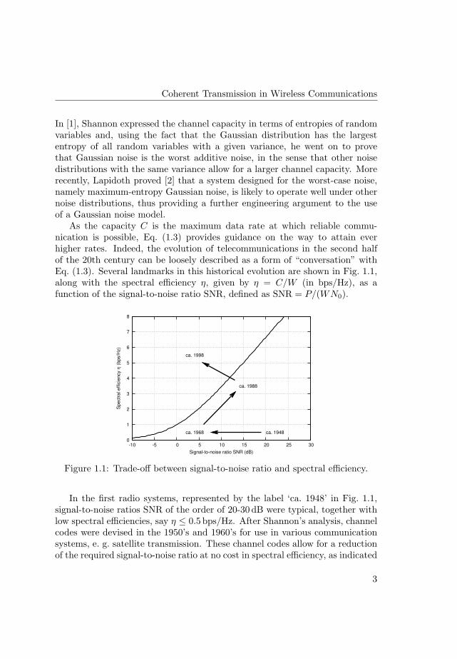
As the capacity C is the maximum data rate at which reliable commu-nication is possible, Eq. (1.3) provides guidance on the way to attain everhigher rates. Indeed, the evolution of telecommunications in the second halfof the 20th century can be loosely described as a form of “conversation” withEq. (1.3). Several landmarks in this historical evolution are shown in Fig. 1.1,along with the spectral efficiency η, given by η = C/W (in bps/Hz), as afunction of the signal-to-noise ratio SNR, defined as SNR = P/(WN0).

0

1

2

3

4

5

6

7

8

-10 -5 0 5 10 15 20 25 30

Sp

ectr

al eff

icie

ncy η

(bps/H

z)

Signal-to-noise ratio SNR (dB)

ca. 1948ca. 1968

ca. 1988

ca. 1998

Figure 1.1: Trade-off between signal-to-noise ratio and spectral efficiency.

In the first radio systems, represented by the label ‘ca. 1948’ in Fig. 1.1,signal-to-noise ratios SNR of the order of 20-30 dB were typical, together withlow spectral efficiencies, say η ≤ 0.5 bps/Hz. After Shannon’s analysis, channelcodes were devised in the 1950’s and 1960’s for use in various communicationsystems, e. g. satellite transmission. These channel codes allow for a reductionof the required signal-to-noise ratio at no cost in spectral efficiency, as indicated

3

1. Introduction

by the label ‘ca. 1968’ in Fig. 1.1. Later, around the 1980’s, requirements forhigher data rates, e. g. for telephone modems, led to the use of multi-levelmodulations, which trade increased power for higher data rates; a label ‘ca.1988’ is placed at a typical operating point of such systems.

When it seemed that the whole space of feasible communications was cov-ered, a new way forward was found. It was discovered that the total “band-width” Weff available for communication, i. e. the total number of indepen-dent pulses that may be sent per unit time through a radio channel, oughtto have two components, one spatial and one temporal [3]. Loosely speaking,Weff = WtWs, where Wt, measured in Hz, is the quantity previously referredto as bandwidth, and Ws is the number of spatial degrees of freedom, typicallyrelated to the number of available antennas. In order to account for this ef-fect, W should be replaced in Eq. (1.3) by Weff and, consequently, the spectralefficiency η becomes

η =C

Wt= Ws log2

(1 +

P

WeffN0

). (1.4)

Exploitation of this “spatial bandwidth” is the underlying principle behind theuse of multiple-antenna (MIMO) systems [4, 5] for wireless communications,where spectral efficiencies exceeding 5 bps/Hz are possible for a fixed signal-to-noise ratio, now defined as SNR = P/(WeffN0); these values of the spectralefficiency are represented by the label ‘ca. 1998’ in Fig. 1.1.

Having sketched how communication engineers have exploited tools derivedfrom the information-theoretic analysis of coherent detection to design efficientcommunication systems for radio and microwave frequencies, we next shift ourattention to optical communications.

1.2 Intensity Modulation in Optical Communications

In parallel to the exploitation of the radio and microwave frequencies, muchhigher frequencies have also been put into use. One reason for this move is thefact that the available bandwidth becomes larger as the frequency increases. Atoptical frequencies, in particular, bandwidth is effectively unlimited. Moreover,at optical frequencies efficient “antennas” are available for the transmitting andreceiving ends of the communication link, in the form of lasers and photodiodes,and an essentially lossless transmission medium, the optical fibre, exists. As aconsequence, optical fibres, massively deployed in the past few decades, carryvery high data rates, easily reaching hundreds of gigabits/second.

4

Intensity Modulation in Optical Communications

Most optical communication systems do not modulate the quadrature am-plitude x(t) of the electromagnetic field, but the instantaneous field intensity,defined as |x(t)|2. The underlying reason for this choice is the difficulty ofbuilding oscillators at high frequencies with satisfactory phase stability proper-ties. At the receiver side, coherent detection is often unfeasible, due to similarproblems with the oscillator phase stability. Direct detection, based on thephotoelectric effect, is frequently used as an alternative.

The photoelectric effect manifests itself as a random process with discreteoutput. More precisely, the measurement of a direct detection receiver overan interval (0, T ) is a random integer number (of photons, or quanta of light),distributed according to a Poisson distribution with mean υ. The mean υ, givenby υ =

∫ T

0|y(t)|2 dt, depends on the instantaneous squared modulus of the field

at the receiver, |y(t)|2, and is independent of the phase of the complex-valuedamplitude y(t). Since the variance of a Poisson random variable coincides withits mean υ, it is in general non-zero and there is a noise contribution arisingfrom the signal itself. This noise contribution is called shot noise.

In information theory, a common model for optical communications systemswith intensity modulation and direct detection is the Poisson channel, originallyproposed by Bar-David [6]. A short, yet thorough, historical review by Verdu[7] lists the main contributions to the information-theoretic analysis of thePoisson channel. The input to the Poisson channel is a continuous-time signal,subject to a constraint on the peak and average value. The input is usuallydenoted by λ(t), which corresponds to an instantaneous field intensity, i. e.λ(t) = |y(t)|2, in our previous notation. In an arbitrary interval (0, T ), theoutput is a random variable distributed according to a Poisson distributionwith mean υ =

∫ T

0λ(t) dt. As found by Wyner [8], the capacity of the Poisson

channel is approached by functions λ(t) whose variation rate grows unbounded.Practical constraints on the variation rate of λ(t) may be included by assumingthat the input signal is piecewise constant [9], in which case the Poisson channelis naturally represented by a discrete-time channel model, whose output yk hasa Poisson distribution of the appropriate mean.

Next to the Poisson channel models, physicists have also independentlystudied various channel models for communication at optical frequencies; fora relatively recent review, see the paper by Caves [10]. In particular, thedesign and performance of receivers for optical coherent detection has beenconsidered. In this case, it is worthwhile remarking that direct applicationof Eq. (1.3) with N0 given by the corresponding value of Eq. (1.1) at opticalfrequencies, proves problematic since N0 ' 0, which would indicate an infinite

5

1. Introduction

capacity. Phenomena absent in the models for radio communication, must betaken into account. A good overview of such phenomena is given by Oliver [11].

Under different assumptions on signal, noise, and/or detection method,different models and therefore different values for the channel capacity are ob-tained [10, 12–15]. To any extent, and regardless of the precise value of thechannel capacity at optical frequencies, it is safe to state that deployed optical-fibre communications systems are, qualitatively, somehow still around theirequivalent of ‘ca. 1948’ in Fig. 1.1. Designers have not yet pushed towardsthe ultimate capacity limit, in contrast to the situation in wireless communica-tions which was sketched during the discussion on Fig. 1.1. Both modulation(binary on-off keying) and multiplexing methods (wavelength division mul-tiplexing) have remained remarkably constant along the years. Nevertheless,and in anticipation of future needs for increased spectral efficiency, research hasbeen conducted on channel codes [16] —corresponding roughly to ‘ca. 1968’—,modulation techniques [17], multi-level modulations [18] —for ‘ca. 1988’—, ormultiple-laser methods [19,20] —as the techniques in ‘ca. 1998’—.

A common thread of the lines of research listed in the previous paragraph isthe extension of techniques common to radio frequencies to optical frequencies.In a similar vein, it may also prove fruitful to extend to optical frequenciessome key features of the models used for radio frequencies. One such keyfeature is the presence of additive maximum-entropy Gaussian noise at thechannel output; as we previously mentioned, Shannon proved that this noisedistribution allows for the lowest possible channel capacity when the signal ispower constrained. For other channel models, a similar role could be played bythe corresponding maximum-entropy distribution; this is indeed the case fornon-negative output and exponential additive noise, as found by Verdu [21].This observation suggests an extension of the discrete-time Poisson channel soas to include maximum-entropy additive noise. Such a channel model includestwo key traits of the Poisson channel, namely non-negativity of the input signaland the quantized nature of the channel output and adds the new feature ofa maximum-entropy additive noise. In the next section we incorporate theseelements into the definition of the additive energy channels.

1.3 The Additive Energy Channels

The family of additive energy channels occupies an intermediate region betweenthe discrete-time Poisson channel and the discrete-time Gaussian channel. Asin the Poisson channel, communication in the additive energy channels is non-

6

The Additive Energy Channels

coherent, in the sense that the signal and noise components are not representedby a complex-valued quadrature amplitude, but rather by a non-negative num-ber, which can be identified with the squared modulus of the quadrature am-plitude. From the Gaussian channel, the additive energy channels inherit theproperties of discreteness in time and of additivity between a useful signal anda noise component, drawn according to a maximum-entropy distribution.

In analogy with Eq. (1.2), the k-th channel output, denoted by y′k, is givenby the sum of a useful signal x′k and a noise component z′k, that is

y′k = x′k + z′k. (1.5)

In general, we refer to additive energy channels, in plural, since there are twodistinct variants, depending on whether the output is continuous or discrete.

When the output is discrete, the energy is a multiple of a quantum of energyof value ε0. The useful signal component x′k is now a random variable with aPoisson distribution of mean |xk|2, say the signal energy in the k-th componentof an AWGN channel. The additive noise component z′k is distributed accordingto a geometric (also called Bose-Einstein) distribution, which has the largestentropy of all distributions for discrete, non-negative random variables subjectto a fixed mean value [22].

For continuous output, the value of the signal (resp. additive noise) compo-nent x′k (resp. z′k) coincides with the signal energy in the k-th coordinate of anAWGN channel, i. e. x′k = |xk|2 (resp. z′k = |zk|2), a non-negative number. Thenoise z′k follows an exponential distribution, since zk is Gaussian distributed.The exponential density is the natural continuous counterpart of the geometricdistribution and also has the largest entropy among the densities for continu-ous, non-negative random variables with a constraint on the mean [22]. Thechannel model with continuous output is an additive exponential noise channel,studied in a different context by Verdu [21]. The continuous-output channelmodel may also be derived from the discrete-output model by letting the num-ber of quanta grow unbounded, simultaneously keeping fixed the total energy.Equivalently, the energy of a single quantum ε0 may be let go to zero while thetotal average energy is kept constant.

The additive energy channel models are different from the most commoninformation-theoretic model for non-coherent detection, obtained by replacingthe AWGN output signal yk by its squared modulus (see e. g. the recent study[23] and references therein). The channel output, now denoted by y′′k , is then

y′′k = |yk|2 = |xk + zk|2. (1.6)

7

1. Introduction

By construction, the output y′′k conditional on xk follows a non-central chi-square distribution and is therefore not the sum of the energies of xk and zk,i. e. y′′k 6= |xk|2 + |zk|2.

The main contribution of this dissertation is the information-theoretic anal-ysis of the additive energy channels. We will see that, under a broad set ofcircumstances, the information rates and error probabilities in the additive en-ergy channels are very close to those attained in the Gaussian channel with thesame signal-to-noise ratio. Somewhat surprisingly, the performance of directdetection turns out to be close to that of coherent detection, where we haveborrowed terminology from optical communications. In Section 1.4, we outlinethe main elements of this analysis, as a preview of the dissertation itself.

1.4 Outline of the Dissertation

In this dissertation, we analyze a family of additive energy channels from thepoint of view of information theory. Since these channels are mathematicallysimilar to the Gaussian channel, we find it convenient to apply tools and tech-niques originally devised for Gaussian channels, with the necessary adaptationswherever appropriate. In some cases, the adaptations shed some new light onthe results for the Gaussian channel, in which case we also discuss at somelength the corresponding results.

In Chapter 2, we formally describe the additive energy channels, both forcontinuous output ( additive exponential noise channel) and for discrete output(quantized additive energy channel). In the latter, the analysis is carried out interms of quanta, with a brief application at the end of the chapter of the resultsto the case where the quanta of energy are photons of an arbitrary frequency.

Four information-theoretic quantities, covering both theoretical and practi-cal aspects of the reliable transmission of information, are studied: the channelcapacity, the constrained capacity when a given digital modulation format isused, the minimum energy per bit, and the pairwise error probability.

As we stated before Eq. (1.3), the channel capacity gives the fundamentallimit on the transmission capabilities of a channel. More precisely, the capac-ity is the highest data rate at which reliable transmission of information overa channel is possible. In Chapter 3, the channel capacity of the additive en-ergy channels is determined. The capacity of the continuous additive energychannel is shown to coincide with that of a Gaussian channel with identicalsignal-to-noise ratio. Then, an upper bound —the tightest known to date—to the capacity of the discrete-time Poisson channel is obtained by applying a

8

Outline of the Dissertation

method recently used by Lapidoth [24] to derive upper bounds to the capacityof arbitrary channels. The capacity of the quantized additive energy channelis shown to have two distinct functional forms: if additive noise is dominant,the capacity approaches that of the continuous channel with the same energyand noise levels; when Poisson noise prevails, the capacity is similar to that ofa discrete-time Poisson channel with no additive noise.

An analogy with radiation channels of an arbitrary frequency, for whichthe quanta of energy are photons, is presented. Additive noise is found to bedominant when frequency is low and, simultaneously, the signal-to-noise ratiolies below a threshold; the value of this threshold is well approximated by theexpected number of quanta of additive noise.

Unfortunately, the capacity is often difficult to compute and knowing itsvalue does not necessarily lead to practical, workable methods to approach it.On the other hand, the minimum energy per bit (or its inverse, the capacityper unit cost) turns out to be easier to determine and further proves usefulin the performance analysis of systems working at low levels of signal energy,a common operating condition. Even closer to a practical figure of merit isthe constrained capacity, which estimates the largest amount of informationwhich can be transmitted by using a specific digital modulation format. InChapter 4, we cover coded modulation methods for the Gaussian channel, withparticular emphasis laid on the performance at low signal-to-noise ratios, theso-called wideband regime, of renewed interest in the past few years after animportant paper by Verdu [25]. Some new results on the characterization of thewideband regime are presented. The discussion is complemented by an analysisof bit-interleaved coded modulation, a simple and efficient method proposedby Caire [26] to use binary codes with non-binary modulations.

In Chapter 5, an extension of digital modulation methods from the Gaussianchannels to the additive energy channel is presented, and their correspondingconstrained capacity when used at the channel input determined. Special at-tention is paid to the asymptotic form of the capacity at low and high levels ofsignal energy. In the low-energy region, our work complements previous workby Prelov and van der Meulen [27, 28], who considered a general discrete-timeadditive channel model, and determined the asymptotic Taylor expansion atzero signal-to-noise ratio, in that the additive energy channels are constrainedon the mean value of the input, rather than the variance, and similarly the noiseis described by its mean, not its variance; the models considered by Prelov andvan der Meulen rather deal with channels where the second-order moments,both for signal energy and noise level, are of importance. Our work extendstheir analysis to the family of additive energy channels, where the first-order

9

1. Introduction

moments are constrained. In the high-energy limit, simple pulse-energy mod-ulations are presented which achieve a larger constrained capacity than theircounterparts for the Gaussian channel.

In addition, techniques devised by Verdu [29] to compute the capacity perunit cost are exploited to determine the minimum energy per nat (recall that1 nat = log2 e bits, or about 1.4427 bits), which is found to equal the averageenergy of the additive noise component for all the channel models we study.We note here that this result was known to hold in two particular cases, namelythe discrete-time Gaussian and Poisson channels [29,30].

We complement our study of the constrained capacity by the computationof the pairwise error probability, an important tool to estimate the perfor-mance of practical binary codes used in conjunction with digital modulations.In Chapter 6, the error probability of binary channel codes in the additiveenergy channels is studied. Saddlepoint approximations to the pairwise errorprobability are given, both for binary modulation and for bit-interleaved codedmodulation. The methods yield new simple approximations to the error prob-ability in the fading Gaussian channel. It is proved that the error rates in thecontinuous additive energy channel are close to those of the coherent transmis-sion at identical signal-to-noise ratio. Finally, constellations minimizing thepairwise error probability in the additive energy channels are presented, andtheir form compared to that of the constellations which maximize the con-strained capacity at high signal energy levels.

Concluding the dissertation, Chapter 7 contains a critical discussion of themain findings presented in the preceding chapters and sketches possible exten-sions and future lines of work.

10

2

The Additive Energy Channels

2.1 Introduction: The Communication Channel

In this dissertation we study the transmission of information across a communi-cation channel from the point of view of information theory. As schematicallydepicted in Fig. 2.1, very similar to the diagram in Shannon’s classical pa-per [1], information is transmitted by sending a message w, generated at thesource of the communication link, to the receiving end. The meaning, form, orcontent of the message are not relevant for the communication problem, andonly the number of different messages generated by the source is relevant. Forconvenience, we model the message w as an integer number.

The encoder transforms the message into an array of n symbols, which wedenote by x. The symbols in x are drawn from an alphabet X , or set, thatdepends on the underlying channel. In this dissertation, symbols are eithercomplex or non-negative real numbers, as is common practice for the modellingof, respectively, wireless radio and optical-fibre channels.

The symbol for encoder output x also stands for the communication channelinput. The channel maps the array x onto another array y of n symbols, anarray which is detected at the receiver. The channel is noisy, in the sense thatx (and therefore w) may not be univocally recoverable from y.

The decoder block generates a message estimate, w, from y and delivers it

EncoderSource ChannelNoisy

Decoder Destination

yxMessage w Message w

Figure 2.1: Generic communication link.

11

2. The Additive Energy Channels

to the destination. The noisy nature of the communication channel causes theestimate w to possibly differ from the original message w. A natural problemis to make the probability of the estimate being wrong low enough, where theprecise meaning of low enough depends on the circumstances and applications.

Information theory studies both theoretical and practical aspects of howto generate an estimate w very likely to coincide with the source message w.First, and through the concept of channel capacity, information theory givesan answer to the fundamental problem of how many messages can be reliablydistinguished at the receiver side in the limit n → ∞. Here reliably meansthat the probability that the receiver’s estimate of the message, w, differs fromthe original message at the source, w, is vanishingly small. In Chapter 3, wereview the concept of channel capacity, and determine its value for the channelmodels described in this chapter.

Pairs of encoder and decoder which allow for the reliable transmission of thelargest possible number of messages are said to achieve the channel capacity.In practice, simple yet suboptimal encoder and decoders are used. Informationtheory also provides tools to analyze the performance of these specific encodersand decoders. The performance of some encoder and decoder pairs for themodels described in this chapter are covered in Chapters 4, 5, and 6.

Models with arrays as channel input and output naturally appear in theanalysis of so-called waveform channels, for which functions of a continuoustime variable t are transformed into a discrete array of numbers via an ap-plication of the sampling theorem or a Fourier decomposition. Details of thisdiscretization can be found, for instance, in Chapter 8 of Gallager’s book [31].Since the time variable is discretized, these models often receive the namediscrete-time, a naming convention we adopt.

In the remainder of this chapter, we present and discuss the channel modelsused in the dissertation. The various models are defined by the alphabet, orset, of possible channel inputs; the alphabet of possible channel outputs; and aprobability density function pY|X(y|x) (for continuous output, if the output isdiscrete, a probability mass function PY|X(y|x) is used) on the set of outputsy for each input x. We consider memoryless and stationary channels, for whichpY|X(y|x) (resp. PY|X(y|x)) admits a decomposition

pY|X(y|x) =n∏

k=1

pY |X(yk|xk), (2.1)

where the symbols xk and yk are the k-th component of their respective arrays.The conditional density pY |X(·|·) (resp. PY |X(·|·)) does not depend on the

12

Complex-Valued Additive Gaussian Noise Channel

value of k. An alternative name for the output conditional density is channeltransition matrix, denoted by Q(·|·). This name is common when the channelinput and output alphabets are discrete.

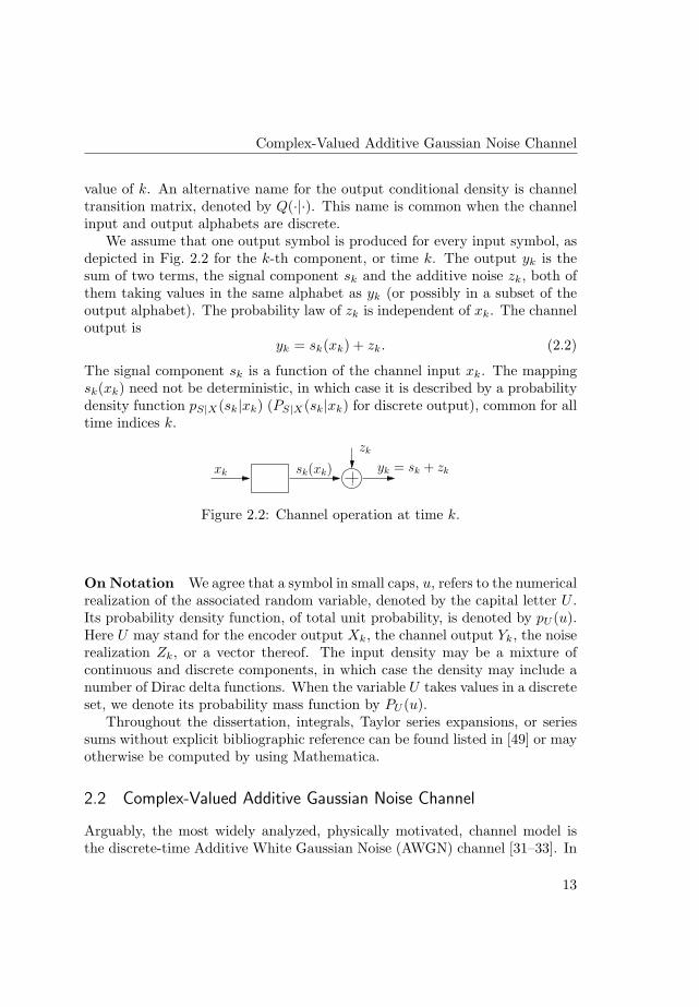
We assume that one output symbol is produced for every input symbol, asdepicted in Fig. 2.2 for the k-th component, or time k. The output yk is thesum of two terms, the signal component sk and the additive noise zk, both ofthem taking values in the same alphabet as yk (or possibly in a subset of theoutput alphabet). The probability law of zk is independent of xk. The channeloutput is

yk = sk(xk) + zk. (2.2)

The signal component sk is a function of the channel input xk. The mappingsk(xk) need not be deterministic, in which case it is described by a probabilitydensity function pS|X(sk|xk) (PS|X(sk|xk) for discrete output), common for alltime indices k.

yk = sk + zk

zk

sk(xk)xk

Figure 2.2: Channel operation at time k.

On Notation We agree that a symbol in small caps, u, refers to the numericalrealization of the associated random variable, denoted by the capital letter U .Its probability density function, of total unit probability, is denoted by pU (u).Here U may stand for the encoder output Xk, the channel output Yk, the noiserealization Zk, or a vector thereof. The input density may be a mixture ofcontinuous and discrete components, in which case the density may include anumber of Dirac delta functions. When the variable U takes values in a discreteset, we denote its probability mass function by PU (u).

Throughout the dissertation, integrals, Taylor series expansions, or seriessums without explicit bibliographic reference can be found listed in [49] or mayotherwise be computed by using Mathematica.

2.2 Complex-Valued Additive Gaussian Noise Channel

Arguably, the most widely analyzed, physically motivated, channel model isthe discrete-time Additive White Gaussian Noise (AWGN) channel [31–33]. In

13

2. The Additive Energy Channels

this case, the time components arise naturally from an application of the sam-pling theorem to a waveform channel, as well as in the context of a frequencydecomposition of the channel into narrowband parallel subchannels.

We consider the complex-valued AWGN channel, whose channel input xk

and output yk at time index k = 1, . . . , n, are complex numbers related by

yk = xk + zk. (2.3)

In this case, the channel input xk and its contribution to the channel outputsk(xk) coincide; they will differ for other channel models. The noise componentzk is drawn according to a circularly-symmetric complex Gaussian density ofvariance σ2, a fact shorthanded to Zk ∼ NC(0, σ2). The noise density is

pZ(z) =1

πσ2e−

|z|2σ2 . (2.4)

The channel transition matrix is Q(y|x) = pZ(y − x).We define the instantaneous (at time k) signal energy, denoted by ε(xk),

as |xk|2. Similarly, the noise instantaneous energy ε(zk) is ε(zk) = |zk|2. Theaverage noise energy, where the averaging is performed over the possible real-izations of zk, is E[|Zk|2] = Var(Zk) = σ2.

The channel is used under a constraint on the total energy ε(x), of the form

ε(x) =n∑

k=1

ε(xk) =n∑

k=1

|xk|2 ≤ nEs, (2.5)

where Es denotes the maximum permitted energy per channel use.The average signal-to-noise ratio, denoted by SNR, is given by

SNR =Es

σ2. (2.6)

Here, and with no loss of generality, we assume that the constraint in Eq. (2.5)holds with equality. This step will be justified in Chapter 3, when we statehow the channel capacity links the constraint on the total energy per message,as in Eq. (2.5), with a constraint on the average energy per channel use, orequivalently on the average signal-to-noise ratio.

It is common practice to replace the AWGN model given in Eqs. (2.3) by analternative model whose input signal x′k and channel output y′k are respectivelygiven by xk =

√Esx

′k and

y′k =1σ

yk =√

SNRx′k + z′k, (2.7)

14

Additive Exponential Noise Channel

so that both signal x′k and additive noise z′k have unit average energy, i. e.E[|X ′

k|2] = 1 and Z ′k ∼ NC(0, 1). The channel transition matrix is then

Q(y|x) =1π

e−|y−√

SNRx|2 . (2.8)

Both forms of the AWGN channel model are equivalent since they describe thesame physical realization.

2.3 Additive Exponential Noise Channel

We next introduce the additive exponential noise (AEN) channel as a variationof an underlying AWGN channel. Since we use the symbols for the variables xk,zk, and yk for both channels, we distinguish the AWGN variables by appendinga prime.

In the AEN channel, the channel output is an energy, rather than a com-plex number as it was in the AWGN case. In the previous section, we definedthe instantaneous energy of the signal and noise variables as the squared mag-nitude of the complex number x′k or z′k, and avoided referring to the energyof the output y′k. The reason for this avoidance is that there are two naturaldefinitions for the output energy.

First, in the AEN channel, the channel output yk is defined to be the sumof the energies in x′k and z′k, that is, yk = xk + zk, where the signal and noisecomponents xk and zk are related to their Gaussian counterparts by

xk = ε(x′k) = |x′k|2, zk = ε(z′k) = |z′k|2. (2.9)

Figure 2.3 shows the relationship between the AWGN and AEN channels. Wehasten to remark that this postulate is of a mathematical nature, possiblyindependent of any underlying physical model, since the quantity ε(x′k)+ε(z′k)cannot be directly derived from y′k only.

The inputs xk and outputs yk are non-negative real numbers, as befits anenergy. The correspondence with the AWGN channel, xk = |x′k|2, leads to anatural constraint on the average energy per channel use Es,

∑nk=1 xk ≤ nEs,

where Es is the constraint in the AWGN channel.The noise energy zk = ε(z′k) = |z′k|2, that is the squared amplitude of a

circularly-symmetric complex Gaussian noise, has an exponential density [32]of mean En = σ2,

pZ(z) = 1En

e−z

En u(z), (2.10)

15

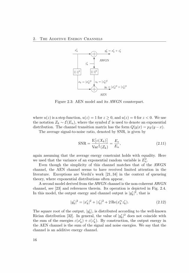
2. The Additive Energy Channels

|(·)|2|(·)|2

AWGNz′

k

y′

k= x

′

k+ z

′

k

zk = |z′k|2

AEN

yk = |x′

k|2 + |z′

k|2

xk = |x′

k|2

x′

k

Figure 2.3: AEN model and its AWGN counterpart.

where u(z) is a step function, u(z) = 1 for z ≥ 0, and u(z) = 0 for z < 0. We usethe notation Zk ∼ E(En), where the symbol E is used to denote an exponentialdistribution. The channel transition matrix has the form Q(y|x) = pZ(y−x).

The average signal-to-noise ratio, denoted by SNR, is given by

SNR =E

[ε(Xk)

]

Var12 (Zk)

=Es

En, (2.11)

again assuming that the average energy constraint holds with equality. Herewe used that the variance of an exponential random variable is E2

n.Even though the simplicity of this channel matches that of the AWGN

channel, the AEN channel seems to have received limited attention in theliterature. Exceptions are Verdu’s work [21, 34] in the context of queueingtheory, where exponential distributions often appear.

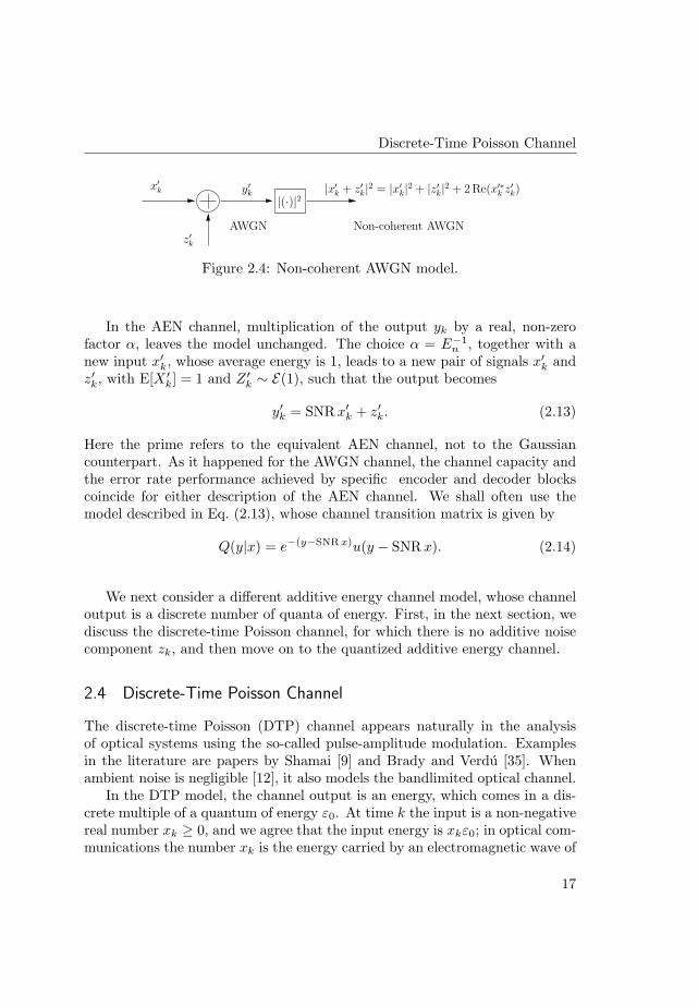
A second model derived from the AWGN channel is the non-coherent AWGNchannel, see [23] and references therein. Its operation is depicted in Fig. 2.4.In this model, the output energy and channel output is |y′k|2, that is

|y′k|2 = |x′k|2 + |z′k|2 + 2 Re(x′∗k z′k). (2.12)

The square root of the output, |y′k|, is distributed according to the well-knownRician distribution [32]. In general, the value of |y′k|2 does not coincide withthe sum of the energies ε(x′k) + ε(z′k). By construction, the output energy inthe AEN channel is the sum of the signal and noise energies. We say that thechannel is an additive energy channel.

16

Discrete-Time Poisson Channel

|(·)|2x′

k y′

k

z′

k

AWGN

|x′

k+ z

′

k|2 = |x′

k|2 + |z′

k|2 + 2 Re(x′∗

kz′

k)

Non-coherent AWGN

Figure 2.4: Non-coherent AWGN model.

In the AEN channel, multiplication of the output yk by a real, non-zerofactor α, leaves the model unchanged. The choice α = E−1

n , together with anew input x′k, whose average energy is 1, leads to a new pair of signals x′k andz′k, with E[X ′

k] = 1 and Z ′k ∼ E(1), such that the output becomes

y′k = SNR x′k + z′k. (2.13)

Here the prime refers to the equivalent AEN channel, not to the Gaussiancounterpart. As it happened for the AWGN channel, the channel capacity andthe error rate performance achieved by specific encoder and decoder blockscoincide for either description of the AEN channel. We shall often use themodel described in Eq. (2.13), whose channel transition matrix is given by

Q(y|x) = e−(y−SNR x)u(y − SNR x). (2.14)

We next consider a different additive energy channel model, whose channeloutput is a discrete number of quanta of energy. First, in the next section, wediscuss the discrete-time Poisson channel, for which there is no additive noisecomponent zk, and then move on to the quantized additive energy channel.

2.4 Discrete-Time Poisson Channel

The discrete-time Poisson (DTP) channel appears naturally in the analysisof optical systems using the so-called pulse-amplitude modulation. Examplesin the literature are papers by Shamai [9] and Brady and Verdu [35]. Whenambient noise is negligible [12], it also models the bandlimited optical channel.

In the DTP model, the channel output is an energy, which comes in a dis-crete multiple of a quantum of energy ε0. At time k the input is a non-negativereal number xk ≥ 0, and we agree that the input energy is xkε0; in optical com-munications the number xk is the energy carried by an electromagnetic wave of

17

2. The Additive Energy Channels

the appropriate frequency. The channel is used under a constraint on the (max-imum) average number of quanta per channel use, εs,

∑nk=1 xk ≤ nεs, with

the understanding that the average energy per channel use Es is εsε0 = Es.The channel output depends on the input xk via a Poisson distribution with

parameter xk, that is, Yk = Sk ∼ P(xk), where the symbol P is used to denotea Poisson distribution. Hence, the conditional output distribution is given by

PS|X(s|x) = e−x xs

s!, (2.15)

which also gives the channel transmission matrix Q(y|x), with s replaced by y.

Since the channel output Yk is a Poisson random variable, its variance isequal to xk [36], Var(Yk) = xk. Differently from AWGN or AEN channels,noise is now signal-dependent, coming from the signal term sk itself. We referto this noise as shot noise or Poisson noise.

As the number of quanta sk becomes arbitrarily large for a fixed value ofinput energy xkε0, the standard deviation of the channel output, of value

√sk,

becomes negligible compared to its mean, sk, and the density of the outputenergy skε0, viewed as a continuous random variable, approaches

pS|X(skε0|xkε0) = lim∆x→0,xk→∞

xkε0fixed

1∆x

Pr(

xk − ∆x

2≤ sk ≤ xk +

∆x

2

)(2.16)

= δ((sk − xk)ε0

), (2.17)

i. e. a delta function, as for the signal energy in the AWGN and AEN channels,models for which there is no Poisson noise at the input.

2.5 Quantized Additive Energy Channel

The quantized additive energy channel (AE-Q) appears as a natural general-ization of the discrete-time Poisson and the additive exponential channels.

First, it shares with the DTP channel the characteristic that the outputenergy is discrete, an integer number of quanta of energy ε0 each.

In parallel, it generalizes the DTP channel in the sense that an additivenoise component is present at the channel output. The correspondence withthe AEN channel is established by assuming that the noise component hasa geometric distribution, the natural discrete counterpart of the exponentialdensity in Eq. (2.10). Also, the geometric distribution has the highest entropy

18

Quantized Additive Energy Channel

among all discrete, non-negative random variables of a given mean, a propertyshared by the exponential density among the continuous random variables [22].

The output yk is an integer number of quanta of energy, each of energy ε0.As in the additive exponential noise channel, the output yk at time k is thesum of a signal and an additive noise components, that is

yk = sk + zk, k = 1, . . . , n, (2.18)

where the numbers yk, sk and zk are now non-negative integers, i. e. are in{0, 1, 2, . . . }.

The input is a non-negative real number xk ≥ 0, related to its AWGN(and AEN) equivalent by xkε0 = |x′k|2, where x′k is the AWGN value. Thereis a constraint on the total energy, expressed in terms of the average numberof quanta per channel use, εs, by

∑nk=1 xk ≤ nεs. As in the discrete-time

Poisson case, the signal component at the output sk has a Poisson distributionof parameter xk, whose formula is given in Eq. (2.15).

The additive noise zk has a geometric distribution of mean εn, that is

PZ(z) =1

1 + εn

(εn

1 + εn

)z

. (2.19)

We agree on the shorthand Zk ∼ G(εn), where the symbol G denotes a geomet-ric distribution. Its variance is εn(1 + εn).

In order to establish a correspondence between the various channel models,we choose εnε0 = σ2 = En, the average noise energies in the AWGN and AENchannels. From the discussion at the end of Section 2.4, the AEN model isrecovered in the limiting case where the number of quanta becomes very large,and consequently the Poisson noise becomes negligible.

In the AE-Q channel, we identify two limiting situations, the G and Pregimes, distinguished by which noise source, either additive geometric noiseor Poisson noise, is predominant.

In the G regime, additive geometric noise dominates over signal-dependentnoise. This happens when εn À 1 and xk ¿ ε2

n. Note that, in addition tolarge number of quanta, a second condition relating the noise and signal levelsis of importance. Then, the (in)equalities Var(Yk) ' Var(Zk) ' ε2

n À xk hold.In the P regime, Poisson noise is prevalent. In terms of variances, Var(Yk) '

Var(Sk) ' xk À Var(Zk). Since the additive geometric noise is negligible, thesignal-to-noise ratio for the AEN or AWGN channel models would becomeinfinite in this case.

It is obvious that the transition between the G and P regimes does nottake place in the AWGN and AEN models, where increasing the signal energy

19

2. The Additive Energy Channels

makes the additive noise component ever smaller. Moreover, since the modelsremain unchanged when both signal and noise components are multiplied bya constant value, these alternative forms are characterized by the ratio of thenoise and signal energy levels, and not by their absolute values taken separately.A consequence is that signal-to-noise ratio can be freely apportioned to signalor noise components, and the choices leading to Eqs. (2.7) and (2.13) oftenprove convenient.

On the other hand, the AE-Q channel is sensitive to the absolute values ofsignal and noise, in addition to their ratio, since application of a scaling factormay easily change operation from the G to the P regime, or vice versa. Thepresence of the quantum as a fundamental unit of energy and the discretenessof the output fundamentally alter the behaviour of the channel under changesof scale. For the DTP or AE-Q channel models it is the absolute energies, notonly their ratio, what determines the channel performance.

To the best of our knowledge the AE-Q channel model is new. A discretecounterpart of the chi-square (squared Rician) distribution, which describesthe output of the non-coherent AWGN channel in Eq. (2.12), is the Laguerredistribution with parameters x and εn [37], and is studied in the literature onoptical communications. In Section 2.6, we particularize the AE-Q channel forthe case when the quanta of energy are photons of frequency ν.

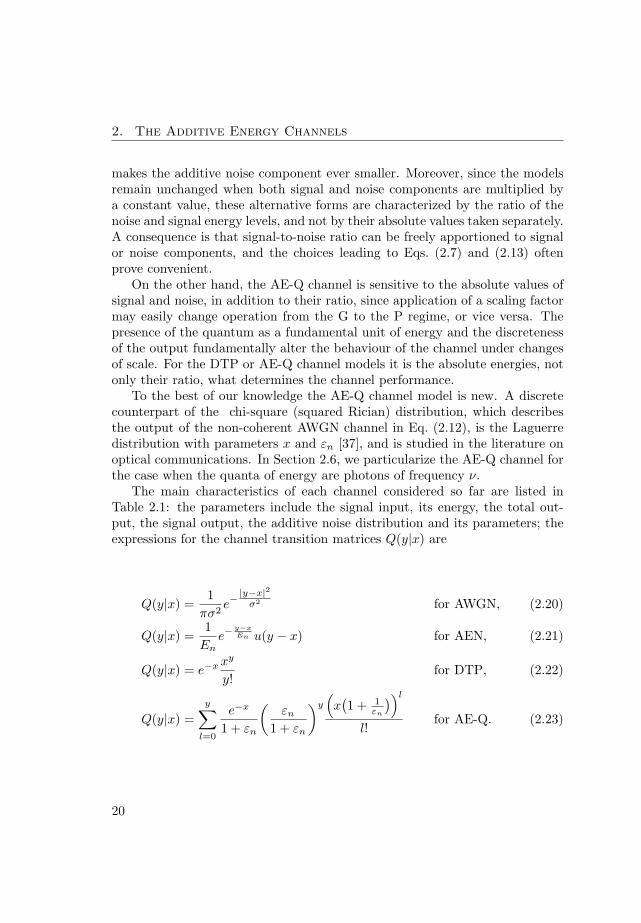
The main characteristics of each channel considered so far are listed inTable 2.1: the parameters include the signal input, its energy, the total out-put, the signal output, the additive noise distribution and its parameters; theexpressions for the channel transition matrices Q(y|x) are

Q(y|x) =1

πσ2e−

|y−x|2σ2 for AWGN, (2.20)

Q(y|x) =1

Ene−

y−xEn u(y − x) for AEN, (2.21)

Q(y|x) = e−x xy

y!for DTP, (2.22)

Q(y|x) =y∑

l=0

e−x

1 + εn

(εn

1 + εn

)y

(x(1 + 1

εn

))l

l!for AE-Q. (2.23)

20

Photons as Quanta of Energy

AWGN AEN DTP AE-Q

Input xk Alphabet C [0,∞) [0,∞) [0,∞)Signal Energy |xk|2 xk xkε0 xkε0

Output yk Alphabet C [0,∞) {0, 1, . . . } {0, 1, . . . }Signal Output sk xk xk ∼ P(xk) ∼ P(xk)Signal Output Mean xk xk xk xk

Signal Output Variance 0 0 xk xk

Additive Noise zk ∼ NC(0, σ2) ∼ E(En) 0 ∼ G(εn)Average Noise Energy σ2 En = σ2 0 εnε0 = En

Noise Variance Var(Zk) σ2 E2n 0 εn(1 + εn)

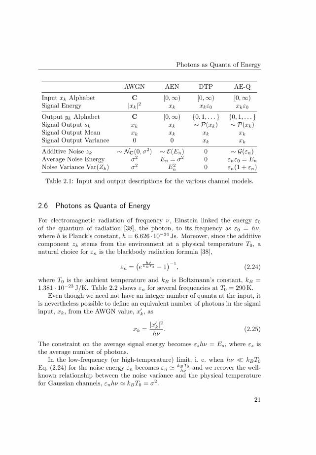
Table 2.1: Input and output descriptions for the various channel models.

2.6 Photons as Quanta of Energy

For electromagnetic radiation of frequency ν, Einstein linked the energy ε0

of the quantum of radiation [38], the photon, to its frequency as ε0 = hν,where h is Planck’s constant, h = 6.626 ·10−34 Js. Moreover, since the additivecomponent zk stems from the environment at a physical temperature T0, anatural choice for εn is the blackbody radiation formula [38],

εn =(e

hνkBT0 − 1

)−1, (2.24)

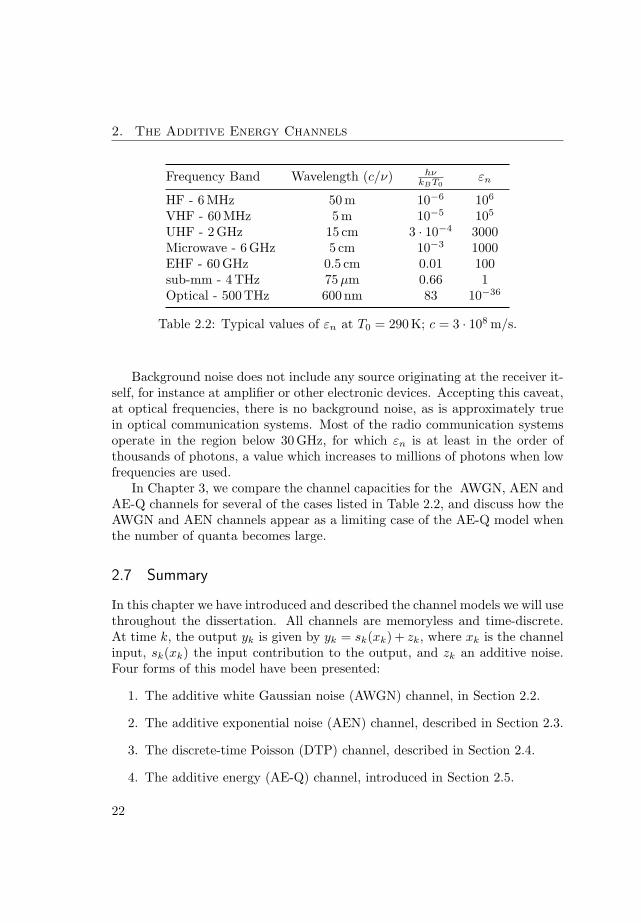
where T0 is the ambient temperature and kB is Boltzmann’s constant, kB =1.381 · 10−23 J/K. Table 2.2 shows εn for several frequencies at T0 = 290 K.

Even though we need not have an integer number of quanta at the input, itis nevertheless possible to define an equivalent number of photons in the signalinput, xk, from the AWGN value, x′k, as

xk =|x′k|2hν

. (2.25)

The constraint on the average signal energy becomes εshν = Es, where εs isthe average number of photons.

In the low-frequency (or high-temperature) limit, i. e. when hν ¿ kBT0

Eq. (2.24) for the noise energy εn becomes εn ' kBT0hν and we recover the well-

known relationship between the noise variance and the physical temperaturefor Gaussian channels, εnhν ' kBT0 = σ2.

21

2. The Additive Energy Channels

Frequency Band Wavelength (c/ν) hνkBT0

εn

HF - 6MHz 50 m 10−6 106

VHF - 60MHz 5 m 10−5 105

UHF - 2GHz 15 cm 3 · 10−4 3000Microwave - 6 GHz 5 cm 10−3 1000EHF - 60GHz 0.5 cm 0.01 100sub-mm - 4THz 75 µm 0.66 1Optical - 500THz 600 nm 83 10−36

Table 2.2: Typical values of εn at T0 = 290 K; c = 3 · 108 m/s.

Background noise does not include any source originating at the receiver it-self, for instance at amplifier or other electronic devices. Accepting this caveat,at optical frequencies, there is no background noise, as is approximately truein optical communication systems. Most of the radio communication systemsoperate in the region below 30 GHz, for which εn is at least in the order ofthousands of photons, a value which increases to millions of photons when lowfrequencies are used.

In Chapter 3, we compare the channel capacities for the AWGN, AEN andAE-Q channels for several of the cases listed in Table 2.2, and discuss how theAWGN and AEN channels appear as a limiting case of the AE-Q model whenthe number of quanta becomes large.

2.7 Summary

In this chapter we have introduced and described the channel models we will usethroughout the dissertation. All channels are memoryless and time-discrete.At time k, the output yk is given by yk = sk(xk) + zk, where xk is the channelinput, sk(xk) the input contribution to the output, and zk an additive noise.Four forms of this model have been presented:

1. The additive white Gaussian noise (AWGN) channel, in Section 2.2.

2. The additive exponential noise (AEN) channel, described in Section 2.3.

3. The discrete-time Poisson (DTP) channel, described in Section 2.4.

4. The additive energy (AE-Q) channel, introduced in Section 2.5.

22

Summary

Using the AWGN as a basis for the comparison, relationships between thevarious channels have been derived:

• The AEN is derived by postulating that the channel output is given bythe sum of the energies of the signal and noise components in the AWGNchannel.

• The AE-Q is derived from the AEN model by postulating that energy isdiscrete and the channel output is a non-negative integer, the number ofenergy quanta.

• The DTP is an AE-Q channel whose additive noise component is zero.

In the DTP and AE-Q channels, energy is discrete. In Section 2.6 we haveused radiation as a guide to obtain the orders of magnitude of the signal andnoise components. We use these numerical values in Chapter 3 to compare thecommunication capabilities of the AE-Q channel with its AWGN counterpart.

A key feature of the AWGN channel is the presence of additive maximum-entropy Gaussian noise at the channel output. For other channel models, asimilar role is played by the corresponding maximum-entropy distribution. Us-ing the DTP channel as the baseline,

• The AE-Q is derived by postulating the presence of an additive, maximum-entropy noise component. This additive noise component has a geomet-ric (or Bose-Einstein) distribution. Note that this differs from the usualpractice in the analysis of the DTP channel, where an additive noisecomponent with Poisson distribution is often considered.

• The AEN is derived from the AE-Q channel by letting the number ofquanta become infinite, keeping fixed the energy value. Equivalently, theenergy of the quantum ε0 goes to zero, having kept fixed the energy. Inthe limit, additive noise has an exponential density, and the Poisson noiseeffectively vanishes.

Table 2.1, on page 21, summarizes the characteristics of the various mod-els. All channels, bar the AWGN, operate with energies rather than with thecomplex amplitude in the Gaussian channel. As the AWGN admits a physicalmotivation, it might prove convenient to briefly discuss the physical meaningof the additive energy channels.

In terms of electromagnetic theory, the complex amplitude in the Gaussianmodel corresponds to the amplitude and phase of electromagnetic fields: the

23

2. The Additive Energy Channels

component sk is generated by a far-away antenna, and the noise zk is producedby the environment. Discreteness in time appears by considering, say, narrowparallel frequency sub-bands. An AWGN model assumes that the fields areadded at the receiver, and then detected as a complex number. In the additiveenergy channels, noise and signal are postulated to be incoherent, so that theirenergies can be added. Since the discrete-time additive energy channels cannotbe derived from the discrete-time AWGN channel, possible links with physicalchannels would require analyzing the continuous-time AWGN channel. Someelements of this possible analysis are mentioned in Chapter 7.

24

3

Capacity of the Additive Energy Channels

3.1 Outline of the Chapter

In this chapter we determine the capacity of the additive energy channels. Asan introduction, we review in Section 3.2 the concept of channel capacity anddiscuss its relevance for the problem of reliable transmission of information. Wealso provide some tools necessary to compute its value. In addition, we definethe concept of minimum energy per bit, which is related to the capacity perunit energy. The presentation borrows elements from standard textbooks oninformation theory, namely Gallager [31], Blahut [39], Cover and Thomas [22].

The first channel we consider, in Section 3.3, is the standard additive Gaus-sian noise channel. Then, in Section 3.4 we determine the capacity of theadditive exponential noise (AEN) channel, presented in Section 2.3.

In Section 3.5, we provide good upper and lower bounds to the capacityof the discrete-time Poisson channel (DTP), introduced in Section 2.4. Thebounds we provide are tighter than previous results in the literature, such asthose by Brady and Verdu [35] or Lapidoth and Moser [24].

Finally, we bound the capacity of the quantized additive energy channel(AE-Q) in Section 3.6. We construct the bounds from knowledge of the be-haviour in the two cases discussed previously, namely the AEN and the DTPchannels. These two cases respectively correspond to the G and P regimesof the AE-Q channel (see Section 2.5, page 19), and show markedly differentbehaviour. Since upper and lower bounds are close to each other in each ofthese two regimes, the channel capacity of the AE-Q is determined to a highdegree of accuracy.

25

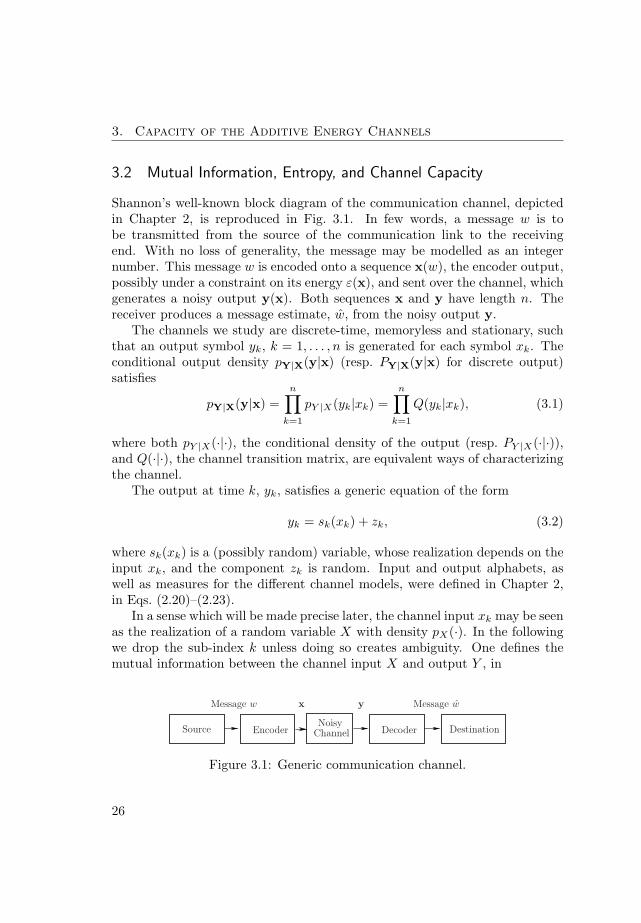
3. Capacity of the Additive Energy Channels

3.2 Mutual Information, Entropy, and Channel Capacity

Shannon’s well-known block diagram of the communication channel, depictedin Chapter 2, is reproduced in Fig. 3.1. In few words, a message w is tobe transmitted from the source of the communication link to the receivingend. With no loss of generality, the message may be modelled as an integernumber. This message w is encoded onto a sequence x(w), the encoder output,possibly under a constraint on its energy ε(x), and sent over the channel, whichgenerates a noisy output y(x). Both sequences x and y have length n. Thereceiver produces a message estimate, w, from the noisy output y.

The channels we study are discrete-time, memoryless and stationary, suchthat an output symbol yk, k = 1, . . . , n is generated for each symbol xk. Theconditional output density pY|X(y|x) (resp. PY|X(y|x) for discrete output)satisfies

pY|X(y|x) =n∏

k=1

pY |X(yk|xk) =n∏

k=1

Q(yk|xk), (3.1)

where both pY |X(·|·), the conditional density of the output (resp. PY |X(·|·)),and Q(·|·), the channel transition matrix, are equivalent ways of characterizingthe channel.

The output at time k, yk, satisfies a generic equation of the form

yk = sk(xk) + zk, (3.2)

where sk(xk) is a (possibly random) variable, whose realization depends on theinput xk, and the component zk is random. Input and output alphabets, aswell as measures for the different channel models, were defined in Chapter 2,in Eqs. (2.20)–(2.23).

In a sense which will be made precise later, the channel input xk may be seenas the realization of a random variable X with density pX(·). In the followingwe drop the sub-index k unless doing so creates ambiguity. One defines themutual information between the channel input X and output Y , in

EncoderSource ChannelNoisy

Decoder Destination

yxMessage w Message w

Figure 3.1: Generic communication channel.

26

Mutual Information, Entropy, and Channel Capacity

Definition 3.1. The mutual information I(X; Y ) between the channel inputX, with density pX(x), and the channel output Y is the quantity

I(X;Y ) =∫∫

pX(x)Q(y|x) logQ(y|x)pY (y)

dy dx, (3.3)

where pY (y), the output density, is given by pY (y) =∫

pX(x)Q(y|x) dx.

Throughout the dissertation, logarithms are taken in base e, and the mu-tual information is measured in nats. The same holds for other information-theoretic quantities, such as entropies or channel capacities. Further, we agreethat 0 log 0 = 0. In general, though, plots of the channel capacity will be inbits. In some of the cases we consider the output is discrete and/or the inputdensity may contain Dirac delta’s.

In our analysis of digital modulation in Chapters 4 and 5, x is drawn froma set X . In that case, we denote the corresponding mutual information by CXand refer to it as constrained capacity or coded modulation capacity, where theconstraint comes from using a specific modulation format.

When the random variables are purely discrete or continuous, one can definetheir (differential) entropy H(U) (we use the same symbol for both cases).

Definition 3.2. The differential entropy H(X) of a continuous random vari-able X with density pX(x) is given by

H(X) = −∫

pX(x) log pX(x) dx. (3.4)

Definition 3.3. The entropy H(X) of a discrete random variable X withdistribution PX(x) is given by

H(X) = −∑

x

PX(x) log PX(x). (3.5)

Similar definitions hold for the conditional differential entropy, as well as theconditional entropy H(Y |X). For instance, in the discrete case, the conditionalentropy between two random variables Y and X is given by

H(Y |X) = −∑

x

PX(x)∑

y

PY |X(y|x) log PY |X(y|x). (3.6)

The conditional differential entropies have the analogous definition.

27

3. Capacity of the Additive Energy Channels

We are most interested in cases where the variable Y is a (possibly stochas-tic) function of another variable X, viz. Y = S(X) + Z. Whenever the (dif-ferential) entropies H(X) and H(X|Y ), or H(Y ) and H(Y |X), are finite themutual information respectively admits the well-known decompositions

I(X;Y ) = H(Y )−H(Y |X) = H(X)−H(X|Y ). (3.7)

In the channels we study, inputs are used under an energy constraint,namely Es for the AWGN and AEN channels and εs for the AE-Q and DTPchannels. Recall that for each time index, the instantaneous signal energy (orcost, in general) ε(xk) is given by ε(xk) = |xk|2 for the AWGN channel and byε(xk) = xk for the AEN, AE-Q and DTP channels. For an energy constraintE, one defines the channel capacity C(E) as

Definition 3.4. The channel capacity with energy constraint E is the supre-mum among all possible input distributions of the mutual information betweenchannel input and output,

C(E) = suppX(·)

I(X; Y ), (3.8)

where the optimization is subject to the constraint, E[ε(X)

] ≤ E.

Note that the constraint on the total energy has been replaced by a con-straint on the average energy of the random variable X. Additionally, in thechannels we study the largest mutual information is attained when the inequal-ity constraint on the average energy is satisfied with equality. The originalconstraint on the maximum energy is therefore equivalent to a constraint onthe average energy.

Associated to the definition of channel capacity, a coding theorem sharplydetermines the limits on the reliability of communication. Shannon’s codingtheorem states [1,22,31,39] that, as the length of the encoder output sequencex, n, becomes large, the probability that the receiver’s message estimate, w,differs from the original message at the source, w, is vanishingly small. Let theset of messages w have cardinality |W| and define the rate R as R = 1

n log |W|.Denote the message estimate at the receiver by w:

Theorem 3.5 (Noisy-Channel Coding Theorem). For each ε > 0 for all nlarge enough, there exist an encoder and decoder such that the probability oferror, Pr(W 6= W ) is at most ε, if R < C.

28

Mutual Information, Entropy, and Channel Capacity

Moreover, when R > C the bit error probability at the receiver cannot bemade small.

The exact computation of the channel capacity is possible only in somespecific cases. The AWGN case is a well-known example, and the AEN channelwill turn out to share this trait. In general, one resorts to computing boundsto the capacity. A straightforward method to derive lower bounds is

Proposition 3.6 (Lower Bound to Capacity). A fixed input density pX(x)which satisfies the energy constraint achieves a mutual information I(X; Y )lower than the channel capacity, I(X; Y ) ≤ C(E).

There is also a simple procedure to derive upper bounds from a fixed outputdensity, which need not correspond to a valid channel output.

Proposition 3.7 (Upper Bound to Capacity). Let pY (y) be an arbitrary chan-nel output density. Then, for every γ ≥ 0 and every energy E the followingexpression gives an upper bound to the channel capacity at energy E, C(E),

C(E

) ≤ maxx

(∫Q(y|x) log

Q(y|x)pY (y)

dy − γ(ε(x)− E)

). (3.9)

We prove the result in Appendix 3.A; the discrete case is essentially identicaland is omitted. The proof builds on a result by Blahut (in the proof of theconvergence of the algorithm to compute the channel capacity, Section 5.4 of hisbook [39]). Other appearances of similar results are in Gallager’s book [31], inSection 4.5 and Problem 4.17; in Section 3.3 of Csiszar and Korner’s book [40];the analysis of the capacity of the non-coherent discrete-time Rayleigh-fadingchannel [41]; and the derivation of upper bounds to the capacity by Lapidothand Moser [24]. Our formulation includes the effect of the constraint.

The capacity per unit energy (or unit cost in general), which we denote byC1 is a close relative to the channel capacity. It was defined by Verdu [29] asthe largest information which can be reliably sent over the channel per unitcost. In our channel models the capacity per unit cost is closely related to thesmallest energy per bit required to transmit information reliably.

Definition 3.8. In a channel with capacity C(E

)at energy E, the capacity

per unit energy C1 is given by

C1 = supE

C(E

)

E. (3.10)

29

3. Capacity of the Additive Energy Channels

Similarly, the minimum energy per bit is defined as Eb,min = infEE

C(E) , wherethe capacity is measured in bits.

If the capacity is in nats, it is clear from the definitions that

Eb,min =log 2C1

. (3.11)

Since the dependence on the cost constraint E is removed, the capacity perunit energy often proves easier to determine than the channel capacity itself.In particular, we have [29]

Theorem 3.9. If the channel has an input x0 with zero energy, i. e. ε(x0) = 0,then the capacity per unit energy is given by

C1 = supx

D(Q(y|x)||Q(y|x0)

)

ε(x), (3.12)

where D(Q(y|x)||Q(y|x0)

)is the divergence between the output distributions

for inputs x and x0, given by

D(Q(y|x)||Q(y|x0)

)=

∑y

Q(y|x) logQ(y|x)Q(y|x0)

. (3.13)

For channels with continuous output, the divergence in Eq. (3.13) is definedin the natural manner.

3.3 Capacity of the Gaussian Noise Channel

We described the additive Gaussian noise (AWGN) channel in Section 2.2.Under an signal energy constraint Es, and for circularly-symmetric complexGaussian noise with variance σ2, the capacity is given in

Theorem 3.10. The capacity of the complex-valued AWGN channel is

C(SNR) = log(1 + SNR), (3.14)

where SNR is the signal-to-noise ratio, SNR = Es/σ2.

The proof [1] depends on the fact that a Gaussian density maximizes thedifferential entropy among all the densities with the same variance [1, 33].

30

Capacity of the Additive Exponential Noise Channel

Proposition 3.11. The density which maximizes the differential entropy of acomplex-valued random variable, subject to a constraint on the variance σ2

0, isthe Gaussian density NC(µ, σ2

0), where µ is arbitrary. Its entropy HNC(σ2

0) is

HNC(σ2

0) = log(πeσ20). (3.15)

3.4 Capacity of the Additive Exponential Noise Channel

We described the additive exponential noise (AEN) channel in Section 2.3. Itis a discrete-time model as in Eq. (3.2), with non-negative, real-valued input xk

and output yk. The input is used under a constraint,∑n

k=1 xk ≤ nEs, whereEs is the energy per channel use. The additive noise component samples areindependently drawn from an exponential distribution, Zk ∼ E(En), with En

the average noise energy.The capacity of the AEN channel coincides with the capacity of the equiv-

alent AWGN channel,

Theorem 3.12. The capacity of the additive-exponential noise channel, C, is

C(SNR) = log(1 + SNR), (3.16)

where SNR is the signal-to-noise ratio, SNR = Es/En.

The capacity of this channel was determined by Verdu [21], in a differentcontext. His proof exploits that an exponential density maximizes the differen-tial entropy among the distributions of non-negative random variables [1, 21]:

Proposition 3.13. The density which maximizes the differential entropy of anon-negative random variable U , subject to a constraint on the mean ε, is theexponential density. Its entropy HExp(ε) is

HExp(ε) = 1 + log ε = log eε. (3.17)

We also need the following result,

Proposition 3.14. Let Y be a continuous non-negative real-valued randomvariable of the form Y = X +Z; X has mean Es and Z is additive exponentialnoise of mean En. The output Y has exponential distribution of mean Es +En

(and thus maximum differential entropy) when the input density pX(x) is

pX(x) =Es

(Es + En)2exp

(− x

Es + En

)+

En

Es + Enδ(x), x ≥ 0. (3.18)

31

3. Capacity of the Additive Energy Channels

We shall later see that a similar density maximizes the output entropy inthe quantized additive energy channel.

We now reproduce the proof of Theorem 3.12.

Proof. For a given input density pX(·), the mutual information I(X; Y ) satisfies

I(X;Y ) = H(Y )−H(Y |X) (3.19)= H(Y )−H(X + Z|X) (3.20)= H(Y )−H(Z), (3.21)

as the noise is additive. A maximum is achieved when H(Y ) is maximum, thatis when Y itself it exponentially distributed. This condition is satisfied for thedensity in Proposition 3.14. As the output mean is Es + En, we have

C = maxpX(·)

I(X;Y ) = log(Es + En)− log En. (3.22)

In the Gaussian case, the capacity-achieving input is Gaussian, the samedistribution that the noise has. However, as found by Verdu, with additiveexponential noise the input is not purely exponential, but has a delta at x = 0,

3.5 Capacity of the Discrete-Time Poisson Channel

3.5.1 Introduction and Main Results

In this section, and before embarking on the analysis of the quantized additiveenergy channel, we study the channel capacity of the discrete-time Poisson(DTP) channel. The channel was described in Section 2.5. Briefly said, it hasa non-negative, real-valued input xk, and an integer output yk drawn from aPoisson distribution with parameter xk, that is Yk ∼ P(xk). The input is usedunder an energy constraint,

∑nk=1 xk ≤ nεs, εs being the average number of

quanta of energy per channel use.In the context of optical communications, where this channel model some-

times appears, the capacity C(εs) was estimated by Gordon [12] as,

C(εs) ' 12(HGeom(εs)− log2(2πeγe)

), (3.23)

where γe ' 0.5772 . . . is Euler’s constant, and HGeom(t) is the entropy of ageometric distribution with mean t,

HGeom(t) = (1 + t) log2(1 + t)− t log2(t). (3.24)

32

Capacity of the Discrete-Time Poisson Channel

This mutual information is obtained by an exponential density at the channelinput, a density sometimes conjectured to be optimal [12, 15]. As εs becomeslarge, the mutual information can be further simplified, and approximated by

C(εs) ' 12

log2 εs − 1. (3.25)

From an information-theoretic perspective, Brady and Verdu [35] computedsome asymptotic bounds for the channel capacity. Their analysis was recentlyrefined by Lapidoth and Moser [42], who derived the (tighter) bounds

C(εs) ≥ 12

log2 εs + (1 + εs) log2

(1 +

1εs

)−

(1 +

√π

24εs

)log2 e, (3.26)

C(εs) ≤ 12

log2 εs + oεs(1), (3.27)

where the error term oεs(1) tends to zero as εs → ∞. The upper bound is of

asymptotic nature.A critical examination of the proofs for these results [12,35] shows that the

blocking elements in obtaining simple formulas are mainly two. Firstly, thereis no simple formula for the entropy of a random variable with a Poisson dis-tribution, especially compared to the neat formula for the differential entropyof a continuous variable with Gaussian density (see Eq. (3.15) on page 31).The major difficulty here is the evaluation of the term log m!, where m is aninteger. A common solution makes use of the Stirling approximation, whichis accurate for moderate and large values of m, but leads to non exact ex-pressions. We attack this problem by using an integral representation of thefunction log m! [43, 44], as we will see in Section 3.5.2. As a by-product of theanalysis, we shall also determine the entropy of discrete random variables witha negative binomial distribution.

The second major difficulty is the determination of the optimum inputdensity. In Section 3.5.3 we study in detail the mutual information of the familyof gamma densities. We shall see how some gamma densities achieve a largermutual information for low quanta counts. An exact integral representationof the mutual information will be given. As an example, for the exponentialinput density, the exact mutual information I(XE(εs);Y

)(in nats) is

I(XE(εs);Y ) = (εs + 1) log(εs + 1) +∫ 1

0

ε2s(1− u)

1 + εs(1− u)du

log u− εsγe. (3.28)

33

3. Capacity of the Additive Energy Channels

Asymptotically, as εs →∞, we find that its behaviour is

I(XE(εs); Y ) ' 12

log2 εs − 0.188, (3.29)

that is, higher than Gordon’s approximation in Eq. (3.25). As a by-productof the analysis, tight lower and upper bounds to the channel capacity can becomputed. A lower bound to the capacity is the mutual information achievablewith a gamma input, S ∼ G(1/2, εs), in Eq. (3.46). We have numericallychecked, but not proved, the additional inequality

C(εs) ≥ I(XG(1/2,εs); Y ) ≥ 12

log(1 + εs). (3.30)

Our best upper bound admits the simple expression

C(εs) ≤ log

((1 +

√2e− 1√1 + 2εs

)(εs + 1

2

)εs+ 12

√eεεs

s

). (3.31)

As εs becomes large, this upper bound asymptotically tends to

C(εs) ≤ 12

log εs +√

2e− 1√2√

εs

+ O(

1εs

), (3.32)

in line with the bound in Eq. (3.27).The remainder of this section is structured as follows. First, in Section 3.5.2

we give closed-form expressions for the entropy of random variables with Pois-son or negative binomial distributions. In Section 3.5.3 similar closed-formexpressions are given for the mutual information of a DTP channel when theinput has a gamma density; these expressions give lower bounds to the channelcapacity. In Section 3.5.4 we provide an upper bound to the channel capacity.Finally, numerical results are presented in Section 3.5.5.

3.5.2 Entropy of Poisson (and Derived) Random Variables

In our computations we shall make extensive use of the following exact identityfor the logarithm of Euler’s gamma function [44], log Γ(x),

log Γ(x) =∫ 1

0

(1− ux−1

1− u− (x− 1)

)du

log u. (3.33)

34

Capacity of the Discrete-Time Poisson Channel

Euler’s gamma function [44] is defined as

Γ(x) = ax

∫ ∞

0

ux−1e−au du, (3.34)

where a is positive real number, a > 0. We often take a = 1, the commondefinition of the gamma function. Recall that Euler derived his gamma functionas a generalization the factorial m! and that for integer m we have the identitym! = Γ(m + 1). Therefore

log m! = log Γ(m + 1) =∫ 1

0

(1− um

1− u−m

)du

log u. (3.35)

These expressions do not seem to admit an evaluation in terms of more funda-mental functions but are nevertheless easily computed and, more importantly,they may be manipulated algebraically to simplify some expressions involvinglog Γ(x) or log m!, as we now see. The technique was used by Boersma [43] todetermine the entropy of a Poisson distribution.

Proposition 3.15. The entropy HPois(x) of a random variable distributedaccording to a Poisson law with parameter x is

HPois(x) = x− x log x +∫ 1

0

(1− e−x(1−u)

1− u− x

)du

log u. (3.36)

The formula is exact and easy to evaluate with the aid of a computer. Thederivation is straightforward; details can be found in Appendix 3.B.

The integral in Eq. (3.36) is proper and converges: at u = 0, the integrandtends to 0; at u = 1, an expansion of the exponential term around u = 1 yields

limu→1

(1− e−x(1−u)

1− u− x

)1

log u=

x2

2. (3.37)

Here we have removed a common term (u−1) from numerator and denominatorand then applied the L’Hopital’s rule.

It is worthwhile determining the asymptotic form, as x →∞, of the entropyof a Poisson distribution. To do so, we consider a slightly more general function,which will appear later in this chapter:

Proposition 3.16. As x →∞, the function f(x) given by

f(x) = x− x log x +∫ 1

0

(uν−1 1− e−x(1−u)

1− u− x

)du

log u, (3.38)

35

3. Capacity of the Additive Energy Channels

where ν > 0, behaves as

f(x) =(ν − 1

2

)γe + 1 +

(ν − 1

2

)log x− 1

x

(112− (ν − 1)2

2

)

+∫ 1

0

((1− u)ν−1

u log(1− u)+

1u2− 1

u

(ν − 1

2

))

du + O(

1x2

). (3.39)

In particular, the entropy of the Poisson distribution (ν = 1), grows as

HPois(x) =12

log(2πex)− 112x

+ O(

1x2

). (3.40)

The asymptotic formula for the Poisson distribution coincides with thatderived in [43].

The proof is the result of a collaboration with Dr. Hennie Ter Morsche,from the Department of Mathematics at Technische Universiteit Eindhoven.

Proof. The derivation of Eq. (3.39) can be found in Appendix 3.C. The par-ticularization for the Poisson distribution uses the identity

12γe + 1 +

∫ 1

0

(1

u log(1− u)+

1u2− 1

2u

)du =

12

log(2πe). (3.41)

If the parameter s of a Poisson variable changes a new discrete randomvariable is generated. Let us consider the general family of gamma densities,which may be seen as a generalization of the exponential density. Each memberof the family is characterized by a parameter ν and the density pX(x) is

pX(x) =νν

Γ(ν)εsνxν−1e−

νxεs . (3.42)

The number εs is the mean of the variable X. The exponential density isobtained by setting ν = 1. The output induced by a gamma density is anegative binomial distribution [36], with distribution PY (y)

PY (y) =Γ(y + ν)y!Γ(ν)

ννεsy

(εs + ν)y+ν. (3.43)

For ν = 1 we obtain the geometric distribution of mean εs, as we should.We have the following result,

36

Capacity of the Discrete-Time Poisson Channel

Proposition 3.17. The entropy HNegBin(ν, εs) of a random variable distributedaccording to a negative binomial law with mean εs and parameter ν is

HNegBin(ν, εs) = (εs + ν) log(εs + ν)− ν log ν − εs log εs

+∫ 1

0

(1− pgf(u)

)1− uν−1

1− u

du

log u, (3.44)

where pgf(u) =(1 + εs

ν (1− u))−ν .

The derivation of Eq. (3.44) exploits the identity Eq. (3.33) to obtain analternative form of Γ(y + ν) and y!. It can be found in Appendix 3.D.

For the geometric random variable we recover the entropy in Eq. (3.24).As in happened for the entropy of a Poisson distribution, the integral in

Eq. (3.44) converges for u → 1. Applying L’Hopital’s rule twice yields

limu→1

(1− pgf(u)

)(1− uν−1)

(1− u) log u= εs(1− ν). (3.45)

3.5.3 Lower Bound: Mutual Information with Gamma Input

As we mentioned in Section 3.2 lower bounds to the channel capacity arestraightforward to generate. A fixed input density achieves a mutual infor-mation I(X;Y ), in general lower than the capacity. We now exploit the rep-resentation derived in the previous section to compute the mutual informationin the family of gamma densities. Each of them gives thus a lower bound.

We denote the input by XG(ν,εs), to make the gamma density explicit.

Theorem 3.18. A lower bound to the capacity of the DTP channel with energyconstraint εs is given by the mutual information achieved by an input withgamma density with parameter ν, denoted by I(XG(ν,εs); Y ), and given by

I(XG(ν,εs);Y ) = (εs + ν) logεs + ν

ν+ εs

(ψ(ν + 1)− 1

)

−∫ 1

0

((1− νν

(ν + εs(1− u))ν

)uν−1

1− u− εs

)du

log u, (3.46)

where ψ(y) is Euler’s digamma function, ψ(y) = Γ′(y)/Γ(y).

37

3. Capacity of the Additive Energy Channels

The proof is included in Appendix 3.E.A particularization to ν = 1, the exponential density, gives the achievable

mutual information I(XE(εs);Y ) as

I(XE(εs); Y ) = (εs + 1) log(εs + 1) +∫ 1

0

ε2s(1− u)

1 + εs(1− u)du

log u− εsγe. (3.47)

Here we used that ψ(2) = 1− γe, γe being Euler’s constant.These exact formulas, even though they do not seem to admit an expression

in terms of more fundamental functions, are relatively easy to compute.

3.5.4 Duality-based Upper Bound

We consider now the family of output distributions obtained in a Poisson chan-nel when the input density p∆(x) is used,

p∆(x) = ∆ δ(x) + (1−∆) pG(ν,εs)(x), (3.48)

that is a mixture of a gamma density with parameter ν and mean εs, denotedby pG(ν,εs)(x), chosen with probability 1 − ∆, and a delta at x = 0 whoseprobability is ∆. Accordingly, the output distribution is a mixture of a nega-tive binomial distribution with mean εs and parameter ν, and the zero-outputvariable. The output distribution, P∆(y) is

P∆(y) =

∆ + (1−∆)νν

(εs + ν)ν, y = 0,

(1−∆)Γ(y + ν)y!Γ(ν)

ννεsy

(εs + ν)y+ν, y > 0.

(3.49)

Each distribution gives an upper bound via Eq. (3.9), with Q(y|x) = e−x yx

y! .The flexibility in the choice of ν and ∆ allows us to derive a tight bound.

For this family, let us define a function κ(x) as

κ(x) =∑

y

Q(y|x) logQ(y|x)P∆(m)

− γ(x− εs). (3.50)

The function is computed in Appendix 3.F, and is found to have the form

38

Capacity of the Discrete-Time Poisson Channel

κ(x) = κ0(x) + κ1(x, γ) + κ2(γ), with the summands in turn given by

κ0(x) = −x + x log x +∫ 1

0

(x− uν−1 1− e−x(1−u)

1− u

)du

log u

− e−x log

(1 +

∆(1−∆)

(1 +

εs

ν

)ν)

(3.51)

κ1(x, γ) = −x

(γ − log

εs + ν

εs

)(3.52)

κ2(γ) = ν logεs + ν

ν+ γεs − log(1−∆). (3.53)

From Proposition 3.7, an upper bound to the capacity is given by maxx κ(x).We now separately examine the three summands to locate the maximum.

First, κ2(γ) is constant and has therefore no impact in the localization ofthe maximum over x. Then, choosing γ = log εs+ν

εsmakes κ1(x, γ) = 0 and

therefore constant, with no impact on the localization of the maximum over x.We consider only the variation of κ0(x) with x.

Initially, consider ∆ = 0, later we will optimize ∆ in order to tighten thebound. From Proposition 3.16, the behaviour as x →∞ of κ0(x) is given by

κ0(x) = −(ν − 1

2

)γe − 1− (

ν − 12

)log x +

1x

(112− (ν − 1)2

2

)

−∫ 1

0

((1− u)ν−1

u log(1− u)+

1u2− 1

u

(ν − 1

2

))

du + O(

1x2

), (3.54)

and therefore diverges to +∞ if ν < 12 . This fact is corroborated by Fig. 3.2,

which shows the values of κ0(x) in the range 0 ≤ x ≤ 10, for some values of ν.For ν ≥ 1

2 , the maximum over x appears at x = 0, and maxx κ0(x) = κ0(x =0) = 0. Therefore, using the values for γ and κ1(x, γ), an upper bound to thecapacity is given by κ2(γ), whose value is

κ2(γ) = ν logεs + ν

ν+ γεs = (εs + ν) log(ν + εs)− εs log εs − ν log ν. (3.55)

For ν = 1 we obtain C(εs) ≤ HGeom(εs), a trivial statement as the geometricdistribution has maximum entropy.

As κ2(γ) decreases as ν becomes smaller, the best upper bound is obtainedby setting ν = 1

2 . Moreover, for the choice ν = 12 a finite asymptotic limit is

39

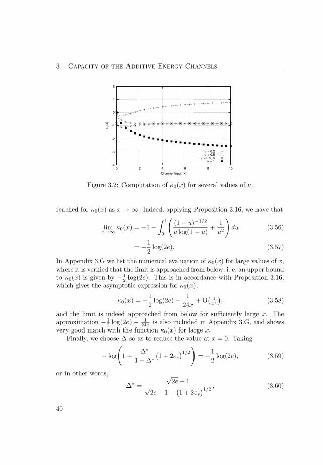
3. Capacity of the Additive Energy Channels

-4

-3

-2

-1

0

1

2

0 2 4 6 8 10

κ 0(x

)

Channel Input (x)

ν = 0.2ν = 0.5

ν = 0.5, ∆ν = 1

Figure 3.2: Computation of κ0(x) for several values of ν.

reached for κ0(x) as x →∞. Indeed, applying Proposition 3.16, we have that

limx→∞

κ0(x) = −1−∫ 1

0

((1− u)−1/2

u log(1− u)+

1u2

)du (3.56)

= −12

log(2e). (3.57)

In Appendix 3.G we list the numerical evaluation of κ0(x) for large values of x,where it is verified that the limit is approached from below, i. e. an upper boundto κ0(x) is given by − 1

2 log(2e). This is in accordance with Proposition 3.16,which gives the asymptotic expression for κ0(x),

κ0(x) = −12

log(2e)− 124x

+ O(

1x2

), (3.58)

and the limit is indeed approached from below for sufficiently large x. Theapproximation − 1

2 log(2e) − 124x is also included in Appendix 3.G, and shows

very good match with the function κ0(x) for large x.Finally, we choose ∆ so as to reduce the value at x = 0. Taking

− log

(1 +

∆∗

1−∆∗(1 + 2εs

)1/2

)= −1

2log(2e), (3.59)

or in other words,

∆∗ =√

2e− 1√

2e− 1 +(1 + 2εs

)1/2, (3.60)

40

Capacity of the Discrete-Time Poisson Channel

then the value at x = 0 coincides with the value as x → ∞, and κ0(0) =limx→∞ κ0(x). This effect is visible in Fig. 3.2, where the function κ0(x) de-creases from its value at x = 0 to a local minimum, and increases afterwards.We have also verified numerically that κ′0(x) is positive after the local mini-mum, that is the function is monotonic increasing and never reaches the valueκ0(0).

Summarizing all the considerations so far, we choose an input density ofthe form Eq. (3.48), with ν = 1/2 and the optimum ∆∗ in Eq. (3.60). Thisyields an output distribution PY (y), which is used together with the parameterγ = log εs+ν

εsto derive an upper bound to the capacity, using Proposition 3.7.

The maximum over x is located at x = 0 and x → ∞ and is such that thefollowing upper bound is obtained

C(εs) ≤ −12

log(2e) + ν logεs + ν

ν+ εs log

εs + ν

εs− log(1−∆∗) (3.61)

= log

(1 +

√2e− 1√1 + 2εs

)+ log

(εs + 1

2

)εs+ 12

√eεεs

s. (3.62)

As it could be expected from Lapidoth’s result in Eq. (3.27), the upperbound grows asymptotically as 1

2 log εs for large εs,

12

log εs +√

2e− 1√2√

εs

+ O(ε−1s

), (3.63)

where we used that log(1 + t) = t + O(t−1

), as t → 0.

3.5.5 Some Numerical Results

Figure 3.3 shows several bounds and approximations to the channel capacity,

1. Gordon’s approximate formula Eq. (3.23).

2. Lapidoth’s lower bound Eq. (3.26).

3. The exact mutual information Eq. (3.46) with two densities of the gammafamily, namely ν = 1

2 and ν = 1 (exponential).

4. The upper bound derived from the gamma density with ν = 12 , Eq. (3.62).

5. An upper bound assuming a geometric distribution, HGeom(εs).

41

3. Capacity of the Additive Energy Channels

0

0.5

1

1.5

2

2.5

3

3.5

4

0 50 100 150 200

Chan

nel C

ap

acity (

bits p

er

ch

ann

el u

se

)

Average Number of Input Quanta

Maximum EntropyUpper Bound

Lower Bound (ν = 0.5)Gaussian ApproximationLapidoth’s Lower Bound

Lower Bound (ν = 1)Gordon’s Formula

Figure 3.3: Upper and lower bounds to the channel capacity.

6. A Gaussian approximation to the capacity, CGaus(εs) = 12 log2(1 + εs).

In general our results follow the asymptotic expression for the capacity,12 log2 εs, but are tighter than the previously known bounds, by Gordon andLapidoth. The gamma density with ν = 1

2 is uniformly better than the expo-nential input, beating it by about 0.188 bits/channel use, the difference betweenthe two asymptotic expansions of the capacity, namely

I(XG(1/2,εs);Y ) =12

log2 εs + o(1), (3.64)

I(XG(1,εs);Y ) =12

log2 εs − 0.188 + o(1). (3.65)

We have determined both expansions numerically.In the range depicted in Fig. 3.3 the corresponding mutual information is

very closely given by the Gaussian approximation CGaus(εs). Figure 3.4 depictssome further curves to better compare the spectral efficiencies with CGaus. InFig. 3.4a we show the difference

I(XG(ν,εs); Y )− CGaus(εs), (3.66)

for the mutual information for two gamma inputs, with ν = 1 and ν = 12 .

The difference of C(εs) with respect to the upper bound in Eq. (3.62) is alsodepicted. Remarkably, the gamma density with ν = 1

2 seems to be aboveCGaus. This is further supported by the results plotted in Fig. 3.4b, a zoom

42

Capacity of the Discrete-Time Poisson Channel

in logarithmic scale of the previous plot, where the depicted range is increasedup to εs = 1036 quanta.

These computations allow us to numerically determine an additional termin the asymptotic expansion to the mutual information for ν = 1

2 ,

I(XG(1/2,εs);Y ) ' 12

log εs +0.324√

εs+ o(ε−1/2

s ). (3.67)

The plot of the upper bound in Fig. 3.4b matches with its asymptotic form,

12

log εs +√

2e− 1√2√

εs

+ O(ε−1s ). (3.68)

-0.3

-0.2

-0.1

0

0.1

0.2

0.3

0.4

0.5

0.6

0 50 100 150 200 250

Diffe

ren

ce w

rt G

au

ssia

n A

ppro

xim

atio

n (

bits)

Average Number of Input Quanta

Upper BoundLower Bound - Gamma(1/2)Lower Bound - Exponential

(a) Difference for low quanta counts.

10-20

10-15

10-10

10-5

100

100

105

1010

1015

1020

1025

1030

1035

Diffe

ren

ce w

rt G

au

ssia

n A

ppro

xim

atio

n (

bits)

Average Number of Input Quanta

Upper BoundLower Bound - Gamma(1/2)

(b) Difference for large quanta counts.

Figure 3.4: Comparison of channel capacity with Gaussian approximation.

From these numbers we conjecture that CGaus is always a lower boundto the channel capacity, even though we have not been able to prove it. It issignificant that the upper bound in Eq. (3.62), also represented in Fig. 3.4b, ap-proaches CGaus rather rapidly; the difference between the two is below 0.1 bitsfor 150 quanta/mode, falling to 0.01 bits at about 15000 quanta/mode. Thenarrow gap between the best lower and upper bounds constitutes the tightestpair of bounds known so far for this channel.

43

3. Capacity of the Additive Energy Channels

3.6 Capacity of the Quantized Additive Energy Channel

3.6.1 Introduction and Main Results

We now move on to study the capacity of the quantized additive energy (AE-Q) channel, which was described in Section 2.5. Briefly said, in the AE-Qchannel, the non-negative real-valued input xk and the integer-valued outputyk are related as

yk = sk(xk) + zk, (3.69)

where the output variables are distributed as Sk ∼ P(xk), and Zk ∼ G(εn),i. e. with Poisson and geometric distributions respectively. The input is usedunder an energy constraint,

∑nk=1 xk ≤ nεs, where εs is the average energy per

channel use.As with the discrete-time Poisson channel, we determine the channel ca-

pacity C(εs, εn) by providing tight upper and lower bounds. The main resultsare presented in subsequent sections and summarized here for convenience.

Upper bounds are given in Theorem 3.19 and Theorem 3.21,

C(εs, εn) ≤ min(CG(εs, εn), CP(εs)), (3.70)

where CG(εs, εn) and CP(εs) are respectively given by

CG(εs, εn) = HGeom(εs + εn)−HGeom(εn),

CP(εs) = log

((1 +

√2e− 1√1 + 2εs

)(εs + 1

2

)εs+ 12

√eεεs

s

). (3.71)

Here HGeom(t) is the entropy of a geometric distribution with mean t, given byEq. (3.24). Both functions CG(εs, εn) and CP(εs) are monotonically increasingfunctions of εs. Roughly speaking, CG is closer to the true capacity for lowvalues of εs, whereas CP is more accurate for higher values of εs. Note thatCP(εs) does not depend on εn.

This threshold behaviour can be seen in Fig. 3.5, which depicts the upperand lower bounds to the capacity as a function of the input number of quantaεs and for several values of εn. The upper bound in solid lines does not dependon εn, as is due to the intrinsic noise in the signal itself sk. When the additivenoise zk can be neglected, the total noise at the output does not disappear,but is dominated by the signal-dependent noise. Neglecting the signal noise,the second upper bound (in dashed lines) essentially takes the opposite path.

44

Capacity of the Quantized Additive Energy Channel

0

5

10

15

20

10-2

100

102

104

106

108

1010

1012

Cha

nne

l C

ap

acity (

bits)

Average Number of Input Quanta ε s

CG, ε n = 1Lower Bound, ε n = 1CG, ε n = 10

3

Lower Bound, ε n = 103

CG, ε n = 106

Lower Bound, ε n = 106

CP

Figure 3.5: Upper bounds to the capacity for several values of εn.

There exists a threshold ε∗s = ε2n such that the behaviour of the AE-Q

channel is dominated by additive geometric noise below it (the G regime),and by signal-dependent Poisson noise above it (P regime). When εn is largeenough, a good approximation to the location of the threshold is ε∗s = ε2

n or,

εn =ε∗sεn

=ε∗sε0

εnε0=

E∗s

En= SNR∗ (3.72)

that is the signal-to-noise ratio of the equivalent AWGN and AEN channels.In terms of the signal-to-noise ratio of the underlying AWGN channel, belowSNR∗ = εn the capacities of the AE-Q and AWGN channels are very similar,whereas sufficiently above SNR∗ the capacity of the AE-Q channel is half thecapacity of the AWGN channel.

For each value of εn the lower bound CLB(εs, εn) depicted in Fig. 3.5 (indashed-dotted lines) is the achievable mutual information with an exponentialinput identical to that of the additive exponential noise channel,

CLB(εs, εn) = HGeom(εs + εn)− εn

εs + εnHGeom(εn)

− εs

εs + εn

(12

log 2πe +12

log(

εn(1 + εn)112

)×

× eεn(1+εn)+ 1

12εs+εn Γ

(0,

εn(1 + εn) + 112

εs + εn

)), (3.73)

45

3. Capacity of the Additive Energy Channels

where Γ(0, t) is an incomplete gamma function, Γ(0, t) =∫∞

tu−1e−u du. De-

spite its unwieldy appearance, the formula is simple to evaluate numerically.Upper and lower bounds are respectively derived in Sections 3.6.2 and 3.6.3.

Numerical results, particularized for the case when quanta are identified withphotons, are presented and discussed in Section 3.6.4. In this case, the thresh-old signal-to-noise ratio of the equivalent AWGN channel is given by

SNR∗ = εn ' 6 · 1012

ν, (3.74)

where ν is the frequency (in Hertz). In decibels, SNR∗ (dB) ' 37.8−10 log10 ν,where the frequency is in GHz.

3.6.2 Upper Bounds to the Capacity

In this section we shall give two upper bounds to the capacity C of the quantizedadditive energy channel as a function of the average signal energy εs and theaverage geometric noise energy εn. The first one will be directly related to theadditive exponential noise channel, and the second derived from the discrete-time Poisson channel. Obviously, the smallest of them also constitutes an upperbound, tighter than each of them separately.

Our first result is the following

Theorem 3.19. The capacity of the AE-Q channel is upper bounded by

C(εs, εn) ≤ CG(εs, εn) = HGeom(εs + εn)−HGeom(εn), (3.75)

where HGeom(t) is the entropy of a geometric distribution of mean t.

Since HGeom(t), is given by Eq. (3.24), HGeom(t) = (1+t) log(1+t)−t log t,an equivalent expression for the upper bound is

CG(εs, εn) = (1 + εs + εn) log(1 + εs + εn)− (εs + εn) log(εs + εn)− (1 + εn) log(1 + εn) + εn log εn. (3.76)

We have also the following corollary,

Corollary 3.20. For finite values of εs, CG(εs, εn) is bounded by

log(

1 +εs

εn + 1

)< CG(εs, εn) < log

(1 +

εs

εn

). (3.77)

The capacity of the AE-Q channel is therefore strictly upper bounded by thecapacity of an AEN channel of signal-to-noise ratio SNR = εs/εn.

46

Capacity of the Quantized Additive Energy Channel

We now prove Theorem 3.19.

Proof. For any input pX(x) the mutual information clearly satisfies

I(X;Y ) = H(Y )−H(Y |X) (3.78)

≤ HGeom(εs + εn)−H(S(X) + Z|X)

, (3.79)

as the geometric distribution has the highest entropy under the given con-straints. Then, as conditioning reduces entropy,

H(S(X) + Z|X) ≥ H

(S(X) + Z|X,S

)(3.80)

= H(Z|X, S) = H(Z), (3.81)

and Z is independent of the input X. Therefore,

I(X; Y ) ≤ HGeom(εs + εn)−HGeom(εn). (3.82)

As this holds for all inputs the theorem follows.

We now move on to prove the formulas comparing the upper bound withthe capacity of the additive exponential noise channel.

Proof. First, we prove the strict inequality

log(εs + εn)− log εn > CG(εs, εn), (3.83)

for all values of εs > 0, εn ≥ 0. Using the definition of CG(εs, εn), we have

(1 + εs + εn) log(εs + εn)− (1 + εs + εn) log(1 + εs + εn)− (1 + εn) log(εn) + (1 + εn) log(1 + εn) > 0, (3.84)

that is,

(1 + εs + εn) logεs + εn

1 + εs + εn> (1 + εn) log

εn

1 + εn. (3.85)

Proving this is equivalent to proving that the function

f(t) = (1 + t) logt

1 + t= (1 + t) log t− (1 + t) log(1 + t) (3.86)

47

3. Capacity of the Additive Energy Channels

is monotonically increasing for t > 0. Its first derivative f ′(t) is

f ′(t) = log t +1 + t

t− log(1 + t)− 1 (3.87)

=1t− log

(1 +

1t

), (3.88)

which is positive since log(1 + t′) < t′ for positive t′.We now move on to prove the second strict inequality. For εs > 0, εn ≥ 0.

CG(εs, εn) > log(εs + εn + 1)− log(εn + 1). (3.89)

Using the definition of CG(εs, εn) and cancelling common terms,

(εs + εn) log(1 + εs + εn)− (εs + εn) log(εs + εn)− εn log(1 + εn) + εn log εn > 0, (3.90)

a condition equivalent to

(εs + εn) log1 + εs + εn

εs + εn> εn log

1 + εn

εn. (3.91)

This equation is true whenever the function f(t)

f(t) = t log(

1 +1t

)(3.92)

is monotonically increasing for t > 0. Equivalently, its first derivative f ′(t),

f ′(t) = log(

1 +1t

)+ t

− 1t2

1 + 1t

= log(

1 +1t

)− 1

t + 1, (3.93)

must be positive for t > 0. This condition may be rewritten as

log(

1 +1t

)>

1t + 1

, (3.94)

or, exponentiating in both sides,

1 +1t

> e1

t+1 > 1 +1

t + 1, (3.95)

where the last inequality is due to the fact that et > 1 + t. Accordingly,f ′(t) > 0 since t + 1 > t.

48

Capacity of the Quantized Additive Energy Channel

Our second upper bound is in

Theorem 3.21. The capacity of the AE-Q channel is upper bounded by

C(εs, εn) ≤ CP(εs) = log

((1 +

√2e− 1√1 + 2εs

)(εs + 1

2

)εs+ 12

√eεεs

s

). (3.96)

Note that this formula does not depend on the additive noise εn, as willbecome apparent from it being derived from the discrete-time Poisson channel.The proof of Theorem 3.21 is similar to that of Theorem 3.19. It exploits thata genie has knowledge of the exact value of the additive noise component.

Proof. The variables X, S(X), and Y (S) form a Markov chain in this order,

X → S(X) → Y = S(X) + Z. (3.97)

Hence, by the data processing inequality (Theorem 2.8.1 in [22]),

I(X; Y ) ≤ I(X; S(X)

), (3.98)

that is the mutual information achievable in the discrete-time Poisson channel.The bound follows then from Eq. (3.31), as an upper bound to the latter isalso an upper bound to the AE-Q channel.

3.6.3 A Lower Bound to the Capacity

Our lower bound is derived from the mutual information achievable by theinput which achieves the largest output entropy. This input is characterized in

Proposition 3.22. In the AE-Q channel the output entropy H(Y ) is maxi-mized when the input density pX(x) is given by

pX(x) =εs

(εs + εn)2exp

(− x

εs + εn

)+

εn

εs + εnδ(x), x ≥ 0. (3.99)

As a particular case we recover the exponential input, which maximizes theoutput entropy of a DTP channel [12]. Also, the form of the density is analogousto the result in the additive exponential noise channel, in Proposition 3.13.

The proof needs the probability generating function (pgf) pgf(u) of z. Fora geometric random variable of mean x, the pgf is given in

49

3. Capacity of the Additive Energy Channels

Proof. Since Y is a discrete random variable, its entropy is maximum when itsdistribution is geometric. In that case the pgf E[uY ] is given by

pgfGeom(εn)(u) =(1 + εn(1− u)

)−1. (3.100)

Similarly, for a Poisson distribution with mean x, its pgf is pgfPois(x)(u) =e−x(1−u). As for the signal component at the output, its pgf is a mixture ofPoisson distributions, of value

pgf(u) =∫ ∞

0

pX(x) pgfPois(x)(u)dx (3.101)

=∫ ∞

0

(εs

(εs + εn)2e−

xεs+εn +

εn

εs + εnδ(x)

)e−x(1−u)dx (3.102)

=εs

εs + εn

1((εs + εn)(1− u) + 1

) +εn

εs + εn(3.103)

=1 + εn(1− u)

(εs + εn)(1− u) + 1. (3.104)

As Y is the sum of two independent random variables, its pgf is the productof the corresponding pgf’s, Eqs. (3.100) and (3.104), which gives

((εs + εn)(1− u) + 1

)−1, (3.105)

the pgf of a geometric distribution with mean εs + εn, as desired.

We shall also need the following upper bound to the entropy of a randomvariable Y with a given variance VarY (Theorem 9.7.1 of [22]),

H(Y ) ≤ 12

log 2πe

(VarY +

112

). (3.106)

We have then the following

Theorem 3.23. A lower bound CLB(εs, εn) to the capacity of the AE-Q chan-nel is

CLB(εs, εn) = HGeom(εs + εn)− εn

εs + εnHGeom(εn)

− εs

εs + εn

(12

log 2πe +12

log(

εn(1 + εn) +112

)×

× eεn(1+εn)+ 1

12εs+εn Γ

(0,

εn(1 + εn) + 112

εs + εn

)), (3.107)

50

Capacity of the Quantized Additive Energy Channel

where Γ(0, t) is an incomplete gamma function, Γ(0, t) =∫∞

tu−1e−u du.

An alternative integral expression is

CLB(εs, εn) = − εs

(εs + εn)2

∫ ∞

0

12

log 2πe

(x + εn(1 + εn) +

112

)e−

xεs+εn dx

+ HGeom(εs + εn)− εn

εs + εnHGeom(εn). (3.108)

Proof. We choose as an input the density in Eq. (3.99) in Proposition 3.22. Byconstruction, the output is then geometric with mean εs + εn and the outputentropy H(Y ) is therefore given by H(Y ) = HGeom(εs + εn). We compute themutual information with this input as H(Y )−H(Y |X).

We now move on to estimate the second term, the conditional entropy, as

H(Y |X) =∫ ∞

0

H(Y |x)

(εs

(εs + εn)2e−

xεs+εn +

εn

εs + εnδ(x)

)dx (3.109)

=εn

εs + εnH(Y |x = 0) +

εs

(εs + εn)2

∫ ∞

0

H(Y |x)e−x

εs+εn dx. (3.110)

The first term is the entropy of a geometric distribution, that is H(Y |x = 0) =HGeom(εn). And the second is upper bounded by Eq. (3.106),

H(Y |x) ≤ 12

log 2πe

(Var(Y |x) +

112

)(3.111)

=12

log 2πe +12

log(

x + εn(1 + εn) +112

). (3.112)

Hence,∫ ∞

0

H(Y |x)e−x

εs+εn dx ≤ 12

log 2πe

∫ ∞

0

e−x

εs+εn dx

+∫ ∞

0

12

log(

x + εn(1 + εn) +112

)e−

xεs+εn dx

(3.113)

= (εs + εn)12

log 2πe + (εs + εn)12

log(

εn(1 + εn) +112

)×

× eεn(1+εn)+ 1

12εs+εn Γ

(0,

εn(1 + εn) + 112

εs + εn

). (3.114)

51

3. Capacity of the Additive Energy Channels

We determined the integral in Eq. (3.113) by using Mathematica; here Γ(0, t)is an incomplete gamma function, defined as Γ(0, t) =

∫∞t

u−1e−u du. Hence,

H(Y |X) ≤ εn

εs + εnHGeom(εn) +

εs

εs + εn

(12

log 2πe +12

log(

εn(1 + εn) +112

)×

× eεn(1+εn)+ 1

12εs+εn Γ

(0,

εn(1 + εn) + 112

εs + εn

)). (3.115)

3.6.4 Numerical Results and Discussion

In this section, we compute the upper and lower bounds which we have derivedin previous pages. We start by evaluating the difference between the upperand lower bounds from Theorems 3.19, 3.21, and 3.23. The quantity

min(CG(εs, εn),CP(εs)

)− CLB(εs, εn) (3.116)

is plotted in Fig. 3.5 as a function of εs for several values of εn, viz. 1, 100, 1000,and 106 quanta. In all cases, the difference between upper and lower boundsis at most 1.1 bits, a relatively small value. At low εs, the gap converges toabout 0.6 bits (depicted in Fig. 3.6 as a horizontal line), which is the differencebetween the Gaussian bound to the output differential entropy H(Y |X = x),assuming a variance εs + εn(1 + εn) ' ε2

n, and the differential entropy ofexponential noise, that is,

12

log(2πe ε2n)− log(eεn) =

12

log2π

e' 0.60441 bits. (3.117)

For high values of εn the gap gets close to this asymptotic value (see especiallythe curve for εn = 106). Most of the loss is likely caused by a pessimisticestimate of the conditional output entropy H(Y |X), which may be closer tothe additive entropy H(Y ) than we have been able to prove. If this were thecase the true channel capacity C(εs, εn) would be closely given by the upperbound in Theorem 3.19.

At high εs the gap seems to converge to about 0.18 bits (shown in Fig. 3.6 asa horizontal line), the same gap between the capacity of the discrete-time Pois-son channel and the mutual information with exponential input. A different

52

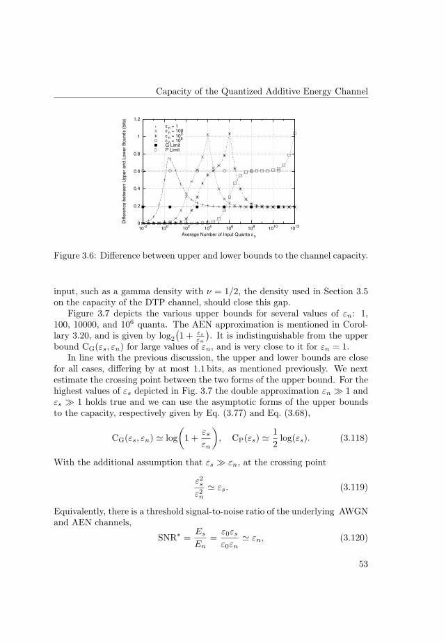
Capacity of the Quantized Additive Energy Channel

0

0.2

0.4

0.6

0.8

1

1.2

10-2

100

102

104

106

108

1010

1012

Diffe

ren

ce

betw

een

Upp

er

an

d L

ow

er

Bo

und

s (

bits)

Average Number of Input Quanta ε s

ε n = 1ε n = 100ε n = 10

3

ε n = 106

G LimitP Limit

Figure 3.6: Difference between upper and lower bounds to the channel capacity.

input, such as a gamma density with ν = 1/2, the density used in Section 3.5on the capacity of the DTP channel, should close this gap.

Figure 3.7 depicts the various upper bounds for several values of εn: 1,100, 10000, and 106 quanta. The AEN approximation is mentioned in Corol-lary 3.20, and is given by log2

(1 + εs

εn

). It is indistinguishable from the upper

bound CG(εs, εn) for large values of εn, and is very close to it for εn = 1.In line with the previous discussion, the upper and lower bounds are close

for all cases, differing by at most 1.1 bits, as mentioned previously. We nextestimate the crossing point between the two forms of the upper bound. For thehighest values of εs depicted in Fig. 3.7 the double approximation εn À 1 andεs À 1 holds true and we can use the asymptotic forms of the upper boundsto the capacity, respectively given by Eq. (3.77) and Eq. (3.68),

CG(εs, εn) ' log(

1 +εs

εn

), CP(εs) ' 1

2log(εs). (3.118)

With the additional assumption that εs À εn, at the crossing point

ε2s

ε2n

' εs. (3.119)

Equivalently, there is a threshold signal-to-noise ratio of the underlying AWGNand AEN channels,

SNR∗ =Es

En=

ε0εs

ε0εn' εn, (3.120)

53

3. Capacity of the Additive Energy Channels

0

5

10

15

20

-20 0 20 40 60 80 100 120

Cha

nne

l C

ap

acity (

bits)

Signal-to-Noise Ratio ε s/ε n (dB)

CGCG - AEN Approximation

CPLower Bound

(a) εn = 1

0

5

10

15

20

-40 -20 0 20 40 60 80 100C

ha

nne

l C

ap

acity (

bits)

Signal-to-Noise Ratio ε s/ε n (dB)

CGCP

Lower Bound

(b) εn = 100

0

5

10

15

20

-60 -40 -20 0 20 40 60 80

Ch

an

ne

l C

ap

acity (

bits)

Signal-to-Noise Ratio ε s/ε n (dB)

CGCP

Lower Bound

(c) εn = 104

0

5

10

15

20

-80 -60 -40 -20 0 20 40 60

Ch

an

ne

l C

ap

acity (

bits)

Signal-to-Noise Ratio ε s/ε n (dB)

CGCP

Lower Bound

(d) εn = 106

Figure 3.7: Upper bounds to the capacity for several values of εn.

such that the behaviour is limited by additive geometric noise below it (i. e. itfalls in the G region), and by the Poisson, signal-dependent noise above it (i.e. the P region). The position of the threshold roughly corresponds to inputenergy value for which the Poisson noise variance Var(S) = εs coincides withthe additive noise variance Var(Z).

For the upper plots in Fig. 3.7 the position of the threshold is also given bythe expression (3.119), even though the amount of additive noise is not large.

54

Conclusions

Photons as Quanta of Energy We conclude our discussion by applyingthe results of the AE-Q channel capacity to a channel where photons are theunit of energy. The details of this correspondence were given in Section 2.6,on page 21, and summarized in Table 2.2 therein. For a fixed frequency ν,one can identify the variables εs and εn with respectively the energy of theuseful signal and of thermal noise in a physical channel which makes use ofelectromagnetic radiation to convey information. Moreover, εn is given byEq. (2.24), the average number of thermal photons at a given temperature.

More concretely, the four cases presented in Fig. 3.7 correspond to frequen-cies 4THz (εn = 1), 60GHz (εn = 100), 600 MHz (εn = 104), and 6 MHz(εn = 106). For each of these cases the threshold signal-to-noise ratio SNR∗

has the respective values 0 dB, 20 dB, 40 dB, and 60 dB, as corresponds to usingEq. (3.120),

SNR∗ = εn =(e

hνkBT0 − 1

)−1 ' kBT0

hν' 6 · 1012

ν. (3.121)

In decibels, SNR∗ (dB) ' 37.8− 10 log10 ν, where the frequency is in GHz.Below threshold, the capacity of the AE-Q channel is closely given by

C(εs, εn) ' log(

1 +εs

εn

)' log

(1 +

Es

kBT0

), (3.122)

where Es is the average signal energy and kBT0 the one-sided noise spectraldensity of an equivalent AWGN channel.

Above the threshold SNR∗ the slope of the capacity as a function of log(εs)changes to the value 1/2. An intriguing connection, which is worthwhile men-tioning, can be made with non-coherent communications in Gaussian chan-nels [23], where one of the two signal quadratures is not used, and a similarchange in slope in the capacity takes place. A similar effect appears in phase-noise limited channels [45].

3.7 Conclusions

In this chapter we have determined the channel capacity of several additiveenergy channels. First, we have seen that the capacity of the complex-valuedadditive Gaussian noise channel coincides with that of the additive exponentialnoise channel with identical levels of signal and additive noise.

Second, we have obtained some new results on the capacity of the discrete-time Poisson (DTP) channel. We have derived what seems to be the tightest

55

3. Capacity of the Additive Energy Channels

known upper bound. An important tool in this analysis has been a simplemethod to upper bound the capacity as function of an input distribution. Inaddition, we have also derived closed-form proper integral expressions for theentropy of Poisson and negative binomial distributions, as well as for the aver-age mutual information of a gamma input in the discrete-time Poisson channel.This analysis has been published in [46].

As we discussed in Chapter 2, the AE-Q channel is an intermediate modelbetween the DTP and AEN channels. At one extreme, the additive exponentialnoise channel may be seen as a continuous version of the AE-Q. Next to thedifference in the output alphabet (that is integer, instead of real-valued output),a more important effect is the absence or presence of Poisson (signal-dependent)noise, besides the additive noise component. In the AE-Q channel, as in theDTP channel, noise is partly signal-dependent. When this Poisson noise istaken into account, we have seen that two regimes appear,

• the G regime, where capacity is limited by additive geometric noise, and

• the P regime, where the limiting factor is Poisson noise.

We have computed the capacity by deriving upper and lower bounds. Theydiffer by (at most) about 1.1 bits, and we expect that the channel capacity isclose to the upper bound. In that case, in the G regime, the channel capacityis almost the capacity of the equivalent AWGN or AEN channels,

log(

1 +εs

εn

), (3.123)

whereas in the P regime the capacity is close to the DTP value, 12 log εs.

Finally, we have briefly discussed the analogy with radiation channels, forwhich the G regime corresponds to the thermal regime, in which additive Gaus-sian noise is predominant. An unexpected trait of the model is that the con-dition to lie in the G regime is not only to be at low frequency, as would beexpected, but also to have signal-noise ratio below a threshold. Poisson noise ismacroscopically visible when it prevails over additive noise, an effect which canarise in one of two ways: by reducing the additive noise level, i. e. by increasingthe frequency or lowering the background temperature, or by increasing the sig-nal level and so indirectly the variance of the signal itself, which is proportionalto the mean (for a Poisson distribution).

For the frequencies commonly used in radio or wireless communications, thethreshold is located at above 30 dB, and therefore the capacity of the AE-Q and

56

An Upper Bound to the Channel Capacity

AWGN channels would coincide for all practical effects. However, for higherfrequencies or larger values of signal-to-noise ratio, a discrepancy between thetwo models would appear. An interesting question is to establish the extent towhich the AE-Q represents a real limit to the capacity of a radio or wirelesscommunication link. Needless to say, at optical frequencies the AE-Q modelcollapses into a discrete-time Poisson channel, widely considered as a validmodel for communication under the so-called direct detection.

Preliminary results on the analysis of the AE-Q channel were presentedat the International Symposium on Information Theory (ISIT) 2006 [47], andat ISIT 2007 [48]. A paper is to be submitted to the IEEE Transactions onInformation Theory.

3.A An Upper Bound to the Channel Capacity

Let pin(x) be a density on the input alphabet, satisfying the input constraint,∫

ε(x)pin(x) dx ≤ E. (3.124)

The density pin(x) induces a corresponding output density, p1(y), p1(y) =∫pin(x)Q(y|x) dx, and achieves a mutual information

I(Xin;Y1

)=

∫∫pin(x)Q(y|x) log

Q(y|x)p1(y)

dx dy, (3.125)

which in general will be smaller than the capacity C(E).The right-hand side in Eq. (3.9) satisfies

maxx

(∫Q(y|x) log

Q(y|x)p(y)

dy − γ(ε(x)− E))

= (3.126)

=∫

pin(x′)

(max

x

(∫Q(y|x) log

Q(y|x)p(y)

dy − γ(ε(x)− E)))

dx′ (3.127)

≥∫

pin(x′)(∫

Q(y|x′) logQ(y|x′)

p(y)dy − γ(ε(x′)− E)

)dx′ (3.128)

≥∫

pin(x′)∫

Q(y|x′) logQ(y|x′)

p(y)dy dx′, (3.129)

where Eq. (3.127) uses that∫

pin(x′) dx′ = 1 and x′ is a dummy variable. Whenobtaining Eq. (3.128) we used that the integral becomes smaller by replacing

57

3. Capacity of the Additive Energy Channels

maxx f(x) by f(x′) at each x′, as f(x′) ≤ maxx f(x). Finally Eq. (3.129) fol-lows since γ ≥ 0 and the input density pin(x) satisfies the constraint Eq. (3.124).

We continue by proving that the right-hand side in Eq. (3.129) is an upperbound to I(Xin; Y1). Indeed, cancelling common terms,

∫pin(x′)

∫Q(y|x′) log

Q(y|x′)p(y)

dy dx′ −∫∫

pin(x)Q(y|x) logQ(y|x)p1(y)

dx dy

=∫

pin(x′)∫

Q(y|x′) logp1(y)p(y)

dy dx′ (3.130)

=∫

p1(y) logp1(y)p(y)

dy ≥ 0. (3.131)

Here we used the definition of p1(y) and the fact that the divergence betweentwo densities is non-negative.

We have therefore proved that

maxx

(∫Q(y|x) log

Q(y|x)p(y)

dy − γ(ε(x)− E))≥ I(Xin; Y1

)(3.132)

for all input densities which satisfy the input constraint. Since this holds forall densities, it must also hold for the supremum, the channel capacity C(E).

3.B Entropy of a Poisson Distribution

Using the value of PS(s|x) = e−x xs

s! and log PS(s|x) = −x+ s log x− log s!, theentropy HPois(x) is written as

HPois(x) = x− x log x +∞∑

s=0

PS(s|x) log s!, (3.133)

where we substituted the mean value. Using Eq (3.35) the last summand is

∞∑s=0

PS(s|x) log s! =∞∑

s=0

e−x xs

s!

∫ 1

0

(1− us

1− u− s

)du

log u(3.134)

=∫ 1

0

(1− e−xexu

1− u− x

)du

log u, (3.135)

where we have interchanged the order of summation and integration and addedup the various terms in the infinite sum.

58

Asymptotic Form of f(x)

3.C Asymptotic Form of f(x)

This analysis was carried out in collaboration with Dr. Hennie Ter Morsche,from the Department of Mathematics at Technische Universiteit Eindhoven.

Let I denote the integral

I =∫ 1

0

(x− (1− u)ν−1 1− e−xu

u

)du

log(1− u). (3.136)

This integral is derived from the one in Eq. (3.38) by the change of variablesu′ = 1− u. For convenience, let us express I as the sum I = I1 + I2 − I3 + I4,where

I1 =∫ 1/x

0

(x− (1− u)ν−1 1− e−xu

u

)du

log(1− u), (3.137)

I2 = x

∫ 1

1/x

du

log(1− u), (3.138)

I3 =∫ 1

1/x

(1− u)ν−1 1u

du

log(1− u), (3.139)

I4 =∫ 1

1/x

(1− u)ν−1 e−xu

u

du

log(1− u). (3.140)

We approximate each of these integrals for large x, determining an expansionup to order x−1.

In I1, let us change the variable to t = xu. Then

I1 =∫ 1

0

(1−

(1− t

x

)ν−1 1− e−t

t

)dt

log(1− t

x

) . (3.141)

Using the Taylor expansions of (1− z)ν−1 and log−1(1− z), given by

(1− z)ν−1 = 1− (ν − 1)z + az2 + O(z3) (3.142)

log−1(1− z) = −1z

+12

+z

12+ O(z2), (3.143)

59

3. Capacity of the Additive Energy Channels

with a = 12 (ν − 1)(ν − 2), back in Eq. (3.141), we get for I1 the expression

I1 =∫ 1

0

(1−

(1− (ν − 1)

t

x+ a

t2

x2+ O

(t3

x3

))1− e−t

t

)×

×(−x

t+

12

+t

12x+ O

(t2

x2

))dt (3.144)

=∫ 1

0

(−x

t+

12

+t

12x

)(1− 1− e−t

t

)dt + O

(1x2

)+

+∫ 1

0

((ν − 1)

t

x

1− e−t

t

)(−x

t+

12

)dt + O

(1x2

)+

−∫ 1

0

(a

t2

x2

1− e−t

t

)(−x

t

)dt + O

(1x2

)(3.145)

= −x

∫ 1

0

1t

(1− 1− e−t

t

)dt +

12

+(ν − 1

2

) ∫ 1

0

(1− e−t

t

)dt+

+1x

(124 + 1

e

(− 1

12 + ν−12 + a

))+ O

(1x2

). (3.146)

Here we used that∫ 1

0(1− e−t) dt = e−1.

We now move on to I2. By adding and subtracting a term u−1 to theintegrand, the integral is computed as

I2 = x

∫ 1

1/x

(1

log(1− u)+

1u− 1

u

)du (3.147)

= x

∫ 1

1/x

(1

log(1− u)+

1u

)du− x

∫ 1

1/x

1u

du (3.148)

= x

∫ 1

1/x

(1

log(1− u)+

1u

)du− x log x. (3.149)

Now, we extend the lower integration limit to 0, by writing∫ 1

1/x

(1

log(1− u)+

1u

)du =

∫ 1

0

(1

log(1− u)+

1u

)du

−∫ 1/x

0

(1

log(1− u)+

1u

)du, (3.150)

60

Asymptotic Form of f(x)

a valid operation since, as u → 0, we deduce from Eq. (3.143) that(

1log(1− u)

+1u

)=

12

+u

12+ O(u2). (3.151)

Hence, the contribution of the second integral can be evaluated asymptotically,

x

∫ 1

1/x

(1

log(1− u)+

1u

)du = x

∫ 1

0

(1

log(1− u)+

1u

)du− 1

2− 1

24x+ O

(1x2

),

(3.152)

and we obtain the expression for I2,

I2 = x

∫ 1

0

(1

log(1− u)+

1u

)du− 1

2− 1

24x− x log x + O

(1x2

). (3.153)

We move on to I3. We add and subtract a term 1u − 1

2 to the function1

log(1−u) in the integrand, and write

I3 =∫ 1

1/x

(1− u)ν−1

(1

u log(1− u)+

1u2− 1

2u

)du

−∫ 1

1/x

(1− u)ν−1

(1u2− 1

2u

)du. (3.154)

Since

limu→0

((1− u)ν−1 ·

(1

u log(1− u)+

1u2− 1

2u

))=

112

+ O(u), (3.155)

we can shift the lower integration limit to 0 in the first integral. This is com-pensated by subtracting the integral

∫ 1/x

0

(1− u)ν−1

(1

u log(1− u)+

1u2− 1

2u

)du =

112x

+ O(

1x2

), (3.156)

where the error term is O(

1x2

). The resulting integral between 0 and 1 does

not depend on x. The second term, which we denote by I3′ , is given by

I3′ = −∫ 1

1/x

(1− u)ν−1

(1u2− 1

2u

)du. (3.157)

61

3. Capacity of the Additive Energy Channels

By adding and subtracting a function 1− (ν − 1)u, we rewrite I3′ as

I3′ = −∫ 1

1/x

((1− u)ν−1 − 1 + (ν − 1)u

)(1u2− 1

2u

)du

−∫ 1

1/x

(1− (ν − 1)u

)(1u2− 1

2u

)du. (3.158)

Again, since((1− u)ν−1 − 1 + (ν − 1)u

)(1u2− 1

2u

)= a + O(u) (3.159)

around u = 0, we can shift the lower integration order to 0. In doing so, wemust include the summand

∫ 1/x

0

((1− u)ν−1 − 1 + (ν − 1)u

)(1u2− 1

2u

)du =

a

x+ O

(1x2

). (3.160)

The resulting integral between 0 and 1 does not depend on x.The remaining integral in the evaluation of I3 is evaluated as

−∫ 1

1/x

(1u2− 1

u

(ν − 1

2

)+

ν − 12

)du =

1u

+(

ν − 12

)log u− ν − 1

2u

∣∣∣∣1

1/x

(3.161)

= 1− ν − 12

− x +(

ν − 12

)log x +

ν − 12x

. (3.162)

Hence, collecting the previous expressions, I3 admits the asymptotic expression

I3 =∫ 1

0

(1− u)ν−1

(1

u log(1− u)+

1u2− 1

2u

)du+

−∫ 1

0

((1− u)ν−1 − 1 + (ν − 1)u

)(1u2− 1

2u

)du +

3− ν

2+

− x +(

ν − 12

)log x +

1x

(− 1

12+ a +

ν − 12

)+ O

(1x2

). (3.163)

Finally, we split I4 into two parts, I4′ and I4′′ , respectively given by

I4′ =∫ 1/2

1/x

(1− u)ν−1 e−xu

u

du

log(1− u)(3.164)

I4′′ =∫ 1

1/2

(1− u)ν−1 e−xu

u

du

log(1− u). (3.165)

62

Asymptotic Form of f(x)

In the first one, I4′ let us add and subtract a term 1u − 1

2 , to obtain

I4′ =∫ 1/2

1/x

(1− u)ν−1 e−xu

u

(1

log(1− u)+

1u− 1

2

)du

−∫ 1/2

1/x

(1− u)ν−1 e−xu

u

(1u− 1

2

)du. (3.166)

The first summand of I4′ , of value

∫ 1/2

1/x

(1− u)ν−1 e−xu

u

(1

log(1− u)+

1u− 1

2

)du, (3.167)

has the form∫ 1/2

1/xg(u)e−xu du, where, using Eq. (3.143),

g(u) = (1− u)ν−1

(1

u log(1− u)+

1u2− 1

2u

)=

112

+ O(u). (3.168)

Replacing this expansion back in the integral, we obtain

∫ 1/2

1/x

e−xu

(112

+ O(u))

du =1

12ex+ O(e−

x2 ) +

∫ 1/2

1/x

e−xu O(u) du (3.169)

=1

12ex+ O

(1x2

), (3.170)

where we used that

∫ 1/2

1/x

e−xuun du = O(

1xn+1

), (3.171)

for large x and n integer.Changing variables, to t = xu, we get for the second contribution to I4′

−x

∫ x/2

1

(1− t

x

)ν−1e−t

t2dt +

12

∫ x/2

1

(1− t

x

)ν−1e−t

tdt. (3.172)

63

3. Capacity of the Additive Energy Channels

The Taylor expansion in Eq. (3.142) gives for the first of these summands

− x

∫ x/2

1

(1− (ν − 1)

t

x+ a

t2

x2+ O

(t3

x3

))e−t

t2dt =

= −x

∫ x/2

1

e−t

t2dt + (ν − 1)

∫ x/2

1

e−t

tdt− a

x

∫ x/2

1

e−tdt−∫ x/2

1

O(

tx2

)e−tdt

(3.173)

= −x

∫ ∞

1

e−t

t2dt +

∫ ∞

1

(ν − 1)e−t

tdt− a

ex+ O

(1x2

), (3.174)

where we replaced the upper integration order by ∞, which introduced anexponentially small error term O(e−x), and used Eq. (3.171). Similarly, thesecond summand in Eq. (3.172) can be expressed as

12

∫ x/2

1

(1− (ν − 1)

t

x+ O

(t2

x2

))e−t

tdt =

=12

∫ x/2

1

e−t

tdt +

12x

∫ x/2

1

(ν − 1)e−tdt +∫ x/2

1

O(

tx2

)e−tdt

(3.175)

=12

∫ ∞

1

e−t

tdt− 1

2ex(ν − 1) + O

(1x2

), (3.176)

where we also replaced the upper integration order by ∞, with the correspond-ing error term O(e−x).

The last remaining term is I4′′ ,

I4′′ =∫ 1

1/2

(1− u)ν−1 e−xu

u

du

log(1− u). (3.177)

The magnitude of its contribution |I4′′ | is upper bounded by

|I4′′ | = e−x2

∣∣∣∣∣∫ 1

1/2

(1− u)ν−1 e−xu

u

du

log(1− u)

∣∣∣∣∣, (3.178)

since the function is the integrand is regular, and the exponential functiondecays with increasing u. Since the integral exists, we conclude that

I4′′ = O(e−

x2). (3.179)

64

Asymptotic Form of f(x)

Finally, combining Eqs. (3.146), (3.153), (3.163), (3.170) (3.174), (3.176),and Eq. (3.179), the value of I is given by

I = −x

∫ 1

0

(1t− 1

t2+

e−t

t2

)dt− 3− ν

2+

12− (

ν − 12

) ∫ 1

0

(1− e−t

t

)dt

+ x

∫ 1

0

(1

log(1− u)+

1u

)du− 1

2− x log x−

(ν − 1

2

)log x

−∫ 1

0

(1− u)ν−1

(1

u log(1− u)+

1u2− 1

2u

)du

+∫ 1

0

((1− u)ν−1 − 1 + (ν − 1)u

)(1u2− 1

2u

)du + x− x

∫ ∞

1

e−t

t2dt

+∫ ∞

1

(ν − 1

2

)e−t

tdt +

1x

(112− a− ν − 1

2

)+ O

(1x2

). (3.180)

Here we cancelled the common terms in the coefficient of x−1. Further, recallthat a = 1

2 (ν − 1)(ν − 2).Further simplification is brought about by the facts that

∫ 1

0

(− 1

log(1− t)− 1

t2+

e−t

t2

)dt +

∫ ∞

1

e−t

t2dt = (3.181)

=∫ 1

0

(− 1

log(1− t)− 1

t2+

e−t

t2+ e−1/t

)dt = 0 (3.182)

∫ 1

0

1− e−t

tdt−

∫ ∞

1

e−t

tdt =

∫ 1

0

1− e−t − e−1/t

tdt = γe, (3.183)

which, together with some straightforward combinations, implies that

I = −(ν − 1

2

)γe − x log x− 3− ν

2+ x− (

ν − 12

)log x +

1x

(112− (ν − 1)2

2

)

−∫ 1

0

((1− u)ν−1

u log(1− u)+

(1− (ν − 1)u

)(1u2− 1

2u

))du + O

(1x2

)(3.184)

= −(ν − 1

2

)γe − x log x− 1 + x− (

ν − 12

)log x +

1x

(112− (ν − 1)2

2

)

−∫ 1

0

((1− u)ν−1

u log(1− u)+

1u2− 1

u

(ν − 1

2

))

du + O(

1x2

). (3.185)

65

3. Capacity of the Additive Energy Channels

3.D Entropy of a Negative Binomial Distribution

The moment generating function E[etX ] of a variable X with gamma dis-tribution, denoted by mgfG(ν,εs)(t), and the probability generating functionE[uX ] of a random variable X with negative binomial distribution, denoted bypgfNegBin(ν,εs)(u), are respectively given by

mgfG(ν,εs)(t) =νν

(ν − εst)ν(3.186)

pgfNegBin(ν,εs)(u) =νν

(ν + εs(1− u))ν= mgfG(ν,εs)(u− 1). (3.187)

By definition the entropy is the sum

HNegBin(ν, εs) = −∞∑

y=0

PY (y) log PY (y) (3.188)

= −∞∑

y=0

PY (y)(

logΓ(y + ν)y!Γ(ν)

+ logνν

(εs + ν)ν+ y log

εs

εs + ν

)(3.189)

= − logνν

(εs + ν)ν− εs log

εs

εs + ν−

∞∑y=0

PY (y)(

logΓ(y + ν)y!Γ(ν)

)(3.190)

= (εs + ν) log(εs + ν)− ν log ν − εs log εs −∞∑

y=0

PY (y)(

logΓ(y + ν)y!Γ(ν)

).

(3.191)

We first expand the logarithm using Eq. (3.33),

logΓ(y + ν)y!Γ(ν)

=∫ 1

0

(1− uy+ν−1 − 1 + uy − 1 + uν−1

1− u

)du

log u(3.192)

= −∫ 1

0

((1− uν−1)(1− uy)

1− u

)du

log u. (3.193)

The last summand in Eq. (3.191) then equals∞∑

y=0

PY (y)(∫ 1

0

((1− uν−1)(1− uy)

1− u

)du

log u

)(3.194)

=∫ 1

0

((1− uν−1)(1− pgf(u))

1− u

)du

log u. (3.195)

66

Mutual Information for a Gamma Density Input

3.E Mutual Information for a Gamma Density Input

The mutual information I(XG(ν,εs);Y ) is the sum I(XG(ν,εs);Y ) = H(Y ) −H(Y |X). The output entropy H(Y ) is directly given by Eq. (3.44), since theoutput is distributed according to a negative binomial distribution. As forthe conditional entropy H(Y |X), from its very definition we note that it is afunction of the entropy of a Poisson random variable, given by Eq. (3.36),

H(Y |X) =∫ ∞

0

pX(x)HPois(x) dx (3.196)

=∫ ∞

0

pX(x)(

x− x log x +∫ 1

0

(1− e−x(1−u)

1− u− x

)du

log u

)dx

(3.197)

= εs +∫ 1

0

(1−mgf(u− 1)

1− u− εs

)du

log u−

∫ ∞

0

pX(x)x log x dx.

(3.198)

The remaining integral can be evaluated in terms of the digamma function [49],∫ ∞

0

pX(x)x log x dx = εsψ(ν + 1)− εs logν

εs. (3.199)

Putting all elements together and grouping the obvious terms gives thedesired expression.

3.F Computation of the Function κ(x)

By construction, the function κ(x) is given by

κ(x) = −HPois(x)−∞∑

y=0

Q(y|x) log P∆(y)− γ(x− εs). (3.200)

The second summand includes the expression log P∆(y), where P∆(y) givenby Eq. (3.49), the channel output under the density Eq. (3.48). The secondsummand is given by

∞∑y=0

Q(y|x) log P∆(y) = Q(0|x) log P∆(0) +∞∑

y=1

Q(y|x) log P∆(y), (3.201)

67

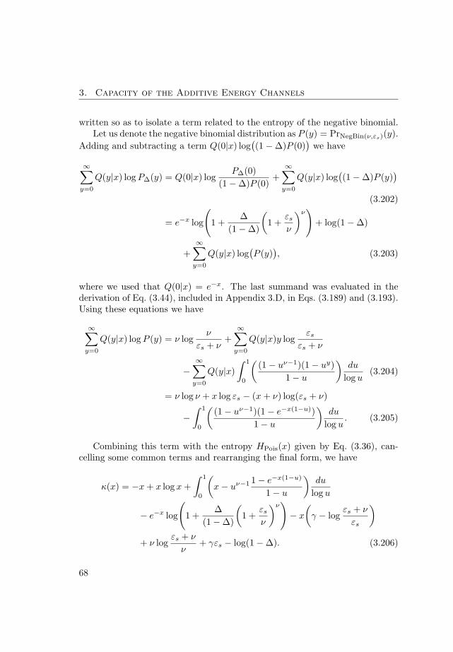
3. Capacity of the Additive Energy Channels

written so as to isolate a term related to the entropy of the negative binomial.Let us denote the negative binomial distribution as P (y) = PrNegBin(ν,εs)(y).

Adding and subtracting a term Q(0|x) log((1−∆)P (0)

)we have

∞∑y=0

Q(y|x) log P∆(y) = Q(0|x) logP∆(0)

(1−∆)P (0)+

∞∑y=0

Q(y|x) log((1−∆)P (y)

)

(3.202)

= e−x log

(1 +

∆(1−∆)

(1 +

εs

ν

)ν)

+ log(1−∆)

+∞∑

y=0

Q(y|x) log(P (y)

), (3.203)

where we used that Q(0|x) = e−x. The last summand was evaluated in thederivation of Eq. (3.44), included in Appendix 3.D, in Eqs. (3.189) and (3.193).Using these equations we have

∞∑y=0

Q(y|x) log P (y) = ν logν

εs + ν+

∞∑y=0

Q(y|x)y logεs

εs + ν

−∞∑

y=0

Q(y|x)∫ 1

0

((1− uν−1)(1− uy)

1− u

)du

log u(3.204)

= ν log ν + x log εs − (x + ν) log(εs + ν)

−∫ 1

0

((1− uν−1)(1− e−x(1−u))

1− u

)du

log u. (3.205)

Combining this term with the entropy HPois(x) given by Eq. (3.36), can-celling some common terms and rearranging the final form, we have

κ(x) = −x + x log x +∫ 1

0

(x− uν−1 1− e−x(1−u)

1− u

)du

log u

− e−x log

(1 +

∆(1−∆)

(1 +

εs

ν

)ν)− x

(γ − log

εs + ν

εs

)

+ ν logεs + ν

ν+ γεs − log(1−∆). (3.206)

68

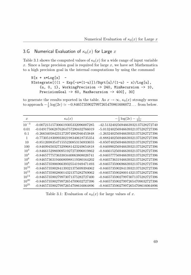
Numerical Evaluation of κ0(x) for Large x

3.G Numerical Evaluation of κ0(x) for Large x

Table 3.1 shows the computed values of κ0(x) for a wide range of input variablex. Since a large precision goal is required for large x, we have set Mathematicato a high precision goal in the internal computations by using the command

N[x + x*Log[x] -NIntegrate[((1 - Exp[-x*(1-u)])/Sqrt[u]/(1-u) - x)/Log[u],

{u, 0, 1}, WorkingPrecision -> 240, MinRecursion -> 10,PrecisionGoal -> 60, MaxRecursion -> 400], 30]

to generate the results reported in the table. As x →∞, κ0(x) strongly seemsto approach− 1

2 log(2e) ' −0.84657359027997265470861606072 . . . from below.

x κ0(x) − 12

log(2e)− 124x

10−3 -0.007215157306619305332096007285 -42.513240256946639321375282727400.01 -0.049175062876264757290432766019 -5.0132402569466393213752827273960.1 -0.266340584231272974982946453848 -1.2632402569466393213752827273961 -0.773051830993302198340618735354 -0.88824025694663932137528272739610 -0.851269835471555230853156933655 -0.850740256946639321375282727396100 -0.846994503273299681423249654818 -0.846990256946639321375282727396103 -0.846615298690951927273996819862 -0.846615256946639321375282727396104 -0.846577757363383440063808026741 -0.846577756946639321375282727396106 -0.846573631946680988119380164202 -0.846573631946639321375282727396108 -0.846573590696639325541949471493 -0.8465735906966393213752827273961010 -0.846573590284139321375699394062 -0.8465735902841393213752827273961012 -0.846573590280014321375282769062 -0.8465735902800143213752827273961014 -0.846573590279973071375282727400 -0.8465735902799730713752827273961020 -0.846573590279972654709032727396 -0.8465735902799726547090327273961025 -0.846573590279972654708616064896 -0.846573590279972654708616064896

Table 3.1: Evaluation of κ0(x) for large values of x.

69

4

Digital Modulation in the Gaussian Channel

4.1 Introduction

In the introduction to Chapter 2, where Shannon’s model for the communica-tion channel was introduced, we mentioned the existence of an encoder, whichtransforms the source message into a form appropriate for reliable transmis-sion across a channel. From a systems point of view, the encoder performs twotasks, that can be broadly described as coding and modulation:

1. The encoder adds redundancy to the source message, so that the dele-terious effect of channel noise can be overcome. This is the domain ofchannel coding, which will be treated in some detail in Chapter 6.

2. The encoder transforms the source message into a set of modulation sym-bols. This set is judiciously chosen by taking into proper account thenature of the channel characteristics and impairments.

When the coding and modulation tasks are jointly performed at both theencoder and the decoder, we talk of coded modulation. Alternatively, for bit-interleaved coded modulation, the two tasks may be carried out sequentially:first, the source message is encoded with a binary code; the encoder output isthen mapped onto a set of modulation symbols. At the decoder, the reverseoperations are carried out. If we do not wish to distinguish among the twooptions, we rather use the words digital modulation.

In this chapter, we study digital modulation for the Gaussian channel. SinceGaussian channels are often used to model communication systems operatingat radio and microwave frequencies, much previous work has been done in thefield, see e. g. the recent reviews [50,51]. Part of the content of this chapter is

71

4. Digital Modulation in the Gaussian Channel

a review of this body of work, as a prelude to deriving similar results on digitalmodulation for the additive energy channels, in Chapter 5.

Much attention has been paid recently to the performance of coded modula-tion in the so-called “wideband regime”, where signal-to-noise ratio is very low,see for instance [25, 52]. The reasons for this increased attention are twofold:from a practical point of view, many wireless systems operate at low signal-to-noise ratio and theoretical results in this field are of directly applicable. Inaddition, mathematical analysis is somewhat simpler than in the general case,leading to neat closed-form expressions for some information-theoretic quanti-ties. In this chapter, we shall also study the performance in this regime andderive some new results, described in more detail below. In Chapter 5, weextend our analysis to the additive energy channels.

In Chapter 3, the channel capacity was defined as the largest rate at whichmessages can be reliably sent over the channel. For some channels, we foundthe form of the distribution at the channel input which achieves the capacity.Other input distributions also allow for vanishingly small error probabilities,but at a rate, the constrained capacity, that is in general lower than the chan-nel capacity. In practical communication systems, this reduction in rate maybe compensated by the ease of design allowed by simple modulation sets, asopposed to using the capacity-achieving input. In Section 4.2 we consider theconstrained capacity for some common digital modulation formats, such asphase-shift keying (PSK) or quadrature-amplitude modulation (QAM).

Since the constrained capacity does not admit a simple expression, it oftenproves convenient to study alternative figures of merit, such as the capacityper unit energy or the minimum energy-to-noise ratio [25, 52]; they approxi-mate the constrained capacity by its second-order Taylor series around zerosignal-to-noise ratio. In Sections 4.2.2 and 4.2.3, we review these concepts andprovide an independent derivation of the Taylor series, which does not dependon Prelov’s previous analysis [52]. The method used for the derivation willprove directly applicable to the additive energy channels in Chapter 5. An-other figure of merit, relevant at large signal-to-noise ratios, is the shapinggain, which determines the asymptotic loss incurred by not using the optimumchannel input. The shaping gain is considered in Section 4.2.6.

In Section 4.3 we describe bit-interleaved coded modulation, in generalterms and particularized to the Gaussian channel, and analytically determineits behaviour at low signal-to-noise ratio.

The results presented in this chapter have been partly published in [53]and a paper has been submitted to the IEEE Transactions on InformationTheory [54].

72

Coded Modulation in the Gaussian Channel

4.2 Coded Modulation in the Gaussian Channel

4.2.1 Constrained Capacity

In Chapters 2 and 3, we considered the discrete-time additive Gaussian noisechannel model. Its output is a complex-valued vector (y1, . . . , yn), whose k-thcomponent yk is given by the sum

yk =√

SNR xk + zk. (4.1)

Here the zk are independent samples of circularly symmetric complex-valuedGaussian noise of variance 1, zk ∼ NC(0, 1), and each xk is k-th the complex-valued channel input, namely a modulation symbol drawn from a set with unitaverage energy. SNR is the average signal-to-noise ratio at the receiver.

Input symbols are drawn according to a common distribution PX(·) from aset X with |X | = 2m elements. When the symbols used with equal probabil-ities, m bits are required to choose a symbol. We define the first and secondconstellation moments, respectively denoted by µ1(X ) and µ2(X ), as

µ1(X ) =∑

x∈XxPX(x), µ2(X ) =

∑

x∈X|x|2PX(x). (4.2)

Often, constellations have zero mean, i. e. µ1(X ) = 0, and unit energy, that isµ2(X ) = 1. Similarly, we define a variance as σ2(X ) = µ2(X )− ∣∣µ1(X )

∣∣2.The capacity C of the Gaussian channel was given by Theorem 3.10, C(SNR) =

log(1 + SNR). We define the bit-energy-to-noise ratio as

BNR =SNR

C(SNR)log 2. (4.3)

namely the average received energy normalized to a bit of information. Itshould be noted that a bit need not be effectively transmitted, since C maybe smaller than 1 bit. This quantity is commonly used to compare systemsoperating at low signal-to-noise ratio in the Gaussian channel, in part because,as we shall see, most modulation formats asymptotically attain the same BNRat low capacities, easing the performance comparison among different formats.

Even though the common notation for BNR is Eb/N0, we prefer the alter-native symbol BNR because it can be used for the additive energy channels,for which a noise spectral density N0 is not necessarily defined. Moreover, thesymbol BNR maintains the symmetry with respect to the acronym SNR andleads to formulas which are, possibly, easier to read.

73

4. Digital Modulation in the Gaussian Channel

In order to achieve the capacity C, the channel input must be a properlychosen complex Gaussian distribution. In practice, however, it is common tofix a finite constellation set for the channel input. Well-known examples [32,50] are phase-shift keying (PSK), quadrature-amplitude modulation (QAM),amplitude-phase shift keying (APSK), or pulse-amplitude modulation (PAM).

When the symbols in X are used with probabilities PX(x), the mutualinformation I(X;Y ) between channel input X and output Y , or constrainedcoded modulation capacity CX for short, is given by Eq. (3.3) on page 27. Thename constrained capacity is justified by the fact that the mutual informationgives the maximum rate at which information can be reliably transmitted overthe channel by using the input the distribution PX(x), in an analogous manneras the channel capacity gives the maximum rate at which information can bereliably transmitted over the channel for all possible input distributions.

For the Gaussian channel, the channel transition matrix Q(y|x) is given by

Q(y|x) =1π

exp(−|y −

√SNRx|2), (4.4)

as in Chapter 2, Eq. (2.8) on page 15. We have then

Definition 4.1. For the additive Gaussian noise channel with average signal-to-noise ratio SNR, the constrained capacity CX with a modulation set X usedwith probabilities PX(x) is

CX (SNR) = −E

[log

( ∑

x′∈XPX(x′) exp

(−|√

SNR(X − x′) + Z|2 + |Z|2))]

.

(4.5)

The expectation is performed over all input symbols X and all possible noiserealizations Z, Z ∼ NC(0, 1).

If the symbols are used with equal probabilities, i. e. PX(x) = M−1, werefer to the constrained capacity as uniform capacity, and denote it by Cu

X .Figure 4.1 shows the constrained coded modulation capacity for several

typical modulations as a function of SNR and of BNR, defined as BNR =SNR

CX (SNR) log 2. Note that plot 4.1b has the x and y axes reversed with respectto the common practice, as in [50], and so shows BNR as a function of thecapacity CX , rather than the capacity as a function of BNR. Behind thischoice lies the convention in plotting a function f(x) which reserves the x axisto present the free variable x and uses the y axis to depict the function f(x). In

74

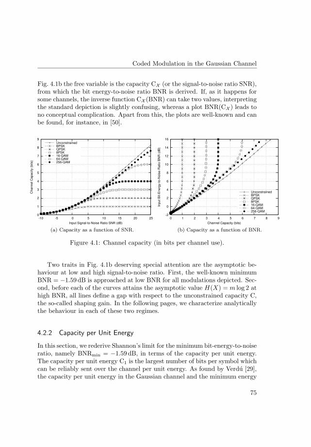
Coded Modulation in the Gaussian Channel

Fig. 4.1b the free variable is the capacity CX (or the signal-to-noise ratio SNR),from which the bit energy-to-noise ratio BNR is derived. If, as it happens forsome channels, the inverse function CX (BNR) can take two values, interpretingthe standard depiction is slightly confusing, whereas a plot BNR(CX ) leads tono conceptual complication. Apart from this, the plots are well-known and canbe found, for instance, in [50].

0

1

2

3

4

5

6

7

8

9

-10 -5 0 5 10 15 20 25

Cha

nnel C

apa

city (

bits)

Input Signal-to-Noise Ratio SNR (dB)

UnconstrainedBPSKQPSK8PSK16-QAM64-QAM256-QAM

(a) Capacity as a function of SNR.

-2

0

2

4

6

8

10

12

14

16

0 1 2 3 4 5 6 7 8 9

Inpu

t B

it-E

ne

rgy-t

o-N

ois

e R

atio

BN

R (

dB

)

Channel Capacity (bits)

UnconstrainedBPSKQPSK8PSK16-QAM64-QAM256-QAM

(b) Capacity as a function of BNR.

Figure 4.1: Channel capacity (in bits per channel use).

Two traits in Fig. 4.1b deserving special attention are the asymptotic be-haviour at low and high signal-to-noise ratio. First, the well-known minimumBNR = −1.59 dB is approached at low BNR for all modulations depicted. Sec-ond, before each of the curves attains the asymptotic value H(X) = m log 2 athigh BNR, all lines define a gap with respect to the unconstrained capacity C,the so-called shaping gain. In the following pages, we characterize analyticallythe behaviour in each of these two regimes.

4.2.2 Capacity per Unit Energy

In this section, we rederive Shannon’s limit for the minimum bit-energy-to-noiseratio, namely BNRmin = −1.59 dB, in terms of the capacity per unit energy.The capacity per unit energy C1 is the largest number of bits per symbol whichcan be reliably sent over the channel per unit energy. As found by Verdu [29],the capacity per unit energy in the Gaussian channel and the minimum energy

75

4. Digital Modulation in the Gaussian Channel

per bit, obtained from Eq. (3.11), are respectively given by

C1 =1σ2

, Eb,min = σ2 log 2. (4.6)

Alternatively, C1 can be determined by using Theorem 3.9 on page 30.Another equivalent form is the minimum bit-energy-to-noise ratio BNRmin,

BNRmin = Eb,minσ2 = log 2, or -1.59 dB. This quantity is the well-known Shannon

limit. As previously mentioned, this result is apparent from Fig. 4.1b.

4.2.3 Asymptotic Behaviour at Low SNR

In this section, we examine the asymptotic behaviour of the constrained ca-pacity CX as SNR → 0. We provide some analytic results which complementthe recent study by Verdu of the “wideband, power-limited regime” [25].

Before considering the effect of modulation, let us first discuss the uncon-strained case. A Taylor expansion of the capacity C around SNR = 0 gives

C = log(1 + SNR) = SNR− 12 SNR2 +O(SNR3). (4.7)

The inverse function, which gives SNR as a function of C, is

SNR = eC − 1 = C + 12C2 + O(C3). (4.8)

In terms of the bit-energy-to-noise ratio BNR, we have

BNR = log 2 + 12C log 2 + O(C2), (4.9)

or, keeping only the linear term in BNR,

C ' (BNR− log 2

) 2log 2

. (4.10)

The capacity is positive if the bit-energy-to-noise ratio exceeds log 2, or about−1.59 dB, in line with the analysis of the capacity per unit energy. Additionally,the capacity can be approximated by an affine function when BNR is small.Recently, Verdu suggested approximating the constrained capacity CX by anaffine function of BNR (in decibels, BNRdB = 10 log10 BNR), that is,

CX ' α0

(BNRdB − BNRdB

0 ), (4.11)

where α0 and BNRdB0 depend on the constellation set through the first terms

of the Taylor series of CX (SNR) at SNR = 0. In general, we have

76

Coded Modulation in the Gaussian Channel

Definition 4.2 (Taylor coefficients). We denote by c1 and c2 the first twocoefficients of a Taylor expansion of the capacity around SNR = 0, i. e.C(SNR) = c1 SNR+c2 SNR2 +o(SNR2).

We will use the same notation for constrained capacity and for the additiveenergy channels, where the expansion is around zero energy.

Then we have (Theorem 9 of [25]),

Theorem 4.3. As SNR → 0, the channel capacity admits an expression interms of BNR of the form

CX ' γ0

(BNRdB − BNRdB

0

)+ o

((∆BNRdB)

), (4.12)

where ∆BNRdB = BNRdB − BNRdB0 , γ0 is a wideband slope, and BNR0 the

BNR at SNR → 0. γ0 and BNR0 are respectively given by

γ0 = − c21

c210 log10 2, BNR0 =

log 2c1

. (4.13)

For the unconstrained case c1 = 1 and c2 = − 12 . In [52], Prelov and Verdu

determined c1 and c2 for proper-complex constellations, introduced by Neeserand Massey [55]. These constellations satisfy µ2′(X ) = 0, where

µ2′(X ) =∑

x∈Xx2PX(x), (4.14)

is a second-order pseudo-moment, borrowing notation from the paper [55]. Wedefine a pseudo-variance σ2(X ) as σ2(X ) = µ2′(X )− µ2

1(X ). We compute thecoefficients for slightly more general modulation formats in

Theorem 4.4. The first two Taylor-series coefficients of the coded modulationcapacity over a signal set X used with probabilities PX(x) are given by

c1 = σ2(X ) = µ2(X )−∣∣µ1(X )

∣∣2 (4.15)

c2 = −12

(σ4(X ) +

∣∣σ2(X )∣∣2

). (4.16)

In particular, when the average symbol is zero, and the mean energy is one,

c1 = 1, c2 = −12

(1 +

∣∣µ2′(X )∣∣2

), (4.17)

77

4. Digital Modulation in the Gaussian Channel

and the bit-energy-to-noise ratio at zero SNR is BNR0 = log 2.The second-order coefficient is bounded by −1 ≤ c2 ≤ − 1

2 , the maximum(c2 = −1/2) being attained when the constellation has uncorrelated real andimaginary parts and the energy is equally distributed among the real and imag-inary parts.

Note that constellation sets with unit energy and zero mean achieve theminimum energy per bit at low SNR.

Proof. The formulas for c1 and c2 can be derived from Theorem 5 of [52]. Thedetails are given in Appendix 4.A. An alternative direct proof, which does notrequire knowledge of Theorem 5 in [52], may be found in Appendix 4.B. Theminimum BNR is directly given by Theorem 4.3.

It is obvious that c2 ≤ − 12 . From the Cauchy-Schwartz inequality we deduce

that |µ2′(X )| =∣∣E[X2]

∣∣ ≤ E[|X|2] = µ2(X ), and therefore c2 ≥ −1. The

maximum c2 = − 12 is attained when µ2′(X ) = 0, that is when E[X2] = 0. This

condition is equivalent to

E[X2r ]− E[X2

i ] = 0, and E[XrXi] = 0. (4.18)

Therefore, the real and imaginary parts must be uncorrelated (E[XrXi] = 0 =E[Xr] E[Xi]) and with the same energy in the real and imaginary parts; this isindeed satisfied by proper-complex constellations [55].

The first part, giving c1, can be found as Theorem 4 of [25]. The formula forc2 seems to be new; note however that it can be easily derived from Theorem 5in [52]. Application of Theorem 4.4 to some signal constellations of practicalinterest (used with equal probabilities) yields the following corollary.

Corollary 4.5. Pulse amplitude modulation (PAM) with 2m levels has c2 =−1.

A mixture of nr |Xn|−PSK constellations for n = 1, . . . , nr has c2 = − 12 if

|Xn| > 2 for all rings/sub-constellations n = 1, . . . , nr.

Proof. In PAM, all symbols lie on a line in the complex plane, up to an irrele-vant constant phase factor, we have |µ2′(X )| = µ2(X ) = 1.

Assume a PSK modulation with |X | > 2. Up to a constant, irrelevantphase, the sum over the constellation symbols in µ2′(X ) gives

µ2′(X ) =1|X |

|X |−1∑

i=0

ej2 2πi|X| =

1|X |

1− ej22π|X||X|

1− ej2 2π|X|

= 0, (4.19)

78

Coded Modulation in the Gaussian Channel

as ej4π = 1. This is true only if the denominator is nonzero, which is satisfiedfor |X | > 2. When |X | = 2, we have

∣∣µ2′(X )∣∣2 = 1.

Let ε2n be the squared modulus of the symbols at ring n. For simplicity,assume all rings have the same phase origin. We can split the sum over X asa sum over rings indexed by n,

µ2′(X ) =1|X |

nr∑n=1

ε2n1− ej2

2π|Xn||Xn|

1− ej2 2π|Xn|

. (4.20)

This number is zero if |Xn| > 2 for all n.

This result is a generalization of Theorems 11.1 and 11.2 of [25], where theresults held for QPSK or mixtures of QPSK constellations. This result coversQAM and APSK modulations, for instance.

The expansion of the mutual information can be transformed into an ex-pansion of the output channel entropy, by using the decomposition I(X; Y ) =H(Y )−H(Y |X), and H(Y |X) = H(Z) = log πe,

Corollary 4.6. The entropy of the AWGN channel output H(Y ) has the ex-pansion at SNR = 0

H(Y ) = log πe + c1 SNR+c2 SNR2 +O(SNR5/2). (4.21)

In this section we have given closed-form approximations to the channelcapacity as a function of the signal-to-noise ratio for low values of the signal-to-noise ratio. An interesting byline, recently analyzed by Verdu [25], links thecoefficients c1 and c2 with two physical parameters in a radio communicationchannel, power and bandwidth. We next discuss this relationship.

4.2.4 Power and Bandwidth Trade-Off

In previous pages we have computed the first terms of the Taylor expansionof the constrained coded modulation capacity around SNR = 0. Next to theintrinsic theoretical value of the results, the analysis also possesses some prac-tical value, since many communication systems operate in Gaussian noise atlow signal-to-noise ratio SNR. In this section we explore this link.

For a communication systems engineer interested in maximizing the datarate over a Gaussian channel, two physical variables are critical, namely thepower P , or energy per unit time, and the bandwidth W , or number of channel

79

4. Digital Modulation in the Gaussian Channel

uses per unit time. Assuming additive Gaussian noise with spectral densityN0, the signal-to-noise ratio SNR is then given by SNR = P/(N0W ).

The condition of low SNR applies to a wide variety of practical communica-tion systems, whenever the condition that the available energy at each channeluse is very low, that is, SNR ¿ 1. For fixed P and N0, this is attained byletting the bandwidth increase unbounded, W →∞.

The capacity measured in bits per unit time is a natural figure of merit forthe communications system. This capacity is given by CW = W log(1+SNR),where C the capacity considered in previous sections or in Chapter 3, has unitsof bits per unit time per Hertz. When W is very large, we have that

CW = W log(

1 +P

N0W

)=

P

N0− P 2

2N20 W

+ O(

P 3

N30 W 2

). (4.22)

For coded modulation systems whose Taylor expansion around SNR = 0 hascoefficients c1 and c2,

CXW = c1P

N0+ c2

P 2

N20 W

+ O

(P 5/2

N5/20 W 3/2

). (4.23)

To first-order, the capacity increases linearly with the ratio P/N0, thatis linearly with the power P for fixed N0. Following Verdu, we consider thefollowing general situation. Two alternative transmission systems, respectivelyrepresented by an index i = 1, 2, with given power Pi and bandwidth Wi,achieve respective capacities per channel use Ci with Taylor coefficients c1i

and c2i. In general, the capacities per unit time CiWi will differ.A natural comparison between the two methods is to hold the power fixed,

that is P1 = P2, and derive, as a function of W1, the bandwidth W2 required tohave the same capacity per unit time, C1W1 = C2W2. Verdu carried out thisanalysis [25] and found that the bandwidth expansion is given by the ratio ofthe wideband slopes of alternatives 1 and 2, where the wideband slope is givenby Theorem 4.3, and

W2

W1=

c21

c22. (4.24)

For instance, BPSK (c22 = −1), needs a bandwidth two times as big as QPSK(c21 = −1/2) to transmit the same rate. However, the form of Eq. (4.23) showsthat the dependence of the capacity per unit time CW on the bandwidth Wis rather weak. Since the capacity varies linearly with the available power P ,a better way of achieving the same capacity is by varying P .

80

Coded Modulation in the Gaussian Channel

A natural trade-off between the two alternatives starts by fixing the powerP1 and bandwidth W1 of system 1, and therefore signal-to-noise ratio SNR1

and capacity per unit time C1W1. Then, one can fix the power P2 (or thebandwidth W2), and then determine how much bandwidth W2 (resp. powerP2) is required to achieve the same capacity, that is C1W1 = C2W2. Thefollowing result determines the form of the trade-off between the power andthe bandwidth for two alternative systems transmitting at the same rate,

Theorem 4.7. Let two modulations attain respective capacities per channeluse Ci, i = 1, 2, with respective Taylor coefficients c1i and c2i for SNR → 0.Consider system 1 as baseline, with power P1, bandwidth W1, signal-to-noiseratio SNR1 and capacity C1W1. Define ∆P = P2/P1 and ∆W = W2/W1 asthe power and bandwidth expansion ratios between alternatives 1 and 2.

In a neighbourhood of SNR1 = 0 the capacities in bits per second, C1W1

and C2W2 are equal when the expansion factors ∆P and ∆W are related as

∆W =

(c22 SNR1 +o(SNR1)

)(∆P )2

c11 + c21 SNR1 +o(SNR1)− c12∆P, (4.25)

for ∆W as a function of ∆P and, if c12 6= 0,

∆P =c11

c12+

(c21

c12− c22c

211

c312∆W

)SNR1 +o(SNR1), (4.26)

for ∆P as a function of ∆W .

Proof. The proof can be found in Appendix 4.C.

Remark that we use the approximation SNR1 → 0. As a consequence,replacing the value of ∆P from Eq. (4.26) into Eq. (4.25) gives

∆W =1 + O(SNR1)

1∆W + o(1)

, (4.27)

which is not exact, but consistent with the approximation that SNR1 is small.The previous theorem leads to the following derived results. For simplicity,

we drop the terms o(SNR1) and replace the equality signs by approximateequalities.

Corollary 4.8. To a first approximation, c11P1 ' c12P2, and a difference incoefficient c1 immediately translates into a power loss.

81

4. Digital Modulation in the Gaussian Channel

Corollary 4.9. For ∆P = 1, we obtain

∆W ' c22 SNR1

c11 + c21 SNR1−c12, (4.28)

and for the specific case c11 = c12, ∆W ' c22/c21.

The latter formula was previously obtained by Verdu [25] as a ratio ofwideband slopes. As noticed in [25], and previously mentioned in Eq. (4.24),the loss in bandwidth may be significant when ∆P = 1. But this point isjust one of a curve relating ∆P and ∆W . For instance, with no bandwidthexpansion we have

Corollary 4.10. For c11 = c12 = 1, and choosing ∆W = 1, ∆P ' 1 +(c21 −

c22

)SNR1.

In decibels, and since SNR1 is small, we may use a Taylor expansion of thelogarithm function, and have ∆P ' 4.34

(c21 − c22

)SNR1 dB, where SNR1 is

in linear scale. In fact, there is no strong reason to limit ourselves to ∆W = 1.For instance, for ∆W = 1

10 , or a bandwidth compression of a factor 10, and forthe QPSK/BPSK comparison, one gets ∆P ' 1+9.5 SNR1 ' 41.26 SNR1 dB,which is indeed negligible for vanishing SNR.

Figure 4.2 shows the trade-off curves between QPSK (baseline) and BPSK.For ∆P = 1, the bandwidth expansion is indeed 2 times. However, for SNR1 =−20 dB, if a power loss of 1 + 1

2 SNR1 ' 0.02 dB is accepted, there is nobandwidth increase. Increasing power further, bandwidth may even be reduced.In either case, as SNR1 → 0, the additional power loss turns negligible.

For signal-to-noise ratios below -10 dB, the approximation in Theorem 4.7seems to be very accurate for “reasonable” power or bandwidth expansionratios. A quantitative definition would lead to the problem of the extent towhich the second order approximation to the capacity is correct, a question onwhich we do not dwell further.

Note that the curve derived from Theorem 4.7 diverges to ∆W →∞ if

∆P =c11 + c21 SNR1

c12, (4.29)

which is typically close to ∆P = 1 for low SNR. As we get away from ∆P = 1,the bandwidth expansion quickly becomes smaller. The anomalous behaviourat large ∆P , namely the non-monotonicity of the curve, is due to the expansionat low SNR breaking down, more concretely from the minus sign of square root

82

Coded Modulation in the Gaussian Channel

0

0.2

0.4

0.6

0.8

1

1.2

1.4

1.6

1.8

2

10-5

10-4

10-3

10-2

10-1

100

101

Ba

ndw

idth

Exp

an

sio

n ∆

W =

WB

PS

K/W

QP

SK

Power Increase ∆P = PBPSK-PQPSK (in dB)

SNR1 = -10 dBSNR1 = -10 dB, ExactSNR1 = -20 dBSNR1 = -20 dB, ExactSNR1 = -30 dBSNR1 = -30 dB, Exact

(a) Power Expansion in logarithmic scale (in dB).

10-3

10-2

10-1

100

101

1 1.1 1.2 1.3 1.4 1.5B

an

dw

idth

Exp

an

sio

n ∆

W =

WB

PS

K/W

QP

SK

Power Increase ∆P = PBPSK/PQPSK

SNR1 = -10 dBSNR1 = -10 dB, ExactSNR1 = -20 dBSNR1 = -20 dB, ExactSNR1 = -30 dBSNR1 = -30 dB, Exact

(b) Power Expansion in linear scale.

Figure 4.2: Trade-off ∆P vs. ∆W between QPSK (baseline) and BPSK.

in Eq. (4.142) in the proof of the theorem. In this region, the assumption oflow SNR ceases being valid and the results become meaningless.

This analysis complements Verdu’s approach to determine the form of trade-off between these two system variables, power and bandwidth. Next, we brieflyconsider the effect of fully-interleaved fading.

4.2.5 Effect of Fading on the Low SNR Regime

We now briefly study the effect of fading on the expansion at the low powerregime. The fading model we consider is a fully-interleaved model, where theoutput yk at time k has a form similar to Eq. (4.1),

yk =√

SNR hk xk + zk, (4.30)

where zk is a sample of Gaussian noise, hk is a complex-valued fading coefficient,and xk is the input. At each time instant, a new value hk is used; its phaseassumed known at the receiver. For general fading distributions, we have thefollowing (see Theorem 12 of [25]),

Theorem 4.11. For a fading distribution with finite moments satisfying E[χ] =1, the Taylor expansion of the constrained capacity at low SNR is

CX (SNR) = c1 SNR+c2 E[χ2] SNR2 + o(SNR2), (4.31)

83

4. Digital Modulation in the Gaussian Channel

where c1 and c2 denote the first two terms in the expansion of the capacity inthe absence of fading, Eqs. (4.15) and (4.16).

In Chapter 6 we shall use a Nakagami fading model to study the errorperformance of channel codes over Gaussian channels. In this case the squaredfading coefficient χk = |hk|2 follows a gamma distribution

pχ(χk) =m

mf

f χmf−1k

Γ(mf )e−mf χk , (4.32)

where the parameter mf is a real positive number, 0 < mf < ∞. SinceE[χk] = 1, and signal and noise have average unit energy, SNR representsthe average SNR at the receiver. This fading model is slightly more generalthan the standard Nakagami-mf fading, since we lift the usual restriction tomf ≥ 0.5 [32, 51]. As the distribution is well-defined for 0 < mf < 0.5,reliable transmission is possible for mf > 0. We recover the unfaded AWGNchannel by letting mf → +∞, a Rayleigh fading model by setting mf = 1and (an approximation to) Rician fading with parameter KRic by fixing mf =(KRic + 1)2/(2KRic + 1).

Using the values of the moments of Nakagami-mf fading, E[χ] = 1, andE[χ2] = 1 + 1/mf (see Eq. (3.34)), we characterize the effect of Nakagamifading in the power and bandwidth requirements for a given modulation in theGaussian channel,

Theorem 4.12. Consider a modulation set X with average unit energy andused with power P , bandwidth W , and signal-to-noise ratio SNR. Let the capac-ity in absence of fading be characterized at low SNR by the coefficients c1 = 1and c2. When used over a Nakagami-mf channel, then c2(mf ) =

(1 + 1

mf

)c2.

When used in the Nakagami-mf channel with power P (mf ) and bandwidthW (mf ), if P (mf ) = P , W (mf ) = W

(1 + 1

mf

), and if W (mf ) = W , P (mf ) =

P(1− c2

mfSNR

).

As expected, for unfaded AWGN, when mf → ∞, we have E[χ2] = 1.Rayleigh fading (mf = 1) incurs in a bandwidth expansion of a factor 2 if thepower remains fixed. On the other hand, if bandwidth is kept unchanged, thereis a power penalty in dB of about 10 log10(1− c2 SNR) ' −10c2 SNR / log 10 '−4.343c2 SNR dB, a negligible amount for all practical effects since SNR → 0.The worst possible fading is mf → 0, which requires an unbounded bandwidthexpansion or incurs an unlimited power penalty.

84

Coded Modulation in the Gaussian Channel

4.2.6 Asymptotic Behaviour at High SNR

In Figs. 4.1a and 4.1b, on page 75, we saw that there seemed to be only smalldifferences among the various modulations in the low and high BNR extremes.In the last sections, we characterized analytically the behaviour at low BNRand showed that there are indeed no large differences in the rates achievablefor the different modulations.

For fixed SNR and SNR → ∞, the family of squared QAM constellationsapproaches an asymptotic mutual information, which differs from the mutualinformation by a constant. In this section we relate this asymptotic behaviourwith the so-called shaping gain. We define the shaping gain of a constellationX as the ratio between the energy required to achieve a given input entropyH(XX ) and the energy required by a Gaussian input to attain the same entropy.

For a fixed energy Es, the largest entropy is achieved by a complex Gaus-sian distribution of variance Es, H(X) = log(πeEs), as we saw in Chapter 3,on page 31. For a fixed entropy an arbitrary constellation requires a largerenergy than a Gaussian input. The differential entropies of two distributions,respectively uniformly distributed in a square and a circle, are given by [50,56]

Proposition 4.13. A constellation with average energy Es uniformly dis-tributed in a square (−∆, ∆)× (−∆, ∆), ∆ =

√3Es/2, has differential entropy

H(X) = log(6Es).A constellation with average energy Es uniformly distributed in a circle has

radius ρ =√

2Es and differential entropy H(X) = log(2πEs).

Proof. Within a square of size 2∆, the uniform input density p(sr, si) satisfies(2∆)2p(sr, si) = 1. The value of ∆ is adjusted to the right average energy,

Es =∫ ∆

−∆

∫ ∆

−∆

14∆2

(s2r + s2

i ) dsr dsi =2∆2

3. (4.33)

This relates ∆ and the average energy, ∆2 = 3Es/2. The differential entropyof the uniform distribution is readily computed to be log(4∆2) = log(6Es).

In a circle of radius ρ, the uniform input density p(r) = (πρ2)−1 satisfies2π

∫ ρ

0r3p(r) dr = Es, and therefore ρ2 = 2Es. The differential entropy is then

−2π

∫ ρ

0

1πρ2

r log1

πρ2dr = log(πρ2) = log(2πEs). (4.34)

Then, for a square constellation the shaping gain is πe6 , or 1.53 dB, whereas a

circular constellation requires the marginally smaller shaping gain e2 , or 1.33 dB.

85

4. Digital Modulation in the Gaussian Channel

In Chapter 5, we shall carry out a similar analysis for the additive energychannels and determine their shaping gains.

This section concludes the analysis of coded modulation in the Gaussianchannel. We next move to describe and analyze the technique of bit-interleavedcoded modulation.

4.3 Bit-Interleaved Coded Modulation

4.3.1 On Bit-Interleaved Coded Modulation

As we saw in Section 4.2.3, for low signal-to-noise ratio the capacity of theGaussian channel can be closely approached by using binary modulation, suchas BPSK. For a fixed bit-energy-to-noise ratio BNR more efficient use of thechannel is obtained by using QPSK modulation. Since the real and imaginaryparts of the channel output yk are separable into independent components foreither BPSK or QPSK, the channel is as a binary-input, real-valued outputchannel with additive Gaussian noise. For this channel there exist good binarylinear codes, viz. turbo-like codes [50], which get close to the capacity C.

For larger signal-to-noise ratios, constellations with more than two sym-bols are required. Since the shaping gain is relatively small, as we saw inSection 4.2.6, 2m-ary modulations with equiprobable symbols are frequentlyused. When m is an integer, and for 2m-QAM modulation, or 2m-PSK mod-ulation modulations, Ungerboeck proposed [57] the use of convolutional codes,combined with set-partitioning and trellis coding. These codes are efficientlydecoded with the Viterbi algorithm.

A natural question is how well binary linear codes mapped with a binarymapping rule onto 2m-ary modulations do perform, without set-partitioningand the trellis coding construction. A practical answer was given by pragmatictrellis-coded modulation [50], which replaced Ungerboeck’s channel codes bya standard 64-state convolutional code. From the theoretical point of view,a more radical break with Ungerboeck’s paradigm was the work by Caire etal. [26] on bit-interleaved coded modulation (BICM).

The operation of a bit-interleaved coded modulation scheme is depicted inFig. 4.3. The source generates a message, which the encoder maps onto a binarycodeword b = (b11, · · · , bm1, . . . , b1n, · · · , bmn), of length mn, where |X | = 2m,and n is the number of channel uses. Code selection is independent of theconstellation set X ; more precisely, binary inputs and binary codes are used.Next, a mapper µ uses m consecutive binary digits to compute a (complex-valued) channel-input symbol xk = µ(b1k, . . . , bmk), for k = 1, . . . , n. A typical

86

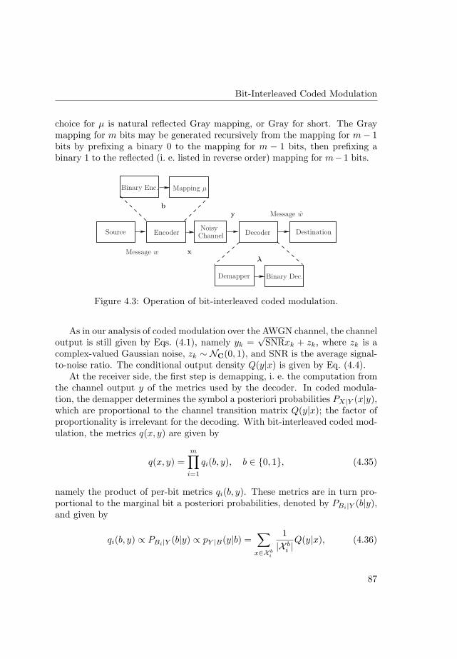
Bit-Interleaved Coded Modulation

choice for µ is natural reflected Gray mapping, or Gray for short. The Graymapping for m bits may be generated recursively from the mapping for m− 1bits by prefixing a binary 0 to the mapping for m − 1 bits, then prefixing abinary 1 to the reflected (i. e. listed in reverse order) mapping for m−1 bits.

Source Destination

y Message w

λ

Message w x

Mapping µBinary Enc.

b

Encoder

Binary Dec.

DecoderChannelNoisy

Demapper

Figure 4.3: Operation of bit-interleaved coded modulation.

As in our analysis of coded modulation over the AWGN channel, the channeloutput is still given by Eqs. (4.1), namely yk =

√SNRxk + zk, where zk is a

complex-valued Gaussian noise, zk ∼ NC(0, 1), and SNR is the average signal-to-noise ratio. The conditional output density Q(y|x) is given by Eq. (4.4).

At the receiver side, the first step is demapping, i. e. the computation fromthe channel output y of the metrics used by the decoder. In coded modula-tion, the demapper determines the symbol a posteriori probabilities PX|Y (x|y),which are proportional to the channel transition matrix Q(y|x); the factor ofproportionality is irrelevant for the decoding. With bit-interleaved coded mod-ulation, the metrics q(x, y) are given by

q(x, y) =m∏

i=1

qi(b, y), b ∈ {0, 1}, (4.35)

namely the product of per-bit metrics qi(b, y). These metrics are in turn pro-portional to the marginal bit a posteriori probabilities, denoted by PBi|Y (b|y),and given by

qi(b, y) ∝ PBi|Y (b|y) ∝ pY |B(y|b) =∑

x∈X bi

1|X b

i |Q(y|x), (4.36)

87

4. Digital Modulation in the Gaussian Channel

where X bi is the set of constellation symbols with bit b in the i-th position of

the binary label. An alternative form is the log-likelihood ratio form,

λi = logPBi|Y (1|y)PBi|Y (0|y)

= log

∑x∈X 1

iQ(y|x)

∑x∈X 0

iQ(y|x)

. (4.37)

It is clear that the marginal a posteriori probabilities for the bit Bi may be re-covered from λi. The log-likelihood ratios constitute a set of sufficient statisticsfor the decoding.

Finally, an estimate of the source message is generated. In practice, ifturbo-like codes are used, a variation of iterative decoding is used. We finallynote that very good error performance is possible with simple linear codes,such as convolutional codes or turbo-like codes [26].

4.3.2 Bit-Interleaved Coded Modulation Capacity

The presentation in the previous section naturally leads to a BICM channelcapacity, which in general is smaller than the coded modulation capacity weconsidered in previous sections. For a given constellation set X , we denotedthe constrained capacity by CX . Analogously, we denote the BICM capacityfor a given constellation set X and mapping rule µ by CX ,µ.

From the decoder’s point of view, and following Caire’s analysis [26], thechannel is separated into a set of parallel subchannels, such that the input tosubchannel i is bit bi; the channel output has the form of a log-likelihood ratioλi. As the log-likelihood ratios are a sufficient statistics for the decoding,

I(Bi; Λi) = I(Bi;Y ). (4.38)

For infinite interleaving, and assuming the subchannels are independent,this would give a total rate CX ,µ equal to the mutual informations in eachsubchannel, I(Bi; Y ), that is CX ,µ =

∑mi=1 I(Bi;Y ). This total rate is the so-

called BICM capacity. The ratios λi are generated simultaneously, by assuminga uniform prior over the remaining bits in the symbol. The correlation amongthe m ratios, for i = 1, . . . , n, in the same symbol is ignored. We shall later seethat this loss is small.

We next define the BICM capacity for a generic channel, not necessarilyGaussian. One such example of interest is provided by the additive energychannels, which we will study in Chapter 5.

88

Bit-Interleaved Coded Modulation

Definition 4.14. For a channel with transition matrix Q(y|x) the capacityBICM CX ,µ with a fixed modulation set X and mapping rule µ is given by

CX ,µ =m∑

i=1

I(Bi; Y ), (4.39)

where

I(Bi; Y ) = E

[log

∑x′∈XB

iQ(Y |x′)

12

∑x′∈X Q(Y |x′)

]. (4.40)

The expectation is performed over the bit values b, the input symbols x in X bi ,

and the channel realizations Y .

Remark 4.15. In recent joint work with Albert Guillen i Fabregas, we have an-alyzed the BICM decoder from the point of view of mismatched decoding [58].For the decoding metric in Eq. (4.35), we have proved that the correspondinggeneralized mutual information [58] is indeed given by Caire’s BICM capacity,even though the interleaver is finite. This proves the achievability of the BICMcapacity. A similar result had been presented in [59].

This alternative definition proves useful for the analysis at low SNR,

Proposition 4.16. For a channel with transition matrix Q(y|x), modulationset X and mapping rule µ, the BICM capacity CX ,µ is

CX ,µ =m∑

i=1

12

∑

b=0,1

(CuX − Cu

X bi), (4.41)

where CuX and Cu

X bi

are, respectively, the constrained capacities for equiprobablesignalling in X and X b

i .

Proof. By definition, the BICM capacity is the sum over i = 1, . . . ,m of themutual informations I(Bi;Y ). We rewrite this mutual information as

I(Bi;Y ) =12

∑

b∈{0,1}E

[log

∑x′∈X b

iQ(Y |x′)

12

∑x′∈X Q(Y |x′)

](4.42)

=12

∑

b∈{0,1}E

[log

(∑x′∈X b

i

2|X |Q(Y |x′)

Q(Y |X)Q(Y |X)

12

∑x′∈X

2|X |Q(Y |x′)

)],

(4.43)

89

4. Digital Modulation in the Gaussian Channel

where we have modified the variable in the logarithm by including a factor2|X |Q(Y |X) in both numerator and denominator. Splitting the logarithm,

I(Bi;Y ) =12

∑

b∈{0,1}E

[log

∑x′∈X b

i

2|X |Q(Y |x′)

Q(Y |X)

]

+12

∑

b∈{0,1}E

[log

Q(Y |X)1|X |

∑x′∈X Q(Y |x′)

]. (4.44)

For fixed b, the expectations are respectively recognized as (minus) themutual information achievable by using equiprobable signalling in X b

i , CuX b

i,

and the mutual information achieved by equiprobable signalling in X , CuX .

Figures 4.4a and 4.4b depict the BICM channel capacity (in bits per channeluse) CX ,µ for several modulations and mapping rules in the Gaussian channel.The cases depicted correspond to commonly used modulations and mappingrules: QPSK with Gray and anti-Gray mappings, 8PSK with Gray and setpartitioning mappings, and 16-QAM with Gray and set-partitioning mappings(see for instance [26] for the exact mapping rules). As found in [26], the BICMcapacity is close to that of coded modulation when Gray mapping is used. Useof set-partitioning leads to a significant loss in capacity.

The good behaviour of Gray mapping is somewhat limited at high SNR, ascan be seen in Fig. 4.4b where BNR is plotted as a function of the capacity. Inthe following section, we consider the asymptotic behaviour at low SNR, andcharacterize it analytically. Among other things, we shall be able to explainbehaviour such as that for QPSK and anti-Gray mapping, which has a nega-tive slope at BNR0. This plot shows why the notation BNR0 is preferable toBNRmin, as the minimum BNR is not necessarily attained at zero capacity.

4.3.3 Asymptotic Behaviour at Low SNR

In the previous section, we derived the BICM capacity CX ,µ, and plotted itas a function of SNR in Fig. 4.4a. In the same plot, the CM channel capacityCX , which assumes equiprobable signalling over the input constellation set, isalso shown. As a function of the signal-to-noise ratio SNR, in Fig. 4.4, theBICM capacity is close to the CM value when Gray mapping is used. However,the plot as a function of the BNR (see Fig. 4.4b) reveals the suboptimality ofBICM for low rates, or equivalently, in the power-limited regime.

90

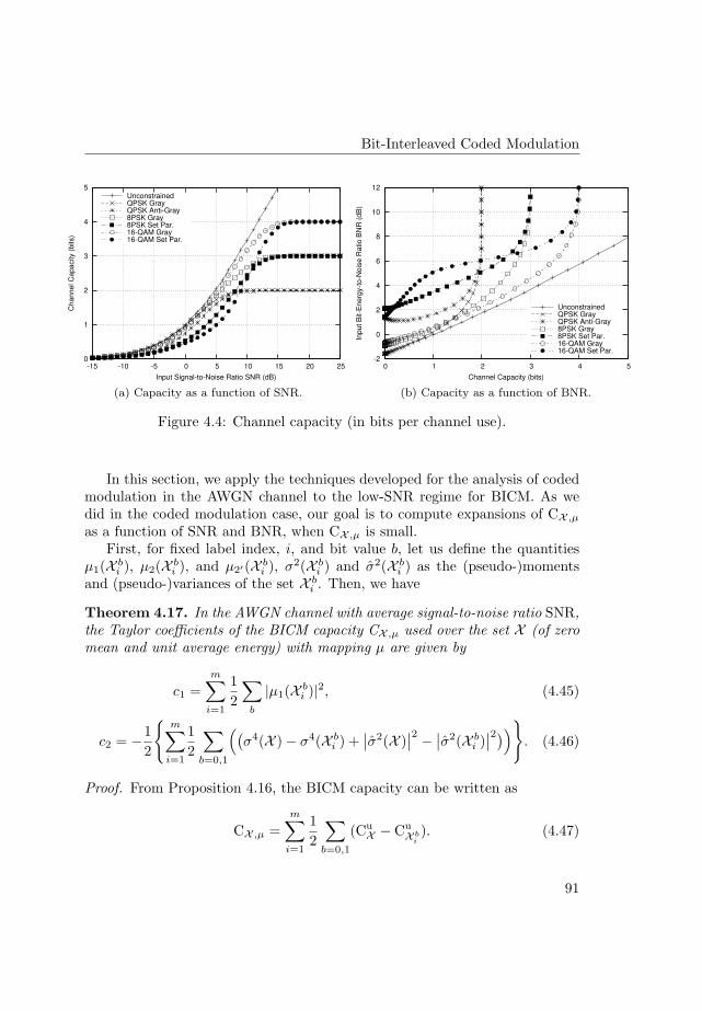
Bit-Interleaved Coded Modulation

0

1

2

3

4

5

-15 -10 -5 0 5 10 15 20 25

Cha

nn

el C

apa

city (

bits)

Input Signal-to-Noise Ratio SNR (dB)

UnconstrainedQPSK GrayQPSK Anti-Gray8PSK Gray8PSK Set Par.16-QAM Gray16-QAM Set Par.

(a) Capacity as a function of SNR.

-2

0

2

4

6

8

10

12

0 1 2 3 4 5In

pu

t B

it-E

ne

rgy-t

o-N

ois

e R

atio B

NR

(d

B)

Channel Capacity (bits)

UnconstrainedQPSK GrayQPSK Anti-Gray8PSK Gray8PSK Set Par.16-QAM Gray16-QAM Set Par.

(b) Capacity as a function of BNR.

Figure 4.4: Channel capacity (in bits per channel use).

In this section, we apply the techniques developed for the analysis of codedmodulation in the AWGN channel to the low-SNR regime for BICM. As wedid in the coded modulation case, our goal is to compute expansions of CX ,µ

as a function of SNR and BNR, when CX ,µ is small.First, for fixed label index, i, and bit value b, let us define the quantities

µ1(X bi ), µ2(X b

i ), and µ2′(X bi ), σ2(X b

i ) and σ2(X bi ) as the (pseudo-)moments

and (pseudo-)variances of the set X bi . Then, we have

Theorem 4.17. In the AWGN channel with average signal-to-noise ratio SNR,the Taylor coefficients of the BICM capacity CX ,µ used over the set X (of zeromean and unit average energy) with mapping µ are given by

c1 =m∑

i=1

12

∑

b

|µ1(X bi )|2, (4.45)

c2 = −12

{m∑

i=1

12

∑

b=0,1

((σ4(X )− σ4(X b

i ) +∣∣σ2(X )

∣∣2 −∣∣σ2(X b

i )∣∣2)

)}. (4.46)

Proof. From Proposition 4.16, the BICM capacity can be written as

CX ,µ =m∑

i=1

12

∑

b=0,1

(CuX − Cu

X bi). (4.47)

91

4. Digital Modulation in the Gaussian Channel

Since the summands CuX and Cu

X bi

admit a Taylor expansion given in Theo-rem 4.1,

c1 =m∑

i=1

12

∑

b=0,1

(1− (

µ2(X bi )− |µ1(X b

i )|2))

(4.48)

=m∑

i=1

((1− 1

2

∑

b=0,1

µ2(X bi )

)+

12

∑

b=0,1

|µ1(X bi )|2

)(4.49)

=m∑

i=1

12

∑

b=0,1

|µ1(X bi )|2, (4.50)

since 12

∑b=0,1 µ2(X b

i ) = µ2(X ) = 1 by construction.The quadratic coefficient c2 follows from a similar application of Theo-

rem 4.1.

Table 4.1 shows the values of the coefficients c1 and c2, as well as theminimum bit signal-to-noise ratio BNR0 for various cases, namely QPSK withGray (Q–Gr) and anti-Gray mapping (Q–A-Gr), 8PSK and 16-QAM modula-tions and Gray and set partitioning mappings (respectively 8–Gr, 8-SP, 16-Gr,and 16–SP). Note that for QPSK with anti-Gray mapping the slope at BNR0 isnegative. From Theorem 4.3 this should correspond with a positive coefficientc2, as it indeed does. A similar effect takes place for 8PSK and set partitioning,even though it is barely noticeable in the plot.

Modulation and Mapping

Q–Gr Q–A-Gr 8–Gr 8–SP 16–Gr 16–SP

c1 1.0000 0.5000 0.8536 0.4268 0.8000 0.5000BNR0 0.6931 1.3863 0.8121 1.6241 0.8664 1.3863BNR0 (dB) -1.5917 1.4186 -0.9041 2.1062 -0.6226 1.4186

c2 -0.5000 0.2500 -0.2393 0.0054 -0.1600 -0.3100

Table 4.1: Bit signal-to-noise ratio and coefficients c1, c2 for BICM in AWGN.

In general, it seems to be difficult to draw general conclusions for arbitrarymappings from Theorem 4.17. A notable exception, however, is the analysisunder natural reflected Gray mapping.

92

Bit-Interleaved Coded Modulation

Theorem 4.18. For 2m-PAM and 22m-QAM (m a positive integer) and nat-ural, binary-reflected Gray mapping, the coefficient c1 in the Taylor expansionof the BICM capacity CX ,µ at low SNR is

c1 =3 · 22m

4(22m − 1), (4.51)

and the minimum BNR0 is

BNR0 =4(22m − 1)

3 · 22mlog 2. (4.52)

Proof. For 2m-PAM, the Gray mapping construction makes µ1(X bi ) = 0, for

b = 0, 1 and all bit positions except one, which we take with no loss of generalityto be i = 1. Therefore,

c1 =12

∣∣µ1(X 01 )

∣∣2 +12

∣∣µ1(X 11 )

∣∣2 =∣∣µ1(X 0

1 )∣∣2 =

∣∣µ1(X 11 )

∣∣2. (4.53)

The last equalities follow from the symmetry between 0 and 1.Symbols lie on a line in the complex plane with values±β

(1, 3, 5, . . . , 2m−1),

with β2 = 3/(22m − 1); this follows from setting 2n = 2m in the formula1n

∑ni=1(2i− 1)2 = 1

3 ((2n)2 − 1). The average symbol has modulus |µ1(X 01 )| =

β2m−1, and therefore

c1 =∣∣µ1(X 0

1 )∣∣2 =

3 · 22m

4(22m − 1). (4.54)

Extension to 22m-QAM is clear, by taking the Cartesian product along realand imaginary parts. Now, two indices i contribute, each with an identicalform to that of PAM. As the energy along each axis of half that of PAM, thenormalization factor β2

QAM also halves and overall c1 does not change.

The results for BPSK, QPSK (2-PAM×2-PAM), and 16-QAM (4-PAM×4-PAM), as presented in Table 4.1, match with the Theorem, as they should.

It is somewhat surprising that the loss with respect to coded modulationat low SNR is bounded,

Corollary 4.19. As m → ∞, and under the conditions of Theorem 4.18,BNR0 approaches 4

3 log 2 ' −0.3424 dB from below.

93

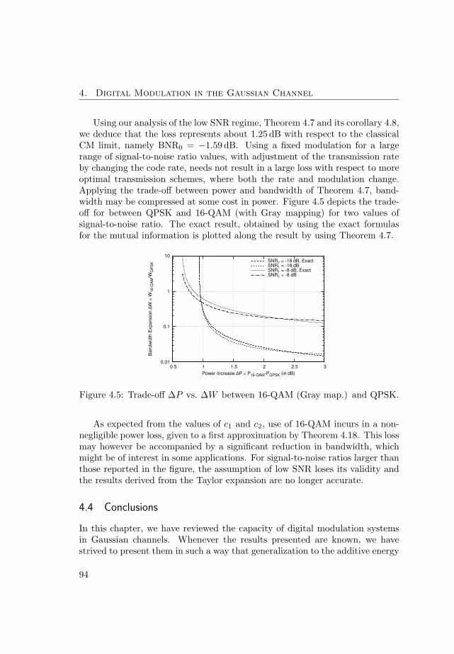
4. Digital Modulation in the Gaussian Channel

Using our analysis of the low SNR regime, Theorem 4.7 and its corollary 4.8,we deduce that the loss represents about 1.25 dB with respect to the classicalCM limit, namely BNR0 = −1.59 dB. Using a fixed modulation for a largerange of signal-to-noise ratio values, with adjustment of the transmission rateby changing the code rate, needs not result in a large loss with respect to moreoptimal transmission schemes, where both the rate and modulation change.Applying the trade-off between power and bandwidth of Theorem 4.7, band-width may be compressed at some cost in power. Figure 4.5 depicts the trade-off for between QPSK and 16-QAM (with Gray mapping) for two values ofsignal-to-noise ratio. The exact result, obtained by using the exact formulasfor the mutual information is plotted along the result by using Theorem 4.7.

0.01

0.1

1

10

0.5 1 1.5 2 2.5 3

Ba

nd

wid

th E

xpa

nsio

n ∆

W =

W1

6-Q

AM

/WQ

PS

K

Power Increase ∆P = P16-QAM-PQPSK (in dB)

SNR1 = -18 dB, ExactSNR1 = -18 dBSNR1 = -8 dB, ExactSNR1 = -8 dB

Figure 4.5: Trade-off ∆P vs. ∆W between 16-QAM (Gray map.) and QPSK.

As expected from the values of c1 and c2, use of 16-QAM incurs in a non-negligible power loss, given to a first approximation by Theorem 4.18. This lossmay however be accompanied by a significant reduction in bandwidth, whichmight be of interest in some applications. For signal-to-noise ratios larger thanthose reported in the figure, the assumption of low SNR loses its validity andthe results derived from the Taylor expansion are no longer accurate.

4.4 Conclusions

In this chapter, we have reviewed the capacity of digital modulation systemsin Gaussian channels. Whenever the results presented are known, we havestrived to present them in such a way that generalization to the additive energy

94

CM Capacity Expansion at Low SNR

channel is straightforward. In addition, there are a few novel contributions inthe analysis:

1. The first two derivatives of the constrained capacity at zero SNR havebeen computed for general modulation sets.

2. The trade-off between power penalty and bandwidth expansion betweentwo alternative systems at low SNR has been determined. It general-izes Verdu’s analysis of the wideband regime, which estimated only thebandwidth expansion. We have shown that no bandwidth expansion mayoften be achieved at a negligible (but non-zero) cost in power.

3. A similar trade-off between power penalty and bandwidth expansion forgeneral Nakagami-mf fading has been computed, with similar conclusionsas in the point above: bandwidth expansion may be large at no powercost, but absent at a tiny power penalty.

4. The capacity at low BNR for BICM has been characterized by simpleexpressions. For binary reflected Gray mapping, the capacity loss at lowSNR with respect to coded modulation is bounded by about 1.25 dB.

In the next chapter, we build on the analysis presented here and show thatthese results admit a natural extension to the additive energy channels.

4.A CM Capacity Expansion at Low SNR

Since the constellation moments are finite, we have that E[|X|2+α

]< ∞ for

α > 0. Therefore, as SNR → 0, for µ > 0 the technical condition

SNR2+α E[|X|2+α

] ≤ (− log√

SNR)µ, (4.55)

necessary to apply Theorem 5 of [52] holds.Let us define a 2× 1 vector x(r) = (xr xi)T , with components the real and

imaginary parts of symbol s, respectively denoted by xr and xi. The covariancematrix of x(r), denoted by cov(X), is given by

cov(X) =(

E[(Xr − xr)2] E[(Xr − xr)(Xi − xi)

]E

[(Xr − xr)(Xi − xi)

]E[(Xi − xi)2]

), (4.56)

where xr and xi are the mean values of the real and imaginary parts of theconstellation.

95

4. Digital Modulation in the Gaussian Channel

Theorem 5 of [52] gives c1 = Tr(cov(X)) and c2 = −Tr(cov2(X)), or

c1 = E[(Xr − xr)2] + E[(Xi − xi)2] (4.57)

c2 = −(E2[(Xr − xr)2] + E2[(Xi − xi)2] + 2E2

[(Xr − xr)(Xi − xi)

]). (4.58)

The coefficient c1 coincides with that in Eq. (4.15).As for c2, let us add a subtract a term E[(Xr − xr)2] E[(Xi − xi)2] to

Eq. (4.58). Then,

c2 = −(

12 E2[(Xr − xr)2] + 1

2 E2[(Xi − xi)2] + E[(Xr − xr)2] E[(Xi − xi)2]

+ 12 E2[(Xr − xr)2] + 1

2 E2[(Xi − xi)2]

− E[(Xr − xr)2] E[(Xi − xi)2] + 2E2[(Xr − xr)(Xi − xi)

]),

(4.59)

which in turn can be written as

c2 = −12

(E2

[|X − x|2] +∣∣E[(X − x)2]

∣∣2), (4.60)

a form which coincides with Eq. (4.16), by noting that

E[|X − x|2] = E

[|X|2]− |x|2 = µ2(X )− ∣∣µ1(X )∣∣2 (4.61)

E[(X − x)2] = E[X2]− x2 = µ2′(X )− µ21(X ). (4.62)

4.B CM Capacity Expansion at Low SNR – AWGN

The constrained capacity CX is given by Eq. (4.5),

CX = −∑

x

P (x)∫

Y

Q(y|x) log

( ∑

x′∈XP (x′)e−|γ(x−x′)+z|2+|z|2

)dy, (4.63)

where, for the sake of brevity, we have set γ =√

SNR.We first rewrite each of the exponents in the log(·) in Eq. (4.63),

exp(−|γ(x− x′) + z|2 + |z|2) = exp

(−γ2|x− x′|2 − 2γr(x− x′)), (4.64)

where we have used the function r(y), defined as

r(y) = Re(yz∗). (4.65)

96

CM Capacity Expansion at Low SNR – AWGN

In general, we will take y = x− x′.Now we use a Taylor expansion of et around t = 0, et = 1 + t + 1

2 t2 + 16 t3 +

124 t4 + O

(t5

)to transform Eq. (4.64) into

1− γ2|x− x′|2 − 2γr(x− x′) +12

(−γ2|x− x′|2 − 2γr(x− x′)

)2

+16

(−γ2|x− x′|2 − 2γr(x− x′)

)3

+124

(−γ2|x− x′|2 − 2γr(x− x′)

)4

+ O(γ5) (4.66)

= 1− γ2|x− x′|2 − 2γr(x− x′) +12γ4|x− x′|4 + γ22r2(x− x′)

+ γ32|x− x′|2r(x− x′)− γ42|x− x′|2r2(x− x′)

− γ3 43r3(x− x′) + γ4 2

3r4(x− x′) + O(γ5). (4.67)

With the substitutions,

a′1 = −2r(x− x′) (4.68)

a′2 = −|x− x′|2 + 2r2(x− x′) (4.69)

a′3 = 2|x− x′|2r(x− x′)− 43r3(x− x′) (4.70)

a′4 =12|x− x′|4 − 2|x− x′|2r2(x− x′) +

23r4(x− x′). (4.71)

the sum over x′ in Eq. (4.63) becomes

∑

x′∈XP (x′)

(1 + γa′1 + γ2a′2 + γ3a′3 + γ4a′4 + O(γ5)

)(4.72)

=(1 + γa1 + γ2a2 + γ3a3 + γ4a4 + O(γ5)

). (4.73)

where the coefficients al, with l = 1, 2, 3, 4, are given by al =∑

x′∈X a′lP (x′).Of special interest is a1,

a1 = −2∑

x′∈Xr(x− x′)P (x′) = −2

(r(x− x)

), (4.74)

since r(y) is linear in its argument and x is the mean value of the constellation.

97

4. Digital Modulation in the Gaussian Channel

As next step we expand the logarithm in Eq. (4.73) using log(1 + t) =t− 1

2 t2 + 13 t3− 1

4 t4 +O(t5

), where y is small. The term in t4 is needed to catch

all factors in γ4. Then

log(1+γa1 + γ2a2 + γ3a3 + γ4a4 + O(γ5)

)(4.75)

= γa1 + γ2a2 + γ3a3 + γ4a4 − 12(γa1 + γ2a2 + γ3a3 + γ4a4

)2

+13(γa1 + γ2a2 + γ3a3 + γ4a4

)3

− 14(γa1 + γ2a2 + γ3a3 + γ4a4

)4 + O(γ5) (4.76)

= γa1 + γ2a2 + γ3a3 + γ4a4 − 12(γ2a2

1 + 2γ3a1a2 + γ4a22 + 2γ4a1a3

)

+13(γ3a3

1 + 3γ4a21a2

)− γ4 14a41 + O(γ5) (4.77)

= γa1 + γ2

(a2 − 1

2a21

)+ γ3

(a3 − a1a2 +

13a31

)

+ γ4

(a4 − 1

2a22 − a1a3 + a2

1a2 − 14a41

)+ O(γ5). (4.78)

The remaining steps are the averaging over the input symbol x and thenoise realization z. To save space, we sometimes use the symbol EX,Z to makeexplicit the variable (X, Z) over which the averaging is performed.

Throughout, we have factors depending on

EZ rk1(χ1)rk2(χ2), (4.79)

χ1 and χ2 complex numbers, and k1, k2 are 0, 1, 2, 3, or 4. We have then

Lemma 4.20. Let the function r(y) be r(y) = Re(yz∗), where z is a complexGaussian random variable, z ∼ NC(0, 1), and y is a complex number. Then

EZ rk1(χ1)rk2(χ2) = 0, if k1 + k2 is odd. (4.80)

and

EZ r(χ1)r(χ2) =12|χ1||χ2| cos(ϕ1 − ϕ2) (4.81)

EZ r(χ1)r3(χ2) =34|χ1||χ2|3 cos(ϕ1 − ϕ2) (4.82)

EZ r2(χ1)r2(χ2) =14|χ1|2|χ2|2

(2 + cos 2(ϕ1 − ϕ2)

). (4.83)

98

CM Capacity Expansion at Low SNR – AWGN

Here ϕ1 and ϕ2 are the phases of the complex numbers χ1 and χ2 respectively.In particular,

EZ r2(χ1) =12|χ|2 (4.84)

EZ r4(χ1) =34|χ|4. (4.85)

Proof. Using a polar decomposition of the numbers χ1, χ2, and z, we havewith the obvious definitions,

χ1 = |χ1|ejϕ1 , χ2 = |χ2|ejϕ2 , z = |z|ejϕz . (4.86)

The realization of the variable whose expectation is to be computed is then

(Re

(|χ1||z|ejϕ1e−jϕz))k1

(Re

(|χ2||z|ejϕ2e−jϕz))k2

(4.87)

|χ1|k1 |χ2|k2 |z|k1+k2 cosk1(ϕ1 − ϕz

)cosk2

(ϕ2 − ϕz

). (4.88)

We carry out the expectation separately for the modulus and phase,

EZ |z|k1+k2 cosk1(ϕ1 − ϕz

)cosk2

(ϕ2 − ϕz

)(4.89)

= E|Z| |z|k1+k2 EΦz cosk1(ϕ1 − ϕz

)cosk2

(ϕ2 − ϕz

). (4.90)

For the phase, Mathematica gives

EΦz cosk1(ϕ1 − ϕz

)cosk2

(ϕ2 − ϕz

)=

12 cos(ϕ1 − ϕ2), k1 = 1, k2 = 138 cos(ϕ1 − ϕ2), k1 = 1, k2 = 318

(2 + cos 2(ϕ1 − ϕ2)

), k1 = 2, k2 = 2

0, k1 + k2 odd.(4.91)

and for the modulus,

E|Z| |Z|k1+k2 =

{1, k1 + k2 = 22, k1 + k2 = 4.

(4.92)

We now put all terms together in Eq. (4.78), proceeding from γ up to γ4.We use the appropriate equation in the previous lemma at each step.

99

4. Digital Modulation in the Gaussian Channel

First, using Eq. (4.80) in the term with γ, for which k1 = 1 and k2 = 0,

EZ [A1] = EZ

[−2(r(x)− r(x)

)]= 0. (4.93)

Then, for γ2, Eq. (4.84) gives

EZ [A2] = EZ

[ ∑

x′∈XP (x′)

(−|x− x′|2 + 2r2(x− x′)

)](4.94)

=∑

x′∈XP (x′)

(−|x− x′|2 + |x− x′|2

)= 0, (4.95)

and

EZ

[−1

2A2

1

]= −2 EZ

[r2(x− x)

]= −|x− x|2. (4.96)

Now, for γ3, Eq. (4.80) with k1 = 1 or k1 = 3 and k2 = 0 yields

EZ [A3] = EZ

[ ∑

x′∈XP (x′)

(2|x− x′|2r(x− x′)− 4

3r3(x− x′)

)]= 0, (4.97)

and

EZ

[13A3

1

]= −8

3EZ

[r3(x− x)

]= 0, (4.98)

and also

EZ [−A1A2] = 2 EZ

[r(x− x)

∑

x′′∈XP (x′)

(−|x− x′′|2 + 2r2(x− x′′)

)]= 0.

(4.99)

And finally, for γ4, Eqs. (4.84) and (4.85) give

EZ [A4] =∑

x′∈XP (x′) EZ

[12|x− x′|4 − 2|x− x′|2r2(x− x′) +

23r4(x− x′)

]

(4.100)

=∑

x′∈XP (x′)

(12|x− x′|4 − |x− x′|4 +

12|x− x′|4

)= 0. (4.101)

100

CM Capacity Expansion at Low SNR – AWGN

Next,

EZ

[−1

2A2

2

]= −1

2EZ

[( ∑

x′∈XP (x′)

(−|x− x′|2 + 2r2(x− x′)

))2](4.102)

= −12

EZ

[( ∑

x′∈XP (x′)

(−|x− x′|2 + 2r2(x− x′)

))×

×( ∑

x′′∈XP (x′′)

(−|x− x′′|2 + 2r2(x− x′′)

))],

(4.103)

since x′ and x′′ are dummy variables. Multiplying the terms in brackets fac-tor by factor and using Eqs. (4.84) and (4.85) in the Lemma, the summandcorresponding to x′ and x′′ becomes

P (x′)P (x′′)|x− x′|2|x− x′′|2(

1 + cos 2(ϕ(x− x′)− ϕ(x− x′′)

))(4.104)

= P (x′)P (x′′)|x− x′|2|x− x′′|2 cos2(ϕ(x− x′)− ϕ(x− x′′)

)(4.105)

= P (x′)P (x′′)(Re

((x− x′)(x− x′′)∗

))2

(4.106)

= P (x′)P (x′′)(Re

(|x|2 − xx′′∗ − x′x∗ + x′x′′∗))2

(4.107)

= P (x′)P (x′′)(|x|4 +

(Re(xx′′∗)

)2 +(Re(x′x∗)

)2 +(Re(x′x′′∗)

)2

− 2|x|2 Re(xx′′∗)− 2|x|2 Re(x′x∗) + 2|x|2 Re(x′x′′∗)+ 2 Re(xx′′∗)Re(x′x∗)− 2Re(xx′′∗)Re(x′x′′∗)

− 2 Re(x′x∗)Re(x′x′′∗)). (4.108)

Here we used that 1 + cos 2α = 2 cos2 α. Then, we average over x, x′ and x′′

and combine some expectations since x, x′ and x′′ are dummy variables takingvalues in the same set. Using the definition of x, we get

EX,Z

[−1

2A2

2

]= −EX,X′

[|X|4 + 3

(Re(XX ′∗)

)2 − 4|X|2 Re(Xx∗)

+ 2|X|2|x|2 − 2 Re2(Xx∗)], (4.109)

101

4. Digital Modulation in the Gaussian Channel

Then, with Eqs. (4.82) and (4.83), the next term of γ4 is

EZ

[−A1A3

]= 2 EZ

[r(x− x)

( ∑

x′∈XP (x′)

(2|x− x′|2r(x− x′)− 4

3r3(x− x′)

))]

(4.110)

=∑

x′∈X2P (x′)

(|x− x||x− x′|3 cos

(ϕ(x)− ϕ(x′)

)

− |x− x||x− x′|3 cos(ϕ(x)− ϕ(x′)

))= 0.

(4.111)

The following term in γ4 becomes

EZ

[A2

1A2

]= EZ

[4r2(x− x)

( ∑

x′∈XP (x′)

(−|x− x′|2 + 2r2(x− x′)

)]

(4.112)

= 2∑

x′P (x′)|x− x|2|x− x′|2

(1 + cos 2

(ϕ(x)− ϕ(x− x′)

))

(4.113)

= 4∑

x′P (x′)

(|x− x|2|x− x′|2 cos2

(ϕ(x)− ϕ(x− x′)

))(4.114)

= 4∑

x′P (x′)

(Re

((x− x)(x− x′)∗

))2

. (4.115)

We now expand the factor(Re

((x− x)(x− x′)∗

))2

,

(Re

((x− x)(x− x′)∗

))2

= |x|4 +(Re(xx′∗))2 +

(Re(xx∗)

)2 +(Re(xx′∗)

)2

− 2|x|2 Re(xx′∗)− 2|x|2 Re(xx∗) + 2|x|2 Re(xx′∗)+ 2Re(xx′∗)Re(xx∗)− 2Re(xx′∗)Re(xx′∗)− 2Re(xx∗) Re(xx′∗). (4.116)

Grouping terms, carrying out the averaging over X ′ and X, and using that the

102

CM Capacity Expansion at Low SNR – AWGN

variables are dummy, we get

EX,Z

[A2

1A2

]= 4 EX,X′

[|X|4 +

(Re(XX ′∗))2 + 2

(Re(xX∗)

)2

− 4|X|2 Re(X∗x) + 2|X|2|x|2 − 2|x|4]. (4.117)

Finally,

EZ

[−1

4a41

]= −4EZ

[r4(x)

]= −3|x− x|4. (4.118)

This coefficient can also be expanded,

|x− x|4 =(|x|2 + |x|2 − 2Re(x∗x)

)2 (4.119)

= |x|4 + |x|4 + 4(Re(x∗x)

)2 + 2|x|2|x|2− 4|x|2 Re(x∗x)− 4|x|2 Re(x∗x), (4.120)

and summed over x,

EX,Z

[−1

4a41

]= −3EX

[|X|4 + |x|4 + 4

(Re(X∗x)

)2 + 2|X|2|x|2

− 4|X|2 Re(X∗x)− 4|x|4]

(4.121)

= −3EX

[|X|4 − 3|x|4 + 4

(Re(X∗x)

)2 + 2|X|2|x|2 − 4|X|2 Re(X∗x)].

(4.122)

We finally collect all the coefficients of powers of γ, up to γ4. The non-zerocontributions stem from Eqs. (4.96), (4.109), (4.117), and (4.122). Therefore,

CX = c1γ2 + c2γ

4 + O(γ5) (4.123)

= c1 SNR+c2 SNR2 +O(SNR5/2). (4.124)

The first-order coefficient (in γ2) is recovered from Eq. (4.96),

c1 = EX [|X − x|2]. (4.125)

103

4. Digital Modulation in the Gaussian Channel

The second-order coefficient of the constrained capacity (in γ4) is derivedby grouping Eqs. (4.109), (4.117), and (4.122),

c2 = EX,X′[|X|4 + 3

(Re(XX ′∗)

)2 − 4|X|2 Re(Xx∗) + 2|X|2|x|2 − 2Re2(Xx∗)

− 4|X|4 − 4(Re(XX ′∗))2 − 8

(Re(xX∗)

)2 + 16|X|2 Re(X∗x)

− 8|X|2|x|2 + 8|x|4 + 3|X|4 − 9|x|4 + 12(Re(X∗x)

)2

+ 6|X|2|x|2 − 12|X|2 Re(X∗x)]

(4.126)

= EX,X′[2(Re(X∗x)

)2 − (Re(XX ′∗))2 − |x|4

]. (4.127)

Finally, we verify that c2 coincides with

c2 = −12

(E2

X

[|X − x|2] +∣∣EX [(X − x)2]

∣∣2)

. (4.128)

To do so, let us expand the summands in Eq. (4.127). First,

EX,X′(Re(XX ′∗)

)2 = EX,X′

[(XX ′∗)2 + (X∗X ′)2 + 2|X|2|X ′|2

4

](4.129)

=12

(Re

(EX [X2] EX′ [X ′2]∗

)+ EX |X|2 EX′ |X ′|2

)

(4.130)

=12

(∣∣EX [X2]∣∣2 + E2

X |X|2). (4.131)

Similarly, we obtain

EX

(Re(X∗x)2 =

12

(Re

(x2 E∗X [X2]

)+ |x|2 EX |X|2

). (4.132)

Therefore,

c2 = Re(x2 E∗X [X2]

)+ |x|2 EX |X|2− 1

2

∣∣EX [X2]∣∣2− 1

2E2

X |X|2− |x|4, (4.133)

104

Determination of the Power and Bandwidth Trade-Off

which indeed coincides with Eq. (4.128), since

c2 = −12

(E2

X

[|X − x|2] +∣∣EX [(X − x)2]

∣∣2)

(4.134)

= −12

((EX |X|2 − |x|2

)2 +∣∣EX X2 − x2

∣∣2)

(4.135)

= −12

(E2

X |X|2 + |x|4 − 2|x|2 EX |X|2

+ |EX X2|2 + |x4| − 2Re(x2 E∗X X2))

. (4.136)

4.C Determination of the Power and Bandwidth Trade-Off

In order to have the same capacities bandwidth and/or power must change toaccount for the difference in capacity, so that

c11P1

N0+ c21

P 21

W1N20

+ o(W1 SNR21) = c12

P2

N0+ c22

P 22

W2N20

+ o(W2 SNR22).

(4.137)

Simplifying common factors, we obtain

c11 + c21 SNR1 +o(SNR1) = c12P2

P1+

(c22 + o(SNR1)

)P 22

P 21

W1

W2SNR1 . (4.138)

Or, with the definitions ∆P = P2/P1, and ∆W = W2/W1,

c11 + c21 SNR1 +o(SNR1) = c12∆P +(c22 SNR1 +o(SNR1)

) (∆P )2

∆W, (4.139)

and

∆W =

(c22 SNR1 +o(SNR1)

)(∆P )2

c11 + c21 SNR1 +o(SNR1)− c12∆P. (4.140)

This equation gives the trade-off between ∆P and ∆W , for a fixed (small)SNR1, so that the capacities of scenarios 1 and 2 coincide.

Next we solve for the inverse, i. e. for ∆P as a function of ∆P . First, let usdefine the quantities a = c22 SNR1 +o(SNR1) and b = c11+c21 SNR1 +o(SNR1).

105

4. Digital Modulation in the Gaussian Channel

Rearranging Eq. (4.140) we have a(∆P )2+c12∆W∆P−b∆W = 0 and therefore

∆P =−c12∆W ±

√(c12∆W )2 + 4ab∆W

2a(4.141)

=c12∆W

2a

(−1±

√1 +

4ab

c212∆W

). (4.142)

Often we have c22 < 0, and then the negative root is a spurious solution. Wechoose then the positive root. Since ab is of order SNR1, we can use the Taylorexpansion (1 + 4t)1/2 = 1 + 2t− 2t2 + o(t2), to write

∆P =c12∆W

2a

(2ab

c212∆W

− 2a2b2

c412(∆W )2

)(4.143)

=b

c12− ab2

c312∆W

. (4.144)

Since SNR1 → 0, we group the non-linear terms in SNR1 and so get

∆P =c11 + c21 SNR1

c12− c22c

211 SNR1

c312∆W

+ o(SNR1) (4.145)

=c11

c12+

(c21

c12− c22c

211

c312∆W

)SNR1 +o(SNR1). (4.146)

106

5

Digital Modulation in the Additive EnergyChannels

5.1 Introduction

In this chapter, we extend the analysis of digital modulation of Chapter 4 to thefamily of additive energy channels. As in Chapter 4, the presentation is builtaround the concept of mutual information achievable with a given constellationset X ; we call this mutual information constrained coded modulation capacityand denote it by the symbol CX . The constellation we consider is pulse energymodulation (PEM), a set of non-negative real numbers x, used with proba-bilities P (x). The name PEM is in agreement with the standard terminologyused in Gaussian channels or in optical communications, e. g. pulse-amplitudemodulation (PAM). We reserve the word amplitude to refer to the quadratureamplitude, a complex-valued quantity, meanwhile the word energy refers to thesquared modulus of the (quadrature) amplitude.

As we saw in Chapter 4, in amplitude modulation the constellation pointshave the form

±βPAM

(12

+ (i− 1))

, i = 1, . . . , 2m−1, (5.1)

where βPAM is a normalization factor fixed to ensure average unit energy. Allpoints are used with the same probability, namely 1/2m. By construction, con-secutive points are separated by a distance βPAM. A straightforward extensionto the additive energy channels would be to consider a set of the form,

β(i− 1), i = 1, . . . , 2m, (5.2)

where β is another normalization factor which also ensures average unit energy.Instead, we consider a slightly more general constellation set constructed by

107

5. Digital Modulation in the Additive Energy Channels

choosing a positive real number λ > 0 and taking the constellation points

βPEM

((i− 1)λ

), i = 1, . . . , 2m, (5.3)

where βPEM is a third normalization factor. Further details on the constellationare given in Section 5.2. Note that uniform PEM is recovered by setting λ = 1.Having at our disposition a family of constellations dependent on a parameter λallows us to determine the optimum value of λ for a given channel property. Aswe shall see in Chapter 6, the pairwise error probability is minimized for λ = 1in the additive exponential noise channel and for λ = 2 in the discrete-timePoisson channel. In this chapter, we determine the values of λ which maximizethe constrained coded modulation capacity at high and low signal energy.

We carry out the analysis for the three additive energy channels of Chap-ter 2, namely

1. The additive exponential noise channel (AEN).

2. The discrete-time Poisson channel (DTP).

3. The (quantized) additive energy channel (AE-Q).

Of these, the DTP channel in particular possesses some practical interest, sinceit is often used to model optical communication systems. Even though thereare some results in the literature on the capacity of such channels, as we sawin Chapter 3, there seems to be no extensive study of the capabilities of non-binary modulation in this channel (see the recent review [15]). The resultspresented here are a contribution to fill this gap.

The text is sequentially organized, respectively covering the AEN, DTP, andAE-Q channels in Sections 5.3, 5.4 and 5.5. For each channel, the presentationfollows closely the structure of the Gaussian case, the study being further splitinto a part on coded modulation, including the capacity per unit energy and theshaping gain, and a second part on bit-interleaved coded modulation (BICM).Specifically, we compute the BICM capacity and study its closeness to CXand conclude that BICM is likely to constitute a good alternative for the codedesign in these channels.

Particular attention will be paid to the performance in the low energyregime, as was done in the Gaussian channel. Prelov and van der Meulen, ina series of papers [27, 28], considered a general discrete-time additive channelmodel and determined the asymptotic Taylor expansion at zero signal-to-noiseratio. Our work differs from theirs in that the additive energy channels are con-strained on the mean value of the input, rather than the variance, and similarly

108

Constellations for Pulse Energy Modulation

the noise is described by its mean, not its variance; the models considered byPrelov and van der Meulen rather deal with channels where the second-ordermoments, both for signal energy and noise level, are of importance. Our workextends their analysis to the family of additive energy channels, where thefirst-order moments are constrained.

Another relevant body of work is that of Guo, Shamai, and Verdu [60] andPalomar and Verdu, [61], who determined the form of the first derivative of theconstrained capacity CX for arbitrary signal-to-noise ratio by exploiting a linkwith estimation theory, e. g. with the minimum mean square error (MMSE)estimator in the Gaussian channel. Their tools, applied to the additive energychannels, could be used to compute the first derivative at zero signal energy,one of the quantities we determine. However, the extension to compute thesecond-order derivative does not seem to be straightforward, so we have chosento apply the proof method developed in Chapter 4 to find the value of the firstderivatives of CX at zero signal energy.

Finally, we show that the minimum energy per bit of the Gaussian channel,namely σ2 log 2, coincides with the minimum energy per bit of the additiveenergy channels, when the average level of the additive noise in the lattermodels is set to σ2. Unlike the Gaussian channel, where the number log 2, or−1.59 dB was a universal constant at low SNR for general modulation formats,the performance at low energy strongly depends on the size of the constellationand the channel model.

5.2 Constellations for Pulse Energy Modulation

By construction, the input symbols in the additive energy channels are realnon-negative numbers. The optimum input distribution for the AEN channelwas determined by Verdu [21], a result recalled in Eq. (3.18), and has the form

pX(x) = Es

(Es+En)2 e−x

Es+En + En

Es+Enδ(x), x ≥ 0. (5.4)

Here En is the noise average energy and Es the constraint on the average signalenergy. In the DTP channel, the optimum input is not known, but the densityin Eq. (3.48), from Chapter 3, was found to be a good choice, especially forlarge quanta counts. This density is given by

pX(x) = (1+2εs)1/2√

2e−1+(1+2εs)1/21√

2πxεse−

x2εs +

√2e−1√

2e−1+(1+2εs)1/2 δ(x), (5.5)

where εs is the average number of quanta per channel use. Qualitatively, theoptimum density for the AE-Q channel should lie between these two densities,

109

5. Digital Modulation in the Additive Energy Channels

its functional form depending on the precise values of εs and on the averagenumber of quanta of additive noise, εn.

In principle, the optimum densities for the AEN and AE-Q channels dependon the value of the signal (Es or εs) and noise (En or εn) levels. In this chapter,we consider an alternative input, namely scaled constellations αX , where Xhas unit energy and α is the average signal energy (Es or εs). This pulse-energymodulation (PEM) follows the common practice in the Gaussian channels withamplitude or phase modulations. Additionally, we let the discrete constellationX depend on a free parameter λ, which will be optimized in later sections toapproximate, in a sense to be made precise later, the optimum input densities.

Let the parameter λ be a positive real number, λ > 0. We define the set ofconstellation symbols Xλ as the 2m points

Xλ ={β(i− 1)λ

}, i = 1, . . . , 2m, (5.6)

where β is a normalization factor, β−1 = 12m

∑2m

i=1(i − 1)λ. We assume thatthe points are used with identical probabilities, namely 1/2m. When λ = 1, werecover a uniform PEM constellation with equispaced, equiprobable symbols.

As the number of points 2m increases, the discrete constellation Xλ ap-proaches a continuous distribution, which we denote by X∞λ , and whose formcan be seen in Fig. 5.1 for several values of λ. For λ > 1 the constellationdensity, being less flat than the uniform, is somewhat closer to the optimumdensities for the AEN and DTP channels above. We shall exploit this observa-tion to determine the optimum λ for these channel models. To the best of ourknowledge, this study is new, the problem of coded modulation in the AENchannel not having been studied in the past, and the study of the DTP channelhaving focused on the analysis of the uncoded error probability.

The main features of the limiting continuous constellation X∞λ are listed in

Proposition 5.1. The constellation X∞λ has bounded support in the interval[0, λ + 1] and a non-uniform density given by

pX(x) =x

1λ−1

λ(1 + λ)1λ

(5.7)

within the interval [0, λ+1] and zero outside. Its mean (or first-order moment)µ1(X∞λ ) is one, and its second-order moment is given by µ2(X∞λ ) = (λ+1)2

2λ+1 .A scaled constellation αXλ, with α > 0, has density

f(x) =x

1λ−1

α1λ λ(1 + λ)

1λ

(5.8)

110

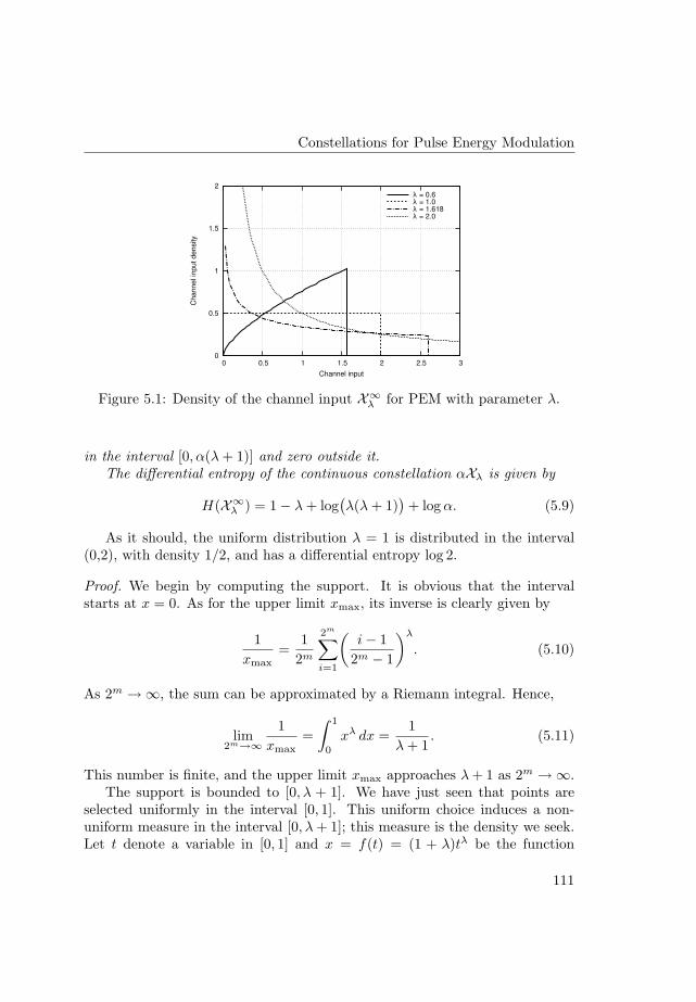
Constellations for Pulse Energy Modulation

0

0.5

1

1.5

2

0 0.5 1 1.5 2 2.5 3

Ch

anne

l in

pu

t d

ensity

Channel input

λ = 0.6λ = 1.0λ = 1.618λ = 2.0

Figure 5.1: Density of the channel input X∞λ for PEM with parameter λ.

in the interval [0, α(λ + 1)] and zero outside it.The differential entropy of the continuous constellation αXλ is given by

H(X∞λ ) = 1− λ + log(λ(λ + 1)

)+ log α. (5.9)

As it should, the uniform distribution λ = 1 is distributed in the interval(0,2), with density 1/2, and has a differential entropy log 2.

Proof. We begin by computing the support. It is obvious that the intervalstarts at x = 0. As for the upper limit xmax, its inverse is clearly given by

1xmax

=1

2m

2m∑

i=1

(i− 1

2m − 1

)λ

. (5.10)

As 2m →∞, the sum can be approximated by a Riemann integral. Hence,

lim2m→∞

1xmax

=∫ 1

0

xλ dx =1

λ + 1. (5.11)

This number is finite, and the upper limit xmax approaches λ + 1 as 2m →∞.The support is bounded to [0, λ + 1]. We have just seen that points are

selected uniformly in the interval [0, 1]. This uniform choice induces a non-uniform measure in the interval [0, λ + 1]; this measure is the density we seek.Let t denote a variable in [0, 1] and x = f(t) = (1 + λ)tλ be the function

111

5. Digital Modulation in the Additive Energy Channels

changing the measure. Then, since the measure dx of an infinitesimal intervalaround x, must coincide with the measure dt of the corresponding intervalaround t, that is dx = (1 + λ)λtλ−1 dt, we have that

dt =1

(1 + λ)λtλ−1dx =

x1λ−1

(1 + λ)1λ λ

dx. (5.12)

The formulas for the scaled constellation follow from a new change of mea-sure, now x′ = αx. Since the probability must remain unchanged, the densityof x′ therefore satisfies f(x′) dx′ = f(x) dx. Since dx′ = αdx, we have

f(x′) = f(x)dx

dx′=

x′1λ−1

α1λ λ(1 + λ)

1λ

. (5.13)

The entropy of the limiting scaled constellation may be directly computedfrom its density, or obtained from Theorem 9.6.4 of [22].

5.3 Coded Modulation in the Exponential Noise Channel

5.3.1 Constrained Capacity

The channel model for the exponential noise channel was presented in Chap-ter 2, and we now briefly review it. The channel output consists of a real-valuedvector y = (y1, . . . , yn). For each index k, the output yk is given by the sum

yk = SNR xk + zk, (5.14)

where the zk are independent samples of additive noise, exponentially dis-tributed as Zk ∼ E(1), SNR is the average signal-to-noise ratio, and xk is thechannel input. The channel capacity, of value C(SNR) = log(1 + SNR), isachieved when the channel input has the density given by Eq. (5.4). Sincethe capacity cost function has the same form as in the Gaussian channel, thecapacity per unit energy also coincides with its value in the Gaussian channel,an assertion which will be verified in Section 5.3.2.

In this section, we study the constrained capacity for pulse energy modu-lation (PEM), where the input symbols are drawn from a constellation set X .Symbols in X are used with probabilities P (x), and have arbitrary first- andsecond-order moments, µ1(X ) and µ2(X ).

112

Coded Modulation in the Exponential Noise Channel

The constellation is assumed to have |X | = 2m elements. For later use, weadd a point at infinity, defined as x|X |+1 = ∞. It is useful to sort the symbolsin increasing order, i. e. x1 ≤ x2 ≤ . . . ≤ x|X |.

As a final notational convention, the conditional output density Q(y|x) is

Q(y|x) = e−(y−SNR x)u(y − SNR x), (5.15)

where u(t) is the step function, so that the density is zero for y < SNRx.In contrast with the Gaussian case, there exists a closed-form expression

for the constrained capacity,

Proposition 5.2. In the AEN channel, the constrained capacity CX (SNR) forsignalling over a fixed modulation set X with probabilities P (x) with an averagesignal-to-noise ratio SNR is given by

CX (SNR) = −∑

x∈XP (x)

∑

xj≥x

(eSNR(x−xj) − eSNR(x−xj+1)

)log

( ∑

x′≤xj

P (x′)e− SNR(x−x′)

).

(5.16)

Proof. Eq. (3.3) on page 27, gives the mutual information across a communi-cations channel. Writing down the expectations over all input symbols x andnoise realizations z, we obtain

CX = −|X |∑

l=1

P (xl)∫ ∞

0

e−z log

( ∑

x′∈XP (x′)e−γ(xl−x′)u

(γ(xl − x′) + z

))

dz.

(5.17)

We split the integral into consecutive sections of length γ(xj+1−xj), starting atj = l (the sent symbol) and extending the sum to infinity with the conventionx|X |+1 = ∞. Then

∫ ∞

0

e−zf(xl, z) dz =|X |∑

j=l

∫ γ(xj+1−xl)

γ(xj−xl)

e−zf(xl, z) dz, (5.18)

where f(xl, z) is the logarithm function in Eq. (5.17). Within each interval thefunction f(xl, z) is constant, since

u(γ(xl − x′) + z

)= 1, for x′ ≤ xj , (5.19)

u(γ(xl − x′) + z

)= 0, for x′ > xj , (5.20)

113

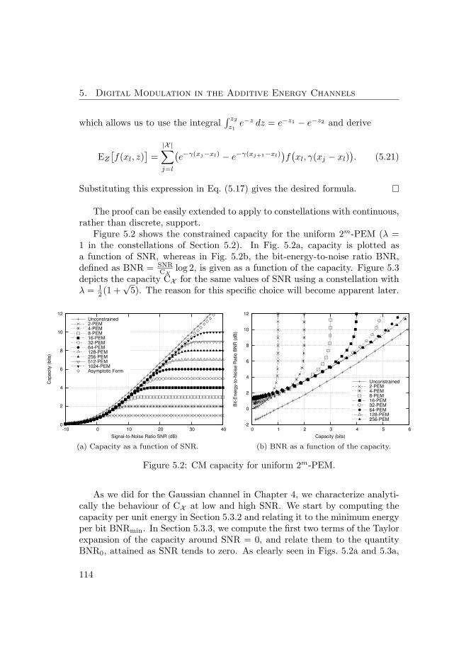
5. Digital Modulation in the Additive Energy Channels

which allows us to use the integral∫ z2

z1e−z dz = e−z1 − e−z2 and derive

EZ

[f(xl, z)

]=

|X |∑

j=l

(e−γ(xj−xl) − e−γ(xj+1−xl)

)f(xl, γ(xj − xl)

). (5.21)

Substituting this expression in Eq. (5.17) gives the desired formula.

The proof can be easily extended to apply to constellations with continuous,rather than discrete, support.

Figure 5.2 shows the constrained capacity for the uniform 2m-PEM (λ =1 in the constellations of Section 5.2). In Fig. 5.2a, capacity is plotted asa function of SNR, whereas in Fig. 5.2b, the bit-energy-to-noise ratio BNR,defined as BNR = SNR

CXlog 2, is given as a function of the capacity. Figure 5.3

depicts the capacity CX for the same values of SNR using a constellation withλ = 1

2 (1 +√

5). The reason for this specific choice will become apparent later.

0

2

4

6

8

10

12

-10 0 10 20 30 40

Ca

pacity (

bits)

Signal-to-Noise Ratio SNR (dB)

Unconstrained2-PEM4-PEM8-PEM16-PEM32-PEM64-PEM128-PEM256-PEM512-PEM1024-PEMAsymptotic Form

(a) Capacity as a function of SNR.

-2

0

2

4

6

8

10

12

0 1 2 3 4 5 6

Bit-E

nerg

y-t

o-N

ois

e R

atio

BN

R (

dB

)

Capacity (bits)

Unconstrained2-PEM4-PEM8-PEM16-PEM32-PEM64-PEM128-PEM256-PEM

(b) BNR as a function of the capacity.

Figure 5.2: CM capacity for uniform 2m-PEM.

As we did for the Gaussian channel in Chapter 4, we characterize analyti-cally the behaviour of CX at low and high SNR. We start by computing thecapacity per unit energy in Section 5.3.2 and relating it to the minimum energyper bit BNRmin. In Section 5.3.3, we compute the first two terms of the Taylorexpansion of the capacity around SNR = 0, and relate them to the quantityBNR0, attained as SNR tends to zero. As clearly seen in Figs. 5.2a and 5.3a,

114

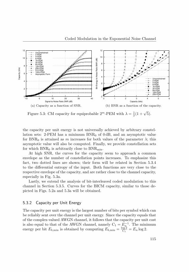
Coded Modulation in the Exponential Noise Channel

0

2

4

6

8

10

12

-10 0 10 20 30 40

Ca

pacity (

bits)

Signal-to-Noise Ratio SNR (dB)

Unconstrained2-PEM4-PEM8-PEM16-PEM32-PEM64-PEM128-PEM256-PEM512-PEM1024-PEMAsymptotic Form

(a) Capacity as a function of SNR.

-2

0

2

4

6

8

10

12

0 1 2 3 4 5 6B

it-E

nerg

y-t

o-N

ois

e R

atio

BN

R (

dB

)

Capacity (bits)

Unconstrained2-PEM4-PEM8-PEM16-PEM32-PEM64-PEM128-PEM256-PEM

(b) BNR as a function of the capacity.

Figure 5.3: CM capacity for equiprobable 2m-PEM with λ = 12 (1 +

√5).

the capacity per unit energy is not universally achieved by arbitrary constel-lation sets: 2-PEM has a minimum BNR0 of 0 dB, and an asymptotic valuefor BNR0 is attained as m increases for both values of the parameter λ; thisasymptotic value will also be computed. Finally, we provide constellation setsfor which BNR0 is arbitrarily close to BNRmin.

At high SNR, the curves for the capacity seem to approach a commonenvelope as the number of constellation points increases. To emphasize thisfact, two dotted lines are shown; their form will be related in Section 5.3.4to the differential entropy of the input. Both functions are very close to therespective envelope of the capacity, and are rather close to the channel capacity,especially in Fig. 5.3a.

Lastly, we extend the analysis of bit-interleaved coded modulation to thischannel in Section 5.3.5. Curves for the BICM capacity, similar to those de-picted in Figs. 5.2a and 5.3a will be obtained.

5.3.2 Capacity per Unit Energy

The capacity per unit energy is the largest number of bits per symbol which canbe reliably sent over the channel per unit energy. Since the capacity equals thatof the complex-valued AWGN channel, it follows that the capacity per unit costis also equal to that of the AWGN channel, namely C1 = E−1

n . The minimumenergy per bit Eb,min is obtained by computing Eb,min = log 2

C1= En log 2.

115

5. Digital Modulation in the Additive Energy Channels

It takes the same energy to transmit a bit in the complex-valued AWGN andthe AEN channels when the noise variance of the AWGN channel, σ2, equalsthe noise mean of the AEN channel, En. This fact was to be expected sincethe channel capacity is log(1+SNR) in both cases. The minimum bit-energy-to-noise ratio BNRmin, given by BNRmin = Eb,min

En= log 2, equals −1.59 dB, in

agreement with the results depicted in Figs. 5.2b and 5.3b.Alternatively, we can use Theorem 3.9 on page 30, to determine C1,

C1 = supx

D(Q(y|x)||Q(y|x = 0)

)

Esx(5.22)

= supx

1Esx

∫ ∞

SNR x

e−(y−SNR x) loge−(y−SNR x)

e−ydy (5.23)

= supx

1En

∫ ∞

SNR x

e−(y−SNR x) dy =1

Ensup

x1 =

1En

. (5.24)

To write Eq. (5.23), we used the definition of the divergence between twoprobability distributions and the form of the channel transition probabilityQ(y|x) in Eq. (5.15). The remaining steps are straightforward.

5.3.3 Asymptotic Behaviour at Low SNR

We start by characterizing the behaviour at low SNR of the constrained capac-ity CX in

Proposition 5.3. In the AEN channel, the constrained capacity CX (SNR)using a signal set X with average energy constraint SNR, admits a Taylor seriesexpansion of the form CX (SNR) = c1 SNR+c2 SNR2 +O(SNR3), as SNR → 0,with c1 and c2 given by

c1 = −|X |−1∑

j=1

(xj+1 − xj)qj log qj (5.25)

c2 =12σ2(X ) +

|X |−1∑

j=1

(xj+1 − xj)(

12 (xj + xj+1)qj − q′j

)log qj , (5.26)

where σ2(X ) = µ2(X )− µ21(X ), qj =

∑x′≤xj

P (x′) and q′j =∑

x′≤xjx′P (x′).

Proof. The detailed derivation can be found in Appendix 5.A.

116

Coded Modulation in the Exponential Noise Channel

We verify next that this characterization indeed describes the results inFig. 5.2. For the special case of equiprobable 2m-PEM, the proposition becomes

Corollary 5.4. In the AEN channel, 2m-PEM modulation with parameter λhas

c1 = − 2m

∑2m

j=1(j − 1)λ

2m−1∑

j=1

(jλ − (j − 1)λ

) j

2mlog

j

2m. (5.27)

For 2-PEM, c1 = log 2 and BNR0 = 1, or 0 dB. As m →∞, an asymptoticlimit is reached,

limm→∞

c1 =λ

λ + 1, (5.28)

limm→∞

c2 = − λ2

2(1 + 2λ)2, (5.29)

and therefore

limm→∞

BNR0 =λ + 1

λlog 2. (5.30)

As λ → ∞ and m → ∞, BNR0 approaches log 2, the value derived from thecapacity per unit energy; under the same conditions c2 approaches − 1

8 .

Proof. Eq. (5.27) immediately follows from the constellation definition.As m → ∞, the probability qj =

∑x′≤xj

P (x′) of the limiting continuousdistribution is given by the Riemann integral

qj =∫ xj

0

x1λ−1

λ(1 + λ)1λ

dx =(

xj

λ + 1

) 1λ

. (5.31)

Therefore, the first-order coefficient is given by

c1 = −∫ λ+1

0

(xj

λ + 1

) 1λ

log(

xj

λ + 1

) 1λ

dxj =λ

λ + 1. (5.32)

Next, the parameter q′j is given by the integral

q′j =∫ xj

0

xx

1λ−1

λ(1 + λ)1λ

dx =(

xj

λ + 1

)1+ 1λ

. (5.33)

117

5. Digital Modulation in the Additive Energy Channels

Approximating the sum in the formula for c2 by an integral, and setting 12 (xj +

xj+1) = xj , we get

xjqj − q′j = xj

(xj

λ + 1

) 1λ

−(

xj

λ + 1

)1+ 1λ

= λ

(xj

λ + 1

)1+ 1λ

, (5.34)

and, since the constellation variance is σ2(X ) = λ2

1+2λ , we get

c2 =12

λ2

1 + 2λ+

∫ λ+1

0

λ

(xj

λ + 1

)1+ 1λ

log(

xj

λ + 1

) 1λ

dxj (5.35)

=12

λ2

1 + 2λ− λ2(λ + 1)

(1 + 2λ)2= − λ2

2(1 + 2λ)2. (5.36)

As seen in Fig. 5.2b, the value of 2-PEM indeed approaches zero capacityat 0 dB. Uniform PEM requires a bit energy of 2 log 2 as the number of pointsincreases, a loss of 3 dB compared to the asymptotic value in the AWGN case.Use of the optimum constellation, with λ = 1

2 (1 +√

5) reduces this loss byabout 1 dB, since BNR0 = 1

2 (1 +√

5) log 2, or 0.50 dB. Further reductions arepossible by increasing λ, but BNRmin is approached relatively slowly.

A more efficient method of attaining the minimum BNRmin is by usingflash signalling [25], a generalized form of binary modulation with two pointsat positions 0, with probability p, and 1/(1−p), with probability 1−p. Indeed

Corollary 5.5. The coefficients c1 and c2 of binary modulation with one sym-bol at x = 0 used with probability p are

c1 = − p

1− plog p, c2 =

p

2(1− p)

(1 +

log p

1− p

). (5.37)

As p → 1, the coefficient c1 → 1, and the minimum bit-energy-to-noise ratioapproaches BNR → log 2. As for c2, it approaches −1/4.

Proof. There is just one term in the summation over j in Eq. (5.16), q1 = pand q′1 = 0 and x2 = (1− p)−1. Also µ2(X ) = (1− p)2. Then

c1 = −P (x1)(x2 − x1) log P (x1) = − p

1− plog p (5.38)

c2 = 12

((1− p)−1 − 1

)+ (x2 − x1)

(12 (x1 + x2)q1 − q′1

)log q1 (5.39)

=12

p

1− p+

12

p

(1− p)2log p =

12

p

1− p

(1 +

log p

1− p

). (5.40)

118

Coded Modulation in the Exponential Noise Channel

The limits as p → 1 are readily computed by using the Taylor expansionlog p = p− 1− 1

2 (p− 1)2 + O(p− 1)3.

For instance, the choice p ' 0.77 already gives BNR0 ' −1 dB. For thischoice the symbols are located at positions 0 and (1− p)−1 ' 4.27, a relativelycompact constellation. In order to achieve a similar value of BNR0, a value ofλ ' 6.85 would be required, a much less effective method than flash signalling,since the constellation is more peaky and needs more points (recall that BNR0

is attained as m →∞, and that for 2-PEM BNR0 is 0 dB).

5.3.4 Asymptotic Behaviour at High SNR

We estimate the asymptotic behaviour of CX at high SNR of the constellationsdescribed in Section 5.2 by following a method very close to that of the Gaussianchannel in Section 4.2.6. We first assume that the input is described by thelimiting continuous density in Eq. (5.7), and then approximate the output(differential) entropy H(Y ) by the differential entropy of the input H(X). Aswe shall shortly see, the PEM constellations described in Section 5.2 allow forrather neat closed-form expressions.

As we saw in Proposition 5.1, the differential entropy of the input Xλ is

H(Xλ) = 1− λ + log(λ(λ + 1)

). (5.41)

Scaled by SNR, its entropy is H(Xλ) + log SNR. As for the noise entropy, aswe determined in Proposition 3.13 on page 31, is given by H(Y |X) = H(Z) =log(e). The asymptotic expansion of the capacity at high SNR is

CXλ(SNR) ' log SNR−λ + log

(λ(λ + 1)

). (5.42)

This formula begets the natural question of determining the value of λ whichmaximizes its value. Setting the first derivative to zero, we derive the optimumλ as the solution of

−1 +1λ

+1

λ + 1= 0 =⇒ −λ(λ + 1) + λ + λ + 1 = 0, (5.43)

that is λ2 − λ − 1 = 0. The positive solution of this equation is λ = 1+√

52 '

1.618 . . . , the golden number. Hence, choosing λ as the golden number maxi-mizes the capacity at large SNR in the constellation family described in Sec-tion 5.2.

119

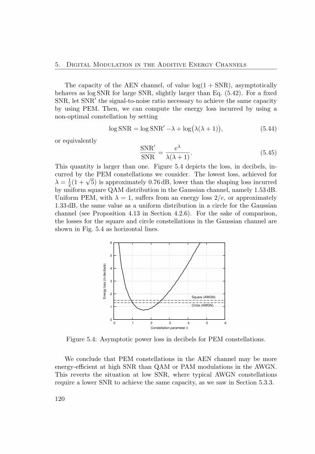
5. Digital Modulation in the Additive Energy Channels

The capacity of the AEN channel, of value log(1 + SNR), asymptoticallybehaves as log SNR for large SNR, slightly larger than Eq. (5.42). For a fixedSNR, let SNR′ the signal-to-noise ratio necessary to achieve the same capacityby using PEM. Then, we can compute the energy loss incurred by using anon-optimal constellation by setting

log SNR = log SNR′−λ + log(λ(λ + 1)

), (5.44)

or equivalentlySNR′

SNR=

eλ

λ(λ + 1). (5.45)

This quantity is larger than one. Figure 5.4 depicts the loss, in decibels, in-curred by the PEM constellations we consider. The lowest loss, achieved forλ = 1

2 (1 +√

5) is approximately 0.76 dB, lower than the shaping loss incurredby uniform square QAM distribution in the Gaussian channel, namely 1.53 dB.Uniform PEM, with λ = 1, suffers from an energy loss 2/e, or approximately1.33 dB, the same value as a uniform distribution in a circle for the Gaussianchannel (see Proposition 4.13 in Section 4.2.6). For the sake of comparison,the losses for the square and circle constellations in the Gaussian channel areshown in Fig. 5.4 as horizontal lines.

0

1

2

3

4

5

6

0 1 2 3 4 5 6

Ene

rgy lo

ss (

in d

ecib

els

)

Constellation parameter λ

Square (AWGN)

Circle (AWGN)

Figure 5.4: Asymptotic power loss in decibels for PEM constellations.

We conclude that PEM constellations in the AEN channel may be moreenergy-efficient at high SNR than QAM or PAM modulations in the AWGN.This reverts the situation at low SNR, where typical AWGN constellationsrequire a lower SNR to achieve the same capacity, as we saw in Section 5.3.3.

120

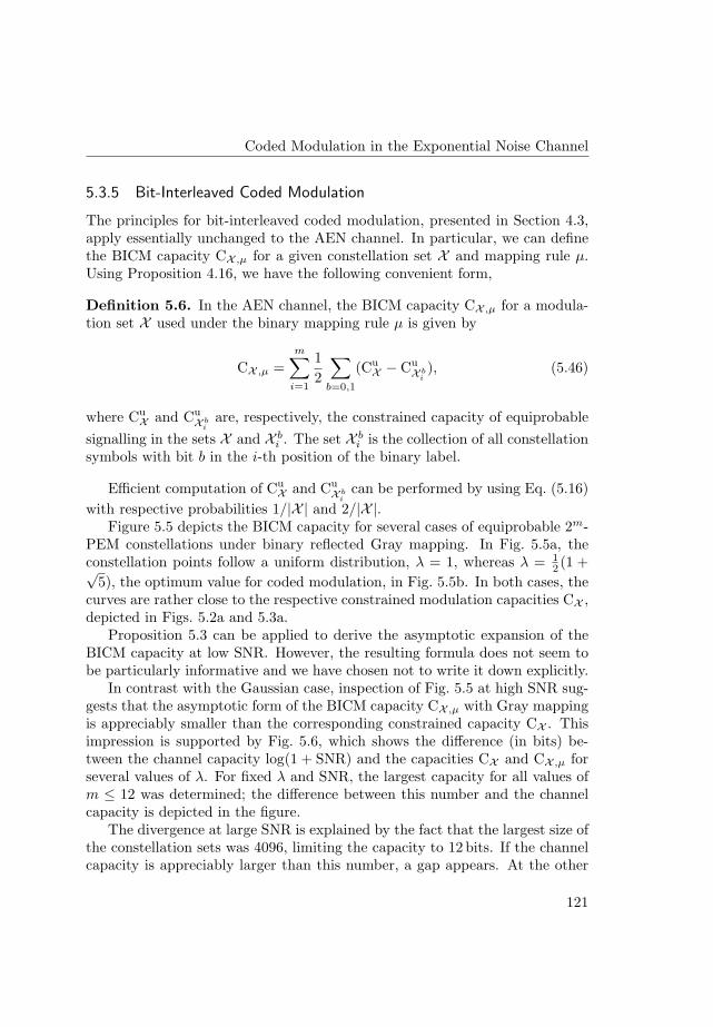
Coded Modulation in the Exponential Noise Channel

5.3.5 Bit-Interleaved Coded Modulation

The principles for bit-interleaved coded modulation, presented in Section 4.3,apply essentially unchanged to the AEN channel. In particular, we can definethe BICM capacity CX ,µ for a given constellation set X and mapping rule µ.Using Proposition 4.16, we have the following convenient form,

Definition 5.6. In the AEN channel, the BICM capacity CX ,µ for a modula-tion set X used under the binary mapping rule µ is given by

CX ,µ =m∑

i=1

12

∑

b=0,1

(CuX − Cu

X bi), (5.46)

where CuX and Cu

X bi

are, respectively, the constrained capacity of equiprobablesignalling in the sets X and X b

i . The set X bi is the collection of all constellation

symbols with bit b in the i-th position of the binary label.

Efficient computation of CuX and Cu

X bi

can be performed by using Eq. (5.16)with respective probabilities 1/|X | and 2/|X |.

Figure 5.5 depicts the BICM capacity for several cases of equiprobable 2m-PEM constellations under binary reflected Gray mapping. In Fig. 5.5a, theconstellation points follow a uniform distribution, λ = 1, whereas λ = 1

2 (1 +√5), the optimum value for coded modulation, in Fig. 5.5b. In both cases, the

curves are rather close to the respective constrained modulation capacities CX ,depicted in Figs. 5.2a and 5.3a.

Proposition 5.3 can be applied to derive the asymptotic expansion of theBICM capacity at low SNR. However, the resulting formula does not seem tobe particularly informative and we have chosen not to write it down explicitly.

In contrast with the Gaussian case, inspection of Fig. 5.5 at high SNR sug-gests that the asymptotic form of the BICM capacity CX ,µ with Gray mappingis appreciably smaller than the corresponding constrained capacity CX . Thisimpression is supported by Fig. 5.6, which shows the difference (in bits) be-tween the channel capacity log(1 + SNR) and the capacities CX and CX ,µ forseveral values of λ. For fixed λ and SNR, the largest capacity for all values ofm ≤ 12 was determined; the difference between this number and the channelcapacity is depicted in the figure.

The divergence at large SNR is explained by the fact that the largest size ofthe constellation sets was 4096, limiting the capacity to 12 bits. If the channelcapacity is appreciably larger than this number, a gap appears. At the other

121

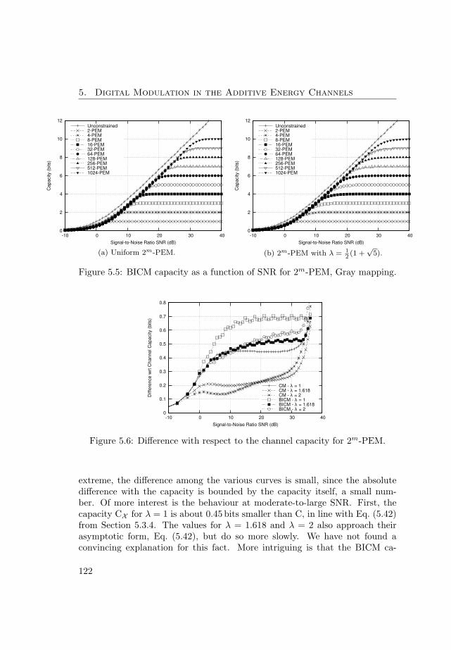
5. Digital Modulation in the Additive Energy Channels

0

2

4

6

8

10

12

-10 0 10 20 30 40

Ca

pacity (

bits)

Signal-to-Noise Ratio SNR (dB)

Unconstrained2-PEM4-PEM8-PEM16-PEM32-PEM64-PEM128-PEM256-PEM512-PEM1024-PEM

(a) Uniform 2m-PEM.

0

2

4

6

8

10

12

-10 0 10 20 30 40C

ap

acity (

bits)

Signal-to-Noise Ratio SNR (dB)

Unconstrained2-PEM4-PEM8-PEM16-PEM32-PEM64-PEM128-PEM256-PEM512-PEM1024-PEM

(b) 2m-PEM with λ = 12(1 +

√5).

Figure 5.5: BICM capacity as a function of SNR for 2m-PEM, Gray mapping.

0

0.1

0.2

0.3

0.4

0.5

0.6

0.7

0.8

-10 0 10 20 30 40

Diffe

ren

ce

wrt

Ch

an

ne

l C

apacity (

bits)

Signal-to-Noise Ratio SNR (dB)

CM - λ = 1CM - λ = 1.618CM - λ = 2BICM - λ = 1BICM - λ = 1.618BICM - λ = 2

Figure 5.6: Difference with respect to the channel capacity for 2m-PEM.

extreme, the difference among the various curves is small, since the absolutedifference with the capacity is bounded by the capacity itself, a small num-ber. Of more interest is the behaviour at moderate-to-large SNR. First, thecapacity CX for λ = 1 is about 0.45 bits smaller than C, in line with Eq. (5.42)from Section 5.3.4. The values for λ = 1.618 and λ = 2 also approach theirasymptotic form, Eq. (5.42), but do so more slowly. We have not found aconvincing explanation for this fact. More intriguing is that the BICM ca-

122

Coded Modulation in the Discrete-Time Poisson Channel

pacities are around 0.25–0.30 bits lower than the CM capacities at high SNR.This trait, which was not appreciable in the Gaussian channel, should relate tothe decoding metric for BICM, which ignores the correlation among the log-likelihood ratios. Moreover, the use of a mapping other than natural reflectedGray might yield some additional improvement.

5.4 Coded Modulation in the Discrete-Time Poisson Channel

5.4.1 Introduction

We now move on to the analysis of the discrete-time Poisson (DTP) channel.As we saw in Chapter 2, in this channel information is modulated onto theinput symbol energy, as it was in the AEN channel. Energy at the channeloutput is quantized, and the input energy constraint is given in terms of theaverage number of quanta, denoted by εs.

The input at time k, a non-negative real-valued number xk, induces a non-negative integer-valued output yk distributed according to a Poisson distribu-tion of parameter εsxk, Yk ∼ P(εsxk), there is no additive noise. We assumethat xk is drawn with probability P (xk) from a set X ; the set X is normalizedto unit energy. The cardinality of X is |X | = 2m, that is m bits are requiredto index a symbol. The conditional output density Q(y|x) is

Q(y|x) = e−εsx (εsx)y

y!. (5.47)

The analysis in this section examines the transmission capabilities of thechannel under pulse-energy modulations, with special attention being paid tothe family described in Section 5.2. As such, our study complements existingwork, such as [15], by deriving some new results:

• The performance at low quanta-count εs is described with techniques im-ported from the analysis of the Gaussian channel at low signal-to-noiseratio. In particular, the capacity per unit energy, the first two deriva-tives of the mutual information at zero quanta count, and the minimumnumber of quanta per bit for generic PEM formats are determined.

• The asymptotic form of the constrained coded modulation capacity athigh quanta counts is determined by using a Gaussian approximation. Aconstellation with small loss with respect to the capacity is provided.

123

5. Digital Modulation in the Additive Energy Channels

• Bit-interleaved coded modulation is shown to be a good method to designpractical channel codes, since its capacity is close to that of coded modu-lation. In addition, the performance loss with uniform PEM modulationand Gray mapping at low quanta counts is given by a simple expression.

These items are respectively covered in Sections 5.4.3-5.4.4, 5.4.5, and 5.4.6.

5.4.2 Constrained Capacity

From the definition of mutual information in Eq. (3.3) on page 27, we definethe constrained capacity CX for a fixed modulation set X as

Definition 5.7. In the DTP channel with average quanta count εs, the ca-pacity CX for signalling over a modulation set X with probabilities P (x) is

CX (εs) = −∑

x

P (x)∞∑

y=0

e−εsx (εsx)y

y!log

( ∑

x′∈XP (x′)eεs(x−x′)

(x′

x

)y)

.

(5.48)

If necessary, we also use the convention x log x = 0 for x = 0. Further, forx = 0, the only possible output is y = 0, and Eq. (5.48) is well-defined by thenatural limiting procedure replacing the summation over y by

log

( ∑

x′∈XP (x′)e−εsx′

). (5.49)

Figures 5.7 and 5.8 show the capacity for equiprobable 2m-PEM, respec-tively with λ = 1 and λ = 1 +

√3. In both cases, the upper plot depicts the

capacity as a function of εs, whereas the lower one shows the number of quantaper bit εb, defined in analogy to the AWGN and AEN channels as εb = εs

CXlog 2,

as a function of the capacity CX . Since for this channel the capacity is notknown, we also depict the upper and lower bounds from Chapter 3.

We will see in Section 5.4.5 how the choice λ = 1 +√

3 maximizes theasymptotic expression of the capacity CX at high εs under a Gaussian approx-imation. These asymptotic expressions match well with the envelope of thecapacity curves as the number of constellation points increases. To any extent,the constrained capacity for this value of λ is markedly larger than for uniformPEM, λ = 1; inspection of the plots shows an energy gain factor above 3 fora fixed capacity or about 0.65 bits for fixed εs. Further, constellations withλ = 1 +

√3 are better than uniform PEM also for low εs.

124

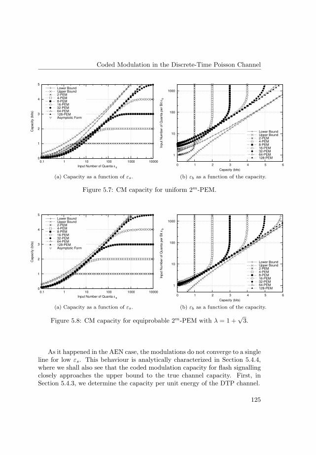
Coded Modulation in the Discrete-Time Poisson Channel

0

1

2

3

4

5

0.1 1 10 100 1000 10000

Cap

acity (

bits)

Input Number of Quanta ε s

Lower BoundUpper Bound2-PEM4-PEM8-PEM16-PEM32-PEM64-PEM128-PEMAsymptotic Form

(a) Capacity as a function of εs.

1

10

100

1000

0 1 2 3 4 5 6In

pu

t N

um

be

r of

Qua

nta

pe

r B

it ε

b

Capacity (bits)

Lower BoundUpper Bound2-PEM4-PEM8-PEM16-PEM32-PEM64-PEM128-PEM

(b) εb as a function of the capacity.

Figure 5.7: CM capacity for uniform 2m-PEM.

0

1

2

3

4

5

0.1 1 10 100 1000 10000

Cap

acity (

bits)

Input Number of Quanta ε s

Lower BoundUpper Bound2-PEM4-PEM8-PEM16-PEM32-PEM64-PEM128-PEMAsymptotic Form

(a) Capacity as a function of εs.

1

10

100

1000

0 1 2 3 4 5 6

Inpu

t N

um

be

r of

Qu

an

ta p

er

Bit ε

b

Capacity (bits)

Lower BoundUpper Bound2-PEM4-PEM8-PEM16-PEM32-PEM64-PEM128-PEM

(b) εb as a function of the capacity.

Figure 5.8: CM capacity for equiprobable 2m-PEM with λ = 1 +√

3.

As it happened in the AEN case, the modulations do not converge to a singleline for low εs. This behaviour is analytically characterized in Section 5.4.4,where we shall also see that the coded modulation capacity for flash signallingclosely approaches the upper bound to the true channel capacity. First, inSection 5.4.3, we determine the capacity per unit energy of the DTP channel.

125

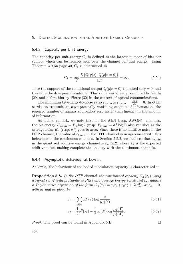
5. Digital Modulation in the Additive Energy Channels

5.4.3 Capacity per Unit Energy

The capacity per unit energy C1 is defined as the largest number of bits persymbol which can be reliably sent over the channel per unit energy. UsingTheorem 3.9 on page 30, C1 is determined as

C1 = supx

D(Q(y|x)||Q(y|x = 0)

)

εsx= ∞, (5.50)

since the support of the conditional output Q(y|x = 0) is limited to y = 0, andtherefore the divergence is infinite. This value was already computed by Verdu[29] and before him by Pierce [30] in the context of optical communications.

The minimum bit-energy-to-noise ratio εb,min is εb,min = log 2C1

= 0. In otherwords, to transmit an asymptotically vanishing amount of information, therequired number of quanta approaches zero faster than linearly in the amountof information.

As a final remark, we note that for the AEN (resp. AWGN) channels,the bit energy Eb,min = En log 2 (resp. Eb,min = σ2 log 2) also vanishes as theaverage noise En (resp. σ2) goes to zero. Since there is no additive noise in theDTP channel, the value of εb,min in the DTP channel is in agreement with thisbehaviour in the continuous channels. In Section 5.5.2, we shall see that εb,min

in the quantized additive energy channel is εn log 2, where εn is the expectedadditive noise, making complete the analogy with the continuous channels.

5.4.4 Asymptotic Behaviour at Low εs

At low εs the behaviour of the coded modulation capacity is characterized in

Proposition 5.8. In the DTP channel, the constrained capacity CX (εs) usinga signal set X with probabilities P (x) and average energy constraint εs, admitsa Taylor series expansion of the form CX (εs) = c1εs +c2ε

2s +O(ε3

s), as εs → 0,with c1 and c2 given by

c1 =∑

x∈XxP (x) log

x

µ1(X )(5.51)

c2 =12σ2(X )− 1

2µ2(X ) log

µ2(X )µ2

1(X ). (5.52)

Proof. The proof can be found in Appendix 5.B.

126

Coded Modulation in the Discrete-Time Poisson Channel

For constellations with unit mean energy, the bit energy at zero capacityεb, εb0, is given by Theorem 4.3,

εb0 = log 2

(∑

x∈XxP (x) log x

)−1

. (5.53)

Since the function t log t is convex, this quantity is in general larger than zero,the value of εb,min derived from the capacity per unit energy.

For the PEM constellations described in Section 5.2, it is possible to com-pute the asymptotic limit as the number of points becomes infinite,

Corollary 5.9. For 2-PEM, c1 = log 2 and BNR0 = 1, or 0 dB.In the DTP channel, as m →∞, 2m-PEM with parameter λ has

limm→∞

c1 = log (λ + 1)− λ

λ + 1(5.54)

limm→∞

c2 =12

(λ2

2λ + 1− (λ + 1)2

2λ + 1log

(λ + 1)2

2λ + 1

), (5.55)

and therefore

limm→∞

εb0 =log 2

log (λ + 1)− λλ+1

. (5.56)

As λ → ∞ and m → ∞, BNR0 approaches 0, the value derived from thecapacity per unit energy; under the same conditions c2 approaches −∞.

For instance, uniform 2m-PEM modulation in the discrete-time Poissonchannel requires about εb,min = log 2

log 2− 12' 3.59 quanta/bit, as the number of

quanta vanishes, εs → 0.

Proof. For the PEM constellations under consideration, average energy is oneand µ1(X ) = 1. For large m, the sum over the modulation symbols is replacedby a Riemann integral, and we have

limm→∞

c1 =∫ λ+1

0

x1λ−1

λ(1 + λ)1λ

x log x dx = log (λ + 1)− λ

λ + 1. (5.57)

εb,min follows immediately.The limit for the second-order coefficient c2 is obtained by using the formula

for µ2(X ) in Proposition 5.1.

127

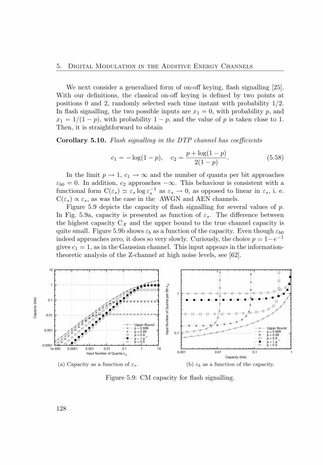
5. Digital Modulation in the Additive Energy Channels

We next consider a generalized form of on-off keying, flash signalling [25].With our definitions, the classical on-off keying is defined by two points atpositions 0 and 2, randomly selected each time instant with probability 1/2.In flash signalling, the two possible inputs are x1 = 0, with probability p, andx1 = 1/(1 − p), with probability 1 − p, and the value of p is taken close to 1.Then, it is straightforward to obtain

Corollary 5.10. Flash signalling in the DTP channel has coefficients

c1 = − log(1− p), c2 =p + log(1− p)

2(1− p). (5.58)

In the limit p → 1, c1 → ∞ and the number of quanta per bit approachesεb0 = 0. In addition, c2 approaches −∞. This behaviour is consistent with afunctional form C(εs) ' εs log ε−1

s as εs → 0, as opposed to linear in εs, i. e.C(εs) ∝ εs, as was the case in the AWGN and AEN channels.

Figure 5.9 depicts the capacity of flash signalling for several values of p.In Fig. 5.9a, capacity is presented as function of εs. The difference betweenthe highest capacity CX and the upper bound to the true channel capacity isquite small. Figure 5.9b shows εb as a function of the capacity. Even though εb0

indeed approaches zero, it does so very slowly. Curiously, the choice p = 1−e−1

gives c1 = 1, as in the Gaussian channel. This input appears in the information-theoretic analysis of the Z-channel at high noise levels, see [62].

0.0001

0.001

0.01

0.1

1

10

1e-005 0.0001 0.001 0.01 0.1 1 10

Ca

pa

city (

bits)

Input Number of Quanta ε s

Upper Boundp = 0.999p = 0.99p = 0.9p = 1-e

-1

p = 0.5

(a) Capacity as a function of εs.

0.1

1

0.001 0.01 0.1 1

Inpu

t N

um

be

r of

Qu

an

ta p

er

Bit ε

b

Capacity (bits)

Upper Boundp = 0.999p = 0.99p = 0.9p = 1-e

-1

p = 0.5

(b) εb as a function of the capacity.

Figure 5.9: CM capacity for flash signalling.

128

Coded Modulation in the Discrete-Time Poisson Channel

5.4.5 Asymptotic Behaviour at High εs

We now move on to the estimate of the asymptotic behaviour of the constrainedcapacity at high εs. The constrained capacity may be written as the differencebetween two terms, the output entropy H(Y ) and the conditional entropyH(Y |X). We approximate the output entropy the same way we did in theAWGN and AEN channels, namely by approximating H(Y ) by the differentialentropy of the input H(X), when the input is a continuous density. As we sawin Proposition 5.1, the differential entropy of the scaled input εsXλ is

H(Xλ) = 1− λ + log(λ(λ + 1)

)+ log εs. (5.59)

As for the conditional entropy, differently from the AWGN/AEN channels,noise is not additive in the DTP channel, a fact which must be properly takeninto account. We use a Gaussian approximation to the conditional entropy,which is also valid as an asymptotic formula for the entropy of a Poisson dis-tribution, H(Y |X = x) ' 1

2 log(2πex) (see Proposition 3.40 in Section 3.5.2).Integrated over the input x, this gives

H(Y |X) '∫ εs(λ+1)

0

x1λ−1

ε1λs λ(1 + λ)

1λ

12

log(2πex) dx (5.60)

=12

(log

(2πeεs(λ + 1)

)− λ). (5.61)

Therefore, assuming the Gaussian approximation is valid, the asymptotic be-haviour of C at high εs is given by

C(εs) ' 1− λ + log(λ(λ + 1)

)+ log εs − 1

2

(log

(2πeεs(λ + 1)

)− λ)

(5.62)

=12

log εs +12(1− λ

)+

12

log(λ2(λ + 1)

)− 12

log(2π). (5.63)

As we did in the AEN case, it is interesting to determine the value of λ withthe highest asymptotic capacity. It is derived by computing the first derivativewith respect to λ and setting it to zero,

−12

+1λ

+1

2(λ + 1)= 0 =⇒ −λ(λ + 1) + 2(λ + 1) + λ = 0, (5.64)

that is λ2 − 2λ− 2 = 0. Its positive root is λ = 1 +√

3 ' 2.732 . . . .

129

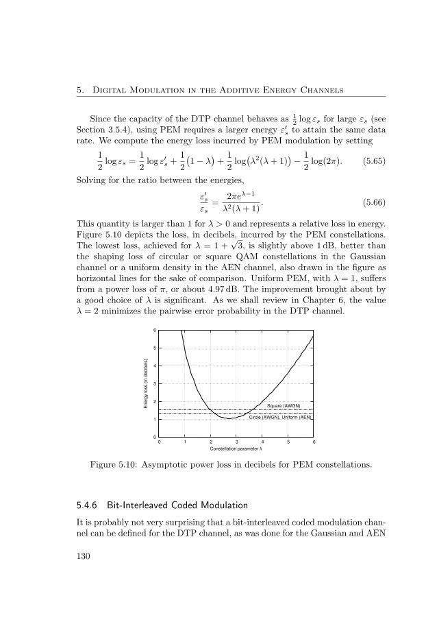
5. Digital Modulation in the Additive Energy Channels

Since the capacity of the DTP channel behaves as 12 log εs for large εs (see

Section 3.5.4), using PEM requires a larger energy ε′s to attain the same datarate. We compute the energy loss incurred by PEM modulation by setting

12

log εs =12

log ε′s +12(1− λ

)+

12

log(λ2(λ + 1)

)− 12

log(2π). (5.65)

Solving for the ratio between the energies,

ε′sεs

=2πeλ−1

λ2(λ + 1). (5.66)

This quantity is larger than 1 for λ > 0 and represents a relative loss in energy.Figure 5.10 depicts the loss, in decibels, incurred by the PEM constellations.The lowest loss, achieved for λ = 1 +

√3, is slightly above 1 dB, better than

the shaping loss of circular or square QAM constellations in the Gaussianchannel or a uniform density in the AEN channel, also drawn in the figure ashorizontal lines for the sake of comparison. Uniform PEM, with λ = 1, suffersfrom a power loss of π, or about 4.97 dB. The improvement brought about bya good choice of λ is significant. As we shall review in Chapter 6, the valueλ = 2 minimizes the pairwise error probability in the DTP channel.

0

1

2

3

4

5

6

0 1 2 3 4 5 6

Ene

rgy lo

ss (

in d

ecib

els

)

Constellation parameter λ

Square (AWGN)

Circle (AWGN), Uniform (AEN)

Figure 5.10: Asymptotic power loss in decibels for PEM constellations.

5.4.6 Bit-Interleaved Coded Modulation

It is probably not very surprising that a bit-interleaved coded modulation chan-nel can be defined for the DTP channel, as was done for the Gaussian and AEN

130

Coded Modulation in the Discrete-Time Poisson Channel

channels. In particular, we have a BICM capacity CX ,µ, given by the expres-sion (4.39) or alternatively by a definition similar to that of Eq. (5.46).

Figure 5.11 depicts the BICM capacity for several equiprobable 2m-PEMmodulation and Gray mapping. The upper and lower bounds to the channelcapacity from Chapter 2 are also depicted. The most remarkable fact is thatthe curves are very close to those of the coded modulation capacity.

0

1

2

3

4

5

0.1 1 10 100 1000 10000

Cap

acity (

bits)

Input Number of Quanta ε s (dB)

Lower BoundUpper Bound2-PEM4-PEM8-PEM16-PEM32-PEM64-PEM128-PEM

(a) Uniform 2m-PEM.

0

1

2

3

4

5

0.1 1 10 100 1000 10000

Cap

acity (

bits)

Input Number of Quanta ε s (dB)

Lower BoundUpper Bound2-PEM4-PEM8-PEM16-PEM32-PEM64-PEM128-PEM

(b) 2m-PEM with λ = 1 +√

3.

Figure 5.11: BICM capacity as a function of εs for 2m-PEM and Gray mapping.

The loss incurred by BICM with respect to the upper bound to the channelcapacity is depicted in Fig. 5.12. More precisely, for each value of εs and λ,the highest BICM capacity for all m ≤ 7 is determined, and subtracted fromthe upper bound to the channel capacity; the result is plotted as a function ofεs. The same steps are repeated for the constrained capacity.

The BICM capacity is very close to that of coded modulation, as was thecase in the Gaussian channel. Qualitatively, the behaviour of the various curvesis very similar to that of the AEN channel. For low εs the difference amongthe various curves is small, since the absolute difference with the capacity isbounded by the capacity itself, a small number; all curves coincide becausethe highest capacity is achieved by 2-PEM, and in that case CX and CX ,µ

coincide. For larger values of εs, the capacities CX and CX ,µ approach anasymptotic form, whose value for CX is very closely given by the expressionsin Section 5.4.5.

For the DTP channel, a neat formula exists for the linear terms of theTaylor expansion of CX ,µ around εs. Then, we have

131

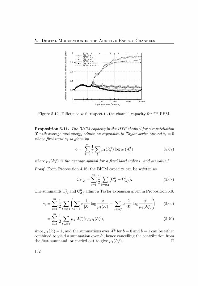
5. Digital Modulation in the Additive Energy Channels

0

0.2

0.4

0.6

0.8

1

0.1 1 10 100 1000 10000

Diffe

rence w

rt U

pper

Bo

un

d t

o C

han

nel C

ap

acity (

bits)

Input Number of Quanta ε s

CM - λ = 1BICM - λ = 1CM - λ = 2BICM - λ = 2CM - λ = 2.732BICM - λ = 2.732

Figure 5.12: Difference with respect to the channel capacity for 2m-PEM.

Proposition 5.11. The BICM capacity in the DTP channel for a constellationX with average unit energy admits an expansion in Taylor series around εs = 0whose first term c1 is given by

c1 =m∑

i=1

12

∑

b

µ1(X bi ) log µ1(X b

i ) (5.67)

where µ1(X bi ) is the average symbol for a fixed label index i, and bit value b.

Proof. From Proposition 4.16, the BICM capacity can be written as

CX ,µ =m∑

i=1

12

∑

b=0,1

(CuX − Cu

X bi). (5.68)

The summands CuX and Cu

X bi

admit a Taylor expansion given in Proposition 5.8,

c1 =m∑

i=1

12

∑

b=0,1

(∑

x∈Xx

1|X | log

x

µ1(X )−

∑

x∈X bi

x2|X | log

x

µ1(X bi )

)(5.69)

=m∑

i=1

12

∑

b=0,1

µ1(X bi ) log µ1(X b

i ), (5.70)

since µ1(X ) = 1, and the summations over X bi for b = 0 and b = 1 can be either

combined to yield a summation over X , hence cancelling the contribution fromthe first summand, or carried out to give µ1(X b

i ).

132

Coded Modulation in the Quantized Additive Energy Channel

As in the Gaussian case, we can compute the result in Theorem 5.11 fornatural Gray mapping (see the definition on page 87). Then

Corollary 5.12. For uniform 2m-PEM and Gray mapping, c1 is given by

c1 =12

2m−1 − 12m − 1

log2m−1 − 12m − 1

+12

3 2m−1 − 12m − 1

log3 2m−1 − 1

2m − 1. (5.71)

As m →∞, the coefficient c1 approaches c1 → log 33/4

2 ' 0.13, whereas theminimum bit energy approaches εb0 → 7.24 dB.

The loss represents about 1.69 dB with respect to the CM limit as m →∞,which was found in Corollary 5.9 to be εb0 = 5.55 dB.

Proof. For 2m-PEM, the Gray mapping construction above makes µ1(X bi ) = 1

for b = 0, 1 and all bits but one, say i = 1. Therefore,

c1 =12µ1(X 0

1 ) log µ1(X 01 ) +

12µ1(X 1

1 ) log µ1(X 11 ). (5.72)

Symbols xi, i = 0, . . . , 2m − 1 take the value xi = 2i2m−1 , and therefore

µ1(X 01 ) =

22m − 1

12m−1

2m−1−1∑

i=0

i =2m−1 − 12m − 1

, (5.73)

µ1(X 11 ) =

22m − 1

12m−1

2m−1∑

i=2m−1

i =32m−1 − 1

2m − 1. (5.74)

The coefficient c1 then follows. The limit m →∞ is obvious.

5.5 Coded Modulation in the Quantized Additive Energy Channel

5.5.1 Constrained Capacity

The quantized additive energy (AE-Q) channel was introduced in Chapter 2as an intermediate between the additive exponential (AEN) and discrete-timePoisson (DTP) channels. From the former, it inherits the trait that the channeloutput at time k yk is the sum of a signal and an additive noise components,respectively denoted by sk and zk, i. e. yk = sk + zk. It shares with the DTPchannel the properties that the output yk is a non-negative integer and that

133

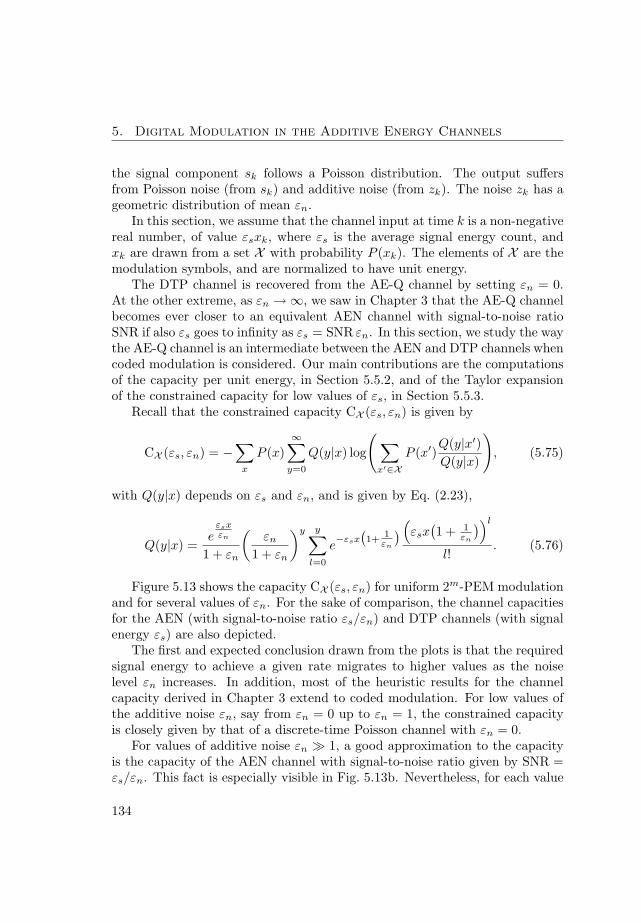
5. Digital Modulation in the Additive Energy Channels

the signal component sk follows a Poisson distribution. The output suffersfrom Poisson noise (from sk) and additive noise (from zk). The noise zk has ageometric distribution of mean εn.

In this section, we assume that the channel input at time k is a non-negativereal number, of value εsxk, where εs is the average signal energy count, andxk are drawn from a set X with probability P (xk). The elements of X are themodulation symbols, and are normalized to have unit energy.

The DTP channel is recovered from the AE-Q channel by setting εn = 0.At the other extreme, as εn →∞, we saw in Chapter 3 that the AE-Q channelbecomes ever closer to an equivalent AEN channel with signal-to-noise ratioSNR if also εs goes to infinity as εs = SNR εn. In this section, we study the waythe AE-Q channel is an intermediate between the AEN and DTP channels whencoded modulation is considered. Our main contributions are the computationsof the capacity per unit energy, in Section 5.5.2, and of the Taylor expansionof the constrained capacity for low values of εs, in Section 5.5.3.

Recall that the constrained capacity CX (εs, εn) is given by

CX (εs, εn) = −∑

x

P (x)∞∑

y=0

Q(y|x) log

( ∑

x′∈XP (x′)

Q(y|x′)Q(y|x)

), (5.75)

with Q(y|x) depends on εs and εn, and is given by Eq. (2.23),

Q(y|x) =e

εsxεn

1 + εn

(εn

1 + εn

)y y∑

l=0

e−εsx

(1+

1εn

) (εsx

(1 + 1

εn

))l

l!. (5.76)

Figure 5.13 shows the capacity CX (εs, εn) for uniform 2m-PEM modulationand for several values of εn. For the sake of comparison, the channel capacitiesfor the AEN (with signal-to-noise ratio εs/εn) and DTP channels (with signalenergy εs) are also depicted.

The first and expected conclusion drawn from the plots is that the requiredsignal energy to achieve a given rate migrates to higher values as the noiselevel εn increases. In addition, most of the heuristic results for the channelcapacity derived in Chapter 3 extend to coded modulation. For low values ofthe additive noise εn, say from εn = 0 up to εn = 1, the constrained capacityis closely given by that of a discrete-time Poisson channel with εn = 0.

For values of additive noise εn À 1, a good approximation to the capacityis the capacity of the AEN channel with signal-to-noise ratio given by SNR =εs/εn. This fact is especially visible in Fig. 5.13b. Nevertheless, for each value

134

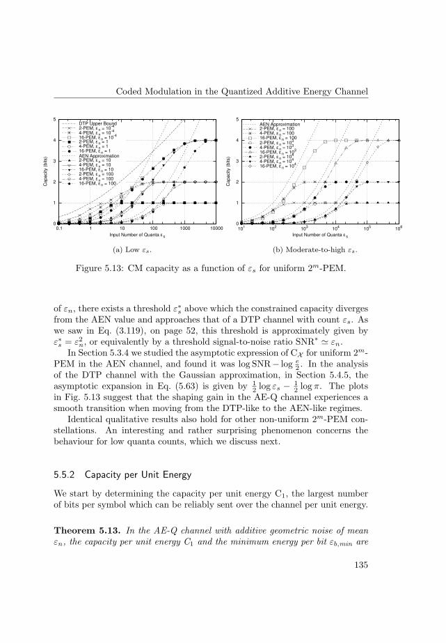
Coded Modulation in the Quantized Additive Energy Channel

0

1

2

3

4

5

0.1 1 10 100 1000 10000

Cap

acity (

bits)

Input Number of Quanta ε s

DTP Upper Bound2-PEM, ε n = 10

-4

4-PEM, ε n = 10-4

16-PEM, ε n = 10-4

2-PEM, ε n = 14-PEM, ε n = 116-PEM, ε n = 1AEN Approximation2-PEM, ε n = 104-PEM, ε n = 1016-PEM, ε n = 102-PEM, ε n = 1004-PEM, ε n = 10016-PEM, ε n = 100

(a) Low εs.

0

1

2

3

4

5

101

102

103

104

105

106

Cap

acity (

bits)

Input Number of Quanta ε s

AEN Approximation2-PEM, ε n = 1004-PEM, ε n = 10016-PEM, ε n = 1002-PEM, ε n = 10

3

4-PEM, ε n = 103

16-PEM, ε n = 103

2-PEM, ε n = 104

4-PEM, ε n = 104

16-PEM, ε n = 104

(b) Moderate-to-high εs.

Figure 5.13: CM capacity as a function of εs for uniform 2m-PEM.

of εn, there exists a threshold ε∗s above which the constrained capacity divergesfrom the AEN value and approaches that of a DTP channel with count εs. Aswe saw in Eq. (3.119), on page 52, this threshold is approximately given byε∗s = ε2

n, or equivalently by a threshold signal-to-noise ratio SNR∗ ' εn.In Section 5.3.4 we studied the asymptotic expression of CX for uniform 2m-

PEM in the AEN channel, and found it was log SNR− log e2 . In the analysis

of the DTP channel with the Gaussian approximation, in Section 5.4.5, theasymptotic expansion in Eq. (5.63) is given by 1

2 log εs − 12 log π. The plots

in Fig. 5.13 suggest that the shaping gain in the AE-Q channel experiences asmooth transition when moving from the DTP-like to the AEN-like regimes.

Identical qualitative results also hold for other non-uniform 2m-PEM con-stellations. An interesting and rather surprising phenomenon concerns thebehaviour for low quanta counts, which we discuss next.

5.5.2 Capacity per Unit Energy

We start by determining the capacity per unit energy C1, the largest numberof bits per symbol which can be reliably sent over the channel per unit energy.

Theorem 5.13. In the AE-Q channel with additive geometric noise of meanεn, the capacity per unit energy C1 and the minimum energy per bit εb,min are

135

5. Digital Modulation in the Additive Energy Channels

respectively given by

C1 =1εn

, εb,min = εn log 2. (5.77)

The energy per bit has its natural meaning. Its form is reminiscent of theresults for the Gaussian channel, Eb,min = σ2 log 2, and for the exponentialchannel Eb,min = En log 2.

Proof. The proof can be found in Appendix 5.C.

This is the natural counterpart of the result in the AEN channel, wherethe minimum energy per bit was found to be En. The presence of Poissonnoise does not reduce the capacity per unit energy, or equivalently increase theminimum energy per bit.

5.5.3 Asymptotic Behaviour at Low εs

For a capacity CX , it is natural to define a number of quanta per bit, εb, asεb = εs

CXlog 2. As we saw in the DTP channel, this quantity plays an analogous

role to that of BNR in Gaussian channels. The capacity curves in Fig. 5.13may be turned around and represented as εb versus the channel capacity. Theresulting plot is depicted in Fig. 5.14. One immediately notices an unexpectedbehaviour in the region CX → 0, namely the seeming divergence to infinityof number of quanta per bit εb. This impression is further corroborated byFig. 5.14b, essentially a logarithmic unfolding of the previous plot, in whichthe x scale is plotted in logarithmic scale, so as to better examine the shape ofthe curve.

This odd behaviour is no artifact of the computations, as stated in

Proposition 5.14. In the AE-Q channel with geometric noise of mean εn > 0and average signal count εs, the Taylor expansion of the constrained capacityCX (εs, εn) around εs = 0 is given by

CX (εs, εn) =12σ2(X )

ε2s

εn+ O(ε3

s). (5.78)

Since the linear term is zero, the energy per bit at vanishing εs is εb0 = ∞.

Proof. The proof can be found in Appendix 5.D.

136

Coded Modulation in the Quantized Additive Energy Channel

10-1

100

101

102

103

104

0 0.5 1 1.5 2 2.5 3 3.5 4

Inpu

t N

um

be

r of

Qua

nta

pe

r B

it ε

b

Capacity (bits)

DTP Upper Bound2-PEM, ε n = 10

-4

4-PEM, ε n = 10-4

2-PEM, ε n = 14-PEM, ε n = 1AEN Approximation2-PEM, ε n = 1016-PEM, ε n = 102-PEM, ε n = 10016-PEM, ε n = 100

(a) Linear scale.

10-1

100

101

102

103

104

10-7

10-6

10-5

10-4

10-3

10-2

10-1

100

101

Inpu

t N

um

be

r of

Qua

nta

pe

r B

it ε

b

Capacity (bits)

(b) Logarithmic scale; legend as left.

Figure 5.14: Bit energy versus CM capacity CX for uniform 2m-PEM.

Since the result holds for arbitrary PEM modulations, the use of flash sig-nalling (binary modulation, with one symbol at zero used with probability p)does not achieve a finite εb0. It would however, achieve a large c2 coefficient,since c2 = p

2(1−p) → ∞ for flash signalling with probability p → 1, as we sawin the proof of Corollary 5.5.

This is a most surprising fact, for which we have not found an intuitiveexplanation. In Sections 5.3.3 and 5.4.4, on the respective analysis of thelimiting cases AEN and DTP, we saw that the required energy per bit atzero SNR had a finite, well-defined value. It would have been natural thatthe intermediate case, the AE-Q channel, changes these well-defined values ina smooth transition between the two extremes. The transition seems to behowever different, as implied by the curves in Fig. 5.14b and Proposition 5.14.For the DTP channel, εb0 is finite, of value

εb0 = log 2

(∑

x∈XxP (x) log x

)−1

, (5.79)

given in Theorem 5.8. From this point, the addition of some additive noise εn,however small, makes the curve εb

AE-Q(CX ) diverge from the DTP value. Thedual behaviour takes place in the transition to the AEN limit.

This seeming contradiction is solved by noting that this happens at a verysmall capacity, below 10−3 bits for εn = 10−4, as seen in Fig. 5.14b. For even

137

5. Digital Modulation in the Additive Energy Channels

lower values of εn, the divergence takes place at even lower capacities. A similartransition takes place when approaching the AEN limit. Fortunately, the di-vergence is not visible in the limit, unless one wishes to work at tiny capacities.Further, if a system operated at such low rates, it could be argued whether εb

is an appropriate figure of merit, as opposed to εs. An interesting question iswhat impact this behaviour may have for situations when the channel is notclose to either limit, such as εn in the order of hundreds.

We note that we have not been able to analytically determine the positionof the inflection point in the curves for εb(CX ), which would correspond to theminimum energy per bit for a given modulation set. To any extent, an absolutelower bound to the energy per bit is given by εb,min = εn log 2.

5.5.4 Bit-Interleaved Coded Modulation

We conclude our analysis of the AE-Q channel by briefly considering bit-interleaved coded modulation. A BICM capacity can be defined as in thepreviously studied channels, and its value computed. When using Gray map-ping, the results turn out to be very close to the CM case, and identical con-clusions to the ones reached previously can be derived for BICM. In particular,there is a transition between the AEN and the DTP channels, with the AE-Q channel model bridging the gap between the two of them. We concludethat bit-interleaved coded modulation is likely to be a good method to generalchannel codes for the AE-Q channel.

In addition, thanks to the decomposition of the BICM capacity in Propo-sition 4.16, it is clear that the first term c1 of the Taylor series of the capacityaround εs = 0 is zero, in line with the result for coded modulation.

5.6 Conclusions

The additive energy channel models were constructed in Chapter 2 in such away that the AE-Q channel has the AEN and DTP channels as limiting forms.This idea was further supported in Chapter 3, where we saw that the capacity ofthe AE-Q channel indeed converges to the capacity of these limiting cases in anatural manner. In this chapter, we have examined this transition when codedmodulation is considered and we have in the process extended the analysis ofcoded modulation, carried out for the Gaussian channel in Chapter 4, to theadditive energy channels.

More specifically, we have determined the capacity achievable by a familyof pulse-energy modulations (PEM) whose constellation points have the form

138

Conclusions

β(i− 1)λ, for i = 1, . . . , 2m, where λ > 0 is a parameter and β a normalizationfactor; points are used with the same probabilities. As m becomes very large,the constellation can be described by a continuous density with support limitedto the interval [0, λ + 1]. In addition, we have considered flash signalling, ageneralized form of binary modulation with two points at positions 0, withprobability p, and 1/(1− p), with probability 1− p.

For the various additive energy channels, we have computed the constrainedcapacity CX achievable by using a set X and the bit-interleaved coded mod-ulation (BICM) capacity CX ,µ for the set X under mapping rule µ. As forthe Gaussian channel, both capacities are rather similar when binary reflectedGray mapping is used for BICM. BICM is therefore likely to be a good methodto perform channel coding in the energy channels, by using simple binary codes,such as convolutional or turbo-like codes.

The behaviour of the constrained capacity at low energy levels, when thecapacity becomes vanishingly small, has been determined. The main resultsare summarized in Table 5.1, where the capacity per unit energy, the minimumenergy per nat1, and the energy at zero-capacity for PEM modulation andflash signalling are presented. It is remarkable that the energy per nat (or thecapacity per unit energy) shows a smooth transition between the AWGN andDTP channels, going through the AEN and AE-Q models: for all models, it isequal to the average energy of the additive noise component.

Even though the capacity per unit energy of the Gaussian channel is at-tained by any zero-mean unit-energy constellation, this result does not extendto the additive energy channels. The performance of a specific modulation for-mat at low energy levels strongly depends on the modulation format itself. Asseen in Table 5.1, the minimum energy per nat is attained by the appropriatelimits of PEM(λ) of flash signalling in the AEN and DTP channels. Intrigu-ingly, it is not the case for the AE-Q channel, whose energy per nat at zeroenergy is infinite. These seemingly contradictory extremes have been recon-ciled in Section 5.5.3 by looking at somewhat higher channel capacities, forwhich the AE-Q model represents a smooth transition between the AEN andDTP channel models. Care must be exercised when analyzing the asymptoticbehaviour, as it may not be representative of a more practical scenario.

For all the channel models, we have computed the first two coefficients of

1In the chapter, we have rather considered the energy per bit. Since log 2 nats=1 bit,giving the energy per nat removes the ubiquitous factor log 2 in the formulas for the energyper bit and makes for more compact results. Needless to say, this change of units has noeffect on the conclusions.

139

5. Digital Modulation in the Additive Energy Channels

Channel model AWGN AEN DTP AE-Q

Cap./unit energy 1/σ2 1/En ∞ 1/εn

Min. energy/nat σ2 En 0 εn

c1 – 2m-PEM (λ) 1 λλ+1 log (λ + 1)− λ

λ+1 0Energy at zero σ2 ≥ En > 0 ∞c1 – flash (p) 1 − p

1−p log p − log(1− p) 0Energy at zero σ2 ≥ En > 0 ∞

Table 5.1: Minimum energies in the additive energy channels.

the Taylor expansion of the capacity at zero energy, namely

C(γ) = c1γ + c2γ2 + o(γ2), (5.80)

where γ is SNR for the AEN (and AWGN) channels, and εs for the DTP andAE-Q channels. The coefficients c1 are given by Propositions 5.3, 5.8, and 5.14,

cAEN1 = −

|X |−1∑

j=1

(xj+1 − xj)qj log qj (5.81)

cDTP1 =

∑

x∈XxP (x) log

x

µ1(X )(5.82)

cAE-Q1 = 0, (5.83)

where qj =∑

s′≤sjP (x′). The linear coefficients c1 for 2m-PEM and flash

signalling are given in Table 5.1. As for the coefficients c2, they are given by

cAEN2 =

12σ2(X ) +

|X |−1∑

j=1

(sj+1 − sj)(

12 (sj + sj+1)qj − q′j

)log qj , (5.84)

cDTP2 =

12σ2(X )− 1

2µ2(X ) log

µ2(X )µ2

1(X ), (5.85)

cAE-Q2 =

12εn

σ2(X ), (5.86)

where σ2(X ) = µ2(X ) − µ21(X ), and q′j =

∑s′≤sj

s′P (x′). This analysis com-plements the results obtained for the Gaussian channel, in Proposition 4.4.

140

CM Capacity Expansion at Low SNR – AEN

Next to the low-energy region, we have studied the asymptotic expressionof the capacity for large energy levels. From Eqs. (5.42) and (5.63) (under aGaussian approximation), we have

CAENX ' log SNR−λ + log

(λ(λ + 1)

), (5.87)

CDTPX ' 1

2 log εs + 12

(1− λ

)+ 1

2 log(λ2(λ + 1)

)− 12 log(2π), (5.88)

for 2m-PEM constellations with parameter λ. The value of λ which maximizesthese expressions was determined, and found to be λAEN = 1

2 (1 +√

5) andλDTP = 1 +

√3. The AE-Q channel shows a transition between the two as the

number of quanta grows and Poisson noise becomes more important, comparedto the additive noise. Uniform PEM was found to suffer from an energy lossfactor of e

2 (AEN) and π (DTP), to be compared with the value πe6 for square

constellations in the Gaussian channel. Optimizing λ reduced these values to1.19 (AEN), saving 0.58 dB, and 1.27 (DTP), a reduction of 3.92 dB.

Even though some of the results seem of a rather technical nature, it ishoped that the analysis presented in this section may prove useful in the designand performance analysis of, at least, some optical communication systems. Inthe following chapter we complement the analysis presented so far by studyingthe pairwise error probability for binary codes, a fundamental tool to studythe effective performance of channel codes.

5.A CM Capacity Expansion at Low SNR – AEN

We follow the same steps as for AWGN, with the necessary adaptations. Forthe sake of compactness, we define γ = SNR and respectively denote the first-and second-order moments of the constellation by µ1 and µ2. Recall that theCM capacity is

CX = −|X |∑

l=1

P (xl)|X |∑

j=l

(e−γ(xj−xl) − e−γ(xj+1−xl)

)log

( ∑

x′≤xj

P (x′)e−γ(xl−x′)

).

(5.89)

For each of the summands in the log(·) in Eq. (5.89) we use et = 1 + t +12 t2 + O(t3) to obtain

e−γ(xl−x′) = 1 + γ(x′ − xl) + 12γ2

(x′2 + x2

l − 2x′xl

)+ O(γ3). (5.90)

141

5. Digital Modulation in the Additive Energy Channels

Let us now define the variables qj , q′j , and q′′j respectively as

qj =∑

x′≤xj

P (x′), q′j =∑

x′≤xj

x′P (x′), q′′j =∑

x′≤xj

x′2P (x′). (5.91)

Rearranging, the sum in the logarithm over x′ such that x′ ≤ xj gives

∑

x′≤xj

eγ(x′−xl)P (x′) = qj

(1 + γ

q′jqj− γxl + 1

2γ2q′′jqj− γ2xl

q′jqj

+ 12γ2x2

l + O(γ3)

).

(5.92)

Taking logarithms, and using the expansion log(1 + t) = t − 12 t2 + O(t3)

around γ = 0, we obtain

log qj + γq′jqj− γxl + 1

2γ2q′′jqj− γ2xl

q′jqj

+ 12γ2x2

l − 12γ2

(q′jqj− xl

)2

+ O(γ3)

(5.93)

= log qj + γq′jqj− γxl + 1

2γ2q′′jqj− 1

2γ2

(q′jqj

)2

+ O(γ3). (5.94)

We now move on to the summation over j in Eq. (5.89). We use the Taylorexpansion of the exponential function in the summation over j, separating thelast term as special. Starting at it, j = |X |, we note that the sum over x′ ≤ x|X |includes all symbols, and its contribution to the sum is(1− γ(x|X | − xl) + 1

2γ2(x|X | − xl)2)×

×(

log qj + γq′jqj− γxl + 1

2γ2q′′jqj− 1

2γ2

(q′jqj

)2)

+ O(γ3) (5.95)

=(1− γ(x|X | − xl) + 1

2γ2(x|X | − xl)2)(

γ(µ1 − xl) + 12γ2

(µ2 − µ2

1

))+ O(γ3),

(5.96)

since∑

x′ P (x′) = 1. Carrying out the expectation over xl, and discardingterms of order O(γ3), this term contributes with

∑

l

P (xl)(γ(µ1 − xl) + 1

2γ2(µ2 − µ2

1

)− γ2(x|X | − xl)(µ1 − xl))

= (5.97)

= − 12γ2

(µ2 − µ2

1

). (5.98)

142

CM Capacity Expansion at Low SNR – AEN

As for the terms j < |X |, the following terms contribute|X |−1∑

j=l

(γ(xj+1 − xj) + 1

2γ2(x2j − x2

j+1 − 2(xj − xj+1)xl))(

log qj + γq′jqj− γxl

)

(5.99)

=|X |−1∑

j=l

{γ(xj+1 − xj) log qj + 1

2γ2(x2j − x2

j+1) log qj − γ2(xj − xj+1)xl log qj

+ γ2(xj+1 − xj)

(q′jqj− xl

)}. (5.100)

The only remaining step is the averaging over xl, which yields

CX = −∑

l

P (xl)|X |−1∑

j=l

{γ(xj+1 − xj) log qj + 1

2γ2(x2j − x2

j+1) log qj

− γ2(xj − xj+1)xl log qj + γ2(xj+1 − xj)

(q′jqj− xl

)}

+ 12γ2

(µ2 − µ2

1

)+ O(γ3). (5.101)

The order of the double summation over l and j can be reversed, with thesummation limits becoming|X |−1∑

j=1

∑

l≤j

P (xl)

{γ(xj+1 − xj) log qj + γ2(xj − xj+1)

(12 (xj + xj+1)− xl

)log qj

+ γ2(xj+1 − xj)

(∑x′≤xj

x′P (x′)

qj− xl

)}(5.102)

=|X |−1∑

j=1

(γ(xj+1 − xj)qj log qj + γ2(xj − xj+1)

(12 (xj + xj+1)qj − q′j

)log qj

).

(5.103)

Therefore the desired expression for the CM capacity is

CX = −|X |−1∑

j=1

(γ(xj+1 − xj)qj log qj − γ2(xj+1 − xj)

(12 (xj + xj+1)qj − q′j

)log qj

)

+ 12γ2

(µ2 − µ2

1

)+ O(γ3). (5.104)

143

5. Digital Modulation in the Additive Energy Channels

5.B CM Capacity Expansion at Low εs – DTP

The CM capacity is

CX = −∑

x

P (x)∞∑

y=0

Q(y|x) log

( ∑

x′∈XP (x′)eεs(x−x′)

(x′

x

)y)

. (5.105)

For the sake of compactness, we respectively denote the first- and second-ordermoments of the constellation by µ1 and µ2.

Using the Taylor expansion of the exponential, et = 1 + t + 12 t2 + O(t3), we

notice that, in the low εs region, there are only three possible channel outputsto order ε3

s, namely

y = 0, Q(y|x) = 1− εsx + 12ε2

sx2 + O(ε3

s) (5.106)

y = 1, Q(y|x) = εsx− ε2sx

2 + O(ε3s) (5.107)

y = 2, Q(y|x) = 12ε2

sx2 + O(ε3

s) (5.108)

y ≥ 2, Q(y|x) = O(ε3s). (5.109)

Since each of these cases behaves differently, we examine them separately.We rewrite the variable in the log(·) in Eq. (5.105) with the appropriate

approximation. When the output is y = 0, the variable is∑

x′∈XP (x′)eεs(x−x′) =

∑

x′∈XP (x′)

(1 + εs(x− x′) + 1

2ε2s(x− x′)2 + O(ε3

s))

(5.110)

= 1 + εs(x− µ1) + 12ε2

s(x2 + µ2 − 2xµ1) + O(ε3

s). (5.111)

Taking logarithms, and using the formula log(1+t) = t− 12 t2+O(t3), we obtain

εs(x− µ1) + 12ε2

s(x2 + µ2 − 2xµ1)− 1

2ε2s(x

2 + µ21 − 2xµ1) + O(ε3

s) (5.112)

= εs(x− µ1) + 12ε2

s

(µ2 − µ2

1

)+ O(ε3

s). (5.113)

When the output is y = 1, the variable in the logarithm in Eq. (5.105) is∑

x′∈XP (x′)eεs(x−x′) x

′

x=

1x

∑

x′∈XP (x′)x′

(1 + εs(x− x′) + O(ε2

s))

(5.114)

=1x

(µ1 + εs

(xµ1 − µ2

)+ O(ε2

s))

(5.115)

=µ1

x

(1 +

εs

µ1

(xµ1 − µ2

)+ O(ε2

s)). (5.116)

144

Capacity per Unit Energy in the AE-Q Channel

Taking logarithms, and using the Taylor expansion of the logarithm, we get

logµ1

x+

εs

µ1

(xµ1 − µ2

)+ O(ε2

s). (5.117)

We will later verify that no higher-order terms are required.At last, for y = 2, the variable in the logarithm in Eq. (5.105) is

∑

x′∈XP (x′)eεs(x−x′) x

′2

x2=

1x2

∑

x′∈XP (x′)x′2

(1 + O(εs)

)(5.118)

=1x2

(µ2 + O(εs)

)(5.119)

=µ2

x2

(1 + O(εs)

). (5.120)

Taking logarithms, and using the Taylor expansion of the logarithm, we get

logµ2

x2+ O(εs). (5.121)

Later, we will verify that no higher-order terms are required.After carrying out the averaging over y, we first combine Eqs. (5.113), (5.117)

and (5.121) with the probabilities in Eqs. (5.106)–(5.108) and then group allterms up to O(ε3

s) to derive(1− εsx + 1

2ε2sx

2)(

εs(x− µ1) + 12ε2

s

(µ2 − µ2

1

))+

+(εsx− ε2

sx2)(

logµ1

x+

εs

µ1

(xµ1 − µ2

))+ 1

2ε2sx

2 logµ2

x2+ O(ε3

s) (5.122)

= εs(x− µ1) + 12ε2

s

(µ2 − µ2

1

)− ε2s(x

2 − xµ1) + εsx logµ1

x

− ε2sx

2 logµ1

x+ ε2

s

1µ1

(x2µ1 − xµ2

)+ 1

2ε2sx

2 logµ2

x2+ O(ε3

s). (5.123)

The expectation over x is straightforward, and gives

CX = εs

∑

x∈XP (x)x log

x

µ1+

12ε2

s

(µ2 − µ2

1 − µ2 logµ2

µ21

)+ O(ε3

s). (5.124)

5.C Capacity per Unit Energy in the AE-Q Channel

From Theorem 3.9, the capacity per unit energy can computed as

C1 = supx

D(Q(y|x)||Q(y|x = 0)

)

εsx. (5.125)

145

5. Digital Modulation in the Additive Energy Channels

Using Eq. (5.76) for Q(·|·) and the definition of divergence, we have

D(Q(y|x)||Q(y|x = 0)

)=

∑y

Q(y|x) log

(e

εsxεn

y∑

l=0

e−α αl

l!

), (5.126)

where α = εsx(1 + 1

εn

). Let us define P (l) = e−α αl

l! and the quantityq(y) =

∑yl=0 P (l), i. e. the cumulative distribution function of a Poisson ran-

dom variable with mean α.Moving the exponential out of the logarithm, we obtain

D(Q(y|x)||Q(y|x = 0)

)=

εsx

εn+

∑y

Q(y|x) log(q(y)

). (5.127)

Hence, the capacity per unit energy is given by

C1 =1εn

+ supx

∑y Q(y|x) log

(q(y)

)

εsx. (5.128)

Since q(y) ≤ 1, its logarithm is always non-positive, and

C1 ≤ 1εn

. (5.129)

The proof is completed by proving that

limx→∞

eεsxεn

εsx(1 + εn)

(∑y

(εn

1 + εn

)y

q(y) log(q(y)

))

= 0, (5.130)

where we expressed Q(y|x) as a function of q(y). If this condition holds true,then Eq. (5.129) becomes an equality.

In Eq. (5.130) we split the summation over y into two parts, from 0 toy∗ = bαc, and from y∗ + 1 to infinity. In the first part, e−α αy

y! is an increasingfunction in y, and therefore

q(y) =y∑

l=0

P (l) ≥y∑

l=0

P (0) = (y + 1)P (0) = (y + 1)e−α. (5.131)

Hence, the summation for y ≤ y∗ is bounded as

y∗∑y=0

(εn

1 + εn

)y

q(y) log(q(y)

) ≥y∗∑

y=0

(εn

1 + εn

)y

(y + 1)e−α(log(y + 1)− α

).

(5.132)

146

Capacity per Unit Energy in the AE-Q Channel

And, multiplying by the exponential factor eεsxεn , we have

y∗∑y=0

e−εsx

(εn

1 + εn

)y

(y + 1) log(y + 1)−y∗∑

y=0

e−εsx

(εn

1 + εn

)y

(y + 1)α.

(5.133)

As y →∞, each of these two summands goes to zero. The second has the form

e−εsx

y∗∑y=0

(εn

1 + εn

)y

(y + 1)α, (5.134)

which decays exponentially in x, since the sum satisfies

y∗∑y=0

(εn

1 + εn

)y

(y + 1) ≤∞∑

y=0

(εn

1 + εn

)y

(y + 1) = (1 + εn)2, (5.135)

and e−εsxα(1 + εn)2 vanishes for large x. Similarly, the summation

y∗∑y=0

(εn

1 + εn

)y

(y + 1) log(y + 1) (5.136)

remains bounded, since it is the partial sum of a convergent series, with n-thcoefficient βn(n + 1) log(n + 1) and β = εn/(1 + εn) < 1. This is verified bythe checking the ratio test, as

limn→∞

βn(n + 1) log(n + 1)βn−1n log n

= β < 1. (5.137)

Boundedness of the partial sum implies that, after multiplying times an expo-nential factor e−εsx, the first summand vanishes as x →∞.

Next, we consider the remainder of the summation in Eq. (5.130),∞∑

y=y∗+1

(εn

1 + εn

)y

q(y) log(q(y)

). (5.138)

Clearly, q(0) = e−α ≤ q(y) ≤ 1 and therefore −α ≤ log q(y) ≤ 0, so eachsummand is negative and bounded by

(εn

1 + εn

)y

q(y) log(q(y)

) ≥ −α

(εn

1 + εn

)y

q(y) ≥ −α

(εn

1 + εn

)y

. (5.139)

147

5. Digital Modulation in the Additive Energy Channels

Summing over y,∞∑

y=y∗+1

(εn

1 + εn

)y

q(y) log(q(y)

) ≥ −α(1 + εn)(

εn

1 + εn

)y∗+1

. (5.140)

Using the definition of α = εsx(1+ 1

εn

)and taking into account the denom-

inator εsx(1 + εn) in Eq. (5.130), we must study the behaviour of

−εn + 1εn

eεsxεn

(εn

1 + εn

)y∗+1

= −εn + 1εn

eεsxεn

−(y∗+1) log(1+ 1

εn

)(5.141)

as x →∞. By construction, y∗ + 1 > α, and therefore

εsx

εn− (y∗ + 1) log

(1 +

1εn

)<

εsx

εn− εsx

(1 +

1εn

)log

(1 +

1εn

)(5.142)

= εsx

(1εn−

(1 +

1εn

)log

(1 +

1εn

)). (5.143)

Since t ≤ (1 + t) log(1 + t) for t > 0, a fact which follows from the inequalitylog(1 + t) ≤ t, this left-hand side of Eq. (5.142) is strictly upper bounded by afunction ax, where a is negative. Hence, the function in Eq. (5.141) vanishesexponentially as x →∞, and so does the term

eεsxεn

εsx(1 + εn)

∞∑y=y∗+1

(εn

1 + εn

)y

q(y) log(q(y)

). (5.144)

This proves the limit in Eq. (5.130) and shows that Eq. (5.129) holds withequality.

5.D CM Capacity Expansion at Low εs – AE-Q

The constrained capacity for coded modulation is

CX = −∑

x

P (x)∞∑

y=0

Q(y|x) log

(∑x′∈X P (x′)Q(y|x′)

Q(y|x)

), (5.145)

where Q(y|x) is given by Eq. (2.23), namely

Q(y|x) =1

1 + εn

(εn

1 + εn

)y(

y∑

l=0

(1 + εn

εn

)l

e−εsx (εsx)l

l!

). (5.146)

148

CM Capacity Expansion at Low εs – AE-Q

As it happened in the discrete-time Poisson channel, the Taylor expansionof the exponential, et = 1 + t + 1

2 t2 + O(t3), implies that there are only threepossible channel outputs s to order ε3

s, that is,

s = 0, P (s|x) = 1− εsx +12(εsx)2 + O(ε3

s) (5.147)

s = 1, P (s|x) = εsx− (εsx)2 + O(ε3s) (5.148)

s = 2, P (s|x) =12(εsx)2 + O(ε3

s) (5.149)

s > 2, P (s|x) = O(ε3s). (5.150)

Hence the channel output y = s + z only includes these contributions. Wedistinguish three cases, viz. y = 0, y = 1, and y ≥ 2.

In the first case, y = s = z = 0, and Q(y|x) becomes

Q(y|x) =1

1 + εn

(1− εsx +

12(εsx)2 + O(ε3

s)

). (5.151)

For y = 1, we combine the outputs s = 0 and s = 1,

Q(y|x) =εn

(1 + εn)2

(1− εsx +

12(εsx)2 +

1 + εn

εn

(εsx− (εsx)2

)+ O(ε3

s)

)

(5.152)

=εn

(1 + εn)2

(1 +

εs

εnx− ε2

sx2

(12

+1εn

)+ O(ε3

s)

). (5.153)

For y ≥ 2, we combine the outputs s = 0, s = 1, and s = 2,

Q(y|x) =εy

n

(1 + εn)y+1

(1− εsx +

12(εsx)2 +

(εsx− (εsx)2

)(1 + εn

εn

)

+12(εsx)2

(1 + εn

εn

)2

+ O(ε3s)

)(5.154)

=εy

n

(1 + εn)y+1

(1 +

εs

εnx +

ε2s

2ε2n

x2 + O(ε3s)

), (5.155)

after combining some terms together.

149

5. Digital Modulation in the Additive Energy Channels

We next rewrite the numerator and denominator in the log(·) in Eq. (5.145)with the appropriate approximation. For y = 0, the common term (1 + εn)−1

cancels, and the numerator is

∑

x′∈XQ(y|x′)P (x′) =

∑

x′∈X

(1− εsx

′ +12(εsx

′)2 + O(ε3s)

)P (x′) (5.156)

=(

1− εsµ1 +12ε2sµ2

)+ O(ε3

s). (5.157)

In the denominator, we keep the expansion

1− εsx + 12 (εsx)2 O(ε3

s). (5.158)

Taking logarithms of Eqs. (5.157) and (5.158), using the formula log(1 + t) =t− 1

2 t2 + O(t3), and combining numerator and denominator, we obtain

log(

1− εsµ1 +12ε2sµ2 + O(ε3

s))− log

(1− εsx +

12(εsx)2 + O(ε3

s))

(5.159)

= −εsµ1 +12ε2sµ2 − 1

2ε2

sµ21 + εsx− 1

2(εsx)2 +

12(εsx)2 + O(ε3

s) (5.160)

= −εs(µ1 − x) +12ε2

s(µ2 − µ21) + O(ε3

s). (5.161)

If the output is y = 1, we use Eq. (5.153). Summing over x′ in the numer-ator, we get

∑

x′∈XQ(y|x′)P (x′) =

(1 +

εs

εnµ1 −

(12

+1εn

)µ2ε

2s + O(ε3

s)

), (5.162)

with the agreement that a common term εn/(1 + εn)2 has been cancelled.Combining numerator and denominator, taking logarithms, and using the

Taylor expansion of the logarithm, we obtain

εs

εnµ1 −

(12

+1εn

)µ2ε

2s −

ε2s

2ε2n

µ21 −

εs

εnx +

(12

+1εn

)x2ε2

s +ε2s

2ε2n

x2 + O(ε3s)

(5.163)

=(µ1 − x)εs

εn−

((12

+1εn

)µ2 +

µ21

2ε2n

− x2(1 + εn)2

2ε2n

)ε2

s + O(ε3s). (5.164)

150

CM Capacity Expansion at Low εs – AE-Q

If the output is y ≥ 2, in an analogous way we use Eq. (5.155) to rewritethe logarithm of the ratio of numerator and denominator as

log

(1 +

εs

εnµ1 +

ε2s

2ε2n

µ2 + O(ε3s)

)− log

(1 +

εs

εnx +

ε2s

2ε2n

x2 + O(ε3s)

).

(5.165)

Using now the Taylor expansion of the logarithm, we obtain

εs

εnµ1 +

ε2s

2ε2n

µ2 − ε2s

2ε2n

µ21 −

εs

εnx− ε2

s

2ε2n

x2 +ε2

s

2ε2n

x2 + O(ε3s) (5.166)

=εs

εn(µ1 − x) +

ε2s

2ε2n

(µ2 − µ21) + O(ε3

s). (5.167)

The remaining steps are the averaging over x and y. We first carry out theexpectation over x. From Eq. (5.161), the averaging over x yields

∑x

11 + εn

(1− εsx +

12(εsx)2

)((x− µ1)εs +

12ε2s

(µ2 − µ2

1

))+ O(ε3

s)

(5.168)

=1

1 + εn

(12ε2s

(µ2 − µ2

1

)− ε2s

(µ2 − µ2

1

))+ O(ε3

s) (5.169)

=1

1 + εn

12ε2s

(µ2

1 − µ2

)+ O(ε3

s). (5.170)

Similarly, from Eq. (5.164) we obtain (bar for a constant factor εn

(1+εn)2 )

∑x

(1 +

εs

εnx− ε2

sx2

(12

+1εn

))×

×(

(µ1 − x)εs

εn−

((12

+1εn

)µ2 +

µ21

2ε2n

− x2(1 + εn)2

2ε2n

)ε2

s

)+ O(ε3

s)

(5.171)

=

(−

(12

+1εn

)µ2 − µ2

1

2ε2n

+µ2(1 + εn)2

2ε2n

+ε2

s

ε2n

(µ21 − µ2)

)ε2

s + O(ε3s)

(5.172)

= (µ21 − µ2)

ε2s

2ε2n

+ O(ε3s). (5.173)

151

5. Digital Modulation in the Additive Energy Channels

And finally, from Eq. (5.167), for y ≥ 2, we get

∑x

εyn

(1 + εn)y+1

(1 +

εs

εnx +

ε2s

2ε2n

x2

)(εs

εn(µ1 − x) +

ε2s

2ε2n

(µ2 − µ21)

)+ O(ε3

s)

(5.174)

=εy

n

(1 + εn)y+1

(ε2

s

2ε2n

(µ2 − µ21) +

ε2s

ε2n

(µ21 − µ2)

)+ O(ε3

s)

(5.175)

=εy

n

(1 + εn)y+1

ε2s

2ε2n

(µ21 − µ2) + O(ε3

s). (5.176)

The summation over y ≥ 2 can be carried out and yields

∞∑y=2

εyn

(1 + εn)y=

ε2n

1 + εn. (5.177)

Then, combining Eq. (5.177) into Eq. (5.176), and summing with Eqs. (5.170)and (5.173) (including the factor εn

(1+εn)2 ), we obtain

11 + εn

12ε2

s

(µ2

1 − µ2

)(

1 +1

εn(1 + εn)+

1ε2n

ε2n

1 + εn

)+ O(ε3

s) (5.178)

=12ε2

s

(µ2

1 − µ2

) 1εn

+ O(ε3s). (5.179)

And, finally, the expansion for CX follows,

CX =12(µ2 − µ2

1)ε2

s

εn+ O(ε3

s). (5.180)

152

6

Pairwise Error Probability for Coded Transmission

6.1 Introduction

As we saw in Chapter 3, the channel capacity gives the largest rate at whichinformation can be sent reliably, i. e. at low error rates, over a communicationchannel. Reliability is obtained by the operation of a channel code, or morepractically of an encoder and a decoder, respectively located at the transmittingand receiving ends of the channel. We discussed in Chapters 4 and 5 someaspects of the operation of the channel code, related to the use of variousmodulation formats and to the use of bit-interleaved coded modulation (BICM)as a method to combine good binary codes with these modulations.

A possible continuation of our study would be the design of such binarycodes. Instead, we have opted for a simpler alternative, in which we estimatethe so-called pairwise error probability, rather than the performance of specificchannel codes. Since the pairwise error probability is a key element in theanalysis of the code performance, the tools developed here may prove to beuseful in future code design for the additive energy channels.

In this chapter we follow a common practice in the optical communicationsliterature, as represented by Helstrom [63] and Einarsson [64], and provide ap-proximations to the error probability, rather than true upper and lower bounds,the usual approach in an information-theoretic analysis. As we shall see, thesaddlepoint approximation yields an accurate estimate of the pairwise errorprobability. The methodology is presented in Sections 6.2 and 6.3.

In Sections 6.4 and 6.5, we analyze binary transmission and BICM in Gaus-sian fading channels and derive accurate and easy to compute approximationsto the pairwise error probability. We next consider the two limiting cases ofthe additive energy channel, namely the additive exponential noise channel, inSection 6.6, and the discrete-time Poisson channel, in Section 6.7. The results

153

6. Pairwise Error Probability for Coded Transmission

presented in these sections seem to be new, except for some special cases ofthe binary DTP channel. One of the most intriguing results, to be presentedin Section 6.6, is the closeness of the error rates for binary transmission in theAWGN channel and its AEN equivalent.

6.2 Error Probability and the Union Bound

Two fundamental figures of merit measure the probability of error: the worderror rate and the bit error rate. We start our exposition with their definition.

Let a specific message, say message w, be selected at the transmitter; allmessages have the same probability. We assume that the message is representedby a sequence of l0 input (information) bits. Then, we encode the message witha binary code and identify it with a binary codeword b, an array of l codedbits. The codeword is mapped onto an array of modulation symbols of lengthn by using a mapping rule µ : {0, 1}m → X , which groups m consecutive bitsand outputs a corresponding modulation symbol xk,

xk = µ(bm(k−1)+1, bm(k−1)+2, . . . , bm(k−1)+m), for k = 1, . . . , n. (6.1)

Since a modulation symbol x is uniquely selected by m bits, we denote thesequence of bits corresponding to the symbol x by

(b1(x), . . . , bm(x)

).

The corresponding k-th channel output is denoted by yk. At the receiver,the decoder uses a metric function q : X × Y → R to make a decision onwhich codeword was sent; here Y denotes the output alphabet. For a receivedsequence y = (y1, . . . , yn), the codeword with largest metric

n∏

k=1

q(µ(bm(k−1)+1, . . . , bm(k−1)+m), yk

)(6.2)

is selected as estimate of the transmitted codeword. In case of ties one of thecandidate codewords is randomly chosen.

The word error rate, which we denote by Pw, is the probability of selectinga codeword different from the one transmitted. Similarly, we define the biterror rate, denoted by Pb, as the average number of input bits in error.

Exact expressions for the error probabilities Pw or Pb are difficult to obtain,and one often resorts to some form of bounding, the simplest of which is proba-bly the union bound. The union bound is built on the realization that an errorevent is the union of many pairwise error events. Even though these pairwiseerror events are in general not statistically independent, an accurate estimate

154

Approximations to the Pairwise Error Probability

of the error probability in a region above the cut-off rate [65] is obtained bysumming their probabilities. Since many existing channel codes operate in thisregion, viz. convolutional codes or turbo-like codes in the floor region, the unionbound has wide applicability.

The word error rate Pw is upper bounded by

Pw ≤∑

d

Ad pep(d), (6.3)

where d is the Hamming distance between two codewords, namely the numberof bits in which they differ, and Ad denotes the number of codewords at Ham-ming distance d. As for the bit error rate, Pb is given by the right-hand sideof Eq. (6.3) with Ad replaced by A′d =

∑j′

j′

l0Aj′,d, Aj′,d being the number of

codewords at output Hamming distance d and input Hamming distance j′. Ineither case, the pairwise error probability pep(d) is of fundamental importance,and we devote the remainder of this chapter to its study.

6.3 Approximations to the Pairwise Error Probability

In this section, we discuss the estimation of the pairwise error probability byusing a method similar to the analysis in Sections 5.3 and 5.4 of Gallager’sbook [31], or to the presentation of Chapters 2 and 3 of Viterbi’s book [65].

We assume that the decoding metric function is of the form

q(µ(b1, . . . , bm), y

)=

m∏

i=1

qi(bi, y), (6.4)

namely the product of per-bit metric functions qi : {0, 1} × Y → R. Inspiredby the analysis of BICM in Section 4.3, we let the function qi be given by

qi(b, y) =∑

x′∈X bi

Q(y|x′), (6.5)

where X bi is the set of symbols with bit b at label index i. One simple example

of a different metric is qi(b, y) = maxx′∈X bi

Q(y|x′). Since our analysis can beeasily extended to general metrics, we concentrate on the metric in Eq. (6.5).

Later, we will make use of the fact that the metric qi in Eq. (6.5) is propor-tional to the transition probability Qi(y|b) of the i-th BICM parallel channel,

Qi(y|b) =1|X b

i |∑

x′∈X bi

Q(y|x′). (6.6)

155

6. Pairwise Error Probability for Coded Transmission

Let us denote by bj and b′j the j-th bits of the transmitted and alternativecodewords respectively. Taking logarithms in Eq. (6.2), the decoder makes apairwise error if the pairwise score Ξpw, or score for short, given by

Ξpw =n∑

k=1

m∑

i=1

logqi(b′m(k−1)+i, yk)

qi(bm(k−1)+i, yk), (6.7)

is positive, i. e. if Ξpw > 0. When Ξpw = 0 an error is made with probability12 . The pairwise score is the sum of n symbol scores Ξs, in turn given by thesum of m bit scores1 Ξb, with their obvious definitions.

It proves fruitful to view the bit score Ξb as a random variable, whosedistribution depends on all the random elements in the channel, including thetransmitted bit b and the index i. For each value of k, a choice is made at thetransmitter between the mapping rule µ in Eq. (6.1) and its binary complement.This choice is known at the receiver. Denoting the cumulant transform [67] ofthe bit score by κ1(r) = log E[erΞb ], we have

Definition 6.1. The cumulant transform of the bit score Ξb is given by

κ1(r) = log E[erΞb ] = log

(1m

m∑

i=1

12

∑

b∈{0,1}EY

[qi(b, Y )r

qi(b, Y )r

]), (6.8)

where the bit b is the binary complement of b and Y is the set of possiblechannel outputs with bit b is transmitted at position i; the expectation over Yis done according to the transition probability Qi(y|b), in Eq. (6.6).

Clearly, only the bit indices for which bj 6= b′j have a (possibly) non-zerobit score; the number of such positions is the Hamming distance d. Since bitsin the same symbol are affected by the same noise, the bit scores are generallystatistically dependent. This dependence can be analyzed in a number of ways:

1. Assume the codeword length is infinite, so that the bits bj belong todifferent symbols with probability 1.

2. Carry out an averaging over all possible interleavers of a given size n, andcompute the average pairwise error probability, in a situation reminiscentof the uniform interleaving appearing in the analysis of turbo-like codes.

1In [66] we gave the somewhat clumsy name “a posteriori log-likelihood ratio” to the bitscore. We use here the shorter name bit score, which has the additional advantage of beingwell-defined for metrics other than the one in Eq. (6.5).

156

Approximations to the Pairwise Error Probability

3. Include in the analysis information of the position where bits are mappedinto. Here, the Hamming distance is not the only relevant variable, asthe position of the bits at which the codewords differ is also important.

For the binary-input Gaussian channel, all three alternatives coincide. ForBICM, we choose the first option, as in [26]. We further discuss the validity ofthis choice in Section 6.5.3, where the analysis of Yeh et al. [68] for the secondalternative is exploited to study QPSK modulation over fading channels.

We can compute the pairwise error probability as the tail probability of arandom variable, the pairwise score, in a form that we shall use in our analysis,

Proposition 6.2. The pairwise error probability pep(d) is given by

pep(d) = Pr

(d∑

j=1

Ξb,j > 0

)+

12

Pr

(d∑

j=1

Ξb,j = 0

), (6.9)

where the variables Ξb,j are bit scores.

In estimates of tail probabilities, such as in Proposition 6.2, use of the cu-mulant transform proves convenient [67]. Let us denote the cumulant transformof the pairwise score by κpw(r). For independent, identically distributed bitscores, we have κpw(r) = dκ1(r) [67]. The main advantage brought about byusing the cumulant transform is that the behaviour of the random variable isto great extent determined by its behaviour around the saddlepoint r, definedas the value r for which κ′pw(r) = 0 and therefore κ′1(r) = 0.

Proposition 6.3. The saddlepoint is located at r = 12 , that is κ′1

(12

)= 0. In

addition, the next derivatives of the cumulant transform verify

κ′′1(r) =E

[Ξ2

berΞb

]

E[erΞb

] ≥ 0, κ′′′1 (r) =E

[Ξ3

berΞb

]

E[erΞb

] = 0. (6.10)

Remark that we are explicitly using the metric in Eq. (6.5).

Proof. The computation is included in Appendix 6.A.

The cumulant transform, evaluated at the saddlepoint, appears in the Cher-noff (or Bhatthacharyya) bound to the pairwise error probability,

Proposition 6.4 (Chernoff Bound). The Chernoff bound to the pairwise errorprobability is

pep(d) ≤ edκ1(r). (6.11)

157

6. Pairwise Error Probability for Coded Transmission

This result gives a true bound and very easy to compute. It is further knownto correctly give the asymptotic exponential decay [39] of the error probabilityfor large d. However, it is not exact and in some cases, such as Gaussianfading channels, is not tight. As we next see, the saddlepoint approximationcomplements the Chernoff bound by including a multiplicative coefficient toobtain an expression of the form α · edκ1(r).

In Appendix 6.B we derive the saddlepoint approximation to the tail prob-ability of a continuous random variable, including an estimate of the approxi-mation error. The derivation was published in [66]. Even though the derivationis valid for small values of the saddlepoint r, we do not exploit this propertyas r = 1

2 . Unlike other presentations, such as Gallager’s [31], we are mainlyinterested in finite values of d. Using that κ′′′1 (r) = 0 and denoting the fourthderivative of κ1(r) by κIV

1 (r), we have

Theorem 6.5. In channels with continuous bit score Ξb, the pairwise errorprobability can be approximated to first-order by

pep(d) ' 1√2πdκ′′1(r)r

edκ1(r), (6.12)

where r = 12 . The second-order approximation is

pep(d) '(

1 +1

dκ′′1(r)

(− 1

r2+

κIV1 (r)

8κ′′1(r)

))1√

2πdκ′′1(r)redκ1(r). (6.13)

Higher-order expansions are characterized by having a correction factor α

polynomial in inverse powers of(dκ′′1(r)

)−1. In the next section we computethe pairwise error probability in the binary-input AWGN channel by explicitlyusing the bit score. The effect of the correction α is found to be negligible.

The approximation is different when the bit score takes values on the pointsof a lattice, i. e. it has the form α + iβ, where β is the span of the lattice, αan offset, and i indexes the random variable. In that case, the probabilitydistribution is well approximated (see section 5.4 of [31]) by

Theorem 6.6. For a discrete random variable Z inscribed in a lattice of spanβ, with cumulant transform κ(r), let r be the root of κ′(r) = 0. Then, thesaddlepoint approximation to the probability mass function is given by

PZ(z) ' βeκ(r)−rz

√2πκ′′(r)

. (6.14)

158

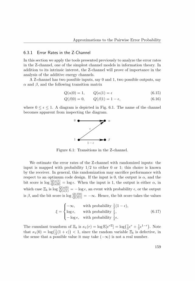
Approximations to the Pairwise Error Probability

6.3.1 Error Rates in the Z-Channel

In this section we apply the tools presented previously to analyze the error ratesin the Z-channel, one of the simplest channel models in information theory. Inaddition to its intrinsic interest, the Z-channel will prove of importance in theanalysis of the additive energy channels.

A Z-channel has two possible inputs, say 0 and 1, two possible outputs, sayα and β, and the following transition matrix

Q(α|0) = 1, Q(α|1) = ε (6.15)Q(β|0) = 0, Q(β|1) = 1− ε, (6.16)

where 0 ≤ ε ≤ 1. A diagram is depicted in Fig. 6.1. The name of the channelbecomes apparent from inspecting the diagram.

0

1

α

β

1 − ε

ε

Figure 6.1: Transitions in the Z-channel.

We estimate the error rates of the Z-channel with randomized inputs: theinput is mapped with probability 1/2 to either 0 or 1; this choice is knownby the receiver. In general, this randomization may sacrifice performance withrespect to an optimum code design. If the input is 0, the output is α, and thebit score is log Q(α|1)

Q(α|0) = log ε. When the input is 1, the output is either α, in

which case Ξb is log Q(α|0)Q(α|1) = − log ε, an event with probability ε, or the output

is β, and the bit score is log Q(β|0)Q(β|1) = −∞. Hence, the bit score takes the values

ξ =

−∞, with probability 12 (1− ε),

log ε, with probability 12 ,

− log ε, with probability 12ε.

(6.17)

The cumulant transform of Ξb is κ1(r) = log E[erΞ] = log(

12εr + 1

2ε1−r). Note

that κ1(0) = log(

12 (1 + ε)

)< 1, since the random variable Ξb is defective, in

the sense that a possible value it may take (−∞) is not a real number.

159

6. Pairwise Error Probability for Coded Transmission

Using Proposition 6.3, the saddlepoint is located at r = 1/2, which also canbe verified by direct computation. The second derivative at the saddlepoint isreadily found to be κ′′1(r) = log2 ε. We have the following

Theorem 6.7. In the Z-channel, the bit score takes only two real values,namely ± log ε. Its cumulant transform is

κ1(r) = log(

12εr +

12ε1−r

). (6.18)

At the saddlepoint, located at r = 1/2, κ1(r) = 12 log ε and κ′′1(r) = log2 ε. For

two codewords at Hamming distance d, κpw(r) = dκ1(r).The pairwise error probability in the Z-channel is given by

pep(d) =

2√2πd

(∑ d−12

j=0 εj

)ε(d+1)/2, d odd,

2√2πd

(12 +

∑ d2j=1 εj

)εd/2, d even.

(6.19)

Proof. The first part of the theorem, on the cumulant transform, is a restate-ment of the previous analysis. The approximation to the pairwise error prob-ability is derived in Appendix 6.C.

6.4 Error Probability in Binary-Input Gaussian Channels

6.4.1 Channel Model

We now consider BPSK modulation over the Gaussian channel. The set-upis as follows. A codeword b, with n bits, b = (b1, . . . , bn), is mapped onto asequence of binary symbols xk, with xk = {−1, +1}; the mapping rule is

xk = −1, if bk = 0; xk = +1, if bk = 1. (6.20)

At the channel output, a complex-valued vector y = (y1, . . . , yn) is detected.For each index k, k = 1, . . . , n, the output yk is given by the sum

yk =√

SNRhk xk + zk, (6.21)

where zk is Gaussian noise, Zk ∼ NC(0, 1), SNR is the average signal-to-noiseratio at the receiver, and hk is a fading coefficient. We assume the fully-interleaved fading model of Section 4.2.5 on page 83. The squared fading

160

Error Probability in Binary-Input Gaussian Channels

coefficient χk = |hk|2 follows a gamma distribution

pχk(χ) =

mmf

f χmf−1

Γ(mf )e−mf χ, (6.22)

where mf is a real non-negative number. The phase of hk is assumed knownat the receiver. Recall that unfaded AWGN is recovered by letting mf → +∞and Rayleigh fading by setting mf = 1.

This is the standard model for BPSK modulation. In the absence of fading,it also models the transmission of QPSK signals; whenever there is fading andQPSK is used there is some residual correlation among the channel outputsthrough the fading coefficient hk. This effect will be studied in Section 6.5.3.

6.4.2 Exact Pairwise Error Probability in the absence of Fading

In this section, we present some standard results for BPSK modulation. Thematerial is presented in terms of the bit score in order to ease the generalizationto other channels. With no fading, hk = 1, and we have

Theorem 6.8. In the binary-input AWGN channel the bit score has a normaldistribution, Ξb ∼ N (−4 SNR, 8 SNR), independent of the value of the trans-mitted bit. The bit score is drawn randomly and independently at each channelrealization and the pairwise score for two codewords at Hamming distance dalso has a normal distribution, Ξpw ∼ N (−4dSNR, 8d SNR).

The pairwise error probability is given by

pep(d) = Pr(Ξpw > 0) = Q(√

2dSNR), (6.23)

where Q(x) is the Gaussian tail function Q(x) = (2π)−1/2∫ +∞

xe−t2/2 dt.

This formula is the well-known formula for the pairwise error probabilityfor BPSK [32, 69]. It is exact, a trait not shared by the equivalent results weshall derive for more general channels. We derive it by using the bit score.

Proof. Assume symbol x is sent. The value of Ξb depends on the noise z as

ξb = logexp

(−|√SNR(x− x′) + z|2)

exp(−|z|2) = −4 SNR−4Re(√

SNRxz∗), (6.24)

where we used the mapping rule in Eq. (6.20). Since the noise z is distributed asNC(0, 1), the bit score has a normal distribution N (−4 SNR, 8 SNR). Further,the bit score does not depend on the value of b.

161

6. Pairwise Error Probability for Coded Transmission

For the d values where b and b′ differ the bit scores Ξb are drawn randomlyand independently. Since the sum of d Gaussian variables is a Gaussian withmean and variance the sum of means and variances, so does the distributionof the pairwise score. Using Proposition 6.2, we have that

pep(d) = Pr

(d∑

j=1

Ξj > 0

)=

1√16πd SNR

∫ +∞

0

e−(t+4d SNR)2

16d SNR dt. (6.25)

and Eq. (6.23) follows from the definition Q(x) = (2π)−1/2∫ +∞

xe−t2/2 dt.

A well-known approximation to the Q(·) function [32,70] is

Q(√

2d SNR) =e−d SNR

2√

πd SNR

(1− 1

2d SNR+

1 · 3(2dSNR)2

+ . . .

), (6.26)

an equation used sometimes to extract information on the asymptotic be-haviour of the error probability with increasing d or SNR. In the followingsection, we show that such an expression naturally appears when the exacterror probability is computed by means of the saddlepoint approximation.

6.4.3 Pairwise Error Probability in Nakagami Fading

In general, the bit score Ξb depends on all the random elements in the channel.For fading channels we use that the random elements in the channel output yare the noise and the fading realizations, respectively z and h.

Theorem 6.9. In the binary Nakagami-mf fading channel, κ1(r) is given by

κ1(r) = −mf log(

1 +4r SNR

mf− 4r2 SNR

mf

). (6.27)

In first-order approximation, the pairwise error probability is

pep(d, SNR) ' 12√

πd SNR

(1 +

SNRmf

)−mf d+12. (6.28)

The second-order approximation is

pep(d, SNR) ' 12√

πd SNR

(1 +

SNRmf

)−mf d+12(

1− 12dSNR

− 18dmf

).

(6.29)

162

Error Probability in Binary-Input Gaussian Channels

The pairwise error probability is upper bounded by

pep(d) ≤(

1 +SNRmf

)−mf d

. (6.30)

In particular, for AWGN, when mf →∞,

pep(d) ≤ e−d SNR. (6.31)

Even though an exact form of the density of Ξb may be relatively difficultto obtain, the cumulant transform admits a rather simple derivation. As acomplement, in Appendix 6.D we determine the exact bit error probability foruncoded transmission in Rayleigh channels by using the bit score.

Remark 6.10. For non-stationary channels, e. g. in the presence of memoryacross the fading coefficients h, the bit scores Ξb,j are not independent andthe appropriate joint density should be used to compute the total cumulanttransform κpw(r), which is no longer dκ1(r). Furthermore, the code spectrumAd in the union bound, Eq. (6.3), should be expanded to properly take intoaccount the distribution of the Hamming weight d within the codeword.

Proof. Using the definition of the bit score, we write κ1(r) as

κ1(r) = log EE[erΞb |H = h

], (6.32)

where the inner expectation is for a fixed fading realization. Conditioned on arealization of the fading h, Eq. (6.24) shows that Ξb is normally distributed,Ξb ∼ N (−4χSNR, 8χSNR), where χ = |h|2. As for the unfaded case, Ξb doesnot depend on the transmitted bit b. The cumulant transform of a Gaussianrandom variable of mean µ and variance σ2 is µr + 1

2σ2r2 [32], which gives

E[erΞb |H = h

]= E

[erΞb |χ]

= e−4rχ SNR +4r2χ SNR, (6.33)

from which we deduce in turn that

κ1(r) = log∫ +∞

0

mmf

f χmf−1

Γ(mf )e−mf χ e−4rχ SNR +4r2χ SNR dχ (6.34)

= −mf log(

1 +4r SNR

mf− 4r2 SNR

mf

). (6.35)

163

6. Pairwise Error Probability for Coded Transmission

The first derivatives at the saddlepoint, located at r = 1/2, are given by

κ′′1(r) =8 SNR

1 + SNRmf

, κIV1 (r) =

192 SNR2

mf

(1 + SNR

mf

)2 . (6.36)

Theorem 6.5 gives the error probability estimates. For the second-orderapproximation, some straightforward computations give

α = 1− 12dSNR

− 18dmf

. (6.37)

The Chernoff bound is a restatement of Proposition 6.4.

For Rayleigh fading (mf = 1), Eqs. (6.28) and (6.29) constitute a general-ization of the well-known Chernoff bound in Eq. (6.30), namely

pep(d) ≤ (1 + SNR)−d. (6.38)

Further, for mf → ∞, i. e. for the AWGN channel, the approximationgives the first two terms in the classical expansion of the Q(·) function, seeEq. (6.26). This suggests that the saddlepoint approximation generalizes theclassical expansion of the Q(·) function from AWGN to fading channels.

We next show some numerical results that illustrate the accuracy of theproposed method as well as its asymptotic behavior. Figure 6.2 compares theerror probability simulation with the saddlepoint approximations for BPSK inNakagami fading with parameter mf = 0.3, 0.5, 1 and 4. In particular, we showthe following: the Chernoff bound Eq. (6.30), the saddlepoint approximation,both in first-order Eq. (6.28) and second-order, Eq. (6.29), and the simulationof the bit-error rate. The curves for simulation and saddlepoint approximationare very close, especially when the second order term is included. The second-order effect is noticeable only for low values of mf . Figure 6.2a shows theresults of uncoded transmission and Fig. 6.2b the word error rate for Hammingdistance d = 5. Results for convolutional and turbo-like codes may be foundin [71].

The saddlepoint approximation gives an accurate result at a fraction ofthe complexity required by alternative computation methods [72], such as the(exact) formula for the uncoded case (a Gauss hypergeometric function), ornumerical integration of Craig’s form of the Q(·) function. Furthermore, asopposed to the numerical integration, the saddlepoint approximation is usefulin an engineering sense, as it highlights the individual role of all the relevant

164

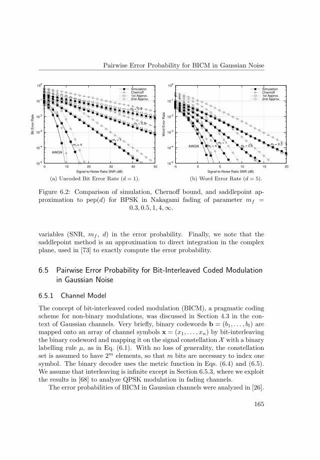
Pairwise Error Probability for BICM in Gaussian Noise

10-5

10-4

10-3

10-2

10-1

100

0 10 20 30 40 50

Bit E

rro

r R

ate

Signal-to-Noise Ratio SNR (dB)

mf = 0.3

mf = 0.5

mf = 1

mf = 4

AWGN

SimulationChernoff1st Approx.2nd Approx.

(a) Uncoded Bit Error Rate (d = 1).

10-5

10-4

10-3

10-2

10-1

100

-5 0 5 10 15 20W

ord

Err

or

Ra

te

Signal-to-Noise Ratio SNR (dB)

mf = 0.3mf = 0.5

mf = 1mf = 4AWGN

SimulationChernoff1st Approx.2nd Approx.

(b) Word Error Rate (d = 5).

Figure 6.2: Comparison of simulation, Chernoff bound, and saddlepoint ap-proximation to pep(d) for BPSK in Nakagami fading of parameter mf =

0.3, 0.5, 1, 4,∞.

variables (SNR, mf , d) in the error probability. Finally, we note that thesaddlepoint method is an approximation to direct integration in the complexplane, used in [73] to exactly compute the error probability.

6.5 Pairwise Error Probability for Bit-Interleaved Coded Modulationin Gaussian Noise

6.5.1 Channel Model

The concept of bit-interleaved coded modulation (BICM), a pragmatic codingscheme for non-binary modulations, was discussed in Section 4.3 in the con-text of Gaussian channels. Very briefly, binary codewords b = (b1, . . . , bl) aremapped onto an array of channel symbols x = (x1, . . . , xn) by bit-interleavingthe binary codeword and mapping it on the signal constellation X with a binarylabelling rule µ, as in Eq. (6.1). With no loss of generality, the constellationset is assumed to have 2m elements, so that m bits are necessary to index onesymbol. The binary decoder uses the metric function in Eqs. (6.4) and (6.5).We assume that interleaving is infinite except in Section 6.5.3, where we exploitthe results in [68] to analyze QPSK modulation in fading channels.

The error probabilities of BICM in Gaussian channels were analyzed in [26].

165

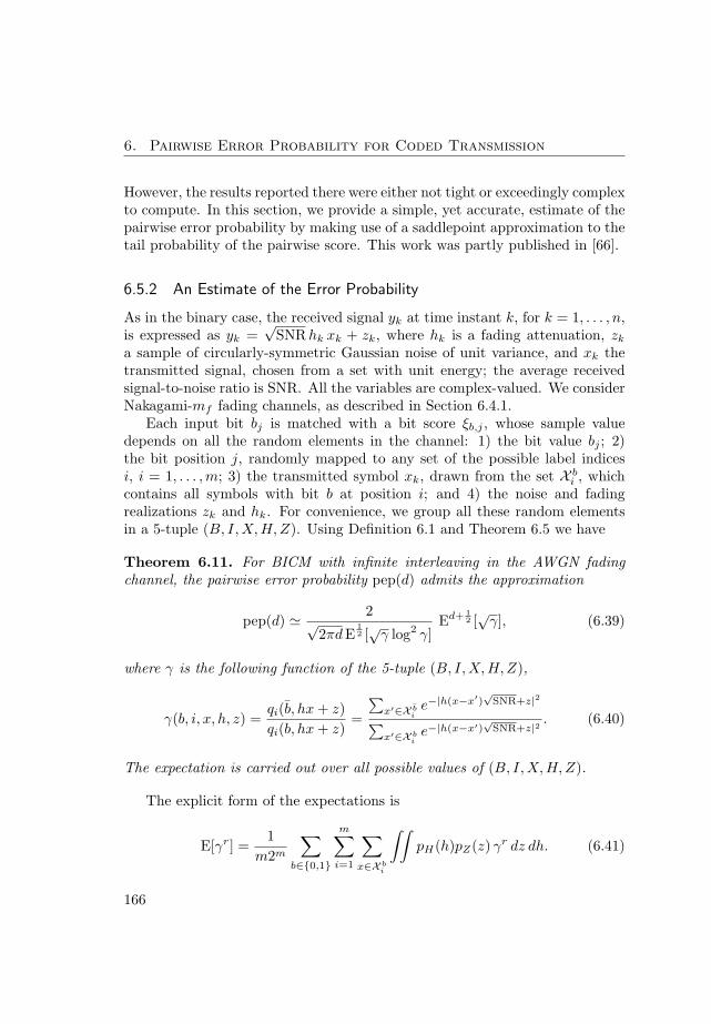
6. Pairwise Error Probability for Coded Transmission

However, the results reported there were either not tight or exceedingly complexto compute. In this section, we provide a simple, yet accurate, estimate of thepairwise error probability by making use of a saddlepoint approximation to thetail probability of the pairwise score. This work was partly published in [66].

6.5.2 An Estimate of the Error Probability

As in the binary case, the received signal yk at time instant k, for k = 1, . . . , n,is expressed as yk =

√SNR hk xk + zk, where hk is a fading attenuation, zk

a sample of circularly-symmetric Gaussian noise of unit variance, and xk thetransmitted signal, chosen from a set with unit energy; the average receivedsignal-to-noise ratio is SNR. All the variables are complex-valued. We considerNakagami-mf fading channels, as described in Section 6.4.1.

Each input bit bj is matched with a bit score ξb,j , whose sample valuedepends on all the random elements in the channel: 1) the bit value bj ; 2)the bit position j, randomly mapped to any set of the possible label indicesi, i = 1, . . . , m; 3) the transmitted symbol xk, drawn from the set X b

i , whichcontains all symbols with bit b at position i; and 4) the noise and fadingrealizations zk and hk. For convenience, we group all these random elementsin a 5-tuple (B, I,X, H,Z). Using Definition 6.1 and Theorem 6.5 we have

Theorem 6.11. For BICM with infinite interleaving in the AWGN fadingchannel, the pairwise error probability pep(d) admits the approximation

pep(d) ' 2√2πd E

12 [√

γ log2 γ]Ed+ 1

2 [√

γ], (6.39)

where γ is the following function of the 5-tuple (B, I,X, H,Z),

γ(b, i, x, h, z) =qi(b, hx + z)qi(b, hx + z)

=

∑x′∈X b

ie−|h(x−x′)

√SNR+z|2

∑x′∈X b

ie−|h(x−x′)

√SNR+z|2 . (6.40)

The expectation is carried out over all possible values of (B, I, X,H, Z).

The explicit form of the expectations is

E[γr] =1

m2m

∑

b∈{0,1}

m∑

i=1

∑

x∈X bi

∫∫pH(h)pZ(z) γr dz dh. (6.41)

166

Pairwise Error Probability for BICM in Gaussian Noise

This expectation can be easily evaluated by numerical integration using theappropriate quadrature rules. Unfortunately, there seems to be no tractable,simple expression for the final result.

Proof. From Definition 6.1 we extract the function γ in Eq. (6.40). Proposi-tion 6.3 shows that the saddlepoint is located at r = 1/2. As computed inProposition 6.3, κ′′1(r) is given by

κ′′1(r) =E[Ξ2

berΞb ]

E[erΞb ]=

E[√

γ log2 γ]E

[√γ] . (6.42)

We next compare the saddlepoint approximation with the alternative meth-ods given in [26] to compute the pairwise error probability pep(d) for BICM: theBhattacharyya union bound and the expurgated BICM union bound. Clearly,the Bhattacharyya union bound is simply the Chernoff bound in Proposition 6.4using the definitions in Theorem 6.11, namely pep(d) ≤ edκ1(r) = Ed[

√γ].

Let pepex(d) denote the pairwise error probability in the expurgated bound.We start the analysis with Eqs. (48-49) in [26] – p. 938 –, which read

pepex(d) =1

2πj

∫ r+j∞

r−j∞ψex(r)d dr

r, (6.43)

where

ψex(r) =1

m2m

m∑

i=1

1∑

b=0

∑

x∈X bi

E[er∆(x,x)

], (6.44)

and the function ∆(x, x′) had been defined in (their) Eq. (33) – p. 936 – as

∆(x, x) = logQ(y|x)Q(y|x)

. (6.45)

Here x is the transmitted symbol, and x its nearest neighbour in X bi , i. e., with

complementary bit b in label index i, and Q(y|x) the channel transition matrix.These equations are very close to our analysis. First, the saddlepoint ap-

proximation is an efficient method to carry out the integration in the complexplane in Eq. (6.43), by choosing r to be the saddlepoint. Then, the expecta-tion in Eq. (6.44) coincides with the expectation used in Theorem 6.11 and the

167

6. Pairwise Error Probability for Coded Transmission

cumulant transform of the bit score is (almost) κ1(r) = log ψex(r). It is notcompletely so because the role of ∆(x, x) is played in our analysis by

log

∑x′∈X b

iQ(y|x′)

∑x′∈X b

iQ(y|x′) . (6.46)

Caire’s equation (6.45) can be obtained by taking only one term in each summa-tion, respectively x and x. From Definition 6.1 we see that this is equivalent tochanging the decoder metric qi(b, y). Depending the specific metric and map-ping rule Caire’s approximation may be accurate or not. For example, in thesimulation results for the set-partitioning mapping reported in [26], the unionbound was not close to the simulation. This inaccuracy was solved in the sim-ulations in [66] by using Eq. (6.46). To any extent, the added complexity fromtaking all terms in Eq. (6.46) is negligible.

Figure 6.3 depicts the pairwise error probability between two codewords atHamming distance d = 5 for several modulations and channel models. Themodulations are 8-PSK, 16-QAM and 64-QAM, all with Gray mapping, andthe channel models AWGN and Rayleigh fading. In all cases the saddlepointapproximation shows an excellent match with the simulation results. Resultsfor convolutional and turbo-like code ensembles may be found in [66].

10-8

10-7

10-6

10-5

10-4

10-3

10-2

10-1

100

0 5 10 15 20

Wo

rd E

rro

r R

ate

Signal-to-Noise Ratio SNR (dB)

8-PSK - Simul.8-PSK - Chernoff8-PSK - Saddl. App.16-QAM - Simul.16-QAM - Chernoff16-QAM - Saddl. App.64-QAM - Simul.64-QAM - Chernoff64-QAM - Saddl. App.

(a) AWGN channel.

10-6

10-5

10-4

10-3

10-2

10-1

100

0 5 10 15 20

Wo

rd E

rro

r R

ate

Signal-to-Noise Ratio SNR (dB)

8-PSK - Simul.8-PSK - Chernoff8-PSK - Saddl. App.16-QAM - Simul.16-QAM - Chernoff16-QAM - Saddl. App.64-QAM - Simul.64-QAM - Chernoff64-QAM - Saddl. App.

(b) Rayleigh fading channel.

Figure 6.3: Comparison of simulation, Chernoff bound, and saddlepoint ap-proximation to pep(d) for d = 5 over 8-PSK, 16-QAM, and 64-QAM.

168

Pairwise Error Probability for BICM in Gaussian Noise

6.5.3 On the Memory among the Channel Outputs

We have assumed in our analysis, as it was done in [26], that bit interleaving isinfinite and that the l BICM sub-channels from bit bj to log-likelihood ratio λj

are independent, and so are the corresponding bit scores. For finite interleaving,some of the d bits in which the two codewords differ may belong to the samesymbol and therefore suffer from the same noise, and some residual statisticaldependence among the bit scores Ξb,j appears, as we mentioned in Section 6.3.In this section we study what arguably constitutes the simplest case, namelyQPSK with Gray mapping under Nakagami fading.

In general, the d bits fall into a number of symbols, each of them havingbetween 1 and m bits. Since it appears almost impossible to know how thesebits are distributed onto the n symbols, it seems more appropriate to computean average pairwise error probability, by averaging over all possible distribu-tions of d bits onto n symbols. Following [68], let us define w = min(m, d)and denote a possible pattern by π` = (`0, . . . , `w), where `v is the number ofsymbols with v bits. Clearly, d =

∑wv=1 v`v and `0 = n−∑w

v=1 `v. A countingargument gives the probability of the pattern π` as

P(π` = (`0, . . . , `w)

)=

(m1

)`1(m2

)`2 · · · (mw

)`w

(mnd

) n!`0!`1!`2!· · · `w!

(6.47)

At this point, it would convenient to define the cumulant transforms ofgeneric symbol scores Ξs for a given Hamming weight in the symbol. Then,κv(r) is such cumulant transform for a Hamming weight v. Definition 6.1corresponds to v = 1 and is thus consistent with this idea. Since we limitourselves to QPSK, we postpone the definition of κ2(r). In Theorem 6.5 weassumed that the cumulant transform of the pairwise score is κpw(r) is givenby dκ1(r). In general, and for a given pattern, one would have that

κpw(r, π`) =w∑

v=1

`vκv(r), (6.48)

since the symbol scores are assumed to be independent. A theorem analogousto Theorem 6.5 can then be formulated. Moreover, the average over all possi-ble patterns π` of the conditional pairwise error probability gives the averagepairwise error probability.

When l →∞ and m > 1 the probability that the bit scores are dependenttends to zero, but does so relatively slowly, as proved in the following

169

6. Pairwise Error Probability for Coded Transmission

Proposition 6.12. The probability that all d bits are independent is Prind

Prind =md

(l/m

d

)(

ld

) . (6.49)

For large l, the probability of πall one = (1, . . . , 1) is

Prind ' e−d(d−1)(m−1)

2l ' 1− d(d−1)(m−1)2l . (6.50)

Proof. We use that `1 = d, `v = 0 for v > 1, and `0 = n− d. The derivation ofthe approximation can be found in Appendix 6.E.

For BPSK, or m = 1, there is no dependence, as it should. We next have

Proposition 6.13. In the Nakagami fading channel with QPSK modulationand Gray mapping, the cumulant transform of the symbol score when two bitsbelong to the same symbol, denoted by κ2(r), is given by

κ2(r) = −mf log(

1 +4r SNR

mf− 4r2 SNR

mf

). (6.51)

Proof. Separating the real and imaginary parts, and respectively denoting themby 1 and 2, the channel has an equivalent output

y1 =√

SNRRe(x)h + Re(z), y2 =√

SNR Im(x)h + Im(z). (6.52)

Conditioned on h, Eq. (6.24) shows that, say, Ξb,1 takes the value

ξb,1 = − SNRχ(Re(x)− Re(x′)

)2 − 2√

SNR√

χ Re(x− x′)Re(z), (6.53)

that is Ξb,1 ∼ N (−2χSNR, 4χSNR). The same analysis gives identical distri-bution for Ξb,2. Eq. (6.55) then follows from the binary case in Theorem 6.9.When χ = |h|2 is the same value for both 1,2, then

κ2(r) = log EE[erΞb,1+rΞb,2 |χ]

= log E[e−2(2rχ SNR +2r2χ SNR)], (6.54)

from which we proceed as in the binary case, in Theorem 6.9.

When the bits belong to different symbols, the same proof shows that anindividual bit behaves as BPSK with signal-to-noise ratio 1

2 SNR. Therefore,the cumulant transform of one such bit score is given by

κ1(r) = −mf log(

1 +2r SNR

mf− 2r2 SNR

mf

). (6.55)

170

Pairwise Error Probability for BICM in Gaussian Noise

For this case, we can index all possible partitions by considering `2, thenumber of symbols with 2 bits. Clearly, this number can take the values `2 =max(0, d− dl/2e), . . . , bd/2c. Applying Eq. (6.47), we obtain

P (`2) =2`1

(ld

) n!(n− `1 − `2)!`1!`2!

. (6.56)

Finally, combining this formula with Proposition 6.13, we average over allpossible mappings of the d bits onto the l/2 QPSK symbols and derive

Theorem 6.14. The average pairwise error probability pep(d) of QPSK withcodeword length l in Nakagami fading is

pep(d) '∑

`2

2`1

(ld

) n!(n− `1 − `2)!`1!`2!

(1 + SNR

2mf

)−mf `1(1 + SNR

mf

)−mf `2

√2π

(`1

SNR1+ SNR

2mf

+ `22 SNR1+ SNR

mf

) ,

(6.57)

where `2 is limited to max(0, d− dl/2e) ≤ `2 ≤ bd/2c, `1 + 2`2 = d.The (averaged) Chernoff bound is

pep(d) ≤∑

`2

2`1

(ld

) n!(n− `1 − `2)!`1!`2!

(1 +

SNR2mf

)−mf `1(1 +

SNRmf

)−mf `2

.

(6.58)

Proof. By construction, the pairwise score is the sum of `1 symbols with Ham-ming weight 1 and `2 symbols with Hamming weight 2, with respective cumu-lant transforms given by Eqs. (6.55) and (6.51). The conditional transform atthe saddlepoint is therefore given by

κpw(r) = −mf `1 log(

1 +SNR2mf

)−mf `2 log

(1 +

SNRmf

). (6.59)

The second derivative can be recovered from Theorem 6.9,

κ′′pw(r) = `14 SNR

1 + SNR2mf

+ `28 SNR

1 + SNRmf

. (6.60)

Figure 6.4 depicts the pairwise error probabilities of Eq. (6.57) for d = 3 andd = 6 in Nakagami fading with mf = 0.5 and mf = 1. Two short interleavers

171

6. Pairwise Error Probability for Coded Transmission

are considered, l = 10 and l = 200. In all cases the effect from the correlation,appearing as a knee in the curves takes place at very low values of pairwiseerror probability, easily below 10−6. Further, the transition takes place at everlower values by increasing the length l or the distance d. In a practical scenario,the effect due to the correlation among the log-likelihood ratios is unlikely todetermine the error probabilities, being other variables, for instance the perfectchannel estimation, which possibly determine the error rates.

10-25

10-20

10-15

10-10

10-5

100

-20 0 20 40 60 80 100

Word

Err

or

Rate

Signal-to-Noise Ratio SNR (dB)

d = 3, l = 10, mf = 0.5d = 3, l = 200, mf = 0.5d = 3, l = 10, mf = 1d = 3, l = 200, mf = 1d = 6, l = 10, mf = 0.5d = 6, l = 200, mf = 0.5d = 6, l = 10, mf = 1d = 6, l = 200, mf = 1

Figure 6.4: Saddlepoint approximation pep(d) for QPSK in Nakagami fadingmf = 0.5, 1; Hamming distance d = 3, 6, and codeword length l = 10, 200.

Going back to the general BICM case, the apparent closeness of the BICMprobability analysis with the simulation results is likely due to the limited effectof the dependence across the log-likelihood ratios, compared to a situation withno statistical independence (infinite interleaving). It would be interesting tocharacterize this effect quantitatively and find the threshold signal-to-noiseratio at which the dependence starts being noticeable.

A second conclusion one can draw is that for finite interleaving and high-enough signal-to-noise ratio, the error probability will be determined by theworst possible π`, that having the largest tail for the log-likelihood ratio. Thisimplies that any analysis based on infinite interleaving fails for large enoughSNR. A caveat is in order, since this large enough may be extremely large.

172

Error Probability in the Exponential Noise Channel

6.5.4 Cumulant transform asymptotic analysis

An interesting result of [66], proved by Albert Guillen i Fabregas, concerns thelimit for large SNR of BICM. For the AWGN channel with no fading BICMbehaves as a binary modulation, in the sense that

limSNR→∞

κ1(r)SNR

= −d2min

4, (6.61)

where d2min = minx,x′∈X |x − x′|2 is the minimum squared Euclidean distance

of the constellation. For some standard modulations, the minimum distance isgiven by (see for instance Table I of [74])

d2min = 4 sin2 π

2mfor 2m-PSK, (6.62)

d2min =

1222m − 1

for 2m-PAM, (6.63)

d2min =

6(2m − 1)

for 2m-QAM. (6.64)

Note that the mapping does not affect the result.The loss with respect to binary modulation (d2

min = 4) for 8-PSK amountsto 8.34 dB, for 16-QAM is 10 dB, and for 64-QAM becomes 16.23 dB. At lowSNR, these values match well with the simulations reported in Fig. 6.3, whencompared with the binary case included in Fig. 6.2b.

We will later see that a similar result holds for the additive energy channels.

6.6 Error Probability in the Exponential Noise Channel

In this section, we study the pairwise error probability in the additive exponen-tial noise (AEN) channel. As for the Gaussian channel, we build our analysisaround the pairwise and bit scores. The results presented here seem to be newand are somewhat surprising, in the sense that the pairwise error probabilityis very close to that of an AWGN channel with identical signal-to-noise ratio:

• The Chernoff bound to the pairwise error probability for BPSK and bi-nary modulation in the AEN channel coincide.

• For BICM at large signal-to-noise ratio SNR, and comparing the Chernoffbounds to the pairwise error probability, 22m-PEM in AEN incurs in apower loss of 3

2 (about 1.76 dB) with respect to 22m-QAM in AWGN.

173

6. Pairwise Error Probability for Coded Transmission

This similarity strongly suggests that binary codes will achieve essentially thesame performance in these two channels.

6.6.1 Channel Model for Binary Modulation

We start with the study of binary modulation (2-PEM). At the transmitter,each bit bk is mapped onto a binary symbol xk, with xk = {0, +2}; the mappingrule µ is

xk = 0, if bk = 0; xk = +2, if bk = 1, (6.65)

used with probability 1/2, and its complement µ, used with probability 1/2.The choice between µ and µ is made known to the receiver.

At the channel output, and for each index k, the output yk is given by

yk = SNR xkχk + zk, (6.66)

where zk is a real-valued, exponentially distributed, noise Zk ∼ E(1), SNR isthe average signal-to-noise ratio at the receiver, and χk is a fading coefficienthaving a gamma distribution, as in Eq. (6.22). For a fixed fading realization,assumed known at the receiver, the channel transition probability Q(y|x) is

Q(y|x) = e−(y−SNR xχ)u(y − SNRxχ). (6.67)

The presence of the fading is a natural generalization of the exponential channelwe have considered so far and fits smoothly with its Gaussian counterpart. Inthe additive energy channels, we use the name “gamma fading” rather thanNakagami fading, since the latter is usually expressed in terms of the complexamplitude, rather than the energy.

6.6.2 Error Probability in the absence of Fading

We first consider the case without fading, obtained by setting χk = 1 in themodel, Eq. (6.66). The natural counterpart of the Gaussian result is

Theorem 6.15. The binary AEN channel is a Z-channel with transition prob-ability ε = e−2 SNR. The cumulant transform of the bit score is

κ1(r) = log(

12e−2r SNR +

12e−2(1−r) SNR

)(6.68)

= − SNR+ log cosh(SNR(2r − 1)

), (6.69)

174

Error Probability in the Exponential Noise Channel

and the pairwise error probability for Hamming distance d is

pep(d) '

2√2πd

(∑ d−12

j=0 e−2j SNR

)e−(d+1) SNR, d odd,

2√2πd

(12 +

∑ d2j=1 e−2j SNR

)ε−d SNR, d even

. (6.70)

The Chernoff bound to the pairwise error probability is

pep(d) ≤ e−d SNR. (6.71)

Proof. Let symbol x be transmitted and x denote its complement. The bitscore ξb depends on the noise realization z as

ξb = loge−(SNR x+z−SNR x)u(SNR x + z − SNR x)e−(SNR x+z−SNR x)u(SNR x + z − SNRx)

(6.72)

= log(e− SNR(x−x)u(SNR(x− x) + z)

). (6.73)

There are two possibilities, u(SNR(x− x) + z) = 0 or u(SNR(x− x) + z) = 1.The first takes place when SNR(x− x) + z < 0 and occurs with a probability

∫ SNR(x−x)

0

e−t dt = 1− e− SNR(x−x). (6.74)

In this case ξb = −∞. In the second case, SNR(x− x) + z ≥ 0, an event withprobability e− SNR(x−x), and inducing a bit score ξb = − SNR(x− x).

Using the randomized mapping, there are three possible values of ξb,

ξb =

−∞, with probability 12 (1− e−2 SNR),

−2 SNR, with probability 12 ,

2 SNR, with probability 12e−2 SNR.

(6.75)

This corresponds to a Z-channel with transition probability ε = e−2 SNR. Therest of the theorem is an application of Theorem 6.7.

Remark that the use of the continuous saddlepoint approximation, given inTheorem 6.5 would lead to inexact results.

Since the Chernoff bound coincides with the value of BPSK in the AWGNchannel, given in Eq. (6.31), the error performance of both modulation formatswould be similar for identical levels of signal-to-noise ratio.

175

6. Pairwise Error Probability for Coded Transmission

Also, the error probability decays as e−(d+1) SNR when d is odd, slightlyfaster than in the Chernoff bound. This effect may create some room to designefficient codes for this channel, since the error probability for d odd is similar tothe error probability with d + 1, buying, so to speak, some Hamming distancefrom the channel itself. A similar effect was noticed by van de Meeberg in theanalysis of binary symmetric channels [75]. A special case of d odd is uncodedtransmission, for which d = 1, and the exact bit error rate is

Pb = Pr(Ξ > 0) =12e−2 SNR. (6.76)

This value should be compared with the saddlepoint approximation, Pb '2√2π

e−2 SNR ' 0.798e−2 SNR, a reasonably good approximation.Figure 6.5 depicts the word error rate with 2-PEM for several values of d.

Simulations match well with the approximation in Theorem 6.15. The Chernoffbound does not give the correct dependence with d for odd d, especially ford = 1; this problem does not arise for the saddlepoint approximation.

10-8

10-7

10-6

10-5

10-4

10-3

10-2

10-1

100

-4 -2 0 2 4 6 8 10

Word

Err

or

Rate

Signal-to-Noise Ratio SNR (dB)

SimulationChernoffApprox.d = 1d = 2d = 3d = 4d = 5d = 6

Figure 6.5: Comparison of simulation and saddlepoint approximation to pep(d)of 2-PEM in the AEN channel, d = 1, . . . , 6.

6.6.3 Error Probability with Gamma Fading

We complete our analysis of the AEN channel by considering the effect ofgamma fading. In this case, it is possible to compute an exact expression forthe uncoded error probability. Conditioned to a fading realization, the error

176

Error Probability in the Exponential Noise Channel

probability is given by12e−2χ SNR, (6.77)

and after averaging over the fading realizations,

Pb =∫ +∞

0

mmf

f χmf−1

Γ(mf )e−mf χ 1

2e−2χ SNR dχ =

12

(1 +

2SNRmf

)−mf

, (6.78)

obtained from the definition of the gamma function, see Eq. (3.34). This niceformula does not seem to extend easily to the pairwise error probability. How-ever, we have

Theorem 6.16. In the binary AEN channel with gamma fading, the cumulanttransform of the bit score Ξb is given by

κ1(r) = log

(12

(1 +

2r SNRmf

)−mf

+12

(1 +

2(1− r) SNRmf

)−mf)

. (6.79)

The Chernoff bound to the pairwise error probability is

pep(d) ≤(

1 +SNRmf

)−mf d

. (6.80)

The saddlepoint approximation to the pairwise error probability is

pep(d) '

2√2πd

(∑ d−12

j=0

(1 + (d+1+2j) SNR

mf

)−mf)

, d odd,

2√2πd

(12

(1 + d SNR

mf

)−mf

+∑ d

2j=1

(1 + (d+2j) SNR

mf

)−mf)

, d even.

(6.81)

Proof. Conditioned on a fading realization χ, it is clear from the proof of The-orem 6.15 that Ξb has the discrete distribution of a Z-channel with transitionprobability ε = e−2χ SNR. Using the definition of Ξb, we rewrite κ1(r) as

κ1(r) = log E E[erΞ|χ]

, (6.82)

where the inner expectation is for a fixed fading realization. The momentgenerating function, eκ1(r), is derived from Theorem 6.15,

E[esΞb |χ]

=12e−2sχ SNR +

12e−2(1−s)χ SNR, (6.83)

177

6. Pairwise Error Probability for Coded Transmission

from which we deduce that

κ1(r) = log12

∫ +∞

0

mmf

f χmf−1

Γ(mf )e−mf χ

(e−2rχ SNR + e−2(1−r)χ SNR

)dχ (6.84)

= log

(12

(1 +

2r SNRmf

)−mf

+12

(1 +

2(1− r) SNRmf

)−mf)

. (6.85)

From Proposition 6.3, the saddlepoint is located at r = 1/2, and

κ1(r) = −mf log(

1 +SNRmf

). (6.86)

The Chernoff bound is then obtain by using Proposition 6.4.The saddlepoint approximation follows from integrating the approximation

in the absence of fading, given in Theorem 6.15, and using the definition of theGamma function.

In practice, the sums over j in Eq. (6.81) are dominated by the first term,and good approximations would be obtained by using only them.

In this result, we have not used a direct saddlepoint approximation to thetail probability of Ξpw, such as that of Theorem 6.5. The reason is that thelatter approximation is not tight for large values of mf , that is small fading,when the score becomes ever more “discrete”. To any extent, the equation inthe absence of fading can be integrated term by term and the final formulagives a good approximation, as can be seen from Fig. 6.6, where simulationand the approximation for uncoded 2-PEM in gamma fading of parametermf = 0.3, 0.5, 1, 4,∞ are compared. Similarly good match is observed for thepairwise error probability pep(d).

6.6.4 Bit-Interleaved Coded Modulation

In Section 6.5, we discussed bit-interleaved modulation (BICM) for Gaussiannoise and gave a saddlepoint approximation to its pairwise error probability.For BICM, the channel model in Eq. (6.66) is still valid, with the addition thatthe symbols xk are not directly indexed by the mapping rule in Eq. (6.65), butrather the binary codeword b is mapped onto an array of channel symbols x bybit-interleaving the binary codeword and mapping it on the signal constellationX with a binary labelling rule µ. We have then

178

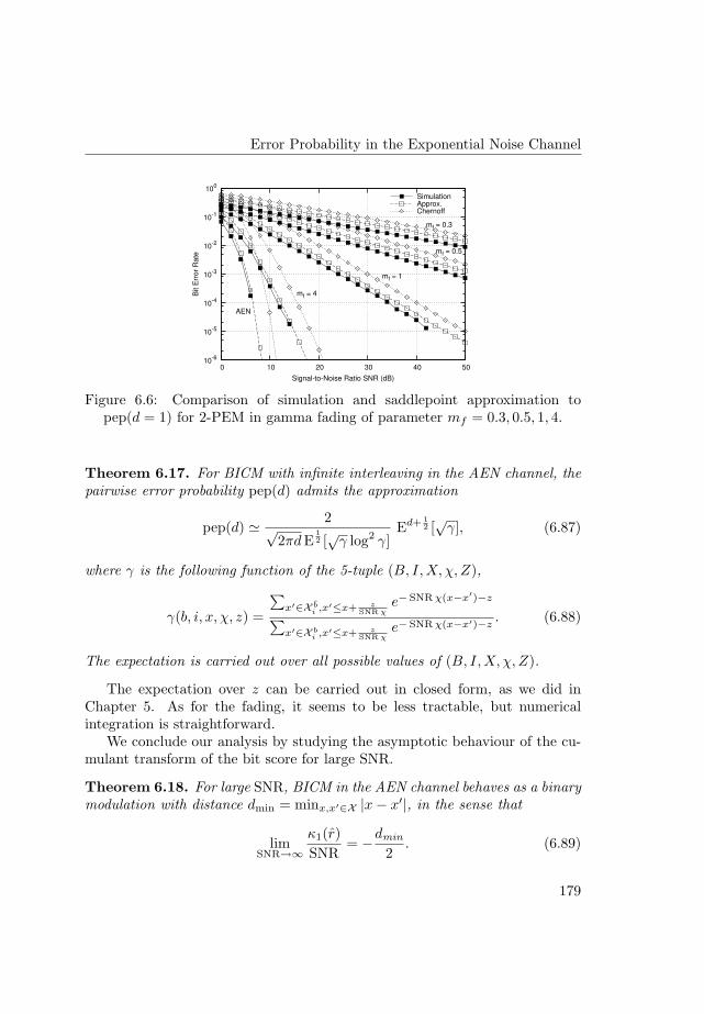
Error Probability in the Exponential Noise Channel

10-6

10-5

10-4

10-3

10-2

10-1

100

0 10 20 30 40 50

Bit E

rro

r R

ate

Signal-to-Noise Ratio SNR (dB)

mf = 0.3

mf = 0.5

mf = 1

mf = 4

AEN

SimulationApprox.Chernoff

Figure 6.6: Comparison of simulation and saddlepoint approximation topep(d = 1) for 2-PEM in gamma fading of parameter mf = 0.3, 0.5, 1, 4.

Theorem 6.17. For BICM with infinite interleaving in the AEN channel, thepairwise error probability pep(d) admits the approximation

pep(d) ' 2√2πd E

12 [√

γ log2 γ]Ed+ 1

2 [√

γ], (6.87)

where γ is the following function of the 5-tuple (B, I, X, χ, Z),

γ(b, i, x, χ, z) =

∑x′∈X b

i ,x′≤x+ zSNR χ

e− SNR χ(x−x′)−z

∑x′∈X b

i ,x′≤x+ zSNR χ

e− SNR χ(x−x′)−z. (6.88)

The expectation is carried out over all possible values of (B, I,X, χ, Z).

The expectation over z can be carried out in closed form, as we did inChapter 5. As for the fading, it seems to be less tractable, but numericalintegration is straightforward.

We conclude our analysis by studying the asymptotic behaviour of the cu-mulant transform of the bit score for large SNR.

Theorem 6.18. For large SNR, BICM in the AEN channel behaves as a binarymodulation with distance dmin = minx,x′∈X |x− x′|, in the sense that

limSNR→∞

κ1(r)SNR

= −dmin

2. (6.89)

179

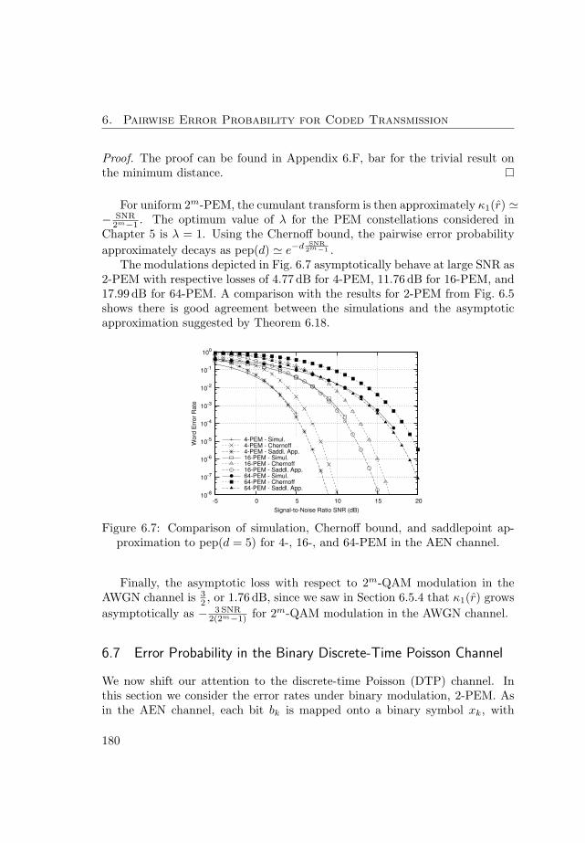
6. Pairwise Error Probability for Coded Transmission

Proof. The proof can be found in Appendix 6.F, bar for the trivial result onthe minimum distance.

For uniform 2m-PEM, the cumulant transform is then approximately κ1(r) '− SNR

2m−1 . The optimum value of λ for the PEM constellations considered inChapter 5 is λ = 1. Using the Chernoff bound, the pairwise error probabilityapproximately decays as pep(d) ' e−d SNR

2m−1 .The modulations depicted in Fig. 6.7 asymptotically behave at large SNR as

2-PEM with respective losses of 4.77 dB for 4-PEM, 11.76 dB for 16-PEM, and17.99 dB for 64-PEM. A comparison with the results for 2-PEM from Fig. 6.5shows there is good agreement between the simulations and the asymptoticapproximation suggested by Theorem 6.18.

10-8

10-7

10-6

10-5

10-4

10-3

10-2

10-1

100

-5 0 5 10 15 20

Wo

rd E

rro

r R

ate

Signal-to-Noise Ratio SNR (dB)

4-PEM - Simul.4-PEM - Chernoff4-PEM - Saddl. App.16-PEM - Simul.16-PEM - Chernoff16-PEM - Saddl. App.64-PEM - Simul.64-PEM - Chernoff64-PEM - Saddl. App.

Figure 6.7: Comparison of simulation, Chernoff bound, and saddlepoint ap-proximation to pep(d = 5) for 4-, 16-, and 64-PEM in the AEN channel.

Finally, the asymptotic loss with respect to 2m-QAM modulation in theAWGN channel is 3

2 , or 1.76 dB, since we saw in Section 6.5.4 that κ1(r) growsasymptotically as − 3 SNR

2(2m−1) for 2m-QAM modulation in the AWGN channel.

6.7 Error Probability in the Binary Discrete-Time Poisson Channel

We now shift our attention to the discrete-time Poisson (DTP) channel. Inthis section we consider the error rates under binary modulation, 2-PEM. Asin the AEN channel, each bit bk is mapped onto a binary symbol xk, with

180

Error Probability in the Binary Discrete-Time Poisson Channel

xk = {0, +2}; the mapping rule µ is

xk = 0, if bk = 0; xk = +2, if bk = 1, (6.90)

used with probability 1/2, and its complement µ, used with probability 1/2.The choice between µ and µ is known at the receiver.

At time k, the channel output yk follows a Poisson distribution with param-eter εsxkχk, where εs is the average signal count, and χk is a fading coefficienthaving a gamma distribution, as in Eq. (6.22). For a fixed fading realization(known at the receiver) the channel transition probability Q(y|x) is

Q(y|x) = e−εsxχ (εsxχ)y

y!. (6.91)

We directly estimate the performance for the binary DTP channel in

Theorem 6.19. In the absence of fading, the binary DTP channel is a Z-channel with transition probability ε = e−2εs . The pairwise error probabilityadmits the saddlepoint approximation

pep(d) =

2√2πd

(∑ d−12

j=0 e−2jεs

)e−(d+1)εs , d odd,

2√2πd

(12 +

∑ d2j=1 e−2jεs

)ε−dεs , d even

. (6.92)

The Chernoff bound to the pairwise error probability is

pep(d) ≤ e−dεs . (6.93)

In the presence of gamma fading, the Chernoff bound is

pep(d) ≤(

1 +εs

mf

)−mf d

, (6.94)

and the saddlepoint approximation to the pairwise error probability is

pep(d) '

2√2πd

(∑ d−12

j=0

(1 + (d+1+2j)εs

mf

)−mf)

, d odd,

2√2πd

(12

(1 + dεs

mf

)−mf

+∑ d

2j=1

(1 + (d+2j)εs

mf

)−mf)

, d even.

(6.95)

181

6. Pairwise Error Probability for Coded Transmission

The theorem coincides with the result for the AEN channel, replacing SNRby εs. Therefore, the comments and figures in Sections 6.6.2 and 6.6.3 applyunchanged to the DTP channel.

Proof. We prove the equivalence to a Z-channel. Under input randomization, asymbol x1 = 0 is chosen with probability 1/2, in which case the output is y = 0,and the bit score is ξb = log e−2εs = −2εs. The symbol x2 = 2εs is chosen withprobability 1/2. We distinguish two cases, y = 0, where ξb = log e2εs = 2εs,and y > 0, for which ξb = −∞. This coincides with the binary AEN channel.Therefore the proofs of Theorems 6.15 and 6.16 apply.

As for bit-interleaved coded modulation, we have the following

Theorem 6.20. For BICM with infinite interleaving in the DTP channel, thepairwise error probability pep(d) admits the approximation

pep(d) ' 2√2πd E

12 [√

γ log2 γ]Ed+ 1

2 [√

γ], (6.96)

where γ is the following function of the 5-tuple (B, I,X, χ, Y ),

γ(b, i, x, χ, y) =

∑x′∈X b

ix′y e− SNR χx′

∑x′∈X b

ix′y e− SNR χx′ . (6.97)

The expectation is carried out over all possible values of (B, I, X, χ, Y ).

We conclude our analysis by studying the asymptotic behaviour of the cu-mulant transform of the bit score for large εs.

Theorem 6.21. As the average number of quanta εs goes to infinity, the cu-mulant transform of the bit score evaluated at the saddlepoint behaves as

limεs→∞

κ1(r)εs

= − minx,x′∈X

12(√

x−√

x′)2

. (6.98)

The limit for uniform 2m-PEM modulation is given by

limεs→∞

κ1(r)εs

= −(

1−√

2m − 22m − 1

)2

. (6.99)

182

Error Probability in the Binary Discrete-Time Poisson Channel

For a given constellation set, the largest limit (in absolute value) is achievedwhen the modulation points xj, j = 1, . . . , 2m, are placed at

xj = (j − 1)26

(2m+1 − 1)(2m − 1). (6.100)

For this modulation set, the limit as εs →∞ is

limεs→∞

κ1(r)εs

=3

(2m+1 − 1)(2m − 1). (6.101)

The optimum constellation was also given in [64]. Note that the optimumvalue of λ for the PEM constellations considered in Chapter 5 is λ = 2.

Using the Chernoff bound, the pairwise error probability approximately

decays as pep(d) ' e−d 3εs

(2m+1−1)(2m−1) for the optimum constellation and as

pep(d) ' e−dεs

(1−

√2m−22m−1

)2

for the uniform constellation. For the cases de-picted in Fig. 6.8a, the asymptotic energy loss of uniform 2m-PEM with re-spect to binary modulation are 14.73 dB for 4-PEM, 29.39 dB for 16-PEM, and41.97 dB for 64-PEM, in good agreement with Fig. 6.5.

10-8

10-7

10-6

10-5

10-4

10-3

10-2

10-1

100

-5 0 5 10 15 20 25 30 35 40

Word

Err

or

Ra

te

Input Number of Quanta ε s (dB)

4-PEM - Simul.4-PEM - Chernoff4-PEM - Saddl. App.16-PEM - Simul.16-PEM - Chernoff16-PEM - Saddl. App.64-PEM - Simul.64-PEM - Chernoff64-PEM - Saddl. App.

(a) Uniformly spaced constellation.

10-8

10-7

10-6

10-5

10-4

10-3

10-2

10-1

100

-10 0 10 20 30 40

Word

Err

or

Ra

te

Input Number of Quanta ε s (dB)

4-PEM - Simul.4-PEM - Chernoff4-PEM - Saddl. App.16-PEM - Simul.16-PEM - Chernoff16-PEM - Saddl. App.64-PEM - Simul.64-PEM - Chernoff64-PEM - Saddl. App.

(b) Optimized constellation.

Figure 6.8: Comparison of simulation, Chernoff bound, and saddlepoint ap-proximation to pep(d = 5) for 4-, 16-, and 64-PEM in the DTP channel.

As for the optimum constellation, depicted in Fig. 6.8b, the energy losswith respect to binary modulation is reduced to 8.45 dB for 4-PEM, 21.90 dB

183

6. Pairwise Error Probability for Coded Transmission

for 16-PEM, and 34.26 dB for 64-PEM. As m becomes large, the exponentis approximately 3

22−2m, similar to the value 3 2−2m achieved by 2m-PAM inGaussian channels, as a function of SNR. In general, simulation results matchwell with the limit given by the theorem and with the saddlepoint approxima-tion. On the other hand, the Chernoff bound is somewhat loose, as expected.

6.8 Conclusions

In this chapter, we have studied the computation of the pairwise error proba-bility, an essential tool to estimate the error rates of practical channel codes.Unlike other common approaches to the subject, we have not derived truebounds to the error probability, such as the Chernoff bound, but have rathercomputed a saddlepoint approximation to the probability. In general, the ap-proximation has been found to be very close to the exact simulation values. Thesaddlepoint approximation for continuous random variables has been derivedanew, and its expansion up to second order determined. This approximationis valid for all values of the saddlepoint, even as it approaches zero.

We have found it useful to define a new quantity, the pairwise score, arandom variable which depends on all the random elements in the channel andwhose positive tail probability gives the pairwise error probability. For twocodewords at Hamming distance d, the pairwise score is in turn the sum of dbit scores. For memoryless and stationary channels with binary input the bitscores are independent, but in general are statistically dependent. We havecarried out our analysis of bit-interleaved coded modulation by assuming thatthey are independent, as proposed by Caire et al. [26].

Throughout the chapter we have considered a specific decoding metric,defined in Section 6.3, similar to the one used in BICM decoding. The methodspresented in this chapter can however be easily extended to other metrics.

When applied to the AWGN channel, the formulas we have found seemto rank among the simplest yet closest approximations to the error probabil-ity. Two special cases are of particular interest, the fully-interleaved Nakagamifading channel, considered in Section 6.4, and the performance under BICM,discussed in Section 6.5. In the analysis of BICM, have solved a small inconsis-tency in the bounds presented in the paper [26] by Caire et al.. In Section 6.5.3we have briefly considered the subject of finite interleaving and determined theperformance of QPSK in fully-interleaved Nakagami fading channels. The ef-fect of the finite interleaving has been found to be negligible.

184

Saddlepoint Location

We have seen how the AEN and the DTP channels with binary input admita natural modelling as a Z-channel. We have determined the saddlepoint ap-proximation to the error probability of the Z-channel, and therefore also to theother channels. We have considered gamma fading channels, a natural counter-part to Nakagami fading in the AWGN channel. Intriguingly, the performanceof binary modulation in the exponential channel is almost identical to that ofBPSK in Gaussian noise, for all the values of the fading parameter.

As for BICM, we have seen that the performance of 2m-PEM at large signal-to-noise ratio in the AEN channel remains close to that of an AWGN channelwith identical signal-to-noise ratio. More specifically, the pairwise error proba-bility asymptotically decays in both channels as e−a SNR 2−m

for large SNR andlarge m; a is a constant factor of value a = 3/2 for 2m-QAM modulation inthe AWGN channel and a = 1 for 2m-PEM modulation in the AEN channel.

Regarding non-binary transmission in the DTP channel, general formu-las for the pairwise error probability have been given. These formulas showthat equispaced 2m-PEM modulation is non-optimal, as already discovered byEinarsson [64]. For the optimum constellation, a PEM modulation with pa-rameter λ = 2, the asymptotic behaviour of the error probability as a functionof the quanta count coincides with that of a Gaussian channel using 2m-PAMmodulation, i. e. it asymptotically decays as e−aεs2−2m

for large εs and largem; here a = 3 for the AWGN channel and a = 3/2 for the DTP channel.

An interesting possible extension of the present work would include theanalysis of the general quantized additive energy channel, in order to determinethe way the functional form of the pairwise error probability changes betweenthe additive exponential and discrete-time Poisson limits.

6.A Saddlepoint Location

For each i, and conditioned on b, the output density Qi(y|b) is given byEq. (6.6). Since the metric qi(b, y) is proportional to Qi(y|b), we have that

E[erΞ] =∫ (

12Qi(y|0)er log

Qi(y|1)Qi(y|0) +

12Qi(y|1)er log

Qi(y|0)Qi(y|1)

)dy (6.102)

=∫ (

12Q1−r

i (y|0)Qri (y|1) +

12Q1−r

i (y|1)Qri (y|0)

)dy. (6.103)

This quantity is symmetric around r = 12 , since it remains unchanged if we

replace r by 1− r.

185

6. Pairwise Error Probability for Coded Transmission

The first derivative of κ1(r) is given by κ′1(r) =E[ΞberΞb

]

E[erΞb

] , and is thus zero

when E[Ξbe

rΞb]

= 0. We concentrate on E[Ξbe

rΞb], readily computed as

∫12

(Qi(y|0) log

Qi(y|1)Qi(y|0)

(Qi(y|1)Qi(y|0)

)r

+ Qi(y|1) logQi(y|0)Qi(y|1)

(Qi(y|0)Qi(y|1)

)r)

dy

(6.104)

=∫

12

(Qi(y|0)

(Qi(y|1)Qi(y|0)

)r

−Qi(y|1)(

Qi(y|1)Qi(y|0)

)r)

logQi(y|1)Qi(y|0)

dy, (6.105)

which is zero at r = 12 thanks to the symmetry.

As for the other derivatives, we have that

κ′′1(r) =E

[Ξ2

berΞb

]

E[erΞb

] − E2[Ξbe

rΞb]

E2[erΞb

] (6.106)

κ′′′1 (r) =E

[Ξ3

berΞb

]E

[erΞb

]

E2[erΞb

] − 3 E[Ξ2

berΞb

]E

[Ξbe

rΞb]

E2[erΞb

] +2E3

[Ξbe

rΞb]

E3[erΞb

] ,

(6.107)

which, evaluated at the saddlepoint, respectively become

κ′′1(r) =E

[Ξ2

berΞb

]

E[erΞb

] , κ′′′1 (r) =E

[Ξ3

berΞb

]

E[erΞb

] . (6.108)

We thus find that the second derivative is proportional to

12

∫ (Qi(y|0)

(Qi(y|1)Qi(y|0)

)r

+ Qi(y|1)(

Qi(y|1)Qi(y|0)

)r)

log2 Qi(y|1)Qi(y|0)

dy, (6.109)

which is positive at r = 12 . As for the third derivative, it is proportional to

12

∫ (Qi(y|0)

(Qi(y|1)Qi(y|0)

)r

−Qi(y|1)(

Qi(y|1)Qi(y|0)

)r)

log3 Qi(y|1)Qi(y|0)

dy, (6.110)

which is zero at r = 12 , thanks to the symmetry.

186

A Derivation of the Saddlepoint Approximation

6.B A Derivation of the Saddlepoint Approximation

We wish to estimate the tail probability Pr(Z > z0) for Z, a continuous randomvariable with density pZ(z). Instead of the density, we represent Z by itscumulant transform κ(r), defined as κ(r) = log E[erZ ], r a complex number.

Often, the saddlepoint approximation is derived by assuming that Z is thesum of d random variables Xi, Z =

∑dj=1 Xj , and the asymptotic behaviour

as d → ∞ is studied. Since in our problem there need be no asymptotics,we prefer to work with Z directly. To any extent, when the variables Xj

are independent, the cumulant transform of Z is the sum of the transformsfor each component, and the analysis applies unchanged. Bar for this changeof emphasis, the presentation follows closely, and slightly generalizes, Olver’sbook [70], and Jensen’s [67].

The tail probability can be recovered from κ(r) by Fourier inversion:

Pr(Z >z0) =1

2πj

∫ j∞

r=−j∞eκ(r)−rz0

dr

r. (6.111)

An application of Cauchy’s integral theorem allows us to shift the integra-tion path to the right, from the imaginary axis to a line L = (r− j∞, r + j∞)that crosses the real axis at another point r.

It is most convenient to choose r the real number which verifies κ′(r) = z0.Since complex-variable analytic functions do not reach extreme points, thispoint is a saddlepoint. It exists and is unique due to the convexity of κ(r)for r real. The shifted integration path can be parameterized by r = r + jri,−∞ < ri < ∞, or (r− r) = jri. Using this new variable of integration we nowexpand the argument of the exponential term in a Taylor series around r,

κ(r)− rz0 = κ(r)− rz0 +κ′′(r)

2!(jri)2 + R2(ri), (6.112)

where we have used that the first derivative is zero and R2(ri) includes theremaining terms in the expansion around r,

R2(ri) =∞∑

`=3

κ(`)(r)`!

(jri)`. (6.113)

187

6. Pairwise Error Probability for Coded Transmission

Eq. (6.111) can then be rewritten as

Pr(Z > z0) =12π

eκ(r)−rz0

∫ +∞

−∞e−

κ′′(r)2 r2

i eR2(ri)dri

r + jri(6.114)

=12π

eκ(r)−rz0

∫ +∞

−∞e−

κ′′(r)2 r2

i eR2(ri)r − jri

r2 + r2i

dri, (6.115)

where we have multiplied numerator and denominator times a factor r − jri.We next use the Taylor series of the exponential to expand eR2(ri), and

express it in powers of ri. Including the factor r − jri in the expansion,

(r − jri)eR2(ri) = (r − jri)∞∑

m=0

1m!

( ∞∑

`=3

κ(`)(r)`!

(jri)`

)m

(6.116)

=∞∑

m=0

ηm rmi , (6.117)

where the terms with common factor rmi are grouped, and their corresponding

coefficient denoted by ηm. The symmetry of the integrand in Eq. (6.115) impliesthat the integral of the terms with odd m is zero; we need thus consider onlyeven values of m, which we parameterize by m = 2n. The first few terms are

η0 = r, η2 = 0, (6.118)

η4 = −κ(3)(r)3!

+ rκIV (r)

4!, (6.119)

η6 =κ(5)(r)

5!− r

κ(6)(r)6!

− r12!

(κ(3)(r)

3!

)2

. (6.120)

The next step is the normalization of the `-th order derivatives, or `-thcumulant, by κ′′(r). The normalized `-th derivative, denoted by κ(`)(r), is

κ(`)(r) = κ(`)(r)κ′′(r), (6.121)

and the coefficients η2n become polynomials in κ′′(r). The degree of the polyno-mials will prove useful when tracking the various terms in the final expansion.

The tail probability in Eq. (6.115) becomes

Pr(Z > z0) = eκ(r)−rz0

∞∑n=0

η2nτ(2n), (6.122)

188

A Derivation of the Saddlepoint Approximation

a weighted sum of integrals τ(2n), for non-negative n, of the form

τ(2n) =12π

∫ +∞

−∞e−

κ′′(r)2 x2 x2n

r2 + x2dx. (6.123)

For n = 0,

12π

∫ +∞

−∞e−

κ′′(r)2 x2 1

r2 + x2dx =

12r

erfc

(r

√κ′′(r)

2

)exp

(r2 κ′′(r)

2

), (6.124)

where erfc(x) is the error complementary function erfc(x) = 2π

∫∞x

e−t2 dt. Ithas an asymptotic series

erfc(x) =e−x2

x√

π

∞∑m=0

(−1)m 1 · 3 ·· · · (2m− 1)2mx2m

, (6.125)

and therefore

τ(0) =1

r2√

2πκ′′(r)

∞∑m=0

(−1)m 1 · 3 ·· · · (2m− 1)r2m

(κ′′(r)

)m . (6.126)

In general, when n 6= 0, we can expand the fraction in the integrand byexplicitly carrying out the division. We obtain then

x2n

r2 + x2=

n−1∑

i=0

(−1)n−i−1r2(n−i−1)x2i + (−1)n r2n

r2 + x2, (6.127)

a sum which we next integrate term by term. Each summand,

12π

∫ +∞

−∞e−

κ′′(r)2 x2

x2i dx, (6.128)

is seen to be proportional to the 2i-th moment of a normal random variablewith zero mean and variance

(κ′′(r)

)−1, and therefore

12π

∫ +∞

−∞e−

κ′′(r)2 x2

x2i dx =1 · 3· · · (2i− 1)√

2π(κ′′(r)

)i+ 12. (6.129)

When i = 0, we agree that the product 1· · · (2i− 1) is 1.

189

6. Pairwise Error Probability for Coded Transmission

Combining the summands in Eq. (6.127) back into Eq. (6.123), and usingthe expansion (6.126) for the last summand in Eq. (6.127), we get

τ(2n) =n−1∑

i=0

(−1)n−i−1r2(n−i−1) 1 · 3· · · (2i− 1)√

2π(κ′′(r)

)i+ 12

+ (−1)nr2n 1r2

√2πκ′′(r)

∞∑m=0

(−1)m 1 · 3 ·· · · (2m− 1)r2m

(κ′′(r)

)m (6.130)

=1

r2√

2πκ′′(r)

(n−1∑

i=0

(−1)n−i−1r2(n−i) 1 · 3 ·· · ·(2i− 1

)(κ′′(r)

)i

+∞∑

m=0

(−1)n+mr2(n−m) 1 · 3 ·· · · (2m− 1)(κ′′(r)

)m

)(6.131)

=1

r2√

2πκ′′(r)

∞∑m=n

(−1)n+mr2(n−m) 1 · 3 ·· · · (2m− 1)(κ′′(r)

)m . (6.132)

To derive Eq. (6.131) we used some obvious algebraic combinations, and thelast equation follows by noting that the first n− 1 terms in both summationsexactly cancel each other. Factoring out the first term in the series, we obtain

τ(2n) =1 · 3 ·· · · (2n− 1)

r2√

2πκ′′(s)(κ′′(r)

)n

(1− 2n + 1

r2κ′′(r)+

(2n + 1)(2n + 3)

r4(κ′′(r)

)2 + . . .

).

(6.133)

The classical saddlepoint approximation is obtained by taking only τ(0),and then the leading term in Eq. (6.133),

Pr(Z > z0) ' η0τ(0)eκ(r)−rz0 =1√

2πκ′′(r)reκ(r)−rz0 . (6.134)

Note that it loses its validity for small r, in which case we may use Eq. (6.124),

Pr(Z > z0) =12

erfc(

r

√κ′′(r)

2

)exp

(12r2κ′′(r)2

)eκ(r)−rz0 . (6.135)

This approximation remains valid for small values of the saddlepoint, since theprobability tends to 1/2 for r → 0.

Higher-order approximations are obtained by extending the procedure. Forinstance, the following non-zero contribution comes from η4, or n = 2. The

190

A Derivation of the Saddlepoint Approximation

leading coefficient of τ(4) in Eq. (6.133) is(κ′′(r)

)− 52 , a term multiplied in

by η4, linear in κ′′(r). The effective leading coefficient is thus(κ′′(r)

)− 32 , and

coefficients up to the same order must be considered in τ(0),

τ(0) ' 1r2

√2πκ′′(r)

(1− 1

r2κ′′(r)

). (6.136)

Similarly for τ(4),

τ(4) ' 1 · 3r2

√2πκ′′(r)

(κ′′(r)

)2 . (6.137)

Since η6 (Eq. (6.120)) has a term proportional to(κ′′(r)

)2, the leading term ofτ(6) must be included as well,

τ(6) ' 1 · 3 · 5r2

√2πκ′′(r)

(κ′′(r)

)3 . (6.138)

The second-order saddlepoint approximation is

Pr(Z > z0) ' (η0τ0 + η4τ4 + η6τ6)eκ(r)−rz0 , (6.139)

where only one the last term in Eq. (6.120) for η6 is to be included. Explicitly,

Pr(Z > z0) ' αeκ(r)−rz0

r√

2πκ′′(r), (6.140)

where the factor α is given by

α =r

r

(1− 1

r2κ′′(r)

)+

(−κ(3)(r)

3!+ r

κIV (r)4!

)1 · 3

r(κ′′(r)

)2

− r12!

(κ(3)(r)

3!

)2 1 · 3 · 5r(κ′′(r)

)3 (6.141)

= 1− 1r2κ′′(r)

− κ(3)(r)

2r(κ′′(r)

)2 +κIV (r)

8(κ′′(r)

)2 −15

(κ(3)(r)

)2

72(κ′′(r)

)3 . (6.142)

This additional term in the expansion also serves as an estimate of the errormade by the approximation.

In general, the first term of the expansion gives a very good approximationto the real tail probability, with no need of considering extra terms.

191

6. Pairwise Error Probability for Coded Transmission

6.C Pairwise Error Probability in the Z-Channel

The distribution of the pairwise score Ξpw is discrete and can be inscribed ina lattice with span 2| log ε| = −2 log ε, since ε < 1. Also, the set of possiblevalues of the pairwise score is

{−d,−(d− 2), . . . , d− 2, d}× | log ε|.

The approximations differ depending on whether d is odd or even. When dis odd, the score is positive for ξpw ∈ {1, 3, . . . , d} × | log ε|, points of the form(2j+1)×| log ε|, where j runs from 0 up to d−1

2 . Using Theorem 6.6, we obtain

pep(d) = Pr(Ξpw > 0) 'd−12∑

j=0

βe−r(2j+1)| log ε|√

2πdκ′′1(r)edκ1(r). (6.143)

And replacing the values of the lattice span β, κ1(r), and κ′′1(r), we have that

Pr(Ξpw > 0) 'd−12∑

j=0

2| log ε|e 12 (2j+1) log ε

√2πd log2 ε

ed 12 log ε (6.144)

=2√2πd

ε(d+1)/2

d−12∑

j=0

εj . (6.145)

Similarly, if d is even, the values of the score ξpw leading to an erroneousdecision are ξpw = 0, with an error probability of 1/2, and ξpw = 2, 4, . . . , d,when an error is surely made. This latter set has the form 2j, where j runsfrom 1 to d/2. Then,

pep(d) = 12 Pr(Ξpw = 0) + Pr(Ξpw > 0) (6.146)

' 12

β√2πdκ′′1(r)

edκ1(r) +

d2∑

j=1

βe−r2j| log ε|√

2πdκ′′1(r)edκ1(r) (6.147)

=2√2πd

εd/2

(12

+

d2∑

j=1

εj

). (6.148)

6.D Error Probability of Uncoded BPSK in Rayleigh Fading

The uncoded error probability in binary-input (BPSK), Rayleigh fading, Gaus-sian noise channels admits a closed-form expression [32]. We derive it in this

192

Probability of All-One Sequence

Appendix by using the bit score. Conditioned on the fading realization h, orχ = |h|2, we saw in the proof of Theorem 6.9 that Ξb ∼ N (−4χSNR, 8χSNR).Averaging over all possible values of χ, and using Mathematica, we obtain

pΞb(ξb) =

∫ +∞

0

e−χ 1√16χπ SNR

e−(ξb+4χ SNR)2

16χ SNR dχ (6.149)

=

1

4√

SNR(1+SNR)exp

(− ξb

2

(1 +

√1+SNRSNR

)), ξb ≥ 0

1

4√

SNR(1+SNR)exp

(− ξb

2

(1−

√1+SNRSNR

))ξb < 0.

(6.150)

The distribution is a two-sided exponential; its decay is slower than that of anormal random variable.

The error probability Pw is the tail Ξb > 0 and takes the value

Pw =∫ +∞

0

14√

SNR(1 + SNR)exp

(−ξb

2

(1 +

√1 + SNR

SNR

))dξb (6.151)

=12

(1−

√SNR

1 + SNR

), (6.152)

where in the last equation we have multiplied times√

1 + SNR−√SNR. Thisequation coincides with the error probability of binary transmission in fadingchannels [32], as it should.

6.E Probability of All-One Sequence

We use Stirling’s approximation to the factorial, n! ' nne−n√

2πn, to Eq. (6.49)in order to obtain

Prind 'md

(lm

) lm e−

lm

√lm (l − d)l−de−(l−d)

√l − d

(lm − d

) lm−d

e−(

lm−d

)√lm − d lle−l

√l

(6.153)

=l

lm

(l −md)lm−d+ 1

2

(l − d)l−d+ 12

ll, (6.154)

193

6. Pairwise Error Probability for Coded Transmission

with the obvious simplifications and groupings of common terms. Extractinga factor l in (l − d) and (l −md), we get

Prind '(

1− md

l

)− lm+d− 1

2(

1− d

l

)l−d+12. (6.155)

Since the powers of l in numerator and denominator cancel.Taking logarithms, the right-hand side of Eq. (6.155) becomes

(− l

m+ d− 1

2

)log

(1− md

l

)+

(l − d +

12

)log

(1− d

l

). (6.156)

We now use Taylor’s expansion of the logarithm log(1 + t) ' t − 12 t2 + o(t3),

and discard all powers of l higher than l−2,

log Prind '(− l

m+ d− 1

2

)(−md

l− m2d2

2l2

)

+(

l − d +12

)(−d

l− d2

2l2

)(6.157)

' d +md2

2l− md2

l+

md

2l− d− d2

2l+

d2

l− d

2l(6.158)

= −md2

2l+

md

2l+

d2

2l− d

2l= −d(d− 1)

2l(m− 1). (6.159)

Finally, recovering the exponential,

Prind ' e−d(d−1)

2l (m−1). (6.160)

6.F Cumulant Transform Asymptotic Analysis - AEN

The cumulant transform κ1(r) is

κ1(r) = log E

[(∑x′∈X1

ie− SNR(x−x′)−zu(SNR(x− x′) + z)

∑x′∈X0

ie− SNR(x−x′)−zu(SNR(x− x′) + z)

)r]. (6.161)

In the limit SNR →∞, we can take the dominant terms in the sums and

limSNR→∞

κ1(r)SNR

= limSNR→∞

1SNR

log E

[(e− SNR(x−x)−z

e−z

)r](6.162)

194

Cumulant Transform Asymptotic Analysis - DTP

where x denotes the signal constellation symbol closest to and below x, in thecomplementary set X 1

i . Cancelling the common term e−z, we have that

limSNR→∞

κ1(r)SNR

= limSNR→∞

1SNR

log E[er SNR(x−x)

]. (6.163)

The expectation now has the form of a sum over input bits, label positions,and symbols. The dominant summand is that with smallest distance x − x,which is also the (negative) minimum distance in the constellation, −dmin, and

limSNR→∞

κ1(r)SNR

= limSNR→∞

1SNR

log E[e−r SNR dmin

](6.164)

= −rdmin. (6.165)

6.G Cumulant Transform Asymptotic Analysis - DTP

The cumulant transform κ1(r) is

κ1(r) = log E

[(∑x′∈X 1

ie−εsx′(εsx

′)y/y!∑

x′∈X 0i

e−εsx′(εsx′)y/y!

)r]. (6.166)

In the limit εs →∞, we can take the dominant terms in the sums and

limεs→∞

κ1(r)εs

= limεs→∞

1εs

log E

[(Q(y|x)Q(y|x)

)r](6.167)

where x denotes the transmitted symbol closest and x denotes the closest sym-bol in the complementary set X 1

i .Carrying out the expectation over y, we get

∞∑y=0

(Q(y|x)Q(y|x)

)1/2 =∞∑

y=0

1y!

e−12 εsx(εsx)y/2e−

12 εsx(εsx)y/2 (6.168)

= e−12 εsxe−

12 εsxeεs

√xx (6.169)

= e−12 εs(

√x−√x)2 . (6.170)

As next step, we carry out the expectation over x, which has the form of asum over input bits, label positions, and symbols. The dominant summand is

195

6. Pairwise Error Probability for Coded Transmission

that with smallest distance (√

x−√x), and we have that

limεs→∞

κ1(r)εs

= −minx,x

12(√

x−√x)2

. (6.171)

A natural problem is the determination of the constellation X which mini-mizes this exponent. One such constellation has points xj , j = 1, . . . , 2m at

xj = (j − 1)2α, (6.172)

where α is a factor to have normalized energy

1 = α1

2m

2m∑

j=1

12(j − 1)2 = α

12m

162m(2m − 1)(2m+1 − 1) (6.173)

and therefore α = 6(2m+1−1)(2m−1) . The difference between adjacent symbols

(and exponent of the pairwise error probability) is indeed independent of j,

12(√

x−√

x)2 =

12α =

3(2m+1 − 1)(2m − 1)

. (6.174)

196

7

Discussion and Recommendations

A detailed list of the main contributions of our study can be found in the Sum-mary, as well as in the outline to the dissertation, included in the introductorychapter, starting at page 8. In this chapter, we critically discuss the resultspresented in previous chapters, their possible relevance for practical communi-cation systems, and some links with other bodies of work. As a complement,we propose several possible extensions of the research into new directions.

As explained in some detail in Chapters 1 and 2, the additive energy chan-nels incorporate traits of two standard channel models for the transmission ofinformation via electromagnetic radiation, namely the discrete-time additivewhite Gaussian noise (AWGN) channel and the discrete-time Poisson (DTP)channel. Whereas in the AWGN channel the channel output is a complex-valued quadrature amplitude, given by the sum of a useful signal and an addi-tive noise component, in the additive energy channels the output is, as for theDTP channel, a non-negative number, an energy. The non-negativity of theoutput is shared with the non-coherent discrete-time AWGN (NC-GN) chan-nel, whose channel output is the squared modulus of the output of a coherentAWGN channel. Unlike the additive energy channels, for which the output isgiven by the sum of the signal and noise energies, the channel output in theNC-GN channel is affected by an additional beat term (cross-product) betweensignal and additive noise components.

We have considered two distinct cases, depending on whether the channeloutput is continuous (additive exponential noise channel —AEN—) or discrete(quantized additive energy channel —AE-Q—), in which case the energy comesas an integer number of quanta, each of them with energy ε0. When thequantum of energy ε0 vanishes, keeping the total energy constant, the AE-Qchannel model degenerates into the AEN model. Finally, one can establisha link between the AE-Q channel and the DTP channel by noting that the

197

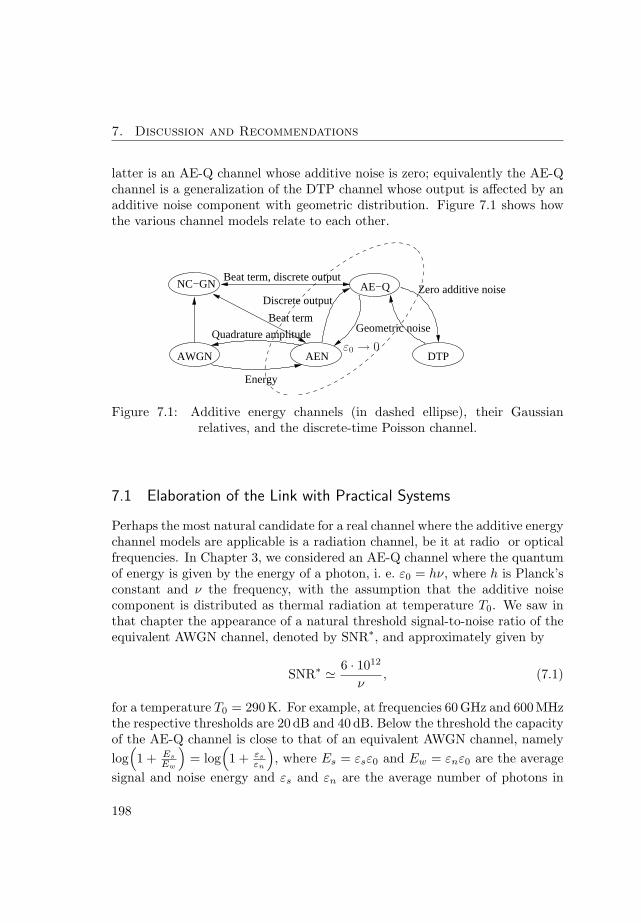
7. Discussion and Recommendations

latter is an AE-Q channel whose additive noise is zero; equivalently the AE-Qchannel is a generalization of the DTP channel whose output is affected by anadditive noise component with geometric distribution. Figure 7.1 shows howthe various channel models relate to each other.

AEN

AE−Q

DTPAWGN

Beat term, discrete output

Geometric noise

Zero additive noise Discrete output

NC−GN

Beat term

Quadrature amplitude

Energy

ε0 → 0

Figure 7.1: Additive energy channels (in dashed ellipse), their Gaussianrelatives, and the discrete-time Poisson channel.

7.1 Elaboration of the Link with Practical Systems

Perhaps the most natural candidate for a real channel where the additive energychannel models are applicable is a radiation channel, be it at radio or opticalfrequencies. In Chapter 3, we considered an AE-Q channel where the quantumof energy is given by the energy of a photon, i. e. ε0 = hν, where h is Planck’sconstant and ν the frequency, with the assumption that the additive noisecomponent is distributed as thermal radiation at temperature T0. We saw inthat chapter the appearance of a natural threshold signal-to-noise ratio of theequivalent AWGN channel, denoted by SNR∗, and approximately given by

SNR∗ ' 6 · 1012

ν, (7.1)

for a temperature T0 = 290K. For example, at frequencies 60 GHz and 600MHzthe respective thresholds are 20 dB and 40 dB. Below the threshold the capacityof the AE-Q channel is close to that of an equivalent AWGN channel, namelylog

(1 + Es

Ew

)= log

(1 + εs

εn

), where Es = εsε0 and Ew = εnε0 are the average

signal and noise energy and εs and εn are the average number of photons in

198

Extensions of the Channel Model

signal and thermal noise. Above threshold, the capacity asymptotically ap-proaches the value 1

2 log εs. A similar change in the slope of the capacity from1 to 1

2 takes place in the NC-GN channel, as determined by Katz [23].Another possible link could be made with the self-noise which appears in

some channel measurements of wireless systems [76], or with phase noise, whichis known to progressively becomes the limiting factor in performance for highenough frequencies. The general problem is to elaborate the possible relation-ship between phase noise, self-noise, and Poisson noise.

Since most radio receivers are based on some form of coherent detection,further research should be carried out on the possibility of designing energy-modulation transmitters and direct-detection receivers for waveform channelsat either radio or optical frequencies.

Even though it is not reported in the dissertation, it is worthwhile men-tioning that a linear amplifier model can be naturally defined for the AE-Qchannel. In this model, each quantum at the input generates, independentlyof the remaining quanta, a random number of quanta at the output. It can beshown [77] that this model leads to a natural definition of noise figure and ofFriis’s formula for the noise figure of a chain of amplifiers.

It is intriguing that the capacity of coherent detection may be achieved eventhough no explicit use is made of the quadrature components of the signal. Anexplanation for this effect is likely to need some use of quantum informationtheory, possibly with an identification of the concepts “quantum” and “classi-cal” capacity with some of the channels we have mentioned here. Some stepsalong this line were carried out by Helstrom [78], who however did not con-sider the additive energy channel models we have studied, but rather modelsbased on a non-coherent detection, which leads to a chi-square or a Laguerredistribution, as we previously mentioned.

In a recent paper [79], Ben Schumacher, a pioneer in the field of quantuminformation theory, is quoted as saying that “interesting restrictions on experi-mental operations yield interesting information theories”. The additive energychannels might thus be seen as “an interesting restriction on experimental oper-ations” which naturally leads to an “information theory” deserving some study.In this dissertation, we have presented some elements of such an analysis.

7.2 Extensions of the Channel Model

The family of additive energy channels naturally admits more models than theones we have considered. For example, in the AE-Q channel model the channel

199

7. Discussion and Recommendations

output at time k yk is given by the sum yk = sk +zk, where sk is a useful signalwith Poisson distribution, and zk an additive noise with geometric distribution.

A first natural extension of the model is the addition of a second Poissonnoise source, say vk, with Poisson distribution of a given mean, so that thechannel output becomes yk = sk + vk + zk. In fact, in the analysis of opticalchannels, a DTP channel model of the form yk = sk + vk is often used; in thiscase the noise source vk receives the name dark current and its origin is linkedto an undesired source of ambient light or to the working of the photodiode.

Another possible extension relates to the effect of signal fading. Inclusion offully-interleaved gamma-mf fading is straightforward; as we saw in Chapter 3 inthe context of DTP channels, the signal sk has in this case a negative binomialdistribution with coefficient m. Along this line, a physical reasoning for theappearance of a gamma distribution in the fading would also be of interest.

A natural question is the determination of the capacity in presence of a darkcurrent or of fading. Concerning the dark current, its effect on the capacityof the DTP channel was studied by Lapidoth and Moser [42] and Brady andVerdu [35]. As for the fading, it is straightforward that the capacity of theAEN channel with gamma fading also coincides with that of an AWGN withgamma fading; in both cases the fading amplitude is assumed known at thereceiver. This follows from the fact that the capacities of the AEN and AWGNchannels with identical signal-to-noise ratio coincide.

Moreover, and as we mentioned previously, we saw in Chapter 3 that thecapacity of the AE-Q channel has two distinct forms as a function of the signal-to-noise ratio. Below a threshold, additive geometric noise prevails over thesignal-dependent Poisson noise; above the threshold the situation is reversed.In a similar vein, it would be interesting to determine the effect of gammafading on the position of the threshold signal-to-noise ratio.

Other extensions refer to studying the capacity of the non-coherent Gaus-sian channel and its discrete counterpart, where the output has a Laguerredistribution [37]. Recently, the NC-GC channel was extensively studied byKatz and Shamai [23]; the capacity of the discrete non-coherent model seemsto have received little attention in the literature.

Another research topic relates to finding the exact capacity or the capacity-achieving distributions of the DTP and AE-Q channels. Taking into accountthe experience from the DTP channel [35,42], this problem is likely to be hard.A possibly simpler problem is finding an alternative, simpler derivation of thebounds to the capacity of the DTP channel.

As we discussed in Chapter 1, multiple-antenna systems have receivedwidespread attention in the past few years since their use increases the number

200

Refinement of the Analysis of Coding and Modulation

of degrees of freedom available for communication. In order to account forthe presence of multiple antennas (or multiple-input multiple-output in gen-eral, MIMO), the scalar model yk = xk + zk should replaced by an equationrelating signal and noise vectors through a mixing matrix. In contrast withthe Gaussian channels, this mixing matrix has non-negative coefficients, andthe optimality of standard matrix decomposition techniques to split the chan-nel into a set of parallel sub-channels [4, 5] should be established. Otherwise,an extension of the matrix decomposition techniques to non-negative matricescould be necessary.

The matrix decomposition techniques would allow one to extend the MIMOresults from microwave systems to similar optical designs, such as mode-groupdiversity multiplexing [20], a concept for the design of transparent parallel linksproposed by the optical communications group at TU/e. Direct extensionsof the Gaussian-channel results to optical frequencies have been reported byStuart [19] and by Shah et al. [80], the latter using coherent detection.

Other model extensions include the consideration of multi-user scenarios.For the multiple-access AEN channel, Verdu found that its capacity regioncoincides with that of the AWGN channel [21]. Other multiple-user channels,such as the broadcast channel, still need to be studied.

We have recently obtained some results on the multiple-access additive en-ergy channels [48]. Of special interest is the analysis of the effect of feedback onthe multiple-access channel. Recall that, in an information-theoretic context,feedback means that the value of the channel outputs y1, y2, . . . , yk are madeknown at the transmitter before sending the signal at time k + 1, xk+1. Thesignal xk+1 may therefore be a function of the channel outputs y1, y2, . . . , yk.For the single-user case, feedback does not increase the capacity [22], but it cando so for the multiple-user AWGN channel [22]. Despite the apparent similar-ity of the capacity regions of the AWGN and AEN channels, feedback does notenlarge the capacity region of the latter. For details, refer to [48]. Moreover,the threshold signal-to-noise ratio in the AE-Q channel depends on the numberof active users. Essentially, the more users there are, the larger their aggregatePoisson noise is, and the lower the threshold.

7.3 Refinement of the Analysis of Coding and Modulation

Not only are the channel capacities of the AWGN and the AEN/AE-Q channelsclose under a broad set of conditions, we have also seen in Chapters 5 and 6that there exist simple digital modulation formats whose constrained capacity

201

7. Discussion and Recommendations

is similar to the channel capacity, and that the error rates of binary codes overthese channels are close to those in the AWGN channel.

We have determined the first two derivatives of the constrained capacity atzero signal energy by direct computation. It would be worthwhile to explorefurther the link with estimation theory recently found by Guo, Shamai, andVerdu [60, 61] to provide an alternative computation for our results, possiblyfor arbitrary values of the signal energy. Along this line, we have found thatthe first-order coefficient of the constrained capacity over the AE-Q channelis zero, which implies that the minimum energy per bit is attained at a finitesignal energy, whose value we have been unable to determine.

At the other range of signal energy, an exact form of the shaping gain of theDTP channel for our family of pulse energy modulations (PEM), with no use ofa Gaussian approximation, is open. Since the approximation is quite good, thepractical improvement is however likely to be small. Knowing the shaping gainfor the DTP channel would allow for an extension of the quantitative analysisof PEM modulation to the AE-Q channel, and possibly for a determination ofthe threshold signal-to-noise ratio for the constrained capacity, rather than thechannel capacity considered in the dissertation.

A side-line of our analysis of the wideband regime in the Gaussian channelwas the extension of the trade-off between power and bandwidth to account forthe possibility of variations in the power, next to the bandwidth change studiedby Verdu [25]. It seems to be simple to extend our analysis to multiple-userGaussian channels, thereby extending the results by Caire et al. [81].

As final element, we have estimated the pairwise error probability in someadditive energy channels by using the union bound and a saddlepoint approx-imation to the pairwise error probability. A possible complement would be touse EXIT chart techniques [69] to optimize codes and modulation mappings.

From a more mathematical point of view, it would be useful to improve theaccuracy of the saddlepoint approximation, possibly by estimating the errorincurred by them. An extension of the saddlepoint approximation to generalrandom variables, thereby removing the distinction between lattice and con-tinuous random variables when using the approximation would have interest initself, and would moreover lead to a method to consider the error probabilityin the AE-Q channel, which we have not considered in its full generality.

202

Bibliography

[1] C. E. Shannon, “A mathematical theory of communication,” Bell Sys.Tech. J., vol. 27, pp. 379–423, 623–656, Jul., Oct. 1948.

[2] A. Lapidoth, “Nearest neighbor decoding for additive non-Gaussian noisechannels,” IEEE Trans. Inf. Theory, vol. 42, no. 5, pp. 1520–1529,Sep. 1996.

[3] A. S. Y. Poon, R. W. Brodersen, and D. N. C. Tse, “Degrees of freedomin multiple-antenna channels: A signal space approach,” IEEE Trans. Inf.Theory, vol. 51, no. 2, pp. 523–536, Feb. 2005.

[4] G. J. Foschini and M. J. Gans, “On limits of wireless communications ina fading environment when using multiple antennas,” Wireless PersonalCommunications, vol. 6, pp. 311–355, 1998.

[5] E. Telatar, “Capacity of multi-antenna Gaussian channels,” Eur. Trans.Telecom., vol. 10, no. 6, pp. 585–595, Nov.-Dec. 1999.

[6] I. Bar-David, “Communication under the Poisson regime,” IEEE Trans.Inf. Theory, vol. 15, no. 1, pp. 31–37, Jan. 1969.

[7] S. Verdu, “Poisson communication theory,” in Proc. Intl. Technion Comm.Day in honor of Israel Bar-David, March 25, Haifa, Israel, 1999.

[8] A. D. Wyner, “Capacity and error exponent for the direct detection photonchannel - part I,” IEEE Trans. Inf. Theory, vol. 34, no. 6, pp. 1449–1461,Nov. 1988.

[9] S. Shamai (Shitz), “Capacity of a pulse amplitude modulated direct de-tection photon channel,” IEE Proc. - Part I, vol. 137, no. 6, pp. 424–430,Dec. 1990.

203

Bibliography

[10] C. M. Caves and P. D. Drummond, “Quantum limits on bosonic commu-nication rates,” Rev. Mod. Phys., vol. 66, no. 2, pp. 481–537, Apr. 1994.

[11] B. M. Oliver, “Thermal and quantum noise,” Proc. IEEE, vol. 53, pp.436–454, May 1965.

[12] J. P. Gordon, “Quantum effects in communication systems,” Proc. IRE,vol. 50, no. 9, pp. 1898–1908, Sep. 1962.

[13] ——, “Noise at optical frequencies; information theory,” in Proc. IntlSchool of Physics “Enrico Fermi”, Course XXXI. London: AcademicPress, 1964, pp. 156–181.

[14] Y. Yamamoto and H. A. Haus, “Preparation, measurement and informa-tion capacity of optical quantum states,” Rev. Mod. Phys., vol. 58, no. 4,pp. 1001–1020, Oct. 1986.

[15] J. M. Kahn and K.-P. Ho, “Spectral efficiency limits and modula-tion/detection techniques for DWDM systems,” IEEE J. Sel. TopicsQuantum Electron., vol. 10, no. 2, pp. 259–272, Mar./Apr. 2004.

[16] V. W. S. Chan, “Coding and error correction in optical fiber communica-tions systems,” in Optical Fiber Communications III, I. P. Kaminow andT. L. Koch, Eds. San Diego: Academic Press, 1997, vol. A, pp. 42–62.

[17] A. H. Gnauck and P. J. Winzer, “Optical phase-shift-keyed transmission,”J. Lightw. Technol., vol. 23, no. 1, pp. 115–130, Jan. 2005.

[18] J. Conradi, “Bandwidth-efficient modulation formats for digital fibertransmission systems,” in Optical Fiber Telecommunications IVB: Systemsand Impairments, I. P. Kaminow and T. Li, Eds. San Diego: AcademicPress, 2002, pp. 862–901.

[19] H. R. Stuart, “Dispersive multiplexing in multimode optical fiber,” Sci-ence, vol. 289, pp. 281–283, Jul. 2000.

[20] T. Koonen, H. van den Boom, I. Tafur Monroy, and G.-D. Khoe, “Highcapacity multi-service in-house networks using mode group diversity mul-tiplexing,” in Proc. of Opt. Fibre Comm. Conf., 2004, OFC 2004, vol. 2,2004, p. FG4.

[21] S. Verdu, “The exponential distribution in information theory,” Prob. Per.Inf., vol. 32, no. 1, pp. 86–95, Jan-Mar 1996.

204

[22] T. M. Cover and J. A. Thomas, Elements of Information Theory. JohnWiley and Sons, 1991.

[23] M. Katz and S. Shamai (Shitz), “On the capacity-achieving distributionof the discrete-time noncoherent and partially coherent AWGN channels,”IEEE Trans. Inf. Theory, vol. 50, no. 10, pp. 2257–2270, Oct. 2004.

[24] A. Lapidoth and S. M. Moser, “Capacity bounds via duality with applica-tions to multiple-antenna systems on flat-fading channels,” IEEE Trans.Inf. Theory, vol. 49, no. 10, pp. 2426–2467, Oct. 2003.

[25] S. Verdu, “Spectral efficiency in the wideband regime,” IEEE Trans. Inf.Theory, vol. 48, no. 6, pp. 1319–1343, Jun. 2002.

[26] G. Caire, G. Taricco, and E. Biglieri, “Bit-interleaved coded modulation,”IEEE Trans. Inf. Theory, vol. 44, no. 3, pp. 927–946, May 1998.

[27] V. V. Prelov and E. C. van der Meulen, “An asymptotic expression forthe information and capacity of a multidimensional channel with weakinput signals,” IEEE Trans. Inf. Theory, vol. 39, no. 6, pp. 1728 – 1735,Sep. 1993.

[28] ——, “Higher order asymptotics of mutual information for nonlinear chan-nels with nongaussian noise,” in Proc. 2003 Int. Symp. Inf. Th. ISIT 2003,2003, p. 83.

[29] S. Verdu, “On channel capacity per unit cost,” IEEE Trans. Inf. Theory,vol. 36, no. 5, pp. 1019–1030, Sep. 1990.

[30] J. R. Pierce, E. C. Posner, and E. R. Rodemich, “The capacity of thephoton counting channel,” IEEE Trans. Inf. Theory, vol. IT-27, no. 1, pp.61–77, Jan. 1981.

[31] R. G. Gallager, Information Theory and Reliable Communication. JohnWiley and Sons, 1968.

[32] J. G. Proakis, Digital Communications. McGraw-Hill, 1995.

[33] D. Tse and P. Viswanath, Fundamentals of Wireless Communication.Cambridge: Cambridge Univ. Press, 2005.

[34] V. Anantharam and S. Verdu, “Bits through queues,” IEEE Trans. Inf.Theory, vol. 42, no. 1, pp. 4–19, Jan. 1996.

205

Bibliography

[35] D. Brady and S. Verdu, “The asymptotic capacity of the direct detec-tion photon channel with a bandwidth constraint,” in Proc. 28th AllertonConf., Allerton House, Monticello, Sep. 1990, pp. 691–700.

[36] W. Feller, An Introduction to Probability Theory and Its Applications,2nd ed. John Wiley and Sons, 1971, vol. 2.

[37] R. M. Gagliardi and S. Karp, Optical Communications. New York: JohnWiley and Sons, 1976.

[38] L. Mandel and E. Wolf, Optical Coherence and Quantum Optics. Cam-bridge University Press, 1995.

[39] R. E. Blahut, Principles and Practice of Information Theory. Addison-Wesley, 1987.

[40] I. Csiszar and J. Korner, Information Theory: Coding Theorems for Dis-crete Memoryless Systems, 1st ed. Academic Press, Inc. 1981.

[41] I. C. Abou-Faycal, M. D. Trott, and S. Shamai (Shitz), “The capacityof discrete-time memoryless Rayleigh-fading channels,” IEEE Trans. Inf.Theory, vol. 47, no. 4, pp. 1290–1301, May 2001.

[42] A. Lapidoth and S. M. Moser, “Bounds on the capacity of the discrete-timePoisson channel,” in Proc. 41st Allerton Conf., Oct. 2003.

[43] R. J. Evans, J. Boersma, N. M. Blachman, and A. A. Jagers, “The entropyof a Poisson distribution: Problem 87-6,” SIAM Rev., vol. 30, no. 2, pp.314–317, Jun. 1988.

[44] G. E. Andrews, R. Askey, and R. Roy, Special Functions. Cambridge:Cambridge University Press, 1999.

[45] A. Lapidoth, “On phase noise channels at high SNR,” in Proc. IEEE Inf.Theory Workshop, Bangalore (India), 2002, pp. 1–4.

[46] A. Martinez, “Spectral efficiency of optical direct detection,” J. Opt. Soc.Am. B, vol. 24, no. 4, pp. 739–749, Apr. 2007.

[47] ——, “Capacity bounds for the Einstein radiation channel,” in Proc. ofInt. Symp. Inf. Theory ISIT 2006, Seattle, USA, pp. 366–370.

[48] ——, “Variations on the Gaussian multiple-access channel,” in Proc. ofInt. Symp. Inf. Theory ISIT 2007, Nice, France, pp. 2386–2390.

206

[49] I. S. Gradshteyn and I. M. Ryzhik, Tables of Integrals, Series, and Prod-ucts, A. Jeffrey, Ed. Academic Press, 1994.

[50] G. D. Forney, Jr. and G. Ungerboeck, “Modulation and coding for linearGaussian channels,” IEEE Trans. Inf. Theory, vol. 44, no. 6, pp. 2384–2415, Oct. 1998.

[51] E. Biglieri, J. Proakis, and S. Shamai (Shitz), “Fading channels:Information-theoretic and communications aspects,” IEEE Trans. Inf.Theory, vol. 44, no. 6, pp. 2619–2692, Oct. 1998.

[52] V. Prelov and S. Verdu, “Second order asymptotics of mutual informa-tion,” IEEE Trans. Inf. Theory, vol. 50, no. 8, pp. 1567–1580, Aug. 2004.

[53] A. Martinez, A. Guillen i Fabregas, and G. Caire, “Bit-interleaved codedmodulation in the wideband regime,” in Proc. of Int. Symp. Inf. TheoryISIT 2007, Nice, France, pp. 2131–2135.

[54] A. Martinez, A. Guillen i Fabregas, G. Caire, and F. Willems, “Bit-interleaved coded modulation in the wideband regime,” submitted to IEEETrans. Inf. Th.

[55] F. D. Neeser and J. L. Massey, “Proper complex random processes withapplications to information theory,” IEEE Trans. Inf. Theory, vol. 39,no. 4, pp. 1293–1302, Jul. 1993.

[56] G. D. Forney, Jr., R. G. Gallager, G. R. Lang, F. M. Longstaff, and S. U.Qureshi, “Efficient modulation for band-limited channels,” IEEE J. Sel.Areas Commun., vol. 2, no. 5, pp. 632–647, Sep. 1984.

[57] G. Ungerboeck, “Channel coding with multi-level/phase signals,” IEEETrans. Inf. Theory, vol. IT-28, pp. 55–67, Jan. 1982.

[58] A. Ganti, A. Lapidoth, and I. E. Telatar, “Mismatched decoding revisited:general alphabets, channels with memory, and the wide-band limit,” IEEETrans. Inf. Theory, vol. 46, no. 7, pp. 2315–2328, Nov. 2000.

[59] A. Martinez and F. Willems, “A coding theorem for bit-interleaved codedmodulation,” in Proc. of the 27th WIC Benelux Symposium, 2006.

[60] D. Guo, S. Shamai (Shitz), and S. Verdu, “Mutual information and mini-mum mean-square error in Gaussian channels,” IEEE Trans. Inf. Theory,vol. 41, no. 4, pp. 1261–1282, Apr. 2005.

207

Bibliography

[61] D. P. Palomar and S. Verdu, “Representation of mutual information viainput estimates,” IEEE Trans. Inf. Theory, vol. 53, no. 2, pp. 453–470,Feb. 2007.

[62] S. Golomb, “The limiting behavior of the Z-channel,” IEEE Trans. Inf.Theory, vol. 26, no. 3, p. 372, May 1980.

[63] C. W. Helstrom, “Computing the performance of optical receivers withavalanche diode detectors,” IEEE Trans. Commun., vol. 36, no. 1, pp.61–66, Jan. 1988.

[64] G. Einarsson, Principles of Lightwave Communications. John Wiley andSons, 1996.

[65] A. J. Viterbi and J. K. Omura, Principles of Digital Communication andCoding. McGraw-Hill, 1979.

[66] A. Martinez, A. Guillen i Fabregas, and G. Caire, “Error probability ofbit-interleaved coded modulation,” IEEE Trans. Inf. Theory, vol. 52, no. 1,pp. 262–271, Jan. 2006.

[67] J. L. Jensen, Saddlepoint Approximations. Oxford: Clarendon Press, 1995.

[68] P.-C. Yeh, S. Zummo, and W. Stark, “Error probability of bit-interleavedcoded modulation in wireless environments,” IEEE Trans. Veh. Technol.,vol. 55, no. 2, pp. 722–728, Mar. 2006.

[69] S. ten Brink, “Convergence behavior of iteratively decoded parallel con-catenated codes,” IEEE Trans. Comm., vol. 49, no. 10, pp. 1727–1737,Oct. 2001.

[70] F. W. J. Olver, Asymptotics and Special Functions. New York: AcademicPress, 1974.

[71] A. Martinez, A. Guillen i Fabregas, and G. Caire, “A closed-form approx-imation for the error probability of coded BPSK fading channels,” IEEETrans. Wir. Comm., vol. 6, no. 6, pp. 2051 – 2054, Jun. 2007.

[72] M. K. Simon and M.-S. Alouini, Digital Communication over Fad-ing Channels: A Unified Approach to Performance Analysis. Wiley-Interscience, 2000.

208

[73] E. Biglieri, G. Caire, G. Taricco, and J. Ventura-Traveset, “Simple methodfor evaluating error probabilities,” Electron. Lett., vol. 32, no. 3, pp. 191–192, Feb. 1996.

[74] A. Lozano, A. M. Tulino, and S. Verdu, “Optimum power allocationfor parallel Gaussian channels with arbitrary input distributions,” IEEETrans. Inf. Theory, vol. 52, no. 7, pp. 3033–3051, Jul. 2006.

[75] L. van de Meeberg, “A tightened upper bound on the error probabilityof binary convolutional codes with Viterbi decoding,” IEEE Trans. Inf.Theory, vol. 20, no. 3, pp. 389 – 391, May 1974.

[76] R. Laroia, “Lessons unlearnt in wireless,” in Proc. of the 2006 Intl. ZurichSem. Comm., 2006.

[77] A. Martinez, “Quantum noise in linear amplifiers revisited,” in Proc. Conf.on Information Systems and Sciences, CISS 2006, 2006.

[78] C. W. Helstrom, Quantum Detection and Estimation Theory. AcademicPress, 1976.

[79] S. D. Bartlett, T. Rudolph, and R. W. Spekkens, “Reference frames, su-perselection rules, and quantum information,” Rev. Mod. Phys., vol. 79,no. 2, pp. 555–609, Apr.-Jun. 2007.

[80] A. R. Shah, R. C. J. Hsu, A. Tarighat, A. H. Sayed, and B. Jalali, “Coher-ent optical MIMO (COMIMO),” J. Lightw. Technol., vol. 23, no. 8, pp.2410 – 2419, Aug. 2005.

[81] G. Caire, D. Tuninetti, and S. Verdu, “Suboptimality of TDMA in thelow-power regime,” IEEE Trans. Inf. Theory, vol. 50, no. 4, pp. 608–620,Apr. 2004.

209

Index

AE-Q channel, 18–25, 28, 32, 44–57, 108, 133–138, 140, 185,197–199

multiple-acces, 201AEN channel, 7, 8, 15–20, 22–23,

25, 28, 29, 31–32, 45–47,49, 53, 55, 56, 108, 109,112–123, 126, 128, 129, 138–141, 154, 173–180, 184–185,197, 198

multiple-access, 201APSK modulation, 74, 79AWGN channel, 2, 6, 7, 10, 13–

25, 28–31, 45–46, 53, 55–57, 71–106, 115, 116, 118,120, 126, 128, 129, 139, 140,154, 158, 160–173, 184, 197,198

non-coherent, 197, 199, 200

bandwidth, 1, 2, 4, 79–84, 105–106spatial, 4temporal, 4

bit error probability, 29bit-interleaved coded modulation, 71,

72, 86–94, 108, 124, 153,155, 184

AE-Q channel, 138AEN channel, 121–123, 173, 178–

180AWGN channel, 153, 165–173DTP channel, 130–133, 182–184

bit-interleaved coded modulation ca-pacity, 88–94, 139

AEN channel, 121–123AWGN channel, 88–95DTP channel, 130–133

blackbody radiation, 21BPSK modulation, 80, 82, 86, 160–

165, 170, 173, 175, 185

capacity per unit cost, 9, 10capacity per unit energy, 25, 29, 30,

72, 76, 108, 139AE-Q channel, 134–136AEN channel, 112, 115–117AWGN channel, 75–76, 139DTP channel, 123, 126–127

capacity per unit time, 80–83channel capacity, 2–6, 8–9, 12, 14,

17, 72, 73, 153additive energy channels, 25–

57AE-Q channel, 134, 200, 201

211

Index

AEN channel, 112, 116, 200,201

AWGN channel, 116, 200, 201DTP channel, 131, 200

Chernoff bound, 157, 158, 164, 167,173, 175–177, 181, 184

chi-square distribution, 8, 20, 199coded modulation, 71, 72, 108, 131,

134, 138AE-Q channel, 133–138AEN channel, 112–120DTP channel, 124–130Gaussian channel, 73–86

coded modulation capacity, 74–75,95, 107, 108, 123, 139

AE-Q channel, 133–138AEN channel, 112–120DTP channel, 124–130Gaussian channel, 76–86

constrained capacity, 8–10, 72, 94,95, 107, 112, 124, 133, 134

convolutional code, 155, 164, 168cumulant transform, 157, 158, 160,

163, 187

decoder, 11–12, 17, 28, 71, 87, 88,153, 154, 156, 165

BICM, 89decoding metric, 154, 155, 165, 168,

185decoding score

bit, 156, 158–163, 166, 169, 173–175, 182

bit, cumulant transform, 159,162, 163, 174, 177, 179, 180,182

pairwise, 156, 166, 171, 173,178, 192

pairwise, cumulant transform,163, 169

symbol, cumulant transform, 170demapper, 87detection

coherent, 2, 4, 5, 8, 10, 199,201

coherent, optical, 5direct, 5, 8, 199non-coherent, 6, 7, 29, 55, 199

digital modulation, 8, 10DTP channel, 5, 6, 8–10, 17–18, 20,

22–25, 28, 32–43, 46, 49,52, 53, 55–57, 108, 109, 123–133, 138–141, 180–185, 197,200

electromagnetic field, 2, 5, 17, 21,23

encoder, 11–13, 17, 26, 28, 71, 86,153, 154

entropy, 3, 7, 27–28, 32, 129conditional, 27–28, 129differential, 27–28, 30, 31, 111,

115, 119, 129geometric random variable, 44,

46, 50–52maximum, 3, 6, 7, 23negative binomial, 33–37, 56,

67, 68output, 49Poisson random variable, 33–

37, 56, 68error probability, 8, 10, 17, 28, 72,

110exponential distribution, 7, 15, 16,

18, 19, 23, 31, 33, 36, 38,42, 45, 52, 112

212

fading, 83, 153, 157, 158, 160, 161,200

AWGN channel, 83–84, 95gamma, 84, 95, 160, 162–167,

172, 174, 176–178, 181, 184,185, 200

Rayleigh, 161, 168flash signalling, 118–119, 125, 128,

137, 139, 140Fourier decomposition, 12, 14, 24frequencies

optical, 4–6, 11, 17, 20, 22, 198,199

radio, 1, 2, 4, 6, 11, 22, 71, 79,198, 199

G regime, 19–22, 25, 45, 56–57gamma distribution, 33, 34, 36–38,

41–43, 53, 56, 66–67, 200geometric distribution, 7, 18, 19, 23,

32, 36, 37, 39, 41, 44, 47,49–51, 134, 136, 198, 200

golden number, 114, 118–121, 141

Laguerre distribution, 20, 199, 200laser, 4

multiple, 6, 201log-likelihood ratio, 88

mapping, 86, 88–91, 121, 139, 154,156, 160, 161, 165, 168, 171,174, 175, 178, 181

anti-Gray, 90, 92Gray, 87, 90, 92–95, 121, 123,

124, 131, 133, 138, 139, 168,169

set-partitioning, 90, 92MIMO systems, 4, 201minimum bit-energy-to-noise ratio,

76, 78, 90, 92, 93

AEN channel, 116minimum energy per bit, 8–10, 25,

30, 109, 114, 139, 202AE-Q channel, 135, 138AEN channel, 115, 118, 136DTP channel, 123, 126, 133

minimum energy-to-noise ratio, 75minimum signal-energy-to-noise ra-

tio, 72, 75MMSE estimator, 109mode-group diversity multiplexing,

201modulation, 71–73, 76–79, 94, 95,

107, 108, 139multiple antenna, 201mutual information, 25–29, 33–34,

37–38, 41, 42, 45, 47, 49,51, 52, 56, 57, 67

negative binomial distribution, 34–38, 56, 200

noise, 1–3, 5–7, 9, 13–15, 17additive, 7, 9, 10, 13, 15, 17–

20, 22–24, 31, 44, 45, 49,54–56, 109, 110, 112, 123,126, 133–135, 137, 139, 141,197, 198, 200

exponential, 6, 32, 174Gaussian, 2, 3, 6, 13, 15, 30, 56phase, 55, 199Poisson, 9, 18–20, 23, 45, 54,

56–57, 136, 141, 199–201self-, 199shot, 5, 18spectral density, 1, 2, 55, 79–

81, 105–106thermal, 1, 55, 56, 198, 199

noise energy, 31, 46, 55

213

Index

on-off keying (OOK), 6, 128optical communications, 4–6, 8optical fibres, 4

P regime, 19–22, 25, 45, 56–57pairwise error probability, 8, 10, 108,

130, 141, 202AE-Q channel, 185, 202AEN channel, 173–180, 184–185,

202AWGN channel, 160–173, 175,

180, 184, 202DTP channel, 180–185

PAM modulation, 17, 74, 78, 93,107, 120, 173, 184, 185

PEM modulation, 107–112, 114, 115,117–121, 123, 124, 127, 130–131, 133–135, 137–141, 202

photodiode, 4, 200photon, 5, 8, 9, 21–22, 46, 54–55,

198Poisson channel, 5–6Poisson distribution, 5, 7, 18, 19,

23, 32–37, 44, 50, 56, 58,67, 123, 200

entropy, 129power, 79–84, 105–106PSK modulation, 72, 74, 78, 86, 90,

92–94, 173

QAM modulation, 72, 74, 79, 85,86, 90, 92–94, 120, 130, 168,173, 180

QPSK modulation, 79, 80, 82, 86,157, 169–172, 184

quantum of energy, 7–9, 17–20, 23,46, 54–55, 197–199

Rician distribution, 16, 20

saddlepoint approximation, 153, 158,160, 162–164, 166–168, 175–178, 181, 184, 185, 202

sampling theorem, 1, 2, 12, 14shaping gain, 72, 75, 85, 86, 108,

202AE-Q channel, 135AEN channel, 119–120, 141DTP channel, 129–130, 141

signal-to-noise ratio, 3–4, 8–10, 14,16, 19, 20

spectral efficiency, 3–4, 6

turbo-like code, 155, 156, 164, 168

wideband regime, 9, 72, 76–84, 95,202

wireless communications, 4, 6

Z channel, 159–160, 174, 175, 177,181, 182, 185

214

Curriculum Vitae

A. Martinez was born in October 1973 in Zaragoza, Spain. In 1997 he re-ceived the M. Sc. in Telecommunications Engineering from the University ofZaragoza, in Spain. In the period 1998-2003 he was employed at the researchcentre of the European Space Agency in Noordwijk, the Netherlands, workingon the design of digital communication systems for satellite communications.The main focus of his work was the analysis and design of coded modulationsystems, ranging from modulation and channel coding to some aspects relatedto the implementation of channel decoders and demodulators.

In April 2003 he joined the Signal Processing group at the Faculty of Electri-cal Engineering in the Technische Universiteit Eindhoven, in the Netherlandsto work on optical communication theory under the project mode-group di-versity multiplexing. In this period, he analyzed different channel models fornon-coherent communications. He also contributed to the design and imple-mentation of a demonstrator of the mode-group diversity multiplexing tech-nique, a method to transparently multiplex several simultaneous transmissionchannels over an optical fibre, using a single frequency band.

In 2007 he spent four months at University of Cambridge, in the UnitedKingdom, supported by the British Royal Society, working on the performanceanalysis and design of digital modulation systems.

His research interest is communication theory in general, with special at-tention to the interplay between communication theory and physics.

215