information-theoretic distribution test with application

This article was downloaded by: [Texas A&M University Libraries]On: 16 May 2013, At: 00:25Publisher: Taylor & FrancisInforma Ltd Registered in England and Wales Registered Number: 1072954 Registered office: Mortimer House,37-41 Mortimer Street, London W1T 3JH, UK

Econometric ReviewsPublication details, including instructions for authors and subscription information:http://www.tandfonline.com/loi/lecr20

Information-Theoretic Distribution Test withApplication to NormalityThanasis Stengos a & Ximing Wu ba Department of Economics, University of Guelph, Guelph, Ontario, Canadab Department of Agricultural Economics, Texas A&M University, College Station, Texas, USAPublished online: 07 Jan 2010.

To cite this article: Thanasis Stengos & Ximing Wu (2009): Information-Theoretic Distribution Test with Application toNormality, Econometric Reviews, 29:3, 307-329

To link to this article: http://dx.doi.org/10.1080/07474930903451565

PLEASE SCROLL DOWN FOR ARTICLE

Full terms and conditions of use: http://www.tandfonline.com/page/terms-and-conditions

This article may be used for research, teaching, and private study purposes. Any substantial or systematicreproduction, redistribution, reselling, loan, sub-licensing, systematic supply, or distribution in any form toanyone is expressly forbidden.

The publisher does not give any warranty express or implied or make any representation that the contentswill be complete or accurate or up to date. The accuracy of any instructions, formulae, and drug doses shouldbe independently verified with primary sources. The publisher shall not be liable for any loss, actions, claims,proceedings, demand, or costs or damages whatsoever or howsoever caused arising directly or indirectly inconnection with or arising out of the use of this material.

http://www.tandfonline.com/loi/lecr20

http://dx.doi.org/10.1080/07474930903451565

http://www.tandfonline.com/page/terms-and-conditions

Econometric Reviews, 29(3):307–329, 2010Copyright © Taylor & Francis Group, LLCISSN: 0747-4938 print/1532-4168 onlineDOI: 10.1080/07474930903451565

INFORMATION-THEORETIC DISTRIBUTION TESTWITH APPLICATION TO NORMALITY

Thanasis Stengos1 and Ximing Wu2

1Department of Economics, University of Guelph, Guelph, Ontario, Canada2Department of Agricultural Economics, Texas A&M University,College Station, Texas, USA

� We derive general distribution tests based on the method of maximum entropy (ME) density.The proposed tests are derived from maximizing the differential entropy subject to given momentconstraints. By exploiting the equivalence between the ME and maximum likelihood (ML)estimates for the general exponential family, we can use the conventional likelihood ratio (LR),Wald, and Lagrange multiplier (LM) testing principles in the maximum entropy framework.In particular, we use the LM approach to derive tests for normality. Monte Carlo evidencesuggests that the proposed tests are compatible with and sometimes outperform some commonlyused normality tests. We show that the proposed tests can be extended to tests based on regressionresiduals and non-i.i.d. data in a straightforward manner. An empirical example on productionfunction estimation is presented.

Keywords Distribution test; Maximum entropy; Normality.

JEL Classification C1; C12; C16.

1. INTRODUCTION

Testing that a given sample comes from a particular distribution hasbeen one of the most important topics in inferential statistics and can betraced back to as early as Pearson’s (1900) �2 goodness-of-fit test. Thanksto the prominent role of the central limit theorem in statistics, testing fornormality has received an extensive treatment in the literature, see Thode(2002) for a comprehensive review on this topic. In this article, we presentsome alternative normality tests based on the method of maximumentropy (ME) density. The proposed tests are derived from maximizing thedifferential entropy subject to known moment constraints. By exploiting

Address correspondence to Ximing Wu, Department of Agricultural Economics, Texas A&MUniversity, College Station, TX 77843-2124, USA; E-mail: [email protected]

Dow

nloa

ded

by [

Tex

as A

&M

Uni

vers

ity L

ibra

ries

] at

00:

25 1

6 M

ay 2

013

308 T. Stengos and X. Wu

the equivalence between ME and maximum likelihood (ML) estimationfor the exponential family, we can use the conventional likelihood ratio(LR), Wald, and Lagrange multiplier (LM) testing principles in themaximum entropy framework. Hence, our tests share the optimalityproperties of the standard maximum likelihood based tests. Using theLM approach, we show that the ME method leads to simple yet powerfultests for normality. We propose some flexible maximum entropy densitiescharacterized by a small number of generalized moments, which nest thenormal density as a special case. The corresponding tests utilize somegeneralized moments that effectively capture deviations from the normaldistribution. Our Monte Carlo simulations show that the proposed testscompare favorably and often outperform some commonly used tests in theliterature, especially when the sample size is small. In addition, we showthat the proposed method can be easily extended to: i) other distributionsthan the normal distribution; ii) regression residuals; iii) dependentand/or heteroskedastic data. Finally, we apply the proposed normality teststo residuals from a regression model of a production function using abenchmark dataset that has been extensively used in the literature.

The article is organized as follows. In the next section, we presentthe information theoretic framework on which we base our analysis.We then proceed to derive our normality tests and discuss their properties.In the following section we present some simulation results. Finally,before we conclude, we discuss some possible extensions and an empiricalapplication. The appendix collects the proofs of the main results.

2. INFORMATION-THEORETIC DISTRIBUTION TEST

2.1. Maximum Entropy Density

According to Golan (2008), which provides an excellent review andsynthesis of Information and Entropy Econometrics (IEE), “� � � , IEE is thesubdiscipline of processing information from limited and noisy data withminimal a priori information on the data-generating process. In particular,IEE is a research that directly or indirectly builds on the foundations ofInformation Theory and the principle of [ME].”

Information entropy, the central concept of information theory, wasintroduced by Shannon (1949). Entropy is an index of disorder anduncertainty. Facing the fundamental question of drawing inferences fromlimited and insufficient data, Jaynes proposed the ME principle, whichhe viewed as a generalization of Bernoulli and Laplace’s Principle ofInsufficient Reason. The ME principle states that among all distributionsthat satisfy certain informational constraints, one should choose theone that maximizes Shannon’s information entropy. According to Jaynes(1957), the ME distribution is “uniquely determined as the one which

Dow

nloa

ded

by [

Tex

as A

&M

Uni

vers

ity L

ibra

ries

] at

00:

25 1

6 M

ay 2

013

Information-Theoretic Distribution Test 309

is maximally noncommittal with regard to missing information, and thatit agrees with what is known, but expresses maximum uncertainty withrespect to all other matters.” Shore and Johnson (1980) developedaxiomatic foundations for this approach.

The ME density is obtained by maximizing the entropy subject to somemoment constraints. Let x be a random variable distributed according toa probability density function (pdf) f0(x), and X1,X2, � � � ,Xn be an i.i.d.random sample from f0(x). The unknown density f0(x) is assumed to becontinuously differentiable, positive on the interval of support (usually thereal line if there is no prior information on the support of the density)and bounded. Suppose we maximize the entropy

maxf

: W = −∫

f (x) log f (x)dx ,

subject to ∫f (x)dx = 1,∫

gk(x)f (x)dx = �k , k = 1, 2, � � � ,K ,

where gk(x) is continuously differentiable and �k = 1n

∑ni=1 gk(Xi). This

constrained optimization problem is called a primal formulation, where theoperation is carried out with respect to the underlying density functionf (x). Alternatively, one can formulate this problem as an unconstrainedoptimization. The unconstrained objective function then takes the form

max�0,��,�K

−∫

f (x) log f (x)dx − �0

( ∫f (x)dx − 1

)

−K∑k=1

�k

( ∫gk(x)f (x)dx − �k

)�

This dual formulation offers several advantages. First, an unconstrainedoptimization is simpler, second the dimension of the optimization problemis reduced to K LMs, and third, that formulation allows a directcomparison with traditional likelihood methods.

It is straightforward to derive the solution, from the dual formulation,

f (x ; �) = exp(

−�0 −K∑k=1

�kgk(x)), (1)

Dow

nloa

ded

by [

Tex

as A

&M

Uni

vers

ity L

ibra

ries

] at

00:

25 1

6 M

ay 2

013


where �k is the LM associated with the kth moment constraint inthe optimization problem, and �0 = log

( ∫exp

(− ∑Kk=1 �kgk(x)

)dx) < ∞

ensures that f (x ; �) integrates to one. The maximized entropy W = �0 +∑Kk=1 �k �k .The ME density is of the generalized exponential family and can be

completely characterized by the moments Egk(x), k = 1, 2, � � � ,K . We callthese moments “characterizing moments,” whose sample counterparts arethe sufficient statistics of the estimated ME density f (x ; �). A wide rangeof distributions belong to this family. For example, the Pearson family andits extensions described in Cobb et al. (1983), which nest normal, beta,gamma, and inverse gamma densities as special cases, are all ME densitieswith simple characterizing moments.

In general, there is no analytical solution for the ME density problem,and nonlinear optimization methods are required (Ornermite and White,1999; Wu, 2003; Zellner and Highfield, 1988). We use Lagrange’s methodto solve this problem by iteratively updating �

�(t+1) = �(t) − �−1b,

where at the (t + 1)th stage of the updating, bk = ∫gk(x)f (x ; �(t))dx − �k

is the difference between the predicted and the empirical moment, andthe Hessian matrix � takes the form

�k,j =∫

gk(x)gj(x)f(x ; �(t)

)dx , 0 ≤ k, j ≤ K �

This updating scheme is essentially the Newton–Raphson algorithm. Thepositive-definitiveness of the Hessian ensures the existence of a uniquesolution.1

Given Eq. (1), we can also estimate f (x ; �) using ML. The maximizedlog-likelihood

l =n∑

i=1

log f(xi ; �

) = −n∑

i=1

(�0 +

K∑k=1

�kgk(xi))

= −n(�0 +

K∑k=1

�k �k

)= −nW �

1Let �′ = [�0, �1, � � � , �K ] be a nonzero vector and g0(x) = 1, we have

�′�� =K∑k=0

K∑j=0

�k�j

∫gk(x)gj (x)f (x , �)dx =

∫ ( K∑k=0

�k gk(x))2

f (x ; �)dx > 0�

Hence, � is positive-definite.

Dow

nloa

ded

by [

Tex

as A

&M

Uni

vers

ity L

ibra

ries

] at

00:

25 1

6 M

ay 2

013


Therefore, when the distribution is of the generalized exponentialfamily, ML and ME estimates are equivalent provided that the samplecounterparts of �k , k = 1, � � � ,K , are known. Moreover, they are alsoequivalent to the method of moments (MM) estimator. This ME/ML/MMestimator only requires the knowledge of sample characterizing moments.

Although ML and ME are equivalent in our case, there are someconceptual differences. For ML, the restricted estimates are obtainedby imposing certain constraints on the parameters. In contrast, for ME,the dimension of parameters is determined by the number of momentrestrictions imposed: the more moment restrictions, the more complexand thus the more flexible the distribution is. To reconcile these twomethods, we note that a ME estimate with m moment restrictions has asolution of the form

f (x ; �) = exp(

−�0 −m∑

k=1

�kgk(x)),

which implicitly sets �j , j = m + 1,m + 2, � � � , to be zero. When we imposemore moment restrictions, say,

∫gm+1(x)f (x ; �)dx = �m+1, we let the data

choose the appropriate value of �m+1.2 In this sense, the estimate with moremoment restrictions is in fact less restricted, or more flexible. ME andML share the same objective function (up to a proportion) which isdetermined by the moment restrictions of the ME problem. Therefore,one can regard the ME approach as a method of model selection, whichgenerates a ML solution.

2.2. Information Theoretic Estimators and Tests

The development of IEE, which is founded on information theoryand the ME principle, is greatly affected by advances in statistics andeconometrics. Maasoumi (1993), Ebrahimi et al. (1999), Bera and Bilias(2002), Golan (2002, 2007, 2008), and Golan and Maasoumi (2008)provide excellent reviews and a synthesis of IEE during the last century.In particular, Fig. 2.1 and 2.2 of Golan (2008) present a long-term anda short term history of IEE. Golan (2002, 2007) provide overviews basedon special issues on IEE in Journal of Econometrics Vol. 107 and Vol. 138,respectively, while Golan and Maasoumi (2008) offer a review in a specialissue of Econometric Reviews, Vol. 27. In the Econometric Reviews special issueon IEE, Golan and Maasoumi (2008) review the links between information

2Denote �m = [�1, � � � , �m ]. The only case that �m+1 = 0 is when the moment restriction∫gm+1(x)f (x ; �m)dx = �m+1 is not binding, or the (m + 1)th moment is identical to its prediction

based on the ME density f (x ; �m) from the first m moments. In this case, the (m + 1)th momentcontains no additional information that can further reduce the entropy.

Dow

nloa

ded

by [

Tex

as A

&M

Uni

vers

ity L

ibra

ries

] at

00:

25 1

6 M

ay 2

013


measures and hypothesis testing as well as applications to dynamic models,Bayesian econometrics, empirical likelihood methods, and nonparametriceconometrics. In this article, we will focus primarily on IEE and testing.

The early work that influenced the philosophy and approach of IEEinclude Pearson’s work on goodness-of-fit measure and MM, Fisher’s MLmethod, and later on Neyman and Pearson’s Minimum chi-square method,and Sargan’s Instrumental Variables method (see Bera and Bilias, 2002and references therein). Hansen (1982) developed the general theory ofthe Generalized Method of Moments (GMM) which builds on all of theprevious work. GMM recognizes while it does not specify the completedistribution of the data, the economic model does place restriction onpopulation moment conditions. GMM thus bases its model constructionand parameter estimation on population moment restrictions.

The development of GMM shares the same basic philosophy of somerecent Information-Theoretic (IT) methods. At about the same time,the foundations of the empirical likelihood (EL) were established (Owen,1988; Qin and Lawless, 1994). This method proposes a nonparametriclikelihood method without assuming knowledge of the exact likelihood ofthe underlying data generating process. The connection of the GMM toIEE and IT was later established in some recent econometrics literature(Imbens et al., 1998; Kitamura and Stutzer, 1997). The EL method isfurther extended to the Generalized Empirical Likelihood (GEL) method(Imbens, 2002; Kitamura, 2006; Smith, 2004, 2005).

In a parallel and independent research, in the late 1980s and early1990s, the ME method was generalized by Golan et al. (1996). Thisline of research develops an estimation method that is capable ofhandling ill-posed problem. It imposes minimal distributional assumption,can incorporate exact or stochastic moment conditions and incorporateprior information in a straightforward manner. This method, known asthe Generalized Maximum Entropy (GME) estimator, provides a viablealternative to the GEL family estimators. One important advantage ofthe GME is that it is simpler to calculate, while the GEL family estimatorsare typically associated with difficult saddlepoint optimization problems.

A more recent addition to the IEE family estimators is the BayesianMethod of Moments (BMOM) by Zellner (1996). To avoid a likelihoodfunction Zellner proposed to maximize the differential (Shannon) entropysubject to the empirical moments of the data. This yields the mostconservative (closest to uniform) post data density. In that way the BMOMuses only assumptions on the realized error terms which are used toderive the post data density. To do so, the BMOM equates the posteriorexpectation of a function of the parameter to its sample value and choosesthe posterior to be the (differential) ME distribution subject to thatconstraint.

Dow

nloa

ded

by [

Tex

as A

&M

Uni

vers

ity L

ibra

ries

] at

00:

25 1

6 M

ay 2

013


Hypothesis testing based on the principle of ME has been discussedthoroughly since the original article of Jaynes (1957). Because the LMs�k take the value zero if the kth constraint is not binding, a directionaltest with respect to a given moment condition is equivalent to testing�k = 0. In fact, this test principle is consistent with Neyman’s (1937) smoothtest, which appeared even earlier. This test is essentially an information-theoretic test in the sense that the test statistic is equivalent to the entropyof the uniform distribution under the null hypothesis.

Another important IT concept, the Kullback–Leibler InformationCriterion (KLIC), is also commonly used in statistical estimations andinferences. Let f and g be two distributions with a common support. TheKLIC is defined as ∫

f (x) logf (x)g (x)

dx ,

which is non-negative and equals zero if and only if f (x) = g (x) almosteverywhere. Note that the KLIC is not a true distance as it is asymmetricand does not satisfy the triangle inequality. This criterion measures thediscrepancy between two distributions. Since the KLIC is very sensitiveto even a small discrepancy between two distributions, it is expectedto perform well for estimations and tests on distributions. Haberman(1984) used the KLIC to select distributions satisfying a vector of momentconditions.

Starting with the seminal work by Owen (1988), the IT approach isfurther generalized to regressions and general inferences. In addition,a more general family of discrepancy measure is used. Considertwo discrete distributions with common support p = (p1, � � � , pn) andq = (q1, � � � , qn). Cressie and Read (1984) proposed a family of discrepancystatistics

I�(p, q) = 1�(1 + �)

n∑i=1

[(piqi

)2

− 1],

which is indexed by a single parameter �.One can then define a family of estimators as

min�,�

I�(1/n, �), subject ton∑

i=1

�(zi , �)�i = 0 andn∑

i=1

�i = 1, (2)

where E [�(zi , �)] = 0 is given moment conditions, and 1/n is theempirical distribution of the data. Instead of using the empiricaldistribution, estimator (2) reweighs observations such that they satisfygiven moment conditions. Associated with the moment conditions is a

Dow

nloa

ded

by [

Tex

as A

&M

Uni

vers

ity L

ibra

ries

] at

00:

25 1

6 M

ay 2

013


vector of Lagrangian multipliers, which essentially determines the consistentdistribution �i , i = 1, � � � ,n. This estimator has several special cases ofinterest. For example, when � = 1, it is the empirical likelihood estimator(Owen, 1988; Qin and Lawless, 1994), which is defined as

min�,�

n∑i=1

ln �i , subject ton∑

i=1

�(zi , �)�i = 0 andn∑

i=1

�i = 1�

When � → 0, the estimator takes the form

min�,�

n∑i=1

�i ln �i , subject ton∑

i=1

�(zi , �)�i = 0 andn∑

i=1

�i = 1,

which is empirical tilting estimator corresponding to the KLIC (Imbenset al., 1998; Kitamura and Stutzer, 1997). When � = 2, it is equivalent to thecontinuously updating GMM estimator of Hansen et al. (1996), defined by

min�,�

n∑i=1

1n(n2�2

i − 1), subject ton∑

i=1

�(zi , �)�i = 0 andn∑

i=1

�i = 1�

All these estimators are first order equivalent to the classical GMMestimator and enjoy certain higher order efficiency advantages.

IT overidentification tests follow naturally from the above generalizedempirical likelihood estimators. Imbens et al. (1998) discussed threeformulations. The Average Moment test compares the estimated momentsto zero, which is similar to the J statistic of the classical GMM estimator.The LMs test is a direct test on the LMs of the minimization problem(2), which is the same approach as used in this study. Lastly, theCriterion Function test examines the discrepancy between the empiricaldistribution and the estimated distribution that satisfied given conditionmean conditions. All three tests have asymptotic �2 distributions underthe null hypothesis. Imbens et al. (1998) show that these IT testshave better small sample performances compared to the conventionaloveridentification GMM test.

In this article, we use the classical ME approach for distribution tests.Consider a M dimension parameter space M . Suppose we want to testthe hypothesis that � ∈ m , a subspace of M , where m ≤ M . Because ofthe equivalence between ME and ML, we can use the traditional LR, Wald,and LM principles to construct test statistics.3 For j = m,M , let �j be the

3Imbens et al. (1998) discussed similar tests in the IT generalized empirical likelihoodframework. The proposed tests differ from their tests, which minimize the discrete Kullback–Leiblerinformation criterion (cross entropy) or other Cressie–Read family of discrepancy indices subjectto moment constraints.

Dow

nloa

ded

by [

Tex

as A

&M

Uni

vers

ity L

ibra

ries

] at

00:

25 1

6 M

ay 2

013


ML estimates in j , lj and Wj be their corresponding log-likelihood andME, we have

− f (x ; �m) log f (x ; �m)dx

=∫ ( m∑

k=0

�m,kgk(x))f (x ; �m)dx

=m∑

k=0

�m,k

∫gk(x)f (x ; �m)dx =

m∑k=0

�m,k

∫gk(x)f (x ; �M )dx

=∫ ( m∑

k=0

�m,kgk(x))f (x ; �M )dx = −

∫f (x ; �M ) log f (x ; �m)dx �

The fourth equality follows because the first m moments of f (x ; �m) areidentical to those of f (x ; �M ). Consequently, the log-likelihood ratio

LR = −2(lm − lM ) = 2n(Wm − WM )

= −2n( ∫

f (x ; �m) log f (x ; �m)dx −∫

f (x ; �M ) log f (x ; �M )dx)

= 2n( ∫

f (x ; �M ) log f (x ; �M )dx −∫

f (x ; �M ) log f (x ; �m)dx)

= 2n∫

f (x ; �M ) logf (x ; �M )f (x ; �m

dx ,

which is the Kullback–Leibler distance between f (x ; �M ) and f (x ; �m)multiplied by twice the sample size. Hence if the true model f (x ; �M ) nestsf (x ; �m), the quasi-ML estimate f (x ; �m) minimizes the Kullback–Leiblerstatistic between f (x ; �M ) and f (x ; �m), as shown in White (1982).

If we partition �u = (�m , �M−m) = (�1u , �2u) for the unrestricted modeland similarly �r = (�1r , 0) for the restricted model, then the score function

S(x ; �m , �M−m) =( ln f

�m(x ; �m , �M−m)

ln f�M−m

(x ; �m , �M−m)

),

and the Hessian

�(x ; �m , �M−m) = 2 ln f

�m�′m(x ; �m , �M−m)

2 ln f�m�′

M−m(x ; �m , �M−m)

2 ln f�M−m�′

m(x ; �m , �M−m)

2 ln f�M−m�′

M−m(x ; �m , �M−m)

�

Dow

nloa

ded

by [

Tex

as A

&M

Uni

vers

ity L

ibra

ries

] at

00:

25 1

6 M

ay 2

013


We also partition similarly the inverse of the information matrix� = −E(H ) as

�−1 =(�11 �12

�21 �22

)�

The Wald test statistic is then defined as

WALD = n�′2u(�

22)−1�2u ,

and the LM test statistic is defined as

LM = 1n

n∑i=1

S(xi ; �1r , 0

)′�−1

n∑i=1

S(xi ; �1r , 0

)�

All three tests are asymptotically equivalent and distributed as �2 with (M −m) degrees of freedom under the null hypothesis (see for example, Engle,1984).

3. TESTS OF NORMALITY

In this section, we use the proposed ME method to derive tests fornormality. Since the LR and the Wald procedures require the estimationof the unrestricted ME density, which in general has no analytical solutionand can be computationally involved, we focus on the LM test, whichenjoys a simple closed form.

3.1. Flexible ME Density Estimators

Suppose a density can be rewritten as or approximated by a sufficientlyflexible ME density

f0(x) = exp(

−2∑

k=0

�kxk −K∑k=3

�kgk(x))�

Two conditions are required to ensure that f0(x) is integrable over thereal line. First, the dominant term in the exponent must be an evenfunction; otherwise, f0(x) will explode at either tail as |x | → ∞. Second,the coefficient associated with the dominant term, which is an evenfunction by the first condition, must be positive; otherwise f0(x) willexplode to ∞ at both tails as |x | → ∞.

The LM test of normality amounts to testing whether �k = 0for k = 3, � � � ,K . In practice, only a small number of moments�k = 1

n

∑ni=1 gk(xi) are used for the test, especially when the sample size

Dow

nloa

ded

by [

Tex

as A

&M

Uni

vers

ity L

ibra

ries

] at

00:

25 1

6 M

ay 2

013


is small. In this article, we consider three simple, yet flexible functionalforms. To avoid scale effect, it is assumed that the data have beenstandardized throughout the text.

If we approximate f0(x) using the ME density subject to the first fourarithmetic moments, the solution takes the form

f1(x) = exp(

−4∑

k=0

�kxk

)�

This classical exponential quartic density was first discussed by Fisher(1922) and studied in the maximum entropy framework in Zellner andHighfield (1988), Ornermite and White (1999), and Wu (2003).

In practice, it is well known that the third and fourth sample momentscan be sensitive to outliers. In addition to the robustness consideration,Dalén (1987) shows that sample moments are restricted by sample size,which makes higher order moments unsuitable for small sample problem.A third problem with the quartic exponential form is that this specificationdoes not admit �4 > 3 if �3 = 0, where �i denotes the ith arithmeticmoment. To see this point denote � = [�1, � � � , �4]. Stohs (2003) showsthat for the one-to-one mapping � = M (�), the gradient matrix � with�ij = �i+j − �i�j , 1 ≤ i , j ≤ 4, is positive definite and so is �−1. Denote� (4,4) the lower-right-corner entry of �−1. It follows � (4,4) > 0. Considera distribution with � = [0, 1, 0, 3], which are identical to the first fourmoments of the standard normal distribution. Clearly, �2 = 1/2 and�1 = �3 = �4 = 0. Suppose we introduce a small disturbance d� = [0, 0, 0, �],where � > 0. Since d� = −�−1d�, we have d�4 = −� (4,4)� < 0. It thenfollows that �4 < 0, which renders the approximation f1(x) nonintegrable.

Although f1(x) is rather flexible, the limitation discussed aboveprecludes the applicability of the ME density to symmetric fat-taileddistributions, which occur frequently in practice, especially in financialdata. Hence, we consider an alternative specification which can bemotivated by the fat-tailed Student’s t distribution. We note that the tdistribution with r degrees of freedom has the density

Tr (x) = �(r+12

)√r��

(r2

)(1 + x2

r

)(r+1)/2 = �(r+12

)√r��

(r2

) exp{− r + 1

2log

(1 + x2

r

)},

which can be characterized as an exponential distribution with a generalmoment log

(1 + x2

r

). Accordingly, we can modify the normal density by

adding an extra moment condition that E log(1 + x2

r

)equals its sample

Dow

nloa

ded

by [

Tex

as A

&M

Uni

vers

ity L

ibra

ries

] at

00:

25 1

6 M

ay 2

013


estimate. The resulting general ME density

f ′1 (x) = exp

(−

2∑k=0

�kxk − �3 log(1 + x2

r

)),

where r > 0. Since log(1 + x2

r

) = o(x), x2 is the dominant term for all r ,which implies that �2 > 0 to ensure the integrability of f ′

1 (x) over the realline. The presence of log

(1 + x2

r

)allows the ME density to accommodate

symmetric fat-tailed distributions.To make the specification more flexible, we further introduce a term to

capture skewness and asymmetry. One possibility is to use tan−1(x) whichis an odd function and bounded between (−�/2, �/2). Formally, Lye andMartin (1993) derive the generalized t distribution from the generalizedPearson family defined by

dfdx

= −( ∑2

k=1 �kxk)f (x)

(r 2 + x2)�

The solution takes the form

f2(x) = exp(

−2∑

k=0

�kxk − �3 tan−1

(xr

)− �4 log(r 2 + x2)

), r > 0�

Since the degrees of freedom r is unknown, we set r = 1, which allows themaximum degree of fat-tailedness.4 Alternatively, one can view r as thescale parameter and setting r = 1 is consistent with our standardization ofthe data. The alternative ME density is then defined as

f2(x) = exp(

−2∑

k=0

�kxk − �3 tan−1(x) − �4 log(1 + x2)

)�

We further notice an asymmetry between tan−1(x) and log(1 + x2) in thesense that the former is bounded while the latter is unbounded. Therefore,we consider yet another alternative, wherein we replace log(1 + x2) bytan−1(x2).5 We note that Park and Bera (Forthcoming) used the momentfunction tan−1(x2) to represent the peakedness of densities. Our third

4A t distribution with one degree of freedom is the Cauchy distribution, which has the fattesttails within the family of t distributions. See also Lye and Martin (1994) on the connection betweentesting for normality and the generalized Student t distribution. Premaratne and Bera (2005) alsoused the moment function tan−1(x).

5We also tried [tan−1(x)]2. The performance was essentially the same as that with tan−1(x2).

Dow

nloa

ded

by [

Tex

as A

&M

Uni

vers

ity L

ibra

ries

] at

00:

25 1

6 M

ay 2

013


ME density is defined as

f3(x) = exp(

−2∑

k=0

�kxk − �3 tan−1(x) − �4 tan−1(x2)

)�

It is expected that tan−1(x) and tan−1(x2) will mimic the behavior ofx3 and x4 yet at the same time remain bounded such that f3(x) isable to accommodate distributions with exceptionally large skewness andkurtosis. Note that f3(x) is in spirit close to Gallant’s (1981) flexibleFourier transformation where low-order polynomials are combined with atrigonometric series to achieve a balance of parsimony and flexibility. InWu and Stengos (2005), we also consider sin(x) and cos(x) for flexibleME densities. Generally, using periodic functions like sin(x) and cos(x)requires rescaling the data to be within [−�, �]. Although in principlethey are equally suitable for density approximations, we do not considerspecifications with sin(x) and cos(x) in this study as rescaling the data tobe within [−�, �], rather than standardizing them, requires us to calculatethe asymptotic variance under normality for each dataset.

The introduction of general moments offers a considerably higherdegree of flexibility as we are not restricted to polynomials. Generally,by choosing general moments appropriately from distributions that areknown to accommodate given moment conditions, we make the MEdensity more robust and at the same time more flexible. As an illustration,Fig. 1 shows ME approximations to a �2 distribution with five degrees of

FIGURE 1 Approximation of �25 distribution: true distribution (solid), f1 (dash-dotted), f2 (dotted),f3 (dashed).

Dow

nloa

ded

by [

Tex

as A

&M

Uni

vers

ity L

ibra

ries

] at

00:

25 1

6 M

ay 2

013


freedom by f1(x), f2(x) and f3(x). Although they have relatively simplefunctional forms, all three ME densities are shown to capture the generalshape of the �25 density quite well.

3.2. Normality Tests

In this section we derive the LM tests for normality based on the MEdensities f1(x), f2(x) and f3(x) presented in the previous section. When�3 = �4 = 0, all three densities reduce to the standard normal density.6 Theinformation matrix of f1(x) under standard normality is

�1 =

1 0 1 0 30 1 0 3 01 0 3 0 150 3 0 15 03 0 15 0 105

,

and the score function under normality is S1 = n[0, 0, 0, �3, �4 − 3].It follows that the LM test statistic is

t1 = 1nS ′1�

−11 S1 = n

(�23

6+ (�4 − 3)2

24

)�

This the familiar JB test of normality. Bera and Jarque (1981) derivedthis test as a LM test for the Pearson family of distributions, and White(1982) derived it as an information matrix test. More recently, Bontempsand Meddahi (2005) applied the Stein Equation to the mean of Hermitepolynomials to arrive at the same test. Bai and Ng (2005), however, notethat the convergence of (�4−3)2

24 to its asymptotic distribution could berather slow and the sample kurtosis can deviate substantially from its truevalue even with a large number of observations.

Instead of using the coefficients of skewness and kurtosis, whose smallsample properties are unsatisfactory, we next consider tests based onalternative ME densities f2(x) and f3(x). Under normality, the information

6Shannon (1949) shows that among all distributions that possess a density function f (x)and have a given variance 2, the entropy W = − ∫

f (x) log f (x)dx is maximized by the normaldistribution. The entropy of the normal distribution with variance 2 is log(

√2�e ). Vasicek (1976)

uses this property to test a composite hypothesis of normality, based on a nonparametric estimatesof sample entropy.

Dow

nloa

ded

by [

Tex

as A

&M

Uni

vers

ity L

ibra

ries

] at

00:

25 1

6 M

ay 2

013


matrix of f2(x) takes the form

�2 =

1 0 1 0 0�53345320 1 0 0�6556795 01 0 3 0 1�22209410 0�6556795 0 0�4497009 0

0�5334532 0 1�2220941 0 0�5529086

,

and the score

S2 = n[0, 0, 0, �a , �b − 0�5334532],

where �a = 1n

∑ni=1 tan

−1(Xi) and �b = 1n

∑ni=1 log(1 + X 2

i ). The corres-ponding LM test is given by

t2 = 1nS ′2�

−12 S2 = n

(50�54269�2

a + 32�027545(�b − 0�5334532)2)�

Similarly, the information matrix for f3(x) under normality is

�3 =

1 0 1 0 0�52995670 1 0 0�6556795 01 0 3 0 1�06642260 0�6556795 0 0�4497009 0

0�5299567 0 1�0664226 0 0�4839857

,

and the score

S3 = n[0, 0, 0, �a , �c − 0�5299567],

where �c = 1n

∑ni=1 tan

−1(X 2i ). The LM test statistic is then computed as

t3 = − 1nS ′3�

−13 S3 = n(50�54269�2

a + 16�882261(�c − 0�5299567)2)�

The following theorem shows that all three tests are asymptoticallydistributed according to a �2 distribution with two degrees of freedomunder normality.

Theorem 1. Under the assumption that E |x |4+� < ∞ for � > 0, the teststatistics tl , t2, and t3 are distributed asymptotically as �2 with two degrees of freedomunder normality.

The proof of Theorem 1 is presented in the Appendix.

Dow

nloa

ded

by [

Tex

as A

&M

Uni

vers

ity L

ibra

ries

] at

00:

25 1

6 M

ay 2

013


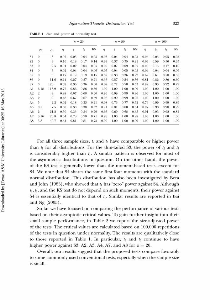
4. SIMULATIONS

In this section, we use Monte Carlo simulations to assess the sizeand power of the proposed tests. Following Bai and Ng (2005), weconsider some well known distributions such as the normal, the t andthe �2, as well as distributions from the generalized lambda family. Thegeneralized lambda distribution, denoted by F�, is defined in terms of theinverse of the cumulative distribution F −1(u) = �1 + [u�3 − (1 − u)�4]/�2,0 < u < 1. This family nests a wide range of symmetric and asymmetricdistributions. In particular, we consider the following symmetric andasymmetric distributions:

S1: N (0, 1);S2: t distribution with 5 degrees of freedom;S3: e1I (z ≤ 0�5) + e2I (z > 0�5), where z ∼ U (0, 1), e1 ∼ N (−1, 1), and

e2 ∼N (1, 1);S4: F�, �1 = 0, �2 = 0�19754, �3 = 0�134915, �4 = 0�134915;S5: F�, �1 = 0, �2 = −1, �3 = −0�8, �4 = −0�8;S6: F�, �1 = 0, �2 = −0�397912, �3 = −0�16, �4 = −0�16;S7: F�, �1 = 0, �2 = −1, �3 = −0�24, �4 = −0�24;A1: lognormal: exp(e), e ∼ N (0, 1);A2: �2 distribution with 3 degrees of freedom;A3: exponential: − ln(e), e ∼ U (0, 1);A4: F�, �1 = 0, �2 = 1, �3 = 1�4, �4 = 0�25;A5: F�, �1 = 0, �2 = −1, �3 = −0�0075, �4 = −0�03;A6: F�, �1 = 0, �2 = −1, �3 = −0�1, �4 = −0�18;A7: F�, �1 = 0, �2 = −1, �3 = −0�001, �4 = −0�13;A8: F�, �1 = 0, �2 = −1, �3 = −0�0001, �4 = −0�17.

The first seven distributions are symmetric and the next eight areasymmetric, with a wide range of skewness and kurtosis coefficients asshown in Table 1. For each distribution, we draw 10,000 random samples ofsize n = 20, 50, 100, respectively, and compute the normality test statisticsdiscussed above. For the sake of comparison, we also compute thecommonly used Kolmogorov–Smirnov (KS) test. We note that the general-purpose KS test has very low power. Instead, we use the Lillie test, whichis a special version of KS test tailored for the test of normality, see Thode(2002). All tests were computed based on standardized samples and allsimulations were implemented in Matlab 6.5.

Table 1 reports the results of the normality tests at the 5% significancelevel. The first row reflects the size and the rest show the power of the tests.It is noted that all three moment-based tests are under-sized when n = 20or 50. As n increases, the size of all tests converges to the theoretical level,and their powers generally increase.

Dow

nloa

ded

by [

Tex

as A

&M

Uni

vers

ity L

ibra

ries

] at

00:

25 1

6 M

ay 2

013


TABLE 1 Size and power of normality test

n = 20 n = 50 n = 100

�3 �4 t1 t2 t3 KS t1 t2 t3 KS t1 t2 t3 KS

S1 0 3 0.02 0.03 0.04 0.05 0.03 0.04 0.04 0.05 0.05 0.05 0.05 0.05S2 0 9 0.16 0.18 0.17 0.14 0.39 0.37 0.35 0.21 0.63 0.59 0.56 0.33S3 0 2�5 0.01 0.02 0.04 0.05 0.00 0.07 0.09 0.07 0.00 0.15 0.17 0.10S4 0 3 0.02 0.04 0.04 0.06 0.03 0.04 0.05 0.05 0.04 0.04 0.04 0.06S5 0 6 0.17 0.19 0.19 0.15 0.39 0.38 0.36 0.22 0.62 0.61 0.58 0.35S6 0 11�6 0.24 0.27 0.27 0.21 0.56 0.57 0.54 0.36 0.81 0.82 0.80 0.60S7 0 126 0.32 0.36 0.36 0.30 0.69 0.71 0.70 0.53 0.92 0.93 0.92 0.79A1 6�18 113�9 0.72 0.86 0.86 0.80 1.00 1.00 1.00 0.99 1.00 1.00 1.00 1.00A2 2 9 0.48 0.67 0.68 0.60 0.96 0.99 0.99 0.96 1.00 1.00 1.00 1.00A3 2 9 0.48 0.67 0.67 0.59 0.96 0.99 0.99 0.96 1.00 1.00 1.00 1.00A4 5 2�2 0.02 0.18 0.23 0.21 0.08 0.73 0.77 0.52 0.79 0.99 0.99 0.89A5 0�5 7�5 0.30 0.38 0.38 0.32 0.74 0.81 0.80 0.64 0.97 0.98 0.98 0.92A6 2 21�2 0.30 0.35 0.34 0.29 0.66 0.69 0.68 0.53 0.91 0.93 0.92 0.81A7 3�16 23�8 0.61 0.78 0.78 0.71 0.98 1.00 1.00 0.98 1.00 1.00 1.00 1.00A8 3�8 40�7 0.64 0.81 0.81 0.75 0.99 1.00 1.00 0.99 1.00 1.00 1.00 1.00

For all three sample sizes, t2 and t3 have comparable or higher powerthan t1 for all distributions. For the thin-tailed S3, the power of t2 and t3is considerably higher than t1. A similar pattern is observed for most ofthe asymmetric distributions in question. On the other hand, the powerof the KS test is generally lower than the moment-based tests, except forS4. We note that S4 shares the same first four moments with the standardnormal distribution. This distribution has also been investigated by Beraand John (1983), who showed that t1 has “zero” power against S4. Althought2, t3, and the KS test do not depend on such moments, their power againstS4 is essentially identical to that of t1. Similar results are reported in Baiand Ng (2005).

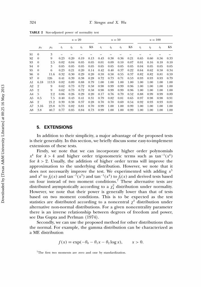
So far we have focused on comparing the performance of various testsbased on their asymptotic critical values. To gain further insight into theirsmall sample performance, in Table 2 we report the size-adjusted powerof the tests. The critical values are calculated based on 100,000 repetitionsof the tests in question under normality. The results are qualitatively closeto those reported in Table 1. In particular, t2 and t3 continue to havehigher power against S3, A2, A3, A4, A7, and A8 for n = 20.

Overall, our results suggest that the proposed tests compare favorablyto some commonly used conventional tests, especially when the sample sizeis small.

Dow

nloa

ded

by [

Tex

as A

&M

Uni

vers

ity L

ibra

ries

] at

00:

25 1

6 M

ay 2

013


TABLE 2 Size-adjusted power of normality test

n = 20 n = 50 n = 100

�3 �4 t1 t2 t3 KS t1 t2 t3 KS t1 t2 t3 KS

S1 0 3 – – – – – – – – – – – –S2 0 9 0.23 0.20 0.19 0.13 0.43 0.38 0.36 0.21 0.65 0.60 0.56 0.33S3 0 2�5 0.02 0.04 0.05 0.05 0.01 0.09 0.10 0.07 0.01 0.16 0.18 0.10S4 0 3 0.05 0.05 0.05 0.05 0.05 0.05 0.05 0.05 0.04 0.05 0.05 0.05S5 0 6 0.23 0.21 0.20 0.14 0.42 0.40 0.37 0.22 0.64 0.62 0.58 0.34S6 0 11�6 0.32 0.30 0.29 0.20 0.59 0.58 0.55 0.37 0.82 0.82 0.81 0.59S7 0 126 0.41 0.39 0.38 0.28 0.72 0.73 0.71 0.53 0.93 0.93 0.93 0.79A1 6�18 113�9 0.82 0.89 0.88 0.79 1.00 1.00 1.00 1.00 1.00 1.00 1.00 1.00A2 2 9 0.62 0.73 0.72 0.58 0.98 0.99 0.99 0.96 1.00 1.00 1.00 1.00A3 2 9 0.62 0.73 0.72 0.58 0.98 0.99 0.99 0.96 1.00 1.00 1.00 1.00A4 5 2�2 0.06 0.26 0.29 0.20 0.17 0.76 0.79 0.52 0.88 0.99 0.99 0.89A5 0�5 7�5 0.40 0.43 0.41 0.31 0.79 0.82 0.81 0.65 0.97 0.98 0.98 0.91A6 2 21�2 0.39 0.38 0.37 0.28 0.70 0.70 0.69 0.54 0.92 0.93 0.93 0.81A7 3�16 23�8 0.73 0.82 0.81 0.70 0.99 1.00 1.00 0.99 1.00 1.00 1.00 1.00A8 3�8 40�7 0.77 0.85 0.84 0.73 0.99 1.00 1.00 0.99 1.00 1.00 1.00 1.00

5. EXTENSIONS

In addition to their simplicity, a major advantage of the proposed testsis their generality. In this section, we briefly discuss some easy-to-implementextensions of these tests.

Firstly, we note that we can incorporate higher order polynomialsxk for k > 4 and higher order trigonometric terms such as tan−1(xk)for k > 2. Usually, the addition of higher order terms will improve theapproximation to the underlying distribution. However, we note that itdoes not necessarily improve the test. We experimented with adding x5

and x6 to f2(x) and tan−1(x3) and tan−1(x4) to f3(x) and derived tests basedon four instead of two moment conditions.7 These alternative tests aredistributed asymptotically according to a �24 distribution under normality.However, we note that their power is generally lower than that of testsbased on two moment conditions. This is to be expected as the teststatistics are distributed according to a noncentral �2 distribution underalternative non-normal distributions. For a given noncentrality parameterthere is an inverse relationship between degrees of freedom and power,see Das Gupta and Perlman (1974).

Secondly, we can use the proposed method for other distributions thanthe normal. For example, the gamma distribution can be characterized asa ME distribution

f (x) = exp(−�0 − �1x − �2 log x), x > 0�

7The first two moments are zero and one by standardization.

Dow

nloa

ded

by [

Tex

as A

&M

Uni

vers

ity L

ibra

ries

] at

00:

25 1

6 M

ay 2

013


Because Ex and E log x are the characterizing moments for the gammadistribution, the presence of any additional terms in the exponent of f (x)would reject the hypothesis that x is distributed according to a gammadistribution. Let fK (x) = exp(−�0 − �1x − �2 log x − ∑K

k=3 �kgk(x)), the testof �k = 0 for k ≥ 3 is then the LM test for gamma distribution. Thediscussion in the previous section suggests that the natural candidates forgk(x) may include polynomials of x and log x , and trigonometric terms ofx and log x .

Thirdly, we can generalize our tests to regression residuals within theframework of White and McDonald (1980). Consider a classical linearmodel

Yi = Zi� + �i , i = 1, � � � ,n� (3)

Since the error term �i is not observed, one has to replace it with theresidual �i . The following theorem ensures that the test statistics computedfrom the residuals �i share the same asymptotic distribution as those fromthe true errors �i .

Theorem 2. Assume the following assumptions hold:

1. �Zi� is a sequence of uniformly bounded fixed 1 × K vectors such thatZ ′Z /n →Mz, a positive definite matrix, ��i� is a sequence of iid randomvariables with E�i = 0, E�2

i = 2i < ∞, and � is an unknown K × 1 vector.

2. E |�i |4+� < ∞ for � > 0.3. The density of �i , f (�), is uniformly continuous, positive on the interval of

support and bounded.

Let �i be the standardized residuals. Define �3 = 1n

∑ni=1 �

3i ,

�4 = 1n

∑ni=1 �

4i , �a = 1

n

∑ni=1 tan

−1(�i), �b = 1n

∑ni=1 log(1 + �2

i ), and�c = 1

n

∑ni=1 tan

−1(�2i ). Then under normality, the test statistics

t1 = n(�23/6 + (�4 − 3)2/24

) ∼ �22,

t2 = n(50�54269�2

a + 32�027545(�b − 0�5334532)2) ∼ �22,

t3 = n(50�54269�2

a + 16�882261(�c − 0�5299567)2) ∼ �22�

The proof of Theorem 2 is presented in the Appendix.Furthermore, for time series or heteroskedastic data, we can use

the approach of Bai and Ng (2005) or Bontemps and Meddahi (2005).In general, for non-i.i.d. data, to test that the LMs associated with samplemoments of gk(x) in the ME density are zero, we need to calculate aHeteroskedastic–Autocorrelation–Consistent (HAC) covariance matrix for

Dow

nloa

ded

by [

Tex

as A

&M

Uni

vers

ity L

ibra

ries

] at

00:

25 1

6 M

ay 2

013


those moments, see Richardson and Smith (1993) on the use of HACstandard errors in testing for normality.8

Finally, as an illustration, we apply the proposed normality tests toregression residuals. We use data on the production cost of some U.S.electricity generating companies from Christensen and Greene (1976).We estimate a flexible cost function with 123 observations:

c = �0 + �1q + �2q2 + �3pf + �4pl + �5pk + �6qpf + �7qpk + �8qpl + �,

where c is the total cost, q is the total output, pf , pl , and pk are the price offuel, labor, and capital, respectively, and � is the error term. All variablesare expressed in logarithmic form. It is expected that the distribution ofthe Ordinary Least Squares (OLS) residuals from a production functionregression is skewed to the right due to the presence of firm specific, non-negative efficiency components in the error term. Nonetheless, the KS testfails to reject the normality hypothesis. On the other hand, all three LMtests reject the normality hypothesis with p-values of 0.03, 0.01, and 0.02,respectively.

6. CONCLUSION

In this article, we derive some general distributional tests from MEdensity methodology. The proposed tests are derived from maximizing thedifferential entropy subject to given moment constraints. By exploiting theequivalence between the ME and the ML estimates for the exponentialfamily, we can use the conventional LR, Wald, and LM testing principlesin the maximum entropy framework. Hence, our tests share the optimalityproperties of the standard ML based tests. In particular, we show thatthe ME approach leads to simple yet powerful LM tests for normality.We derive the asymptotic properties of the proposed tests and show thatthey are asymptotically equivalent to the popular Jarque–Bera test. OurMonte Carlo simulations show that the proposed tests have desirablesmall sample properties. They are comparable and often outperformsome conventional tests for normality. In addition, we show that theproposed method can be generalized to tests for other distributions thanthe normal. Also, extensions to regression residuals and non-i.i.d. dataare straightforward. In principle, the proposed methodology can be alsoapplied to distributional tests for truncated distributions, as in Bera et al.(1984) and Lye and Martin (1998), something that we leave for futureresearch.

8We thank a referee for this reference.

Dow

nloa

ded

by [

Tex

as A

&M

Uni

vers

ity L

ibra

ries

] at

00:

25 1

6 M

ay 2

013


APPENDIX

Proof of Theorem 1

Proof. The assumption that E |x |4+� < ∞ for � > 0 ensures the existenceof E �3 and E �4. One can easily show that

√n�3 ∼ N (0, 6) and

√n(�4 −

3) ∼ N (0, 24) if xi is iid and normally distributed (see for example, Stuartet al., 1994). Since cov(�3, �4) = 0, it follows that under normality

t1 = n(�23

6+ (�4 − 3)2

24

)∼ �22�

Similarly, since tan−1(x) = o(x), tan−1(x2) = o(x) and log(1 + x2) = o(x)as |x | → ∞, their expectations also exist under the assumption thatE |x |4+� < ∞ for � > 0. We then have

√n�a ∼ N (0, 1/50�54269),

√n(�b −

0�5334532) ∼ N (0, 1/32�027545), and√n(�c − 0�5299567) ∼ N (0, 1/

16�8882261) under normality. In addition, since cov(�a , �b) = 0 andcov(�a , �c) = 0, it follows that under normality

t2 = n(50�54269�2

a + 32�027545(�b − 0�5334532)2) ∼ �22,

t3 = n(50�54269�2

a + 16�8882261(�c − 0�5299567)2) ∼ �22�

Proof of Theorem 2

Proof. Assumption 1 sets forth the classical linear model (except for thenormality of �i) and ensures that �n

as→ �0. Given Assumptions 1 and 2, onecan show that |�3 − �3| as→ 0 and |�4 − �4| as→ 0 using Lemmas 1 and 2 ofWhite and McDonald (1980). Using Corollary A of Serfling (1980, p. 19),one can show that since t1

as→ t1, t1d→ t1 given Assumption 3. Since t1 ∼ �22 by

Theorem 1 in Section 3, we have t1 ∼ �22. Similarly, since tan−1(x) = o(x),tan−1(x2) = o(x) and log(1 + x2) = o(x) as |x | → ∞, Assumptions 1 and2 ensure that |�a | as→ 0, |�b − �b | as→ 0, and |�c − �c | as→ 0. Using the similararguments as the proof for t1, one can show that t2

d→ �22 and t3d→ �22.

ACKNOWLEDGMENTS

We want to thank the associate editor, two anonymous referees,seminar participants at Penn State University, the 2004 European Meetingof the Econometric Society, and the 2004 Canadian Econometrics StudyGroup for comments. Financial support from SSHRC of Canada isgratefully acknowledged.

Dow

nloa

ded

by [

Tex

as A

&M

Uni

vers

ity L

ibra

ries

] at

00:

25 1

6 M

ay 2

013


REFERENCES

Bai, J., Ng, S. (2005). Tests for skewness, kurtosis and normality for time series data. Journal ofBusiness and Economic Statistics 23(1):49–60.

Bera, A., Bilias, Y. (2002). The MM, ME, ML, EL, EF, and GMM approaches to estimation:A synthesis. Journal of Econometrics 107:51.

Bera, A., Jarque, C. (1981). Efficient tests for normality, heteroskedasticity and serial independenceof regression residuals: Monte Carlo evidence. Economics Letters 7:313–318.

Bera, A., Jarque, C., Lee, L. F. (1984). Testing the normality assumption in limited dependentvariable models. International Economic Review 25:563–578.

Bera, A., John, S. (1983). Tests for multivariate normality. Communication in Statistics, Theory andMethods 12(1):103–117.

Bontemps, C., Meddahi, N. (2005). Testing normality: A gmm approach. Journal of Econometrics124(1):149–186.

Christensen, L. R., Greene, W. H. (1976). Economies of scale in U.S. electric power generation.Journal of Political Economy 84:655–676.

Cobb, L., Koppstein, P., Chen, N. (1983). Estimation and moment recursion relations formultimodal distributions of the exponential family. Journal of American Statistical Association8(381):124–130.

Cressie, N., Read, T. (1984). Multinomial goodness-of-fit tests. Journal of the Royal Statistical Society,Series B 46:440–464.

Dalén, J. (1987). Bounds on standardized sample moments. Statistics and Probability Letters 5:329–31.Das Gupta, S., Perlman, M. D. (1974). Power of the noncentral F test: effect of additional variates

in Hotelling’s t2 test. Journal of the American Statistical Association 69:174–180.Ebrahimi, N., Maasoumi, E., Soofi, E. (1999). Ordering univariate distributions by entropy and

variance. Journal of Econometrics 90:317–336.Econometric Reviews (2008). Special issues on IEE. 27:317–609.Engle, R. (1984). Wald, likelihood ratio and lagrange multiplier tests in econometrics. In:

Grilliches, Z., Intrilligator, M. D., eds. Handbook of econometrics, Vol. 3. North Holland:Elsevier.

Fisher, R. A. (1922). On the mathematical foundations of theoretical statistics. PhilosophicalTransactions of the Royal Society of London, Series A 222:309–68.

Gallant, A. R. (1981). On the bias in flexible functional forms and an essentially unbiased form.Journal of Econometrics 15:211–241.

Golan, A. (2002). Information and entropy econometrics – editor’s view. Journal of Econometrics107:1–16.

Golan, A. (2007). Information and entropy econometrics – volume overview and synthesis. Journalof Econometrics 138:379–387.

Golan, A. (2008). Information and entropy econometrics – a review and synthesis. Foundations andTrends in Economics 2:1–145.

Golan, A., Maasoumi, E. (2008). Information theoretic and entropy methods: An overview.Econometric Reviews 27:317–328.

Golan, A., Judge, G., Miller, D. (1996). Maximum Entropy Econometrics: Robust Estimation with LimitedData. Chichester: John Wiley & Sons.

Haberman, S. J. (1984). Adjustment by minimum discriminant information. Annals of Statistics12:971–988.

Hansen, L. P. (1982). Large sample properties of generalized methods of moments estimators.Econometrica 50:1029–1054.

Hansen, L. P., Heaton, J., Yaron, A. (1996). Finite sample properties of some alternative gmmestimators. Journal of Business and Economic Statistics 14:262–280.

Imbens, G. W., Spady, R. H., Johnson, P. (1998). Information theoretic approaches to inference inmoment condition models. Econometrica 66:333–357.

Imbens, G. W. (2002). Generalized method of moments and empirical likelihood. Journal of Business& Economic Statistics 20:493–507.

Jaynes, E. T. (1957). Information theory and statistical mechanics. Physics Review 106:620–630.Kitamura, Y., Stutzer, M. (1997). An information theoretic alternative to generalized method of

moments estimation. Econometrica 65:861–874.

Dow

nloa

ded

by [

Tex

as A

&M

Uni

vers

ity L

ibra

ries

] at

00:

25 1

6 M

ay 2

013


Kitamura, Y. (2006). Empirical likelihood methods in econometrics: theory and practice. CowlesFoundation Discussion Paper No. 1569.

Lye, J. N., Martin, V. L. (1993). Robust estimation, nonnormalities, and generalized exponentialdistributions. Journal of American Statistical Association 88(421):261–267.

Lye, J. N., Martin, V. L. (1994). Non-linear time series modelling and distributional flexibility.Journal of Time Series Analysis 15:65–84.

Lye, J. N., Martin, V. L. (1998). Truncated distribution families. In: Creedy, J., Martin, V. L.eds. Nonlinear Economic Models: Cross-sectional. Time Series and Neural Network Application,Cheltenham, UK: Edward Elgar, pp. 47–68,

Maasoumi, E. (1993). A compendium on information theory in economics and econometrics.Econometrics Reviews 12:137–181.

Neyman, J. (1937). Smooth test for goodness of fit. Scandinavian Aktuarial 20:149–199.Ornermite, D., White, H. (1999). An efficient algorithm to compute maximum entropy densities.

Econometric Reviews 18(2):141–167.Owen, A. (1988). Empirical likelihood ratio confidence intervals for a single functional. Biometrika

75:237–249.Park, J., Bera, A. forthcoming, Maximum entropy autoregressive conditional heteroskedasticity

model. Journal of Econometrics 150:219–230.Pearson, K. (1900). On a criterion that a given system of deviations from the probable in the case

of correlated systems of variables is such that it can be reasonably supposed to have arisenin random sampling. Philosophical Magazine 50(5):157–175.

Premaratne, G., Bera, A. (2005). A test for symmetry with leptokurtic financial data. Journal ofFinancial Econometrics 3(2):169–187.

Qin, J., Lawless, J. (1994). Empirical likelihood and general estimating functions. Annals of Statistics22:300–325.

Richardson, M., Smith, T. (1993). A test for multivariate normality in stock returns. Journal ofBusiness 66:295–321.

Serfling, R. J. (1980). Approximation Theorems of Mathematical Statistics. New York: John Wiley & Sons,Inc.

Shannon, C. E. (1949). The Mathematical Theory of Communication. Urbana: University of IllinoisPress.

Shore, J. E., Johnson, R. (1980). Axiomatic derivation of the principle of maximum entropy andthe principle of minimum crossentropy. IEEE Transactions on Information Theory 26(1):26–37.

Smith, R. J. (2004). GEL Criteria for Moment Condition Models. Manuscript, University of Warwick.Smith, R. J. (2005). Local GEL Methods for Conditional Moment Restrictions. Working Paper,

University of Cambridge, Cambridge, England.Stohs, S. (2003). A Bayesian Updating Approach to Crop Insurance Ratemaking. Ph.D. thesis, University

of California at Berkeley.Stuart, A., Ord, K., Arnold, S. (1994). Kendall’s Advanced Theory of Statistics. Vol. 2A, New York:

Oxford University Press.Thode, H. (2002). Testing for Normality. New York: Marcel Dekker.Vasicek, O. (1976). A test for normality based on sample entropy. Journal of the Royal Statistical

Society, Series B 38:54–59.White, H. (1982). Maximum likelihood estimation of misspecified models. Econometrica 50:1–26.White, H., McDonald, G. M. (1980). Some large-sample tests for nonnormality in the linear

regression model. Journal of American Statistical Association 75:16–28.Wu, X. (2003). Calculation of maximum entropy densities with application to income distribution.

Journal of Econometrics 115:347–354.Wu, X., Stengos, T. (2005). Partially adaptive estimation via maximum entropy densities. Econometrics

Journal 8:352–366.Zellner, A., Highfield, R. A. (1988). Calculation of maximum entropy distribution and

approximation of marginal posterior distributions. Journal of Econometrics 37:195–209.Zellner, A. (1996). Bayesian method of moments/instrumental variable (BMOM/IV) analysis of

mean and regression models. In: Lee, J. C., Johnson, W. C., Zellner, A. eds. Modeling andPrediction: Honoring Seymour Geisser. Springer-Verlag, pp. 61–75.

Dow

nloa

ded

by [

Tex

as A

&M

Uni

vers

ity L

ibra

ries

] at

00:

25 1

6 M

ay 2

013

information-theoretic distribution test with application

Documents