information theory and coding { image, video and audio...
TRANSCRIPT
Information theory and coding –Image, video and audio compression
Markus Kuhn
Computer Laboratory
http://www.cl.cam.ac.uk/Teaching/2003/InfoTheory/mgk/
Michaelmas 2003 – Part II

Structure of modern audiovisualcommunication systems
SignalSensor+sampling
Perceptualcoding
Entropycoding
Channelcoding
Noise Channel
Humansenses Display
Perceptualdecoding
Entropydecoding
Channeldecoding
- - - -
-?
?� � � �
2

Entropy coding review – Huffman
0
0
0
0
0
1
1
1
1
1
x
y z0.05 0.05
0.100.15
0.25
1.00
0.60
v w
0.40
0.200.20 u0.35
Huffman’s algorithm constructs an optimal code-word tree for a set ofsymbols with known probability distribution. It iteratively picks the twoelements of the set with the smallest probability and combines them intoa tree by adding a common root. The resulting tree goes back into theset, labeled with the sum of the probabilities of the elements it combines.The algorithm terminates when less than two elements are left.
3

Other variable-length code tablesHuffman’s algorithm generates an optimal code table.Disadvantage: this code table (or the distribution from which is wasgenerated) needs to be stored or transmitted.Adaptive variants of Huffman’s algorithm modify the coding tree in the encoder and decodersynchronously, based on the distribution of symbols encountered so far. This enables one-passprocessing and avoids the need to transmit or store a code table, at the cost of starting with aless efficient encoding.
Unary codeEncode the natural number n as the bit string 1n0. This code is optimalwhen the probability distribution is p(n) = 2−(n+1).Example: 3, 2, 0→ 1110, 110, 0
Golomb codeSelect an encoding parameter b. Let n be the natural number to beencoded, q = bn/bc and r = n−qb. Encode n as the unary code wordfor q, followed by the (log2 b)-bit binary code word for r.Where b is not a power of 2, encode the lower values of r in blog2 bc bits, and the rest in dlog2 bebits, such that the leading digits distinguish the two cases.
4

Examples:
b = 1: 0, 10, 110, 1110, 11110, 111110, . . . (this is just the unary code)b = 2: 00, 01, 100, 101, 1100, 1101, 11100, 11101, 111100, 111101, . . .b = 3: 00, 010, 011, 100, 1010, 1011, 1100, 11010, 11011, 11100, 111010, . . .b = 4: 000, 001, 010, 011, 1000, 1001, 1010, 1011, 11000, 11001, 11010, . . .
Golomb codes are optimal for geometric distributions of the form p(n) = un(u − 1) (e.g., runlengths of Bernoulli experiments) if b is chosen suitably for a given u.
S.W. Golomb: Run-length encodings. IEEE Transactions on Information Theory, IT-12(3):399–401, July 1966.
Elias gamma codeStart the code word for the positive integer n with a unary-encodedlength indicator m = blog2 nc. Then append from the binary notationof n the rightmost m digits (to cut off the leading 1).
1 = 0 4 = 11000 7 = 11011 10 = 11100102 = 100 5 = 11001 8 = 1110000 11 = 11100113 = 101 6 = 11010 9 = 1110001 . . .
P. Elias: Universal codeword sets and representations of the integers. IEEE Transactions onInformation Theory, IT-21(2)194–203, March 1975.
More such variable-length integer codes are described by Fenwick in IT-48(8)2412–2417, August2002. (Available on http://ieeexplore.ieee.org/)
5
Entropy coding review – arithmetic coding
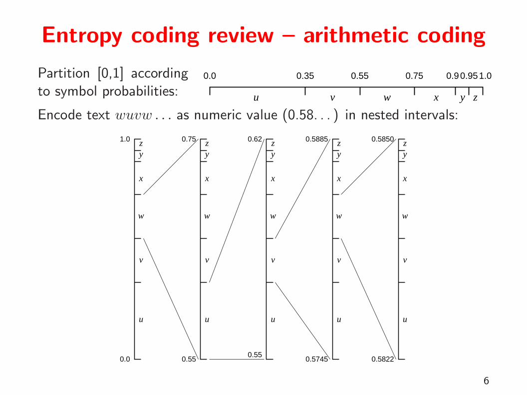
Partition [0,1] accordingto symbol probabilities: u v w x y z
0.950.9 1.00.750.550.350.0
Encode text wuvw . . . as numeric value (0.58. . . ) in nested intervals:
zy
x
v
u
w
zy
x
v
u
w
zy
x
v
u
w
zy
x
v
u
w
zy
x
v
u
w
1.0
0.0 0.55
0.75 0.62
0.550.5745
0.5885
0.5822
0.5850
6
Arithmetic coding
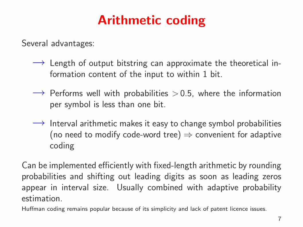
Several advantages:
→ Length of output bitstring can approximate the theoretical in-formation content of the input to within 1 bit.
→ Performs well with probabilities > 0.5, where the informationper symbol is less than one bit.
→ Interval arithmetic makes it easy to change symbol probabilities(no need to modify code-word tree)⇒ convenient for adaptivecoding
Can be implemented efficiently with fixed-length arithmetic by roundingprobabilities and shifting out leading digits as soon as leading zerosappear in interval size. Usually combined with adaptive probabilityestimation.Huffman coding remains popular because of its simplicity and lack of patent licence issues.
7
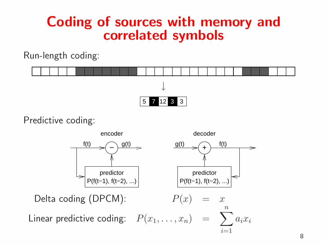
Coding of sources with memory andcorrelated symbols
Run-length coding:
↓5 7 12 33
Predictive coding:
P(f(t−1), f(t−2), ...)predictor
P(f(t−1), f(t−2), ...)predictor
− +f(t) g(t) g(t) f(t)
encoder decoder
Delta coding (DPCM): P (x) = x
Linear predictive coding: P (x1, . . . , xn) =n∑i=1
aixi
8
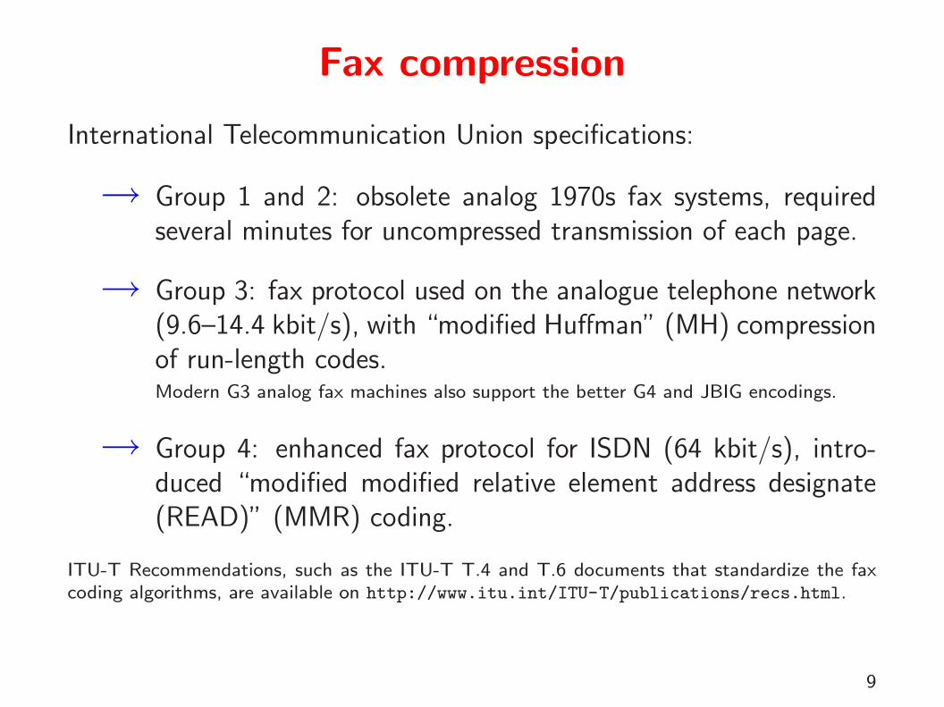
Fax compression
International Telecommunication Union specifications:
→ Group 1 and 2: obsolete analog 1970s fax systems, requiredseveral minutes for uncompressed transmission of each page.
→ Group 3: fax protocol used on the analogue telephone network(9.6–14.4 kbit/s), with “modified Huffman” (MH) compressionof run-length codes.Modern G3 analog fax machines also support the better G4 and JBIG encodings.
→ Group 4: enhanced fax protocol for ISDN (64 kbit/s), intro-duced “modified modified relative element address designate(READ)” (MMR) coding.
ITU-T Recommendations, such as the ITU-T T.4 and T.6 documents that standardize the faxcoding algorithms, are available on http://www.itu.int/ITU-T/publications/recs.html.
9

Group 3 MH fax code
• Run-length encoding plus modified Huffmancode
• Fixed code table (from eight sample pages)
• separate codes for runs of white and blackpixels
• termination code in the range 0–63 switchesbetween black and white code
• makeup code can extend length of a run bya multiple of 64
• termination run length 0 needed where runlength is a multiple of 64
• single white column added on left side be-fore transmission
• makeup codes above 1728 equal for blackand white
• 12-bit end-of-line marker: 000000000001(can be prefixed by up to seven zero-bitsto reach next byte boundary)
Example: line with 2 w, 4 b, 200 w, 3 b, EOL →1000|011|010111|10011|10|000000000001
pixels white code black code0 00110101 00001101111 000111 0102 0111 113 1000 104 1011 0115 1100 00116 1110 00107 1111 000118 10011 0001019 10100 000100
10 00111 000010011 01000 000010112 001000 000011113 000011 0000010014 110100 0000011115 110101 00001100016 101010 0000010111
. . . . . . . . .63 00110100 00000110011164 11011 0000001111
128 10010 000011001000192 010111 000011001001. . . . . . . . .
1728 010011011 000000110010110
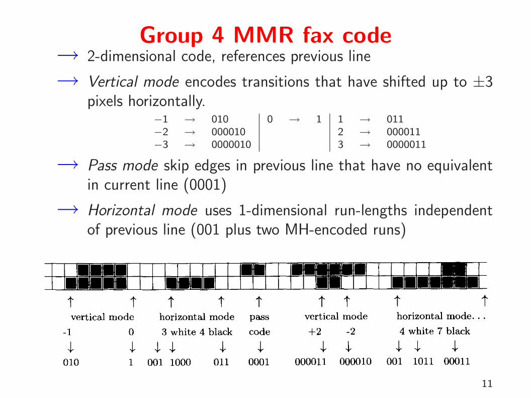
Group 4 MMR fax code→ 2-dimensional code, references previous line
→ Vertical mode encodes transitions that have shifted up to ±3pixels horizontally.
−1 → 010 0 → 1 1 → 011−2 → 000010 2 → 000011−3 → 0000010 3 → 0000011
→ Pass mode skip edges in previous line that have no equivalentin current line (0001)
→ Horizontal mode uses 1-dimensional run-lengths independentof previous line (001 plus two MH-encoded runs)
11
JBIG (Joint Bilevel Experts Group)→ lossless algorithm for 1–6 bits per pixel
→ main applications: fax, scanned text documents
→ context-sensitive arithmetic coding
→ adaptive context template for better prediction efficiency withrastered photographs (e.g. in newspapers)
→ support for resolution reduction and progressive coding
→ “deterministic prediction” avoids redundancy of progr. coding
→ “typical prediction” codes common cases very efficiently
→ typical compression factor 20, 1.1–1.5× better than Group 4fax, about 2× better than “gzip -9” and about ≈3–4× betterthan GIF (all on 300 dpi documents).
Information technology — Coded representation of picture and audio information — progressivebi-level image compression. International Standard ISO 11544:1993.Example implementation: http://www.cl.cam.ac.uk/~mgk25/jbigkit/
12

JBIG encodingBoth encoder and decoder maintain statistics on how the black/whiteprobability of each pixel depends on these 10 previously transmittedneighbours:
?
Based on the counted numbers nLPS and nMPS of how often the lessand more probable symbol (e.g., black and white) have been encoun-tered so far in each of the 1024 contexts, their probabilities are esti-mated as
pLPS =nLPS + δ
nLPS + δ + nMPS + δParameter δ = 0.45 is an empirically optimized start-up aid. To keep the estimation adaptable(for font changes, etc.) both counts are divided by a common factor before nLPS > 11.
To simplify hardware implementation, the estimator is defined as an FSM with 113 states, eachrepresenting a point in the (nLPS, nMPS) plane. Is makes a transition only when the arithmetic-coding interval is renormalized to output another bit. The new state depends on whether renor-malization was initiated by the less and more probable symbol.
13
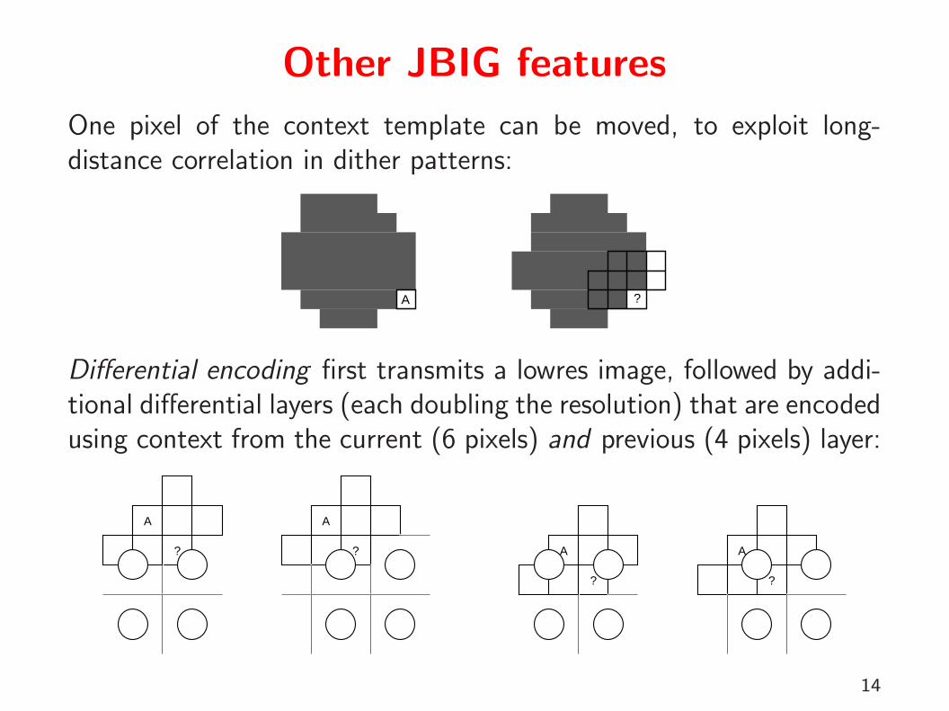
Other JBIG features
One pixel of the context template can be moved, to exploit long-distance correlation in dither patterns:
A ?
Differential encoding first transmits a lowres image, followed by addi-tional differential layers (each doubling the resolution) that are encodedusing context from the current (6 pixels) and previous (4 pixels) layer:
A
?
A
? A
?
A
?
14

JBIG resolution reductionMultiply neighbour pixels with filter coefficients and make the newreduced-resolution pixel black if the sum is 5 or more:
2 11
2 4 2
1 2 1
?
−3−1
−3 ?
filter coefficients example from exception list
This applies a low-pass filter to the high-resolution layer to avoid aliasing and a high-pass filterto the low-resolution layer to preserve gray-scale dithering. An exception list suppresses zigzagedges.
Example:
original subsampled JBIG reduced
15
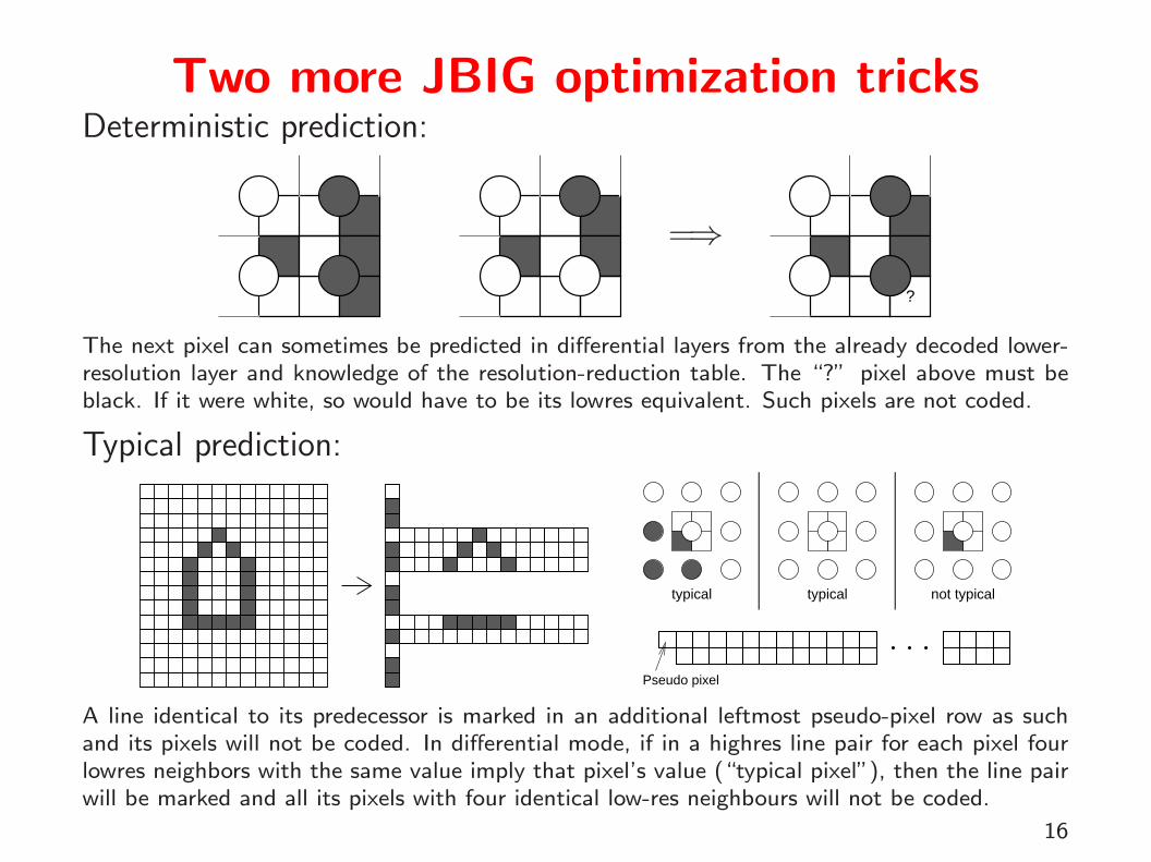
Two more JBIG optimization tricksDeterministic prediction:
=⇒?
The next pixel can sometimes be predicted in differential layers from the already decoded lower-resolution layer and knowledge of the resolution-reduction table. The “?” pixel above must beblack. If it were white, so would have to be its lowres equivalent. Such pixels are not coded.
Typical prediction:
typical typical not typical
Pseudo pixel
A line identical to its predecessor is marked in an additional leftmost pseudo-pixel row as suchand its pixels will not be coded. In differential mode, if in a highres line pair for each pixel fourlowres neighbors with the same value imply that pixel’s value (“typical pixel”), then the line pairwill be marked and all its pixels with four identical low-res neighbours will not be coded.
16

Dependence and correlationRandom variables X, Y are dependent iff ∃x, y:
P (X = x ∧ Y = y) 6= P (X = x) · P (Y = y).
If X, Y are dependent, then
⇒ ∃x, y : P (X = x |Y = y) 6= P (X = x) ∨P (Y = y |X = x) 6= P (Y = y)
⇒ H(X|Y ) < H(X) ∨H(Y |X) < H(Y )
Random variables are correlated iff
E((X − E(X)) · (Y − E(Y ))) 6= 0
Correlation implies dependence, but dependence doesnot always lead to correlation. However, most depen-dency in audiovisual data is a consequence of correla-tion, which is algorithmically much easier to exploit.
−1 0 1−1
0
1
Dependent but not correlated:
17
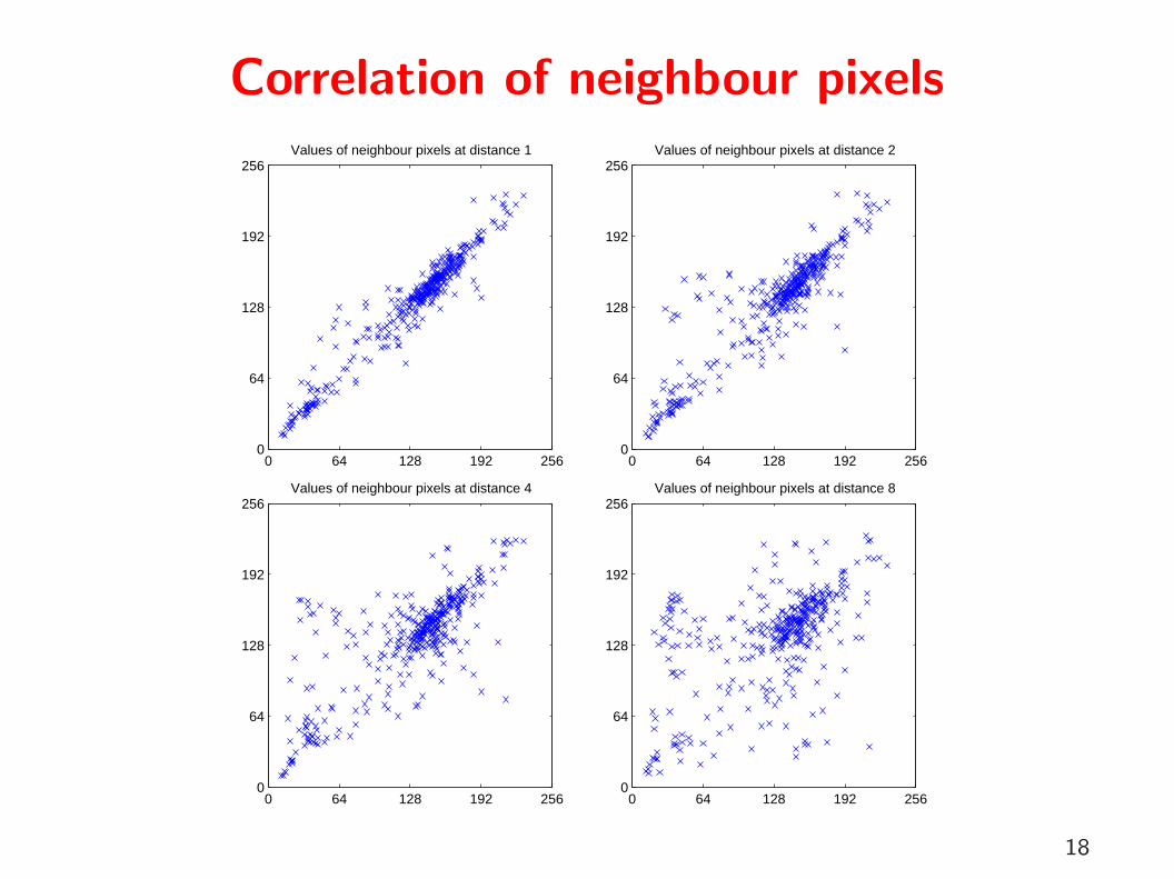
Correlation of neighbour pixels
0 64 128 192 2560
64
128
192
256Values of neighbour pixels at distance 1
0 64 128 192 2560
64
128
192
256Values of neighbour pixels at distance 2
0 64 128 192 2560
64
128
192
256Values of neighbour pixels at distance 4
0 64 128 192 2560
64
128
192
256Values of neighbour pixels at distance 8
18
Covariance and correlation
We define the covariance of two random vectors X and Y as
Cov(X, Y ) = E{[X−E(X)]·[Y −E(Y )]} = E(X ·Y )−E(X)·E(Y )
and the variance as Var(X) = Cov(X,X).The correlation coefficient
ρX,Y =Cov(X,Y )√
Var(X) ·Var(Y )
is a normalized form of the covariance in the range [−1, 1] with ρX,Y = ±1⇔ ∃a, b : Y = aX+b.
For a random vector X = (X1, X2, . . . , Xn) we define the covariancematrix
Cov(X) = (Cov(Xi, Xj))i,j = E((X− E(X)) · (X− E(X))T
)The elements of a random vector X are uncorrelated iff Cov(X) is adiagonal matrix.
19
Decorrelation by coordinate transform
0 64 128 192 2560
64
128
192
256Neighbour−pixel value pairs
−64 0 64 128 192 256 320−64
0
64
128
192
256
320Decorrelated neighbour−pixel value pairs
−64 0 64 128 192 256 320
Probability distribution and entropy
correlated value pair (H = 13.90 bit)decorrelated value 1 (H = 7.12 bit)decorrelated value 2 (H = 4.75 bit)
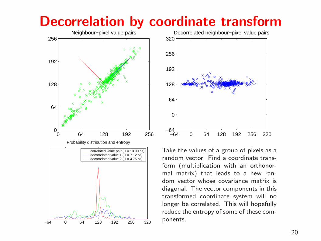
Take the values of a group of pixels as arandom vector. Find a coordinate trans-form (multiplication with an orthonor-mal matrix) that leads to a new ran-dom vector whose covariance matrix isdiagonal. The vector components in thistransformed coordinate system will nolonger be correlated. This will hopefullyreduce the entropy of some of these com-ponents.
20
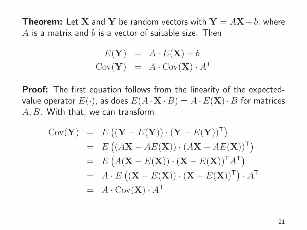
Theorem: Let X and Y be random vectors with Y = AX + b, whereA is a matrix and b is a vector of suitable size. Then
E(Y) = A · E(X) + b
Cov(Y) = A · Cov(X) · AT
Proof: The first equation follows from the linearity of the expected-value operator E(·), as does E(A ·X ·B) = A ·E(X) ·B for matricesA,B. With that, we can transform
Cov(Y) = E((Y − E(Y)) · (Y − E(Y))T
)= E
((AX− AE(X)) · (AX− AE(X))T
)= E
(A(X− E(X)) · (X− E(X))TAT
)= A · E
((X− E(X)) · (X− E(X))T
)· AT
= A · Cov(X) · AT
21

Karhunen-Loeve transform (KLT)Take the n pixel values of an image (or in practice a small 8× 8 pixelblock) as an n-dimensional random vector X.
How can we find a transform matrix A such that Cov(AX) = A ·Cov(X) · AT becomes a diagonal matrix? A would provide us thetransformed representation Y = AX of our image, in which all pixelsare uncorrelated.
Note that Cov(X) is symmetric. It therefore has n real eigenvaluesλ1 ≥ λ2 ≥ · · · ≥ λn and a set of associated mutually orthogonaleigenvectors b1, b2, . . . , bn of length 1 with
Cov(X)bi = λibi.
We convert this set of equations into matrix notation using the matrixB = (b1, b2, . . . , bn) that has these eigenvectors as columns and thediagonal matrix D = diag(λ1, λ2, . . . , λn) that consists of the corre-sponding eigenvalues:
Cov(X)B = BD22
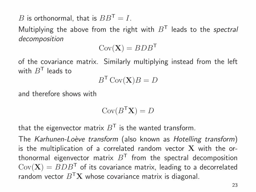
B is orthonormal, that is BBT = I.
Multiplying the above from the right with BT leads to the spectraldecomposition
Cov(X) = BDBT
of the covariance matrix. Similarly multiplying instead from the leftwith BT leads to
BT Cov(X)B = D
and therefore shows with
Cov(BTX) = D
that the eigenvector matrix BT is the wanted transform.
The Karhunen-Loeve transform (also known as Hotelling transform)is the multiplication of a correlated random vector X with the or-thonormal eigenvector matrix BT from the spectral decompositionCov(X) = BDBT of its covariance matrix, leading to a decorrelatedrandom vector BTX whose covariance matrix is diagonal.
23
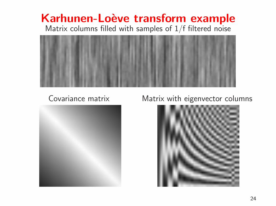
Karhunen-Loeve transform exampleMatrix columns filled with samples of 1/f filtered noise
Covariance matrix Matrix with eigenvector columns
24

Matrix with normalised KLTeigenvector columns
Matrix with Discrete CosineTransform base vector columns
Breakthrough: Ahmed/Natarajan/Rao discovered the DCT as an ex-cellent approximation of the KLT for typical photographic images, butfar more efficient to calculate.Ahmed, Natarajan, Rao: Discrete Cosine Transform. IEEE Transactions on Computers, Vol. 23,January 1974, pp. 90–93.
25
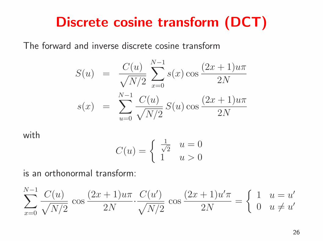
Discrete cosine transform (DCT)
The forward and inverse discrete cosine transform
S(u) =C(u)√N/2
N−1∑x=0
s(x) cos(2x+ 1)uπ
2N
s(x) =N−1∑u=0
C(u)√N/2
S(u) cos(2x+ 1)uπ
2N
with
C(u) =
{ 1√2
u = 0
1 u > 0
is an orthonormal transform:
N−1∑x=0
C(u)√N/2
cos(2x+ 1)uπ
2N· C(u′)√
N/2cos
(2x+ 1)u′π
2N=
{1 u = u′
0 u 6= u′
26

The 2-dimensional variant of the DCT applies the 1-D transform onboth rows and columns of an image:
S(u, v) =C(u)√N/2
C(v)√N/2·
N−1∑x=0
N−1∑y=0
s(x, y) cos(2x+ 1)uπ
2Ncos
(2y + 1)vπ
2N
s(x, y) =N−1∑u=0
N−1∑v=0
C(u)√N/2
C(v)√N/2
· S(u, v) cos(2x+ 1)uπ
2Ncos
(2y + 1)vπ
2N
A range of fast algorithms have been found for calculating 1-D and2-D DCTs (e.g., Ligtenberg/Vetterli).
27

Whole-image DCT
2D Discrete Cosine Transform (log10)
−4
−3
−2
−1
0
1
2
3
4
Original image
28
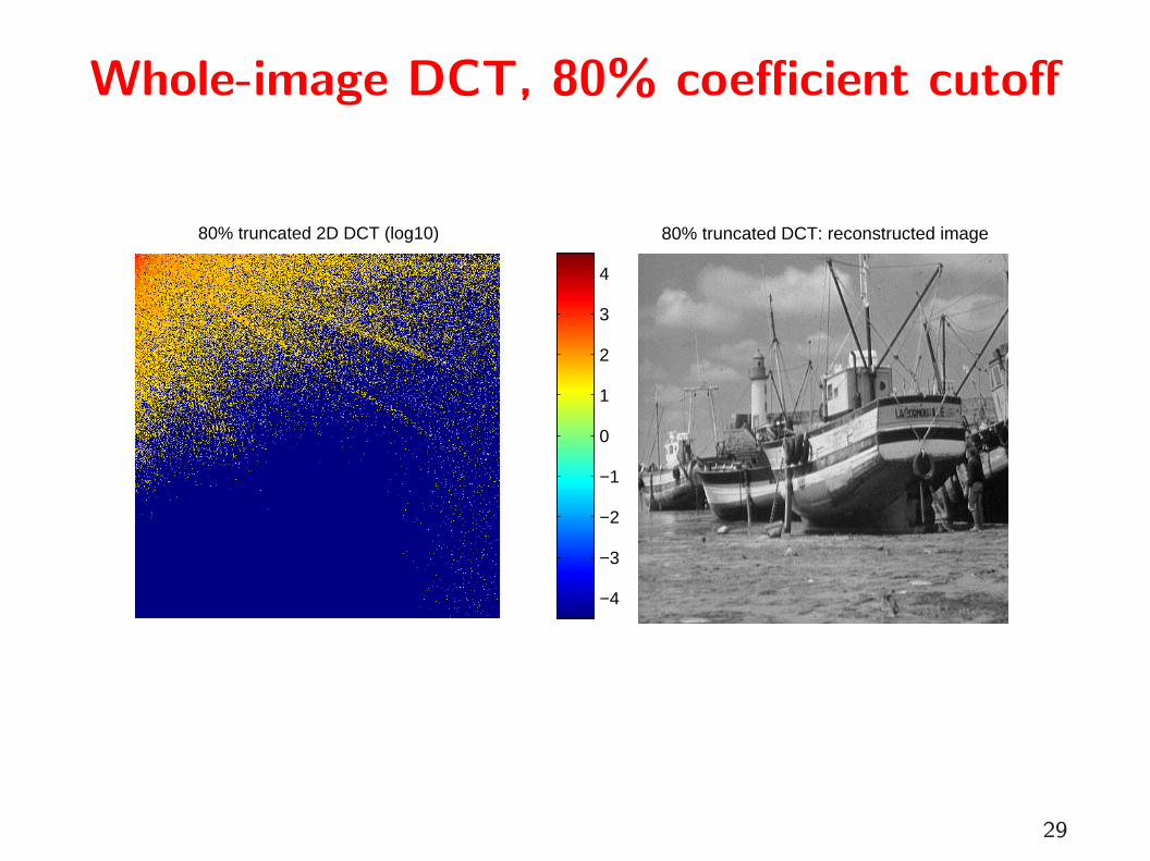
Whole-image DCT, 80% coefficient cutoff
80% truncated 2D DCT (log10)
−4
−3
−2
−1
0
1
2
3
4
80% truncated DCT: reconstructed image
29
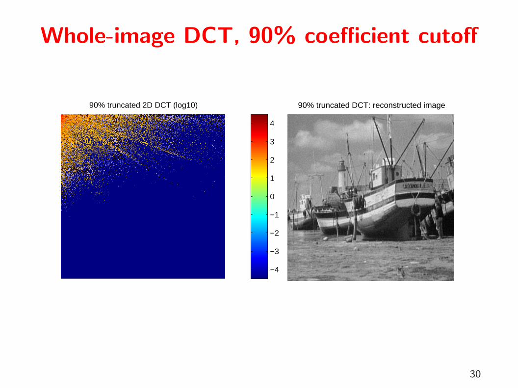
Whole-image DCT, 90% coefficient cutoff
90% truncated 2D DCT (log10)
−4
−3
−2
−1
0
1
2
3
4
90% truncated DCT: reconstructed image
30
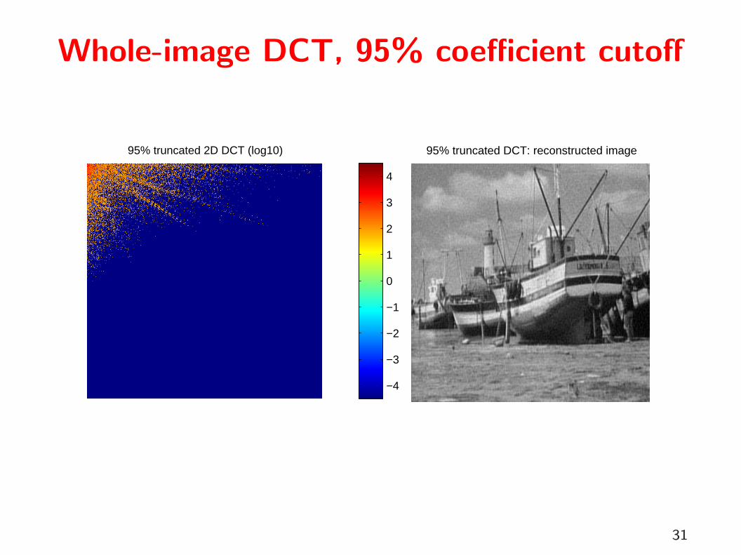
Whole-image DCT, 95% coefficient cutoff
95% truncated 2D DCT (log10)
−4
−3
−2
−1
0
1
2
3
4
95% truncated DCT: reconstructed image
31
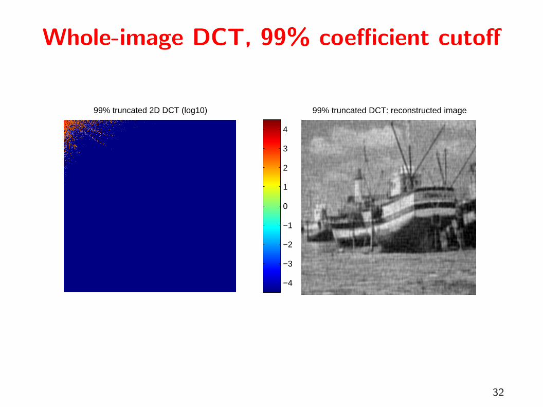
Whole-image DCT, 99% coefficient cutoff
99% truncated 2D DCT (log10)
−4
−3
−2
−1
0
1
2
3
4
99% truncated DCT: reconstructed image
32

Base vectors of 8×8 DCT
33

Psychophysics of perceptionSensation limit (SL) = lowest intensity stimulus that can still be perceived
Difference limit (DL) = smallest perceivable stimulus difference at givenintensity level
Weber’s lawDifference limit ∆φ is proportional to the intensity φ of the stimulus(except for a small correction constant a describe deviation of experi-mental results near SL):
∆φ = c · (φ+ a)
Fechner’s scaleDefine a perception intensity scale ψ using the sensation limit φ0 asthe origin and the respective difference limit ∆φ = c ·φ as a unit step.The result is a logarithmic relationship between stimulus intensity andscale value:
ψ = logcφ
φ0
34
Fechner’s scale matches older subjective intensity scales that followdifferentiability of stimuli, e.g. the astronomical magnitude numbersfor star brightness introduced by Hipparchos (≈150 BC).
Stevens’ lawA sound that is 20 DL over SL is perceived as more than twice as loudas one that is 10 DL over SL, i.e. Fechner’s scale does not describewell perceived intensity. A rational scale attempts to reflect subjectiverelations perceived between different values of stimulus intensity φ.Stevens observed that such rational scales ψ follow a power law:
ψ = k · (φ− φ0)a
Example coefficients a: temperature 1.6, weight 1.45, loudness 0.6,brightness 0.33.
35
DecibelCommunications engineers often use logarithmic units:
→ Quantities often vary over many orders of magnitude→ difficultto agree on a common SI prefix
→ Quotient of quantities (amplification/attenuation) usually moreinteresting than difference
→ Signal strength usefully expressed as field quantity (voltage,current, pressure, etc.) or power, but quadratic relationshipbetween these two (P = U2/R = I2R) rather inconvenient
→ Weber/Fechner: perception is logarithmic
Plus: Using magic special-purpose units has its own odd attractions (→ typographers, navigators)
Neper (Np) denotes the natural logarithm of the quotient of a fieldquantity F and a reference value F0.
Bel (B) denotes the base-10 logarithm of the quotient of a power Pand a reference power P0. Common prefix: 10 decibel (dB) = 1 bel.
36

Where P is some power and P0 a 0 dB reference power, or equallywhere F is a field quantity and F0 the corresponding reference level:
10 dB · log10
P
P0
= 20 dB · log10
F
F0
Common reference values are indicated with an additional letter afterthe “dB”:
0 dBW = 1 W
0 dBm = 1 mW = −30 dBW
0 dBµV = 1 µV
0 dBSPL = 20 µPa (sound pressure level)
0 dBSL = perception threshold (sensation limit)
3 dB = double power, 6 dB = double pressure/voltage/etc.10 dB = 10× power, 20 dB = 10× pressure/voltage/etc.W.H. Martin: Decibel – the new name for the transmission unit. Bell System Technical Journal,January 1929.
37
RGB video colour coordinatesHardware interface (VGA): red, green, blue signals with 0–0.7 V
Electron-beam current and photon count of cathode-ray displays areroughly proportional to (v − v0)γ, where v is the video-interface orcontrol-grid voltage and γ is a device parameter that is typically inthe range 1.5–3.0. In broadcast TV, this CRT non-linearity is com-pensated electronically in TV cameras. A welcome side effect is thatit approximates Stevens’ scale and therefore helps to reduce perceivednoise.
Software interfaces map RGB voltage linearly to {0, 1, . . . , 255} or 0–1
How numeric RGB values map to colour and luminosity depends atpresent still highly on the hardware and sometimes even on the oper-ating system or device driver.
The new specification “sRGB” aims to standardize the meaning ofan RGB value with the parameter γ = 2.2 and with standard colourcoordinates of the three primary colours.http://www.w3.org/Graphics/Color/sRGB, http://www.srgb.com/, IEC 61966
38

YUV video colour coordinates
The human eye processes colour and luminosity at different resolutions.To exploit this phenomenon, many image transmission systems use acolour space with a luminance coordinate
Y = 0.3R + 0.6G+ 0.1B
and colour (“chrominance”) components
V = R− Y = 0.7R− 0.6G− 0.1B
U = B − Y = −0.3R− 0.6G+ 0.9B
39

YCrCb video colour coordinates
Since −0.7 ≤ V ≤ 0.7 and −0.9 ≤ U ≤ 0.9, a more convenientnormalized encoding of chrominance is:
Cb =U
2.0+ 0.5
Cr =V
1.6+ 0.5
Modern image compression techniques operate on Y , Cr, Cb channelsseparately, using half the resolution of Y for storing Cr, Cb.
Some digital-television engineering terminology:
If each pixel is represented by its own Y , Cr and Cb byte, this is called a “4:4:4” format. In thecompacter “4:2:2” format, a Cr and Cb value is transmitted only for every second pixel, reducingthe horizontal chrominance resolution by a factor two. The “4:2:0” format transmits in alternat-ing lines either Cr or Cb for every second pixel, thus halving the chrominance resolution bothhorizontally and vertically. The “4:1:1” format reduces the chrominance resolution horizontallyby a quarter and “4:1:0” does so in both directions. [ITU-R BT.601]
40
The human auditory system
→ frequency range 20–16000 Hz (babies: 20 kHz)
→ sound pressure range 0–140 dBSPL (about 10−5–102 pascal)
→ mechanical filter bank (cochlea) splits input into frequencycomponents, physiological equivalent of Fourier transform
→ most signal processing happens in the frequency domain wherephase information is lost
→ some time-domain processing below 500 Hz and for directionalhearing
→ sensitivity and difference limit are frequency dependent
41

Equiloudness curves and the unit “phon”
Each curve represents a loudness level in phon. At 1 kHz, the loudness unit
phon is identical to dBSPL and 0 phon is the sensation limit.42
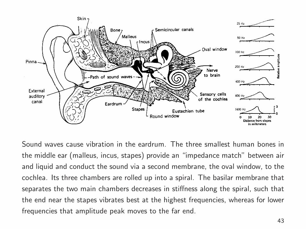
Sound waves cause vibration in the eardrum. The three smallest human bones in
the middle ear (malleus, incus, stapes) provide an “impedance match” between air
and liquid and conduct the sound via a second membrane, the oval window, to the
cochlea. Its three chambers are rolled up into a spiral. The basilar membrane that
separates the two main chambers decreases in stiffness along the spiral, such that
the end near the stapes vibrates best at the highest frequencies, whereas for lower
frequencies that amplitude peak moves to the far end.43
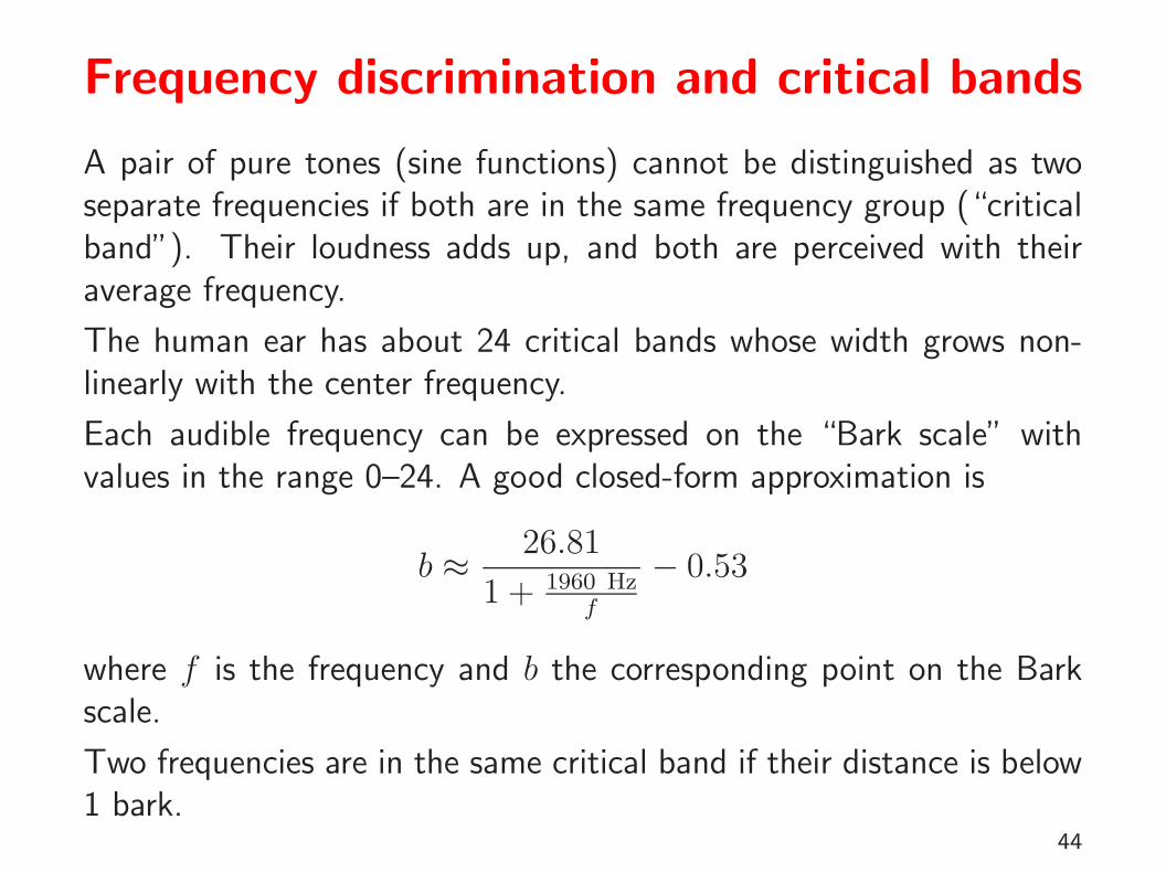
Frequency discrimination and critical bands
A pair of pure tones (sine functions) cannot be distinguished as twoseparate frequencies if both are in the same frequency group (“criticalband”). Their loudness adds up, and both are perceived with theiraverage frequency.
The human ear has about 24 critical bands whose width grows non-linearly with the center frequency.
Each audible frequency can be expressed on the “Bark scale” withvalues in the range 0–24. A good closed-form approximation is
b ≈ 26.81
1 + 1960 Hzf
− 0.53
where f is the frequency and b the corresponding point on the Barkscale.
Two frequencies are in the same critical band if their distance is below1 bark.
44
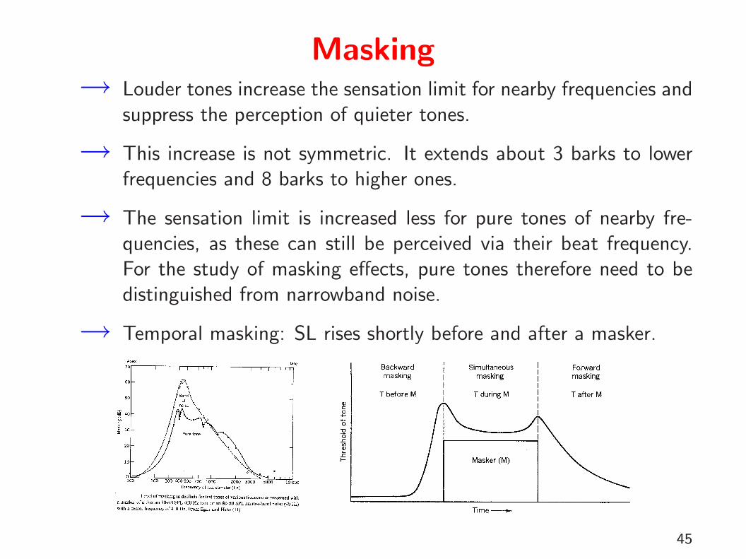
Masking→ Louder tones increase the sensation limit for nearby frequencies and
suppress the perception of quieter tones.
→ This increase is not symmetric. It extends about 3 barks to lowerfrequencies and 8 barks to higher ones.
→ The sensation limit is increased less for pure tones of nearby fre-quencies, as these can still be perceived via their beat frequency.For the study of masking effects, pure tones therefore need to bedistinguished from narrowband noise.
→ Temporal masking: SL rises shortly before and after a masker.
45
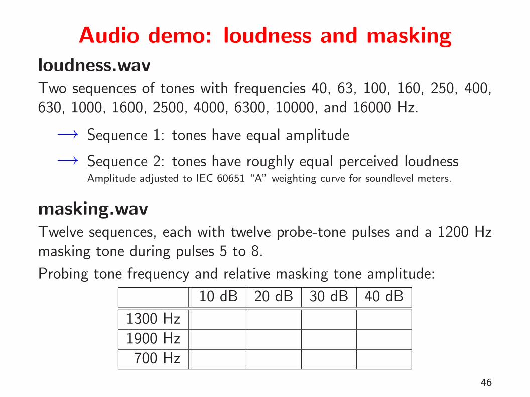
Audio demo: loudness and maskingloudness.wavTwo sequences of tones with frequencies 40, 63, 100, 160, 250, 400,630, 1000, 1600, 2500, 4000, 6300, 10000, and 16000 Hz.
→ Sequence 1: tones have equal amplitude
→ Sequence 2: tones have roughly equal perceived loudnessAmplitude adjusted to IEC 60651 “A” weighting curve for soundlevel meters.
masking.wavTwelve sequences, each with twelve probe-tone pulses and a 1200 Hzmasking tone during pulses 5 to 8.
Probing tone frequency and relative masking tone amplitude:
10 dB 20 dB 30 dB 40 dB
1300 Hz1900 Hz
700 Hz
46
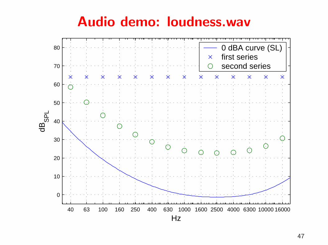
Audio demo: loudness.wav
40 63 100 160 250 400 630 1000 1600 2500 4000 6300 10000 16000
0
10
20
30
40
50
60
70
80
Hz
dBS
PL
0 dBA curve (SL)first seriessecond series
47
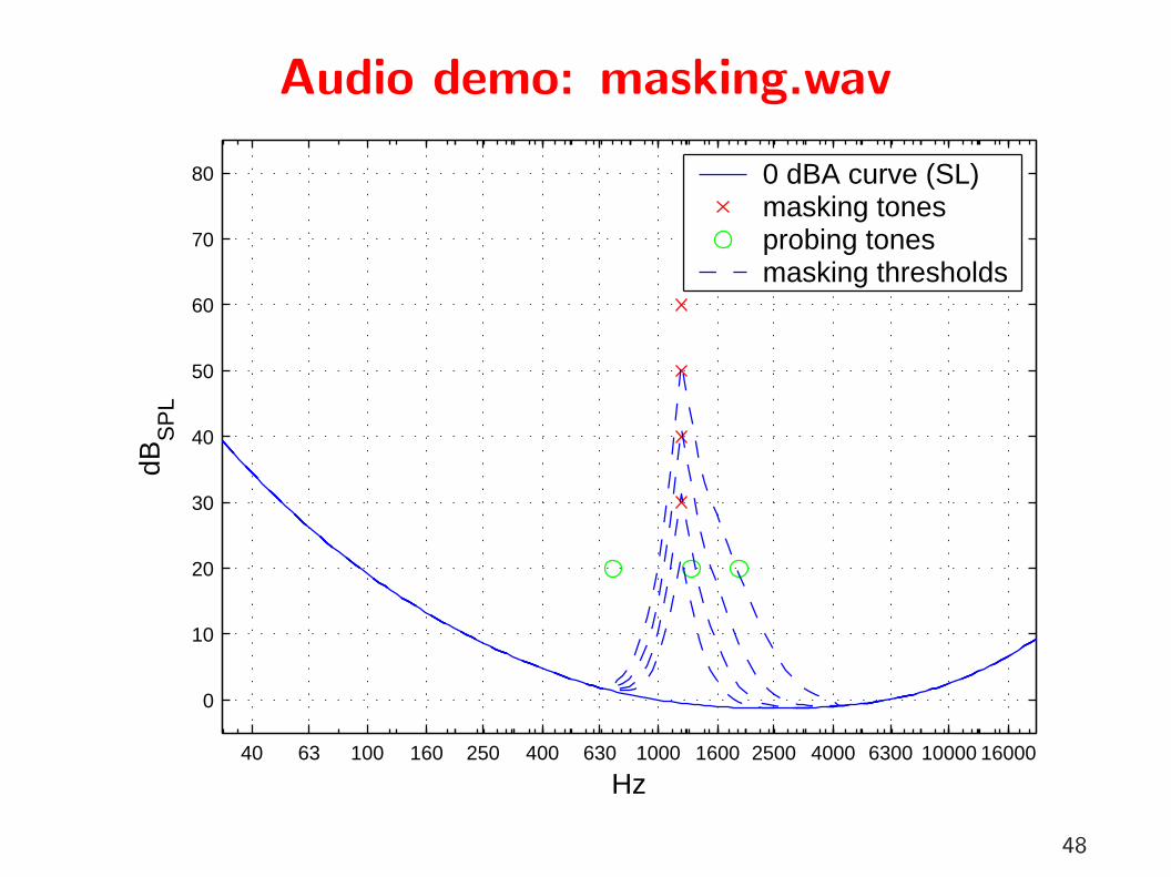
Audio demo: masking.wav
40 63 100 160 250 400 630 1000 1600 2500 4000 6300 10000 16000
0
10
20
30
40
50
60
70
80
Hz
dBS
PL
0 dBA curve (SL)masking tonesprobing tonesmasking thresholds
48
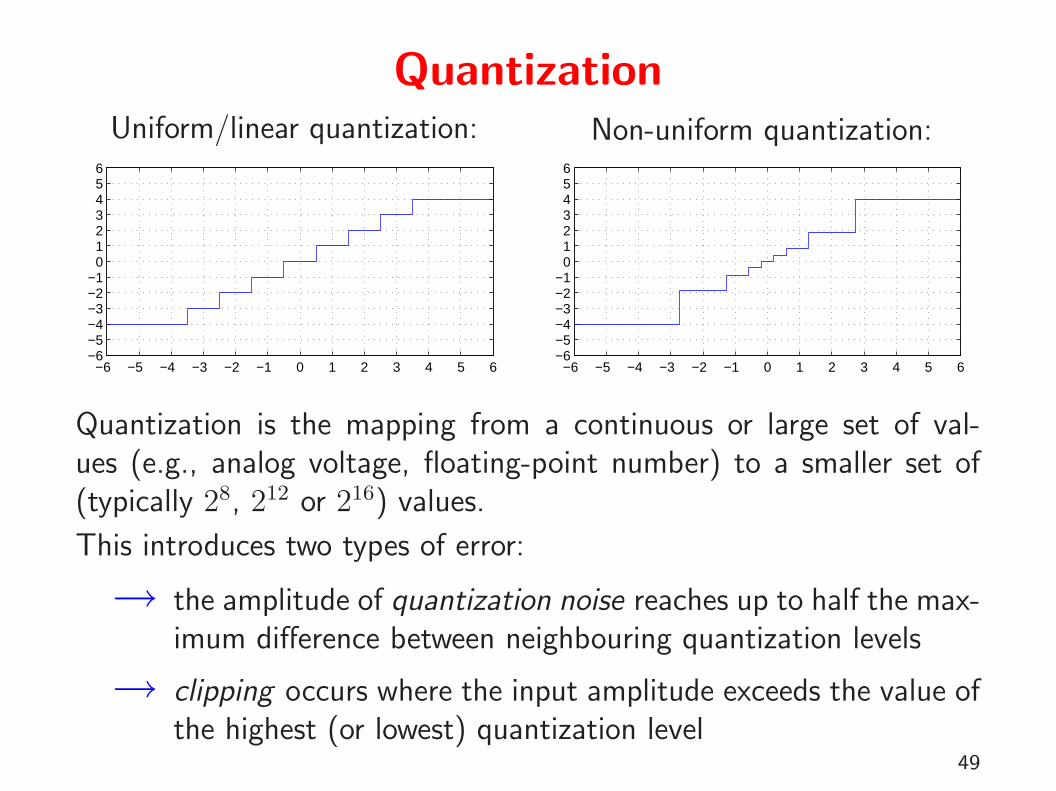
QuantizationUniform/linear quantization:
−6 −5 −4 −3 −2 −1 0 1 2 3 4 5 6−6−5−4−3−2−1
0123456
Non-uniform quantization:
−6 −5 −4 −3 −2 −1 0 1 2 3 4 5 6−6−5−4−3−2−1
0123456
Quantization is the mapping from a continuous or large set of val-ues (e.g., analog voltage, floating-point number) to a smaller set of(typically 28, 212 or 216) values.
This introduces two types of error:
→ the amplitude of quantization noise reaches up to half the max-imum difference between neighbouring quantization levels
→ clipping occurs where the input amplitude exceeds the value ofthe highest (or lowest) quantization level
49

Example of a linear quantizer (resolution R, peak value V ):
y = max
{−V,min
{V,R
⌊x
R+
1
2
⌋}}Adding a noise signal that is uniformly distributed on [0, 1] instead of adding 1
2helps to spread
the frequency spectrum of the quantization noise more evenly. This is known as dithering.
Variant with even number of output values (no zero):
y = max
{−V,min
{V,R
(⌊x
R
⌋+
1
2
)}}Improving the resolution by a factor of two (i.e., adding 1 bit) reducesthe quantization noise by 6 dB.
Linearly quantized signals are easiest to process, but analog input levelsneed to be adjusted carefully to achieve a good tradeoff between thesignal-to-quantization-noise ratio and the risk of clipping. Non-uniformquantization can reduce quantization noise where input values are notuniformly distributed and can approximate human perception limits.
50

Logarithmic quantization
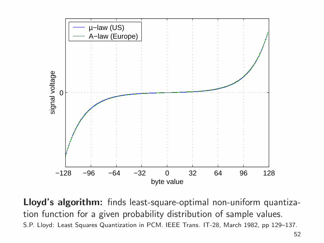
Rounding the logarithm of the signal amplitude makes the quantiza-tion error scale-invariant and is used where the signal level is not verypredictable. Two alternative schemes are widely used to make thelogarithm function odd and linearize it across zero before quantization:
µ-law:
y =V log(1 + µ|x|/V )
log(1 + µ)sgn(x) for −V ≤ x ≤ V
A-law:
y =
{ A|x|1+logA
sgn(x) for 0 ≤ |x| ≤ VA
V (1+logA|x|V )
1+logAsgn(x) for V
A≤ |x| ≤ V
European digital telephone networks use A-law quantization (A = 87.6), North American onesuse µ-law (µ=255), both with 8-bit resolution and 8 kHz sampling frequency (64 kbit/s). [ITU-TG.711]
51
−128 −96 −64 −32 0 32 64 96 128
0
sign
al v
olta
ge
byte value
µ−law (US)A−law (Europe)
Lloyd’s algorithm: finds least-square-optimal non-uniform quantiza-tion function for a given probability distribution of sample values.S.P. Lloyd: Least Squares Quantization in PCM. IEEE Trans. IT-28, March 1982, pp 129–137.
52

Joint Photographic Experts Group – JPEGWorking group “ISO/TC97/SC2/WG8 (Coded representation of picture and audio information)”was set up in 1982 by the International Organization for Standardization.
Goals:
→ continuous tone gray-scale and colour images
→ recognizable images at 0.083 bit/pixel
→ useful images at 0.25 bit/pixel
→ excellent image quality at 0.75 bit/pixel
→ indistinguishable images at 2.25 bit/pixel
→ feasibility of 64 kbit/s (ISDN fax) compression with late 1980shardware (16 MHz Intel 80386).
→ workload equal for compression and decompression
JPEG standard (ISO 10918) was finally published in 1994.William B. Pennebaker, Joan L. Mitchell: JPEG still image compression standard. Van NostradReinhold, New York, ISBN 0442012721, 1993.
Gregory K. Wallace: The JPEG Still Picture Compression Standard. Communications of theACM 34(4)30–44, April 1991, http://doi.acm.org/10.1145/103085.103089
53
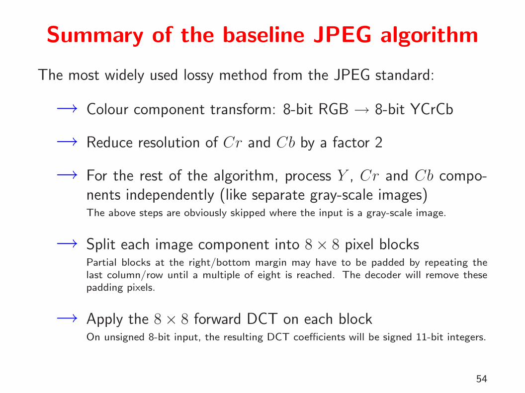
Summary of the baseline JPEG algorithm
The most widely used lossy method from the JPEG standard:
→ Colour component transform: 8-bit RGB → 8-bit YCrCb
→ Reduce resolution of Cr and Cb by a factor 2
→ For the rest of the algorithm, process Y , Cr and Cb compo-nents independently (like separate gray-scale images)The above steps are obviously skipped where the input is a gray-scale image.
→ Split each image component into 8× 8 pixel blocksPartial blocks at the right/bottom margin may have to be padded by repeating thelast column/row until a multiple of eight is reached. The decoder will remove thesepadding pixels.
→ Apply the 8× 8 forward DCT on each blockOn unsigned 8-bit input, the resulting DCT coefficients will be signed 11-bit integers.
54
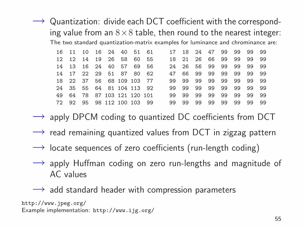
→ Quantization: divide each DCT coefficient with the correspond-ing value from an 8×8 table, then round to the nearest integer:The two standard quantization-matrix examples for luminance and chrominance are:
16 11 10 16 24 40 51 61 17 18 24 47 99 99 99 99
12 12 14 19 26 58 60 55 18 21 26 66 99 99 99 99
14 13 16 24 40 57 69 56 24 26 56 99 99 99 99 99
14 17 22 29 51 87 80 62 47 66 99 99 99 99 99 99
18 22 37 56 68 109 103 77 99 99 99 99 99 99 99 99
24 35 55 64 81 104 113 92 99 99 99 99 99 99 99 99
49 64 78 87 103 121 120 101 99 99 99 99 99 99 99 99
72 92 95 98 112 100 103 99 99 99 99 99 99 99 99 99
→ apply DPCM coding to quantized DC coefficients from DCT
→ read remaining quantized values from DCT in zigzag pattern
→ locate sequences of zero coefficients (run-length coding)
→ apply Huffman coding on zero run-lengths and magnitude ofAC values
→ add standard header with compression parameters
http://www.jpeg.org/
Example implementation: http://www.ijg.org/
55

Storing DCT coefficients in zigzag order
0 1
2
3
4
5 6
7
8
9
10
11
12
13
14 15
16
17
18
19
20
21
22
23
24
25
26
27 28
29
30
31
32
33
34
35 36
37
38
39
40
41
42
43
44
45
46
47
48 49
50
51
52
53
54
55
56
57 58
59
60
61
6362
horizontal frequency
vert
ical
freq
uenc
y
After the 8×8 coefficients produced by the discrete cosine transformhave been quantized, the values are processed in the above zigzag orderby a run-length encoding step.The idea is to group all higher-frequency coefficients together at the end of the sequence. As manyimage blocks contain little high-frequency information, the bottom-right corner of the quantizedDCT matrix is often entirely zero. The zigzag scan helps the run-length coder to make best useof this observation.
56

Huffman coding in JPEGs value range
0 01 −1, 12 −3,−2, 2, 33 −7 . . .− 4, 4 . . . 74 −15 . . .− 8, 8 . . . 155 −31 . . .− 16, 16 . . . 316 −63 . . .− 32, 32 . . . 63
. . . . . .i −(2i − 1) . . .− 2i−1, 2i−1 . . . 2i − 1
DCT coefficients have 11-bit resolution and would lead to huge Huffman
tables (up to 2048 code words). JPEG therefore uses a Huffman table only
to encode the magnitude category s = dlog2(|v| + 1)e of a DCT value v.
A sign bit plus the (s− 1)-bit binary value |v| − 2s−1 are appended to each
Huffman code word, to distinguish between the 2s different values within
magnitude category s.When storing DCT coefficients in zigzag order, the symbols in the Huffman tree are actuallytuples (r, s), where r is the number of zero coefficients preceding the coded value (run-length).
57

Arithmetic coding in JPEG
As an option, the Huffman coder in JPEG can be replaced with an arith-metic coder. The coder used is identical to the JBIG one (113-stateadaptive estimator, etc.). It processes a sequence of binary decisions,therefore each integer value (DC coefficient difference, AC coefficient,lossless difference) to be coded is first transformed into a bit stringusing a variant of the Elias gamma code, which is then fed bit-by-bitinto the arithmetic coder with a suitable context.If the integer v to be coded is zero, only the bit 0 is fed into the arithmetic coder. Otherwise, thecoder receives a 1 bit, followed by the sign bit of v, followed by the unary-coded value dlog2 |v|e,followed by the dlog2 |v|e − 1 bits after the leading 1 bit of the binary notation of |v| − 1.
The coding context used depends on the bit position, in the case of the third bit (|v| > 1?) alsoon the second bit (v < 0?). In the case of the first three bits, the context also depends on thezigzag index number for AC coefficients, or on the first few bits of the previous DC coefficientdifference for a DC coefficient.
In other words, integer values are first coded with a fixed Huffmancode that outputs bits with roughly equal probability, and then thearithmetic coder adapts to exploit the remaining bit bias, as well asthe dependence on a selected small set of previously coded bits.
58

Lossless JPEG algorithm
In addition to the DCT-based lossy compression, JPEG also defines alossless mode. It offers a selection of seven linear prediction mecha-nisms based on three previously coded neighbour pixels:
1 : x = a2 : x = b3 : x = c4 : x = a+ b− c5 : x = a+ (b− c)/26 : x = b+ (a− c)/27 : x = (a+ b)/2
c b
a ?
Predictor 1 is used for the top row, predictor 2 for the left-most row.The predictor used for the rest of the image is chosen in a header. Thedifference between the predicted and actual value is fed into either aHuffman or arithmetic coder.
59

Advanced JPEG featuresBeyond the baseline and lossless modes already discussed, JPEG pro-vides these additional features:
→ 8 or 12 bits per pixel input resolution for DCT modes
→ 2–16 bits per pixel for lossless mode
→ progressive mode permits the transmission of more-significantDCT bits or lower-frequency DCT coefficients first, such thata low-quality version of the image can be displayed early duringa transmission
→ the transmission order of colour components, lines, as well asDCT coefficients and their bits can be interleaved in many ways
→ the hierarchical mode first transmits a low-resolution image,followed by a sequence of differential layers that code the dif-ference to the next higher resolution (like JBIG’s progressivemode)
60

Moving Pictures Experts Group – MPEG→ MPEG-1: Coding of video and audio optimized for 1.5 Mbit/s
(1× CD-ROM). ISO 11172 (1993).
→ MPEG-2: Adds support for interlaced video scan, optimizedfor broadcast TV (2–8 Mbit/s) and HDTV, scalability options.Used by DVD and DVB. ISO 13818 (1995).
→ MPEG-4: Adds algorithmic or segmented description of audio-visual objects for very-low bitrate applications. ISO 14496(2001).
→ System layer multiplexes several audio and video streams, timestamp synchronization, buffer control.
→ Standard defines decoder semantics.
→ Asymmetric workload: Encoder needs significantly more com-putational power than decoder (for bit-rate adjustment, motionestimation, perceptual modeling, etc.)
http://mpeg.telecomitalialab.com/
61

MPEG video coding→ Uses YCrCb colour transform, 8×8-pixel DCT, quantization,
zigzag scan, run-length and Huffman encoding, similar to JPEG
→ the zigzag scan pattern is adapted to handle interlaced fields
→ Huffman coding with fixed code tables defined in the standardMPEG has no arithmetic coder option.
→ adaptive quantization
→ SNR and spatially scalable coding (enables separate transmis-sion of a moderate-quality video signal and an enhancementsignal to reduce noise or improve resolution)
→ Predictive coding with motion compensation based on 16×16macro blocks.
J. Mitchell, W. Pennebaker, Ch. Fogg, D. LeGall: MPEG video compression standard.ISBN 0412087715, 1997. (CL library: I.4.20)
B. Haskell et al.: Digital Video: Introduction to MPEG-2. Kluwer Academic, 1997.(CL library: I.4.27)
John Watkinson: The MPEG Handbook. Focal Press, 2001. (CL library: I.4.31)
62

MPEG motion compensation
current picturebackward
reference picture
forward
reference picture
time
Each MPEG image is split into 16×16-pixel large macroblocks. The predic-
tor forms a linear combination of the content of one or two other blocks of
the same size in a preceding (and following) reference image. The relative
positions of these reference blocks are encoded along with the differences.63

MPEG reordering of reference imagesDisplay order of frames:
I B B B P B B B P B B B P
time
Coding order:
I B B B B B BP P B P B
time
B
MPEG distinguishes between I-frames that encode an image independent of any others, P-framesthat encode differences to a previous P- or I-frame, and B-frames that interpolate between thetwo neighboring B- and/or I-frames. A frame has to be transmitted before the first B-frame thatmakes a forward reference to it. This requires the coding order to differ from the display order.
64

MPEG system layer: buffer management
encoderencoderbuffer
decoderbuffer
decoder
time time
fixed−bitratechannel
buffe
r co
nten
t
buffe
r co
nten
t
enco
der
deco
der
MPEG can be used both with variable-bitrate (e.g., file, DVD) and fixed-bitrate (e.g., ISDN)channels. The bitrate of the compressed data stream varies with the complexity of the inputdata and the current quantization values. Buffers match the short-term variability of the encoderbitrate with the channel bitrate. A control loop continuously adjusts the average bitrate via thequantization values to prevent under- or overflow of the buffer.
The MPEG system layer can interleave many audio and video streams in a single data stream.Buffers match the bitrate required by the codecs with the bitrate available in the multiplex andencoders can dynamically redistribute bitrate among different streams.
MPEG encoders implement a 27 MHz clock counter as a timing reference and add its value as asystem clock reference (SCR) several times per second to the data stream. Decoders synchronizewith a phase-locked loop their own 27 MHz clock with the incoming SCRs.
Each compressed frame is annotated with a presentation time stamp (PTS) that determines whenits samples need to be output. Decoding timestamps specify when data needs to be available tothe decoder.
65
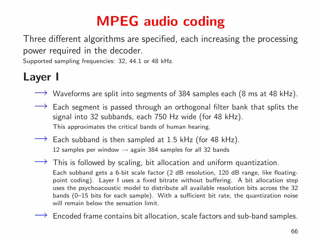
MPEG audio codingThree different algorithms are specified, each increasing the processingpower required in the decoder.Supported sampling frequencies: 32, 44.1 or 48 kHz.
Layer I
→ Waveforms are split into segments of 384 samples each (8 ms at 48 kHz).
→ Each segment is passed through an orthogonal filter bank that splits thesignal into 32 subbands, each 750 Hz wide (for 48 kHz).This approximates the critical bands of human hearing.
→ Each subband is then sampled at 1.5 kHz (for 48 kHz).12 samples per window → again 384 samples for all 32 bands
→ This is followed by scaling, bit allocation and uniform quantization.Each subband gets a 6-bit scale factor (2 dB resolution, 120 dB range, like floating-point coding). Layer I uses a fixed bitrate without buffering. A bit allocation stepuses the psychoacoustic model to distribute all available resolution bits across the 32bands (0–15 bits for each sample). With a sufficient bit rate, the quantization noisewill remain below the sensation limit.
→ Encoded frame contains bit allocation, scale factors and sub-band samples.
66
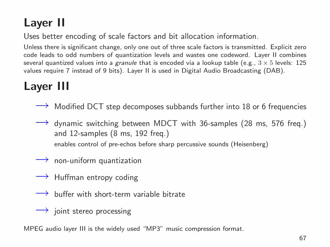
Layer IIUses better encoding of scale factors and bit allocation information.Unless there is significant change, only one out of three scale factors is transmitted. Explicit zerocode leads to odd numbers of quantization levels and wastes one codeword. Layer II combinesseveral quantized values into a granule that is encoded via a lookup table (e.g., 3× 5 levels: 125values require 7 instead of 9 bits). Layer II is used in Digital Audio Broadcasting (DAB).
Layer III
→ Modified DCT step decomposes subbands further into 18 or 6 frequencies
→ dynamic switching between MDCT with 36-samples (28 ms, 576 freq.)and 12-samples (8 ms, 192 freq.)enables control of pre-echos before sharp percussive sounds (Heisenberg)
→ non-uniform quantization
→ Huffman entropy coding
→ buffer with short-term variable bitrate
→ joint stereo processing
MPEG audio layer III is the widely used “MP3” music compression format.
67

Psychoacoustic modelsMPEG audio encoders use a psychoacoustic model to estimate the spectraland temporal masking that the human ear will apply. The subband quan-tization levels are selected such that the quantization noise remains belowthe masking threshold in each subband.
The masking model is not standardized and each encoder developer canchose a different one. The steps typically involved are:
→ Fourier transform for spectral analysis
→ Group the resulting frequencies into “critical bands” within whichmasking effects will not vary significantly
→ Distinguish tonal and non-tonal (noise-like) components
→ Apply masking function
→ Calculate threshold per subband
→ Calculate signal-to-mask ratio (SMR) for each subband
Masking is not linear and can be estimated accurately only if the actual sound pressure levelsreaching the ear are known. Encoder operators usually cannot know the sound pressure levelselected by the decoder user. Therefore the model must use worst-case SMRs.
68
Voice encoding
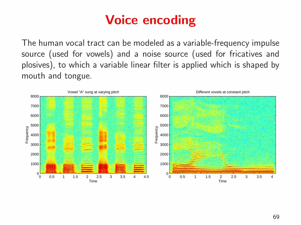
The human vocal tract can be modeled as a variable-frequency impulsesource (used for vowels) and a noise source (used for fricatives andplosives), to which a variable linear filter is applied which is shaped bymouth and tongue.
Time
Fre
quen
cy
Vowel "A" sung at varying pitch
0 0.5 1 1.5 2 2.5 3 3.5 4 4.50
1000
2000
3000
4000
5000
6000
7000
8000
Time
Fre
quen
cy
Different vovels at constant pitch
0 0.5 1 1.5 2 2.5 3 3.5 40
1000
2000
3000
4000
5000
6000
7000
8000
69

Vector quantization
A multi-dimensional signal space can be encoded by splitting it intoa finite number of volumes. Each volume is then assigned a singlecodeword to represent all values in it.
Example: The colour-lookup-table file format GIF requires the com-pressor to map RGB pixel values using vector quantization to 8-bitcode words, which are then entropy coded.
Literature
References used in the preparation of this part of the course in addition to those quoted previously:
• D. Salomon: A guide to data compression standards. ISBN 0387952608, 2002.
• A.M. Kondoz: Digital speech – Coding for low bit rate communications systems.ISBN 047195064.
• L. Gulick, G. Gescheider, R. Frisina: Hearing. ISBN 0195043073, 1989.
• H. Schiffman: Sensation and perception. ISBN 0471082082, 1982.
• British Standard BS EN 60651: Sound level meters. 1994.
70

Exercise 1 Compare the quantization techniques used in the digital tele-phone network and in audio compact disks. Which factors to you think ledto the choice of different techniques and parameters here?
Exercise 2 Which steps of the JPEG (DCT baseline) algorithm cause aloss of information? Distinguish between accidental loss due to roundingerrors and information that is removed for a purpose.
Exercise 3 How can you rotate by multiples of ±90◦ or mirror a DCT-JPEG compressed image without losing any further information. Why mightthe resulting JPEG file not have the exact same file length?
Exercise 4 Decompress this G3-fax encoded line:1101011011110111101100110100000000000001
Exercise 5 You adjust the volume of your 16-bit linearly quantizing sound-card, such that you can just about hear a 1 kHz sine wave with a peakamplitude of 200. What peak amplitude do you expect will a 90 Hz sinewave need to have, to appear equally loud (assuming ideal headphones)?
71
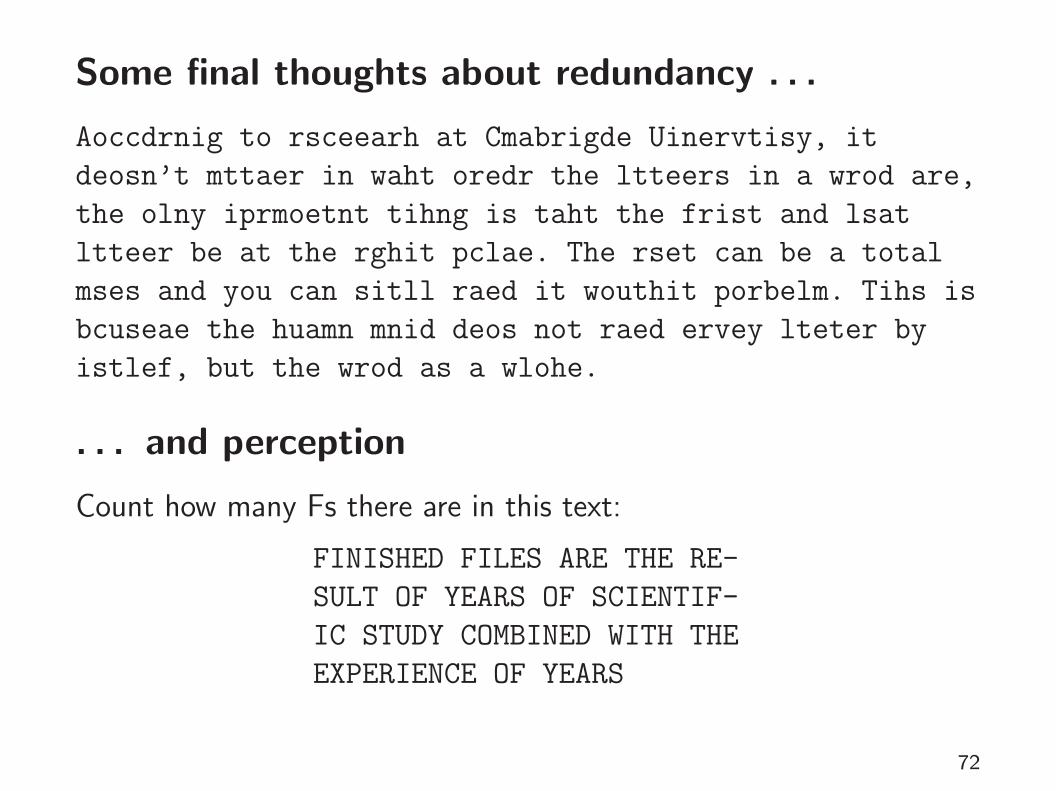
Some final thoughts about redundancy . . .
Aoccdrnig to rsceearh at Cmabrigde Uinervtisy, it
deosn’t mttaer in waht oredr the ltteers in a wrod are,
the olny iprmoetnt tihng is taht the frist and lsat
ltteer be at the rghit pclae. The rset can be a total
mses and you can sitll raed it wouthit porbelm. Tihs is
bcuseae the huamn mnid deos not raed ervey lteter by
istlef, but the wrod as a wlohe.
. . . and perception
Count how many Fs there are in this text:
FINISHED FILES ARE THE RE-
SULT OF YEARS OF SCIENTIF-
IC STUDY COMBINED WITH THE
EXPERIENCE OF YEARS
72