infrared and terahertz imaging through self-mixing

Infrared and terahertz imaging through self-mixing

interferometry in quantum cascade lasers

Anno Accademico 2012/2013

Curriculum Fisica della Materia e Applicata

UNIVERSITÀ DEGLI STUDI DI BARI “ALDO MORO”

Facoltà di Scienze Matematiche, Fisiche e Naturali

Relatori:

Prof. Gaetano Scamarcio

Dott. Francesco MezzapesaLaureando:

Maurangelo Petruzzella

Sessione Estiva

Corso di Laurea Magistrale in Fisica

Summary

Summary 1

Introduction 3

1. Terahertz imaging review 7

1.1 The terahertz gap 7

1.2 Terahertz time-domain spectroscopy 11

1.3 Time-of-flight measurement 16

1.4 Near-field techniques 17

1.5 CW schemes 20

1.6 Imaging applications 23

2. Optical feedback 27

2.1 The model 28

2.2 Steady state solutions 30

2.3 Self-mixing interferometry in semiconductor laser diodes 32

2.4 Regimes 37

2.5 Quantum cascade lasers 40

2.6 Quantum cascade laser against optical feedback 45

3. Experimental Setups 50

3.1 Sources 50

Mid-IR QCL 50

THz QCL 52

3.2 Mid-IR Setup 56

3.3 THz Setup 58

3.4 Beam waist 59

3.5 Beam focusing 61

4. Imaging Results 66

4.1 Mid-IR imaging results 66

4.2 THz imaging results 73

4.3 Fringe visibility 75

5. Preliminary results 79

Conclusions and future work 80

Ringraziamenti 82

Bibliography 83

Introduction 3

Introduction

Best known for the development of the elegant mathematical formulation

of the electromagnetic theory and the partial differential equations named

after him, the Scottish physicist James Clerk-Maxwell also dabbled in

photography throughout his life. One of his lesser-known contributions

lies in the field of colour vision and consists in the propose of the first

permanent colour image, obtained overlapping three photographic plates

taken with a red, blue, and green colour filters (Fig. 1)1

Fig. 1. The first permanent color photograph made with the three-color method suggested by

James Clerk Maxwell in 1856 and experimentally taken in 1861 by Thomas Sutton. The subject

was a tartan ribbon tied into a bow. The photographic plates are exposed in Maxwell’s house,

which became a museum in Scotland.

1 On the theory of colours in relation to colour-blindness. Edinb. Trans. Scot. Soc. arts IV 1856, pp 394-400. Scientific Papers Vol. I pp. 119-127

Introduction 4

Like him, many scientists have been enthralled by imaging science, and

during the last century a huge number of schemes has emerged, exploiting

photons which belong not only to the tiny visible slice of the

electromagnetic spectrum.

Up-to-date real-world applications make use of radar false-color images of

clouds for weather forecast, x-ray pictures of broken bones or baggage

content for security screening, thermal images for military use on the

battlefield, high-resolution infrared photographs of the earth taken from

satellite orbits, and many other categories too numerous to be listed here.

Different wavelengths and techniques are suited for different purposes in

every-day life and in a motley onset of research fields.

Notwithstanding, during the last thirty years, the terahertz (THz) range,

i.e. the electromagnetic region sandwiched between mid-infrared and

microwaves (0.1-10 THz, 3cm-1-330cm-1, 30 µμ m-3mm), has attracted

attention because of its unique interaction proprieties with matter. Indeed,

the so-call T-rays can pass through materials that appear opaque at visible

wavelengths, such as ceramic, clothes, plastics and packaging, while being

reflected from metals. These features, combined with the fact that most

spectroscopic signatures of substances of great interest - drugs and

explosives first of all – lie in the terahertz regime, have led to the flourish of

THz imaging science and THz systems used for multidisciplinary non-

destructive evaluations. Besides, thanks to its non-ionizing energy and the

peculiar absorption from water molecules, this radiation has been

exploited in medical diagnosis, in screen for skin cancers and tooth decays

too.

Introduction 5

However, up to now both the lack of compact sources and detectors and

the high THz absorption of atmosphere has still limited the use of THz

radiation in laboratory. For these reasons, this region has been considered

a terra nullius where both photonics and electronics have tried to face these

problems from two opposite sides, with different schemes and approaches.

Under these circumstances, one of the most promising devices coming

from the photonics branch is the quantum cascade laser (QCL). Through

this system - demonstrated in 1994 in mid-Infrared and re-invented in 2001

to work in THz regime - it is possible to design optical transitions in the

ranges of 1-5 THz and 15-100 THz, making use of the principles of

quantum mechanics.

This thesis discusses the implementation of an imaging system, which

makes use of a THz and Mid-Infrared QCL in self-mixing configuration.

This coherent scheme, in which a laser is used both as source and detector,

exploits the interference between the electric field inside the cavity laser

and the back-coupled radiation reflected or scattered from an external

target, in order to get the image of a sample.

This text is organized as follows.

Chapter 1 reviews THz imaging techniques with pulse and continuous

sources, giving some details about near field approaches.

Chapter 2 discusses optical feedback in quantum cascade lasers,

presenting the working principles of self-mixing interferometry in

conventional laser and comparing differences with the QCL dynamics.

Chapter 3 describes mid-infrared and THz setups, with a focus on some

experimental critical aspects.

Introduction 6

Chapter 4 illustrates and discusses imaging results with different samples,

drafting some experimental evidences about the dynamics of QCL

subjected to optical feedback.

Chapter 5 analyses preliminary results and highlights the opportunities to

extend this scheme in order to acquire the charge-distribution of a

semiconductor device.


Chapter 1

1. Terahertz imaging review Terahertz imaging review

In this chapter is presented an overview of active imaging techniques in

the terahertz domain. After discussing some of the features of this

unexplored spectral region (1.1), imaging schemes which make us of

broadband and continuous (CW) sources are respectively reviewed in

paragraph 1.2 and 1.5. In addition, near field methods and tomographic

techniques are sketched in paragraph 1.3 and 1.4. We conclude the chapter

outlining a series of applications for imaging terahertz that involves a vast

number of different research areas (paragraph 1.6).

1.1 The terahertz gap

The terahertz (THz) region lies in the frequency range from 0.1 to 10 THz

and exists between two readily developed frequency bands: the

microwave and the infrared. This so-called terahertz gap has historically

been defined by the relative lack of well-established sources and detectors

and is therefore explored to a lesser extent.

While in the microwave regime, electromagnetic radiation is typically

generated through high-frequency oscillating charges and the photon

energy involved is smaller than thermal energy k T, in the infrared range


generation mechanisms employ optical transitions between quantized

energy levels in a semiconductor. The terahertz domain is therefore the

natural bridge between the classical and quantum mechanical descriptions

of electromagnetic waves and their interactions with matter. Much of the

advances in terahertz science and technology have emerged from the

overlap originated from these two different points of view, borrowing

ideas from each.

Although terahertz technology is still in its infancy, this region has been

investigated since 1970s by space scientists. The reason resides in the fact

that more than 98 percent of the photons released since the Big Bang,

which give information about chemical compositions of the interstellar

medium and planetary atmospheres, fall in the sub-millimeter and far-

infrared bands.

Moreover, many molecules that constitute the atmosphere exhibit their

rotovibrational spectra in the THz region. Thus, the so-called T-rays are

suited as spectroscopic tools for pollution monitoring.

On the other hand, every long-distance application that has been

suggested in the last years, had to come up against the downside of

atmospheric absorption (Figure 1.1), which can reach some decibel (dB)

per meter at standard humidity conditions. In this direction, the

development of source with a narrowed emission spectrum is a crucial

aspect.


Figure 1.1 Signal attenuation in the range of 0.5-5 THz caused by atmospheric absorption at

normal humidity from water vapor and oxygen. Taken from HITRAN database.

A great number of devices have been proposed as terahertz sources, each

of those employing a characteristics physical mechanism to generate

radiation.

Figure 1.2 Sources output power versus frequency. Adapted from [1]


Figure 1.2 tries to summarize them, depending on the average emission

power as a function of frequency. Sources fall into three broad categories:

solid state (counting harmonic frequency multipliers, transistors and

monolithic microwave integrated circuits), vacuum (including backward-

wave oscillators, grating-vacuum devices, klystrons, traveling-wave tubes,

and gyrotrons), and laser and photonic (including quantum cascade lasers,

optically pumped molecular lasers and a variety of optoelectronic radio

frequency generators).

Quantum cascade laser, above all, is the most promising compact source

for frequencies higher than 1 THz, nevertheless up to now it requires

cryogenic cooling. We will describe its working principles in details in

paragraph 2.5


1.2 Terahertz time-domain spectroscopy

Figure 1.3 Typical schematic for terahertz time-domain spectroscopy. Adapted from [2]

During the last twenty years most research developments in terahertz

sensing and imaging have made use of terahertz time-domain

spectroscopy (THz-TDS), first introduced by van Exter in 1989 [3]. The

basic general TDS experimental setup is based on a pump-probe scheme

(Figure 1.3). Here, femtosecond laser produces an infrared pulse train at a

repetition rate usually near 100 MHz, which is separated in a pump and a

probe beam by means of a beam splitter. The former arrives at the emitter

and gives rise to a sub-picosecond THz pulse, which travels through the

sample and is focused onto an ultra-fast detector. The THz-induced

transients in the detector are measured by the probe pulse, which is

delayed by a mechanical delay line. In this way, the amplitude E(t) of the

THz electric-field is detected by temporally sampling the waveform using

the probe pulse.

The two most popular mechanisms for the generation and the detection of

THz broadband fields involve transient photocurrents in photoconductive


antennas and second-order effects in nonlinear optical crystals. We will

give a qualitative description of these processes below.

Photoconductive techniques make use of the optical resonant excitation of

a semiconductor to generate currents through the production of electrons–

holes pairs (see Figure 1.4 (a)). A metal pattern is typically deposited on a

semiconductor substrate, in the form of an H-like antenna structure. A

static bias applied across the electrodes accelerates the free carriers that are

optically generated by the femtosecond-laser and, simultaneously, the

charge density decays mainly by trapping in defect sites. According to the

Maxwell’s equations, the impulse current arising from this acceleration

and decay of free carriers is the source of a subpicosecond pulse of

electromagnetic radiation ( E(t) ∼ ∂J/ ∂t ), which contains frequency

components from approximately 0.1 to 5 THz. The antenna can be

modeled as a hertzian dipole and its design also helps to couple the THz

radiation into free space.

The underlying physics of photoconductive detection is almost the same as

the generation method described above (see Figure 1.4 (b)). Again, the

infrared beam is focused at the center of an antenna, generating hole

electrons pairs. When the THz pulse arrives during the lifetime of the

carriers they are accelerated towards the electrodes. Although this short

current pulse is too fast to be resolved using conventional electronics, the

average current (averaged over many identical pulses) can be measured as

a function of the delay between the optical gate pulse and the THz pulse.

Fast photoconductors such as radiation-damaged silicon-on-sapphire

(SoS), low-temperature-grown gallium arsenide (LT-GaAs) or indium

phosphide (InP) are used to provide sub-picosecond sampling resolution.


Figure 1.4. Photoconductive emitter (a) and photoconductive detector antenna (b) mounted on a

hemispherical lens. (c) Scheme for free-space EO sampling: probe polarizations with and without

a THz field are shown before and after the polarization chain. From [4]

The second class of schemes employed to generate and detect broadband

THz radiation exploits respectively optical rectification and Pockels effect

exhibited by second-order nonlinear crystals.

When an optical pulse of frequency ω and duration t ,

E(t) = E e ( / ) e interacts with a non-centrosymmetric medium, such

as Zinc telluride (ZnTe), the nonlinear polarization induced by the optical

rectification replicates the pulse envelope P(t) = P e ( / ) . This generation

process can be interpreted as the difference mixing between all possible

pairs of spectral components within the bandwidth of the fs-optical pulse

and, using the nonlinear optics formalism, we can write the polarization as

P( )(0) = ϵ χ( )

,

(0, ω,−ω)E (ω)E∗(ω),

where 𝑖, 𝑗, 𝑘 are the cartesian indexes and χ( ) is the second-order nonlinear

susceptibility tensor. Neglecting walk-off effects, the polarization acts as


the source of the electromagnetic field. Thus a broadband terahertz field is

generated, whose bandwidth is roughly the inverse of the optical pulse

duration t .

THz detection via nonlinear effects is carried out through the Pockels

effect: while the linearly polarized optical pulse propagates through the

electro-optic crystal, the THz field induces a birefringence in the medium,

resulting in an elliptical polarization of the probe beam. After passing

through a λ/4-plate the probe beam is split in two orthogonal polarized

components via a Wollaston prism. A balanced photo-detector measures

the intensity difference between these two components, which is

proportional to the THz field amplitude.

Figure 1.5 (left) Examples of time-domain terahertz waveform emitted from p-InAs

photoconductive switch and 4-N,N-dimethylamino-4’-N’-methyl-stilbazolium tosylate (DAST)

organic electro-optic crystal and (right) their Fourier-transformed spectra. Dips correspond to

water vapor rotational absorption lines [2]. The electro-optic generation shows an higher dynamic

range

Typical electric field amplitude waveforms and corresponding spectra of

both generation mechanisms are illustrated in Figure 1.5. Through a

spectroscopic point of view, THz-TDS directly measures the complex


refractive index of the specimen and accesses its complex permittivity

without using the Kramers-Kronig relationship. Nevertheless, conversion

efficiency is on the order of 10-4-10-6, resulting in low average pulse power

levels that range from nanowatt to microwatt.

Most of THz imaging research has been done replicating a TDS modified

setup demonstrated by Hu and Nuss in 1995 [6]. Here, a complete time-

domain waveform data set is acquired one pixel at a time, raster-scanning

the target through a focalized THz beam: phases and amplitudes of any

subset of frequency components of the transmitted pulse can be used to

infer different types of information about the sample, as shown in Figure

1.6.

Figure 1.6 THz-TDS transmission images of a chocolate bar. (a) Variations in peak-to-peak

amplitudes of the transmitted pulse. Here, the embossed lettering is only visible because of

scattering effects at the stepped edges, whereas the almonds are clearly visible due to their

stronger THz absorption. (b) Variation in transit time of the pulse, reflecting the accumulated

phase of the field. The thickness of the sample is quite clear. Adapted from [6]

1.3 Time-of-flight measurement 16

1.3 Time-of-flight measurement

Figure 1.7. (a) Reflected intensity THz image of a 3.5-in floppy disk. (b) Time-of-flight strip at

y=15mm. Red and blue lines indicate positive and negative refractive index discontinuities (air-to-

plastic, plastic-to-air). The metal hub gives rise to multiple reflections, which appear in the region

beneath it. (c) Reflection from a single input pulse. Adapted from [7]

THz-TDS in reflection geometry can also acquire the positions and the

magnitudes of the longitudinal dielectric-constant changes in a multilayer

structure. When a single-cycle picosecond-long THz pulse is incident

normally upon an object, the reflected waveform consists of a train of

attenuated pulses, which originates from interfaces located at different

positions in the sample. This scheme, named time-of-flight measurement,

was first proposed in 1997 ( [7]) and its application was demonstrated to

nondestructive identification of defects in low-density, low-absorption

space shuttle foam insulator, where other techniques failed [8]. As an

example, Figure 1.7 shows a time-of-flight measurement of a 3.5’’ floppy

disk.


1.4 Near-field techniques

Diffraction is the main limitation to the spatial resolution of all imaging

systems. The minimum resolution is related to the spot diameter of the

investigation beam, which can roughly be expressed as the wavelength

multiplied by the f-number of the optics. As a consequence, spatial

resolution achievable with terahertz waves lays in the sub-millimeter

range, which is comparable to the resolution of the human eye.

One way to image sub-wavelength objects bypassing the diffraction limit

consists in acquiring not only the propagating electrical field but also the

evanescent waves that build up in a one-wavelength zone close to the

sample under study. Like many of the cases already shown, some

established optical techniques have been extended to the terahertz domain.

Since its first demonstration in 1998 [9], terahertz sub-wavelength imaging

has become one of the most active research areas in the terahertz

community. The following discussion aims to give a brief overview of this

rich and dynamic subject. We refer to established reviews on THz

microscopy for details [10] [11] [12].

The simplest way to achieve a sub-wavelength resolution consists in using

an aperture located within a wavelength from the object under

investigation. Using this trick, only the non-diffracted field that enters the

aperture contributes to the formation of the image, resulting in a resolution

determined by the size of the aperture rather than the wavelength of the

radiation [9].

Zhang and co-workers developed in 2000 the so-called dynamic aperture

technique, which has no optical counterpart [13]. This architecture makes

use of a modified version of THz-TDS imaging setup, where the optical


beam is focused to a much smaller area than the THz beam, so that the

zone in which the THz radiation interacts with the photogenerated carriers

is limited to a few tens of micrometers. In this way, the dimension of the

optical pump governs the resolution.

The main disadvantages introduced by aperture-based methods includes

the frequency cut-off of the metal waveguide created by the aperture and

intrinsic power losses.

Another category of remarkable near-field techniques that exploit the

scattering radiation from a metal probe, are the so-called aperture-less

near-field microscopies (ANSOM). Two different implementations of this

imaging method in the THz range were first reported by Kersting in 2003

[14] and by Planken in 2002 [15].

Figure 1.8 Aperture-less near field techniques. (a) Vibrating tip method: the forward scattered

field is directly measured in the far field via a lock-in scheme. (b) Collection in the near-field with

a fixed tip: only the component of the electric field parallel to the optical probe is measured

though EO sampling.


The idea proposed by Kersting’s group makes use of a sharp vibrating

metal tip in the near field of the sample (Figure 1.8 (a)). An incident THz

beam is focused on its surface. The metal probe is moved back and forth

along the surface normal with a small amplitude: scattered radiations

underneath the tip is modulated at the vibration frequency and can be

acquired by a lock-in detection. The resolution depends either on the

distance between the tip and the sample or the edge dimensions. Recently,

Keilmann’s group used the same principles to demodulate the continuous

near field scattered off by an atomic force microscope tip locked at higher

harmonics, reaching λ/3000 resolution [16].

Another strategy to measure directly the evanescent field instead of

making it propagating, is shown in Figure 1.8 (b)

Here, a stationary tip induces a change in the local electric field that can be

measured through a non-standard electro-optic technique. In spite of the

conventional TDS configuration, the terahertz beam counter propagates

with respect to the optical pump pulse. The EO crystal is archly oriented so

that the susceptibility tensor vanishes for components of the THz field

polarized parallel to the crystal surface. In this way, only the normal

component induced by the proximity of the metal tip to the crystal can be

detected via the electro-optic effect. Here, the resolution is limited by the

size of the tip and the optical spot diameter inside the non-linear crystal.

Up to now, this is the only both spectroscopic and sub-micrometer-

resolution imaging implemented with terahertz waves.

1.5 CW schemes 20

1.5 CW schemes

Figure 1.9 General raster-scan scheme using CW THz source

In parallel with developments of new multidisciplinary applications using

pulsed time-domain techniques, tremendous progresses have also been

made in continuous-wave THz technology. Any combinations of THz

sources and detectors have been used in a universal raster-scanning

scheme (Figure 1.9), where the transmitted, the reflected or the scattered

optical power from a target is measured. Such incoherent imaging systems

have been reported using pyroelectric detectors [17], superconducting

Josephson junctions [18], room-temperature Schottky diodes [19], Golay

cells [20] and cryogenically cooled bolometers [21].

Besides, although real-time imaging in the spectral region above 1 THz is

still technologically challenging, a 25m stand-off video-rate (30 frames per

second) imaging using a quantum cascade laser and a room-temperature

commercial focal plane array microbolometric cameras has been

demonstrated ( [22] [23] and [24]). The experimental setup and some

imaging demonstrations are shown in Figure 1.10.

1.5 CW schemes 21

Figure 1.10 Experimental setup for imaging over a distance of 25m: a QCL, mounted in a pulse-

tube cryocooler, emits a beam that is collimated by an off-axis paraboloid mirror, before

collection by a spherical mirror. In con-figuration (1), an object is placed 2 m before a spherical

mirror, while in configuration (2), the sample is placed after a second off-axis paraboloid mirror.

Visible frequency thumb print (d), and the same THz reflection image of the placed inside a paper

envelope (c). Visible and THz image of a dried seed pod are shown in (d) and (e)-(f), taken

respectively with configuration (1) and (2)

1.5 CW schemes 22

More recently, millimeter-wave imaging systems exploiting terahertz

detection via nonlinear plasma excitation in graphene and nanowire based

field-effect transistors have also been developed ( [25] and [26]

respectively). In this case, the incoming oscillating electric field, which is

applied between source and gate electrodes, yields a modulation of both

density and velocity of carriers, generating a constant voltage proportional

to the incoming optical power. Scanning electron micrographs of these

promising nanofabricated detectors are shown in Figure 1.11

Figure 1.11 False-color scanning electron micrograph of nanowire-based FET (a) and graphene-

based FET(b). (a) Source (S) and Drain (S) are located at opposite end of a InAs nanowire. (b) log-

periodic circular-toothed antenna patterned between the source and gate of a Graphene-based

FET. Imaging has been demonstrated at 0.3THz. Adapted from [25] and [26]

Unlike THz-TDS, the majority of continuous-wave imaging systems are

sensitive only to the intensity of the electric field and therefore they lose

the information encoded in its phase. Exceptions reported in literature

includes coherent techniques based on photomixing [27], a pseudo-

heterodyne method consisting in the mixing between the longitudinal

modes of a multimode QCL [28], a recent implemented electro-optic

harmonic sampling which makes use of a QCL phase-locked to a near-


infrared fs-laser comb [29] and, finally, the self-mixing approach, first

extended in the THz regime by Dean et al [30].

Generally speaking, the use of CW sources has three main advantages over

pulsed systems [31]:

i. Long-range imaging is possible at certain frequency windows where

atmospheric attenuation is relatively low.

ii. Looking for a specific absorption feature, a narrow-linewidth CW

source provides an higher spectral resolution.

iii. Simplicity and less expensive optical components.

However in some specific applications the full set of data acquired through

THz-TDS is more suitable.

1.6 Imaging applications

Terahertz radiation has unique proprieties that have been exploited in a

list of promising employments in a huge range of different research fields

including medical and pharmaceutical science, security, industrial non-

destructive evaluation, material science, art conservation and astronomy.

What follows is a brief and incomplete list of applications.

The ability of THz radiation to cross common non-metallic materials

(plastics, clothes, packaging, organic tissues) combined with the possibility

for identification of distinct spectral fingerprints of most of illegal drugs

and explosives has inspired many security applications, including weapon

detection.

Due to its non-invasive nature, THz imaging research has also been

applied in biological and medical diagnosis. In particular, because sub-


cutaneous skin cancers have different hydration levels from ordinary

tissue, they can be identified exploiting the strongly absorption through

polar molecules experienced by THz waves.

The water sensitivity of THz waves can also be availed to control the

content of foods or the agricultural products without opening packaging.

Imaging exploiting T-ray has found applications in non-destructive

measurements in pharmaceutics industry, such as monitoring of coating

thickness and refractive-index profile of tablets [32]. Recently, the art

conservation has taken advantages of terahertz technology to measure the

thickness of covered layers of historical paintings, revealing previously

sketched artworks.

A huge number of industrial applications can benefit from the

transparency of THz radiation of packaging. Examples taken from the

semiconductor area includes the evaluation of silicon solar cells, polymers

and dielectric films or the estimation of material properties such as the

mobility, the conductivity, the doping level, the carrier density and the

plasma oscillations of a device.

Figure 1.12 illustrates a selection of the applications listed above.


Figure 1.12. Selection of THz-imaging applications. (a) Absorption fingerprints of different

explosives in the range 0.1-4 THz. (b1) Photograph of the sole of a shoe containing objects inside.

(b2) Hidden objects revealed through TDS: a razor blade, a ceramic block and a small square of a

plastic explosive material. Optical (c1) and THz (c2) image of an historical portrait. (d1) Three-

dimensional thickness and (d2) refractive index extrapolation of a pharmaceutical tablet without

opening the packaging. (e) Medical diagnosis demonstration of a carcinoma (From

www.Teraview.com)


Chapter 2

2. Optical feedback Optical feedback Studies about the intrinsic nonlinear dynamics of lasers date back to the

seminal work of Haken in 1975 [33], who connected their mathematical

description with chaotic turbulence seen in fluids. A plethora of complex

phenomena appears when a semiconductor laser is subjected to optical

feedback, i.e. back-reflected or scattered coherent radiation interact with

the light already present in the cavity laser.

The chapter is organized as follows. The Lang-Kobayashi model is

presented (2) and the steady-state solutions for carriers and fields are then

discussed (2.2). The self-mixing (SM) scheme, the interferometric technique

on which this work is based, is illustrated in paragraph 2.3, while we pay

particular attention to general feedback regimes of classical semiconductor

lasers in paragraph 2.4. Finally, the general proprieties of quantum cascade

lasers are outlined in paragraph 2.5 and novel results about the effects of

optical feedback in these sources are discussed in paragraph 2.6.

2.1 The model 28

2.1 The model

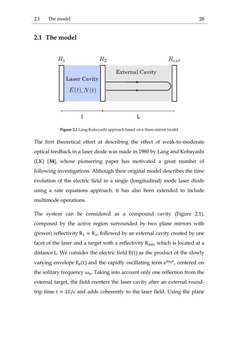
Figure 2.1 Lang-Kobayashi approach based on a three-mirror model

The first theoretical effort at describing the effect of weak-to-moderate

optical feedback in a laser diode was made in 1980 by Lang and Kobayashi

(LK) [34], whose pioneering paper has motivated a great number of

following investigations. Although their original model describes the time

evolution of the electric field in a single (longitudinal) mode laser diode

using a rate equations approach, it has also been extended to include

multimode operations.

The system can be considered as a compound cavity (Figure 2.1),

composed by the active region surrounded by two plane mirrors with

(power) reflectivity R = R , followed by an external cavity created by one

facet of the laser and a target with a reflectivity R , which is located at a

distance L. We consider the electric field E(t) as the product of the slowly

varying envelope E (t) and the rapidly oscillating term e , centered on

the solitary frequency ω . Taking into account only one reflection from the

external target, the field reenters the laser cavity after an external round-

trip time τ = 2𝐿/𝑐 and adds coherently to the laser field. Using the plane

2.1 The model 29

wave approximation and the mean field limit, i.e. neglecting spatial

variation of the field amplitude in the transversal plane and along the

optical cavity, this process can be described via a modified version of the

Lamb’s rate equation with the inclusion of a time-delayed term:

ddtE (t)e = iω (N) + 1/2 (G(N) − Γ ) E (t)e +

k𝜏E (t − τ)e ( ).

The first term represents the possible difference between ω and the

instantaneous frequency of the Fabry-Pérot resonator, given by ω =

qπc/ηl, where q is an integer and η and l are respectively the refractive

index and the length of the active medium. A strong ansatz is made here:

the changes in carrier density N(t) caused by the changes in the electric

field profile lead to variations of the refractive index due to plasma

loading, which in turn affects the instant frequency of the laser. This

mechanism, named phase-amplitude coupling, can be better explicated

though the definition of a linewidth enhancement factor:

α =4πλ

dηdN

dGdN

. 2.1

The second contribution in the E-field equation arises from the effective

amplification, given by the difference between the stimulated emission G

and the cavity losses Γ . The final term is the original addition made by

Lang and Kobayashi, which accounts the effect of the time-delayed

feedback coupled with the coefficient

k = ϵ (1 − R )RR

, 2.2


where the dimensionless parameter ϵ quantifies the spatial mode overlap

between the back-reflected light and the lasing mode (typically ϵ = 0.01 −

0.5) and 𝜏 is the laser cavity round-trip. This expression can be obtained

by requiring the continuity of the electric field at the boundary of the two

cavities and when the condition R ≫ R holds. When small

perturbations of η , G , ω - due to variations in carrier density near the

unperturbed laser threshold - are considered, LK equations can be

rearranged as

ddtE (t) =

12(1 + iα)G(N(t) − N )E (t) +

k𝜏E (t − τ)e . 2.3

The rate equation for the carrier density completes the picture:

ddtN(t) = −

N𝜏− G(N(t) − N )|E| + µμ. 2.4

Here, the first and the second terms describe respectively the spontaneous

and stimulated emission (𝜏 is the carrier lifetime, N is the carrier density

at threshold), while µμ quantifies the electrical injection.

2.2 Steady state solutions

We can get some physical insights considering the real phase and the

amplitude of the field E(t) = E (𝑡)𝑒 ( ) and searching steady-state

solutions: E (t) = E (t − τ) = E , N(t) = N and φ(t) = (ω − ω )t.

After some algebra we can obtain steady-state solutions for frequencies,

carrier density and optical power:

(ω − ω ) τ = C sin[𝜔 (τ)τ + arctan 𝛼]

2.5


N − N (τ) =2kGτ

cos[ω (τ)τ] 2.6

|𝐸 | =1

G(N − N ) µμ −𝑁𝜏

2.7

where

C =k𝜏τ 1 + 𝛼 2.8

represents a dimensionless parameter which controls the dynamical

behavior of the system. Owing to this analysis it is clear that the optical

retroaction modifies the threshold carrier density and hence the gain and

the emitted power of the laser.

Figure 2.2 (a) Round trip phase difference versus the instantaneous frequency for two feedback

parameters 𝑪𝟏 (solid line) and 𝑪𝟐 = 𝟐𝑪𝟏 (dashed line). (b) Modes (stars) and antimodes (triangles)

sustained by the cavity

Eq. 2.5 is a transcendental relationship owing to the dependence of the

frequency of the laser on the external round trip 𝜏, and can be solved

numerically. Figure 2.2 (a) shows the graphical solution of Eq. 2.5 for two

different feedback parameters: many frequencies 𝜔 are sustained by the

compound cavity and their number is controlled by the parameter C .

Steady-state solutions can be found setting to zero the round trip phase of


the field ∆𝜑(τ) = (ω − ω ) τ = 0 . As can been seen, increasing the

feedback or τ, new solutions arise in pairs. This effect can be interpreted as

the constructive (mode) and destructive (anti-mode) interference between

the cavity and the reflected fields. This explanation is endorsed by the fact

that these modes are separated in frequency by a free spectral range of the

external cavity. However, in a relatively weak-feedback condition, it has

been analytically shown that only one solution is stable of all the possible

frequencies of the system (Figure 2.2 (b)), which corresponds to the

maximum gain (and to the minimum threshold) mode.

From an experimental perspective, the estimation of the feedback

parameter appears difficult because of the uncertainty on the coupling 𝜀.

To access k, one measures the effective difference between the current

threshold in the presence and without the feedback, respectively 𝐼 and

𝐼 . This difference is proportional to k via:

∆I =𝐼 − 𝐼

𝐼= 𝑘

𝜏1 + 𝐺𝑁 𝜏

. 2.9

2.3 Self-mixing interferometry in semiconductor laser diodes

The study of optical feedback has led to a big amount of fundamental

physical knowledge in photonics and, at the same time, has stimulated the

development of practical applications, such as coherent echo detection,

chaotic signal communications and self-mixing interferometry. In the

latter, the laser source acts as a coherent detector, sensitive to changes in

the amount of the back-coupled radiation and of its experienced phase–


shift, which is caused by the presence of an external target. Interferometric

measurements exploit the so called weak-to-moderate regime, where the

fraction of the perturbing field brought back in the laser cavity is in the

range of approximately 10-8-10-4 of the free-running field intensity. In these

conditions, the mathematical analysis previously conducted can be

simplified, making the assumption 𝑘 ≪ 𝜏 /2𝜏 , and a straightforward

expression for the emitted power can be derived:

P(ϕ) = P [1 + m F(ϕ)]. 2.10

Here, P is the optical power without feedback, 𝑚 = 2𝑘𝜏 /𝜏 is the

modulation index, ϕ = 𝜔(𝜏)𝜏 is the phase accumulated during the external

round-trip by the electrical field and F can be implicitly defined as

F(𝜏) = cos[𝜏𝜔(𝜏)] , whose periodic waveform strongly depends on C

through Equation 2.5.

Owning to the characteristics of the interferometric signal and the value of

C, different regimes can be identified:

i. C < 0.1, very weak feedback regime. The function F(ϕ) resembles

the cosine function of a conventional Michelson interferometer.

ii. 0.1 < C < 1 , weak feedback regime. The function F(ϕ) becomes

distorted, and takes an asymmetrical shape that can be exploited

to acquire information about the direction of the target

displacement.

iii. 1 < C < 4.6, moderate feedback regime. The function F(ϕ) becomes

two-valued and the interferometric signal shows a sawtooth-like

behavior with hysteresis. The modulation index shows an


experimental saturation when the amount of the back-coupled

radiation is increased.

iv. C > 4.6 , strong feedback regime. The F(ϕ) becomes five-valued,

and the systems leaves the self-mixing regime and can experience

mode-hopping, coherent collapse or routes to chaos.

Figure 2.3 shows more insight into the features of the self-mixing signal

when the parameter C is varied to cover all the regions previously defined.

Irrespective of the feedback regime, the modulation function shows a

periodicity of 2𝜋. This means that if the external reflector is moved along

the longitudinal direction, SMI signal reproduces itself every λ/2

displacement.

Figure 2.3 Calculated SMI modulation waveform as a function of the phase for different values of

the feedback parameter: (a) C=0.1, (b) C=0.7, (c) C=3, (d) C=6. It is assumed 𝛂 = 𝟔. Adapted from

[35]

A small value of C (Figure 2.3 (a)) can be interpreted as a small coupling

between the external and the internal cavity, which results in a

symmetrical waveform very similar to a standard interferometer, with

different power in the two arms. As the value of C approaches unity

(Figure 2.3 (b)), the signal gets asymmetric and the discrimination of the


direction of motion of the target is possible with no need for two

quadrature readings.

However, when 𝐶 = 1 the system becomes bistable: it has three solutions

for certain values of the phase, whereof one is non-physical. A stability

analysis can be performed to identify which branch is stable. Let’s consider

as an example Figure 2.3 (c), and suppose that the system is in the state W:

when the phase is increased, it moves along the curve up to the point X,

where it jumps down to point X’, which is located on the adjacent stable

branch. Vice versa, if the system is placed in X’ and the phase is decreased,

point Y is reached, and an upper jump to point Y’ subsequently occurs.

Therefore, in the moderate regime the interferometric modulation exhibits

hysteresis and discontinuous step-like transitions.

An analytical expression for the hysteresis phase period 𝜙 can be

calculated finding in Equation 2.5 the phase where the derivative of the

angular frequency diverges:

ϕ = 2 C − 1 + arccos(−𝐶 ) − 𝜋 . 2.11

Surprisingly, the hysteresis duration depends only on the feedback

coefficient C, showing an almost linear behavior for C>3.

Another change in the behavior of the system occurs at the threshold

C=4.6: a new bifurcation takes place, and for certain values of the phase

five solutions appear (Figure 2.3 (d)). Here, when the system reaches point

X, two possible evolutions exist, since the system can jump down to two

distinct stable points, namely X’ and X’’. Similarly, when point Y is

reached with decreasing phase, the system can jump up to points Y’ or Y’’.


The intrinsic dynamics of the laser under investigation governs which of

the jumps occurs.

One of the crucial points for the coherent phenomenon just reviewed is its

applicability to a vast range of metrology measurements. Traditional

quantities measured exploiting SM interferometry are displacements

velocities, vibrations, absolute distances and angles.

At the same time, owing to the complex relationship between carriers and

photons involved, SMI has been employed to access physical laser

quantities such as the linewidth, the coherence length and the alpha factor.

In traditional configuration the signal is read from a photodiode integrated

in the packaging of commercial laser diodes. Another solution consists in

monitoring the perturbation of the voltage across the device [36]. In fact,

the voltage is related to the carrier density by the Schottky relation

N = N exp𝑒𝑉2𝐾𝑇

, 2.12

where N is the intrinsic carrier density, k is the Boltzmann’s constant, and

T is the temperature. When this expression is combined with equation 2.6

the following simple relationship is obtained:

ΔV(ϕ) = −Δ𝑃(ϕ)𝑅𝜂. 2.13

Here we have denoted with 𝑅 the diode differential resistance at

threshold and 𝜂 = 𝑑𝑃/𝑑𝐼 the efficiency of the laser diode. The physical

meaning is therefore clear: when the laser power is increased by the optical

feedback the change in the voltage across the junctions can be thought as a

voltage drop that would result from an equivalent increase in the injection

current in the absence of feedback. It is important to note that according to

equation 2.13 the laser power and the junction voltage are in phase

2.4 Regimes 37

opposition. These considerations do not take into account the change in the

DC bias of the laser, which is related to the feedback parameter C.

The drawback of this voltage-based scheme is that the junction output is

affected by a worse signal to noise ratio with respect to the optical power

acquired via a photodiode.

Indeed, the differential resistance r = dV/dI = 2kT/eI found across

the laser diode carries Johnson noise, which is given - in rms current- by

in=[4kTB/rdiff]1/2 where B is the bandwidth of the electronic system; this

quantity adds in quadrature to the shot noise coming from the bias current

and the total noise results therefore greater than the electronic one which

characterized a typical photodetector.

2.4 Regimes

The discussion above has been carried out having a special consideration

for interferometric applications. Nevertheless, pioneering works focused

on more fundamental questions linked to the dynamics of the laser and its

stability against back-coupled radiation. Theory and experiments have

been chasing each other for the last thirty years, trying to explain

fascinating complexity, which arise from the optical feedback in

semiconductor laser.

This has been summarized by the diagram illustrated in Figure 2.4,

designed for the first time in the seminal paper of Tkach and Chraplyvy in

1986 ( [37]).

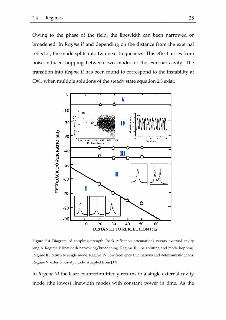
At the lowest feedback levels, Regime I, the laser operates on a single

external cavity mode that is originated from the solitary laser mode.

2.4 Regimes 38

Owing to the phase of the field, the linewidth can been narrowed or

broadened. In Regime II and depending on the distance from the external

reflector, the mode splits into two near frequencies. This effect arises from

noise-induced hopping between two modes of the external cavity. The

transition into Regime II has been found to correspond to the instability at

C=1, when multiple solutions of the steady state equation 2.5 exist.

Figure 2.4 Diagram of coupling-strength (back reflection attenuation) versus external cavity

length. Regime I: linewidth narrowing/broadening. Regime II: line splitting and mode hopping.

Regime III: return to single mode. Regime IV: low frequency fluctuations and deterministic chaos:

Regime V: external cavity mode. Adapted from [37].

In Regime III the laser counterintuitively returns to a single external cavity

mode (the lowest linewidth mode) with constant power in time. As the

84 Experimental Observations

Figure 4.1 Regimesof operation of alaser withexternal feedback.Source: After [19],© 1986 IEEE.

to this chaotic state is characterized by a series of bifurcations which will be carefullyoutlinedanddetailedinSection4.4, ‘WeakFeedbackEffects’.Thelowfrequency fluctuationregimewill beintroducedanditsdynamical statediscussedinSection4.6 ‘ModerateOpticalFeedback’.Still further increaseintheoptical feedback level resultsinatransitiontoanothersingle mode, constant intensity, and narrow linewidth regime (Regime V) when thediodelaser facet facing themirror hasbeen anti-reflection coated. Thisregimecannot bereachedwhen diodes with uncoated facets are used. Regime V, in which the laser is operatingon a steady state, will not be discussed as it is rather uninteresting from the dynamicalviewpoint.

In thenext few sections themost important effects in each of thefeedback regimeswillbe discussed with emphasis on the sequence of bifurcations as a function of the feedbackstrength. Inaddition, someparticular experimental effectsthat occur inshort external cavitiesand also in doublecavity systemswill beoutlined (Sections4.7 and 4.8). Onesection willbedevoted to multimodeeffects (Section 4.9). In thissection theexternal cavity feedbackphenomenaunder singleor multimodeoperationof thelaser will becontrasted. IntheControlsection (Section 4.10) we discuss several experimental procedures to alleviate the chaoticbehavior of thelaser in theexternal cavity but still retain all theoperational characteristicsof thelaser. Thefollowing section reviewstheexperimental literatureof thesemiconductorlaser in an external cavity with theaddition of current modulation of thelaser. Indeed, onesuch techniqueisto takeadvantageof modulation toopen loopstabilizetheexternal cavitylaser. Thepenultimatesectionof thischapter discussestheeffectsandphenomenaobserved


Figure 4.10 Bifurcationdiagramof theinversionasafunctionof feedback strength for aninjectioncurrent of 13× Jth and theexternal delay is1nsec.Source: After [40] ©1992 IEEE.

Thepumping of thelaser isset at 13× Ith and theexternal delay is1ns. Thebifurcationparameter isthefeedback strength andonly theintersection pointsof thenormalized carrierdensity corresponding to traversal through thePoincareplanein thedirection of decreasingfieldamplitudearerecorded[40] inFigure4.10(a). Thesameinformation iscontained inthebifurcation diagram in terms of thephasedelay in Figure4.10(b). In addition, Figure 4.11showsthePoincaresectionof thevariousattractorsat fixed feedback levelsin theinversionand phase delay plane. Figure 4.12 shows the time series at selected feedback ratios. Thefeedback strength for alaser with aFabry–Perot cavity laser isdetermined from

= 1−R2RextR2

(4.15)

and 2 is thepower reflected from theexternal cavity relative to thepower from the lasermirror. This is the same quantity that is represented in Equation (4.5) but normalized tothesolitary laser cavity round-trip time. Additionally, thecoupling fraction into thediodeisassumed tobeunity. For aDFB laser diode becomescomplex and it hastobedeterminedfromarather complicated nonlinear expression involving thedetailsof thegrating [38, 39].However, here isassumed tobepositiveandreal, andany possiblephasecanbeincludedin therather arbitrary phase 0 .


Figure 4.32 (a) Timeseriesof theregular LFF and (b) theRF spectrum.Source: After [73].

The wealth of bifurcations and the abundance of complex dynamics that have beenobserved experimentally have been conveniently summarized in the Introduction to thischapter and aredepicted in Figure4.1. Thecharacterized behavior at all feedback regimeswasexperimentally described for anumber of different semiconductor laser typesandunderdifferent experimental situations. Substantially thesamebehavior, thebasicbifurcationsandtheir dynamics were observed under multimode operation as well as when operated withfrequency selectedelementsintheexternal cavity. Similar dynamical behavior wasobservedin DFB lasers in an external cavity operating on a single longitudinal mode as well as inFabry–Perot lasersunder multimodeoperation. In thenext few sectionswewill examine indetail not only specific external cavity arrangements, but will also focus on experimentalsituations between multimodeor single-modebehavior.

4.7 SHORT CAVITY REGIMEThe case of optical feedback from short external cavities has several unusual features anddeserves special attention. When ashort external cavity is used, the product ext remainssmall even for weak feedback, and so thenumber of external cavity modes and antimodes

I

II

III

IV

V

2.4 Regimes 39

feedback is still increased, and independently of the length of the external

cavity, the system undergoes a transition to a chaotic state known as

coherence collapse: it enters Regime IV. This is characterized by a

dramatically broadened optical and noise spectra, which contains many

external cavity modes. The low current injection regime near the solitary

laser threshold is also known as the low frequency fluctuations regime, so

named from the irregular and slow power oscillation events caused by the

competition of a great number of possible external frequencies, none of

which is stable. The route to this chaotic state starts with a series of Hopf

bifurcations, which are characteristic of a huge number of systems

belonging to different areas of physics. The broadened spectrum appears

continuous or spike-like depending on the length of the cavity, which can

be greater or less than L = c/2f ∗, where f ∗ is the cut-off frequency of the

laser diode associated with high frequency modulation.

Still further increase in the optical feedback level results in a final transition

to another single mode, constant intensity, and narrow linewidth regime

(Regime V), namely external cavity mode. This regime can be reached only

by uncoating the laser facet and is typically exploited in spectroscopic

applications.

Applications of SMI phenomena are located in the lower left side of the

diagram, whereas chaos has been proposed as a cryptography tool. SMI

obviously requires coherence of the returning field addition to the in-

cavity unperturbed field, while chaos can be also generated from

incoherent coupling.


2.5 Quantum cascade lasers

Quantum cascade lasers are unipolar semiconductor devices in which laser

action is achieved in intersubband states located in the conduction band.

These levels arise from the spatial confinement of electrons in few-

nanometer-thick quantum-wells of a heterostructure. QCLs derive its

name from the multistage scheme used, in which each electron travels

through an active region sequentially replicated tens of times and emits

multiple photons. This unique propriety leads to internal quantum

efficiency greater than one and intrinsic high-powers: hundreds of

milliwatts in continuous mode and peak pulse powers in the range of

Watts have been achieved. Although the first idea of using intersubband

transitions and tunneling in a cascade structure to produce light

amplification was proposed by Kazarinov and Suris in 1971 [38], only in

1994 the first QC laser was experimentally demonstrated at Bell Labs [39],

after the refinement of molecular beam epitaxy and improvements over

transport models in heterostructures. Many differences with classical

diode laser are inherently related with the use of intersubband transition.

Energy space between subbands can be designed by engineering the

thickness of quantum wells and barriers. Thus, lasing in a remarkably

wide range (3-200 μm) has been proved. In this way, the emission

wavelength is independent from the energy gap of the constituent

semiconductors. Moreover, since the initial and the final states involved in

the stimulated emission have the same curvature in the reciprocal space,

the related joint density states is very sharp as in gas laser. This results in a

narrow linewidth theoretically predicted [40] and experimentally


measured [41], as small as 100kHz, reaching the quantum-limited

frequency fluctuations (Hz) when the system is stabilized [42].

In order to acquire a simplified physical picture of working principles of

QCLs, the active region can be modeled as a four-level system (Figure 2.5

(a)). When an electric field is applied, electrons are injected by tunneling

from the subband 4 into level 3, which acts as the upper level of the laser.

Here, carriers undergo stimulated emission from 3 to 2 and then quickly

relax to 1, typically via a designed non-radiative longitudinal optical (LO)

phonon interaction.

Neglecting the thermal backfilling from level 2, we can write a set of rate

equations for electron sheet density in the upper 𝑛 and the lower 𝑛 levels

( [43]):

dndt

= ηJe−nτ

− G(n − n )S, 2.14

dndt

=nτ

−nτ

− G(n − n )S, 2.15

where η is the injection efficiency, S(t) is the photon number, G is the gain

coefficient, τ (τ ) is the total electron lifetime of level 3 (2), τ the

characteristic time of the transition 3 → 2.

An expression for the propagation gain G is obtained requiring steady-

state condition

G ∼ Γωδω

τ 1 −ττ

|𝑧 | . 2.16


Here, Γ is the spatial overlap of the guided mode with the active module,

𝑧 = ⟨2|𝑧|3⟩ is the dipole matrix element of the transition obtained

through the Fermi’s golden rule. The latter is proportional to the

stimulated-emission cross-section and heavily depends on the overlap and

the symmetry of the initial and final wavefunctions; δω is the spontaneous

emission linewidth of the Lorentzian-shaped transition.

From these considerations it can be inferred that a population inversion

and a positive gain are achieved when τ < τ . The traditional approach

used in mid-infrared QCL has been to couple level 2 and level 1 via non-

radiative optical phonon interaction, which occurs at very fast rate (0.2-0.3

picoseconds) with respect to picosecond electrons radiative transition in

subbands.

Besides, due to its ultra-fast carrier dynamics comparable to photon rates,

quantum cascade laser is the only semiconductor system belonging to A-

class lasers (Arecchi’s classification). Therefore, it does not exhibit typical

relaxation oscillations, showing an overdamped transient dynamics

towards the steady state, which allows intrinsic modulation bandwidths

up to several tens of gigahertz.

The development of QCLs below the Restrahlen band (energy below the

optical phonon absorption band of polar semiconductor, <20meV) has

been more challenging than the ones working in the mid-infrared, due to

two main difficulties. Foremost, the mid-infrared strategy of fast

depopulation of the lower lever through LO-phonon scattering is more

strenuous at terahertz frequencies, since the photon energies are lower

than the LO-phonon energies (36 meV for GaAs). Owing to the small

distance between the previously defined level 3 and 2, the selective


depopulation of the sole lower state is difficult, as the upper laser state will

be however coupled with level 1. In other words, the condition for the

population inversion is hardly achievable, because τ is comparable to τ .

Figure 2.5. (a) General four-level scheme of QCL. Conduction-band diagrams for traditional

terahertz design schemes: (b) chirped superlattice (c) resonant-phonon (d) bound-to-continuum.

Two identical modules of each one are shown. The squared of the wavefunctions are plotted

(upper and lower radiative in red and blue, respectively). Minibands are represented as gray

shaded regions. Adapted from [44]

Second, as free carriers absorption scales proportionally to the square of 𝜆,

clever projects of waveguides are required to minimize the modal overlap

with any doped semiconductor cladding layers.


Since the first demonstration in 2002, three different active structures have

been proposed, namely chirped superlattice (Figure 2.5 (b)), bound-to-

continuum (Figure 2.5 (d)), and resonant-phonon (Figure 2.5 (c)) to

overcome these problems. Nevertheless room-temperature operation is

still a big goal.

The chirped-superlattice (CSL) design exploits the formation of mini bands

when nm-thick quantum wells are stacked together to create a superlattice

[45]. The radiative transition can be designed to involve the lowest state of

upper mini band and the top state of the next one, similarly to

conventional inter-band transitions in laser diodes. In this way a

population inversion is established since scattering of electrons between

the tightly coupled states within the miniband is faster than the inter-

miniband one. LO-phonons are indirectly involved in the electron gas

cooling.

An evolution of CSL scheme consists in the bound-to-continuum approach

[46]. Here, the upper radiative level is a bound defect state while the lower

laser state and the depopulation remains the same. Consequently, the

transition is more diagonal in real space: the upper-state lifetime and the

injection efficiency increase to the detriment of oscillator strength.

Finally, resonant-phonon approach has been extended in the THz region (

[47]) through a trick: the wave function of the lower radiative state is

spread over several quantum wells via a tunneling mechanism, while the

upper state remains localized. Thus, the spatial overlap with the injector,

located a LO-phonon energy down, is spatially differentiated.


2.6 Quantum cascade laser against optical feedback

The study of the optical feedback has been traditionally conducted on bulk

semiconductor lasers. Recently, many groups have extended these

investigations on quantum cascade laser and increasing interest about

unforeseen results has emerged.

The theoretical model underlying the physics of the optical feedback in

QCL is still based on the Lang-Kobayashi approach.

One example, which confirms the applicability of such framework, is

represented by the measure of the linewidth enhancement factor of QCLs

trough self-mixing interferometry: a value near zero confirming pre-

existing theories has been measured in Mid-IR [48] and THz [49] cascade

structure (Figure 2.6). Moreover, it seems to increase when the driving

current is raised. In turn, this fact has dramatic implications both with the

linewidth of the laser (which scales with (1 + 𝛼 ) through the famous

Schawlow–Townes formula) and with the dynamical behavior of these

sources against the optical feedback. We will focus on the second issue.

Figure 2.6. Measured alpha-factor as a function of the injection current for (a) a Mid-IR DFB QCL

[48] and (b) a THz QCL [49]


Partially owing to this negligible value of 𝛼 , it is believed that QCLs

operate in the weak feedback regime beforehand defined (C < 1). The

reasons of this small coupling propriety can also be attributed to the long

cavity length of QCLs (about 1mm). These combined effects reduce by a

factor 100 the feedback parameter, in comparison with diode lasers for a

given external cavity length.

Very recently, the effects of optical feedback on the dynamical behavior of

QCLs have been numerically and experimentally studied [50], reporting an

unexpected ultra-stability of such systems. In fact, it seems that when the

optical feedback is increased, QCLs do not experience the onset of

nonlinear phenomena (including mode-hopping, intensity pulsation and

incoherent collapse) illustrated above (see Figure 2.4), typical of

conventional laser diodes, but remain in a single longitudinal mode

regime. Figure 2.7 illustrates the different behaviors of a quantum cascade

laser and a laser diode: stable continuous emission characterizes the QCL

with a feedback amount two order of magnitude higher than the critical

value for which coherent collapse appears in laser diodes.


Figure 2.7 Experimental fast Fourier transform of signal detected by (a) the PD integrated laser

diode and (b) the voltage modulation across a QCL device. Figure (b) illustrates the stable CW

emission a QCL subjected a high optical feedback (𝐤 = 𝟕. 𝟓 ∙ 𝟏𝟎 𝟐). Figure (a) shows the coherence

collapse in a LD, with 𝐤 = 𝟏 ∙ 𝟏𝟎 𝟑. The inset displays the time-behavior of a laser diode in a

coherence collapse regime. Adapted from [50]

Both the low value of the alpha factor and the photon to carrier lifetime

ratio can theoretically explain these strong evidences: the critical value of

the coefficient k which causes CW instabilities, increases up to one order of

magnitude, with decreasing 𝛼 and with high photon to carrier lifetime

ratio (Figure 2.8).

Figure 2.8 Numerical simulations of the effect of the LEF and the photon to carrier lifetime ratio

on the critical feedback level. When 𝛂 < 𝛂𝐂 the QCL enters the ultra-stable regime. Adapted from

[50]

(b)(a)

k < kc

k > kc

Laser diode QCL

(a) (b)


We conclude this discussion with a practical consideration. Due to the lack

of detectors, the most suitable way to reveal the self-mixing signal consists

in monitoring the change of the voltage drop across the device. An

analytical expression which links carriers to photons in a cascade structure

is not trivial in QCLs, therefore eq. 2.12, which works well for a laser diode,

cannot be trivially applied to QCLs. Nonetheless, the general equation 2.13

can be supposed to hold.

3.1 Sources 50

Chapter 3

3. Experimental Setups Experimental Setups In this chapter experimental setups are presented. Paragraph 3.1 gives

some details about the sources used: a commercial Mid-IR and custom

THz quantum cascade laser. Paragraphs 3.2 and 3.3 describe the

experimental schemes respectively in the Mid-IR and terahertz regime,

through which imaging of various samples has been carried out without

the use of an external detector. The two final sections illustrate some

aspects related to the spot of the beam. An estimation about the beam

waist (3.4) and the research of the focal plane (3.5) can be intrinsically

accomplished through self-mixing.

3.1 Sources Mid-IR QCL

One of the sources adopted in the experiment is a commercial quantum

cascade laser (Alpes Lasers, mod. RT-CW-DFB-QCL), working at

wavelength of 6.24µμm (equivalently 48 THz , or 1600cm-1) at room

temperature. Although it can operate in both continuous and pulsed mode,

only the first configuration has been used in the experiment. The laser can

be tuned from 1598 to 1609 cm-1 by changing its temperature through a

Peltier controller. This feature combined with the relative narrow nominal

linewidth (5MHz) makes it suited for spectroscopic applications too.

3.1 Sources 51

Figure 3.1 Current-voltage (right) and light-voltage (left) characteristics of the QCL, for different working temperatures

Figure 3.1 shows the electrical and the optical proprieties of the device, for

a wide range of temperatures. When stabilized at 10°C, the device exhibits

a slope dP/dI = 0.20W/A , a threshold current I = 460𝑚𝐴 and a

differential resistance of dV/dI = 3Ω . Figure 3.2 illustrates spectra for

different temperature and driving current. As many other QCLs, it is

characterized by a large divergence of the order of 40 -60 degrees.

Figure 3.2 Nominal spectra of the Mid-IR QCL for different driving currents and temperatures

3.1 Sources 52

THz QCL

Figure 3.3 Simulated conduction band structure of the 3.9THz-QCL under an average electric

field of 1.5 kV/cm. The two upper-level lasers are depicted in green and red.

The terahertz quantum cascade laser used emits at 79,1µm (3.9 THz). It is a

modified version of the bound-to-continuum scheme, and its design was

originally proposed by Losco et al. [51]. As it has been written before, this

approach appears to be favorable in the THz domain, thanks to the

diagonal character (in real space) of the optical transition, which facilitates

a selective carrier injection.

The original feature of the device is the design of the active region: two

identical optical transitions are expected from two upper laser levels,

closely separated by about 1 meV in energy (see Figure 3.3).

The existence of these two upper states has two main consequences. First,

it allows twice the number of electrons to be stored in roughly the same

3.1 Sources 53

energy range, which comes out useful for high-current and high-

temperature operations. On the other hand, the dipole matrix element of

each transition is smaller (~ 5 nm) than typical for standard THz QCLs

emitting at the same frequency.

A cascading structure with this property can be realized engineering the

thickness of the barriers and the wells of a heterostructure. When the

Schrödinger equation coupled with the Poisson equation is solved, the

eigenfunctions and the respective energy levels are obtained. Figure 3.3

shows the calculated conduction band of the QCL, when an electric field is

applied.

The device was grown by molecular beam epitaxy employing a

GaAs/Al0.15Ga0.85As heterostructure on a nominally undoped GaAs

substrate with a surface plasmon waveguide. A 500 nm thick heavily

doped (3.0 × 1018cm-3, Si) layer defines the lower contact of the laser for the

designed single plasmon waveguide. The active region is repeated 120

times and the growth ends with a heavily doped (5.0 × 1018cm-3, Si) 200nm-

thick GaAs contact layer.

The layer thicknesses of the active module, starting from the injector, are

4.0/10.5/2.3/18.2/1.9/18.3/0.7/14.7/0.7/12.5/1.5/11.0/2.7/11.0/3.0/11.0

nanometers (Al0.15Ga0.85As barriers are written in bold).

Experimental current-voltage and light-voltage characteristics are shown

in Figure 3.4.

3.1 Sources 54

Figure 3.4 Current-voltage (blue dots) and light-voltage characteristics (red dots) of the laser

under investigation. The dimensions of the points correspond to the errors of the measurement.

Figure 3.5 Spectrum of the THz-QCL when driven at 𝐈 = 𝟎. 𝟔𝟗𝐀 measured via FTIR.

Moreover, the experimental spectrum acquired via a Fourier transform

infrared spectrometer (FTIR) is presented in the Figure 3.5: a longitudinal

120 122 124 126 128 130 132

0

5000

10000

15000

Opt

ical

Pow

er (a

.u.)

Wavenumber (cm-1)

3.79�THz�79.1�μm�

3.1 Sources 55

single mode is observed near the laser threshold, while multimode

behavior is expected at higher driving currents.

Lasing at 3.9 THz with a threshold current density of 82 A/cm2 at 5 K was

demonstrated. The maximum output power is achieved near 400 A/cm2,

still 4-5 times above threshold. Lasing is observed also in pulsed mode up

to 70 K, with a peak power level in excess of several milliwatts at 10 K.

These good performances and the high dynamic-range of the device

indicate that both transitions are contributing in parallel to lasing.

3.2 Mid-IR Setup 56

3.2 Mid-IR Setup

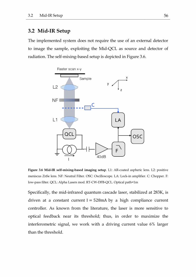
The implemented system does not require the use of an external detector

to image the sample, exploiting the Mid-QCL as source and detector of

radiation. The self-mixing-based setup is depicted in Figure 3.6.

Figure 3.6 Mid-IR self-mixing-based imaging setup. L1: AR-coated aspheric lens. L2: positive

meniscus ZnSe lens. NF: Neutral Filter. OSC: Oscilloscope. LA: Lock-in amplifier. C: Chopper. F:

low-pass filter. QCL: Alpha Lasers mod. RT-CW-DFB-QCL. Optical path=1m

Specifically, the mid-infrared quantum cascade laser, stabilized at 283K, is

driven at a constant current I = 528mA by a high compliance current

controller. As known from the literature, the laser is more sensitive to

optical feedback near its threshold; thus, in order to maximize the

interferometric signal, we work with a driving current value 6% larger

than the threshold.

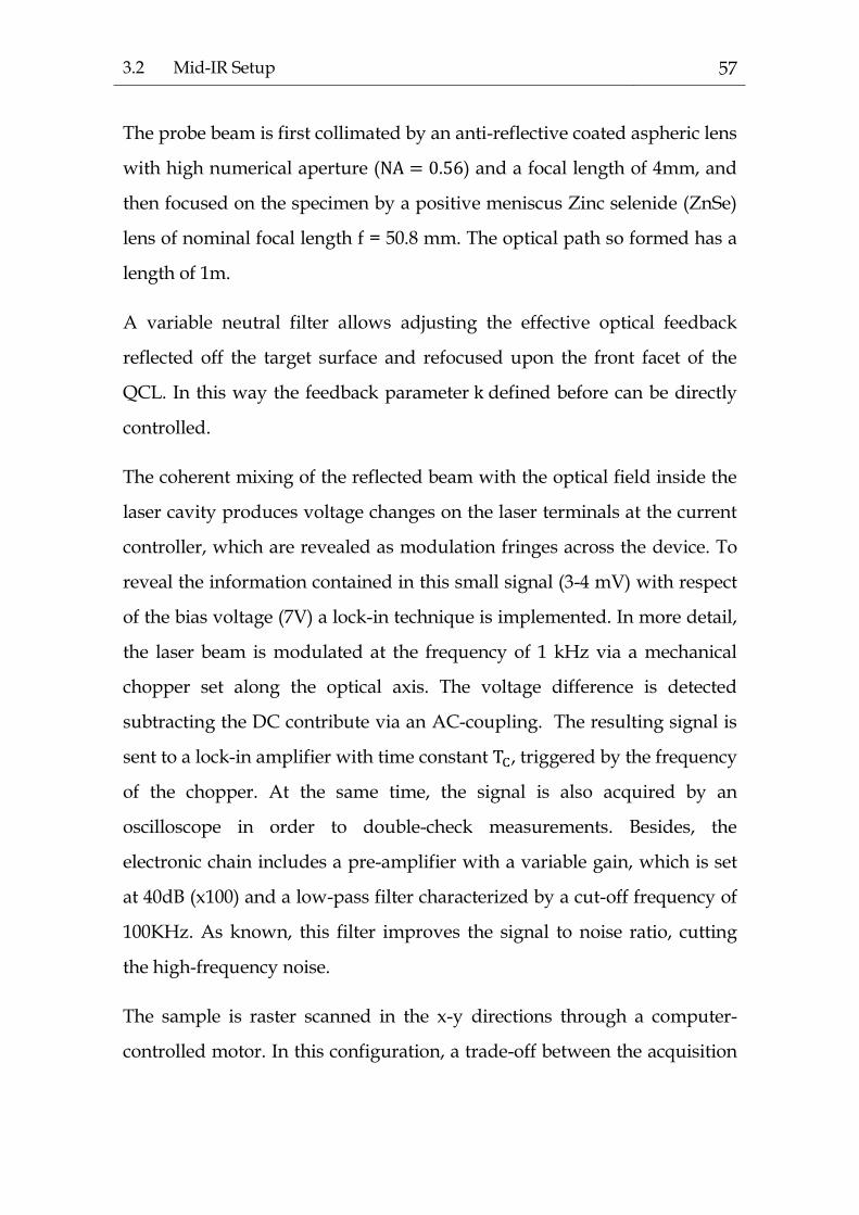
3.2 Mid-IR Setup 57

The probe beam is first collimated by an anti-reflective coated aspheric lens

with high numerical aperture (NA = 0.56) and a focal length of 4mm, and

then focused on the specimen by a positive meniscus Zinc selenide (ZnSe)

lens of nominal focal length f = 50.8 mm. The optical path so formed has a

length of 1m.

A variable neutral filter allows adjusting the effective optical feedback

reflected off the target surface and refocused upon the front facet of the

QCL. In this way the feedback parameter k defined before can be directly

controlled.

The coherent mixing of the reflected beam with the optical field inside the

laser cavity produces voltage changes on the laser terminals at the current

controller, which are revealed as modulation fringes across the device. To

reveal the information contained in this small signal (3-4 mV) with respect

of the bias voltage (7V) a lock-in technique is implemented. In more detail,

the laser beam is modulated at the frequency of 1 kHz via a mechanical

chopper set along the optical axis. The voltage difference is detected

subtracting the DC contribute via an AC-coupling. The resulting signal is

sent to a lock-in amplifier with time constant T , triggered by the frequency

of the chopper. At the same time, the signal is also acquired by an

oscilloscope in order to double-check measurements. Besides, the

electronic chain includes a pre-amplifier with a variable gain, which is set

at 40dB (x100) and a low-pass filter characterized by a cut-off frequency of

100KHz. As known, this filter improves the signal to noise ratio, cutting

the high-frequency noise.

The sample is raster scanned in the x-y directions through a computer-

controlled motor. In this configuration, a trade-off between the acquisition

3.3 THz Setup 58

time and the SNR exists. Reasonable values for the scan velocity along the

x-axis ranges from 0,1 to 0,5 mm/s, with steps of 250µμm in the y-direction.

3.3 THz Setup

Figure 3.7 THz Self-mixing-based imaging setup. PR: parabolic reflector. OSC: Oscilloscope. LA:

Lock-in amplifier. C: Chopper. F: low-pass Filter. QCL: CW Quantum cascade laser, Optical

path=0.5m

The setup discussed in paragraph 3.2 can be easily modified to work with

the terahertz quantum cascade laser as a source (Figure 3.7). Here, the QCL

is mounted on the cold finger of a continuous-flow cryostat fitted with a

polymethylpentene (TPX) window and kept at a heat sink temperature of

15 K. The THz QCL beam is collimated using a 2 inch f/1 = 50 mm 90°

gold-plated off-axis paraboloidal reflector and focused by a second

identical reflector at normal incidence upon the remote target.

3.4 Beam waist 59

Because of the high divergence of the laser, the beam is expected to cover

the entire surface of the mirror. Therefore, in the optical path where the

beam is collimated, its diameter is estimated to be of some millimeters. The

radiation was then coupled back into the laser cavity along an optical path

of about 0.5 m.

In our experiments, the THz QCL was driven at a constant current I = 700

mA for CW mode operation. The electronic chain used is the same

described above. Again, the effect of feedback - SM signal - was measured

as voltage modulation across the terminals of the device.

As usual in terahertz experiments, a pre-alignment of the apparatus is

realized using a He-Ne source, which is focalized on the facet of the

quantum cascade laser and follows the same optical path experienced by

the THz beam. The alignment’s beam is then switch off, because it has been

demonstrated that its presence strongly affects the voltage across the QCL.

3.4 Beam waist

As illustrated in chapter one, the dimension of the probe spot is one of the

most important figures of merit, which governs the spatial resolution of an

imaging system. The measurement of the beam waist 𝜔 can be

accomplished via the known knife-edge method: a plate with a sharp edge

is moved along the direction of interest γ, while a detector acquires the

spatial integrated power. It can be demonstrated that, assuming the beam

to be Gaussian with intensity 𝐼 = 𝐼 𝑒 𝑒 , the total power can be

expressed as a function of the coordinate of the plate edge, say x, as

𝑃(𝑥) =𝑃2

1 − erf√2𝑥𝜔

,

3.4 Beam waist 60

where P is the total power and ω is the 1/e radii of the beam in the x

directions. Instead of using an external detector, one can access the same

information in reflection geometry, exploiting the change in the DC

voltage across the laser, which is proportional to the optical power

reflected.

Figure 3.8 reports the measurements of the beam waist of the THz

radiation along x and y direction, both using a detector and through

optical feedback. The beam appears elliptical with 𝜔 ≅ 330𝜇𝑚 > 𝜔 ≅

150𝜇𝑚, and the values obtained by the two methods agree.

Figure 3.8 Knife-edge method exploited to measure the beam waist of the THz beam along the x

(a) (b) and y directions (c) (d). Signal in transmission (b) (d) and reflection configuration measured

through SMI (a) (c)

(a)

Tran

smis

sion

[a.u

.]

SMI S

igna

l [m

V]

Tran

smis

sion

[a.u

.]

(b)

(c) (d)


3.5 Beam focusing

Figure 3.9 Intensity of a simulated Gaussian beam

As any other THz imaging system discussed before, one of the main

experimental problems is related to the focusing of the probe beam. In

principle, the surface of the sample under investigation must be in the

focal plane of the final lens. Deviations from this condition result in the

decrease of the spatial resolution. We can make some quantitative

considerations recalling some arguments of physical optics.

Supposing the beam profile to be Gaussian (Figure 3.9), the target can be

assumed to be located in the focal plane if its deviations from the latter are

less than the Rayleigh length, defined as

𝑧 = 𝜋𝜔𝜆.

Here, 𝜆 is the wavelength of the radiation and 𝜔 is the beam waist, that is

the radial size of the beam in its narrowest point. When we use the

estimations of the beam waist acquired via knife-edge method, 𝜔 (𝜆 =

wop

2wo

zR


6,25𝜇𝑚) = 35𝜇𝑚 , and 𝜔 (𝜆 = 79.1𝜇𝑚) = 350𝜇𝑚 , we obtain z , =

615µμm and z , = 4,8mm.

Figure 3.10 Technique to find the correct focus position through self-mixing. DC signal measured

across the QCL versus the longitudinal position of the target. In blue the experimental points, in

red the Gaussian fit.

Self-mixing scheme offers a simple strategy to verify if the beam is

correctly focalized on the target. The solution consists in monitoring the

DC SM signal while the target is sequentially moved along the

longitudinal axis: the maximum in the signal corresponds to the maximal

optical intensity that couples back in the laser cavity. Figure 3.10 shows an

example of this procedure for the Mid-IR laser; the width of the peak

inferred from a Gaussian fit is 𝑤 = 1000 ± 180𝜇𝑚 which is comparable to

2z , .

A simple semi-quantitative model based on ray optics supports the

validity of this approach. Let’s consider the target located at a distance 𝑑

from the focal plane 𝑓 of the final lens of the optical system. A collinear


ray placed at position 𝑦 from the optical axis, after being reflected back

from the target, returns in a radial position 𝑦 ′, which is different from 𝑦

(see Figure 3.11)

Figure 3.11 Self-focusing scheme offered by self-mixing configuration

If d is big enough, the radiation cannot be coupled back into the laser

cavity. Using the ABCD matrix formalism we can calculate the radial

coordinate of a ray - which has an initial position 𝑦 before the final lens 1

(𝜃 = 0) - after travelling through the complete optical chain again:

𝑦𝜃 = 𝕊(𝑓 ) ∙ 𝕃(𝑓 ) ∙ 𝕊(𝐿) ∙ 𝕃(𝑓 ) ∙ 𝕊(𝑑 + 𝑓 ) ∙ 𝕄 ∙ 𝕊(𝑑 + 𝑓 ) ∙ 𝕃(𝑓 ) ∙

𝑦𝜃

where

𝕃(𝑓) = 1 0−1/𝑓 1 , 𝕊(𝑥) = 1 𝑥

0 1 , 𝕄 = 1 00 1

are the matrix operators for, respectively, a thin lens of focal f, a free-space

propagation of a distance x, and a mirror reflection. Assuming θ = 0 and

the onset of parameters used in the mid-IR setup, a linear relationship is

obtained: y ≅ 10d[mm] ∙ y [mm]µμm. For d = 1mm and y ranging from 0 to

f1 f2L

yi

yf

d

yi’


25𝑚𝑚 the dimensions of the back coupled spot can result two times

greater than typical QCL facet dimensions (10x100 𝜇𝑚).


Chapter 4

4. Imaging Results Imaging Results This chapter is devoted to presenting the experimental results obtained

through self-mixing approach, used as an imaging tool. Paragraph 4.1 and

4.2 illustrate imaging outcomes achieved with mid-infrared and a terahertz

setup. The role of the phase in these configurations is then discussed. The

chapter ends with a focus on some aspects related to the visibility of the

interferometric fringes. The non-conventional behaviour of the source

against the amount of the optical feedback is reported in section 4.3

4.1 Mid-IR imaging results

Figure 4.1 (a) Optical microscope image of a lithographic mask. (b) Self-mixing voltage across the

Mid-IR QCL, obtained by scanning the same sample in the x direction, revealing jumps in the DC

voltage of the laser which correspond to the two different materials

0 10 20 30 40 50 60

0 0,5 1 1,5 2 2,5

SM

I Sig

nal [

mV

]

x [mm]

(a)220µm

138µm

160µmCr

SiO2

x [mm]


The most intriguing peculiarity of the self-mixing-based imaging is its

sensitivity to the phase of the field. Two pieces of information can be

discerned from such a coherent scheme:

i) The incoherent amount of the radiation scattered or reflected

from a sample, codified in the parameter k of the Lang-

Kobayashi model.

ii) The change in the phase of the field due to a modification of the

optical path experienced by photons.

While the first contribute influences both the waveform of the

interferometric signal and the DC-voltage of the laser, the second governs

the periodic modulation of the voltage across the device. Unlike other

coherent imaging systems reviewed in chapter 1, these two terms cannot

be easily extracted separately, but they mix together. In order to illustrate

these concepts, let’s consider a flat sample constituted by a series of stripes

made of two materials with different reflectivity. Inter alia, the term flat

indicates that any roughness has much smaller dimensions than 𝜆.

One practical example of such structure is a mask employed in optical

lithography, which is made up of alternating bands of chromium (𝑅 (𝜆 =

6𝜇𝑚) = 0.582) and quartz (𝑅 (𝜆 = 6𝜇𝑚) = 0.03) with different widths.

Assuming that the sample is not tilted, when its image is acquired

employing the setup discussed in paragraph 3.2, only the DC signal will

give (incoherent) information about its composition. This is shown in

Figure 4.1, where the highest value of the voltage corresponds to the

2 The values of optical constants are taken from Handbook of Optical Constants of Solids, E.D. Palik, Academic Press, 1991.


material with higher reflectivity. However, when the mask is purposely

rotated along the yaw axis, interferometric modulations superimposed on

the dc signal arise from the effective longitudinal displacement seen by the

sensor. Figure 4.2 shows SMI signal versus the x and y coordinates, when a

+0.125° (a), 0° (b), -0.125°(c) tilted mask is raster-scanned. Interferometric

fringes with typical shapes of the weak regime are clearly evident in the

area where only Chromium is present (𝑥 > 5).

On the other hand, the phase modulation overlies the greater voltage

variations, which arise from the reflectivity discontinuities of the sample.

Besides, because of the opposite effective longitudinal motion of the target

in (a) and (c), the slopes of the modulation waveform are reversed.

Finally, we can infer the tilt angle of the specimen and three-dimensional

information. Recalling that every fringe is equivalent to a 𝜆/2 displacement

along z, the angle is easily obtained counting the number of the fringes N

(10 in our case)

𝜃 = arccos𝑁𝜆/2𝑥

= 0.115°,

where x=15mm indicates the path of the scan along the x direction. The

precision of this measurement can be calculated by error propagation,

considering an error of one fringe ( 𝜆/2~3𝜇𝑚) in the longitudinal

coordinate of the target:

𝛿𝜃 =1

1 − 𝑁𝜆/2𝑥

𝜆/2𝑥

≅𝜆2𝑥= 0,002°.


The value so measured is in good agreement with the nominal value

imposed by the mechanical stage, and the difference can be attributed to

the tilt in the y-direction, evident in Fig. 4.2. (b)


Figure 4.2 Three-dimensional image of the lithographic mask acquired with three different tilts (a) yaw=0.125°(b) yaw=0° (c) yaw=-0.125°. For 𝐱 > 𝟓, the sample is made only by 𝐂𝐫


Figure 4.3 Effect of optical feedback levels on the phase sensitivity in QCL based imaging. The

intensity of SM signal is in mV and is shown via a false-color scale. (a) Reflectivity image at a high

level of optical feedback. (b) Phase information (SM fringes) is retrieved only by reducing the

feedback level. At the bottom, a single trace acquired at a fixed y position

The dynamical behavior of the QCL subjected to optical feedback has

dramatic consequences on the capability of retrieving information about

the phase of the field. In fact, we have experimentally demonstrated that

fringes gradually disappear as the optical feedback (k) is increased.

[1] M. S. Vitiello, L. Consolino, S. Bartalini, A. Taschin, A. Tredicucci, M. Inguscio, and P. De Natale, Nature Photon. 6(8), 525-528 (2012).

[2] F. P. Mezzapesa, L. L. Columbo, M. Brambilla, M. Dabbicco, S. Borri, M. S. Vitiello, H. E. Beere, D. A. Ritchie, and G. Scamarcio, Opt. Express (2013), in press.

[3] P. Dean, Y. L. Lim, A. Valavanis, R. Kliese, M. Nikolić, S. P. Khanna, M. Lachab, D. Indjin, Z. Ikonić, P. Harrison, A. D. Rakić, E. H. Linfield, an d A. G. Davies, Opt. Lett. 36(13), 2587-2589 (2011).

1 mm

(a)

(b)

Fig. 1: Effect of optical feedback levels on the phase sensitivity in QCL based imaging. The intensity of SM signal is in mV. (a) Reflectivity image at high level of optical feedback. (b) Phase information (SM fringes) are retrieved only by reducing the feedback level.

Al

PC

12

0

40

20

0 62 4 8 10

60


Figure 4.3 shows a representative reflection image as acquired by raster-

scanning a specimen. In the case, the sample is part of a compact-disc front

surface, consisting of a label of aluminum deposited on a diffusive

substrate of polycarbonate. The target is again purposely tilted (yaw =

0.125°) to acquire the phase profile. Fringes associated with the spatial

phase information are not visible in Figure 4.3 (a), and can be retrieved

only by reducing the optical feedback, as shown in Figure 4.3 (b). A

possible explanation is presented in paragraph 4.3.

Moreover, due to a scattering mechanism at interfaces, the morphology of

a sample can be surveyed with the use of the DC signal only. Figure 4.4

illustrates the demonstration: a one-cent euro coin is imaged. Fringes are

not visible because of the high optical feedback

Figure 4.4 Mid-IR false-color image of 1-cent coin using SM, which demonstrates the capability of the system to resolve morphology of the sample.

1mm

0 250125

mV

Mid-IR


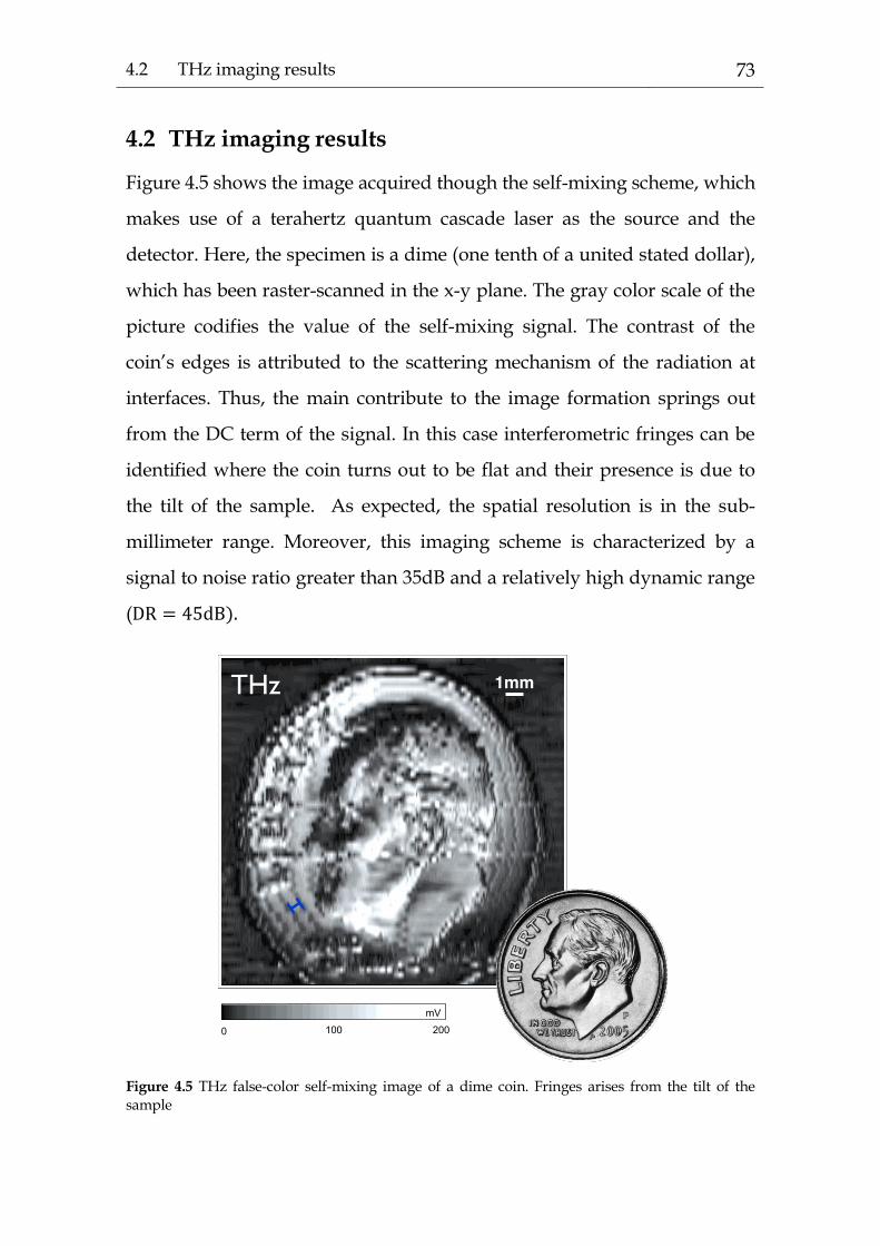
4.2 THz imaging results

Figure 4.5 shows the image acquired though the self-mixing scheme, which

makes use of a terahertz quantum cascade laser as the source and the

detector. Here, the specimen is a dime (one tenth of a united stated dollar),

which has been raster-scanned in the x-y plane. The gray color scale of the

picture codifies the value of the self-mixing signal. The contrast of the

coin’s edges is attributed to the scattering mechanism of the radiation at

interfaces. Thus, the main contribute to the image formation springs out

from the DC term of the signal. In this case interferometric fringes can be

identified where the coin turns out to be flat and their presence is due to

the tilt of the sample. As expected, the spatial resolution is in the sub-

millimeter range. Moreover, this imaging scheme is characterized by a

signal to noise ratio greater than 35dB and a relatively high dynamic range

(DR = 45dB).

Figure 4.5 THz false-color self-mixing image of a dime coin. Fringes arises from the tilt of the sample

0

1mm

200100

mV

THz


Figure 4.6 Optical (a) and 3.8 THz (b) image of a leaf, showing the capability of the system to

reveal the presence of water, which is strongly absorbed by terahertz radiations

0

70

35

mV

(b)

1mm

(a)


Figure 4.6 shows another example of application of the implemented

imaging system. Here the sample under investigation consists of a leaf,

fixed upon a substrate of SiO . Owing to the strong absorption coefficient

of water at terahertz frequency (𝛼 = 800𝑐𝑚 at 3.8 THz) its water content

can be mapped. Although not yet quantitative, this can be considered as

the first demonstration towards spectroscopic imaging through self-mixing

at terahertz frequencies.

4.3 Fringe visibility

Figure 4.7 Fringe amplitude versus the feedback strength parameter k for the Mid-IR QCL.

As anticipated in paragraph 4.1, the amplitude of the interference fringes is

a function of the feedback parameter k. In conventional laser diodes


subjected to a weak feedback, the amplitude monotonically grows when

the feedback is increased until a saturation value is reached [52].

A different behavior characterizes quantum cascade lasers as shown in

Figure 4.7. Here, the magnitude of the fringes is acquired by moving a

metallic (Al) target along the longitudinal direction. The feedback

parameter is indirectly measured through the equation

𝑘 =𝐼 − 𝐼𝐼

𝜏2𝜏

where (I ) and (I ) are the pump intensities at threshold with and

without the feedback, τ is the laser cavity round-trip (for a 1mm long

cavity τ = 35ps), τ is the photon lifetime, assumed equal to 10ps.

Observing Figure 4.7 it can be ascertained that for k < k ∶= 1.3 ∙ 10 the

amplitude dV increases with the feedback (region a), reaching a plateau for

k > 0.6 ∙ 10 (region b); for k > k (region c) fringes gradually disappear.

Figure 4.8 displays different shapes of the modulation signal when k is

increased over the critical value: the more the feedback is increased, the

more the signal seems to get symmetric resembling the geometry of the

very-week regime. When k ≅ 2.9 ∙ 10 , the signal merges with the noise

of the system, and no information can be got from the phase profile.

From these considerations, it is evident the strong relationship between the

imaging system implemented and the more fundamental aspects related to

optical feedback in QCLs. Therefore, more investigations are necessary to

gain insight into these dynamics.


Figure 4.8 Waveforms of the interferometric signal from k=0,0013 to k=0,0029. When the feedback

is increased the amplitude of the fringes decreases and the signal gets symmetric

75#

80#

85#

90#

95#

20# 30# 40# 50# 60# 70# 80#

27#

32#

37#

42#

47#

20# 30# 40# 50# 60# 70# 80#

12#

17#

22#

27#

32#

20# 30# 40# 50# 60# 70# 80#

k=0,00128

90#

95#

100#

105#

110#

30# 35# 40# 45# 50# 55# 60# 65# 70# 75# 80#

40#42#44#46#48#50#52#54#56#58#

30 35 40 45 50 55 60 65 70 75 80

0

5

10

15

20

20# 30# 40# 50# 60# 70# 80# 90#90#

95#

100#

105#

110#

0 2 4 6 8 10 12 14 16

0

5

10

15

20

20# 30# 40# 50# 60# 70# 80# 90#90#

95#

100#

105#

110#

0 2 4 6 8 10 12 14 16

0

5

10

15

20

20# 30# 40# 50# 60# 70# 80# 90#90#

95#

100#

105#

110#

0 2 4 6 8 10 12 14 16

0

5

10

15

20

20# 30# 40# 50# 60# 70# 80# 90#90#

95#

100#

105#

110#

0 2 4 6 8 10 12 14 16

0

5

10

15

20

20# 30# 40# 50# 60# 70# 80# 90#90#

95#

100#

105#

110#

0 2 4 6 8 10 12 14 16

SM

I Sig

nal [

mV

]

k=0,00143

SM

I Sig

nal [

mV

]

k=0,00165

SM

I Sig

nal [

mV

]

k=0,00253

SM

I Sig

nal [

mV

]

k=0,00293

SM

I Sig

nal [

mV

]

Longitudinal displacement [um]


Figure 4.9 DC voltage versus the feedback parameter k. The upper axis reports the correspondent

optical power measured without feedback. The red dotted line derives from an experimental

quadratic fit

Finally Figure 4.9 illustrates the behavior of the DC voltage as a function of

the feedback parameter k.

The measurement has been accomplished inserting a series of

Polymethylpentene (TPX) filters along the optical axis and measuring the

change in the DC voltage drop across the device, originated by the

feedback from a metallic target. The upper axis reports the optical power

without the feedback, measured behind the filters. The voltage linearly

increases with the feedback, showing saturation for high feedback. This

curve can be used to calibrate the sensor to acquire quantitative

information about reflectivity of unknown targets.

Chapter 5

5. Preliminary results

This chapter has been omitted in the online version of this work

because the results which it reports are under publication.

Conclusions and future work

This thesis has discussed the design, the implementation and the

characterization of two imaging apparatus, in the mid-infrared and the

terahertz regime, based on self-mixing interferometry with quantum

cascade lasers.

Some aspects related to the heterodyne principle of this scheme have been

investigated, with a particular focus on the phase retrieval associated with

different information content of the sample.

Moreover, some differences between the behaviour of quantum cascade

lasers and conventional laser diodes under optical feedback have emerged.

It seems that the recently demonstrated ultra-stable regime in QCL

subjected to feedback influences the fringe visibility of the self-mixing

signal.

Finally, preliminary results about the measurement of carrier-density

profile have been drafted, although more research has to be carried out in

order to compare the experiments to the underlying theory.

Theoretically, owing to the property of coherence of the system, SMI could

be used to implement a holographic scheme in which the modulus of

reflectivity of the target is kept constant while its phase could change.

Conclusions and future work 81

From another point of view, an interesting evolution of this work could be

the implementation of a complete terahertz three-dimensional imaging,

borrowing tomographic approaches traditionally belonging to other

regions of the electromagnetic spectrum, such as computed tomography,

synthetic aperture or Kirchhoff migration tomography [11].

Another interesting area to investigate resides in the capability of the self-

mixing to derive quantitative spectroscopic information from the sample.

In such a way, the laser could be wavelength-tuned with the purpose of

studying samples with different absorption coefficients, exploiting the

intrinsic narrow linewidth of quantum cascade lasers.

Moreover more efforts are required to confirm the preliminary

observations about the possibility of the system to map a charge

distribution of an optically pumped semiconductor. Other semiconductors

(GaAs, InAs) could be used as substrates, and more work must be

accomplished in order to estimate the sensitivity of the SM method and, at

the same time, to exclude other possible causes of modifications of the

optical proprieties (thermal effects above all).

In the end, future work will endorse studies about non-conventional

material behaviours through self-mixing interferometry. These will include

investigations on complex optical constants of metamaterials, i.e.

structures whose optical proprieties can be artificially engineered, and the

exotic dynamics associated with them, such as negative refraction, and

hyperbolic behaviour.

Ringraziamenti

Desidero ringraziare il Prof. Gaetano Scamarcio per aver reso

appassionante questo lavoro sin dal suo principio, per la sua guida

illuminata e lungimirante , per la disponibilità sempre mostrata.

Un ringraziamento particolare è rivolto al Dott. Francesco Mezzapesa, con

il quale ho avuto la fortuna di condividere le frustrazioni e le gioie del

laboratorio. Ricorderò a lungo la sua proficua creatività e la sua contagiosa

passione per la ricerca.

Ringrazio il Prof. Maurizio Dabbicco per esser stato il costante riferimento

scientifico con il quale discutere di aspetti fondamentali e sperimentali; per

i suoi corsi ed insegnamenti difficilmente inquadrabili in pochi libri di

testo.

Devo inoltre la mia gratitudine al Dott. Lorenzo Columbo, al Dott.

Francesco De Lucia e al Dott. Pietro Patimisco la cui proficua interazione è

stata preziosa su diversi fronti di questo lavoro.

Ringrazio poi la Dott.ssa Cinzia Di Franco e la Dott.ssa Maria Vittoria

Santacroce per avermi seguito durante l’attività di tirocinio.

Un sentito ringraziamento va poi alla Dott.ssa M. Dell’Olio per il suo

contributo alla revisione linguistica.

Un ringraziamento finale va poi alla mia famiglia, ai miei colleghi, agli

amici tutti e a Myriam.

Bibliography 83

Bibliography

[1] C.M Armstrong, "The truth about terahertz," Spectrum, IEEE, vol. 49, no. 9, pp. 36-41, September 2012.

[2] Masayoshi Tonouchi, "Cutting-edge terahertz technology," Nature Photonics, vol. 1, no. 2, pp. 97-105, Feb. 2007.

[3] M. V., Fattinger, C., & Grischkowsky, D. Exter, "Terahertz time-domain spectroscopy of water vapor," Optics Letters, vol. 14, no. 20, pp. 1128-1130, 1989.

[4] Yun-Shik Lee, Principles of Terahertz Science and Technology.: Springer, 2009.

[5] B. B., Nuss, M. C Hu, "Imaging with terahertz waves," Optics letters, vol. 20, no. 16, pp. 1716-1718, 1995.

[6] D. M., Gupta, M., Neelamani, R., Baraniuk, R. G., Rudd, J. V., & Koch, M. Mittleman, "Recent advances in terahertz imaging," Applied Physics B, vol. 68, no. 6, pp. 1085-1094, 1999.

[7] Stefan Hunsche, Luc Boivin, and Martin C. Nuss Daniel M. Mittleman, "T-ray tomography," Opt. Lett., vol. 22, pp. 904-906, 1997.

[8] Hua Zhong et al., "Nondestructive defect identification with terahertz time-of-flight tomography," ensors Journal, IEEE, vol. 5, no. 2, pp. 203-208, 2005.

[9] Koch M, Brener I and Nuss M C Hunsche S, "THz near-field imaging,"

Bibliography 84

Opt. Commun, vol. 152, no. 22, p. 6, 1998.

[10] J. Z. Xu, and X. C. Zhang T. Yuan, "Development of terahertz wave microscopes," Infrared, vol. 45, no. 5-6, pp. 417–425, Oct. 2004.

[11] W. L., Deibel, J., & Mittleman, D. M. Chan, "Imaging with terahertz radiation," Reports on Progress in Physics, vol. 70, no. 8, p. 1325, 2007.

[12] A. J. L. Adam, "Review of near-field terahertz measurement methods and their applications," Journal of Infrared, Millimeter, and Terahertz Waves, vol. 32, no. 8-9, pp. 976-1019, 2011.

[13] Jiang Z, Xu G X and Zhang X-C Chen Q, "Near-field terahertz imaging with a dynamic aperture," Opt. Lett., vol. 25, no. 4, p. 1122, 2000 2000.

[14] Kersting R and Cho G C Chen H-T, "Terahertz imaging with nanometer resolution," Appl. Phys. Lett., vol. 83, no. 11, p. 3009, 2003.

[15] van der Valk N C J and Planken P C M, "Electro-optic detection of subwavelength terahertz spot sizes in the near field of a metal tip," Appl. Phys. Lett, vol. 81, no. 60, p. 1558, 2002.

[16] F. Keilmann, J. Wittborn, J. Aizpurua, and R. Hillenbrand A. J. Huber, "Terahertz near-field nanoscopy of mobile carriers in single semiconductor nanodevices," Nano Letters, vol. 8, no. 11, pp. 3766-3770, 2008.

[17] K., Ogawa, Y., Watanabe, Y., & Inoue, H. Kawase, "Non-destructive terahertz imaging of illicit drugs using spectral fingerprints," Opt. Expres, vol. 11, no. 20, pp. 2549-2554.

[18] A. D. Hellicar, L. Li, S. M. Hanham, N. Nikolic, J. C. Macfarlane and K. E. Leslie J.Du, "Terahertz imaging using a high-Tc superconducting Josephson junction detector," Superconductor Science and Technology, vol. 21, no. 12, p. 125025, 2008.

[19] S., Alton, J., Baker, C., Lo, T., Beere, H. E., & Ritchie, D. Barbieri, "Imaging with THz quantum cascade lasers using a Schottky diode mixer," Opt. Express, vol. 13, no. 17, pp. 6497-6503, 2005.

[20] K Lien and Johns, Michael L and Gladden, Lynn and Worrall, Christopher H and Alexander, Paul and Beere, Harvey E and Pepper, Michael and Ritchie, David A and Alton, Jesse and Barbieri, Stefano

Bibliography 85

and others Nguyen, "Three-dimensional imaging with a terahertz quantum cascade laser," Optics express, vol. 14, no. 6, pp. 2123-2129, 2006.

[21] Juraj, et al Darmo, "Imaging with a Terahertz quantum cascade laser," Optics Express , vol. 12, no. 9, pp. 1879-1884, 2004.

[22] A. W., & Hu, Q. Lee, "Real-time, continuous-wave terahertz imaging by use of a microbolometer focal-plane array," Optics Letters, vol. 30, no. 19, pp. 2563-2565, 2005.

[23] A. W., Qin, Q., Kumar, S., Williams, B. S., Hu, Q., & Reno, J. L. Lee, "Real-time terahertz imaging over a standoff distance ≫ 25," Applied physics letters, vol. 89, no. 14, pp. 141125-141125.

[24] G. Karunasiri, D. R. Chamberlin,P. R. Robrish and J. Faist3 B. N. Behnken, "Real-time imaging using a 2.8 THz quantum cascade laser and uncooled infrared microbolometer camera," Optics Letters, vol. 33, no. 4, p. 440, 2008.

[25] M. S. Vitiello, D. Coquillat, A. Lombardo, A. C. Ferrari, W. Knap, M. Polini, V. Pellegrini & A. Tredicucci L. Vicarelli, "Graphene field-effect transistors as room-temperature terahertz detectors," Nature Materials, vol. 11, no. 10, pp. 865-871, 2012.

[26] L and Coquillat, D and Pea, M and Ercolani, D and Beltram, F and Sorba, L and Knap, W and Tredicucci, A and Vitiello, MS Romeo, "Nanowire-based field effect transistors for terahertz detection and imaging systems," Nanotechnology, vol. 24, no. 21, p. 214005, 2013.

[27] K.J. Siebert et al., "Continuous-wave all-optoelectronic terahertz imaging," Applied Physics Letters, vol. 90, no. 16, pp. 3003-3005, 2002.

[28] Jesse Alton, Harvey E. Beere, David Ritchie Stefano Barbieri, "Imaging with THz quantum cascade lasers using a Schottky diode mixer ," Optics Express, vol. 13, no. 17, pp. 6497-6503, 2005.

[29] M., Jagtap, V. Ravaro et al., "Continuous-wave coherent imaging with terahertz quantum cascade lasers using electro-optic harmonic sampling," Applied Physics Letters, vol. 102, no. 9, pp. 091107-091107, 2013.

Bibliography 86

[30] Yah Leng Lim, Alex Valavanis, Russell Kliese, Milan Nikolić, Suraj P. Khanna, Mohammad Lachab, Dragan Indjin, Zoran Ikonić, Paul Harrison, Aleksandar D. Rakić, Edmund H. Linfield, and A. Giles Davies Paul Dean, "Terahertz imaging through self-mixing in a quantum cascade laser," Optics letters, vol. 36, no. 13, pp. 2587-2589, 2011.

[31] H Zhong, J. Xu, K. Lin, J.-S. Hwang and X-C Zhang1 N. Karpowicz, "Comparison between pulsed terahertz time-domain imaging and continuous wave terahertz imaging ," Semicond. Sci. Technol., vol. 20, pp. S293–S299, 2005.

[32] Yao-Chun Shen, "Terahertz pulsed spectroscopy and imaging for pharmaceutical applications: A review," International journal of pharmaceutics, vol. 417, no. 1, pp. 48-60, 2011.

[33] H. Haken, "Analogy between higher instabilities in fluids and lasers," Physics Letters A, vol. 53, no. 1, pp. 77-78, 1975.

[34] R. Lang and K. Kobayashi, "External optical feedback effects on semiconductor injection laser properties," Quantum Electronics, IEEE Journal of , vol. 16, no. 3, pp. 347-355, 1980.

[35] D. M., & Shore, K. A. Kane, Unlocking dynamical diversity: optical feedback effects on semiconductor lasers.: Wiley, 2005.

[36] N. P. Rea, and T. Wilson R. Juškaitis, "Semiconductor laser confocal microscopy," Applied Optics, vol. 4, no. 33, pp. 578-584, 1994.

[37] R.W. Tkach and A.R. Chraplyvy, "Regimes of feedback effects in 1.5 um distributed feedback lasers," IEEE J. Lightwave Technology, vol. 4, pp. 1655–1661, 1986.

[38] R. A. Surisr R. F. Kazarinov, "Possibility of the amplification of electromagnetic waves in a semiconductor with a superlattice ," Fiz. Tech. Poluprovodn, vol. 5, no. 4, pp. 797-800, 1971.

[39] Jerome Faist et al., "Quantum Cascade Laser," Science, vol. 264, no. 5158, pp. 553-556, Apr. 1994.

[40] M. Yamanishi, T. Edamura, K. Fujita, N. Akikusa, and H. Kan, "Theory of the Intrinsic Linewidth of Quantum-Cascade Lasers: Hidden Reason for the Narrow Linewidth and Line-Broadening by Thermal

Bibliography 87

Photons," Quantum Electronics, IEEE Journal of, vol. 44, no. 1, pp. 12-29, Jan. 2008.

[41] S. Bartalini et al., "Measuring frequency noise and intrinsic linewidth of a room-temperature DFB quantum cascade laser," Optics Express, vol. 19, no. 19, pp. 17996-18003, 2011.

[42] Miriam S. Vitiello et al., "Quantum-limited frequency fluctuations in a terahertz laser," Nat Photon, vol. 6, no. 8, pp. 525-528, Aug. 2012.

[43] MK Haldar, "A simplified analysis of direct intensity modulation of quantum cascade lasers," Quantum Electronics, IEEE Journal of, vol. 41, no. 11, pp. 1349-1355, 2005.

[44] B. S. Williams, "Terahertz quantum-cascade lasers," Nature photonics, vol. 1, no. 9, pp. 517-525., 2007.

[45] R., Tredicucci, A., Beltram, F., Beere, H. E., Linfield, E. H., Davies, A. G.,D. A. Ritchie2, R. C. Iotti, Rossi F. Köhler, "Terahertz semiconductor-heterostructure laser," Nature, vol. 417, no. 6885, pp. 156-159, 2002.

[46] G., Ajili, L., Faist, J., Beere, H., Linfield, E., Ritchie, D., & Davies, G. Scalari, "Far-infrared (λ≃ 87 μm) bound-to-continuum quantum-cascade lasers operating up to 90k," Applied physics letters, vol. 82, no. 19, pp. 3165-3167, 2003.

[47] S. Kumar, H. Callebau, Q. Hu, and J. L. Reno B. S. Williams, "Terahertz quantum-cascade laser at λ ≈ 100 μm using metal waveguide for mode confinement," Applied physics letters, vol. 83, no. 11, pp. 2124-2126, 2003.

[48] Gensty T, Elsässer W, Giuliani G, Mann C. von Staden J, "Measurements of the alpha factorof a distributed-feedback quantum cascade laser," Opt. Lett., vol. 31, no. 17, pp. 2574-6, 2006.

[49] J-H Xu, L. Mahler, A. Tredicucci, F. Beltram, Guido Giuliani, H. E. Beere, and D. A. Ritchie R. P. Green, "Linewidth enhancement factor of terahertz quantum cascade lasers," Applied Physics Letters, vol. 92, no. 7, pp. 071106-071106, 2008.

[50] L. L. Columbo, M. Brambilla, M. Dabbicco, S. Borri, M. S. Vitiello, H. E. Beere, D. A. Ritchie, and G. Scamarcio F. P. Mezzapesa, "Intrinsic stability of quantum cascade lasers against optical feedback," Optics

Bibliography 88

Express , vol. 21, no. 11, pp. 13748–13757, 2013.

[51] T., Xu, J. H., Green, R. P., Tredicucci, A., Beere, H. E., & Ritchie, D. A Losco, "THz quantum cascade designs for optimized injection," Physica E: Low-dimensional Systems and Nanostructures, vol. 40, no. 6, pp. 2207-2209, 2008.

[52] S., Giuliani, G., Merlo, S. Donati, "Laser diode feedback interferometer for measurement of displacements without ambiguity," Quantum Electronics, IEEE Journal of, vol. 31, no. 1, pp. 113-119, 1995.

[53] E. Garmire and A. Kost, Nonlinear Optics in Semiconductors I.: Academic 1999.

[54] Daryoosh Saeedkia, Handbook of terahertz technology for imaging, sensing and communications.: Woodhead Publishing Series in Electronic and Optical Materials, 2013.

infrared and terahertz imaging through self-mixing

Documents