Infrastructure, Comparative Advantage, and Trade in a

Dynamic Ricardian Model ∗

Akihiko Yanase †

GSICS, Tohoku University

July 31, 2013

Abstract

This paper develops a dynamic two-country model with a stock of national public good,

which has a positive effect on the productivity in the production of private goods and

the evolution of the stock is determined by the national government, and a continuum of

private goods. With one-factor Ricardian world, each good is produced in either of the

two countries, and the country with a higher labor endowment, a lower depreciation rate

of the public-good stock, and/or a lower rate of time preference will become an exporter of

goods which are more dependent on the stock of public good. If the national governments

take the world prices as given when they determine the paths of public goods under free

trade, the country that has a comparative advantage in goods which are more dependent

on the stock of public good enjoys a higher steady-state stock of the public good under

free trade than under autarky, while the other country’s steady-state stock of the public

good under free trade becomes lower than the autarkic level. This paper also examines the

welfare effects of trade liberalization. In the short run where the stocks of public goods are

at the autarkic steady-state levels, the country that has a comparative advantage in goods

which are less dependent on the stock of public good unambiguously gains from trade. It

is ambiguous whether the country that has a comparative advantage in goods which are

more dependent on the stock of public good becomes better off, but will gain from trade in

the long run if the depreciation rate of the public good is not very large.

Key Words: Infrastructure; Two-country trade; Ricardian model with a contin-

uum of goods; Trade patterns; Gains from trade

JEL classification: F11; H41; H54

∗Very preliminary draft: Please do not quote without permission. Comments welcome.†Graduate School of International Cultural Studies, Tohoku University. 41 Kawauchi, Aoba-ku, Sendai

980-8576, JAPAN. E-mail: yanase@intcul.tohoku.ac.jp

1

1 Introduction

Public infrastructure has a great impact on a nation’s economic development and social wel-

fare. In particular, for a trading country, various kinds of public intermediate goods that are

utilized as public infrastructure can play an important role in determining trade patterns and

increasing the gains from trade. Among trading countries, how and in what scale governments

should supply these public intermediate goods are recognized as important policies for gaining

economic advantage.

The fundamental role of public infrastructure is to make the economy better off indirectly

by augmenting private firms’ productivity. When one considers such kind of public goods,

i.e., public goods that have external effects on productivity, these goods generally have a

characteristic of durable or capital goods. That is, it will be more reasonable to consider public

goods that can be accumulated over time when the stock of such goods has positive external

effects on the production side.1 With this kind of motivation, McMillan (1978) developed a

dynamic three-sector (two private goods and a public intermediate good), one-factor (labor)

trade model of a small open economy with optimal supply of the public intermediate good.

It is shown that the stock of public intermediate good determines the slope of the production

possibility frontier and thus determines the pattern of international trade. McMillan’s model

is recently re-examined by Yanase and Tawada (2012), who show the possibility of multiple

steady states and history-dependent dynamic paths. Moreover, they discuss whether trade is

gainful or not in McMillan’s model.

This paper extends the small-country model of McMillan (1978) and Yanase and Tawada

(2012) in the following two directions. First, a world economy consisting of two countries

rather than a small country is considered. In the presence of international trade in private

goods whose productivity depends on the stock of public good, the prices of private goods are

endogenously determined in the world market. This means that under free trade, the countries

may or may not take into consideration the effect of a change in the world price on the national

welfare when they determine the paths of the stock of public goods. This paper considers both

cases, i.e., the case of price-taking governments in which the national governments take the

world prices as given and the case of strategically-acting governments in which the national

governments take into account of the terms-of-trade effects.

The second direction of the extension is to consider a continuum of private goods, based

on Dornbusch et al. (1977), rather than two goods. The assumption of continuum goods

makes the analysis of many-goods world tractable. Because in the Dornbusch et al. (1977)

1There is a large literature that examines trade model with public intermediate goods in a static framework.

See Abe (1990), Altenburg (1992), Ishizawa (1988), Long and Shimomura (2007), Manning and McMillan (1979),

Shimomura (2007), Suga and Tawada (2007), Tawada and Okamoto (1983), and Tawada and Abe (1984).

2

model, like other Ricardian type models, the reason for trade is based on exogenous differences

in technology across countries. By incorporating the external effect of public infrastructure

on productivity, the differences in technology across countries are endogenously determined

in the present study. In this sense, this paper is also closely related to the recent studies on

institutions and trade (e.g., Costinot, 2009; Cunat and Melitz, 2012).

This paper considers a world economy consisting of two countries. In each country, a con-

tinuum of private goods are produced by using a single primary factor, labor, with technologies

that exhibit constant returns to scale. The labor productivity is assumed to depend on the

stock of a public good, which is produced by employing labor as an input and accumulates

over time. The national government in each country determines the path of the public good

production so as to maximize the national welfare, which is defined as the lifetime utility of a

representative household.

With the above setup, I begin with the optimal intertemporal resource allocation including

public goods determined by the national governments under autarky. It is shown that the

country with a higher labor endowment, a lower depreciation rate of the public-good stock,

and/or a lower rate of time preference will have a comparative advantage in goods which are

more dependent on the stock of public good.

I then proceed to the dynamic equilibrium under free trade. With one-factor Ricardian

world, each good is produced in either of the two countries. In the case of price-taking govern-

ments in which the national governments take the world prices as given when they determine

the paths of public goods under free trade, the country that has a comparative advantage in

goods which are more dependent on the stock of public good enjoys a higher steady-state stock

of the public good under free trade than under autarky, while the other country’s steady-state

stock of the public good under free trade becomes lower than the autarkic level. In the case of

strategic governments where the national governments take into account of the terms-of-trade

effects when they determine the paths of public goods, it is shown that both countries have an

incentive to increase the production of public goods compared with the non-strategic case for

a given pair of the stock of public goods and their shadow prices. However, each government’s

incentive to improve its terms-of-trade may also have inverse effects on the path of shadow

prices, and thus it is ambiguous whether the governments’ strategic incentives increase the

steady-state stocks of public goods compared with the non-strategic case.

This paper also examines the welfare effects of trade liberalization in the short run, where

the stocks of public goods are at the autarkic steady-state levels, and in the long run, where

the economies are at the steady state under free trade. In the short run, the country that

has a comparative advantage in goods which are less dependent on the stock of public good

unambiguously gains from trade. It is ambiguous whether the country that has a comparative

3

advantage in goods which are more dependent on the stock of public good becomes better off,

but will gain from trade in the long run if the depreciation rate of the public good is not very

large.

Section 2 sets up the two country dynamic model with a continuum of private goods and a

national public good. Section 3 considers an autarkic situation where there is no trade between

countries. The analysis derives the determinants of comparative advantage. Section 4 analyzes

outcomes under free trade. The cases of non-strategic governments and strategic governments

are respectively examined. The welfare effects of trade are also analyzed. Section 5 concludes

the paper.

2 Model

I consider a world economy consisting of two countries, home and foreign, in which a continuum

of private goods indexed by z ∈ [0, 1] are produced by using a single primary factor, labor,

with technologies that exhibit constant returns to scale. The production function of each good

in the home country is given by Y (z) = α(z,R)L(z), where Y (z) and L(z) are the output and

labor input, respectively, in sector z ∈ [0, 1]. The labor productivity, α(z,R), is dependent on

the stock of public good R, and I assume that the following specific functional form:

α(z,R) = Rη(z), η(z) ∈ [0, 1], η′(z) < 0.

This functional form implies that the production elasticity of the public good stock in sector z

is equal to η(z). The foreign country has the same production technology, and thus the output

in each sector is given by Y ∗(z) = α(z,R∗)L∗(z), where the variables with an asterisk are those

in the foreign country.

Each private-good market is assumed to be under perfect competition. Let us denote

the price of good z by p(z). With the above-mentioned constant returns technology, the

representative firm’s profit maximization in each sector implies that

p(z) =w

Rη(z)(1)

must hold if Y (z) > 0 and Y (z) = 0 if p(z) < w/Rη(z).

The public good is produced by the national government according to the production func-

tion G = f(LR), where LR is a labor input in the public sector. I assume that the production

function satisfies the following properties:

f ′ > 0, f ′′ < 0, limLR→0

f ′ = ∞, limLR→∞

f ′ = 0, f(0) = 0.

4

Given the initial stock R0 > 0, the public intermediate good is assumed to accumulate over

time according to2

R = f(LR)− δR, (2)

where δ > 0 is the depreciation rate of the stock of the public good. The foreign country is

assumed to have the same production technology, but the depreciation rate may differ from

that in the home country, and thus R∗ = f(L∗R)− δ∗R∗.

At each moment in time, the economy must face the following full employment constraint

on labor:∫ 10 L(z)dz + LR = L, where L is the endowment of effective labor and is assumed to

be given and constant over time. With this constraint and using private production functions,

the production possibility frontier for a given LR and R is obtained as follows:∫ 1

0R−η(z)Y (z)dz = L− LR. (3)

As for the consumption side of the economy, I assume a representative household who has

a Cobb-Douglas preference u =∫ 10 b(z) lnC(z)dz with

∫ 10 b(z)dz = 1, C(z) is the consumption

of good z. Letting ρ be the rate of time preference, the lifetime utility of the household is thus

given by

U =

∫ ∞

0e−ρtu(t)dt =

∫ ∞

0e−ρt

∫ 1

0b(z) lnC(z, t)dz

dt.

Let us denote the household’s total expenditure at each moment of time by E, and assume

that no borrowing or lending is permitted. Then, the household’s optimal consumption must

satisfy C(z) = b(z)E/p(z), z ∈ [0, 1]. Substituting this optimal consumption into the lifetime

utility, it follows that

U =

∫ ∞

0e−ρt

lnE(t)−

∫ 1

0b(z) ln p(z, t)dz

dt+

B

ρ, (4)

where B ≡∫ 10 b(z) ln b(z)dz.

3 Autarky

In this section, I assume that the two countries do not trade the goods and derive the dynamic

equilibrium under autarky. Under autarky, it holds that Y (z, t) = C(z, t) for all z ∈ [0, 1] and

t ∈ [0,∞). It is also true that (1) holds for all z ∈ [0, 1]. With no international borrowing or

lending and constant returns technology, it holds that E = w(L − LR).3 Substituting these

expressions into (4), the lifetime utility of the representative household is rewritten as

U =

∫ ∞

0e−ρt ln[L− LR(t)] + h lnR(t) dt+ B

ρ, (5)

2A dot over a variable denotes the derivative with respect to time. To avoid unnecessary complication in the

notation, I omit time arguments, denoted by t, when no confusion arises from doing so.3I implicitly assume that the government supplies the public good with optimal income taxes in a similar

manner to Manning et al. (1985) or Feehan and Matsumoto (2000).

5

where h ≡∫ 10 η(z)b(z)dz < 1. Therefore, under autarky, the home government’s problem is to

choose the time path of LR so as to maximize (5) subject to (2).4

Let us define the current-value Hamiltonian associated with the home government’s dynamic

optimization problem as follows:

H = ln(L− LR) + h lnR+ θf(LR)− δR.

The first-order condition is

∂H

∂LR= 0 ⇒ θf ′(LR)(L− LR) = 1. (6)

The costate variable, θ, changes over time according to

θ = (ρ+ δ)θ − h

R, (7)

and the transversality condition is given by limt→∞ e−ρtθ(t)R(t) = 0.

Eq.(6) implicitly defines the optimal level of LR as a function of θ and L. Denote it by

λ(θ, L), which has the following properties:

∂λ

∂θ=

(L− λ)f ′

θ[f ′ − (L− λ)f ′′]> 0,

∂λ

∂L=

f ′

f ′ − (L− λ)f ′′ > 0.

Then, (2) is rewritten as

R = f(λ(θ, L))− δR. (8)

The dynamic equilibrium path of the home country under autarky is thus characterized by a

system of differential equations (7) and (8).

Let us denote a pair of steady-state stock of public good in the home country and its shadow

price by (Ra, θa). It can be verified from (7) and (8) that there exists a unique steady state.5

Moreover, the linearized system around the steady state isR(t)

θ(t)

=

−δ f ′λθ

(ρ+ δ)θa/Ra ρ+ δ

R(t)−Ra

θ(t)− θa

,

and the determinant of the Jacobian matrix is shown to be negative, which indicates that the

characteristic roots are of opposite signs. Therefore, the steady state is a local saddle point.

4The profit maximization condition (1) and the optimal consumption condition imply Y (z) = C(z) =

b(z)w(L− LR)/p(z) = b(z)Rη(z)(L− LR) holds under autarky. This means that (3) is satisfied.5Applying the steady-state condition θ = 0 in (7) yields θ = h/[(ρ + δ)R], which indicates that θ is mono-

tonically decreasing in R, with limits ∞ when R → 0 and 0 when R → ∞. As for the steady-state condition

R = 0, (8) indicates that θ and R are positively related and θ is nonnegative for all R ∈ [0,∞). Therefore, there

exists a unique steady state.

6

From (7) and (8), it can be verified that the steady-state stock of the public good is

increasing in L and decreasing in δ:

∂Ra

∂L=

f ′λθRa

δRa + θaf ′λθ> 0,

∂Ra

∂δ= −Ra(ρ+ δ)Ra + θaf

′λθ(ρ+ δ)(δRa + θaf ′λθ)

< 0,

∂Ra

∂ρ= − f ′λθRaθa

(ρ+ δ)(δRa + θaf ′λθ)< 0.

These results indicate that the steady-state stock of public good becomes higher in the home

country than in the foreign country if the home country has the higher endowment of effective

labor, lower depreciation rate of the public good stock, and/or lower rate of time preference.

Intuitively, these results can be interpreted as follows. The endowment of effective labor affects

the dynamics of the economy only through a change in R because the dynamics of θ given by

(7) is independent of L, and the optimal level of labor input in the public sector, LR = λ(θ, L),

is positively related to L. Therefore, a higher L implies more employment in the public sector,

and thus a higher stock of the public good in the long run. From (8), lower depreciation rate

contributes the accumulation of R. In addition, (7) implies that for a given R, a reduction in

δ leads to a higher shadow value of the public good in the steady state, and LR = λ(θ, L) is

increasing in θ. Both effects leads to an increase in the flow of public good, and thus in the

steady-state stock Ra. Finally, the rate of time preference affects the dynamics of the economy

only through (7), and a reduction in ρ leads to a higher θ in order to hold θ = 0, and thus

brings the economy a higher steady-state stock of the public good.

Suppose that L > L∗, δ < δ∗, and/or ρ < ρ∗, and thus Ra > R∗a. Since the unit labor

coefficient of each good in the steady state is given by 1/α(z,Ra) in the home country and it

is given by 1/α(z,R∗a) in the foreign country. In this model setup, the home country has an

absolute advantage in every goods. However, letting A(z,R,R∗) ≡ α(z,R)/α(z,R∗), since

∂A

∂z=

(Ra

R∗a

)(lnRa − lnR∗

a)η′(z) < 0,

the home country will have a comparative advantage in goods that are more dependent on the

stock of public good while the foreign country will have a comparative advantage in goods that

are less dependent on the public good.

To sum up, the long-run comparative advantage in each country is described as follows.

Proposition 1 The country with a higher endowment of effective labor, a lower rate of de-

preciation of public good stock, and/or a lower rate of time preference will have a comparative

advantage in goods that are more dependent on the stock of public good.

7

4 Free Trade

Suppose now that the two countries open international trade. I assume that L > L∗, δ < δ∗, or

ρ < ρ∗ holds and both countries are initially under autarkic steady state. These assumptions

imply that the home country specializes in goods z ∈ [0, z) and the foreign country specializes

in goods z ∈ (z, 1], where z denotes a marginal good to be determined in the competitive

equilibrium.

The profit-maximization condition (1) implies that

p(z) =

w

Rη(z)∀z ∈ [0, z],

w∗

R∗η(z) ∀z ∈ [z, 1].(9)

in the competitive equilibrium in the world market of each private good. In addition, the

marginal good z satisfies the following condition:

w

w∗ =Rη(z)

R∗η(z) . (10)

Eqs.(9) and (10) indicate that the equilibrium prices of private goods in the world market and

the pattern of international specialization at each moment in time are dependent on the stock

of public goods in both countries. This implies two possibilities of governments’ behavior; one

is the case of non-strategic governments in which the government in each country determines

the optimal resource allocation without considering the terms of trade effect that a change

in the stock of public goods, and the other is the case of strategic governments in which the

government in each country strategically determines the time path of the public good pursuing

the improvement of the country’s terms of trade.

4.1 Non-strategic governments

In this subsection I assume non-strategic governments in the sense that the governments do

not take account of the effect of a change in the stock of pubic goods on the world prices.

Since there are no private assets, no international borrowing or lending occurs under free trade

in private goods. With constant-returns technology, this means that the home country faces

the budget constraint E = w(L − LR) =∫ z0 p(z)Y (z)dz at each moment in time, and the

foreign country’s budget constraint is similarly given by E∗ = w∗(L∗ −L∗R) =

∫ 1z p(z)Y ∗(z)dz.

Therefore, the dynamic optimization problem of the government in each country to choose the

time paths of LR and Y (z), z ∈ [0, z], taking the time paths of p(z), z ∈ [0, 1] and z as given,

so as to maximize the national welfare

U =

∫ ∞

0e−ρt

ln

∫ z(t)

0p(z, t)Y (z, t)dz −

∫ 1

0b(z) ln p(z, t)dz

dt+

B

ρ,

8

subject to (2) and (3).

The current-value Hamiltonian associated with this dynamic optimization problem is de-

fined as

H = ln

∫ z

0p(z)Y (z)dz + θf(LR)− δR+ ω

L− LR −

∫ z

0R−η(z)Y (z)dz

.

The first-order condition for optimal allocation of private goods’ output is

∂H

∂Y (z)=

p(z)∫ z0 p(z)Y (z)dz

− ωR−η(z) = 0. (11)

Integrating (11) with respect to z over an interval [0, z] yields L−LR = 1/ω. Substituting this

equation into the first-order condition for the optimal labor input for public production

∂H

∂LR= θf ′(LR)− ω = 0,

it follows that (6) is obtained under free trade as well. The adjoint equation is

θ = (ρ+ δ)θ − ω

R

∫ z

0η(z)R−η(z)Y (z)dz. (12)

The market-clearing condition for goods produced in the home country (i.e., z ∈ [0, z)) is

C(z) + C∗(z) =b(z)(E + E∗)

p(z)

=b(z)

[∫ z0 p(z)Y (z) +

∫ 1z p(z)Y ∗(z)

]p(z)

= Y (z). (13)

Integrating (13) with respect to z over an interval [0, z] yields

[1− σ(z)]

∫ z

0p(z)Y (z)dz = σ(z)

∫ 1

zp(z)Y ∗(z)dz, (14)

where σ(z) ≡∫ z0 b(z)dz < 1. Substituting the above equation into (13) and rearranging terms

yield

p(z)Y (z) =b(z)

σ(z)

∫ z

0p(z)Y (z)dz.

Using the above equation, (11) can be rewritten as

Y (z) =b(z)

ωR−η(z)σ(z). (15)

Substituting (15) into (12), the home country’s adjoint equation can be rewritten as

θ = (ρ+ δ)θ − ϵ(z)

σ(z)R, (16)

where ϵ(z) ≡∫ z0 η(z)b(z)dz < h.

9

From the foreign government’s dynamic optimization problem solved in a similar manner

to the home government’s, the dynamics of the stock of public good is derived as

R∗ = f(λ(θ∗, L∗))− δ∗R∗ (17)

and that of the shadow price of R∗ is derived as

θ∗ = (ρ∗ + δ∗)θ∗ − h− ϵ(z)

[1− σ(z)]R∗ . (18)

The marginal good z is determined in the competitive equilibrium of the world market.

Substituting the national income in the home country is∫ z0 p(z)Y (z) = w(L−LR), that in the

foreign country is∫ 1z p(z)Y ∗(z) = w∗(L∗−L∗

R), and (10) into the trade balance condition (14),

it follows thatL∗ − L∗

R

L− LR

(R

R∗

)−η(z)

=1− σ(z)

σ(z). (19)

The dynamic equilibrium path of the world economy under free trade is thus characterized

by a system of differential equations (8), (16), (17), (18), and (19) with LR = λ(θ, L) and

L∗R = λ(θ∗, L∗).

Let us denote a pair of steady-state stock of public good in the home country and its shadow

price by (Rf , θf , R∗f , θ

∗f ). The properties of the steady state equilibrium are characterized by

the following proposition.

Proposition 2 There exist at least one steady-state, free-trade equilibrium. If the economic

fundamentals of the two countries (i.e., the endowments of effective labor, depreciation rates

of public good stock, or rates of time preference) are not very different and if the depreciation

rates are not very large, there exists a unique and saddlepoint-stable steady state.

Proof. See Appendix.

The effect of trade on steady-state stock levels of public goods From the above-

mentioned discussions, it holds that the steady-state conditions for R = 0 are the same under

autarky and free trade, and so are the steady-state conditions for R∗ = 0. The home country’s

steady-state condition for θ = 0 under autarky is rewritten as θ = h/[(ρ + δ)R], whereas the

free-trade counterpart is θ = ϵ(z)/[(ρ+δ)σ(z)R]. Since h =∫ 10 η(z)b(z)dz is a weighted average

of η(z) over an interval [0, 1] and η(z) is decreasing in z, it follows that

h− ϵ(z)

σ(z)=

h∫ z0 b(z)dz −

∫ z0 η(z)b(z)dz

σ(z)=

∫ z0 [h− η(z)]b(z)dz

σ(z)< 0.

That is, under free trade, the θ = 0 locus is located above the θ = 0 locus under autarky.

Therefore, given the fact that the R = 0 locus is upward-sloping and the θ = 0 locus is

10

downward-sloping in R − θ space, Ra < Rf holds. For the foreign country, the steady-state

condition for θ∗ = 0 under free trade is rewritten as θ∗ = [h − ϵ(z)]/(ρ∗ + δ∗)[1 − σ(z)]R∗.

Because

h− h− ϵ(z)

1− σ(z)=

−h∫ z0 b(z)dz +

∫ z0 η(z)b(z)dz

1− σ(z)> 0,

the θ∗ = 0 locus under free trade is located below the θ∗ = 0 locus under autarky. Therefore,

it holds that R∗a > R∗

f .

Proposition 3 In comparison with the autarkic steady state, free trade increases the steady-

state stock of public good in the country that has a comparative advantage in goods that are

more dependent on the stock of public good.

An intuition behind Proposition 3 is as follows. Suppose that the home country has a

comparative advantage in goods that are more dependent on R. After opening international

trade, the home country specializes in these goods and meet the demands in both home and

foreign countries. This implies that the home country will increase its need for accumulating

R under free trade. The opposite is true for the foreign country: it will reduce the need for

accumulating the stock of public good under free trade.

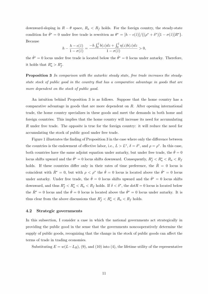
Figure 1 illustrates the finding of Proposition 3 in the case where only the difference between

the countries is the endowment of effective labor, i.e., L > L∗, δ = δ∗, and ρ = ρ∗. In this case,

both countries have the same adjoint equation under autarky, but under free trade, the θ = 0

locus shifts upward and the θ∗ = 0 locus shifts downward. Consequently, R∗f < R∗

a < Ra < Rf

holds. If these countries differ only in their rates of time preference, the R = 0 locus is

coincident with R∗ = 0, but with ρ < ρ∗ the θ = 0 locus is located above the θ∗ = 0 locus

under autarky. Under free trade, the θ = 0 locus shifts upward and the θ∗ = 0 locus shifts

downward, and thus R∗f < R∗

a < Ra < Rf holds. If δ < δ∗, the dotR = 0 locus is located below

the R∗ = 0 locus and the θ = 0 locus is located above the θ∗ = 0 locus under autarky. It is

thus clear from the above discussions that R∗f < R∗

a < Ra < Rf holds.

4.2 Strategic governments

In this subsection, I consider a case in which the national governments act strategically in

providing the public good in the sense that the governments noncooperatively determine the

supply of public goods, recognizing that the change in the stock of public goods can affect the

terms of trade in trading economies.

Substituting E = w(L−LR), (9), and (10) into (4), the lifetime utility of the representative

11

Figure 1: Comparison of steady-state stocks of public goods between autarky and free trade

(the case where L > L∗)

household in the home country under free trade is given by6

U =

∫ ∞

0e−ρt

[1− σ(z(t))] ln

[R(t)

R(t)∗

]η(z(t))+ ln[L− LR(t)] + ϵ(z(t)) lnR(t) + [h− ϵ(z(t))] lnR∗(t)

dt

+B

ρ. (20)

The representative household’s lifetime utility in the foreign country is analogously derived as

follows:

U∗ =

∫ ∞

0e−ρ∗t

σ(z(t)) ln

[R(t)∗

R(t)

]η(z(t))+ ln[L∗ − L∗

R(t)] + ϵ(z(t)) lnR(t) + [h− ϵ(z(t))] lnR∗(t)

dt

+B

ρ∗. (21)

In the case of strategic governments, these governments’ objective functions explicitly depend

on state variables, i.e., the stock of public goods, and control variables, i.e., the labor input on

the public production. Notice that the marginal good z is also dependent on these state and

control variables because it is determined by the balance-of-trade condition (19). From (19),

the equilibrium value of z as a function of (R,R∗, LR, L∗R) has the following properties:

∂z

∂R= −η(z)

RΣ,

∂z

∂R∗ =η(z)

R∗Σ,

∂z

∂LR=

1

(L− LR)Σ,

∂z

∂L∗R

= − 1

(L∗ − L∗R)Σ

, (22)

6In light (9), w(L− LR) =∫ z

0p(z)Y (z)dz can be rewritten as L− LR =

∫ z

0R−η(z)Y (z)dz, which reduces to

the PPF condition (3).

12

where Σ ≡ η′(z) ln(R/R∗)− b(z)/[1−σ(z)]σ(z), the sign of which is negative if R > R∗. The

intuition behind (22) is as follows. An increase in R, ceteris paribus, raises the home country’s

productivity of each good in comparison with the foreign country, and thus extends the range

of goods that the home country has a comparative advantage. Therefore, ∂z/∂R > 0 holds. An

increase in R∗ has an opposite effect: it extends the range of goods that the foreign country has

a comparative advantage, and thus ∂z/∂R∗ < 0. An increase in LR reduces the total supply

of labor to the private sectors in the home country, L − LR. Other things being equal, the

resulting excess demand in the home labor market induces the home country’s relative wage

w/w∗ to increase. In light of (10), the range of goods that the home country has a comparative

advantage becomes smaller. By the same reasoning, an increase in L∗R increases z.

Since each national government faces the dynamic constraint of public goods accumulation,

these governments’ behavior can be characterized as a differential game. There are two equi-

librium concepts frequently employed in applications of differential game theory in economics;

one is the open-loop Nash equilibrium, in which each player’s equilibrium strategy is a simple

function independent of the current state of the system, and the other is the Markov perfect

Nash equilibrium, in which each player designs its optimal strategy as a feedback decision rule

dependent only on the state variable. Both equilibrium concepts satisfy time consistency, but

the only the Markov perfect Nash equilibrium satisfies subgame perfectness (see, for example,

Long, 2010). However, I focus on the open-loop Nash equilibrium because of its tractability.

This strategy concept requires that governments can commit themselves to particular strategy

paths at the beginning of the game, and I simply assume that the commitment is credible.

Formally, the open-loop Nash equilibrium of this dynamic contribution game is defined as a

pair of time paths (LR(t), L∗R(t))∞t=0, such that LR(t)∞t=0 maximizes the home country’s

national welfare (20) subject to the dynamics of the stock of public good R (i.e., (2)) and (19),

taking L∗R(t)∞t=0 as given, and L∗

R(t)∞t=0 maximizes the foreign country’s national welfare

(21) subject to the dynamics of R∗ and (19), taking LR(t)∞t=0 as given.

Let us define the current value Hamiltonian associated with the home government’s dynamic

optimization problem as follows:

H = ln[L−LR]+[1−σ(z)]η(z)+ϵ(z) lnR+h−ϵ(z)− [1−σ(z)]η(z) lnR∗+θf(LR)−δR.

In light of the fact that z is dependent on LR and R, the optimality conditions are given by

∂H

∂LR= − 1

L− LR+ θf ′(LR) + [1− σ(z)]η′(z)

∂z

∂LRln

R

R∗ = 0, (23)

θ = ρθ − ∂H

∂R= (ρ+ δ)θ − [1− σ(z)]η(z) + ϵ(z)

R− [1− σ(z)]η′(z)

∂z

∂Rln

R

R∗ , (24)

and the transversality condition.

13

Compared with (6), the first-order condition for the optimal LR, (23), contains an additional

term [1 − σ(z)]η′(z)(∂z/∂LR) ln(R/R∗), which reflects the home government’s incentive to

improve the home country’s terms of trade. Because both countries are assumed to be initially

at the autarkic steady state with Ra > R∗a, this term is unambiguously positive. This implies

that in comparison with the non-strategic case, the home government has an incentive to

choose a higher level of LR. Intuitively, by increasing LR, the home government can reduce the

total labor allocated to private production and thereby raise the home country’s relative wage

w/w∗. Higher relative wage of the home country implies an increase in the relative prices of

home exports, compared to foreign exports; in other words, the home country’s terms of trade

improve.

A similar terms-of-trade effect appears in the last term of the adjoint equation (24), the

sign of which is positive. In addition, the second term in (24) is different from that in (16).

Comparing the second terms in the respective equations, it follows that

ϵ(z)

σ(z)R− [1− σ(z)]η(z) + ϵ(z)

R=

[1− σ(z)][ϵ(z)− η(z)σ(z)]

σ(z)R> 0

since ϵ(z)− η(z)σ(z) =∫ z0 [η(z)− η(z)]b(z) > 0. To sum up,

ϵ(z)

σ(z)>

[1− σ(z)]η(z) + ϵ(z)

R+ [1− σ(z)]η′(z)

∂z

∂Rln

R

R∗

holds and thus, for a given pair or (R, θ), the rate of decrease in θ when the home government

acts strategically is smaller than that in the case where the home government is non-strategic.

The above inequality also indicates that the θ = 0 locus implied by (24) lies below the θ = 0

locus implied by (16); the steady-state shadow value of the public good for a given R is lower

when the home government acts strategically than when the government is non-strategic. The

reason will be as follows. As shown in (22), an increase in R extends the range of goods that

the home country has a comparative advantage. However, this increase in z reduces, in light of

(10) reduces the home country’s relative wage. Therefore, the terms-of-trade effect induced by

an increase in R has a negative impact on welfare, implying a lower θ than in the case where

the home government is non-strategic.

To summarize the above discussions, the home government’s strategic incentive to improve

its terms of trade moves the R = 0 locus outward and the θ = 0 locus downward compared with

the case where the home government is non-strategic. Therefore, it is ambiguous whether the

steady-state level of R under free trade is higher when the home government acts strategically

than when the home government is non-strategic. If the incentive to increase LR is large enough

to offset the downward force of the θ = 0 locus, Rf becomes higher in the strategic case than

in the non-strategic case.

14

The foreign government’s optimality conditions can be derived in a similar manner. Let us

define the current value Hamiltonian as follows:

H∗ = ln[L∗ − L∗R] + h− ϵ(z) + σ(z)η(z) lnR∗ + ϵ(z)− σ(z)η(z) lnR.

The optimality conditions are obtained as follows:

∂H∗

∂L∗R

= − 1

L∗ − L∗R

+ θ∗f ′(L∗R) + σ(z)η′(z)

∂z

∂L∗R

lnR∗

R= 0, (25)

θ∗ = (ρ∗ + δ∗)θ∗ − σ(z)η(z) + h− ϵ(z)

R∗ − σ(z)η′(z)∂z

∂R∗ lnR∗

R, (26)

As with the home government, (25) reveals that the foreign government has an incentive to

a higher level of L∗R compared to the non-strategic case. The adjoint equation (26) is also

different from (18) because of the foreign government’s incentive to an improvement in the

country’s terms of trade. Comparing the second and third terms in (26) with the second term

in (18), it follows that

h− ϵ(z)

[1− σ(z)]R∗ −σ(z)η(z) + h− ϵ(z)

R∗ + σ(z)η′(z)∂z

∂R∗ lnR∗

R

=

σ(z)h− ϵ(z)− η(z)[1− σ(z)][1− σ(z)]R∗ − σ(z)η′(z)

∂z

∂R∗ lnR∗

R.

The first term in the right-hand side of the above equation is negative because h−ϵ(z)−η(z)[1−

σ(z)] =∫ 1z [η(z) − η(z)]b(z)dz < 0, while the second term becomes positive. Therefore, unlike

the home government, it is ambiguous whether the foreign government’s strategic incentive to

improve its terms of trade moves the θ = 0 locus upward or downward. Consequently, there is

little to say about the comparison of R∗f between the non-strategic case and the strategic case.

4.3 Gains from trade?

In this subsection, I investigate whether each country can gain from trade liberalization by

comparing welfare levels under autarky and free trade. In the following analysis, I assume

that the governments are non-strategic under free trade because in this case the comparisons

of steady-state stock levels of public goods are determined.

In light of (4) and E = w(L− LR), the home country’s instantaneous welfare is given by7

u = lnw + ln(L− LR)−∫ 1

0b(z) ln p(z)dz.

Under autarkic steady state, it holds that p(z) = wR−η(z)a for all z ∈ [0, 1]. Substituting this

into the above expression, the home country’s steady-state welfare under autarky is derived as

ua = ln[L− λ(θa, L)] + h lnRa. (27)

7I omit the constant term relating to B =∫ 1

0b(z) ln b(z)dz because this term has no effects on the results.

15

Assuming that the governments are non-strategic, the home country’s instantaneous welfare

under free trade is rewritten as follows:

u = ln[L− λ(θ, L)] + ϵ(z) + η(z)[1− σ(z)] lnR+ h− ϵ(z)− η(z)[1− σ(z)] lnR∗.

In the short run, where the stocks of public goods are at the autarkic levels, the above equation

is rewritten so that R and R∗ are replaced by Ra and R∗a, respectively. Therefore, the short-run

change in the home country’s welfare is

ua − u|(R,R∗)=(Ra,R∗a)

= lnL− λ(θa, L)

L− λ(θ, L)+ h− ϵ(z)− η(z)[1− σ(z)] ln Ra

R∗a

.

Since h − ϵ(z) − η(z)[1 − σ(z)] < 0 and Ra > R∗a, the second term in the right-hand side of

the above equation is unambiguously negative. By contrast, the first term becomes positive

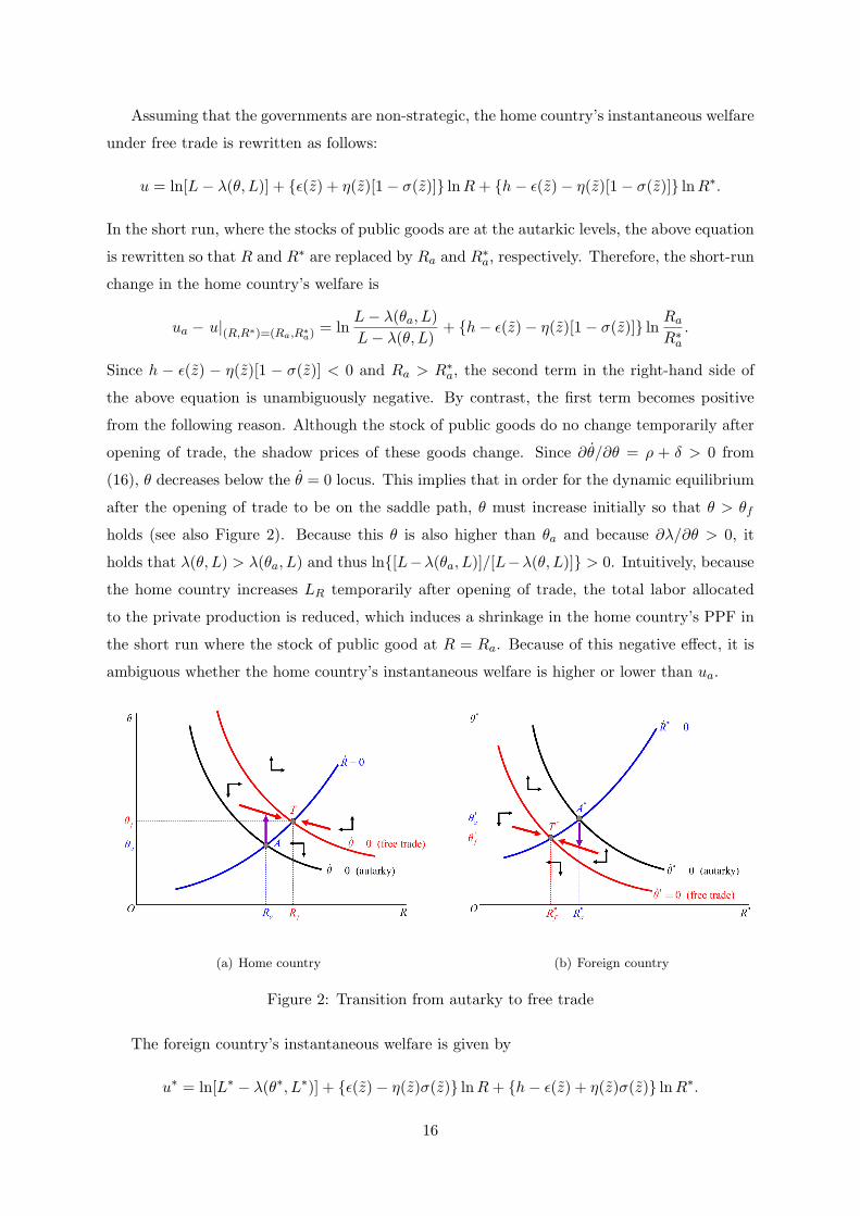
from the following reason. Although the stock of public goods do no change temporarily after

opening of trade, the shadow prices of these goods change. Since ∂θ/∂θ = ρ + δ > 0 from

(16), θ decreases below the θ = 0 locus. This implies that in order for the dynamic equilibrium

after the opening of trade to be on the saddle path, θ must increase initially so that θ > θf

holds (see also Figure 2). Because this θ is also higher than θa and because ∂λ/∂θ > 0, it

holds that λ(θ, L) > λ(θa, L) and thus ln[L−λ(θa, L)]/[L−λ(θ, L)] > 0. Intuitively, because

the home country increases LR temporarily after opening of trade, the total labor allocated

to the private production is reduced, which induces a shrinkage in the home country’s PPF in

the short run where the stock of public good at R = Ra. Because of this negative effect, it is

ambiguous whether the home country’s instantaneous welfare is higher or lower than ua.

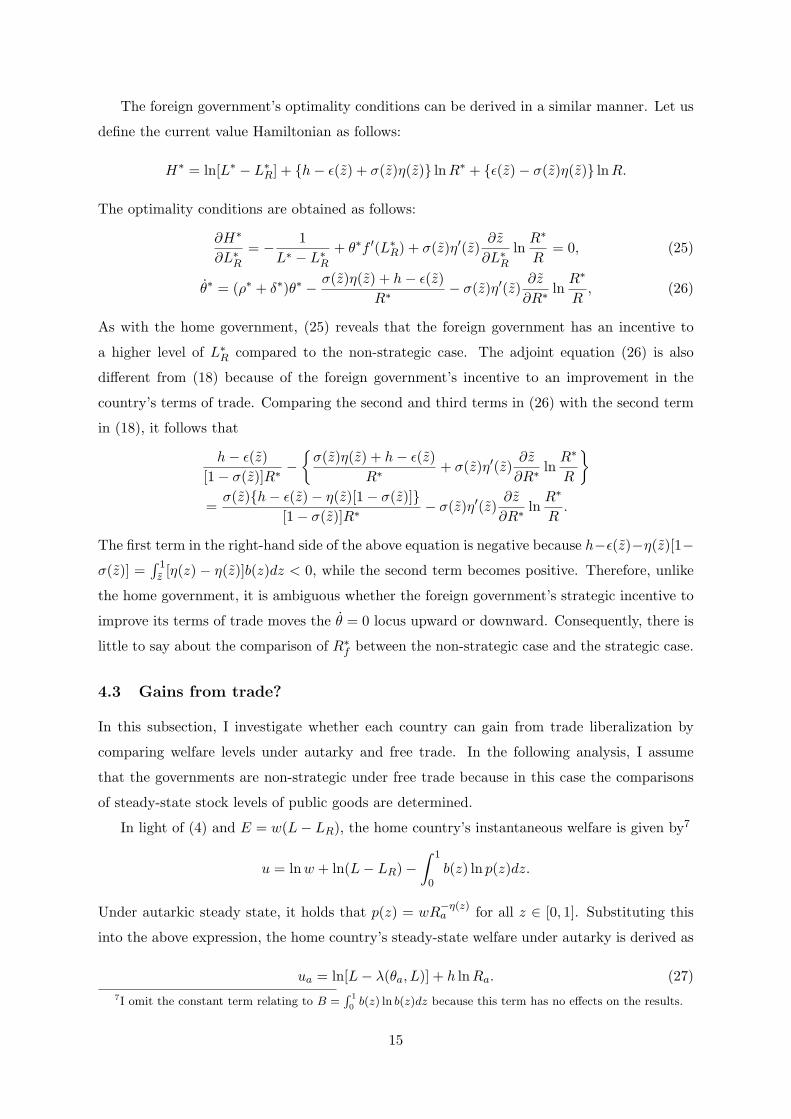
(a) Home country (b) Foreign country

Figure 2: Transition from autarky to free trade

The foreign country’s instantaneous welfare is given by

u∗ = ln[L∗ − λ(θ∗, L∗)] + ϵ(z)− η(z)σ(z) lnR+ h− ϵ(z) + η(z)σ(z) lnR∗.

16

Therefore, the short-run change in the foreign country’s welfare is

u∗a − u∗|(R,R∗)=(Ra,R∗a)

= lnL∗ − λ(θ∗a, L

∗)

L∗ − λ(θ∗, L∗)+ η(z)σ(z)− ϵ(z) ln Ra

R∗a

.

It holds that η(z)σ(z)− ϵ(z) < 0. In addition, after opening of trade, θ∗ temporarily decreases

so that it is lower than θ∗f . Because this temporary value of θ∗ is lower than θ∗a, it holds

that λ(θ∗, L∗) < λ(θ∗a, L∗) and thus ln[L − λ(θ∗a, L

∗)]/[L − λ(θ∗, L∗)] < 0. To sum up, the

right-hand side of the above equation is unambiguously negative; after opening of trade, foreign

country reduces L∗R temporarily, and hence more labor is allocated to private production, which

makes the foreign country’s PPF to expand, and hence the foreign country gains from trade in

the short run.

Proposition 4 Suppose that the governments are non-strategic. Then, the country exporting

the goods that are less dependent on the stock of public good gains from trade in the short run.

Next consider the long-run welfare effect of trade, where the stocks of public goods are at

the steady-state levels, (R,R∗) = (Rf , R∗f ). The respective countries’ instantaneous welfare at

the steady state are derived as follows:

uf = ln[L− λ(θf , L)] + ϵ(z) + η(z)[1− σ(z)] lnRf + h− ϵ(z)− η(z)[1− σ(z)] lnR∗f ,

(28)

u∗f = ln[L∗ − λ(θ∗f , L∗)] + ϵ(z)− η(z)σ(z) lnRf + h− ϵ(z) + η(z)σ(z) lnR∗

f . (29)

Comparing (27) with (28), it follows that

ua − uf = lnL− λ(θa, L)

L− λ(θf , L)+ h ln

Ra

Rf+ h− ϵ(z)− η(z)[1− σ(z)] ln

Rf

R∗f

.

Since R∗f < Ra < Rf as shown in Figure 1, the second and third terms in the right-hand

side of the above equation are negative. At the same time, because θa < θf , the first term is

positive. The first and second terms indicate the conflicting forces of trade liberalization on the

home country’s long-run PPF: an opening of trade increases the steady-state stock of public

good in the home country on the one hand, but reduces the total labor available in the private

production. However, it can be verified that the former positive effect on the PPF outweighs

the latter negative effect if the depreciation rate of the stock of public good is not very large.

To see this, let us define Γ(R) ≡ Rh[L− f−1(δR)]. In light of (6), it follows that

Γ′(R)

Γ(R)=

h(L− LR)f′(LR)− δR

R(L− LR)f ′(LR)=

h− δθR

R.

Evaluating at R = Ra, it is clear from (7) that the numerator of the right-hand side of the

above equation is ρh/(ρ+ δ) > 0, and thus Γ′(Ra) > 0. Evaluating at R = Rf , (16) indicates

17

that the numerator is h − [δ/(ρ + δ)]ϵ(z)/σ(z), which is ambiguous in sign. However, if δ is

sufficiently small, Γ′(Rf ) can also be positive and Γ(R) can be monotonically increasing. If

this is the case, Γ(Ra) < Γ(Rf ) holds.

Proposition 5 Suppose that the governments are non-strategic. If the depreciation rate of

the stock of public good is not very large, then the country exporting the goods that are more

dependent on the stock of public good will gain from trade in the long run.

Now consider the foreign country. From (27), with asterisks, and (29), it follows that

u∗a − u∗f = lnL∗ − λ(θ∗a, L

∗)

L∗ − λ(θ∗f , L∗)

+ h lnR∗

a

R∗f

− η(z)σ(z)− ϵ(z) lnR∗

f

Rf.

The first, second, and third terms in the right-hand side of the above equation are negative,

positive, and negative, respectively. However, because R∗a > R∗

f , the sum of the first and second

terms will be positive if δ∗ is not very large. Therefore, the long-run welfare effect of trade on

the foreign country, which exports the goods that are less dependent on the stock of public

good, is ambiguous.

5 Concluding Remarks

In this paper I developed a dynamic two-country model with a stock of national public good,

which has a positive effect on the productivity in the production of private goods and the

evolution of the stock is determined by the national government, and a continuum of private

goods. With one-factor Ricardian world, it was shown that the country with a higher labor

endowment, a lower depreciation rate of the public-good stock, and/or a lower rate of time

preference will become an exporter of goods which are more dependent on the stock of public

good. If the national governments take the world prices as given when they determine the

paths of public goods under free trade, the country that has a comparative advantage in goods

which are more dependent on the stock of public good enjoys a higher steady-state stock of the

public good under free trade than under autarky, while the other country’s steady-state stock

of the public good under free trade becomes lower than the autarkic level. I also examined the

case where the governments acts strategically to pursue an improvement of the terms of trade

in respective countries, and in this case the effects of trade on the steady-state stocks of public

goods are shown to be ambiguous because of such terms-of-trade effects.

The welfare effects of trade liberalization were also examined. In the short run where the

stocks of public goods are at the autarkic steady-state levels, the country that has a comparative

advantage in goods which are less dependent on the stock of public good unambiguously gains

from trade. It is ambiguous whether the country that has a comparative advantage in goods

18

which are more dependent on the stock of public good becomes better off, but will gain from

trade in the long run if the depreciation rate of the public good is not very large.

Throughout this paper I assumed that in the case of strategic governments, these govern-

ments use open-loop strategies to determine their respective production levels of public goods.

However, the open-loop Nash equilibrium generally lacks subgame perfectness, and deriving

the Markov perfect Nash equilibrium in this game would be more appropriate. In addition,

this paper assumed that the public goods are accumulated only through the public investment.

However, the accumulation of infrastructure is not only due to the efforts of public sectors but

also private sectors. Therefore, it will also be interesting to extend the model to a case in

which the public goods are accumulated through the contributions of private firms as well as

national governments. Moreover, the basic model developed in this paper can be applied to

investigations of several policy issues such as the effects of international transfers. These issues

are remained for future research.

Appendix

Proof of Proposition 2 In light of (2), (6), and (16), the home country’s steady-state

conditions R = θ = 0 can be rewritten as the following single equation:

(ρ+ δ)f(LR)

f ′(LR)(L− LR)δ=

ϵ(z)

σ(z). (A.1)

The foreign country’s counterpart is

(ρ∗ + δ∗)f(L∗R)

f ′(L∗R)(L

∗ − L∗R)δ

∗ =h− ϵ(z)

1− σ(z). (A.2)

Let us denote the left-hand side of (A.1) by g(LR), which satisfies the following properties:

g(0) = 0, g(L) = ∞, g′(LR) =ρ+ δ

δ

f ′(LR)2 − f(LR)f

′′(LR)(L− LR) + f(LR)f′(LR)

f ′(LR)(L− LR)2> 0.

By using l’Hopital’s rule, it holds that limz→0 ϵ(z)/σ(z) = limz→0 ϵ′(z)/σ′(z) = η(0). Since

ϵ(1)/σ(1) = h and η′(z) < 0, the solution for LR satisfying (A.1) is uniquely determined and

is shown to be negatively dependent on z. A similar computation reveals that the solution for

L∗R satisfying (A.2) is unique and negatively dependent on z.

Substituting (A.1) and (A.2) into (19) with the steady-state relationships R = f(LR)/δ

and R∗ = f(L∗R)/δ

∗, it follows that

f ′(LR)

f ′(L∗R)

[f(L∗

R)/δ∗

f(LR)/δ

]1+η(z)

=ρ+ δ

ρ∗ + δ∗h− ϵ(z)

ϵ(z).

Let us define the left-hand side of the above equation by Φl(z) and the right-hand side by

Φr(z). It is clear that Φl(z) is continuous in z and both Φl(0) and Φl(1) take positive values.

19

Φr(z) is also continuous in z and has the following properties:

limz→0

Φr(z) = ∞, limz→1

Φr(z) = 0, Φ′r(z) = − ρ+ δ

ρ∗ + δ∗hη(z)b(z)

ϵ(z)2< 0,

Therefore, there exist at least one steady-state solution for z in (0, 1). If, in addition, the

differences in the endowments of effective labor, depreciation rates of public good stock, or

rates of time preference between countries are such that the home country has a comparative

advantage in the goods that are more dependent on the stock of public goods, R∗f/Rf ≤ 1

holds. If the differences in these parameters are not very large, Φl(z) will also be monotone

and non-decreasing in z. In this case, the steady state is uniquely determined.

Linearizing the system around the steady state, it follows that

R

θ

R∗

θ∗

0

=

−δ f ′λθ 0 0 0(ρ+δ)θf

Rfρ+ δ 0 0 − (ρ+δ)θf [η(z)σ(z)−ϵ(z)]b(z)

ϵ(z)σ(z)

0 0 −δ∗ f∗′λ∗θ 0

0 0(ρ∗+δ∗)θ∗f

R∗f

ρ∗ + δ∗ − (ρ∗+δ∗)θ∗fh−ϵ(z)−η(z)[1−σ(z)]b(z)[h−ϵ(z)][1−σ(z)]

−1−σ(z)σ(z)

η(z)Rf

1−σ(z)σ(z)

λθL−λ

1−σ(z)σ(z)

η(z)R∗

f−1−σ(z)

σ(z)

λ∗θ

L∗−λ∗ −η′(z) lnRf

R∗f+ b(z)

[1−σ(z)]σ(z)

×

R−Rf

θ − θf

R∗ −R∗f

θ∗ − θ∗f

0

, (A.3)

where f∗ ≡ f(L∗R) and λ∗ ≡ λ(θ∗, L∗).

Let us denote the Jacobian matrix in (A.3) by J , and the corresponding eigenvalue as m.

Then m is determined by the characteristic equation

Ω(m) ≡∣∣∣J −mI

∣∣∣ = 0, where I ≡

I4 0

0 0

.

Because the dynamical system has two predetermined variables R and R∗, there exists a unique

saddle path converging to the steady state if the characteristic equation Ω(m) have two roots

with negative real parts. Suppose that L ≈ L∗, δ ≈ δ∗, and ρ ≈ ρ∗, Then, it holds that

λ ≈ λ∗, Rf ≈ R∗f , and θf ≈ θ∗f .

8 Therefore, the characteristic equation can be rewritten as

8I assume, for instance, L = L∗ +∆L, where ∆L > 0 is sufficiently small. Then, the home country still has

a comparative advantage in the goods that are more dependent on the stock of public good, and thus there is a

marginal good.

20

Ω(m) = Ω1(m)Ω2(m), where9

Ω1(m) ≡ m2 − ρm− (ρ+ δ)

(δ +

f ′λθθfRf

),

Ω2(m) ≡ Ω1(m)

σ(z)[1− σ(z)]− f ′λθ

η(z)σ(z)− ϵ(z)

σ(z)2[1− σ(z)]Rf

[θ(m+ δ)− η(z)

Rf

].

Since λθ > 0, the two solutions to Ω1(m) = 0 have opposite signs. Regarding Ω2(m), since

η(z) is decreasing in z, it holds that η(z)σ(z)− ϵ(z) =∫ z0 [η(z)− η(z)]b(z)dz < 0. Therefore, if

δ is not very large, the two solutions to Ω2(m) = 0 also have opposite signs.

Finally, it can be verified that Ω(0) = 0. It follows that the implicit function theorem

ensures that even if the economic fundamentals of the two countries are slightly different with

each other, the existence, uniqueness, and stability of the steady state are established (Chen

et al., 2008). 2

References

[1] Abe, K. (1990), A Public Input As a Determinant of Trade, Canadian Journal of Eco-

nomics 23, 400–407.

[2] Altenburg, L. (1992), Some Trade Theorems with a Public Intermediate Good, Canadian

Journal of Economics 25, 310–332.

[3] Chen, B.-L., K. Nishimura, and K. Shimomura (2088), Time Preference and Two-country

Trade, International Journal of Economic Theory 4, 29–52.

[4] Costinot, A. (2009), On the Origins of Comparative Advantage, Journal of International

Economics 77, 255–264.

[5] Cunat, A. and M.C. Melitz (2012), Volatility, Labor Market Flexibility, and the Pattern

of Comparative Advantage, Journal of the European Economic Association 10, 225–254.

[6] Dornbusch, R., S. Fischer, and P.A. Samuelson (1977), Comparative Advantage, Trade,

and Payments in a Ricardian Model with a Continuum of Goods, American Economic

Review 67, 823–839.

[7] Feehan, J.P. and M. Matsumoto, Productivity-Enhancing Public Investment and Benefit

Taxation: The Case of Factor-Augmenting Public Inputs, Canadian Journal of Economics

33, 114–121.

[8] Ishizawa, S. (1988), Increasing Returns, Public Inputs, and International Trade, American

Economic Review 78, 794–795.9In deriving Ω2(m), I used the relationship ϵ(z)/σ(z) = [h− ϵ(z)]/[1− σ(z)] from (16) and (18).

21

[9] Long, N.V. (2010), A Survey of Dynamic Games in Economics, World Scientific.

[10] Long, N.V. and K. Shimomura (2007), Voluntary Contributions to a Public Good: Non-

Neutrality Results, Pacific Economic Review 12, 153–170.

[11] Manning, R., J.R. Markusen, and J. McMillan (1985), Paying for Public Inputs, American

Economic Review 75, 235–238.

[12] Manning, R. and J. McMillan (1979), Public Intermediate Goods, Production Possibilities,

and International Trade, Canadian Journal of Economics 12, 243–257.

[13] McMillan, J. (1978), A Dynamic Analysis of Public Intermediate Goods Supply in Open

Economy, International Economic Review 19, 665–678.

[14] Shimomura, K. (2007), Trade Gains and Public Goods, Review of International Economics

15, 948–954.

[15] Suga, N. and M. Tawada (2007), International Trade with a Public Intermediate Good

and the Gains from Trade, Review of International Economics 15, 284–293.

[16] Tawada, M. and H. Okamoto (1983), International Trade with a Pubic Intermediate Good,

Journal of International Economics 17, 101–115.

[17] Tawada, M. and K. Abe (1984), Production Possibilities and International Trade with a

Public Intermediate Good, Canadian Journal of Economics 17, 232–248.

[18] Yanase, A. and M. Tawada (2012), History-Dependent Paths and Trade Gains in a Small

Open Economy with a Public Intermediate Good, International Economic Review 53,

303–314.

22