1

Infrastructure: Real Assets and Real Returns

Ron Bird*, Harry Liem and Susan Thorp

University of Technology, Sydney

Sydney, Australia

The Paul Woolley Centre for Capital Market Dysfunctionality, UTS

Working Paper Series 11

Previous version: September 2011

This version: April 2012

Abstract

Little empirical work has been done on infrastructure as an asset class despite

increased allocations by institutional investors. We build a robust factor model of

infrastructure returns using US and Australian infrastructure and utility data to test

manager claims that infrastructure investments offer benefits via a combination of

monopolistic and defensive assets. We find evidence of excess returns and inflation

hedging, but not of defensive characteristics. We compare option-based models

designed to replicate infrastructure asset returns, and identify the regulatory risk

premium. A combination of inflation linked bonds and covered call strategies results

in improved defensive and inflation hedging characteristics.

Keywords: inflation hedging, regulatory risk premium, infrastructure assets

JEL classification: G12, G14

* Corresponding author.

E-mail: Ron.Bird@uts.edu.au

Phone: +61 2 9514 7716

Fax: +61 2 9514 7711

Room: CM05D.03.22B

PO Box 123, Broadway NSW 2007, Australia

The authors wish to acknowledge the generous support of the Paul Woolley Centre at the University of

Technology, Sydney (UTS). In addition, Thorp acknowledges support under Australian Research

Council (ARC) DP 0877219. The Chair of Finance and Superannuation at UTS receives support from

the Sydney Financial Forum (Colonial First State Global Asset Management), the NSW Government,

the Association of Superannuation Funds of Australia (ASFA), the Industry Superannuation Network

(ISN), and the Paul Woolley Centre, UTS. The authors also wish to thank John Doukas, two

anonymous referees, and attendees at the 2011 Paul Woolley Conference in Sydney for their valuable

comments and suggestions.

2

1. Introduction

Pension funds around the world have been investing in infrastructure with the aim of

providing better long duration, real (inflation adjusted) retirement benefits to

members. While infrastructure has been seen as a suitable institutional investment in

Australia, Canada and the UK since the 1990s, it has only recently increased in

popularity in the US and, unlike hedge funds or private equity, has not been the focus

of much academic research, partly because of limited data (Dechant et al., 2010;

Martin, 2010; Newell and Peng, 2008).

In this paper we define infrastructure as encompassing the utility sector (power

generation and distribution) as well as the ‘pure’ infrastructure sector (toll roads,

communications and airports). Institutional investors most commonly delegate

infrastructure investment to managers but may also undertake direct investment

(Inderst, 2009).1 We consider investment in both listed and unlisted Australian

infrastructure assets, either directly or through managed funds. Outside of Australia,

where less data is available, we focus on the listed infrastructure markets.

Initially researchers viewed infrastructure as having characteristics akin to real

estate: a long life cycle, heterogeneity, illiquidity and inflation hedging ability

(Dechant et al., 2010; Newell and Peng 2007, 2008). However, a defining feature of

the sector is the prevalence of ‘natural monopolies’ in the provision of essential

services (such as energy or water) and of economies of scale created by large

distribution networks (Dimasi, 2010). Researchers now concur that infrastructure is a

distinct asset class having oligopolistic or monopolistic characteristics, because of

restrictions on ownership and on the uses to which infrastructure can be put. Natural

monopolies and industries enjoying economies of scale are often regulated by

1 Infrastructure investment methods are described in detail in the appendix.

3

government restrictions on prices, returns, output levels or barriers to entry.

Consequently, infrastructure investments require compensation for regulatory risk. In

many countries, infrastructure consists of mature utilities, increasingly facing

deregulation and privatisation (Inderst, 2009). As a result, the ability to deliver

superior performance may diminish as the industry matures (deregulates).

We make the following three contributions to literature. First, we suggest style

factors common to both US and Australian infrastructure investments. We extend our

analysis by applying an asymmetric GARCH model to take account of observed

volatility clustering in excess returns and we test both the defensive and the inflation

hedging ability of the asset class. We find evidence of excess returns and inflation

hedging features in infrastructure investments in the US and Australia. While we do

find some desirable characteristics, we caution against sample size and time period

biases given the limitations of our data set.

Second, we test the defensive ability of infrastructure investments during equity

down markets. We find no evidence of defensive characteristics. Despite claims that it

is a defensive sector, Australian listed infrastructure funds performed very poorly

during the Global Financial Crisis.2

Third, we investigate the possibility of using derivatives to replicate infrastructure

returns and the ability of infrastructure investment to realise a return in excess of the

regulatory risk premium. We find that in Australia, but not in the US, investors

achieved returns in excess of comparable option strategies. Infrastructure investing

exposes investors to assets with an unknown amount of political risk so we suggest

2 Notably, large infrastructure firms such as Macquarie and Babcock & Brown were criticised for ‘asset

gathering’ using leverage, thereby generating transaction, advisory, base and performance fees for the

parent company. In March 2009 Babcock and Brown was placed into voluntary administration due to

its over-reliance on short-term debt while Macquarie restructured and survived as Intoll Group.

4

how investors can create the desired defensive and real return payoff profile using a

combination of inflation linked bond and covered call option strategies.

We review background literature in Section 2, set out the model in Section 3 and

discuss data in Section 4. Section 5 presents our empirical results on the excess

returns, downside protection and inflation hedging characteristics of infrastructure.

Section 6 focuses on the pricing of regulatory risk, while Section 7 suggests how a

synthetic real defensive asset can be constructed that combines the defensive and

inflation hedging characteristics of infrastructure. Section 8 provides concluding

remarks and suggestions for further research.

2. Background Literature

The available empirical work on private infrastructure investment has been surveyed

by Dechant et al. (2010), Inderst (2009), Martin (2010), and Newell and Peng (2007,

2008). Newell and Peng (2007) find that during the period from 1995 to 2006,

infrastructure investment in Australia exhibited higher returns, but also higher

volatility, than equity markets. We suggest this finding is largely attributable to the

relatively high leverage employed by the listed infrastructure managers in Australia.

The period examined by Newell and Peng (2007) excludes the Global Financial

Crisis, during which a number of highly levered infrastructure groups such as

Macquarie Infrastructure and Babcock and Brown were forced to liquidate or

restructure. Newell and Peng (2008) find that in the US, infrastructure (excluding

utilities) underperformed stocks and bonds during the period from 2000 to 2006,

while utilities outperformed stocks and bonds. Bitsch et al. (2010) investigate a

unique database of global unlisted infrastructure deals and conclude that the desired

characteristics of stable long-term and inflation linked returns have yet to be proven

5

empirically. They argue that infrastructure deals are highly levered, and returns

largely driven by market and political risk. DeFrancesco et al. (2011) find some

evidence of excess returns in unlisted Australian infrastructure but rely on a small

sample.

In terms of inflation hedging ability, Armann and Weisdorf (2008) and Martin

(2010) find a positive correlation between infrastructure returns and inflation. On the

other hand, Bitsch et al. (2010), using global unlisted infrastructure data, find no

evidence of inflation hedging. Here we update the data used by Newell and Peng

(2007, 2008) and propose a model that caters for additional style factors.

3. The Model

3.1. Market factors

Investment in infrastructure represents an allocation to equities, with a large asset base

(high book-to-price ratio) and low but stable earnings growth, and thus can be priced

using a number of style biases (or beta factors) and a risk-adjusted excess return

(equation (1)). In the US, style tilts can be captured using the Fama and French (1993)

SMB (Small minus Big stocks) and HML (High minus Low book-to-price stocks)

factors.3 For Australia, we use the ASX Small Ordinaries returns minus the ASX 100

returns to proxy SMB, and the BMI Value minus BMI Growth index returns to

approximate HML. The ASX Small Ordinaries index represents the stocks in the ASX

300, excluding the 100 largest stocks (which are captured in the ASX 100 index). The

BMI (Broad Market Indices) are created by S&P. All indices are market capitalisation

weighted and these factors are measurable, interpretable and tradeable. Equation (1)

presents the standard Fama-French model.

3 Data can be downloaded from

http://mba.tuck.dartmouth.edu/pages/faculty/ken.french/data_library.html

6

Rit – Rft = αi + βi,m (Rm,t – Rft) + βi,s * SMBt + βi,v * HMLt + εit (1)

where Rit is the rate of return of asset class i at time t, Rft is the risk-free rate at time t

and αi is the intercept, or the risk-adjusted excess returns. In terms of factor exposure,

(Rm,t – Rft) represents the equity risk premium, and βi,m measures the sensitivity of

excess returns of the asset class to the equity risk premium. SMBt is the differential

return between smaller and larger capitalised companies, and HMLt is the differential

return between high and low book-to-price companies with sensitivities βi,s and βi,v

respectively, εit is the error (residual) portion or the return not related to the other

factors at time t, with an expected value of zero and variance described in Section 3.5.

3.2. Illiquidity

Serial correlation in returns may be high in illiquid, unlisted asset classes, where

valuations for alternative assets can be appraisal-based rather than transaction-based

since a lack of a tradable market for the underlying assets means that appraisers rely

on previous valuations as an anchor point for current valuations. Somewhat

surprisingly, we find no evidence for serial correlation in returns to Australian

unlisted infrastructure in our dataset.4 Also surprising is that Australian unlisted

infrastructure funds are open ended and offer monthly unit pricing, despite the funds

themselves being invested in a small number of highly illiquid assets valued on a

quarterly or annual basis. In reality, redemption tends to be at “best endeavours” –

4 We suggest four types of noise reduce serial correlation. The first lies in the accrual of income into

the monthly unit pricing. The second is changes in foreign currency values which create translation

effects for unhedged overseas assets. The third is that some infrastructure managers allocate a portion

of their funds to listed infrastructure assets. The fourth lies in the Discounted Cash Flow (DCF)

valuation process. This method offers users a large number of input parameters for adjustment, such as

bond yields, traffic growth rates, utilisation rates and assumed equity betas. Such valuation noise can

reduce the serial correlation in returns.

7

that is, within 12 months of receiving a redemption notice, and at the manager’s

discretion.

3.3. Protection in down markets

It is important to understand the defensive abilities of infrastructure during periods of

market stress. To test market timing ability, Treynor and Mazuy (1966) include a

quadratic term in the market excess return since returns to defensive assets are

expected to fall less than the market during times of stress. Equation (2) extends

equation (1) to include the market timing component (Rmt – Rft)2

where a significant

positive coefficient (βi,timing) suggests positive market timing ability.

Rit – Rft = αi + βi,m (Rm,t – Rft) + βi,s * SMBt + βi,v * HMLt + βi,timing (Rmt - Rft)2 + εit (2)

3.4. Inflation hedging abilities

Investors allocate to infrastructure because of its perceived inflation hedging abilities

(Armann and Weisdorf, 2008; Martin, 2010). Here we measure sensitivity to inflation

expectations by comparing infrastructure returns with returns to US and Australian

inflation-linked bonds (also known in the US as Treasury Inflation Protected

Securities, or TIPS), using the Barclays US TIPS index and the UBS Australian

Inflation Linked bond index, which are liquid and tradeable and thus offer a direct,

monthly pricing relationship. Formula (3) extends formula (1) with an inflation factor.

Rit - Rft = αi + βi,m (Rm,t – Rft) + βi,s * SMB + βi,v * HML + βi,inflation * TIPS + εit (3)

8

A significant positive coefficient (βi,inflation) suggests inflation hedging ability where

TIPS represents the inflation premium, or the returns on Treasury Inflation Protected

Securities (TIPS) for the US (or the UBS inflation-linked bond index for Australia),

minus the relevant risk-free rate.5

3.5. Variance equation

We model conditional heteroskedasticity and non-linearities in the errors εit using

maximum likelihood estimation and the GJR-GARCH approach (Glosten et al.,

1993). The GJR-GARCH model captures asymmetric conditional volatility hit via an

indicator term It−1 in the GARCH equation:

hit = γ0 + γ1ε2

i,t-1 + γ2hi,t-1 + γ3ε2

i,t-1It-1 (4)

where It−1 = 0 if εi,t-1 ≥ 0, and It−1 = 1 if εi,t-1 <0.

In this case, γ0 is a constant intercept impacting the long run unconditional volatility,

γ1 is a weighting to the previous period’s squared shock ε2

i,t-1, γ2 is a weighting to the

previous period’s predicted volatility hi,t-1 and γ3 is a sensitivity to negative return

shocks ε2

i,t-1It-1. In our model, we use t rather than normal distributed errors in

estimation to capture fat tails. The degrees of freedom for the t-distribution are

provided in Tables 3, 4 and 5.

4. The Data

4.1. Listed infrastructure

5 For completeness we also tested infrastructure inflation hedging abilities directly by using CPI. We

obtain similar results.

9

The UBS infrastructure performance series used in this study are free float-adjusted,

market capitalisation-weighted total return indices covering both the listed

infrastructure and utilities sectors. The UBS indices are widely considered to be the

most comprehensive set of listed infrastructure indices available and remain the

standard benchmark for infrastructure managers worldwide. Table 1 contains a list of

the available UBS infrastructure indices.

<< INSERT TABLE 1 >>

4.2. Australian unlisted infrastructure

Mercer provided a unique, net-of-fees return data series for ten unidentified

Australian unlisted infrastructure managers, representing 105 underlying assets worth

A$11.1 billion and covering some of the largest infrastructure managers in Australia.

The largest manager comprises 25 assets, worth A$5.5 billion or 50 per cent of the

total combined assets. The managers do not distinguish between pure infrastructure

(non-utility assets such as toll roads, airports or railroads) and utility assets. In other

words, most infrastructure funds hold both types of assets. Aggregating by summing

the value of all underlying projects for each manager shows that utilities comprise 59

per cent of the underlying assets in our sample. The managers have domestic and

international investments: 43 per cent of assets are in Australia, 21 per cent are in the

UK, 19 per cent are in the US and 17 per cent are in the rest of the world. We do not

know how much is invested on an unhedged basis, and so currency fluctuations may

impact reported returns. While the return data provided by the managers extends back

to January 1995, the collection of data on the assets inside the funds has only begun

recently (2010), and we do not have access to historic asset values. Thus, we opted to

create an equally weighted (rather than asset weighted) index to capture the

performance of the Australian unlisted infrastructure sector. In the Mercer data set,

10

survivorship bias is minimised as we are not aware of any funds being deleted for

poor performance. In terms of selection bias, these funds by no means represent a

complete list of the infrastructure opportunities, and some funds also choose not to

participate in the Mercer database. However, it should also be acknowledged that not

many infrastructure funds in Australia have a long data history comparable to the

funds included in the Mercer data set. Thus we suggest the Mercer data set offers an

adequate representation of the Australian unlisted infrastructure history.

5. Empirical Results

5.1. Descriptive statistics

Based on data availability we have selected indices from Table 1 that are available

over the period from 1995 to 2009. The descriptive statistics are shown in Table 2.

<< INSERT TABLE 2 >>

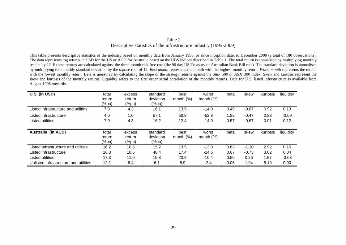
As can be seen from Table 2, all infrastructure sectors created excess returns over the

risk-free rate over the period from 1995 to 2009.6 Listed infrastructure exhibits much

higher volatility and also a higher beta to equity markets than listed utilities. Many

sectors also exhibit a negative skew and positive kurtosis, suggesting a returns profile

similar to a written call option and/or the use of leverage.7 No sector returns show

significant first order autocorrelation.

5.2. Factor model estimation results

6 In table 2 the total return for the combined Australian listed infrastructure and utilities index lies

below the total returns reported for the separate listed infrastructure and listed utility indices, despite

the index being a weighted average. We verified with UBS Australia that the data and calculations

employed are correct. At every point in time a combined index is created as a weighted composite of

the subindices. The low return is a function of time-varying weights. The weight in listed infrastructure

varied from 10 per cent at the start of the period (when infrastructure outperformed utilities) to 50 per

cent by the end of the period (when infrastructure underperformed utilities). 7 It is quite possible the lack of negative skew in Australian unlisted is more a function of the valuation

process than a reflection of the fundamentals of the actual asset class.

11

<< INSERT TABLE 3 >>

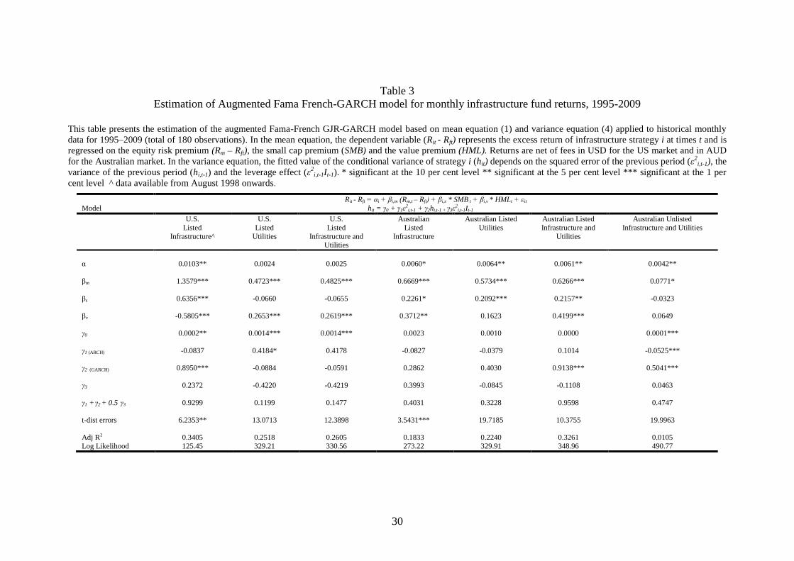
Table 3 shows estimation results for the Fama-French factor model of excess returns

to US listed infrastructure, to Australian listed infrastructure and utilities, and to

Australian unlisted infrastructure and utilities. We estimate significant equity betas

(βm) for US infrastructure (1.35) and Australian infrastructure (0.67) and more

defensive equity betas for listed utilities, between 0.47 and 0.57. Four of the sectors

display a positive significant style tilt towards small stocks (βs), while for the other

three the tilt is negative but insignificant. The majority of the sectors favour value

stocks (βv), with the notable exception of US infrastructure, which is dominated by

communication (growth) stocks with a low fixed asset base.

There are persistent GARCH effects (γ2) but no sign of significant asymmetries (γ3).

With the adjusted R2 varying between 0.18 and 0.34 the model provides a reasonable

fit for listed infrastructure and utility sectors but for Australian unlisted infrastructure

and utilities the model provides a very poor fit (R2 of 0.01). Interestingly, we do not

find evidence of leverage effects (γ3), but we do find strong evidence of GARCH

effects, even for unlisted infrastructure. Under a strict appraisal based valuation

process, one would not expect to find GARCH effects, but constant return volatility.

The GARCH effects suggest unlisted infrastructure appraisal processes are influenced

by market factors. The proportion of excess return unexplained by the factor model

raises the possibility of a regulatory risk premium, which we discuss in Section 6.

5.3. Defensive properties

<< INSERT TABLE 4 >>

12

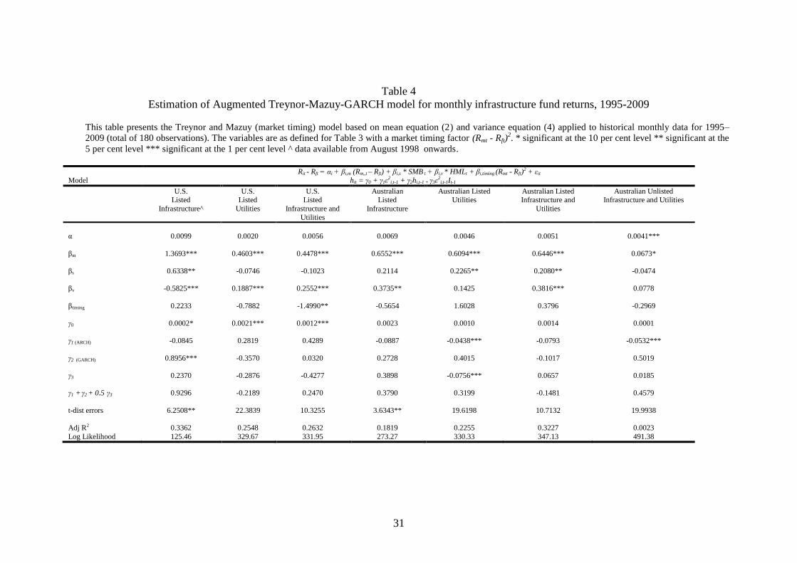
Table 4 shows the performance of infrastructure and utility stocks during up and down

equity markets. The negative coefficient for βtiming in Table 4 is evidence of

deteriorating performance for US utilities and Australian listed infrastructure during

market downturns, although we note that this is not statistically significant. We

conjecture that this is a function of the leverage employed by listed fund managers (in

Australia), and also the high gearing of underlying assets.

<< INSERT FIGURE 1>>

Figure 1 graphs the performance of infrastructure assets during up and down equity

markets and also the predicted forecast returns for the asset class as derived using

equation (2). As can be seen, the relationship is concave rather than convex for US

utilities and Australian listed infrastructure. The downward slope in the line indicates

that a downturn in equity markets results in increasingly poor performance from US

utility stocks, as well as Australian listed infrastructure stocks, and that during times

of financial stress (negative equity markets), some types of infrastructure and utilities

may not possess the desired defensive characteristics.

5.4. Inflation hedging properties

<< INSERT TABLE 5 >>

Table 5 shows that US and Australian utility sectors have inflation hedging ability

based on the sensitivity (βinflation) to inflation linked bonds (TIPS), and consistent with

findings by Armann and Weisdorf (2008) and Martin (2010) for the US. However,

pure infrastructure (non-utility) stocks show no evidence of inflation hedging:

regulated utilities appear to have more ability to pass inflation increases to customers

without much loss in demand. While energy generation and distribution assets can

face relatively inelastic demand, the situation for non-utility assets may be different.

13

Toll roads may experience a fall in traffic volume when tariffs are increased: there

may be stickiness in prices resulting from money illusion as customers focus on

nominal, as opposed to real price increases (Diamond et al., 1997).

6. Pricing of regulatory risk

6.1. Regulated versus unregulated assets: introducing option based models

Henisz and Zelner (1999, p.1) emphasise “the importance of regulatory risk in sectors

characterised by large sunk costs, substantial economies of scale and highly

politicised pricing, such as telecommunications and electricity generation”. We argue

that investors in infrastructure assets are exposed to two types of regulatory risk:

1. Investors in large infrastructure businesses with significant regulated energy or

utility activities typically negotiate rates of return on equity (ROE) in the range

of 10.0 to 15.0 per cent. Thus, from a fundamental perspective, regulatory risk

limits tariff increases, which can be viewed as analogous to the government

exercising an implicit (out of the money) call option. Investors are effectively

allowed to retain an asset with monopolistic characteristics (as Dimasi, 2010,

notes through either the provision of essential services or monopolies of scale),

but in return forego the possibility of supernormal profits that would cause

welfare losses.

2. Governments can act as ‘lender of last resort’ to infrastructure projects and may

support the private sector partner during times of distress if the infrastructure

services are deemed essential to the community. Thus, investors effectively hold

a put option to sell assets back to the government if the asset price declines.

14

Thus, we derive the following equation for the returns of regulated assets:

Rregulated asset = Runregulated asset + Pregulatory call option – Pregulatory put option (5)

where Pregulatory call option reflects the receipt of the monopoly premium compensating

for the regulatory cap, and Pregulatory put option reflects the implicit premium paid for

regulatory assistance on the downside. This payoff profile is shown in Figure 2.

<< INSERT FIGURE 2 >>

6.2. Regulated versus unregulated assets: initial comparison

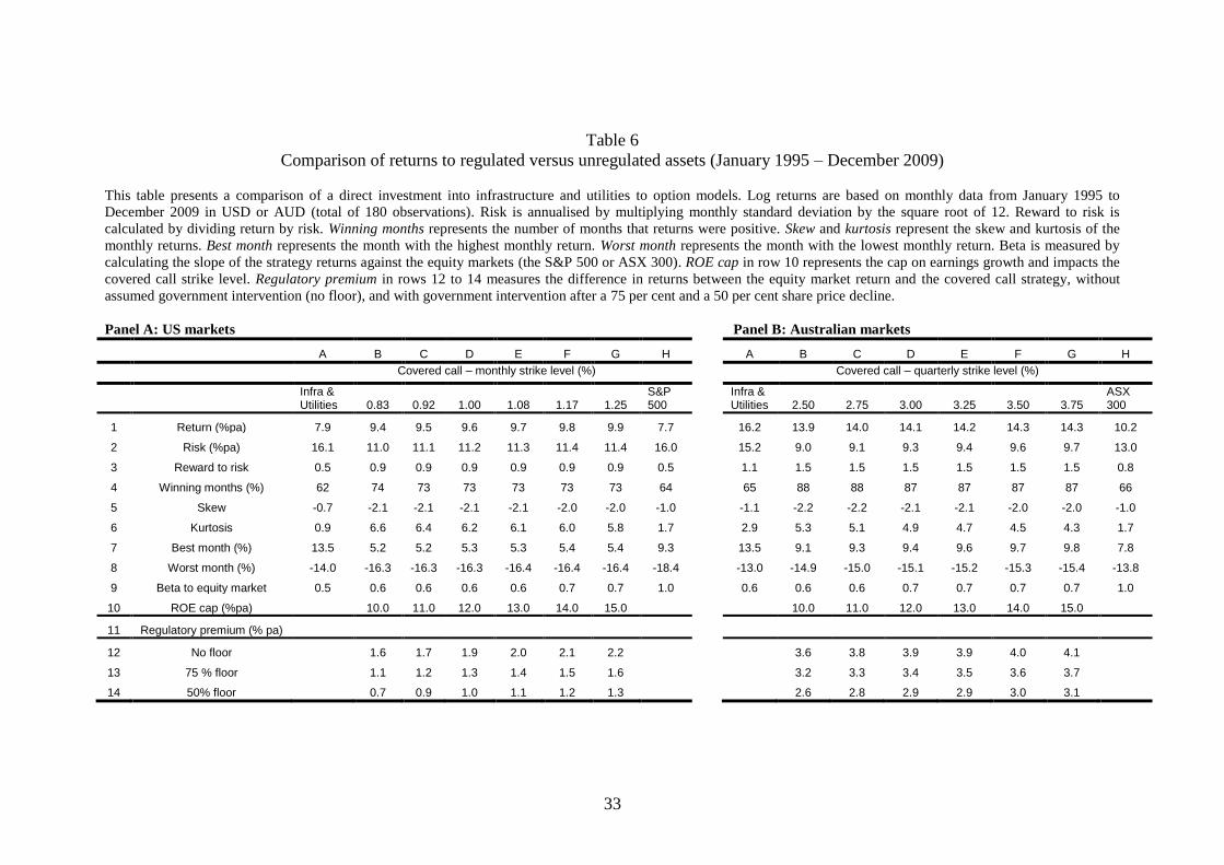
<< INSERT TABLE 6 >>

Table 6 shows comparative performance of the US and Australian markets. The

returns on a direct investment in the listed infrastructure and utility sectors in the US

and Australia are shown in row 1, column A, while an investment in unregulated

assets is proxied by the broad market index in row 1, column H. It can be seen that the

regulated assets (the infrastructure and utility sector) outperform the unregulated

assets (the broad market index) in both the US and Australia over the period

investigated. The premium is 0.2 per cent per annum in the US (7.9 minus 7.7 per

cent), and 6.0 per cent in Australia (16.2 minus 10.2 per cent). On this basis, an

investment in regulated assets in the infrastructure and utilities sector seems attractive.

6.3. Regulated versus unregulated assets: implementing the ROE cap

We now evaluate the performance of the regulated asset assuming that the

government has initiated a cap on the return on equity of the unregulated asset

represented in column H (the S&P 500, or the ASX 300). Row 10, columns B to G

15

show premiums of 10 to 15 per cent imposed on the unregulated asset. Refer to Figure

2 for more details on how the premium received (Pregulatory call option) is derived from a

calibration in the strike price. Using the first part of equation (5), we then find

Rregulated asset = Runregulated asset + Pregulatory call option (6)

Row 1, columns B to G show the returns to the covered call strategies. As can be

seen, in the US the regulated assets (row 1, column A) now underperform the covered

call strategies (row 1, columns B to G). In Australia, the regulated assets still

outperform the covered call strategies. Row 3, columns B to G show that in both the

US and Australia the covered call strategy increases the reward to risk ratio. In

addition, row 9, columns B to G suggest covered call strategies exhibit a similar

equity beta to regulated assets (0.6 to 0.7). By subtracting the returns in row 1 in

columns B to G from column H we can derive the additional return (premium)

received for selling the call option. We find in the US the premium ranges between

1.6 and 2.2 per cent per annum (row 12, columns B to G), based on an assumed ROE

cap range of 10 to 15 per cent. In Australia, the additional premium is higher at

between 3.6 and 4.1 per cent.

6.4. Regulated versus unregulated assets: the cost of downside protection

In the previous discussion we did not consider the potential of government

intervention on the downside (hence the term “no floor” was used in row 12). We now

assume the investor receives access to an implicit government put option, where, in

case of distress, the government has an incentive to subsidise or rescue infrastructure

projects that are too large or important to fail. We examine three possible scenarios:

16

no floor (no intervention expected), distressed intervention (intervention expected

after asset prices decline by 75 per cent) and regular intervention (intervention

expected after asset prices decline by 50 per cent). As can be seen in rows 12 to 14,

buying a put option reduces the premium received from selling the call. The cost of

the implicit put reduces the net premium received by around 1 per cent in both the US

and Australia. Overall, we find that in the US regulated assets (row 1, column A)

outperformed unregulated assets (row 1, column H) by 0.2 per cent. However, after

taking into account the implicit regulatory restrictions, this is no longer the case. In

Australia, we find that regulated assets (row 1, column A) outperform unregulated

assets (row 1, column H) by 6.0 per cent and continue to do so even after

implementing the option based strategies. In other words, whereas in the US an

investor would have been better off investing in a combination of the unregulated

assets with option protection, in Australia, investors would have been better off

investing in the infrastructure and utilities sector directly.

However, the aforementioned option based model does not take into account that: a)

option based strategies with specific strike prices need to be tailor-made by

investment banks and customised in the Over The Counter (OTC) market, thereby

exposing investors to counterparty credit risk b) infrastructure was shown to have

some inflation hedging ability and c) some transaction costs may be involved. For

completeness, we compare the net premiums received from the option program to

listed option return indices for some of the available strike prices. We find the

difference between our theoretical returns and the listed product equivalent to be

minimal. In our strategies the transaction costs are reduced because the options are

held until maturity, that is, no intra-month trading needs to take place.

17

7. A synthetic real defensive asset

We propose a synthetic approach that combines the desired defensive and inflation

hedging characteristics of infrastructure with a proxy for the regulatory risk premium.

The synthetic approach relies solely on exchange-traded instruments. We use a

covered call to capture the regulatory risk premium and defensive and inflation

hedging characteristics via an investment in inflation-linked bonds.

1. Covered call strategy. The BXM index, provided by the Chicago Board

Options Exchange (CBOE) simulates continuous call writing for one

month out of the money calls on the S&P 500. It is liquid and readily

tradeable. For Australia we use a comparable index (XBW), which

involves writing of nearby, just out of the money three-month call

options.8

2. Put option strategy. A floor on the portfolio is implemented through an

investment in a bond portfolio. This bond portfolio consists of Treasury

Inflation Protected Securities (TIPS), which are government guaranteed.

The investment is made through the Barclays US TIPS index or the UBS

Australia Inflation Linked bond index.9

We follow a dynamic updating process to create the synthetic portfolio. The period

from January 1995 to December 1997 is used to set the initial (in-sample) factor

weights based on regressing listed infrastructure and utility returns against the covered

8 For BXM data refer http://www.cboe.com/micro/bxm/#historical. For XBW data refer

http://www.asx.com.au/products/indices/types/buy_write/history.htm. 9 The investment can be made through direct securities, passive index funds (unlisted funds) or

Exchange Traded Funds (listed funds).

18

call index and the inflation linked bond (TIPS) index as risk factors. This period is

chosen to reflect at least 30 monthly data points for the initial weight estimates. The

factor weights are then dynamically adjusted as the next monthly (out-of-sample) data

point becomes available and the regression is updated using the lengthened lookback

period. The dynamic weights are used to determine the replicated returns for the

subsequent month. This results in an allocation which converges to around a 50 per

cent dollar weight to the covered call index and 50 per cent to TIPS. The covered call

allocation creates the exposure to the equity and regulatory risk premium while the

allocation to TIPS creates the desired inflation hedging characteristics and floor.

7.1. Return characteristics of the synthetic asset

<< INSERT TABLE 7 >>

Table 7 compares the outcome from a direct investment in infrastructure and a

synthetically created exposure for both the US and Australian markets. The synthetic

asset has a lower equity beta (0.3) and higher inflation hedging beta (0.5 to 0.7) than

the direct investment, both desirable characteristics. The synthetic asset has a higher

return than the direct investment in the US but a lower return in Australia.10

Even in

Australia, the synthetic asset may still generate comparable results to the direct

investment in the long run, provided the excess returns generated by the direct

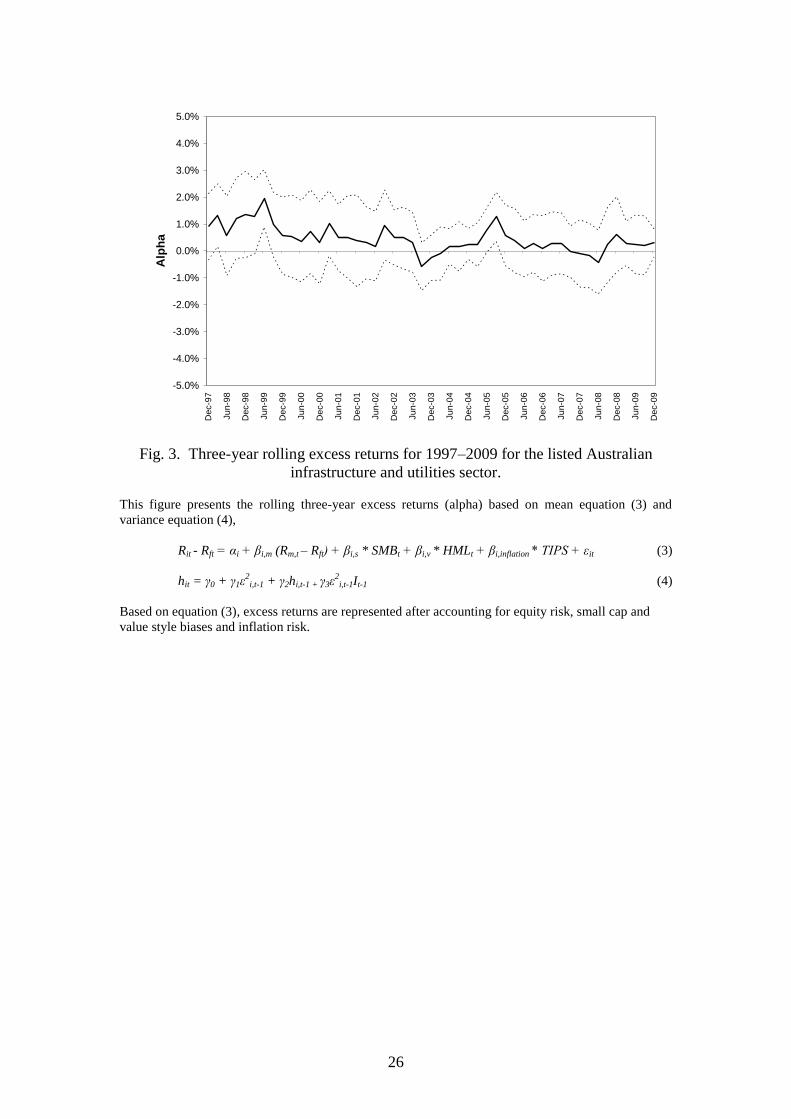
investment are on a declining trend. We show the trend in historical excess returns for

the direct investment using the rolling three-year alpha in Figure 3.

<< INSERT FIGURE 3 >>

10

It can be argued that over the period unique factors were at play in Australia (which were absent in

the US) which overstate the expected return that one can expect from direct investment. These include

a high concentration of highly geared listed infrastructure funds. In addition, for a period of time, assets

could be purchased at a discount from distressed state governments such as the state of Victoria. These

conditions may not occur again in the future, as a) the gearing level of infrastructure funds has reduced

and b) competition for the limited number of suitable projects domestically has increased.

19

Figure 3 suggests there has indeed been a reduction in excess returns generated by

Australian infrastructure and utilities in recent periods. Biais et al. (2009) demonstrate

how in equilibrium, after an initial period of success, an industry grows, attracting

human and financial capital, while rents of managers increase. This increase in rents

undermines the net returns obtained by investors and can eventually make incentives

so expensive that excessive risk taking prevails in the last part of the cycle. As noted

earlier, we observed this sequence of events to occur for Australian infrastructure

managers such as Macquarie Infrastructure Group and Babcock and Brown.

7.2. Risk characteristics of the synthetic asset

<< INSERT FIGURE 4 >>

Figure 4 shows the historical maximum drawdown charts for the US and Australian

direct investment compared to the synthetic asset. As can be seen the drawdown for

the synthetic asset is much less than it is for direct investment in both the US and

Australian markets. Thus, once again, the synthetic asset offers superior defensive

characteristics compared to the direct investment. As a final test of the robustness of

the synthetic asset compared to the direct investment in infrastructure we employ a

bootstrap to simulate both direct investment and synthetic asset returns. We measure

the defensive abilities of the direct investment and the synthetic asset under simulated

conditions. The results are shown in Table 8.

<< INSERT TABLE 8 >>

Table 8 indicates that the synthetic asset outperforms direct investment in both the US

and Australia in terms of VaR and Expected Shortfall over the simulated periods.

20

8. Conclusion

We confirm that excess returns exist in both US and Australian infrastructure

investment suggesting additional factors (e.g. a regulatory risk premium) have a role

to play in explaining the variation in infrastructure returns. In addition, we confirm

findings by Armann and Weisdorf (2008) and Martin (2010) that both US and

Australian infrastructure investments offer some inflation protection. However, we

find inflation hedging is limited to the utility sector, but not present in the non-utility

infrastructure sector. We compare the historically achieved excess return to the

required regulatory premium using a comparable option based model (Table 6). We

find that in the US, investors were better off investing in option based strategies. In

Australia, however, the historically achieved returns in the infrastructure sector

exceeded those from the option based strategy. In addition, we suggest how a

synthetic portfolio consisting of exchange traded covered calls and inflation linked

bond portfolios can offer comparable defensive and inflation hedging characteristics.

The returns to unlisted infrastructure could be further investigated. Bitsch et al.

(2010), based on a study of global unlisted infrastructure deals, suggest returns to be

highly correlated to equity markets.11

Yet, for Australian unlisted infrastructure we

find no sensitivity to the public equity markets at either the aggregate index level or

individual manager level. In addition, we expect indices on illiquid assets to embed

serial correlation. While we earlier explained that exposure to accrued income, foreign

exchange movements, listed assets and the DCF valuation methodology may create

noise around unit pricing, this topic can be further researched, subject to data

availability.

11

Furthermore, literature suggests that investments in unlisted firms, whether direct or through active

managers, underperform investments in listed firms, refer Nielsen (2011) and Phalippou (2009).

21

Finally, Bond et al. (2007) as well as Dechant and Finkenzeller (2011) suggest real

estate has superior defensive characteristics to infrastructure. At the same time Newell

and Peng (2007) find correlations between infrastructure and real estate have

increased over time, suggesting some of the unique diversification benefits of

infrastructure are disappearing. From an institutional investor’s perspective it will be

interesting to see if infrastructure can eventually replace real estate in overseas

institutional portfolios to the same extent as it has in Australia.

Appendix. Methods of investing in infrastructure

This appendix describes the methods of investing in infrastructure. Infrastructure

companies can be listed on the stock exchange or unlisted and traded in private

markets. Investments can be made by directly buying the listed companies/assets or

indirectly by investing through a fund. Infrastructure funds themselves can also be

either listed or unlisted. Source: Inderst (2009) and company websites.

Indirect investment Direct investment

Listed

markets

Indirect investment refers to

investment through fund managers

that invest in listed infrastructure

companies.

In Australia this has been

particularly popular with retail

investors who prefer the daily

liquidity.

An example of an unlisted

infrastructure fund manager that

invests in listed infrastructure

companies is RARE.

http://www.rareinfrastructure.com/

Direct investment refers to infrastructure

companies or funds listed on the stock

exchange.

Listed infrastructure companies (including

utilities) account for around 5% of the

global stock markets. An example of such

a company is AGL Energy.

http://www.agl.com.au/

Listed infrastructure funds invest in

unlisted assets. Listed infrastructure funds

are most common in Australia where they

account for 50% of the infrastructure and

utilities sector (which in itself represents

5% of the Australian market

capitalisation). An example of a listed

infrastructure fund over the period

investigated is Intoll (formerly Macquarie

Infrastructure Group, subsequently

restructured and acquired by the Canada

Pension Plan Investment Board).

http://www.intoll.com/

22

Unlisted

markets

Indirect investment in unlisted

assets has been popular for pension

funds in Australia, through

specialist fund managers which are

unlisted themselves, such as

Industry Funds Management

(IFM).

Investments for funds tend to be

concentrated in 10 to 15 large

investments.

http://www.industryfundsmanagem

ent.com/

Some of the bigger Canadian and Dutch

pension plans have started to invest

directly. They are often co-investors with

specialist funds, and thereby hope to build

up the internal expertise in-house over

time. For example, in Canada, the Ontario

Municipal Employees Retirement System

(OMERS) has invested in infrastructure

through its subsidiary Borealis

Infrastructure, set up in 1998.

http://www.borealis.ca

References

Armann, V. and Weisdorf, M.A., ‘Hedging inflation with infrastructure assets’, in Benaben, B., and S.

Goldenberg, Inflation Risks and Products: The Complete Guide, Risk Books, 2008, pp. 111-126.

Biais, B., Rochet, J.C., and Woolley, P., ‘Rents, learning and risk in the financial sector and other

innovative industries’, Working Paper (Paul Woolley Centre, Toulouse School of Economics,

2009).

Bitsch, F., Buchner, A., and Kaserer, C., ‘Risk, return and cash flow characteristics of infrastructure

fund investments’, EIB Papers, Vol. 15(1), 2010, pp. 106-136.

Bond, S.A., Hwang, S., Mitchell, P., and Stachell, S.E., ‘Will private equity and hedge funds replace

real estate in mixed-asset portfolios? Not likely’, Journal of Portfolio Management – Special Real

Estate Issue, Vol. 33, 2007, pp. 74-84.

Chan, K.C., Chen, C.R., and Lung, P.P., ‘Business cycles and net buying pressure in the S&P 500

futures options’, European Financial Management, Vol. 16(4), 2010, pp. 624-657.

Dechant, T., Finkenzeller, K., and Schäfers, W., ‘Infrastructure: a new dimension of real estate?’,

Journal of Property Investment and Finance, Vol. 28(4), 2010, pp. 263-274.

Dechant, T., and Finkenzeller, K., ‘Real estate or infrastructure? Evidence from conditional asset

allocation’, Working Paper (University of Regensburg, 2010).

DeFrancesco, A., Newell, G., and Peng, H.W., ‘The performance of unlisted infrastructure in

investment portfolios’, Journal of Property Research, Vol. 28(1), 2011, pp. 59-74.

Diamond, P., Shafir, E., and Tversky, A., ‘Money illusion’, Quarterly Journal of Economics, Vol.

112(2), 1997, pp. 341-374.

Dimasi, J., ‘Evaluating infrastructure reforms and regulation’, Working Paper (Australian Competition

and Consumer Commission, 2010).

Fama, E.F., and French, K.R., ‘Common risk factors in the returns on stocks and bonds’, Journal of

Financial Economics, Vol. 33(1), 1993, pp. 3–56.

Glosten, L.R., Jagannathan, R. and Runkle, D.E., ‘On the relation between the expected value and the

volatility of the nominal excess returns on stocks’, Journal of Finance, Vol. 48(5), 1993, pp. 1779-

1801.

Henisz, W.J., and Zelner, B.A., ‘Political risk and infrastructure Investment’, Working Paper (Wharton

School – University of Pennsylvania, 1999).

Inderst, G., ‘Pension fund investment in infrastructure’, Working Paper (OECD, 2009).

Martin, G.A., ‘The long horizon benefits of traditional and new real assets in the institutional portfolio’,

Journal of Alternative Investments, Vol. 13(1), 2010, pp. 6-29.

23

Newell, G., and Peng, H.W., ‘The significance of infrastructure in investment portfolios’, Pacific Rim

Real Estate Conference, Fremantle, 2007.

Newell, G., and Peng, H.W., ‘The role of U.S. infrastructure in investment portfolios’, Journal of Real

Estate Portfolio Management, Vol. 14(1), 2008, pp. 21-33.

Nielsen, K.M., ‘The return to direct investment in private firms: new evidence on the private equity

premium puzzle’, European Financial Management, Vol. 17(3), 2011, pp. 436-463.

Phalippou, L., ‘Beware of venturing into private equity’, Journal of Economic Perspectives, Vol. 23(1),

2009, pp. 147–166.

Treynor, J.L., and Mazuy, K., ‘Can mutual funds outguess the market?’, Harvard Business Review,

Vol. 44(4), 1966, pp. 131-136.

24

US infrastructure (1998-2009) US utilities (1995-2009)

Australian infrastructure (1995-2009) Australian utilities (1995-2009)

Fig. 1. Evidence of defensive abilities.

This figure presents an illustration of the defensive abilities of infrastructure and utilities under the

Treynor and Mazuy (1966) model as presented by mean equation (2), Rit - Rft = αi + βi,m (Rm,,t – Rft) +

βi,s * SMB t + βi,v * HMLt + βi,timing (Rmt - Rft)2 + εit. The figure plots the observed asset returns on the y-

axis versus the equity market returns on the x-axis at each point in time. The predicted outcome from

equation (2) is represented as the solid line. When equity market returns turn increasingly negative,

under Treynor and Mazuy a convex solid line is expected, i.e. the forecast asset returns should fall less

than the corresponding market returns.

-60.0%

-40.0%

-20.0%

0.0%

20.0%

40.0%

60.0%

-20.0% -15.0% -10.0% -5.0% 0.0% 5.0% 10.0% 15.0%

U.S. Equity Risk premium

U.S

. In

fra

str

uc

ture

pre

miu

m

-20.0%

-15.0%

-10.0%

-5.0%

0.0%

5.0%

10.0%

15.0%

-20.0% -15.0% -10.0% -5.0% 0.0% 5.0% 10.0% 15.0%

U.S. Equity Risk premium

U.S

. U

tili

ty p

rem

ium

-30.0%

-25.0%

-20.0%

-15.0%

-10.0%

-5.0%

0.0%

5.0%

10.0%

15.0%

20.0%

-20.0% -15.0% -10.0% -5.0% 0.0% 5.0% 10.0% 15.0%

Australian Equity Risk premium

Au

str

ali

an

Uti

lity

pre

miu

m

-30.0%

-25.0%

-20.0%

-15.0%

-10.0%

-5.0%

0.0%

5.0%

10.0%

15.0%

20.0%

-20.0% -15.0% -10.0% -5.0% 0.0% 5.0% 10.0% 15.0%

Australian Equity Risk premium

Au

str

ali

an

In

fra

str

uc

ture

pre

miu

m

25

Fig. 2. Modelling the regulatory risk premium.

This figure presents the payoff diagram of a regulated asset. The option collar reflects the impact of

government intervention on both the up and down side of an asset price and is established by buying a

protective put while writing an out-of-the-money covered call. The maximum profit is reached at the

strike price of the written call (the negotiated cap on the return on equity), while the maximum loss

occurs at the strike price of the bought put (the level at which the government is likely to buy back the

asset) if the asset is deemed to provide essential services to the community. The dotted line represents a

covered call strategy, while the solid line represents the covered call combined with the bought put

strategy. Chan et al. (2010) suggest the trading profits for selling options are higher during economic

contraction periods than during expansion periods.

Call options

Evidence indicates that investors in large infrastructure businesses with significant regulated energy or

utility activities require rates of return on equity (ROE) in the range of 10 to 15 per cent. For

infrastructure, if ROEmax is the maximum allowed regulatory ROE, this is translated into a monthly call

option sale with a strike price K equal to ROEmax/12 in the US or a quarterly option sale with a strike

price K equal to ROEmax/4 in Australia. For example, a 12 per cent limit on ROE is proxied as selling an

out of the money monthly call option with a 1 per cent (12 per cent divided by 12 months) premium.

We assume that in the long run, the ROE growth cap implies a profit growth limit, and thus a share

price growth limit. In general the share price growth (g) rate equals the retention rate (rr) on profits

times return on equity (ROE), or g = rr x ROE. Here we use total return indices with dividends

reinvested, or rr=1 in which case g = ROE (all profits are retained).

Put options

Put options are used to estimate the cost of government intervention after a decline in the asset value S

to a minimum floor Smin, as infrastructure offers essential community services. The intervention floor

Smin is translated into a monthly put option purchase with a strike price K equal to Smin/12 in the US or a

quarterly option purchase with a strike price K equal to Smin/4 in Australia.

Asset price at expiration ($)

Profit ($)

Covered call

Collar

Put strike

Call strike

26

Fig. 3. Three-year rolling excess returns for 1997–2009 for the listed Australian

infrastructure and utilities sector.

This figure presents the rolling three-year excess returns (alpha) based on mean equation (3) and

variance equation (4),

Rit - Rft = αi + βi,m (Rm,t – Rft) + βi,s * SMBt + βi,v * HMLt + βi,inflation * TIPS + εit (3)

hit = γ0 + γ1ε2

i,t-1 + γ2hi,t-1 + γ3ε2i,t-1It-1 (4)

Based on equation (3), excess returns are represented after accounting for equity risk, small cap and

value style biases and inflation risk.

-5.0%

-4.0%

-3.0%

-2.0%

-1.0%

0.0%

1.0%

2.0%

3.0%

4.0%

5.0%

Dec-9

7

Ju

n-9

8

Dec-9

8

Ju

n-9

9

Dec-9

9

Ju

n-0

0

Dec-0

0

Ju

n-0

1

Dec-0

1

Ju

n-0

2

Dec-0

2

Ju

n-0

3

Dec-0

3

Ju

n-0

4

Dec-0

4

Ju

n-0

5

Dec-0

5

Ju

n-0

6

Dec-0

6

Ju

n-0

7

Dec-0

7

Ju

n-0

8

Dec-0

8

Ju

n-0

9

Dec-0

9

Alp

ha

27

US - direct investment Australia - direct investment

US - synthetic asset Australia - synthetic asset

Fig. 4. Maximum drawdown experience for direct investment compared to synthetic

asset (1998–2009).

This figure presents out-of-sample drawdown charts, defined as the percentage loss that an asset incurs

from its peak value to its lowest subsequent value. For example, an asset that halves in value before

returning to its subsequent peak is deemed to have a maximum drawdown of 50 per cent. Drawdown

charts are used to measure an asset’s defensive ability.

-60%

-50%

-40%

-30%

-20%

-10%

0%

12/3

1/19

94

10/3

1/95

08/3

0/96

06/3

0/97

04/3

0/98

02/2

6/99

12/3

1/99

10/3

1/00

08/3

1/01

06/2

8/02

04/3

0/03

02/2

7/04

12/3

1/04

10/3

1/05

08/3

1/06

06/2

9/07

04/3

0/08

02/2

7/09

12/3

1/09

-60%

-50%

-40%

-30%

-20%

-10%

0%

12/3

1/97

08/3

1/98

04/3

0/99

12/3

1/99

08/3

1/00

04/3

0/01

12/3

1/01

08/3

0/02

04/3

0/03

12/3

1/03

08/3

1/04

04/2

9/05

12/3

0/05

08/3

1/06

04/3

0/07

12/3

1/07

08/2

9/08

04/3

0/09

12/3

1/09

-60%

-50%

-40%

-30%

-20%

-10%

0%

12/3

1/97

08/3

1/98

04/3

0/99

12/3

1/99

08/3

1/00

04/3

0/01

12/3

1/01

08/3

0/02

04/3

0/03

12/3

1/03

08/3

1/04

04/2

9/05

12/3

0/05

08/3

1/06

04/3

0/07

12/3

1/07

08/2

9/08

04/3

0/09

12/3

1/09

-60%

-50%

-40%

-30%

-20%

-10%

0%

12/3

1/97

08/3

1/98

04/3

0/99

12/3

1/99

08/3

1/00

04/3

0/01

12/3

1/01

08/3

0/02

04/3

0/03

12/3

1/03

08/3

1/04

04/2

9/05

12/3

0/05

08/3

1/06

04/3

0/07

12/3

1/07

08/2

9/08

04/3

0/09

12/3

1/09

28

Table 1

Overview of UBS infrastructure indices (monthly data is provided)

This table presents relevant sub-indices of the UBS global infrastructure and utilities index, which

covers over 200 stocks, with a 40 per cent weight to the U.S., 40 per cent to Europe and 20 per cent to

Asia. Ninety per cent of the UBS global index comprises utility companies. Given the available data

history and index constituents, we focus on the US and Australian sub-indices

As at December 2009, the US infrastructure and utilities index contained 89 companies with a total

market capitalisation of US$526.2 bn. The US index comprises 94 per cent utilities and has little pure

(non-utility) infrastructure such as privatised communications, airports or toll roads. As such US

subsectors are not provided by UBS. The number of US infrastructure stocks in the UBS index is

limited to only three, all in the communication sector.

As at December 2009, The Australian index covered 15 companies with a combined value of A$50.5

bn. The ratio of infrastructure stocks to utility stocks has declined to 37 per cent from a peak of 50 per

cent following the default and restructuring of infrastructure stocks such as Macquarie Infrastructure

Group and Babcock & Brown after the Global Financial Crisis. For Australia, there is a concentration

risk: the top three stocks (Origin, AGL and Transurban) account for 61 per cent of the combined index.

Index Date started Description

U.S. market (in USD)

Infrastructure and

utilities

Jan 1990 Combined infrastructure (6 per cent) and utilities (94 per cent)

Infrastructure (1)

Aug 1998 Concession, lease or freehold for transportation and

communication

Utilities Jan 1990 Power generation, transmission and distribution

– Power generation Jan 2000 Involved in generation of electricity, including hydro and

renewable sources.

– Transmission /

Distribution

Jan 2000 Utility businesses exposed to transmission and distribution

assets (e.g. electricity transmission towers, pipelines,

distribution networks

– Integrated Utilities Jan 2000 Vertically integrated electricity/gas companies

Australian market (in AUD)

Infrastructure and

utilities

Jan 1995 Combined infrastructure (37 per cent) and utilities (63 per

cent)

Infrastructure Jan 1995 Concession, lease or freehold for transportation and

communication

– Airports April 1997 Revenue from collection of aircraft landing fees, terminal fees

and revenue from airport retail, property and parking

– Communication Feb 2003 Revenue from communication usage fees (e.g. broadcast,

mobile towers, satellites, fibre optics)

– Toll Roads Jan 1995 Revenue from collection of tolls

Utilities Jan 1995 Power generation, transmission and distribution

– Integrated Utilities Jan 1995 Vertically integrated electricity/gas companies

– Power generation Jan 1995 Involved in generation of electricity, including renewable

water.

– Transmission /

Distribution

Jan 1997 Utility businesses exposed to transmission and distribution

assets (e.g. electricity transmission towers, pipelines,

distribution networks

.

29

Table 2

Descriptive statistics of the infrastructure industry (1995-2009)

This table presents descriptive statistics of the industry based on monthly data from January 1995, or since inception date, to December 2009 (a total of 180 observations).

The data represents log returns in USD for the US or AUD for Australia based on the UBS indices described in Table 1. The total return is annualised by multiplying monthly

results by 12. Excess returns are calculated against the three-month risk free rate (the 90 day US Treasury or Australian Bank Bill rate). The standard deviation is annualised

by multiplying the monthly standard deviation by the square root of 12. Best month represents the month with the highest monthly return. Worst month represents the month

with the lowest monthly return. Beta is measured by calculating the slope of the strategy returns against the S&P 500 or ASX 300 index. Skew and kurtosis represent the

skew and kurtosis of the monthly returns. Liquidity refers to the first order serial correlation of the monthly returns. Data for U.S. listed infrastructure is available from

August 1998 onwards.

U.S. (in USD) total return (%pa)

excess return (%pa)

standard deviation

(%pa)

best month (%)

worst month (%)

beta skew kurtosis liquidity

Listed infrastructure and utilities 7.9 4.3 16.1 13.5 -14.0 0.49 -0.67 0.92 0.13

Listed infrastructure 4.0 1.0 57.1 50.8 -53.8 1.82 -0.47 2.83 -0.09

Listed utilities 7.9 4.3 16.2 12.4 -14.0 0.57 -0.67 0.91 0.12

Australia (in AUD) total return (%pa)

excess return (%pa)

standard deviation

(%pa)

best month (%)

worst month (%)

beta skew kurtosis liquidity

Listed Infrastructure and utilities 16.2 10.5 15.2 13.5 -13.0 0.63 -1.10 2.92 0.16

Listed infrastructure 16.3 10.6 48.4 17.4 -24.6 0.67 -0.73 3.02 0.04

Listed utilities 17.3 11.6 15.8 20.9 -10.4 0.56 0.25 1.97 -0.03

Unlisted infrastructure and utilities 12.1 6.4 6.1 8.9 -2.4 0.06 1.94 5.19 0.00

30

Table 3

Estimation of Augmented Fama French-GARCH model for monthly infrastructure fund returns, 1995-2009

This table presents the estimation of the augmented Fama-French GJR-GARCH model based on mean equation (1) and variance equation (4) applied to historical monthly

data for 1995–2009 (total of 180 observations). In the mean equation, the dependent variable (Rit - Rft) represents the excess return of infrastructure strategy i at times t and is

regressed on the equity risk premium (Rm – Rft), the small cap premium (SMB) and the value premium (HML). Returns are net of fees in USD for the US market and in AUD

for the Australian market. In the variance equation, the fitted value of the conditional variance of strategy i (hit) depends on the squared error of the previous period (ε2

i,t-1), the

variance of the previous period (hi,t-1) and the leverage effect (ε2

i,t-1It-1). * significant at the 10 per cent level ** significant at the 5 per cent level *** significant at the 1 per

cent level ^ data available from August 1998 onwards.

Model

Rit - Rft = αi + βi,m (Rm,t – Rft) + βi,s * SMB t + βi,v * HMLt + εit

hit = γ0 + γ1ε2i,t-1 + γ2hi,t-1 + γ3ε

2i,t-1It-1

U.S.

Listed

Infrastructure^

U.S.

Listed

Utilities

U.S.

Listed

Infrastructure and Utilities

Australian

Listed

Infrastructure

Australian Listed

Utilities

Australian Listed

Infrastructure and

Utilities

Australian Unlisted

Infrastructure and Utilities

α

βm

βs

βv

γ0

γ1 (ARCH)

γ2 (GARCH)

γ3

γ1 + γ2 + 0.5 γ3

t-dist errors

Adj R2

Log Likelihood

0.0103**

1.3579***

0.6356***

-0.5805***

0.0002**

-0.0837

0.8950***

0.2372

0.9299

6.2353**

0.3405

125.45

0.0024

0.4723***

-0.0660

0.2653***

0.0014***

0.4184*

-0.0884

-0.4220

0.1199

13.0713

0.2518

329.21

0.0025

0.4825***

-0.0655

0.2619***

0.0014***

0.4178

-0.0591

-0.4219

0.1477

12.3898

0.2605

330.56

0.0060*

0.6669***

0.2261*

0.3712**

0.0023

-0.0827

0.2862

0.3993

0.4031

3.5431***

0.1833

273.22

0.0064**

0.5734***

0.2092***

0.1623

0.0010

-0.0379

0.4030

-0.0845

0.3228

19.7185

0.2240

329.91

0.0061**

0.6266***

0.2157**

0.4199***

0.0000

0.1014

0.9138***

-0.1108

0.9598

10.3755

0.3261

348.96

0.0042**

0.0771*

-0.0323

0.0649

0.0001***

-0.0525***

0.5041***

0.0463

0.4747

19.9963

0.0105

490.77

31

Table 4

Estimation of Augmented Treynor-Mazuy-GARCH model for monthly infrastructure fund returns, 1995-2009

This table presents the Treynor and Mazuy (market timing) model based on mean equation (2) and variance equation (4) applied to historical monthly data for 1995–

2009 (total of 180 observations). The variables are as defined for Table 3 with a market timing factor (Rmt - Rft)2. * significant at the 10 per cent level ** significant at the

5 per cent level *** significant at the 1 per cent level ^ data available from August 1998 onwards.

Model

Rit - Rft = αi + βi,m (Rm,,t – Rft) + βi,s * SMB t + βi,v * HMLt + βi,timing (Rmt - Rft)2 + εit

hit = γ0 + γ1ε2i,t-1 + γ2hi,t-1 + γ3ε

2i,t-1It-1

U.S. Listed

Infrastructure^

U.S. Listed

Utilities

U.S. Listed

Infrastructure and

Utilities

Australian Listed

Infrastructure

Australian Listed Utilities

Australian Listed Infrastructure and

Utilities

Australian Unlisted Infrastructure and Utilities

α

βm

βs

βv

βtiming

γ0

γ1 (ARCH)

γ2 (GARCH)

γ3

γ1 + γ2 + 0.5 γ3

t-dist errors

Adj R2

Log Likelihood

0.0099

1.3693***

0.6338**

-0.5825***

0.2233

0.0002*

-0.0845

0.8956***

0.2370

0.9296

6.2508**

0.3362

125.46

0.0020

0.4603***

-0.0746

0.1887***

-0.7882

0.0021***

0.2819

-0.3570

-0.2876

-0.2189

22.3839

0.2548

329.67

0.0056

0.4478***

-0.1023

0.2552***

-1.4990**

0.0012***

0.4289

0.0320

-0.4277

0.2470

10.3255

0.2632

331.95

0.0069

0.6552***

0.2114

0.3735**

-0.5654

0.0023

-0.0887

0.2728

0.3898

0.3790

3.6343**

0.1819

273.27

0.0046

0.6094***

0.2265**

0.1425

1.6028

0.0010

-0.0438***

0.4015

-0.0756***

0.3199

19.6198

0.2255

330.33

0.0051

0.6446***

0.2080**

0.3816***

0.3796

0.0014

-0.0793

-0.1017

0.0657

-0.1481

10.7132

0.3227

347.13

0.0041***

0.0673*

-0.0474

0.0778

-0.2969

0.0001

-0.0532***

0.5019

0.0185

0.4579

19.9938

0.0023

491.38

32

Table 5

Estimation of inflation hedging model for monthly infrastructure fund returns, 1995-2009

This table presents estimation results for the inflation hedging model of infrastructure investment returns based on mean equation (3) and variance equation (4) applied to

historical monthly data for 1995–2009 (total of 180 observations). The variables are as defined for Table 3. In addition, in the mean equation, an inflation hedging factor TIPS

is added. * significant at the 10 per cent level ** significant at the 5 per cent level *** significant at the 1 per cent level ^ data available from August 1998 onwards.

Model

Rit - Rft = αi + βi,m (Rm,t – Rft) + βi,s * SMB t + βi,v * HMLt + βi,inflation * TIPS + εit

hit = γ0 + γ1ε2

i,t-1 + γ2hi,t-1 + γ3ε2i,t-1It-1

U.S.

Listed Infrastructure^

U.S.

Listed Utilities

U.S.

Listed Infrastructure and

Utilities

Australian

Listed Infrastructure^^

Australian Listed

Utilities

Australian Listed Infrastructure

and Utilities

Australian Unlisted

Infrastructure and Utilities

α

βm

βs

βv

βinflation

γ0

γ1 (ARCH)

γ2 (GARCH)

γ3

γ1 + γ2 + 0.5 γ3

t-dist errors

Adj R2

Log Likelihood

0.0101*

1.3368***

0.6566***

-0.5812***

0.1306

0.0002*

-0.0836

0.8950***

0.2365

0.9296

6.3184***

0.3329

125.52

0.0020

0.4654***

-0.0702

0.2579***

0.4007**

0.0012***

0.4478

-0.0097

-0.4460

0.2151

11.4158

0.2636

331.77

0.0021

0.4740***

-0.0698

0.2558***

0.4062***

0.0012***

0.4509

0.0341

-0.4485

0.2675

10.5438

0.2727

333.28

0.0033

0.9950***

0.1853**

0.1355

-0.2441

0.0001

0.0598

0.8497***

0.1671

0.9930

3.6450***

0.4684

325.27

0.0069**

0.5560***

0.1955*

0.2092

0.2666

0.0011

-0.0254

0.4870

-0.1296

0.3968

19.9298

0.2287

327.79

0.0055**

0.5971***

0.2548***

0.4109***

0.5731***

0.0000

0.1259

0.8970***

-0.1298

0.9580

10.7616

0.3539

354.14

0.0041***

0.0848**

-0.0366

0.0751

-0.0028

0.0001

-0.0545

0.5025

0.0388

0.4673

19.9954

0.0044

490.20

33

Table 6

Comparison of returns to regulated versus unregulated assets (January 1995 – December 2009)

This table presents a comparison of a direct investment into infrastructure and utilities to option models. Log returns are based on monthly data from January 1995 to

December 2009 in USD or AUD (total of 180 observations). Risk is annualised by multiplying monthly standard deviation by the square root of 12. Reward to risk is

calculated by dividing return by risk. Winning months represents the number of months that returns were positive. Skew and kurtosis represent the skew and kurtosis of the

monthly returns. Best month represents the month with the highest monthly return. Worst month represents the month with the lowest monthly return. Beta is measured by

calculating the slope of the strategy returns against the equity markets (the S&P 500 or ASX 300). ROE cap in row 10 represents the cap on earnings growth and impacts the

covered call strike level. Regulatory premium in rows 12 to 14 measures the difference in returns between the equity market return and the covered call strategy, without

assumed government intervention (no floor), and with government intervention after a 75 per cent and a 50 per cent share price decline.

Panel A: US markets Panel B: Australian markets

A B C D E F G H A B C D E F G H

Covered call – monthly strike level (%) Covered call – quarterly strike level (%)

Infra & Utilities 0.83 0.92 1.00 1.08 1.17 1.25

S&P 500

Infra & Utilities 2.50 2.75 3.00 3.25 3.50 3.75

ASX 300

1 Return (%pa) 7.9 9.4 9.5 9.6 9.7 9.8 9.9 7.7 16.2 13.9 14.0 14.1 14.2 14.3 14.3 10.2

2 Risk (%pa) 16.1 11.0 11.1 11.2 11.3 11.4 11.4 16.0 15.2 9.0 9.1 9.3 9.4 9.6 9.7 13.0

3 Reward to risk 0.5 0.9 0.9 0.9 0.9 0.9 0.9 0.5 1.1 1.5 1.5 1.5 1.5 1.5 1.5 0.8

4 Winning months (%) 62 74 73 73 73 73 73 64 65 88 88 87 87 87 87 66

5 Skew -0.7 -2.1 -2.1 -2.1 -2.1 -2.0 -2.0 -1.0 -1.1 -2.2 -2.2 -2.1 -2.1 -2.0 -2.0 -1.0

6 Kurtosis 0.9 6.6 6.4 6.2 6.1 6.0 5.8 1.7 2.9 5.3 5.1 4.9 4.7 4.5 4.3 1.7

7 Best month (%) 13.5 5.2 5.2 5.3 5.3 5.4 5.4 9.3 13.5 9.1 9.3 9.4 9.6 9.7 9.8 7.8

8 Worst month (%) -14.0 -16.3 -16.3 -16.3 -16.4 -16.4 -16.4 -18.4 -13.0 -14.9 -15.0 -15.1 -15.2 -15.3 -15.4 -13.8

9 Beta to equity market 0.5 0.6 0.6 0.6 0.6 0.7 0.7 1.0 0.6 0.6 0.6 0.7 0.7 0.7 0.7 1.0

10 ROE cap (%pa) 10.0 11.0 12.0 13.0 14.0 15.0 10.0 11.0 12.0 13.0 14.0 15.0

11 Regulatory premium (% pa)

12 No floor 1.6 1.7 1.9 2.0 2.1 2.2 3.6 3.8 3.9 3.9 4.0 4.1

13 75 % floor 1.1 1.2 1.3 1.4 1.5 1.6 3.2 3.3 3.4 3.5 3.6 3.7

14 50% floor 0.7 0.9 1.0 1.1 1.2 1.3 2.6 2.8 2.9 2.9 3.0 3.1

34

Table 7

Comparison of returns on direct infrastructure investment and synthetic asset

This table presents a comparison of the characteristics of a direct infrastructure investment versus replication using exchange traded instruments comprising covered calls

and inflation linked bonds. Out-of-sample returns are based on monthly data from January 1998 to December 2009 in USD or AUD (total of 144 observations). Risk is

annualised by multiplying monthly standard deviation by the square root of 12. Reward to risk is calculated by dividing return by risk. Winning months represents the

number of months that returns were positive. Skew and kurtosis represent the skew and kurtosis of the monthly returns. Best month represents the month with the highest

monthly return. Worst month represents the month with the lowest monthly return. Beta to the stock market is measured by calculating the slope of the strategy returns

against the S&P 500 or ASX 300 total return index. Beta to inflation measures the slope against the inflation linked bond total return index.

U.S. Infrastructure

and Utilities

Replicator Australian

Infrastructure and Utilities

Australian unlisted

Infrastructure and Utilities

Replicator

Return (%pa) 5.0 6.6 Return (%pa) 12.3 11.4 9.1

Risk (%pa) 17.1 6.7 Risk (%pa) 15.2 6.1 6.0

Reward to risk 0.3 1.0 Reward to risk 0.8 1.9 1.5

Wining months 61% 74% Wining months 64% 78% 76%

Skew -0.6 -2.4 Skew -0.1 2.1 -1.2

Kurtosis 0.6 14.7 Kurtosis 1.0 6.1 3.6

Best month (%) 12.2 6.8 Best month (%) 13.5 8.9 4.8

Worst month (%) -14.0 -12.3 Worst month (%) -13.0 -2.4 -7.2

Beta to S&P 500 0.5 0.3 Beta to ASX 300 0.6 0.1 0.3

Beta to inflation 0.5 0.7 Beta to inflation 0.5 0.1 0.5

35

Table 8

Defensive abilities of direct investment compared to synthetic asset under simulated

conditions

This table presents a comparison of the downside risk. 1,000 runs of 12 annual returns are created for

both the direct investment and the synthetic asset by using resampling with replacement from the

monthly historical data (total of 180 observations), to create a total of 144,000 simulated data points

(1,000 runs x 12 years x 12 months). Monthly Value at Risk (VaR) and Expected Shortfall (ES) are

then calculated under simulated conditions. Value at Risk refers to the percentile threshold which is not

expected to be exceeded in more than 5 per cent of the cases. Expected shortfall measures the average

of all observations below the 5th percentile.

US market Australian market

VaR ES VaR ES

Direct Investment Mean (%) -7.6 -11.2 -6.1 -8.3

Standard deviation (%) 1.5 1.3 0.6 1.0

Synthetic asset Mean (%) -2.5 -5.3 -2.2 -3.7

Standard deviation (%) 0.7 1.3 0.5 0.6