initial-boundary value problems for an extensible beam
TRANSCRIPT

JOURNAL OF MATHEMATICAL ANALYSIS AND APPLICATIONS 42, 61-90 (1973)
Initial-Boundary Value Problems for an Extensible Beam
J. M. BALL*
School of Applied Sciences, University of Sussex, Brighton, England
Submitted by Peter D. Lax
1. INTRODUCTION
In this paper we discuss certain initial-boundary value problems for the nonlinear beam equation
where the constants OL and k are positive. Equation (1.1) was proposed by Woinowsky-Krieger [28] as a model for
the transverse deflection U(X, t) of an extensible beam of natural length I whose ends are held a fixed distance apart. The nonlinear term represents the change in the tension of the beam due to its extensibility. The model has also been discussed by Eisley [13], while related experimental results have been given by Burgreen [6].
Dickey [lo] recently considered the initial-boundary value problem for (1.1) in the case when the ends of the beam are hinged, so that
u(0, t) = u(Z, t) = uzz(O, t) = u& t) = 0. U-2)
The initial deflection us(x) and the initial velocity z+(x) of each point x of the beam are assumed given. Dickey showed how the model affords a description of the phenomenon of “dynamic buckling.” Assuming a Gale&in expansion for the deflection at time t, he was then able to prove, using a compactness argument, that the resulting infinite system of ordinary differential equations has a unique solution for all time. Dickey has also studied [ll] the system of ordinary differential equations corresponding to the case 01 = 0. Equation (1.1) then represents a vibrating string and for certain problems of this kind exact solutions are known (Oplinger [22]).
* Present address: Heriot-Watt University, Edinburgh, Scotland.
61 Copyright 0 1973 by Academic Press, Inc. All rights of reproduction in any form reserved.
62 BALL
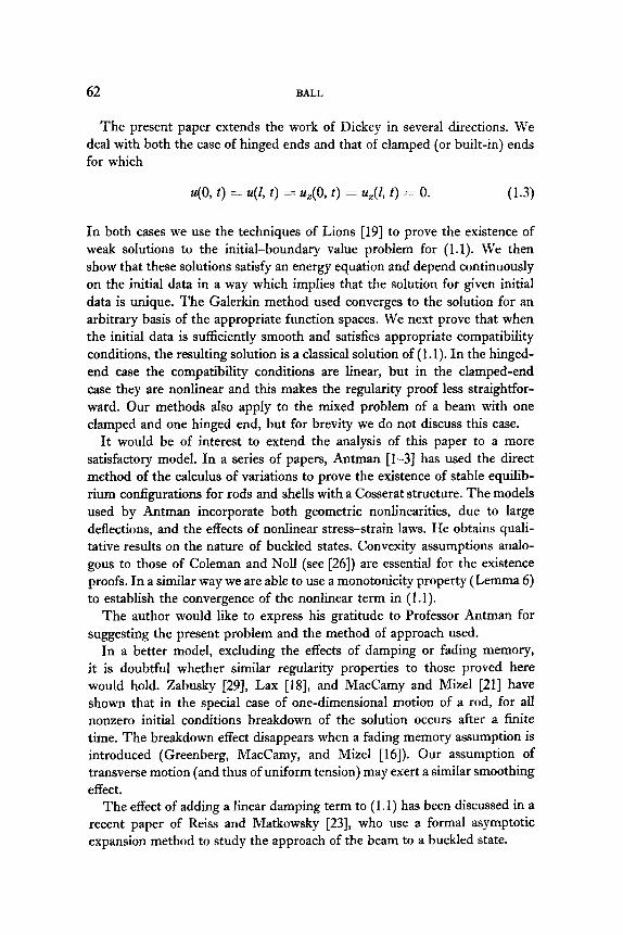
The present paper extends the work of Dickey in several directions. We deal with both the case of hinged ends and that of clamped (or built-in) ends for which
u(0, f) = u(2, t) = z&(0, f) = z&(2, t) = 0. (1.3)
In both cases we use the techniques of Lions [19] to prove the existence of weak solutions to the initial-boundary value problem for (1.1). We then show that these solutions satisfy an energy equation and depend continuously on the initial data in a way which implies that the solution for given initial data is unique. The Galerkin method used converges to the solution for an arbitrary basis of the appropriate function spaces. We next prove that when the initial data is sufficiently smooth and satisfies appropriate compatibility conditions, the resulting solution is a classical solution of (1 .l). In the hinged- end case the compatibility conditions are linear, but in the clamped-end case they are nonlinear and this makes the regularity proof less straightfor- ward. Our methods also apply to the mixed problem of a beam with one clamped and one hinged end, but for brevity we do not discuss this case.
It would be of interest to extend the analysis of this paper to a more satisfactory model. In a series of papers, Antman [l-3] has used the direct method of the calculus of variations to prove the existence of stable equilib- rium configurations for rods and shells with a Cosserat structure. The models used by Antman incorporate both geometric nonlinearities, due to large deflections, and the effects of nonlinear stress-strain laws. He obtains quali- tative results on the nature of buckled states. Convexity assumptions analo- gous to those of Coleman and No11 (see [26]) are essential for the existence proofs. In a similar way we are able to use a monotonicity property (Lemma 6) to establish the convergence of the nonlinear term in (1.1).
The author would like to express his gratitude to Professor Antman for suggesting the present problem and the method of approach used.
In a better model, excluding the effects of damping or fading memory, it is doubtful whether similar regularity properties to those proved here would hold. Zabusky [29], Lax [18], and MacCamy and Mizel [21] have shown that in the special case of one-dimensional motion of a rod, for all nonzero initial conditions breakdown of the solution occurs after a finite time. The breakdown effect disappears when a fading memory assumption is introduced (Greenberg, MacCamy, and Mizel [16]). Our assumption of transverse motion (and thus of uniform tension) may exert a similar smoothing effect.
The effect of adding a linear damping term to (1.1) has been discussed in a recent paper of Reiss and Matkowsky [23], who use a formal asymptotic expansion method to study the approach of the beam to a buckled state.
INITIAL-BOUNDARY VALUE PROBLEMS 63
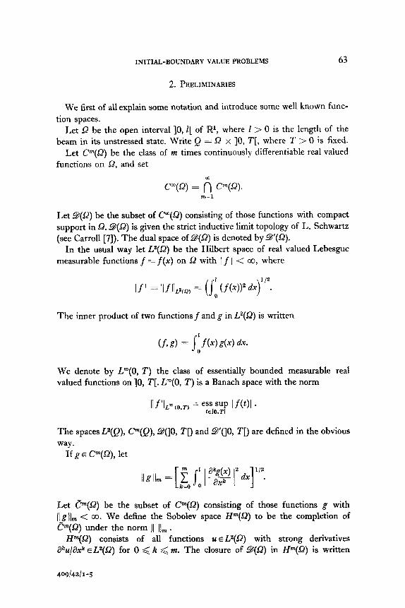
2. PRELIMINARIES
We first of all explain some notation and introduce some well known func- tion spaces.
Let Q be the open interval 10, I[ of IF, where I > 0 is the length of the beam in its unstressed state. Write Q = 52 x 10, T[, where T > 0 is fixed.
Let Cm(Q) be the class of m times continuously differentiable real valued functions on 52, and set
C”(Q) = fi Cy2). VZ=l
Let 9(G) be the subset of P(sZ) consisting of those functions with compact support in 52.9(G) is g iven the strict inductive limit topology of L. Schwartz (see Carroll [7]). The dual space of S(J2) is denoted by 9(G).
In the usual way let P(G) be the Hilbert space of real valued Lebesgue measurable functions f = f(x) on G with / f 1 < co, where
If I = llfllp,*, = (11 (f(x))” q2.
The inner product of two functions f and g in L2(@ is written
(f, g> = p4 g&4 dx*
We denote by L”(0, T) the class of essentially bounded measurable real valued functions on IO, T[. L”(0, T) is a Banach space with the norm
The spaces L”(Q), Cm(Q), 9(]0, T[) and 9’(]0, T[) are defined in the obvious way.
If g E Cm@), let
II B I/m = [F. I2 1 qg I2 dx] 1/z- = 0
Let &(Q) be the subset of Cm(G) consisting of those functions g with ]\g]lrn < CO. We define the Sobolev space H”(G) to be the completion of @(G!) under the norm )I IJm.
Z?(Q) consists of all functions u EP(SZ) with strong derivatives @~/ax” EP(G) for 0 < K < m. The closure of 9(s2) in P(G) is written
409/42/I-5
64 BALL
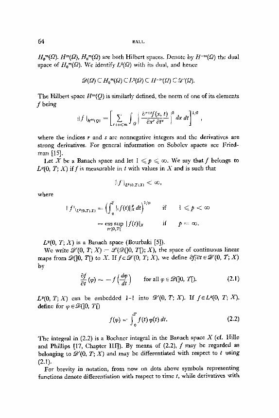
f&“(Q). fw4, ffoyq are both Hilbert spaces. Denote by H-“(Q) the dual space of Z&,m(sZ). We identifyL”(Q) with its dual, and hence
9(Q) c H,“(Q) c l?(l2) c fP(Q) c Lqq.
The Hilbert space f-i”(Q) is similarly defined, the norm of one of its elements f being
where the indices r and s are nonnegative integers and the derivatives are strong derivatives. For general information on Sobolev spaces see Fried- man [15].
Let X be a Banach space and let 1 < p < co. We say that f belongs to Lp(O, T; X) if f. IS measurable in t with values in X and is such that
where
ilf ii L”(O,T:XJ -=c a,
i’f II L*(O.T;x) = if 1 <p-COO
LP(0, T; X) is a Banach space (Bourbaki [5]). We write 9’(0, T; X) = S(9?(]0, T[); X), the space of continuous linear
maps from 9(]0, T[) to X. If f e9’(0, T; X), we define af/at E~‘(O, T, X)
by
$P) = -r(g) for all q E 9(]0, T[). (2.1)
LP(O, T; X) can be embedded 1-l into 9’(0, T; X). If f~Lp(0, T; X), define for 9 ~9(]0, T[)
f(v) = j$&) fit. (2.2)
The integral in (2.2) is a Bochner integral in the Banach space X (cf. Hille and Phillips [17, Chapter III]). By means of (2.2), f may be regarded as belonging to 69’(0, T, X) and may be differentiated with respect to t using (2.1).
For brevity in notation, from now on dots above symbols representing functions denote differentiation with respect to time t, while derivatives with

INITIAL-BOUNDARY VALUE PROBLEMS 65
respect to distance x along the beam are written P%/axm = ~(~1. Constants are frequently denoted by C, their dependence on relevant parameters being mentioned where necessary.
3. THE MODEL
Consider an extensible beam whose ends are held at x = 0 and x = 1+ d. Let H be the axial force set up in the beam when it is constrained to lie along the x-axis. The model for the deflection u(x, t) which we discuss is
ii + w(4) - (/3 + k ) u(l) I”) u(2) = 0, (3.1)
where a = EIjp, /3 = H/p, k = EA,I2pl, and H = EAAll, where E is the Young’s modulus, I the cross-sectional second moment of area, p the density and A, the cross-sectional area. We adopt the convention that if H is positive it represents a tensile force. Clearly 01 > 0 and k > 0; these conditions are essential for the proofs which follow.
The initial conditions are
u(x, 0) = u&x), (3.2a)
ti(x, 0) = q(x). (3.2b)
In Section 4 we consider the boundary conditions corresponding to hinged ends
u(0, t> = u(Z, t) = u’“‘(0, t) = u’yz, t) = 0, (3.3)
while in Section 5 we consider the boundary conditions corresponding to clamped ends,
u(0, t) = u(l, t> = u’l’(0, t) = u”‘(l, t) = 0. (3.4)
All the solutions whose existence we prove satisfy the energy equation
( zi I2 + a 1 u(*) I2 + ,f3 1 u(l) I2 + (k/2) I u(l) I4 = h, (3.5)
where
(3.6)
Consider the functional
G(u) = E ,

66 BALL
where u is subject either to (3.3) or (3.4) an d is supposed to be twice continu- ously differentiable in x. Then it is well known (Courant-Hilbert [9]) that G(U) attains its minimum value, which is rr2/la in the case (3.3) and 41r2,/12 in the case (3.4).
Denote by H,,it. the classical Euler buckling load of the beam.
Hcrit,, = - EIT’/~’ for hinged ends, (3.8a) while
H wit. = - 4Eh2/12 for clamped ends. (3.8b)
Then it is clear that if H 3 Hcrit, then h >, 0, while if H < Hcrlt. then there are initial conditions which allow h to be positive, negative, or zero.
The case h < 0 corresponds to motion about a buckled state, for 1 u(l) ] cannot be zero in this case.
4. HINGED ENDS
In this section we establish the existence of weak solutions of the equation (3.1) subject to the initial conditions (3.2) and the boundary conditions (3.3). We prove that the weak solutions are unique, satisfy the energy equation (3.5) and depend continuously on the initial data. We then prove that when the initial data is smooth enough and satisfies certain compatibility conditions the solution is a classical one. Precise meanings to the terms “weak solution” and “classical solution” are given in the statements of the theorems. As general references we cite Lions [19, pp. I-261 and Sather [24], where the method is applied to a nonlinear hyperbolic equation. The results of this section include those of Dickey.
Define
(i) Definitions and Preliminary Lemmas
S, = {y E fW-4 I y, yc2’, Y4’ +z f&V-4>,
& = { y E H4(Q) I y, Y (2) E ffc’(Q)h S, = Ho1(f2) n H2(Q).
S,, and S, are easily seen to be complete subspaces of the Hilbert spaces H6(Q) and H4(J2) respectively.
LEMMA 1. Let f E HI(B) and suppose f (4) = 0 for som 6 E a.
Then
Ifl <waf”‘I. (4.1)

INITIAL-BOUNDARY VALUE PROBLEMS 67
Proof. By the Sobolev embedding theorem (see Friedman [15, p. 30]), f can be regarded as belonging to CO(a) and hence f (0 = 0 has a meaning. Suppose f E Cl(a). Then
f(x) = p’(S) ds for x E Q.
so
(f(x))” = (l;f”‘(s) ds)’ < / j-r I2 ds ( j [I (f ‘l’(s))” ds / .
Therefore
/ f 1” < ,: 1 x - 6 1 dx 1 f”’ j2 < ; 1 f (‘) 12.
For a general f E s(Q), (4.1) follows by an approximation argument. 0
By a basis of a Banach space X, we mean a set of linearly independent elements of X whose finite linear combinations are dense in X.
LEMMA 2. s, = sin(nrrx/l), n = 1, 2 ,..., is a basis of the spaces S,, , S, , S, and L2(Q).
Proof. That {sn} is a basis of L2(sZ) is well known. Suppose s E So and let E > 0 be given. As s ~3) eL2(Q), there exist IV, a, ,..., aN such that
Let
1 ~(6) - il a,s, I2 < E.
944 = - il 4 (&)” ~$4
so that I(s - q~)(~) I2 < c. By the Sobolev embedding theorem, s belongs to C6(@, and so by Rolle’s theorem there exist 4i E 0 such that
(s - qy’ (&) = 0, O,<i<5.
Lemma 1 now implies that
i. I(s - q)‘~’ (2 < ce.
Hence {s,,} is a basis of So; similarly {s,} is a basis of S, and of S, . 0

68 BALL
LEMMA 3 (Gronwall). Suppose f~L”(0, T) and that K > 0, C, are constants. If
f(t) < Co + K J “f(s) ds 0
for all t E [0, T] then
f(t) < COeKt.
Proof. See Carroll [7, p. 1241. c]
LEMMA 4. Suppose X and Y are Hilbert spaces or separable Banach spaces with dual spaces X’ and Y’. Suppose Y is continuously and densely embedded in x. If
u, + u in Lm(O, T; X’) weak* and
42 - x in L”(0, T; Y’) weak*, then
x=ti in L”(0, T; Y’).
Proof. The assumptions on X imply that L”(0, T; X’) is the dual space of Ll(0, T; X) (see Bochner and Taylor [4] and DieudonnC [12]) and that
I’ u (t) k(t)) dt - s’ u(t) (g(O) dt for all g E L1(O, T; X). 0 0
Thus for a11 x E X, q~ E 9(]0, T[)
Hence
1’ @b,(t) (4 dt - j-= v(t>uW (4 dt. 0 0
%(dW-fU(~)(~)
(using (2.2)) and so
Similarly, ti,(q~) ( y) -+ x(q) (y) for all y E Y and v E .9(]0, T[). Thus ti(v) = x(q) in Y’ for all q~ E~(]O, T[) and the result follows. 0
LEMMA 5. Let X be a Banach space. If f E L*(O, T; X) and f E L*(O, T; X), then f, possibly after redejnition on a set of measure zero, is continuous from [0, T] --f X. Indeed, for almost all s, t E [0, T],
f(t) -f(s) = I:'&) da.

INITIAL-BOUNDARY VALUE PROBLEMS 69
Proof. See Wilcox [27, Theorem 2.21. A similar lemma, due to Lions, is proved in Carroll [7, p. 1761. 0
The next lemma establishes a monotonicity property for the nonlinear term in (3.1).
LEMMA 6. If u, v E S, then
(I u (1' 12 u(2) - 1 21(1) 12 v(2) u - v) < 0.
Proof.
(I uu) 12 u(2) _ 1 v(1) 12.792) u _ 7,q
rT.z 1 u(l) 12 ((u(l), zjm) - 1 u(l) I") + ) v(l) 12 ((u(l), v(l)) - j v(l) I")
< 1 u(l) 12 (I u(l)
= - (I u(l) 1 -
1 VW 1 - I u(l) I”) + 1 v(l) 12 (I u(l) 1 1 v(l) 1 - 1 v(l) 12)
v(l) I) (I u(l) 13 - 1 v(l) I”) < 0. 0
(ii) Weak Solutions
we establish the existence of a weak solution to the In this subsection initial-boundary value problem (3.1)-(3.3). The solution need not satisfy the boundary conditions ~‘~‘(0, t) = ~(~‘(1, t) = 0 in any classical sense, although we shall show later (Theorem 4) that it does do so if u0 and u1 are smooth enough and if
2$)(O) = Q(Z) = 241(O) = u,(Z) = 0.
THEOREM 1. If uO E S, , u1 E L2(L?), then there exists u = u(x, t) with
u EL”(O, T; S,),
ti EL”(O, T; L2(sZ)),
such that u satisjes the initial conditions (3.2) and the equation (3.1) in the sense that
(ii, v) + a(~(~), c#~‘) - (18 + k I u(l) 2 / ) (uc2), 9’) = 0 for all v E S, . (4.2)
Proof.
Approximating solutions. Let (wj} be a basis of S, . If
u,(t) = f &n(t> wi i=l
70 BALL
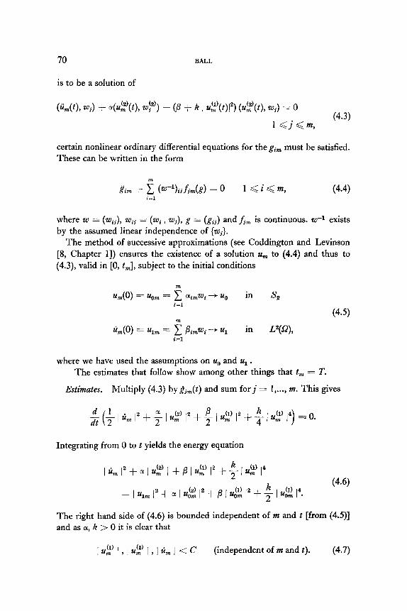
is to be a solution of
(ii,(t), Wj) + a@:‘(t), wj2)) - (J3 + k / u$(t)l*) @2’(t), Wj) = 0
1 <j<m, (4.3)
certain nonlinear ordinary differential equations for the gi, must be satisfied. These can be written in the form
L?im + ,El (w-‘>ijh9n(.!?> = O 1 <i<m, (4-4)
where w = (w,), wij = (wi , wj), g = (gij) andfj, is continuous. we1 exists by the assumed linear independence of {Wj}.
The method of successive approximations (see Coddington and Levinson [8, Chapter I]) ensures the existence of a solution U, to (4.4) and thus to (4.3), valid in [0, t,], subject to the initial conditions
U,(O) = Uom = iI OLimWi -+ U. in Ss
km(O) = Ulm = f pi,Wi ---f 241 in L2(Q), i=l
where we have used the assumptions on z+, and u1 . The estimates that follow show among other things that t, = T.
Estimates. Multiply (4.3) by ii,(t) and sum for j = I,..., m. This gives
Integrating from 0 to t yields the energy equation
The right hand side of (4.6) is bounded independent of m and t [from (4.91 and as 01, k > 0 it is clear that
1 ui’ 1 , j 242) I>l%nl <c (independent of m and t). (4.7)

INITIAL-BOUNDARY VALUE PROBLEMS 71
Convergence. The estimates just derived, together with Lemma 1, show that
04nl is bounded in L”(O, T; S,),
%J is bounded in L”(O, T; W4), and
{I 242’ 12 u$‘) is bounded in L”(0, T; L2(sZ)).
In particular, {u,} is bounded in Hi(Q). Furthermore, the injection W(Q) -L2(Q) is compact by the Rellich-Kondrachoff theorem (Lions and Magenes [20, p. 1 lo]). Thus, using the classical diagonal procedure, we may extract a subsequence (~3 of {u,} with the properties
uu + u in L”(0, T; S,) weak*,
lii,-+V in L”(0, T; L*(Q)) weak*,
u, + w in L”(Q) strongly and a.e., (43) and
(1) 2 (2) I %I I 44 -x in L”(0, T; L2(i2)).
Lemma 4 implies that zi = v. As u, + u in L2(Q) weak* it follows that u = w. The next step is to show that
x = ( 11(1) 12u(2) (4-9)
To this end let v eL2(0, T; S,). From Lemma 6 it follows that
I 1 (I UF’ 12 24:’ - ] v(l) 12 d2), uu - v) dt < 0.
But
As p + co, the first integral on the right hand side converges to s,‘(x, u) dt, while the second integral tends to zero since uU + u in L2(Q) strongly.
Hence as
I 1 (I v(l) I2 d2), II, - v) dt + /: (I v(1) 12 v(2), u - v) dt,
it follows that
I v(l) I2 d2), u - v) dt < 0.
72 BALL
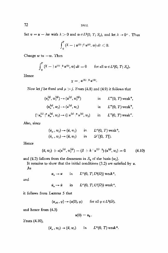
Set v = u - hw with h > 0 and w E L2(0, T; S,), and let h -+ Of. Thus
s =(X-I u(l) I2 d2’, w) dt .< 0. 0
Change w to -w. Then
f 1 (X - 1 u(l) I2 d2), w) dt = 0 for all w E L*(O, T; S,).
Hence x = 1 u(1) 12 u(2),
Now let j be fixed and p > j. From (4.8) and (4.9) it follows that
(@, wyi”‘) -+ (u (2), 49 in L”(0, T) weak*,
(4% Wj) -+ (zi2), Wj) in L”(0, T) weak*,
(I u:’ I2 u:‘, wj) -+ (I u(l) I2 uc2), wi) in L”(0, T) weak*.
Also, since
(%I ) wj> - (4 wj> in L”(0, T) weak*,
(4 , wj) + (ii, wj) in WQ TD. Hence
(ii, Wj) + ,11(24(‘), Wp)) - (p + k 1 L!(l) I”) (Ut2), Wj) = 0 (4.10)
and (4.2) follows from the denseness in S, of the basis {wj>. It remains to show that the initial conditions (3.2) are satisfied by u. As
u, + u in Lm(O, T; L2(Q)) weak*,
and ti,--+li in L”(0, T; L*(Q)) weak*,
it follows from Lemma 5 that
@,o 7 9’) - MO)> d for all 9) E L2(9),
and hence from (4.5) u(0) = f40 .
From (4.10),
(ii, , wj) -+ (ii, wj) in L”(0, T) weak*.

INITIAL-BOUNDARY VALUE PROBLEMS 13
Thus from Lemma 5 with X = R,
(f&(O), 4 - w% 4. But
and so
(4(o), w,.) - (Ul 14
Ii(O) = 111 . 0
Remark. We sketch another proof of the convergence of the nonlinear term, following that of Dickey, and using the special form of the term. For v E U(0, T, L2(Q)) we have that
f : (x - ) u(l) I2 zP), cp) dt
= s
1 (x - 1 I$’ 1’ uf’, v) dt + s: 1 u(l) 1’ (u?’ - uc2), p) dt
But
+ j: (I ut’ I2 - 1 u(l) I”) (u;! cp) dt.
<c I u, - u 1 dt --+ 0.
The other integrals also tend to zero and the arbitrariness of p implies that
x zrz 1 u(l) 12 u(2).
(iii) Dependence on Initial Conditions
Next we show that the solution u in Theorem 1 satisfies the energy equa- tion (34, and that u depends continuously on the initial data u,, and u1 . In particular we prove that u is unique. The following lemma is a special case of Lemma 8.3, p. 298 of Lions and Magenes [20], originally due to Strauss [25]. We omit the proof, which relies on an intricate regularization procedure.
LEMMA 7. Let V be continuously and densely embedded in L2(sZ) and let V’ be the dual of V so that V C L2(Q) C VI’. If 9 E V define Aa+ E P’ by

74 BALL
AZ+(p) = ct(4(2), v’“)) for p E 1; So that A2 E Y(V, V’). Suppose w E L”(0, T, V), ti E L”(0, T; L*(Q)) and that w satisfies the equation
ti + A% =f,
and the initial conditions w(0) = w,, , G(O) = wl . Suppose w,, E Fr, w1 E L2(Q) and f~ L2(0, T; L2(Q)). Then for all t E [0, T],
1 zi(t)12 + a 1 wt2)(t)(2 = j w1 12 + a I wp 2 I + 2 j: (f, G) da. (4.11)
THEOREM 2. Suppose u, v are two solutions of (4.2) with
u, v ELrn(O, I’; S,),
zi, ti E L”(0, T; LZ(Q)),
and suppose that u, v satisfy the initial conditions
u(O) = uo , C(O) = u1 ) $0) = vo , d(O) = q ,
with u. , v. E S, and u1 , vl gL2(Q). Let w = u - v. Then
) ti(t)12 + a 1 w(‘)(t)12 < [I u1 - vl j2 + 01 I ut’ - vt’ I”] exp(Kt), (4.12)
where K is a continuous function of I uh2’ j , I u, I , j vr) I and I v, I .
Proof. We apply Lemma 7 with V = S, , w. = u, - v, , w1 = u1 - vl and
f(t) = (/3 + h ( u”‘(t)~“) zP’(t) - (/3 + k j v’l’(t)l2) v’*)(t).
It is clear that f E L2(0, T; L2(Q)) and we conclude that
1 ti(t)l” + a: 1 w(2)(t)l2 = I u1 - v1 I2 + (Y 1 u:’ - vt’ I2 + 2 jt (f, ti) du. 0
(4.13) But
f(u) = (/3 + h j u”‘(u)l”) w@)(u) + h(I u”‘(u)l” - ( v’“(u)I”) .(2’(u)
= (j3 + h 1 u”‘(u)l”) w(2)(u) - h(u(0) + v(u), W”‘(U)) vyu>
and hence
12 j: (f, 4 da 1 < C j: I ~(~‘(4l I +4 du
,( & jt (I ti(u)12 A- a I W(a’(~>12) da. 0
(4.12) now follows from (4.13) and Lemma 3.
INITIAL-BOUNDARY VALUEPROBLEMS 75
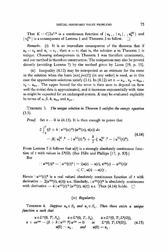
That K = C/2cA2 is a continuous function of 1 111 ) , 1 w, j , 1 ur’ j and 1 wf’ 1 is a consequence of Lemma 1 and Theorem 3 to follow. 0
Remarks. (i) It is an immediate consequence of the theorem that if u,, = o0 and ul = a, , then u = V; that is, the solution u in Theorem 1 is unique. Choosing subsequences in Theorem 1 was therefore unnecessary, and our method is therefore constructive. The uniqueness may also be proved directly (avoiding Lemma 7) by the method given by Lions [19, p. 151.
(ii) Inequality (4.12) may be interpreted as an estimate for the error in the solution when the basis {sin(jn,/Z)} (in any order) is used, as in this case the approximate solutions satisfy (3.1). In (4.12) set w = U, , w0 = u,,,,, , w, = Ulrn . The upper bound for the error is then seen to depend on how well the initial data is approximated, and it increases exponentially with time as might be expected for an undamped system. K may be evaluated explicitly in terms of 01, /3, k, uorn and ulm .
THEOREM 3. The unique solution in Theorem 1 satisfies the energy equation (3.5).
Proof. Set w = 0 in (4.13). It is then enough to prove that
d1’(a)12) (zP’(u), ti(u)) da
= )a(1 24:’ I2 - j P(Q12) + f (I uy I4 - I U’qt)14). (4.14)
From Lemma 5 it follows that u(t) is a strongly absolutely continuous func- tion of t with values in L2(Q). (See Hille and Phillips [17, p. 831.)
But
) 1 uys)l2 - 1 dl)(t)l2 / = I(u(s) - u(t), zP)(s) - u’2’(t))l
< c j u(s) - u(t)1 .
Hence j G(t)12 is a real valued absolutely continuous function of t with derivative - 2(u’2)(t), C(t)) a.e. Similarly, 1 uc1)(t)14 is absolutely continuous with derivative - 4 ( u(1)(t)[2 (u(2)(t), C(t)) a.e. Thus (4.14) holds. c]
(iv) Regularify
THEOREM 4. Suppose I+, E S, and u1 E S, . Then there exists a unique function u such that
u ELrn(O, T, S,), ri EP(0, T; S,), ii E L”(0, T; L2(!2)), ii -+ d4) - (/3 + k 1 u(l) 1”) uf2) = 0 in Lm(O, T;L2(Q), (4.15)
40) = %.I , and Ii(O) = u1 .

76 BALL
Proof. The proof closely follows that of Theorem 1.
Approximating solutions. We use the basis {sj) = {sin(j?rJv/I)) of S, . (See Lemma 2). The approximating solutions urn are of the form
um(t) = f gim(t) si (4.16) i=l
and satisfy the equation
ii, + cm: - (/3 + R 124:’ I”) 242’ = 0 . (4.17)
in [0, tm] subject to the initial conditions
u,JO) = uo,n -+ u. in S,
&n(O) = %l - 111 in s (4.18)
2’
Estimates. The basic energy estimate (4.7) holds as before, and shows that t, = T. It follows from (4.17) and (4.18) that
) tim( < c. (4.19)
Now differentiate (4.17) with respect to t and take the inner product with . . II,, to obtain
3 (d/&) (I ii, I2 + a / d2) I”) = (pi$’ + R / 242’ [* zi$) + 2K(& ti$‘) *Z’, ii,)
< (I B I + ,Jz I &’ I”> Id! I I %I I
+ 2k ) u2’ / 1 z$’ 1 1 UE’ ( 1 ii, 1 .
By Lemma 1 and (4.7)
(d/m) (I ii, I2 + 01 I ti$’ I”) < c ) tiy / ( ii, ]
< & (I &n I2 + 01 I d? I”>.
It follows from (4.19) and Lemma 3 that
( ii, j ,I ti$ j < c (independent of m and t). (4.20)
As OL > 0, (4.17) yields the bound
124:’ j < c. (4.21)
Convergence. Using the estimates just derived, Lemma 1 and the methods

INITIAL-BOUNDARY VALUE PROBLEMS 77
of Theorem 1, it is easy to show the existence of a subsequence (u,> of {uUm} such that
and
in L”(0, T; S,) weak*,
in L”(0, T; S,) weak*,
in L”(0, T; L2(!2)) weak*,
in P(Q) strongly and a.e.,
j uf’ I2 u$’ + 1 u(l) I2 u(‘) in L”‘(0, T; S,) weak*.
These convergence properties establish the theorem. The proof parallels exactly that of Theorem 1. u is unique by Theorem 2. iJ
Remark. By the Sobolev embedding theorem, u,, and u(t) are equivalent to functions in C”(a) and, therefore, (Friedman [ 15, p. 391) satisfy the hinged- end boundary conditions (3.3). Similarly ~(0, t) = u(Z, t) = 0 for all t E [0, T]. The embedding theorem also shows that u E CO(Q).
The next theorem establishes that under certain conditions u is a classical solution; that is u E C4@) x C2([0, T]) and satisfies (3.1)-(3.3). By putting x = 0, I and t = 0 in (3.1) it is clear that necessary conditions for the existence of a classical solution are the “compatibility conditions” uh4’(0) = u?‘(E) = 0. Roughly speaking, the theorem says that these condi- tions are sufficient.
THEOREM 5. Let u. E So and u1 E S, . Then
u EL”(O, T; So), ti E Lm(O, T; S,), ii EL”(O, T; S,), (4.22)
ii EL=‘(O, T; L2(Q)) and u E Cl(Q) n [C5(@ x C2([0, TJ)].
Proof. As in Theorem 4 we use the basis (sj) of So. The approximating solutions u, are of the form (4.16) and satisfy (4.17) in [O, t,] subject to the initial conditions
Urn(O) = Uom - uo in S 09 z&(O) = ulm -+ u1 in S, .
The bounds (4.7), (4.20) and (4.21) hold and show that t, = T. Taking the inner product of (4.17) with zi$(t) leads to
) (djdt) (1 ~2:’ I2 + 01 1 u,$’ 1”) = (/3 + k 1 ~(2’ I’) (u:‘, 6:;‘)
< C(l ti$ I2 + 01 [ 242’ I”).
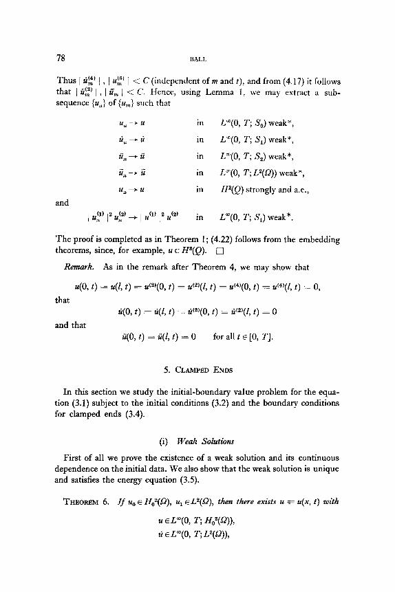
78 BALL
Thus 1 tic4’ / 1 , ~2’ 1 < C (independent of m and t), and from (4.17) it follows that j ti$ [ , 1 zi:, 1 < C. Hence, using Lemma 1, we may extract a sub- sequence {u,,> of {urn} such that
and
u, + u in L”(0, T; S,,) weak*,
li, - li in L”(0, T; S,) weak*,
ii, - ii in L”(0, T; S,) weak*,
ii,+ ii in L”(0, T; L2(sZ)) weak*,
u,+u in P(Q) strongly and a.e.,
(1) 2 (2) 1% I %L -I u
(1) 2 (2) I u
in L”(0, T; A’,) weak*.
The proof is completed as in Theorem 1; (4.22) follows from the embedding theorems, since, for example, u E P(Q). 0
Remark. As in the remark after Theorem 4, we may show that
u(0, t) = u(l, t) = zP’(0, t) = uyz, t) = uyo, t) = uy1, t) = 0,
that
and that
qo, t) = ti(l, t) = tiyo, t) = zql, t) = 0
ii(0, t) = qz, t) = 0 for all t E [0, TJ.
5. CLAMPED ENDS
In this section we study the initial-boundary value problem for the equa- tion (3.1) subject to the initial conditions (3.2) and the boundary conditions for clamped ends (3.4).
(i) Weak Solutions
First of all we prove the existence of a weak solution and its continuous dependence on the initial data. We also show that the weak solution is unique and satisfies the energy equation (3.5).
THEOREM 6. If u0 E l&,2(Q), ul EL*(Q), then there exists u = u(x, t) with
11 EP(0, T; H,2(Q)),
22 E L”(0, T; L2(9)),
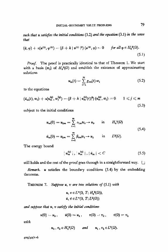
INITIAL-BOUNDARY VALUE PROBLEMS 79
such that u satisfies the initial conditions (3.2) and the equation (3.1) in the sense that
(ii, cp) + c+(2), $2’) - (j? + k 1 u(l) I”) (u(2), lp) = 0 for azzp E H,2(Q).
(5.1)
Proof. The proof is practically identical to that of Theorem 1. We start with a basis {Us} of Ha2(Q) and establish the existence of approximating solutions
%l(t> = f gimw wi (5.2) i-l
to the equations
(i&(t), Wj) + a@~‘, wl”‘) - @ + k 1 u$(t)l2) (u?‘, Wj) = 0 1 <j<m
subject to the initial conditions
u,(O) = uom = 5 %lPi+~o in i=l
in The energy bound
(5.3)
Ho2(QR)
(5.4)
L2(Q).
(5.5)
still holds and the rest of the proof goes through in a straightforward way. 0
Remark. u satisfies the boundary conditions (3.4) by the embedding theorems.
THEOREM 7. Suppose u, w are two soZution.s of (5.1) with
u, v EL=‘(O, T; Ho2(sZ)),
22, d ELyO, T; L2(Q))
and suppose that u, v satisfy the initial conditions
u(O) = uo 3 $0) = ill , 40) = 00 , $0) = 01
with
uo , ~0 E Ho2G’) and u, 3 “1 EL2(-Q).
409/4211-6
80 BALL
Set w = u - ZI. Then
j ti(t)12 + 01 1 w(2’(t)/2 < [I u1 - @I I2 + o! / uI;” -- e$) I’] exp(li;t) (5.6)
where KI is a continuous function of j uf) 1 , 1 u1 1 , 1 $) 1 and 1 z’~ j .
Proof. The proof runs parallel to that of Theorem 2. In applying Lem- ma 7 we set V == Hs2(Q). q
Remark. Setting u,, = z’s and ui = z’~ in (5.6) demonstrates the uniqueness of the weak solution in Theorem 6. The Galerkin method is therefore constructive. A direct proof of uniqueness can again be given following [19, p. 151.
THEOREM 8. The unique solution in Theorem 6 satisjies the energy equation.
Proof. Identical to that of Theorem 3. c]
(ii) Smoother Solutions
This subsection contains a lemma and a preliminary regularity result. Let X be the Hilbert space Hss(Q) n H*(Q).
LEMMA 8. There are constants Ci such that for all f E X,
/f(i) 1 < ci / f’i”’ 1 i = 0, 1,2, 3.
Proof. By the embedding theorems and Rolle’s theorem, there exists f1 , 0 < [i < I with f u)(ei) = 0. Therefore there exist [s, & , 0 < 52 < t1 -=c f, -=c I with f 12)(E2) = f (“‘(6) = 0, and there exists t4, 0 < 6, < f4 < 5s < I with f (“‘(5,) = 0. The result now follows from Lemma 1.
THEOREM 9. If u0 E X, u1 E H,,z(Q) then there exists a unique function u z u(x, t) with
u ELrn(O, T; X),
ti EL”(O, T; H,,2(Q)),
ii E L”(0, T; L2(sZ)),
such that u satisfies the initial conditions (3.2) and the equation
ii + ~(4) - (fi + k I u(1) 12) uf2) = 0 in L”(0, T;L2(SZ)). (5.7)

INITIAL-BOUNDARY VALUE PROBLEMS 81
Proof. Let {q} be a basis of X. The approximating solutions u, are of the form (5.2) and satisfy (5.3), and the initial conditions
and z&(O) = u,,1- Ul in hV=9.
{u,} satisfies the bounds (5.5). Multiply (5.3) by &JO) and sum for j = l,..., m. Thus
I tim( = l(d!J - (B + k I u!?tb I”) dz , Kn(O>)l f c I &(O>l * Thus
I %7Gol < c. (5.8)
Now differentiate (5.3) with respect to t to obtain
(5, Wj) + oi(zif$ wj2)) (5.9
= /qzi%‘, Wj) + 42(u$, zii') (u?', Wj) + 1 u$ I2 (zi$', Wj)].
Multiply (5.9) by j&,(t) and sum for j = l,..., nz. It follows that
From (5.8) and Lemma 3 we deduce the bounds
I ii, I , / 62) I < c. (5.10)
In the usual way follows the existence of u with
u EP(O, T; Ho2(Q)),
and such that
zi EL='(O, T; Ho2(G')), ii eLm(O, T; L2(Q)),
(ii, w) + Lx(zP), w(2)) - (p + k ( u(l) I”) (u(2), w) = 0 foralloEX. (5.11)
It remains to show that u eLm(O, T; X). But from (5.11), for almost all t and for all w E X, ol(uf2), vc2)) eLm(O, T).

82 BALL
Hence, for almost all t, u satisfies (3.1) and so utJ) EL~(O, T; L2(sZ)). Lemma 8 now shows that u EL”(O, T; X). 0
(iii) Regularity and an Associated Linear Equation
If u E P(Q) x P([O, T]), and if u satisfies (3.1), (3.2) and (3.4), then we call u a classical solution of the initial-boundary value problem. Setting t = 0, x = 0, I in (3. l), we see that necessary conditions for a classical solution are that
,-@ - (p + h j 21:) 1”) u:’ = a~$) - (p + h Iu~’ I’) ut’ = 0 at x = 0,l.
(5.12)
To obtain a result in the other direction is less straightforward than in the hinged-end case. This is due to the nonlinearity of the compatibility condi- tions (5.12). In the hinged-end case (see Theorem 5), functions u satisfying the boundary and compatibility conditions belonged to the linear space S,, . Each approximating solution u, then automatically satisfied the boundary and compatibility conditions, and it was possible to obtain convergence to a classical solution in suitable Banach spaces. Functions u,, satisfying (5.12), however, do not form a linear space, and the method of Theorem 5 is inappli- cable.
To overcome this problem we first consider an associated linear equation for which it is possible to obtain a classical solution using the Galerkin method. The following theorem is a statement of this result.
THEOREM 10. Let f be a continuous real valued function on [0, TJ such that
f,f&Lm(O, T). (5.13) Let I+, E I+?$) with
u. = 24:’ = m$’ -f(O) up) = CU@ - f(0) uf’ = 0
where OL > 0. Let
at x = 0, 1,
(5.14)
241 E x = H&2) n H4(Q).
Then there exists a unique function y = y(x, t) with
y E L”(0, T; H,*(Q) n lP(Q)), j E L”(0, T; X), ji E L”(0, T; H,,*(Q)), 9 EL~(O, T; L*(Q)),
y E Cl(Q) n [C5(@ x C*(P, TJ)l,
(5.15)

INITIAL-BOUNDARY VALUE PROBLEMS 83
such that y satisfies the linear equation
y + cty’4’ -f(t) y’2’ = 0 (5.16)
and the initial conditions
Y(O) = no Y j(0) = u1 . (5.17)
Remarks. (i) The conditions (5.14) are well defined by the embedding theorems.
(ii) (5.16) is the equation for the deflection of a beam with time varying axial force proportional to f(t). Th eorem 10 relates the smoothness of the deflection to the smoothness off.
The proof of Theorem 10 needs several preliminary results, which are given in the next subsection.
(iv) A Special Basis for the Galerkin Method
LEMMA 9. Let
Y = f (0)/a*
Conside the ordinary differential equation Lw = Aw subject to the boundary conditions w = w(l) = 0 at x = 0 and x = 1, where
Then
Lw f w3(4) - p’2’.
(i) There exist an in.nity of eigenvalues hi whose absolute values are unbounded and for which zero is not an accumulation point.
(ii) To each e@envalue hi corresponds a unique normalized eigenfunction wi . For convenience, enumerate the &. so that 0 < ) XI 1 < 1 X, 1 < **’ . Zero (= b) may be an eigenvalue, in which case let w. be the corresponding non- trivial eigenfunction.
(iii) The normalixed eigenfunctions wi form a basis of L2(9). Any g E L2(sZ) can be expanded in a series g(x) = xi (wi ,g) wi(x), convergence holding in L2Q-2).
Proof. The lemma is a well known consequence of the theory of Green’s functions and compact operators. See Coddington and Levinson [8, Chap- ter 71, Courant and Hilbert [9], and Everitt [14]. The uniqueness of wi is easy to prove but unnecessary for our purposes. q
LEMMA 10. Let M be the subspace of L2(sZ) generated by w. if X = 0 is an

84 BALL
eigenvalue of L, and be empty otherwise. Let 123~ be the orthogonal complement of M in L2(Q). Then for ally E ML n X,
IYi ~/~,I-‘Iw.
Proof. From Lemma 9, y = xr=, a,w, in L*(Q), where a, = (y, w,). Since Ly E MI, Ly = Cyz”=, b,w, inL2(Q), where b, = (Ly, w,.) = hrar . By Parseval’s relation,
1 Ly I2 = F A:aF, ly12= f a:. 7=1 r=l
The result follows. [7
LEMMA 11. J’or aZZyEMLnX, ly(“‘( <CiLyI.
Proof.
1 y’2’ 12 = (y’4’, y) = (Y4’ - d2’, Y) + Y(Y'2', Y) < 1 y’*’ - yy2’ I I y I + I y I I y@’ I I Al 1-l I Y'"' - YY2’ 1 < c I y(2) I ) y'"' - yy'2' 1 .
Hence 1 y’2’ / < c / y(4) - $2) 1 .
Now
I y'4' 12 = (yC"),y'4' - yy'2') + y(y'4',y'2')
< / y'4' 1 ly'4' - yy'2' 1 + c I y'"' I 1 y'4' - YY'*' I * Hence
Let
ly’4’ 1 < c jy’4’ - yyf2’ 1 . 0
Y = (y E fP(Q) 1 y, y’l’, y’l’ - yy’2’, y’5’ - yy’3’ E H&J)),
which is a closed subspace of H6(SZ) and hence is a Hilbert space. The main result of this subsection is
THEOREM 11. (wj} is a basis of X and of Y.
Proof. (a) We first prove that (wi} is a basis of X. Let v E X and suppose E > 0. Then v = v0 + v1 , where v0 = 0 or pw, and vr E Ml n X. Since Lv, E Ml, there exists a finite linear combination Z of the wi (i = 1, 2,...) such that 1 Lq - Z 1 < E. By replacing w, by wjIXj we may write Z = LZI , where ZI is another finite linear combination of the wi . By Lemmas 10 and 11, II v, - ZI IIx < CE. Hence II ZI - (ZI + vO)llx < CE.

INITIAL-BOUNDARY VALUE PROBLEMS 85
(b) To prove that {wJ is a basis of Y, first suppose that x E Y n H8(Q). Then x = x0 + x1, where x0 = 0 or pwo and x1 E ML n Y n HE(Q). Given E > 0, there exists a linear combination 2s of the wi (i = 1, 2,...) such that 1 L2(x1 - Za)\ < E. Since L(xI - Z2) E AI-!- n X, by Lemma 11 it follows that 1 L(xi4’ - ZA4’)I < CE. Using the relations
(Xl - z21 b+4) = qxy - @) + y(Xf+2) - g-2)) r = 1,2, 3,4,
it is easy to prove that
II x1 - 4 &p(Q) < CL Thus
II x - (5 + XONfp(P, < G
showing that (wi} is a basis of Y n H8(Q). Suppose now that y E Y. There exist {yr} E Y n H*(Q) such that
11 yr - y l/r -+ 0. Given E > 0, choose r such that jl y,. - y (jr < 42 and a linear combination Z of the wi such that 11 y,. - Zllr < 42. Then IIy - Zllr < E. Thus {wj} is a basis of Y. 0
Note. (wj} is not an orthogonal basis of X or Y.
(v) Proof of Theorem 10
Approximating solutions. We use the basis {wi} of X and Y discussed in the last subsection. The approximating solutions ym are of the form
y&) = 2 &n(t) wi i-l
and satisfy in [0, t,,J
(jim(t) + aY2(t) -f (t)Y2)(t)9 wj) = O 1 <j<m (5.18)
and the initial conditions
y&9 = ho -+ u. in Y, j,(O) = yml + ul in X.
From the assumptions on f it follows that
jL, , Y,,, EL”‘@, T; Y). (5.19)
Estimates. Since
4 Cd’4 (I 9, I2 + 01 I Y? I’) = f (t) (Y?, j,n) < I f(t)1 I &’ I I j, I ,

86 BALL
from Lemma 3 follow the energy bounds
(5.20)
Differentiate (5.18) with respect to t to obtain
(La(O + d7w -f(t)&‘(t) -j(t)y!?%), Wj) = 0. (5.21)
The bounds
IjimI,IP~‘I cc (5.22)
follow in the same way as (5.10). Next differentiate (5.21) with respect to t to obtain
(j;,(t) + 4$?(t) -f(t)j&t) - 2f(t)j?‘(t) -f(t)y2’(t), w,) = 0. (5.23)
Since j& and j;, eLm(O, T; Y) it follows from Lemma 5 that 1 jQt)ls and 1 jE)(t)j2 are absolutely continuous functions of t with-,-derivatives 2( ym(t), j%(t)) and 2(Y%), jt?(t)) a.e. . Multiplying (5.23) by hSm and summing for j = I,..., m thus gives
Q (44 (I %I I2 + 01 I A? I21
= (f@>YL? + mbt’ +m YE ji,)
< I %I I (I f(t)1 IA? I + 2 I f(t)1 I df’ I + I J(t)1 I Y2 I)
,< C(1 + I jzn I2 + a I je 12).
Hence if we can show that I j;,(O)1 and ( j;:)(O)1 are uniformly bounded, it will follow that
l.Y?J,Iji?I-G (5.24)
But from (5.21),
I %(0)12 = I(EY2 -f(mJ~; -f(O)& , j;,(O))I
and consequently
I %&(0)I < c.
To show that 1 j$?(O)l < C we use the properties of the basis {Wj}. From (5.18) we deduce that

INITIAL-BOUNDARY VALUE PROBLEMS 87
and that
(ji,(O) + gJ% -f(O) Yzl , Y% - %Y%> = 0. (5.26)
Add (5.25) to LY x (5.26) and use the fact thatf(0) = a~. Then
I ji,(O) + ~Yzl -f(O) y$ I2 = 0. Hence
j m (0) + ay:)o -f(O) y:; = 0
and 1 y:)(O)1 < C follows from the assumptions on ymo .
Convergence. We can now extract a subsequence {yU} of {ym) satisfying
Yu-+Y in L”(0, T; H,2(Q)) weak*,
Yu+9 in Lm(O, T; H,,2(Q)) weak*, ji,-+ji in L”(0, T; II&~(Q)) weak*,
j;, -+ 7 in and
L”(0, T; L2(Q)) weak*,
Yu-+Y in W(Q) strongly and a.e.
Hence
(ji, v) + “(y(2), v(2)) =f(t) (y(2), v) for all v E X. (5.27)
By the same method as in Theorem 9, y EL~(O, T; X) and
jj + yy’4’ - f(t) y(2) = 0 a.e. in LO, Tl. (5.28)
Differentiating (5.28) once and twice with respect to x shows that yf5), yfs) EL=‘(O, T; L2(Q)), and hence that y satisfies (5.15). That y satisfies (5.17) follows in the usual manner. q
(vi) Classical Solutions
The existence of a classical solution to (3.1) (3.2) and (3.4) now follows rapidly from Theorem 10.
THEOREM 12. Let u,, E fP(f2) and satisfy (5.12). Let u, EX. Then the unique solution u in Theorem 9 is such that
u E L”(0, T; Ho2(Q) n W(Q)),
zi E L”(0, T; X), ii E L”(0, T; Ho2(sz)), (5.29) ii E Lm(O, T; L2(Q)),
u E Cl(Q) n [P(a) x C*([O, T])].
88
Proof. Let
B.\LL
Then
and
f(t) = p + k ) uyty.
f(t) = 2k(uyt), P(t)) = - 2k(u”‘(t), zi(t))
f’(f) = - 2k(zi’2J(t), zqt)) - 2k(u’2)(t), ii(t)).
Hence f, f, j’~L”(0, T). Also
f(0) = /I + K / u$’ j2.
Theorem 10 now guarantees the existence of y satisfying (5.15)-(5.17). Subtract (5.16) from (5.7), letting w = u - y. Thus
Hence
g! + aw'4) -f(t) w’(4) Fzz 0. (5.30)
and so
(22, ti) + cx(w’4), ti) = f(t) (zb, w(2))
$(;Id*+ql w(2) 12) < c 1 ti 1 1 w’2) 1 .
Thus w = 0 and u = y. The theorem follows. q
Remark. Clearly u satisfies the boundary conditions (3.4) and the compa- tibility conditions
au'4) - (p + k / ~'1) I")@ = au(5) - (/j' + k 1 ~'1) I")u'"' zz 0
at x = 0 and 1.
ACKNOWLEDGMENT
The author would like to thank Professor D. E. Edmunds for his encouragement and many helpful suggestions during the course of this work.
REFERENCES
1. S. hTMAN, Equilibrium states of nonlinearly elastic rods. J. filath. Anal. Appl. 23 (1968). 459-470.
2. S. ANTMAN, Existence of solutions of the equilibrium equations for nonlinearly elastic rings and arches, 1. Math. Mech. 20 (1970), 281-302.
3. S. ANTMAN, Existence and non-uniqueness of axisymmetric equilibrium states of nonlinearly elastic shells, Arch. Rut. Mech. Anal. 40 (1971), 329-372.

INITIAL-BOUNDARY VALUE PROBLEMS 89
4. S. BOCHNER AND A. E. TAYLOR, Linear functionals on certain spaces of abstractly- valued functions, Ann. Moth. 39 (1938), 913-944.
5. N. BOURBAKI, “Integration,” Chapters 1-4, Hermann, Paris, 1966. 6. D. BURGREEN, Free vibrations of a pin-ended column with constant distance
between pin ends, J. Appl. Mech. 18 (1951), 135-139. 7. R. W. CARROLL, “Abstract Methods in Partial Differential Equations,” Harper
and Row, New York, 1969. 8. E. A. CODDINGTON ~WD N. LEVINSON, “ Theory of Ordinary Differential Equa-
tions,” McGraw-Hill, New York, 1955. 9. R. COURANT XND D. HILBERT, “Methods of Mathematical Physics,” Vol. 1,
Wiley-Interscience, New York, 19.53. 10. R. W. DICKEY, Free vibrations and dynamic buckling of the extensible beam,
J. Math. Anal. Appl. 29 (1970), 443-454. 11. R. W. DICKEY, Infinite systems of nonlinear oscillation equations related to the
string, Proc. Amer. Math. Sot. 23 (1969), 459-468. 12. J. DIEUDONNB, Sur le theoreme de Lebesgue-Nikodym (III), Ann. Univ. Grenoble,
23 (1947-48), 25-53. 13. J. G. EISLEY, Nonlinear vibrations of beams and rectangular plates, Z. Angew.
Math. Phys. 15 (1964), 167-175. 14. W. N. EVERITT, The Sturm-Liouville problem for fourth-order differential
equations, Quart. /. Math. Oxford Ser. 8 (1957), 146160. 15. A. FRIEDiUAN, “Partial Differential Equations,” Holt, Rinehart and Winston,
New York, 1969. 16. J. R4. GREENBERG, R. C. MAcCan%Y AND V. J. MIZEL, On the existence, uniqueness
and stability of solutions of the equation o’(u,)u,, + huzl, = pout*, J. Math. Mech. 17 (1968), 707-727.
17. E. HILLE AND R. PHILLIPS, “Functional Analysis and Semi-groups,” Amer. Math. Sot. Colloq. Pub., Vol. 31, 1957.
18. P. D. LAX, Development of singularities of nonlinear hyperbolic partial differential equations, J. Math. Phys. 5 (1964), 611-613.
19. J. L. LIONS, “Quelques methodes de resolution des problemes aux limites non lineaires,” Dunod Gauthier-Villars, Paris, 1969.
20. J. L. LIONS AND E. ~JAGENES, “Problemes aux limites non homogknes et applica- tions,” Vol. 1, Dunod, Paris, 1968.
21. R. C. i%cC.mw AND V. J. MIZEL, Existence and non-existence in the large of solutions of quasilinear wave equations, Arch. Rat. Mech. Anal. 25 (1967), 299-320.
22. D. W. OPLINGER, Frequency response of a nonlinear stretched string, J. Acoust. Sot. Amer. 32 (1960), 1529-1538.
23. E. L. REISS AND B. J. MATKOWSKY, Nonlinear dynamic buckling of a compressed elastic column, Quart. Appl. Math. 29 (1971), 245-260.
24. J. SATHER, The initial-boundary value problem for a non-linear hyperbolic equation in relativistic quantum mechanics, J. Math. Mech. 16 (1966), 27-X).
25. W. STRAUSS, On continuity of functions with values in various Banach spaces, Pacific J. Math. 19 (1966), 543-551.
26. C. TRUESDELL AND W. NOLL, “The non-linear field theories of mechanics,” Handbuch der Physik (S. Flugge, Ed.), Vol. III, Springer, Berlin, 1965.
27. C. H. WILCOX, Initial-boundary value problems for linear hyperbolic partial differential equations of the second order, Arch. Rat. Mech. Anal. 10 (1962), 361-400.

90 BALL
28. S. WOINOWSKY-KRIEGER, The effect of axial force on the vibration of hinged bars, J. Appl. Mech. 17 (1950), 35-36.
29. N. J. ZABUSKY, Exact solution for the vibrations of a nonlinear continuous made string, J. Math. Phys. 3 (1962), 1028-1039.