initial estimating and refining volatility estimating and refining volatility following an idea of...

Initial Estimating and Refining volatility

Following an idea of Peter Jäckel it is shown, how an initial guess has to be taken to backoutvolatility from given option prices (here only calls are used) - with astonishing good quality.

The original uses more numerical computations, which I replace by Lambert's W function.

In a second part the guess is refined to a numerical solution using Newton's method, whereonly some steps are needed to achieve machine precision: Through Lambert's function andan appropriate scaling about 3 steps are enough by using a higher order method.

Reference: Peter Jaeckel "By Implication", http://www.btinternet.com/~pjaeckel/ByImplication.pdf "Probably the most complicated trivial issue in financial mathematics: how to compute Black's implied volatility robustly, simply, efficiently, and fast."

AVt, Aug & Sep 2007

Classic Worksheet Interface, Maple 11.01, Windows, Jun 8 2007 Build ID 296069

:= N → x + 1

2

1

2

erf

x

2

:= BSCall → ( ), , , ,S K t r v − S

N +

+

ln

S

Kr t

v t

1

2v t e

( )−r tK

N −

+

ln

S

Kr t

v t

1

2v t

Using the transformations = µ

ln

Future

Strike

2 ([negative] moneyness), = σ

volatility t

2 (standard deviation)

one can write a Black-Scholes call in a normed form as

:= c → ( ),µ σ − eµ

N +

µσ

σ e( )−µ

N −

µσ

σ

Then a normed put writes as = ( )c ,−µ σ − ( )c ,µ −σ and parity 'call - put' becomes − eµ e( )−µ

.

The premium = price - payoff (the payoff is the limit for σ = 0) is symmetric in µ, it can be written as

:= C → ( ),µ σ − + eµ

cN +

µσ

σ e( )− µ

cN −

µσ

σ

:= cN → ξ1

2

erfc

ξ

2

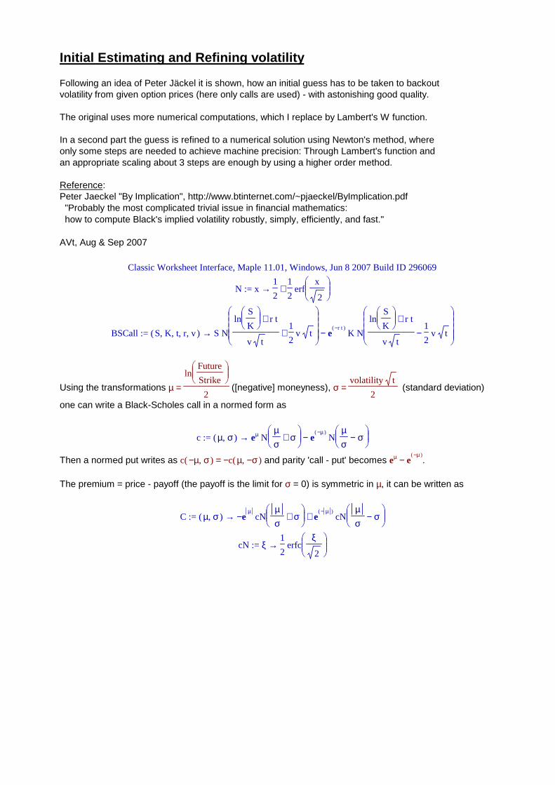
Here := cN → ξ − 1 ( )N ξ is the complementary cumulative normal distribution. For numerical reasonsone should not use that definition directly, but has to look into the implementation of N to have a goodone (usually N is done for negative inputs and the rest by symmetry). Here I used the complementaryerror function.

One wants to solve for 'volatility' σ, if moneyness µ and the premium (corresponding to a price) are given.

For a given price one usually starts in the inflection point = σ µ and a linear approximation there gives aninitial guess for the standard deviation σ for the given premium value (to be used for a Newton refinement):

, = 0∂

∂2

σ2( )C ,µ σ = σ µ

:= initialSigma1 → ( ),µ premium + µπ2

eµ

+ − premium e

µ( )cN 2 µ

1

2e

( )− µ

However if the premium is off the inflection point and close to 0 that is a bad idea. But one can use a series in σ = 0 (actually an asymptotic series for cN), cut off beyond exponent 3 andsolve for a given premium. Sorting out complex solutions one achieves at the following explicite formula:

:= initialSigma0 → ( ),µ premiumµ

3

LambertW

1

3

µ π 2

premium

( ) / 2 3

π

Here Lambert's W function is used - not that well known, but one can look it up at Mathworld or Wikipedia:( )LambertW y solves the equation = x ex y, so it is a "kind of logarithm" (use the series for exp).

A rough, but sufficient numerical approximation for LambertW is given below.

Now a good, but dirty guess for refining to a numerical solution is by choosing the appropriate one,where there is a simple criterion when to switch between the both (it was estimated numerical andis not 'theoretical' correct):

:= dirtyGuess → ( ),µ premium {( )initialSigma0 ,µ premium ≤ premium ( )C ,µ ( )theSwitchµ( )initialSigma1 ,µ premium < ( )C ,µ ( )theSwitchµ premium

:= theSwitch → µ 1.1 ( ) − 1 e( )−0.68 µ 0.89

Note that these function behave 'correctly' for small moneyness or a small premium(however initialSigma0 will loose all information about the premium there).

= lim → +premium 0

( )initialSigma0 ,µ premium 0

, = lim → µ 0

( )initialSigma0 ,µ premium 0 = lim → µ 0

( )initialSigma1 ,µ premium2 π premium

2

Glueing

Peter Jäckel has the fine idea to smoothly glue the 2 basic solution using a power function

Σ ( ),µ premium → :=

+ ( ) − 1 ( )w ,µ premium ( )initialSigma0 ,µ premium ( )w ,µ premium ( )initialSigma1 ,µ premium

:= w → ( ),µ premium

min ,

premium

( )C ,µ µ

( )α µ

1

where the exponent in our situation translates as follows (I guess ...):

:= α → µ

ln

− σ`*` σlow

− σhigh σlow

ln

b`*`

( )C ,µ µ

:= σ* ( )initialSigma1 ,µ 0

:= b* ( )C ,µ σ*

:= σlow ( )initialSigma0 ,µ b*

:= σhigh ( )initialSigma1 ,µ b*

I was too lazy to show the correct behaviour of Sigma in (0,0), but a careful numericalimplementation should regard this like the following (with counterparts in BS values):

:= Sigma_numeric → ( ),µ premium

0.1 10-9 < premium 0.1 10-9

+ π2

premium 0.1 10-9 and < µ 0.1 10-9 ≤ 0.1 10-9 premium

( )Σ ,µ premium and ≤ 0.1 10-9 µ ≤ 0.1 10-9 premium

However it is easier to care for such a thing from outside estimating Σ.

This seem quite complicated. But passing to numerics it will simplify quite a lot.

The Numerics

The above does not really care for µ = 0 and 0 < σ, one can use a simple version for erf( )−1

, roughlyvalid for abs(y) < 0.5 and quite good for 0 <= x/sqrt(2) <= 1/2: by inverting an [1,2]-Padeapproximation for ( )erf x one can take(3-sqrt(9-3*Pi*y^2))/y/sqrt(Pi).

However for domains larger than those considered here one uses a better quantile funtion than that Q.

:= Q → y

0 = y 0

( ) − 1 ( )− + η 1 ( ) + η 1 3

η and < η 1 = η

π3

y

Of course we need some numerical approximation for Lambert's W function (taken from DESY):

:= W → x

− ( )ln − x 4

− 1

1

( )ln x( )ln ( )ln x < 376 x

+ 0.665 ( ) + 1 0.0195 ( )ln + x 1 ( )ln + x 1 0.04 and ≤ 0 x ≤ x 376

:= initialSigma0_numeric ( )initialSigma0 ,µ σ = LambertW W

Then it is astonishing that the smoothed Σ (as an initial guess) becomes a relatively simple procedure combining the stuff from above (making heavy use of Maple):

Sigma_proc ,µ premiumproc( ) :=

result t1 t2 t3 t23 t27 t33 t35 t16 t28 t29 t6 t15 t11 t30 t32 t9 t12 t26 t18 t19 t31 t5 t25, , , , , , , , , , , , , , , , , , , , , , , ,local

t34 t13 t21 t4, , , ;

global ;π := t21 ( )abs µ ;

:= t30 ( )exp −t21 ;

:= t27 ∗ / 1 2 t30;

:= t23 ^2 ( ) / 1 2 ;

:= t19 ( )exp t21 ;

:= t28 ∗ ∗t23 t19 ^π ( ) / 1 2 ;

:= t18 ^t21 ( ) / 1 2 ;

:= t25 ∗t19 ( )erfc ∗t18 t23 ;

:= t12 − + ∗ / 1 2 t25 t27;

:= t33 − t18 ∗ / 1 2 ∗t12 t28;

:= t35 ∗ / 1 2 t23;

:= t9 / t21 t33;

:= t26 ∗ / 1 2 t28;

:= t6 − + ∗ / 1 2 ∗t19 ( )erfc ∗( ) + t9 t33 t35 ∗( )erfc ∗( ) − + t9 t18 ∗t12 t26 t35 t27;

:= t34 / ( )1 ∗3 π ;

:= t32 ∗t21 ^3 ( ) / 1 2 ;

:= t31 − + ∗ / 1 2 t30 ∗ / 1 2 t25;

:= t29 ∗ ∗t23 t21 π;

:= t16 ∗^( ) / t29 premium ( ) / 2 3 t34;

:= t15 ( )ln t16 ;

:= t13 ( )ln + t16 1 ;

:= t11 / 1 t12;

:= t5 ∗^( ) / t29 t6 ( ) / 2 3 t34;

:= t4 ( )ln t5 ;

:= t3 ( )ln + t5 1 ;

t2 / 1 3 t32 piecewise < 376 t5 − ( )ln − t5 4 ∗( ) − 1 / 1 t4 ( )ln t4 and ≤ 0 t5 ≤ t5 376, , ,( / ∗− :=

+ ∗ ∗0.665 ( ) + 1 ∗0.0195 t3 t3 0.04) ( ) / 1 2^ ;

:= t1 ( )min ,1 ^( )∗premium t11 ( ) / ( )ln ( ) / ( ) + t2 t33 + + t18 ∗( ) + t31 t6 t26 t2 ( )ln ∗t6 t11 ;

result / 1 3 ( ) − 1 t1 t32 piecewise < 376 t16 − ( )ln − t16 4 ∗( ) − 1 / 1 t15 ( )ln t15, ,(∗ / ∗ :=

and ≤ 0 t16 ≤ t16 376 + ∗ ∗0.665 ( ) + 1 ∗0.0195 t13 t13 0.04, ) ( ) / 1 2^

∗t1 ( ) + t18 ∗( ) + premium t31 t26 + end proc

Now just write down the function for the initial guess (for Maple write it as a procedure):

:= initialSigma → ( ),µ premium

0 = premium 0

2 ( )Q + premium µ = µ 0( )Sigma_proc ,µ premium otherwise

initialSigma ,µ premiumproc( ) :=

if then end if = premium 0 return 0 ;

if then end if = µ 0 return ∗( )sqrt 2 ( )Q + premium ( )abs µ ;

( )Sigma_proc ,µ premium

end proc

For coding: find some source code in C at the end.

Let us compare the error (here I use a way to simulate the procedure to be coded in C):

For that graphics recalling the usage of µ one sees that it will cover strikes in a rangeFuture / exp(1) ... Future * exp(1), which is certainly enough. The grey wireframe is the version using theSwitch (which is done where both solutions areof same size, but different sign), in magnitude they are like the smoothed = coloured version.

To the right side there is a buckling, exactly at zero level - standing for the inflection points = σ µ and to the left side the error wave crosses zero more or less along theSwitch of the simple version.

The graphics for the premium shows that the errors are really small (grey surface = exactvalues and blue wireframe = result, if the initial guess (taken from the exaxt values) are feedinto the formula:

( )C ,µ ( )initialSigma ,µ ( )C ,µ σ( )C ,µ σ

Translating between usual coordinates and the normed situation turns out to be as follows:

initialVolatility , , , ,S K t r Priceproc( ) :=

local ;, , , , , ,F µ σ Intrinsic Premium premium initSigma

:= F ∗( )exp ∗r t S;

:= µ ∗ / 1 2 ( )ln / F K ;

:= Intrinsic ( )max ,0 − S ∗K ( )exp − ∗r t ;

:= Premium − Price Intrinsic;

:= premium ∗ / Premium ( )exp ∗ / 1 2 ∗r t ( )sqrt ∗K S ;

:= initSigma ( )initialSigma ,( )abs µ premium ;

return ∗ / 2 initSigma ( )sqrt t

end proc

Examples in real world coordinates

Take a BS price ( )BSCall , , , ,S K t r v , estimate an initial vol from that and feed it into a BS pricer asnew volatility ( )BSCall , , , ,S K t r ( )initialVolatility , , , ,S K t r ( )BSCall , , , ,S K t r v to compare the pictures.

The result is fine: the grey surfaces are the exact BS value and the blue wireframes show the valuesrecalculated from the initial guessed volatility.

Calculation is done through simulating the procedures to be coded in C (faster, avoiding symbolics).

>

:= tstData [ ], , = S 100 = t 3 = r 0.03

:= tstData [ ], , = S 100 = t 1 = r 0.03

:= tstData

, , = S 100 = t

1

12 = r 0.03

Refining the guess towards a numerical solution

Halley's method ... is about twice as 'fast' as the usual Newton-Raphson to solve equations,but needs some care (and Jaeckel does that) and works best for 'almost linear functions'.

Let's look at the function surface:

The black curve are the inflection points. For fixed µ the function looks nice enough to (almost) carelessapply Halley's method - down to the pink curve (which is theSwitch from above). Below I would use usualNewton with some refinement (see later) - down to the white line = σ .2 µ: below that the arguments forthe (complementary) Normal distribution are larger than 5 and usual double precision does not really doa good job to result in reasonable, precise values for σ (and prices), I would use brute bracketting to control it.

Here is my suggestion for the near-flat region:

For < µσ2

the surface is reasonable 'linear' in σ to apply Newton-Raphson. Below re-scale using

initialSigma0.Then there the function should also become quite linear (as the approximative, analytic solution is good).

We will see: one does not really need Halley's method, already a few Newton steps are enough!

For re-scaling simply replace LambertW by the logarithm (since we have extreme values and log is anasymptotic approximation, for more see below).

:= χ → ( ),µ premium1

3

µ 3

ln

1

3

µ π 2

premium

( ) / 2 3

π

Then visualize what happens:

:= B → ( ),µ σ

piecewise , , ≤ σ

1

2µ 2 ( )χ ,µ ( )C ,µ σ ``

B is the re-scaled function (times 2, to get it nicely into one graphic) resulting in the red surface andthe grey surface is the original premium surface. Obviously one can expect Newton-Raphson to worknicely, since on the red surface the values are almost linear in σ.

Cutting is done along µ = σ2

, depending on an initial guess for σ (say using the simple version).

Justifying the use of log

One has to justify the use of log instead of LambertW, i.e. to give evidence that the argument withinthe log is greater to use the square root. For that plot the situation (and cut off at some upper value,do not take 5, take 9):

min ,9

1

3

µ π 2

( )C ,µ σ

( ) / 2 3

π

We set premium = ( )C ,µ σ . For decreasing σ that E becomes greater than 1 below σ = µ (theexpression is 'almost' identical 1 along the black diagonal ... a bit strange ...) and is increasing.

The red curve on the surface is for the expression in σ = µ / 2 (having a projection on the bottom).

It is of magnitude 7 in our range ( ~ 6.88 in µ = 0 and increasing to infinity outside by monotony).

Now using an initial guess for a σ from given premium (and fixed µ) this initial error is small enoughthat we will not hit the half-diagonal and thus we talk about log of some E greater than 6 (ok, somehandwaving towards 0 ...).

So one can take the squareroot and the scaling χ is defined.

If you feel uncomfortable with that argumentation: just use ( )log + E 1 , it will do as well.

Newton method for the premium function

These functions below take the premium to make an initial guess for and refines it through theNewton method until a relative step size eps is achieved (as it is done in Jäckel's paper).

They return a pair of values: the approximative solution and the number of steps used for that.

Take some care using the below; it uses relative changes in sigma, which does not work in 0(devision becomes undefined and numerically that happens even close to 0). However this isjust where the derivative vanishes and can be avoided.

Before coding the Newton method for the re-scaled situation I want to modify the initial guessingfor the Newton method to care for numerical exceptions and use non-symbolics if possible:

initialSigma_num ,µ premiumproc( ) :=

local ;result

:= result 0.;

try catch : finally end try := result ( )evalhf ( )initialSigma ,µ premium := result 0 return result

end proc

:= vega → ( ),µ σ e

− − / 1 2µ 2

σ2 / 1 2 σ2

2

π

= ( )vega ,µ σ∂∂σ

( )C ,µ σ

true

newton_C , ,µ premium epsproc( ) :=

local ;, , , , , , , ,maxSteps x x_new fx Dfx i relativeStepChange m p

:= maxSteps 20;

:= m ( )evalhf µ ;

:= p ( )evalhf premium ;

if then end if = p 0. return [ ],0 0 ;

:= x ( )evalhf ( )initialSigma ,m p ;

if then end if = ^x 2 0. return [ ],0 0 ;

:= i 0;

≤ i maxStepswhile do

:= fx ( )evalhf − ( )C ,m x p ;

:= Dfx ( )evalhf ( )vega ,m x ;

if then end if = Dfx 0. return [ ],x ( )max ,0 i ;

:= x_new ( )evalhf − x / fx Dfx ;

:= i + i 1;

if then end if = ^x_new 2 0. return [ ],x_new ( )max ,0 i ;

:= relativeStepChange ( )abs ( )evalhf − / x x_new 1 ;

:= x x_new;

if then end if < relativeStepChange eps break

end do;

return [ ],x i

end proc

Derivative for the re-scaled premium

One needs the derivative of ( )χ ( )C ,µ σ for coding the Newton method (to find the formulabelow one uses a general ( )f σ to recognize the patterns involved):

= ∂∂σ

( )χ ,µ ( )C ,µ σ1

4( )vega ,µ σ 2

z

ln

6 z

9 π

( ) / 3 2

= zµ

( )C ,µ σ

true

newton_C_rescaled , ,µ premium epsproc( ) :=

local ;, , , , , , , , , ,maxSteps x x_new fx Dfx i relativeStepChange m p q z

:= maxSteps 20;

:= m ( )evalhf µ ;

if then end if = m 0. ;



:= q ( )evalhf ( )χ ,µ p ;

if then end if = q 0. return [ ],0 0 ;

:= x ( )initialSigma_num ,m p ;


:= i 0;


:= fx ( )evalhf − ( )χ ,m ( )C ,m x q ;

:= z ( )evalhf / ( )abs m ( )C ,m x ;

:= Dfx ( )evalhf ∗ / 1 4 ∗ ∗ / ( )sqrt 2 ( )vega ,m x z ^( )ln ∗ / 1 9 ∗( )sqrt / 6 π z ( ) / 3 2 ;


:= x_new ( )evalhf − x / fx Dfx ;

:= i + i 1;

if then end if = x_new 0. return [ ],x_new ( )max ,0 i ;

:= relativeStepChange ( )abs ( )evalhf − / x x_new 1 ;

:= x x_new;

if then end if < relativeStepChange eps break

end do;

return [ ],x i

end proc

2 remarks

Before proceeding here are 2 examples concerning the sense or nonsense of workingtoo deep in the flat region.

The following inputs are pretty valid and also give expected results

:= sTst 0.02

:= mTst 0.2

= ( )C ,mTst sTst 0.298923738971 10-25

:= somePremium 0.298923738971 10-25

:= someInitial 0.0199949671938514928

= ( )newton_C_rescaled , ,mTst somePremium 0.1 10-7 [ ],0.019999999999953 2.

= ( )C ,mTst 0.019999999999953 0.298923739085 10-25

= ( )c ,mTst sTst 0.40267200508222

So for this example the method finds the solution within 2 steps and a precision of ~ 13 places. Fine.However we talk about premium from option prices. But subtractng .3e-25 from a price (of .4) isbeyond usual 'machine epsilon' (besides the fact that option prices are merely that acurate).

:= sTst 0.01

:= mTst 0.4

= ( )C ,mTst sTst 0.18255778326 10-352

:= somePremium 0.18255778326 10-352

:= someInitial 0.

= ( )newton_C_rescaled , ,mTst somePremium 0.1 10-7 [ ],0. 0.

= ( )C ,mTst 0. -0.

= ( )c ,mTst sTst 0.82150465160568

This is even more extreme (while the input formally is quite moderate, if only looking at pictures),again the solution is exact up to 10 places (no Newton steps performed, just the initial guess).

But here the premium itself is smaller than a number representable in double precision.

One would need a relative working precision as it is provided by Maple (or similar):

= ( )χ ,mTst ( )C ,mTst σ ( )χ ,mTst somePremium

0.010000000000190

After that caveats (and justification for the exception handling) it is time to view results:

Now have a look at the results

I coded different procedures for the abolute and relative errors and the number of steps to achievethe results.

If the input = premium ( )C ,µ σ is below a representable number it will be ignored, since I use'hardware evaluation' and no symbolics.

dummyError ,µ σproc( ) :=

local ;premium

global ;EPS

:= premium ( )evalhf ( )C ,µ σ ;

≤ ( )evalhf σ ( )evalhf ∗( )abs µ 0.66if then

< ( )abs premium 0.1*10^(-305) return ``if then

return − σ [ ]( )newton_C_rescaled , ,µ premium EPS 1else

end if

return − σ [ ]( )newton_C , ,µ premium EPS 1else

end if;

``

end proc

dummyErrorRelative ,µ σproc( ) :=

local ;premium

global ;EPS




return / ( )abs − σ [ ]( )newton_C_rescaled , ,µ premium EPS 1 σelse

end if

return − 1 ( )abs / [ ]( )newton_C , ,µ premium EPS 1 σelse

end if;

``

end proc

dummySteps ,µ σproc( ) :=

local ;premium

global ;EPS



< ( )abs premium 0.1*10^(-305) return 0if then

return [ ]( )newton_C_rescaled , ,µ premium EPS 2else

end if

return [ ]( )newton_C , ,µ premium EPS 2else

end if;

``

end proc

Execution is stopped, if a Newton step is smaller than EPS = .1e-7.

:= EPS 0.1 10-15

:= theRange , .. 01

2 .. 0

1

2

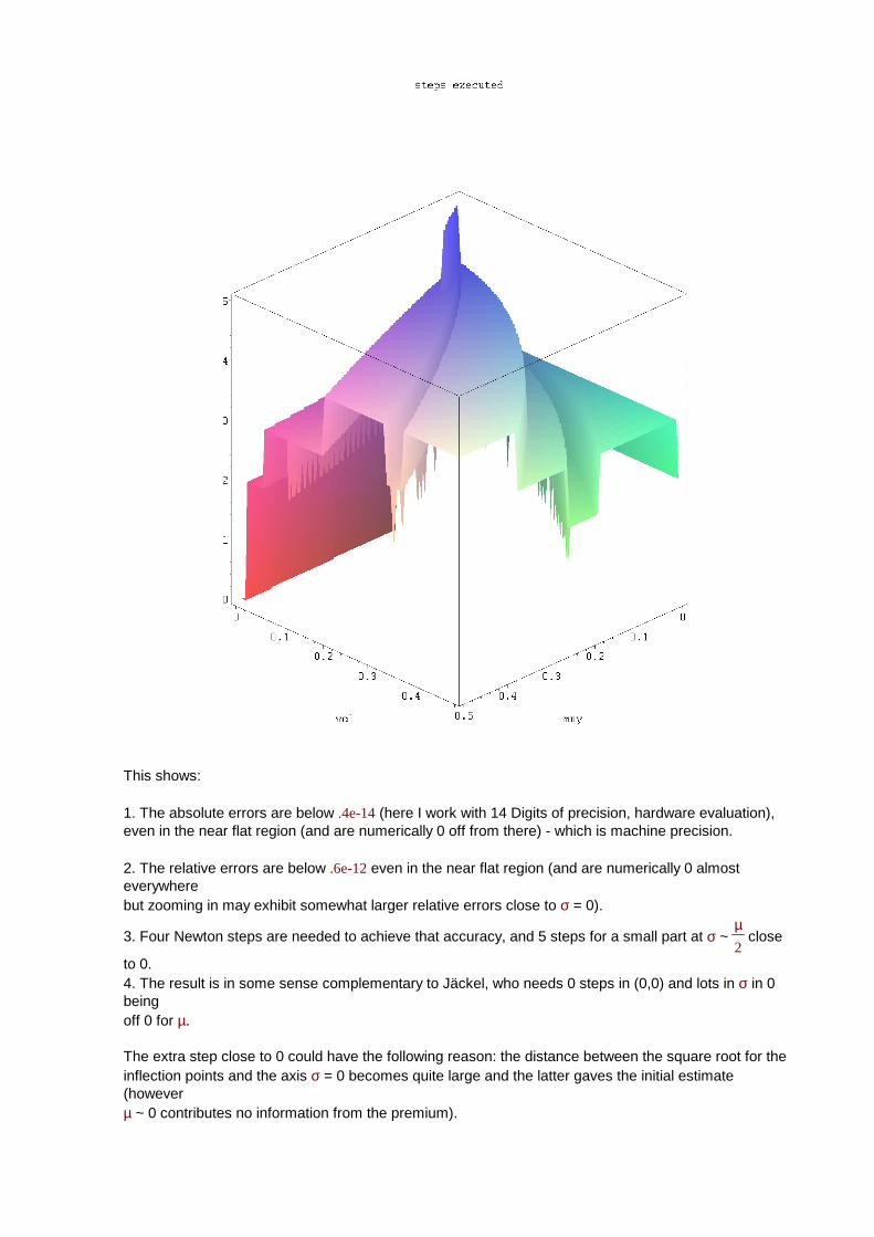
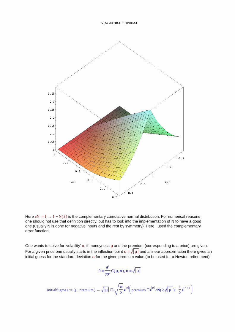
This shows:

1. The absolute errors are below .4e-14 (here I work with 14 Digits of precision, hardware evaluation),even in the near flat region (and are numerically 0 off from there) - which is machine precision.

2. The relative errors are below .6e-12 even in the near flat region (and are numerically 0 almost everywhere but zooming in may exhibit somewhat larger relative errors close to σ = 0).

3. Four Newton steps are needed to achieve that accuracy, and 5 steps for a small part at σ ~ µ2

close

to 0.4. The result is in some sense complementary to Jäckel, who needs 0 steps in (0,0) and lots in σ in 0 beingoff 0 for µ.

The extra step close to 0 could have the following reason: the distance between the square root for theinflection points and the axis σ = 0 becomes quite large and the latter gaves the initial estimate (howeverµ ~ 0 contributes no information from the premium).

BTW: from the last picture one can rediscover the inflection curve σ = µ (less Newton steps are neededthere). And one should select the 'valley' towards σ ~ 0.3 to use rescaling, for the picture I used

= .66µ σ to switch to the re-scaled version).

The special case µ = 0 is not covered by the above, but it is of same quality.

Higher Order method

The graphics above already suggest, that a 'Newton method with higher order' is not imperativelyneeded. Anyway: try it. For the version based on checking relative stepsize one essentially savesonly 1 step and I do not exhibit that.

Instead let's look at the usual, absolute stepsize for stopping the iteration.

This eliminates the ugly additional step on half the diagonal towards 0 which we have above.

Instead of Halley's method one can use a series inversion of order 2 (Lagrange inversion) written as

x + n 1 = − − xn ξ1 Ξ ξ2

2 with = ξ

( )f xn

( )( )D f xn

and = Ξ( )( )D f xn

( )( )( )D( )2

f xn

, called Chebychev method

chebyshev_C , ,µ premium epsproc( ) :=

local ;, , , , , , , , , ,maxSteps x x_new fx Dfx i absoluteStepChange m p L1f L2f

:= maxSteps 20;

:= m ( )evalhf ( )abs µ ;



:= x ( )evalhf ( )initialSigma ,m p ;


:= i 0;


:= fx ( )evalhf − ( )C ,m x p ;

:= Dfx ( )evalhf ( )vega ,m x ;


:= L1f ( )evalhf / fx Dfx ;

:= L2f ( )evalhf − / ^m 2 ^x 3 x ;

:= x_new ( )evalhf − − x L1f ∗ / 1 2 ∗L2f ^L1f 2 ;

:= i + i 1;


:= absoluteStepChange ( )abs ( )evalhf − x x_new ;

:= x x_new;

if then end if < absoluteStepChange eps break

end do;

return [ ],x i

end proc

A higher-order method for the re-scaled version needs g'' / g' , some laborious work gives

∂

∂2

σ2( )χ ,µ ( )f σ /

∂∂σ

( )χ ,µ ( )f σ = +

− + 1

3 η2

( )( )D f σ

( )f σ( )( )( )D

( )2f σ( )( )D f σ

using the abbreviations = η1

( )ln Z, = Z

µ2

3 π3 ( )f σ

while using = f ( ) → σ ( )C ,µ σ , µ fixed.

chebyshev_C_rescaled , ,µ premium epsproc( ) :=

local ;, , , , , , , , , , , , , , ,maxSteps x x_new gx Dgx i absoluteStepChange m p q z L1g L2g Zη L2f

:= maxSteps 20;

:= m ( )evalhf ( )abs µ ;

if then end if = m 0. ;



:= q ( )evalhf ( )χ ,µ p ;

if then end if = q 0. return [ ],0 0 ;

:= x ( )initialSigma_num ,m p ;


:= i 0;


:= gx ( )evalhf − ( )χ ,m ( )C ,m x q ;

:= z ( )evalhf / ( )abs m ( )C ,m x ;

:= Dgx ( )evalhf ∗ / 1 4 ∗ ∗ / ( )sqrt 2 ( )vega ,m x z ^( )ln ∗ / 1 9 ∗( )sqrt / 6 π z ( ) / 3 2 ;

if then end if = Dgx 0. return [ ],x ( )max ,0 i ;

:= L1g ( )evalhf / gx Dgx ;

= ^x 3 0. ; := x_new ( )evalhf − x L1g := i + i 1if then

else

:= Z ( )evalhf ∗ / 1 3 ∗ / ( )abs µ ( )sqrt / ( ∗ )2 3 π ( )C ,m x ;

:= η ( )evalhf / 1 ( )ln Z ;

:= L2f ( )evalhf − / ^m 2 ^x 3 x ;

:= L2g ( )evalhf − + ∗ / ( ) − 1 ∗ / 3 2 η ( )vega ,m x ( )C ,m x L2f ;

:= x_new ( )evalhf − − x L1g ∗ / 1 2 ∗L2g ^L1g 2 ;

:= i + i 1

end if;


:= absoluteStepChange ( )abs ( )evalhf − x x_new ;

:= x x_new;

if then end if < absoluteStepChange eps break

end do;

return [ ],x i

end proc

dummyError ,µ σproc( ) :=

local ;premium

global ;EPS




return − σ [ ]( )chebyshev_C_rescaled , ,µ premium EPS 1else

end if

return − σ [ ]( )chebyshev_C , ,µ premium EPS 1else

end if;

``

end proc

dummyErrorRelative ,µ σproc( ) :=

local ;premium

global ;EPS




return − 1 ( )abs / [ ]( )chebyshev_C_rescaled , ,µ premium EPS 1 σelse

end if

return / ( )abs − σ [ ]( )chebyshev_C , ,µ premium EPS 1 σelse

end if;

``

end proc

dummySteps ,µ σproc( ) :=

local ;premium

global ;EPS



< ( )abs premium 0.1*10^(-305) return 0if then

return [ ]( )chebyshev_C_rescaled , ,µ premium EPS 2else

end if

return [ ]( )chebyshev_C , ,µ premium EPS 2else

end if;

``

end proc

:= EPS 0.1 10-15

:= theRange , .. 01

2 .. 0

1

2

Also let's compare with Figure 9 in Jäckel's paper: we need 2 steps and at most 3 withincreasing volatility (for larger ranges use a reasonable quantile function Q).

:= EPS 0.1 10-15

:= theRange , .. -1

100000

1

100000 .. 0

1

2

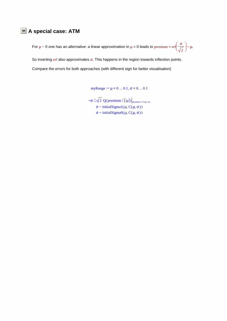
A special case: ATM

For µ ~ 0 one has an alternative: a linear approximation in µ = 0 leads to = premium −

erf

σ

2µ.

So inverting erf also approximates σ. This happens in the region towards inflection points.

Compare the errors for both approaches (with different sign for better visualisation)

:= myRange , = µ .. 0. 0.1 = σ .. 0. 0.1

− + σ 2 ( )Q + premium µ = premium ( )C ,µ σ

− σ ( )initialSigma1 ,µ ( )C ,µ σ − σ ( )initialSigma0 ,µ ( )C ,µ σ

The blue surface is through the initialSigma1, the grey one from inverting the error function, and initialSigma0 is in red (changed some signs for nice plotting), the grid is plotted at error level = 0.

Just note that a more precise version for erf( )−1

than the used Q does not change the picture.

:= invErf → y ( )RootOf , − ( )erf x y x

:= myRange , = µ .. 0. 0.1 = σ .. 0. 0.1

− + σ 2 ( )invErf + premium µ = premium ( )C ,µ σ

− σ ( )initialSigma ,µ ( )C ,µ σ

There are some numerical issues close to 0, which I am too lazy to clean up here.

Compilable Code for the initial guess

The following code compiles with Dev-c++ (which already has erfc in its library), oneonly has to replace the Maple function 'piecewise' by some if-else construct:

Warning, the function names {erfc} are not recognized in the target language

#include <math.h>

double mySigma (double mu, double premium){ double result; double t1; double t2; double t23; double t16; double t26; double t15; double t3; double t28; double t11; double t30; double t13; double t31; double t32; double t33; double t9; double t29; double t18; double t19; double t25; double t4; double t6; double t21; double t5; double t34; double t35; double t27; double t12; t21 = fabs(mu); t19 = sqrt(t21); t18 = exp(t21); t23 = sqrt(0.2e1); t28 = 0.17724538509055e1 * t18 * t23; t30 = exp(-t21); t27 = t30 / 0.2e1; t25 = t18 * erfc(t19 * t23); t12 = -t25 / 0.2e1 + t27; t32 = t19 - t12 * t28 / 0.2e1; t26 = t28 / 0.2e1; t35 = t23 / 0.2e1; t9 = t21 / t32; t6 = -t18 * erfc((t9 + t32) * t35) / 0.2e1 + erfc((t9 - t19 + t12 * t26) * t35) * t27; t34 = 0.10610329539460e0; t33 = -t30 / 0.2e1 + t25 / 0.2e1; t31 = t21 * sqrt(0.3e1); t29 = 0.314159265358979324e1 * t21 * t23; t16 = pow(0.1e1 / premium * t29, 0.2e1 / 0.3e1) * t34;

t15 = log(t16); t13 = log(t16 + 0.1e1); t11 = 0.1e1 / t12; t5 = pow(0.1e1 / t6 * t29, 0.2e1 / 0.3e1) * t34; t4 = log(t5); t3 = log(t5 + 0.1e1); if (0.0e0 <= t5 && t5 <= 0.376e3) t2 = -t32 * pow(0.665e0 * (0.1e1 + 0.195e-1 * t3) * t3 + 0.4e-1, -0.1e1 / 0.2e1) / 0.3e1; else if (0.376e3 < t5) t2 = -t32 * pow(log(t5 - 0.4e1) - (0.1e1 - 0.1e1 / t4) * log(t4), -0.1e1 / 0.2e1) / 0.3e1; else { } t1 = (0.1e1 <= pow(premium * t11, log((t2 + t32) / (t19 + (t33 + t6) * t26 + t2)) / log(t6 * t11)) ? 0.1e1 : pow(premium * t11, log((t2 + t32) / (t19 + (t33 + t6) * t26 + t2)) / log(t6 * t11))); if (0.0e0 <= t16 && t16 <= 0.376e3) result = t1 * (t19 + (premium + t31) * t26) + (0.1e1 - t1) * t32 * pow(0.665e0 * (0.1e1 + 0.195e-1 * t13) * t13 + 0.4e-1, -0.1e1 / 0.2e1) / 0.3e1; else if (0.376e3 < t16) result = t1 * (t19 + (premium + t31) * t26) + (0.1e1 - t1) * t32 * pow(log(t16 - 0.4e1) - (0.1e1 - 0.1e1 / t15) * log(t15), -0.1e1 / 0.2e1) / 0.3e1; else { } return(result);}

initial estimating and refining volatility estimating and refining volatility following an idea of...

Documents