Initial formation and evolution of channel-shoal patterns in estuaries A. Hibma1*, H.M. Schuttelaars1,2 and H.J. de Vriend1,3

1* Delft University of Technology. Faculty of Civil Engineering and Geoscience. P.O. Box 5048. 2600 GA Delft, The Netherlands. Tel: +31 15 2789449. Fax: +31 15 2785124. A.Hibma@ct.tudelft.nl 2 Institute for Marine and Atmospheric research Utrecht (IMAU), Utrecht University, The Netherlands. 3 WL | Delft Hydraulics. The Netherlands. ABSTRACT: A complex process-based model is used to simulate the formation of channels and shoals in a schematised estuary. The model set-up enables a comparison with results obtained with idealised models. Initial as well as long-term simulations are made. Dominant wavelengths of channel-shoal patterns are investigated together with their dependency on width and depth of the basin and the local maximum velocity. Prevalent wavelengths range between 5 and 10 km and increase with increasing width and flow velocity. Initial model results are compared with idealised models. The dominant wavelengths are of the same order of magnitude as those found in the idealised model of Schramkowski et al. (2002) and their dependency on width and velocity agrees qualitatively. (Exponential) growth of the perturbations during long-term simulations provides information on the validity limits of the idealised models. Subsequent pattern formation and changes of dominant wavelengths are attributed to non-linear interactions. Morphological developments during long-term simulations suggest that channel-shoal patterns evolve into a unique morphodynamic equilibrium state, independent of the initial perturbation. This complex non-linear approach is an innovative step towards an integrated model approach in which different model types and field data are combined in order to make optimal use of each research method. keywords: estuaries, morphology, numerical model, shoals, channels, sand bars 1 INTRODUCTION Estuaries attract a variety of human activities, such as navigation, recreation, fishing, sand mining, land reclamation and in some cases hydrocarbon mining. On the other hand, many estuaries form the basis of highly valuable and often unique ecosystems. They provide nursing, resting and feeding grounds for many species. The interests of these various functions of an estuary can be in mutual conflict. From a management point of view it is important to predict the morphological response of these systems to human activities or changes in environmental conditions. Channels and shoals form highly dynamic elements in estuaries. Presently, predictive capability regarding their morphological behaviour is rather limited. Research on this subject uses different types of models, each giving insight into a certain aspect of the morphodynamics (de Vriend, 1996; de Vriend and Ribberink, 1996).

In a previous study (Hibma et al., 2003a) a complex process-based model of estuarine morphodynamics is shown to produce channel and shoal patterns closely resembling those observed in nature. Figure 1 shows a result of this study for an initial and for an advanced stage of channel-shoal formation. The patterns exhibit a characteristic wavelength in longitudinal direction, which increases during the simulation until a relatively stable, near equilibrium pattern is established. The mechanisms behind the formation of these channel-shoal patterns and the prevalent wavelength selection are difficult to extract from the complex model. To reveal the morphological behaviour systematically, use can be made of idealised models. These models use simplifications in model formulations and geometry, such that prevailing morphological processes can be isolated and analysed (Schuttelaars and de Swart, 1999; Seminara and Tubino, 2001; Schramkowski et al., 2002). However, these models are restricted to initial (linear) growth of channel-shoal patterns in idealised situations. In this contribution results of both types of models are used. This approach of combining idealised and complex numerical models, can both improve insight into processes and validate the models. In this paper we focus on the growth of channel-shoal patterns and accompanying wavelength dominance. To validate the complex model results and to provide insight into the growth mechanisms and processes influencing wavelength selection, the initial growth rates are compared with those of idealised models. After this validation we make a step forward by simulating the long-term evolution of the channel-shoal pattern. In the next section the model approach is described, providing background for the model assumptions, the model set-up and the simulations carried out. Section 3 describes the initial growth of the perturbations resulting from short-term simulations with the complex model. In Section 4 these results are validated by comparing the feedback mechanisms found in complex and idealised models, and by comparing model results on dominant wavelengths. The dependency on width and depth of the basin and the local velocity are investigated. Subsequently, long-term model simulations are carried out and described in Section 6. The transition from the linear to the strongly non-linear pattern formation is discussed in Section 7. fig. 1 2 MODEL APPROACH AND ANALYSIS Model set-up In this study a complex process-based model (Delft3D) (Wang et al. 1991; Roelvink and van Banning, 1994) is used to simulate the formation of channels and shoals in an estuary. The model system describes the water motion by the shallow water equations. In this study, the 2-D depth-averaged version of the model is used, as 3D-effects are not essential for the pattern formation (Coeveld et al., 2003). The sediment transport can be described by a bed-load or total-load transport formula (using a variety of semi-empirical formulae), or by a quasi-three-dimensional advection-diffusion solver for suspended

sediment, including temporal and spatial lag-effects. The bathymetric changes are proportional to the divergence of the sediment flux field. In order to compare the initial pattern formation resulting from the complex model with the results of the idealised model, it is essential that the physical formulations in the two models are as similar as possible. In an earlier study (Hibma et al., 2003a), it is concluded that mutual validation of results from idealised and complex process-based models is difficult, due to differences in model assumptions and formulations. In Hibma et al. (2003b), the complex model was adapted, such that a comparison of width-averaged velocities, concentrations and bed profiles was possible for estuaries of arbitrary length. It was concluded that the adaptations and remaining differences in model formulations bear no qualitative influence on the model results, except for the boundary condition to the bed level at the entrance of the estuary, which is fixed in the idealised model. In the present study, this boundary condition is adopted in the complex model. In this way, it can be assumed that the remaining differences in model formulation between the two model types do not obstruct a comparison of results (model formulations are given in Hibma et al. (2003b)). In accordance with the idealised models, sediment transport is calculated using an advection-diffusion model. Most physical parameters, are derived from the dynamic seaward (western) part of the Western Scheldt estuary. The dispersion coefficient for the suspended sediment transport is taken 10 m2/s. The bed material consists of uniform sand with a grain size of 200 µm. At the seaward boundary a periodic water level variation is imposed, simulating the M2 tidal component with an amplitude of 1.75 m. For the bottom roughness a constant Chézy coefficient of 50 m1/2/s is used. In order to compare the results with the idealised two-dimensional models, the geometry of the estuary is schematised to a rectangular basin (see Fig. 2). The landward and lateral boundaries are non-erodible. Simulations are made on a grid with a mesh size of 125 m x 125 m. The width of the modelled basin, B, is 5000 m. Hibma et al. (2003a) show that the width and depth of the basin influence the prevalent wavelength. To study the influence of the width, also a narrow basin of 500 m width is simulated. Both basins are 100 km long and start from a bed level, which is considered as an equilibrium profile. This profile is obtained by an one-dimensional simulation during 500 years starting from a linear sloping bed profile, which decreases from 10 m below MSL at the seaward end to 1 m above MSL at the landward boundary. The resulting profile has a maximum depth of 13 m near the entrance of the basin (see Fig. 2b). The adjustments of this profile during the simulation periods are an order of magnitude smaller than the bed level changes induced by the (imposed) perturbations and therefore the profile can be regarded as an equilibrium profile. Fig. 2 Contrary to the model of Hibma et al. (2003a), the bottom profile is not perturbed randomly, but sinusoidally. This facilitates the investigation of growth rates of patterns of a certain wavelength. These periodic perturbations are described by

2 2'( , ) sin( )cos( )L T

h x y A x yπ πλ λ

=

in which A is the amplitude, λL is the wavelength in longitudinal x-direction and λT is the wavelength in transversal y-direction. Perturbations with various wavelengths are imposed on the equilibrium bed of the basin. The wavelength of these perturbations is 1 to 20 km in longitudinal direction (λL), hereafter referred to as λ1 to λ20, respectively. The amplitude of the initial perturbations is 0.1 m. The largest transversal wavelength is two times the basin width (λT = 2B), which means that the perturbations form an alternating pattern. This is labelled as the first mode in the idealised models. Simulations with higher modes (n = 2 to 5 and 10, where λT = 2B/n) are also made. Long-term as well as short-term simulations are made, for a narrow and wide basin. The short-term simulations are computations over one tidal cycle. An overview of the simulations is given in Table 1. Analysis of model results Analysis of the model results is focused on the growth rates of the perturbations. The growth rates represent the increase of the amplitude of the perturbation and are presented as a yearly value. Fourier analysis is applied to determine the evolution of the amplitude of each perturbation during the simulation. In the idealised models the mean bed level is assumed locally horizontal and in equilibrium. In the complex model a constant bed level is approximated by analysing the results for a section of the basin. The adaptation of the underlying profile is subtracted from the model results before the Fourier analysis is applied. The change in amplitude of the Fourier components are translated into growth rates of the perturbations with various wavelengths. Negative growth rates indicate amplitude decay, positive growth rates amplification. The largest growth rate among different imposed perturbations indicates the fastest growing or prevalent wavelength of the channel-shoal pattern formation. A morphological equilibrium is expected to be reached when the amplitudes of all perturbations have ceased to change. The change in amplitude of the perturbations after one tidal cycle (short-term) is regarded as the initial growth or decay. Results are presented in the next section. These changes are assumed to be indicative for the linear domain and will be compared to idealised models, as described in Section 4. Long-term simulations are made for about 200 years. Over this period non-linear interactions are playing a dominant role. The results of the long-term simulations are analysed to demonstrate the pattern transformation due to these non-linear interactions and to define the range of linearity of the processes. The results are described in Section 5 and discussed in Section 6. 3 INITIAL MODEL RESULTS

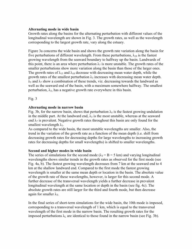
Alternating mode in wide basin Growth rates along the basins for the alternating perturbation with different values of the longitudinal wavelength are shown in Fig. 3. The growth rates, as well as the wavelength corresponding to the largest growth rate, vary along the estuary. Figure 3a concerns the wide basin and shows the growth rate variation along the basin for five perturbations of different wavelength. From these perturbations, λ10 is the fastest growing wavelength from the seaward boundary to halfway up the basin. Landwards of this point, there is an area where perturbation λ7 is more unstable. The growth rates of the smaller perturbations show more variation along the basin than those of the larger ones. The growth rates of λ15 and λ10 decrease with decreasing mean water depth, while the growth rates of the smallest perturbation λ3 increases with decreasing mean water depth. λ5 and λ7 show a combination of these trends, viz. decreasing towards the landward as well as the seaward end of the basin, with a maximum somewhere halfway. The smallest perturbation, λ3, has a negative growth rate everywhere in this basin. Fig. 3 Alternating mode in narrow basin Fig. 3b, for the narrow basin, shows that perturbation λ5 is the fastest growing undulation in the middle part. At the landward end, λ3 is the most unstable, whereas at the seaward end λ7 is prevalent. Negative growth rates throughout this basin are only found for the smallest wavelength λ1. As compared to the wide basin, the most unstable wavelengths are smaller. Also, the trend in the variation of the growth rate as a function of the mean depth (i.e. shift from decreasing growth rates for decreasing depths for large wavelengths to increasing growth rates for decreasing depths for small wavelengths) is shifted to smaller wavelengths. Second and higher modes in wide basin The series of simulations for the second mode (λT = B = 5 km) and varying longitudinal wavelengths shows similar trends in the growth rates as observed for the first mode (see Fig. 4a, b). The fastest growing wavelength decreases from 7 km at the seaward end to 4 km at the shallow landward end. Compared to the first mode the fastest growing wavelength is smaller at the same mean depth or location in the basin. The absolute value of the growth rate of these wavelengths, however, is larger for this second mode. A further decrease of the transversal wavelength yields a further decrease in prevalent longitudinal wavelength at the same location or depth in the basin (see fig. 4c). The absolute growth rates are still larger for the third and fourth mode, but then decrease again for smaller λT. In the final series of short-term simulations for the wide basin, the 10th mode is imposed, corresponding to a transversal wavelength of 1 km, which is equal to the transversal wavelength of the first mode in the narrow basin. The resulting growth rates for the imposed perturbations λL are identical to those found in the narrow basin (see Fig. 3b).

From these series of simulations for the wide basin we conclude that the dominant longitudinal wavelength decreases as the transversal wavelength decreases. The largest growth rates are found for a transversal wavelength between 2 and 2.5 km and a longitudinal wavelength between 4 and 7 km, depending on the location. Fig. 4 Second mode in narrow basin Simulations for the second-mode perturbations in the narrow basin show smaller growth rates than for the alternating mode. Interestingly, the fastest growing wavelength for this second mode is larger, unlike what was found in the wide basin (see Fig. 4d). As discussed in the next section, this may be caused by a stronger damping of the smaller wavelengths. Summerising, the model results show that: 1 Wavelength of fastest growing perturbation in along-channel direction, λL, increases

with increasing water depth. 2 Perturbations having large wavelengths show decrease of growth rates with decreasing

mean water depth, while perturbations having small wavelengths show decrease of growth rates with increasing mean water depth. Maximum growth rates are found in between.

3 The fastest growing wavelength for the alternating mode in the narrow basin is smaller compared to the wide basin.

4a Fastest growing wavelengths, λL, are smaller for higher modes (smaller λT). b Identical growth rates in wide and narrow basin for same transversal wavelength

(10th and first mode, respectively). 5 The fourth mode is most unstable in the wide basin and the alternating mode in the

narrow basin, with prevalent longitudinal wavelengths between 3 and 7 km. 4 VALIDATION OF INITIAL MODEL RESULTS The simulations described in the foregoing show that evolving channel-shoal patterns have dominant wavelengths that depend on physical parameters like the width and depth of the basin. This dependency is also observed in nature (Dalrymple and Rhodes, 1995). To increase insight into the physical mechanisms and the observed dependency of preferred wavelengths on physical parameters, we use results obtained with idealised models. Here we discuss some agreements and differences between our model results and those from idealised models. Feedback mechanisms The mechanism responsible for growth of the perturbations is a positive feedback between flow and bathymetric changes. This feedback mechanism is studied by Coeveld et al. (2003) using the same modelling system, but in its three-dimensional mode. The tidally averaged residual flow, sediment transport and initial sedimentation/erosion

patterns are investigated for a 2.5 km wide rectangular basin, where alternating undulations with a wavelength of 10 km are applied on a horizontal bed at MSL -10 m. A distinction between primary and secondary flow is made. Primary flow is defined as the depth-averaged flow and secondary flow as the flow normal to the depth-averaged flow. It is found that positive feedback is established by the along-channel directed part of the horizontal residual circulations, which converges above the shoals, hence causes deposition there, and diverges above the channel, where it causes erosion (see Fig. 5). The secondary flow is shown to be an order of magnitude smaller than the primary residual flow and of minor importance to the morphological development of channel-shoal systems as described above, at least as long as the basin is as a whole is straight.. Therefore it is concluded that two-dimensional depth-averaged flow formulations suffice (Coeveld et al., 2003; also see Hibma et al., in press). Fig. 5 Ad result 1) In previous studies a positive feedback between water motion, sediment transport and bottom is demonstrated, using stability analyses of idealised models valid in the linear or weakly non-linear domain (Schuttelaars and de Swart, 1999; Seminara and Tubino, 2001; Schramkowski et al., 2002). The model parameters and formulations in the 2DH idealised model of Schramkowski et al. (2002) are close to the settings used in our process-based model. Like Coeveld et al., they find a positive feedback due to convergence and divergence of advective sediment transport. Additionally, the idealised model gives insight into the selection of a prevalent wavelength (result 1). They show that small wavelengths are damped due to bed slope effects. For very long wavelengths the residual velocity decreases, which decreases the growth rate. Due to these counteracting effects on wavelength selection, a fastest-growing mode is found (Schramkowski et al., 2002). Comparison with idealised models Ad result 2) Schramkowski et al. (2002) find that the most unstable perturbation in a 5 km wide basin is of the order of the tidal excursion length, which is defined as the characteristic velocity divided by the tidal period (7 km for a characteristic velocity in the basin of 1 m/s). In the complex model the prevalent wavelength for the alternating mode varies from 7 to 10 km along the wide basin, which is close to this tidal excursion length. The decrease in preferred wavelength (result 2) can be explained by a decrease in the velocities (and therefore the tidal excursion length) towards the landward end of the basin, which can be observed in Fig. 6 (solid line). The influence of the velocity on the prevalent wavelength is further investigated by a series of simulations for which the tidal amplitude of the imposed water level at the seaward boundary is decreased to 1 m, which leads to smaller maximum velocities (dashed line in Fig. 6). Figure 7 shows that the dominant wavelength also decreases compared to the result observed in Fig. 4b and is approximately 5 km at all locations along the basin. This constant value for the prevalent wavelength when the maximum velocity is approximately constant favours the conclusions of Schramkowski et al. that the dominant wavelength scales with the tidal excursion length.

Fig. 6 Fig. 7 Ad result 3) In the narrow basin the velocities are equal to those in the wide basin. Therefore, the same prevalent wavelength is expected in the model of Schramkowski et al. In the complex model it is observed that the length scales are smaller than in the wide basin (result 3). From the study of Schramkowski et al. a slight dependency on the width can be concluded, but this is not further investigated. Using another idealised model, Seminara and Tubino (2001) investigate the influence of the width-to-depth ratio on the prevalent wavelength. Their model results show that for an increasing width-to-depth ratio the wavenumber in longitudinal direction increases. Thus for increasing widths decreasing wavelengths are found, wich is in contrast to the complex model results. Considering the depth as variable in the ratio it implies decreasing wavelengths with decreasing depth, which does comply with our model results. However, the role of the depth in this relation is more likely to be played by the velocity, as discussed before. The depth is indirectly incorporated by its influence on the water motion, which in this case reveals a decreasing velocity with decreasing depth as observed in Fig. 6 (solid line). Ad result 4) With respect to the influence of the width of the basin it should be noted that the dominant longitudinal and transversal wavelength can not be considered independently (result 4). From the fact that we find identical growth rates for λL in the wide and narrow basin when we impose λT = 1 km (corresponding to mode n = 10 and n = 1, respectively), we can conclude that it is not the transversal mode number, but the wavelength that is linked to the prevalent λL. Therefore it can be expected that fastest growing longitudinal wavelengths for the alternating mode differ in the narrow basin and wide basin. The transversal wavelength of this mode is smaller in the narrow basin, which favours smaller longitudinal wavelengths, as described in the previous section. The decrease of λL for decreasing λT was not observed in the narrow basin (see Fig. 4d). This can be explained using the results of Schramkowski et al. described above. They found that the damping due to bed slope effects increases for small wavelengths. The second mode in the narrow basin involves very small wavelengths, for which this damping effect can dominate. Because this damping is more effective on the smallest λL, it results in a dominance of larger wavelengths λL than found for the first mode. The absolute growth rates are much smaller than for the first mode, which also indicates a stronger effect of damping. The damping effect on small wavelengths relatively decreases for increasing friction. For the critical friction, which is the minimum value for which perturbations shift from negative to positive growth, the first mode is the most unstable (dominant) mode. In the domain where the friction is far above this critical value, perturbations of shorter transversal wavelength can be more unstable. For friction values comparable to the complex model the most unstable mode is n = 5, which is in good agreement with the result of this complex model.

In summary, comparison of the initial channel-shoal formation resulting from idealised and complex models shows that the prevalent wavelength depends on the width of the basin and the local flow velocity. In both model types the positive feedback mechanism is driven by advective processes. This gives confidence in the validity of the complex model. In the following, the model is used for long-term simulations, extending the pattern formation into the non-linear domain, where idealised models are no longer valid. 5 LONG-TERM MODEL RESULTS Long-term simulations were made for the wide basin, imposing different modes and longitudinal wavelengths. In this section we present the results for the second mode (λT = B), imposing initial perturbations λL corresponding to the initially fastest growing wavelengths as obtained from the foregoing analysis, viz. 5, 6 and 7 km (see Fig. 4b). The second mode is chosen for this series of simulations, because it is observed that this mode remains dominant during the simulation. When the first mode is imposed, higher modes develop, while convergence to lower modes occur for initially imposed higher modes, as discussed at the end of this section. To study the change in dominant longitudinal wavelengths for a constant mode, the second mode is initially imposed. The pattern imposed by the initial perturbations gradually changes in amplitude and wavelength λL. Figure 8 shows the amplitude evolution of the imposed perturbation λ6 during 275 years. The results are given for the section between x = 25 and 55 km. Figure 4b shows that at this location λ6 is the fastest growing perturbation for the second mode. This is also observed in Fig. 8 for the first decennia of the long-term simulation, where the amplitude of λ6 increases fastest. However, after approximately 75 years the amplitude of λ6 is exceeded by the amplitude corresponding to a wavelength of 7.5 km, which is not initially imposed. From Fig. 4b it is not expected that wavelengths of 7 km or longer grow fastest initially at this location, because growth rates decrease for perturbations with wavlengths smaller and larger than the preferred 6 km. The amplitude of λ7.5 continues to increase during 250 years, after which it more or less stabilises. This indicates that the evolving pattern approaches an equilibrium state. Also the ever slower evolution of the overall pattern (not shown) during the last period of the simulation suggests that the system tends towards a more or less dynamic equilibrium with a constant dominant wavelength. In most of the estuary the dominant wavelength of this overall channel-shoal pattern lies between 5 and 8 km, while initially 4 to 7 km was found. Fig 8 The development of a dominant wavelength that differs from the imposed perturbations as observed in Fig. 8 suggests that the initial perturbation should not determine the final pattern. Two simulations with the narrow basin illustrate this. The bed of the basin is perturbed with alternating undulations of wavelength 1 km and 10 km, respectively. The underlying profile is linearly sloping from 15 m below MSL at the seaward end to 1 m

above MSL. This profile deviates slightly from the equilibrium profile, thus inducing a larger tide-averaged sediment transport and decreasing the calculation time significantly. On the other hand, the changes of the (width-averaged) underlying profile are still negligible compared to the local changes induced by the channel-shoal pattern formation. Independent of the initial perturbation, the dominant wavelength after 100 years is approximately 3 km in either case. Figure 9 shows that large-scale patterns may evolve from smaller-scale ones, but also that small-scale formations can develop on top of larger-scale initial patterns. Figure 10a presents the amplitude of the initially imposed λ10 and the developing smaller wavelengths during the simulated period for the section around x = 65 km. The growth of the initially imposed λ10 is smaller than that of the emerging smaller-scale modes. After 100 years the amplitude of smaller wavelengths exceeds the imposed perturbation. Additionally, Figure 10b shows the amplitudes in the basin with the initially imposed λ1. At the end of the simulation the same preference of wavelengths is observed as in Fig. 10a, but the amplitude of the prevalent Fourier component, with a wavelength of 3.3 km, is larger. In Fig. 10a this component is still growing, while in Fig. 10b it has almost stabilised. Fig. 9 Fig. 10 In the results described so far, λT remains constant during the simulation period. Though the fourth mode has larger initial growth rates in the wide basin (see Fig. 4), the long-term simulations for this mode show that the increase of dominant wavelength, as observed in longitudinal direction, also occurs for the transversal direction (see also illustrated in Fig. 1). The result is a lower dominant mode. The opposite, a shift from low to higher modes is also observed, when the initially imposed mode is too low. 6 DISCUSSION The long-term development of the amplitudes of the different perturbation modes shows that these amplitudes grow exponentially during the initial formation of the pattern. The time-span of this exponential growth varies for the different modes. Figure 8 shows exponential growth of perturbation λ6 during 60 years and the growth of λ7.5 can be regarded as exponential during 120 years. Also the amplitudes of damped perturbations decay exponentially. The exponential growth suggests that during this initial period the amplitudes are so small that non-linear interaction of the perturbations can be neglected. Hence, the evolution can be described using a linear set of equations. This allows for the comparison between the initial results of the complex model and idealised models. The prevalent wavelength is related to the local velocity and the width of the basin. In the long-term simulations an increase of the dominant wavelength was observed for the second and higher modes in the wide basin. This can be explained by a change in the local velocities over the width of the basin as a channel-shoal pattern emerges. The velocities decrease over the deposition areas and increase in the eroding channels. The increased velocity in the channels increases the inertial length scale and is likely to increase the meander wavelength.

The opposite, the emergence of smaller dominant wavelengths, is observed for the first mode, when the imposed perturbations are much longer than the initially preferred lengths. These observations, as well as the results for the narrow basin, suggest that channel-shoal patterns evolve into a unique morphodynamic equilibrium state, independent of the initial perturbation. For basins with initially small and random perturbations, therefore including all wavelengths, it is expected and observed that the evolving channel-shoal pattern shows similar characteristics and increasing lengthscales, resulting in a unique morphodynamic equilibrium state. As discussed in Hibma et al. (2003b), a static equilibrium with the tidally averaged sediment transport identically equal to zero cannot be found using this model. Therefore, a dynamic equilibrium state is considered to be reached when the amplitudes of all perturbations have ceased to change. Starting from different initial perturbations, the achieved morphodynamic equilibria are not identical, but have the same pattern characteristics, composed of the same dominant wavelengths. The increase of the dominant longitudinal wavelength is stronger in the case of a random inintial perturbation than in the model simulations described in the present paper. This is attributed to the additional change in transversal wavelength, which was chosen constant here. When starting from random perturbations, the initially emerging dominant transversal wavelength is small (smaller than imposed in the present long-term simulations), and it is accompanied by small dominant longitudinal wavelengths. Both tend to increase, and since the longitudinal wavelength also depends on λT, the increase of the latter is enhanced. During the long-term simulations the period of exponential growth of the perturbations indicates the applicability range of the idealised models. At a certain time, the amplitude ceases to grow or decay exponentially, after which the linearisation of the equations is no longer valid. The subsequent evolution of the pattern, among which the change in preferent wavelength, is determined by non-linear interactions and can therefore not be described by linearised models. Model results for this stage of pattern development can be validated against field data. Patterns resulting from the complex model and from field observations are shown to agree in Hibma et al. (2003a). A comparison of model results and observed empirical relationships between physical parameters and aggregated properties of the channel-shoal pattern is subject of further study. 7 CONCLUSION A complex (process-based) model system was applied to simulate the formation of channels and shoals in an estuary. The estuary was schematised as an elongated (L = 100 km) rectangular basin. The initial bed topography was formed by a quasi-equilibrium profile on which sinusoidal perturbations of different wavelength were applied. The growth of channel-shoal patterns with different initial wavelengths was investigated and the dependency on the width, depth and flow velocity in the basin was studied. In order to increase the insight into the processes responsible for the channel-shoal formation, initial

model results were compared to idealised models. Long-term simulations were made to investigate the effect of non-linear processes. The results of the short-term model simulations show that the wavelength of the fastest growing perturbation increases for increasing velocity and increasing width. In a wide estuary (B = 5 km) the most unstable of the imposed perturbations has a longitudinal wavelength of 3 to 6 km and a transversal wavelength of 2.5 km (fourth mode). For the alternating mode (λT = 10 km), the most unstable longitudinal wavelength λL is 7 to 10 km. In a narrow estuary (B = 500 m) the preferred wavelengths are smaller. For the alternating mode the dominant wavelength λL varies from 7 km at the deep seaward end to 3 km at the shallow landward end. Comparison with the idealised model of Schramkowski et al. (2002) shows agreement concerning the preferred wavelength in the wide basin. This suggests that this wavelength should be proportional to the tidal excursion length, hence the characteristic flow velocity. This mutual validation of results from the idealised and complex models is a step forward in the modelling of estuarine morphodynamics. The growth curves during the long-term simulations over 100 to 250 years exhibit an exponential growth during the first decennia. During this period the linear approach of the idealised models is valid. The subsequent development of the channel-shoal pattern in the complex model can be attributed to non-linear processes. The long-term simulations show that modes with a wavelength different from the one of the initially imposed perturbations develop. The minor changes in amplitude of the channel-shoal patterns at the end of the long-term simulations suggest that a morphodynamic equilibrium state is reached. The wavelength of this equilibrium pattern is independent of the initial perturbation. Similar to the initial formation, the dominant wavelengths seem to depend on the width of the basin and the local maximum velocity, which influence the flow meandering via the lateral boundaries and inertia, respectively. ACKNOWLEDGEMENT The work presented herein was done in the framework of the DIOC-programme 'Hydraulic Engineering and Geohydrology' of Delft University of Technology, in theme 1 (Aggregated-scale prediction in morphodynamics), Project 1.4. It is embedded as such in Project 03.01.03 (Coasts) of the Delft Cluster strategic research programme on the sustainable development of low-lying deltaic areas. The second author was supported by NWO-ALW grant no. 810.63.12. The Delft3D model was provided by WL | Delft Hydraulics. REFERENCES Dalrymple, R.W. and R.N. Rhodes (1995). Estuarine dunes and bars. In: Geomorphology

and sedimentology of estuaries (Perillo, G.M.E., ed.). Elsevier, Amsterdam, 359-422.

Coeveld, M., A. Hibma and M.J.F. Stive (2003). Feedback mechanisms in channel-shoal formation. Coastal Sediments Conference (published on CD).

Hibma, A., H.J. de Vriend and M.J.F. Stive (2003a). Numerical modelling of shoal pattern formation in well-mixed elongated estuaries. Estuarine and Coastal Shelf Science, vol. 57 (5-6) p.981-991.

Hibma, A., Schuttelaars H.M. & Wang Z.B. (2003b). Comparison of longitudinal equilibrium profiles of estuaries in idealized and process-based models. Ocean Dynamics, vol. 53 (3) p.252-269.

Hibma, A., M.J.F. Stive and Z.B. Wang (in press). Estuarine morphodynamics. In: Coastal Morphodynamic Modeling. Special Issue Coastal Engineering. Ed. C.V. Lakhan.

Roelvink, J.A. and G.K.F.M. van Banning (1994). Design and development of DELFT3D and application to coastal morphodynamics. In: Babovic and Maksimovic (eds.), Hydroinformatics, Balkema, Rotterdam, p. 451-456.

Schramkowski, G.P., H.M. Schuttelaars and H.E. de Swart (2002). The effect of geometry and bottom friction on local bed forms in a tidal embayment. Continental Shelf Research, 22, 1821-1833.

Schuttelaars, H.M. and H.E. de Swart (1999). Initial formation of channels and shoals in a short tidal embayment. J. Fluid Mech., vol. 386, p. 15-42.

Schuttelaars, H.M. and H.E. de Swart (2000). Multiple morphodynamic equilibria in tidal embayments. Journal of Geophysical Research, vol.105, no. C10, p. 24,105-24,118.

Seminara, G. and M. Tubino (2001). Sand bars in tidal channels. Part one: free bars. J. Fluid Mech. vol. 11.

Vriend, H.J. de (1996). Mathematical modelling of meso-tidal barrier island coasts. Part I: Empirical and semi-empirical models. In: P.L.-F. Liu (ed.), Advances in coastal and ocean engineering (2), 115-149.

Vriend, H.J. de and J.S. Ribberink (1996). Mathematical modelling of meso-tidal barrier island coasts. Part II: Process-based simulation models. In: P.L.-F. Liu (ed.), Advances in coastal and ocean engineering (2), 151-197.

Wang, Z.B., H.J. de Vriend, and T. Louters (1991). A morphodynamic model for a tidal inlet, The Second International Conference on Computer Modelling in Ocean Engineering.

Wang, Z.B., T. Louters and H.J. de Vriend (1995). Morphodynamic modelling of a tidal inlet in the Wadden Sea, Journal of Marine Geology 126 (1995) 289-300.

TABLES B (m) λL (km) mode n

(λT = 2B/n) Fig.

5000 1 to 20 1 - 5, 10 3a, 4a-c 500 1 to 20 1, 2 3b, 4d

short-term (initial)

5000, Awl = 1m 1 to 20 2 6, 7 5000 5, 6 and 7 2 8 long-term

(non-linear) 500 1 and 10 1 9, 10 Table 1: Model experiments

FIGURE CAPTIONS: Figure 1. Channel-shoal pattern after (a) 16 years and (b) 110 years of model simulation, starting from a linear sloping bottom profile on which small random perturbations are applied. Fourier analyses show that the dominant wavelength after 16 years is 3.5 km with an amplitude of 1.0 m, and 10 km with an amplitude of 11 m after 110 years. Figure 2. (a) Top view and (b) side view of idealised estuary. (c) Imposed perturbation h'. Figure 3. Initial growth of alternating perturbations along the basin in (a) wide basin of 5 km width and (b) narrow basin of 500 m width. Figure 4. Initial growth of prevalent perturbations in wide basin (B = 5 km) for (a) λT = 10 km (first mode), (b) λT = 5 km (second mode), (c) λT = 2.5 km (n = 4) and (d) in the narrow basin for λT = B = 500 m (second mode). Note that the growth scale differs. Figure 5. Tidally averaged residual sediment transport pattern in model of Coeveld et al. (2003), showing convergence above the shoals (light areas) and divergence above the channels (dark areas) in along-channel direction. This favours sedimentation on the shoals and erosion of the channels, which enhances the amplification of the undulating bottom pattern. Figure 6. Amplitude of maximum velocities along the basin. The itdal amplitudes imposed at the entrance are A = 1.75m and A = 1m. Figure 7. Initial growth of the fastest growing perturbations along the basin of 5 km width and an imposed tidal amplitude A = 1 m and λT = 5 km (second mode). Figure 8. Amplitude of different wavelengths in 5 km wide basin during 275 years for x = 25 - 55 km. Imposed perturbation λL = 6 km and λT = 5 km. Figure 9. (a) Initial bottom perturbation λ1 and (b) bathymetry after 100 years. (c) Initial bottom perturbation λ10 and (d) bathymetry after 100 years. Figure 10. Amplitude of different meander wavelengths in a narrow basin (500 m), around km 65. An alternating pattern of (a) 10 km and (b) 1 km is imposed.

(a) (b) Figure 1:

Figure 2.

Figure 3.

Figure 4.

Figure 5

Figure 6

Figure 7

Figure 8.

Figure 9

(a) (b) Figure 10