Innovation Races and theStrategic Role of Cash Holdings:

Evidence from Pharmaceutical Patents�

Enrique SchrothUniversity of Lausanne andSwiss Finance Institutey

Dezsö SzalayUniversity of Warwickz

Abstract

Firms that race to innovate �rst may hold cash not only to invest timely but also todo it faster than the competitors, pushing them to hold more cash. We use data fromUS patents and their citations to identify and measure the dependency of innovationsuccess on cash holdings in such races. We �nd that a �rm�s cash holdings increaseits probability of winning a race while its rivals�cash decrease it. The cash sensitivityof winning increases through the mid 80s and the 90s. This increase is due to theincreased concentration of incumbency strength among fewer incumbents. Hence, cashholdings have become strategically more important for the average, R&D-intensive,�rm.

JEL Classi�cation: G39, L13, 031.

Keywords: Patent race, cash sensitivity, strategic e¤ects, consistent estimation,incumbency.

�We thank Rui Albuquerque, Jean Imbs, Erwan Morellec, Jean-Chales Rochet, Norman Schürho¤, Mar-garet Slade, Elu Von Thadden, Mike Waterson, Toni Whited and seminar participants at Goethe University(Frankfurt), the 2007 AEA Meetings (Chicago), the 2007 CEPR European Symposium on Financial Markets(Gerzensee) and the 2007 EFA Meetings (Ljubljana) for their helpful comments.

yDepartment of Finance, Bâtiment Extranef 251, CH-1015 Lausanne, Switzerland. Tel.: +41 21 692 3346.Fax: +41 21 692 3435. E-mail: enrique.schroth@unil.ch.

zDepartment of Economics, Gibbet Hill Road, Coventry CV4 7AL, UK. Tel.: +44 24 7615 0048. Email:Dezso.Szalay@warwick.ac.uk.

Innovation Races and theStrategic Role of Cash Holdings:

Evidence from Pharmaceutical Patents

Abstract

Firms that race to innovate �rst may hold cash not only to invest timely but also todo it faster than the competitors, pushing them to hold more cash. We use data fromUS patents and their citations to identify and measure the dependency of innovationsuccess on cash holdings in such races. We �nd that a �rm�s cash holdings increaseits probability of winning a race while its rivals�cash decrease it. The cash sensitivityof winning increases through the mid 80s and the 90s. This increase is due to theincreased concentration of incumbency strength among fewer incumbents. Hence, cashholdings have become strategically more important for the average, R&D-intensive,�rm.

JEL Classi�cation: G39, L13, 031.

Keywords: Innovation races, cash sensitivity, strategic e¤ects, consistent estima-tion, incumbency.

1

A recent strand of the empirical corporate �nance literature studies why American public�rms are increasing their cash holdings.1 As shown by Bates, Kahle and Stulz (2006), theaverage American public �rm has more than doubled its cash to assets ratio over the lasttwenty years. A question that remains open is what has changed over time to make cashmore valuable to the corporation.

Another strand of the literature highlights the role of corporate cash policy as insuranceagainst the risk of giving up valuable investment opportunities. Within this literature, Boltonand Scharfstein (1990) and Froot, Scharfstein and Stein (1993) argue that the severity ofa �rm�s risk of under-investment may strongly depend on what its rivals are doing. R&Dintensive industries are a classic example of such interdependence because �rms will raceto innovate �rst to maximize the returns from their investment. In a racing environment,holding cash will be necessary not only to invest timely but also to do it faster than thecompetitors, pushing them to hold more cash. Therefore, cash will have an importantstrategic role and each �rm�s success in innovation will depend on its own cash and itsrivals�.

This paper is about the measurement of the strategic value of cash holdings throughthe sensitivity of the �rm�s innovation success to its own cash and that of its competitorsover time. It asks what has happened to this sensitivity through the 80s and the 90s, andwhether or not this sensitivity has changed due to competitive pressure from its direct rivals.To answer these questions we construct a data set tailored to capture the strategic dimensionof the R&D e¤ort. We use data on the pre-clinical stage of the drug development process,where pharmaceutical �rms race to secure, through a patent, exclusivity in the clinical trialsand the marketing of the drug.

Our observational unit is a patent race. We construct all such races between 1975 and1999 using all of the US patents in Category 3 (Drugs and Medical) in the NBER Patentsand Citations Data File that can be merged with COMPUSTAT. Pharmaceutical patentsare ideal because they belong to Cohen et al.�s (2000) �discrete technology�category. Dis-crete innovations comprise single patents and �rms use them for their original purpose: toblock imitation.2 Further, the patent grant summarizes the outcome of the pre-clinical drugdiscovery research, i.e., what �rm was �rst. It is during this stage that the �rms race to bethe innovator, and thus when their research e¤orts are most interdependent.

Each observation associates the outcome of the race to the characteristics of all its com-petitors. With this empirical design we can estimate the parameters of a selection model ofthe winner in the Nash Equilibrium of the race. One source of heterogeneity across �rms inthe same race is their cash availability. Hence, we can directly ask whether the probabilitythat a �rm wins an innovation race depends on the �rm�s and on the �rm�s rivals� cashholdings.

One main challenge consists of identifying the competitors in each race. To identify theincumbents to each race, we exploit the link between each patent and its citations in the

2

NBER data base. The incumbents to the race are the �rms that own the technology uponwhich the next innovation builds. Given that each patent must cite the technology it buildson, we are able to list all the incumbents for every race. Further, the citations count allowsus to measure the value of the incumbency of each cited �rm (Hall, Ja¤e and Trajtenberg,2005).

Identifying the entrants to each race is not as straightforward. Indeed, a large numberof patent winners don�t appear in the citations list. To �nd the entrants, we implement amethod for scoring all �rms that have won at least one patent in a given �ve year periodas an entrant. This set is clearly very large. Our scoring method is derived from the samemodel that selects the winner, a multinomial logit model. We aggregate winning probabilitiesover a given time interval and transform the high-dimensional multinomial logit (which hasas many dimensions as potential entrants) to a linear regression where the dimensionalitybecomes the number of cross-sectional units. From this estimation we can rank entrant �rmsin terms of the likelihood of winning a given patent in a given year. Building on this rankingwe select a set of �rms that contains the winner, conditional that an entrant wins, with aprobability close to one.

Overall, we �nd that innovation success is very sensitive to cash holdings. Own cashincreases the probability of winning and rivals�cash decreases it. This results is extremelyrobust and has been consistently measured over and above the factors that traditionallypredict innovation success. Moreover, it has been identi�ed using exogenous variation incash holdings. Indeed, part of our empirical exercise deals with �nding good instruments forcash holdings.

The cash balance is likely to be endogenous because it is chosen to increase the �rm�scompetitiveness in the race. Since we specify the innovation success as a function of the cashholdings once they are given, we risk having unobservable �rm characteristics in the residualthat correlate with cash. Our choice of instruments for cash follows two di¤erent literatures.Following the cash management literature (Opler, Pinkowitz, Stulz and Williamson, 1999;Almeida, Campello and Weisbach, 2004), we instrument a �rms�cash level with lags of cash,assets, outstanding debt and sales. Following the empirical industrial organization literature(Berry, 1994), we add measures of the rivals�competitive strength (average experience, laggedcash and incumbency of rivals). With these instruments, we compute Instrumental Variablesestimators whenever we use linear estimators and implement Petrin and Train�s (2003) two-stage method whenever we use non-linear estimators. Our set of instruments over-identifythe parameters of our model.

We ask how the sensitivity of innovation to cash has changed over time and what hasdriven its evolution. The average overall sensitivity exhibits a U shape: high in the late 70s,low in the early 80s and increasing in the mid 80s through the 90s. We �nd that the increasein sensitivity has been more pronounced for entrant �rms than for the average (where theaverage is taken over incumbents and entrants). Moreover, we show that the sensitivity

3

for the average �rm increases as the incumbency value per incumbent becomes more right-skewed. Further, our measured sensitivity is neither driven by a time trend nor changesin external costs of �nance common to all players, e.g., benchmark interest rates or creditspreads.

The role of incumbency is crucial to interpret this evidence. Incumbents and entrantshave di¤erent incentives to innovate: incumbents win to increase or preserve their marketpower and entrants win to start sharing the oligopoly rents. The empirical literature onthe strategic e¤ects in patent races suggests that incumbency is advantageous. Blundell,Gri¢ th and Van Reenen (1999) have shown that incumbent �rms�leadership persists alongsequences of related innovations. Given that incumbency values do have a positive e¤ect onthe winning probability in our data, we conclude that fewer incumbent �rms have accumu-lated more valuable innovations along the technology sequence and that this has made themmore competitive. Therefore, the entrants and even the average incumbent have faced biggerdisadvantages over time. In this sense, the average �rm has been e¤ectively more �nanciallyconstrained by smaller winning probabilities, and has relied more on its own cash holdingsto be successful.

Bates, Kahle and Stulz (2006) have recently shown that US �rms hold twice as muchcash than they did in 1980. Their results point to the increase in cash �ow volatility andR&D expenditures as the main cause. In our patent race context, the winning probability isproportional to the per �rm innovation hazard rates. In turn, lower hazard rates imply riskiercash �ows and riskier R&D investments. We observe that the importance of the di¤erencesin cash holdings across pharmaceutical �rms has increased. Therefore, our results suggestthat the growing asymmetry between incumbent and entrant �rms in the pharmaceuticalindustry, which seems to be itself a natural evolution of an industry with strong incumbencye¤ects, may explain why the riskiness of the average �rm has increased and why such �rmsappear to be more dependent on their own cash holdings.

Haushalter, Klasa and Maxwell (2007) show that �rms hold more cash when their returnsare more correlated with, and their capital intensities are closer, to the industry average.Hence they conclude that cash matters more in industries with more investment interdepen-dence. Here we verify interdependence in the pre-clinical stage of drug development throughthe joint determination of all competitors�cash holdings and patenting probabilities. Ourcontribution to this literature is to show, with direct measures, that the changes in thestrategic position of �rms in an industry with interdependent investment signi�cantly a¤ectthe value of cash holdings. Namely, the tougher the rivals, the more valuable the cash.

The change in the cash sensitivity of innovation due to strategic e¤ects implies that the�rm is not only �nancially constrained by its own exogenous characteristics but also by thoseof its rivals and of the race itself. Even cash-rich �rms may compete with equally rich or richerones, be forced to increase their spending to win and depend more, in equilibrium, on theirinternally generated resources. This is one important di¤erence with the previous literature

4

on investment and �nancing constraints (see Kaplan and Zingales, 2000, for a synthesis),where the typical exercise consists of comparing the average �rm�s cash sensitivity of R&Dexpenditures across samples of �rms that are constrained and unconstrained according toonly �rm-speci�c characteristics (e.g., the KZ index, size, etc.).

Guedj and Scharfstein (2004) have also studied �nancing constraints and the role ofcash in the pharmaceutical industry. They analyze variation in the investment continuationdecisions in the stage that follows the patent grant, i.e., clinical trials. Financing constraintsat this stage are driven less by competitive behavior within the industry and more by internalagency con�icts.

Following the critiques by Kaplan and Zingales (1997), Erickson and Whited (2000),and Alti (2003) recent empirical research has found ingenious ways to identify the severityof �nancing constraints for �rm investment. For example, Almeida, Campello and Weis-bach (2004) use the cash �ow sensitivity of cash holdings to side-step measurement errors inTobin�s Q and Hennessy, Levy and Whited (2005) use an optimal investment rule that incor-porates the interaction between marginal and average Q. Here we show that the comparisonof the sensitivity of innovation to cash across di¤erent estimation periods is meaningful andinformative of the tightness of �nancing constraints because the sensitivity is monotone inthe strategic position of the �rm.

In the following section we develop our hypothesis in the context of the relevant litera-ture. Section II describes our data sources and summarizes our sample. Section III explainsin detail the strategy used to estimate our model. We outline our main empirical challengesand explain how we overcome them. Section IV shows the results of estimating our modelwith patents won by entrant �rms. We use these estimates to implement the pre-selectionof entrants to each race. Section V shows the results of estimating the model with incum-bents and entrants in all races. Section VI analyzes the determinants of the estimated cashsensitivity of innovation. We measure to what extent the cash sensitivity is explained bythe strategic position of the average �rm in a race (experience of competitors, incumbencyconcentration). Section VII concludes brie�y.

I Hypothesis development

A Product innovation, patenting and corporate �nance

There are recent contributions that study the relationship between innovation and �nancingfrictions at the patenting level. Atanassov, Nanda and Seru (2005) study the relationshipbetween innovation intensity and �nancing choice. They �nd that the more the �rm is pub-licly �nanced, the more patents it receives in a given year. They use this result to argue that

5

public �nance is cheaper than relationship-based �nance for �rms pursuing more innovativeprojects. This evidence is strongly indicative of the existence of �nancing constraints forinnovative investment. They use patent counts across all industries in a non-racing environ-ment, where innovation success is independent of the characteristics of rival �rms.

Guedj and Scharfstein (2004) study the optimality of continuation decisions at di¤erentphases of clinical trials for new drugs. Small �rms face �nancing frictions due to agencycosts, as the managers of small biotech �rms with few patents will continue the developmentof patents that have failed previous trials. They focus on �nancing constraints after patentshave been won, where the decisions to continue innovating are also independent of the rivals�actions.

B Why should cash matter?

We are silent as to what imperfection renders �rms reliant on their cash holdings. Ourgoal is to measure accurately the cash sensitivity of innovation and to identify empiricallyits determinants. While there are several sources of imperfections in �nancing contracts, wenote that all of them share at least one result: �rst-best investment is not feasible and second-best investment depends on available cash. This is summarized very clearly by Kaplan andZingales (1997).3

Several authors have discussed the source of �nancing constraints for publicly traded�rms. In Almeida, Campello and Weisbach (2004), �rms have limited borrowing capacitydue to liquidation costs. A higher cash availability allows �rms to implement an investmentcloser to its �rst-best level. In Rochet and Villeneuve (2004), publicly traded �rms face �xedcosts of issuing securities when they need external �nance. In Schroth and Szalay (2007),the equilibrium cost of �nance increases with the amount borrowed when the R&D e¤ort of�rms in a patent race is unobservable and unveri�able.

One conclusion emerging of the literatures on �nancing constraints and on strategic R&Dis that �nancing frictions will not only give rise to a positive dependency of the race�s equi-librium winning probability on the �rm�s own cash holdings but also a negative dependencyon the rivals�cash holdings. Omitting these interactions among �rms would lead to a biasedmeasurement of the sensitivity of innovation to cash holdings. Also, a common result inthe literature is that factors that reduce the revenue side of the lender�s individual rational-ity constraint increase the equilibrium cost of �nance. In the context of a race, a smallerprobability of winning will imply a lower expected payo¤ to the �rm and therefore a lowerexpected repayment to the lender. As a result, the cost of �nance will be higher for a givenborrowed amount. The racing �rm will therefore face tighter �nancing constraints when itscompetitors are tougher. As Blundell, Gri¢ th and Van Reenen (1999) have shown, moreincumbency gives �rms an advantage over their competitors in the race. As a consequence,the dependency on cash should decrease with own incumbency and increase with the rivals�.

6

Bond, Harho¤ and Van Reenen (2003) show that R&D �ows do not adjust signi�cantlyduring the research program once the program has been setup. Hence, the outcome of patentraces depends on the initial R&D intensity and not in its time variation during the program.Therefore, the e¤ects of cash holdings on the outcome of the race, if any, will be capturedby a lagged vector of cash holdings. Further, if di¤erences in cash holdings across playersmatter, then �rms will also choose strategically how much cash to hold in �rst place toimprove their competitiveness. In other words, we have to treat the lagged cash holdings asendogenous.

C Summary

We conclude that the right approach to study empirically the cash sensitivity of innovationis to focus on the given cash holdings of all competing �rms as the determinants of theinnovation success.

We summarize our discussion with the following working hypotheses:

Hypothesis 1 (cash matters strategically) The instrumented cash holdings have a pos-itive e¤ect on innovation success over and above experience and incumbency values.Moreover, the instrumented cash holdings of the rival �rms in the race have a negativee¤ect on innovation success.

We also conclude that we can test whether or not the cash sensitivity of innovationmeasures the tightness of �nancing constraints by determining if it is related to the racecharacteristics as predicted by the theory. Namely, we hypothesize that:

Hypothesis 2 (determinants of the cash sensitivity) The average e¤ect of a �rm�s cashholdings on innovation is larger when the �rm faces more experienced rivals and tougherincumbents.

II A �rst look at the data

A Pharmaceutical patents

The NBER Patents and Citations Data File records all utility patents granted in the UnitedStates between 1963 and 1999. It links the patents granted after 1975 to all the patents theycite and to the CUSIP code of their assignees.4 This data set is an ideal starting point toidentify the role of cash holdings in innovation races because each patent summarizes theoutcome of the race, that is, who is the winner. Moreover, the outcome can be linked to the

7

characteristics of the �rms in the race. The link to the citations �le allows us to identify the�rms who own the technology over which a new innovation is built. As we shall see, this isa way to identify the incumbent �rms for every race.

The CUSIP codes allow us to �nd the �rms��nancial information in COMPUSTAT. Wematch the �rms in the NBER data to their COMPUSTAT�s records one, two and threeyears before the patent application date. The US Food and Drug Administration estimatesthe length of the pre-clinical period to be between one and three years, with a mean of 18months.5

Because we rely on patents as a measure of innovative success, we must focus on anindustry where patents are crucial to reap the returns to R&D investment and where eachsingle patent corresponds to one innovation race. This is the case for the drugs industry (seeLevin et al., 1987, Cohen, Nelson and Walsh, 2000, and Hall, 2004).6 We restrict our sampleto patents in the technological category 3, i.e., Drugs and Medical, and the subcategories 31,33 and 39: Drugs, Biotechnology, and Miscellaneous Drugs, respectively. Although we focuson pharmaceutical patents, we note that our method can be applied in a straight forwardway to the study of any race in any industry provided that a satisfactory measure of successis available.

The race for the patent is the optimal stage to test for strategic interactions during thedrug discovery process. The exclusivity rights on a new drug are only up for grabs during thepre-clinical stage. After that, only the patent holder may conduct the clinical trials withoutthe threat of imitation. Further, new drugs are classi�ed as �discrete innovations� in thesense that they (i) comprise single patents and, (ii) the patents are used to block imitation,not to form patent pools (see Hall, 2004).

Panel A of Figure 1 shows that the total number of Category 3 US patents awarded peryear has steadily increased since 1975. In 1999 there were almost 10,000 patents awarded.The total number of patents awarded between 1975 and 1999 is 91,565.

<INSERT FIGURE 1 ABOUT HERE>

1. Patent citations and market values

We use patent citations to measure the market value of each patent. Hall, Ja¤e and Tra-jtenberg (2005) have argued that citations re�ect economic value because if a citing �rm iswilling to invest in further developing an innovation, then this innovation must have beenvaluable in the �rst place. Indeed, they use the NBER Patents and Citations Data Fileto show that an additional citation per patent increases the �rm�s market value by 3% onaverage. Lanjouw and Schankerman (1999) identify a patent�s private value through the

8

decision to renew the patent. They also �nd that the count of received citations is amongthe best predictors of patent value, especially for pharmaceuticals.

Panel B of Figure 1 plots the average market value per patent each year, measured bythe adjusted number of citations the patent receives. Following Hall, et al. (2002) we havecorrected the bias in the raw count of citations per patent due to time di¤erences in thepropensity of applicants and reviewers to cite. The raw counts are therefore divided by theyearly factors they provide. While the total number of patents has increased, the value perpatent doesn�t show a clear trend. However, the market value per patent is the highest inthe late 90s.

2. COMPUSTAT match

We cannot match all the patents to COMPUSTAT because not all winners are publiclytraded �rms. In fact, there is a large proportion of patents owned by universities. Table Isummarizes and compares the main characteristics of the patents that can be matched withthe those of the patent universe.

<INSERT TABLE I ABOUT HERE>

We �nd a COMPUSTAT match for the winners of about one third of the total numberof patents. Panel A shows that there is little di¤erence in terms of the mean and mediannumber of �rms cited by patent. Expectably, the patents that remain after the merge withCOMPUSTAT are more valuable and the winners have more patenting experience. Thisdi¤erence is partially explained by the fact that the COMPUSTAT-merged sample has amuch smaller proportion of patents with no citations.

In Panel B, we repeat this analysis within the 5 year intervals of our 25 year sample.The di¤erences in patenting experience before and after the merge are pronounced. Thedi¤erences between the average number of citations received and the average number of�rms cited by patent are also signi�cantly di¤erent from zero, but aren�t large relative totheir average values. However, it is clear that any inference based on the COMPUSTAT-merged sample is speci�c to the racing behavior for innovations of publicly traded �rms withsigni�cant patenting experience.

B Who wins patents?

1. Incumbents and entrants

A key determinant of success in the racing environment of innovation is whether or notthe competitor is an incumbent. In an innovation race, the incumbents are those �rms with

9

property rights over the technology upon which the next innovation builds. Blundell, Gri¢ thand Van Reenen (1999) �nd that British manufacturing �rms with more market dominanceinnovate more often. Hence, they argue, incumbents have an important advantage overentrants in the race for the next innovations along the sequence.7 Therefore, to measure thee¤ects of all competitors�cash constraints in a race correctly, we need to identify them overand above the e¤ects of incumbency.

We also use the citations �le to measure incumbency. If patent i cites patent j, then jrepresents part of the previously existing technology that j builds on. Moreover, the ownerof j has an incumbency stake in the race for i. An incumbency measure based on citationsis robust because it is actually the legal obligation of the applicant to cite all the prior artof the innovations he claims. In fact, the patent examiner, who must be a specialist in the�eld, examines these citations and decides which ones to be included �nally in the award.

A �rm is an entrant to a race if it owns no cited patents, or if the cited patents it ownsare no longer valid, i.e., older than 20 years. Table II summarizes the main characteristicsof incumbent and entrant patent winners in the data.

<INSERT TABLE II ABOUT HERE>

2. Di¤erences in cash and size

Table II shows the average cash holdings and the total asset value of the winning �rms, oneyear before the patent application. Winners appearing in the list of citations (incumbents)generally hold less cash on average and have a smaller average asset value than non-cited win-ners in the same �ve-year period. But the di¤erences are relatively small for both variablesin all periods.

The proportion of cash with respect to total assets is surprisingly steady for both typesof winners over the whole sample period. This proportion ranges from 9.3% to 12.6% forincumbents and from 7.5% to 12.5% for entrants. Both types of winners hold the leastamount of cash relative to assets between 1980 and 1984.

3. Incumbency

Clearly, incumbents di¤er in terms of their citations�value and age. The incentives of theincumbent to continue innovating depend on the value of the current technology and how longthe incumbent expects to keep pro�ting from it. We measure incumbency with the citationcounts for all cited patents of the same age owned by the same �rm. Let I0if ; I1if ; :::; I19ifdenote the incumbency values of �rm f for patent i for all the ages of citations. Hence, a�rm is an entrant if and only if Iaif = 0 for all a = 0; 1; :::; 19:

10

Table II summarizes the total incumbency index per �rm per race, which is de�ned as

Iif =

19Xa=0

Iaif � (20� a) : (1)

According to this de�nition, the younger and the more cited the patent, the larger its con-tribution to the total incumbency index of the �rm. The average incumbency index of in-cumbent winners decreases sharply after 1979, but remains fairly constant until it increasesagain for the 1995-1999 period.

Table II shows also the proportion of races won by entrants and incumbents in eachperiod. After the merge with COMPUSTAT, there are fewer patents won by incumbents.However, the merged data base still captures the same clear trend as the patent universe:the proportion of races won by incumbent �rms increases over time.

4. Di¤erences in experience

We use the number of patents accumulated by the �rm in Category 3 one year before anygiven patent to measure the �rm�s patenting experience in the same �eld. Note that this isnot the same measure as incumbency. The incumbency status of a �rm to a race is basedonly on the count of citations in the same category that must also be younger than 20 years.Hence, �rms with a lot of experience may be entrants to a given race.

The average number of patents accumulated by entrant winners is much larger than theincumbents�. An entrant winner between 1995 and 1999 has an average stock of 2,185 patentswhereas an average incumbent has only about 300. This comparison illustrates clearly thedi¤erence between experience and incumbency in the patent race context. Both are keydeterminants of success for very di¤erent reasons. Superior patenting experience measuresthe �rm�s advantage to conduct R&D and �le patents in the �eld (i.e., Category 3), whereasincumbency measures the �rm�s advantage to keep on innovating along a given technologysequence.

C Summary

The merger of the NBER Patents and Citations Data File with COMPUSTAT includes athird of all US Category 3 patents between 1975 and 1999. It is a sample of relativelymore valuable patents won by larger �rms with more experience patenting in the �eld withrespect to the patent population. We learn that entrants to each race are not entrants tothe pharmaceutical industry: they are large �rms with superior patenting experience in thispatent class.

11

We learn too that there are important di¤erences between winning �rms that are entrantsor incumbents to any given patent. Entrant winners are slightly larger and hold about thesame proportion of cash as incumbents do. They are also signi�cantly more experienced thanthe incumbent winners. Although they have no advantages from incumbency, entrants winoften. It seems that what they lack in incumbency, they make up in cash and experience.The fact that incumbent �rms win increasingly more often over time suggests that theiradvantage has become stronger over time. Indeed, incumbency values also increase overtime.

The conclusions from the previous discussion can only be considered preliminary becausewe have only compared the winners of races. We can only get an accurate inference throughthe comparison of success rates and the �rm characteristics of all the �rms in the race. Thisdiscussion has shown clearly that, in order to identify the e¤ect of cash holdings on innovationwe have to account for the other two main determinants of winning a race: experience andincumbency. To measure the e¤ect of cash on the success probability over and above thesetwo, we must also take into account the di¤erent value of patents raced for, and how thisvalue modulates the relationship. We continue by explaining the econometric methodologyto assess these e¤ects and the empirical challenges that arise.

III The econometric strategy

A Nash equilibrium in innovation races

Our starting point is the probability that a �rm f wins the race for a given patent i againstall other �rms g 2 Fi who also compete for it. Let �rm f�s date of innovation, Tf ; be randomwith a distribution

Pr (Tf � �) = 1� e��f � ;where �f is the hazard rate of arriving and patenting the discovery. The winner is the �rstone to arrive at innovation. With independent Poisson processes 8f 2 Fi; the probabilitythat �rm f wins race i is

Pr(�rm f wins race i) = Pr (Tf � Tg 8g 2 Fi) =�fPg2Fi �g

:

In the Nash equilibrium of the race, �rm f�s hazard rate can be written as a function ofher given characteristics and the other player�s hazard rates. The �rm�s choice of a hazardrate depends on her traditional sources of advantage, i.e., experience and incumbency. The�rm�s cash holdings will determine the borrowing costs to implement the desired hazardrate and will therefore condition the choice of � in equilibrium (see Bond, Harho¤ and VanReenen, 2003).

12

Let the potentially relevant characteristics of each �rm be its cash holdings, Wf ; itspatenting experience, Ef ; the vector of the �rm�s incumbency values speci�c to that race,If ; and a vector of other control variables, cf . Therefore, the �rms�best response hazardrates can be written as the system

�f = � (Wf ; Ef ; If ; cf ;��f ) 8f 2 Fi;

and a Nash Equilibrium is a vector of hazard rates �� that solves the system. Further, thisimplies that we can write each �rm�s equilibrium hazard rate and its winning probability asa function of all other �rms�characteristics, i.e.,

Pr (f wins race i) =�f (W;E; I; c)Pg2Fi �g (W;E; I; c)

8f 2 Fi: (2)

Note thatW;E; I and c are vector notation for the characteristics of all �rms.

This representation is general enough to any form of competition within the racing frame-work. Firms could either choose directly their hazard rates of innovation or indirectly thelevel of R&D that maps concavely into the hazard rate. The crucial point here is thatthe Nash equilibrium winning probabilities can always be written as a function of all thecompetitor�s given characteristics.

Note that we use a general setup based on Dasgupta and Stiglitz, (1980) and Reinganum,(1983) but the derivation of (2) doesn�t depend on several of the commonly used assumptionsin that literature. First, we don�t need to assume that the winner of the race �takes it all�but only that winning is the best outcome for any player. Second, we don�t need to makeassumptions about the intended use of the patent raced for. The intended use, e.g., to enforceit, license it, keep it for its option value, is irrelevant provided that we have a good cardinalmeasure of the �rm�s private value, which we do. The essential feature of this setup is thatthere is uncertainty in the outcome, and the robust result is that the winning probabilitiescan be written as a ratio of the a �rm�s hazard rate to the sum of all the competitors�dueto the Poisson assumption. We now discuss an econometric speci�cation that captures thisresult and tests directly for its comparative statics.

B A multinomial logit approach

We use a multinomial logit (MNL) speci�cation to characterize the selection of a winner forevery patent in our data set. This speci�cation allows us to identify the comparative staticsof equation (2) : Under the MNL speci�cation, �rm f is selected as the winner of patent ifrom among the set of �rms Fi if

�W lnWf + �EEf + �0IIf +

0cf + �f + "if � maxg2Fi

�WWg + �EEg + �0IIg +

0cg + �g + "ig;

13

where "if represents the randomness in the race outcome, which is unobserved by all the�rms at the start of the race and is assumed to be distributed independently across �rmswith an extreme value distribution. This assumption implies that

Pr(�rm f wins race i) =exp(�W lnWf + �EEf + �

0IIf +

0cf + �f )Pg2Fi exp(�W lnWg + �EEg + �

0IIg +

0cg + �g): (3)

The parameters to estimate are �W ; �E and the vectors �I and ; while �f represents thecharacteristics of f that are unobserved by the econometrician but known by all the �rms.

The MNL speci�cation is ideal for two reasons. First, the MNL is a very good approachto test the comparative statics of the equilibrium of the patent race precisely because it mapsthe given characteristics of the game directly into the winning probabilities. As in equation(2) ; the MNL allows us to eliminate the equilibrium hazard rates and focus on the observableoutcome, that is, who is the winner.

Second, the MNL is ideal for the racing setup because the winning probabilities arederived from the comparison of every competitors�vector of characteristics. A rejection ofthe null hypothesis that �W = 0 implies that winning the race is determined jointly byall the competitor�s cash holdings. In particular, our hypothesis that @ Pr(f wins)

@Wf> 0 and

@ Pr(f wins)@Wg 6=f

< 0 is true if and only if �W > 0:

A positive estimate of �W would imply that �rms are e¤ectively cash constrained andthe innovation investment is suboptimal with respect to the race equilibrium investment.Moreover, larger values of �W imply a larger sensitivity of the probability of winning withrespect to di¤erences in cash holdings across �rms in the race. We can then test whetheror not the changes in sensitivity are explained by changes in the �rm�s strategic position.Higher sensitivities will be consistent with tighter �nancing constraints whenever they occurjointly with a worsening of the �rm�s strategic position. In such a case, the lower expectedpayo¤s would make �rms e¤ectively more constrained and cash di¤erences across playerswould matter more. 8

C Estimation challenges

1. Speci�cation

The base linear index for all our estimated speci�cations is

�W lnWf + �EEf + �0IIf +

0cf ; (4)

where lnWf is the logarithm of the value of cash holdings by �rm f one year before thepatent application, and Ef is the total number of patents accumulated by f also until one

14

year before the patent application.9 In If we include the total, time-adjusted, number ofcitations received by patents owned by f and cited by patent i for seven di¤erent vintages,i.e., I0if ; I2if ; :::; I4if and

P9a=5 Iaif and

P19a=10 Iaif :

10

To assess the e¤ects of the value of the patent raced for in the equilibrium outcome, wesplit the sample into four sub-samples with the patents of each value quartile. We estimatethe parameters of (4) in each quartile. The theoretical e¤ect of the value of the patent onthe equilibrium probabilities of winning is ambiguous. On one hand, a higher patent valueimplies a higher payo¤ to any �rm in case it wins, which implies a looser ex-ante �nancingconstraint. On the other hand, this change shifts all the player�s best response hazard ratesin the same direction (see Schroth and Szalay, 2007): The sample split allows us to addressempirically the net e¤ects of patent value on �nancing constraints by comparing the estimatesof �W across value quartiles. Note that the MNL speci�cation cannot identify the e¤ects ofany variable that doesn�t vary across �rms in the race, so the parametric inclusion of thepatent value into (4) is not a valid approach.

Since we have a 25-year sample, we also expect the parameters in (4) to change over time.For the same reasons as with patent value, we study time as a modulator of the relationshipbetween cash holdings and innovation success, and the best way to study this relationship isto use �ve �ve-year samples and to compare the model estimates across time. In short, weestimate every given speci�cation for every value quartile and �ve-year period combination.

2. Endogenous cash holdings

The cash sensitivity is measured here through �W , which is identi�ed through the variationin success frequencies and di¤erences in cash holdings across �rms. Knowing that the levelof cash they hold relative to their competitors before the race are a crucial determinant ofthe success probability, �rms will choose how much cash to hold before the race starts as afunction of the other players�and their own characteristics. Since it is likely that there areseveral unobservable characteristics of the �rm that drive this choice, it is likely that lnWf

and �f are correlated.

To estimate �W consistently, we use a set of instruments for lnWf that are at the samedecision stage as the unobservables in �f . Hence, we minimize the risk of any residualcorrelation between �f and the projection of lnWf on its instruments. The instruments weuse are:

1. the logarithm of cash, two and three years before the patent application;

2. the logarithms of total assets, two and three years before the patent application;

3. the logarithms of sales, two and three years before the patent application;

15

4. the logarithms of total debt outstanding, two and three years before the patent appli-cation;

5. the averages of each of the previous variables for all the other rival �rms in the samerace;

6. the average patenting experience for all other rival �rms in the same race;

7. the average incumbency value per �rm per vintage for all other rival �rms in the samerace.

Our choice of instruments is based in the previous literature of the demand for cashholdings (Opler et al., 1999; Almeida, et al. 2004) plus determinants related to the com-petition a �rm expects to face in the race. The lags of cash and total assets are used tocapture di¤erences in the levels of cash and the lags of sales and debt are used to capturedi¤erences in the changes in cash holdings. The rivals�averages of these variables, experi-ence and incumbency are used to measure the expected toughness of competitors. Indeed,if cash is chosen to minimize the need of external �nance and its costs, then this choice willdepend in the expected winning probability, which in turn is a function of the rivals�averagecharacteristics.

We use the same set of instruments for each estimation. Our choice of instruments willbe subject to a test of over-identifying restrictions.

3. De�ning the set of �rms in each race

It is crucial to determine the set of �rms racing for each patent, i.e., Fi: As we discussedearlier, the incumbents are found in the citations of each patent and their incumbency valuesare given by the citations received by their cited patents. However, we don�t have a list ofentrants, except for the winner for entrant-won races.

In principle, any �rm in the same industrial classi�cation (e.g., 2 digit SIC code) as the�rms who win patents in Category 3 is a potential entrant. However, it is clear that toomany �rms have severe disadvantages with respect to the likely winners and e¤ectively don�tparticipate in the race. Hence, our goal is to de�ne for every patent a subset of the topranked non-cited �rms in the industry in terms of their likelihood of winning a given race ata given time. We continue by explaining how we rank and choose the entrant selection sizefor each race.

16

IV Evidence from patents won by non-cited �rms

The goal of this section is to select systematically those �rms that are most likely to beracing for any given patent among the set of all �rms that are not cited but have won atleast one patent in Category 3 in a given �ve-year period. Hence, we need to implement �rsta ranking criterion and then to decide on the size of the selection. As we shall see below, thescoring step follows from the assumed data generating process, i.e., from (3) : Therefore, wecan already use the estimates computed in this step to make inference about our hypotheses.

A Entrant scoring

Clearly, the set to select the top ranked �rms from is large. Estimating a MNL selec-tion model for the whole set is infeasible. To solve this problem, we follow Berry�s (1994)approach: to transform the non-linear representation of the average equilibrium winningprobabilities in (3) into a linear relationship of the observed winning percentages, which isestimable using linear methods.11

The method is as follows. Since (3) computes the probability of selection of a given �rmto a race, it can also be used in the aggregate to measure the share of patents won by agiven �rm over a period of time. Let F I

i and FEi be the sets of incumbents and entrants,

respectively and Fi � F Ii [FE

i : Let sjt be the share of patents that �rm f wins as an entrantin year t, i.e., the probability that j wins an �average�patent in t. Let s0t be the probabilitythat the typical patent in t is won by any of the incumbents. From (3) we take logarithmson sjt for any �rm f 2 FE

i and s0t to obtain

ln sft � ln s0t = �W lnWft�1 + �EEft�1 + �0IIft�1 +

0cjt + �ft

� lnXg2Fi

exp(�W lnWgt�1 + �EEgt�1 + �0IIft�1 +

0cgt + �gt)

� lnXg2FIi

exp(�W lnWgt�1 + �EEgt�1 + �0IIgt�1 +

0cgt + �gt)

+ lnXg2Fi

exp(�W lnWgt�1 + �EEgt�1 + �0IIft�1 +

0cgt + �gt)

Note that �0IIf = 0 for all f 2 FEi : Note too that the sum of the incumbents indices, i.e.,P

g2FIiexp(:) is constant across f and varies only across time. Hence, this term can be simply

written as a constant plus yearly dummies, simplifying the model to

ln sft � ln s0t = �0 + �01d+ �W lnWft�1 + �EEft�1 + 0cft + �ft; (5)

where d is a vector of the four yearly dummy variables in each �ve-year estimation sample.This transformation is very intuitive. It says that the di¤erences across entrant �rms�share

17

of patents won in a year relative to the share of patents won by incumbents is explained bythe di¤erences across the entrant �rms�characteristics in the same period. Hence, if we treatthe unobservable �ft as the structural error, we can estimate the parameters, �0;�1; �W ; �Eand from the regression of ln sft� ln s0t on lnWft�1; Eft�1 and cft for all potential entrant�rms in t.

This procedure has several advantages. One big advantage is that this method transformsthe dimensionality of the selection problem into the number of cross-sectional units in thepanel. Hence, we can use a very large number of potential entrants every period. In fact,we use all �rms who win at least a patent in a �xed �ve-year period. Another advantageis that we can use a straightforward instrumental variables estimator because the model isestimable by linear methods.

The biggest advantage is that the dependent variable is by itself the score we need inorder to rank �rms in terms of the likelihood of participating in each race. Indeed, thepredicted ln sft � ln s0t ranks all �rms active in t according to the probability that theymight win against a given set of incumbents.

B Results

1. Cash holdings and patenting experience

We estimate (5) by stacking the �ve yearly winning shares cross-sections of all entrants ineach �ve-year estimation period and patent quartiles.12 We use an instrumental variablesestimator in all cases, and the set of instruments described above. All estimations alsoinclude dummy variables for each year, and cf includes 2-digit SIC code �xed e¤ects. Theresults are shown in Table III.

<INSERT TABLE III ABOUT HERE>

Panel A of Table III shows positive estimates of �W for the patents in the upper half of thevalue distribution. In both cases, we can reject with more than 99% con�dence that �W = 0:This result supports our hypothesis that the winning probability for an average patent in theperiod-value cluster depends positively on the �rm�s own cash holdings and negatively on thecompetitors�. The lack of sensitivity in the lower half of the value distribution may be dueto the fact that there are many patents of little value, for which little cash is required in the�rst place. Patenting experience matters little in explaining patenting success in this period,most likely because patent experience di¤erences across �rms in this period are small. Ourspeci�cation test statistic is distributed �2 under the null hypothesis that the instrumentsused over-identify the model�s parameters. The value obtained in all cases is well in theacceptance region.

18

In Panel B we see that the estimates of �W are positive and signi�cantly di¤erent fromzero in all but the �rst quartile of the patent value sampling distribution. Note that the esti-mate decreases as we go from the second to the fourth quartile. The most likely explanationfor this result is that, as patent value increases, �nancing constraints are looser because thepayo¤ in the good states is higher.

Experience now has an estimated positive e¤ect on the probability of winning in the topthree quartiles, as di¤erences in experience across �rms get more pronounced. As before,we cannot reject the null hypothesis that the instruments used over-identify the model�sparameters.

Throughout Panels C, D and E we see positive estimates of �W : In almost all casesthey are signi�cantly di¤erent from zero with 99% con�dence. It is clear from these resultsthat the di¤erences in cash holdings across entrant �rms are an important predictor of thedi¤erences in success probabilities over and above experience. Given that our instruments forcash over-identify the model�s parameters, we attribute this e¤ect to the fact that �nancingconstraints bind signi�cantly. Further, the fact that the estimated coe¢ cients are smallerin races for more valuable patents is consistent with �nancing constraints for entrants beinglooser in races with a higher expected payo¤.

2. Cash sensitivity across time

Several comparisons of our estimates across time but within quartiles are in order too.The intercept coe¢ cient decreases across time clusters. The negative of the intercept isinterpreted as the average index of the incumbents competitiveness to the races for a givenperiod. We saw earlier that the incumbents�winning frequency had an upward trend, whichis captured here by the downward trend in the estimated intercepts. Finally, the estimatesof �W also increase over time, although not as clearly.

To have a more clear picture of the evolution of this sensitivity over time, we interpretour estimates of �W in terms of the changes in the expected number of patents won per yeargiven changes in cash holdings and experience. These results are reported in Table IV.

C Interpretation of results

Table IV shows that our estimates of �W are not only statistically signi�cant, but alsoeconomically signi�cant. There we report the expected change in the number of patents bya given �rm in a given year with respect to a change in a one sample standard deviationincrease in the �rm�s cash holdings, ceteris paribus. The values of all other variables are setto their sample mean. We report below each estimate the average number of patents per �rmper year in the sample to highlight their relative importance. We also report the changes in

19

patents per �rm per year with respect to one sample standard deviation in increase in thepatenting experience of the �rm.

<INSERT TABLE IV ABOUT HERE>

We see in Table IV that cash holdings di¤erences across entrant �rms predict signi�cantdi¤erences in patents won per year. Overall, the estimated expected increase in the averagenumber of patents per �rm per year given an increase in one sample standard deviationof cash holdings is between 0.24 and 2.4. In the period of highest sensitivity, the averageincrease in patents per year with respect to a one sample standard deviation in cash holdingsis of around 50% of the patents won. After the mid 70s, this increase is above 20% for allquartiles.

These changes are illustrated also in Figure 2. Panel A shows the changes in the numberof patents and Panel B shows the changes corrected for overall patenting activity. In bothcases, the sensitivity has increased. The increase in sensitivity is most pronounced from 1990to 1999.

<INSERT FIGURE 2 ABOUT HERE>

We note that the increase in sensitivity has occurred jointly with the fact that incumbentshave become more competitive over time. The more competitive the incumbents, the smallerthe success probability of an entrant, the lower the expected payo¤ from the race and thehigher the �nancing costs given a cash balance. Hence, it appears that �nancing constraintsfor entrants as a whole have become tighter over time. We analyze this e¤ect formally inSection VI, using these results and those for the full sample.

The e¤ect of a one sample standard deviation increase in cash holdings is generally morepowerful than a one sample standard deviation increase in patenting experience, in the caseof entrants. The e¤ects here range from 0.17 to 0.81 patents per year. The importance ofcash holdings relative to experience for entrants seems to have increased slowly in the mid70s and 80s and fast in the 90s.

D Entrants�selection

We use the estimates reported in Table III to predict the score of each �rm. The score isthe probability that an entrant �rm wins a representative period t patent and it is computedfrom �̂0 + �̂

01d + �̂W lnWft�1 + �̂EEft�1 + ̂

0cft for all �rms that win at least one patentas an entrant. This implies a group of between 11 to 45 �rms per year and patent value

20

quartile. We rank �rms according to their score within the year and value quartile. Sincethere are 25 years in our sample and four value quartiles, we generate 100 rankings.

Panel A of Table V reports the average cumulative scores, i.e., winning probabilities, forthe top ranked �rms. The predicted probability that the winning entrants is within the topten �rms, given that the winner of the patent is an entrant, is on average 0.76. The winneris almost surely within the top �fteen. Hence, there is little gain to include as entrants to arace �rms ranked below 20 or 15.

<INSERT TABLE V ABOUT HERE>

In what follows, the set of entrants to any patent will be the top ten entrants in the sameyear and value quartile. Using �fteen entrants would certainly increase the chances that ourset captures all the sources of interaction between competitors but it would come at a veryhigh computational cost. The dimensionality of the MNL estimation with incumbents andentrants is already large. We have estimated the models that follow with �fteen entrants inthe last �ve year period value quartiles and have observed extremely similar results. Theyare available to the reader upon request. We note too that for entrant won races, we use theactual winner and the top nine in addition to the winner. The actual winner has a top tenscore almost always.

In the next Section we estimate the model�s parameters using all patents, and the charac-teristics of both incumbents and entrants as they simultaneously determine the winner. Thiswill provide further insight into the role of cash holdings in relation to speci�c characteristicsof each patent raced for, e.g., the incumbency value.

V Evidence from all patents

A Selection description

1. Number of incumbents

Panel B of Table V shows that almost 95% of patents cite fewer than 10 �rms. However,the incumbency values of some of these are insigni�cant because the citations are too old orreceive no citations themselves. The right column shows the cumulative relative contributionof each �rms�incumbency value to the total incumbency value of patent i: From (1) ; thetotal incumbency value is simply the sum of all �rm�s incumbency values, i.e., Ii =

Pf2Fi Iif :

The cumulative incumbency value of the �rst four incumbents relative to the patent�s totalincumbency value is on average 95% and has a median of 100%.

21

Our set of competing �rms in a race, Fi, contains the four incumbents with the highestincumbency value and the ten entrants with the highest estimated winning scores in theestimation cluster. Tables VI and VII summarize the main characteristics of this selection.

<INSERT TABLE VI ABOUT HERE>

2. Cash holdings and total assets

The comparison between entrants and incumbents in our selection for each race is very similarto the comparison between winning entrants and winning incumbents that we discussedpreviously. Entrants have slightly more assets than the average incumbents. Both types ofcompetitor�s roughly hold 10% of their assets in cash, except between 1985 and 1989, whenthey hold around 12%. Entrants to each race are also much more experienced, and theirexperience advantage increases over time.

3. Evolution of incumbency values

Table VII summarizes the incumbency values of the selected incumbents (as we discussedabove, the incumbency values of the remaining cited �rms are negligible). Panel A showsthese summaries for the whole patent universe and Panel B does it for the patents remainingafter the COMPUSTAT merge and usable for our next estimation stage.

<INSERT TABLE VII ABOUT HERE>

The incumbency value per incumbent �rm has a U shape except for the extreme vintages(less than one and more than ten years old). For the �ve vintages in between there is a steadyincrease in incumbency value from 1985 until 1999. The incumbency value of the extremevintages decrease monotonically. Very old citations are unlikely to have a major e¤ect onracing behavior. Hence, we expect that the increase in the incumbency values of youngervintages gives incumbents an important advantage over entrants. The distribution of theincumbency value per incumbent �rm is also more right-skewed in the 90s with respect tothe 80s for the intermediate vintages. As a result, we also expect the incumbency advantagesto be concentrated in some but not all incumbents to a race. In the next section we discussthe estimation of the model and the measurement of these e¤ects.

B Method

Our goal now is to estimate the parameters of (3) by maximum likelihood using the set ofselected ten entrants and four incumbents to each race. The estimation is not straightforward

22

because some �rm characteristics may be omitted. If these �rm characteristics, representedby �f ; are correlated with some explanatory variable, then the errors in the selection of thewinner of the race are not independent of the linear index and the MNL formula in (3) is nolonger valid.13

We argued previously that lnWf must be correlated with �f : To solve this problem, wefollow the control function approach proposed by Petrin and Train (2003). This approachconsists of estimating �f consistently with a �rst stage regression of lnWf on its instruments.Since the projection of lnWf on its instruments is uncorrelated with �f ; the residual of thisregression is the correlated component. Hence, the model can be estimated in two stages,where the second stage computes the maximum likelihood estimates of (3) ; including the�rst stage residuals, �̂f ; in the linear index. Following also Petrin and Train (2003), we usea bootstrap estimator for the parameter estimates�standard errors.

Table VIII shows the estimates of our base speci�cation for all patents awarded between1995 and 1999. The estimates of the cash sensitivities for whole sample period (1975 to1999) are shown in Table IX. For parsimony, we omit here the parameter estimates forall other four time periods. The inference is qualitatively similar to period 1975-1999. Theresults are available upon request.

<INSERT TABLE VIII ABOUT HERE>

C Base case results

1. Cash holdings

Table VIII shows positive and statistically signi�cant (with 99% con�dence) estimates of �Wfor the patents in all quartiles. Hence, the probability that a �rm wins an average patent ineach period-value cluster depends positively on the �rm�s own cash holdings and negativelyon the competitors�cash holdings. The estimate of �W is also positive and signi�cant withat least 95% con�dence all but the third quartile between 1980 and 1994, and for all but the�rst quartile between 1975 and 1979. Otherwise its zero.

We showed previously that cash holdings di¤erences across entrants were a very power-ful determinant of the di¤erences in winning probabilities across entrants for entrant wonpatents. Here we compare entrants and incumbents and use all patents and the di¤erencesin cash matter too. In the next subsection we will interpret these estimates to study thetime pattern of this sensitivity.

23

2. Experience and incumbency

Patenting experience has a positive and signi�cant e¤ect in all cases, in line with our expec-tations. The experience e¤ect was small and sometimes insigni�cant in the estimations thatcompared only entrant �rms. Now we are selecting the winner from among entrants andincumbents, where experience di¤erences are more pronounced. The larger estimates pickup this e¤ect.

The e¤ect of the value of less than one year old patents is almost always zero. Thesepatents may be too young to pick up any e¤ect, or too young for the incumbent to cannibalizetheir value with newer patents building on them. Patents aged between one and �ve yearshave a strong e¤ect on the probability of success: the more valuable the incumbent �rm�s ownpatents, the more likely it is to keep on winning and the more valuable the other incumbent�spatents, the less likely it is to do so. This e¤ect is seen very clearly in all estimation sub-samples. Older patents have still a positive e¤ect, but much smaller and sometimes nil. Thiscon�rms our point that the e¤ect of cash holdings can only be measured accurately once weaccount for the other two important determinants of innovation success: incumbency andexperience.

There are two interpretations for the positive coe¢ cient of the incumbency value. The�rst is that the incumbent has more incentives to keep competition soft than the entrantto make competition tougher in the innovation sequence. The second is that previous inno-vations may create better technological opportunities to the previous winners (incumbents)than to the previous losers (entrants). We believe that our estimates are more likely tocapture the �rst e¤ect. Indeed, the incumbency value coe¢ cient will capture technologicalopportunity only to the extent that it favours one type of player more than the other becausethe left hand side of (2) is the probability of winning conditional on the fact that there is awinner. Hence, the component of technological opportunity common to all players cancelsout. Further, a patent award is by de�nition a public disclosure of a new technology, so theadvantageous e¤ects of technological opportunity through incumbency should show up inonly very young citations. The evidence shows they show up in citations older than one andas old as �ve years.

3. Other results

The �rm�s size, measured by total assets has a negative e¤ect on the winning probability. Sizeis used mainly as a control variable, but the negative sign is hard to interpret. Even thoughsize is likely to a¤ect the �nancing conditions of the �rm, e.g., through collateral, it appearsto have no clear e¤ect on the winning probability over cash, experience and incumbency.Hence, it is possible that size rather a¤ects the sensitivity of the winning probability to cashby loosening �nancing constraints. In our next speci�cation we study the role of size as aproxy for easier access to external �nance, following an approach similar to the sample splitsin Almeida, et al., (2004) or Whited (2006).

24

Note too that the �rst stage error component is signi�cant almost everywhere. Thisimplies that our �rst stage control function approach has e¤ectively captured importantcorrelated unobservable components.

D Interpretation

Table IX shows a signi�cant sensitivity of the winning probability to cash holdings. Weset the values of all other variables to their sample mean and evaluate the e¤ect of a onesample standard deviation increase in cash on the probability of winning a given patent. Theincrease in the winning probability ranges up to 0.11 (quartile 4, 1975-1979). The e¤ects arethe strongest in the 90s, ranging between 0.04 and 0.08, and the proportion of patents wonper year per �rm in those same years ranges between 0.07 and 0.1.

<INSERT TABLE IX ABOUT HERE>

There is no clear trend in the sensitivity to cash holdings, as there was when we comparedentrant patents only. It is clear though that the 90s have seen an apparent average tighteningof �nancing constraints, as the sensitivity increases with respect to the 80s and catches upto the levels of the late 70s. Also, the e¤ects of cash are often stronger than the e¤ects ofexperience, although not as often as in the case of entrants only.

E Controlling for access to external �nance

1. Speci�cation

We follow here the literature on external �nancing constraints and allow for the dependencyof innovation success on cash to change according to measures of the �rm�s access to external�nance. As in that literature, we expect larger �rms to be less constrained than smallerones: all other things constant, larger �rms have more non-liquid assets that can be usedas collateral to improve �nancing conditions for a given investment and require less cash oftheir own. Similarly to the size sample-split approach, we expect the success probabilityshould be less sensitive to cash for lager �rms. Hence, we specify the linear index in (3) as

�W lnWf + �WS lnWf � lnSf + �EEf + �0IIf ; (6)

where Sf is total asset value. We predict that �W > 0; �WS < 0 and the total e¤ect of achange in cash holdings is positive. The results are shown in Table X.

<INSERT TABLE X ABOUT HERE>

25

Note too that this e¤ect is di¤erent from the e¤ect where large �rms can hold more cashbecause they have more assets. That e¤ect is already captured through the instruments inthe �rst stage.

2. Results and Interpretation

This speci�cation �ts the data slightly better than the previous one. Pseudo-R2 coe¢ cientshave increased slightly. The e¤ect of size has now a clear interpretation, as the negativeestimate of �WS in most cases con�rms that cash holdings matter less for larger �rms.

In Table XI analyzes the total e¤ects of one sample standard deviation changes in cashholdings and experience. The e¤ects are of almost the same size as those in Table IX, andalso economically signi�cant when compared to the average number of patents per year per�rm.

<INSERT TABLE XI ABOUT HERE>

Figure 3 shows the time pattern of the changes in winning probabilities with respectto changes in cash holdings. There is a clear U shaped pattern for all patents in the topthree value quartiles. This pattern coincides with the pattern of incumbency values for allvintages between 1 and 5 years old. It suggests strongly that the increase in the sensitivityof innovation success to cash holdings, especially in the 90s, is picking up this e¤ect.

<INSERT FIGURE 3 ABOUT HERE>

VI Explaining the changes in the cash sensitivity of

innovation

Our results so far have shown that di¤erences in cash holdings across �rms in the same racefor a drug patent are powerful predictors of the di¤erences in winning probabilities acrossthese �rms, over and above experience and incumbency values. In particular, �rms withmore cash are more likely to win. We have identi�ed this e¤ect through the comparison ofsuccess rates across races and across �rms within races. Therefore, success also depends onhow much more cash the �rm has relative to its rivals.

26

A Facts about the cash sensitivity of innovation

The sensitivity of the average �rm�s probability of winning patent races in the drugs industrywith respect to cash holdings has increased in the 90s with respect to the early 80s. Weobserve this pattern when the sensitivity is measured using either the set of all potentialentrants over entrant won patents only or the set of incumbents and pre-selected entrantsover all patents. In the former case, the sensitivity increases throughout the whole sampleperiod.

What explains these changes in the cash sensitivity over time? What has changed exoge-nously over this period to account for such patterns? To answer these question we make threeobservations based on our results: (i) incumbents have won an increasing share of patents overtime; (ii) incumbency values have a positive e¤ect on the winning probability; and (iii) thetime pattern of the average sensitivity mirrors the time pattern of the average incumbencyvalue per incumbent per race; i.e., decreasing until 1985, and increasing thereafter.

From observations (i) and (ii), we learn that the average cash sensitivity for all potentialentrants, over races won by entrants, moves together with the incumbents�winning intensity.Hence, as entrants face e¤ectively tougher incumbents, the selection of those who have anychance of winning depends more on their cash holdings.

B Determinants of the sensitivity

Observation (iii) is better illustrated in Table XII, which analyzes the determinants of theestimated sensitivities of the probability of winning a given patent with respect to cashholdings. We regress the 20 sensitivity values of each time period and patent value quartilecombination, as reported in Table XI, on the possible determinants.

<INSERT TABLE XII ABOUT HERE>

Our main regressor is the average incumbency value per incumbent �rm in the averagerace in the estimation cluster. We show the estimates of its e¤ects on the cash sensitivityin columns (1) through (7). To keep the speci�cation parsimonious, we use the incumbencyvalue of citations from two vintages: younger and older than �ve years of age. As we sawbefore, the vintages younger than �ve years old have the most signi�cant e¤ects on thewinning probabilities. All the speci�cations include either a time trend or time dummies.

Columns (1) and (2) report the OLS estimates of the e¤ects of the incumbency value withand without an intercept. The model without an intercept provides the best �t, whereas themodel with intercept is rejected. In column (2), the coe¢ cient on the average incumbencyvalue per �rm is positive (0.0219), and signi�cant with 90% con�dence. Columns (3) and

27

(4) report a more e¢ cient, quartile-speci�c, random e¤ects estimator. Both cases showthat the average cash sensitivity for both incumbents and the selected entrants is positivelyassociated with the average incumbency value per incumbent. The coe¢ cient is signi�cantwith 95% or 99% con�dence. An increase of one sample standard deviation of the averageincumbency value (0.48) is associated with an average increase of the cash sensitivity of0:48 � 0:022 = 0:011. This increase is signi�cant relative to the average sample sensitivity(0.03), and almost doubles the contemporaneous e¤ect of the time trend.

Table XII shows clearly that the average cash sensitivity for both incumbents and the se-lected entrants moves together with the average incumbency value per incumbent. Increasesin the average incumbency value per incumbent increase the competitiveness of incumbentswith respect to entrants, and thus with respect to the average �rm in the race. Moreover,the skewness of the incumbency value per incumbent follows a similar pattern too: it de-creases until the mid 80s, then increases. Therefore, fewer incumbents have become morecompetitive with respect to the remaining incumbents and the entrants in any given race.The average sensitivity is then essentially capturing the incumbency concentration over theset of �rms in the race, and it is higher when the average �rm faces a tougher incumbent.We conclude from this evidence that some incumbent �rms have accumulated more valuableinnovations along the technology sequence and this has made them more competitive. As aresult, �rms without ownership of the building technologies have faced bigger disadvantagesover time. Facing smaller probabilities of winning, the average �rm has become e¤ectivelymore �nancially constrained and has relied more on their own cash holdings to be successful.

Columns (5) and (6) show that the co-movement is robust to adding further controlsfor time-changing costs of �nance. We include the �ve-year average annual Bank Primeloan rate and the �ve-year average of the Moody�s AAA corporate, one year to maturity,credit spread (the results for BAA ratings are very similar and thus omitted). Both haveno signi�cant e¤ect on the cash sensitivity. Our sensitivity measure adjusts to changes inthe asymmetry between competing �rms, i.e., the incumbency values, and not to changes infactors that a¤ect all �rms symmetrically, e.g., the benchmark cost of �nance. Therefore,we have clearly identi�ed a large increase in the importance of internal resources to �nanceinnovation in pharmaceuticals since the mid 80s due to changes in the strategic environmentand not in the external �nancing environment.

Naturally, the average �rm, and especially entrants, have used their patenting experienceto counter the more concentrated incumbency disadvantage, but the e¤ect of experience hasremained steady. It has only partially substituted the advantages of using own cash. Indeed, columns (8) and (9) of Table XII show that the cash sensitivity of winning is notassociated with either the entrants�nor the incumbents�experience.

Our results point to a natural evolution of an industry where incumbency gives an ad-vantage. In such a case, the asymmetry between entrants and incumbents will typicallygrow. Bates, Kahle and Stulz (2006) show that the typical U.S. public �rm holds twice as

28

much more cash in 2004 than it used to do in 1980. They attribute this change mainly tothe increase in cash �ow volatility and R&D expenditures. The cash holdings of the �rmsracing for drugs have not increased as dramatically, but the importance of the di¤erencesin cash holdings certainly has. Moreover, decreases in the winning probability in the con-text of patent races map one to one into per �rm innovation hazard rates, which in turnimply riskier cash �ows and riskier R&D investments. Hence, increases in the competitiveadvantage of incumbents imply increases in the volatility of entrants�cash �ows and R&D in-vestment. Therefore, we believe that our results are in line with those of Bates et al. (2006).Further, this paper provides an explanation to what is behind the increase in riskiness forpharmaceutical �rms that are entrants to given technology lines.

VII Concluding remarks

This paper has shown that the cash holdings of a �rm and of its competitors�in an innovationrace matter. These e¤ect are robust, and have been consistently measured over and abovethe factors that traditionally predict innovation success. We have attributed the averageincreased dependency of innovation success on cash holdings to the increased concentration ofthe competitive advantage of technology leaders over laggards in the pharmaceutical industry.

Our inference is limited only to the pharmaceutical industry because we have used onlydata on drugs patents. It is not clear whether or not patent data mirror well the strategicbehavior towards innovation in other industries. However, our empirical methodology isapplicable to any industry where �rms derive larger bene�ts from innovating �rst. Futureapplications of it would require accurate data on innovation counts.

The increased dependency of cash seems to be an economy-wide phenomenon. Futureresearch could apply our methods to industries where innovators have �rst-mover advantagesto see if the reason there is also the growing asymmetry between incumbents and entrants.Future research could also ask what has had a more powerful e¤ect on the importance of cashfor innovation: changes in the industry�s strategic environment or changes in the external�nancing conditions.

29

References

Almeida, Heitor, Murillo Campello, and Michael Weisbach, �The Cash Flow Sen-sitivity of Cash,�Journal of Finance, 2004, 59 (4), 1777�1804.

Alti, Aydogan, �How Sensitive is Investment to Cash Flow When Financing is Friction-less?,�Journal of Finance, 2003, 58, 707�722.

Atanassov, Julian, Vikram Nanda, and Amit Seru, �Finance and Innovation: TheCase of Publicly Traded Firms,� 2005. Working paper, University of Michigan andArizona State University.

Bates, Thomas, Kathleen Kahle, and René Stulz, �Why Do U.S. Firms Hold so MuchMore Cash Than They Used to?,�2006. Working Paper, University of Arizona and OhioState University.

Berry, Steven, �Estimating Discrete-Choice Models of Product Di¤erentiation,�RANDJournal of Economics, 1994, 25 (2), 242�262.

Blundell, Richard, Rachel Gri¢ th, and John Van Reenen, �Market Share, MarketValue and Innovation in a Panel of British Manufacturing Firms,�Review of EconomicStudies, 1999, 66, 529�554.

Bolton, Patrick and David Scharfstein, �A Theory of Predation Based on AgencyProblems in Financial Contracting,�American Economic Review, 1990, 80, 93�106.

Bond, Stephen, Dietmar Harho¤, and John Van Reenen, �Investment, R&D andFinancial Constraints in Britain and Germany,�Annales d�Economie et de Statistique,2003, Forthcoming.

Cohen, Wesley, Richard Nelson, and John Walsh, �Protecting Their IntellectualAssets: Appropriability Conditions and Why U.S. Manufacturing Firms Patent (orNot),�2000. Working Paper No. 7552, NBER.

Dasgupta, Partha and Joseph Stiglitz, �Uncertainty, Industrial Structure, and theSpeed of R&D,�The Bell Journal of Economics, 1980, 11 (1), 1�28.

Erickson, Timothy and Toni Whited, �Measurement Error and the Relationship Be-tween Investment and Q,�Journal of Political Economy, 2000, 108, 1027�1057.

Fazzari, Steven, Glenn Hubbard, and Bruce Petersen, �Financing Constraints andCorporate Investment,�Brookings Papers on Economic Activity, 1988, 1, 141�195.

, , and , �Investment-Cash Flow Sensitivities Are Useful: A Comment onKaplan and Zingales,�Quarterly Journal of Economics, 2000, 115, 695�705.

30

Foley, Fritz, Jay Hartzell, Sheridan Titman, and Garry Twite, �Why Do FirmsHold So Much Cash? A Tax-Based Explanation,� Journal of Financial Economics,2007, forthcoming.

Froot, Kenneth, David Scharfstein, and Jeremy Stein, �Risk Management: Coor-dinating Corporate Investment and Financing Policies,�Journal of Finance, 1993, 48,1629�1658.

Guedj, Ilan and David Scharfstein, �Organizational Scope and Investment: Evidencefrom the Drug Development Strategies and Performance of Biopharmaceutical Firms,�2004. Working paper, MIT and Harvard Business School.

Hall, Bronwyn, �Exploring the Patent Explosion,�2004. NBERWorking Paper No 10605.

, Adam Ja¤e, and Manuel Trajtenberg, �The NBER Patent-Citations Data File:Lessons, Insights and Methodological Tools,� in Adam Ja¤e and Manuel Trajtenberg,eds., Patent, Citations and Innovations: A Window on the Knowledge Economy, MITPress, 2002, chapter 13, pp. 403�459.

, , and , �Market Value and Patent Citations,�RAND Journal of Economics,2005, 36 (1), 16�38.

Haushalter, David, Sandy Klasa, and William Maxwell, �The In�uence of Prod-uct Market Dynamics on a Firm�s Cash Holdings and Hedging Behavior,� Journal ofFinancial Economics, 2007, 84 (3), 797�825.

Hennessy, Christopher, Amon Levy, and Toni Whited, �Testing Q Theory withFinancing Frictions,�Journal of Financial Economics, 2005, Forthcoming.

Ja¤e, Adam and Manuel Trajtenberg, Patents, Citations and Innovations, Cambridge,MA: MIT Press, 2002.

Kaplan, Steven and Luigi Zingales, �Do Investment-Cash Flow Sensitivities ProvideUseful Measures of FInancing Constraints?,�Quarterly Journal of Economics, 1997,112, 169�215.

and , �Investment-Casf Flow Sensitivities are Not Useful Measures of FinancialConstraints,�Quarterly Journal of Economics, 2000, 115, 707�712.

Keynes, John Maynard, The General Theory of Employment, Interest and Money, Lon-don, UK: McMillan, 1936.

Lanjouw, Jean and Mark Schankerman, �The Quality of Ideas: Measuring Innovationwith Multiple Indicators,�1999. NBER Working paper No. 7345.

31

Levin, Richard, Alvin Klevorick, Richard Nelson, and Sidney Winter, �Appropri-ating the Returns from Industrial Research and Development,�Brookings Papers onEconomic Activity, 1987, 3, 783�831.

Opler, Tim, Lee Pinkowitz, René Stulz, and RohanWilliamson, �The Determinantsof Corporate Cash Holdings,�Journal of Financial Economics, 1999, 52, 3�46.

Petrin, Amil and Kenneth Train, �Omitted Product Attributes in Discrete Choice Mod-els,�2003. NBER Working Paper 9452.

Reinganum, Jennifer, �Uncertain Innovation and the Persistence of Monopoly,�AmericanEconomic Review, 1983, 73, 741�748.

Rochet, Jean-Charles and Stéphane Villeneuve, �Liquidity Risk and Corporate De-mand for Hedging Insurance,�2004. Working paper, University of Toulouse.

Schroth, Enrique and Dezsö Szalay, �Financially Constrained Innovation Races: Evi-dence from Pharmaceutical Patents,�2007. Working paper, HEC Lausanne and War-wick University.

Whited, Toni, �External Finance Constraints and the Intertemporal Pattern of Intermit-tent Investment,�Journal of Financial Economics, 2006, 81, 467 �502.

32

Footnotes

1. See Bates, Kahle and Stulz (2006) and Foley, Hartzell, Titman and Twite (2007).

2. Firms that develop �complex technologies�(software, electrical equipment) accumulatebundles of patents to induce rivals to negotiate property rights over complementarytechnologies (Hall, 2004).

3. This consensus synthesizes from the debate between Fazzari, Hubbard and Petersen(1988, 2000) and Kaplan and Zingales (1997, 2000). The basic intuition of why cashholdings matter goes back to Keynes (1936, p. 196).

4. See Hall, Ja¤ee and Trajtenberg (2002) for a description of its contents, and Ja¤ee andTrajtenberg (2002) for an extensive summary of the data, and a discussion of its mainuses and value.

5. US FDA�s Center for Drug Evaluation and Research Handbook, available at:

http://www.fda.gov/cder/handbook/.

6. It is widely acknowledged that �rms in many other industries use other mechanismsto protect the competitive advantages of R&D (e.g., superior marketing, customerservice, client switching costs). In such industries, patent records do not represent wellthe innovations and the races for them.

7. The advantage of incumbents over entrants in innovation races is explained by the�e¢ ciency e¤ect�: entrants have little incentives to innovate whenever they expect toughcompetition from the incumbents�coexisting old technology. The oligopolist �rms havegreater incentives to remain a �soft�oligopoly that the entrants to compete in a �tough�one.

8. Kaplan and Zingales (1997) show that optimal investment may well be convex orconcave in the �rm�s cash holdings and therefore the investment sensitivity to cash�ow is not informative of the tightness of �nancing constraints. Note that here wemeasure the sensitivity of the outcome of the race, i.e., who wins, and not of the inputto the race, i.e., investment.

9. All of the results that follow are identical when using two instead of one-year lags forcash holdings and �rm size. The results are available upon request.

10. We have also estimated all the speci�cations that follow with the twenty yearly vintages.The e¤ects of patents older than �ve years are very small compared to the e¤ects of theyounger ones. Hence, we group all citations older than �ve years in the two vintagesproposed above, i.e., the 5 to 10 and the 10 to 20 year-old citations. For parsimony, wereport only the speci�cation that groups the twenty vintages in seven. This groupinghas virtually no e¤ect on the estimates of all other parameters.

33

11. Berry (1994) discusses this method for the estimation of the average determinantsof the indirect utility function when agents make discrete consumption choices. Themethod is general enough to apply to many other contexts, e.g., ours.

12. An alternative is to compute patent winning shares over �ve years and estimate themodel with only one cross-section of participating �rms. The yearly aggregation hasthe advantage that it captures better the dynamics of entry and exit, as it de�nesshares only with �rms observed participating in one year. Further, this aggregationallows for rankings that change yearly and uses also time variation in experience andcash.

13. The MNL probability that f wins the race is Pr(�rm f wins race i) =RA"idG("0i);

where A"i is the set of "i that lead to the selection of f over all other �rms g 2 Fi; i.e.,

A"i = f"ij�W lnWf + �EEf + �

0IIf +

0cf + �f + "if �maxg2Fi �WWg + �EEg + �

0IIg +

0cg + �g + "igg:

If the joint distribution G ("i1; "i2; :::; "iFi) is of the extreme value type and all �f areobservable, then the MNL probability that �rm f is selected is

exp(�W lnWf + �EEf + �0IIf +

0cf + �f )Pg2Fi exp(�W lnWg + �EEg + �

0IIg +

0cg + �g):

If �f is unobservable, then the errors "if + �f are correlated with lnWf and the inte-gration to obtain the MNL formula is not possible.

34

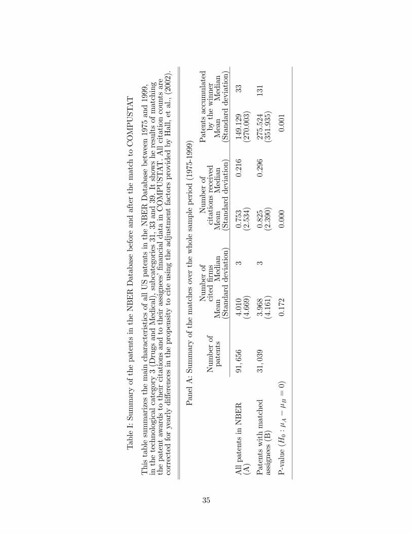
TableI:SummaryofthepatentsintheNBERDatabasebeforeandafterthematchtoCOMPUSTAT

ThistablesummarizesthemaincharacteristicsofallUSpatentsintheNBERDatabasebetween1975and1999,

inthetechnologicalcategory3(DrugsandMedical),subcategories31,33and39.Itshowsheresultsofmatching

thepatentawardstotheircitationsandtotheirassignees��nancialdatainCOMPUSTAT.Allcitationcountsare

correctedforyearlydi¤erencesinthepropensitytociteusingtheadjustmentfactorsprovidedbyHall,etal.,(2002).

PanelA:Summaryofthematchesoverthewholesampleperiod(1975-1999)

Numberof

Numberof

Patentsaccumulated

Numberof

cited�rms

citationsreceived

bythewinner

patents

Mean

Median

Mean

Median

Mean

Median

(Standarddeviation)

(Standarddeviation)

(Standarddeviation)

AllpatentsinNBER

91;656

4:010

30:753

0:216

149:129

33(A)

(4:669)

(2:534)

(270:003)

Patentswithmatched

31;039

3:968

30:825

0:296

275:524

131

assignees(B)

(4:161)

(2:390)

(351:935)

P-value(H

0:�A��B=0)

0:172

0:000

0:001

35

TableI,continued

PanelB:Summaryofthematchesateach�ve-yearperiod

Numberof

Numberof

Patentsaccumulated

Numberof

cited�rms

citationsreceived

bythewinner

patents

Mean

Median

Mean

Median

Mean

Median

(Standarddeviation)

(Standarddeviation)

(Standarddeviation)

1.From

1975to1979

AllpatentsinNBER

8;312

2:123

20:728

0:351

33:701

12(A)

(1:381)

(1:157)

(49:997)

Patentswithmatched

4;069

2:167

20:780

0:350

42:652

25assignees(B)

(1:445)

(1:316)

(46:726)

P-value(H

0:�A��B=0)

0:050

0:000

0:000

2.From

1980to1984

AllpatentsinNBER

10;341

2:737

20:748

0:394

92:682

37(A)

(2:025)

(1:239)

(125:809)

Patentswithmatched

4;414

2:794

20:787

0:394

140:398

102

assignees(B)

(2:037)

(1:385)

(134:391)

P-value(H

0:�A��B=0)

0:062

0:059

0:000

3.From

1980to1984

AllpatentsinNBER

14;448

3:244

20:718

0:385

135:782

37(A)

(2:700)

(1:163)

(206:488)

Patentswithmatched

5;462

3:484

30:781

0:396

224:557

160

assignees(B)

(2:876)

(1:360)

(230:016)

P-value(H

0:�A��B=0)

0:000

0:007

0:000

4.From

1980to1984

AllpatentsinNBER

21;186

3:911

30:714

0:366

172:088

38(A)

(3:731)

(1:146)

(282:673)

Patentswithmatched

7;325

4:218

30:817

0:383

312:031

188

assignees(B)

(3:992)

(1:314)

(348:238)

P-value(H

0:�A��B=0)

0:000

0:000

0:000

5.From

1980to1984

AllpatentsinNBER

37;369

5:133

30:795

0:218

182:568

36(A)

(6:201)

(1:565)

(326:741)

Patentswithmatched

9;769

5:331

40:891

0:236

434:697

260

assignees(B)

(5:628)

(1:432)

(453:162)

P-value(H

0:�A��B=0)

0:000

0:000

0:000

36

TableII:SummarystatisticsofthepatentwinnersintheNBERDatabase

ThistablesummarizesthemaincharacteristicsofthewinnersofallUSpatentsintheNBERDatabasebetween1975and1999,inthetechnological

category3(DrugsandMedical),subcategories31,33and39.Thetotalincumbencyindexof�rm

finpatentiisde�nedas:

I if=P 8j

citedbyi

ownedbyf

#(citations j)�(20�age j),

wherejisapatentcitedbyithatisatmost20yearsoldandthathasbeencited#(citations j)times.All�rmsthatownatleastoneofthe

patentscitedbyithatcontributespositivelytoitsincumbencyvalueareclass�edastheincumbentstothatpatent.Patentwinnersthatarenot

incumbentsareclassi�edasanentranttotheraceforthepatent.Allcitationcountsarecorrectedforyearlydi¤erencesinthepropensitytocite

usingtheadjustmentfactorsprovidedbyHalletal.(2002).

Cashholdings

Totalassets

Patents

Numberof

Incumbency

Proportionofpatentswon

oneyear

oneyear

accumulated

citations

Index

Aftermatch

Beforematch

beforepatent

beforepatent

bythewinner

received

with

with

($Millions)

($Millions)

(corrected)

COMPUSTAT

COMPUSTAT

1.From1975to1979

Incumbent

Mean

241:364

2;187:744

49:189

0:725

238:469

0:289

0:550

Winners

StandardDeviation

(182:309)

(2;174:927)

(59:845)

(1:376)

(698:279)

(0:453)

(0:498)

Observations

856

856

2;567

2;567

2;567

856

2;567

Entrant

Mean

280:969

2;267:456

161:642

0:755

NA

0:711

0:450

Winners

StandardDeviation

(214:164)

(2;024:886)

(143:102)

(1:123)

(0:453)

(0:498)

Observations

2;103

2;103

6;037

6;037

2;103

6;037

2.From1980to1984

Incumbent

Mean

377:349

4;064:571

132:842

0:722

117:338

0:386

0:657

Winners

StandardDeviation

(270:983)

(4;753:242)

(137:684)

(1:288)

(337:773)

(0:487)

(0:475)

Observations

1;198

1;198

3;661

3;661

3;661

1;198

3;661

Entrant

Mean

369:046

4;903:361

703:802

0:776

NA

0:614

0:343

Winners

StandardDeviation

(290:366)

(5;307:917)

(444:496)

(1:293)

(0:487)

(0:475)

Observations

1;909

1;909

7;581

7;581

1;909

7;581

3.From1985to1989

Incumbent

Mean

695:150

5;510:010

210:914

0:669

98:533

0:384

0:665

Winners

StandardDeviation

(743:006)

(5;476:525)

(240:588)

(1:015)

(311:977)

(0:486)

(0:472)

Observations

1;520

1;520

4;848

4;848

4;848

1;520

4;848

Entrant

Mean

708:548

5;630:285

1;930:572

0:843

NA

0:616

0:335

Winners

StandardDeviation

(773:050)

(6;233:403)

(937:203)

(1:606)

(0:486)

(0:472)

Observations

2;443

2;443

10;889

10;889

2;443

10;889

4.From1990to1994

Incumbent

Mean

911:323

9;709:647

271:897

0:707

95:047

0:399

0:700

Winners

StandardDeviation

(1;129:975)

(9;125:851)

(340:712)

(1:262)

(320:758)

(0:490)

(0:458)

Observations

2;017

2;017

7;072

7;072

7;072

2;017

7;072

Entrant

Mean

1;174:322

9;848:718

2;053:102

0:808

NA

0:601

0:300

Winners

StandardDeviation

(1;282:219)

(9;008:386)

(1;028:775)

(1:186)

(0:490)

(0:458)

Observations

3;035

3;035

14;865

14;865

3;035

14;865

5.From1995to1999

Incumbent

Mean

1;411:071

14;271:320

295:380

0:850

120:659

0:454

0:775

Winners

StandardDeviation

(1;496:463)

(11;447:310)

(407:733)

(3:694)

(368:084)

(0:498)

(0:418)

Observations

3;018

3;018

12;519

12;519

12;519

3;018

12;519

Entrant

Mean

1;596:365

13;756:320

2;184:703

0:827

NA

0:546

0:225

Winners

StandardDeviation

(1;310:266)

(9;192:063)

(938:460)

(4:082)

(0:498)

(0:418)

Observations

3;624

3;624

4;725

4;725

3;624

4;725

37

Table III: Estimates of the model�s parameters for patents won by non-cited �rms

This table shows the estimates of the parameters of the model that selects a winner toeach patent from the set of all non-cited �rms that won at least one patent in the same�ve-year period. The estimates were computed using an instrumental variables estimator,following Berry�s (1994) method. The estimable model is:

ln sft � ln s0t = �W lnWft�1 + �EEft�1 + 0cft + �ft;

where sft is the share of patents won by �rm f in year t, and s0t is the share of patentswith self-cited winners, i.e., won by an incumbent. The regressors are listed below. Theinstruments for cash holdings are the logarithm of sales, cash, assets and outstandingdebt, all in years t� 2 and t� 3, and the averages of sales, assets, outstanding debt andaccumulated patents by all other �rms in the same period. The estimates�standard errorsare computed using a covariance matrix estimator robust to correlation within the same 2-digit SIC code. They are shown in brackets under the parameter estimate. The estimationuses all US patents won by listed �rms in COMPUSTAT, between 1975 and 1999, in thetechnological category 3 (Drugs and Medical), subcategories 31, 33 and 39. Patents areclassi�ed into quartiles according to the number of citations they receive. The number ofcitations is asjusted to re�ect time di¤erences in the propensity to cite, using the factorsprovided by Hall, et al., (2002). All speci�cations include dummy variables for all but oneof the 2-digit SIC codes observed in the sample and for all but one of the sample years.

Panel A: Estimation Period from 1975 to 1979Quartiles for Numbers of Citations by Patent(1) (2) (3) (4)

Logarithm of cash holdings, 1 year 0:053 0:044 0:207 0:129before the patent was awarded (lnWft�1) (0:118) (0:092) (0:057)��� (0:038)���

Total patents accumulated by the �rm �0:0004 0:0015 0:0000 0:0007up to one year before the award (Eft�1) (0:001) (0:001)� (0:001) (0:001)

Constant �4:465 �5:093 �5:756 �5:226(0:711)��� (0:458)��� (0:326)��� (0:242)���

Number of observations 72 131 158 147R2 0:06 0:23 0:30 0:21F statistic 2; 869:714 26; 203:956 46; 417:519 17:265P value of F Statistic 0:000 0:000 0:000 0:000Test of Over Identifying Restrictions 6:120 9:746 12:171 19:787P value of �2 statistic 0:865 0:940 0:935 0:535

Panel B: Estimation Period from 1980 to 1984Quartiles for Numbers of Citations by Patent(1) (2) (3) (4)

Logarithm of cash holdings, 1 year 0:101 0:267 0:159 0:144before the patent was awarded (lnWft�1) (0:088) (0:074)��� (0:064)�� (0:058)��

Total patents accumulated by the �rm 0:0003 0:0007 0:0012 0:0007up to one year before the award (Eft�1) (0:000) (0:000)�� (0:000)��� (0:000)�

Constant �3:775 �5:776 �6:248 �6:014(0:460)��� (0:347)��� (0:377)��� (0:327)���

Number of observations 65 110 136 130R2 0:15 0:31 0:34 0:23F statistic 319:918 28:156 33:911 105:087P value of F Statistic 0:000 0:000 0:000 0:000Test of Over Identifying Restrictions 7:841 9:110 19:128 6:595P value of �2 statistic 0:727 0:909 0:262 0:980

38

Table III, continued.

Panel C: Estimation Period from 1985 to 1989Quartiles for Numbers of Citations by Patent(1) (2) (3) (4)

Logarithm of cash holdings, 1 year 0:233 0:145 0:135 0:101before the patent was awarded (lnWft�1) (0:127)� (0:053)��� (0:056)�� (0:046)��

Total patents accumulated by the �rm 0:0001 0:0006 0:0008 0:0005up to one year before the award (Eft�1) (0:000) (0:000)��� (0:000)��� (0:0002)��

Constant �5:958 �6:389 �6:527 �5:928(0:876)��� (0:306)��� (0:318)��� (0:371)���

Number of observations 65 138 178 199R2 0:05 0:46 0:47 0:31F statistic 10:882 19; 485:801 1; 341:881 8:365P value of F Statistic 0:000 0:000 0:000 0:000Test of Over Identifying Restrictions 3:183 26:334 33:785 16:578P value of �2 statistic 0:988 0:092 0:009 0:829

Panel D: Estimation Period from 1990 to 1994Quartiles for Numbers of Citations by Patent(1) (2) (3) (4)

Logarithm of cash holdings, 1 year 0:207 0:279 0:218 0:176before the patent was awarded (lnWft�1) (0:076)��� (0:052)��� (0:036)��� (0:038)���

Total patents accumulated by the �rm 0:0001 0:0001 0:0005 0:0004up to one year before the award (Eft�1) (0:000) (0:000) (0:000)��� (0:000)���

Constant �6:38 �7:247 �7:164 �6:586(0:427)��� (0:332)��� (0:193)��� (0:186)���

Number of observations 98 131 220 211R2 0:24 0:39 0:49 0:44F statistic 723:838 2; 346:024 37:223 88:97P value of F Statistic 0:000 0:000 0:000 0:000Test of Over Identifying Restrictions 9:265 1:586 9:310 7:605P value of �2 statistic 0:902 1:000 0:952 0:990

Panel E: Estimation Period from 1995 to 1999Quartiles for Numbers of Citations by Patent(1) (2) (3) (4)

Logarithm of cash holdings, 1 year 0:298 0:228 0:209 0:262before the patent was awarded (lnWft�1) (0:050)��� (0:044)��� (0:044)��� (0:047)���

Total patents accumulated by the �rm 0:0004 0:0002 0:0003 0:0003up to one year before the award (Eft�1) (0:0001)��� (0:0001)�� (0:0001)��� (0:0001)���

Constant �8:61 �7:788 �7:177 �8:449(0:394)��� (0:269)��� (0:238)��� (0:353)���

Number of observations 180 135 77 146R2 0:52 0:53 0:50 0:51F statistic 26:986 91:423 37:758 5; 898:445P value of F Statistic 0:000 0:000 0:000 0:000Test of Over Identifying Restrictions 29:743 13:748 6:205 12:666P value of �2 statistic 0:028 0:617 0:961 0:758

a Estimates followed by ���, �� and � are statistically di¤erent from zero with 0.01, 0.05 and 0.1signi�cance levels, respectively.b The F-statistic is computed under the null hypothesis that all the model�s parameters are zero.c The �2 statistic is computed under the null hypothesis that the instruments provide enoughexogenous variation to overidentify the model�s parameters.

39

TableIV:Economicsigni�canceoftheestimatesofthemodel�sparametersestimatedusingpatentswonbynon-cited�rms

Thistableshowsthechangeintheexpectednumberofpatentswonperyearper�rmwithrespecttocashholdingsandprevious

patentingexperience.Thechangesandtheirstandarderrors(shownunderneaththem

inbrackets)areestimatedusingthedelta

methodonthemodelestimatesshowninTableIII.TheestimationusesallUSpatentswonby�rmslistedinCOMPUSTAT,

betweenbetween1975and1999,inthetechnologicalcategoty3(DrugsandMedical),sub-categories31,33and39.Patentsare

classi�edintoquartilesaccordingtothenumberofcitationstheyreceive.Thenumberofcitationsisadjustedtore�ectyearly

di¤erencesinthepropensitytocite,usingthefactorsprovidedbyHall,etal.(2002).

Changeswithrespecttoonesamplestandarddeviationincreaseinthe�rm�s:

Cashholdings,oneyearbefore

Patentsaccumulated,oneyear

thepatentwasawarded

beforethepatentwasawarded

Quartilesofthe

Quartilesofthe

numberofcitationsbypatent

numberofcitationsbypatent

(1)

(2)

(3)

(4)

(1)

(2)

(3)

(4)

1.EstimationPeriod:1975-1979

Changeintheexpectednumber

0:0706

0:0187

0:6949

0:3922

0:0765

0:4106

0:0733

0:1544

ofpatentsper�rmperyear

(0:2342)

(0:2324)

(0:2245)��� (0:1358)���

(0:169)

(0:1972)��(0:1331)

(0:1334)

Patentsper�rmperyear

2:1017

2:5813

2:6458

2:2007

2:1017

2:5813

2:6458

2:2007

2.EstimationPeriod:1980-1984

Changeinthexpectednumber

0:1305

1:1378

0:4647

0:4689

0:1741

0:2545

0:7083

0:2754

ofpatentsper�rmperyear

(0:1407)

(0:3849)��� (0:2193)��(0:2211)��

(0:1008)�(0:1903)

(0:2048)���(0:1574)�

Patentsper�rmperyear

1:7130

2:4505

2:5752

2:1004

1:7130

2:4505

2:5752

2:1004

3.EstimationPeriod:1985-1989

Changeintheexpectednumber

0:5440

0:6228

0:5227

0:3808

0:0793

0:6581

0:7843

0:3955

ofpatentsper�rmperyear

(0:3159)�(0:2575)��(0:2462)��(0:1953)�

(0:1894)

(0:1488)��� (0:1795)���(0:1905)��

Patentsper�rmperyear

1:9820

2:6213

2:6699

2:1722

1:9820

2:6213

2:6699

2:1722

4.EstimationPeriod:1990-1994

Changeintheexpectednumber

0:2410

1:3742

1:2416

0:8676

0:2299

0:1385

0:5046

0:4215

ofpatentsper�rmperyear

(0:1672)

(0:3218)��� (0:2556)���(0:2129)���

(0:1596)

(0:1136)

(0:1218)���(0:1115)���

Patentsper�rmperyear

2:2611

2:6167

2:9050

2:5984

2:2611

2:6167

2:9050

2:5984

5.EstimationPeriod:1995-1999

Changeintheexpectednumber

2:4275

1:3188

1:1925

1:6341

0:8164

0:3928

0:5224

0:5821

ofpatentsper�rmperyear

(0:4772)��� (0:3708)���(0:318)���(0:38)���

(0:224)���(0:2021)�(0:1514)���(0:2152)���

Patentsper�rmperyear

4:2556

3:1744

2:9776

3:1855

4:2556

3:1744

2:9776

3:1855

aEstimatesfollowedby

���,��and�arestatisticallydi¤erentfrom

zerowith0.01,0.05and0.1signi�cancelevels,respectively.

40

TableV:Selectionof�rmsthatraceforeachpatent

Thistabledescribestheselectionofcitedandnon-cited�rmsforeverypatentrace.

Potentialentrantsarerankedaccordingtothepredictedprobabilitiesofwinninga

patentineverygivenyear,usingthemodelandtheestimatesisTableIII.

Theincumbencyvalueofpatenti,citingall�rmf�spatents,isde�nedas:

I i=P 8

citedf

P 8jcitedbyi

ownedbyf#(citations j)�(20�age j),

wherejisapatentcitedbyithatisatmost20yearsoldandthathasbeencited

#(citations j)times.All�rmsthatownatleastoneofthepatentscitedbyithat

contributespositivelytoitsincumbencyvalueareclass�edastheincumbentstothat

patent.Patentwinnersthatarenotincumbentsareclass�edasanentranttotherace

forthepatent.Allcitationcountsarecorrectedforyearlydi¤erencesinthepropensity

tociteusingtheadjustmentfactorsprovidedbyHalletal.(2002).

PanelA:Selectionof�rmsthatarenotcitedbythepatent(�Entrants�)

Cumulativeprobabilityofwinning,giventhatthewinnerisnotacited�rm

Ranking

Mean

Median

10:096

0:108

50:392

0:400

10

0:757

0:774

15

0:955

0:971

20

1:000

1:000

Numberofselections

100

PanelB:Selectionof�rmsthatarecitedbythepatent(�Incumbents�)

Numberof�rmscitedperpatent

Cumulativerelativeincumbency

Cumulative

valuespercited�rm

Number

frequency

Ranking

Median

Mean

126:25

10:707

0:699

247:02

20:980

0:861

361:91

31:000

0:923

472:05

41:000

0:951

579:49

51:000

0:966

1094:52

10

1:000

0:986

Numberofpatents

91;656

Numberofpatents

91;656

41

Table VI: Summary statistics of the characteristics of the �rms selected to each race

This table summarizes the main characteristics of the �rms selected as the most likelyparticipants in every given patent race. The selection includes the top four cited �rms(incumbents) according to their contribution to the incumbency value of every patentand the top ten non-cited �rms (entrants) according to the predicted probability ofwinning every given patent among the set of all non-cited �rms with at least one patentin the same year. The probabilities are predicted using the model and the estimatesreported in Table III. Each selection includes the actual winner, and it is done forall US patents in the NBER Database, between 1975 and 1999, category 3 (Drugs andMedical), subcategories 31, 33 and 39.

Cash holdings, Total assets, Patentsone year before one year before accumulatedpatent award patent award by the($ Millions) ($ Millions) winner

1. From 1975 to 1979Selected Mean 218:303 2; 019:305 35:618Incumbents Standard Deviation (85:474) (1; 029:481) (44:165)

Observations 5; 878 5; 878 5; 878

Selected Mean 276:385 2; 776:869 129:301Entrants Standard Deviation (140:380) (2; 317:138) (113:864)

Observations 29; 590 29; 590 29; 590

2. From 1980 to 1984Selected Mean 350:492 3; 059:526 96:876Incumbents Standard Deviation (130:734) (2; 102:791) (123:386)

Observations 7; 351 7; 351 7; 351

Selected Mean 419:558 4; 672:930 477:353Entrants Standard Deviation (232:966) (5; 357:519) (283:267)

Observations 31; 070 31; 070 31; 070

3. From 1985 to 1989Selected Mean 549:988 4; 405:751 153:849Incumbents Standard Deviation (356:459) (2; 572:547) (213:735)

Observations 10; 406 10; 406 10; 406

Selected Mean 900:992 7; 444:320 959:211Entrants Standard Deviation (1; 704:136) (8; 988:671) (682:861)

Observations 39; 630 39; 630 39; 630

4. From 1990 to 1994Selected Mean 975:789 9; 688:180 219:141Incumbents Standard Deviation (527:601) (6; 298:604) (318:013)

Observations 13; 977 13; 977 13; 977

Selected Mean 1; 252:073 12; 399:550 1; 201:756Entrants Standard Deviation (1; 304:270) (11; 031:950) (764:014)

Observations 50; 520 50; 520 50; 520

5. From 1995 to 1999Selected Mean 1; 323:478 14; 451:770 289:835Incumbents Standard Deviation (703:680) (5; 122:284) (423:305)

Observations 19; 501 19; 501 19; 501

Selected Mean 1; 832:491 18; 354:430 1; 363:011Entrants Standard Deviation (1; 232:780) (10; 099:930) (926:430)

Observations 66; 354 66; 354 66; 398

42

TableVII:Averageincumbencyvaluesofincumbent�rmsselectedtoeachrace

Thistableshowstheaverageincumbencyvaluesforeachselectedincumbent�rm,conditionalontheageofthecitations.The

selectionincludesthetopfourcited�rms(incumbents)accordingtotheircontributiontotheincumbencyvalueofeverypatent

ThetablereportsthesummarystatisticsforallUSpatentswithobservedcitationsintheNBERDatabase,between1975and

1999,incategory3(DrugsandMedical),subcategories31,33and39,andforallpatentsthatcanbematchedtoCOMPUSTAT

usingtheCUSIPnumbersofthe�rmsselectedtoeachrace.

PanelA:Valueofcitationsperselectedincumbent,usingallpatentswithobservedcitations

Ageofcitations,inyears

Age<1

1�Age<2

2�Age<3

3�Age<4

4�Age<5

5�Age<10

10�Age<20

1.From

1975to1979

Mean

1:976

0:851

1:662

2:039

2:447

6:084

1:87

StandardDeviation

(9:074)

(5:916)

(11:192)

(12:077)

(14:227)

(19:047)

(8:816)

Skewness

9:754

27:704

20:806

17:249

18:598

11:461

9:372

NumberofIncumbents

9,579

9,579

9,579

9,579

9,579

9,579

9,579

2.From

1980to1984

Mean

1:46

0:267

0:361

0:410

0:373

4:821

4:725

StandardDeviation

(9:239)

(1:290)

(1:547)

(1:970)

(1:760)

(19:276)

(17:494)

Skewness

13:857

10:018

9:467

9:069

10:145

12:248

9:751

NumberofIncumbents

13,440

13,440

13,440

13,440

13,440

13,440

13,440

3.From

1985to1989

Mean

1:248

0:235

0:302

0:334

0:336

1:59

6:092

StandardDeviation

(9:185)

(1:737)

(1:518)

(1:425)

(1:592)

(5:405)

(29:612)

Skewness

16:539

34:431

27:664

8:381

9:364

8:247

13:218

NumberofIncumbents

18,779

18,779

18,779

18,779

18,779

18,779

18,779

4.From

1990to1994

Mean

0:985

0:285

0:393

0:426

0:410

1:404

4:136

StandardDeviation

(9:231)

(1:942)

(2:289)

(2:209)

(2:442)

(4:441)

(29:619)

Skewness

27:052

23:170

23:791

21:473

25:302

10:487

15:589

NumberofIncumbents

27,899

27,899

27,899

27,899

27,899

27,899

27,899

5.From

1995to1999

Mean

1:406

0:542

0:595

0:548

0:525

2:228

2:002

StandardDeviation

(15:158)

(3:526)

(3:745)

(3:167)

(2:772)

(6:891)

(8:094)

Skewness

22:098

18:599

25:669

20:837

17:708

12:963

8:142

NumberofIncumbents

47,688

47,688

47,688

47,688

47,688

47,688

47,688

43

TableVII,continued

PanelB:Valueofcitationsperselectedincumbent,usingallpatentsmatchedtoCOMPUSTAT

Ageofcitations,inyears

Age<1

1�Age<2

2�Age<3

3�Age<4

4�Age<5

5�Age<10

10�Age<20

1.From

1975to1979

Mean

2:327

0:791

1:499

1:771

2:113

6:277

2:178

StandardDeviation

(9:976)

(4:761)

(8:800)

(9:263)

(9:239)

(15:834)

(9:763)

Skewness

9:098

13:060

18:402

16:439

8:965

4:529

9:263

NumberofIncumbents

5,878

5,878

5,878

5,878

5,878

5,878

5,878

2.From

1980to1984

Mean

1:823

0:260

0:368

0:458

0:406

5:292

5:642

StandardDeviation

(10:431)

(1:285)

(1:635)

(2:283)

(1:939)

(19:267)

(19:535)

Skewness

10:272

10:152

10:126

8:564

9:814

9:580

9:508

NumberofIncumbents

7,351

7,351

7,351

7,351

7,351

7,351

7,351

3.From

1985to1989

Mean

1:374

0:250

0:308

0:357

0:390

1:712

5:847

StandardDeviation

(9:291)

(2:167)

(1:717)

(1:549)

(1:813)

(5:205)

(19:722)

Skewness

15:356

31:237

31:896

8:557

8:887

6:331

10:194

NumberofIncumbents

10,406

10,406

10,406

10,406

10,406

10,406

10,406

4.From

1990to1994

Mean

0:977

0:250

0:374

0:444

0:443

1:520

3:341

StandardDeviation

(7:361)

(1:409)

(1:883)

(2:259)

(2:910)

(4:725)

(18:816)

Skewness

15:460

15:592

22:010

22:210

23:574

10:753

21:933

NumberofIncumbents

13,977

13,977

13,977

13,977

13,977

13,977

13,977

5.From

1995to1999

Mean

0:994

0:507

0:563

0:500

0:460

2:280

2:220

StandardDeviation

(7:515)

(3:195)

(2:821)

(2:142)

(1:946)

(6:673)

(8:699)

Skewness

13:692

16:761

23:748

21:552

16:498

13:292

7:329

NumberofIncumbents

19,501

19,501

19,501

19,501

19,501

19,501

19,501

44

Table VIII: Estimates of the model�s parameters for all usable patents

This table shows the estimates of the parameters of the model that selects a winner of eachpatent from the set of pre-selected entrants and incumbents. The estimates were computedusing maximum likelihood and Petrin and Train�s (2003) method to instrument endogenousregressors in the multinomial logit setup. The estimable model is:

Pr(�rm f wins race i) =exp(�W lnWf+�SSf+�EEf+

0cif+�f )Pg exp(�W lnWg+�SSg+�EEg+

0cig+�g):

where the regressors are listed below, and �f represents the unobserved �rm characteristicsthat are correlated with cash. The instruments for cash holdings are the logarithms of cash,sales, total assets and outstanding debt, all lagged two and three years, and the averages ofcash, sales, debt and accumulated patents of all other rival �rms in the same race. Thestandard errors of the parameter estimates are computed using a bootstrap estimator. Theyare shown in brackets underneath the parameter estimate. The estimation uses all USpatents won by COMPUSTAT �rms from 1975 to 1999, in the techonological category 3(Drugs and Medical), subcategories 31, 33 and 39. Patents are classi�ed into quartilesaccording to the number of citations received. The number of citations is asjusted for timedi¤erences in the propensity to cite, using the factors provided by Hall, et al., (2002).

Estimation Period from 1995 to 1999Quartiles for Numbers of Citations by Patent(1) (2) (3) (4)

Logarithm of cash holdings, 1 year 0:616 0:688 0:917 0:646before the patent was awarded (lnWf ) (0:041)��� (0:062)��� (0:069)��� (0:050)���

Logarithm of total assets, 1year �1:128 �0:933 �0:470 �0:508before patent was awarded (lnSf ) (0:064)��� (0:092)��� (0:096)��� (0:099)���

Total patents accumulated by the �rm 0:001 0:001 0:000 0:000up to one year before the award (Ef ) (0:000)��� (0:000)��� (0:000)��� (0:000)���

Citations received by the �rm�s citedpatents, by age (in years):

Age < 1 0:003 �0:002 �0:003 �0:019(0:006) (0:006) (0:029) (0:015)

1 � Age < 2 0:244 0:169 0:676 0:230(0:022)��� (0:023)��� (0:121)��� (0:020)���

2 � Age < 3 0:235 0:187 0:483 0:169(0:021)��� (0:025)��� (0:075)��� (0:019)���

3 � Age < 4 0:121 0:109 0:267 0:087(0:021)��� (0:023)��� (0:063)��� (0:019)���

4 � Age < 5 0:193 0:156 0:114 0:082(0:025)��� (0:034)��� (0:087) (0:021)���

5 � Age < 10 0:094 0:115 0:006 0:021(0:009)��� (0:014)��� (0:015) (0:005)���

10 � Age < 20 0:044 0:017 0:074 0:056(0:003)��� (0:006)��� (0:012)��� (0:004)���

First stage error �0:090 �0:458 �1:745 �1:133component (�̂g) (0:087) (0:164)��� (0:142)��� (0:105)���

Number of observations 29,789 13,483 8,754 21,823�2 statistic 2; 799:746 1; 429:349 1; 026:918 1; 889:034P value of �2 statistic 0:000 0:000 0:000 0:000Pseudo R2 0:224 0:236 0:297 0:221

a Estimates followed by ���, �� and � are statistically di¤erent from zero with 0.01, 0.05 and 0.1signi�cance levels, respectively.b The �2 statistic is computed under the null hypothesis that all the model�s parameters are zero.

45

TableIX:Economicsigni�canceoftheestimatesofthemodel�sparametersesimatedwithallusablepatents

Thistableshowsthechangeintheexpectedprobabilityofwinningagivenpatentwithrespecttocashholdingsandprevious

patentingexperience.Thechangesandtheirstandarderrors(shownunderneaththem

inbrackets)areestimatedusingthedelta

methodonthemodelestimatesshowninTableVIII.TheestimationusesallUSpatentswonby�rmslistedinCOMPUSTAT,

betweenbetween1975and1999,inthetechnologicalcategoty3(DrugsandMedical),sub-categories31,33and39.Patentsare

classi�edintoquartilesaccordingtothenumberofcitationstheyreceive.Thenumberofcitationsisadjustedtore�ectyearly

di¤erencesinthepropensitytocite,usingthefactorsprovidedbyHall,etal.(2002).

Changeswithrespecttoonesamplestandarddeviationincreaseinthe�rm�s:

Cashholdings,oneyearbefore

Patentsaccumulated,oneyear

thepatentwasawarded

beforethepatentwasawarded

Quartilesofthe

Quartilesofthe

numberofcitationsbypatent

numberofcitationsbypatent

(1)

(2)

(3)

(4)

(1)

(2)

(3)

(4)

1.EstimationPeriod:1975-1979

Changeintheexpectedprobability

0:0171

0:0094

0:0279

0:1124

0:0785

0:0291

0:0107

0:0315

ofwinningapatent

(0:0119)

(0:0041)��(0:0051)��� (0:0074)���

(0:0162)��� (0:0063)���(0:0035)���(0:0048)���

Patentsper�rmperyear

0:0969

0:0882

0:0836

0:0813

0:0969

0:0882

0:0836

0:0813

2.EstimationPeriod:1980-1984

Changeinthexpectedprobability

0:0422

0:0071

�0:0033

0:0101

0:0447

0:0166

0:0629

0:0633

ofwinningapatent

(0:0104)��� (0:004)�

(0:0031)

(0:0039)���

(0:0081)��� (0:0036)���(0:0041)���(0:0045)���

Patentsper�rmperyear

0:0952

0:0869

0:0814

0:0784

0:0952

0:0869

0:0814

0:0784

3.EstimationPeriod:1985-1989

Changeintheexpectedprobability

0:0727

0:0014

�0:0060

0:0287

0:0441

0:0689

0:0821

0:0682

ofwinningapatent

(0:0168)��� (0:0034)

(0:0036)�(0:0045)���

(0:0067)��� (0:0041)���(0:0037)���(0:0035)���

Patentsper�rmperyear

0:0914

0:0838

0:0793

0:0770

0:0914

0:0838

0:0793

0:0770

4.EstimationPeriod:1990-1994

Changeintheexpectedprobability

0:0823

0:0623

0:0024

�0:0072

0:0226

0:0495

0:0684

0:0592

ofwinningapatent

(0:0078)��� (0:0054)���(0:0022)

(0:0023)���

(0:0042)��� (0:004)���(0:0029)���(0:003)���

Patentsper�rmperyear

0:0923

0:0864

0:0784

0:0767

0:0923

0:0864

0:0784

0:0767

5.EstimationPeriod:1995-1999

Changeintheexpectedprobability

0:0446

0:0533

0:0848

0:0426

0:0587

0:0904

0:0270

0:0310

ofwinningapatent

(0:0035)��� (0:0057)���(0:0085)��� (0:0039)���

(0:0027)��� (0:0052)���(0:0039)���(0:0025)���

Patentsper�rmperyear

0:0901

0:1056

0:0772

0:0762

0:0901

0:1056

0:0772

0:0762

aEstimatesfollowedby

���,��and�arestatisticallydi¤erentfrom

zerowith0.01,0.05and0.1signi�cancelevels,respectively.

46

Table X: Estimates of the model�s parameters for all usable patents

This table shows the estimates of the parameters of the model that selects a winner of eachpatent from the set of pre-selected entrants and incumbents. The estimates were computedusing maximum likelihood and Petrin and Train�s (2003) method to instrument endogenousregressors in the multinomial logit setup. The estimable model is:

Pr(�rm f wins race i) =exp(�W lnWf+�SSf+�EEf+

0cif+�f )Pg exp(�W lnWg+�SSg+�EEg+

0cig+�g):

where the regressors are listed below, and �f represents the unobserved �rm characteristicsthat are correlated with cash. The instruments for cash holdings are the logarithms of cash,sales, total assets and outstanding debt, all lagged two and three years, and the averages ofcash, sales, debt and accumulated patents of all other rival �rms in the same race. Thestandard errors of the parameter estimates are computed using a bootstrap estimator. Theyare shown in brackets underneath the parameter estimate. The estimation uses all USpatents won by COMPUSTAT �rms from 1975 to 1999, in the techonological category 3(Drugs and Medical), subcategories 31, 33 and 39. Patents are classi�ed into quartilesaccording to the number of citations received. The number of citations is asjusted for timedi¤erences in the propensity to cite, using the factors provided by Hall, et al., (2002).

Panel A: Estimation Period from 1975 to 1979Quartiles for Numbers of Citations by Patent(1) (2) (3) (4)

Logarithm of cash holdings, 1 year 0:475 �0:035 0:638 3:361before the patent was awarded (lnWf ) (0:200)�� (0:099) (0:100)��� (0:215)���

Logarithm of cash holdings times �0:033 0:035 �0:013 �0:199total assets (lnWf � lnSf ) (0:021) (0:011)��� (0:010) (0:022)���

Total patents accumulated by the �rm 0:007 0:003 0:001 0:003up to one year before the award (Ef ) (0:001)��� (0:001)��� (0:000)��� (0:000)���

Citations received by the �rm�s citedpatents, by age (in years):

Age < 1 �0:042 �0:096 �0:051 �0:009(0:106) (0:062) (0:039) (0:021)

1 � Age < 2 0:733 0:118 0:026 0:048(0:154)��� (0:022)��� (0:011)�� (0:011)���

2 � Age < 3 0:104 0:086 0:026 0:005(0:041)�� (0:021)��� (0:012)�� (0:005)

3 � Age < 4 0:035 0:088 0:035 0:008(0:025) (0:015)��� (0:009)��� (0:005)�

4 � Age < 5 0:042 0:054 0:022 0:035(0:018)�� (0:012)��� (0:007)��� (0:006)���

5 � Age < 10 0:038 0:033 0:015 0:023(0:016)�� (0:008)��� (0:005)��� (0:003)���

10 � Age < 20 �10:316 �12:555 �12:400 �11:636(467:420) (529:325) (496:626) (684:447)

First stage error �1:018 �1:613 �1:388 1:486component (�̂g) (0:233)��� (0:129)��� (0:133)��� (0:349)���

Number of observations 2,807 9,515 11,661 10,219�2 statistic 184:285 434:396 370:479 732:633P value of �2 statistic 0:000 0:000 0:000 0:000Pseudo R2 0:150 0:108 0:077 0:176

a Estimates followed by ���, �� and � are statistically di¤erent from zero with 0.01, 0.05 and 0.1signi�cance levels, respectively.b The �2 statistic is computed under the null hypothesis that all the model�s parameters are zero.

47

Table X, continued.

Panel B: Estimation Period from 1980 to 1984Quartiles for Numbers of Citations by Patent(1) (2) (3) (4)

Logarithm of cash holdings, 1 year 0:441 �0:343 �0:818 0:208before the patent was awarded (lnWf ) (0:224)�� (0:143)�� (0:143)��� (0:131)

Logarithm of cash holdings times 0:044 0:062 0:096 0:011total assets (lnWf � lnSf ) (0:014)��� (0:011)��� (0:014)��� (0:013)

Total patents accumulated by the �rm 0:001 0:001 0:002 0:002up to one year before the award (Ef ) (0:000)��� (0:000)��� (0:000)��� (0:000)���

Citations received by the �rm�s citedpatents, by age (in years):

Age < 1 �0:250 �0:178 �0:196 �0:062(0:202) (0:086)�� (0:125) (0:034)�

1 � Age < 2 1:375 0:729 0:602 0:398(0:532)��� (0:129)��� (0:067)��� (0:038)���

2 � Age < 3 1:637 0:627 0:442 0:238(0:268)��� (0:108)��� (0:058)��� (0:029)���

3 � Age < 4 0:261 0:382 0:297 0:151(0:105)�� (0:090)��� (0:045)��� (0:023)���

4 � Age < 5 0:921 0:317 0:313 0:204(0:173)��� (0:071)��� (0:046)��� (0:031)���

5 � Age < 10 0:014 0:034 0:025 0:001(0:012) (0:006)��� (0:004)��� (0:003)

10 � Age < 20 0:024 0:028 0:020 0:017(0:014)� (0:007)��� (0:004)��� (0:003)���

First stage error �1:246 �1:271 �2:015 �1:527component (�̂g) (0:236)��� (0:256)��� (0:213)��� (0:192)���

Number of observations 3,392 9,136 13,123 11,014�2 statistic 184:898 296:688 881:076 834:065P value of �2 statistic 0:000 0:000 0:000 0:000Pseudo R2 0:126 0:078 0:165 0:190

a Estimates followed by ���, �� and � are statistically di¤erent from zero with 0.01, 0.05 and 0.1signi�cance levels, respectively.b The �2 statistic is computed under the null hypothesis that all the model�s parameters are zero.

48

Table X, continued.

Panel C: Estimation Period from 1985 to 1989Quartiles for Numbers of Citations by Patent(1) (2) (3) (4)

Logarithm of cash holdings, 1 year 0:529 0:476 �0:086 0:651before the patent was awarded (lnWf ) (0:167)��� (0:118)��� (0:103) (0:074)���

Logarithm of cash holdings times 0:014 �0:059 �0:005 �0:040total assets (lnWf � lnSf ) (0:015) (0:010)��� (0:010) (0:008)���

Total patents accumulated by the �rm 0:001 0:001 0:001 0:001up to one year before the award (Ef ) (0:000)��� (0:000)��� (0:000)��� (0:000)���

Citations received by the �rm�s citedpatents, by age (in years):

Age < 1 �0:151 �0:183 �0:083 �0:018(0:257) (0:042)��� (0:033)�� (0:016)

1 � Age < 2 2:853 1:209 0:579 0:265(0:509)��� (0:144)��� (0:073)��� (0:043)���

2 � Age < 3 1:212 1:087 0:654 0:215(0:284)��� (0:108)��� (0:055)��� (0:026)���

3 � Age < 4 0:601 0:548 0:161 0:119(0:167)��� (0:094)��� (0:034)��� (0:026)���

4 � Age < 5 0:863 0:473 0:16 0:095(0:165)��� (0:089)��� (0:041)��� (0:021)���

5 � Age < 10 0:145 0:228 0:175 0:089(0:037)��� (0:022)��� (0:015)��� (0:010)���

10 � Age < 20 0:007 0:028 0:005 0:007(0:006) (0:005)��� (0:003) (0:003)���

First stage error �0:544 0:305 �0:776 �0:690component (�̂g) (0:134)��� (0:178)� (0:112)��� (0:088)���

Number of observations 4,003 12,183 16,526 15,617�2 statistic 345:685 1; 075:617 1; 519:107 1; 561:553P value of �2 statistic 0:000 0:000 0:000 0:000Pseudo R2 0:203 0:215 0:229 0:254

a Estimates followed by ���, �� and � are statistically di¤erent from zero with 0.01, 0.05 and 0.1signi�cance levels, respectively.b The �2 statistic is computed under the null hypothesis that all the model�s parameters are zero.

49

Table X, continued.

Panel D: Estimation Period from 1990 to 1994Quartiles for Numbers of Citations by Patent(1) (2) (3) (4)

Logarithm of cash holdings, 1 year 1:251 1:212 �0:138 �0:491before the patent was awarded (lnWf ) (0:132)��� (0:123)��� (0:070)�� (0:082)���

Logarithm of cash holdings times �0:009 �0:005 0:023 0:042total assets (lnWf � lnSf ) (0:010) (0:010) (0:005)��� (0:007)���

Total patents accumulated by the �rm 0:000 0:001 0:001 0:001up to one year before the award (Ef ) (0:000)��� (0:000)��� (0:000)��� (0:000)���

Citations received by the �rm�s citedpatents, by age (in years):

Age < 1 �0:122 �0:139 �0:03 �0:016(0:113) (0:111) (0:025) (0:011)

1 � Age < 2 1:001 1:261 0:429 0:305(0:170)��� (0:129)��� (0:048)��� (0:032)���

2 � Age < 3 1:041 0:509 0:456 0:123(0:137)��� (0:085)��� (0:042)��� (0:022)���

3 � Age < 4 0:142 0:227 0:136 0:175(0:044)��� (0:045)��� (0:036)��� (0:020)���

4 � Age < 5 0:482 0:253 0:075 0:048(0:091)��� (0:054)��� (0:027)��� (0:016)���

5 � Age < 10 0:147 0:156 0:143 0:03(0:032)��� (0:024)��� (0:014)��� (0:009)���

10 � Age < 20 0:031 0:035 0:009 0:002(0:007)��� (0:007)��� (0:003)��� (0:003)

First stage error �1:308 �1:627 �1:268 �1:87component (�̂g) (0:167)��� (0:144)��� (0:090)��� (0:098)���

Number of observations 7,539 11,302 22,904 19,982�2 statistic 427:708 794:330 1; 682:844 2; 045:315P value of �2 statistic 0:000 0:000 0:000 0:000Pseudo R2 0:134 0:169 0:184 0:261

a Estimates followed by ���, �� and � are statistically di¤erent from zero with 0.01, 0.05 and 0.1signi�cance levels, respectively.b The chi2 statistic is computed under the null hypothesis that all the model�s parameters are zero.

50

Table X, continued.

Panel E: Estimation Period from 1995 to 1999Quartiles for Numbers of Citations by Patent(1) (2) (3) (4)

Logarithm of cash holdings, 1 year 0:939 0:806 1:380 0:308before the patent was awarded (lnWf ) (0:096)��� (0:118)��� (0:142)��� (0:126)��

Logarithm of cash holdings times �0:066 �0:035 �0:053 0:029total assets (lnWf � lnSf ) (0:009)��� (0:011)��� (0:013)��� (0:012)��

Total patents accumulated by the �rm 0:001 0:001 0:000 0:000up to one year before the award (Ef ) (0:000)��� (0:000)��� (0:000)��� (0:000)���

Citations received by the �rm�s citedpatents, by age (in years):

Age < 1 0:003 �0:002 �0:003 �0:02(0:006) (0:006) (0:029) (0:015)

1 � Age < 2 0:24 0:173 0:674 0:241(0:022)��� (0:023)��� (0:120)��� (0:019)���

2 � Age < 3 0:224 0:182 0:48 0:171(0:020)��� (0:024)��� (0:074)��� (0:018)���

3 � Age < 4 0:12 0:102 0:265 0:085(0:020)��� (0:024)��� (0:063)��� (0:019)���

4 � Age < 5 0:194 0:15 0:11 0:081(0:024)��� (0:033)��� (0:086) (0:021)���

5 � Age < 10 0:098 0:113 0:006 0:021(0:009)��� (0:013)��� (0:015) (0:005)���

10 � Age < 20 0:044 0:017 0:072 0:055(0:003)��� (0:006)��� (0:012)��� (0:004)���

First stage error �0:811 �1:494 �1:872 �1:742component (�̂g) (0:089)��� (0:147)��� (0:135)��� (0:097)���

Number of observations 29,789 13,483 8,754 21,823�2 statistic 2493:025 1330:706 1018:776 1868:082P value of �2 statistic 0:000 0:000 0:000 0:000Pseudo R2 0:199 0:220 0:295 0:218

a Estimates followed by ���, �� and � are statistically di¤erent from zero with 0.01, 0.05 and 0.1signi�cance levels, respectively.b The �2 statistic is computed under the null hypothesis that all the model�s parameters are zero.

51

TableXI:Economicsigni�canceoftheestimatesofthemodel�sparametersestimatedwithallusablepatents

Thistableshowsthechangeintheexpectedprobabilityofwinningagivenpatentwithrespecttocashholdingsandprevious

patentingexperience.Thechangesandtheirstandarderrors(shownunderneaththem

inbrackets)arecomputedusingthedelta

methodonthemodelestimatesshowninTableX.TheestimationusesallUSpatentswonby�rmslistedinCOMPUSTAT,

betweenbetween1975and1999,inthetechnologicalcategoty3(DrugsandMedical),sub-categories31,33and39.Patentsare

classi�edintoquartilesaccordingtothenumberofcitationstheyreceive.Thenumberofcitationsisadjustedtore�ectyearly

di¤erencesinthepropensitytocite,usingthefactorsprovidedbyHall,etal.(2002).

Changeswithrespecttoonesamplestandarddeviationincreaseinthe�rm�s:

Cashholdings,oneyearbefore

Patentsaccumulated,oneyear

thepatentwasawarded

beforethepatentwasawarded

Quartilesofthe

Quartilesofthe

numberofcitationsbypatent

numberofcitationsbypatent

(1)

(2)

(3)

(4)

(1)

(2)

(3)

(4)

1.EstimationPeriod:1975-1979

Changeintheexpectedprobability

0:0153

0:0129

0:0285

0:1054

0:0841

0:0310

0:0125

0:0334

ofwinningapatent

(0:0119)

(0:0043)��� (0:0054)���(0:0071)���

(0:0166)��� (0:0063)���(0:0036)���(0:005)���

Patentsper�rmperyear

0:0969

0:0882

0:0836

0:0813

0:0969

0:0882

0:0836

0:0813

2.EstimationPeriod:1980-1984

0:0411

0:0058

�0:0019

0:0111

0:0437

0:0169

0:0649

0:0625

Changeinthexpectedprobability

(0:0104)��� (0:004)

(0:0031)

(0:004)���

(0:008)���(0:0036)��� (0:0041)���(0:0045)���

ofwinningapatent

Patentsper�rmperyear

0:0952

0:0869

0:0814

0:0784

0:0952

0:0869

0:0814

0:0784

3.EstimationPeriod:1985-1989

Changeintheexpectedprobability

0:0742

�0:0010

�0:0074

0:0213

0:0438

0:0711

0:0833

0:0718

ofwinningapatent

(0:0167)��� (0:0034)

(0:0035)��(0:0047)���

(0:0066)��� (0:0042)���(0:0038)���(0:0036)���

Patentsper�rmperyear

0:0914

0:0838

0:0793

0:0770

0:0914

0:0838

0:0793

0:0770

4.EstimationPeriod:1990-1994

Changeintheexpectedprobability

0:0801

0:0617

0:0028

�0:0054

0:0232

0:0498

0:0694

0:0609

ofwinningapatent

(0:0077)��� (0:0054)���(0:0022)

(0:0023)��

(0:0043)��� (0:004)���(0:0029)���(0:0031)���

Patentsper�rmperyear

0:0923

0:0864

0:0784

0:0767

0:0923

0:0864

0:0784

0:0767

5.EstimationPeriod:1995-1999

Changeintheexpectedprobability

0:0201

0:0342

0:0798

0:0380

0:0597

0:1006

0:0243

0:0326

ofwinningapatent

(0:0025)��� (0:0047)���(0:0082)��� (0:0036)���

(0:0027)��� (0:0054)���(0:0038)���(0:0026)���

Patentsper�rmperyear

0:0901

0:1056

0:0772

0:0762

0:0901

0:1056

0:0772

0:0762

aEstimatesfollowedby

���,��and�arestatisticallydi¤erentfrom

zerowith0.01,0.05and0.1signi�cancelevels,respectively.

52

TableXII:Analysisofthechangesinthecashsensitivityofwinningapatent

Thistableshowstheanalysisofthedeterminantsofthesensitivityoftheprobabilityofwinningagivenpatentwithrespectto

cashholdings.Theanalysisisconductedthroughalinearregressionofthesensitivitymeasure,showninTableXI,onthe

factorsshownbelow.Eachobservationusedintheanalysisisformedbypairingthesensitivityestimateofeachestimation

clusterwiththeaveragevalueofthepotentialdeterminantinthesamecluster.The20observationscorrespondtoallthetime

period-patentvaluequartilecombinations.Theparametersassociatedtoeachregressorareestimatedbyordinaryleastsquares

(OLS)orwithaquartile-speci�c,random

e¤ectsestimator(RE).

(1)

(2)

(3)

(4)

(5)

(6)

(7)

(8)

(9)

Estimator

OLS

OLS

RE

RE

RE

RE

RE

OLS

RE

Averagecitationsreceivedbythe

citedpatents,byage(inyears):

Age<5

0:0291

0:0219

0:0219

0:02656

0:0257

0:0237

(0:0205)(0:0112)�(0:0106)��(0:0098)��� (0:0132)��(0:0126)�

Age�5

0:0034

(0:0023)

Timeperiod

0:0086

0:0059

0:0059

0:0073

0:0073

0:0065

0:0542

0:0542

(1to5)

(0:0067)(0:0026)��(0:0025)��

(0:0037)��(0:0054)

(0:0027)��(0:0339)

(0:0313)�

Timedummies

Yes

Five-yearaveragebankprime

�0:0007

yearlyloanrate

(0:0015)

Five-yearaverageAAAyearly

�0:0024

Moody�screditspread

(0:0085)

Averageincumbents�experience

�0:0004�0:0004

inestimationcluster

(0:0006)

(0:0006)

Averageentrants�experience

�0:0001�0:0001

inestimationcluster

(0:0001)

(0:0001)

Constant

�0:0132

(0:0308)

Numberofobservations

2020

2020

2020

2020

20

AdjustedR2

0:014

0:482

0:410

Fstatistic

1:13

10:31

5:63

Pvalue

0:345

0:001

0:007

�2statistic

22:901

23:411

23:46

19:324

23:07

19:863

Pvalueof�2statistic

0:000

0:000

0:000

0:000

0:000

0:000

Hausmantest

0:170

0:00

0:48

0:11

0:13

0:11

Pvalue

0:92

1:00

0:98

0:99

0:99

0:95

aEstimatesfollowedby

���,��and�arestatisticallydi¤erentfrom

zerowith0.01,0.05and0.1signi�cancelevels,respectively.

bThe�2andFstatisticsarecomputedunderthenullhypothesisthatallthemodel�sparametersarezero.

cTheHausmanTeststatisiticiscomputedunderthenullhypothesisthattheRandom

E¤ectsestimatorisconsistent.

53

Figure 1: This �gure plots the total number of patents awarded per year (Panel A)and the time series of the average number of adjusted citations per patent (Panel B).It uses all US patents in the NBER Patents and Citations Data File between 1975and 1999, in the technological category 3 (Drugs and Medical), subcategories 31, 33and 39. All citation counts are corrected for yearly di¤erences in the propensity tocite using the adjustment factors provided by Hall, et al., (2002).

Panel A

0

2,000

4,000

6,000

8,000

10,000

12,000

1975 1977 1979 1981 1983 1985 1987 1989 1991 1993 1995 1997 1999

Year

Patents per year

Panel B

0.6

0.65

0.7

0.75

0.8

0.85

1975 1977 1979 1981 1983 1985 1987 1989 1991 1993 1995 1997 1999

Year

Citations received, deflated

54

Figure 2: This �gure plots the average change in the number of patents per entrant�rm per year with respect to an increase of a one sample standard deviation of the�rm�s cash holdings. We use the estimates of the model in (5), which are reportedin Table III. This model estimates the selection of a winning entrant among all�rms who have won at least one patent in the same �ve year period as an entrant.The model is estimated for each patent value quartile and each �ve-year periods.Panel A shows the expected change in the number of patents and Panel B shows theexpected change in the number of patents relative to the average number of patentsper �rm per year. The thick solid plot uses the estimates for the patents in the �rstquartile of the value distribution;the thin solid plot uses the second quartile; thedashed plot uses the third and the dotted plot the fourth.

(0.1334)^{}

(0.1574)^{*}

(0.1905)^{**}

(0.1115)^{***}

(0.2152)^{***}

Panel A

0.00

0.50

1.00

1.50

2.00

2.50

3.00

1975­1979 1980­1984 1985­1989 1990­1994 1995­1999

Estimation period

Patents per year

First value quartile Second value quartile Third value quartile Fourth value quartile

Panel B

0%

10%

20%

30%

40%

50%

60%

1975­1979 1980­1984 1985­1989 1990­1994 1995­1999

Estimation Period

Percentage change in patents per year

First value quartile Second value quartile Third value quartile Fourth value quartile

55

Figure 3: This �gure plots the average change in the probability of winning a givenpatent with respect to an increase of a one sample standard deviation of the �rm�scash holdings. We use the estimates of the model in 3, which are reported in TableX. This model estimates the selection of a winning �rm among a set of pre-selectedincumbents and entrants. The model is estimated for each value quartile and each�ve-year period. The thick solid plot uses the estimates for the patents in the �rstquartile of the value distribution;the thin solid plot uses the second quartile; thedashed plot uses the third and the dotted plot the fourth.

­0.02

0.00

0.02

0.04

0.06

0.08

0.10

0.12

1975­1979 1980­1984 1985­1989 1990­1994 1995­1999

Estimation period

Change in the probability of

winning the race

First value quartile Second value quartile

Third value quartile Fourth value quartile

56