innovations in mortgage markets and increased spending on housing
TRANSCRIPT

FEDERAL RESERVE BANK OF SAN FRANCISCO
WORKING PAPER SERIES
Working Paper 2007-05 http://www.frbsf.org/publications/economics/papers/2007/wp07-05bk.pdf
The views in this paper are solely the responsibility of the authors and should not be interpreted as reflecting the views of the Federal Reserve Bank of San Francisco or the Board of Governors of the Federal Reserve System.
Innovations in Mortgage Markets and
Increased Spending on Housing
Mark S. Doms Federal Reserve Bank of San Francisco
John Krainer
Federal Reserve Bank of San Francisco
July 2007

Innovations in Mortgage Markets and Increased
Spending on Housing
Mark Doms John Krainer ∗
Federal Reserve Bank Federal Reserve Bank
of San Francisco of San Francisco
July 2007
∗The opinions expressed in this paper are solely those of the authors and do not necessarily reflect the
views of the Federal Reserve Bank of San Francisco or the Board of Governors of the Federal Reserve
System. The authors would like to thank Brent Ambrose, Raphael Bostic, Fred Furlong, Stuart Gabriel,
Simon Gilchrist, Simon Kwan, Karen Pence, Paul Willen, and seminar participants at the AREUEA summer
meetings, the Federal Reserve Banks of San Francisco and Atlanta, and USC for helpful comments. Elizabeth
Kite and Meryl Motika provided excellent research assistance. We thank Anita Todd for editorial assistance.
1

— Abstract —
Innovations in the mortgage market since the mid-1990s have effectively reduced a number of
financing constraints. Coinciding with these innovations, we document a significant change
in the propensity for households to own their homes, as well as substantial increases in the
share of household income devoted to housing. These changes in housing expenditures are
especially large for those groups that faced the greatest financial constraints, and are robust
across the changing composition of households and their geographic location. We present
evidence that young, constrained households may have used newly designed mortgages to
finance their increased expenditures on housing.
JEL Class.: D11, D12, O33, R21
Mark Doms John Krainer
Federal Reserve Federal Reserve
Bank of San Francisco Bank of San Francisco
101 Market Street, MS 1130 101 Market Street, MS 1130
San Francisco, CA 94105 San Francisco, CA 94105

1 Introduction
Financing constraints hinder the smoothing of housing and non-housing consumption. How-
ever, relative to the early 1990s, innovations in the mortgage market have effectively reduced
these constraints in a variety of ways.1 For instance, the increase in the menu of mortgage
instruments allows consumers to better match housing decisions with permanent income in-
stead of current income. Also, mortgage lenders have increased their ability to measure and
price the risk of mortgage applicants, allowing, among other things, lower down payment
requirements. Finally, consumers face lower costs today for refinancing existing mortgages
and extracting home equity, effectively increasing the liquidity of their homes. Coinciding
with these developments in the mortgage market has been a marked increase in the demand
for owner-occupied housing, as witnessed by a sharp increase in the homeownership rate and
also in the share of income devoted to housing consumption.
Innovations in the mortgage market and the increase in demand for housing are likely
linked. To explore this linkage, we model the consumer’s housing consumption problem
in the face of several financing constraints. As the financing constraints are relaxed by
innovations in the mortgage market, households enjoy higher utility and optimally choose
to increase the share of income devoted to housing. Coupled to these models, our empirical
strategy examines the timing of the house purchase decision (the extensive margin) and
also on the share of income devoted to housing by homeowners (the intensive margin). In
1

terms of the house purchase decision, the homeownership rate witnessed a remarkable 5
percentage point increase between 1994 and 2004 after being relatively stable for several
decades. The homeownership rate increased sharply for young households, especially for
households with relatively high educational attainment; it is these households that have the
greatest discrepancy between current income and permanent income, and therefore it is these
households that would benefit greatly from innovations in mortgage markets.
On the intensive margin, owner-occupied households have increased the share of their
income devoted to housing by several percentage points from 1997 to 2005. We document
that lower income households increased their spending on housing more sharply than did
higher income households, consistent with the view that higher income households faced less
binding financing constraints. To address a competing hypothesis that households increased
their share of income going to housing because housing became a more attractive asset,
we examine how spending varied between markets differentiated by observed house price
appreciation. We find that spending on housing as a share of income increased markedly in
virtually all markets, regardless of what happened to house prices in those markets. Insofar
as alternative mortgage products may have increased the potential for housing consumption
smoothing, we find that young and educated households have chosen mortgage products
with relatively low mortgage interest rates.
This paper builds upon a growing literature on the evolution of financial constraints
2

in housing markets and their effects on the consumption of housing, housing prices, and
the consumption and prices of other goods and assets in the economy. The paper that is
perhaps the most similar to ours is Gerardi, Rosen, and Willen (2006); in that paper, the
authors argue that homeowners have improved their ability to better match their future
income with house prices, and the reason for this better matching is because of innovations
in mortgages. Chambers, Garriga, and Schlagenhauf (2005) also examine the changes in the
home ownership rate via a dynamic general equilibrium model. They argue, like us, that
mortgage market innovations are a quantitatively important part of the explanation for the
rise in the homeownership rate in the 1990s.2 Our paper differs from these two papers in
that we examine empirically how demand for housing has increased at the time that these
mortgage market innovations have taken place. We identify the demographic groups whose
behavior has changed the most, while presenting some preliminary evidence on the way these
changes in housing consumption were financed.
The paper is organized as follows. In Section 2 we provide a brief summary of develop-
ments in the mortgage market that have reduced the constraints faced by home buyers and
owners. Section 3 outlines a household’s consumption/housing consumption problem to mo-
tivate the main empirical predictions of mortgage market innovation for consumer behavior.
Section 4 presents a series of empirical results from a wide variety of datasets that support
the implications of the model and Section 5 concludes.
3

2 Innovations in the mortgage industry
Since the mid-1990s, the most profound changes in the mortgage market appear to have
stemmed from improvements in the ability of mortgage issuers to gather and process infor-
mation. Information technology has reduced the costs incurred in the mortgage origination
process, has assisted lenders in learning about the credit quality of borrowers and the value
of collateral, and helped in offering a greater array of mortgage products.
In terms of reducing the costs associated with the mortgage origination process, lenders
must share information with credit bureaus, title companies, appraisers, and insurers, among
others. Prior to the availability of easy-to-use email and fax machines, much of the data
needed to make an underwriting decision was assembled slowly as the different parties ex-
changed information through the mail. The industry now speaks of the “paperless” mortgage
and its potential to dramatically reduce the amount of time between closing of the loan and
securitization.3 Danforth (1999) estimates that, prior to the introduction of internet-based
features to the mortgage origination process, transaction costs associated with mortgage
origination reached three percentage points of total loan value. While it is difficult to ob-
tain precise mortgage lending costs for commercial banks or mortgage companies, one crude
measure suggests that labor productivity in the mortgage industry increased substantially
(about 2-1/2 times) from the early 1990s to the mid-2000s. Also, the points and spreads for
1-year adjustable rate mortgages (ARMs) have drifted steadily down over the past decade.4
4

Statistical models designed to estimate changes in collateral value, or automated valuation
models (AVMs), have gained widespread use in the mortgage industry over the past decade.
AVMs have been particularly important for reducing the cost of refinancing, as many lenders
rely heavily on the AVM for a quick estimate of the collateral value to see whether the
borrower (re)qualifies for the new mortgage loan.5
Statistical models are also used to produce credit scores, and beginning in the mid-1990s,
credit scores have been used by the mortgage industry.6 Credit scoring models have led
to better risk management and have helped lenders to form better estimates of repayment
probabilities, particularly for borrowers with more opaque credit quality, like first-time and
low-income home buyers.7 As a result, credit scoring could have helped a greater share of
the population to become eligible for a mortgage and could have also helped reduce the down
payment requirements for others.
A final class of innovations concerns the design of the mortgage instruments themselves.
Product differentiation in the mortgage market reflects the great diversity of tastes and
demographics amongst borrowers, as well as the financial conditions in the overall economy.8
Beyond the simple matching of tastes, lenders have incentive to offer a menu of contracts as a
way of mitigating the adverse selection problems in the borrower pool.9 While the traditional
30-year fixed rate mortgage remains a popular instrument, other less-traditional instruments
have gained market share, especially during the early 2000s.10 These instruments vary by
5

interest rate charged, term, amortization and payment schedule, and differ substantially
from more traditional fixed-rate or even many adjustable-rate mortgages. One reason that
mortgage issuers are better able to tailor mortgage instruments to consumers is because
of thicker secondary markets and the increased ability of participants in these secondary
markets to assess the risk of mortgage-backed securities.
3 A simple model of housing consumption
This section presents a simple model that demonstrates how consumers respond to mortgage
market innovations that relax different types of financial constraints. The first constraint
is the down payment requirement when purchasing a home. As shown in several surveys,
the households that are most likely to benefit from the loosening of this constraint are
households with few non-housing assets, such as the young and lower income. A second
constraint households face is how much they can borrow relative to current income.11 This
constraint is particularly binding for young, college-educated households whose future income
may be much higher than current income. To illustrate this point, Figure 1 shows indexes of
average wages estimated by age for different educational attainment categories using the 2000
Decennial Census.12 A striking result from Figure 1 is the extent to which wages increase
for individuals with a college education over their 20’s and 30’s, and how current income can
be significantly below permanent income. For individuals with only a high-school education
6

or less, real incomes typically grow much more slowly over time.
To explore the way in which innovations that relax financial constraints might be expected
to affect the consumption decisions of households, we develop a two period model of a
household with preferences for a consumption good c and a housing good h. A household
lives for two periods, receiving period income y1 and y2. There is no uncertainty. Preferences
are given by,
2∑t=1
βt−1 (cθth
1−θt )1−γ
1− γ. (1)
Expenditures on housing consist of a down payment, expressed as a fraction, δ, of the
value of the house, h (the per-unit price of housing is set equal to 1), and mortgage payments
made in the first and second periods, m1 and m2. These constraints can all be written as,
c1 + m1 + δh ≤ y1, (2)
c2 + m2 ≤ y2, (3)
m1 + m2 = (1− δ)h. (4)
Equations (2) and (3) are the budget constraints for the first and second periods, and (4)
is the solvency constraint requiring borrowers to eventually repay the loan in full.
7

The household problem is to choose c1, c2, and h to maximize (1) subject to (2)-(4).
The problem is admittedly simplified, as it abstracts away from the rent-to-buy decision,
uncertainty over income or interest rates, bequests motives, and the like. However, the
problem illustrates two of the three constraints we wish to focus on. The first is the down
payment constraint which limits the amount of the housing purchase that can be financed.
Housing is perfectly divisible in this model, so low income households are not shut out of the
housing market. Instead, they consume small quantities of housing. If we were to specify
a minimum amount of the housing good, h̄ that can be purchased, then the down payment
constraint can be much more important for households with initially low income. Indeed,
if prices are such that a household can not afford to buy the minimum quantity h̄, then
reducing the down payment constraint will literally make homeownership possible.
The second constraint that the problem highlights is the timing of the repayment of the
mortgage. We consider cases where the repayment schedule is constant over time (m1 = m2),
as is the case for the standard fixed-rate fully amortizing loan. Alternatively, we can allow
for payments to grow over time, m1 < m2. As stated above, this shifting of the burden
of the mortgage repayment from early in the life of the loan to the latter periods has been
one of the defining characteristics of the so-called alternative mortgage products. Other
representations of the timing constraint could include, for example, a constraint on m1 not
exceeding a certain fraction of y1. These other representations yield results very similar to
8

those presented below.
The model is solved numerically. In these simulations, the housing preference parameter,
(1− θ), is set to .3, slightly above the share of income that the average household devotes to
housing. The parameter γ is equal to 2; the greater the value of γ, the less easily households
can substitute consumption in one period for another. The main results are not sensitive to
to the choice of γ, so long as γ > 1.
We study two hypothetical households that differ by their income growth; both house-
holds have the same income in period 1, but one household enjoys income growth of 50
percent in the second period (similar to the growth experienced by educated households
over a multi-year period), while the other household’s income grows by just 10 percent. We
examine the effect of changes in the down payment constraint on the housing expenditures
made by the two households. We also consider two different scenarios for the timing of the
mortgage repayment. In the first, the mortgage payments are equal in both periods. In the
second scenario, the mortgage payment is allowed to grow in the spirit of some alternative
mortgage products. In this scenario, we assume that m2 = 1.5 ∗m1.
The model’s solution includes utility, spending on consumption of the nonhousing good
(c1 and c2), and spending on housing. To better match available empirical measures, we
focus on the share of income spent on housing, and the model’s results are summarized in
Figure 2. This figure shows how the share of income spent on housing varies by income
9

growth, the down payment constraint, and the alternative scenarios for the timing of the
mortgage payment. Several points emerge from the simulations. First, housing expenditures
as a share of income increase as the down payment constraint is eased from 20 percent
to 5 percent, regardless of income growth or assumptions about the timing of the mortgage
payments. Second, the slope of these expenditure functions is greater for high income growth
households (dashed lines) than for households with low income growth (solid lines). Third,
shifting the burden of the mortgage repayment to the second period (when income is higher)
induces households to spend more on housing. These changes in housing expenditures are
larger for high income growth households than they are for lower income households. Indeed,
for low income growth households that have access to a mortgage that grows over time (bold
solid line), there comes a point where the down payment constraint no longer binds, and
further relaxation of the constraint does not change the housing consumption decision.
These results are based on a very simple model that examines two of the three innovations
we have emphasized. A more complex multi-period model is required to examine the effects
of the third innovation–the lower costs associated with refinancing and extracting equity
from the home. Such an extension yields many of the same qualitative results from the
simple two-period model. Namely, if households are allowed access to their home equity
to use as income insurance, then reducing the costs of equity extraction (making the home
equity more liquid) will have the effect of making the home a more attractive asset, all else
10
equal, and demand for housing will increase. The increase in the liquidity of home equity
will benefit all households, and particularly those with fewer non-housing assets (such as the
young and lower income), and those with volatile income.13
4 Empirical results
The models presented in the previous section generate a diverse set of predictions. As one of
the important margins of housing adjustment from the consumer’s perspective is the rent-
to-buy margin, our first set of results examines the change in the homeownership rate from
1994 to 2004. Then, focusing only on homeowners, we examine how the share of income
devoted to housing has increased over time. The final set of results explores the choice of
mortgage characteristics by demographic groups.
4.1 Changes in homeownership rates
Our models illustrate how innovations in mortgage markets would increase demand for hous-
ing, and one manifestation of that increased demand would be an increase in the homeown-
ership rate.14 The homeownership rate fluctuated within a tight range between 1970 and
1994. Starting in 1994, the homeownership rate began a steady rise of five percentage points
to 69 percent in 2004, and has since remained close to this elevated level. The 1994 to 2004
increase in the homeownership rate reflected an increase of 12 million homeowners.15
11

One factor behind the increase in the homeownership rate could have been the improve-
ment in overall economic conditions, as the 1994-2004 period witnessed a period of above-
average growth. However, there are several reasons to discount the improving economy story.
First, although economic growth was strong overall during this period, there was a recession
in 2001, and despite this downturn, the homeownership rate steadily increased. Further, as
has been documented in numerous studies, gains in real income were largely confined to the
upper tail of the income distribution during this time period (see Autor, Katz, and Kearney
2005), and, as we show and discuss below, the homeownership rate increased rapidly for the
low to middle income groups. Finally, looking over a longer time period (back to the 1960s),
changes in the homeownership rate do not correlate closely with economic cycles.
Another reason ownership rates could have increased is in response to demographic
change. For instance, the median age of the population has been increasing as the baby
boomers work their way up the age scale; if older people are more likely to be homeowners,
then the increase in the homeownership rate could simply reflect changing demographics.
Table 1 shows the change in the homeownership rate by various demographic breakdowns
for 1994 and 2004 using the Current Population Survey (CPS) outgoing rotation panel in
conjunction with the Residential Vacancy and Homeownership Survey. As discussed in other
research and shown in Table 1, homeownership rates increased between 1994 and 2004 for
nearly every demographic sub-group, but the largest increases occurred for the young and
12

college-educated.
To be more precise about the role of changing demographics, we decompose the change
in the homeownership rate into the change attributable to changes in demographics and into
changes in the propensity for homeownership for each demographic group. Using the pro-
cedure proposed by Fairlie (2005) that follows the spirit of Blinder-Oaxaca decompositions,
we find that changes in the demographic distribution between 1994 and 2004 account for
less than 20 percent of the increase in the homeownership rate. Most of the increase in the
homeownership rate is attributable to an increased propensity for homeownership by each
demographic slice of the population.
The models in section 3 are consistent with the results in Table 1 in several ways. Through
the credit scoring channel, down payment requirements would be reduced, and that would
assist the younger households that are traditionally cash constrained. Also, households with
steep expected earnings profiles may be able to purchase their desired home earlier by using
financing instruments that have payments that increase over time; that is, households where
the head is college-educated. The households headed by younger people enjoyed the largest
increase in ownership; according to our models, it is this group that may have faced the
largest relaxation in borrowing constraints. Further down in Table 1 are results by age and
education. As mentioned in the model section, we examine education because the curvature
of lifetime earnings profiles varies tremendously by educational attainment. Within the
13

younger groups (households where the head is less than 40), it is the college educated that
have increased their homeownership rates the fastest.
The results in Table 1 hold up to more formal analysis. Probit models of homeownership
were estimated with the variables presented in Table 1 (age, education, income, etc.) and
other controls include number of children, prime age adults, and seniors. The models were
estimated where all of the independent variables were interacted with year (1994 or 2004).
The number of estimated parameters is therefore large and we do not present them here.
When simultaneously controlling for a wide variety of variables, the demographic groups that
enjoyed the largest statistical increase in homeownership are those groups shown in Table 1,
namely the young and higher-educated.
4.2 Housing costs as a share of income
The models in section 3 suggest several reasons why households would increase their lifetime
expenditures on housing relative to income. We examine changes in household spending
on housing relative to income, where housing costs include mortgage payments, utilities,
property taxes, home insurance, condo fees, and other regularly occurring costs associated
with homeownership that are collected in the American Housing Survey (AHS). There are
several micro-level data sets with some measure of housing costs and income, including
the Panel Survey of Income Dynamics, the Survey of Consumer Finance, the Consumer
14

Expenditure Survey, and the AHS. Although each data set possesses its own advantages,
we focus on the results from the AHS because the AHS has a larger sample than the other
surveys. Also, the AHS has some geographic detail, which, as we explain further below, could
potentially be important for identification. Finally, the AHS has a wealth of information
about the home, the demographics of its occupants, and the way the home is financed.
We use observations from the AHS in the odd-numbered years between 1997 and 2005.
We limit the sample from 1997 onward because the data are consistent over this time and
edit flags are available. To be included in the analysis, we required observations to have
reported mortgage payments, at least 50 percent of salary income not imputed, and the
households were homeowners. In the analysis, we focus on the ratio of total housing costs
to income. However, our results are robust to other measures as well, including the ratio
of total mortgage costs to income and the cost of servicing just the primary mortgage to
income.16
A visual representation of total housing cost to income is presented in Figure 3, the kernel
density over our sample period. There is a notable rightward shift from 1997 to 2005 in these
unconditional distributions. To more closely examine this rightward shift, we estimate a set
of models of the form:
hit = α + βXit + γt + εit (5)
15

where hit is some measure of housing cost to gross income for family i and time t, and
γ is a vector of time dummies. To ensure that the year dummy results do not arise from
changing demographics, we include control variables, X, that measure basic information
about the household, including educational attainment, the number of children, prime age
adults, and elderly in the household. Further, we include a set of five age dummies for
the head of household (20-29, 30-39, 40-49, 50-59, and 60-69). 17 A Tobit model is used
to estimate these equations because the dependent variable is left-censored at zero and we
impose a right-censor at 80.18
Table 2 reports results from differing specifications of equation (5). In all of the models,
we include year fixed effects to examine the change in the ratio of housing costs to income
over time for the mean household. The first column reports the estimates from a model
that includes only year dummies. Column 2 reports the results for year dummies and basic
demographic controls. As discussed above, the homeownership rate rose considerably during
the sample period, resulting in a potential change in sample. To control for the possibility
that the coefficients on the time dummies may be influenced by the influx of new homeowners,
the model reported in column 3 includes the number of years the family has been living in
the home and the number of years squared in addition to the demographic controls in column
2.19 Finally, columns 4 and 5 include dummy variables for the metropolitan statistical area
(MSA) of the household; column 5 drops those observations where the MSA is not reported
16

while column 4 codes those observations as their own unique MSA.
In terms of the coefficients on the year dummies, all of the models show that the share
of income devoted to housing has increased several percentage points from 1997 to 2005,
and this result is robust to numerous specifications.20 In terms of the demographic controls,
we generally find that higher educated households tend to spend a smaller share of their
income on housing, as do households with persons over the age of 60. The opposite is
true of households with more than one prime age adult. Perhaps not surprisingly, the total
housing costs-to-income ratio falls as age increases. Households whose heads are of age 60
to 70 pay about 5-7 percentage points less in mortgage payments relative to income than
households in their 20s. As a robustness check, the models were estimated separately by year
and the coefficients on the demographic variables changed little over time.21 Although these
demographic controls are interesting in and of themselves, the main motivation for including
them is to ensure that the results for the time dummies do not arise from demographic
changes in the sample.
One of the main implications from the model section was that those households facing
binding financial constraints will benefit the most from financial innovations. Applying this
logic, lower income households are more likely to face finance constraints than higher income
households. To examine how the share of income devoted to housing varies by income,
Table 3 reports models estimated separately for each income quintile.22 The two groups that
17

experienced the largest increases over time are the two lowest income quintiles, where the
increase in housing expenditure share increased by approximately 3-3/4 percentage points
from 1997 to 2005. By contrast, the sample that makes up the highest income quintile
increased their share of income to housing by only 1-1/2 percentage points.
The model section also highlighted how households may benefit from mortgage innova-
tions by age and educational attainment. Table 4 shows the results by age and educational
attainment; the younger members of both educational groups–those with high school or
less and those with some college or more–witnessed similar increases in the share of income
devoted to housing costs. Additionally, when the models are estimated by income quin-
tile interacted with educational attainment (not shown), the lower income groups in both
educational categories witnessed the largest increases in housing costs-to-income ratios.
4.3 Possible alternative explanations
The increased expenditure shares on housing could arise for reasons other than those sug-
gested by our models. For instance, over the period we examine, house prices increased
sharply and steadily. If households’ expectations about future gains subsequently increased,
then households may increase their demand for housing and increase their share of income
devoted to housing. Another possible reason for increased expenditure shares on housing
could arise from expectations that future income will be higher, leading to increased spending
18

on housing and on other goods as well. We investigate each of these possible explanations
in turn.
Although house prices increased significantly during our sample period (1997-2005), the
changes were less than uniform across the country. In particular, several locations along
the Atlantic and Pacific coasts witnessed tremendous increases whereas many other areas,
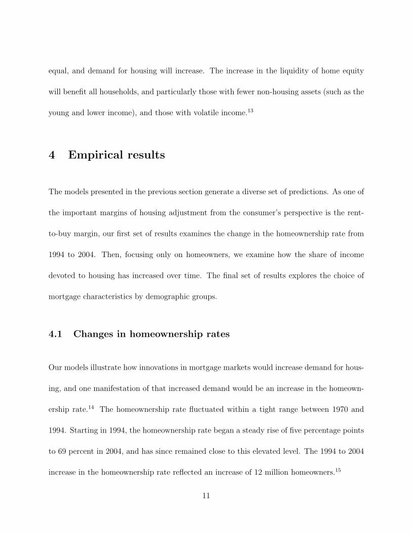
especially in the south, experienced much more muted increases. To illustrate this point,
Figure 4 shows the kernel density of house price appreciation from 2000 to 2005 for the
MSAs in our sample.23 We split the AHS data into four quartiles based on the change in
home prices, and then re-estimate the models for each group.24 The results are presented
in Table 5. As a baseline, column 1 presents the model estimates from the entire sample
and replicates the results in Table 2. The change in expenditure shares varies somewhat
across regions, but not systematically with the degree of local housing market conditions.
However, if expectations for house price appreciation are influenced not by local conditions
but instead solely by national conditions (which we find unlikely), then the results in Table
5 do not rule out the possibility that increased expectations of appreciation could be partly
responsible for increased expenditures shares on housing.
Another possible explanation for our results is that spending shares on all goods may
have increased, perhaps as a reflection of increased future income expectations. After all,
the aggregate savings rate fell considerably during our sample period. To examine this hy-
19

pothesis, we examined information from the Consumer Expenditure Survey (CES). Relative
to the AHS, the CES does not contain geographical information or detailed information on
costs associated with the servicing of property debt. However, an advantage of the CES
is that it does contain information on expenditures other than housing costs. We compute
several expenditure share measures using these data from 1994 to 2003 and run regressions
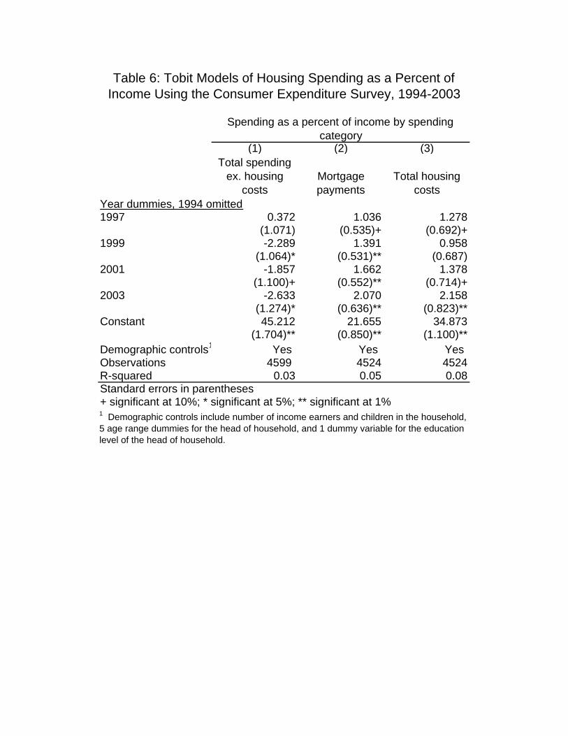
similar to those using the AHS data. The results are presented in Table 6. In the first column
we show results from a regression of spending relative to income that excludes housing on a
set of year dummies and demographic characteristics for households that are homeowners.
Between 1994 and 2003, there appears to be a slight decrease in the share of income devoted
to non-housing consumption. The second column shows the same basic regression but where
the dependent variable is the share of income going to mortgage payments. Roughly speak-
ing, the decrease in the share of income going to other consumption goods is matched by
the increase in income going to housing. This result is interesting in that it suggests that
the increase in expenditures for housing did not come directly out of saving but instead out
of consumption of other goods.25
4.4 Mortgage and demographic characteristics
The empirical sections above examined homeownership and the share of income devoted to
housing of homeowners. In this section, we examine the choice of mortgage characteris-
20

tics. Recall that according to our model, younger, cash-constrained households with steep
expected income profiles would stand to benefit from mortgages with low initial payments.
One way households can reduce their mortgage payments, at least for a time, is to finance
their housing consumption with mortgage products that have relatively low introductory
interest rates.
The AHS data contain limited information about the primary mortgage of homeowners,
including the interest rates for the primary and secondary mortgages. Using this information,
we construct an average mortgage interest rate where the interest rates are weighted by
the value of the mortgage. We then examine the relationship between interest rates and
demographic characteristics, and those results are presented in Table 7. Before discussing the
results, an important omitted variable in our models is credit quality. Given the importance
of this variable, the results in Table 7 have to be viewed with greater skepticism than the
results in the previous tables. With that caveat in mind, the results in Table 7 are entirely
consistent with our models.
The first three columns of Table 7 are probit models where the dependent variable equals
one if the average interest rate is in the lowest quintile for a year. The first column shows
the results for the entire sample and the second and third columns estimate the models
separately by whether households are in the bottom or top half of the income distribution.
In addition to the controls used in Tables 2-6, the controls in Table 7 also include dummy
21

variables for the income decile of the household; it is hoped that these controls may be
correlated with the unobserved credit quality of households.
The first three columns of Table 7 show that households headed by individuals with
at least some college education are more likely to be in the lowest interest rate quintile.
However, this result may be tainted from a positive correlation between education and credit
quality that is not captured by the income deciles. The remaining rows of the table show the
coefficients for the age dummies; in all three columns, younger households are more likely
to have lower interest rates on their mortgages. This result is somewhat surprising as credit
quality is likely to be inversely related to age. Comparing columns 2 and 3, we find that the
age profile of interest rates is greater for lower income households than for higher income
households. Again, lower income households are more likely to face the constraints addressed
in our model, and therefore may be more inclined to choose mortgage instruments that offer
initially low interest rates. We also estimated models where the dependent variable is the
average interest rate; those models yield results that are qualitatively very similar to the
probit results.26
5 Conclusion
Over the last decade there have been several innovations in mortgage markets, such as the
lowering of down payment requirements, the increased flexibility in repayment schedules,
22

and the reduction of costs associated with extracting equity from homes. We develop a
model that generates testable implications of how these innovations would affect household
behavior. For instance, the lowering of down payment requirements should result in home-
ownership increasing, especially for young people who are traditionally cash constrained. In
fact, we show that between 1994 and 2004, the homeownership rate for young people rose
sharply. Our model predicts that lower down payments and more flexible mortgage payment
schedules should lead to higher housing consumption for previously constrained households.
Empirically we document that households have increased the share of their income devoted
to housing by a substantial margin. The result is robust to the changing composition of
households and also to location; the share of income devoted to housing costs has increased
significantly in markets, regardless of what happened to housing prices in those markets.
Finally, we find that young educated households have dramatically increased their housing
expenditures between 1995 and 2005, but appear to be financing these expenditures with
mortgages that have relatively low interest rates. We interpret this finding to be suggestive
that these households may be financing their increased housing consumption with alterna-
tive, flexible mortgage products.
23

References
Alm, J., and Follain, J. (1984). “Alternative Mortgage Instruments , the Tilt Problem, andConsumer Welfare.” Journal of Financial and Quantitative Analysis. 19(1), 113-126.
Autor, D., Katz, L., and Kearney, M. (2005). “Trends in U.S. Wage Inequality: Re-Assessingthe Revionists,” NBER working paper no. 11627.
Barakova, I., Bostic, R., Calem, P., and Wachter, S., (2003). “Does Credit Quality Matterfor Ownership?” Journal of Housing Economics. 12(4), 318-336.
Bennett, P., Peach, R., and Peristiani, S., (2001). Journal of Money, Credit, and Banking.33(4), 955-975.
Bostic, R., and Surette, B. (2001). “Have the Doors Opened Wider? Trends in OwnershipRates by Race and Income.” Journal of Real Estate Finance and Economics, 23(November),pp. 411-34.
Campbell, J. (2006). “Household Finance.” Presidential Address to the American FinanceAssociation.
Chambers, M., Garriga, C., and Schlagenhauf (2005). “Accounting for Changes in theHomeownership Rate.” working paper.
Danforth, D., (1999). “Online Mortgage Business Puts Consumers in the Driver’s Seat.”Secondary Mortgage Markets. 16(1), 2-8.
Davidoff, T. (2005). “Labor income, Housing Prices, and Homeownership.” Journal ofUrban Economics.
Doms, M. and Krainer, J. (2006). “Innovations in Mortgage Markets and Increased Spendingon Housing,” Federal Reserve Bank of San Francisco working paper.
Dynan, K., Elmendorf, D., and Sichel, D. (2006). “The Evolution of Household IncomeVolatility,” working paper.
Fairlie, Robert W. (2005). “An extension of the Blinder-Oaxaca decomposition technique tologit and probit models,” Journal of Economic and Social Measurement, 30: 305-316.
Gabriel, S., and Rosenthal, S., (2005). “Homeownership in the 1980s and 1990s: AggregateTrends and Racial Gaps.” Journal of Urban Economics. 57, 101-127.
Gerardi, C., Rosen H., and Willen, P. (2006). “Do Innovations on Wall Street Help People onMain Street? The Case of the Mortgage Market,” Federal Reserve Bank of Boston workingpaper.
24

Green, R., and Wachter, S. (2005). “The American Mortgage in Historical and InternationalContext.” Journal of Economic Perspectives. 19(4), 93-114.
Hochstein, M., 2000. “Paperless Mortgage Closes; Month’s Work Done in Hours.” TheAmerican Banker. July 26.
Hurst, E., and Stafford, F. (2004). “Home Is Where the Equity Is: Mortgage Refinancingand Household Consumption.” Journal of Money, Credit, and Banking. 36(6), 985-1014.
Koijen, R., Van Hemert, O., and Van Nieuwerburgh, S. (2006). “Mortgage Timing.” NYUStern School working paper.
Krainer, J. (2006). “Mortgage Innovation and Consumer Choice,” Federal Reserve Bank ofSan Francisco Economic Letter, no. 38.
LaCour-Little, M. (2000). “The Evolving Role of Technology in Mortgage Finance,” Journalof Housing Research, 11(2), 173-205.
LeRoy, S. (1996). “Mortgage Valuation under Optimal Prepayment.” Review of FinancialStudies. 9, 817-844.
Li, W. (2005). “Moving Up: Trend in Homeownership and Mortgage Indebtedness.” FederalReserve Bank of Philadelphia Business Review, 26-34.
Ortalo-Magne, F., and Rady, S. (2005). “Housing Market Dynamics: On the Contributionof Income Shocks and Credit Constraints.” Review of Economic Studies.
Stanton, R., and Wallace, N. (1998). “Mortgage Choice: What’s the Point?” Real EstateEconomics. 26, 173-205.
Stein, J. (1995). “Prices and Trading Volume in the Housing Market: A Model with Down-payment Effects.” Quarterly Journal of Economics, 110, 379-406.
Vickery, J. (2006). “Interest Rates and Consumer Choice in the Residential Mortgage Mar-ket.” Federal Reserve Bank of New York working paper.
25
Notes
1 See Green and Wachter (2005) and Gerardi, Rosen, and Willen (2006) for longer-term
historical descriptions of changes in the mortgage market and see LaCour-Little (2000) for
a discussion of more recent changes.
2 Bostic and Surette (2001) document the narrowing of the homeownership gap between
whites and minorities over the past several decades, attributing a large part to mortgage
market innovations such as credit scoring. Li (2005) notes that in addition to the increase in
homeownership rates in the 1990’s, leverage (the loan-to-value ratio) conditional on home-
ownership has also increased. See also Davidoff (2006) and Ortalo-Magne and Rady (2005).
3 See Hochstein 2000.
4 See Doms and Krainer (2007) for a fuller description of these measures.
5 See Bennett, Peach, and Peristiani (2001) for evidence of structural change in the
propensity to refinance.
6 See LaCour-Little (2000) for an excellent summary of the role of technology in mortgage
finance.
7 See Barakova, Bostic, Calem, and Wachter (2003).
8 Vickery (2006) documents that the choice between fixed-rate and adjustable-rate mort-
gage loans is very sensitive to the level of interest rates. Koijen, van Hemert, and Van
Nieuwerburgh (2006) show that the variation in the total share of adjustable-rate mortgages
over time is linked to the bond risk premium embedded in mortgage interest rates.
9 See, for example, LeRoy (1996) and Stanton and Wallace (1998).
26

10 While demand for alternative mortgage products surged in the early 2000s, these prod-
ucts could not be considered new at the time. For example, the graduated payment mortgage
was first offered in 1977. See Alm and Follain (1984) for an analysis of the possible consumer
gains to using this and other flexible mortgage products. Campbell (2006) notes that, his-
torically, consumers have been slow to demand financial products that would seemingly be
welfare enhancing. See Krainer (2006) for further discussion on the prevalence of alternative
mortgages.
11 The down payment and income constraints arise, in part, because of information asym-
metries between borrowers and lenders. The down payment constraint guards against moral
hazard that might lead borrowers to default on their loans. The payment-to-income con-
straints can be justified by the notion that lenders might not know what a borrower’s true
income growth prospects are.
12 The results in Figure 1 hold using other datasets as well.
13 Dynan, Elmendorf, and Sichel (2007) have explored this idea, arguing that innovations
in mortgage markets may have helped households to better smooth nonhousing consumption.
Hurst and Stafford (2004) examine the propensity to refinance for liquidity-constrained and
non liquidity-constrained households.
14 Housing services, the variable in the consumer’s model, is difficult to measure. We as-
sume that most households that became homeowners increased their flow of housing services
from when they rented.
15 For more comprehensive discussions on the increase in the homeownership rate, see
Bostic and Surrette (2000), Gabriel and Rosenthal (2005), and Li (2005).
16 We examined primary mortgage cost to abstract away from a change in debt structure
27

of households, such as a shift away from revolving credit to a home equity line of credit or
a second mortgage.
17 Households headed by individuals 70 years old or older are excluded. The results in
this paper are robust to a wide array of other measures of demographics.
18 The results are robust to choice of the right-censoring value.
19 Our results are robust to a other specifications that control for new homeowners.
20 The general result that the share of income devoted to housing has increased is consistent
with results using other data sets, including the Survey of Consumer Finances, the Panel
Survey of Income Dynamics, and the Consumer Expenditure Survey.
21 One of the implications of the model is that the share of income devoted to housing
would become more constant over time. However, discerning whether a flattening of the
age-housing cost profile has occurred is difficult using a data set that spans only 8 years.
To make more definitive statements whether housing costs-age profiles have changed shape,
data for a sufficient period of time after the changes in mortgage markets have taken place
would be required. The results presented here are limited to suggesting that more is being
spent on housing for all age groups.
22 The sample sizes in Table 3 are skewed to the higher income quintiles because the
income quintiles are computed using the entire AHS sample, which includes renters. Renters
tend to have lower incomes than homeowners. The results are robust to income quintiles
being computed using only homeowners.
23 We examined the price change for a number of different periods, and our results are
robust to the time period examined.
28

24 Several of the models run in Table 2 control for MSA in that a dummy variable is
used for all time periods. This dummy variable will pick up mean differences in housing
expenditures-to-income by region but will not capture changes in housing expenditures-to-
income by region.
25 There are several reasons why our results can be consistent with the decline in the
national savings rate. First, the regressions in Table 6 represent the mean household whereas
the national savings rate, in essence, weights households by income. As we saw previously,
higher income households did not increase their housing expenditures as a share of income
by as much as lower income households. Further, the decrease in the official national savings
rate stems, in part, from an increase in health care expenditures. In the official statistics,
employer contributions also go towards consumption, which reduces the savings rate.
26 We also examined other observable characteristics of the mortgage, such as whether the
mortgage is adjustable or not. Unfortunately, the AHS data do not provide other information
on how and when the interest rate is adjustable. For instance, a traditional 10-1 ARM would
be coded the same as a 1-year ARM that offered a low initial teaser rate.
29

Figure 1: Mean Income Profiles by Age and Education
1.0
1.1
1.2
1.3
1.4
1.5
1.6
1.7
1.8
1.9
2.0
22 24 26 28 30 32 34 36 38 40 42 44 46 48 50 52 54 56 58 60
Age
Inde
x of
ave
rage
ann
ual i
ncom
e, a
ge 2
2=1.
0 Colllege
High school
Less than high school
Results from tobit models of the log of salary and wage income on a fourth-degree polynomial of age for each of three education groups. The models were estimated using data on full-time workers from the 2000 decennial census.

Figure 2: Housing Expenditure Shares, Income Growth, and Financial Constraints
23%
25%
27%
29%
31%
5% 8% 11% 14% 17% 20%
Downpayment requirement as a percent of house price
Hou
sing
exp
endi
ture
s/in
com
e, p
erce
nt
Income growth = 10%, mortgage payment growth = 50%
Income growth = 50%,mortgage payment growth = 0%
Income growth = 10%, mortgage payment growth = 0%
Income growth = 50%, mortgage payment growth = 50%

2005
2001
1997
0
.01
.02
.03
.04
0 20 40 60 80Total housing costs as a percent of income
Source: American Housing survey (various years) and authors' calculations. The distribution is right censored at 80.
Figure 3: Kernel Densities of Total Housing Costs as a Percentof Income for Home Owners, by Year
0.000
0.005
0.010
0.015
0.020
0.025D
ensi
ty
0 50 100 150Percent change in house prices, 2000-2005
Note: MSA house price data are from OFHEO and observations are weighted by the prevalence in the AHS.
Percent Change, 2000-2005Figure 4: Kernel Density of House Price Changes Across MSAs

Change1994 2004 2004-1994
Age of head of household18-29 26.6 33.2 6.630-39 55.8 61.8 6.040-49 70.5 74.1 3.650-59 77.8 79.6 1.860+ 77.9 81.4 3.5
Education (in years of schooling) of head of household12 years or less 61.3 64.1 2.813 or more 66.6 72.9 6.3
Age and education of head of household18-29 12 years or less 25.4 30.0 4.6
13 or more 27.7 35.6 7.9
30-39 12 years or less 50.2 52.0 1.813 or more 60.4 67.9 7.5
40-49 12 years or less 63.6 66.1 2.513 or more 75.8 79.6 3.8
50-59 12 years or less 73.4 73.2 -0.213 or more 82.5 83.7 1.2
60+ 12 years or less 75.3 78.2 2.913 or more 83.4 86.0 2.6
Income quartile of family income1st quartile 41.2 44.7 3.52nd quartile 58.6 63.8 5.23rd quartile 72.9 78.5 5.64th quartile 87.1 91.1 4.0
Source: Current Population Survey and authors' calculations
Rates by year
Table 1: Homeownership Rates by Demographic Groups, 1994 to 2004

Year dummies (1997 omitted) (1) (2) (3) (4) (5)
1999 -0.211 -0.253 -0.255 -0.239 0.052(0.176) (0.173) (0.171) (0.170) (0.273)
2001 0.885 0.863 0.886 0.863 0.713(0.173)** (0.170)** (0.169)** (0.168)** (0.270)**
2003 1.093 1.184 1.206 1.262 1.647(0.172)** (0.169)** (0.168)** (0.167)** (0.269)**
2005 2.632 2.702 2.714 2.860 3.263(0.172)** (0.170)** (0.169)** (0.167)** (0.272)**
Demographic Controls
Education of head of household (=1 if some college or more, =0 otherwise) -1.653 -1.987 -2.116 -4.190
(0.113)** (0.112)** (0.113)** (0.192)**Age of head of household dummies (less than 30 omitted):
30<=Age<=39 -2.076 -1.067 -2.322 -2.872(0.223)** (0.225)** (0.220)** (0.362)**
40<=Age<=49 -2.966 -0.542 -3.203 -3.856(0.215)** (0.223)* (0.213)** (0.354)**
50<=Age<=59 -3.770 -0.428 -4.017 -4.444(0.226)** (0.242)+ (0.224)** (0.366)**
60<=Age<=69 -5.630 -1.611 -5.753 -7.184(0.341)** (0.354)** (0.337)** (0.526)**
Number of children 1.262 1.226 1.244 1.396(0.054)** (0.054)** (0.053)** (0.085)**
Number of prime age adults -3.350 -3.066 -3.581 -3.326(0.081)** (0.080)** (0.080)** (0.118)**
Number of elderly adults -1.534 -1.356 -1.997 -1.492(0.187)** (0.185)** (0.185)** (0.273)**
Years living in the house -0.405(0.045)**
Years living in the house, squared -0.002(0.003)
SMSA dummies No No No Yes
Yes, SMSA unknown dropped
Constant 20.156 31.067 32.112 34.714 35.482(0.120)** (0.324)** (0.326)** (3.873)** (5.990)**
Observations 72443 72443 72443 72443 31020
+ significant at 10%; * significant at 5%; ** significant at 1%
Table 2: Tobit Models of Total Housing Costs as a Percent of Income
Notes: Standard errors in parentheses, all models estimated by maximum likelihood. All data from the American Housing Survey.

AllYear dummies (1997 omitted) observations 1 2 3 4 5
1999 -0.253 -1.128 -0.181 0.510 0.020 -0.985(0.173) (1.001) (0.441) (0.298)+ (0.218) (0.183)**
2001 0.863 1.970 1.527 1.239 1.071 -1.295(0.170)** (0.970)* (0.439)** (0.293)** (0.217)** (0.180)**
2003 1.184 1.425 1.402 1.314 1.321 -0.247(0.169)** (0.972) (0.433)** (0.291)** (0.215)** (0.179)
2005 2.702 3.910 3.801 2.709 2.453 1.455(0.170)** (0.998)** (0.430)** (0.295)** (0.215)** (0.178)**
Education of head of household (=1 if some college or more, =0 otherwise) -1.653 7.903 3.915 3.246 2.310 1.983
(0.113)** (0.652)** (0.281)** (0.192)** (0.151)** (0.154)**Age of head of household dummies (less than 30 omitted)30<=Age<=39 -2.076 2.751 0.003 0.906 0.348 0.088
(0.223)** (1.159)* (0.483) (0.341)** (0.287) (0.331)40<=Age<=49 -2.966 3.065 -0.809 0.228 -0.431 -1.126
(0.215)** (1.114)** (0.478)+ (0.333) (0.281) (0.323)**50<=Age<=59 -3.770 0.369 -2.112 -1.678 -2.078 -2.298
(0.226)** (1.155) (0.504)** (0.353)** (0.293)** (0.325)**60<=Age<=69 -5.630 -1.358 -5.579 -3.829 -4.353 -5.339
(0.341)** (1.639) (0.771)** (0.568)** (0.458)** (0.434)**
Number of children 1.262 2.495 1.525 0.991 0.959 0.802(0.054)** (0.314)** (0.134)** (0.092)** (0.069)** (0.058)**
Number of prime age adults -3.350 2.287 0.174 -0.349 -0.545 -0.061(0.081)** (0.480)** (0.219) (0.148)* (0.111)** (0.084)
Number of elderly adults -1.534 4.100 0.714 -0.050 0.003 0.694(0.187)** (0.987)** (0.443) (0.325) (0.243) (0.198)**
Constant 31.067 21.089 18.192 14.746 14.025 11.359(0.324)** (1.684)** (0.785)** (0.565)** (0.470)** (0.480)**
Observations 72438 7537 11637 15254 18212 19798Notes: Standard errors in parentheses, all models estimated by maximum likelihood. All data from the American Housing Survey.+ significant at 10%; * significant at 5%; ** significant at 1%
Income quintile (1=lowest, 5=highest)
Table 3: Tobit Models of Total Housing Costs as a Percent of Income by Income Quintile

(1) (2) (3) (4) (5) (6) (7)
Year dummies (1997 omitted) All Age<=39 40<=Age<=49 Age>=50 Age<=39 40<=Age<=49 Age>=50
1999 -0.253 -0.095 -0.322 -0.345 -0.075 -0.518 -0.309(0.173) (0.571) (0.517) (0.504) (0.339) (0.358) (0.400)
2001 0.863 2.205 0.527 1.732 0.595 -0.248 0.921(0.170)** (0.574)** (0.515) (0.500)** (0.335)+ (0.353) (0.388)*
2003 1.184 2.209 1.195 1.014 1.503 0.887 0.692(0.169)** (0.580)** (0.514)* (0.502)* (0.333)** (0.351)* (0.377)+
2005 2.702 4.224 2.976 2.039 3.300 2.021 2.278(0.170)** (0.594)** (0.520)** (0.511)** (0.329)** (0.352)** (0.375)**
Education of head of household (=1 if some college or more, =0 otherwise) -1.653
(0.113)**Age of head of household dummies (less than 30 omitted)30<=Age<=39 -2.076
(0.223)**40<=Age<=49 -2.966
(0.215)**50<=Age<=59 -3.770
(0.226)**60<=Age<=69 -5.630
(0.341)**
Number of children 1.262 1.447 1.770 2.250 0.968 0.814 1.793(0.054)** (0.153)** (0.149)** (0.237)** (0.093)** (0.097)** (0.191)**
Number of prime age adults -3.350 -4.324 -3.316 -3.228 -5.255 -3.747 -2.743(0.081)** (0.361)** (0.228)** (0.206)** (0.222)** (0.166)** (0.146)**
Number of elderly adults -1.534 1.250 3.724 -2.987 1.533 2.667 -2.137(0.187)** (1.031) (0.816)** (0.285)** (0.663)* (0.587)** (0.218)**
Constant 31.067 28.722 25.828 25.047 29.697 26.368 22.895(0.324)** (0.785)** (0.584)** (0.566)** (0.456)** (0.419)** (0.421)**
Observations 72438 7737 7746 10456 15645 14711 16143Standard errors in parentheses+ significant at 10%; * significant at 5%; ** significant at 1%
High School or Less Some College or More
Table 4: Tobit Models of Total Housing Costs as a Percent of Income by Educational Attainment and Age
All observations 1 2 3 4
SMSA not defined
Year dummies (1997 omitted)
1999 -0.253 -0.020 1.244 -0.742 -0.448 -0.437(0.173) (0.501) (0.510)* (0.608) (0.665) (0.215)*
2001 0.863 0.673 1.630 0.579 -0.218 0.894(0.170)** (0.498) (0.500)** (0.608) (0.646) (0.212)**
2003 1.184 1.639 2.483 0.829 1.020 0.978(0.169)** (0.493)** (0.500)** (0.604) (0.652) (0.210)**
2005 2.702 3.047 3.576 2.072 3.783 2.554(0.170)** (0.496)** (0.503)** (0.615)** (0.666)** (0.210)**
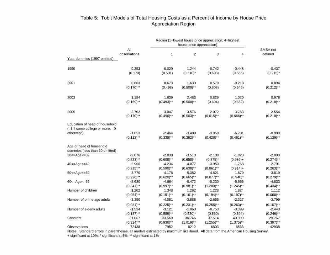
Education of head of household (=1 if some college or more, =0 otherwise) -1.653 -2.464 -3.409 -3.959 -6.701 -0.900
(0.113)** (0.338)** (0.362)** (0.428)** (0.461)** (0.139)**
Age of head of household dummies (less than 30 omitted)30<=Age<=39 -2.076 -2.838 -3.513 -2.138 -1.823 -2.000
(0.223)** (0.608)** (0.658)** (0.875)* (0.936)+ (0.274)**40<=Age<=49 -2.966 -4.234 -4.077 -3.950 -1.768 -2.791
(0.215)** (0.590)** (0.638)** (0.861)** (0.914)+ (0.263)**50<=Age<=59 -3.770 -4.178 -5.382 -4.621 -1.879 -3.819
(0.226)** (0.620)** (0.665)** (0.877)** (0.940)* (0.279)**60<=Age<=69 -5.630 -4.664 -8.472 -8.230 -5.665 -4.833
(0.341)** (0.997)** (0.981)** (1.200)** (1.245)** (0.434)**Number of children 1.262 1.348 1.282 1.228 1.824 1.112
(0.054)** (0.151)** (0.161)** (0.194)** (0.197)** (0.068)**Number of prime age adults -3.350 -4.081 -3.888 -2.655 -2.327 -3.799
(0.081)** (0.225)** (0.231)** (0.255)** (0.263)** (0.107)**Number of elderly adults -1.534 -3.121 -1.063 -0.753 -0.399 -2.443
(0.187)** (0.586)** (0.530)* (0.560) (0.594) (0.246)**Constant 31.067 33.560 36.746 37.514 40.999 29.767
(0.324)** (0.930)** (1.019)** (1.255)** (1.375)** (0.397)**Observations 72438 7952 8212 6803 6533 42938Notes: Standard errors in parentheses, all models estimated by maximum likelihood. All data from the American Housing Survey.+ significant at 10%; * significant at 5%; ** significant at 1%
Region (1=lowest house price appreciation, 4=highest house price appreciation)
Table 5: Tobit Models of Total Housing Costs as a Percent of Income by House Price Appreciation Region
(1) (2) (3)Total spending
ex. housing costs
Mortgage payments
Total housing costs
Year dummies, 1994 omitted1997 0.372 1.036 1.278
(1.071) (0.535)+ (0.692)+1999 -2.289 1.391 0.958
(1.064)* (0.531)** (0.687)2001 -1.857 1.662 1.378
(1.100)+ (0.552)** (0.714)+2003 -2.633 2.070 2.158
(1.274)* (0.636)** (0.823)**Constant 45.212 21.655 34.873
(1.704)** (0.850)** (1.100)**Demographic controls1 Yes Yes YesObservations 4599 4524 4524R-squared 0.03 0.05 0.08Standard errors in parentheses+ significant at 10%; * significant at 5%; ** significant at 1%
Table 6: Tobit Models of Housing Spending as a Percent of Income Using the Consumer Expenditure Survey, 1994-2003
Spending as a percent of income by spending category
1 Demographic controls include number of income earners and children in the household, 5 age range dummies for the head of household, and 1 dummy variable for the education level of the head of household.

(1) (2) (3) (4) (5) (6)
All households
Households below median
income
above median income
All households
Households below median
income
Household above median
incomeHead of household has some college education 0.023 0.018 0.025 -0.196 -0.251 -0.210
(0.004)** (0.006)** (0.005)** (0.013)** (0.028)** (0.015)**Age of head of household dummies (less than 30 omitted)30<=Age<=39 -0.028 -0.035 -0.019 0.141 0.207 0.103
(0.007)** (0.009)** (0.010)+ (0.022)** (0.046)** (0.027)**40<=Age<=49 -0.036 -0.040 -0.030 0.215 0.284 0.208
(0.007)** (0.009)** (0.009)** (0.021)** (0.045)** (0.027)**50<=Age<=59 -0.033 -0.057 -0.017 0.286 0.402 0.234
(0.007)** (0.009)** (0.010)+ (0.023)** (0.049)** (0.028)**60<=Age<=69 -0.027 -0.051 -0.014 0.290 0.496 0.234
(0.011)* (0.015)** (0.016) (0.038)** (0.082)** (0.044)**Demographic controls yes yes yes yes yes yesObservations 54648 16948 37575 54411 17062 37586R-squared 0.28 0.16 0.33Standard errors in parentheses+ significant at 10%; * significant at 5%; ** significant at 1%Demographic controls include the same variable reported in tables 2-6, dummy variables for income decile, and dummy variables for SMSA.
Expected change in probability from a probit model of a household being in the
bottom quintile of interest ratesOLS coefficients of the interest rate on the
primary and second mortgages
Table 7: Interest Rates on Mortgages and Demographic Characteristics