innovative concepts for on-line synchronous generator parameter

INNOVATIVE CONCEPTS FOR ON-LINE SYNCHRONOUS GENERATOR

PARAMETER ESTIMATION

by

Elias Kyriakides

A Dissertation Presented in Partial Fulfillment of the Requirements for the Degree

Doctor of Philosophy

ARIZONA STATE UNIVERSITY

December 2003

INNOVATIVE CONCEPTS FOR ON-LINE SYNCHRONOUS GENERATOR

PARAMETER ESTIMATION

by

Elias Kyriakides

has been approved

December 2003

APPROVED:

, Chair

Supervisory Committee

ACCEPTED:

Department Chair

Dean, Graduate College

iii

ABSTRACT

A method to identify synchronous generator parameters from on-line

measurements is presented. Generator parameters are employed in the construction of

models used in transient stability studies and other routine power engineering studies.

These studies are critical for the operation of the power system, and therefore accurate

representation of synchronous generators and their parameters is important. The existing

off-line techniques are often not practical and do not capture the behavior of the generator

at all operating levels. Generator parameters vary due to aging, changes of the generator

internal temperature, magnetic saturation, and coupling between the generator and

external systems. The method proposed in this dissertation estimates generator

parameters at any operating level, taking into consideration the effect of saturation and

other phenomena in the operation of the synchronous generator.

Estimation of synchronous generator parameters is a fairly complex mathematical

procedure, and there is a need for an easily used mechanism for model parameter

estimation. The proposed method is based on least squares estimation and on a

simplified synchronous generator model. The method is developed to be used with a

Visual C++ engine and graphic user interface (GUI), so that the practicing power

engineer may link machine measurements taken in an on-line environment with the

estimator. A GUI application which is user friendly and self guiding is presented.

An observer for the estimation of damper winding currents is developed. The

observer constructs estimates of the damper winding currents by using voltage and

current measurements from the system and a priori system knowledge. The observer is

integrated into the parameter identification algorithm.

iv

A saturation model of the inductances of the synchronous generator is proposed

and implemented in the estimator. Saturation affects a number of inductances in the

generator. Accurate representation of saturation leads to accurate estimates that reflect

the true status of the machine at every operating point. Saturation in both the direct and

quadrature axes of the generator is considered.

Results from both simulated and actual measurements are presented. The

feasibility of each of the proposed models is evaluated. Parameter estimation is

performed for a number of generators at different operating points to enhance the

confidence in the proposed algorithm. It is possible to use the proposed method to track

generator parameters over time so that impeding internal generator faults can be detected

and remedial action can be undertaken to avoid costly outages.

v

ACKNOWLEDGMENTS

I would like to express my deep appreciation and gratitude to my advisor Dr.

Gerald T. Heydt for his valuable help, support, and guidance. His expertise, insightful

ideas, and motivation have been instrumental in this research work. His teaching and

research style and his work ethics have been particularly inspiring to me, and I plan to

treasure these values indefinitely. I would also like to thank Professor Richard G. Farmer

of Arizona State University for his comments and suggestions throughout the project

period. His experience in this field was particularly helpful at various instances

throughout the project. His willingness to help at all times is gratefully appreciated. The

support and guidance of Dr. Vijay Vittal of Iowa State University has been a constant

motivation for this research work. The advice and useful comments of Dr. Vittal on

saturation and synchronous generator modeling are highly appreciated. Special thanks

are due to Dr. Bajarang Agrawal and Mr. Doug Selin of Arizona Public Service (APS)

for their interest in the project, constructive comments and advice, as well as for

furnishing many data files for testing the proposed algorithm. Their willingness to offer

their input to this project is greatly appreciated. The comments of Mr. Dale Bradshaw of

Tennessee Valley Authority (TVA) and Mr. John Demcko of APS are also appreciated.

The contribution of W. C. Rees who worked on the early stages of this project is

acknowledged. Dr. G. Karady, Dr. K. Holbert, Mr. S. Borkar, and Mr. J. Gu of Arizona

State University worked on other parts of the project. I would also like to thank the

members of my supervisory committee for their support during my academic studies.

Finally, the financial support of both the Arizona Public Service and the Power Systems

Engineering Research Center is acknowledged.

vi

TABLE OF CONTENTS

Page

LIST OF TABLES ……………………………………………………………….. x

LIST OF FIGURES ……………………………………………………………….. xii

NOMENCLATURE ……………………………………………………………….. xvi

CHAPTER

1 INTRODUCTION ……………………………………………………... 1

Motivation …….....…………………………………………….….. 1

Objectives ………..………………………………………………... 3

Identification of synchronous generator parameters: an overview .. 5

Literature review …………………………………………….……. 6

Statement of originality …………………………………………… 18

2 MODELING OF SYNCHRONOUS GENERATORS ………………... 20

System identification ….…………………….…………………….. 20

Model selection …………………………………………………… 20

Modeling of synchronous generators …………………………….. 24

Park’s transformation ……………………………………………... 25

Formulation of voltage equations ……………..………….……….. 29

3 SATURATION OF SYNCHRONOUS GENERATOR INDUCTANCES 35

Introduction ……………………………………………………….. 35

Preparation of the generator model to account for saturation …….. 40

Derivation of flux equations for the d and q axes saturation ……... 45

vii

CHAPTER Page

Implementation of saturation in the parameter estimation process .. 53

Description of generators studied and list of data sets used ………. 56

Denomination of case studies …………………………….……….. 59

Summary ………………………………………………………….. 61

4 DEVELOPMENT OF AN OBSERVER FOR THE DAMPER WINDING CURRENTS .…………………………………………. 62

Introduction ……………………………………………………….. 62

Observers and observability ………………………………………. 65

Observer design …………………………………………………… 71

Verification of observer operation using EMTP simulated data ….. 76

5 STATE ESTIMATION ………………………………………………... 80

Introduction ……………………………………………………….. 80

Theory of norms …………………………………………………... 81

Selection of the minimization norm ………………………………. 84

Analysis of case studies …………………………………………... 89

Least squares and the Moore-Penrose pseudoinverse …………….. 94

Configuration of the state estimator ………………………………. 96

Summary ………………………………………………………….. 98

6 PARAMETER ESTIMATION USING SYNTHETIC DATA ………... 101

Introduction ……………………………………………………….. 101

Calculation of generator parameters ……………………………… 102

Estimation of generator parameters ………………………………. 105

viii

CHAPTER Page

Multiple simultaneous parameter estimation ……………………... 109

7 NOISE FILTERING AND BAD DATA IDENTIFICATION ………... 112

Introduction ……………………………………………………….. 112

Filtering …………………………………………………………… 114

Filtering of the field measurements ……………………………….. 124

Filtering of the stator measurements ……………………………… 129

Summary ………………………………………………………….. 134

8 PARAMETER ESTIMATION FROM ACTUAL MEASUREMENTS 136

Introduction ……………………………………………………….. 136

Results of parameter estimation from actual measurements ……… 137

Multiple parameter estimation ……………………………………. 143

Application of the algorithm to different machines and different operating points …………………………………………….… 146

Calculation of standard machine parameters from estimated derived parameters ………………………………………….… 153

9 GRAPHIC USER INTERFACE IMPLEMENTATION USING VISUAL C++ ……………………………………………………... 156

Introduction ……………………………………………………….. 156

Input dialog and estimator configuration …………………………. 157

State estimator implementation …….……………………………... 160

Output dialog and estimated parameters ………………………….. 160

Interpretation of the rms error and the chi-squared test …………... 162

Confidence interval for estimated parameters …………………….. 165

ix

CHAPTER Page

10 CONCLUSIONS AND FUTURE STEPS …………………………….. 169

Comments from industry ………………………………………….. 169

Conclusions ……………………………………………………….. 171

Future steps ………………………………………………………... 177

REFERENCES ……………………………………………………………………... 179

APPENDIX

A CALCULATION OF SYNCHRONOUS GENERATOR PARAMETERS 193

B SATURATION CURVE AND STABILITY STUDY DATA SHEETFOR A SAMPLE SYNCHRONOUS GENERATOR …………………. 202

C OVERVIEW OF PROPOSED MAGNETIC SATURATION FUNCTIONS …………………………………………………………... 205

D SELECTION OF THE NUMERICAL DIFFERENTIATION FORMULA 210

E DATA FORMATS SUPPORTED BY THE ESTIMATOR …………….. 217

F PARAMETER ESTIMATION RESULTS USING ACTUAL DATA .... 222

G MATLAB CODE FOR PARAMETER ESTIMATION USING ACTUAL MEASUREMENTS ……………………….………………... 229

H VISUAL C++ CODE FOR PARAMETER ESTIMATION AND GUIIMPLEMENTATION USING ACTUAL MEASUREMENTS ……….. 245

x

LIST OF TABLES

Table Page

3.1 Generators studied and their characteristics ……………………………..…... 57

3.2 List of data sets obtained from actual measurements ………………………... 58

3.3 List of case studies in the dissertation …………………………………….…. 60

5.1 Exact values of synchronous generator parameters ……………………..….. 91

5.2 Estimated generator parameters and residuals for case study S-NF-03-03 .… 91

5.3 Percent errors of estimated generator parameters for case study S-NF-03-03 91

5.4 Estimated generator parameters and residuals for case study S-NC-03-04 … 91

5.5 Percent errors of estimated generator parameters for case study S-NC-03-04 92

5.6 Definitions and properties of vector norms ………………………………….. 99

5.7 Concepts pertaining to the pseudoinverse of a matrix ………………….…… 100

6.1 Calculated parameters for use in the testing of the estimator algorithm …….. 104

6.2 Distinguishing characteristics of the three candidate models ……………….. 105

6.3 Estimated parameters using EMTP generated data (case study E-NF-01-05) 108

6.4 Multiple simultaneous parameter estimation (case study E-NF-03-06) …….. 109




8.1 Estimated parameters for the three proposed models for generator FC5HP (case study R-NC-01-10) ……………………………………………………. 139

8.2 Calculation of unsaturated parameters from the estimated parameters of generator FC5HP (case study R-NC-01-10) ………………………………… 141

xi

Table Page

8.3 Multiple simultaneous parameter estimation for generator FC5HP (case study R-NC-03-11) ………………………………………………………….. 144

8.4 Calculation of unsaturated parameters for generator FC5HP (case study R-NC-03-11) …………………………………………………………………… 144

8.5 Multiple simultaneous parameter estimation for generator FC5HP (case study R-NC-03-12) ………………………………………………………….. 145

8.6 Calculation of unsaturated parameters for generator FC5HP (case study R-NC-03-12) …………………………………………………………………… 146

8.7 Parameter estimation results for Redhawk gas turbines 1 and 2 …………….. 148

8.8 Calculation of standard parameters from the estimated derived parameters ... 154

8.9 Comparison of estimated standard parameters to manufacturer standard parameters (case study R-NC-01-10) ………………………………………... 155

10.1 Comments from the power engineering industry ……………………………. 170

10.2 Sources of possible differences between estimated and manufacturer parameters 176

A.1 Available quantities from manufacturer stability study data sheet ………….. 195

C.1 Candidate saturation function models ……………………………………….. 206

D.1 Estimation of parameters for ∆T=0.1 and SNR=∞ (case study S-NF-02-13) 212

D.2 Estimation of parameters for ∆T=0.1 and SNR=200 (case study S-NC-02-14) 212

D.3 Comparison of percent relative error in estimating parameter a for case studies S-NF-02-13 and S-NC-02-14 ………………………………………... 213

D.4 Comparison of percent relative error in estimating parameter b for case studies S-NF-02-13 and S-NC-02-14 ………………………………………... 213

D.5 Ranking of the methods in order of increasing error ………………………... 214

E.1 Arrangement of data in the text format data file …………………………….. 219

F.1 Parameter estimation results for Redhawk steam turbines 1 and 2 …………. 224

xii

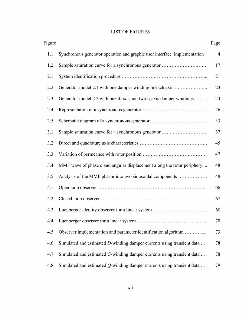
LIST OF FIGURES

Figure Page

1.1 Synchronous generator operation and graphic user interface implementation 4

1.2 Sample saturation curve for a synchronous generator ………………….…… 17

2.1 System identification procedure ……………………………………………... 21

2.2 Generator model 2.1 with one damper winding in each axis ………………... 23

2.3 Generator model 2.2 with one d-axis and two q-axis damper windings …….. 23

2.4 Representation of a synchronous generator …………………………………. 26

2.5 Schematic diagram of a synchronous generator …………………………….. 33

3.1 Sample saturation curve for a synchronous generator …….………………… 37

3.2 Direct and quadrature axis characteristics …………………………………… 45

3.3 Variation of permeance with rotor position …………………………………. 47

3.4 MMF wave of phase a and angular displacement along the rotor periphery ... 48

3.5 Analysis of the MMF phasor into two sinusoidal components ……………… 48

4.1 Open loop observer ………………………………………………………….. 66

4.2 Closed loop observer ………………………………………………………… 67

4.3 Luenberger identity observer for a linear system ……………………………. 68

4.4 Luenberger observer for a linear system …………………………………….. 70

4.5 Observer implementation and parameter identification algorithm ………….. 73

4.6 Simulated and estimated D-winding damper currents using transient data …. 78

4.7 Simulated and estimated G-winding damper currents using transient data …. 78

4.8 Simulated and estimated Q-winding damper currents using transient data …. 79

xiii

Figure Page

4.9 Magnification of portion of iQ to demonstrate the difference between the simulated and observed signals ……………………………………………… 79

5.1 Loci of the three major Hölder unit norms for a vector 3ℜ∈x ……………. 84

5.2 Flowchart for example on norm minimization selection ……………….…… 90

5.3 Pictorial of an estimator for synchronous generator parameter identification 100

6.1 Flowchart for synthetic data and estimator implementation ………………… 106

7.1 Filtering and bad data detection/rejection configuration ……………….…… 114

7.2 Magnitude response of a low pass filter …………………………………….. 115

7.3 Moving average filter implementation ………………………………………. 116

7.4 Magnitude response of a moving average filter ……………………………... 117

7.5 Phase response of a moving average filter …………………………………... 117

7.6 Cascade implementation of a low pass Butterworth digital filter …………… 119

7.7 Frequency response of a sample Butterworth filter …………………………. 120

7.8 Example of a multiple parallel filtering method for the successive attenuation of transition band frequency components ………………….…… 123

7.9 Time domain field voltage for generator FC5HP as measured by a DFR …... 125

7.10 Time domain field current for generator FC5HP as measured by a DFR …… 126

7.11 Frequency spectrum of the field voltage for generator FC5HP ……………... 126

7.12 Frequency spectrum of the field current for generator FC5HP ……………… 127

7.13 Frequency spectrum in the vicinity of DC for the DFR measured field current for generator FC5HP ………………………………………………… 128

7.14 Frequency spectrum in the vicinity of DC for the filtered field current for generator FC5HP …………………………………………………………….. 128

xiv

Figure Page

7.15 Time domain filtered field current for generator FC5HP …………………… 129

7.16 Unfiltered d axis voltage in the time domain for generator FC5HP ………… 131

7.17 Frequency content of the d axis voltage for generator FC5HP before filtering 132

7.18 Frequency content of the d axis voltage for generator FC5HP after filtering 133

7.19 d axis voltage in the time domain after spike and noise filters are applied for generator FC5HP ……………………………………………………………. 133

8.1 Algorithm for estimator implementation for actual measurements …….…… 138

8.2 Change of LAD with operating point for Redhawk gas turbine generators …... 151

8.3 Saturated and unsaturated values of LAD for Redhawk gas turbine generators 151

8.4 Change of LAQ with operating point for Redhawk gas turbine generators …... 152

8.5 Saturated and unsaturated values of LAQ for Redhawk gas turbine generators 152

9.1 Input window of the Estimator ……………………………………………… 157

9.2 View of the Help window of the Estimator …………………………………. 159

9.3 Flowchart for GUI and estimator implementation …………………………... 161

9.4 Output window of the Estimator …………………………………………….. 162

9.5 Chi-squared test probability function ………………………………………... 164

A.1 Direct axis equivalent circuit …………………………………….………….. 198

A.2 Equivalent circuits for d axis inductances ……………………….………….. 199

A.3 Quadrature axis equivalent circuit …………………………………………... 201

B.1 Saturation curve for the Four Corners generating station unit #5 .…………... 203

B.2 Stability study data for the Four Corners generating station unit #5 ………….. 204

C.1 Actual saturation curve for a synchronous generator ………………………... 208

xv

Figure Page

C.2 Model 1 saturation curve as compared to the manufacturer saturation curve 208



D.1 Relative error in parameter a for ∆T=0.1 and for various SNRs ……….…… 215

D.2 Relative error in parameter a for ∆T=0.2 and for various SNRs ……….…… 216

D.3 Relative error in parameter a for ∆T=0.05 and for various SNRs …………... 216

E.1 Sample configuration (.cfg) data file following the COMTRADE format ….. 220

E.2 Sample data (.dat) file following the COMTRADE format ………………… 221

F.1 Change of LAD with operating point for Redhawk steam turbine generators ... 226

F.2 Saturated and unsaturated values of LAD for Redhawk steam turbine generators ……………………………………………………………………. 227

F.3 Change of LAQ with operating point for Redhawk steam turbine generators ... 227

F.4 Saturated and unsaturated values of LAQ for Redhawk steam turbine generators ……………………………………………………………………. 228

xvi

NOMENCLATURE

a a axis of a three phase system

A nn× matrix of a linear system

abc Stator per-phase quantities on conventional a-b-c axes

AC Alternating current

Ad Flux component of direct axis

Ad0 Flux component of direct axis where saturation starts

AG Saturation constant used in the calculation of the saturation function

ANN Artificial neural networks

APS Arizona Public Service Company

Aq Flux component of quadrature axis

Aq0 Flux component of quadrature axis where saturation starts

ASCII American Standard Code for Information Interchange

AT Ampere-turns of a winding

b b axis of a three phase system

B mn× matrix of a linear system

BG Saturation constant used in the calculation of the saturation function

c c axis of a three phase system

C np× matrix of a linear system

COMTRADE IEEE Standard Common Format for Transient Data Exchange

D Damper winding on the direct axis of a synchronous generator

D mp× matrix of a linear system

xvii

DC Direct current

DFR Digital fault recorder

dq0 Stator transformation to direct, quadrature and zero axis parameters

E Generator internal voltage, leading terminal voltage V

E pn× matrix used in a Luenberger observer to drive error to zero

EMF Electromotive force

EMTP Electromagnetic Transients Program

Estimator Application developed for on-line estimation of synchronous generator parameters

Et Generator terminal voltage, also see Vt

FC4HP

High pressure unit of steam generator 4 located at Four Corners generating station

FC5HP

High pressure unit of steam generator 5 located at Four Corners generating station

FIR Finite impulse response

F(ϑ ) Air gap MMF distribution

G Damper winding on the quadrature axis of a synchronous generator

GT1 Gas turbine unit 1, located at Redhawk generating station

GT2 Gas turbine unit 2, located at Redhawk generating station

GUI Graphic user interface

H nm× matrix containing the coefficients of the unknown parameters

i Instantaneous current

i0 Stationary current, proportional to zero sequence current

i0dq Vector containing the odq currents

xviii

ia Current through stator phase a

iabc Vector containing the abc currents

IA Field current at 1 p.u. voltage on air gap line

ib Current through stator phase b

IB Field current at 1 p.u voltage on open circuit characteristic

IB Stator current base

ic Current through stator phase c

IC Field current at 1.2 p.u voltage on open circuit characteristic

id Current through direct axis

iD Current through damper winding D

IEC International Electrotechnical Commission

IEEE Institute of Electrical and Electronics Engineers

iF Current through field winding

IFB Rotor current base

iFDGQ Vector containing rotor currents in both axes

IFrated Rated field current

iG Current through damper winding G

IIR Infinite Impulse Response

Imxm Identity matrix of dimension m

in Neutral current

iq Current through quadrature axis

iQ Current through damper winding Q

xix

IRLS Iteratively reweighted least squares

It Current at the terminals of the generator

J(x) Residual

k Multiplying factor in Park’s transformation, equal to 23

k Constant representing the effect of saturation

K Constant relating phase current and MMF in the winding

K Degrees of freedom of the chi-squared distribution

Ksd Saturation factor for direct axis

Ksq Saturation factor for quadrature axis

L0 Equivalent zero sequence inductance (L0=x0 in p.u.)

L1 1-norm or sum of absolute deviations norm

L2 2-norm or least squares norm

L∞ infinite norm or maximum norm

la Stator phase winding a leakage inductance

Laa Stator phase winding a self inductance

Lab Stator phase winding a to b mutual inductance

Lac Stator phase winding a to c mutual inductance

LaD Stator phase winding a to damper winding D mutual inductance

LAD Direct axis magnetizing mutual inductance

LADs Saturated direct axis magnetizing mutual inductance

LADu Unsaturated direct axis magnetizing mutual inductance

LaF Stator phase winding a to field winding mutual inductance

xx

LaG Stator phase winding a to damper winding G mutual inductance

LaQ Stator phase winding a to damper winding Q mutual inductance

LAQ Quadrature axis magnetizing mutual inductance

LAQs Saturated quadrature axis magnetizing mutual inductance

LAQu Unsaturated quadrature axis magnetizing mutual inductance

LaR 43× matrix inductance matrix

LB Stator inductance base

Lba Stator phase winding b to a mutual inductance

Lbb Stator phase winding b self inductance

Lbc Stator phase winding b to c mutual inductance

LbD Stator phase winding b to damper winding D mutual inductance

LbF Stator phase winding b to field winding mutual inductance

LbG Stator phase winding b to damper winding G mutual inductance

LbQ Stator phase winding b to damper winding Q mutual inductance

Lca Stator phase winding c to a mutual inductance

Lcb Stator phase winding c to b mutual inductance

Lcc Stator phase winding c self inductance

LcD Stator phase winding c to damper winding D mutual inductance

LcF Stator phase winding c to field winding mutual inductance

LcG Stator phase winding c to damper winding G mutual inductance

LcQ Stator phase winding c to damper winding Q mutual inductance

ld Direct axis leakage inductance

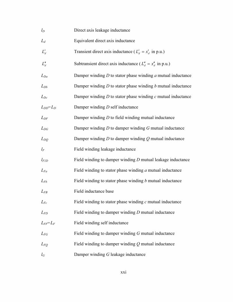
xxi

lD Direct axis leakage inductance

Ld Equivalent direct axis inductance

dL′ Transient direct axis inductance ( dd xL ′=′ in p.u.)

dL ′′ Subtransient direct axis inductance ( dd xL ′′=′′ in p.u.)

LDa Damper winding D to stator phase winding a mutual inductance

LDb Damper winding D to stator phase winding b mutual inductance

LDc Damper winding D to stator phase winding c mutual inductance

LDD=LD Damper winding D self inductance

LDF Damper winding D to field winding mutual inductance

LDG Damper winding D to damper winding G mutual inductance

LDQ Damper winding D to damper winding Q mutual inductance

lF Field winding leakage inductance

lF1D Field winding to damper winding D mutual leakage inductance

LFa Field winding to stator phase winding a mutual inductance

LFb Field winding to stator phase winding b mutual inductance

LFB Field inductance base

LFc Field winding to stator phase winding c mutual inductance

LFD Field winding to damper winding D mutual inductance

LFF=LF Field winding self inductance

LFG Field winding to damper winding G mutual inductance

LFQ Field winding to damper winding Q mutual inductance

lG Damper winding G leakage inductance

xxii

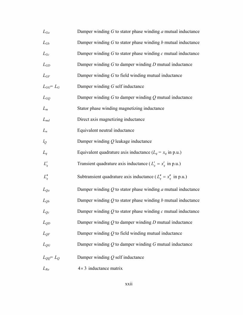
LGa Damper winding G to stator phase winding a mutual inductance

LGb Damper winding G to stator phase winding b mutual inductance

LGc Damper winding G to stator phase winding c mutual inductance

LGD Damper winding G to damper winding D mutual inductance

LGF Damper winding G to field winding mutual inductance

LGG= LG Damper winding G self inductance

LGQ Damper winding G to damper winding Q mutual inductance

Lm Stator phase winding magnetizing inductance

Lmd Direct axis magnetizing inductance

Ln Equivalent neutral inductance

lQ Damper winding Q leakage inductance

Lq Equivalent quadrature axis inductance (Lq = xq in p.u.)

qL′ Transient quadrature axis inductance ( qq xL ′=′ in p.u.)

qL ′′ Subtransient quadrature axis inductance ( qq xL ′′=′′ in p.u.)

LQa Damper winding Q to stator phase winding a mutual inductance

LQb Damper winding Q to stator phase winding b mutual inductance

LQc Damper winding Q to stator phase winding c mutual inductance

LQD Damper winding Q to damper winding D mutual inductance

LQF Damper winding Q to field winding mutual inductance

LQG Damper winding Q to damper winding G mutual inductance

LQQ= LQ Damper winding Q self inductance

LRa 34× inductance matrix

xxiii

LRR 33× inductance matrix

Ls Stator phase winding inductance

m number of measurements

MATLAB® MATrix LABoratory: Software package for high-performance numerical computations

MD Stator to damper winding D mutual inductance

MF Stator to field winding mutual inductance

MFB Field mutual inductance base

MFC Microsoft foundation classes: used in Visual C++ programming

MG Stator to damper winding G mutual inductance

MIMO Multiple input-multiple output

MMF Magnetomotive force

MMFa MMF in phase a

MMFAD MMF in the direct axis

MMFAQ MMF in the quadrature axis

MMFb MMF in phase b

MMFc MMF in phase c

ML Maximum likelihood

MQ Stator to damper winding Q mutual inductance

Ms Stator phase winding mutual inductance

MX Direct axis mutual inductance

MY Quadrature axis mutual inductance

xxiv

n Number of unknowns

Na Effective turns in phase a

NERC North American Electric Reliability Council

Nm Number of measurements

Ns Number of states

OCC Open circuit characteristic

ode Ordinary differential equation

OEM Output error estimation

p Pulse order of harmonic component

P Active power

P Park’s transformation matrix

P0 DC component of permeance distribution

P2 Amplitude of AC component of permeance distribution

PSERC Power Systems Engineering Research Center

)(ϑP Permeance distribution

Q Reactive power

Q Damper winding on the quadrature axis of a synchronous generator

QR QR decomposition; a matrix is resolved into two matrices: Q and R

r=ra=rb=rc=R1 Stator resistance

RB Stator resistance base

rD Damper winding D equivalent resistance

rF Field winding equivalent resistance

xxv

RFB Field winding resistance base

rG Damper winding G equivalent resistance

RML Recursive maximum likelihood

rms Root mean square

rn Equivalent neutral resistance

rQ Damper winding Q equivalent resistance

SB Stator and rotor MVA base

SCC Short Circuit Characteristic

SNR Signal to noise ratio

SSFR Standstill frequency response

ST1 Steam turbine unit 1, located at Redhawk generating station

ST2 Steam turbine unit 2, located at Redhawk generating station

SVD Singular value decomposition

t Time

tB Time base

TIF Telephone Influence Factor

tJ Threshold value of the residual J(x)

TVA Tennessee Valley Authority

U4 44× unit matrix

u(t) 1×m vector of the input states to a system

v Instantaneous voltage

V Voltage phasor

xxvi

v0 Zero axis voltage, proportional to zero sequence voltage

V0 Saturation threshold on OCC curve

v0dq Vector of 0dq voltages

va Stator phase a voltage

vab Line to line voltage between phases a and b

vabc Vector of abc voltages

vb Stator phase b voltage

VB Stator voltage base

vbc Line to line voltage between phases b and c

vc Stator phase c voltage

vca Line to line voltage between phases c and a

vd Direct axis voltage

vD Damper winding D voltage

VFB Field (rotor) voltage base

vF Field winding voltage

vG Damper winding G voltage

Visual C++ Microsoft Visual C++: Software package for development of graphical environments and user friendly interfaces

vn Neutral voltage component

vq Quadrature axis voltage

vQ Damper winding Q voltage

Vt Generator terminal voltage

w(t) 1)( ×− pn state vector

xxvii

x Vector of unknown parameters in the matrix equation zHx =

x Vector of estimated parameters in the matrix equation zHx =

X Reactance in Ω or in per unit

x0 Equivalent zero sequence reactance

XAD Direct axis magnetizing mutual reactance

XADu Direct axis unsaturated magnetizing mutual reactance

XAQ Quadrature axis magnetizing mutual reactance

XAQu Quadrature axis unsaturated magnetizing mutual reactance

xd Equivalent direct axis reactance

dvx′ Transient direct axis reactance

dvx ′′ Subtransient direct axis reactance

xl Stator leakage reactance

xLm Stator leakage reactance

xq Equivalent quadrature axis reactance

qx′ Transient quadrature axis reactance

qvx ′′ Subtransient quadrature axis reactance

x(t) 1×n vector of the states of a system

y(t) 1×p vector of the output states of a system

z Right hand side vector in the matrix equation zHx =

z(t) 1)( ×− pn state vector of an observer to a system

α Significance level for χ2 test

xxviii

α

Angle indicating the relative position of the direct and quadrature axes (0˚ and 90˚ respectively)

γ Angle along the rotor periphery of the stator with respect to phase a

δ Synchronous machine torque angle in electrical radians

∆AT Saturation component of flux

∆ATd Saturation component of the flux in the direct axis

∆ATq Saturation component of the flux in the quadrature axis

∆H Noise content in H matrix

x∆ Estimated correction to the estimated parameters

∆t Time step between measurements

∆z Noise content in z vector

ϑ Angular displacement of d axis from a axis in mechanical radians

λ Instantaneous flux linkage

λ0 Zero sequence flux linkage

λ0dq Flux linkage vector of 0dq components

λa Flux linkage of axis a

λabc Vector of stator flux linkages

λad Flux linkage in the direct axis

λaq Flux linkage in the quadrature axis

λat Terminal flux linkage

λb Flux linkage of axis b

λc Flux linkage of axis c

λd Flux linkage of direct axis

xxix

λD Damper winding D flux linkage

λF Field winding flux linkage

λFDGQ Vector of rotor flux linkages

λG Damper winding G flux linkage

0.1Iλ Value of the saturation function at 1 p.u. voltage

2.1Iλ Value of the saturation function at 1.2 p.u. voltage

Iλ Saturation function

Idλ Saturation function for direct axis

Iqλ Saturation function for quadrature axis

λq Flux linkage of quadrature axis

λQ Damper winding Q flux linkage

µ Mean

σ Standard deviation

0dτ ′ Direct axis transient open circuit time constant

0dτ ′′ Direct axis subtransient open circuit time constant

0qτ ′ Quadrature axis transient open circuit time constant

0qτ ′′ Quadrature axis subtransient open circuit time constant

)(ϑΦ Air gap flux distribution

)(ϑdΦ Air gap flux distribution in the direct axis

)(ϑqΦ Air gap flux distribution in the quadrature axis

χ2 Variable for chi-square test

xxx

ω Synchronous angular frequency in radians per second

ωB Base synchronous angular frequency in radians per second

Ωc Cutoff frequency of a low pass filter

ωR Rated synchronous angular frequency in radians per second

⋅ Absolute value

( )′⋅ Derivative of a variable or matrix with respect to time

^ Estimated quantity

( ) 1−⋅ Inverse

p. p norm of a vector, 1≥p

( )+⋅ Pseudoinverse

( )T⋅ Transpose

CHAPTER 1

INTRODUCTION

1.1 Motivation

The main motivation of this work is the need for accurate models of synchronous

generators. These models are used in transient stability studies and other routine power

engineering studies. Standard parameters of synchronous generator models can be

obtained from dedicated tests or from manufacturer data. The aim of this work is to

estimate synchronous generator model parameters by utilizing recorded operating data.

Estimation of synchronous machine model parameters is a fairly complex mathematical

procedure, and there is a need for an easily used mechanism for model parameter

estimation. A graphic user interface -menu driven- synchronous generator parameter

estimator is developed to assist practicing engineers in the estimation process.

The research work described in this report was further motivated by the operating

history of an 800 MW synchronous machine (unit #5) located at the Four Corners

Generating Station of the Arizona Public Service Company (APS). This unit has

undergone outages on a number of occasions due to a short circuit in its field winding.

On each occasion that this outage occurred the rotor had to be rebuilt, thus leading to

increased costs and possibly decreased reliability for the company. It is beneficiary to

develop a method such that a short circuit in the field winding is detected promptly. In

this way, remedial action or preventive measures can be taken so as to avoid costly

outages. Since turn-to-turn shorts in the field winding in effect alter the field resistance, a

measurement (or calculation) of this resistance in different time intervals may enable the

user to monitor the unit for possible short circuits. Therefore, it is necessary to track over

2

time the estimate of the field resistance and to issue a warning when the resistance value

falls below a specified limit. If, at any instance, the field resistance falls below the

indicated limit, then the unit can be taken out of service and repaired to avoid a possible

forced outage.

Generator parameters are in general not constant throughout the useful life of a

synchronous generator. Some parameters, such as the magnetizing inductances in the

direct and quadrature axes, vary at different operating points due to the effect of magnetic

saturation. These and other parameters also change because of aging, since generator

parameters are properties of physical materials in the generator windings that undergo

changes in their physical characteristics as they age. Further, major changes in generator

parameters occur after a repair. For example, rewinding of the rotor of a generator would

cause the field resistance to be different than its designed value. For these reasons,

parameter estimation is necessary to ensure that the parameters used in different power

system studies are accurate, and to enhance the confidence in the interpretation of the

results of such studies.

An additional motivation of this work is that regional coordinating councils (such

as the North American Electric Reliability Council (NERC)) often require of their utility

company members that generator parameter tests be done periodically. The development

of on-line parameter estimators holds the promise of satisfying this requirement.

3

1.2 Objectives

The main objective of this research work is to develop a method to identify

synchronous generator parameters from on-line measurements. It is also desired to

develop a graphic user interface (GUI) application which will be user friendly and self

guiding so as to facilitate prompt estimation of the desired parameters. In this way,

possible fault conditions can be detected and remedy action can be undertaken.

Moreover, it is necessary to develop an algorithm that will enable bad measurement

detection and rejection so as to increase the reliability of the results. Another objective of

this research work is to develop the saturation model of the inductances of a synchronous

machine. A number of inductances in the synchronous machine model experience

significant change in their values depending on the operating condition of the machine.

The effect of saturation is modeled and incorporated it in the GUI so as to obtain accurate

estimates that reflect the true status of the machine at every operating point.

Secondary objectives of the research include

• Development of an observer for damper currents

• Calculation of the error characteristics of the estimation

• Development of an index of confidence

• Calculation of a range of values for each estimated parameter

• Study of which machine parameters can be estimated, and which can not

• Evaluation of alternative GUI features.

Fig. 1.1 shows the activities related to a synchronous generator, their relation to the

graphic user interface, and the estimation method proposed in this research work.

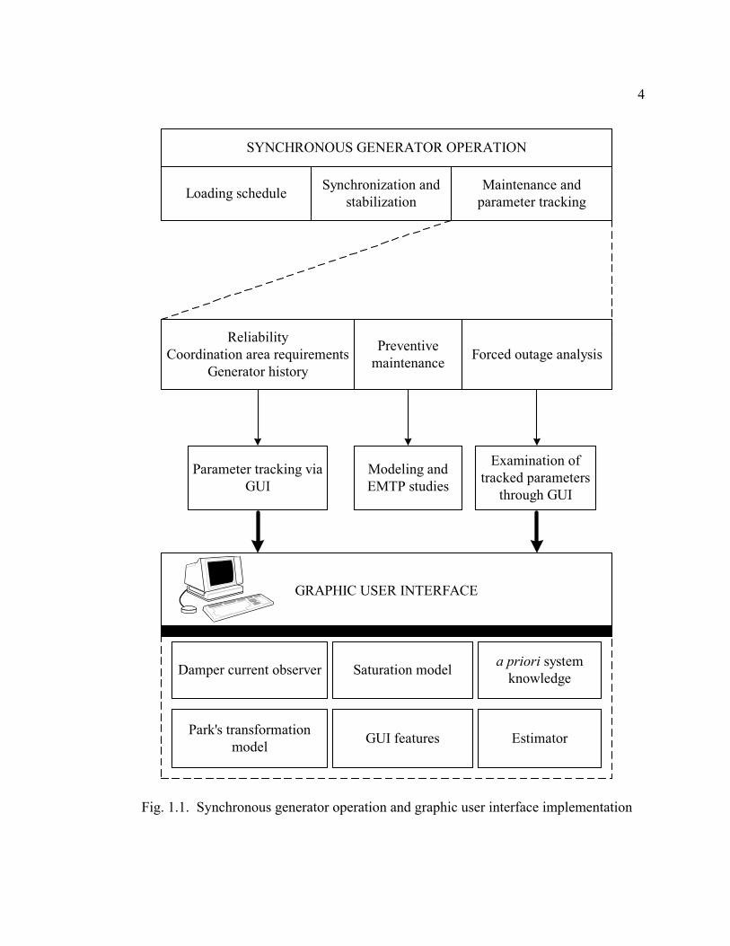
4

SYNCHRONOUS GENERATOR OPERATION

Loading schedule Synchronization andstabilization

Maintenance andparameter tracking

ReliabilityCoordination area requirements

Generator history

Preventivemaintenance Forced outage analysis

Parameter tracking viaGUI

Modeling andEMTP studies

Examination oftracked parameters

through GUI

Damper current observer

Park's transformationmodel

GRAPHIC USER INTERFACE

GUI features

Saturation model a priori systemknowledge

Estimator

Fig. 1.1. Synchronous generator operation and graphic user interface implementation

5

1.3 Identification of synchronous generator parameters: an overview

The power system state estimation problem has attracted the attention of many

researchers since the late sixties [1]-[3], [4]. The main aim was to develop a technique to

monitor the power system and to calculate some of the system states by using other

available data. The interest in generator parameter identification arose about a decade

later.

Traditionally, synchronous generator parameters are obtained by manufacturer

data sheets and then verified and enhanced by off-line tests, as described in IEEE

Standards [5], [6]. Several researchers between 1969 and 1971 developed methods to

find additional parameter values based on the synchronous generator models by Dandeno

[7], Schulz [8], and Dineley [9]. Jackson and Winchester [10] developed direct and

quadrature axis equivalent circuits for round rotor synchronous generators. During the

same period, Canay [11] focused on developing equivalent circuits for field and damper

windings to estimate generator parameters. A significant contribution was made by Yu

and Moussa in 1971 [12] who reported a systematic procedure that can be implemented

to determine the parameters of the equivalent circuits of synchronous generators.

Off-line methods, however, are neither practical nor accurate in most cases.

Decommiting a generator for parameter measuring is not economical for a utility -

especially if the specific generator is a base unit. Furthermore, under different loading

conditions certain generator parameters may vary slightly and therefore off-line methods

may not be accurate enough for certain applications. Finally, the effect of saturation of

generator inductances cannot be accounted for in off-line studies. Saturation is a critical

6

concept in generator operation; in order to consider it in the estimation process, one has

to account for the operating level of the generator at the particular estimation interval [5],

[13]-[15].

Contrary to off-line methods, on-line methods to identify machine parameters are

very attractive to utilities because of their minimal interference in the normal operation of

the generator. Ideally, generator parameters may be calculated under different operating

conditions, both in steady state and transient operation. In 1977 Lee and Tan [16]

proposed an algorithm to determine the parameters of a salient pole generator from data

obtained during a sudden short circuit. In 1981, Dandeno [17] used on-line frequency

response measurements from two large turbo generators to identify machine parameters;

during the same period, Nishiwaki [18] used the extended Kalman filter to identify

dynamic stability constants for small disturbances under steady state operating

conditions. In 1982 Bollinger [19] proposed a technique to estimate system parameters

by utilizing wide bandwidth noise signals in an excitation signal which acts as a

disturbance to the system.

1.4 Literature review

The literature search for this research work focuses mainly on the following

topics:

• Analysis and modeling of synchronous generators

• Estimation of parameters of synchronous generators

• Differential equations and their numerical solutions

7

• Estimation techniques and the generalized inverse

• Computer analysis methods

• Noise filtering

• Observers and observability

• Magnetic saturation.

• Analysis and modeling of synchronous generators

The classic Westinghouse Transmission and Distribution Handbook provides

information for the construction and operation of synchronous machines [20]. Another

useful handbook in the field of electrical machinery is the Electric Motor Repair by

Rosenberg [21]. It is a handbook for the “practically minded” concentrating on the

winding, repair, and troubleshooting of a large number of AC and DC motors and

controllers. Power System Stability and Control by Kundur [13] and Power System

Control and Stability by Anderson and Fouad [14] provide an extensive and detailed

analysis of synchronous machines, in both theory and modeling. They dedicate three

chapters on this topic and, among others, they cover the dq0 transformation, the per unit

representation, equivalent circuits, and analysis in both steady state and transient

operation. Saadat in Power System Analysis [22] concentrates on the transient analysis of

the synchronous generator and on balanced and unbalanced faults. Saadat offers

coverage on the Park’s transformation and on deriving the generator equation in the rotor

frame of reference.

8

Anderson, Agrawal, and Van Ness [23] provide an extensive analysis of

synchronous machines. They dedicate a chapter on synchronous machine modeling and

provide an extensive analysis of the direct and quadrature axis equations. They also

examine thoroughly Park’s transformation, while in one of their chapters they concentrate

on parameter computation, measured data from field tests, and sample test results. Very

useful sources of information are the books Electric Machinery [24] and Analysis of

Electric Machinery [25]. Both books contain the theory of synchronous machines and

analysis of steady state operation. In addition, [25] offers interesting details on

operational impedances and time constants, linearized equations, and a chapter on the

asynchronous and unbalanced operation of synchronous machines.

• Estimation of parameters of synchronous generators

As mentioned in Section 1.3, the interest in the field of synchronous generator

parameter estimation arose in the late sixties. In the last fifteen years, this interest was

enhanced by a number of researchers.

Keyhani, who has conducted research on parameter estimation using a number of

different techniques, has offered extensive literature on this topic. One of the methods

used by Keyhani was the estimation of parameters from Standstill Frequency Response

(SSFR) test data [26], [27]. In this approach, curve fitting techniques are used to derive

the transfer functions of the direct axis and quadrature axis using the available test data.

The parameters of the model are then calculated from nonlinear equations, which relate

the machine parameters and the time constants corresponding to the transfer functions

9

[27]. However, noise-corrupted data cause multiple parameter sets to be estimated. To

obtain a unique set of parameters, Keyhani used a maximum likelihood estimation (ML)

technique [26]. The results indicate that a unique and relatively accurate parameter set is

estimated even though the data are corrupted with noise.

Keyhani in [28] offers an evaluation of the performance of the ML method using

case studies and SSFR data from tests on a 722 MVA generator. It is shown that the ML

method gives estimates with very small error, while the noise has no noticeable effect on

the estimator. The ML algorithm and SSFR data were also used in [29] to estimate

parameters of a three phase salient pole 5 kVA synchronous machine. The equivalent

circuit models were developed and on-line dynamic responses were performed to validate

the identified models.

Tsai, Keyhani, Demcko, and Farmer used small-disturbance responses and the

ML estimation technique to identify an on-line synchronous generator model [30]. The

first step was to identify the machine linear model parameters. Consequently, the

saturation models of the machine were identified using the estimated mutual inductances

under a wide range of operating conditions. It was shown that when the MMF saturation

model was used, the simulated responses of the developed model matched closely with

the measured responses.

Another method used by Keyhani was the identification of synchronous machine

linear parameters from standstill step voltage input data [31]. The procedure involves

applying a step voltage as an input and estimation of the parameters of the time constant

and equivalent circuit models. The initial values of the parameters to be estimated are

10

extracted from the operational inductances which are derived from the measured time

domain data.

Tsai, Keyhani, Demcko, and Selin presented a new approach to develop a model

of the saturated synchronous generator using artificial neural networks (ANN) [32].

ANN are possible to be trained after being arranged in a certain pattern. The pattern used

in this network is a feed-forward network and the learning scheme is of the error back-

propagation form. Moreover, the training pattern was based on on-line small disturbance

responses and the ML algorithm. The important conclusion of this paper is the fact that

the developed ANN saturation model is capable of predicting the machine nonlinear

changes which were not used in the training process.

Eitelberg in [33] uses a linearly formulated least squares problem to obtain

approximate parameter values. Consequently, a numerical search method is used to solve

the nonlinear problem of magnitude and phase fitting. Boje [34] proposes time domain

measurements for determining selected parameters of synchronous machines. These are

proposed as an alternative to standstill frequency domain tests, since as the authors argue,

the proposed method uses simpler equipment and model parameters are obtained directly

in parametric form. However, as with traditional SSFR testing, this method does not

model the machine at normal operating conditions.

Karayaka, Keyhani, Agrawal, Selin, and Heydt in [35]-[37] concentrated on large

synchronous utility generators to develop a procedure of parameter estimation from on-

line measurements. In [35] a one-machine infinite bus system is simulated in the abc

frame of reference using parameters provided by the manufacturer. The armature circuit

11

parameters are hence calculated using the recursive maximum likelihood (RML)

estimation technique. Based on these estimates, the field winding and some damper

parameters are estimated using an Output Error Estimation (OEM) technique. It is found

that even with highly corrupted data the estimated and actual parameters are in good

agreement. In [36] the authors present a method to estimate machine parameters using

synthetic data as previously, but also real time operating data from a utility generator.

This study showed that noise-corrupted data could be handled up to a certain point.

Below a certain signal-to-noise ratio (SNR), estimation of machine parameters was not

possible. The estimation of machine parameters using data obtained on-line showed that

there was a reasonable agreement between estimated and actual curves.

The above methods were repeated by the authors using Artificial Neural

Networks [37]. The data used to train the ANN were taken from real time operating data

and the developed models were validated with measurements not used in the training of

ANN and with large disturbance responses. It was shown that ANN models could

correctly interpolate between patterns not used in training.

Rico, Heydt, Keyhani, Agrawal, and Selin attempted to estimate machine

parameters using orthogonal series expansions such as Fourier, Walsh, and Hartley series

[38], [39]. In [38] the authors propose the use of the Hartley series for fitting operating

data such as voltage and current measurements and the use of linear state estimation to

identify the coefficients of the series. In this way, the machine parameters can be

identified. At the same time, this method is tested for noise corruption in the

measurements. The authors show that the error in the estimation is below 1% even for

12

SNR of 50:1. In [39] the authors expand their previous study to include Walsh and

Fourier series in machine parameter estimation. A matrix of coefficients common to all

orthogonal series expansions is used. The results show that the estimated parameters are

in good agreement with the actual parameters. Also, this method takes into account the

dependence of the parameters with respect to the operating point. More information on

orthogonal series expansions for various power system components such as synchronous

generators and transmission lines can be found in [40].

Finally, Kyriakides and Heydt in [41] and [42] offer an algorithm for the

estimation of synchronous generator parameters from measurements that are taken at the

machine terminals while the generator serves its load. This report is an extension of the

idea presented in the papers.

• Differential equations and their numerical solutions

The need to numerically solve differential equations is of particular importance in

this research work. The model under study involves coupled differential equations,

which have to be solved iteratively for data generation and program testing. The Taylor

series uses a pth order series to estimate the solution. The Euler series uses the first two

terms of the Taylor series, resulting in a first order approximation that has an error of the

order of the time step used. If the time step is small enough (the size depends on the

application), then the Euler method is a good approximation that can be easily

implemented. Multistep methods are also available such as the midpoint method, the

Milne’s method and the Adams-Bashforth method. These, however, require more than

13

one starting value and are hence difficult to implement. Coverage and examples of the

above methods are offered in [43], [44]. Other methods such as the trapezoidal and the

parabolic methods can also be found in the literature [43], [45]-[48].

Perhaps the most widely used method, because of its ease of programming and

accuracy, is the Runge-Kutta-Fehlberg integration method. Many variations of this

method are available in computer packages such as MATLAB. Perhaps the most famous

methods are those incorporated in the ode23 and ode45 m-files provided by MATLAB

[49]. ode23 uses a simple second and third order pair of formulas for medium accuracy

while ode45 uses a fourth and fifth order pair for higher accuracy. Detailed explanation

of these methods can be found in [43], [45], [48].

• Estimation techniques and the generalized inverse

Estimation techniques such as state estimation, least squares, and maximum

likelihood are used in engineering applications interchangeably. For the purposes of this

research the mathematical model is desired to be transformed in a form realizable by a

state estimation algorithm. State estimation is a process during which a number of

unknown system state variables or parameters are assigned a value based on

measurements from that system [50].

Schweppe [1]-[3] was one of the first to propose and develop the idea of state

estimation for the monitoring of power systems. Wood and Wollenberg dedicate a

chapter of their book on state estimation [50]. They offer insight to maximum likelihood

concepts and derive the least squares equations used in state estimation. An introduction

14

on advanced topics on state estimation and a lot of examples on AC network state

estimation are offered. Advanced topics include bad data detection, estimation of

quantities not being measured, network observability, and pseudo-measurements.

A book for the fundamentals of state estimation is that by Heydt [43]. It offers an

introduction to state estimation and its applications in power engineering. Moreover, it

proceeds in more advanced sections such as bad data identification and accuracy of state

estimators. Information on the generalized inverse or pseudoinverse that will be used in

this research can be found in both Heydt [43] and Wollenberg [50]. Albert [51] offers the

theory behind the pseudoinverse and different manipulations or transformations of the

inverse itself.

• Computer analysis methods

A major part of this research is the use of computer packages such as MATLAB

and Visual C++ for the filtering of the measured signals, the implementation of the state

estimation algorithm, and the development of a graphic user interface. Computer

analysis methods are therefore of fundamental importance. A book in this area is the

book by Heydt [43], which provides theory and practical applications on a number of

topics applicable to this research work. Moreover, state estimation and the pseudoinverse

are extensively covered as mentioned in the previous section.

Pratap [52] offers a helpful guide for MATLAB. Visual C++ and MFC

programming are treated in several books [53]-[57]. No book suffices in itself because of

15

the vast capabilities of this programming language and the specialized functions of this

application.

• Noise filtering

In between the data acquisition and the estimator implementation there are a

number of other processes that need to be performed to prepare the data in a form that

can be used by the estimator. One of the most fundamental processes is the filtering of

the measured data for the removal of inconsistent measurements and noise. Various

filters have been developed and implemented for the purposes of noise filtering. The

filters considered for this work are digital discrete filters. Representative types of digital

filters are the Butterworth, Chebyshev, Bessel, and moving average filters [58]-[60].

A filter almost always introduces a phase shift to the filtered signal. This phase

shift is not desired, since the various frequency components of the signal are phase

shifted by a different amount. Therefore, a zero phase shift filter is desired to be

implemented so that there is no phase difference between the original and filtered signals.

Information on zero phase shift filters can be found in [59], [61]-[63]. Zero phase digital

filters effectively filter the signal in both the forward and the reverse directions. The

resulting sequence has zero phase distortion and twice the filter order.

Bad data detection and rejection algorithms have been considered and

implemented to remove outliers from the measurements. Such outliers appear in the form

of spikes in the data sets and are inconsistent measurements. References [64]-[66]

16

propose new methods for the implementation of bad data detection and rejection

algorithms in power system state estimation problems.

• Observers and observability

The theory of observers and observability is a well researched area in control

systems with vast applications in other areas as well. Observers are utilized in this

research work to identify unmeasurable signals in order to facilitate the estimation

process. Various sources can be used to familiarize with the concept of an observer.

DeRusso [67] and Luenberger [68] address the subject of observers and observer design.

The two papers by Luenberger [69], [70] are state of the art in the field of control systems

and they are the first to introduce what has later been known as the Luenberger observer.

Luenberger observers are considered in Chapter 4.

• Magnetic saturation

Saturation of the generator magnetic circuits is an important concept in this

research work. The effect of saturation has been the subject of many scientific papers

and is still a subject of active research due to the importance of the change of the

generator parameters with operating conditions and the difficulty for modeling saturation

accurately. Reference [71] identifies saturation representation as the most important

factor in the improvement of synchronous machine models. Saturation and different

methods to model it are considered in IEEE standards such as [5], as well as a number of

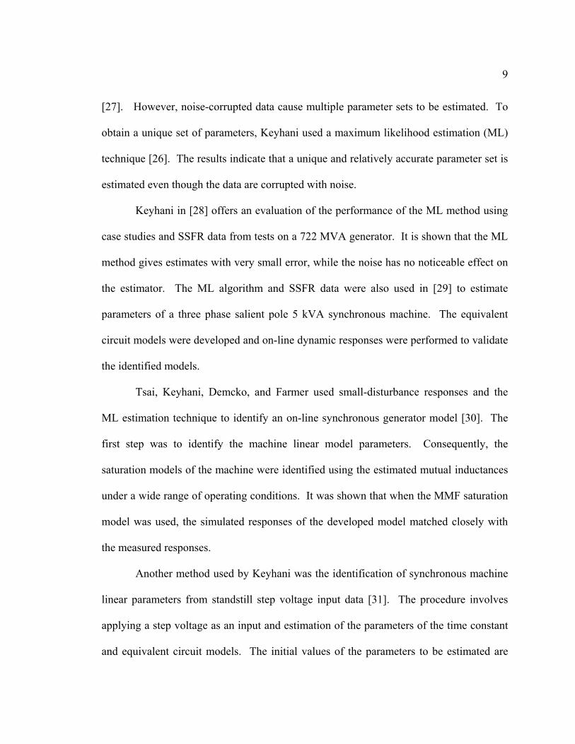
research articles and books [11], [13]-[15], [72], [73]. Fig. 1.2 shows a sample saturation

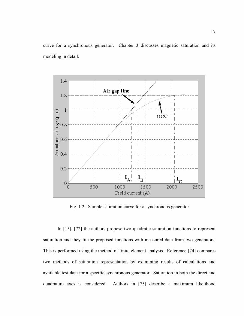
17

curve for a synchronous generator. Chapter 3 discusses magnetic saturation and its

modeling in detail.

Fig. 1.2. Sample saturation curve for a synchronous generator

In [15], [72] the authors propose two quadratic saturation functions to represent

saturation and they fit the proposed functions with measured data from two generators.

This is performed using the method of finite element analysis. Reference [74] compares

two methods of saturation representation by examining results of calculations and

available test data for a specific synchronous generator. Saturation in both the direct and

quadrature axes is considered. Authors in [75] describe a maximum likelihood

18

estimation algorithm to identify saturated inductances of a synchronous machine. The

saturation was modeled from operating data that were generated from small voltage

excitation disturbances. An alternative method to model saturation by using a linearized

generator model and stochastic approximation to solve for the parameters of the model is

presented in [73]. The authors in [76] present a saturation representation by using a finite

element numerical analysis technique. However, the method does not apply to all

operating conditions.

1.5 Statement of originality

The research work described in this dissertation is a contribution to electric power

engineering and especially to the field of synchronous generators. A number of the

research findings deserve mention in this section. References [41], [42], and [77]-[81]

document the author’s main publications related to this research.

A method to estimate synchronous generator parameters will be shown in this

report. The results from the parameter estimation show considerable improvement over

studies performed in the last few decades. The method was applied to a number of

synchronous generators from different manufacturers and different generating stations.

The parameters were estimated at various operating levels and the results, as presented in

this dissertation, show a consistency among data sets of same machines.

An observer has been developed for the identification of damper winding

currents. Damper windings appear in the synchronous generator model and the

knowledge of these currents is instrumental in the estimation process. It should be noted

19

that this is the first time that a method for the estimation of damper winding currents is

developed. The method was verified through simulation data, since it is currently not

possible to obtain actual measurements of damper winding currents. The method was

subsequently applied to the estimation of damper currents from actual generator data.

Finally, a method to estimate the quadrature axis characteristic from the available

direct axis characteristic is described. A saturation model has been developed for use in

on-line identification of synchronous generator parameters. The saturation model

accounts for the operating point of the machine and corrects the mutual inductances that

are affected by saturation.

CHAPTER 2

MODELING OF SYNCHRONOUS GENERATORS

2.1 System identification

The system identification procedure consists of a number of processes depending

on the type of the task that is desired to be performed. In general, there are three basic

entities that need to be available in order to perform any kind of system identification.

These entities are the availability of a data set for the system, a set of candidate models,

and an identification method or rule that will be used to identify the system parameters

[82]. The system identification procedure is an iterative process with respect to the

selection of the model of the system. A number of candidate models need to be tested so

as to select the one that fits best to the actual response of the system. The selection

process can be aided by the use of a priori knowledge of the system behavior and

expected parameters, and by the comparison of the error characteristics obtained by each

model. Fig. 2.1 shows the procedure that is followed in the system identification problem

described in this report. This chapter concentrates on the selection of a model for the

synchronous generator to be used in the identification procedure.

2.2 Model selection

In order to formulate the state estimation equation for a synchronous generator, it

is necessary to employ a mathematical model, which will represent the synchronous

generator in the conditions under study. There are a number of practical models available

for synchronous generators depending on the type of study that is desired to be performed

and the level of detail that the generator windings are modeled. Regardless of the model

21

chosen, it is necessary to consider an arrangement of three stator windings that are 120

electrical degrees apart, and a rotor structure that has at least one field winding and a

variable number of damper windings in the direct and quadrature axes. The configuration

of the rotor structure is the one that differentiates the various models of synchronous

generators.

Data set

Problem definition

Are the resultssatisfactory?

Selection ofcandidate model

Selection ofidentification method

Estimation of parameters

Model validation

Revise model

Use model

YES

NO

Fig. 2.1. System identification procedure

22

The order of a synchronous generator model is dictated by the number of rotor

circuits in the direct and quadrature axes and usually ranges from first order to third

order. Practical experience backed by simulation results and results from field tests show

that a third order representation suffices for detailed analysis of synchronous generators.

Lower order models are often used in a variety of studies (for example, stability studies)

or for the representation of various types of generators (for example, hydro generators

and turbine generators).

Various recommended synchronous generator models are suggested in IEEE

standards, such as in [83]. Models 2.1 and 2.2, as shown in Figs 2.2 and 2.3 respectively,

have been selected as candidates to perform the system identification procedure. The

criterion for the selection of the two models was twofold: enough detail to obtain accurate

estimates and simplicity in the model structure to make the estimation process simple to

develop and program. Model 2.1 comprises one field winding and one damper

(amortisseur) winding in the direct axis, and one damper winding in the quadrature axis.

Model 2.2 has the same number of circuits in the direct axis, but has two damper

windings in the quadrature axis to develop a symmetric model. In this chapter model 2.2

will be analyzed since the development of the model equations is similar for both models.

23

-

+VF

ld

LAD

lF

rF

lD

rD

lF1D

lq

LAQ lQ

rQ

Fig. 2.2. Generator model 2.1 with one damper winding in each axis [83]

-

+VF

ld

LAD

lF

rF

lD

rD

lF1D

lq

LAQ lG

rG

lQ

rQ

Fig. 2.3. Generator model 2.2 with one d axis and two q axis damper windings [83]

24

2.3 Modeling of synchronous generators

The synchronous generator model that will be analyzed in the remainder of this

chapter is model 2.2, as defined in [83]. This model comprises three stator windings that

are 120 electrical degrees apart and one rotor structure that is composed of two imaginary

axes: the direct axis and the quadrature axis. The direct axis (d axis) comprises one field

winding and one damper winding, while the quadrature axis (q axis) comprises two

damper windings. The two damper windings on the q axis assist in obtaining a

symmetric model with respect to the two imaginary axes and are particularly useful in the

correct representation of round rotor synchronous generators. Measurements of the

currents and voltages in the three stator windings and the field winding are usually

available, and these will therefore be used as the states of the model under consideration.

The damper currents in a synchronous generator are not possible to be measured. This

shortcoming will be dealt with in Chapter 4 where an observer for the estimation of the

damper currents will be presented.

The seven windings mentioned above (three in the stator and four in the rotor) are

magnetically coupled. This coupling is a function of the rotor position and therefore the

flux linking each winding is also a function of the rotor position [14]. Hence, the

instantaneous terminal voltage of any winding takes the form,

λ′−−= riv , (2.1)

where r is the winding resistance, i is the current, and λ is the flux linkage. The prime

symbol (´) denotes a derivative with respect to time. It should be noted that in this

notation it is assumed that the direction of positive stator currents is out of the terminals,

25

since the synchronous machine under consideration is a generator [25]. Before

proceeding further with this derivation, it will be useful to refer to the Park’s

transformation which will be an essential tool for this analysis.

2.4 Park’s transformation

In the late 1920s Park [84], [85] formulated a change of variables which replaced

the variables associated with the stator windings of synchronous machines with variables

associated with fictitious windings that are rotating with the rotor [25]. The configuration

of these fictitious windings is illustrated in Fig. 2.4. The direction of rotation and the

alignment of the d axis and q axis are defined in agreement with IEC Standard 34-10 [86]

and IEEE Standard 100-1984 [87].

Park’s transformation eliminates the time-varying inductances from the voltage

equations. Stanley [88], Kron [89], and Brereton [90] also worked on this subject and

developed similar equations transforming either the rotor or the stator variables to

variables in fictitious windings in different reference frames. In the case of the

synchronous machine, the time-varying inductances can be eliminated only if the

reference frame is fixed in the rotor and therefore Park’s transformation will be used [25].

It should be noted that the transformation that will be used in this chapter is not exactly

the same as the one suggested by Park [84], [85], but rather an improvement of Park’s

method as suggested by various researchers such as Lewis [91], Concordia (discussion in

[91]), and Krause and Thomas [92]. Since Park was the first to propose the method of

26

changing the variables associated with the stator windings, the transformation is named

after Park.

ϑ

a axis

c axis

q axisd axis

b axis

direction ofrotation

iF

iFiD

iD

iaia

ib

ib

ic

ic

iQ

iQiG

iG

Fig. 2.4. Representation of a synchronous generator

The d axis of the rotor is defined to be at an angle ϑ radians with respect to a

fixed reference position at some instant of time. If the stator phase currents ia, ib, and ic

are projected along the d and q axes of the rotor, the following relationships are obtained,

.)]3/2cos()3/2cos(cos[)3/2(

)]3/2sin()3/2sin(sin[)3/2(

πϑπϑϑ

πϑπϑϑ

++−+×=

++−+×=

cbad

cbaq

iiii

iiii

(2.2)

It should be noted that in this formulation, the reference axis was chosen to be axis a, to

avoid an extra angle of displacement in all the terms.

The effect of the above transformation is to convert the stator quantities from

phases a, b, and c to new variables, the frame of which moves with the rotor. However,

since there are three variables in the stator, it is necessary to have three variables in the

rotor for balance. The third variable is on a third axis: the stationary axis. It is a

27

stationary current proportional to the zero-sequence current and it is zero under balanced

conditions. Therefore, from (2.2), a matrix P called Park’s transformation is defined,

such that,

abcdq Pii =0 , (2.3)

where the current vectors are defined as,

=

q

ddqiii

i0

0 and

=

c

b

a

abciii

i . (2.4)

The Park’s transformation is thus defined as,

+−

+−=

)32sin()3

2sin(sin

)32cos()3

2cos(cos2

12

12

1

32

πϑπϑϑ

πϑπϑϑP . (2.5)

It is apparent, that in order to perform this transformation it is necessary to

calculate the angleϑ . The flux of the main field winding is along the direction of the d

axis of the rotor. This flux produces an EMF that is lagging by 90°. Therefore, the

machine EMF E is mainly along the q axis of the rotor [14]. If a machine with terminal

voltage V is considered, the phasor E should lead the phasor V if this machine is to be

operated as a generator. The angle between E and V is denoted as the machine torque

angle δ if V is in the direction of phase a (reference phase). Considering Fig. 2.2, at time

0=t , the phasor V is located at the reference axis a. The q axis is located at an angle δ

and the d axis is located at an angle 2πδ +=ϑ . At 0>t , the reference axis is located at

an angle tRω with respect to axis a. Therefore, the d axis of the rotor is located at,

28

2πδωϑ ++= tR rad, (2.6)

where ωR is the rated (synchronous) angular frequency in rad/s and δ is the synchronous

torque angle in electrical radians.

Park’s transformation can also be used to convert voltages and flux linkages from

abc quantities to 0dq quantities. The expressions are identical to the expressions for the

current and are given by,

abcdq Pvv =0 and abcdq Pλλ =0 . (2.7)

Furthermore, if the transformation is unique, an inverse transformation exists, and the abc

quantities can be calculated if the 0dq quantities are known. In this case,

dqabc iPi 01−= , (2.8)

where the inverse Park’s transformation is given by,

++

−−=−

)32sin()3

2cos(2

1

)32sin()3

2cos(2

1

sincos2

1

321

πϑπϑ

πϑπϑ

ϑϑ

P . (2.9)

Park’s transformation is an orthogonal matrix. This can be shown by examining

the column vectors of the matrix. The column vectors of P are orthonormal since

0=⋅ vu and 1=u for every u, v in P. Then by definition the matrix P is orthogonal

and IPPT = . Since the inverse of a square matrix is unique, it is also true that IPPT = .

This implies that TPP =−1 . Consequently, P is power invariant and therefore the same

power expression can be used in both the abc and 0dq frames of reference [14]. It is easy

to show that,

29

qqddccbbaa ivivivivivivp ++=++= 00 . (2.10)

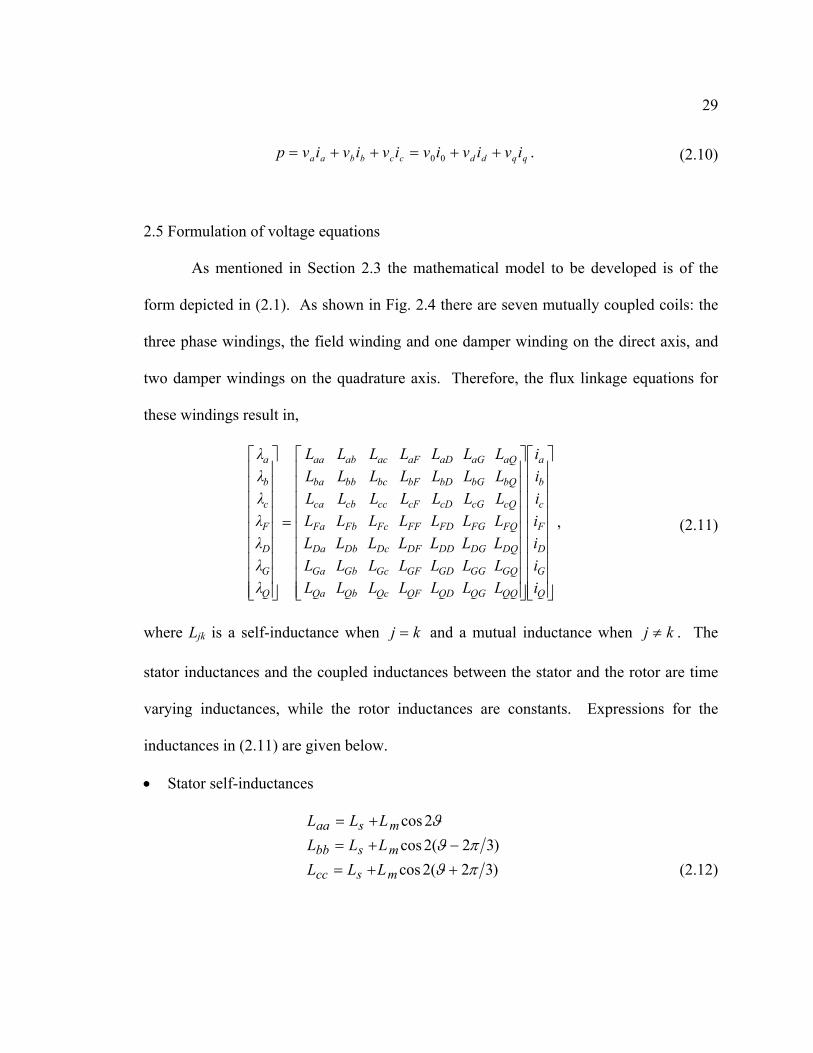
2.5 Formulation of voltage equations

As mentioned in Section 2.3 the mathematical model to be developed is of the

form depicted in (2.1). As shown in Fig. 2.4 there are seven mutually coupled coils: the

three phase windings, the field winding and one damper winding on the direct axis, and

two damper windings on the quadrature axis. Therefore, the flux linkage equations for

these windings result in,

=

Q

G

D

F

c

b

a

QQQGQDQFQcQbQa

GQGGGDGFGcGbGa

DQDGDDDFDcDbDa

FQFGFDFFFcFbFa

cQcGcDcFcccbca

bQbGbDbFbcbbba

aQaGaDaFacabaa

Q

G

D

F

c

b

a

iiiiiii

LLLLLLLLLLLLLLLLLLLLLLLLLLLLLLLLLLLLLLLLLLLLLLLLL

λλλλλλλ

, (2.11)

where Ljk is a self-inductance when kj = and a mutual inductance when kj ≠ . The

stator inductances and the coupled inductances between the stator and the rotor are time

varying inductances, while the rotor inductances are constants. Expressions for the

inductances in (2.11) are given below.

• Stator self-inductances

)32(2cos)32(2cos

2cos

πϑπϑ

ϑ

++=−+=

+=

mscc

msbb

msaa

LLLLLLLLL

(2.12)

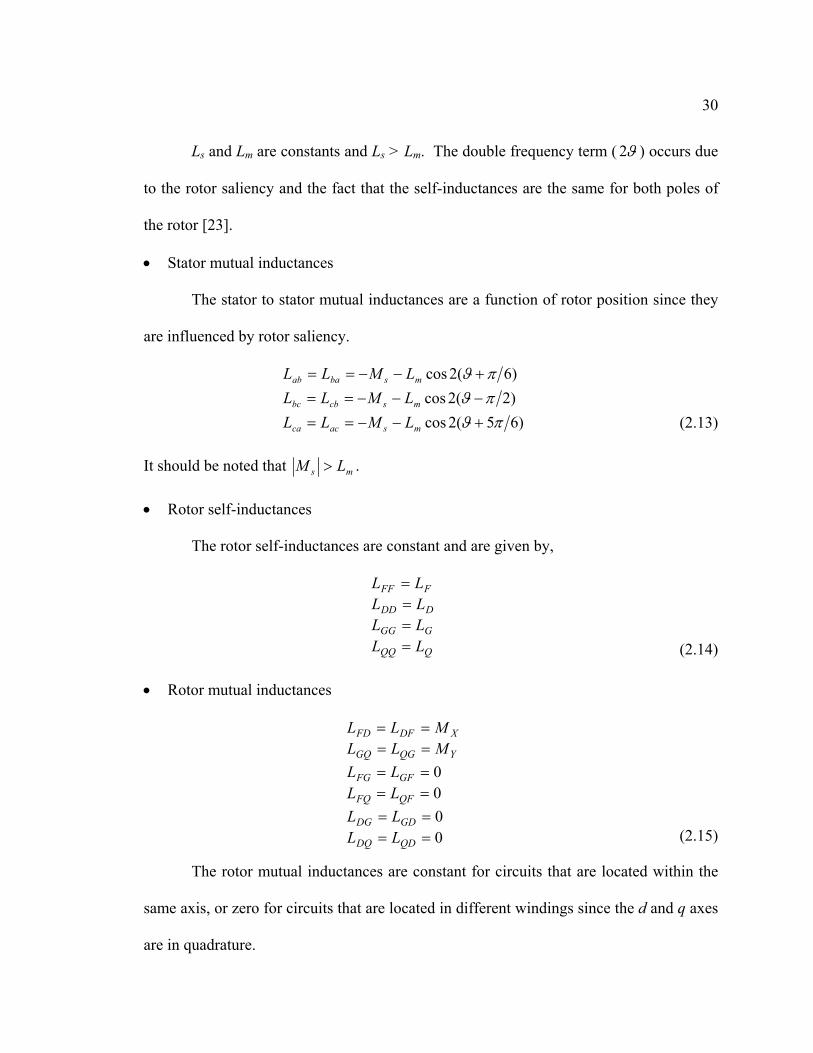
30

Ls and Lm are constants and Ls > Lm. The double frequency term ( ϑ2 ) occurs due

to the rotor saliency and the fact that the self-inductances are the same for both poles of

the rotor [23].

• Stator mutual inductances

The stator to stator mutual inductances are a function of rotor position since they

are influenced by rotor saliency.

)65(2cos)2(2cos)6(2cos

πϑπϑπϑ

+−−==−−−==+−−==

msacca

mscbbc

msbaab

LMLLLMLLLMLL

(2.13)

It should be noted that ms LM > .

• Rotor self-inductances

The rotor self-inductances are constant and are given by,

QQQ

GGG

DDD

FFF

LLLLLLLL

====

(2.14)

• Rotor mutual inductances

0000

============

QDDQ

GDDG

QFFQ

GFFG

YQGGQ

XDFFD

LLLLLLLL

MLLMLL

(2.15)

The rotor mutual inductances are constant for circuits that are located within the

same axis, or zero for circuits that are located in different windings since the d and q axes

are in quadrature.

31

• Stator-to-rotor mutual inductances

)32cos()32cos(

cos

πϑπϑ

ϑ

+==−==

==

FFccF

FFbbF

FFaaF

MLLMLLMLL

)32cos()32cos(

cos

πϑπϑ

ϑ

+==−==

==

DDccD

DDbbD

DDaaD

MLLMLLMLL

)32sin()32sin(

sin

πϑπϑ

ϑ

+==−==

==

GGccG

GGbbG

GGaaG

MLLMLLMLL

)32sin(

)32sin(

sin

πϑ

πϑ

ϑ

+==

−==

==

QQccQ

QQbbQ

QQaaQ

MLL

MLL

MLL

(2.16)

It is observed that (2.11) has time-varying terms which will cause complication

when their derivatives are taken. Thus, it is convenient to refer all quantities to a rotor

frame of reference through a Park’s transformation. The Park’s transformation is only

applied to the stator portion of the equation. To achieve this, (2.11) is premultiplied by

400

UP

, as shown in (2.17). P is the Park’s transformation and U4 is a 44× unit

matrix,

.0

00

00

00

0

44

1

44

=

−

FDGQ

abc

RRRa

aRaa

FDGQ

abcii

UP

UP

LLLL

UP

λλ

UP

(2.17)

The above operation results in,

=

Q

G

D

F

q

d

QYQ

YGG

DXD

XFF

QGq

DFd

Q

G

D

F

q

d

iiiiiii

LMkMMLkM

LMkMMLkM

kMkMLkMkML

L

λλλλλλλ 000

00000000

00000000

00000000000000

,

(2.18)

where mssqmssd LMLLLMLL23,

23

−+=++= , ss MLL 20 −= , and 23=k .

32

Fig. 2.5 shows the schematic diagram of a synchronous generator assuming a

representation of one damper winding in the direct axis and two damper windings in the

quadrature axis. A neutral impedance to ground is also shown. Using matrix notation,

the generator voltage equations become,

nvλriv −′−−= , (2.19)

where the neutral voltage contribution vn is given by,

′′′

−

−=

c

b

a

n

c

b

a

nn

iii

Liii

rv111111111

111111111

. (2.20)

Equation (2.19) in its expanded form becomes,

+

′′′′′′′

−

−=

−−−−

0

000000000000000000000000000000000000000000

n

Q

G

D

F

c

b

a

Q

G

D

F

c

b

a

Q

G

D

F

c

b

a

Q

G

D

F

c

b

a

v

iiiiiii

rr

rr

rr

r

vvvv

vvv

λλλλλλλ

.

(2.21)

In (2.21) the voltage is expressed in terms of both currents and flux linkages.

This is not desirable and therefore one of the two variables has to be replaced. Equation

(2.18) is employed to replace the flux linkage by the current variables. The choice of

replacing the flux linkages rather than the currents is based on mainly two reasons. The

main reason is that the available data from on-line measurements are voltage and current

states. There will be no need to convert the currents into flux linkages in the above

equation. The second reason is that the relationship between the voltages vd and vq and

the state variables is much simpler than the one involving flux linkages.

33

rF

LFiFvF

rG

LGvG=0 iG

rQ

LQvQ=0 iQ

rD

LDvD=0 iD Lbb

rc

ra

rb

rn

Laa

Lcc

Ln

va

vbvn ic

ib

ia

in

a

b

c

nvc

Fig. 2.5. Schematic diagram of a synchronous generator

Substituting all known parameters into (2.21), the mathematical model can be

derived as,

.

00000000

00000000

000000000000003

000000000000000000000000000

0000000003

00

00

′′′′′′′

+

−

−−−

+

−=

−−−−

Q

G

D

F

q

d

QYQ

YGG

DXD

XFF

QGq

DFd

n

Q

G

D

F

q

d

Q

G

D

F

DFd

QGq

n

Q

G

D

F

q

d

iiiiiii

LMkMMLkM

LMkMMLkM

kMkMLkMkML

LL

iiiiiii

rr

rr

kMkMrLkMkMLr

rr

vvvv

vvv

ωωωωωω

(2.22)

34

All quantities in (2.22) are in actual units. The per-unitized form of (2.22) will be

considered in Chapter 3. Equation (2.22) effectively achieves to formulate the state

variables (voltages and currents) in a form suitable for state estimation. The above

equation can be easily rearranged in the form zHx = , where x is a vector of the unknown

parameters and H and z are a known matrix and vector respectively, provided that all the

terms are linear. The only nonlinearity in the above equations derives from the presence

of the synchronous speed ω. However, the synchronous speed does not vary significantly

within the small intervals that are used during the estimation process because of the large

time constants of synchronous generators. Therefore, (2.22) can safely be considered as

linear.

Another interesting observation made from the above equation is that the zero

sequence voltage is dependent only on 0i and 0i′ . In other words, it is decoupled from

the remaining six equations and can be solved separately. The other equations are

coupled in the form of a passive network except for the presence of the speed voltage

terms. Finally, all elements in the matrices of the coefficients are constants with the

exception of ω, which however, can be considered as a constant as explained previously.

CHAPTER 3

SATURATION OF SYNCHRONOUS GENERATOR INDUCTANCES

3.1 Introduction

As noted in Chapter 1, the operating parameters of generators change according to

the operating conditions. This is mainly due to the magnetic saturation experienced by

the generator inductances. Saturation is a phenomenon that becomes apparent when the

current through an inductor exceeds a certain limit. In effect, saturation of an inductor

occurs when the core of the inductor can no longer store magnetic energy.

An inductor is usually constructed using a ferromagnetic material such as iron or

one of its alloys. A ferromagnetic material is composed of small domains whose dipole

moments are randomly oriented. When the material is completely demagnetized, the net

magnetic moment over the material is zero. As the current through the inductor increases

(measured by means of the magnetic field intensity), the domains in the material tend to

align in the direction of the magnetic field intensity. As more domains are aligned, the

magnetic flux density increases. When all domains have aligned in the direction of the

magnetic field intensity, the flux density reaches its saturation density and cannot

increase further in the same fashion. As the magnetic field intensity increases beyond the

saturation point, relatively small increases of the magnetic flux density occur. When a

large number of magnetic domains align in this way, the material is said to be in its

saturation region [93].

Saturation representation is critical in the correct modeling of synchronous

machines. Reference [71] identifies saturation representation as the most important

factor in the effort for improved synchronous machine models. The q axis reactance xq is

36

the dominant factor in determining the rotor angle δ for a particular operating condition.

The d axis reactance xd is the dominant factor in determining the excitation voltage and

the power/load angle characteristics. The margins of the steady state stability are

calculated through knowledge of the power/load angle characteristics. Further, xd plays

an important role in the determination of the short circuit current [94]. Since both xd and

xq are affected by saturation, it is necessary to model saturation so as to increase the

reliability of the estimated parameters and benefit from such an estimation in improving

the planning of the operation of synchronous machines.

The main effect of saturation in a synchronous generator is the decrease of its

mutual inductances depending on the operating level of the generator. Such a decrease

may be considerable as the generator is driven higher into saturation. Therefore, it is

imperative that the effect of saturation be modeled in the parameter estimation procedure.

In general, the only available data for a synchronous generator are those obtained

from the saturation curve of the machine and especially by the open circuit characteristic

that is depicted on the saturation curve. An example of a typical saturation curve of a

synchronous generator can be seen in Appendix B.1. The saturation curve is composed

of three parts: the air gap line, the open circuit characteristic (OCC), and the short circuit

characteristic (SCC). The SCC is a plot of the armature current versus the field current

and is the rightmost straight line on the data sheet of the saturation curve as shown in Fig.

B.1 of Appendix B. The SCC is not used for saturation calculations.

The air gap line and the OCC are plots of the field current required to overcome

the reluctance of the air-gap, where the horizontal axis is the field current in units of

37

amperes and the vertical axis is the per unit armature voltage of the generator. The air

gap line is tangent to the OCC and the deviation of the OCC from the air gap line

indicates the degree of saturation of the generator inductances. Fig. 3.1 shows a sample

saturation curve for a synchronous generator. This saturation curve will aid in analyzing

the methodology that is followed for the consideration of saturation for synchronous

generator inductances.

The representation of saturation is rather cumbersome because it is not possible to

represent all the nonlinearities in a generator and the interaction between all the circuits

within the stator and the rotor (including the fictitious windings) with any single model

for all the operating conditions. Therefore, a number of assumptions have to be made in

order to enable satisfactory modeling of saturation.

Fig. 3.1. Sample saturation curve for a synchronous generator

38

One of the major assumptions that needs to be made in the modeling of saturation

is that only the mutual inductances LAD and LAQ saturate. LAD and LAQ appear in the

model of the synchronous generator when (2.22) is transformed into its correct per unit

form. This transformation will be considered in the next section. As far as the leakage

inductances are concerned, these are assumed not to saturate since leakage fluxes are in

air for a significant portion of their paths. Further, it is assumed that there is no magnetic

coupling between the direct and quadrature axes because of saturation, and therefore no

flux is produced that links one axis with the windings of the other axis. Finally, in order

to be able to model saturation using the OCC, it is necessary to assume that the effect of

saturation under loaded conditions is the same as under no load conditions [13]. In

reality, the load saturation curve is not exactly the same as the OCC, but lies somewhat to

the right of the OCC [95].

The effects of saturation for the mutual inductances LAD and LAQ may be

represented by two saturation factors, one for each inductance [5], [13], [14]. The

saturated inductances are given by,

,AQusqAQs

ADusdADsLKLLKL

==

(3.1)

where Ksd and Ksq represent the saturation factors in each axis and the subscripts u and s

refer to the unsaturated and saturated values of the inductance respectively. The two

saturation factors represent the degree of saturation in the direct and quadrature axes.

The saturation factors are in general not the same for both axes.

39

In the case of salient pole machines, Ksq is assumed to be unity for all loading

conditions and thus LAQ is considered a constant inductance [13], [14]. This is because

the path for the quadrature axis flux is mainly in air and therefore the saturation

experienced by LAQ is insignificant. In the case of round rotor machines, saturation is

significant in both the direct and quadrature axes. Both saturation factors need to be

calculated from the d axis and q axis saturation curves. However, q axis saturation

curves are typically not available and it is typically assumed that the q axis saturation

factor is equal to the d axis saturation factor [13]. The assumption of equal saturation

factors effectively assumes that the reluctance of the magnetic path is homogeneous

around the periphery of the rotor [13]. The assumption of equal saturation effects also

implies that the magnetic excitation in the direct and quadrature axes is equal.

For more accurate representation of saturation it is necessary to model the q axis

saturation as well. For round rotor synchronous machines the q axis saturates appreciably

more than the d axis because of the presence of rotor teeth in the magnetic path of the q

axis [13]. All of the flux along the q axis passes through the rotor teeth and therefore, for

the same amount of air gap flux density the teeth saturate more than the d axis. Further,

saturation in the q axis occurs at a lower flux than saturation in the d axis [96].

References [72] and [97] describe saturation modeling in both the d and q axes by

using finite element analysis. Finite element analysis is an accurate method of

representing magnetic saturation, but the computational intensity of this method makes it

impractical for on-line applications. References [74], [96], and [98]-[100], describe

alternative methods to calculate the q axis saturation characteristic for both round rotor

40

and salient pole synchronous generators. The ideas discussed in [96] and [100] will be

used in Section 3.3 to develop a model to estimate the q axis characteristic from the

available d axis characteristic. Although the methodology used to derive the model is

different from the one used in [96], the resulting models are identical for both methods.

Section 3.2 modifies (2.22) as derived in Chapter 2, to a per unit model that

clearly shows the mutual inductances. The modified model enables an easier

representation of saturation. Section 3.3 develops the methodology to estimate the q axis

saturation curve from the available d axis saturation curve, while Section 3.4 shows how

the saturation factors for both the d and q axes can be calculated and applied in the

estimation procedure. Section 3.5 offers a list of the synchronous generators from which

data sets have been used to evaluate the parameter estimation algorithm. These data sets

have been obtained on-site through a digital fault recorder (DFR) at different operating

points. A list of the data sets and the operating points at which they have been obtained

is also offered in the same section. Section 3.6 offers a list of the case studies that are

described in this dissertation.

3.2 Preparation of the generator model to account for saturation

In order to enable the implementation of the saturation model as discussed in the

previous section, the generator model of (2.22) needs to be transformed in such a way so

as to make the presence of the saturating inductances LAD and LAQ evident. This is

achieved by selecting appropriate base quantities that link both the stator and the rotor

41

and converting the model into its per unit form. This section discusses the transformation

of the model into the desired form.

Per unit conversion can also aid in the understanding of the method, simplify

some of the expressions, and generalize the method to enable the estimation of

parameters of any given synchronous generator. Moreover, the stator voltages are in the

kilovolt range while the field quantities are often smaller; thus, per-unitization aids in the

conceptual understanding of the magnitudes of all signals involved. Finally, conversion

of the model into its per unit form enables the user to detect unrealistic values of the

estimated parameters. If the rated power and voltage are taken as the base quantities,

then the per unit values of the parameters of nearly all the generators under consideration

will fall within a certain range of values.

The power and voltage bases selected for the stator are the respective rated

quantities from the manufacturer stability study data sheet. The rotor base quantities

need to be defined in accordance to the selection of the stator base quantities. Since both

the stator and rotor windings are coupled electromagnetically, it is necessary to select the

same time base in both circuits [91]. The choice of a common time base forces the base

mutual inductance to be the geometric mean of the base self inductances [23]. Further,

the power base of the rotor circuit is selected to be equal to the power base of the stator

circuits. An analysis of the procedure for the selection of the bases for both the stator and

rotor circuits and the calculation of generator parameters is offered in Appendix A.

The direct consequence of the selection of the same time base in the stator and

rotor circuits is that the mutual inductances between circuits in the same axis (d and q

42

axes) are equal. Therefore, the following relationships expressed in per unit can be used

to simplify the synchronous generator model of (2.22).

AQYQG

ADXDFLMkMkMLMkMkM

======

(3.2)

LAD and LAQ are defined as the direct and quadrature axis magnetizing mutual inductances

respectively. Further, the generator self inductances in both the direct and quadrature

axes can be separated into two inductances: the mutual inductance and the leakage

inductance. The direct axis self inductances are given by,

,DADD

FADF

dADd

LLLLLL

l

l

l

+=+=+=

(3.3)

while the quadrature axis self inductances are given by,

,QAQQ

GAQG

qAQq

LLLLLL

l

l

l

+=+=+=

(3.4)

where il denotes a leakage inductance for winding i.

Finally, it is needed to premultiply the second part of the equation of the model by

the inverse of the rated frequency ωB in order to obtain a dimensionally correct per unit

form of the equation. The reason for this adjustment to the model can be shown in two

ways. Consider the model equation in compact form. This is given by,

actualactualactualactualactual ILIRV ′−−= , (3.5)

where V, I, and I ′ are vectors, R and L are matrices and the subscript actual refers to the

fact that the quantities in the vectors or matrices are actual quantities and not per unit.

43

Substituting each quantity with the product of its base and its per unit value, (3.5)

becomes,

pubpubpubpubpub IILLIIRRVV ′−−= . (3.6)

Since LωX = and b

bb I

VX = , the inductance base is given by,

bB

bb Iω

VL = . (3.7)

Therefore, (3.6) becomes,

pubpubB

bpupubbpub IIL

IV

IRIRVV ′−−=ω

, (3.8)

which if simplified gives the desired per unit form,

pupuB

pupupu ILIRV ′−−=ω1 .

(3.9)

Alternatively, it can be argued that, since all quantities need to be expressed in per

unit, it is necessary to express the time in per unit as well. The time component is present

in the current derivative vector of (2.22). The time base (which is the same for both

stator and rotor circuits as explained above), is given by the inverse of the rated

frequency in radians per second, and therefore a current derivative in per unit should be

written as,

Btdt

di ,

where i is in per unit and tB is the time base in seconds. This can be rearranged as,

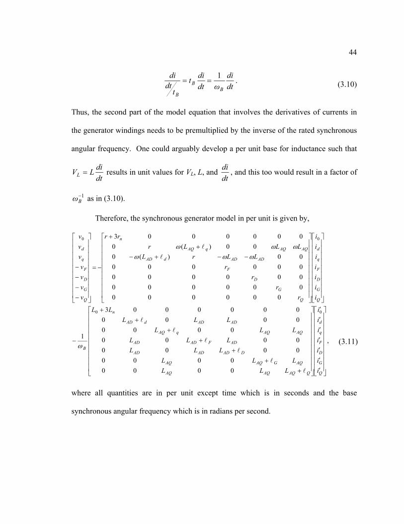
44

dtdi

ωdtdit

tdt

di

BB

B

1== . (3.10)

Thus, the second part of the model equation that involves the derivatives of currents in

the generator windings needs to be premultiplied by the inverse of the rated synchronous

angular frequency. One could arguably develop a per unit base for inductance such that

dtdiLVL = results in unit values for VL, L, and

dtdi , and this too would result in a factor of

1−Bω as in (3.10).

Therefore, the synchronous generator model in per unit is given by,

,

00000000

00000000

000000000000003

1

00000000000000000000000000)(0

00)(00000003

00

00

′′′′′′′

++

++

++

+

−

−−+−+

+

−=

−−−−

Q

G

D

F

q

d

QAQAQAQ

AQGAQAQ

DADADAD

ADFADAD

AQAQqAQ

ADADdAD

n

B

Q

G

D

F

q

d

Q

G

D

F

ADADdAD

AQAQqAQ

n

Q

G

D

F

q

d

iiiiiii

LLLLLL

LLLLLL

LLLLLL

LL

iiiiiii

rr

rr

LLrLLLLr

rr

vvvv

vvv

l

l

l

l

l

l

l

l

ω

ωωωωωω

(3.11)

where all quantities are in per unit except time which is in seconds and the base

synchronous angular frequency which is in radians per second.

45

3.3 Derivation of flux equations for the d and q axes saturation

Typically, the only information that is available regarding saturation for

synchronous generators is obtained from the manufacturer supplied d axis saturation

curve. This information does not allow representation of saturation in the q axis of the

machine. Fig. 3.2 shows a typical saturation characteristic for both the direct and

quadrature axes. In this section a method will be shown to estimate the q axis open

circuit characteristic from the available d axis characteristic. The resulting model is

identical to the model proposed in [96], but the methodology used in this dissertation is

different.

Air

gap

volta

ge (p

u)

Field current (pu)

d axis saturation curve

q axis saturation curve

q axis air gap lined axis air gap lineSlope = LAD

Slope = LAQ

0

Ad0

Aq0

Fig. 3.2. Direct and quadrature axis characteristics

46

The effect of saturation can be related to the air gap flux density distribution. As

can be observed from Fig. 3.2, an additional amount of magnetomotive force (MMF) or

field current is required to overcome the reluctance of the air gap and to produce the same

amount of flux that would be produced if saturation did not exist (i.e. if the air gap line

represented higher values of field current as well as lower).

The air gap flux distribution Φ is given by,

)()()( ϑϑϑ PF=Φ , (3.12)

where )(ϑF is the air gap MMF distribution, )(ϑP is the air gap permeance distribution,

and ϑ is the angular displacement from the center of the direct axis.

The flux produced by the stator winding follows a path that incorporates the stator

iron, the air gap, and the rotor iron. Fig. 3.3 shows the variation of the permeance of this

path as a function of rotor position. The permeance distribution can be approximated by,

)2cos()( 20 ϑϑ PPP += , (3.13)

where P0 and P2 are constants. The double frequency variation occurs because the

permeances of the north and south poles are equal [13]. Some higher order even

harmonics of permeance exist but they are negligible.

The MMF wave of phase a has a sinusoidal distribution about the rotor periphery

and is given by,

γcosaa KiMMF = , (3.14)

where γ is the angle along the rotor periphery of the stator with respect to the center of

phase a as shown in Fig. 3.4, ia is the instantaneous current through the winding, and K is

47

a constant. The MMF waves produced by each phase are displaced 120 degrees apart.

The MMF waves for phases b and c are given by,

),3

2cos(

)3

2cos(

πγ

πγ

+=

−=

cc

bb

KiMMF

KiMMF

(3.15)

Fig. 3.3. Variation of permeance with rotor position

The MMF of phase a has a sinusoidal distribution in space (neglecting the space

harmonics) with its peak centered on the axis of phase a. The peak amplitude of the

MMF wave is equal to Naia, where Na is the effective turns per phase. Using the same

principles as described in Chapter 2 with the use of Park’s transformation, the peak MMF

wave may be analyzed into two sinusoidally distributed components, one centered on the

direct axis and the other on the quadrature axis. This is physically plausible since each

48

component acts on specific air gap geometry [13]. Fig. 3.5 shows the analysis of the

MMF phasor into two components.

+

Phase a Phase b Phase c

a -a ab -bc-c -c

π20 π

γ

Fig. 3.4. MMF wave of phase a and angular displacement along the rotor periphery [13]

ϑcosaaiN

ϑsinaaiN−

ϑ

aMMF

d axis

q axis

Fig. 3.5. Analysis of the MMF phasor into two sinusoidal components

49

Therefore the peak MMF in each axis is given by,

.sincos

ϑϑ

aaAQ

aaAD

iNMMFpeakiNMMFpeak

==

(3.16)

Substituting the variable AT to replace the ampere-turns product Naia, the peak MMF in

both axes is given by,

)cos( αϑ −= ATMMFpeak , (3.17)

where a = 0 degrees for the d axis and a = 90 degrees for the q axis. In order to

incorporate the effect of saturation, a component that describes the amount of extra MMF

that is required to overcome the reluctance of the air gap in each axis is needed to be

included in the model. Therefore, the peak MMF in any axis is given by,

ATATMMFpeak ∆−−= )cos( αϑ , (3.18)

where AT∆ is the saturation component of the flux. The saturation component is zero if

there is no saturation. If the generator is operating in the saturation region, then this

saturation component is a function of the flux density at the operating point. One way to

represent the saturation component in each axis is,

,)(

)(2

0

20

qqq

ddd

AAkAT

AAkAT

−=∆

−=∆

(3.19)

where Ad and Aq are the flux components of each axis at the operating point of the

machine, Ad0 and Aq0 are the points where saturation starts in the d axis and q axis

respectively, and k is a constant that depends on saturation.

Using (3.13) and (3.18), the flux distribution for each axis as defined in (3.12) can

be expressed as,

50

)].2cos(][sin)sin[()()]2cos(][cos)cos[()(

20

20

ϑϑϑϑϑϑϑϑ

PPATATPPATAT

qq

dd

+∆−=Φ+∆−=Φ

(3.20)

The average flux density in each axis can be obtained by taking the integral of each flux

distribution through the period of each function.

The average flux density in the direct axis is given by,

).3

(4)2

(

]4sin1613sin

61

2sin)(41sin)

2()

2(

21[2

)]3cos(cos21

cos2cos)2cos1(21)2cos1(

21[2

]2coscoscos2coscoscos[2

)]2cos(][cos)cos[(2

20

20

2

222

202

02

0

2

2

2

020

2

2

202

22

0

2

2

20

PPAT

PPAT

PATPAT

PPATP

PATP

PAT

dPAT

PATATPATP

dPATPATATPATP

dPPATATA

d

d

d

d

d

dd

dd

+∆−+=

+∆−

+++∆−+=

+∆−

∆−+++=

∆−∆−+=

+∆−=

−

−

−

−

∫

∫

∫

π

ϑϑ

ϑϑϑπ

ϑϑϑ

ϑϑϑϑπ

ϑϑϑϑϑϑϑπ

ϑϑϑϑπ

π

π

π

π

π

π

π

π

(3.21)

The flux distribution in the q axis is symmetric and therefore it is only necessary

to integrate over half the period. The average flux density in the quadrature axis is thus

given by,

51

).3

(4)2

(

]4sin1613cos

61

2sin)(41cos)

2()

2(

21[4

)]3sinsin(21

sin2cos)2cos1(21)2cos1(

21[4

]2cossinsin2cossinsin[4

)]2cos(][sin)sin[(22

20

20

2022

202

02

0

2

2

0

020

2

0

202

22

0

2

0

20

PPAT

PPAT

PATPAT

PPATP

PATP

PAT

dPAT

PATATPATP

dPATPATATPATP

dPPATATA

q

q

q

q

q

qq

qq

−∆−−=

−∆+

−−−∆+−=

+−∆−

∆−−+−=

∆−∆−+=

+∆−=

∫

∫

∫

π

ϑϑ

ϑϑϑπ

ϑϑϑ

ϑϑϑϑπ

ϑϑϑϑϑϑϑπ

ϑϑϑϑπ

π

π

π

π

(3.22)

Using (3.19), (3.21) and (3.22) are written as,

)3

()(4)2

( 20

20

20

PPAA

πkP

PATA ddd +−−+= , (3.23)

)3

()(4)2

( 20

20

20

PPAAπkPPATA qqq −−−−= . (3.24)

In order to estimate the q axis characteristic, the constants P0, P2, and k need to be

determined for the generator under consideration. The constant k is zero if there is no

saturation, and nonzero if the generator is operating in the saturation region. Considering

the case where k = 0, (3.23) and (3.24) are simplified as,

)2

( 20

PPATAd += , (3.25)

)2

( 20

PPATAq −= , (3.26)

52

and give the unsaturated (air gap) portion of the open circuit characteristic of the two

axes. The slope of the air gap line in each axis is given by the mutual magnetizing

inductance of each axis, and therefore for a characteristic that relates flux and ampere

turns, (3.25) and (3.26) can be used to relate the mutual inductances to the constants P0

and P2.

ADud XPP

ATA

=+= )2

( 20 (3.27)

AQuq XPP

ATA

=−= )2

( 20 (3.28)

Solving (3.27) and (3.28) for P0 and P2,

2)(

0AQuADu XXP +

= , (3.29)

AQuADu XXP −=2 . (3.30)

Solving (3.23) for k, the value of k can be determined by the knowledge of a point

on the d axis saturation characteristic. The value of k is given by,

)]3

()(4[])2

([ 20

20

20

PPAAπ

APPATk ddd +−−+= , (3.31)

and can be used in (3.24) along with P0 and P2 to determine Aq for any value of AT and

thus plot the q axis characteristic. Since Aq0 is not known, it is estimated to be

approximately half of Ad0. In other words, it is assumed that the q axis starts to saturate at

half the flux that the d axis saturates. This is because the rotor teeth are in the magnetic

path of the q axis and all of the flux passes through these teeth [13]. Therefore the

density of the magnetic material in the q axis is approximately twice of that in the d axis,

assuming equal rotor tooth and slot widths.

53

3.4 Implementation of saturation in the parameter estimation process

As noted in Section 3.1, the effects of saturation for the mutual inductances LAD

and LAQ may be represented by two saturation factors as shown in (3.1) which is revisited

below.

AQusqAQs

ADusdADsLKLLKL

==

(3.1)

The saturation factors Ksd and Ksq relate the degree of saturation in each axis to

the available saturation characteristics (either supplied from the manufacturer, or

estimated). Therefore, a saturation function needs to be defined to simulate the actual

saturation curve so as to enable calculation of the saturation factors at any operating

point. A number of saturation functions have been proposed in the literature. Appendix

C examines the accuracy of the proposed functions as well as other possible functions

that can be used to model the saturation curve of a synchronous generator. From the

results of Appendix C it is shown that an exponential function of the form,

,,,0

0

0)( 0 λλ

λλeA

λat

atλλB

GI atG >

≤

= − (3.32)

is the most suitable candidate from the proposed models to correctly duplicate the

saturation curve provided by the manufacturer. λΙ is the flux linkage component required

to overcome the reluctance of the air gap and is an indication of the degree of saturation,

λat is the open circuit terminal flux linkage at the operating condition, and λ0 is the

assumed saturation threshold, which can be obtained from the saturation curve [14]. λ0 is

the per unit flux linkage at the point where the OCC deviates from the air-gap line. AG

and BG are constants and they can be determined by the knowledge of two points on the

54

saturation curve. These points are usually the 1.0 p.u. and 1.2 p.u. terminal flux linkages

as shown in Fig. 3.1.

To calculate AG and BG the value of the function at the two selected flux linkages

(or terminal voltages) needs to be calculated first. From Fig. 3.1 at the two terminal

voltages selected (1.0 p.u. and 1.2 p.u.), the values of λI are given by,

.2.1

2.12.1

0.1

A

ACI

A

ABI

III

III

⋅−

=

−=

λ

λ

(3.33)

Using (3.32) to solve for the constants AG and BG, it can be shown that [14],

.2.1

ln5

2.1

0.1

2.1

2.1

2.12

=

=

I

IG

I

IG

B

A

λλ

λλ

(3.34)

Using the values for AG, BG, and the saturation threshold λ0, the saturation function λI can

be calculated for any operating condition by calculating the terminal flux linkage λat.

The terminal flux linkage λat is given by,

22aqadat λλλ += , (3.35)

where,

.qlddqlqaq

dlqqdldadixrivixλλ

ixrivixλλ+−−=+=++=+=

(3.36)

Alternatively,

tltat IjxrEλ )( ++= , (3.37)

where all quantities are in per unit.

55

The saturation factors for the direct and quadrature axes can then be calculated as,

,Iqat

atsq

Idat

atsd

λλλ

K

λλλ

K

+=

+=

(3.38)

where λId and λIq are calculated from (3.32) for the d and q axis respectively, using the

open circuit characteristics for each axis if they are both available. If the q axis

characteristic is neither available nor can be estimated using a method such as in Section

3.3, then the saturation factor for the q axis can be assumed to be equal to the saturation

factor for the d axis for a round rotor synchronous generator. The latter has been the

approach that was used in the estimation of parameters from actual generator data as

described in Chapter 8.

In the estimator implementation algorithm there are three different scenarios that

need to be considered for the implementation of saturation. The first scenario involves

the estimation of both LAD and LAQ, the second the estimation of one of the two

parameters and the third the estimation of parameters other than the two mutual

inductances. In the first two scenarios it is assumed that other parameters may or may

not be estimated as well. There is no impact by the estimation of other parameters on the

implementation of the saturation algorithm.

Considering the first scenario, estimating both mutual inductances does not

require any implementation of the saturation algorithm within the estimator. The

inductances that will be estimated are the saturated inductances at the operating point

under consideration. The unsaturated inductances can then be calculated by performing

56

the inverse operation on the estimated saturated inductances. Therefore, the unsaturated

inductances can be obtained by,

,ˆ

ˆ

ˆˆ

sq

AQAQu

sd

ADADu

KL

L

KL

L

=

=

(3.39)

where ^ denotes an estimated quantity.

In the second scenario, if only one of the two inductances needs to be estimated,

then it is necessary to adjust the other inductance for saturation prior to the estimation

process in order to obtain the correct saturated value for the inductance to be estimated.

The correction for saturation for the inductance that is not going to be estimated can be

performed according to (3.1), while the unsaturated value for the estimated inductance

can be obtained as in (3.39).

Finally, if none of the two inductances need to be estimated, then it is necessary to

correct both for saturation prior to the implementation of the estimation algorithm. The

saturated inductances are calculated using (3.1).

3.5 Description of generators studied and list of data sets used

This section offers an overview of the generators from which measurements have

been obtained to test and verify the accuracy of the proposed method. Parameter

estimation results using data sets from these generators are described in Chapter 8. Table

3.1 lists the generators, their location, and their characteristics. Table 3.2 lists the data

57

sets that have been used for the purposes of this dissertation and the associated case study

number.

TABLE 3.1

Generators studied and their characteristics

Generator name

Location Type Rated power (MVA)

Rated voltage

(kV)

XADu (p.u.)

XAQu (p.u.)

Manufacturer

FC4HP Four

Corners

Steam

turbine 483 22 1.64 1.56 General Electric

FC5HP Four

Corners

Steam

turbine 483 22 1.64 1.56 General Electric

GT1 Redhawk Gas

turbine 213.7 18 1.781 1.692 General Electric

GT2 Redhawk Gas

turbine 213.7 18 1.781 1.692 General Electric

ST1 Redhawk Steam

turbine 240 18 1.924 1.79 ALSTOM

ST2 Redhawk Steam

turbine 240 18 1.924 1.79 ALSTOM

58

TABLE 3.2

List of data sets obtained from actual measurements

Operating point Data set name Corresponding

generator

Case study no.

Active power

(MW)

Reactive power

(MVAr)

FC5HP.dat

FC5HP R-NC-01-10 R-NC-03-11 R-NC-03-12

142.2 -3.73

GT1A.dat GT1 R-NC-03-13 148.4 13.26

GT1B.dat GT1 R-NC-03-14 145.2 10.87

GT1ACase1.dat GT1 R-NC-03-15 109.5 1.42






GT2A.dat GT2 R-NC-03-21 109.1 9.03

GT2B.dat GT2 R-NC-03-22 108.4 10.61

RedhawkST1.dat ST1 R-NC-03-23 167.13 24.28

ST1Case1.dat ST1 R-NC-03-24 123.91 6.90

ST1Case2.dat ST1 R-NC-03-25 138.62 13.29

ST1Case3.dat ST1 R-NC-03-26 61.34 4.19

ST1Case4.dat ST2 R-NC-03-27 125.55 15.49

ST1Case5.dat ST1 R-NC-03-28 140.35 11.25

ST1Case6.dat ST1 R-NC-03-29 146.58 15.79

RedhawkST2.dat ST2 R-NC-03-30 144.49 16.75

59

3.6 Denomination of case studies

This section explains the labeling of the case studies performed hereafter. This

will enable the reader to follow the case studies in an easier manner and realize their use

and purpose without having to refer to the manuscript. The numbering consists of four

parts with a generic format of X-XX-XX-XX, where X represents the number of digits or

letters in that part. The first part consists of one letter: S for synthetic data obtained by

the numerical solution of the differential equations of the model, E for EMTP simulated

data, or R for real data. The second part shows whether the case study was conducted

with noisy data or whether it was noise free. The letters NF depict noise free

measurements, while the letters NC depict noise contaminated measurements. The third

and fourth parts are numeric and depict the number of parameters being estimated and the

sequential number of the case study respectively.

For example, if a case study is conducted with synthetic data and without noise to

estimate four parameters and this is the sixth study to be contacted in this research work,

then it will be denoted as S-NF-04-06. If the next case study to be conducted is using

real data with noise to calculate one parameter, it will be denoted as R-NC-01-07. Table

3.3 provides a summary of the case studies conducted for the purposes of this

dissertation.

60

TABLE 3.3

List of case studies in the dissertation

Case study Description Section E-NF-00-01 Observation of damper winding currents in steady state operation 4.4 E-NF-00-02 Observation of damper winding currents in transient operation 4.4 S-NF-03-03 Estimation of parameters for a small system with noise free

measurements to determine the best minimization norm 5.3, 5.4

S-NC-03-04 Estimation of parameters for a small system with noisy measurements to determine the best minimization norm

5.3, 5.4

E-NF-01-05 Estimation of generator parameters from EMTP noise free data 6.3 E-NF-03-06 Multiple simultaneous estimation of generator parameters from

EMTP noise free data using models 2.1 and 2.2 6.4

E-NF-03-07 Multiple simultaneous estimation of generator parameters from EMTP noise free data using models 2.1 and 2.2

6.4

E-NF-02-08 Multiple simultaneous estimation of generator parameters from EMTP noise free data using model 2.2x

6.4

E-NF-03-09 Multiple simultaneous estimation of generator parameters from EMTP noise free data using model 2.2x

6.4

R-NC-01-10 Estimation of parameters for generator FC5HP using actual data 8.2 R-NC-03-11 Multiple simultaneous estimation of generator parameters from

actual measurements for generator FC5HP 8.3

R-NC-03-12 Multiple simultaneous estimation of generator parameters from actual measurements for generator FC5HP

8.3

R-NC-03-13 Estimation of parameters for generator GT1 8.4 R-NC-03-14 Estimation of parameters for generator GT1 8.4 R-NC-03-15 Estimation of parameters for generator GT1 8.4 R-NC-03-16 Estimation of parameters for generator GT1 8.4 R-NC-03-17 Estimation of parameters for generator GT1 8.4 R-NC-03-18 Estimation of parameters for generator GT1 8.4 R-NC-03-19 Estimation of parameters for generator GT1 8.4 R-NC-03-20 Estimation of parameters for generator GT1 8.4 R-NC-03-21 Estimation of parameters for generator GT2 8.4 R-NC-03-22 Estimation of parameters for generator GT2 8.4 S-NF-02-23 Parameter estimation for a sample system using noise free synthetic

data to investigate the accuracy of various differentiation formulae D.1

S-NC-02-24 Parameter estimation for a sample system using noisy synthetic data to investigate the accuracy of various differentiation formulae

D.1

R-NC-03-26 Estimation of parameters for generator ST1 F.1 R-NC-03-26 Estimation of parameters for generator ST1 F.1 R-NC-03-27 Estimation of parameters for generator ST1 F.1 R-NC-03-28 Estimation of parameters for generator ST1 F.1 R-NC-03-29 Estimation of parameters for generator ST1 F.1 R-NC-03-30 Estimation of parameters for generator ST1 F.1 R-NC-03-31 Estimation of parameters for generator ST1 F.1 R-NC-03-32 Estimation of parameters for generator ST2 F.1

61

3.7 Summary

This chapter described the need for correct representation of magnetic saturation

in synchronous generators. Further, it is necessary to represent saturation in both the

direct and quadrature axes for more accurate modeling. A method to estimate the q axis

saturation curve from the available d axis saturation curve was shown. The results shown

in this dissertation correspond to the representation of saturation using equal saturation

factors in both axes.

The synchronous generator model was modified to enable easier implementation

of saturation. The calculation of saturation factors was demonstrated in Section 3.4.

Finally, Sections 3.5 and 3.6 offer a list of the generators studied for the purposes of

testing the developed algorithm, and the associated case studies.

CHAPTER 4

DEVELOPMENT OF AN OBSERVER FOR THE DAMPER WINDING CURRENTS

4.1 Introduction

The synchronous generator model that was developed in Chapter 2 and the

subsequent per unit model of Chapter 3 essentially formulates a multiple input-multiple

output (MIMO) system. The system is formed in a state equation of the form,

ILRIV ′−−= , (4.1)

where the matrices R and L contain parameters of the generator that are either known or

desired to be estimated, and the vectors V, I, and I ′ contain the voltages and currents that

are assumed to be measured directly from the generator terminals.

Equation (3.11), which is revisited below,

,

00000000

00000000

000000000000003

1

00000000000000000000000000)(0

00)(00000003

00

00

′′′′′′′

++

++

++

+

−

−−+−+

+

−=

−−−−

Q

G

D

F

q

d

QAQAQAQ

AQGAQAQ

DADADAD

ADFADAD

AQAQqAQ

ADADdAD

n

B

Q

G

D

F

q

d

Q

G

D

F

ADADdAD

AQAQqAQ

n

Q

G

D

F

q

d

iiiiiii

LLLLLL

LLLLLL

LLLLLL

LL

iiiiiii

rr

rr

LLrLLLLr

rr

vvvv

vvv

l

l

l

l

l

l

l

l

ω

ωωωωωω

(3.11)

is the full matrix equation of the model of the synchronous generator. An examination of

the voltage and current vectors shows that the last three equations of the model involve

the voltage across and the current through each one of the three damper windings D, G,

and Q. Damper (amortisseur) windings form one of the most important factors for

63

damping in power systems. The action of damper windings is very crucial to the

operation of electrical generators and to the stability of the power system as a whole.

In the case of salient pole generators, damper windings consist of metal bars

placed in slots in the pole faces and connected together at each end. These bars can be

connected together via a closed ring on both sides of the pole. In this case, they are

called complete or connected damper windings. It is also possible for these bars not to be

connected in between the poles, but each pole to have its own independent set of metal

bars. In this case, the damper windings are known as incomplete, non-connected, or open

windings [101].

In the case of round rotor generators (steam and gas turbines), their rotors are

made up of solid steel forgings [13]. These generators do not usually have damper

windings but the solid steel rotor core provides a path for eddy currents. The eddy

currents in the rotor path produce the same effect as damper windings. In some cases,

certain manufacturers provide for additional damping effects and negative sequence

braking by using interconnected metal wedges in the field winding slots or by providing

separate copper rods underneath the wedges [13].

There are several reasons for providing damper windings for synchronous

machines. Damper windings provide starting torque for synchronous motors, condensers,

and converters, and are used to suppress hunting. Hunting is the damped mechanical

oscillation of the rotor about its new steady state angle after the mechanical speed of the

rotor has changed [24]. The suppression of hunting has been the first application of the

damper windings.

64

Further, damper windings are used to damp oscillations that are started by

switching or faults. The existence of damper windings causes the oscillations to damp

out faster. In the case of asymmetrical faults, the damper currents provide a braking

torque and therefore the accelerating torque is reduced during the fault. Another

important application of damper windings is the balancing of the terminal voltage of each

phase during unbalanced loading. Damper windings decrease the negative sequence

reactance and therefore they decrease the negative sequence voltage [101].

Additionally, during current surges in the armature circuit (in case of internal

faults), the damper windings reduce the stress on the insulation of the field winding by

the induced flux through the windings. Finally, the damper windings provide additional

torque for synchronizing generators. They help to pull the generator back into step after

synchronism is lost because of a fault [101].

In the case of the voltages in (3.11), all damper winding voltages vD, vG, and vQ

are zero since there is no voltage source in the damper windings. In the case of a doubly

excited synchronous generator the model of (3.11) can still describe the synchronous

machine but vG will not be zero. As previously indicated, damper currents are zero (or

very small) in the steady state operation of the synchronous generator, and nonzero

during transients. However, it is not possible to measure the damper currents directly

using physical instruments - even in the case that the damper windings are not fictitious.

Therefore, it is necessary to estimate the damper currents by means of an observer prior

to the implementation of the state estimator for the generator parameters.

65

4.2 Observers and observability

In general, a linear system may be represented in a state space realization of the

form,

,)()()()()()(tDutCxtytButAxtx

+=+=&

(4.2)

where x(t) nℜ∈ is the vector of the states of the system, u(t) mℜ∈ is the input to the

system, and y(t) pℜ∈ is the output of the system. For the purposes of the observer

design, A nxnℜ∈ , B nxmℜ∈ , C pxnℜ∈ , and D pxmℜ∈ must be time invariant and known

except in the case of adaptive observers, where it is possible to estimate both the states

and some of the parameters of the system simultaneously.

Observers are dynamic systems that use current and past values of the plant input,

output, and known states to generate an estimate of the unknown (unmeasurable) states.

The plant parameters need to be known and the plant should be observable. A simple test

for observability is the requirement that the subsystem of (4.2) described by (A, C) has

full column rank [102]-[105]. The synchronous generator model of (3.11) can be shown

to be observable.

Various observer configurations have been proposed in the literature and are

mainly categorized into open loop observers and closed loop observers. Open loop

observers are simple in construction, but since the complete dynamics of the plant are

rarely known exactly, no control is provided over the error generated by the observer

[67]. A general open loop observer is shown in Fig. 4.1.

66

Plant

Model

u(t) y(t)

x1(t)x2(t)

xn(t)

Fig. 4.1. Open loop observer

An improvement over the open loop observer is the closed loop observer. A

schematic diagram of such an observer is shown in Fig. 4.2. An error signal between the

plant and the observer is generated, and control over the state error can be achieved.

Appropriate selection of the eigenvalues of the (A-LC) matrix can cause the error to go to

zero at a relatively short time.

The concept of an observer for a dynamic process was introduced by Luenberger

in 1966 [69]. Luenberger recognized that often the full state vector of a system is not

available, either because there is no access to all the states or because the instrumentation

required to measure all the states is very expensive. Therefore, it is desired to obtain an

approximation of the unavailable states so as to enable the design of feedback or other

control laws even in cases where the entire state vector is unknown.

67

u(t) y(t))()()()()()(tDutCxtytButAxtx

+=+=&

Plant

Observer

)()(ˆ)(ˆ)()(ˆ)(ˆtDutxCtytButxAtx

+=+=&

)(ˆ tx

L

)(ˆ ty

Fig. 4.2. Closed loop observer

One of the variations of the Luenberger observer is the identity observer [68],

[70]. Let the system under consideration be of the form,

,)()()()()(

tCxtytButAxtx

=+=&

(4.3)

where all the matrices are as defined in (4.2) and are time-invariant and known. The

system is assumed to be n dimensional and the output vector to be p dimensional. It is

also necessary for the system to be completely observable. The identity observer is of the

form,

,)()]()([)()( tButCztyEtAztz +−+=& (4.4)

where E nxpℜ∈ , and is selected so that the eigenvalues of A-EC have negative real parts

so that the error is reduced to zero in a finite time.

68

The error tends to zero at a rate determined by the dominant eigenvalue of A-EC,

and the state of the observer will converge to the state of the observed system. A good

practice is to select the eigenvalues of A-EC to be more negative than the eigenvalues of

the observed system so that the convergence is fast enough. However, the eigenvalues

cannot be moved arbitrarily towards minus infinity, since that will force the observer to

act like a differentiator and be extremely sensitive to noise [70]. An identity observer is

shown in Fig. 4.3. The identity observer estimates the whole state vector.

E

B

)(ty)(tu B

A

CsI )(tx

A

CsI )(tz )(tCz

Fig. 4.3. Luenberger identity observer for a linear system

An improvement over the identity observer is the reduced order observer. Since

usually some of the states are measurable, it is possible to construct an observer of order

n-p rather than n (p are the measured states and n is the dimension of the full state). This

provides better performance and uses a dynamic system of lower dimension, which

improves the speed of the observation.

An example of such an observer can be seen in Fig. 4.4. As before, the system

matrices need to be time invariant and known. Assuming the system is of the form of

69

(4.3), it is possible to apply a transformation T to the state vector so that the new state

vector becomes,

,

)()(

=

=

CV

T

tTxtx

(4.4)

where V is selected so that T is nonsingular. The new state vector can then be partitioned

as,

.)()(

)(

=tytw

tx (4.5)

This is because,

).()( tCxty = (4.6)

The vector w(t) is now an n-p dimensional vector which is desired to be estimated.

In partitioned form, the system under consideration becomes,

).()()(

)()(

2

1

2221

1211 tuBB

tytw

AAAA

tytw

+

=

&

& (4.7)

Multiplying the bottom part of (4.7) by an arbitrary matrix E xppn )( −ℜ∈ , and subtracting

from the top part,

).()()()()]()()[()()(

21

221221112111

tuEBBtyEAAEEAEAtEytwEAAtyEtw

−+−+−+−−=− &&

(4.8)

Using )()()( tEytwtz −= ,

).()()()()()()( 21221221112111 tuEBBtyEAAEEAEAtzEAAtz −+−+−+−=& (4.9)

From the state z(t) of the observer, the original state of (4.7) can be estimated as,

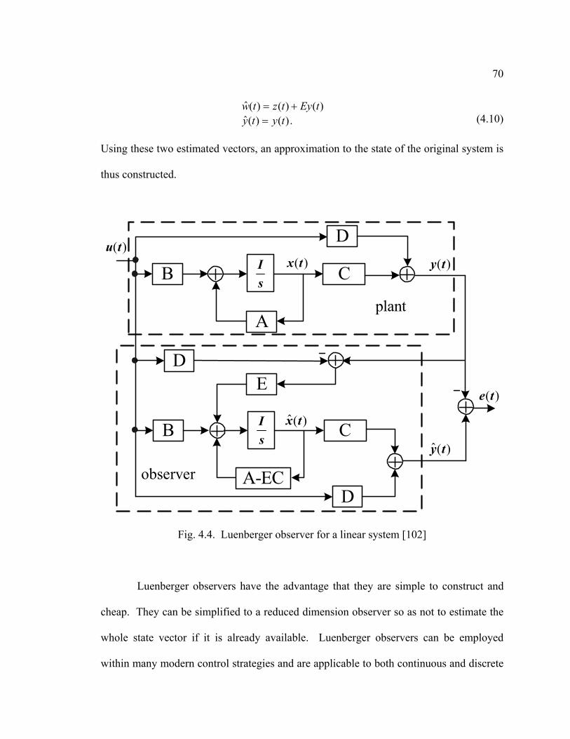
70

.)()(ˆ)()()(ˆ

tytytEytztw

=+= (4.10)

Using these two estimated vectors, an approximation to the state of the original system is

thus constructed.

)(ˆ ty

)(teE

D

B

A-EC

CsI )(ˆ tx

Dobserver

D)(ty

)(tu

B

A

CsI )(tx

plant

Fig. 4.4. Luenberger observer for a linear system [102]

Luenberger observers have the advantage that they are simple to construct and

cheap. They can be simplified to a reduced dimension observer so as not to estimate the

whole state vector if it is already available. Luenberger observers can be employed

within many modern control strategies and are applicable to both continuous and discrete

71

systems. Finally, if they are well designed, they do not suffer from noise amplification

and are ideal for applications where the model of the system is well known.

On the other hand, if the model is not well known, the reduced order Luenberger

observer will not perform as desired. The identity observer will offer better results, but

still the uncertainty that always exists in the parameters will cause some errors in the

observation. Also, care must be taken in the selection of matrix E that specifies the rate

of convergence of the estimation. If the eigenvalues of A-EC are very small (towards

minus infinity), the observer will act as a differentiator and the system noise will be

amplified. Finally, Luenberger observers cannot be applied in case A, B, C, and D are not

completely known and time invariant.

4.3 Observer design

Usually, available data for synchronous generators are the stator phase currents

and voltages at the terminals of the machine, and the field voltage and current. As stated

in Section 4.1, in order to formulate the parameter estimation problem, it is necessary to

have measurements for the damper currents iD, iG, and iQ.

The conventional observer configurations that are reported in the literature and

were described in Section 4.2, transform the system model in the form,

BuAxx +=& , (4.11)

which can easily be realized by a block diagram. Nevertheless, transformation of the

system into an observable canonical form as above, leads to a system that is nonlinear in

the parameters. This is because the system under consideration is of the form,

72

ILRIV ′−−= , (4.12)

which if rearranged in the same form as (4.11) becomes,

VLRILI 11 −− −−=′ . (4.13)

Hence, both the matrix inverse and the matrix product in (4.13) will contain the product

of two or more parameters which are desired to be estimated, thus forming a nonlinear

system. It is likely that the parameters that occur in a product will not be possible to be

separated in an estimation process except using linearization. Linearization will

introduce a finite amount of error and will render the estimation process more complex.

Finally, a requirement for the design of an observer using (4.11) and one of the available

methods such as the Luenberger observer, is that the initial conditions of the system are

known. In this case, the initial conditions are not known since the damper winding

currents are unmeasurable.

Considering the difficulties for the implementation of a “standard” observer, it is

desired to construct an “abstract” observer based on the existing knowledge about the

system. The observer should be able to construct estimates of the damper winding

currents by using voltage and current measurements from the system and a priori system

knowledge. The observer should be designed in such a way so as to be effectively

utilized by the parameter identification algorithm as shown in Fig. 4.5.

For the construction of the observer, the last three equations of the synchronous

generator model in (3.11) can be rearranged so as to obtain expressions for the damper

winding currents. The three equations are given by,

73

DDADB

FADB

dADB

DDD iLω

iLω

iLω

irv ′+−′−′−−==− )(1110 l (4.14)

QAQB

GGAQB

qAQB

GGG iLω

iLω

iLω

irv ′−′+−′−−==−1)(110 l (4.15)

QQAQB

GAQB

qAQB

QQQ iLω

iLω

iLω

irv ′+−′−′−−==− )(1110 l , (4.16)

where for the purposes of the development of the observer the current derivatives will be

replaced by the forward difference formula,

ttittiti

∆−∆+

≈′ )()()( . (4.17)

A discussion for the selection of (4.17) as the numerical approximation of the derivative

is offered in Section 5.5 and Appendix D.

Unknown plant(Approximate model known)

Observer

Parameteridentification

algorithm

V

I

a priorisystem

knowledge

QGD iii ˆ,ˆ,ˆ

Estimatedparameters

+

-I

e

Fig. 4.5. Observer implementation and parameter identification algorithm

74

Using (4.17) for the damper current iD, and writing (4.14) in discrete form,

)∆

)()1()((1))()((1)(0t

niniLω

niniLω

nir DDDAD

BFdAD

BDD

−+++′+′+= l . (4.18)

Solving for iD(n+1), an expression can be obtained in terms of known measurements and

the previously calculated value of iD. The damper current iD can thus be obtained by,

))()((∆

)()∆

1()1( niniL

tLni

Ltωr

ni FdDAD

ADD

DAD

BDD ′+′

+−

+−=+

ll. (4.19)

The quadrature axis damper winding currents iG and iQ can be obtained by the

simultaneous solution of (4.15) and (4.16) as shown in the following development.

Solving (4.15) for iG(n+1),

)(∆

)()1()()∆

1()1(

)∆

)()1((1)

∆)()1(

)((1)(1)(0

niL

tLni

LL

niL

Lni

Ltωr

ni

tnini

Lωt

niniL

ωniL

ωnir

qGAQ

AQQ

GAQ

AQQ

GAQ

AQG

GAQ

BGG

QQAQ

B

GGGAQ

BqAQ

BGG

′+

−+

+++

−+

−=+⇒

−++

−+++′+=

llll

l

(4.20)

Similarly, solving (4.16) for iQ(n+1),

)(∆

)()1()()∆

1()1(

)∆

)()1()((1)

∆)()1(

(1)(1)(0

niL

tLni

LL

niL

Lni

Ltωr

ni

tnini

Lωt

niniL

ωniL

ωnir

qQAQ

AQG

QAQ

AQG

QAQ

AQQ

QAQ

BQQ

QQqAQ

B

GGAQ

BqAQ

BQQ

′+

−+

+++

−+

−=+⇒

−+++

−++′+=

llll

l

(4.21)

Substituting (4.20) into (4.21) the damper current in the Q winding can be obtained as,

).())((

∆

)())((

∆)(

))((

∆)(1)1(

2

22

niLLL

tL

niLLL

tωrLni

LLL

tωrLni

qAQGAQQAQ

GAQ

GAQGAQQAQ

BGAQQ

AQGAQQAQ

BQGAQQ

′

−++−

−+++

−++

+−=+

ll

l

llll

l

(4.22)

Finally, substituting (4.22) into (4.20) the damper current in the G winding can be

obtained as,

75

).(1))(()(

∆

)())((

∆)(

))((

∆)(1)1(

2

22

niLLL

LL

tL

niLLL

tωrLni

LLL

tωrLni

qAQGAQQAQ

GAQ

GAQ

AQ

QAQGAQQAQ

BQAQG

AQGAQQAQ

BGQAQG

′

−

−++++

−+++

−++

+−=+

ll

l

l

llll

l

(4.23)

Equations (4.19), (4.22), and (4.23) constitute the observer for the estimation of

the damper winding currents. The damper currents at each step are expressed in terms of

generator parameters, known measurements of stator and rotor currents, as well as

estimates of the damper currents at the previous time step. The generator parameters

involved in the three observer equations are mainly parameters of damper windings,

which can be readily calculated from manufacturer data as shown in Appendix A. Two

of the parameters that occur in the observer equations are parameters that are usually

desired to be estimated. These parameters are the magnetizing inductances LAD and LAQ.

Nevertheless, these inductances can be calculated approximately from the manufacturer

data sheet without inhibiting the correct operation of the observer. The case studies that

will be described in the next section lead to errors in the damper currents that are very

low. If magnetizing inductances of a magnitude that differs by 10% is used in the

observer, the error magnitudes in the damper currents do not increase by more than 0.5%.

This behavior is observed in more than one test case and thus it can safely be concluded

that the observer operation is not sensitive to changes in LAD and LAQ (for example, if

saturation is not considered during the observer implementation).

Another point of ambiguity in the observer equations is the value that needs to be

assigned to the initial conditions )0(Di , )0(Gi , and )0(Qi . The initial conditions are

needed to initiate the observation process. As the case studies will demonstrate in the

76

next section, the initial conditions can be assumed to be zero without loss of accuracy in

the damper currents. Assigning zero initial conditions when these are not available

generates estimates that are suboptimal [82].

4.4 Verification of observer operation using EMTP simulated data

Since damper winding currents are not measurable in actual generators, it is not

possible to determine the validity of the observer using actual measurements from field

tests. Therefore, it is necessary to test the observer using measurements generated by

well known and well tested simulation programs such as the Electromagnetic Transients

Program (EMTP). EMTP is extensively used by utilities to simulate the behavior of

synchronous generators and power systems in general, in both steady state and transient

operation. Data from the EMTP simulation are free of noise and one has access to all

generator parameters and signals. Furthermore, EMTP provides the simulated damper

currents in the direct and quadrature axes. Possible agreement of the observer generated

damper currents with the EMTP generated damper currents will increase the confidence

in using the generated signals from the observer into the parameter estimation process.

The synchronous generator under consideration as described in Appendix A was

simulated using EMTP both in the steady state and in the transient mode.

In the first case study (E-NF-00-01), the machine is operating in steady state. The

damper winding currents are observed according to the observer equations (4.19), (4.22),

and (4.23) with the initial conditions assumed to be zero. All estimated damper currents

77

match the simulated damper currents and are equal to zero to five decimal places, as

expected from a synchronous generator that operates in steady state.

The error between the estimated and simulated currents can be calculated using

the formula,

100%2

2 ×−

=simulated

observedsimulated

iii

error , (4.24)

where 2. denotes the 2-norm (square root of the sum of the squares of all the elements).

A discussion of norms is offered in Chapter 5. The errors in the three damper winding

currents iD, iG, and iQ for the steady state data case are 0.16%, 0.28% and 0.14%

respectively.

In the second simulated case study (E-NF-00-02), transient data were considered.

A permanent line to line fault was applied at 0.25 seconds between phases b and c. The

observed damper currents as compared to the EMTP simulated damper currents for each

axis can be seen in Figs 4.6, 4.7, and 4.8. As can be seen from the graphs, the estimated

damper currents match the simulated damper currents. The percent errors between the

simulated and estimated damper currents can be calculated in the same way as in the

steady state case. The errors in the three damper winding currents iD, iG, and iQ for the

transient data case are 0.03%, 0.63% and 0.16% respectively. Since the difference

between the simulated and estimated signals is not discernible in Figs 4.6, 4.7, and 4.8, a

portion of iQ as shown in Fig. 4.8 was magnified to visualize the difference between the

two signals. This difference is shown in Fig. 4.9.

78

Fig. 4.6. Simulated and estimated D-winding damper currents using transient data

Fig. 4.7. Simulated and estimated G-winding damper currents using transient data

79

Fig. 4.8. Simulated and estimated Q-winding damper currents using transient data

Fig. 4.9. Magnification of portion of iQ to demonstrate the difference between the

simulated and observed signals

CHAPTER 5

STATE ESTIMATION

5.1 Introduction

State estimation is a process during which a number of unknown system state

variables or parameters are assigned a value based on measurements from that system

[50]. In the estimation process, any information that is known about the system is

utilized. Such information may be the knowledge of the system configuration, the system

constraints, the accuracy of the measuring instruments, known system parameters,

previous experience from the system operation, and measurements from the system.

The system is usually arranged in the form [ ][ ] [ ]zxH = , where H is a matrix of

dimensions nm× , x is a vector of dimension n, and z is a vector of dimension m. In this

notation m is the number of measurements and n is the number of parameters to be

estimated. If nm = , then the system is completely determined. In other words, the

number of equations is equal to the number of unknowns and if there is a solution to the

system (if H is invertible), then there is a unique solution that can be found by inverting

the matrix H. Therefore, [ ] [ ] [ ]zHx 1−= . (From hereon, the brackets denoting matrices

will be dropped for simplicity, unless the context of the equation is not clear). In the

overdetermined case, it is not possible to invert H since nm ≠ . The solution is not

unique since in general it is not possible to satisfy all the equations exactly for any choice

of the unknowns. A solution should be selected such that the error in satisfying each

equation is minimum. This error is called the residual of the solution and can be

computed by,

xHzr ˆ−= , (5.1)

81

where x is the vector of the estimated parameters. The residual measures how well the

estimated vector x satisfies the linear system zHx = . If the residual vector is zero, then

x is the exact solution. However, in real systems the residual r is never zero, since the

model is just an approximation of the system (linear approximation and simplifying

assumptions to create a manageable model). Moreover, noise is present in the

measurements because of the instrumentation and round off errors in the data recording

devices. Therefore it is desired that all the entries of the residual vector be “small” in

order to gain confidence in the estimated parameters. The residual vector is often an m

vector, where m is usually in the range of thousands. Therefore, it is not convenient to

examine the whole residual vector to ascertain the validity of the estimates. It is

necessary to have a quantifying means of assigning a number to each residual vector

based on its length. Such a means of measuring the size of a vector is offered by a norm.

5.2 Theory of norms

A vector norm is a function that assigns a nonnegative real number x to each

vector nx ℜ∈ . There are a number of functions that can calculate a norm and the

selection of a certain function is based on the application and on the ease of computation

of the specified norm. Nevertheless, all norms satisfy the following properties,

,

000

yxyxxαxαxx

x

+≤+=

=⇔=≥

(5.2)

82

for all nyx ℜ∈, and all constants α [106], [107]. The first two properties force all

vectors but the zero vector to have positive length. The third property states that –x and x

have the same length and that 2x has twice the length of x. Finally, the last property is

the triangle inequality which states that the sum of the sides of a triangle is never smaller

than the length of the third side.

In general, the Hölder definition of a vector norm is defined by,

ppn

ppp xxxx

1

21 )( +++= L , (5.3)

where xi are the elements of vector x and p is any number such that 1≥p . One can

compute the norm of a vector using any value of p (even non-integer). In practice, three

p-norms are used: the 1-norm (or L1), the 2-norm (or L2), and the infinity-norm (or L∞).

The selection of these norms is based on their ease of computation and their applicability

in various problems. In the solution of an overdetermined system of equations of the

form zHx = , the objective is to minimize the pth norm of the vector of the residuals,

min pp zxHr −= ˆ , (5.4)

using any value for p.

The L1 norm also known as the grid norm or the norm of the least sum of the

absolute deviations is given by,

∑=

=+++=n

iin xxxxx

1211 L . (5.5)

The minimization of the Hölder 1-norm effectively minimizes the sum of the absolute

deviations and therefore it is possible to downplay the effect of outliers (inconsistent

83

observations with the remainder of the measurements). For this reason, the 1-norm is

considered as a robust norm. A robust estimation will produce estimates which are

consistent with different data sets containing noise that is not correlated between data

sets.

The L2 norm also known as the least squares or Euclidean norm is given by,

21

2122

22

12 )()( xxxxxx Tn =+++= L , (5.6)

and is traditionally the most widely used norm because it can be easily implemented as

can be seen in Section 5.4. Minimization of the residual vector in a least squares sense in

effect solves the system so that the sum of the squares of the error of each equation is

minimized. The method of least squares gives the best linear unbiased estimate for any

distribution with finite variance [108].

The L∞ norm also known as the maximum or Chebyshev norm is given by,

inixx

≤≤∞=

1max , (5.7)

and minimizes the largest residual. This norm is useful in applications where there is a

prescribed maximum limit for any given residual. Whereas both the L1 and L2 norms

permit isolated large residuals, in the case of experimental data L∞ is not a robust norm

since it assigns high weight on large residuals that do not have an influence on the

computed solution [109].

In order to visualize the major norms that are usually used, the loci that occur

from the calculation of each of the 1, 2, and infinite unit norms for a three dimensional

vector are displayed in Fig. 5.1. The 1-norm results in an octahedron, the 2-norm in a

84

sphere, and the infinity-norm in a cube. In general the three norms obey the inequality

[106],

nxxxx ℜ∈∀≥≥∞21 . (5.8)

L1

L2

L∞

Fig. 5.1. Loci of the three major unit Hölder norms for a vector 3ℜ∈x

5.3 Selection of the minimization norm

The selection of the minimization norm is often critical in a variety of

applications. The L∞ method has been traditionally used extensively in astronomy for the

determination of the orbits of planets by philosophers such as Laplace [110] and

Legendre [111]. Legendre was also the first one to propose the least squares method to

solve a system of inconsistent, overdetermined equations [111]. According to the

original explanation by Legendre, “By this method, a kind of equilibrium is established

among the errors which, since it prevents the extremes from dominating, is appropriate

for revealing the state of the system which most nearly approaches the truth.” The L2

norm has been traditionally adopted a few years later by most applications in science and

later in engineering because of its ease of computation and the fact that it is easy to

85

comprehend and relate to real life examples. An estimator based on the L2 minimization

method is easy to be implemented by means of matrix algebra. Moreover, for a Gaussian

error distribution, the L2 method is optimal. On the other hand, the L1 norm was shown to

be extremely robust and has been used extensively in applications such as robust

estimation, model fitting (constrained and unconstrained), analysis of variance, and

hypotheses testing.

It is therefore necessary to test all possible norms and deduce which ones are

applicable for the problem under consideration. Since p norms other than 1, 2, and ∞

lead to cumbersome calculations and have no definite benefits on the estimation results,

these are rejected in advance. Two important objectives of the estimation method in this

research work are to propose an estimator that is both simple in concept and fast in

implementation. Use of minimization norms other than 1, 2, and ∞ defeat both

objectives.

For the purposes of the synchronous generator parameter estimation, a study was

conducted to compare the results of the three major norms in minimizing the residual

[77]. In this study, the three solutions were evaluated based on the accuracy of the results

and on the computation time required by each method. The methodology behind the

estimation procedure will be deferred to subsequent sections since it is the same as the

methodology adopted for this research work. This section and Section 5.4 will

concentrate on the results obtained by the minimization of the residual based on the three

candidate norms.

86

For illustration purposes it is desired to estimate three parameters, namely the

stator phase resistance r, the equivalent field winding resistance rF, and the equivalent

quadrature axis inductance Lq. The measurements were generated by the numerical

solution of the differential equations that describe the model as developed in Section 2.5.

In this case however, the model comprises five equations and not seven as in (2.22). This

is because only one damper winding was considered. Since the measurements are

synthetic, the values of all parameters are known exactly and a definite comparison can

be performed for the error of the estimation for each minimization method. Two sets of

measurements are used for the purposes of this example, resulting in a system of ten

equations and three unknowns.

Two case studies were performed. In the first case study (denominated as case S-

NF-03-03), a small amount of noise was added to the measurements. This noise was

added to only one of the voltage measurements and the signal-to-noise ratio (SNR) is in

the order of 7000. Essentially, the measurement sets are noise free. In the second case

study (S-NC-03-04), a more significant amount of noise is added. The SNR is in the

order of 50, and the noise is added primarily to the voltage measurements. The purpose

of the two studies is to compare the performance of all three methods under both noise

free and noise contaminated conditions. For both cases, the example eventually reduces

into a matrix equation of the form,

zHx = , (5.9)

where H is a 10x3 coefficient matrix, x is a 3x1 vector of the unknown parameters, and z

is a 10x1 vector of measurements.

87

A brief description of each method is in order. For the p = 1 case, it is desired to

minimize the sum of the absolute deviations of all ten equations. Let the deviation for

each equation be denoted by ri. Since ri is either positive, negative, or zero, it can be

declared that,

−+ −= iii rrr , (5.10)

where 0≥+ir , 0≥− −

ir , and 0=× −+ii rr [112]. The problem is solved using linear

programming. After adding the artificial variables Ai for each equation, the problem

becomes,

∑∑==

−+ ++10

1

10

1)(min

ii

iii AMrr , (5.11)

subject to,

[ ] z

xxrr

HHII =

−+−+

−− ,,, . (5.12)

This formulation is readily solved by setting up a tableau according to the simplex

method [112]. There are ten initial basis variables (the artificial variables Ai), and 26

state variables in the objective function.

For the p = 2 case, it is desired to minimize the sum of the squares of the

deviations of each row in the matrix equation. Such a minimization is achieved by

obtaining the pseudoinverse of matrix H,

zHx +=ˆ , (5.13)

where one form of the pseudoinverse may be given by,

88

TT HHHH 1)( −+ = . (5.14)

The pseudoinverse will be revisited and analyzed in the next section.

For the p = ∞ case, it is desired to minimize the maximum of the absolute

deviations ri. Let the objective function be denoted by s. Therefore,

∞−== bAxiris maxmin , (5.15)

subject to,

−

≥

− z

zsx

eHeH , (5.16)

where e is a vector of ones, with the number of rows being equal to the number of rows

of H. Since the constraints are inequality constraints, it is necessary to add both a

surplus and an artificial variable to each equation, in order to solve this problem as a

linear programming problem. Therefore, the linear programming problem becomes,

+ ∑

=

20

1min

iiAMs , (5.17)

subject to,

[ ] [ ]

−

=+−

− z

zAX

sx

eHeH , (5.18)

where X and A are vectors that incorporate the surplus and artificial variables

respectively. The initial basis variables in the tableau incorporate the artificial variables

Ai, while for this example, the total number of variables in the objective function is 44.

89

5.4 Analysis of case studies

The parameter estimation method for the three norms as analyzed in the previous

section is applied to a sample synchronous generator whose parameters are known

exactly. The values of the three parameters that are desired to be estimated are as shown

in Table 5.1. As mentioned in Section 5.3, it is desired to perform two case studies to

study the effect of noise in the parameter estimation using the three norms. In the first

case study (S-NF-03-03), a small amount of noise was added to the measurements to

slightly perturb the solution of the system (the measurements are synthetic, and therefore

the error in the estimated parameters would have been zero). This noise was added to

only one of the voltage measurements and the signal-to-noise ratio (SNR) was in the

order of 7000. Essentially, the measurement sets were noise free. In the second case

study (S-NC-03-04), a more significant amount of noise was added. The SNR was in the

order of 50, and the noise was added primarily to the voltage measurements. Fig. 5.2

shows a flowchart of the procedure followed to obtain the results for the example under

consideration.

The results for all three cases for both low noise data and high noise data are

depicted in Tables 5.2 and 5.4 respectively. The residuals for p = 1, 2, and ∞ are

computed for each set of estimated parameters and are also depicted in Tables 5.2 and

5.4. It is noted that as expected, the residuals on the diagonal are less than or equal to the

other residuals in their columns. For example, for the p = 2 case, it is expected that the

least squares residual is smaller than or equal to the least squares residuals of the p = 1

and p = ∞ cases.

90

Tables 5.3 and 5.5 show the percent errors of the estimated parameters relative to

the exact values of those parameters. An “average” error for each case is also computed

to give a better idea of the accuracy of the estimation for each case.

Simulate synchronous generator

Obtain stator (vabc, iabc) androtor (vF, iF) measurements

START

END

Form Hx=z

Find byminimizing L1 norm

Introduce noise(case study S-NC-03-04)

Perturb system mininally(case study S-NF-03-03)

x Find byminimizing L2 norm

Find byminimizing norm

x x∞L

Fig. 5.2. Flowchart for example on norm minimization selection

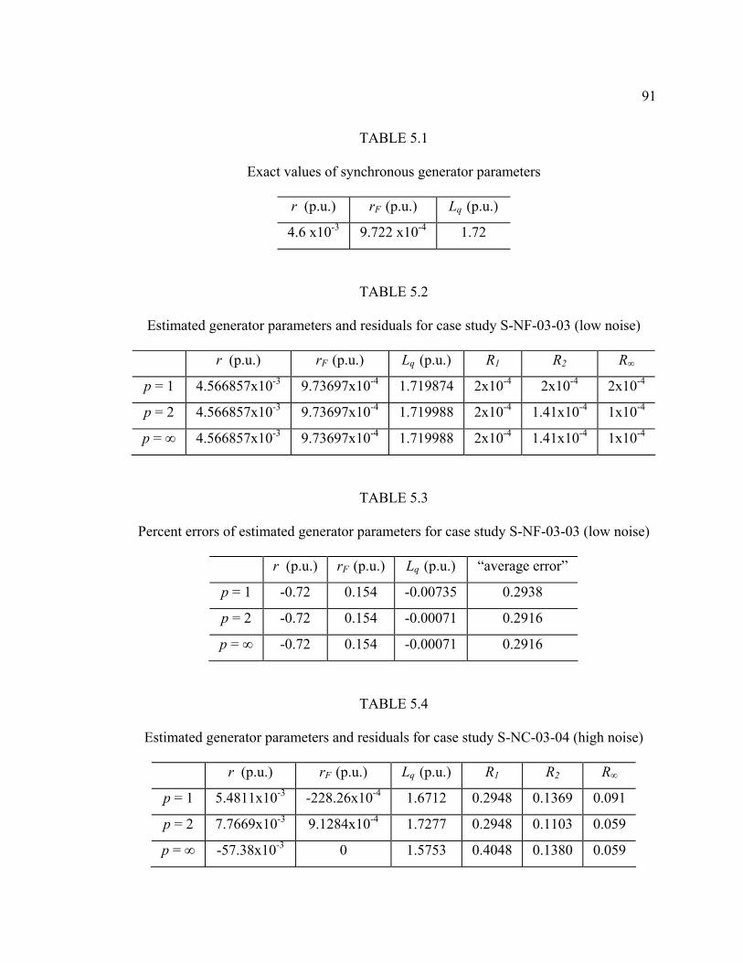
91

TABLE 5.1

Exact values of synchronous generator parameters

r (p.u.) rF (p.u.) Lq (p.u.)

4.6 x10-3 9.722 x10-4 1.72

TABLE 5.2

Estimated generator parameters and residuals for case study S-NF-03-03 (low noise)

r (p.u.) rF (p.u.) Lq (p.u.) R1 R2 R∞

p = 1 4.566857x10-3 9.73697x10-4 1.719874 2x10-4 2x10-4 2x10-4

p = 2 4.566857x10-3 9.73697x10-4 1.719988 2x10-4 1.41x10-4 1x10-4

p = ∞ 4.566857x10-3 9.73697x10-4 1.719988 2x10-4 1.41x10-4 1x10-4

TABLE 5.3

Percent errors of estimated generator parameters for case study S-NF-03-03 (low noise)

r (p.u.) rF (p.u.) Lq (p.u.) “average error”

p = 1 -0.72 0.154 -0.00735 0.2938

p = 2 -0.72 0.154 -0.00071 0.2916

p = ∞ -0.72 0.154 -0.00071 0.2916

TABLE 5.4

Estimated generator parameters and residuals for case study S-NC-03-04 (high noise)

r (p.u.) rF (p.u.) Lq (p.u.) R1 R2 R∞

p = 1 5.4811x10-3 -228.26x10-4 1.6712 0.2948 0.1369 0.091

p = 2 7.7669x10-3 9.1284x10-4 1.7277 0.2948 0.1103 0.059

p = ∞ -57.38x10-3 0 1.5753 0.4048 0.1380 0.059

92

TABLE 5.5

Percent errors of estimated generator parameters for case study S-NC-03-04 (high noise)

r (p.u.) rF (p.u.) Lq (p.u.) “average error”

p = 1 19.16 -2448 -2.84 823.3

p = 2 68.85 -6.11 0.45 25.14

p = ∞ -1347 100 -8.41 485.1

In the low noise case, it is observed that the solutions to the problem are almost

identical when using any of the norms under study. Nevertheless, p = 2 and p = ∞ give

greater accuracy of estimation in one parameter, and a smaller residual, thus causing

them to be the favored solutions. The comparison is mainly based on the percent errors

of each parameter and not on the resulting residual, since as shown before, it is always

true that,

nxxxx ℜ∈∀≥≥∞21 . (5.19)

In the high noise case the L2 norm is clearly the best minimization norm for this

particular example. The percent errors in the estimation of some of the parameters in the

p = 1 and p = ∞ cases are unacceptable, and therefore it seems that these cases are

particularly sensitive for these noisy data. On the other hand, the method of least squares

seems to be able to reduce the effect of the excessive noise in the measurements.

Another important consideration in the selection of the minimization method is the

computation time. Since this problem consists of only ten equations, the computation

time for all three cases is negligible and therefore, no computational burden will be

93

imposed no matter which norm is selected. However, for larger problems, in general

p = 2 is the fastest minimization method.

As far as ease of computation is concerned, the L2 minimization method is by far

the most easy to implement because of the availability of clearly defined and well tested

computer algorithms such as the pseudoinverse which will be analyzed in the next

section. The implementation of the L1 and L∞ minimization methods require the use of

linear programming which may become quite complicated for large systems. Another

possible method to implement the L1 and L∞ solution of a system is via the use of the

iteratively reweighted least squares method (IRLS). Nevertheless, the IRLS method

requires a certain number of iterations, which render this approach slow to implement.

As noted in the previous section, a possible advantage of the L1 minimization

method is its robustness with respect to outlier rejection. However, if adequate

prefiltering mechanisms and bad data detection and rejection algorithms are utilized, then

this powerful advantage of the L1 method will be negated, again making the L2 method

more efficient and accurate.

The above example and related arguments indicate that the minimization method

that should be selected for this work is the least squares method based on the L2 norm. An

analysis of the least squares technique and its implementation for the synchronous

generator parameter estimation algorithm is presented in the following sections.

94

5.5 Least squares and the Moore-Penrose pseudoinverse

As described in Chapter 2, the resulting model can be rearranged in the form,

zHx = , (5.20)

where H is a matrix of dimensions nm× containing the coefficients of the unknown

parameters, x is a vector of dimension n that is desired to be estimated, and z is a vector

of dimension m containing measurements obtained from the system. Since nm > , (5.20)

constitutes an overdetermined system of equations that usually does not have an exact

solution. Therefore, it is desired to find a solution vector x that minimizes the quantity,

22

ˆ)ˆ()ˆ()ˆ( xHzxHzxHzxf T −=−−= . (5.21)

The right hand side of (5.21) is equal to the square of the 2-norm of the residual vector.

By (5.6) the problem can be reformulated as the desire to find a solution such that the

sum of the squares of the residual of each equation is minimal, thus the name least

squares solution is given to the solution vector x .

Using (5.21), it is desired to find a convenient form of representing x in terms of

the known matrix-vector pair H, z. The minimum of a function occurs at the point where

its derivative is equal to zero. Differentiating (5.21) with respect to x ,

.ˆ0ˆ220

0]ˆˆˆˆ[ˆˆ

ˆ

ˆ 2

1

zHxHHxHHzH

xHHxxHzzHxzzxx

fxf

xf

TT

TT

TTTTTT

=⇒=+−⇒

=+−−∂∂

=

∂∂∂∂

=∂∂

M

(5.22)

95

Hence, if [ ] 1−HH T exists the vector of the estimated parameters can be found by,

[ ] zHHHx TT 1ˆ −= . (5.23)

The quantity [ ] TT HHH 1− is termed as the Moore-Penrose pseudoinverse or the

generalized inverse and is symbolized by +H . The pseudoinverse also exists if [ ]HH T is

not invertible. If [ ] 1−THH exists, then the pseudoinverse is given by [ ] 1−TT HHH . If

none of the above inverses exist, then the pseudoinverse can be found by the method of

the singular value decomposition [106]. The pseudoinverse is unique. It should be noted

that in the case of a square matrix 1−+ = HH . The mathematical definition of the

pseudoinverse (or of any other generalized inverse) is accompanied by four conditions

known as the Penrose conditions [43]. +H is defined as the pseudoinverse of H if and

only if these four conditions are satisfied:

.)(.4)(.3

.2.1

HHHHHHHHHHHH

HHHH

T

T

++

++

+++

+

=

=

=

=

(5.24)

The solution to the system (5.20) can be calculated using a variety of techniques

including the Cholesky factorization [106], the QR factorization [106], [113], and the

singular value decomposition (SVD) [106], [113]. The technique chosen in the

implementation of the estimator is the SVD since it is the most accurate. Its

computational time is greater than the other available methods but the accuracy of the

method is the prevailing factor for its use. The SVD is directly related to the calculation

96

of the pseudoinverse as developed above and it is a proven stable method for the solution

of least squares problems.

5.6 Configuration of the state estimator

As shown in Sections 2.5 and 5.4 it is desired to arrange the equation of the model

(3.11) in the form zHx = . The developed model of the synchronous machine is of the

form,

ILRIV ′−−= , (5.25)

where V, I, and I ′ are vectors of the system voltages and currents, and R and L are

matrices containing the system constant parameters. As explained in Chapter 4, some of

the current states are not possible to be measured, but they are possible to be estimated.

Therefore the voltage and current vectors are known. Moreover, some of the elements of

matrices R and L are also known, whereas the rest of the elements need to be estimated.

An important drawback is that the current derivative vector I ′ is not known. Therefore,

it has to be assigned values through an approximation.

Numerical differentiation of measured signals can create numerous problems in

practice, since the division by the small time step between the measurements leads to the

amplification of high frequency noise. Usually, in most applications only a single

differentiation is possible even if a proper noise filter is implemented. For this reason,

the selection of the differentiation formula to approximate the derivative needs to be

carefully selected. Appendix D considers a least squares estimation of the coefficients of

a differential equation using five methods for the calculation of the derivatives of the

97

signal. Three of the proposed methods use formulae obtained from the approximation of

derivatives via the use of the interpolation polynomial, whereas two methods use

integration formulae modified so as to accommodate the estimation problem at hand.

Various case studies were performed with both varying time step between the

measurements and noise free/noise contaminated measurements. Although, when no

noise was present Simpson’s rule and higher order differentiation formulae prevailed in

the accuracy of the estimated parameters, when noise was added to the measurements, the

first order differentiation formula (forward difference formula),

ttittiti

∆)()∆()( −+

≈′ ,

(5.26)

was clearly the best choice for the approximation of the derivatives of the signal and for

the estimation of the unknown parameters.

Once all the data are obtained and the numerical differentiation is performed, the

matrix equation needs to be rearranged in the form zHx = , where H and z are a known

matrix and vector respectively. At the same time, it is desired that an algorithm be found

such that it will be possible to select which parameters are to be estimated with no need

to rearrange the code of the program. In such a way, the algorithm can be easily adapted

by a visual platform since this is one of the major objectives of this research work.

To show how this algorithm works and how the data are arranged in the desired

form, (3.11) is reconsidered. Since the last three equations of the synchronous generator

model have been used for the development of the observer, the remaining four equations

will be used for the implementation of the estimator. Assuming that parameters LAD, LAQ,

98

and rF are desired to be estimated, and rearranging the equation in the form zHx = , the

following matrix equation is obtained.

.

0000000000000000000000003

1

000000000000000000000003

0)(1

0)(1)(

0)()(1000

00

0

0

−−−−−

′′′′′′′

+

−

−

+

−=

′+′+′

′+′+′++−

++′+′+′

Q

G

D

F

q

d

Q

G

D

F

q

d

F

q

d

n

B

Q

G

D

F

q

d

d

q

n

F

AQ

AD

FDFdB

QGqB

DFd

QGqDFdB

VVVV

VVV

iiiiiii

LL

ω

iiiiiii

rωωr

rr

rLL

iiiiω

iiiω

iiiω

iiiωiiiω

l

l

l

l

l

(5.27)

In this way, the four unknown parameters and their coefficients are isolated on the left

hand side, and all elements of the right hand side are known. Moreover, the right hand

side reduces to a vector and therefore the system takes the final form zHx = . It should

be noted that (5.27) is constructed using data from a single time step. The resulting

system will consist of a large number of equations identical to (5.27) to reflect every time

step in the available measurements. For example, if m measurements (data points) are

obtained, then this system will have 4m equations.

5.7 Summary

This chapter concentrated on the theory supporting state estimators, norm

selection and minimization, and the configuration of a state estimator for parameter

identification. Table 5.6 summarizes some useful definitions for vector norms and some

99

common properties. Table 5.7 depicts some of the concepts pertaining to the

pseudoinverse of a matrix, while Fig. 5.3 shows a pictorial of the estimator for the

parameter identification of a synchronous generator.

TABLE 5.6

Definitions and properties of vector norms

Definitions and properties Description

,

000

yxyxxαxαxx

x

+≤+=

=⇔=≥

All norms satisfy these properties

ppn

ppp xxxx

1

21 )( +++= L Definition of a p norm ( ℜ∈≥ pp ,1 )

∑=

=+++=n

iin xxxxx

1211 L

1-norm, or grid norm

21

2122

22

12 )()( xxxxxx Tn =+++= L

2-norm, or least squares norm

inixx

≤≤∞=

1max ∞-norm, or maximum norm

nxxxx ℜ∈∀≥≥∞21 Relationship between 1,2, and ∞ norms

100

TABLE 5.7

Concepts pertaining to the pseudoinverse of a matrix

Equation Description

zHx +=ˆ Solution of an overdetermined linear system THHTHH 1)( −=+ One of the possible methods to calculate the

pseudoinverse of a matrix 22

ˆ)ˆ()ˆ()ˆ( xHzxHzxHzxf T −=−−=

The least squares solution is equivalent to the minimization of this function – relationship to the 2-norm

.)(.4)(.3

.2.1

HHHHHHHHHHHH

HHHH

T

T

++

++

+++

+

=

=

=

=

Any pseudoinverse should satisfy these requirements

Measurements

Park's

transfo

rmati

on

Filtering

ILRIV ′−−=Observer for damper

winding currents

Saturation model EstimatorEstimate model

parameters based onmeasurements and a

priori knowledge

Fig. 5.3. Pictorial of an estimator for synchronous generator parameter identification

CHAPTER 6

PARAMETER ESTIMATION USING SYNTHETIC DATA

6.1 Introduction

The work performed in Chapters 2, 3, and 5 enabled the development of the

synchronous generator model that is used in this research work and the configuration of

the state estimator in order to implement the parameter identification procedure. To

ascertain the correctness and the validity of the algorithm to be developed, it is of vital

importance to test it with data for which the parameters to be estimated are known. In

this way, the algorithm can be tested for conceptual or unintended errors, and the

accuracy of the method can be evaluated.

The testing of the algorithm needs to be performed in three stages. First, the

algorithm needs to be tested with synthetic noise free data generated by the direct

numerical solution of the differential equations of the model as depicted in (3.11). This

stage will illustrate whether the system is stable under various disturbances and whether

the estimation is possible to be performed. Ideally, the deviations of the estimates from

their true value should be very small, and in effect comparable to the round off error of

the computer that is used to perform the estimation. This procedure does not produce any

distinguishing results for the candidate models since, as expected, all parameters are

estimated exactly. Nevertheless, this procedure is an important part of the algorithm

development procedure as it offers reassurance in the estimation process and in the

viability of the algorithm. The results for the estimation of the parameters using this

method will not be presented in this dissertation. An explanation of the procedure and

some preliminary results are offered in [114].

102

The second stage of the algorithm testing is to implement the estimation process

with synchronous generator data that are noise free. Since all measurements from

synchronous generators contain a finite unknown amount of noise, it is useful to first

simulate the synchronous generator using a program that is currently used by utilities

such as the Electromagnetic Transients Program (EMTP). EMTP is suitable for testing

the estimation algorithm because data from the simulation are free of noise, and one has

access to all generator parameters and signals. Consequently, “measurements” of the

system can be obtained, and a good assessment of the viability of the designed estimator

can thus be performed. Parameter estimation with EMTP noise free data will be the

subject of this chapter.

Finally, the estimator needs to be tested using actual generator data. Firstly,

generator data obtained from the same generator that has been simulated in the second

stage of the testing of the algorithm are used to obtain solid conclusions about the

estimation method. If the results of the estimation with data from such a generator are

satisfactory, data sets from other generators should be used for a final evaluation of the

algorithm. Parameter estimation using actual measurements is considered in Chapter 8.

6.2 Calculation of generator parameters

The parameters of the synchronous generator model as depicted in (2.22) and

(3.11) need to be calculated for a specific synchronous generator. This calculation will

enable the simulation of the generator to obtain “measurements” of the system, and will

offer the opportunity to compare the estimated parameters with the actual parameters and

103

deduce whether the proposed algorithm can be implemented. Synchronous generator

parameters can be calculated using a combination of sources, namely the manufacturer

stability data and saturation curve for a specific generator, equivalent circuit calculations,

or even from IEEE standards [5], [6] that specify data for a number of different

synchronous generators for demonstration purposes.

In this case, the generator constants are calculated using the manufacturer stability

data sheet and the saturation curve for the generator under study. Using data for an

existing generator can create more confidence in the results when actual measurements

from that generator are utilized to implement the estimation. Equivalent circuits are

utilized as appropriate to obtain the values of the generator parameters.

In order to illustrate the type of calculation needed and the kind of manufacturers’

data required, attention turns to a specific example. The specific example is a cross-

compound generator located in the southwest U.S.A. The generator contains a high

pressure unit rated at 483 MVA and a low pressure unit rated at 426 MVA. This

illustrative generator shall be used throughout Chapters 6, 7, and 8. For this generator,

detailed calculations can be seen in Appendix A while the manufacturer’s data sheet and

the saturation curve can be seen in Appendix B. Table 6.1 lists the parameters and their

value as calculated in Appendix A. The only difference in the parameters of Appendix A

and Table 6.1 is the value of the stator resistance r. For the purposes of synthetic data the

stator resistance was assigned the value of 0.0027 p.u. The difference in stator resistance

does not affect any of the subsequent analysis. The inductances in Table 6.1 represent

unsaturated values and are calculated via the manufacturer data as shown in Appendix A.

104

TABLE 6.1

Calculated parameters for use in the testing of the estimator algorithm

(Parameters are for the generator described in Appendix A)

Parameter Value (p.u.) Parameter name

L0 0.15 Equivalent zero sequence inductance

LAD 1.64 d axis magnetizing mutual inductance

LAQ 1.56 q axis magnetizing mutual inductance

Ld 1.80 Equivalent direct axis inductance

LD 1.68125 Self inductance of damper winding D

LF 1.75791 Field winding self inductance

LG 1.978537 Self inductance of damper winding G

Ln 100 Equivalent neutral inductance

Lq 1.72 Equivalent quadrature axis inductance

LQ 1.593 Self inductance of damper winding Q

MD 1.339054 Stator to damper winding D mutual inductance

MF 1.339054 Stator to field mutual inductance

MG 1.2737 Stator to damper winding G mutual inductance

MQ 1.2737 Stator to damper winding Q mutual inductance

MX 1.64 Rotor mutual inductance in the d axis circuit

MY 1.56 Rotor mutual inductance in the q axis circuit

r 0.0027 Stator phase resistance

rD 0.0125 Equivalent resistance of damper winding D

rF 9.722x10-4 Equivalent field resistance

rG 0.01071 Equivalent resistance of damper winding G

rn 100 Equivalent neutral resistance

rQ 0.01632 Equivalent resistance of damper winding Q

105

6.3 Estimation of generator parameters

As mentioned in Chapter 2, the system identification procedure is an iterative

process with respect to the selection of the model of the system. A number of candidate

models need to be tested so as to select the one that best fits the actual response of the

system. Two candidate models have been proposed in Chapter 2: model 2.1 and model

2.2 as defined in IEEE Standards [83]. Further, a modification of model 2.2 has been

proposed in Chapter 3 to incorporate the effect of saturation and to simplify the

estimation process. The modified model will be referred to as model 2.2x. It is desired

to compare the results for all three models to the manufacturer supplied parameters for

the synchronous generator under consideration. Table 6.2 shows a description of some of

the distinguishing characteristics of the three models. Fig. 6.1 is a flowchart for the

estimation of synchronous generator parameters from simulated noise free data.

TABLE 6.2

Distinguishing characteristics of the three candidate models

Characteristic Model 2.1 Model 2.2 Model 2.2x

Number of damper windings in the d axis

1 1 1

Number of damper windings in the q axis

1 2 2

Number of equations in the model

6 7 7

Model parameters rn, L0, Ln, r, Ld, Lq, MF, MD, MQ, rF, rD, rQ, LF, LD, LQ, MX

Same as model 2.1 plus rG, LG, MG, MY

Same as model 2.2 but MX, MY, MF, MD, MG, MQ, LF, LD, LG, LQ, Ld, Lq, are replaced by expressions involving LAD, LAQ, and the leakage inductances

106

Obtain abc statorvoltages and currents,

odq stator currents

Calculate the power angle δ

START

END

Convert line-line voltagesto phase voltages

Perform Park's transformationto convert abc quantities to

0dq quantities

Convert all measurementsto per unit quantities

Estimate generatorparameters

Calculate derivativesof currents

Obtain rotor voltagesand currents (field and

damper)

Calculate generatorparameters from

manufacturer data

Simulate synchronousgenerator

Fig. 6.1. Flowchart for synthetic data and estimator implementation

A small description of the simulated data is in order at this point. A synchronous

generator with operating parameters identical to the parameters depicted in Table 6.1 was

107

simulated in steady state operation in EMTP. The generator served a load with an active

power demand of 356 MW and a reactive power demand of 26 MVAr. The simulation

was run up to 5 s, and the sampling time for the measurements was 0.2 ms. The

measurements were then read into a text file per the format described in Table E.1 of

Appendix E. These measurements were then used in the parameter identification

procedure as shown in the flowchart of Fig. 6.1.

Table 6.3 depicts the estimated parameters for all three models and the

corresponding calculated parameters from manufacturer’s data (case study E-NF-01-05).

A percent error of each parameter is also depicted in the same table. All parameters have

been estimated individually assuming that all other parameters are known. For all case

studies saturation is considered not to have any effect on the generator inductances since

the generator was simulated to run in the steady state non-saturated region. This region

corresponds to the straight portion of the saturation curve as shown in Fig. B.1.

Therefore, no correction for saturation needs to be performed for the estimation of any

parameter in this chapter.

The results of Table 6.3 show that all parameters can be estimated accurately

regardless of the model used. The maximum error obtained using models 2.1 and 2.2 is

0.39% and occurs for the field inductance LF. The maximum error obtained using model

2.2x is 0.16% and occurs for the mutual magnetizing inductance LAQ. For all three

models, the stator resistance r and the field resistance rF are estimated with 0% error.

A comparison between models 2.1 and 2.2 shows that all estimated parameters for

both models are equal, so no definite conclusions can be extracted from these results as to

108

which model should be selected. Further, no definite comparisons can be made between

model 2.2x and the other two models, since the parameters estimated with model 2.2x are

different with the exception of r and rF. Therefore, the decision as to which model is the

dominant model for the parameter identification procedure will have to be relegated to

the estimation using actual measurements in Chapter 8. Nevertheless, an obvious

advantage of model 2.2x can be mentioned. Model 2.2x requires the estimation of less

parameters and offers an easier method to implement saturation.

TABLE 6.3

Estimated parameters using EMTP generated data (case study E-NF-01-05)

Model 2.1 Model 2.2 Model 2.2x

Parameter

Manufacturer value (p.u.)

Estimated parameter

(p.u.)

% Error

Estimated parameter

(p.u.)

% Error

Estimated parameter

(p.u.)

% Error

Ld 1.80 1.7986 0.08 1.7986 0.08 N/A N/A

Lq 1.72 1.7225 0.14 1.7225 0.14 N/A N/A

LF 1.75791 1.7510 0.39 1.7510 0.39 N/A N/A

kMF 1.64 1.6408 0.05 1.6408 0.05 N/A N/A

LAD 1.64 N/A N/A N/A N/A 1.6418 0.10

LAQ 1.56 N/A N/A N/A N/A 1.5625 0.16

r 0.0027 0.0027 0 0.0027 0 0.0027 0

rF 9.722x10-4 9.722x10-4 0 9.722x10-4 0 9.722x10-4 0

109

6.4 Multiple simultaneous parameter estimation

The estimated parameters in case study E-NF-01-05 in Section 6.3 are estimated

individually assuming that all other parameters are known. Although in some cases this

is the desired situation in practice, in other cases it may be required to estimate more than

one parameter at a time. Thus it is necessary to implement the parameter identification

procedure for multiple parameter estimation to deduce whether the error characteristics of

the estimation vary significantly, or even whether multiple parameter estimation is

feasible. For multiple parameter estimation to be feasible it is desired that the percent

error obtained for each parameter is approximately the same in both individual parameter

estimation and multiple parameter estimation.

First, multiple parameter estimation for models 2.1 and 2.2 will be considered.

Table 6.4 depicts the results obtained for case study E-NF-03-06. Three parameters (Ld,

Lq, and rF) were estimated simultaneously for both models. Table 6.5 shows the results

obtained for case study E-NF-03-07, where Ld, Lq, and LF were simultaneously estimated.

TABLE 6.4

Multiple simultaneous parameter estimation (case study E-NF-03-06)

Model 2.1 Model 2.2

Parameter


Estimated parameter

(p.u.)

% Error

Estimated parameter

(p.u.)

% Error

Ld 1.80 1.7986 0.08 1.7986 0.08

Lq 1.72 1.7225 0.14 1.7225 0.14

rF 9.722x10-4 9.722x10-4 0 9.722x10-4 0

110

TABLE 6.5


Model 2.1 Model 2.2

Parameter


Estimated parameter

(p.u.)

% Error

Estimated parameter

(p.u.)

% Error

Ld 1.80 1.7986 0.08 1.7986 0.08

Lq 1.72 1.7225 0.14 1.7225 0.14

LF 1.75791 1.7510 0.39 1.7510 0.39

Tables 6.6 and 6.7 show two of the case studies that were performed for observing

how multiple parameter estimation affects the estimated parameters in the case of model

2.2x. Table 6.6 shows the results for case study E-NF-02-08, where the magnetizing

mutual inductances LAD and LAQ were estimated simultaneously. Table 6.7 shows the

results for case study E-NF-03-09 where LAD, LAQ, and rF were estimated simultaneously.

TABLE 6.6


Model 2.2x

Parameter


Estimated parameter

(p.u.)

% Error

LAD 1.64 1.6418 0.10

LAQ 1.56 1.5625 0.16

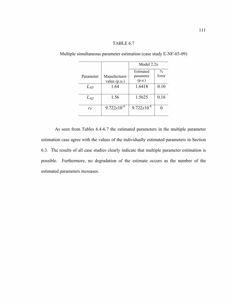
111

TABLE 6.7


Model 2.2x

Parameter


Estimated parameter

(p.u.)

% Error

LAD 1.64 1.6418 0.10

LAQ 1.56 1.5625 0.16

rF 9.722x10-4 9.722x10-4 0

As seen from Tables 6.4-6.7 the estimated parameters in the multiple parameter

estimation case agree with the values of the individually estimated parameters in Section

6.3. The results of all case studies clearly indicate that multiple parameter estimation is

possible. Furthermore, no degradation of the estimate occurs as the number of the

estimated parameters increases.

CHAPTER 7

NOISE FILTERING AND BAD DATA IDENTIFICATION

7.1 Introduction

A crucial aspect of the parameter estimation process when using actual data is the

removal of outliers and inconsistent data, and the filtering of high frequency noise from

the measurements. No matter how technologically advanced the measuring instruments

are, or how carefully the measurements are obtained or processed, noise is always present

in some form. Commonly, measurements have errors resulting mainly from meter and

communication errors, incomplete metering, or inaccuracy of metering equipment.

Further, round off errors (e.g. analog to digital conversion error) are usually another

significant addition to inaccurate measurements. Round off errors are created by either

the limited capability of the recording instrument, or by the format of the data file and the

subsequent processing of the data by the computer. Therefore, prior to any estimation it

is necessary to perform bad data detection and rejection, and filtering of the noise.

Another potential component of “noise” is the appearance of harmonics in several

of the instrumented signals. In the field winding, vF(t) and iF(t) are usually derived from

solid state controlled rectifiers and harmonics of order p, 2p, 3p, … (p: pulse order)

appear in the “DC” field circuit. Park’s transformation model does not include these

harmonics nor their action on machine flux or stator signals. Similarly, in the stator,

asymmetric pole configuration and pole saliency result in harmonics in the AC generated

voltage. These signals are also not modeled. IEEE Standards 50.12 and 50.13 limit the

harmonics by limiting the telephone influence factor (TIF). These limits are translated to

about the 0.3% range for phase currents (for positive and negative sequence harmonics),

113

and to about 0.2% for zero sequence currents [58]. For the purposes of the parameter

estimation described in this dissertation, these harmonics are neglected and assumed to be

measurement noise. An observation of the magnitude of the harmonics in the signals of

interest indicates that these harmonics are small and can be safely neglected without

degrading the accuracy of the estimated parameters.

As mentioned in Chapter 6, eight signals are typically measured for a

synchronous generator: the stator line to line voltages, the stator currents, and the rotor

(field) voltage and current. The main frequency components of interest for the field

measurements are at or near DC. For the stator measurements it is possible to perform

filtering of the AC measurements (50-60 Hz range), or of the 0dq transformed signals (at

or near DC). Although filtering of the actual signals in the abc reference frame presents

its own advantages, in this particular application, it was found that the stator

measurements are most effectively filtered after the 0dq transformation. This is because

the 0dq transformed signals have components of interest that are at or near DC. This is

helpful in the filter design process, as the cutoff frequencies are well defined. In the case

of the AC signals, depending on the generator under study, it is not known whether the 50

Hz or 60 Hz components are the fundamental components. Thus, the filter design would

not be globally acceptable and would have to be redesigned based on the frequency of the

power supplied by each generator. Fig. 7.1 shows the filtering and bad data

detection/rejection configuration.

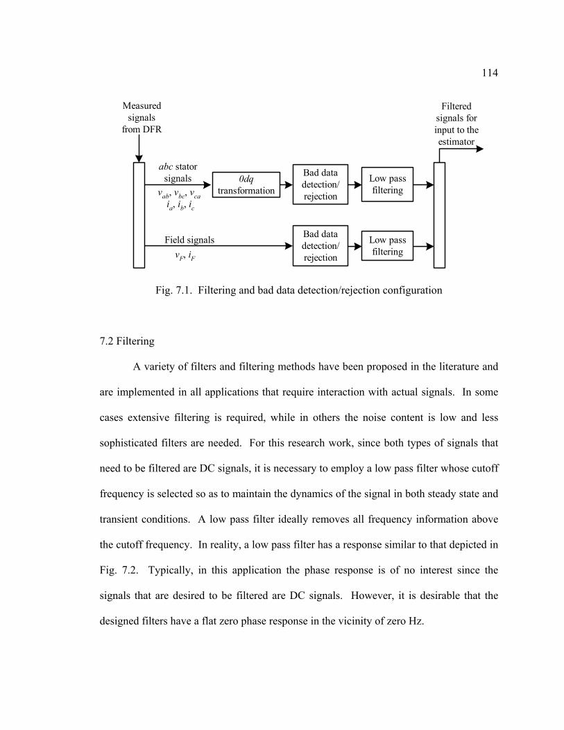
114

Measuredsignals

from DFR

abc statorsignals

Field signals

vab, vbc, vca ia, ib, ic

vF, iF

0dqtransformation

Bad datadetection/rejection

Low passfiltering

Filteredsignals forinput to theestimator

Bad datadetection/rejection

Low passfiltering

Fig. 7.1. Filtering and bad data detection/rejection configuration

7.2 Filtering

A variety of filters and filtering methods have been proposed in the literature and

are implemented in all applications that require interaction with actual signals. In some

cases extensive filtering is required, while in others the noise content is low and less

sophisticated filters are needed. For this research work, since both types of signals that

need to be filtered are DC signals, it is necessary to employ a low pass filter whose cutoff

frequency is selected so as to maintain the dynamics of the signal in both steady state and

transient conditions. A low pass filter ideally removes all frequency information above

the cutoff frequency. In reality, a low pass filter has a response similar to that depicted in

Fig. 7.2. Typically, in this application the phase response is of no interest since the

signals that are desired to be filtered are DC signals. However, it is desirable that the

designed filters have a flat zero phase response in the vicinity of zero Hz.

115

Fig. 7.2. Magnitude response of a low pass filter

Representative types of low pass filters are the moving average filter, the

Butterworth filter, the Chebyshev filter, and the elliptic filter [58]-[60]. The filters that

are considered in this research work are the moving average filter and the Butterworth

filter. Chebyshev and elliptic filters have similar characteristics to Butterworth filters but

have considerable ripple in their passbands. A passband is the region where the filter

allows the frequency components to pass through. Therefore, the frequencies that will be

allowed to pass through the filter will be amplified by different amounts. This

nonuniform change in the magnitude of the frequencies of each signal may cause

inaccuracies during the estimation process.

The moving average filter in the discrete time domain is given by [58],

116

∑−

=−=

1

0

1 N

iinn x

Ny , (7.1)

where xn-i are the input data and N is the degree of the moving average. After

transforming (7.1) into the z-domain, the transfer function of an N-point moving average

is given by,

∑−

=

∆−∆ =1

0

1)(N

i

TjiTj eN

eH ωω . (7.2)

The moving average filter is the fastest digital filter available and an exceptionally

good smoothing filter in the time domain. Moreover, it is relatively easy to program.

However, it has a slow roll off, which may allow some frequencies to pass through.

Further, significant attenuation may occur within the frequency range of interest while its

frequency domain filtering qualities are not so admirable. A model of a moving average

filter is shown in Fig. 7.3. The magnitude and phase responses of a 40 point moving

average filter for a signal that has a time step between measurements of 0.1 ms is shown

in Figs 7.4 and 7.5.

Z-2 Z-3 Z -N Z -1 x n x n-1 xn-2 xn-3 x n-N

yn

+ + ++ +

Fig. 7.3. Moving average filter implementation

117

Fig. 7.4. Magnitude response of a moving average filter

Fig. 7.5. Phase response of a moving average filter

118

The moving average filter in this research work is used as a supplementary filter

for signals that do not require excessive filtering or for signals that require a slight

improvement before filtering with the Butterworth filter.

The second type of low pass filter considered is the Butterworth filter. This filter

belongs to the category of infinite impulse response (IIR) digital filters. IIR filters have

input-output characteristics that are governed by linear difference equations with constant

coefficients [115]. Further, these difference equations are recursive since each value of

the filtered signal is computed using previously computed values of the filtered signal.

Finite impulse response (FIR) filters on the other hand, use only values of the unfiltered

signal to compute the values of the filtered signal, and are thus non-recursive filters. IIR

filters have the advantage over FIR filters that they can meet the given specifications with

a lower order filter because of the recursive differential equations that are used in the

filter implementation.

The Butterworth filter is considerably more difficult to program but it has a good

transient response and a fast roll off. The general Nth order Butterworth filter has a

magnitude squared function in the discrete case [59],

Ncjj

jH 22

)(11)(ΩΩ+

=Ω , (7.3)

where Ωc is the cutoff frequency. The cutoff frequency is the frequency where the

magnitude of the filter is 3 dB below the maximum magnitude in the passband region.

As N increases, the frequency response becomes sharper. However, at the cutoff

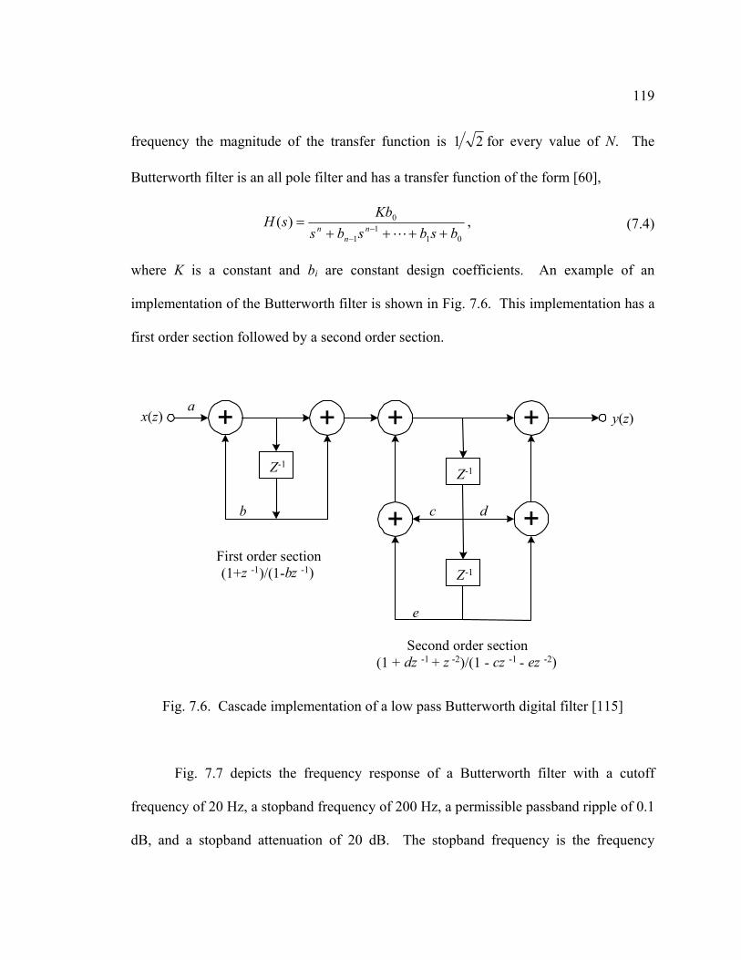
119

frequency the magnitude of the transfer function is 21 for every value of N. The

Butterworth filter is an all pole filter and has a transfer function of the form [60],

011

1

0)(bsbsbs

KbsH n

nn ++++

= −− L

, (7.4)

where K is a constant and bi are constant design coefficients. An example of an

implementation of the Butterworth filter is shown in Fig. 7.6. This implementation has a

first order section followed by a second order section.

++ + +

+ +

Z -1 Z-1

Z-1

a

b c d

e

First order section(1+ z -1 )/(1- b z -1)

Second order section (1 + dz -1 + z -2)/(1 - cz -1 - ez -2 )

x(z) y(z)

Fig. 7.6. Cascade implementation of a low pass Butterworth digital filter [115]

Fig. 7.7 depicts the frequency response of a Butterworth filter with a cutoff

frequency of 20 Hz, a stopband frequency of 200 Hz, a permissible passband ripple of 0.1

dB, and a stopband attenuation of 20 dB. The stopband frequency is the frequency

120

beyond which the magnitude of a low pass filter approaches zero in order to eliminate the

frequency components in the stopband region.

Fig. 7.7. Frequency response of a sample Butterworth filter

From the frequency response of Fig. 7.7 it can be observed that the passband

magnitude is maximally flat and therefore all the frequency components in the passband

region will be unscathed from the filtering process (or at worst they will be all attenuated

by the same amount). On the other hand, the frequency components in the two regions

following the passband (the transition band and the stopband) will be attenuated

depending on the magnitude of the response at those frequencies.

121

Observation of the phase response shows that the frequency components in the

passband region may not experience the same amount of phase delay. Although the

signals under consideration in this research work are DC signals and this would not have

a considerable effect on them, some of the transient behavior of the synchronous

generator might be altered by changing the phase of the small frequency components in

the vicinity of DC. Therefore, it is desired to use a filter that introduces no phase shift

during the filtering process. This is achieved by performing a zero phase digital filtering

[59], [61]-[63]. The idea behind zero phase digital filtering is to filter the signal in the

forward direction and then reverse the filtered sequence and perform the filtering process

in the reverse direction. The resulting sequence has zero phase distortion and twice the

filter order.

The resulting recursive equation of a zero phase digital filter is of the form,

,][]2[]1[][]1[][][

32

10

nanyanyanyanbnxbnxbnxbny

na

nb

−−−−−−−++−+=

L

L

(7.5)

where na and nb are the lengths of the coefficient vectors a and b respectively, and n is

the order of the filter. x and y are the unfiltered and filtered signals respectively.

During the course of the filtering of the actual signals obtained from the

synchronous generator, it was found that a single Butterworth filter was not sufficient to

filter all noisy frequency components successfully. This is due to the limitations that are

imposed on every filter because of the stability requirements. Designing any filter that is

maximally flat in the vicinity of DC and at the same time attenuating sharply all

frequency components beyond a frequency close to DC (for example 10 Hz) is

122

unrealistic. The resulting filter would be unstable and certainly the filtered signal would

bear no resemblance to the original signal.

As will be shown in the frequency responses of all the measured signals in the

next section, there is no clear separation between the actual signal and the noise content.

Consequently, the transition band, during which the magnitude response of the filter is

allowed to attenuate, is basically nonexistent. Therefore, a stable low pass filter will

attenuate all high frequency components successfully, but will not attenuate the low

frequency noisy components in a satisfactory manner.

As a solution to this problem, all the designed filtering processes used in this

research work utilize a variable number of Butterworth filters depending on the noise

content and the frequency distribution of the noise for each signal. The proposed method

is thus referred to as multiple parallel filtering. Multiple parallel filtering in effect applies

the same stable Butterworth filter (or any other filter of choice), to slowly attenuate all

frequency components that are located in the transition band. The result of each

subsequent filter is a frequency spectrum whose noisy content is attenuated little by little

until the desired result is achieved.

Fig. 7.8 illustrates the idea of multiple parallel filtering using a number of parallel

identical Butterworth filters. In this example, each filter has a cutoff frequency of 100 Hz

and a stopband frequency of 800 Hz selected so as to show the slight improvement of

each subsequent filter. Fig. 7.8(a) shows the unfiltered signal, while Fig. 7.8(b) shows

the signal after the application of the first Butterworth filter. Figs 7.8(c) and (d) show the

signal after the application of the second and sixth Butterworth filters respectively. The

123

magnitude of the high frequency components reduces after the application of each low

pass filter. At the end of the filtering process the high frequency components are

minimized.

(a) (b)

(c) (d)

Fig. 7.8. Example of a multiple parallel filtering method for the successive attenuation of

transition band frequency components

124

7.3 Filtering of the field measurements

The stator and rotor measurements are filtered using two separate algorithms

because of differences between the measurement of the two types of signals by the

recording instrument. In this section, the filtering of DFR measured rotor (field)

quantities for the generator under consideration is described. The filtering of stator

measurements is relegated to Section 7.4. A specific case is considered to demonstrate

the filtering of both the field and stator signals, as well as the estimation of the

parameters in Section 8.2. The generator for the case under consideration is FC5HP

located at the Four Corners Generating Station of the Arizona Public Service Company

(APS). The generator is operating at the steady state; the active power at the terminals of

the generator is 142.2 MW and the reactive power is 3.7 MVAr at a lagging power factor.

The data used throughout this chapter are obtained from measurements at the terminals of

the synchronous generator while it is serving its load.

The field voltage and current are slowly varying DC signals. They are measured

through a six pulse rectifier and thus their time plots have a rather unusual appearance as

shown in Figs 7.9 and 7.10. An examination of the frequency spectrum of the two

signals as shown in Figs 7.11 and 7.12 indicates that both signals (and especially the

voltage) are highly corrupted with high frequency components. In the case of the

frequency spectrum of the current as seen in Fig. 7.12, the main frequency component

can be seen clearly at the center of the plot. Other frequency components are very small

and can be seen at lower magnitudes. The apparent overlapping of frequency

components is due to the choice of the dimensions of the horizontal axis and the size of

125

the elements used to mark each frequency point. The high frequency components for

both the voltage and the current need to be minimized to obtain the actual DC signals. It

should be noted that the frequency spectrum in both graphs and in subsequent graphs in

the rest of the chapter is shifted so that the zero frequency component is at the middle of

the spectrum. Further, where applicable, the frequency spectrum is truncated to show

only the frequencies of interest or to enable the visualization of the spectrum more

clearly. The frequency components of a signal in general range up to the Nyquist

frequency which is half of the sampling frequency. The Nyquist frequency for the

signals under consideration in this chapter is 5 kHz.

Fig. 7.9. Time domain field voltage for generator FC5HP as measured by a DFR

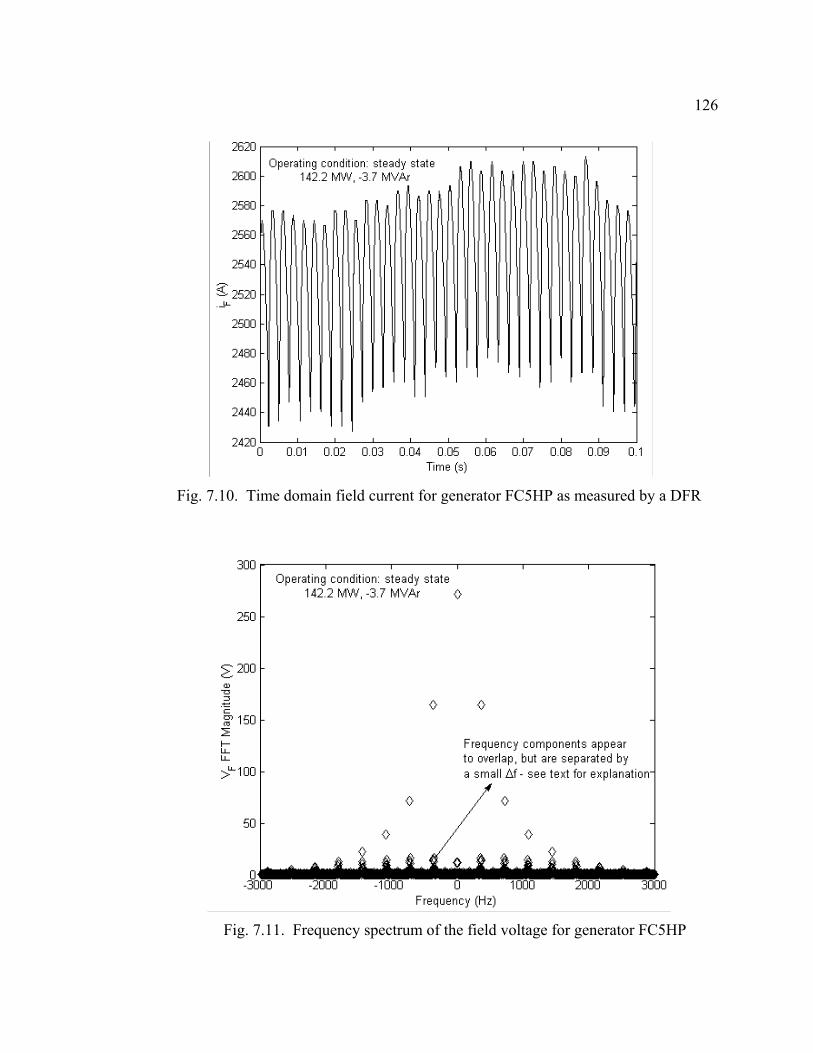
126

Fig. 7.10. Time domain field current for generator FC5HP as measured by a DFR

Fig. 7.11. Frequency spectrum of the field voltage for generator FC5HP

127

Fig. 7.12. Frequency spectrum of the field current for generator FC5HP

Considering the field current, a multiple parallel Butterworth filtering process

transforms the measured field current (whose main noise components are shown in Fig.

7.13) into a DC-like signal after the removal of high frequency components. The same

frequency components are depicted in Fig. 7.14 after the filtering process. The final

filtered signal in the time domain can be seen in Fig. 7.15.

A comparison of the ripple in the original DFR measured field current and in the

filtered field current as a percentage of the DC component of the signal, is an indication

of the effect of filtering on the field current. The ripple can be calculated by dividing the

difference of the maximum and minimum values of a signal by the DC value of the

signal. In the case of the unfiltered signal of Fig. 7.10, the ripple is calculated to be 7.7%,

while in the case of the filtered signal of Fig. 7.15, the ripple is 1.7%. The filtering

process for the field voltage is similar to that of the field current and will not be repeated.

128

Fig. 7.13. Frequency spectrum in the vicinity of DC for the DFR measured field current

for generator FC5HP

Fig. 7.14. Frequency spectrum in the vicinity of DC for the filtered field current for

generator FC5HP

129

Fig. 7.15. Time domain filtered field current for generator FC5HP

7.4 Filtering of the stator measurements

The measurements obtained from the stator terminals of the synchronous

generator are the three line-to-line voltages vab, vbc, and vca and the three currents ia, ib,

and ic. These signals do not have the complications that are associated with the field

signals as shown in the previous section, but they still contain a certain amount of noise

that needs to be removed in order to optimize the performance of the estimator.

The filtering process for the stator measurements is performed after the

calculation of the phase voltages and after the transformation of the abc voltages and

currents into 0dq signals through Park’s transformation as illustrated in Chapter 2. A

possible concern in any type of measurements is the presence of outliers or inconsistent

130

data. Such outliers appear in the form of spikes in the time domain plot of each signal.

Outliers are caused by metering errors and can be safely removed without risking

inaccuracies in the estimation process. Therefore, prior to the filtering of high frequency

components in any signal, a bad data detection and rejection algorithm is implemented to

remove outliers.

The process followed for this algorithm is first to detect a spike in any of the

signals by browsing through all the measurements obtained for each signal. For the

purposes of this application, a spike is defined to be greater than 10% of the value of the

signal at the previous step. Due to the small time constants of synchronous generators,

none of the measurements can vary by 10% or more within two consecutive steps even in

the transient case. The only possibility for such a variation is if the generator experiences

a short circuit fault. However, the detection algorithm is able to check for such a

possibility and keep the measurement as is. If a spike in any one signal is detected, then

the whole data set for that time step is removed.

After the implementation of the bad data detection and rejection algorithm, a

multiple parallel filtering process is implemented similar to the description in the

previous section. Filter characteristics are chosen depending on the location and on the

size of the noisy frequency components, but in general, the filters for all the signals have

a cutoff frequency of approximately 10 Hz and a stopband frequency of 100 Hz with a

stopband attenuation of about 60-80 dB. This general characteristic for a noise filter

enables the automatic filtering of signals from any synchronous generator without the

need to examine each of the signals individually.

131

As an example, the filtering process of the direct axis voltage (vd) will be

demonstrated. Again, in this section, all measurements depicted are for the same 483

MVA synchronous generator considered in the previous section and in Chapter 6 and

Appendix A. Fig. 7.16 depicts the time domain signal of vd as calculated by the

combination of the phase voltages of the generator through Park’s transformation. vd is

expected to be a DC signal (or a slowly varying signal). Observation of Fig. 7.16 shows

a rather noisy signal as well as an outlier in the form of a spike. A portion of the

frequency content of vd is shown in Fig. 7.17. The zero frequency component is not

shown in order to focus on the frequency components of interest.

Fig. 7.16. Unfiltered d axis voltage in the time domain for generator FC5HP

132

Fig. 7.17. Frequency content of the d axis voltage for generator FC5HP before filtering

(zero frequency component not shown)

The result of the implementation of the bad data detection and rejection algorithm

and the filtering process can be observed in Figs 7.18 and 7.19. It can be seen that the

majority of the noisy frequency components have been eliminated or reduced

significantly. Frequency components in the vicinity of DC are retained to track possible

transient behavior of the generator. The resulting time domain signal shows both the

removal of the spike and the DC nature of the signal. The filtering process for all other

stator signals is identical to the one described in this section for vd.

133

Fig. 7.18. Frequency content of the d axis voltage for generator FC5HP after filtering

Fig. 7.19. d axis voltage in the time domain after spike and noise filters are applied for

generator FC5HP

134

7.5 Summary

This chapter concentrated on the filtering of the measurements prior to the

implementation of the estimation algorithm. The filtering process comprises the removal

of inconsistent measurements (outliers) and the minimization of high frequency noise

components. All filtered signals are DC signals (or transformed DC signals) and

appropriate low pass filters were utilized to remove noise components above certain

frequencies. Low frequency components were retained to capture possible slow

variations in the behavior of the signals.

The filters used for the purposes of this application were the Butterworth and

moving average filters. Other filters such as the Elliptic and Chebychev filters were

considered but not implemented because they were inferior in performance to the other

available filters.

The filtering of rotor and stator signals was considered separately in Sections 7.3

and 7.4 respectively. Case study results indicate satisfactory performance of the filters,

rejection of bad data, and minimization of the noise in measurements. Finally, a new

approach to filtering was introduced: multiple parallel filtering. This approach enables

the application of successive identical filters to slowly attenuate high frequency

components without affecting the components of interest. A single low pass filter would

not perform successfully in this application because of the characteristics of the signal

under study. It is not possible to design a single filter with both a low cutoff frequency

and a high attenuation, since an unstable filter results. Multiple parallel filtering allows

135

the minimization of high frequency components and medium frequency components by

using successive stable filters that have a low attenuation.

CHAPTER 8

PARAMETER ESTIMATION FROM ACTUAL MEASUREMENTS

8.1 Introduction

Implementation of any proposed algorithm using actual measurements is the

ultimate test for its viability and applicability to the system under study. After the

successful testing of the parameter estimation algorithm using both synthetic and EMTP

data as demonstrated in Chapter 6, it is necessary to test the estimator using data obtained

from synchronous generators and observe whether the proposed method agrees to the

practical results.

Synchronous generator measurements for the purpose of this research work are

obtained through a digital fault recorder (DFR). A DFR is effectively a data acquisition

system that is used to monitor the performance of generation and transmission

equipment, and therefore is connected permanently to utility generators. DFRs are

typically used by the majority of the utilities to monitor the operation of generators. For

this particular estimation methodology, the measurements are obtained at the terminals of

committed synchronous generators (the units serve their typical loads). Different

operating levels are considered to examine the accuracy of the proposed method with

varying degrees of excitation and different saturation levels. The measurements are

stored in a data file that can be read by the estimator. The data files are typically of the

COMTRADE data file format [116], which is an approved IEEE data format for storage

of measurements. The data can either be in ASCII format or binary format. A short

description of the COMTRADE data format that is also supported by the designed

estimator is given in Appendix E.

137

In between the data acquisition and the estimator implementation there are a

number of other processes that need to be performed to prepare the data in a form that

can be used by the estimator. Fig. 8.1 shows a flowchart of the procedure followed to

perform the parameter estimation. The measurements obtained for the stator voltages are

sometimes line to line measurements, and therefore it may be necessary to transform

these signals into phase quantities. Further, the power angle δ needs to be calculated in

order to perform the Park's transformation as explained in Chapter 2. The above

transformations and the procedure as illustrated in Fig. 8.1 are shown in detail in

Appendices G and H as used in the code of the estimator.

8.2 Results of parameter estimation from actual measurements

The last part of the system identification procedure is the parameter estimation

from the filtered measurements. The estimator configuration follows the procedure

described in Section 5.6 and the procedure followed in the parameter estimation from

EMTP simulated measurements of Chapter 6. The estimation of parameters from EMTP

measurements did not clearly distinguish the dominant model between the proposed

models (models 2.1, 2.2, and 2.2x), and therefore all three models will be tested with

actual measurements.

In contrast to the simulated data set, an examination of the actual data sets

obtained from the synchronous generator terminals and used for the parameter estimation

described in this section, indicates that the generators operate within the saturation

region. Therefore, the estimator algorithm needs to adjust the parameters for saturation

138

as explained in Chapter 3. The parameters obtained from the estimator reflect the true

state of the system including saturation.

Obtain stator (abc)measurements andfield measurements

Calculate the power angle

START

END

Obtain MVA andkV base and

known parameters

Convert line-line voltagesto phase voltages

Calculate active and reactive powerand power factor at each point

Filter high frequency noise infield voltage and current

Reject outliers in statormeasurements

Filter high frequencynoise in statormeasurements

δ

Convert all measurementsto per unit quantities

Implement observer fordamper winding currents

Estimate generatorparameters

Calculate derivativesof currents

Perform Park's transformationto convert abc to 0dq

Fig. 8.1. Algorithm for estimator implementation for actual measurements

139

Table 8.1 depicts the estimated parameters in each of the three proposed models

using actual measurements from generator FC5HP (case study R-NC-01-10). All

parameters are individually estimated assuming that all other parameters are known. In

the case of model 2.2x, LAD and LAQ are the only parameters affected by saturation since

all other inductances have been expressed in terms of these mutual inductances according

to (3.11). In the case of models 2.1 and 2.2 a number of parameters is affected by

saturation and these parameters are adjusted prior to the estimation procedure if they are

not desired to be estimated. Therefore, Table 8.1 depicts the saturated values of the

parameters (where applicable).

TABLE 8.1

Estimated parameters for the three proposed models for generator FC5HP

(case study R-NC-01-10)

Parameter (p.u.) Model 2.1 Model 2.2 Model 2.2x

Ld 1.6146 1.6147 N/A

Lq 1.5648 1.5794 N/A

LF 1.49493 1.49493 N/A

kMF 1.5355 1.5355 N/A

LAD N/A N/A 1.5963

LAQ N/A N/A 1.4057

r -0.0061185 -0.01273 -0.01273

rF 8.386x10-4 8.386x10-4 8.386x10-4

140

As mentioned above, the estimated inductances of Table 8.1 potentially reflect the

true state of the system including the effect of saturation. Since the exact values of the

parameters at every operating point are not known, it is not possible to derive any definite

conclusions about the accuracy of the estimated parameters. Therefore, it is desired to

nullify the effect of saturation by applying the inverse of the appropriate saturation factor

to each of the saturated inductances. This will offer estimates of the unsaturated

inductances and a comparison to the manufacturer values may be obtained. However, the

manufacturer values of the parameters have been calculated by off-line tests and testing

methods that may not necessarily reflect the operating point under consideration.

Moreover, manufacturer values are typically design values for a series of manufactured

generators, and consequently differences between designed and actual parameter values

do exist. Therefore, the percent difference between the estimated parameters and the

manufacturer parameters cannot be classified as a percent error as in the case of the

simulated measurements. The difference between the estimates and their “nominal”

values is referred to as a percent deviation. The percent deviation cannot be used as a

verification or rejection of the proposed method, but it can offer an insight as to whether

the estimates obtained are reasonable or not. In general, it is more important to have

consistency in the estimated parameters between various data sets from the same

generator, than to have results with varying degrees of accuracy.

Table 8.2 depicts the percent deviation of the estimated parameters from the

manufacturer suggested values for the parameters, after the effect of saturation has been

nullified to obtain an estimate of the unsaturated values of the inductances. All three

141

models are considered to enable comparison of the estimation method between all the

candidate models.

TABLE 8.2

Calculation of unsaturated parameters from the estimated parameters of generator FC5HP



Parameter


Estimated parameter

(p.u.)

% Deviation

Estimated parameter

(p.u.)

% Deviation

Estimated parameter

(p.u.)

% Deviation

Ld 1.80 1.757 2.4 1.757 2.4 N/A N/A

Lq 1.72 1.702 1.0 1.724 0.2 N/A N/A

LF 1.75791 1.627 7.4 1.627 7.4 N/A N/A

kMF 1.64 1.671 1.9 1.671 1.9 N/A N/A

LAD 1.64 N/A N/A N/A N/A 1.737 5.9

LAQ 1.56 N/A N/A N/A N/A 1.529 2.0

r 0.0046 -0.00612 233 -0.01273 377 -0.01273 377

rF 8.454x10-4 8.386x10-4 0.8 8.386x10-4 0.8 8.386x10-4 0.8

Table 8.2 shows that the results obtained from all three models are similar.

Results from models 2.2 and 2.2x are slightly improved due to the more accurate

modeling of the quadrature axis. A discussion for some of the results from the three

models is appropriate at this point. The field resistance is estimated with a deviation of

0.8% in all three models. Estimation of the field resistance is a critical aspect of the

142

overall estimation procedure since one of the motivations for this research work is the

tracking of the change in the field resistance to detect and prevent short circuits in the

field winding. The nominal field winding resistance noted as the manufacturer value in

Table 8.2 is an approximate quantity since the generator under consideration has been

rewound a number of times because of short circuits in the field winding. Therefore, no

definite comparison can be performed between the estimated and the nominal value.

Nevertheless, the estimation procedure gains considerable confidence from these results

since the deviation between the two values is very small.

Values for Ld, Lq, and kMF are estimated within a reasonable accuracy in both

models 2.1 and 2.2, with Lq being estimated more accurately in model 2.2. The percent

deviations for these parameters vary from 0.2 to 2.4%. In the case of the field inductance

LF, the percent deviation attained is in the order of 7.4%. This result is not considered

satisfactory, but similarly to the case of the field resistance, the nominal value of LF may

not be accurate because of the rewinding of the field winding of this particular generator.

In the case of model 2.2x, LAQ is estimated with a deviation of 2.0% from its

nominal value, while LAD is estimated with a deviation of 5.9%. A portion of the

deviation of LAD can be attributed to the field inductance LF, since in model 2.2x the field

inductance was expressed as FADF lLL += , where lF is the leakage inductance of the

field winding. Therefore, the estimated LAD will reflect any possible inaccuracy of lF

because of the rewinding of the field winding.

Finally, the results for the stator resistance in all three models show that currently

the stator resistance cannot be estimated accurately. The amount of noise in the

143

measurements and the representation of saturation are two of the reasons for the

inaccuracy in the stator resistance. A number of case studies were performed to observe

how using different saturation factors and various filtering mechanisms affect the stator

resistance. For example, if no saturation is modeled, then the estimated stator resistance

was positive and much higher than the manufacturer value of r. As saturation factors of

increasing values were introduced to adjust LAD and LAQ, the value of the stator resistance

reduced and in some cases the estimated value was negative as in the case of Table 8.2.

The inability to estimate r within a satisfactory degree of accuracy is not an obstacle to

this method of estimation. Typically, there is no interest in estimating r. The main

parameters of interest are Ld, Lq (or LAD and LAQ), and rF.

8.3 Multiple parameter estimation

Multiple parameter estimation from actual measurements is an important aspect of

the estimator. In many cases (like the one under consideration in this research work) it is

possible that there is uncertainty in more than one parameter. Therefore it is imperative

that the feasibility of multiple parameter estimation is investigated. Ideally, it is desired

that the percent deviation obtained for each parameter is the same in both individual

parameter estimation and multiple parameter estimation.

Two case studies are performed. In the first case study (R-NC-03-11), Ld, Lq, and

rF are estimated simultaneously for models 2.1 and 2.2, while LAD, LAQ, and rF are

estimated simultaneously for model 2.2x. The estimated parameters are depicted in Table

8.3, while the unsaturated parameters calculated from the estimated parameters are

144

depicted in Table 8.4. It can be observed that for all three models the estimated

parameters and their percent deviations are identical to the corresponding parameters in

the individual parameter estimation of Table 8.1 and Table 8.2.

TABLE 8.3

Multiple simultaneous parameter estimation for generator FC5HP (case study R-NC-03-11)

Parameter (p.u.) Model 2.1 Model 2.2 Model 2.2x

Ld 1.6146 1.6147 N/A

Lq 1.5648 1.5794 N/A

LAD N/A N/A 1.5963

LAQ N/A N/A 1.4057

rF 8.386x10-4 8.386x10-4 8.386x10-4

TABLE 8.4

Calculation of unsaturated parameters for generator FC5HP (case study R-NC-03-11)


Parameter


Estimated parameter

(p.u.)

% Deviation

Estimated parameter

(p.u.)

% Deviation

Estimated parameter

(p.u.)

% Deviation

Ld 1.80 1.757 2.4 1.757 2.4 N/A N/A

Lq 1.72 1.702 1.0 1.724 0.3 N/A N/A

LAD 1.64 N/A N/A N/A N/A 1.737 5.9

LAQ 1.56 N/A N/A N/A N/A 1.529 2.0

rF 8.454x10-4 8.386x10-4 0.8 8.386x10-4 0.8 8.386x10-4 0.8

145

In the second case study (R-NC-03-12), Ld, Lq, and LF are estimated

simultaneously for models 2.1 and 2.2, while LAD, LAQ, and LF are estimated

simultaneously for model 2.2x. The estimated parameters are depicted in Table 8.5,

while the unsaturated parameters calculated from the estimated parameters are depicted

in Table 8.6. As in the previous case study, the estimated parameters and their percent

deviations are identical to the corresponding parameters in the individual parameter

estimation of Table 8.1 and Table 8.2.

TABLE 8.5

Multiple simultaneous parameter estimation for generator FC5HP


Parameter Model 2.1 Model 2.2 Model 2.2x

Ld 1.6146 1.6147 N/A

Lq 1.5648 1.5794 N/A

LAD N/A N/A 1.5963

LAQ N/A N/A 1.4057

LF 1.49493 1.49493 N/A

The results of the multiple simultaneous parameter estimation case studies

indicate that more than one parameter can be estimated at the same time. It was shown

that there is no degradation of the percent deviation of the estimated parameters from

their nominal values. Therefore, the confidence for the use of the estimator to estimate

146

multiple parameters simultaneously is reinforced. In case that the confidence in some of

the synchronous generator parameters is limited (for example, because of alterations to

the generator circuitry), multiple parameter estimation holds the key to a reliable

estimation procedure.

TABLE 8.6

Calculation of unsaturated parameters for generator FC5HP (case study R-NC-03-12)


Parameter


Estimated parameter

(p.u.)

% Deviation

Estimated parameter

(p.u.)

% Deviation

Estimated parameter

(p.u.)

% Deviation

Ld 1.80 1.757 2.4 1.757 2.1 N/A N/A

Lq 1.72 1.702 1.0 1.724 0.3 N/A N/A

LAD 1.64 N/A N/A N/A N/A 1.737 5.9

LAQ 1.56 N/A N/A N/A N/A 1.529 2.0

LF 1.75791 1.627 7.4 1.627 7.4 N/A N/A

8.4 Application of the algorithm to different machines and different operating points

Sections 8.2 and 8.3 discussed the parameter estimation procedure and some of

the results obtained using measurements from generator FC5HP. It is necessary to

perform parameter estimation for different generators and at different operating points to

ensure that the method is applicable to other generators as well. Using measurements

from different generators enables the examination of the accuracy of the proposed

method, while the estimation at various operating points for each generator ensures that

the results are consistent.

147

The case studies described in Sections 8.2 and 8.3 and a number of other case

studies that were performed, permit the extraction of some conclusions pertaining to the

model used in the estimation procedure. Clearly the estimates obtained from models 2.2

and 2.2x are superior to the ones obtained from model 2.1. This is due to the modeling of

one extra damper winding in the quadrature axis of the generator; this winding causes the

model to be symmetric with regards to the direct and quadrature axes. Results from

models 2.2 and 2.2x are similar considering that the estimates of LAD and LAQ contain the

error from the field winding inductance LF and other quantities such as the mutual

inductances between axes in the stator and the rotor (see (2.22), (3.11), and Table 6.2 for

a comparison of the two models). A clear advantage of model 2.2x is that it offers an

easier way of representing the magnetic saturation in a synchronous generator.

Therefore, model 2.2x is the preferred model. The parameter estimation results presented

in this section and in Appendix F are obtained through the utilization of model 2.2x.

Table 8.7 shows the parameter estimation results for ten data sets obtained from

two identically designed units at the Redhawk generating station of APS. Eight of the

data sets are obtained from GT1, while two of the data sets are obtained from GT2.

Although the two units may have some differences in their parameters since no two units

are exactly identical, the use of more data sets will allow the extraction of useful results

pertaining to the accuracy of the method when applied to different generators and the

representation of saturation. The two units are gas turbine units rated at 213.7 MVA and

18 kV. Their characteristics are described in Table 3.1.

148

TABLE 8.7

Parameter estimation results for Redhawk gas turbines 1 and 2*

% deviation

Case study Unit # ADL

(p.u.) AQL

(p.u.) Fr

(p.u.) Ksd iF

(A) P

(MW) Q

(MVAr) ADuL

(p.u.) AQuL

(p.u.) LAD LAQ

R-NC-03-13 GT1 1.5394 1.6787 7.008x10-4 0.9479 1021.7 148.40 13.26 1.624 1.771 8.8 4.7

R-NC-03-14 GT1 1.6073 1.6735 7.020x10-4 0.9487 982.72 145.2 10.87 1.694 1.764 4.9 4.3

R-NC-03-15 GT1 1.5998 1.6865 7.205x10-4 0.9474 826.96 109.5 1.42 1.688 1.780 5.2 5.2

R-NC-03-16 GT1 1.5882 1.6724 6.854x10-4 0.9485 853.08 111.13 5.69 1.674 1.763 6.0 4.2

R-NC-03-17 GT1 1.5748 1.6941 6.730x10-4 0.9472 844.43 108.83 4.34 1.663 1.788 6.6 5.7

R-NC-03-18 GT1 1.6009 1.6387 6.352x10-4 0.9473 874.65 119.14 4.43 1.690 1.730 4.7 3.6

R-NC-03-19 GT1 1.5682 1.7516 7.716x10-4 0.9477 845.12 110.11 4.43 1.651 1.848 7.0 9.2

R-NC-03-20 GT1 1.5607 1.7557 7.619x10-4 0.9511 921.00 119.87 15.63 1.641 1.846 7.8 8.3

R-NC-03-21 GT2 1.5795 1.6741 6.980x10-4 0.9491 861.96 109.1 9.03 1.664 1.764 6.6 4.3

R-NC-03-22 GT2 1.5891 1.6760 6.922x10-4 0.9495 863.21 108.40 10.61 1.674 1.765 6.0 4.3

Mean (µ) 7.041 x10-4 1.6667 1.782

Standard deviation (σ)

1.442 x10-9 0.0225 0.0375

* From the manufacturer data sheet: LAD = 1.781 p.u., LAQ = 1.692 p.u., while rF is unavailable.

149

Three parameters were estimated from each data set: LAD, LAQ, and rF. The

operating point of the generator for each data set is shown, as well as the field current.

The saturation factor for the direct axis is calculated and shown in the table for each case

study. It is assumed that the saturation factor is the same in both the direct and

quadrature axes.

It is necessary to apply the saturation factor to the estimated saturated inductances

in order to obtain the unsaturated inductances. This will allow comparison to the

manufacturer data and enable the assessment of the estimation method. Table 8.7 depicts

the estimated unsaturated mutual inductances and their deviation from the manufacturer

supplied mutual inductances. It should be noted that the manufacturer inductances LAD

and LAQ are 1.781 p.u. and 1.692 p.u. respectively.

It is of practical interest to examine the change of the two mutual inductances

with excitation, using both the estimated saturated values as well as the values corrected

for saturation to obtain the unsaturated values. Fig. 8.2 shows the change in the estimated

direct axis mutual inductance LAD with the field current. A linear regression model is

fitted to observe the trend in the estimated inductance over increasing saturation levels.

As expected, there is a decrease in the apparent value of the inductance as the generator is

driven to higher operating points.

Fig. 8.3 compares both the saturated and the unsaturated values of LAD for all case

studies. The stacked column graph shows the estimated parameters and the correction for

saturation. An overall agreement between the unsaturated values is observed. The

150

unsaturated values of LAD have a mean of 1.6667 p.u. and a standard deviation of 0.0225

p.u. All of the values of the unsaturated inductance LAD agree to one decimal place.

The results of each case study for the quadrature axis mutual inductance LAQ are

summarized in Figs 8.4 and 8.5. The estimated values of the quadrature axis mutual

inductance at different operating points are shown in Fig. 8.4. The trend in the saturated

value of the inductance is decreasing, although the decrease is not as evident as in the

case of LAD. It should be noted that the variation of LAQ is slightly higher than that of LAD

since the standard deviation among the unsaturated parameters is 0.0375 p.u. The mean

of the unsaturated parameters is 1.782. A comparison between the unsaturated values of

LAQ at each operating point is offered in Fig. 8.5, where the saturated inductances are

corrected for saturation using the appropriate saturation factor at each operating point.

With the exception of two data sets, the unsaturated values of the inductance agree to one

decimal place.

Appendix F presents parameter estimation results for two steam turbine

generators located at the Redhawk generating station of APS. A number of case studies

are performed and an analysis similar to the analysis of this section is offered.

151

1.5

1.52

1.54

1.56

1.58

1.6

1.62

1.64

800 850 900 950 1000 1050

Field current (A)

L AD

(p.u

.)

Fig. 8.2. Change of LAD with operating point for Redhawk gas turbine generators

1.4

1.45

1.5

1.55

1.6

1.65

1.7

1.75

L AD (

p.u.

)

826.96 844.43 845.12 853.08 861.96 863.21 874.65 921 982.72 1021.7

Field current (A)

Estimated LAD LAD corrected for saturation Fig. 8.3. Saturated and unsaturated values of LAD for Redhawk gas turbine generators

152

1.5

1.55

1.6

1.65

1.7

1.75

1.8

1.85

1.9

800 850 900 950 1000 1050

Field current (A)

L AQ

(p.u

.)

Fig. 8.4. Change of LAQ with operating point for Redhawk gas turbine generators

1.5

1.55

1.6

1.65

1.7

1.75

1.8

1.85

1.9

L AQ

(p.u

.)

826.96 844.43 845.12 853.08 861.96 863.21 874.65 921 982.72 1021.7

Field current (A)

Estimated LAQ LAQ corrected for saturation Fig. 8.5. Saturated and unsaturated values of LAQ for Redhawk gas turbine generators

153

8.5 Calculation of standard machine parameters from estimated derived parameters

Typically machine parameters obtained from manufacturer data are as shown in

the stability study data sheet in Appendix B.2. These machine parameters are referred to

as standard machine parameters and include the direct and quadrature axis reactances and

their transient and subtransient counterparts, as well as the transient and subtransient time

constants. However, the estimated parameters obtained through the model developed in

Chapters 2 and 3 are derived parameters from these standard machine parameters.

Therefore, it is necessary to calculate the standard parameters from the estimated

parameters obtained through the developed algorithm. Table 8.8 summarizes the

formulae that are needed to perform the conversion from derived parameters to standard

parameters. Table 8.9 compares estimated standard parameters to manufacturer standard

parameters for case study R-NC-01-10 (generator FC5HP).

The results of Table 8.9 show a good correlation between the estimated standard

parameters and the manufacturer standard parameters. The correction for saturation

typically improves the estimates. Some of the parameters such as the transient and

subtransient inductances are estimated with errors less than 0.3%. The highest error is

observed for the direct axis transient open circuit time constant and it is equal to 5.5%.

154

TABLE 8.8

Calculation of standard parameters from the estimated derived parameters*

Parameter name Parameter symbol Formula

Equivalent direct axis reactance dx dADL l+

Transient direct axis reactance dx′

FAD

dADdF

LLLl

ll

+

+

Subtransient direct axis reactance dx ′′

FDAD

d

L ll

l111

1

+++

Equivalent quadrature axis reactance qx qAQL l+

Transient quadrature axis reactance qx′

GAQ

qAQqG

LLLl

ll

+

+

Subtransient quadrature axis reactance qx ′′

QGAQ

q

L ll

l111

1

+++

Direct axis transient open circuit time

constant 0dτ ′

FB

FAD

rLω

l+

Direct axis subtransient open circuit

time constant 0dτ ′′ ]

111[1

FAD

DDB

Lr

l

l

++

ω

Quadrature axis transient open circuit

time constant 0qτ ′

GB

GAQ

rLω

l+

Quadrature axis subtransient open

circuit time constant 0qτ ′′ ]

111[1

GAQ

QQB

Lr

l

l

++

ω

*Note: Time constants are in seconds. All other quantities are in per unit.

155

TABLE 8.9

Comparison of estimated standard parameters to manufacturer standard parameters

(case study R-NC-01-10)*

Parameter Manufacturer value

Value at operating point

Unsaturated value

% Deviation

dx 1.80 1.7563 1.897 5.4

dx′ 0.27 0.2698 0.2704 0.15

dx ′′ 0.19 0.18998 0.19003 0.02

qx 1.72 1.5657 1.6894 1.78

qx′ 0.49 0.48251 0.48861 0.28

qx ′′ 0.19 0.18994 0.18999 0.005

0dτ ′ 3.70 3.60802 3.90376 5.5

0dτ ′′ 0.032 0.03196 0.03209 0.28

0qτ ′ 0.49 0.45179 0.48243 1.54

0qτ ′′ 0.059 0.05778 0.05877 0.39

*Note: Time constants are in seconds. All other quantities are in per unit.

CHAPTER 9

GRAPHIC USER INTERFACE IMPLEMENTATION USING VISUAL C++

9.1 Introduction

One of the major objectives of this research work is to develop a visual graphic

user interface (GUI) in the form of a Windows application for a synchronous generator

state estimator. This application will enable the practicing engineer and interested

utilities to estimate the parameters of a synchronous generator without having to

decommit the unit or get involved in time consuming off-line tests. The application

developed during this research work is unique due to three main characteristics: on-line

operation, portability, and user friendly interaction.

On-line operation is the distinguishing characteristic of the proposed estimator. It

enables on-line and expeditious estimation of any given synchronous generator based on

measurements of the field and stator voltages and currents. Such measurements are

readily available and in large quantities in every utility.

Moreover, the application developed is portable, since it can be installed in any

personal computer operating under Windows. It does not require a Visual C++

environment, since it is a stand-alone application, able to operate without the support of

external C++ libraries.

Finally, user friendly interaction is achieved by means of the dialogs and context-

sensitive help provided on request. The input and output dialogs are self explanatory and

will be analyzed in Sections 9.2 and 9.4 respectively. Moreover, these dialogs and each

of their components are analyzed within the program itself in the Help section. General

157

guidelines for correct operation of the program and interpretation of the results are also

provided.

9.2 Input dialog and estimator configuration

The main window of the estimator offers a variety of options on its toolbar,

similar to any other Windows program. To initiate the process of estimating generator

parameters, the user must open the input screen as shown in Fig. 9.1. This is achieved by

selecting the option Estimator on the toolbar of the main window, and then selecting the

Set up Estimator option.

Fig. 9.1. Input window of the Estimator

As can be seen in Fig. 9.1, the input screen is user friendly. The user can set up

the Estimator and calculate the parameters of the synchronous generator that is to be

158

studied by following the directions on the input screen. The first step is to enter the name

of the data file in the edit box as shown in Fig. 9.1. This can be done by clicking on the

Browse button and navigating through the hard disk of the computer or any external

drives until the desired file is located. The file can be of any data format type (for

example .dat or .txt). If applicable, the user can select the IEEE COMTRADE option by

clicking on the respective radio button and the Estimator will read the measurements as

obtained directly from the measuring device that is connected to the generator. These

files typically follow the IEEE COMTRADE Standard for power systems [116]. An

example of each data format that is supported by the application can be seen in Appendix

E.

The second step on behalf of the user is to input the required parameters as

contained in the manufacturer data sheet of the synchronous generator (see Appendix B

for a sample manufacturer data sheet). Sample values are shown in Fig. 9.1 and these are

the values obtained from the generator manufacturer data of Appendix B.

The user is able to select various options pertaining to the estimation process. It is

possible to perform either a least squares estimation (L2 minimization) or a minimization

of absolute deviations using the L1 norm [77]. In this research work, the estimation was

performed in a least squares sense.

Further, the user may select the level of filtering that is desired. Of the two

options, the full filtering is preferred since it will minimize the noise content in the

measured signals. Finally, the user is given the option to apply weights to the

measurements. This is particularly useful if it is known that certain measurements are

159

less reliable than other measurements. Further documentation on all the options is

provided through context-sensitive help or through the buttons that are located on the

input window. Fig. 9.2 shows a view of the Help window developed for the Estimator.

The final step of this process is to select the parameters that need to be estimated.

The user has the opportunity to select up to five parameters for estimation. This selection

can be performed by simply clicking on the check box corresponding to the parameter to

be estimated, as shown in Fig. 9.1.

Fig. 9.2. View of the Help window of the Estimator

160

9.3 State estimator implementation

After completing the steps mentioned in the previous section, the user clicks the

Start Estimator button to enable estimation of the parameters. No other interaction is

required from the user. The Estimator is responsible to read the data from the input file,

perform the bad data detection and rejection algorithms, filter the noise from the

measurements, and calculate the current derivatives. It implements the state estimation

algorithm and returns the values of the estimated parameters as an output. The C++ code

for the non GUI part of the application can be seen in Appendix H. The Estimator

flowchart can be seen in Fig. 9.3.

9.4 Output dialog and estimated parameters

Upon execution of the main program of the application the values of the estimated

parameters, the rms error, and the confidence level in the estimated parameters are

returned to the graphic user interface for output. The resulting output window can be

seen in Fig. 9.4. On the left side of the output window, the user can see the parameters

that he/she previously selected and their estimated value in per unit. The rms error on the

lower right side of the estimator is a measure of confidence on the estimated parameters

and is given by,

tsmeasuremenofnumberresidualerrorrms = , (9.1)

where,

)ˆ()ˆ()( 2 zxHzxHresidual T −−= , (9.2)

and x is the vector of the estimated parameters.

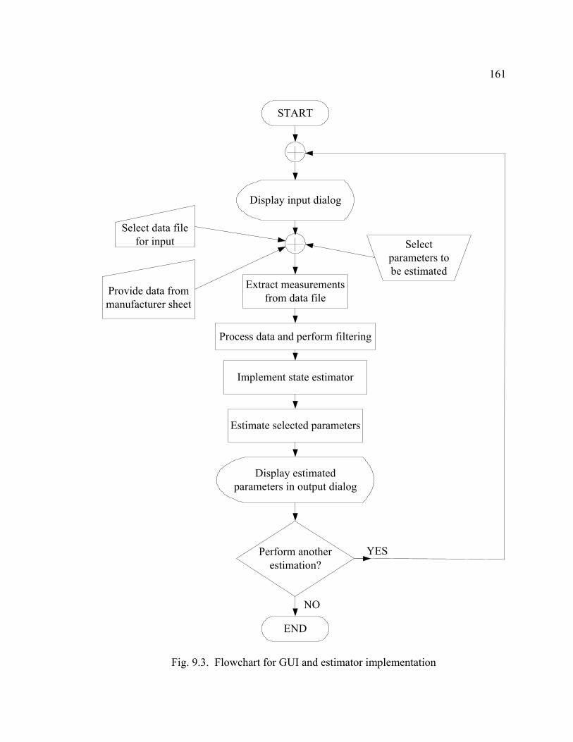
161

Extract measurementsfrom data file

Perform anotherestimation?

Display input dialog

START

END

Provide data frommanufacturer sheet

Select data filefor input Select

parameters tobe estimated

Process data and perform filtering

Implement state estimator

Estimate selected parameters

Display estimatedparameters in output dialog

YES

NO

Fig. 9.3. Flowchart for GUI and estimator implementation

162

Fig. 9.4. Output window of the Estimator

Finally, a confidence level is offered to the user. The confidence level has three

states: high, average, or low. In this fashion, the user can verify whether the

measurements used are reliable or not. Section 9.5 discusses how such a confidence level

can be derived through the χ2 test, and Section 9.6 proposes a method to calculate a

confidence interval for the estimated parameters.

9.5 Interpretation of the rms error and the chi-squared test

Small values of rms error as calculated by the Estimator in Fig. 9.4, indicate high

reliability of results. Larger values of rms error indicate results that cannot be trusted for

correct interpretation. The residual, which is the basis for the calculation of the rms error,

is ideally equal to zero for error free estimations. Its value represents a measure of how

163

closely the estimated values follow the measured or expected values. Instead of relying

on intuition as to how large or how small the residual or the rms error should be, a

standardized method could be followed to ascertain reliability of the results. A widely

used method for such purposes is the χ2 test. This method will be analyzed in this

section.

The residual J(x) is a random number since the measurement errors are random

numbers as well. Therefore, it can be shown that J(x) has a probability density function

known as a chi-squared distribution, also written as χ2(K). K is called the degrees of

freedom of the chi-squared distribution and is defined as,

sm NNK −= , (9.3)

where Nm is the number of measurements, and Ns is the number of states. The mean

value of the chi-squared distributed residual is K, and its standard deviation is K2 [50].

To ascertain how large a residual needs to be so as to be considered as a bad

estimation, the χ2 test has to be set up. A threshold value of J(x) has to be decided and

this value is denoted tJ. Such threshold values can be in the order of three times the

standard deviation as noted above. Therefore, if JtxJ >)( , then bad measurements or

unreliable estimation is detected. The next step is to calculate the probability that

JtxJ >)( . This probability is called the significance level α and it is desired to be as

small as possible.

An alternative way but similar to the above procedure, is to set the significance

level first and then calculate the threshold value. This can allow indication of the

probability of the occurrence of false alarms, which is equal to α. For example, by setting

164

α to 0.01, the probability of receiving a false alarm for unreliable estimation is 1%.

Knowing the value of α, the threshold value tJ can be calculated and compared to the

residual J(x). If tJ is greater that J(x), then the estimated results are reliable. Fig. 9.5

graphically shows the chi-squared test and how to determine reliability of the results as

explained in this section. Tables for threshold values at various degrees of freedom and

various significance levels are available in the literature [117].

Residual (J)

Prob

abili

ty J

(x)>

t J

K tJ

1.0

α

00

Fig. 9.5. Chi-squared test probability function

165

9.6 Confidence interval for estimated parameters

The estimated parameters always contain a certain level of inaccuracy because of

the finite amount of noise in the measurements. Using improved filtering methods or an

increased number of measurements may reduce the inaccuracy, but the values obtained

can never be exact. It is therefore advantageous to be able to specify a confidence

interval for each estimated parameter based on the instrumentation used to obtain

measurements, on the number of measurements used, and on the particular configuration

of the system model.

The final form of the equation of the model is given by zHx = , where H is an

nm× matrix containing the coefficients of the parameters to be estimated, x is an 1×n

vector that is desired to be estimated, and z is an 1×m vector that contains both known

parameters and measurements. Clearly, both H and z contain a certain level of

measurement uncertainty (in the form of noise). H contains measurement noise in all its

nonzero entries, whereas z contains measurement noise in all of its entries since its entries

are a sum of products between known values of parameters and their measured

coefficients.

Most instrumentation devices offer an accuracy of measurement for each scale

that is used. For example, if a meter on a transmission line has a scale of 100 MW and an

accuracy of ± 2 MW, then this can be associated to a percentage confidence of any

measurement. (The usual practice is to associate the accuracy to a value equal to three

times the standard deviation of the normal probability function of the distribution of the

error [50], but here a different formulation is proposed). Therefore, if a measurement of

166

100 MW is obtained by the instrument, the user can assume that the actual value of the

measured power is between 98 and 102 MW. Similarly, if the indication of the

instrument is Y MW, then the user can assume that the actual measurement is between

1002YY + and

1002YY − . In general, if an instrument has a full scale denoted as FS, an

accuracy σ, and a measured indication Y, then the actual measurement Y can be assumed

to be between,

SS FσYYY

FσYY +≤≤− .

(9.4)

All measurements in H and z of zHx = can therefore be expressed in terms of the

meter accuracy similarly to (9.4), and the model equation can be rearranged as

)∆()∆( zzxHH +=+ , (9.5)

where ∆H and ∆z contain the adjustment for the inaccurate terms. The solution of the

system can thus be obtained by,

)∆()∆(ˆ zzHHx ++= + (9.6)

In order to find a confidence interval for the estimated solution, it is necessary to

estimate the possible maximum deviation x∆ from the solution x . A least squares

solution for zHx = satisfies the normal equations,

zHHxH TT = . (9.7)

Similarly, a least squares solution for (9.5) satisfies the normal equations,

0)]∆()∆)(∆[()∆( =+−+++ zzxxHHHH T . (9.8)

167

It should be noted that in this application, rank(H) = rank(H+∆H) = n. The full column

rank in H is due to the fact that the entries in matrix H are the coefficients of the

unknown parameters; all of these coefficients are nonzero (n is the number of the

parameters to be estimated). Further, H+∆H has a full column rank since noise

components appear in the same locations in ∆H as do in H (noise only appears in

measurements, all other elements are zero). If H does not have a full column rank, then

the upper bound of the matrix pseudoinverse does not necessarily tend to zero as the

perturbation tends to zero.

Subtracting the noise free solution (9.7) from (9.8) and expanding without

neglecting any second order terms, the deviation from the true solution can be obtained

as,

)∆∆()∆()(∆)]∆()∆[(ˆ∆ HxzHHHxzHHHHHx TT −++−++= ++ . (9.9)

Although (9.9) is an “exact” mean square solution for the deviation x∆ , the main

disadvantage of this approach is that it is necessary to know x: the noise free, mean

square solution of the linearized system Hx = z. However, if x were known, then it would

not be necessary to attempt to estimate x∆ . Therefore, an alternative approach needs to

be followed to obtain an approximate equation that does not involve knowledge of the

true mean square solution. The alternative approach proposed in the remainder of this

section involves the approximation of the pseudoinverse of )∆( HH + . This

approximation will enable the expansion of (9.6), and an easier method of isolating x∆ .

First, consider the scalar case. Suppose that it is desired to find an approximate

equation for the inverse of the quantity )( hδh + . This quantity can be rewritten as,

168

1111 )1()( −−−− +=+ hδhhhδh . (9.10)

Using Taylor series expansion and expanding up to the third term,

))(1()( 21111 L−+−=+ −−−− hδhhδhhhδh . (9.11)

Equation (9.11) may be used to relate the scalar case to the matrix case. The

pseudoinverse of )∆( HH + can be written as,

)∆)(∆(∆)∆( +++++++ +−≈+ HHHHHHHHHHH . (9.12)

Substituting (9.12) into (9.6), an expression in terms of x and x∆ can be obtained.

.)])(([

]))(([

))]()(([

)()(ˆ

zHHHHHHHHH

zHHHHHHHHzH

zzHHHHHHHHH

zzHHx

∆+∆+∆+++∆+−++

+∆+−+∆+∆+++≈

∆++∆+∆+++∆+−+≈

∆++∆+=

(9.13)

The first term of (9.13) is recognized as the solution to the noise free system zHx = and

therefore the remainder of (9.13) can be called the deviation x∆ from the true solution.

Rearranging (9.13),

,∆)]∆)(∆(∆()∆(∆ˆ∆ zHHHHHHIHzIHHHHHx mxmmxm+++++++ +−+−≈ (9.14)

where H and z are known, and ∆H and ∆z can be estimated as explained in the beginning

of the section. The confidence interval can thus be calculated as,

xxxxx ˆ∆ˆˆˆ∆ˆ +≤≤− . (9.15)

CHAPTER 10

CONCLUSIONS AND FUTURE STEPS

10.1 Comments from industry

The research work performed in this dissertation attempts to solve a well defined

industry problem namely the identification of synchronous generator parameters at

various operating levels and the tracking of parameters over time to potentially prevent

system outages. A number of utilities and private companies have expressed an interest

in this research work and the graphic user interface that is being developed. A number of

industry members is involved directly or indirectly in this work and at times offered

suggestions, comments, and constructive criticism about the development of the

estimator.

All the issues raised by the industry are of practical manner. Some of the major

issues include the unavailability of damper winding current measurements and the

implementation of a saturation model for synchronous generator inductances. Some

other issues that have been discussed are the differences in the configuration of the

exciter in synchronous generators, the extension of this research work to other generators,

and the improvement of the confidence in the results by using measurements from

various generators. Table 10.1 summarizes some of the comments and concerns received

by industry members during private discussions or during various presentations of this

research work at international conferences.

170

TABLE 10.1

Comments from the power engineering industry

Area Industry comment Plan of action

Exciter Is the estimator applicable to brushless exciter applications?

The estimator requires voltage and current measurements from the field winding. It is necessary for the exciter to have brushes in order to be able to obtain these measurements. However, it may be possible to develop an observer for the field voltage and current. This subject is under investigation.

Damper windings

The damper windings cannot be measured. How does the estimator obtain these measurements?

Chapter 4 describes an observer for damper winding currents. Results from simulated data verify its operation.

Magnetic saturation

Can magnetic saturation be implemented in the estimator?

A model for magnetic saturation is currently used as shown in Chapter 3. A model to estimate the q axis characteristic from the d axis characteristic has been developed by a number of researchers and is also presented in Chapter 3.

Superconducting synchronous condensers

Can the estimator be applied to a superconducting synchronous condenser?

The idea proposed in this research work can be applied to any generator that can be described by a model similar to the one of a round rotor synchronous generator.

Further experience

Is it possible to obtain further experience with the estimator using data from other generators?

A number of synchronous generator data have been obtained from APS. These data pertain to six different generators (both steam and gas turbines). Some of the results are shown and analyzed in Chapter 8 and Appendix F.

171

10.2 Conclusions

In this dissertation, a method to identify synchronous generator parameters from

on-line measurements is presented. Knowledge of parameter values at different operating

levels enables the correct representation of synchronous generators in stability studies

and other routine power engineering studies. Proper representation of synchronous

generators leads to increased accuracy in the results obtained from these studies as well

as better operation and maintenance of the power system network. Additionally, the

ability to foresee turn to turn short circuits in the generator field winding potentially

enables the engineers to avoid forced outages, thus saving the company huge amounts of

money in downtime, rewinding of the generator, and lost dividends from the operation of

the generator.

The method proposed in this report is based on least squares estimation of a

system of equations based on measurements obtained while the generator is connected to

the power system and serves its load. The on-line collection of measurements makes the

method superior to off-line methods since it is possible to estimate generator parameters

at various operating levels. The developed model of the system was shown to contain

seven differential equations that represent the stator and the rotor of the generator as well

as three damper windings.

One of the most important obstacles in the parameter estimation algorithm is the

unavailability of damper winding currents. Currently there is no proven technology for

the direct measurement of damper winding currents using physical instruments.

Moreover, damper windings are often fictitious and they are an effect of eddy currents in

172

the rotor path. Therefore it is necessary to estimate damper winding currents. An

observer for the estimation of damper currents that is based on the model of the system

and a priori knowledge about the system was proposed in this dissertation and

implemented in the parameter estimation algorithm. Comparison to both steady state and

transient simulated measurements showed that the damper currents were estimated

accurately.

Magnetic saturation affects some of the generator inductances significantly. In

order to enable estimation of parameters at various operating levels, it is imperative to

model saturation effectively so that the estimated parameters reflect the true state of the

system. A saturation model was implemented in this dissertation based on knowledge of

the saturation curve of the direct axis. A saturation factor that was calculated from the

saturation model was used to modify the values of inductances that were used in the

estimation process. Parameter estimation results show that magnetic saturation is

represented effectively. A possible improvement of the saturation representation is to

calculate separate saturation factors for the direct and quadrature axes. Because of the

unavailability of q axis saturation data, it is necessary to approximate the q axis saturation

characteristic. A method to estimate the q axis open circuit characteristic from the

available d axis open circuit characteristic is shown in Chapter 3.

Noise suppression is of major concern in this research work. Actual generator

data always contain noise that needs to be reduced in order to improve the accuracy of the

estimated parameters. Several types of digital filters have been considered in order to

filter out high frequency noise in the stator and rotor measurements. The Butterworth

173

filter is selected to be implemented because of its desirable characteristics in the

passband, and especially because of the small amount of ripple in its response. A

multiple parallel filtering method was proposed to implement noise filtering in an

effective manner because of the spread of the frequency spectrum of the signals.

Multiple parallel filtering in effect applies the same filter a number of times to slowly

attenuate all frequency components that are located in the transition band of a signal. For

“noise” that is actually harmonics, in either the field or armature, a small possible

improvement might be obtained by modeling the effects of these harmonics rather than

simply discarding the harmonic portion of the spectrum.

Three synchronous generator models have been proposed in this dissertation.

Model 2.2x seems to be the dominant model because of its more accurate modeling of the

quadrature axis, the easier implementation of saturation, and the favorable results

obtained from synthetic data and actual measurements.

The synchronous generator models and the proposed method were verified using

synthetic data obtained from the solution of the differential equations of the model and

from the simulation of the generator in EMTP. The latter method allowed the estimation

of generator parameters with a maximum error of 0.39%, while the stator resistance and

the field resistance were estimated exactly.

The proposed method was subsequently tested using on-line measurements from

synchronous generators. In case study R-NC-01-10, the field resistance was estimated

with a deviation of 0.8% for all three proposed models for generator FC5HP. The direct

axis inductance Ld was estimated with a deviation of 2.4% for both models 2.1 and 2.2,

174

while the quadrature axis inductance Lq was estimated with a deviation of 1.0% for model

2.1 and 0.2% for model 2.2 respectively. In the case of model 2.2x, the direct axis

mutual inductance LAD was estimated with a deviation of 5.9%, while the quadrature axis

mutual inductance LAQ was estimated with a deviation of 2.0%. It is possible that the

deviation of the estimated parameters from the manufacturer supplied parameters is due

to inaccurate modeling of saturation, change of generator parameters over time, and the

fact that the rotor of the generator under study has been rewound at least three times

during its operating history. Therefore it is possible that the manufacturer supplied

parameters do not reflect the present state of the generator.

In this dissertation it was demonstrated that multiple parameter estimation is

feasible. A number of case studies performed using both synthetic and actual

measurements illustrated that the accuracy of the estimation does not degrade as the

number of parameters increases. This enables the estimation of more than one parameter

at a time and it is a particularly useful result since there is often uncertainty in more than

one generator parameter.

In order to ascertain the validity and the accuracy of the proposed algorithm for

other synchronous generators, and to examine whether it is possible to estimate

parameters at different operating points, a number of case studies were performed. Data

sets from gas turbines GT1 and GT2, as well as from steam turbines ST1 and ST2

indicated a consistency in the estimated parameters over a range of operating points. A

decreasing trend in the value of the mutual inductances was observed as the generators

were driven deeper into the saturation region. This is consistent with magnetic saturation

175

theory, since the apparent value of the inductance is expected to decrease as the magnetic

field intensity increases beyond the saturation threshold of the magnetic material.

Further, the estimated unsaturated inductances at all operating points had small deviations

from the mean for all generators under study. This shows a consistency in the

representation of saturation at all operating levels. It should also be noted that for the

steam turbine units the stator resistance was unavailable. Nevertheless, consistent

estimates were obtained.

Table 10.2 presents possible sources of deviation from manufacturer supplied

parameters. These deviations may be due to inaccuracies in the estimated parameters and

the modeling of the generator, or due to inaccuracies in the manufacturer supplied

parameters.

The method presented in this dissertation is developed to be used with a Visual

C++ engine and graphic user interface (GUI), so that the practicing power engineer may

link synchronous generator measurements taken in an on-line environment with the

Estimator. The GUI application is user friendly and self guiding so as to enable prompt

estimation of the desired parameters. The required data that are needed to perform the

estimation process can be read off the manufacturer data sheet for the generator under

study, and can be supplied to the input screen of the Estimator. The data file and the

desired parameters that need to be estimated can also be selected on the input screen.

The estimated parameters are then displayed on the output screen.

176

TABLE 10.2

Principal sources of differences between estimated and manufacturer parameters

Type of deviation Source of deviation Description of deviation Inaccuracy in estimated

parameters Filtering It may be possible that in some cases noise is not filtered completely, or that some frequency

components of interest are filtered out. Inaccuracy in estimated

parameters Harmonics Harmonics in the measured signals were treated as noise. It may be possible that some of the

harmonic components are not noise and that these components have an effect on the actual machine performance.

Inaccuracy in estimated parameters

Linear model The model representing the synchronous generator is a linear model. However, physical systems are generally nonlinear. Representing a nonlinear model as linear introduces a degree of inaccuracy.


Representation of magnetic saturation

Saturation is a highly nonlinear, complex phenomenon. To represent saturation a number of assumptions are made. Some of these assumptions have an impact on the accuracy of the estimates.


Modeling A synchronous generator is a complex system with many parameters. In order to develop a practical model of the system, assumptions need to be made as to whether certain components of the system deserve modeling. It is possible that some of the neglected components have an effect on the machine performance at certain operating levels.


Measurements Noise, incomplete metering, spikes, and A/D conversion error cause inaccuracies in the measurements. A filtering mechanism cannot extract perfect measurements from noisy measurements and therefore the estimated parameters will contain a certain amount of error.

Inaccuracy in manufacturer parameters

Manufacturer supplied parameters not accurate

Generators are manufactured based on design data. In some cases these design data are shown on the manufacturer stability data sheet. Therefore the actual parameters of each manufactured generator may differ from the design (desired) parameters.


Manufacturer supplied parameters not accurate

It is possible that some of the parameters reported on the manufacturer stability data sheet are not measured directly but are calculated parameters. ANSI Standard C50.13-1977 indicates which tests should be performed on a generator, and which can be substituted by results obtained from tests on a duplicate generator. For example, transient and subtransient reactances are typically calculated, not measured.


Machine repairs Often machines undergo repairs (e.g. rewinding the field of the rotor). These repairs cause changes in the machine parameters. Sometimes the changes are significant.


Differences in operating point and operating

conditions

The machine parameters reported in the manufacturer data sheets are measured at specific operating conditions and a certain level of excitation and temperature. The operating conditions of the machine in the estimation interval are probably different. Further, aging causes changes in the physical properties of the machine parts; these changes are reflected in the machine parameters.

177

10.3 Future steps

The results obtained from the proposed method and their subsequent analysis in

this report demonstrate that the parameter identification algorithm proposed is potentially

an accurate method for the estimation of generator parameters. Therefore, future steps

need to be directed towards the enhancement of the accuracy of the results and the

utilization of the acquired knowledge for the improvement of certain features of the

algorithm.

One of the most important issues that deserve attention is the modeling of

magnetic saturation. A saturation model was proposed and implemented in this research

work. Because of the unavailability of q axis saturation data, the saturation in the two

axes of the generator was assumed to be the same. However, this is not generally true. A

method for the estimation of the q axis characteristic from the d axis characteristic was

shown. This method needs to be applied into the parameter estimation algorithm and

ascertain its validity.

The operational parameters of six synchronous generators were estimated through

multiple data sets for each generator. Nevertheless, it is necessary to test the proposed

algorithm with a variety of generators from different utilities and different manufacturers

to verify the applicability of the estimation method. A greater range of operating points

needs to be examined to draw solid conclusions and possibly improve the parameter

estimation procedure.

Furthermore, in order to fully explore the capabilities of this methodology, it is

required to apply the proposed method in the transient case. Estimation of generator

178

parameters using transient data will potentially prove to be a powerful method for the

better understanding of the behavior of a generator in such situations and possibly the

improvement of models that are currently being used in a number of power engineering

studies.

An interest from various industry members was expressed in the possibility to use

the proposed method for the identification of model parameters for other types of

generators such as salient pole generators and superconducting synchronous condensers.

One of the future steps of this research work is to explore this possibility.

The GUI application that was developed in this research work has been designed

to enable a user friendly estimation. Multiple data formats can be read and the estimation

procedure is automated. Several supplementary features for further improving the

appearance and operation of the application are under consideration for implementation.

Such features include the display of a level of confidence and a range for the estimated

parameters, and the storing of the estimated parameters over time to enable tracking of

possible generator malfunction. The GUI application will be offered to a number of

electric utilities for further testing and constructive criticism on its features and

capabilities. After appropriate testing and enhancement of its features, it is desired to

commercialize the prototype application by developing it into a software package.

REFERENCES

[1] F. C. Schweppe and J. Wildes, “Power system static state estimation, Pt. I: Exact

model,” IEEE Transactions on Power Apparatus and Systems, vol. 89, pp.120-

125, Jan. 1970.

[2] F. C. Schweppe and D. B. Rom, “Power system static state estimation, Pt. II:

Approximate model,” IEEE Transactions on Power Apparatus and Systems, vol.

89, pp.125-130, Jan. 1970.

[3] F. C. Schweppe, “Power system static state estimation, Pt. III: Implementation,”

IEEE Transactions on Power Apparatus and Systems, vol. 89, pp.130-135, Jan.

1970.

[4] R. E. Larson, W. F. Tinney, L. P. Hajdu, and P. S. Piercy, “State estimation in

power systems, Pt. II: Implementation and applications,” IEEE Transactions on

Power Apparatus and Systems, vol. PAS-89, pp. 353-459, Mar. 1970.

[5] IEEE Guide: Test Procedures for Synchronous Machines, IEEE Standard 115-

1995, Dec. 1995.

[6] IEEE Standard Procedures for Obtaining Synchronous Machine Parameters by

Standstill Frequency Response Testing, IEEE Standard 115A-1987, May 1987.

[7] P. L. Dandeno, P. Kundur, and R. P. Schulz, “Recent trends and progress in

synchronous machine modeling in the electric utility industry,” IEEE

Proceedings, vol. 62, pp. 941-950, July 1974.

[8] R. P. Schulz, “Synchronous machine modeling,” IEEE Symposium on Adequacy

and Philosophy of Modeling: Dynamic System Performance, IEEE Publications,

75CH0970-4-PWR, pp. 24-28.

180

[9] J. L. Dineley and A. J. Morris, “Synchronous generator transient control – Pt I:

Theory and evaluation of alternative mathematical models,” IEEE Transactions

on Power Apparatus and Systems, vol. PAS-92, pp. 417-422, Apr. 1973.

[10] W. B. Jackson and R. L. Winchester, “Direct and quadrature axis equivalent

circuits for solid-rotor turbine generators,” IEEE Transactions on Power

Apparatus and Systems, vol. PAS-88, pp. 1121-1136, July 1969.

[11] I. M. Canay, “Causes of discrepancies on calculation of rotor quantities and exact

equivalent diagram of the synchronous machine,” IEEE Transactions on Power

Apparatus and Systems, vol. PAS-88, pp. 1114-1120, July 1969.

[12] Y. Yu and H. A. M. Moussa, “Experimental determination of exact equivalent

circuit parameters of synchronous machines,” IEEE Transactions on Power

Apparatus and Systems, vol. PAS-90, pp. 2555-2560, Dec. 1971.

[13] P. Kundur, Power System Stability and Control, New York: McGraw-Hill Inc.,

1994.

[14] P. M. Anderson and A. A. Fouad, Power System Control and Stability, Ames: The

Iowa State University Press, 1977.

[15] R. P. Schulz, R. G. Farmer, C. J. Goering, S. M. Bennett, D. A. Selin, and D. K.

Sarma, “Benefit assessment of finite-element based generator saturation model,”

IEEE Transactions on Power Systems, vol. PWRS-2, no. 4, pp. 1027-1033, Nov.

1987.

181

[16] C. C. Lee and Q. T. Tan, “A weighted-least-squares parameter estimator for

synchronous machines,” IEEE Transactions on Power Apparatus and Systems,

vol.1, no. 1, pp. 97-101, Feb. 1977.

[17] P. L. Dandeno, P. Kundur, A. T. Poray, and H. M. Z. El-Din, “Adaptation and

validation of turbogenerator model parameters through on-line frequency

response measurements,” IEEE Transactions on Power Apparatus and Systems,

vol. PAS-100, no.4, pp. 1656-1664, Apr. 1981.

[18] M. N. T. Nishiwaki, S. Yokokawa, and K. Ohtsuka, “Identification of parameters

for power system stability analysis using a Kalman filter,” IEEE Transactions on

Power Apparatus and Systems, vol. PAS-100, no. 7, pp. 3304-3311, July 1981.

[19] K. E. Bollinger, H. S. Khalil, L. C. C. Li, and W. E. Norum, “A method for on-

line identification of power system model parameters in the presence of noise,”

IEEE Transactions on Power Apparatus and Systems, vol. PAS-101, no. 9, pp.

3105-3111, Sep. 1982.

[20] Westinghouse Electric Corporation Central Station Engineers, Electrical

Transmission and Distribution Reference Book, 4th edition, East Pittsburgh:

Westinghouse Electric Corporation, 1964.

[21] R. Rosenberg, Electric Motor Repair, San Francisco: Rinehart Press, 1970.

[22] H. Saadat, Power System Analysis, Boston: McGraw-Hill Inc., 1999.

[23] P. M. Anderson, B. L. Agrawal, and J. E. Van Ness, Subsynchronous Resonance

in Power Systems, New York: IEEE Press, 1990.

182

[24] A. E. Fitzgerald, C. Kingsley Jr., and S. D. Umans, Electric Machinery, New

York: McGraw-Hill Inc., 1983.

[25] P. C. Krause, O. Wasynczuk, and S. D. Sudhoff, Analysis of Electric Machinery,

New York: IEEE Press, 1995.

[26] A. Keyhani, S. Hao, and G. Dayal, “Maximum likelihood estimation of solid-

rotor synchronous machine parameters from SSFR test data,” IEEE Transactions

on Energy Conversion, vol. 4, no. 3, pp. 551-558, Sep. 1989.

[27] A. Keyhani, S. Hao, and G. Dayal, “The effects of noise on frequency-domain

parameter estimation of synchronous machine models,” IEEE Transactions on

Energy Conversion, vol. 4, no. 4, pp. 600-607, Dec. 1989.

[28] A. Keyhani, S. Hao, and R. P. Schulz, “Maximum likelihood estimation of

generator stability constants using SSFR test data,” IEEE Transactions on Energy

Conversion, vol. 6, no. 1, pp. 140-154, Mar. 1991.

[29] A. Keyhani, H. Tsai, and T. Leksan, “Maximum likelihood estimation of

synchronous machine parameters from standstill time response data,” IEEE

Transactions on Energy Conversion, vol. 9, no. 1, pp. 98-114, Mar. 1994.

[30] H. Tsai, A. Keyhani, J. Demcko, and R. G. Farmer, “On-line synchronous

machine parameter estimation from small disturbance operating data,” IEEE

Transactions on Energy Conversion, vol. 10, no. 1, pp. 25-36, Mar. 1995.

[31] A. Tumageanian and A. Keyhani, “Identification of synchronous machine linear

parameters from standstill step voltage input data,” IEEE Transactions on Energy

Conversion, vol. 10, no. 2, pp. 232-240, June 1995.

183

[32] H. Tsai, A. Keyhani, J. A. Demcko, and D. A. Selin, “Development of a neural

network based saturation model for synchronous generator analysis,” IEEE

Transactions on Energy Conversion, vol. 10, no. 4, pp. 617-624, Dec. 1995.

[33] E. Eitelberg and R. G. Harley, “Estimating synchronous machine electrical

parameters from frequency response tests,” IEEE Transactions on Energy

Conversion, vol. EC-2, no. 1, pp. 132-138, Mar. 1987.

[34] E. S. Boje, J. C. Balda, R. G. Harley, and R. C. Beck, “Time-domain

identification of synchronous machine parameters from simple standstill tests,”

IEEE Transactions on Energy Conversion, vol. 5, no. 1, pp. 164-175, Mar. 1990.

[35] H. B. Karayaka, A. Keyhani, B. Agrawal, D. Selin, and G. T. Heydt,

“Methodology development for estimation of armature circuit and field winding

parameters of large utility generators,” IEEE Transactions on Energy Conversion,

vol. 14, no. 4, pp. 901-908, Dec. 1999.


“Identification of armature circuit and field winding parameters of large utility

generators,” IEEE Power Engineering Society Winter Meeting, vol. 1, pp. 29-34,

1999.


“Identification of armature, field, and saturated parameters of a large steam

turbine-generator from operating data,” IEEE Transactions on Energy

Conversion, vol. 15, no. 2, June 2000.

184

[38] J. Rico, G. T. Heydt, A. Keyhani, B. Agrawal, and D. Selin, “Synchronous

machine parameter estimation using the Hartley series,” IEEE Transactions on

Energy Conversion, vol. 16, no.1, pp. 49-54, Mar. 2001.

[39] J. Rico, G. T. Heydt, A. Keyhani, B. Agrawal, and D. Selin, “An algebraic

approach for identifying operating point dependent parameters of synchronous

machines using orthogonal series expansions,” IEEE Transactions on Energy

Conversion, vol. 16, no.1, pp. 92-98, Mar. 2001.

[40] E. Acha and M. Madrigal, Power Systems Harmonics: Computer Modelling and

Analysis, Chichester: John Wiley & Sons, Ltd., 2001.

[41] E. Kyriakides, G. T. Heydt, and V. Vittal, “On-line estimation of synchronous

generator parameters using an observer for damper currents and a graphical user

interface,” IEEE Transactions on Energy Conversion, Aug. 2003, to be published.

[42] E. Kyriakides and G. T. Heydt, “Estimation of synchronous generator parameters

using an observer for damper currents and a graphical user interface,” Journal of

Electric Power System Research, to be published.

[43] G. T. Heydt, Computer Analysis Methods for Power Systems, Scottsdale: Stars in

a Circle Publications, 1996.

[44] R. J. Hosking, D. C. Joyce and J. C. Turner, First Steps in Numerical Analysis,

London: Edward Arnold, 1991.

[45] G. Lindfield and J. Penny, Numerical Methods Using MATLAB, New Jersey:

Prentice Hall, 2000.

185

[46] M. K. Jain, S. R. K. Iyenkar, and R. K. Jain, Numerical Methods for Scientific and

Engineering Computation, New York: John Wiley and Sons, 1985.

[47] M. G. Salvadori and M. L. Baron, Numerical Methods in Engineering,

Englewood Cliffs: Prentice-Hall Inc., 1961.

[48] R. G. Stanton, Numerical Methods for Science and Engineering, Englewood

Cliffs: Prentice-Hall Inc., 1961.

[49] The MathWorks Inc., MATLAB User’s Guide, Version 6.1, Natick, 2001.

[50] A. J. Wood and B. F. Wollenberg, Power Generation, Operation and Control,

New York: John Wiley and Sons, Inc., 1996.

[51] A. Albert, Regression and the Moore-Penrose Pseudoinverse, New York:

Academic Press, 1972.

[52] R. Pratap, Getting Started with MATLAB 5, New York: Oxford University Press,

1999.

[53] D. Bennett, Visual C++ 5.0; Developer’s Guide, Indianapolis: Sam’s Publishing,

1997.

[54] W. H. Murray and C. H. Pappas, Visual C++ Handbook, Berkeley: McGraw-Hill

Inc., 1994.

[55] J. Bates and T. Tompkins, Using Visual C++ 6, Indianapolis: Que, 1998.

[56] H. Schildt, MFC Programming from the Ground Up, Berkeley, McGraw-Hill

Inc., 1998.

[57] L. Atkinson, M. Atkinson and E. Mitchell, Using Microsoft C/C++ 7, Carmel:

Que, 1992.

186

[58] G. T. Heydt, Electric Power Quality, West Lafayette: Stars in a Circle

Publications, 1991.

[59] A. V. Oppenheim and R. W. Schafer, Discrete-Time Signal Processing, New

Jersey: Prentice Hall, 1989.

[60] D. E. Johnson, J. R. Johnson and H. P. Moore, A Handbook of Active Filters, New

Jersey: Prentice Hall, 1980.

[61] The MathWorks Inc., MATLAB, Signal Processing Toolbox User’s Guide, 2001.

[62] F. Gustafsson, "Determining the initial states in forward-backward filtering,"

IEEE Transactions on Signal Processing, vol. 44, pp. 988-992, Apr. 1996.

[63] J. Kormylo and V. Jain, “Two-pass recursive digital filter with zero phase shift,”

IEEE Transactions on Acoustics, Speech, and Signal Processing, vol. 22, Issue 5,

pp. 384–387, Oct. 1974.

[64] I. W. Slutsker, “Bad data identification in power system state estimation based on

measurement compensation and linear residual calculation,” IEEE Transactions

on Power Systems, vol. 4, no. 1, pp. 53-60, Feb. 1989.

[65] J. L. Durán-Paz, F. Pérez-Hidalgo, and M. J. Durán-Martinez, “Bad data detection

of unequal magnitudes in state estimation of power systems,” IEEE Power

Engineering Review, vol. 22, Issue 4, pp. 57-60, Apr. 2002.

[66] W. L. Peterson and A. A. Girgis, “Multiple bad data detection in power system

state estimation using linear programming,” Proceedings of the Twentieth

Southeastern Symposium on System Theory, pp. 405 –409, Mar. 1988.

187

[67] P. M. DeRusso, R. J. Roy, C. M. Close, and A. A. Desrochers, State Variables for

Engineers, New York: John Wiley and Sons, Inc., 1998.

[68] D. G. Luenberger, Introduction to Dynamic Systems: Theory, Models and

Applications, New York: John Wiley and Sons, Inc., 1979.

[69] D. G. Luenberger, “Observers for multivariable systems,” IEEE Transactions on

Automatic Control, vol. 11, pp. 190-197, 1966.

[70] D. G. Luenberger, “An introduction to observers,” IEEE Transactions on

Automatic Control, vol. 16, pp. 596-602, Dec. 1971.

[71] F. P. de Mello and L. N. Hannett, “Validation of synchronous machine models

and derivation of model parameters from tests,” IEEE Transactions on Power

Apparatus and Systems, pp. 662-672, Feb. 1981.

[72] S. H. Minnich, R. P. Schulz, D. H. Baker, D. K. Sarma, R. G. Farmer, and J. H.

Fish, “Saturation functions for synchronous generators from finite elements,”

IEEE Transactions on Energy Conversion, vol. EC-2, no. 4, pp. 680-692, Dec.

1987.

[73] J. C. Wang, H. D. Chiang, C. T. Huang, and Y. T. Chen, “Identification of

synchronous generator saturation models based on on-line digital measurements,”

IEE Proceedings on Generation, Transmission and Distribution, vol. 142, no.3,

pp.225-232, May 1995.

[74] F. P. de Mello and L. N. Hannett, “Representation of saturation in synchronous

machines,” IEEE Transactions on Power Systems, vol. PWRS-1, no.4, pp. 8-18,

Nov. 1986.

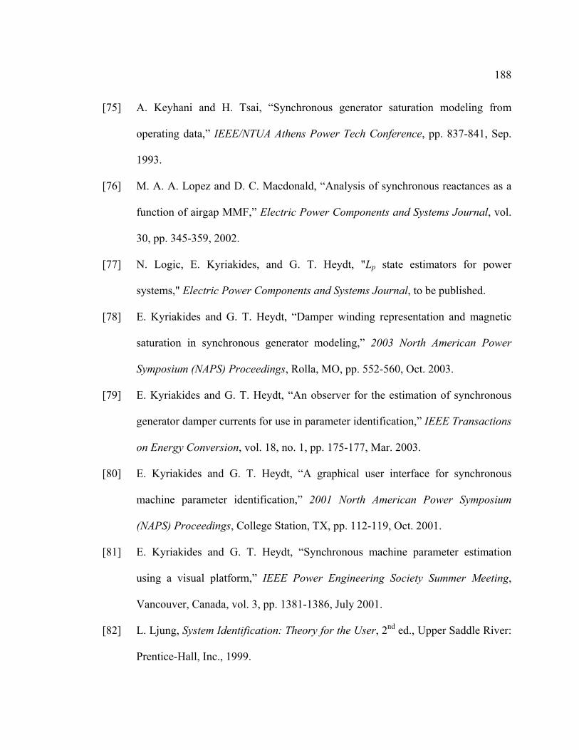
188

[75] A. Keyhani and H. Tsai, “Synchronous generator saturation modeling from

operating data,” IEEE/NTUA Athens Power Tech Conference, pp. 837-841, Sep.

1993.

[76] M. A. A. Lopez and D. C. Macdonald, “Analysis of synchronous reactances as a

function of airgap MMF,” Electric Power Components and Systems Journal, vol.

30, pp. 345-359, 2002.

[77] N. Logic, E. Kyriakides, and G. T. Heydt, "Lp state estimators for power

systems," Electric Power Components and Systems Journal, to be published.

[78] E. Kyriakides and G. T. Heydt, “Damper winding representation and magnetic

saturation in synchronous generator modeling,” 2003 North American Power

Symposium (NAPS) Proceedings, Rolla, MO, pp. 552-560, Oct. 2003.

[79] E. Kyriakides and G. T. Heydt, “An observer for the estimation of synchronous

generator damper currents for use in parameter identification,” IEEE Transactions

on Energy Conversion, vol. 18, no. 1, pp. 175-177, Mar. 2003.

[80] E. Kyriakides and G. T. Heydt, “A graphical user interface for synchronous

machine parameter identification,” 2001 North American Power Symposium

(NAPS) Proceedings, College Station, TX, pp. 112-119, Oct. 2001.

[81] E. Kyriakides and G. T. Heydt, “Synchronous machine parameter estimation

using a visual platform,” IEEE Power Engineering Society Summer Meeting,

Vancouver, Canada, vol. 3, pp. 1381-1386, July 2001.

[82] L. Ljung, System Identification: Theory for the User, 2nd ed., Upper Saddle River:

Prentice-Hall, Inc., 1999.

189

[83] IEEE Guide for Synchronous Generator Modeling Practices in Stability Analyses,

IEEE Standard 1110-1991, Mar. 1991.

[84] R. H. Park, “Two-reaction theory of synchronous machines – generalized

methods of analysis – Part I,” AIEE Transactions, vol. 48, pp. 716-727, July 1929.

[85] R. H. Park, “Two-reaction theory of synchronous machines, Part II,” AIEE

Transactions, vol. 52, pp. 352-355, June 1933.

[86] Rotating Electrical Machines. Part 10: Conventions for Description of

Synchronous Machines, IEC Standard 34-10-1975, International Electrotechnical

Commission, Geneva, 1975.

[87] IEEE Standard Dictionary of Electrical and Electronics Terms, IEEE Standard

100-1984, New York, 1984.

[88] H. C. Stanley, “An analysis of the induction motor,” AIEE Transactions, Vol. 57

(Supplement), pp. 751-755, 1938.

[89] G. Kron, Equivalent Circuits of Electric Machinery, New York: John Wiley and

Sons, Inc., 1951.

[90] D. S. Brereton, D. G. Lewis, and C. G. Young, “Representation of induction

motor loads during power system stability studies,” AIEE Transactions, vol. 76,

pp. 451-461, Aug. 1957.

[91] W. A. Lewis, “A basic analysis of synchronous machines, Pt. 1,” AIEE

Transactions on Power Apparatus and Systems, vol. PAS-77, pp. 436-455, 1958.

190

[92] P. C. Krause and C. H. Thomas, “Simulation of symmetrical induction

machinery,” IEEE Transactions on Power Apparatus and Systems, vol. PAS-84,

pp. 1038-1052, 1965.

[93] S. A. Nasar and L. E. Unnewehr, Electromechanics and Electric Machines, New

York: John Wiley & Sons, Inc., 1979.

[94] A. M. El-Serafi and A. S. Abdallah, “Saturated synchronous reactances of

synchronous machines,” IEEE Transactions on Energy Conversion, vol. 7, no.3

pp. 570-579, Sep. 1992.

[95] M. S. Sarma, Synchronous Machines: Their Theory, Stability, and Excitation

Systems, New York: Gordon and Breach, Science Publishers, Inc., 1979.

[96] N. C. Kar, T. Murata, and J. Tamura, “A new method to evaluate the q-axis

saturation characteristic of cylindrical-rotor synchronous generator,” IEEE

Transactions on Energy Conversion, vol. 15, no. 3, pp. 269-276, Sep. 2000.

[97] K. Ide, S. Wakui, K. Shima, M. Takahashi, K. Miyakawa, and Y. Yagi, “Analysis

of saturated synchronous reactances of large turbine generator by considering

cross-magnetizing reactances using finite elements,” IEEE Transactions on

Energy Conversion, vol. 14, no. 1, pp. 66-71, Mar. 1999.

[98] E. Levi, “Modelling of magnetic saturation in smooth air-gap synchronous

machines,” IEEE Transactions on Energy Conversion, vol. 12, no. 2, pp.151-156,

June 1997.

191

[99] S. A. Tahan and I. Kamwa, “A two-factor saturation model for synchronous

machines with multiple rotor circuits,” IEEE Transactions on Energy Conversion,

vol. 10, no. 4, pp. 609-616, Dec. 1995.

[100] A. M. El-Serafi and N. C. Kar, “Methods for determining the Q-axis saturation

characteristics of salient-pole synchronous machines from the measured D-axis

characteristics,” IEEE Transactions on Energy Conversion, vol. 18, no. 1, pp. 80-

86, Mar. 2003.

[101] E. W. Kimbark, Power System Stability, Vol. III, New York: John Wiley & Sons,

Inc., 1956.

[102] D. Schröder, Intelligent Observer and Control Design for Nonlinear Systems,

Berlin: Springer, 2000.

[103] W. J. Rugh, Linear System Theory, Upper Saddle River: Prentice Hall, 1996.

[104] W. S. Levine, The Control Handbook, New York: IEEE Press, 1996.

[105] T. Kailath, Linear Systems, Englewood Cliffs: Prentice-Hall, 1980.

[106] G. H. Golub and C. F. Van Loan, Matrix Computations, Baltimore: The Johns

Hopkins University Press, 1996.

[107] D. S. Watkins, Fundamentals of Matrix Computations, 2nd ed., New York: John

Wiley & Sons, Inc., 2002.

[108] A. Bjerhammar, Theory of Errors and Generalized Matrix Inverses, Amsterdam:

Elsevier Scientific Publishing Company, 1973.

[109] R.L. Branham, Jr., Scientific Data Analysis, An Introduction to Overdetermined

Systems, New York: Springer-Verlag, 1990.

192

[110] P. S. Laplace, marquis de Bowditch, Celestial Mechanics, Vol. 1-4, (translation),

Bronx, NY: Chelsea, 1966.

[111] A. M. Legendre, Nouvelles méthodes pour la détermination des orbites des

comètes, 1805.

[112] V. Chvátal, Linear Programming, New York: W. H. Freeman and Company,

1983.

[113] G. Strang, Introduction to Linear Algebra, Wellesley: Wellesley-Cambridge

Press, 1998.

[114] E. Kyriakides, “On-line estimation of synchronous generator parameters using a

visual platform,” Ph.D. Qualifying Examination Report, Dept. of Electrical

Engineering, Arizona State University, Tempe, Apr. 2001.

[115] S. Haykin and B. Van Veen, Signals and Systems, New York: John Wiley &

Sons, Inc., 1999.

[116] IEEE Standard Common Format for Transient Data Exchange (COMTRADE) for

Power Systems, IEEE Standard C37-111.1999, Mar. 1999.

[117] E. S. Pearson and H. O. Hartley, Biometrika Tables for Statisticians, vol.1, 1966.

[118] General Electric Company, “No load saturation curve,” Schenectady, New York,

1971.

[119] General Electric Company, “Generator data for stability study, Revision 7,”

Schenectady, New York, 1971.

APPENDIX A

CALCULATION OF SYNCHRONOUS GENERATOR PARAMETERS

194

A.1 Introduction

This Appendix offers a comprehensive treatment of the calculation of generator

parameters from the stability study data sheet and the generator saturation curve as

provided by the generator manufacturer. The parameter calculation is based on the

consideration that the model to be developed is Model 2.2 as defined in IEEE standards

[83], and the derivation of the model equation as developed in Section 2.5.

As noted in Section 6.2, in order to ascertain the validity of the program it is

necessary to test it with both synthetic data (user generated) and EMTP simulated noise

free data. This testing necessitates the knowledge of the operating parameters of the

generator under consideration. Further, when real data are used to perform the

estimation, knowledge of the operational parameters will provide a higher degree of

confidence in the estimated parameters.

To demonstrate the process for the calculation of generator parameters from

manufacturer data, a sample generator is considered. This generator is a cross-compound

generator located in the southwest U.S.A., rated at 483 MVA. The manufacturer stability

study data sheet and the generator saturation curve for the generator under consideration

are provided in Appendix B.

A.2 Calculation of generator parameters

Table A.1 shows the quantities that are obtained from the stability study data

sheet in order to calculate the generator parameters. Furthermore, from the generator

saturation curve it is possible to calculate the value of the field current at rated voltage (1

195

p.u.). This value is obtained from the air gap line of the no-load saturation curve in

Appendix B. Hence,

A1226=FratedI . (A.1)

TABLE A.1

Available quantities from manufacturer stability study data sheet

Quantity Value

Rated power 483 MVA

Rated Voltage 22 kV, Y connected

dx 1.80 p.u.

dvx′ 0.27 p.u.

dvx ′′ 0.19 p.u.

qx 1.72 p.u.

qx′ 0.49 p.u.

qvx ′′ 0.19 p.u.

lx 0.16 p.u.

0x 0.15 p.u.

r 0.0046 p.u.

0dτ ′ 3.7 s

0dτ ′′ 0.032 s

0qτ ′ 0.49 s

0qτ ′′ 0.059 s

196

Stator base quantities

p.u64.1H10359284.464.1

p.u.64.116.080.1

radians377

1602

11

H106581.246273.60126752

706.12701

0020704.146273.12675706.12701

A46273.12675706.12701

161

V706.127013

22000

phaseMVA1613

483

3

3

=⇒×==⇒

=−=−=−==

===

×===

Ω===

===

==

==

−

−

AD

Bmd

LmdddmdAD

RB

B

BB

B

BB

B

BB

B

B

LLL

xxLLL

t

IVL

IVR

VMVA

VSI

V

S

l

πω

πω

(A.2)

To obtain MF:

At open circuit the mutual inductance LaF and the flux linkage in phase a are

given by:

ϑλϑ cos,cos FFaFaF MiML == . (A.3)

The instantaneous voltage of phase a is ϑω sinFRFa Miv = , where Rω is the rated

synchronous speed [14]. Hence, the peak phase voltage is equal to FRF Mi ω .

From the air gap line of the no-load saturation curve in Appendix B, the value of

the field current at rated voltage (1 p.u.) is 1226 A.

Hence,

H1086471277.382 3−×=⇒= FF

BF M

iVMω

. (A.4)

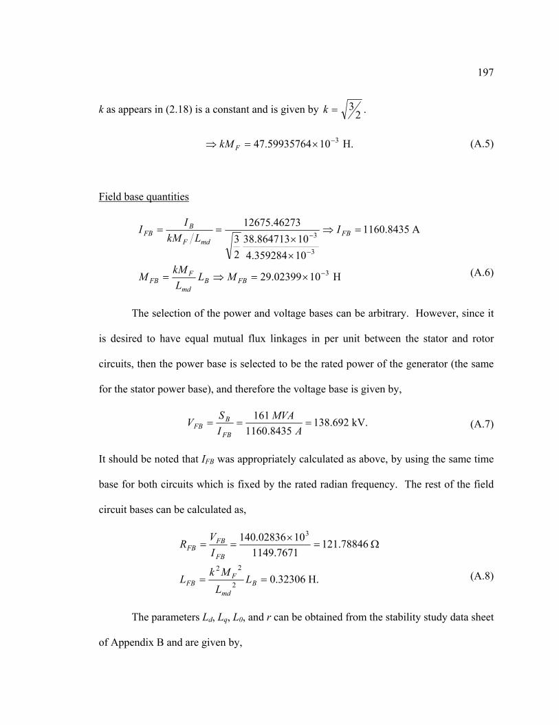
197

k as appears in (2.18) is a constant and is given by 23=k .

H.1059935764.47 3−×=⇒ FkM (A.5)

Field base quantities

H1002399.29

A8435.1160

10359284.410864713.38

23

46273.12675

3

3

3

−

−

−

×=⇒=

=⇒

××

==

FBBmd

FFB

FBmdF

BFB

MLL

kMM

ILkM

II

(A.6)

The selection of the power and voltage bases can be arbitrary. However, since it

is desired to have equal mutual flux linkages in per unit between the stator and rotor

circuits, then the power base is selected to be the rated power of the generator (the same

for the stator power base), and therefore the voltage base is given by,

kV.692.1388435.1160

161===

AMVA

ISVFB

BFB (A.7)

It should be noted that IFB was appropriately calculated as above, by using the same time

base for both circuits which is fixed by the rated radian frequency. The rest of the field

circuit bases can be calculated as,

H.32306.0

78846.1217671.1149

1002836.140

2

22

3

==

Ω=×

==

Bmd

FFB

FB

FBFB

LLMkL

IVR

(A.8)

The parameters Ld, Lq, L0, and r can be obtained from the stability study data sheet

of Appendix B and are given by,

198

p.u.0046.0.p.u150.0

p.u.72.1p.u.80.1

1

000=⇒====

=⇒==⇒==⇒=

rRrrrrLxLLxLLxL

cba

qqq

ddd

(A.9)

First, the d axis quantities are calculated. Using the direct axis equivalent circuit

of Fig. A.1, it can be shown that in per unit,

.p.u64.1====−=−=−== XDFddFFDDADmd MkMkMLLLLL lll (A.10)

LAD

rF

id

vF

ωλ q

id+iF+iD

lF

iF

vd

iD

ld

lD

rD

r

vD=0

Fig. A.1. Direct axis equivalent circuit [13], [14]

Fig. A.2(a) and Fig. A.2(b) show the equivalent circuits for the d axis inductances

in the transient and subtransient case respectively. By inspection of Fig. A.2(a),

p.u.75791.164.111791.0p.u.11791.0)]27.08.1/()16.027.0[(64.1)]/()[(

=⇒+=+==−−=′−−′=

FADFF

ddddADFLLL

LLLLl

ll (A.11)

By inspection of Fig. A.2(b),

199

)()()(

1111

ddADddFFAD

ddFADD

FDAD

dd LLLLLL

LL

llll

lll

ll

l−′′−−′′−

−′′=⇒

+++=′′ . (A.12)

All the values in the right hand side of (A.12) are known. Therefore,

p.u.68125.1p.u.04125.0

=⇒+==

DADDD

DLLL l

l (A.13)

lF

LADLd

'

ld

(a)

Ld' '

ld

LAD

lF

lD

(b)

Fig. A.2. Equivalent circuits for d axis inductances:

(a) transient inductance, (b) subtransient inductance [13], [14]

The field resistance can be found in three ways. It may be provided in the

manufacturer data sheets or even supplied by the utility in the case that it has been

measured on site. A third way is to be calculated by observing that the time constant of

200

the transient current of the field winding is actually the d axis transient open circuit time

constant 0dτ ′ [14]. Hence,

F

Fd r

Lτ =′ 0 . (A.14)

However, in this case, the field resistance is supplied by APS and is given by,

p.u.10722.9 4−×=Fr (A.15)

The damper winding resistance can be estimated from the d axis subtransient time

constant as shown below [14]:

++

′′=

FAD

DdB

D

lL

lτω

r11

11

0 p.u.01253759.0=⇒ Dr (A.16)

The q axis quantities are calculated similarly to the d axis quantities. Fig. A.3

shows the quadrature axis equivalent circuit with two damper windings denoted G and Q.

The leakage inductance of the quadrature axis ql is equal to the leakage inductance of the

direct axis dl .

.p.u56.1====−=−=−= YQGqqQQGGAQ MkMkMLLLL lll (A.17)

Similar to the development of the equations for the direct axis from the transient and

subtransient circuits,

p.u.978536.1p.u.4185365854.0)]/()[(

=⇒+==′−−′=

GAQGG

qqqqAQG

LLLLLLL

l

ll

(A.18)

201

p.u.593.1

p.u.033.0)()(

)(

=⇒+=

=⇒−′′−−′′−

−′′=

QAQQQ

QqqAQqqGGAQ

qqGAQQ

LLL

lLLLL

LL

l

llll

lll

(A.19)

LAQ

rQ

iq

vQ=0

ωλ d

iq+iG+iQ

lQ

iQ

vq

iG

lq

lG

rG

r

vG=0

Fig. A.3. Quadrature axis equivalent circuit [13], [14]

The damper winding resistances for the q axis are given by,

p.u.0107107.00

=⇒′+

= GqB

GAQG r

τωlL

r (A.20)

++

′′=

GAQ

QqB

Q

lL

lτω

r11

11

0 p.u.01632.0=⇒ Qr (A.21)

Finally, the equivalent neutral resistance and inductance are supplied by APS and

are given by,

p.u.100p.u.100

==

n

nLr

(A.22)

APPENDIX B

SATURATION CURVE AND STABILITY STUDY DATA SHEET FOR A SAMPLE

SYNCHRONOUS GENERATOR

203

B.1 Generator saturation curve

Fig. B.1 shows the saturation curve used in the calculation of machine constants

in Appendix A. This curve is for generator FC5HP that is located at the Four Corners

Generating Station of APS.

Fig. B.1. Saturation curve for the Four Corners generating station unit #5 [118]

204

B.2 Stability Study Data Sheet

Fig. B.2 shows the stability study data sheet that has been used to calculate the

synchronous generator parameters in Appendix A.

Fig. B.2. Stability study data for the Four Corners generating station unit #5 [119]

APPENDIX C

OVERVIEW OF PROPOSED MAGNETIC SATURATION FUNCTIONS

206

C.1 Introduction

In order to implement the saturation of generator inductances effectively, it is

necessary to model the saturation curve as supplied by the manufacturer as accurately as

possible. As mentioned in Chapter 3, various saturation functions have been proposed in

the literature with varying degrees of accuracy. This appendix examines a number of

proposed saturation models (both existing models and new proposed models). The

comparison between the computed saturation curve and the actual saturation curve will

indicate the best saturation function out of the proposed models.

C.2 Proposed saturation functions

A number of candidate generic models are examined in this section. These

models are depicted in Table C.1. Other candidate models have also been examined but

only the three proposed models of Table C.1 will be discussed for demonstration

purposes.

TABLE C.1

Candidate saturation function models

Model number Saturation function

1 )( 0VVBI

teAλ −⋅=

2 cVbVaλ ttI ++= 24 )()(

3 cVVbVVaλ ttI +−+−= )sinh()cosh( 00

207

C.3 Comparison of saturation functions to the actual saturation curve

Fig. C.1 depicts the actual saturation curve for a synchronous generator. Both the

air-gap line and the open circuit characteristic (OCC) are shown. The saturation curve

was duplicated from the actual saturation curve of Appendix B.

In order to plot the saturation functions from the proposed models, the constants

in the model equations need to be assigned a numerical value. V0 is the threshold

saturation constant as mentioned in Chapter 3, and can be obtained by direct observation

of the saturation curve in Fig. C.1. λI is the saturation function and it is assigned the

value of zero for 0VVt < in order to obtain the air-gap line up to V0. The constants A, B,

a, b, and c are calculated by using data from the actual saturation curve. It should be

noted that instead of terminal voltages, flux linkages may also be used as described in

Chapter 3. Model 1 needs two data points to create a system of two equations in two

unknowns, while models 2 and 3 need three data points.

The results of the simulation of the three models are depicted in Figs C.2-C.4.

Fig. C.2 shows the saturation curve obtained using the first model. This is the model that

is used extensively to model saturation in contemporary practices. Comparison to the

saturation curves obtained from the other models in Figs C.3 and C.4 verifies that this

model is superior to any of the other models that have been proposed.

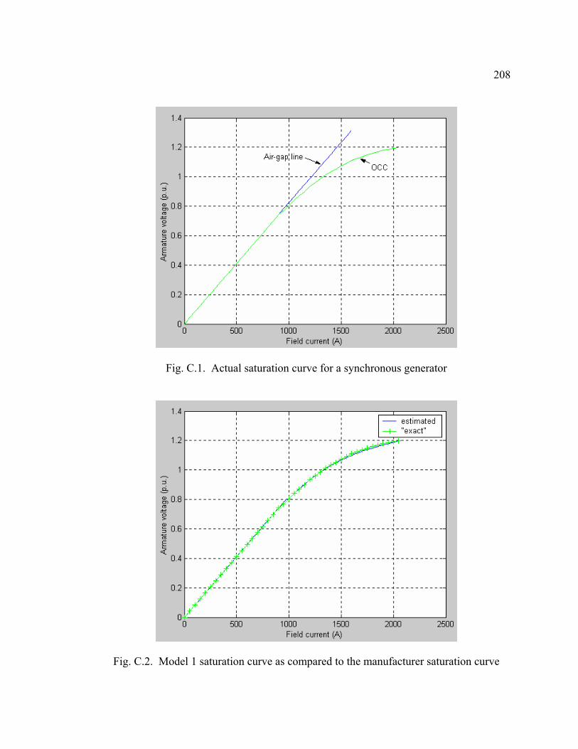
208

Fig. C.1. Actual saturation curve for a synchronous generator

Fig. C.2. Model 1 saturation curve as compared to the manufacturer saturation curve

209



APPENDIX D

SELECTION OF THE NUMERICAL DIFFERENTIATION FORMULA

211

D.1 Selection of the numerical differentiation formula

The synchronous machine model of (2.22) and (3.11) raises the need to

approximate the derivative of the measured signals by an appropriate differentiation

formula. In order to select a suitable differentiation formula, a scalar differential

equation was selected to perform a number of case studies. These case studies include

the testing of various candidate methods, as well as the estimation of the parameters in

both noise free and noise contaminated environments. The results obtained by these case

studies will give some indication or reassurance for the most appropriate method to be

utilized in the actual model of the synchronous machine.

Assume that it is desired to estimate parameters a and b in a model of the form,

baxx +=& , (D.1)

where x is considered to be a measured scalar signal. This model is the scalar equivalent

model of the model developed for the purposes of this dissertation. Let 1−=a and

1=b , so that the differential equation becomes,

1+−= xx& , (D.2)

which has the solution,

1)( += −tetx . (D.3)

Noise free data can be constructed by the solution of (D.3) and noise can be added

as necessary to create data with various signal to noise ratios (SNRs). Moreover, since

the time vector t can be arbitrarily selected, a number of case studies may be performed

with different time steps to enable comparison of all methods depending on both the level

of noise and the time step used.

212

Tables D.1 and D.2 show two representative case studies. The first case study

considers noise free data with a time step of 0.1 s, while the second case study considers

data that have been contaminated with noise to create a SNR of 200 and that also have a

time step of 0.1 s.

TABLE D.1

Estimation of parameters for ∆T = 0.1 and SNR = ∞ (case study S-NF-02-13)

Method a b

Trapezoidal rule -0.9992 0.9992

Simpson’s rule -1.0000 1.0000

Forward difference formula -0.9516 0.9516

Third order difference form. -0.9998 0.9998

Fifth order diff. formula -1.0000 1.0000

TABLE D.2

Estimation of parameters for ∆T = 0.1 and SNR = 200 (case study S-NC-02-14)

Method a b

Trapezoidal rule -1.01707 1.01719

Simpson’s rule -1.02162 1.01933

Forward difference formula -0.99029 1.00097

Third order difference form. -1.15118 1.24195

Fifth order diff. formula -1.11691 1.12961

213

Tables D.3 and D.4 compare the two case studies that are displayed in Tables D.1

and D.2. In particular, the percent errors for parameters a and b are computed for each

method, and for both noise free and noise contaminated measurements. Table D.5 ranks

the five methods in order of increasing error. The top ranked method exhibits the smaller

percent error in each case study.

TABLE D.3

Comparison of percent relative error in estimating parameter a for case studies

S-NF-02-13 and S-NC-02-14

Simpson’s Trapezoidal 1st order 3rd order 5th order

No noise 0 0.08 4.84 0.02 0

Noise 2.16 1.71 0.97 15.12 11.7

TABLE D.4

Comparison of percent relative error in estimating parameter b for case studies

S-NF-02-13 and S-NC-02-14

Simpson’s Trapezoidal 1st order 3rd order 5th order

No noise 0 0.08 4.84 0.02 0

Noise 1.93 1.72 0.10 24.2 12.96

214

TABLE D.5

Ranking of the methods in order of increasing error

NO NOISE NOISE

1. Simpson’s 1. Forward difference

2. Fifth order 2. Trapezoidal

3. Third order 3. Simpson’s

4. Trapezoidal 4. Fifth order

5. Forward difference 5. Third order

A number of other case studies were performed for various signal to noise ratios.

Fig. D.1 shows the relative error in parameter a for a time step of 0.1 s. Fig. D.2 shows

the relative error in parameter a for a time step of 0.2 s, while Fig. D.3 shows the relative

error in parameter a for a time step of 0.05 s. From the three graphs it can be seen that in

general the Trapezoidal and the Simpson’s rule give better estimates at low signal to

noise ratios (i.e. in heavily polluted measurements). However, the errors obtained at

these levels are in the order of 20% or higher, and therefore the results are not useful

unless a noise filter is introduced. Therefore, one should direct the attention to slightly

higher signal to noise ratios where the estimates are considered reasonable.

For the case studies where the signal to noise ratios are in the order of 400 and

above, three methods seem to prevail: the Trapezoidal, the Simpson’s, and the forward

difference formula. The forward difference formula seems to offer better results than the

other two methods. In conjunction with the ranking of Table D.5 (where the forward

215

difference formula was ranked as the best in a noisy environment), a decision can be

made for the implementation of the forward difference formula for the numerical

differentiation of the problem at hand.

Fig. D.1. Relative error in parameter a for ∆T = 0.1 and for various SNRs

216



APPENDIX E

DATA FORMATS SUPPORTED BY THE ESTIMATOR

218

E.1 Introduction

As mentioned in Chapter 9, there are two data formats that are supported by the

Estimator: an abc data format that can be read as a text file (.txt extension), and a

combination of two data files that follow the COMTRADE format of the IEEE Std. C37-

111.1999 (.cfg and .dat extensions) [116]. The purpose of having two data formats

supported by the Estimator is to accommodate all possible configurations of data files

currently used by utilities. The COMTRADE format data file is the output of digital fault

recorders (DFRs) that are typically used for recording measurements at the terminals of a

synchronous generator, while .txt files can be generated using a variety of word

processors. An example of each data format is shown in Sections E.2 and E.3

respectively.

E.2 Text file (abc) data format

Input data in the form of a text file (.txt extension) is a convenient data format for

data that have been preprocessed after the required measurements have been obtained

from the data recording device. The data are arranged in columns in the order shown in

Table E.1. There are nine columns that are required. The first column contains the time

measurement, while the remaining eight columns contain the stator and field voltages and

currents.

219

TABLE E.1

Arrangement of data in the text format data file

Time (s)

Vab (kV)

Vbc (kV)

Vca (kV)

VF (V)

Ia (kA)

Ib (kA)

Ic (kA)

IF (kA)

0 -29.4 20.9 8.5 274.0 -2.37 1.23 1.05 1.19

4.70x10-4 -30.3 16.6 13.6 114.0 -2.46 0.97 1.40 1.16

9.40x10-4 -30.2 12.0 18.2 -60.7 -2.37 0.53 1.75 1.12

1.41x10-3 -29.1 6.8 22.2 -231.0 -2.19 0.09 2.02 1.08

1.88x10-3 -27.0 1.3 25.4 311.0 -1.93 -0.44 2.28 1.18

E.3 COMTRADE data format

The second option that is supported by the Estimator is the format that is based on

the COMTRADE data format which is an IEEE standard. A DFR outputs two data files,

the first being a configuration data file containing general information for the signals,

while the second file is a .dat file and contains the measurements at the generator

terminals.

A sample configuration file can be seen in Fig. E.1. A thorough explanation of

each item in the configuration file is offered in [116]. In general, the first two lines in the

file contain the heading and the number of channels that were used to record data. The

next section of the file that is arranged in numerical order contains information for each

measurement. This information contains the channel number, the generator unit under

study, the quantity that is being measured in that channel, the unit of measurement (e.g. V

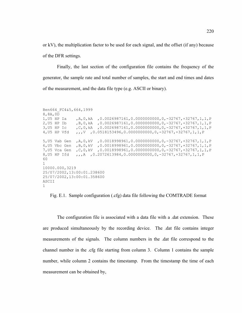
220

or kV), the multiplication factor to be used for each signal, and the offset (if any) because

of the DFR settings.

Finally, the last section of the configuration file contains the frequency of the

generator, the sample rate and total number of samples, the start and end times and dates

of the measurement, and the data file type (e.g. ASCII or binary).

Ben664_FC4&5,664,1999 8,8A,0D 1,U5 HP Ia ,A,0,kA ,0.0026987161,0.0000000000,0,-32767,+32767,1,1,P 2,U5 HP Ib ,B,0,kA ,0.0026987161,0.0000000000,0,-32767,+32767,1,1,P 3,U5 HP Ic ,C,0,kA ,0.0026987161,0.0000000000,0,-32767,+32767,1,1,P 4,U5 HP Vfd ,,,V ,0.0518153496,0.0000000000,0,-32767,+32767,1,1,P

5,U5 Vab Gen ,A,0,kV ,0.0018998961,0.0000000000,0,-32767,+32767,1,1,P 6,U5 Vbc Gen ,B,0,kV ,0.0018998961,0.0000000000,0,-32767,+32767,1,1,P 7,U5 Vca Gen ,C,0,kV ,0.0018998961,0.0000000000,0,-32767,+32767,1,1,P 8,U5 HP Ifd ,,,A ,0.2072613984,0.0000000000,0,-32767,+32767,1,1,P 60 1 10000.000,3219 25/07/2002,13:00:01.238600 25/07/2002,13:00:01.358600 ASCII 1

Fig. E.1. Sample configuration (.cfg) data file following the COMTRADE format

The configuration file is associated with a data file with a .dat extension. These

are produced simultaneously by the recording device. The .dat file contains integer

measurements of the signals. The column numbers in the .dat file correspond to the

channel number in the .cfg file starting from column 3. Column 1 contains the sample

number, while column 2 contains the timestamp. From the timestamp the time of each

measurement can be obtained by,

221

sµtimemulttimestampt )()( ×= , (E.1)

where timemult is the timestamp multiplication factor obtained from the last line of the

.cfg file. A sample .dat file can be seen in Fig. E.2.

1, 0, -5104, -192, 5184, 11328, -8192, -8128, 16256, 12240 2, 100, -4976, -432, 5296, 10432, -7664, -8640, 16240, 12304 3, 200, -4864, -640, 5392, 9840, -7104, -9168, 16208, 12352 4, 300, -4736, -864, 5472, 9136, -6528, -9696, 16144, 12368 5, 400, -4592, -1088, 5552, 8336, -5952,-10176, 16048, 12384 6, 500, -4448, -1312, 5632, 7680, -5376,-10656, 15952, 12400 7, 600, -4304, -1504, 5696, 6912, -4784,-11104, 15824, 12400 8, 700, -4144, -1728, 5760, 6112, -4192,-11552, 15664, 12384 9, 800, -3984, -1936, 5808, 5376, -3600,-11968, 15488, 12384 10, 900, -3824, -2128, 5840, 4624, -3008,-12384, 15296, 12368 11, 1000, -3664, -2336, 5872, 3840, -2416,-12768, 15104, 12352 12, 1100, -3488, -2528, 5904, 3072, -1824,-13152, 14880, 12320 13, 1200, -3312, -2720, 5904, 2304, -1216,-13504, 14640, 12288 14, 1300, -3120, -2912, 5920, 1520, -608,-13856, 14384, 12272

Fig. E.2. Sample data (.dat) file following the COMTRADE format

APPENDIX F

PARAMETER ESTIMATION RESULTS USING ACTUAL DATA

223

F.1 Estimation of parameters for two steam turbine generators

Parameter estimation results in Chapter 8 for generators FC5HP, GT1, and GT2

indicated good correlation between manufacturer supplied parameters and estimated

parameters at different operating points. The increase in the excitation levels of the gas

turbines GT1 and GT2 indicated a general decreasing trend in the estimated mutual

inductances. This was expected from synchronous generator theory. Further, the

correction factor applied for saturation resulted in unsaturated inductances with very

small variations.

This appendix offers parameter results from two steam turbine generators located

at the Redhawk generating station of APS. Seven data sets from generator ST1 and one

data set from generator ST2 are analyzed. The two generators are rated at 213.7 MVA

and 18 kV. The manufacturer supplied inductances LAD and LAQ are 1.924 p.u. and 1.79

p.u. respectively. The characteristics for the two generators are described in Table 3.1.

The analysis procedure is similar to the one provided in Chapter 8. Three

parameters were estimated from each data set: LAD, LAQ, and rF. The operating point of

the generator for each data set is shown, as well as the field current. Table F.1 depicts the

parameter estimation results for the eight data sets obtained from the two units, as well as

information regarding the operating point, the estimated inductances corrected for

saturation, and the deviation from the manufacturer supplied parameters.

224

TABLE F.1

Parameter estimation results for Redhawk steam turbines 1 and 2*

% deviation Case study Unit # ADL

(p.u.) AQL

(p.u.) Fr

(p.u.) Ksd iF

(A) P

(MW) Q

(MVAr) ADuL

(p.u.) AQuL

(p.u.) LAD LAQ

R-NC-03-26 ST1 1.5243 1.7871 6.6587x10-4 0.9285 1015.8 167.13 24.28 1.6417 1.9247 14.7 7.5

R-NC-03-27 ST1 1.5891 1.7862 6.3587x10-4 0.8842 819.85 123.91 6.90 1.7972 2.0201 6.6 12.9

R-NC-03-28 ST1 1.5734 1.752 6.2501x10-4 0.8864 890.22 138.62 13.29 1.7750 1.9765 7.7 10.4

R-NC-03-29 ST1 1.6843 1.7956 5.5220x10-4 0.8831 650.36 61.34 4.19 1.9073 2.0333 0.9 13.6

R-NC-03-30 ST1 1.6015 1.7021 6.2198x10-4 0.8834 855.89 125.55 15.49 1.8129 1.9268 5.8 7.6

R-NC-03-31 ST1 1.5646 1.8458 6.9660x10-4 0.8833 882.95 140.35 11.25 1.7713 2.0897 7.9 16.7

R-NC-03-32 ST1 1.5401 1.814 7.3236x10-4 0.8889 918.56 146.58 15.79 1.7326 2.0407 9.9 14.0

R-NC-03-33 ST2 1.5252 1.7852 6.5160x10-4 0.8802 930.34 144.49 16.75 1.7328 2.0281 9.9 13.3

Mean (µ) 6.4768x10-4 1.7714 2.0050

Standard deviation (σ)

2.55 x10-9 0.0051 0.0029

* From the manufacturer data sheet: LAD = 1.924 p.u., LAQ = 1.79 p.u., while rF is unavailable

225

It should be noted that there are two potential factors that may affect the results

obtained for these two particular generators. Firstly, the stator resistance for the two units

is not supplied by the manufacturer. Therefore, an arbitrary (but typical) value for the

resistance needs to be used in the estimation process. The estimates will certainly be

affected by this inaccuracy, since the calculation of the power angle δ and some of the

elements in the measurement vector z depend or the stator resistance. Secondly, the field

voltage and current multiplication factors from the DFR are reversed in the configuration

data file. Although this is corrected after the data files are read by the Estimator, the

calibration of the channels is probably slightly off. This will mostly affect the estimate of

the field resistance, but will also have an impact on the other estimated parameters.

Fig. F.1 shows the change in the estimated direct axis mutual inductance LAD with

the field current. A linear regression model is fitted to observe the trend in the estimated

inductance over increasing saturation levels. A significant decrease in the apparent value

of the inductance is observed as the generator is driven to higher operating points.

Fig. F.2 compares both the saturated and the unsaturated values of LAD for all case

studies for the steam turbine generators. The stacked column graph shows the estimated

parameters and the correction for saturation. The unsaturated values of LAD have a mean

of 1.7714 p.u. and a standard deviation of 0.0051 p.u.

The results of each case study for the quadrature axis mutual inductance LAQ are

summarized in Figs F.3 and F.4. The estimated values of the quadrature axis mutual

inductance at different operating points are shown in Fig. F.3. In this case there is no

apparent trend in the saturated values of the inductance. There are four leverage points

226

(two above the mean value of the inductance and two below), causing the regression

model to be approximately a constant. The mean of the unsaturated quadrature axis

mutual inductance is 2.005 p.u. and the standard deviation is 0.0029 p.u. A comparison

between the unsaturated values of LAQ at each operating point is offered in Fig. F.4,

where the saturated inductances are corrected for saturation using the appropriate

saturation factors at each operating point.

1.48

1.5

1.52

1.54

1.56

1.58

1.6

1.62

1.64

1.66

1.68

1.7

600 650 700 750 800 850 900 950 1000 1050

Field current (A)

L AD

(p.u

.)

Fig. F.1. Change of LAD with operating point for Redhawk steam turbine generators

227

1

1.1

1.2

1.3

1.4

1.5

1.6

1.7

1.8

1.9

2

L AD

(p.u

.)

650.36 819.85 855.89 882.95 890.22 918.56 930.34 1015.8

Field current (A)

Estimated LAD LAD corrected for saturation Fig. F.2. Saturated and unsaturated values of LAD for Redhawk steam turbine generators

1.6

1.65

1.7

1.75

1.8

1.85

1.9

600 650 700 750 800 850 900 950 1000 1050

Field current (A)

L AQ

(p.u

.)

Fig. F.3. Change of LAQ with operating point for Redhawk steam turbine generators

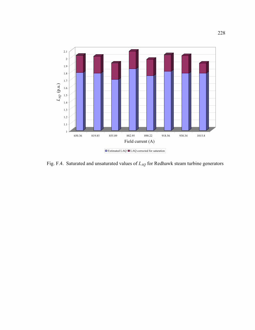
228

1

1.1

1.2

1.3

1.4

1.5

1.6

1.7

1.8

1.9

2

2.1

L AQ

(p.u

.)

650.36 819.85 855.89 882.95 890.22 918.56 930.34 1015.8

Field current (A)

Estimated LAQ LAQ corrected for saturation

Fig. F.4. Saturated and unsaturated values of LAQ for Redhawk steam turbine generators

APPENDIX G

MATLAB CODE FOR PARAMETER ESTIMATION USING ACTUAL

MEASUREMENTS

230

%************************************************************************************ %*Estimation of synchronous generator parameter using actual DFR measurements * %*As an example, this m-file estimates the parameters of Redhawk GT1 gas turbine * %*This file estimates the generator parameters per model 2.2x * %*One damper winding in d-axis, and two damper windings in q-axis * %*All inductances are written in terms of LAD, LAQ, and leakage inductances * %*Copyright: Elias Kyriakides * %*Last updated: November 2, 2003 * %************************************************************************************ clear all; mvab = (213.7e6)/3; %MVA base kvb = 18000/sqrt(3); %voltage base ib = mvab/kvb; %current base cfb = 560.8695433; %field current base vfb = mvab/cfb; %field voltage base ns = 7; %no. of states %Read data file dummy = csvread('C:\My Documents\RESEARCH\external data\realdataRedhawk\GT1A.dat'); %Input multiplication factors from .cfg file m1 = 0.0014249221; %Vab m2 = 0.0014249221; %Vbc m3 = 0.0014249221; %Vca m4 = 0.0013817426; %Ia m5 = 0.0013817426; %Ib m6 = 0.0013817426; %Ic m7 = 0.1036306992; %IF m8 = 0.0259076748; %VF timemult = 1; %time multiplication factor t(:,1)=dummy(:,2); nt = length(t1); %To initialize iabc and vabc vabc=zeros(nt,ns); iabc=zeros(nt,ns); vabc(:,1)=dummy(1:nt,3); %phase A-B line-line voltage vabc(:,2)=dummy(1:nt,4); %phase B-C line-line voltage vabc(:,3)=dummy(1:nt,5); %phase C-A line-line voltage iabc(:,1)=dummy(1:nt,6); %phase A current iabc(:,2)=dummy(1:nt,7); %phase B current iabc(:,3)=dummy(1:nt,8); %phase C current ifl(:,1)=dummy(1:nt,9); %field current vfl(:,1)=dummy(1:nt,10); %field voltage

231

%Multiply read data by the relevant multiplication factors: t = t*(timemult*1E-6); %readings in microseconds vabc(:,1) = vabc(:,1)*m1*1000; %readings in kV vabc(:,2) = vabc(:,2)*m2*1000; %readings in kV vabc(:,3) = vabc(:,3)*m3*1000; %readings in kV iabc(:,1) = iabc(:,1)*m4*1000; %readings in kA iabc(:,2) = iabc(:,2)*m5*1000; %readings in kA iabc(:,3) = iabc(:,3)*m6*1000; %readings in kA ifl = ifl*m7; vfl = vfl*m8; vfl=-vfl; %in the Park's voltage equations field voltages are negative %Field measurements filters %Plots of unfiltered quantities plot(t,vfl) title('Plot of VF data') xlabel('time (s)') ylabel('VF') figure; plot(t,ifl) title('Plot of iF data') xlabel('time (s)') ylabel('iF') figure; %and their FFT: dt=t(2)-t(1); % define time between samples N=nt; %define number of samples h=fft(vfl)/N; % take fft h=fftshift(h); % rotate to center zero frequency Fnq=1/(2*dt); % calc maximum frequency T=N*dt; % calc period of waveshape df=1/T; % calc frequency resolution fq=-Fnq+[0:(N-1)]'*df +df/2; % create frequency vector for plot mag=abs(h); % magnitude of fft plot(fq(1:N), mag,'d'); ylabel('VF FFT Magnitude') figure; vfl_unfilteredFFT_zerofrcomp=real(mean(vfl)); h=fft(ifl)/N; % take fft h=fftshift(h); % rotate to center zero frequency Fnq=1/(2*dt); % calc maximum frequency

232

T=N*dt; % calc period of waveshape df=1/T; % calc frequency resolution fq=-Fnq+[0:(N-1)]'*df +df/2; % create frequency vector for plot mag=abs(h); % magnitude of fft plot(fq,mag,'d'); ylabel('IF FFT Magnitude') figure; ifl_unfilteredFFT_zerofrcomp=real(mean(ifl)); %Filter field voltage: %Find order and normalized frequency using the buttord function fN=1/(2*dt); %Nyquist frequency fc=50; %cutoff frequency fstop=1000;% frequency where stopband begins Wp=fc/fN; %passband corner frequency Ws=fstop/fN; %stopband corner frequency Rp=0.01; %passband ripple in dB (max permissible passband loss in dB) Rs=40; %stopband attenuation in dB (number of dB the stopband is down from the passband) [n, Wn]=buttord(Wp, Ws, Rp, Rs); [b,a]=butter(n, Wn); %order and normalized cutoff frequency vflfiltered=filtfilt(b,a,vfl); %zero phase filtering %re-filter for y=1:50 vflfiltered=filtfilt(b,a,vflfiltered); y=y+1; end %Filter field current fc=20; %cutoff frequency fstop=130;% frequency where stopband begins Wp=fc/fN; %passband corner frequency Ws=fstop/fN; %stopband corner frequency Rp=0.001; %passband ripple in dB (max permissible passband loss in dB) Rs=50; %stopband attenuation in dB (number of dB the stopband is down from the passband) [n, Wn]=buttord(Wp, Ws, Rp, Rs); [b,a]=butter(n, Wn); %order and normalized cutoff frequency iflfiltered=filtfilt(b,a,ifl);

233

%re-filter for y=1:150 iflfiltered=filtfilt(b,a,iflfiltered); y=y+1; end %Plot FFT of field voltage and current N=nt; h=fft(vflfiltered)/N; h=fftshift(h); Fnq=1/(2*dt); % calc maximum frequency T=N*dt; % calc period of waveshape df=1/T; % calc frequency resolution fq=-Fnq+[0:(N-1)]'*df +df/2; % create frequency vector for plot mag=abs(h); plot(fq,mag,'d'); ylabel('VF filtered FFT magnitude using zero phase filtering (final filter)'); xlabel('frequency') axis([-80 80 0 inf]) figure; %time data plot(t(1:N), real(vflfiltered)) ; ylabel('VF filtered time data with zero phase filtering'); xlabel('time') figure; vfl_filteredFFT_zerofrcomp=real(mean(vflfiltered)); h=fft(iflfiltered)/N; h=fftshift(h); Fnq=1/(2*dt); % calc maximum frequency T=N*dt; % calc period of waveshape df=1/T; % calc frequency resolution fq=-Fnq+[0:(N-1)]'*df +df/2; % create frequency vector for plot mag=abs(h); plot(fq,mag,'d'); ylabel('iF filtered FFT magnitude using zero phase filtering (final filter)'); xlabel('frequency') axis([-80 80 0 inf]) figure; %time data plot(t(1:N), real(iflfiltered)) ; ylabel('iF filtered time data with zero phase filtering'); xlabel('time') figure; ifl_filteredFFT_zerofrcomp=real(mean(iflfiltered)); %Up to here for filtering of field quantities. %****************************************************************************

234

%Put the filtered VF, iF back to their original vectors %Moreover, correct for any possible reduction in the amplitude of the signal because of the %filtering clear vfl ifl %because they contain the original data, now they will contain the filtered vfl=vflfiltered*(vfl_unfilteredFFT_zerofrcomp/vfl_filteredFFT_zerofrcomp); ifl=iflfiltered*(ifl_unfilteredFFT_zerofrcomp/ifl_filteredFFT_zerofrcomp); % Vfl and Ifl are written to the phase data matrices vabc(1:nt,4)=vfl; %the field quantities are stored in the 4th column in the vabc and iabc matrices iabc(1:nt,4)=ifl; % impedance/phase r=0.003; %stator per phase resistance xq=1.865; %per phase direct axis impedance % Delta calculation and phase-neutral conversion of the voltages for (e=1:nt) P(e,1)=(vabc(e,1)*iabc(e,1)-vabc(e,2)*iabc(e,3))/(3*mvab); %per phase active power in p.u. Q(e,1)=(vabc(e,1)*iabc(e,3)+vabc(e,2)*iabc(e,1)+vabc(e,3)*iabc(e,2))/(sqrt(3)*3*mvab);

%per phase reactive power in p.u. end; thetapq(1:nt,1)=atan2(Q,P); %power factor angle (atan2 takes into account all possible quadrants) %The block below calculates the angle between the voltages of two phases taking into %account the different quadrants and a possibility of "divide by zero" problem %Note: %The angle is calculated using the following equation %thetavabc(i,j)=atan(-diff. of two voltage/(sqrt(3)*sum of two voltages)) %the tolerance for avoiding the "divide by zero problem is taken to be 1e-6. for (e=1:nt) %for "nt" number of data points for (j=1:3) %for 3 phases phase1=next(j); %gets the next phase in the phase sequence A-B-C-A..... phase2=next(phase1); if (vabc(e,phase1)+vabc(e,phase2)>0) %sum of voltages greater than zero if (abs(-sqrt(3)*(vabc(e,phase1)+vabc(e,phase2)))>1e-6) %sum far greater than zero thetavabc(e,j)=pi+(atan((vabc(e,phase1)-vabc(e,phase2))/(-sqrt(3)*(vabc(e,phase1)+

abc(e,phase2))))) ; %the angle lies in the second quadrant else thetavabc(e,j)=pi+sign(vabc(e,phase1)-vabc(e,phase2))*pi/2; %sum close to zero end; elseif (vabc(e,phase1)-vabc(e,phase2)<0) %difference of voltages less than zero if (abs(-sqrt(3)*(vabc(e,phase1)+vabc(e,phase2)))>1e-6)

%sum of the voltages greater than zero thetavabc(e,j)=2*pi+(atan((vabc(e,phase1)-vabc(e,phase2))/(-sqrt(3)*(vabc(e,phase1)+ vabc(e,phase2))))); %angle lies in the 3rd quadrant else thetavabc(e,j)=2*pi+sign(vabc(e,phase1)-vabc(e,phase2))*pi/2;

%divide by zero is taken care of along with the third quadrant

235

end; else if (abs(-sqrt(3)*(vabc(e,phase1)+vabc(e,phase2)))>1e-6)

%the remaining: the first quadrant!! thetavabc(e,j)=(atan((vabc(e,phase1)-vabc(e,phase2))

/(-sqrt(3)* (vabc(e,phase1)+vabc(e,phase2))))); else thetavabc(e,j)=sign(vabc(e,phase1)-vabc(e,phase2))*pi/2; %divide by zero problem again! end; end; end; end; %End of calculation of the angle between two phases %Calculate the instantaneous phase-neutral rms voltage for (e=1:nt) for (j=1:3) phase1=next(j); phase2=next(phase1); vtrms(e,j)=(-(vabc(e,phase1)+vabc(e,phase2))/(cos(thetavabc(e,j)))/(sqrt(2)*kvb*sqrt(3))); end; end; for (e=1:nt) for (j=1:3) vabc(e,j)=vtrms(e,j)*sqrt(2)*kvb*cos(thetavabc(e,j)-pi/6); end; end; %End of conversion of voltage from line-line to phase-neutral voltage %Similar calculations are performed for getting the angle currents of the two phases. %The calculations are performed only for phase A. for (e=1:nt) phase1=2; phase2=3; if (iabc(e,phase1)+iabc(e,phase2)>0) if (abs(-sqrt(3)*(iabc(e,phase1)+iabc(e,phase2)))>1e-6) thetaia(e,1)=pi+(atan((iabc(e,phase1)-iabc(e,phase2))

/(-sqrt(3)*(iabc(e,phase1)+iabc(e,phase2))))); else thetaia(e,1)=pi+sign(iabc(e,phase1)-iabc(e,phase2))*pi/2; end; elseif (iabc(e,phase1)-iabc(e,phase2)<0) if (abs(-sqrt(3)*(iabc(e,phase1)+iabc(e,phase2)))>1e-6) thetaia(e,1)=2*pi+(atan((iabc(e,phase1)-iabc(e,phase2))

/(-sqrt(3)*(iabc(e,phase1)+iabc(e,phase2))))); else thetaia(e,1)=2*pi+sign(iabc(e,phase1)-iabc(e,phase2))*pi/2; end;

236

else if (abs(-sqrt(3)*(iabc(e,phase1)+iabc(e,phase2)))>1e-6) thetaia(e,1)=(atan((iabc(e,phase1)-iabc(e,phase2))

/(-sqrt(3)*(iabc(e,phase1)+iabc(e,phase2))))); else thetaia(e,1)=sign(iabc(e,phase1)-iabc(e,phase2))*pi/2; end; end; end; %End of calculation of angle theta for Phase A %Calculate the rms current for phase A for each time step for (e=1:nt) phase1=2; phase2=3; iarms(e,1)=-((iabc(e,phase1)+iabc(e,phase2))/(cos(thetaia(e,1)))/(sqrt(2)*ib)); end; j=sqrt(-1); %calculate the instantaneous machine generated emf by the formula %ef=vt+(r+jxq)*Ia for (e=1:nt) ef(e,1)=vtrms(e,1)+iarms(e,1)*xq*cos(pi/2-thetapq(e,1))+iarms(e,1)*r*cos(-thetapq(e,1))+j*iarms(e,1)*xq*sin(pi/2-thetapq(e,1))+j*iarms(e,1)*r*sin(-thetapq(e,1)); end; %delta is the angle between the generated emf phasor and terminal voltage phasor. delta(1:nt,1)=angle(ef(1:nt)); plot(t,delta*180/pi) title('delta unfiltered (degrees)') figure; %The instantaneous value of delta may contain large spikes which need to be smoothened out. %The filter below disregards the new value and uses the previous value in the time series if the %two adjacent values differ by 5 degrees. The value 5 degrees is arbitrary and can be varied to %obtain better results. for (e=2:nt) if (abs(delta(e)-delta(e-1))>= (5*pi/180)) delta(e)=delta(e-1); end; end; plot(t,delta*180/pi) title('delta filtered (degrees)') figure;

237

deltaunfilteredFFT_zerofrcomp=mean(delta(1:nt)); %Second filter for delta in addition to the one for the spikes. This is a moving average filter run=20; %no. of terms in the moving average filter for (e=run+1:nt) delta(e-run)=mean(delta(e-run:e-1)); end; deltafilteredFFT_zerofrcomp=mean(delta(1:nt-run)); %correct for the filter factor: delta = delta*(deltaunfilteredFFT_zerofrcomp/deltafilteredFFT_zerofrcomp); plot(t(1:nt-run),delta(1:nt-run)*180/pi) title('delta filtered (improved) (degrees)') figure; %Since time zero is arbitrary, we need to select when our time reference is located. By definition %at t=0, the axis a is aligned with the d axis, so Va should be max at time=0 %Search when Va is first maximum %For this data set, the first maximum occurs at t = 2.8ms (t(29)) %Start using data from vabc(29,:) etc, and make t(29)=0 t=(t*1000-2.8)*1E-3; %do it this way to avoid round off errors t(1:28)=[]; %remove first 28 data vabc(1:28,:)=[]; iabc(1:28,:)=[]; delta(1:28)=[]; thetavabc(1:28)=[]; nt=nt-28; %convert actual voltage and current data to dq0 parks=zeros(nt*3,3); %A test variable to get the Park's transformation matrix for each time step for (count=1:nt) theta(count)=120*pi*t(count)+delta(count)+pi/2+thetavabc(1,1)-pi/6;

%theta in the Park's transformation tp=zeros(ns,ns); %Park's transformation matrix for individual time step tp(1,1:3)=sqrt(1/2); %the first row in the Park's transformation matrix is 1/sqrt(2) %the cosine terms in the second row of the Park's transformation matrix tp(2,1)=cos(theta(count)); tp(2,2)=cos(theta(count)-(2*pi/3)); tp(2,3)=cos(theta(count)+(2*pi/3)); %the sine terms in the third row of the Park's transformation matrix tp(3,1)=sin(theta(count)); tp(3,2)=sin(theta(count)-(2*pi/3)); tp(3,3)=sin(theta(count)+(2*pi/3)); %the rest of the rows contain 1 on the diagonal for damper and field windings

238

for (e=4:ns) tp(e,e)=1; end; tp(1:3,1:3)=tp(1:3,1:3)*sqrt(2/3); temp=tp*iabc(count,1:ns)'; %convert the time series current data into dq0 currents idq0(count,1:ns)=temp'; temp=tp*vabc(count,1:ns)'; %convert the time series voltage data into dq0 voltages vdq0(count,1:ns)=temp'; %End of Park's transformation. %Filter dq0 of voltages and currents %This block filters the variation in the dq0 components of the voltage. The filter below disregards the new %value and uses the previous value in the time series if the two adjacent values differ by 10%. The figure %10% is arbitrary and can be varied to obtain better results. %If any measurement is a spike, then the whole measurement is replaced by its previous. for (e=2:nt) for (j=1:3) if (abs((vdq0(e,j)-vdq0(e-1,j))/vdq0(e-1,j))>(0.1)) vdq0(e,1:3)=vdq0(e-1,1:3); idq0(e,1:3)=idq0(e-1,1:3); end; if (abs((idq0(e,j)-idq0(e-1,j))/idq0(e-1,j))>(0.1)) vdq0(e,1:3)=vdq0(e-1,1:3); idq0(e,1:3)=idq0(e-1,1:3); end; end; end; %Take out the individual 0dq vectors from the 0dq matrices V0=vdq0(:,1); Vd=vdq0(:,2); Vq=vdq0(:,3); i0=idq0(:,1); id=idq0(:,2); iq=idq0(:,3); %Do Butterworth filters to remove frequency components above 10 Hz (approximately) N=nt; %Find order and normalized frequency using the buttord function fN=1/(2*dt); %Nyquist frequency fc=5; %cutoff frequency fstop=200;% frequency where stopband begins Wp=fc/fN; %passband corner frequency Ws=fstop/fN; %stopband corner frequency Rp=0.001; %passband ripple in dB (max permissible passband loss in dB) Rs=80; %stopband attenuation in dB (number of dB the stopband is down from the passband)

239

[n, Wn]=buttord(Wp, Ws, Rp, Rs); [b,a]=butter(n, Wn); %order and normalized cutoff frequency V0filtered=filtfilt(b,a,V0); Vdfiltered=filtfilt(b,a,Vd); Vqfiltered=filtfilt(b,a,Vq); i0filtered=filtfilt(b,a,i0); idfiltered=filtfilt(b,a,id); iqfiltered=filtfilt(b,a,iq); %re-filter for y=1:200 V0filtered=filtfilt(b,a,V0filtered); Vdfiltered=filtfilt(b,a,Vdfiltered); Vqfiltered=filtfilt(b,a,Vqfiltered); i0filtered=filtfilt(b,a,i0filtered); idfiltered=filtfilt(b,a,idfiltered); iqfiltered=filtfilt(b,a,iqfiltered); y=y+1; end %put signals back into the 0dq matrix vdq0(1:N,1)=V0filtered; vdq0(1:N,2)=Vdfiltered; vdq0(1:N,3)=Vqfiltered; idq0(1:N,1)=i0filtered; idq0(1:N,2)=idfiltered; idq0(1:N,3)=iqfiltered; % convert current dq0 data in per unit idq0pu(:,1:3)=idq0(:,1:3)/ib; idq0pu(:,4:ns)=idq0(:,4:ns)/cfb; % convert voltage dq0 data in per unit vdq0pu(:,1:3)=vdq0(:,1:3)/kvb; vdq0pu(:,4:ns)=vdq0(:,4:ns)/vfb; %End of perunitization

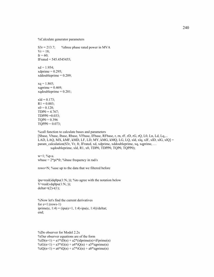
240

%Calculate generator parameters S3r = 213.7; %three phase rated power in MVA Vr = 18; fr = 60; IFrated = 545.4545455; xd = 1.954; xdprime = 0.295; xddoubleprime = 0.209; xq = 1.865; xqprime = 0.469; xqdoubleprime = 0.201; xld = 0.173; R1 = 0.003; x0 = 0.128; TDP0 = 4.767; TDPP0 =0.033; TQP0 = 0.396 TQPP0 = 0.073; %call function to calculate bases and parameters [Sbase, Vbase, Ibase, Rbase, VFbase, IFbase, RFbase, r, rn, rF, rD, rG, rQ, L0, Ln, Ld, Lq,... LAD, LAQ, MX, kMF, kMD, LF, LD, MY, kMG, kMQ, LG, LQ, xld, xlq, xlF, xlD, xlG, xlQ] = param_calculation(S3r, Vr, fr, IFrated, xd, xdprime, xddoubleprime, xq, xqprime, …

xqdoubleprime, xld, R1, x0, TDP0, TDPP0, TQP0, TQPP0); w=1; %p.u. wbase = 2*pi*fr; %base frequency in rad/s rows=N; %use up to the data that we filtered before ipu=real(idq0pu(1:N,:)); %to agree with the notation below V=real(vdq0pu(1:N,:)); deltat=t(2)-t(1); %Now let's find the current derivatives for e=1:(rows-1) iprime(e, 1:4) = (ipu(e+1, 1:4)-ipu(e, 1:4))/deltat; end; %Do observer for Model 2.2x %Our observer equations are of the form %iD(n+1) = a1*iD(n) + a2*(idprime(n)+iFprime(n) %iG(n+1) = a3*iG(n) + a4*iQ(n) + a5*iqprime(n) %iQ(n+1) = a6*iQ(n) + a7*iG(n) + a8*iqprime(n)

241

%First assign the constants to avoid repeating the same calculations a1 = 1 - wbase*rD*deltat/(xlD+LAD); a2 = -LAD*deltat/(xlD+LAD); den = (LAQ+xlQ)*(LAQ+xlG)-LAQ^2; a3 = 1 - rG*wbase*deltat*(LAQ+xlQ)/den; a4 = LAQ*rQ*wbase*deltat/den; a5 = (LAQ*deltat/(LAQ+xlG))*(LAQ*xlG/den - 1); a6 = 1 - rQ*wbase*deltat*(LAQ+xlG)/den; a7 = LAQ*rG*wbase*deltat/den; a8 = -LAQ*deltat*xlG/den; %Initial conditions: iD(1,1)=0; iG(1,1)=0; iQ(1,1)=0; %Now calculate the damper currents: for e = 1:rows-2 iD(e+1,1) = a1*iD(e,1) + a2*(iprime(e,2)+iprime(e,4)); iG(e+1,1) = a3*iG(e,1) + a4*iQ(e,1) + a5*iprime(e,3); iQ(e+1,1) = a6*iQ(e,1) + a7*iG(e,1) + a8*iprime(e,3); end %Plot damper currents plot(t(1:rows-1),iD,t(1:rows-1),iG,':',t(1:rows-1),iQ,'.' ) title('estimated i_D, i_G and i_Q') legend('i_D', 'i_G', 'i_Q') figure; %Find derivatives for iD, iG and iQ: for e=1:(rows-3) iDprime(e,1) = (iD(e+1,1)-iD(e,1))/deltat; iGprime(e,1) = (iG(e+1,1)-iG(e,1))/deltat; iQprime(e,1) = (iQ(e+1,1)-iQ(e,1))/deltat; end; %IMPLEMENTATION OF SATURATION %First, calculate saturation constants AGSAT and BGSAT in the following expression % SG = AGSAT*exp(BGSAT*(VT - V0)); %Saturation constants are specific to the generator IA = IFrated; IB = 577; %Note this as AFNL in GUI IC = 820; Sg1 = (IB-IA)/IB; Sg2 = (IC-1.2*IA)/(1.2*IA);

242

BGSAT = -5*log(Sg1/Sg2); AGSAT = (Sg1^2)/Sg2; lamdaad(:,1) = V(:,3) + r*ipu(:,3) + xld*ipu(:,2); lamdaaq(:,1) = -V(:,2) - r*ipu(:,2) + xld*ipu(:,3); lamdaat=(sqrt((mean(lamdaad))^2+(mean(lamdaaq))^2))/sqrt(3);

%The sqrt(3) is to correct for the different base in the open circuit characteristic %Calculate saturation effect in d-axis (lamdaId) lamdaId = AGSAT*exp(BGSAT*(lamdaat-0.82)); Ksd = lamdaat/(lamdaat+lamdaId); %for lack of q-axis data assume saturation is the same in both axes Ksq=Ksd; %Correct inductances for saturation LADs=LAD*Ksd; LAQs=LAQ*Ksq; %End of saturation calculations %Make rows=rows-1 for simplicity rows=rows-1; disp('Estimation of parameters for Model 2.2x with saturation included') %Estimate LAD j=1; for e=2000:(rows-20) H(j,:)=[(1/wbase)*(iprime(e,2)+iprime(e,4)+iDprime(e,1))]; H(j+1,:)=[-w*(ipu(e,2)+ipu(e,4)+iD(e,1))]; H(j+2,:)=[(1/wbase)*(iprime(e,2)+iprime(e,4)+iDprime(e,1))]; Z(j,1)=-V(e,2)-r*ipu(e,2)-w*(LAQs+xlq)*ipu(e,3)-w*LAQs*iG(e,1)-w*LAQs*iQ(e,1)- (1/wbase)*xld*iprime(e,2); Z(j+1,1)=-V(e,3)+w*xld*ipu(e,2)-r*ipu(e,3)-(1/wbase)*((LAQs+xlq)*iprime(e,3)+

LAQs*iGprime(e,1)+ LAQs*iQprime(e,1)); Z(j+2,1)=-V(e,4)-rF*ipu(e,4)-(1/wbase)*xlF*iprime(e,4); j=j+3; end x=pinv(H)*Z clear H Z x

243

%Estimate LAQ j=1; for e=2000:(rows-20) H(j,:)=[w*(ipu(e,3)+iG(e,1)+iQ(e,1))]; H(j+1,:)=[(1/wbase)*(iprime(e,3)+iGprime(e,1)+iQprime(e,1))]; H(j+2,:)=[0]; Z(j,1)=-V(e,2)-r*ipu(e,2)-w*xlq*ipu(e,3)-(1/wbase)*((LADs+xld)*iprime(e,2)+

LADs*iprime(e,4) + LADs*iDprime(e,1)); Z(j+1,1)=-V(e,3)+w*(LADs+xld)*ipu(e,2)-r*ipu(e,3)+w*LADs*ipu(e,4)+w*LADs*iD(e,1)- (1/wbase)*xlq*iprime(e,3); Z(j+2,1)=-V(e,4)-rF*ipu(e,4)-(1/wbase)*(LADs*iprime(e,2)+(LADs+xlF)*iprime(e,4)+ LADs*iDprime(e,1)); j=j+3; end x=pinv(H)*Z clear H Z x %Estimate LAD, LAQ j=1; for e=2000:(rows-20) H(j,:)=[(1/wbase)*(iprime(e,2)+iprime(e,4)+iDprime(e,1)), w*(ipu(e,3)+iG(e,1)+iQ(e,1))]; H(j+1,:)=[-w*(ipu(e,2)+ipu(e,4)+iD(e,1)), (1/wbase)*(iprime(e,3)+iGprime(e,1)+

iQprime(e,1))]; H(j+2,:)=[(1/wbase)*(iprime(e,2)+iprime(e,4)+iDprime(e,1)), 0]; Z(j,1)=-V(e,2)-r*ipu(e,2)-w*xlq*ipu(e,3)-(1/wbase)*xld*iprime(e,2); Z(j+1,1)=-V(e,3)+w*xld*ipu(e,2)-r*ipu(e,3)-(1/wbase)*xlq*iprime(e,3); Z(j+2,1)=-V(e,4)-rF*ipu(e,4)-(1/wbase)*xlF*iprime(e,4); j=j+3; end x=pinv(H)*Z clear H Z x %Estimate rF j=1; for e=2000:(rows-20) H(j,:)=[0]; H(j+1,:)=[0]; H(j+2,:)=[ipu(e,4)]; Z(j,1)=-V(e,2)-r*ipu(e,2)-w*(LAQs+xlq)*ipu(e,3)-w*LAQs*iG(e,1)-w*LAQs*iQ(e,1)- (1/wbase)*((LADs+xld)*iprime(e,2)+LADs*iprime(e,4)+LADs*iDprime(e,1)); Z(j+1,1)=-V(e,3)+w*(LADs+xld)*ipu(e,2)-r*ipu(e,3)+w*LADs*ipu(e,4)+w*LADs*iD(e,1)-

244

(1/wbase)*((LAQs+xlq)*iprime(e,3)+LAQs*iGprime(e,1)+LAQs*iQprime(e,1)); Z(j+2,1)=-V(e,4)-(1/wbase)*(LADs*iprime(e,2)+(LADs+xlF)*iprime(e,4) +

LADs*iDprime(e,1)); j=j+3; end x=pinv(H)*Z clear H Z x %Estimate r j=1; for e=2000:(rows-20) H(j,:)=[ipu(e,2)]; H(j+1,:)=[ipu(e,3)]; H(j+2,:)=[0]; Z(j,1)=-V(e,2)-w*(LAQs+xlq)*ipu(e,3)-w*LAQs*iG(e,1)-w*LAQs*iQ(e,1)- (1/wbase)*((LADs+xld)*iprime(e,2)+LADs*iprime(e,4)+LADs*iDprime(e,1)); Z(j+1,1)=-V(e,3)+w*(LADs+xld)*ipu(e,2)+w*LADs*ipu(e,4)+w*LADs*iD(e,1)- (1/wbase)*((LAQs+xlq)*iprime(e,3)+LAQs*iGprime(e,1)+LAQs*iQprime(e,1)); Z(j+2,1)=-V(e,4)-rF*ipu(e,4)-(1/wbase)*(LADs*iprime(e,2)+(LADs+xlF)*iprime(e,4)+ LADs*iDprime(e,1)); j=j+3; end x=pinv(H)*Z clear H Z x %Estimate LAD, LAQ, rF j=1; for e=2000:(rows-20) H(j,:)=[(1/wbase)*(iprime(e,2)+iprime(e,4)+iDprime(e,1)), w*(ipu(e,3)+iG(e,1)+iQ(e,1)), 0]; H(j+1,:)=[-w*(ipu(e,2)+ipu(e,4)+iD(e,1)), (1/wbase)*(iprime(e,3)+iGprime(e,1)+

iQprime(e,1)), 0]; H(j+2,:)=[(1/wbase)*(iprime(e,2)+iprime(e,4)+iDprime(e,1)), 0, ipu(e,4)]; Z(j,1)=-V(e,2)-r*ipu(e,2)-w*xlq*ipu(e,3)-(1/wbase)*xld*iprime(e,2); Z(j+1,1)=-V(e,3)+w*xld*ipu(e,2)-r*ipu(e,3)-(1/wbase)*xlq*iprime(e,3); Z(j+2,1)=-V(e,4)-(1/wbase)*xlF*iprime(e,4); j=j+3; end x=pinv(H)*Z clear H Z x

APPENDIX H

VISUAL C++ CODE FOR PARAMETER ESTIMATION AND GUI

IMPLEMENTATION USING ACTUAL MEASUREMENTS

246

/////////////////////////////////////////////////////////////////////////////////////////////////////////////////////////////////////////////////////////// //Portion of graphic user interface implementation file // //Constructs a user friendly Windows based dialog system to read input data files and known // //data to estimate the user selected synchronous generator parameters // //Copyright: Elias Kyriakides // /////////////////////////////////////////////////////////////////////////////////////////////////////////////////////////////////////////////////////////// // CDialog1Dlg.cpp : implementation file // #include "stdafx.h" #include "Estimator.h" #include "CDialog1Dlg.h" #include <iostream> #include <fstream> #include <vector> #include <iomanip> #include <math.h> #include <stdlib.h> #include "Dialog2Dlg.h" #include <stdio.h> #include <string> #include "LinAlg.h" //To allow use of the linear algebra package in this file #include "LAStreams.h" //To allow use of streams of the linear algebra package #include "svd.h" //To allow use of the singular value decomposition capabilities //of the linear algebra package using namespace std; #ifdef _DEBUG #define new DEBUG_NEW #undef THIS_FILE static char THIS_FILE[] = __FILE__; #endif #undef min //To make LinAlg compatible with MFC #undef max double X[16][2]; //X is the matrix containing the estimated parameters //Initialized it here to access it from all functions (global) //The first column contains the value of the estimated parameter //The second column is 1 if that parameter was estimated and zero otherwise. //X[15][0] contains the rms error of the estimation

247

///////////////////////////////////////////////////////////////////////////// // CDialog1Dlg dialog CDialog1Dlg::CDialog1Dlg(CWnd* pParent /*=NULL*/) : CDialog(CDialog1Dlg::IDD, pParent) //AFX_DATA_INIT(CDialog1Dlg) m_filename = _T(""); m_rF = FALSE; m_r = FALSE; m_r3rn = FALSE; m_Lq = FALSE; m_Ld = FALSE; m_MF = FALSE; m_MD = FALSE; m_L03Ln = FALSE; m_LDdamper = FALSE; m_LF = FALSE; m_MR = FALSE; m_rD = FALSE; m_Comtradedata = 0; //causes the Comtrade data radio button to be selected at startup m_L2method = 0; //causes the L2 estimation method radio button to be selected at startup m_frequency = 60.0; m_Ifield_airgap = 1226.0; m_xLm = 0.160; m_S3Base = 483.0; m_V3Base = 22.0; m_R1 = 0.0046; m_x0 = 0.150; m_xd = 1.80; m_xq = 1.72; m_Ln = 100.0; m_rn = 100.0; m_taudoubleprimed = 0.032; m_taudoubleprimeqzero = 0.059; m_tauprimedzero = 3.7; m_xdoubleprimedv = 0.190; m_xdoubleprimeqv = 0.190; m_xprimedv = 0.270; m_EnableWeights=0; //causes the Enable Weights button to be selected at startup m_FullFilter = 0; //causes the Full Filter button to be selected at startup m_rQ = FALSE; m_LQdamper = FALSE; m_MQ = FALSE; //AFX_DATA_INIT void CDialog1Dlg::DoDataExchange(CDataExchange* pDX) CDialog::DoDataExchange(pDX); //AFX_DATA_MAP(CDialog1Dlg) DDX_Text(pDX, IDC_FILENAME, m_filename); DDX_Check(pDX, IDC_rF, m_rF);

248

DDX_Check(pDX, IDC_r, m_r); DDX_Check(pDX, IDC_r3rn, m_r3rn); DDX_Check(pDX, IDC_Lq, m_Lq); DDX_Check(pDX, IDC_Ld, m_Ld); DDX_Check(pDX, IDC_MF, m_MF); DDX_Check(pDX, IDC_MD, m_MD); DDX_Check(pDX, IDC_L03Ln, m_L03Ln); DDX_Check(pDX, IDC_LDdamper, m_LDdamper); DDX_Check(pDX, IDC_LF, m_LF); DDX_Check(pDX, IDC_MR, m_MR); DDX_Check(pDX, IDC_rD, m_rD); DDX_Radio(pDX, IDC_Comtradedata, m_Comtradedata); DDX_Radio(pDX, IDC_L2method, m_L2method); DDX_Text(pDX, IDC_frequency, m_frequency); DDX_Text(pDX, IDC_Ifield_airgap, m_Ifield_airgap); DDX_Text(pDX, IDC_xLm, m_xLm); DDX_Text(pDX, IDC_S3Base, m_S3Base); DDX_Text(pDX, IDC_V3Base, m_V3Base); DDX_Text(pDX, IDC_R1, m_R1); DDX_Text(pDX, IDC_x0, m_x0); DDX_Text(pDX, IDC_xd, m_xd); DDX_Text(pDX, IDC_xq, m_xq); DDX_Text(pDX, IDC_Ln, m_Ln); DDX_Text(pDX, IDC_rn, m_rn); DDX_Text(pDX, IDC_taudoubleprimed, m_taudoubleprimed); DDX_Text(pDX, IDC_taudoubleprimeqzero, m_taudoubleprimeqzero); DDX_Text(pDX, IDC_tauprimedzero, m_tauprimedzero); DDX_Text(pDX, IDC_xdoubleprimedv, m_xdoubleprimedv); DDX_Text(pDX, IDC_xdoubleprimeqv, m_xdoubleprimeqv); DDX_Text(pDX, IDC_xprimedv, m_xprimedv); DDX_Radio(pDX, IDC_EnableWeights, m_EnableWeights); DDX_Radio(pDX, IDC_FullFilter, m_FullFilter); DDX_Check(pDX, IDC_rQ, m_rQ); DDX_Check(pDX, IDC_LQdamper, m_LQdamper); DDX_Check(pDX, IDC_MQ, m_MQ); //AFX_DATA_MAP UpdateOKUI(); //Disables "Start Estimator" button at startup when empty BEGIN_MESSAGE_MAP(CDialog1Dlg, CDialog) //AFX_MSG_MAP(CDialog1Dlg) ON_BN_CLICKED(IDC_BROWSE, OnBrowse) ON_EN_CHANGE(IDC_FILENAME, OnChangeFilename) ON_BN_CLICKED(IDC_rF, OnrF) ON_BN_CLICKED(IDC_r, Onr) ON_BN_CLICKED(IDC_r3rn, Onr3rn) ON_BN_CLICKED(IDC_Lq, OnLq) ON_BN_CLICKED(IDC_Ld, OnLd) ON_BN_CLICKED(IDC_MF, OnMF) ON_BN_CLICKED(IDC_MD, OnMD) ON_BN_CLICKED(IDC_rD, OnrD) ON_BN_CLICKED(IDC_L03Ln, OnL03Ln)

249

ON_BN_CLICKED(IDC_LF, OnLF) ON_BN_CLICKED(IDC_MR, OnMR) ON_BN_CLICKED(IDC_LDdamper, OnLDdamper) ON_BN_CLICKED(IDC_HelpButton1, OnHelpButton1) ON_BN_CLICKED(IDC_HelpButton2, OnHelpButton2) ON_BN_CLICKED(IDC_HelpButton3, OnHelpButton3) ON_BN_CLICKED(IDC_HelpButton4, OnHelpButton4) ON_BN_CLICKED(IDC_rQ, OnrQ) ON_BN_CLICKED(IDC_LQdamper, OnLQdamper) ON_BN_CLICKED(IDC_MQ, OnMQ) ON_EN_KILLFOCUS(IDC_S3Base, OnKillfocusS3Base) ON_EN_KILLFOCUS(IDC_V3Base, OnKillfocusV3Base) ON_EN_KILLFOCUS(IDC_Ifield_airgap, OnKillfocusIfieldairgap) ON_EN_KILLFOCUS(IDC_frequency, OnKillfocusfrequency) ON_EN_KILLFOCUS(IDC_rn, OnKillfocusrn) ON_EN_KILLFOCUS(IDC_Ln, OnKillfocusLn) ON_EN_KILLFOCUS(IDC_xd, OnKillfocusxd) ON_EN_KILLFOCUS(IDC_xq, OnKillfocusxq) ON_EN_KILLFOCUS(IDC_xprimedv, OnKillfocusxprimedv) ON_EN_KILLFOCUS(IDC_xdoubleprimedv, OnKillfocusxdoubleprimedv) ON_EN_KILLFOCUS(IDC_xdoubleprimeqv, OnKillfocusxdoubleprimeqv) ON_EN_KILLFOCUS(IDC_x0, OnKillfocusx0) ON_EN_KILLFOCUS(IDC_xLm, OnKillfocusxLm) ON_EN_KILLFOCUS(IDC_R1, OnKillfocusR1) ON_EN_KILLFOCUS(IDC_tauprimedzero, OnKillfocustauprimedzero) ON_EN_KILLFOCUS(IDC_taudoubleprimed, OnKillfocustaudoubleprimed) ON_EN_KILLFOCUS(IDC_taudoubleprimeqzero, OnKillfocustaudoubleprimeqzero) //AFX_MSG_MAP END_MESSAGE_MAP() ///////////////////////////////////////////////////////////////////////////// // CDialog1Dlg message handlers void CDialog1Dlg::OnBrowse() CFileDialog dlg( true, NULL, NULL, OFN_HIDEREADONLY, _T("Text files (.txt)|*.txt|") _T("Data files (.dat)|*.dat|") _T("IEEE Comtrade files (.cfg; .dat)|*.cfg; *.dat|") _T("|") ); if (IDOK!=dlg.DoModal()) return; m_FileNameFull = dlg.GetPathName(); UpdateData(false); UpdateOKUI(); //Disables "Start Estimator" button when it is emptied

250

void CDialog1Dlg::OnOK() extern double X[16][2]; //X is the matrix containing the estimated parameters mainprogram(); //Calls the function mainprogram. //When this process ends, the estimator finishes. CDialog::OnOK(); MessageBox("The Estimator has finished.", "Simulation Finished", MB_OK | MB_ICONINFORMATION); CDialog2Dlg dlg2; //Declares the output dialog //Presentation of results: CString Y[15]="r+3*rn","r","Lq","Ld","MF","MD","rF","rD","L0+3*Ln","LF","MR","LD","rQ","LQ","MQ";

//String matrix containing the names of the estimated parameters int e=0; for (int i=0; i<15; i++) if (X[i][1]==1) dlg2.m_param1 = Y[i]; dlg2.m_out1 = X[i][0]; e=i; i=15;//to force break of the for loop since an estimated parameter was detected if (e==14) goto PointA; for (i=e+1; i<15; i++) if (X[i][1]==1) dlg2.m_param2 = Y[i]; dlg2.m_out2 = X[i][0]; e=i; i=15; if (e==14) goto PointA; for (i=e+1; i<15; i++) if (X[i][1]==1) dlg2.m_param3 = Y[i]; dlg2.m_out3 = X[i][0]; e=i; i=15; if (e==14) goto PointA; for (i=e+1; i<15; i++) if (X[i][1]==1)

251

dlg2.m_param4 = Y[i]; dlg2.m_out4 = X[i][0]; e=i; i=15; if (e==14) goto PointA; for (i=e+1; i<15; i++) if (X[i][1]==1) dlg2.m_param5 = Y[i]; dlg2.m_out5 = X[i][0]; e=i; i=15; dlg2.m_error = X[15][0]; //outputs the rms error of the estimation PointA: if (IDOK == dlg2.DoModal()) //implements the output dialog void CDialog1Dlg::OnCancel() MessageBox("This will cancel the estimation.", "Exit the Estimator", MB_OK | MB_ICONINFORMATION); CDialog::OnCancel(); CDialog::OnOK(); void CDialog1Dlg::UpdateOKUI() CString strFileName; GetDlgItemText(IDC_FILENAME, strFileName); GetDlgItem(IDOK)->EnableWindow(strFileName!=_T("")); void CDialog1Dlg::OnChangeFilename() CString strFileName; CEdit *pEdit = (CEdit *)GetDlgItem(IDC_FILENAME); // Get the edit control named IDC_FILENAME ASSERT_VALID(pEdit); CButton *pBtnOK = (CButton *)GetDlgItem(IDOK); // Get the OK button ASSERT_VALID(pBtnOK); pEdit->GetWindowText(strFileName); // get the text from the control into strFileName if ( strFileName.IsEmpty() )

252

pBtnOK->EnableWindow(FALSE); else pBtnOK->EnableWindow(TRUE); void CDialog1Dlg::mainprogram() ///////////////////////////////////////////////////////////////////////////////////////////////////////////////////////////////////////////// // This file reads the data supplied in the input file and stores the data into columns. It then // arranges the data in the form Hx=Z (with the help of the Linear Algebra package), and // estimates the parameters required by the user. ///////////////////////////////////////////////////////////////////////////////////////////////////////////////////////////////////////////// //Last modified on December 11, 2002 //Check state of "file" radio buttons to select the data format int radioState_Comtrade; //It will be assigned to 0 or 1 depending on state of button CButton* pRadio_Comtrade = (CButton*)GetDlgItem(IDC_Comtradedata); radioState_Comtrade = pRadio_Comtrade->GetCheck(); int radioState_abc=0; //not really needed? see if else statement below CButton* pRadio_abc = (CButton*)GetDlgItem(IDC_abcdata); radioState_abc = pRadio_abc->GetCheck(); //Depending on the selection of the data format, the program will now divide into two sections //These nine vectors are used to store the measurements from the selected data file vector<double> t, IA, IB, IC, VF, VAB, VBC, VCA, IF; double a1, a2, a3, a4, a5, a6, a7, a8, a9; if (radioState_Comtrade==1) //If the user selects the option to read a Comtrade data file: //read .cfg file first CString strFile1 = m_FileNameFull; //procedure to get name of .cfg file CString strFile2 = strFile1; //we have read the .dat file (strFile1) strFile2=m_FileNameFull; strFile2.Replace(".dat", ".cfg");

char heading[3]; int channels; char dum1[6]; int ch1; //holds channel numbers char dum2[3]; char dum3[2]; //dum3, 4 compose the channel identifier char dum4[2]; char dum5[8]; //channel phase identification and units char dum6; //the comma after the unit float at; //channel multiplier

253

float bt; //channel offset float skew; //time skew float minpo; //minimum possible data value float maxpo; //maximum possible data value int qp; //VT or CT ratio primary int qs; //VT or CT ratio secondary char q1; //primary or secondary data sealing identifier int freq; //frequency int samplingrates; //number of sampling rates float samplerate; //sample rate in Hz int lastno; //last sample number char date1[26]; //start date and time char date2[26]; //end date and time char datatype[10];//Data file type, e.g. ASCII float timemult; //Time stamp multiplication factor vector<int> ch; vector<double> a, b; ifstream cfgfile; cfgfile.open(strFile2); //Read the first two informatory lines cfgfile >> heading; cfgfile >> channels; cfgfile >> dum1; //Read all channels (each channel the characteristics of one variable) for (int k=0; k<channels; k++) cfgfile >> ch1; cfgfile >> dum2; cfgfile >> dum3; cfgfile >> dum4; cfgfile >> dum5; cfgfile >> dum6; cfgfile >> at; cfgfile >> dum6; cfgfile >> bt; cfgfile >> dum6; cfgfile >> skew; cfgfile >> dum6; cfgfile >> minpo; cfgfile >> dum6; cfgfile >> maxpo; cfgfile >> dum6; cfgfile >> qp; cfgfile >> dum6; cfgfile >> qs; cfgfile >> dum6; cfgfile >> q1; ch.push_back(ch1); a.push_back(at); b.push_back(bt);

254

//Now read the rest of the data in the configuration file cfgfile >> freq >> samplingrates >> samplerate >> dum6 >> lastno; cfgfile >> date1 >> date2 >> datatype >> timemult; cfgfile.close(); //closes the configuration data file //Now read the .dat file //Location zero contains the sample number char dum7; vector<int> measnumber; //the .dat file has one more column which contains int a10; /the measurement number. ifstream datafile; datafile.open(m_FileNameFull); for (int q = 0; q<lastno; q++)

datafile >> a10 >> dum7 >> a1 >> dum7 >> a2 >> dum7 >> a3 >> dum7 >> a4 >> dum7 >> a5>> dum7 >> a6 >> dum7 >> a7 >> dum7 >> a8 >> dum7 >> a9;

measnumber.push_back(a10); // append to end of vector and... t.push_back(a1); // expand it, if necessary IA.push_back(a2); IB.push_back(a3); IC.push_back(a4); VF.push_back(a5); VAB.push_back(a6); VBC.push_back(a7); VCA.push_back(a8); IF.push_back(a9); datafile.close(); //closes the .dat data file //Multiplying factors int k1 = t.size(); for (int j=0; j<k1-1; j++) t[j] = t[j]*(timemult/1E-6); //the time is in microseconds // To find the correct quantity for each signal we need to multiply the stored signal by its channel // multiplier a and add any offset b that may exist. These were read from the configuration data file. //Further, multiply stator V and I by 1000 IA[j] = 1000*(IA[j] * a[0] + b[0]); IB[j] = 1000(IB[j] * a[1] + b[1]); IC[j] = 1000(IC[j] * a[2] + b[2]); VF[j] = VF[j] * a[3] + b[3]; VAB[j] = 1000(VAB[j]* a[4] + b[4]); VBC[j] = 1000(VBC[j]* a[5] + b[5]); VCA[j] = 1000(VCA[j]* a[6] + b[6]); IF[j] = IF[j] * a[7] + b[7];

255

//end of reading Comtrade data files if (radioState_abc==1) //read a normal abc data file ifstream datafile (m_FileNameFull); while (datafile >> a1 >> a2 >> a3 >> a4 >> a5 >> a6 >> a7 >> a8 >> a9) //reads data row by row t.push_back(a1); // append to end of vector and... VAB.push_back(a2);// expand it, if necessary VBC.push_back(a3); VCA.push_back(a4); VF.push_back(a5); IA.push_back(a6); IB.push_back(a7); IC.push_back(a8); IF.push_back(a9); datafile.close(); //closes the data file //end of reading abc data // The following segment calculates the current and voltage bases and all the machine parameters // that can be calculated from the manufacturer's data. If some of these are selected to be // estimated then they are ignored in the estimation process. If not, then they are used to estimate // the selected parameters //We need to define the constant k and pi double k = sqrt(3.0/2.0); double pi=4*atan(1); //this is one way of calculating pi //stator bases double SBase=(m_S3Base*1E6)/3.0; double VBase=(m_V3Base*1E3)/sqrt(3.0); double IBase= SBase/VBase; double w=2*pi*m_frequency; double LBase=VBase/(w*IBase); //parameters I double MF=(VBase*sqrt(2))/(w*m_Ifield_airgap); double Lmd=(m_xd-m_xLm)*LBase; double kMFactual=k*MF; //field bases double IFBase=IBase/(kMFactual/Lmd); double VFBase=SBase/IFBase;

256

double LFBase=pow(kMFactual,2.0)*LBase/pow(Lmd,2.0); double MFBase=(kMFactual/Lmd)*LBase; //parameters II double kMF=kMFactual/MFBase; double rn=m_rn; double Ln=m_Ln; double kMD=kMF; double MR=kMF; double kMQ=m_xq-m_xLm; double Ld=m_xd; double Lq=m_xq; double L0=m_x0; double r=m_R1; double LAD=kMF; double Lprimed=m_xprimedv; double ld=m_xLm; double lF=LAD*((Lprimed-ld)/(Ld-Lprimed)); double LF=lF+LAD; double Ldoubleprimed=m_xdoubleprimedv; double lD=(LAD*lF*(Ldoubleprimed-ld))/(LAD*lF-lF*(Ldoubleprimed-ld)-LAD*(Ldoubleprimed-ld)); double LD=lD+LAD; double rD=(Ldoubleprimed*(LD*LF-pow(LAD,2.0)))/(Lprimed*LF*m_taudoubleprimed*w); double lq=ld; double LAQ=Lq-lq; double Ldoubleprimeq=m_xdoubleprimeqv; double lQ=LAQ*(Ldoubleprimeq-lq)/(Lq-Ldoubleprimeq); double LQ=LAQ+lQ; double rQ=LQ/(m_taudoubleprimeqzero*w); double rF=LF/(m_tauprimedzero*w); //end of calculating machine bases and machine parameters ****************************** int rows = t.size(); //calculates the # of rows of the vectors and sets it to m //abc voltages and currents in the data files are in kV and kA. Transform them into V and A for (int j=0; j<rows; j++) IA[j] *= 1000*0.0026987161; IB[j] *= 1000*0.0026987161; IC[j] *= 1000*0.0026987161; VAB[j]*= 1000*0.0018998961; VBC[j]*= 1000*0.0018998961; VCA[j]*= 1000*0.0018998961; IF[j]*= 0.2072613984; VF[j]*= 0.0518153496;

257

//then phase quantities are calculated from the line quantities ***************************** //and the torque angle delta is calculated ********************************************* vector<double> P(rows), Q(rows), thetapq(rows); for (j=0; j<rows; j++) P[j]=(VAB[j]*IA[j]-VBC[j]*IC[j])/(3*SBase); //per phase active power in pu Q[j]=(VAB[j]*IC[j]+VBC[j]*IA[j]+VCA[j]*IB[j])/(sqrt(3)*3*SBase);

//per phase reactive power in pu thetapq[j]=atan2(Q[j],P[j]); //power factor angle at each measurement (atan2 takes into account all possible quadrants) // The next for loop calculates the angle between the voltages two phases taking into account the // different quadrants and a possibility of "divide by zero" problem. The angle is calculated using // the equation: // thetavabc(j,e)=atan(-diff. of two voltages/(sqrt(3)*sum of two voltages)) the tolerance for // avoiding the divide by zero problem is set to 1e-6. vector<double> thetavabc1(rows), thetavabc2(rows), thetavabc3(rows), thetaia(rows); // 3 vectors containing the angles between the phases of two voltages and a vector containing the // angle of phase a //Since we cannot use matrices (do not know their size and do not want to assign arbitrary size), //use a slightly different algorithm to do the following than the one used in the MATLAB file //first phase for (j=0; j<rows; j++) if (VBC[j]+VCA[j]>0) //checks if the sum of the voltages is greater than zero if (abs(-sqrt(3.0)*(VBC[j]+VCA[j]))>1E-6) //sum not close to zero thetavabc1[j]=pi+(atan((VBC[j]-VCA[j])/(-sqrt(3.0)*(VBC[j]+VCA[j])))); //the angle lies in the second quadrant else //(if sum is close to zero, the angle is going to be either 90 or 270) int y=CDialog1Dlg::sign(VBC[j],VCA[j]);

//returns the sign of the difference between the two voltages (+ or -) thetavabc_view(j,e)=pi+y*pi/2;

else

if (VBC[j]-VCA[j]<0) //checks if the difference of the voltages is less than zero

if (abs(-sqrt(3.0)*(VBC[j]-VCA[j]))>1e-6) //sum of the voltages greater than zero

thetavabc1[j]=2*pi+(atan((VBC[j]-VCA[j])/(- sqrt(3.0)*(VBC[j]+VCA[j])))); //the angle lies in the third quadrant

else //if sum is close to zero

258

int y=CDialog1Dlg::sign(VBC[j],VCA[j]); //returns

the sign of the difference between the two voltages (+ or -) thetavabc1[j]=2*pi+y*pi/2; else

if (abs(-sqrt(3.0)*(VBC[j]+VCA[j]))>1e-6) //the remaining case: the first quadrant

thetavabc1[j]=(atan((VBC[j]-VCA[j])/(-sqrt(3.0)*(VBC[j]+VCA[j])))); //the angle lies in the first quadrant else //if sum is close to zero int y=CDialog1Dlg::sign(VBC[j],VCA[j]);

//returns the sign of the difference between the two voltages (+ or -) thetavabc1[j]=y*pi/2; //second phase for (j=0; j<rows; j++) if (VCA[j]+VAB[j]>0) //checks if the sum of the voltages is greater than zero if (abs(-sqrt(3.0)*(VCA[j]+VAB[j]))>1E-6) //sum not close to zero thetavabc2[j]=pi+(atan((VCA[j]-VAB[j])/(-sqrt(3.0)*(VCA[j]+VAB[j])))); //the angle lies in the second quadrant else //(if sum is close to zero, the angle is going to be either 90 or 270) int y=CDialog1Dlg::sign(VCA[j],VAB[j]);


else if (VCA[j]-VAB[j]<0)

//checks if the difference of the voltages is less than zero if (abs(-sqrt(3.0)*(VCA[j]-VAB[j]))>1e-6)

//sum of the voltages greater than zero thetavabc2[j]=2*pi+(atan((VCA[j]-VAB[j])/(-sqrt(3.0)*(VCA[j]+VAB[j])))); //the angle lies in the third quadrant else //if sum is close to zero

int y=CDialog1Dlg::sign(VCA[j],VAB[j]); //returns the sign of the difference between the two voltages (+ or -)

thetavabc2[j]=2*pi+y*pi/2; else

if (abs(-sqrt(3.0)*(VCA[j]+VAB[j]))>1e-6) //the remaining case: the first quadrant

thetavabc2[j]=(atan((VCA[j]-VAB[j])/(-sqrt(3.0)*(VCA[j]+VAB[j])))); //the angle lies in the first quadrant else //if sum is close to zero

259

int y=CDialog1Dlg::sign(VCA[j],VAB[j]);

//returns the sign of the difference between the two voltages (+ or -) thetavabc2[j]=y*pi/2; //third phase for (j=0; j<rows; j++) if (VAB[j]+VBC[j]>0) //checks if the sum of the voltages is greater than zero if (abs(-sqrt(3.0)*(VAB[j]+VBC[j]))>1E-6) //sum not close to zero thetavabc3[j]=pi+(atan((VAB[j]-VBC[j])/(-sqrt(3.0)*(VAB[j]+VBC[j])))); //the angle lies in the second quadrant else //(if sum is close to zero, the angle is going to be either 90 or 270) int y=CDialog1Dlg::sign(VAB[j],VBC[j]);


else if (VAB[j]-VBC[j]<0) //checks if the difference of the voltages is less than zero if (abs(-sqrt(3.0)*(VAB[j]-VBC[j]))>1e-6)

//sum of the voltages greater than zero thetavabc3[j]=2*pi+(atan((VAB[j]-VBC[j])/(-sqrt(3.0)*(VAB[j]+VBC[j])))); //the angle lies in the third quadrant else //if sum is close to zero

int y=CDialog1Dlg::sign(VAB[j],VBC[j]); //returns the sign of the difference between the two voltages (+ or -)

thetavabc3[j]=2*pi+y*pi/2; else

if (abs(-sqrt(3.0)*(VAB[j]+VBC[j]))>1e-6) //the remaining case: the first quadrant

thetavabc3[j]=(atan((VAB[j]-VBC[j])/(-sqrt(3.0)*(VAB[j]+VBC[j])))); //the angle lies in the first quadrant else //if sum is close to zero

int y=CDialog1Dlg::sign(VAB[j],VBC[j]); //returns the sign of the difference between the two voltages (+ or -)

thetavabc3[j]=y*pi/2; //End of calculation of the angle between two phases

260

//Calculate the instantaneous phase-neutral rms voltage vector<double> vtrms1(rows), vtrms2(rows), vtrms3(rows); for (j=0; j<rows; j++) vtrms1[j]=(-(VBC[j]+VCA[j])/(cos(thetavabc1[j]))/(sqrt(2.0)*VBase*sqrt(3.0))); vtrms2[j]=(-(VCA[j]+VAB[j])/(cos(thetavabc2[j]))/(sqrt(2.0)*VBase*sqrt(3.0))); vtrms3[j]=(-(VAB[j]+VBC[j])/(cos(thetavabc3[j]))/(sqrt(2.0)*VBase*sqrt(3.0))); vector<double> Va(rows), Vb(rows), Vc(rows); //phase voltages for (j=0; j<rows; j++) Va[j]=vtrms1[j]*sqrt(2.0)*VBase*cos(thetavabc1[j]-pi/6); Vb[j]=vtrms2[j]*sqrt(2.0)*VBase*cos(thetavabc2[j]-pi/6); Vc[j]=vtrms3[j]*sqrt(2.0)*VBase*cos(thetavabc3[j]-pi/6); //End of conversion of voltage from line-line to phase-neutral voltage //Similar calculations are performed for getting the angle currents. //The calculations are performed only for phase A. for (j=0; j<rows; j++) if (IB[j]+IC[j]>0) //checks if the sum of the currents is greater than zero if (abs(-sqrt(3.0)*(IB[j]+IC[j]))>1E-6) //sum not close to zero thetaia[j]=pi+(atan((IB[j]-IC[j])/(-sqrt(3.0)*(IB[j]+IC[j])))); //the angle lies in the second quadrant else //(if sum is close to zero, the angle is going to be either 90 or 270) int y=CDialog1Dlg::sign(IB[j],IC[j]);

//returns the sign of the difference between the two currents (+ or -) thetaia[j]=pi+y*pi/2; else if (IB[j]-IC[j]<0) //checks if the difference of the currents is less than zero if (abs(-sqrt(3.0)*(IB[j]-IC[j]))>1e-6) //sum of the currents greater than zero thetaia[j]=2*pi+(atan((IB[j]-IC[j])/(-sqrt(3.0)*(IB[j]+IC[j])))); //the angle lies in the third quadrant else //if sum is close to zero int y=CDialog1Dlg::sign(IB[j],IC[j]);

//returns the sign of the difference between the two currents (+ or -) thetaia[j]=2*pi+y*pi/2; else if (abs(-sqrt(3.0)*(IB[j]+IC[j]))>1e-6)

//the remaining case: the first quadrant thetaia[j]=(atan((IB[j]-IC[j])/(-sqrt(3.0)*(IB[j]+IC[j]))));

//the angle lies in the first quadrant

261

else //if sum is close to zero int y=CDialog1Dlg::sign(IB[j],IC[j]);

//returns the sign of the difference between the two currents (+ or -) thetaia[j]=y*pi/2; //End of calculation of the angle for phase A //Calculate the rms current for phase A for each time step vector<double> Iarms(rows); for (j=0; j<rows; j++) Iarms[j]=-((IB[j]+IC[j])/(cos(thetaia[j]))/(sqrt(2.0)*IBase)); //Calculate the instantaneous machine generated emf by the formula //ef=vt+(r+jxq)*Ia //It was agreed upon between APS and ASU that for the best results (delta) the internal //emf be calculated using Xq instead of Xd. //To avoid using complex numbers, calculate real and complex parts separately vector<double> Efreal(rows), Efimag(rows), delta(rows); for (j=0; j<rows; j++) Efreal[j]=vtrms1[j] + Iarms[j]*m_xq*cos(pi/2-thetapq[j]) + Iarms[j]*r*cos(-

thetapq[j]); Efimag[j]=Iarms[j]*m_xq*sin(pi/2-thetapq[j])+Iarms[j]*r*sin(-thetapq[j]); delta[j]=atan2(Efimag[j], Efreal[j]); //The instantaneous value of delta may contain large spikes which need to be smoothened out. //The simple filter below disregards the new value and uses the previous value in //the time series if the two adjacent values differ by 5 degrees. The figure 5 degrees is //arbitrary and can be varied to obtain better results. for (j=1; j<rows; j++) if (abs(delta[j]-delta[j-1])>= (5*pi/180)) delta[j]=delta[j-1];

262

//Second filter for delta in addition to the one for the spikes. //This is a moving average filter //First calculate the zero frequency component of the unfiltered delta double sum=0.0; for (j=0; j<rows; j++) sum+=delta[j]; double deltaunfiltered_zerofrcomp=sum/rows; int run=20; //no. of terms in the moving average filter for (j=run; j<rows; j++) sum=0.0; for (int e=(j-run); e<j; e++) sum+=delta[e]; delta[j-run]=sum/run; //Now calculate the zero frequency component of the filtered delta sum=0.0; for (j=0; j<(rows-run); j++) sum+=delta[j]; double deltafiltered_zerofrcomp=sum/(rows-run); //correct for the filter factor: for (j=0; j<(rows-run); j++) delta[j] *= deltaunfiltered_zerofrcomp/deltafiltered_zerofrcomp; //Now rows becomes rows-run, since we used a MAF for delta rows-=run; //end of calculating phase quantities and delta ***************************************** //transform abc voltages and currents into 0dq quantities ********************************* vector<double> theta(rows), I0(rows), Id(rows), Iq(rows), V0(rows), Vd(rows), Vq(rows); //the angle theta of Park's and the resulting 0dq vectors vector<double> P21(rows), P22(rows), P23(rows),P31(rows), P32(rows), P33(rows) ;

//the 2nd and 3rd rows of Park's matrix at each time step

double P11, P12, P13; //the elements of the first row of the Park's transformation matrix (constant)

P11=P12=P13=1/sqrt(3.0);

for (j=0; j<rows; j++) theta[j]=2*pi*m_frequency*t[j] + delta[j] + pi/2 + thetavabc1[0] - pi/6;

//the angle theta in the Park's transformation matrix

263

P21[j] = sqrt(2.0/3.0)*cos(theta[j]); P22[j] = sqrt(2.0/3.0)*cos(theta[j]-2*pi/3); P23[j] = sqrt(2.0/3.0)*cos(theta[j]+2*pi/3); P31[j] = sqrt(2.0/3.0)*sin(theta[j]); P32[j] = sqrt(2.0/3.0)*sin(theta[j]-2*pi/3); P33[j] = sqrt(2.0/3.0)*sin(theta[j]+2*pi/3); V0[j] = P11*Va[j] + P12*Vb[j] + P13*Vc[j]; //zero voltage component Vd[j] = P21[j]*Va[j] + P22[j]*Vb[j] + P23[j]*Vc[j]; Vq[j] = P31[j]*Va[j] + P32[j]*Vb[j] + P33[j]*Vc[j]; I0[j] = P11*IA[j] + P12*IB[j] + P13*IC[j]; Id[j] = P21[j]*IA[j] + P22[j]*IB[j] + P23[j]*IC[j]; Iq[j] = P31[j]*IA[j] + P32[j]*IB[j] + P33[j]*IC[j]; //End of Park's transformation ***************************************************** //Begin filtering of rotor and stator quantities ****************************************** //Reads user's decision whether he wants to apply a full filter or not. int radioState_FullFilter; //It will be assigned to 0 or 1 depending on state of button CButton* pRadio_FullFilter = (CButton*)GetDlgItem(IDC_FullFilter); radioState_FullFilter = pRadio_FullFilter->GetCheck(); //No matter what the decision is, we need to perform the following spike filter for all 0dq currents and //voltages. This filter compares successive sets of two measurements. If they differ by more than 10%, //then measurement (k+1) is replaced by measurement k (all of the currents and voltages at that //point. So basically the previous measurement is duplicated for (j=1; j<rows; j++) if (abs((V0[j]-V0[j-1])/V0[j-1])>(0.1) || abs((Vd[j]-Vd[j-1])/Vd[j-1])>(0.1) || abs((Vq[j]-Vq[j-1])/Vq[j-1])>(0.1)) V0[j]=V0[j-1]; Vd[j]=Vd[j-1]; Vq[j]=Vq[j-1]; I0[j]=I0[j-1]; Id[j]=Id[j-1]; Iq[j]=Iq[j-1]; if (abs((I0[j]-I0[j-1])/I0[j-1])>(0.1) || abs((Id[j]-Id[j-1])/Id[j-1])>(0.1) || abs((Iq[j]-Iq[j-1])/Iq[j-1])>(0.1)) V0[j]=V0[j-1]; Vd[j]=Vd[j-1]; Vq[j]=Vq[j-1]; I0[j]=I0[j-1];

264

Id[j]=Id[j-1]; Iq[j]=Iq[j-1]; //If he chooses not to use a full filter, then just use a 20pt moving average filter for //the field quantities only. //Create filtered matrices to be used by either the if or the else statement vector<double> V0filtered(rows), Vdfiltered(rows), Vqfiltered(rows), I0filtered(rows),

Idfiltered(rows), Iqfiltered(rows); vector<double> VFfiltered(rows), IFfiltered(rows); if (radioState_FullFilter==1) //If the user selects the option to use a full filtering algorithm: //do Butterworth filters else //keep the 0dq signals as they are but put them in the "filtered" matrices for program continuity for (j=0; j<rows; j++) V0filtered[j]=V0[j]; Vdfiltered[j]=Vd[j]; Vqfiltered[j]=Vq[j]; I0filtered[j]=I0[j]; Idfiltered[j]=Id[j]; Iqfiltered[j]=Iq[j];

rows+=run; //First calculate the zero frequency component of the unfiltered field signals double sum1=0.0, sum2=0.0; for (j=0; j<rows; j++) sum1+=VF[j]; sum2+=IF[j]; double VFunfiltered_zerofrcomp=sum1/rows; double IFunfiltered_zerofrcomp=sum2/rows; int run=20; //no. of terms in the moving average filter for (j=run; j<rows; j++) sum1=sum2=0.0; for (int e=(j-run); e<j; e++) sum1+=VF[e]; sum2+=IF[e];

265

VFfiltered[j-run]=sum1/run; IFfiltered[j-run]=sum2/run; //Now calculate the zero frequency component of the filtered field quantities sum1=0.0, sum2=0.0; for (j=0; j<(rows-run); j++) sum1+=VFfiltered[j]; sum2+=IFfiltered[j]; double VFfiltered_zerofrcomp=sum1/(rows-run); double IFfiltered_zerofrcomp=sum2/(rows-run); // correct for the filter factor: for (j=0; j<(rows-run); j++) VFfiltered[j] *= VFunfiltered_zerofrcomp/VFfiltered_zerofrcomp; IFfiltered[j] *= IFunfiltered_zerofrcomp/IFfiltered_zerofrcomp; rows-=run; // We make rows=rows-run again to keep the same variable for the rest of

// the program and to make sure that we delete the last 'run' elements in the // other matrices

//End of filtering of rotor and stator quantities ***************************************** //Calculate pu quantities of field and 0dq signals vector<double> V0pu(rows), Vdpu(rows), Vqpu(rows), I0pu(rows), Idpu(rows),

Iqpu(rows), VFpu(rows), IFpu(rows); //convert field quantities to pu for (j=0; j<rows; j++) // if no filtering was selected, rows is now rows-run, else it is

// the same as before VFpu[j]=VFfiltered[j]/VFBase; IFpu[j]=IFfiltered[j]/IFBase;

266

//convert stator 0dq quantities to pu for (j=0; j<rows; j++) V0pu[j] = V0filtered[j]/VBase; Vdpu[j] = Vdfiltered[j]/VBase; Vqpu[j] = Vqfiltered[j]/VBase; I0pu[j] = I0filtered[j]/IBase; Idpu[j] = Idfiltered[j]/IBase; Iqpu[j] = Iqfiltered[j]/IBase; //End of pu conversion ******************************************************************* //Calculation of the current derivatives *******************************************************

vector<double> I0prime(rows-1), Idprime(rows-1), Iqprime(rows-1), IFprime(rows-1); //declare current derivative vectors double deltat=t[1]-t[0]; for (j=0; j<(rows-1); j++) I0prime[j]=(I0pu[j+1]-I0pu[j])/deltat; Idprime[j]=(Idpu[j+1]-Idpu[j])/deltat; Iqprime[j]=(Iqpu[j+1]-Iqpu[j])/deltat; IFprime[j]=(IFpu[j+1]-IFpu[j])/deltat; //End of calculation of current derivatives **************************************************** //Observer implementation **************************************************************** // Declare vectors for damper currents and their derivatives vector<double> iD(rows), iQ(rows), iDprime(rows), iQprime(rows); //Find initial values of iD and iQ iD[0] = -(kMD/LQ)*deltat*Idprime[0]-(MR/LD)*deltat*IFprime[0]; iQ[0] = -(kMQ/LQ)*deltat*Iqprime[0]; //Now calculate iD and iQ for (j=0; j<rows-2; j++) iD[j+1] = (1-(rD/LD)*deltat)*iD[j]-(kMD/LD)*deltat*Idprime[j]-(MR/LD)*deltat*IFprime[j]; iQ[j+1] = (1-(rQ/LQ)*deltat)*iQ[j]-(kMQ/LQ)*deltat*Iqprime[j]; //Find derivatives for iD and iQ: for (j=0; j<rows-3; j++)

267

iDprime[j] = (iD[j+1]-iD[j])/deltat; iQprime[j] = (iQ[j+1]-iQ[j])/deltat; //End of Observer Implementation ********************************************************** //Begin Estimator *********************************************************************** rows-=3; //rows is now rows-3 extern double X[16][2]; //X is external to enable access from different functions for (int e=0; e<16; e++) for (int j=0; j<2; j++) X[e][j]=0.0; //initialize X w=1.0; //in per unit //These are the R and L matrices resulting from Park's Transformation double R[6][6], L[6][6]; for (j=0; j<6; j++) for (int e=0; e<6; e++) R[j][e] = 0; L[j][e] = 0; R[0][0] = r+3*rn; R[1][1] = r; R[1][2] = w*Lq; R[1][5] = w*kMQ; R[2][1] = -w*Ld; R[2][2] = r; R[2][3] = -w*kMF; R[2][4] = -w*kMD; R[3][3] = rF; R[4][4] = rD; R[5][5] = rQ; L[0][0] = L0+3*Ln; L[1][1] = Ld; L[1][3] = kMF; L[1][4] = kMD; L[2][2] = Lq; L[2][5] = kMQ; L[3][1] = kMF; L[3][3] = LF; L[3][4] = MR; L[4][1] = kMD; L[4][3] = MR; L[4][4] = LD; L[5][2] = kMQ; L[5][5] = LQ;

268

//finished forming R and L matrices //We want to formulate our data in the form H*x = Z where H is the matrix of the coefficients //of the unknowns, x is the vector containing the unknowns and Z is the vector containing the //measurements. // Select elements to be estimated in the input dialog: // At the same time, if a parameter is set to zero (selected), the proper state/states // is/are assigned in matrix H, to save computation time (less 'for' loops). int rows1=6*rows; //number of rows in H and Z vector<double> H1(rows1), H2(rows1), H3(rows1), H4(rows1), H5(rows1), H6(rows1),

H7(rows1), H8(rows1); vector<double> H9(rows1), H10(rows1), H11(rows1), H12(rows1), H13(rows1),

H14(rows1), H15(rows1), Z(rows1); //Initialize to zero for (j=0; j<rows1; j++) H1[j]=0; H2[j]=0; H3[j]=0; H4[j]=0; H5[j]=0; H6[j]=0; H7[j]=0; H8[j]=0; H9[j]=0; H10[j]=0; H11[j]=0; H12[j]=0; H13[j]=0; H14[j]=0; H15[j]=0; Z[j]=0; CDialog1Dlg::Onr3rn(); if (m_r3rn==TRUE) R[0][0]=0; int j=0; for (int i=0; i<rows1; i+=6) H1[i] = I0pu[j]; j++; X[0][1] =1; //parameter has been selected if 1 CDialog1Dlg::Onr(); if (m_r==TRUE) R[1][1]=0; R[2][2]=0; //r occurs in two positions (not counting R[0][0]). int j=0; for (int i=1; i<rows1; i+=6) H2[i] = Idpu[j]; H2[i+1] = Iqpu[j]; j++; //Therefore, it will result in two //assignments in H. X[1][1] =1; CDialog1Dlg::OnLq(); if (m_Lq==TRUE) R[1][2]=0; L[2][2]=0; //Lq occurs in two positions int j=0;

269

for (int i=1; i<rows1; i+=6) H3[i] = w*Iqpu[j]; H3[i+1] = Iqprime[j]; j++; X[2][1] =1; CDialog1Dlg::OnLd(); if (m_Ld==TRUE) R[2][1]=0; L[1][1]=0; //Ld occurs in two positions int j=0; for (int i=2; i<rows1; i+=6) H4[i] = -w*Idpu[j]; H4[i-1] = Idprime[j]; j++; X[3][1] =1; CDialog1Dlg::OnMF(); if (m_MF==TRUE) R[2][3]=0; L[1][3]=0; L[3][1]=0; //MF occurs in three positions int j=0; for (int i=2; i<rows1; i+=6) H5[i] = -w*IFpu[j]; H5[i-1] = IFprime[j]; H5[i+1] = Idprime[j]; j++; X[4][1] =1; CDialog1Dlg::OnMD(); if (m_MD==TRUE) R[2][4]=0; L[1][4]=0; L[4][1]=0; //MD occurs in three positions int j=0; for (int i=2; i<rows1; i+=6) H6[i] = -w*iD[j]; H6[i-1] = iDprime[j]; H6[i+2] = Idprime[j]; j++; X[5][1] =1; CDialog1Dlg::OnrF(); if (m_rF==TRUE) R[3][3]=0; int j=0; for (int i=3; i<rows1; i+=6) H7[i] = IFpu[j]; j++; X[6][1] =1; CDialog1Dlg::OnrD(); if (m_rD==TRUE) R[4][4]=0; int j=0; for (int i=4; i<rows1; i+=6) H8[i] = iD[j]; j++; X[7][1] =1;

270

CDialog1Dlg::OnL03Ln(); if (m_L03Ln==TRUE) L[0][0]=0; int j=0; for (int i=0; i<rows1; i+=6) H9[i] = I0prime[j]; j++; X[8][1] =1; CDialog1Dlg::OnLF(); if (m_LF==TRUE) L[3][3]=0; int j=0; for (int i=3; i<rows1; i+=6) H10[i] = IFprime[j]; j++; X[9][1] =1; CDialog1Dlg::OnMR(); if (m_MR==TRUE) L[3][4]=0; L[4][3]=0; //MR occurs in two positions int j=0; for (int i=3; i<rows1; i+=6) H11[i] = iDprime[j]; H11[i+1] = IFprime[j]; j++; X[10][1] =1; CDialog1Dlg::OnLDdamper(); if (m_LDdamper==TRUE) L[4][4]=0; int j=0; for (int i=4; i<rows1; i+=6) H12[i] = iDprime[j]; j++; X[11][1] =1; CDialog1Dlg::OnrQ(); if (m_rQ==TRUE) L[5][5]=0; int j=0; for (int i=5; i<rows1; i+=6) H13[i] = iQ[j]; j++; X[12][1] =1; CDialog1Dlg::OnLQdamper(); if (m_LQdamper==TRUE) L[5][5]=0; int j=0; for (int i=5; i<rows1; i+=6) H14[i] = iQprime[j]; j++; X[13][1] =1;

271

CDialog1Dlg::OnMQ(); if (m_MQ==TRUE) R[1][5]=0; L[2][5]=0; L[5][2]=0; //MQ occurs in three positions int j=0; for (int i=5; i<rows1; i+=6) H15[i] = Iqprime[j]; H15[i-3]=iQprime[j]; H15[i-4]=w*iQ[j]; j++; X[14][1] =1; // Now, set up vector Z, which contains known parameters/measurements. Each set of 6 elements of Z is //basically Equation (3.11) of dissertation, with all elements transfered to the RHS. // If a parameter is desired to be estimated, it has been already set to zero previously. j=0; for (int i=0; i<rows1; i+=6) Z[i] = -V0pu[j] - R[0][0]*I0pu[j] - L[0][0]*I0prime[j]; Z[i+1] = -Vdpu[j] - R[1][1]*Idpu[j] - R[1][2]*Iqpu[j] - R[1][5]*iQ[j] - L[1][1]*Idprime[j] - L[1][3]*IFprime[j] - L[1][4]*iDprime[j]; Z[i+2] = -Vqpu[j] - R[2][1]*Idpu[j] - R[2][2]*Iqpu[j] - R[2][3]*IFpu[j] - R[2][4]*iD[j] - L[2][2]*Iqprime[j] - L[2][5]*iQprime[j]; Z[i+3] = VFpu[j] - R[3][3]*IFpu[j] - L[3][1]*Idprime[j] - L[3][3]*IFprime[j] - L[3][4]*iDprime[j]; Z[i+4] = -R[4][4]*iD[j] - L[4][1]*Idprime[j] - L[4][3]*IFprime[j] - L[4][4]*iDprime[j]; Z[i+5] = -R[5][5]*iQ[j] - L[5][2]*Iqprime[j] - L[5][5]*iQprime[j]; j++; //Finished forming Z double Ha=Z[1]; double Hb=Z[2]; double Hc=Z[3]; double Hd=Z[4]; double He=Z[5]; double Hf=Z[6]; // Declare Matrix Hdash and vector Zdash using the Linear Algebra package and copy into // them H and Z respectively. This will enable the calculation of the pseudoinverse of H // and the vector of the estimated parameters, x. Matrix Hdash(rows1, 15); //The matrix is initialized to zero upon construction Vector Zdash(rows1); //The vector is initialized to zero upon construction MatrixDA Hdasha(Hdash); //Create a view of the matrix to copy elements of H to Hdash for (i=0; i<rows1; i++) Hdasha(i+1,1) = H1[i]; Hdasha(i+1,2) = H2[i]; Hdasha(i+1,3) = H3[i]; Hdasha(i+1,4) = H4[i]; Hdasha(i+1,5) = H5[i]; Hdasha(i+1,6) = H6[i]; Hdasha(i+1,7) = H7[i]; Hdasha(i+1,8) = H8[i]; Hdasha(i+1,9) = H9[i]; Hdasha(i+1,10) = H10[i]; Hdasha(i+1,11) = H11[i]; Hdasha(i+1,12) = H12[i];

272

Hdasha(i+1,13) = H13[i]; Hdasha(i+1,14) = H14[i]; Hdasha(i+1,15) = H15[i]; //Copying of H completed for (i=0; i<rows1; i++) Zdash(i+1)=Z[i]; //Copying of Z complet //Now do the pseudoinverse SVD svd(Hdash); // Perform the SVD decomposition of matrix Hdash // Compute the solution vector Xdash (=pinv(Hdash) *Zdash) Vector Xdash = SVD_inv_mult(svd,Zdash); //Now copy Xdash into X (normal c++ vector) for (i=0; i<15; i++) X[i][0]=Xdash(i+1); //Copying of X completed //Calculation of rms error: double residual=0.0; double rms_error=0.0; vector<double> HXZ(rows1); //=H*X-Z for (i=0; i<rows1; i++) HXZ[i]=X[0][0]*H1[i]+X[1][0]*H2[i]+X[2][0]*H3[i]+X[3][0]*H4[i]+X[4][0]*H5[i]+X[5][0]*H6[i]+X[6][0]*H7[i]+X[7][0]*H8[i]+X[8][0]*H9[i]+X[9][0]*H10[i]+X[10][0]*H11[i]+X[11][0]*H12[i]+X[12][0]*H13[i]+X[13][0]*H14[i]+X[14][0]*H15[i]-Z[i]; for (i=0;i<rows; i++) residual +=HXZ[i]*HXZ[i]; residual = sqrt(residual); rms_error = residual/rows; X[15][0] = rms_error; void CDialog1Dlg::OnrF() //If clicked, it assigns TRUE to this variable CButton* prF = (CButton*)GetDlgItem(IDC_rF); if (prF->GetCheck()) m_rF = TRUE; else m_rF = FALSE; void CDialog1Dlg::Onr() CButton* pr = (CButton*)GetDlgItem(IDC_r); if (pr->GetCheck()) m_r = TRUE;

273

else m_r = FALSE; void CDialog1Dlg::Onr3rn() CButton* pr3rn = (CButton*)GetDlgItem(IDC_r3rn); if (pr3rn->GetCheck()) m_r3rn = TRUE; else m_r3rn = FALSE; void CDialog1Dlg::OnLq() CButton* pLq = (CButton*)GetDlgItem(IDC_Lq); if (pLq->GetCheck()) m_Lq = TRUE; else m_Lq = FALSE; void CDialog1Dlg::OnLd() CButton* pLd = (CButton*)GetDlgItem(IDC_Ld); if (pLd->GetCheck()) m_Ld = TRUE; else m_Ld = FALSE; void CDialog1Dlg::OnMF() CButton* pMF = (CButton*)GetDlgItem(IDC_MF); if (pMF->GetCheck()) m_MF = TRUE; else m_MF = FALSE; void CDialog1Dlg::OnMD() CButton* pMD = (CButton*)GetDlgItem(IDC_MD); if (pMD->GetCheck()) m_MD = TRUE; else m_MD = FALSE; void CDialog1Dlg::OnrD() CButton* prD = (CButton*)GetDlgItem(IDC_rD); if (prD->GetCheck()) m_rD = TRUE; else m_rD = FALSE; void CDialog1Dlg::OnL03Ln() CButton* pL03Ln = (CButton*)GetDlgItem(IDC_L03Ln); if (pL03Ln->GetCheck()) m_L03Ln = TRUE; else m_L03Ln = FALSE; void CDialog1Dlg::OnLF() CButton* pLF = (CButton*)GetDlgItem(IDC_LF); if (pLF->GetCheck()) m_LF = TRUE; else m_LF = FALSE; void CDialog1Dlg::OnMR() CButton* pMR = (CButton*)GetDlgItem(IDC_MR);

274

if (pMR->GetCheck()) m_MR = TRUE; else m_MR = FALSE; void CDialog1Dlg::OnLDdamper() CButton* pLDdamper = (CButton*)GetDlgItem(IDC_LDdamper); if (pLDdamper->GetCheck()) m_LDdamper = TRUE; else m_LDdamper = FALSE; void CDialog1Dlg::OnrQ() CButton* prQ = (CButton*)GetDlgItem(IDC_rQ); if (prQ->GetCheck()) m_rQ = TRUE; else m_rQ = FALSE; void CDialog1Dlg::OnLQdamper() CButton* pLQdamper = (CButton*)GetDlgItem(IDC_LQdamper); if (pLQdamper->GetCheck()) m_LQdamper = TRUE; else m_LQdamper = FALSE; void CDialog1Dlg::OnMQ() CButton* pMQ = (CButton*)GetDlgItem(IDC_MQ); if (pMQ->GetCheck()) m_MQ = TRUE; else m_MQ = FALSE; int CDialog1Dlg::next(int e) //used to obtain the next phase in the sequence A-B-C-A int phase; if (e==3) phase=1; else phase=e+1; return phase; int CDialog1Dlg::sign(double V1, double V2) //returns the sign of the difference of two numbers if (V1-V2>0) return 1.0; else if (V1-V2<0) return -1.0; else return 0.0;

275

void CDialog1Dlg::OnKillfocusS3Base() //If changed removes previous default value from the respective edit box UpdateData(TRUE); void CDialog1Dlg::OnKillfocusV3Base() UpdateData(TRUE); void CDialog1Dlg::OnKillfocusIfieldairgap() UpdateData(TRUE); void CDialog1Dlg::OnKillfocusfrequency() UpdateData(TRUE); void CDialog1Dlg::OnKillfocusrn() UpdateData(TRUE); void CDialog1Dlg::OnKillfocusLn() UpdateData(TRUE); void CDialog1Dlg::OnKillfocusxd() UpdateData(TRUE); void CDialog1Dlg::OnKillfocusxq() UpdateData(TRUE); void CDialog1Dlg::OnKillfocusxprimedv() UpdateData(TRUE); void CDialog1Dlg::OnKillfocusxdoubleprimedv() UpdateData(TRUE); void CDialog1Dlg::OnKillfocusxdoubleprimeqv() UpdateData(TRUE); void CDialog1Dlg::OnKillfocusx0() UpdateData(TRUE); void CDialog1Dlg::OnKillfocusxLm() UpdateData(TRUE); void CDialog1Dlg::OnKillfocusR1() UpdateData(TRUE); void CDialog1Dlg::OnKillfocustauprimedzero() UpdateData(TRUE); void CDialog1Dlg::OnKillfocustaudoubleprimed() UpdateData(TRUE); void CDialog1Dlg::OnKillfocustaudoubleprimeqzero() UpdateData(TRUE);