innovative fresh water production process for fossil … library/research/coal/ewr... · innovative...

Innovative Fresh Water Production Process for Fossil

Fuel Plants

Final Report

Reporting Period: 9/30/02-10/31/06

Principal Investigators: James F. Klausner and Renwei Mei Graduate Students: Yi Li, Jessica Knight

December 2006

DOE Award Number DE-FG26-O2NT41537

University of Florida Department of Mechanical and Aerospace Engineering

Gainesville, Florida 32611

Disclaimer*

“This report was prepared as an account of work sponsored by an agency of the United States Government. Neither the United States Government nor any agency thereof, nor any of their employees, makes any warranty, express or implied, or assumes any legal liability or responsibility for the accuracy, completeness, or usefulness of any information, apparatus, product, or process disclosed, or represents that its use would not infringe privately owned rights. Reference herein to any specific commercial product, process, or service by trade name, trademark, manufacturer, or otherwise does not necessarily constitute or imply its endorsement, recommendation, or favoring by the United States Government or any agency thereof. The views and opinions of authors expressed herein do not necessarily state or reflect those of the United States Government or any agency thereof.” Abstract

This project concerns a diffusion driven desalination (DDD) process where warm water is evaporated into a low humidity air stream, and the vapor is condensed out to produce distilled water. Although the process has a low fresh water to feed water conversion efficiency, it has been demonstrated that this process can potentially produce low cost distilled water when driven by low grade waste heat. This report summarizes the progress made in the development and analysis of a Diffusion Driven Desalination (DDD) system. Detailed heat and mass transfer analyses required to size and analyze the diffusion tower using a heated water input are described. The analyses agree quite well with the current data and the information available in the literature. The direct contact condenser has also been thoroughly analyzed and the system performance at optimal operating conditions has been considered using a heated water/ambient air input to the diffusion tower. The diffusion tower has also been analyzed using a heated air input. The DDD laboratory facility has successfully been modified to include an air heating section. Experiments have been conducted over a range of parameters for two different cases: heated air/heated water and heated air/ambient water. A theoretical heat and mass transfer model has been examined for both of these cases and agreement between the experimental and theoretical data is good. A parametric study reveals that for every liquid mass flux there is an air mass flux value where the diffusion tower energy consumption is minimal and an air mass flux where the fresh water production flux is maximized. A study was also performed to compare the DDD process with different inlet operating conditions as well as different packing. It is shown that the heated air/heated water case is more capable of greater fresh water production with the same energy consumption than the ambient air/heated water process at high liquid mass flux. It is also shown that there can be significant advantage when using the heated air/heated water process with a less dense less specific surface area packed bed. Use of one configuration over the other depends upon the environment and the desired operating conditions.

II

Table of Contents 1. Introduction.................................................................................................................... 1 1.1 Description of DDD Process.................................................................................. 1 1.2 Advantages of the DDD Process Compared with HDH and MEH ....................... 3 1.3 Disadvantages of the DDD Process ....................................................................... 4 2. Experimental Facility..................................................................................................... 4 2.1 Description of Individual Components.................................................................. 8 3. Heat and Mass Transfer for the Diffusion Tower........................................................ 15 3.1 Heat and Mass Transfer Model for the Diffusion Tower ................................... 15 3.2 Operating Performance ....................................................................................... 20 3.3 Pressure Drop through the Packing Material ....................................................... 22 4. Heat and Mass Transfer for the Direct Contact Condenser with Packing ................... 23 4.1 Physical Model .................................................................................................... 23 4.2 Mathematic Model .............................................................................................. 24 4.3 Operating Performance ........................................................................................ 28 5. DDD Process Design, Analysis, and Optimization ..................................................... 32 6. Economic Analysis ...................................................................................................... 42 7. Heat and Mass Transfer for the Diffusion Tower using Heated Air............................ 46 7.1 Physical Model.....................................................................................................46 7.2 Mathematical Model ............................................................................................47 7.3 Heated Air/Ambient Water Results .....................................................................50 7.4 Heated Air/Heated Water Results........................................................................56 8. Optimization of the DDD Process using Heated Air ................................................... 62 8.1 Optimization Results for the Heated Air/Heated Water Process .........................62 8.2 Comparison of the Heated Air/Heated Water Process to the Heated Water

Ambient Air Process ............................................................................................67 8.3 Comparison of the Heated Air/Heated Water Process using HD Q-PAC and Q-

PAC Packed Beds ................................................................................................69 9. Summary ...................................................................................................................... 71 References........................................................................................................................ 73 Appendix A Onda’s Correlation ...................................................................................... 75 Appendix B Co-current Flow Condenser Experimental Data with Packing ................... 76 Appendix C Counter-current Flow Condenser Experimental Data with Packing ........... 77 Appendix D Diffusion Tower Experimental Data with Air Heating Heated Air/Heated

Water.......................................................................................................... 78 Appendix E Diffusion Tower Experimental Data with Air Heating Heated Air/Ambient

Water.......................................................................................................... 79 Nomenclature................................................................................................................... 80

1

1. Introduction

It is well understood that fresh water is indispensable to life, industrial development, economic growth, preservation of natural resources and social well-being. Due to economic and social development, the demand for fresh water resources continues to grow. It is estimated that fresh water shortages affect the lives of hundreds of millions of people on a daily basis worldwide [1]. The utilization of mineralized water desalination is one of the viable approaches to mitigating fresh water shortages. Desalination technologies are currently used throughout the world and have been under development for the past century.

Humidification Dehumidification (HDH) is a relatively new desalination technology which has been under development over the last 20 years. It is a process in which water vapor diffuses into dry air from saline water, thus humidifing the air. The water vapor is condensed out from the saturated air to produce fresh water (dehumidification of the air). Muller-Holst [2] described an experimental Multi Effect Humidification (MEH) facility driven by solar energy. Its performance was considered over a wide range of operating conditions. Al-Hallaj and Selman [3] provide an excellent comprehensive review of the HDH process. Although there is a significant advantage for this type of technology because it provides a means for low pressure, low temperature desalination driven off of waste heat, it was concluded that it is not currently cost competitive with reverse osmosis (RO) and multistage flash evaporation (MSF).

Therefore, an economically feasible diffusion driven distillation process must improve on the progress made in HDH desalination. Klausner et al. [4] have reported on a diffusion driven desalination (DDD) process that is potentially economically viable for large scale fresh water production (>1 million gallons per day). 1.1 Description of DDD Process

A simplified schematic diagram of the DDD process and system, designed to be operated off of waste heat discharged from thermoelectric power plants, is shown in Fig. 1. The process includes three main fluid circulation systems denoted as mineralized water, air/vapor, and freshwater. In the mineralized water system, low pressure condensing steam from an adjacent power plant heats the mineralized feed water in the main feed water heater (a). The main feed water heater is typically a main condenser when used in conjunction with thermoelectric power plants. Because the required feed water exit temperature from the heater can be relatively low for the DDD process, the required heat input can be provided by a variety of sources such as low pressure condensing steam in a power plant, exhaust from a combustion engine, waste heat from an oil refinery, low grade geothermal energy, or other waste heat sources. The heated feed water then is sprayed into the top of the diffusion tower (b). A portion of feed water will evaporate and diffuse rapidly into the air. Evaporation in the tower is driven by a concentration gradient at the liquid/vapor interface and bulk air, as dictated by Fick’s law. Via gravity, the water falls downward through a packed bed in the tower which is composed of very high surface area packing material. A thin film of feed water will form over the packing material and contact the upward flowing air through the diffusion tower. The diffusion tower should be designed such that the air/vapor

2

mixture leaving it should be fully saturated. The purpose of heating the water prior to entering the diffusion tower is that the rate of diffusion and the exit humidity ratio increase with increasing temperature, thus yielding greater production. The water not evaporated in the diffusion tower, will be collected at the bottom and discharged.

In the air/vapor system, low humidity cold air is pumped into the bottom of the diffusion tower, and flows upward to be heated and humidified by the feed water. As mentioned before, the air/vapor mixture leaving the diffusion tower is saturated and drawn into the direct contact condenser (c), where it is cooled and dehumidified by the fresh water in the condenser. The air could be directed back to the diffusion tower and used repeatedly. The condenser is another important component of the DDD process, because film condensation heat transfer is tremendously degraded in the presence of non-condensable gas. In order to overcome this problem Bharathan et al. [5] describe the use of direct-contact heat exchangers. The direct contact condenser approach is best suited for the DDD process.

In the freshwater system, the cold fresh water will gain heat and mass in the condenser. After discharging from the direct contact condenser, it will be cooled in a conventional shell-and-tube heat exchanger (d) by the incoming feed water. Here, the intake feed water flow is preheated by the heat removed from the fresh water, which helps to reduce the amount of energy needed in the main feed water heater. Finally, a portion of the cooled fresh water will be directed back to the direct contact condenser to condense the water vapor from the air/vapor mixture discharging from the diffusion tower. The remaining fresh water is production.

Main Feed Water Heater (a)

Main Feed Pump

Seawater Reservoir

Fresh WaterPump

Water Cooler (d)

Cooler Pump

DiffusionTower (b)

Direct ContactCondenser (c)

Exhaust

Fresh WaterProduction

Fresh WaterStorage Tank

Low Pressure SteamSeawater

Air/VaporFresh Water

Forced DraftBlower

Power Plant

Figure 1 Flow Diagram for Diffusion Driven Desalination Process

3

Furthermore, a new DDD process has been considered by Klausner et. al. during the past year. A simplified schematic diagram of the new DDD process and system, designed to be operated off of waste heat discharged from thermoelectric power plants, is shown in Fig. 2. The new development involves heating the intake air to the diffusion tower using a portion of the waste heat and heating the feed water with the remaining waste heat. This process is well suited for power plants employing air cooled condensers. Several advantages are gained with this configuration. First, the air/vapor mixture will discharge the diffusion tower at a higher temperature and higher absolute humidity. Second, the feed water flow rate can be reduced to achieve significantly higher fresh water conversion efficiency (about 60%) without reducing the fresh water production rate.

Water Cooled Condenser

Forced DraftBlower

Main Feed Pump

Power Plant

Sea/Brackish/Storm/Run-off/Waste

Water Reservoir

Fresh WaterPump

Fresh WaterCooler

Chiller Pump

DiffusionTower

Direct ContactCondenser

Exhaust

Fresh WaterProduction

Air CooledCondenser

Fresh WaterStorage Tank

Low Pressure SteamUntreated Water

Air/VaporFresh Water

Figure 2 Flow Diagram for Diffusion Driven Desalination Process with Air Heating 1.2 Advantages of the DDD Process Compared with HDH and MEH 1) The DDD process utilizes thermal stratification in the seawater to provide improved

performance. In fact, the DDD process can produce fresh water without any additional heating by utilizing the seawater thermal stratification.

2) The thermal energy required for the DDD process may be entirely driven by waste heat therefore eliminating the need for additional heating sources. This helps keep the DDD plant compact, which translates to reduced cost. The DDD process recommends using the heat source that is best suited for the region requiring fresh water production. The DDD process is very well suited to be integrated with steam power plants, specifically in using the waste heat generated from these plants. The current proposed project will focus on using solar heating, wind energy, and geothermal energy resources to drive the desalination process.

3) In the DDD process the evaporation occurs in a forced draft packed bed diffusion tower as opposed to a natural draft humidifier. The diffusion tower is packed with

4

low pressure-drop, high surface area packing material, that provides significantly greater surface area. This is very important because the rate of water evaporation is directly proportional to the liquid/vapor surface area available. In addition, the forced draft provides for high heat and mass transfer coefficients. Thus, a diffusion tower is capable of high production rates in a very compact and low capital cost unit. The price paid in using forced draft is the pumping power required to pump the fluids through the system, but the projected cost is low, thus providing the potential for an economically competitive desalination technology.

4) The DDD process uses a direct contact condenser to extract fresh water from the air/water vapor mixture. This type of condenser is significantly more efficient than the conventional tube condenser, as is used with the HDH process. Thus, the condenser will be considerably more compact for a given design production rate, resulting in reduction of cost.

5) The diffusion tower and direct contact condenser can accommodate very large flow rates, and thus economies of scale can be taken advantage of to produce large production rates.

6) No specialized components are required to manufacture a DDD plant. All of the components required to fabricate a DDD plant are manufactured in bulk and are readily available from different suppliers. This facet of production also translates to reduced cost.

1.3 Disadvantage of the DDD Process

The fraction of feed water converted to fresh water using the conventional DDD process is largely dependent on the difference in high and low temperatures in the system. When driving the process using low grade waste heat, this temperature difference will be moderate. Thus the fraction of feed water converted to fresh water will be low. With the air heating configuration, the fresh water conversion efficiency is significantly improved. For either configuration, a large amount of water and air must be pumped through the facility to accomplish a sizable fresh water production rate. This disadvantage is an inherent characteristic of the DDD process. However, as long as the production cost of fresh water using the DDD process is cost competitive, it is a tolerable characteristic. 2. Experimental Facility

In the 2004 annual report by Klausner et al [6], the direct contact condenser of a diffusion driven desalination facility was described and its performance based on thermodynamic and dynamic transport considerations was discussed. In addition, an experiment was developed to validate an analytical model for the DDD process. The overall fresh water production efficiency of the entire experiment was explored. Through continuing research, there are several research objectives for the DDD project that have been explored this year. One major research objective is to analyze the effect of co-current and counter-current flows on the performance of the direct contact condenser and efficiency of the DDD process. Another major objective is to modify the facility to adequately heat the input dry air. Theoretical considerations suggest that heating the input air can significantly enhance the fresh water conversion efficiency. Thus, the

5

performance of the DDD process with heated input air will be explored. Currently, the first objective has been successfully achieved and is described in detail within the report. The co-current and counter-current flow experiments in the direct contact condenser are used to validate and guide the modeling effort. The original analytical model was calibrated using the experimental data. Further improvements to the model are required and will be discussed in the report. Also, the facility has been modified to accommodate heated air, and preliminary experimental data have been collected. These results will be explored in the report. The objectives of the current experimental investigation are as follows:

a) Modify the laboratory scale diffusion driven desalination facility to adequately heat the input dry air.

b) Provide sufficient instrumentation such that detailed heat and mass transfer measurements may be made as well as measurements of fresh water production and energy consumption.

c) Conduct an array of experiments over the range of parameter space considered in the analysis, and make extensive measurements of heat and mass transfer coefficients, and evaporation rate, with a heated air input.

d) Compare the experimental results with the analytical results. e) Examine the dimensionless correlations for the heat transfer coefficient for air and

water flow through packed beds. Make adjustments to the analytical model as required.

f) Perform a parametric study using the heated air concept to determine the peformance of the DDD process. Fig. 3 shows a pictorial view of the modified laboratory-scale DDD facility. Fig. 4

shows a schematic diagram of the modified experimental facility. The main feed water, which simulates the seawater, is drawn from one municipal water line. The feed water initially passes through a vane type flow meter and then enters a preheater which is capable of raising the feed water temperature to 50° C. The feed water then flows through the main heater, which can raise the temperature to saturated conditions. The feed water temperature is controlled with a PID feedback temperature controller where the water temperature is measured at the outlet of the main heater. The feed water is then sent to the top of the diffusion tower, where it is sprayed over the top of the packing material. The water sprayed on top of the packing material gravitates downward and that which is not evaporated is collected at the bottom of the diffusion tower in a sump and discharged through a drain. The temperature of the discharge water is measured with a thermocouple. Strain gauge type pressure transducers are mounted at the bottom and top of the diffusion tower to measure the static pressure. A magnetic reluctance differential pressure transducer is used to measure the pressure drop across the length of the packing material.

The dry air is drawn through a 3.68 kW (5.0 horsepower) centrifugal blower whose speed is regulated using a three phase autotransformer. The air exiting the blower flows through a 10.2 cm nominal vertical duct where a thermal mass flow rate meter measures the air flow rate. Figure 5 shows a schematic of the air heating section. The U-shaped air heater section is required to ensure enough pipe length for fully developed

6

flow for the air flow measurement. The air flow meter is placed before the air heater since it was calibrated using ambient air. The air flows down the duct where a 4 kW tubular heater is installed. A thin sheet of aluminum lines the inside of the duct to guarantee that the duct does not exceed its maximum operating temperature. The amount of power supplied to the air heater is controlled by a single-phase autotransformer. The temperature and inlet relative humidity of the air are measured with a thermocouple and a resistance type humidity gauge downstream of the mass flow meter and heater, in the horizontal section of pipe. The air is forced through the packing material in the diffusion tower and discharges through a duct at the top of the diffusion tower. At the top of the tower, the temperature and humidity of the discharge air are measured in the same manner as at the inlet.

Figure 3 Pictorial view of the laboratory-scale DDD experiment

The condenser is comprised of two stages in a twin tower structure. The main

feed water, which simulates the cold fresh water, is drawn from another municipal water line. The feed fresh water is separated into two waterlines and passes through two different turbine flow meters. After the fresh water temperature is measured at the inlet of the condenser tower, it is sprayed from the top of each tower.

The air drawn by the centrifugal blower flows out of the top of the diffusion tower with an elevated temperature and absolute humidity. It then flows into the first stage of the direct contact condenser, which is also called the co-current flow stage. Here, the cold fresh water and wet air will have heat and mass exchange as they both flow to the bottom of this tower. The twin towers are connected by two PVC elbows where the temperature and relative humidity of air are measured by a thermocouple and a resistance type humidity gauge. The air is then drawn into the bottom of the second stage of the condenser. Because the fresh water is sprayed from the top and the wet air comes from the bottom, this stage of the condenser is denoted as the counter-current flow stage. The air will continue being cooled down and dehumidified by the cold fresh water until it is

7

discharged at the top of the second stage. At this outlet, the temperature and humidity of the discharge air are measured in the same manner as at the inlet.

Figure 4 Schematic diagram of DDD facility

The water sprayed on top of the condenser gravitates toward the bottom. The

portion of the water condensate from the vapor is collected together with the initial inlet cold fresh water at the bottom of the twin towers and discharged through a drain. The temperature of the discharge water is measured with a thermocouple.

There are two optional components with the condenser. One is a traditional fin tube surface condenser and the other is the packing material. Whether or not they are required depends on the fresh water production efficiency yielded by the direct contact condenser. The best condenser performance is achieved with packing. The tube surface condenser has not been used with the current experiments.

8

Figure 5 Schematic of the air heating section modification

2.1 Description of Individual Components Diffusion Tower A schematic representation of the diffusion tower is shown in Fig. 6. The diffusion tower consists of three main components: a top chamber containing the air plenum and spray distributor, the main body containing the packing material, and the bottom chamber containing the air distributor and water drain. The top and bottom chambers are constructed from 25.4 cm (10” nominal) ID PVC pipe and the main body is constructed from 24.1 cm ID acrylic tubing with wall thickness of 0.64 cm. The three sections are connected via PVC bolted flanges. The transparent main body accommodates up to 1 m of packing material along the length.

Direct contact condenser A schematic representation of the direct contact condenser is shown in Fig. 7. The condenser includes two towers. Each tower consists of two main components: a top chamber containing the air plenum and spray distributor, and a bottom chamber containing the packing material and water drain. The top chamber is constructed from 25.4 cm (10” nominal) ID acrylic tubing and the bottom chamber is constructed from 25.1 cm ID PVC pipe. The two sections are connected via PVC bolted flanges. The transparent body accommodates up to 30 cm (1 ft) of packing material along the length. The two towers are connected by two 25.4 cm (10” nominal) ID PVC elbows which provide sufficient space for both holding drain water and providing an air flow channel. Water Distributor The water distributors for the entire experimental system consist of 3 full cone standard spray nozzles manufactured by Allspray. The three nozzles each maintain a uniform cone angle of 60°. The nozzle is designed to allow a water capacity of about 14.7 lpm, and it is placed more than 50 cm away from the packing material in the

11

Figure 8 Pictorial view of spray nozzle

Air Heater The air heater is a 4 kW 1.21 cm diameter round cross section tubular heater. It has a 240 V rating and has a watt density of 194 W/cm2. The sheath is Incoloy, which has a maximum temperature of 815°C. It has a sheath length of 254 cm and a heated length of 236 cm. The heater has been bent to fit inside the 9.5 cm inner diameter pipe. Figure 9 shows the bent heater shape. The power to the heater is controlled with a single-phase autotransformer.

Figure 9 Pictorial view of bent heater

Packing Material The packing material used in the initial experiments is HD Q-PAC manufactured by Lantec and is shown pictorially in Fig. 10. The HD Q-PAC, constructed from polyethylene, was specially cut using a hotwire so that it fits tightly into the main body of the diffusion tower. The specific area of the packing is 267 m2/m3 and its effective diameter for modeling purposes is 1 cm. Water Mass Flow Meter The vane-type water mass flow meter, constructed by Erdco Corporation, has a range of 1.5-15.14 lpm. It has been calibrated using the catch and weigh method. The flow meter has a 4 to 20 mA output that is proportional to flow rate and has an uncertainty of ± 1% of the full scale.

The turbine water flow meters, constructed by Proteus Industries Inc., have a range of 5.7-45.4 lpm. They are also calibrated using the catch and weigh method. These flow meters have a 0 to 20 mA or 0-5 V output that is proportional to flow rate, and an uncertainty of ± 1.5% of the full scale.

12

Figure 10 Pictorial view of packing matrix

Air Mass Flow Meter The air mass flow rate is measured with a model 620S smart insertion thermal mass flow meter. The flow meter has a response time of 200 ms with changes in mass flow rate. The mass flow meter has a microprocessor-based transmitter that provides a 0-10 V output signal. The mass flow meter electronics are mounted in a NEMA 4X housing. The meter range is 0-1125 SCFM of air at 25°C and 1 atm (14 PSIG). The uncertainty of the flow meter is ± 1% Full scale + 0.5 % Reading. Relative Humidity The relative humidity is measured with two duct-mounted HMD70Y resistance-type humidity and temperature transmitters manufactured by Vaisala Corp. The humidity and temperature transmitters have a 0-10 V output signal and have been factory calibrated. Temperature and Pressure All temperature measurements used in the thermal analysis are measured with type E thermocouples. The pressures at the inlet and exit of the diffusion tower are

13

measured with two Validyne P2 static pressure transducers. All of the wetted parts are constructed with stainless steel. The transducers have an operating range of 0-.34 atm (0-5 psi) and have a 0-5 VDC proportional output. The transducers have an uncertainty of ±0.25% of full scale. They are shock resistant and operate in environments ranging in temperature from –20° to 80° C. The pressure drop across the test section is measured with a DP15 magnetic reluctance differential pressure transducer. The pressure transducer signal is conditioned with a Validyne carrier demodulator. The carrier demodulator produces a 0-10 VDC output signal that is proportional to the differential pressure. The measurement uncertainty is ± 0.25% of full scale. Data Collection Facility A digital data acquisition facility has been developed for measuring the output of the instrumentation on the experimental facility. The data acquisition system consists of a 16-bit analog to digital converter and a multiplexer card with programmable gain manufactured by Computer Boards calibrated for type J thermocouples and 0-10V input ranges. A software package, SoftWIRE, which operates in conjunction with MS Visual Basic, allows a user defined graphical interface to be specified specifically for the experiment. SoftWIRE also allows the data to be immediately sent to an Excel spreadsheet. An example program layout using SoftWIRE is shown in Fig. 11.

Figure 11 Example program of SoftWIRE

The experimental data acquisition system is designed by using the Virtual

Instrumentation module. The control and observation panels are shown in Figs. 12-14. On the “Main” panel, shown in Fig. 12, there is a switch button to begin or stop the data acquisition program. Once the program begins, the experimental data will be recorded in a database file. The file’s name, destination and recording frequency can be defined on this panel. Also, all of the experimental measurements are displayed here in real time.

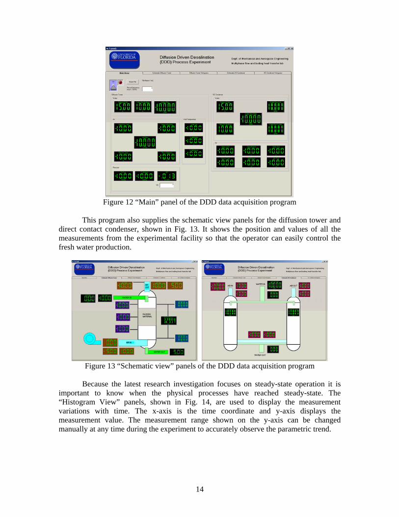
14

Figure 12 “Main” panel of the DDD data acquisition program

This program also supplies the schematic view panels for the diffusion tower and

direct contact condenser, shown in Fig. 13. It shows the position and values of all the measurements from the experimental facility so that the operator can easily control the fresh water production.

Figure 13 “Schematic view” panels of the DDD data acquisition program

Because the latest research investigation focuses on steady-state operation it is

important to know when the physical processes have reached steady-state. The “Histogram View” panels, shown in Fig. 14, are used to display the measurement variations with time. The x-axis is the time coordinate and y-axis displays the measurement value. The measurement range shown on the y-axis can be changed manually at any time during the experiment to accurately observe the parametric trend.

15

Figure 14 “Histogram view” panels of the DDD data acquisition program

Ion Chromatograph One objective of the experimental facility is to quantify the purity of fresh water produced with the DDD facility. For this purpose a Dionex ICS-90 isochromatic ion chromatograph has been installed in the Multiphase Heat Transfer and Fluid Dynamics laboratory. The ICS-90 is capable of measuring mineral concentrations down to several parts per billion. 3. Heat and Mass Transfer for the Diffusion Tower

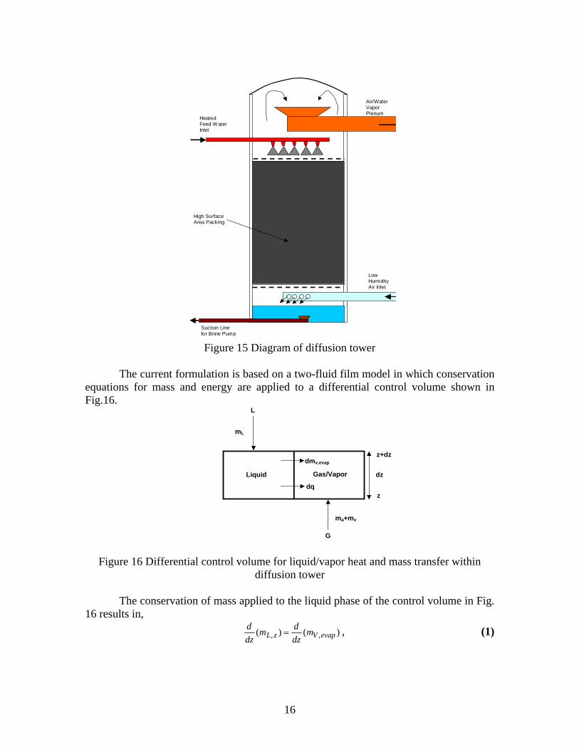
The evaporation of mineralized water in the diffusion tower, shown in Fig. 15, is achieved by spraying heated feed water on top of a packed bed and blowing the dry air counter currently through the bed. The falling liquid will form a thin film over the packing material while in contact with the low humidity turbulent air stream. Heat and mass transfer principles govern the evaporation of the water and the humidification of the air stream. When the system is operating at design conditions, the exit air stream humidity ratio should be as high as possible. The ideal state of the exit air/vapor stream from the diffusion tower is saturated.

3.1 Heat and Mass Transfer Model for the Diffusion Tower

The most widely used model to estimate the heat and mass transfer associated with air/water evaporating systems is, that due to Merkel [7], which is used to analyze cooling towers. However Merkel’s analysis contains two restrictive assumptions, 1) On the water side, the mass loss by evaporation of water is negligible and 2) The Lewis number is unity.

Merkel’s analysis is known to under-predict the required cooling tower volume and is not useful for the current analysis since the purpose of the diffusion tower is to maximize the evaporation of water for desalination. Baker and Shryock [8] have presented a detailed analysis of Merkel’s original work and have elucidated the error contributed from specific assumptions. Sutherland [9], Osterle [10], and El-Dessouky et al. [11] have presented improved analyses for counter flow cooling towers, yet they inherently contain simplifications that diminish the rigor.

16

Suction Line for Brine Pump

Heated Feed Water Inlet

Low Humidity Air Inlet

Air/Water Vapor Plenum

High Surface Area Packing

Figure 15 Diagram of diffusion tower

The current formulation is based on a two-fluid film model in which conservation

equations for mass and energy are applied to a differential control volume shown in Fig.16.

Liquid Gas/Vapor

G

ma+mv

L

mL

dz

z

z+dzdmv,evap

dq

Figure 16 Differential control volume for liquid/vapor heat and mass transfer within diffusion tower

The conservation of mass applied to the liquid phase of the control volume in Fig.

16 results in, )()( ,, evapVzL m

dzdm

dzd

= , (1)

17

where m is the mass flow rate, the subscript L denotes the liquid, v denotes the vapor, and evap denotes the portion of liquid evaporated. Likewise, the conservation of mass applied to the gas (air/vapor mixture) side is expressed as,

)()( ,, evapVzV mdzdm

dzd

= . (2)

For an air/water-vapor mixture the humidity ratio ω, is related to the relative humidity, Φ, through,

)()(622.0

asat

asat

a

VTPPTP

mm

Φ−Φ

==ω , (3)

where P is the total system pressure and Psat(Ta) is the water saturation pressure corresponding to the air temperature Ta. Using the definition of the mass transfer coefficient applied to the differential control volume in conjunction with the perfect gas law, the gradient of the evaporation rate is expressed as,

AT

TPT

TPR

Makm

dzd

a

asat

i

isatVwGevapV )

)()(()( ,

Φ−= , (4)

where Gk is the mass transfer coefficient on gas side, a is the specific area of the packing material, aw is the wetted specific area, VM is the vapor molecular weight, R is the universal gas constant, Ti is the liquid/vapor interfacial temperature and A is the cross sectional area of the diffusion tower. Combining Eqs. (2), (3), and (4) the gradient of the humidity ratio in the diffusion tower is expressed as,

)622.0

)((

ai

isatVGTP

TTP

RM

Gak

dzd

ωωω+

−= , (5)

where G = Ama is the air mass flux. Equation (5) is a first order ordinary differential

equation with dependent variable, ω, and when solved yields the variation of humidity ratio along the length of the diffusion tower. In order to evaluate the liquid/vapor interfacial temperature it is recognized that the energy convected from the liquid is the same as that convected to the gas,

)()( aiGiLL TTUTTU −=− , (6) where UL and UG are the respective liquid and gas heat transfer coefficients, and the interfacial temperature is evaluated from,

LG

aLGL

i

UU

TUUT

T+

−=

1 . (7)

In general the liquid side heat transfer coefficient is much greater than that on the gas side, thus the interfacial temperature is only slightly less than that of the liquid.

The conservation of energy applied to the liquid phase of the control volume yields,

ATTUahdz

mdhm

dzd

aLFgevapV

LL )()(

)( , −+= , (8)

where U is the overall heat transfer coefficient and h is the enthalpy. Noting that LLpL dTCdh = and combining with Eqs. (8) and (1) results in an expression for the gradient of water temperature in the diffusion tower,

18

LCTTUa

Chh

dzd

LG

dzdT

Lp

aL

Lp

LFgL )()( −+

−=

ω , (9)

where L= AmL is the water mass flux. Equation (9) is also a first order ordinary

differential equation with TL being the dependent variable and when solved yields the water temperature distribution through the diffusion tower.

The conservation of energy applied to the air/water-vapor phase of the control volume yields,

.)(

)()( ,

ATTUa

hdz

mdhmhm

dzd

aL

FgevapV

VVaa

−−

=++− , (10)

Noting that the specific heat of the air/vapor mixture is evaluated as,

Vp

Va

VPa

Va

amixp C

mmm

Cmm

mC

++

+= , (11)

and combining with Eqs. (10) and (2) yields the gradient of air temperature in the diffusion tower,

)1()()(

11

ωω

ω +−

++

−=GC

TTUaC

Thdzd

dzdT

mixp

aL

mixp

aLa . (12)

Equation (12) is also a first order ordinary differential equation with Ta being the dependent variable and when solved yields the air/vapor mixture temperature distribution along the height of the diffusion tower.

Equations (5), (9), and (12) comprise a set of coupled ordinary differential equations that are used to solve for the humidity ratio, water temperature, and air/vapor mixture temperature distributions along the height of the diffusion tower. However, since a one-dimensional formulation is used, these equations require closure relationships. Specifically, the overall heat transfer coefficient and the gas side mass transfer coefficient are required. A significant difficulty that has been encountered in this analysis is that correlations for the water and air/vapor heat transfer coefficients for film flow though a packed bed, available in the open literature (McAdams et al. [12] and Huang and Fair [13]), are presented in dimensional form. Such correlations are not useful for the present analysis since a special matrix type packing material is utilized, and the assumption employed to evaluate those heat transfer coefficients are questionable. In order to overcome this difficulty the mass transfer coefficients are evaluated for the liquid and gas flow using a widely tested correlation and a heat and mass transfer analogy is used to evaluate the heat transfer coefficients. This overcomes the difficulty that gas and liquid heat transfer coefficients cannot be directly measured because the interfacial film temperature is not known.

The mass transfer coefficients associated with film flow in packed beds have been widely investigated. The most widely used and perhaps most reliable correlation is that proposed by Onda et al. [14]. Onda’s correlation, shown in Appendix A, is used to calculate the mass transfer coefficients in the diffusion tower, kG and kL. However, it was found at Onda’s correlation under-predicted the wetted specific area of the packing material. Therefore, a correction was made as follows,

⎪⎭

⎪⎬⎫

⎪⎩

⎪⎨⎧

⎥⎥⎦

⎤

⎢⎢⎣

⎡⎟⎟⎠

⎞⎜⎜⎝

⎛−−= − 5/105.02/1

4/3

Re2.2exp1 LLLAL

cw WeFraa

σσ , (13)

19

See Appendix A for details. As mentioned previously, the heat and mass transfer analogy is used to compute

the heat transfer coefficients for the liquid side and the gas side. Therefore the heat transfer coefficients are computed as follows,

heat transfer coefficient on the liquid side

2/12/1Pr L

L

L

L

ScShNu

= , (14)

2/1)(L

LPLLLL D

KCkU ρ= , (15)

heat transfer coefficient on the gas side

3/13/1Pr G

G

G

G

ScShNu

= , (16)

3/23/1 )()(G

GPGGGG D

KCkU ρ= , (17)

overall heat transfer coefficient 111 )( −−− += GL UUU , (18)

where K denotes thermal conductivity and D denotes the molecular diffusion coefficient.

In order to test the proposed heat and mass transfer model, consideration is first given to the cooling data of McAdams et al. [12]. The data shown are for air water counter current flow in a 15.24 cm bed packed with 2.54 cm carbon Raschig rings. Using the analysis presented above, the exit water temperature, exit air temperature, and exit humidity ratio are computed using the following procedure: 1) guess the exit water temperature; 2) compute the temperature distributions and humidity distribution through the packed bed using Eqs. (5), (9), and (12); 3) Check whether the predicted inlet water temperature agrees with the measured inlet water temperature, and stop the computation if agreement is found, otherwise repeat the procedure from step 1. A comparison between the measured exit water temperature, exit air temperature, and exit humidity ratio reported by McAdams et al. with those computed using the current model are shown in Figs. 17 a and b. As seen in the figures the comparison is generally good. The exit air temperature and exit humidity ratio are slightly under-predicted. The exit water temperature is slightly over-predicted. It is noted that McAdams et al. were not confident with the humidity measurement, and there is some error in the measurement because when the humidity ratio is converted to relative humidity for some data, the computed values exceed 100%. The actual humidity should lie closer to the predicted values.

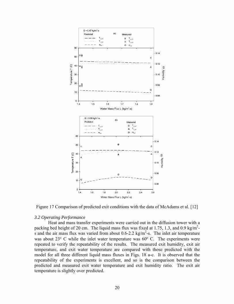
20

ω

ω

Figure 17 Comparison of predicted exit conditions with the data of McAdams et al. [12]

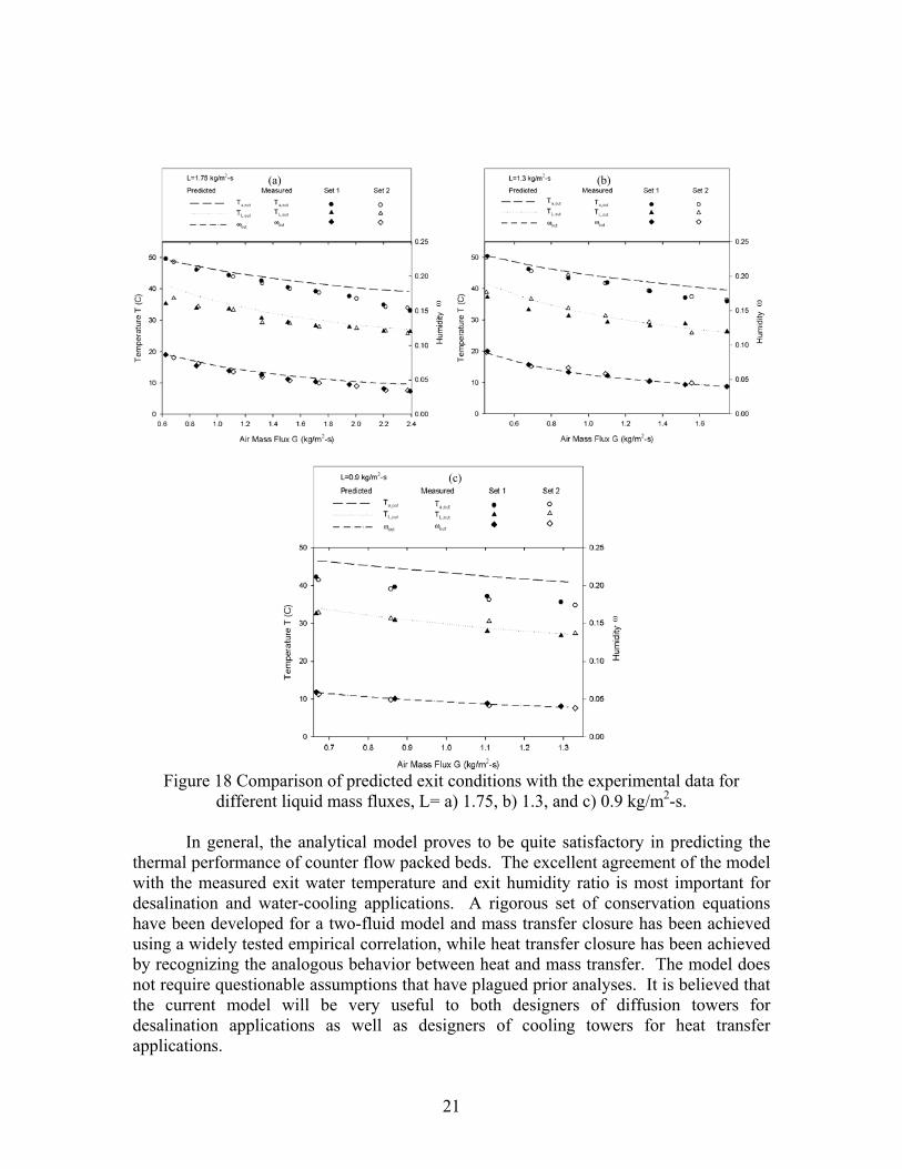
3.2 Operating Performance Heat and mass transfer experiments were carried out in the diffusion tower with a

packing bed height of 20 cm. The liquid mass flux was fixed at 1.75, 1.3, and 0.9 kg/m2-s and the air mass flux was varied from about 0.6-2.2 kg/m2-s. The inlet air temperature was about 23° C while the inlet water temperature was 60° C. The experiments were repeated to verify the repeatability of the results. The measured exit humidity, exit air temperature, and exit water temperature are compared with those predicted with the model for all three different liquid mass fluxes in Figs. 18 a-c. It is observed that the repeatability of the experiments is excellent, and so is the comparison between the predicted and measured exit water temperature and exit humidity ratio. The exit air temperature is slightly over predicted.

21

ω

ω

ω

Figure 18 Comparison of predicted exit conditions with the experimental data for

different liquid mass fluxes, L= a) 1.75, b) 1.3, and c) 0.9 kg/m2-s.

In general, the analytical model proves to be quite satisfactory in predicting the thermal performance of counter flow packed beds. The excellent agreement of the model with the measured exit water temperature and exit humidity ratio is most important for desalination and water-cooling applications. A rigorous set of conservation equations have been developed for a two-fluid model and mass transfer closure has been achieved using a widely tested empirical correlation, while heat transfer closure has been achieved by recognizing the analogous behavior between heat and mass transfer. The model does not require questionable assumptions that have plagued prior analyses. It is believed that the current model will be very useful to both designers of diffusion towers for desalination applications as well as designers of cooling towers for heat transfer applications.

(a) (b)

(c)

22

3.3 Pressure Drop through the Packing Material

The pressure drop through the packing material on the air side influences the energy consumption prediction of the DDD process. Therefore experiments considering the air pressure drop with water loading is another important objective in the research. This experiment is executed without heating the water. The comparison of the predicted pressure drop and the experimental data are shown below in Fig. 19 for different water mass flux loadings.

0

10

20

30

40

50

60

70

80

90

100

0 0.2 0.4 0.6 0.8 1 1.2 1.4 1.6 1.8

Air Mass Flux G (kg/m2-s)

Spec

ific

Pres

sure

Dro

p ∆P

/∆z

(Pa/

m)

0

10

20

30

40

50

60

70

80

90

1000 0.2 0.4 0.6 0.8 1 1.2 1.4 1.6 1.8

increasing L

Water Mass Flux L (kg/m2-s)

0.8 1.7 2.0

Data

Prediction

Figure 19 Air specific pressure drop variation with air mass flux for water mass flux L

The pressure drop is predicted using the empirical correlation specified by the

manufacturer of the packing material. Figure 19 clearly shows that the pressure drop correlation is accurate for HD Q-Pac packing material. Another interesting result is that the air specific pressure drop increases with increasing water mass flow rate under the same air mass flow rate. The air side dimensional pressure drop correlation is:

)10176.1654.01054.3( 4244252GGLLGG VVVV

zP ρρ ×++×=

∆ − (19)

where z is the height of the packing material (m), P∆ is the pressure drop through the packing (Pa), Gρ is the gas density (kg/m3), GV is the superficial gas velocity through the packing (m/s), and LV ′ is the superficial liquid velocity through the packing (m/s).

Using π -theory, the following dimensionless variables are identified as being

important to the pressure drop: 2GG

G VPEu

ρ∆

= ,G

GGGD

DVµ

ρ=Re ,

L

LLLD

DVµ

ρ=Re and

zD

=ε . Equation (19) may be rearranged as,

44

32

21 ReReRe GDLDLDG CCCEu ++=ε (20) DC 5

1 1054.3 −×= (21)

23

DC

L

L2

2

2 654.0ρµ

= (22)

724

444

3 10176.1D

CGL

GL

ρρµµ

×= (23)

where D is the cross section diameter of the packing (m), Lρ is the liquid density (kg/m3), Lµ is liquid viscosity (Pa-s), Gµ is gas viscosity (Pa-s). Although the constants in Eqn. (21) - (23) are dimensional, Eqn. (20) elucidates the dimensionless variables that control pressure drop through packed bed. 4. Heat and Mass Transfer for the Direct Contact Condenser with Packing

Heat and mass transfer models for the diffusion tower have been reported in the

2004 annual report [6], and are not included here. 4.1 Physical Model

A one dimensional two fluid condensation model is used to quantify the change in mean humidity ratio through the condenser. Conservation equations for mass and energy are applied to a differential control volume for co-current flow which is shown in Figure 20.

Liquid Gas/Vapor

G

ma+mv

L

mL

dz

z

z+dz

dmv,cond

dqloss”dq

Figure 20 Differential control volume for liquid/gas heat and mass transfer within co-

current condenser

Similarly, a one dimensional two fluid counter-current differential control volume is shown in Fig.21. Conservation equations for mass and energy are applied to the control volume.

24

Liquid Air/Vapor

G

ma+mv

L

mL

dz

z

z+dzdmv,cond

dq dqloss”

Figure 21 Differential control volume for liquid/gas heat and mass transfer within

counter-current condenser

Within the direct contact condenser, the transverse air temperature distribution could play an important role in the condensation process. Therefore, a non-uniform distribution of the air temperature in the transverse direction is considered in the analysis. The flow structure within the packing material is shown in Figure 22. The local humidity based on local transverse air temperature is averaged, and the mean humidity is used on the one dimensional conservation equations.

x

l

Packing material

Water film

Air/Vapor

Figure 22 Flow structure within the packing material

4.2 Mathematic Model

As mentioned previously, the air temperature non-uniformity within the co-current flow condenser may influence the condensation process. Therefore, a non-uniform distribution of the air temperature in the transverse direction is considered in the condensation analysis. Because the air in the channel is highly turbulent, following Kays and Crawford [15], a 1/7th law variation of temperature is assumed as,

7/1

,

, 1 ⎟⎠⎞

⎜⎝⎛ −=

−

−

lx

TTTT

caL

xaL . (24)

where Ta,c is the centerline air temperature, l is the half width of the flow channel, and x is the transverse axis. The centerline air temperature can be solved as,

( )LaLca TTTT −+= 2.1, . (25)

25

The transverse distribution of air temperature is calculated from Eqn (24). The local humidity ratio ω, based on local transverse air temperature Ta,x, is related to the relative humidity Φ through as

)()(622.0

,

,

xasat

xasat

a

Vx TPP

TPmm

Φ−

Φ==ω , (26)

where P (kPa) is the total system pressure, and Psat (kPa) is the water saturation pressure corresponding to the local air temperature Ta,x and can be calculated using an empirical representation of the saturation line,

( )32exp)( dTcTbTaTPsat +−= , (27) where empirical constants are a=0.611379, b=0.0723669, c=2.78793e-4, d=6.76138e-7, and T(°C) is the saturation temperature. The local humidity ratio is area averaged, and the mean humidity ωm is used in the one dimensional condensation model (Eqs (28), (29) and (30) ).

Noting that the relative humidity of air remains 100% during the condensation process, the absolute humidity ω is only a function of air temperature Ta. Differentiating Eqn. (26) and combining with Eqn. (27), the gradient of humidity can be expressed as,

)32()(

2aam

asat

a dTcTbTPP

Pdz

dTdzd

+−−

= ωω . (28)

The gradient of water temperature in the condenser is found by considering the energy conservation in liquid phase as,

LCTTUa

CThTh

dzd

LG

dzdT

Lp

aL

Lp

LLaFgL )())()(( −−

−−=

ω , (29)

The gradient of air temperature in the condenser is found by considering energy conservation in the gas phase. Equations presented in Appendix A are used to evaluate the overall heat transfer coefficient in Eqs (29) and (30). Because heat loss is observed in the experiments, it is considered as an additional term in the energy conservation of the air side,

)1)((/

)1)(()(

)1()( "

maGp

oloss

maGp

aL

mGp

aLa

TGCADq

TGCTTUa

dzd

CTh

dzdT

ωπ

ωω

ω +−

+−+

++

−= , (30)

The specific heat of the air/vapor mixture is evaluated as,

VpVa

VPa

Va

aGp C

mmm

Cmm

mC

++

+= . (31)

Here Do (m) is the cross section diameter of the packed bed, qloss” (kW/m2) is the heat loss flux, and A (m2) is the total exposed area to the ambient temperature. Finally, Eqs. (28 - 30) are used to evaluate the heat and mass transfer performance in the co-current condenser.

A similar mass and energy balance analysis has been done for the counter-current flow condenser. The equations for evaluating the humidity gradient and air temperature gradient are same as that for co-current flow. The gradient of water temperature in the condenser is found by considering the energy conservation in the liquid phase as,

LCpTTUa

Cphh

dzd

LG

dzdT

L

aL

L

LFgL )()( −+

−=

ω , (32)

26

Thus, Eqs. (28), (32) and (30) are used to evaluate the heat and mass transfer process in the counter-current flow condenser, and Onda’s correlation and heat and mass transfer analogy shown in Appendix A are used to close them.

If |ωm-ω|>1e-5

Compute Ta,c from Eq. (25),Ta,x from Eq. (24), ωx from Eq. (26);

area average ωx to get ωm

If z < H

Output Tl,,out, Ta,out,, ωout

Stop Start

Define fluid property functions

Input TL,in, Ta,in, ωin at z=0

Update TL, Ta, ω for current z location

Calculate U by analogy method from Appendix A

Calculate kG, kL using Onda’s correlation from Appendix A

Calculate Ta, TL and ω at next z location using Eqs. (28-30); use 4th order Runge - Kutta method

Calculate fluid properties from the fluid property functions

Set ω =ωm , and ωm = ωin at z=0

Yes

Yes

No

No

Figure 23 Flow diagram of the co-current flow condenser computation

For the co-current flow condensation analysis presented above, the exit water

temperature, exit air temperature, and exit humidity ratio are computed using the following procedure: 1) specify the inlet water temperature, air temperature and bulk humidity; 2) compute the temperatures and bulk humidity at the next step change in height using Eqs (28 – 30); 3) compute the local humidity in the x-direction at this z location using Eqs (24 – 26) and area average the humidity; 4) check whether the area average humidity is the same as the bulk humidity; repeat steps 2 – 4 until agreement is achieved; 5) proceed to a new height, and restart computation from step 2; 6) compute the temperatures and humidity through the condenser using steps 2 – 5 until the computed

27

height matches the experimental height. Detailed flow diagram of the co-current flow condenser computation is shown in Fig.23.

Output Tl,,out, Ta,out,, ωout

Stop Start

Define fluid property functions

Calculate U by analogy method from Appendix A

Calculate kG, kL using Onda’s correlation from Appendix A

Calculate Ta, TL and ω at next z location using Eqs. (28), (30)

and (32); use 4th order Runge - Kutta method

Calculate fluid properties from the fluid property functions

If |ωm-ω| >1e-5

Compute Ta,c from Eq. (25),Ta,x from Eq. (24), ωx from Eq. (26);

area average ωx to get ωm

If z < H Guess TL,out at z=0

Update TL, Ta, ω for the current z location

Set ωm = ω, and ωm = ωin at z=0

Yes

Yes

No

No

Input TL,in at z = H, input Ta,in, and ωin

at z = 0

If |TL- TL,in | > 0.1

No Yes

Figure 24 Flow diagram of the counter-current flow condenser computation

For the counter-current condensation analysis, the exit water temperature, exit air

temperature, and exit humidity ratio are computed using the following procedure: 1) specify the inlet water temperature, air temperature and bulk humidity; 2) guess the exit water temperature; 3) compute the temperatures and bulk humidity at the next step change in height using Eqs. (28), (30) and (32); 4) compute the local humidity at that height using Eqs. (24 – 26), and area average the humidity; 5) check whether the

28

computed bulk humidity agrees with the area average humidity, repeat steps 3 – 5 until agreement is achieved; 6) proceed to a new height, and restart the computation from step 3; 7) compute the temperatures and humidity through the condenser using steps 3 – 6 until the computed height matches the experimental height; 8) check whether the computed inlet water temperature agrees with the specified inlet water temperature, and stop the computation if agreement is found, otherwise repeat the procedure from step 2. A detailed flow diagram of the computation procedure is shown in Fig. 24. 4.3 Operating Performance

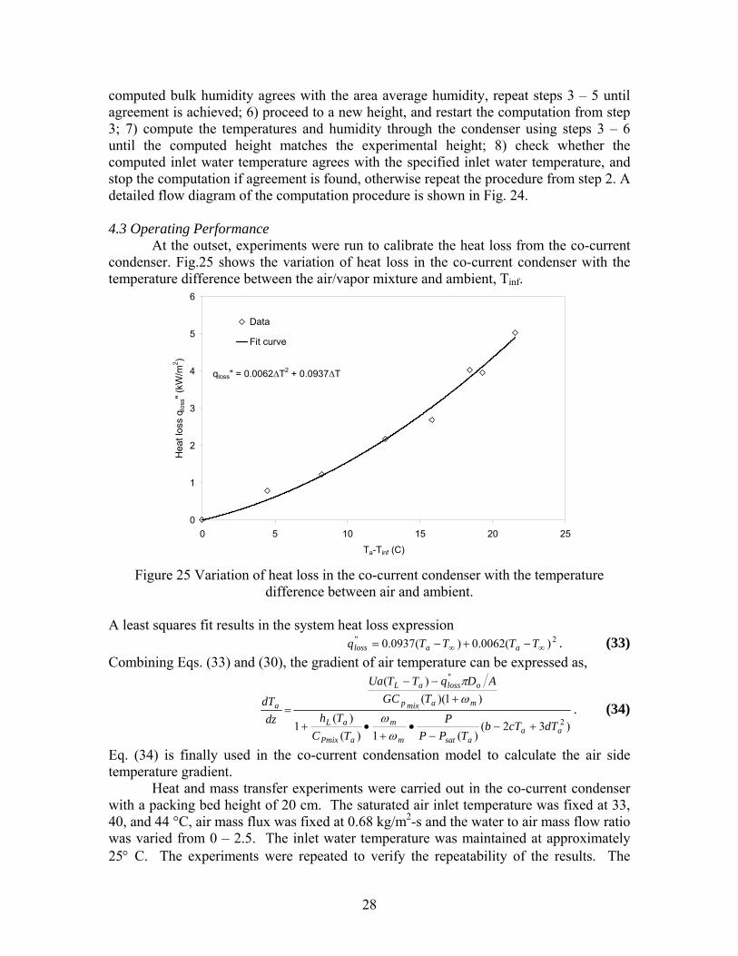
At the outset, experiments were run to calibrate the heat loss from the co-current condenser. Fig.25 shows the variation of heat loss in the co-current condenser with the temperature difference between the air/vapor mixture and ambient, Tinf.

qloss" = 0.0062∆T2 + 0.0937∆T

0

1

2

3

4

5

6

0 5 10 15 20 25

Ta-Tinf (C)

Hea

t los

s q l

oss"

(kW

/m2 )

Data

Fit curve

Figure 25 Variation of heat loss in the co-current condenser with the temperature

difference between air and ambient.

A least squares fit results in the system heat loss expression 2" )(0062.0)(0937.0 ∞∞ −+−= TTTTq aaloss . (33)

Combining Eqs. (33) and (30), the gradient of air temperature can be expressed as,

)32()(1)(

)(1

)1)(()(

2

"

aaasatm

m

aPmix

aL

mamixp

olossaL

a

dTcTbTPP

PTC

ThTGC

ADqTTUa

dzdT

+−−

•+

•+

+−−

=

ωω

ωπ

. (34)

Eq. (34) is finally used in the co-current condensation model to calculate the air side temperature gradient.

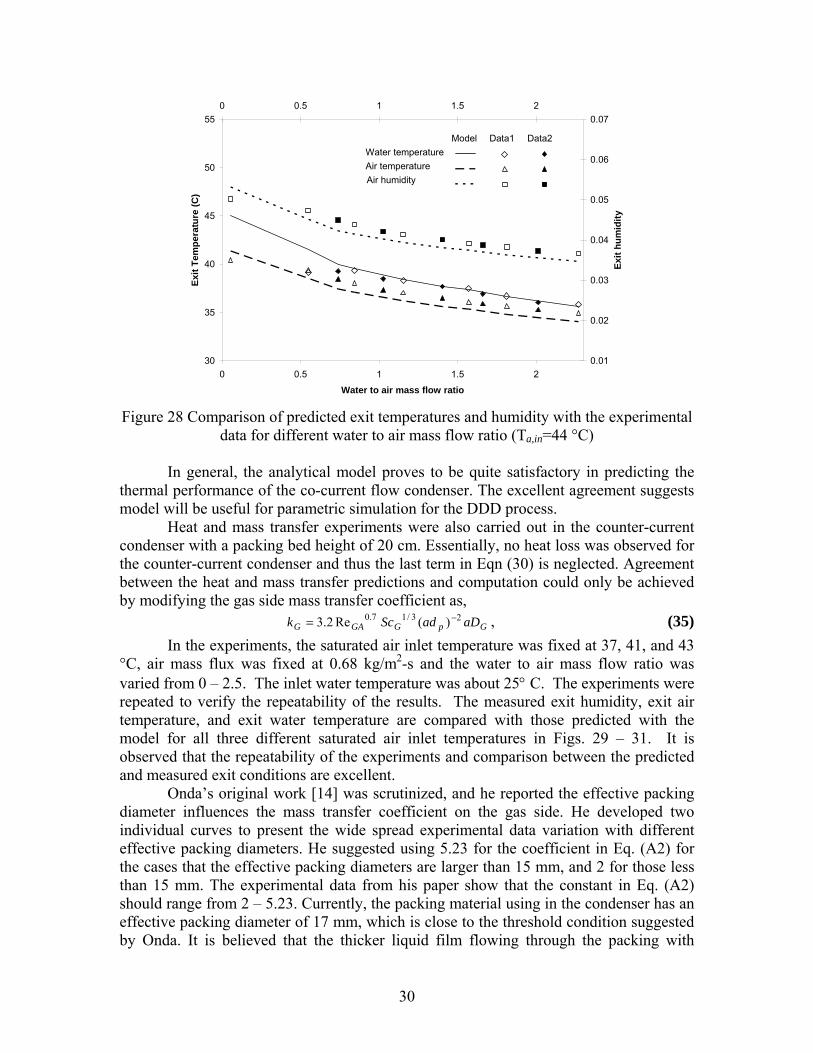
Heat and mass transfer experiments were carried out in the co-current condenser with a packing bed height of 20 cm. The saturated air inlet temperature was fixed at 33, 40, and 44 °C, air mass flux was fixed at 0.68 kg/m2-s and the water to air mass flow ratio was varied from 0 – 2.5. The inlet water temperature was maintained at approximately 25° C. The experiments were repeated to verify the repeatability of the results. The

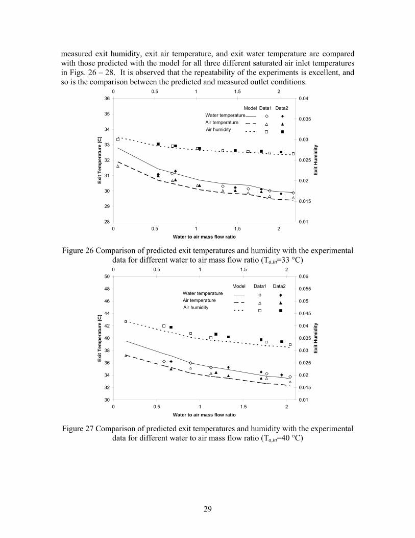
29

measured exit humidity, exit air temperature, and exit water temperature are compared with those predicted with the model for all three different saturated air inlet temperatures in Figs. 26 – 28. It is observed that the repeatability of the experiments is excellent, and so is the comparison between the predicted and measured outlet conditions.

28

29

30

31

32

33

34

35

36

0 0.5 1 1.5 2

Water to air mass flow ratio

Exit

Tem

pera

ture

(C)

0.01

0.015

0.02

0.025

0.03

0.035

0.040 0.5 1 1.5 2

Exit

Hum

idity

Water temperature

Air humidityAir temperature

Data1Model Data2

Figure 26 Comparison of predicted exit temperatures and humidity with the experimental

data for different water to air mass flow ratio (Ta,in=33 °C)

30

32

34

36

38

40

42

44

46

48

50

0 0.5 1 1.5 2


Exit

Tem

pera

ture

(C)

0.01

0.015

0.02

0.025

0.03

0.035

0.04

0.045

0.05

0.055

0.060 0.5 1 1.5 2

Exit

Hum

idity

Water temperature


Data1Model Data2



30

30

35

40

45

50

55

0 0.5 1 1.5 2


Exit

Tem

pera

ture

(C)

0.01

0.02

0.03

0.04

0.05

0.06

0.070 0.5 1 1.5 2

Exit

hum

idity

Water temperature


Data1Model Data2



In general, the analytical model proves to be quite satisfactory in predicting the thermal performance of the co-current flow condenser. The excellent agreement suggests model will be useful for parametric simulation for the DDD process.

Heat and mass transfer experiments were also carried out in the counter-current condenser with a packing bed height of 20 cm. Essentially, no heat loss was observed for the counter-current condenser and thus the last term in Eqn (30) is neglected. Agreement between the heat and mass transfer predictions and computation could only be achieved by modifying the gas side mass transfer coefficient as,

GpGGAG aDadSck 23/17.0 )(Re2.3 −= , (35) In the experiments, the saturated air inlet temperature was fixed at 37, 41, and 43

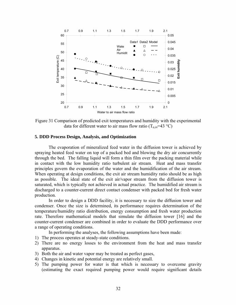
°C, air mass flux was fixed at 0.68 kg/m2-s and the water to air mass flow ratio was varied from 0 – 2.5. The inlet water temperature was about 25° C. The experiments were repeated to verify the repeatability of the results. The measured exit humidity, exit air temperature, and exit water temperature are compared with those predicted with the model for all three different saturated air inlet temperatures in Figs. 29 – 31. It is observed that the repeatability of the experiments and comparison between the predicted and measured exit conditions are excellent.

Onda’s original work [14] was scrutinized, and he reported the effective packing diameter influences the mass transfer coefficient on the gas side. He developed two individual curves to present the wide spread experimental data variation with different effective packing diameters. He suggested using 5.23 for the coefficient in Eq. (A2) for the cases that the effective packing diameters are larger than 15 mm, and 2 for those less than 15 mm. The experimental data from his paper show that the constant in Eq. (A2) should range from 2 – 5.23. Currently, the packing material using in the condenser has an effective packing diameter of 17 mm, which is close to the threshold condition suggested by Onda. It is believed that the thicker liquid film flowing through the packing with

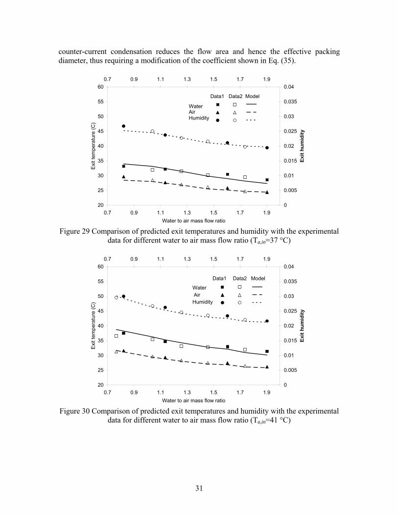
31

counter-current condensation reduces the flow area and hence the effective packing diameter, thus requiring a modification of the coefficient shown in Eq. (35).

20

25

30

35

40

45

50

55

60

0.7 0.9 1.1 1.3 1.5 1.7 1.9Water to air mass flow ratio

Exi

t tem

pera

ture

(C)

0

0.005

0.01

0.015

0.02

0.025

0.03

0.035

0.040.7 0.9 1.1 1.3 1.5 1.7 1.9

Exit

hum

idity

Data1 Model

WaterAirHumidity

Data2



20

25

30

35

40

45

50

55

60

0.7 0.9 1.1 1.3 1.5 1.7 1.9Water to air mass flow ratio

Exi

t tem

pera

ture

(C)

0

0.005

0.01

0.015

0.02

0.025

0.03

0.035

0.040.7 0.9 1.1 1.3 1.5 1.7 1.9

Exit

hum

idity

Data1 Model

WaterAirHumidity

Data2



32

20

25

30

35

40

45

50

55

60

0.7 0.9 1.1 1.3 1.5 1.7 1.9 2.1Water to air mass flow ratio

Exi

t tem

pera

ture

(C)

0

0.005

0.01

0.015

0.02

0.025

0.03

0.035

0.04

0.045

0.050.7 0.9 1.1 1.3 1.5 1.7 1.9 2.1

Exit

hum

idity

Data1 ModelWateAirHumidit

Data2


data for different water to air mass flow ratio (Ta,in=43 °C) 5. DDD Process Design, Analysis, and Optimization

The evaporation of mineralized feed water in the diffusion tower is achieved by spraying heated feed water on top of a packed bed and blowing the dry air concurrently through the bed. The falling liquid will form a thin film over the packing material while in contact with the low humidity ratio turbulent air stream. Heat and mass transfer principles govern the evaporation of the water and the humidification of the air stream. When operating at design conditions, the exit air stream humidity ratio should be as high as possible. The ideal state of the exit air/vapor stream from the diffusion tower is saturated, which is typically not achieved in actual practice. The humidified air stream is discharged to a counter-current direct contact condenser with packed bed for fresh water production.

In order to design a DDD facility, it is necessary to size the diffusion tower and condenser. Once the size is determined, its performance requires determination of the temperature/humidity ratio distribution, energy consumption and fresh water production rate. Therefore mathematical models that simulate the diffusion tower [16] and the counter-current condenser are combined in order to evaluate the DDD performance over a range of operating conditions.

In performing the analyses, the following assumptions have been made: 1) The process operates at steady-state conditions. 2) There are no energy losses to the environment from the heat and mass transfer

apparatus. 3) Both the air and water vapor may be treated as perfect gases, 4) Changes in kinetic and potential energy are relatively small. 5) The pumping power for water is that which is necessary to overcome gravity

(estimating the exact required pumping power would require significant details

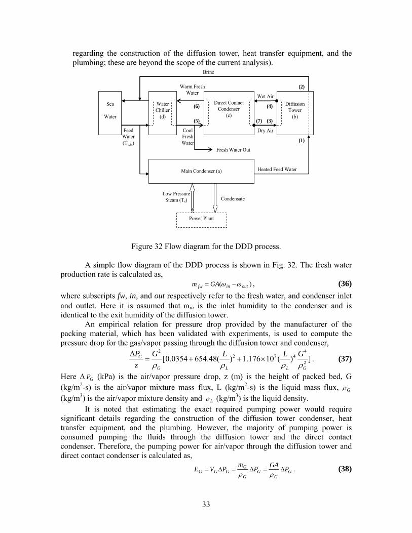
33

regarding the construction of the diffusion tower, heat transfer equipment, and the plumbing; these are beyond the scope of the current analysis).

Diffusion

Tower (b)

Water Chiller

(d)

Sea

Water

Direct Contact

Condenser (c)

Main Condenser (a)

Power Plant

Fresh Water Out

Condensate

Warm Fresh Water

Cool Fresh Water

Wet Air

Dry Air

Heated Feed Water

Low Pressure Steam (Ts)

(1)

(2)

(3)

(4)

(7) (5)

(6)

Brine

Feed Water (Tb,in)

Figure 32 Flow diagram for the DDD process.

A simple flow diagram of the DDD process is shown in Fig. 32. The fresh water production rate is calculated as,

)( outinfw GAm ωω −= , (36) where subscripts fw, in, and out respectively refer to the fresh water, and condenser inlet and outlet. Here it is assumed that ωin is the inlet humidity to the condenser and is identical to the exit humidity of the diffusion tower.

An empirical relation for pressure drop provided by the manufacturer of the packing material, which has been validated with experiments, is used to compute the pressure drop for the gas/vapor passing through the diffusion tower and condenser,

2 42 7 4

2[0.0354 654.48( ) 1.176 10 ( ) ]G

G L L G

P G L L Gz ρ ρ ρ ρ

∆= + + × . (37)

Here ∆ GP (kPa) is the air/vapor pressure drop, z (m) is the height of packed bed, G (kg/m2-s) is the air/vapor mixture mass flux, L (kg/m2-s) is the liquid mass flux, Gρ (kg/m3) is the air/vapor mixture density and Lρ (kg/m3) is the liquid density.

It is noted that estimating the exact required pumping power would require significant details regarding the construction of the diffusion tower condenser, heat transfer equipment, and the plumbing. However, the majority of pumping power is consumed pumping the fluids through the diffusion tower and the direct contact condenser. Therefore, the pumping power for air/vapor through the diffusion tower and direct contact condenser is calculated as,

GG

GG

GGGG PGAP

mPVE ∆=∆=∆=

ρρ. (38)

34

From assumption 5, the pumping power for water is that which is necessary to overcome gravity in raising water to the top of the diffusion tower and condenser is,

gHmPm

E LLL

LL =∆=

ρ. (39)

The total pumping energy consumption rate for the DDD process includes the pumping power consumed by the diffusion tower and condenser for both the water side and air/vapor side as,

GLtotal EEE += . (40) So the energy consumption rate per unit of fresh water production is defined as,

fw

totalfw m

EE = . (41)

where Etotal is the total pumping energy consumption rate. The objective of the computational analysis is to explore the influence of the

operating parameters on the DDD process performance. These parameters include the water/air/vapor temperatures, humidity ratio, water mass flux, air to feed water mass flow ratio, and tower size. The water mass flux and the air to feed water mass flow ratio through the tower are two primary controlling variables in the analysis.

For all computations considered in the diffusion tower, the water inlet temperature, gas inlet temperature, inlet humidity ratio, specific area and diameter of the packing material are fixed as 50° C, 26° C, 0.023, 267 m2/m3 and 0.018m. The inlet feed water mass flux is varied from 0.5 kg/m2-s to 3 kg/m2-s, meanwhile the air to feed water mass flow ratio (ma/mL1) is varied from 0.5 to 1.5 for every fixed inlet feed water mass flux. All the cases analyzed in this report are below the flooding curve of the packing material. The reason that the inlet feed water temperature is fixed at 50° C is that this is typically the highest water temperature that can be expected to exit the main condenser of a thermoelectric power plant.

Diffusion Tower Size

Figure 33 shows the required diffusion tower height for different inlet water mass flux and varying air to feed water mass flow ratio. The tower height is computed such that the maximum possible humidity ratio leaves the diffusion tower. For every fixed air to feed water mass flow ratio, the required diffusion tower height decreases with increasing inlet water mass flux and decreases with increasing air to feed water mass flow ratio.

Figure 33 shows that for a fixed inlet water temperature and the maximum possible exit humidity ratio, the required diffusion tower height is strongly influenced by both the inlet water mass flux and the air to feed water mass flow ratio. It is particularly noteworthy that the typically required diffusion tower height does not exceed 2 meters for an air to feed water mass flow ratio above unity. This is an important consideration in evaluating the cost of fabricating a desalination system. Due to the small size of the diffusion tower, it is feasible to manufacture the tower off site and deliver it to the plant site and thus lower the overall cost.

35

Air to Feed Water Mass Flow Ratio

0.4 0.6 0.8 1.0 1.2 1.4

Diff

usio

n To

wer

Hei

ght (

m)

0

1

2

3

4

5

0.511.522.53

Diffusion TowermL (kg/m2-s)

Figure 33 Required diffusion tower height with variations in air to feed water mass flow

ratio Maximum Exit Humidity Ratio from Diffusion Tower

Figure 34 shows the maximum possible exit humidity ratio for different inlet water mass flux and varying air to feed water mass flow ratios. For fixed inlet water and air temperatures, the maximum possible exit humidity ratio is strongly dependent on the air to feed water mass flow ratio and is largely independent of the inlet water mass flux. These results indicate that increasing the air to water mass flow ratio will not necessarily assist in increasing the fresh water production since the exit humidity ratio decreases with increasing air to water mass flow ratio.


0.4 0.6 0.8 1.0 1.2 1.4

Max

imum

Exi

t Hum

idity

Rat

io

0.04

0.05

0.06

0.07

0.08

0.09

0.511.522.53


Figure 34 Maximum exit humidity ratio dependence on air to feed water mass flow ratio

Exit Air Temperature from Diffusion Tower

Figure 35 shows the exit air temperature for different inlet water mass flux and

varying air to feed water mass flow ratios. The exit air temperature is sensitive to variations in both the inlet water mass flux and the air to feed water mass flow ratio.

36


0.4 0.6 0.8 1.0 1.2 1.4

Exit

Air T

empe

ratu

re (C

)

38

40

42

44

46

48

50

52

0.511.522.53


Figure 35 Exit air temperature variation with air to feed water mass flow ratio

Diffusion Tower Pressure Drop

Figure 36 shows the variation of the water side pressure drop across the diffusion tower with varying air to feed water mass flow ratio. The water pressure drop decreases with increasing inlet water mass flux and decreases rapidly with increasing air to feed water mass flow ratio. Figures 36 illustrates that the water side pressure drop follows the same trend as the diffusion tower height, which is to be expected since the water side pressure drop is due to the gravitational head which must be overcome to pump the water to the top of the diffusion tower.


0.4 0.6 0.8 1.0 1.2 1.4

Wat

er P

ress

ure

Dro

p (k

Pa)

0

10

20

30

40

50

0.511.522.53


Figure 36 Water side pressure drop variation with air to feed water mass flow ratio

Figure 37 shows the variation of the air side pressure drop with the air to feed

water mass flow ratio. For high water mass flux, the air side pressure drop increases rapidly when the air to feed water mass flow ratio exceeds 0.5.

37


0.4 0.6 0.8 1.0 1.2 1.4

Air/V

apor

Pre

ssur

e D

rop

(kP

a)

0.0

0.2

0.4

0.6

0.8

1.0

1.2

1.4

0.511.522.53


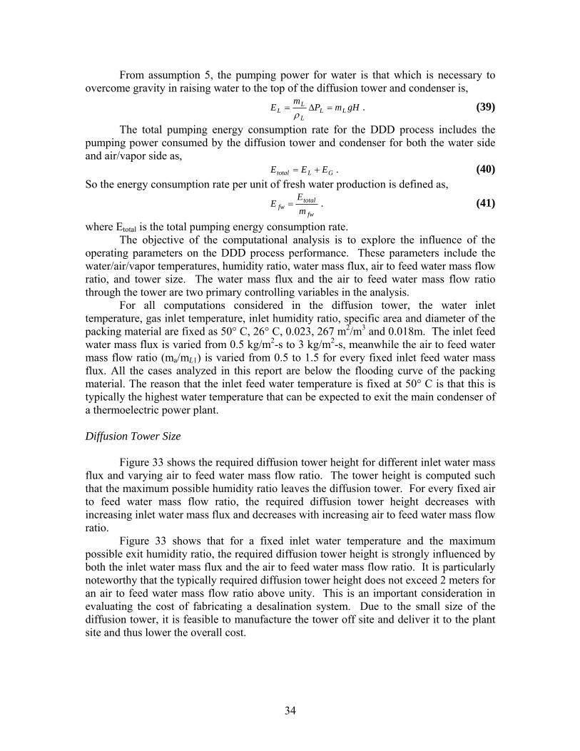
Figure 37 Air/vapor side pressure drop variation with air to feed water mass flow ratio

The main energy consumption for the DDD process is due to the pressure loss

through the diffusion tower and condenser. Although the air side pressure drop is much lower than that for water, the volumetric flow rate of air is much larger than that of water. Thus, both the air and water pumping power contribute significantly to the total energy consumption. Temperature and Humidity Variation in the Direct Contact Condenser

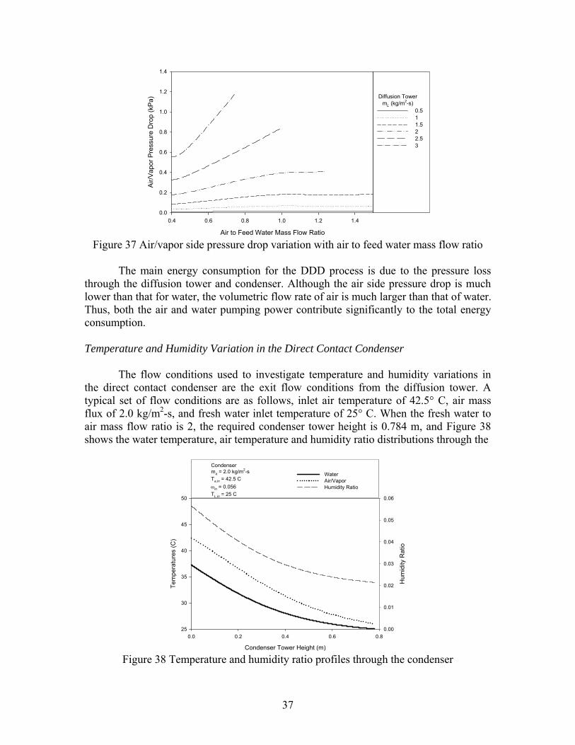
The flow conditions used to investigate temperature and humidity variations in the direct contact condenser are the exit flow conditions from the diffusion tower. A typical set of flow conditions are as follows, inlet air temperature of 42.5° C, air mass flux of 2.0 kg/m2-s, and fresh water inlet temperature of 25° C. When the fresh water to air mass flow ratio is 2, the required condenser tower height is 0.784 m, and Figure 38 shows the water temperature, air temperature and humidity ratio distributions through the

Condenser Tower Height (m)

0.0 0.2 0.4 0.6 0.8

Tem

pera

ture

s (C

)

25

30

35

40

45

50

Hum

idity

Rat

io

0.00

0.01

0.02

0.03

0.04

0.05

0.06

WaterAir/VaporHumidity Ratio

Condenserma = 2.0 kg/m2-sTa,in = 42.5 C ωin = 0.056TL,in = 25 C

Figure 38 Temperature and humidity ratio profiles through the condenser

38

condenser. With a fresh water mass flux of 4.0 kg/m2-s, the exit humidity ratio is approximately 0.0235, which corresponds to a fresh water production rate of about 0.064 kg/m2-s.

Figure 39 shows the condenser exit water temperature, minimum air temperature and exit humidity ratio variation with varying fresh water to air mass flow ratio with the same inlet air temperature and mass flux. Although not shown, all the values decrease with increasing inlet water mass flux. However, the results in Figure 39 show that there is no further decreases in exit humidity ratio when the fresh water to air mass flow ratio exceeds 2. Thus the optimum fresh water to air mass flow ratio that yields the maximum fresh water production is 2.

Fresh Water to Air Mass Flow Ratio

2 4 6 8 10

Tem

pera

ture

s (C

)

0

10

20

30

40

50

60

Hum

idity

Rat

io0.00

0.02

0.04

0.06

0.08

0.10

0.12

WaterAir/VaporHumidity Ratio

Condenserma = 0.5 kg/m2-sTa,in = 48.7 C ωin = 0.078TL,in = 25 C

Figure 39 Condenser temperature and humidity ratio variation with fresh water to air

mass flow ratio

Direct Contact Condenser Height

Figure 40 shows the required condenser height for different air mass flux with a constant fresh water to air mass flow ratio of 2 in the condenser. The tower height is computed such that the minimum humidity ratio leaves the condenser. For a fixed feed water mass flux at the inlet of the diffusion tower, the required condenser height decreases with increasing air mass flux, and it also decreases with decreasing the feed water mass flux with the same air mass flux. Figure 40 indicates that the condenser height follows the same trend as the diffusion tower exit air temperature, which is to be expected since the required condenser height strongly depends on the air inlet humidity ratio.

39

Air Mass Flux (kg/m2-s)

0.0 0.5 1.0 1.5 2.0 2.5 3.0

Con

dens

er H

eigh

t (m

)

0.6

0.7

0.8

0.9

1.0

1.1

1.2

1.3

0.511.522.53


Condensermfw/ma = 2

Condenser

Figure 40 Required direct contact condenser height with variations in air mass flux

Fresh Water Exit Temperature from Direct Contact Condenser

Because the sink temperature is 25° C, the minimum condenser exit air temperature is taken as 26° C. Figure 41 shows the condenser fresh water exit temperature for different inlet feed water mass flux in the diffusion tower and varying air mass flux. The fresh water exit temperature is sensitive to variations in both the feed water inlet mass flux and air mass flux.


0.0 0.5 1.0 1.5 2.0 2.5 3.0

Exit

Fres

h W

ater

Tem

pera

ture

(C)

34

36

38

40

42

44

46

48

50

0.511.522.53


Condensermfw/ma = 2

Condenser

Figure 41 Condenser fresh water exit temperature variation with air mass flux

Fresh Water Production Efficiency

Figure 42 shows the fresh water production efficiency of the system with varying air mass flux. It is clear that there exists a maximum fresh water production efficiency, and that maximum occurs with an air to feed water mass flow ratio close to unity. It is also interesting to note that the maximum fresh water production efficiency tends to approach a value of 0.032 for all operating conditions considered. The maximum production efficiency is largely controlled by the ratio of the diffusion tower inlet water temperature to the sink temperature. In this case, it is 1.12.

40


0.0 0.5 1.0 1.5 2.0 2.5 3.0

Fres

h W

ater

Pro

duct

ion

Effic

ienc

y (m

fw/m

L)

0.022

0.024

0.026

0.028

0.030

0.032

0.034

0.511.522.53


Condensermfw/ma = 2

Figure 42 Variation of the fresh water production efficiency with air mass flux

Energy Consumption

Perhaps the most important consideration in this analysis is the rate of energy consumption due to pumping because the operating cost of the DDD process is largely dependent on the cost of electricity to drive the pumps and blowers. Figure 43 shows the energy consumption rate for the diffusion tower for different inlet feed water mass flux and varying air to feed water mass flow ratios. The energy consumption increases with increasing inlet water mass flux for a fixed air to feed water mass flow ratio. It is particularly interesting that a minimum energy consumption occurs when the air to feed water mass flow ratio is approximately 0.5. As the inlet water mass flux decreases, the energy consumption becomes relatively insensitive to variations in the air to feed water mass flow ratio.


0.4 0.6 0.8 1.0 1.2 1.4

Ene

rgy

Con

sum

ptio

n R

ate

(kW

-hr/k

g fw)

0.000

0.002

0.004

0.006

0.008

0.511.522.53


Figure 43 Variation of the energy consumption with air to feed water mass flow ratio in

diffusion tower

Figure 44 shows the energy consumption rate for the direct contact condenser with fixed fresh water to air mass flow ratio of 2. It shows clearly that there exists a critical point for every feed water mass flux. When the air mass flux is higher than the

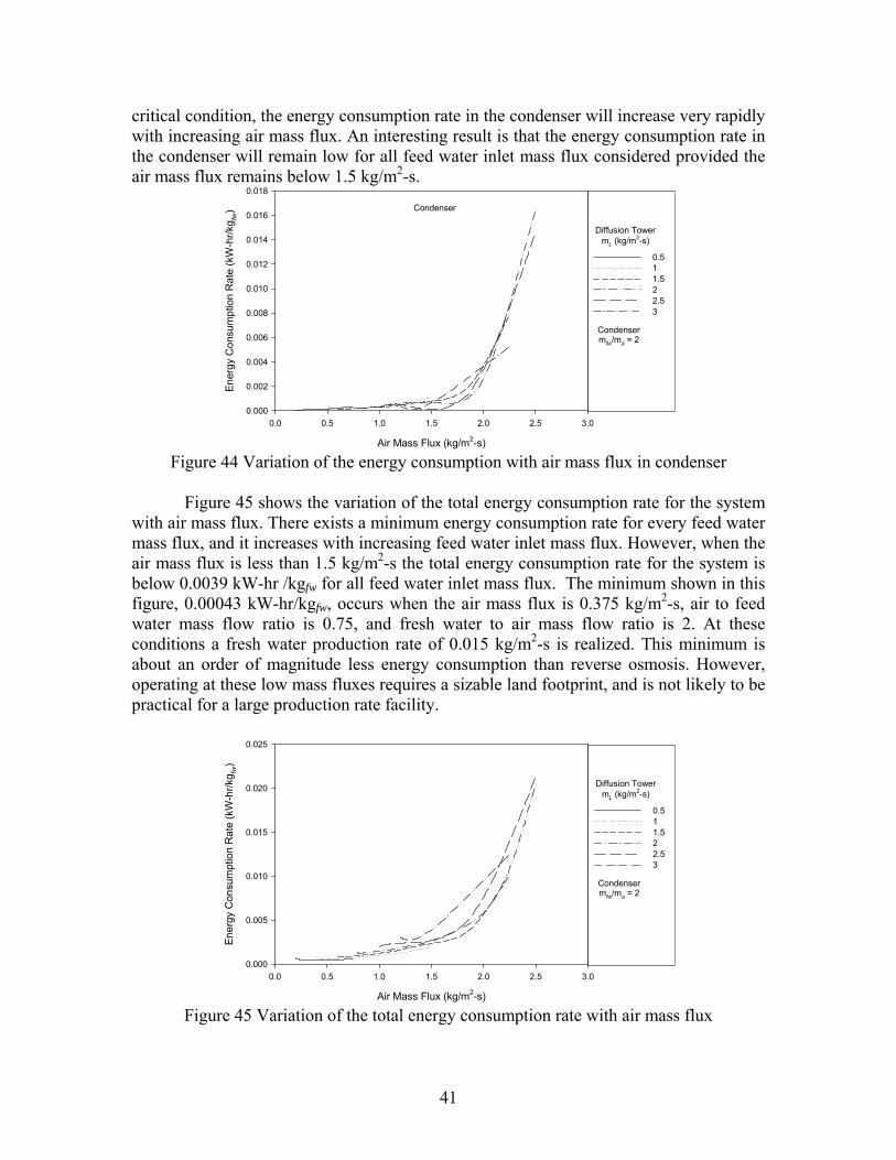
41

critical condition, the energy consumption rate in the condenser will increase very rapidly with increasing air mass flux. An interesting result is that the energy consumption rate in the condenser will remain low for all feed water inlet mass flux considered provided the air mass flux remains below 1.5 kg/m2-s.


0.0 0.5 1.0 1.5 2.0 2.5 3.0

Ener

gy C

onsu

mpt

ion

Rat

e (k

W-h

r/kg fw

)

0.000

0.002

0.004

0.006

0.008

0.010

0.012

0.014

0.016

0.018

0.511.522.53


Condensermfw/ma = 2

Condenser

Figure 44 Variation of the energy consumption with air mass flux in condenser

Figure 45 shows the variation of the total energy consumption rate for the system

with air mass flux. There exists a minimum energy consumption rate for every feed water mass flux, and it increases with increasing feed water inlet mass flux. However, when the air mass flux is less than 1.5 kg/m2-s the total energy consumption rate for the system is below 0.0039 kW-hr /kgfw for all feed water inlet mass flux. The minimum shown in this figure, 0.00043 kW-hr/kgfw, occurs when the air mass flux is 0.375 kg/m2-s, air to feed water mass flow ratio is 0.75, and fresh water to air mass flow ratio is 2. At these conditions a fresh water production rate of 0.015 kg/m2-s is realized. This minimum is about an order of magnitude less energy consumption than reverse osmosis. However, operating at these low mass fluxes requires a sizable land footprint, and is not likely to be practical for a large production rate facility.


0.0 0.5 1.0 1.5 2.0 2.5 3.0

Ener

gy C

onsu

mpt

ion

Rat

e (k

W-h

r/kg fw

)

0.000

0.005

0.010

0.015

0.020

0.025

0.511.522.53


Condensermfw/ma = 2

Figure 45 Variation of the total energy consumption rate with air mass flux

42

Finally, the optimum operating conditions of the system should satisfy competing requirements: high fresh water production efficiency and low energy consumption rate. Based on data presented in Fig. 42 and Fig. 45, a reasonable optimum operating condition has an air mass flux of 1.5 kg/m2-s, air to feed water mass flow ratio of 1, and fresh water to air mass flow ratio of 2. These conditions can yield a fresh water production efficiency of 0.0314 and energy consumption rate of 0.0023 kW-hr/kgfw. 6. Economic Analysis

As an example, consider a 100 MW power plant where the thermal efficiency is 40%. The total input energy is then 250 MW and the waste heat is 150 MW. If the power plant operates with 9.7cmHg pressure in the main condenser, there would be approximately 150 MW of energy at 50° C available from low pressure condensing steam. If retrofitted with a diffusion driven desalination (DDD) plant, there is a potential to produce as much as 1.03 million gallons/day of fresh water assuming the feed water temperature enters the diffusion tower at 50° C. The energy consumption from the feed water, air, and cold fresh water pumps in the DDD process is about 0.0023 kW-hr per kilogram of fresh water. This requires a land footprint of approximately 0.47 acres. The total electrical power requirement is 380 kW in total. The thermal energy consumed in the DDD process is waste heat, and is not of concern for the economic analysis.

The fresh water production cost strongly depends on the process capacity, site characteristics and design features. The system capacity defines the required sizes for various process equipment, pumping units, and required heat exchanger surface area. Site characteristics have a strong influence on the type of pretreatment and post-treatment equipment, and consumption rate of chemicals. Process design features affect consumption of electric power and chemicals (Wangnick et al [17] and Hisham et al [18]). Production cost is divided into direct and indirect capital costs and annual operating costs. Direct capital costs include the purchase cost of major equipment, auxiliary equipment, land and construction. Indirect capital costs include labor, maintenance, and amortization. They are usually expressed as percentages of the total direct capital cost. Land – The cost of land may vary considerably, from zero to a sum that depends on site characteristics. Government-owned plants normally have zero charges. Plants constructed under build-own-operate-transfer (BOOT) contracts with governments or municipalities can have near zero or greatly reduced charges. The price of the land near the coast of Florida varies significantly from 1k - 1,000k $/acre. Building construction – Construction costs vary from $100-1,000/m2. This cost is site-specific and depends on the building type. Buildings could include a control room, laboratory, offices and workshops. Process equipment – This category includes processing equipment, as well as instrumentation and controls, pipes and valves, electric wiring, pumps, process cleaning systems, and pre- and post-treatment equipment. These are some of the most expensive items, and their cost depends on the type of process and capacity. Equipment costs may

43

be less than $1,000 (e.g., a laboratory-scale RO unit used to treat low-salinity water). On the other hand, the equipment cost for a 100,000 m3/day RO system could approach $50 million. MSF and MEE equipment are generally more expensive than that of RO systems — current estimates for a plant capacity of 27,000 m3/day are $40 million. Because the increase in salinity concentration of the DDD discharge water is small, there is no need for post-treatment. Also the feed water flow is supplied by the main pumps used in the power plant’s cooling system. So the capital cost of the pre-treatment, post-treatment and main feed water pumps will not be included in this analysis. The other process equipment costs among different manufacturers range from $200k-$1,700k. Auxiliary equipment – The following are considered auxiliary equipment: open intakes or wells, transmission piping, storage tanks, generators and transformers, pumps, pipes and valves. The current analysis will not include these items.

As an example, consider the DDD system coupled with a 100 MW power plant. The capital cost calculations are based on the following assumptions: 1) interest rate i = 5% 2) plant life n = 30 yr

3) amortization factor ai = 1)1(

)1(−+

+n

n

iii = 0.0651 /yr

4) plant availability f = 0.9 5) chemical costs are not considered 6) electricity is considered as operating cost 7) the specific cost of operating labor is typically $0.1/m3 for the thermal processes and

$0.05/m3 for RO. Because the DDD is a low temperature and pressure process, the labor cost is assumed lower which typically ranges from γ = 0.025 – 0.05 $/m3.

Table 1 Summary of direct costs

Name Land Building construction Major equipment Cost ($) 470-470,000 190,202-1,902,023 200,000-1,700,000 Total Direct Cost DC ($) 390,672-4,072,023

Table 2 Details of cost calculations

Name Formula Result Annual fixed charges Afixed ($)

DCaiAC fixed ⋅= 25,433 – 265,089

Annual labor cost Alabor ($) 365⋅⋅⋅= fwlabor mfAC γ 31,975 – 63,959 Total annual cost Atotal ($) laborfixedtotal ACACAC += 57,408 – 329,048 Unit product cost in terms of production Aunit, p ($/m3)

1, )365( −⋅⋅⋅= fwtotalpunit mfACAC 0.045 – 0.257

The computation reveals that the production cost, not including electricity costs,

ranges from 0.17 – 0.97 $/103 gal. For illustrative purposes, we take the production cost to be 0.6$/103gal. Here two cases are considered:

44

First, the DDD utility is economically independent from the power plant, which means although the DDD process the waste heat from the power plant, it needs to pay the electricity cost in additional to basic production cost. So the fresh water profit in this situation can be calculated as,

elecfwpunitfwfw QEACQ −−=Π , , (42) where Πfw ($/103 gal) is the net fresh water profit, Qfw ($/103 gal) is the retail price of fresh water, and Qelec ($/kW-hr) is the retail price of electricity. Here ACunit,p is 0.6$/103gal. Figure 46 shows the net fresh water profit variation with the electricity retail price for different fresh water retail price. The fresh water profit decreases with increasing electricity cost, and increases with increasing the fresh water price. As seen in Fig. 46, profit is only realized when the fresh water retail price is greater than 1 $/103gal.

Second, the DDD utility is combined with a power plant, which means this combined system has a fresh water production capacity of 1.03 million gallons/day besides the electricity production. But the total electrical power requirement of the DDD process will be subtracted from the total electricity production of the power plant as the operating cost. The daily profit of the combined system is calculated from,

elecfwelecfwfwtotal EEm Π−+Π=Π )( , (43) where Πtotal ($/day) is the daily profit of the combined system, Eelec (MW) is the electricity production capacity of the power plant before combining with the DDD system, and Πelec ($/kWhr) is the electricity profit. The percent increase in profit of the combined power plant is calculated as,

elecelec

elecelectotal

EEΠ

Π−Π=β . (44)

Electricity Retail Price ($/kW-hr)

0.04 0.06 0.08 0.10 0.12 0.14 0.16 0.18 0.20

Net

Fre

sh W

ater

Pro

fit ($

/103 ga

l)

0

1

2

3

4

5

6

123456

Water Retail Price($/103 gallon)

Figure 46 Net fresh water profit with electricity retail price for different fresh water retail

price.

The percent increase in profit for the power plant combined with the DDD process for different fresh water profits is shown in Fig. 47. This figure shows that the profit increase decreases with increasing electricity profit. It is also important to note that the profit increase of the combined power and DDD plant tends to be zero when the electricity profit is higher than $0.2/kW-hr, which is not likely in the near future. The profit increase grows almost proportionally with the fresh water price that can be

45

commanded on the open market. It clearly shows that the combined power and DDD plants yield a profit increase when the fresh water is sold at a rate higher than 1 $/103gal. This is strongly competitive in most regions of the world.

Electricity Profit ($/kW-hr)

0.001 0.01 0.1

Pro

fit In

crea

se (

%)

1

10

100

1000

123456

Water Profit($/103 gallon)

0.2

Figure 47 Percent increase in profit with electricity profit for different fresh water profit

A recent survey [19] by the NUS Consulting Group studying water rates across

the world found that rates increased from 2001 to 2002 in 12 of 14 countries surveyed. The result is shown in Figure 48. The survey was based on prices as of July 1, 2002 for an organization with an annual usage of 10,000 cubic meters. Where there was more than a single supplier, an unweighted average of available prices was used. The percentage change for each country was calculated using the local currency in order to eliminate currency exchange distortion. Water rates in the United States were among the lowest in the countries surveyed and were one half to one third the rates charged in most European countries. And it is also important to recognize that most countries investigated show a positive increase in water price, which reflects the increased demand for fresh water.

Fresh Water Cost ($/103 gallon)

0 2 4 6 8

Germany

Denmark

United Kingdom

The Netherlands

France

Belgium

Italy

Spain

Finland

Sweden

Australia

United States

South Africa

Canada20012002

Figure 48 Water price in different countries for year 2001 & 2002

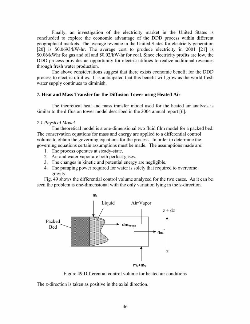
46

Finally, an investigation of the electricity market in the United States is conclueded to explore the economic advantage of the DDD process within different geographical markets. The average revenue in the United States for electricity generation [20] is $0.0693/kW-hr. The average cost to produce electricity in 2001 [21] is $0.06/kWhr for gas and oil and $0.02/kW-hr for coal. Since electricity profits are low, the DDD process provides an opportunity for electric utilities to realize additional revenues through fresh water production.

The above considerations suggest that there exists economic benefit for the DDD process to electric utilities. It is anticipated that this benefit will grow as the world fresh water supply continues to diminish. 7. Heat and Mass Transfer for the Diffusion Tower using Heated Air The theoretical heat and mass transfer model used for the heated air analysis is similar to the diffusion tower model described in the 2004 annual report [6]. 7.1 Physical Model

The theoretical model is a one-dimensional two fluid film model for a packed bed. The conservation equations for mass and energy are applied to a differential control volume to obtain the governing equations for the process. In order to determine the governing equations certain assumptions must be made. The assumptions made are:

1. The process operates at steady-state. 2. Air and water vapor are both perfect gases. 3. The changes in kinetic and potential energy are negligible. 4. The pumping power required for water is solely that required to overcome

gravity. Fig. 49 shows the differential control volume analyzed for the two cases. As it can be

seen the problem is one-dimensional with the only variation lying in the z-direction.

Figure 49 Differential control volume for heated air conditions

The z-direction is taken as positive in the axial direction.

qHL”

Packed Bed dmVevap

ma+mV

mL

Liquid Air/Vapor

z

z + dz

47

7.2 Mathematical Model The conservation of mass on the control volume for the air/vapor mixture yields,

, ,( ) ( )V z V evapd dm mdz dz

= , (45)

where m represents the mass flow rate, the subscripts V and evap denote vapor and the vapor evaporated from the liquid respectively. Similarly, conservation of mass on the liquid side yields,

, ,( ) ( )L z V evapd dm mdz dz

− = , (46)

where the subscript L denotes liquid. The humidity ratio, ω, and relative humidity, Φ, are defined for an air/vapor

mixture as follows, 0.622 ( )

( )V sat a

a sat a

m P Tm P P T

ω Φ= =

−Φ, (47)

where P is the total pressure of the system, and Psat(Ta) is the saturation pressure of the vapor evaluated at the air temperature Ta. The small change in system pressure is not accounted for in evaluating the properties. The definition of the mass transfer coefficient is applied to the differential control volume to obtain the following,

, , ,( ) ( ( ) ( ))V evap G w V sat L V ad m k a T T Adz

ρ ρ ∞= − , (48)

where kG is the gas mass transfer coefficient, aw is the wetted specific area, and A is the cross sectional area of the diffusion tower. It should be noted that the total specific area of the packing, a, is the total surface area of packing per unit volume of space occupied. The rate of change of evaporation can be further reduced by considering the perfect gas law. By applying the perfect gas law [15] to Equation 48, the rate of evaporation becomes,

,( ) ( )( ) V sat i sat a

V evap G wi a

M P T P Td m k a Adz R T T

⎡ ⎤Φ= −⎢ ⎥

⎣ ⎦, (49)

where MV is the molecular weight of vapor, R is the universal gas constant, and Ti is the liquid/vapor interfacial temperature. By combining Equations 46-48 the gradient of the humidity ratio is,

( )0.622

G W V sat i

i a

k a M P Td Pdz G R T Tω ω

ω⎡ ⎤

= −⎢ ⎥+⎣ ⎦, (50)

where amGA

= is the air mass flux. Equation 50 is a first order ordinary differential

equation with dependent variable ω. When solved, the humidity ratio along the axial z direction is obtained. Equation 50 requires a value of the liquid/vapor interfacial temperature, Ti. The interfacial temperature is found by recognizing that the energy convected from the liquid is the same as that convected to the gas,

( ) ( )L L i G i aU T T U T T− = − , (51) where UL and UG are the heat transfer coefficients of liquid and gas respectively. The interfacial temperature is obtained by solving Equation 51 and is,

48

( / )1 ( / )

L G L ai

G L

T U U TTU U

+=

+. (52)

The conservation of energy on the liquid side of the differential volume yields the following,

,( )( ) ( )V evapL L fg L a

d d mm h h Ua T T Adz dz

= + − , (53)

where h is the enthalpy, U is the overall heat transfer coefficient, and hfg is the latent heat of evaporation. Equation 53 can be further manipulated by utilizing the following:

L pL Ldh C dT= and ( ) L LL LL L

dhd d mm h h mdz dz dz

= + , and ( ) ( ) ( )fg a V a L ah T h T h T= − . The

gradient of the liquid temperature, TL, then reduces to the following, ( ) ( )fg L L aL

PL PL

h h Ua T TdT G ddz L dz C C L

ω − −= + , (54)

where LmLA

= is the liquid mass flux, CP is the specific heat, and a is the overall specific

area of the packing material. Equation 54 is also a first order ordinary differential that when solved will yield the temperature distribution of the water throughout the diffusion tower.

Likewise, conservation of energy of the air/vapor mixture is obtained from the differential control volume and yields,

",( ) ( )a Va V V evap fg L a HL

d dm h m h m h Ua T T A q ddz dz

π⎛ ⎞− + + = − − +⎜ ⎟⎝ ⎠

(55)

As in the liquid energy equation, Equation 55 can be simplified by utilizing the fact that the air mass flow rate is held constant throughout the entire process such that:

.. . . .

( ) Va Va V a Va v V

dh dhd d mm h m h m m hdz dz dz dz

+ = + + , a aPa

dh dTCdz dz

= , and V aPV

dh dTCdz dz

= .

Equation 55 then becomes,

"( ) ( ) ( )vaa vPa PV L a L a HL

dT d mm C m C h T Ua T T A q ddz dz

π− + = − − + . (56)

Equation 56 can be simplified by noting that the CPmix, specific heat of the mixture, is evaluated as,

a VPmix Pa PV

a V a V

m mC C Cm m m m

= ++ +

(57)

Recalling the evaluation of the latent heat of evaporization from the liquid conservation equation, and combining Equations 56 and Equation 57 the gradient of air temperature through the diffusion tower is evaluated as,

"( ) ( ) 411 (1 ) (1 )

a L a L a HL

Pmix Pmix Pmix

dT h T Ua T T qddz dz C C G Gd C

ωω ω ω

−= − + −

+ + + (58)

49

where d is the diameter of the diffusion tower and "HLq is the heat flux loss from the air.

Equation 58 is also a first order ordinary differential equation with dependent variable Ta. Equations 50, 54, and 58 are a set of coupled ordinary differential equations that when solved simultaneously give solutions for the distributions of humidity ratio, air temperature, and water temperature throughout the diffusion tower. However, since a one-dimensional model is utilized, closure must be achieved. This requires that both the heat transfer coefficient and mass transfer coefficient be known. Directly measuring the heat transfer coefficients is not possible because of the fact that the interfacial film temperature cannot be measured. Therefore to overcome this difficulty the heat and mass transfer analogy [22] has been utilized. The heat transfer coefficient for the liquid side is evaluated using,

1/ 2 1/ 2PrL L

L L

Nu ShSc

= (59)

1/ 2

LL L L PL

L

KU k CD

ρ⎛ ⎞

= ⎜ ⎟⎝ ⎠

(60)

Similarly, the heat transfer coefficient for the gas side is calculated as,

1/3 1/3PrG G

G G

Nu ShSc

= (61)

( )2/3

1/3 GG G G PG

G

KU k CD

ρ⎛ ⎞

= ⎜ ⎟⎝ ⎠

(62)

where D is the molecular diffusion coefficient and K is the thermal conductivity. Thus the overall heat transfer coefficient is evaluated as,

( )1 1L L GU U U− −= + (63)

The mass transfer coefficient is evaluated using a widely known and well tested correlation. Onda’s correlation [14] allows for evaluation of the mass transfer coefficients in packed beds. Onda’s correlation, found in Appendix A, is used to calculate the mass transfer coefficients, kG and kL. In the correlation the coefficient, C, can take on two possible values C=5.23 for 15pd > mm and C=2.00 for 15pd ≤ mm. The difference in C values accounts for the fact that kGa for the smaller packing ( 15pd ≤ mm) tends to increase monotonously with increasing specific area, a. Li et al. [23] provided an explanation for the phenomena of the decreased mass transfer coefficient and is believed to be the cause of liquid hold-up in the packed bed which is responsible for liquid bridging and reduced area for mass transfer. The current packed bed has a diameter of 18 mm which is close to the cut off for both sizes. Thus for the packed bed used in the current investigation, either constant value would be appropriate. Similar to the analysis described by Klausner et al. [16], the heated air/ambient water uses C=5.23. The coefficient for the heated air/heated water case, however, uses C=2.0. The value of C for a given case is that which gives better agreement with the measured data collected. This change in constant can perhaps be attributed to the fact that at higher air temperatures the air that enters the packed bed is dryer and thus more water is evaporated. However, due to the increase in evaporation there is an increased hold up of the liquid in the packing due to an accelerating gas stream. The increase in hold up could

50

possibly cause more liquid bridging in the packing thereby decreasing the local mass transfer.

The wetted area for the current experiments differs from that computed via Onda’s correlation. It was found that the specific wetted area remains nearly constant for varying air to water mass flow ratios. This was determined by first using Onda’s correlation to calculate the wetted specific area. There was slight variation in the comparison of the theoretical and experimental data. An analysis was then performed to determine what the specific wetted area should be to obtain adequate results. Interestingly, over the range of operating conditions considered in this work, the specific wetted area is found to be simply a constant,

0.5wa a= . (64) The value of the heat loss, "

HLq , is experimentally determined and is diffusion tower specific. There was negligible heat loss for the heated air/ambient water case thus the heat loss flux term is taken to be zero. The heat loss for the heated air/heated water case is experimentally calibrated for various air mass fluxes. Figure 50 shows the calibration curve for the heated air/heated water heat loss flux for varying air mass flux.

To solve the three coupled equations for the humidity ratio, air temperature, and water temperature distributions in the diffusion tower, the following solution procedure is followed:

1. Specify the water mass flux, air mass flux, inlet water temperature, inlet air temperature, and inlet humidity ratio.

2. Guess a value of the exit water temperature. 3. Compute the exit humidity ratio, exit water temperature, and exit air temperature

utilizing Equations 50, 54, and 58 until z reaches the height of the packed bed. 4. Compare the values of the calculated inlet water temperature and specified inlet

water temperature. If they match, the analysis is complete. If they differ, repeat the procedure beginning from step 2.

Experiments were conducted to obtain data for the two different cases: heated

air/ambient water and heated air/heated water. For both cases, the air mass flux was held constant at about 0.77 kg/m2-s, 1.16 kg/m2-s, and 1.55 kg/m2-s while the liquid mass flux was varied between 0.6 kg/m2-s to 1.3 kg/m2-s. The height of the packed bed was held constant at 0.38 m. All experiments conducted were performed in a parameter space beneath the flooding curve for the packed bed. For the model analysis, the inlet water temperature, inlet air temperature, and inlet absolute humidity were all used to compute the exit conditions. Comparisons between the predicted and measured exit conditions from the model are described next. 7.3 Heated Air/Ambient Water Results

Six different data sets were recorded for the heated air/ambient water case. Two different data sets per air mass flux were taken to ensure the repeatability of the experiments. For all experiments, the inlet air, water, and humidity were held constant at about 60.9 °C, 25.2 °C, and 0.0060 respectively. Figures 51 to 53 show the comparison between the predicted exit values and the measured exit values. The comparison between the two is quite good. The exit absolute humidity and exit water temperature are

51

predicted with fairly good accuracy while the exit air temperature is slightly underpredicted for all data sets.


0.6 0.8 1.0 1.2 1.4 1.6

Hea

t Los

s Fl

ux (k

W/m

2 )

0.5

1.0

1.5

2.0

2.5

3.0

3.5

Figure 50 Calibration curve of the heat loss flux for the heated air/heated water case

From the data collected it can be seen that the heated air/ambient water case does not yield good production. The exit air temperature is approximately 25-26 °C for each value of the liquid mass flux as well as air mass flux, which indicates that the air is cooled to the temperature of the water. This is supported by the fact that the temperature difference of the exit water and exit air is nearly a constant 1-2 °C. Thus it is clear that reliance on heated air is inefficient because upon entering the tower the air is immediately cooled close to the water temperature. All of the energy is being used to heat up the water and as a result the mass transfer is poor. As the absolute humidity shows, there is no optimum value as the exit humidity is essentially constant. Further, the change in humidity from the inlet to the outlet essentially remains a constant at about 0.0125. This indicates that regardless of the diffusion tower liquid mass flux only a small fraction of water will be evaporated.

Figure 54(a-c) shows the repeatability of the six different experiments for the different flow conditions. As shown in the figures, the repeatability of the experiments is very good. However, the figures also elucidate the fact that the heated air/ambient water case is very inefficient. There is little variation between the values recorded for the six different experiments despite the different air and water mass fluxes used in the experimental measurements. For example, consider the exit air temperature shown in Fig. 54 (a). For the three values of air mass flux the exit air temperature remains almost a constant despite the varying liquid mass flux. The exit water temperature and the exit humidity also demonstrate similar behavior. The process will exhibit the same behavior despite the operating conditions chosen.

52

Details of the experimental data can be found in Appendix D.

ωout ωout ωin

Water Mass Flux L (kg/m2

-s)

0.6 0.8 1.0 1.2 1.4

Tem

pera

ture

(C)

15

20

25

30

35

Abso

lute

Hum

idity

0.00

0.01

0.02

0.03

0.04

0.05

G = 0.77 kg/m2-sPredicted Measured

Ta,out

Tw,out

Ta,out

Tw,out

Inlet Conditions

Ta,in (C) = 60.10

Tw,in (C) = 25.32

= 0.007515

(a)

ωout ωout ωin


-s)

0.6 0.8 1.0 1.2 1.4

Tem

pera

ture

(C)

15

20

25

30

35A

bsol

ute

Hum

idity

0.00

0.01

0.02

0.03

0.04

0.05


Ta,out

Tw,out

Ta,out

Tw,out

Inlet Conditions

Ta,in (C) = 61.79

Tw,in (C) = 25.19

= 0.004064

(b)

Figure 51 Comparison of predicted and measured exit temperatures and humidity for

similar air mass flux G = 0.77 kg/m2-s: a) Set 1 b) Set 2

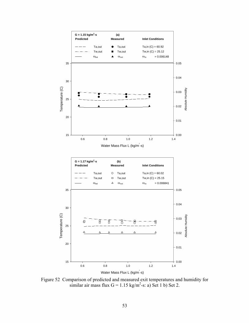
53

ωout ωout ωin


-s)

0.6 0.8 1.0 1.2 1.4

Tem

pera

ture

(C)

15

20

25

30

35

Abs

olut

e H

umid

ity

0.00

0.01

0.02

0.03

0.04

0.05


Ta,out

Tw,out

Ta,out

Tw,out

Inlet Conditions

Ta,in (C) = 60.92

Tw,in (C) = 25.12

= 0.006148

(a)

ωout ωout ωin


-s)

0.6 0.8 1.0 1.2 1.4

Tem

pera

ture

(C)

15

20

25

30

35A

bsol

ute

Hum

idity

0.00

0.01

0.02

0.03

0.04

0.05


Ta,out

Tw,out

Ta,out

Tw,out

Inlet Conditions

Ta,in (C) = 60.02

Tw,in (C) = 25.15

= 0.006841

(b)


similar air mass flux G = 1.15 kg/m2-s: a) Set 1 b) Set 2.

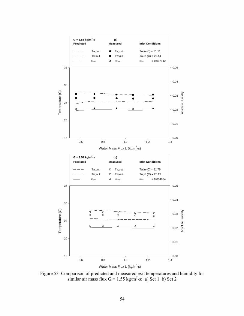
54

ωout ωout ωin


-s)

0.6 0.8 1.0 1.2 1.4

Tem

pera

ture

(C)

15

20

25

30

35

Abs

olut

e H

umid

ity

0.00

0.01

0.02

0.03

0.04

0.05


Ta,out

Tw,out

Ta,out

Tw,out

Inlet Conditions

Ta,in (C) = 61.11

Tw,in (C) = 25.14

= 0.007112

(a)

ωout ωout ωin


-s)

0.6 0.8 1.0 1.2 1.4

Tem

pera

ture

(C)

15

20

25

30

35A

bsol

ute

Hum

idity

0.00

0.01

0.02

0.03

0.04

0.05


Ta,out

Tw,out

Ta,out

Tw,out

Inlet Conditions

Ta,in (C) = 61.79

Tw,in (C) = 25.19

= 0.004064

(b)



55


0.5 0.6 0.7 0.8 0.9 1.0 1.1 1.2 1.3

Exi

t Air

Tem

pera

ture

(C)

20

22

24

26

28

30

G Set 1 Set 2

0.79 kg/m2-s

1.55 kg/m2-s

1.79 kg/m2-s

(a)

Water Mass Flux (kg/m2-s)

0.5 0.6 0.7 0.8 0.9 1.0 1.1 1.2 1.3

Exi

t Wat

er T

empe

ratu

re (C

)

10

15

20

25

30

35

40

G Set 1 Set 20.79 kg/m2-s

1.55 kg/m2-s

1.79 kg/m2-s

(b)

Figure 54 Repeatability of different experiments for different exit parameters: a) Exit air

temperature, b) Exit water temperature, c) Exit absolute humidity

56


0.5 0.6 0.7 0.8 0.9 1.0 1.1 1.2 1.3

Exi

t Abs

olut

e H

umid

ity

0.00

0.01

0.02

0.03

0.04

G Set 1 Set 2

0.79 kg/m2-s

1.55 kg/m2-s

1.79 kg/m2-s

(c)

Figure 54 Continued

7.4 Heated Air/Heated Water Results

As in the previous case, six different data sets were taken, two for each different air mass flux. For all six experiments the inlet air temperature, water temperature, and humidity were held constant at about 60.9 °C, 60.6 °C, and 0.0077 respectively. Figures 55 to 57 show the comparison between the predicted and measured exit temperatures and humidity. For all sets of data the exit water temperature and exit humidity are predicted with considerable accuracy. The air temperature is slightly overpredicted in all cases.

For all air mass fluxes studied, the exit air temperature and exit water temperature increase with increasing water mass flux. As the liquid mass flux increases the exit humidity also increases due to the increase in the amount of liquid available to evaporate.

57

ωout ωout ωin


-s)

0.6 0.8 1.0 1.2 1.4

Tem

pera

ture

(C)

0

10

20

30

40

50

Abs

olut

e H

umid

ity

0.00

0.02

0.04

0.06

0.08

0.10


Ta,out

Tw,out

Ta,out

Tw,out

Inlet Conditions

Ta,in (C) = 60.99

Tw,in (C) = 60.48

= 0.006854

(a)

ωout ωout ωin


-s)

0.6 0.8 1.0 1.2 1.4

Tem

pera

ture

(C)

0

10

20

30

40

50

Abs

olut

e H

umid

ity

0.00

0.02

0.04

0.06

0.08

0.10


Ta,out

Tw,out

Ta,out

Tw,out

Inlet Conditions

Ta,in (C) = 61.41

Tw,in (C) = 60.75

= 0.006207

(b)


similar air mass flux G = 0.79 kg/m2-s: a) Set 1 b) Set 2.

58

ωout ωout ωin


-s)

0.6 0.8 1.0 1.2 1.4

Tem

pera

ture

(C)

0

10

20

30

40

50

Abso

lute

Hum

idity

0.00

0.02

0.04

0.06

0.08

0.10


Ta,out

Tw,out

Ta,out

Tw,out

Inlet Conditions

Ta,in (C) = 61.29

Tw,in (C) = 60.87

= 0.007919

(a)

ωout ωout ωin


-s)

0.6 0.8 1.0 1.2 1.4

Tem

pera

ture

(C)

0

10

20

30

40

50A

bsol

ute

Hum

idity

0.00

0.02

0.04

0.06

0.08

0.10


Ta,out

Tw,out

Ta,out

Tw,out

Inlet Conditions

Ta,in (C) = 60.90

Tw,in (C) = 60.79

= 0.008120

(b)

Figure 56 Comparison of predicted and measured exit temperatures and humidity for similar air mass flux G = 1.15 kg/m2-s: a) Set 1 b) Set 2

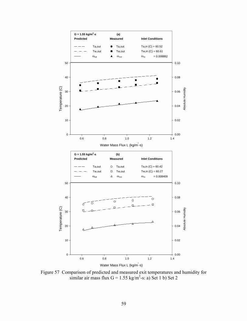
59

ωout ωout ωin


-s)

0.6 0.8 1.0 1.2 1.4

Tem

pera

ture

(C)

0

10

20

30

40

50

Abs

olut

e H

umid

ity

0.00

0.02

0.04

0.06

0.08

0.10


Ta,out

Tw,out

Ta,out

Tw,out

Inlet Conditions

Ta,in (C) = 60.52

Tw,in (C) = 60.61

= 0.008882

(a)

ωout ωout ωin


-s)

0.6 0.8 1.0 1.2 1.4

Tem

pera

ture

(C)

0

10

20

30

40

50A

bsol

ute

Hum

idity

0.00

0.02

0.04

0.06

0.08

0.10


Ta,out

Tw,out

Ta,out

Tw,out

Inlet Conditions

Ta,in (C) = 60.42

Tw,in (C) = 60.27

= 0.008409

(b)



60

Figures 58(a-c) demonstrates the repeatability of the six experiments for the heated air/heated water case. As shown in the figures the repeatability for all of the experiments is quite reasonable. These figures show that at the lower air mass flux the maximum exit humidity is obtained. It is also interesting that both the exit air temperature and exit water temperature decrease with increasing air mass flux. This suggests that the residence time plays a key role in the heat and mass transfer. A decrease in residence time implies that there is less time for heat and mass transfer to occur thereby explaining the decreased temperatures as well as humidity with increasing air mass flux. As demonstrated, the theoretical model developed is obviously a good design tool that can be utilized to achieve the desired production rate.

Details of the experimental data collected for the heated air heated water case can be viewed in Appendix E.


0.4 0.6 0.8 1.0 1.2 1.4

Exit

Air T

empe

ratu

re (C

)

30

35

40

45

50

G Set 1 Set 2

0.79 kg/m2-s

1.55 kg/m2-s

1.79 kg/m2-s

(a)

Figure 58 Repeatability of experiments for different exit parameters: a) Exit air

temperature, b) Exit water temperature, c) Exit absolute humidity

61

Water Mass Flux (kg/m2-s)

0.4 0.6 0.8 1.0 1.2 1.4

Exi

t Wat

er T

empe

ratu

re (C

)

25

30

35

40

45

G Set 1 Set 2

0.79 kg/m2-s

1.55 kg/m2-s

1.79 kg/m2-s

(b)


0.4 0.6 0.8 1.0 1.2 1.4

Exi

t Abs

olut

e H

umid

ity

0.03

0.04

0.05

0.06

0.07

G Set 1 Set 2

0.79 kg/m2-s

1.55 kg/m2-s

1.79 kg/m2-s

(c)

Figure 58 Continued

62

8. Optimization of the DDD Process using Heated Air

An analysis similar to the one proposed in Section 4 is used to optimize the heated air DDD process for the heated air/heated water case. The heated air/ambient water case is not considered, as experimental data showed that it was an ineffective process. The heat and mass transfer model described in Section 6 is used to model the heated air/heated water DDD process. The assumptions made in this analysis are the same as those listed in Section 4. Equations 50, 54, and 58 are used to evaluate the absolute humidity, water temperature, and air temperature respectively through the diffusion tower. The heat and mass transfer analogy is used to evaluate the heat transfer coefficients and Onda’s correlation is used to evaluate the mass transfer coefficients assuming a constant wetted area. The parameters used in the optimization study are described in Section 4. Equation 36 is used to evaluate the fresh water production rate, however for this case it is assumed that the carrier air circulates in a closed loop and the inlet humidity to the diffusion tower is the outlet humidity from the condenser. Equation 37 gives the pressure drop on the gas side. Equations 38, 39, and 40 provide the pumping power on the gas side, pumping power on the liquid side, and the total pumping power respectively. Finally, Equation 41 gives the energy consumption rate per unit of fresh water production. 8.1 Optimization Results for the Heated Air/Heated Water Process

Using the analysis described above and the theory discussed in Section 6, a parametric analysis is performed to determine the effects of certain operating variables on the performance of the heated air/heated water process. In performing the analysis, the air inlet temperature, water inlet temperature, specific packing area, diameter of the packing material, and inlet humidity ratio were all held constant at 60° C, 60° C, 267 m2/m3, 0.018 m, and 5.25% respectively. Nine different values of the inlet feedwater mass flux, L, were considered 0.15, 0.25, 0.5, 0.75, 1.20, 1.55, 2.0, 2.5, 3.0 kg/m2-s. The inlet air mass flux, G, was varied continuously from 0.04 to 23.2 kg/m2-s for each inlet feedwater flux. For each air mass flux, the maximum absolute humidity was determined, and the tower height, air exit temperature, and water exit temperature were recorded. All calculations were performed in a parameter space below the flooding curve of the packing material.

Figure 59 depicts the tower height as a function of the inlet air mass flux. The tower height reported is the computed tower height required to achieve the maximum exit absolute humidity. For all inlet liquid mass fluxes, the tower height decreases with increasing inlet air mass flux. This is important because as the air mass flux increases, the tower height decreases which translates to less required materials and thus reduced cost. However, as the air mass flux increases the power required to pump the air also increases. It should be noted that the tower height for high liquid mass flux and low air mass flux was restricted to values less than 5 m. This is to ensure that the tower heights considered are realistic.

63


0 5 10 15 20 25

Tow

er H

eigh

t (m

)

0

1

2

3

4

5

6

Liquid Mass Flux L (kg/m2-s)

0.150.250.500.751.201.552.002.503.00

Figure 59 Tower height at the maximum exit absolute humidity as a function of the inlet

air mass flux G

Figure 60 shows the exit air temperature with varying air mass flux. The exit air temperature decreases with increasing air mass flux until it reaches a minimum value then increases. It is also worthy to note that the highest exit air temperatures are realized when the air mass flux is low.

Figure 61 depicts the maximum exit absolute humidity as a function of air mass flux for varying liquid mass flux values. For all liquid mass flux values, the exit humidity decreases with increasing air mass flux. The maximum exit humidity is achieved with the higher liquid mass fluxes. This phenomenon can be attributed to the fact that the heat capacity of the water is large with larger mass fluxes, and the water temperature will not decrease as much with a given amount of evaporation. Thus as the liquid mass flux decreases the exit absolute humidity decreases as well. The maximum exit humidity is realized for low values of the air mass flux. It is important to note that the maximum exit air temperature and maximum humidity for all liquid mass fluxes are achieved for values of the air mass flux less than about 2.00 kg/m2-s. While the exit air temperature and exit absolute humidity are maximum at low air mass flux, this does not imply that the fresh water production will also be high.

The fresh water production is an important parameter in evaluating the economy of the process. Figure 62 shows the fresh water production flux with varying air mass flux. For each value of the liquid mass flux the fresh water production flux increases until it reaches an optimum condition. This is important because it indicates that for every liquid mass flux there is a value of the air mass flux that can produce the maximum amount of fresh water. It is also important to notice that as the liquid mass flux increases, the fresh water production flux increases. Thus a higher production can be achieved at higher

64


0 5 10 15 20 25

Exi

t Air

Tem

pera

ture

(C)

25

30

35

40

45

50

55

60

65


0.150.250.500.751.201.552.002.503.00

Figure 60 Exit air temperature at maximum absolute humidity as a function of the air mass flux


0 5 10 15 20 25

Exi

t Abs

olut

e H

umid

ity

0.00

0.02

0.04

0.06

0.08

0.10

0.12

0.14

0.16

0.18


0.150.250.500.751.201.552.002.503.00

Figure 61 Maximum exit absolute humidity with varying air mass flux

liquid mass flux. Interestingly, for all liquid mass flux the maximum fresh water production does not occur below 2.00 kg/m2-s where the maximum exit humidity is realized.

The energy consumption rate is also an important parameter in evaluating the economy of the DDD process. Figure 63(a-b) shows the energy consumption rate for the

65

diffusion tower with varying air mass flux for the different values of the liquid mass flux. Figure 63(a) shows the full range of air mass flux while Figure 63(b) shows a smaller range. For all values of liquid mass flux, the energy consumption rate increases with increasing air mass flux. The higher the air mass flux, the more pumping power required to drive the process. As the graphs reveal there is a minimum energy consumption rate for each liquid mass flux. Beyond that optimum value, the energy consumption steadily increases. From Figure 63(a) it can be seen that operating at higher air mass flux is impractical due to the high energy consumption rate. In the 2004 annual report is was determined that the ideal operating condition in the condenser is for air mass flux below 1.5 kg/m2-s to ensure low energy consumption. Figure 63(b) reiterates this condition for the diffusion tower. Below an air mass flux of 1.5 kg/m2-s, the energy consumption is low.


0 5 10 15 20 25

Fres

h W

ater

Pro

duct

ion

Flux

(kg/

m2 -s

)

0.00

0.05

0.10

0.15

0.20

0.25


0.150.250.500.751.201.552.002.503.00

Figure 62 Fresh water production flux with varying air mass flux

Figure 64 shows the fresh water production efficiency versus the air mass flux for varying liquid mass flux. The fresh water production efficiency increases with increasing air mass flux until it reaches a maximum condition, and then it steadily decreases. As the liquid mass flux increases the maximum fresh water production efficiency decreases. The maximum efficiency occurs for low liquid mass flux while the maximum fresh water production occurs for high liquid mass flux. An optimal operating condition is one that has high fresh water production and low energy consumption.

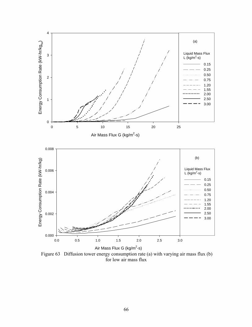
66


0 5 10 15 20 25

Ene

rgy

Con

sum

ptio

n R

ate

(kW

-hr/k

g fw)

0

1

2

3

4


0.150.250.500.751.201.552.002.503.00

(a)


0.0 0.5 1.0 1.5 2.0 2.5 3.0

Ene

rgy

Con

sum

ptio

n R

ate

(kW

-hr/k

g)

0.000

0.002

0.004

0.006

0.008


0.150.250.500.751.201.552.002.503.00

(b)

Figure 63 Diffusion tower energy consumption rate (a) with varying air mass flux (b) for low air mass flux

67


0 5 10 15 20

Fres

h W

ater

Pro

duct

ion

Effi

cien

cy (m

fw/m

L)

0.0

0.1

0.2

0.3

0.4


0.150.250.500.751.201.552.002.503.00

Figure 64 Fresh water production efficiency with varying air mass flux realized for the

lower air and liquid mass fluxes

8.2 Comparison of the heated air/heated water process to the heated water/ambient air process

In this analysis the heated air/heated water DDD process is compared against the heated water/ambient air DDD process described in depth in the 2004 annual report. In performing the analysis of the heated air/heated water the analysis described in Section 6 is used with the air inlet temperature, water inlet temperature, specific packing area, diameter of the packing material, and inlet absolute humidity held constant at 60° C, 60° C, 267 m2/m3, 0.018 m, and 0.0065 respectively. The values obtained for the heated water/ambient air case are calculated using the model presented in the 2004 annual report where the inlet water temperature, inlet air temperature, inlet humidity ratio, specific area, and diameter of the packing are held at 60° C, 26° C, 0.023, 267 m2/m3, and 0.018 m respectively. To obtain the predictions for comparison calculations were run for nine different liquid mass fluxes: 0.15, 0.25, 0.5, 0.75, 1.20, 1.55, 2.0, 2.5, 3.0 kg/m2-s. For each liquid mass flux, the gas mass flux was varied. For each liquid mass flux, the minimum energy consumption rate was recorded over the range of air mass flux. The values of the fresh water production flux, and fresh water production efficiency reported are those corresponding to the point of minimum energy consumption. Figures 65 and 66 show the fresh water production flux, energy consumption rate, and fresh water production efficiency for the two different configurations.

Figure 65 shows the fresh water production efficiency and energy consumption rate with varying liquid mass flux for both of the processes. The energy consumption rate for both shows little difference for liquid mass fluxes greater than about 1.3 kg/m2-s. However at low mass flux the heated water/ambient air case has a considerably less energy consumption rate. The fresh water production efficiency of the heated air/heated water process is greater for all values of liquid mass flux, although at large liquid mass

68

flux the difference is not significant. It should be noted that when comparing the two configurations there is more thermal energy input for the heated air/heated water case than the heated water/ambient air case, and the energy consumption rate only reflects the electrical energy consumed. Figure 66 shows the fresh water production flux and energy consumption rate for varying liquid mass flux for both processes. It is observed that the heated air/heated water process has a greater fresh water production flux for all values of the liquid mass fluxes considered. However at low liquid mass flux, the energy consumption rate is higher for the heated air/heated water configuration. Thus the decision to use one process over the other depends upon the source of waste heat and operating conditions.

This comparison reveals that for higher liquid flow rates the heated air/heated water case is equally comparable in energy consumption rate but has a higher fresh water production efficiency and fresh water production flux. On a small scale, this equates to a smaller tower size by utilizing the heated air/heated water DDD process. Less tower height is required for the heated air/heated water process in order to generate the same amount of fresh water produced in the heated water/ambient process. This translates to lower production cost and less space required.


0.0 0.5 1.0 1.5 2.0 2.5 3.0 3.5

Fres

h W

ater

Pro

duct

ion

Effi

cien

cy (m

fw/m

L)

0.02

0.03

0.04

0.05

0.06

0.07

0.08

0.09

Ene

rgy

Con

sum

ptio

n R

ate

(kW

-hr/k

g)

0.0000

0.0001

0.0002

0.0003

0.0004

0.0005

0.0006

0.0007

0.0008Hot Air/Hot Water

Ambient Air/Hot Water

Hot Air/Hot Water


Inlet Conditions:Ta,in = 60 C Tw,in = 60 C φin = 5.25%Hot Air/Hot Water

Ambient Air/Hot Water Ta,in = 26 C Tw,in = 60 C φin = 80.17%

Hot Air/Hot Water

Figure 65 Fresh water production efficiency and energy consumption rate for varying

liquid mass flux for 60 °C inlet conditions

69


0.0 0.5 1.0 1.5 2.0 2.5 3.0 3.5

Fres

h W

ater

Pro

duct

ion

Flux

(kg/

m2 -s

)

0.00

0.02

0.04

0.06

0.08

0.10

Ene

rgy

Con

sum

ptio

n R

ate

(kW

-hr/k

g)

0.0000

0.0001

0.0002

0.0003

0.0004

0.0005

0.0006

0.0007

0.0008


Hot Air/Hot Water


Hot Air/Hot Water

Inlet Conditions:Ta,in = 60 C Tw,in = 60 C φin = 5.25%Hot Air/Hot Water

Ambient Air/Hot Water Ta,in = 26 C Tw,in = 60 C φin = 80.17%

Figure 66 Fresh water production flux and energy consumption rate for varying liquid

mass flux for 60 °C inlet conditions

8.3 Comparison of the heated air/heated water process using HD Q-PAC and Q-PAC packed beds

For the next analysis two different types of packed bed are used with the heated air/heated water process. The theoretical model proposed in Section 6 is used to calculate the parameters, however a different wetted specific area is used. A modified Onda’s correlation, which is found in Appendix A, is used for the mass transfer coefficients and the wetted specific area for both configurations. HD Q-PAC, the packing material described in Section 2.1 and used in the experimental facility, is compared with Q-PAC. The Q-PAC material is also produced by Lantec and is manufactured to have lower pressure drop, reduced incidence of fouling, and flooding at higher air mass flow rates giving it a wider range of operation. Lantec supplied the gas side pressure drop, GP∆ (kPa), across the Q-PAC packed bed as

2 42

2[0.0078 1.3788( ) 0.30715( ) ]G

G l l G

P G L L Gz ρ ρ ρ ρ

∆= + + , (65)

Figures 67 and 68 show the fresh water production, fresh water efficiency, and energy consumption of the heated air/heated water process for the two configurations. Again the computations shown in the graph correspond to the points of minimum energy consumption rate for each liquid mass flux. Figure 67 shows the fresh water production efficiency and energy consumption rate with varying liquid mass flux. The Q-PAC packed bed configuration is obviously much more energy efficient than the HD Q-PAC configuration. As the liquid mass flux increases the variation in the energy consumption rate of the two configurations increases. There is little variation in the fresh water

70

production efficiency, however the Q-PAC appears to have a slightly better fresh water production efficiency for all values of the liquid mass flux explored.


0.0 0.5 1.0 1.5 2.0 2.5 3.0 3.5

Fres

h W

ater

Pro

duct

ion

Effi

cien

cy (m

fw/m

L)

0.030

0.035

0.040

0.045

0.050

0.055

0.060

0.065

Ene

rgy

Con

sum

ptio

n R

ate

(kW

-hr/k

g)

0.0002

0.0003

0.0004

0.0005

0.0006

0.0007

Q-PAC Material

HD Q-PAC MaterialHD Q-PAC Material

Q-PAC Material

Inlet Conditions: Ta,in = 60 C Tw,in = 60 C φin = 5.25%


mass flux for HD Q-PAC and Q-PAC packed bed


0.0 0.5 1.0 1.5 2.0 2.5 3.0 3.5

Fres

h W

ater

Pro

duct

ion

Flux

(kg/

m2 -s

)

0.00

0.02

0.04

0.06

0.08

0.10

0.12E

nerg

y C

onsu

mpt

ion

Rat

e (k

W-h

r/kg)

0.0002

0.0003

0.0004

0.0005

0.0006

0.0007

Q-PAC Material

HD Q-PAC MaterialHD Q-PAC Material

Q-PAC Material

Inlet Conditions: Ta,in = 60 C Tw,in = 60 C φin = 5.25%


mass flux for HD Q-PAC and Q-PAC packed bed

71

Figure 68 shows the variation in the fresh water production flux and energy consumption rate for varying liquid mass flux. There is very little variation in the fresh water production flux between the HD Q-PAC and Q-PAC packed bed configurations. However, at high liquid mass flux, the Q-PAC appears to have a slightly higher fresh water production flux. Despite the minimal difference in fresh water production between the two beds, the energy consumption rate remains the key difference. Figure 68 demonstrates that the Q-PAC packed can be utilized to produce the same quantity of fresh water product but at a lower energy cost. The downside of the Q-PAC is that much more footprint area is needed to achieve the same quantity of production. Despite this fact, however, the Q-PAC could prove to be especially important for large scale DDD facilities. If space is not an issue then the Q-PAC configuration would be advantageous for the lesser energy consumption rate. Further research should be conducted on the Q-PAC to determine the exact wetting and performance. 9. Summary

The development of a Diffusion Driven Desalination facility has been completed, and the results are promising. A detailed analysis shows that the waste heat from a 100 MW power plant can be used to produce 1.03 million gallons of fresh water per day using the DDD process. The energy used to drive the process is low thermodynamic availability waste heat, and the only energy cost is that used to power the pumps and fans. An economic simulation of the DDD system shows that the production costs of the DDD combined power plant is very competitive compared with the costs required for reverse osmosis or flash evaporation technologies. A laboratory scale DDD facility, which includes the diffusion tower, direct contact condenser and air heating section has been fabricated. The whole system has been fully instrumented for detailed heat and mass transfer measurements. Extensive measurements of the diffusion tower and direct contact condenser were made to validate their simulated performance. The analytical model of the diffusion tower proves to be quite satisfactory in predicting the thermal performance of counter flow packed beds with both air and water heating. The analytical model of the direct contact condensers proves to be quite satisfactory in predicting the thermal performance of both the co-current and counter-current flow packed beds.

Current analysis shows that the Diffusion Driven Desalination process appears to be an economically attractive distillation process. The precise values presented in the report need to be viewed with caution since losses other than pressure losses have not been considered, and the assumed feed water temperature into the diffusion tower may be optimistic. Nevertheless, the trends presented demonstrate the potential that can be gained from the DDD process, and it provides useful and practical guidance for choosing the operating conditions to achieve near optimum performance.

Although the Diffusion Driven Desalination facility is a promising technology for fresh water production using waste heat from electric power plants, current industry practice will limit its implementation until the value of fresh water sharply increases. The current practice of electric power plants is to pump a very large rate of cooling water through the main condenser so that the temperature rise of the water across the condenser is only about 6° C. The DDD requires the discharge water from the condenser to be approximately 40° C. This could be accomplished by lowering the flow rate through the condenser and providing more heat transfer surface area to compensate for the reduced

72

heat transfer rate. This would require a power plant installing a DDD facility to also replace or modify the main condenser. This is not a likely scenario. The best prospect for incorporating the DDD facility into an electric power plant for fresh water production is with the fabrication of new plants where the main condenser could be sized appropriately for the specified flow conditions. Another promising option is to incorporate DDD into power plants installing air-cooled condensers. The heated air discharging the condenser could be directly ducted to the diffusion tower.

The air heating concept has also been thoroughly explored. The heated air/heated water case proved to be a more effective process than the heated air/ambient water case. A parametric study to determine the effect of certain operating variables on the maximum freshwater production was completed for the heated air/heated water DDD process. For each liquid mass flux there is an optimal air mass flux where the maximum fresh water production flux is produced. There is also a location where the energy consumption for pumping through the diffusion tower is minimized.

The heated air/heated water process was compared to other DDD processes, specifically the heated water/ambient air case and the heated air/heated water process utilizing the Q-PAC packed bed, a less dense and lower pressure drop packing material. The comparison showed that the heated air/heated water DDD process has its advantages and disadvantages at different operating conditions. In comparison to the heated water/ambient air it was shown that the heated air/heated water process requires more electrical energy than the heated water/ambient air process at low liquid mass flux; however the fresh water production efficiency for the heated air/heated water is greater for all values of liquid mass flux. The fresh water production for the heated air/heated water process is greater for all liquid mass flux. In the comparison with the heated air/heated water using the Q-PAC packing, it was shown that similar fresh water production can be achieved at a lower energy cost by using Q-PAC. Further studies are required to determine the wettability of Q-PAC and its wetted fraction as part of the DDD process. Extensive research has already been performed on the DDD process and while the future of the process looks optimistic, further research needs to be done. The DDD process needs to be further examined on a larger scale. A pilot facility should be constructed and the DDD performance should be analyzed over long term operation in an industrial setting. As of yet, the DDD process has not been analyzed using a saline feed water source in the diffusion tower. Using such a source, water quality testing of the fresh water produced in the DDD process should be conducted. This is important in determining the type of post treatment the product water may require.

73

References [1] World Resources Institute, United Nations Development Programme, the United

Nations Environment Programme, and the World Bank, “World Resources 2000 – 2001 People and Ecosystems”, 2 104-105 (Sep 2000).

[2] Muller-Holst, H., Engelhardt, M., Scholkopf, W., Jul 1999, Small-scale thermal seawater desalination simulation and optimization of system design, Desalination 122-3, 255-262.

[3] Al-Hallaj, S., Selman, J.R., 2002, A comprehensive study of solar desalination with a humidification – dehumidification cycle, a report by the Middle East Desalination Research Center, Muscat, Sultanate of Oman.

[4] Klausner, J.F., Li,Y., Mei, R., 2004, Innovative diffusion driven desalination process, Journal of Energy Resources Technology.

[5] Bharathan, D., Parsons, B.K., and Althof, J.A., 1988, Direct-Contact Condensers for Open-Cycle OTEC Applications, National Renewable Energy Laboratory Report SERI/TP-252-3108 for DOE Contract No. DE-AC02-83CH10093.

[6] Klausner, J.F., Mei, R., and Li,Y. et al., 2004, Innovative Fresh Water Production Process for Fossil Fuel Plants, U.S. DOE - Energy Information Administration annual report.

[7] F. Merkel, Verdunstungskuhlung, VDI Forschungsarbeiten, 275, Berlin, 1925. [8] D.R. Baker, H.A. Shryock, A comprehensive approach to the analysis of cooling

tower performance, Journal of Heat Transfer, (1961) 339-350. [9] J.W. Sutherland, Analysis of mechanical-draught counterflow air/water cooling

towers, Journal of Heat Transfer, vol. 105, (1983) 576-583. [10] F. Osterle, On the analysis of counter-flow cooling towers, International Journal of

Heat and Mass Transfer, vol. 34, No. 4/5, (1991) 1316-1318. [11] H.T.A. El-Dessouky, A. Ai-Haddad, F. Ai-Juwayhel, A modified analysis of

counter flow wet cooling towers, Journal of Heat Transfer, vol. 119, (1997) 617-626.

[12] W.H. McAdams, J.B. Pohlenz, and R.C. St. John, Transfer of heat and mass between air and water in a packed tower, Chemical Engineering Progress, 45, (1949) 241-252.

[13] C.C. Huang, and J.R. Fair, Direct-contact gas-liquid heat transfer in a packed column, Heat Transfer Engineering, 10, No. 2, (1989) 19-28.

[14] K. Onda, H. Takechi, and Y. Okumoto, Mass transfer coefficients between gas and liquid phases in packed columns, Journal of Chemical Engineering of Japan, 1, (1968) 56-62.

[15] Kays, W.M. and Crawford, M.E, “Convective Heat and Mass Transfer”, 2nd Edition, McGraw-Hill Higher Education, 243 (1980).

[16] Klausner J.F., Li Y. and Mei R., “Evaporative Heat and Mass Transfer for the Diffusion Driven Desalination Process”, in press J. Heat & Mass Transfer, Springer Verlag, New York (2005).

[17] Wangnick, K. (2002), 2002 IDA Worldwide Desalting Plants Inventory Report No. 17, produced by Wangnick Consulting for IDA, Gnarrenburg, Germany.

74

[18] Hisham M. Ettouney and Hisham T. El-Dessouky, Kuwait Univ., Ron S. Faibish and Peter J. Gowin, IAEA, Evaluating the Economics of Desalination, Chemical Engineering Progress, Dec. 2002, pp 32-39.

[19] Survey by the NUS Consulting Group, based on the municipal water price as of July 1, 2002 in U.S.

[20] U.S. DOE - Energy Information Administration, Electric Power Monthly Annual, August, 2001, U.S.

[21] Nuclear Energy Institute, “The Economic Benefits Of Oyster Creek Generating Station”, Prepared for AmerGen Energy Co. LLC, Ocean County, New Jersey (March 2004).

[22] Eckert, E.R.G., Goldstein, R.J.,“Measurements in Heat Transfer”, Hemisphere Publishing Corp., Washington, Chap. 9 (1976).

[23] Li, Y., Klausner, J., Mei, R., Knight, J., 2006, “Direct Condensation in Packed Beds,” International J. of Heat Transfer, 49, 4751-4761.

[24] Water Desalting Committee of the American Water Works Association., 2004, “Water Desalting Planning Guide For Water Utilities,” John Wiley & Sons, Inc., New Jersey (2004).

[25] Clarke, R., and King, J., “The Water Atlas,” The New Press, New York, (2004). [26] Beverage Marketing Corporation, New York. Quoted by Olson, E.D., Poling, D.,

Solomon, G., February 1999, “Bottled Water Pure Drink or Pure Hype?,” Natural Resources Defense Council (NRDC), Retrieved on September 1, 2006, http://www.nrdc.org/water/drinking/bw/chap2.asp.

75

Appendix A Onda’s correlation

3/14.05.03/2 )(Re0051.0

⎥⎥⎦

⎤

⎢⎢⎣

⎡= −

L

Lg

adSck pLLwL ρ

µ (A1)

GpGGAG aDadSck 23/17.0 )(Re23.5 −= (A2)

⎪⎭

⎪⎬

⎫

⎪⎩

⎪⎨

⎧

⎥⎥⎥

⎦

⎤

⎢⎢⎢

⎣

⎡

⎟⎟⎠

⎞⎜⎜⎝

⎛−−= − 5/105.02/14

3

Re2.2exp1 LLLAL

cw WeFraa

σσ (A3)

LwLW a

Lµ

=Re , G

GA aGµ

=Re , L

LA aLµ

=Re ,

LL

LL D

Scρ

µ= ,

GG

GG D

Scρ

µ= ,

gaLFr

LL ρ

2= ,

aLWe

LLL σρ

2=

The equation of aw has been modified from the Onda’s original correlation [14]. Heat transfer coefficient on the liquid side

2/1)(L

LPLLLL D

KCkU ρ= (A4)

Heat transfer coefficient on the gas side

3/23/1 )()(G

GPGGGG D

KCkU ρ= (A5)

where K denotes thermal conductivity and D denotes the molecular diffusion coefficient.

76

Appendix B Co-current Flow Condenser Experimental Data with Packing

Water flow rate

(kg/s)

Air flow rate (kg/s)

Water inlet temperature

(C)

Water exit temperature

(C)

Air inlet temperature

(C)

Air exit temperature

(C)

Air inlet humidity

Air exit humidity

0.068 0.031 28.3 29.9 32.8 29.6 0.035 0.027 0.059 0.031 28.3 30.0 32.7 29.7 0.035 0.027 0.051 0.031 28.5 30.2 32.8 29.9 0.035 0.027 0.041 0.031 28.4 30.3 32.6 30.0 0.034 0.027 0.032 0.031 28.1 30.3 32.6 30.3 0.034 0.028 0.022 0.031 27.9 31.1 32.8 30.7 0.034 0.028

0.017 0.031 28.1 31.1 32.7 31.0 0.034 0.029 0.024 0.031 28.0 31.3 32.7 30.7 0.034 0.028 0.033 0.031 28.3 30.4 32.7 30.4 0.034 0.028 0.046 0.031 28.2 30.2 32.7 30.0 0.034 0.027 0.056 0.031 28.2 30.1 33.0 29.9 0.034 0.027 0.064 0.032 28.3 29.8 32.7 29.9 0.033 0.027

Water

flow rate (kg/s)



(C)


(C)


(C)


(C)

Air inlet humidity

Air exit humidity

0.062 0.030 28.0 33.7 40.3 32.9 0.050 0.032 0.055 0.031 28.2 34.2 40.1 33.4 0.049 0.033 0.034 0.030 28.0 35.3 40.2 34.3 0.049 0.035 0.027 0.030 27.8 36.0 40.2 35.1 0.049 0.037 0.018 0.030 27.8 36.2 40.3 36.6 0.049 0.040

0.020 0.030 27.8 36.2 40.3 36.2 0.049 0.039 0.036 0.031 27.9 35.6 40.3 35.0 0.049 0.037 0.041 0.031 28.0 35.3 40.4 34.4 0.049 0.036 0.052 0.031 28.0 34.5 40.3 33.9 0.049 0.034 0.060 0.031 28.1 34.1 40.4 33.5 0.049 0.034

Water

flow rate (kg/s)



(C)


(C)


(C)


(C)

Air inlet humidity

Air exit humidity

0.069 0.030 28.6 35.8 44.5 35.0 0.061 0.037 0.055 0.030 28.0 36.7 44.9 35.7 0.062 0.038 0.047 0.030 28.0 37.5 44.8 36.1 0.062 0.039 0.034 0.030 28.4 38.3 44.1 37.1 0.060 0.041 0.025 0.030 28.0 39.3 43.9 38.1 0.059 0.044 0.016 0.030 28.0 39.1 44.1 39.4 0.060 0.047

0.023 0.031 27.9 39.3 43.8 38.5 0.059 0.045 0.032 0.031 28.0 38.5 43.6 37.4 0.058 0.042 0.043 0.030 28.1 37.7 44.4 36.5 0.061 0.040 0.051 0.031 28.2 36.9 44.2 35.9 0.060 0.039 0.061 0.030 28.3 36.0 44.1 35.3 0.060 0.037

77

Appendix C Counter-current Flow Condenser Experimental Data with Packing

Water

flow rate (kg/s)



(C)


(C)


(C)


(C)

Air inlet humidity

Air exit humidity

0.024 0.029 20.4 40.3 42.7 34.8 0.057 0.036 0.033 0.030 20.5 38.5 42.7 31.9 0.057 0.031 0.041 0.031 20.4 37.2 42.7 30.1 0.057 0.027 0.051 0.031 19.7 34.8 42.8 28.4 0.058 0.025

0.061 0.030 19.5 33.3 42.8 27.1 0.058 0.023 0.054 0.030 19.7 34.0 42.9 28.0 0.058 0.024 0.045 0.030 19.8 34.8 42.9 29.1 0.058 0.026 0.034 0.030 20.3 37.0 42.9 31.7 0.058 0.030 0.030 0.030 20.5 37.8 42.9 33.1 0.058 0.033

Water

flow rate (kg/s)



(C)


(C)


(C)


(C)

Air inlet humidity

Air exit humidity

0.024 0.029 19.5 37.5 40.8 31.6 0.051 0.030 0.035 0.031 19.3 34.6 40.6 29.4 0.051 0.026 0.048 0.030 19.4 32.9 40.9 27.4 0.052 0.023 0.058 0.031 19.0 31.3 40.7 26.2 0.051 0.022

0.053 0.031 18.9 31.9 40.7 26.5 0.051 0.022 0.044 0.030 19.1 32.7 40.7 27.5 0.051 0.023 0.038 0.031 19.3 33.1 40.7 28.3 0.051 0.025 0.031 0.030 19.3 35.5 40.8 29.6 0.051 0.027 0.023 0.030 19.4 36.6 40.8 31.4 0.051 0.030

Water

flow rate (kg/s)



(C)


(C)


(C)


(C)

Air inlet humidity

Air exit humidity

0.024 0.031 19.9 33.2 36.5 29.7 0.041 0.027 0.033 0.030 20.1 32.2 36.8 27.7 0.041 0.024 0.048 0.030 19.4 30.4 36.8 25.8 0.041 0.021 0.062 0.030 19.5 28.6 37.0 24.4 0.041 0.019

0.054 0.030 19.4 29.5 37.0 24.7 0.041 0.020 0.044 0.030 19.3 30.2 37.0 26.2 0.041 0.022 0.038 0.031 20.3 31.4 37.1 27.0 0.041 0.023 0.031 0.031 20.5 32.0 37.1 28.5 0.042 0.025

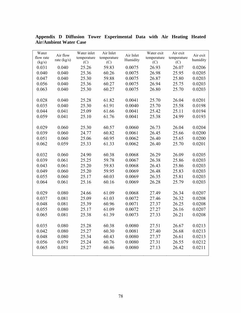
78

Appendix D Diffusion Tower Experimental Data with Air Heating Heated Air/Ambient Water Case

Water

flow rate (kg/s)



(C)

Air Inlet temperature

(C)

Air Inlet Humidity


(C)


(C)

Air exit humidity

0.031 0.040 25.26 59.83 0.0075 26.93 26.07 0.0206 0.040 0.040 25.36 60.26 0.0075 26.98 25.95 0.0205 0.047 0.040 25.30 59.88 0.0075 26.87 25.80 0.0203 0.056 0.040 25.36 60.27 0.0075 26.94 25.75 0.0203 0.063 0.040 25.30 60.27 0.0075 26.80 25.70 0.0203

0.028 0.040 25.28 61.82 0.0041 25.70 26.04 0.0201 0.035 0.040 25.30 61.91 0.0040 25.70 25.58 0.0198 0.044 0.041 25.09 61.66 0.0041 25.42 25.11 0.0194 0.059 0.041 25.10 61.76 0.0041 25.38 24.99 0.0193

0.029 0.060 25.30 60.57 0.0060 26.73 26.04 0.0204 0.039 0.060 24.77 60.82 0.0061 26.45 25.66 0.0200 0.051 0.060 25.06 60.95 0.0062 26.40 25.65 0.0200 0.062 0.059 25.33 61.33 0.0062 26.40 25.70 0.0201

0.032 0.060 24.90 60.38 0.0068 26.29 26.09 0.0205 0.039 0.061 25.25 59.78 0.0067 26.38 25.86 0.0203 0.043 0.061 25.20 59.83 0.0068 26.43 25.86 0.0203 0.049 0.060 25.20 59.95 0.0069 26.48 25.83 0.0203 0.055 0.060 25.17 60.03 0.0069 26.35 25.81 0.0203 0.064 0.061 25.16 60.16 0.0069 26.28 25.79 0.0203

0.029 0.080 24.66 61.09 0.0068 27.49 26.34 0.0207 0.037 0.081 25.09 61.03 0.0072 27.46 26.32 0.0208 0.048 0.081 25.39 60.96 0.0071 27.37 26.25 0.0208 0.055 0.080 25.17 61.09 0.0072 27.27 26.16 0.0207 0.065 0.081 25.38 61.39 0.0073 27.33 26.21 0.0208

0.035 0.080 25.28 60.38 0.0080 27.51 26.67 0.0213 0.042 0.080 25.27 60.30 0.0081 27.40 26.68 0.0213 0.048 0.080 25.34 60.43 0.0080 27.37 26.61 0.0213 0.056 0.079 25.24 60.76 0.0080 27.31 26.55 0.0212 0.065 0.081 25.27 60.46 0.0080 27.13 26.42 0.0211

79

Appendix E Diffusion Tower Experimental Data with Air Heating Heated

Air/Heated Water Case

Water flow rate

(kg/s)



(C)

Air Inlet temperature

(C)

Air Inlet Humidity


(C)


(C)

Air exit humidity

0.034 0.040 60.82 61.03 0.0066 37.21 42.28 0.0550 0.039 0.039 60.99 61.15 0.0066 37.81 43.57 0.0591 0.047 0.039 59.99 61.71 0.0066 38.84 44.74 0.0632 0.054 0.040 60.58 60.94 0.0069 39.96 44.76 0.0631 0.061 0.041 61.02 60.61 0.0071 40.41 45.54 0.0661 0.068 0.041 59.48 60.52 0.0074 40.91 45.03 0.0642

0.036 0.041 61.00 61.35 0.0059 35.99 42.30 0.0566 0.043 0.040 60.79 61.57 0.0059 36.27 44.03 0.0624 0.050 0.040 60.75 61.69 0.0061 37.30 44.71 0.0649 0.056 0.041 60.89 61.53 0.0064 39.12 44.10 0.0627 0.064 0.042 60.31 60.94 0.0066 39.63 44.89 0.0656

0.032 0.059 61.01 61.10 0.0078 33.65 37.74 0.0420 0.041 0.060 61.66 61.08 0.0078 34.46 39.70 0.0474 0.047 0.061 61.12 60.93 0.0080 35.02 40.20 0.0489 0.055 0.060 60.05 61.23 0.0079 36.14 40.98 0.0511 0.063 0.059 60.52 62.10 0.0081 39.87 42.18 0.0550

0.033 0.061 60.79 60.52 0.0080 32.46 37.51 0.0416 0.038 0.060 60.76 60.69 0.0080 33.51 38.44 0.0448 0.046 0.060 60.97 61.03 0.0081 34.65 39.70 0.0482 0.056 0.061 60.86 61.10 0.0082 35.95 40.85 0.0498 0.062 0.060 60.57 61.16 0.0083 37.06 41.33 0.0510

0.030 0.080 60.94 60.11 0.0088 30.75 34.51 0.0353 0.039 0.080 61.01 60.29 0.0090 31.88 35.91 0.0387 0.048 0.080 60.45 60.48 0.0088 33.04 37.40 0.0426 0.056 0.081 60.40 60.78 0.0089 34.88 38.02 0.0442 0.066 0.080 60.26 60.94 0.0090 36.02 39.01 0.0468

0.032 0.080 59.69 59.94 0.0080 31.03 35.02 0.0350 0.036 0.080 61.29 59.73 0.0083 30.82 35.97 0.0378 0.046 0.080 60.83 61.09 0.0084 32.97 37.12 0.0410 0.055 0.081 60.57 60.96 0.0086 34.43 37.90 0.0429 0.064 0.081 58.98 60.40 0.0088 34.99 38.97 0.0458

80

Nomenclature A control surface area (m2) a specific area of packing material (m2/m3) ai amortization factor (yr–1) Cdrag aerodynamic drag on droplet Cp specific heat of air (kJ/kg) c electric cost, ($/m3) D molecular diffusion coefficient (m2/s) DC direct capital cost ($) dp diameter of the packing material (m) E Power from a power plant (MW) f plant availability G air mass flux (kg/m2-s) g gravitational acceleration (m/s2) H diffusion tower height (m) h enthalpy (kJ/kg) hfg latent heat of vaporization (kJ/kg) i interest rate k specific chemicals cost ($/m3) kG mass transfer coefficient (m/s) L water mass flux (kg/m2-s) MV vapor molecular weight (kg/kmol) m mass flow rate (kg/s) mdrop mass of an individual droplet (kg) mp plant capacity (m3 /day) n plant life (yr) Pa partial pressure of air (Pa or kPa) Psat partial pressure of vapor (Pa or kPa) P electrical power consumption for pumps (W, kW or MW) PR performance ratio (kg product/kg steam) q heat exchanged in condenser (W) R universal gas constant (kJ/kmol-K) Ra engineering gas constant for air (kJ/kg-K) r energy convert efficiency S heating steam cost ($/MkJ) T temperature (°C or °K) U heat transfer coefficient (W/m2-K) u air/vapor velocity (m/s) V control volume (m3) VG air/vapor volume flow rate (m3/s) vd droplet velocity (m/s) w specific consumption of electric power (kWh/m3) Ф relative humidity

81

ω humidity ratio µ dynamic viscosity (kg/m-s) ρ density (kg/m3) σL surface tension of liquid (N/m) σC critical surface tension of the packing material (N/m) γ specific cost of operating labor ($/m3) γd mass transfer coefficient for droplet condensation (m/s) λ average latent heat of steam (kJ/kg) Subscripts a air b seawater c cold fresh water DC direct contact condenser Dif diffusion tower DDD DDD system d droplet elec electricity evap the portion of liquid evaporated fw fresh water H high i interface L low l water in liquid phase mix air/vapor mixture nopack without packing v water in vapor phase in inlet parameter out exit parameter pack with packing s steam sat saturate state Total total input waste waste

innovative fresh water production process for fossil … library/research/coal/ewr... · innovative...

Documents