EPA/540/R-95/519August 1995

Rapid Optical ScreenTool (ROSTTM)

Innovative Technology Evaluation Report

NATIONAL RISK MANAGEMENT RESEARCH LABORATORYOFFICE OF RESEARCH AND DEVELOPMENT

U.S. ENVIRONMENTAL PROTECTION AGENCYCINCINNATI, OHIO 45268

NATIONAL EXPOSURE RESEARCH LABORATORYOFFICE OF RESEARCH AND DEVELOPMENT

U.S. ENVIRONMENTAL PROTECTION AGENCYLAS VEGAS, NEVADA 89193

@ p R on Recycled Paper

Notice

The information in this document has been funded wholly or in part by the U.S. Environmental Protection Agency in partialfulfillment of Contract No. 68-CO-0047, Work Assignment No. O-40, to PRC Environmental Management, Inc. It has beensubject to the Agency’s peer and administrative review, and it has been approved for publication as an EPA document. Theopinions, tindings, and conclusions expressed herein are those of the contractor and not necessarily those of the EPA or othercooperating agencies. Mention of company or product names is not to be construed as an endorsement by the agency.

Foreword

The U.S. Environmental Protection Agency is charged by Congress with protecting the Nation’s land,air, and water resources. Under a mandate of national environmental laws, the Agency strives to formulate andimplement actions leading to a compatible balance between human activities and the ability of natural systemsto support and nurture life. To meet this mandate, EPA’s research program is providing data and technicalsupport for solving environmental problems today and building a science knowledge base necessary to manageour ecological resources wisely, understand how pollutants affect our health, and prevent or reduce environmentalrisks in the future.

The National Risk Management Research Laboratory is the Agency’s center for investigation oftechnological and management approaches for reducing risks from threats to human health and the environment.The focus of the Laboratory’s research program is on methods for the prevention and control of pollution to air,land, water and subsurface resources; protection of water quality in public water systems ; remediation ofcontaminated sites and ground water; and prevention and control of indoor air pollution. The goal of this researcheffort is to catalyze development and implementation of innovative, cost-effective environmental technologies;develop scientific and engineering information needed by EPA to support regulatory and policy decisions; andprovide technical support and information transfer to ensure effective implementation of environmentalregulations and strategies.

This publication has been produced as part of the Laboratory’s strategic long-term research plan. It ispublished and made available by EPA’s Office of Research and Development to assist the user community andto link researchers with their clients.

E. Timothy Oppelt, DirectorNational Risk Management Research Laboratory

.

Abstract

In August 1994, a demonstration of cone penetrometer-mounted sensor technologies took place to evaluate theireffectiveness in sampling and analyzing the physical and chemical characteristics of subsurface soil at hazardous wastesites. The effectiveness of each technology was evaluated by comparing each technology’s results to the resultsobtained using conventional reference method technologies. The demonstration was developed under theEnvironmental Protections Agency’s Superfund Innovative Technology Evaluation Program.

Three technologies were evaluated: the rapid optical screening tool (ROSry) developed by Loral Corporation andDakota Technologies, Inc., the site characterization and analysis penetrometer system (SCAPS) laser inducedfluorescence sensor developed by the Tri-Services (Army, Navy, and Air Force), and the conductivity sensordeveloped by Geoprobe Systems. These technologies were designed to provide rapid sampling and real-time,relatively low cost analysis of the physical and chemical characteristics of subsurface soil to quickly distinguishcontaminated areas from noncontaminated areas.

Three sites were selected for the demonstration, each contained varying concentrations of coal tar waste and petroleumfuels, and wide ranges in soil texture.

This demonstration found that the ROST technology produced screening level data. Specifically, the qualitativeassessment showed that the stratigraphic and chemical cross sections were comparable to the reference methods. Thequantitative assessment showed that during the 1994 demonstration, the ROST? data could not be used as a reliablepredictor of actual contaminant concentration. Based on this study, the ROS’I”“’ appears to be capable of rapidly andreliably mapping the relative magnitude of the vertical and horizontal extent of subsurface contamination when thatcontamination is fluorescent. This type of contamination includes petroleum fuels and polynuclear aromatichydrocarbons. The design of the ROST”‘s fluorescence detection system also allows this technology to identifyspecific waste types, such as jet petroleum (JP-4), diesel fuel, or coal tar. This chemical mapping capability, whencombined with the stratigraphic data produced by the cone penetrometer creates a powerful tool for sitecharacterization.

iv

Table of Contents

Section

Notice.. . . . . . . . . . . . . . . . . . . . . . . . . . . . . . . . . . . . . . . . . . . . . . . . . . . . . . . . . . . . . . . . . . . . . . . . . . iiForeword

.... . . . . . . . . . . . . . . . . . . . . . . . . . . . . . . . . . . . . . . . . . . . . . . . . . . . . . . . . . . . . . . . . . . . . . . . .

Abstract .......................................................................... ivList of Figures

.... . . . . . . . . . . . . . . . . . . . . . . . . . . . . . . . . . . . . . . . . . . . . . . . . . . . . . . . . . . . . . . . . . . . . VIII

List of Tables .................................................................................. ..i ............. VIIIList of Abbreviations and Acronyms ..................................................... ixAcknowledgments .................................................................. xi

Executive Summary ..................................................................................................................................... 1

Introduction . . . . . . . . . . . . . . . . . . . . . . . . . . . . . . . . . . . . . . . . . . . . . . . . . . . . . . . . . . . . . . . . . . . 3Demonstration Background, Purpose, and Objectives . . . . . . . . . . . . . . . . . . . . . . . . . . . . . . . 3Demonstration Design .......................................................... 4

Qualitative Evaluation ................................................... 4Quantitative Evaluation ................................................. 6

Deviations from the Approved Demonstration Plan .................................. 7Site Descriptions ....................................................... ..... 7

Reference Method Results ................................................ ........ 9Reference Laboratory Procedures ......................................... ........ 9

Sample Holding Times .......................................... ........ 9Sample Preparation .............................................. ........ 9Initial and Continuing Calibrations ................................. ....... 10Sample Analysis .............................: ................. ....... 10Detection Limits .............................................. ....... 11Quality Control Procedures ...................................... . . . . . . 11Confirmation of Analytical Results ................................ . . . . . . . 12Data Reporting . . . . . . . . . . . . . . . . . . . . . . . . . . . . . . . . . . . . . . . . . . . . . . . . . . ....... 12

Quality Assessment of Reference Laboratory Data ......................... ....... 12Accuracy . . . . . . . . . . . . . . . . . . . . . . . . . . . . . . . . . . . . . . . . . . . . . . . . . . . . . . . ........ 12Precision . . . . . . . . . . . . . . . . . . . . . . . . . . . . . . . . . . . . . . . . . . . . . . . . . . . . . . . ....... 12Completeness . . . . . . . . . . . . . . . . . . . . . . . . . . . . . . . . . . . . . . . . . . . . . . . . . ........ 12

Use of Qualified Data for Statistical Analysis .............................. ........ 13Chemical Cross Sections ....................................... ....... 13

Atlantic Site ........................................... ....... 13York-Site . . . . . . . . . . . . . . . . . . . . . . . . . . . . . . . . . . . . . . . . . . . . . . . . ....... 13Fort Riley Site .................................................. 17

Quality Assessment of Geotechnical Laboratory Data . . . . . . . . . . . . . . . . . . . . . . . . . . 17Geotechnical Laboratory .................. , ....................... 17Borehole Logging . . . . . . . . . . . . . . . . . . . . . . . . . . . . . . . . . . . . . . . . . . . . . 17Sampling Depth Control ........................................ 17

V

Section

Table of Contents (Continued)

Stratigraphic Cross Sections ............................................. 17Atlantic Site . . . . . . . . . . . . . . . . . . . . . . . . . . . . . . . . . . . . . . . . . . . . . . . . . . . . 19York Site . . . . . . . . . . . . . . . . . . . . . . . . . . . . . . . . . . . . . . . . . . . . . . . . . . . . . . 19Fort Riley Site .................................................. 21

4 Rapid Optical Screening Tool ...................................................... 22Background Information ............................................. ....-. .... 22

Components . . . . . . . . . . . . . . . . . . . . . . . . . . . . . . . . . . . . . . . . . . . . . . . . . . . . . . . . . . 22Cone Penetrometer Truck System .................................. 22ROSTTMTechnology . . . . . . . . . . . . . . . . . . . . . . . . . . . . . . . . . . . . . . . . . . . . . 23Nd:YAG Laser .................................................. 23Tunable Dye Laser .............................................. 23Fiber Optic Cable ............................................... 24Detection System ............................................... 24Control Computer ............................................... 25

General Operating Procedures ........................................... 25Training and Maintenance Requirements ................................... 26Cost . . . . . . . . . . . . . . . . . . . . . . . . . . . . . . . . . . . . . . . . . . . . . . . . . . . . . . . . . . . . . . . . 26Observations . . . . . . . . . . . . . . . . . . . . . . . . . . . . . . . . . . . . . . . . . . . . . . . . . . . . . . . . . 26

DataPresentation . . . . . . . . . . . . . . . . . . . . . . . . . . . . . . . . . . . . . . . . . . . . . . . . . . . . . . . . . . . . . 28ChemicalDataa . . . . . . . . . . . . . . . . . . . . . . . . . . . . . . . . . . . . . . . . . . . . . . . . . . . . . . . . 28

Atlantic Sitee . . . . . . . . . . . . . . . . . . . . . . . . . . . . . . . . . . . . . . . . . . . . . . . . . . . . 28York Sitee . . . . . . . . . . . . . . . . . . . . . . . . . . . . . . . . . . . . . . . . . . . . . . . . . . . . . . 31Fort Riley Site ...................................................33

Cone Penetrometer Data ................................................ 36Atlantic Site .................................................... 36York Sitee . . . . . . . . . . . . . . . . . . . . . . . . . . . . . . . . . . . . . . . . . . . . . . . . . . . . . . 36Fort Riley Site .................................................. 37

5 Data Comparison.. . . . . . . . . . . . . . . . . . . . . . . . . . . . . . . . . . . . . . . . . . . . . . . . . . . . . . . . . . . . . . . . 39Qualitative Assessment . . . . . . . . . . . . . . . . . . . . . . . . . . . . . . . . . . . . . . . . . . . . . . . . . . . . . . 39

Stratigraphic Cross Sections . . . . . . . . . . . . . . . . . . . . . . . . . . . . . . . . . . . . . . . . . . . . 39Atlantic Site . . . . . . . . . . . . . . . . . . . . . . . . . . . . . . . . . . . . . . . . . . . . . . . . . . 39YorkSite . . . . . . . . . . . . . . . . . . . . . . . . . . . . . . . . . . . . . . . . . . . . . . . . . . . . 40Fort Riley Sitee . . . . . . . . . . . . . . . . . . . . . . . . . . . . . . . . . . . . . . . . . . . . . . . . . . . 40

Summary . . . . . . . . . . . . . . . . . . . . . . . . . . . . . . . . . . . . . . . . . . . . . . . . . . . . . . . . . . . . . . 40Chemical Cross Sections . . . . . . . . . . . . . . . . . . . . . . . . . . . . . . . . . . . . . . . . . . . . . . 41

Atlantic Site ..................................................41YorkSitee . . . . . . . . . . . . . . . . . . . . . . . . . . . . . . . .. . . . . . . . . . . . . . 42Fort Riley Site . . . . . . . . . . . . . . . . . . . . . . . . . . . . . . . . . . . . . . . . . . . . . . . . . . . 43

Total Organic Carbon.. . . . . . . . . . . . . . . . . . . . . . . . . . . . . . . . . . . . . . . . . . . . . . . . . . . 44Quantitative Assessment . . . . . . . . . . . . . . . . . . . . . . . . . . . . . . . . . . . . . . . . . . . . . . . . . . . . . 44

6 Applications Assessment ............................................................................................................ 51

7 Developer Comments and Technology Update ..................................... ... 53Loral Comments (April 1995) .................................................. 53DTI Comments(May1995) . . . . . . . . . . . . . . . . . . . . . . . . . . . . . . . . . . . . . . . . . . . . . . . . . . . . 56Technology Update . . . . . . . . . . . . . . . . . . . . . . . . . . . . . . . . . . . . . . . . . . . . . . . . . . . . . . . . . . . . . 57

Converting Rapid Optical Screening Tool (ROSTTM) Fluorescence Intensities toConcentration Equivalents ........................................... . 57Calibration Derived from Site Materials with In Situ Fluorescence Measurements ....... . 58

vi

Section Page

Calibration Derived from Synthetic Standards with “Above Ground”Fluorescence Measurements . . . . . . . . . . . . . . . . . . . . . . . . . . . . . . . . . . . . . . . . . . . . . 58

Approach 1: Designation of POL and Soil Type . . . . . . . . . . . . . . . . . . . . . . . . 59Approach 2: Specific POL Material, Designated Soil Type . . . . . . . . . . . . . . . . 59Approach 3: Specific POL Material and Soil from the Site . . . . . . . . . . . . . . . 59

8 References .................................................................................................................... 60

Appendix

A Qualitative, Quantitative, Geotechnical, and TOC Data ............................................................................................ 61

vii

List of Figures

Figure Page

2-13-l3-23-33-43-53-63-73-83-94-l4-24-34-44-54-64-74-84-94-104-115-l5-25-3

Typical Transect Sampling Line and Stratified Random Sampling Grid ..................... 6TPH Reference Method Chemical Cross Section - Atlantic Site ......................... 14PAH Reference Method Chemical Cross Section - Atlantic Site ... .... ............... 14TPH Reference Method Chemical Cross Section - York Site ...................... ... 15PAH Reference Method Chemical Cross Section - York Site . . . . . . . . . . . . . . . . . . . . . . . . . 15TPH Reference Method Chemical Cross Section - Fort Riley Site ..................... 16PAH Reference Method Chemical Cross Section - Fort Riley Site ..................... 16Reference Method Stratigraphic Cross Section - Atlantic Site ........................ 18Reference Method Stratigraphic Cross Section - York Site .......................... 18Reference Method Stratigraphic Cross Section - Fort Riley Site . . . . . . . . . . . . . . . . . . . . . . . 19System Components . . . . . . . . . . . . . . . . . . . . . . . . . . . . . . . . . . . . . . . . . . . . . . . . . . . . . . . . 24ROSTTM Chemical Cross Section - Atlantic Site ................................... 30Typical WTM - Atlantic Site ................................................... 32ROSTTM Chemical Cross Section - York Site ..................................... 32Typical WTM-York Sitee . . . . . . . . . . . . . . . . . . . . . . . . . . . . . . . . . . . . . . . . . . . . . . . . . . . 33ROST Chemical Cross Section - Fort Riley Site ................................. 34FVD-Fort Riley Site . . . . . . . . . . . . . . . . . . . . . . . . . . . . . . . . . . . . . . . . . . . . . . . . . . . . . . . . 35Typical WM - Fort Riley Site ................................................. 35Cone Penetrometer Stratigraphic Cross Section - Atlantic Site ....................... 37Cone Penetrometer Stratigraphic Cross Section - York Site .......................... 37Cone Penetrometer Stratigraphic Cross Section - Fort Riley Site ...................... 38Normalized LIF and Qualitative Reference Data - Atlantic Site ........................ 42Normalized LIF and Qualitative Reference Data - York Site .......................... 43Normalized LIF and Qualitative Reference Data - Fort Riley Site ...................... 44

List of Tables

Table Page

2-l3-l4-l4-24-35-l5-25-37-l

Criteria for Data Quality Characterization ......................................... 5Comparison of Geologists Data and Geotechnical Laboratory Data - All Sites ............ 20Quantitative ROSTTM Data - Atlantic Site . . . . . . . . . . . . . . . . . . . . . . . . . . . . . . . . . . . . . . . . . 29Quantitative ROSTTM Data - York Site . . . . . . . . . . . . . . . . . . . . . . . . . . . . . . . . . . . . . . . . . . . 29Quantitative ROSTTM Data - Fort Riley Site ....................................... 30Regression Analysis Results for Initial ROSTTM Push and Reference Methods - All Sites .... 46Regression Analysis Results for Averaged ROSTTM Push and Reference Methods - All Sites 47Data for Mean ROSTTM - All Sites . . . . . . . . . . . . . . . . . . . . . . . . . . . . . . . . . . . . . . . . . . . . . . . 49Summary of TPH Results for Quantitative Evaluation .... ........................... 54

..VIiIi

List of Abbreviations and Acronyms

ASTMbgsBTEXCCALcmcm/sDQODSODTIEPAERAETSFIDFMGPFVDGCHPLCHzICALITERLCSLIFMDLMethod OA-1pgfkgpgRmg/Lmg/kgmg/mLMjmL

::TPMSMSDNDSUNd:YAGNRMRLNERL-CRDnmns%D%RSDPAHPE

American Society for Testing and Materialsbelow ground surfacebenzene, toluene, ethylbenzene, and xylenecontinuing calibrationcentimetercentimeter per seconddata quality objectivedigital storage oscilloscopeDakota Technologies, Inc.Environmental Protection AgencyEnvironmental Resource AssociatesEnvironmental Technical Servicesflame ionization detectorFormer Manufactured Gas Plantfluorescence versus depthgas chromatographhigh performance liquid chromatographypulses per secondinitial calibrationinnovative technology evaluation reportlaboratory control sampleslaser induced fluorescencemethod detection limitUniversity of Iowa Hygienics Laboratory Methodmicrograms per kilogrammicrogram per litermilligram per litermilligram per kilogrammilligram per millilitermillijoulesmillilitermillimeterMeasurement and Monitoring Technologies Programmatrix spikematrix spike duplicateNorth Dakota State Universityneodymium-doped yttrium aluminum garnetNational Risk Management Research LaboratoryNational Exposure Research Laboratory-Characterization Research Divisionnanometernanosecondpercent differencepercent relative standard deviationpolynuclear aromatic hydrocarbonperformance evaluation

ix

List of Abbreviations and Acronyms (Continued)

PIDPMTPOLppbppmPRCPRLPTIQAQAPjPQCROST’-‘+’RPDSCAPSSITETERTOCTPHTPMUSCSUSDAV O CVPHWTM

photoionization detectorphotomultiplier tubepetroleum, oils, and lubricantsparts per billionparts per millionPRC Environmental Management, Inc.PACE reporting limit

Photon Technology, Inc.quality assurancequality assurance project planquality controlRapid Optical Screening Toolrelative percent differenceSite Characterization and Analysis Penetrometer SystemSuperfund Innovative Technology Evaluationtechnology evaluation recordtotal organic carbontotal petroleum hydrocarbontechnical project managerUnified Soil Classification SystemUnited States Department of Agriculturevolatile organic compoundvolatile petroleum hydrocarbonwavelength-time matrix

X

Acknowledgments

We wish to acknowledge the support of all those who helped plan and conduct this demonstration, interpret data, andprepare this report. In particular, for demonstration site access and relevant background information, Dean Harger(Iowa Electric Company), Ron Buhrman (Burlington Northern Railroad), and Abdul Al-Assi (U.S. Army Directorateof Engineering and Housing); for turn-key implementation of this demonstration, Eric Hess, Darrell Hamilton, andHarry Ellis (PRC Environmental Management, Inc.); for editorial and publication support, Suzanne Ladish and FrankDouglas; for peer and technical reviews, Dr. T. Vo-Dinh (Oak Ridge National Laboratory), Grace Bujewski (SandiaNational Laboratories), and Jeff Kelley (Nebraska Department of Environmental Quality); and for EPA projectmanagement, Lary Jack (National Exposure Research Laboratory-Characterization Research Division) (702) 798-2373). In addition, we gratefully acknowledge the participation of the technology developers Loral Corporation andDakota Technologies (Rapid Optical Screening Tool) (612) 456-2339 and (701) 237-4908, respectively).

xi

Section 1Executive Summary

Recent changes in environmental site characteriza-tion have resulted in the application of cone penetro-meter technologies to site characterization. With avariety of in situ physical and chemical sensors, thistechnology is seeing an increased frequency of use inenvironmental site characterization. Cone penetrometertechnologies employ a wide array of sampling tools andproduce limited investigation-derived waste.

The Environmental Protection Agency’s (EPA)Monitoring and Measurement Technologies Program(MMTP) at the National Exposure Research Laboratory,Las Vegas, Nevada, selected cone penetrometer sensorsas a technology class to be evaluated under theSuperfund Innovative Technology Evaluation (SITE)Program. In August 1994, a demonstration of conepenetrometer-mounted sensor technologies took place toevaluate how effective they were in analyzing thephysical and chemical characteristics of subsurface soilat hazardous waste sites. Prior to this demonstration,two separate predemonstration sampling efforts wereconducted to provide the developers with site-specificsamples. These samples were intended to provide datafor site-specific calibration of the technologies andmatrix interferences.

The main objective of this demonstration was toexamine technology performance by comparing eachtechnology’s results relative to physical and chemicalcharacterization techniques obtained using conventionalreference methods. The primary focus of thedemonstration was to evaluate the ability of thetechnologies to detect the relative magnitude offluorescing subsurface contaminants. This evaluation isdescribed in this report as the qualitative evaluation. Asubordinate focus was to evaluate the possiblecorrelations or comparability of the technologieschemical data with reference method data. Thisevaluation is described in this report as the quantitativeevaluation. All of the technologies were designed andmarketed to produce only qualitative screening data.The reference methods for evaluating the physical

characterization capabilities were stratigraphic logscreated by a geologist from soil samples collected by adrill rig equipped with hollow stem augers, and soilsamples analyzed by a geotechnical laboratory. Thereference methods for evaluating the chemicalcharacterization capabilities were EPA Method 418.1and SW-846 Methods 8310 and 8020, and University ofIowa Hygienics Laboratory Method OA-1. In addition,the effect of total organic carbon (TOC) on technologyperformance was evaluated.

Three technologies were evaluated: the rapidoptical screening tool (ROST”“) developed by LoralCorporation and Dakota Technologies, Inc. (DTI), thesite characterization and analysis penetrometer system(SCAPS) developed by the Tri-Services (Army, Navy,and Air Force), and the conductivity sensor developedby Geoprobe@ Systems. Results of the demonstrationare summarized by technology and by data type(chemical or physical) in individual innovativetechnology evaluation reports (ITER). In addition to thethree technology-specific ITERs, a general ITER thatexamines cone penetrometry, hydraulic probe samplers,and hollow stem auger drilling in greater detail has beenprepared.

The purpose of this ITER is to chronicle thedevelopment of the ROSY, its capabilities, associatedequipment, and accessories. The report concludes withan evaluation of how closely the results obtained usingthe technology compare to the results obtained using thereference methods.

The ROST” evolved from U.S. GovernmentDepartment of Defense funded research performed atNorth Dakota State University (NDSU). The fundingwas sponsored by the U.S. Department of Defense Tri-Services SCAPS committee. The technology is beingcommercialized and marketed by a consortium ofgovernment and industry led by the Loral Corporation.Loral Corporation owns the marketing rights to ROST”with development assistance provided by DTI, Tri-

Services, and the U.S. Advanced Research ProjectsAgency. The technology was generally designed toprovide rapid sampling and real-time, relatively low costscreening level analysis of the physical and chemicalcharacteristics (primarily petroleum fuels and coal tars)of subsurface soil to quickly distinguish contaminatedareas from noncontaminated areas. The ROSY” mea-sures fluorescence and is attached to a standard conepenetrometer tool, which provides a continuous readingof subsurface physical characteristics. This is translatedby software into various soil classifications. Thiscapability will allow investigation and remediationdecisions to be made more efficiently on site and willreduce the number of samples that need to be submittedfor costly confirmatory analyses.

One hazardous waste site each was selected in Iowa,Nebraska, and Kansas to demonstrate the technologies.The sites were selected because of their varying concen-trations of coal tar waste and petroleum fuels, andbecause of their ranges in soil textures.

This demonstration found that the ROST” producesscreening level data. Specifically, the qualitativeassessment showed that the stratigraphic and the chemi-cal cross sections were comparable to the referencemethods. The ROSY’ showed advantages relative to thereference methods in that the technology does not requirethe collection of samples for analysis because analysisoccurs in situ. This capability helps the technologyavoid the problems with sample recovery encounteredwith the reference methods during this demonstration.The relatively continuous data output from the ROST”eliminated the data interpolation required for the refer-ence methods, and it provided greater resolution. TheROST” can also be used to identify changes in wastetype during a site characterization. Through the use ofa wavelength-time-matrix (WTM), the ROST” canidentify classes of contaminants, such as gasoline, diesel,jet petroleum (JP-4), and coal tar. The qualitativeassessment showed that relative to the degree of contam-ination; for example, low, medium, and high, thetechnology’s data and the reference data were wellcorrelated. Changes in TOC concentration did notappear to affect the technology’s performance.

The in situ nature of the ROSY minimized thealtering of soil samples, a possibility inherent withconventional sampling, transport, and analysis. Further-more, the cone penetrometer rods are steam cleaneddirectly upon removal from the ground, reducingpotential contamination hazards to field personnel. Inaddition, the continuous data output for both the chemi-cal and physical properties of soil produced by the

ROST” appears to be a valuable tool for qualitative sitecharacterization.

The quantitative assessment found that the ROST”data exhibited little correlation to any of the referencedata concentrations of the target analytes. The lack ofcorrelation for the quantitative evaluation cannot besolely attributed to the technology. Rather, it is likelydue to the combined effect of matrix heterogeneity, lackof technology calibration, uncertainties regarding theexact contaminants being measured, and the age andconstituents in the waste. Based on the data from thisdemonstration, it is not possible to conclude that thetechnology can or cannot be quantitative in its currentconfiguration. Based on the effects listed above, a highdegree of correlation should not be expected in compari-sons with conventional technologies.

Verification of this technology’s performance shouldbe done only on a qualitative level. Even though itcannot quantify levels of contamination or identifyindividual compounds, it can produce qualitative contam-inant distribution data very similar to corresponding dataproduced by conventional reference methods, such asdrilling and laboratory sample analysis. The generalmagnitude of the technology’s data is directly correlatedto the general magnitude of contamination detected bythe reference methods. The performance of the ROW’”during this demonstration showed that it could generatesite characterization data faster than the referencemethods and with little to no waste generation relative tothe reference methods. The cost associated with usingthis technology to produce the qualitative data used inthis demonstration was approximately $41,000 whichincluded the cone penetrometer truck and cone pen-etrometer sensor, and the ROSY. Due to the increasedquality control and visitor distractions, it is likely thatthe actual “production mode” cost of the ROSToperation would be less than that exhibited during thisdemonstration. This can be compared to the approxi-mate $55,000 used to produce the reference methodcross sections, which were not available until 30 daysafter the demonstration. The ROSY cost less than thereference methods, it produced almost 1,200 more datapoints (continuously), and provided data in a real-timefashion.

The question that this demonstration can not answeris whether or not it is better to have fewer data points atthe highest data quality level or more data points at alower data quality level. Issues such as matrix heteroge-neity may greatly reduce the need for definitive leveldata in an initial site characterization. Sampling andanalysis must always be done to effectively use theROSY and critical samples will always require defini-tive analysis.

2

Section 2Introduction

The purpose of this ITER is to present informationon the demonstration of the ROST”‘, a technologydesigned to analyze the chemical characteristics ofsubsurface soil. Since the ROST”’ must currently beused in conjunction with a cone penetrometer truck, thegeological data collection abilities of the cone penetro-meter truck also were evaluated during this demonstra-tion.

This technology was demonstrated in conjunctionwith two other sensor technologies: (1) the SCAPSsensor designed by the Tri-Services (the U.S. Army,the U.S. Air Force, and the U.S. Navy), and (2) theconductivity sensor developed by Geoprol# Systems.The results of the demonstration of the other two tech-nologies are presented in individual ITERs similar to thisdocument. An additional general ITER was preparedwhich discusses the history, sampling, and other capabilities of cone penetrometry, hydraulic probe samplers,and hollow stem auger drilling. Complete details of thedemonstration, descriptions of the sites, and the experi-mental design are provided in the final demonstrationplan for geoprobe- and cone penetrometer-mountedsensors (PRC 1994). This information is briefly sum-marized for this document.

This section summarizes general information aboutthe demonstration, such as the purpose, objectives, anddesign. Section 3 presents and discusses the validity ofthe data produced by the reference methods in theevaluation of the ROST”’ technology. Section 4 dis-cusses the ROST”’ technology, its capabilities, equip-ment and accessories, and costs. Section 5 evaluateshow closely the results obtained using the ROST”’compare to the results obtained using the referencemethods. Section 6 discusses the potential applicationsof the technology. Section 7 presents the developer’scomments on this ITER as well as an update on thecurrent application of the technology. Section 8 providescomplete references for the documents cited in thisreport.

Demonstration Background, Purpose,and Objectives

The demonstration was developed under the MMTP.The MMTP is a component of the EPA’s SITE Pro-gram. The goal of the MMTP is to identify and demon-strate new, viable technologies that can identify, quan-tify, or monitor changes in contaminants at hazardouswaste sites or that can be used to characterize a site lessexpensively, better, faster, and/or safer than referencemethods.

The ROST” uses laser induced fluorescence (LIF)to detect the presence and absence of fluorescing com-pounds, such as petroleum fuels and coal tar wastes.The technology is incorporated into a standard CP sensorand advanced into the soil with a standard cone pen-etrometer truck.

The ROST”’ was designed to provide rapid samplingand real-time, relatively low cost screening level analysisof the physical and chemical characteristics of subsurfacesoil. The ROSY was designed to analyze the chemicalcharacteristics of the subsurface soil by quickly identify-ing the presence or absence of contamination, andpossibly, approximate concentrations. Since the ROST”’can be deployed with a CP sensor, it also is possible toobtain physical properties of subsurface soils as theROST” sensor is advanced. These capabilities allowinvestigation and remediation decisions to be made moreefficiently and quickly, reducing overall project costssuch as the number of samples that need to be submittedfor confirmatory analyses and the need for multiplemobilizations.

The primary focus of the demonstration was toevaluate the ability of the technologies to detect therelative magnitude of fluorescing subsurface contami-nants, and in some cases their ability to measure subsur-face stratigraphy. This evaluation is described in this

report as the qualitative evaluation. A secondary focuswas to evaluate the possible correlations or comparabilityof the technologies chemical data with reference methoddata. This evaluation is described in this report as thequantitative evaluation. All of the technologies weredesigned and marketed to produce qualitative screeningdata.

There were three objectives for the qualitativeevaluations, and one objective for the quantitativeevaluations conducted during this demonstration. Thefirst qualitative objective evaluated for the ROST” wasits ability to vertically delineate subsurface soil contami-nation and physical properties of the soil. Cross sectionsof subsurface contaminant plumes and soil stratigraphyproduced by ROSY were visually compared to corre-sponding cross sections produced by the referencemethods. The second qualitative objective evaluated theability of the ROST”” to characterize physical propertiesof subsurface soils. The third qualitative objective wasto evaluate reliability, ruggedness, cost, and range ofapplication of the ROST”‘. The ROSY was quantita-tively evaluated on how its data compared to the refer-ence methods, and an attempt was made to identify itsthreshold detection limits.

Demonstration Design

The experimental design of this demonstration wascreated to meet the specific quantitative and qualitativeobjectives described above. The experimental designwas approved by all demonstration participants prior tothe start of the demonstration. This experimental designis detailed in the fmal demonstration plan (PRC 1994).

Sample results from the ROST”’ were compared toresults from the reference methods. The referencemethods are commonly used means of obtaining thesame data as that produced by an innovative technology.For this demonstration, the reference methods includedstandard SW-846 methods for measuring petroleumhydrocarbons and polynuclear aromatic hydrocarbons(PAH), and borehole logging and sampling by a geolo-gist using continuous samples from hollow stem augerdrilling. These comparisons were used to determine thequality of data produced by the technology. Two dataquality levels were considered during this evaluation:definitive and screening data. These data quality levelsare described in the EPA’s “Data Quality ObjectivesProcess for Superftmd - Interim Final Guidance” (1993).

Definitive data are generated using rigorous analyti-cal methods, such as approved EPA reference methods.Data are analyte-specific, with confirmation of analyteidentity and concentration. Methods produce tangibleraw data (e.g., chromatograms, spectra, digital values)

in the form of paper printouts or computer-generatedelectronic files. Data may be generated at the site or atan off-site location, as long as the qualityassurance/quality control (QA/QC) requirements aresatisfied. For the data to be definitive, either analyticalor total measurement error must be determined.

Screening data are generated by rapid, less precisemethods of analysis with less rigorous sample prepara-tion. Sample preparation steps may be restricted tosimple procedures, such as dilution with a solvent,instead of elaborate extraction/digestion and cleanup.Screening data provide analyte identification and quanti-fication, although the quantification may be relativelyimprecise. At least 10 percent of the screening data areconfirmed using analytical methods and QA/QC proce-dures and criteria associated with definitive data.Screening data without associated confirmation data arenot considered to be of known quality.

Since this technology is new and innovative, ap-proved EPA methods for in situ LIF analysis do notexist. For the purpose of this demonstration, the lack ofapproved EPA methods did not preclude ROST”’ frombeing considered a definitive level technology. Theevaluation of this technology as to its quantitativecapabilities was included to provide potential users acomplete picture of the technology’s capabilities in itspresent configuration during the demonstration. In theconfiguration demonstrated, the developer never claimedthe technology was quantitative. Recent developeradvances in data interpretation may increase the likeli-hood that the technology can be quantitative. The maincriteria for data quality level assignment was based onthe comparability of the technology’s data to dataproduced by the reference methods. Table 2-l definesthe statistical parameters used to define the data qualitylevels produced by ROSY.

The sampling and analysis methods used to collectthe baseline data for this demonstration are currentlyaccepted by EPA as providing legally defensible data.This data is defined as definitive level data by Superfundguidance. Therefore, for the purpose of this demonstra-tion, these technologies and analytical methods wereconsidered reference methods.

Qualitative Evaluation

Qualitative evaluations were made through observa-tions and by comparing stratigraphic and chemical crosssections from the technology to cross sections producedfrom the reference methods. The reference methods forthe stratigraphic cross sections were continuous samplingwith a hollow stem auger advanced by a drill rig and

4

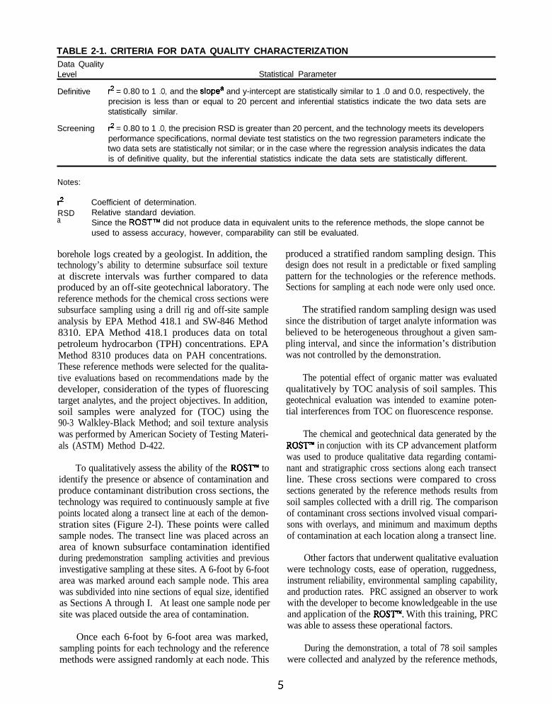
TABLE 2-1. CRITERIA FOR DATA QUALITY CHARACTERIZATIONData QualityLevel Statistical Parameter

Definitive 6 = 0.80 to 1 .O, and the slope* and y-intercept are statistically similar to 1 .0 and 0.0, respectively, theprecision is less than or equal to 20 percent and inferential statistics indicate the two data sets arestatistically similar.

Screening ? = 0.80 to 1 .O, the precision RSD is greater than 20 percent, and the technology meets its developersperformance specifications, normal deviate test statistics on the two regression parameters indicate thetwo data sets are statistically not similar; or in the case where the regression analysis indicates the datais of definitive quality, but the inferential statistics indicate the data sets are statistically different.

Notes:

? Coefficient of determination.RSD Relative standard deviation.a Since the ROSTTM did not produce data in equivalent units to the reference methods, the slope cannot be

used to assess accuracy, however, comparability can still be evaluated.

borehole logs created by a geologist. In addition, thetechnology’s ability to determine subsurface soil textureat discrete intervals was further compared to dataproduced by an off-site geotechnical laboratory. Thereference methods for the chemical cross sections weresubsurface sampling using a drill rig and off-site sampleanalysis by EPA Method 418.1 and SW-846 Method8310. EPA Method 418.1 produces data on totalpetroleum hydrocarbon (TPH) concentrations. EPAMethod 8310 produces data on PAH concentrations.These reference methods were selected for the qualita-tive evaluations based on recommendations made by thedeveloper, consideration of the types of fluorescingtarget analytes, and the project objectives. In addition,soil samples were analyzed for (TOC) using the90-3 Walkley-Black Method; and soil texture analysiswas performed by American Society of Testing Materi-als (ASTM) Method D-422.

To qualitatively assess the ability of the ROST” toidentify the presence or absence of contamination andproduce contaminant distribution cross sections, thetechnology was required to continuously sample at fivepoints located along a transect line at each of the demon-stration sites (Figure 2-l). These points were calledsample nodes. The transect line was placed across anarea of known subsurface contamination identifiedduring predemonstration sampling activities and previousinvestigative sampling at these sites. A 6-foot by 6-footarea was marked around each sample node. This areawas subdivided into nine sections of equal size, identifiedas Sections A through I. At least one sample node persite was placed outside the area of contamination.

Once each 6-foot by 6-foot area was marked,sampling points for each technology and the referencemethods were assigned randomly at each node. This

produced a stratified random sampling design. Thisdesign does not result in a predictable or fixed samplingpattern for the technologies or the reference methods.Sections for sampling at each node were only used once.

The stratified random sampling design was usedsince the distribution of target analyte information wasbelieved to be heterogeneous throughout a given sam-pling interval, and since the information’s distributionwas not controlled by the demonstration.

The potential effect of organic matter was evaluatedqualitatively by TOC analysis of soil samples. Thisgeotechnical evaluation was intended to examine poten-tial interferences from TOC on fluorescence response.

The chemical and geotechnical data generated by theROSY in conjuction with its CP advancement platformwas used to produce qualitative data regarding contami-nant and stratigraphic cross sections along each transectline. These cross sections were compared to crosssections generated by the reference methods results fromsoil samples collected with a drill rig. The comparisonof contaminant cross sections involved visual compari-sons with overlays, and minimum and maximum depthsof contamination at each location along a transect line.

Other factors that underwent qualitative evaluationwere technology costs, ease of operation, ruggedness,instrument reliability, environmental sampling capability,and production rates. PRC assigned an observer to workwith the developer to become knowledgeable in the useand application of the ROST”. With this training, PRCwas able to assess these operational factors.

During the demonstration, a total of 78 soil sampleswere collected and analyzed by the reference methods,

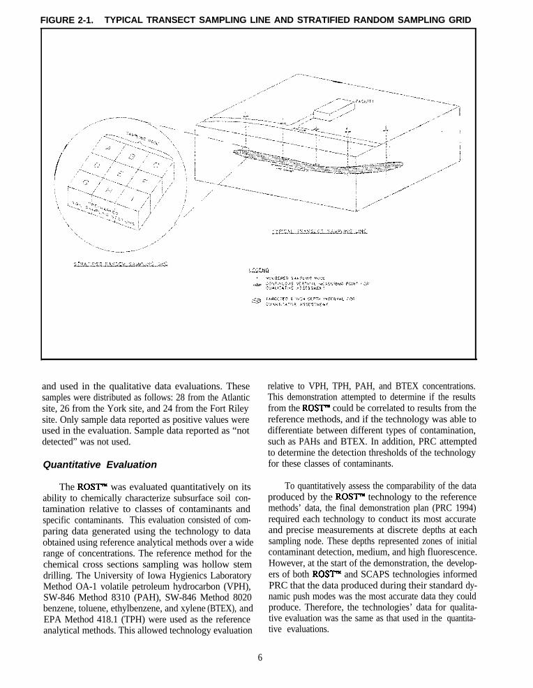
FIGURE 2-1. TYPICAL TRANSECT SAMPLING LINE AND STRATIFIED RANDOM SAMPLING GRID

and used in the qualitative data evaluations. Thesesamples were distributed as follows: 28 from the Atlanticsite, 26 from the York site, and 24 from the Fort Rileysite. Only sample data reported as positive values wereused in the evaluation. Sample data reported as “notdetected” was not used.

relative to VPH, TPH, PAH, and BTEX concentrations.This demonstration attempted to determine if the resultsfrom the ROST” could be correlated to results from thereference methods, and if the technology was able todifferentiate between different types of contamination,such as PAHs and BTEX. In addition, PRC attemptedto determine the detection thresholds of the technology

Quantitative Evaluation for these classes of contaminants.

The ROST”‘ was evaluated quantitatively on itsability to chemically characterize subsurface soil con-tamination relative to classes of contaminants andspecific contaminants. This evaluation consisted of com-paring data generated using the technology to dataobtained using reference analytical methods over a widerange of concentrations. The reference method for thechemical cross sections sampling was hollow stemdrilling. The University of Iowa Hygienics LaboratoryMethod OA-1 volatile petroleum hydrocarbon (VPH),SW-846 Method 8310 (PAH), SW-846 Method 8020benzene, toluene, ethylbenzene, and xylene (BTEX), andEPA Method 418.1 (TPH) were used as the referenceanalytical methods. This allowed technology evaluation

To quantitatively assess the comparability of the dataproduced by the ROST” technology to the referencemethods’ data, the final demonstration plan (PRC 1994)required each technology to conduct its most accurateand precise measurements at discrete depths at eachsampling node. These depths represented zones of initialcontaminant detection, medium, and high fluorescence.However, at the start of the demonstration, the develop-ers of both ROST” and SCAPS technologies informedPRC that the data produced during their standard dy-namic push modes was the most accurate data they couldproduce. Therefore, the technologies’ data for qualita-tive evaluation was the same as that used in the quantita-tive evaluations.

6

The locations for the reference method sampling forthe quantitative evaluation were selected after reviewingboth the ROST” and SCAPS data for a site. Sampleintervals that showed similar data from both technologieswere selected as reference method sampling intervals.Reference method sampling intervals represented zonesof initial contaminant detection, medium, and highfluorescence. The data produced at these intervals wasused to quantify contamination, identify contaminants,establish a technology’s precision and resolution, andestablish a technology’s contamination detection thresh-olds .

For the quantitative evaluation, data produced by theROST”’ was averaged over a 12-inch push intervalcorresponding to intervals sampled for reference methodanalysis. This data was used to determine a meanfluorescence over that interval. This data was com-pared to corresponding mean reference method concen-trations for any given interval. To create these meanreference method concentrations, PRC collected fivereplicate samples from the 12-inch intervals identified asreference method sampling intervals based on theROST” and SCAPS data. Each replicate sample wascollected from a randomly assigned section at eachsample node. The mean fluorescence for the ROST”was compared to the mean constituent concentration forthe same interval, as generated by the reference methodanalysis and the replicate sampling.

The data developed by the ROST” was compared toreference method data for the following compounds orclasses of compounds: TPH, total BTEX, VPH, totalPAH, total naphthalene (naphthalene, l-methylnaphtha-lene, and 2-methynaphthalene) and individual com-pounds (BTEX, naphthalene, I-methylnaphthalene,2-methyaphthalene, acenaphthene, fluoranthene,pyrene, benzoapyrene, and anthracene). These compari-sons were described in the August 1994 final demonstra-tion plan.

Method precision also was examined during thedemonstration. The ROST” was required to produce10 separate readings or measurements at given depthswithout moving the sensor between readings. Fromthese 10 measurements at each discrete depth, precisioncontrol limits were established. This data also allowedan examination of technology resolution and precision.

For the quantitative evaluation, a total of 103 soilsamples were collected and analyzed by the referencemethods. The distribution of these samples was asfollows: 8 replicate sampling intervals producing38 samples at the Atlantic site, 7 replicate samplingintervals producing 35 samples at the York site, and

30 samples from 6 replicate sampling intervals at theFort Riley site. Only sample data reported as positivevalues were used in the evaluation. Sample data re-ported as “not detected” was not used.

Deviations from the ApprovedDemonstration Plan

The primary deviation from the demonstration plan(PRC 1994) dealt with the statistical analysis for thequantitative evaluation.

Since the technology did not produce data directlyrepresenting the concentration of contaminants, or datain the same units as the reference method analysis, theWilcoxon Rank Sum Test could not be used, and thecomparison of the technology’s data to 99 percentconfidence intervals was not made. In addition, theeffect of soil moisture was not examined due to the factthat the bulk of the contaminated zones at each site wereat or near saturation. Finally, the demonstration planidentified a hydraulic probe sampler as the referencemethod for collecting the soil samples used in thequantitative evaluations. However, due to sample matrixaffects (running sands), the hydraulic probe samplescould not meet the soil sampling objectives regardingsample volume. The inability of this method to producefull sample recovery was caused by the saturated finesands encountered at many of the target sampling depths.To allow for adequate sample volume, PRC changed thereference method for this soil sampling to hollow stemaugering and split spoon sampling.

Site Descriptions

The demonstration took place at three sites withinEPA Region 7. The three sites are the(1) Atlantic-Poplar Street Former Manufactured GasPlant (FMGP) site (Atlantic site), (2) York FMGP site(York site), and (3) the Fort Riley Building 1245 site(Fort Riley site). Brief summaries for each site aregiven below. Complete details are located in the August1994 final demonstration plan.

The Atlantic site is located in Atlantic, Iowa. Thesite is surrounded by gas stations, grain elevators, a seedsupply company, and a railroad right-of-way. Allstructures associated with the FMGP have been demol-ished. A gas station now operates on the location of theFMGP.

The Atlantic Coal Gas Company operated theFMGP from 1905 to 1925. During that time, an un-known quantity of coal tar was disposed of on site. In

7

addition to the coal tar waste, more recent releases ofpetroleum from two nearby gas stations also haveoccurred. An investigation conducted at the site from1990 to 1992 identified the following primary contami-nants: BTEX and PAHs. The local groundwater con-tains free petroleum product and pure coal tar.

The York site is located in York, Nebraska. Thesite encompasses nearly a half acre in an industrialsection of the city. The site is bordered by a formerrailroad right-of-way, a concrete company, a seedcompany, and a farm supply store. The site is nearlylevel, and one building occupied by the FMGP is stillpresent. The York Gas and Electric company operated

the FMGP from 1899 to 1930. Coal tar waste wasdisposed of at the site. Current information on the sitesuggests that coal tar waste and its constituents should bethe only waste encountered.

The Fort Riley site is located at Building 1245 onthe east side of the Camp Funston area at Fort Riley,Kansas. Between 1942 and 1990, five 12,000-gallonsteel underground storage tanks were located at this site.The tanks were used to store leaded and unleadedgasoline, diesel fuel, and military operations‘gasoline.Soil at the site is contaminated with gasoline and dieselbelieved to be the result of past petroleum fuel releasesfrom the underground storage tanks.

Section 3Reference Method Results

All soil samples collected during this demonstrationwere submitted to PACE, Inc. (PACE), for chemicaland geotechnical analysis. The PACE laboratory inLenexa, Kansas, performed the methods 418.1, 8020,and OA-1 analyses, while the PACE laboratory in St.Paul, Minnesota, performed the Method 8310 analyses.PACE subsequently subcontracted the geotechnicalanalyses to Environmental Technical Services (ETS),Petaluma, California. The chemical data supplied by thereference laboratory, the geotechnical data supplied bythe geotechnical laboratory, and the data produced by theon-site professional geologist are discussed in thissection.

Reference Laboratory Procedures

Samples collected during this demonstration werehomogenized and split for the following analyses:

* TPH by EPA Method 418.1 (EPA 1986)

* PAH by EPA SW-846 Method 8310 (EPA1986)

* BTEX by EPA SW-846 Method 8020 (EPA1986)

* Total VPH as gasoline by University of IowaHygienic Laboratory Method OA-1 (UniversityHygienic Laboratory 1991)

* Soil texture and TOC by the 90-3 Walk-1ey-Black Method (Page 1982)

The results of these analyses are summarized inAppendix A, Tables A-l and A-9. The results arereported as wet-weight values as required in thedemonstration plan (PRC 1994). The data is grouped byanalytical method, site, and whether the data is intendedfor qualitative or quantitative data evaluation. Thechemical cross sections produced by the qualitative dataare presented and discussed later in this section.

The data from the PACE laboratory was internallyreviewed by PACE personnel before the data wasdelivered to PRC. PRC personnel conducted a datareview on the results provided by PACE following EPAguidelines (1991). PRC reviewed the raw data andchecked the calculated sample values.

The following sections discuss specific proceduresused to identify and quantitate TPHs, VPHs, PAHs,BTEX, and TOC. Most of these procedures involvedrequirements that were mandatory to guarantee thequality of the data generated.

In addition to being generally discussed in thissection, all of the reference method results used to assessthe ROSY are presented in Appendix A, TablesA-l through A-9.

Sample Holding Times

The required holding times from the date of samplereceipt for each analytical method used to analyze thesoil samples were as follows: University of IowaHygienics Laboratory Method OA-1 (MethodOA-1), 14 days for extraction and analysis; EPASW-846 Method 8020 (BTEX), 14 days for extractionand analysis; EPA Method 418.1 (TPH), 14 days forextraction and 40 days for analysis; EPASW-846 Method 8310 (PAH), 14 days for extraction and40 days for analysis; and 90-3 Walkley-Black Method(TOC), 28 days for extraction and analysis.

All holding times for the samples were met duringthis demonstration.

Sample Preparation

Preparation of soils for TPH analysis was performedfollowing EPA Method 418.1. This method uses aSoxhlet extraction as stated in SW-846 Method9071. The soil sample extracts were analyzed for TPHusing SW-846 Method 418.1.

9

Extracts for VPH analysis were prepared followingMethod OA-1. The BTEX sample preparation require-ments were carried out as specified in that method.

The preparation of soil samples for TOC analysiswere carried out as specified in the 90-3 Walkley-BlackMethod.

Sonication extraction, Method SW-846 3550, wasused for the preparation of soil samples forSW-846 Method 8310 analysis. The preparation ofsamples for PAH analysis by SW-846 Method 8310 werecarried out according to the method requirements.

Initial and Continuing Calibrations

Initial calibrations (ICAL) were performed beforesample analysis began. ICALs for SW-846 Methods8020, 8310, and 418.1 consisted of the analysis of fiveconcentrations of standards. Method OA-1 required theanalysis of three concentrations of standards for theICAL. Linearity for these ICALs was evaluated bycalculating the percent relative standard deviation(%RSD) of the calibration factors. The %RSD QC limitfor SW-846 Methods 8020 and 8310 and MethodOA-1 was 20 percent. The calibration factors werecalculated by dividing the response (measured as the areaunder the peak or peak height) by the amount ofcompound injected on the gas chromatograph (CC)column. The 90-3 Walkley-Black Method for TOCrequired a daily calibration to a reference sulfatesolution. This ICAL was performed in duplicate. Allinitial calibrations met the respective methodrequirements.

Continuing calibrations (CCAL) were performed ona daily basis to check the response of the detector byanalyzing a mid-concentration standard and comparingthe calibration factor to that of the mean calibrationfactor from the ICAL.

Calibration factors were monitored in accordancewith the SW-846 and OA-1 Methods. No CCAL wasperformed for the 90-3 Walkley-Black Method. SixCCALs exceeded the 15 percent difference (%D) criteriafor various BTEX compounds. This resulted in sampleresults being qualified as estimated (J) and usable forlimited purposes. Various PAH compounds in sixSW-846 Method 8310 CCALs exceeded 15 %D for oneof the two detectors. Sample results for the compoundsexceeding 15 %D were qualified as estimated (J) andusable for limited purposes. SW-846 Method 8310 usestwo detectors, an ultraviolet detector and a fluorescencedetector. Since one detector’s CCAL response waswithin QC guidelines, this data is considered useable.

Retention times of the single analytes weremonitored through the amount of retention time shiftfrom the CCAL standard as compared to the ICALstandard. The retention time windows for SW-846Method 8310 were set by taking three times the standarddeviation of the retention times that were calculated fromthe ICAL and CCAL standards. The retention timewindows for SW-846 Method 8020 were set by PACE atplus or minus 0.07 minutes for benzene, ethylbenzene,m-xylene, and plus or minus 0.10 minutes for toluene.No CCAL retention times for the individual PAHanalytes were outside the retention time windows.CCAL retention times for the individual BTEX analyteswere observed outside the retention time windows as setby the ICAL. No samples were qualified based on thisQC criteria because the retention time shifts wereadjusted appropriately by PACE for sample identificationand quantitation.

Following the ICAL, a method blank was analyzedto verify that the instrument met the methodrequirements. Following this, sample analysis maycontinue for 24 hours. As stated in SW-846 Method8000, a CCAL must be analyzed and the calibrationfactor verified on each working day. Sample analysismay continue as long as CCAL standards meet themethod requirements.

Sample Analysis

Specific PAH and BTEX compounds were identifiedin a sample by matching retention times of peaks foundafter analyzing the sample with those compounds foundin PAH and BTEX standards. VPH was identified in asample by matching peak patterns found after analyzingthe sample with those compounds found in VPHstandards. Peak patterns may not always match exactlybecause of the way the VPHs were manufactured orbecause of the effects of weathering. When peakpatterns do not match, the analyst must decide thevalidity of the identification of VPHs. For this reason,peak pattern identification is highly dependent on theexperience and interpretation of the analyst.

Quantitation of PAHs, BTEX compounds, TPHs,and VPHs was performed by measuring the response ofthe peaks in the sample to those same peaks identified inthe ICAL standard. The reported results of thiscalculation were based on wet weights (except forPAHs), as required by PRC. PAH data was reported ona dry-weight basis. PRC converted this data towet-weight based results dividing the dry-weight resultby the percent moisture of the original wet sample.Quantitation of TOC was performed by measuring thevolume of potassium dichloride (K&07) titrated andcalculating the milliequivalents of K2Cr20, titrated.

10

This value was then multiplied by conversion factorsdefined in the method and subsequently divided by thegrams of sample. TOC results were reported on awet-weight basis.

Sample extracts can frequently exceed thecalibration range determined during the ICAL. Whenthis occurred, the extracts were diluted to obtain peaksthat fall within the linear range of the detector. ForBTEX compounds and VPHs, this linear range wasdefined as the highest standard concentration response ofthe analytes of interest analyzed during the ICAL. Thelinear range for TPHs was defined as an absorbancemaximum of 0.8. For PAHs, as defined in SW-846Method 8310, the linear range was from 8 times themethod detection limit (MDL) to 800 times the MDLwith the following exception: benzo(ghi)perylenerecovery at 80 times and 800 times the MDL are low.Once a sample was diluted to within the linear range, itwas analyzed again. Dilutions were performed whenappropriate on the samples for this demonstration.

Detection Limits

The PACE reporting limit (PRL) for PAHs wascalculated by multiplying the calibration correctionfactor based on dry weight, times the MDL for eachspecific PAH. PRLs for BTEX compounds weredetermined by the lowest concentration standard of theICAL. The BTEX ICAL concentration range was from10 micrograms per liter (ug/L) to 100 pg/L. The PBLfor benzene, toluene, and ethyl benzene was 50micrograms per kilogram bg/kg) and 100 pg/kg fortotal xylene. The three levels of standard concentrationsfor the VPH ICAL ranged from 2 milligrams permilliliter (mg/mL) to 8 mg/mL. The PRL for VPH was5 milligrams per kilograms (mg/kg). For TPH, thecalibration range was calculated by calibrating theinfrared detector using a series of working standards. Aplot was then prepared of absorbance versus milligrampetroleum hydrocarbons per 100 milliliter (mL) solution.The PRL for TPH was 10 mg/kg. The MDL for TOCanalysis was 10 mg/kg wet weight.

Quality Control Procedures

A number of QC measures were used by PACE asrequired by SW-846 Methods 8310 and 8020, EPAMethod 418.1, Method OA-1, and the90-3 Walkley-Black Method. These QC measuresincluded the analyses of method blanks, instrumentblanks, laboratory control samples (LCS), matrix spike(MS) and matrix spike duplicates (MSD), and the use ofsample surrogate recoveries.

All method and instrument blanks met theappropriate QC criteria, except for two method blanksanalyzed by Method 418.1. TPH was reported asslightly above the PRL of 10 mg/kg in two methodblanks. Due to the low values reported in the twomethod blanks, the sample results were not qualified.

Surrogate standards were added to all samples,method blanks, MSs, and LCSs for the SW-846 Methods8310 and 8020, and Method OA-1. All surrogaterecoveries for SW-846 Method 8020 were within the QCacceptance criteria of 42 to 140 percent for soil. Sevensamples were qualified as estimated (J) and usable forlimited purposes based on surrogate recoveries for theMethod OA-1. The QC acceptance criteria for surrogaterecovery for Method OA-1 was 67 to 127 percent.Thirty soil samples for SW-846 Method 8310 analysiswere qualified as estimated (J) and usable for limitedpurposes based on surrogate recoveries observed outsidethe QC limits of 58 to 140 percent. Two surrogateswere used for Method 8310. Samples were qualifiedonly when both surrogates were outside the QC limitsand no dilution analysis was performed. Numerous soilsamples required dilution for the Method 8310 analysisbecause of petroleum interference. Dilution of thesesamples resulted in corresponding reductions insurrogate concentrations. When this occurred, theresultant concentration of surrogate was below its MDL.In cases where dilution resulted in failure to detect thesurrogate, no coding of the data was implemented.

MS samples are samples to which a known amountof the target analytes are added. There were 10 MSsperformed during the analysis by Method 418.1. Eightof the MS samples were affected by high concentrationsof target analytes in the spiked samples. No sampleswere qualified. Eleven MSs were performed during theanalysis of samples by Method 8310. All but three MSsand MSDs were outside the QC limits for percent recov-ery and relative percent difference (RPD). These QCexceedences were due to petroleum matrix interference.The data associated with the QC samples was not qual-ified because EPA guidelines state that samples cannotbe qualified based on MS and MSD results alone(1991). There were seven MS and MSD samplesanalyzed by Method 8020 and five by MethodOA-1. The MSs and MSDs analyzed by Method8020 did not meet QC acceptance criteria for percentrecoveries or RPDs. No samples were qualified basedon these MS and MSD results due to the reasons statedabove. All MS and MSDs analyzed by MethodOA-1 and 90-3 Walkley-Black Method met all QCacceptance criteria and were considered acceptable.

11

All LCSs met QC acceptance criteria and were con-sidered acceptable for all soil samples analyzed bySW-846 Method 8310, Method OA-1,90-3 Walkley-Black Method, and Method 418.1. Onesoil LCS analyzed by Method 8020 was outside the QCcontrol limits. The soil LCS percent recovery fortoluene was below the QC limit. Twenty soil sampleswere qualified as estimated (J) and usable for limitedpurposes.

Also, three equipment rinsate blanks and one tripblank were analyzed to assess the efficiency of fielddecontamination and shipping methods, respectively.There was no contamination found above PRLs in any ofthese blanks, indicating decontamination procedureswere adequate.

Confirmation of Analytical Results

Confiiation of positive results was not required byany of the analytical methods performed exceptSW-846 Method 8310. Confirmation of positive PAHresults by Method 8310 was performed by the use of twotypes of detectors. Both an ultraviolet detector and afluorescence detector were used in the analysis of PAHs.The only requirement for using either detector for quan-titation was that they meet the QC criteria for linearity(ICAL) and %D (CCAL). If either detector failed eitherof these criteria, it could not be used for quantitation,but it could be used for confirmation of positive results.

Data Reporting

The results reported and qualified by the referencemethod contained two types of qualifier codes. Somedata was coded with a “J,” which is defined by PACE asdetected but below the PRL; therefore, the result is anestimated concentration. The second code, “MI,” wasdefined as matrix interference. Generally, the effect ofa matrix interference is to reduce or enhance sampleextraction efficiency.

Quality Assessment of ReferenceLaboratory Data

This section discusses the accuracy, precision, andcompleteness of the reference method data.

Accuracy

Accuracy of the reference methods wereindependently assessed through the use of performanceevaluation (PE) samples purchased from EnvironmentalResource Associates (ERA) located in Arvada,Colorado, containing a known quantity of TPH. Inaddition, LCSs and past PE audits of the reference

laboratory were used to verify analytical accuracy.Based on a review of this data, the accuracy of thereference methods were considered acceptable.

Precision

Precision for the reference method results wasdetermined by evaluating field duplicates, laboratoryduplicate, and MS and MSD sample results. Precisionwas evaluated by determining the RPDs for sampleresults and their respective duplicate sample results.

The MS and MSD RPD results for the PAHcompounds averaged 25 percent for all of the 11 MS andMSD sample pairs. However, there was one MS andMSD sample pair that had a RPD of 99.9 for1-methyl-naphthalene. If this point was removed, theoverall average would decrease to 20 percent. Theaverage RPD for the seven BTEX MS and MSD samplepairs was less than 25 percent. Only four BTEX RPDswere outside advisory QC guidelines defined by thereference laboratory’s control charts. All five VPH MSand MSD sample RPDs met advisory QC guidelines setby the reference laboratory’s control charts. The10 TPH MS and MSD sample pairs were consideredacceptable.

Laboratory duplicate samples are two separateanalyses performed on the sample. During the analysisof demonstration samples, 10 TPH laboratory duplicatesamples were prepared and analyzed. All TPHlaboratory duplicate RPD result values were less than25 percent. This was considered to be acceptable.

Completeness

Results were obtained for all of the soil samples.PACE J-coded values that were detected below the PRL,but above the MDL. As previously discussed, sampleswere J-coded based on one or more of the advisory QCguidelines not being met (i.e., surrogate and spikerecoveries). Also, some samples were J-coded based onBTEX CCALs not meeting QC guidelines. PRC did notconsider this serious enough to preclude the use of thisdata because the %Ds for the CCALS did not exceed theQC guidelines by more than 10 percent. The analyteswith %Ds outside the QC guidelines were not detectedin most of the samples associated with the CCALs. TheJ-coded data is valid and usable for statistical analysisbecause the QC guidelines were based on advisorycontrol limits set by either the reference analyticalmethods or by PACE. This data set should beconsidered representative of data produced byconventional technologies. For this reason, the actualcompleteness of data used was 100 percent.

12

Use of Qualified Data for Statistical Analysis

One hundred percent of the reference laboratoryresults were reported and validated by approved QCprocedures. The data review indicated that J-coded datawas acceptable for meeting the demonstration objectiveof providing baseline data to compare against thedemonstrated technologies.

None of the QA/QC problems was consideredserious enough to preclude the use of J-coded data forthis demonstration. The surrogate and spike recoverycontrol limits were for advisory purposes only, and nocorrective action was required for the surrogaterecoveries that were outside of this range. RPD resultsfor MSs and MSDs that did not meet advisory QCcontrol limits were common when the matrix containeda high concentration of petroleum. Again, these wereadvisory limits and no corrective action was required.These same general results would be seen by anylaboratory using the reference analytical methods onsuch highly contaminated samples.

Also, rejection of a large percentage of data wouldincrease the apparent variation between the referencelaboratory data and the data from the technology. Thisapparent variation would probably be of similarmagnitude to that introduced by using the data. Forthese reasons, the J-coded data was used.

Chemical Cross Sections

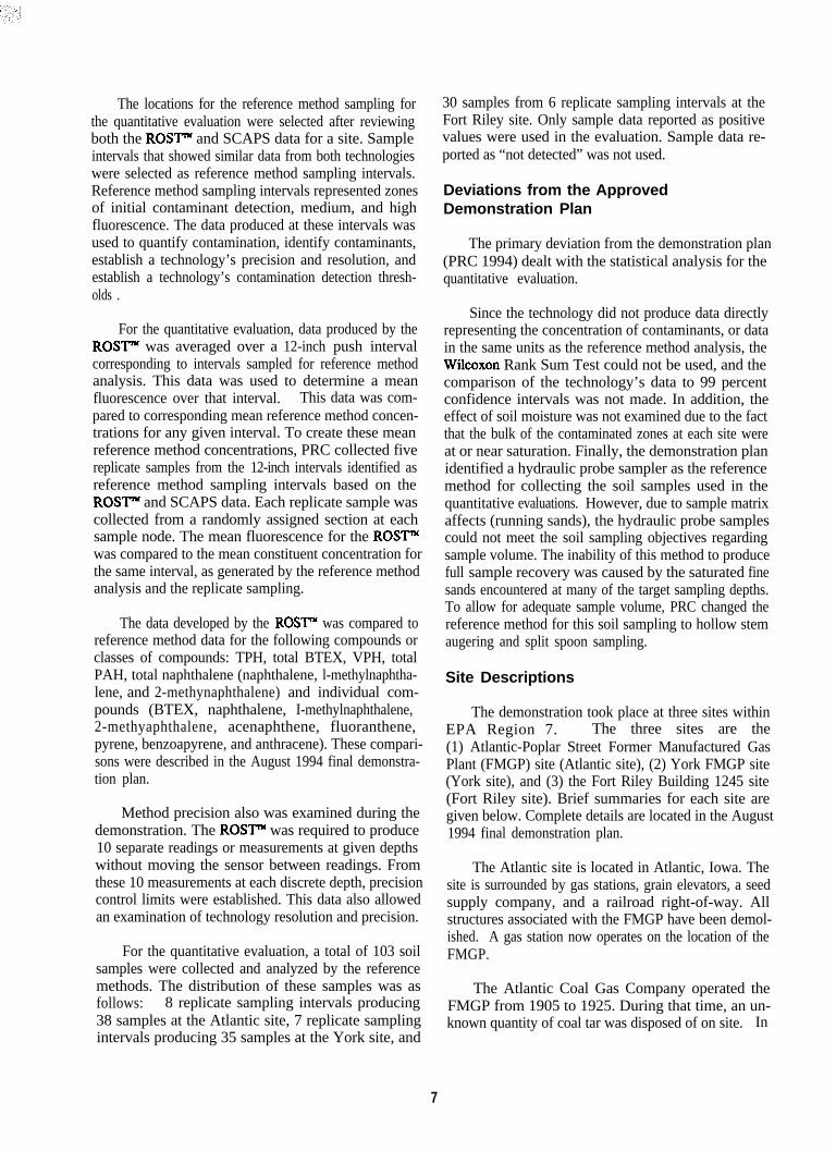
Chemical cross sections were created from thereference analytical data produced for the qualitativedata evaluation (see Appendix A, Tables A-l through A-6). These samples were collected by a professionalgeologist on site during the logging of boreholes. Thecross sections were hand contoured. The contourintervals were selected to best represent a conventionalapproach to the delineation of subsurface contamination.The cross sections are presented on Figures 3-l to3-6. A written interpretation of these cross sections ispresented below.

Atlantic Site

The five sampling nodes formed a northwest tosoutheast trending transect across the site (Figure3-l). Node 1 on the far northwestern edge of the crosssection represented an area that was not impacted by thecontamination from the Atlantic site. Just southeast ofthis location at Node 2, two distinct layers ofcomamination were identified. The upper zone extendedfrom approximately 1 foot to 5 feet below groundsurface (bgs). This zone was characterized by TPHcontamination ranging from 100 to 10,000 parts per

million ppm). The lower zone of contaminationextended from approximately 22 feet to 28 feet bgs. TheTPH concentrations in this zone ranged from 100 togreater than 10,000 ppm. These two zones expandedand blended together as Node 3 was approached.Around Nodes 3 and 4, the thickness of the TPH plumeremained fairly constant, extending from approximately1 foot to 31 feet bgs. The central portion of this zoneexhibited TPH contamination greater than 1,000 ppm.The remainder of this zone exhibited TPH contaminationin the range of 100 to 1,000 ppm. As the farsoutheastern edge of the transect was approached atNode 5, the highest concentrations in the center of theplume pinched out, leaving a contamination zone thatextended from just below the ground surface toapproximately 27 feet bgs. This zone exhibitedcontamination in the range of 100 to 1,000 ppm.

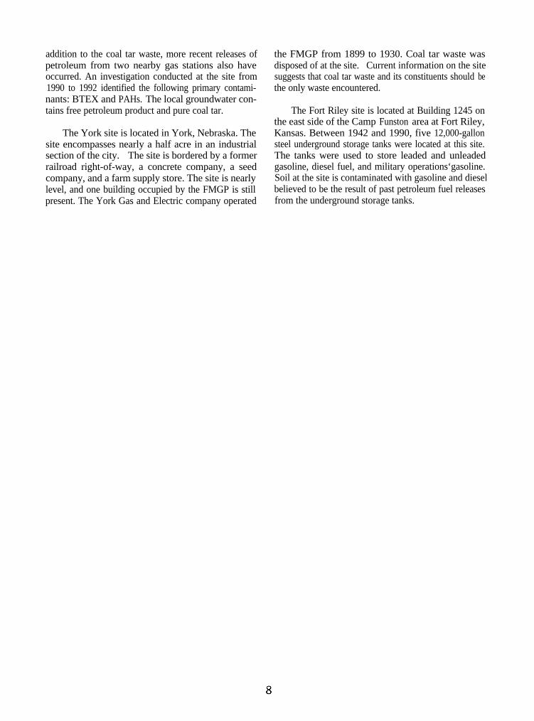
The total PAH cross section along this same transectexhibited a slightly different distribution (Figure3-2). As with the TPH cross section, the total PAHcross section began at Node 1 in the area exhibiting nosigns of contamination. At Node 2, again two zones ofcontamination were detected. The upper zone extendedfrom the ground surface to approximately 7 feet bgs.This zone deepened toward the east. The concentrationsof total PAHs in this zone ranged from 10 to greaterthan 100 ppm. The lower zone extended fromapproximately 14 to 30 feet bgs. The concentrations oftotal PAHs in this zone ranged from 10 to greater than100 ppm. Concentrations greater than 100 ppm were notexhibited at this depth in the nodes occurring furthereast. The distribution of the 10 to 100 ppm dippedbelow the ground surface at progressive depths farthereast of Node 2. At Node 5, this upper zone began atapproximately 7 feet bgs. This zone also reached itsmaximum depth around Nodes 3 and 4, approximately30 feet bgs. Around Nodes 3 and 4 were two lenses oftotal PAH contamination in excess of 100 ppm. Thelargest of these zones appeared to be thickest aroundNode 3, extending from approximately 7 to 16 feet bgs.This zone thinned to the east and pinched out betweenNodes 4 and 5. A smaller lens of greater than 100 ppmtotal PAH contamination was exhibited at Node 4. Thiszone extended between 7 to 9 feet bgs. This zone wasnot detected in Nodes 3 or 5.

York Site

The five sampling nodes formed a north to southtrending transect. The TPH and total PAH distributionsappeared to be similar, except at Node 5, at the Yorksite (Figures 3-3 and 34). At Node 5, the TPHcontamination was more extensive, extending from 1 to25 feet bgs. At this same locations, the PAHcontamination extended from 13 to 2 1 feet bgs.

13

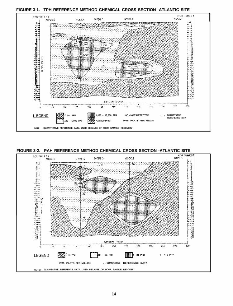
FIGURE 3-1. TPH REFERENCE METHOD CHEMICAL CROSS SECTION -ATLANTIC SITE

1

I EGEND < loo PPM 1,000 - 10,000 PPM NO - NOT DETECTED . - OUANTITATIVEREFERENCE DATA

100 - 1,000 PPM >10,000 PPM PPM - PARTS PER MILLION

NOTE: QUANTITATIVE REFERENCE DATA USED BECAUSE OF POOR SAMPLE RECOVERY

FIGURE 3-2. PAH REFERENCE METHOD CHEMICAL CROSS SECTION -ATLANTIC SITE

LEGEND < 10 PPM pzJ10 - loo PPM > loo PPU T - < 1 PPY

PPM - PARTS PER MILLION . - OUANITATIVE REFERENCE DATA

NOTE: QUANITATIVE REFERENCE DATA USED BECAUSE OF POOR SAMPLE RECOVERY

14

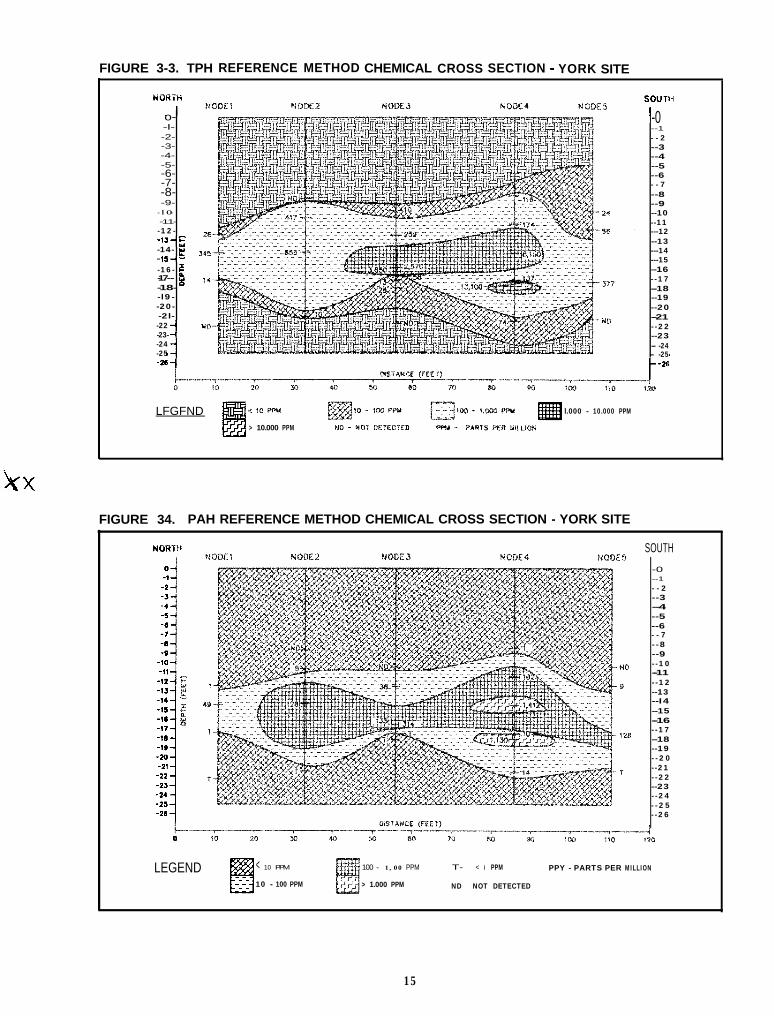
FIGURE 3-3. TPH REFERENCE METHOD CHEMICAL CROSS SECTION YORK SITE

o--l--2--3--4--5--6--7--8--9--lO--11-

-12--1,-E-14- e-15-w-16- E-17- --18- x-l9--20--2l--22-23-d-24-25 11

i-0--1

- - 2--3--4--5--6- - 7--8--9--10--11---12--13---14---15--16--17--18--19--20--21--22--23- -24- -25

LFGFND l.000 - 10.000 PPM

> 10.000 PPM

FIGURE 34. PAH REFERENCE METHOD CHEMICAL CROSS SECTION - YORK SITE

SOUTH

-0--1

- - 2--3--4--5--6- - 7- -8--9--10--11--12--13--I4--15--16--17--18--19- - 2 0--21- -22--23--24- - 2 5- -26

LEGEND < 10 PPM 100 - 1,00 PPM T- < I PPM PPY - PARTS PER MILLION

10 - 100 PPM > 1.000 PPM ND - NOT DETECTED

15

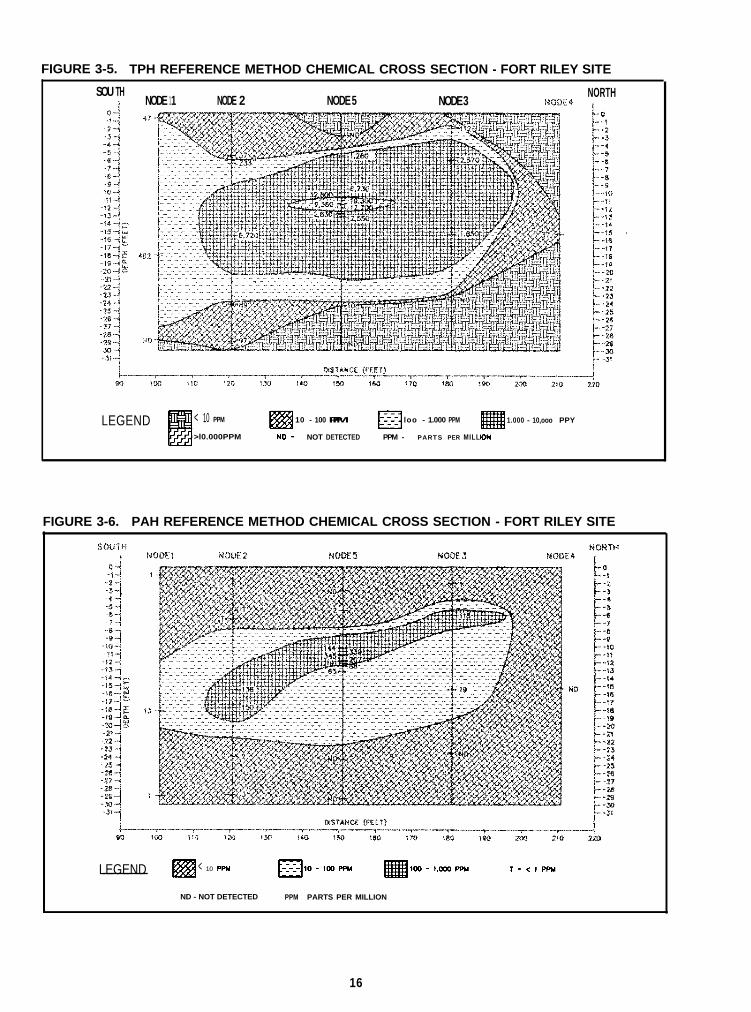
FIGURE 3-5. TPH REFERENCE METHOD CHEMICAL CROSS SECTION - FORT RILEY SITE

SOU TH NORTHNODE 11 NODE 2 NODE 5 NODE 3

LEGEND < 10 PPM 10 - 100 PPM loo - 1.000 PPM 1.000 - 10,ooo PPY

>l0.000PPM NOT DETECTED PPM - PARTS PER MILL

FIGURE 3-6. PAH REFERENCE METHOD CHEMICAL CROSS SECTION - FORT RILEY SITE

LEGEND < 10 PPPPU

ND - NOT DETECTED PPM - PARTS PER MILLION

16

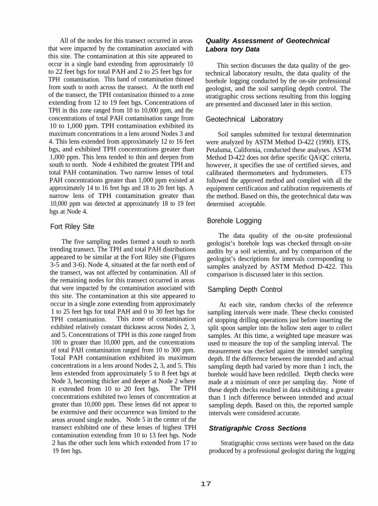
All of the nodes for this transect occurred in areasthat were impacted by the contamination associated withthis site. The contamination at this site appeared tooccur in a single band extending from approximately 10to 22 feet bgs for total PAH and 2 to 25 feet bgs forTPH contamination. This band of contamination thinnedfrom south to north across the transect. At the north endof the transect, the TPH contamination thinned to a zoneextending from 12 to 19 feet bgs. Concentrations ofTPH in this zone ranged from 10 to 10,000 ppm, and theconcentrations of total PAH contamination range from10 to 1,000 ppm. TPH contamination exhibited itsmaximum concentrations in a lens around Nodes 3 and4. This lens extended from approximately 12 to 16 feetbgs, and exhibited TPH concentrations greater than1,000 ppm. This lens tended to thin and deepen fromsouth to north. Node 4 exhibited the greatest TPH andtotal PAH contamination. Two narrow lenses of totalPAH concentrations greater than 1,000 ppm existed atapproximately 14 to 16 feet bgs and 18 to 20 feet bgs. Anarrow lens of TPH contamination greater than10,000 ppm was detected at approximately 18 to 19 feetbgs at Node 4.

Fort Riley Site

The five sampling nodes formed a south to northtrending transect. The TPH and total PAH distributionsappeared to be similar at the Fort Riley site (Figures3-5 and 3-6). Node 4, situated at the far north end ofthe transect, was not affected by contamination. All ofthe remaining nodes for this transect occurred in areasthat were impacted by the contamination associated withthis site. The contamination at this site appeared tooccur in a single zone extending from approximately1 to 25 feet bgs for total PAH and 0 to 30 feet bgs forTPH contamination. This zone of contaminationexhibited relatively constant thickness across Nodes 2, 3,and 5. Concentrations of TPH in this zone ranged from100 to greater than 10,000 ppm, and the concentrationsof total PAH contamination ranged from 10 to 300 ppm.Total PAH contamination exhibited its maximumconcentrations in a lens around Nodes 2, 3, and 5. Thislens extended from approximately 5 to 8 feet bgs atNode 3, becoming thicker and deeper at Node 2 whereit extended from 10 to 20 feet bgs. The TPHconcentrations exhibited two lenses of concentration atgreater than 10,000 ppm. These lenses did not appear tobe extensive and their occurrence was limited to theareas around single nodes. Node 5 in the center of thetransect exhibited one of these lenses of highest TPHcontamination extending from 10 to 13 feet bgs. Node2 has the other such lens which extended from 17 to19 feet bgs.

Quality Assessment of GeotechnicalLabora tory Data

This section discusses the data quality of the geo-technical laboratory results, the data quality of theborehole logging conducted by the on-site professionalgeologist, and the soil sampling depth control. Thestratigraphic cross sections resulting from this loggingare presented and discussed later in this section.

Geotechnical Laboratory

Soil samples submitted for textural determinationwere analyzed by ASTM Method D-422 (1990). ETS,Petaluma, California, conducted these analyses. ASTMMethod D-422 does not define specific QA\QC criteria,however, it specifies the use of certified sieves, andcalibrated thermometers and hydrometers. ETSfollowed the approved method and complied with all theequipment certification and calibration requirements ofthe method. Based on this, the geotechnical data wasdetermined acceptable.

Borehole Logging

The data quality of the on-site professionalgeologist’s borehole logs was checked through on-siteaudits by a soil scientist, and by comparison of thegeologist’s descriptions for intervals corresponding tosamples analyzed by ASTM Method D-422. Thiscomparison is discussed later in this section.

Sampling Depth Control

At each site, random checks of the referencesampling intervals were made. These checks consistedof stopping drilling operations just before inserting thesplit spoon sampler into the hollow stem auger to collectsamples. At this time, a weighted tape measure wasused to measure the top of the sampling interval. Themeasurement was checked against the intended samplingdepth. If the difference between the intended and actualsampling depth had varied by more than 1 inch, theborehole would have been redrilled. Depth checks weremade at a minimum of once per sampling day. None ofthese depth checks resulted in data exhibiting a greaterthan 1 inch difference between intended and actualsampling depth. Based on this, the reported sampleintervals were considered accurate.

Stratigraphic Cross Sections

Stratigraphic cross sections were based on the dataproduced by a professional geologist during the logging

17

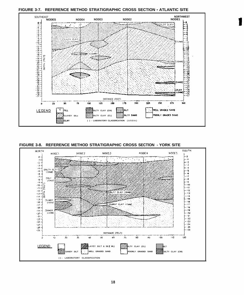
FIGURE 3-7. REFERENCE METHOD STRATIGRAPHIC CROSS SECTION - ATLANTIC SITE

SOUTHEAST NORTHWESTa NODES NODE4 NODE3 NODE2 NODE1 ,

DISTANCE (FEET)““__“_“__;. ~~_ .__~~_ ~.~.““_‘_“.“_~~.“~~~_~~“~~““,~~~~,_~

0 100

SILTY CLAY (CH)

CLAYEY SILc SILTY CLAY (CL)

( ) - LABORATORY CLASSlflCATlON ( U S D A )

FIGURE 3-8. REFERENCE METHOD STRATIGRAPHIC CROSS SECTlON - YORK SITE

LEGEND CLAYEY SILT & SILT ML)( SILTY CLAY (CL) SILT

SANDY SILT WELL GRADED SAND POORLY GRADED SAND SILTY CLAY (CM)

( ) - LABORATORY CLASSIFICATION (USDA)

18

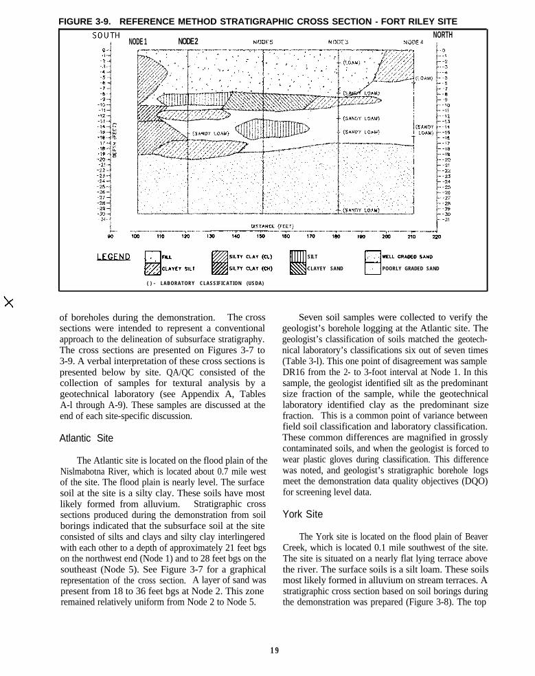
FIGURE 3-9. REFERENCE METHOD STRATIGRAPHIC CROSS SECTION - FORT RILEY SITENORTH

NODE 1 NODE 2

SILT

CLAYEY SAND POORLY GRADED SAND

( ) - LABORATORY CLASSIFICATION (USDA)

of boreholes during the demonstration. The crosssections were intended to represent a conventionalapproach to the delineation of subsurface stratigraphy.The cross sections are presented on Figures 3-7 to3-9. A verbal interpretation of these cross sections ispresented below by site. QA/QC consisted of thecollection of samples for textural analysis by ageotechnical laboratory (see Appendix A, TablesA-l through A-9). These samples are discussed at theend of each site-specific discussion.

Atlantic Site

The Atlantic site is located on the flood plain of theNislmabotna River, which is located about 0.7 mile westof the site. The flood plain is nearly level. The surfacesoil at the site is a silty clay. These soils have mostlikely formed from alluvium. Stratigraphic crosssections produced during the demonstration from soilborings indicated that the subsurface soil at the siteconsisted of silts and clays and silty clay interlingeredwith each other to a depth of approximately 21 feet bgson the northwest end (Node 1) and to 28 feet bgs on thesoutheast (Node 5). See Figure 3-7 for a graphicalrepresentation of the cross section. A layer of sand waspresent from 18 to 36 feet bgs at Node 2. This zoneremained relatively uniform from Node 2 to Node 5.

Seven soil samples were collected to verify thegeologist’s borehole logging at the Atlantic site. Thegeologist’s classification of soils matched the geotech-nical laboratory’s classifications six out of seven times(Table 3-l). This one point of disagreement was sampleDR16 from the 2- to 3-foot interval at Node 1. In thissample, the geologist identified silt as the predominantsize fraction of the sample, while the geotechnicallaboratory identified clay as the predominant sizefraction. This is a common point of variance betweenfield soil classification and laboratory classification.These common differences are magnified in grosslycontaminated soils, and when the geologist is forced towear plastic gloves during classification. This differencewas noted, and geologist’s stratigraphic borehole logsmeet the demonstration data quality objectives (DQO)for screening level data.

York Site

The York site is located on the flood plain of BeaverCreek, which is located 0.1 mile southwest of the site.The site is situated on a nearly flat lying terrace abovethe river. The surface soils is a silt loam. These soilsmost likely formed in alluvium on stream terraces. Astratigraphic cross section based on soil borings duringthe demonstration was prepared (Figure 3-8). The top

19

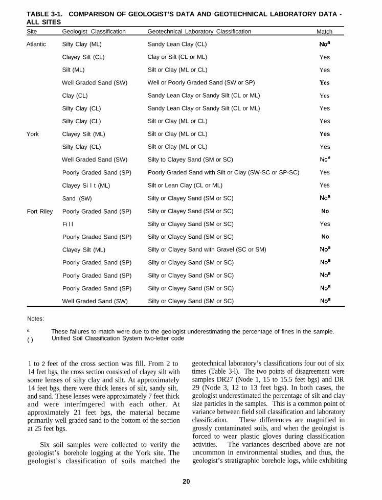
TABLE 3-1. COMPARISON OF GEOLOGIST’S DATA AND GEOTECHNICAL LABORATORY DATA -ALL SITESSite Geologist Classification Geotechnical Laboratory Classification Match

Atlantic Silty Clay (ML)

Clayey Silt (CL)

Silt (ML)

Well Graded Sand (SW)

Clay (CL)

Silty Clay (CL)

Silty Clay (CL)

York Clayey Silt (ML)

Silty Clay (CL)

Well Graded Sand (SW)

Poorly Graded Sand (SP)

Clayey Si l t (ML)

Sand (SW)

Fort Riley Poorly Graded Sand (SP)

Fi l l

Poorly Graded Sand (SP)

Clayey Silt (ML)

Poorly Graded Sand (SP)

Poorly Graded Sand (SP)

Poorly Graded Sand (SP)

Well Graded Sand (SW)

Sandy Lean Clay (CL)

Clay or Silt (CL or ML)

Silt or Clay (ML or CL)

Well or Poorly Graded Sand (SW or SP)

Sandy Lean Clay or Sandy Silt (CL or ML)

Sandy Lean Clay or Sandy Silt (CL or ML)

Silt or Clay (ML or CL)

Silt or Clay (ML or CL)

Silt or Clay (ML or CL)

Silty to Clayey Sand (SM or SC)

Poorly Graded Sand with Silt or Clay (SW-SC or SP-SC)

Silt or Lean Clay (CL or ML)

Silty or Clayey Sand (SM or SC)

Silty or Clayey Sand (SM or SC)

Silty or Clayey Sand (SM or SC)

Silty or Clayey Sand (SM or SC)

Silty or Clayey Sand with Gravel (SC or SM)

Silty or Clayey Sand (SM or SC)

Silty or Clayey Sand (SM or SC)

Silty or Clayey Sand (SM or SC)

Silty or Clayey Sand (SM or SC)

Noa

Yes

Yes

Yes

Yes

Yes

Yes

Yes

Yes

Yes

Yes

Noa

No

Yes

No

Noa

Noa

Noa

Noa

Noa

Notes:

a These failures to match were due to the geologist underestimating the percentage of fines in the sample.( ) Unified Soil Classification System two-letter code

1 to 2 feet of the cross section was fill. From 2 to14 feet bgs, the cross section consisted of clayey silt withsome lenses of silty clay and silt. At approximately14 feet bgs, there were thick lenses of silt, sandy silt,and sand. These lenses were approximately 7 feet thickand were interfmgered with each other. Atapproximately 21 feet bgs, the material becameprimarily well graded sand to the bottom of the sectionat 25 feet bgs.

Six soil samples were collected to verify thegeologist’s borehole logging at the York site. Thegeologist’s classification of soils matched the

geotechnical laboratory’s classifications four out of sixtimes (Table 3-l). The two points of disagreement weresamples DR27 (Node 1, 15 to 15.5 feet bgs) and DR29 (Node 3, 12 to 13 feet bgs). In both cases, thegeologist underestimated the percentage of silt and claysize particles in the samples. This is a common point ofvariance between field soil classification and laboratoryclassification. These differences are magnified ingrossly contaminated soils, and when the geologist isforced to wear plastic gloves during classificationactivities. The variances described above are notuncommon in environmental studies, and thus, thegeologist’s stratigraphic borehole logs, while exhibiting

20

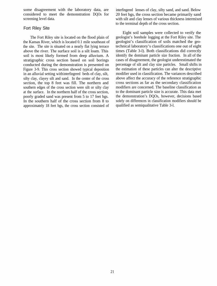
some disagreement with the laboratory data, areconsidered to meet the demonstration DQOs forscreening level data.

Fort Riley Site

The Fort Riley site is located on the flood plain ofthe Kansas River, which is located 0.1 mile southeast ofthe site. The site is situated on a nearly flat lying terraceabove the river. The surface soil is a silt loam. Thissoil is most likely formed from deep alluvium. Astratigraphic cross section based on soil boringsconducted during the demonstration is presented onFigure 3-9. This cross section showed typical depositionin an alluvial setting with interfingered beds of clay, silt,silty clay, clayey silt and sand. In the center of the crosssection, the top 8 feet was fill. The northern andsouthern edges of the cross section were silt or silty clayat the surface. In the northern half of the cross section,poorly graded sand was present from 5 to 17 feet bgs.In the southern half of the cross section from 8 toapproximately 18 feet bgs, the cross section consisted of

interfingered lenses of clay, silty sand, and sand. Below20 feet bgs, the cross section became primarily sandwith silt and clay lenses of various thickness intermixedto the terminal depth of the cross section.

Eight soil samples were collected to verify thegeologist’s borehole logging at the Fort Riley site. Thegeologist’s classification of soils matched the geo-technical laboratory’s classifications one out of eighttimes (Table 3-l). Both classifications did correctlyidentify the dominant particle size fraction. In all of thecases of disagreement, the geologist underestimated thepercentage of silt and clay size particles. Small shifts inthe estimation of these particles can alter the descriptivemodifier used in classification. The variances describedabove affect the accuracy of the reference stratigraphiccross sections as far as the secondary classificationmodifiers are concerned. The baseline classification asto the dominant particle size is accurate. This data metthe demonstration’s DQOs, however, decisions basedsolely on differences in classification modifiers should bequalified as semiqualitative Table 3-l.

21

Section 4Rapid Optical

This section describes the ROSY technologyevaluated under this demonstration. The descriptionprovided is based on information provided by thedeveloper, on information PRC obtained from reportsand journal articles written about the technology, and onobservations made during the demonstration. Thedescription includes background information on thetechnology and its components. General operatingprocedures, training and maintenance requirements, andcost of the technology also are discussed.

Background Information

The Department of Defense, through the U.S. AirForce’s Armstrong Laboratory, has supported researchat NDSU to develop tunable dye laser systems for fieldenvironmental analysis since 1989. A prototype tunablesystem built at NDSU was integrated with a conepenetrometer truck and demonstrated at Tinker AirForce Base in 1992. Follow-up demonstrations of thetunable dye laser systems for optical cone penetrometrywere carried out in late 1993 and 1994 at the followingair force bases: Plattsburgh, Patrick, and Dover. Thissecond round of demonstrations used an improvedprototype built by DTI. DTI is a small business formedby two individuals who developed the original tunabledye laser system at NDSU.

In 1993, a consortium comprised of UnisysCorporation, DTI, NDSU, and the U.S. Air ForceArmstrong Laboratory received a TechnologyReinvestment Project award from the Advance ResearchProjects Agency, which led to the development of theROST”. Loral Corporation acquired the portion ofUnisys responsible for the ROSY development andservices on May 5, 1995. For this demonstration,ROST” was temporarily installed on a conepenetrometer truck supplied by a subcontractor to PRC.The subcontractor selected was Fugro Geosciences, Inc.(Fugro); however, the developer stated that ROST” iscompatible with almost any standard cone penetrometertruck.

Screening Tool

Components

This subsection describes the components of ROSYand the cone penetrometer truck system.

Cone Penetrometer Truck System

A complete cone penetrometer truck system consistsof a truck, hydraulic rams and associated controllers,and the CP itself. The weight of the truck provides astatic reaction force, typically 20 tons, to advance theCP. The hydraulic system working against the staticreaction on force advances l-meter-long segments of3.57-centimeter-diameter threaded push rod into theground. The CP, which is mounted on the end of theseries of push rods, contains sensors that continuouslylog tip stress and sleeve friction. The ROW”technology’s fiber optic cables, mirrors, supports, andsapphire window are built into a “sub” which is fitted toa standard CP. This CP is fitted with tip stress andsleeve friction sensors. The data from CP sensors areused to map subsurface stratigraphy. Conductivity orpore pressure sensors can be driven into the groundsimultaneously with the modified CP. Soil, ground-water, and soil gas sampling tools can also be used withthe cone penetrometer truck. These capabilities arediscussed in greater detail in the general ITER.Generally, sampling tools and sensors are not usedconcurrently due to the necessity for sampler retrievalafter each sample is collected.

In favorable stratigraphies, push depths of 50 metersor greater have been achieved. The CP can be pushedthrough asphalt, but concrete must be cored prior toadvancing the CP. Advancing sensors and samplingtools with the cone penetrometer truck may be difficultor impossible in the following subsurface environments:

l Gravel unitsl Cemented sands and clays. Buried debrisl Bouldersl Bedrock

22

The cone penetrometer truck used with the ROST”during this demonstration was fitted with a steam cleanerto decontaminate the push rods as they were withdrawnfrom the ground. The decontamination water iscontained in the decontamination apparatus and it can bedirectly discharged into a storage container. The cleanwater, pressure sprayer, and grouting pump are mountedin a trailer that is towed by a support vehicle.

ROSTTMTechnology

The main ROST” system components are:

l Neodymium-doped Yttrium Aluminum Garnet(Nd:YAG) primary laser

l Tunable dye laser pumped by the Nd:YAGlaser

l Fiber optic cable and CP “sub”l Detection system comprised of a mono-

chromator, photomultiplier tube (PMT), anddigital storage oscilloscope (DSO)

l Control computer

In the prototypes that preceded ROST”‘, thecomponents of the tunable dye laser were arranged on a122-centimeter (cm) by 61-cm optical breadboard, whichsat on top of a cart in which the other components wereplaced. The ROST” technology used in thisdemonstration is more compact and integrated. TheROST” components are assembled into two half-heightinstrumentation racks. Each rack is approximately66-cm high by 51-cm wide by 61-cm deep. A diagramthat shows how the ROW’” system components arearranged in the racks is shown on Figure 4-l. The mainROST” components are discussed in more detail below.All of the electronic components are powered by agasoline generator, independent of the cone penetrometertruck power system.

Nd:YAG Laser

The primary laser is a Nd:YAG laser with a secondharmonic generation option manufactured by Big SkyLaser Technologies. It generates 532 nanometers (nm)of light at a repetition rate of 50 pulses per second (Hz).The near-Gaussian output beam is approximately6.35 cm in diameter. The primary laser is rated at apulse energy of 50 millijoules per pulse (MJ).. It requiresstandard Il0-volt line voltage; a dedicated 20-ampcircuit is recommended. Because water to cool theNd:YAG rod is supplied by an internal circulator in thepower supply, no external source of cooling water isrequired. The light from the primary laser pumps thedye laser.

Tunable Dye Laser

The dye laser converts the fixed wavelength light ofthe Nd:YAG laser into wavelengths that can beoptimized for the contaminant(s) of interest. The dyelaser is pumped by the Nd:YAG laser output. Theoutput wavelength range of the dye laser depends onwhich dye is used. The dye was Rhodamine 6G for thisdemonstration. The wavelength range that can begenerated from Rhodamine 6G is approximately 560 to6oomn.

The dye laser uses Bethune prism dye cells, whichare right angle prisms with a narrow bore through whichthe dye flows. The collimated light from the Nd:YAGlaser enters the hypotenuse face of the prism. Afterundergoing total internal reflection at the other twofaces, the light creates a highly uniform illumination ofthe dye solution that is flowing through the Bethunecells. The developer states that a major advantage of theBethune cells is that the Nd:YAG laser light does nothave to be focused into the dye cell. Collimated light (ornearly so) is sufficient to maintain the total internalreflection condition.

The wavelength of the monochromatic laser light,which is produced in the oscillator of the dye laser, isselected to be optimal for the detection of specificcompounds. The oscillator consists of the Bethune cell,cavity mirrors, and a wavelength dispersing element (adiffraction grating in this case). The broad Rhodamine6G fluorescence (560 to 600 nm) that exits the bore ofthe Bethune prism cell hits a feedback element thatreflects a portion of the light back through the Bethunecell bore. The feedback element, which can be awedged piece of fused silica, also serves as the outputcoupler of the dye laser. On this second passage, thelight is amplified by stimulated emission into a narrowpencil of light. On the other side of the prism cell, thepencil of light grazes the surface of a diffraction grating.The diffraction grating disperses the light. That is, itspatially separates light into its wavelength componentsin the same fashion as a prism. A tuning mirror returnsthe diffracted light back to the grating at which point thereturn beam is rediffracted. Only a narrow range ofwavelengths within the rediffracted beam follow theproper path to pass back through the Bethtme cell. Thismonochromatic light is further intensified by stimulatedemission as it passes back through the dye cell. It exitsthe laser cavity through the feedback element. Byvarying the angle of the tuning mirror, one may selectthe wavelength of light which finally exits the dye lasercavity, which is why the dye laser is referred to astunable.

23

FIGURE 4-l. SYSTEM COMPONENTS

A. Control rackB. Spectrometer rackC. Nd:YAG power supply

0D. Optical breadboard

E. Frequency doubling crystalF. Nd:YAG laser headG. Dye laserH. MonochromatorI. Stepper motor controller/driverJ. Photomultiplier tube and housingK. High voltage power supplyL. Stepper motor reset buttonM. Water reservoirN. Dye reservoir0. Monitor

P. KeyboardQ. Utility DrawerR ComputerS. OscilloscopeT. Temperature Controller

The monochromatic laser light emerging from the sapphire window is referred to as the delivery fiber.oscillator of the dye laser is amplified as it passes The return fiber (or fibers) is referred to as a collectionthrough a second Bethune cell, which is also energized fiber (or fibers). The delivery and collection fibers runfrom the Nd:YAG laser. The amplified beam then from the dye laser through the center of the series ofpasses through a frequency doubling crystal, which push rods to which the CP is attached.converts a portion of the incoming light into photons ofhalf the wavelength, in this case in the range 280 to The fibers have three concentric layers. The light300 nm. The unconverted visible light is removed by a travels through the innermost zone known as the core.blocking filter and the remaining light is focused onto the The middle layer is a cladding material that has a higherlaunch end of the fiber optic cable. reflective index than the core fiber. This difference in

reflective index causes internal reflection as light toFiber Optic Cable move through the core. In effect, the cladding traps

light within the core. The outer layer is a protectiveThe fiber optic cable delivers excitation light from abrasion-resistant buffer. For additional protection, the

the dye laser through the sapphire window in the fibers are inserted into furcation tubing.modified CP and returns any fluorescence emissionarising from aromatics contamination in the soil back to For this demonstration, the developer used a singlethe PMT, which is a component of the detection system. delivery fiber and a single collection fiber. SensitivityThe sapphire window is typically 2 to could be increased with additional collection fibers.3 millimeters (mm) thick and 6.35 mm in diameter.This window is mounted flush with the outside of the Detection Systemstandard CP sensor casing. The window is located about20 to 25 centimeters above the terminal end of the CP The detection system consists of a monochromator,sensor casing. This window allows laser light to pass PMT. and a DSO. The monochromator incorporatesfrom the ROSTn and into the soil. The window also entrance and exit slits, a diffraction grating, and severaltransmits LIF from the soil back into a return fiber optic mirrors. The monochromator acts as a variablecable. Sapphire is used due to its good optical wavelength narrow bandpass filter. By acquiringtransmission characteristics and due to its abrasion fluorescence data at a series of wavelengths, theresistance. The fiber that transmits the laser light to the fluorescence technician can determine the wavelength of

24

maximum intensity in the fluorescence spectrum. Thelight passing through the monochromator at thiswavelength is converted to an electrical signal by thePMT. The signal from the PMT is fed to the DSO,which displays the waveform (fluorescence intensity asa function of time following the excitation laser pulse).Typically, the data are acquired over a window of 100 to500 nanoseconds (ns). The DSO also averages the signalfrom several consecutive laser shots. After the selectednumber of laser shots have been averaged, the waveformis downloaded to the control computer for permanentstorage and post-processing of the data.

Control Computer

The ROST” technology is controlled by a personalcomputer, which also is used for off-line data analysis.Several ROST” technology motors are controlled by thecomputer: one to drive the tuning mirror of the dyelaser oscillator, one to position the frequency doublingcrystal, and one to drive the monochromator wavelengthselection. The control computer also sets the highvoltage on the PMT and provides communication withthe DSO via a GPIB bus.

General Operating Procedures

The sapphire window is located in a “sub” that isfitted to a standard CP. These push rods areapproximately 1 meter long and must be continuouslyadded as the CP is advanced using a hydraulic ram. Thestandard penetration rate is approximately 2 centimetersper second (cm/s). The maximum depth of a push isdetermined by soil matrix conditions and the staticreaction force of the cone penetrometer truck. Astandard 20-ton cone penetrometer truck was used forthis demonstration.

The CP also provides continuous monitoring of tipstress and sleeve friction. These data are downloadedonto a computer with software that classifies the soiltype.

When sensors are not attached to the push rods,conventional soil, soil gas, and groundwater samplingtools can be fitted to the push rods for environmentalsampling. In addition, cone penetrometer trucks can beused to install small diameter piezometers.

Before collecting data at a site, the ROST” iscalibrated. The ROST” operator attaches a sealed vialcontaining 10,000 ppm solution of gasoline to thesapphire window. The emission wavelength of the laseris set and multiple laser shots are fired at the solutionand the resultant fluorescence is measured. The data

system is then calibrated to read 100 percent fluo-rescence based on the fluorescence of the standard at thepredetermined emission monitoring wavelength. Allsubsequent data is reported as a percent fluorescencerelative to the standard.

The ROST” technology can be operated in bothdynamic (push) and static modes. In the dynamic mode,the modified CP equipped with the sapphire window andfiber optics is advanced at a rate between 1.5 and2.5 cm/s. In this mode, which the developer refers to asFVD (fluorescence versus depth), the excitation laserwavelength and fluorescence emission monitoringwavelength are held constant. The fluorescenceemission intensity is plotted as a function of depth bgs.The developer selected an excitation wavelength in therange 280 to 295 nm for this demonstration. Thiswavelength range was selected because naphthalene, amajor PAH constituent of coal tar and diesel fuel,fluoresces strongly under these conditions. The emissionmonochromator was set at a wavelength determinedduring the laboratory analysis of the predemonstrationsamples. It was set at 400 nm for the Atlantic and Yorksites, and at 360 nm at the Fort Riley site. With theselaser and detector settings, the ROST” was configuredto detect the presence or absence of primary fluorescingcompounds associated with the petroleum fuel and coaltar contamination expected during this demonstration.

For this demonstration, the laser repetition rate was50 Hz. The DSO in the current ROST” systemconfiguration averages the time-integrated signal fromthese 50 pulses to produce a fluorescence datum for thatdepth. The spatial resolution was, therefore, 2 cm. Thecomplete averaged fluorescence intensity versus depthprofile was archived for post-processing.

Once areas of significant contamination have beenidentified in the dynamic mode, ROST” can be operatedin the static mode to identify the general class ofcontamination present. In this mode, the CP is held ata fixed depth. The fluorescence technician, who isobserving the fluorescence signal visually, can simplysignal the hydraulic operator to halt the push. ROST”also can operate in the static mode when additional pushrods are added to the string.

During the static mode, ROST” can obtainmultidimensional data representations, called wave-length-time-matrices (WTM). These differ from the twodimensional FVDs that are plots of relative fluorescenceintensity versus depth. A WTM represents a3-dimensional plot of relative fluorescence intensityversus fluorescence lifetimes versus wavelength. WTMsproduce contaminant class specific three-dimensionalfigures. Preliminary research indicates that this

25

characteristic image can be used in a fashion similar tofingerprinting to identify contamination. This data canbe used to identify contaminants present, for example,the type of fuel that is present. For WTM acquisition,either the excitation or the fluorescence emissionwavelength can be varied. Normally the excitationwavelength is held constant and the emission monitoringwavelength is varied. This was the procedure usedduring the demonstration. For a WTM, the data from100 to 200 laser pulses are averaged at each of a seriesof return emission wavelengths separated by 10 nm,between 50 and 300 nm. The acquisition of a WTMtakes about 5 minutes longer than the time required toadd an additional probe rod for continued probeadvancement.

Training and Maintenance Requirements

One person is needed to operate the ROST”technology and two are needed to operate the conepenetrometer truck. A crew chief operates thehydraulics of the cone penetrometer truck and monitorsthe push depth, cone tip resistance, sleeve friction, andpore pressure or conductivity measurements if taken.The rod person screws on additional push rods aftercompleting each l-meter push. The fluorescencetechnician operates the ROSY technology.

The technology is presently offered only as a servicefrom Loral Corporation. Their operators are fullytrained in the operation and maintenance of theequipment and the interpretation of the data. The typicaloperator has a bachelor’s degree in a science orengineering discipline, plus any prerequisite environ-mental field training. Typically the ROST”‘ operatorshave 30 days of training in the use of the technology.This training consists of classroom and on-the-jobtraining.

Cost

Because the ROST” technology is still in thedevelopmental stage, a specific sales cost for thetechnology has not been established. Currently, use ofthe ROST” technology is contracted out on a job-by-jobbasis. The developer envisions ROST”‘ being sold as acomplete unit eventually. Training would likely beincorporated into the sale price.

The developer estimates that the daily rate for use ofa cone penetrometer truck and ROSY would bebetween $5,000 and $5,500. Mobilization and operatorper diem costs are not included. The ROSY technologyand one operator costs $2,800 per day if a conepenetrometer truck is already being supplied. Thesecosts also do not include mobilization or per diem. The

ROSY technology was used with a Fugro conepenetrometer truck. The cone penetrometer truck costsincurred during the demonstration were $2,350 per day,which included mobilization for the Fugro conepenetrometer truck and two operators. If the cost ofsubcontracting the cone penetrometer truck is added tothe daiiy use charge of the ROSY technology, a dailyuse rate for a complete ROST” rig, as used in thisdemonstration, would be approximately $5,150 per day.The total cost of the three site characterizationsperformed using ROST’” would have been approximately$41,200. For comparison, the predemonstrationactivities produced similar data at the three sites,however, it required more personnel and on-siteanalytical capabilities at an approximate cost of $43,000.The predemonstration resulted in fewer data points,relative to the continuous data output of the ROSY andCP. In addition, the predemonstration activities onlyproduced one borehole log at each site. Another costcomparison can be made relative to the costs accruedproducing the reference cross sections for thisdemonstration. Data acquisition and production costs ofthe reference cross sections cost approximately $55,000,including approximately $30,000 for drilling services,approximately $8,000 for the on-site geologist andsampler, approximately $12,000 for off-site analyticalservices, and approximately $5,000 for handling anddisposal of investigation derived waste.

Observations

An observer was assigned to the ROST” technologydemonstration to assess the following operational factors:

l costl Ease of operation, ruggedness, and reliabilityl Sampling capabilities and production rates

A summary of the observations made during theROST” demonstration is included in the followingparagraphs. The developers’ corrective actions andresponses to some of these observations are presented inSection 7.

The cone penetrometer truck equipment, aspreviously stated, was supplied by Fugro Geosciences,Inc., Houston, Texas. The cone penetrometer truckconsisted of a driver’s cab and an enclosed 15- by 8-footrear compartment, which housed the cone penetrometertruck pushing equipment and tools, and the electronicequipment used by both the cone penetrometer truck andROSY. The technology’s components were supplied bythe developer and included the equipment previouslyidentified in this section of this report. In addition, theROST”” system used a printer to allow in-the-fieldprintouts of push data.

26

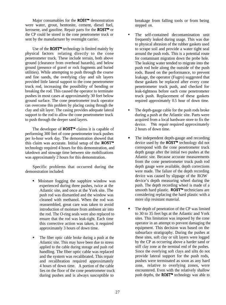
Major consumables for the ROST” demonstrationwere water, grout, bentonite, cement, diesel fuel,kerosene, and gasoline. Repair parts for the ROST” orthe CP could be stored in the cone penetrometer truck or l

sent by the manufacturer by overnight carrier.

Use of the ROST” technology is limited mainly byphysical factors relating directly to the conepenetrometer truck. These include terrain, both aboveground (clearance from overhead hazards), and belowground (presence of gravel or rock fragments and buriedutilities). While attempting to push through the coarseand fine sands, the overlying clay and silt layersprovided little lateral support to the cone penetrometertruck rod, increasing the possibility of bending orbreaking the rod. This caused the operator to terminatepushes in most cases at approximately 30 feet belowground surface. The cone penetrometer truck operatorcan overcome this problem by placing casing through theclay and silt layer. The casing provides adequate lateral l

support to the rod to allow the cone penetrometer truckto push through the deeper sand layers.

The developer of ROST” claims it is capable ofperforming 300 feet of cone penetrometer truck pushesper lo-hour work day. The demonstration showed that athis claim was accurate. Initial setup of the ROST”technology required 4 hours for this demonstration, andtakedown and stowage time between site mobilizationswas approximately 2 hours for this demonstration.

Specific problems that occurred during thedemonstration included:

* Moisture fogging the sapphire window wasexperienced during three pushes, twice at theAtlantic site, and once at the York site. Thepush rod was dismantled and the window wascleaned with methanol. When the rod wasreassembled, great care was taken to avoidintroduction of moisture from ambient air into *

the rod. The O-ring seals were also replaced toensure that the rod was leak-tight. Each timethis corrective action was taken, it requiredapproximately 3 hours of down time.

The fiber optic cable broke during a push at theAtlantic site. This may have been due to stressapplied to the cable during storage and push rodhandling. The fiber optic cable was replacedand the system was recalibrated. This repairand recalibration required approximately4 hours of down time. A portion of the cablelies on the floor of the cone penetrometer truckduring pushes and is always susceptible to

breakage from falling tools or from beingstepped on.

The self-contained decontamination unitfrequently leaked during usage. This was dueto physical abrasion of the rubber gaskets usedto scrape soil and provide a water tight sealaround the push rods. This is a potential routefor contaminant migration down the probe hole.The leaking water tended to migrate into thepush rod hole along the outside of the pushrods. Based on the performance, to preventleakage, the operator (Fugro) suggested thatthese gaskets be replaced after every conepenetrometer truck push, and checked forleak-tightness before each cone penetrometertruck push. Replacement of these gasketsrequired approximately 0.5 hour of down time.

The depth-gauge cable for the push rods brokeduring a push at the Atlantic site. Parts wereacquired from a local hardware store to fix thedevice. This repair required approximately2 hours of down time.

The independent depth-gauge and recordingdevice used by the ROST”’ technology did notcorrespond with the cone penetrometer truckdepth gauge after the initial two pushes at theAtlantic site. Because accurate measurementsfrom the cone penetrometer truck push roddepth gauge were available, depth correctionswere made. The failure of the depth recordingdevice was caused by slippage of the ROWdevice’s depth measuring wheel during thepush. The depth recording wheel is made of asmooth hard plastic. ROST” technicians areconsidering replacing the hard plastic with amore slip resistant material.

The depth of penetration of the CP was limitedto 30 to 35 feet bgs at the Atlantic and Yorksites. This limitation was imposed by the coneoperator in an attempt to prevent damaging theequipment. This decision was based on thesubsurface stratigraphy. During the pushes atthese sites, soft clay or silt layers were loggedby the CP as occurring above a harder sand orstiff clay zone at the terminal end of the pushes.Since the overlying soft clays and silts do notprovide lateral support for the push rods,pushes were terminated as soon as any hardzone, relative to overlying zones, wereencountered. Even with the relatively shallowpush depths, the ROST” technology was able to

27

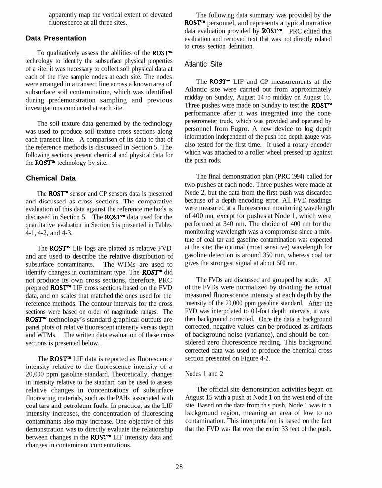
apparently map the vertical extent of elevatedfluorescence at all three sites.

Data Presentation

To qualitatively assess the abilities of the ROST”technology to identify the subsurface physical propertiesof a site, it was necessary to collect soil physical data ateach of the five sample nodes at each site. The nodeswere arranged in a transect line across a known area ofsubsurface soil contamination, which was identifiedduring predemonstration sampling and previousinvestigations conducted at each site.

The soil texture data generated by the technologywas used to produce soil texture cross sections alongeach transect line. A comparison of its data to that ofthe reference methods is discussed in Section 5. Thefollowing sections present chemical and physical data forthe ROST”’ technology by site.

Chemical Data

The ROST”’ sensor and CP sensors data is presentedand discussed as cross sections. The comparativeevaluation of this data against the reference methods isdiscussed in Section 5. The ROSY data used for thequantitative evaluation in Section 5 is presented in Tables4-1, 4-2, and 4-3.

The ROST” LIF logs are plotted as relative FVDand are used to describe the relative distribution ofsubsurface contaminants. The WTMs are used toidentify changes in contaminant type. The ROST” didnot produce its own cross sections, therefore, PRCprepared ROSY” LIF cross sections based on the FVDdata, and on scales that matched the ones used for thereference methods. The contour intervals for the crosssections were based on order of magnitude ranges. TheROST” technology’s standard graphical outputs arepanel plots of relative fluorescent intensity versus depthand WTMs.. The written data evaluation of these crosssections is presented below.

The ROST” LIF data is reported as fluorescenceintensity relative to the fluorescence intensity of a20,000 ppm gasoline standard. Theoretically, changesin intensity relative to the standard can be used to assessrelative changes in concentrations of subsurfacefluorescing materials, such as the PAHs associated withcoal tars and petroleum fuels. In practice, as the LIFintensity increases, the concentration of fluorescingcontaminants also may increase. One objective of thisdemonstration was to directly evaluate the relationshipbetween changes in the ROSF LIF intensity data andchanges in contaminant concentrations.

The following data summary was provided by theROST” personnel, and represents a typical narrativedata evaluation provided by ROST”. PRC edited thisevaluation and removed text that was not directly relatedto cross section definition.

Atlantic Site

The ROST” LIF and CP measurements at theAtlantic site were carried out from approximatelymidday on Sunday, August 14 to midday on August 16.Three pushes were made on Sunday to test the ROST”performance after it was integrated into the conepenetrometer truck, which was provided and operated bypersonnel from Fugro. A new device to log depthinformation independent of the push rod depth gauge wasalso tested for the first time. It used a rotary encoderwhich was attached to a roller wheel pressed up againstthe push rods.

The final demonstration plan (PRC 1994) called fortwo pushes at each node. Three pushes were made atNode 2, but the data from the first push was discardedbecause of a depth encoding error. All FVD readingswere measured at a fluorescence monitoring wavelengthof 400 mn, except for pushes at Node 1, which wereperformed at 340 nm. The choice of 400 nm for themonitoring wavelength was a compromise since a mix-ture of coal tar and gasoline contamination was expectedat the site; the optimal (most sensitive) wavelength forgasoline detection is around 350 run, whereas coal targives the strongest signal at about 500 nm.

The FVDs are discussed and grouped by node. Allof the FVDs were normalized by dividing the actualmeasured fluorescence intensity at each depth by theintensity of the 20,000 ppm gasoline standard. After theFVD was interpolated to 0.l-foot depth intervals, it wasthen background corrected. Once the data is backgroundcorrected, negative values can be produced as artifactsof background noise (variance), and should be con-sidered zero fluorescence reading. This backgroundcorrected data was used to produce the chemical crosssection presented on Figure 4-2.

Nodes 1 and 2

The official site demonstration activities began onAugust 15 with a push at Node 1 on the west end of thesite. Based on the data from this push, Node 1 was in abackground region, meaning an area of low to nocontamination. This interpretation is based on the factthat the FVD was flat over the entire 33 feet of the push.

28

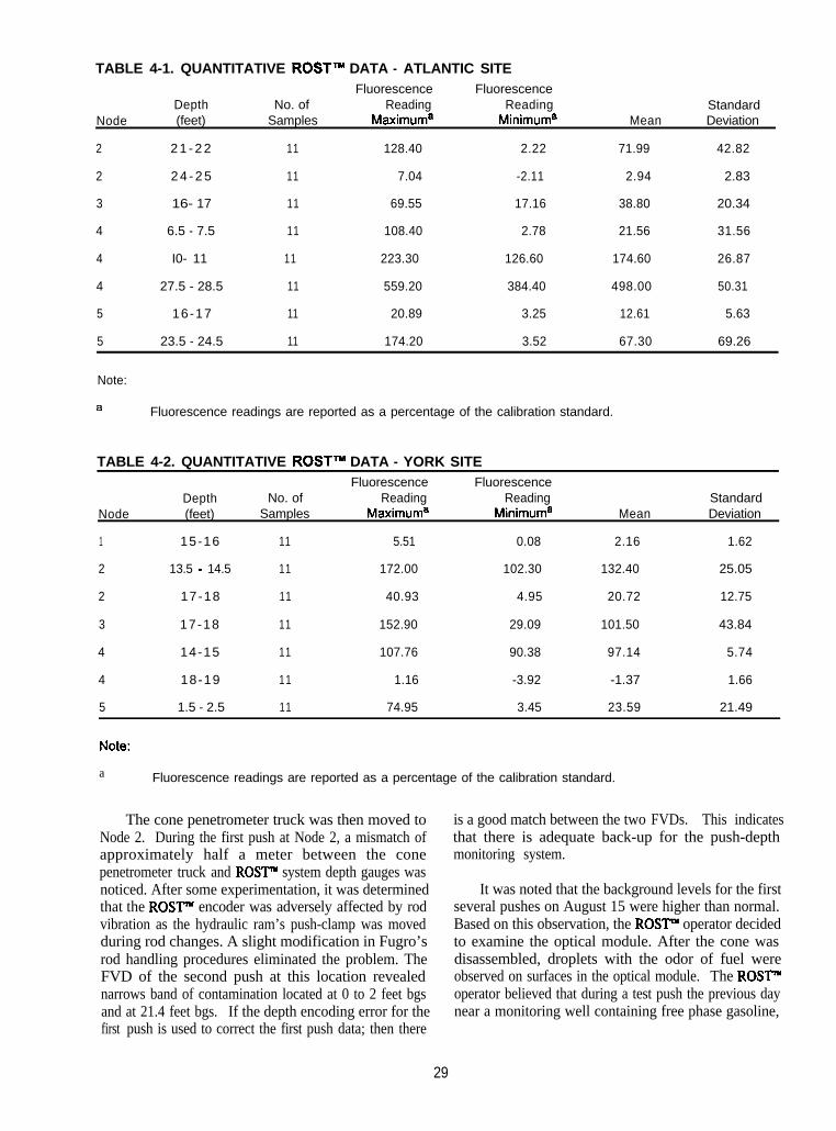
TABLE 4-1. QUANTITATIVE ROSTTM DATA - ATLANTIC SITEFluorescence Fluorescence

Depth No. of Reading ReadingNode (feet) Samples Maximuma Minimuma

2 2 1 - 2 2 11 128.40 2.22

2 2 4 - 2 5 11 7.04 -2.11

3 16- 17 11 69.55 17.16

4 6.5 - 7.5 11 108.40 2.78

4 I0- 11 11 223.30 126.60

4 27.5 - 28.5 11 559.20 384.40

5 16-17 11 20.89 3.25

5 23.5 - 24.5 11 174.20 3.52

StandardMean Deviation

71.99 42.82

2.94 2.83

38.80 20.34

21.56 31.56

174.60 26.87

498.00 50.31

12.61 5.63

67.30 69.26

Note:

a Fluorescence readings are reported as a percentage of the calibration standard.

TABLE 4-2. QUANTITATIVE ROSTTM DATA - YORK SITE

Node

1

2

2

Depth No. of(feet) Samples

15-16 11

13.5 - 14.5 11

17-18 11

Fluorescence FluorescenceReading Reading

Maximuma Minimuma

5.51 0.08

172.00 102.30

40.93 4.95

Mean

2.16

132.40

20.72

StandardDeviation

1.62

25.05

12.75

3 17-18 11 152.90 29.09 101.50 43.84

4 14-15 11 107.76 90.38 97.14 5.74

4 18-19 11 1.16 -3.92 -1.37 1.66

5 1.5 - 2.5 11 74.95 3.45 23.59 21.49

a Fluorescence readings are reported as a percentage of the calibration standard.

The cone penetrometer truck was then moved toNode 2. During the first push at Node 2, a mismatch ofapproximately half a meter between the conepenetrometer truck and ROSY system depth gauges wasnoticed. After some experimentation, it was determinedthat the ROSY encoder was adversely affected by rodvibration as the hydraulic ram’s push-clamp was movedduring rod changes. A slight modification in Fugro’srod handling procedures eliminated the problem. TheFVD of the second push at this location revealednarrows band of contamination located at 0 to 2 feet bgsand at 21.4 feet bgs. If the depth encoding error for thefirst push is used to correct the first push data; then there

is a good match between the two FVDs.. This indicatesthat there is adequate back-up for the push-depthmonitoring system.

It was noted that the background levels for the firstseveral pushes on August 15 were higher than normal.Based on this observation, the ROST” operator decidedto examine the optical module. After the cone wasdisassembled, droplets with the odor of fuel wereobserved on surfaces in the optical module. The ROST”’operator believed that during a test push the previous daynear a monitoring well containing free phase gasoline,

29

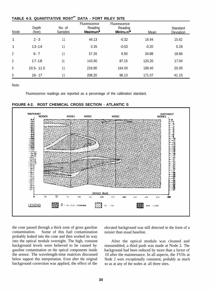
TABLE 4-3. QUANTITATIVE ROSTMT

DATA - FORT RILEY SITEFluorescence Fluorescence

Depth No. of Reading ReadingNode (feet) Samples Maximuma Minimuma

1 2 - 3 11 44.13 -0.32

1 13-14 11 0.35 -0.53

2 6 - 7 11 57.26 6.50

2 17-18 11 143.90 87.15

5 10.5- 11.5 11 216.90 164.00

5 16- 17 11 208.20 96.13

Mean

16.94

-0.20

34.88

120.20

188.40

171.07

StandardDeviation

15.62

0.26

18.66

17.04

20.05

41.15

Note:

Fluorescence readings are reported as a percentage of the calibration standard.

FIGURE 4-2. ROST CHEMICAL CROSS SECTION - ATLANTIC SS S

S S O NORTHWEST, NODE5 NODE4 NODE3 NODE2 NODE1 ,

DISTANCE (feet)25 50 75 100 125 150 175 200 225 250 275

LEGEND 0 - 10 (% OF STANDARD) m 10 - loo loo - 1.000

the cone passed through a thick zone of gross gasolinecontamination. Some of this fuel contaminationprobably leaked into the cone and then worked its wayinto the optical module overnight. The high, constantbackground levels were believed to be caused bygasoline contamination on the optical components insidethe sensor. The wavelength-time matrices discussedbelow support this interpretation. Even after the originalbackground correction was applied, the effect of the

elevated background was still detected in the form of anoisier than usual baseline.

After the optical module was cleaned andreassembled, a third push was made at Node 2. Thebackground had been reduced by more than a factor of10 after the maintenance. In all aspects, the FVDs atNode 2 were exceptionally consistent, probably as muchso as at any of the nodes at all three sites.

30

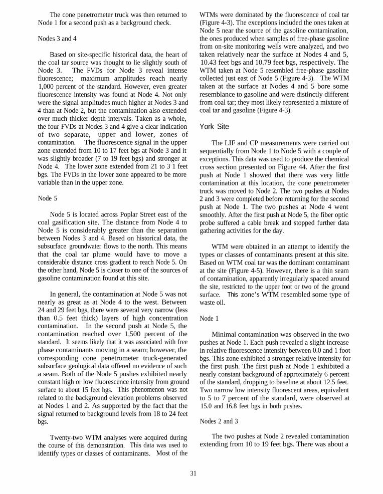
The cone penetrometer truck was then returned toNode 1 for a second push as a background check.

Nodes 3 and 4

Based on site-specific historical data, the heart ofthe coal tar source was thought to lie slightly south ofNode 3. The FVDs for Node 3 reveal intensefluorescence; maximum amplitudes reach nearly1,000 percent of the standard. However, even greaterfluorescence intensity was found at Node 4. Not onlywere the signal amplitudes much higher at Nodes 3 and4 than at Node 2, but the contamination also extendedover much thicker depth intervals. Taken as a whole,the four FVDs at Nodes 3 and 4 give a clear indicationof two separate, upper and lower, zones ofcontamination. The fluorescence signal in the upperzone extended from 10 to 17 feet bgs at Node 3 and itwas slightly broader (7 to 19 feet bgs) and stronger atNode 4. The lower zone extended from 21 to 3 1 feetbgs. The FVDs in the lower zone appeared to be morevariable than in the upper zone.

Node 5

Node 5 is located across Poplar Street east of thecoal gasification site. The distance from Node 4 toNode 5 is considerably greater than the separationbetween Nodes 3 and 4. Based on historical data, thesubsurface groundwater flows to the north. This meansthat the coal tar plume would have to move aconsiderable distance cross gradient to reach Node 5. Onthe other hand, Node 5 is closer to one of the sources ofgasoline contamination found at this site.

In general, the contamination at Node 5 was notnearly as great as at Node 4 to the west. Between24 and 29 feet bgs, there were several very narrow (lessthan 0.5 feet thick) layers of high concentrationcontamination. In the second push at Node 5, thecontamination reached over 1,500 percent of thestandard. It seems likely that it was associated with freephase contaminants moving in a seam; however, thecorresponding cone penetrometer truck-generatedsubsurface geological data offered no evidence of sucha seam. Both of the Node 5 pushes exhibited nearlyconstant high or low fluorescence intensity from groundsurface to about 15 feet bgs. This phenomenon was notrelated to the background elevation problems observedat Nodes 1 and 2. As supported by the fact that thesignal returned to background levels from 18 to 24 feetbgs.

Twenty-two WTM analyses were acquired duringthe course of this demonstration. This data was used toidentify types or classes of contaminants. Most of the

WTMs were dominated by the fluorescence of coal tar(Figure 4-3). The exceptions included the ones taken atNode 5 near the source of the gasoline contamination,the ones produced when samples of free-phase gasolinefrom on-site monitoring wells were analyzed, and twotaken relatively near the surface at Nodes 4 and 5,10.43 feet bgs and 10.79 feet bgs, respectively. TheWTM taken at Node 5 resembled free-phase gasolinecollected just east of Node 5 (Figure 4-3). The WTMtaken at the surface at Nodes 4 and 5 bore someresemblance to gasoline and were distinctly differentfrom coal tar; they most likely represented a mixture ofcoal tar and gasoline (Figure 4-3).

York Site

The LIF and CP measurements were carried outsequentially from Node 1 to Node 5 with a couple ofexceptions. This data was used to produce the chemicalcross section presented on Figure 44. After the firstpush at Node 1 showed that there was very littlecontamination at this location, the cone penetrometertruck was moved to Node 2. The two pushes at Nodes2 and 3 were completed before returning for the secondpush at Node 1. The two pushes at Node 4 wentsmoothly. After the first push at Node 5, the fiber opticprobe suffered a cable break and stopped further datagathering activities for the day.

WTM were obtained in an attempt to identify thetypes or classes of contaminants present at this site.Based on WTM coal tar was the dominant contaminantat the site (Figure 4-5). However, there is a thin seamof contamination, apparently irregularly spaced aroundthe site, restricted to the upper foot or two of the groundsurface. This zone’s WTM resembled some type ofwaste oil.

Node 1

Minimal contamination was observed in the twopushes at Node 1. Each push revealed a slight increasein relative fluorescence intensity between 0.0 and 1 footbgs. This zone exhibited a stronger relative intensity forthe first push. The first push at Node 1 exhibited anearly constant background of approximately 6 percentof the standard, dropping to baseline at about 12.5 feet.Two narrow low intensity fluorescent areas, equivalentto 5 to 7 percent of the standard, were observed at15.0 and 16.8 feet bgs in both pushes.

Nodes 2 and 3

The two pushes at Node 2 revealed contaminationextending from 10 to 19 feet bgs. There was about a

31

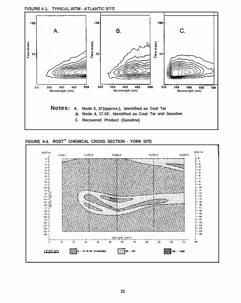
300 350 400 460Wavelength (nm) Wavelength (nm)

Notes: A . Node 2, 2l’(approx.), Identified asB. Node 4, 17.19’, Identified as Coal

C. Recovered Product (Gasoline)

Wavelength (nm)

Coal TarTar and Gasoline

FIGURE 4-4. ROSTTM CHEMICAL CROSS SECTION - YORK SITE

1t

32

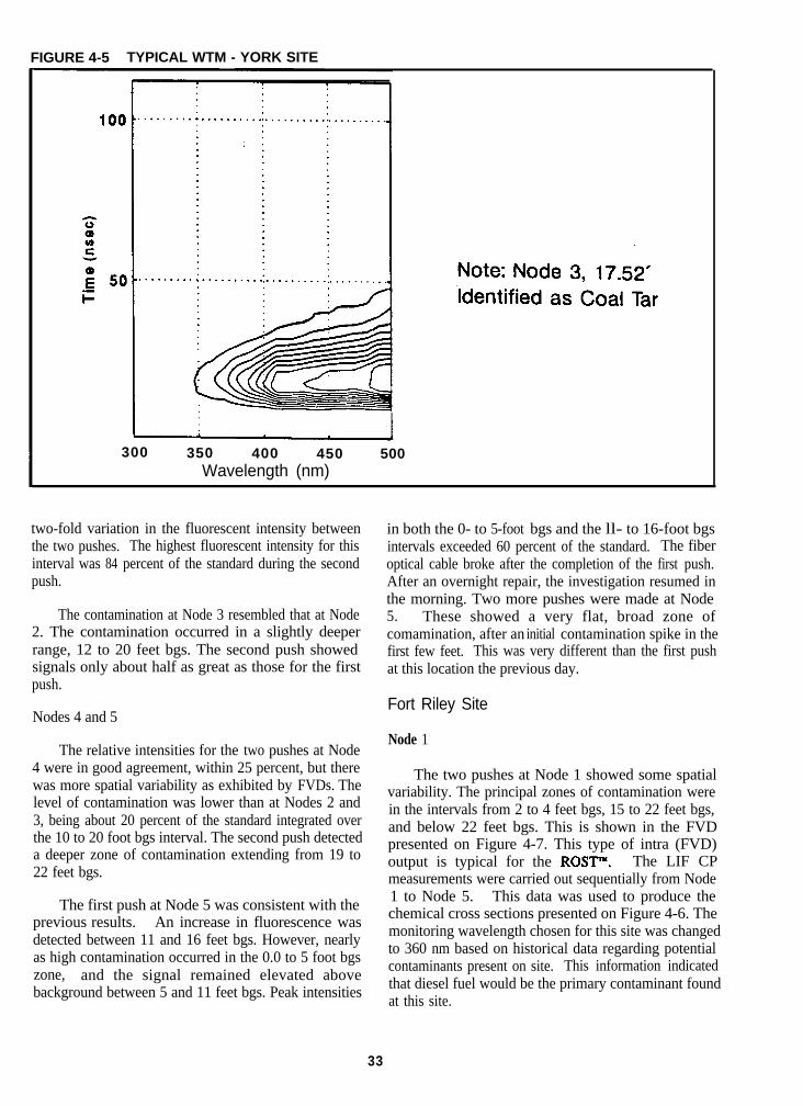
FIGURE 4-5. TYPICAL WTM - YORK SITE

300 350 400 450Wavelength (nm)

500

two-fold variation in the fluorescent intensity betweenthe two pushes. The highest fluorescent intensity for thisinterval was 84 percent of the standard during the secondpush.

The contamination at Node 3 resembled that at Node2. The contamination occurred in a slightly deeperrange, 12 to 20 feet bgs. The second push showedsignals only about half as great as those for the firstpush.

Nodes 4 and 5

The relative intensities for the two pushes at Node4 were in good agreement, within 25 percent, but therewas more spatial variability as exhibited by FVDs. Thelevel of contamination was lower than at Nodes 2 and3, being about 20 percent of the standard integrated overthe 10 to 20 foot bgs interval. The second push detecteda deeper zone of contamination extending from 19 to22 feet bgs.

The first push at Node 5 was consistent with theprevious results. An increase in fluorescence wasdetected between 11 and 16 feet bgs. However, nearlyas high contamination occurred in the 0.0 to 5 foot bgszone, and the signal remained elevated abovebackground between 5 and 11 feet bgs. Peak intensities

in both the 0- to 5-foot bgs and the ll- to 16-foot bgsintervals exceeded 60 percent of the standard. The fiberoptical cable broke after the completion of the first push.After an overnight repair, the investigation resumed inthe morning. Two more pushes were made at Node5. These showed a very flat, broad zone ofcomamination, after an initial contamination spike in thefirst few feet. This was very different than the first pushat this location the previous day.

Fort Riley Site

Node 1

The two pushes at Node 1 showed some spatialvariability. The principal zones of contamination werein the intervals from 2 to 4 feet bgs, 15 to 22 feet bgs,and below 22 feet bgs. This is shown in the FVDpresented on Figure 4-7. This type of intra (FVD)output is typical for the ROSY. The LIF CPmeasurements were carried out sequentially from Node1 to Node 5. This data was used to produce thechemical cross sections presented on Figure 4-6. Themonitoring wavelength chosen for this site was changedto 360 nm based on historical data regarding potentialcontaminants present on site. This information indicatedthat diesel fuel would be the primary contaminant foundat this site.

33

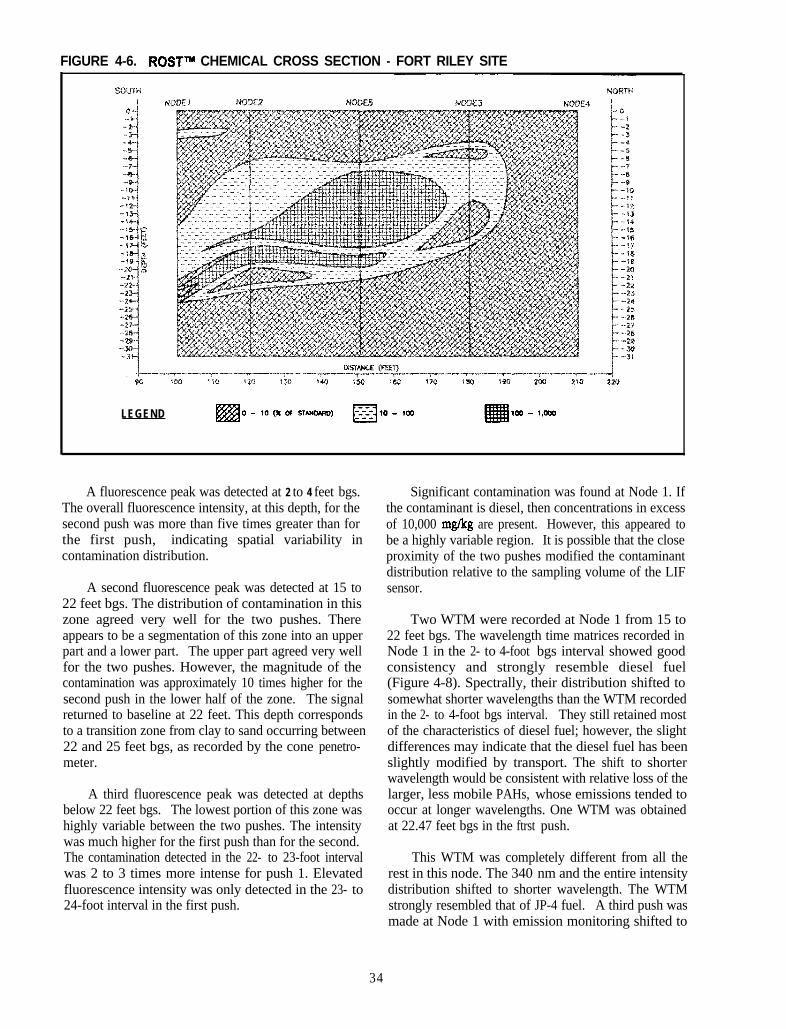
FIGURE 4-6. ROSTm CHEMICAL CROSS SECTION - FORT RILEY SITE

LEGEND

A fluorescence peak was detected at 2 to 4 feet bgs. Significant contamination was found at Node 1. IfThe overall fluorescence intensity, at this depth, for thesecond push was more than five times greater than forthe first push, indicating spatial variability incontamination distribution.

A second fluorescence peak was detected at 15 to22 feet bgs. The distribution of contamination in thiszone agreed very well for the two pushes. Thereappears to be a segmentation of this zone into an upperpart and a lower part. The upper part agreed very wellfor the two pushes. However, the magnitude of thecontamination was approximately 10 times higher for thesecond push in the lower half of the zone. The signalreturned to baseline at 22 feet. This depth correspondsto a transition zone from clay to sand occurring between22 and 25 feet bgs, as recorded by the cone penetro-meter.

A third fluorescence peak was detected at depthsbelow 22 feet bgs. The lowest portion of this zone washighly variable between the two pushes. The intensitywas much higher for the first push than for the second.The contamination detected in the 22- to 23-foot intervalwas 2 to 3 times more intense for push 1. Elevatedfluorescence intensity was only detected in the 23- to24-foot interval in the first push.

the contaminant is diesel, then concentrations in excessof 10,000 mg/kg are present. However, this appeared tobe a highly variable region. It is possible that the closeproximity of the two pushes modified the contaminantdistribution relative to the sampling volume of the LIFsensor.

Two WTM were recorded at Node 1 from 15 to22 feet bgs. The wavelength time matrices recorded inNode 1 in the 2- to 4-foot bgs interval showed goodconsistency and strongly resemble diesel fuel(Figure 4-8). Spectrally, their distribution shifted tosomewhat shorter wavelengths than the WTM recordedin the 2- to 4-foot bgs interval. They still retained mostof the characteristics of diesel fuel; however, the slightdifferences may indicate that the diesel fuel has beenslightly modified by transport. The shift to shorterwavelength would be consistent with relative loss of thelarger, less mobile PAHs, whose emissions tended tooccur at longer wavelengths. One WTM was obtainedat 22.47 feet bgs in the ftrst push.

This WTM was completely different from all therest in this node. The 340 nm and the entire intensitydistribution shifted to shorter wavelength. The WTMstrongly resembled that of JP-4 fuel. A third push wasmade at Node 1 with emission monitoring shifted to

34

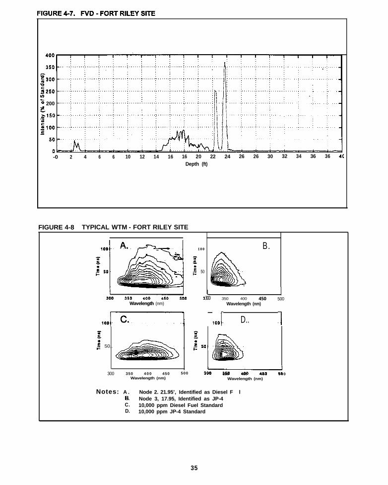
5 200Es150.Z

-0 2 4 6 6 10 12 14 16 16 20 22 24 26 26 30 32 34 36 36 40

Depth (ft)

FIGURE 4-8. TYPICAL WTM - FORT RILEY SITE

100

;id

:G 50

Wavelength (nm)

L300

B.

350 400 450 500Wavelength (nm)

,,,~] ,,,I. D.. .I;i5

tC

:F 50,. :, G50,

I300 350 4 0 0 450 500 30-350 400 450 500

Wavelength (nm) Wavelength (nm)

Notes: A . Node 2. 21.95’, Identified as Diesel FB. l0. Node 3, 17.95, Identified as JP-4C. 10,000 ppm Diesel Fuel StandardD. 10,000 ppm JP-4 Standard

35

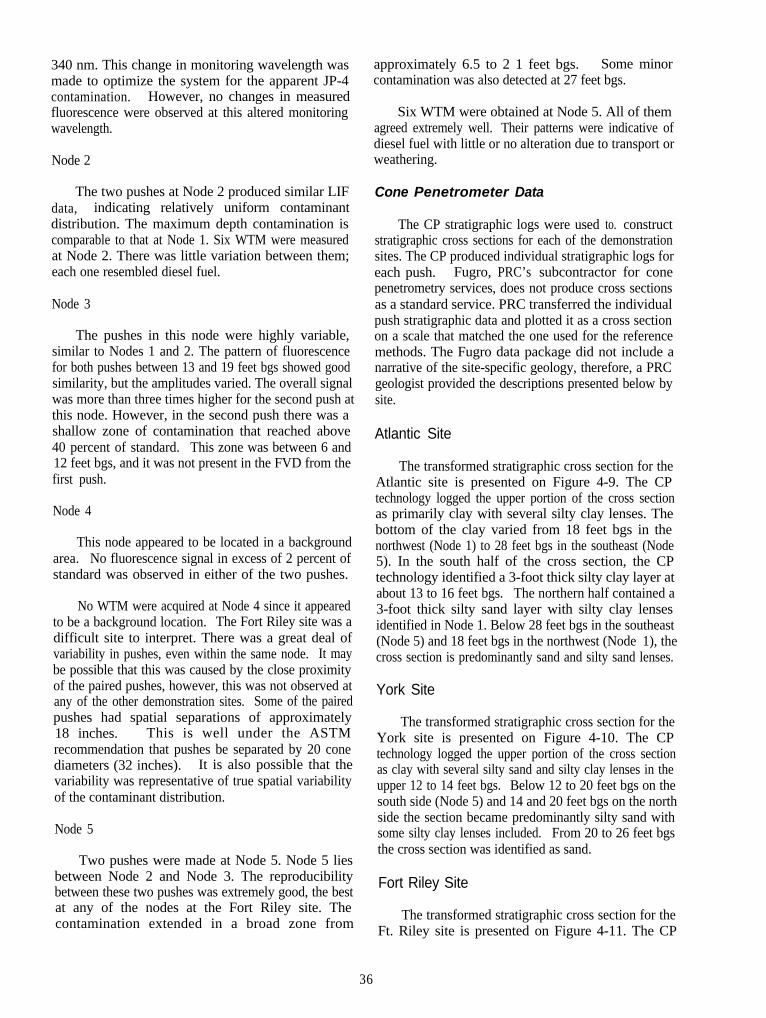
340 nm. This change in monitoring wavelength wasmade to optimize the system for the apparent JP-4contamination. However, no changes in measuredfluorescence were observed at this altered monitoringwavelength.

Node 2

The two pushes at Node 2 produced similar LIFdata, indicating relatively uniform contaminantdistribution. The maximum depth contamination iscomparable to that at Node 1. Six WTM were measuredat Node 2. There was little variation between them;each one resembled diesel fuel.

Node 3

The pushes in this node were highly variable,similar to Nodes 1 and 2. The pattern of fluorescencefor both pushes between 13 and 19 feet bgs showed goodsimilarity, but the amplitudes varied. The overall signalwas more than three times higher for the second push atthis node. However, in the second push there was ashallow zone of contamination that reached above40 percent of standard. This zone was between 6 and12 feet bgs, and it was not present in the FVD from thefirst push.

Node 4

This node appeared to be located in a backgroundarea. No fluorescence signal in excess of 2 percent ofstandard was observed in either of the two pushes.

No WTM were acquired at Node 4 since it appearedto be a background location. The Fort Riley site was adifficult site to interpret. There was a great deal ofvariability in pushes, even within the same node. It maybe possible that this was caused by the close proximityof the paired pushes, however, this was not observed atany of the other demonstration sites. Some of the pairedpushes had spatial separations of approximately18 inches. This is well under the ASTMrecommendation that pushes be separated by 20 conediameters (32 inches). It is also possible that thevariability was representative of true spatial variabilityof the contaminant distribution.

Node 5

Two pushes were made at Node 5. Node 5 liesbetween Node 2 and Node 3. The reproducibilitybetween these two pushes was extremely good, the bestat any of the nodes at the Fort Riley site. Thecontamination extended in a broad zone from

approximately 6.5 to 2 1 feet bgs. Some minorcontamination was also detected at 27 feet bgs.

Six WTM were obtained at Node 5. All of themagreed extremely well. Their patterns were indicative ofdiesel fuel with little or no alteration due to transport orweathering.

Cone Penetrometer Data

The CP stratigraphic logs were used to. constructstratigraphic cross sections for each of the demonstrationsites. The CP produced individual stratigraphic logs foreach push. Fugro, PRC’s subcontractor for conepenetrometry services, does not produce cross sectionsas a standard service. PRC transferred the individualpush stratigraphic data and plotted it as a cross sectionon a scale that matched the one used for the referencemethods. The Fugro data package did not include anarrative of the site-specific geology, therefore, a PRCgeologist provided the descriptions presented below bysite.

Atlantic Site

The transformed stratigraphic cross section for theAtlantic site is presented on Figure 4-9. The CPtechnology logged the upper portion of the cross sectionas primarily clay with several silty clay lenses. Thebottom of the clay varied from 18 feet bgs in thenorthwest (Node 1) to 28 feet bgs in the southeast (Node5). In the south half of the cross section, the CPtechnology identified a 3-foot thick silty clay layer atabout 13 to 16 feet bgs. The northern half contained a3-foot thick silty sand layer with silty clay lensesidentified in Node 1. Below 28 feet bgs in the southeast(Node 5) and 18 feet bgs in the northwest (Node 1), thecross section is predominantly sand and silty sand lenses.

York Site

The transformed stratigraphic cross section for theYork site is presented on Figure 4-10. The CPtechnology logged the upper portion of the cross sectionas clay with several silty sand and silty clay lenses in theupper 12 to 14 feet bgs. Below 12 to 20 feet bgs on thesouth side (Node 5) and 14 and 20 feet bgs on the northside the section became predominantly silty sand withsome silty clay lenses included. From 20 to 26 feet bgsthe cross section was identified as sand.

Fort Riley Site

The transformed stratigraphic cross section for theFt. Riley site is presented on Figure 4-11. The CP

36

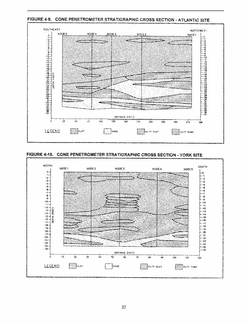
37

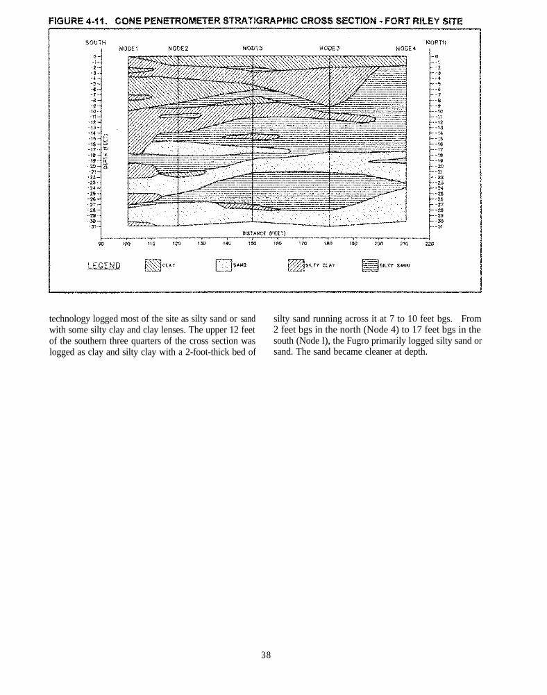
technology logged most of the site as silty sand or sand silty sand running across it at 7 to 10 feet bgs. Fromwith some silty clay and clay lenses. The upper 12 feet 2 feet bgs in the north (Node 4) to 17 feet bgs in theof the southern three quarters of the cross section was south (Node l), the Fugro primarily logged silty sand orlogged as clay and silty clay with a 2-foot-thick bed of sand. The sand became cleaner at depth.

38

Section 5Data Comparison

The data produced by the ROST”’ technology andthe CP was evaluated using the criteria described inSection 1. The qualitative and quantitative dataevaluations are discussed separately. The qualitativeevaluation examined the chemical cross section producedfrom the ROST” data, and stratigraphic cross sectionsproduced from the CP data. The quantitative evaluationstatistically compares the ROSY technology’s data withanalytical data produced by the reference methods.

Qualitative Assessment

The qualitative assessment presents the evaluation ofboth the stratigraphic and chemical mapping potential ofthe ROST” and CP relative to the reference methods.In addition, the potential affects of TOC on the ROW”technology’s measurements are examined. Both thereference and technology cross sections were producedfrom collocated sampling areas as discussed in Section1. Since these methods were sampling spatially differentlocations, matrix heterogeneity will impact thecomparisons of both the physical and chemical crosssections. Based on a review of the demonstration data,this impact appears to have had minimal impact on thequalitative data evaluation. The qualitative nature of thecomparisons, and the level of data quality may havemasked much of the effect of matrix heterogeneity forthis evaluation.

Stratigraphic Cross Sections

The following sections present descriptions of thesimilarities and differences observed between thestratigraphic cross sections produced from the CP dataand the reference method. For this comparison, PRCused the CP sensor cross sections shown in Section 3.These cross sections were produced directly from theindividual stratigraphic logs produced at each node.These cross sections have been produced at the samescale as the reference stratigraphic cross sections shownin Section 2. These comparisons are qualitative and, assuch, are subjective in nature. However, these

comparisons were made by a certified professionalgeologist (American Institute of Professional Geologists)with over 17 years of experience in this field.

Atlantic Site

The cone penetrometer truck subsurface geologicalcross section compared favorably to the referencemethods’ cross section as far as general mapping ofstratigraphy. The CP logged the upper portion of thecross section primarily as clay with several silty claylenses. The corresponding portion of the referencestratigraphic cross section identified this portion as siltyclay and clayey silt with several silt lenses. The depthof the clay and silty clay in the CP cross section variedfrom 19 feet bgs in the northwest (Node 1) to 28 feet bgsin the southeast (Node 5), and the reference cross sectionidentified these same soil textures at 21 in the northwest(Node 1) and 28 feet bgs in the southeast (Node 5).Below 28 feet bgs in the southeast (Node 5) and 19 feetbgs in the northwest (Node 1). the CP cross section ispredominantly sand with silty sand lenses which closelymatches the reference cross section.

At the Atlantic site, the technology showed goodcorrelation with the respective reference geological crosssections. However, one difference was noted. Thereference methods had trouble collecting samples forlogging purposes in the running sands that generallyoccurred from 20 feet bgs to the termination of theborehole. This lack of complete sample recovery iscommon for this method of borehole logging. Theon-site geologist used indirect logging methods, such aslogging drill cuttings or monitoring drilling rates anddown pressure of the drill rig during drilling, to fill inthe resultant gaps in the borehole logs at depth. The CPtechnology does not need to physically collect soilsamples to produce borehole logs, and thus, is not asaffected by running sands. This explains the greaterdetail shown in the CP cross section belowapproximately 20 feet bgs.

3 9

Seven samples were collected at the Atlantic site forgeotechnical analysis. Only six of these samplescorresponded to measured intervals by the CP. Theresults of these analyses were compared to thecorresponding CP stratigraphic data. Three out of thesix samples showed intermethod agreement. The threeremaining samples were not matched due to the CP,once overestimating the fraction of fines (DR19), andtwice underestimating the percentage of sand (DR17 andDR18). This resulted in the CP technology identifyingintervals as silty sand when it was identified by thereference methods as a sand once, and identifying asandy lean clay as a clay or silty clay twice. Thisindicates that the CP technology cannot resolve smallshifts in particle size distribution.

York Site

The CP stratigraphic cross sections showed goodcorrelation with the reference cross sections at the Yorksite. The CP did not identify the surface fill which wasidentified by the reference methods as extending fromthe ground surface to 2 feet bgs. Below this zone, theCP logged primarily clay with several silty sand and siltyclay lenses extending from 12 to 14 feet bgs. Thereference methods logged this section similarly exceptthat the clayey silt extended from 15 to 19 feet bgs. TheCP logged the remainder of the section below 12 feetbgs, on the south side (Node 5), and 14 feet bgs, on thenorth side (Node l), as predominantly silty sand andsand with some silty clay lenses included. The referencemethods identified this same portion of the section aswell graded sand with silt and silty clay and sandy siltlenses. The lack of correlation relative to the thin sand,silt, and clay lenses may be more representative of thereference methods’ inability to resolve thin strata, in astandard field logging mode. The detail of the referencemethod can be increased by spending more timeexamining sample cores, however, time and cost factorsoften prohibit fine detailed examination of sample cores.The CP produces the same level of detail whenever it isused. Running sands were not a problem at this site.

Six samples were collected at the York site forgeotechnical analysis. The results of these analyses werecompared to the corresponding CP stratigraphic data.Four out of the six samples showed intermethodagreement. The remaining two samples were notmatched due to the CP’s lack of resolution relative todetecting small increases in the distribution of coarseparticles (Node l-18.5 to 19 feet bgs and Node 3-16.5to 17 feet bgs). This indicates that the CP has troubleresolving shifts in coarse particle size distribution in amatrix dominated by silts and clays, relative to thereference methods.

Fort Riley Site

The CP’s cross sections showed good correlationwith the reference methods’ cross sections at the FortRiley site. The CP technology logged most of thesection as silty sand or sand with some silty clay andclay lenses as did the reference methods. The upper12 feet of the southern portion of the CP cross section islogged as clay and silty clay with a 2-foot-thick bed ofsilty sand extending from 7 to 10 feet bgs. Thereference methods did not identify the sand layer, ratherit logged it as silty clay, silt and fill.. From 2 feet bgs inthe north (Node 4) to 17 feet bgs in the south (Node l),the CP primarily logged silty sand or sand. Thereference methods logged this as poorly graded sandstarting at 5 feet bgs in the north (Node 4) and extendingto 19 feet bgs in the south (Node 1). The sand logged bythe CP became well graded at depth; this agrees with thereference methods which identified all the sand below17 feet bgs as well graded sand. The CP exhibited afiner resolution of stratigraphy in the saturated sandsidentified at depth. This is similar to the findings at theAtlantic site.

Eight samples were collected at the Fort Riley sitefor geotechnical analysis. The results of these analyseswere compared to the corresponding CP stratigraphicdata. Six of the samples showed acceptable intermethodmatches. The two samples that did not match may haveben caused by the CP’s inability to resolve small changein particle size distributions. The CP identified onesample as a silty clay when the reference methodlaboratory identified the sample as a silty sand or sandyclay and the second sample was identified as a sand bythe CP and as a silty or clay sand with gravel by thereference method (DR02 and DR05, respectively).

Summary

The CP and the reference methods produced similarstratigraphic cross sections relative to the referencemethod. Generally, the CP and the reference methodsshowed good agreement in identifying the dominantparticle size in soil. However, the CP did showdeviation from the reference methods when small shiftsin particle size distribution occurred. However, the CPprovided a finer resolution of strata, identifying morethin stratigraphic units than the reference method. Thisdifference was magnified when running sands wereencountered at the Atlantic and Fort Riley sites. Thismay be due to its ability to continuously acquire soiltextural data during a push, and the common limitationsof a geologist’s logs where strata are less than severalinches thick. An additional difficulty with the referencemethods was their inability to retrieve samples fromrunning sands. This caused significant data gaps at

40

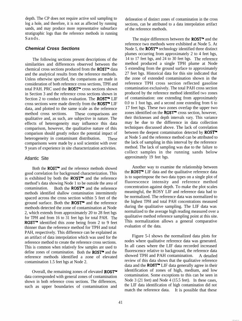
depth. The CP does not require active soil sampling tolog a hole, and therefore, it is not as affected by runningsands, and may produce more representative subsurfacestratigraphic logs than the reference methods in runningS a n d s .

Chemical Cross Sections

The following sections present descriptions of thesimilarities and differences observed between thechemical cross sections produced from the ROSY dataand the analytical results from the reference methods.Unless otherwise specified, the comparisons are made inconsideration of both reference cross sections, TPH andtotal PAH. PRC used the ROST” cross sections shownin Section 3 and the reference cross sections shown inSection 2 to conduct this evaluation. The ROST”” LIFcross sections were made directly from the ROST” LIFdata, and plotted to the same scale as the referencemethod cross sections. These comparisons arequalitative and, as such, are subjective in nature. Theeffects of heterogeneity may influence this datacomparison, however, the qualitative nature of thiscomparison should greatly reduce the potential impact ofheterogeneity in contaminant distribution. Thesecomparisons were made by a soil scientist with over9 years of experience in site characterization activities.

Atlantic Site

Both the ROST” and the reference methods showedgood correlation for background characterization. Thisis exhibited by both the ROST” and the referencemethod’s data showing Node 1 to be outside the area ofcontamination. Both the ROST” and the referencemethods identified shallow contamination intermittentlyspaced across the cross section within 5 feet of theground surface. Both the ROST” and the referencemethods detected the zone of contamination at Node2, which extends from approximately 20 to 28 feet bgsfor TPH and from 16 to 31 feet bgs for total PAH. TheROST” identified this zone being from 2 to 9 feetthinner than the reference method for TPH and totalPAH, respectively. This difference can be explained asan artifact of data interpolation which was used for thereference method to create the reference cross sections.This is common when relatively few samples are used todefine zones of contamination. Both the ROSY and thereference methods identified a zone of elevatedcontamination 1.5 feet bgs at Node 2.

Overall, the remaining zones of elevated ROST”data corresponded with general zones of contaminationshown in both reference cross sections. The differences,such as upper boundaries of contamination and

delineation of distinct zones of contamination in the crosssections, can be attributed to a data interpolation artifactof the reference methods.

The major differences between the ROST” and thereference two methods were exhibited at Node 5. AtNode 5, the ROSY technology identified three distinctplumes occurring from approximately 2 to 4 feet bgs,14 to 17 feet bgs, and 24 to 30 feet bgs. The referencemethod produced a single TPH plume at Node5 extending from the ground surface to approximately27 feet bgs. Historical data for this site indicated thatthe zone of extended contamination shown in thereference TPH cross section reflected gasolinecontamination exclusively. The total PAH cross sectionproduced by the reference method identified two zonesof contamination: one extending from approximately0.0 to 1 foot bgs, and a second zone extending from 6 to17 feet bgs. These two zones overlap the upper twozones identified on the ROSY cross section, however,their thicknesses and depth intervals vary. This variancemay be due to the difference in data collectiontechniques discussed above. The lack of correlationbetween the deepest contamination detected by ROST”at Node 5 and the reference method can be attributed tothe lack of sampling in this interval by the referencemethod. The lack of sampling was due to the failure tocollect samples in the running sands belowapproximately 19 feet bgs.

Another way to examine the relationship betweenthe ROW“ LIF data and the qualitative reference datais to superimpose the two data types on a single plot offluorescence intensity and reference methodconcentration against depth. To make the plot scalesmeaningful, the ROSY LIF and reference data had tobe normalized. The reference data was normalized tothe highest TPH and total PAH concentrations measuredduring the qualitative sampling. The LIF data wasnormalized to the average high reading measured over aqualitative method reference sampling point at this site.This normalization allows a general comparativeevaluation of the data.

Figure 5-l shows the normalized data plots fornodes where qualitative reference data was generated.In all cases where the LIF data recorded increasedfluorescence relative to background, the reference datashowed TPH and PAH contamination. A detailedreview of this data shows that the qualitative referencedata and the ROSY LIF data generally agree in theiridentification of zones of high, medium, and lowcontamination. Some exceptions to this can be seen inNode 3 (21 feet) and Node 4 (15.5 feet). In these cases,the LIF data identification of high contamination did notmatch the reference data. It is possible that these

41

differences are due to matrix heterogeneity and/or slighterrors in relative sampling depth recording.

York Site

The ROW” cross section showed little correlationto the reference method’s cross sections at Node 1. TheROST” technology only detected contamination from0 to 1 foot bgs at this node, however, the referencemethod detected both TPH and total PAH contaminationfrom 12 to 18 feet bgs at this node.

Nodes 2, 3, 4, and 5 showed better correlationbetween the reference methods’ cross sections and theROSTn cross section.

The differences between the reference cross sectionand the ROST” cross section could be the combinationof an artifact of data interpolation for the reference crosssection, and the finer definition provided by ROST”which produces continuous profiles with a 2 cmresolution. The variation between the ROST”’ andreference methods cross sections could also be attributedto the small sample volume used by the ROSTntechnology relative to the reference method.

Figure 5-2 shows the normalized line graphs of thefive ROSY LIF pushes at the York site.

In all but one case, the LIF data exhibited elevatedfluorescence relative to background, at the point wherequalitative reference data reported TPH or total PAHcontamination above background. At Node 4 (18.5 feetbgs), the reference data reported TPH and total PAHcontamination at 100 percent and 80 percent of thehighest reading, while the LIF data detected nofluorescence above background. The reference TPHconcentration was 13,000 ppm, and the total PAHconcentration was 1,130 ppm. The reference samplingpoint and the LIF sampling point was separatedhorizontally by approximately 2 feet. An examination ofthe corresponding CP log shows that at this LIFsampling interval the LIF window was measuringfluorescence inside a clay seam. It is possible that thisclay lens has resisted contaminant infiltration, supportingthe LIP data showing no comamination. This illustratesthe value of the combined LIF and CP data. The highcontamination detected by the reference sampling mayreflect its larger sample volume and samplehomogenization, or heterogeneity in the geometry of theclay lens.

A detailed review of the remaining data shows thatthe relative magnitudes between the two types of datawere in agreement. Zones of high reference readingscorresponded to zones of high LIF readings. Thisrelationship appears to hold for medium and low zonesof contamination.

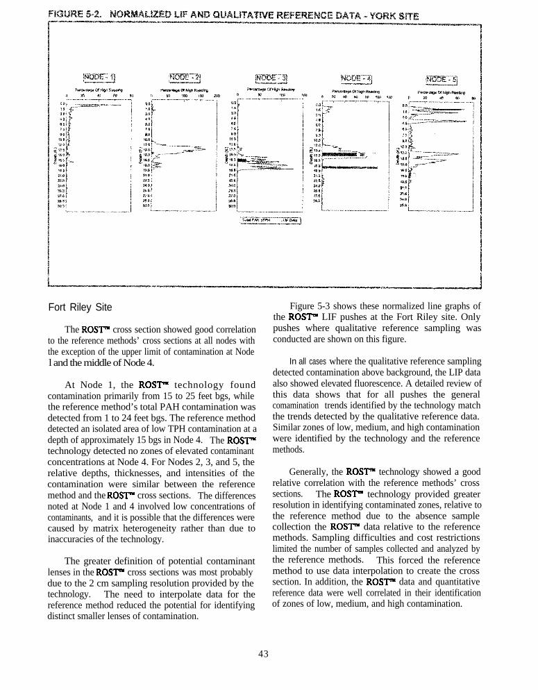
Fort Riley Site

The ROSY cross section showed good correlationto the reference methods’ cross sections at all nodes withthe exception of the upper limit of contamination at Nodel and the middle of Node 4.

At Node 1, the ROSY technology foundcontamination primarily from 15 to 25 feet bgs, whilethe reference method’s total PAH contamination wasdetected from 1 to 24 feet bgs. The reference methoddetected an isolated area of low TPH contamination at adepth of approximately 15 bgs in Node 4. The ROSFtechnology detected no zones of elevated contaminantconcentrations at Node 4. For Nodes 2, 3, and 5, therelative depths, thicknesses, and intensities of thecontamination were similar between the referencemethod and the ROSY cross sections. The differencesnoted at Node 1 and 4 involved low concentrations ofcontaminants, and it is possible that the differences werecaused by matrix heterogeneity rather than due toinaccuracies of the technology.

The greater definition of potential contaminantlenses in the ROST” cross sections was most probablydue to the 2 cm sampling resolution provided by thetechnology. The need to interpolate data for thereference method reduced the potential for identifyingdistinct smaller lenses of contamination.

Figure 5-3 shows these normalized line graphs ofthe ROST” LIF pushes at the Fort Riley site. Onlypushes where qualitative reference sampling wasconducted are shown on this figure.

In all cases where the qualitative reference samplingdetected contamination above background, the LIP dataalso showed elevated fluorescence. A detailed review ofthis data shows that for all pushes the generalcomamination trends identified by the technology matchthe trends detected by the qualitative reference data.Similar zones of low, medium, and high contaminationwere identified by the technology and the referencemethods.

Generally, the ROSF technology showed a goodrelative correlation with the reference methods’ crosssections. The ROW” technology provided greaterresolution in identifying contaminated zones, relative tothe reference method due to the absence samplecollection the ROW” data relative to the referencemethods. Sampling difficulties and cost restrictionslimited the number of samples collected and analyzed bythe reference methods. This forced the referencemethod to use data interpolation to create the crosssection. In addition, the ROW” data and quantitativereference data were well correlated in their identificationof zones of low, medium, and high contamination.

43

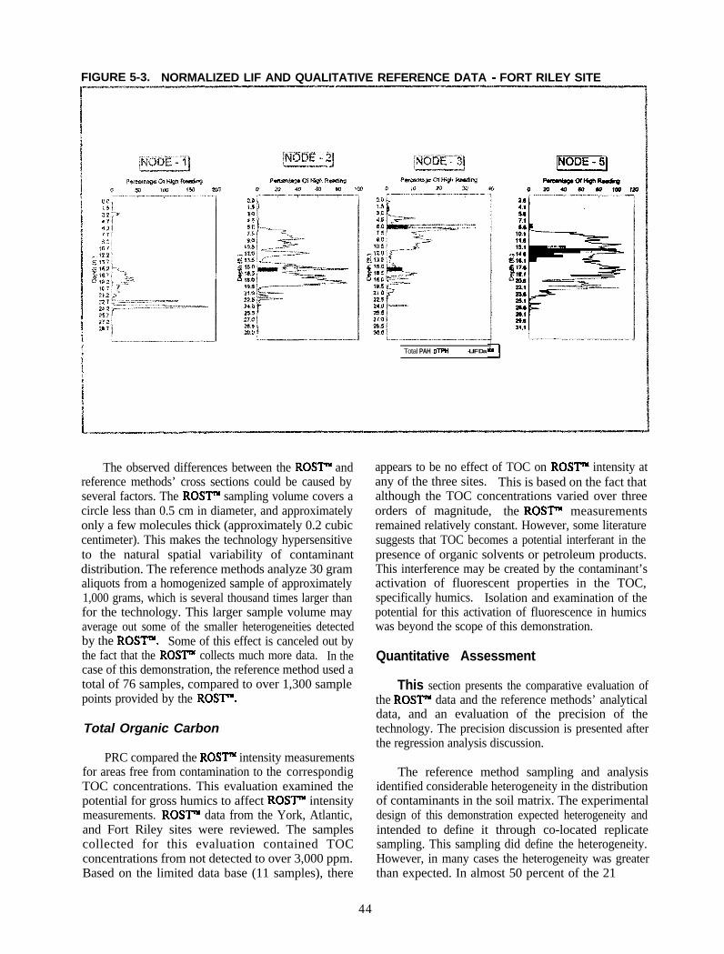
FIGURE 5-3. NORMALIZED LIF AND QUALITATIVE REFERENCE DATA - FORT RILEY SITE

Total PAH OTPti -LIF Da

The observed differences between the ROW” andreference methods’ cross sections could be caused byseveral factors. The ROW” sampling volume covers acircle less than 0.5 cm in diameter, and approximatelyonly a few molecules thick (approximately 0.2 cubiccentimeter). This makes the technology hypersensitiveto the natural spatial variability of contaminantdistribution. The reference methods analyze 30 gramaliquots from a homogenized sample of approximately1,000 grams, which is several thousand times larger thanfor the technology. This larger sample volume mayaverage out some of the smaller heterogeneities detectedby the ROST”. Some of this effect is canceled out bythe fact that the ROST”’ collects much more data. In thecase of this demonstration, the reference method used atotal of 76 samples, compared to over 1,300 samplepoints provided by the ROS’I”‘.

Total Organic Carbon

PRC compared the ROST” intensity measurementsfor areas free from contamination to the correspondigTOC concentrations. This evaluation examined thepotential for gross humics to affect ROST” intensitymeasurements. ROST’“’ data from the York, Atlantic,and Fort Riley sites were reviewed. The samplescollected for this evaluation contained TOCconcentrations from not detected to over 3,000 ppm.Based on the limited data base (11 samples), there

44

appears to be no effect of TOC on ROW” intensity atany of the three sites. This is based on the fact thatalthough the TOC concentrations varied over threeorders of magnitude, the ROSTn measurementsremained relatively constant. However, some literaturesuggests that TOC becomes a potential interferant in thepresence of organic solvents or petroleum products.This interference may be created by the contaminant’sactivation of fluorescent properties in the TOC,specifically humics. Isolation and examination of thepotential for this activation of fluorescence in humicswas beyond the scope of this demonstration.

Quantitative Assessment

This section presents the comparative evaluation ofthe ROST” data and the reference methods’ analyticaldata, and an evaluation of the precision of thetechnology. The precision discussion is presented afterthe regression analysis discussion.

The reference method sampling and analysisidentified considerable heterogeneity in the distributionof contaminants in the soil matrix. The experimentaldesign of this demonstration expected heterogeneity andintended to define it through co-located replicatesampling. This sampling did define the heterogeneity.However, in many cases the heterogeneity was greaterthan expected. In almost 50 percent of the 21 quan-

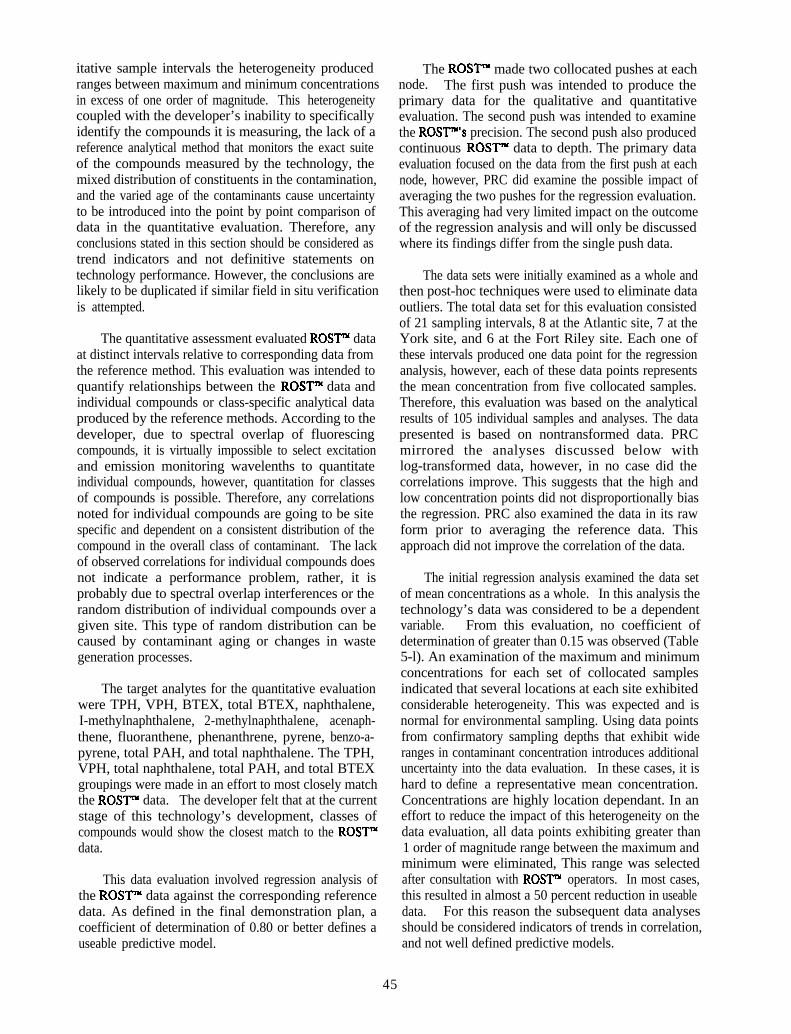
itative sample intervals the heterogeneity producedranges between maximum and minimum concentrationsin excess of one order of magnitude. This heterogeneitycoupled with the developer’s inability to specificallyidentify the compounds it is measuring, the lack of areference analytical method that monitors the exact suiteof the compounds measured by the technology, themixed distribution of constituents in the contamination,and the varied age of the contaminants cause uncertaintyto be introduced into the point by point comparison ofdata in the quantitative evaluation. Therefore, anyconclusions stated in this section should be considered astrend indicators and not definitive statements ontechnology performance. However, the conclusions arelikely to be duplicated if similar field in situ verificationis attempted.

The quantitative assessment evaluated ROST” dataat distinct intervals relative to corresponding data fromthe reference method. This evaluation was intended toquantify relationships between the ROW” data andindividual compounds or class-specific analytical dataproduced by the reference methods. According to thedeveloper, due to spectral overlap of fluorescingcompounds, it is virtually impossible to select excitationand emission monitoring wavelenths to quantitateindividual compounds, however, quantitation for classesof compounds is possible. Therefore, any correlationsnoted for individual compounds are going to be sitespecific and dependent on a consistent distribution of thecompound in the overall class of contaminant. The lackof observed correlations for individual compounds doesnot indicate a performance problem, rather, it isprobably due to spectral overlap interferences or therandom distribution of individual compounds over agiven site. This type of random distribution can becaused by contaminant aging or changes in wastegeneration processes.

The target analytes for the quantitative evaluationwere TPH, VPH, BTEX, total BTEX, naphthalene,I-methylnaphthalene, 2-methylnaphthalene, acenaph-thene, fluoranthene, phenanthrene, pyrene, benzo-a-pyrene, total PAH, and total naphthalene. The TPH,VPH, total naphthalene, total PAH, and total BTEXgroupings were made in an effort to most closely matchthe ROST” data. The developer felt that at the currentstage of this technology’s development, classes ofcompounds would show the closest match to the ROST”data.

This data evaluation involved regression analysis ofthe ROST” data against the corresponding referencedata. As defined in the final demonstration plan, acoefficient of determination of 0.80 or better defines auseable predictive model.

The ROST” made two collocated pushes at eachnode. The first push was intended to produce theprimary data for the qualitative and quantitativeevaluation. The second push was intended to examinethe ROST”‘s precision. The second push also producedcontinuous ROST”” data to depth. The primary dataevaluation focused on the data from the first push at eachnode, however, PRC did examine the possible impact ofaveraging the two pushes for the regression evaluation.This averaging had very limited impact on the outcomeof the regression analysis and will only be discussedwhere its findings differ from the single push data.

The data sets were initially examined as a whole andthen post-hoc techniques were used to eliminate dataoutliers. The total data set for this evaluation consistedof 21 sampling intervals, 8 at the Atlantic site, 7 at theYork site, and 6 at the Fort Riley site. Each one ofthese intervals produced one data point for the regressionanalysis, however, each of these data points representsthe mean concentration from five collocated samples.Therefore, this evaluation was based on the analyticalresults of 105 individual samples and analyses. The datapresented is based on nontransformed data. PRCmirrored the analyses discussed below withlog-transformed data, however, in no case did thecorrelations improve. This suggests that the high andlow concentration points did not disproportionally biasthe regression. PRC also examined the data in its rawform prior to averaging the reference data. Thisapproach did not improve the correlation of the data.

The initial regression analysis examined the data setof mean concentrations as a whole. In this analysis thetechnology’s data was considered to be a dependentvariable. From this evaluation, no coefficient ofdetermination of greater than 0.15 was observed (Table5-l). An examination of the maximum and minimumconcentrations for each set of collocated samplesindicated that several locations at each site exhibitedconsiderable heterogeneity. This was expected and isnormal for environmental sampling. Using data pointsfrom confirmatory sampling depths that exhibit wideranges in contaminant concentration introduces additionaluncertainty into the data evaluation. In these cases, it ishard to define a representative mean concentration.Concentrations are highly location dependant. In aneffort to reduce the impact of this heterogeneity on thedata evaluation, all data points exhibiting greater than1 order of magnitude range between the maximum andminimum were eliminated, This range was selectedafter consultation with ROW’” operators. In most cases,this resulted in almost a 50 percent reduction in useabledata. For this reason the subsequent data analysesshould be considered indicators of trends in correlation,and not well defined predictive models.

45

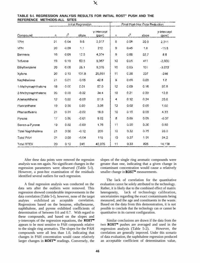
TABLE 5-l. REGRESSION ANALYSIS RESULTS FOR INITIAL ROST” PUSH AND THEREFERENCE METHODS-ALL SITES

After these data points were removed the regressionanalysis was nm again. No significant changes in theregression parameters were observed (Table 5-l).However, a post-hoc examination of the residualsidentified several outliers for each regression.

A final regression analysis was conducted on thedata sets after the outliers were removed. Thisregression showed considerable improvements in thedata correlation (Table 5-l), however, none of the targetanalytes exhibited an acceptable correlation.Regressions based on the benzene, ethylbenzene,naphthalene, and pyrene exhibited coefficients ofdetermination of between 0.6 and 0.7. With regard tothese compounds, and based on the slopes andy-intercepts of the regression equations, the ROSY”appears to be most sensitive to PAH compounds relativeto the single ring aromatics. The slopes for the PAHcompounds were all less than 1.0, indicating thatchanges in PAH concentration would cause relativelylarger changes in ROSY readings. Conversely, the

slopes of the single ring aromatic compounds weregreater than one, indicating that a given change incontaminant concentration would cause a relativelysmaller change in ROST”’ measurements.

The lack of correlation for the quantitativeevaluation cannot be solely attributed to the technology.Rather, it is likely due to the combined effect of matrixheterogeneity, lack of technology calibration,uncertainties regarding the exact contaminants beingmeasured, and the age and constituents in the waste.Based on the data from this demonstration, it is notpossible to conclude that the technology can or cannot bequantitative in its current configuration.

Similar conclusions are drawn if the data from thetwo ROST” pushes are averaged and used in theregression analysis (Table 5-2). However, thecorrelations are generally improved. Under this scenarioof data evaluation, the naphthalene regression producedan acceptable coefficient of determination value,

46

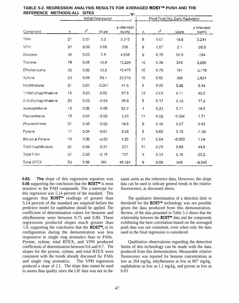
TABLE 5-2. REGRESSION ANALYSIS RESULTS FOR AVERAGED ROSTTM PUSH AND THEREFERENCE METHODS-ALL SITES *II*-

-

0.83. The slope of this regression equation was0.06 supporting the conclusion that the ROST” is mostsensitive to the PAH compounds. The y-intercept forthis regression was 5.14 percent of the standard. Thissuggests that ROST” readings of greater than5.14 percent of the standard are required before thepredictive model for naphthalene should be applied. Thecoefficient of determination values for benzene andethylbenzene were between 0.75 and 0.80. Theseregressions produced slopes much greater than1.0, supporting the conclusion that the ROW“, in itsconfiguration during the demonstration was lessresponsive to single ring aromatics than to PAHs.Pyrene, xylene, total BTEX, and VPH producedcoefficients of determination between 0.6 and 0.7. Theslopes for the pyrene, xylene, and total BTEX wereconsistent with the trends already discussed for PAHsand single ring aromatics. The VPH regressionproduced a slope of 2.1. The slope data carnnot be usedto assess data quality since the LIF data was not in the

same units as the reference data. However, the slopedata can be used to indicate general trends in the relativefluorescence, as discussed above.

The qualitative determination of a detection limit orthreshold for the RON”” technology was not possiblegiven the data produced from this demonstration.Review, of the data presented in Table 5-2 shows that therelationship between the ROSY data and the compoundsexhibiting the best correlation based on the averagedpush data was not consistent, even when only the dataused in the final regression is considered.

Qualitative observations regarding the detectionlimits of this technology can be made with the dataproduced from this demonstration. Measurable relativefluorescence was reported for benzene concentrations aslow as 264 mg/kg, ethylbenzene as low as 807 mg/kg,naphthalene as low as 1.1 mg/kg, and pyrene as low as0.03 mg/kg.

47

ROST” reported negative relative fluorescence fortwo quantitative samples. For these samples, ROSrYreported a relative fluorescence of -1.37 and-0.20 (Table 5-3). These readings are equivalent to zerofluorescence. The reference methods indicated thatthese intervals contained measurable concentrations ofthese four compounds (Appendix A). The ROST”reading of -1.37 occurred at a sample interval thatcontained, at its minimum, total PAH, TPH, and VPHconcentrations of 799 ppm, 1,878 ppm, and 175 ppm,respectively. The ROST” reading of -0.20 occurred ata sample interval that contained, at its minimum,concentrations of total PAH, TPH, and VPH of 31 ppm,1,416 ppm, and 1,102 ppm, respectively. This could beinterpreted as false correlation based on the averagedpush data was not consistent, even when only the dataused in the final regression is considered. Increases inrelative negative readings. Two false negatives out of21 sample points equates to a false negative rate of10 percent.

Another qualitative method for assigning a detectionthreshold is to determine the relative fluorescence at thex-intercept for the benzene, ethylbenzene, naphthalene,(based on averaged pushes) and pyrene regressionmodels discussed above. The x-intercept represents the0 mg/kg point on the fluorescence versus concentrationgraph. For the benzene and ethylbenzene the relativefluorescence intensity at the x-intercept was -0.17 and21, respectively. For the naphthalene and pyrene therelative fluorescence at the x-intercept was 85 and4, respectively.

To examine the potential for site-induced affects onthe data evaluation, the data was divided by site andregression analyses were nm on the resultant three datasets. This regression analysis began with data setswhose gross outliers had been removed. These outlierswere defined as data points where the maximum andminimmn values varied by over one order of magnitude.

This site-specific regression showed the following:xylene, naphthalene, pyrene, and total PAH regressionsexhibited acceptable correlations (3 greater than0.80) at the Atlantic site; no compounds showedacceptable correlations at the York site; and acceptablecorrelations were exhibited for VPH, naphthalene, andtotal BTEX at the Fort Riley site. The number ofsamples resulting in these acceptable correlations rangedfrom 3 to 5, out of a maximum of 6 to 8. This smallsample set greatly limits the use of this data to formpredictive models. However, these regressions exhibitedthe same trends in their slopes, as exhibited in the dataset as a whole. The slopes for the PAHs were all less

than 1.0, and the single ring aromatic compoundsproduced regression equations with slopes greater than1.0.

The potential causes other than sample matrixeffects such as heterogeneity, of the relatively poorcorrelations of ROST”” data to reference data seenduring this demonstration were examined. The FVDwavelengths used for emission wavelength monitoringmay have affected the comparability of the ROST” datato the reference method data. ROST” utilized an FVDwavelength of 400 nm for the Atlantic and York sites,and 360 mn for the Fort Riley site. ROST” explainedthat 400 nm would provide the best FVD-monitoringwavelength for coal tar-contaminated sites, and that360 nm would provide the best FVD-monitoringwavelength for petroleum-contaminated sites. To assessthe use of these wavelengths, WTMs were compared tothe emission monitoring wavelengths used at each site.It was observed that the WTMs from the Atlantic andYork sites produced maximum fluorescence intensities atgreater wavelengths than the ones used for the emissionwavelength monitoring. This means that the ROST”was not monitoring the wavelength which exhibited thegreatest fluorescence intensity. For fluorescencemethods the wavelengths of the greatest fluorescenceintensity provides the most accurate and linear results.By not monitoring at the wavelength of maximumfluorescence intensity the ROST”” was monitoring on therising or falling limbs of the fluorescence wave forms ofthe primary fluorescing contaminant. In this area,similar to a side slope of a hill or mountain, large shiftsin the fluorescence intensity of the contaminant matrixcould result in relatively smaller changes in measuredfluorescence.

According to the developers, saturation effects forthe detection system used in the ROST” do not appearuntil soil contamination exceeds approximately1,000 ppm. These effects could result in inaccurate LIFdata. This type of error would only impact the mostcontaminated areas seen during this demonstration, andit would result in underestimates of contamination. It islikely that the areas of contamination potentially causingthis effect would be identified as grossly contaminatedeven with underestimated LIF results. ROST” wasmonitoring the rising and falling arm of the fluorescencewave form, and therefore, was not monitoring thewavelength of maximum fluorescence intensity thatshould produce the most accurate and linear results.

A related problem was noted concerning thecalibration procedures employed by ROST”. ROST”performed calibration before each CP push by placing asolution of 10,000 pg/mL gasoline over the sapphire

48

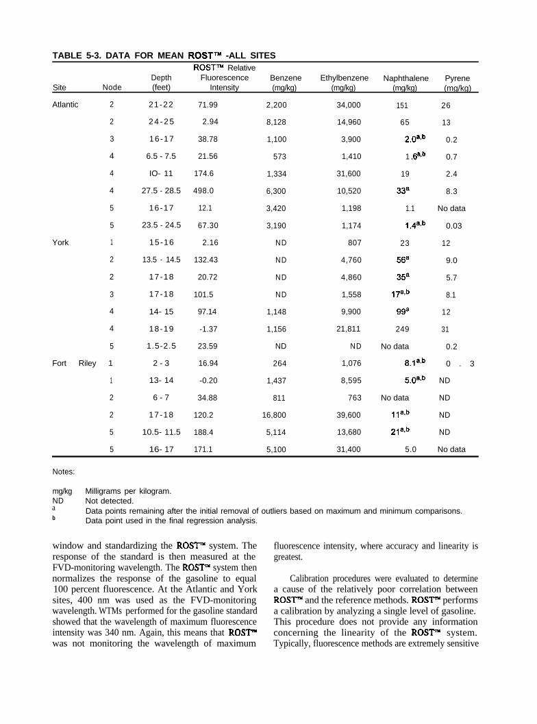
TABLE 5-3. DATA FOR MEAN ROSTTM -ALL SITES

Site NodeDepth(feet)

ROSTTM RelativeFluorescence Benzene Ethylbenzene Naphthalene Pyrene

Intensity (mg/kg) (mg/kg) (mg/kg) (mg/kg)

Atlantic 2 21-22

2 2 4 - 2 5

3 16-17

4 6.5 - 7.5

4 IO- 11

4 27.5 - 28.5

5 16-17

5 23.5 - 24.5

York 1 15-16

2 13.5 - 14.5

2 17-18

3 17-18

4 14- 15

4 18-19

5 1.5-2.5

Fort Riley 1 2 - 3

1 13- 14

2 6 - 7

2 17-18

5 10.5- 11.5

5 16- 17

71.99

2.94

38.78

21.56

174.6

498.0

12.1

67.30

2.16

132.43

20.72

101.5

97.14

-1.37

23.59

16.94

-0.20

34.88

120.2

188.4

171.1

2,200 34,000

8,128 14,960

1,100 3,900

573 1,410

1,334 31,600

6,300 10,520

3,420 1,198

3,190 1,174

ND 807

ND 4,760

ND 4,860

ND 1,558

1,148 9,900

1,156 21,811

ND ND

264 1,076

1,437 8,595

811 763

16,800 39,600

5,114 13,680

5,100 31,400

151 26

65 13

2.oa*b 0.2

1 .6aeb 0.7

19 2.4

33a 8.3

1.1 No data

1.4a*b 0.03

23 12

56a 9.0

35a 5.7

17avb 8.1

99a 12

249 31

No data 0.2

8.1asb 0 . 3

5.0asb ND

No data ND

1W ND

2w ND

5.0 No data

Notes:

mg/kg Milligrams per kilogram.ND Not detected.ab

Data points remaining after the initial removal of outliers based on maximum and minimum comparisons.Data point used in the final regression analysis.

window and standardizing the ROW” system. Theresponse of the standard is then measured at theFVD-monitoring wavelength. The ROST” system thennormalizes the response of the gasoline to equal100 percent fluorescence. At the Atlantic and Yorksites, 400 nm was used as the FVD-monitoringwavelength. WTMs performed for the gasoline standardshowed that the wavelength of maximum fluorescenceintensity was 340 nm. Again, this means that ROST”was not monitoring the wavelength of maximum

fluorescence intensity, where accuracy and linearity isgreatest.

Calibration procedures were evaluated to determinea cause of the relatively poor correlation betweenROST” and the reference methods. ROSP performsa calibration by analyzing a single level of gasoline.This procedure does not provide any informationconcerning the linearity of the ROW” system.Typically, fluorescence methods are extremely sensitive

49

and linear over a wide range, a l,OOO-fold or greaterlinear range is not uncommon. However, fluorometryis limited to low concentrations.

Inherent instrument precision for the ROST”measurements at the York, Atlantic, and Fort Riley siteswas evaluated by calculating the percent relativestandard deviation (%RSD) of each set of11 measurements for each depth sampled. Replicatemeasurements were taken at three separate nodes at theAtlantic and Fort Riley sites and at only one node at the

York site. The precision measurements taken at theAtlantic and Fort Riley sites were at a total of five andfour different depths, respectively. The York site onlyhad one depth sampled. The %RSD was calculated bydividing the standard deviation from the 11 replicatemeasurements by the mean. This number is multipliedby 100. The maximum inherent instrument precision atthe York, Atlantic, and Fort Riley sites was 4.1, 3.5,and 1.7, respectively. Based on this data, the standarddeviations are most likely due to heterogeneity incontaminant distribution.

50

Section 6Applications Assessment

The ROSY technology is only available as aservice from the developers and it is designed to beoperated by trained technicians. The ROST”’ doesrequire some type of platform to advance the sensor intothe ground. Currently, this is done with a conepenetrometer truck either provided by the developers orby the customer. The ROST” is designed to becompatible with most standard cone penetrometer trucks.This technology has been tested at a variety of militaryand industrial installations, and as of the date of thisreport, it has been used for several commercial sitecharacterizations. As demonstrated, this technology canrapidly acquire data defining zones of generalcontamination, as long as the contamination has afluorescent signature. This data can greatly facilitate sitecharacterization activities.

During this demonstration, the cost of thistechnology, including a CP sensor, was less than thereference methods used to produce the qualitative data.The LIF sensor and CP sensor produced far more datain real-time, resulting in improved physical and chemicalresolution relative to the reference method. However,this improved resolution and real-time data was at alower level of data quality (screening versus definitive).

The qualitative assessment portion of this demon-stration showed that this technology is comparable toreference methods in its ability to map subsurfacecontaminant plumes at petroleum fuel and coal tarcontamination sites. This demonstration showed thatboth ROST” and the reference methods identifiedsimilar zones of subsurface petroleum and coal tarcontamination at each of the three demonstration sites.Many of the differences between the ROSY and thereference methods can be explained by their respectivemethods of data collection. The ROST” produces acontinuous profile, while the reference methods take afew selective samples targeting boundaries and zones ofcontamination. In addition, the reference methods haddifficulty retrieving samples in running sands, addingpotential data gaps. The ROSY technology producedrelatively continuous data on petroleum and coal tar

contaminant distribution over a 30-foot depth inapproximately 1.5 hours during the demonstration. Thereference methods would be able to collect samples overthis interval, however, definitive analytical serviceswould require, at best, several days. Even if thereference methods used on-site analysis, and producedonly screening level data, it would take several hours toprovide data on the samples. Therefore, on-time criticalprojects that can use screening level data, or on projectswhere it is more critical to cover large areas in greaterdetail, the ROST”” technology seems appropriate.

Another powerful aspect of this technology is that itcan be advanced with a standard CP to providecontinuous descriptions of the subsurface soilconcurrently with the chemical data. This demonstrationfound that the subsurface logging capabilities of the CPwere comparable to the reference methods. Similaritiesbetween the two data sets were observed even withoutsite-specific borings to calibrate the CP logging toolprior to deployment. The major limitation of the CPlogging was its apparent inability to detect slight shifts inparticle size distribution. It is questionable if thislimitation would greatly impact the use of the data. Forexample, a silt and clayey silt would probably be dealtwith similarly in a hydrogeological perspective.

The quantitative data assessment for this technologyindicated that the ROST” data was most correlated tonaphthalene concentrations. The small data set sizeslimit the use of the predictive model (created from theregression analysis). Any predictive model should bebased on site-specific calibration and confirmation. Theregression analysis showed some correlation between thetechnology’s results and individual compounds. Thetechnology’s data was not well correlated to TPH andVPH measurements (.07 and .67, respectively). Thegenerally poor correlation with the quantitative data fromclasses of compounds may be partially due to matrixheterogeneity, analytical limitations of the referencemethods, ROST’” calibration procedures, and theemission monitoring wavelengths used by the ROSYduring the demonstration. Basically, the calibration and

51

emission wavelength selection were not optimum for thesite-specific classes of contaminants. This apparentlydid not greatly affect the qualitative evaluation, only thequantitative evaluation. This is consistent with thecurrent evolutionary stage of this technology at the timeof the demonstration in August 1994. The identificationof individual compounds is not a current application ofthis technology. However, the collection of WTM dataallows the ROST” to identify changes in constituentcompostion, and in many cases, allows ROST”’ toidentify types of contaminants such as diesel fuel,gasoline, jet fuel, and coal tar. Thii capability can assistin the identification and attribution of contaminantsources.

Based on the results of this demonstration, the useof site-specific calibration samples for the application ofROST” may be of most value in determining emissionmonitoring wavelengths and possibly in calibrationactivities. Future development of this technology mayallow this type of calibration for quantitation (see Section7). The effects of site-specific calibration samples forthe ROST” was not evaluated during this demonstration.Site-specific calibration may allow a more representativeestimation of contaminant concentration distribution. Inother words, with this type. of calibration, perhaps theROST” data would exhibit more similar trends to thereference method data, for example, as the contaminantconcentrations increase or decrease, the ROST”’ datawould show a more consistent relationship relative toincreases or decreases in contaminant concentration.

Based on this demonstration, this technology appearsto produce screening level data. The lack of bettercorrelations may not be wholly attributable to thetechnology performance, rather it may have been due tothe relatively small reference method data set size, thelack of a reference method that measures the same suiteof compounds as the ROST” sensor monitors, thecomplex interactions between the fluorescingcompounds, and the soil matrix which resulted in theobserved heterogeneity. The first two factors can beaddressed with changes in experimental design andinnovations in analytical methods, however, the finalfactors will require more research to isolate specificmatrix interactions and to resolve the heterogeneityissue.

If this technology, in the configuration demon-strated, is to be evaluated in the field, this demonstrationhas shown that on a point-by-point quantitative basis, itis unlikely that significant correlation to reference datawill be observed. This is due to a combination ofheterogeneity effects, limitations in conventionalsampling and analysis, and the complex interaction ofwaste aging and constituent distribution of relativefluorescence. It is possible that site-specific calibrations,

different reference analytical methods, alternativesampling methods, or a less heterogeneous matrix wouldimprove the potential for significant correlation betweenROSTT and the reference method data. Therefore,based on the results of this demonstration, fieldevaluations of this technology should be restricted toqualitative evaluations consisting of cross sectioncomparisons of simply verifying that LIF highscorrespond to higher levels of contamination. This lattercomparison will also be affected by effects listed above.

Although there are many advantages to thistechnology, a potential user should be aware of potentialdisadvantages. This technology has a sampling volumeseveral thousand times smaller than conventionalsampling analysis. This makes the technology verysensitive to matrix heterogeneity. Some of thissensitivity is reduced (vertically) by the averaging offifty data points every 2 cm. This affect can also beminimized by the sampling of more push locations toreduce the sensitivity in a horizontal orientation. At adata collection rate of approximately 300 linear feet perday (4,572 data points), additional pushes can beconducted without greatly increasing project duration.The LIF results can be influenced by the age andconstituent distribution of wastes. This fact coupled withheterogeneity effects, and a lack of site-specificinstrument calibration, makes field verification of LIFresults difficult. The use of the LIF and CP sensors isrestricted to the maximum push depth of the conepenetrometer truck. This depth can be as much as300 feet, or in the case of the demonstration, 30 to70 feet. These shallow depths were realized whendeeper strata exhibited increased cone tip resistance andsleeve friction, and at location where strata at shallowerdepths would not provide adequate lateral support for thepush rod. These conditions greatly increase the chancefor push rod breakage and sensor loss.

This technology can currently provide rapidassessment of the distribution of fluorescent material inthe subsurface. When these materials are PAHs orpetroleum fuels, the technology can be used to map theextent of subsurface contamination. The WTM data canalso be used to provide qualitative identification of wastetype or at a minimum, it can identify changes inconstituent distributions. All of this dam can be used toguide critical conventional soil sampling, and theplacement of groundwater monitoring wells. All of thisdata can be produced and interpreted in the field. Thisreal-time sampling and analysis allows the use ofcontingency based sampling, which assists incharacterizing a site with a single mobilization. Theseaspects coupled with its low waste production duringdecontamination make this technology a powerful andeffective site characterization tool.

52

Section 7Developer Comments and Technology Update

The developers of the ROST” technology submittedboth editorial and technical comments on the draft ITER.Only comments not resulting in changes to the report arepresented below. The technical comments are presentedverbatim in italics. The response to the comments ispresented below each developer comment in plain type.

Loral Comments (April 1995)

1. Complications caused by spatial inhomogeneity.The statistics of the quantitative sampling, shown inTable 7-1, emphasize how large are the variances in thechemical concentrations obtained by the referencemethods. The RSD is greater than 50% for 17 of the21 (81 %) quantitative evaluation sampling intervals, andgreater than 100% for 12 of the 21 (57%) intervals. Atthe 99-percent confidence level only three of the21 locations for quantitative evaluation give TPHconcentrations different from zero.

We feel that the draft report minimizes thedifficulties posed by the heterogeneity problem and, moresignificantly. fails properly to take it into account in thequantitative evaluation of ROST”s performance. Frompage 4-10 of the draft ITER; “An examination of themaximum and minimum concentration for each set ofcollocated samples indicated that several locations ateach site exhibited considerable heterogeneity. This wasexpected and is normal for environmental sampling.Using data points from confirmatory sampling depthsthat exhibit wide ranges in contaminant concentrationintroduces additional uncertainty into the dataevaluation. In these cases, it is hard to define arepresentative mean concentrarion. Concentrations arehighly location dependent (sic). In an effort to reducethe impact of the heterogeneity on the data evaluation,all data points exhibiting greater than 1 order ofmagnitude range between the maximum and minimumwere eliminated. This range was selected afierconsultation with ROSTm operators. In most cases, thisresulted in almost a 50percent reduction in usable data.For this reason the subsequent data analyses should be

considered indicators of trends in correlation, and notwell defined predictive models. "

We are troubled by several things. In the firstplace, the “ROST” operations” were not consultedabout eliminating data points on the basis or rangebetween minimum and maximum. To state that weagreed with this procedure is untrue. We don’t believethat this method of rejecting data is statistically valid. Itis also unclear whether the procedure was to reject alljive values (for the set of five collocated samples) or justthose that led to more than an order of magnitudevariation. Note that the rejection criterion eliminatesNode 4, 6.5-7.5 feet at the Atlantic site with a RSD of65 percent (one of the lower values) and retains Node4, 14-15 feet at York with a RSD of 104 percent.

PRC consulted both ROST” and SCAPSrepresentatives regarding the elimiition of data points.PRC conducted the initial data review for thequantitative evaluation based on the entire data set. Thisinitial data review showed no correlation between thetechnology’s results and the reference method data. Inaddition, PRC noted that several data points exhibitedconsiderable spatial variation. To reduce the impact ofthe observed spatial variability, PRC conducted a post-hoc review of the raw data in an attempt to identifypoints that showed the greatest spatial variability. PRCreviewed th e 99 percent confidence intervals around themean concentrations for the quantitative data. In manycases, the confidence intervals ranged into negativeconcentrations on the low ends, and at both the high andlow ends were far more extreme thau actually measured.PRC then considered the concentration ranges within areplicate sampling interval. These ranges representedactual measured concentrations o f contaminant s within asampling interval. This nonparametric approach is morerepresentative of reality than statistically generatedconfidence intervals that span negative concentrations forintervals where the low concentration was in the 100’s or1,000’s of ppm. When sample intervals were identifiedas outliers based on this criteria, all the replicate data forthe interval was eliminated.

53

TABLE 7-1. SUMMARY OF TPH RESULTS FOR QUANTITATIVE EVALUATIONSite

At/an tic

York

Fort Ri ley

N o d e D e p t h T P H - m e a n T P H - S D R S D (%)

N o d e 2 2 1 - 2 2 1 1 , 0 9 0 2 , 6 9 0 2 4

24-25*** 4 , 0 0 4 4 , 5 9 2 1 1 4

Node 3 16-17*** 425 577 136

N o d e 4 6.5-7.5*** 2 5 5 1 6 6 5 5

10-11 2 , 4 3 6 1 , 1 3 0 4 6

27.5-28.5*** 1 , 0 9 4 1 , 1 5 7 1 0 6

N o d e 5 1 6 - 1 7 2 0 1 1 7 7 ‘ 8 8

23.5-24.5”*** 2 3 9 3 6 7 1 5 4

N o d e 1 15 -1 6 *** 7 7 3 9 0 5 1 1 7

N o d e 2 13.5 -14.5’** 1 , 5 3 9 1 , 0 3 6 6 7

17-18*** 4 9 7 5 3 5 1 0 8

N o d e 3 1 7 - 1 8 7 7 8 5 1 3 6 6

N o d e 4 1 4 - 1 5 2 , 2 8 1 2 , 3 6 1 1 0 4

18-19*** 1 , 8 7 8 2 , 1 5 5 1 1 5

N o d e 5 1.5-2.5 6 0 6 8 1 1 3

N o d e 1 2.3*** 5 , 7 2 8 6 , 6 9 9 1 1 7

13-14*** 1 , 4 1 6 1 , 6 0 8 1 1 4

N o d e 2 6- 7 *** 2,-l 69 3 , 1 8 7 1 4 7

1 7 - 1 8 1 3 , 1 5 0 4 . 1 8 3 2

N o d e 3 1 0 . 5 - l 1 . 5 2 2 , 4 8 0 4 , 9 3 5 2 6

1 6 - 1 7 3 , 9 2 6 3 , 4 7 1 8 8

N o t e s :H. Data rejected by PRC on the basis of range criterion.

TPH varies in mg/kg.

The report then goes on to apply a correlationcoefficient criterion even though the independentvariables (the reference data) are so imprecise. Thestandard regression analysis is inappropriate when thereis a high degree of imprecision in the independentvariable. Replacement of the widely varying values bythe mean does not improve matters. Moreover,allowance was not made for any similar variability’sin the ROSY values, even though they will also beaffected by the spatial inhomogeneity.

As defined in the final demonstration plan (PRC1994), the reference dam was considered accurate andprecise. PRC concedes that the reference data exhibitedsome variation within each interval, however, thisimpact was reduced when PRC eliminated over50 percent of the data based on the criteria discussedabove. In addition, PRC also evaluated the ROST”’technology based on the mean of its replicate pushes

over all quantitative sampling intervals. This showedlittle improved correlation. The ITER has been revisedto include a detailed discussion of the impact of matrixheterogeneity and it will explain that the lack ofcorrelation could be due to matrix, instrument, andanalytical factors in any combination. PRC feels thatthis data must remain in the report to give potential userssome frame of reference if they plan to conductconfirmatory sampling. In addition, the trends identifiedby the slope data from the regression data also seems topresent consistent and valuable data.

We all knew going into the demonstration thatsampling could turn out to be the Achilles heel of theevaluation. Note the following quote from the FinalDemonstration Plan: “Total precision is controlled bytwo sources: analytical error and spatial soil variability.These sources cannot be readily separated and the mostserious concern for this demonstration is the total

54

precision, not its sources. '' The QA/QC checks addressthe analytical error, which is negligible. The spatial soilvariability was to have been address through theestablishment of 99-percent confidence intervals: “Tocreate (these) confidence intervals, PRC will collect fivereplicate samples from 6-inch intervals, collocated to theUnisys and Tri-Services technologies quantitativesampling intervals. '' (Page 6-8)

The final demonstration plan (PRC 1994) explainsthat the 99 percent confidence intervals were intended tocreate pseudo PE samples. If the resultant technologydata fell within this confidence interval, the technologywould be determined to have acceptable accuracy.However, since the technology did not produce data thatrepresented contaminant concentrations in ppm or anyother comparable unit of measure, this comparison couldnot be made. This is explained in the ITER.

Obviously it was expected that analytical errorwould be of much less significance than the uncertaintiescause by inhomogeneity in the contaminant distributionof the soil. The quality control/quality assuranceprocedures described in Chapter 2 verified that goodlaboratory practice was followed in the chemicalanalyses. Thus, we accept the stipulation on page2-8 “Based on a review of this data, the referencemethod accuracy requirements were met: if it isunderstood that the terms reference method accuracy andprecision refers to the analytical measurements, but notthe overall measurement. The total precision (dominatedby the sampling problem) is poor and the referencemethods cannot be considered as a “gold standard '' forpurposes of assessing ROSY’s capabilities. Consider,for example, a precision test to the “reference '' data.How many of the individual reference values fall within20% of the mean value for each co-located samplinginterval? In the case of Atlantic, only 6 of the 38 totaldeterminations satisfy a 20% precision criterion. In fact,less than half (16/38) even satisfy a 50% precisioncriterion. To use the mean values and treat them aserrorless is highly misleading.

Matrix heterogeneity is an inherent condition in theenvironment, and not an artifact of sampling as impliedin the comment above. In the case of thisdemonstration, and possibly any other attempt toquantitatively evaluate the ROW” technology, thesmaller size of the ROSY sampling volume maymagnify the effect of matrix heterogeneity. Thesampling volume of the ROST”’ technology is 100’s to1000’s of times smaller than the sample volume used todrive regulatory decisions.

PRC agrees that the reference methods used may noteven measure the same compounds measured by the

technology, however, these methods were chosen andpresented in the final demonstration plan (PRC 1994) asbeing the closest matches in the suite of regulatoryanalytical methods. The ITER has been revised toclarify that the analytical methods are merely attempts toidentify potential correlation between the technology’sdata and analytical data used to drive regulatorydecisions. In addition, the ITER has been revised toclarify that the quantitative evaluation is only intended toprovide a baseline look at the quantitative potential of thetechnology.

The developer’s use of the precision criteria as acomparative tool to assess the heterogeneity of thematrix is a misuse of the criteria. The 20 percentcriteria was intended to evaluate inherent methodprecision. The reference analytical methods produceddata that met or exceeded this criteria.

PRC will clarify that the reference data is affectedby heterogeneity, and discuss the potential impacts ofthis heterogeneity on the results and data interpretationfor this ITER.

Given the above facts, we are particularly dismayedthat the confidence intervals were deleted from the darainterpretation yet language such as “The quantitativeassessment found that the ROST”data was [sic] poorlycorrelated to any of the concentrations of the targetanalytes. The data produced from this demonstration didnot identify a consistent relationship between ROST”fluorescence data and the reference data. '' Thesestatements are unjustified and too easily taken out ofcontext.

The ITER has been revised to clarify that given theconfiguration of the technology, as used in thisdemonstration, it cannot produce quantitative data. Thisis based on a lack of calibration and the inability toevaluate the technology’s performance in an in situmode. However, the regression data will remain in thereport to provide potential technology users withinformation regarding attempted quantitative evaluation.

We also feel that the quantitative evaluation isemphasized out of proportion in the draft report. Wediscussed with PRC on several occasions that thequantity directly measured by ROST” (as well asSCAPS) is a fluorescence intensity that depends(predictably) on instrumental parameters (laser power,gain settings on detectors, etc.) And is propom’onal toconcentration. However, the proportionality factor canbe approximated only be calibrations on spiked samples.The calibrations require using soil and petroleumproducts as close as possible to what is encountered inthe ground and have to be repeated if there are large

55

variations in the soil lithology or product composition(gasoline vs. Coal tar, for example). Since ROST”is ascreening tool and was being evaluated as such, theparties agreed not to include such calibrations. We wereagreeable to a comparison of the ROST”data and thequantitative evaluation results to see what sort ofcorrelations might emerge, but were never claiming theROST” in the tested configuration is a “definitive”method.

PRC agrees that the ITER focused too heavily onthe quantitative aspect of the technology. The ITER hasbeen revised to focus on the qualitative application andperformance of the technology.

PRC collected two sets of site-specific samples foreach site and presented them to the developers, includinganalytical data. The developers were aware that PRCexpected them to produce some type of concentrationdata, as explained in the developer-approveddemonstration plan. The developers opted not tocalibrate the technology. Therefore, any calibrationclaims not supported by data collected during thedemonstration wil l be written by the developers, andincluded in Section 7 Developer Comments andTechnology Update. In addition, the ITER has beenrevised to clarify that this technology, in theconfiguration demonstrated, cannot produce quantitativedata, and produces screening level data that canno t beconfirmed by existing analytical methods.

Using the mean values without accounting for thevariability in the reference values renders the whole” r2 > 0.80” exercise meaningless. In fact, if one appliesregression criteria to the reference data themselves, theyfail miserably! Let’s pretend that jive differentcombinations of drilling companies and testinglaboratories of their choice were involved in thequantitative test. Assign the square that come first inalphabetical order at each unique node-depthcombination to the results obtained by drilling company“alpha” and the laboratory they use. Assign the results

from each node for the next letter in alphabetical orderto the “beta '' and so forth. Then use the mean value ofthe results for each node/depth as the “right” answer(ignoring the standard deviations) and compare againstthe results of the alpha test, the beta test, etc. What dowe find? Most of the determinations fail at the r2 >0.80 criterion.

The replicate sampling was conducted to define thespatial variability of the matrix. This allowed theelimination of quantitative evaluation samples thatexhibited excessive spatial variability. If the abovecomparison is conducted on the reduced data set, the

reference method would not perform as described above.In addition, the correlation coefficient criteria statedabove was only used to determine if the technology wasproducing definitive or screening level data. Allregression data is included in the ITER to allow potentialusers to determine the value of this approach of dataevaluation, relative to the technology. The ITER has notbeen revised based on this developer comment.

DTI Comments (May 1995)

On May 31, 1995, DTI submitted additionalcomments on the draft ITER. A total of eight commentswere submitted, in addition to a ROSY executivesummary. Of these comments , five were revisit&ions ofcomments made in Loral’s April 1995 comment letter.Two of the remaining three comments were new and arepresented and responded to below. The last remainingcomment was an update of the technology applicationand it will be included in the technology update thatfollows the response comments.

We strongly urge that you eliminate all attempts tocorrelate ROST”fluorescence data with concentrationsof individual compounds (e.g., xylene or pyrene). Thisis comparable to trying to correlate a TPH-gasolinemeasurement with the concentration of a singlecompenent, say isooctane, from a complex mixture. Thenature of the fluorescence measurements is such that anysuch apparent correlation is an illusion since the spectraof the different compounds overlap with each other. It isvirtually impossible to choose a set of excitation andemission conditions such that only a compound isexcited. We never claimed this sort of capability.

You make the statement in the draft ITER “For thepurpose of this demonstration, the lack of approved EPAmethods did not preclude ROST” from being considereda definitive level technology. " This is setting up a brickwall for us. As you note, “Definitive data are generatedusing rigorous analytical methods, such as approvedEPA reference methods. Data are analyte specific. withconfirmation of analyte identity and concentration. '' Wenever stated that ROST” could be a definitive leveltechnology and were always careful to point out that thefluorescence intensity is compound class sensitive, notindividual compound sensitive. On the other hand, itdoes make sense to examine correlations of ROST”fluorescence data with concentrations of classes ofcompounds, such as naphthalenes, PAHs, BTEX ormeasurements such as 418.1 or OA-1.

The ITER has been revised to reflect the developer-intended use of the technology and the complexitiesassociated with individual compound quantitation.

56

Did you check on the TRPH values from continuoussampling at Atlantic? The TPH values for 8-8.5 feet and8.5-9 feet seem very low in comparison to the trends inthe naphthalene concentrations.

The concentrations reported in the data tables matchthe concentrations reported by the laboratory.

Technology Update

This update is based on on direct correspondencefrom DTI and Loral Corp.

As of June 1, 1995, ROW” can be used to gen-erate semiquantitative estimates of TPH concentration.This involves post-data collection processing and waitingfor confirmatory analysis on select, site-specificcalibration samples.

Some type of calibration is necessary to convertfrom percentages to actual units, such as ppm. Choosingcalibration factors is not simple in this case. One thinglearned from this demonstration is that the samplingshould be as close as possible to the ROW”measurement to minimize~ heterogeneity. The procedureby the Navy SCAPS for validation reduces this distanceto only a few inches. They have not quantitated whatsort of variation is observed in this case. Overboring thesame sample (true overboring) might be even better andthe Army SCAPS is exploring this alternative. Anotheroption is to place recovered material on the window.This removes the sample variability problem, but leavesthe sample disruption problem.

By observation, DTI found that a scale factor of 10to 12 works best for the two coal tar sites (Atlantic andYork) and a factor of 100 works best for the Fort Rileysite. Multiplying the fluorescence percentages by thesescale factors gives an estimate of the TPH values. Thistype of post field work data processing is now a standardROST” practice.

The following technology update was supplied bythe developers on June 5, 1995.

Since the time of the SITE demonstrationmeasurements (August 1994), the ROST%strumentationand procedures have been improved in several ways:

1. As before, the fluorescence intensity is reported as apercentage relative to the fluorescence intensity of areference solution which is acquired prior to each push.We formerly referred to this as a "percent of standard. ''We now refer to it as ''percent of reference. Thereference solution provides an end-to-end system checkand normalizes the data for any variation in the power of

the laser light used to excite the contaminant, length ofcable carrying the excitation and emission light,background noise, and other instrument settings such asmonochromator slitwidth. We have now gone to a singlereference solution, referred to as “M-l “, to providebetter comparability from one site to another. Thecomposition of M-I has been chosen so that itsfluorescence emission covers the wavelength range ofcommonly occurring POLK

2. The voltage distribution on the photomulitplier tubehas been modified. Two benefits have resulted. Thelinear response range extends to higher signal levels andthe noise has been reduced.

3. Software procedures for subtracting the instrumentalbaseline from the fluorescence vs. depth plots have beenelaborated. These procedures, in conjunction with thereduced electrical noise mentioned above, havedrastically improved the ROST” ability to detect small,but real fluorescence signals.

4. The ROSTYnodule that fits between the cone and thepush rods and contains the sapphire window has beenredesigned. The opportunity for contamination to get onthe mirrors has been eliminated. The collectionefficiency of the optics has been increased.

5. A multiple wavelength capability, such that thefluorescence vs. depth measurements can be made at upto four wavelengths simultaneously, is underdevelopment.

6. Several calibration procedures for converting theROST”jluorescence data from the percent of referenceformat to concentration units have been developed andare under evaluation. These procedures are outlined inthe accompanying document.

Converting Rapid Optical Screening Tool(ROSTnn) Fluorescence Intensities to Con-cen tration Equivalents

ROST” senses the aromatic hydrocarbon con-stituents ofpetroleum, oil, and lubricants (POL) by theirfluorescence response to ultraviolet wavelength laserexcitation. All chemical analysis methods (includinglaboratory-based ones) measure variables related toconcentration, not concentration itself Conversion fromthe measured variable to concentration requires acalibration curve. Several calibration options forrelating the raw ROST” fluorescence data tocontaminant concentrations are under evaluation, but thebest option (or options) have not been determined yet.The SITE demonstration and similar ROST” studiesshow how difficult it is to validate in situ measurements.

57

The reference percentage data format is well-suitedfor field screening applications, in which the goal is todelineate contaminant plume boundaries and to definethe relative distribution of contamination over the site.The fluorescence intensity is proportional to POLconcentration over a wide range of concentration. Thereliability of LIF-CPT for screening sites in this fashion,i.e., without any formal calibration procedure, has beendemonstrated on many occasions. This form of datapresentation, in which the instrument response isexpressed relative to some reference compound (hat mayor may not be actually present at the site) is similar toother site assessment methods, e.g., organic vapormonitors. However, since ROST” is much closer toconventional analytical methodology in its amendabilityto QA/QC criteria, its flexibility, and the level of detailit provides, a client may want to perform an instrumentcalibration, which allows POL concentrations to bereported in concentration units such as mg/kg.

The following factors must be considered in theselection and preparation of calibration standards:

1. The measured fluorescence is a composite of thecontributions from all fluorescence chemical componentsin the sample. Thus, aging and weathering processesthat affect chemical composition must be considered.

2. The fluorescence response of a petroleum-impactedsoil sample is affected by the soil composition andphysical properties. For example, a contaminantexhibits higher fluorescence intensity on sand than itdoes on a soil matrix with high clay content. The effectis believed to be related to available surface areaconsiderations.

3. Calibration standards can be difficult to prepare forlow concentrations of volatile fuels, such as gasoline and

jet fuel.

Two basic strategies are available: (1) Obtaining thecalibration “standards” by actual sampling at the site;(2) Making calibration standards based on assumptionson the soil type and POL that exists in the ground. Eachof these, and the relative advantages and disadvantages,are discussed below. Note that the former is theprocedure used during the SITE demonstration andsimilar validation studies to date.

Calibration Derived from Site Materials withIn Situ Fluorescence Measurements

Method validation studies for LIF and other in situsensors have generally used calibration standards

obtained directly from the ground by soil borings, whichare then submitted for analysis by approved laboratorymethods. The major advantage of this approach is thatthe influence of confounding variables such asweathering, soil moisture, soil matrix, and otherchanges, are eliminated. The concentrations areestablished with the stana’ard analytical methods soregulatory agencies readily accept the results. Theprimary disadvantage of in situ calibration or validationmethods is that it can be extremely difficult to obtain asample for the conventional analysis from the samelocation as surveyed by ROST. The more homogeneouslythe contamination is distributed, the less this is aconcern.

An option well worth considering is to subject anysample provided to a laboratory for analysis to an“above ground ” ROST”jluorescence measurement. Thissecond reading provides a quality check on the soilsample to ensure it is representative of the soil measuredin situ by the ROST”system. Note, however, that the“uphole” measurement doesn ‘t precisely replicate theconditions of the in situ push data, since the degree ofsoil compression is not the same.

Calibration Derived from SyntheticStandards with “Above Ground”Fluorescence Measurements

Another method, which closely resemblestraditionally analytical methodology, uses standards forpurposes of constructing the calibration curve. Thesynthetic calibration standard approach eliminates theneed for any soil borings. The laboratory methodsgenerally use solution standards, which are highlyhomogeneous and easily made by conventional weighingand volumetric procedures. The calibration samples forROST” are prepared by quantitatively spiking thepetroleum product(s) of interest on to soil. Thus, for themost exacting requirements, the choice of the POL andsoil for the calibration phase is crucial since theproportionaIity factor between fluorescence response andconcentration depends on both the POL type and the soilmatrix itself. The added material should match thetarget POL analyte as closely as possible. One of thedifficulties in establishing the target POL analyte is thatoften many different petroleum products are present at aparticular site. The actual contaminant may represent acombination of POL products. In addition, thecontaminant will have weathered from long-termexposure at the site. Many other quantifying analyticalmethods also encounter this problem.

58

Depending on the objectives of the investigation,there are several approaches to designing a calibrationprocedure with synthetic standards:

Approach 1: Designation of POL andSoil Type

The client can assume that their contaminant issimilar to a common product (gasoline, diesel fuel, coaltar, etc.) and their soil is similar to typical soil types(sand, silt, clay). If these assumptions are made, theconversion from the raw percent of fluorescence formatto concentration units can be made using standard tablesdetermined from laboratory studies. Note: These tablesexist currently for common fuels on sand and are underconstruction for common fuels on clay and silt. Thisapproach assumes a linear response of the instrument tothe various contaminant concentrations.

Approach 2: Specific POL Material, DesignatedSoil Type

The client provides contaminant from the site thatcan be spiked in the laboratory onto reference soils andthen analyzed by ROST. A set of standards is preparedby inoculating the soil samples with a series ofincreasing amounts of the target analyte. The spikedsamples are tumbled for 24-48 hours to ensure uniformdistribution of the fuel.

Approach 3: Specific POL Material and Soilfrom the Site

The client provides contaminant from the site andclean soil samples from the site. Contaminants from thesite can then be spiked onto these soils and then analyzedby ROST. The soil is gatheredfrom below the surface ata depth of I-2 feet, to reduce hydrocarbon contaminadonfrom aerosols and other airborne particulates. Thisoption is the most specific of the synthetic calibrationstandard approaches. However, please note that thecalibration still assumes that the soil and product used inthe calibration is representative of the site.

59

Section 8References

American Society for Testing and Materials (ASTM). 1990. Standard Test Method for Particle-Size Analysis ofSoils.”

Environmental Protection Agency (EPA). 1986. “Laboratory Manual Physical/Chemical Methods.” In Test Methodsfor Evaluating Solid Waste. Volume 1B.

EPA. 1991. National Functional Guidelines for Organic Data Review. Contract Laboratory Program. June.

EPA. 1993. Data Quality Objectives Process for Superfund - Interim Final Guidance.

Page, A. L., ed. 1982. “Chemical and Microbiological Properties.” In Methods of Soil Analysis. 2nd EditionNumber 9. Part 2.

PRC Environmental Management, Inc. 1994. “Final Demonstration Plan for the Evaluation of Cone Penetrometer- andGeoprobeQ-Mounted Sensors.” August. I

University Hygienic Laboratory. 1991. “Method OA- 1 for Determination of Volatile Petroleum Hydrocarbons(Gasoline).” University of Iowa. Iowa City, Iowa.

60

APPENDIX A

Table

A-l.A-2.A-3.A-4.A-5.A-6.A-7.A-8.A-9.

Qualitative, Quantitative, Geotechnical, and TOC Data

Qualitative Reference Laboratory Data for TPH and PAH - Atlantic Site ...................Qualitative Reference Laboratory Data for TPH and PAH - York Site .....................Qualitative Reference Laboratory Data for TPH and PAH - Fort Riley Site . . . . . . . . . . . . . . . . .Quantitative Reference Laboratory Data - Atlantic Site .................................Quantitative Reference Laboratory Data - York Site ...................................Quantitative Reference Laboratory Data - Fort Riley Site ...............................Geotechnical and TOC Data - Atlantic Site ..........................................Geotechnical and TOC Data - York Site .............................................Geotechnical and TOC Data - Fort Riley Site ........................................

626364656667686969

61

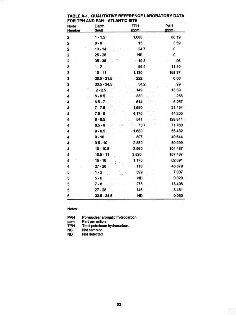
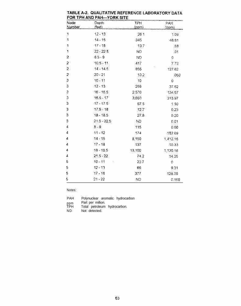
Notes:

PAH Polynuclear aromatic hydrocarbonppm Part per million.TPH Total petroleum hydrocarbon.ND Not detected.

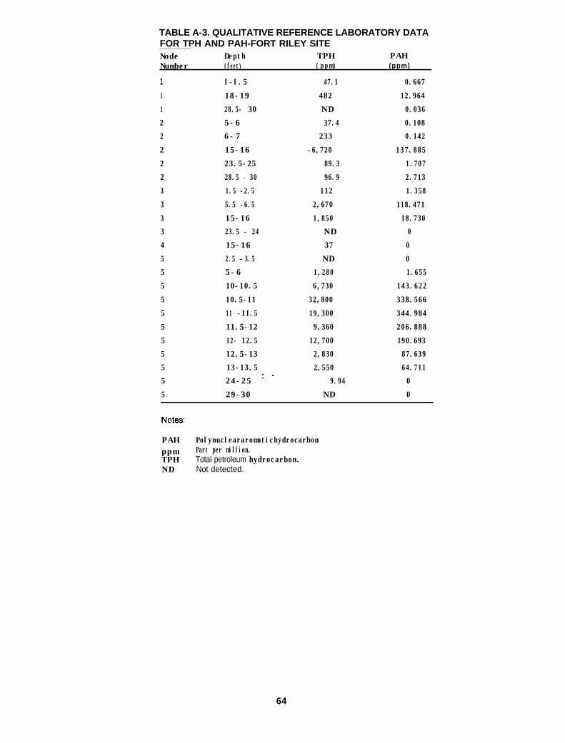
TABLE A-3. QUALITATIVE REFERENCE LABORATORY DATAFOR TPH AND PAH-FORT RILEY SITENode Depth TPH PAHNumber (feet) (ppm) (ppm)

1 l-l.5 47.1 0.667

1 18-19 482 12.964

1 28.5- 30 N D 0.036

2 5-6 37.4 0.108

2 6-7 233 0.142

2 15-16 -6,720 137.885

2 23.5-25 89.3 1.707

2 28.5 - 30 96.9 2.713

3 1.5 -2.5 112 1.358

3 5.5 -6.5 2,670 118.471

3 15-16 1,850 18.730

3 23.5 - 24 N D 0

4 15-16 37 0

5 2.5 -- 3.5 ND 0

5 5-6 1,280 1.655

5 10-10.5 6,730 143.622

5 10.5-11 32,800 338.566

5 11 -11.5 19,300 344.984

5 11.5-12 9,360 206.888

5 12- 12.5 12,700 190.693

5 12.5-13 2,830 87.639

5 13-13.5 2,550 64.711

*5 24-25 9.94 0

5 29-30 ND 0

PAH Polynucleararomatichydrocarbonppm Part per million.TPH Total petroleum hydrocarbon.N D Not detected.

64

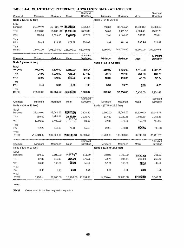
TotalPAH

TotalBTEX 25590.00

Chemical Minimum

Node 4 (10 to 11 feet)

33,550.W @$#$#j,

Maximum Mean

~~~_“__Standard StandardDeviation Minimum Maximum Mean Deviation

Node 4 (27.5 to 28.5 feet)

RY DATA - ATLANTIC SITEStandard Standard

Chemical Minimum Maximum Mean Deviation Minimum Maximum Mean Deviation

Node 2 (21 to 22 feet) Node 2 (24 to 25 feet)

Ethyl-benzene 25,0W.W 42,000.W &jtj$j;~ 7,035.62

TPH 8,850.00. .

15400.00 Q:ll,Q##jtJ 2689.89

VPH 910.00 2,000.00 +j&~@j: ..x.. . . F.. 427.22

TotalPAH 70.42 918.32 672.69 354.08

TotalBTEX 15400.00 293,000.00 221,200.00 53,049.03

250.00 39,ooo.oo 14,690.OO 16,663.45

36.00 9,880.OO 4,004.40 4592.73

7.90 1.400.00 53758 579.81

3.99 691.99 290.96 324.69

1,250.00 260,000.00 93,950.oo 109,210.58

Ethyl-

Ethyl-benzene

TPH

VPH

TotalPAH

TotalBTEX

1,300.00 23,000.00 10,520.OO 10,146.77

117.00 3,030.oo 1,093.60 1,156.83

42.00 970.00 452.40 461.91

29,ooo.oo 35,000.00 ~@@j@ 2408.32

959.00 3,780.00 z’;m@j3 . . . . . ..>... 1,129.72

1,200.00 1,400.00 1,320.00: ..a.. F.. 83.67

12.26 148.10 77.91 60.07

218,700.OO 307,000.00 ~~~~~@J 34,028.49 13,700.00 193,000.00 96,740.00 85,721.28

29.51 270.81 @gjj@j 98.83

Chemical Minimum

Node 5 (16 to 17 feet)

Ethyl-benzene 390.00

TPH 87.80

VPH 36.00

TotalPAH 0.48

TotalBTEX 5,490.oo

StandardMaximum Mean Deviation

2,100.00 1,198.00. . .+: . . . .<. 811.80

516.00 $$w#.$ 177.36

160.00 Q&Q8 59.36

4.72 2:‘%..< 1.79

28,700.00 15,798.00 11,794.98

Minimum Maximum

Node 5 (23.5 to 24.5 feet)Mean

StandardDeviation

940.00 1,700.00 : 301.30

48.20 893.00 238.50 366.76

52.00 160.00 $@B 46.38

1.96 5.11 &@9 1.26

14,330.oo 22,200.00 @$$#jjg 3,340.21

Notes:

Values used in the final regression equations

65

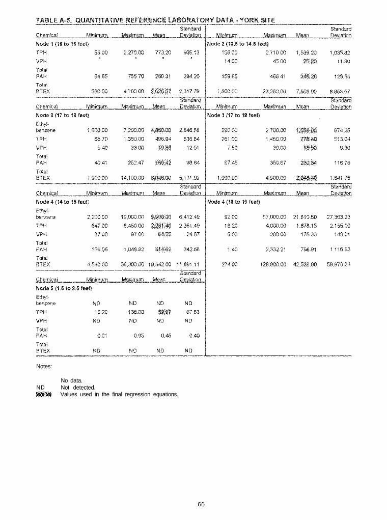
Notes:

No data.ND Not detected.wiw‘y Values used in the final regression equations.

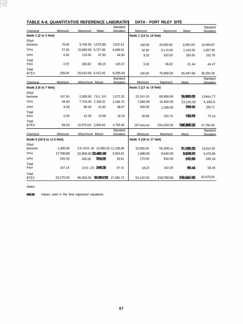
TABLE A-6. QUANTITATIVE REFERENCE LABORATRY DATA - FORT RILEY SITE

Chemical Minimum

Node 1 (2 to 3 feet)

Ethyl-benzene 79.00

TPH 27.50

VPH 6.00

TotalPAH 0.97

TotalBTEX 339.00

Chemical Minimum

Node 2 (6 to 7 feet)

Ethyl-benzene 107.50

TPH 48.60

VPH 9.00

TotalPAH 0.05

TotalBTEX 89.00

Chemical Minimum

Node 5 (10.5 to 11.5 feet)

Ethyl-1,400.000benzene

TPH 17,700.00

VPH 250.00

TotalPAH 157.14

TotalBTEX 23,270.00

100.00 20,000.00 8,595.OO 10,009.87

32.90 3,1 IO.00 1,416.00 1,607.95

9.20 320.00 183.55 152.78

0.02 96.62 31.44 44.47

Standard StandardMaximum Mean Deviation Minimum Maximum Mean Deviation

Node 1 (13 to 14 feet)

3,700.00 I,075.80 1502.51

15,800.00 5,727.98 6,698.52

110.00 47.50 44.90

260.60 89.15 105.57

20,610.00 6,412.40 8,295.04 230.00 70,900.00 26,497.60 35,204.28

Standard StandardMaximum Mean Deviation Minimum Maximum Mean Deviation

Node 2 (17 to 18 feet)

2,000.00 7 6 2 . 5 0 1,072.32

7,720.00 2,169.32 3,186.75

98.00 41.83 48.87

42.05 10.98 18.15

10,070.OO 2,956.63 4,756.48 147,ooo.oo 254,000.00., .,

f&#$$# 47,704.30

Standard StandardMaximum Mean Deviation Minimum Maximum Mean Deviation

Node 5 (16 to 17 feet)

29,000 .W 13,680.00 11,238.86 20,000.00 55,000.w f&@J@B 13,612.49

32,800.00 Bg#B.@ 5,934.81 1,090.00 9,630.00.,. .,. .,.G%km~ 3,470.96

430.00 $$&#B 80.81 170.00 930.00 $%@I 289.34

3 4 0 . 2 6 #$@$I# 67.41 18.23 162.28 B!%!% 58.45

96,300.00 5$@#.# 27,580.73 63,100.00 219,700.00 &$fJ$j:@ 62,975,05.L.. .

28,000.00 60,900.00 r#&@&gg 13464.77

7,050.00 16,900.00.,.,.13,150.00 4,182.ll

530.00 1,200.00 ?f&JBBr 259.71

60.66 224.76 *:$i&# 72.14

Notes:

. . . . . . . . . . . . . . . . .3?Mw Values used in the final regression equations.

67

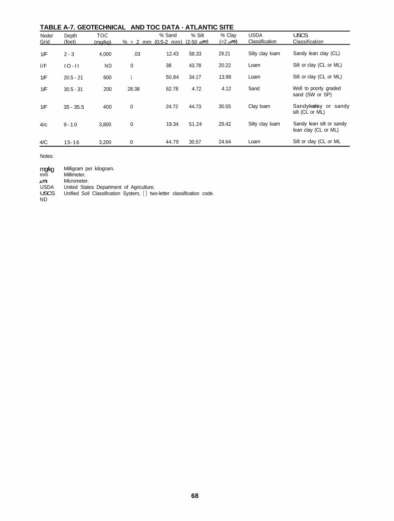
TABLE A-7. GEOTECHNICAL AND TOC DATA - ATLANTIC SITENode/ Depth TOC % Sand % Silt % ClayGrid (feet) (mg/kg) % > 2 mm (0.5-2 mm) (2-50 urn) (<2 urn)

1/F 2 - 3 4,000 .03 12.43 58.33 29.21

l/F I O - I I ND 0 38 43.78 20.22

1/F 20.5 - 21 600 1 50.84 34.17 13.99

1/F 30.5 - 31 200 28.38 62.78 4.72 4.12

1/F 35 - 35.5 400 0 24.72 44.73 30.55

4/c 9 - 1 0 3,800 0 19.34 51.24 29.42

4/C 15-16 3,200 0 44.79 30.57 24.64

Notes:

USDAClassification

Silty clay loam

Loam

Loam

Sand

Clay loam

Silty clay loam

Loam

USCSClassification

Sandy lean clay (CL)

Silt or clay (CL or ML)

Silt or clay (CL or ML)

Well to poorly gradedsand (SW or SP)

Sandy clay or sandyleansilt (CL or ML)

Sandy lean silt or sandylean clay (CL or ML)

Silt or clay (CL or ML

mg/kg Milligram per kilogram.mm Millimeter.ctm Micrometer.USDA United States Department of Agriculture.USCS Unified Soil Classification System, ( ) two-letter classification code.ND

68

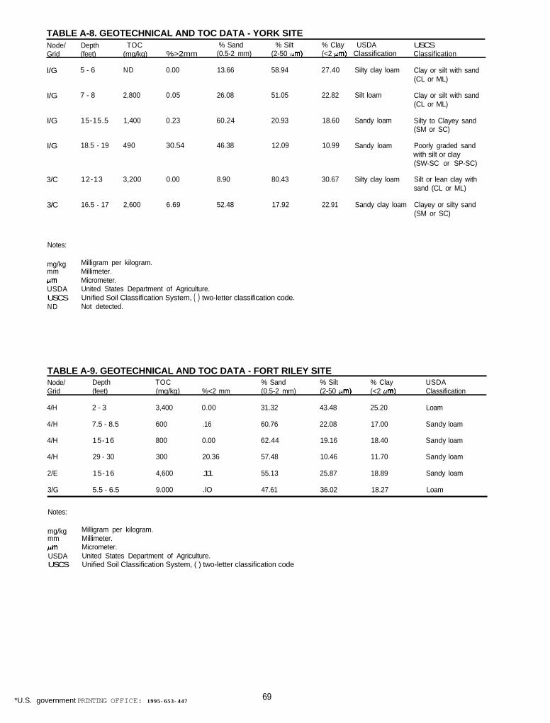
TABLE A-8. GEOTECHNICAL AND TOC DATA - YORK SITENode/ Depth TOC % Sand % SiltGrid (feet) (mg/kg) %>2mm (0.5-2 mm) (2-50 urn)

% Clay USDA(<2 urn) Classification

USCSClassification

l/G

l/G

l/G

l/G

5 - 6 ND 0.00 13.66 58.94 27.40

7 - 8 2,800 0.05 26.08 51.05 22.82

15-15.5 1,400 0.23 60.24 20.93 18.60

18.5 - 19 490 30.54 46.38 12.09 10.99

3/C 12-13 3,200 0.00 8.90 80.43 30.67

3/C 16.5 - 17 2,600 6.69 52.48 17.92 22.91

Notes:

mg/kgmmpmUSDAUSCSND

Milligram per kilogram.Millimeter.Micrometer.United States Department of Agriculture.Unified Soil Classification System, ( ) two-letter classification code.Not detected.

Silty clay loam Clay or silt with sand(CL or ML)

Silt loam Clay or silt with sand(CL or ML)

Sandy loam Silty to Clayey sand(SM or SC)

Sandy loam Poorly graded sandwith silt or clay(SW-SC or SP-SC)

Silty clay loam Silt or lean clay withsand (CL or ML)

Sandy clay loam Clayey or silty sand(SM or SC)

TABLE A-9. GEOTECHNICAL AND TOC DATA - FORT RILEY SITENode/ Depth TOC % Sand % SiltGrid (feet) (mg/kg) %<2 mm (0.5-2 mm) (2-50 urn)

4/H 2 - 3 3,400 0.00 31.32 43.48

4/H 7.5 - 8.5 600 .16 60.76 22.08

4/H 15-16 800 0.00 62.44 19.16

4/H 29 - 30 300 20.36 57.48 10.46

2/E 15-16 4,600 .11 55.13 25.87

3/G 5.5 - 6.5 9.000 .lO 47.61 36.02

% Clay(<2 urn)

25.20

17.00

18.40

11.70

18.89

18.27

USDAClassification

Loam

Sandy loam

Sandy loam

Sandy loam

Sandy loam

Loam

Notes:

mg/kg Milligram per kilogram.mmb4mUSDAUSCS

Millimeter.Micrometer.United States Department of Agriculture.Unified Soil Classification System, ( ) two-letter classification code

*U.S. government PRINTING OFFICE: 1995-653-447 69