INPUT-OUTPUT CHARACTERIZATION OF AN ULTRASONIC

TESTING SYSTEM BY DIGITAL SIGNAL ANALYSIS

James H. Williams, Jr., Samson S. Lee, and Hira KaragulleMassachusetts Institute of Technology

Cambridge, Massachusetts 0213g

The Input-output characteristics of an ultrasonic testing system used for"stress wave factor" measurements were studied by coupling the transmittingand receiving transducers face to face, without a specimen in between. Someof the fundamentals of digital signal processing used are summarized.

The inputs and outputs were digitized and processed in a microcomputer byusing digital slgnal-processlng techniques. The entire ultrasonic test system,including transducers and all electronic components, was modeled as a discrete-time, linear, shlft-lnvarlant system. A digital bandpass filter was introducedto reduce noise effects on the output signal. The output due to a broadbandinput was deconvolved with the input to obtain the unit-sample response and thefrequency response of the dlscrete-tlme system. Then the impulse response andfrequency response of the contlnuous-tlme ultrasonic test system were estimatedby interpolating the defining points in the unlt-sample response and frequencyresponse of the dlscrete-tlme system. The ultrasonic test system was found tobehave as a linear-phase bandpass filter.

The unlt-sample response and frequency response of the dlscrete-tlme modelof the test system were used to compute the output of the test system for avariety of inputs. The agreement between predicted and measured outputs wasexcellent for rectangular pulse inputs of various amplitudes and durations andfor tone burst and slngle-cycle inputs with center frequencies within the pass-band of the test system. The Input-output limits on the llnearlty of thesystem were determined.

INTRODUCIION

Conventional ultrasonic testing (UT) is conducted either in the through-thickness transmission or pulse-echo modes (ref. l). In the through-thlcknesstransmission mode, the transmitting and receiving transducers are coupled toopposite faces of the structure under inspection, and the transmitted wavefield is analyzed. In the pulse-echo mode, the transmitting and receivingtransducers, which may be combined into a single transducer, are coupled to thesame face of the structure under inspection, and the reflected wave field isanalyzed.

Recently Vary et al. (refs. 2 and 3) introduced an ultrasonic nondestruc-tive evaluation (NDE) parameter called the stress wave factor (SWF). It issimilar to the pulse-echo test mode in that separate transmitting and receivingtransducers are coupled to the same face of the structure. However, unlikeconventional pulse-echo testing, which is generally limited to the analysis ofnonoverlapplng reflected wave echoes, the SWF is also valid for the analysis

311

https://ntrs.nasa.gov/search.jsp?R=19860013511 2018-08-23T21:21:28+00:00Z

of overlapping echoes. Specifically, an input pulse having a broadband fre-quency spectrum is applied to the transmitting transducer and the number ofoscillations of the output signal at the receiving transducer exceeding a pre-selected voltage threshold is defined as the SWF. The SWF has been correlatedwith mechanical properties of carbon-flber-relnforced composites (refs. 2to 4). Williams et al. (ref. 5) theoretically and experimentally studied theultrasonic Input-output characteristics of the SWF test configuration in athick, Isotroplc, elastic plate. The extension of that work to thin plates iscurrently in progress (ref. 6).

An important step toward the quantitative analysis of Input-output rela-tions in any ultrasonic NDE procedure is the quantitative characterization ofthe experimental test system without a test specimen. The effects on the out-put signal of the ultrasonic transducers, the coupling of the transducers tothe test specimen, and electronic components such as filters, amplifiers,attenuators, and cables in the experimental system must be characterized beforethe test speclmen's effects on the output signal can be isolated.

lhls study is part of an overall effort to develop quantitative analysesof the SWF and computer-alded nondestructive evaluation (CANDE, pronounced"candy") capabilities. The experimental UT system is characterized by directlycoupling the transmitting and receiving transducers face to face without a testspecimen. Input and output signals are digitized with a digital oscilloscopeand are processed with a microcomputer by using digital slgnal-processlng tech-niques. The transfer function of the experimental UT system without any testspecimen was obtained.

The results of this study should provide a useful example in the charac-terization of any UT system that has separate transmitting and receiving trans-ducers. Furthermore, developments in CANDE should be facilitated by thedigital slgnal-processlng procedures summarized herein.

FUNDAMENIALS OF DIGIIAL SIGNAL PROCESSING

A few results in digital signal processing are summarized in this section.Digital slgnal-processlng techniques are discussed extensively in the litera-ture (refs. 7 to lO). Primarily, the notations in reference 7 are followed inthis outline.

Digital signal processing is concerned with the representation of signalsby sequences of numbers and the processing of those sequences. Sequencescorrespond to dlscrete-tlme signals derived from sampling contlnuous-tlmesignals. The notation x(n) denotes a sequence of numbers whose entriesdepend on the independent parameter n. The sequence x(n) is defined onlyfor integer values of n and represents successive samples of a continuous-time signal. For example, the sequence x(n) is derived from periodicsampling of the contlnuous-tlme analog signal Xa(t), where t is time,according to

x(n) = Xa(nT) (1)

where T is the sampling period. The reciprocal of T is the sampling rateor sampling frequency. The availability of hlgh-speed digital computers andefficient slgnal-processlng algorithms has accelerated the implementation of

312

digital slgnal-processlng techniques over that of contlnuous-tlme, analogslgnal-processing techniques. With the proper analysis, results from thedigital signal processing of a sequence derived from sampling a contlnuous-tlmesignal can accurately approximate results from contlnuous-tlme signal analyses.

A dlscrete-tlme system is defined mathematically as a unique transforma-tion that maps an input sequence x(n) into an output sequence y(n).Discrete-tlme, linear, shlft-lnvarlant systems are dlscrete-tlme analogs ofcontlnuous-tlme, linear, tlme-lnvarlant systems. Table l summarizes the input-output properties of dlscrete-tlme, linear and linear shlft-lnvarlant systemsand their corresponding analogs in contlnuous-tlme systems. Discrete-tlmesystems can be further characterized as stable and causal. A stable system isone for which every bounded input x(n) produces a bounded output y(n). A

causal system is one for which the output y(n) for n equal to no dependsonly on the input x(n) for n less than or equal to no. All subsequentdiscussions here are limited to dlscrete-time, linear, shlft-lnvarlant systemsthat are stable and causal.

The response of a linear, shlft-lnvarlant system can be characterized bythe unlt-sample response h(n) via the convolution sum given in equation (l-l)in table I. As a consequence, it can also be shown that the steady-stateresponse of a linear, shlft-lnvarlant system to a slnusoldal input is sinusol-dal of the same frequency as the input but with a magnitude and phase deter-mined by the system. It is this property of linear, shlft-lnvarlant systemsthat makes representations of signals in terms of slnusolds or complex exponen-tials (i.e., Fourier representations) so useful in linear system theory. Also,it should be mentioned that the process of obtaining y(n) from known x(n)and h(n) is called convolution, and the process of obtaining h(n) fromknown x(n) and y(n) is called deconvolutlon.

Table 2 summarizes Fourier representations of contlnuous-tlme signals andof sequences. Fourier representations appear as equation pairs whose constitu-ents are often referred to as the synthesis and analysis equations, as indi-

cated in table 2. In equation (2-1b), Xa(J_) is a continuous function inradlan frequency Q and is the Fourier transform of the contlnuous-tlme signalXa(t), where the symbol j is defined as the square root of -l. If Xa(t)has units of voltage, Xa(j_) has units of voltage per radlan frequency (orsimply volt-second); Xa(JQ) is in general complex and can be specified by itsmagnitude and phase.

If Xa(t) is a real-valued function of time, the magnitude and phase ofXa(j_) will be an even and odd function of frequency, respectively. Thus, itis only necessary to present the magnitude and phase of Xa(J_) for positivefrequencies. If Xa(t) is real and an even function of tlme, the phase ofXa(j_) is zero. If Xa(t) is real and an odd function of time, the phaseof Xa(JQ) is ±_/2. If Xa(t) is shifted (i.e., advanced or delayed) intime, the magnitude of Xa(J_) is not affected, but a phase linearly propor-tional to frequency (i.e., linear phase) is introduced in the phase of Xa(j_).More specifically, the phase (in radlans) is proportional to the radlan fre-quency with a proportionality constant having units of time. The negative ofthe value of the proportionality constant is the time delay (ref. 9).

313

The remainder of table 2 deals wlth the Fourier representations of

sequences. If properly computed, the Fourier transform Xa(J_) can beapproximated by the Fourier representation of a sequence derived from samplingXa(t). Examples of the Fourier representations of contlnuous-tlme signalsand sequences are illustrated in figure l and will be discussed shortly.

In equation (2-2b) in table 2 X(eJ_) is a continuous function of radlanfrequency _ and is the (discrete time) Fourier transform of a sequence x(n).The frequency _ is in units of radlans per increment of n, which is simplyradlans. If x(n) has units of voltage, X(eJ_) has units of voltage perradlan. The Fourier transform of a sequence is useful for analyzing general

sequences. The discrete Fourier series representations of a periodic sequencex(n) of period N are also shown in table 2. A periodic sequence _(n) _fperiod N is one such that _(n) equals _(n + N). In equation (2-3b) X(k)is a periodic sequence of period N, and the numbers in this sequence are thediscrete Fourier series coefficients of the periodic sequence _(n) having

period N. If _(n) has units of voltage, _(k) has units of voltage also.The discrete Fourier series of a periodic sequence serves as a prelude to thediscrete Fourier transform (DFT). In equation (2-4b) X(k) is a sequence oflength N and is called the DFT of a flnlte-length sequence x(n) of lengthN (ref. 7). If x(n) has units of voltage, X(k) has units of voltage also.The DFT is useful for digital signal processing because sequences processed bya computer are of finite length and also because efficient DFT computationalalgorithms are available.

By comparing the entries in table 2 for the discrete Fourier series of aperiodic sequence of period N and the DFT of a finlte-length sequence oflength N, it is observed that the DFT representation is obtained from thediscrete Fourier series representation by interpreting the flnlte-lengthsequence as one period of a periodic sequence. The properties of the DFT aresimilar to those of the Fourier transform, except that because of the impliedperiodicity, shifts of x(n) in n by one period N and an integer multipleof one period are indistinguishable and a shift in n of larger than N isthe same as a shorter shift.

The DFT was computed via a fast Fourier transform (FFT) algorithm. Theinverse DFT computed via an inverse FFT (IFFT) algorithm was used to evaluatex(n) from X(k). The FFT computation is particularly efficient when thelength of the sequence is an integer power of 2. A sequence of length N iscalled an N-polnt sequence. The DFT of an N-polnt sequence is called anN-polnt DFT and is computed via an N-polnt FFT algorithm. Figure l illustratesthat the Fourier transform of a contlnuous-tlme signal can be reconstructedapproximately from the DFT of a sequence derived from sampling the continuous-time signal. Again, note that where DFT relations are concerned, a finite-length sequence is represented as one period of a periodic sequence.

Figure l shows Fourier representations of continuous-tlme signals and ofsequences derived from sampling the contlnuous-tlme signals. In part (1) offigure l(a), the contlnuous-tlme signal Xa(t) is assumed to be bandllmltedin frequency with Fourier representation Xa(J_) as shown. The highest fre-quency of Xa(t) Is assumed to be _o/2. In part (ll) of figure l(a), asequence x(n) results from the periodic sampling of Xa(t) with a samplingIng period of T. The Fourier transform of the sequence x(n) into a contin-uous function X(eJ_) is also shown. It is observed that X(eJ_) can beobtained from Xa(J_) by the superposltlon of an infinite number of Xa(J_)

314

shifted in frequency _ by integer multiples of 2_. The magnitude and fre-quency of X(eJ_) are scaled from those of Xa(J_) by I/T and T, respec-tively. The Fourier transform Xa(j_) can be recovered exactly, except forthe scaling factors, from the Fourier transform X(eJ_) of the sequence x(n)in the interval of -_ _ _ _ _ by low-pass filtering X(eJ_) with a cutoff

frequency of _, on one condition. The condition is that _oT/2 < _ so thatthere will be no overlapping of superposed Xa(J_) in forming X(eJ_). Thiscondition is known as the "sampling theorem" and assures that if a continuous-time signal Xa(t) is sampled at a frequency greater than twice the highestfrequency of Xa(jQ), then X(eJ_) is identical to Xa(J_) in the interval-_ < _ _ _, except for scaling factors. Because Xa(J_) is recovered, thecontlnuous-tlme signal Xa(t) can be recovered from the sequence x(n). Thisminimum required sampling frequency is called the Nyqulst rate or the Nyqulstfrequency (refs. 7, 9, and lO). The distortion due to overlapping of super-posed Xa(J_) when the sampling theorem is violated is called allaslng. Inpart (ll) in figure l(a), the case where there is no overlapping of superposedXa(J_) is illustrated; thus the signal is not allased.

Whereas figure l(a) deals with general contlnuous-tlme signals,figure l(b) deals with flnlte-duratlon contlnuous-tlme signals. In part (1)

in figure l(b), a contlnuous-tlme signal Xa(t) with nonzero values over afinite time duration and its Fourier representation Xa(J_) are shown. Theduration where the signal is nonzero is assumed to be to, and sampling thecontlnuous-tlme signal wlth a sampling period T is assumed to result in asequence of length N. It is observed that Xa(J_) for a flnlte-duratlonsignal is not bandllmlted in frequency. In part (il) in figure l(b), asequence x(n) results from the periodic sampling of Xa(t) with a samplingperiod of T. All numbers in the sequence x(n) are zero for n < 0 andfor n > N - I. Thus x(n) is a flnite-length sequence of length N. TheFourier transform of the sequence x(n) into the continuous function X(eJ_)is also shown. Similar to the results in figure l(a), X(eJ_) can be obtainedfrom Xa(J_) by the superposltlon of an infinite number of Xa(J_) shifted infrequency _ by integer multiples of 2_. However, for this case, becauseXa(J_) is not bandllmlted in frequency, there is overlapping of superposedXa(J_) in forming X(eJ_). Thus there is allaslng and Xa(J_) cannot berecovered exactly from X(eJ_) in the interval -_ _ _ _ _. However, if thesampling frequency is greater than twice most of the significant frequencycomponents in Xa(J_), then Xa(J_) can still be approximated adequately byX(eJ_). The DFT X(k) of the flnlte-length sequence x(n) is often computedinstead of X(eJ_). However, in DFT evaluations, a finlte-length sequenceis represented as one period of a periodic sequence.

In part (Ill) of figure l(b), a periodic sequence _(n) of period Nconstructed by using the N-polnt sequenc_ _(n) as a period is shown. Thediscrete FourleL series representation X(k) of the periodic sequence _(n)is also shown; X(k) is a periodic sequence of period N. The DFT X_k) ofthe finlte-length sequence x(n) can be interpreted as a period of X(k) for0 < k < N - l as shown. It is observed that X(eJ_) can be obtained from

X(k) by interpolating points in _(k). Because Xa(J_) can be approximatedadequately by X(eJ_) if the sampling frequency is greater than twi_e most ofthe significant frequency components in Xa(J_), interpolations of X(k) orX(k) can be used to estimate Xa(J_). The numbers in X(k) are scaledapproximately from the values of Xa(j_) by a factor of I/T, and the spacingbetween successive numbers in the sequence X(k) can be interpreted as 2_/(NT)

315

In radlan frequency, which is the frequency domain resolution. Again, thereconstruction of the Fourier transform of a flnlte-duratlon, contlnuous-tlme

signal from the DFT of a flnlte-length sequence by interpolation is generallyan approximation due to allaslng.

Table 3 lists the conditions for the special case where there Is exactcorrespondence (to within a scaling factor) of the Fourier transform of acontlnuous-tlme signal and the DFT of a flnlte-length sequence derived fromsampling (ref. lO). Also, the N-polnt sequence x(n) can be considered as anM-polnt sequence If M Is greater than N with the last M-N numbers In theM-polnt sequence being zero. As discussed here next regarding convolutionprocedures, sometimes It is convenient to extend the length of a sequence byappending zeroes.

Because the response of a linear, shlft-lnvariant system can be evaluatedvla the convolution sum In equation (l-l) in table l, convolution representa-tions are discussed here. Table 4 summarizes convolution representations of

contlnuous-tlme signals and of sequences. The Fourier representations of theconvolutions are also given In table 4. Equation (4-1a) gives the linear con-volution of contlnuous-tlme signals Xal(t) and Xa2(t), resulting In Xa3(t).The Fourier representation of the convolution Is given in equation (4-1b).Convolution In the tlme domain results In multiplication in the frequencydomain. Conversely, because of the duality between time and frequency domainsIn Fourier representations, convolution in the frequency domain results Inmultiplication In the tlme domain, such as tlme windowing (ref. 9). The con-cepts of periodic and clrcularconvolutlons are introduced as preludes to theefficient evaluation of linear convolution of sequences using DFT procedures.

Equation (4-2a) In table 4 gives the periodic convolution of two periodicsequences _l(n) and _2(n), each of period N, resulting In a periodicsequence _3(n) of period N. By restricting attention to one period of theperiodic convolution, circular convolution of two N-polnt sequences xl(n)and x2(n) to obtain an N-polnt sequence x3(n) can be defined from theperiodic convolution and Is given In equation (4-3a). The two periodicsequences _l(n) and _2(n), each of period N, are constructed by using theN-polnt sequences xl(n) and x2(n) as periods, respectively. Equations (2-3b)and (2-4b) In table 2 have been used to obtain the simplified equation (4-3b)because _l(n) and _2(n) are equal to xl(n) and x2(n) for n rangingfrom zero to N - I. Thus _l(k) and X2(k) for 0 < k < N - l become Xl(k)and X2(k), respectively. The circular convolution of-N-polnt sequences Iscalled an N-polnt circular convolution. The designation "circular" Is derivedfrom a graphical representation of how an N-point sequence can be used to con-struct a periodic sequence of period N (ref. 7). It can be imagined that theN points from the N-polnt sequence are equally spaced In angle around a circlewith a circumference of exactly N points. The periodic sequence of periodN is obtained by traveling around the circumference of the circle a number ata time recording the N-polnt sequence repeatedly. Also, a rotation of thecircle corresponds to circular shifting of the N-polnt sequence (ref. 7).

The linear convolution of an Nl-Polnt sequence xl(n) and an N2-Polntsequence x2(n) is defined as

Nl-l

x3(n) = _ xl(m) x2(n- m) (2)m=O

316

Because the resulting sequence x3(n) is of length N1 + N2 - 1 (ref. 7),the evaluation of linear convolution via circular convolution requires allsequences to be of the same length, which has to be N1 + N2 - I.Equation (4-4a) in table 4 gives the linear convolution of finlte-lengthsequences xl(n) and x2(n) to obtain a flnlte-length sequence x3(n )evaluated via circular convolution. Computation of circular convolution usingDFT is preferred over the direct evaluation of linear convolution because ofcomputational efficlencles. The (N1 + N2 - l)-point DFT's of the two convolv-%ng sequences are computed via an FFT algorithm and then multiplied accordingto equation (4-4b). The (N1 + N2 - l)-polnt inverse DFT of the product iscomputed vla an IFFT algorithm, and the result is the desired linear convolu-tion. Because the original sequences xl(n ) and x2(n) are of lengths N1and N2, respectively, N2 - 1 and N1 - 1 zeroes are appended to xl(n)and x2(n), respectively, to yield two (N 1 . N2 - l)-point sequences for the(N 1 + N2 - l)-point circular convolution. Alternatively, if linear convolu-tlon of two (N 1 + N2 - l)-point sequences is conducted via an (N 1 + N2 - l)-point circular convolution, the last N2 - 1 numbers in one sequence to beconvolved must be zeroes and the last N1 - 1 numbers in the other sequenceto be convolved must be zeroes. In practice, the sequences are extended to alength that is greater than N1 + N2 - 1 and is an integer power of 2 forefficient FFT computation.

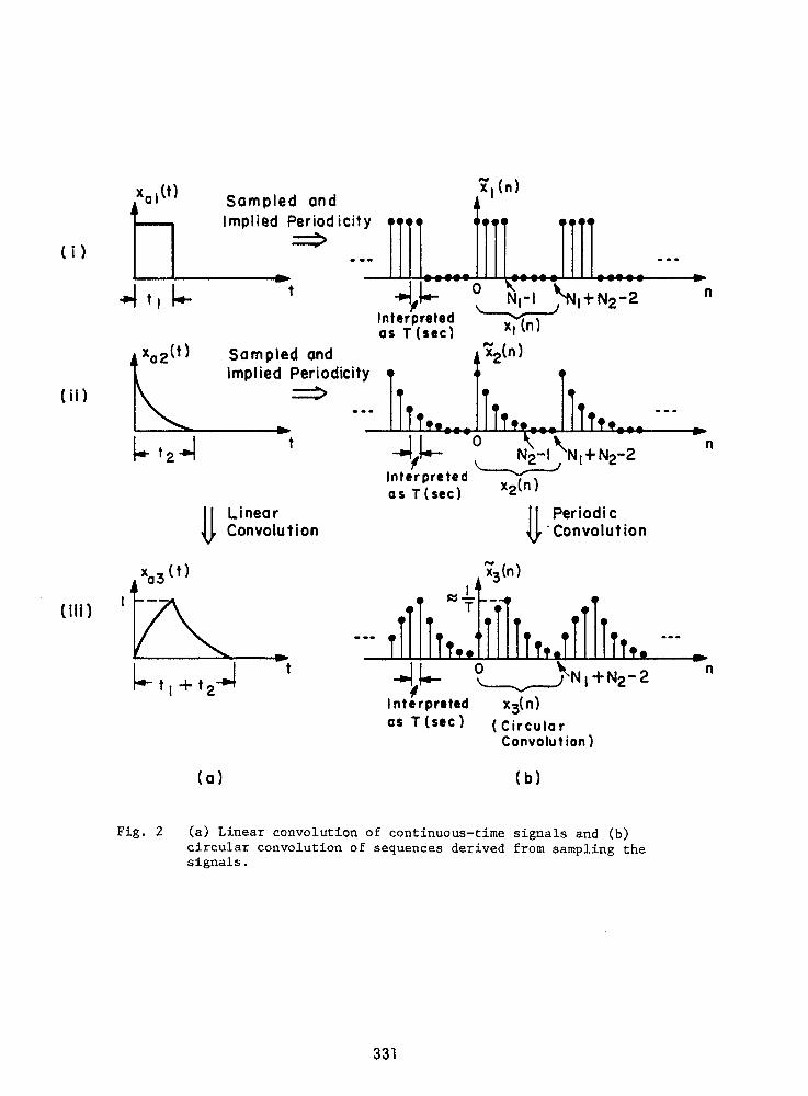
Figure 2 shows convolution representation of contlnuous-tlme signals andtheir sequences derived by sampling. In figure 2(a), continuous-tlme signalsXal(t) of duration t I and Xa2(t) of duration t 2 are convolved to formthe continuous-tlme signal Xa3(t ) of duration t I + t 2. In part (1) offigure 2(b), the contlnuous-tlme signal Xal(t ) is sampled with a samplingperiod T and is assumed to produce an Nl-Polnt sequence. Then N2 - 1zeroes are appended to form an (N 1 + N2 - l)-point sequence xl(n ). Next aperiodic sequence _l(n) of period N1 + N2 - 1 is constructed by usingxl(n) as a period. Similarly, in part (11) in figure 2(b), the periodicsequence _2(n) of period N1 + N2 - 1 is obtained from Xa2(t), whichis assumed to produce an N2-Point sequence when sampled with a sampling periodT. Periodic convolution of %l(n) and _2(n) results in the periodicsequence _3(n). Then x3(n ) can be identified from the circular convolutionportion of _3(n) by restricting attention to one period of the periodicsequence. It is observed that Xa3(t) can be approximated from the inter-polation of the (N 1 . N2 - l)-point sequence x3(n ). The numbers in x3(n )are scaled approximately from the value of Xa3(t ) by a factor of I/T and thespacing between successive numbers in the sequence x3(n ) can be interpretedas T. Because the circular convolution is obtained via a DFT, restrictions onthe DFT apply to the convolution also. Thus the sampling theorem applies tosampling the contlnuous-tlme signals if Xa3(t ) is to be approximatedadequately by the sequence x3(n ).

In practice, if a contlnuous-tlme signal is to be sampled, the samplingfrequency and the sampling length must be specified. Table 5 summarizes thesignificance of the sampling parameters. Equation (5-I) is based on theearlier discussion in relation to figure l(a).

EXPERIMENTAL SYSTEM

A schematic of the experimental system including the specimen is shown infigure 3. This is a typical stress-wave-factor test configuration. The goal

317

of this study was to characterize the experimental test system without the testspecimen. Thus, all testing in this study was conducted with the transmittingand receiving transducers directly coupled face to face without any testspecimen in between.

The system consisted of a pulse/functlon generator (Wavetek model 191); a5-MHz (corresponding to -3-dB point) low-pass filter (Allen Avionics F2516);broadband (O.1 to 3.0 MHz) transmitting and receiving transducers (ParametrlcsVI05) having an approximately flat sensitivity of -85 dB relative to l V/_bar;an ultrasonic interface couplant (Acoustic Emission Technology SC-6); an ultra-sonic preamplifier (custom built by Parametrlcs) havlng a gain of 40 dB in thefrequency bandwidth l kHz to lO MHz; a varlable-frequency filter (A.P. CircuitCorporation AP 220-5), which could be used as a low-pass, hlgh-pass, bandpass,or bandstop filter in the frequency range lO Hz to 2.5 MHz; a digital oscillo-scope (Nicolet model 2090 with plug-ln model 204-A), which could sample andstore analog signals at sampling frequencies from 0.05 Hz to 20 MHz (corre-sponding to sampling periods from 20 sec to 50 nsec) up to 4096 points; andan IBM personal computer (IBM PC), which was interfaced with the digitaloscilloscope.

The varlable-frequency filter was used as a 0.4, to 2.6-MHz (correspondingto -3-dB points) bandpass filter,:selected on the basis of the receiving trans-ducer frequency response. All signals were sampled at a sampling frequency of20 MHz (i.e., one sample every 50 nsec) for 256 points. Thus each recordedsignal was 12.8 _sec in duration. The 5-MHz low-pass filter was selected viaantlallaslng considerations. Table 6 is a BASIC language program listing forthe FFT and IFFT computations used in this study. All DFT and inverse DFTevaluations in this study were conducted by using this program.

DIGITAL CHARACTERIZATION OF EXPERIMENTAL SYSTEM

The objective of this study was to obtain the system transfer character-istics between the input to the transmitting transducer and the output fromthe receiving transducer after signal conditioning. A schematic of the experi-mental system is shown in figure 3. Once again, note that the experiment wasconducted with the transmitting and receiving transducers coupled face to facewithout a test specimen. Thus, the "system" under study consisted of thetransmitting transducer, the coupling between transmitting and receiving trans-ducers, the recelvlng transducer, the ultrasonic preamplifier, the variable-frequency filter, and all necessary cables.

A contlnuous-tlme system can be described by its impulse response ha(t)and its frequency response Ha(J_). In this study, the ha(t) and Ha(J_)of the test system were computed from the unlt-sample response h(n) and theDFT of h(n) denoted H(k), respectively, of a dlscrete-tlme model of thecontlnuous-tlme system.

The experimental system was assumed to be a dlscrete-tlme, linear, shift-Invarlant system. As shown in figure 3, channel l of the digital oscilloscopesampled the contlnuous-tlme input signal to the transmitting transducer. Theresulting dlscrete-tlme signal is called the input sequence and is denoted byx(n). Similarly, channel 2 of the digital oscilloscope sampled the continuous-time output signal from the receiving transducer after preampllflcatlon andbandpass filtering. The resulting dlscrete-tlme signal is called the output

318

sequence and Is denoted by y(n). Thus, the objective of thts study was toobtain the dlscrete-ttme system transfer characteristics between x(n) andy(n). The dlscrete-ttme system besides being linear and shtft-tnvartant wasobserved to be stable and causal. A schematic of the digital slgnal-processtngprocedures applied to obtain the unlt-sample response and frequency responseof the discrete-time system is shown in figure 4.

The pulse/function generator produced an approximately rectangular pulse20 nsec in duration. The rectangular pulse was passed through the 5-MHz low-pass filter before it reached the dlglta] oscllloscope. Figure 5 shows thetime histories of the input and output slgnals by llnearly interpolating thedefining points tn the input and output sequences x(n) and y(n). The inputand output slgnals were approxlmately 3 and 4 ,sec long, respectively. Thusfor the sampllng period 50 nsec, only approximately the first 60 and 80 numbersIn the sequences x(n) and y(n), respectively, were nonzero. Actually, thesequences x(n) and y(n) were of length 256 after sampllng; that is, thedigital oscilloscope recorded 256 points each for the input and output signals.Then 768 zeroes were appended to the sequences to produce x(n) and y(n) oflength 1024. Extended sequences were used to facilitate evaluatlon of linearconvolution vla the DFT, as discussed later. The OFT's X(k) and Y(k) forx(n) and y(n), respectively, were evaluated by using a 1024-point FFT algo-rithm based on 1024-point x(n) and y(n). Because the input and outputsignals were of finite duration, they were not bandllmlted In frequency. How--ever, because the sampling frequency (20 MHz) was greater than most of thesignificant frequency components In the input signal (significant up to 5 MHz)and the output signal (significant up to 2.6 MHz), the sampling theorem assuredan adequate approximation of the Fourier transform of the input and outputsignals by the DFT of the input and output sequences. Approximations of themagnitude and phase of the Fourier transform of the input and output signalsare shown in figure 5. The magnitude and phase of the Fourier transform wereobtained by linearly interpolating the defining points in the magnitude andphase of the DFT of the input and output sequences. The magnitude shown Infigure 5 is presented on a decibel scale, normalized wlth respect to themagnitude of the largest component In the Fourier transform. The magnitudesof the largest components in the Fourier transforms of the input and outputwere 2.3xi0-7 and 9.3x10-7 V-sec, corresponding to frequencies of 0.4 and1.4 MHz, respectively. When the magnitude was small, both the magnitude andthe phase were erratic because of sensitivity to noise contamination (fig. 5).

Letting the 1024-polnt DFT of the unit-sample response h(n) of thedlscrete-tlme system be defined as H(k), we can then use equation (4-4b) intable 4 to relate the DFT of the input X(k) and the DFT of the output Y(k)as

Y(k) = H(k) X(k) (3)

where 0 < k _ 1023 for thls case. Then H(k) for the system can be evaluatedby rearranglng equation (3) as

H(k) = Y(k)/X(k) (4)

The inverse DFT of H(k) is the desired unlt-sample response h(n). Theprocedure for obtaining h(n) from known x(n) and y(n) is calleddeconvolutlon.

319

However, results from attempts to perform the direct division in equation(4), using X(k) and Y(k), as shown in figure 5, were unsatisfactory becauseof noise. Thus, the output y(n) was filtered digitally before division.The digital filter was selected by trial and error. Various digital filterswere applied, and the resulting H(k) and the unlt-sample response h(n) wereused to evaluate output properties for various inputs and were compared withexperimental results. The digital filter selected was a bandpass filter uti-lizing time windowing via a ?Ol-polnt Blackman window (ref. ?). Specifically,the digital filter was obtained via the following steps: (1) obtain the unit-sample response hd(n) of a desired ideal bandpass filter of 0.2 to 4.5 MHz,(2) shift hd(n) by 350 points to obtain the unlt-sample response h3(n),and (3) multiply h3(n) by a 701-polnt Blackman window wl(n) to obtain a701-polnt unlt-sample response h4(n) of the filter. These steps are illus-trated in figure 4 also. The resulting digital filter was a causal, linear-phase bandpass filter. Step l identified the desired bandpass filter. Becausean ideal filter is noncausal, as indicated by its hd(n), which is nonzerofor n less than zero, step 2 shifted hd(n) by delaying it by 350 points.A causal filter is especially important for real-tlme signal processing.

Because the desired digital filter was a finite impulse response (FIR)filter, which by definition should have a unlt-sample response of finite dura-

tion (ref. 7), h3(n) was truncated and only numbers between n of zero and701, inclusively, were retained. To minimize the effects of truncation,h3(n) was multiplied by a ?Ol-polnt Blackman window wl(n) in step 3 toform h4(n). The length of 701 points minimized the effects of truncationand yet allowed a 1024-polnt DFT evaluatlon. The length of the sequence

h4(n) of the filter affected the DFT evaluation because filtering in thefrequency domain (i.e., multiplying the responses of the filter and the signalin the frequency domain) corresponded to convolution in the time domain.Because only the first BO numbers in the sequence y(n) were nonzero, properevaluation of the linear convolution of the sequence y(n) wlth the sequence

h4(n), which was nonzero for the first 701 numbers, required at least a780-polnt DF1, according to discussions associated with equation (4.-.4)intable 4. By increasing the number of points to the nearest integer power of 2,which for this case was I024, I024 polnt sequences and I024 DFT's resulted.Thus, sufficient zeroes were appended to any sequence to extend its length toI024 points, unless otherwise indicated. Also, 1024-polnt DFT's evaluated viaa 1024.polnt FFT were used, unless otherwise indicated.

The 1024-polnt DFT of the unlt-sample response of the digital bandpassfilter designed by time windowing the unlt-sample response of an ideal bandpassfilter with a Blackman window is denoted by H2(k). Using equation (4-4b) intable 4, the DFI_ of the output after digital filtering was H2(k) Y(k).Then equation (4) could be modified as

Hl(k) = H2(k) Y(k)/X(k) (5)

where Hi(k) was an approximation to H(k), and 0 _ k _ I023.

The unlt-sample response hi(n) was obtained from HI(k) by performingan inverse DFT via an IFFT algorithm. Because hl(n) corresponded to ha(t),which is a real function of time, hi(n) was a sequence of real numbers andcorresponded to the real part of the IFFT. Because a shift of 350 points (cor-responding to 17.5 _sec) was introduced in the design of the causal, digital

320

bandpass filter, the unlt-sample response hi(n) had to be shifted back by350 points to remove the artifact introduced by the digital filter. Thls wasdone after the rectangular windowing procedure discussed in the next paragraph.

The individual values in the sequence hi(n) for n _ 355 and n _ 450were small, less than I/lO0th of the maximum value In the sequence. Thesesmall values were due to noise contamination introduced during signal recordingand also by the digital filtering. So, the sequence hl(n) was tlmewindowed by a rectangular window w2(n) defined by

l for 355 < n < 450w2(n) = (6)

0 otherwise

Thus, the numbers in hi(n) were not affected for 355 < n < 450, but allothers had been set to zero. The resulting sequence obtalned by multiplyinghi(n) and w2(n) Is denoted as h2(n). Thls tlme windowing significantlysmoothed the phase of HI(k) In the hlgh-frequency region.

After the rectangular windowing, the sequence h2(n) was shifted back350 points to remove the shift (i.e., time delay) introduced by the bandpass

digital filter discussed earlier. The 1024-polnt sequence h2(n) was shiftedto obtain h(n) according to circular shifting, which In thls case became

h2(n . 350) for 0 _ n _ I023 - 350

h(n) = (h2 (n - 1024 . 350) for 1024 - 350 _n _ 1023 (7)

(o otherwise

The sequence h(n) was the unlt-sample response of the test system. Thenumbers In h(n) were zero for n _ lO0 due to the windowing described inequation (6). Circular shifting was used instead of linear shifting becauseh2(n) was the result of a few DFT evaluations and, when a DFT evaluationwas performed, a flnlte-length sequence was implied as a period of a periodicsequence. Thus, circular shifting procedures corresponding to shifting aperiodic sequence were required.

The DFT of the unlt-sample response h(n) was H(k). Because h(n) wasnonzero only for <lO0, the first 512 points of h(n) were used to computeH(k) vla a 512-polnt FFl. Thus, H(k) as obtained was a 512-polnt sequence;H(k) was the frequency response of the dlscrete-tlme model of the test system.

Figure 6(a) shows the impulse response ha(t) of the test system asobtained by linearly interpolating the defining points In the unlt-sampleresponse h(n). An impulse response has units of response per unlt of exclta-tlon multiplied by tlme (ref. ll). Thus, ha(t) In flgure 6(a) Is shown wlthunits of volts per volt-second. The duration of the unlt-sample response wasapproximately 3 _sec. Figure 6(b) shows the magnitude and phase of the fre-quency response Ha(J_) of the test system as estimated by linearly inter-polating the defining points in the frequency response H(k). A frequencyresponse magnitude has units of response per unlt of excitation (ref. ll).Thus, the magnitude of Ha(J_) has units of volts per volt. The magnitudeof Ha(j_) Is shown In figure 6(c) on a decibel scale, normalized wlthrespect to the magnitude of the largest component in Ha(J_), which is

321

2.7xi0-7 V/V corresponding to a frequency of 1.7 MHz. The normalized magni-tude had a maximum value at 1.7 MHz, and the values of the normalized magnitudedecreased by 6 dB from the maximum value at 0.6 and 2.3 MHz. The phase of

Ha(J_) was linear from 0.3 to 2.7 MHz. The llnear-phase behavior indi-cates that inputs of frequencies from 0.3 to 2.7 MHz will result in outputsdelayed in time without distortion. (However, distortion occurred because the

magnitude of Ha(J_) was not constant from 0.3 to 2.7 MHz.) The introducedtime delay corresponding to the linear phase can be computed to be 0.49 _sec.As shown by the magnitude plot, the system was insensitive to frequencies below0.6 MHz and above 2.3 MHz; the information in these frequencies was easily con-taminated by noise and also displayed the effects of digital filtering. Thus,to summarize, the system behaved as a llnear-phase bandpass filter in thefrequency range 0.6 to 2.3 MHz.

RESULTS AND DISCUSSION

The outputs of the test system due to different inputs can be predictedby using the unlt-sample response h(n) and frequency response H(k) of thedlscrete-tlme model of the test system. If the input is x(n) and the outputis y(n), the input-output relationship is given by the convolution inequation (l-l) in table I. For flnlte-length sequences, equation (l-l) can bewritten in a similar form as equation (2). The convolution is convenientlyevaluated via the DFT. If the DFT of the input is X(k), the DFT of the output

Y(k) can be evaluated by using equation (3). So, the output y(n) due to theinput x(n) is the inverse DFI of Y(k). The frequency response H(k) isshown in figure 6. Figures 7 to lO show the outputs of the system to variousinputs. The time histories of the predicted outputs were obtained by linearlyinterpolating the defining points in the sequence y(n) as obtained via theDFT procedure for 512-polnt DF_'s.

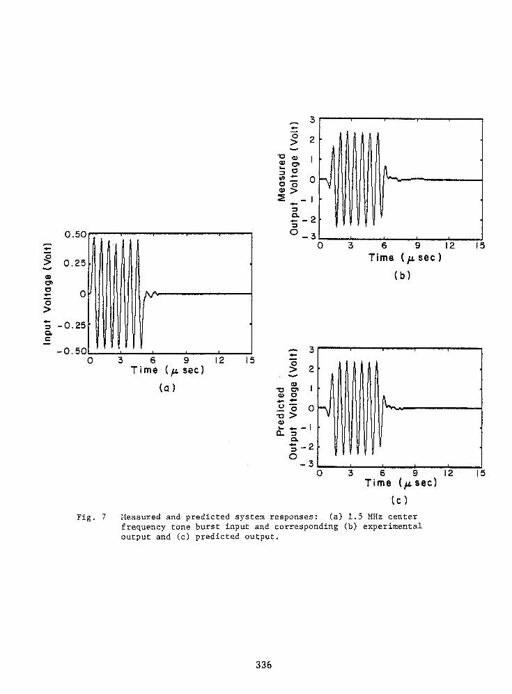
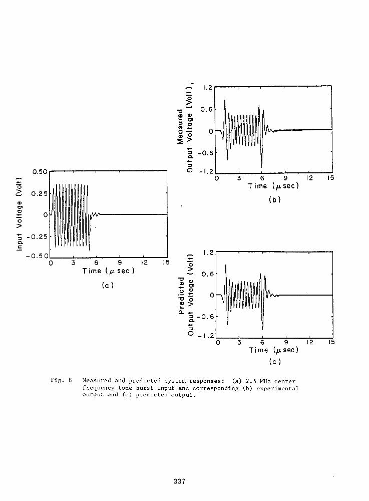
Figures 7 and 8 show the outputs of the system to tone burst inputs ofapproximately 6 _sec in duration and 1.5 and 2.5 MHz in center frequency,respectively. The agreement between the experlmentally measured and thepredicted outputs was excellent. The arrival times of peaks of individualcycles were predicted to within ±25 nsec in both cases. The measured peakamplitudes of all the individual cycles were correctly predicted to withinmaximum errors of 5 and g percent for the 1.5- and 2.5-MHz inputs, respec-tively. Similar agreement was also obtained for center frequencies rangingfrom 0.5 to 3 MHz.

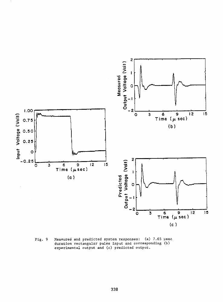
Figure 9 shows the output of the system to a 7.5-_sec-duratlon rectangularpulse input. The agreement between the experimentally measured and the pre-dicted outputs was excellent. The arrival times of peaks of individual cycleswere predicted to within ±25 nsec. The measured peak amplitudes of the indi-vidual cycles were correctly predicted to within a maximum error of 5 percent.From figure 9, for the approximate time of 5 to 7 _sec, both the measured andthe predicted outputs were constant in time. The constant values correspondedto 0 and 0.046 V for the measured and predicted outputs, respectively. Sim-ilar agreement was also obtained for pulse durations ranging down to 0.85 _sec.

322

Figure 10 shows the output of the system to one cycle of 1.75-MHz-frequency input at 2.3 V peak to peak. The arrival times of peaks of lndtvtd-ual cycles were predicted to within ±25 nsec. The shapes of the measured andpredicted outputs agreed well, but the amplitude of the predicted output wassomewhat larger than that of the measured output. As shown In figure 10, thepredicted and measured peak-to-peak output amplitudes were 8.7 and 7.2 V,respectively. The predicted output was larger than the measured output whenthe input and output exceeded 1.4 and 5.1 V peak to peak, respectively. Thisnonlinearity indicates that the linear model used in the prediction becomesinadequate for large-amplitude inputs and outputs. When the input and outputwere less than 1.4 and 5.1 V peak to peak, respectively, the measured outputpeak amplitudes were correctly predicted to within a maximum error of6 percent. Restrictions on both input and output amplitudes were imposedbecause the nonlinearity may be due to the input or the output or both.

CONCLUSIONS

The SWF ultrasonic test system Input-output characteristics were investi-gated by directly coupling the transmitting and receiving transducers face toface without a test specimen. Some of the fundamentals of digital signal proc-essing were summarized. Input and output signals were digitized by using adigital oscilloscope, and the digitized data were processed in a microcomputerby using digital slgnal-processlng techniques.

The contlnuous-tlme test system was modeled as a dlscrete-tlme, linear,shlft-lnvarlant system. In estimating the unlt-sample response and frequencyresponse of the dlscrete-tlme system, it was necessary to use digital filteringto remove Iow-amplltude noise, which interfered with deconvolutlon calcula-tions. A digital bandpass filter constructed with the assistance of a Blackmanwindow and a rectangular time window were used. Approximations of the impulseresponse and the frequency response of the contlnuous-tlme test system wereobtained by linearly interpolating the defining points of the unit-sampleresponse and the frequency response of the dlscrete-tlme system. The testsystem behaved as a llnear-phase bandpass filter in the frequency range 0.6 to2.3 MHz. These frequencies were selected in accordance with the criterionthat they were 6 dB below the maximum peak of the amplitude of the frequencyresponse.

Furthermore, by using the unit-sample response and the frequency responseof the dlscrete-tlme system and the assumption of a linear, shlft-invarlantsystem, the output of the system to various inputs was predicted and theresults were compared with the corresponding measurements on the system. Thepredicted output was obtained by linearly interpolating the defining points ofthe dlscrete-tlme output sequence. Tone bursts of various center frequenciesand durations, rectangular pulses of various durations, and angle cycle inputsat 1.75 MHz with various amplitudes were considered. Excellent agreementbetween the predicted and measured results was obtained for tone bursts withcenter frequencies from 0.5 to 3 MHz and rectangular pulses. Excellent agree-ment between the predicted and measured results was also obtained for one-cycleinputs of various amplitudes, as long as the input and output were less than5.1 V peak to peak, respectively, at a 40-dB system gain. These results arespecific for the particular set of components in the test system.

323

The results of this study will be useful in the quantitative analysis ofthe SWF when test specimens are inserted between the transducers. With knowntest system characteristics, the effects on the output signal due to the testspecimen having a variety of flaw states can be isolated. Furthermore, usingand discussing digital slgnal-processlng methods extensively may facilitatedevelopments in CANDE.

REFERENCES

I. J. Krautkramer and H. Krautkramer, Ultrasonic Testing of Materials, SecondEdition, Sprlnger-Verlag, N.Y., 1977.

2. A. Vary and R.F. Lark, "Correlation of Fiber Composite Tensile Strengthwith the Ultrasonic Stress Wave Factor", Journal of Testing and Evalua-tion, vol. 7, no. 4, July 1979, pp. 185-191.

3. A. Vary and K.J. Bowles, "An Ultrasonlc-Acoustlc Technique for Nondestruc-tive Evaluation of Fiber Composite Quality", Polymer Engineering andScience, vol. 19, no. 5, Apr. 1979, pp. 373-376.

4. J.H. Williams, Jr., and N.R. Lampert, "Ultrasonic Evaluation of Impact-Damaged Graphite Fiber Composite", Materials Evaluation, vol 38, no. 12,Dec. 1980, pp. 68-72.

5. J.H. Williams, Jr., H. KaragUlle, and S.S. Lee, "Ultrasonic Input-Outputfor Transmitting and Receiving Longitudinal Transducers Coupled to SameFace of Isotroplc Elastic Plate", Materials Evaluation, vol. 40, no. 6,May 1982, pp. 655-662.

6. H. KaragUlle, "Ultrasonic Input-Output for Transmlttlng and ReceivingTransducers Coupled to Same Face of Isotroplc Elastic Plates", DoctoralThesis Proposal, Submitted to the Department of Mechanical Engineering,Massachusetts Institute of Technology, Cambridge, Mass., Oct. 1982.

?. A.V. Oppenhelm and R.W. Schafer, Digital Signal Processing, Prentice-Hall, Inc., Englewood Cliffs, N.J., 1975.

8. S.D. Stearns, Digital Signal Analysis, Hayden Book Company, Inc.,Rochelle Park, N.J., 1975.

9. A.V. Oppenhelm, A.S. Willsky, with I.T. Young, Signals and Systems,Prentlce-Hall, Inc., Englewood Cliffs, N.J., 1983.

lO. E.O. Brigham, The Fast Fourier Transform, Prentlce-Hall, Inc., EnglewoodCliffs, N.J., 1974.

II. S.H. Crandall and W.D. Mark, Random Vibration in Mechanical Systems,Academic Press, N.Y., 1963.

324

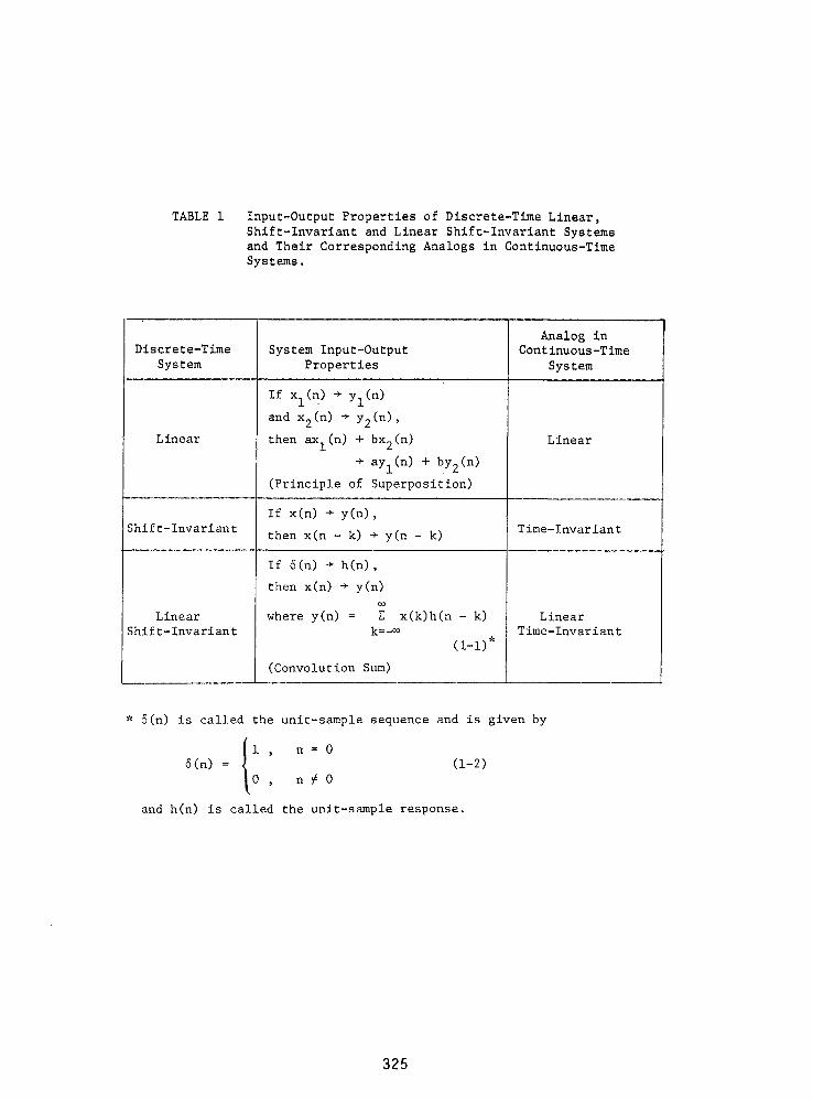
TABLE 1 Input-Output Properties of Discrete-Time Linear,

Shift-lnvariant and Linear Shift-lnvariant Systems

and Their Corresponding Analogs in Continuous-Time

Systems.

Analog inDiscrete-Time System Input-Output Contlnuous-Time

System Properties System

If xl(n) . Yl(n)

and x2(n) + Y2(n),

Linear then axl(n) + bx2(n) Linear

. aYl(n) + bY2 (n)

(Principle of Superposition)

If x(n) . y(n),

Shift-lnvariant then x(n - k) . y(n - k) Time-lnvariant

If 6(n) . h(n),

then x(n) + y(n)

Linear where y(n) = _ x(k)h(n - k) LinearShift-lnvariant k=-_ Time-lnvariant

(i-i)*

(Convolution Sum)

* _(n) is called the unit-sample sequence and is given by

i , n= 0

6(n) = (1-2)

0 , n# 0

and h(n) is called the unit-sample response.

325

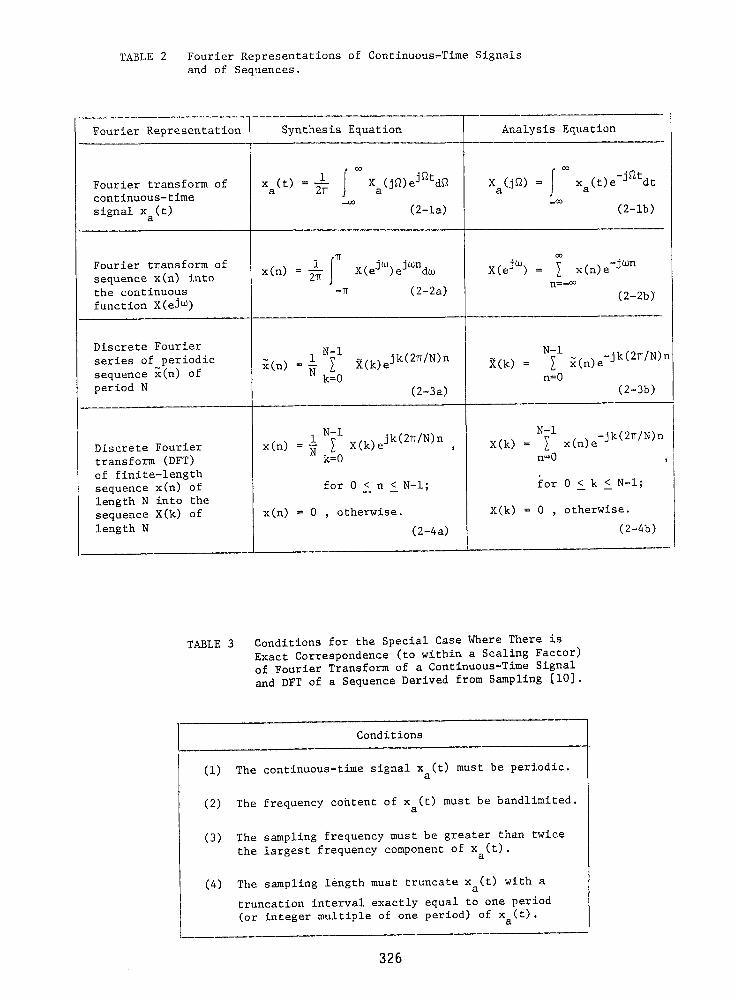
TABLE 2 Fourier Representations of Continuous-Time Signalsand of Sequences.

Fourier Representation Synthesis Equation Analysis Equation

1 I °° Xa(J_)eJ_td_ I °° Xa(t)e-J_tdtFourier transform of Xa(t) = _ Xa(J_) =¢ontinuous- time

signal Xa(t) _oo (2-1a) _co (2-1b)

Fourier transform of x(n) = 1 I_ • •sequence x(n) into 2-_ X(e3°J)eJ°_nd_ X(eJ°°) = x(n)e-J_n

the continuous -_ (2-2a) n=-°°function X(eJ °°) (2-2b7

Discrete FourierN-I N-I

series of periodic x(n) 1 eJk(2_/N)n e-Jk(2_/N)nsequence x(n) of = N _ X(k) X(k) -- _ x(n)

period N k=0 n=0(2-3a) (2-3b)

N-I N-I= 1

Discrete Fourier x(n) _ [ X(k)e jk(2Z/N)n , X(k) = [ x(n)e -jk(2_/N)ntransform (DFT) k=0 n=0

of finite-length

sequence x(n) of for 0 < n < N-I; for 0 < k < N-I;length N into the

sequence X(k) of x(n) = 0 , otherwise. X(k) = 0 , otherwise.

length N (2-4a) (2-4b)

TABLE 3 Conditions for the Special Case Where There is

Exact Corresponden¢e (to within a Scaling Factor)

of Fourier Transform of a Contlnuous-Time Signal

and DFT of a Sequence Derived from Sampling [i0].

Conditions

(i) The continuous-time signal x (t) must be periodic.a

(2) The frequency cohtent of x (t) must be bandlimited.a

(3) The sampling frequency must be greater than twice

the largest frequency component of x (t).a

(4) The sampling length must truncate x (t) with aa

truncation interval exactly equal to one period(or integer multiple of one period) of x (t).

a

326

TABLE 4 Convolution Representations of Continuous-Time Signalsand of Sequences.

Fourier RepresentationConvolution Representation Definition of Convolution

Linear convolution of

contlnuous-time signals Xa3(t ) = ] XaI(T)Xa2(t-T)dT Xa3(J_ ) = Xal(J_)Xa2(J_)Xal(t) and Xa2(t)

(4-1a) (4-1b)

Periodic convolution of N-I

periodic sequences x3(n) = _ _l(m)_2(n-m) _3(k ) = _l(k)_2(k)El(n) and _2(n), each m=0of period N (4-2a) (4-2b)

N-I

Circular convolution of x3(n ) = [ xl(m)_2(n-m) X3(k ) = _l(k)_2(k)finite-length sequences m=0 ,

xl(n) and x2(n) , each of

length N. The sequences for 0 < n < N-I; for 0 < k < N-I;

are represented asperiods of periodic

sequences x1(n) and x3(n) = 0 , otherwise. X3(k) = 0 , otherwise.

_(n),each 8f period N. (4-3a) This is same as:

X3(k ) = Xl(k)X2(k )

(4-3b)

NI+N 2-2

Linear convolution via x3(n) = _ _l(m)_2(n-m) X3(k ) = Xl(k)X2(k)circular convolution of m=0

finite-length sequences

xl(n) with length N 1 for 0 < n < NI+N2-2 ; for 0 < k < NI+N2-2 ;and x2(n) with length N2. -- --

Thesequencelengthis ofincreasedeach to x3(n) = 0 , otherwise. X3(k) = 0 , otherwise.

NI+N2-1 by appending (4-4a) (4-4b)sufficient number of

zeroes to each sequence.

The resulting sequences

are represented as

periods of periodic

sequences xl(n) and

x2(n), each of period

NI+N2-1

327

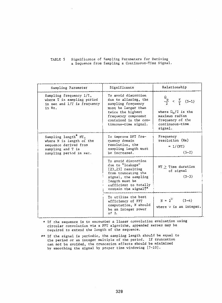
TABLE 5 Significance of Sampling Parameters for Deriving

a Sequence from Sampling a Continuous-Time Signal.

Sampling Parameter Significance Relationship

Sampling frequency I/T, To avoid distortion

where T is sampling period due to aliasing, the o < _ (5-1)in sec and I/T is frequency sampling frequency 2 T

in Hz. must be larger than

twice the highest where _o/2 is the

frequency component maximum radiancontained in the con- frequency of the

tinuous-time signal, continuous-time

signal.

Sampling length* NT, To improve DFT fre- Frequency

where N is length of the quency domain resolution (Hz)

sequence derived from resolution, the = I/(NT)sampling and T is sampling length must

sampling period in sec. be increased. (5-2)

To avoid distortion

due to "leakage" NT > Time duration[23,25] resulting

of signalfrom truncating the

signal, the sampling (5-3)

length must besufficient to totally

contain the signal_*

To utilize the best

efficiency of FFT N = 2V (5-4)

computation, N should where _ is an integer.be an integer powerof 2.

* If the sequence is to encounter a linear convolution evaluation usingcircular convolution via a FFT algorithm, appended zeroes may be

required to extend the length of the sequence.

** If the signal is periodic, the sampling length should be equal to

the period or an integer multiple of the period. If truncationcan not be avoided, the truncation effects should be minimized

by smoothing the signal by proper time windowing [7-10].

328

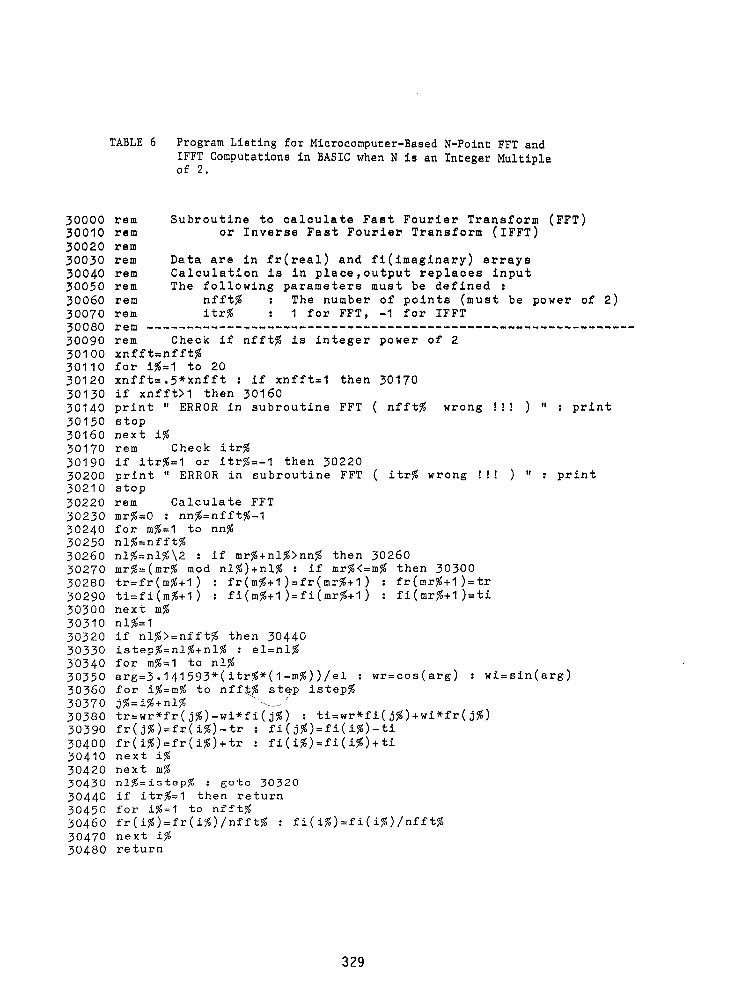
TABLE 6 Program Listing for Microcomputer-Based N-Point FFT and

IFFT Computations in BASIC when N is an Integer Multipleof 2.

30000 rem Subroutine to calculate Fast Fourier Transform (FFT)30010 rem or Inverse Fast Fourier Transform (IFFT)30020 rem30030 rem Data are in fr(real) and fi(imaginary) arrays30040 rem Calculation is in place,output replaces input30050 rem The following parameters must be defined :30060 rem nfft% : The number of points (must be power of 2)30070 rem itr% : I for FFT, -1 for IFFT30080 rem30090 rem Check if nfft% is integer power of 2

30100 xnfft=nfft%30110 for i%=I to 2030120 xnfft=.5*xnfft : if xnfft=l then 30170

30130 if xnfft>1 then 3016030140 print " ERROR in subroutine FFT ( nfft% wrong I!! ) " : print30150 stop

30160 next i%30170 rem Check itr%30190 if itr%=1 or itr%=-1 then 3022030200 print " ERROR in subroutine FFT ( itr% wrong !!! ) " : print30210 stop30220 rem Calculate FFT

30230 mr%=0 : nn%=nfft%-130240 for m%=I to nn%30250 nl%=nfft%

30260 nl%=nl%\2 : if mr%+nl%>nn% then 3026030270 mr%=(mr% mod nl%)+nl% : if mr%<=m% then 3030030280 tr=fr(m%+1) : fr(m%+l)=fr(mr%+1) : fr(mr%+l)=tr30290 ti=fi(m%+1) : fi(m%+1)=fi(mr%+l) : fi(mr%+1)=ti30300 next m%30310 ni%=I30320 if nl%>=nfft% then 30440

30330 istep%=nl%+nl% : el=nl%3'0340 for m%=I to nl%30350 arg=3.141593*(itr%*(1-m%))/el : wr=cos(arg) : wi=sin(arg)

30360 for i%=m% to nfft_% st_p istep%30370 j%=i%+nl% _J30380 tr=wr*fr(j%)-wi*fi(j%) : ti=wr*fi(j%)+wi*fr(j%)30390 fr(j%)=fr(i%)-tr : fi(j%)=fi(i%)-ti

30400 fr(i%)=fr(i%)+tr : fi(i%)=fi(i%)+ti30410 next i%30420 next m%30430 nl%=istep% : goto 30320

30440 if itr%=1 then return30450 for i%=I to nfft%30460 fr(i%)=fr(i%)/nfft% : fi(i%)=fi(i%)/nfft%30470 next i%30480 return

329

Signal or Sequence Fourier Representation

(i)

o t -__._q.oo __.._.o ,0,

U Sampled 2 21

.X (e j= )

T]T3TITTT t;;n' A(ii)

TTT(r _ i , *'"

-iot_ _._ n -z= -= o _" 2=- _r _oTk'\Interpreted as T (sec) 2 2

(a)

o__,o-_ , o n

_ SampledI (ej¢°)

x(n)

(ii)

// _" Interpreted as T (sec),_kImplied Periodicity

.I(k)

TTT+?TTTTT.+T]T,..I+TJT,.TTT,."'" _ +. _" ..... ,_? ?_,_I' I'**+_ t+ ""=

x(n) OFT 3r"(k)Interpreted Interpreted,__as T (sec) as -_ (radlsec)

(b)

Fig. i Fourier representations of (a) continuous-time signal and

sequence derived from sampling, and of (b) finite-duration

continuous-time signal, sequence derived from sampling and

the sequence with implied periodicity.

330

s°°d°nd llTliiciTTI7Implied Periodi

(i) =:¢>gte

O__..jt_q I "t"N2 2 nInterpretedas T (see)

Sampled ond JT t'_2(n) lJir

implied Periodicity

T;C o--- N

Interpretedas T (sec) x2(n)

_ Lineor _ PeriodicConvolution , "Convolution

(iii) t T -

"T T_,. TT,.T Th."_t I --I-t 2-_ t __t__ O__N i .i. N2_2 --n

Interpreted xB(n)os T(se¢) (Circular

Convolution)

(o) (b)

Fig. 2 (a) Linear convolution of continuous-time signals and (b)

circular convolution of sequences derived from sampling thesignals.

331

Digital Oscilloscope

Pulse I Function Generator Lowpass Sampling b, JFilter Rate

Cutoff atLength o 5 MHz _ o Channel I

Output I

_) Frequency _ o Channel 2

Variable FrequencyFilter

Ultrasonic

Preamplifier Bandpass

co 0.4 MHz -- 2.6MHz --'11r_ IKHz- IOMHz

Micro computer

il FlTransmitting Rece ivingTransducerTra nsduce r

k Specimen J j RubberJ/_ Support

\\\\\\\\\\\\\\\\\\'

Fig. 3 Schematic of experimental components with specimen showing the "stresswave factor" test configuration. (All tests in this study were conductedwith transducers coupled face to face without a test specimen.)

Input _ h (n)

x (n) F FT Inversion ]:FFT i_>_]h(n)= h2(n+350)l 0 < n < 1023

1' [ h (n) =0 for n >1003

Yt(k)

Output 1024 - Point Y(k) L,<

h3( + FFT I _55 450 to2s FFT Response

_n Rectangular Window H (k)

h4(n) O <_k <_.511

co Shift I _5o Notation:co i

co h-,a(n) : hd(n-350)I' --I o

t __.c_o_

ho(O,)Tl"'(°'- TTTT)ITTTIIT ,,,.,.. TI 'r,z,_. _ _'FIoe 0 _ "-nUnit - Sample Response 700

of Bondpass Filter Blackmon Window

Fig. 4 Schematic of digital signal processing procedures applied to experimental

input and output sequences to evaluate unit-sample response and frequencyresponse of experimental system.

.-- 1.5 "" .3

=o> 2•.. 1.0 "_

=" I

o . t-,- 0.5 "5o > 0 --

. 0 '_' ' "= I:3 Q.

--= -0.5 0 - 2_o 3 _ _ ,'2 5 o 3 6 9 ,2 ,s

Time (p. sec) Time (p.sec)

._ 0 ,..°_ - Sl"' "_ 2O_,... -20 _ "5l>-

"I_ ::3 GI.o.

o: ._'_ _, -6o_8 _, 60 -_°° _E3: -J JO 80 O -80O 04 , , I 04Z v 0 2 4 6 8 I0 Z v 0 2 4 6 8 I0

Frequency (MHz) Frequency (MHz)

7/" "_' 7/" ,

0 _ 0

_.{ __._== ====-_r ==-,rn 0.o 2 4 6 8 Io 0 2 4 6 s Io

Frequency (MHz) Frequency (MHz)

(o) (b)

Fig. 5 Time history, magnitude and phase of (a) input signal and(b) output signal.

334

<'_'-o o ,..--\

"==:_ ,_-zo_._. :_ ,

"-- _ _ - 40

L 0o (_ -60z

V ,, I 1 I t

_ 1.0 0 2 4 6 8 I0,_ u Frequency (MHz)

_, 0.5n,'o

_"_ 0

_E"-0.5

I I l l I ' ' ' _"0 3 6 9 12 15 "_

Time (p.sec) -o_ :r LI _ t(a) o

° ° /(lJ¢,n

c.- -- "/'rl.n i, ,, i I , i

0 2 4 6 8 I0

Frequency (MHz)

(b)Fig. 6 Experimentally determined (a) impulse response and (b)

frequency response of test system.

335

i f , ,

_ o_- ,

.,_-20.50 .... 0 _ 3 , , , ,

0 :3 6 9 12 150.25 Time (/a,. sec )

(b)

X -o 25e-

-0.50 a , , i _ 3 ....

0 3 6 9 12 15 _--Time (/_ sec) 2

(a) _, l°.-_,

a" "_ - I2_

3! , , , ,0 3 6 9 12 5

Time (/_sec)(c)

Fig. 7 l,Ieasured and predicted system responses: (a) 1.5 MHz centerfrequency tone burst input and corresponding (b) experimentaloutput and (c) predicted output.

336

1.2_m

0.6

0.50 , , , 0 , , i0 3 6 9 12 15

o Time (/_ sec)> 0.25

(blo

: ° ]0

•-., -0.25c-- ^ _,..' ,,-'."-u.ou I , I I

0 3 6 9 12 15 o

Time (_ sec ) "._> 0.6

Ca) ®o

•-" 0

-0.6Q.

0 -I .2 , , , ,0 3 6 9 12 15

Time (_ sec)

(c)

Fig. 8 Measured and predicted system responses: (a) 2.5 MHz center

frequency tone burst input and corresponding (b) experimental

output and (c) predicted output.

337

o>

oJ

R-I4,"

01.00 .... 2 , f , I

,v_,._;..-- 0 3 6 9 12 5"6 0.75 Time (p. sec)>•"-" (b)

0.50O

o 0.25>

= 0 -e_

---0.25 , , I , "-" 2= l

0 3 6 9 12 15 ""

Time (p. sec) _ I

(a) g

I

0_ I I I I

O 3 6 9 12 15Time (p. sec)

(c)

Fig. 9 Measured and predicted system responses: (a) 7.65 _sec

duration rectangular pulse input and corresponding (b)

experimental output and (c) predicted output.

338

5.0 ' ' '

2.5

&

o4"

R-z5

1.50 , , 0_5.0 , , , ,0 3 6 9 12 15

"6 Time (/J. sec )> 0.75

= (b)o= 0 ',-,_---- - -" -'--o>

-0.75c

- 1.5( , , , , " '0 3 6 9 12 5 --

Time (/a. sec) 2.5(a) "_ _

,e- _

:_ _',__-_ .L_

X-2.5

0 -5.0 , , , ,0 3 6 9 12 15

Time (_. sec )

(c)

Fig. i0 Measured and predicted system responses: (a) One

cycle of 1.75 MHz frequency input at 2.3 Volts

peak-to-peak and corresponding (b) experimental output

and (c) predicted output.

339