INSTABILITY AND THE INCENTIVES FOR CORRUPTION

FILIPE R. CAMPANTE�, DAVIN CHOR AND QUOC-ANH DO

We investigate the relationship between corruption and political stabil-ity, from both theoretical and empirical perspectives. We propose amodel of incumbent behavior that features the interplay of two effects: ahorizon effect, whereby greater instability leads the incumbent to em-bezzle more during his short window of opportunity, and a demandeffect, by which the private sector is more willing to bribe stable in-cumbents. The horizon effect dominates at low levels of stability, be-cause firms are unwilling to pay high bribes and unstable incumbentshave strong incentives to embezzle, whereas the demand effect gainssalience in more stable regimes. Together, these two effects generate anon-monotonic, U-shaped relationship between total corruption andstability. On the empirical side, we find a robust U-shaped pattern be-tween country indices of corruption perception and various measures ofincumbent stability, including historically observed average tenures ofchief executives and governing parties: regimes that are very stable orvery unstable display higher levels of corruption when compared withthose in an intermediate range of stability. These results suggest thatminimizing corruption may require an electoral system that featuressome re-election incentives, but with an eventual term limit.

1. INTRODUCTION

THIS PAPER investigates how political stability affects the incentives of in-cumbents to engage in corrupt behavior. At a basic level, access to publicoffice provides opportunities for extracting corruption rents, and the pos-sibility of losing office naturally constrains an incumbent’s window of op-portunity for doing so. In addition, many lucrative projects that generatethese rents, such as the exploitation of a natural resource or constructioncontracts, often take time to deliver their full monetary returns, and can behalted if the incumbent is removed or if the opposition has sufficient clout toblock the project. One would thus expect that an incumbent’s security oftenure and his ability to marshal support for his favored projects, bothcrucial components of political stability, should be key in determining hiswillingness and ability to extract these rents.1 We tackle this relationshipbetween incumbent stability and corruption from both theoretical and em-pirical perspectives.

�Corresponding author: Filipe R. Campante, Harvard Kennedy School, Harvard University,79 JFK St., Cambridge, MA 02138, USA. E-mail: filipe_campante@ksg.harvard.edu

1Note that we do not limit our concept of stability to the violent or unconstitutional removalof the incumbent, as is often the narrower use of the term ‘‘political instability.’’

March 2009

As a conceptual starting point, it is important to recognize that the term‘‘corruption’’ encompasses a wide range of related, but nevertheless distinct,ways in which public officials may improperly derive private gain, such asembezzling or misappropriating public funds, accepting kickbacks for favorsor licenses, or engaging in nepotism.2 A key insight of this paper is that poli-tical stability can have contrasting effects on different forms of corrupt activity.

On the one hand, a lower level of stability shortens the incumbent’seffective decision-making horizon, which can lead to more corrupt behavioralong the lines of Olson’s (1991) ‘‘roving bandit.’’ An incumbent who is veryunstable would find it optimal to steal more today instead of letting the poolof resources accumulate into the future, given the uncertainty over whetherhe will still be in power tomorrow. We can thus expect corruption in theform of direct embezzlement – the diversion of public resources straight intoone’s pocket – to decrease as the incumbent’s position becomes more stable.This horizon effect can be thought of as a ‘‘supply’’-driven effect, as it has todo with the willingness of the public official to supply or divert resourcestoward corruption.3

On the other hand, other forms of corruption entail a long-term re-lationship between the incumbent and a third party, for example when abribe is paid by a private firm for a resource concession that will take severalyears to exploit. In this situation, the private sector’s willingness to paybribes actually increases with political stability, as businesses will be moreinclined to wheel-and-deal with an incumbent whose position they assess tobe more secure. Put otherwise, a stable regime is more conducive for anincumbent and the private sector to develop the connections through whichthe flow of bribes will run. We dub this effect the demand effect, because it isdriven by the private sector’s demand for corruption.4

This paper’s first point is to develop a model that formalizes the interplaybetween these two effects. In our setup, a self-interested incumbent makes anoptimal allocation of public resources to two different forms of corruptactivity, namely direct ‘‘embezzlement’’ and third-party ‘‘licensing.’’ (These

2Glaeser and Goldin (2006), Nye (1967), Rose-Ackerman (1999), and Svensson (2005) amongothers have drawn similar distinctions on the different manifestations of corruption. Olken(2007) uncovers an interesting example of how incumbents appear to substitute between dif-ferent forms of corruption. In a field experiment involving road-building projects in Indonesia,the use of an external audit led to a decrease in direct stealing of project funds, but resultedinstead in an increase in nepotism in hiring decisions related to the projects.

3This horizon effect will be mitigated if there is a possibility that the incumbent can return topower some time after being ousted. Such a political return will presumably be likelier whenthere is more turnover and instability in the political environment. We have explored thispossibility in an extension using an infinite-horizon Bellman approach, in which we find that this‘‘resurrection’’ effect dampens the horizon effect, but does not reverse it.

4The idea of modeling corruption as the outcome of demand and supply forces within anunofficial market is not new, with Shleifer and Vishny (1993) being a seminal piece. One con-tribution of our paper is to analyze how political stability interacts with these demand–supplyeffects to influence the level of corruption.

labels serve as shorthand for the multiple types of activities typically re-garded as corruption, with the main distinction being that ‘‘licensing’’ in-volves an interaction with the private sector.) However, the incumbent’sposition is potentially unstable, in that there is some probability each periodthat he will be ousted or that his policies will be blocked.

We show that the two aforementioned effects combine to generate a non-monotonic relationship between total corruption and stability that approx-imates a U-shape. At low levels of stability, the horizon effect unambiguouslyprevails, and total corruption falls as the incumbent’s stability improves. Onthe other hand, the demand effect dominates in more stable regimes, leadingto a positive relationship between total corruption and stability over higherranges of the latter. The underlying logic is intuitive: the private sector is re-luctant to bribe an unstable incumbent; hence, direct stealing will be the mainsource of corruption revenues in highly unstable regimes. In the face of a smallincrease in stability over this low range, the private sector remains pensiveabout investing heavily in bribes, leaving the unstable incumbent with fewopportunities to substitute from embezzlement into licensing. This marginalincrease in stability therefore reduces total corruption because it lengthens theincumbent’s expected horizon and directly decreases his incentive to embezzle.However, over higher ranges of stability, bribery becomes more enticing, andthis opens the door for the demand effect, because the prospect of long-termdeals raises the private sector’s demand for corruption. Corruption thus in-creases with stability in relatively stable regimes, as long as the incumbent’sability to extract rents from the private sector is sufficiently high so as to makebribery an important source of corruption revenues.

The picture that emerges from our model is consistent with a lot of anec-dotal evidence. On one end of the spectrum, countries such as Brazil (in theearly 1990s) and Pakistan have grappled with a combination of low stabilityand high corruption. For example, Easterly (2003) surmises that ‘‘politicalinstability has made Pakistan’s successive governments more like MancurOlson’s (2000) ‘roving bandit’, who loots only for today’’ (p. 464). Con-versely, autocratic regimes such as Mexico under the Institutional Revolu-tionary Party (PRI), Kenya under Daniel Arap Moi, and Indonesia underSuharto were stable for long periods, but saw extensive corruption as theruling elite exercised a monopoly over rent-seeking activities. Last but notleast, competitive democracies fall conveniently in the category of inter-mediate stability and lower levels of corruption.5 We discuss in detail howour theory is relevant for understanding individual countries’ experienceswith corruption with a pair of case studies, for Brazil and Mexico. These

5As further illustration, it has been suggested that the reason why the Baltic countries had abetter track record on corruption than other transition economies was that ‘‘because [their]governments are [relatively] weak and fast-changing, they are also limited in their ability toadvance their financial backers’ interests’’ (The Economist, December 11, 2004, p. 48). This isprecisely the spirit behind the demand effect that we have outlined.

countries provide sharp illustrations of the horizon and demand effects, withobservers having written about how corruption has ebbed and flowed inthese countries as political stability has fluctuated.

The paper’s second main point is empirical: we uncover a U-shapedpattern between the country-level indices of corruption perception com-monly used in empirical work, and various measures of political stability.6

The strength of this pattern, which is documented extensively in section 3,can be verified along many dimensions. This U-shaped relationship showsup consistently in our main specification using the Kaufmann, Kraay, andMastruzzi (2006, henceforth KKM) corruption perception measure, evenafter we control for a battery of additional determinants of corruptiondeemed important in the literature. It is also robust to the use of theTransparency International (TI) and International Country Risk Guide(ICRG) indices, two additional measures that are also widely used in em-pirical work. We obtain these results using two different measures of poli-tical stability: (i) the historically observed average tenure of a country’s chiefexecutive and (ii) the average tenure of the party in power. (We also findsupportive results using a more indirect measure of stability, the governingcoalition’s share of seats in the legislative.) Our findings hold both in a cross-section of countries (where we average the relevant variables over time), aswell as when estimation is performed on the yearly data using dynamic panelGMM techniques that help to allay concerns over endogeneity arising fromcountry-specific unobservables or reverse causality. Finally, we find supportfor a corollary concerning the relationship between corruption and the sizeof government. Our model predicts that the latter variable is positivelycorrelated to stability, and hence also stands in a U-shaped pattern withcorruption; we do indeed find some evidence for such a pattern in the data.

Our analysis yields meaningful policy implications regarding what in-stitutional settings might be optimal for keeping corruption at bay. The non-monotonic relationship between corruption and political stability identifiedin our theory and supported in our empirical analysis suggests that a com-bination of the possibility of re-election and the presence of term limits isnecessary: the former counteracts the incentives to embezzle posed by thehorizon effect, whereas the latter keeps the demand effect in check.

1.1 Related Literature

Our paper falls within an extensive literature on the causes of corruption.7 Itbuilds on a well-established body of empirical work that has identified

6Interestingly, in one of the first cross-country studies on corruption, Mauro (1995) reported apositive correlation between the Business International corruption index for 1980–1983 and asubjective index of political stability from the same source. However, his paper did not explorethe possibility of a non-monotonic relationship.

7For an overview of issues, see Bardhan (1997), Lambsdorff (1999), and Svensson (2005).

various systematic determinants of corruption, including ethnolinguisticfractionalization (Mauro, 1995), the presence of economic rents (Ades andDi Tella, 1999), the level of democracy (Treisman, 2000), and electoral rules(Persson et al., 2003). As we will show, our empirical results are robust to theinclusion of these controls, which suggests that political stability also be-longs on this list as a key proximate determinant of the incentives for cor-ruption. While political stability has previously been linked to outcomessuch as aggregate growth (Alesina and Perotti, 1996; Alesina et al., 1996),this is one of the first attempts (to the best of our knowledge) to model andestimate a link to corruption.

Several earlier studies have alluded to a potential link between corruptionand stability. DeLong and Shleifer’s (1993) and Olson’s (1991, 2000)discussions of the importance of decision-making horizons on the behaviorof incumbents, and to some extent the models of electoral account-ability such as Barro (1973) and Ferejohn (1986), include forces similar toour horizon effect.8 As for the demand effect, similar considerations areimplicit in Rose-Ackerman’s (1999) discussion of the role of checks andbalances on the government in curbing corruption. Along similar lines,Fredriksson and Svensson (2003) analyze how corruption and instabilityinteract in influencing policy in a lobbying model. While their papercontains ideas that resemble the horizon and demand effects, it doesnot deal directly with the impact of stability on corruption, takinginstead the incumbent’s propensity for corruption as an exogenousparameter. In a different but related context, Acemoglu (2005) also obtainsa U-shaped relationship between a ruler’s incentives to act in detrimentof public welfare and the inherent strength of the state, arising from asimilar interplay between his incentives to invest in the economy and hisability to extract rents. While his mechanism operates via investment inpublic goods, ours is based on the possibility of accumulating resources intothe future.

Most recently, and quite importantly, a growing body of work based onmicrolevel measures of corruption has emerged that strongly affirms theempirical relevance of the key mechanisms underlying our theory. Usingevidence from Brazilian municipality audits, Ferraz and Finan (2007)compare mayors who are in their first term in office with those who are intheir second term, which by law has to be their last one. They show thatmayors in their mandatory last term tend to be more corrupt, a result that isentirely consistent with the horizon effect. More direct support comes fromGamboa-Cavazos et al. (2006), who explicitly test an extension of our

8Shleifer and Vishny’s (1993) prediction that weak decentralized governments would exhibitmore corruption also hints at a relationship with political stability. Their mechanism, however,is the lack of coordination among different public officials, whom private firms need to bribe toobtain licenses that are complementary to each other. Our model, by contrast, focuses on publicofficials who deal with corruption opportunities that are essentially unrelated.

model. They obtain measures of local corruption reported by private firmsin Mexico, and regress them on measures of the stability of state governors,namely the number of years left in office and their legislative support.Their finding of a U-shaped relationship between corruption and thesestability variables is an important piece of evidence that complementsthe cross-country results we obtain, and further strengthens the case for ourframework.9 The paper proceeds as follows. Section 2 presents the modeland our key theoretical results. While we present the model in a moregeneral setting in which the incumbent can divert some resources towardbolstering his stability, for pedagogical purposes, we first build up the in-tuition from a baseline case in which the incumbent treats his stability as anexogenous parameter. We also discuss here two country case studies thatprovide further illustration for the horizon and demand effects thatwe propose. We then turn in section 3 to the cross-country evidence on theU-shaped relationship between corruption and political stability. Section 4concludes.

2. THEORY: HOW INSTABILITY SHAPES THE

INCENTIVES FOR CORRUPTION

2.1 The Model

2.1.1 Basic Setup. We consider an infinite-horizon economy with an initialpool of available resources, K0, the allocation of which is controlled by anincumbent. There is some probability a that the incumbent and his policiessurvive from one period to the next; a thus measures the incumbent’s sta-bility. For simplicity, this incumbent derives personal utility only from di-verting resources toward his corruption rents. At any given point in time, t,resources can be diverted through either (i) ‘‘Embezzlement,’’ Et, whichentails direct stealing, or (ii) ‘‘Licensing,’’ Lt, which involves granting privatesector firms control over some of the resources in exchange for an upfrontbribe payment. In addition, the incumbent can choose to spend someamount, Pt, out of the initial pool of resources to boost his own stability(and thereby increase his probability of staying in power to enjoy futurerents): a is an increasing function of Pt, a(Pt).

10

The distinctive characteristic of the forms of corruption we gather underthe ‘‘licensing’’ label is that they entail an interaction between the incumbentand private sector firms. Let p(Lt, a(Pt)) denote the ex ante expected value ofprofits reaped by the private firm from the license Lt. The key assumption

9Le et al. (2004) find mixed evidence when investigating the cross-country relationship be-tween corruption and stability, but their analysis uses measures of stability that focus morenarrowly on political violence and unrest.

10In the event that the incumbent is ousted, we assume he receives a zero payoff in all sub-sequent periods.

here is that p is an increasing function of stability. (In deriving theequilibrium below, we will in fact impose the simplifying assumption thatthe licenses become void when the incumbent is ousted, but we do not needto go to this extreme.) This captures the idea that, to the extent that there isan intertemporal dimension in the corrupt relationship, the presence of theincumbent in power is valuable to the firm with whom he maintains thatrelationship: an unstable incumbent will be less likely to be able to deliver onhis side of the deal, and hence will be less valuable to his prospective private-sector partner. In particular, we specify that p(Lt, 0)¼ 0, so that firms haveno interest in bribing an unstable incumbent who has zero probability ofbeing in power in the next period.11 We assume that the incumbent has theability to extract a fraction s of expected profits as an upfront bribe paymentfor the license; s thus measures the incumbent’s bargaining power withrespect to the private sector.

Finally, in each period, the remaining untouched resources are trans-formed into the pool of resources available in the next period, subject todiminishing returns: Ktþ 1¼A(Kt�Et�Lt�Pt)

g. This has the interpreta-tion of being a growth equation with technological parameter A. In otherwords, what is not embezzled, licensed, or spent in boosting stability is leftfor the ‘‘rest of the economy’’ and accumulates over time. This sequence ofevents is summarized in Figure 1.

START OFPERIOD t

Incumbent decides Et , Lt and Pt

Firm pays Incumbent for licenserights to Lt

Remaining resources areaccumulated into next period:Kt+1 = A(Kt − Et − Lt)

�

START OFPERIOD t+1

Firm realizes pay-off from Lt

Incumbent decides onEt+1, Lt+1, and Pt+1…Incumbent’s policy

continued withprobability �(Pt)

� happens:

Figure 1. Sequence of events.

11This description of the ‘‘demand side’’ of the corrupt relationship can be reconciled with amodel of ‘‘political cycles’’ in which an incumbent might increase the number of licenses issuedjust before an election, when his stability is at its lowest. In our setup, this increased supplywould be met by a low level of demand given the unstable position of the incumbent, and hencefetch a low ‘‘price’’ per license. It is therefore possible for corruption rents from licensing to fallduring such periods of low stability.

The incumbent’s problem is one of maximizing his expected income.12 Thesequence problem for the incumbent can be described by

maxEt�0;Lt�0;Pt�0

X1t¼0

aðPtÞt½Et þ spðLt; aðPtÞÞ�;ð1Þ

where Ktþ1 ¼ AðKt � Et � Lt � PtÞg:

Our definition of corruption in each period, Gt, is the amount of illicitincome that the incumbent receives, normalized by the resources available atthe start of the period, namely

Gt ¼Et þ spðLt; aðPtÞÞ

Kt: ð2Þ

The normalization ensures that the measure of corruption is not subject toscale effects, so that larger countries are not deemed more corrupt simplybecause there are more resources available.

2.1.2 Stability. We now elaborate on our formulation of incumbent stabil-ity. The variable Pt captures the idea that the stability of the incumbent can beaffected by the resource allocation decisions he makes. Concretely, one canthink of Pt as an amalgam of expenditures that can improve his stability indifferent ways, including: public goods spending that is valued by the masses,such as on education, healthcare or infrastructure; expenditures that can beused to restrain public opposition, such as military or police spending; andpatronage strategically dispensed to cultivate political support from key votersor political players. While we will refer to Pt as ‘‘public goods provision,’’the important thing for our purposes is that this expenditure boosts the in-cumbent’s stability but also diverts resources away from his own pocket.Following this discussion, we specify stability to be a function of the incum-bent’s choice of Pt, denoted by g(Pt), where g( � ) is increasing and concave,with g(0)¼ 0. This function enables us to describe how effective public goodsprovision is in bolstering the incumbent’s position.

In practice, however, an incumbent’s stability also depends on some factorsthat he cannot easily affect. We incorporate this feature by assuming thatoverall stability also depends on the intrinsic stability of the polity, denoted byzA[0, 1]. We interpret z as an exogenous, ‘‘systemic’’ level of stabilitycapturing underlying features such as the ethnic composition of the popula-tion or cultural norms, which are largely beyond the incumbent’s control.Note that these deep-seated features can in turn be mapped into a desired levelof public goods provision, Pz, defined by g(Pz)¼ z. For instance, following

12We implicitly assume that the incumbent can smooth his consumption over time, for ex-ample, by depositing the income in an offshore account. We treat such funds as unrecoverableby the state should the incumbent be ousted. For simplicity, there is no time discounting inaddition to what is implicitly introduced by the stability parameter.

Alesina et al. (1999), a more fractionalized polity with a lower z would inequilibrium have a lower desired level of public goods provision, because eachindividual attaches a smaller value to public goods consumption by otherpeople who do not belong to his/her ethnic group.

In sum, we specify stability (with a slight abuse of notation) to bea¼ a(z, g(P)), where the latter expression allows us to distinguish betweenthe components of stability that are under the incumbent’s control, andthose that are beyond it.

2.2 Benchmark Case: Exogenous Stability

It is useful to start by presenting a benchmark special case of the model inwhich stability is entirely beyond the incumbent’s control, namely where g(P)and hence a are constants. This special case conveys the basic intuition in itssharpest form; we will then move on to show how the intuition generalizes,and how new testable predictions can be obtained in the more general model.

2.2.1 Characterizing the Equilibrium. For ease of exposition, we focus on asimple case for the private sector’s expected profit function: p(Lt, a)¼ aAFLt,where AF is the private sector technology parameter. This corresponds to asituation where the license is valid for one period only, period tþ 1, andproduction is undertaken with an AK technology, subject to the possibilitythat the license will be voided in the event of a discontinuation of the in-cumbent’s policies.13 The problem in (1) can now be reformulated as aBellman equation with value function V( � ):

VðK0Þ ¼ maxE0�0;L0�0

fE0 þ saAFL0 þ aVðK1Þg;

where K1 ¼ AðK0 � E0 � L0Þg:ð3Þ

It is easy to show, from the first-order conditions with respect to E0 and L0,that one of these quantities must be zero, except in a knife-edge scenario.(This is a consequence of the linear functional forms in this baseline model.In an appendix available on request, we have also established our resultswith an objective function that is jointly concave in both embezzlement andlicensing revenues, and which therefore allows both forms of corruption tocoexist in equilibrium.) Which of these two cases will prevail depends on theparameters of the model. If saAFo 1, then the marginal gain from a smallincrement in E0 exceeds that from a similar increment in L0. In this case, theincumbent does not allocate any resources to licensing, and corruption takesonly the form of embezzlement. Conversely, if saAF4 1, then the incumbentreaps private revenues through licensing only. The analysis is most

13The basic results in the propositions below hold for a fairly general class of functional formsfor p(Lt, a) satisfying pL4 0, pa4 0, and pLa4 0.

interesting when the cutoff value of a separating the two cases, a� � 1=sAF ,lies in the interval [0, 1], which happens when sAF4 1. Intuitively, this con-dition means that the incumbent’s ability to extract surplus and the privatetechnology parameter are high enough, so that licensing is attractive over partof the relevant [0, 1] range for a. We now characterize the two cases:

Case 1. saAFo 1, i.e. a<1=sAF .

In this case, Lt¼ 0 for all t � 0. Using the FOCs, the Envelope Theorem,and (2), one can solve for the level of embezzlement-related corruption:

G0 ¼ 1� ðAagÞ1

1�g

K0

Gt ¼ 1� ag; 8t � 1

9>=>;: ð4Þ

Observe that corruption depends on the initial endowment of resources, K0,only in the very first period (t¼ 0); from t¼ 1 onwards, the model is in a ‘‘steadystate’’ in which corruption remains constant, given the parameter values.14

Case 2. saAF4 1, i.e. a>1=sAF .

Here, the marginal gain from a small increment in L0 exceeds that from asimilar increase in E0. The incumbent now does not allocate any resources toembezzlement, and corruption takes only the form of licensing revenues.From the FOCs and (2), this yields the following expression for corruption:

G0 ¼ sAFa 1�Aagð Þ

11�g

K0

" #

Gt ¼ sAFað1� agÞ; 8t � 1

9>>=>>;: ð5Þ

2.2.2 Corruption and Stability. We now analyze the comparative statics forcorruption with respect to stability, focusing on the steady state (t � 1).15

14In this basic framework, we thus have a ‘‘cleaning-up’’ property, in which any amount of theperiod-0 endowment in excess of the steady-state value of Kt is consumed immediately and theeconomy reaches a steady state with a constant level of corruption in one period. This ‘‘cleaning-up’’ property holds whenever the incumbent’s per-period utility is linear in Et.

15The difference between comparative statics in steady state and in transition has to do withwhether the pool of resources at the start of the period is exogenous, or whether this is taken tobe the steady-state value of Kt. More precisely, a change in a will shift the economy toward anew steady state; G0 thus captures the short-run behavior of corruption in transition, while Gt

(t � 1) describes the behavior of corruption in the new steady state. From the expressions in (4)and (5), it is clear that the response of corruption to a is qualitatively similar in both transitionand steady state, so long as K0 is sufficiently large. Note also that a quick substitution of a ¼1=sAF into the expressions for G0 and Gt from the two cases shows that corruption is indeed acontinuous function of stability for all periods.

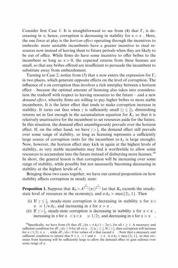
Consider first Case 1. It is straightforward to see from (4) that Gt is de-creasing in a; hence, corruption is decreasing in stability for ao a�. Here,the one force at play is the horizon effect operating through the incentives toembezzle: more unstable incumbents have a greater incentive to steal re-sources now instead of leaving them to future periods when they are likely tobe out of office. While firms do have some incentive to offer bribes to theincumbent so long as a4 0, the expected returns from these licenses aresmall, so that any bribes offered are insufficient to persuade the incumbent tosubstitute away from embezzlement.

Turning to Case 2, notice from (5) that a now enters the expression for Gt

in two places, which generate opposite effects on the level of corruption. Theinfluence of a on corruption thus involves a rich interplay between a horizoneffect – because the optimal amount of licensing also takes into considera-tion the tradeoff with respect to leaving resources to the future – and a newdemand effect, whereby firms are willing to pay higher bribes to more stableincumbents. It is the latter effect that tends to make corruption increase instability. It turns out that when g is sufficiently small ðg � 1

2Þ, diminishing

returns set in fast enough in the accumulation equation for Kt, so that it isrelatively unattractive for the incumbent to set resources aside for the future.In this situation, the demand effect unambiguously prevails over the horizoneffect. If, on the other hand, we have g> 1

2, the demand effect still prevails

over some range of stability, so long as licensing represents a sufficientlylarge source of corruption rents for the incumbent (sAF is large enough).Now, however, the horizon effect may kick in again at the highest levels ofstability, as very stable incumbents may find it worthwhile to allow someresources to accumulate into the future instead of disbursing more licenses.16

In short, the general lesson is that corruption will be increasing over somerange of stability, while possibly but not necessarily becoming decreasing instability at the highest levels of a.

Bringing these two cases together, we have our central proposition on howstability affects corruption in steady state:

Proposition 1. Suppose that K0>A1

1�gðagÞg

1�g (so that K0 exceeds the steady-state level of resources in the economy), and sAF4maxf2g, 1g. Then

(i) If g � 12, steady-state corruption is decreasing in stability a for a<

a� � 1=sAF , and increasing in a for a4 a�.(ii) If g> 1

2, steady-state corruption is decreasing in stability a for aoa�,

increasing in a for a�<a<a�� � 1=2g, and decreasing in a for a4a��.

16Specifically, we have from (5) that dGt=da ¼ sAF ð1� 2agÞ, for all t � 1. A necessary andsufficient condition for dGt=da � 0 for all a[ ½a�; 1� is g � 1

2. If g> 1

2, then corruption will increase

for a<1=2g � a��, while dGt=da<0 for values of a that exceed a��. Note that a necessary andsufficient condition to ensure that 0o a�o 1 and a��4 a� is sAF4maxf2g, 1g, so that rev-enues from licensing will be sufficiently large to allow the demand effect to gain salience oversome range of a.

In words, our model generates a steady state where at first corruption de-creases with stability, and eventually starts to increase (with a possibility thatit starts to decrease once again for very high levels of stability). Put differ-ently, we end up with a non-monotonic relationship between corruption andstability, which will look like a U-shape so long as diminishing returns playan important role in the accumulation of resources: very stable and veryunstable incumbents will tend to be more corrupt than those at an inter-mediate range of stability.

The logic that drives this result is very intuitive, and it is the key messageof our paper. In the range of low stability, firms are unwilling to pay highbribes to unstable incumbents, so that embezzlement becomes themain means for self-enrichment. As a result, the horizon effect dominates:corruption falls as the incumbent’s stability improves and the incentive toembezzle decreases. Beyond a certain level of stability, however, licensingbecomes the more profitable option, as sufficiently stable incumbentsare able to extract larger bribes from firms. Therefore, the demand effectkicks in over the range of high stability so long as sAF is sufficiently large:corruption increases as stability improves, because firms are willing to offerever larger amounts of bribes. This demand effect is sure to dominate overat least some range of high stability, although the horizon effect, whichnaturally affects both types of corruption, may under some circumstancesregain the upper hand at the very highest levels of stability. The overallU-shaped pattern, by which we mean that corruption decreases in stabilityfor lower levels of a, and then eventually starts to increase, is the key testableprediction of our model.

Furthermore, the model yields several interesting predictions on the effectsof parameter shifts:

Proposition 2. Based on the expressions for steady-state corruption in (4)and (5):

(i) Corruption is weakly increasing in the incumbent’s bargaining powervis-a-vis the private sector, s, and the productivity of the privatesector technology, AF.

(ii) Over the range of a where the demand effect dominates, in response toa given rise in s or AF, the increase in corruption is larger when theincumbent is more stable (i.e. a is higher).

Proof. By inspection of (4) and (5), it is clear that s and AF increase cor-ruption from licensing while not affecting corruption from embezzlement.This establishes part (i) of the proposition. For part (ii), it is easy to checkfrom (5) that the cross-derivative with respect to sAF and a is positive,whenever Gt is increasing in a. ’

This proposition lends itself to a natural interpretation. Part (i) follows fromthe fact that corruption revenues from the private sector risewhen either the bargaining position of the government is strengthened orwhen the private sector technology improves. As for part (ii), notice thats and AF affect the corruption revenues from licensing, but not fromembezzlement. As a result, these parameters gain salience in the range ofa where licensing dominates, resulting in a larger increase in corruptionwhen the incumbent is more stable. Note that our formulation takes s tobe independent of a, but one could also expect more stable incumbents tocommand more bargaining power over the private sector. Incorporatingthis simple extension would only reinforce the upward-sloping relationshipbetween corruption and stability for the high levels of a where the demandeffect prevails.

2.3 General Case: Endogenous Stability

Armed with the intuition from this benchmark case, we now turn to considerthe general formulation in which the incumbent can divert resources tobolster his stability: a¼ a(z, g(P)). For concreteness, we think of Pz, thedesired level of public goods provision defined in section 2.1.2, as estab-lishing a ‘‘ceiling’’ on stability, whereby any shortfall of public goods pro-vision with respect to this level will weaken the incumbent’s position. Wethus model stability, a, as a ¼ minðz; gðPÞÞ: Note that this boils down to anassumption that public goods provision and intrinsic stability are (perfect)complements from the standpoint of how they contribute to a. In otherwords, polities that are intrinsically more stable allow an incumbent to bettertranslate spending on public goods into enhanced stability. Two things areworth stressing in that regard, the first one being that we do not need perfectcomplementarity: our results hold as long as there is sufficient com-plementarity between the endogenous and exogenous components of stabil-ity, so that z and g(P) covary together. Second, while this complementarity isultimately an empirical question (to which our results will speak indirectly),we believe there is a priori good reason to consider it plausible. To the extentthat the systemic component z is tied to deeper features of the polity such asethnic fractionalization, if z and P were instead substitutes, one would thenexpect to see higher levels of endogenous public goods provision in moreethnically fractionalized countries, to try to compensate for the poor sys-temic stability in these polities. This would be at odds, however, with theempirical evidence that fractionalization tends to be associated with lesspublic goods spending (Alesina et al., 1999). Moreover, one might thenexpect to observe no specific relationship between ethnic fractionalizationand overall political stability, a(z, g(P)), whereas it has instead been estab-lished that the correlation between these two variables is indeed clearly ne-gative (Alesina et al., 2003).

The incumbent’s problem from the benchmark case, (3), can now beadapted as follows:

VðK0Þ ¼ maxE0�0;L0�0;P0�0

fE0 þ sminðz; gðP0ÞÞAFLt

þminðz; gðP0ÞÞVðK1Þg;

where K1 ¼ AðK0 � E0 � L0 � P0Þg:ð6Þ

We can now state a result that mirrors Proposition 1 on the non-monotonicrelationship between corruption and stability:

Proposition 3. Suppose that g(P) belongs to the class of increasing concavefunctions g(P)¼ (cP)r, where c4 0 and 0o ro 1. Moreover, suppose thatA and K0 are sufficiently large, and that sAF4 2. Then there exists~a�; ~a�� [ ½0; 1�, with ~a�<~a��, such that:

(i) If g � 12, steady-state corruption is decreasing in stability a for a<~a�,

and increasing in a for a>~a�.(ii) If g> 1

2, steady-state corruption is decreasing in stability a for a<~a�,

increasing in a for ~a�<a<~a��, and decreasing in a for a>~a��.

The proof of this proposition is similar to, albeit more extended than, thatfor the baseline model (details available in a separate appendix on request).Intuitively, when there is sufficient complementarity between z and g(P),both of them covary together. At low levels of z, the incumbent thus has littleincentive to set aside resources for public goods, because this has little in-cremental effect on his actual stability, so that corruption will be high when ais low. On the other hand, at high levels of z, there is some incentive to raiseP; nevertheless, because the mechanism for improving stability [the functiong( � )] exhibits diminishing returns, this rise in P is relatively moderate anddoes not detract from the fact that a significant quantum of resources is stillbeing allocated to embezzlement or licensing. In short, corruption remainshigh when a is high. It is moreover straightforward to see that the com-parative statics from Proposition 2 continue to hold in this extension.

On a separate note, we are now in a position to derive a testable im-plication concerning how corruption and stability covary with the level ofpublic goods provision. In our model, we interpret public goods provision asequivalent to the size of government, given that P is the only form of gov-ernment expenditure. This yields the following result:

Proposition 4 (Size of Government). Given the same parameter conditionsas in Proposition 3, if corruption is U-shaped with respect to stability,then corruption also stands in a U-shaped relationship with respect to thesize of government.

Proof. Public goods provision is weakly increasing in the level of intrinsicstability, given the complementarity between z and P. Thus, the relationshipbetween corruption and the size of government inherits the same shape asthat between corruption and (intrinsic) stability. ’

In words, governments which are either very small or very large are asso-ciated with more corruption, but those of an intermediate size witness lowerlevels of corruption. In our model, the reason for this pattern is that gov-ernments are very small or very large because they are, respectively, in-trinsically highly unstable or highly stable, and both of these extremes areassociated with high levels of corruption.

2.4 Case Studies

The logic of our model can be vividly illustrated through a couple of countrycase studies. These examples highlight how the horizon and demand effectscan be useful for understanding an individual country’s experiences withcorruption and political stability over time.

2.4.1 Brazil. Brazil in the 1990s is a clear example of a country that startedwith very low levels of stability and high levels of corruption, but which latertransitioned into a less corrupt regime as stability improved. Its experience istherefore consistent with the ‘‘downward-sloping arm’’ of the U-shape be-tween corruption and stability, driven by the horizon effect.17

In the 1980s, Brazil underwent a transition from military rule todemocracy. Soon afterwards, however, in 1992, the first directly electedpresident in 29 years, Fernando Collor de Mello, became the first Brazilianpresident to be impeached, as evidence of widespread and rampant corrup-tion mounted against him and his closest associates. According to Geddesand Ribeiro Netto (1999, p. 22), it is apparent that ‘‘corruption did increasein Brazil during the 1980s and early 1990s . . . The amounts of moneydescribed and numbers of people implicated in corruption schemes investi-gated. . . are substantially greater than those described in earlier inquiries.’’Similarly, Skidmore (1999, p. 8) describes the levels of corruption during theCollor administration as ‘‘unprecedented.’’

One feature consistently stressed by many scholars that have studied thisperiod was the high level of instability. The electoral rules created during thedemocratic transition led to a proliferation of political parties, so that itbecame extremely hard for the chief executive to build a stable coalition. Nofewer than 17 parties were represented in Congress by 1990, with the threelargest delegations not adding up to a simple majority. Collor’s party,despite his winning the presidential election, held only 6.3% of the legislative

17What follows draws upon Geddes and Ribeiro Neto (1999), Skidmore (1999), and Souza(1999).

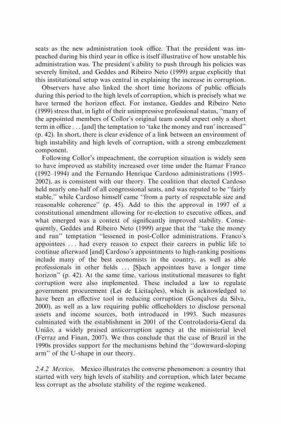
seats as the new administration took office. That the president was im-peached during his third year in office is itself illustrative of how unstable hisadministration was. The president’s ability to push through his policies wasseverely limited, and Geddes and Ribeiro Neto (1999) argue explicitly thatthis institutional setup was central in explaining the increase in corruption.

Observers have also linked the short time horizons of public officialsduring this period to the high levels of corruption, which is precisely what wehave termed the horizon effect. For instance, Geddes and Ribeiro Neto(1999) stress that, in light of their unimpressive professional status, ‘‘many ofthe appointed members of Collor’s original team could expect only a shortterm in office . . . [and] the temptation to ‘take the money and run’ increased’’(p. 42). In short, there is clear evidence of a link between an environment ofhigh instability and high levels of corruption, with a strong embezzlementcomponent.

Following Collor’s impeachment, the corruption situation is widely seento have improved as stability increased over time under the Itamar Franco(1992–1994) and the Fernando Henrique Cardoso administrations (1995–2002), as is consistent with our theory. The coalition that elected Cardosoheld nearly one-half of all congressional seats, and was reputed to be ‘‘fairlystable,’’ while Cardoso himself came ‘‘from a party of respectable size andreasonable coherence’’ (p. 45). Add to this the approval in 1997 of aconstitutional amendment allowing for re-election to executive offices, andwhat emerged was a context of significantly improved stability. Conse-quently, Geddes and Ribeiro Neto (1999) argue that the ‘‘take the moneyand run’’ temptation ‘‘lessened in post-Collor administrations. Franco’sappointees . . . had every reason to expect their careers in public life tocontinue afterward [and] Cardoso’s appointments to high-ranking positionsinclude many of the best economists in the country, as well as ableprofessionals in other fields . . . [S]uch appointees have a longer timehorizon’’ (p. 42). At the same time, various institutional measures to fightcorruption were also implemented. These included a law to regulategovernment procurement (Lei de Licitacoes), which is acknowledged tohave been an effective tool in reducing corruption (Goncalves da Silva,2000), as well as a law requiring public officeholders to disclose personalassets and income sources, both introduced in 1993. Such measuresculminated with the establishment in 2001 of the Controladoria-Geral daUniao, a widely praised anticorruption agency at the ministerial level(Ferraz and Finan, 2007). We thus conclude that the case of Brazil in the1990s provides support for the mechanisms behind the ‘‘downward-slopingarm’’ of the U-shape in our theory.

2.4.2 Mexico. Mexico illustrates the converse phenomenon: a country thatstarted with very high levels of stability and corruption, which later becameless corrupt as the absolute stability of the regime weakened.

Starting in 1929, the PRI was in power in Mexico for more than sevendecades without interruption. This was undoubtedly a very stable regime,under control of the president whose powers were ‘‘almost those of amonarch’’ (Preston and Dillon, 2004, p. 52). The president himself selectedparty candidates for congressional posts, and turned the PRI-dominatedlegislature into a rubber-stamping machine for his decisions. Although re-election was prohibited, long political horizons were guaranteed by the factthat the president got to pick the party’s candidate for his succession – whichamounted to anointing his successor, in a process nicknamed dedazo (‘‘fingertap’’) – and the ‘‘unwritten rule that former presidents and their familieswould not be criticized, let alone prosecuted’’ (p. 57).

Our theory would therefore predict high levels of corruption as a result, asis indeed the conclusion of just about every observer. According to Prestonand Dillon (2004), ‘‘among the system’s basic codes of conduct, corruptionseemed to be one of the most fundamental’’ (p. 57). Moreover, the demandeffect would predict that licensing and bribery would have been an importantpart of the way corruption manifested itself. This is confirmed by existingaccounts: ‘‘With business heavily dependent on government contracts, thelines between the public and private sectors were often blurred. An executivereceiving a substantial government contract would include in his costcalculations, as a matter of course, a commission for the official whoapproved the deal . . . [G]overnment officials often became silent partnersin the deals they authorized’’ (p. 184). Indeed, this link between stability andcorruption in the PRI regime has not gone unnoticed: ‘‘Authoritarian ruletended to breed corruption. Because PRI officials were finally accountable tono one but the President, it behooved special interests to ply them withbribes, and with the President drawn from the same party over the decades,incoming administrations had little incentive to clean house or punish abusesby their predecessors’’ (p. 326).

Starting in the 1990s, however, stability started to decrease toward a moremoderate level consistent with a better-functioning democracy, and thistransition appears to have been accompanied by some reduction in corrup-tion, in line with our model. Ernesto Zedillo became president in 1994 afterthe dedazo system was disrupted by the assassination of Carlos Salinas’sanointed successor. Zedillo implemented reforms in the electoral processthat reduced the party’s control over election results, and in 1997, for thefirst time in modern Mexican history, the PRI was left with less than 50% ofthe seats in the lower house of Congress. As a culmination of this process,the opposition won the 2000 presidential elections behind Vicente Fox. Fox’sparty, however, controlled less than 40% of the seats in both houses. Underthese circumstances, ‘‘democratic checks were restricting his powers to adegree faced by no previous Mexican president . . . [T]he Congress hadbecome far more assertive, defeating a considerable percentage of the bills heproposed and rewriting everything’’ (p. 514).

While there is widespread disappointment that Fox did not live up fully tohigh public expectations on corruption eradication, it has nevertheless beenargued that the administration ‘‘actually made important investments in thefuture of clean government . . . bringing the anticorruption agency up toglobal standards’’ (Rosenberg, 2003). An acclaimed ‘‘freedom of informa-tion act’’ was also implemented. This suggests that corruption has decreasedsomewhat. In short, the Mexican experience of falling corruption as stabilityimproved is consistent with the ‘‘upward-sloping arm’’ of our U-shape.

3. EMPIRICS: CROSS-COUNTRY EVIDENCE

Having developed a set of theoretical predictions on the relationship be-tween corruption and stability, we turn now to the cross-country empiricalevidence. We first discuss the measures we employ, particularly the variablesthat we use to capture stability (section 3.1). Using these data, we demon-strate a systematic U-shaped pattern linking corruption and stability, onethat is remarkably robust to the use of different corruption indices as wellas measures of incumbent stability (section 3.2). We also find suggestiveevidence of a U-shaped relationship between corruption and the size ofgovernment, consistent with a key corollary of the model (section 3.3).

3.1 Measures of Corruption Perception and Political Stability

3.1.1 Corruption Perception. Corruption is a particularly difficult phe-nomenon to quantify, much less compare across countries, given the illicitnature of such transactions. Following much of the cross-country empiricalliterature, we focus therefore on indices of corruption perception that arebased on institutional assessments or surveys.18 Our main dependent vari-able is the ‘‘Control of Corruption’’ measure from KKM (2006), a com-prehensive effort that pools together country governance indices fromdisparate sources. In all, 31 indices from 25 different organizations (such asGallup International, the World Bank, and the World Economic Forum)were collected and aggregated using an unobserved components methodol-ogy, yielding an extensive dataset with more than 150 countries. KKMreports scores between 1996 and 2002 at two-year intervals, and thereafterfor 2002–2005 on an annual basis.

We also use two other leading corruption indicators to corroborate ourresults, namely the Corruption Perceptions Index (CPI) and the ICRG. TheCPI is released annually by TI, a global anticorruption civic organization.Like KKM, it also combines institutional assessments of corruption, butuses a non-parametric aggregation procedure instead. The CPI is deliber-ately more selective in its choice of indices included in the aggregation;

18See Kaufmann et al. (2007) for a detailed response to criticisms against such corruptionmeasures.

the 2005 CPI, for example, was based on 16 indices from 10 differentorganizations (see Lambsdorff, 2005, for details). As a result, the CPI isavailable for slightly fewer countries, exceeding 100 countries only after2001. The aggregation approach adopted by KKM and the CPI is intendedto reduce the effects of biases that might be inherent in any single sourceindex. To further screen out potentially less reliable data points, we droppedall observations that were based on fewer than three source indices in ouranalysis. (None of our conclusions change if we instead use all the datapoints; results available on request.)

Our third and final corruption index – the ICRG – is based on a distinctmethodology independently developed by Political Risk Services, a privatecountry risk assessment agency. The ICRG country ratings cover a broad setof political and economic categories, including one component on corrup-tion within the political system. These ratings are available on a commercialbasis – ICRG clients are understood to include firms seeking businessopportunities overseas – and so the ICRG corruption score focuses onaspects of corruption that are pertinent to the conduct of private business.The ICRG is released on a monthly basis for up to 140 countries. Weaveraged the monthly corruption scores to obtain an annual measure, whenall 12 months of corruption ratings were available.19

For comparability, we linearly rescaled all three measures so that theyrange between � 2.5 and 2.5, with higher values corresponding to moreperceived corruption. Overall, the three indices are very highly correlated.The KKM and CPI country mean scores (averaged over 2002–2005) sport ahigh correlation coefficient of 0.98. The correlation with the 2002–2005ICRG country average is only slightly lower (0.88 with KKM and 0.90 withthe CPI), which suggests that the ICRG may be picking up on slightlydifferent dimensions of country corruption.20 These indices provide anatural starting point for our empirical tests of the U-shaped relationshipbetween total corruption and political stability, because they in principleprovide assessments of overall corruption, without excluding specific corruptactivities – such as embezzlement or licensing – that are subject to thedifferent effects highlighted in our theory. The CPI, for example, states thatits component sources are selected from surveys that do not emphasize oneform of corruption over another (Lambsdorff, 2005, p. 5).21 While the ICRG

19It should be noted that the ICRG is a component index used in KKM, but not in the CPI.20The high level of agreement between alternative corruption perception indices is also noted

by Svensson (2005).21‘‘It has been suggested in numerous publications that distinctions should be made between

these forms of corruption, for example between nepotism and corruption in the form ofmonetary transfers. Yet, none of the data included in the CPI emphasize one form of corruptionat the expense of other forms. The sources can be said to aim at measuring the same broadphenomenon. As also emphasized in the background documents of previous years, the sourcesdo not distinguish between administrative and political corruption, nor between petty and grandcorruption’’ (Lambsdorff, 2005).

focuses more on political corruption such as close ties between politiciansand firms, it does not exclude more direct and petty forms of extortion andbribery that hinder the regular conduct of business activities.

3.1.2 Political Stability. Turning to our key explanatory variable, weworked with two distinct sets of stability measures, the first of which focuseson the historically observed average length of incumbent tenures. We viewthis as a simple means to capture how long a political incumbent can expectto hold onto the reins of executive power given recent conditions in thecountry, with a longer average tenure corresponding to a higher level ofincumbent stability. To construct this measure, we used an encyclopedia –WorldStatesmen.org – that compiles chronologies of heads of state andheads of government for countries and territories around the world,including their party affiliation and dates of political transitions. Thisencyclopedia is extremely comprehensive and regularly updated (politicalchanges in real time are typically updated within a week), while also fullydisclosing the list of sources and contributors consulted in assembling thechronologies. As a cross-check, we compared the accounts in World-Statesmen.org for consistency with Beck et al.’s (2001) Database of PoliticalInstitutions (DPI), to corroborate the years in which political transitionsoccurred (see Appendix A for details).22

We construct these average tenure measures using a 20-year window.Specifically, for each year in our sample, we calculate average tenure as 20divided by one plus the number of observed government changes that tookplace in the preceding 20 years. Two separate variables were constructedcounting, respectively, changes in individual chief executives, and changes inthe party holding the seat of chief executive. While political titles differacross countries, we took the chief executive to be the de facto head ofgovernment as coded in the DPI.23 In particular, for most communist states,we follow the DPI in coding the secretary-general of the communist party asthe chief executive.24 For our purposes, we treat military rulers andindependents as separate and distinct parties, while also counting all interim

22We did not use the DPI as our main source, because it documents the identity and party ofthe chief executive as of January 1 of each year, and does not record instances of multiplechanges within a calendar year.

23Panama offers an example of a country where the nominal head of government did notcommand real executive power for a long period. General Manuel Noriega is coded by the DPIas the chief executive between 1982 and 1989, even though he never assumed the formal post ofPresident. There are also a handful of countries in which the post to which chief executivepowers are attached switched midway during the sample period. For example, Bangladeshswitched from a presidential to a parliamentary system in 1992. Our codings follow whoever thechief executive is, as designated in the DPI, regardless of the exact title of the relevant post.

24An exception here is China under Deng Xiaoping, who never held the position of secretary-general, although he was the unquestioned de facto leader from 1978 until his death in 1997. Ourcodings designate Deng as the chief executive during these years, although this is incon-sequential for the average party tenure measure.

and acting heads of government. We count situations in which an incumbentswitches party affiliation while in power as a change in party. We adopt thesemechanical rules to avoid making judgment calls about how substantialthese changes to the political scene were; implicitly, this rule views the needfor an acting head or for a change in party allegiance to be a signal of somepotential instability in the political status quo.

We report results using both ‘‘Executive Tenure’’ and ‘‘Party Tenure,’’because good arguments can be made in favor of both as measures of therelevant decision-making horizon of political officeholders. On the one hand,‘‘Executive Tenure’’ likely understates political stability in countries, such asJapan and Mexico, which experienced regular turnover of heads of govern-ment, even though the ruling party (the LDP and PRI, respectively)remained entrenched for several decades. On the other hand, changes inindividual chief executives are often accompanied by turnover across thegovernment hierarchy and patronage networks, in which case the decision-making horizon for corrupt agents would be better captured by ‘‘ExecutiveTenure’’ rather than by ‘‘Party Tenure.’’ It is reassuring therefore that ourempirical results work well with either tenure measure.

When constructing these variables, we adopt a 20-year window to allow asufficiently long period over which to assess the average duration of anincumbent’s stay in power. With the first year in the KKM sample being1996, the earliest window we use is 1976–1995, and so we can calculateaverage tenure using a full 20-year window for countries that becameindependent before 1976. This covers most of the countries that gainedindependence in the post-World War II wave of decolonization. Forcountries that gained independence more recently, we can still calculateaverage tenure using only the years since independence, but this comes at thecost of introducing more noise as we shorten the window over which theaverage is taken. For this reason, we typically exclude these young countries(most of which are from the former Soviet Union) from our sample. In ourpreferred specifications, we also drop Switzerland because average tenure isarguably a poor proxy for political stability in this instance: the Swiss havepractised a unique seven-member presidency for more than 150 years, inwhich the post of chief executive rotates yearly among the seven members,and thus the average tenure of individual chief executives severely under-states how stable the polity is.25

Our second measure of political stability is more straightforward todescribe. We focus here on the strength of the incumbent’s position in thecountry’s legislative body. To this effect, we use the ‘‘Majority’’ variablefrom the DPI, which is equal to the share of seats in the legislature occupiedby the governing party or coalition. A higher fraction of seats controlled by

25In practice, our results from the cross-section regressions do not change much when weinclude Switzerland; results available on request.

the ruling party would imply a lower likelihood of the opposition impedingpolicy decisions (including decisions, e.g. to award licenses and contracts tofavored private firms) or attempting to oust the incumbent, so that highervalues of ‘‘Majority’’ would correspond to more incumbent stability.

3.2 The U-Shape between Corruption and Stability

We proceed to our results on the robust U-shaped relationship betweencorruption and incumbent stability. We consider evidence from two types ofempirical specifications: (i) cross-section regressions, where the dependentvariable is the average corruption score from 2002 to 2005 for each country;and (ii) regressions where the dependent variable is the corruption score fromindividual years pooled across all years from 1996 to 2005. Since all threecorruption indices display a high level of persistence over time, it is natural toattempt first to identify any relationship between corruption and stability atthe cross-country level through the cross-section regressions.26 We then turnto the pooled regressions to make full use of all the years of information at ourdisposal. Here, we also use dynamic panel techniques that allow us to accountfor country fixed effects, while instrumenting for political stability to addresspotential problems arising from reverse causality.

3.2.1 Average Incumbent Tenure. We present first the results from thecross-section regressions using average incumbent tenure as our measure ofpolitical stability. In order to pick up the non-monotonic relationship be-tween corruption and stability, we include both stability and its square onthe right-hand side of our regressions. Specifically, we estimate the followingvia ordinary least squares:

Corrupi ¼ b0 þ ba � Stabi þ ba2 � ðStabiÞ2 þ bXXi þ ei; ð7Þ

where i indexes country. The dependent variable, Corrupi, is the mean cor-ruption score from 2002 to 2005, where the sample includes only thosecountries for which all four years of corruption scores were available. We use‘‘Executive Tenure’’ and ‘‘Party Tenure’’ as measures of political stability,Stabi, in Tables 1 and 2, respectively. Xi denotes additional determinants ofcorruption included as control variables, with bX being the correspondingcoefficient vector. Because our focus here is on the long-run determinants ofcorruption, the explanatory variables on the right-hand side of (7) areaverages over the same lagged window used in the construction of theaverage tenure variable unless otherwise stated (this is 1982–2001 in mostcolumns). We report Huber–White robust standard errors for the coefficientestimates, to account for possible heteroskedasticity in the residuals, ei.

26The correlation between the KKM scores (and likewise for the CPI) in any two years be-tween 1996 and 2005 is in excess of 0.9. The ICRG is slightly less persistent over time, with apairwise correlation between any two years exceeding 0.68.

(Table A1 provides summary statistics for the variables used in this cross-section analysis, while Appendix A documents how these variables werecollected or constructed.)

Table 1a reveals a clear, robust U-shaped relationship between the KKMcorruption index and political stability as measured by the average tenure ofthe chief executive. Throughout columns (1)–(6), we obtain a negativesignificant coefficient on log ‘‘Executive Tenure,’’ and a positive significantcoefficient on log ‘‘Executive Tenure’’ squared. Corruption is thus decreas-ing in stability for low ranges of average tenure, while increasing in stabilityat high ranges. The estimates imply a U-shape with a fairly stable turningpoint, with corruption reaching its minimum at around seven to nine yearsof executive tenure in our full specifications in columns (5) and (6). The lastrow confirms that this turning point lies in the interior of the relevantwindow of 0–20 years with a high probability (typically in excess of 95%), ascalculated from 1,000 Monte Carlo draws from the asymptotic multivariatenormal distribution of the coefficient estimates.

Column (1) presents a bare-bones regression, in which only log ‘‘ExecutiveTenure’’ and its square are included on the right-hand side. We already findevidence in this minimal specification of a U-shaped relationship betweencorruption and stability, although the R2 is understandably low (¼ 0.03) giventhe small number of covariates.27 Column (2) introduces log real GDP percapita [from the World Development Indicators (WDI)] and its square, as wellas region dummies, to help to control for any components in the corruptionindex that might be systematically correlated with a country’s overall economicperformance. Not surprisingly, the income coefficient comes out negative andhighly significant; the squared term suggests some concavity in the relationshipbetween corruption and income, but the overall pattern is consistent with thestylized fact that richer countries are perceived as being less corrupt.

This U-shaped pattern continues to be remarkably robust to the intro-duction of many other explanatory variables for corruption advanced in theliterature. Column (3) adds a measure of ethnic fractionalization (fromAlesina et al., 2003), democracy (from the Polity IV database), and a full setof legal origin dummies. Consistent with Treisman (2000), we find thatdemocracies tend to be less corrupt (significant at the 10% level). While theregression does suggest that ethnic fragmentation is associated with morecorruption (Mauro, 1995), this effect is not statistically significant. Despitethe inclusion of these important determinants of corruption, the KKM indexretains its significant U-shape with respect to log ‘‘Executive Tenure.’’28 We

27While we have also experimented with a cubic polynomial in stability in the regressions,none of the coefficients in log ‘‘Executive Tenure,’’ its square or its cube show up as statisticallysignificant. Given the limited number of data points in the regression, it does not appearpractical to attempt to fit a cubic specification.

28The U-shape remains robust if we add the ethnic fractionalization, democracy, or legalorigin dummies into the regression separately; regressions available on request.

TABLE1A

THEU-S

HAPE

BETWEENC

ORRUPTIO

NANDA

VERAGEC

HIE

FEXECUTIV

ETENURE(INC

ROSS-S

ECTIO

N)

Dependentvariable:

(1)

(2)

(3)

(4)

(5)

(6)

(7)

(8)

(9)

KKM

mean(2002–2005)

Min.

spec.

Full

spec.

Cook’s

o4/n

10-year

window

86–05

window

Ten.not

logged

LnExec.Tenure

�0.988��

�1.103����1.211����1.104����1.219����0.859����0.583��

�0.949����0.175���

(0.485)

(0.224)

(0.233)

(0.231)

(0.248)

(0.200)

(0.251)

(0.354)

(0.039)

(LnExec.Tenure)2

0.294��

0.296���

0.296���

0.269���

0.306���

0.199���

0.148

0.217�

0.008���

(0.135)

(0.068)

(0.070)

(0.071)

(0.077)

(0.058)

(0.090)

(0.113)

(0.002)

LnRealGDPper

cap.

2.984���

3.435���

3.726���

3.962���

3.391���

3.424���

3.895���

0.751���

(0.668)

(0.733)

(0.728)

(0.868)

(0.808)

(0.754)

(0.922)

(0.216)

(LnRealGDPper

cap.)2

�0.225����0.245����0.263����0.279����0.237����0.246����0.273���

0.658���

(0.041)

(0.046)

(0.045)

(0.054)

(0.050)

(0.046)

(0.055)

(0.199)

Ethnic

fractionalization

0.207

�0.051

�0.132

�0.165

�0.159

�0.272

�0.187

(0.203)

(0.223)

(0.273)

(0.228)

(0.234)

(0.293)

(0.271)

Dem

ocracy

�0.040�

�0.037�

�0.025

�0.045��

�0.030

�0.012

�0.023

(0.021)

(0.019)

(0.026)

(0.023)

(0.018)

(0.020)

(0.026)

Imports/GDP

�0.004

�0.004�

�0.004�

�0.005��

�0.003

�0.004

(0.003)

(0.002)

(0.002)

(0.002)

(0.002)

(0.002)

Fuel/totalexports

0.005���

0.004��

0.005���

0.005���

0.005���

0.004��

(0.001)

(0.002)

(0.002)

(0.002)

(0.002)

(0.002)

Ores/totalexports

�0.002

�0.003

�0.001

�0.002

�0.003

�0.003

(0.004)

(0.004)

(0.002)

(0.003)

(0.004)

(0.004)

Plurality

�0.099

�0.002

0.001

�0.048

�0.029

(0.132)

(0.118)

(0.111)

(0.139)

(0.132)

Inv.districtmagnitude

�0.049

�0.029

0.089

0.049

�0.057

(0.127)

(0.105)

(0.126)

(0.182)

(0.119)

Presidentialism

0.159

0.036

0.136

0.121

0.184

(0.148)

(0.140)

(0.120)

(0.122)

(0.146)

TABLE1A

Continued

Dependentvariable:

(1)

(2)

(3)

(4)

(5)

(6)

(7)

(8)

(9)

KKM

mean(2002–2005)

Min.

spec.

Full

spec.

Cook’s

o4/n

10-year

window

86–05

window

Ten.not

logged

Regiondummies

No

Yes

Yes

Yes

Yes

Yes

Yes

Yes

Yes

Legalorigin

dummies

No

No

Yes

Yes

Yes

Yes

Yes

Yes

Yes

Number

ofobs.(n)

136

125

120

116

105

97

118

91

105

R2

0.03

0.85

0.86

0.88

0.89

0.91

0.88

0.90

0.89

Turningpoint(inyears)

5.37

6.46

7.72

7.80

7.32

8.65

7.15

8.86

11.24

MC

prob.A

(0,20)[or(0,10)]

0.995

1.000

0.998

0.995

0.997

0.971

0.758

0.883

1.000

Notes:Robuststandard

errors

inparentheses,with� ,��

,and���denotingsignificance

atthe10%,5%

,and1%

levels,respectively.Sampleincludes

only

countriesindependentbythestart

oftherelevanttenure

window;CHE

isexcluded.Right-hand-sidecontrols

(exceptcountryfixed

factors

andethnic

fractionalization)are

averages

over

1982–2001;theexceptionsare

column(7)whereaverages

over

1992–2001are

used,andcolumn(8)whereaverages

over

2002–2005are

used(or2002–2004forvariableswithout2005data).Countriesdropped

incolumn(6)under

theCookdistance

criterionare

BWA,CAN,

CHL,GNQ,NZL,PNG,SGP,andUSA.The‘‘MC

prob.’’row

reportstheMonte

Carloprobabilitythattheturningpointlies

intheinteriorofthe

relevanttenure

window,basedon1,000drawsfrom

themultivariate

norm

aldistributionofthecoeffi

cientestimates.

add in column (4) a set of variables associated with economic rents,proposed by Ades and Di Tella (1999). Following their lead, we controlfor fuel and ore exports (normalized by total exports) to capture theavailability of expropriable rents, while we proxy for the degree of competi-tion that the domestic economy is exposed to with the value of importsnormalized by GDP. Column (5) adds several variables capturing character-istics of political systems. Following Persson et al. (2003), we include anindicator variable for whether legislative seats are allocated under a pluralityvote rule, which in principle promotes more accountability from individualpoliticians and should thus reduce corrupt behavior.29 We also control forinverse district magnitude (number of electoral districts divided by seats),where the intuition is that smaller districts help to improve accountability.Last but not least, we include a measure for presidentialism, followingKunicova’s (2005) argument that presidential systems tend to be associatedwith more corruption. The results in Table 1a confirm that controlling forthese additional determinants does not detract from the significance of theU-shape with respect to executive tenure.

We subject our central finding to a series of robustness tests in theremaining columns. Given the small number of observations in these cross-section regressions, a key concern would be whether any outliers orinfluential observations might be driving our results. Column (6) demon-strates that the U-shape remains robust even when we drop those observa-tions that are deemed potentially influential for the coefficient estimatesunder Cook’s distance criterion (Cook, 1977), which recommends furtherexploring observations for which the Cook distance metric exceeds 4/(sample size).30 Column (7) examines what happens when we use a shorter10-year window in computing executive tenure (the auxillary controls in thisregression are 10-year averages over 1992–2001, the same years covered bythe tenure window). We continue to obtain a U-shape, although thecoefficient on squared stability is now just marginally insignificant at the10% level. It is worth noting too that the point estimates on the coefficientsof log ‘‘Executive Tenure’’ and its square are both smaller in magnitude(attenuated toward zero) when compared with the corresponding fullspecification in column (5). This is consistent with the interpretation thatthe tenure measure constructed with the 10-year window is subject to moreclassical measurement error, and that a sufficiently long window is necessary

29Our results are similar if we use a more continuous measure of plurality that equals 1 if allseats are won under plurality rule; 2/3 if a majority of seats are won under plurality rule butsome are allocated under proportional representation (PR) rules; 1/3 if a majority of seats areallocated under PR with a minority won by a plurality vote; and 0 if all legislative seats areallocated under PR rules.

30Our results hold when alternative measures of influence are used to trim the dataset, such asthe DFITS metric (Welsch and Kuh, 1977), Welsch distance (Welsch, 1982), or the COVRATIOcriterion (Belsley et al., 1980).

to compute average tenure more precisely.31 We return in column (8) to theuse of a 20-year window, but construct our tenure measure with a window(1986–2005) that overlaps contemporaneously with the corruption variableson the left-hand side. We once again find a robust U-shaped pattern, similarto the full specification using a lagged window instead. (The controls in thisspecification are averages over 2002–2005, or 2002–2004 when 2005 data arenot available; the results are similar using 1986–2005 averages.) Finally,column (9) verifies that our central findings are not affected when we run theregressions using average tenure in years (instead of log tenure). That said,our preferred specifications are those that use log tenure, because the tenuremeasures are by construction proportional to the reciprocal of the number ofchanges of chief executive and thus display a lot of right skew.32

Table 1b confirms that the U-shaped relationship between corruption andlog ‘‘Executive Tenure’’ continues to hold with other leading corruptionindices. We perform here the same regression specifications in Table 1a usingthe CPI and the ICRG mean scores as dependent variables instead (forexpositional brevity, the table does not report the coefficients on theauxiliary controls). Using the CPI scores in the top panel, the U-shapewith respect to log ‘‘Executive Tenure’’ remains a consistent feature of thedata despite the smaller number of CPI observations. While we do losestatistical significance on the squared stability term when we experiment witha 10-year window [column (7)] or a contemporaneous window [column (8)],this does not detract much from the central message of a U-shape withrespect to stability with an interior turning point. Our central results alsohold with the ICRG mean scores (bottom panel). Although the resultsweaken a little as we move toward the full specification in column (5), andwhen we trim the dataset using the Cook distance criterion in column (6), thepoint estimates remain consistent with a U-shape. Overall, the strength ofthe U-shape is quite remarkable, especially in light of the small cross-sectionsample size and the extensive set of control variables used.

Table 2 repeats our cross-section regression exercise using ‘‘Party Tenure’’as the measure of stability instead. We once again find evidence of aU-shaped pattern, particularly between the KKM corruption index andlog ‘‘Party Tenure’’ (top panel). Not surprisingly, the implied turning pointcorresponds to a longer average tenure compared with Table 1a [equal to

31Not surprisingly, when we use an even shorter five-year window for computing averagetenure, the coefficients on stability and its square are even further attenuated toward zero and nolonger statistically significant. Note also that if we include countries that gained independenceafter 1982 by calculating average tenure using a truncated window starting in their year ofindependence, we find a similar attenuation in the coefficients of stability and its square, onceagain suggesting that the shortened window results in an average tenure measure that is morenoisy.

32We have in effect been penalizing ourselves by using log tenure, as the U-shaped relationshipbetween corruption and stability is even more statistically significant when tenure is left un-logged (results available on request).

TABLE1B

THEU-S

HAPE

BETWEENC

ORRUPTIO

NANDA

VERAGEC

HIE

FEXECUTIV

ETENURE(INC

ROSS-S

ECTIO

N)

(1)

(2)

(3)

(4)

(5)

(6)

(7)

(8)

(9)

Min.

spec.

Full

spec.

Cook’s

o4/n

10-year

window

86–05

window

Ten.not

logged

Dependentvariable:CPImean(2002–2005)

LnExec.Tenure

�1.740��

�0.966����1.110����0.841����0.930����0.872����0.707��

�1.061��

�0.173���

(0.700)

(0.331)

(0.326)

(0.303)

(0.306)

(0.264)

(0.343)

(0.499)

(0.045)

(LnExec.Tenure)2

0.543���

0.207��

0.246���

0.182��

0.214��

0.205���

0.204

0.228

0.007���

(0.194)

(0.089)

(0.092)

(0.087)

(0.087)

(0.074)

(0.131)

(0.172)

(0.002)

Number

ofobs.(n)

83

83

81

81

78

70

89

74

78

R2

0.06

0.86

0.88

0.90

0.90

0.95

0.89

0.90

0.90

Turningpoint(inyears)

4.96

10.30

9.60

10.12

8.77

8.34

5.68

10.20

12.12

MC

prob.A

(0,20)[or(0,10)]

0.999

0.890

0.921

0.880

0.921

0.973

0.832

0.789

1.000

Dependentvariable:IC

RG

mean(2002–2005)

LnExec.Tenure

�1.310����1.297����1.369����1.215����0.899��

�0.554

�0.842�

�1.258�

�0.183���

(0.428)

(0.391)

(0.392)

(0.393)

(0.403)

(0.371)

(0.479)

(0.640)

(0.056)

(LnExec.Tenure)2

0.403���

0.353���

0.332���

0.299���

0.189

0.082

0.296�

0.326

0.007���

(0.119)

(0.118)

(0.112)

(0.113)

(0.116)

(0.099)

(0.176)

(0.205)

(0.003)

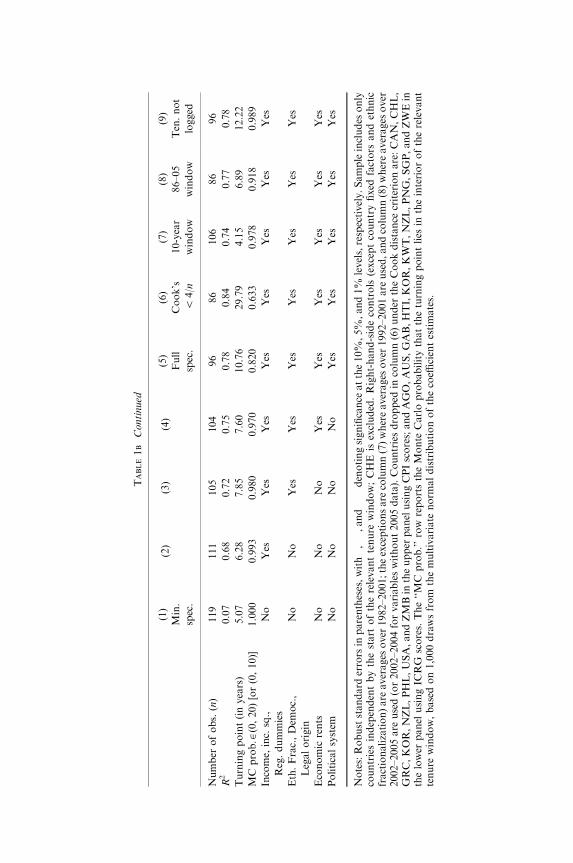
TABLE1B

Continued

(1)

(2)

(3)

(4)

(5)

(6)

(7)

(8)

(9)

Min.

spec.

Full

spec.

Cook’s

o4/n

10-year

window

86–05

window

Ten.not

logged

Number

ofobs.(n)

119

111

105

104

96

86

106

86

96

R2

0.07

0.68

0.72

0.75

0.78

0.84

0.74

0.77

0.78

Turningpoint(inyears)

5.07

6.28

7.85

7.60

10.76

29.79

4.15

6.89

12.22

MC

prob.A

(0,20)[or(0,10)]

1.000

0.993

0.980

0.970

0.820

0.633

0.978

0.918

0.989

Income,

inc.

sq.,

Reg.dummies

No

Yes

Yes

Yes

Yes

Yes

Yes

Yes

Yes

Eth.Frac.,Dem

oc.,

Legalorigin

No

No

Yes

Yes

Yes

Yes

Yes

Yes

Yes

Economic

rents

No

No

No

Yes

Yes

Yes

Yes

Yes

Yes

Politicalsystem

No

No

No

No

Yes

Yes

Yes

Yes

Yes

Notes:Robuststandard

errors

inparentheses,with� ,��

,and���denotingsignificance

atthe10%,5%

,and1%

levels,respectively.Sampleincludes

only

countriesindependentbythestart

oftherelevanttenure

window;CHE

isexcluded.Right-hand-sidecontrols

(exceptcountryfixed

factors

andethnic

fractionalization)are

averages

over

1982–2001;theexceptionsare

column(7)whereaverages

over

1992–2001are

used,andcolumn(8)whereaverages

over

2002–2005are

used(or2002–2004forvariableswithout2005data).Countriesdropped

incolumn(6)under

theCookdistance

criterionare:CAN,CHL,

GRC,KOR,NZL,PHL,USA,andZMBin

theupper

panelusingCPIscores;andAGO,AUS,GAB,HTI,KOR,KWT,NZL,PNG,SGP,andZWEin

thelower

panel

usingIC

RG

scores.The‘‘MC

prob.’’row

reportstheMonte

Carloprobabilitythattheturningpointlies

intheinterioroftherelevant

tenure

window,basedon1,000drawsfrom

themultivariate

norm

aldistributionofthecoeffi

cientestimates.

TABLE2

THEU-S

HAPE

BETWEENC

ORRUPTIO

NANDA

VERAGEPARTYTENURE(INC

ROSS-S

ECTIO

N)

(1)

(2)

(3)

(4)

(5)

(6)

(7)

(8)

(9)

Min.

spec.

Full

spec.

Cook’s

o4/n

10-year

window

86–05

window

Ten.not

logged

Dependentvariable:KKM

mean(2002–2005)

LnPartyTenure

�1.061�

�0.819����0.803����0.722����0.728����0.684����0.520��0.649��0.083��

(0.559)

(0.264)

(0.266)

(0.257)

(0.261)

(0.206)

(0.293)

(0.340)

(0.041)

(LnPartyTenure)2

0.252�

0.188��

0.147��

0.129�

0.130�

0.139���

0.112

0.108

0.003

(0.146)

(0.072)

(0.071)

(0.068)

(0.071)

(0.049)

(0.099)

(0.089)

(0.002)

Number

ofobs.(n)

136

125

120

116

105

93

118

91

105

R2

0.02

0.84

0.85

0.87

0.88

0.92

0.89

0.90

0.87

Turningpoint(inyears)

8.23

8.87

15.47

16.44

16.38

11.70

10.15

20.35

16.06

MC

prob.A

(0,20)[or(0,10)]

0.935

0.956

0.698

0.639

0.639

0.928

0.663

0.585

0.778

Dependentvariable:CPImean(2002–2005)

LnPartyTenure

�1.640��

�0.705�

�0.741��

�0.648�

�0.713��

�0.663��

�0.421

�0.838��0.111��

(0.733)

(0.415)

(0.365)

(0.336)

(0.351)

(0.322)

(0.389)

(0.434)

(0.048)

(LnPartyTenure)2

0.409��

0.121

0.101

0.100

0.122

0.117

0.039

0.125

0.004�

(0.205)

(0.114)

(0.101)

(0.091)

(0.097)

(0.087)

(0.137)

(0.117)

(0.002)

Number

ofobs.(n)

83

83

81

81

78

69

89

74

78

R2

0.04

0.85

0.88

0.90

0.90

0.94

0.89

0.91

0.90

Turningpoint(inyears)

7.43

18.52

39.31

25.45

18.79

16.93

209.56

28.37

15.19

MC

prob.A

(0,20)[or(0,10)]

0.949

0.693

0.444

0.539

0.640

0.651

0.553

0.524

0.829

TABLE2

Continued

(1)

(2)

(3)

(4)

(5)

(6)

(7)

(8)

(9)

Min.

spec.

Full

spec.

Cook’s

o4/n

10-year

window

86–05

window

Ten.not

logged

Dependentvariable:IC

RG

mean(2002–2005)

LnPartyTenure

�1.589����1.188����1.083��

�1.042��

�0.731

�0.589

�0.794

�1.140��0.126��

(0.495)

(0.438)

(0.440)

(0.447)

(0.465)

(0.410)

(0.535)

(0.681)

(0.055)

(LnPartyTenure)2

0.410���

0.280��

0.204�

0.208�

0.119

0.092

0.229

0.241

0.004�

(0.129)

(0.114)

(0.115)

(0.113)

(0.122)

(0.102)

(0.182)

(0.175)

(0.002)

Number

ofobs.(n)

119

111

105

104

96

88

106

86

96

R2

0.06

0.66

0.71

0.74

0.78

0.84

0.74

0.77

0.77

Turningpoint(inyears)

6.94

8.36

14.28

12.19

21.54

24.58

5.64

10.65

14.64

MC

prob.A

(0,20)[or(0,10)]

0.998

0.971

0.719

0.814

0.632

0.653

0.873

0.837

0.862

Income,

inc.

sq.,Reg.dummies

No

Yes

Yes

Yes

Yes

Yes

Yes

Yes

Yes

Eth.Frac.,Dem

oc.,Legalorigin

No

No

Yes

Yes

Yes

Yes

Yes

Yes

Yes

Economic

rents

No

No

No

Yes

Yes

Yes

Yes

Yes

Yes

Politicalsystem

No

No

No

No

Yes

Yes

Yes

Yes

Yes

Notes:See

Tables1aandb.Countriesdropped

incolumn(6)are:BFA,BWA,CAN,CHL,GNQ,ISR,JP

N,NZL,PNG,SGP,USA

intheupper

panel

usingKKM

scores;CAN,CHL,GRC,NZL,PHL,SGP,TUR,USA,ZMBin

themiddle

panel

usingCPIscores;andAUS,GAB,HTI,KWT,NZL,

PNG,SGP,ZWEin

thelower

panel

usingIC

RG

scores.

16.38 years in our full specification in column (5), or 11.70 years in column(6) when trimming influential observations using Cook’s distance criterion],reflecting the higher frequency of turnover in individual chief executivescompared with changes in the party in power.33 It is also reassuring that ourcoefficients on average party tenure and its square are most preciselyestimated when we parse our sample down in column (6) to omit potentiallyinfluential observations. Our results are slightly weaker when the CPI meanscore is used (middle panel), with the coefficient on the squared party tenureterm tending to drop out of the range of conventional statistical significancein several specifications. In the bottom panel with the ICRG mean score, wegenerally find favorable evidence of a U-shaped relationship with respect tolog ‘‘Party Tenure,’’ although this is not statistically significant in column (5)with the full set of control variables.

Figure 2 neatly summarizes this relationship between corruption and theaverage tenure measures. The vertical axis in Figure 2A plots the residualsfrom the KKM index after controlling for all the right-hand-side variables inour column (5) specification, except for log ‘‘Executive Tenure’’ and itssquare. Figure 2B does the same for the log ‘‘Party Tenure’’ measure. Boththe quadratic fit and a non-parametric kernel regression clearly illustrate thenon-monotonic pattern between corruption and stability, with corruptionbeing on average higher in countries that exhibit either very high or very lowincumbent tenure lengths, and being on average lower in countries in anintermediate range of political stability.34

Our next step is to analyze the results when pooling together theobservations from each individual year (between 1996 and 2005). For this,we run ordinary least-squares regressions of the form

Corrupit ¼ ba � Stabi;t�1 þ ba2 � ðStabi;t�1Þ2 þ bXXi;t�1 þDt þ ni þ eit; ð8Þ

where i indexes country, and t indexes year. We run all regressions with yearfixed effects, Dt, because both the KKM and CPI indices are normalized ineach year and thus cannot be compared cardinally across years. We use one-year lagged values for all the explanatory variables, including our measuresof political stability, in order to reduce the possibility of reverse causality.(As before, Xi,t� 1 denotes a set of additional control variables. Regressionresults using contemporaneous instead of lagged control variables are similarand available on request.) Note that our average tenure measures for each

33The relatively lower Monte Carlo probability of an interior turning point is a consequenceof this longer average party tenure, because the turning point is located closer to the upperbound of the (0, 20) interval.

34In Figure 2B, the kernel regression appears to suggest that there is a final downward-slopingarm to the non-monotonic relationship at the highest levels of average party tenure, as ourtheory would predict in the case where g is sufficiently large (diminishing returns do not set intoo rapidly in the accumulation process for resources). We do not wish to over-emphasize thispoint, however, given the limited data points available.

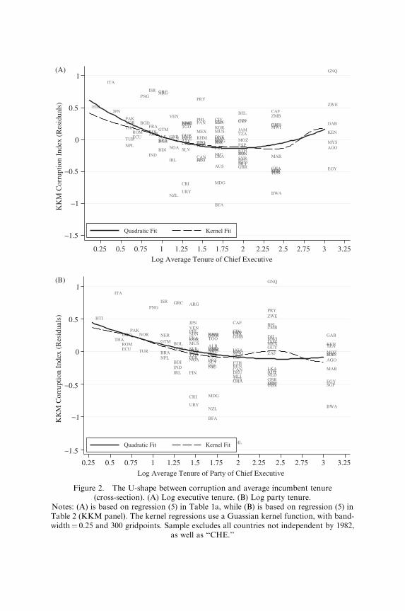
−1.5

−1

−0.5

0

0.5

1

KK

M C

orru

ptio

n In

dex

(Res

idua

ls)

0.25 0.5 0.75 1 1.25 1.5 1.75 2 2.25 2.5 2.75 3 3.25Log Average Tenure of Chief Executive

(A)

−1.5

−1

−0.5

0

0.5

1

KK

M C

orru

ptio

n In

dex

(Res

idua

ls)

0.25 0.5 0.75 1 1.25 1.5 1.75 2 2.25 2.5 2.75 3 3.25Log Average Tenure of Party of Chief Executive

(B)

Quadratic Fit Kernel Fit

Quadratic Fit Kernel Fit

Figure 2. The U-shape between corruption and average incumbent tenure(cross-section). (A) Log executive tenure. (B) Log party tenure.

Notes: (A) is based on regression (5) in Table 1a, while (B) is based on regression (5) inTable 2 (KKM panel). The kernel regressions use a Guassian kernel function, with band-width¼ 0.25 and 300 gridpoints. Sample excludes all countries not independent by 1982,

as well as ‘‘CHE.’’

year are now calculated using a lagged 20-year moving window. Because theearliest window used is 1976–1995 (to calculate average tenure leading up to1996), we retain only those countries in our dataset that were independent by1976; as before, we also drop the Swiss observation. Last but not least, weallow for within-country correlation in the residuals (induced by the country-specific error term, ni), and therefore report robust standard errors clusteredby country. (We present an alternative specification with country fixed effectswhen we turn to our dynamic panel estimation later below.)

Table 3 presents the results when the measure of stability is log ‘‘ExecutiveTenure.’’ Column (1) is a minimum specification run with the KKM index asthe dependent variable and with only year fixed effects as additionalcontrols, while column (2) includes the entire set of control variables thatwe saw in the full specification in column (5) of Tables 1 and 2. Both columnsdemonstrate that the U-shape between corruption and average executivetenure continues to hold in the pooled sample, with a turning point that iscomparable to that from the prior cross-section regressions. [The results aresimilarly strong with more parsimonious sets of auxiliary controls such as incolumns (2)–(4) of Tables 1 and 2.]

We extend the analysis in column (3) to test the predictions fromProposition 2 relating to the bargaining strength of the incumbent, s. Tosee its effects on the U-shaped relationship between corruption and stability,we introduce s into the regression and also interact it with both stability andits square:

Corrupit ¼ ba � Stabi;t�1 þ ba2 � ðStabi;t�1Þ2 þ bssi þ ba;s � siStabi;t�1

þ ba2;s � siðStabi;t�1Þ2 þ bXXi;t�1 þDt þ ni þ eit: ð9Þ

We consider two possible proxies for s. We first use a measure of theregulatory barriers to starting a business, from the World Bank’s DoingBusiness database, which is based on the data methodology developed byDjankov et al. (2002). Specifically, this s proxy is the number of days(averaged over 2003–2005, and rescaled to lie between 0 and 1) needed to setup a new business following all official procedures. In principle, by imposinghigh and costly barriers to entry, an incumbent is in a position to extract ahigher share of the rents enjoyed by the private sector, as firms will have tomake more concessions to circumvent such regulatory hold-up. A second sproxy that we consider is the ‘‘Regulatory Quality’’ governance index fromKKM.35 Constructed in much the same way as KKM’s ‘‘Control ofCorruption’’ index, this measure aggregates institutional assessments ofcountry government’s ability to ‘‘formulate and implement sound policiesand regulations that permit and promote private sector development’’

35We thank a referee for suggesting this alternative proxy for the political incumbent’s bar-gaining power.

TABLE3

THEU-S

HAPE

BETWEENC

ORRUPTIO

NANDA

VERAGEC

HIE

FEXECUTIV

ETENURE

(DEPENDENTV

ARIA

BLE:A

NNUALC

ORRUPTIO

NSCORES,1996–2005,U

NBALANCEDPANEL)

Corruptionindex:

(1)

(2)

(3)

(4)

(5)

(6)

(7)

(8)

(9)

(10)

KKM

KKM

KKM

KKM

KKM

KKM

CPI

CPI

ICRG

ICRG

sproxy:

––

‘‘Days’’

‘‘Days’’

‘‘Reg’’

‘‘Reg’’

‘‘Reg’’

‘‘Reg’’

‘‘Reg’’

‘‘Reg’’

OLS

OLS

OLS

GMM

OLS

GMM

OLS

GMM

OLS

GMM

Min.spec.

Fullspec.

Fullspec.

Fullspec.

Fullspec.

Fullspec.

Fullspec.

Fullspec.

Fullspec.

Fullspec.

LnExec.Tenure

�1.001��

�0.941���

�1.256���

�0.760��

�0.506��

�0.370

�0.506�

�0.738���

�0.579�

�0.863

(0.412)

(0.231)

(0.311)

(0.333)

(0.208)

(0.265)

(0.285)

(0.261)

(0.334)

(0.565)

(LnExec.Tenure)2

0.311���

0.230���

0.278���

0.179��

0.128��

0.102

0.105

0.145��

0.156�

0.180

(0.113)

(0.063)

(0.095)

(0.089)

(0.061)

(0.076)

(0.077)

(0.071)

(0.093)

(0.140)

sproxy

�1.402�

–0.099

–0.094

–�0.345

–

(0.726)

(0.163)

(0.230)

(0.295)

(LnExec.Tenure)�

s2.015��

0.397

0.366�

0.236�

0.485�

0.233�

0.875��

0.616���

(0.960)

(0.560)

(0.199)

(0.140)

(0.291)

(0.127)

(0.364)

(0.199)

(LnExec.Tenure)2�

s�0.417

�0.001

�0.090

�0.047

�0.134

�0.053

�0.213�

�0.148

(0.290)

(0.195)

(0.059)

(0.050)

(0.084)

(0.051)

(0.116)

(0.091)

Number

ofobs.(n)

871

564

528

528

500

500

563

563

723

723

Number

ofcountries

137

94

87

87

94

94

87

87

91

91

R2

0.04

0.89

0.89

–0.91

–0.90

–0.69

–

p-V

alue(Interaction¼0)

––

0.002

0.064

0.078

0.001

0.205

0.036

0.018

0.034

Turningpoint(inyears)

5.00

7.75

9.06

6.92

7.27

6.63

8.71

12.00

6.78

10.33

MC

prob.A

(0,20)

0.998

0.998

0.961

0.966

0.946

0.889

0.881

0.762

0.970

0.827

Yeardummies

Yes

Yes

Yes

Yes

Yes

Yes

Yes

Yes

Yes

Yes

Income,

inc.

sq.,Reg.dummies

No

Yes

Yes

Yes

Yes

Yes

Yes

Yes

Yes

Yes

Eth.Frac.,Dem

oc.,Legalorigin

No

Yes

Yes

Yes

Yes

Yes

Yes

Yes

Yes

Yes

Economic

rents

No

Yes

Yes

Yes

Yes

Yes

Yes

Yes

Yes

Yes

Politicalsystem

No

Yes

Yes

Yes

Yes

Yes

Yes

Yes

Yes

Yes

Notes:Robust

standard

errors

inparentheses,with� ,��

,and���denotingsignificance

atthe10%,5%,and1%

levels,respectively.In

allOLScolumns,standard

errors

are

clustered

bycountry.Sample

includes

only

countriesindependentbefore

1976,and‘‘CHE’’is

dropped.Right-hand-sidevariables(exceptcountryfixed

factors,ethnic

frac-

tionalization,and‘‘Days’’)are

one-yearlags.Thep-valueisreported

forat-testofwhether

thenet

interactioneff

ectbetweenln

‘‘Exec.Tenure’’andthesproxyequals0,when

evaluatedatthemedianvalueofln

‘‘Exec.Tenure’’in

theregressionsample.Theturningpointforcolumnswiththeseinteractionterm

sisevaluatedatthemedianvalueofthes

proxyin

theregressionsample.Thelastrowreportstheprobabilitythattheturningpointlies

intheinteriorof(0,20),basedon1,000Monte

Carlodrawsfrom

themultivariate

norm

aldistributionofthecoeffi

cientestimates.

(KKM, p. 4). We use the negative of this index as an alternative proxy forgovernmental regulatory hold-up.36

While these proxies are admittedly imperfect, the results are encouraging.Column (3) presents the regressions using the ‘‘Days’’ proxy. First of all, itconfirms that the basic U-shaped pattern with respect to ‘‘Executive Tenure’’still holds.37 Furthermore, the results are consistent with the comparativestatics in Proposition 2: the coefficient on the interaction term between log‘‘Executive Tenure’’ and our s proxy is positive and statistically significantat the 5% level. To be fully precise, the net interaction effect between thesetwo variables is given by the empirical cross-derivative of corruption withrespect to stability and s, which is equal to ba;s þ 2ba2;s�(log ‘‘ExecutiveTenure’’). This empirical cross-derivative is indeed positive when evaluatedat the median value of log ‘‘Executive Tenure’’ in the regression sample, andwe can formally reject the null hypothesis that this net interaction effect isequal to zero ( p-value¼ 0.002). This result is best illustrated in a diagram:Figure 3A shows that when the value of ‘‘Days’’ is increased, the U-shapedcurve between the corruption residuals and stability is shifted up, with thisshift being more pronounced at higher levels of executive tenure. Thus, anincrease in the bargaining power of the incumbent generates a larger increasein corruption at higher levels of stability.38 Using a one-year lag of the‘‘Regulatory Quality’’ index as our s proxy instead in column (5), we obtainvery similar results: the interaction coefficient between the s proxy and log‘‘Executive Tenure’’ is positive and significant, and we also reject the nullhypothesis of a zero net interaction effect at the 10% level ( p-value¼ 0.078).

We explore in columns (4) and (6) a means to exploit the panel structure ofour dataset more extensively, in a way that also helps to allay concerns overpotential endogeneity issues arising from unobserved country fixed char-acteristics or reverse causality. Consider the following model:

Corrupit ¼ ba � Stabi;t�1 þ ba2 � ðStabi;t�1Þ2 þ ba;s � siStabi;t�1

þ ba2;s � siðStabi;t�1Þ2 þ bXXi;t�1 þDt þDi þ eit; ð10Þ

which is similar to (9), except that we have now included Di as a countryfixed effect. Estimating (10) using conventional fixed effects is likely to leadto biased coefficient estimates, because our key right-hand-side variable,the stability of the political incumbent, as well as country income per capita,

36As with the KKM corruption index, we drop those ‘‘Regulatory Quality’’ observations thatare based on fewer than three component indices.

37For all specifications where the interaction effect with a s proxy is considered, the turningpoint reported is that obtained when setting the s proxy to its median value in the regressionsample.

38These tests for Proposition 2 are only slightly weaker when run in the cross-section analysis.The coefficients there have similar signs, although significance levels are lower given the smallsample size in cross-section.

−0.5

−1

0

0.5

1

KK

M C

orru

ptio

n In

dex

(Res

idua

ls)

0.25 0.5 0.75 1 1.25 1.5 1.75 2 2.25 2.5 2.75 3 3.25

Log Average Tenure of Chief Executive

(A)

−1

−0.5

0

0.5

1

KK

M C

orru

ptio

n In

dex

(Res

idua

ls)

0.25 0.5 0.75 1 1.25 1.5 1.75 2 2.25 2.5 2.75 3 3.25

Log Average Tenure of Party of Chief Executive

(B)

Figure 3. The U-shape between corruption and average incumbent tenure (pooledobservations). (A) Log executive tenure. (B) Log party tenure.

Notes: (A) is based on the regression in Table 3, column (3), while (B) is based on Table 4,column (3). Sample excludes countries not independent by 1976, as well as ‘‘CHE.’’ Re-siduals are obtained by regressing the KKM corruption measure against all right-hand-side variables except the relevant log tenure measure, log tenure sq., (log tenure) � (Days),and (log tenure sq.) � (Days). Fitted lines are plotted at the 10th, 50th, and 90th percentile

in sample values of Days, respectively.

are both plausibly going to depend on the level of observed corruption inpreceding periods. In other words, the error term, eit, is not strictly exogenousas required under fixed effects estimation [Corr(eit,Stabi,tþ s) 6¼ 0, for s � 0].To address this, we perform a dynamic panel GMM estimation using laggedlevels of corruption, stability, stability squared, stability interacted with‘‘Days,’’ stability squared interacted with ‘‘Days,’’ ‘‘Days,’’ log income percapita, and log income per capita squared as instruments in the first-differenced version of (10) for these right-hand-side variables involvingstability and income per capita (Arellano and Bond, 1991). At the sametime, we also use lagged first differences of these variables as instruments inthe levels version of (10), to improve the efficiency of the estimates, and allayconcerns related to weak instruments when the right-hand-side variables arepersistent (Arellano and Bover, 1995; Blundell and Bond, 1998).39

This dynamic panel GMM estimation helps to reinforce the message fromthe prior OLS regressions: in column (4), we continue to obtain a statisticallysignificant quadratic U-shaped relationship linking corruption and averagetenure. The estimated coefficient on the interaction between log ‘‘ExecutiveTenure’’ and ‘‘Days’’ remains positive, although this is not significant; thatsaid, we do reject the null hypothesis of a zero net interaction effect at the 10%level ( p-value¼ 0.064).40 We find mixed results when running the dynamicpanel estimation using the ‘‘Regulatory Quality’’ proxy in column (6): we losesignificance on the U-shape with respect to log ‘‘Executive Tenure,’’ butobtain a positive and significant net interaction effect between log ‘‘ExecutiveTenure’’ and our s proxy (we reject the null hypothesis of a zero netinteraction effect; p-value¼ 0.001).

The remainder of Table 3 provides some reassurance that our results aresimilarly valid with both the CPI and the ICRG indices. We present the OLSand dynamic panel specifications using lagged ‘‘Regulatory Quality’’ as thes proxy as this has slightly more explanatory power for the dependentcorruption variable when compared with the ‘‘Days’’ proxy.41 (The resultsusing the ‘‘Days’’ proxy are similar and available on request.) The evidencepoints overall toward a U-shape with respect to log ‘‘Executive Tenure,’’

39We implement this using the xtabond2 Stata command developed in Roodman (2006).40Several basic specification tests (not reported in Table 3) verify that the key underlying

assumptions for the dynamic panel model – including the requirement that eit be uncorrelatedwith past values of the right-hand-side variables – are not violated. We reject the null hypothesisof no first-order serial correlation in the first-differences of the residuals at the 5% level ( p-value¼ 0.023). At the same time, we do not reject the null hypothesis of no second-order serialcorrelation ( p-value¼ 0.104). The Sargan–Hansen statistic is small [w2(183)¼ 73.41]; hence, wecannot reject the identifying restrictions for the validity of the instruments ( p-value¼ 1.000),subject to the caveat that this test tends to be weak when the set of instruments is large. We alsoreach similar conclusions with these diagnostic tests in the column (6) dynamic panel GMMspecification using the ‘‘Regulatory Quality’’ proxy.

41The KKM ‘‘Regulatory Quality’’ index is only available every two years from 1996 to 2002.When necessary, we associate the index value for each year with the next year as well (e.g. weassociate the index value for 1996 with 1997 as well).

as well as a positive interaction effect with the s proxy (although the resultsare less significant in the final column that subjects the ICRG index to thedynamic panel estimation).42

For completeness, Table 4 conducts the parallel exercise using ‘‘PartyTenure’’ as the measure of incumbent stability, and we obtain strikinglysimilar results. The coefficients on log ‘‘Party Tenure’’ and its squarecontinue to paint a consistent story regarding the non-monotonic relation-ship between corruption and average tenure. Figure 3B illustrates thisU-shaped pattern, and also makes evident the impact of ‘‘Days’’ inincreasing corruption, particularly at higher levels of stability.

We thus conclude that the evidence strongly supports the presence of aU-shaped relationship between corruption and stability, when stability ismeasured by the historically observed average tenures of either the chiefexecutive or the party in power.

3.2.2 Legislative Majority. We turn briefly then to consider the empiricalevidence when political stability is measured instead by the strength of theincumbent’s position in the legislature, as proxied by ‘‘Majority.’’ Theseresults are presented in Table 5, which summarizes findings from both cross-section and pooled regressions.

Reassuringly, our key conclusions are broadly unchanged. In the baselinecross-section KKM regression in column (1) that includes only ‘‘Majority’’and its square as explanatory variables, we already find a significant U-shaped pattern with an interior turning point, which suggests that corrup-tion bottoms out when the incumbent’s ‘‘Majority’’ is around 0.75 (when theruling coalition holds about three-quarters of the legislative seats). (Asbefore, the right-hand-side variables in these cross-section regressions are20-year lagged averages between 1982 and 2001; hence, we include onlycountries that were independent before 1982.) This non-monotonic patternin the cross-section persists with more parsimonious sets of auxiliarycontrols, or when we drop potentially influential observations using Cook’sdistance criterion (regressions not shown). When we pool together all theyearly observations and use one-year lags of ‘‘Majority’’ as our keyexplanatory variable following the specification in equation (8) with a fullset of controls, the U-shape loses statistical significance [column (2)].43

Nevertheless, statistical significance is restored when we further include the‘‘Days’’ proxy in column (3) following the specification in equation (9). Wemoreover find favorable evidence of a positive net interaction effect between‘‘Majority’’ and our ‘‘Days’’ proxy for s (we reject the null hypothesis of a

42Our results also hold in specifications that use more parsimonious sets of control variables(regressions not shown).

43We do not drop the newly independent countries or Switzerland, because the one-year lagsof ‘‘Majority’’ are a valid measure of legislative strength in these countries. Our results do notchange substantially if we drop these countries.

TABLE4

THEU-S

HAPE

BETWEENC

ORRUPTIO

NANDA

VERAGEPARTYTENURE

(DEPENDENTV

ARIA

BLE:A

NNUALC

ORRUPTIO

NSCORES,1996–2005,U

NBALANCEDPANEL)

Corruptionindex:

(1)

(2)

(3)

(4)

(5)

(6)

(7)

(8)

(9)

(10)

KKM

KKM

KKM

KKM

KKM

KKM

CPI

CPI

ICRG

ICRG

sproxy:

––

‘‘Days’’

‘‘Days’’

‘‘Reg’’

‘‘Reg’’

‘‘Reg’’

‘‘Reg’’

‘‘Reg’’

‘‘Reg’’

OLS

OLS

OLS

GMM

OLS

GMM

OLS

GMM

OLS

GMM

Min.spec.

Fullspec.

Fullspec.

Fullspec.

Fullspec.

Fullspec.

Fullspec.

Fullspec.

Fullspec.

Fullspec.

LnPartyTenure

�1.052��

�0.772���

�1.593���

�1.300���

�0.454��

�0.473

�0.659��

�1.014���

�0.555

�0.996�

(0.504)

(0.293)

(0.428)

(0.461)

(0.185)

(0.399)

(0.258)

(0.350)

(0.360)

(0.553)

(LnPartyTenure)2

0.258�

0.164��

0.331���

0.270��

0.109��

0.125

0.156��

0.258��

0.146�

0.288��

(0.131)

(0.072)

(0.109)

(0.130)

(0.047)

(0.111)

(0.066)

(0.108)

(0.088)

(0.138)

sproxy

�3.870���

–�0.266

–�0.476

–�1.104���

–

(1.065)

(0.245)

(0.288)

(0.389)

(LnPartyTenure)�

s4.447���

0.161

0.602��

0.369��

0.951���

0.191

1.625���

0.661���

(1.224)

(0.617)

(0.280)

(0.146)

(0.349)

(0.178)

(0.443)

(0.235)

(LnPartyTenure)2�

s�0.960���

0.113

�0.110

�0.103�

�0.216��

�0.031

�0.383���

�0.175�

(0.307)

(0.237)

(0.074)

(0.060)

(0.096)

(0.073)

(0.126)

(0.095)

Number

ofobs.(n)

871

564

528

528

500

500

563

563

723

723

Number

ofcountries

137

94

87

87

94

94

87

87

91

91

R2

0.03

0.88

0.89

–0.91

–0.91

–0.70

–

p-V

alue(Interaction¼0)

––

0.000

0.086

0.000

0.565

0.001

0.186

0.001

0.310

Turningpoint(inyears)

7.67

10.51

12.17

8.97

9.28

6.53

8.56

7.62

7.37

5.78

MC

prob.A

(0,20)

0.951

0.913

0.857

0.948

0.944

0.922

0.991

0.945

0.998

0.987

Yeardummies

Yes

Yes

Yes

Yes

Yes

Yes

Yes

Yes

Yes

Yes

Income,

inc.

sq.,

Reg.dummies

No

Yes

Yes

Yes

Yes

Yes

Yes

Yes

Yes

Yes

Eth.Frac.,Dem

oc.,

Legalorigin

No

Yes

Yes

Yes

Yes

Yes

Yes

Yes

Yes

Yes

Economic

rents

No

Yes

Yes

Yes

Yes

Yes

Yes

Yes

Yes

Yes

Politicalsystem

No

Yes

Yes

Yes

Yes

Yes

Yes

Yes

Yes

Yes

Notes:Robuststan

darderrorsin

parentheses,with� ,��

,an

d���denotingsign

ificance

atthe10%,5%

,an

d1%

levelsrespectively.In

allOLScolumns,stan

darderrorsareclustered

by

country.Sam

pleincludes

onlycountriesindependentbefore

1976,an

d‘‘CHE’’isdropped.Right-han

d-sidevariab

les(exceptcountryfixedfactors,ethnicfractionalization,an

d‘‘Days’’)

areone-year

lags.Thep-valueisreported

forat-testofwhether

thenetinteractioneffectbetweenln

‘‘Party

Tenure’’an

dthesproxy

equals0,when

evaluated

atthemedianvalueofln

‘‘Party

Tenure’’in

theregressionsample.Theturningpointforcolumnswiththeseinteractionterm

sisevaluated

atthemedianvalueofthesproxy

intheregressionsample.T

helastrow

reportstheprobab

ilitythat

theturningpointlies

intheinteriorof(0,20),based

on1,000Monte

Carlo

drawsfrom

themultivariate

norm

aldistributionofthecoeffi

cientestimates.

TABLE5

THEU-S

HAPE

BETWEENC

ORRUPTIO

NANDLEGISLATIV

EM

AJO

RIT

Y

Corruptionindex:

(1)

(2)

(3)

(4)

(5)

(6)

(7)

(8)

(9)

KKM

KKM

KKM

CPI

CPI

CPI

ICRG

ICRG

ICRG

sproxy:

––

‘‘Days’’

––

‘‘Days’’

––

‘‘Days’’

Cross-section

Pooled

Pooled

Cross-section

Pooled

Pooled

Cross-section

Pooled

Pooled

Ind.by1982

Ind.by1982

Ind.by1982

Majority

�5.721��

�0.756

�2.976���

�4.200

�0.712

�3.771��

�4.808

�0.409

�6.540���

(2.305)

(0.576)

(1.048)

(3.379)

(0.838)

(1.543)

(3.945)

(1.192)

(2.059)

(Majority)2

3.571��

0.244

1.773��

2.222

0.230

2.529�

2.754

0.161

4.591���

(1.547)

(0.447)

(0.851)

(2.461)

(0.654)

(1.297)

(2.728)

(0.894)

(1.658)

sproxy

�2.584��

�3.430��

�7.329���

(0.995)

(1.454)

(2.059)

(Majority)�

s8.524��

11.867��

23.359���

(3.459)

(5.313)

(7.123)

(Majority)2�

s�5.816��

�8.826�

�16.833���

(2.907)

(4.555)

(5.844)

Number

ofobs.(n)

108

678

640

79

759

739

97

906

860

Number

ofcountries

108

114

106

79

107

101

97

108

101

R2

0.87

0.88

0.88

0.90

0.86

0.87

0.76

0.65

0.66

p-V

alue(Interaction¼0)

––

0.007

––

0.022

––

0.002

Turningpoint

0.80

1.55

0.99

0.95

1.55

0.86

0.87

1.27

0.75

MC

prob.A

(0,1)

0.937

0.335

0.510

0.644

0.503

0.681

0.761

0.769

0.899

Yeardummies

No

Yes

Yes

No

Yes

Yes

No

Yes

Yes

Income,

inc.

sq.,Reg.Dummies

Yes

Yes

Yes

Yes

Yes

Yes

Yes

Yes

Yes

Eth.Frac.,Dem

oc.,Legalorigin

Yes

Yes

Yes

Yes

Yes

Yes

Yes

Yes

Yes

Economic

rents

Yes

Yes

Yes

Yes

Yes

Yes

Yes

Yes

Yes

Politicalsystem

Yes

Yes

Yes

Yes

Yes

Yes

Yes

Yes

Yes

Notes:Robust

standard

errors

inparentheses,with� ,��

,and���denotingsignificance

atthe10%,5%,and1%

levels,respectively.In

all‘‘Pooled’’columns,thesestandard

errorsare

clustered

bycountry.Thedependentvariablein

the‘‘Cross-section’’columnsisthemeancorruptionscore

over

2002–2005,whileright-hand-sidevariablesare

averages

over

1982–2001.In

the‘‘Pooled’’columns,

theright-hand-sidevariablesare

one-yearlags.

Thep-valueis

reported

forat-test

ofwhether

thenet

interactioneff

ectbetween

‘‘Majority’’andthesproxyequals0,when

evaluatedatthemedianvalueof‘‘Majority’’in

theregressionsample.Forthespecificationsinvolvinginteractioneff

ects,theturning

pointwithrespectto

‘‘Majority’’isevaluatedatthemedianvalueofthesproxyin

theregressionsample.Thelastrowofthetablereportstheprobabilitythattheturningpoint

lies

intheinteriorof(0,1),basedon1,000Monte

Carlodrawsfrom

themultivariate

norm

aldistributionofthecoeffi

cientestimates.

zero net interaction effect; p-value¼ 0.007). Repeating this exercise with theother corruption indices in the remaining columns of Table 5, we find that thestatistical significance of our results generally weakens. That said, in the fullspecifications where the interaction effect of ‘‘Days’’ on stability is alsoconsidered [columns (6) and (9)], we find particularly strong evidence for aU-shaped relationship linking corruption and ‘‘Majority.’’44 Moreover, weagain find a positive net interaction effect between stability and our ‘‘Days’’proxy for the incumbent’s bargaining power [ p-value¼ 0.022 and 0.002,respectively, in columns (6) and (9)].

3.3 Corruption and the Size of Government

Last but not least, we investigate the relationship between corruption and thesize of government, motivated by our earlier theoretical prediction (in Pro-position 4) that this should also be a U-shaped pattern. The relationshipbetween these two variables has drawn some recent attention: Alesina andAngeletos (2005), for instance, present a model in which a positive relationbetween corruption and the size of government is taken as a premise, wherebya larger government implies a larger scope for rent-seeking activities. How-ever, this relationship has not been easy to verify empirically: Glaeser andSaks (2006), for example, find no significant correlation between corruptionconvictions and the size of government at the state level in the United States.Understanding the nature of the relationship between these two variables isclearly an important topic in its own right, given the implications it bears forwhat an appropriate size of government might be in order to minimize theincentives for public officeholders to engage in corrupt activities.

As it turns out, we do find some suggestive evidence of a U-shaped patternlinking corruption and the size of government, as shown in Table 6. We usetotal government consumption expenditures as a share of GDP, taken fromthe WDI, to proxy for the size of government, as is standard in this litera-ture. We focus first on the cross-section regression specifications, becausethis rids the analysis of budget cycle effects that could confound inter-pretation of the results by averaging the data over several years.

Column (1) reports a U-shaped pattern, significant at the 1% level, be-tween the mean KKM corruption score and the size of government when nofurther controls are added. In this baseline specification, corruption reachesits minimum when the level of government expenditures sits at about 20% ofGDP. This turning point lies well within the range of government sizesobserved in the sample (between 0% and 50%). This relationship weakenswhen we add in a full set of controls [column (2)], but is restored when we

44The Monte Carlo probability of the turning point lying in the interior of [0, 1] is relativelysmall in columns (6) and (9), due to the fact that the point estimate of this turning point whenevaluated at the median value of ‘‘Days’’ is already close to the upper bound of this interval inboth these specifications.

TABLE6

THEU-S

HAPE

BETWEENC

ORRUPTIO

NAND

THESIZ

EOFG

OVERNMENT

Corruptionindex:

(1)

(2)

(3)

(4)

(5)

(6)

(7)

(8)

(9)

KKM

KKM

KKM

CPI

CPI

CPI

ICRG

ICRG

ICRG

Cross-section

Cross-section

Pooled

Cross-section

Cross-section

Pooled

Cross-section

Cross-section

Pooled

Ind.by1982

Ind.by1982

Ind.by1982

Ind.by1982

Ind.by1982

Ind.by1982

Min.spec.

Full.spec.

Full.spec.

Min.spec.

Full.spec.

Full.spec.

Min.spec.

Full.spec.

Full.spec.

Govt.Spending/G

DP

�0.263���

�0.051

�0.076����0.368���

�0.066�

�0.056�

�0.201���

�0.020

�0.033

(0.050)

(0.038)

(0.023)

(0.096)

(0.039)

(0.031)

(0.054)

(0.063)

(0.044)

(Govt.Spending/G

DP)2

0.006���

0.001

0.002���

0.007��

0.001

0.001

0.004���

0.000

0.001

(0.001)

(0.001)

(0.001)

(0.003)

(0.001)

(0.001)

(0.001)

(0.002)

(0.001)

Number

ofobs.(n)

135

106

677

84

79

760

118

97

903

Number

ofcountries

135

106

113

84

79

105

118

97

108

R2

0.18

0.87

0.88

0.33

0.89

0.86

0.12

0.75

0.65

Turningpoint

23.51

17.30

16.54

25.86

23.79

19.47

23.83

20.65

11.63

MC

prob.A

(0,50)

1.000

0.948

1.000

0.961

0.930

0.950

0.997

0.876

0.899

Yeardummies

No

No

Yes

No

No

Yes

No

No

Yes

Income,

inc.

sq.,

Reg.dummies

No

Yes

Yes

No

Yes

Yes

No

Yes

Yes

Eth.Frac.,Dem

oc.,

Legalorigin

No

Yes

Yes

No

Yes

Yes

No

Yes

Yes

Economic

rents

No

Yes

Yes

No

Yes

Yes

No

Yes

Yes

Politicalsystem

No

Yes

Yes

No

Yes

Yes

No

Yes

Yes

Notes:

Robust

standard

errors

inparentheses,with� ,��

,and���denotingsignificance

atthe10%

,5%

,and1%

levels,

respectively.In

all‘‘Pooled’’

columns,thesestandard

errors

are

clustered

bycountry.Thedependentvariablein

the‘‘Cross-section’’columnsisthemeancorruptionscore

over

2002–

2005,whileright-hand-sidevariablesare

averages

over

1982–2001.In

the‘‘Pooled’’columns,theright-hand-sidevariablesare

one-yearlags.Thelastrowof

thetable

reportstheprobabilitythattheturningpointlies

intheinteriorof(0,50),basedon1,000Monte

Carlodrawsfrom

themultivariate

norm

al

distributionofthecoeffi

cientestimates.

turn to the pooled specification based on annual observations [column (3)].When using the other corruption measures, we find in general that the sta-tistical significance of any U-shape with respect to government size is strongin the minimum baseline specification, but weakens as we add further aux-iliary controls. Overall though, the point estimates never overturn the basicU-shaped relationship. Of note, throughout all specifications, the MonteCarlo probability of the turning point lying in the interior of the relevant[0, 50] range is large (always in excess of 0.9).

In sum, we find some suggestive evidence that corruption is decreasing inthe size of government for countries where the level of these governmentexpenditures is low, but this relationship turns into a positively sloped oneover high ranges of government expenditures.

4. CONCLUDING REMARKS

This paper has investigated the relationship between the level of corruptionand the degree of instability to which political incumbents are exposed, bothfrom theoretical and empirical perspectives. Our theoretical frameworkpredicts that corruption and stability are related in a non-monotonic patternthat approximates a U-shape, building on the interaction between the hor-izon effect, by which a less stable incumbent is more willing to embezzle, andthe demand effect, according to which higher bribes will be offered to a morestable incumbent.

On the empirical side, we find that the cross-country evidence displays aU-shaped relationship between corruption and political stability, as meas-ured by historically observed incumbent tenure lengths or by the legislativemajority of the government. This result is largely robust to the inclusion ofmany political and economic control variables, as well as across variousestimation methods. We see this robustness as suggesting that cross-countrycorruption perception indices do contain useful information beyond theiroft-noted correlation with GDP per capita. (It is hard to believe that thenon-linear relationships uncovered could be attributed to random noise.)

While the available empirical evidence supports the U-shaped prediction,a natural next step will be to pursue tests to separately identify the horizonand demand effects within a common setting. In this regard, we believe thatturning to micro-level data is a promising direction along which to bridgetheory and empirics. Most encouragingly, some work based on Mexicanfirm-level data on corruption has already tested our theory, with the pre-liminary results being quite supportive (Gamboa-Cavazos et al., 2006). Ourhope is that further micro-level evidence will allow us to separately measuredifferent types of corruption along the lines suggested by the theory, and weintend to continue working in this direction as part of this research agenda.

As a final note, it is worth highlighting some policy implications stemmingfrom our analysis. The horizon effect suggests that the possibility of

re-election should be an important incentive in defusing an incumbent’stendency to embezzle. On the other hand, the demand effect cautions thatlong-standing incumbents are more liable to engage in long-term illicit li-censing relations with private firms. When these two effects are combined,our theory implies that there is an optimal length of tenure at which themarginal incentive to license more exactly offsets the marginal disincentiveto engage in more embezzlement. This suggests that an electoral system inwhich there is the possibility of re-election, but which nevertheless imposesterm limits on politicians, is well placed to approximate such an optimalcompromise between the horizon and demand effects. In fact, the dataconfirm that the length of executive tenure that minimizes corruption – the‘‘turning point’’ of the U-shape – is around eight years, remarkably close tothe term limits (two terms of four years) that are observed in practice inmany countries. Advertently or inadvertently, the designers of these electoralinstitutions appear to have built in a system that balances off the horizonand demand effects highlighted in our analysis.

APPENDIX A

A.1. Corruption Perception Indices

KKM: From KKM’s (2006) ‘‘Control of Corruption’’ index, itself a com-posite of different corruption ratings aggregated by an unobserved compo-nents methodology. On a scale of � 2.5 to 2.5. The negative of the originalindex is used, so that higher numbers correspond to more perceived cor-ruption. Data are available for 1996–2002 at two-year intervals, and there-after for 2002–2005 on an annual basis. We drop all observations that wereaggregated from less than three source indices. For the cross-section re-gressions, the dependent variable is the mean KKM score from 2002 to 2005;we restrict the sample to only those countries where all four years of datawere available.

CPI: From TI. The CPI is linearly rescaled from its original range of 0–10,to a � 2.5 to 2.5 scale, with higher numbers corresponding to more perceivedcorruption. Data used are annual observations from 1996 to 2005. The CPIis also based on corruption scores from different agencies, but its aggrega-tion methodology is non-parametric in nature, using only the ordinal ranksof each country. We use only those data points that CPI aggregates based onat least three sources; these are the data points that TI reports in its annualranking of countries. For the cross-section regressions, the dependent vari-able is the mean score for only those countries for which four continuousyears of data were available for 2002–2005. (Year 2002 is the first for whichCPI coverage exceeds 100 countries.)

ICRG: From the Political Risk Services Group, a commercial provider ofcountry risk assessments. The ICRG political risk-rating index contains asubcomponent for corruption, which is what we use. The original ICRG

corruption index is coded on a scale of 0–6, and is available on a monthlybasis. We linearly rescaled the scores to lie on a � 2.5 to 2.5 interval with ahigher score corresponding to more corruption, and took the simple averageof monthly scores to obtain an annual score (for each country, this iscomputed only for those years in which all 12 months of corruption data areavailable). For the cross-section regressions, we use the mean ICRG scorefor 2002–2005, where only countries with all four years of data are includedin the sample. For more details on the ICRG methodology, see: http://www.prsgroup.com/ICRG_Methodology.aspx

A.2. Political Stability

Average tenure: The historically observed average tenure (in years) for po-litical incumbents over a 20-year window. Calculated as 20/(1þ x), where xis the number of political changes observed in the preceding 20-year window.

TABLE A1 SUMMARY STATISTICS

N Min. Median Max. Mean Std. dev.

A. Corruption perception indices

KKM (2002–2005) 166 � 2.465 0.386 1.748 0.097 1.027

CPI (2002–2005) 102 � 2.338 0.65 1.788 0.231 1.197

ICRG (2002–2005) 140 � 2.5 0.616 2.5 0.422 0.949

B. Political stability measures

Avg Executive Tenure (1982–2001) 162 0.952 4.25 20 5.967 5.106

Avg Party Tenure (1982–2001) 162 1.333 5 20 7.773 6.217

Majority (1982–2001) 160 0.303 0.760 1 0.734 0.181

C. Other variables

Log real GDP per capita (1982–2001) 152 6.222 8.295 10.411 8.332 1.106

Ethnic Fractionalization 163 0 0.484 0.930 0.454 0.258

Democracy (1982–2001) 156 0 3.053 10 4.105 3.768

Imports/GDP (%, 1982–2001) 162 4.993 36.284 176.450 41.759 23.353

Fuel/Total Exports (%, 1982–2001) 154 0.001 3.709 96.538 16.068 26.009

Ore/Total Exports (%, 1982–2001) 155 0.004 2.719 75.145 8.777 14.662

Plurality (1982–2001) 149 0 1 1 0.685 0.448

Inverse District Magnitude (1982–2001) 142 0.007 0.211 1.429 0.438 0.412

Presidentialism (1982–2001) 162 0 0.85 1 0.648 0.413

Days to start a business (2003–2005) 134 2 40.5 203 50.117 37.210

Regulatory Quality (1996–2005) 134 � 1.854 � 0.096 2.386 � 0.091 0.948

Government Spending/GDP

(%, 1982–2001)

159 4.449 16.234 43.280 16.653 6.420

Notes: In Panel A, for each corruption index, only those countries with all four years of dataavailable are included when calculating the mean corruption score from 2002–2005. Summarystatistics for variables in Panels B and C are for the sample of countries for which the KKMmean (2002–2005) score was computed.

We compute two separate average tenure measures for (i) individual chiefexecutives and (ii) the party in power (holding the seat of the chief executive).

The information on political changes was compiled from: http://www.worldstatesmen.org. We checked the political chronologies fromWorldStatesmen.org for consistency against the August 2005 version of theDPI. The DPI contains two variables ‘‘PRTYIN’’ and ‘‘EXECME’’ thatcode, respectively, the number of years that the party of the chief executivehas been in power and the name of the party of the chief executive, as ofJanuary 1 of each year from 1975 to 2004. These variables allow us toidentify years in which political changes occurred, although they are notideal because they do not pick up instances of extreme political volatilitywhen more than one change occurred in a year. Notwithstanding this, weused these DPI variables as a cross-check. Reassuringly, few discrepancieswere found, and these were resolved by consulting additional sources onpolitical histories, such as the Zarate Political Collections.

Majority: From the DPI. Variable used is ‘‘MAJ,’’ which is the fraction ofseats in the legislature held by members of the governing coalition, as ofJanuary 1 of each year.

A.3. Additional Variables

Real GDP per capita: From the World Bank WDI. Real PPP-adjusted GDPper capita (in constant 2000 international dollars).

Ethnic fractionalization: From Alesina et al. (2003). Equal to 1 minus theHerfindahl Index of population shares of ethnic groups within a country.(This variable does not vary over time.)

Democracy: Polity IV democracy score, on a scale of 0–10. The referencedate for the annual observations in the Polity IV dataset is December 31 ofeach year. We match these to the data corresponding to January 1 of thefollowing year for consistency with the DPI.

Fuel exports: From the WDI. Value of fuel exports as a percentage of totalmerchandize exports.

Ore exports: From the WDI. Value of ore and metal exports as a per-centage of total merchandize exports.

Imports: From the WDI. Imports of goods and services as a percentage ofGDP.

Presidentialism: Calculated from the DPI. The DPI variable ‘‘SYSTEM’’codes political systems as: 0 for a direct presidential system; 1 for a strongpresident elected by a legislative assembly; and 2 for a parliamentary system.Our presidentialism variable is equal to (2� ‘‘SYSTEM’’)/2, so higher valuesindicate more political power concentrated with the president.

Plurality: Equal to the ‘‘PLURALTY’’ variable from the DPI. Variable is1 if a first-past-the-post rule is used in elections to the legislature for at leastsome seats. Variable is coded as 0 if all seats are determined by proportional

representation (PR) rules, or if elections are not free (all legislators areappointed or there is no competition under one-party rule).

Inverse of district magnitude: Calculated as 1/‘‘MDMH’’. The ‘‘MDMH’’variable is from the DPI, and is equal to the number of legislative seats perelectoral district.

Legal origin: From La Porta et al. (1999). Dummy variables for British,French, Scandinavian, German, and socialist legal origin.

Region dummies: Following the World Bank’s classifications, dummyvariables for: East Asia and the Pacific; East Europe and Central Asia;Middle East and North America; South Asia; West Europe; North America;Sub-Saharan Africa; Latin America; and the Caribbean.

Days to start a business: Days required to start a business following allformally required procedures. Mean taken over the years 2003–2005(countries with less than three years of data are dropped). From DoingBusiness: Benchmarking Business Regulations, a World Bank database.

Regulatory quality: From KKM (2006). The negative of the ‘‘RegulatoryQuality’’ index is used, so higher scores correspond to a business environ-ment that is less favorable toward private sector firms. As with the ‘‘Controlof Corruption’’ index, we drop all observations aggregated on the basis offewer than three source indices.

Size of government: From the WDI. Total government consumptionexpenditure as a share of GDP.

Year of independence: From the CIA World Fact Book.

ACKNOWLEDGMENTS

We owe special thanks to Philippe Aghion, Alberto Alesina, and AndreiShleifer for their patient guidance and helpful comments. We also thank theeditor, Enrico Spolaore, and two anonymous referees for many suggestions thatimproved the paper. Thanks also to Daron Acemoglu, Beatriz Armendariz,Abhijit Banerjee, Leon Berkelmans, Michael Kremer, David Laibson, JamesRobinson, Francesco Trebbi, Matt Weinzierl, as well as seminar participants atHarvard, the 10th SpringMeeting of Young Economists (Geneva), the PoliticalEconomics Student Conference (Cambridge, MA), the 9th World Congress ofthe Econometric Society (London), and the 20th Annual Meeting of the Euro-pean Economic Association (Amsterdam). Mary-Ann Tan and Lucas Broseprovided outstanding research assistance. All remaining errors are ours.

FILIPE R. CAMPANTE DAVIN CHOR

Harvard University Singapore Management University

QUOC-ANH DO

Harvard University

REFERENCES

Acemoglu, D., 2005, Politics and economics in weak and strong states. Journal ofMonetary Economics 52, 1199–1226.

Ades, A. and R. Di Tella, 1999, Rents, competition, and corruption. AmericanEconomic Review 89, 982–993.

Alesina, A. and G. M. Angeletos, 2005, Corruption, inequality, and fairness. Journalof Monetary Economics 52, 1227–1244.

——— and R. Perotti, 1996, Income distribution, political instability and investment.European Economic Review 40, 1202–1229.

———, R. Baqir, and W. Easterly, 1999, Public goods and ethnic divisions. QuarterlyJournal of Economics 114, 1243–1284.

———, A. Devleeschauwer, W. Easterly, S. Kurlat, and R. Wacziarg, 2003, Frac-tionalization. Journal of Economic Growth 8, 155–194.

———, S. Ozler, N. Roubini, and P. Swagel, 1996, Political instability and economicgrowth. Journal of Economic Growth 2, 189–213.

Arellano, M. and S. R. Bond, 1991, Some tests of specifications for panel data:Monte Carlo evidence and an application to employment equations. Reviewof Economic Studies 58, 277–297.

——— and O. Bover, 1995, Another look at the instrumental-variable estimation oferror-components models. Journal of Econometrics 68, 29–51.

Bardhan, P., 1997, Corruption and development: a review of issues. Journal ofEconomic Literature 35, 1320–1346.

Barro, R., 1973, The control of politicians: an economic model. Public Choice 14,19–42.

Beck, T., G. Clarke, A. Groff, P. Keefer, and P. Walsh, 2001, New tools and new testsin comparative political economy: the database of political institutions. WorldBank Economic Review 15, 165–176.

Belsley, D. A., E. Kuh, and R. E. Welsch, 1980, Regression Diagnostics: IdentifyingInfluential Data and Sources of Collinearity (John Wiley & Sons, New York).

Blundell, R. and S. Bond, 1998, Initial conditions and moment restrictions indynamic panel data models. Journal of Econometrics 87, 115–143.

Cahoon, B. M., 1998, Worldstatesmen.org, http://www.worldstatesmen.org/Cook, R. D., 1977, Detection of influential observations in linear regression.

Technometrics 19, 15–18.DeLong, J. B. and A. Shleifer, 1993, Princes and merchants: European city growth

before the industrial revolution. Journal of Law and Economics 36, 671–702.Djankov, S., R. La Porta, F. Lopez-de-Silanes, and A. Shleifer, 2002, The regulation

of entry. Quarterly Journal of Economics 117, 1–37.Easterly, W., 2003, The political economy of growth without development: a case

study of Pakistan, in: D. Rodrik, ed., In Search of Prosperity: AnalyticalNarratives of Growth (Princeton University Press, Princeton, NJ) pp. 439–472.

Ferejohn, J., 1986, Incumbent performance and electoral control. Public Choice 30,5–25.

Ferraz, C. and F. Finan, 2007, Reelection incentives and political corruption:evidence from Brazilian audit reports. Mimeo, UCLA.

Fredriksson, P. G. and J. Svensson, 2003, Political instability, corruption and policyformation: the case of environmental policy. Journal of Public Economics 87,1383–1405.

Gamboa-Cavazos, M., V. Garza-Cantu, and E. Salinas, 2006, The organizationof corruption: political horizons and industrial interests. Mimeo, HarvardUniversity.

Geddes, B. and A. Ribeiro Neto, 1999, Institutional sources of corruption in Brazil,in: K. S. Rosenn and R. Downes, eds., Corruption and Political Reform in Brazil:The Impact of Collor’s Impeachment (North-South Center Press at the Universityof Miami, Miami, FL) pp. 21–48.

Glaeser, E. and C. Goldin, 2006, Corruption and reform: introduction, in:E. Glaeser and C. Goldin, eds., Corruption and Reform: Lessons from America’sHistory (University of Chicago Press, Chicago, IL) pp. 3–22.

——— and R. Saks, 2006, Corruption in America. Journal of Public Economics 90,1053–1072.

Goncalves da Silva, M. F., 2000, A Economia Polıtica da Corrupcao no Brasil (Senac,Sao Paulo).

Kaufmann, D., A. Kraay, and M. Mastruzzi, 2006, Governance matters V: gov-ernance indicators for 1996–2005. World Bank Policy Research Working PaperNo. 4012.

———, ———, and ———, 2007, The world governance indicators project: answeringthe critics. World Bank Policy Research Working Paper No. 4149.

Kunicova, J., 2005, Political corruption: another peril of presidentialism? Mimeo,Caltech.

Lambsdorff, J., 1999, Corruption in empirical research: a review. Available at: http://www.transparency.org/working_papers/lambsdorff/lambsdorff _eresearch.html

———, 2005, The methodology of the 2005 Corruption Perceptions Index.Transparency International. Available at: http://www.icgg.org/downloads/CPI_Methodology.pdf

La Porta, R., F. Lopez-de-Silanes, A. Shleifer, and R. Vishny, 1999, The quality ofgovernment. Journal of Law, Economics and Organization 15, 222–279.

Le, Q., G. Mehlkop, and P. Graeff, 2004, The mechanism of corruption and politicalinstability. Mimeo, Seattle University.

Mauro, P., 1995, Corruption and growth. Quarterly Journal of Economics 110,681–712.

Nye, J. S., 1967, Corruption and political development: a cost–benefit analysis.American Political Science Review 61, 417–427.

Olken, B., 2007, Measuring corruption: evidence from a field experiment inIndonesia. Journal of Political Economy 115, 200–249.

Olson, M., 1991, Autocracy, democracy, and prosperity, in: R. Zeckhauser, ed.,Strategy and Choice (MIT Press, Cambridge, MA) pp. 131–157.

———, 2000, Power and Prosperity: Outgrowing Communist and Capitalist Dictator-ships (Basic Books, New York).

Persson, T., G. Tabellini, and F. Trebbi, 2003, Electoral rules and corruption.Journal of the European Economic Association 1, 958–989.

Preston, J. and S. Dillon, 2004, Opening Mexico: The Making of a Democracy(Farrar, Straus & Giroux, New York).

Roodman, D., 2006, How to do xtabond2: an introduction to ‘‘Difference’’ and‘‘System’’ GMM in Stata. Working Paper No. 103, Center for Global Develop-ment, Washington, DC.

Rose-Ackerman, S., 1999, Corruption and Government: Causes, Consequences, andReform (Cambridge University Press, Cambridge, UK).

Rosenberg, T., 2003, The taint of the greased palm. The New York Times Magazine,August 10th issue, p. 28.

Shleifer, A. and R. Vishny, 1993, Corruption. Quarterly Journal of Economics 108,599–617.

Skidmore, T., 1999, Collor’s downfall in historical perspective, in: K. S. Rosenn andR. Downes, eds., Corruption and Political Reform in Brazil: The Impact of Collor’s

Impeachment (North-South Center Press at the University of Miami, Miami, FL)pp. 1–20.

Souza, A. D., 1999, Collor’s impeachment and institutional reform in Brazil, in: K. S.Rosenn and R. Downes, eds., Corruption and Political Reform in Brazil: TheImpact of Collor’s Impeachment (North-South Center Press at the University ofMiami, Miami, FL) pp. 87–118.

Svensson, J., 2005, Eight questions about corruption. Journal of Economic Perspec-tives 19, 19–42.

The Economist, 2004, All change: the benefits of instability. The Economist,December 11th issue, p. 48.

Treisman, D., 2000, The causes of corruption: a cross-national study. Journal ofPublic Economics 76, 399–457.

Welsch, R. E., 1982, Influence functions and regression diagnostics, in: R. L. Launerand A. F. Siegel, eds., Modern Data Analysis (Academic Press, New York)pp. 149–169.

——— and E. Kuh, 1977, Linear regression diagnostics. Technical Report No.923-77, Sloan School of Management, MIT, Cambridge, MA.

World Bank 2005, Doing business: benchmarking business regulations. Available at:http://rru.worldbank.org/DoingBusiness/

Zarate, R. O. de, 2005, Zarate Political Collections (ZPC). Available at http://www.terra.es/personal2/monolith/home.htm