instance-based learning: a survey
TRANSCRIPT

Chapter 6Instance-Based Learning: A Survey
Charu C. AggarwalIBM T. J. Watson Research CenterYorktown Heights, [email protected]
6.1 Introduction . . . . . . . . . . . . . . . . . . . . . . . . . . . . . . . . . . . . . . . . . . . . . . . . . . . . . . . . . . . . . . . . . . . . . . 1576.2 Instance-Based Learning Framework . . . . . . . . . . . . . . . . . . . . . . . . . . . . . . . . . . . . . . . . . . . . . . 1596.3 The Nearest Neighbor Classifier . . . . . . . . . . . . . . . . . . . . . . . . . . . . . . . . . . . . . . . . . . . . . . . . . . . 160
6.3.1 Handling Symbolic Attributes . . . . . . . . . . . . . . . . . . . . . . . . . . . . . . . . . . . . . . . . . . . . 1636.3.2 Distance-Weighted Nearest Neighbor Methods . . . . . . . . . . . . . . . . . . . . . . . . . . . . 1636.3.3 Local Distance Scaling . . . . . . . . . . . . . . . . . . . . . . . . . . . . . . . . . . . . . . . . . . . . . . . . . . . 1646.3.4 Attribute-Weighted Nearest Neighbor Methods . . . . . . . . . . . . . . . . . . . . . . . . . . . . 1646.3.5 Locally Adaptive Nearest Neighbor Classifier . . . . . . . . . . . . . . . . . . . . . . . . . . . . . 1676.3.6 Combining with Ensemble Methods . . . . . . . . . . . . . . . . . . . . . . . . . . . . . . . . . . . . . . . 1696.3.7 Multi-Label Learning . . . . . . . . . . . . . . . . . . . . . . . . . . . . . . . . . . . . . . . . . . . . . . . . . . . . . 169
6.4 Lazy SVM Classification . . . . . . . . . . . . . . . . . . . . . . . . . . . . . . . . . . . . . . . . . . . . . . . . . . . . . . . . . . 1716.5 Locally Weighted Regression . . . . . . . . . . . . . . . . . . . . . . . . . . . . . . . . . . . . . . . . . . . . . . . . . . . . . . 1726.6 Lazy Naive Bayes . . . . . . . . . . . . . . . . . . . . . . . . . . . . . . . . . . . . . . . . . . . . . . . . . . . . . . . . . . . . . . . . . 1736.7 Lazy Decision Trees . . . . . . . . . . . . . . . . . . . . . . . . . . . . . . . . . . . . . . . . . . . . . . . . . . . . . . . . . . . . . . 1736.8 Rule-Based Classification . . . . . . . . . . . . . . . . . . . . . . . . . . . . . . . . . . . . . . . . . . . . . . . . . . . . . . . . . 1746.9 Radial Basis Function Networks: Leveraging Neural Networks for Instance-Based
Learning . . . . . . . . . . . . . . . . . . . . . . . . . . . . . . . . . . . . . . . . . . . . . . . . . . . . . . . . . . . . . . . . . . . . . . . . . 1756.10 Lazy Methods for Diagnostic and Visual Classification . . . . . . . . . . . . . . . . . . . . . . . . . . . . . 1766.11 Conclusions and Summary . . . . . . . . . . . . . . . . . . . . . . . . . . . . . . . . . . . . . . . . . . . . . . . . . . . . . . . . 180
Bibliography . . . . . . . . . . . . . . . . . . . . . . . . . . . . . . . . . . . . . . . . . . . . . . . . . . . . . . . . . . . . . . . . . . . . . 181
6.1 IntroductionMost classification methods are based on building a model in the training phase, and then using
this model for specific test instances, during the actual classification phase. Thus, the classificationprocess is usually a two-phase approach that is cleanly separated between processing training andtest instances. As discussed in the introduction chapter of this book, these two phases are as follows:
• Training Phase: In this phase, a model is constructed from the training instances.
• Testing Phase: In this phase, the model is used to assign a label to an unlabeled test instance.
Examples of models that are created during the first phase of training are decision trees, rule-basedmethods, neural networks, and support vector machines. Thus, the first phase creates pre-compiledabstractions or models for learning tasks. This is also referred to as eager learning, because themodels are constructed in an eager way, without waiting for the test instance. In instance-based
157

158 Data Classification: Algorithms and Applications
learning, this clean separation between the training and testing phase is usually not present. Thespecific instance, which needs to be classified, is used to create a model that is local to a specific testinstance. The classical example of an instance-based learning algorithm is the k-nearest neighborclassification algorithm, in which the k nearest neighbors of a classifier are used in order to create alocal model for the test instance. An example of a local model using the k nearest neighbors couldbe that the majority class in this set of k instances is reported as the corresponding label, thoughmore complex models are also possible. Instance-based learning is also sometimes referred to aslazy learning, since most of the computational work is not done upfront, and one waits to obtain thetest instance, before creating a model for it [9]. Clearly, instance-based learning has a different setof tradeoffs, in that it requires very little or no processing for creating a global abstraction of thetraining data, but can sometimes be expensive at classification time. This is because instance-basedlearning typically has to determine the relevant local instances, and create a local model from theseinstances at classification time. While the obvious way to create a local model is to use a k-nearestneighbor classifier, numerous other kinds of lazy solutions are possible, which combine the powerof lazy learning with other models such as locally-weighted regression, decision trees, rule-basedmethods, and SVM classifiers [15,36,40,77]. This chapter will discuss all these different scenarios.It is possible to use the traditional “eager” learning methods such as Bayes methods [38], SVMmethods [40], decision trees [62], or neural networks [64] in order to improve the effectiveness oflocal learning algorithms, by applying them only on the local neighborhood of the test instance atclassification time.
It should also be pointed out that many instance-based algorithms may require a pre-processingphase in order to improve the efficiency of the approach. For example, the efficiency of a nearestneighbor classifier can be improved by building a similarity index on the training instances. In spiteof this pre-processing phase, such an approach is still considered lazy learning or instance-basedlearning since the pre-processing phase is not really a classification model, but a data structure thatenables efficient implementation of the run-time modeling for a given test instance.
Instance-based learning is related to but not quite the same as case-based reasoning [1, 60, 67],in which previous examples may be used in order to make predictions about specific test instances.Such systems can modify cases or use parts of cases in order to make predictions. Instance-basedmethods can be viewed as a particular kind of case-based approach, which uses specific kinds ofalgorithms for instance-based classification. The framework of instance-based algorithms is moreamenable for reducing the computational and storage requirements, noise and irrelevant attributes.However, these terminologies are not clearly distinct from one another, because many authors usethe term “case-based learning” in order to refer to instance-based learning algorithms. Instance-specific learning can even be extended to distance function learning, where instance-specific dis-tance functions are learned, which are local to the query instance [76].
Instance-based learning methods have several advantages and disadvantages over traditionallearning methods. The lazy aspect of instance-based learning is its greatest advantage. The globalpre-processing approach of eager learning algorithms is inherently myopic to the characteristicsof specific test instances, and may create a model, which is often not optimized towards specificinstances. The advantage of instance-based learning methods is that they can be used in order tocreate models that are optimized to specific test instances. On the other hand, this can come at acost, since the computational load of performing the classification can be high. As a result, it mayoften not be possible to create complex models because of the computational requirements. In somecases, this may lead to oversimplification. Clearly, the usefulness of instance-based learning (as inall other class of methods) depends highly upon the data domain, size of the data, data noisiness anddimensionality. These aspects will be covered in some detail in this chapter.
This chapter will provide an overview of the basic framework for instance-based learning, andthe many algorithms that are commonly used in this domain. Some of the important methods such asnearest neighbor classification will be discussed in more detail, whereas others will be covered at amuch higher level. This chapter is organized as follows. Section 6.2 introduces the basic framework

Instance-Based Learning: A Survey 159
for instance-based learning. The most well-known instance-based method is the nearest neighborclassifier. This is discussed in Section 6.3. Lazy SVM classifiers are discussed in Section 6.4. Lo-cally weighted methods for regression are discussed in section 6.5. Locally weighted naive Bayesmethods are introduced in Section 6.6. Methods for constructing lazy decision trees are discussedin Section 6.7. Lazy rule-based classifiers are discussed in Section 6.8. Methods for using neuralnetworks in the form of radial basis functions are discussed in Section 6.9. The advantages of lazylearning for diagnostic classification are discussed in Section 6.10. The conclusions and summaryare discussed in Section 6.11.
6.2 Instance-Based Learning FrameworkThe earliest instance-based algorithms were synonymous with nearest neighbor pattern classifi-
cation [31, 33], though the field has now progressed well beyond the use of such algorithms. Thesealgorithms were often criticized for a number of shortcomings, especially when the data is highdimensional, and distance-function design is too challenging [45]. In particular, they were seen tobe computationally expensive, intolerant of attribute noise, and sensitive to the choice of distancefunction [24]. Many of these shortcomings have subsequently been addressed, and these will bediscussed in detail in this chapter.
The principle of instance-based methods was often understood in the earliest literature as fol-lows:
“. . . similar instances have similar classification.” ( Page 41, [11])
However, a broader and more powerful principle to characterize such methods would be:
Similar instances are easier to model with a learning algorithm, because of the simplification ofthe class distribution within the locality of a test instance.
Note that the latter principle is a bit more general than the former, in that the former principleseems to advocate the use of a nearest neighbor classifier, whereas the latter principle seems to sug-gest that locally optimized models to the test instance are usually more effective. Thus, accordingto the latter philosophy, a vanilla nearest neighbor approach may not always obtain the most accu-rate results, but a locally optimized regression classifier, Bayes method, SVM or decision tree maysometimes obtain better results because of the simplified modeling process [18, 28, 38, 77,79]. Thisclass of methods is often referred to as lazy learning, and often treated differently from traditionalinstance-based learning methods, which correspond to nearest neighbor classifiers. Nevertheless,the two classes of methods are closely related enough to merit a unified treatment. Therefore, thischapter will study both the traditional instance-based learning methods and lazy learning methodswithin a single generalized umbrella of instance-based learning methods.
The primary output of an instance-based algorithm is a concept description. As in the case ofa classification model, this is a function that maps instances to category values. However, unliketraditional classifiers, which use extensional concept descriptions, instance-based concept descrip-tions may typically contain a set of stored instances, and optionally some information about how thestored instances may have performed in the past during classification. The set of stored instancescan change as more instances are classified over time. This, however, is dependent upon the under-lying classification scenario being temporal in nature. There are three primary components in allinstance-based learning algorithms.

160 Data Classification: Algorithms and Applications
1. Similarity or Distance Function: This computes the similarities between the training in-stances, or between the test instance and the training instances. This is used to identify alocality around the test instance.
2. Classification Function: This yields a classification for a particular test instance with the useof the locality identified with the use of the distance function. In the earliest descriptionsof instance-based learning, a nearest neighbor classifier was assumed, though this was laterexpanded to the use of any kind of locally optimized model.
3. Concept Description Updater: This typically tracks the classification performance, and makesdecisions on the choice of instances to include in the concept description.
Traditional classification algorithms construct explicit abstractions and generalizations (e.g., de-cision trees or rules), which are constructed in an eager way in a pre-processing phase, and areindependent of the choice of the test instance. These models are then used in order to classify testinstances. This is different from instance-based learning algorithms, where instances are used alongwith the training data to construct the concept descriptions. Thus, the approach is lazy in the sensethat knowledge of the test instance is required before model construction. Clearly the tradeoffsare different in the sense that “eager” algorithms avoid too much work at classification time, butare myopic in their ability to create a specific model for a test instance in the most accurate way.Instance-based algorithms face many challenges involving efficiency, attribute noise, and signifi-cant storage requirements. A work that analyzes the last aspect of storage requirements is discussedin [72].
While nearest neighbor methods are almost always used as an intermediate step for identifyingdata locality, a variety of techniques have been explored in the literature beyond a majority voteon the identified locality. Traditional modeling techniques such as decision trees, regression model-ing, Bayes, or rule-based methods are commonly used to create an optimized classification modelaround the test instance. It is the optimization inherent in this localization that provides the great-est advantages of instance-based learning. In some cases, these methods are also combined withsome level of global pre-processing so as to create a combination of instance-based and model-based algorithms [55]. In any case, many instance-based methods combine typical classificationgeneralizations such as regression-based methods [15], SVMs [54,77], rule-based methods [36], ordecision trees [40] with instance-based methods. Even in the case of pure distance-based methods,some amount of model building may be required at an early phase for learning the underlying dis-tance functions [75]. This chapter will also discuss such techniques within the broader category ofinstance-based methods.
6.3 The Nearest Neighbor ClassifierThe most commonly used instance-based classification method is the nearest neighbor method.
In this method, the nearest k instances to the test instance are determined. Then, a simple modelis constructed on this set of k nearest neighbors in order to determine the class label. For example,the majority class among the k nearest neighbors may be reported as the relevant labels. For thepurpose of this paper, we always use a binary classification (two label) assumption, in which casethe use of the majority class is relevant. However, the method can be easily extended to the multi-class scenario very easily by using the class with the largest presence, rather than the majorityclass. Since the different attributes may be defined along different scales (e.g., age versus salary),a common approach is to scale the attributes either by their respective standard deviations or theobserved range of that attribute. The former is generally a more sound approach from a statistical

Instance-Based Learning: A Survey 161
point of view. It has been shown in [31] that the nearest neighbor rule provides at most twice theerror as that provided by the local Bayes probability.
Such an approach may sometimes not be appropriate for imbalanced data sets, in which the rareclass may not be present to a significant degree among the nearest neighbors, even when the testinstance belongs to the rare class. In the case of cost-sensitive classification or rare-class learning themajority class is determined after weighting the instances with the relevant costs. These methodswill be discussed in detail in Chapter 17 on rare class learning. In cases where the class label iscontinuous (regression modeling problem), one may use the weighted average numeric values ofthe target class. Numerous variations on this broad approach are possible, both in terms of thedistance function used or the local model used for the classification process.
• The choice of the distance function clearly affects the behavior of the underlying classifier. Infact, the problem of distance function learning [75] is closely related to that of instance-basedlearning since nearest neighbor classifiers are often used to validate distance-function learningalgorithms. For example, for numerical data, the use of the euclidian distance assumes aspherical shape of the clusters created by different classes. On the other hand, the true clustersmay be ellipsoidal and arbitrarily oriented with respect to the axis system. Different distancefunctions may work better in different scenarios. The use of feature-weighting [69] can alsochange the distance function, since the weighting can change the contour of the distancefunction to match the patterns in the underlying data more closely.
• The final step of selecting the model from the local test instances may vary with the appli-cation. For example, one may use the majority class as the relevant one for classification, acost-weighted majority vote, or a more complex classifier within the locality such as a Bayestechnique [38, 78].
One of the nice characteristics of the nearest neighbor classification approach is that it can be usedfor practically any data type, as long as a distance function is available to quantify the distancesbetween objects. Distance functions are often designed with a specific focus on the classificationtask [21]. Distance function design is a widely studied topic in many domains such as time-seriesdata [42], categorical data [22], text data [56], and multimedia data [58] or biological data [14].Entropy-based measures [29] are more appropriate for domains such as strings, in which the dis-tances are measured in terms of the amount of effort required to transform one instance to the other.Therefore, the simple nearest neighbor approach can be easily adapted to virtually every data do-main. This is a clear advantage in terms of usability. A detailed discussion of different aspects ofdistance function design may be found in [75].
A key issue with the use of nearest neighbor classifiers is the efficiency of the approach in theclassification process. This is because the retrieval of the k nearest neighbors may require a runningtime that is linear in the size of the data set. With the increase in typical data sizes over the last fewyears, this continues to be a significant problem [13]. Therefore, it is useful to create indexes, whichcan efficiently retrieve the k nearest neighbors of the underlying data. This is generally possiblefor many data domains, but may not be true of all data domains in general. Therefore, scalabilityis often a challenge in the use of such algorithms. A common strategy is to use either indexing ofthe underlying instances [57], sampling of the data, or aggregations of some of the data points intosmaller clustered pseudo-points in order to improve accuracy. While the indexing strategy seemsto be the most natural, it rarely works well in the high dimensional case, because of the curse ofdimensionality. Many data sets are also very high dimensional, in which case a nearest neighborindex fails to prune out a significant fraction of the data points, and may in fact do worse than asequential scan, because of the additional overhead of indexing computations.
Such issues are particularly challenging in the streaming scenario. A common strategy is to usevery fine grained clustering [5, 7] in order to replace multiple local instances within a small cluster(belonging to the same class) with a pseudo-point of that class. Typically, this pseudo-point is the

162 Data Classification: Algorithms and Applications
centroid of a small cluster. Then, it is possible to apply a nearest neighbor method on these pseudo-points in order to obtain the results more efficiently. Such a method is desirable, when scalability isof great concern and the data has very high volume. Such a method may also reduce the noise that isassociated with the use of individual instances for classification. An example of such an approach isprovided in [7], where classification is performed on a fast data stream, by summarizing the streaminto micro-clusters. Each micro-cluster is constrained to contain data points only belonging to aparticular class. The class label of the closest micro-cluster to a particular instance is reported as therelevant label. Typically, the clustering is performed with respect to different time-horizons, and across-validation approach is used in order to determine the time-horizon that is most relevant at agiven time. Thus, the model is instance-based in a dual sense, since it is not only a nearest neighborclassifier, but it also determines the relevant time horizon in a lazy way, which is specific to thetime-stamp of the instance. Picking a smaller time horizon for selecting the training data may oftenbe desirable when the data evolves significantly over time. The streaming scenario also benefitsfrom laziness in the temporal dimension, since the most appropriate model to use for the same testinstance may vary with time, as the data evolves. It has been shown in [7], that such an “on demand”approach to modeling provides more effective results than eager classifiers, because of its ability tooptimize for the test instance from a temporal perspective. Another method that is based on thenearest neighbor approach is proposed in [17]. This approach detects the changes in the distributionof the data stream on the past window of instances and accordingly re-adjusts the classifier. Theapproach can handle symbolic attributes, and it uses the Value Distance Metric (VDM) [60] in orderto measure distances. This metric will be discussed in some detail in Section 6.3.1 on symbolicattributes.
A second approach that is commonly used to speed up the approach is the concept of instanceselection or prototype selection [27, 41, 72, 73, 81]. In these methods, a subset of instances maybe pre-selected from the data, and the model is constructed with the use of these pre-selected in-stances. It has been shown that a good choice of pre-selected instances can often lead to improvementin accuracy, in addition to the better efficiency [72, 81]. This is because a careful pre-selection ofinstances reduces the noise from the underlying training data, and therefore results in better clas-sification. The pre-selection issue is an important research issue in its own right, and we refer thereader to [41] for a detailed discussion of this important aspect of instance-based classification. Anempirical comparison of the different instance selection algorithms may be found in [47].
In many rare class or cost-sensitive applications, the instances may need to be weighted differ-ently corresponding to their importance. For example, consider an application in which it is desirableto use medical data in order to diagnose a specific condition. The vast majority of results may be nor-mal, and yet it may be costly to miss a case where an example is abnormal. Furthermore, a nearestneighbor classifier (which does not weight instances) will be naturally biased towards identifyinginstances as normal, especially when they lie at the border of the decision region. In such cases,costs are associated with instances, where the cost associated with an abnormal instance is the sameas the relative cost of misclassifying it (false negative), as compared to the cost of misclassifyinga normal instance (false positive). The weights on the instances are then used for the classificationprocess.
Another issue with the use of nearest neighbor methods is that it does not work very well whenthe dimensionality of the underlying data increases. This is because the quality of the nearest neigh-bor decreases with an increasing number of irrelevant attributes [45]. The noise effects associatedwith the irrelevant attributes can clearly degrade the quality of the nearest neighbors found, espe-cially when the dimensionality of the underlying data is high. This is because the cumulative effectof irrelevant attributes often becomes more pronounced with increasing dimensionality. For thecase of numeric attributes, it has been shown [2], that the use of fractional norms (i.e. Lp-norms forp < 1) provides superior quality results for nearest neighbor classifiers, whereas L∞ norms providethe poorest behavior. Greater improvements may be obtained by designing the distance function

Instance-Based Learning: A Survey 163
more carefully, and weighting more relevant ones. This is an issue that will be discussed in detail inlater subsections.
In this context, the issue of distance-function design is an important one [50]. In fact, an entirearea of machine learning has been focussed on distance function design. Chapter 18 of this bookhas been devoted entirely to distance function design, and an excellent survey on the topic may befound in [75]. A discussion of the applications of different similarity methods for instance-basedclassification may be found in [32]. In this section, we will discuss some of the key aspects ofinstance-function design, which are important in the context of nearest neighbor classification.
6.3.1 Handling Symbolic Attributes
Since most natural distance functions such as the Lp-norms are defined for numeric attributes,a natural question arises as to how the distance function should be computed in data sets in whichsome attributes are symbolic. While it is always possible to use a distance-function learning ap-proach [75] for an arbitrary data type, a simpler and more efficient solution may sometimes bedesirable. A discussion of several unsupervised symbolic distance functions is provided in [22],though it is sometimes desirable to use the class label in order to improve the effectiveness of thedistance function.
A simple, but effective supervised approach is to use the value-difference-metric (VDM), whichis based on the class-distribution conditional on the attribute values [60]. The intuition here is thatsimilar symbolic attribute values will show similar class distribution behavior, and the distancesshould be computed on this basis. Thus, this distance function is clearly a supervised one (unlikethe euclidian metric), since it explicitly uses the class distributions in the training data.
Let x1 and x2 be two possible symbolic values for an attribute, and P(Ci|x1) and P(Ci|x2) be theconditional probabilities of class Ci for these values, respectively. These conditional probabilitiescan be estimated in a data-driven manner. Then, the value different metric VDM(x1,x2) is definedas follows:
VDM(x1,x2) =k
∑i=1
(P(Ci|x1)−P(Ci|x2))q (6.1)
Here, the parameter q can be chosen either on an ad hoc basis, or in a data-driven manner. Thischoice of metric has been shown to be quite effective in a variety of instance-centered scenarios[36, 60]. Detailed discussions of different kinds of similarity functions for symbolic attributes maybe found in [22, 30].
6.3.2 Distance-Weighted Nearest Neighbor Methods
The simplest form of the nearest neighbor method is when the the majority label among the k-nearest neighbor distances is used. In the case of distance-weighted neighbors, it is assumed that allnearest neighbors are not equally important for classification. Rather, an instance i, whose distancedi to the test instance is smaller, is more important. Then, if ci is the label for instance i, then thenumber of votes V ( j) for class label j from the k-nearest neighbor set Sk is as follows:
V ( j) = ∑i:i∈Sk,ci= j
f (di) (6.2)
Here f (·) is either an increasing or decreasing function of its argument, depending upon when direpresents similarity or distance, respectively. It should be pointed out that if the appropriate weightis used, then it is not necessary to use the k nearest neighbors, but simply to perform this averageover the entire collection.

164 Data Classification: Algorithms and Applications
YY
X
Y
X
(a) Axis-Parallel (b) Arbitrarily Oriented
FIGURE 6.1: Illustration of importance of feature weighting for nearest neighbor classification.
6.3.3 Local Distance Scaling
A different way to improve the quality of the k-nearest neighbors is by using a technique, that isreferred to as local distance scaling [65]. In local distance scaling, the distance of the test instanceto each training example Xi is scaled by a weight ri, which is specific to the training example Xi.The weight ri for the training example Xi is the largest distance from Xi such that it does not containa training example from a class that is different from Xi. Then, the new scaled distance ˆd(X ,Xi)between the test example X and the training example Xi is given by the following scaled value:
ˆd(X ,Xi) = d(X ,Xi)/ri (6.3)
The nearest neighbors are computed on this set of distances, and the majority vote among the knearest neighbors is reported as the class labels. This approach tends to work well because it picksthe k nearest neighbor group in a noise-resistant way. For test instances that lie on the decisionboundaries, it tends to discount the instances that lie on the noisy parts of a decision boundary, andinstead picks the k nearest neighbors that lie away from the noisy boundary. For example, consider adata point Xi that lies reasonably close to the test instance, but even closer to the decision boundary.Furthermore, since Xi lies almost on the decision boundary, it lies extremely close to another trainingexample in a different class. In such a case the example Xi should not be included in the k-nearestneighbors, because it is not very informative. The small value of ri will often ensure that such anexample is not picked among the k-nearest neighbors. Furthermore, such an approach also ensuresthat the distances are scaled and normalized by the varying nature of the patterns of the differentclasses in different regions. Because of these factors, it has been shown in [65] that this modificationoften yields more robust results for the quality of classification.
6.3.4 Attribute-Weighted Nearest Neighbor Methods
Attribute-weighting is the simplest method for modifying the distance function in nearest neigh-bor classification. This is closely related to the use of the Mahalanobis distance, in which arbitrarydirections in the data may be weighted differently, as opposed to the actual attributes. The Maha-lanobis distance is equivalent to the Euclidian distance computed on a space in which the differentdirections along an arbitrarily oriented axis system are “stretched” differently, according to the co-variance matrix of the data set. Attribute weighting can be considered a simpler approach, in whichthe directions of stretching are parallel to the original axis system. By picking a particular weight

Instance-Based Learning: A Survey 165
to be zero, that attribute is eliminated completely. This can be considered an implicit form of fea-ture selection. Thus, for two d-dimensional records X = (x1 . . .xd) and Y = (y1 . . .yd), the featureweighted distance d(X ,Y ,W ) with respect to a d-dimensional vector of weights W = (w1 . . .wd) isdefined as follows:
d(X ,Y ,W ) =
√√√√
d
∑i=1
wi · (xi− yi)2. (6.4)
For example, consider the data distribution, illustrated in Figure 6.1(a). In this case, it is evidentthat the feature X is much more discriminative than feature Y , and should therefore be weighted toa greater degree in the final classification. In this case, almost perfect classification can be obtainedwith the use of feature X , though this will usually not be the case, since the decision boundary isnoisy in nature. It should be pointed out that the Euclidian metric has a spherical decision boundary,whereas the decision boundary in this case is linear. This results in a bias in the classification pro-cess because of the difference between the shape of the model boundary and the true boundaries inthe data. The importance of weighting the features becomes significantly greater, when the classesare not cleanly separated by a decision boundary. In such cases, the natural noise at the decisionboundary may combine with the significant bias introduced by an unweighted Euclidian distance,and result in even more inaccurate classification. By weighting the features in the Euclidian dis-tance, it is possible to elongate the model boundaries to a shape that aligns more closely with theclass-separation boundaries in the data. The simplest possible weight to use would be to normalizeeach dimension by its standard deviation, though in practice, the class label is used in order to deter-mine the best feature weighting [48]. A detailed discussion of different aspects of feature weightingschemes is provided in [70].
In some cases, the class distribution may not be aligned neatly along the axis system, but maybe arbitrarily oriented along different directions in the data, as in Figure 6.1(b). A more generaldistance metric is defined with respect to a d×d matrix A rather than a vector of weights W .
d(X ,Y ,A) =√
(X −Y)T ·A · (X−Y). (6.5)
The matrix A is also sometimes referred to as a metric. The value of A is assumed to be the inverseof the covariance matrix of the data in the standard definition of the Mahalanobis distance for un-supervised applications. Generally, the Mahalanobis distance is more sensitive to the global datadistribution and provides more effective results.
The Mahalanobis distance does not, however take the class distribution into account. In su-pervised applications, it makes much more sense to pick A based on the class distribution of theunderlying data. The core idea is to “elongate” the neighborhoods along less discriminative direc-tions, and to shrink the neighborhoods along more discriminative dimensions. Thus, in the modifiedmetric, a small (unweighted) step along a discriminative direction, would result in relatively greaterdistance. This naturally provides greater importance to more discriminative directions. Numerousmethods such as the linear discriminant [51] can be used in order to determine the most discrim-inative dimensions in the underlying data. However, the key here is to use a soft weighting of thedifferent directions, rather than selecting specific dimensions in a hard way. The goal of the matrix Ais to accomplish this. How can A be determined by using the distribution of the classes? Clearly, thematrix A should somehow depend on the within-class variance and between-class variance, in thecontext of linear discriminant analysis. The matrix A defines the shape of the neighborhood within athreshold distance, to a given test instance. The neighborhood directions with low ratio of inter-classvariance to intra-class variance should be elongated, whereas the directions with high ratio of theinter-class to intra-class variance should be shrunk. Note that the “elongation” of a neighborhooddirection is achieved by scaling that component of the distance by a larger factor, and thereforede-emphasizing that direction.

166 Data Classification: Algorithms and Applications
Let D be the full database, and Di be the portion of the data set belonging to class i. Let µrepresent the mean of the entire data set. Let pi = |Di|/|D| be the fraction of records belonging toclass i, µi be the d-dimensional row vector of means of Di, and Σi be the d×d covariance matrix ofDi. Then, the scaled1 within class scatter matrix Sw is defined as follows:
Sw =k
∑i=1
pi ·Σi. (6.6)
The between-class scatter matrix Sb may be computed as follows:
Sb =k
∑i=1
pi(µi− µ)T (µi− µ). (6.7)
Note that the matrix Sb is a d× d matrix, since it results from the product of a d× 1 matrix witha 1× d matrix. Then, the matrix A (of Equation 6.5), which provides the desired distortion of thedistances on the basis of class-distribution, can be shown to be the following:
A = S−1w ·Sb ·S−1
w . (6.8)
It can be shown that this choice of the metric A provides an excellent discrimination between the dif-ferent classes, where the elongation in each direction depends inversely on ratio of the between-classvariance to within-class variance along the different directions. The aforementioned description isbased on the discussion in [44]. The reader may find more details of implementing the approach inan effective way in that work.
A few special cases of the metric of Equation 6.5 are noteworthy. Setting A to the identitymatrix corresponds to the use of the Euclidian distance. Setting the non-diagonal entries of A entriesto zero results in a similar situation to a d-dimensional vector of weights for individual dimensions.Therefore, the non-diagonal entries contribute to a rotation of the axis-system before the stretchingprocess. For example, in Figure 6.1(b), the optimal choice of the matrix A will result in greaterimportance being shown to the direction illustrated by the arrow in the figure in the resulting metric.In order to avoid ill-conditioned matrices, especially in the case when the number of training datapoints is small, a parameter ε can be used in order to perform smoothing.
A = S−1/2w · (S−1/2
w ·Sb ·S−1/2w + ε · I) ·S−1/2
w . (6.9)
Here ε is a small parameter that can be tuned, and the identity matrix is represented by I. Theuse of this modification assumes that any particular direction does not get infinite weight. This isquite possible, when the number of data points is small. The use of this parameter ε is analogous toLaplacian smoothing methods, and is designed to avoid overfitting.
Other heuristic methodologies are also used in the literature for learning feature relevance. Onecommon methodology is to use cross-validation in which the weights are trained using the originalinstances in order to minimize the error rate. Details of such a methodology are provided in [10,48].It is possible to also use different kinds of search methods such as Tabu search [61] in order toimprove the process of learning weights. This kind of approach has also been used in the contextof text classification, by learning the relative importance of the different words, for computing thesimilarity function [43]. Feature relevance has also been shown to be important for other domainssuch as image retrieval [53]. In cases where domain knowledge can be used, some features canbe eliminated very easily with tremendous performance gains. The importance of using domainknowledge for feature weighting has been discussed in [26].
1The unscaled version may be obtained by multiplying Sw with the number of data points. There is no difference fromthe final result, whether the scaled or unscaled version is used, within a constant of proportionality.

Instance-Based Learning: A Survey 167
YA BA B
X
Y BA
B
X
(a) Axis-Parallel (b) Arbitrarily Oriented
FIGURE 6.2: Illustration of importance of local adaptivity for nearest neighbor classification.
The most effective distance function design may be performed at query-time, by using a weight-ing that is specific to the test instance [34,44]. This can be done by learning the weights only on thebasis of the instances that are near a specific test instance. While such an approach is more expen-sive than global weighting, it is likely to be more effective because of local optimization specific tothe test instance, and is better aligned with the spirit and advantages of lazy learning. This approachwill be discussed in detail in later sections of this survey.
It should be pointed out that many of these algorithms can be considered rudimentary forms ofdistance function learning. The problem of distance function learning [3, 21, 75] is fundamental tothe design of a wide variety of data mining algorithms including nearest neighbor classification [68],and a significant amount of research has been performed in the literature in the context of theclassification task. A detailed survey on this topic may be found in [75]. The nearest neighborclassifier is often used as the prototypical task in order to evaluate the quality of distance functions[2, 3, 21, 45, 68,75], which are constructed using distance function learning techniques.
6.3.5 Locally Adaptive Nearest Neighbor Classifier
Most nearest neighbor methods are designed with the use of a global distance function suchas the Euclidian distance, the Mahalanobis distance, or a discriminant-based weighted distance, inwhich a particular set of weights is used over the entire data set. In practice, however, the importanceof different features (or data directions) is not local, but global. This is especially true for highdimensional data, where the relative importance, relevance, and noise in the different dimensionsmay vary significantly with data locality. Even in the unsupervised scenarios, where no labels areavailable, it has been shown [45] that the relative importance of different dimensions for findingnearest neighbors may be very different for different localities. In the work described in [45], therelative importance of the different dimensions is determined with the use of a contrast measure,which is independent of class labels. Furthermore, the weights of different dimensions vary withthe data locality in which they are measured, and these weights can be determined with the useof genetic algorithm discussed in [45]. Even for the case of such an unsupervised approach, it hasbeen shown that the effectiveness of a nearest neighbor classifier improves significantly. The reasonfor this behavior is that different features are noisy in different data localities, and the local featureselection process sharpens the quality of the nearest neighbors.
Since local distance functions are more effective in unsupervised scenarios, it is natural to ex-plore whether this is also true of supervised scenarios, where even greater information in available
168 Data Classification: Algorithms and Applications
in the form of different labels in order to make inferences about the relevance of the different di-mensions. A recent method for distance function learning [76] also constructs instance-specificdistances with supervision, and shows that the use of locality provides superior results. However,the supervision in this case is not specifically focussed on the traditional classification problem,since it is defined in terms of similarity or dissimilarity constraints between instances, rather thanlabels attached to instances. Nevertheless, such an approach can also be used in order to constructinstance-specific distances for classification, by transforming the class labels into similarity or dis-similarity constraints. This general principle is used frequently in many works such as those dis-cussed by [34, 39, 44] for locally adaptive nearest neighbor classification.
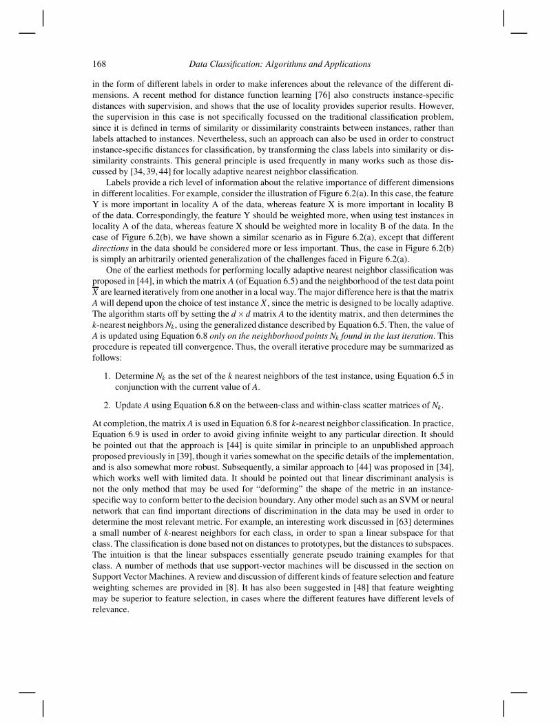
Labels provide a rich level of information about the relative importance of different dimensionsin different localities. For example, consider the illustration of Figure 6.2(a). In this case, the featureY is more important in locality A of the data, whereas feature X is more important in locality Bof the data. Correspondingly, the feature Y should be weighted more, when using test instances inlocality A of the data, whereas feature X should be weighted more in locality B of the data. In thecase of Figure 6.2(b), we have shown a similar scenario as in Figure 6.2(a), except that differentdirections in the data should be considered more or less important. Thus, the case in Figure 6.2(b)is simply an arbitrarily oriented generalization of the challenges faced in Figure 6.2(a).
One of the earliest methods for performing locally adaptive nearest neighbor classification wasproposed in [44], in which the matrix A (of Equation 6.5) and the neighborhood of the test data pointX are learned iteratively from one another in a local way. The major difference here is that the matrixA will depend upon the choice of test instance X , since the metric is designed to be locally adaptive.The algorithm starts off by setting the d×d matrix A to the identity matrix, and then determines thek-nearest neighbors Nk, using the generalized distance described by Equation 6.5. Then, the value ofA is updated using Equation 6.8 only on the neighborhood points Nk found in the last iteration. Thisprocedure is repeated till convergence. Thus, the overall iterative procedure may be summarized asfollows:
1. Determine Nk as the set of the k nearest neighbors of the test instance, using Equation 6.5 inconjunction with the current value of A.
2. Update A using Equation 6.8 on the between-class and within-class scatter matrices of Nk.
At completion, the matrix A is used in Equation 6.8 for k-nearest neighbor classification. In practice,Equation 6.9 is used in order to avoid giving infinite weight to any particular direction. It shouldbe pointed out that the approach is [44] is quite similar in principle to an unpublished approachproposed previously in [39], though it varies somewhat on the specific details of the implementation,and is also somewhat more robust. Subsequently, a similar approach to [44] was proposed in [34],which works well with limited data. It should be pointed out that linear discriminant analysis isnot the only method that may be used for “deforming” the shape of the metric in an instance-specific way to conform better to the decision boundary. Any other model such as an SVM or neuralnetwork that can find important directions of discrimination in the data may be used in order todetermine the most relevant metric. For example, an interesting work discussed in [63] determinesa small number of k-nearest neighbors for each class, in order to span a linear subspace for thatclass. The classification is done based not on distances to prototypes, but the distances to subspaces.The intuition is that the linear subspaces essentially generate pseudo training examples for thatclass. A number of methods that use support-vector machines will be discussed in the section onSupport Vector Machines. A review and discussion of different kinds of feature selection and featureweighting schemes are provided in [8]. It has also been suggested in [48] that feature weightingmay be superior to feature selection, in cases where the different features have different levels ofrelevance.

Instance-Based Learning: A Survey 169
6.3.6 Combining with Ensemble Methods
It is evident from the aforementioned discussion that lazy learning methods have the advantageof being able to optimize more effectively to the locality of a specific instance. In fact, one issuethat is encountered sometimes in lazy learning methods is that the quest for local optimizationcan result in overfitting, especially when some of the features are noisy within a specific locality.In many cases, it may be possible to create multiple models that are more effective for differentinstances, but it may be hard to know which model is more effective without causing overfitting.An effective method to achieve the goal of simultaneous local optimization and robustness is touse ensemble methods that combine the results from multiple models for the classification process.Some recent methods [4,16,80] have been designed for using ensemble methods in order to improvethe effectiveness of lazy learning methods.
An approach discussed in [16] samples random subsets of features, which are used for nearestneighbor classification. These different classifications are then combined together in order to yielda more robust classification. One disadvantage of this approach is that it can be rather slow, espe-cially for larger data sets. This is because the nearest neighbor classification approach is inherentlycomputationally intensive because of the large number of distance computations for every instance-based classification. This is in fact one of the major issues for all lazy learning methods. A recentapproach LOCUST discussed in [4] proposes a more efficient technique for ensemble lazy learning,which can also be applied to the streaming scenario. The approach discussed in [4] builds invertedindices on discretized attributes of each instance in real time, and then uses efficient intersection ofrandomly selected inverted lists in order to perform real time classification. Furthermore, a limitedlevel of feature bias is used in order to reduce the number of ensemble components for effectiveclassification. It has been shown in [4] that this approach can be used for resource-sensitive lazylearning, where the number of feature samples can be tailored to the resources available for classi-fication. Thus, this approach can also be considered an anytime lazy learning algorithm, which isparticularly suited to the streaming scenario. This is useful in scenarios where one cannot controlthe input rate of the data stream, and one needs to continuously adjust the processing rate, in orderto account for the changing input rates of the data stream.
6.3.7 Multi-Label Learning
In traditional classification problems, each class is associated with exactly one label. This isnot the case for multi-label learning, in which each class may be associated with more than oneclass. The number of classes with which an instance is associated is unknown a-priori. This kindof scenario is quite common in many scenarios such as document classification, where a singledocument may belong to one of several possible categories.
The unknown number of classes associated with a test instance creates a challenge, because onenow needs to determine not just the most relevant classes, but also the number of relevant ones fora given test instance. One way of solving the problem is to decompose it into multiple independentbinary classification problems. However, such an approach does not account for the correlationsamong the labels of the data instances.
An approach known as ML-KNN is proposed in [78], where the Bayes method is used in orderto estimate the probability that a label belongs to a particular class. The broad approach used in thisprocess is as follows. For each test instance, its k nearest neighbors are identified. The statisticalinformation in the label sets of these neighborhood instances is then used to determine the label set.The maximum a-posteriori principle is applied to determine the label set of the test instance.
Let Y denote the set of labels for the multi-label classification problem, and let n be the totalnumber of labels. For a given test instance T , the first step is to compute its k nearest neighbors.Once the k nearest neighbors have been computed, the number of occurrences C = (C(1) . . .C(n)) ofeach of the n different labels is computed. Let E1(T, i) be the event that the test instance T contains

170 Data Classification: Algorithms and Applications
the label i, and E0(T, i) be the event that the test instance T does not contain the label i. Then, inorder to determine whether or not the label i is included in test instance T , the maximum posteriorprinciple is used:
b = argmaxb∈{0,1}{P(Eb(T, i)|C)}. (6.10)
In other words, we wish to maximize between the probability of the events of label i being includedor not. Therefore, the Bayes rule can be used in order to obtain the following:
b = argmaxb∈{0,1}
{P(Eb(T, i)) ·P(C|Eb(T, i))
P(C)
}
. (6.11)
Since the value of P(C) is independent of b, it is possible to remove it from the denominator, withoutaffecting the maximum argument. This is a standard approach used in all Bayes methods. Therefore,the best matching label may be expressed as follows:
b = argmaxb∈{0,1}{
P(Eb(T, i)) ·P(C|Eb(T, i))}. (6.12)
The prior probability P(Eb(T, i)) can be estimated as the fraction of the labels belonging to a par-ticular class. The value of P(C|Eb(T, i)) can be estimated by using the naive Bayes rule.
P(C|Eb(T, i)) =n
∏j=1
P(C( j)|Eb(T, i)). (6.13)
Each of the terms P(C( j)|Eb(T, i)) can be estimated in a data driven manner by examining amongthe instances satisfying the value b for class label i, the fraction that contains exactly the count C( j)for the label j. Laplacian smoothing is also performed in order to avoid ill conditioned probabilities.Thus, the correlation between the labels is accounted for by the use of this approach, since each ofthe terms P(C( j)|Eb(T, i)) indirectly measures the correlation between the labels i and j.
This approach is often popularly understood in the literature as a nearest neighbor approach,and has therefore been discussed in the section on nearest neighbor methods. However, it is moresimilar to a local naive Bayes approach (discussed in Section 6.6) rather than a distance-basedapproach. This is because the statistical frequencies of the neighborhood labels are used for localBayes modeling. Such an approach can also be used for the standard version of the classificationproblem (when each instance is associated with exactly one label) by using the statistical behaviorof the neighborhood features (rather than label frequencies). This yields a lazy Bayes approach forclassification [38]. However, the work in [38] also estimates the Bayes probabilities locally only overthe neighborhood in a data driven manner. Thus, the approach in [38] sharpens the use of localityeven further for classification. This is of course a tradeoff, depending upon the amount of trainingdata available. If more training data is available, then local sharpening is likely to be effective. Onthe other hand, if less training data is available, then local sharpening is not advisable, because itwill lead to difficulties in robust estimations of conditional probabilities from a small amount ofdata. This approach will be discussed in some detail in Section 6.6.
If desired, it is possible to combine the two methods discussed in [38] and [78] for multi-labellearning in order to learn the information in both the features and labels. This can be done byusing both feature and label frequencies for the modeling process, and the product of the label-based and feature-based Bayes probabilities may be used for classification. The extension to thatcase is straightforward, since it requires the multiplication of Bayes probabilities derived form twodifferent methods. An experimental study of several variations of nearest neighbor algorithms forclassification in the multi-label scenario is provided in [59].

Instance-Based Learning: A Survey 171
6.4 Lazy SVM ClassificationIn an earlier section, it was shown that linear discriminant analysis can be very useful in adapting
the behavior of the nearest neighbor metric for more effective classification. It should be pointed outthat SVM classifiers are also linear models that provide directions discriminating between the dif-ferent classes. Therefore, it is natural to explore the connections between SVM and nearest neighborclassification.
The work in [35] proposes methods for computing the relevance of each feature with the useof an SVM approach. The idea is to use a support vector machine in order to compute the gradientvector (local to test instance) of the rate change in class label in each direction, which is parallelto the axis. It has been shown in [35] that the support vector machine provides a natural way toestimate this gradient. The component along any direction provides the relevance R j for that featurej. The idea is that when the class labels change at a significantly higher rate along a given directionj, then that feature should be weighted more in the distance metric. The actual weight wj for thefeature j is assumed to be proportional to eλ·R j , where λ is a constant that determines the level ofimportance to be given to the different relevance values. A similar method for using SVM to modifythe distance metric is proposed in [54], and the connections of the approach to linear discriminantanalysis have also been shown in this work.
Note that the approaches in [35, 54] use a nearest neighbor classifier, and the SVM is onlyused to learn the distance function more accurately by setting the relevance weights. Therefore, theapproach is still quite similar to that discussed in the last section. A completely different approachwould be to use the nearest neighbors in order to isolate the locality around the test instance, andthen build an SVM that is optimized to that data locality. For example, in the case of Figures 6.3(a)and (b) the data in the two classes is distributed in such a way that a global SVM cannot separatethe classes very well. However, in the locality around the test instances A and B, it is easy to createa linear SVM that separates the two classes well. Such an approach has been proposed in [23, 77].The main difference between the work in [23] and [77] is that the former is designed for the L2-distances, whereas the latter can work for arbitrary and complex distance functions. Furthermore,the latter also proposes a number of optimizations for the purpose of efficiency. Therefore, we willdescribe the work in [77], since it is a bit more general. The specific steps that are used in thisapproach are as follows:
1. Determine the k-nearest neighbors of the test instance.
2. If all the neighbors have the same label, then that label is reported, otherwise all pairwisedistances between the k-nearest neighbors are computed.
3. The distance matrix is converted into a kernel matrix using the kernel trick and a local SVMclassifier is constructed on this matrix.
4. The test instance is classified with this local SVM classifier.
A number of optimizations such as caching have been proposed in [77] in order to improve theefficiency of the approach. Local SVM classifiers have been used quite successfully for a variety ofapplications such as spam filtering [20].
172 Data Classification: Algorithms and Applications
KNN Locality
Y
A
X
KNN L litKNN Locality
B
Y
B
X
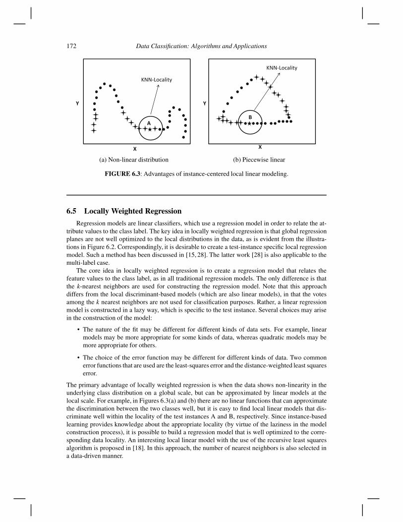
(a) Non-linear distribution (b) Piecewise linear
FIGURE 6.3: Advantages of instance-centered local linear modeling.
6.5 Locally Weighted RegressionRegression models are linear classifiers, which use a regression model in order to relate the at-
tribute values to the class label. The key idea in locally weighted regression is that global regressionplanes are not well optimized to the local distributions in the data, as is evident from the illustra-tions in Figure 6.2. Correspondingly, it is desirable to create a test-instance specific local regressionmodel. Such a method has been discussed in [15, 28]. The latter work [28] is also applicable to themulti-label case.
The core idea in locally weighted regression is to create a regression model that relates thefeature values to the class label, as in all traditional regression models. The only difference is thatthe k-nearest neighbors are used for constructing the regression model. Note that this approachdiffers from the local discriminant-based models (which are also linear models), in that the votesamong the k nearest neighbors are not used for classification purposes. Rather, a linear regressionmodel is constructed in a lazy way, which is specific to the test instance. Several choices may arisein the construction of the model:
• The nature of the fit may be different for different kinds of data sets. For example, linearmodels may be more appropriate for some kinds of data, whereas quadratic models may bemore appropriate for others.
• The choice of the error function may be different for different kinds of data. Two commonerror functions that are used are the least-squares error and the distance-weighted least squareserror.
The primary advantage of locally weighted regression is when the data shows non-linearity in theunderlying class distribution on a global scale, but can be approximated by linear models at thelocal scale. For example, in Figures 6.3(a) and (b) there are no linear functions that can approximatethe discrimination between the two classes well, but it is easy to find local linear models that dis-criminate well within the locality of the test instances A and B, respectively. Since instance-basedlearning provides knowledge about the appropriate locality (by virtue of the laziness in the modelconstruction process), it is possible to build a regression model that is well optimized to the corre-sponding data locality. An interesting local linear model with the use of the recursive least squaresalgorithm is proposed in [18]. In this approach, the number of nearest neighbors is also selected ina data-driven manner.

Instance-Based Learning: A Survey 173
6.6 Lazy Naive BayesLazy learning has also been extended to the case of the naive Bayes classifiers [38,79]. The work
in [38] proposes a locally weighted naive Bayes classifier. The naive Bayes classifier is used in asimilar way as the local SVM method [77], or the locally weighted regression method [15] discussedin previous sections. A local Bayes model is constructed with the use of a subset of the data inthe neighborhood of the test instance. Furthermore, the training instances in this neighborhood areweighted, so that training instances that are closer to the test instance are weighted more in themodel. This local model is then used for classification. The subset of data in the neighborhood ofthe test instance are determined by using the k-nearest neighbors of the test instance. In practice,the subset of k neighbors is selected by setting the weight of any instance beyond the k-th nearestneighbor to 0. Let D represent the distance of the test instance to the kth nearest neighbor, and direpresent the distance of the test instance to the ith training instance. Then, the weight wi of the ithinstance is set to the following:
wi = f (di/D). (6.14)
The function f (·) is a monotonically non-increasing function, which is defined as follows:
f (y) = max{1− y,0}. (6.15)
Therefore, the weight decreases linearly with the distance, but cannot decrease beyond 0, once thek-nearest neighbor has been reached. The naive Bayes method is applied in a standard way, exceptthat the instance weights are used in estimating all the probabilities for the Bayes classifier. Highervalues of k will result in models that do not fluctuate much with variations in the data, whereas verysmall values of k will result in models that fit the noise in the data. It has been shown in [38] thatthe approach is not too sensitive to the choice of k within a reasonably modest range of values ofk. Other schemes have been proposed in the literature, which use the advantages of lazy learning inconjunction with the naive Bayes classifier. The work in [79] fuses a standard rule-based learner withnaive Bayes models. A technique discussed in [74] lazily learns multiple Naive Bayes classifiers,and uses the classifier with the highest estimated accuracy in order to decide the label for the testinstance.
The work discussed in [78] can also be viewed as an unweighted local Bayes classifier, wherethe weights used for all instances are 1, rather than the weighted approach discussed above. Further-more, the work in [78] uses the frequencies of the labels for Bayes modeling, rather than the actualfeatures themselves. The idea in [78] is that the other labels themselves serve as features, since thesame instance may contain multiple labels, and sufficient correlation information is available forlearning. This approach is discussed in detail in Section 6.3.7.
6.7 Lazy Decision TreesThe work in [40] proposes a method for constructing lazy decision trees, which are specific to
a test instance, which is referred to as LazyDT. In practice, only a path needs to be constructed,because a test instance follows only one path along the decision tree, and other paths are irrele-vant from the perspective of lazy learning. As discussed in a later section, such paths can also beinteractively explored with the use of visual methods.
One of the major problems with decision trees is that they are myopic, since a split at a higherlevel of the tree may not be optimal for a specific test instance, and in cases where the data contains
174 Data Classification: Algorithms and Applications
many relevant features, only a small subset of them may be used for splitting. When a data setcontains N data points, a decision tree is allowed only O(log(N)) (approximately balanced) splits,and this may be too small in order to use the best set of features for a particular test instance. Clearly,the knowledge of the test instance allows the use of more relevant features for construction of theappropriate decision path at a higher level of the tree construction.
The additional knowledge of the test instance helps in the recursive construction of a path inwhich only relevant features are used. One method proposed in [40] is to use a split criterion, whichsuccessively reduces the size of the training associated with the test instance, until either all in-stances have the same class label, or the same set of features. In both cases, the majority classlabel is reported as the relevant class. In order to discard a set of irrelevant instances in a particulariteration, any standard decision tree split criterion is used, and only those training instances, thatsatisfy the predicate in the same way as the test instance will be selected for the next level of thedecision path. The split criterion is decided using any standard decision tree methodology such asthe normalized entropy or the gini-index. The main difference from the split process in the tradi-tional decision tree is that only the node containing the test instance is relevant in the split, and theinformation gain or gini-index is computed on the basis of this node. One challenge with the use ofsuch an approach is that the information gain in a single node can actually be negative if the originaldata is imbalanced. In order to avoid this problem, the training examples are re-weighted, so that theaggregate weight of each class is the same. It is also relatively easy to deal with missing attributesin test instances, since the split only needs to be performed on attributes that are present in the testinstance. It has been shown [40] that such an approach yields better classification results, becauseof the additional knowledge associated with the test instance during the decision path constructionprocess.
A particular observation here is noteworthy, since such decision paths can also be used to con-struct a robust any-time classifier, with the use of principles associated with a random forest ap-proach [25]. It should be pointed out that a random forest translates to a random path created bya random set of splits from the instance-centered perspective. Therefore a natural way to imple-ment the instance-centered random forest approach would be to discretize the data into ranges. Atest instance will be relevant to exactly one range from each attribute. A random set of attributes isselected, and the intersection of the ranges provides one possible classification of the test instance.This approach can be repeated in order to provide a very efficient lazy ensemble, and the numberof samples provides the tradeoff between running time and accuracy. Such an approach can be usedin the context of an any-time approach in resource-constrained scenarios. It has been shown in [4]how such an approach can be used for efficient any-time classification of data streams.
6.8 Rule-Based ClassificationA method for lazy rule-based classification has been proposed in [36], in which a unification has
been proposed between instance-based methods and rule-based methods. This system is referred toas Rule Induction from a Set of Exemplars, or RISE for short. All rules contain at most one conditionfor each attribute on the left-hand side. In this approach, no distinction is assumed between instancesand rules. An instance is simply treated as a rule in which all interval values on the left hand side ofthe rule are degenerate. In other words, an instance can be treated as a rule, by choosing appropriateconditions for the antecedent, and the class variable of the instance as the consequent. The conditionsin the antecedent are determined by using the values in the corresponding instance. For example, ifan attribute value for the instance for x1 is numeric valued at 4, then the condition is assumed to be

Instance-Based Learning: A Survey 175
4≤ xi ≤ 4. If x1 is symbolic and its value is a, then the corresponding condition in the antecedent isx1 = a.
As in the case of instance-centered methods, a distance is defined between a test instance and arule. Let R = (A1 . . .Am,C) be a rule with the m conditions A1 . . .Am in the antecedent, and the classC in the consequent. Let X = (x1 . . .xd) be a d-dimensional example. Then, the distance Δ(X ,R)between the instance X and the rule R is defined as follows.
Δ(X ,R) =m
∑j=1
δ(i)s. (6.16)
Here s is a real valued parameter such as 1,2,3, etc., and δ(i) represents the distance on the ithconditional. The value of δ(i) is equal to the distance of the instance to the nearest end of the rangefor the case of a numeric attribute and the value difference metric (VDM) of Equation 6.1 for thecase of a symbolic attribute. This value of δ(i) is zero, if the corresponding attribute value is a matchfor the antecedent condition. The class label for a test instance is defined by the label of the nearestrule to the test instance. If two or more rules have the same accuracy, then the one with the greatestaccuracy on the training data is used.
The set of rules in the RISE system are constructed as follows. RISE constructs good rules byusing successive generalizations on the original set of instances in the data. Thus, the algorithm startsoff with the training set of examples. RISE examines each rule one by one, and finds the nearestexample of the same class that is not already covered by the rule. The rule is then generalized in orderto cover this example, by expanding the corresponding antecedent condition. For the case of numericattributes, the ranges of the attributes are increased minimally so as to include the new example, andfor the case of symbolic attributes, a corresponding condition on the symbolic attribute is included.If the effect of this generalization on the global accuracy of the rule is non-negative, then the ruleis retained. Otherwise, the generalization is not used and the original rule is retained. It should bepointed out that even when generalization does not improve accuracy, it is desirable to retain themore general rule because of the desirable bias towards simplicity of the model. The procedure isrepeated until no rule can be generalized in a given iteration. It should be pointed out that someinstances may not be generalized at all, and may remain in their original state in the rule set. In theworst case, no instance is generalized, and the resulting model is a nearest neighbor classifier.
A system called DeEPs has been proposed in [49], which combines the power of rules and lazylearning for classification purposes. This approach examines how the frequency of an instance’s sub-set of features varies among the training classes. In other words, patterns that sharply differentiatebetween the different classes for a particular test instance are leveraged and used for classifica-tion. Thus, the specificity to the instance plays an important role in this discovery process. Anothersystem, HARMONY, has been proposed in [66], which determines rules that are optimized to thedifferent training instances. Strictly speaking, this is not a lazy learning approach, since the rules areoptimized to training instances (rather than test instances) in a pre-processing phase. Nevertheless,the effectiveness of the approach relies on the same general principle, and it can also be generalizedfor lazy learning if required.
6.9 Radial Basis Function Networks: Leveraging Neural Networks forInstance-Based Learning
Radial-basis function networks (RBF) are designed in a similar way to regular nearest neighborclassifiers, except that a set of N centers are learned from the training data. In order to classify a testinstance, a distance is computed from the test instance to each of these centers x1 . . .xN , and a density

176 Data Classification: Algorithms and Applications
function is computed at the instance using these centers. The combination of functions computedfrom each of these centers is computed with the use of a neural network. Radial basis functions canbe considered three-layer feed-forward networks, in which each hidden unit computes a function ofthe form:
fi(x) = e−||x−xi||2/2·σ2i . (6.17)
Here σ2i represents the local variance at center xi. Note that the function fi(x) has a very similar form
to that commonly used in kernel density estimation. For ease in discussion, we assume that this isa binary classification problem, with labels drawn from {+1,−1}, though this general approachextends much further, even to the extent of regression modeling. The final function is a weightedcombination of these values with weights ci.
f ∗(x) =N
∑i=1
wi · fi(x). (6.18)
Here x1 . . .xN represent the N different centers, and wi denotes the weight of center i, which islearned in the neural network. In classical instance-based methods, each data point xi is an individualtraining instance, and the weight wi is set to +1 or −1, depending upon its label. However, in RBFmethods, the weights are learned with a neural network approach, since the centers are derived fromthe underlying training data, and do not have a label directly attached to them.
The N centers x1 . . .xN are typically constructed with the use of an unsupervised approach[19, 37, 46], though some recent methods also use supervised techniques for constructing the cen-ters [71]. The unsupervised methods [19, 37, 46] typically use a clustering algorithm in order togenerate the different centers. A smaller number of centers typically results in smaller complexity,and greater efficiency of the classification process. Radial-basis function networks are related tosigmoidal function networks (SGF), which have one unit for each instance in the training data. Inthis sense sigmoidal networks are somewhat closer to classical instance-based methods, since theydo not have a first phase of cluster-based summarization. While radial-basis function networks aregenerally more efficient, the points at the different cluster boundaries may often be misclassified.It has been shown in [52] that RBF networks may sometimes require ten times as much trainingdata as SGF in order to achieve the same level of accuracy. Some recent work [71] has shown howsupervised methods even at the stage of center determination can significantly improve the accu-racy of these classifiers. Radial-basis function networks can therefore be considered an evolution ofnearest neighbor classifiers, where more sophisticated (clustering) methods are used for prototypeselection (or re-construction in the form of cluster centers), and neural network methods are usedfor combining the density values obtained from each of the centers.
6.10 Lazy Methods for Diagnostic and Visual ClassificationInstance-centered methods are particularly useful for diagnostic and visual classification, since
the role of a diagnostic method is to find diagnostic characteristics that are specific to that test-instance. When an eager model is fully constructed as a pre-processing step, it is often not optimizedto finding the best diagnostic characteristics that are specific to a particular test instance. Therefore,instance-centered methods are a natural approach in such scenarios. The subspace decision pathmethod [6] can be considered a lazy and interactive version of the decision tree, which providesinsights into the specific characteristics of a particular test instance.
Kernel density estimation is used in order to create a visual profile of the underlying data. It isassumed that the data set D contains N points and d dimensions. The set of points in D are denoted

Instance-Based Learning: A Survey 177
−2 −1.5 −1 −0.5 0 0.5 1 1.5
−2−1
01
20
0.1
0.2
0.3
0.4
0.5
0.6
0.7
0.8
0.9
1
Attribute Y
* Test Instance
Attribute X
Acc
urac
y D
ensi
ty fo
r D
omin
ant C
lass
−2 −1.5 −1 −0.5 0 0.5 1 1.5
−2−1
01
20
0.1
0.2
0.3
0.4
0.5
0.6
0.7
0.8
0.9
1
Attribute Y
* Test Instance
Attribute X
Acc
urac
y D
ensi
ty fo
r D
omin
ant C
lass
(a) Accuracy Density Profile Isolation of Data
FIGURE 6.4: Density profiles and isolation of data.
by X1 . . .XN . Let us further assume that the k classes in the data are denoted by C1 . . .Ck. The numberof points belonging to the class Ci is ni, so that∑k
i=1 ni =N. The data set associated with the class i isdenoted by Di. This means that ∪k
i=1Di = D. The probability density at a given point is determinedby the sum of the smoothed values of the kernel functions Kh(·) associated with each point in thedata set. Thus, the density estimate of the data set D at the point x is defined as follows:
f (x,D) =1n· ∑
Xi∈DKh(x−Xi). (6.19)
The kernel function is a smooth unimodal distribution such as the Gaussian function:
Kh(x−Xi) =1√
2π ·h · e− ||x−Xi||2
2h2 . (6.20)
The kernel function is dependent on the use of a parameter h, which is the level of smoothing. Theaccuracy of the density estimate depends upon this width h, and several heuristic rules have beenproposed for estimating the bandwidth [6].
The value of the density f (x,D) may differ considerably from f (x,Di) because of the differencein distributions of the different classes. Correspondingly, the accuracy density A(x,Ci,D) for theclass Ci is defined as follows:
A(x,Ci,D) =ni · f (x,Di)
∑ki=1 ni · f (x,Di)
. (6.21)
The above expression always lies between 0 and 1, and is simply an estimation of the Bayesianposterior probability of the test instance belonging to class Ci. It is assumed that the a-priori proba-bility of the test instance belonging to class Ci, (without knowing any of its feature values) is simplyequal to its fractional presence ni/N in class Ci. The conditional probability density after knowingthe feature values x is equal to f (x,Di). Then, by applying the Bayesian formula for posterior prob-abilities,the condition of Equation 6.21 is obtained. The higher the value of the accuracy density,the greater the relative density of Ci compared to the other classes.
Another related measure is the interest density I (x,Ci,D), which is the ratio of the density ofthe class Ci to the overall density of the data.
I (x,Ci,D) =f (x,Di)
f (x,D). (6.22)

178 Data Classification: Algorithms and Applications
The class Ci is over-represented at x, when the interest density is larger than one. The dominantclass at the coordinate x is denoted by C M (x,D), and is equal to argmaxi∈{1,...k}I (x,Ci,D). Cor-respondingly, the maximum interest density at x is denoted by I M (x,D) = maxi∈{1,...k}I (x,Ci,D).Both the interest and accuracy density are valuable quantifications of the level of dominance of thedifferent classes. The interest density is more effective at comparing among the different classes ata given point, whereas the accuracy density is more effective at providing an idea of the absoluteaccuracy at a given point.
So far, it has been assumed that all of the above computations are performed in the full dimen-sional space. However, it is also possible to project the data onto the subspace E in order to performthis computation. Such a calculation would quantify the discriminatory power of the subspace E atx. In order to denote the use of the subspace E in any computation, the corresponding expressionwill be superscripted with E . Thus the density in a given subspace E is denoted by f E(·, ·), theaccuracy density by AE(·, ·, ·), and the interest density by I E(·, ·, ·). Similarly, the dominant classis defined using the subspace-specific interest density at that point, and the accuracy density profileis defined for that particular subspace. An example of the accuracy density profile (of the dominantclass) in a 2-dimensional subspace is illustrated in Figure 6.4(a). The test instance is also labeled inthe same figure in order to illustrate the relationship between the density profile and test instance.
It is desired to find those projections of the data in which the interest density value I M E(t,D)
is the maximum. It is quite possible that in some cases, different subspaces may provide differentinformation about the class behavior of the data; these are the difficult cases in which a test instancemay be difficult to classify accurately. In such cases, the user may need to isolate particular datalocalities in which the class distribution is further examined by a hierarchical exploratory process.While the density values are naturally defined over the continuous space of quantitative attributes, ithas been shown in [6] that intuitively analogous values can be defined for the interest and accuracydensities even when categorical attributes are present.
For a given test example, the end user is provided with unique options in exploring variouscharacteristics that are indicative of its classification. A subspace determination process is used onthe basis of the highest interest densities at a given test instance. Thus, the subspace determinationprocess finds the appropriate local discriminative subspaces for a given test example. These are thevarious possibilities (or branches) of the decision path, which can be utilized in order to explore theregions in the locality of the test instance. In each of these subspaces, the user is provided with avisual profile of the accuracy density. This profile provides the user with an idea of which branch islikely to lead to a region of high accuracy for that test instance. This visual profile can also be utilizedin order to determine which of the various branches are most suitable for further exploration. Oncesuch a branch has been chosen, the user has the option to further explore into a particular regionof the data that has high accuracy density. This process of data localization can quickly isolate anarbitrarily shaped region in the data containing the test instance. This sequence of data localizationscreates a path (and a locally discriminatory combination of dimensions) that reveals the underlyingclassification causality to the user.
In the event that a decision path is chosen that is not strongly indicative of any class, the user hasthe option to backtrack to a higher level node and explore a different path of the tree. In some cases,different branches may be indicative of the test example belonging to different classes. These arethe “ambiguous cases” in which a test example could share characteristics from multiple classes.Many standard modeling methods may classify such an example incorrectly, though the subspacedecision path method is much more effective at providing the user with an intensional knowledgeof the test example because of its exploratory approach. This can be used in order to understand thecausality behind the ambiguous classification behavior of that instance.
The overall algorithm for decision path construction is illustrated in Figure 6.5. The details ofthe subroutines in the procedure are described in [6], though a summary description is providedhere. The input to the system is the data set D, the test instance t for which one wishes to find the
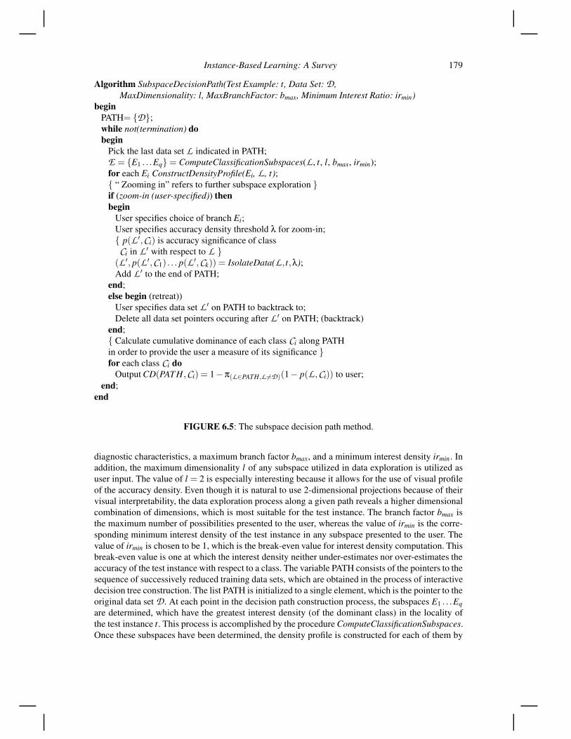
Instance-Based Learning: A Survey 179
Algorithm SubspaceDecisionPath(Test Example: t, Data Set: D,MaxDimensionality: l, MaxBranchFactor: bmax, Minimum Interest Ratio: irmin)
beginPATH= {D};while not(termination) dobegin
Pick the last data set L indicated in PATH;E = {E1 . . .Eq}= ComputeClassificationSubspaces(L , t, l, bmax, irmin);for each Ei ConstructDensityProfile(Ei, L , t);{ “ Zooming in” refers to further subspace exploration }if (zoom-in (user-specified)) thenbegin
User specifies choice of branch Ei;User specifies accuracy density threshold λ for zoom-in;{ p(L ′,Ci) is accuracy significance of classCi in L ′ with respect to L }(L ′, p(L ′,C1) . . . p(L ′,Ck)) = IsolateData(L, t,λ);Add L ′ to the end of PATH;
end;else begin (retreat))
User specifies data set L ′ on PATH to backtrack to;Delete all data set pointers occuring after L ′ on PATH; (backtrack)
end;{ Calculate cumulative dominance of each class Ci along PATHin order to provide the user a measure of its significance }for each class Ci do
Output CD(PATH,Ci) = 1−π(L∈PATH,L =D)(1− p(L,Ci)) to user;end;
end
FIGURE 6.5: The subspace decision path method.
diagnostic characteristics, a maximum branch factor bmax, and a minimum interest density irmin. Inaddition, the maximum dimensionality l of any subspace utilized in data exploration is utilized asuser input. The value of l = 2 is especially interesting because it allows for the use of visual profileof the accuracy density. Even though it is natural to use 2-dimensional projections because of theirvisual interpretability, the data exploration process along a given path reveals a higher dimensionalcombination of dimensions, which is most suitable for the test instance. The branch factor bmax isthe maximum number of possibilities presented to the user, whereas the value of irmin is the corre-sponding minimum interest density of the test instance in any subspace presented to the user. Thevalue of irmin is chosen to be 1, which is the break-even value for interest density computation. Thisbreak-even value is one at which the interest density neither under-estimates nor over-estimates theaccuracy of the test instance with respect to a class. The variable PATH consists of the pointers to thesequence of successively reduced training data sets, which are obtained in the process of interactivedecision tree construction. The list PATH is initialized to a single element, which is the pointer to theoriginal data set D. At each point in the decision path construction process, the subspaces E1 . . .Eqare determined, which have the greatest interest density (of the dominant class) in the locality ofthe test instance t. This process is accomplished by the procedure ComputeClassificationSubspaces.Once these subspaces have been determined, the density profile is constructed for each of them by

180 Data Classification: Algorithms and Applications
the procedure ConstructDensityProfile. Even though one subspace may have higher interest densityat the test instance than another, the true value of a subspace in separating the data locality aroundthe test instance is often a subjective judgement that depends both upon the interest density of thetest instance and the spatial separation of the classes. Such a judgement requires human intuition,which can be harnessed with the use of the visual profile of the accuracy density profiles of the var-ious possibilities. These profiles provide the user with an intuitive idea of the class behavior of thedata set in various projections. If the class behavior across different projections is not very consis-tent (different projections are indicative of different classes), then such a node is not very revealingof valuable information. In such a case, the user may choose to backtrack by specifying an earliernode on PATH from which to start further exploration.
On the other hand, if the different projections provide a consistent idea of the class behavior, thenthe user utilizes the density profile in order to isolate a small region of the data in which the accuracydensity of the data in the locality of the test instance is significantly higher for a particular class.This is achieved by the procedure IsolateData. This isolated region may be a cluster of arbitraryshape depending upon the region covered by the dominating class. However, the use of the visualprofile helps to maintain the interpretability of the isolation process in spite of the arbitrary contourof separation. An example of such an isolation is illustrated in Figure 6.4(b), and is facilitated bythe construction of the visual density profile. The procedure returns the isolated data set L ′ alongwith a number of called the accuracy significance p(L ′,Ci) of the class Ci. The pointer to this newdata set L ′ is added to the end of PATH. At that point, the user decides whether further explorationinto that isolated data set is necessary. If so, the same process of subspace analysis is repeated onthis node. Otherwise, the process is terminated and the most relevant class label is reported. Theoverall exploration process also provides the user with a good diagnostic idea of how the local datadistributions along different dimensions relate to the class label.
6.11 Conclusions and SummaryIn this chapter, we presented algorithms for instance-based learning and lazy-learning. These
methods are usually computationally more expensive than traditional models, but have the advan-tage of using information about the test instance at the time of model construction. In many sce-narios, such methods can provide more accurate results, when a pre-processed model cannot fullycapture the underlying complexities of the data. The other advantage of instance-based methods isthat they are typically very simple and easy to implement for arbitrary data types, because the com-plexity is usually abstracted in determining an appropriate distance function between objects. Sincedistance function design has been widely studied in the literature for different data types, this allowsthe use of this methodology for arbitrary data types. Furthermore, existing model-based algorithmscan be generalized to local variations in order to transform them to instance-learning methods. Suchmethods have great diagnostic value for specific test instances, since the model is constructed localto the specific test instance, and also provides knowledge to the analyst that is test-instance specific.Lazy methods are highly flexible and can be generalized to streaming and other temporal scenarios,where the laziness of the approach can be used in order to learn the appropriate temporal horizon,in which lazy learning should be performed.

Instance-Based Learning: A Survey 181
Bibliography[1] A. Aamodt and E. Plaza. Case-based reasoning: Foundational issues, methodological varia-
tions, and system approaches, AI communications, 7(1):39–59, 1994.
[2] C. Aggarwal, A. Hinneburg, and D. Keim. On the surprising behavior of distance metrics inhigh dimensional space, Data Theory—ICDT Conference, 2001; Lecture Notes in ComputerScience, 1973:420–434, 2001.
[3] C. Aggarwal. Towards systematic design of distance functions for data mining applications,Proceedings of the KDD Conference, pages 9–18, 2003.
[4] C. Aggarwal and P. Yu. Locust: An online analytical processing framework for high dimen-sional classification of data streams, Proceedings of the IEEE International Conference onData Engineering, pages 426–435, 2008.
[5] C. Aggarwal and C. Reddy. Data Clustering: Algorithms and Applications, CRC Press, 2013.
[6] C. Aggarwal. Toward exploratory test-instance-centered diagnosis in high-dimensional classi-fication, IEEE Transactions on Knowledge and Data Engineering, 19(8):1001–1015, 2007.
[7] C. Aggarwal, J. Han, J. Wang, and P. Yu. A framework for on demand classification of evolvingdata streams. In IEEE TKDE Journal, 18(5):577–589, 2006.
[8] D. Aha, P. Clark, S. Salzberg, and G. Blix. Incremental constructive induction: An instance-based approach, Proceedings of the Eighth International Workshop on Machine Learning,pages 117–121, 1991.
[9] D. Aha. Lazy learning. Kluwer Academic Publishers, 1997.
[10] D. Aha. Tolerating noisy, irrelevant and novel attributes in instance-based learning algorithms,International Journal of Man-Machine Studies, 36(2):267–287, 1992.
[11] D. Aha, D. Kibler, and M. Albert. Instance-based learning algorithms, Machine Learning,6(1):37–66, 1991.
[12] D. Aha. Lazy learning: Special issue editorial, Artificial Intelligence Review, 11:7–10, 1997.
[13] F. Angiulli. Fast nearest neighbor condensation for large data sets classification, IEEE Trans-actions on Knowledge and Data Engineering, 19(11):1450–1464, 2007.
[14] M. Ankerst, G. Kastenmuller, H.-P. Kriegel, and T. Seidl. Nearest Neighbor Classification in3D Protein Databases, ISMB-99 Proceedings, pages 34–43, 1999.
[15] C. Atkeson, A. Moore, and S. Schaal. Locally weighted learning, Artificial Intelligence Re-view, 11(1–5):11–73, 1997.
[16] S. D. Bay. Combining nearest neighbor classifiers through multiple feature subsets. Proceed-ings of ICML Conference, pages 37–45, 1998.
[17] J. Beringer and E Hullermeier. Efficient instance-based learning on data streams, IntelligentData Analysis, 11(6):627–650, 2007.
[18] M. Birattari, G. Bontempi, and M. Bersini. Lazy learning meets the recursive least squaresalgorithm, Advances in neural information processing systems, 11:375–381, 1999.

182 Data Classification: Algorithms and Applications
[19] C. M. Bishop. Improving the generalization properties of radial basis function neural networks,Neural Computation, 3(4):579–588, 1991.
[20] E. Blanzieri and A. Bryl. Instance-based spam filtering using SVM nearest neighbor classifier,FLAIRS Conference, pages 441–442, 2007.
[21] J. Blitzer, K. Weinberger, and L. Saul. Distance metric learning for large margin nearest neigh-bor classification, Advances in neural information processing systems: 1473–1480, 2005.
[22] S. Boriah, V. Chandola, and V. Kumar. Similarity measures for categorical data: A comparativeevaluation. Proceedings of the SIAM Conference on Data Mining, pages 243–254, 2008.
[23] L. Bottou and V. Vapnik. Local learning algorithms, Neural COmputation, 4(6):888–900,1992.
[24] L. Breiman, J. Friedman, R. Olshen, and C. Stone. Classification and Regression Trees,Wadsworth, 1984.
[25] L. Breiman. Random forests, Machine Learning, 48(1):5–32, 2001.
[26] T. Cain, M. Pazzani, and G. Silverstein. Using domain knowledge to influence similarity judge-ments, Proceedings of the Case-Based Reasoning Workshop, pages 191–198, 1991.
[27] C. L. Chang. Finding prototypes for nearest neighbor classifiers: IEEE Transactions on Com-puters, 100(11):1179–184, 1974.
[28] W. Cheng and E. Hullermeier. Combining instance-based learning and logistic regression formultilabel classification, Machine Learning, 76 (2–3):211–225, 2009.
[29] J. G. Cleary and L. E. Trigg. K∗: An instance-based learner using an entropic distance measure,Proceedings of ICML Conference, pages 108–114, 1995.
[30] S. Cost and S. Salzberg. A weighted nearest neighbor algorithm for learning with symbolicfeatures, Machine Learning, 10(1):57–78, 1993.
[31] T. Cover and P. Hart. Nearest neighbor pattern classification, IEEE Transactions on Informa-tion Theory, 13(1):21–27, 1967.
[32] P. Cunningham, A taxonomy of similarity mechanisms for case-based reasoning, IEEE Trans-actuions on Knowledge and Data Engineering, 21(11):1532–1543, 2009.
[33] B. V. Dasarathy. Nearest Neighbor (NN) Norms: NN Pattern Classification Techniques, IEEEComputer Society Press, 1990.
[34] C. Domeniconi, J. Peng, and D. Gunopulos. Locally adaptive metric nearest-neighbor classi-fication, IEEE Transactions on Pattern Analysis and Machine Intelligence, 24(9):1281–1285,2002.
[35] C. Domeniconi and D. Gunopulos. Adaptive nearest neighbor classification using support vec-tor machines, Advances in Neural Information Processing Systems, 1: 665–672, 2002.
[36] P. Domingos. Unifying instance-based and rule-based induction, Machine Learning,24(2):141–168, 1996.
[37] G. W. Flake. Square unit augmented, radially extended, multilayer perceptrons, In NeuralNetworks: Tricks of the Trade, pages 145–163, 1998.

Instance-Based Learning: A Survey 183
[38] E. Frank, M. Hall, and B. Pfahringer. Locally weighted Naive Bayes, Proceedings of the Nine-teenth Conference on Uncertainty in Artificial Intelligence, pages 249–256, 2002.
[39] J. Friedman. Flexible Nearest Neighbor Classification, Technical Report, Stanford University,1994.
[40] J. Friedman, R. Kohavi, and Y. Yun. Lazy decision trees, Proceedings of the National Confer-ence on Artificial Intelligence, pages 717–724, 1996.
[41] S. Garcia, J. Derrac, J. Cano, and F. Herrera. Prototype selection for nearest neighbor classi-fication: Taxonomy and empirical study, IEEE Transactions on Pattern Analysis and MachineIntelligence, 34(3):417–436, 2012.
[42] D. Gunopulos and G. Das. Time series similarity measures. In Tutorial notes of the sixth ACMSIGKDD International Conference on Knowledge Discovery and Data Mining, pages 243–307, 2000.
[43] E. Han, G. Karypis, and V. Kumar. Text categorization using weight adjusted k-nearest neigh-bor classification, Proceedings of the Pacific-Asia Conference on Knowledge Discovery andData Mining, pages 53–65, 2001.
[44] T. Hastie and R. Tibshirani. Discriminant adaptive nearest neighbor classification, IEEE Trans-actions on Pattern Analysis and Machine Intelligence, 18(6):607–616, 1996.
[45] A. Hinneburg, C. Aggarwal, and D. Keim. What is the nearest neighbor in high dimensionalspaces? Proceedings of VLDB Conference, pages 506–515, 2000.
[46] Y. S. Hwang and S. Y. Bang. An efficient method to construct a radial basis function neuralnetwork classifier, Neural Networks, 10(8):1495–1503, 1997.
[47] N. Jankowski and M. Grochowski, Comparison of instance selection algorithms, I algorithmssurvey, Lecture Notes in Computer Science, 3070:598–603, 2004.
[48] R. Kohavi, P. Langley, and Y. Yun. The utility of feature weighting in nearest-neighbor algo-rithms, Proceedings of the Ninth European Conference on Machine Learning, pages 85–92,1997.
[49] J. Li, G. Dong, K. Ramamohanarao, and L. Wong. Deeps: A new instance-based lazy discoveryand classification system, Machine Learning, 54(2):99–124, 2004.
[50] D. G. Lowe. Similarity metric learning for a variable-kernel classifier, Neural computation,7(1):72–85, 1995.
[51] G. J. McLachlan. Discriminant analysis and statistical pattern recognition, Wiley-Interscience, Vol. 544, 2004.
[52] J. Moody and C. Darken. Fast learning in networks of locally-tuned processing units, Neuralcomputation, 1(2), 281–294, 1989.
[53] J. Peng, B. Bhanu, and S. Qing. Probabilistic feature relevance learning for content-basedimage retrieval, Computer Vision and Image Understanding, 75(1):150–164, 1999.
[54] J. Peng, D. Heisterkamp, and H. Dai. LDA/SVM driven nearest neighbor classification, Com-puter Vision and Pattern Recognition Conference, 1–58, 2001.
[55] J. R. Quinlan. Combining instance-based and model-based learning. Proceedings of ICMLConference, pages 236–243, 1993.
184 Data Classification: Algorithms and Applications
[56] G. Salton and M. J. McGill. Introduction to modern information retrieval. McGraw-Hill, 1983.
[57] H. Samet. Foundations of multidimensional and metric data structures, Morgan Kaufmann,2006.
[58] M. Sonka, H. Vaclav, and R. Boyle. Image Processing, Analysis, and Machine Vision. Thom-son Learning, 1999.
[59] E. Spyromitros, G. Tsoumakas, and I. Vlahavas. An empirical study of lazy multilabel classi-fication algorithms, In Artificial Intelligence: Theories, Models and Applications, pages 401–406, 2008.
[60] C. Stanfil and D. Waltz. Toward memory-based reasoning, Communications of the ACM,29(12):1213–1228, 1986.
[61] M. Tahir, A. Bouridane, and F. Kurugollu. Simultaneous feature selection and feature weight-ing using Hybrid Tabu Search in K-nearest neighbor classifier, Pattern Recognition Letters,28(4):483–446, 2007.
[62] P. Utgoff. Incremental induction of decision trees, Machine Learning, 4(2):161–186, 1989.
[63] P. Vincent and Y. Bengio. K-local hyperplane and convex distance nearest algorithms, NeuralInformation Processing Systems, pages 985–992, 2001.
[64] D. Volper and S. Hampson. Learning and using specific instances, Biological Cybernetics,57(1–2):57–71, 1987.
[65] J. Wang, P. Neskovic, and L. Cooper. Improving nearest neighbor rule with a simple adaptivedistance measure, Pattern Recognition Letters, 28(2):207–213, 2007.
[66] J. Wang and G. Karypis. On mining instance-centric classification rules, IEEE Transactionson Knowledge and Data Engineering, 18(11):1497–1511, 2006.
[67] I. Watson and F. Marir. Case-based reasoning: A review, Knowledge Engineering Review,9(4):327–354, 1994.
[68] K. Weinberger, J. Blitzer, and L. Saul. Distance metric learning for large margin nearest neigh-bor classification, NIPS Conference, MIT Press, 2006.
[69] D. Wettschereck, D. Aha, and T. Mohri. A review and empirical evaluation of feature weight-ing methods for a class of lazy learning algorithms, Artificial Intelligence Review, 11(1–5):273–314, 1997.
[70] D. Wettschereck and D. Aha. Weighting features. Case-Based Reasoning Research and De-velopment, pp. 347–358, Springer Berlin, Heidelberg, 1995.
[71] D. Wettschereck and T. Dietterich. Improving the performance of radial basis function net-works by learning center locations, NIPS, Vol. 4:1133–1140, 1991.
[72] D. Wilson and T. Martinez. Reduction techniques for instance-based learning algorithms, Ma-chine Learning 38(3):257–286, 2000.
[73] D. Wilson and T. Martinez. An integrated instance-based learning algorithm, Computers andIntelligence, 16(1):28–48, 2000.
[74] Z. Xie, W. Hsu, Z. Liu, and M. L. Lee. Snnb: A selective neighborhood based naive Bayes forlazy learning, Advances in Knowledge Discovery and Data Mining, pages 104–114, Springer,2002.

Instance-Based Learning: A Survey 185
[75] L. Yang. Distance Metric Learning: A Comprehensive Survey, 2006. http://www.cs.cmu.edu/~liuy/frame_survey_v2.pdf
[76] D.-C. Zhan, M. Li, Y.-F. Li, and Z.-H. Zhou. Learning instance specific distances using metricpropagation, Proceedings of ICML Conference, pages 1225–1232, 2009.
[77] H. Zhang, A. Berg, M. Maire, and J. Malik. SVM-KNN: Discriminative nearest neighborclassification for visual category recognition, Computer Vision and Pattern Recognition, pages2126–2136, 2006.
[78] M. Zhang and Z. H. Zhou. ML-kNN: A lazy learning approach to multi-label learning, PatternRecognition, 40(7): 2038–2045, 2007.
[79] Z. Zheng and G. Webb. Lazy learning of Bayesian rules. Machine Learning, 41(1):53–84,2000.
[80] Z. H. Zhou and Y. Yu. Ensembling local learners through multimodal perturbation, IEEETransactions on Systems, Man, and Cybernetics, Part B: Cybernetics, 35(4):725–735, 2005.
[81] X. Zhu and X. Wu. Scalable representative instance selection and ranking, Proceedings ofIEEE International Conference on Pattern Recognition, Vol 3:352–355, 2006.