arX

iv:0

705.

1124

v1 [

cond

-mat

.sof

t] 8

May

200

7

One- and two-component bottle-brush polymers: simulations

compared to theoretical predictions

Hsiao-Ping Hsu, Wolfgang Paul, and Kurt BinderInstitut fur Physik, Johannes Gutenberg-Universitat, D-55099 Mainz, Germany

Summary: Scaling predictions and results from self-consistent field calculations for bottle-brush polymerswith a rigid backbone and flexible side chains under goodsolvent conditions are summarized and their validity andapplicability is assessed by a comparison with MonteCarlo simulations of a simple lattice model. It is shownthat under typical conditions, as they are also presentin experiments, only a rather weak stretching of the sidechains is realized, and then the scaling predictions basedon the extension of the Daoud-Cotton blob picture arenot applicable.

Also two-component bottle brush polymers are consid-ered, where two types (A,B) of side chains are grafted, as-suming that monomers of different kind repel each other.In this case, variable solvent quality is allowed for, suchthat for poor solvent conditions rather dense cylinder-like structures result. Theories predict “Janus Cylinder”-type phase separation along the backbone in this case.The Monte Carlo simulations, using the pruned-enrichedRosenbluth method (PERM) then are restricted to rathershort side chain length. Nevertheless, evidence is ob-tained that the phase separation between an A-rich partof the cylindrical molecule and a B-rich part can onlyoccur locally. The correlation length of this microphaseseparation can be controlled by the solvent quality. Thislack of a phase transition is interpreted by an analogywith models for ferromagnets in one space dimension.

I. Introduction

Flexible macromolecules can be grafted to various sub-strates by special endgroups. Such “polymer brushes”find widespread applications[1, 2, 3, 4, 5] and also posechallenging theoretical problems, such as an understand-ing of the conformational statistics and resulting geomet-rical structure of these tethered chain molecules. Onlythis latter aspect shall be considered in the present pa-per, for chains grafted to a straight line or a very nar-row cylinder. This problem is a limiting case of “bot-tle brush” polymers where side chains are grafted to along macromolecule that forms the backbone of the bot-tle brush. When this backbone chain is also a flexiblepolymer and the grafting density is not very high, a“comb polymer”[6] results, which is outside of consider-ation here. Also we shall not discuss the case where thebackbone chain is very short, so the conformation wouldresemble a “star polymer”.[7, 8, 9, 10, 11] Here we restrictattention to either stiff backbone chains or high graft-ing density of side chains at flexible backbones. In the

lattice case stiffening of the backbone occurs due to ex-cluded volume interactions, and a cylindrical shape of themolecule as a whole results. In fact, many experimentshave been carried out where with an appropriate chemicalsynthesis bottle brush polymers with a worm-like cylin-drical shape were produced [12, 13, 14, 15, 16]. The recentpapers[14, 15, 16] contain a more detailed bibliography onthis rapidly expanding field.On the theoretical side, two aspects of the confor-

mation of bottle brush polymers where mostly dis-cussed: (i) conformation of a side chain when the back-bone can be treated as a rigid straight line or thincylinder[10, 17, 18, 19, 20, 21, 22, 23, 24, 25, 26, 27] (ii) confor-mation of the whole bottle brush when the backboneis (semi)flexible.[28, 29, 30, 31, 32, 33, 34, 35, 36, 37, 38, 39, 40]

The latter problem is left out of consideration in thepresent paper. Problem (i), the stretching of the sidechains in the radial direction in the case of sufficientlyhigh grafting density, was mostly discussed in terms ofa scaling description, [10, 17, 18, 19, 20, 24, 25, 26] extendingthe Daoud-Cotton [8] “blob picture”[41, 42, 43] from starpolymers to bottle brush polymers. If one uses the Floryexponent[44, 45] ν = 3/5 in the scaling relation for theaverage root mean square end-to-end distance of a sidechain, Re ∝ σ(1−ν)/(1+ν)N2ν/(1+ν), where σ is the graft-ing density and N is the number of effective monomericunits of a side chain, one obtains Re ∝ σ1/4N3/4. Theseexponents happen to be identical to those which onewould obtain assuming that the chains attain quasi-two-dimensional configurations, resulting if each chain isconfined to a disk of width σ−1.[27] Although this lat-ter picture is a misconception, in experimental studies(e.g. [14, 15]) this hypothesis of quasi-two-dimensionalchains is discussed as a serious possibility. Therefore wefind it clearly necessary to first review the correct scalingtheory based on the blob picture, and discuss in detailwhat quantities need to be recorded in order to distin-guish between these concepts. Thus, in the next sectionwe shall give a detailed discussion of the scaling conceptsfor bottle brush polymers with rigid backbones.Thereafter we shall describe the Monte Carlo test

of these predictions, that we have recently per-formed using the pruned enriched Rosenbluth method(PERM).[46, 47, 48, 49] After a brief description of theMonte Carlo methodology, we present our numerical re-sults and compare them to the pertinent theoretical pre-dictions.In the second part of this paper, we discuss the

extension from one-component to two-component bot-tle brush polymers. Just as in a binary polymerblend (A,B) typically the energetically unfavorable in-

2

teraction (described by the Flory-Huggins parameterχ [44, 45, 50, 51, 52]) should cause phase separation be-tween A-rich and B-rich domains. However, just asin block copolymers where A chains and B-chains aretethered together in a point,[53, 54, 55] no macroscopicphase separation but only “microphase separation” ispossible: for a binary (A,B) bottle brush with a rigidbackbone one may expect formation of “Janus Cylin-der” structures.[56, 57, 58] This means, phase separationoccurs such that the A-chains assemble in one half of thecylinder, the B chains in the other half, separated fromthe A-chains via a flat interface containing the cylinderaxis. However, it has been argued that the long rangeorder implied by such a “Janus cylinder” type struc-ture has a one-dimensional character, and therefore truelong range order is destroyed by fluctuations at nonzerotemperature.[58] Only local phase separation over a finitecorrelation length along the cylinder axis may persist.[58]

We shall again first review the theoretical backgroundon this problem, and then describe the simulation evi-dence. We conclude our paper by a summary and out-look on questions that are still open, briefly discussingalso possible consequences on experimental work. How-ever, we shall not deal with the related problems of mi-crophase separation of a bottle brush with only one kindof side chains induced by deterioration of the solventquality[59, 60] or by adsorption on flat substrates.[61, 62, 63]

II. Conformation of Side Chains of BottleBrushes under Good Solvent Conditions:Theoretical Background

The most straightforward approach to understand theconformations of chains in polymer brushes and starpolymers under good solvent conditions uses the con-cept to partition the space available for the chains intocompartments, called “blobs”. The idea is that in eachsuch region there occur only monomers of one chain, nomonomers of any other chains occur in such a blob, andhence self-avoiding walk statistics holds in each blob.This means, if a (spherical) blob has a radius rB andcontains n monomers, these numbers must be related via

rB = anν , ν ≈ 0.588 , n≫ 1 . (1)

Here a is a length of the order of the size of an effec-tive monomer, and we emphasize from the start that it iscrucial to use the correct value of the self-avoiding walkexponent ν, as it is provided from renormalization groupcalculations[64] or accurate Monte Carlo simulations.[65]

If one would ignore the small difference between ν andthe Flory estimate 3/5, one would already miss an impor-tant distinction between two different scaling regimes fora brush on a flat substrate.[66] An almost trivial condi-tion of this “blobology”[43] is that each of the N effectivemonomeric units of a chain must belong to some blob.

So we have

N = nnB , (2)

where nB is the number of blobs belonging to one par-ticular chain.Finally we note that the space available to the chains

must be densely filled with blobs. It then remains todiscuss which factors control the blob size rB.

[43] Thesimplest case is a polymer brush on a flat substrate (un-der good solvent conditions, as assumed here through-out): if we neglect, for simplicity, any local fluctuationsin the grafting density, the distance between graftingsites simply is given by σ−1/2. Putting rB = σ−1/2 inEquation (1), we find n = (σa2)−1/2ν , i.e. each chainis a string of nB = N/n = N(σa2)1/2ν blobs. Accord-ing to the simple-minded description of polymer brushesdue to Alexander,[41] this string simply is arranged like aone-dimensional cigar, and one would conclude that theheight of a flat brush is

h = σ−1/2nB = Na(σa2)1/(2ν)−1/2 . (3)

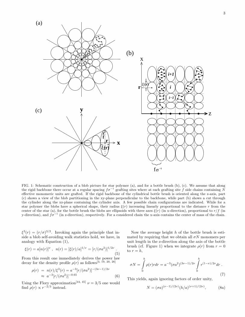
The free end of the chain is in the last blob and hence theend-to-end distance Re ≈ h in this “Alexander picture”of polymer brushes.[1, 41, 42, 43] However, a more detailedtheory of polymer brushes, such as the self-consistentfield theory in the strong stretching limit,[67, 68, 69] yieldsa somewhat different behavior: the end monomer is notlocalized at the outer edge of the brush, but rather can belocated anywhere in the brush, according to a broad dis-tribution; also the monomer density in polymer brushesat flat substrates is not constant up to the brush heighth, but rather decreases according to a parabolic profile.So even for a polymer brush at a flat substrate alreadya description in terms of non-uniform blob sizes, thatincrease with increasing distance z from the substrate,is required.[70] However, in the following we shall disre-gard all these caveats about the Alexander picture forflat brushes, and consider its generalization to the bottlebrush geometry, where polymer chains are tethered to aline rather than a flat surface. Then we have to partitionspace into blobs of nonuniform size and shape in order torespect the cylindrical geometry (Figure 1).In the discussion of brushes in cylindrical geometry in

terms of blobs in the literature[19, 20, 26] the non-sphericalcharacter of the blob shape is not explicitly accounted for,and it rather is argued that one can characterize the blobsby one effective radius ξ(r) depending on the radial dis-tance r from the cylinder axis. One considers a segmentof the array of length L containing p polymer chains.[19]

On a surface of a cylinder of radius r and length L thereshould then be p blobs, each of cross-sectional area ξ2(r);geometrical factors of order unity are ignored throughout.Since the surface area of the cylindrical segment is Lr,we must have[19, 20, 26]

pξ2(r) = Lr , ξ(r) = (Lr/p)1/2 = (r/σ)1/2 . (4)

If the actual non-spherical shape of the blobs (Figure 1)is neglected, the blob volume clearly is of the order of

3

rf

ξ(r)xr

y

(a)

(c)

ξ (r)

z

x

i

i+1

i−1

fσ −1

r

(b)

FIG. 1: Schematic construction of a blob picture for star polymer (a), and for a bottle brush (b), (c). We assume that alongthe rigid backbone there occur at a regular spacing fσ−1 grafting sites where at each grafting site f side chains containing Neffective monomeric units are grafted. If the rigid backbone of the cylindrical bottle brush is oriented along the z-axis, part(c) shows a view of the blob partitioning in the xy-plane perpendicular to the backbone, while part (b) shows a cut throughthe cylinder along the xz-plane containing the cylinder axis. A few possible chain configurations are indicated. While for astar polymer the blobs have a spherical shape, their radius ξ(r) increasing linearly proportional to the distance r from thecenter of the star (a), for the bottle brush the blobs are ellipsoids with three axes ξ(r) (in x-direction), proportional to r/f (iny-direction), and fσ−1 (in z-direction), respectively. For a considered chain the x-axis contains the center of mass of the chain.

ξ3(r) = (r/σ)3/2. Invoking again the principle that in-side a blob self-avoiding walk statistics hold, we have, inanalogy with Equation (1),

ξ(r) = a[n(r)]ν , n(r) = [ξ(r)/a]1/ν = [r/(σa2)]1/2ν .(5)

From this result one immediately derives the power lawdecay for the density profile ρ(r) as follows[3, 19, 20, 26]

ρ(r) = n(r)/ξ3(r) = a−3[r/(σa2)]−(3ν−1)/2ν

≈ a−3[r/(σa2)]−0.65 (6)

Using the Flory approximation[44, 45] ν = 3/5 one wouldfind ρ(r) ∝ r−2/3 instead.

Now the average height h of the bottle brush is esti-mated by requiring that we obtain all σN monomers perunit length in the z-direction along the axis of the bottlebrush (cf. Figure 1) when we integrate ρ(r) from r = 0to r = h,

σN =

h∫

0

ρ(r)rdr = a−3(σa2)(3ν−1)/2ν

h∫

0

r(1−ν)/2νdr .

(7)This yields, again ignoring factors of order unity,

N = (σa)(ν−1)/(2ν)(h/a)(ν+1)/(2ν), (8a)

4

h/a = (σa)(1−ν)/(1+ν)N2ν/(1+ν) = (σa)0.259N0.74 .(8b)

Note that the use of the Flory estimate ν = 3/5 wouldsimply yield h ∝ σ1/4N3/4, which happens to be identicalto the relation that one obtains when one partitions thecylinder of height L and radius h into disks of height σ−1,requiring hence that each chain is confined strictly intoone such disk. Then each chain would form a quasi-two-dimensional self-avoiding walk formed from n′

blob = N/n′

blobs of diameter σ−1. Since we have σ−1 = an′ν again,we would conclude that the end-to-end distance R of sucha quasi-two-dimensional chain is

R = σ−1(n′

blob)3/4 = σ−1n′−3/4N3/4

= a(σa)−1+3/4νN3/4 = a(σa)1/4N3/4 . (9)

Putting then R = h, Equation (8b) results when we usethere ν = 3/5. However, this similarity between Equa-tions (8b), (9) is a coincidence: in fact, the assump-tion of a quasi-two-dimensional conformation does notimply a stretching of the chain in radial direction. Infact, when we put the x-axis of our coordinate system

in the direction of the end-to-end vector ~R of the chain,we would predict that the y-component of the gyrationradius scales as

Rgy = a(σa)1/4N3/4 , (10)

since for quasi-two-dimensional chains we have Rgx ∝Rgy ∝ R, all these linear dimensions scale with the samepower laws. On the other hand, if the Daoud-Cotton-like[8] picture {Figure 1a} holds, in a strict sense, onewould conclude that Rgy is of the same order as the sizeof the last blob for r = h,

Rgy = ξ(r = h) = (h/σ)1/2

= a(σa)−ν/(1+ν)Nν/(1+ν) (11)

Clearly this prediction is very different from Equa-tion (10), even with the Flory exponent ν = 3/5 we findfrom Equation (11) that Rgy ∝ σ−3/8N3/8. Hence it isclear that an analysis of all three components of the gy-ration radius of a polymer chain in a bottle brush is verysuitable to distinguish between the different versions ofscaling concepts discussed in the literature.However, at this point we return to the geometrical

construction of the filling of a cylinder with blobs, Fig-ure 1. We explore the consequences of the obvious factthat the blobs cannot be simple spheres, when we re-quire that each blob contains monomers from a singlechain only, and the available volume is densely packedwith blobs touching each other.As mentioned above, ξ(r) was defined from the avail-

able surface area of a cylinder at radius r, cf. Equa-tion (4). It was argued that for each chain in the surfacearea Lr of such a cylinder a surface area ξ2(r) is available.However, consideration of Figure 1 shows that these sur-faces are not circles but rather ellipses, with axes fσ−1

and r/f . The blobs hence are not spheres but rather

ellipsoids, with three different axes: fσ−1 in z-directionalong the cylinder axes, r/f in the y-direction tangentialon the cylinder surface, normal to both the z-directionand the radial direction, and the geometric mean of thesetwo lengths (rσ−1)1/2, in the radial x-direction. Since thephysical meaning of a blob is that of a volume region inwhich the excluded volume interaction is not screened,this result implies that the screening of excluded volumein a bottle brush happens in a very anisotropic way: thereare three different screening lengths, fσ−1 in the axial z-direction, (rσ−1)1/2 in the radial x-direction, and r/f inthe third, tangential, y-direction. Of course, it remainsto be shown by a more microscopic theory that such ananisotropic screening actually occurs.However, the volume of the ellipsoid with these three

axes still is given by the formula

Vellipsoid = (σ−1f)(r/f)(rσ−1)1/2 = (rσ−1)3/2 = [ξ(r)]3

(12)with ξ(r) given by Equation (4), and hence the volumeof the blob has been correctly estimated by the sphericalapproximation. As a consequence, the estimations of thedensity profile ρ(r), Equation (6), and resulting brushheight h, Equation (8b), remain unchanged.More care is required when we now estimate the linear

dimensions of the chain in the bottle brush. We now ori-ent the x-axis such that the xz-plane contains the centerof mass of the considered chain. As Figure 1b indicates,we can estimate Rgz assuming a random walk picture interms of blobs. When we go along the chain from thegrafting site towards the outer boundary of the bottlebrush, the blobs can make excursions with ∆z = ±fσ−1,independent of r. Hence we conclude, assuming that theexcursions of the nblob steps add up randomly

R2gz =

nblob∑i=1

(fσ−1)2 = nblob(fσ−1)2 ,

Rgz = fσ−1√nblob . (13)

Hence we must estimate the number of blobs nblob perchain in a bottle brush. We must have

nblob =

nblob∑i=1

1 =

h∫

0

[ξ(r)]−1dr (14)

Note from Figure 1 that we add an increment 2ξ(ri) tor when we go from the shell i to shell i+ 1 in the cylin-drical bottle brush. So the discretization of the integralin Equation (14) is equivalent to the sum. From Equa-tion (14) we then find, again ignoring factors of orderunity

nblob = σ1/2h1/2 = (σa)1/(1+ν)Nν/(1+ν) , (15)

and consequently

Rgz = fa(σa)−2ν+1

2ν+2Nν/[2(1+ν)] ∝ σ−0.685N0.185 (16)

5

With Flory exponents we hence conclude nblob ∝σ5/8N3/8, and thus Rgz ∝ fσ−11/16N3/16. The estima-tion of Rgy is most delicate, of course, because when weconsider random excursions away from the radial direc-tions, the excursions ∆y = ±ξ(r) are non-uniform. Sowe have instead of Equation (13),

R2gy =

nblob∑i=1

ξ2(ri) =

h∫

0

ξ(r)dr, (17)

in analogy with Equation (14). This yields R2gy =

σ−1/2h3/2 and hence

Rgy = σ−1/4h3/4 = a(σa)−(2ν−1)/(2ν+2)N3ν/(2ν+2)

∝ σ−0.055N0.555 (18)

while the corresponding result with Flory exponentsis Rgy ∝ σ−1/16N9/16. These different results forRgx ∝ h {Equation (8b)}, Rgy {Equation (18)} andRgz {Equation (16)} clearly reflect the anisotropic struc-ture of a chain in a bottle brush. Note that the resultfor Rgy according to Equation (18) is much larger thanthe simple Daoud-Cotton-like prediction, Equation (11),but is clearly smaller than the result of the quasi-two-dimensional picture, Equation (10).As a consistency check of our treatment, we note that

also Equation (7) can be formulated as a discrete sumover blobs

N =

nblob∑i=1

n(r) =

h∫

0

[n(r)/ξ(r)]dr =

h∫

0

[r/(σa)]1/2ν−1/2dr ,

(19)which yields Equation (8a), as it should be.Finally we discuss the crossover towards mushroom be-

havior. Physically, this must occur when the distancebetween grafting points along the axis, fσ−1, becomesequal to aNν . Thus we can write

h = aNνh(σaNν), (20)

where we have absorbed the extra factor f in the scalingfunction h(ζ). We note that Equation (8b) results fromEquation (20) when we request that

h(ζ ≫ 1) ∝ ζ(1−ν)/(1+ν), (21)

and hence a smooth crossover between mushroom be-havior and radially stretched polymer conformations oc-curs for σaNν of order unity, as it should be. Analogouscrossover relations can be written for the other linear di-mensions, too:

Rgz = aNνRgz(ζ), Rgz(ζ ≫ 1) ∝ ζ−(2ν+1)/(2ν+2),(22)

Rgy = aNνRgy(ζ), Rgy(ζ ≫ 1) ∝ ζ−(2ν−1)/(2ν+2),(23)

The agreement between Equation (16) and Equation (22)or Equation (18) and Equation (23), respectively, pro-vides a check on the self-consistency of our scaling argu-ments.

However, it is important to bear in mind thatthe blob picture of polymer brushes, as developed byAlexander,[41] Daoud and Cotton,[8] Halperin[1, 43] andmany others, is a severe simplification of reality, sinceits basic assumptions that (i) all chains in a polymerbrush are stretched in the same way, and (ii) the chainends are all at a distance h from the grafting sites,are not true. Treatments based on the self-consistentfield theory[67, 68, 69, 71, 72, 73, 74, 75, 76] and computersimulations[3, 22, 66, 70, 77, 78, 79, 80, 81, 82, 83] have shownthat chain ends are not confined at the outer bound-ary of the brush, and the monomer density distributionis a nontrivial function, that cannot be described by theblob model. However, it is widely believed that the blobmodel yields correctly the power laws of chain linear di-mensions in terms of grafting density and chain length, sothe shortcomings mentioned above affect the pre-factorsin these power laws only. In this spirit, we have extendedthe blob model for brushes in cylindrical geometry in thepresent section, taking the anisotropy in the shape ofthe blobs into account to predict the scaling behaviorof both the brush height h (which corresponds to thechain end-to-end distance R and the x-component Rgxof the gyration radius) and of the transverse gyration ra-dius components Rgy , Rgz. To our knowledge, the latterhave not been considered in the previous literature.

III. Monte Carlo Methodology

We consider here the simplest lattice model of poly-mers under good solvent conditions, namely, the self-avoiding walk on the simple cubic lattice. The backboneof the bottle brush is just taken to be the z-axis of thelattice, and in order to avoid any effects due to the endsof the backbone, we choose periodic boundary conditionsin the z-direction. The length of the backbone is taken tobe Lb lattice spacings, and the lattice spacing henceforthis taken as one unit of length. Note that in order to avoidfinite size effects Lb has to be chosen large enough so thatno side chain can interact with its own “images” createdby the periodic boundary condition, i.e. Rgz ≪ Lb.

We create configurations of the bottle brush poly-mers applying the pruned-enriched-Rosenbluth method(PERM).[46, 47, 48, 49, 87, 88, 89, 90] This algorithm isbased on the biased chain growth algorithm of Rosen-bluth and Rosenbluth,[91] and extends it by re-samplingtechnique (“population control”[46]) with depth-firstimplementation. Similar to a recent study of starpolymers[47, 48] all side chains of the bottle brush aregrown simultaneously, adding one monomer to each sidechain one after the other before the growth process ofthe first chain continues by the next step.

6

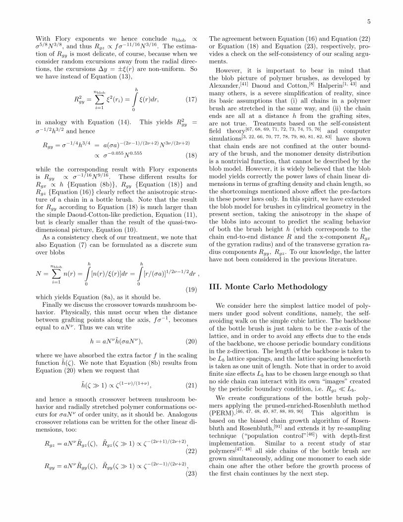
FIG. 2: Snapshot picture of a bottle brush polymer withLb = 128 σ = 1/4, and N = 2000 on the simple cubic lattice.Note that different chains are displayed in different colors todistinguish them, and the periodic boundary condition is un-done for the sake of a better visibility in the visualization ofthis configuration.

When a monomer is added to a chain of length n− 1(containing n monomers) at the nth step, one scans theneighborhood of the chain end to identify the free neigh-boring sites of the chain end, to which a monomer couldbe added. Out of these nfree sites available for the addi-tion of a monomer one site is chosen with the probabilitypn,i for the ith direction. One has the freedom to sam-ple these steps from a wide range of possible distribu-tions, e.g. pn,i = 1/nfree, if one site is chosen at random,and this additional bias is taken into account by suitableweight factors. The total weight Wn of a chain of lengthn with an unbiased sampling is determined recursivelyby Wn = Πnk=1wk = Wn−1wn. While the weight wn isgained at the nth step with a probability pn,i, one has touse wn/pn,i instead of wn. The partition sum of a chainof length n (at the nth step) is approximated as

Zn ≈ Zn ≡M−1n

Mn∑α=1

Wn(α), (24)

where Mn is the total number of configurations {α}, andaverages of any chain property (e.g. its end-to-end dis-tance, gyration radius components, etc.) A(α) are ob-tained as

An =1

Mn

Mn∑α=1

A(α)Wn(α)

Zn(25)

As is well-known from Ref. [84], for this original biasedsampling[91] the statistical errors for large n are veryhard to control. This problem is alleviated by popula-tion control.[87] One introduces two thresholds

W+n = C+Zn, W−

n = C−Zn , (26)

where Zn is the current estimate of the partition sum,and C+ and C− are constants of order unity. The opti-mal ratio between C+ and C− is found to be C+/C− ∼ 10in general. If Wn exceeds W+

n for the configuration α,one produces k identical copies of this configuration, re-places their weight Wn by Wn/k, and uses these copiesas members of the population for the next step, whereone adds a monomer to go from chain length n to n+ 1.However, if Wn < W−

n , one draws a random number η,uniformly distributed between zero and one. If η < 1/2,the configuration is eliminated from the population whenone grows the chains from length n to n+1. This “prun-ing” or “enriching” step has given the PERM algorithmits name. On the other hand, if η ≥ 1/2, one keeps theconfiguration and replaces its weight Wn by 2Wn. In adepth-first implementation, at each time one deals withonly a single configuration until a chain has been growneither to the end of reaching the maximum length or tobe killed in between, and handles the copies by recursion.Since only a single configuration has to be rememberedduring the run, it requires much less memory.

In our implementation, we usedW+n = ∞ andW−

n = 0for the first configuration hitting chain length n. For thefollowing configurations, we usedW+

n = CZn(cn/c0) andW−n = 0.15W+

n , here C = 3.0 is a positive constant, andcn is the total number of configurations of length n al-ready created during the run. The bias of growing sidechains was used by giving higher probabilities in the di-rection where there are more free next neighbor sites andin the outward directions perpendicular to the backbone,where the second part of bias decreases with the lengthof side chains and increases with the grafting density. To-tally 105 ∼ 106 independent configurations were obtainedin most cases we simulated.

Typical simulations used backbone lengths Lb =32, 64, and 128, f = 1 (one chain per grafting site of thebackbone, although occasionally also f = 2 and f = 4were used), and grafting densities σ = 1/32, 1/16, 1/8,1/4, 1/2 and 1. The side chain length N was varied up toN = 2000. So a typical bottle brush with Lb = 128, σ =1/4 (i.e., nc = 32 side chains) and N = 2000 containsa total number of monomers Ntot = Lb + ncN = 64128.Figure 2 shows a snapshot configuration of such a bottlebrush polymer. Note that most other simulation algo-rithms for polymers[65, 84, 85, 86] would fail to produce alarge sample of well-equilibrated configurations of bottlebrush polymers of this size: dynamic Monte Carlo al-gorithms using local moves involve a relaxation time (inunits of Monte Carlo steps per monomer [MCS]) of or-der Nz where z = 2ν + 1 if one assumes that the sidechains relax independently of each other and one ap-plies the Rouse model[92] in the good solvent regime.[85]

For N = 2000 such an estimate would imply that thetime between subsequent statistically independent con-figurations is of the order of 107 MCS, which clearly isimpractical. While the pivot algorithm[65] would pro-vide a significantly faster relaxation in the mushroomregime, the acceptance rate of the pivot moves quickly

7

deteriorates when the monomer density increases. Thisalgorithm could equilibrate the outer region of the bottlebrush rather efficiently, but would fail to equilibrate thechain configurations near the backbone. The configura-tional bias algorithm[86, 93] would be an interesting alter-native when the monomer density is high, but it is notexpected to work for very long chains, such as N = 2000.Also, while the simple enrichment technique is useful tostudy both star polymers[94] and polymer brushes on flatsubstrates[95] it also works only for chain lengths up toabout N = 100. Thus, existing Monte Carlo simulationsof one-component bottle brushes under good solvent con-ditions either used the bond fluctuation model[85, 96] onthe simple cubic lattice applying local moves with sidechain lengths up to N = 41[30] or N = 64[36] or the pivotalgorithm[65] with side chain lengths up to N = 80,[34]

but considering flexible backbone of length L = 800. Analternative approach was followed by Yethiraj[31] whostudied an off-lattice tangent hard sphere model by apivot algorithm in the continuum, for N ≤ 50. All thesestudies addressed the question of the overall conforma-tion of the bottle brush for a flexible backbone, and didnot address in detail the conformations of the side chains.Only the total mean square radius of gyration of theside chains was estimated occasionally, obtaining[30, 36]

R2g ∝ N1.2 or[31] R2

g ∝ N1.36 and[34] R2g ∝ N1.4. How-

ever, due to the smallness of the side chain lengths usedin these studies, as quoted above, these results have tobe considered as somewhat preliminary, and also a sys-tematic study of the dependence on both N and σ wasnot presented. We also note that the conclusions of thequoted papers are somewhat contradictory.An interesting alternative simulation method to the

Monte Carlo study of polymeric systems is MolecularDynamics,[85] of course. While in corresponding stud-ies of a bead-spring model of polymer chains for flatbrushes[81] chain lengths N up to N = 200 were used,for chains grafted to thin cylinders[22] the three chainlengths N = 50, 100 and 150 were used. For N = 50,also four values of grafting density were studied.[22] Mu-rat and Grest[22] used these data to test the scaling pre-diction for the density profile, Equation (6), but foundthat ρ(r) is better compatible with ρ(r) ∝ r−0.5 ratherthan ρ(r) ∝ r−0.65. However, forN = 50 the range wherethe power law is supposed to apply is very restricted, andhence this discrepancy was not considered to be a prob-lem for the theory.[22]

Thus, we conclude that only due to the use of thePERM algorithm has it become possible to study suchlarge bottle brush polymers as depicted in Figure 2. Nev-ertheless, as we shall see in the next section, even for suchlarge side chain lengths one cannot yet reach the asymp-totic region where the power laws derived in the previoussection are strictly valid.

IV. Monte Carlo Results for One-Component Bottle-Brush Polymers

(a)

2

1.5

1

0.6 1 10 100 1000 10000

<R

x2 > /

N 2ν

N

σ = 1/4σ = 1/8σ = 1/16σ = 1/32σ = 1/64σ = 1/128

(b)

0.1

0.095

0.09

0.085

0.08 1 10 100 1000 10000

<R

y2 > /

N2ν

N

σ = 1/4σ = 1/8σ = 1/16σ = 1/32σ = 1/64σ = 1/128

(c)

0.6

0.5

0.4

0.3

1 10 100 1000 10000

<R

z2 > /

N2ν

N

σ = 1/128σ = 1/64σ = 1/32σ = 1/16σ = 1/8σ = 1/4

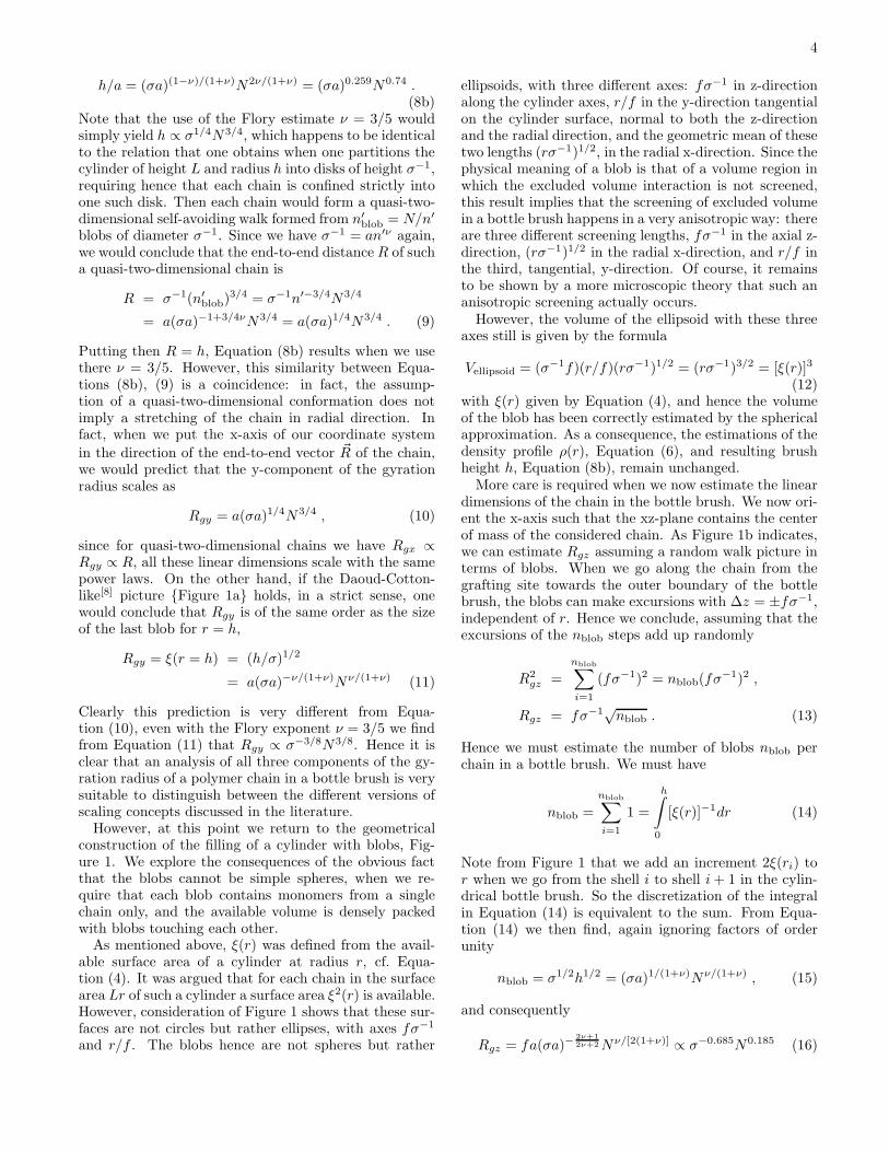
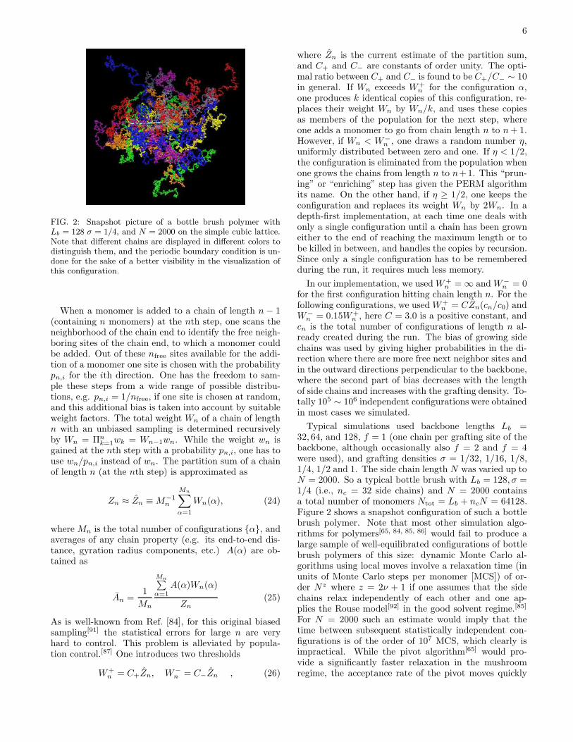
FIG. 3: Log-log plot of the mean square end-to-end distancecomponents 〈R2

x〉 (a), 〈R2

y〉 (b), and 〈R2

z〉 (c) versus side chainlength N , for various choices of the grafting density σ as indi-cated. All data refer to f = 1 (one chain per possible graftingsite) and N > 5. Note that the x-direction for every chain isthe normal direction from its center of mass position to thebottle brush backbone. All data are for Lb = 128. The chainmean square linear dimensions are all normalized by N2ν .

In Figures 3 and 4, we present our data for the meansquare end-to-end radii and gyration radii components ofthe side chains. Note that for each chain configuration aseparate local coordinate system for the analysis of thechain configuration needs to be used; while the z-axis isalways oriented simply along the backbone, the x-axisis oriented perpendicular to the z-axis and goes throughthe center of mass of the chain in this particular config-uration. The y-axis then also is fixed simply from therequirement that it is perpendicular to both the x- andz-axes.

For a polymer mushroom (which is obtained if the

8

(a)

0.3

0.2

0.1

0.05 10 100 1000 10000

<R

2 gx >

/ N

2ν

N

σ = 1/4σ = 1/8σ = 1/16σ = 1/32σ = 1/64σ = 1/128

(b)

0.04

0.038

0.036 10 100 1000 10000

<R

2 gy >

/ N

2ν

N

σ = 1/4σ = 1/8σ = 1/16σ = 1/32σ = 1/64σ = 1/128

(c) 0.13

0.1

0.07

0.04 10 100 1000 10000

<R

2 gz >

/ N

2ν

N

σ = 1/128σ = 1/64σ = 1/32σ = 1/16σ = 1/8σ = 1/4

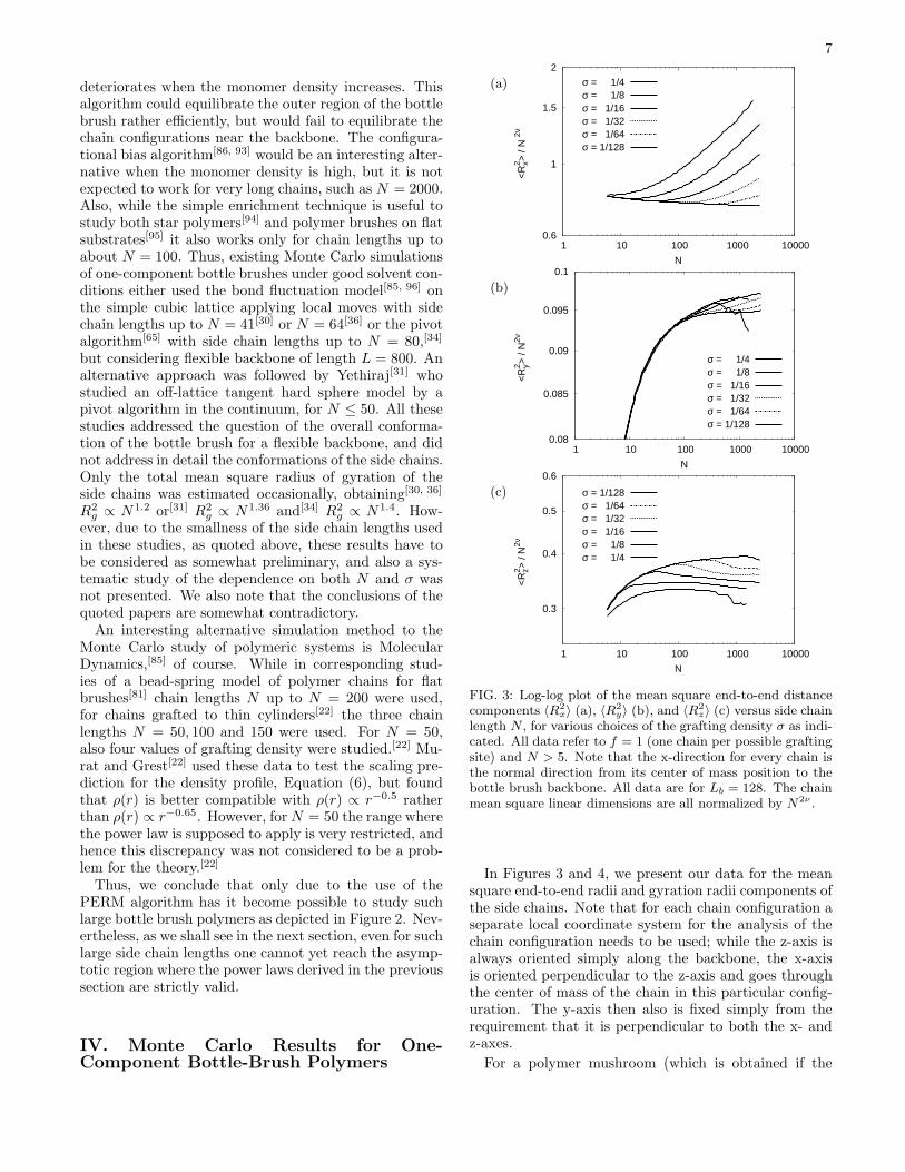
FIG. 4: Log-log plot of the mean square gyration radius com-ponents 〈R2

gx〉 (a), 〈R2

gy〉 (b), and 〈R2

gz〉 (c), versus side chainlength N . Only data for N > 10 are included. All dataare for f = 1, Lb = 128, and various choices of σ. All chainmean square linear dimensions are normalized by N2ν withν = ν3 ≈ 0.588.

grafting density σ is sufficiently small) we expect that allchain linear dimensions scale as Nν , for sufficiently longchains. Therefore we have normalized all mean squarelinear dimensions in Figures 3 and 4 by a factor N2ν ,using the theoretical value[64, 65] ν = 0.588. However, aswe see from Figures 3, 4 in the range 10 ≤ N ≤ 103 dis-played there, even for the smallest σ presented, wherea single side chain is simulated, the shown ratios arenot constant. This fact indicates that corrections toscaling[64, 65] should not be disregarded, and this prob-lem clearly complicates the test of the scaling predic-tions derived above. For the largest value of σ included(σ = 1/4), the irregular behavior of some of the data(Figure 3b,c, Figure 4b) indicate a deterioration of sta-

(a) 2.2

1.8

1.2

0.8 0.01 0.1 1 10 100

(R2 x+

R2 y)

/ N

2ν

ζ

Lb = 32

Lb = 64

Lb = 128

(b) 2

1.4

1

0.8 0.01 0.1 1 10 100

(R2 x+

R2 y)

/ N

2ν

ζ

slope = 0.519

Lb = 32

Lb = 64

Lb = 128

FIG. 5: Log-log plot of R2

⊥ = R2

x + R2

y divided by N2ν

vs. ζ = σNν , including all data for N > 5, and three choices ofLb as indicated (a), or alternatively removing data affected bythe finite size of the backbone length via the periodic bound-ary condition (b). The slope indicated in (b) by the dottedstraight line corresponds to the scaling estimate from Equa-tion (21), 2(1− ν)/(1 + ν) ≈ 0.519.

tistical accuracy. This problem gets worse for increasingnumber of side chains nc.

A further complication is due to the residual finite sizeeffect. Figure 5 shows a plot of R2

⊥= R2

x + R2y vs. the

scaling variable ζ = σNν . One can recognize that forsmall Lb but large N and not too large σ systematicdeviations from scaling occur (Figure 5a), which simplyarise from the fact that an additional scaling variable(related to 〈R2

z〉1/2/Lb) comes into play when 〈R2z〉1/2 no

longer is negligibly smaller than Lb. While for real bot-tle brush polymers with stiff backbone effects due to thefinite lengths of the backbone are physically meaningfuland hence of interest, the situation is different in oursimulation due to the use of periodic boundary condi-tions. The choice of periodic boundary conditions is mo-tivated by the desire to study the characteristic structurein a bottle brush polymer far away from the backboneends, not affected by any finite size effects. However, if〈R2

gz〉1/2 becomes comparable to Lb, each chain interactswith its own periodic images, and this is an unphysical,undesirable, finite size effect. Therefore in Figure 5b, thedata affected by such finite size effects are not included.One finds a reasonable data collapse of the scaled meansquare end-to-end distance when one plots the data ver-sus the scaling variable ζ = σNν . These results consti-

9

(a)

0.5

0.1

0.05 0.01 0.1 1 10 100

<R

gx2 > /

N2ν

ζ = σNν

slope = 0.519

σ = 1/128σ = 1/64σ = 1/32σ = 1/16σ = 1/8σ = 1/4

(b)

0.5

0.1

0.02 0.01 0.1 1 10 100

<R

gy2 > /

N2ν

ζ = σNν

slope = -0.111

σ = 1/128σ = 1/64σ = 1/32σ = 1/16σ = 1/8σ = 1/4

(c)

0.5

0.1

0.02 0.01 0.1 1 10 100

<R

gz2 > /

N2ν

ζ = σNν

slope = -1.370

σ = 1/128σ = 1/64σ = 1/32σ = 1/16σ = 1/8σ = 1/4

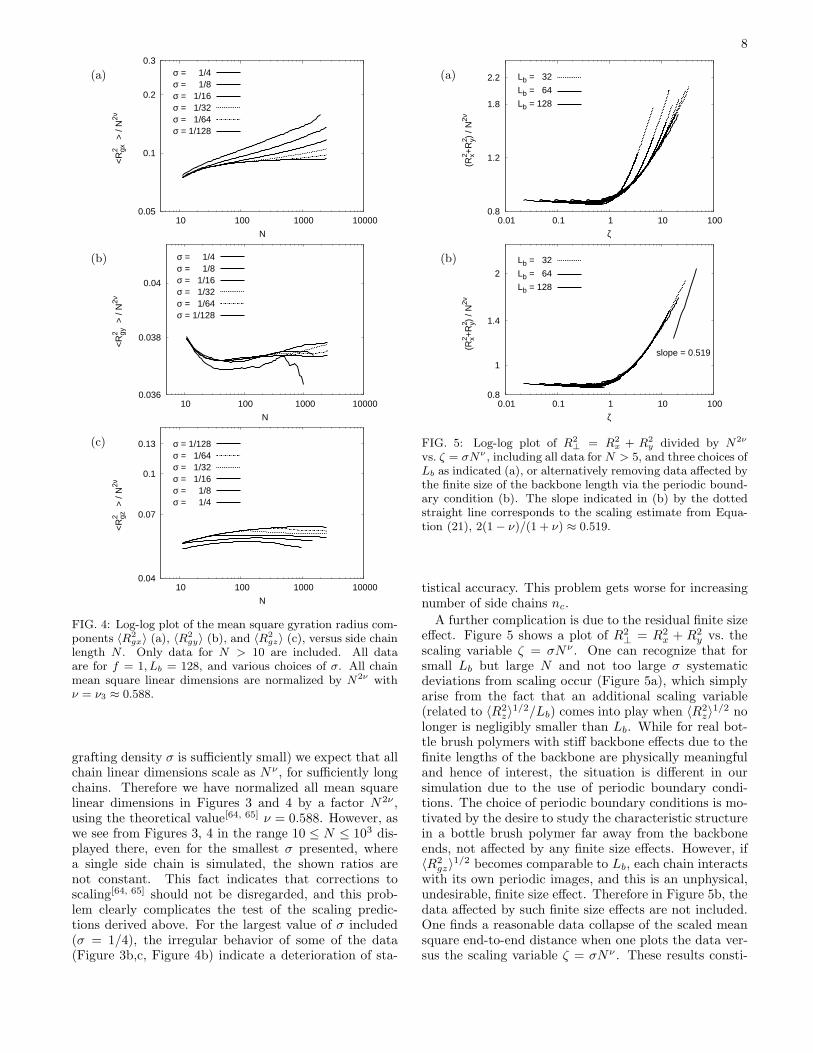
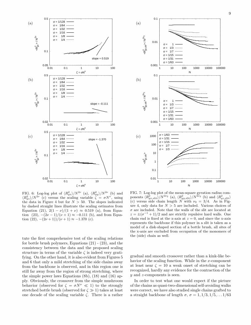
FIG. 6: Log-log plot of 〈R2

gx〉/N2ν (a), 〈R2

gy〉/N2ν (b) and〈R2

gz〉/N2ν (c) versus the scaling variable ζ = σNν , usingthe data in Figure 4 but for N > 50. The slopes indicatedby dashed straight lines illustrate the scaling estimates fromEquation (21), 2(1 − ν)/(1 + ν) ≈ 0.519 (a), from Equa-tion (23), −(2ν − 1)/(ν + 1) ≈ −0.111 (b), and from Equa-tion (22), −(2ν + 1))/(ν + 1) ≈ −1.370 (c).

tute the first comprehensive test of the scaling relationsfor bottle brush polymers, Equations (21) - (23), and theconsistency between the data and the proposed scalingstructure in terms of the variable ζ is indeed very grati-fying. On the other hand, it is also evident from Figures 5and 6 that only a mild stretching of the side chains awayfrom the backbone is observed, and in this region one isstill far away from the region of strong stretching, wherethe simple power laws Equations (8b), (18) and (16) ap-ply. Obviously, the crossover from the simple mushroombehavior (observed for ζ = σNν ≪ 1) to the stronglystretched bottle brush (observed for ζ ≫ 1) takes at leastone decade of the scaling variable ζ. There is a rather

(a)

0.001

0.01

0.1

1 10 100 1000 10000 100000

<R

gx,s

lit2

>

/ N

2ν2

N

σ = 1σ = 1/3σ = 1/7σ = 1/15σ = 1/31σ = 1/63

(b)

0.001

0.01

0.1

1 10 100 1000 10000 100000

<R

gy,s

lit2

>

/ N

2ν2

N

σ = 1σ = 1/3σ = 1/7σ = 1/15σ = 1/31σ = 1/63

(c)

0.01

0.1

1

10

100

1000

1 10 100 1000 10000 100000

<R

gz,s

lit2

>

N

σ = 1/63σ = 1/31σ = 1/15σ = 1/7σ = 1/3

FIG. 7: Log-log plot of the mean-square gyration radius com-ponents 〈R2

gx,slit〉/N2ν2 (a), 〈R2

gy,slit〉/N2ν2 (b) and 〈R2

gz,slit〉(c) versus side chain length N with ν2 = 3/4. As in Fig-ure 4, only data for N > 5 are included. Various choices ofσ are included. Note that the walls of the slit are located atz = ±(σ−1 + 1)/2 and are strictly repulsive hard walls. Onechain end is fixed at the x-axis at z = 0, and since the x-axisrepresents the backbone if this polymer in a slit is taken as amodel of a disk-shaped section of a bottle brush, all sites ofthe x-axis are excluded from occupation of the monomers ofthe (side) chain as well.

gradual and smooth crossover rather than a kink-like be-havior of the scaling function. While in the x-componentat least near ζ = 10 a weak onset of stretching can berecognized, hardly any evidence for the contraction of they and z-components is seen.

In order to test what one would expect if the pictureof the chains as quasi-two-dimensional self-avoiding walkswere correct, we have also studied single chains grafted toa straight backbone of length σ, σ = 1, 1/3, 1/5, . . .1/63

10

(a)

0.01

0.1

1

0.01 0.1 1 10 100

<R

gx,s

lit2 >

/N2

ν

σNν

slope=3/2ν-2

σ = 1σ = 1/3σ = 1/7

σ = 1/15σ = 1/31σ = 1/63

(b)

0.01

0.1

1

0.01 0.1 1 10 100

<R

gy,s

lit2 >

/N2

ν

σNν

slope=3/2ν-2

σ = 1σ = 1/3σ = 1/7

σ = 1/15σ = 1/31σ = 1/63

(c)

1e-05

1e-04

0.001

0.01

0.1

1

0.01 0.1 1 10 100

<R

gz,s

lit2 >

/N2

ν

Nν / (σ-1+1)

slope = -2σ = 1/3σ = 1/7

σ = 1/15σ = 1/31σ = 1/63

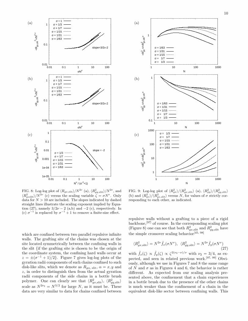
FIG. 8: Log-log plot of 〈Rgx,slit〉/N2ν (a), 〈R2

gy,slit〉/N2ν , and

〈R2

gzslit〉/N2ν (c) versus the scaling variable ζ = σNν . Onlydata for N > 10 are included. The slopes indicated by dashedstraight lines illustrate the scaling exponent implied by Equa-tion (27), namely 3/2ν − 2 (a,b) and −2 (c), respectively. In(c) σ−1 is replaced by σ−1 + 1 to remove a finite-size effect.

which are confined between two parallel repulsive infinitewalls. The grafting site of the chains was chosen at thesite located symmetrically between the confining walls inthe slit {if the grafting site is chosen to be the origin ofthe coordinate system, the confining hard walls occur atz = ±(σ−1 + 1)/2}. Figure 7 gives log-log plots of thegyration radii components of such chains confined to suchdisk-like slits, which we denote as Rgα, slit, α = x, y andz, in order to distinguish then from the actual gyrationradii components of the side chains in a bottle brushpolymer. One can clearly see that 〈R2

gx,slit〉, 〈R2gy,slit〉

scale as N2ν2 = N3/2 for large N , as it must be. Thesedata are very similar to data for chains confined between

(a)

1

1 10 100 1000

<R

gx2 >/<

Rgx

,slit

2

>

N

σ = 1/63σ = 1/31σ = 1/15σ = 1/7σ = 1/3

(b)

0.1

1

1 10 100 1000

<R

gy2 >/<

Rgy

,slit

2

>

N

σ = 1/63σ = 1/31σ = 1/15σ = 1/7σ = 1/3

(c)

1

10

100

1000

1 10 100 1000

<R

gz2 >/<

Rgz

,slit

2

>

N

σ = 1/3σ = 1/7σ = 1/15σ = 1/31σ = 1/63

FIG. 9: Log-log plot of 〈R2

gx〉/〈R2

gx,slit〉 (a), 〈R2

gy〉/〈R2

gy,slit〉(b) and 〈R2

gz〉/〈R2

gz,slit〉 versus N , for values of σ strictly cor-responding to each other, as indicated.

repulsive walls without a grafting to a piece of a rigidbackbone,[97] of course. In the corresponding scaling plot(Figure 8) one can see that both R2

gx,slit and R2gy,slit have

the simple crossover scaling behavior[45, 98]

〈R2gx,slit〉 = N2ν fx(σN

ν), 〈R2gy,slit〉 = N2ν fy(σN

ν)(27)

with fx(ζ) ∝ fy(ζ) ∝ ζ2(ν2−ν)/ν with ν2 = 3/4, as ex-

pected, and seen in related previous work.[97, 99] Obvi-ously, although we use in Figures 7 and 8 the same rangeof N and σ as in Figures 4 and 6, the behavior is ratherdifferent. As expected from our scaling analysis pre-sented above, the confinement that a chain experiencesin a bottle brush due to the presence of the other chainsis much weaker than the confinement of a chain in theequivalent disk-like sector between confining walls. This

11

(a)

1e-04

0.001

0.01

0.1

1

1 10 100

<ρ(

r)>

r

slope = -0.65

σ = 1/128σ = 1/64σ = 1/32σ = 1/16σ = 1/8σ = 1/4

(b)

1e-04

0.001

0.01

0.1

1

1 10 100

<ρ(

r)>

r

slope = -0.65

σ = 1/128σ = 1/64σ = 1/32σ = 1/16σ = 1/8σ = 1/4

(c)

1e-04

0.001

0.01

0.1

1

1 10 100

<ρ(

r)>

r

slope = -0.65

σ = 1/128σ = 1/64σ = 1/32σ = 1/16σ = 1/8σ = 1/4

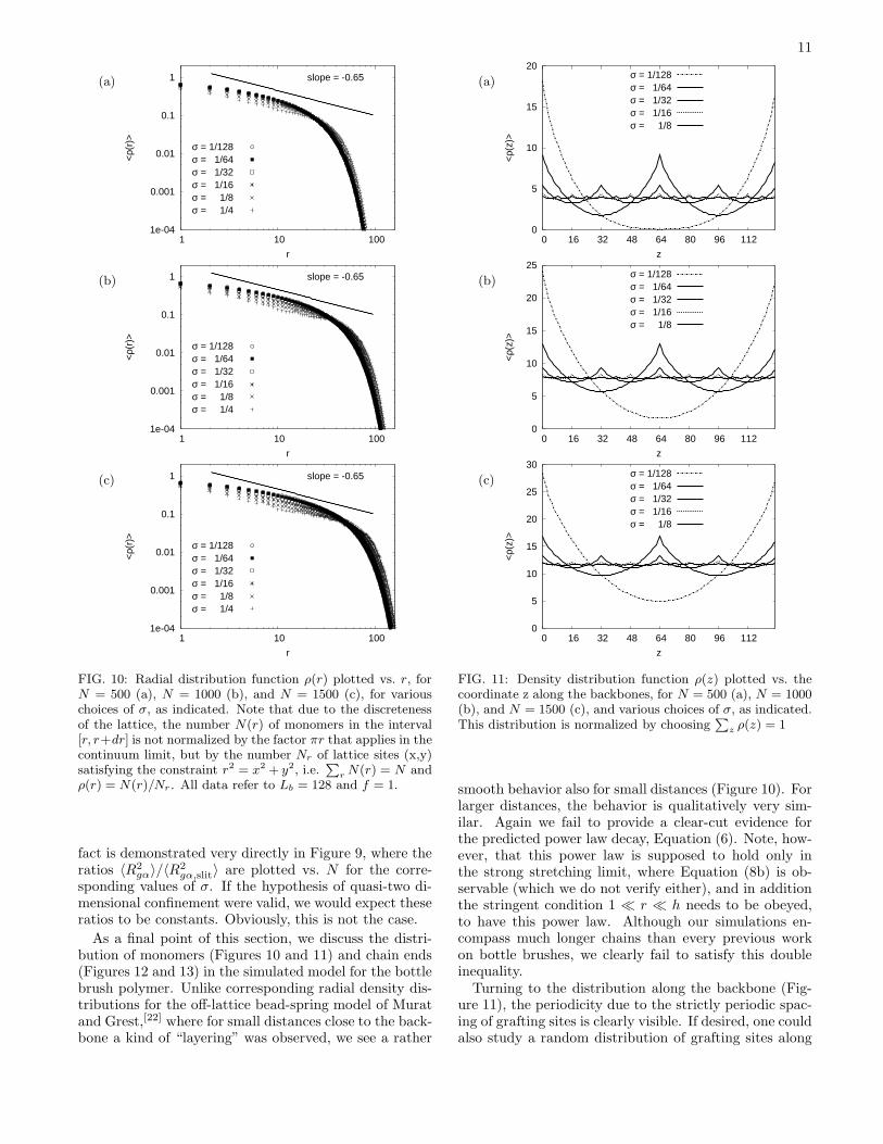
FIG. 10: Radial distribution function ρ(r) plotted vs. r, forN = 500 (a), N = 1000 (b), and N = 1500 (c), for variouschoices of σ, as indicated. Note that due to the discretenessof the lattice, the number N(r) of monomers in the interval[r, r+dr] is not normalized by the factor πr that applies in thecontinuum limit, but by the number Nr of lattice sites (x,y)satisfying the constraint r2 = x2 + y2, i.e.

P

rN(r) = N and

ρ(r) = N(r)/Nr . All data refer to Lb = 128 and f = 1.

fact is demonstrated very directly in Figure 9, where theratios 〈R2

gα〉/〈R2gα,slit〉 are plotted vs. N for the corre-

sponding values of σ. If the hypothesis of quasi-two di-mensional confinement were valid, we would expect theseratios to be constants. Obviously, this is not the case.

As a final point of this section, we discuss the distri-bution of monomers (Figures 10 and 11) and chain ends(Figures 12 and 13) in the simulated model for the bottlebrush polymer. Unlike corresponding radial density dis-tributions for the off-lattice bead-spring model of Muratand Grest,[22] where for small distances close to the back-bone a kind of “layering” was observed, we see a rather

(a)

0

5

10

15

20

0 16 32 48 64 80 96 112

<ρ(

z)>

z

σ = 1/128σ = 1/64σ = 1/32σ = 1/16σ = 1/8

(b)

0

5

10

15

20

25

0 16 32 48 64 80 96 112

<ρ(

z)>

z

σ = 1/128σ = 1/64σ = 1/32σ = 1/16σ = 1/8

(c)

0

5

10

15

20

25

30

0 16 32 48 64 80 96 112

<ρ(

z)>

z

σ = 1/128σ = 1/64σ = 1/32σ = 1/16σ = 1/8

FIG. 11: Density distribution function ρ(z) plotted vs. thecoordinate z along the backbones, for N = 500 (a), N = 1000(b), and N = 1500 (c), and various choices of σ, as indicated.This distribution is normalized by choosing

P

z ρ(z) = 1

smooth behavior also for small distances (Figure 10). Forlarger distances, the behavior is qualitatively very sim-ilar. Again we fail to provide a clear-cut evidence forthe predicted power law decay, Equation (6). Note, how-ever, that this power law is supposed to hold only inthe strong stretching limit, where Equation (8b) is ob-servable (which we do not verify either), and in additionthe stringent condition 1 ≪ r ≪ h needs to be obeyed,to have this power law. Although our simulations en-compass much longer chains than every previous workon bottle brushes, we clearly fail to satisfy this doubleinequality.Turning to the distribution along the backbone (Fig-

ure 11), the periodicity due to the strictly periodic spac-ing of grafting sites is clearly visible. If desired, one couldalso study a random distribution of grafting sites along

12

(a)

0

2

4

6

8

0 16 32 48 64 80 96 112

<ρ e

(z)>

z

σ = 1/128σ = 1/64σ = 1/32σ = 1/16σ = 1/8

(b)

4

6

8

10

12

0 16 32 48 64 80 96 112

<ρ e

(z)>

z

σ = 1/128σ = 1/64σ = 1/32σ = 1/16σ = 1/8

(c)

10

12

14

0 16 32 48 64 80 96 112

<ρ e

(z)>

z

σ = 1/128σ = 1/64σ = 1/32σ = 1/16σ = 1/8

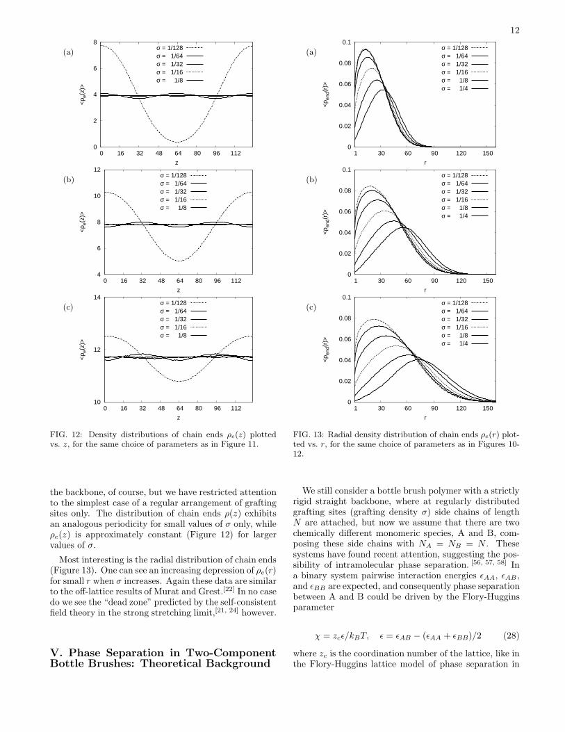
FIG. 12: Density distributions of chain ends ρe(z) plottedvs. z, for the same choice of parameters as in Figure 11.

the backbone, of course, but we have restricted attentionto the simplest case of a regular arrangement of graftingsites only. The distribution of chain ends ρ(z) exhibitsan analogous periodicity for small values of σ only, whileρe(z) is approximately constant (Figure 12) for largervalues of σ.

Most interesting is the radial distribution of chain ends(Figure 13). One can see an increasing depression of ρe(r)for small r when σ increases. Again these data are similarto the off-lattice results of Murat and Grest.[22] In no casedo we see the “dead zone” predicted by the self-consistentfield theory in the strong stretching limit,[21, 24] however.

V. Phase Separation in Two-ComponentBottle Brushes: Theoretical Background

(a)

0

0.02

0.04

0.06

0.08

0.1

150 120 90 60 30 1

<ρ e

nd(r

)>

r

σ = 1/128σ = 1/64σ = 1/32σ = 1/16σ = 1/8σ = 1/4

(b)

0

0.02

0.04

0.06

0.08

0.1

150 120 90 60 30 1

<ρ e

nd(r

)>

r

σ = 1/128σ = 1/64σ = 1/32σ = 1/16σ = 1/8σ = 1/4

(c)

0

0.02

0.04

0.06

0.08

0.1

150 120 90 60 30 1

<ρ e

nd(r

)>

r

σ = 1/128σ = 1/64σ = 1/32σ = 1/16σ = 1/8σ = 1/4

FIG. 13: Radial density distribution of chain ends ρe(r) plot-ted vs. r, for the same choice of parameters as in Figures 10-12.

We still consider a bottle brush polymer with a strictlyrigid straight backbone, where at regularly distributedgrafting sites (grafting density σ) side chains of lengthN are attached, but now we assume that there are twochemically different monomeric species, A and B, com-posing these side chains with NA = NB = N . Thesesystems have found recent attention, suggesting the pos-sibility of intramolecular phase separation. [56, 57, 58] Ina binary system pairwise interaction energies ǫAA, ǫAB,and ǫBB are expected, and consequently phase separationbetween A and B could be driven by the Flory-Hugginsparameter

χ = zcǫ/kBT, ǫ = ǫAB − (ǫAA + ǫBB)/2 (28)

where zc is the coordination number of the lattice, like inthe Flory-Huggins lattice model of phase separation in

13

���������������������������������������������������������������������������������������������������������������������������������������������������������������������������������������������������������������������������������������������������������������������������������������������������������������������������������������������������������������������������������������������������������������������������������������������������������������������������������������������������������������

���������������������������������������������������������������������������������������������������������������������������������������������������������������������������������������������������������������������������������������������������������������������������������������������������������������������������������������������������������������������������������������������������������������������������������������������������������������������������������������������������������������

B

A

B

A

zx

y

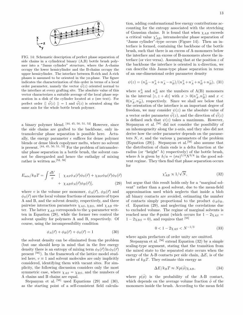
FIG. 14: Schematic description of perfect phase separation ofside chains in a cylindrical binary (A,B) bottle brush poly-mer into a “Janus cylinder” structure, where the A-chainsoccupy the lower hemicylinder and the B-chains occupy theupper hemicylinder. The interface between B-rich and A-richphases is assumed to be oriented in the yz-plane. The figureindicates the characterization of this order in terms of a localorder parameter, namely the vector ~ψ(z) oriented normal tothe interface at every grafting site. The absolute value of thisvector characterizes a suitable average of the local phase sep-aration in a disk of the cylinder located at z (see text). For

perfect order 〈| ~ψ(z) |〉 = 1 and ~ψ(z) is oriented along thesame axis for the whole bottle brush polymer.

a binary polymer blend. [44, 45, 50, 51, 52] However, sincethe side chains are grafted to the backbone, only in-tramolecular phase separation is possible here. Actu-ally, the energy parameter ǫ suffices for dense polymerblends or dense block copolymer melts, where no solventis present. [44, 45, 50, 51, 52] For the problem of intramolec-ular phase separation in a bottle brush, the solvent can-not be disregarded and hence the enthalpy of mixingrather is written as.[52, 56]

Emix/kBT =

∫dV

v[ χASφA(~r)φS(~r) + χBSφB(~r)φS(~r)

+ χABφA(~r)φB(~r)], (29)

where v is the volume per monomer, φA(~r), φB(~r) andφS(~r) are the local volume fractions of monomers of typesA and B, and the solvent density, respectively, and threepairwise interaction parameters χAS , χBS, and χAB en-ter. The latter χAB corresponds to the χ-parameter writ-ten in Equation (28), while the former two control thesolvent quality for polymers A and B, respectively. Ofcourse, using the incompressibility condition

φA(~r) + φB(~r) + φS(~r) = 1 (30)

the solvent density can be eliminated from the problem(but one should keep in mind that in the free energydensity there is an entropy of mixing term φS(~r) lnφS(~r)present [56]). In the framework of the lattice model stud-ied here, v ≡ 1 and solvent molecules are only implicitlyconsidered, identifying them with vacant sites. For sim-plicity, the following discussion considers only the mostsymmetric case, where χAS = χBS , and the numbers ofA chains and B chains are equal.Stepanyan et al. [56] used Equations (29) and (30),

as the starting point of a self-consistent field calcula-

tion, adding conformational free energy contributions ac-counting for the entropy associated with the stretchingof Gaussian chains. It is found that when χAB exceedsa critical value χ∗

AB, intramolecular phase separation of“Janus cylinder”-type occurs (Figure 14). Then an in-terface is formed, containing the backbone of the bottlebrush, such that there is an excess of A-monomers belowthe interface and an excess of B-monomers above the in-terface (or vice versa). Assuming that at the position z ofthe backbone the interface is oriented in x-direction, wecan describe this Janus-type phase separation in termsof an one-dimensional order parameter density

ψ(z) = (n+B−n+

A+n−

A−n−

B)/(n+A+n−

A+n+B+n−

B), (31)

where n±

A and n±

B are the numbers of A(B) monomers

in the interval [z, z + dz] with x > 0(n+A, n

+B) and x <

0(n−

A, n−

B), respectively. Since we shall see below thatthe orientation of the interface is an important degree offreedom, we may consider ψ(z) as the absolute value of

a vector order parameter ~ψ(z), and the direction of ~ψ(z)is defined such that ψ(z) takes a maximum. However,Stepanyan et al. [56] did not consider the possibility ofan inhomogeneity along the z-axis, and they also did notderive how the order parameter depends on the parame-ters N , σ, and the various χ parameters of the problem{Equation (29)}. Stepanyan et al.[56] also assume thatthe distribution of chain ends is a delta function at theradius (or “height” h) respectively) of the bottle brush,where h is given by h/a = (σa)1/4N3/4 in the good sol-vent regime. They then find that phase separation occursfor

χ∗

AB ∝ 1/√N, (32)

but argue that this result holds only for a “marginal sol-vent” rather than a good solvent, due to the mean-fieldapproximation used which neglects that inside a bloball binary contacts are avoided, estimating the numberof contacts simply proportional to the product φAφB ,cf. Equation (29), and neglecting the correlations dueto excluded volume. The regime of marginal solvents isreached near the θ-point (which occurs for 1 − 2χAS =1− 2χBS = 0), and requires that [56]

0 < 1− 2χAS < N−1/3 (33)

where again prefactors of order unity are omitted.Stepanyan et al. [56] extend Equation (32) by a simple

scaling-type argument, stating that the transition fromthe mixed state to the separated state occurs when theenergy of the A-B contacts per side chain, ∆E, is of theorder of kBT . They estimate this energy as

∆E/kBT ≈ Np(φ)χAB , (34)

where p(φ) is the probability of the A-B contact,which depends on the average volume fraction φ of themonomers inside the brush. According to the mean field

14

A

A

B

B

zx

y

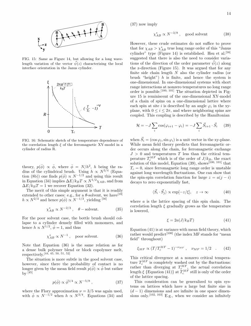
FIG. 15: Same as Figure 14, but allowing for a long wave-

length variation of the vector ~ψ(z) characterizing the localinterface orientation in the Janus cylinder.

cT

ξ

R

T

−νTTc

( −1)

Bk T2π Γ(Τ)2R

0

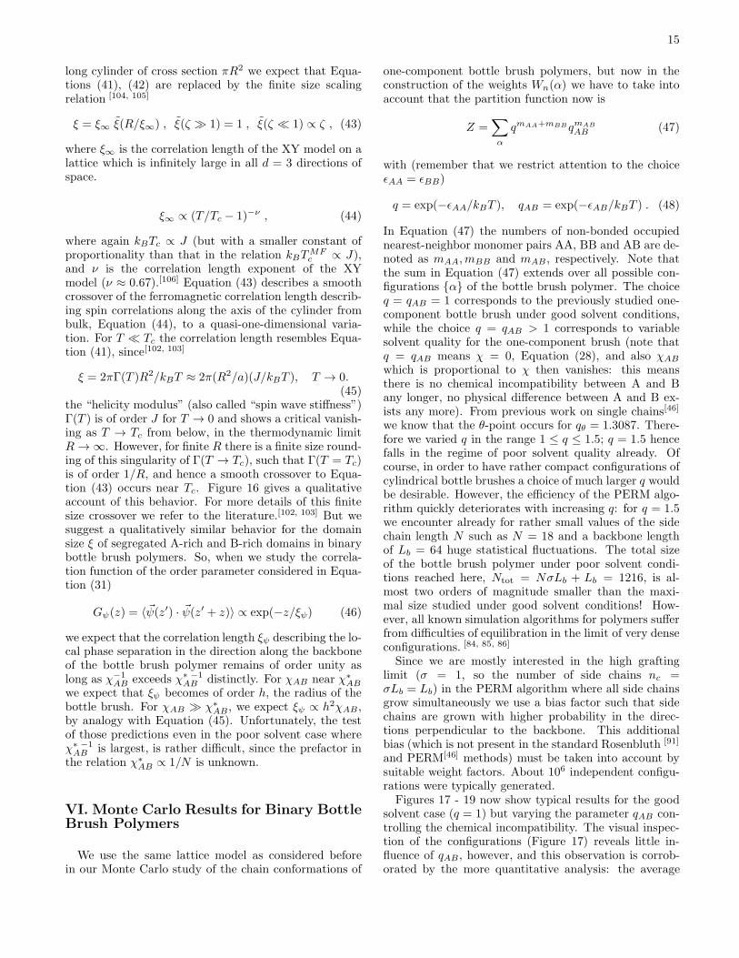
FIG. 16: Schematic sketch of the temperature dependence ofthe correlation length ξ of the ferromagnetic XY-model in acylinder of radius R.

theory, p(φ) ∝ φ, where φ = N/h2, h being the ra-dius of the cylindrical brush. Using h ∝ N3/4 (Equa-tion (8b)) one finds p(φ) ∝ N−1/2 and using this resultin Equation (34) implies ∆E/kBT ∝ N1/2χAB, and from∆E/kBT = 1 we recover Equation (32).The merit of this simple argument is that it is readily

extended to other cases: e.g., for a θ-solvent, we have[18]

h ∝ N2/3 and hence p(φ) ∝ N−1/3, yielding [56]

χ∗

AB ∝ N−2/3 , θ − solvent. (35)

For the poor solvent case, the bottle brush should col-lapse to a cylinder densely filled with monomers, andhence h ∝ N1/2, φ = 1, and thus

χ∗

AB ∝ N−1 , poor solvent. (36)

Note that Equation (36) is the same relation as fora dense bulk polymer blend or block copolymer melt,respectively.[44, 45, 50, 51, 52]

The situation is more subtle in the good solvent case,however, since there the probability of contact is nolonger given by the mean field result p(φ) ∝ φ but ratherby [45]

p(φ) ∝ φ5/4 ∝ N−5/8 , (37)

where the Flory approximation ν = 3/5 was again used,with φ ∝ N−1/2 when h ∝ N3/4. Equations (34) and

(37) now imply

χ∗

AB ∝ N−3/8 , good solvent (38)

However, these crude estimates do not suffice to provethat for χAB > χ∗

AB true long range order of this “Janus

cylinder” type (Figure 14) is established. Hsu et al.[58]

suggested that there is also the need to consider varia-

tions of the direction of the order parameter ~ψ(z) alongthe z-direction (Figure 15). It was argued that for anyfinite side chain length N also the cylinder radius (orbrush “height”) h is finite, and hence the system isone-dimensional. In one-dimensional systems with shortrange interactions at nonzero temperatures no long rangeorder is possible.[100, 101] The situation depicted in Fig-ure 15 is reminiscent of the one-dimensional XY-modelof a chain of spins on a one-dimensional lattice whereeach spin at site i is described by an angle ϕi in the xy-plane, with 0 ≤ i ≤ 2π, and where neighboring spins arecoupled. This coupling is described by the Hamiltonian

H = −J∑i

cos(ϕi+1 − ϕi) = −J∑i

~Si+1 · ~Si (39)

when ~Si = (cosϕi, sinϕi) is a unit vector in the xy-plane.While mean field theory predicts that ferromagnetic or-der occurs along the chain, for ferromagnetic exchangeJ > 0 and temperatures T less than the critical tem-perature TMF

c which is of the order of J/kB, the exactsolution of this model, Equation (39), shows[100, 101] thatTc = 0, since ferromagnetic long range order is unstableagainst long wavelength fluctuations. One can show thatthe spin-spin correlation function for large z = a(j − i)decays to zero exponentially fast,

〈~Si · ~Sj〉 ∝ exp[−z/ξ], z → ∞ (40)

where a is the lattice spacing of this spin chain. Thecorrelation length ξ gradually grows as the temperatureis lowered,

ξ = 2a(J/kBT ) (41)

Equation (41) is at variance with mean field theory, whichrather would predict[100] (the index MF stands for “meanfield” throughout)

ξMF ∝ (T/TMFc − 1)−νMF , νMF = 1/2 . (42)

This critical divergence at a nonzero critical tempera-ture TMF

c is completely washed out by the fluctuations:rather than diverging at TMF

c , the actual correlationlength ξ {Equation (41)} at TMF

c still is only of the orderof the lattice spacing.This consideration can be generalized to spin sys-

tems on lattices which have a large but finite size in(d − 1) dimensions and are infinite in one space dimen-sions only.[102, 103] E.g., when we consider an infinitely

15

long cylinder of cross section πR2 we expect that Equa-tions (41), (42) are replaced by the finite size scalingrelation [104, 105]

ξ = ξ∞ ξ(R/ξ∞) , ξ(ζ ≫ 1) = 1 , ξ(ζ ≪ 1) ∝ ζ , (43)

where ξ∞ is the correlation length of the XY model on alattice which is infinitely large in all d = 3 directions ofspace.

ξ∞ ∝ (T/Tc − 1)−ν , (44)

where again kBTc ∝ J (but with a smaller constant ofproportionality than that in the relation kBT

MFc ∝ J),

and ν is the correlation length exponent of the XYmodel (ν ≈ 0.67).[106] Equation (43) describes a smoothcrossover of the ferromagnetic correlation length describ-ing spin correlations along the axis of the cylinder frombulk, Equation (44), to a quasi-one-dimensional varia-tion. For T ≪ Tc the correlation length resembles Equa-tion (41), since[102, 103]

ξ = 2πΓ(T )R2/kBT ≈ 2π(R2/a)(J/kBT ), T → 0.(45)

the “helicity modulus” (also called “spin wave stiffness”)Γ(T ) is of order J for T → 0 and shows a critical vanish-ing as T → Tc from below, in the thermodynamic limitR → ∞. However, for finite R there is a finite size round-ing of this singularity of Γ(T → Tc), such that Γ(T = Tc)is of order 1/R, and hence a smooth crossover to Equa-tion (43) occurs near Tc. Figure 16 gives a qualitativeaccount of this behavior. For more details of this finitesize crossover we refer to the literature.[102, 103] But wesuggest a qualitatively similar behavior for the domainsize ξ of segregated A-rich and B-rich domains in binarybottle brush polymers. So, when we study the correla-tion function of the order parameter considered in Equa-tion (31)

Gψ(z) = 〈~ψ(z′) · ~ψ(z′ + z)〉 ∝ exp(−z/ξψ) (46)

we expect that the correlation length ξψ describing the lo-cal phase separation in the direction along the backboneof the bottle brush polymer remains of order unity aslong as χ−1

AB exceeds χ∗ −1AB distinctly. For χAB near χ∗

ABwe expect that ξψ becomes of order h, the radius of thebottle brush. For χAB ≫ χ∗

AB, we expect ξψ ∝ h2χAB,by analogy with Equation (45). Unfortunately, the testof those predictions even in the poor solvent case whereχ∗ −1AB is largest, is rather difficult, since the prefactor in

the relation χ∗AB ∝ 1/N is unknown.

VI. Monte Carlo Results for Binary BottleBrush Polymers

We use the same lattice model as considered beforein our Monte Carlo study of the chain conformations of

one-component bottle brush polymers, but now in theconstruction of the weights Wn(α) we have to take intoaccount that the partition function now is

Z =∑α

qmAA+mBBqmAB

AB (47)

with (remember that we restrict attention to the choiceǫAA = ǫBB)

q = exp(−ǫAA/kBT ), qAB = exp(−ǫAB/kBT ) . (48)

In Equation (47) the numbers of non-bonded occupiednearest-neighbor monomer pairs AA, BB and AB are de-noted as mAA,mBB and mAB, respectively. Note thatthe sum in Equation (47) extends over all possible con-figurations {α} of the bottle brush polymer. The choiceq = qAB = 1 corresponds to the previously studied one-component bottle brush under good solvent conditions,while the choice q = qAB > 1 corresponds to variablesolvent quality for the one-component brush (note thatq = qAB means χ = 0, Equation (28), and also χABwhich is proportional to χ then vanishes: this meansthere is no chemical incompatibility between A and Bany longer, no physical difference between A and B ex-ists any more). From previous work on single chains[46]

we know that the θ-point occurs for qθ = 1.3087. There-fore we varied q in the range 1 ≤ q ≤ 1.5; q = 1.5 hencefalls in the regime of poor solvent quality already. Ofcourse, in order to have rather compact configurations ofcylindrical bottle brushes a choice of much larger q wouldbe desirable. However, the efficiency of the PERM algo-rithm quickly deteriorates with increasing q: for q = 1.5we encounter already for rather small values of the sidechain length N such as N = 18 and a backbone lengthof Lb = 64 huge statistical fluctuations. The total sizeof the bottle brush polymer under poor solvent condi-tions reached here, Ntot = NσLb + Lb = 1216, is al-most two orders of magnitude smaller than the maxi-mal size studied under good solvent conditions! How-ever, all known simulation algorithms for polymers sufferfrom difficulties of equilibration in the limit of very denseconfigurations. [84, 85, 86]

Since we are mostly interested in the high graftinglimit (σ = 1, so the number of side chains nc =σLb = Lb) in the PERM algorithm where all side chainsgrow simultaneously we use a bias factor such that sidechains are grown with higher probability in the direc-tions perpendicular to the backbone. This additionalbias (which is not present in the standard Rosenbluth [91]

and PERM[46] methods) must be taken into account bysuitable weight factors. About 106 independent configu-rations were typically generated.Figures 17 - 19 now show typical results for the good

solvent case (q = 1) but varying the parameter qAB con-trolling the chemical incompatibility. The visual inspec-tion of the configurations (Figure 17) reveals little in-fluence of qAB, however, and this observation is corrob-orated by the more quantitative analysis: the average

16

(a)

(b)

(c)

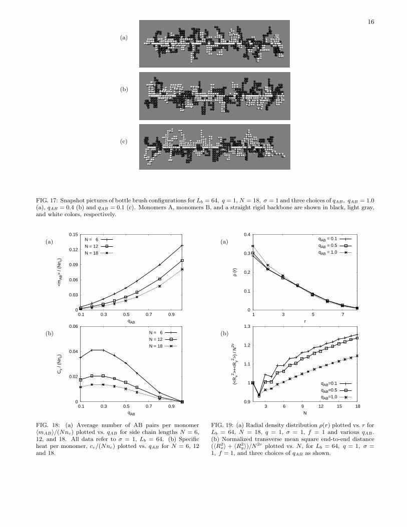
FIG. 17: Snapshot pictures of bottle brush configurations for Lb = 64, q = 1, N = 18, σ = 1 and three choices of qAB , qAB = 1.0(a), qAB = 0.4 (b) and qAB = 0.1 (c). Monomers A, monomers B, and a straight rigid backbone are shown in black, light gray,and white colors, respectively.

(a)

0

0.03

0.06

0.09

0.12

0.15

0.1 0.3 0.5 0.7 0.9

<m

AB>

/ (N

n c)

qAB

N = 6

N = 12

N = 18

(b)

0

0.02

0.04

0.06

0.1 0.3 0.5 0.7 0.9

Cv

/ (N

n c)

qAB

N = 6

N = 12

N = 18

FIG. 18: (a) Average number of AB pairs per monomer〈mAB〉/(Nnc) plotted vs. qAB for side chain lengths N = 6,12, and 18. All data refer to σ = 1, Lb = 64. (b) Specificheat per monomer, cv/(Nnc) plotted vs. qAB for N = 6, 12and 18.

(a)

0

0.1

0.2

0.3

0.4

7 5 3 1

ρ (r

)

r

qAB = 0.1

qAB = 0.5

qAB = 1.0

(b)

0.9

1

1.1

1.2

1.3

3 6 9 12 15 18

(<R

x2 >+

<R

y2 >)

/ N2ν

N

qAB=0.1

qAB=0.5

qAB=1.0

FIG. 19: (a) Radial density distribution ρ(r) plotted vs. r forLb = 64, N = 18, q = 1, σ = 1, f = 1 and various qAB .(b) Normalized transverse mean square end-to-end distance(〈R2

x〉 + 〈R2

y〉)/N2ν plotted vs. N , for Lb = 64, q = 1, σ =1, f = 1, and three choices of qAB as shown.

17

cm (1)BR

Rcm (2)A Rcm (3)B Rcm (4)Az

x

y

Rα

cm (n)1

2 4

3

n

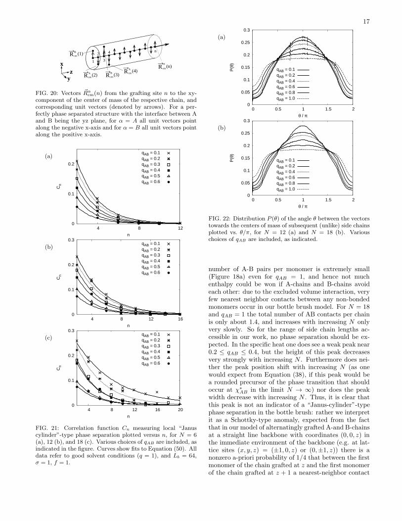
FIG. 20: Vectors ~Rαcm(n) from the grafting site n to the xy-

component of the center of mass of the respective chain, andcorresponding unit vectors (denoted by arrows). For a per-fectly phase separated structure with the interface between Aand B being the yz plane, for α = A all unit vectors pointalong the negative x-axis and for α = B all unit vectors pointalong the positive x-axis.

(a)

0

0.1

0.2

4 8 12

Cn

n

qAB = 0.1qAB = 0.2qAB = 0.3qAB = 0.4qAB = 0.5qAB = 0.6

(b)

0

0.1

0.2

0.3

4 8 12 16

Cn

n

qAB = 0.1qAB = 0.2qAB = 0.3qAB = 0.4qAB = 0.5qAB = 0.6

(c)

0

0.1

0.2

0.3

4 8 12 16 20

Cn

n

qAB = 0.1qAB = 0.2qAB = 0.3qAB = 0.4qAB = 0.5qAB = 0.6

FIG. 21: Correlation function Cn measuring local “Januscylinder”-type phase separation plotted versus n, for N = 6(a), 12 (b), and 18 (c). Various choices of qAB are included, asindicated in the figure. Curves show fits to Equation (50). Alldata refer to good solvent conditions (q = 1), and Lb = 64,σ = 1, f = 1.

(a)

0

0.05

0.1

0.15

0.2

0.25

0.3

0 0.5 1 1.5 2

P(θ

)

θ / π

qAB = 0.1qAB = 0.2qAB = 0.4qAB = 0.6qAB = 0.8qAB = 1.0

(b)

0

0.05

0.1

0.15

0.2

0.25

0.3

0 0.5 1 1.5 2

P(θ

)

θ / π

qAB = 0.1qAB = 0.2qAB = 0.4qAB = 0.6qAB = 0.8qAB = 1.0

FIG. 22: Distribution P (θ) of the angle θ between the vectorstowards the centers of mass of subsequent (unlike) side chainsplotted vs. θ/π, for N = 12 (a) and N = 18 (b). Variouschoices of qAB are included, as indicated.

number of A-B pairs per monomer is extremely small(Figure 18a) even for qAB = 1, and hence not muchenthalpy could be won if A-chains and B-chains avoideach other: due to the excluded volume interaction, veryfew nearest neighbor contacts between any non-bondedmonomers occur in our bottle brush model. For N = 18and qAB = 1 the total number of AB contacts per chainis only about 1.4, and increases with increasing N onlyvery slowly. So for the range of side chain lengths ac-cessible in our work, no phase separation should be ex-pected. In the specific heat one does see a weak peak near0.2 ≤ qAB ≤ 0.4, but the height of this peak decreasesvery strongly with increasing N . Furthermore does nei-ther the peak position shift with increasing N (as onewould expect from Equation (38), if this peak would bea rounded precursor of the phase transition that shouldoccur at χ∗

AB in the limit N → ∞) nor does the peakwidth decrease with increasing N . Thus, it is clear thatthis peak is not an indicator of a “Janus-cylinder”-typephase separation in the bottle brush: rather we interpretit as a Schottky-type anomaly, expected from the factthat in our model of alternatingly grafted A-and B-chainsat a straight line backbone with coordinates (0, 0, z) inthe immediate environment of the backbone (e.g. at lat-tice sites (x, y, z) = (±1, 0, z) or (0,±1, z)) there is anonzero a-priori probability of 1/4 that between the firstmonomer of the chain grafted at z and the first monomerof the chain grafted at z + 1 a nearest-neighbor contact

18

(a)

0

0.01

0.02

0.03

0.04

0.1 0.2 0.3 0.4 0.5 0.6

Cv

/ (N

n c)

qAB

N = 6N = 12N = 18

(b)

0

0.1

0.2

0.3

0.4

7 5 3 1

ρ (r

)

qAB = 0.1

qAB = 0.3

qAB = 0.5

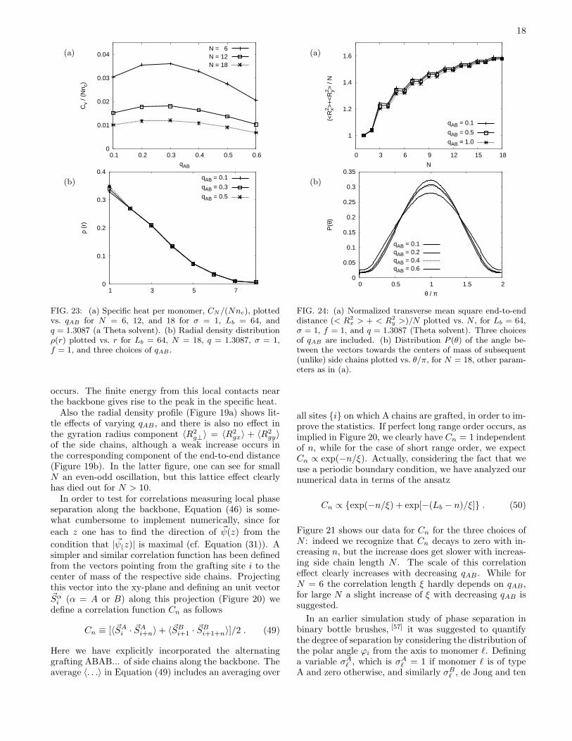
FIG. 23: (a) Specific heat per monomer, CN/(Nnc), plottedvs. qAB for N = 6, 12, and 18 for σ = 1, Lb = 64, andq = 1.3087 (a Theta solvent). (b) Radial density distributionρ(r) plotted vs. r for Lb = 64, N = 18, q = 1.3087, σ = 1,f = 1, and three choices of qAB .

occurs. The finite energy from this local contacts nearthe backbone gives rise to the peak in the specific heat.Also the radial density profile (Figure 19a) shows lit-

tle effects of varying qAB , and there is also no effect inthe gyration radius component 〈R2

g⊥〉 = 〈R2gx〉 + 〈R2

gy〉of the side chains, although a weak increase occurs inthe corresponding component of the end-to-end distance(Figure 19b). In the latter figure, one can see for smallN an even-odd oscillation, but this lattice effect clearlyhas died out for N > 10.In order to test for correlations measuring local phase

separation along the backbone, Equation (46) is some-what cumbersome to implement numerically, since for

each z one has to find the direction of ~ψ(z) from the

condition that |~ψ(z)| is maximal (cf. Equation (31)). Asimpler and similar correlation function has been definedfrom the vectors pointing from the grafting site i to thecenter of mass of the respective side chains. Projectingthis vector into the xy-plane and defining an unit vector~Sαi (α = A or B) along this projection (Figure 20) wedefine a correlation function Cn as follows

Cn ≡ [〈~SAi · ~SAi+n〉+ 〈~SBi+1 · ~SBi+1+n〉]/2 . (49)

Here we have explicitly incorporated the alternatinggrafting ABAB... of side chains along the backbone. Theaverage 〈. . .〉 in Equation (49) includes an averaging over

(a)

1

1.2

1.4

1.6

0 3 6 9 12 15 18

(<R

x2 >+

<R

y2 > /

N

N

qAB = 0.1

qAB = 0.5

qAB = 1.0

(b)

0

0.05

0.1

0.15

0.2

0.25

0.3

0.35

0 0.5 1 1.5 2

P(θ

)

θ / π

qAB = 0.1qAB = 0.2qAB = 0.4qAB = 0.6

FIG. 24: (a) Normalized transverse mean square end-to-enddistance (< R2

x > + < R2

y >)/N plotted vs. N , for Lb = 64,σ = 1, f = 1, and q = 1.3087 (Theta solvent). Three choicesof qAB are included. (b) Distribution P (θ) of the angle be-tween the vectors towards the centers of mass of subsequent(unlike) side chains plotted vs. θ/π, for N = 18, other param-eters as in (a).

all sites {i} on which A chains are grafted, in order to im-prove the statistics. If perfect long range order occurs, asimplied in Figure 20, we clearly have Cn = 1 independentof n, while for the case of short range order, we expectCn ∝ exp(−n/ξ). Actually, considering the fact that weuse a periodic boundary condition, we have analyzed ournumerical data in terms of the ansatz

Cn ∝ {exp(−n/ξ) + exp[−(Lb − n)/ξ]} . (50)

Figure 21 shows our data for Cn for the three choices ofN : indeed we recognize that Cn decays to zero with in-creasing n, but the increase does get slower with increas-ing side chain length N . The scale of this correlationeffect clearly increases with decreasing qAB. While forN = 6 the correlation length ξ hardly depends on qAB,for large N a slight increase of ξ with decreasing qAB issuggested.

In an earlier simulation study of phase separation inbinary bottle brushes, [57] it was suggested to quantifythe degree of separation by considering the distribution ofthe polar angle ϕi from the axis to monomer ℓ. Defininga variable σAℓ , which is σAℓ = 1 if monomer ℓ is of typeA and zero otherwise, and similarly σBℓ , de Jong and ten

19

(a)

0

0.1

0.2

0.3

0.4

4 8 12 16

Cn

n

qAB = 0.1qAB = 0.2qAB = 0.3qAB = 0.4qAB = 0.5qAB = 0.6

(b)

0

0.1

0.2

0.3

0.4

0.5

4 8 12 16

Cn

n

qAB = 0.1qAB = 0.2qAB = 0.3qAB = 0.4qAB = 0.5qAB = 0.6

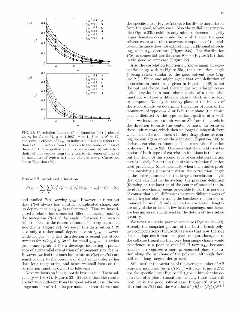
FIG. 25: Correlation function Cn { Equation (49) } plottedvs. n, for Lb = 64, q = 1.3087, σ = 1, f = 1, N = 12,and various choices of qAB , as indicated. Case (a) refers to achoice of unit vectors from the z-axis to the center of mass ofthe chain that is grafted at z = i, while case (b) refers to achoice of unit vectors from the z-axis to the center of mass ofall monomers of type α in the xy-plane at z = i. Curves arefits to Equation (50).

Brinke [57] introduced a function

P (φ) =∑ℓ

∑ℓ′

(σAℓ σBℓ′ + σBℓ σ

Aℓ′ )δ(|ϕi − ϕj | − φ) (51)

and studied P (φ) varying χAB. However, it turns outthat P (φ) always has a rather complicated shape, andits dependence on χAB is rather weak. Thus we investi-gated a related but somewhat different function, namelythe histogram P (θ) of the angle θ between the vectorsfrom the axis to the centers of mass of subsequent unlikeside chains (Figure 22). We see in this distribution P (θ)also only a rather small dependence on χAB, however:while for qAB = 1 this distribution is essentially struc-tureless for π/2 ≤ θ ≤ 3π/2, for small qAB = 1 a ratherpronounced peak at θ ≈ π develops, indicating a prefer-ence of antiparallel orientation of subsequent side chains.However, we feel that such indicators as P (φ) or P (θ) aresensitive only to the presence of short range order ratherthan long range order, and hence we shall focus on thecorrelation function Cn in the following.Next we focus on binary bottle brushes in a Theta sol-

vent (q = 1.3087). Figures 23 - 25 show that the resultsare not very different from the good solvent case: the av-erage number of AB pairs per monomer (not shown) and

the specific heat (Figure 23a) are hardly distinguishablefrom the good solvent case. Also the radial density pro-file (Figure 23b) exhibits only minor differences, slightlylarger densities occur inside the brush than in the goodsolvent cases, and the transverse component of the end-to-end distance does not exhibit much additional stretch-ing, when qAB decreases (Figure 24a). The distributionP (θ) is somewhat less flat near θ = π (Figure 24b) thanin the good solvent case (Figure 22).

Also the correlation function Cn shows again an expo-nential decay with n (Figure 25a), the correlation lengthξ being rather similar to the good solvent case (Fig-ure 21). Since one might argue that our definition ofa correlation function as given in Equation (49) is notthe optimal choice, and there might occur larger corre-lation lengths for a more clever choice of a correlationfunction, we tried a different choice which is also easyto compute. Namely, in the xy-plane at the index i ofthe z-coordinate we determine the center of mass of themonomers of type α = A or B in that plane (the choiceof α is dictated by the type of chain grafted at z = i).

Then we introduce an unit vector ~Sαi from the z-axis inthe direction towards this center of mass. In terms ofthese unit vectors, which then no longer distinguish fromwhich chain the monomers α in the i’th xy-plane are com-ing, we can again apply the definition, Equation (49) toderive a correlation function. This correlation functionis shown in Figure 25b. One sees that the qualitative be-havior of both types of correlation functions is the same,but the decay of this second type of correlation functioneven is slightly faster than that of the correlation functionused previously. Since normally, when one studies prob-lems involving a phase transition, the correlation lengthof the order parameter is the largest correlation lengththat one can find in the system, the previous definition(focusing on the location of the center of mass of the in-dividual side chains) seems preferable to us. It is possibleof course that such differences between different ways ofmeasuring correlations along the backbone remain so pro-nounced for small N only, where the correlation lengthsare only of the order of a few lattice spacings, and henceare less universal and depend on the details of the studiedquantity.

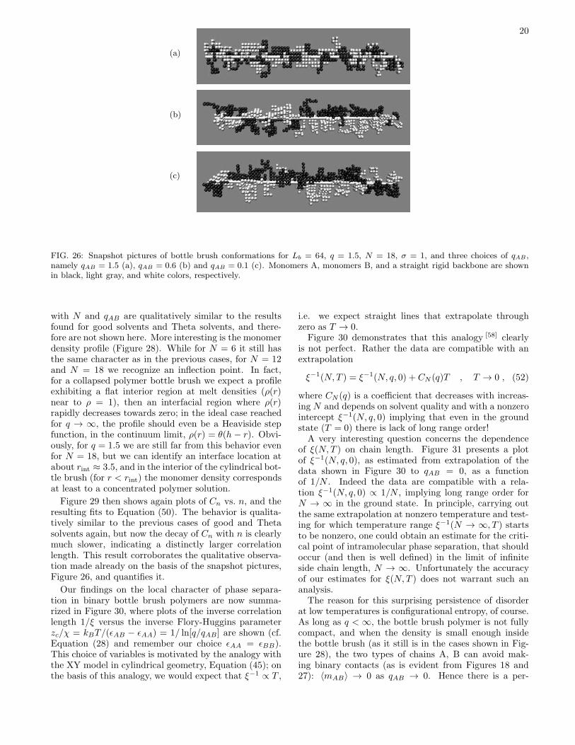
We now turn to the poor solvent case (Figures 26 - 29).Already the snapshot picture of the bottle brush poly-mer conformations (Figure 26) reveals that now the sidechains adopt much more compact configurations, due tothe collapse transition that very long single chains wouldexperience in a poor solvent. [45] If now qAB becomessmall, one recognizes a more pronounced phase separa-tion along the backbone of the polymer, although therestill is no long range order present.

Still, neither the variation of the average number of ABpairs per monomer 〈mAB〉/(Nnc) with qAB (Figure 27a)nor the specific heat (Figure 27b) give a hint for the oc-currence of a phase transition: in fact, these data stilllook like in the good solvent case, Figure 18! Also thedistribution P (θ) and the variation of (〈R2

x〉+〈R2y〉)/N2/3

20

(a)

(b)

(c)

FIG. 26: Snapshot pictures of bottle brush conformations for Lb = 64, q = 1.5, N = 18, σ = 1, and three choices of qAB ,namely qAB = 1.5 (a), qAB = 0.6 (b) and qAB = 0.1 (c). Monomers A, monomers B, and a straight rigid backbone are shownin black, light gray, and white colors, respectively.

with N and qAB are qualitatively similar to the resultsfound for good solvents and Theta solvents, and there-fore are not shown here. More interesting is the monomerdensity profile (Figure 28). While for N = 6 it still hasthe same character as in the previous cases, for N = 12and N = 18 we recognize an inflection point. In fact,for a collapsed polymer bottle brush we expect a profileexhibiting a flat interior region at melt densities (ρ(r)near to ρ = 1), then an interfacial region where ρ(r)rapidly decreases towards zero; in the ideal case reachedfor q → ∞, the profile should even be a Heaviside stepfunction, in the continuum limit, ρ(r) = θ(h − r). Obvi-ously, for q = 1.5 we are still far from this behavior evenfor N = 18, but we can identify an interface location atabout rint ≈ 3.5, and in the interior of the cylindrical bot-tle brush (for r < rint) the monomer density correspondsat least to a concentrated polymer solution.

Figure 29 then shows again plots of Cn vs. n, and theresulting fits to Equation (50). The behavior is qualita-tively similar to the previous cases of good and Thetasolvents again, but now the decay of Cn with n is clearlymuch slower, indicating a distinctly larger correlationlength. This result corroborates the qualitative observa-tion made already on the basis of the snapshot pictures,Figure 26, and quantifies it.

Our findings on the local character of phase separa-tion in binary bottle brush polymers are now summa-rized in Figure 30, where plots of the inverse correlationlength 1/ξ versus the inverse Flory-Huggins parameterzc/χ = kBT/(ǫAB − ǫAA) = 1/ ln[q/qAB] are shown (cf.Equation (28) and remember our choice ǫAA = ǫBB).This choice of variables is motivated by the analogy withthe XY model in cylindrical geometry, Equation (45); onthe basis of this analogy, we would expect that ξ−1 ∝ T ,

i.e. we expect straight lines that extrapolate throughzero as T → 0.Figure 30 demonstrates that this analogy [58] clearly

is not perfect. Rather the data are compatible with anextrapolation

ξ−1(N, T ) = ξ−1(N, q, 0) + CN (q)T , T → 0 , (52)

where CN (q) is a coefficient that decreases with increas-ing N and depends on solvent quality and with a nonzerointercept ξ−1(N, q, 0) implying that even in the groundstate (T = 0) there is lack of long range order!A very interesting question concerns the dependence

of ξ(N, T ) on chain length. Figure 31 presents a plotof ξ−1(N, q, 0), as estimated from extrapolation of thedata shown in Figure 30 to qAB = 0, as a functionof 1/N . Indeed the data are compatible with a rela-tion ξ−1(N, q, 0) ∝ 1/N , implying long range order forN → ∞ in the ground state. In principle, carrying outthe same extrapolation at nonzero temperature and test-ing for which temperature range ξ−1(N → ∞, T ) startsto be nonzero, one could obtain an estimate for the criti-cal point of intramolecular phase separation, that shouldoccur (and then is well defined) in the limit of infiniteside chain length, N → ∞. Unfortunately the accuracyof our estimates for ξ(N, T ) does not warrant such ananalysis.The reason for this surprising persistence of disorder

at low temperatures is configurational entropy, of course.As long as q < ∞, the bottle brush polymer is not fullycompact, and when the density is small enough insidethe bottle brush (as it still is in the cases shown in Fig-ure 28), the two types of chains A, B can avoid mak-ing binary contacts (as is evident from Figures 18 and27): 〈mAB〉 → 0 as qAB → 0. Hence there is a per-

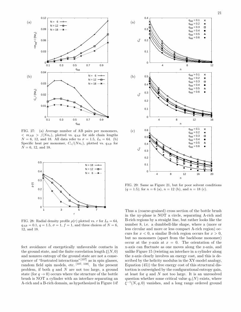
21

(a)

0

0.03

0.06

0.09

0.12

0.1 0.3 0.5 0.7 0.9

<m

AB>

/ (N

n c)

qAB

N = 6

N = 12

N = 18

(b)

0

0.01

0.02

0.03

0.04

0.1 0.3 0.5 0.7 0.9

Cv

/ (N

n c)

qAB

N = 6

N = 12

N = 18

FIG. 27: (a) Average number of AB pairs per monomers,< mAB > /(Nnc), plotted vs. qAB for side chain lengthsN = 6, 12, and 18. All data refer to σ = 1.5, Lb = 64. (b)Specific heat per monomer, Cv/(Nnc), plotted vs. qAB forN = 6, 12, and 18.

0

0.1

0.2

0.3

0.4

0.5

7 5 3 1

ρ (r

)

r

N = 18

N = 12

N = 6

FIG. 28: Radial density profile ρ(r) plotted vs. r for Lb = 64,qAB = 0.1, q = 1.5, σ = 1, f = 1, and three choices of N = 6,12, and 18.

fect avoidance of energetically unfavorable contacts inthe ground state, and the finite correlation length ξ(N, 0)and nonzero entropy of the ground state are not a conse-quence of “frustrated interactions”[107] as in spin glasses,random field spin models, etc. [107, 108]. In the presentproblem, if both q and N are not too large, a groundstate (for q → 0) occurs where the structure of the bottlebrush is NOT a cylinder with an interface separating anA-rich and a B-rich domain, as hypothesized in Figure 14!

(a)

0

0.1

0.2

0.3

0.4

4 8 12

Cn

n

qAB = 0.1qAB = 0.2qAB = 0.3qAB = 0.4qAB = 0.5qAB = 0.6

(b)

0

0.1

0.2

0.3

0.4

0.5

4 8 12 16

Cn

n

qAB = 0.1qAB = 0.2qAB = 0.3qAB = 0.4qAB = 0.5qAB = 0.6

(c)

0

0.1

0.2

0.3

0.4

0.5

0.6

4 8 12 16 20

Cn

n

qAB = 0.1qAB = 0.2qAB = 0.3qAB = 0.4qAB = 0.5qAB = 0.6

FIG. 29: Same as Figure 21, but for poor solvent conditions(q = 1.5); for n = 6 (a), n = 12 (b), and n = 18 (c).

Thus a (coarse-grained) cross section of the bottle brushin the xy-plane is NOT a circle, separating A-rich andB-rich regions by a straight line, but rather looks like thenumber 8, i.e. a dumbbell-like shape, where a (more orless circular and more or less compact A-rich region) oc-curs for x < 0, a similar B-rich region occurs for x > 0,but no monomers (apart from the backbone monomer)occur at the y-axis at x = 0. The orientation of thex-axis can fluctuate as one moves along the z-axis, andunlike Figure 15 (twisting an interface in a cylinder alongthe z-axis clearly involves an energy cost, and this is de-scribed by the helicity modulus in the XY-model analogy,Equation (45)) the free energy cost of this structural dis-tortion is outweighed by the configurational entropy gain,at least for q and N not too large. It is an unresolvedquestion whether some critical value qc(N) exists, whereξ−1(N, q, 0) vanishes, and a long range ordered ground

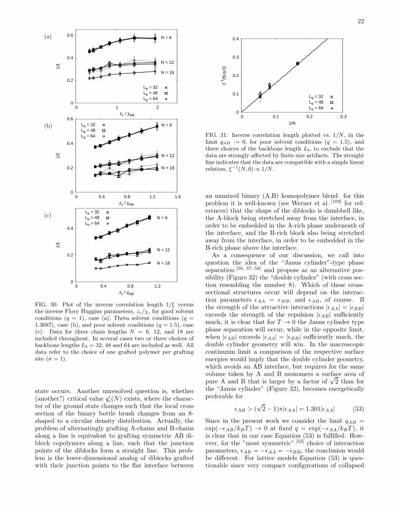
22

(a)

0

0.2

0.4

0.6

0 1 2

1/ξ

zc / χAB

N = 6

N = 12

N = 18

Lb = 32Lb = 48Lb = 64

(b)

0

0.2

0.4

0.6

0 0.4 0.8 1.2 1.6

1/ξ

zc / χAB

N = 18

N = 12

N = 6Lb = 32Lb = 48Lb = 64

(c)

0

0.2

0.4

0 0.4 0.8 1.2

1/ξ

zc / χAB

N = 18

N = 12

N = 6Lb = 32Lb = 48Lb = 64

FIG. 30: Plot of the inverse correlation length 1/ξ versusthe inverse Flory Huggins parameters, zc/χ, for good solventconditions (q = 1), case (a), Theta solvent conditions (q =1.3087), case (b), and poor solvent conditions (q = 1.5), case(c). Data for three chain lengths N = 6, 12, and 18 areincluded throughout. In several cases two or three choices ofbackbone lengths Lb = 32, 48 and 64 are included as well. Alldata refer to the choice of one grafted polymer per graftingsite (σ = 1).

state occurs. Another unresolved question is, whether(another?) critical value q′c(N) exists, where the charac-ter of the ground state changes such that the local crosssection of the binary bottle brush changes from an 8-shaped to a circular density distribution. Actually, theproblem of alternatingly grafting A-chains and B-chainsalong a line is equivalent to grafting symmetric AB di-block copolymers along a line, such that the junctionpoints of the diblocks form a straight line. This prob-lem is the lower-dimensional analog of diblocks graftedwith their junction points to the flat interface between

0

0.1

0.2

0.3

0.4

0 0.1 0.2 0.3

ξ-1(N

,q,0

)

1/N

Lb = 32Lb = 48Lb = 64

FIG. 31: Inverse correlation length plotted vs. 1/N , in thelimit qAB → 0, for poor solvent conditions (q = 1.5), andthree choices of the backbone length Lb, to exclude that thedata are strongly affected by finite size artifacts. The straightline indicates that the data are compatible with a simple linearrelation, ξ−1(N, 0) ∝ 1/N .

an unmixed binary (A,B) homopolymer blend: for thisproblem it is well-known (see Werner et al. [109] for ref-erences) that the shape of the diblocks is dumbbell like,the A-block being stretched away from the interface, inorder to be embedded in the A-rich phase underneath ofthe interface, and the B-rich block also being stretchedaway from the interface, in order to be embedded in theB-rich phase above the interface.As a consequence of our discussion, we call into

question the idea of the “Janus cylinder”-type phaseseparation [56, 57, 58] and propose as an alternative pos-sibility (Figure 32) the “double cylinder” (with cross sec-tion resembling the number 8). Which of these cross-sectional structures occur will depend on the interac-tion parameters ǫAA = ǫBB, and ǫAB, of course. Ifthe strength of the attractive interactions |ǫAA| = |ǫBB|exceeds the strength of the repulsion |ǫAB| sufficientlymuch, it is clear that for T → 0 the Janus cylinder typephase separation will occur, while in the opposite limit,when |ǫAB| exceeds |ǫAA| = |ǫBB| sufficiently much, thedouble cylinder geometry will win. In the macroscopiccontinuum limit a comparison of the respective surfaceenergies would imply that the double cylinder geometry,which avoids an AB interface, but requires for the samevolume taken by A and B monomers a surface area ofpure A and B that is larger by a factor of

√2 than for

the “Janus cylinder” (Figure 32), becomes energeticallypreferable for

ǫAB > (√2− 1)π|ǫAA| = 1.301|ǫAA| (53)

Since in the present work we consider the limit qAB =exp(−ǫAB/kBT ) → 0 at fixed q = exp(−ǫAA/kBT ), itis clear that in our case Equation (53) is fulfilled. How-ever, for the ”most symmetric” [52] choice of interactionparameters, ǫAB = −ǫAA = −ǫBB, the conclusion wouldbe different. For lattice models Equation (53) is ques-tionable since very compact configurations of collapsed

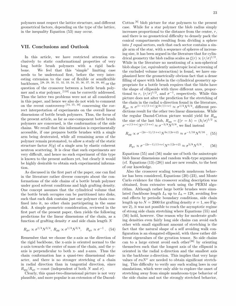
23

polymers must respect the lattice structure, and differentgeometrical factors, depending on the type of the lattice,in the inequality Equation (53) may occur.

VII. Conclusions and Outlook

In this article, we have restricted attention ex-clusively to static conformational properties of verylong bottle brush polymers with a rigid back-bone. We feel that this “simple” limiting caseneeds to be understood first, before the very inter-esting extension to the case of flexible or semiflexiblebackbones, [28, 29, 30, 31, 32, 33, 34, 35, 36, 37, 38, 39, 40] or thequestion of the crossover between a bottle brush poly-mer and a star polymer, [110] can be correctly addressed.Thus the latter two problems were not at all consideredin this paper, and hence we also do not wish to commenton the recent controversy [14, 15, 16] concerning the cor-rect interpretation of experiments on the overall lineardimensions of bottle brush polymers. Thus, the focus ofthe present article, as far as one-component bottle brushpolymers are concerned, is the conformation of the sidechains. We recall that this information is experimentallyaccessible, if one prepares bottle brushes with a singlearm being deuterated, while all remaining arms of thepolymer remain protonated, to allow a study of the staticstructure factor S(q) of a single arm by elastic coherentneutron scattering. It is clear that such experiments arevery difficult, and hence no such experiment of this typeis known to the present authors yet, but clearly it wouldbe highly desirable to obtain such experimental informa-tion.As discussed in the first part of the paper, one can find

in the literature rather diverse concepts about the con-formations of the side chains of a bottle brush polymerunder good solvent conditions and high grafting density.One concept assumes that the cylindrical volume thatthe bottle brush occupies can be partitioned into disks,such that each disk contains just one polymer chain con-fined into it, no other chain participating in the samedisk. A simple geometric consideration, reviewed in thefirst part of the present paper, then yields the followingpredictions for the linear dimensions of the chain, as afunction of grafting density σ and side chain length N

Rgx ∝ σ1/4N3/4, Rgy ∝ σ1/4N3/4, Rgz ∝ σ−1 . (54)

Remember that we choose the z-axis as the direction ofthe rigid backbone, the x-axis is oriented normal to thez-axis towards the center of mass of the chain, and the y-axis is perpendicular to both x- and z-axes. Thus thechain conformation has a quasi-two dimensional char-acter, and there is no stronger stretching of a chainin radial direction than in tangential direction, sinceRgy/Rgx = const (independent of both N and σ).Clearly, this quasi-two-dimensional picture is not very

plausible, and more popular is an extension of the Daoud-

Cotton [8] blob picture for star polymers to the presentcase. While for a star polymer the blob radius simplyincreases proportional to the distance from the center, r,and there is no geometrical difficulty to densely pack theconical compartments resulting from dividing a sphereinto f equal sectors, such that each sector contains a sin-gle arm of the star, with a sequence of spheres of increas-ing size, it has been argued in the literature that for cylin-drical geometry the blob radius scales as ξ(r) ∝ (r/σ)1/2.While in the literature no mentioning of a non-sphericalblob shape (or, equivalently anisotropic local screening ofthe excluded volume interaction) is found, we have em-phasized here the geometrically obvious fact that a densefilling of space with blobs in the cylindrical geometry ap-propriate for a bottle brush requires that the blobs havethe shape of ellipsoids with three different axes, propor-tional to r, (r/σ)1/2, and σ−1, respectively. While thispicture does not alter the prediction for the stretching ofthe chain in the radial x-direction found in the literature,Rgx ∝ σ(1−ν)/(1+ν)N2ν/(1+ν) ≈ σ1/4N3/4, different pre-dictions result for the other two linear dimensions. Whilethe regular Daoud-Cotton picture would yield for Rgythe size of the last blob, Rgy = ξ(r = h) = (h/σ)1/2 ∝σ−ν/(1+ν)Nν/(1+ν) ≈ σ−3/8N3/8, we find instead

Rgy ∝ σ−(2ν−1)/(1+ν)N3ν/(2ν+2) ≈ σ−1/16N9/16 , (55)

Rgz ∝ σ−(2ν−1)/(1+ν)Nν/(2ν+2) ≈ σ5/8N3/8 . (56)

Equations (55) and (56) make use of both the anisotropicblob linear dimensions and random walk-type arguments(cf. Equations (13)-(28)) and are new results, to the bestof our knowledge.Also the crossover scaling towards mushroom behav-

ior has been considered, Equations (20)-(23), and MonteCarlo evidence for this crossover scaling description wasobtained, from extensive work using the PERM algo-rithm. Although rather large bottle brushes were simu-lated (backbone length Lb up to Lb = 128, avoiding freeend effects by periodic boundary conditions, side chainlength up toN = 2000 for grafting density σ = 1, see Fig-ure 2), it was not possible to reach the asymptotic regimeof strong side chain stretching where Equations (55) and(56) hold, however. One reason why for moderate graft-ing densities even fairly long side chains can avoid eachother with small significant amount of stretching is thefact that the natural shape of a self avoiding walk con-figuration is an elongated ellipsoid, with three rather dif-ferent eigenvalues of the gyration tensor. So side chainscan to a large extent avoid each other[36] by orientingthemselves such that the longest axis of the ellipsoid isoriented in the radial x-direction and the smallest axisin the backbone z-direction. This implies that very largevalues of σaNν are needed to obtain significant stretch-ing. This difficulty to verify any such scaling laws in oursimulations, which were only able to explore the onset ofstretching away from simple mushroom-type behavior ofthe side chains and not the strongly stretched behavior,

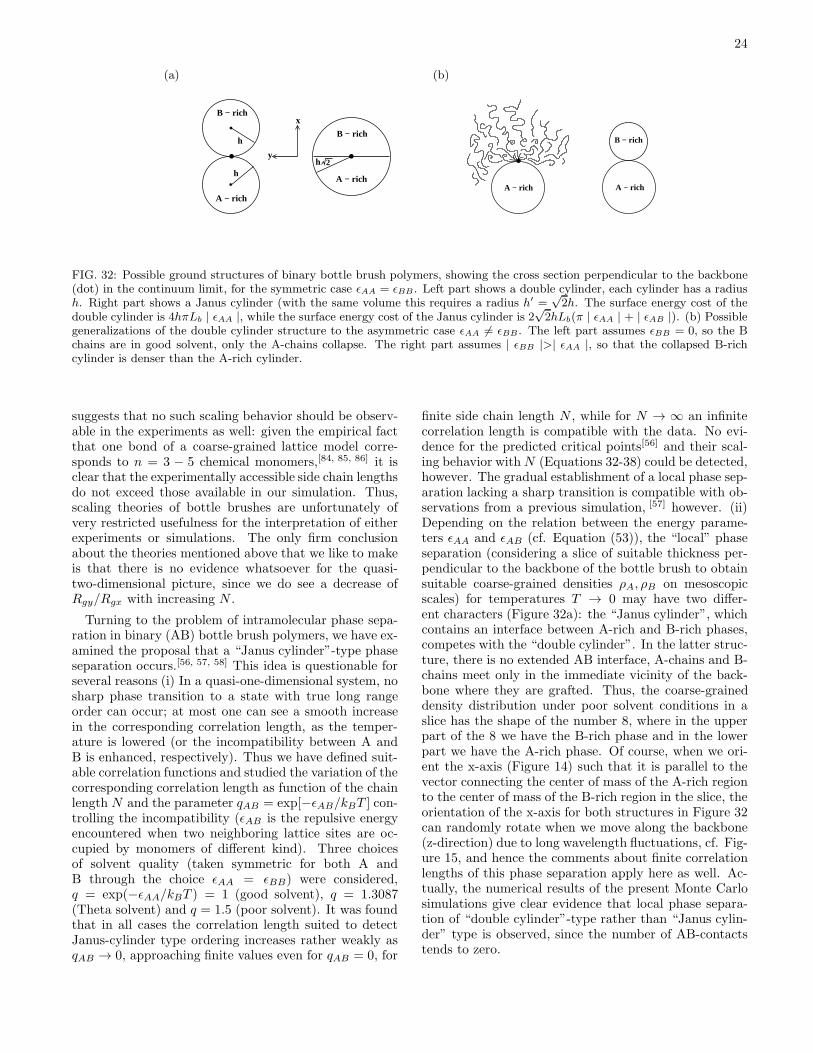
24

(a) (b)

2h

B − rich

B − rich

A − rich

A − rich

h

h

x

y

B − rich

A − richA − rich

FIG. 32: Possible ground structures of binary bottle brush polymers, showing the cross section perpendicular to the backbone(dot) in the continuum limit, for the symmetric case ǫAA = ǫBB . Left part shows a double cylinder, each cylinder has a radiush. Right part shows a Janus cylinder (with the same volume this requires a radius h′ =

√2h. The surface energy cost of the

double cylinder is 4hπLb | ǫAA |, while the surface energy cost of the Janus cylinder is 2√2hLb(π | ǫAA | + | ǫAB |). (b) Possible

generalizations of the double cylinder structure to the asymmetric case ǫAA 6= ǫBB . The left part assumes ǫBB = 0, so the Bchains are in good solvent, only the A-chains collapse. The right part assumes | ǫBB |>| ǫAA |, so that the collapsed B-richcylinder is denser than the A-rich cylinder.

suggests that no such scaling behavior should be observ-able in the experiments as well: given the empirical factthat one bond of a coarse-grained lattice model corre-sponds to n = 3 − 5 chemical monomers,[84, 85, 86] it isclear that the experimentally accessible side chain lengthsdo not exceed those available in our simulation. Thus,scaling theories of bottle brushes are unfortunately ofvery restricted usefulness for the interpretation of eitherexperiments or simulations. The only firm conclusionabout the theories mentioned above that we like to makeis that there is no evidence whatsoever for the quasi-two-dimensional picture, since we do see a decrease ofRgy/Rgx with increasing N .

Turning to the problem of intramolecular phase sepa-ration in binary (AB) bottle brush polymers, we have ex-amined the proposal that a “Janus cylinder”-type phaseseparation occurs.[56, 57, 58] This idea is questionable forseveral reasons (i) In a quasi-one-dimensional system, nosharp phase transition to a state with true long rangeorder can occur; at most one can see a smooth increasein the corresponding correlation length, as the temper-ature is lowered (or the incompatibility between A andB is enhanced, respectively). Thus we have defined suit-able correlation functions and studied the variation of thecorresponding correlation length as function of the chainlength N and the parameter qAB = exp[−ǫAB/kBT ] con-trolling the incompatibility (ǫAB is the repulsive energyencountered when two neighboring lattice sites are oc-cupied by monomers of different kind). Three choicesof solvent quality (taken symmetric for both A andB through the choice ǫAA = ǫBB) were considered,q = exp(−ǫAA/kBT ) = 1 (good solvent), q = 1.3087(Theta solvent) and q = 1.5 (poor solvent). It was foundthat in all cases the correlation length suited to detectJanus-cylinder type ordering increases rather weakly asqAB → 0, approaching finite values even for qAB = 0, for

finite side chain length N , while for N → ∞ an infinitecorrelation length is compatible with the data. No evi-dence for the predicted critical points[56] and their scal-ing behavior withN (Equations 32-38) could be detected,however. The gradual establishment of a local phase sep-aration lacking a sharp transition is compatible with ob-servations from a previous simulation, [57] however. (ii)Depending on the relation between the energy parame-ters ǫAA and ǫAB (cf. Equation (53)), the “local” phaseseparation (considering a slice of suitable thickness per-pendicular to the backbone of the bottle brush to obtainsuitable coarse-grained densities ρA, ρB on mesoscopicscales) for temperatures T → 0 may have two differ-ent characters (Figure 32a): the “Janus cylinder”, whichcontains an interface between A-rich and B-rich phases,competes with the “double cylinder”. In the latter struc-ture, there is no extended AB interface, A-chains and B-chains meet only in the immediate vicinity of the back-bone where they are grafted. Thus, the coarse-graineddensity distribution under poor solvent conditions in aslice has the shape of the number 8, where in the upperpart of the 8 we have the B-rich phase and in the lowerpart we have the A-rich phase. Of course, when we ori-ent the x-axis (Figure 14) such that it is parallel to thevector connecting the center of mass of the A-rich regionto the center of mass of the B-rich region in the slice, theorientation of the x-axis for both structures in Figure 32can randomly rotate when we move along the backbone(z-direction) due to long wavelength fluctuations, cf. Fig-ure 15, and hence the comments about finite correlationlengths of this phase separation apply here as well. Ac-tually, the numerical results of the present Monte Carlosimulations give clear evidence that local phase separa-tion of “double cylinder”-type rather than “Janus cylin-der” type is observed, since the number of AB-contactstends to zero.

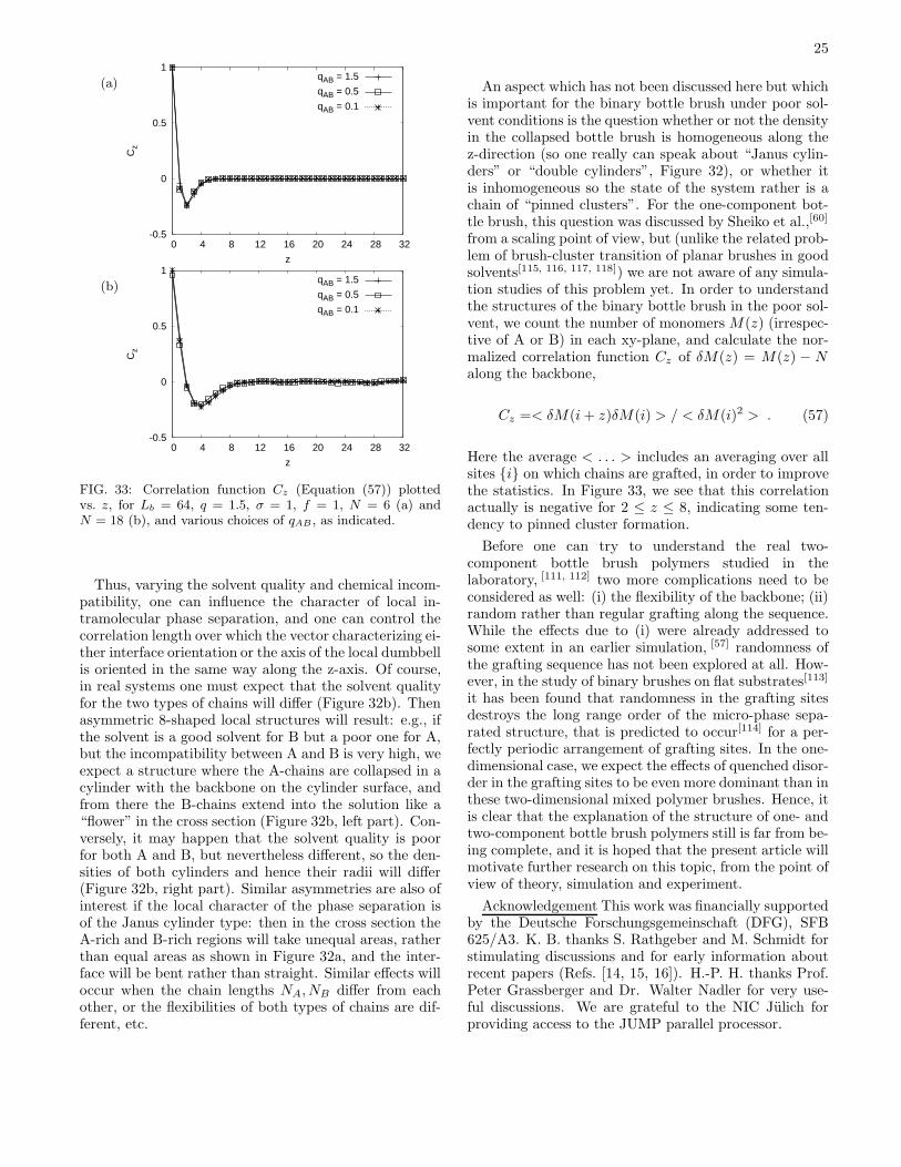
25

(a)

-0.5

0

0.5

1

0 4 8 12 16 20 24 28 32

Cz

z

qAB = 1.5

qAB = 0.5

qAB = 0.1

(b)

-0.5

0

0.5

1

0 4 8 12 16 20 24 28 32

Cz

z

qAB = 1.5

qAB = 0.5

qAB = 0.1

FIG. 33: Correlation function Cz (Equation (57)) plottedvs. z, for Lb = 64, q = 1.5, σ = 1, f = 1, N = 6 (a) andN = 18 (b), and various choices of qAB , as indicated.

Thus, varying the solvent quality and chemical incom-patibility, one can influence the character of local in-tramolecular phase separation, and one can control thecorrelation length over which the vector characterizing ei-ther interface orientation or the axis of the local dumbbellis oriented in the same way along the z-axis. Of course,in real systems one must expect that the solvent qualityfor the two types of chains will differ (Figure 32b). Thenasymmetric 8-shaped local structures will result: e.g., ifthe solvent is a good solvent for B but a poor one for A,but the incompatibility between A and B is very high, weexpect a structure where the A-chains are collapsed in acylinder with the backbone on the cylinder surface, andfrom there the B-chains extend into the solution like a“flower” in the cross section (Figure 32b, left part). Con-versely, it may happen that the solvent quality is poorfor both A and B, but nevertheless different, so the den-sities of both cylinders and hence their radii will differ(Figure 32b, right part). Similar asymmetries are also ofinterest if the local character of the phase separation isof the Janus cylinder type: then in the cross section theA-rich and B-rich regions will take unequal areas, ratherthan equal areas as shown in Figure 32a, and the inter-face will be bent rather than straight. Similar effects willoccur when the chain lengths NA, NB differ from eachother, or the flexibilities of both types of chains are dif-ferent, etc.

An aspect which has not been discussed here but whichis important for the binary bottle brush under poor sol-vent conditions is the question whether or not the densityin the collapsed bottle brush is homogeneous along thez-direction (so one really can speak about “Janus cylin-ders” or “double cylinders”, Figure 32), or whether itis inhomogeneous so the state of the system rather is achain of “pinned clusters”. For the one-component bot-tle brush, this question was discussed by Sheiko et al.,[60]

from a scaling point of view, but (unlike the related prob-lem of brush-cluster transition of planar brushes in goodsolvents[115, 116, 117, 118]) we are not aware of any simula-tion studies of this problem yet. In order to understandthe structures of the binary bottle brush in the poor sol-vent, we count the number of monomers M(z) (irrespec-tive of A or B) in each xy-plane, and calculate the nor-malized correlation function Cz of δM(z) = M(z) − Nalong the backbone,

Cz =< δM(i+ z)δM(i) > / < δM(i)2 > . (57)

Here the average < . . . > includes an averaging over allsites {i} on which chains are grafted, in order to improvethe statistics. In Figure 33, we see that this correlationactually is negative for 2 ≤ z ≤ 8, indicating some ten-dency to pinned cluster formation.

Before one can try to understand the real two-component bottle brush polymers studied in thelaboratory, [111, 112] two more complications need to beconsidered as well: (i) the flexibility of the backbone; (ii)random rather than regular grafting along the sequence.While the effects due to (i) were already addressed tosome extent in an earlier simulation, [57] randomness ofthe grafting sequence has not been explored at all. How-ever, in the study of binary brushes on flat substrates[113]

it has been found that randomness in the grafting sitesdestroys the long range order of the micro-phase sepa-rated structure, that is predicted to occur[114] for a per-fectly periodic arrangement of grafting sites. In the one-dimensional case, we expect the effects of quenched disor-der in the grafting sites to be even more dominant than inthese two-dimensional mixed polymer brushes. Hence, itis clear that the explanation of the structure of one- andtwo-component bottle brush polymers still is far from be-ing complete, and it is hoped that the present article willmotivate further research on this topic, from the point ofview of theory, simulation and experiment.

Acknowledgement This work was financially supportedby the Deutsche Forschungsgemeinschaft (DFG), SFB625/A3. K. B. thanks S. Rathgeber and M. Schmidt forstimulating discussions and for early information aboutrecent papers (Refs. [14, 15, 16]). H.-P. H. thanks Prof.Peter Grassberger and Dr. Walter Nadler for very use-ful discussions. We are grateful to the NIC Julich forproviding access to the JUMP parallel processor.

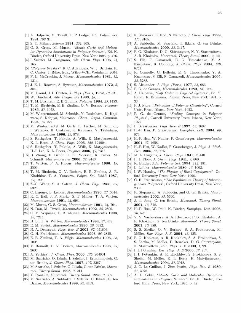
26

[1] A. Halperin, M. Tirrell, T. P. Lodge, Adv. Polym. Sci.1991 100 31.

[2] S. T. Milner, Science 1991, 251, 905.[3] G. S. Grest, M. Murat, “Monte Carlo and Molecu-

lar Dynamics Simulations in Polymer Science”, Ed. K.Binder, Oxford University Press, New York 1995, p. 476.

[4] I. Szleifer, M. Carignano, Adv. Chem. Phys. 1996, 94,165.

[5] “Polymer Brushes”, R. C. Advincula, W. J. Brittain, K.C. Caster, J. Ruhe, Eds., Wiley-VCH, Weinheim, 2004.

[6] F. L. McCrackin, J. Mazur, Macromolecules 1981, 14,1214.

[7] J. E. L. Roovers, S. Bywater, Macromolecules 1972, 5,384.

[8] M. Daoud, J. P. Cotton, J. Phys. (Paris) 1982, 43, 531.[9] W. Burchard, Adv. Polym. Sci 1983, 48, 1.

[10] T. M. Birshtein, E. B. Zhulina, Polymer 1984, 25, 1453.[11] T. M. Birshtein, E. B. Zhulina, O. V. Borisov, Polymer

1986, 27, 1078.[12] M. Wintermantel, M. Schmidt, Y. Tsukahara, K. Kaji-

wara, S. Kahjiya, Makromol. Chem., Rapid. Commun.1994, 15, 279.

[13] M. Wintermantel, M. Gerle, K. Fischer, M. Schmidt,I. Wataoka, H. Urakawa, K. Kajiwara, Y. Tsukahara,Macromolecules 1996, 29, 978.

[14] S. Rathgeber, T. Pakula, A. Wilk, K. Matyjaszewski,K. L. Beers, J. Chem. Phys. 2005, 122, 124904.

[15] S. Rathgeber, T. Pakula, A. Wilk, K. Matyjaszewski,H.-I. Lee, K. L. Beers, Polymer 2006, 47, 7318.

[16] B. Zhang, F. Grohn, J. S. Pedersen, K. Fisher, M.Schmidt, Macromolecules 2006, 39, 8440.

[17] T. Witten, P. A. Pincus, Macromolecules 1986, 19,2509.

[18] T. M. Birshtein, O. V. Borisov, E. B. Zhulina, A. R.Khokhlov, T. A. Yurasova, Polym. Sci. USSR 1987,29, 1293.

[19] Z.-G. Wang, S. A. Safran, J. Chem. Phys. 1988, 89,5323.

[20] C. Ligoure, L. Leibler, Macromolecules 1990, 23, 5044.[21] R. C. Ball, J. F. Marko, S. T. Milner, T. A. Witten,

Macromolecules 1991, 24, 693.[22] M. Murat, G. S. Grest, Macromolecues 1991, 24, 704.[23] N. Dan, M. Tirrell, Macromolecules 1992, 25, 2890.[24] C. M. Wijmans, E. B. Zhulina, Macromolecules 1993,

26, 7214.[25] H. Li, T. A. Witten, Macromolecules 1994, 27, 449.[26] E. M. Sevick, Macromolecules 1996, 29, 6952.[27] N. A. Denesyuk, Phys. Rev. E 2003, 67, 051803.[28] G. H. Fredrickson, Macromolecules 1993, 26, 2825.[29] E. B. Zhulina, T. A. Vilgis, Macromolecules 1995, 28,

1008.[30] Y. Rouault, O. V. Borisov, Macromolecules 1996, 29,

2605.[31] A. Yethiraj, J. Chem. Phys. 2006, 125, 204901.[32] M. Saariaho, O. Ikkala, I. Szleifer, I. Erukhimovich, G.

ten Brinke, J. Chem. Phys. 1997, 107, 3267.[33] M. Saariaho, I. Szleifer, O. Ikkala, G. ten Brinke, Macro-

mol. Theory Simul. 1998, 7, 211.[34] Y. Rouault, Macromol. Theory Simul. 1998, 7, 359.[35] M. Saariaho, A. Subbotin, I. Szleifer, O. Ikkala, G. ten

Brinke, Macromolecules 1999, 32, 4439.

[36] K. Shiokawa, K. Itoh, N. Nemoto, J. Chem. Phys. 1999,111, 8165.

[37] A. Subbotin, M. Saariaho, I. Ikkala, G. ten Brinke,Macromolecules 2000, 33, 3447.

[38] P. G. Khalatur, D. G. Shirvanyanz, N. Y. Starovoitovo,A. R. Khokhlov, Macromol. Theory Simul. 2000, 9, 141.

[39] S. Elli, F. Ganazzoli, E. G. Timoshenko, Y. A.Kuznetsov, R. Connolly, J. Chem. Phys. 2004, 120,6257.

[40] R. Connolly, G. Bellesia, E. G. Timoshenko, Y. A.Kuznetsov, S. Elli, F. Ganazzoli, Macromolecules 2005,38, 5288.

[41] S. Alexander, J. Phys. (Paris) 1977, 38, 983.[42] P. G. de Gennes, Macromolecules 1980, 13, 1069.[43] A. Halperin, “Soft Order in Physical Systems”, Ed. Y.

Rabin, R. Bruinsma, Plenum Press, New York 1994, p.33

[44] P. J. Flory, “Principles of Polymer Chemistry”, CornellUniv. Press, Ithaca, New York, 1953.

[45] P. G. de Gennes, “Scaling Concepts in PolymerPhysics”, Cornell University Press, Ithaca, New York,1979.

[46] P. Grassberger, Phys. Rev. E 1997, 56, 3682.[47] H.-P. Hsu, P. Grassberger, Europhys. Lett. 2004, 66,

874.[48] H.-P. Hsu, W. Nadler, P. Grassberger, Macromolecules

2004, 37, 4658.[49] H.-P. Hsu, W. Nadler, P. Grassberger, J. Phys. A: Math.

Gen. 2005, 38, 775.[50] M. L. Huggins, J. Chem. Phys. 1941, 9, 440.[51] P. J. Flory, J. Chem. Phys. 1941, 9, 660.[52] K. Binder, Adv. Polymer Sci. 1994, 112, 181.[53] L. Leibler, Macromolecules 1980, 13, 1602.[54] I. W. Hamley, “The Physics of Block Copolymers”, Ox-

ford University Press, New York, 1998.[55] G. H. Fredrickson, “The Equilibrium Theory of Inhomo-

geneous Polymers”, Oxford University Press, New York,2006.

[56] R. Stepanyan, A. Subbotin, and G. ten Brinke, Macro-molecules 2002, 35, 5640.

[57] J. de Jong, G. ten Brinke, Macromol. Theory Simul.2004, 13, 318.

[58] H.-P. Hsu, W. Paul, K. Binder, Europhys. Lett. 2006,76, 526.

[59] V. V. Vasilevskaya, A. A. Klochkov, P. G. Khalatur, A.R. Khokhlov, G. ten Brinke, Macromol. Theory Simul.2001, 10, 389.

[60] S. S. Sheiko, O. V. Borisov, S. A. Prokhorova, M.Moller, Eur. Phys. J. E. 2004, 13, 125.

[61] P. G. Khalatur, A. R. Khokhlov, S. A. Prokhorova, S.S. Sheiko, M. Moller, P. Reineker, D. G. Shirvanyanz,N. Starovoltova, Eur. Phys. J. E 2000, 1, 99.

[62] I. I. Potemkin, Eur. Phys. J. E 2003, 12, 207.[63] I. I. Potemkin, A. R. Khokhlov, S. Prokhorova, S. S.

Sheiko, M. Moller, K. L. Beers, K. Matyijaszewski,Macromolecules 2004, 37, 3918.

[64] J. C. Le Guillou, J. Zinn-Justin, Phys. Rev. B 1980,21, 3976.

[65] A. D. Sokal, “Monte Carlo and Molecular DynamicsSimulations in Polymer Science”, Ed. K. Binder, Ox-ford Univ. Press, New York, 1995, p. 47.

27

[66] T. Kreer, S. Metzger, M. Muller, K. Binder, J.Baschnagel, J. Chem. Phys. 2004, 120, 4012.

[67] S. T. Milner, T. A. Witten, M. Cates, Macromolecules1988, 21, 2610.

[68] A. M. Skvortsov, A. A. Gorbunov, I. V. Pavlushkov, E.B. Zhulina, O. V. Borisov, V. A. Priamitsyn, Polym.Sci USSR 1988, 30, 1706.

[69] E. B. Zhulina, O. V. Borisov, V. A. Pryamitsyn, T. M.Birshtein, Macromolecules 1991, 24, 140.

[70] J. Wittmer, A. Johner, J. F. Joanny, K. Binder, J.Chem. Phys. 1994, 101, 4379.

[71] T. Cosgrove, T. Heath, B. van Lent, F. Leermakers, J.Scheutjens, Macromolecules 1987, 20, 1692.

[72] C. M. Wijmans, J. M. H. M. Scheutjens, E. B. Zhulina,Macromolecules 1992, 25, 2657.

[73] C. M. Wijmans, E. B. Zhulina, G. J. Fleer, Macro-molecules 1994, 27, 3238.

[74] R. R. Netz, M. Schick, Macromolecules 1998, 31, 5105.[75] M. Manghi, M. Aubouy, C. Gay, C. Ligoure, Eur. Phys.

J. E 2001, 5, 519.[76] E. B. Zhulina, T. M. Birshtein, O. V. Borisov, Eur.

Phys. J. E 2006, 20, 243.[77] M. Murat, G. S. Grest, Macromolecules 1989, 22, 4054.[78] A. Chakrabarti, R. Toral, Macromolecuels 1990, 23,

2016.[79] P. Y. Lai, K. Binder, J. Chem. Phys. 1991, 95, 9288.[80] G. S. Grest, M. Murat, Macromolecules 1993, 26, 3108.[81] G. S. Grest, Macromolecules 1994, 27, 418.[82] D. I. Dimitrov, A. Milchev, K. Binder, J. Chem. Phys.

2006, 125, 034905.[83] D. I. Dimitrov, A. Milchev, K. Binder, D. W. Heermann,

Macromol. Theory Simul. 2006, 15, 573.[84] K. Kremer, K. Binder, Computer Phys. Repts. 1988, 7,

259.[85] K. Binder, “Monte Carlo and Molecular Dynamics Sim-

ulations in Polymer Science”, Ed. K. Binder, OxfordUniv. Press, New York 1995, p. 1.

[86] K. Binder, J. Baschnagel, M. Muller, “Simulation Meth-ods for Polymers”, Ed. M. J. Kotelyanskii, D. N.Theodorou, M. Dekker, New York 2004, p. 125.

[87] H.-P. Hsu, P. Grassberger, AIP Conf. Proc. 2004, 690,384.

[88] H. Frauenkron, P. Grassberger, and W. Nadler, e-printcond-mat/9806321 1998.

[89] H. Frauenkron, M. S. Causo, P. Grassberger, Phys. Rev.E 1999, 59, R16.

[90] H.-P. Hsu, W. Nadler, P. Grassberger, Macromolecules2004, 37, 4658.

[91] M. N. Rosenbluth, A. W. Rosenbluth, J. Chem. Phys.

1955, 23, 356.[92] M. Doi, S. F. Edwards, “Theory of Polymer Dynamics”,

Clarendon Press, Oxford, 1986.[93] D. Frenkel, G. C. A. M. Mooij, B. Smit, J. Phys.: Con-

dens. Matter 1992, 4, 3053.[94] K. Ohno, K. Binder, J. Stat. Phys. 1991, 64, 781.[95] K. Ohno, T. Sakamoto, T. Minagawa, Y. Okabe,

Macromlecules 2007, 40, 723.[96] I. Carmesin, K. Kremer, Macromolecules 1988, 21,

2819.[97] H.-P. Hsu, P. Grassberger, J. Chem. Phys. 2004, 120,

2034.[98] M. Daoud, P. G. de Gennes, J. Phys. (France) 1977,

38, 85.[99] A. Milchev, K. Binder, Eur. Phys. J. B 1998, 3, 477.

[100] “Phase transitions and Critical Phenomena”, Vol 1.Eds. C. Domb, M. S. Green, Academic Press, New York,1971.

[101] R. J. Baxter, “Exactly Solved Models in Statistical Me-chanics”, Academic Press, New York, 1982.

[102] J. L. Richard, G. Sarma, J. Phys. C 1981, 14, L617.[103] M. E. Fisher, V. Privman, Phys. Rev. B 1975, 32, 477.[104] “Finite Size Scaling and Numerical Simulation of Sta-

tistical Systems”, Ed. V. Privman, World Scientific, Sin-gapore, 1990.

[105] K. Binder, “Computational Methods in Field Theory”,Eds. H. Gausterer, C. B. Lang, Springer, Berlin, 1992,p. 59.

[106] J. Zinn-Justin, Phys. Repts. 2001, 344, 159.[107] K. Binder, A. P. Young, Rev. Mod. Phys. 1986, 58, 801.[108] K. Binder, W. Kob, “Glassy Materials and Disordered

Solids. An Introduction to Their Statistical Mechanics”,World Scientific, Singapore, 2005.

[109] A. Werner, F. Schmid, K. Binder, M. Muller, Macro-molecules 1996, 29, 8241.

[110] N. A. Desenyuk, Phys. Rev. E 2003, 68, 031803.[111] T. Stephan, S. Muth, M. Schmidt, Macromolecules

2002, 35, 9857.[112] C. Li, N. Gunari, K. Fischer, A. Janshoff, M. Schmidt,

Angew. Chem. Int. Ed. 2004, 43, 1101.[113] L. Wenning, M. Muller, K. Binder, Europhys. Lett.

2005, 71, 639.[114] M. Muller, Phys. Rev. E 2002, 65, 030802.[115] P. Y. Lai, K. Binder, J. Chem. Phys. 1992, 97, 586.[116] G. S. Grest, M. Murat, Macromolecules 1993, 26, 3108.[117] C. Yeung, A. C. Balazs, D. Jasnow, Macromolecules

1993, 26, 1914.[118] H. Tang, I. Szleifer, Europhys. Lett. 1994, 28, 19.