institute for research on poverty discussion paper no. · pdf fileinstitute for research on...

Institute for Research on Poverty Discussion Paper no. 1339-08

Expanding Wallets and Waistlines: The Impact of Family Income on the BMI of Women and Men

Eligible for the Earned Income Tax Credit

Maximilian D. Schmeiser Department of Consumer Science and Institute for Research on Poverty

University of Wisconsin–Madison E-mail: [email protected]

July 2008

IRP Publications (discussion papers, special reports, and the newsletter Focus) are available on the Internet. The IRP Web site can be accessed at the following address: http://www.irp.wisc.edu

Abstract

The rising rate of obesity has reached epidemic proportions and is now one of the most serious

public health challenges facing the US. However, the underlying causes for this increase are unclear. This

paper examines the effect of family income changes on body mass index (BMI) and obesity using data

from the National Longitudinal Survey of Youth 1979 cohort. It does so by using exogenous variation in

family income in a sample of low-income women and men. This exogenous variation is obtained from the

correlation of their family income with the generosity of state and federal Earned Income Tax Credit

(EITC) program benefits. Income is found to significantly raise the BMI and probability of being obese

for women with EITC-eligible earnings, and have no appreciable effect for men with EITC-eligible

earnings. The results imply that the increase in real family income from 1990 to 2002 explains between

10 and 21 percent of the increase in sample women’s BMI and between 23 and 29 percent of their

increased obesity prevalence.

JEL classifications: I1; H2 Keywords: Obesity; Body Mass Index; EITC

Expanding Wallets and Waistlines: The Impact of Family Income on the BMI of Women and Men

Eligible for the Earned Income Tax Credit

I. INTRODUCTION

The weight of Americans has increased significantly over the past 30 years, with the average

weight of men and women between the ages of 20 and 74 increasing by 9 percent and 12 percent,

respectively, between 1971 and 2002 (Ogden et al., 2004). This trend understates increases in the level of

obesity, defined as a body mass index1 (BMI) greater than or equal to 30, which has more than doubled in

the past 30 years. Among twenty- to seventy-four-year-olds, obesity prevalence increased from 15 percent

in 1979–1980 to over 30 percent in 1999–2002 (Flegal et al., 2002; Hedley et al., 2004). Excessive

fatness, or obesity, is now recognized as one of the most serious public health challenges facing the

United States (U.S. DHHS, 2001) and other industrialized countries (International Obesity Task Force,

2005).

The concerns about the increasing prevalence of obesity are founded in the association between

obesity and adverse health outcomes and increased health expenditures. Obesity has been linked to an

increased risk of numerous comorbidities, including high blood pressure, high blood cholesterol, type 2

diabetes mellitus, coronary heart disease, osteoarthritis, asthma, and gallbladder disease (Must et al.,

1999; Mokdad et al., 2003). Moreover, obesity has been found to significantly lower life expectancy,

particularly among young adults (Fontaine et al., 2003). With the rise in obesity, poor diet and physical

inactivity have now become the number two preventable causes of death in the United States, behind only

tobacco in the number of lives claimed each year (Mokdad et al., 2004; 2005).

The numerous obesity-related illnesses invariably lead obese persons to have higher medical

expenditures than the non-obese. Finkelstein et al. (2003) estimate that annual medical expenditures for

obese persons are on average 37 percent higher than for non-obese persons. They also estimate that

1Body mass index is defined as weight in kilograms divided by height in meters squared or weight in pounds divided by height in inches squared multiplied by 703 (NIH, 1998).

2

obesity-related illnesses are responsible for 9.1 percent of U.S. health expenditures, or $92.6 billion (2002

dollars), and that half of these expenditures are covered by Medicare and Medicaid. Thus obesity and

obesity-related illnesses also have implications for taxpayers and state and federal budgets. Aside from

increasing Medicare and Medicaid expenditures, the high prevalence of obesity may have important

implications for the solvency of the social security system, as obesity has been linked to the decision to

take early Social Security retirement benefits (Burkhauser and Cawley, 2006).

Researchers have identified several factors that contribute to the rise in obesity including falling

food prices, technological innovation in food processing, increasing female labor force participation,

increasingly sedentary work, and reduced smoking (Lakdawalla and Philipson, 2002; Cutler et al., 2003;

Anderson et al., 2003; Chou et al., 2004). However, this research has largely ignored the role of rising

income. Studies that have examined the role of income2 on obesity within the United States have been

unable to account for the potential endogeneity and reverse causality between income and weight and

obesity prevalence. (See Conley and Glauber, 2005; and Cawley, 2004).

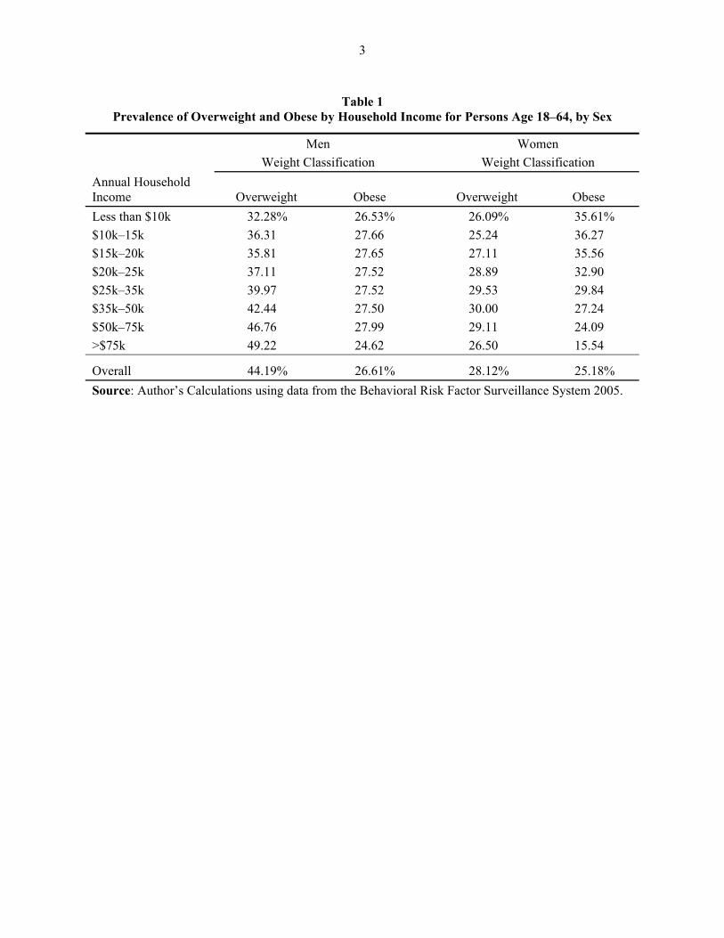
As shown in Table 1, there exists a negative correlation between income and obesity prevalence

for women. As such, public programs to increase income or food budgets may be naively viewed as one

potential policy mechanism for decreasing obesity. Understanding the causal association between income

and BMI would contribute to more effective public-health interventions, and if income positively affects

obesity rates, avert counterproductive policies.

Income may directly affect weight through its effect on the consumption and expenditure of

calories. Increased income may cause a worker’s weight to increase in two ways. The worker may use the

additional to income to purchase additional calories for home consumption, or substitute restaurant meals,

which are generally more calorie-dense than food consumed at home (Lin and Frazão, 1997). Changes in

wages may also indirectly alter weight through their impact on labor supply and time allocation. To the

2Previous studies attempting to explain the rise in weight and obesity have used various measures of income including family income (Anderson et al., 2003), household income (Lakdawalla and Philipson, 2002; Chou et al., 2004; Quintana-Domeque, 2005), Social Security income (Cawley et al., 2007), and wage rate (Lakdawalla and Philipson, 2002).

3

Table 1 Prevalence of Overweight and Obese by Household Income for Persons Age 18–64, by Sex

Men Women Weight Classification Weight Classification Annual Household Income Overweight Obese Overweight Obese Less than $10k 32.28% 26.53% 26.09% 35.61% $10k–15k 36.31 27.66 25.24 36.27 $15k–20k 35.81 27.65 27.11 35.56 $20k–25k 37.11 27.52 28.89 32.90 $25k–35k 39.97 27.52 29.53 29.84 $35k–50k 42.44 27.50 30.00 27.24 $50k–75k 46.76 27.99 29.11 24.09 >$75k 49.22 24.62 26.50 15.54

Overall 44.19% 26.61% 28.12% 25.18% Source: Author’s Calculations using data from the Behavioral Risk Factor Surveillance System 2005.

4

extent that the calories expended in labor differ from the calories expended in leisure, changes in labor

supply will alter weight (Lakdawalla and Philipson, 2002). Increased labor supply may also increase

demand for convenience foods, which are more calorie-dense and thus increase weight (Chou et al.,

2004).

This paper estimates the causal impact of family income on BMI using a fixed effect instrumental

variables (IV) estimation strategy. It does so within a panel dataset of women and men in which

exogenous variation in family income is identified using differences in the level of their state Earned

Income Tax Credit (EITC) supplement at a point in time, and variations in the value of federal and state

EITC benefits over time. The IV results indicate that income has a positive effect on BMI and the

probability of being obese for low-income women, with the effect of income on BMI increasing over the

BMI distribution.

This paper proceeds in the following manner. The second section of this paper reviews the

literature on income and BMI. The third section provides background on the EITC program. The fourth

section details the data used in the analysis. The fifth section outlines the identification strategy and

empirical methods, while the sixth section provides the empirical results. The paper concludes with a

discussion of the results.

II. RELATED STUDIES

Cross-nationally, a positive correlation between income and BMI exists, with the prevalence of

obesity being far greater in developed countries than less developed countries, and obesity rates

increasing as per capita incomes increase (Seidell and Rissanen, 1998; WHO, 2003; Swinburn et al.,

2004). Within less developed nations, those of higher socioeconomic status are more likely to be obese

(Sobal and Stunkard, 1989). However, for women in the United States, the opposite is true: the prevalence

of obesity is lower among those of higher socioeconomic status. For men in the United States, obesity

(BMI ≥ 30) prevalence is relatively constant across family income, while the prevalence of overweight

(25 ≤ BMI < 30) increases with household income. Table 1 reports clinical weight classification by

5

household income for American men and women based on data from the 2005 Centers for Disease

Control and Prevention Behavioral Risk Factor Surveillance System (BRFSS).3 Table 1 shows that

obesity rates for men are approximately 27 percent across household income categories. For women, a

strong negative correlation between household income and obesity is apparent, with the prevalence of

obesity for those women with household incomes less than $15,000 per year at 36 percent being more

than twice that of women with household incomes of more than $75,000 per year at 16 percent.

Correlational estimates of the relationship between income and BMI may not accurately capture

the causal relationship, as there are numerous unobserved factors which could be simultaneously affecting

income and BMI, including genetics, environment, and health status. In addition, income may be causally

affected by BMI; Cawley (2004) finds evidence that for obese white women, weight lowers wages.

Failure to account for endogeneity or reverse causality between income and BMI would render OLS

estimates biased and inconsistent. In order to overcome these concerns, several studies have taken an IV

approach to estimating the causal impact of income on BMI.

Using the European Community Household Panel (ECHP), Quintana-Domeque (2005) makes use

of the exogenous variation in family income resulting from receipt of inheritance, gifts, or lottery

winnings of 2000 Euros or more to instrument for income. Results show that, of the 9 nations included in

the survey, statistically significant estimates of the impact of income on BMI are only found for Denmark

and Italy in the case of women, and for Finland in the case of men. In all three of these cases the

estimated BMI-income elasticity is found to be negative. Unfortunately, the instrument is quite weak with

an F-statistic well below 10 in the first stage.

Cawley et al. (2007) exploit the Social Security “notch,” which unintentionally provided double

indexation against inflation for certain birth cohorts—leading those in the notch to have higher Social

Security incomes than those not affected by the notch—as an instrument for Social Security income.

3BRFSS data are used as opposed to National Longitudinal Survey of Youth 1979 Cohort (NLSY79) data, as, for a given year, the NLSY79 only captures persons within a 9 year age range. For example, in the 2002 wave there are persons between the ages of 37 and 45. However, the cross-tabulation of income and clinical weight classification is qualitatively similar using the NLSY79 data.

6

Though their instrument appears to be quite powerful, they are unable to identify any statistically

significant relationship between additional Social Security income and BMI for either men or women.

However, given the instrument used, the results represent a local average treatment effect for a relatively

small segment of the population: the low-income elderly.

This study significantly expands the population for which causal estimates of the effect of family

income on BMI have been generated. This study contributes to the existing literature by generating causal

estimates of the impact of family income on BMI and the probability of being obese for women and men

eligible for the Earned Income Tax Credit (EITC). While changes in the federal EITC program have

previously been used to estimate the impact of income on child development (Dahl and Lochner, 2005) it

introduces an additional source of exogenous variations in income from the state EITC programs.

III. BACKGROUND ON THE EITC PROGRAM

The federal EITC was originally enacted in 1975 to offset the payroll taxes of workers with low

earnings. Since then, it has been expanded in scope and size in 1986, 1990, and most recently in 1993.

Targeted at low-income working families, the EITC is now the nation’s largest antipoverty program for

non-elderly individuals, with expenditures of nearly $41.5 billion and over 22 million recipients in tax

year 2005 (Center on Budget and Policy Priorities, 2007). The EITC subsidizes wages of low-income

earners conditional on their participation in the labor force. It provides an incentive for those not working

to enter the labor force, but may increase or decrease hours worked by the employed depending on the

relative size of the uncompensated and income elasticities of labor supply.

Figure 1 displays the three distinct earnings ranges over which the EITC operates for tax year

2007. For a single, childless individual, a credit rate of 7.65 percent is applied to the first $5,590 in labor

earnings, for a maximum benefit of $428. For a family with one child, a credit rate of 34 percent is

applied to earnings up to $8,390, for a maximum benefit of $2,853; while for a family with two or more

children, a credit rate of 40 percent is applied to earnings up to $11,790, for a maximum benefit of

$4,716. Beginning at earnings of $7,000 for single, childless individuals, and $15,390 for both families

Figure 1Credit Regions of the Federal EITC Program for Tax Year 2007

0

500

1000

1500

2000

2500

3000

3500

4000

4500

5000

0 2500 5000 7500 10000 12500 15000 17500 20000 22500 25000 27500 30000 32500 35000 37500

Annual Family Income ($)

EITC

Pay

men

t ($)

No Children One Child Two or More Children

B

B

A

C

C

D DD

B C

8

with one eligible child and families with two or more eligible children, the maximum benefits are reduced

at a rate of 7.65 percent, 15.98 percent, and 21.06 percent, respectively. Federal EITC benefits are

completely phased out at $12,590 for single, childless individuals; $33,241 for families with one eligible

child; and $37,783 for families with two or more eligible children. For married persons filing jointly, the

break-even point is extended by $2,000 in an attempt to partially offset the marriage disincentive.

In addition to the federal EITC, since January 2006, 19 states and the District of Columbia have

operated their own supplemental EITC programs. The value of a taxpayer’s state EITC is generally set as

a fraction of their federal EITC.4 The state credits vary significantly in terms of their generosity relative to

the federal EITC, and not all are refundable.5

This paper exploits the exogenous variation in income resulting from the changes in labor supply

that are brought about by the expansion of both federal and state EITC programs in order to identify the

effect of income on BMI or obesity. Given that individual fixed effects are used, the identifying variation

is derived from individuals altering their labor supply decision over time in response to changes in the

maximum combined federal and state EITC benefit for which they were eligible in the previous calendar

year.

IV. DATA

This paper uses data from the restricted-access National Longitudinal Survey of Youth 1979

cohort (NLSY79). The NLSY79 is a nationally representative sample of individuals who were between

the ages of 14 and 21 on December 31, 1978. The first wave of the NLSY79 contained information on

12,686 individuals, including an oversample of poor and minority families. NLSY79 interviews were

conducted annually from 1979 to 1994, and have been conducted biennially since 1994. This paper makes

4Minnesota’s EITC is not linked to the federal EITC program. 5As of January 2006, State EITC programs exist in: Colorado; Delaware; D.C.; Illinois; Indiana; Iowa;

Kansas; Maine; Maryland; Massachusetts; Minnesota; New England; New Jersey; New York; Oklahoma; Oregon; Rhode Island; Vermont; Virginia; and Wisconsin.

9

use of the 1990 through 2002 waves of the NLSY79 (Tax Years 1989 through 2001), as the major

changes in the Earned Income Tax Credit program occurred beginning in tax year 1991.6

The outcome of interest, BMI, and the clinical weight classifications derived from BMI, are

constructed using self-reported weight and height data. A respondent’s weight is asked in each wave of

the NLSY79 between 1990 and 2002, with the exception of 1991, while height is asked in only the 1981,

1982, and 1985 waves of the NLSY79. In order to construct BMI for each wave from 1990 through 2002,

excluding 1991, weight from the relevant wave of the NLSY79 is used in conjunction with the 1985

height of respondents.7 Given that self-reported weight and height are known to contain measurement

error, the self-reported values from the NLSY79 are adjusted by race and gender following Cawley and

Burkhauser (2006).8 As pregnancy distorts a woman’s weight, 351 pregnant women are excluded from

the sample at the time of their pregnancy.

Table 2 presents mean adjusted BMI for the EITC eligible sample of women and men employed

in the regression in the first and last year of the sample period (1990 and 2002), as well as the prevalence

of overweight/obese (BMI ≥ 25) and obesity (BMI ≥ 30) calculated using adjusted BMI. Between 1990

and 2002, the mean BMI of sample women increased from 26.95 to 29.76, while for men, the mean BMI

increased from 27.84 to 29.43. With the increase in BMI, the prevalence of obesity for women increased

from 25.17 percent in 1990 to 49.03 percent in 2002. For men, the prevalence of obesity increased from

28.99 percent in 1990 to 38.24 percent in 2002.

Data are also included on the various state-level characteristics identified by the previous

literature as contributing to the increased prevalence of obesity. To account for the effect of smoking on

BMI, data on the average price of a pack of cigarettes was obtained from various volumes of

6The 1991 wave of the NLSY79 is omitted as data on weight was not collected in that wave. 7As all respondents are at least 20 years of age in 1985 their height in 1985 should represent their final

adult height and remain constant through the end of the sample period examined here. 8The correlation between BMI and adjusted BMI and obesity prevalence and adjusted obesity prevalence

are both quite high, with coefficients of 0.99 and 0.90, respectively.

10

Table 2 Mean Adjusted BMI and Clinical Weight Classification by Year and Sex

1990

Adjusted BMI 2002

Adjusted BMI Mean BMI Women 26.95 29.76 Percent of Women Overweight/Obese (BMI ≥25) 54.05 69.31 Percent of Women Obese (BMI ≥30) 25.17 49.03 Mean BMI Men 27.84 29.43 Percent of Men Overweight/Obese (BMI ≥25) 66.22 80.62 Percent of Men Obese (BMI ≥30) 28.99 38.24

11

Orzechowski and Walker’s Tax Burden on Tobacco. These prices were adjusted to 2005 dollars using the

Bureau of Labor Statistics annual Consumer Price Index (CPI).

Since food prices in general, and the relative price of fast-food to home-cooked meals in

particular, are likely to affect weight, two corresponding state-level food price indices are constructed

following Chou et al. (2004). Data on fast-food meal prices and grocery food prices come from the

American Chamber of Commerce Researchers’ Association (ACCRA) Cost of Living Index, which is

published quarterly. The state-specific real fast-food meal price index was constructed from the price of a

McDonald’s Quarter-Pounder with Cheese, an 11″–12″ thin crust cheese pizza from Pizza Hut or Pizza

Inn, and a thigh and drumstick from Kentucky Fried Chicken or Church’s. The real grocery food price

index used the prices of all 22 grocery food items available in the ACCRA Cost of Living Index9.

The NLSY79 sample is divided into those who are eligible for the EITC and those who are not by

imputing federal EITC eligibility using the National Bureau of Economic Research (NBER) TAXSIM

program. The TAXSIM program is an online tax simulation for calculating liabilities under U.S. federal

and state income tax laws from individual data for tax years 1960 through 2013. The TAXSIM program

determined EITC eligibility for the NLSY79 sample on the basis of the labor income of the respondent

and his or her spouse, social security income, unemployment insurance income, the respondent’s marital

status, and the number of children under age 18 in the family. The data from the NLSY79 and TAXSIM

determined EITC eligibility and were merged with the characteristics of the federal EITC program from

the House Ways and Means Committee Green Book, 2004, and the characteristics of state EITC programs

from Leigh (2004).

9These 22 items are: a pound of T-Bone Steak; a pound of ground beef; a pound of Jimmy Dean or Owens brand pork sausages; a pound of frying chicken; a 6 oz can of Starkist or Chicken of the Sea chunk light tuna; half a gallon of whole milk; one dozen Grade A large eggs; one pound of Blue Bonnet or Parkay brand margarine; 8 oz canister of Kraft brand grated parmesan cheese; 10 lbs white or red potatoes; a pound of bananas; a head of iceberg lettuce; a 24 oz loaf of white bread; an 11.5 oz can of Maxwell House, Hills Brothers, or Folgers coffee; a 4 pound sack of sugar; an 18 oz box of Kellogg’s Corn Flakes or Post’s Toasties; a 15–17 oz can of Del Monte or Green Giant brand sweet peas; a 14.5 oz can of Hunt’s or Del Monte tomatoes; a 29 oz can of peaches; a 12 oz can of Minute Maid frozen orange juice; a 16 oz bag of frozen whole kernel corn; and a 2 liter bottle of Coca Cola.

12

Changes in wages could have both direct and indirect effects on weight through changes in

consumption and changes in labor supply. Given that the identification strategy employed in this paper

relies on exogenous changes in labor supply to identify the effect of family income on BMI, this paper

restricts the sample to those individuals with their own labor earnings that make them eligible for the

EITC.

Restricting the sample to those with their own EITC eligible labor earnings and those women

who are not pregnant, combined with missing values for height, weight, income, and other variables of

interest, all waves of the NLSY79 from 1990 to 2002 included in this analysis yield a final value of 4,769

person-year observations on 1,223 women, and 2,869 person-year observations on 818 men.

V. EMPIRICAL METHODS

V.1. Identification Strategy

Over the course of the 1990s, the federal government significantly expanded the EITC program.

The maximum EITC benefit available to taxpayers with two or more qualifying children increased in real

terms (2005 dollars) from $1,425 in 1990 to $4,410 in 2000. From tax year 1985 through tax year 1990, a

single phase-in rate of 14.0 percent was applied to all taxpayers with qualifying children; however, in

1991 different phase-in rates were applied to taxpayers with one qualifying child and taxpayers with two

or more qualifying children. These respective phase-in rates subsequently increased at different rates. In

tax year 1994, a small maximum credit of $306 ($403 in 2005 dollars) was extended to taxpayers with no

qualifying children, and different phase-in, plateau, and phase-out regions were established for taxpayers

with no qualifying children, one qualifying child, or two or more qualifying children.

In 1989, the first year of analysis, only 3 states (Rhode Island, Vermont, and Wisconsin) had state

EITC programs in place. By 2002, the last year of analysis, 15 states and the District of Columbia had

EITC programs in place. Moreover, between 1989 and 2002, many states adjusted the generosity of their

credits relative to the federal credit both upwards and downwards.

13

This paper uses exogenous variation in EITC benefits to identify the causal effect of income on

BMI or the prevalence of obesity. The instrument used is the maximum combined value of federal and

state EITC benefits for which a family was eligible, which varies by state, year, and number of children.

For example, an EITC eligible person with two children in New York State observed in the 2002 wave of

the NLSY79 would have been eligible for a maximum federal EITC benefit for tax year 2001 of $4,420

(2005 dollars) and a maximum state EITC benefit of $1,326 (2005 dollars), for a combined maximum

benefit of $5,746.

In order for the maximum value of EITC benefits for which a family is eligible to be a valid

instrument, it must be uncorrelated with the error in the second stage (the unobserved determinants of

BMI), but correlated with family income. There is no reason to suspect that the large nonlinear changes in

the federal EITC program that Congress enacted over the last 20 years—shown in Figure 2 and Table 3—

should be related to changes in an individual’s weight. Moreover, a large body of literature has

established a significant relationship between expansions of the EITC and changes in labor supply, and

thus income.10 As expected, the EITC is strongly predictive of family income in the EITC eligible

populations, with first stage F-statistics well above 10.

Ideally, an instrument for family income would be available for the entire population, allowing

for estimates of the causal effect of family income on BMI generally. Instead, by using the maximum

value of EITC benefits for which a family is eligible as an instrument, the population examined here is

restricted to those eligible for the EITC program. However, with over 22 million EITC claims filed for tax

year 2005, the EITC eligible population comprises tens of millions of low-income persons—a highly

policy-relevant group. With 132.8 million individual tax returns filed for tax year 2005, EITC claimants

compose 16.6 percent of all individual tax returns (IRS, 2007).

10See Hotz and Scholz (2003) for a review of the literature on the effect of the EITC on employment and hours worked.

Figure 2Maximum Value of Federal EITC Benefits (2005 $), by Eligible Children

0

500

1,000

1,500

2,000

2,500

3,000

3,500

4,000

4,500

5,000

1989 1990 1991 1992 1993 1994 1995 1996 1997 1998 1999 2000 2001

Tax Year

2005

Dol

lars

No Children One Child Two or More Children

15

Table 3 Federal Earned Income Tax Credit Maximum Benefit Amount Tax Year 1989–2001

Tax Year Maximum Benefit

(Unadjusted $) Maximum Benefit

(2005 $) 1989

No children 0 0 One child 910 1,433 Two children 910 1,433

1990 No children 0 0 One child 953 1,424 Two children 953 1,424

1991 No children 0 0 One child 1,192 1,709 Two children 1,235 1,771











Source: IRS (www.irs.gov) and author’s calculations.

16

V.2. Estimation

In order to identify causal effects, BMI and the probability of being obese is estimated using two-

stage least squares and two-stage quantile regressions with individual level fixed effects. Individual level

fixed effects are included in order to control for all time-invariant individual level determinants of BMI

and obesity. The model used to estimate the effect of family income on the two measures of fatness (F)

used in this analysis, BMI or the prevalence of obesity, takes the form:

iststititist PXIF εβββα ++++= 321 (1)

where i indexes individuals, s indexes states, and t indexes time. The dependent variable Fist is the

adjusted Body Mass Index or an indicator for the obesity status of respondent i at time t, Iit is the

respondent’s total family earnings for the previous calendar year in thousands of dollars, Xit is a vector of

individual level control variables, Pst is a vector of state level control variables and εist is the error term.

The vector of individual level controls, Xit, includes age, age squared, foreign born status,

race/ethnicity, marital status, number of own children, number of adults in the household, education,

residence in a metropolitan statistical area (MSA), receipt of food stamps, receipt of AFDC/TANF,

Armed Forces Qualifying Test (AFQT) percentile score, and work limitation status. With the inclusion of

individual fixed effects, race/ethnicity, foreign born status, education, AFQT score, and residence in an

MSA are dropped from the model. The vector of state level control variables, Pst, includes the average

price of a pack of cigarettes, the fast-food price index, and the grocery food price index. Given the

upward trend in BMI and obesity over the 1990s, a time trend and year dummies were alternately

included in the model.

In order to disentangle the effect of hours of work and occupational strenuousness, subsequent

specifications also include the number of hours worked in the previous calendar year and the Lakdawalla

and Philipson (2002) measure of occupational strenuousness. Moreover, given that the coefficient on

17

hours of work may suffer from the same biases as income, one specification of the model instruments for

both income and hours worked used as instruments the maximum value of the EITC and its one-year lag.

An IV estimation strategy is used to address the potential endogeneity and reverse causality in the

relationship between income and BMI. The first stage of the IV regression takes the form:

iststitistist PXEITCI υϕφγδ ++++= , (2)

where the dependent variable Iit is an individual’s total family income for the previous calendar year, and

the instrument is EITCist , the maximum value of the combined federal and state Earned Income Tax

Credit for which an individual was eligible in the previous tax year based on his or her number of

children. The maximum value of the EITC for the previous calendar year is used as opposed to the current

year’s value, as income reported in the NLSY79 is for the previous calendar year.

The second stage of the IV model is identical to model (1) except that family income I is now

replaced by its fitted value ^I from the first-stage regression yielding:

iststitistist PXIF εβββα ++++= 32

^

1 . (3)

As pointed out by Cawley et al. (2005) and Kan and Tsai (2004), changes in income may

differentially affect individuals at different points in the BMI distribution. Least squares-based methods

may provide limited information on the effect of income on BMI if these methods could potentially mask

large effects at either end of the BMI distribution. In order to explore the relationship between income and

BMI over different portions of the BMI distribution two different methods are employed. The first is an

IV Quantile regression, which takes the form of model (3) but allows the estimation of different marginal

effects at various points in the BMI distribution. Here estimates are provided at the 10th, 25th, 50th, 75th,

and 90th percentiles of BMI.

The second method used to account for potential nonlinearity in the relationship between income

and BMI is to construct indicator variables for the clinical weight classification obese (BMI ≥30).

Estimates of the relationship between income and obesity are generated using an IV linear probability

model, which again takes the form of model (3).

18

VI. EMPIRICAL RESULTS

The negative correlation between income and BMI for women can be broken by controlling for

only a few standard demographic characteristics. Table 4 presents OLS estimates of the effect of family

income on BMI as several covariates are added to the regression. With just family income, or even

income and age and age squared in the regression, the coefficient on income is negative. However, with

the addition of race the coefficient on income becomes positive, and the addition of education further

increases the magnitude of the coefficient.

The least squares estimates of the impact of family income on BMI from the full model are

presented in Table 5 for EITC eligible men and Table 6 for EITC eligible women. The Quantile estimates

are then presented in Tables 7 and 8 for men and women, respectively. Lastly, the linear probability

estimates of the effect of income on obesity prevalence are presented in Table 9 for men and Table 10 for

women. Across all IV models and specifications there is no case where a statistically significant

relationship between income and BMI is found for men. Thus, the remainder of this paper focuses on the

effect of income on the BMI and obesity prevalence of women.

Table 6 presents the least squares estimates of the effect of family income on BMI for women

with EITC eligible labor earnings. In the OLS model, shown in column 1, an additional $1,000 of family

income is associated with an increase of roughly 0.02 BMI units. For the average woman in the sample, a

one unit increase in BMI is equivalent to gaining 5.8 pounds of weight.11 In column 2, individual fixed

effects are added to the OLS model, and yield an increase of roughly 0.01 BMI units for each additional

$1,000 in family incomes. Column 3 presents IV estimates with no fixed effects. Relative to the OLS

estimate with no fixed effects, the magnitude of the coefficient on family income increases significantly,

indicating that an additional $1,000 of family income is associated with an increase of roughly 0.14 BMI

11The average woman in the sample has an adjusted height of five feet, four inches, and an adjusted weight of 174 pounds in 2002. Using the formula BMI= weight (lb) / [height (in)]2 x 703 one BMI unit translates into 5.8 pounds of weight.

19

Table 4 Body Mass Index Regressions for Women

Independent Variable (1)

OLS (2)

OLS (3)

OLS (4)

OLS Family Income ($1,000s) -0.0036 -0.0094 0.0062 0.0127 (-0.35) (-0.92) (0.62) (1.24) Age and Age Squared X X X Race Dummies X X Education Dummies X

Sample Size 4,769 4,769 4,769 4,769 R-Squared 0.00 0.01 0.06 0.06 t statistics are in parentheses. Standard errors are clustered at the state level. *p< 0.10, **p< 0.05, and ***p< 0.01.

20

Table 5 Body Mass Index Regressions for Men with EITC Eligible Earnings

(1) (2) (3) (4) (5) (6) (7) (8) (9) (10) (11) (12) Independent Variable OLS OLS IV IV IV IV IV IV IV IV IV IV

Family Income ($1,000s) -0.0038 -0.0068 0.4587 0.0064 0.0103 0.007 -0.0055 -0.0041 0.0001 0.0036 0.0022 0.0053 (0.77) (1.33) (0.94) (0.23) (0.35) (0.23) (0.15) (0.10) 0.00 (0.13) (0.08) (0.18) Hours Worked in Previous Year -0.0002* -0.0002* 0.0005 0.0003 -0.0002 -0.0002 (1.75) (1.83) (0.43) (0.19) (1.55) (1.57) Occupational Strenuousness 0.0001 0.0001 (0.10) (0.32) Instrument for Hours X X Time Trend X X

X X

Year Dummies Individual FEs X X X X X X X X X X

Sample Size 2,869 2,869 2,869 2,869 2,869 2,869 2,869 2,869 2,869 2,869 2,869 2,869 R-Squared 0.12 0.13 0.13 0.13 0.13 0.14 0.07 0.11 0.14 0.14 0.14 0.14 First-Stage F-Statistic for Income 120.63 72.42 68.29 59.76 36.97 33.23 73.92 69.42 72.88 69.61 First-Stage F-Statistic for Hours 3.58 3.11 t statistics are in parentheses. Standard errors are clustered at the state level. *p< 0.10, **p< 0.05, and ***p< 0.01. The models also include individual characteristics variables and state characteristics variables.

21

Table 6 Body Mass Index Regressions for Women with EITC Eligible Earnings

(1) (2) (3) (4) (5) (6) (7) (8) (9) (10) (11) (12) Independent Variable OLS OLS IV IV IV IV IV IV IV IV IV IV

Family Income ($1,000s) 0.0197 0.0122** 0.1440* 0.1657** 0.1819** 0.1882* 0.3076 0.2385 0.1523** 0.1669* 0.2030*** 0.2206*** (1.83) (2.36) (1.92) (2.18) (2.12) (1.81) (0.87) (1.08) (2.01) (1.95) (3.02) (2.94)

-0.0004* -0.0004 -0.0036 -0.0022 -0.0004 -0.0005** Hours Worked in Previous Year (1.78) (1.53) (0.38) (0.26) (1.63) (2.48)

0.0002 0.0001 Occupational Strenuousness (0.73) (0.48)

Instrument for Hours X XX X

X X

Time Trend Year Dummies Individual FEs X X X X X X X X X X

Sample Size 4,769 4,769 4,769 4,769 4,769 4,769 4,769 4,769 4,769 4,769 4,769 4,769 R-Squared 0.14 0.12 0.12 0.11 0.12 0.12 0.11 0.11 0.14 0.14 0.14 0.14 First-Stage F-Statistic for

Income 112.39 20.49 17.41 12.30 11.10 8.10 19.83 16.90 29.06 25.42 First-Stage F-Statistic for

Hours 2.09 0.76 t statistics are in parentheses. Standard errors are clustered at the state level. *p< 0.10, **p< 0.05, and ***p< 0.01. The models also include individual characteristics variables and state characteristics variables.

22

Table 7 Body Mass Index Quantile Regressions for Men with EITC Eligible Earnings

(1) (2) (3) (4) (5) Independent Variable 10th Percentile 25th Percentile 50th Percentile 75th Percentile 90th Percentile

Family Income ($1,000s) 0.0001 -0.0086 -0.0117 -0.0099 0.0151 (0.01) (0.33) (0.66) (0.29) (0.37) Includes Hours Worked as Independent Variable No No No No No Family Income ($1,000s) 0.0011 -0.0032 -0.0122 -0.0023 0.0189 (0.03) (0.11) (0.61) (0.06) (0.42) Includes Hours Worked as Independent Variable Yes Yes Yes Yes Yes

Sample Size 2,869 2,869 2,869 2,869 2,869 t statistics are in parentheses. Standard errors are clustered at the state level. *p< 0.10, **p< 0.05, and ***p< 0.01. The models also include individual characteristics variables, state characteristics variables, and individual fixed effects.

23

Table 8 Body Mass Index Quantile Regressions for Women with EITC Eligible Earnings

(1) (2) (3) (4) (5) Independent Variable 10th Percentile 25th Percentile 50th Percentile 75th Percentile 90th Percentile

Family Income ($1,000s) 0.1117 0.1710** 0.1881*** 0.2370*** 0.2361** (1.06) (2.43) (3.26) (3.18) (1.98) Includes Hours Worked as Independent Variable No No No No No Family Income ($1,000s) 0.1201 0.1906** 0.2014*** 0.2428*** 0.2504** (1.04) (2.53) (3.13) (2.98) (1.98) Includes Hours Worked as Independent Variable Yes Yes Yes Yes Yes

Sample Size 4,769 4,769 4,769 4,769 4,769

t statistics are in parentheses. Standard errors are clustered at the state level. *p< 0.10, **p< 0.05, and ***p< 0.01. The models also include individual characteristics variables, state characteristics variables, and individual fixed effects.

24

Table 9 Obese Regressions for Men with EITC Eligible Earnings

(1) (2) (3) (4) (5) Independent Variable OLS OLS IV IV IV

Family Income ($1,000s) -0.001 -0.0014** 0.0058 0.0065 0.0058 (1.57) (1.99) (1.46) (1.51) (1.28) Hours Worked in Previous Year -0.0001* -0.0001* (1.91) (1.86) Occupational Strenuousness 0.0001 (0.26) Individual FEs X X X X

Sample Size 2,869 2,869 2,869 2,869 2,869 R-Squared 0.03 0.04 0.04 0.04 0.04 First-Stage F-Statistic for Income 72.42 68.29 59.76 Z statistics are in parentheses. Standard errors are clustered at the state level. *p< 0.10, **p< 0.05, and ***p< 0.01. The models also include individual characteristics variables and state characteristics variables.

25

Table 10 Obese Regressions for Women with EITC Eligible Earnings

(1) (2) (3) (4) (5) Independent Variable OLS OLS IV IV IV

Family Income ($1,000s) 0.0002 0.0005 0.0294*** 0.0330*** 0.0364** (0.39) (0.84) (3.04) (2.92) (2.56) Hours Worked in Previous Year -0.0001*** -0.0001** (2.84) (2.45) Occupational Strenuousness 0.0001 (1.51) Individual FEs X X X X

Sample Size 4,769 4,769 4,769 4,769 4,769 R-Squared 0.04 0.05 0.05 0.05 0.05 First-Stage F-Statistic for Income 20.49 17.41 12.30 Z statistics are in parentheses. Standard errors are clustered at the state level. *p< 0.10, **p< 0.05, and ***p< 0.01. The models also include individual characteristics variables and state characteristics variables.

26

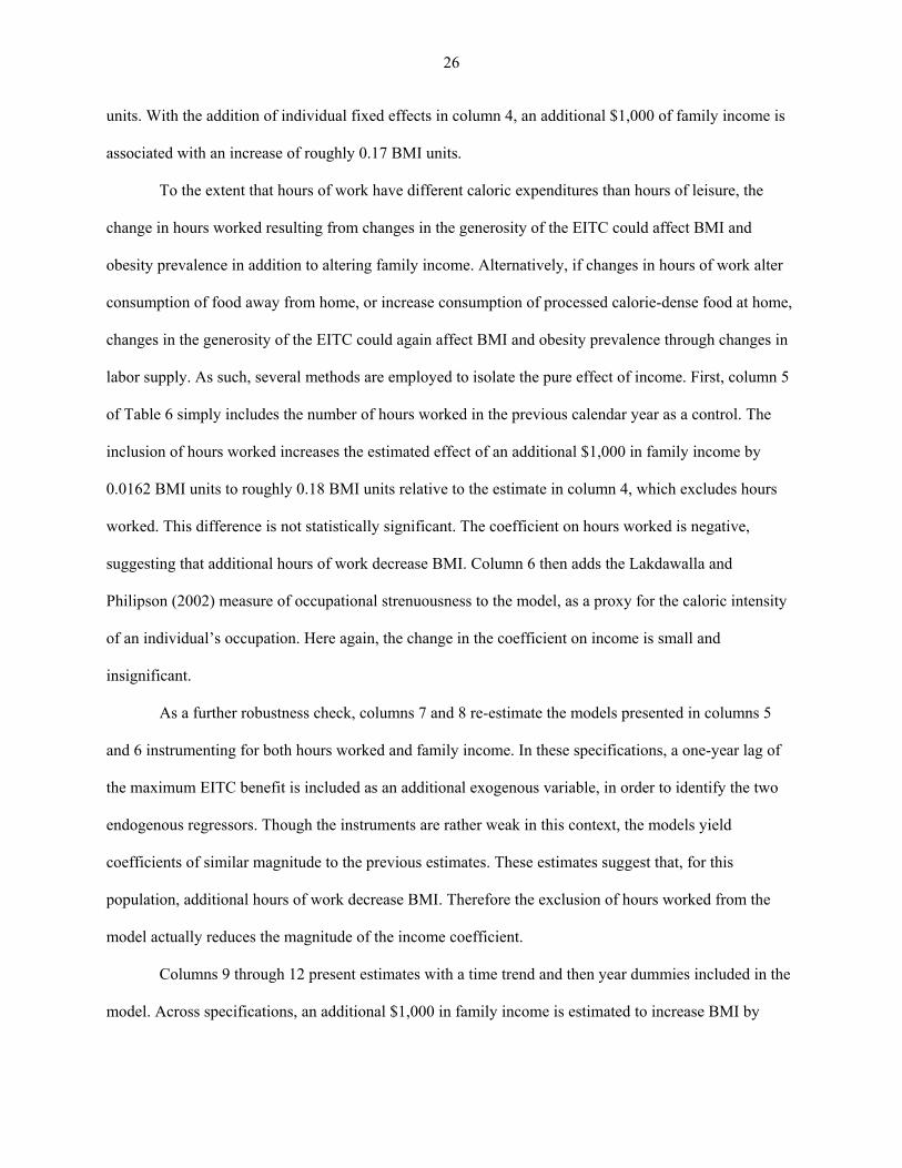
units. With the addition of individual fixed effects in column 4, an additional $1,000 of family income is

associated with an increase of roughly 0.17 BMI units.

To the extent that hours of work have different caloric expenditures than hours of leisure, the

change in hours worked resulting from changes in the generosity of the EITC could affect BMI and

obesity prevalence in addition to altering family income. Alternatively, if changes in hours of work alter

consumption of food away from home, or increase consumption of processed calorie-dense food at home,

changes in the generosity of the EITC could again affect BMI and obesity prevalence through changes in

labor supply. As such, several methods are employed to isolate the pure effect of income. First, column 5

of Table 6 simply includes the number of hours worked in the previous calendar year as a control. The

inclusion of hours worked increases the estimated effect of an additional $1,000 in family income by

0.0162 BMI units to roughly 0.18 BMI units relative to the estimate in column 4, which excludes hours

worked. This difference is not statistically significant. The coefficient on hours worked is negative,

suggesting that additional hours of work decrease BMI. Column 6 then adds the Lakdawalla and

Philipson (2002) measure of occupational strenuousness to the model, as a proxy for the caloric intensity

of an individual’s occupation. Here again, the change in the coefficient on income is small and

insignificant.

As a further robustness check, columns 7 and 8 re-estimate the models presented in columns 5

and 6 instrumenting for both hours worked and family income. In these specifications, a one-year lag of

the maximum EITC benefit is included as an additional exogenous variable, in order to identify the two

endogenous regressors. Though the instruments are rather weak in this context, the models yield

coefficients of similar magnitude to the previous estimates. These estimates suggest that, for this

population, additional hours of work decrease BMI. Therefore the exclusion of hours worked from the

model actually reduces the magnitude of the income coefficient.

Columns 9 through 12 present estimates with a time trend and then year dummies included in the

model. Across specifications, an additional $1,000 in family income is estimated to increase BMI by

27

between 0.15 and 0.22 BMI units. These estimates are not statistically different from those excluding the

time trend or year dummies.

For women, the IV coefficient estimates on family income are statistically significant in

all specifications except those that also instrument for hours worked. The use of IVs yields a

significant increase in the coefficient estimate on family income across specifications, as the

results of Hausmann tests (not reported here) reject equality between OLS and IV estimates.

Based on the median estimates from column 5, which include hours worked but exclude

occupational strenuousness, the coefficient on family income indicates that an additional $1,000 of family

income is associated with an increase in average weight of approximately 1.06 pounds. The IV coefficient

estimates presented in Table 6 imply that an additional $1,000 of family income is associated with an

increase in average weight of between 0.84 and 1.80 BMI units.

To allow for the possibility that the effect of income on BMI varies across the BMI

distribution, IV Quantile models were estimated at the 10th, 25th, 50th, 75th, and 90th percentiles of

the sample’s BMI. For women, these percentiles correspond to BMIs of 20.37, 22.95, 26.78,

32.22, and 37.39. For men, these percentiles correspond to BMIs of 22.71, 24.84, 27.74, 31.53,

and 35.53.

Table 8 presents the IV Quantile estimates for women, which demonstrate a clear upward trend in

the association between family income and BMI across the BMI distribution. The first specification

presents results without the inclusion of hours worked, while the second specification adds hours worked

to the model. At the 10th percentile of women’s BMI an additional $1,000 of family income is associated

with an increase of roughly 0.11 BMI units, while at the 90th percentile of women’s BMI an additional

$1,000 of family income is associated with an increase of roughly 0.24 BMI units. As in previous

estimates, the inclusion of hours worked increases the effect of income on BMI, though the change is not

statistically significant. With hours worked included, the estimate at the 10th percentile of women’s BMI

indicates that an additional $1,000 of family income is now associated with an increase of roughly 0.12

28

BMI units, while at the 90th percentile of women’s BMI an additional $1,000 of family income is now

associated with an increase of roughly 0.25 BMI units. The coefficient estimates are significant in every

percentile but the 10th at a minimum of the 5 percent level.

Given the numerous negative health outcomes associated with being obese, knowledge of the

extent to which additional income impacts obesity may be of particular value. In order to investigate this

relationship linear probability models of the effect of family income on an indicator for obese (BMI≥ 30)

are estimated. Table 10 presents the linear probability estimates for women. Similar to the estimates of the

effect of family income on BMI, the IV results show significant increases in the magnitude of the effect

of family income on the probability of a woman being obese, relative to the standard OLS estimates.

Columns 3 through 5 of Table 10 present the IV linear probability estimates of the effect of

family income on obesity. In column 3, an additional $1,000 in family income increases the probability of

being obese by 2.94 percentage points. Adding hours worked in column 4 increases the effect of an

additional $1,000 in family income to 3.30 percentage points. Including both hours worked and

occupational strenuousness in column 5 further increases the effect of an additional $1,000 in family

income to 3.64 percentage points. All the coefficients on family income are significant at a minimum of

the 5 percent level.

VII. CONCLUSIONS

The results presented in this paper indicate that correlational estimates of the impact of income on

BMI or obesity prevalence are strongly biased downward. For both men and women, and across all

models and specifications, the OLS estimates suggested a much smaller effect of family income on BMI

or obesity prevalence than the estimates produced using IVs. This paper provides robust evidence of a

positive causal link between income and BMI or obesity prevalence for women. Consistent with previous

literature, no statistically significant relationship between income and weight is found for men. For

women an additional $1,000 of family income is associated with an increase in BMI of between 0.14 and

29

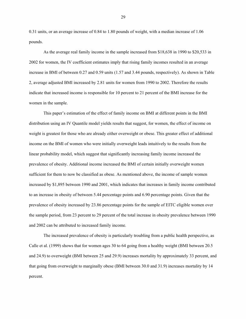
0.31 units, or an average increase of 0.84 to 1.80 pounds of weight, with a median increase of 1.06

pounds.

As the average real family income in the sample increased from $18,638 in 1990 to $20,533 in

2002 for women, the IV coefficient estimates imply that rising family incomes resulted in an average

increase in BMI of between 0.27 and 0.59 units (1.57 and 3.44 pounds, respectively). As shown in Table

2, average adjusted BMI increased by 2.81 units for women from 1990 to 2002. Therefore the results

indicate that increased income is responsible for 10 percent to 21 percent of the BMI increase for the

women in the sample.

This paper’s estimation of the effect of family income on BMI at different points in the BMI

distribution using an IV Quantile model yields results that suggest, for women, the effect of income on

weight is greatest for those who are already either overweight or obese. This greater effect of additional

income on the BMI of women who were initially overweight leads intuitively to the results from the

linear probability model, which suggest that significantly increasing family income increased the

prevalence of obesity. Additional income increased the BMI of certain initially overweight women

sufficient for them to now be classified as obese. As mentioned above, the income of sample women

increased by $1,895 between 1990 and 2001, which indicates that increases in family income contributed

to an increase in obesity of between 5.44 percentage points and 6.90 percentage points. Given that the

prevalence of obesity increased by 23.86 percentage points for the sample of EITC eligible women over

the sample period, from 23 percent to 29 percent of the total increase in obesity prevalence between 1990

and 2002 can be attributed to increased family income.

The increased prevalence of obesity is particularly troubling from a public health perspective, as

Calle et al. (1999) shows that for women ages 30 to 64 going from a healthy weight (BMI between 20.5

and 24.9) to overweight (BMI between 25 and 29.9) increases mortality by approximately 33 percent, and

that going from overweight to marginally obese (BMI between 30.0 and 31.9) increases mortality by 14

percent.

30

The finding that the additional family income generated by the increased labor supply of women

in response to the expansion of the EITC program increased the BMI and the prevalence of obesity

among eligible women is somewhat disconcerting. However, this finding in no significant way detracts

from the success of the EITC program in increasing labor force participation and the incomes of low-

income women. Instead, the possibility that additional income or expanded food budgets may in fact

increase the prevalence of obesity should be considered when designing programs specifically to combat

obesity.

Unfortunately, the choice of IV limits the broad generalizability of the results presented here;

generating a local average treatment effect of family income on EITC eligible persons. However, given

that the instrument used, eligibility for the Earned Income Tax Credit, applies to 22 million low-income

families, or 16.6 percent of all individual income tax returns, the results are applicable to a large portion

of the American population, and given their low-income status, certainly to those with the greatest

prevalence of obesity. Moreover, despite the limitation of the instrument used, the diversity of the EITC

eligible population would imply that the results presented here are likely consistent for the broader low-

income population. However, caution should be used in extrapolating beyond the low-income population,

given the possibility that income elasticities could vary over different ranges of income, or different types

of income.

31

References

Anderson, P. M., K. F. Butcher, and P. B. Levine. 2003. “Maternal Employment and Overweight Children.” Journal of Health Economics 22(3): 477–504.

Burkhauser, R. V., and J. Cawley. 2006. “The Importance of Objective Health Measures in Predicting Early Receipt of Social Security Benefits: The Case of Fatness.” Paper presented at the Retirement Research Conference, Washington, DC.

Calle, E. E., M. J. Thun, J. M. Petrelli, C. Rodriguez, and C. W. Heath. 1999. “Body-Mass Index and Mortality in a Prospective Cohort of U.S. Adults.” New England Journal of Medicine 341(15): 1097–1105.

Cawley, J. 2004. “The Impact of Obesity on Wages.” Journal of Human Resources 39(2): 451–474.

Cawley, J., J. Moran, and K. Simon. 2007. “The Impact of Income on Weight and Clinical Weight Classification: Evidence for the Elderly from the Social Security Benefits Notch.” Paper presented at the 2007 American Economic Association Annual Meeting.

Cawley, J., and R. V. Burkhauser. 2006. “Beyond BMI: The Value of More Accurate Measures of Fatness and Obesity in Social Science Research.” Working Paper No. 12291, National Bureau of Economic Research, Cambridge, MA.

Center on Budget and Policy Priorities. 2007. The 2007 Earned Income Tax Credit Outreach Kit. Tax Credit Outreach Team, Washington, DC.

Chou, S., M. Grossman, and H. Saffer. 2004. “An Economic Analysis of Adult Obesity: Results from the Behavioral Risk Factor Surveillance System.” Journal of Health Economics 23(3): 565–587.

Conley, D., and R. Glauber. 2005. ‘‘Gender, Body Mass and Economic Status.’’ Working Paper No. 11343, National Bureau of Economic Research, Cambridge, MA.

Cutler, D. M., E. L. Glaeser, and J. M. Shapiro. 2003. “Why Have Americans Become More Obese?” Journal of Economic Perspectives 17(3): 93–118.

Dahl, G. B., and L. Lochner. 2005. “The Impact of Family Income on Child Achievement.” Working Paper No. 11279, National Bureau of Economic Research, Cambridge, MA.

DeNavas-Walt, C., B. D. Proctor, and C. H. Lee. 2005. Income, Poverty, and Health Insurance Coverage in the United States: 2004. U.S. Census Bureau, Current Population Reports, P60-229. Washington, DC: GPO.

Drewnowski, A. 2000. “Nutrition Transition and Global Dietary Trends.” Nutrition 16(7/8): 486–487.

Ellwood, D. T. 2001. “The Impact of the Earned Income Tax Credit and Social Policy Reforms on Work, Marriage, and Living Arrangements.” In Making Work Pay: The Earned Income Tax Credit and Its Impact on American Families, edited by Meyer and Holtz-Eakin. New York, NY: The Russell Sage Foundation.

Finkelstein, E. A., I. C. Fiebelkorn, and G. Wang, G. 2003. “National Medical Spending Attributable to Overweight and Obesity: How Much, and Who’s Paying?” Health Affairs 22(4): 8.

32

Flegal, K. M., M. D. Carroll, C. L. Ogden, and C. L. Johnson. 2002. “Prevalence and Trends in Obesity among U.S. Adults, 1999–2000.” Journal of the American Medical Association 288(14): 1723–1727.

Fontaine, K. R., D. T. Redden, C. Wang, A. O. Westfall, and D. B. Allison. 2003. “Years of Life Lost Due to Obesity.” Journal of the American Medical Association 289(2): 187–193.

Hedley, A. A., C. L. Ogden, C. L. Johnson, M. D. Carroll, L. R. Curtain, and K. M. Flegal. 2004. “Prevalence of Overweight and Obesity among US Children, Adolescents, and Adults, 1999–2002.” Journal of the American Medical Association 291(23): 2847–2850.

International Obesity Task Force. 2005. EU Platform on Diet, Physical Activity, and Health, 2005. From http://www.iotf.org/media/euobesity3.pdf. (Accessed December 10, 2006)

Kan, K., and W. D. Tsai. 2004. “Obesity and Risk Knowledge.” Journal of Health Economics 23(5): 907–934.

Lakdawalla, D., and T. Philipson. 2002. “The Growth of Obesity and Technological Change: A Theoretical and Empirical Investigation.” Working Paper No. 8965, National Bureau of Economic Research, Cambridge, MA.

Leigh, A. 2004. “Who Benefits from the Earned Income Tax Credit? Incidence among Recipients, Coworkers and Firms.” Discussion Paper 494, Center for Economic Policy Research, Australian National University.

Mokdad, A. H., E. S. Ford, B. A. Bowman, W. H. Dietz, F. Vinicor, V. S. Bales, and J. S. Marks. 2003. “Prevalence of Obesity, Diabetes, and Obesity-Related Health Risk Factors, 2001.” Journal of the American Medical Association 289(1): 76–79.

Mokdad, A. H., J. S. Marks, D. F. Stroup, and J. L. Gerberding. 2004. “Actual Causes of Death in the United States, 2000.” Journal of the American Medical Association 291(10): 1238–1245.

Mokdad, A. H., J. S. Marks, D. F. Stroup, and J. L. Gerberding. 2005. “Correction: Actual Causes of Death in the United States, 2000.” Journal of the American Medical Association 293(3): 293–294.

Must, A., J. Spadano, E. H. Coakley, A. E. Field, G. Colditz, and W. H. Dietz. 1999. “The Disease Burden Associated With Overweight and Obesity.” Journal of the American Medical Association 282(16): 1523–1529.

National Heart, Lung, and Blood Institute, National Institutes of Health. 1998. “Clinical Guidelines on the Identification, Evaluation, and Treatment of Overweight and Obesity in Adults: The Evidence Report.” Obesity Research 6(Suppl. 2): 51s–215s.

Ogden, C. L., C. D. Fryar, M. D. Carroll, and K. M. Flegal. 2004. Mean Body Weight, Height, and Body Mass Index, United States 1960–2002. U.S. Department of Health and Human Services, National Center for Health Statistics, Hyattsville, MD.

Orzechowski, W., and R. Walker. 2002. Tax Burden on Tobacco: Historical Compilation, Vol. 36. Orzechowski and Walker: Arlington, VA.

http://www.iotf.org/media/euobesity3.pdf

33

Popkin, B. M. 2001. “The Nutrition Transition and Obesity in the Developing World.” The Journal of Nutrition 131(3): s871–s873.

Quintana-Domeque, C. 2005. “The Income Gradient in Body Mass Index.” Working Paper, Department of Economics, Princeton University, Princeton, NJ.

Seidell, J. C., and A. M. Rissanen. 1998. “Time Trends in the Worldwide Prevalence of Obesity.” In Handbook of Obesity, edited by G. A. Bray, C. Bouchard, and W. P. T. James. New York, NY: Marcel Dekker.

Sobal, J., and A. J. Stunkard. 1989. “Socioeconomic Status and Obesity: A Review of the Literature.” Psychological Bulletin 105(2): 260–275.

Stock, J. H., J. H. Wright, and M. Yogo. 2002. “A Survey of Weak Instruments and Weak Identification in Generalized Method of Moments.” Journal of Business and Economics Statistics 20(4): 518–529.

Swinburn, B., I. Caterson, J. C. Seidell, and W. P. T. James. 2004. “Diet, Nutrition and the Prevention of Excess Weight Gain and Obesity.” Public Health Nutrition 7(1A): 123–146.

U.S. Department of Health and Human Services. 2001. The Surgeon General’s Call to Action to Prevent and Decrease Overweight and Obesity. U.S. Government Printing Office, Washington, DC.

U.S. Department of Health and Human Services. 2005. Health United States 2005. National Center for Health Statistics, Hyattsville, MD.

U.S. Department of the Treasury. Internal Revenue Service. 2007. Tax Stats at a Glance FY 2005. http://www.irs.gov/taxstats/article/0,,id=102886,00.html (Accessed May 7, 2007)

Wooldridge, J. M. 2002. Econometric Analysis of Cross Section and Panel Data. Cambridge, MA: The MIT Press.

World Health Organization (WHO). 2003. Diet, Nutrition, and the Prevention of Chronic Diseases. WHO Technical Report Series 916. Geneva.

institute for research on poverty discussion paper no. · pdf fileinstitute for research on...

Documents