institute for space studies - nasa
TRANSCRIPT
INSTITUTE FOR SPACE STUDIES
MEASUREMENT OF THE COSMIC MICROWAVE BACKGROUND BY OPTICAL OBSERVATIONS
OF INTERSTELLAR MOLECULES
John Francis Clauser
R__(ACCESS0k4 NUMEP 2 U)
-(PAGES) (CODE)
Z (NASA CR ONTM nA)NME)CAGRY
GODDARD SPACE FLIGHT CENTER
NATIONAL AERONAUTICS AND SPACE ADMINISTRATION
Reprouced byIo NATIONAL TECHNICAL J]z- NFORMATION SERVICE
N70-32531
MEASUREMENT OF THE COSMIC MICROWAVE BACKGROUND BY OPTICAL OBSERAVTIONS OF INTERSTELLAR MOLECULES
John Francis Clauser
Columbia University
00
000 0 0 0 0o 000
sotft D i er sev a p
nations economcdevelopment
and technological advancement 0 0 0
NATIONAL TECHNICAL INFORMATION SERVICE
n 0
00
This document has been approved for public release and sale
MEASUREMENT OF THE COSMIC MICROWAVE BACKGROUND
BY OPTICAL OBSERVATIONS OF INTERSTELLAR MOLECULES
John Francis Clauser
Submitted in partial fulfillment
of the requirements for the degree of
Doctor of Philosophy inthe Faculty of Pure Science
Columbia University
TABLE OF CONTENTS
Table of Symbols 1
1 Introduction
A Cosmic Microwave Background Background 7
B Observational Difficulties 10
C Interstellar Molecules 10
D Purpose of Dissertation 12
2 The Use of Interstellar Molecules to Obtain Upper Limits and Measurements
of the Background Intensity
A Excitation Temperature of Interstellar Molecules 14
B Astronomical Situation 16
C Calculation of T 17iJ
D Why Molecules 19
E Statistical Equilibrium of an Assembly of Multi-Level Systems Interacting with Radiation 21
F Equations of Statistical Equilibrium 25
G Case I 26
H Case II 27
I Case HI 29
J Sufficient Conditions for Thermal Equilibrium to Hold 34
3 Optical Transition Strength Ratio
A CN and CH+ 37
B Matrix Elements of the Molecular Hamiltonian 38
C Line Strengths 40
i
4 Techniques of Spectrophotometry and Plate Synthesis
A Available Plates and Spectrophotometry 43
B Synthesis Programs 46
5 Results of Synthesis
A Curve of Growth Analysis 50
B CN(J = 0 - 1) Rotational Temperature and Upper Limit to the Backshyground Radiation at X 2 64mm 53
C Upper Limit to Background Radiation at X= 1 32rm 53
D Radiation Upper Limit at X = 0 359mm 54
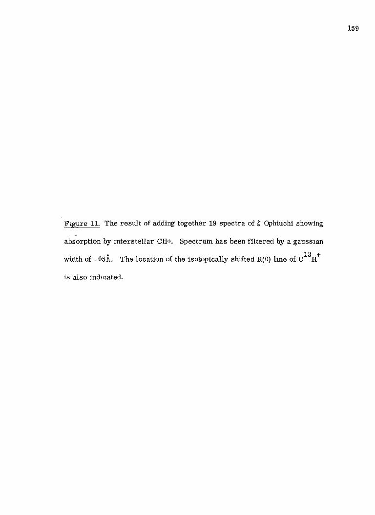
13 + E Detection of Iterstellar C H 55
X=F Radiation Upper limits at 0 560 and X = 0 150m 56
G Discussion of Upper Limits 57
6 Alternate Radiative Excitation Mechanisms 59
A Criterion for Fluorescence to be Negligible 60
B Vibrational Fluorescence 61
C Electronic Fluorescence 62
C CN Band Systems 63a
C R Upper Limits 64b 01
7 Collisional Excitation in H I Regions
A Difference Between H I and H II Regions 67
B Earlier Work on the Place of Origin of the Molecular Interstellar Lines 68
C Collisional Mechanisms in H I Regions 70
D Excitation by H Atoms 71
E Electron Density 74
iii
F Cross Sections for Excitation of CN by Electrons 75
G Excitation Rate from Electrons 79
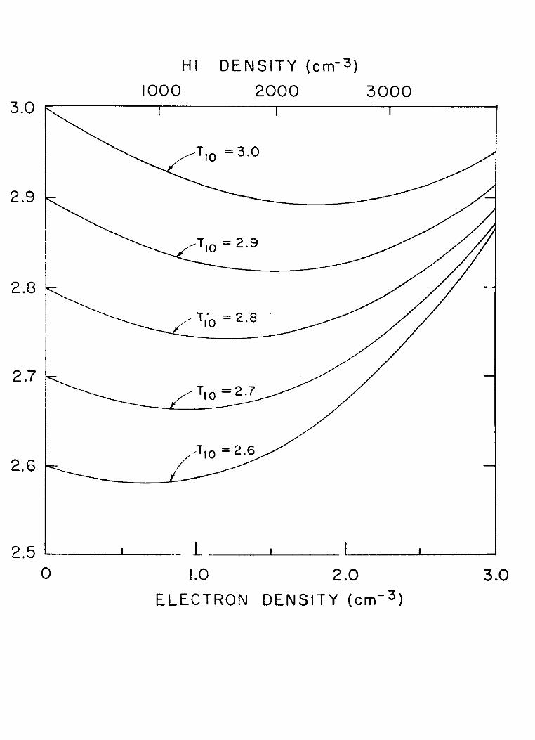
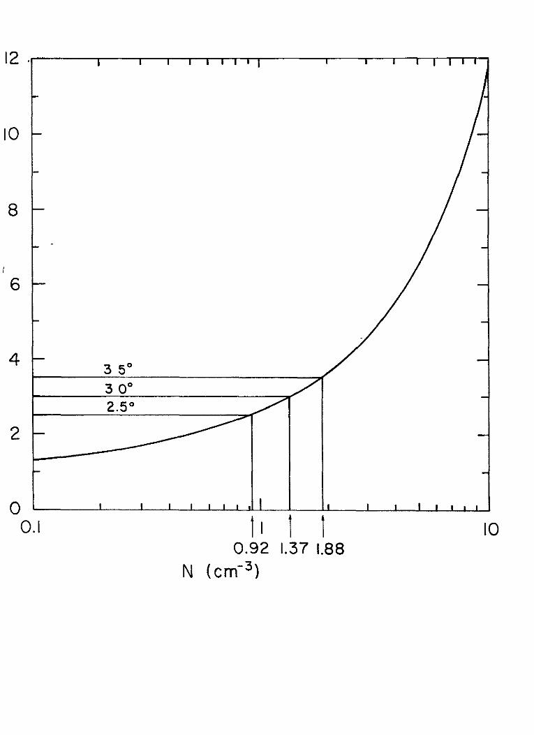
H Cowparison of T with T10 to Determine Electron Density 80
I Excitation by Ions 80
J Discussion 81
8 Collisional Excitation in H II Regions 82
A Semi Classical Approximation 83
B Matrix Elements of Interaction Hamiltonian 84
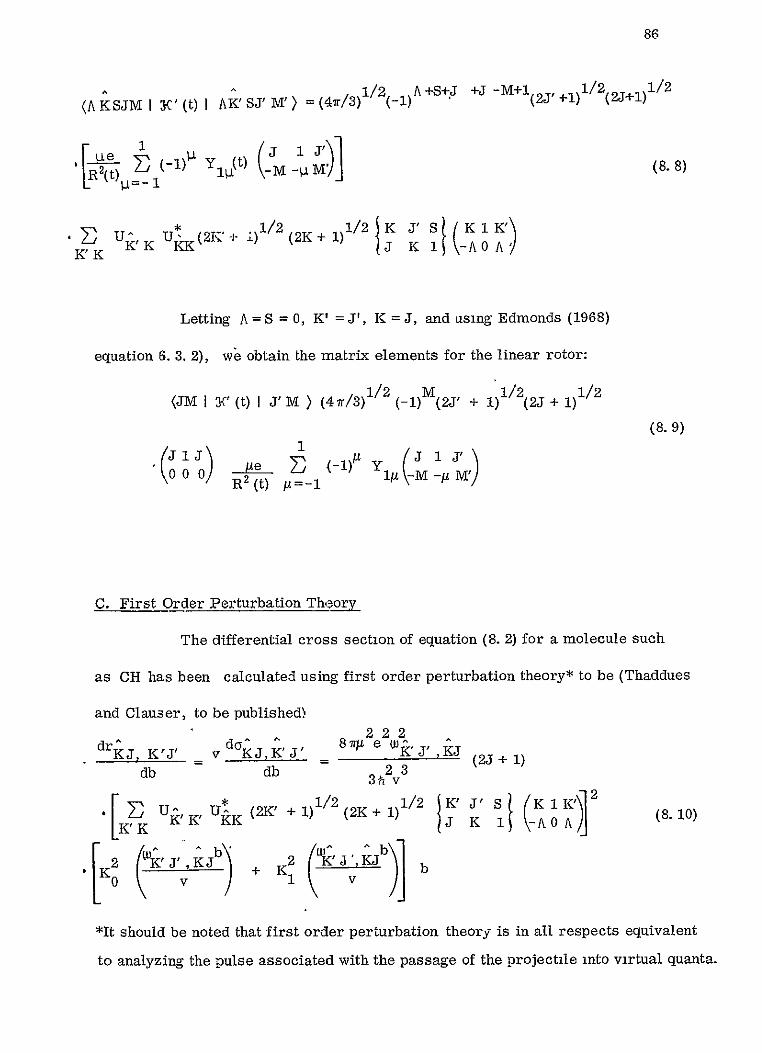
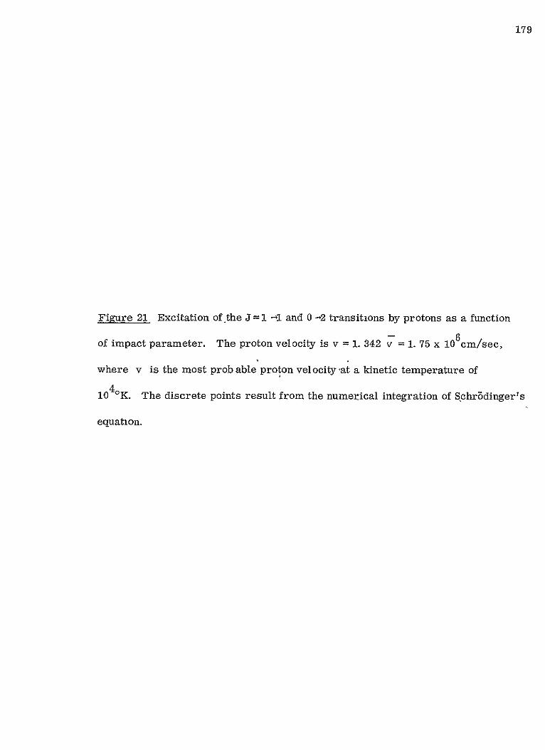
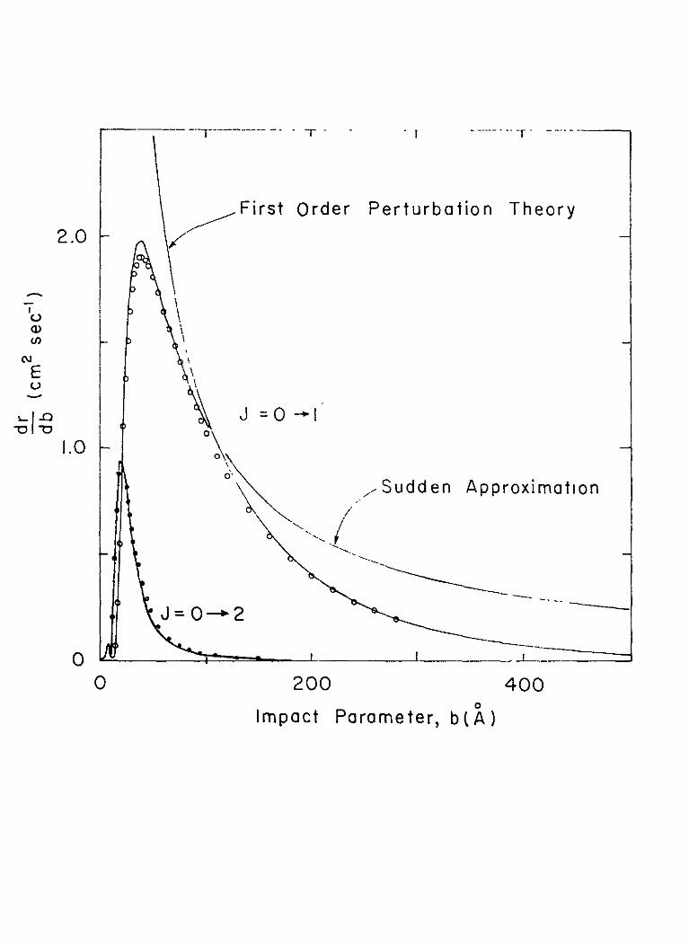
C First Order Perturbation Theory 86
D Quantum Mechanical Sudden Approximation 87
E Numerical Solution of Schrbdingers Equation 90
F Num erical Results 94
9 Further Evidence that the CN Excitation Originates Non-Collisionally in an H I Region 99
A T10 Invariaice 100
B H I - CN Velocity Correlations L01
10 Conclusions 105
APPEN DICES
Al Matrix Elements of the Molecular Hamiltonian 110
A2 Evaluation of the Reduced Matrix Elements of the Dipole Moment Operatorl2
A3 Vibrational Fluorescence Rate 114
A4 Noise Filtering and Statistical Analysis of Errors 115
A Maximum Likelihood Estimation 116
B Case A 119
iv
C Case B 120
D Case C 120
E Interpretation 121
F Removal of Effect of Finite Slit Width 122
G Error Estimates for Spectral Line Depth 123
A5 Calculation of Filter Functions 124
Acknowledgements 126
Bibliography 128
Tables 134
Figures 139
TABLE OF SYMBOLS
- a a amplitude of state 3 at transformed time w
allowed electric dipole
A molecular fine structure constant
A13 Einstein coefficient for spontaneous decay
b impact parameter
bII galactic latitude
B Be B 0 molecular rotation constants
Bii Einstein coefficient for absorption and stimulated emission
c speed of light
Ckq I44-k+1 - Ykq Racahs normalization for spherical Harmonics
C tensor operator with components Ckq
D Debye unite of electric dipole moment = 10 shy 1 8esu-cm
D D denominators used in Chapter 2
(( y) matrix elements of the finite rotation operator in terms of Euler angles aB y
e electronic charge
e e electronic states
Eienergy of level i
f f oscillator strength
gi statistical weight of level i
g() optimal filter function for signal
h = 2Trh Plancks constant
hslit slit function (rectangular peak)
2
h (x) optimal filter function which also removes effectsof finite slit width
FHamiltonian operator
R matrix elements of Y
J J total angular momentum (excluding nuclear) operator and corresponding quantum number
0 J1 Bessel functions
k Boltzmanns constant
k kf initial and final electron propogation vector
K quantum number corresponding to K
label of molecular state which reduces to state with quantum namber K whan molecular fine structure constant A vanishes
K N+ A
K K modified Bessel functions
tIl galactic longitude (degrees)
m redaced projectile mass
m electron mass
M magnetic quantum number corresponding to level i
N e electron number density (cm - 3
n(X) grain noise as function of wavelength
nl number bf systems in level i
NP a proton number density (cm - 3
NH H I number density (cm - 3 )
N angular momentum operator for end-over-end rotation
(rot)rj L2HO-nl-London factor
3
fq(vib) I2 Franck - Condon facLor
9R (vib-rot) operator for vibration-rotation transitions
p(y I ) conditional probability density of y given 0
P pn real part of amplitude of state j at transformed time wn
P transition probability from state i to state j
q(y) a posterori probability of measurement y (equation A4 4)
qj qjn imaginary part of amplitude of state j at transformed time wn
Q(H) probability that the actual value of a quantity will be in designated interval H
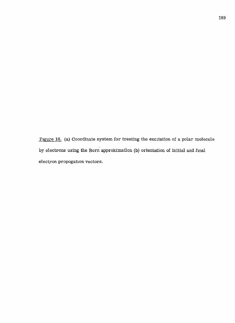
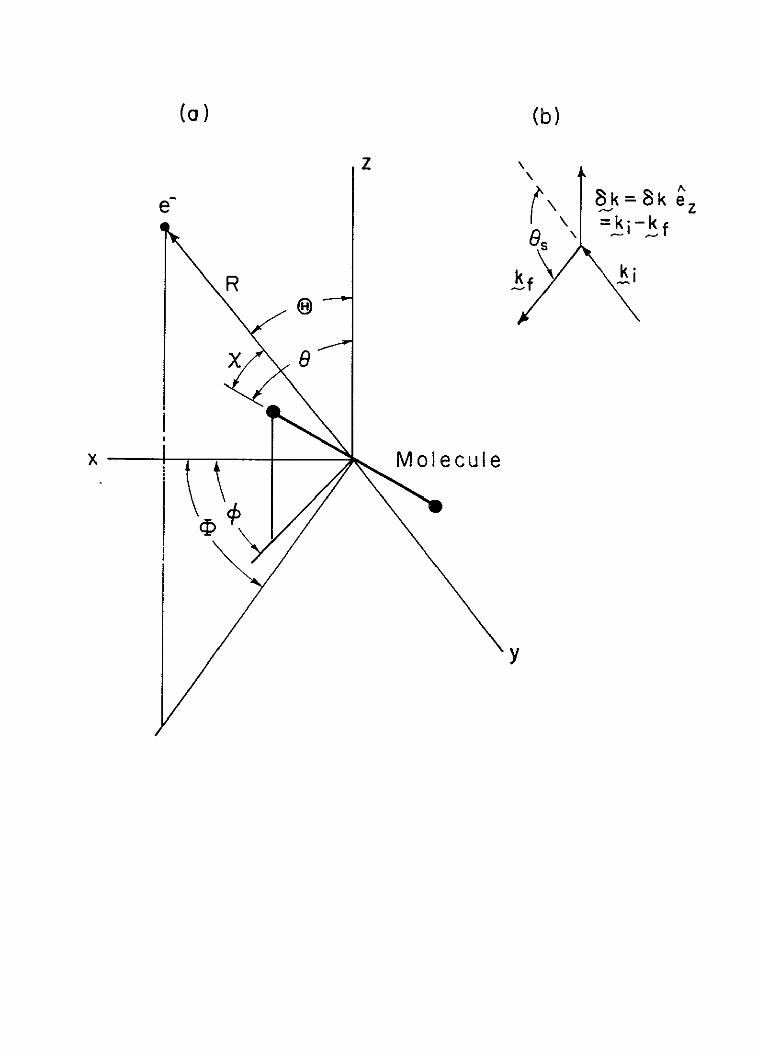
r optical depth ratio (equation 2 6)
(e) r(p) r r r collisional excitation rate from level i to level j for unit
if iJ iJ flux of incident particles electrons protons
(r ) thermal velocity average of r
R radius vector of projectile
Rn(X) autocorrelation function for plate grain noise (equation A4 2)
R excitation rate from level i to level j by process other than iJ direct radiation
s= SilSif (equation 2 7)
S S electron spin operator and corresponding quantum number
S transition strength (equations 2 3 and 2 5)
s(X) noise free spectrum as function of wavelength
S(1) spin tensor operator
t time
T temperature
TB brightness temperature (equation 2 9)
4
T excitation temperature of levels i and j (equation 2 1)
u(N) energy density of radiation at frequency v per unit frequency interval in erg cmshy 3 Hz shy 1
=u()
UKK transformation matrix which diagonahzes molecular Hamiltonian matrix
v projectile velocity
vv vibrational states
v I-8-kTm average reduced projectile velocity
v - k-T-ijW most probable reduced projectile velocity
w sinh- (vtb)v (transformed time - equation 8 23)
W equivalent width of absorption line (area for unit base line height)
y(X) measured spectrum as function of wavelength
y(X) densitometer measurement of y()
y( X) filtered y(X )
Y normalized spherical harmonics
Y spherical harmonic tensor operator
a unspecified quantum number
a(X) continuum height
aH aHe polarizability of H He
absorption line depth
most probable value of S
im see equation ( A4 8 )
y = 0 577 (Eulers constant)
8 (x) Dirc delta function tobe taken in the sense of a generalized function (Lighthill 1959)
5
m 1 for m = n = 0 form 4 n (Kronecker Delta)
5 b increment in b
6 k =k -kIk-f
6w increment in w
e 1 C2 CH upper limit ratio discrepancy
1 limit to error region
0 polar angle specifying molecular orientation in laboratory frame
a sscattering angle
polar coordinate specifying projectile position in laboratory frame
X wavelength
A electronic angular momentum quantum number in Appendix 4 half interval for filter integration
AL wavelength of spectral line center
F electric dipole moment
v frequency (Hz)
vi = (E i - E)h (equation 2 2)
ii = B u (A +B~a)( nn for thermal equalibrium -3 ij ij iJ ij 1 equation 2 11)
pelectromc state with A = 1
a standard defiation
a13 cross section for excitation from level i to level j
Z electronic state with A = 0
T i]optical depth of spectral line which is due to transition
ij from level i to level j
0 azimuthal angle specifying molecular orientation in laboratory frame
6
polar coordinate specifying projectile position in laboratory frame
x angle between molecular axis and R
4molecular wave function
total wave function
w = 2nv
1M 2 3N M2 M3) Wigner 3j symbol
1 1 2 3 igner 6j symbol
1L2 3
7
CHAPTER 1
INTRODUCTION
A Cosmic Microwave Background Background
The existence of a blackbody background radiation as a permanent
remnant of the flash of radiation of the big bang was first suggested by
Gamow and his collaborators (Gamow 1948 Alpher and Herman 1958) Using
Friedmans (1922 1924) solution to the field equations of General Relativity
for an expanding isotropic homogeneous universe Gamow and his associates
attempted to explain the present element abundances in terms of nuclear
reactions occurring during the iirst few seconds or minutes of the expansion
They showed the following (Alpher and Herman 1950 Gamow
1949 1953 Alpher Hermanand Gamow 1967)
1 At early epochs radiation would be in thermal equilibrium and
thus would have a thermal spectrum More importantat that time it would be
the dominant component of the total energy density
2 As the universe expanded the radiant energy decreased as the
inverse fourth power of the scale factor On the other hand the matter rest energy
density decreased only as the inverse third power of the scale factor hence
eventually it became the dominant component of the total energy density
3 At an epoch when the temperatureas approximately 104 0 K the
radiation decoupled from the matter In spite of the complexities of this deshy
coupling process the distortion of the blackbody spectrum of the radiation by
this process would be small Peebles (1968) has since treated this process
in some detail and has shown this to be essentially a consequence of the fact that
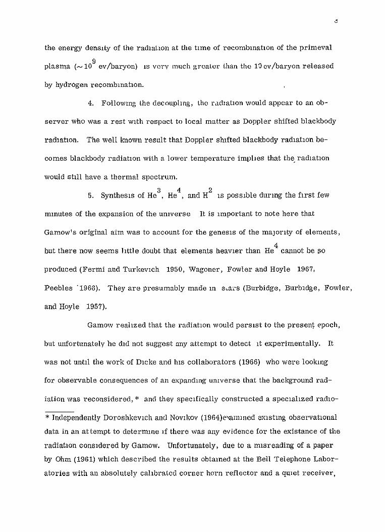
the energy density of the radiation at the time of recombination of the primeval
plasma (-109 evbaryon) is verv much greater than the 10 evbaryon released
by hydrogen recombination
4 Following the decoupling the radiation would appear to an obshy
server who was a rest with respect to local matter as Doppler shifted blackbody
radiation The well known result that Doppler shifted blackbody radiation beshy
comes blackbody radiation with a lower temperature implies that the radiation
would still have a thermal spectrum
3 4 25 Synthesis of He He and H is possible during the first few
minutes of the expansion of the universe It is important to note here that
Gamows original aim was to account for the genesis of the majority of elements
but there now seems little doubt that elements heavier than He4 cannot be so
produced (Fermi and Turkevich 1950 Wagoner Fowler and Hoyle 1967
Peebles 1966) They are presumably made in s ars (Burbidge Burbidge Fowler
and Hoyle 1957)
Gamow realized that the radiation would persist to the present epoch
but unfortunately he did not suggest any attempt to detect it experimentally It
was not until the work of Dicke and his collaborators (1966) who were looking
for observable consequences of an expanding universe that the background radshy
iation was reconsidered and they specifically constructed a specialized radioshy
Independently Doroshkevich and Novikov (1964)emmined existing observational
data in an attempt to determine if there was any evidence for the existance of the
radiation considered by Gamow Unfortunately due to a misreading of a paper
by Ohm (1961) which described the results obtained at the Bell Telephone Laborshy
atories with an absolutely calibrated corner horn reflector and a quiet receiver
telescope for its detection However the radiation was irst detected by
Penzias and Wilson (1965) when it was pointed out to them by Dicke that the
excess antenna temperature of unknown origin of their exceptionally quiet
microwave radiometer might be due to the radiation which the Princeton group
was seeking The second observation of the radiation followed within a year
and was that of Dickes co-workers Roll and Wilkinson (1966) Their measureshy
ments as well as others made subsequently are shown in Figure 1 The best
present estimates suggest - 2 70K for the temperature of this radiation
One of the important predictions of the theory is that the radiation
should have a spectrum corresponding to that of a blackbody For a tempershy
ature -3 0K this would peak at about a millimeterin wavelength As can be
seen from Figure 1 the thermal character of this radiation has been confirmed
over more than two decades in frequency in the long wavelength portion of the
spectrum However since most of the energy density lies at the short waveshy
length portion where measurements have not yet been made it is of great
importance that observations be extended to this spectral region If the
thermal character of this radiation is eventually confirmed it will provide
very compelling and perhaps conclusive evidence in favor of the expanding
universe
they came to the conclusion that there was no evidence for its existence Penzias
and Wilson (1965) eventually used the same instrument to first detect the radshy
iation
10
B Observational Difficulties
Direct observations have not been made at shprt wavelengths because
of the presence of atmospheric H20 and 02 absorption lines These increase
in both strength and number as one goes to shorter wavelengths Their resulting
opacity causes the atmosphere to radiate with an intensity which is large compared
with that of the background In addition the blackbody background intensity
begins to fall off exponentially with increasing frequency beyond about a millishy
meter in wavelength Thus it appears that beyond X 3mm for all practical
purposes the radio window is closed and one must place radiometers above
the atmosphere in order to make direct background measurements
Fortunately it is possible to-circumvent the problem of atmospheric
opacity by using observations of optical spectra which are due to absorption by
the interstellar molecules CN CH CH+ An analysis of the absorption spectra
of these molecules can be used to determine to what extent the molecules are
being excited by the background radiation A measure of this excitation can
then be used to infer the intensity of the existing background
This dissertation describes how this is done The resulting measureshy
ments made by the use of these molecules are shown in Figure 1 where they are
labeled CN CH CHI+
C Interstellar Molecules
The optical interstellar absorption lines due to the interstellar moleshy
cules CN CH CH+ were discovered by Adams and Dunham (1937 Dunham
1941 Adams 1941 1943 1949) Following the suggestion of Swings and Rosenshy
feld (1937) that the line at X4300 3A might be due to CH McKellar (1940)
succeeded in identifying this feature with CH as well as the line at X 3874 6
with CN At that time he predicted the presence of several other lines of CH
as well as the presence of the R(1) line of CN at 3874 OA Acting on the suggesshy
tion of McKellar Adams succeeded in observing the additional lines of CH as
well as the faint CN R(1) line Douglas and Herzberg (1941) then produced
CH+ in the laboratory and positively identified the features at X4232 6A and
X 3957 OA as due to that molecule
It is surprising to consider that McKellars (1941) estimate of 2 30K
for the rotational temperature of the interstellar CN in front of C Ophiuchi was
probably the first measurement of the cosmic microwave background - twentyshy
eight years ago His temperature measurement was made from Adams visual
estimates of the absorption line strengthsso his result was crude At the time
though he attributed little significance to this result stating (McKellar 1940)
the effective or rotational temperature of intershystellar space must be extremely low if indeed the conshycept of such a temperature in a region with so low a denshysity of both matter and radiation has any meaning
His 2 30 K measurement is also mentioned in Herzbergs (1959p 496) Spectra
of Diatomic Molecules suggesting that it has of course only a very reshy
strictive meaning
The starting point of our work was a crucial suggestion by N J Woolf
based in turn on a discussion by McKellar (1940) which preceeded Adams disshy
covery (McKellar 1941) of CN X 3874 0 He suggested that the absence of
excited state CN lines placed a severe limit on the temperature of background
12
radiation As we shall see not only do these molecules set upper limits to this
radiation but in all probability they may also be used to effect an actual measureshy
ment of it
In additioX to our work on this problem (Thaddeus and Clauser 1966
Clauser and Thaddeus 1969 and Bortolot Clauser and Thaddeus 1969) similar
work has also been pursued by Field and Hitchcock (1966) while Shklovsky (1966)
made an early suggestion that McKellars (1941) observation was a consequence
of the background radiation
D Purpose of Dissertation
Th3 central purpose of this dissertation is to extract-the largest
feasible amount of information on the short wavelength spectrum of the microshy
wave background radiation from a number of spectra of interstellar molecules
that were available in the summer of 1966 The work may be divided into roughly
two parts an observational part and a theoretical part In the observational part
we first show how one calculates the background intensity from the spectra of
the interstellar molecules (Chapters 2 and 3) Second in order to utilize the
existing spectrograms we develop new techniques of spectrophotometry (Chapter
4 Appendix 4) Third we present the results of the application of these tech shy
niques to the problem at hand and the resulting upper limits to and measurements
of the intensity of the background radiation (Chapter 5)
On the theoretical side we first consider what assumptions concerning
the location of the molecules will be necessary such that (1) the molecules will
set upper limits to the background intensity and (2) the molecules will yield
13
reliable measurements of the background intensity It will be seen that the use
of the molecules to set intensity upper limits places only minor restrictions on
the molecular environment however their use to make intensity measurements
requires the absence of alternate molecular excitation mechanisms (Chapter 2)
We therefore provide an analysis which considers possible excitation
schemes that are consistent with our present understanding of the conditions found
in the interstellar medium We find that a necessary assumption for the moleshy
cules to yield reliable intensity measurements is that they reside in a normal
H I region (Chapters 67 and 8)
After a review of the existing evidence that the molecules doreside
in an H I region we proceed to present new evidence to further substantiate
this contention This wilL consist of (1) the observe invariance of the excitation
of the interstellar molecules and (2) the results of new 21cm H I observations
in the direction of these molecular clouds (Chapter 9)
14
CHAPTER 2
THE USE OF INTERSTELLAR MOLECULES TO OBTAIN UPPER LIMITS AND
MEASUREMENTS OF THE BACKGROUND INTENSITY
A Excitation Temperature of Interstellar Molecules
The method which we exploit to obtain information concerning the
short wavelength spectrum of the background radiation is the familiar one used
to find the temperature of molecules and their environment from molecular
spectra (Herzberg 1959) It is a general tool widely used in astronomy to
determine the temperature of planetary and stellar atmospheres and finds
considerable application in the laboratory to the study of flames rocket
exhausts etc
INgt
-
Sor INTERSTELLAR COUDESTAR HI CLOUD SPECTROGRAPH
A typical observational situation is illustrated schematically above
The intensity in absorption of lines in a molecular electronic band is proportional
both to the square of the transition matrtx element and the population of the lower
level of the transition As long as the molecules are in thermal equilibrium
(or at least their rotational degrees of freedom are in thermal equihbrium) the
relative populations of the rotational lervls are in turn given by the usual Bnltzshy
mann expression
15
ni g1 _
1 -1
exp -(E i -E kTl (21)n g 1J J
where
n is the population of level i and I
gi is the statistical weight of that level
E is the energy of that level1
It is now clear that the relative intensity of optical absorption lines in the band
is a function of T alone and may be used to determine T if the rotational term
scheme and relative transition matrix elements of the molecule are known as is
usually the case Even if thermal equilibrium does not hold it should be obvious
that equation (2 1) can be used to define an excitation or rotational tempshy
erature Ti with respect to any two levels 1 and 3
Consider now possible causes of this excitation it could be due to
either radiation or collisions If radiation which has a thermal spectrum with
temperature TB is the only (or dominant) cause of the molecular excitation
then on purely thermodynamic grounds Tij TT In this case only the emission
and absorption of photons with frequencies
v = (E- EJ h=w 2r (22)
in the molecular frame of rest are involved in the excitation and only the portion
of the radiation spectrum over the narrow Doppler width
-51i0AV Vi 1]
of the transition is involved in the excitation of the molecules Thus if the
radiation does not have a thermal spectrum but over these intervals it has the
16
same intensity as that of a blackbody temperature T B then the relation
T B = Tl will hold
On the other hand if the excitation is collisional or is due to a
mixture of radiative and collisional processes T will generally set aniJ
upper limit to the intensity of radiation at v Thus we see that a measurementii
of T liwill yield useful information on the background radiation density
B Astronomical Situation
In the astronomical situation of interest to us the molecules are
located in a tenuous interstellar cloud while the source of radiation against
which ahsorption is being observed is an 0 or B star at a typical distance of
100 pc Since the interstellar lines are very sharpand for the molecules at
least always weak the largest telescopes and Coude spectrographs are required
to detect the lines In fact virtually all the molecular observations have been
made with three instruments the Mt Wilson 100-inch the Mt Palomar
200-inch and the Lick Observatory 120-inch reflectors
There are several reasons why interstellar lines have so far only
been investigated against early stars Perhaps the most important is the high
intrinsic luminosity of these objects which allows high resolution spectroscopy
to be done in reasonable exposure times to distances of up to several hundred
parsecs For much smaller path lengths the probability of intercepting an
interstellar cloud which possesses appreciable molecular absorption is very
slight There is the additional factor that 0 and B stars have been so recently
formed that they usually lie near the galactic plane and thus in the vicinity (or
at least the direction) of interstellar matter Also an important technical conshy
17
sideration is that the spectra ol these sLars are comparativelv leatureless many
e1 the spectral lines are due to ionized atomns and the lines are usually wide
due to the high temperature andor rotation of the star In marked contrast to
the situation with cool stars ihre is therelore little ikeli-hood that the intershy
stellar lines will be blended or oheiured b slellar features Purely-from the
technical point of view we thus sec that early stars are ideal objects to use as
light sources for long ranle optical absorption spectros(opy of interstellar matter
C Calculation of T
It is straight forward to (al(ulate T from the observed absorption
intensities of lines in a molecular band The observed optical depth I of
an absorption line which is due to a transition from level i to level il is
given by
T 8nv) N Sn (hcg1) (2 3)
where Si is the line strength This is defined as the square of the electricshy
dipole matrix element summed over the degenerate mdgnetic states and polai iza-
Lions of the transition (Condon and Shortley 1951 p 98)
s U I inflg1cqIj)m) (24)sniin cj mi lq j
where A is the electric-chpole iomenl ol the molecule an( C q =T
Y where the Y are the normnlized -pherical harmonies This
summation may be expressed in terms of the reduced matrix element (Edmonds
1968 equation 5 4 7)
18
sl =2 (i Ic(1) Iij gt1 2 (25)
where C (1)=4E73 Y(1) is a spherical tensor operator of order one
Thus for two optical absorption lines of nearly the same wavelength
that are due to transitions to levels i and j from low lying levels i and j
respectively
thv1
r -= s exp - i---]| (26)Tj
Here we have defined
s - I (2 7)
The calculation of this quantity for the specific molecular systems of interest
will be taken up in Chapter 3 Equation (2 6) may be rewritten to give the
excitation or rotational temperature
hv
T T (2-8)1 kln(sr)
It should be noted in passing that since only the logarithm of the
optical depth appears in equation (2 8) the rotational temperature may be well
qetermined even though the optical depths are poorly known
If the interstellar lines are optically thin the optical depths are
proportional to the equivalent widths of these lines (area of absorption line for
unit continuum height) Fortunately most of the interstellar lines considered
in this study are weak so that the correction for saturation is small and good
approximate results may be obtained by taking r equal to the equivalent width
19
ratio However accurate temperature measurements will require a correction
for saturation via a curve of-growth for the clouds which contain these molecules
A description of these corrections appears in Chapter 5
D Why Molecules
We must now consider which kinds of atoms or molecules found in
the interstellar medium are useful as radiant thermometers for measurement
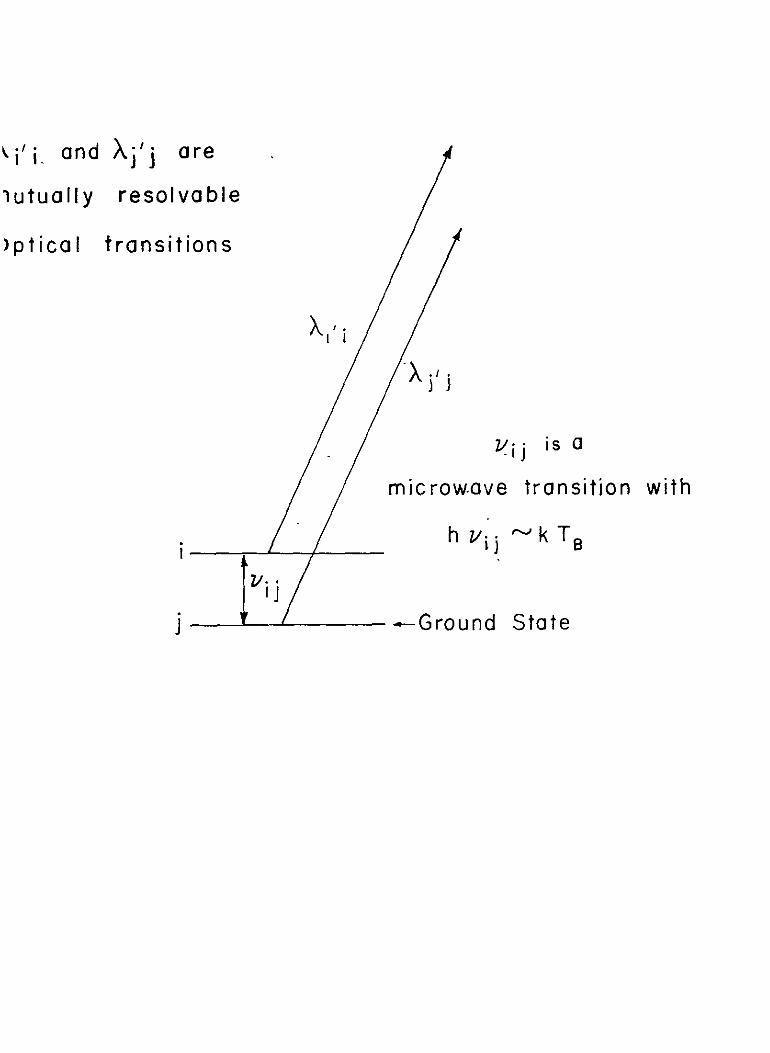
of the background radiation What is required to make such measurements
possible is an atom or molecule which has (1) a low lying level with energy
separation from the ground state - kT 2cm for a blackbody radiation
temperature T s3degK (2) an allowed (electric-dipole) transition connecting
this level with a lower level which has an observable population and (3) allowed
optical absorption transitions originating in each of these levels blearly these
optical transitions must be mutually reolvable and of course -to beobservable
from the ground they must have wavelengths Xgt 30001 The required term
diagram for such a species is shown in Figure 2
We can see that there is nothing in principle which restricts us to
use molecules However atomic fine-structure separations are typically much
greater than 2cm For example the lowest lying fine-structure level of any
interstellar atom so far observed from the ground belongs to Ti II and this is
97cm - I above the ground state On the other hand hyperfine levels have
separations which are too small and are connected by magnetic-dipole transitions
-1 - the H I hyperfine separation is only 032cm
The rotational andor fine structur6 energy level separations within
20
the electronic ground states of the three molecular species observed optically in
the interstellar medium - the CN CH and CH+ free radicals - have energies
-1 not very much greater than 1 88cm The J = 0- 1 energy level separation
of the X2Z (v=0) electronic ground state of CN is especially favorable with a
separation of only 3 78cm - 1 Partial term diagrams for these molecules are
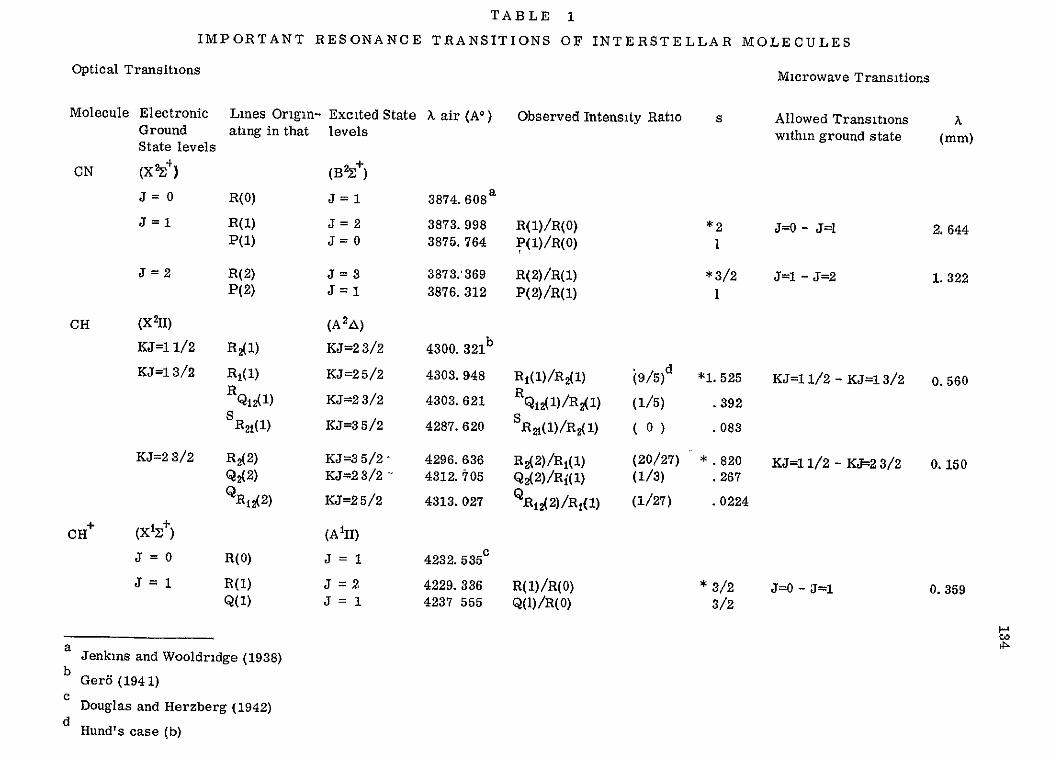
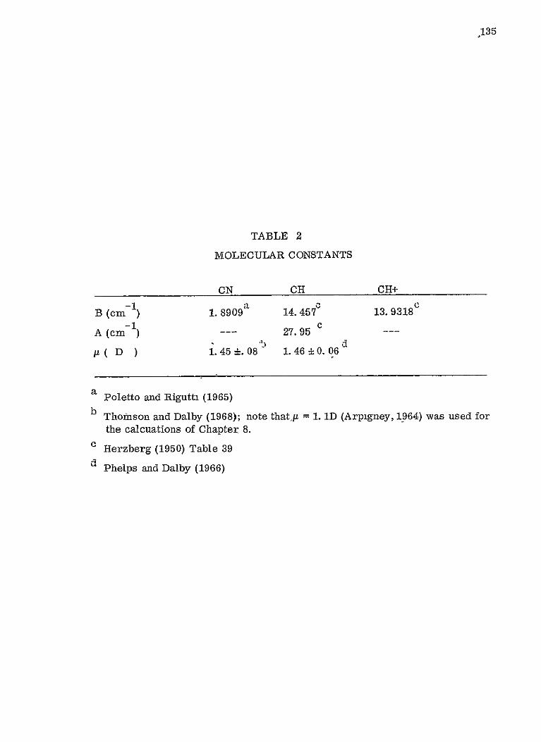
shown in Figure 3 Precise molecular data is listed in Table 1
2 + 2 +The R(0) absorption lines of the (0 0) band of the B Z - X2z
electronic system of CN at X3874 0O and X3874 81 arrise from the J = 1
level All of the CN lines are easily separated with a good Coud6 spectrograph
It should be noted however that even in the best spectrographs the lines are not
fully resolved i e the observed line width -0 02Z is not the true Doppler
line width of the interstellar cloud but is determined instead by the resolution
of the instrument and is typically 0 05A
The level separations of the CH and CH+ molecules are sufficiently
great that no molecules are observed to be in an excited level However these
two molecules are still of great value to the problem of the background radiation
since the absence of the excited states lines can be used to set upper limits to
the radiation intensity at very short wavelengths
The lowest excited state in CH+ is the J = 1 level 27 9cm - above
the J = 0 ground state and the corresponding R(0) and R(1) transitions of the
(0 0) bind of the X1 - A 1I electronic system occur at X4232 51 and X4229 A
2 The CH electronic ground state configuration is a 2I state intershy
mediate between Hunds cases (a) and (b) Accordingly transitions are allowed
from the KJ = 1 12 ground state to both the fine-structure level KJ = 1 32
21
-1 which lies at 17 Scm above the ground state and to the KJ = 2 32 excited
-1 rotational level 66 8cm above the ground state The strongest optical transshy
ition from these thr~e levels are the R2(1) and R (1) and the R2(2) lines in X2I 2oo
the (0 0) -band of the X IT- A A electronic system at 43-0 31 X4303 9A
and 4296 6k respectively A detailed treatment of the relative intensities of
the optical transitions of CH appears in Chapter 3
The J = 2 level of the CN electronic ground state is similarly useful
for setting an upper limit to the background intensity Since it is 7 6cm - 1 above
the J = 1 level its populations will be quite small For this reason the R(2)
hhe originating in this level has not yet been detected but it is probably only
about a factor of three below detection (Bortolot Clauser and Thaddeus 1969)
and a further extensio- of the techniques developej in this dissertation might
yield its detection
On the other hand without an enormous extension of present obshy
servational techniques the CH R2 ( ) and the CH+ R(1) lines are below the
threshold of detectability if their temperature - 30K
E Statistical Equilibrium of an Assembly of Multi-Level Systems Interacting
with Radiation
When all its components are considered departure from thermal
equilibrium is one of the most conspicuous features of the interstellar medium
It contains for example dilute 104K starlight H I atoms with a kinetic tempshy
erature of - 100K 104K H U protons and electrons grains which are thought
to be in this vicinity of 20K and high energy cosmic rays It is obvious that
22
in -ts totality it cannot be characterized by a unique temperature
At first glance there would therefore appear to be no reason to
assume that interstellar CN should single out the microwave background with
which to be in thermal equilibrium However for the rotational degrees of
freedom of CN it will be shown that this is probably the case
In order to discuss the statistical equilibrium of interstellar molecular
systems it is probably wise to be specific about a few conventions and definshy
itions that will continually appear during the discussion
Thermal Equilibrium An assembly of systems is in thermal equilibrium when
all of its parts are characterized by the same temperature
Statistical Equilibrium If an assembly of systems with energy levels E is in1
statistical equilibrium when the populations of these levels have time-independent
populations
Due to the long time scale of interstellar processes (and the short
time scale for observations) there are often grounds for assuming statistical
equilibrium to apply even though extreme departures from thermal equilibrium
are known to exist All of the assemblies which we will be considering i e
clouds of interstellar molecules will be in statistical equilibrium This may
be seen from the fact that an isolated polar molecule such as CN CH or CH+
interacting background radiation will achieve statistical equilibrium with this
radiation typically in less than 10 sec On the other hand it will exist in
11 the interstellar medium for at least 10 sec before it is destroyed by radiative
dissociation Thus the assumption of a constant number of molecules in statisshy
tical equilibrium is clearly a very good one
23
Excitation Temperature Boltzmanns law states that if an assembly of systems
with energy levels E1 is in thermal equilibrium then the populations in these
levels will be distributed according td Boltzmanns law - equation (2 1) shy
which may be used to define T in terms of the level populations If there is
thermal equilibrium at temperature T then all T = T Alternately if thermal
equilibrium is not established equa ion (2 1) may be used to define T as theij
excitation temperature of the levels i j
Brightness Temperature Boltzmanns law when applied to the radiation field
yields Plancks law for the density of unpolarized isotropic thermal radiation
u() =87 hv3c - 3 (erg cm liz (29) exp(j)-1
and uij u( vi) If the spectrum of the radiation is not thermal it is convenshy
tional to use equation k2 9) to define the brightness temperature TB(vi) Since B ij
u j is a monatomc function of TB (vij) the latter is frequently used in this
case as a measure of the radiation density at frequency v
Principle of Detailed Balance The principle of detailed balance states that the
transition rates for an elementary process and its inverse process are equal
This is just due to the invariance of transition matrix elements under time shy
reversal (see for example Tolman 1938 p 521) Hence if the transition rate
for a given process R from level i to level j is given by R thenii
Although the principle of detailed balance djes not strictly hold in a relativistic
theory including spin (Heitler 1954 p 412)- for our purposes it may be considshy
ered correct
24
gRi i g Rij exp-[-(E i - E)kT (2 10)
where T is the kinetic temperature of the exciting agent In the following
analysis we will make the important assumption that kr E-E which is true
for the molecular levels of interest if the kinetic temperature of the colliding
particles is 1250 K or higher Then we may set the above exponential equal to
one A temperature in the vicinity of 125 K is the usual one derived for
normal H I region(Dieter and Goss 1966) The suggestion that shielding from
the interstellar radiation field by grains may yield significantly lower tempershy
atures in dense dark H I regions does not apply to the clouds in which CN
CH and CH+ have been observed since these clouds are reddened less than
1 magnitude
The statistical weight factors arrise in (2 10) from the fact that
the elementary process in question occurs from one state to another but the
labels i and j refer to levels Following Condon and Shortley (1951) we refer
to a level i as the set of g magnetic states with the same angular momentum
and energy E
Einstein Coefficient A j(sec I A1] is the probability per unit time that a
system will spontaneously emit radiation of frequency V and make a transition
from level 1 to level j Hence the rate of such transitions for n molecules in1
level iis-nA
-1 -1 3
Einstein Coefficient BijseC erg cm Hz) Bju j is the probability per unit
time that a system will absorb radiation from a field of energy density u at
frequency v and make a transition from level ] to level i For n molecules ] 3
in level j the absorption rate is then just n B u For consistency with the3 13 1shy
principle of detailed balance B u must then be the rate of stimulation of emission of 13
of radiation at frequency v by the radiation field ui For n molecules in iJ 13i
25
level i the rate for this process is eqaal to nBu For a two level systemI3
in equilibrium with thermal radiation then
n B -1- (2 11) nJ ij A +B u
1) 13 )I
if we wish to identify TB TT then we must have
gB = giBi (2 12)
and
OTh3amprhv A 3 (2 13)
F Equations of Statistical Equilibrium
Let us now consider an a~sembly of multileVel systems such as
diatomic molecules in an interstellar cloud We shall assume the molecules to
ba excited by background radiation and other processes as well These might
be collisions fluorescent cycles through higher electronic state etc but we
shall make no initial restrictions on them at least at first specifying them only
by Rjj as the rate of transitions induced by them from level J to level J
For statistical equilibrium of the ni molecules in level J we
require
dn odt E jRjt J (214)
J1=0 Jo-shy
26
J(i
- [nj(A j + Bjj uJJ)- 7JIBJTJ ] (214 J= 0 contd)
+F [nj(Ajtj + Bjju- j) njBjjujj Jt )J
For interstellar molecules in tM presence of non-thermal radiation
and additional interactions T will then be a complicated functlon of the various13
transition rates given by the solution of equations (2 14) Fortunately we do
not need to solve these equations in general but can obtan results for three
specific cases relating the molecular excitation temperature to the radiation
density at the frequency of the microwave transition The first two will apply
to CN and CH+ while the third will apply to CH
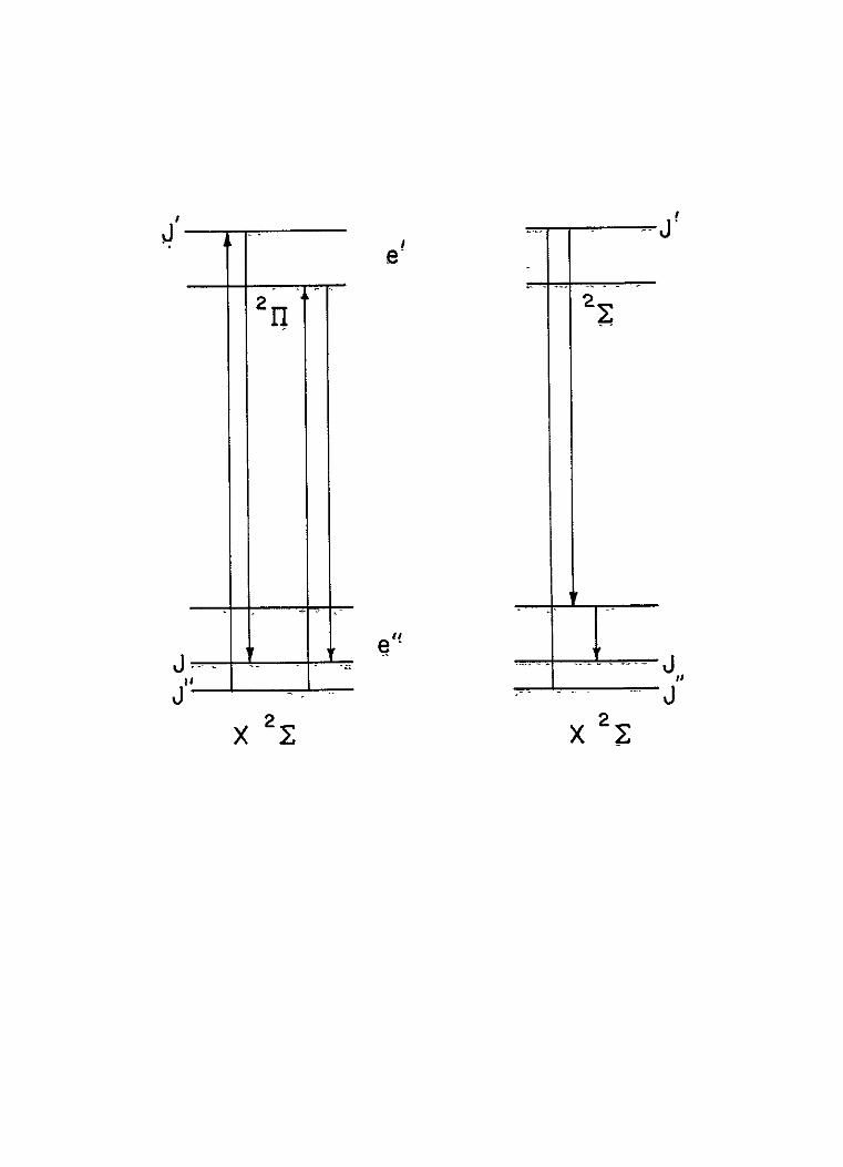
In the treabment of cases I and II which refer to diatomic molecules
with 2 electronic ground states th levels will be denoted by their total
(excluding nuclear) angular momentum J In the treatment of case III which
refers to a molecule such as CH with both spin and orbital angular momentum
in its electronic ground state we will for simplicity of notation refer to the
levels KJ = 1 12 1 32 and 2 32 as 0 1 and 2 respectively
G Case I
Let us first consider the simplest case of interest that of a cloud
of interstellar diatomic molecules which posses a Z electronic ground state
(so that the allowed rotational transitions satisfy the simple selection rule
AJ = plusmn1) interacting only with background Assuming that higher multipole
transitions may be neglected we will show that Tj+I = TB( J I J)
27
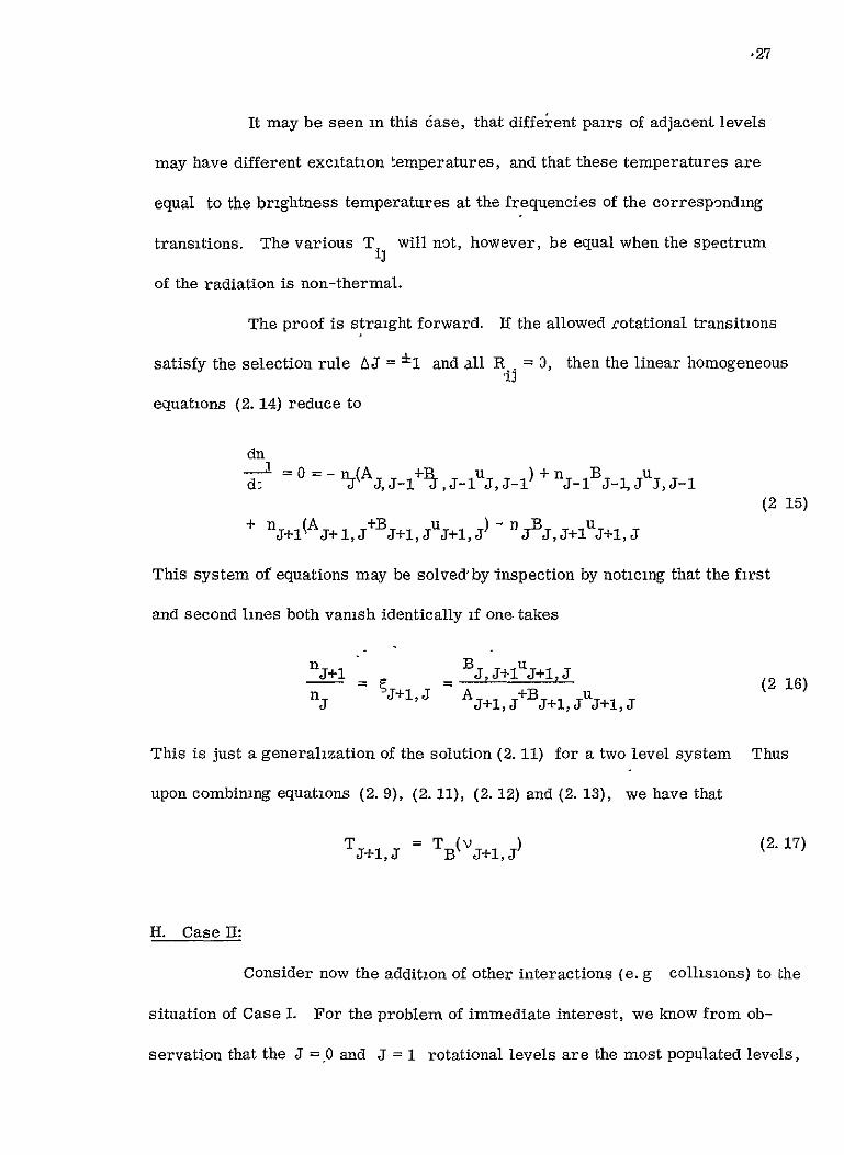
It may be seen in this dase that different pairs of adjacent levels
may have different excitation temperatures and that these temperatures are
equal to the brightness temperatures at the frequencies of the corresponding
transitions The various T will not however be equal when the spectrumii
of the radiation is non-thermal
The proof is straight forward If the allowed rotational transitions
satisfy the selection rule AJ = - 1 and all Ri = 3 then the linear homogeneous
equations (2 14) reduce to
dn d = 0=- nJ(AJ J-1 jluJ J-1 ) + nJ-iBJ_1 juJJ-1
(2 15) + nj+I(Aj+ J+B+ JUj+l J) - jBJJ+lUj+ J
This system of equations may be solved by Inspection by noticing that the first
and second lines both vanish identically if one takes
nj+1 BJ J+1uj+liJ 16)
- A +B u(2nj - J+IJ J5+13 J+J J+1J
This is just a generalization of the solution (2 11) for a two level system Thus
upon combining equations (2 9) (2 11) (2 12) and (2 13) we have that
TJ+IJ = TB(V J+I) (2 17)
H Case II
Consider now the addition of other interactions (e g collisions) to the
situation of Case I For the problem of immediate interest we know from obshy
servation that the J =0 and J = 1 rotational levels are the most populated levels
28
and that these two populations are not inverted (or for the case of CH+ only
the J = 0 level is observably populated)
We will show that T10 and T 2 1 will in general set an upper limit
to the brightness temperatures TB(v 1 0 ) and T B(v21 Hence if the CN R(2)
and the CH+ R(1) absorption lines are not detected (assuming that the corresshy
ponding CN R(1) and CH+ R(0) lines are observed) an upper limit to their optical
depths will set upper limits to the radiation densities at the frequencies of the
CN (1 - 2) and the CH+ (0 - 1) rotational transitions
The proof for this case is somewhat more involved If the allowed
rotational transitions satisfy the selection rule A J = 1 1 but R =0 (we make
no assumptions concerning the selection rules for the additional processes) then
equations (2 14) specialize to
dnj =0= -23=0 R +23nnj 1dt -nj + Rjj dt J1=0 j t=O
-nj(Aj IJ-1+J J-1nJJ-1) + nJ-1BJ-ljujJ-1 (218)
+n (A +B u )-B i
J+1 J+1J J+1 J J+1 J-nJBj J+Uj+J
Using equation (2 10) we can rewrite equations (2 18) for J = 0
~(1 g~nj
-+ =+ o iln 10 A f gjtn0 (2 19)
0 A10 B10U10
and for J = 1
29
nC _ + I - 2
A1 0+B1 0u1 0 -1 B 01 u 1 + l g 1 (220)A 21 + $21 21
Consider first equation (2 20) We aregivent (from observation) that n Ini lt
g gl for all J 2 Hence the individual terms of the summation are all
positive so that nIn 0 10 and T1 0 - will be an upper limit to TB(VI0 )
Also note from equation (2 14) that we can redefine u1 0 such that R 10
R01 =0 Let us denote this by ul i u110 and in the same respect define
I0 1 0 1 We note that shy
n1I
- q1 (221) o
since we have introduced no negative terms into (2 19) by this proceedure
We are now in a position to consider equation (2 20) Introducing
and 4 into this equation we have
n 10n gn2 1 0nR 1shy
___ + __ J=2 gn nI 21 AA + B21 21+
By our previous reasoning and by the use of inequality (2 21) we find that n2 21 thus T21 will be aii upper limit to TB (V2 1 )
I Case III
Finally we proceed to consider the case of an interstellar cloud of
CH molecules excited by both radiation and collisions Again we appeal to
observation and notice that the lowest level is by far the most populated
30
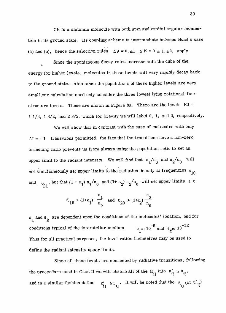
CH is a diatomic molecule with both spin and orbital angular momenshy
tum in its ground state Its coupling scheme is intermediate between Hunds case
(a) and (b) hence the selection rules AJ = 0 plusmn1 A K = 0-plusmn1 2 apply
Since the spontaneous decay rates increase with the cube of the
energy for higher levels molecules in these levels will very rapidly decay back
to the ground state Also since the populations of these higher levels are very
small our calculation need only consider the three lowest lying rotational-fine
structure levels These are shown in Figure 3a There are the levels KJ =
1 12 1 32 and 2 32 which for brevity we will label 0 1 and 2 respectively
We will show that in contrast with the case of molecules with only
j = 1 transitions permitted the fact that the transitions have a non-zero
branching ratio prevents us from always using the population ratio to set an
upper limit to the radiant intensity We will find that n In 0 and n2n 0 will
not simultaneously set upper limits to the radiation density at frequencies V10
and 2 but that (1 + I ) nIn 0 and (1+ F2 ) n2n 0 will set upper limits i e
n n and 20 (1+E2) n2
1 n 010 0 0
l and e2 are dependent upon the conditions of the molecules location and for
conditions typical of the interstellar medium e1 10- 5 and e2t 10 - 1 2
Thus for all practical purposes the level ratios themselves may be used to
define the radiant intensity upper limits
Since all these levels are connected by radiative transitions following
-the proceedure used in Case II we will absorb all of the R into u u
and in a similar fashion define F It will be noted that the p (or V) 13 ij] i
KJ Label
2 32
B
1 2 0iI
0 and 1 in thermal equilibriumFigure 3 a- Transitions A try to keep levels
Transitions B and C depopulate level 1 and populate levels 2 and 0 The
population of level 1 may become depressed if the rate of transitions B
that of transitions Abecomes very large with respect to
32
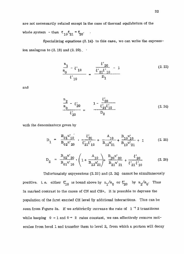
are not necessarily related except in the case of thermal equilibrium of the
whole system - then C10 21 = 20
Specializing equations (2 14) to this case we can write the expressshy
ion analagous to (2 19) and (220) shy
n 120 1 (2 23) n 1i0 21 10
10
and
n2 20 20 (2 24)
20 D2
with the denominators given by
B III4 A B u D1 B01u110 20 + A10 + 10U10 (225)
1 BU U BBv21 B 1 202 20 i0 21 12u121
- udeg 1+ _o + Bo20u0 + 20 (226) 2 B0 1 u1 0 B12 u121 B2 1u 2 1 +2110
Unfortunately expressions (2 23) and (2 24) cannot be simultaneously
positive i e either is bound above by nln0 or by nn Thus10 1 020
in marked contrast to the cases of CN and CH+ it is possible to depress the
population of the first excited CH level by additional interactions This can be
seen from Figure 3a If we arbitririly increase the rate of 1 _ 2 transitions
while keeping 0 - 1 and 0 - 2 rates constant we can effectively remove molshy
ecules from level 1 and transfer them to level 2 from which a portion will decay
33
to level 0 This prodess will effectively decrease nirn0 It will occur if the
1 - 2 rate becomes large with respect to radiative 1 - 0 decay rate
Let us consider equatiois (2 23 - 2 26) slightly further If
A (B U ) is large corresponding to a small rate B ut then the10 12 21 12 21
denominators D and D2 will be large and n IA0 and n2n 0 will set very
good upper limits This term is always large uhless we have an enormous flux
at 21 For CH 20011 the strongest suggested source of radiation
at this wavelength is thermal radiation from interstellar grains (Partridge and
Peebles 1967) For the expected brightness of these
A10 (B12a21) = 1C 1 105 (2 27)
0 ( 1 + 10-5)so is bounded by nn 10 1
The same term also appears in the denominator D2 multiplied by the
factor 0 Since u0 is now bounded all that is required is a
minimum energy density a 20 e g that radiated by grains and D2 will
also be large Taking the maximum energy density at i 0 allowed by observation
and the minimum at v 0 provided by grains then
B0 2aU 0 A2Al B 1Eu1+ ) (228)
B01u10 u2 E2
- 1 2 )Hence we also are safe in using n2n (1+1 0 to bound 20
Nor can we call on collisions to significantly weaken these upper
limits In order to weaken the upper limits we require a selective excitation
rate for R with no associated increase in R and R otherwise the12 1 01 021
populations of at least one of the levels 1 or 2 would have an observable
population
34
However excitation of molecular rotation by collisions (of the first
kind) with projectiles whose kinetic energy is very much greater than the 0 - 1
and 1 - 2 level spacing is not a selective process Thus collisions cannot proshy
vide the selective 1 - 2 excitation necessary to depress the KJ = 1 32 level
population In addition even with the largest excitation cross sections due to
the longest range forces (Coulomb) charged particle densities of at least 100
-3 cm would be required for there to be any effect at all As we will see later
there is specific evidencethat the charged particle densities are nowhere near
this high
The only way tb significantly weaken our upper limits is to have
narrow band radiation at -2 00A which selectively excites the KJ = 1 32 shy
2 32 transition of CH The temperature calculated for this radiation must
be at least as high as 12 K Although such line radiation cannot be totally
ruled out by present observational work it seems highly unlikely that such
radiation might exist in the interstellar medium with an intensity this great
It must be sufficiently narrow band that it not excite the CH X150p transition
and the CH+ X359A transition
Thus it appears that we are quite safe in general in assuming that
n n and n n set safe upper bounds to q and C and that the tempershy1 0 20 10 20
atures corresponding to these population ratios provide good upper limits to the
brightness temperatures at 1 0 and 0
J Sufficient Conditions for Thermal Equilibrium to Hold
From equations (2 14) and (2 15) it can be seen that for molecules
35
- with a E ground state nn will yield an actualmeasurement tof TB(v]
if all Ri ltlt B0110-whereu 1 0 is the intensity necessary to produce 2 7degK
excitation At present we need only concern ourselves with CNsince this is the
only m6lecule in which an excited state population has been observed
The spontaneous decay rate may be written (Condon and Shortley
1951 p 98) in terms of the line sttength s and rotation constant B as
647r4 v 3 5127r4B3 3
JJ- 1 3hc3 (2J+1) J J-1 - 3h 2J+1 JJ-1
Application of Edmonds(1968) equation (5 4 5) to equation (2 5) yields
u (2J-1)(2J+1) -IIJ (2 30)
in terms of the Wigner 3j symbol and hence
5124B3 4 2
3h 2J+1 M (231)JJ-1
From a study of the optical stark effect of ON Thomson and Dalby
(1968) have recently determined the CN dipole moment to be 1 45 plusmn 08D
Tins agrees wellwith the predictions of molecular orbital calculations (Huo 1967)
which indicate that the dipole moment is expected to be in the range 1 2 - 2 5D
and more or less confirms the work of Arpigney (1964) who deduced pu = LID
from an analysis of cometary spectra
of CN has been determined to high precisionThe rotation constant B 0 -shy
by an analysis of the violet band to be B0 = 1 8909cm (Poletto and Rigutti 1965)
in Appendix 2 which may be used for evaluating the Expressions are derived
corresponding Einstein coetct i-mi- or CH
36
Using these values of B and p equation (2 33) yields for CN
-5 -I 10 = 11889 x 10 sec
- 5 - 1secA21 = 11 413 x 10
What we must show in order to claim that the CN is in thermal
equilibrium with the background radiation is that the R are much smaller
than
9 1 A B u 10 (hv_10 869 x10601 8 (2 32)0 1 (2
where u 1 0 is the intensity at v 1 0 necessary to produce an excitation temperature
T = 2 70 K
For most quantum mechanical processes the excitation rates fall off
very rapidly with increasing J since the dipole term in the interaction potenshy
tial is usually the dominant one and has selection rules AJ = 1 Thus it will
be sufficient for our purposes to simply show that for a given process R 0 1
ltlt B 0110 We will see in Chapters 6 7 and 8 that this is probably so if
the CN is in an H I (non-ionized) region of space of reasonable density but
that it is not necessarily so if the CN resides in an H II (ionized) region
37
CHAPTER 3
OPTICAL TRANSITION STRENGTH RATIO
A CN and CH+
In the last Chapter we saw that the rotational temperature may be
calculated in terms of r the observed optical depth ratio and s the theoretical
transition strength ratio defined by equation (2 8)
For lines in the same band s is independent of the electronic osshy
cillator strength and Franck-Condon factor and often depends upon only the
angular momentum quantum numbers of the participating levels K K J and
J The CN violet system is a good example of this Although this transition
2 2 is 2E- 2 the p-dolibling produced by the electron spin is too small to
be resolved in interstellar spectra and on the grounds of spectroscopic
stability (Condon and Shortley 1951 p 20) we are justified in calculating
intensities (and assigningquantum numbers in Figure 3 as our tse of J for K
S1 1 implies) as though the transitibn were 5- 5
Thus when a molecule is well represented in either Hunds case
(a) or (b) as are both CN and CH+ the Sii are proportional to the H6nl-
London factors (Herzberg 1959 p 208) and we have
J + Ji + I -
j j + j +1 (31)
However for the case of CH which is intermediate between these
two representations the calculation is somewhat more involved It requires
a transformation of the matrix elements of the electric-dipole moment operator
38
calculated in the pure Hunds case (b) representation to the mixed represenshy
tation in which the molecular Hamiltonian matrix is diagonal
To effect this transformation we need the matrices which diagonalize
the molecular Hamiltonian matrix hence we also calculate this Hamiltonian
matrix in the Hunds case (b) representation and then calculate the transformation
matrices which diagonalize it As a check we notice that the resulting line strength
ratio agrees with equation (3 1) when we specialize our results to the case of a
rigid rotor
B Matrix Elements of the Molecular Hamiltonian
Since the rotational energy of CH is large with respect to its fine
structure even for the lowest rotational levels we calculate the molecular
Hamiltoman in Hunds case (b) In this representation the appropriate coupling
scheme is (Herzberg 1959 p 221)
K=N+A J=K+S (32)
where in units of A
A is the corhponent of electronic angular momentum along the
internuclear axis
N is the molecular rotational angular momentum and
S is the spin angular momentum of the electron
Appealing again to spectroscopic stability we ignore X- doublets and hyperfine
structure since these interactions like p- doublets are unresolved in intershy
stellar optical spectra
Following Van Vleck (1951) the molecular Hamiltonian is
39
2 2
X=B(K -- A2) + AASz (33)
where A is the spin-orbit coupling constant SZ is the spin angurar momentum
projected along the internuclear axis and B = h221 where I is the molecular
moment of inertia Ther term in S mixes together states of different K when
the fine structure is appreciable with respect to the rotational energy and effects
the transition away from Hunds case (b) towards case (a)
The matrix elements of this Hamiltonian for the Hunds cage (b)
coupling scheme are calculated in Appendix 1 to be
(AKSJ I Y I AKSJ) = B CK(K+I) -A2 ] 8 KK
(34))A+K+K+S+J 1 K 12
11KS 1 (KA 0 A)
If the 3j and 6j symbol are evaluated algebraically this single
expression yields both Van Vlecks (1951) equation (24) for the diagonal and
his equation (25) for the off-diagonal matrix elements but with the opposite
sign convention for the off-diagonal terms
Van Vleck (1951) has calculated these matrix elements by exploiting the anshy
omalous commutation relations of the angular momentum components referred
to the molecular frame He showed that the problem corresponds to the familiar
case of spin-orbit coupling in atoms However since his results yield the
opposite sign convention from ours and are of little value for calculating intensities
we have recalculated them here by more standard means
A misprint occurs in Van Vlecks equation (25) An exponent of 12 has been 2 2 12omitted from the last factor which should read [(K + 1) - A ] The correct
expression appears in the earlier paper of Hill and Van Vleck (1928)
40
Here selection rules may be seen implicit in the properties of the
3j and 6j symbols The selection rule AK = 0 t 1 for the molecular Hamilshy
tonian in case (b) for example follows from the requirement that the rwo
K 1 K of the 3j symbol in equation (3 4) satisfy the triangular rule
For a molecule intermediate between Hunds case (a) and (b) in
general K is no longer a good quantum number in the representation where the
Hamiltonian of equation (34) is diagonal We may however label a given state
with the value of K which it assumes when the molecular fine structure constant
A vanishes We will distinguish K by a carat when it is used as a label in
this way The stationary state is then written as IA KSJ ) and the unitary
matrix which transforms from case (b) to the diagonal frame as UKK ThisKK
unitary matrix will be used to transform the dipole moment operator into the
representation in which the molecular Hamiltonian is diagonal and may be
calculated from (3 4) by a standard matrix diagonalization proceedure
For the diagonalized molecular Hamiltonian matrix itself we have
AKI SJ I Y IAKSJ ) = KK UKK ASIA S I AKSJ) (35)KKKKK
Inserting into this formula the coupling constants for CH of Table 2 and
diagonalizing the matrices for the upper and lower electronic states of CH
we have the partial energy level scheme shown in Figure 3
C Line Strengths
As before we take the line st-rengths to be proportional to the
absolute square of the electric dipole moment operator reduced matrix element
2 ^ 2S (AKSJaC (1) 11tKSJ) (36)
41
where a represents all other non-diagonal quantum numbers
This reduced matrix element has been evaluated in Appendix 2 for
the CH coupling scheme
l(AK SJO C (1) IUKSJC)I =U UKlUKKKKK K
(-1) A+S+JF+l F(2K+I)(2K+I)(2J+l)(2J+1) 12 (37)
J r (alC q c Aq Al) q
The usual symmetric-top selection rules for electric-dipole transitions
AK = 0 plusmn+1 AJ = 0 plusmn1 are implicit in the 33 and 6j symbols (but note that
the transition to case (a) allows ampK = 2 transitions)
When both the upper and lower states are diagonal in the Hunds case
(b) representation and we let the electronic matrix elements ( cc I Ylq k)
equal one expression (3 7) reduces to that of the Honl-London factors (Herzberg
1959 p 208)
When equation (3 7) is specialized to the case of a rigid rotor (CN
and CH+) with K J K = J and S = 0 and with the electronic matrix element
again equal to oneusing Edmonds (1968) equation (6 3 2) we have
(11J C(1) 1A4 =(2Jt 1)(2J+1) (J1 i I (38)
where q=A-A and qIq lt1
With the molecular constants found inTable 2 the resulting values of scalshy
culated from equations (3 7) and(3 8) for the coupling schemes of CN CH
in agreement with (3 1) for CH+ and CN
42
and CH+ are found in Table 1
43
CHAPTER 4
TECHNIQUES OF SPECTROPHOTOMETRY AND PLATE SYNTHESIS
A Available Plates and Spectrophotometry
The optical lines of interstellar CN are characteristically sharp and
weak and occur in the spectra of only a handful of stars The strongest line
R(0) at X3874 6k has an equi alent width which is seldom as strong as 10mA
while the neighboring R(1) and R(2) lines are weaker by a factor of -4 and
-100 for an excitation temperature -3 0 K
The state of the art in high resolution astronomical spectroscopy for
the detection of weak lines has not greatly improved over the past thirty years shy
the weakest line which is detectable with a reasonable degree of certainty on a
single spectrogram is - I - 3 mk Hence it was _lear at the outset of this work
that a new technique would have to be developed if we were to attempt to detect
the CN R(2) lneas well as to measure accurately the R(1) line
At the beginning of this work the best available spectragrams of
interstellar molecular absorption lines were those of Adams and Dunham from
Mt Wilson MUnch from Mt Palomar and Herbig from the Lick 120-inch
telescope Since long exposures are the rule for these spectrograms and
observing time on large telescopes with good Coude spectrographs is somewhat
difficult to obtain it appeared that the most straight forward way to improve the
signal-to-noise ratio was to add the many available individual platesand to filter
out the high frequency grain noise from the composite spectra
Direct superposition of the spectrograms on the densitometer
(plate stacking) is not practical when many spectra are to be added together
44
or when the spectra are dissimilar In addition this proceedure does not allow
one to independently weight the individual spectra The more flexible method
of computer reduction of the datawas fhlt to be best This technique involved
digitization of the spectra and their cblibration and synthesis on a digital
computer The spectra could then be filtered of grain noise numerically in
the manner suggested by Fellgett (1953) and Westphal (1965) The whole system
turned oat to be very flexible so that the large heterogeneous group of plates
could be added without difficulty
Most of the plates were obtained from the extensive collection of
high-dispersion spectrograms stored in the Mt Wilson Observatory plate fires
There were obtained primarily by Adams and Dunham with the Coud6 spectrograph
of the 100-inch telescope and its 114 camera and were used by Adams (1949)
in his classic study of interstellar lines The spectra of the two ninth magshy
nitude stars BD+660 1674 and BD+66 0 1675 were taken by Miinch (1964) with
the 200-inch telescope The synthesis for C Optuchiincludes six spectra
obtained by Herbig (1968) with the Lick 120-inch telescope using the 160 camera
and were used by him in his recent study of the interstellar cloud in front of
C Ophiuchl (The latter were also analyzed by Field and Hitchcock [1964 in
their discussion of the microwave background ) We are indebted to Drs Munch
and Herbig for the loan of these plates
Similar techniques have been usedby Herbig (1966) for a small number of
similar plates
45
Data such as the emulsion exposure time etc for the individual
plates were copied for the most part from the observing notebook and are
listed in Table 3 Also in this Table are the relative weights (determined
from statistical analysis of grain noise as described below) which the indishy
vidual spectra are given in the final synthesis
It is evident from the Table and from the weights that they by no
means represent a homogeneous collection The weights were determined by
a visual estimate of the grain noise r in s level on tracings which were norshy
malized to the same signal level The normalized tracings were then combined
with the usual prescription of weighting them inversely as the square of the
noise level
These plates were scanned at the California Institute of Technology
on a Sinclair Smith microdensitometer the output of which was fed across the
Caltech campus via shielded cable to an analog-to-digital converter This was
connected to an IBM 7010 computer which wrote the digitized signal on magnetic
tape and subsequent analysis of the data wasdone on an IBM 36075 computer
at the Goddard Institute for Space Studies (GISS) in New Ycrk City
Figure 4 shows the setup of equipment at Caltech The output of
the densitometer was digitized at a constant rate of 100 samples per second
The lead screw was not digitized but also ran at a constant speed The projected
acceptance slit width and lead screw speed were adjusted to suit the dispersion
of the plateand the width of the narrowest spectral features being studied
which were about 0 05A Thus for the Mt Wilson 114 camera plates
(dispersion = 2 9Amm) which comprise the bulk of the data
46
the plate advanced at 5 6mmin (16 3min) For the narrowest lines this
is about five line widths per second In other words at least 20 data points
were obtained per resolution element which is ample for our purposes
- The projected acceptance slit width was adjusted to the dispersion
of the plate being scanned to approximately 16 of the full line width of the
interstellar lines Thus for plates from the 114 camera the projected slit
widh was about 2 9M which leads to negligible signal distortion
Four or more densitometer traces were usually taken in the vicinity
of the three wavelength regions of interest X3874L X42323 and X4300A
Two were required for the comparison spectra on either side of the stellar
spectrum at least one was required for the stellar spectrum itself while a
single scan perpendicular to the dispersion of the spectrograph was necessary
to record intensity calibration wedge bars
In order to establish a reference wavelength common to the stellar
and comparison spectra a razor blade was placed across the emulsion as
shown in Figure 5 A scan started on the razor blade and moved off the edge
onto the spectrum as shown in the Figure with the edge producing an initial
step in the recorded spectrum In addition to providing a wavelength fiducial
mark the step providel a measure of the response time of the electronics and
the optical resolution of the system and in the case of the intensity wedge
provided a dark-plate level
B Synthesis Programs
The computer program for plate synthesis was divided into three
47
sub-programs each sub-program was processed separately with the input for
a given sub-program being-the output~tapes from the previous one There were
named Sys 3 Sys 4 and Sys 5
Sys 3 read the 7040 tapes and data such as the transverse lead screw
position which had been punched manually onto cards and scanned this data for
errors Preliminary plots of each vector versus index were made after it had
been adjusted to start at the fiducial mark step (caused by the razor edge) so
that the index of a given digitized point in the vector was proportional to its
corresponding distance from the razor edge Output of plates corresponding
to different molecules were sorted onto different tapes so that processing of a
tape after this point was for a single spectral region The basic purpose of
Sys 3 was to pre-process as much information as possible to implement the
smooth running of Sys 4
Sys 4 took the left adjusted vectors for -each plate and converted
these to two (or more if there were more than one input stellar spectrum vector)
parallel vectors of intensity and wavelength (shifted to the molecules rest frame)
This was done in two parts using an IBM 2250 CRT display console in conjunction
with the GISS computer The first part used the wedge vector to convert the
recorded plate transmissions to intensity The calibration density wedge bars
had been put on the plate at calibrated light levels the values of which were
stored in the computer
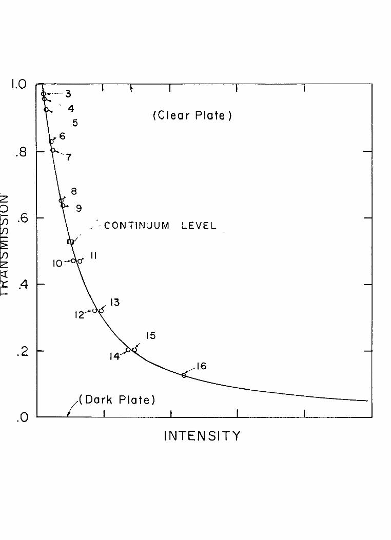
The wedge bars from the density wedge vector appear as rectangular
peaks as shown in Figure 6 The limits of these rectangular bars were detershy
mined in Sys 4 by displaying the wedge vector on the 2250 console and picking
48
out the endjs of the rectangular peaks witha light pen The computer then
averaged the t-ransmission over each wedge bar Since the two sides of the
wedge were put ou the plate at different intensities- the wedge values on one
side were scaled up or down to interleave them between adjacent points on the
other side The composite curve was then fit with five terms of a Laurent series
a typical result of which is shown in Figure 7 The series was finally applied to
each point in each spectral vector converting the plate transmission to intensity
The second part of Sys 4 calibrated the index scale in terms of waveshy
length Each comparison spectrum was displayed on the 2250 Display Console
and the centers of selected lines were located with the console light pen The
corresponding wavelength of each line was then plotted on the 2250 screen as a
function of index Since the dispersion is highly linear over the - 10A traced
in the vicinity of each interstellar line these points appeared on the screen in
a straight line A straight line least-square fit was also displayed on the screen
which aided in the correction of any line misidentification The output of Sys 4
was finally two parallel vectors of intensity and corresponding wavelength approshy
priate to the laboratory frame
In general high resolution Coud6 spectrographs are rather well
matched to the emulsions used in astrophysical spectroscopy and grain noise
which is high frequency with respect to sharp interstellar lines is not conshy
spicuous In order to extract the maximum amoant of statistical information
from the data at hand however a considerable amount of thought was given to
the problem of numerically filtering the final spectra A description of the
statistical analysis appears in Appendix 4 The final result of the analysis
49
was to prescribe afilter function to be used to filter the calculated synthesis
Thus Sys 5 was designed to take the successive outputs from Sys 4
and to add these together with the appropriate statistical weights It then filtered
out the high frequency noise by convolving the synthesis with the above filter
function The final output of Sys 5 for each star and molecule was three vectors
1 Wavelength in the molecular rest frame
2 Unfirtered spectrum
3 Filtered spectrum
50
OHAPTtR 5
RESULTS OF SYNTHlESIS
A Curve of Growth Analysis
Figures 9 10 and 11 show the results of addiig togethefin the manner
just described the available spectra of interstellar CN CH and CH+ for a
number of stars As just mentioned the wavelength scales in these plots sre
those of the molecular rest frame and the final spectra except for CPersei
CN and COphrnchi CN have been numerically filtered The number of inshy
dividual spectra included in each synthesis and the corresponding vertical magshy
nification factor are indicated on the left side of Figure 9
Table 4 lists the visual magnitudes MK spectral types galactic
latitudes as well as the equivalent widths W and optical depths T for the intershy
stellar lines measured The uncertainties of W in all instances result from a
statistical analysis of the grain noise and represent a level of confidence of
955 (see Appendix 4) Also all upper limits set on the strengths of unobsershy
ved lines represent the more conservative confidence level 99 7
For COphiuchi the equivalent widths of the interstellar molecular
lines listed in Table 4 are systematically smaller by - 30 than the values
obtained by Herbig (1968a) from plates taken at the 120-inch Coude We note
ehowever that Dunham (1941) reported W 6mA for the CN R(0) line and
W = 14m for the CH R2(1) line in C Ophiuchi and 0 C Wilson (1948) reported
W = 16 L 2mA for the CH+ R(0) line in C Ophiuchi both from Mt Wilson plates
and both in good agreement with out values of 6 62 13 4 and 19 6 mA reshy
spectively
51
Since most of the spectra from which our values are derived were
also obtained with the 100-inch telescope about thirty years ago this gives us
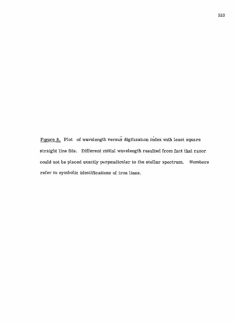
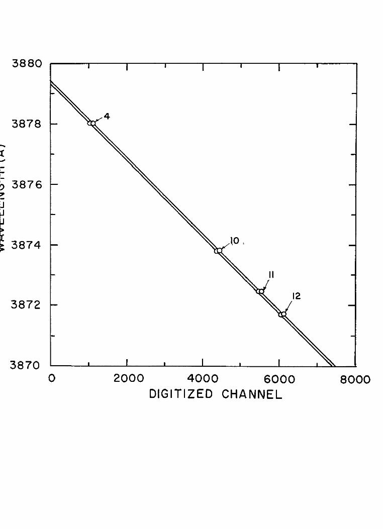
some confidence that the discrepancy is not a result of an error in calibrating
or adding together the spectra but represents instead a systematic difference
between equivalent widths obtained with the 100-inch Coude then and the 120-inch
Coude now Our main interest however is only in the ratio of line strengths
which in the limit of weak lines is independent of systematic uncertainties of this
kind and it is accordingly unnecessary to explore this point further But we
emphasize that the uncertainties listed in Table 4 can only be taken seriously in
a relative sense and are liable to be considerably less than absolute uncertainties
Also included in this Table for completeness are several late B and
early A type stars-whose rotational temperatures have been estimated by other
workers
The calculation of the optical depths in Table 4 requires some knowshy
ledge or assumption concerning the true shape and width of the interstellar molecshy
ular lines In general the lines we are considering are not quite resolved and
it is thus necessary to make several assumptions concerning the curve of growth
Fortunately the CN lines are usually so weak that the correction for saturation
is small and our final results are not very sensitive to these assumptions
bull It is interesting to note however that Adams (1949) was led to suggest that
the molecular absorption spectra may be time variant
52
We assume a gaussian line shape in all cases (see Appendix 4) and
use the curve of growth due to Strbmgren (1948) and Spitzer (1948) and the
tabulation of Ladenburg (1930) For COphiuchi we adopt for the linewidth
parameter b = 0 61kmsec which is the value b = 0 85kmsec found by Herbig
(1968a) for interstellar CH+ in the spectrum of this star corrected for the
apparently systematic difference in the measured equivalent widths of the CN R(0)
line In lieu of any other information we assign b = 0 85kmsec tothe CN
lines of CPersei since this star lies at a distance comparable to cOphiuchi
and is also well off the galactic plane (We have also found with the 300-foot
transit radio telescope at Green Bank that the 21cm profile in the direction of
this star closely re sembles that in the direction of COphiuchi - see Chapter 9)
The signal strengths for the CN lines of the remaining stars shown
in Figure 9 scarcely justify correction for line saturation we simply adopt
b = lkmsec for all remaining stars except BD+66 0 1674 and BD+66 0 1675 to
which we assign b = 5kmsec on the basis of their great distance and low
galactic latitude
The excitation temperatures of interstellar CN may now be calculated
from the ratios of the optical depths listed in Table 4 from equation (3 4)
This was rechecked and a finer abulation made
Further work should be done to obtain a good curve of growth for this star
due to its importance here
53
B CN (J = 0 - 1) Rotational Temperature and Upper Limit to the Background
Radiation at X2 64mm
Table 4 now shows the results of the application of equation (3 4) to
=this data taking v 1 134 x 10 11sec- (X = 2 64mm) corresponding to the 0
J = 0 - I transition in CN The listed value of T 1 0 (CN) results from the ratio
of the optical depths listed in Table 4 The entry labeled AT lowers T 1 0 (CN)
by an amount which is at most comparable to the uncertainty due to the plate grain
noise and therefore our final results as mentioned above do not critically
depend on the assumptions that were made concerning the curve of growth
Tb get an upper limit on the radiation intensity we need consider only
C Ophiuchi where the molecular absorption lines have the greatest signal-to-noise
ratio For this star the weighted mean of the values found from the line strength
ratios R(I)R(0) and P(1)R(0) given respective weights of 4 to 1 the square
of the corresponding values of s (see Chapter 3) yields T B(2 64mm) T 1 0(CN) =
2 74 + 0 22 0K In terms of the intensity of radiation -this becomes
-15 -2 -1 tr-1 H-1 342 x 10 erg cm sec ster HzIV(2 64mm)
C Upper Limit to Background Radiation at X= 1 32mm -
The observed absence in the spectrum of COphiuchi of the CN R(2)
line at X3873 369A places an upper limit to the background intensity at
= 32mm From the spectrum of Figure 9 it is found that the equivalent
width of the CN R(2) line is less than 0 44mi to a level of confidence of 99 7
The curve of growth analysis described above then yields Tlt 0 031 and the
rotational temperature found from equation (3 4) and the R(2)R(1) ratio is
54
TB (1 32mm) -T 21(CN) lt 5 490 K
and
1-14 -2 - 1 shy- -I
erg cm sec ster HzI (1 32mm) lt2 75 x 10
which is still a factor of 8 3 above the intensity of 2 740 K thermal radiation
but a factor of 1 6 below the intensity of 2 74 0 K greybodyradiation This
upper limit is shown in Figure 12
D Radiation Upper Limit at X = 0 359mm
The observed absence of the CH+ R(1) line at X4229 341A in the
spectrum of C Ophiuchi synthesized from 19 spectra of this star and shown in
Figure 11 allows an upper limit to be placed on the intensity of radiation at
the wavelength of the CH+ J = 0 - 1 transition (0 359mm)
As with CN the optical depths listed in Table 4 were calculated using
Herbigs (1968a) value b = 0 85kmsec for the linewidth parameter adjusted
to take into account the apparently systematic difference between our and his
equivalent widths
For the CH+ R(1)R(0) ratio it was found that s = 32 v = 8 35 x 110
10 11Hz and
TB(0 359mm) lt T (CH+) lt9 01 K
or
-14 -2 -1 te-1 H-1 sec ster HzI (0 359mm) lt 10 1 x 10 erg cm
2 i e the extrapolation of the Rayleigh-Jeans intensity I = 2kT v 2e to short
wavelengths Radiation from an optically thin medium such as dust can approximate
a spectrum of this type
55
E Detection of Interstellar C 13H+
R(0) line of C 13H+ Also shown in Figure 11 is the faint trace of the
originally sought by Wilson (1948) and again by Herbig (1968b) A statistical
analysis yields for the equivalent width 0 6 1 3mA to a confidence level of 95
Together with the R(0) line of C 12H+ this yields for the isotopic abundance
ratio along the line of sight C12C 1 3 = -22 in agreement with the h valueau62 + 1 0 0 mareetwt
+55 825 independently found by Bortolot and Thaddeus (1969) and also with the
terrestial value 89 but much greater than the equilibrium value P4 for the
CN bi-cycle (Caughlin 1965) This observation strengthens Herbigs (1968b)
earlier conclusion that the material in the C Ophiuchi cloud did not come from
C1 3 rich stars but raises the question of how one explains the apparent agreeshy
ment of this value with the terrestial one
Bortolot and Thaddeus (1969) suggest that the coincidence of the
C1 3 terrestial abundance with that of the interstellar abundance is due to the
origin of the solar system out of an interstellar medium with a fixed C1 3 abunshy
13dance This notion is consistent with the coincidence of the atmospheric C
abundance of Venus with the terrestial abundance ( Copnes et al 1968) however it
is inconsistent with the recent observations of Lambert and Malia (1968) who
find the solar abundance ratio to be C 13C = 150 t 30 a value which exceeds
the terrestial ratio by nearly a factor of two
Lambert and Malia believe that their observation represents at least
bull There is considerable dispute on the question of the solar C13 abundance
(Cameron 1969)
56
a definite upper limit to the solar C1 3 abundance Since there is no obvious
process which might increase the solar C1 3 abundance further work confirming
their observations will represent strong evidence favoring the suggestion of
Fowler et al (1961) that the planetary abundances are a product of spallation
and is otherwise unrelated to the interstellar C1 3 abundance
F Radiation Upper limits at X= 0 560 and X- 0 150mm
Figure 10 shows the result of the synthesis of seventeen spectra of
Ophiuchi in the vicinity of X= 4300k the strongest lines of CH The observed
absences of the CH R (1) and R 2(2) lines at X- 4304 946A and 4296 636A allow
upper limits to be placed on background intensity at the wavelengths of the
5 6 0mm)CH KJ=1 12- 132( =0 and KJ=1 12- 2 32 (= 0150mm)
transitions We again use b = 0 85mm (corrected)
For the CH KJ = 1 12 - 1 32 transition s was calculated in Chapter
3 to be 1 525 Taking v 1 32 1 12 = 5 3 7 x 10 1 1H z (= 0560mm) equation
(3 4) and the data of Table 4 then yield
TB(0 560mm) -T 1 32 1 12 (CH) lt 6 33 0 K
or
-14 -2 -1ste-1 H-1 10 560mm) f391 x 10 erg cm sec ster Hz
Finally for the CH KJ = 2 32 - 1 12 transition s = 0 820 and
0 150mm) Hence32 1 12 ==2 00 x 1012Hz (X=
TB(0 150mm) fT 32 1 12( C H ) lt 28 5K
2
or
IV 150mm) lt 4 2 x 10 erg cm sec ster Hz
57
G Discussion of Upper Limits
At 1501 the most important source of background might be the
contribution from young galaxies (Low and Tucker 1968 Partridge and
Peebles 1967) However the CH upper limit at 150 is 105 greater than the
expected integrated brightness of these objects and as a result is of little value
The constraints which the other upper limits impose on the background
radiation are shown in Figure 12 Except for the point at 2 64mm they fall well
above the blackbody curve at T = 2 7 0K and all are considerably below the
corresponding greybody curve They immediately represent much of the inforshy
mation we possess on the radiative content of the universe at these wavelengths
It bears final emphasis that as upper limitsall of these points are virtually
independent of any considerations concerning the location or environment of the
molecules
Shivananden et al (1968) have recently reported the detection of
a background flux in the wavelength interval from 4 to 1 3mm with a rocketshy
- - 1 borne wide-band detector They detected a flux of 5 x 10 - 9 W cm 2 ster
which yields a mean intensity over this frequency range of I = 9 6 x 10⁻⁴
-2 -I -1 erg cm ster Hz This flux is represented in Figure 12 by the area
under the line AA Since its mean value is nearly three times greater
than the CH upper limit-which falls right in the center of their frequency range
it may be concluded that either their observation is of a background with highly
irregular spectrum (eg spectral lines) or it is of a flux of quite local origin
which does not extend as far as the major interstellar cloud in front of
Ophiuchi
58
The important question which is unanswered at this point in the
analysis is what is the meaning of the observed J = 1 level population of CN
In the remaining Chapters we will try to show that in all probability this
population provides a good measure of the radiation intensity at X 2 64mm
and the intensity at this wavelength is equal to that of a blackbody temperature
T B = T1 0(CN)
59
CHAPTER 6
ALTERNATE RADIATIVE EXCITATION MECHANISMS
In addition to direct rotational excitation of CN by microwave photons
radiative excitation is possible to both higher vibrational and electronic states
by infrared and optical photons The characteristic lifetimes of these
higher states are very short and virtually all of the molecules will be found in
the ground electronic and vibrational states However indirect rotational
excitation is possible by means of electronic and vibrational fluorescence A
CN molecule can be excited to a high vibrational or electronic level by an optical
photon (from dilute starlight for example) and re-emit a photon while making a
transition back to a rotational level different from the one in which it started
Hence this cycle can effectively populate higher rotational levels and contrishy
bute to the observed rotational temperature Typical cycles are shown in Figure
13
Suich indirect processes are potentially very serious alternate mechshy
anisms for the CN rotational excitation in that they might provide an explanation
for the observed rotational temperature invariance in eleven stars This observed
invariance provides the strongest single piece of evidence that the CN is not
excited by processes other than the cosmic microwave background (See Chapter
9)
The explanation for the invariance in terms of fluorescence could
come in either of two ways First if the excitation is produced by galactic
starlight the inherent uniformity of this radiation might account for the observed
invariance Second the process of CN formation in the interstellar medium
60
is not well understood (see for example Dieter and Goss 1968) and it seems
plausible to suggest that the CN is only formed at certain distances from a star
and thus would always be subject to the same radiation field In this respect
Miinch (1964) has proposed that the CN is being flashed off interstellar grains
by the advancing ionization front atoan H I - H II boundary
However it will be shown in this Chapter that (1) vibrational
fluorescent excitation is negligible by more than six orders of magnitude (2)
Electronic fluorescence is insufficient to account for the observed CN rotational
excitation by at least three orders of magnitude for galactic starlight (3) If
the CN is close enough to a star perhaps the star used to observe itfor fluoresshy
cence to contribute materially to the rotational excitation of the ground state then
the photo-dissociation rate will be so high that the molecules will be destroyed at
a rate much faster than any suggested mechanism for their production In addshy
ition the idea that the molecules are circumstellar is inconsistent with
out present ideas concerning the location of the molecules
A Criterion for Fluorescence to be Negjiible
We saw in Chapter 2 that a sufficient criterion for a process to be
negligible is for Rif J+ lt lt AJ+J where J and J+1 represent
rotational levels in the electronic ground state e
The suggestion by Merrill (1942 1946) that the CN might be circumstellar was
dispelled by Adams (1949 see Chapter 7)
Unless otherwise specified ell will be used to denote either an electronic
or a vibrational state
61
Fluorescent excitation involves first a transition from rotational
level J in the ground electronic and vibrational state e to a level J in a
higher electronic or vibrational state e This will occur at a rate given by
ev Beji evi Subsequently the molecule decays to a rotational level
J in the electronic ground state e Since the excited vibrational or electronic
state lifetimes are very short in general
gt gt AeJ eJ ueJ ejBeJ eJ (6)
Thus for a given band system the total rotational excitation rate is given approxshy
imately by
R j a ev etlJ U ee eJ eJ (6 2)
where aeJ eJ is the branching ratioof eJ - eJ electronic decays
(including cascades through an intermediate electronic state) to all other possible
electronic decays a will generally be I (always 1) Hence a sufficient
criterion for fluorescence to provide negligible rotational excitation is for
uevil etjttBeJ eJ lt ltAjj+1 (6 3)
for all e J
B Vibrational Fluores cence
We will assume that the galactic radiation field near X 4 9p
(the wavelength of the CN v= 0 - Ivibrational transition) is predominantly
dilute starlight Speculation about-the existance of radiation from young galshy
axies (Partridge and Peebles 1967) suggests an additional contribution which
is at most the same order of magnitude so we will neglect this component
62
The energy density of starlight at this wavelength is given by
1 u(4 91) = 8 8 x 10-28erg cm - I-Iz
The Einstein B coefficient for this transition is calculated in Appendix 3 and
from it we calculate that
-R9 4 x 10 - 12 sec 1 v=0 1
This rate is totally negligible with respect to the excitation rate necessary to
produce the observed 2 70 K excitation B01 10 = 8 7 x 10⁻⁶
Thus vibrational
excitation falls short by six orders of magnitude in accounting for the observed
excitation
C Electronic Fluorescence
For electronic transitions in which one electron is involved we can
write the Einstein B coefficient in terms of the electroni oscillator strength
or f value (1X Herzberg 1959) Thus the upper limit for the excitation
by optical photons of frequency v = v ev eTvJ is given by
bullv) ne 2 fe r(vib) 12 trot) 2ult) f vv j JJ+ - mhc v (2J+l) (64)
where (ot 12 are the Honl - London factors and 1 viI 2 are the
Franck - Condon factors
Then the usual sum rules apply
I (rot) 12_ __j2j 2x+1 (65)
Jt MM
63
C
z (vib) 12vv (66)
fEff =1 (67) ee
Since u(v) is a slowly varying function of v and the excitation will be preshy
dominantly via the (0 0) band we may sum over allowed rotational and vibrashy
tional transitions to get rre fee
R UN) emhe (68)01 U(V cv
where v= v e v=0 J1= ev =0 J =0
CN Band Systems -a
CN has two band systems in the visible the well known red
(X2E AA (X2 - ) The fand violet 2 B 2 systems values for these
transitions have been measured to be 0 0034 (Jeunehomme 1965) and 0 027
(Bennett and Dalby 1962) respectively
2 Ultraviolet systems involving electronic states above B Ehave
been studied by Douglasand Routly (1954 1955) and by Carroll (1956) Our
current knowledge of the electronic term scheme of CN is shown in Figure 14
It is of considerable importance to us to know the oscillator strengths
of the CN ultraviolet systems Douglas (1968) has searched unsuccessfully for
these transitions in absorption down to X 14001 ina long path length
White-Cell He has concluded that all of the oscillator strengths for these
ultraviolet systems which terminate in the ground electronic state are less
than the oscillator strength of the violet system ( 027) The CN dissociation
64
energy corresponds to X - 1500 A (Carroll 1956) thus any state with a
large oscillator strength for transitions from theground state must lie beyond
the dissociation limit
C Rel Upper Limits-b -61
It is revealing now to calculate the upper limit for R 01given by
(6 8) assuming f and a to be equal to 1 This is plotted in Figure 15 as a
function of wavelength for a radiation field corresponding to that of the galactic
starlight background (Zimmerman 1964) For the red and violet bands the
measured f values are also shown displacing these upper limits accordingly
Thus it is clear that for any bandsystem the fluorescent excitation
rate due to the galactic background will be - 2 x 10 see or smaller This
is - 6000 times too small to yield the required excitation and we may thus
conclude without further discussion that the galactic starlight background is
not responsible for the CN excitation This is a most important point since
this is the only process which we have been able to find which might account
for the observed independence of T 1 0 (CN) with respect to galactic latitude
longitude or spectral type of the star against which the ON is observed
Now consider the situation in which the star is the source of fluoresshy
cent radiation Figure 15 also shows the upper limit for R 0 1 given by (6 8)
for a radiation field corresponding to that of a line blanketed BOv star at a
distance of 10pc (Hickok and Morton 1968) Again we assume f and C = 1
and see that at this distance the starlight intensity is of the same order as the
galactic starlight Thus if the CN is not circumstellar the radiationfield
65
of the star used to observe it is of insufficient strength to account for the obshy
served rotational excitation
In order to have the fluorescent excitation of the star play a dominant
-5 -1Irole in the rotational excitation of the CN we need R01 - 10 sec There
are two consequences of an excitation rate this high Firstthe flux necessary
to yield this high a rate would require the star to be as close as 0 2pc to theCN
This -proximity is totally contrary to our present ideas concerning the location
of interstellar clouds A review of our present understanding of their location
will be deferred to Chapters 7 and 9 however the main feature which emerges
from this work is that the clouds are not circumstellar but rather broad layers
spanning in several instances more than one star For example the intershy
stellar CN linesof X Persei and CPersel appear to originate in the same
interstellar cloud These clouds appear to have the atoms and the molecules
well mixed and only a moderate radiation field incident upon them (see for
example Herbig 1968a)
Secondly since we know that all of the f values are small
electronic-states which lie belov the dissociation limit the sum rule (6 7)
implies the existance of at least one electronic state above the ionization limit
with an f value approaching unity If a molecule makes a transition to this
state it will have a certain probability for dissociation It is difficult to estimate
what this probability is but we believe a value of - 1 to be a conservative
guess
Then since-the f value of the dissociating state is greatest this
state will produce the fluorescence and the molecules will be destroyed at a
66
-7 -1 -5 shyrate - 10 sec per CN molecule (They will be excited at a rate 10 sec
and 1 of these will dissociate ) In order to maintain an equilibrium population
of CN we must have a continuous production rate for these molecules of equal
magnitude
The production of interstellar molecules is unfortunately not well
understood (see for example Dieter and Goss 1966) and only with difficulty is it
possible to get CH production rates comparable to CH dissociation rates ( 10 - 11
-1 sec per molecule for the CH existing in the interstellar radiation field)
Assuming similar processes to be responsible for the formation of CN it would
appear then hard to understand even the existance of the CN Hence it appears
highly improbable that the observed excitation could be due to the fluorescence
67
CHAPTER 7
COLLISIONAL EXCITATION IN H I REGIONS
In this Chapter we summarize briefly those properties of H I and
H II regions which are pertinent to the problem at hand and we review work
devoted to the location and environment of the interstellar molecules We then
proceed to consider in some detail the possible rotational excitation mechanisms
of the CN if it resides in an H I region of the interstellar medium
A Difference Between H I and H II Regions
Almost 10 of the galactic mass is in gas clouds - 4pc in diameter
which comprise about 10o of the volume of the galactic plane These tend to
be irregular in concentration and composition but are composed mainly of atomic
hydrogen (although H2 may predominate at higher densities) This gas is divided
into two distinct types of regions H I and H II regions (Strdmgren 1939 1948)
H I regions are neutral atomic hydrogen with a kinetic temperature - 1250 K and
4 -3 -3hydrogen number density rarely exceeding 10 cm and usually s 1cm
H II regions on the other hand are the emission nebulae which
surround hot luminous 0 and B stars which have sufficient ultraviolet flux
to fully ionize the surrounding atomic hydrogen These regions then have a
4 -3-temperature 10 OK and density -10cm Since 0 and B stars are comshy
For a review of the interstellar medium see Dieter and Goss (1966) and Vol
VII of Stars and Stellar Systems Nebulae and Interstellar Matter (Middlehurst
and Aller 1968)
68
paratively uncommon and stars later than B 0 have only limited H II regions
associated with them- H II regions only involve - 10 of the mass of the intershy
stellar gas near the galactic plane
A well known but noteworthy feature of the interstellar medium is that
the boundary between the two types of regions is relatively sharp (Str6mgren
1939 1948) This is due to the fact that the radiant energy density beyond the
Lyman limit falls off inversely as the square ofthe distance from the star where
as the total opacity due to the non-ionized component of the gas increases exponenshy
tially with the path length to the star These two effects when included in the
equationsfor ionization equilibrium producea very sharp transition between H I
and H II
B Earlier Work on the Place of Origin of the Molecular Interstellar Lines
Prior to Adams work (1943 1949) Merrill (1942 1946) had suggested
that there might be a difference in the place of origin of the molecular absorption
lines and those of Na I and Ca II known to be interstellar in origin The latter
would presumably originate in the true interstellar clouds far from the star
against which the lines were observedwhile the molecular lines might be produced
in circumstellar clouds and be affected by the stellar radiation field
To clarify this situation Adams measured the velocity correlation
between the H and K lines of Ca II and the molecular lines He found that
all of the evidence suggested a common origin for molecular and atomic lines
in the same clouds and in the same portions of the same clouds He showed
that the molecular lines when present almost invariably correspond to the
69
strongest components of-complex H and K lines Thus there is a close relationshy
ship between the Ca II and the molecular lines as regards both position and in
most cases relative intensities as well
Also contributing to his conclusion were the presence of the same
molecular lines with nearly the-same intensities in wide double stars and numerous
pairs of physically unrelated stars He also found no evidence that the occurrence
of the lines is related to the spectral types of stars which appear to lie nearest
the clouds of their origin
To further support this work Bates and Spitzer (1951) subsequently
showed that Adams visual estimates of the intensities of the molecular lines
yield a correlation with the intensities of the interstellar reddening the latter
is presumably due to the presence of grains Taking advantage of the new and
more accurate atomic and molecular f values Herbig (1968a) has recently conshy
sidered this problem for one particular star t Ophiuchi This was chosen because
it has a single well resolved interstellar cloud in front of it He has arrived at
a similar conclusion that the place of origin of both the molecular and atomic lines
is an interstellar H I cloud His arguements for this conclusion are as follows
Bates and Spitzer (1951) also suggest that the stars in the Pleades represent
a unique case in that the CH+ in the spectra of these stars is probably circumshy
stellar
70
f The pattern of Ca II absorption lines in Ophiuch is repeated
in at least seven stars in this direction many of them well outside the H II
region surrounding t Ophiuchi Since this is the only star in the group involved
in an H II region these lines must be formed in a rather extensive foreground
layer not associated with these stars
2 A similar arguement applies to H I 21cm emission feature
which is not appreciably affected by and extends well beyond the Ophiuchi H II
region This feature is identified with the same cloud containing the other absorbshy
ing molecules
3 If the Na I lines were formed in an H II region the increased
electron presure would depress the sodium ionization and imply an order of
magnitude deficiency in the NaH ratio If one assumes an H I region as the
origin of the Na I lines one gets the solar system NaH and KH abundance
ratios
4 A comparison of the 109 a and H a emission lines originating
in the H II region shows no turbulent width correlation with any of the interstellar
species
Thus Herbig has concluded that for the case of Ophiuchi at least
which is probably the most important star for our work the place of origin of
the molecular lines is an interstellar H I region
C Collisional Mechanisms in H I Regions
We now turn to a consideration of the various collisional excitation
mechanisms of the CN assuming that it does reside in an H I region Since
71
the kinetic temperature here is - 1250K and particles -will have kinetic energies
--4kTr = 229cm it is clear that we need to consider only direct rotational
excitation- Indirect rotational excitation by way of higher electronic and vibrationshy
al states can be immediately ruled outon energetic grounds alone as the thresshy
-holds for excitation of these states are 2024cm - and 9114cm respectively
D Excitation by H A-tonis
Weshall consider first the collisional excitation by neutral hydrogen
atoms We can write for the excitation rate
R 01= fvN H (v) a 01 (v) dv NH v a01 = NHrOl (71)
where
NH is the total H I iiumber density
v is the mean atomic Velocity
a0 1 is the total cross section for rotational excitation
The calculation of a0 1 in terms of molecular parameters is a difficult
problem in the theory of atomic collisions Fortunately the problem is one which
in another guise has been studied from both an experimental and theoretical point
of view This is the problem of microwave pressure broadening (Townes and
Schawlow 1955 p 338)
Virtually all of the experimental work of this subject has been devoted
to an understanding of the interaction between chemically stable systems which
can be conveniently studied under laboratory conditions while H I and CN are
both free radicals The particular short range forces responsible for pressure
72
broadening however do not basically distinguish between free radicals and
chemically stable molecules and it is thus possible to estimate the cross section
for CN rotational excitation by H to an accuracy of perhaps 50 by an appeal
to the laboratory data of similar molecules
A rather similar process which has been described in the literature is
that of the pressure broadening of the H Cl J = 0 - 1 rotational line by collisions
with He atoms at room temperature (Rank et al 1963) The resulting cross
section for the J = 0 - 1 rotational excitation has been calculated from the exshy
perimental results to be 1 6 x 10 - 15 cm 2 (Gordon 1966)
H Cl like CN is a highly polar molecule with AHCI = 1 085D (Bell
and Coop 1938) The bond lengths of the two molecules are also similar shy
r e(HCl) = 1 274d versus r e(CN) = 1 172A (Herzberg 1959 Table 39)
Unfortunately the quantum-mechanical description of the collision
between a polar molecule and a spherically symmetric atom results in a slowly
converging expressioi for the excitation cross section (Anderson 1949) Since
each term scales in a different way with the molecular dipole moment A the
atomic polarizability a and the projectile velocity v there is no precise way
in which we can deduce the CN - H or CN - H2 excitation cross sections from
those of H C1 - He However on the basis of the leading term in the expression
due to the dipole - induced dipole interaction We can estimate that an upper
limit at least for the cross section will scale as (a v)25
Actually for ON - H2 collisions there is a comperable term due to the direct
interaction between the CN dipole moment and the H2 quadrupole moment
73
In addition to a01 for H CI - He collisions Gordon (1966) also gives
the corresponding cross sections for OCS - He and OCS - Ar collisions The
OCS electric dipole moment is small and consequently we have not used this
molecule as a comparison since interactions other than the dipole induced - dipole
type probably are moreimportant But it is encouraging to note that these data
scale according to our prescription
The polarizability a of the colliding atom may be calculated from
the quadratic stark effect of its ground state and has been calculated for both
H and He as well as having been measured for the latter atom (Bethe and Salshy
peter 1957) It is found that aHAHe = (94) 074 = 304
The ratio of the velocit-tes of 1250 K H atoms to 3000 K He atoms is
1 29 Thus we expect a cross section for this process of a0 1(H - CN)=
-15 2 HCI) x45 =71 xl0 a0 1(He-
cm
-Taking Herbigs (1968a) upper limit of 900cm 3 for the neutral hydroshy
gen number density in the cloud containing the CN in front of C Ophiuchi and
5 v = kT( TmHY = 1 6 x 10 cmsec for the mean velocity of 1250 K hydrogen
-6 - 1atoms we get the excitation rate R01 - 1 03 x 10 sec which is smaller
-6 -1Ithan B 0110 = 8 7-x 10sec by a factor of 84 Thus it appears improbable
although not by a large margin that collisional excitation by hydrogen atoms could
account for the observed rotational temperature At most a small portion of the
observed excitation can be attributed to collisions with H atoms
There also exists the possibility that a fraction of the interstellar hydrogen may
be in the form of H2 molecules The ratio of the polarizabilities of He and H2
is given by a1H2 a He = 3G5 (Margenau 1939) so we expect a cross section
01(CN - H) G0 1(CN - H2) = 1 97
74
E Electron Density
In H I regions the ultraviolet flux is of insufficient magnitude to
ionize the hydrogen gas there however there is sufficient radiation to ionize
such more loosely bound but considerably less abundant species as C Mg Si
and Fe primarily C It is generally assumed that the electron density is due to
photoionization of these elements (Middlehurst and Aller 1968) More recently
cosmic rays also have been suggested as a possible source of ionization (Potash
1968 and Spitzer and Tomasko 1968)
-In H I regions of typical density ( 1 cm 3 ) the electron density is
thus quite small For example recent dispersion measurements made with the
-2 -3 help of pulsars yield electron densities of order Ne 2 x 10 cm (Shuter ete
al 1968) averaged over hundreds of thousands of parsecs in the galactic plane
However in the cloud containing the CN in front of COphiuchi where the density
3 may be as high as 900 atomscm the density of these elements and hence the
corresponding electron density will be proportionately higher From a considershy
ation of the expected carbon to hydrogen ratio Herbig (1968a) has estimated that
-3 here it may be as high as Ne 4cme
If either of the optical lines of Na II or Ca I were observed one
could calculate the actual electron density in this cloud from the equations for
It thus appears that two H atoms are roughly four times as effective in exciting
molecular rotation acting alone as they are when bound together in a molecule
Thus we have assumedfor the sake of an upper limit that all of the hydrogen
is in the atomic form
75
ionization equilibrium Since only Na I and Ca II are seen (due to their differshy
ence in ionization potentials) to use the Na ICa II ratio one would have to
assume the abundance ratio of Na to Ca However the calcium abundance is
often anomalously low -and in the case of the C Ophiuchi cloud Herbig points
out that this effect isprobably exaggerated The easiest way to measure the
electron density here would be to attempt to observe the Ca I resonance line at
4227k for this star Herbig has calculated from his upper limit of lt3m for
the equivalent width of this line that N lt 1 9cm - 3 e
It is unfortunate that this line was just off the bottom of the CH+ synshy
thesis described in Chapter 5 of this thesis (this synthesis terminates at 4228A)
Further effort should be made for the detection of this line
F Cross Sections for Excitation of CN by Electrons
In order to estimate the excitation cross section for 1250 R electrons
we must consider the problem quantum mechanically and will use the Born approxshy
imation for this - Because these-results are used later when we consider H II
regions we will solve this problem for the general case of a diatomic molecule
with both spin and orbital angular momentumand specialize to the case of a rigid
rotor for CN Although Massey-(1932) derived a similar expression earlier
his results appear to be in error by a factor of 23 hence we shall present the
calculation here
The usual condition for the validity of this approximation applied to
the excitation of a point dipole is that 2emh2 ltlt 1 or p ltlt 1 27D (Massey 1932)
While we adopt p(CN) = 1 45D and g(CH) = 1 46D (Table 3 2) it is known
76
however that Masseys condition is often too stringent a restriction on the use
of the Born approximation Altshuler (1957) for example obtained good agreeshy
ment with experiment by calculating the diffusion cross section of NH 3 and H20
in the adiabatic Born approximation and these molecules have dipole moments
(1 468D and 1 94D respectively) as large and larger than CN and CH Mittleman
and von Holdt (1957) have moreover calculated the exact cross section for elastic
scattering from a point dipole and find that even at p = 1 46D the diffusion cross
section is only 60 higher than the result in the Born approximation
Let us first write the initial and final assymptotic wave functions for
the electron - molecule system Normalizing the electron wave function to a box
with edge of length L we have
-32 ik R ASJM (72)
f L ei AKSJM
where
AKSJM is the molecular wave function
R is the electrons position vector
and
k and k are the initial and final electron propogation vectors
The interaction Hamiltonian for a point dipole in the field of an electron is
e cos2 X (7 3) R2
where X is the angle between the molecular axis and R as shown inFigure
16a
Following Schiff (1955 equation 30 6) we may write the expression for
tLhe excitation cross section in first order perturbation theory
2J+l d _ kf (2m 2 L6 i I3if 12 (74)
2rsinS dO k IVIM s s I1
77
where 6 is the scattering angle of the electronand we take the z axis to be in s the direction of 6k = k - kf as shown in Figure 16b Then the matrix element
in (7 4) may be expressed simply as
f eiSk-R (I cosy 2 if L 3 AJM 2 - ) Rsin d dA R 2 A KSJM
(7 5)
el_ f eMkRcossiKSJ Icosx AKdL3 AK Sidkd IdRd I d
with all other terms defined in the Figure Note also that (bky)2 = k 2 +
k 2 - 2ki kf cos - Wecan now expand cos X in terms of spherical harmonicsf 1f s 1
y 3 (-1) Y (6 5) 1-1 ( )) (76)Y9--AO2_2 1
Since sect appears nowhere else in (7 5) the only term which will contribute to this
sum is the one with 1 = 0 Hence we have for the matrix element using the
Wigner-Eckart theorm (Edmonds 1968 equation 5 4 1)
-3 2Tne y 3 J f e 5 kRcossine cos~d regdR
if L 0 0
(AK SJMJ Y10 IAKISJM) (77)
L35RM( AK Sa C(1) 11 AKSJ ) L 6R (
Using Edmonds (3 7 8) and integratingequation (7 4) then reduces to
a 8~m2 2w2 kf TTsinO SdO KJKJ = 3(2J+1) 1 AKS 2 k fk 2 2kkcoS62
222 k +k i if I f s
(78) Jinm ~g4 ANI tI
AI)J IIc11C11[^KSJ) 2
2 1 1
I Ikshy3(2J+1) h Ti f
I
78
The evaluation of the reduced molecular matrix element is carried
out in Appendix 2 hence for a diatonic molecule such as CH intermediate
between Hunds cases (a) and (b)
22 k+k
KJKVJ vKJ KJ 2 In -kf (7 9)
E K K S QK I 2 U (2K ) 12(2K1)12 J K 1 (A 0OA)U^
2 2 hWhere k mv and ki = k - 2mwA KJ When specialized to the linear
rotor (7 9) yields
r [Ila-I -I (2JI1) j1 (7 10)jj h2v
which is a factor 23 smaller than Masseys (192) result
Using the approximation that (k + k) (k kf) 2mv2 hOi (711I)
we can average the cross sections over the Maxwell-Boltzmann velocity disshy
tribution Thus for a molecule such as CH 1 222 - -2
(rKJK 32- I I 3hv (2J+1) hwA K J2hw
(712)
12 12 I T) 2IKKJK SK S1j- (K I0 AKI( Utj j (2K+I) (2K+I)
and for the rigid rotor 2222 I 1
Inj I Y(7 13)2- Tm S3h v L 2h k x K
where y= 0 577 (Eulers constaut)
and v =S kTM
The use of the approximation (7 11) results in an error of less than one percent
in the average rate and -we neglect the slight difference between the electron
mass and the reduced electron mass
79
G Excitation Rate from Electrons
Application of equation (7 13) for Herbigs (1968a) estimate of
N - 4cr yields the excitation rate R01 s 5 6 x 10 sec which is 15
times lower than B01u10 On the other hand it is only 3 3 times smaller if
-3 we use Herbigs upper limit of N lt 1 9 cm Thus it appears improbablee
although again not by a large margin that slow electrons could provide sufficient
excitation to account for the observed rotational excitation of CN It also appears
that for a normal CH abundance ratio electrons are approximately as effective
as H atoms in exciting molecular rotation
Since the Born approximation satisfies electric-dipole selection
rules the rate equations may be solved by an equivalent increase of radiative
intensity at the corresponding wavelength (this proceedure was described in
Chapter 2)
The increase in temperature due to excitation by slow electrons
is given in Figure 17 as a function of electron density and observed temperature
and for H I atoms assuming that the CN - H interaction predominantly obeys
electric-dipole selection rules For Herbigs estimate of N = 4cm - 3 thee
correctionto T 1 0 and T 2 1 due to electron excitation is 0 14 0 K and 0 12 K
respectively just comparable with the statistical error of the temperature
measurement
If the electron density is as high as Herbigs upper limit N lt 1 9cm-33 e
the corrections are still less than 0 75 0 K and 0 770 K with the result that the
major part of the excitation must be due to some other process Further study
of X4227 A of Ca I should allow the upper -limit to be considerably depressed
80
H Comparison of T0with T to Determine Electron Density
Since collisional excitation is a nonthermal process the resulting
distribution of level populations will not be thermal In principle this departure
from thermal distribution can be measured and additional information about the
collisional mechanism obtained
The expected T21 for excitationi by a mixture of microwave backshy
ground and 1250 K electrons has been plotted in Figure 18 as a function of
electron or H I density and observed T10 It can be seen that the departure
from thermal equilibrium of the J = 2 level population is too small to be measured
with the present precision of T21 measurement the temperature differences
are at most 0 10K for reasonable electron densities comparable to the
statistical errors involved Thus with the present observational accuracy a
partial contribution from electrons or H atoms cannot be ruled out
L Excitation by Ions
In the next Chapter we will describe a numecttal calculation of the
cross section for rotational excitation by particles with the mass of a proton or
greater Figure 19 shows the results of this method applied to the cross section
for excitation of the CN J = 0 - 1 transition In this curve the abcissa is in
units of the most probable velocity of 104K protons Foran H I region the
excitation will be primarily due to C II ions at 125degK hence the most probable
velocity of these will be down by a factor 131
81
It can be seen that the cross section is falling off very rapidly with velocity
and at the most probable velocity of the ions it will be at least two orders
of magnitude below the value at the most probable velocity of 104K protons
In the next Chapter it will be shown that a number density of approxshy
imately 1 37 protonscm3 at 10 4K is sufficient to provide 30 K excitation of
the CN Assuming charge neutrality in the H I region the ion density will be
3 the same as the electron density ( 4ecm ) Thus the excitation rate here
will be smaller by a factor of approximately 10 and will clearly be negligible
J Discussion
It is thus seen that if the CN resides in an H I region typical of the
major interstellar cloud in front of C Ophiuchi its excitation probably provides
a good measure of the background radiation at 2 64mm No other excitation
mechanisms appear to be of sufficient strength to provide this excitation alshy
though the margin for e and H excitation in the case of COphiuchi is not as
high as one might like There is good evidence that the CN does in fact reside
in an H I region as we discussed earlier in this Chapter Further discussion
of this point will follow in Chapter 9 after we consider the alternative possibility
of the CN residing in an H II region
82
CHAPTER 8
COLLISIONAL EXCITATION IN H II REGIONS
In H II regions virtually all of the collisions experienced by a
molecule will be with charged particles We will now show that as a result
of the long range of the Coulomb force the excitation cross section is sufficientshy
ly large that all of the observed CN excitation could be produced in an H 11
-region of reasonable (-1cm 3)density
Our analysis of Chapter 2 showed that even though the CN may not
yield reliable temperature measurements in this case it will set a reliable
upper limit to it In addition we will now show that if protons are the sole exshy
citing agent for the interstellar CN the resulting rotational temperature will
be a sensitive function of the density of exciting protons Since the intelstellar
medium is a highly inhomogeneous place with respect to density the observed
invariance of the rotational temperature against eleven stars (see Chapter 9)
speaks strongly against the suggestion that the excitation is collisional
We will calculate here the CN J = 1 and J = 2 and the CH KJ =
1 32 level populations which result if the CN J = 1 population is due solely
41 to excitation by 10 K protons Following Chapter 7 we are interested to see
if the present observational upper-limits on thampse levels might be useful in
shedding further light on the CN excitation mechanism Hence our calculations
will be for the most complicated case of interest a diatomic molecule such
as CH with both spin and orbital angular momentum which lies intermediate
between the Hunds case (a) and (b) coupling schemes We can easily specialize
this to the simpler coupling scheme of CN
83
A Semi Classical Approximation
Our calculation of the excitation of molecular rotation will treat
the projectile trajectory classically Such a proceedure is usually valid in
scattering theory when the impact parameter b is large with respect to the
projectile de Broglie wavelength X7 hMv (here M and v are the projectile
mass a velocity relative to the scattering center) For v - 10 6cmsec the
maximum excitation of CN and CH occurs when b 50A so this condition is
well satisfied In addition since the projectile energy is lev while the lower
energy level separations of CN and CH are 10 - 2 to 10- 3ev the energy
loss of the projectile will be small Hence its deflection will also be small
and we may assume it to follow a classical straight line trajectory
The transition rate Rii for a density of N incident projectile
(NI (v) at velocity v) is given by p
R =N rii fvaj (v) N (v) dv (81)Jr J 0 p
where v is the relative velocity of the molecule and the projectiles and
ojj(v) is the (velocity dependent) cross section for excitation of a molecule
initally in level J to level J The cross section is found by summing the
transition probability PJM JM over all initial and final states integrating
over impact parameter and dividing by the statistical weight of the initial
level Written in the differential form this is
2J+1 d
2rb db - i M M (82)MIM
The dynamical variables Df the molecule on the other hand must
84
be treated quaituni mechanically The molecular state vector during the
encounter with the projectile is described by Schrodingers equation in the
form (see for example Schiff 1955 p 196)
i daI-t = aj X (t)e I t
(83)J U
Even with the simplifying assumptions already made no analytic
solution exists for these coupled differential equations for arbitrary values of
v b and the molecular constants B or p We must therefore solve these equations
numericallyand ase a Runge Kutta scheme to do this (see below) First the reshy
quisite matrix elements of the interaction Hamiltonian Y (t) must be calculated
The excitation cross sections may then be found numerically and averaged over
the velocity distribution of the 10 4K protons typical of an H II region Since
the computer time required for the Runge Kutta integration is large for a check
of the resulting rates at other temperatures we use a hybrid of first-order pershy
turbation theory and the quantum mechanical sudden approximation This has
yielded the same cross sections to an accuracy of - 1 near 104K (Thaddeus
and Clauser to be published)
B Matrix Elements of Interaction Hamiltonian
The matrix elements of the Hamiltonian are taken to be those of the
interaction of a point charge with a point dipole Following equations (7 3) and
(7 6) we take the operator to be given by
Mg(t) 3R2=-1 -1 M (9b) y (84)4ri ( y (h)
85
where _R reg and I describe the time dependent spherical polar coordinates of
the position of the projectile in the laboratory frame with origin at the molecular
center of mass and 6 and q represent the spherical polar coordinates specifying
the molecular orientation in the laboratory frame
For a classical straight line trajectory of a projectile with impact
parameter b and relative velocity v the YI (G(t) sect(t)) may be written for the
coordinate scheme shown in Figure 20 as
= 2 ) z Y1 (t) - (38 7r)12 (k+ vt 1 Y1 0 (t) (347r)12 (v 2 b2bz ) 12 (85)
Hence the matrix elements of the Hamfltonian (84) may be written
(AKSJM IY (t) I AK SJ M) = (47r)12 e R(t)
(8 6) 1^
Z (-1)YYlI(t) (AKSJMI CI1P(0 )J AKSJMgt
The C1- are the components of a tensor operator so we can apply
the Wigner-Eckart theorem (Edmonds 1968 equation 54 1) to factor off the
M M dependence Thus
A A 12(AKSJMIy (t)I AKSJ Mgt =(47r3) ye
R 2(t)
(87)
(AKSJIIC(1) IIAKSJ() YjM+t) ( 1 )J-M+ (J J)~j= -1- M
The reduced matrix element in (8 7) has been evaluated in Appendix
2 so that the matrix elements of IC may be written
86
(A A I K (t) I AK SJ M (47r3)12(1) +StJ +J -M+l( 2 J +1) (2J+i)
ji Jl1
D UK U (2K+ 1)1(2+ 1)12 K X S K K
KK KKKJ K 1 -AO A
KtLetting A = S = 0 = J K = J and using Edmonds (1968)
equation 6 3 2) we obtain the matrix elements for the linear rotor
(JM I Y (t) I J ) (4r3)I 2 (-1) M(2J + 1)I2(2J + 1) 1 2
(89)
R 2 (t) P=-1 M - M
C First Order Perturbation Theory
The differential cross section of equation (8 2) for a molecule such
as CH has been calculated using first order perturbation theory to be (Thaddues
and Clauser to be published)
^ 82 2edr ~jK^ J J KJdRJ vv - KJ KJ )KK J = KjK J = i (2J +
3 22v3db db
S K 1 K)] 2
+ 1)12 (2K 1)12 K K(2KCS[KkK + K 1 (810)jKK KUIK 2
+ 2 J b JK
[K0v +K 1 b
It should be noted that first order perturbation theory is in all respects equivalent
to analyzing the pulse associated with the passage of the projectile into virtual quanta
87
where K and- K are modified Bessel functions The transition probabflity0 1
for this process obeys the usual symmetric-top selection rules for electric
dipole transitions To apply equation (8 10) to the simple rotor we again let
A = S =0 K = J and K = J and use Edmonds (1968 equation S 3 2) to evalshy
uate the 6j symbol
drjj djj 8T222 da = vI (2J+1) J 1
db db - 332 13 0 00 0 (811)
[K2 (wjjb)+ K2 (J~JIb )1
Again the 3j symbol leads to the selection rule AJ = ti1 for the linear rotor
Figure 21 shows the application of equation (8 11) to the J = 0 - 1
transition of CN and Figure 22 shows the application of equation (8 12) to the
KJ = 1 12 - 1 32 transition of CH In both cases a logarithmic divergence
of the cross section results at small impact parameters
D Quantum Mechanical Sudden Approximation
The integrated cross section has been calculated for the collision
of a proton with a molecule such as CH using the quantum mechanical sudden
approximation drd the result is
2 2 2 2pe b2 db
rKJ K J IIJ 2pe (2J+l) D (2L+1) f j +i 2 hbv-KJ
L 0 (8 12)
KKKK 122K122KIKI KK ( J K L h-A0 A
S KLK]
88
The integral over impact parameter in equation (8 12) (Grbnbier and Hotreiter
1958 p 202) converges for L gt 1 If K and K are such that the second line
of (8 12) vanishes for L 1 we can write
rKJ KJ = we (2J +1) 2L+I1 3Jv L (L-1)L (L+I)(L+2)3h L(8v 13)
UK UK (2K+1) (2K+1) I J S (KLK
For this case letting A= S = 0 K = J K = J we obtain the excitation rate
for the simple rotor
rjj = 23v (J+)L (L-1)L(L+I)(L+2) (0 0 084 r Me (L+JLj)2l (8 14)
On the other hand if the second line of (8 12) does not vanish for
L 1 the rate diverges at large b and we cannot evaluate the integral in
(8 12) from b = 0 to - we use the latter approximation
Using (8 14) the sum of the many-quanta transition rates from a
given level to all other levels can be calculated exactly For excitation of a
rigid rotor from the ground state to a level with J gt 2 (8 14) yields
22
rQ8J S 2e (2J + 1) (815)01 3h2v (J - 1) J (J+1)(J+2)
and by means of partial fractions we may write
r 2 2 (-1 -J 1 + 2 (816) J=20i h2v J=2 (- +
89
The series terminates and is easily evaluatedshy
= 8__ (8 17) J OJ 2J=2 3h v 3
In the same way it is found that
rli= r 2n1e2 - (8 18)
J=3 3h v 40
and
r 8r2e 4 (8 19) J=4 3h2v 21
Finally the simple 1v velocity dependence of the excitation rate
in the sudden approximation allows the Maxwell-Boltzmann velocity average to
be done analytically The average rates ( r J and (r ) are givenKJ K J -I)
by equations (8 13) and (8 14) with the factor 8TT 2e2 3h2v replaced by
22 2-1 (8 20)
3ht v
where the average reduced projectile velocity
V = (8kTT m)2 (8 21)
and inn is the reduced projectile mass and T is-the kinetic temperature of the
projectiles (temperature of the H II region)
Figures 21 and 22 show the differential cross section in the sudden
approximatioa the derivative of equation (8 12) evaluated for the specific case
of excitation from the CN and CH ground states The divergence of the sudden
approximation for WJ = plusmn 1 transitions (L 1) at large impact parameters is
evident but the finite value of the many -quanta cross sections as revealed in
90
equations (8 13) and (8 14) is also illustrated for the J = 0 - 2 CN transitions
E Numerical Solution of Schrodingers Equation
The descrete points shown in Figures 21 and 22 result from a numshy
erical integration of Schrodingers equation (8 3)and at least to the accuracy inshy
herent in the numerical analysis they represent an exact solution of the excishy
tation problem
The amplitude of the state vector in equation (8 3) is first separated
into real and imaginary parts
a (w) = p (w) + iq(w) (822)
and a change in independent variables is made (Winther and de Boer 1965)
sinh w = vTb (8 23)
Since the matrix elements of the Coulomb interaction given by equations (8 8)
or (8 9) are real Schrodingers equation can then be written as an infinite system
of first order coapled differential equations in the real variable w
dq_(w)_ bcoSh iw (J1 -(w) 1i sin1 1 bb----- - P(W) Co s
dq (w) [ w sinh w b sinh w]
[1( w )dw v v v
(8 24)
cqiF wb sinh w wb sinh w
dw bc hv 3 (j I (w) I i) i(w) Cos v + pi(w) sin-l v ] Here j and i denote the set of quantum numbers AKSJM and A KSJM respecshy
tively (orJM and JM for the simple rotor) and the initial conditions are preshy
scribed at a(-m) while the transition probability is calculated from a (+-)
In practice the infinite set of equations (8 24) are truncated at some
rotational level of the molecule such that the inclusion of higher levels has a
91
negligible result on the transition probability of interest In addition the inteshy
gration is confined to a finite range -w 0 9w w0 The resulting finite set
of 2N real first order differential equations is then solved over a finite inteshy
gration range by the Runge-Kutta method subject only to the initial condition
qi(-Wo) = 0 and pi(-wo) = 5ik or qi(-Wo) = 5ik and pi(-w 0 ) = 0 for all i
(i e the molecule is in a definite state k prior to the collision) The transshy
sition probability due to the collision is then
Pkj = P2 (w0) + q 2 (w0) (8 25)
The specific numerical prediction scheme was a generalization of
Hildebrands (1956 p 236) equations(6 16 7) through (6 16 10) to the solution
of 2N simultaneous differential equation Writing equations (8 24) in the form
= F (p ql w) and - = G (p qi W) (8 26 dw ] dw j i
and defining
ain = pjn + iqjn= P(wn) + iq(w n) (8 27)
then the equations for the aJ n+1 i terms of the ain are the following
P 1n+l p in + 16 (k ljn+2 k2 jn+2 k3n+k4jn
and (8 28)
qj n+1 qin + 136+2m1n2jn m4jdS+2m3jn+
where
k = w F(p in qin w n)
k2j n = 6w F (p +kln2 qin+m ln2 wn+h2)
92
k = 6 w F(p in+k2in2 qin+m2in2 w n+h2)
k 68 F (p+k q +min w+h)43n j in 3in in 3mn n
and
I n = 8wG(pin q w n) m = 8w G(p +k 2q--n 2 h2
j(in qinmlin2 h2)m2jn in =
m3jn =wG (p +k2in 2 q in+m22 wn+ h2)
In = 8wG (pi+k3 qn+mi3m wn+h)
and
8 w = the increment in w
To calculate the cross section of excitation rate for a given initial
level via equations (8 1) and (8 2) the Runge-Kutta integration must be repeated
starting from each state of the level in turn unless it is possible to exploit
the symmetry of the interaction For the simple rotor for example the rates
are symmectrical witn respect to + M
For CH where only excitation fromthe ground state is important
the Runge-Kutta calculation included the interaction between all the states of the
lowest seven rotation-fine structure levels of the molecule while for CN where
excitation from the three lowesL levels is of interest the lowest ten rotational
levels were included in the calculation The integration over w was confined
to the range -4 w lt 4 and the increment 8w in the Runge-Kutta scheme
was adjusted in the range 0 005 to 0 1 depending on b to provide the desired
convergence of the solution Adequate convergence was furthur demonstrated
by varying the number of levels and w0 and by comparing the solution with
the sudden approximation and first order perturbation theory in the appropriate
93
limiting cases Using this scheme each of the points shown in Figures 21 and
22 required approximately one minute of computation on an IBM 36075 computer
Figure 21 shows for CN how the solution calculated from first order
perturbation theory converges for large impact parameters to the numerical
solution and for small impact parameters how the sudden approximation converges
to the numerical solution From a consideration of the orders of magnitude
involved (Thaddeus and Clauser to be published) it might be expected that the
hybrid technique would yield accurate results when applied to CNbut be of only
marginal value for CH This contention is in fact born out as can be seen by
comparing Figures 21 and 22
Figure 21 also shows specifically for the J = 0 - 2 transition of
CN how well the sudden approximation alone is able to describe many-quanta
transitions Coihparable close agreement between the exact and sudden approxshy
imation solutions is obtained for the J = 0 -3 and higher many-quanta CN transhy
sitions not shown in the Figure
94
F Numerical Results
We now turn to the excitation of interstellar CN and CH and
specifically calculate (a) the number density of protons and electrons necessary
to provide the observed 30 K excitation temperature of the J = 1 CN level and
the temperature of the J = 2 and J = 3 levels which then results and (b) the
excitation temperature of the KJ = 1 32 state of CH which this particle density
produces Charge neutrality and a common kinetic temperature for protons and
electrons are assumed and it is supposed that CN and CH are well mixed toshy
gether and thus subject to the same density of charged particles
a) CN
Since for this molecule the population of several levels is appreciable
we are obliged to solve the rate equations (2 14) which reduce to
dnjJW =dn 0 = -n j(Np E R j+AJj_1)+ aJ+IAj+IJ+Np nitn 11 (829)
J-=0 J=0
where n is the population of level J N is the proton (or electron) number
density and Rj is now the sum of the electron and proton collision rates
These equations are to be solved for N n2 and n3 under the condition n n 0
- 1= 3 exp (-2hBkTB) B = 5 7 x 10 10sec TB= 30 K and the normalization
condition F = 1 That is we assume that when levels with J gt 3 are J=o 1
colhsionally excited they immediately relax radiatively to the J = 3 level and
that the population of these higher levels is effectively zero In view of the rapid
increase of the spontaneous emission probability w ith J this approximation proshy
95
duces a negligible error in the final results The rate for many-quanta
transitions from the levels J = 0 1 2 to higher levels is thus simply added
on to the transition rate to the J = 3 level The last column of the rate matrix
in equation (8 29) is thus
( e ) i( p )=rRJ 3 e)J3+ (r JJ) (8 30)
J=3
for J = 0 1 2 where (e) denotes electrons and (p) protons
The electron rates were already calculated in Chapter 7 using the
Born approximation The summation does not extend over the electron rate
since only AJ = plusmn 1 transitions are permitted in the first Born approximation
Note that (r(e) and (r(P) satisfy the principle of detailed balance but for
terms which involve the J = 3 column Rij does not
The proton contribution to the rate matrix is found by two techniques
In the first or approximate method the many-quanta rates are calculated from
the sudden approximation employing equations (8 14) (8 17) (8 18) and
(8 19) since the integral over velocity as given by (8 20) is expressed in closed
form These terms are listed in Table 5 for an H II temperature of 10 4K
For the AJ = plusmn1 (L 1) approximate rates we employ the hybrid
solution described in the section on the sudden approximation Fine intervals
for both the integrations over b (6b = 1i) and v (6v = 0 lv = 0 1(2kTm) m p
were used where v is the most probable proton velocity) and no appreciablem
error is introduced by the numerical integration The approximate single-quanta
rates for CN were calculated in this way for H II temperatures from 50000
to 15 000degK at 10000 intervals the rates for 10 000are listed in Table 5
96
In the second or exact method both the single and many-quanta
transition rates were calculated by means of the numerical integration of
Schr6dingers equation Since the calculation of drdb at a given value of b
and v requires a substantial amount of computer time by this technique (at
least one minute) an economical scheme for the double integration must be
employed Simpsons rule was used for the integration over b with interval
6b ranging from 2A to 10A The second integration over the velocity distrishy
bution was then done by a four point quadrature scheme -- a modification of
Gauss-Hermite quadratftre to deal with integration over the domain 0 to y
Since in terms of v the average over the velocity distrbution is
(rj J)= 4-2 vm-3 f exp (-v2V2m) rjj(v)v dv (8 31) 0
an n point quadrature scheme will eyactly integrate the first 2n - 1 = 7 terms
2 in a power series expansion of rj(v) v in terms of v In the sudden approxshy
2 imation rjj(v) v is exactly proportional to v thus high accuracy might be
expected with a small number of quadrature divisions The divisions of vv andm
corresponding weights used here are those calculated by Huang and Giddens
(1968) The adequacy of only four points in this integration can be demonstrated
by comparing the quadrature velocity average of the approximate rates with the
result of the fine-interval numerical integration given in Table 5 agreement to
better than one per cent is found in all instances
The exact rates averaged in this manner over the velocity distribution
for an H H temperature of 104K are also listed in Table 5 The tendency of
the average exact rates to be smaller than the average approximate rates is due
97
to the divergence of the sudden appioximation at low velocities where the exact
rates instead vanish (since the low frequency photons associated with the passage
oe the projectile cannot produce transitions)
Usingthe results of Table 5 and the molecular constants of Table
2 the rate equations (8 29) truncated at J = 3 are solved numerically and
yield Figures 23 24 and 25 First of all we find from the exact rates that a
-number density NP
= 1 37cm - 3 (and 1 37cm 3 ) at a kinetic temperature of
104K is adequate to account for the observed 31K excitation of the J = 1 CN
level Such a density of charged particles is easily attainable in an H II region
so that the observedexcitation could be produced collisionallyxf the CN resides
in such a region
Next in Figure 24 we see that if collisions excite the J = 1 CN
level to 30 K the J = 2 level will show very nearly the same temperature again
over a wide range of H II temperatures The first significant departure from
thermal cuilibriunmi occurs with the J = 3 level whose fractional population
is only 10 - 3 and as such is not observable with present techniques
Finally Figure 25 shows that the temperature T10 of the J = 1 CN
level is a rapidly varying function of N Since the density of the interstellarP
medium is highly inhomogeneous the invariance of T10 against eleven widely
separated stars would tend to disprove the hypothesis that the excitation is
Note that the calculations in this Chapter used the value yt=1 1D (Arpigney 1964)
for the CN dipole moment instead of the more recently measured value 1 45D
(Thomson and Dalby 1988) The reason is that this was the best available value
at the time the work for this Chapter was done but the slight difference between
these values should not affect appreciably the final values for the proon density
and T21 which we calculate
98
collisiomally induced by heavy charged particles
b) CH
For this molecule we are only interested in the temperature of the
KJ = 1 3 first excited state The numerical integration of Schrodingers
equation averaged over the velocity d Lstributio i by quadrature
yields for the proton excitation rate at an H II temperature of 104 0Kr(P) r(P) shy
r12 1 32 = 9 97 x 10- 8cm 3sec The many quanta transitions to
higher levels and the single quantum transition KJ = 1 12 - 2 32 produce
only slight additional excitation of the KJ = 1 32 level and will be neglected
For the electron excitation rate we use equation (7 12) and find
S 2r(e) = 4 11 x 10-8 cm3see The total excitation rateis thus1 1213
R = r(e) + r = 141 x 10-7 cm 3 sec Since the Einstein coefficient for the
1(J = 1 32 level is 9 184 x 10 sec the fractional population of this level is
n=N RA = 2 10 x 10 3 (8 32)P
-3 for N = 1 37 cm and the excitation temperature in turn isP
T = hv)kln (2n) = 3 760K (833)
for v =5336 x 101 Hz The resultant fractional population is however still
well below the limit of the present threshold of detectability
99
-CHAPTER 9
FURTHER EVIDENCE THAT THE CN EXCITATION ORIGINATES
NON-COLLISIONALLY IN AN H I REGION
In the previous three Chapters we have seen that neither infrared
nor optical photons nor collisions with atoms ions mr electrons are sufficient
to account for the observed rotational excitation of the CN in an H I region
We found howeverthatif the CNis man H II region the observed excitation
could be produced solely by collisions with charged particles The location of
the molecules is thus of crucial importance to our arguement
As we learned in Chapter 7j the question of the place of origin of
the molecular lines was first investigated by Merrill (1942 1946) and subseshy
quently by Adams (1949) and Bates and Spitzer (1951) Herbig (1968a) has more
recently considered this question with specific reference to the interstellar lines
of COphiuchiWith the possible exception of the CH and CH+ interstellar lines
in the direction of the Pleades all of the evidence pointed to an H I origin of the
molecular lines
We will now present further evidence that the CN excitation originates
non-collisionally in an H I region
1 Probably the strongest evidence yet that the excitation is not
collisional is the observed invariance of the CN rotational temperature in eleven
stars
2 We present the results of H I 21cm observations made in the
direction of these stars The CN velocity profiles are shown to correlate well
with the H I velocity profiles in the same direction This is consistent with the
100
contention that the CN is well embedded in an H I region of the interstellar
medium
A T10 Invariance
Let us first consider the observed invariance of the rotational tempshy
erature for eleven widely separated stars This is probably the most cogent
arguemenc that the place of origin of the molecular lines is not an H II region
and that the source of the rotational excitation of the CN is not collisional
Listed in Table 4 are the optical depths of the interstellar CN lines
as well as the rotational temperatures calculated from them The saturation
corrections used in calculating these values were described in Chapter 3 and
appear in this Table under the column labeled AT
In Chapter 8 it was shown that the assumption that the excitation is
due solely to 104K protons (the dominant exciting agent in an H II region) yields
a rotational temperature which is for example from 2 50 K to 3 50 K as the
proton number density varies from only 0 9 to 1 9cm - 3 (see Figure 24)
Considering that the density of the interstellar medium is highly
inhomogeneous one would expect a wide variation in CN rotational temparature
from one cloud to the next if its excitation were local However the present
data do not support this suggestion On the contrary the observed CN rotational
temperature appears to be invariant and independent of cloud location For all
of the entries in Table 4 including a total of eleven stars the data may be
said to be consistent with the idea that the spectrum of the background is thermal
and that the excitation is not due to a local process but rather a universal one
101
Also included in this list for completeness are three late B and A
type stars that have recently been observed by other workers at the 120-inch
Coude Although T 1 0 has been left uncorrected for saturation in these cases
it is evident that the excitation here is also - 30 K These three stars represent
the first observation of CN in front of stars later than B Since extensive H II
regions are only associated with stars earlier than B 0 the very restricted
ionization associated with stars of such comparatively late spectral type as these
three provides very good evidence that collisions with charged particles do not
materially contribute to T10
Hence the temperature invariance while not conclusive is to be
considered to be very strong evidence that the observed interstellar CN excitation
is due to a universal mechanism which is an invariant property of the universe
and independent of the CN location within the interstellar medium
B H I - CN Velocity Correlations
For CN well embedded in an H I region we expect a velocity correlashy
tion between the CN absorption lines and the H I 21cm emission of this cloud
It should be noted that a HI- CN velocity correlation does not prove that the CN
is in fact embedded in an H I region since an H II region will also emit 21cm
line radiation (Riegel 1967) however it would seeinto be a necessary condition
Herbig (1968a) has shown that there is such a velocity correlation
for the cloud in front of C Ophiuchi We have also observed the CN and the H I
21cm velocity profiles for COphiuchi as well as zhose for several other stars
showing interstellar CN The results are presented in Table 4 and Figures
102
25 26 and 27 with the velocities referred to the solar rest frame
The H I 21cm radio observations were made with the 300 foot transit
telescope of the National Radio Astronomy Observatory (Findlay 1963) -with the
100 channel autocorrelation receiver (Shalloway 1964) at an angular resolution
of 10
The frequency resolution of the systemfor these scans was set
between 2 5 kHz and 5 kHz depending upon the desired total frequency range
for the scan This corresponded to a velocity resolution of between 53 and
1 06 kmsecchannel On the other hand the velocity resolution of the optical
observations was -5kmsec and the optical absorption lines were barely reshy
solved However when we superpose the velocity profiles of CN Ca II and
H I we see a reasonable correlation
Figure 26 shows these profileslin the direction of COphiuchi Note
that the optical absorption lines have approximately the same velocity maxima
but that the 21cmcounterpart to these occurs as an assymetrical bump on the
side of the H I peak This peculiarity was noticed by Herbig (1968a) Presumably
the H I emission originates both in front of and behind COphiuchi and represents
two independent partially resolved clouds That the 29kmsec Ca II cloud
appearsto have no strong counterpart in either ON or H I is probably due to
the rather high degree of saturation of the Ca II lines not shared by the H I
emission of the CN absorption In addition the highly irregular occurrence of
CN absorption suggests that a lack of occurrence of CN absorption for this cloud
should not be considered surprising
103
In Figure 27 the H I and CN velocity profiles are given for both
Persei and X Persei which are located within 10 of each other Adams (1949)
noted the identical interstellar velocities as well as other similarities in the
spectra of these two stars We now see that this similarity also holds for the
21cm velocities as well
Finally Figure 28 shows the Ca II CN and H I profiles in the
direction of 20 Aquilae To the extent that the signal-to-noise ratio of the
CN tracing permits one can say that there appear to be three distinct clouds
the first at -23kmsec containing Ca 11 and possibly CN a second at -12kmsec
containing Ca II H I and CN and a third at -2kmsec containing only H I
and CN
The appearance of a CN feature at -2kmsec is somewhat curious
since no corresponding feature occurrs for Ca II The fact that in this cloud
H I is observed but Ca H is not might be explained through the assumption
that this cloud is behind the star however to our knowledge there is no other
case known of any interstellar cloud in which the CN absorption is stronger than
that of Ca II so that in this case the CN feature must only be noise
There is a good possibility that this CN feature is merely a dimple
in the plate grain On the other hand it is tempting to suggest that this is a
unique cloud It appears that only future observations with higher signal-to-noise
ratio profiles for the CN absorption in this star can settle this question
These four stars are the only ones whose signal-to-noise ratio
permitted a comparison of velocity profiles The velocity maxima of these
lines as well as those of the CN lines in the spectra of several other stars
104
are compared in Table 4 in the column labeled v The entries in this column
were made from traveling-nicroscope measurements of the CN lines on the
spectral plates directly
All of the entries in this column (except possibly the aforementioned
cloud in front of 20 Aquilae whose existance appears dubious) shows a reasonshy
able correlation of the molecular Ca II and H I velocity From these obsershy
vations (and from the previous work) we get the picture of discrete H I clouds
in which the molecules are well mixedwith the Ca II and H as being the place
of origin of the interstellar lines
Thus all of our data are consistent with the idea that the CN is well
embedded in a normal H I region and that the observed rotational excitation of
the interstellar CN is not due to collisional or local mechanisms
105
CHAPTER 10
CONCLUSIONS
In this dissertation T 1 0(CN) the J = 0 - 1 excitation temperature
of interstellar CN has been determined to varying degrees 6f accuracy in the
direction of eight stars The primary data for this analysis consisted largely
of old plates found in the Mt Wilson files but included six spectra of COphiuchi
obtained by Herbig with the Lick 120-inch telescope and four spectraof
BD+66 0 1674 and BD+660 1675 obtainedby Minch with the 200-inch telescope
This excitation temperature has also been determined in three other directions
by other workers A summary of these results is listed in Table 4 and discussed
in Chapters 5 and 9
The important result of these measurements is that to within obshy
servational uncertainties T1 0 (CN) appears to be independent of direction as
would be expected if the molecules were excited by cosmic background radiation
alone Unfortunately the uncertainty of T 1 0 (CN) is often of the order of 1 0degK
New observational work on the stars listed in Table 4 is therefore of high priority
and of course interstellar CN lines should be sought in the spectra of other
stars
In the two cases with best signal-to-noise ratio in which CN is obshy
served against the 2nd magnitude stars C Ophiuchi and CPersei T1 0 (CN) is
in remarkable agreement with the direct radio observations of the background at
wavelengths longer than 3 3mm (Figure 1) Consider in particular the series
of direct measurements made by Wilkinson and his collaborators at Princeton
which represent the most extensive collection of direct observations made by a
106
single group and those which extend to shortest wavelength A weighted mean
of their four measurements (extending from X3 2cm to X3 2mm) yields for
the brightness temperature of the background radiation TB= 2 68 h 0 11 0 K
while we find for COphiuchi T 1 0 (CN) = 274 + 0 22 0 K and for CPersei
T 1 0(CN) = 2 74 plusmn 0 300 K A graphical comparison of the radio observations
and CN temperatures is shown in Figure 29
Although the invariance of T10(CN) and the velocity correlation of
CN and H I are the strongest evidence that the CN li es in normal H I regions
a major part of this thesis has been devoted to coAsidering the possible role of
other interstellar processes in the molecular excitation All of the evidence we
have been able to assemble points to the conclusion that the CN molecules lie in
normal H I regions where collisions or the scattering of photons are unable to
account for 30 K excitation
We first considered radiative excitation in Chapter 6 and concluded
that in general in the interstellar medium indirect radiative excitation mechanisms
by way of fluorescent cycles are far too weak to account for the observed excitation
Next we considered collisional excitation and assumed that the CN
in front of C Ophiuchi resides in the dense H I layer whose conditions are those
found by Herbig (1968a) There is good evidence in favor of this assumption
We find that ions may be neglected but electrons and H atoms may not These
latter two components provide roughly equal CN rotational excitation however
using Herbigs upper limit for the densities of these in this cloud we find that they
can contribute at most a small portion of the observed excitation temperature
This fractional upper limit is not as low as one might desire however
107
and it appears that for electrons at least considerable improvement of this
upper limit is possible by further observational work In addition it would be
useful to know if the high H I density of this cloud is characteristic of the clouds
associated with the other stars in our survey In this respect observations and
an analysis similar to that performed by Herbig for COphiuchi should be extenshy
ded to these other stars
We next assume that the CN resides in an H II region We find in
-this case that a modest density of only 1 4 protonscm 3 (and electrons) is
sufficient to account for the 3K observed CN excitation However we find
that in this case the resultant excitation temperature is a sensitive function of
the assumed proton density and it is now hard to account for the observed inshy
variance of T10 in eleven stars In addition three of these stars are of rather
late spectral type and have fairly limited H II regions associated with them
This fact casts strong doubt on the suggestion that the CN is in such a region
Thus on the basis of our current knowledgQ of interstellar conditions
the equilibrium between the CN molecules and - 30 K background radiation is
altogether intelligible However the interstellar molecular spectra offer still
more valuable information on the spectrum of the background radiation at
wavelengths inaccesible to ground-based observation The absence of interstellar
lines from the CN J = 2 level and from the first excited states of CH and CH+
imposes low upper limits to the intensity of the radiation at X= 1 32 0 560 and
0 359mm Since we are concerned only with upper limits to the background other
physical processes in the interstellar medium turn out to be of very slight conshy
sequence in the final analysis and it is only necessary to consider the case of
108
Ophiuchi where the lines can be observed with best signal-to-noise ratio From
the equivalent width measurements and upper limits listed in Table 4 and described
in Chapter 5 we find that
-15 -2 -1 se-1 H I (2 64mm) f-3 24 x 10 erg cm sec ster HzV -14 -2 -1 shy
I(1 32mm) lt 2 75 x 10 -14erg cm sec ster - 1 Hz
-14 -2 -1 se-1 H I (0 560mm)lt3 91 x 10 erg cm sec ster Hz
-14 -2 -1 -
I (0 359mm)lt10 0 x 10- 14erg cm sec ster - I HzV12er m-2 se-1 sr-1
se ster Hz2 x erg cmI (0 150mm)lt4
The relevance of these upper limits to the result of the only attempt
so far to detect the background radiation above the atmosphere (Shivananden et al
1968) was discussed in Chapter 5 It appears that their recent rocket observations
of a large background flux with wavelength in the region of our upper limits must
either be of radiation with a highly irregular spectrum or of radiation which is
quite local in origin and does not extend as far as the -15Kmsec interstellar
cloud in front of COphiuchi
A final word should be said concerning some of the technical aspects
of this dissertation A large part of the data analysis consisted of devising a way
of adding together a large number of spectra using a digital computer These
techniques are of potential value in a number of fields of astrophysics where
signal-to-noise ratio is a principal problem The techniques are described in
Chapter 4
In Appendix 4 there is also a long discussion of the problem of optimal
signal processing of digitized spectrogram tracings Relations are derived for
the optimal filter function the best estimate of spectral line strength and an
error estimate for this line strength
109
Finally a side benifit of this considerable improvenient in signalshy
toI-noise ratio is the detection of C 13H with an abuidande which is in hgreeshy
ment with the value found on the earth and Venus
110
APPENDiIX 1
MATRIX ELEMENTS OF THE MOLECULAR HAMILTONIAN
We wish to calculate the matrix elements of the molecular Hamiltonian
-Y=B(K2 A) + AAS (equation 3 3)
in the Hunds case (b) coupling scheme
K=N+A J=K+S (equation 32)
To calculate the matrix elements of the operator S we must first transform
it into the laboratory frame
q 1 1 A1S 1 S(1q( )21r ~q)( )qq (a hY)(A1q=-i
S(lq) are the tensor components of the spin operator in the laborshy
atory frame and $Dis the finite rotation operator transforming the laboratory
frame to the molecular frame (Edmonds 1968 Chapters 4 and 5) The particular
matrix elements of the rotation operator which appear in equation (Al 1) may be
written as normalized spherical harmonics (Edmonds 1968 equations 4 1 25
and 4 2 7)
(Z1 (qo (0 ) Z q) (Moy) = (- 1 )-q ZM(D O
2)
)(A n ( th q
Sz may then be expressed as the scalar product of two commuting tensor opershy
ators
12 +_(P1)-1) - q S(lq)
q= -1
may
Z =V3Fj1-q
(Al 3)
v -TT7- s(1) Y(l)
The matrix elements of the scalar product of two such operators
may be written (Edmonds 1968 equation 7 1 6)
(AKSJISIAKSJ) 4uT12(l)-shy
(A 4)
(SI S(1) is) (AK ()11 AK)
The first reduced matrix element in equation (Al 4) has been evaluated by
Edmonds (1957 equation 5 4 3) and the second is evalubted in the usual way
by selecting the easiest to compute of the components (A KIM1Y Iq[A K M) and
dividing by the appropriate 3j symbol Thus
(AKIIY(1)IIAK)= (AKOIY 1 0IAK 0 )( 1 )K K 1K (A 4)
The wave function -AKM) of the rotor may also be written in terms
of the matrix elements Z(K) (CL 0 y) of the finite rotation operator Since
2Y 10(0) = (34rr) 1 00( 1) equation (Al 4) then becomes
) 1 13H]j2 2K+1)(2k+112(AKII(l)IAK) =(- 1 )K + A( 0K1 10- s(K- I (2k-+]) (A15)
2--r-r 2nr x f f (K) (k)n ddy0 0 O-h 00O A
The integral over the three Z functions yields a simple product of
two 3j symbols (Edmonds 1957 equation 4 6 2) and equation (Al 5) sim plifies to
(AK Iy(1) 1iAKgt(-1)KI+A (34r)12 [(2K+I)1(2K+I)]2K 1 K
(A l16 )[ (l)K( 2 +1 J ( KA0 A )
Combining these equations we obtain the requisite matrix elements of the moleshy
cular Hamiltonian (equation 3 3) in the Hunds case (b) representation
(AKSJIX I AKSJ) = B[K(K+I) - A2 ] 6KK + AA(-1) P -K+K+S+J
x (2K+1) (2K+1) (2S+1) (S+1) S]12 1 J S (K K 1lK)
112
APPENDIX 2
EVALUATION OF THE REDUCED MATRIX ELEMENTS OF THE DIPOLE MOMENT OPERATOR
We wish to evaluate the reduced matrix element
( AKSJc 11C (1) 11AKSJa)
in the Hunds case (b) coupling scheme
K=N+A J=K+S
First we factor off the S dependence using Edmonds (1968) equation (7 1 7)
(AKSJa 1IC (1) 11AKSJa) = (A2 1)
(-I J Sj(AKa1IC(1)jjA1K~dKS+J~l[(2J+a) (2J+1F 12 K
We evaluate as before by selecting one of the components and
dividing by the appropriate 3j symbol (Edmonds 1968 equation 5 4 1) whence
S+JI+1(-1)11AKJa)=(AKJaIIC(1)
(A2 2)
R(2J+l) (2J+l)] 12KIJ KJS( I ( AKCLMKKL K= =
IC11 0 I AIKcMKtK d K =
= 0)O
In order to calculate the matrix element in equation (A2 2) we must
first transform this component into a frame (primed) which is fixed with respect
to the molecule Using Edmonds (1968 equations 4 1 25 and 4 6 5) we get
C T(1) ((A)2 3)10 q Oq (A) 3q
In a fashion similar to that of Appendix 1 since C 0() =o (1)10 00
we can write
A34T 1 A [K+)(plusmn112 AK K= 0 I C1 OI AKcMK =0) = (-1) 1 [(2K+)(2K+)]24)
2 Ty 2T (K7 (1) (fK)x f0 fo fo ZK i dlfd(
q f AO qO NO ICkq
113
The integral over the three Z functions may again be evaluated by
using Edmonds (1968 equation 4 6 2) Integrating- and transforming from the
Hunds case (b) representation to the represenitation in which the molecular
Hamiltonian is diagonal we have
(AKJt 11C(1) IIAKJamp) = 29 UK UKK (-1)KK 1)f2K
q lq _-A
114
APPENDIX 3
VIBRATIONAL FLUORESCENCE RATE
The Einstein B coefficient for a vibration - rotation transition is
given by
i~vib-rot J83 Pr 2 +(J11+1)BJ2v Jv- (A3 1)
3hSc 2J + I
where P (vib-rot) is the effective electric dipole moment for the transitionvJf vii
Herman and Wallis 1955) Since the P and R branches have approximately
the same wavelength we write the sum over rotational transitions as
3 Ti P vib-rot 2Bv o
V = 0 1 3h2 v=1
Using Oppenheimers (1926) model for an upper limit to B we consider the
effective charge to be at the internuclear spacingwhence
(vib-rot) 2 2 Be = -3 2v=01 WI- f I - 2 4x10 Debye
e
where p is the permanent electric dipole moment of the molecule and B ande
we are molecuar constants of its ground electronic state found in Table 2
and Herzberg (1959 Table 39) Hence we calculate
B 14 3 -1 -1v=O1 453x10 cm Hz erg sec
115
APPENDIX 4
NOISE FILTERING AND STATISTICAL ANALYSIS OF ERRORS
In this Appendix we consider the problem of the optimal measurement
of the strengths of spectral absorption lines embedded in photographic grain noise
This is a very similar problem to one which has been considered in the field of
communication theory i e the determination of the strength position andor
presence of radar echos in receiver noise In the treatment which follows we
shall make use of the literature of this field
The basic problem is (1) to determine the most probable value of the
strength of a spectral line formed in the photographic grain noise noise of a microshy
photometer tracing of a spectrogram and (2) to set error limits for this result
Let us represent the intensity distribution recorded on the plate as a function of
wavelength by
y(X)= a()- S() + n() (A4 1)
where
a(V is the continuum which is assumed to be known or measureable
arbitrarily accurately
s(X) is a spectral line whose shape is also assumed to be known
(The validity of this assumption will be discussed later )
is the height of the absorption line to be determined (the minus
sign signifies absorption)
n(X) is continuous gaussian(Goetz and Gould 1937 Fellgett 1951)
random noise (assumed wide-sense stationary) whose autoshy
correlation function
T R (u) J n(X)n (u+X) dX (A4 2)
is assumed to be measurable arbitrarily accurately
For a good review of this field see An Introduction to the Theory of Random
Signals and Noise (Davenport and Root 1958) hereafter referred to as D ampR
116
Let us also represent by y(Q) our measurement of a spectrogram
on a densitometer with a slit whose transmission as a function of wavelength
is given by hslit() Then
y(X) = pound yhslit] (A4 3)
A similar and not unrelated problem which should also be considered is the removal of the slit scanning function hsh t introduced by the densitometer
As long as the slit is narrow with respect to the most narrow spectral features
one can neglect the signal distortion introduced by its finite width A
common proceedure has been to use a wide slit function as a crude noise filter
This is not an optimal proceedure (for a rectangular slit function) however and
it will be shown that a statistical estimaion of line strength is inherently tied to
the problem of optimal noise filtering The maximum likelihood estimate of a
line strength will be shown io be a function of certain parameters of an optimally
filtered silgnal Our analysis will treat first the problem of processing the
direct signal y(X) and then return to the problem of including the effect of a
finite slit width
A Maximum Likelihood Estimation
As a starting point we shall use a maximum likelihood estimation
for the most probable value of B (VonMises 1964 p 547) and set our error
limits according to the criterion of the Neyman-Pearson theory of hypothesis
testing (VonMises 1964 p 504)
Here ab represents the convolution product given by
[ab]u = a(u - )b(X)dk
Fellgett (1953) has discussed the filtering of densitometer tracings of spectroshy
grams and come to the conclusion that the best filter is a matched jilter
However his filter is only derivable for an infinite length spectrogram and
he provides no suggestion for an estimate of spectral line strength
117
If y =- Yl Y - 2 Yn is a given set of measurements from which
we would like to estimatethe parameter P then the aposteriori probability density
that our measurement will have occurred is
q(y) = p(Y 1)Q P ) (A4 4)
where p(P) is the apriori probability density for the occurrence of P
The apriori probability density p(B) presents a problem because it
is unknown To find it one would need a large ensemble of identical experimental
situations however we do not have such an ensemble We do know however
that 0 (1 e we have no emission lines) Thus the apriori probability of an
occurrence of 0 which does not satisfy this inequality is zero
Outside of this restriction p(B) is unknown and the usual practice
originally due to Gauss (1823) is to assume p(S) to be constant in this region
Equivalently 0 may be regarded as an unknown p6sitive constant
We define 0 to be the maxlmun likelihood estimate df 0 equal to
the value of Bwhich maximizes p(y I ) (called the likelihood function) This is
just equivalent to saying that we choose the value for which makes our obsershy
vation the most probable one It is generally convenient to maximize
log p(y 1B ) instead of p(y IP ) Since the logarithm is a real increasing function
for positive arguements the proceedure is equivalent to that of maximizing
P(Y )-
For an error estimate we must define an interval H which for a
given probability Q the actual value of P lies within this interval Usually
in physics when gaussian statistics apply the domain of a parameter is infinite
or very great in comparison with the error limit range Then the most probable
For example the yk may be the digitized iAtensity points of a spectrogram or
as we shall use later the coefficients of an orthoganal expansion of y
Further justifications for the proceedure is given by VonMises (1964 p 496
548)
p(y 1 ) is tacity assumed to possess one and only ofte maximum in the region where p(P) 0
118
value lies at the center of the interval and one says for example that for 95 5
probability the true value of 0 lies in the interval between B - 2aand B+2o [or
with a probability Q = erf (namp) the true value of 0 lies in the region B- noand
+ nol and the most probable value of 9 = We shall adopt the 95 5
probability (n = 2) but find that Pltno the region is no longer symmetrical
about B
The probability that the true value of 0 lies within the region H is just
Q A) 1)P) (A4 5))H d
f+I p(ycA 1 0) P() dO
where
H is our error limit region
is the region of y for which we will decide that B H and
H+H4 is the allowed domain of B(BgtO)
Since p(s) is constant over H+H equation (A4 5) reduces to fHP(YCAI B)dB
Q(H) = (A4 6)
fH+H-p(yCA j ) dB
What we wish to find is the minimum size region for H such that for a given
probability Q the actual value of $ is in H
If n(X) is a gaussian random process it can be shown (use is made
of the results on pages 336 and 342 of D amp R) by a rather involved analysis which
will be omitted here for the sake of brevity (and to keep from having to type all
of the equations) that p( X) p(y I ) is of the form
exp [-(0- m)22a2 1 for PgtO P() N(Y Q) = N 0 otherwise (A4 7)
where N is a normalizing factor
119
AL+A [y( -a(X) ]f() dXfAL_
=r(Y) (A4 8)-At+A
fAA s(x) f(X) dX
2 (y) = 1 (A4 9)
fLAS(X) f(X) dX
and f(X) is defined by the following integral equation
L- (u-X) f(X) dX = s(u) (A4 10)
Now consider the troublesome domain of 0 To maximize the integral
(A4 6) and to find the maximum point of p(y ) we must consider the three
cases which are illustrated in Figure 30 We must find an error limit region
H of minimum size such that with probability Q = erf (nr2) P will be within
H (our error criterion will yield the probabilities corresponding to the standard
+ no- criterion used in physics)
B Case A -1
If O m- no = c2 erf F Q2-Q7 (A4 11)
=then i and it is easy to show that a minimum error probability occurs for
limits symmetrical about 8 Then with probability Q the true value of o lies in
the interval - lt-8 lt 8jr 8+
As can be seen from Figure 30 in this case we have for equation
(A4 6) 8m+in+11
f0m-np(y I P) do
erf nf2Q=- i (A4 12)
f p(y I ) do 0
120
Equation (A4 12) may be solved for -q to yield-
T= af2 erf- 1 f[F+erf ( rnafv2) Q2i (A4 13)
We can also see now the reason for the definition of fld It is
defined so that the lower limit of the integral in the numerator of (A4 12) is
-greater than or equal to zero i e Pm - ii 0
The limiting case occurs at P = q and from (A4 13) we may solve
tfor r thus rp = Tj = W12 erf 1 [Q2-Q1 mo
For n = 2 2a = 1 7116a
Note that n2reduces to the usual case encountered in physics for
m well into the domain of 0 then
hm Ti =a
m -i C0
C Case B
lt-If 0 lt d then = 6m is still the most probable value of
but it is no longer in the center of the error region and equation (A4 6)
becomes
Jop(y HId erf nf2 Q = f (A4 14)
f p(y 0)dP 0
Solving (A4 14) for p we get
i = a12 erf [Q-(1 - Q) erf( j J2)2 I (A415)
D Case C
If P 0 the maximum value of p(y I ) occurs for P= P 0
since p(y j P) is never stationary in the allowed domain of Pas can be seen
from Figure 30 Then the lower limit of the region is zero and the upper limit
is again given by equation (A4 15) as long as we include the absolute value
121
sign and define rl as is shown in Figure 30
E Interpretation
These results can be interpreted simply in terms of optimal linear
matched filters ( D ampR p 244 Zadeh and Ragazzini 1952 and Van Vleck and
Middleton 1946)
Let us define
(L-X) p (X) for AL- A X A+A (A416)
otherwise
y(X) = - f [y(u) - a u)I g(x- u)du F(y-cz) gI (A4 17)
and
=s(X) = f s(u) g(k-u)du sglI (A4 18)
Then and yre just given by
0 m = y(AL) s tAL) (A4 19)
2 a0 = 1s (A ) (A4 20)
It is clear that y(X) is a representation of y which has been filtered
by the function g If the value Ps(AL) y() 0 it is just the maximumn =
likelihood estimate of the signal strength This is equal to the height of the
filtered zero restored signal at the line center if a normalized filter is used
The integral equation for the filter function may be written by comshy
bining (A4 15) and (A4 16) whence we get
S(-u)- f ARn(X- u) g(X) dx- for -Au A
(A4 21)
=FRg = S(u)
122
Here we have-defined
s(u) = s(AP-u)
F Removal of Effect of Fimte Slit Width
Let us now return to the problem of inverting the slit fuaction In shy
stead of using the function g to filter our data we will use the function hc
whose purpose is to both remove the affect of hslit and to apply g The tandem
filter function for two linear filters applied sequencially is given by the convolution
of the two individual filter functions (Cheng 1961 p 245)
h c h s h t = g (A4 22)
Coniolving both sides of equation (A4 22) with R hslit where
hslit( = h slit(-X) and using equation (A4 21) we have
(R h h )hc=Rgh n slit slit n hslit ((A4 23)23)
=s slit st
where we have defined
=s(X) = F s hsliti s(AL - hA) (A4 24)
By the use of the Wiener-Khintchin theorem (D amp R p 183) we can
identify
R h hIt =R (A4 25)
n slit slit n
as the autoctrrelation for noise which has been filtered by hsit similarly s
is just the pure signal filtered by hslit Thus we have
[R h 1 = s( A- u) (A426)
n C-u
This will just be noted as the integral equation for the optimal filter for extracting
a signal which has been modified by convolving the slit function with it from noise
which has been modified in the same way Thus all we need for the calculation of
the optimal slit and noise removing filter function is R not R This isn n
fortuitous in that R may be measured directly from the digitized tracings by n
123
a simple numerical integration where as R would require additional opticaln
measurements
G Error Estimates for Spectral Line Depth
From equations (A4 22) and (A424) an error estimate for
(taking into account the three cases previously described) is given by
Sr h Rn1 = I(O) (A4 27)n n nO0 n
where h (X) hn(X)h W[hS (A4 28)
c Ac
is the normalized filter which applied to y yields y (normalized) then R is n
just the autocorrelation function of pure plate grain noise which has been acted
upon by hn Thus a measurement of a becomes very simple just measure n Rn(0) ie the autocorrelation of filtered noise in an adjacent region of the plate
where no signal is present This is the way in which errors were calculated for
Table 4
124
APPENDIX 5
CALCULATION OF FILTER FUNCTIONS
Integral equation (A4 26) becomes particularly easy to solve if one
assumes that the noise spectrum is a constant (white noise) for which R(X)
=W 6)and W isgivenby1n n
w = f R (X)dX (A5 1)
Then we have the immediate solution
g(X) =S(fL-X) for AL - AXAL+A
otherwise (A52)
and our likelihood test becomes simply a cross-correlation of the measured
signal with the assumed signal
In practice R (X) will be highly peaked at the origin with a peakn
width controlled by the slit width The measured peak half widths are typically
015A
Using autocorrelation functions R of similar form to those measured n
equation (A4 26) has been solved for a gaussian signal shape with a line width
parameter 05A with a method described below The equation for an bptimal
filter function is of the form
A
R (u - X) f(X)dX = s(u) (A5 3)AA
where I R Rt
n W n
In the case when R (X) 5(X) we know immediately a good approxshy
imate solution is
e(nt s(l) t ( 4)
Denote the linear integral operator of (A5 3) by Q(X) ) then (A5 3) becomes
125
pound(h (X) = s(X) (A55)
let h=s+h where h lt lt h then pound(hl)=s-X(s) =F(s) =s 1 and s 1 lt lt s
We now have a new intbgral equation to solve for the correction
Z(hI) = s1 (A56)
By iterating the same proceedure we get for a solution
6h s n (A5 7) n=O
where
s = s-9(s) =F(s)
s = - 1(S = F2(s)
(A5 8)
sn s -n-I F(s) F (s)
For the cases calculated three iterations were sufficient to reduce the correction
to less than 1
Filters were calculated using this technique assuming that the shape
of a spectral line is gaussian (Strdmgren 1948) Although this assumption has
been criticized by MUnch (1957) and Blaauw (1952) the actual velocity distribution
within an interstellar cloud and hence the resulting spectral line shape is
peculiar to the cloud under consideration Since most of the other high signalshy
to-noise ratio lines in the stars of our survey are well fit by a gaussian line
shape this assumption appears to be very good
The difference between the assumed gaussian signal and the calculated
filter function is found to be only about 5 (actually the solution closely approximates
a gaussian slightly narrower) Since the signal shape is not known this accurately
a gaussian filter function was used for the processing throughout
126
ACKNOWLEDGEMENTS
I would like to express my appreciation to Professor Patrick Thaddeus
for his guidance on this project and the education I gained from working with
him I express my special thanks to Drs G Herbig and G MUnch and to Miss
L Lowen of theMt Wilson and Palomar Observatories for the loan of the plates
on which this work in based and for helpful conversations I acknowledge Dr N
Woolf who first brought to our attention the fact that the interstellar CN rotational
temperature would place an upper bound on the background intensity and I also
thank Dr G Field for helpful conversations
I especially thank MrJ A Westphal for his making available to me
the Caltech densitometer and for his advice and assistance in its use I also
thank Mr C B Ray of the Caltech Computing Center and the Astrophysics
Department and Biological Systems Group of Caltech for making the link-up
possible and Messrs G Snellen and N Wright for their assistance in tracing
the plates and for making this part of the work enjoyable
I wish to acknowledge the National Radio Astronomy Observatory and
the Kitt Peak National Observatory for their generous grants of observing time
and the Mt Wilson and Palomar Observatories for making their facilities availshy
able to me
I also acknowledge Dr R Jastrow for his hospitality at the Goddard
Institute for Space Studies and for the generous grant of computer time needed
for this work I also express my gratitude to Mr M Pine for his work in proshy
gramming the numerical solution of Schrdidmgerts equation for the excitation of
CN and to the systems and operations staff of Computer Applications Inc for
127
their development of an effective computing facility
I acknowledge the Columbia University Physics Department for
financial support under a NASA grant and Mr T Psaropulos for his fine illshy
ustrations
Finally I wish o express my sincerest appreciation to my wife
Maralee for typing this manuscript and for being constantly cheerful while
under the strain of the Ph D program
128
BIBLIOGRAPHY
Adams W S and Dunham T Jr 1937 Pub AA S 9 5
Adams W S 1941 ApJ 93 11 1943 Ap J 97105 1949 Ap J 10_9354
Allen C W 1963 Astrophvsical Quantities (2nd ed London The Athlone Press)
Alpher R A and Herman R 1948 Nature 162776 1950 Rev Mod Phys 22153
Alpher R A Herman R and Gamow G 1967 Proc Natl Acad Sci 58 2179
Altchuler S 1957 Phys Rev 107114
Arpigney C 1964 Ann dAp 27393
Bates D R and Spitzer L Jr 1951 Ap J 113441
Bell R P and Coop I E 1938 Trans Faraday So 34 1209
Bennett R G and Dalby F W 1962 J Chem Phys 36399
Bethe H A and Salpeter E E 1957 Handbuch der Physik (S Flugge ed Berlin Springer Verlag 35 pt 1)
Blaauw A 1952 B A N 11 459 No 436
Bortolot V B Jr Clauser J F and Thaddeus P 1969 Phys Rev Letters 22310
Bortolot V B Jr and Thaddeus P 1969 Ap J 155 L17
Boynton P E Stokes R A and Wilkinson D T 1968 Phys Rev Letters 21462
Burbidge E M Burbidge G R Fowler W A and Hoyle F 1957 Rev Mod Phys 29547
Cameron A G W 1969 private communcation
Carroll P M 1956 Can J Phys 3483
Caughlin G R 1965 Ap J 141688
129
Cheng D K 1961 Analysis of Linear Systems (Reading Mass Addison Wesley Publishing Company Inc)
Clauser J F and Thaddeus P 1969 Proceedings of the Third International Conference on Relativist16 Astrophysics (New York Gordon amp Breach
Condon E U and Shortley G C 1951 The Theora of Atomic Spectra-
Cambridge University Press)(Cambridge
Connes P Connes J Kaplan L D and Benedict W S 1968 ApJ 152731
Condon E U and Shortley G C 1951 -The Theory of Atomic Spectra (Cambridge Cambridge University Press)
Davenport W B and Root W L 1958 An Introduction to the Theory of Random Signals and Noise (New York McGraw Hill Book Company Inc
Dicke R H Peebles P J E Roll P G and Wilkinson D T 1965 Ap J 142414
Dieter N H andGoss M 1966Rev Mod Phys 38256
Douglas A E and Herzberg G 1941 Ap J 94 381 1942 Can J Res 20A 71
Douglas A E and Routley P M 1954 Ap J 119303 1955 Ap J Suppl No 9 1295
Douglas A E 1968 private communication I
Doroshkevich A G and-Novikov I D 1964 Doki Akad Nauk SSSR 154 809 FEnglish translation Soviet Physics Doklady 911(1964)1
Dunham T Jr 1941 Pub AAS 10123
Edmonds A R 1968 Angular Momentum in Quantum Mechanics (2nd ed Princeton Princeton University Press)
Ewing M S Burke B F and Staelin D H 1967 Phys Rev Letters 191251
Fellgett P 1953 J 0 SA 43 271
Fermi E and Turkevich A unpublished - see Alpher and Herman (1950)
Field G B and Hitchcock J L 1966a Phys Rev Letters 16817 1966b Ap J 146 1
Findlay J W 1963 Sky and Telescope 2568
Fowler W A Greenstein J L and Hoy le F 1961 Geo Phys J 6 148
130
Friedman A 1922 Z Physik 10377 1924 Z Physik 21326
Gamow G 1948 Nature 162680 1949 Rev Mod Phys 21367 1953 Vistas in Astronomy (A Beer editor London Pergamon Press 2 1726)
Gerb L I 1941 Zts f Phys 118_27
Goetz A and Gould J 1937 J Soc Motion Picture Engrs 29510
Gordon R G 1966 J Chem Phys 443083
Grenander U 1950 Arktv for Matematik 1 195
Grbbner W and Hofreiter N 1958 Integrltafel (Vienna Springer-Verlag)
Heiles C 1967 Ap J Suppl No 136 1597
Heitler W 1954 The Quantum Theory of Radiation (3rd ed Londan Oxford University Press)
Herbig G H 1966 Zts f Ap 64512 1968a Zts f Ap 68 243 1968b Contributiols from the Lick Observatory No 239
Herman R and Wallis R F 1955 J Chem Phys 23 637
Herzberg G 1959 Spectra of Diatomic Molecules (2nd ed New York D Van Nostrand Co Inc)
Hildebrand F B 1956 Introduction to Numerical Analvsis(New York McGraw Hill Book Company Inc)
Hill E and Van Vleck J H 1928 Phys Rev 32250
Hickok F R and Morton D C 1968 Ap J 152203
Howell T F and Shakeshaft J R 1966 Nature 2101318 1967 Nature 216753
Huang B and Giddens D P 1968 J of Math and Phys 47213
Huo W 1967 private communication
Jenkins F A and Wooldridge D E 1938 Phys Rev 53137
131
Jeunehomme M 1965 J Chem Phys 424086
Ladenburg R von 1930 Zts f Phys 65200
Lambert D L and Mallia E A 1968 Ap Letters 185
Lighthill M J 1959 Introduction to Fourier Analysis and Generalized Funcations
(Cambridge Cambridge University Press)
Low F J and Tucker W H 1968 Phys Rev Letters 211538
Massey H SW 1932 Proc Camb Phil Soc 2899
Margenau H 1939 Rev Mod Phys 11 1
McKellar A 1940 Pub A S P 52 187 1941 Pub Dominion Ap Obs 7 251
Merrill P W 1942 Ap J 95268 1946 Pub ASP 58 354
SystemsMiddlehurst BM and Aller L H 1968 Vol VII of Stars and Stellar
Nebulae and Interstellar Matter (Chicago University of Chicago
Press)
Mittleman M H and von Holdt R E 1965 Phys Rev 140A726
Munch G 1957 Ap J 5742 1964 Ap J 140107
Ohm E A 1961 Bell System Tech J 40 1065
Oppenheimer R J 1926 Proc Camb Phil Soc 23327
Partridge R B and Peebles PJ E 1967Ap J 148377
Penzias A A and Wilson R W 1965 Ap J 142919
Peebles P J E 1966 Ap j 146542 1968 Ap J 1531
Phelps P H and Dalby F W 1966 Phys Rev Letters 163
Poletto G and Rigutti M 1965 Nuovo Cimento 34519
Pottasch S R 1968 BAN 19469
132
Puzanov V I Salomonovich A E and Stankevich k S 1967 Astr Zh 44 1219 [English translation Soviet Astronomy A J 1l 905 (1968) ]
Rank D H Eastman D P Rao B S and Wiggins T A 1963 J Mol Spect 10 34
Riegel K W 1967 Ap J 148 87
Roll P G and Wilkinson D T 1966 Phys Rev Letters 16405
Schiff L I 1955 Quantum Mechanics (New York McGraw Hill Book Company Inc)
Shalloway A M 1964 The NEREM Record
Shklovsky I S 1966 Astron Circular No 364 Acad Sciences USSR
Shivananden K G Houck J H and Harwit M 0 1968 Phys Rev Letters 21 1460
Shuter W L H Venugopal V R and Mahoney M J 1968 Nature220356
Spitzer L Jr 1948 Ap J 108 276
Spitzer L Jr and Tomasko M G 1968 Ap J 152971
Sokes R A Partridge R B and Wilkinson D T 1967 Phys Rev Letters 19 1199
Strdmgren D 1939 Ap J 89526 1948 Ap J 108242
Swings P and Rosenfeld L 1937 Ap J 86483
Thackery A D 1961 Astronomical Spectroscopy (New York The Macmillan Co)
Thaddeus P and Clauser J F 1966 Phys Rev Letters 16819
Thomson R and Dalby F W 1968 Can J Phys 46 2815
Tolman R C 1938 Principles of Statistical Mechanics (London Oxford University Press)
Townes C H and Schalow A L 1955 Microwave Spectroscopy (New York McGraw Hill Book Company Inc)
Van Vleck J H and Middleton D 1946 J Appl Phys 17 940
133
Van Vleck J H 1951 Rev -Mod Phys 23213
Von Mises R 1964 Mathematical Theory of Probability and Statistics (New York Academic Press)
Wagoner R W Fowler W A and Hoyle F 1967 Ap J 1483
Welch W J Keachie S Thornton D D and Wrixton G Phys Rev Letters 18 1068
Westphal J A 1965 Ap J 1421661
Wilkinson D T 1967 Phys Rev Letters 19 1195
Wilson D C 1948 Pub AS P 69 198
Wnther A and deBoer J 1965 California Institute of Technology Techmical Reprint reprinted in Coulomb Excitation (K Alder and A Winther editors New York 1966 Academic Press)
Zadeh L A and Ragazzini J R 1952 Proc L R E 40 1223
Zimmerman H 1964 Astron Nach 28895
TABLE 1
IMPORTANT RESONANCE TRANSITIONS OF INTERSTELLAR MOLECULES
Optical Transitions Microwave Transitions
Molecule Electronic Lines Origin- Excited State X air (A) Observed Intensity Ratio s Allowed Transitions X Ground ating in that levels within ground state (mm) State levels
CN (X2Z4) (B2z)
J = 0 R(0) J = 1 3874608 a
J = I R(1) J = 2 3873998 R(1)R(0) 2 J=0 - J=l 2 644 P(1) J = 0 3875 764 P(1)R(0) I
J = 2 R(2) J = 3 3873369 R(2)R(1) 32 J=1 - J=2 1322 P(2) J = 1 3876 312 P(2)R(1) 1
CH (X2 n1) (A2 A)
KJ=112 112(1) KJ=2 32 4300321b
KJ=1 32 R1 (1) KJ=2 52 4303948 Ri(1)R2(1) j9 5 )d 1 525 KJ=1 12 shy KJ=1 32 0 560 RRQ2() KJ=232 4303 621 RQ 1 2(1)R 2(1) (15) 392 SR21(1) KJ=3 52 4287620 SR21(i)R2(1) ( 0 ) 083
KJ=2 32 R2(2) KJ=3 52 4296636 R2(2)Ri(1) (2027) 820 KJ=I 12 - KJ=2 32 0150 Q92) KJ=2 32 - 4312 705 Q2(2)Rj(1) (13) 267 QRi(2) KJ=252 4313 027 QRIJ2)Rl(1) (127) 0224
CH + (x ) (AII)
J = 0 R(0) J = 1 4232535c
J = 1 R(1) J = 2 4229336 R(1)R(0) 32 J=0 - J=1 0359 Q(1) J = 1 4237 555 Q(1)R(0) 32
a Jenkins and Wooldridge (1938)
b Ger6 (194 1)
c Douglas and Herzberg (1942) d H-unds case (b)
135
TABLE 2
MOLECULAR CONSTANTS
CN CH CH+
a 13 9318c1 1 8909 14457 c B (cm shy
- --- 2795 c ---A (cm I ~ d( D ) 145e 08 146 0 06
a Poletto and Rigutti (1965)
b Thoffson and Dalby (1968) note thatoip = i ID (Arpigney 1964) was used for
the calcuations of Chapter 8
c Herzberg (1950) Table 39
d Phelps and Dalby (1966)
136
TABLE 3
DATA ON PLATES USED IN NUMERICAL SYNTHESIS
Star Plate No Date OCT(beg ) Eposure Slit Emulsion Camera SpectralSeeing Observer Fraction of Synthesis () (minutes) Width (Grating) Width CN CH CH-
Oph Ce2313 51340 10 55 240 6 E-33 114 1 0 2-3 A 0 0 3 1 4 0 Ce2317 51440 1031 270 6 Cr Coat 114 0 5 3-2 A 0 0 4 1 16 0 Ce2328 61540 7 39 360 6 Or Cant 114 0 7 1-2-3 A 5 5 0 0 0 0 Ce2334 617140 7 45 245 51Z- Cr Cant 114 0 5 3-4 A a 0 0 0 0 0 Ce2381 72640 9t 08 127 6 Cr Cont 114 0 8 3-2 D 28 9 23 6 1 0 Ce2414 91340 8 03 50 7 Cr Cant 114 0 5 2 D a 0 10 3 1 9 Ce2495a 11741 16 48 18 7 Cr Cant 114 02 3 D 0 5 0 0 0 1 Ce2495b 11741 17 06 44 7 Cr Cant 114 0 2 3 D 1 7 0 0 1 4
Ce2S1Gb 21641 15-19 10 7 Cr Cont 114 0 2 3 D 0 0 0 2 0 0 Ce2S16e 31641 15 29 48 7 Cr Cont 114 0 2 3 D 7 3 1 7 4 9 Ce2522 51741 13 04 63 7 Cr Cont 114 0 3 3 D 1 4 3 0 0 0
Ce2538 41641 11 42 106 8 Cr S C 114 0 3 4-1 D 0 0 4 6 3 6 Ce2542 42141 10 09 365 6 Baked 114 0 7 3-1 A 5 2 127 0 0
Process Ce2509b 51141 11- 26 30 8 Exp 144-0 114 0 2 2 D 3 3 0 0 0 0
164503 Ce2573 52741 9 59 342 6 CrCoat 114 0 7 2 A 0 6 4 7 23 Ce2578 6 441 816 360 6 CrCoant 114 0 5 4-2 A 3 1 4 4 29 Ce2581 6 541 8 50 332 612 Cr Coat 114 0 5 4-1 A 3 1 0 0 0 0 Ce2582 7 441 7 39 231 6 Or Cont 114 0 3 6-5 A 4 1 14 7 21 2 Ce3847 62445 745 35 91 103-C 114 0 8 2-3 A 1 6 0 0 2 8 E028 31560 160 H 4 4 0 0 0 0 EC26 31560 160 I 3 2 0 0 0 0 BC38 31860 160 H 0 0 4 1 1 7 EC38 31860 160 H 0 0 6 1 18 3 EC55 41660 160 H 0 9 0 0 0 0 EC552 41660 160 H 1 5 0 0 0 0 EC220 8 860 160 H 2 1 0 0 0 0 EC162i 7460 160 H 4 1 0 0 5 4
EC162a 7 460 160 H 3 7 0 0 4 1 EC1890 160 H 0 3 00 0 0 EC1969 61263 160 H 5 5 3 1 8 4
lPer Ce2432 101340 10 57 50 96 5 Or H S 114 0 7 4 A 5 3 Ce2480a 122040 715 40 7 Cr Cant 114 02 3 D 173 Ce2430b 122040 7 55 30 7 Cr Coot 114 0 2 3 D 10 1 Ce2480c 122040 8 25 20 7 Cr Cant 114 0 2 3 D 1 5 Ce2481 -122040 9 33 150 7 J+ Am 114 0 2 2 D 3 0 Ce2492a 11741 8 18 36 7 Cr Coot 114 03 4 D 41 2 Ce2492b 11741 8 54 20 7 Cr COat 114 0 3 4 D 21 4
55 Cyg Ce2378 72440 11 20 290 6 E-33 114 05 3 D 59 0 Ce2390 81940 10 07 378 0 Cr COanL 73 3 D 30 0 Ce13793 81860 73 H E B 11 0
AEAur Cel281 12 636 9022 150 91 5 fI-F+Trl 32 4-3 M 33 0 Ce3658 12 644 1004 110 915 103-OBakd 114 5 A 10 0 Ce9719 3 555 7 33 51 114 IIa-O 32 2-3 S1 57 0
2OAqI Ce3554 9 444 8 21 90 92 103-C 114 0 5 3-4 A 100 0
X Per Ce1534 102237 13 40 90 12 E-33 32 5 Sa 20 0 Ce2867 92442 114 0 3 A 80 0
BD+ 6601675 PC6056 8 161 13 03 167 240 la-0Baked 36 2-3 Mu 78 0
PC6131 93161 12 12 I80 423 Ila-OBaked 36 3 Mu 220
BD+ 6601674 PC7520 9 563 9 32 200 250 fla-oaked 36 2-3 Mu 46 0
PC9091 122amp365 6 15amp 359amp 245 U-0Baked 36 4 Mu 54 0 6 05 319 amp1-2
Ce = Mt Wilson 100-inch PC Mt Palomar 200-inch EC =Lick 120-inch
137
TABLE 4
ttOh 2 1b
tirMKK IVpL-09 Iv
(m) -23 6
b )Kmscc)
6-3 1 54
60
MoI Atom HI C1
CN CN CN
CN CH OH
Line
21cm K
R(O) R(1)
P(1)
R(2) Ri(1)RI(1)
Equvalent WVdth(nl)
6 62 29 2 06l29 1 1229 (0) lt44
13 40l03 (11) lt 53
T Al (CK)
572 -032 155l 024 20 082 022 25 (0) lt 032 10
1 50 03 ( 008)lt 039 71
T( K)l
2 72 22 2 81l 31 (0) lt5 49
(4 54)lt6 33
v(Km ec)
-12 7141 -29 0010 361
-14 8e[0 46 -13 Be(1 041 -14 9ell 13
-14 010 451
OH OH CHe
ClHif
Rip2) R(O) R(1)
R(0)
( 11) ( 53 19 60 08 ( 14)lt 72
60l 31
( 008)4039
( 009)1048
044+ 023 013
18 (19 4)lt28 0 -14
1 07 (6 86)lt9 01
C1C = 62+100 - 22
A ol0]
t Per 2 83 Blib -16 7 162 3 61 HI
CN
21cm
R(O) 9 1257 859+ 07
9
- 070
13 4[21
1 2 311z321
CN R(1) CN P(1) CN R(2) CH ampH+
3 02l57 1 24l57
(44) lt 1 23
2341049 092 044
( 032)K 091
30 30 29
2 7230 2431 54
(4 55)lt8 05 13 8471
CAII HampK 1 3 5 f
i5 Cyg 4 83 B31a 85 7 10 CN CN
R(0) R(1)
b 6 l30 ( 208)(405
32plusmn 16 ( 09)lt 23 14 (2 8)lt5 5
AEAur 5 30 085v - 2 3 1721 10 HI 21cm VUampCH+
CAll MEW C R(0) CN R(1)
5 90290 267+257
28 15 12+ 11 2 35l23
25 11 5(broad)
15 f[6114 5f
20Aql 537 B3v - 83 28210 HI 21m CA K OHLOH+ r-13
-11 8-20 -22 7 -12
4f[ 31 If
CN
CN
R(O)
R(1)-
- 229+l80
7 672
164+140 - 78
3 _ 3 - 35
-
5 5
2 5+1 8 -1 5
-122-21 231
HD 11953 588 Ali - 3 0 132 9 CN R(1) 3 7l 70
H D 208501 5 79 BRIb 1 7 1004 CN R(1) 2 8l 4
XPer 6 08 -17 1 163 1 1 0 HI 21cm CAll HampM
CN R(O)
Cl L(6) CHampCH+
18 -
4+3 1
83 1
+ 33 1 15+3
- 26 34+ 16 4 2 8b 8
13 3 228111 15 41
13 5 23 2111
-15 2f[6)
HD 26571 6 10
B8 Il-lll -20 6 172 4 CN R(1)
a
B D+
66-1675 905 07 + 4 8 1180 5 HI CAll CH CN CN
21cm K RAI) R(O) B1)
125 5l14 0 39 614 0
1 95+ 47 40+ 16 56 2 39 43
-14 -I -21 -17
2-19 511
1g1 22) 391 721 211 01 51
BD+ 66-1674 9 5 0 + 4 8 118 0 5 HI
CAB CH CN
21cm K Bl( R(0) 55 9l7 3 60 10
-14
-17 -17 -17
2 -195[II
9g[ 721 6g11 1 4g11 1
CN R1() 13873 13l 07 15 24563
138
NOTES TO TABLE 4
a G Herbig Lick 120-inch Coude private communcation
b From spectra taken by G Munch (1964) with 200-inch Coude
c M Peimbert 120-inch Coude private communication
d V Bortolot Jr and P Thaddeus 120-inch Coude private communication
e Measured by G Herbig (1968a)
Measured by W S Adams (1949) reduced to the wavelength standards used by Herbig (1968a) Mlinch (1957)
g Measured by G MUnch (1964)
h AT is the correction (decrease) for line saturation
i Equivalenth width optical depth and temperature error limit ranges corresshypond to 95 confidence level except when a line has not specifically been detected with this confidence level Then the upper limit given is to 99 7 and the number in parenthesis is the most probable value
Velocity errors follow the notation of Herbig (1968a) with the first number in brackets being the standard error and the second number being the number of plates meadured
k For a given pair of levels i and j the temperature calculated from n In is listed beside optical depth T n is always calculated from the storgest line originating in level j
139
Figure 1 Direct measurements of the brightness temperature T B of the
fireball radiation These are numbered in chronological order
Waeleygth TB( degK) Investigators
(11) 73 5 3 7 - 1 2 Howell and Shakeshaft (1967)
(12) 492 3 7 b 1 2 Howell and Shakeshaft (1967)
4) 21 0 3 2 plusmnh 1 0 Penzias and Wilson (1967)
3) 207 2 8 -L0 6 Howell and Shakeshaft (1966)
1) 735 3 5 b 1 0 Penzias and Wilson (1965)
2) 3 2 3 0 plusmn 0 5 Roll and Wilkinson (1966) +016
7) 32 269 -021 Stokes Partridge and Wilkinson (1967)
8) +0 12 Stokes Partridge and-0 17 Wilkinson (1967)
5) 15 2 0 0 8 Wetch Keac hie Thornton
and Wrixton (1967)
9) 0 924 3 16 0 26 Ewing Burke afid Staelin (1967)
+ 0 17 6) 0 856 2 56 + 022 Wilkinson (1967)
(10) 0 82 2 9 plusmn0 7 Puzanov Salomonovich and Stankevich (1967)
+ 040 (13) 0 33 2 46 + 040 Boynton Stokes and
044 Wilkinson (1968)
2
-
7N 1Greybody
H2 0 02 02 H20
1 1I111f1
CN
JCH+
CH
ZJ
Z
8 6_
565
-
1 E
C Galactic Background
30 K Blockbody
-c2003 20 t0 I -0 I-2 I-3
10 1020 11 WAVELENGTH (cm)
10
141
Figure 2 Term diagram which is required for an atom or molecule to be able
to be used to measure the cosmic microwave background with the techniques
described here
ii and X i are
iutually resolvable
)ptical transitions
Xli
j
XisO
Vij is a
microwave transition
h z k-kT
-Ground State
with
143
Figure 3 Partial term diagrams for molecules observed optically in the intershy
stellar medium showing transitions which produce the strongest interstellar
lines All levels shown in both the ground and excited electronic states are
in the ground vibrational state
KJ A2
90 352
80
70 J2
Afl
60
50
40
30
20
J
53
B2
I0 2
Of Ehc (cm- )
70
0
R(O) R(2)
P()
2
R)
23 R (I) R (2)
0
R(O) R(I)
60
50
40
30 0150 mm
20-shy
10 I02 132mm 05 mm59m0559mm359 mm
0 X 2
CN
264 mm 2 X2i
CH
X 1
CH +
Figure 4 Schematic diagram of equipment used for tracing plates at California
Institute of Technology
AD CONVERTER 100 PULSESE Ek INTERFACE CLOCK
SPECTRAL PLATE
CONSTANT SPEEdD IBM 7288 MOTOR TELEPROCESSOR
TIME- SHARED -- DENSiTOMETER IBM 7040
COMPUTER
7 TRACK (556 BPI)
MAGNETIC TAPE
ROBINSON LABORATORY WILLIS BOOTH COMPUTING
OF ASTROPHYSICS CENTER
147
Figure 5 Schematic diagram of the areas traced on each plate showing placement
of razor blade for fiducial mark Arrows show direction of scan and slit orienshy
tation
TO PHOTOMULTIPLIER
t I I
--- DIRECTION OF PLATE MOTION
TO LAMP
STELLAR ___ _ _ _SPECTRUMSii I ltIIl
II II I I I ICOMPARISON
SPECTRA
CALIBRATION WEDGES D-INDICATES DIRECTION OF SCAN
149
Figure 6 Wedge bars and corresponding intensities resulting from tracing
plate perpendicular to stellar spectrum Note that opposite sides of the wedge
were put on at different intensities
10 __ _ 04 05
08 6
0 8 9A9
0 4
02deg
00 1
0
10
12 13 1-
1 4 15
16
2000 4000 6000 DIGITIZED CHANNEL
12 pound3
deg
INTENSITY
1 5 deg
16
151
Figure 7 Wedge after compensation for uneven intensities on opposite sides of
plate Square shows average continuum intensity
10 1 1 1
8 6
4 (Clear Plate)
8
i6 - -CONTINUUM LEVEL
r 4 10shy
2
12 13
14
15
0 1
( Dark Plate)
1 1 1
INTENSITY
1
153
Figure 8 Plot of wavelength versus digitization index with least square
straight line fits Different initial wavelength resulted from fact that razor
could not be placed exactly perpendicular to the stellar spectrum Numbers
refer to symbolic identifications of iron lines
3880
3878 4
3876
3874 to
3872 12
3870 0 2000 4000
DIGITIZED 6000
CHANNEL 8000
155
Figu9re Syntheses of the spectra of several stars showing absorption of
interstellar CN All but Ophiuchi and Persei have been numerically
filtered Vertical magnification factor and number of spectra for each case
are noted at left Stellar lines are evident in the spectra of several of these
notably CPersei and 55 Cygni
R()R (2) IR(O)
PI)II
CH
24 spectre
Per xIO
7 spectra
f i
X Per x5 2 spectra
BD+660 1674 x2
BD+66 1675 2 spectra
x2
Aqt x2I
I spectrum
AAur x5 3 spectra
vl2
3 spectra
3870 3872 3874 3876 3878 3880 WAVELENGTH A
157
Figure 10 Synthesis of 17 spectra of t Ophiuchi showing absorption by intershy
stellar CH Spectrum haq been filtered by a gaussian filter function of width
05 A
R2 (2) R20) R(I)
100- Oph 17 s pect ra
95
90 I I
4296 4300 4304 4308 4212
WAVELENGTH A
159
Figire 1 The result of adding together 19 spectra of t Ophiuchi showing
absorption by interstellar CH+ Spectrum has been filtered by a gaussian
width of 05k The location of the isotopically shifted R(0) line of C 13H
is also indicated
100-
II
R()
R(O)C
I
H+ -
I III
R(O)C H+
95
90
-
-
C Oph
19 spectra
85 4228
I I I 4230 4232 4234
0 WAVELENGTH A
4236
161
Figure 12 Limits on the intensity of radiation in the interstellar medium set
by this work (M W) and by further observations by Bortolot et al (1969 - L)
1-9 - -2 -1The area under the line AA represents the flux 5x 10 W cm ster
observed by Shivananden et al (1968)
30 20 13
A
10 X(mm)
06 05 04 MW
9
I-N
(7
0)1-- 5 CD
02deg 1
CH+
3
2
0
0
283 OK MW Blackbody I
CN
CN
200 400 z(GHz)
MW
J L
CH
I1
600 800
163
Figure 13 Typical fluorescent cycles through 2Hand 2 states which populate
level J with respect to level J Note for cycle through 2Istate AJ=O
(Qbranch) transitions are allowed
_______ shy jfI
e
-- e I -tin
2 2xx xx
165
Figure 14 Electronic term diagram for CN showing the well known red and
violet systems and the ultraviolet systems studies by Douglas and Routly
(1954 1955) and Carroll (1956) (Figure after Carroll)
C+ N ID +2 D
3 2 D
D+
4 s2+
--s+90000 I-------s P+ D-
80000 F- +4 S
D+S I --
2 P4 Sp-i
26
JE2 -70000
j- l p 4
D2 T50000
40000 - x gtonO 0 Of
-
Li tCO30000- 0Uc)
30002 ~B
tshy20000 U)
_A2110000
2 gt (n__0 --shy
167
Figure 15 Upper limits to fluorescent excitation rates assuming f and a
equal 1 For the known f values of the red and violet systems the curve
is displaced accordingly
-6 JxIO iii
8
6
4 G q cctic Starlight
2 2 22 shy
f---0034
xO 8
6
S4
r1 2 -D f =027 sI 2 f lt 627)
BOV Star
(Ks-X
at I0 pc
8
6
4 x 27-EE bull 1hi f lt 0271
2
I 1 l IIx l C
1000 2000 4000 6000 10000 20000 WAVELENGTH (A)
169
Figure 16 (a) Coordinate system for treating the excitation of a polar molecule
by electrons using the Born approkilnatin (b) orientation of initial and final
electron propogation vectors
(a)
R
x
ek
ampe
Z
(b)
kf
8k=8ke~
x Molecule
yy-
171
Figure 17 Temperature increase due to partical excitation by electrons and
H I atoms Each curve represents a constant observed excitation temperature
so that the actual brightness is lower by this amount Here we assume that H I -
CN collisions predominantly satisfy electric dipole selection rules for CN excishy
tation
08
HI DENSITY (cm 3 )
1000 2000I iTo OBSERVED
3000
06
04
T2 TEMPERATURE
I
_T
T1 0 =2
Ti =
=21= 2
1=$
X
T21 =
28
02 ~1
1
21 = 30
0
0 10 ELECTRON
20 DENSITY (cm - 3 )
30
Cf
173
Figure 18 T21 of CN which would be expected for excitation by a mixture of
radiation and 125 0 K electrons or H I atoms as a function of observed T10 and
electron or H I density Again we assume that the H I - CN cross section
obeys dipole selection rules for CN excitation
HI DENSITY (cm - 3 )
1000 2000 3000 30
29
28
27 fT1o027
26
25 0 10
ELECTRON
20
DENSITY (cm - 3 ) 30
175
Figure 19 J = 0 - 1 excitation cross-section for protons or singly charged
ions as a function of velocity
6I 8kT =t11
v V - 131x106cmsecir m P
where T = 104 K
E -122x I0
D
-12
t
50 0 O-5V 15 20
RELATIVE ION VELO CI T Y
177
Figure 20 Coordinate system used for treating the excitation of a polar
molecule by protons
Projectile Trajectory
y=oz=b x= vt
9R
z
b
Molecule
y
179
Figure 21 Excitation of the J = 1 -1 and 0 -2 transitions by protons as a function
8of impact parameter The proton velocity is v = 1 342 v = 1 75 x 10 cmsec
where v is the most prob able proton velocity at a kinetic temperature of 4I
10 4K The discrete points result from the numerical integration of Schrdingers
equation
--
- -I
-------T shy - - HTheoryPerturbationFirst Order20
NE ea
LOF a
0
C
0
Sudden Approximation
000 24 2
0 0 20P
Impact Parameter b(A) 40
181
Figure 22 Excitation of the first-excited level of CH from the ground state by
protons as a function of impact parameter As with Figure 21 the proton
velcoity is 1 75 x 106cmsec
00
0 First Order Perturbation Theory 020 0 0
0
0
-
4 0 K J 11K=21 3G
(D
E
I Suddetn Appro-ximation
I I I |I
0I
0 50 100 150 0
Impact Parameter b (A)
183
Figure 23 Number density of protons and electrons as a function of the HII
kinetic temperature required to produce the 30K excitation temperature of the
J = 1 CN level
20
15 Exact Solution
10
Hybrid Approximate Solution
05
0 I
0 4000 8000 12000 16000 T (0 K)
185
Figure 24 Rotation temperature of the J = 2 and 3 CN levels as a function
of the H II kinetic temperature when the number density of charged particles
is such that the rotational temperature of the J = I level is 30 K
--I80
~60O3
Hybrid Approximate Solutions
0 Exact Solution
T3 2 = 5552 0K
40
120 Exact Solution T121 =3005 K
0
0 4000
I I
8000 T (K)
I -
12000 16000
187
Figure 25 Rotational temperature of the J = 1 CN level as a function of the
number density of protons and electrons for an HII temperature of 10 000K
10
12 I I I I I Iii
8
6
43 50
3 0 deg
250
2
0 01
I I
Ii I I
1 1 i
10 092 137 188
N (cm-3 )
189
Figure 26 Velocity profiles of CN and Ca IH absorption in the spectrum of
C Ophiuchi compared with H I 21cm emission in the same direction
-
--
I - -- I - -
OPH
CN 38746 A HI 21 CM
CAI 3933
I
r
I
I
I
I
1
p
K 1
-30 -20 HELIOCENTRIC
-I0 VELOCITY
O (KMSEC)
191
Figure 27 Velocity profile of CN absorption in the spectra of X Persei and
Persei compared with H I 21cm emission in the corresponding directions
These two stars are only separated by about one degree of arc and appear to
share the same interstellar cloud
0
CN38746 A
-HI21 CM
CPER
I I
I
I
X PER
I I
i
A I I - I
-10 0 10 20 30 HELIOCENTRIC VELOCITY (KMSEC)
193
Figure28 Velocity profiles of CN and Ca II absorption in the spectrum of
20 Aquilae compared with H I 21cm emission in the same direction
2O AQL
CN 38746A HI 21CM I
CAll 39336 A I
I J
PIi
pI N
IrvK f
V
III I _ --I Ir
-30 -20 -10 0 HELIOCENTRI-C VELOCITY (KMSEC)
195
Figure 29 Comparison of the excitation temperature T 1 0 (CN) in C Ophiuchi
and C Persei -vith the series of direct measurements of the background radshy
iation made by the Princeton group
X(mm) 3020 10 8 6 5 4 340 l
30
TS (OK)
20
10
Direct measurements TIo(CN) I
0 20 40 60 80 10 120 140 (GHz)
197
Figure 30 Three cases of error limit regions
A Region is symmetric about most probable value which is
K0 area between pm - 71 and 9m+ 71 equals success
probability
B Region not symmetric about most probable value which is
(0 area between zero and )rn + I equals success probability
C Most probable value equals zero area between zero and tj
equals success probability
In all cases total area for positive f is normalized to one
P(yI )
Case A m
A
Case B =3m
I I
Gm- m-2m+shy
m-2
A
Case C 8=0
I f3 mm+ 2o
m- 2o 8 m Bm+2o lty

N70-32531
MEASUREMENT OF THE COSMIC MICROWAVE BACKGROUND BY OPTICAL OBSERAVTIONS OF INTERSTELLAR MOLECULES
John Francis Clauser
Columbia University
00
000 0 0 0 0o 000
sotft D i er sev a p
nations economcdevelopment
and technological advancement 0 0 0
NATIONAL TECHNICAL INFORMATION SERVICE
n 0
00
This document has been approved for public release and sale
MEASUREMENT OF THE COSMIC MICROWAVE BACKGROUND
BY OPTICAL OBSERVATIONS OF INTERSTELLAR MOLECULES
John Francis Clauser
Submitted in partial fulfillment
of the requirements for the degree of
Doctor of Philosophy inthe Faculty of Pure Science
Columbia University
TABLE OF CONTENTS
Table of Symbols 1
1 Introduction
A Cosmic Microwave Background Background 7
B Observational Difficulties 10
C Interstellar Molecules 10
D Purpose of Dissertation 12
2 The Use of Interstellar Molecules to Obtain Upper Limits and Measurements
of the Background Intensity
A Excitation Temperature of Interstellar Molecules 14
B Astronomical Situation 16
C Calculation of T 17iJ
D Why Molecules 19
E Statistical Equilibrium of an Assembly of Multi-Level Systems Interacting with Radiation 21
F Equations of Statistical Equilibrium 25
G Case I 26
H Case II 27
I Case HI 29
J Sufficient Conditions for Thermal Equilibrium to Hold 34
3 Optical Transition Strength Ratio
A CN and CH+ 37
B Matrix Elements of the Molecular Hamiltonian 38
C Line Strengths 40
i
4 Techniques of Spectrophotometry and Plate Synthesis
A Available Plates and Spectrophotometry 43
B Synthesis Programs 46
5 Results of Synthesis
A Curve of Growth Analysis 50
B CN(J = 0 - 1) Rotational Temperature and Upper Limit to the Backshyground Radiation at X 2 64mm 53
C Upper Limit to Background Radiation at X= 1 32rm 53
D Radiation Upper Limit at X = 0 359mm 54
13 + E Detection of Iterstellar C H 55
X=F Radiation Upper limits at 0 560 and X = 0 150m 56
G Discussion of Upper Limits 57
6 Alternate Radiative Excitation Mechanisms 59
A Criterion for Fluorescence to be Negligible 60
B Vibrational Fluorescence 61
C Electronic Fluorescence 62
C CN Band Systems 63a
C R Upper Limits 64b 01
7 Collisional Excitation in H I Regions
A Difference Between H I and H II Regions 67
B Earlier Work on the Place of Origin of the Molecular Interstellar Lines 68
C Collisional Mechanisms in H I Regions 70
D Excitation by H Atoms 71
E Electron Density 74
iii
F Cross Sections for Excitation of CN by Electrons 75
G Excitation Rate from Electrons 79
H Cowparison of T with T10 to Determine Electron Density 80
I Excitation by Ions 80
J Discussion 81
8 Collisional Excitation in H II Regions 82
A Semi Classical Approximation 83
B Matrix Elements of Interaction Hamiltonian 84
C First Order Perturbation Theory 86
D Quantum Mechanical Sudden Approximation 87
E Numerical Solution of Schrbdingers Equation 90
F Num erical Results 94
9 Further Evidence that the CN Excitation Originates Non-Collisionally in an H I Region 99
A T10 Invariaice 100
B H I - CN Velocity Correlations L01
10 Conclusions 105
APPEN DICES
Al Matrix Elements of the Molecular Hamiltonian 110
A2 Evaluation of the Reduced Matrix Elements of the Dipole Moment Operatorl2
A3 Vibrational Fluorescence Rate 114
A4 Noise Filtering and Statistical Analysis of Errors 115
A Maximum Likelihood Estimation 116
B Case A 119
iv
C Case B 120
D Case C 120
E Interpretation 121
F Removal of Effect of Finite Slit Width 122
G Error Estimates for Spectral Line Depth 123
A5 Calculation of Filter Functions 124
Acknowledgements 126
Bibliography 128
Tables 134
Figures 139
TABLE OF SYMBOLS
- a a amplitude of state 3 at transformed time w
allowed electric dipole
A molecular fine structure constant
A13 Einstein coefficient for spontaneous decay
b impact parameter
bII galactic latitude
B Be B 0 molecular rotation constants
Bii Einstein coefficient for absorption and stimulated emission
c speed of light
Ckq I44-k+1 - Ykq Racahs normalization for spherical Harmonics
C tensor operator with components Ckq
D Debye unite of electric dipole moment = 10 shy 1 8esu-cm
D D denominators used in Chapter 2
(( y) matrix elements of the finite rotation operator in terms of Euler angles aB y
e electronic charge
e e electronic states
Eienergy of level i
f f oscillator strength
gi statistical weight of level i
g() optimal filter function for signal
h = 2Trh Plancks constant
hslit slit function (rectangular peak)
2
h (x) optimal filter function which also removes effectsof finite slit width
FHamiltonian operator
R matrix elements of Y
J J total angular momentum (excluding nuclear) operator and corresponding quantum number
0 J1 Bessel functions
k Boltzmanns constant
k kf initial and final electron propogation vector
K quantum number corresponding to K
label of molecular state which reduces to state with quantum namber K whan molecular fine structure constant A vanishes
K N+ A
K K modified Bessel functions
tIl galactic longitude (degrees)
m redaced projectile mass
m electron mass
M magnetic quantum number corresponding to level i
N e electron number density (cm - 3
n(X) grain noise as function of wavelength
nl number bf systems in level i
NP a proton number density (cm - 3
NH H I number density (cm - 3 )
N angular momentum operator for end-over-end rotation
(rot)rj L2HO-nl-London factor
3
fq(vib) I2 Franck - Condon facLor
9R (vib-rot) operator for vibration-rotation transitions
p(y I ) conditional probability density of y given 0
P pn real part of amplitude of state j at transformed time wn
P transition probability from state i to state j
q(y) a posterori probability of measurement y (equation A4 4)
qj qjn imaginary part of amplitude of state j at transformed time wn
Q(H) probability that the actual value of a quantity will be in designated interval H
r optical depth ratio (equation 2 6)
(e) r(p) r r r collisional excitation rate from level i to level j for unit
if iJ iJ flux of incident particles electrons protons
(r ) thermal velocity average of r
R radius vector of projectile
Rn(X) autocorrelation function for plate grain noise (equation A4 2)
R excitation rate from level i to level j by process other than iJ direct radiation
s= SilSif (equation 2 7)
S S electron spin operator and corresponding quantum number
S transition strength (equations 2 3 and 2 5)
s(X) noise free spectrum as function of wavelength
S(1) spin tensor operator
t time
T temperature
TB brightness temperature (equation 2 9)
4
T excitation temperature of levels i and j (equation 2 1)
u(N) energy density of radiation at frequency v per unit frequency interval in erg cmshy 3 Hz shy 1
=u()
UKK transformation matrix which diagonahzes molecular Hamiltonian matrix
v projectile velocity
vv vibrational states
v I-8-kTm average reduced projectile velocity
v - k-T-ijW most probable reduced projectile velocity
w sinh- (vtb)v (transformed time - equation 8 23)
W equivalent width of absorption line (area for unit base line height)
y(X) measured spectrum as function of wavelength
y(X) densitometer measurement of y()
y( X) filtered y(X )
Y normalized spherical harmonics
Y spherical harmonic tensor operator
a unspecified quantum number
a(X) continuum height
aH aHe polarizability of H He
absorption line depth
most probable value of S
im see equation ( A4 8 )
y = 0 577 (Eulers constant)
8 (x) Dirc delta function tobe taken in the sense of a generalized function (Lighthill 1959)
5
m 1 for m = n = 0 form 4 n (Kronecker Delta)
5 b increment in b
6 k =k -kIk-f
6w increment in w
e 1 C2 CH upper limit ratio discrepancy
1 limit to error region
0 polar angle specifying molecular orientation in laboratory frame
a sscattering angle
polar coordinate specifying projectile position in laboratory frame
X wavelength
A electronic angular momentum quantum number in Appendix 4 half interval for filter integration
AL wavelength of spectral line center
F electric dipole moment
v frequency (Hz)
vi = (E i - E)h (equation 2 2)
ii = B u (A +B~a)( nn for thermal equalibrium -3 ij ij iJ ij 1 equation 2 11)
pelectromc state with A = 1
a standard defiation
a13 cross section for excitation from level i to level j
Z electronic state with A = 0
T i]optical depth of spectral line which is due to transition
ij from level i to level j
0 azimuthal angle specifying molecular orientation in laboratory frame
6
polar coordinate specifying projectile position in laboratory frame
x angle between molecular axis and R
4molecular wave function
total wave function
w = 2nv
1M 2 3N M2 M3) Wigner 3j symbol
1 1 2 3 igner 6j symbol
1L2 3
7
CHAPTER 1
INTRODUCTION
A Cosmic Microwave Background Background
The existence of a blackbody background radiation as a permanent
remnant of the flash of radiation of the big bang was first suggested by
Gamow and his collaborators (Gamow 1948 Alpher and Herman 1958) Using
Friedmans (1922 1924) solution to the field equations of General Relativity
for an expanding isotropic homogeneous universe Gamow and his associates
attempted to explain the present element abundances in terms of nuclear
reactions occurring during the iirst few seconds or minutes of the expansion
They showed the following (Alpher and Herman 1950 Gamow
1949 1953 Alpher Hermanand Gamow 1967)
1 At early epochs radiation would be in thermal equilibrium and
thus would have a thermal spectrum More importantat that time it would be
the dominant component of the total energy density
2 As the universe expanded the radiant energy decreased as the
inverse fourth power of the scale factor On the other hand the matter rest energy
density decreased only as the inverse third power of the scale factor hence
eventually it became the dominant component of the total energy density
3 At an epoch when the temperatureas approximately 104 0 K the
radiation decoupled from the matter In spite of the complexities of this deshy
coupling process the distortion of the blackbody spectrum of the radiation by
this process would be small Peebles (1968) has since treated this process
in some detail and has shown this to be essentially a consequence of the fact that
the energy density of the radiation at the time of recombination of the primeval
plasma (-109 evbaryon) is verv much greater than the 10 evbaryon released
by hydrogen recombination
4 Following the decoupling the radiation would appear to an obshy
server who was a rest with respect to local matter as Doppler shifted blackbody
radiation The well known result that Doppler shifted blackbody radiation beshy
comes blackbody radiation with a lower temperature implies that the radiation
would still have a thermal spectrum
3 4 25 Synthesis of He He and H is possible during the first few
minutes of the expansion of the universe It is important to note here that
Gamows original aim was to account for the genesis of the majority of elements
but there now seems little doubt that elements heavier than He4 cannot be so
produced (Fermi and Turkevich 1950 Wagoner Fowler and Hoyle 1967
Peebles 1966) They are presumably made in s ars (Burbidge Burbidge Fowler
and Hoyle 1957)
Gamow realized that the radiation would persist to the present epoch
but unfortunately he did not suggest any attempt to detect it experimentally It
was not until the work of Dicke and his collaborators (1966) who were looking
for observable consequences of an expanding universe that the background radshy
iation was reconsidered and they specifically constructed a specialized radioshy
Independently Doroshkevich and Novikov (1964)emmined existing observational
data in an attempt to determine if there was any evidence for the existance of the
radiation considered by Gamow Unfortunately due to a misreading of a paper
by Ohm (1961) which described the results obtained at the Bell Telephone Laborshy
atories with an absolutely calibrated corner horn reflector and a quiet receiver
telescope for its detection However the radiation was irst detected by
Penzias and Wilson (1965) when it was pointed out to them by Dicke that the
excess antenna temperature of unknown origin of their exceptionally quiet
microwave radiometer might be due to the radiation which the Princeton group
was seeking The second observation of the radiation followed within a year
and was that of Dickes co-workers Roll and Wilkinson (1966) Their measureshy
ments as well as others made subsequently are shown in Figure 1 The best
present estimates suggest - 2 70K for the temperature of this radiation
One of the important predictions of the theory is that the radiation
should have a spectrum corresponding to that of a blackbody For a tempershy
ature -3 0K this would peak at about a millimeterin wavelength As can be
seen from Figure 1 the thermal character of this radiation has been confirmed
over more than two decades in frequency in the long wavelength portion of the
spectrum However since most of the energy density lies at the short waveshy
length portion where measurements have not yet been made it is of great
importance that observations be extended to this spectral region If the
thermal character of this radiation is eventually confirmed it will provide
very compelling and perhaps conclusive evidence in favor of the expanding
universe
they came to the conclusion that there was no evidence for its existence Penzias
and Wilson (1965) eventually used the same instrument to first detect the radshy
iation
10
B Observational Difficulties
Direct observations have not been made at shprt wavelengths because
of the presence of atmospheric H20 and 02 absorption lines These increase
in both strength and number as one goes to shorter wavelengths Their resulting
opacity causes the atmosphere to radiate with an intensity which is large compared
with that of the background In addition the blackbody background intensity
begins to fall off exponentially with increasing frequency beyond about a millishy
meter in wavelength Thus it appears that beyond X 3mm for all practical
purposes the radio window is closed and one must place radiometers above
the atmosphere in order to make direct background measurements
Fortunately it is possible to-circumvent the problem of atmospheric
opacity by using observations of optical spectra which are due to absorption by
the interstellar molecules CN CH CH+ An analysis of the absorption spectra
of these molecules can be used to determine to what extent the molecules are
being excited by the background radiation A measure of this excitation can
then be used to infer the intensity of the existing background
This dissertation describes how this is done The resulting measureshy
ments made by the use of these molecules are shown in Figure 1 where they are
labeled CN CH CHI+
C Interstellar Molecules
The optical interstellar absorption lines due to the interstellar moleshy
cules CN CH CH+ were discovered by Adams and Dunham (1937 Dunham
1941 Adams 1941 1943 1949) Following the suggestion of Swings and Rosenshy
feld (1937) that the line at X4300 3A might be due to CH McKellar (1940)
succeeded in identifying this feature with CH as well as the line at X 3874 6
with CN At that time he predicted the presence of several other lines of CH
as well as the presence of the R(1) line of CN at 3874 OA Acting on the suggesshy
tion of McKellar Adams succeeded in observing the additional lines of CH as
well as the faint CN R(1) line Douglas and Herzberg (1941) then produced
CH+ in the laboratory and positively identified the features at X4232 6A and
X 3957 OA as due to that molecule
It is surprising to consider that McKellars (1941) estimate of 2 30K
for the rotational temperature of the interstellar CN in front of C Ophiuchi was
probably the first measurement of the cosmic microwave background - twentyshy
eight years ago His temperature measurement was made from Adams visual
estimates of the absorption line strengthsso his result was crude At the time
though he attributed little significance to this result stating (McKellar 1940)
the effective or rotational temperature of intershystellar space must be extremely low if indeed the conshycept of such a temperature in a region with so low a denshysity of both matter and radiation has any meaning
His 2 30 K measurement is also mentioned in Herzbergs (1959p 496) Spectra
of Diatomic Molecules suggesting that it has of course only a very reshy
strictive meaning
The starting point of our work was a crucial suggestion by N J Woolf
based in turn on a discussion by McKellar (1940) which preceeded Adams disshy
covery (McKellar 1941) of CN X 3874 0 He suggested that the absence of
excited state CN lines placed a severe limit on the temperature of background
12
radiation As we shall see not only do these molecules set upper limits to this
radiation but in all probability they may also be used to effect an actual measureshy
ment of it
In additioX to our work on this problem (Thaddeus and Clauser 1966
Clauser and Thaddeus 1969 and Bortolot Clauser and Thaddeus 1969) similar
work has also been pursued by Field and Hitchcock (1966) while Shklovsky (1966)
made an early suggestion that McKellars (1941) observation was a consequence
of the background radiation
D Purpose of Dissertation
Th3 central purpose of this dissertation is to extract-the largest
feasible amount of information on the short wavelength spectrum of the microshy
wave background radiation from a number of spectra of interstellar molecules
that were available in the summer of 1966 The work may be divided into roughly
two parts an observational part and a theoretical part In the observational part
we first show how one calculates the background intensity from the spectra of
the interstellar molecules (Chapters 2 and 3) Second in order to utilize the
existing spectrograms we develop new techniques of spectrophotometry (Chapter
4 Appendix 4) Third we present the results of the application of these tech shy
niques to the problem at hand and the resulting upper limits to and measurements
of the intensity of the background radiation (Chapter 5)
On the theoretical side we first consider what assumptions concerning
the location of the molecules will be necessary such that (1) the molecules will
set upper limits to the background intensity and (2) the molecules will yield
13
reliable measurements of the background intensity It will be seen that the use
of the molecules to set intensity upper limits places only minor restrictions on
the molecular environment however their use to make intensity measurements
requires the absence of alternate molecular excitation mechanisms (Chapter 2)
We therefore provide an analysis which considers possible excitation
schemes that are consistent with our present understanding of the conditions found
in the interstellar medium We find that a necessary assumption for the moleshy
cules to yield reliable intensity measurements is that they reside in a normal
H I region (Chapters 67 and 8)
After a review of the existing evidence that the molecules doreside
in an H I region we proceed to present new evidence to further substantiate
this contention This wilL consist of (1) the observe invariance of the excitation
of the interstellar molecules and (2) the results of new 21cm H I observations
in the direction of these molecular clouds (Chapter 9)
14
CHAPTER 2
THE USE OF INTERSTELLAR MOLECULES TO OBTAIN UPPER LIMITS AND
MEASUREMENTS OF THE BACKGROUND INTENSITY
A Excitation Temperature of Interstellar Molecules
The method which we exploit to obtain information concerning the
short wavelength spectrum of the background radiation is the familiar one used
to find the temperature of molecules and their environment from molecular
spectra (Herzberg 1959) It is a general tool widely used in astronomy to
determine the temperature of planetary and stellar atmospheres and finds
considerable application in the laboratory to the study of flames rocket
exhausts etc
INgt
-
Sor INTERSTELLAR COUDESTAR HI CLOUD SPECTROGRAPH
A typical observational situation is illustrated schematically above
The intensity in absorption of lines in a molecular electronic band is proportional
both to the square of the transition matrtx element and the population of the lower
level of the transition As long as the molecules are in thermal equilibrium
(or at least their rotational degrees of freedom are in thermal equihbrium) the
relative populations of the rotational lervls are in turn given by the usual Bnltzshy
mann expression
15
ni g1 _
1 -1
exp -(E i -E kTl (21)n g 1J J
where
n is the population of level i and I
gi is the statistical weight of that level
E is the energy of that level1
It is now clear that the relative intensity of optical absorption lines in the band
is a function of T alone and may be used to determine T if the rotational term
scheme and relative transition matrix elements of the molecule are known as is
usually the case Even if thermal equilibrium does not hold it should be obvious
that equation (2 1) can be used to define an excitation or rotational tempshy
erature Ti with respect to any two levels 1 and 3
Consider now possible causes of this excitation it could be due to
either radiation or collisions If radiation which has a thermal spectrum with
temperature TB is the only (or dominant) cause of the molecular excitation
then on purely thermodynamic grounds Tij TT In this case only the emission
and absorption of photons with frequencies
v = (E- EJ h=w 2r (22)
in the molecular frame of rest are involved in the excitation and only the portion
of the radiation spectrum over the narrow Doppler width
-51i0AV Vi 1]
of the transition is involved in the excitation of the molecules Thus if the
radiation does not have a thermal spectrum but over these intervals it has the
16
same intensity as that of a blackbody temperature T B then the relation
T B = Tl will hold
On the other hand if the excitation is collisional or is due to a
mixture of radiative and collisional processes T will generally set aniJ
upper limit to the intensity of radiation at v Thus we see that a measurementii
of T liwill yield useful information on the background radiation density
B Astronomical Situation
In the astronomical situation of interest to us the molecules are
located in a tenuous interstellar cloud while the source of radiation against
which ahsorption is being observed is an 0 or B star at a typical distance of
100 pc Since the interstellar lines are very sharpand for the molecules at
least always weak the largest telescopes and Coude spectrographs are required
to detect the lines In fact virtually all the molecular observations have been
made with three instruments the Mt Wilson 100-inch the Mt Palomar
200-inch and the Lick Observatory 120-inch reflectors
There are several reasons why interstellar lines have so far only
been investigated against early stars Perhaps the most important is the high
intrinsic luminosity of these objects which allows high resolution spectroscopy
to be done in reasonable exposure times to distances of up to several hundred
parsecs For much smaller path lengths the probability of intercepting an
interstellar cloud which possesses appreciable molecular absorption is very
slight There is the additional factor that 0 and B stars have been so recently
formed that they usually lie near the galactic plane and thus in the vicinity (or
at least the direction) of interstellar matter Also an important technical conshy
17
sideration is that the spectra ol these sLars are comparativelv leatureless many
e1 the spectral lines are due to ionized atomns and the lines are usually wide
due to the high temperature andor rotation of the star In marked contrast to
the situation with cool stars ihre is therelore little ikeli-hood that the intershy
stellar lines will be blended or oheiured b slellar features Purely-from the
technical point of view we thus sec that early stars are ideal objects to use as
light sources for long ranle optical absorption spectros(opy of interstellar matter
C Calculation of T
It is straight forward to (al(ulate T from the observed absorption
intensities of lines in a molecular band The observed optical depth I of
an absorption line which is due to a transition from level i to level il is
given by
T 8nv) N Sn (hcg1) (2 3)
where Si is the line strength This is defined as the square of the electricshy
dipole matrix element summed over the degenerate mdgnetic states and polai iza-
Lions of the transition (Condon and Shortley 1951 p 98)
s U I inflg1cqIj)m) (24)sniin cj mi lq j
where A is the electric-chpole iomenl ol the molecule an( C q =T
Y where the Y are the normnlized -pherical harmonies This
summation may be expressed in terms of the reduced matrix element (Edmonds
1968 equation 5 4 7)
18
sl =2 (i Ic(1) Iij gt1 2 (25)
where C (1)=4E73 Y(1) is a spherical tensor operator of order one
Thus for two optical absorption lines of nearly the same wavelength
that are due to transitions to levels i and j from low lying levels i and j
respectively
thv1
r -= s exp - i---]| (26)Tj
Here we have defined
s - I (2 7)
The calculation of this quantity for the specific molecular systems of interest
will be taken up in Chapter 3 Equation (2 6) may be rewritten to give the
excitation or rotational temperature
hv
T T (2-8)1 kln(sr)
It should be noted in passing that since only the logarithm of the
optical depth appears in equation (2 8) the rotational temperature may be well
qetermined even though the optical depths are poorly known
If the interstellar lines are optically thin the optical depths are
proportional to the equivalent widths of these lines (area of absorption line for
unit continuum height) Fortunately most of the interstellar lines considered
in this study are weak so that the correction for saturation is small and good
approximate results may be obtained by taking r equal to the equivalent width
19
ratio However accurate temperature measurements will require a correction
for saturation via a curve of-growth for the clouds which contain these molecules
A description of these corrections appears in Chapter 5
D Why Molecules
We must now consider which kinds of atoms or molecules found in
the interstellar medium are useful as radiant thermometers for measurement
of the background radiation What is required to make such measurements
possible is an atom or molecule which has (1) a low lying level with energy
separation from the ground state - kT 2cm for a blackbody radiation
temperature T s3degK (2) an allowed (electric-dipole) transition connecting
this level with a lower level which has an observable population and (3) allowed
optical absorption transitions originating in each of these levels blearly these
optical transitions must be mutually reolvable and of course -to beobservable
from the ground they must have wavelengths Xgt 30001 The required term
diagram for such a species is shown in Figure 2
We can see that there is nothing in principle which restricts us to
use molecules However atomic fine-structure separations are typically much
greater than 2cm For example the lowest lying fine-structure level of any
interstellar atom so far observed from the ground belongs to Ti II and this is
97cm - I above the ground state On the other hand hyperfine levels have
separations which are too small and are connected by magnetic-dipole transitions
-1 - the H I hyperfine separation is only 032cm
The rotational andor fine structur6 energy level separations within
20
the electronic ground states of the three molecular species observed optically in
the interstellar medium - the CN CH and CH+ free radicals - have energies
-1 not very much greater than 1 88cm The J = 0- 1 energy level separation
of the X2Z (v=0) electronic ground state of CN is especially favorable with a
separation of only 3 78cm - 1 Partial term diagrams for these molecules are
shown in Figure 3 Precise molecular data is listed in Table 1
2 + 2 +The R(0) absorption lines of the (0 0) band of the B Z - X2z
electronic system of CN at X3874 0O and X3874 81 arrise from the J = 1
level All of the CN lines are easily separated with a good Coud6 spectrograph
It should be noted however that even in the best spectrographs the lines are not
fully resolved i e the observed line width -0 02Z is not the true Doppler
line width of the interstellar cloud but is determined instead by the resolution
of the instrument and is typically 0 05A
The level separations of the CH and CH+ molecules are sufficiently
great that no molecules are observed to be in an excited level However these
two molecules are still of great value to the problem of the background radiation
since the absence of the excited states lines can be used to set upper limits to
the radiation intensity at very short wavelengths
The lowest excited state in CH+ is the J = 1 level 27 9cm - above
the J = 0 ground state and the corresponding R(0) and R(1) transitions of the
(0 0) bind of the X1 - A 1I electronic system occur at X4232 51 and X4229 A
2 The CH electronic ground state configuration is a 2I state intershy
mediate between Hunds cases (a) and (b) Accordingly transitions are allowed
from the KJ = 1 12 ground state to both the fine-structure level KJ = 1 32
21
-1 which lies at 17 Scm above the ground state and to the KJ = 2 32 excited
-1 rotational level 66 8cm above the ground state The strongest optical transshy
ition from these thr~e levels are the R2(1) and R (1) and the R2(2) lines in X2I 2oo
the (0 0) -band of the X IT- A A electronic system at 43-0 31 X4303 9A
and 4296 6k respectively A detailed treatment of the relative intensities of
the optical transitions of CH appears in Chapter 3
The J = 2 level of the CN electronic ground state is similarly useful
for setting an upper limit to the background intensity Since it is 7 6cm - 1 above
the J = 1 level its populations will be quite small For this reason the R(2)
hhe originating in this level has not yet been detected but it is probably only
about a factor of three below detection (Bortolot Clauser and Thaddeus 1969)
and a further extensio- of the techniques developej in this dissertation might
yield its detection
On the other hand without an enormous extension of present obshy
servational techniques the CH R2 ( ) and the CH+ R(1) lines are below the
threshold of detectability if their temperature - 30K
E Statistical Equilibrium of an Assembly of Multi-Level Systems Interacting
with Radiation
When all its components are considered departure from thermal
equilibrium is one of the most conspicuous features of the interstellar medium
It contains for example dilute 104K starlight H I atoms with a kinetic tempshy
erature of - 100K 104K H U protons and electrons grains which are thought
to be in this vicinity of 20K and high energy cosmic rays It is obvious that
22
in -ts totality it cannot be characterized by a unique temperature
At first glance there would therefore appear to be no reason to
assume that interstellar CN should single out the microwave background with
which to be in thermal equilibrium However for the rotational degrees of
freedom of CN it will be shown that this is probably the case
In order to discuss the statistical equilibrium of interstellar molecular
systems it is probably wise to be specific about a few conventions and definshy
itions that will continually appear during the discussion
Thermal Equilibrium An assembly of systems is in thermal equilibrium when
all of its parts are characterized by the same temperature
Statistical Equilibrium If an assembly of systems with energy levels E is in1
statistical equilibrium when the populations of these levels have time-independent
populations
Due to the long time scale of interstellar processes (and the short
time scale for observations) there are often grounds for assuming statistical
equilibrium to apply even though extreme departures from thermal equilibrium
are known to exist All of the assemblies which we will be considering i e
clouds of interstellar molecules will be in statistical equilibrium This may
be seen from the fact that an isolated polar molecule such as CN CH or CH+
interacting background radiation will achieve statistical equilibrium with this
radiation typically in less than 10 sec On the other hand it will exist in
11 the interstellar medium for at least 10 sec before it is destroyed by radiative
dissociation Thus the assumption of a constant number of molecules in statisshy
tical equilibrium is clearly a very good one
23
Excitation Temperature Boltzmanns law states that if an assembly of systems
with energy levels E1 is in thermal equilibrium then the populations in these
levels will be distributed according td Boltzmanns law - equation (2 1) shy
which may be used to define T in terms of the level populations If there is
thermal equilibrium at temperature T then all T = T Alternately if thermal
equilibrium is not established equa ion (2 1) may be used to define T as theij
excitation temperature of the levels i j
Brightness Temperature Boltzmanns law when applied to the radiation field
yields Plancks law for the density of unpolarized isotropic thermal radiation
u() =87 hv3c - 3 (erg cm liz (29) exp(j)-1
and uij u( vi) If the spectrum of the radiation is not thermal it is convenshy
tional to use equation k2 9) to define the brightness temperature TB(vi) Since B ij
u j is a monatomc function of TB (vij) the latter is frequently used in this
case as a measure of the radiation density at frequency v
Principle of Detailed Balance The principle of detailed balance states that the
transition rates for an elementary process and its inverse process are equal
This is just due to the invariance of transition matrix elements under time shy
reversal (see for example Tolman 1938 p 521) Hence if the transition rate
for a given process R from level i to level j is given by R thenii
Although the principle of detailed balance djes not strictly hold in a relativistic
theory including spin (Heitler 1954 p 412)- for our purposes it may be considshy
ered correct
24
gRi i g Rij exp-[-(E i - E)kT (2 10)
where T is the kinetic temperature of the exciting agent In the following
analysis we will make the important assumption that kr E-E which is true
for the molecular levels of interest if the kinetic temperature of the colliding
particles is 1250 K or higher Then we may set the above exponential equal to
one A temperature in the vicinity of 125 K is the usual one derived for
normal H I region(Dieter and Goss 1966) The suggestion that shielding from
the interstellar radiation field by grains may yield significantly lower tempershy
atures in dense dark H I regions does not apply to the clouds in which CN
CH and CH+ have been observed since these clouds are reddened less than
1 magnitude
The statistical weight factors arrise in (2 10) from the fact that
the elementary process in question occurs from one state to another but the
labels i and j refer to levels Following Condon and Shortley (1951) we refer
to a level i as the set of g magnetic states with the same angular momentum
and energy E
Einstein Coefficient A j(sec I A1] is the probability per unit time that a
system will spontaneously emit radiation of frequency V and make a transition
from level 1 to level j Hence the rate of such transitions for n molecules in1
level iis-nA
-1 -1 3
Einstein Coefficient BijseC erg cm Hz) Bju j is the probability per unit
time that a system will absorb radiation from a field of energy density u at
frequency v and make a transition from level ] to level i For n molecules ] 3
in level j the absorption rate is then just n B u For consistency with the3 13 1shy
principle of detailed balance B u must then be the rate of stimulation of emission of 13
of radiation at frequency v by the radiation field ui For n molecules in iJ 13i
25
level i the rate for this process is eqaal to nBu For a two level systemI3
in equilibrium with thermal radiation then
n B -1- (2 11) nJ ij A +B u
1) 13 )I
if we wish to identify TB TT then we must have
gB = giBi (2 12)
and
OTh3amprhv A 3 (2 13)
F Equations of Statistical Equilibrium
Let us now consider an a~sembly of multileVel systems such as
diatomic molecules in an interstellar cloud We shall assume the molecules to
ba excited by background radiation and other processes as well These might
be collisions fluorescent cycles through higher electronic state etc but we
shall make no initial restrictions on them at least at first specifying them only
by Rjj as the rate of transitions induced by them from level J to level J
For statistical equilibrium of the ni molecules in level J we
require
dn odt E jRjt J (214)
J1=0 Jo-shy
26
J(i
- [nj(A j + Bjj uJJ)- 7JIBJTJ ] (214 J= 0 contd)
+F [nj(Ajtj + Bjju- j) njBjjujj Jt )J
For interstellar molecules in tM presence of non-thermal radiation
and additional interactions T will then be a complicated functlon of the various13
transition rates given by the solution of equations (2 14) Fortunately we do
not need to solve these equations in general but can obtan results for three
specific cases relating the molecular excitation temperature to the radiation
density at the frequency of the microwave transition The first two will apply
to CN and CH+ while the third will apply to CH
In the treabment of cases I and II which refer to diatomic molecules
with 2 electronic ground states th levels will be denoted by their total
(excluding nuclear) angular momentum J In the treatment of case III which
refers to a molecule such as CH with both spin and orbital angular momentum
in its electronic ground state we will for simplicity of notation refer to the
levels KJ = 1 12 1 32 and 2 32 as 0 1 and 2 respectively
G Case I
Let us first consider the simplest case of interest that of a cloud
of interstellar diatomic molecules which posses a Z electronic ground state
(so that the allowed rotational transitions satisfy the simple selection rule
AJ = plusmn1) interacting only with background Assuming that higher multipole
transitions may be neglected we will show that Tj+I = TB( J I J)
27
It may be seen in this dase that different pairs of adjacent levels
may have different excitation temperatures and that these temperatures are
equal to the brightness temperatures at the frequencies of the corresponding
transitions The various T will not however be equal when the spectrumii
of the radiation is non-thermal
The proof is straight forward If the allowed rotational transitions
satisfy the selection rule AJ = - 1 and all Ri = 3 then the linear homogeneous
equations (2 14) reduce to
dn d = 0=- nJ(AJ J-1 jluJ J-1 ) + nJ-iBJ_1 juJJ-1
(2 15) + nj+I(Aj+ J+B+ JUj+l J) - jBJJ+lUj+ J
This system of equations may be solved by Inspection by noticing that the first
and second lines both vanish identically if one takes
nj+1 BJ J+1uj+liJ 16)
- A +B u(2nj - J+IJ J5+13 J+J J+1J
This is just a generalization of the solution (2 11) for a two level system Thus
upon combining equations (2 9) (2 11) (2 12) and (2 13) we have that
TJ+IJ = TB(V J+I) (2 17)
H Case II
Consider now the addition of other interactions (e g collisions) to the
situation of Case I For the problem of immediate interest we know from obshy
servation that the J =0 and J = 1 rotational levels are the most populated levels
28
and that these two populations are not inverted (or for the case of CH+ only
the J = 0 level is observably populated)
We will show that T10 and T 2 1 will in general set an upper limit
to the brightness temperatures TB(v 1 0 ) and T B(v21 Hence if the CN R(2)
and the CH+ R(1) absorption lines are not detected (assuming that the corresshy
ponding CN R(1) and CH+ R(0) lines are observed) an upper limit to their optical
depths will set upper limits to the radiation densities at the frequencies of the
CN (1 - 2) and the CH+ (0 - 1) rotational transitions
The proof for this case is somewhat more involved If the allowed
rotational transitions satisfy the selection rule A J = 1 1 but R =0 (we make
no assumptions concerning the selection rules for the additional processes) then
equations (2 14) specialize to
dnj =0= -23=0 R +23nnj 1dt -nj + Rjj dt J1=0 j t=O
-nj(Aj IJ-1+J J-1nJJ-1) + nJ-1BJ-ljujJ-1 (218)
+n (A +B u )-B i
J+1 J+1J J+1 J J+1 J-nJBj J+Uj+J
Using equation (2 10) we can rewrite equations (2 18) for J = 0
~(1 g~nj
-+ =+ o iln 10 A f gjtn0 (2 19)
0 A10 B10U10
and for J = 1
29
nC _ + I - 2
A1 0+B1 0u1 0 -1 B 01 u 1 + l g 1 (220)A 21 + $21 21
Consider first equation (2 20) We aregivent (from observation) that n Ini lt
g gl for all J 2 Hence the individual terms of the summation are all
positive so that nIn 0 10 and T1 0 - will be an upper limit to TB(VI0 )
Also note from equation (2 14) that we can redefine u1 0 such that R 10
R01 =0 Let us denote this by ul i u110 and in the same respect define
I0 1 0 1 We note that shy
n1I
- q1 (221) o
since we have introduced no negative terms into (2 19) by this proceedure
We are now in a position to consider equation (2 20) Introducing
and 4 into this equation we have
n 10n gn2 1 0nR 1shy
___ + __ J=2 gn nI 21 AA + B21 21+
By our previous reasoning and by the use of inequality (2 21) we find that n2 21 thus T21 will be aii upper limit to TB (V2 1 )
I Case III
Finally we proceed to consider the case of an interstellar cloud of
CH molecules excited by both radiation and collisions Again we appeal to
observation and notice that the lowest level is by far the most populated
30
CH is a diatomic molecule with both spin and orbital angular momenshy
tum in its ground state Its coupling scheme is intermediate between Hunds case
(a) and (b) hence the selection rules AJ = 0 plusmn1 A K = 0-plusmn1 2 apply
Since the spontaneous decay rates increase with the cube of the
energy for higher levels molecules in these levels will very rapidly decay back
to the ground state Also since the populations of these higher levels are very
small our calculation need only consider the three lowest lying rotational-fine
structure levels These are shown in Figure 3a There are the levels KJ =
1 12 1 32 and 2 32 which for brevity we will label 0 1 and 2 respectively
We will show that in contrast with the case of molecules with only
j = 1 transitions permitted the fact that the transitions have a non-zero
branching ratio prevents us from always using the population ratio to set an
upper limit to the radiant intensity We will find that n In 0 and n2n 0 will
not simultaneously set upper limits to the radiation density at frequencies V10
and 2 but that (1 + I ) nIn 0 and (1+ F2 ) n2n 0 will set upper limits i e
n n and 20 (1+E2) n2
1 n 010 0 0
l and e2 are dependent upon the conditions of the molecules location and for
conditions typical of the interstellar medium e1 10- 5 and e2t 10 - 1 2
Thus for all practical purposes the level ratios themselves may be used to
define the radiant intensity upper limits
Since all these levels are connected by radiative transitions following
-the proceedure used in Case II we will absorb all of the R into u u
and in a similar fashion define F It will be noted that the p (or V) 13 ij] i
KJ Label
2 32
B
1 2 0iI
0 and 1 in thermal equilibriumFigure 3 a- Transitions A try to keep levels
Transitions B and C depopulate level 1 and populate levels 2 and 0 The
population of level 1 may become depressed if the rate of transitions B
that of transitions Abecomes very large with respect to
32
are not necessarily related except in the case of thermal equilibrium of the
whole system - then C10 21 = 20
Specializing equations (2 14) to this case we can write the expressshy
ion analagous to (2 19) and (220) shy
n 120 1 (2 23) n 1i0 21 10
10
and
n2 20 20 (2 24)
20 D2
with the denominators given by
B III4 A B u D1 B01u110 20 + A10 + 10U10 (225)
1 BU U BBv21 B 1 202 20 i0 21 12u121
- udeg 1+ _o + Bo20u0 + 20 (226) 2 B0 1 u1 0 B12 u121 B2 1u 2 1 +2110
Unfortunately expressions (2 23) and (2 24) cannot be simultaneously
positive i e either is bound above by nln0 or by nn Thus10 1 020
in marked contrast to the cases of CN and CH+ it is possible to depress the
population of the first excited CH level by additional interactions This can be
seen from Figure 3a If we arbitririly increase the rate of 1 _ 2 transitions
while keeping 0 - 1 and 0 - 2 rates constant we can effectively remove molshy
ecules from level 1 and transfer them to level 2 from which a portion will decay
33
to level 0 This prodess will effectively decrease nirn0 It will occur if the
1 - 2 rate becomes large with respect to radiative 1 - 0 decay rate
Let us consider equatiois (2 23 - 2 26) slightly further If
A (B U ) is large corresponding to a small rate B ut then the10 12 21 12 21
denominators D and D2 will be large and n IA0 and n2n 0 will set very
good upper limits This term is always large uhless we have an enormous flux
at 21 For CH 20011 the strongest suggested source of radiation
at this wavelength is thermal radiation from interstellar grains (Partridge and
Peebles 1967) For the expected brightness of these
A10 (B12a21) = 1C 1 105 (2 27)
0 ( 1 + 10-5)so is bounded by nn 10 1
The same term also appears in the denominator D2 multiplied by the
factor 0 Since u0 is now bounded all that is required is a
minimum energy density a 20 e g that radiated by grains and D2 will
also be large Taking the maximum energy density at i 0 allowed by observation
and the minimum at v 0 provided by grains then
B0 2aU 0 A2Al B 1Eu1+ ) (228)
B01u10 u2 E2
- 1 2 )Hence we also are safe in using n2n (1+1 0 to bound 20
Nor can we call on collisions to significantly weaken these upper
limits In order to weaken the upper limits we require a selective excitation
rate for R with no associated increase in R and R otherwise the12 1 01 021
populations of at least one of the levels 1 or 2 would have an observable
population
34
However excitation of molecular rotation by collisions (of the first
kind) with projectiles whose kinetic energy is very much greater than the 0 - 1
and 1 - 2 level spacing is not a selective process Thus collisions cannot proshy
vide the selective 1 - 2 excitation necessary to depress the KJ = 1 32 level
population In addition even with the largest excitation cross sections due to
the longest range forces (Coulomb) charged particle densities of at least 100
-3 cm would be required for there to be any effect at all As we will see later
there is specific evidencethat the charged particle densities are nowhere near
this high
The only way tb significantly weaken our upper limits is to have
narrow band radiation at -2 00A which selectively excites the KJ = 1 32 shy
2 32 transition of CH The temperature calculated for this radiation must
be at least as high as 12 K Although such line radiation cannot be totally
ruled out by present observational work it seems highly unlikely that such
radiation might exist in the interstellar medium with an intensity this great
It must be sufficiently narrow band that it not excite the CH X150p transition
and the CH+ X359A transition
Thus it appears that we are quite safe in general in assuming that
n n and n n set safe upper bounds to q and C and that the tempershy1 0 20 10 20
atures corresponding to these population ratios provide good upper limits to the
brightness temperatures at 1 0 and 0
J Sufficient Conditions for Thermal Equilibrium to Hold
From equations (2 14) and (2 15) it can be seen that for molecules
35
- with a E ground state nn will yield an actualmeasurement tof TB(v]
if all Ri ltlt B0110-whereu 1 0 is the intensity necessary to produce 2 7degK
excitation At present we need only concern ourselves with CNsince this is the
only m6lecule in which an excited state population has been observed
The spontaneous decay rate may be written (Condon and Shortley
1951 p 98) in terms of the line sttength s and rotation constant B as
647r4 v 3 5127r4B3 3
JJ- 1 3hc3 (2J+1) J J-1 - 3h 2J+1 JJ-1
Application of Edmonds(1968) equation (5 4 5) to equation (2 5) yields
u (2J-1)(2J+1) -IIJ (2 30)
in terms of the Wigner 3j symbol and hence
5124B3 4 2
3h 2J+1 M (231)JJ-1
From a study of the optical stark effect of ON Thomson and Dalby
(1968) have recently determined the CN dipole moment to be 1 45 plusmn 08D
Tins agrees wellwith the predictions of molecular orbital calculations (Huo 1967)
which indicate that the dipole moment is expected to be in the range 1 2 - 2 5D
and more or less confirms the work of Arpigney (1964) who deduced pu = LID
from an analysis of cometary spectra
of CN has been determined to high precisionThe rotation constant B 0 -shy
by an analysis of the violet band to be B0 = 1 8909cm (Poletto and Rigutti 1965)
in Appendix 2 which may be used for evaluating the Expressions are derived
corresponding Einstein coetct i-mi- or CH
36
Using these values of B and p equation (2 33) yields for CN
-5 -I 10 = 11889 x 10 sec
- 5 - 1secA21 = 11 413 x 10
What we must show in order to claim that the CN is in thermal
equilibrium with the background radiation is that the R are much smaller
than
9 1 A B u 10 (hv_10 869 x10601 8 (2 32)0 1 (2
where u 1 0 is the intensity at v 1 0 necessary to produce an excitation temperature
T = 2 70 K
For most quantum mechanical processes the excitation rates fall off
very rapidly with increasing J since the dipole term in the interaction potenshy
tial is usually the dominant one and has selection rules AJ = 1 Thus it will
be sufficient for our purposes to simply show that for a given process R 0 1
ltlt B 0110 We will see in Chapters 6 7 and 8 that this is probably so if
the CN is in an H I (non-ionized) region of space of reasonable density but
that it is not necessarily so if the CN resides in an H II (ionized) region
37
CHAPTER 3
OPTICAL TRANSITION STRENGTH RATIO
A CN and CH+
In the last Chapter we saw that the rotational temperature may be
calculated in terms of r the observed optical depth ratio and s the theoretical
transition strength ratio defined by equation (2 8)
For lines in the same band s is independent of the electronic osshy
cillator strength and Franck-Condon factor and often depends upon only the
angular momentum quantum numbers of the participating levels K K J and
J The CN violet system is a good example of this Although this transition
2 2 is 2E- 2 the p-dolibling produced by the electron spin is too small to
be resolved in interstellar spectra and on the grounds of spectroscopic
stability (Condon and Shortley 1951 p 20) we are justified in calculating
intensities (and assigningquantum numbers in Figure 3 as our tse of J for K
S1 1 implies) as though the transitibn were 5- 5
Thus when a molecule is well represented in either Hunds case
(a) or (b) as are both CN and CH+ the Sii are proportional to the H6nl-
London factors (Herzberg 1959 p 208) and we have
J + Ji + I -
j j + j +1 (31)
However for the case of CH which is intermediate between these
two representations the calculation is somewhat more involved It requires
a transformation of the matrix elements of the electric-dipole moment operator
38
calculated in the pure Hunds case (b) representation to the mixed represenshy
tation in which the molecular Hamiltonian matrix is diagonal
To effect this transformation we need the matrices which diagonalize
the molecular Hamiltonian matrix hence we also calculate this Hamiltonian
matrix in the Hunds case (b) representation and then calculate the transformation
matrices which diagonalize it As a check we notice that the resulting line strength
ratio agrees with equation (3 1) when we specialize our results to the case of a
rigid rotor
B Matrix Elements of the Molecular Hamiltonian
Since the rotational energy of CH is large with respect to its fine
structure even for the lowest rotational levels we calculate the molecular
Hamiltoman in Hunds case (b) In this representation the appropriate coupling
scheme is (Herzberg 1959 p 221)
K=N+A J=K+S (32)
where in units of A
A is the corhponent of electronic angular momentum along the
internuclear axis
N is the molecular rotational angular momentum and
S is the spin angular momentum of the electron
Appealing again to spectroscopic stability we ignore X- doublets and hyperfine
structure since these interactions like p- doublets are unresolved in intershy
stellar optical spectra
Following Van Vleck (1951) the molecular Hamiltonian is
39
2 2
X=B(K -- A2) + AASz (33)
where A is the spin-orbit coupling constant SZ is the spin angurar momentum
projected along the internuclear axis and B = h221 where I is the molecular
moment of inertia Ther term in S mixes together states of different K when
the fine structure is appreciable with respect to the rotational energy and effects
the transition away from Hunds case (b) towards case (a)
The matrix elements of this Hamiltonian for the Hunds cage (b)
coupling scheme are calculated in Appendix 1 to be
(AKSJ I Y I AKSJ) = B CK(K+I) -A2 ] 8 KK
(34))A+K+K+S+J 1 K 12
11KS 1 (KA 0 A)
If the 3j and 6j symbol are evaluated algebraically this single
expression yields both Van Vlecks (1951) equation (24) for the diagonal and
his equation (25) for the off-diagonal matrix elements but with the opposite
sign convention for the off-diagonal terms
Van Vleck (1951) has calculated these matrix elements by exploiting the anshy
omalous commutation relations of the angular momentum components referred
to the molecular frame He showed that the problem corresponds to the familiar
case of spin-orbit coupling in atoms However since his results yield the
opposite sign convention from ours and are of little value for calculating intensities
we have recalculated them here by more standard means
A misprint occurs in Van Vlecks equation (25) An exponent of 12 has been 2 2 12omitted from the last factor which should read [(K + 1) - A ] The correct
expression appears in the earlier paper of Hill and Van Vleck (1928)
40
Here selection rules may be seen implicit in the properties of the
3j and 6j symbols The selection rule AK = 0 t 1 for the molecular Hamilshy
tonian in case (b) for example follows from the requirement that the rwo
K 1 K of the 3j symbol in equation (3 4) satisfy the triangular rule
For a molecule intermediate between Hunds case (a) and (b) in
general K is no longer a good quantum number in the representation where the
Hamiltonian of equation (34) is diagonal We may however label a given state
with the value of K which it assumes when the molecular fine structure constant
A vanishes We will distinguish K by a carat when it is used as a label in
this way The stationary state is then written as IA KSJ ) and the unitary
matrix which transforms from case (b) to the diagonal frame as UKK ThisKK
unitary matrix will be used to transform the dipole moment operator into the
representation in which the molecular Hamiltonian is diagonal and may be
calculated from (3 4) by a standard matrix diagonalization proceedure
For the diagonalized molecular Hamiltonian matrix itself we have
AKI SJ I Y IAKSJ ) = KK UKK ASIA S I AKSJ) (35)KKKKK
Inserting into this formula the coupling constants for CH of Table 2 and
diagonalizing the matrices for the upper and lower electronic states of CH
we have the partial energy level scheme shown in Figure 3
C Line Strengths
As before we take the line st-rengths to be proportional to the
absolute square of the electric dipole moment operator reduced matrix element
2 ^ 2S (AKSJaC (1) 11tKSJ) (36)
41
where a represents all other non-diagonal quantum numbers
This reduced matrix element has been evaluated in Appendix 2 for
the CH coupling scheme
l(AK SJO C (1) IUKSJC)I =U UKlUKKKKK K
(-1) A+S+JF+l F(2K+I)(2K+I)(2J+l)(2J+1) 12 (37)
J r (alC q c Aq Al) q
The usual symmetric-top selection rules for electric-dipole transitions
AK = 0 plusmn+1 AJ = 0 plusmn1 are implicit in the 33 and 6j symbols (but note that
the transition to case (a) allows ampK = 2 transitions)
When both the upper and lower states are diagonal in the Hunds case
(b) representation and we let the electronic matrix elements ( cc I Ylq k)
equal one expression (3 7) reduces to that of the Honl-London factors (Herzberg
1959 p 208)
When equation (3 7) is specialized to the case of a rigid rotor (CN
and CH+) with K J K = J and S = 0 and with the electronic matrix element
again equal to oneusing Edmonds (1968) equation (6 3 2) we have
(11J C(1) 1A4 =(2Jt 1)(2J+1) (J1 i I (38)
where q=A-A and qIq lt1
With the molecular constants found inTable 2 the resulting values of scalshy
culated from equations (3 7) and(3 8) for the coupling schemes of CN CH
in agreement with (3 1) for CH+ and CN
42
and CH+ are found in Table 1
43
CHAPTER 4
TECHNIQUES OF SPECTROPHOTOMETRY AND PLATE SYNTHESIS
A Available Plates and Spectrophotometry
The optical lines of interstellar CN are characteristically sharp and
weak and occur in the spectra of only a handful of stars The strongest line
R(0) at X3874 6k has an equi alent width which is seldom as strong as 10mA
while the neighboring R(1) and R(2) lines are weaker by a factor of -4 and
-100 for an excitation temperature -3 0 K
The state of the art in high resolution astronomical spectroscopy for
the detection of weak lines has not greatly improved over the past thirty years shy
the weakest line which is detectable with a reasonable degree of certainty on a
single spectrogram is - I - 3 mk Hence it was _lear at the outset of this work
that a new technique would have to be developed if we were to attempt to detect
the CN R(2) lneas well as to measure accurately the R(1) line
At the beginning of this work the best available spectragrams of
interstellar molecular absorption lines were those of Adams and Dunham from
Mt Wilson MUnch from Mt Palomar and Herbig from the Lick 120-inch
telescope Since long exposures are the rule for these spectrograms and
observing time on large telescopes with good Coude spectrographs is somewhat
difficult to obtain it appeared that the most straight forward way to improve the
signal-to-noise ratio was to add the many available individual platesand to filter
out the high frequency grain noise from the composite spectra
Direct superposition of the spectrograms on the densitometer
(plate stacking) is not practical when many spectra are to be added together
44
or when the spectra are dissimilar In addition this proceedure does not allow
one to independently weight the individual spectra The more flexible method
of computer reduction of the datawas fhlt to be best This technique involved
digitization of the spectra and their cblibration and synthesis on a digital
computer The spectra could then be filtered of grain noise numerically in
the manner suggested by Fellgett (1953) and Westphal (1965) The whole system
turned oat to be very flexible so that the large heterogeneous group of plates
could be added without difficulty
Most of the plates were obtained from the extensive collection of
high-dispersion spectrograms stored in the Mt Wilson Observatory plate fires
There were obtained primarily by Adams and Dunham with the Coud6 spectrograph
of the 100-inch telescope and its 114 camera and were used by Adams (1949)
in his classic study of interstellar lines The spectra of the two ninth magshy
nitude stars BD+660 1674 and BD+66 0 1675 were taken by Miinch (1964) with
the 200-inch telescope The synthesis for C Optuchiincludes six spectra
obtained by Herbig (1968) with the Lick 120-inch telescope using the 160 camera
and were used by him in his recent study of the interstellar cloud in front of
C Ophiuchl (The latter were also analyzed by Field and Hitchcock [1964 in
their discussion of the microwave background ) We are indebted to Drs Munch
and Herbig for the loan of these plates
Similar techniques have been usedby Herbig (1966) for a small number of
similar plates
45
Data such as the emulsion exposure time etc for the individual
plates were copied for the most part from the observing notebook and are
listed in Table 3 Also in this Table are the relative weights (determined
from statistical analysis of grain noise as described below) which the indishy
vidual spectra are given in the final synthesis
It is evident from the Table and from the weights that they by no
means represent a homogeneous collection The weights were determined by
a visual estimate of the grain noise r in s level on tracings which were norshy
malized to the same signal level The normalized tracings were then combined
with the usual prescription of weighting them inversely as the square of the
noise level
These plates were scanned at the California Institute of Technology
on a Sinclair Smith microdensitometer the output of which was fed across the
Caltech campus via shielded cable to an analog-to-digital converter This was
connected to an IBM 7010 computer which wrote the digitized signal on magnetic
tape and subsequent analysis of the data wasdone on an IBM 36075 computer
at the Goddard Institute for Space Studies (GISS) in New Ycrk City
Figure 4 shows the setup of equipment at Caltech The output of
the densitometer was digitized at a constant rate of 100 samples per second
The lead screw was not digitized but also ran at a constant speed The projected
acceptance slit width and lead screw speed were adjusted to suit the dispersion
of the plateand the width of the narrowest spectral features being studied
which were about 0 05A Thus for the Mt Wilson 114 camera plates
(dispersion = 2 9Amm) which comprise the bulk of the data
46
the plate advanced at 5 6mmin (16 3min) For the narrowest lines this
is about five line widths per second In other words at least 20 data points
were obtained per resolution element which is ample for our purposes
- The projected acceptance slit width was adjusted to the dispersion
of the plate being scanned to approximately 16 of the full line width of the
interstellar lines Thus for plates from the 114 camera the projected slit
widh was about 2 9M which leads to negligible signal distortion
Four or more densitometer traces were usually taken in the vicinity
of the three wavelength regions of interest X3874L X42323 and X4300A
Two were required for the comparison spectra on either side of the stellar
spectrum at least one was required for the stellar spectrum itself while a
single scan perpendicular to the dispersion of the spectrograph was necessary
to record intensity calibration wedge bars
In order to establish a reference wavelength common to the stellar
and comparison spectra a razor blade was placed across the emulsion as
shown in Figure 5 A scan started on the razor blade and moved off the edge
onto the spectrum as shown in the Figure with the edge producing an initial
step in the recorded spectrum In addition to providing a wavelength fiducial
mark the step providel a measure of the response time of the electronics and
the optical resolution of the system and in the case of the intensity wedge
provided a dark-plate level
B Synthesis Programs
The computer program for plate synthesis was divided into three
47
sub-programs each sub-program was processed separately with the input for
a given sub-program being-the output~tapes from the previous one There were
named Sys 3 Sys 4 and Sys 5
Sys 3 read the 7040 tapes and data such as the transverse lead screw
position which had been punched manually onto cards and scanned this data for
errors Preliminary plots of each vector versus index were made after it had
been adjusted to start at the fiducial mark step (caused by the razor edge) so
that the index of a given digitized point in the vector was proportional to its
corresponding distance from the razor edge Output of plates corresponding
to different molecules were sorted onto different tapes so that processing of a
tape after this point was for a single spectral region The basic purpose of
Sys 3 was to pre-process as much information as possible to implement the
smooth running of Sys 4
Sys 4 took the left adjusted vectors for -each plate and converted
these to two (or more if there were more than one input stellar spectrum vector)
parallel vectors of intensity and wavelength (shifted to the molecules rest frame)
This was done in two parts using an IBM 2250 CRT display console in conjunction
with the GISS computer The first part used the wedge vector to convert the
recorded plate transmissions to intensity The calibration density wedge bars
had been put on the plate at calibrated light levels the values of which were
stored in the computer
The wedge bars from the density wedge vector appear as rectangular
peaks as shown in Figure 6 The limits of these rectangular bars were detershy
mined in Sys 4 by displaying the wedge vector on the 2250 console and picking
48
out the endjs of the rectangular peaks witha light pen The computer then
averaged the t-ransmission over each wedge bar Since the two sides of the
wedge were put ou the plate at different intensities- the wedge values on one
side were scaled up or down to interleave them between adjacent points on the
other side The composite curve was then fit with five terms of a Laurent series
a typical result of which is shown in Figure 7 The series was finally applied to
each point in each spectral vector converting the plate transmission to intensity
The second part of Sys 4 calibrated the index scale in terms of waveshy
length Each comparison spectrum was displayed on the 2250 Display Console
and the centers of selected lines were located with the console light pen The
corresponding wavelength of each line was then plotted on the 2250 screen as a
function of index Since the dispersion is highly linear over the - 10A traced
in the vicinity of each interstellar line these points appeared on the screen in
a straight line A straight line least-square fit was also displayed on the screen
which aided in the correction of any line misidentification The output of Sys 4
was finally two parallel vectors of intensity and corresponding wavelength approshy
priate to the laboratory frame
In general high resolution Coud6 spectrographs are rather well
matched to the emulsions used in astrophysical spectroscopy and grain noise
which is high frequency with respect to sharp interstellar lines is not conshy
spicuous In order to extract the maximum amoant of statistical information
from the data at hand however a considerable amount of thought was given to
the problem of numerically filtering the final spectra A description of the
statistical analysis appears in Appendix 4 The final result of the analysis
49
was to prescribe afilter function to be used to filter the calculated synthesis
Thus Sys 5 was designed to take the successive outputs from Sys 4
and to add these together with the appropriate statistical weights It then filtered
out the high frequency noise by convolving the synthesis with the above filter
function The final output of Sys 5 for each star and molecule was three vectors
1 Wavelength in the molecular rest frame
2 Unfirtered spectrum
3 Filtered spectrum
50
OHAPTtR 5
RESULTS OF SYNTHlESIS
A Curve of Growth Analysis
Figures 9 10 and 11 show the results of addiig togethefin the manner
just described the available spectra of interstellar CN CH and CH+ for a
number of stars As just mentioned the wavelength scales in these plots sre
those of the molecular rest frame and the final spectra except for CPersei
CN and COphrnchi CN have been numerically filtered The number of inshy
dividual spectra included in each synthesis and the corresponding vertical magshy
nification factor are indicated on the left side of Figure 9
Table 4 lists the visual magnitudes MK spectral types galactic
latitudes as well as the equivalent widths W and optical depths T for the intershy
stellar lines measured The uncertainties of W in all instances result from a
statistical analysis of the grain noise and represent a level of confidence of
955 (see Appendix 4) Also all upper limits set on the strengths of unobsershy
ved lines represent the more conservative confidence level 99 7
For COphiuchi the equivalent widths of the interstellar molecular
lines listed in Table 4 are systematically smaller by - 30 than the values
obtained by Herbig (1968a) from plates taken at the 120-inch Coude We note
ehowever that Dunham (1941) reported W 6mA for the CN R(0) line and
W = 14m for the CH R2(1) line in C Ophiuchi and 0 C Wilson (1948) reported
W = 16 L 2mA for the CH+ R(0) line in C Ophiuchi both from Mt Wilson plates
and both in good agreement with out values of 6 62 13 4 and 19 6 mA reshy
spectively
51
Since most of the spectra from which our values are derived were
also obtained with the 100-inch telescope about thirty years ago this gives us
some confidence that the discrepancy is not a result of an error in calibrating
or adding together the spectra but represents instead a systematic difference
between equivalent widths obtained with the 100-inch Coude then and the 120-inch
Coude now Our main interest however is only in the ratio of line strengths
which in the limit of weak lines is independent of systematic uncertainties of this
kind and it is accordingly unnecessary to explore this point further But we
emphasize that the uncertainties listed in Table 4 can only be taken seriously in
a relative sense and are liable to be considerably less than absolute uncertainties
Also included in this Table for completeness are several late B and
early A type stars-whose rotational temperatures have been estimated by other
workers
The calculation of the optical depths in Table 4 requires some knowshy
ledge or assumption concerning the true shape and width of the interstellar molecshy
ular lines In general the lines we are considering are not quite resolved and
it is thus necessary to make several assumptions concerning the curve of growth
Fortunately the CN lines are usually so weak that the correction for saturation
is small and our final results are not very sensitive to these assumptions
bull It is interesting to note however that Adams (1949) was led to suggest that
the molecular absorption spectra may be time variant
52
We assume a gaussian line shape in all cases (see Appendix 4) and
use the curve of growth due to Strbmgren (1948) and Spitzer (1948) and the
tabulation of Ladenburg (1930) For COphiuchi we adopt for the linewidth
parameter b = 0 61kmsec which is the value b = 0 85kmsec found by Herbig
(1968a) for interstellar CH+ in the spectrum of this star corrected for the
apparently systematic difference in the measured equivalent widths of the CN R(0)
line In lieu of any other information we assign b = 0 85kmsec tothe CN
lines of CPersei since this star lies at a distance comparable to cOphiuchi
and is also well off the galactic plane (We have also found with the 300-foot
transit radio telescope at Green Bank that the 21cm profile in the direction of
this star closely re sembles that in the direction of COphiuchi - see Chapter 9)
The signal strengths for the CN lines of the remaining stars shown
in Figure 9 scarcely justify correction for line saturation we simply adopt
b = lkmsec for all remaining stars except BD+66 0 1674 and BD+66 0 1675 to
which we assign b = 5kmsec on the basis of their great distance and low
galactic latitude
The excitation temperatures of interstellar CN may now be calculated
from the ratios of the optical depths listed in Table 4 from equation (3 4)
This was rechecked and a finer abulation made
Further work should be done to obtain a good curve of growth for this star
due to its importance here
53
B CN (J = 0 - 1) Rotational Temperature and Upper Limit to the Background
Radiation at X2 64mm
Table 4 now shows the results of the application of equation (3 4) to
=this data taking v 1 134 x 10 11sec- (X = 2 64mm) corresponding to the 0
J = 0 - I transition in CN The listed value of T 1 0 (CN) results from the ratio
of the optical depths listed in Table 4 The entry labeled AT lowers T 1 0 (CN)
by an amount which is at most comparable to the uncertainty due to the plate grain
noise and therefore our final results as mentioned above do not critically
depend on the assumptions that were made concerning the curve of growth
Tb get an upper limit on the radiation intensity we need consider only
C Ophiuchi where the molecular absorption lines have the greatest signal-to-noise
ratio For this star the weighted mean of the values found from the line strength
ratios R(I)R(0) and P(1)R(0) given respective weights of 4 to 1 the square
of the corresponding values of s (see Chapter 3) yields T B(2 64mm) T 1 0(CN) =
2 74 + 0 22 0K In terms of the intensity of radiation -this becomes
-15 -2 -1 tr-1 H-1 342 x 10 erg cm sec ster HzIV(2 64mm)
C Upper Limit to Background Radiation at X= 1 32mm -
The observed absence in the spectrum of COphiuchi of the CN R(2)
line at X3873 369A places an upper limit to the background intensity at
= 32mm From the spectrum of Figure 9 it is found that the equivalent
width of the CN R(2) line is less than 0 44mi to a level of confidence of 99 7
The curve of growth analysis described above then yields Tlt 0 031 and the
rotational temperature found from equation (3 4) and the R(2)R(1) ratio is
54
TB (1 32mm) -T 21(CN) lt 5 490 K
and
1-14 -2 - 1 shy- -I
erg cm sec ster HzI (1 32mm) lt2 75 x 10
which is still a factor of 8 3 above the intensity of 2 740 K thermal radiation
but a factor of 1 6 below the intensity of 2 74 0 K greybodyradiation This
upper limit is shown in Figure 12
D Radiation Upper Limit at X = 0 359mm
The observed absence of the CH+ R(1) line at X4229 341A in the
spectrum of C Ophiuchi synthesized from 19 spectra of this star and shown in
Figure 11 allows an upper limit to be placed on the intensity of radiation at
the wavelength of the CH+ J = 0 - 1 transition (0 359mm)
As with CN the optical depths listed in Table 4 were calculated using
Herbigs (1968a) value b = 0 85kmsec for the linewidth parameter adjusted
to take into account the apparently systematic difference between our and his
equivalent widths
For the CH+ R(1)R(0) ratio it was found that s = 32 v = 8 35 x 110
10 11Hz and
TB(0 359mm) lt T (CH+) lt9 01 K
or
-14 -2 -1 te-1 H-1 sec ster HzI (0 359mm) lt 10 1 x 10 erg cm
2 i e the extrapolation of the Rayleigh-Jeans intensity I = 2kT v 2e to short
wavelengths Radiation from an optically thin medium such as dust can approximate
a spectrum of this type
55
E Detection of Interstellar C 13H+
R(0) line of C 13H+ Also shown in Figure 11 is the faint trace of the
originally sought by Wilson (1948) and again by Herbig (1968b) A statistical
analysis yields for the equivalent width 0 6 1 3mA to a confidence level of 95
Together with the R(0) line of C 12H+ this yields for the isotopic abundance
ratio along the line of sight C12C 1 3 = -22 in agreement with the h valueau62 + 1 0 0 mareetwt
+55 825 independently found by Bortolot and Thaddeus (1969) and also with the
terrestial value 89 but much greater than the equilibrium value P4 for the
CN bi-cycle (Caughlin 1965) This observation strengthens Herbigs (1968b)
earlier conclusion that the material in the C Ophiuchi cloud did not come from
C1 3 rich stars but raises the question of how one explains the apparent agreeshy
ment of this value with the terrestial one
Bortolot and Thaddeus (1969) suggest that the coincidence of the
C1 3 terrestial abundance with that of the interstellar abundance is due to the
origin of the solar system out of an interstellar medium with a fixed C1 3 abunshy
13dance This notion is consistent with the coincidence of the atmospheric C
abundance of Venus with the terrestial abundance ( Copnes et al 1968) however it
is inconsistent with the recent observations of Lambert and Malia (1968) who
find the solar abundance ratio to be C 13C = 150 t 30 a value which exceeds
the terrestial ratio by nearly a factor of two
Lambert and Malia believe that their observation represents at least
bull There is considerable dispute on the question of the solar C13 abundance
(Cameron 1969)
56
a definite upper limit to the solar C1 3 abundance Since there is no obvious
process which might increase the solar C1 3 abundance further work confirming
their observations will represent strong evidence favoring the suggestion of
Fowler et al (1961) that the planetary abundances are a product of spallation
and is otherwise unrelated to the interstellar C1 3 abundance
F Radiation Upper limits at X= 0 560 and X- 0 150mm
Figure 10 shows the result of the synthesis of seventeen spectra of
Ophiuchi in the vicinity of X= 4300k the strongest lines of CH The observed
absences of the CH R (1) and R 2(2) lines at X- 4304 946A and 4296 636A allow
upper limits to be placed on background intensity at the wavelengths of the
5 6 0mm)CH KJ=1 12- 132( =0 and KJ=1 12- 2 32 (= 0150mm)
transitions We again use b = 0 85mm (corrected)
For the CH KJ = 1 12 - 1 32 transition s was calculated in Chapter
3 to be 1 525 Taking v 1 32 1 12 = 5 3 7 x 10 1 1H z (= 0560mm) equation
(3 4) and the data of Table 4 then yield
TB(0 560mm) -T 1 32 1 12 (CH) lt 6 33 0 K
or
-14 -2 -1ste-1 H-1 10 560mm) f391 x 10 erg cm sec ster Hz
Finally for the CH KJ = 2 32 - 1 12 transition s = 0 820 and
0 150mm) Hence32 1 12 ==2 00 x 1012Hz (X=
TB(0 150mm) fT 32 1 12( C H ) lt 28 5K
2
or
IV 150mm) lt 4 2 x 10 erg cm sec ster Hz
57
G Discussion of Upper Limits
At 1501 the most important source of background might be the
contribution from young galaxies (Low and Tucker 1968 Partridge and
Peebles 1967) However the CH upper limit at 150 is 105 greater than the
expected integrated brightness of these objects and as a result is of little value
The constraints which the other upper limits impose on the background
radiation are shown in Figure 12 Except for the point at 2 64mm they fall well
above the blackbody curve at T = 2 7 0K and all are considerably below the
corresponding greybody curve They immediately represent much of the inforshy
mation we possess on the radiative content of the universe at these wavelengths
It bears final emphasis that as upper limitsall of these points are virtually
independent of any considerations concerning the location or environment of the
molecules
Shivananden et al (1968) have recently reported the detection of
a background flux in the wavelength interval from 4 to 1 3mm with a rocketshy
- - 1 borne wide-band detector They detected a flux of 5 x 10 - 9 W cm 2 ster
which yields a mean intensity over this frequency range of I = 9 6 x 10⁻⁴
-2 -I -1 erg cm ster Hz This flux is represented in Figure 12 by the area
under the line AA Since its mean value is nearly three times greater
than the CH upper limit-which falls right in the center of their frequency range
it may be concluded that either their observation is of a background with highly
irregular spectrum (eg spectral lines) or it is of a flux of quite local origin
which does not extend as far as the major interstellar cloud in front of
Ophiuchi
58
The important question which is unanswered at this point in the
analysis is what is the meaning of the observed J = 1 level population of CN
In the remaining Chapters we will try to show that in all probability this
population provides a good measure of the radiation intensity at X 2 64mm
and the intensity at this wavelength is equal to that of a blackbody temperature
T B = T1 0(CN)
59
CHAPTER 6
ALTERNATE RADIATIVE EXCITATION MECHANISMS
In addition to direct rotational excitation of CN by microwave photons
radiative excitation is possible to both higher vibrational and electronic states
by infrared and optical photons The characteristic lifetimes of these
higher states are very short and virtually all of the molecules will be found in
the ground electronic and vibrational states However indirect rotational
excitation is possible by means of electronic and vibrational fluorescence A
CN molecule can be excited to a high vibrational or electronic level by an optical
photon (from dilute starlight for example) and re-emit a photon while making a
transition back to a rotational level different from the one in which it started
Hence this cycle can effectively populate higher rotational levels and contrishy
bute to the observed rotational temperature Typical cycles are shown in Figure
13
Suich indirect processes are potentially very serious alternate mechshy
anisms for the CN rotational excitation in that they might provide an explanation
for the observed rotational temperature invariance in eleven stars This observed
invariance provides the strongest single piece of evidence that the CN is not
excited by processes other than the cosmic microwave background (See Chapter
9)
The explanation for the invariance in terms of fluorescence could
come in either of two ways First if the excitation is produced by galactic
starlight the inherent uniformity of this radiation might account for the observed
invariance Second the process of CN formation in the interstellar medium
60
is not well understood (see for example Dieter and Goss 1968) and it seems
plausible to suggest that the CN is only formed at certain distances from a star
and thus would always be subject to the same radiation field In this respect
Miinch (1964) has proposed that the CN is being flashed off interstellar grains
by the advancing ionization front atoan H I - H II boundary
However it will be shown in this Chapter that (1) vibrational
fluorescent excitation is negligible by more than six orders of magnitude (2)
Electronic fluorescence is insufficient to account for the observed CN rotational
excitation by at least three orders of magnitude for galactic starlight (3) If
the CN is close enough to a star perhaps the star used to observe itfor fluoresshy
cence to contribute materially to the rotational excitation of the ground state then
the photo-dissociation rate will be so high that the molecules will be destroyed at
a rate much faster than any suggested mechanism for their production In addshy
ition the idea that the molecules are circumstellar is inconsistent with
out present ideas concerning the location of the molecules
A Criterion for Fluorescence to be Negjiible
We saw in Chapter 2 that a sufficient criterion for a process to be
negligible is for Rif J+ lt lt AJ+J where J and J+1 represent
rotational levels in the electronic ground state e
The suggestion by Merrill (1942 1946) that the CN might be circumstellar was
dispelled by Adams (1949 see Chapter 7)
Unless otherwise specified ell will be used to denote either an electronic
or a vibrational state
61
Fluorescent excitation involves first a transition from rotational
level J in the ground electronic and vibrational state e to a level J in a
higher electronic or vibrational state e This will occur at a rate given by
ev Beji evi Subsequently the molecule decays to a rotational level
J in the electronic ground state e Since the excited vibrational or electronic
state lifetimes are very short in general
gt gt AeJ eJ ueJ ejBeJ eJ (6)
Thus for a given band system the total rotational excitation rate is given approxshy
imately by
R j a ev etlJ U ee eJ eJ (6 2)
where aeJ eJ is the branching ratioof eJ - eJ electronic decays
(including cascades through an intermediate electronic state) to all other possible
electronic decays a will generally be I (always 1) Hence a sufficient
criterion for fluorescence to provide negligible rotational excitation is for
uevil etjttBeJ eJ lt ltAjj+1 (6 3)
for all e J
B Vibrational Fluores cence
We will assume that the galactic radiation field near X 4 9p
(the wavelength of the CN v= 0 - Ivibrational transition) is predominantly
dilute starlight Speculation about-the existance of radiation from young galshy
axies (Partridge and Peebles 1967) suggests an additional contribution which
is at most the same order of magnitude so we will neglect this component
62
The energy density of starlight at this wavelength is given by
1 u(4 91) = 8 8 x 10-28erg cm - I-Iz
The Einstein B coefficient for this transition is calculated in Appendix 3 and
from it we calculate that
-R9 4 x 10 - 12 sec 1 v=0 1
This rate is totally negligible with respect to the excitation rate necessary to
produce the observed 2 70 K excitation B01 10 = 8 7 x 10⁻⁶
Thus vibrational
excitation falls short by six orders of magnitude in accounting for the observed
excitation
C Electronic Fluorescence
For electronic transitions in which one electron is involved we can
write the Einstein B coefficient in terms of the electroni oscillator strength
or f value (1X Herzberg 1959) Thus the upper limit for the excitation
by optical photons of frequency v = v ev eTvJ is given by
bullv) ne 2 fe r(vib) 12 trot) 2ult) f vv j JJ+ - mhc v (2J+l) (64)
where (ot 12 are the Honl - London factors and 1 viI 2 are the
Franck - Condon factors
Then the usual sum rules apply
I (rot) 12_ __j2j 2x+1 (65)
Jt MM
63
C
z (vib) 12vv (66)
fEff =1 (67) ee
Since u(v) is a slowly varying function of v and the excitation will be preshy
dominantly via the (0 0) band we may sum over allowed rotational and vibrashy
tional transitions to get rre fee
R UN) emhe (68)01 U(V cv
where v= v e v=0 J1= ev =0 J =0
CN Band Systems -a
CN has two band systems in the visible the well known red
(X2E AA (X2 - ) The fand violet 2 B 2 systems values for these
transitions have been measured to be 0 0034 (Jeunehomme 1965) and 0 027
(Bennett and Dalby 1962) respectively
2 Ultraviolet systems involving electronic states above B Ehave
been studied by Douglasand Routly (1954 1955) and by Carroll (1956) Our
current knowledge of the electronic term scheme of CN is shown in Figure 14
It is of considerable importance to us to know the oscillator strengths
of the CN ultraviolet systems Douglas (1968) has searched unsuccessfully for
these transitions in absorption down to X 14001 ina long path length
White-Cell He has concluded that all of the oscillator strengths for these
ultraviolet systems which terminate in the ground electronic state are less
than the oscillator strength of the violet system ( 027) The CN dissociation
64
energy corresponds to X - 1500 A (Carroll 1956) thus any state with a
large oscillator strength for transitions from theground state must lie beyond
the dissociation limit
C Rel Upper Limits-b -61
It is revealing now to calculate the upper limit for R 01given by
(6 8) assuming f and a to be equal to 1 This is plotted in Figure 15 as a
function of wavelength for a radiation field corresponding to that of the galactic
starlight background (Zimmerman 1964) For the red and violet bands the
measured f values are also shown displacing these upper limits accordingly
Thus it is clear that for any bandsystem the fluorescent excitation
rate due to the galactic background will be - 2 x 10 see or smaller This
is - 6000 times too small to yield the required excitation and we may thus
conclude without further discussion that the galactic starlight background is
not responsible for the CN excitation This is a most important point since
this is the only process which we have been able to find which might account
for the observed independence of T 1 0 (CN) with respect to galactic latitude
longitude or spectral type of the star against which the ON is observed
Now consider the situation in which the star is the source of fluoresshy
cent radiation Figure 15 also shows the upper limit for R 0 1 given by (6 8)
for a radiation field corresponding to that of a line blanketed BOv star at a
distance of 10pc (Hickok and Morton 1968) Again we assume f and C = 1
and see that at this distance the starlight intensity is of the same order as the
galactic starlight Thus if the CN is not circumstellar the radiationfield
65
of the star used to observe it is of insufficient strength to account for the obshy
served rotational excitation
In order to have the fluorescent excitation of the star play a dominant
-5 -1Irole in the rotational excitation of the CN we need R01 - 10 sec There
are two consequences of an excitation rate this high Firstthe flux necessary
to yield this high a rate would require the star to be as close as 0 2pc to theCN
This -proximity is totally contrary to our present ideas concerning the location
of interstellar clouds A review of our present understanding of their location
will be deferred to Chapters 7 and 9 however the main feature which emerges
from this work is that the clouds are not circumstellar but rather broad layers
spanning in several instances more than one star For example the intershy
stellar CN linesof X Persei and CPersel appear to originate in the same
interstellar cloud These clouds appear to have the atoms and the molecules
well mixed and only a moderate radiation field incident upon them (see for
example Herbig 1968a)
Secondly since we know that all of the f values are small
electronic-states which lie belov the dissociation limit the sum rule (6 7)
implies the existance of at least one electronic state above the ionization limit
with an f value approaching unity If a molecule makes a transition to this
state it will have a certain probability for dissociation It is difficult to estimate
what this probability is but we believe a value of - 1 to be a conservative
guess
Then since-the f value of the dissociating state is greatest this
state will produce the fluorescence and the molecules will be destroyed at a
66
-7 -1 -5 shyrate - 10 sec per CN molecule (They will be excited at a rate 10 sec
and 1 of these will dissociate ) In order to maintain an equilibrium population
of CN we must have a continuous production rate for these molecules of equal
magnitude
The production of interstellar molecules is unfortunately not well
understood (see for example Dieter and Goss 1966) and only with difficulty is it
possible to get CH production rates comparable to CH dissociation rates ( 10 - 11
-1 sec per molecule for the CH existing in the interstellar radiation field)
Assuming similar processes to be responsible for the formation of CN it would
appear then hard to understand even the existance of the CN Hence it appears
highly improbable that the observed excitation could be due to the fluorescence
67
CHAPTER 7
COLLISIONAL EXCITATION IN H I REGIONS
In this Chapter we summarize briefly those properties of H I and
H II regions which are pertinent to the problem at hand and we review work
devoted to the location and environment of the interstellar molecules We then
proceed to consider in some detail the possible rotational excitation mechanisms
of the CN if it resides in an H I region of the interstellar medium
A Difference Between H I and H II Regions
Almost 10 of the galactic mass is in gas clouds - 4pc in diameter
which comprise about 10o of the volume of the galactic plane These tend to
be irregular in concentration and composition but are composed mainly of atomic
hydrogen (although H2 may predominate at higher densities) This gas is divided
into two distinct types of regions H I and H II regions (Strdmgren 1939 1948)
H I regions are neutral atomic hydrogen with a kinetic temperature - 1250 K and
4 -3 -3hydrogen number density rarely exceeding 10 cm and usually s 1cm
H II regions on the other hand are the emission nebulae which
surround hot luminous 0 and B stars which have sufficient ultraviolet flux
to fully ionize the surrounding atomic hydrogen These regions then have a
4 -3-temperature 10 OK and density -10cm Since 0 and B stars are comshy
For a review of the interstellar medium see Dieter and Goss (1966) and Vol
VII of Stars and Stellar Systems Nebulae and Interstellar Matter (Middlehurst
and Aller 1968)
68
paratively uncommon and stars later than B 0 have only limited H II regions
associated with them- H II regions only involve - 10 of the mass of the intershy
stellar gas near the galactic plane
A well known but noteworthy feature of the interstellar medium is that
the boundary between the two types of regions is relatively sharp (Str6mgren
1939 1948) This is due to the fact that the radiant energy density beyond the
Lyman limit falls off inversely as the square ofthe distance from the star where
as the total opacity due to the non-ionized component of the gas increases exponenshy
tially with the path length to the star These two effects when included in the
equationsfor ionization equilibrium producea very sharp transition between H I
and H II
B Earlier Work on the Place of Origin of the Molecular Interstellar Lines
Prior to Adams work (1943 1949) Merrill (1942 1946) had suggested
that there might be a difference in the place of origin of the molecular absorption
lines and those of Na I and Ca II known to be interstellar in origin The latter
would presumably originate in the true interstellar clouds far from the star
against which the lines were observedwhile the molecular lines might be produced
in circumstellar clouds and be affected by the stellar radiation field
To clarify this situation Adams measured the velocity correlation
between the H and K lines of Ca II and the molecular lines He found that
all of the evidence suggested a common origin for molecular and atomic lines
in the same clouds and in the same portions of the same clouds He showed
that the molecular lines when present almost invariably correspond to the
69
strongest components of-complex H and K lines Thus there is a close relationshy
ship between the Ca II and the molecular lines as regards both position and in
most cases relative intensities as well
Also contributing to his conclusion were the presence of the same
molecular lines with nearly the-same intensities in wide double stars and numerous
pairs of physically unrelated stars He also found no evidence that the occurrence
of the lines is related to the spectral types of stars which appear to lie nearest
the clouds of their origin
To further support this work Bates and Spitzer (1951) subsequently
showed that Adams visual estimates of the intensities of the molecular lines
yield a correlation with the intensities of the interstellar reddening the latter
is presumably due to the presence of grains Taking advantage of the new and
more accurate atomic and molecular f values Herbig (1968a) has recently conshy
sidered this problem for one particular star t Ophiuchi This was chosen because
it has a single well resolved interstellar cloud in front of it He has arrived at
a similar conclusion that the place of origin of both the molecular and atomic lines
is an interstellar H I cloud His arguements for this conclusion are as follows
Bates and Spitzer (1951) also suggest that the stars in the Pleades represent
a unique case in that the CH+ in the spectra of these stars is probably circumshy
stellar
70
f The pattern of Ca II absorption lines in Ophiuch is repeated
in at least seven stars in this direction many of them well outside the H II
region surrounding t Ophiuchi Since this is the only star in the group involved
in an H II region these lines must be formed in a rather extensive foreground
layer not associated with these stars
2 A similar arguement applies to H I 21cm emission feature
which is not appreciably affected by and extends well beyond the Ophiuchi H II
region This feature is identified with the same cloud containing the other absorbshy
ing molecules
3 If the Na I lines were formed in an H II region the increased
electron presure would depress the sodium ionization and imply an order of
magnitude deficiency in the NaH ratio If one assumes an H I region as the
origin of the Na I lines one gets the solar system NaH and KH abundance
ratios
4 A comparison of the 109 a and H a emission lines originating
in the H II region shows no turbulent width correlation with any of the interstellar
species
Thus Herbig has concluded that for the case of Ophiuchi at least
which is probably the most important star for our work the place of origin of
the molecular lines is an interstellar H I region
C Collisional Mechanisms in H I Regions
We now turn to a consideration of the various collisional excitation
mechanisms of the CN assuming that it does reside in an H I region Since
71
the kinetic temperature here is - 1250K and particles -will have kinetic energies
--4kTr = 229cm it is clear that we need to consider only direct rotational
excitation- Indirect rotational excitation by way of higher electronic and vibrationshy
al states can be immediately ruled outon energetic grounds alone as the thresshy
-holds for excitation of these states are 2024cm - and 9114cm respectively
D Excitation by H A-tonis
Weshall consider first the collisional excitation by neutral hydrogen
atoms We can write for the excitation rate
R 01= fvN H (v) a 01 (v) dv NH v a01 = NHrOl (71)
where
NH is the total H I iiumber density
v is the mean atomic Velocity
a0 1 is the total cross section for rotational excitation
The calculation of a0 1 in terms of molecular parameters is a difficult
problem in the theory of atomic collisions Fortunately the problem is one which
in another guise has been studied from both an experimental and theoretical point
of view This is the problem of microwave pressure broadening (Townes and
Schawlow 1955 p 338)
Virtually all of the experimental work of this subject has been devoted
to an understanding of the interaction between chemically stable systems which
can be conveniently studied under laboratory conditions while H I and CN are
both free radicals The particular short range forces responsible for pressure
72
broadening however do not basically distinguish between free radicals and
chemically stable molecules and it is thus possible to estimate the cross section
for CN rotational excitation by H to an accuracy of perhaps 50 by an appeal
to the laboratory data of similar molecules
A rather similar process which has been described in the literature is
that of the pressure broadening of the H Cl J = 0 - 1 rotational line by collisions
with He atoms at room temperature (Rank et al 1963) The resulting cross
section for the J = 0 - 1 rotational excitation has been calculated from the exshy
perimental results to be 1 6 x 10 - 15 cm 2 (Gordon 1966)
H Cl like CN is a highly polar molecule with AHCI = 1 085D (Bell
and Coop 1938) The bond lengths of the two molecules are also similar shy
r e(HCl) = 1 274d versus r e(CN) = 1 172A (Herzberg 1959 Table 39)
Unfortunately the quantum-mechanical description of the collision
between a polar molecule and a spherically symmetric atom results in a slowly
converging expressioi for the excitation cross section (Anderson 1949) Since
each term scales in a different way with the molecular dipole moment A the
atomic polarizability a and the projectile velocity v there is no precise way
in which we can deduce the CN - H or CN - H2 excitation cross sections from
those of H C1 - He However on the basis of the leading term in the expression
due to the dipole - induced dipole interaction We can estimate that an upper
limit at least for the cross section will scale as (a v)25
Actually for ON - H2 collisions there is a comperable term due to the direct
interaction between the CN dipole moment and the H2 quadrupole moment
73
In addition to a01 for H CI - He collisions Gordon (1966) also gives
the corresponding cross sections for OCS - He and OCS - Ar collisions The
OCS electric dipole moment is small and consequently we have not used this
molecule as a comparison since interactions other than the dipole induced - dipole
type probably are moreimportant But it is encouraging to note that these data
scale according to our prescription
The polarizability a of the colliding atom may be calculated from
the quadratic stark effect of its ground state and has been calculated for both
H and He as well as having been measured for the latter atom (Bethe and Salshy
peter 1957) It is found that aHAHe = (94) 074 = 304
The ratio of the velocit-tes of 1250 K H atoms to 3000 K He atoms is
1 29 Thus we expect a cross section for this process of a0 1(H - CN)=
-15 2 HCI) x45 =71 xl0 a0 1(He-
cm
-Taking Herbigs (1968a) upper limit of 900cm 3 for the neutral hydroshy
gen number density in the cloud containing the CN in front of C Ophiuchi and
5 v = kT( TmHY = 1 6 x 10 cmsec for the mean velocity of 1250 K hydrogen
-6 - 1atoms we get the excitation rate R01 - 1 03 x 10 sec which is smaller
-6 -1Ithan B 0110 = 8 7-x 10sec by a factor of 84 Thus it appears improbable
although not by a large margin that collisional excitation by hydrogen atoms could
account for the observed rotational temperature At most a small portion of the
observed excitation can be attributed to collisions with H atoms
There also exists the possibility that a fraction of the interstellar hydrogen may
be in the form of H2 molecules The ratio of the polarizabilities of He and H2
is given by a1H2 a He = 3G5 (Margenau 1939) so we expect a cross section
01(CN - H) G0 1(CN - H2) = 1 97
74
E Electron Density
In H I regions the ultraviolet flux is of insufficient magnitude to
ionize the hydrogen gas there however there is sufficient radiation to ionize
such more loosely bound but considerably less abundant species as C Mg Si
and Fe primarily C It is generally assumed that the electron density is due to
photoionization of these elements (Middlehurst and Aller 1968) More recently
cosmic rays also have been suggested as a possible source of ionization (Potash
1968 and Spitzer and Tomasko 1968)
-In H I regions of typical density ( 1 cm 3 ) the electron density is
thus quite small For example recent dispersion measurements made with the
-2 -3 help of pulsars yield electron densities of order Ne 2 x 10 cm (Shuter ete
al 1968) averaged over hundreds of thousands of parsecs in the galactic plane
However in the cloud containing the CN in front of COphiuchi where the density
3 may be as high as 900 atomscm the density of these elements and hence the
corresponding electron density will be proportionately higher From a considershy
ation of the expected carbon to hydrogen ratio Herbig (1968a) has estimated that
-3 here it may be as high as Ne 4cme
If either of the optical lines of Na II or Ca I were observed one
could calculate the actual electron density in this cloud from the equations for
It thus appears that two H atoms are roughly four times as effective in exciting
molecular rotation acting alone as they are when bound together in a molecule
Thus we have assumedfor the sake of an upper limit that all of the hydrogen
is in the atomic form
75
ionization equilibrium Since only Na I and Ca II are seen (due to their differshy
ence in ionization potentials) to use the Na ICa II ratio one would have to
assume the abundance ratio of Na to Ca However the calcium abundance is
often anomalously low -and in the case of the C Ophiuchi cloud Herbig points
out that this effect isprobably exaggerated The easiest way to measure the
electron density here would be to attempt to observe the Ca I resonance line at
4227k for this star Herbig has calculated from his upper limit of lt3m for
the equivalent width of this line that N lt 1 9cm - 3 e
It is unfortunate that this line was just off the bottom of the CH+ synshy
thesis described in Chapter 5 of this thesis (this synthesis terminates at 4228A)
Further effort should be made for the detection of this line
F Cross Sections for Excitation of CN by Electrons
In order to estimate the excitation cross section for 1250 R electrons
we must consider the problem quantum mechanically and will use the Born approxshy
imation for this - Because these-results are used later when we consider H II
regions we will solve this problem for the general case of a diatomic molecule
with both spin and orbital angular momentumand specialize to the case of a rigid
rotor for CN Although Massey-(1932) derived a similar expression earlier
his results appear to be in error by a factor of 23 hence we shall present the
calculation here
The usual condition for the validity of this approximation applied to
the excitation of a point dipole is that 2emh2 ltlt 1 or p ltlt 1 27D (Massey 1932)
While we adopt p(CN) = 1 45D and g(CH) = 1 46D (Table 3 2) it is known
76
however that Masseys condition is often too stringent a restriction on the use
of the Born approximation Altshuler (1957) for example obtained good agreeshy
ment with experiment by calculating the diffusion cross section of NH 3 and H20
in the adiabatic Born approximation and these molecules have dipole moments
(1 468D and 1 94D respectively) as large and larger than CN and CH Mittleman
and von Holdt (1957) have moreover calculated the exact cross section for elastic
scattering from a point dipole and find that even at p = 1 46D the diffusion cross
section is only 60 higher than the result in the Born approximation
Let us first write the initial and final assymptotic wave functions for
the electron - molecule system Normalizing the electron wave function to a box
with edge of length L we have
-32 ik R ASJM (72)
f L ei AKSJM
where
AKSJM is the molecular wave function
R is the electrons position vector
and
k and k are the initial and final electron propogation vectors
The interaction Hamiltonian for a point dipole in the field of an electron is
e cos2 X (7 3) R2
where X is the angle between the molecular axis and R as shown inFigure
16a
Following Schiff (1955 equation 30 6) we may write the expression for
tLhe excitation cross section in first order perturbation theory
2J+l d _ kf (2m 2 L6 i I3if 12 (74)
2rsinS dO k IVIM s s I1
77
where 6 is the scattering angle of the electronand we take the z axis to be in s the direction of 6k = k - kf as shown in Figure 16b Then the matrix element
in (7 4) may be expressed simply as
f eiSk-R (I cosy 2 if L 3 AJM 2 - ) Rsin d dA R 2 A KSJM
(7 5)
el_ f eMkRcossiKSJ Icosx AKdL3 AK Sidkd IdRd I d
with all other terms defined in the Figure Note also that (bky)2 = k 2 +
k 2 - 2ki kf cos - Wecan now expand cos X in terms of spherical harmonicsf 1f s 1
y 3 (-1) Y (6 5) 1-1 ( )) (76)Y9--AO2_2 1
Since sect appears nowhere else in (7 5) the only term which will contribute to this
sum is the one with 1 = 0 Hence we have for the matrix element using the
Wigner-Eckart theorm (Edmonds 1968 equation 5 4 1)
-3 2Tne y 3 J f e 5 kRcossine cos~d regdR
if L 0 0
(AK SJMJ Y10 IAKISJM) (77)
L35RM( AK Sa C(1) 11 AKSJ ) L 6R (
Using Edmonds (3 7 8) and integratingequation (7 4) then reduces to
a 8~m2 2w2 kf TTsinO SdO KJKJ = 3(2J+1) 1 AKS 2 k fk 2 2kkcoS62
222 k +k i if I f s
(78) Jinm ~g4 ANI tI
AI)J IIc11C11[^KSJ) 2
2 1 1
I Ikshy3(2J+1) h Ti f
I
78
The evaluation of the reduced molecular matrix element is carried
out in Appendix 2 hence for a diatonic molecule such as CH intermediate
between Hunds cases (a) and (b)
22 k+k
KJKVJ vKJ KJ 2 In -kf (7 9)
E K K S QK I 2 U (2K ) 12(2K1)12 J K 1 (A 0OA)U^
2 2 hWhere k mv and ki = k - 2mwA KJ When specialized to the linear
rotor (7 9) yields
r [Ila-I -I (2JI1) j1 (7 10)jj h2v
which is a factor 23 smaller than Masseys (192) result
Using the approximation that (k + k) (k kf) 2mv2 hOi (711I)
we can average the cross sections over the Maxwell-Boltzmann velocity disshy
tribution Thus for a molecule such as CH 1 222 - -2
(rKJK 32- I I 3hv (2J+1) hwA K J2hw
(712)
12 12 I T) 2IKKJK SK S1j- (K I0 AKI( Utj j (2K+I) (2K+I)
and for the rigid rotor 2222 I 1
Inj I Y(7 13)2- Tm S3h v L 2h k x K
where y= 0 577 (Eulers constaut)
and v =S kTM
The use of the approximation (7 11) results in an error of less than one percent
in the average rate and -we neglect the slight difference between the electron
mass and the reduced electron mass
79
G Excitation Rate from Electrons
Application of equation (7 13) for Herbigs (1968a) estimate of
N - 4cr yields the excitation rate R01 s 5 6 x 10 sec which is 15
times lower than B01u10 On the other hand it is only 3 3 times smaller if
-3 we use Herbigs upper limit of N lt 1 9 cm Thus it appears improbablee
although again not by a large margin that slow electrons could provide sufficient
excitation to account for the observed rotational excitation of CN It also appears
that for a normal CH abundance ratio electrons are approximately as effective
as H atoms in exciting molecular rotation
Since the Born approximation satisfies electric-dipole selection
rules the rate equations may be solved by an equivalent increase of radiative
intensity at the corresponding wavelength (this proceedure was described in
Chapter 2)
The increase in temperature due to excitation by slow electrons
is given in Figure 17 as a function of electron density and observed temperature
and for H I atoms assuming that the CN - H interaction predominantly obeys
electric-dipole selection rules For Herbigs estimate of N = 4cm - 3 thee
correctionto T 1 0 and T 2 1 due to electron excitation is 0 14 0 K and 0 12 K
respectively just comparable with the statistical error of the temperature
measurement
If the electron density is as high as Herbigs upper limit N lt 1 9cm-33 e
the corrections are still less than 0 75 0 K and 0 770 K with the result that the
major part of the excitation must be due to some other process Further study
of X4227 A of Ca I should allow the upper -limit to be considerably depressed
80
H Comparison of T0with T to Determine Electron Density
Since collisional excitation is a nonthermal process the resulting
distribution of level populations will not be thermal In principle this departure
from thermal distribution can be measured and additional information about the
collisional mechanism obtained
The expected T21 for excitationi by a mixture of microwave backshy
ground and 1250 K electrons has been plotted in Figure 18 as a function of
electron or H I density and observed T10 It can be seen that the departure
from thermal equilibrium of the J = 2 level population is too small to be measured
with the present precision of T21 measurement the temperature differences
are at most 0 10K for reasonable electron densities comparable to the
statistical errors involved Thus with the present observational accuracy a
partial contribution from electrons or H atoms cannot be ruled out
L Excitation by Ions
In the next Chapter we will describe a numecttal calculation of the
cross section for rotational excitation by particles with the mass of a proton or
greater Figure 19 shows the results of this method applied to the cross section
for excitation of the CN J = 0 - 1 transition In this curve the abcissa is in
units of the most probable velocity of 104K protons Foran H I region the
excitation will be primarily due to C II ions at 125degK hence the most probable
velocity of these will be down by a factor 131
81
It can be seen that the cross section is falling off very rapidly with velocity
and at the most probable velocity of the ions it will be at least two orders
of magnitude below the value at the most probable velocity of 104K protons
In the next Chapter it will be shown that a number density of approxshy
imately 1 37 protonscm3 at 10 4K is sufficient to provide 30 K excitation of
the CN Assuming charge neutrality in the H I region the ion density will be
3 the same as the electron density ( 4ecm ) Thus the excitation rate here
will be smaller by a factor of approximately 10 and will clearly be negligible
J Discussion
It is thus seen that if the CN resides in an H I region typical of the
major interstellar cloud in front of C Ophiuchi its excitation probably provides
a good measure of the background radiation at 2 64mm No other excitation
mechanisms appear to be of sufficient strength to provide this excitation alshy
though the margin for e and H excitation in the case of COphiuchi is not as
high as one might like There is good evidence that the CN does in fact reside
in an H I region as we discussed earlier in this Chapter Further discussion
of this point will follow in Chapter 9 after we consider the alternative possibility
of the CN residing in an H II region
82
CHAPTER 8
COLLISIONAL EXCITATION IN H II REGIONS
In H II regions virtually all of the collisions experienced by a
molecule will be with charged particles We will now show that as a result
of the long range of the Coulomb force the excitation cross section is sufficientshy
ly large that all of the observed CN excitation could be produced in an H 11
-region of reasonable (-1cm 3)density
Our analysis of Chapter 2 showed that even though the CN may not
yield reliable temperature measurements in this case it will set a reliable
upper limit to it In addition we will now show that if protons are the sole exshy
citing agent for the interstellar CN the resulting rotational temperature will
be a sensitive function of the density of exciting protons Since the intelstellar
medium is a highly inhomogeneous place with respect to density the observed
invariance of the rotational temperature against eleven stars (see Chapter 9)
speaks strongly against the suggestion that the excitation is collisional
We will calculate here the CN J = 1 and J = 2 and the CH KJ =
1 32 level populations which result if the CN J = 1 population is due solely
41 to excitation by 10 K protons Following Chapter 7 we are interested to see
if the present observational upper-limits on thampse levels might be useful in
shedding further light on the CN excitation mechanism Hence our calculations
will be for the most complicated case of interest a diatomic molecule such
as CH with both spin and orbital angular momentum which lies intermediate
between the Hunds case (a) and (b) coupling schemes We can easily specialize
this to the simpler coupling scheme of CN
83
A Semi Classical Approximation
Our calculation of the excitation of molecular rotation will treat
the projectile trajectory classically Such a proceedure is usually valid in
scattering theory when the impact parameter b is large with respect to the
projectile de Broglie wavelength X7 hMv (here M and v are the projectile
mass a velocity relative to the scattering center) For v - 10 6cmsec the
maximum excitation of CN and CH occurs when b 50A so this condition is
well satisfied In addition since the projectile energy is lev while the lower
energy level separations of CN and CH are 10 - 2 to 10- 3ev the energy
loss of the projectile will be small Hence its deflection will also be small
and we may assume it to follow a classical straight line trajectory
The transition rate Rii for a density of N incident projectile
(NI (v) at velocity v) is given by p
R =N rii fvaj (v) N (v) dv (81)Jr J 0 p
where v is the relative velocity of the molecule and the projectiles and
ojj(v) is the (velocity dependent) cross section for excitation of a molecule
initally in level J to level J The cross section is found by summing the
transition probability PJM JM over all initial and final states integrating
over impact parameter and dividing by the statistical weight of the initial
level Written in the differential form this is
2J+1 d
2rb db - i M M (82)MIM
The dynamical variables Df the molecule on the other hand must
84
be treated quaituni mechanically The molecular state vector during the
encounter with the projectile is described by Schrodingers equation in the
form (see for example Schiff 1955 p 196)
i daI-t = aj X (t)e I t
(83)J U
Even with the simplifying assumptions already made no analytic
solution exists for these coupled differential equations for arbitrary values of
v b and the molecular constants B or p We must therefore solve these equations
numericallyand ase a Runge Kutta scheme to do this (see below) First the reshy
quisite matrix elements of the interaction Hamiltonian Y (t) must be calculated
The excitation cross sections may then be found numerically and averaged over
the velocity distribution of the 10 4K protons typical of an H II region Since
the computer time required for the Runge Kutta integration is large for a check
of the resulting rates at other temperatures we use a hybrid of first-order pershy
turbation theory and the quantum mechanical sudden approximation This has
yielded the same cross sections to an accuracy of - 1 near 104K (Thaddeus
and Clauser to be published)
B Matrix Elements of Interaction Hamiltonian
The matrix elements of the Hamiltonian are taken to be those of the
interaction of a point charge with a point dipole Following equations (7 3) and
(7 6) we take the operator to be given by
Mg(t) 3R2=-1 -1 M (9b) y (84)4ri ( y (h)
85
where _R reg and I describe the time dependent spherical polar coordinates of
the position of the projectile in the laboratory frame with origin at the molecular
center of mass and 6 and q represent the spherical polar coordinates specifying
the molecular orientation in the laboratory frame
For a classical straight line trajectory of a projectile with impact
parameter b and relative velocity v the YI (G(t) sect(t)) may be written for the
coordinate scheme shown in Figure 20 as
= 2 ) z Y1 (t) - (38 7r)12 (k+ vt 1 Y1 0 (t) (347r)12 (v 2 b2bz ) 12 (85)
Hence the matrix elements of the Hamfltonian (84) may be written
(AKSJM IY (t) I AK SJ M) = (47r)12 e R(t)
(8 6) 1^
Z (-1)YYlI(t) (AKSJMI CI1P(0 )J AKSJMgt
The C1- are the components of a tensor operator so we can apply
the Wigner-Eckart theorem (Edmonds 1968 equation 54 1) to factor off the
M M dependence Thus
A A 12(AKSJMIy (t)I AKSJ Mgt =(47r3) ye
R 2(t)
(87)
(AKSJIIC(1) IIAKSJ() YjM+t) ( 1 )J-M+ (J J)~j= -1- M
The reduced matrix element in (8 7) has been evaluated in Appendix
2 so that the matrix elements of IC may be written
86
(A A I K (t) I AK SJ M (47r3)12(1) +StJ +J -M+l( 2 J +1) (2J+i)
ji Jl1
D UK U (2K+ 1)1(2+ 1)12 K X S K K
KK KKKJ K 1 -AO A
KtLetting A = S = 0 = J K = J and using Edmonds (1968)
equation 6 3 2) we obtain the matrix elements for the linear rotor
(JM I Y (t) I J ) (4r3)I 2 (-1) M(2J + 1)I2(2J + 1) 1 2
(89)
R 2 (t) P=-1 M - M
C First Order Perturbation Theory
The differential cross section of equation (8 2) for a molecule such
as CH has been calculated using first order perturbation theory to be (Thaddues
and Clauser to be published)
^ 82 2edr ~jK^ J J KJdRJ vv - KJ KJ )KK J = KjK J = i (2J +
3 22v3db db
S K 1 K)] 2
+ 1)12 (2K 1)12 K K(2KCS[KkK + K 1 (810)jKK KUIK 2
+ 2 J b JK
[K0v +K 1 b
It should be noted that first order perturbation theory is in all respects equivalent
to analyzing the pulse associated with the passage of the projectile into virtual quanta
87
where K and- K are modified Bessel functions The transition probabflity0 1
for this process obeys the usual symmetric-top selection rules for electric
dipole transitions To apply equation (8 10) to the simple rotor we again let
A = S =0 K = J and K = J and use Edmonds (1968 equation S 3 2) to evalshy
uate the 6j symbol
drjj djj 8T222 da = vI (2J+1) J 1
db db - 332 13 0 00 0 (811)
[K2 (wjjb)+ K2 (J~JIb )1
Again the 3j symbol leads to the selection rule AJ = ti1 for the linear rotor
Figure 21 shows the application of equation (8 11) to the J = 0 - 1
transition of CN and Figure 22 shows the application of equation (8 12) to the
KJ = 1 12 - 1 32 transition of CH In both cases a logarithmic divergence
of the cross section results at small impact parameters
D Quantum Mechanical Sudden Approximation
The integrated cross section has been calculated for the collision
of a proton with a molecule such as CH using the quantum mechanical sudden
approximation drd the result is
2 2 2 2pe b2 db
rKJ K J IIJ 2pe (2J+l) D (2L+1) f j +i 2 hbv-KJ
L 0 (8 12)
KKKK 122K122KIKI KK ( J K L h-A0 A
S KLK]
88
The integral over impact parameter in equation (8 12) (Grbnbier and Hotreiter
1958 p 202) converges for L gt 1 If K and K are such that the second line
of (8 12) vanishes for L 1 we can write
rKJ KJ = we (2J +1) 2L+I1 3Jv L (L-1)L (L+I)(L+2)3h L(8v 13)
UK UK (2K+1) (2K+1) I J S (KLK
For this case letting A= S = 0 K = J K = J we obtain the excitation rate
for the simple rotor
rjj = 23v (J+)L (L-1)L(L+I)(L+2) (0 0 084 r Me (L+JLj)2l (8 14)
On the other hand if the second line of (8 12) does not vanish for
L 1 the rate diverges at large b and we cannot evaluate the integral in
(8 12) from b = 0 to - we use the latter approximation
Using (8 14) the sum of the many-quanta transition rates from a
given level to all other levels can be calculated exactly For excitation of a
rigid rotor from the ground state to a level with J gt 2 (8 14) yields
22
rQ8J S 2e (2J + 1) (815)01 3h2v (J - 1) J (J+1)(J+2)
and by means of partial fractions we may write
r 2 2 (-1 -J 1 + 2 (816) J=20i h2v J=2 (- +
89
The series terminates and is easily evaluatedshy
= 8__ (8 17) J OJ 2J=2 3h v 3
In the same way it is found that
rli= r 2n1e2 - (8 18)
J=3 3h v 40
and
r 8r2e 4 (8 19) J=4 3h2v 21
Finally the simple 1v velocity dependence of the excitation rate
in the sudden approximation allows the Maxwell-Boltzmann velocity average to
be done analytically The average rates ( r J and (r ) are givenKJ K J -I)
by equations (8 13) and (8 14) with the factor 8TT 2e2 3h2v replaced by
22 2-1 (8 20)
3ht v
where the average reduced projectile velocity
V = (8kTT m)2 (8 21)
and inn is the reduced projectile mass and T is-the kinetic temperature of the
projectiles (temperature of the H II region)
Figures 21 and 22 show the differential cross section in the sudden
approximatioa the derivative of equation (8 12) evaluated for the specific case
of excitation from the CN and CH ground states The divergence of the sudden
approximation for WJ = plusmn 1 transitions (L 1) at large impact parameters is
evident but the finite value of the many -quanta cross sections as revealed in
90
equations (8 13) and (8 14) is also illustrated for the J = 0 - 2 CN transitions
E Numerical Solution of Schrodingers Equation
The descrete points shown in Figures 21 and 22 result from a numshy
erical integration of Schrodingers equation (8 3)and at least to the accuracy inshy
herent in the numerical analysis they represent an exact solution of the excishy
tation problem
The amplitude of the state vector in equation (8 3) is first separated
into real and imaginary parts
a (w) = p (w) + iq(w) (822)
and a change in independent variables is made (Winther and de Boer 1965)
sinh w = vTb (8 23)
Since the matrix elements of the Coulomb interaction given by equations (8 8)
or (8 9) are real Schrodingers equation can then be written as an infinite system
of first order coapled differential equations in the real variable w
dq_(w)_ bcoSh iw (J1 -(w) 1i sin1 1 bb----- - P(W) Co s
dq (w) [ w sinh w b sinh w]
[1( w )dw v v v
(8 24)
cqiF wb sinh w wb sinh w
dw bc hv 3 (j I (w) I i) i(w) Cos v + pi(w) sin-l v ] Here j and i denote the set of quantum numbers AKSJM and A KSJM respecshy
tively (orJM and JM for the simple rotor) and the initial conditions are preshy
scribed at a(-m) while the transition probability is calculated from a (+-)
In practice the infinite set of equations (8 24) are truncated at some
rotational level of the molecule such that the inclusion of higher levels has a
91
negligible result on the transition probability of interest In addition the inteshy
gration is confined to a finite range -w 0 9w w0 The resulting finite set
of 2N real first order differential equations is then solved over a finite inteshy
gration range by the Runge-Kutta method subject only to the initial condition
qi(-Wo) = 0 and pi(-wo) = 5ik or qi(-Wo) = 5ik and pi(-w 0 ) = 0 for all i
(i e the molecule is in a definite state k prior to the collision) The transshy
sition probability due to the collision is then
Pkj = P2 (w0) + q 2 (w0) (8 25)
The specific numerical prediction scheme was a generalization of
Hildebrands (1956 p 236) equations(6 16 7) through (6 16 10) to the solution
of 2N simultaneous differential equation Writing equations (8 24) in the form
= F (p ql w) and - = G (p qi W) (8 26 dw ] dw j i
and defining
ain = pjn + iqjn= P(wn) + iq(w n) (8 27)
then the equations for the aJ n+1 i terms of the ain are the following
P 1n+l p in + 16 (k ljn+2 k2 jn+2 k3n+k4jn
and (8 28)
qj n+1 qin + 136+2m1n2jn m4jdS+2m3jn+
where
k = w F(p in qin w n)
k2j n = 6w F (p +kln2 qin+m ln2 wn+h2)
92
k = 6 w F(p in+k2in2 qin+m2in2 w n+h2)
k 68 F (p+k q +min w+h)43n j in 3in in 3mn n
and
I n = 8wG(pin q w n) m = 8w G(p +k 2q--n 2 h2
j(in qinmlin2 h2)m2jn in =
m3jn =wG (p +k2in 2 q in+m22 wn+ h2)
In = 8wG (pi+k3 qn+mi3m wn+h)
and
8 w = the increment in w
To calculate the cross section of excitation rate for a given initial
level via equations (8 1) and (8 2) the Runge-Kutta integration must be repeated
starting from each state of the level in turn unless it is possible to exploit
the symmetry of the interaction For the simple rotor for example the rates
are symmectrical witn respect to + M
For CH where only excitation fromthe ground state is important
the Runge-Kutta calculation included the interaction between all the states of the
lowest seven rotation-fine structure levels of the molecule while for CN where
excitation from the three lowesL levels is of interest the lowest ten rotational
levels were included in the calculation The integration over w was confined
to the range -4 w lt 4 and the increment 8w in the Runge-Kutta scheme
was adjusted in the range 0 005 to 0 1 depending on b to provide the desired
convergence of the solution Adequate convergence was furthur demonstrated
by varying the number of levels and w0 and by comparing the solution with
the sudden approximation and first order perturbation theory in the appropriate
93
limiting cases Using this scheme each of the points shown in Figures 21 and
22 required approximately one minute of computation on an IBM 36075 computer
Figure 21 shows for CN how the solution calculated from first order
perturbation theory converges for large impact parameters to the numerical
solution and for small impact parameters how the sudden approximation converges
to the numerical solution From a consideration of the orders of magnitude
involved (Thaddeus and Clauser to be published) it might be expected that the
hybrid technique would yield accurate results when applied to CNbut be of only
marginal value for CH This contention is in fact born out as can be seen by
comparing Figures 21 and 22
Figure 21 also shows specifically for the J = 0 - 2 transition of
CN how well the sudden approximation alone is able to describe many-quanta
transitions Coihparable close agreement between the exact and sudden approxshy
imation solutions is obtained for the J = 0 -3 and higher many-quanta CN transhy
sitions not shown in the Figure
94
F Numerical Results
We now turn to the excitation of interstellar CN and CH and
specifically calculate (a) the number density of protons and electrons necessary
to provide the observed 30 K excitation temperature of the J = 1 CN level and
the temperature of the J = 2 and J = 3 levels which then results and (b) the
excitation temperature of the KJ = 1 32 state of CH which this particle density
produces Charge neutrality and a common kinetic temperature for protons and
electrons are assumed and it is supposed that CN and CH are well mixed toshy
gether and thus subject to the same density of charged particles
a) CN
Since for this molecule the population of several levels is appreciable
we are obliged to solve the rate equations (2 14) which reduce to
dnjJW =dn 0 = -n j(Np E R j+AJj_1)+ aJ+IAj+IJ+Np nitn 11 (829)
J-=0 J=0
where n is the population of level J N is the proton (or electron) number
density and Rj is now the sum of the electron and proton collision rates
These equations are to be solved for N n2 and n3 under the condition n n 0
- 1= 3 exp (-2hBkTB) B = 5 7 x 10 10sec TB= 30 K and the normalization
condition F = 1 That is we assume that when levels with J gt 3 are J=o 1
colhsionally excited they immediately relax radiatively to the J = 3 level and
that the population of these higher levels is effectively zero In view of the rapid
increase of the spontaneous emission probability w ith J this approximation proshy
95
duces a negligible error in the final results The rate for many-quanta
transitions from the levels J = 0 1 2 to higher levels is thus simply added
on to the transition rate to the J = 3 level The last column of the rate matrix
in equation (8 29) is thus
( e ) i( p )=rRJ 3 e)J3+ (r JJ) (8 30)
J=3
for J = 0 1 2 where (e) denotes electrons and (p) protons
The electron rates were already calculated in Chapter 7 using the
Born approximation The summation does not extend over the electron rate
since only AJ = plusmn 1 transitions are permitted in the first Born approximation
Note that (r(e) and (r(P) satisfy the principle of detailed balance but for
terms which involve the J = 3 column Rij does not
The proton contribution to the rate matrix is found by two techniques
In the first or approximate method the many-quanta rates are calculated from
the sudden approximation employing equations (8 14) (8 17) (8 18) and
(8 19) since the integral over velocity as given by (8 20) is expressed in closed
form These terms are listed in Table 5 for an H II temperature of 10 4K
For the AJ = plusmn1 (L 1) approximate rates we employ the hybrid
solution described in the section on the sudden approximation Fine intervals
for both the integrations over b (6b = 1i) and v (6v = 0 lv = 0 1(2kTm) m p
were used where v is the most probable proton velocity) and no appreciablem
error is introduced by the numerical integration The approximate single-quanta
rates for CN were calculated in this way for H II temperatures from 50000
to 15 000degK at 10000 intervals the rates for 10 000are listed in Table 5
96
In the second or exact method both the single and many-quanta
transition rates were calculated by means of the numerical integration of
Schr6dingers equation Since the calculation of drdb at a given value of b
and v requires a substantial amount of computer time by this technique (at
least one minute) an economical scheme for the double integration must be
employed Simpsons rule was used for the integration over b with interval
6b ranging from 2A to 10A The second integration over the velocity distrishy
bution was then done by a four point quadrature scheme -- a modification of
Gauss-Hermite quadratftre to deal with integration over the domain 0 to y
Since in terms of v the average over the velocity distrbution is
(rj J)= 4-2 vm-3 f exp (-v2V2m) rjj(v)v dv (8 31) 0
an n point quadrature scheme will eyactly integrate the first 2n - 1 = 7 terms
2 in a power series expansion of rj(v) v in terms of v In the sudden approxshy
2 imation rjj(v) v is exactly proportional to v thus high accuracy might be
expected with a small number of quadrature divisions The divisions of vv andm
corresponding weights used here are those calculated by Huang and Giddens
(1968) The adequacy of only four points in this integration can be demonstrated
by comparing the quadrature velocity average of the approximate rates with the
result of the fine-interval numerical integration given in Table 5 agreement to
better than one per cent is found in all instances
The exact rates averaged in this manner over the velocity distribution
for an H H temperature of 104K are also listed in Table 5 The tendency of
the average exact rates to be smaller than the average approximate rates is due
97
to the divergence of the sudden appioximation at low velocities where the exact
rates instead vanish (since the low frequency photons associated with the passage
oe the projectile cannot produce transitions)
Usingthe results of Table 5 and the molecular constants of Table
2 the rate equations (8 29) truncated at J = 3 are solved numerically and
yield Figures 23 24 and 25 First of all we find from the exact rates that a
-number density NP
= 1 37cm - 3 (and 1 37cm 3 ) at a kinetic temperature of
104K is adequate to account for the observed 31K excitation of the J = 1 CN
level Such a density of charged particles is easily attainable in an H II region
so that the observedexcitation could be produced collisionallyxf the CN resides
in such a region
Next in Figure 24 we see that if collisions excite the J = 1 CN
level to 30 K the J = 2 level will show very nearly the same temperature again
over a wide range of H II temperatures The first significant departure from
thermal cuilibriunmi occurs with the J = 3 level whose fractional population
is only 10 - 3 and as such is not observable with present techniques
Finally Figure 25 shows that the temperature T10 of the J = 1 CN
level is a rapidly varying function of N Since the density of the interstellarP
medium is highly inhomogeneous the invariance of T10 against eleven widely
separated stars would tend to disprove the hypothesis that the excitation is
Note that the calculations in this Chapter used the value yt=1 1D (Arpigney 1964)
for the CN dipole moment instead of the more recently measured value 1 45D
(Thomson and Dalby 1988) The reason is that this was the best available value
at the time the work for this Chapter was done but the slight difference between
these values should not affect appreciably the final values for the proon density
and T21 which we calculate
98
collisiomally induced by heavy charged particles
b) CH
For this molecule we are only interested in the temperature of the
KJ = 1 3 first excited state The numerical integration of Schrodingers
equation averaged over the velocity d Lstributio i by quadrature
yields for the proton excitation rate at an H II temperature of 104 0Kr(P) r(P) shy
r12 1 32 = 9 97 x 10- 8cm 3sec The many quanta transitions to
higher levels and the single quantum transition KJ = 1 12 - 2 32 produce
only slight additional excitation of the KJ = 1 32 level and will be neglected
For the electron excitation rate we use equation (7 12) and find
S 2r(e) = 4 11 x 10-8 cm3see The total excitation rateis thus1 1213
R = r(e) + r = 141 x 10-7 cm 3 sec Since the Einstein coefficient for the
1(J = 1 32 level is 9 184 x 10 sec the fractional population of this level is
n=N RA = 2 10 x 10 3 (8 32)P
-3 for N = 1 37 cm and the excitation temperature in turn isP
T = hv)kln (2n) = 3 760K (833)
for v =5336 x 101 Hz The resultant fractional population is however still
well below the limit of the present threshold of detectability
99
-CHAPTER 9
FURTHER EVIDENCE THAT THE CN EXCITATION ORIGINATES
NON-COLLISIONALLY IN AN H I REGION
In the previous three Chapters we have seen that neither infrared
nor optical photons nor collisions with atoms ions mr electrons are sufficient
to account for the observed rotational excitation of the CN in an H I region
We found howeverthatif the CNis man H II region the observed excitation
could be produced solely by collisions with charged particles The location of
the molecules is thus of crucial importance to our arguement
As we learned in Chapter 7j the question of the place of origin of
the molecular lines was first investigated by Merrill (1942 1946) and subseshy
quently by Adams (1949) and Bates and Spitzer (1951) Herbig (1968a) has more
recently considered this question with specific reference to the interstellar lines
of COphiuchiWith the possible exception of the CH and CH+ interstellar lines
in the direction of the Pleades all of the evidence pointed to an H I origin of the
molecular lines
We will now present further evidence that the CN excitation originates
non-collisionally in an H I region
1 Probably the strongest evidence yet that the excitation is not
collisional is the observed invariance of the CN rotational temperature in eleven
stars
2 We present the results of H I 21cm observations made in the
direction of these stars The CN velocity profiles are shown to correlate well
with the H I velocity profiles in the same direction This is consistent with the
100
contention that the CN is well embedded in an H I region of the interstellar
medium
A T10 Invariance
Let us first consider the observed invariance of the rotational tempshy
erature for eleven widely separated stars This is probably the most cogent
arguemenc that the place of origin of the molecular lines is not an H II region
and that the source of the rotational excitation of the CN is not collisional
Listed in Table 4 are the optical depths of the interstellar CN lines
as well as the rotational temperatures calculated from them The saturation
corrections used in calculating these values were described in Chapter 3 and
appear in this Table under the column labeled AT
In Chapter 8 it was shown that the assumption that the excitation is
due solely to 104K protons (the dominant exciting agent in an H II region) yields
a rotational temperature which is for example from 2 50 K to 3 50 K as the
proton number density varies from only 0 9 to 1 9cm - 3 (see Figure 24)
Considering that the density of the interstellar medium is highly
inhomogeneous one would expect a wide variation in CN rotational temparature
from one cloud to the next if its excitation were local However the present
data do not support this suggestion On the contrary the observed CN rotational
temperature appears to be invariant and independent of cloud location For all
of the entries in Table 4 including a total of eleven stars the data may be
said to be consistent with the idea that the spectrum of the background is thermal
and that the excitation is not due to a local process but rather a universal one
101
Also included in this list for completeness are three late B and A
type stars that have recently been observed by other workers at the 120-inch
Coude Although T 1 0 has been left uncorrected for saturation in these cases
it is evident that the excitation here is also - 30 K These three stars represent
the first observation of CN in front of stars later than B Since extensive H II
regions are only associated with stars earlier than B 0 the very restricted
ionization associated with stars of such comparatively late spectral type as these
three provides very good evidence that collisions with charged particles do not
materially contribute to T10
Hence the temperature invariance while not conclusive is to be
considered to be very strong evidence that the observed interstellar CN excitation
is due to a universal mechanism which is an invariant property of the universe
and independent of the CN location within the interstellar medium
B H I - CN Velocity Correlations
For CN well embedded in an H I region we expect a velocity correlashy
tion between the CN absorption lines and the H I 21cm emission of this cloud
It should be noted that a HI- CN velocity correlation does not prove that the CN
is in fact embedded in an H I region since an H II region will also emit 21cm
line radiation (Riegel 1967) however it would seeinto be a necessary condition
Herbig (1968a) has shown that there is such a velocity correlation
for the cloud in front of C Ophiuchi We have also observed the CN and the H I
21cm velocity profiles for COphiuchi as well as zhose for several other stars
showing interstellar CN The results are presented in Table 4 and Figures
102
25 26 and 27 with the velocities referred to the solar rest frame
The H I 21cm radio observations were made with the 300 foot transit
telescope of the National Radio Astronomy Observatory (Findlay 1963) -with the
100 channel autocorrelation receiver (Shalloway 1964) at an angular resolution
of 10
The frequency resolution of the systemfor these scans was set
between 2 5 kHz and 5 kHz depending upon the desired total frequency range
for the scan This corresponded to a velocity resolution of between 53 and
1 06 kmsecchannel On the other hand the velocity resolution of the optical
observations was -5kmsec and the optical absorption lines were barely reshy
solved However when we superpose the velocity profiles of CN Ca II and
H I we see a reasonable correlation
Figure 26 shows these profileslin the direction of COphiuchi Note
that the optical absorption lines have approximately the same velocity maxima
but that the 21cmcounterpart to these occurs as an assymetrical bump on the
side of the H I peak This peculiarity was noticed by Herbig (1968a) Presumably
the H I emission originates both in front of and behind COphiuchi and represents
two independent partially resolved clouds That the 29kmsec Ca II cloud
appearsto have no strong counterpart in either ON or H I is probably due to
the rather high degree of saturation of the Ca II lines not shared by the H I
emission of the CN absorption In addition the highly irregular occurrence of
CN absorption suggests that a lack of occurrence of CN absorption for this cloud
should not be considered surprising
103
In Figure 27 the H I and CN velocity profiles are given for both
Persei and X Persei which are located within 10 of each other Adams (1949)
noted the identical interstellar velocities as well as other similarities in the
spectra of these two stars We now see that this similarity also holds for the
21cm velocities as well
Finally Figure 28 shows the Ca II CN and H I profiles in the
direction of 20 Aquilae To the extent that the signal-to-noise ratio of the
CN tracing permits one can say that there appear to be three distinct clouds
the first at -23kmsec containing Ca 11 and possibly CN a second at -12kmsec
containing Ca II H I and CN and a third at -2kmsec containing only H I
and CN
The appearance of a CN feature at -2kmsec is somewhat curious
since no corresponding feature occurrs for Ca II The fact that in this cloud
H I is observed but Ca H is not might be explained through the assumption
that this cloud is behind the star however to our knowledge there is no other
case known of any interstellar cloud in which the CN absorption is stronger than
that of Ca II so that in this case the CN feature must only be noise
There is a good possibility that this CN feature is merely a dimple
in the plate grain On the other hand it is tempting to suggest that this is a
unique cloud It appears that only future observations with higher signal-to-noise
ratio profiles for the CN absorption in this star can settle this question
These four stars are the only ones whose signal-to-noise ratio
permitted a comparison of velocity profiles The velocity maxima of these
lines as well as those of the CN lines in the spectra of several other stars
104
are compared in Table 4 in the column labeled v The entries in this column
were made from traveling-nicroscope measurements of the CN lines on the
spectral plates directly
All of the entries in this column (except possibly the aforementioned
cloud in front of 20 Aquilae whose existance appears dubious) shows a reasonshy
able correlation of the molecular Ca II and H I velocity From these obsershy
vations (and from the previous work) we get the picture of discrete H I clouds
in which the molecules are well mixedwith the Ca II and H as being the place
of origin of the interstellar lines
Thus all of our data are consistent with the idea that the CN is well
embedded in a normal H I region and that the observed rotational excitation of
the interstellar CN is not due to collisional or local mechanisms
105
CHAPTER 10
CONCLUSIONS
In this dissertation T 1 0(CN) the J = 0 - 1 excitation temperature
of interstellar CN has been determined to varying degrees 6f accuracy in the
direction of eight stars The primary data for this analysis consisted largely
of old plates found in the Mt Wilson files but included six spectra of COphiuchi
obtained by Herbig with the Lick 120-inch telescope and four spectraof
BD+66 0 1674 and BD+660 1675 obtainedby Minch with the 200-inch telescope
This excitation temperature has also been determined in three other directions
by other workers A summary of these results is listed in Table 4 and discussed
in Chapters 5 and 9
The important result of these measurements is that to within obshy
servational uncertainties T1 0 (CN) appears to be independent of direction as
would be expected if the molecules were excited by cosmic background radiation
alone Unfortunately the uncertainty of T 1 0 (CN) is often of the order of 1 0degK
New observational work on the stars listed in Table 4 is therefore of high priority
and of course interstellar CN lines should be sought in the spectra of other
stars
In the two cases with best signal-to-noise ratio in which CN is obshy
served against the 2nd magnitude stars C Ophiuchi and CPersei T1 0 (CN) is
in remarkable agreement with the direct radio observations of the background at
wavelengths longer than 3 3mm (Figure 1) Consider in particular the series
of direct measurements made by Wilkinson and his collaborators at Princeton
which represent the most extensive collection of direct observations made by a
106
single group and those which extend to shortest wavelength A weighted mean
of their four measurements (extending from X3 2cm to X3 2mm) yields for
the brightness temperature of the background radiation TB= 2 68 h 0 11 0 K
while we find for COphiuchi T 1 0 (CN) = 274 + 0 22 0 K and for CPersei
T 1 0(CN) = 2 74 plusmn 0 300 K A graphical comparison of the radio observations
and CN temperatures is shown in Figure 29
Although the invariance of T10(CN) and the velocity correlation of
CN and H I are the strongest evidence that the CN li es in normal H I regions
a major part of this thesis has been devoted to coAsidering the possible role of
other interstellar processes in the molecular excitation All of the evidence we
have been able to assemble points to the conclusion that the CN molecules lie in
normal H I regions where collisions or the scattering of photons are unable to
account for 30 K excitation
We first considered radiative excitation in Chapter 6 and concluded
that in general in the interstellar medium indirect radiative excitation mechanisms
by way of fluorescent cycles are far too weak to account for the observed excitation
Next we considered collisional excitation and assumed that the CN
in front of C Ophiuchi resides in the dense H I layer whose conditions are those
found by Herbig (1968a) There is good evidence in favor of this assumption
We find that ions may be neglected but electrons and H atoms may not These
latter two components provide roughly equal CN rotational excitation however
using Herbigs upper limit for the densities of these in this cloud we find that they
can contribute at most a small portion of the observed excitation temperature
This fractional upper limit is not as low as one might desire however
107
and it appears that for electrons at least considerable improvement of this
upper limit is possible by further observational work In addition it would be
useful to know if the high H I density of this cloud is characteristic of the clouds
associated with the other stars in our survey In this respect observations and
an analysis similar to that performed by Herbig for COphiuchi should be extenshy
ded to these other stars
We next assume that the CN resides in an H II region We find in
-this case that a modest density of only 1 4 protonscm 3 (and electrons) is
sufficient to account for the 3K observed CN excitation However we find
that in this case the resultant excitation temperature is a sensitive function of
the assumed proton density and it is now hard to account for the observed inshy
variance of T10 in eleven stars In addition three of these stars are of rather
late spectral type and have fairly limited H II regions associated with them
This fact casts strong doubt on the suggestion that the CN is in such a region
Thus on the basis of our current knowledgQ of interstellar conditions
the equilibrium between the CN molecules and - 30 K background radiation is
altogether intelligible However the interstellar molecular spectra offer still
more valuable information on the spectrum of the background radiation at
wavelengths inaccesible to ground-based observation The absence of interstellar
lines from the CN J = 2 level and from the first excited states of CH and CH+
imposes low upper limits to the intensity of the radiation at X= 1 32 0 560 and
0 359mm Since we are concerned only with upper limits to the background other
physical processes in the interstellar medium turn out to be of very slight conshy
sequence in the final analysis and it is only necessary to consider the case of
108
Ophiuchi where the lines can be observed with best signal-to-noise ratio From
the equivalent width measurements and upper limits listed in Table 4 and described
in Chapter 5 we find that
-15 -2 -1 se-1 H I (2 64mm) f-3 24 x 10 erg cm sec ster HzV -14 -2 -1 shy
I(1 32mm) lt 2 75 x 10 -14erg cm sec ster - 1 Hz
-14 -2 -1 se-1 H I (0 560mm)lt3 91 x 10 erg cm sec ster Hz
-14 -2 -1 -
I (0 359mm)lt10 0 x 10- 14erg cm sec ster - I HzV12er m-2 se-1 sr-1
se ster Hz2 x erg cmI (0 150mm)lt4
The relevance of these upper limits to the result of the only attempt
so far to detect the background radiation above the atmosphere (Shivananden et al
1968) was discussed in Chapter 5 It appears that their recent rocket observations
of a large background flux with wavelength in the region of our upper limits must
either be of radiation with a highly irregular spectrum or of radiation which is
quite local in origin and does not extend as far as the -15Kmsec interstellar
cloud in front of COphiuchi
A final word should be said concerning some of the technical aspects
of this dissertation A large part of the data analysis consisted of devising a way
of adding together a large number of spectra using a digital computer These
techniques are of potential value in a number of fields of astrophysics where
signal-to-noise ratio is a principal problem The techniques are described in
Chapter 4
In Appendix 4 there is also a long discussion of the problem of optimal
signal processing of digitized spectrogram tracings Relations are derived for
the optimal filter function the best estimate of spectral line strength and an
error estimate for this line strength
109
Finally a side benifit of this considerable improvenient in signalshy
toI-noise ratio is the detection of C 13H with an abuidande which is in hgreeshy
ment with the value found on the earth and Venus
110
APPENDiIX 1
MATRIX ELEMENTS OF THE MOLECULAR HAMILTONIAN
We wish to calculate the matrix elements of the molecular Hamiltonian
-Y=B(K2 A) + AAS (equation 3 3)
in the Hunds case (b) coupling scheme
K=N+A J=K+S (equation 32)
To calculate the matrix elements of the operator S we must first transform
it into the laboratory frame
q 1 1 A1S 1 S(1q( )21r ~q)( )qq (a hY)(A1q=-i
S(lq) are the tensor components of the spin operator in the laborshy
atory frame and $Dis the finite rotation operator transforming the laboratory
frame to the molecular frame (Edmonds 1968 Chapters 4 and 5) The particular
matrix elements of the rotation operator which appear in equation (Al 1) may be
written as normalized spherical harmonics (Edmonds 1968 equations 4 1 25
and 4 2 7)
(Z1 (qo (0 ) Z q) (Moy) = (- 1 )-q ZM(D O
2)
)(A n ( th q
Sz may then be expressed as the scalar product of two commuting tensor opershy
ators
12 +_(P1)-1) - q S(lq)
q= -1
may
Z =V3Fj1-q
(Al 3)
v -TT7- s(1) Y(l)
The matrix elements of the scalar product of two such operators
may be written (Edmonds 1968 equation 7 1 6)
(AKSJISIAKSJ) 4uT12(l)-shy
(A 4)
(SI S(1) is) (AK ()11 AK)
The first reduced matrix element in equation (Al 4) has been evaluated by
Edmonds (1957 equation 5 4 3) and the second is evalubted in the usual way
by selecting the easiest to compute of the components (A KIM1Y Iq[A K M) and
dividing by the appropriate 3j symbol Thus
(AKIIY(1)IIAK)= (AKOIY 1 0IAK 0 )( 1 )K K 1K (A 4)
The wave function -AKM) of the rotor may also be written in terms
of the matrix elements Z(K) (CL 0 y) of the finite rotation operator Since
2Y 10(0) = (34rr) 1 00( 1) equation (Al 4) then becomes
) 1 13H]j2 2K+1)(2k+112(AKII(l)IAK) =(- 1 )K + A( 0K1 10- s(K- I (2k-+]) (A15)
2--r-r 2nr x f f (K) (k)n ddy0 0 O-h 00O A
The integral over the three Z functions yields a simple product of
two 3j symbols (Edmonds 1957 equation 4 6 2) and equation (Al 5) sim plifies to
(AK Iy(1) 1iAKgt(-1)KI+A (34r)12 [(2K+I)1(2K+I)]2K 1 K
(A l16 )[ (l)K( 2 +1 J ( KA0 A )
Combining these equations we obtain the requisite matrix elements of the moleshy
cular Hamiltonian (equation 3 3) in the Hunds case (b) representation
(AKSJIX I AKSJ) = B[K(K+I) - A2 ] 6KK + AA(-1) P -K+K+S+J
x (2K+1) (2K+1) (2S+1) (S+1) S]12 1 J S (K K 1lK)
112
APPENDIX 2
EVALUATION OF THE REDUCED MATRIX ELEMENTS OF THE DIPOLE MOMENT OPERATOR
We wish to evaluate the reduced matrix element
( AKSJc 11C (1) 11AKSJa)
in the Hunds case (b) coupling scheme
K=N+A J=K+S
First we factor off the S dependence using Edmonds (1968) equation (7 1 7)
(AKSJa 1IC (1) 11AKSJa) = (A2 1)
(-I J Sj(AKa1IC(1)jjA1K~dKS+J~l[(2J+a) (2J+1F 12 K
We evaluate as before by selecting one of the components and
dividing by the appropriate 3j symbol (Edmonds 1968 equation 5 4 1) whence
S+JI+1(-1)11AKJa)=(AKJaIIC(1)
(A2 2)
R(2J+l) (2J+l)] 12KIJ KJS( I ( AKCLMKKL K= =
IC11 0 I AIKcMKtK d K =
= 0)O
In order to calculate the matrix element in equation (A2 2) we must
first transform this component into a frame (primed) which is fixed with respect
to the molecule Using Edmonds (1968 equations 4 1 25 and 4 6 5) we get
C T(1) ((A)2 3)10 q Oq (A) 3q
In a fashion similar to that of Appendix 1 since C 0() =o (1)10 00
we can write
A34T 1 A [K+)(plusmn112 AK K= 0 I C1 OI AKcMK =0) = (-1) 1 [(2K+)(2K+)]24)
2 Ty 2T (K7 (1) (fK)x f0 fo fo ZK i dlfd(
q f AO qO NO ICkq
113
The integral over the three Z functions may again be evaluated by
using Edmonds (1968 equation 4 6 2) Integrating- and transforming from the
Hunds case (b) representation to the represenitation in which the molecular
Hamiltonian is diagonal we have
(AKJt 11C(1) IIAKJamp) = 29 UK UKK (-1)KK 1)f2K
q lq _-A
114
APPENDIX 3
VIBRATIONAL FLUORESCENCE RATE
The Einstein B coefficient for a vibration - rotation transition is
given by
i~vib-rot J83 Pr 2 +(J11+1)BJ2v Jv- (A3 1)
3hSc 2J + I
where P (vib-rot) is the effective electric dipole moment for the transitionvJf vii
Herman and Wallis 1955) Since the P and R branches have approximately
the same wavelength we write the sum over rotational transitions as
3 Ti P vib-rot 2Bv o
V = 0 1 3h2 v=1
Using Oppenheimers (1926) model for an upper limit to B we consider the
effective charge to be at the internuclear spacingwhence
(vib-rot) 2 2 Be = -3 2v=01 WI- f I - 2 4x10 Debye
e
where p is the permanent electric dipole moment of the molecule and B ande
we are molecuar constants of its ground electronic state found in Table 2
and Herzberg (1959 Table 39) Hence we calculate
B 14 3 -1 -1v=O1 453x10 cm Hz erg sec
115
APPENDIX 4
NOISE FILTERING AND STATISTICAL ANALYSIS OF ERRORS
In this Appendix we consider the problem of the optimal measurement
of the strengths of spectral absorption lines embedded in photographic grain noise
This is a very similar problem to one which has been considered in the field of
communication theory i e the determination of the strength position andor
presence of radar echos in receiver noise In the treatment which follows we
shall make use of the literature of this field
The basic problem is (1) to determine the most probable value of the
strength of a spectral line formed in the photographic grain noise noise of a microshy
photometer tracing of a spectrogram and (2) to set error limits for this result
Let us represent the intensity distribution recorded on the plate as a function of
wavelength by
y(X)= a()- S() + n() (A4 1)
where
a(V is the continuum which is assumed to be known or measureable
arbitrarily accurately
s(X) is a spectral line whose shape is also assumed to be known
(The validity of this assumption will be discussed later )
is the height of the absorption line to be determined (the minus
sign signifies absorption)
n(X) is continuous gaussian(Goetz and Gould 1937 Fellgett 1951)
random noise (assumed wide-sense stationary) whose autoshy
correlation function
T R (u) J n(X)n (u+X) dX (A4 2)
is assumed to be measurable arbitrarily accurately
For a good review of this field see An Introduction to the Theory of Random
Signals and Noise (Davenport and Root 1958) hereafter referred to as D ampR
116
Let us also represent by y(Q) our measurement of a spectrogram
on a densitometer with a slit whose transmission as a function of wavelength
is given by hslit() Then
y(X) = pound yhslit] (A4 3)
A similar and not unrelated problem which should also be considered is the removal of the slit scanning function hsh t introduced by the densitometer
As long as the slit is narrow with respect to the most narrow spectral features
one can neglect the signal distortion introduced by its finite width A
common proceedure has been to use a wide slit function as a crude noise filter
This is not an optimal proceedure (for a rectangular slit function) however and
it will be shown that a statistical estimaion of line strength is inherently tied to
the problem of optimal noise filtering The maximum likelihood estimate of a
line strength will be shown io be a function of certain parameters of an optimally
filtered silgnal Our analysis will treat first the problem of processing the
direct signal y(X) and then return to the problem of including the effect of a
finite slit width
A Maximum Likelihood Estimation
As a starting point we shall use a maximum likelihood estimation
for the most probable value of B (VonMises 1964 p 547) and set our error
limits according to the criterion of the Neyman-Pearson theory of hypothesis
testing (VonMises 1964 p 504)
Here ab represents the convolution product given by
[ab]u = a(u - )b(X)dk
Fellgett (1953) has discussed the filtering of densitometer tracings of spectroshy
grams and come to the conclusion that the best filter is a matched jilter
However his filter is only derivable for an infinite length spectrogram and
he provides no suggestion for an estimate of spectral line strength
117
If y =- Yl Y - 2 Yn is a given set of measurements from which
we would like to estimatethe parameter P then the aposteriori probability density
that our measurement will have occurred is
q(y) = p(Y 1)Q P ) (A4 4)
where p(P) is the apriori probability density for the occurrence of P
The apriori probability density p(B) presents a problem because it
is unknown To find it one would need a large ensemble of identical experimental
situations however we do not have such an ensemble We do know however
that 0 (1 e we have no emission lines) Thus the apriori probability of an
occurrence of 0 which does not satisfy this inequality is zero
Outside of this restriction p(B) is unknown and the usual practice
originally due to Gauss (1823) is to assume p(S) to be constant in this region
Equivalently 0 may be regarded as an unknown p6sitive constant
We define 0 to be the maxlmun likelihood estimate df 0 equal to
the value of Bwhich maximizes p(y I ) (called the likelihood function) This is
just equivalent to saying that we choose the value for which makes our obsershy
vation the most probable one It is generally convenient to maximize
log p(y 1B ) instead of p(y IP ) Since the logarithm is a real increasing function
for positive arguements the proceedure is equivalent to that of maximizing
P(Y )-
For an error estimate we must define an interval H which for a
given probability Q the actual value of P lies within this interval Usually
in physics when gaussian statistics apply the domain of a parameter is infinite
or very great in comparison with the error limit range Then the most probable
For example the yk may be the digitized iAtensity points of a spectrogram or
as we shall use later the coefficients of an orthoganal expansion of y
Further justifications for the proceedure is given by VonMises (1964 p 496
548)
p(y 1 ) is tacity assumed to possess one and only ofte maximum in the region where p(P) 0
118
value lies at the center of the interval and one says for example that for 95 5
probability the true value of 0 lies in the interval between B - 2aand B+2o [or
with a probability Q = erf (namp) the true value of 0 lies in the region B- noand
+ nol and the most probable value of 9 = We shall adopt the 95 5
probability (n = 2) but find that Pltno the region is no longer symmetrical
about B
The probability that the true value of 0 lies within the region H is just
Q A) 1)P) (A4 5))H d
f+I p(ycA 1 0) P() dO
where
H is our error limit region
is the region of y for which we will decide that B H and
H+H4 is the allowed domain of B(BgtO)
Since p(s) is constant over H+H equation (A4 5) reduces to fHP(YCAI B)dB
Q(H) = (A4 6)
fH+H-p(yCA j ) dB
What we wish to find is the minimum size region for H such that for a given
probability Q the actual value of $ is in H
If n(X) is a gaussian random process it can be shown (use is made
of the results on pages 336 and 342 of D amp R) by a rather involved analysis which
will be omitted here for the sake of brevity (and to keep from having to type all
of the equations) that p( X) p(y I ) is of the form
exp [-(0- m)22a2 1 for PgtO P() N(Y Q) = N 0 otherwise (A4 7)
where N is a normalizing factor
119
AL+A [y( -a(X) ]f() dXfAL_
=r(Y) (A4 8)-At+A
fAA s(x) f(X) dX
2 (y) = 1 (A4 9)
fLAS(X) f(X) dX
and f(X) is defined by the following integral equation
L- (u-X) f(X) dX = s(u) (A4 10)
Now consider the troublesome domain of 0 To maximize the integral
(A4 6) and to find the maximum point of p(y ) we must consider the three
cases which are illustrated in Figure 30 We must find an error limit region
H of minimum size such that with probability Q = erf (nr2) P will be within
H (our error criterion will yield the probabilities corresponding to the standard
+ no- criterion used in physics)
B Case A -1
If O m- no = c2 erf F Q2-Q7 (A4 11)
=then i and it is easy to show that a minimum error probability occurs for
limits symmetrical about 8 Then with probability Q the true value of o lies in
the interval - lt-8 lt 8jr 8+
As can be seen from Figure 30 in this case we have for equation
(A4 6) 8m+in+11
f0m-np(y I P) do
erf nf2Q=- i (A4 12)
f p(y I ) do 0
120
Equation (A4 12) may be solved for -q to yield-
T= af2 erf- 1 f[F+erf ( rnafv2) Q2i (A4 13)
We can also see now the reason for the definition of fld It is
defined so that the lower limit of the integral in the numerator of (A4 12) is
-greater than or equal to zero i e Pm - ii 0
The limiting case occurs at P = q and from (A4 13) we may solve
tfor r thus rp = Tj = W12 erf 1 [Q2-Q1 mo
For n = 2 2a = 1 7116a
Note that n2reduces to the usual case encountered in physics for
m well into the domain of 0 then
hm Ti =a
m -i C0
C Case B
lt-If 0 lt d then = 6m is still the most probable value of
but it is no longer in the center of the error region and equation (A4 6)
becomes
Jop(y HId erf nf2 Q = f (A4 14)
f p(y 0)dP 0
Solving (A4 14) for p we get
i = a12 erf [Q-(1 - Q) erf( j J2)2 I (A415)
D Case C
If P 0 the maximum value of p(y I ) occurs for P= P 0
since p(y j P) is never stationary in the allowed domain of Pas can be seen
from Figure 30 Then the lower limit of the region is zero and the upper limit
is again given by equation (A4 15) as long as we include the absolute value
121
sign and define rl as is shown in Figure 30
E Interpretation
These results can be interpreted simply in terms of optimal linear
matched filters ( D ampR p 244 Zadeh and Ragazzini 1952 and Van Vleck and
Middleton 1946)
Let us define
(L-X) p (X) for AL- A X A+A (A416)
otherwise
y(X) = - f [y(u) - a u)I g(x- u)du F(y-cz) gI (A4 17)
and
=s(X) = f s(u) g(k-u)du sglI (A4 18)
Then and yre just given by
0 m = y(AL) s tAL) (A4 19)
2 a0 = 1s (A ) (A4 20)
It is clear that y(X) is a representation of y which has been filtered
by the function g If the value Ps(AL) y() 0 it is just the maximumn =
likelihood estimate of the signal strength This is equal to the height of the
filtered zero restored signal at the line center if a normalized filter is used
The integral equation for the filter function may be written by comshy
bining (A4 15) and (A4 16) whence we get
S(-u)- f ARn(X- u) g(X) dx- for -Au A
(A4 21)
=FRg = S(u)
122
Here we have-defined
s(u) = s(AP-u)
F Removal of Effect of Fimte Slit Width
Let us now return to the problem of inverting the slit fuaction In shy
stead of using the function g to filter our data we will use the function hc
whose purpose is to both remove the affect of hslit and to apply g The tandem
filter function for two linear filters applied sequencially is given by the convolution
of the two individual filter functions (Cheng 1961 p 245)
h c h s h t = g (A4 22)
Coniolving both sides of equation (A4 22) with R hslit where
hslit( = h slit(-X) and using equation (A4 21) we have
(R h h )hc=Rgh n slit slit n hslit ((A4 23)23)
=s slit st
where we have defined
=s(X) = F s hsliti s(AL - hA) (A4 24)
By the use of the Wiener-Khintchin theorem (D amp R p 183) we can
identify
R h hIt =R (A4 25)
n slit slit n
as the autoctrrelation for noise which has been filtered by hsit similarly s
is just the pure signal filtered by hslit Thus we have
[R h 1 = s( A- u) (A426)
n C-u
This will just be noted as the integral equation for the optimal filter for extracting
a signal which has been modified by convolving the slit function with it from noise
which has been modified in the same way Thus all we need for the calculation of
the optimal slit and noise removing filter function is R not R This isn n
fortuitous in that R may be measured directly from the digitized tracings by n
123
a simple numerical integration where as R would require additional opticaln
measurements
G Error Estimates for Spectral Line Depth
From equations (A4 22) and (A424) an error estimate for
(taking into account the three cases previously described) is given by
Sr h Rn1 = I(O) (A4 27)n n nO0 n
where h (X) hn(X)h W[hS (A4 28)
c Ac
is the normalized filter which applied to y yields y (normalized) then R is n
just the autocorrelation function of pure plate grain noise which has been acted
upon by hn Thus a measurement of a becomes very simple just measure n Rn(0) ie the autocorrelation of filtered noise in an adjacent region of the plate
where no signal is present This is the way in which errors were calculated for
Table 4
124
APPENDIX 5
CALCULATION OF FILTER FUNCTIONS
Integral equation (A4 26) becomes particularly easy to solve if one
assumes that the noise spectrum is a constant (white noise) for which R(X)
=W 6)and W isgivenby1n n
w = f R (X)dX (A5 1)
Then we have the immediate solution
g(X) =S(fL-X) for AL - AXAL+A
otherwise (A52)
and our likelihood test becomes simply a cross-correlation of the measured
signal with the assumed signal
In practice R (X) will be highly peaked at the origin with a peakn
width controlled by the slit width The measured peak half widths are typically
015A
Using autocorrelation functions R of similar form to those measured n
equation (A4 26) has been solved for a gaussian signal shape with a line width
parameter 05A with a method described below The equation for an bptimal
filter function is of the form
A
R (u - X) f(X)dX = s(u) (A5 3)AA
where I R Rt
n W n
In the case when R (X) 5(X) we know immediately a good approxshy
imate solution is
e(nt s(l) t ( 4)
Denote the linear integral operator of (A5 3) by Q(X) ) then (A5 3) becomes
125
pound(h (X) = s(X) (A55)
let h=s+h where h lt lt h then pound(hl)=s-X(s) =F(s) =s 1 and s 1 lt lt s
We now have a new intbgral equation to solve for the correction
Z(hI) = s1 (A56)
By iterating the same proceedure we get for a solution
6h s n (A5 7) n=O
where
s = s-9(s) =F(s)
s = - 1(S = F2(s)
(A5 8)
sn s -n-I F(s) F (s)
For the cases calculated three iterations were sufficient to reduce the correction
to less than 1
Filters were calculated using this technique assuming that the shape
of a spectral line is gaussian (Strdmgren 1948) Although this assumption has
been criticized by MUnch (1957) and Blaauw (1952) the actual velocity distribution
within an interstellar cloud and hence the resulting spectral line shape is
peculiar to the cloud under consideration Since most of the other high signalshy
to-noise ratio lines in the stars of our survey are well fit by a gaussian line
shape this assumption appears to be very good
The difference between the assumed gaussian signal and the calculated
filter function is found to be only about 5 (actually the solution closely approximates
a gaussian slightly narrower) Since the signal shape is not known this accurately
a gaussian filter function was used for the processing throughout
126
ACKNOWLEDGEMENTS
I would like to express my appreciation to Professor Patrick Thaddeus
for his guidance on this project and the education I gained from working with
him I express my special thanks to Drs G Herbig and G MUnch and to Miss
L Lowen of theMt Wilson and Palomar Observatories for the loan of the plates
on which this work in based and for helpful conversations I acknowledge Dr N
Woolf who first brought to our attention the fact that the interstellar CN rotational
temperature would place an upper bound on the background intensity and I also
thank Dr G Field for helpful conversations
I especially thank MrJ A Westphal for his making available to me
the Caltech densitometer and for his advice and assistance in its use I also
thank Mr C B Ray of the Caltech Computing Center and the Astrophysics
Department and Biological Systems Group of Caltech for making the link-up
possible and Messrs G Snellen and N Wright for their assistance in tracing
the plates and for making this part of the work enjoyable
I wish to acknowledge the National Radio Astronomy Observatory and
the Kitt Peak National Observatory for their generous grants of observing time
and the Mt Wilson and Palomar Observatories for making their facilities availshy
able to me
I also acknowledge Dr R Jastrow for his hospitality at the Goddard
Institute for Space Studies and for the generous grant of computer time needed
for this work I also express my gratitude to Mr M Pine for his work in proshy
gramming the numerical solution of Schrdidmgerts equation for the excitation of
CN and to the systems and operations staff of Computer Applications Inc for
127
their development of an effective computing facility
I acknowledge the Columbia University Physics Department for
financial support under a NASA grant and Mr T Psaropulos for his fine illshy
ustrations
Finally I wish o express my sincerest appreciation to my wife
Maralee for typing this manuscript and for being constantly cheerful while
under the strain of the Ph D program
128
BIBLIOGRAPHY
Adams W S and Dunham T Jr 1937 Pub AA S 9 5
Adams W S 1941 ApJ 93 11 1943 Ap J 97105 1949 Ap J 10_9354
Allen C W 1963 Astrophvsical Quantities (2nd ed London The Athlone Press)
Alpher R A and Herman R 1948 Nature 162776 1950 Rev Mod Phys 22153
Alpher R A Herman R and Gamow G 1967 Proc Natl Acad Sci 58 2179
Altchuler S 1957 Phys Rev 107114
Arpigney C 1964 Ann dAp 27393
Bates D R and Spitzer L Jr 1951 Ap J 113441
Bell R P and Coop I E 1938 Trans Faraday So 34 1209
Bennett R G and Dalby F W 1962 J Chem Phys 36399
Bethe H A and Salpeter E E 1957 Handbuch der Physik (S Flugge ed Berlin Springer Verlag 35 pt 1)
Blaauw A 1952 B A N 11 459 No 436
Bortolot V B Jr Clauser J F and Thaddeus P 1969 Phys Rev Letters 22310
Bortolot V B Jr and Thaddeus P 1969 Ap J 155 L17
Boynton P E Stokes R A and Wilkinson D T 1968 Phys Rev Letters 21462
Burbidge E M Burbidge G R Fowler W A and Hoyle F 1957 Rev Mod Phys 29547
Cameron A G W 1969 private communcation
Carroll P M 1956 Can J Phys 3483
Caughlin G R 1965 Ap J 141688
129
Cheng D K 1961 Analysis of Linear Systems (Reading Mass Addison Wesley Publishing Company Inc)
Clauser J F and Thaddeus P 1969 Proceedings of the Third International Conference on Relativist16 Astrophysics (New York Gordon amp Breach
Condon E U and Shortley G C 1951 The Theora of Atomic Spectra-
Cambridge University Press)(Cambridge
Connes P Connes J Kaplan L D and Benedict W S 1968 ApJ 152731
Condon E U and Shortley G C 1951 -The Theory of Atomic Spectra (Cambridge Cambridge University Press)
Davenport W B and Root W L 1958 An Introduction to the Theory of Random Signals and Noise (New York McGraw Hill Book Company Inc
Dicke R H Peebles P J E Roll P G and Wilkinson D T 1965 Ap J 142414
Dieter N H andGoss M 1966Rev Mod Phys 38256
Douglas A E and Herzberg G 1941 Ap J 94 381 1942 Can J Res 20A 71
Douglas A E and Routley P M 1954 Ap J 119303 1955 Ap J Suppl No 9 1295
Douglas A E 1968 private communication I
Doroshkevich A G and-Novikov I D 1964 Doki Akad Nauk SSSR 154 809 FEnglish translation Soviet Physics Doklady 911(1964)1
Dunham T Jr 1941 Pub AAS 10123
Edmonds A R 1968 Angular Momentum in Quantum Mechanics (2nd ed Princeton Princeton University Press)
Ewing M S Burke B F and Staelin D H 1967 Phys Rev Letters 191251
Fellgett P 1953 J 0 SA 43 271
Fermi E and Turkevich A unpublished - see Alpher and Herman (1950)
Field G B and Hitchcock J L 1966a Phys Rev Letters 16817 1966b Ap J 146 1
Findlay J W 1963 Sky and Telescope 2568
Fowler W A Greenstein J L and Hoy le F 1961 Geo Phys J 6 148
130
Friedman A 1922 Z Physik 10377 1924 Z Physik 21326
Gamow G 1948 Nature 162680 1949 Rev Mod Phys 21367 1953 Vistas in Astronomy (A Beer editor London Pergamon Press 2 1726)
Gerb L I 1941 Zts f Phys 118_27
Goetz A and Gould J 1937 J Soc Motion Picture Engrs 29510
Gordon R G 1966 J Chem Phys 443083
Grenander U 1950 Arktv for Matematik 1 195
Grbbner W and Hofreiter N 1958 Integrltafel (Vienna Springer-Verlag)
Heiles C 1967 Ap J Suppl No 136 1597
Heitler W 1954 The Quantum Theory of Radiation (3rd ed Londan Oxford University Press)
Herbig G H 1966 Zts f Ap 64512 1968a Zts f Ap 68 243 1968b Contributiols from the Lick Observatory No 239
Herman R and Wallis R F 1955 J Chem Phys 23 637
Herzberg G 1959 Spectra of Diatomic Molecules (2nd ed New York D Van Nostrand Co Inc)
Hildebrand F B 1956 Introduction to Numerical Analvsis(New York McGraw Hill Book Company Inc)
Hill E and Van Vleck J H 1928 Phys Rev 32250
Hickok F R and Morton D C 1968 Ap J 152203
Howell T F and Shakeshaft J R 1966 Nature 2101318 1967 Nature 216753
Huang B and Giddens D P 1968 J of Math and Phys 47213
Huo W 1967 private communication
Jenkins F A and Wooldridge D E 1938 Phys Rev 53137
131
Jeunehomme M 1965 J Chem Phys 424086
Ladenburg R von 1930 Zts f Phys 65200
Lambert D L and Mallia E A 1968 Ap Letters 185
Lighthill M J 1959 Introduction to Fourier Analysis and Generalized Funcations
(Cambridge Cambridge University Press)
Low F J and Tucker W H 1968 Phys Rev Letters 211538
Massey H SW 1932 Proc Camb Phil Soc 2899
Margenau H 1939 Rev Mod Phys 11 1
McKellar A 1940 Pub A S P 52 187 1941 Pub Dominion Ap Obs 7 251
Merrill P W 1942 Ap J 95268 1946 Pub ASP 58 354
SystemsMiddlehurst BM and Aller L H 1968 Vol VII of Stars and Stellar
Nebulae and Interstellar Matter (Chicago University of Chicago
Press)
Mittleman M H and von Holdt R E 1965 Phys Rev 140A726
Munch G 1957 Ap J 5742 1964 Ap J 140107
Ohm E A 1961 Bell System Tech J 40 1065
Oppenheimer R J 1926 Proc Camb Phil Soc 23327
Partridge R B and Peebles PJ E 1967Ap J 148377
Penzias A A and Wilson R W 1965 Ap J 142919
Peebles P J E 1966 Ap j 146542 1968 Ap J 1531
Phelps P H and Dalby F W 1966 Phys Rev Letters 163
Poletto G and Rigutti M 1965 Nuovo Cimento 34519
Pottasch S R 1968 BAN 19469
132
Puzanov V I Salomonovich A E and Stankevich k S 1967 Astr Zh 44 1219 [English translation Soviet Astronomy A J 1l 905 (1968) ]
Rank D H Eastman D P Rao B S and Wiggins T A 1963 J Mol Spect 10 34
Riegel K W 1967 Ap J 148 87
Roll P G and Wilkinson D T 1966 Phys Rev Letters 16405
Schiff L I 1955 Quantum Mechanics (New York McGraw Hill Book Company Inc)
Shalloway A M 1964 The NEREM Record
Shklovsky I S 1966 Astron Circular No 364 Acad Sciences USSR
Shivananden K G Houck J H and Harwit M 0 1968 Phys Rev Letters 21 1460
Shuter W L H Venugopal V R and Mahoney M J 1968 Nature220356
Spitzer L Jr 1948 Ap J 108 276
Spitzer L Jr and Tomasko M G 1968 Ap J 152971
Sokes R A Partridge R B and Wilkinson D T 1967 Phys Rev Letters 19 1199
Strdmgren D 1939 Ap J 89526 1948 Ap J 108242
Swings P and Rosenfeld L 1937 Ap J 86483
Thackery A D 1961 Astronomical Spectroscopy (New York The Macmillan Co)
Thaddeus P and Clauser J F 1966 Phys Rev Letters 16819
Thomson R and Dalby F W 1968 Can J Phys 46 2815
Tolman R C 1938 Principles of Statistical Mechanics (London Oxford University Press)
Townes C H and Schalow A L 1955 Microwave Spectroscopy (New York McGraw Hill Book Company Inc)
Van Vleck J H and Middleton D 1946 J Appl Phys 17 940
133
Van Vleck J H 1951 Rev -Mod Phys 23213
Von Mises R 1964 Mathematical Theory of Probability and Statistics (New York Academic Press)
Wagoner R W Fowler W A and Hoyle F 1967 Ap J 1483
Welch W J Keachie S Thornton D D and Wrixton G Phys Rev Letters 18 1068
Westphal J A 1965 Ap J 1421661
Wilkinson D T 1967 Phys Rev Letters 19 1195
Wilson D C 1948 Pub AS P 69 198
Wnther A and deBoer J 1965 California Institute of Technology Techmical Reprint reprinted in Coulomb Excitation (K Alder and A Winther editors New York 1966 Academic Press)
Zadeh L A and Ragazzini J R 1952 Proc L R E 40 1223
Zimmerman H 1964 Astron Nach 28895
TABLE 1
IMPORTANT RESONANCE TRANSITIONS OF INTERSTELLAR MOLECULES
Optical Transitions Microwave Transitions
Molecule Electronic Lines Origin- Excited State X air (A) Observed Intensity Ratio s Allowed Transitions X Ground ating in that levels within ground state (mm) State levels
CN (X2Z4) (B2z)
J = 0 R(0) J = 1 3874608 a
J = I R(1) J = 2 3873998 R(1)R(0) 2 J=0 - J=l 2 644 P(1) J = 0 3875 764 P(1)R(0) I
J = 2 R(2) J = 3 3873369 R(2)R(1) 32 J=1 - J=2 1322 P(2) J = 1 3876 312 P(2)R(1) 1
CH (X2 n1) (A2 A)
KJ=112 112(1) KJ=2 32 4300321b
KJ=1 32 R1 (1) KJ=2 52 4303948 Ri(1)R2(1) j9 5 )d 1 525 KJ=1 12 shy KJ=1 32 0 560 RRQ2() KJ=232 4303 621 RQ 1 2(1)R 2(1) (15) 392 SR21(1) KJ=3 52 4287620 SR21(i)R2(1) ( 0 ) 083
KJ=2 32 R2(2) KJ=3 52 4296636 R2(2)Ri(1) (2027) 820 KJ=I 12 - KJ=2 32 0150 Q92) KJ=2 32 - 4312 705 Q2(2)Rj(1) (13) 267 QRi(2) KJ=252 4313 027 QRIJ2)Rl(1) (127) 0224
CH + (x ) (AII)
J = 0 R(0) J = 1 4232535c
J = 1 R(1) J = 2 4229336 R(1)R(0) 32 J=0 - J=1 0359 Q(1) J = 1 4237 555 Q(1)R(0) 32
a Jenkins and Wooldridge (1938)
b Ger6 (194 1)
c Douglas and Herzberg (1942) d H-unds case (b)
135
TABLE 2
MOLECULAR CONSTANTS
CN CH CH+
a 13 9318c1 1 8909 14457 c B (cm shy
- --- 2795 c ---A (cm I ~ d( D ) 145e 08 146 0 06
a Poletto and Rigutti (1965)
b Thoffson and Dalby (1968) note thatoip = i ID (Arpigney 1964) was used for
the calcuations of Chapter 8
c Herzberg (1950) Table 39
d Phelps and Dalby (1966)
136
TABLE 3
DATA ON PLATES USED IN NUMERICAL SYNTHESIS
Star Plate No Date OCT(beg ) Eposure Slit Emulsion Camera SpectralSeeing Observer Fraction of Synthesis () (minutes) Width (Grating) Width CN CH CH-
Oph Ce2313 51340 10 55 240 6 E-33 114 1 0 2-3 A 0 0 3 1 4 0 Ce2317 51440 1031 270 6 Cr Coat 114 0 5 3-2 A 0 0 4 1 16 0 Ce2328 61540 7 39 360 6 Or Cant 114 0 7 1-2-3 A 5 5 0 0 0 0 Ce2334 617140 7 45 245 51Z- Cr Cant 114 0 5 3-4 A a 0 0 0 0 0 Ce2381 72640 9t 08 127 6 Cr Cont 114 0 8 3-2 D 28 9 23 6 1 0 Ce2414 91340 8 03 50 7 Cr Cant 114 0 5 2 D a 0 10 3 1 9 Ce2495a 11741 16 48 18 7 Cr Cant 114 02 3 D 0 5 0 0 0 1 Ce2495b 11741 17 06 44 7 Cr Cant 114 0 2 3 D 1 7 0 0 1 4
Ce2S1Gb 21641 15-19 10 7 Cr Cont 114 0 2 3 D 0 0 0 2 0 0 Ce2S16e 31641 15 29 48 7 Cr Cont 114 0 2 3 D 7 3 1 7 4 9 Ce2522 51741 13 04 63 7 Cr Cont 114 0 3 3 D 1 4 3 0 0 0
Ce2538 41641 11 42 106 8 Cr S C 114 0 3 4-1 D 0 0 4 6 3 6 Ce2542 42141 10 09 365 6 Baked 114 0 7 3-1 A 5 2 127 0 0
Process Ce2509b 51141 11- 26 30 8 Exp 144-0 114 0 2 2 D 3 3 0 0 0 0
164503 Ce2573 52741 9 59 342 6 CrCoat 114 0 7 2 A 0 6 4 7 23 Ce2578 6 441 816 360 6 CrCoant 114 0 5 4-2 A 3 1 4 4 29 Ce2581 6 541 8 50 332 612 Cr Coat 114 0 5 4-1 A 3 1 0 0 0 0 Ce2582 7 441 7 39 231 6 Or Cont 114 0 3 6-5 A 4 1 14 7 21 2 Ce3847 62445 745 35 91 103-C 114 0 8 2-3 A 1 6 0 0 2 8 E028 31560 160 H 4 4 0 0 0 0 EC26 31560 160 I 3 2 0 0 0 0 BC38 31860 160 H 0 0 4 1 1 7 EC38 31860 160 H 0 0 6 1 18 3 EC55 41660 160 H 0 9 0 0 0 0 EC552 41660 160 H 1 5 0 0 0 0 EC220 8 860 160 H 2 1 0 0 0 0 EC162i 7460 160 H 4 1 0 0 5 4
EC162a 7 460 160 H 3 7 0 0 4 1 EC1890 160 H 0 3 00 0 0 EC1969 61263 160 H 5 5 3 1 8 4
lPer Ce2432 101340 10 57 50 96 5 Or H S 114 0 7 4 A 5 3 Ce2480a 122040 715 40 7 Cr Cant 114 02 3 D 173 Ce2430b 122040 7 55 30 7 Cr Coot 114 0 2 3 D 10 1 Ce2480c 122040 8 25 20 7 Cr Cant 114 0 2 3 D 1 5 Ce2481 -122040 9 33 150 7 J+ Am 114 0 2 2 D 3 0 Ce2492a 11741 8 18 36 7 Cr Coot 114 03 4 D 41 2 Ce2492b 11741 8 54 20 7 Cr COat 114 0 3 4 D 21 4
55 Cyg Ce2378 72440 11 20 290 6 E-33 114 05 3 D 59 0 Ce2390 81940 10 07 378 0 Cr COanL 73 3 D 30 0 Ce13793 81860 73 H E B 11 0
AEAur Cel281 12 636 9022 150 91 5 fI-F+Trl 32 4-3 M 33 0 Ce3658 12 644 1004 110 915 103-OBakd 114 5 A 10 0 Ce9719 3 555 7 33 51 114 IIa-O 32 2-3 S1 57 0
2OAqI Ce3554 9 444 8 21 90 92 103-C 114 0 5 3-4 A 100 0
X Per Ce1534 102237 13 40 90 12 E-33 32 5 Sa 20 0 Ce2867 92442 114 0 3 A 80 0
BD+ 6601675 PC6056 8 161 13 03 167 240 la-0Baked 36 2-3 Mu 78 0
PC6131 93161 12 12 I80 423 Ila-OBaked 36 3 Mu 220
BD+ 6601674 PC7520 9 563 9 32 200 250 fla-oaked 36 2-3 Mu 46 0
PC9091 122amp365 6 15amp 359amp 245 U-0Baked 36 4 Mu 54 0 6 05 319 amp1-2
Ce = Mt Wilson 100-inch PC Mt Palomar 200-inch EC =Lick 120-inch
137
TABLE 4
ttOh 2 1b
tirMKK IVpL-09 Iv
(m) -23 6
b )Kmscc)
6-3 1 54
60
MoI Atom HI C1
CN CN CN
CN CH OH
Line
21cm K
R(O) R(1)
P(1)
R(2) Ri(1)RI(1)
Equvalent WVdth(nl)
6 62 29 2 06l29 1 1229 (0) lt44
13 40l03 (11) lt 53
T Al (CK)
572 -032 155l 024 20 082 022 25 (0) lt 032 10
1 50 03 ( 008)lt 039 71
T( K)l
2 72 22 2 81l 31 (0) lt5 49
(4 54)lt6 33
v(Km ec)
-12 7141 -29 0010 361
-14 8e[0 46 -13 Be(1 041 -14 9ell 13
-14 010 451
OH OH CHe
ClHif
Rip2) R(O) R(1)
R(0)
( 11) ( 53 19 60 08 ( 14)lt 72
60l 31
( 008)4039
( 009)1048
044+ 023 013
18 (19 4)lt28 0 -14
1 07 (6 86)lt9 01
C1C = 62+100 - 22
A ol0]
t Per 2 83 Blib -16 7 162 3 61 HI
CN
21cm
R(O) 9 1257 859+ 07
9
- 070
13 4[21
1 2 311z321
CN R(1) CN P(1) CN R(2) CH ampH+
3 02l57 1 24l57
(44) lt 1 23
2341049 092 044
( 032)K 091
30 30 29
2 7230 2431 54
(4 55)lt8 05 13 8471
CAII HampK 1 3 5 f
i5 Cyg 4 83 B31a 85 7 10 CN CN
R(0) R(1)
b 6 l30 ( 208)(405
32plusmn 16 ( 09)lt 23 14 (2 8)lt5 5
AEAur 5 30 085v - 2 3 1721 10 HI 21cm VUampCH+
CAll MEW C R(0) CN R(1)
5 90290 267+257
28 15 12+ 11 2 35l23
25 11 5(broad)
15 f[6114 5f
20Aql 537 B3v - 83 28210 HI 21m CA K OHLOH+ r-13
-11 8-20 -22 7 -12
4f[ 31 If
CN
CN
R(O)
R(1)-
- 229+l80
7 672
164+140 - 78
3 _ 3 - 35
-
5 5
2 5+1 8 -1 5
-122-21 231
HD 11953 588 Ali - 3 0 132 9 CN R(1) 3 7l 70
H D 208501 5 79 BRIb 1 7 1004 CN R(1) 2 8l 4
XPer 6 08 -17 1 163 1 1 0 HI 21cm CAll HampM
CN R(O)
Cl L(6) CHampCH+
18 -
4+3 1
83 1
+ 33 1 15+3
- 26 34+ 16 4 2 8b 8
13 3 228111 15 41
13 5 23 2111
-15 2f[6)
HD 26571 6 10
B8 Il-lll -20 6 172 4 CN R(1)
a
B D+
66-1675 905 07 + 4 8 1180 5 HI CAll CH CN CN
21cm K RAI) R(O) B1)
125 5l14 0 39 614 0
1 95+ 47 40+ 16 56 2 39 43
-14 -I -21 -17
2-19 511
1g1 22) 391 721 211 01 51
BD+ 66-1674 9 5 0 + 4 8 118 0 5 HI
CAB CH CN
21cm K Bl( R(0) 55 9l7 3 60 10
-14
-17 -17 -17
2 -195[II
9g[ 721 6g11 1 4g11 1
CN R1() 13873 13l 07 15 24563
138
NOTES TO TABLE 4
a G Herbig Lick 120-inch Coude private communcation
b From spectra taken by G Munch (1964) with 200-inch Coude
c M Peimbert 120-inch Coude private communication
d V Bortolot Jr and P Thaddeus 120-inch Coude private communication
e Measured by G Herbig (1968a)
Measured by W S Adams (1949) reduced to the wavelength standards used by Herbig (1968a) Mlinch (1957)
g Measured by G MUnch (1964)
h AT is the correction (decrease) for line saturation
i Equivalenth width optical depth and temperature error limit ranges corresshypond to 95 confidence level except when a line has not specifically been detected with this confidence level Then the upper limit given is to 99 7 and the number in parenthesis is the most probable value
Velocity errors follow the notation of Herbig (1968a) with the first number in brackets being the standard error and the second number being the number of plates meadured
k For a given pair of levels i and j the temperature calculated from n In is listed beside optical depth T n is always calculated from the storgest line originating in level j
139
Figure 1 Direct measurements of the brightness temperature T B of the
fireball radiation These are numbered in chronological order
Waeleygth TB( degK) Investigators
(11) 73 5 3 7 - 1 2 Howell and Shakeshaft (1967)
(12) 492 3 7 b 1 2 Howell and Shakeshaft (1967)
4) 21 0 3 2 plusmnh 1 0 Penzias and Wilson (1967)
3) 207 2 8 -L0 6 Howell and Shakeshaft (1966)
1) 735 3 5 b 1 0 Penzias and Wilson (1965)
2) 3 2 3 0 plusmn 0 5 Roll and Wilkinson (1966) +016
7) 32 269 -021 Stokes Partridge and Wilkinson (1967)
8) +0 12 Stokes Partridge and-0 17 Wilkinson (1967)
5) 15 2 0 0 8 Wetch Keac hie Thornton
and Wrixton (1967)
9) 0 924 3 16 0 26 Ewing Burke afid Staelin (1967)
+ 0 17 6) 0 856 2 56 + 022 Wilkinson (1967)
(10) 0 82 2 9 plusmn0 7 Puzanov Salomonovich and Stankevich (1967)
+ 040 (13) 0 33 2 46 + 040 Boynton Stokes and
044 Wilkinson (1968)
2
-
7N 1Greybody
H2 0 02 02 H20
1 1I111f1
CN
JCH+
CH
ZJ
Z
8 6_
565
-
1 E
C Galactic Background
30 K Blockbody
-c2003 20 t0 I -0 I-2 I-3
10 1020 11 WAVELENGTH (cm)
10
141
Figure 2 Term diagram which is required for an atom or molecule to be able
to be used to measure the cosmic microwave background with the techniques
described here
ii and X i are
iutually resolvable
)ptical transitions
Xli
j
XisO
Vij is a
microwave transition
h z k-kT
-Ground State
with
143
Figure 3 Partial term diagrams for molecules observed optically in the intershy
stellar medium showing transitions which produce the strongest interstellar
lines All levels shown in both the ground and excited electronic states are
in the ground vibrational state
KJ A2
90 352
80
70 J2
Afl
60
50
40
30
20
J
53
B2
I0 2
Of Ehc (cm- )
70
0
R(O) R(2)
P()
2
R)
23 R (I) R (2)
0
R(O) R(I)
60
50
40
30 0150 mm
20-shy
10 I02 132mm 05 mm59m0559mm359 mm
0 X 2
CN
264 mm 2 X2i
CH
X 1
CH +
Figure 4 Schematic diagram of equipment used for tracing plates at California
Institute of Technology
AD CONVERTER 100 PULSESE Ek INTERFACE CLOCK
SPECTRAL PLATE
CONSTANT SPEEdD IBM 7288 MOTOR TELEPROCESSOR
TIME- SHARED -- DENSiTOMETER IBM 7040
COMPUTER
7 TRACK (556 BPI)
MAGNETIC TAPE
ROBINSON LABORATORY WILLIS BOOTH COMPUTING
OF ASTROPHYSICS CENTER
147
Figure 5 Schematic diagram of the areas traced on each plate showing placement
of razor blade for fiducial mark Arrows show direction of scan and slit orienshy
tation
TO PHOTOMULTIPLIER
t I I
--- DIRECTION OF PLATE MOTION
TO LAMP
STELLAR ___ _ _ _SPECTRUMSii I ltIIl
II II I I I ICOMPARISON
SPECTRA
CALIBRATION WEDGES D-INDICATES DIRECTION OF SCAN
149
Figure 6 Wedge bars and corresponding intensities resulting from tracing
plate perpendicular to stellar spectrum Note that opposite sides of the wedge
were put on at different intensities
10 __ _ 04 05
08 6
0 8 9A9
0 4
02deg
00 1
0
10
12 13 1-
1 4 15
16
2000 4000 6000 DIGITIZED CHANNEL
12 pound3
deg
INTENSITY
1 5 deg
16
151
Figure 7 Wedge after compensation for uneven intensities on opposite sides of
plate Square shows average continuum intensity
10 1 1 1
8 6
4 (Clear Plate)
8
i6 - -CONTINUUM LEVEL
r 4 10shy
2
12 13
14
15
0 1
( Dark Plate)
1 1 1
INTENSITY
1
153
Figure 8 Plot of wavelength versus digitization index with least square
straight line fits Different initial wavelength resulted from fact that razor
could not be placed exactly perpendicular to the stellar spectrum Numbers
refer to symbolic identifications of iron lines
3880
3878 4
3876
3874 to
3872 12
3870 0 2000 4000
DIGITIZED 6000
CHANNEL 8000
155
Figu9re Syntheses of the spectra of several stars showing absorption of
interstellar CN All but Ophiuchi and Persei have been numerically
filtered Vertical magnification factor and number of spectra for each case
are noted at left Stellar lines are evident in the spectra of several of these
notably CPersei and 55 Cygni
R()R (2) IR(O)
PI)II
CH
24 spectre
Per xIO
7 spectra
f i
X Per x5 2 spectra
BD+660 1674 x2
BD+66 1675 2 spectra
x2
Aqt x2I
I spectrum
AAur x5 3 spectra
vl2
3 spectra
3870 3872 3874 3876 3878 3880 WAVELENGTH A
157
Figure 10 Synthesis of 17 spectra of t Ophiuchi showing absorption by intershy
stellar CH Spectrum haq been filtered by a gaussian filter function of width
05 A
R2 (2) R20) R(I)
100- Oph 17 s pect ra
95
90 I I
4296 4300 4304 4308 4212
WAVELENGTH A
159
Figire 1 The result of adding together 19 spectra of t Ophiuchi showing
absorption by interstellar CH+ Spectrum has been filtered by a gaussian
width of 05k The location of the isotopically shifted R(0) line of C 13H
is also indicated
100-
II
R()
R(O)C
I
H+ -
I III
R(O)C H+
95
90
-
-
C Oph
19 spectra
85 4228
I I I 4230 4232 4234
0 WAVELENGTH A
4236
161
Figure 12 Limits on the intensity of radiation in the interstellar medium set
by this work (M W) and by further observations by Bortolot et al (1969 - L)
1-9 - -2 -1The area under the line AA represents the flux 5x 10 W cm ster
observed by Shivananden et al (1968)
30 20 13
A
10 X(mm)
06 05 04 MW
9
I-N
(7
0)1-- 5 CD
02deg 1
CH+
3
2
0
0
283 OK MW Blackbody I
CN
CN
200 400 z(GHz)
MW
J L
CH
I1
600 800
163
Figure 13 Typical fluorescent cycles through 2Hand 2 states which populate
level J with respect to level J Note for cycle through 2Istate AJ=O
(Qbranch) transitions are allowed
_______ shy jfI
e
-- e I -tin
2 2xx xx
165
Figure 14 Electronic term diagram for CN showing the well known red and
violet systems and the ultraviolet systems studies by Douglas and Routly
(1954 1955) and Carroll (1956) (Figure after Carroll)
C+ N ID +2 D
3 2 D
D+
4 s2+
--s+90000 I-------s P+ D-
80000 F- +4 S
D+S I --
2 P4 Sp-i
26
JE2 -70000
j- l p 4
D2 T50000
40000 - x gtonO 0 Of
-
Li tCO30000- 0Uc)
30002 ~B
tshy20000 U)
_A2110000
2 gt (n__0 --shy
167
Figure 15 Upper limits to fluorescent excitation rates assuming f and a
equal 1 For the known f values of the red and violet systems the curve
is displaced accordingly
-6 JxIO iii
8
6
4 G q cctic Starlight
2 2 22 shy
f---0034
xO 8
6
S4
r1 2 -D f =027 sI 2 f lt 627)
BOV Star
(Ks-X
at I0 pc
8
6
4 x 27-EE bull 1hi f lt 0271
2
I 1 l IIx l C
1000 2000 4000 6000 10000 20000 WAVELENGTH (A)
169
Figure 16 (a) Coordinate system for treating the excitation of a polar molecule
by electrons using the Born approkilnatin (b) orientation of initial and final
electron propogation vectors
(a)
R
x
ek
ampe
Z
(b)
kf
8k=8ke~
x Molecule
yy-
171
Figure 17 Temperature increase due to partical excitation by electrons and
H I atoms Each curve represents a constant observed excitation temperature
so that the actual brightness is lower by this amount Here we assume that H I -
CN collisions predominantly satisfy electric dipole selection rules for CN excishy
tation
08
HI DENSITY (cm 3 )
1000 2000I iTo OBSERVED
3000
06
04
T2 TEMPERATURE
I
_T
T1 0 =2
Ti =
=21= 2
1=$
X
T21 =
28
02 ~1
1
21 = 30
0
0 10 ELECTRON
20 DENSITY (cm - 3 )
30
Cf
173
Figure 18 T21 of CN which would be expected for excitation by a mixture of
radiation and 125 0 K electrons or H I atoms as a function of observed T10 and
electron or H I density Again we assume that the H I - CN cross section
obeys dipole selection rules for CN excitation
HI DENSITY (cm - 3 )
1000 2000 3000 30
29
28
27 fT1o027
26
25 0 10
ELECTRON
20
DENSITY (cm - 3 ) 30
175
Figure 19 J = 0 - 1 excitation cross-section for protons or singly charged
ions as a function of velocity
6I 8kT =t11
v V - 131x106cmsecir m P
where T = 104 K
E -122x I0
D
-12
t
50 0 O-5V 15 20
RELATIVE ION VELO CI T Y
177
Figure 20 Coordinate system used for treating the excitation of a polar
molecule by protons
Projectile Trajectory
y=oz=b x= vt
9R
z
b
Molecule
y
179
Figure 21 Excitation of the J = 1 -1 and 0 -2 transitions by protons as a function
8of impact parameter The proton velocity is v = 1 342 v = 1 75 x 10 cmsec
where v is the most prob able proton velocity at a kinetic temperature of 4I
10 4K The discrete points result from the numerical integration of Schrdingers
equation
--
- -I
-------T shy - - HTheoryPerturbationFirst Order20
NE ea
LOF a
0
C
0
Sudden Approximation
000 24 2
0 0 20P
Impact Parameter b(A) 40
181
Figure 22 Excitation of the first-excited level of CH from the ground state by
protons as a function of impact parameter As with Figure 21 the proton
velcoity is 1 75 x 106cmsec
00
0 First Order Perturbation Theory 020 0 0
0
0
-
4 0 K J 11K=21 3G
(D
E
I Suddetn Appro-ximation
I I I |I
0I
0 50 100 150 0
Impact Parameter b (A)
183
Figure 23 Number density of protons and electrons as a function of the HII
kinetic temperature required to produce the 30K excitation temperature of the
J = 1 CN level
20
15 Exact Solution
10
Hybrid Approximate Solution
05
0 I
0 4000 8000 12000 16000 T (0 K)
185
Figure 24 Rotation temperature of the J = 2 and 3 CN levels as a function
of the H II kinetic temperature when the number density of charged particles
is such that the rotational temperature of the J = I level is 30 K
--I80
~60O3
Hybrid Approximate Solutions
0 Exact Solution
T3 2 = 5552 0K
40
120 Exact Solution T121 =3005 K
0
0 4000
I I
8000 T (K)
I -
12000 16000
187
Figure 25 Rotational temperature of the J = 1 CN level as a function of the
number density of protons and electrons for an HII temperature of 10 000K
10
12 I I I I I Iii
8
6
43 50
3 0 deg
250
2
0 01
I I
Ii I I
1 1 i
10 092 137 188
N (cm-3 )
189
Figure 26 Velocity profiles of CN and Ca IH absorption in the spectrum of
C Ophiuchi compared with H I 21cm emission in the same direction
-
--
I - -- I - -
OPH
CN 38746 A HI 21 CM
CAI 3933
I
r
I
I
I
I
1
p
K 1
-30 -20 HELIOCENTRIC
-I0 VELOCITY
O (KMSEC)
191
Figure 27 Velocity profile of CN absorption in the spectra of X Persei and
Persei compared with H I 21cm emission in the corresponding directions
These two stars are only separated by about one degree of arc and appear to
share the same interstellar cloud
0
CN38746 A
-HI21 CM
CPER
I I
I
I
X PER
I I
i
A I I - I
-10 0 10 20 30 HELIOCENTRIC VELOCITY (KMSEC)
193
Figure28 Velocity profiles of CN and Ca II absorption in the spectrum of
20 Aquilae compared with H I 21cm emission in the same direction
2O AQL
CN 38746A HI 21CM I
CAll 39336 A I
I J
PIi
pI N
IrvK f
V
III I _ --I Ir
-30 -20 -10 0 HELIOCENTRI-C VELOCITY (KMSEC)
195
Figure 29 Comparison of the excitation temperature T 1 0 (CN) in C Ophiuchi
and C Persei -vith the series of direct measurements of the background radshy
iation made by the Princeton group
X(mm) 3020 10 8 6 5 4 340 l
30
TS (OK)
20
10
Direct measurements TIo(CN) I
0 20 40 60 80 10 120 140 (GHz)
197
Figure 30 Three cases of error limit regions
A Region is symmetric about most probable value which is
K0 area between pm - 71 and 9m+ 71 equals success
probability
B Region not symmetric about most probable value which is
(0 area between zero and )rn + I equals success probability
C Most probable value equals zero area between zero and tj
equals success probability
In all cases total area for positive f is normalized to one
P(yI )
Case A m
A
Case B =3m
I I
Gm- m-2m+shy
m-2
A
Case C 8=0
I f3 mm+ 2o
m- 2o 8 m Bm+2o lty

2
h (x) optimal filter function which also removes effectsof finite slit width
FHamiltonian operator
R matrix elements of Y
J J total angular momentum (excluding nuclear) operator and corresponding quantum number
0 J1 Bessel functions
k Boltzmanns constant
k kf initial and final electron propogation vector
K quantum number corresponding to K
label of molecular state which reduces to state with quantum namber K whan molecular fine structure constant A vanishes
K N+ A
K K modified Bessel functions
tIl galactic longitude (degrees)
m redaced projectile mass
m electron mass
M magnetic quantum number corresponding to level i
N e electron number density (cm - 3
n(X) grain noise as function of wavelength
nl number bf systems in level i
NP a proton number density (cm - 3
NH H I number density (cm - 3 )
N angular momentum operator for end-over-end rotation
(rot)rj L2HO-nl-London factor
3
fq(vib) I2 Franck - Condon facLor
9R (vib-rot) operator for vibration-rotation transitions
p(y I ) conditional probability density of y given 0
P pn real part of amplitude of state j at transformed time wn
P transition probability from state i to state j
q(y) a posterori probability of measurement y (equation A4 4)
qj qjn imaginary part of amplitude of state j at transformed time wn
Q(H) probability that the actual value of a quantity will be in designated interval H
r optical depth ratio (equation 2 6)
(e) r(p) r r r collisional excitation rate from level i to level j for unit
if iJ iJ flux of incident particles electrons protons
(r ) thermal velocity average of r
R radius vector of projectile
Rn(X) autocorrelation function for plate grain noise (equation A4 2)
R excitation rate from level i to level j by process other than iJ direct radiation
s= SilSif (equation 2 7)
S S electron spin operator and corresponding quantum number
S transition strength (equations 2 3 and 2 5)
s(X) noise free spectrum as function of wavelength
S(1) spin tensor operator
t time
T temperature
TB brightness temperature (equation 2 9)
4
T excitation temperature of levels i and j (equation 2 1)
u(N) energy density of radiation at frequency v per unit frequency interval in erg cmshy 3 Hz shy 1
=u()
UKK transformation matrix which diagonahzes molecular Hamiltonian matrix
v projectile velocity
vv vibrational states
v I-8-kTm average reduced projectile velocity
v - k-T-ijW most probable reduced projectile velocity
w sinh- (vtb)v (transformed time - equation 8 23)
W equivalent width of absorption line (area for unit base line height)
y(X) measured spectrum as function of wavelength
y(X) densitometer measurement of y()
y( X) filtered y(X )
Y normalized spherical harmonics
Y spherical harmonic tensor operator
a unspecified quantum number
a(X) continuum height
aH aHe polarizability of H He
absorption line depth
most probable value of S
im see equation ( A4 8 )
y = 0 577 (Eulers constant)
8 (x) Dirc delta function tobe taken in the sense of a generalized function (Lighthill 1959)
5
m 1 for m = n = 0 form 4 n (Kronecker Delta)
5 b increment in b
6 k =k -kIk-f
6w increment in w
e 1 C2 CH upper limit ratio discrepancy
1 limit to error region
0 polar angle specifying molecular orientation in laboratory frame
a sscattering angle
polar coordinate specifying projectile position in laboratory frame
X wavelength
A electronic angular momentum quantum number in Appendix 4 half interval for filter integration
AL wavelength of spectral line center
F electric dipole moment
v frequency (Hz)
vi = (E i - E)h (equation 2 2)
ii = B u (A +B~a)( nn for thermal equalibrium -3 ij ij iJ ij 1 equation 2 11)
pelectromc state with A = 1
a standard defiation
a13 cross section for excitation from level i to level j
Z electronic state with A = 0
T i]optical depth of spectral line which is due to transition
ij from level i to level j
0 azimuthal angle specifying molecular orientation in laboratory frame
6
polar coordinate specifying projectile position in laboratory frame
x angle between molecular axis and R
4molecular wave function
total wave function
w = 2nv
1M 2 3N M2 M3) Wigner 3j symbol
1 1 2 3 igner 6j symbol
1L2 3
7
CHAPTER 1
INTRODUCTION
A Cosmic Microwave Background Background
The existence of a blackbody background radiation as a permanent
remnant of the flash of radiation of the big bang was first suggested by
Gamow and his collaborators (Gamow 1948 Alpher and Herman 1958) Using
Friedmans (1922 1924) solution to the field equations of General Relativity
for an expanding isotropic homogeneous universe Gamow and his associates
attempted to explain the present element abundances in terms of nuclear
reactions occurring during the iirst few seconds or minutes of the expansion
They showed the following (Alpher and Herman 1950 Gamow
1949 1953 Alpher Hermanand Gamow 1967)
1 At early epochs radiation would be in thermal equilibrium and
thus would have a thermal spectrum More importantat that time it would be
the dominant component of the total energy density
2 As the universe expanded the radiant energy decreased as the
inverse fourth power of the scale factor On the other hand the matter rest energy
density decreased only as the inverse third power of the scale factor hence
eventually it became the dominant component of the total energy density
3 At an epoch when the temperatureas approximately 104 0 K the
radiation decoupled from the matter In spite of the complexities of this deshy
coupling process the distortion of the blackbody spectrum of the radiation by
this process would be small Peebles (1968) has since treated this process
in some detail and has shown this to be essentially a consequence of the fact that
the energy density of the radiation at the time of recombination of the primeval
plasma (-109 evbaryon) is verv much greater than the 10 evbaryon released
by hydrogen recombination
4 Following the decoupling the radiation would appear to an obshy
server who was a rest with respect to local matter as Doppler shifted blackbody
radiation The well known result that Doppler shifted blackbody radiation beshy
comes blackbody radiation with a lower temperature implies that the radiation
would still have a thermal spectrum
3 4 25 Synthesis of He He and H is possible during the first few
minutes of the expansion of the universe It is important to note here that
Gamows original aim was to account for the genesis of the majority of elements
but there now seems little doubt that elements heavier than He4 cannot be so
produced (Fermi and Turkevich 1950 Wagoner Fowler and Hoyle 1967
Peebles 1966) They are presumably made in s ars (Burbidge Burbidge Fowler
and Hoyle 1957)
Gamow realized that the radiation would persist to the present epoch
but unfortunately he did not suggest any attempt to detect it experimentally It
was not until the work of Dicke and his collaborators (1966) who were looking
for observable consequences of an expanding universe that the background radshy
iation was reconsidered and they specifically constructed a specialized radioshy
Independently Doroshkevich and Novikov (1964)emmined existing observational
data in an attempt to determine if there was any evidence for the existance of the
radiation considered by Gamow Unfortunately due to a misreading of a paper
by Ohm (1961) which described the results obtained at the Bell Telephone Laborshy
atories with an absolutely calibrated corner horn reflector and a quiet receiver
telescope for its detection However the radiation was irst detected by
Penzias and Wilson (1965) when it was pointed out to them by Dicke that the
excess antenna temperature of unknown origin of their exceptionally quiet
microwave radiometer might be due to the radiation which the Princeton group
was seeking The second observation of the radiation followed within a year
and was that of Dickes co-workers Roll and Wilkinson (1966) Their measureshy
ments as well as others made subsequently are shown in Figure 1 The best
present estimates suggest - 2 70K for the temperature of this radiation
One of the important predictions of the theory is that the radiation
should have a spectrum corresponding to that of a blackbody For a tempershy
ature -3 0K this would peak at about a millimeterin wavelength As can be
seen from Figure 1 the thermal character of this radiation has been confirmed
over more than two decades in frequency in the long wavelength portion of the
spectrum However since most of the energy density lies at the short waveshy
length portion where measurements have not yet been made it is of great
importance that observations be extended to this spectral region If the
thermal character of this radiation is eventually confirmed it will provide
very compelling and perhaps conclusive evidence in favor of the expanding
universe
they came to the conclusion that there was no evidence for its existence Penzias
and Wilson (1965) eventually used the same instrument to first detect the radshy
iation
10
B Observational Difficulties
Direct observations have not been made at shprt wavelengths because
of the presence of atmospheric H20 and 02 absorption lines These increase
in both strength and number as one goes to shorter wavelengths Their resulting
opacity causes the atmosphere to radiate with an intensity which is large compared
with that of the background In addition the blackbody background intensity
begins to fall off exponentially with increasing frequency beyond about a millishy
meter in wavelength Thus it appears that beyond X 3mm for all practical
purposes the radio window is closed and one must place radiometers above
the atmosphere in order to make direct background measurements
Fortunately it is possible to-circumvent the problem of atmospheric
opacity by using observations of optical spectra which are due to absorption by
the interstellar molecules CN CH CH+ An analysis of the absorption spectra
of these molecules can be used to determine to what extent the molecules are
being excited by the background radiation A measure of this excitation can
then be used to infer the intensity of the existing background
This dissertation describes how this is done The resulting measureshy
ments made by the use of these molecules are shown in Figure 1 where they are
labeled CN CH CHI+
C Interstellar Molecules
The optical interstellar absorption lines due to the interstellar moleshy
cules CN CH CH+ were discovered by Adams and Dunham (1937 Dunham
1941 Adams 1941 1943 1949) Following the suggestion of Swings and Rosenshy
feld (1937) that the line at X4300 3A might be due to CH McKellar (1940)
succeeded in identifying this feature with CH as well as the line at X 3874 6
with CN At that time he predicted the presence of several other lines of CH
as well as the presence of the R(1) line of CN at 3874 OA Acting on the suggesshy
tion of McKellar Adams succeeded in observing the additional lines of CH as
well as the faint CN R(1) line Douglas and Herzberg (1941) then produced
CH+ in the laboratory and positively identified the features at X4232 6A and
X 3957 OA as due to that molecule
It is surprising to consider that McKellars (1941) estimate of 2 30K
for the rotational temperature of the interstellar CN in front of C Ophiuchi was
probably the first measurement of the cosmic microwave background - twentyshy
eight years ago His temperature measurement was made from Adams visual
estimates of the absorption line strengthsso his result was crude At the time
though he attributed little significance to this result stating (McKellar 1940)
the effective or rotational temperature of intershystellar space must be extremely low if indeed the conshycept of such a temperature in a region with so low a denshysity of both matter and radiation has any meaning
His 2 30 K measurement is also mentioned in Herzbergs (1959p 496) Spectra
of Diatomic Molecules suggesting that it has of course only a very reshy
strictive meaning
The starting point of our work was a crucial suggestion by N J Woolf
based in turn on a discussion by McKellar (1940) which preceeded Adams disshy
covery (McKellar 1941) of CN X 3874 0 He suggested that the absence of
excited state CN lines placed a severe limit on the temperature of background
12
radiation As we shall see not only do these molecules set upper limits to this
radiation but in all probability they may also be used to effect an actual measureshy
ment of it
In additioX to our work on this problem (Thaddeus and Clauser 1966
Clauser and Thaddeus 1969 and Bortolot Clauser and Thaddeus 1969) similar
work has also been pursued by Field and Hitchcock (1966) while Shklovsky (1966)
made an early suggestion that McKellars (1941) observation was a consequence
of the background radiation
D Purpose of Dissertation
Th3 central purpose of this dissertation is to extract-the largest
feasible amount of information on the short wavelength spectrum of the microshy
wave background radiation from a number of spectra of interstellar molecules
that were available in the summer of 1966 The work may be divided into roughly
two parts an observational part and a theoretical part In the observational part
we first show how one calculates the background intensity from the spectra of
the interstellar molecules (Chapters 2 and 3) Second in order to utilize the
existing spectrograms we develop new techniques of spectrophotometry (Chapter
4 Appendix 4) Third we present the results of the application of these tech shy
niques to the problem at hand and the resulting upper limits to and measurements
of the intensity of the background radiation (Chapter 5)
On the theoretical side we first consider what assumptions concerning
the location of the molecules will be necessary such that (1) the molecules will
set upper limits to the background intensity and (2) the molecules will yield
13
reliable measurements of the background intensity It will be seen that the use
of the molecules to set intensity upper limits places only minor restrictions on
the molecular environment however their use to make intensity measurements
requires the absence of alternate molecular excitation mechanisms (Chapter 2)
We therefore provide an analysis which considers possible excitation
schemes that are consistent with our present understanding of the conditions found
in the interstellar medium We find that a necessary assumption for the moleshy
cules to yield reliable intensity measurements is that they reside in a normal
H I region (Chapters 67 and 8)
After a review of the existing evidence that the molecules doreside
in an H I region we proceed to present new evidence to further substantiate
this contention This wilL consist of (1) the observe invariance of the excitation
of the interstellar molecules and (2) the results of new 21cm H I observations
in the direction of these molecular clouds (Chapter 9)
14
CHAPTER 2
THE USE OF INTERSTELLAR MOLECULES TO OBTAIN UPPER LIMITS AND
MEASUREMENTS OF THE BACKGROUND INTENSITY
A Excitation Temperature of Interstellar Molecules
The method which we exploit to obtain information concerning the
short wavelength spectrum of the background radiation is the familiar one used
to find the temperature of molecules and their environment from molecular
spectra (Herzberg 1959) It is a general tool widely used in astronomy to
determine the temperature of planetary and stellar atmospheres and finds
considerable application in the laboratory to the study of flames rocket
exhausts etc
INgt
-
Sor INTERSTELLAR COUDESTAR HI CLOUD SPECTROGRAPH
A typical observational situation is illustrated schematically above
The intensity in absorption of lines in a molecular electronic band is proportional
both to the square of the transition matrtx element and the population of the lower
level of the transition As long as the molecules are in thermal equilibrium
(or at least their rotational degrees of freedom are in thermal equihbrium) the
relative populations of the rotational lervls are in turn given by the usual Bnltzshy
mann expression
15
ni g1 _
1 -1
exp -(E i -E kTl (21)n g 1J J
where
n is the population of level i and I
gi is the statistical weight of that level
E is the energy of that level1
It is now clear that the relative intensity of optical absorption lines in the band
is a function of T alone and may be used to determine T if the rotational term
scheme and relative transition matrix elements of the molecule are known as is
usually the case Even if thermal equilibrium does not hold it should be obvious
that equation (2 1) can be used to define an excitation or rotational tempshy
erature Ti with respect to any two levels 1 and 3
Consider now possible causes of this excitation it could be due to
either radiation or collisions If radiation which has a thermal spectrum with
temperature TB is the only (or dominant) cause of the molecular excitation
then on purely thermodynamic grounds Tij TT In this case only the emission
and absorption of photons with frequencies
v = (E- EJ h=w 2r (22)
in the molecular frame of rest are involved in the excitation and only the portion
of the radiation spectrum over the narrow Doppler width
-51i0AV Vi 1]
of the transition is involved in the excitation of the molecules Thus if the
radiation does not have a thermal spectrum but over these intervals it has the
16
same intensity as that of a blackbody temperature T B then the relation
T B = Tl will hold
On the other hand if the excitation is collisional or is due to a
mixture of radiative and collisional processes T will generally set aniJ
upper limit to the intensity of radiation at v Thus we see that a measurementii
of T liwill yield useful information on the background radiation density
B Astronomical Situation
In the astronomical situation of interest to us the molecules are
located in a tenuous interstellar cloud while the source of radiation against
which ahsorption is being observed is an 0 or B star at a typical distance of
100 pc Since the interstellar lines are very sharpand for the molecules at
least always weak the largest telescopes and Coude spectrographs are required
to detect the lines In fact virtually all the molecular observations have been
made with three instruments the Mt Wilson 100-inch the Mt Palomar
200-inch and the Lick Observatory 120-inch reflectors
There are several reasons why interstellar lines have so far only
been investigated against early stars Perhaps the most important is the high
intrinsic luminosity of these objects which allows high resolution spectroscopy
to be done in reasonable exposure times to distances of up to several hundred
parsecs For much smaller path lengths the probability of intercepting an
interstellar cloud which possesses appreciable molecular absorption is very
slight There is the additional factor that 0 and B stars have been so recently
formed that they usually lie near the galactic plane and thus in the vicinity (or
at least the direction) of interstellar matter Also an important technical conshy
17
sideration is that the spectra ol these sLars are comparativelv leatureless many
e1 the spectral lines are due to ionized atomns and the lines are usually wide
due to the high temperature andor rotation of the star In marked contrast to
the situation with cool stars ihre is therelore little ikeli-hood that the intershy
stellar lines will be blended or oheiured b slellar features Purely-from the
technical point of view we thus sec that early stars are ideal objects to use as
light sources for long ranle optical absorption spectros(opy of interstellar matter
C Calculation of T
It is straight forward to (al(ulate T from the observed absorption
intensities of lines in a molecular band The observed optical depth I of
an absorption line which is due to a transition from level i to level il is
given by
T 8nv) N Sn (hcg1) (2 3)
where Si is the line strength This is defined as the square of the electricshy
dipole matrix element summed over the degenerate mdgnetic states and polai iza-
Lions of the transition (Condon and Shortley 1951 p 98)
s U I inflg1cqIj)m) (24)sniin cj mi lq j
where A is the electric-chpole iomenl ol the molecule an( C q =T
Y where the Y are the normnlized -pherical harmonies This
summation may be expressed in terms of the reduced matrix element (Edmonds
1968 equation 5 4 7)
18
sl =2 (i Ic(1) Iij gt1 2 (25)
where C (1)=4E73 Y(1) is a spherical tensor operator of order one
Thus for two optical absorption lines of nearly the same wavelength
that are due to transitions to levels i and j from low lying levels i and j
respectively
thv1
r -= s exp - i---]| (26)Tj
Here we have defined
s - I (2 7)
The calculation of this quantity for the specific molecular systems of interest
will be taken up in Chapter 3 Equation (2 6) may be rewritten to give the
excitation or rotational temperature
hv
T T (2-8)1 kln(sr)
It should be noted in passing that since only the logarithm of the
optical depth appears in equation (2 8) the rotational temperature may be well
qetermined even though the optical depths are poorly known
If the interstellar lines are optically thin the optical depths are
proportional to the equivalent widths of these lines (area of absorption line for
unit continuum height) Fortunately most of the interstellar lines considered
in this study are weak so that the correction for saturation is small and good
approximate results may be obtained by taking r equal to the equivalent width
19
ratio However accurate temperature measurements will require a correction
for saturation via a curve of-growth for the clouds which contain these molecules
A description of these corrections appears in Chapter 5
D Why Molecules
We must now consider which kinds of atoms or molecules found in
the interstellar medium are useful as radiant thermometers for measurement
of the background radiation What is required to make such measurements
possible is an atom or molecule which has (1) a low lying level with energy
separation from the ground state - kT 2cm for a blackbody radiation
temperature T s3degK (2) an allowed (electric-dipole) transition connecting
this level with a lower level which has an observable population and (3) allowed
optical absorption transitions originating in each of these levels blearly these
optical transitions must be mutually reolvable and of course -to beobservable
from the ground they must have wavelengths Xgt 30001 The required term
diagram for such a species is shown in Figure 2
We can see that there is nothing in principle which restricts us to
use molecules However atomic fine-structure separations are typically much
greater than 2cm For example the lowest lying fine-structure level of any
interstellar atom so far observed from the ground belongs to Ti II and this is
97cm - I above the ground state On the other hand hyperfine levels have
separations which are too small and are connected by magnetic-dipole transitions
-1 - the H I hyperfine separation is only 032cm
The rotational andor fine structur6 energy level separations within
20
the electronic ground states of the three molecular species observed optically in
the interstellar medium - the CN CH and CH+ free radicals - have energies
-1 not very much greater than 1 88cm The J = 0- 1 energy level separation
of the X2Z (v=0) electronic ground state of CN is especially favorable with a
separation of only 3 78cm - 1 Partial term diagrams for these molecules are
shown in Figure 3 Precise molecular data is listed in Table 1
2 + 2 +The R(0) absorption lines of the (0 0) band of the B Z - X2z
electronic system of CN at X3874 0O and X3874 81 arrise from the J = 1
level All of the CN lines are easily separated with a good Coud6 spectrograph
It should be noted however that even in the best spectrographs the lines are not
fully resolved i e the observed line width -0 02Z is not the true Doppler
line width of the interstellar cloud but is determined instead by the resolution
of the instrument and is typically 0 05A
The level separations of the CH and CH+ molecules are sufficiently
great that no molecules are observed to be in an excited level However these
two molecules are still of great value to the problem of the background radiation
since the absence of the excited states lines can be used to set upper limits to
the radiation intensity at very short wavelengths
The lowest excited state in CH+ is the J = 1 level 27 9cm - above
the J = 0 ground state and the corresponding R(0) and R(1) transitions of the
(0 0) bind of the X1 - A 1I electronic system occur at X4232 51 and X4229 A
2 The CH electronic ground state configuration is a 2I state intershy
mediate between Hunds cases (a) and (b) Accordingly transitions are allowed
from the KJ = 1 12 ground state to both the fine-structure level KJ = 1 32
21
-1 which lies at 17 Scm above the ground state and to the KJ = 2 32 excited
-1 rotational level 66 8cm above the ground state The strongest optical transshy
ition from these thr~e levels are the R2(1) and R (1) and the R2(2) lines in X2I 2oo
the (0 0) -band of the X IT- A A electronic system at 43-0 31 X4303 9A
and 4296 6k respectively A detailed treatment of the relative intensities of
the optical transitions of CH appears in Chapter 3
The J = 2 level of the CN electronic ground state is similarly useful
for setting an upper limit to the background intensity Since it is 7 6cm - 1 above
the J = 1 level its populations will be quite small For this reason the R(2)
hhe originating in this level has not yet been detected but it is probably only
about a factor of three below detection (Bortolot Clauser and Thaddeus 1969)
and a further extensio- of the techniques developej in this dissertation might
yield its detection
On the other hand without an enormous extension of present obshy
servational techniques the CH R2 ( ) and the CH+ R(1) lines are below the
threshold of detectability if their temperature - 30K
E Statistical Equilibrium of an Assembly of Multi-Level Systems Interacting
with Radiation
When all its components are considered departure from thermal
equilibrium is one of the most conspicuous features of the interstellar medium
It contains for example dilute 104K starlight H I atoms with a kinetic tempshy
erature of - 100K 104K H U protons and electrons grains which are thought
to be in this vicinity of 20K and high energy cosmic rays It is obvious that
22
in -ts totality it cannot be characterized by a unique temperature
At first glance there would therefore appear to be no reason to
assume that interstellar CN should single out the microwave background with
which to be in thermal equilibrium However for the rotational degrees of
freedom of CN it will be shown that this is probably the case
In order to discuss the statistical equilibrium of interstellar molecular
systems it is probably wise to be specific about a few conventions and definshy
itions that will continually appear during the discussion
Thermal Equilibrium An assembly of systems is in thermal equilibrium when
all of its parts are characterized by the same temperature
Statistical Equilibrium If an assembly of systems with energy levels E is in1
statistical equilibrium when the populations of these levels have time-independent
populations
Due to the long time scale of interstellar processes (and the short
time scale for observations) there are often grounds for assuming statistical
equilibrium to apply even though extreme departures from thermal equilibrium
are known to exist All of the assemblies which we will be considering i e
clouds of interstellar molecules will be in statistical equilibrium This may
be seen from the fact that an isolated polar molecule such as CN CH or CH+
interacting background radiation will achieve statistical equilibrium with this
radiation typically in less than 10 sec On the other hand it will exist in
11 the interstellar medium for at least 10 sec before it is destroyed by radiative
dissociation Thus the assumption of a constant number of molecules in statisshy
tical equilibrium is clearly a very good one
23
Excitation Temperature Boltzmanns law states that if an assembly of systems
with energy levels E1 is in thermal equilibrium then the populations in these
levels will be distributed according td Boltzmanns law - equation (2 1) shy
which may be used to define T in terms of the level populations If there is
thermal equilibrium at temperature T then all T = T Alternately if thermal
equilibrium is not established equa ion (2 1) may be used to define T as theij
excitation temperature of the levels i j
Brightness Temperature Boltzmanns law when applied to the radiation field
yields Plancks law for the density of unpolarized isotropic thermal radiation
u() =87 hv3c - 3 (erg cm liz (29) exp(j)-1
and uij u( vi) If the spectrum of the radiation is not thermal it is convenshy
tional to use equation k2 9) to define the brightness temperature TB(vi) Since B ij
u j is a monatomc function of TB (vij) the latter is frequently used in this
case as a measure of the radiation density at frequency v
Principle of Detailed Balance The principle of detailed balance states that the
transition rates for an elementary process and its inverse process are equal
This is just due to the invariance of transition matrix elements under time shy
reversal (see for example Tolman 1938 p 521) Hence if the transition rate
for a given process R from level i to level j is given by R thenii
Although the principle of detailed balance djes not strictly hold in a relativistic
theory including spin (Heitler 1954 p 412)- for our purposes it may be considshy
ered correct
24
gRi i g Rij exp-[-(E i - E)kT (2 10)
where T is the kinetic temperature of the exciting agent In the following
analysis we will make the important assumption that kr E-E which is true
for the molecular levels of interest if the kinetic temperature of the colliding
particles is 1250 K or higher Then we may set the above exponential equal to
one A temperature in the vicinity of 125 K is the usual one derived for
normal H I region(Dieter and Goss 1966) The suggestion that shielding from
the interstellar radiation field by grains may yield significantly lower tempershy
atures in dense dark H I regions does not apply to the clouds in which CN
CH and CH+ have been observed since these clouds are reddened less than
1 magnitude
The statistical weight factors arrise in (2 10) from the fact that
the elementary process in question occurs from one state to another but the
labels i and j refer to levels Following Condon and Shortley (1951) we refer
to a level i as the set of g magnetic states with the same angular momentum
and energy E
Einstein Coefficient A j(sec I A1] is the probability per unit time that a
system will spontaneously emit radiation of frequency V and make a transition
from level 1 to level j Hence the rate of such transitions for n molecules in1
level iis-nA
-1 -1 3
Einstein Coefficient BijseC erg cm Hz) Bju j is the probability per unit
time that a system will absorb radiation from a field of energy density u at
frequency v and make a transition from level ] to level i For n molecules ] 3
in level j the absorption rate is then just n B u For consistency with the3 13 1shy
principle of detailed balance B u must then be the rate of stimulation of emission of 13
of radiation at frequency v by the radiation field ui For n molecules in iJ 13i
25
level i the rate for this process is eqaal to nBu For a two level systemI3
in equilibrium with thermal radiation then
n B -1- (2 11) nJ ij A +B u
1) 13 )I
if we wish to identify TB TT then we must have
gB = giBi (2 12)
and
OTh3amprhv A 3 (2 13)
F Equations of Statistical Equilibrium
Let us now consider an a~sembly of multileVel systems such as
diatomic molecules in an interstellar cloud We shall assume the molecules to
ba excited by background radiation and other processes as well These might
be collisions fluorescent cycles through higher electronic state etc but we
shall make no initial restrictions on them at least at first specifying them only
by Rjj as the rate of transitions induced by them from level J to level J
For statistical equilibrium of the ni molecules in level J we
require
dn odt E jRjt J (214)
J1=0 Jo-shy
26
J(i
- [nj(A j + Bjj uJJ)- 7JIBJTJ ] (214 J= 0 contd)
+F [nj(Ajtj + Bjju- j) njBjjujj Jt )J
For interstellar molecules in tM presence of non-thermal radiation
and additional interactions T will then be a complicated functlon of the various13
transition rates given by the solution of equations (2 14) Fortunately we do
not need to solve these equations in general but can obtan results for three
specific cases relating the molecular excitation temperature to the radiation
density at the frequency of the microwave transition The first two will apply
to CN and CH+ while the third will apply to CH
In the treabment of cases I and II which refer to diatomic molecules
with 2 electronic ground states th levels will be denoted by their total
(excluding nuclear) angular momentum J In the treatment of case III which
refers to a molecule such as CH with both spin and orbital angular momentum
in its electronic ground state we will for simplicity of notation refer to the
levels KJ = 1 12 1 32 and 2 32 as 0 1 and 2 respectively
G Case I
Let us first consider the simplest case of interest that of a cloud
of interstellar diatomic molecules which posses a Z electronic ground state
(so that the allowed rotational transitions satisfy the simple selection rule
AJ = plusmn1) interacting only with background Assuming that higher multipole
transitions may be neglected we will show that Tj+I = TB( J I J)
27
It may be seen in this dase that different pairs of adjacent levels
may have different excitation temperatures and that these temperatures are
equal to the brightness temperatures at the frequencies of the corresponding
transitions The various T will not however be equal when the spectrumii
of the radiation is non-thermal
The proof is straight forward If the allowed rotational transitions
satisfy the selection rule AJ = - 1 and all Ri = 3 then the linear homogeneous
equations (2 14) reduce to
dn d = 0=- nJ(AJ J-1 jluJ J-1 ) + nJ-iBJ_1 juJJ-1
(2 15) + nj+I(Aj+ J+B+ JUj+l J) - jBJJ+lUj+ J
This system of equations may be solved by Inspection by noticing that the first
and second lines both vanish identically if one takes
nj+1 BJ J+1uj+liJ 16)
- A +B u(2nj - J+IJ J5+13 J+J J+1J
This is just a generalization of the solution (2 11) for a two level system Thus
upon combining equations (2 9) (2 11) (2 12) and (2 13) we have that
TJ+IJ = TB(V J+I) (2 17)
H Case II
Consider now the addition of other interactions (e g collisions) to the
situation of Case I For the problem of immediate interest we know from obshy
servation that the J =0 and J = 1 rotational levels are the most populated levels
28
and that these two populations are not inverted (or for the case of CH+ only
the J = 0 level is observably populated)
We will show that T10 and T 2 1 will in general set an upper limit
to the brightness temperatures TB(v 1 0 ) and T B(v21 Hence if the CN R(2)
and the CH+ R(1) absorption lines are not detected (assuming that the corresshy
ponding CN R(1) and CH+ R(0) lines are observed) an upper limit to their optical
depths will set upper limits to the radiation densities at the frequencies of the
CN (1 - 2) and the CH+ (0 - 1) rotational transitions
The proof for this case is somewhat more involved If the allowed
rotational transitions satisfy the selection rule A J = 1 1 but R =0 (we make
no assumptions concerning the selection rules for the additional processes) then
equations (2 14) specialize to
dnj =0= -23=0 R +23nnj 1dt -nj + Rjj dt J1=0 j t=O
-nj(Aj IJ-1+J J-1nJJ-1) + nJ-1BJ-ljujJ-1 (218)
+n (A +B u )-B i
J+1 J+1J J+1 J J+1 J-nJBj J+Uj+J
Using equation (2 10) we can rewrite equations (2 18) for J = 0
~(1 g~nj
-+ =+ o iln 10 A f gjtn0 (2 19)
0 A10 B10U10
and for J = 1
29
nC _ + I - 2
A1 0+B1 0u1 0 -1 B 01 u 1 + l g 1 (220)A 21 + $21 21
Consider first equation (2 20) We aregivent (from observation) that n Ini lt
g gl for all J 2 Hence the individual terms of the summation are all
positive so that nIn 0 10 and T1 0 - will be an upper limit to TB(VI0 )
Also note from equation (2 14) that we can redefine u1 0 such that R 10
R01 =0 Let us denote this by ul i u110 and in the same respect define
I0 1 0 1 We note that shy
n1I
- q1 (221) o
since we have introduced no negative terms into (2 19) by this proceedure
We are now in a position to consider equation (2 20) Introducing
and 4 into this equation we have
n 10n gn2 1 0nR 1shy
___ + __ J=2 gn nI 21 AA + B21 21+
By our previous reasoning and by the use of inequality (2 21) we find that n2 21 thus T21 will be aii upper limit to TB (V2 1 )
I Case III
Finally we proceed to consider the case of an interstellar cloud of
CH molecules excited by both radiation and collisions Again we appeal to
observation and notice that the lowest level is by far the most populated
30
CH is a diatomic molecule with both spin and orbital angular momenshy
tum in its ground state Its coupling scheme is intermediate between Hunds case
(a) and (b) hence the selection rules AJ = 0 plusmn1 A K = 0-plusmn1 2 apply
Since the spontaneous decay rates increase with the cube of the
energy for higher levels molecules in these levels will very rapidly decay back
to the ground state Also since the populations of these higher levels are very
small our calculation need only consider the three lowest lying rotational-fine
structure levels These are shown in Figure 3a There are the levels KJ =
1 12 1 32 and 2 32 which for brevity we will label 0 1 and 2 respectively
We will show that in contrast with the case of molecules with only
j = 1 transitions permitted the fact that the transitions have a non-zero
branching ratio prevents us from always using the population ratio to set an
upper limit to the radiant intensity We will find that n In 0 and n2n 0 will
not simultaneously set upper limits to the radiation density at frequencies V10
and 2 but that (1 + I ) nIn 0 and (1+ F2 ) n2n 0 will set upper limits i e
n n and 20 (1+E2) n2
1 n 010 0 0
l and e2 are dependent upon the conditions of the molecules location and for
conditions typical of the interstellar medium e1 10- 5 and e2t 10 - 1 2
Thus for all practical purposes the level ratios themselves may be used to
define the radiant intensity upper limits
Since all these levels are connected by radiative transitions following
-the proceedure used in Case II we will absorb all of the R into u u
and in a similar fashion define F It will be noted that the p (or V) 13 ij] i
KJ Label
2 32
B
1 2 0iI
0 and 1 in thermal equilibriumFigure 3 a- Transitions A try to keep levels
Transitions B and C depopulate level 1 and populate levels 2 and 0 The
population of level 1 may become depressed if the rate of transitions B
that of transitions Abecomes very large with respect to
32
are not necessarily related except in the case of thermal equilibrium of the
whole system - then C10 21 = 20
Specializing equations (2 14) to this case we can write the expressshy
ion analagous to (2 19) and (220) shy
n 120 1 (2 23) n 1i0 21 10
10
and
n2 20 20 (2 24)
20 D2
with the denominators given by
B III4 A B u D1 B01u110 20 + A10 + 10U10 (225)
1 BU U BBv21 B 1 202 20 i0 21 12u121
- udeg 1+ _o + Bo20u0 + 20 (226) 2 B0 1 u1 0 B12 u121 B2 1u 2 1 +2110
Unfortunately expressions (2 23) and (2 24) cannot be simultaneously
positive i e either is bound above by nln0 or by nn Thus10 1 020
in marked contrast to the cases of CN and CH+ it is possible to depress the
population of the first excited CH level by additional interactions This can be
seen from Figure 3a If we arbitririly increase the rate of 1 _ 2 transitions
while keeping 0 - 1 and 0 - 2 rates constant we can effectively remove molshy
ecules from level 1 and transfer them to level 2 from which a portion will decay
33
to level 0 This prodess will effectively decrease nirn0 It will occur if the
1 - 2 rate becomes large with respect to radiative 1 - 0 decay rate
Let us consider equatiois (2 23 - 2 26) slightly further If
A (B U ) is large corresponding to a small rate B ut then the10 12 21 12 21
denominators D and D2 will be large and n IA0 and n2n 0 will set very
good upper limits This term is always large uhless we have an enormous flux
at 21 For CH 20011 the strongest suggested source of radiation
at this wavelength is thermal radiation from interstellar grains (Partridge and
Peebles 1967) For the expected brightness of these
A10 (B12a21) = 1C 1 105 (2 27)
0 ( 1 + 10-5)so is bounded by nn 10 1
The same term also appears in the denominator D2 multiplied by the
factor 0 Since u0 is now bounded all that is required is a
minimum energy density a 20 e g that radiated by grains and D2 will
also be large Taking the maximum energy density at i 0 allowed by observation
and the minimum at v 0 provided by grains then
B0 2aU 0 A2Al B 1Eu1+ ) (228)
B01u10 u2 E2
- 1 2 )Hence we also are safe in using n2n (1+1 0 to bound 20
Nor can we call on collisions to significantly weaken these upper
limits In order to weaken the upper limits we require a selective excitation
rate for R with no associated increase in R and R otherwise the12 1 01 021
populations of at least one of the levels 1 or 2 would have an observable
population
34
However excitation of molecular rotation by collisions (of the first
kind) with projectiles whose kinetic energy is very much greater than the 0 - 1
and 1 - 2 level spacing is not a selective process Thus collisions cannot proshy
vide the selective 1 - 2 excitation necessary to depress the KJ = 1 32 level
population In addition even with the largest excitation cross sections due to
the longest range forces (Coulomb) charged particle densities of at least 100
-3 cm would be required for there to be any effect at all As we will see later
there is specific evidencethat the charged particle densities are nowhere near
this high
The only way tb significantly weaken our upper limits is to have
narrow band radiation at -2 00A which selectively excites the KJ = 1 32 shy
2 32 transition of CH The temperature calculated for this radiation must
be at least as high as 12 K Although such line radiation cannot be totally
ruled out by present observational work it seems highly unlikely that such
radiation might exist in the interstellar medium with an intensity this great
It must be sufficiently narrow band that it not excite the CH X150p transition
and the CH+ X359A transition
Thus it appears that we are quite safe in general in assuming that
n n and n n set safe upper bounds to q and C and that the tempershy1 0 20 10 20
atures corresponding to these population ratios provide good upper limits to the
brightness temperatures at 1 0 and 0
J Sufficient Conditions for Thermal Equilibrium to Hold
From equations (2 14) and (2 15) it can be seen that for molecules
35
- with a E ground state nn will yield an actualmeasurement tof TB(v]
if all Ri ltlt B0110-whereu 1 0 is the intensity necessary to produce 2 7degK
excitation At present we need only concern ourselves with CNsince this is the
only m6lecule in which an excited state population has been observed
The spontaneous decay rate may be written (Condon and Shortley
1951 p 98) in terms of the line sttength s and rotation constant B as
647r4 v 3 5127r4B3 3
JJ- 1 3hc3 (2J+1) J J-1 - 3h 2J+1 JJ-1
Application of Edmonds(1968) equation (5 4 5) to equation (2 5) yields
u (2J-1)(2J+1) -IIJ (2 30)
in terms of the Wigner 3j symbol and hence
5124B3 4 2
3h 2J+1 M (231)JJ-1
From a study of the optical stark effect of ON Thomson and Dalby
(1968) have recently determined the CN dipole moment to be 1 45 plusmn 08D
Tins agrees wellwith the predictions of molecular orbital calculations (Huo 1967)
which indicate that the dipole moment is expected to be in the range 1 2 - 2 5D
and more or less confirms the work of Arpigney (1964) who deduced pu = LID
from an analysis of cometary spectra
of CN has been determined to high precisionThe rotation constant B 0 -shy
by an analysis of the violet band to be B0 = 1 8909cm (Poletto and Rigutti 1965)
in Appendix 2 which may be used for evaluating the Expressions are derived
corresponding Einstein coetct i-mi- or CH
36
Using these values of B and p equation (2 33) yields for CN
-5 -I 10 = 11889 x 10 sec
- 5 - 1secA21 = 11 413 x 10
What we must show in order to claim that the CN is in thermal
equilibrium with the background radiation is that the R are much smaller
than
9 1 A B u 10 (hv_10 869 x10601 8 (2 32)0 1 (2
where u 1 0 is the intensity at v 1 0 necessary to produce an excitation temperature
T = 2 70 K
For most quantum mechanical processes the excitation rates fall off
very rapidly with increasing J since the dipole term in the interaction potenshy
tial is usually the dominant one and has selection rules AJ = 1 Thus it will
be sufficient for our purposes to simply show that for a given process R 0 1
ltlt B 0110 We will see in Chapters 6 7 and 8 that this is probably so if
the CN is in an H I (non-ionized) region of space of reasonable density but
that it is not necessarily so if the CN resides in an H II (ionized) region
37
CHAPTER 3
OPTICAL TRANSITION STRENGTH RATIO
A CN and CH+
In the last Chapter we saw that the rotational temperature may be
calculated in terms of r the observed optical depth ratio and s the theoretical
transition strength ratio defined by equation (2 8)
For lines in the same band s is independent of the electronic osshy
cillator strength and Franck-Condon factor and often depends upon only the
angular momentum quantum numbers of the participating levels K K J and
J The CN violet system is a good example of this Although this transition
2 2 is 2E- 2 the p-dolibling produced by the electron spin is too small to
be resolved in interstellar spectra and on the grounds of spectroscopic
stability (Condon and Shortley 1951 p 20) we are justified in calculating
intensities (and assigningquantum numbers in Figure 3 as our tse of J for K
S1 1 implies) as though the transitibn were 5- 5
Thus when a molecule is well represented in either Hunds case
(a) or (b) as are both CN and CH+ the Sii are proportional to the H6nl-
London factors (Herzberg 1959 p 208) and we have
J + Ji + I -
j j + j +1 (31)
However for the case of CH which is intermediate between these
two representations the calculation is somewhat more involved It requires
a transformation of the matrix elements of the electric-dipole moment operator
38
calculated in the pure Hunds case (b) representation to the mixed represenshy
tation in which the molecular Hamiltonian matrix is diagonal
To effect this transformation we need the matrices which diagonalize
the molecular Hamiltonian matrix hence we also calculate this Hamiltonian
matrix in the Hunds case (b) representation and then calculate the transformation
matrices which diagonalize it As a check we notice that the resulting line strength
ratio agrees with equation (3 1) when we specialize our results to the case of a
rigid rotor
B Matrix Elements of the Molecular Hamiltonian
Since the rotational energy of CH is large with respect to its fine
structure even for the lowest rotational levels we calculate the molecular
Hamiltoman in Hunds case (b) In this representation the appropriate coupling
scheme is (Herzberg 1959 p 221)
K=N+A J=K+S (32)
where in units of A
A is the corhponent of electronic angular momentum along the
internuclear axis
N is the molecular rotational angular momentum and
S is the spin angular momentum of the electron
Appealing again to spectroscopic stability we ignore X- doublets and hyperfine
structure since these interactions like p- doublets are unresolved in intershy
stellar optical spectra
Following Van Vleck (1951) the molecular Hamiltonian is
39
2 2
X=B(K -- A2) + AASz (33)
where A is the spin-orbit coupling constant SZ is the spin angurar momentum
projected along the internuclear axis and B = h221 where I is the molecular
moment of inertia Ther term in S mixes together states of different K when
the fine structure is appreciable with respect to the rotational energy and effects
the transition away from Hunds case (b) towards case (a)
The matrix elements of this Hamiltonian for the Hunds cage (b)
coupling scheme are calculated in Appendix 1 to be
(AKSJ I Y I AKSJ) = B CK(K+I) -A2 ] 8 KK
(34))A+K+K+S+J 1 K 12
11KS 1 (KA 0 A)
If the 3j and 6j symbol are evaluated algebraically this single
expression yields both Van Vlecks (1951) equation (24) for the diagonal and
his equation (25) for the off-diagonal matrix elements but with the opposite
sign convention for the off-diagonal terms
Van Vleck (1951) has calculated these matrix elements by exploiting the anshy
omalous commutation relations of the angular momentum components referred
to the molecular frame He showed that the problem corresponds to the familiar
case of spin-orbit coupling in atoms However since his results yield the
opposite sign convention from ours and are of little value for calculating intensities
we have recalculated them here by more standard means
A misprint occurs in Van Vlecks equation (25) An exponent of 12 has been 2 2 12omitted from the last factor which should read [(K + 1) - A ] The correct
expression appears in the earlier paper of Hill and Van Vleck (1928)
40
Here selection rules may be seen implicit in the properties of the
3j and 6j symbols The selection rule AK = 0 t 1 for the molecular Hamilshy
tonian in case (b) for example follows from the requirement that the rwo
K 1 K of the 3j symbol in equation (3 4) satisfy the triangular rule
For a molecule intermediate between Hunds case (a) and (b) in
general K is no longer a good quantum number in the representation where the
Hamiltonian of equation (34) is diagonal We may however label a given state
with the value of K which it assumes when the molecular fine structure constant
A vanishes We will distinguish K by a carat when it is used as a label in
this way The stationary state is then written as IA KSJ ) and the unitary
matrix which transforms from case (b) to the diagonal frame as UKK ThisKK
unitary matrix will be used to transform the dipole moment operator into the
representation in which the molecular Hamiltonian is diagonal and may be
calculated from (3 4) by a standard matrix diagonalization proceedure
For the diagonalized molecular Hamiltonian matrix itself we have
AKI SJ I Y IAKSJ ) = KK UKK ASIA S I AKSJ) (35)KKKKK
Inserting into this formula the coupling constants for CH of Table 2 and
diagonalizing the matrices for the upper and lower electronic states of CH
we have the partial energy level scheme shown in Figure 3
C Line Strengths
As before we take the line st-rengths to be proportional to the
absolute square of the electric dipole moment operator reduced matrix element
2 ^ 2S (AKSJaC (1) 11tKSJ) (36)
41
where a represents all other non-diagonal quantum numbers
This reduced matrix element has been evaluated in Appendix 2 for
the CH coupling scheme
l(AK SJO C (1) IUKSJC)I =U UKlUKKKKK K
(-1) A+S+JF+l F(2K+I)(2K+I)(2J+l)(2J+1) 12 (37)
J r (alC q c Aq Al) q
The usual symmetric-top selection rules for electric-dipole transitions
AK = 0 plusmn+1 AJ = 0 plusmn1 are implicit in the 33 and 6j symbols (but note that
the transition to case (a) allows ampK = 2 transitions)
When both the upper and lower states are diagonal in the Hunds case
(b) representation and we let the electronic matrix elements ( cc I Ylq k)
equal one expression (3 7) reduces to that of the Honl-London factors (Herzberg
1959 p 208)
When equation (3 7) is specialized to the case of a rigid rotor (CN
and CH+) with K J K = J and S = 0 and with the electronic matrix element
again equal to oneusing Edmonds (1968) equation (6 3 2) we have
(11J C(1) 1A4 =(2Jt 1)(2J+1) (J1 i I (38)
where q=A-A and qIq lt1
With the molecular constants found inTable 2 the resulting values of scalshy
culated from equations (3 7) and(3 8) for the coupling schemes of CN CH
in agreement with (3 1) for CH+ and CN
42
and CH+ are found in Table 1
43
CHAPTER 4
TECHNIQUES OF SPECTROPHOTOMETRY AND PLATE SYNTHESIS
A Available Plates and Spectrophotometry
The optical lines of interstellar CN are characteristically sharp and
weak and occur in the spectra of only a handful of stars The strongest line
R(0) at X3874 6k has an equi alent width which is seldom as strong as 10mA
while the neighboring R(1) and R(2) lines are weaker by a factor of -4 and
-100 for an excitation temperature -3 0 K
The state of the art in high resolution astronomical spectroscopy for
the detection of weak lines has not greatly improved over the past thirty years shy
the weakest line which is detectable with a reasonable degree of certainty on a
single spectrogram is - I - 3 mk Hence it was _lear at the outset of this work
that a new technique would have to be developed if we were to attempt to detect
the CN R(2) lneas well as to measure accurately the R(1) line
At the beginning of this work the best available spectragrams of
interstellar molecular absorption lines were those of Adams and Dunham from
Mt Wilson MUnch from Mt Palomar and Herbig from the Lick 120-inch
telescope Since long exposures are the rule for these spectrograms and
observing time on large telescopes with good Coude spectrographs is somewhat
difficult to obtain it appeared that the most straight forward way to improve the
signal-to-noise ratio was to add the many available individual platesand to filter
out the high frequency grain noise from the composite spectra
Direct superposition of the spectrograms on the densitometer
(plate stacking) is not practical when many spectra are to be added together
44
or when the spectra are dissimilar In addition this proceedure does not allow
one to independently weight the individual spectra The more flexible method
of computer reduction of the datawas fhlt to be best This technique involved
digitization of the spectra and their cblibration and synthesis on a digital
computer The spectra could then be filtered of grain noise numerically in
the manner suggested by Fellgett (1953) and Westphal (1965) The whole system
turned oat to be very flexible so that the large heterogeneous group of plates
could be added without difficulty
Most of the plates were obtained from the extensive collection of
high-dispersion spectrograms stored in the Mt Wilson Observatory plate fires
There were obtained primarily by Adams and Dunham with the Coud6 spectrograph
of the 100-inch telescope and its 114 camera and were used by Adams (1949)
in his classic study of interstellar lines The spectra of the two ninth magshy
nitude stars BD+660 1674 and BD+66 0 1675 were taken by Miinch (1964) with
the 200-inch telescope The synthesis for C Optuchiincludes six spectra
obtained by Herbig (1968) with the Lick 120-inch telescope using the 160 camera
and were used by him in his recent study of the interstellar cloud in front of
C Ophiuchl (The latter were also analyzed by Field and Hitchcock [1964 in
their discussion of the microwave background ) We are indebted to Drs Munch
and Herbig for the loan of these plates
Similar techniques have been usedby Herbig (1966) for a small number of
similar plates
45
Data such as the emulsion exposure time etc for the individual
plates were copied for the most part from the observing notebook and are
listed in Table 3 Also in this Table are the relative weights (determined
from statistical analysis of grain noise as described below) which the indishy
vidual spectra are given in the final synthesis
It is evident from the Table and from the weights that they by no
means represent a homogeneous collection The weights were determined by
a visual estimate of the grain noise r in s level on tracings which were norshy
malized to the same signal level The normalized tracings were then combined
with the usual prescription of weighting them inversely as the square of the
noise level
These plates were scanned at the California Institute of Technology
on a Sinclair Smith microdensitometer the output of which was fed across the
Caltech campus via shielded cable to an analog-to-digital converter This was
connected to an IBM 7010 computer which wrote the digitized signal on magnetic
tape and subsequent analysis of the data wasdone on an IBM 36075 computer
at the Goddard Institute for Space Studies (GISS) in New Ycrk City
Figure 4 shows the setup of equipment at Caltech The output of
the densitometer was digitized at a constant rate of 100 samples per second
The lead screw was not digitized but also ran at a constant speed The projected
acceptance slit width and lead screw speed were adjusted to suit the dispersion
of the plateand the width of the narrowest spectral features being studied
which were about 0 05A Thus for the Mt Wilson 114 camera plates
(dispersion = 2 9Amm) which comprise the bulk of the data
46
the plate advanced at 5 6mmin (16 3min) For the narrowest lines this
is about five line widths per second In other words at least 20 data points
were obtained per resolution element which is ample for our purposes
- The projected acceptance slit width was adjusted to the dispersion
of the plate being scanned to approximately 16 of the full line width of the
interstellar lines Thus for plates from the 114 camera the projected slit
widh was about 2 9M which leads to negligible signal distortion
Four or more densitometer traces were usually taken in the vicinity
of the three wavelength regions of interest X3874L X42323 and X4300A
Two were required for the comparison spectra on either side of the stellar
spectrum at least one was required for the stellar spectrum itself while a
single scan perpendicular to the dispersion of the spectrograph was necessary
to record intensity calibration wedge bars
In order to establish a reference wavelength common to the stellar
and comparison spectra a razor blade was placed across the emulsion as
shown in Figure 5 A scan started on the razor blade and moved off the edge
onto the spectrum as shown in the Figure with the edge producing an initial
step in the recorded spectrum In addition to providing a wavelength fiducial
mark the step providel a measure of the response time of the electronics and
the optical resolution of the system and in the case of the intensity wedge
provided a dark-plate level
B Synthesis Programs
The computer program for plate synthesis was divided into three
47
sub-programs each sub-program was processed separately with the input for
a given sub-program being-the output~tapes from the previous one There were
named Sys 3 Sys 4 and Sys 5
Sys 3 read the 7040 tapes and data such as the transverse lead screw
position which had been punched manually onto cards and scanned this data for
errors Preliminary plots of each vector versus index were made after it had
been adjusted to start at the fiducial mark step (caused by the razor edge) so
that the index of a given digitized point in the vector was proportional to its
corresponding distance from the razor edge Output of plates corresponding
to different molecules were sorted onto different tapes so that processing of a
tape after this point was for a single spectral region The basic purpose of
Sys 3 was to pre-process as much information as possible to implement the
smooth running of Sys 4
Sys 4 took the left adjusted vectors for -each plate and converted
these to two (or more if there were more than one input stellar spectrum vector)
parallel vectors of intensity and wavelength (shifted to the molecules rest frame)
This was done in two parts using an IBM 2250 CRT display console in conjunction
with the GISS computer The first part used the wedge vector to convert the
recorded plate transmissions to intensity The calibration density wedge bars
had been put on the plate at calibrated light levels the values of which were
stored in the computer
The wedge bars from the density wedge vector appear as rectangular
peaks as shown in Figure 6 The limits of these rectangular bars were detershy
mined in Sys 4 by displaying the wedge vector on the 2250 console and picking
48
out the endjs of the rectangular peaks witha light pen The computer then
averaged the t-ransmission over each wedge bar Since the two sides of the
wedge were put ou the plate at different intensities- the wedge values on one
side were scaled up or down to interleave them between adjacent points on the
other side The composite curve was then fit with five terms of a Laurent series
a typical result of which is shown in Figure 7 The series was finally applied to
each point in each spectral vector converting the plate transmission to intensity
The second part of Sys 4 calibrated the index scale in terms of waveshy
length Each comparison spectrum was displayed on the 2250 Display Console
and the centers of selected lines were located with the console light pen The
corresponding wavelength of each line was then plotted on the 2250 screen as a
function of index Since the dispersion is highly linear over the - 10A traced
in the vicinity of each interstellar line these points appeared on the screen in
a straight line A straight line least-square fit was also displayed on the screen
which aided in the correction of any line misidentification The output of Sys 4
was finally two parallel vectors of intensity and corresponding wavelength approshy
priate to the laboratory frame
In general high resolution Coud6 spectrographs are rather well
matched to the emulsions used in astrophysical spectroscopy and grain noise
which is high frequency with respect to sharp interstellar lines is not conshy
spicuous In order to extract the maximum amoant of statistical information
from the data at hand however a considerable amount of thought was given to
the problem of numerically filtering the final spectra A description of the
statistical analysis appears in Appendix 4 The final result of the analysis
49
was to prescribe afilter function to be used to filter the calculated synthesis
Thus Sys 5 was designed to take the successive outputs from Sys 4
and to add these together with the appropriate statistical weights It then filtered
out the high frequency noise by convolving the synthesis with the above filter
function The final output of Sys 5 for each star and molecule was three vectors
1 Wavelength in the molecular rest frame
2 Unfirtered spectrum
3 Filtered spectrum
50
OHAPTtR 5
RESULTS OF SYNTHlESIS
A Curve of Growth Analysis
Figures 9 10 and 11 show the results of addiig togethefin the manner
just described the available spectra of interstellar CN CH and CH+ for a
number of stars As just mentioned the wavelength scales in these plots sre
those of the molecular rest frame and the final spectra except for CPersei
CN and COphrnchi CN have been numerically filtered The number of inshy
dividual spectra included in each synthesis and the corresponding vertical magshy
nification factor are indicated on the left side of Figure 9
Table 4 lists the visual magnitudes MK spectral types galactic
latitudes as well as the equivalent widths W and optical depths T for the intershy
stellar lines measured The uncertainties of W in all instances result from a
statistical analysis of the grain noise and represent a level of confidence of
955 (see Appendix 4) Also all upper limits set on the strengths of unobsershy
ved lines represent the more conservative confidence level 99 7
For COphiuchi the equivalent widths of the interstellar molecular
lines listed in Table 4 are systematically smaller by - 30 than the values
obtained by Herbig (1968a) from plates taken at the 120-inch Coude We note
ehowever that Dunham (1941) reported W 6mA for the CN R(0) line and
W = 14m for the CH R2(1) line in C Ophiuchi and 0 C Wilson (1948) reported
W = 16 L 2mA for the CH+ R(0) line in C Ophiuchi both from Mt Wilson plates
and both in good agreement with out values of 6 62 13 4 and 19 6 mA reshy
spectively
51
Since most of the spectra from which our values are derived were
also obtained with the 100-inch telescope about thirty years ago this gives us
some confidence that the discrepancy is not a result of an error in calibrating
or adding together the spectra but represents instead a systematic difference
between equivalent widths obtained with the 100-inch Coude then and the 120-inch
Coude now Our main interest however is only in the ratio of line strengths
which in the limit of weak lines is independent of systematic uncertainties of this
kind and it is accordingly unnecessary to explore this point further But we
emphasize that the uncertainties listed in Table 4 can only be taken seriously in
a relative sense and are liable to be considerably less than absolute uncertainties
Also included in this Table for completeness are several late B and
early A type stars-whose rotational temperatures have been estimated by other
workers
The calculation of the optical depths in Table 4 requires some knowshy
ledge or assumption concerning the true shape and width of the interstellar molecshy
ular lines In general the lines we are considering are not quite resolved and
it is thus necessary to make several assumptions concerning the curve of growth
Fortunately the CN lines are usually so weak that the correction for saturation
is small and our final results are not very sensitive to these assumptions
bull It is interesting to note however that Adams (1949) was led to suggest that
the molecular absorption spectra may be time variant
52
We assume a gaussian line shape in all cases (see Appendix 4) and
use the curve of growth due to Strbmgren (1948) and Spitzer (1948) and the
tabulation of Ladenburg (1930) For COphiuchi we adopt for the linewidth
parameter b = 0 61kmsec which is the value b = 0 85kmsec found by Herbig
(1968a) for interstellar CH+ in the spectrum of this star corrected for the
apparently systematic difference in the measured equivalent widths of the CN R(0)
line In lieu of any other information we assign b = 0 85kmsec tothe CN
lines of CPersei since this star lies at a distance comparable to cOphiuchi
and is also well off the galactic plane (We have also found with the 300-foot
transit radio telescope at Green Bank that the 21cm profile in the direction of
this star closely re sembles that in the direction of COphiuchi - see Chapter 9)
The signal strengths for the CN lines of the remaining stars shown
in Figure 9 scarcely justify correction for line saturation we simply adopt
b = lkmsec for all remaining stars except BD+66 0 1674 and BD+66 0 1675 to
which we assign b = 5kmsec on the basis of their great distance and low
galactic latitude
The excitation temperatures of interstellar CN may now be calculated
from the ratios of the optical depths listed in Table 4 from equation (3 4)
This was rechecked and a finer abulation made
Further work should be done to obtain a good curve of growth for this star
due to its importance here
53
B CN (J = 0 - 1) Rotational Temperature and Upper Limit to the Background
Radiation at X2 64mm
Table 4 now shows the results of the application of equation (3 4) to
=this data taking v 1 134 x 10 11sec- (X = 2 64mm) corresponding to the 0
J = 0 - I transition in CN The listed value of T 1 0 (CN) results from the ratio
of the optical depths listed in Table 4 The entry labeled AT lowers T 1 0 (CN)
by an amount which is at most comparable to the uncertainty due to the plate grain
noise and therefore our final results as mentioned above do not critically
depend on the assumptions that were made concerning the curve of growth
Tb get an upper limit on the radiation intensity we need consider only
C Ophiuchi where the molecular absorption lines have the greatest signal-to-noise
ratio For this star the weighted mean of the values found from the line strength
ratios R(I)R(0) and P(1)R(0) given respective weights of 4 to 1 the square
of the corresponding values of s (see Chapter 3) yields T B(2 64mm) T 1 0(CN) =
2 74 + 0 22 0K In terms of the intensity of radiation -this becomes
-15 -2 -1 tr-1 H-1 342 x 10 erg cm sec ster HzIV(2 64mm)
C Upper Limit to Background Radiation at X= 1 32mm -
The observed absence in the spectrum of COphiuchi of the CN R(2)
line at X3873 369A places an upper limit to the background intensity at
= 32mm From the spectrum of Figure 9 it is found that the equivalent
width of the CN R(2) line is less than 0 44mi to a level of confidence of 99 7
The curve of growth analysis described above then yields Tlt 0 031 and the
rotational temperature found from equation (3 4) and the R(2)R(1) ratio is
54
TB (1 32mm) -T 21(CN) lt 5 490 K
and
1-14 -2 - 1 shy- -I
erg cm sec ster HzI (1 32mm) lt2 75 x 10
which is still a factor of 8 3 above the intensity of 2 740 K thermal radiation
but a factor of 1 6 below the intensity of 2 74 0 K greybodyradiation This
upper limit is shown in Figure 12
D Radiation Upper Limit at X = 0 359mm
The observed absence of the CH+ R(1) line at X4229 341A in the
spectrum of C Ophiuchi synthesized from 19 spectra of this star and shown in
Figure 11 allows an upper limit to be placed on the intensity of radiation at
the wavelength of the CH+ J = 0 - 1 transition (0 359mm)
As with CN the optical depths listed in Table 4 were calculated using
Herbigs (1968a) value b = 0 85kmsec for the linewidth parameter adjusted
to take into account the apparently systematic difference between our and his
equivalent widths
For the CH+ R(1)R(0) ratio it was found that s = 32 v = 8 35 x 110
10 11Hz and
TB(0 359mm) lt T (CH+) lt9 01 K
or
-14 -2 -1 te-1 H-1 sec ster HzI (0 359mm) lt 10 1 x 10 erg cm
2 i e the extrapolation of the Rayleigh-Jeans intensity I = 2kT v 2e to short
wavelengths Radiation from an optically thin medium such as dust can approximate
a spectrum of this type
55
E Detection of Interstellar C 13H+
R(0) line of C 13H+ Also shown in Figure 11 is the faint trace of the
originally sought by Wilson (1948) and again by Herbig (1968b) A statistical
analysis yields for the equivalent width 0 6 1 3mA to a confidence level of 95
Together with the R(0) line of C 12H+ this yields for the isotopic abundance
ratio along the line of sight C12C 1 3 = -22 in agreement with the h valueau62 + 1 0 0 mareetwt
+55 825 independently found by Bortolot and Thaddeus (1969) and also with the
terrestial value 89 but much greater than the equilibrium value P4 for the
CN bi-cycle (Caughlin 1965) This observation strengthens Herbigs (1968b)
earlier conclusion that the material in the C Ophiuchi cloud did not come from
C1 3 rich stars but raises the question of how one explains the apparent agreeshy
ment of this value with the terrestial one
Bortolot and Thaddeus (1969) suggest that the coincidence of the
C1 3 terrestial abundance with that of the interstellar abundance is due to the
origin of the solar system out of an interstellar medium with a fixed C1 3 abunshy
13dance This notion is consistent with the coincidence of the atmospheric C
abundance of Venus with the terrestial abundance ( Copnes et al 1968) however it
is inconsistent with the recent observations of Lambert and Malia (1968) who
find the solar abundance ratio to be C 13C = 150 t 30 a value which exceeds
the terrestial ratio by nearly a factor of two
Lambert and Malia believe that their observation represents at least
bull There is considerable dispute on the question of the solar C13 abundance
(Cameron 1969)
56
a definite upper limit to the solar C1 3 abundance Since there is no obvious
process which might increase the solar C1 3 abundance further work confirming
their observations will represent strong evidence favoring the suggestion of
Fowler et al (1961) that the planetary abundances are a product of spallation
and is otherwise unrelated to the interstellar C1 3 abundance
F Radiation Upper limits at X= 0 560 and X- 0 150mm
Figure 10 shows the result of the synthesis of seventeen spectra of
Ophiuchi in the vicinity of X= 4300k the strongest lines of CH The observed
absences of the CH R (1) and R 2(2) lines at X- 4304 946A and 4296 636A allow
upper limits to be placed on background intensity at the wavelengths of the
5 6 0mm)CH KJ=1 12- 132( =0 and KJ=1 12- 2 32 (= 0150mm)
transitions We again use b = 0 85mm (corrected)
For the CH KJ = 1 12 - 1 32 transition s was calculated in Chapter
3 to be 1 525 Taking v 1 32 1 12 = 5 3 7 x 10 1 1H z (= 0560mm) equation
(3 4) and the data of Table 4 then yield
TB(0 560mm) -T 1 32 1 12 (CH) lt 6 33 0 K
or
-14 -2 -1ste-1 H-1 10 560mm) f391 x 10 erg cm sec ster Hz
Finally for the CH KJ = 2 32 - 1 12 transition s = 0 820 and
0 150mm) Hence32 1 12 ==2 00 x 1012Hz (X=
TB(0 150mm) fT 32 1 12( C H ) lt 28 5K
2
or
IV 150mm) lt 4 2 x 10 erg cm sec ster Hz
57
G Discussion of Upper Limits
At 1501 the most important source of background might be the
contribution from young galaxies (Low and Tucker 1968 Partridge and
Peebles 1967) However the CH upper limit at 150 is 105 greater than the
expected integrated brightness of these objects and as a result is of little value
The constraints which the other upper limits impose on the background
radiation are shown in Figure 12 Except for the point at 2 64mm they fall well
above the blackbody curve at T = 2 7 0K and all are considerably below the
corresponding greybody curve They immediately represent much of the inforshy
mation we possess on the radiative content of the universe at these wavelengths
It bears final emphasis that as upper limitsall of these points are virtually
independent of any considerations concerning the location or environment of the
molecules
Shivananden et al (1968) have recently reported the detection of
a background flux in the wavelength interval from 4 to 1 3mm with a rocketshy
- - 1 borne wide-band detector They detected a flux of 5 x 10 - 9 W cm 2 ster
which yields a mean intensity over this frequency range of I = 9 6 x 10⁻⁴
-2 -I -1 erg cm ster Hz This flux is represented in Figure 12 by the area
under the line AA Since its mean value is nearly three times greater
than the CH upper limit-which falls right in the center of their frequency range
it may be concluded that either their observation is of a background with highly
irregular spectrum (eg spectral lines) or it is of a flux of quite local origin
which does not extend as far as the major interstellar cloud in front of
Ophiuchi
58
The important question which is unanswered at this point in the
analysis is what is the meaning of the observed J = 1 level population of CN
In the remaining Chapters we will try to show that in all probability this
population provides a good measure of the radiation intensity at X 2 64mm
and the intensity at this wavelength is equal to that of a blackbody temperature
T B = T1 0(CN)
59
CHAPTER 6
ALTERNATE RADIATIVE EXCITATION MECHANISMS
In addition to direct rotational excitation of CN by microwave photons
radiative excitation is possible to both higher vibrational and electronic states
by infrared and optical photons The characteristic lifetimes of these
higher states are very short and virtually all of the molecules will be found in
the ground electronic and vibrational states However indirect rotational
excitation is possible by means of electronic and vibrational fluorescence A
CN molecule can be excited to a high vibrational or electronic level by an optical
photon (from dilute starlight for example) and re-emit a photon while making a
transition back to a rotational level different from the one in which it started
Hence this cycle can effectively populate higher rotational levels and contrishy
bute to the observed rotational temperature Typical cycles are shown in Figure
13
Suich indirect processes are potentially very serious alternate mechshy
anisms for the CN rotational excitation in that they might provide an explanation
for the observed rotational temperature invariance in eleven stars This observed
invariance provides the strongest single piece of evidence that the CN is not
excited by processes other than the cosmic microwave background (See Chapter
9)
The explanation for the invariance in terms of fluorescence could
come in either of two ways First if the excitation is produced by galactic
starlight the inherent uniformity of this radiation might account for the observed
invariance Second the process of CN formation in the interstellar medium
60
is not well understood (see for example Dieter and Goss 1968) and it seems
plausible to suggest that the CN is only formed at certain distances from a star
and thus would always be subject to the same radiation field In this respect
Miinch (1964) has proposed that the CN is being flashed off interstellar grains
by the advancing ionization front atoan H I - H II boundary
However it will be shown in this Chapter that (1) vibrational
fluorescent excitation is negligible by more than six orders of magnitude (2)
Electronic fluorescence is insufficient to account for the observed CN rotational
excitation by at least three orders of magnitude for galactic starlight (3) If
the CN is close enough to a star perhaps the star used to observe itfor fluoresshy
cence to contribute materially to the rotational excitation of the ground state then
the photo-dissociation rate will be so high that the molecules will be destroyed at
a rate much faster than any suggested mechanism for their production In addshy
ition the idea that the molecules are circumstellar is inconsistent with
out present ideas concerning the location of the molecules
A Criterion for Fluorescence to be Negjiible
We saw in Chapter 2 that a sufficient criterion for a process to be
negligible is for Rif J+ lt lt AJ+J where J and J+1 represent
rotational levels in the electronic ground state e
The suggestion by Merrill (1942 1946) that the CN might be circumstellar was
dispelled by Adams (1949 see Chapter 7)
Unless otherwise specified ell will be used to denote either an electronic
or a vibrational state
61
Fluorescent excitation involves first a transition from rotational
level J in the ground electronic and vibrational state e to a level J in a
higher electronic or vibrational state e This will occur at a rate given by
ev Beji evi Subsequently the molecule decays to a rotational level
J in the electronic ground state e Since the excited vibrational or electronic
state lifetimes are very short in general
gt gt AeJ eJ ueJ ejBeJ eJ (6)
Thus for a given band system the total rotational excitation rate is given approxshy
imately by
R j a ev etlJ U ee eJ eJ (6 2)
where aeJ eJ is the branching ratioof eJ - eJ electronic decays
(including cascades through an intermediate electronic state) to all other possible
electronic decays a will generally be I (always 1) Hence a sufficient
criterion for fluorescence to provide negligible rotational excitation is for
uevil etjttBeJ eJ lt ltAjj+1 (6 3)
for all e J
B Vibrational Fluores cence
We will assume that the galactic radiation field near X 4 9p
(the wavelength of the CN v= 0 - Ivibrational transition) is predominantly
dilute starlight Speculation about-the existance of radiation from young galshy
axies (Partridge and Peebles 1967) suggests an additional contribution which
is at most the same order of magnitude so we will neglect this component
62
The energy density of starlight at this wavelength is given by
1 u(4 91) = 8 8 x 10-28erg cm - I-Iz
The Einstein B coefficient for this transition is calculated in Appendix 3 and
from it we calculate that
-R9 4 x 10 - 12 sec 1 v=0 1
This rate is totally negligible with respect to the excitation rate necessary to
produce the observed 2 70 K excitation B01 10 = 8 7 x 10⁻⁶
Thus vibrational
excitation falls short by six orders of magnitude in accounting for the observed
excitation
C Electronic Fluorescence
For electronic transitions in which one electron is involved we can
write the Einstein B coefficient in terms of the electroni oscillator strength
or f value (1X Herzberg 1959) Thus the upper limit for the excitation
by optical photons of frequency v = v ev eTvJ is given by
bullv) ne 2 fe r(vib) 12 trot) 2ult) f vv j JJ+ - mhc v (2J+l) (64)
where (ot 12 are the Honl - London factors and 1 viI 2 are the
Franck - Condon factors
Then the usual sum rules apply
I (rot) 12_ __j2j 2x+1 (65)
Jt MM
63
C
z (vib) 12vv (66)
fEff =1 (67) ee
Since u(v) is a slowly varying function of v and the excitation will be preshy
dominantly via the (0 0) band we may sum over allowed rotational and vibrashy
tional transitions to get rre fee
R UN) emhe (68)01 U(V cv
where v= v e v=0 J1= ev =0 J =0
CN Band Systems -a
CN has two band systems in the visible the well known red
(X2E AA (X2 - ) The fand violet 2 B 2 systems values for these
transitions have been measured to be 0 0034 (Jeunehomme 1965) and 0 027
(Bennett and Dalby 1962) respectively
2 Ultraviolet systems involving electronic states above B Ehave
been studied by Douglasand Routly (1954 1955) and by Carroll (1956) Our
current knowledge of the electronic term scheme of CN is shown in Figure 14
It is of considerable importance to us to know the oscillator strengths
of the CN ultraviolet systems Douglas (1968) has searched unsuccessfully for
these transitions in absorption down to X 14001 ina long path length
White-Cell He has concluded that all of the oscillator strengths for these
ultraviolet systems which terminate in the ground electronic state are less
than the oscillator strength of the violet system ( 027) The CN dissociation
64
energy corresponds to X - 1500 A (Carroll 1956) thus any state with a
large oscillator strength for transitions from theground state must lie beyond
the dissociation limit
C Rel Upper Limits-b -61
It is revealing now to calculate the upper limit for R 01given by
(6 8) assuming f and a to be equal to 1 This is plotted in Figure 15 as a
function of wavelength for a radiation field corresponding to that of the galactic
starlight background (Zimmerman 1964) For the red and violet bands the
measured f values are also shown displacing these upper limits accordingly
Thus it is clear that for any bandsystem the fluorescent excitation
rate due to the galactic background will be - 2 x 10 see or smaller This
is - 6000 times too small to yield the required excitation and we may thus
conclude without further discussion that the galactic starlight background is
not responsible for the CN excitation This is a most important point since
this is the only process which we have been able to find which might account
for the observed independence of T 1 0 (CN) with respect to galactic latitude
longitude or spectral type of the star against which the ON is observed
Now consider the situation in which the star is the source of fluoresshy
cent radiation Figure 15 also shows the upper limit for R 0 1 given by (6 8)
for a radiation field corresponding to that of a line blanketed BOv star at a
distance of 10pc (Hickok and Morton 1968) Again we assume f and C = 1
and see that at this distance the starlight intensity is of the same order as the
galactic starlight Thus if the CN is not circumstellar the radiationfield
65
of the star used to observe it is of insufficient strength to account for the obshy
served rotational excitation
In order to have the fluorescent excitation of the star play a dominant
-5 -1Irole in the rotational excitation of the CN we need R01 - 10 sec There
are two consequences of an excitation rate this high Firstthe flux necessary
to yield this high a rate would require the star to be as close as 0 2pc to theCN
This -proximity is totally contrary to our present ideas concerning the location
of interstellar clouds A review of our present understanding of their location
will be deferred to Chapters 7 and 9 however the main feature which emerges
from this work is that the clouds are not circumstellar but rather broad layers
spanning in several instances more than one star For example the intershy
stellar CN linesof X Persei and CPersel appear to originate in the same
interstellar cloud These clouds appear to have the atoms and the molecules
well mixed and only a moderate radiation field incident upon them (see for
example Herbig 1968a)
Secondly since we know that all of the f values are small
electronic-states which lie belov the dissociation limit the sum rule (6 7)
implies the existance of at least one electronic state above the ionization limit
with an f value approaching unity If a molecule makes a transition to this
state it will have a certain probability for dissociation It is difficult to estimate
what this probability is but we believe a value of - 1 to be a conservative
guess
Then since-the f value of the dissociating state is greatest this
state will produce the fluorescence and the molecules will be destroyed at a
66
-7 -1 -5 shyrate - 10 sec per CN molecule (They will be excited at a rate 10 sec
and 1 of these will dissociate ) In order to maintain an equilibrium population
of CN we must have a continuous production rate for these molecules of equal
magnitude
The production of interstellar molecules is unfortunately not well
understood (see for example Dieter and Goss 1966) and only with difficulty is it
possible to get CH production rates comparable to CH dissociation rates ( 10 - 11
-1 sec per molecule for the CH existing in the interstellar radiation field)
Assuming similar processes to be responsible for the formation of CN it would
appear then hard to understand even the existance of the CN Hence it appears
highly improbable that the observed excitation could be due to the fluorescence
67
CHAPTER 7
COLLISIONAL EXCITATION IN H I REGIONS
In this Chapter we summarize briefly those properties of H I and
H II regions which are pertinent to the problem at hand and we review work
devoted to the location and environment of the interstellar molecules We then
proceed to consider in some detail the possible rotational excitation mechanisms
of the CN if it resides in an H I region of the interstellar medium
A Difference Between H I and H II Regions
Almost 10 of the galactic mass is in gas clouds - 4pc in diameter
which comprise about 10o of the volume of the galactic plane These tend to
be irregular in concentration and composition but are composed mainly of atomic
hydrogen (although H2 may predominate at higher densities) This gas is divided
into two distinct types of regions H I and H II regions (Strdmgren 1939 1948)
H I regions are neutral atomic hydrogen with a kinetic temperature - 1250 K and
4 -3 -3hydrogen number density rarely exceeding 10 cm and usually s 1cm
H II regions on the other hand are the emission nebulae which
surround hot luminous 0 and B stars which have sufficient ultraviolet flux
to fully ionize the surrounding atomic hydrogen These regions then have a
4 -3-temperature 10 OK and density -10cm Since 0 and B stars are comshy
For a review of the interstellar medium see Dieter and Goss (1966) and Vol
VII of Stars and Stellar Systems Nebulae and Interstellar Matter (Middlehurst
and Aller 1968)
68
paratively uncommon and stars later than B 0 have only limited H II regions
associated with them- H II regions only involve - 10 of the mass of the intershy
stellar gas near the galactic plane
A well known but noteworthy feature of the interstellar medium is that
the boundary between the two types of regions is relatively sharp (Str6mgren
1939 1948) This is due to the fact that the radiant energy density beyond the
Lyman limit falls off inversely as the square ofthe distance from the star where
as the total opacity due to the non-ionized component of the gas increases exponenshy
tially with the path length to the star These two effects when included in the
equationsfor ionization equilibrium producea very sharp transition between H I
and H II
B Earlier Work on the Place of Origin of the Molecular Interstellar Lines
Prior to Adams work (1943 1949) Merrill (1942 1946) had suggested
that there might be a difference in the place of origin of the molecular absorption
lines and those of Na I and Ca II known to be interstellar in origin The latter
would presumably originate in the true interstellar clouds far from the star
against which the lines were observedwhile the molecular lines might be produced
in circumstellar clouds and be affected by the stellar radiation field
To clarify this situation Adams measured the velocity correlation
between the H and K lines of Ca II and the molecular lines He found that
all of the evidence suggested a common origin for molecular and atomic lines
in the same clouds and in the same portions of the same clouds He showed
that the molecular lines when present almost invariably correspond to the
69
strongest components of-complex H and K lines Thus there is a close relationshy
ship between the Ca II and the molecular lines as regards both position and in
most cases relative intensities as well
Also contributing to his conclusion were the presence of the same
molecular lines with nearly the-same intensities in wide double stars and numerous
pairs of physically unrelated stars He also found no evidence that the occurrence
of the lines is related to the spectral types of stars which appear to lie nearest
the clouds of their origin
To further support this work Bates and Spitzer (1951) subsequently
showed that Adams visual estimates of the intensities of the molecular lines
yield a correlation with the intensities of the interstellar reddening the latter
is presumably due to the presence of grains Taking advantage of the new and
more accurate atomic and molecular f values Herbig (1968a) has recently conshy
sidered this problem for one particular star t Ophiuchi This was chosen because
it has a single well resolved interstellar cloud in front of it He has arrived at
a similar conclusion that the place of origin of both the molecular and atomic lines
is an interstellar H I cloud His arguements for this conclusion are as follows
Bates and Spitzer (1951) also suggest that the stars in the Pleades represent
a unique case in that the CH+ in the spectra of these stars is probably circumshy
stellar
70
f The pattern of Ca II absorption lines in Ophiuch is repeated
in at least seven stars in this direction many of them well outside the H II
region surrounding t Ophiuchi Since this is the only star in the group involved
in an H II region these lines must be formed in a rather extensive foreground
layer not associated with these stars
2 A similar arguement applies to H I 21cm emission feature
which is not appreciably affected by and extends well beyond the Ophiuchi H II
region This feature is identified with the same cloud containing the other absorbshy
ing molecules
3 If the Na I lines were formed in an H II region the increased
electron presure would depress the sodium ionization and imply an order of
magnitude deficiency in the NaH ratio If one assumes an H I region as the
origin of the Na I lines one gets the solar system NaH and KH abundance
ratios
4 A comparison of the 109 a and H a emission lines originating
in the H II region shows no turbulent width correlation with any of the interstellar
species
Thus Herbig has concluded that for the case of Ophiuchi at least
which is probably the most important star for our work the place of origin of
the molecular lines is an interstellar H I region
C Collisional Mechanisms in H I Regions
We now turn to a consideration of the various collisional excitation
mechanisms of the CN assuming that it does reside in an H I region Since
71
the kinetic temperature here is - 1250K and particles -will have kinetic energies
--4kTr = 229cm it is clear that we need to consider only direct rotational
excitation- Indirect rotational excitation by way of higher electronic and vibrationshy
al states can be immediately ruled outon energetic grounds alone as the thresshy
-holds for excitation of these states are 2024cm - and 9114cm respectively
D Excitation by H A-tonis
Weshall consider first the collisional excitation by neutral hydrogen
atoms We can write for the excitation rate
R 01= fvN H (v) a 01 (v) dv NH v a01 = NHrOl (71)
where
NH is the total H I iiumber density
v is the mean atomic Velocity
a0 1 is the total cross section for rotational excitation
The calculation of a0 1 in terms of molecular parameters is a difficult
problem in the theory of atomic collisions Fortunately the problem is one which
in another guise has been studied from both an experimental and theoretical point
of view This is the problem of microwave pressure broadening (Townes and
Schawlow 1955 p 338)
Virtually all of the experimental work of this subject has been devoted
to an understanding of the interaction between chemically stable systems which
can be conveniently studied under laboratory conditions while H I and CN are
both free radicals The particular short range forces responsible for pressure
72
broadening however do not basically distinguish between free radicals and
chemically stable molecules and it is thus possible to estimate the cross section
for CN rotational excitation by H to an accuracy of perhaps 50 by an appeal
to the laboratory data of similar molecules
A rather similar process which has been described in the literature is
that of the pressure broadening of the H Cl J = 0 - 1 rotational line by collisions
with He atoms at room temperature (Rank et al 1963) The resulting cross
section for the J = 0 - 1 rotational excitation has been calculated from the exshy
perimental results to be 1 6 x 10 - 15 cm 2 (Gordon 1966)
H Cl like CN is a highly polar molecule with AHCI = 1 085D (Bell
and Coop 1938) The bond lengths of the two molecules are also similar shy
r e(HCl) = 1 274d versus r e(CN) = 1 172A (Herzberg 1959 Table 39)
Unfortunately the quantum-mechanical description of the collision
between a polar molecule and a spherically symmetric atom results in a slowly
converging expressioi for the excitation cross section (Anderson 1949) Since
each term scales in a different way with the molecular dipole moment A the
atomic polarizability a and the projectile velocity v there is no precise way
in which we can deduce the CN - H or CN - H2 excitation cross sections from
those of H C1 - He However on the basis of the leading term in the expression
due to the dipole - induced dipole interaction We can estimate that an upper
limit at least for the cross section will scale as (a v)25
Actually for ON - H2 collisions there is a comperable term due to the direct
interaction between the CN dipole moment and the H2 quadrupole moment
73
In addition to a01 for H CI - He collisions Gordon (1966) also gives
the corresponding cross sections for OCS - He and OCS - Ar collisions The
OCS electric dipole moment is small and consequently we have not used this
molecule as a comparison since interactions other than the dipole induced - dipole
type probably are moreimportant But it is encouraging to note that these data
scale according to our prescription
The polarizability a of the colliding atom may be calculated from
the quadratic stark effect of its ground state and has been calculated for both
H and He as well as having been measured for the latter atom (Bethe and Salshy
peter 1957) It is found that aHAHe = (94) 074 = 304
The ratio of the velocit-tes of 1250 K H atoms to 3000 K He atoms is
1 29 Thus we expect a cross section for this process of a0 1(H - CN)=
-15 2 HCI) x45 =71 xl0 a0 1(He-
cm
-Taking Herbigs (1968a) upper limit of 900cm 3 for the neutral hydroshy
gen number density in the cloud containing the CN in front of C Ophiuchi and
5 v = kT( TmHY = 1 6 x 10 cmsec for the mean velocity of 1250 K hydrogen
-6 - 1atoms we get the excitation rate R01 - 1 03 x 10 sec which is smaller
-6 -1Ithan B 0110 = 8 7-x 10sec by a factor of 84 Thus it appears improbable
although not by a large margin that collisional excitation by hydrogen atoms could
account for the observed rotational temperature At most a small portion of the
observed excitation can be attributed to collisions with H atoms
There also exists the possibility that a fraction of the interstellar hydrogen may
be in the form of H2 molecules The ratio of the polarizabilities of He and H2
is given by a1H2 a He = 3G5 (Margenau 1939) so we expect a cross section
01(CN - H) G0 1(CN - H2) = 1 97
74
E Electron Density
In H I regions the ultraviolet flux is of insufficient magnitude to
ionize the hydrogen gas there however there is sufficient radiation to ionize
such more loosely bound but considerably less abundant species as C Mg Si
and Fe primarily C It is generally assumed that the electron density is due to
photoionization of these elements (Middlehurst and Aller 1968) More recently
cosmic rays also have been suggested as a possible source of ionization (Potash
1968 and Spitzer and Tomasko 1968)
-In H I regions of typical density ( 1 cm 3 ) the electron density is
thus quite small For example recent dispersion measurements made with the
-2 -3 help of pulsars yield electron densities of order Ne 2 x 10 cm (Shuter ete
al 1968) averaged over hundreds of thousands of parsecs in the galactic plane
However in the cloud containing the CN in front of COphiuchi where the density
3 may be as high as 900 atomscm the density of these elements and hence the
corresponding electron density will be proportionately higher From a considershy
ation of the expected carbon to hydrogen ratio Herbig (1968a) has estimated that
-3 here it may be as high as Ne 4cme
If either of the optical lines of Na II or Ca I were observed one
could calculate the actual electron density in this cloud from the equations for
It thus appears that two H atoms are roughly four times as effective in exciting
molecular rotation acting alone as they are when bound together in a molecule
Thus we have assumedfor the sake of an upper limit that all of the hydrogen
is in the atomic form
75
ionization equilibrium Since only Na I and Ca II are seen (due to their differshy
ence in ionization potentials) to use the Na ICa II ratio one would have to
assume the abundance ratio of Na to Ca However the calcium abundance is
often anomalously low -and in the case of the C Ophiuchi cloud Herbig points
out that this effect isprobably exaggerated The easiest way to measure the
electron density here would be to attempt to observe the Ca I resonance line at
4227k for this star Herbig has calculated from his upper limit of lt3m for
the equivalent width of this line that N lt 1 9cm - 3 e
It is unfortunate that this line was just off the bottom of the CH+ synshy
thesis described in Chapter 5 of this thesis (this synthesis terminates at 4228A)
Further effort should be made for the detection of this line
F Cross Sections for Excitation of CN by Electrons
In order to estimate the excitation cross section for 1250 R electrons
we must consider the problem quantum mechanically and will use the Born approxshy
imation for this - Because these-results are used later when we consider H II
regions we will solve this problem for the general case of a diatomic molecule
with both spin and orbital angular momentumand specialize to the case of a rigid
rotor for CN Although Massey-(1932) derived a similar expression earlier
his results appear to be in error by a factor of 23 hence we shall present the
calculation here
The usual condition for the validity of this approximation applied to
the excitation of a point dipole is that 2emh2 ltlt 1 or p ltlt 1 27D (Massey 1932)
While we adopt p(CN) = 1 45D and g(CH) = 1 46D (Table 3 2) it is known
76
however that Masseys condition is often too stringent a restriction on the use
of the Born approximation Altshuler (1957) for example obtained good agreeshy
ment with experiment by calculating the diffusion cross section of NH 3 and H20
in the adiabatic Born approximation and these molecules have dipole moments
(1 468D and 1 94D respectively) as large and larger than CN and CH Mittleman
and von Holdt (1957) have moreover calculated the exact cross section for elastic
scattering from a point dipole and find that even at p = 1 46D the diffusion cross
section is only 60 higher than the result in the Born approximation
Let us first write the initial and final assymptotic wave functions for
the electron - molecule system Normalizing the electron wave function to a box
with edge of length L we have
-32 ik R ASJM (72)
f L ei AKSJM
where
AKSJM is the molecular wave function
R is the electrons position vector
and
k and k are the initial and final electron propogation vectors
The interaction Hamiltonian for a point dipole in the field of an electron is
e cos2 X (7 3) R2
where X is the angle between the molecular axis and R as shown inFigure
16a
Following Schiff (1955 equation 30 6) we may write the expression for
tLhe excitation cross section in first order perturbation theory
2J+l d _ kf (2m 2 L6 i I3if 12 (74)
2rsinS dO k IVIM s s I1
77
where 6 is the scattering angle of the electronand we take the z axis to be in s the direction of 6k = k - kf as shown in Figure 16b Then the matrix element
in (7 4) may be expressed simply as
f eiSk-R (I cosy 2 if L 3 AJM 2 - ) Rsin d dA R 2 A KSJM
(7 5)
el_ f eMkRcossiKSJ Icosx AKdL3 AK Sidkd IdRd I d
with all other terms defined in the Figure Note also that (bky)2 = k 2 +
k 2 - 2ki kf cos - Wecan now expand cos X in terms of spherical harmonicsf 1f s 1
y 3 (-1) Y (6 5) 1-1 ( )) (76)Y9--AO2_2 1
Since sect appears nowhere else in (7 5) the only term which will contribute to this
sum is the one with 1 = 0 Hence we have for the matrix element using the
Wigner-Eckart theorm (Edmonds 1968 equation 5 4 1)
-3 2Tne y 3 J f e 5 kRcossine cos~d regdR
if L 0 0
(AK SJMJ Y10 IAKISJM) (77)
L35RM( AK Sa C(1) 11 AKSJ ) L 6R (
Using Edmonds (3 7 8) and integratingequation (7 4) then reduces to
a 8~m2 2w2 kf TTsinO SdO KJKJ = 3(2J+1) 1 AKS 2 k fk 2 2kkcoS62
222 k +k i if I f s
(78) Jinm ~g4 ANI tI
AI)J IIc11C11[^KSJ) 2
2 1 1
I Ikshy3(2J+1) h Ti f
I
78
The evaluation of the reduced molecular matrix element is carried
out in Appendix 2 hence for a diatonic molecule such as CH intermediate
between Hunds cases (a) and (b)
22 k+k
KJKVJ vKJ KJ 2 In -kf (7 9)
E K K S QK I 2 U (2K ) 12(2K1)12 J K 1 (A 0OA)U^
2 2 hWhere k mv and ki = k - 2mwA KJ When specialized to the linear
rotor (7 9) yields
r [Ila-I -I (2JI1) j1 (7 10)jj h2v
which is a factor 23 smaller than Masseys (192) result
Using the approximation that (k + k) (k kf) 2mv2 hOi (711I)
we can average the cross sections over the Maxwell-Boltzmann velocity disshy
tribution Thus for a molecule such as CH 1 222 - -2
(rKJK 32- I I 3hv (2J+1) hwA K J2hw
(712)
12 12 I T) 2IKKJK SK S1j- (K I0 AKI( Utj j (2K+I) (2K+I)
and for the rigid rotor 2222 I 1
Inj I Y(7 13)2- Tm S3h v L 2h k x K
where y= 0 577 (Eulers constaut)
and v =S kTM
The use of the approximation (7 11) results in an error of less than one percent
in the average rate and -we neglect the slight difference between the electron
mass and the reduced electron mass
79
G Excitation Rate from Electrons
Application of equation (7 13) for Herbigs (1968a) estimate of
N - 4cr yields the excitation rate R01 s 5 6 x 10 sec which is 15
times lower than B01u10 On the other hand it is only 3 3 times smaller if
-3 we use Herbigs upper limit of N lt 1 9 cm Thus it appears improbablee
although again not by a large margin that slow electrons could provide sufficient
excitation to account for the observed rotational excitation of CN It also appears
that for a normal CH abundance ratio electrons are approximately as effective
as H atoms in exciting molecular rotation
Since the Born approximation satisfies electric-dipole selection
rules the rate equations may be solved by an equivalent increase of radiative
intensity at the corresponding wavelength (this proceedure was described in
Chapter 2)
The increase in temperature due to excitation by slow electrons
is given in Figure 17 as a function of electron density and observed temperature
and for H I atoms assuming that the CN - H interaction predominantly obeys
electric-dipole selection rules For Herbigs estimate of N = 4cm - 3 thee
correctionto T 1 0 and T 2 1 due to electron excitation is 0 14 0 K and 0 12 K
respectively just comparable with the statistical error of the temperature
measurement
If the electron density is as high as Herbigs upper limit N lt 1 9cm-33 e
the corrections are still less than 0 75 0 K and 0 770 K with the result that the
major part of the excitation must be due to some other process Further study
of X4227 A of Ca I should allow the upper -limit to be considerably depressed
80
H Comparison of T0with T to Determine Electron Density
Since collisional excitation is a nonthermal process the resulting
distribution of level populations will not be thermal In principle this departure
from thermal distribution can be measured and additional information about the
collisional mechanism obtained
The expected T21 for excitationi by a mixture of microwave backshy
ground and 1250 K electrons has been plotted in Figure 18 as a function of
electron or H I density and observed T10 It can be seen that the departure
from thermal equilibrium of the J = 2 level population is too small to be measured
with the present precision of T21 measurement the temperature differences
are at most 0 10K for reasonable electron densities comparable to the
statistical errors involved Thus with the present observational accuracy a
partial contribution from electrons or H atoms cannot be ruled out
L Excitation by Ions
In the next Chapter we will describe a numecttal calculation of the
cross section for rotational excitation by particles with the mass of a proton or
greater Figure 19 shows the results of this method applied to the cross section
for excitation of the CN J = 0 - 1 transition In this curve the abcissa is in
units of the most probable velocity of 104K protons Foran H I region the
excitation will be primarily due to C II ions at 125degK hence the most probable
velocity of these will be down by a factor 131
81
It can be seen that the cross section is falling off very rapidly with velocity
and at the most probable velocity of the ions it will be at least two orders
of magnitude below the value at the most probable velocity of 104K protons
In the next Chapter it will be shown that a number density of approxshy
imately 1 37 protonscm3 at 10 4K is sufficient to provide 30 K excitation of
the CN Assuming charge neutrality in the H I region the ion density will be
3 the same as the electron density ( 4ecm ) Thus the excitation rate here
will be smaller by a factor of approximately 10 and will clearly be negligible
J Discussion
It is thus seen that if the CN resides in an H I region typical of the
major interstellar cloud in front of C Ophiuchi its excitation probably provides
a good measure of the background radiation at 2 64mm No other excitation
mechanisms appear to be of sufficient strength to provide this excitation alshy
though the margin for e and H excitation in the case of COphiuchi is not as
high as one might like There is good evidence that the CN does in fact reside
in an H I region as we discussed earlier in this Chapter Further discussion
of this point will follow in Chapter 9 after we consider the alternative possibility
of the CN residing in an H II region
82
CHAPTER 8
COLLISIONAL EXCITATION IN H II REGIONS
In H II regions virtually all of the collisions experienced by a
molecule will be with charged particles We will now show that as a result
of the long range of the Coulomb force the excitation cross section is sufficientshy
ly large that all of the observed CN excitation could be produced in an H 11
-region of reasonable (-1cm 3)density
Our analysis of Chapter 2 showed that even though the CN may not
yield reliable temperature measurements in this case it will set a reliable
upper limit to it In addition we will now show that if protons are the sole exshy
citing agent for the interstellar CN the resulting rotational temperature will
be a sensitive function of the density of exciting protons Since the intelstellar
medium is a highly inhomogeneous place with respect to density the observed
invariance of the rotational temperature against eleven stars (see Chapter 9)
speaks strongly against the suggestion that the excitation is collisional
We will calculate here the CN J = 1 and J = 2 and the CH KJ =
1 32 level populations which result if the CN J = 1 population is due solely
41 to excitation by 10 K protons Following Chapter 7 we are interested to see
if the present observational upper-limits on thampse levels might be useful in
shedding further light on the CN excitation mechanism Hence our calculations
will be for the most complicated case of interest a diatomic molecule such
as CH with both spin and orbital angular momentum which lies intermediate
between the Hunds case (a) and (b) coupling schemes We can easily specialize
this to the simpler coupling scheme of CN
83
A Semi Classical Approximation
Our calculation of the excitation of molecular rotation will treat
the projectile trajectory classically Such a proceedure is usually valid in
scattering theory when the impact parameter b is large with respect to the
projectile de Broglie wavelength X7 hMv (here M and v are the projectile
mass a velocity relative to the scattering center) For v - 10 6cmsec the
maximum excitation of CN and CH occurs when b 50A so this condition is
well satisfied In addition since the projectile energy is lev while the lower
energy level separations of CN and CH are 10 - 2 to 10- 3ev the energy
loss of the projectile will be small Hence its deflection will also be small
and we may assume it to follow a classical straight line trajectory
The transition rate Rii for a density of N incident projectile
(NI (v) at velocity v) is given by p
R =N rii fvaj (v) N (v) dv (81)Jr J 0 p
where v is the relative velocity of the molecule and the projectiles and
ojj(v) is the (velocity dependent) cross section for excitation of a molecule
initally in level J to level J The cross section is found by summing the
transition probability PJM JM over all initial and final states integrating
over impact parameter and dividing by the statistical weight of the initial
level Written in the differential form this is
2J+1 d
2rb db - i M M (82)MIM
The dynamical variables Df the molecule on the other hand must
84
be treated quaituni mechanically The molecular state vector during the
encounter with the projectile is described by Schrodingers equation in the
form (see for example Schiff 1955 p 196)
i daI-t = aj X (t)e I t
(83)J U
Even with the simplifying assumptions already made no analytic
solution exists for these coupled differential equations for arbitrary values of
v b and the molecular constants B or p We must therefore solve these equations
numericallyand ase a Runge Kutta scheme to do this (see below) First the reshy
quisite matrix elements of the interaction Hamiltonian Y (t) must be calculated
The excitation cross sections may then be found numerically and averaged over
the velocity distribution of the 10 4K protons typical of an H II region Since
the computer time required for the Runge Kutta integration is large for a check
of the resulting rates at other temperatures we use a hybrid of first-order pershy
turbation theory and the quantum mechanical sudden approximation This has
yielded the same cross sections to an accuracy of - 1 near 104K (Thaddeus
and Clauser to be published)
B Matrix Elements of Interaction Hamiltonian
The matrix elements of the Hamiltonian are taken to be those of the
interaction of a point charge with a point dipole Following equations (7 3) and
(7 6) we take the operator to be given by
Mg(t) 3R2=-1 -1 M (9b) y (84)4ri ( y (h)
85
where _R reg and I describe the time dependent spherical polar coordinates of
the position of the projectile in the laboratory frame with origin at the molecular
center of mass and 6 and q represent the spherical polar coordinates specifying
the molecular orientation in the laboratory frame
For a classical straight line trajectory of a projectile with impact
parameter b and relative velocity v the YI (G(t) sect(t)) may be written for the
coordinate scheme shown in Figure 20 as
= 2 ) z Y1 (t) - (38 7r)12 (k+ vt 1 Y1 0 (t) (347r)12 (v 2 b2bz ) 12 (85)
Hence the matrix elements of the Hamfltonian (84) may be written
(AKSJM IY (t) I AK SJ M) = (47r)12 e R(t)
(8 6) 1^
Z (-1)YYlI(t) (AKSJMI CI1P(0 )J AKSJMgt
The C1- are the components of a tensor operator so we can apply
the Wigner-Eckart theorem (Edmonds 1968 equation 54 1) to factor off the
M M dependence Thus
A A 12(AKSJMIy (t)I AKSJ Mgt =(47r3) ye
R 2(t)
(87)
(AKSJIIC(1) IIAKSJ() YjM+t) ( 1 )J-M+ (J J)~j= -1- M
The reduced matrix element in (8 7) has been evaluated in Appendix
2 so that the matrix elements of IC may be written
86
(A A I K (t) I AK SJ M (47r3)12(1) +StJ +J -M+l( 2 J +1) (2J+i)
ji Jl1
D UK U (2K+ 1)1(2+ 1)12 K X S K K
KK KKKJ K 1 -AO A
KtLetting A = S = 0 = J K = J and using Edmonds (1968)
equation 6 3 2) we obtain the matrix elements for the linear rotor
(JM I Y (t) I J ) (4r3)I 2 (-1) M(2J + 1)I2(2J + 1) 1 2
(89)
R 2 (t) P=-1 M - M
C First Order Perturbation Theory
The differential cross section of equation (8 2) for a molecule such
as CH has been calculated using first order perturbation theory to be (Thaddues
and Clauser to be published)
^ 82 2edr ~jK^ J J KJdRJ vv - KJ KJ )KK J = KjK J = i (2J +
3 22v3db db
S K 1 K)] 2
+ 1)12 (2K 1)12 K K(2KCS[KkK + K 1 (810)jKK KUIK 2
+ 2 J b JK
[K0v +K 1 b
It should be noted that first order perturbation theory is in all respects equivalent
to analyzing the pulse associated with the passage of the projectile into virtual quanta
87
where K and- K are modified Bessel functions The transition probabflity0 1
for this process obeys the usual symmetric-top selection rules for electric
dipole transitions To apply equation (8 10) to the simple rotor we again let
A = S =0 K = J and K = J and use Edmonds (1968 equation S 3 2) to evalshy
uate the 6j symbol
drjj djj 8T222 da = vI (2J+1) J 1
db db - 332 13 0 00 0 (811)
[K2 (wjjb)+ K2 (J~JIb )1
Again the 3j symbol leads to the selection rule AJ = ti1 for the linear rotor
Figure 21 shows the application of equation (8 11) to the J = 0 - 1
transition of CN and Figure 22 shows the application of equation (8 12) to the
KJ = 1 12 - 1 32 transition of CH In both cases a logarithmic divergence
of the cross section results at small impact parameters
D Quantum Mechanical Sudden Approximation
The integrated cross section has been calculated for the collision
of a proton with a molecule such as CH using the quantum mechanical sudden
approximation drd the result is
2 2 2 2pe b2 db
rKJ K J IIJ 2pe (2J+l) D (2L+1) f j +i 2 hbv-KJ
L 0 (8 12)
KKKK 122K122KIKI KK ( J K L h-A0 A
S KLK]
88
The integral over impact parameter in equation (8 12) (Grbnbier and Hotreiter
1958 p 202) converges for L gt 1 If K and K are such that the second line
of (8 12) vanishes for L 1 we can write
rKJ KJ = we (2J +1) 2L+I1 3Jv L (L-1)L (L+I)(L+2)3h L(8v 13)
UK UK (2K+1) (2K+1) I J S (KLK
For this case letting A= S = 0 K = J K = J we obtain the excitation rate
for the simple rotor
rjj = 23v (J+)L (L-1)L(L+I)(L+2) (0 0 084 r Me (L+JLj)2l (8 14)
On the other hand if the second line of (8 12) does not vanish for
L 1 the rate diverges at large b and we cannot evaluate the integral in
(8 12) from b = 0 to - we use the latter approximation
Using (8 14) the sum of the many-quanta transition rates from a
given level to all other levels can be calculated exactly For excitation of a
rigid rotor from the ground state to a level with J gt 2 (8 14) yields
22
rQ8J S 2e (2J + 1) (815)01 3h2v (J - 1) J (J+1)(J+2)
and by means of partial fractions we may write
r 2 2 (-1 -J 1 + 2 (816) J=20i h2v J=2 (- +
89
The series terminates and is easily evaluatedshy
= 8__ (8 17) J OJ 2J=2 3h v 3
In the same way it is found that
rli= r 2n1e2 - (8 18)
J=3 3h v 40
and
r 8r2e 4 (8 19) J=4 3h2v 21
Finally the simple 1v velocity dependence of the excitation rate
in the sudden approximation allows the Maxwell-Boltzmann velocity average to
be done analytically The average rates ( r J and (r ) are givenKJ K J -I)
by equations (8 13) and (8 14) with the factor 8TT 2e2 3h2v replaced by
22 2-1 (8 20)
3ht v
where the average reduced projectile velocity
V = (8kTT m)2 (8 21)
and inn is the reduced projectile mass and T is-the kinetic temperature of the
projectiles (temperature of the H II region)
Figures 21 and 22 show the differential cross section in the sudden
approximatioa the derivative of equation (8 12) evaluated for the specific case
of excitation from the CN and CH ground states The divergence of the sudden
approximation for WJ = plusmn 1 transitions (L 1) at large impact parameters is
evident but the finite value of the many -quanta cross sections as revealed in
90
equations (8 13) and (8 14) is also illustrated for the J = 0 - 2 CN transitions
E Numerical Solution of Schrodingers Equation
The descrete points shown in Figures 21 and 22 result from a numshy
erical integration of Schrodingers equation (8 3)and at least to the accuracy inshy
herent in the numerical analysis they represent an exact solution of the excishy
tation problem
The amplitude of the state vector in equation (8 3) is first separated
into real and imaginary parts
a (w) = p (w) + iq(w) (822)
and a change in independent variables is made (Winther and de Boer 1965)
sinh w = vTb (8 23)
Since the matrix elements of the Coulomb interaction given by equations (8 8)
or (8 9) are real Schrodingers equation can then be written as an infinite system
of first order coapled differential equations in the real variable w
dq_(w)_ bcoSh iw (J1 -(w) 1i sin1 1 bb----- - P(W) Co s
dq (w) [ w sinh w b sinh w]
[1( w )dw v v v
(8 24)
cqiF wb sinh w wb sinh w
dw bc hv 3 (j I (w) I i) i(w) Cos v + pi(w) sin-l v ] Here j and i denote the set of quantum numbers AKSJM and A KSJM respecshy
tively (orJM and JM for the simple rotor) and the initial conditions are preshy
scribed at a(-m) while the transition probability is calculated from a (+-)
In practice the infinite set of equations (8 24) are truncated at some
rotational level of the molecule such that the inclusion of higher levels has a
91
negligible result on the transition probability of interest In addition the inteshy
gration is confined to a finite range -w 0 9w w0 The resulting finite set
of 2N real first order differential equations is then solved over a finite inteshy
gration range by the Runge-Kutta method subject only to the initial condition
qi(-Wo) = 0 and pi(-wo) = 5ik or qi(-Wo) = 5ik and pi(-w 0 ) = 0 for all i
(i e the molecule is in a definite state k prior to the collision) The transshy
sition probability due to the collision is then
Pkj = P2 (w0) + q 2 (w0) (8 25)
The specific numerical prediction scheme was a generalization of
Hildebrands (1956 p 236) equations(6 16 7) through (6 16 10) to the solution
of 2N simultaneous differential equation Writing equations (8 24) in the form
= F (p ql w) and - = G (p qi W) (8 26 dw ] dw j i
and defining
ain = pjn + iqjn= P(wn) + iq(w n) (8 27)
then the equations for the aJ n+1 i terms of the ain are the following
P 1n+l p in + 16 (k ljn+2 k2 jn+2 k3n+k4jn
and (8 28)
qj n+1 qin + 136+2m1n2jn m4jdS+2m3jn+
where
k = w F(p in qin w n)
k2j n = 6w F (p +kln2 qin+m ln2 wn+h2)
92
k = 6 w F(p in+k2in2 qin+m2in2 w n+h2)
k 68 F (p+k q +min w+h)43n j in 3in in 3mn n
and
I n = 8wG(pin q w n) m = 8w G(p +k 2q--n 2 h2
j(in qinmlin2 h2)m2jn in =
m3jn =wG (p +k2in 2 q in+m22 wn+ h2)
In = 8wG (pi+k3 qn+mi3m wn+h)
and
8 w = the increment in w
To calculate the cross section of excitation rate for a given initial
level via equations (8 1) and (8 2) the Runge-Kutta integration must be repeated
starting from each state of the level in turn unless it is possible to exploit
the symmetry of the interaction For the simple rotor for example the rates
are symmectrical witn respect to + M
For CH where only excitation fromthe ground state is important
the Runge-Kutta calculation included the interaction between all the states of the
lowest seven rotation-fine structure levels of the molecule while for CN where
excitation from the three lowesL levels is of interest the lowest ten rotational
levels were included in the calculation The integration over w was confined
to the range -4 w lt 4 and the increment 8w in the Runge-Kutta scheme
was adjusted in the range 0 005 to 0 1 depending on b to provide the desired
convergence of the solution Adequate convergence was furthur demonstrated
by varying the number of levels and w0 and by comparing the solution with
the sudden approximation and first order perturbation theory in the appropriate
93
limiting cases Using this scheme each of the points shown in Figures 21 and
22 required approximately one minute of computation on an IBM 36075 computer
Figure 21 shows for CN how the solution calculated from first order
perturbation theory converges for large impact parameters to the numerical
solution and for small impact parameters how the sudden approximation converges
to the numerical solution From a consideration of the orders of magnitude
involved (Thaddeus and Clauser to be published) it might be expected that the
hybrid technique would yield accurate results when applied to CNbut be of only
marginal value for CH This contention is in fact born out as can be seen by
comparing Figures 21 and 22
Figure 21 also shows specifically for the J = 0 - 2 transition of
CN how well the sudden approximation alone is able to describe many-quanta
transitions Coihparable close agreement between the exact and sudden approxshy
imation solutions is obtained for the J = 0 -3 and higher many-quanta CN transhy
sitions not shown in the Figure
94
F Numerical Results
We now turn to the excitation of interstellar CN and CH and
specifically calculate (a) the number density of protons and electrons necessary
to provide the observed 30 K excitation temperature of the J = 1 CN level and
the temperature of the J = 2 and J = 3 levels which then results and (b) the
excitation temperature of the KJ = 1 32 state of CH which this particle density
produces Charge neutrality and a common kinetic temperature for protons and
electrons are assumed and it is supposed that CN and CH are well mixed toshy
gether and thus subject to the same density of charged particles
a) CN
Since for this molecule the population of several levels is appreciable
we are obliged to solve the rate equations (2 14) which reduce to
dnjJW =dn 0 = -n j(Np E R j+AJj_1)+ aJ+IAj+IJ+Np nitn 11 (829)
J-=0 J=0
where n is the population of level J N is the proton (or electron) number
density and Rj is now the sum of the electron and proton collision rates
These equations are to be solved for N n2 and n3 under the condition n n 0
- 1= 3 exp (-2hBkTB) B = 5 7 x 10 10sec TB= 30 K and the normalization
condition F = 1 That is we assume that when levels with J gt 3 are J=o 1
colhsionally excited they immediately relax radiatively to the J = 3 level and
that the population of these higher levels is effectively zero In view of the rapid
increase of the spontaneous emission probability w ith J this approximation proshy
95
duces a negligible error in the final results The rate for many-quanta
transitions from the levels J = 0 1 2 to higher levels is thus simply added
on to the transition rate to the J = 3 level The last column of the rate matrix
in equation (8 29) is thus
( e ) i( p )=rRJ 3 e)J3+ (r JJ) (8 30)
J=3
for J = 0 1 2 where (e) denotes electrons and (p) protons
The electron rates were already calculated in Chapter 7 using the
Born approximation The summation does not extend over the electron rate
since only AJ = plusmn 1 transitions are permitted in the first Born approximation
Note that (r(e) and (r(P) satisfy the principle of detailed balance but for
terms which involve the J = 3 column Rij does not
The proton contribution to the rate matrix is found by two techniques
In the first or approximate method the many-quanta rates are calculated from
the sudden approximation employing equations (8 14) (8 17) (8 18) and
(8 19) since the integral over velocity as given by (8 20) is expressed in closed
form These terms are listed in Table 5 for an H II temperature of 10 4K
For the AJ = plusmn1 (L 1) approximate rates we employ the hybrid
solution described in the section on the sudden approximation Fine intervals
for both the integrations over b (6b = 1i) and v (6v = 0 lv = 0 1(2kTm) m p
were used where v is the most probable proton velocity) and no appreciablem
error is introduced by the numerical integration The approximate single-quanta
rates for CN were calculated in this way for H II temperatures from 50000
to 15 000degK at 10000 intervals the rates for 10 000are listed in Table 5
96
In the second or exact method both the single and many-quanta
transition rates were calculated by means of the numerical integration of
Schr6dingers equation Since the calculation of drdb at a given value of b
and v requires a substantial amount of computer time by this technique (at
least one minute) an economical scheme for the double integration must be
employed Simpsons rule was used for the integration over b with interval
6b ranging from 2A to 10A The second integration over the velocity distrishy
bution was then done by a four point quadrature scheme -- a modification of
Gauss-Hermite quadratftre to deal with integration over the domain 0 to y
Since in terms of v the average over the velocity distrbution is
(rj J)= 4-2 vm-3 f exp (-v2V2m) rjj(v)v dv (8 31) 0
an n point quadrature scheme will eyactly integrate the first 2n - 1 = 7 terms
2 in a power series expansion of rj(v) v in terms of v In the sudden approxshy
2 imation rjj(v) v is exactly proportional to v thus high accuracy might be
expected with a small number of quadrature divisions The divisions of vv andm
corresponding weights used here are those calculated by Huang and Giddens
(1968) The adequacy of only four points in this integration can be demonstrated
by comparing the quadrature velocity average of the approximate rates with the
result of the fine-interval numerical integration given in Table 5 agreement to
better than one per cent is found in all instances
The exact rates averaged in this manner over the velocity distribution
for an H H temperature of 104K are also listed in Table 5 The tendency of
the average exact rates to be smaller than the average approximate rates is due
97
to the divergence of the sudden appioximation at low velocities where the exact
rates instead vanish (since the low frequency photons associated with the passage
oe the projectile cannot produce transitions)
Usingthe results of Table 5 and the molecular constants of Table
2 the rate equations (8 29) truncated at J = 3 are solved numerically and
yield Figures 23 24 and 25 First of all we find from the exact rates that a
-number density NP
= 1 37cm - 3 (and 1 37cm 3 ) at a kinetic temperature of
104K is adequate to account for the observed 31K excitation of the J = 1 CN
level Such a density of charged particles is easily attainable in an H II region
so that the observedexcitation could be produced collisionallyxf the CN resides
in such a region
Next in Figure 24 we see that if collisions excite the J = 1 CN
level to 30 K the J = 2 level will show very nearly the same temperature again
over a wide range of H II temperatures The first significant departure from
thermal cuilibriunmi occurs with the J = 3 level whose fractional population
is only 10 - 3 and as such is not observable with present techniques
Finally Figure 25 shows that the temperature T10 of the J = 1 CN
level is a rapidly varying function of N Since the density of the interstellarP
medium is highly inhomogeneous the invariance of T10 against eleven widely
separated stars would tend to disprove the hypothesis that the excitation is
Note that the calculations in this Chapter used the value yt=1 1D (Arpigney 1964)
for the CN dipole moment instead of the more recently measured value 1 45D
(Thomson and Dalby 1988) The reason is that this was the best available value
at the time the work for this Chapter was done but the slight difference between
these values should not affect appreciably the final values for the proon density
and T21 which we calculate
98
collisiomally induced by heavy charged particles
b) CH
For this molecule we are only interested in the temperature of the
KJ = 1 3 first excited state The numerical integration of Schrodingers
equation averaged over the velocity d Lstributio i by quadrature
yields for the proton excitation rate at an H II temperature of 104 0Kr(P) r(P) shy
r12 1 32 = 9 97 x 10- 8cm 3sec The many quanta transitions to
higher levels and the single quantum transition KJ = 1 12 - 2 32 produce
only slight additional excitation of the KJ = 1 32 level and will be neglected
For the electron excitation rate we use equation (7 12) and find
S 2r(e) = 4 11 x 10-8 cm3see The total excitation rateis thus1 1213
R = r(e) + r = 141 x 10-7 cm 3 sec Since the Einstein coefficient for the
1(J = 1 32 level is 9 184 x 10 sec the fractional population of this level is
n=N RA = 2 10 x 10 3 (8 32)P
-3 for N = 1 37 cm and the excitation temperature in turn isP
T = hv)kln (2n) = 3 760K (833)
for v =5336 x 101 Hz The resultant fractional population is however still
well below the limit of the present threshold of detectability
99
-CHAPTER 9
FURTHER EVIDENCE THAT THE CN EXCITATION ORIGINATES
NON-COLLISIONALLY IN AN H I REGION
In the previous three Chapters we have seen that neither infrared
nor optical photons nor collisions with atoms ions mr electrons are sufficient
to account for the observed rotational excitation of the CN in an H I region
We found howeverthatif the CNis man H II region the observed excitation
could be produced solely by collisions with charged particles The location of
the molecules is thus of crucial importance to our arguement
As we learned in Chapter 7j the question of the place of origin of
the molecular lines was first investigated by Merrill (1942 1946) and subseshy
quently by Adams (1949) and Bates and Spitzer (1951) Herbig (1968a) has more
recently considered this question with specific reference to the interstellar lines
of COphiuchiWith the possible exception of the CH and CH+ interstellar lines
in the direction of the Pleades all of the evidence pointed to an H I origin of the
molecular lines
We will now present further evidence that the CN excitation originates
non-collisionally in an H I region
1 Probably the strongest evidence yet that the excitation is not
collisional is the observed invariance of the CN rotational temperature in eleven
stars
2 We present the results of H I 21cm observations made in the
direction of these stars The CN velocity profiles are shown to correlate well
with the H I velocity profiles in the same direction This is consistent with the
100
contention that the CN is well embedded in an H I region of the interstellar
medium
A T10 Invariance
Let us first consider the observed invariance of the rotational tempshy
erature for eleven widely separated stars This is probably the most cogent
arguemenc that the place of origin of the molecular lines is not an H II region
and that the source of the rotational excitation of the CN is not collisional
Listed in Table 4 are the optical depths of the interstellar CN lines
as well as the rotational temperatures calculated from them The saturation
corrections used in calculating these values were described in Chapter 3 and
appear in this Table under the column labeled AT
In Chapter 8 it was shown that the assumption that the excitation is
due solely to 104K protons (the dominant exciting agent in an H II region) yields
a rotational temperature which is for example from 2 50 K to 3 50 K as the
proton number density varies from only 0 9 to 1 9cm - 3 (see Figure 24)
Considering that the density of the interstellar medium is highly
inhomogeneous one would expect a wide variation in CN rotational temparature
from one cloud to the next if its excitation were local However the present
data do not support this suggestion On the contrary the observed CN rotational
temperature appears to be invariant and independent of cloud location For all
of the entries in Table 4 including a total of eleven stars the data may be
said to be consistent with the idea that the spectrum of the background is thermal
and that the excitation is not due to a local process but rather a universal one
101
Also included in this list for completeness are three late B and A
type stars that have recently been observed by other workers at the 120-inch
Coude Although T 1 0 has been left uncorrected for saturation in these cases
it is evident that the excitation here is also - 30 K These three stars represent
the first observation of CN in front of stars later than B Since extensive H II
regions are only associated with stars earlier than B 0 the very restricted
ionization associated with stars of such comparatively late spectral type as these
three provides very good evidence that collisions with charged particles do not
materially contribute to T10
Hence the temperature invariance while not conclusive is to be
considered to be very strong evidence that the observed interstellar CN excitation
is due to a universal mechanism which is an invariant property of the universe
and independent of the CN location within the interstellar medium
B H I - CN Velocity Correlations
For CN well embedded in an H I region we expect a velocity correlashy
tion between the CN absorption lines and the H I 21cm emission of this cloud
It should be noted that a HI- CN velocity correlation does not prove that the CN
is in fact embedded in an H I region since an H II region will also emit 21cm
line radiation (Riegel 1967) however it would seeinto be a necessary condition
Herbig (1968a) has shown that there is such a velocity correlation
for the cloud in front of C Ophiuchi We have also observed the CN and the H I
21cm velocity profiles for COphiuchi as well as zhose for several other stars
showing interstellar CN The results are presented in Table 4 and Figures
102
25 26 and 27 with the velocities referred to the solar rest frame
The H I 21cm radio observations were made with the 300 foot transit
telescope of the National Radio Astronomy Observatory (Findlay 1963) -with the
100 channel autocorrelation receiver (Shalloway 1964) at an angular resolution
of 10
The frequency resolution of the systemfor these scans was set
between 2 5 kHz and 5 kHz depending upon the desired total frequency range
for the scan This corresponded to a velocity resolution of between 53 and
1 06 kmsecchannel On the other hand the velocity resolution of the optical
observations was -5kmsec and the optical absorption lines were barely reshy
solved However when we superpose the velocity profiles of CN Ca II and
H I we see a reasonable correlation
Figure 26 shows these profileslin the direction of COphiuchi Note
that the optical absorption lines have approximately the same velocity maxima
but that the 21cmcounterpart to these occurs as an assymetrical bump on the
side of the H I peak This peculiarity was noticed by Herbig (1968a) Presumably
the H I emission originates both in front of and behind COphiuchi and represents
two independent partially resolved clouds That the 29kmsec Ca II cloud
appearsto have no strong counterpart in either ON or H I is probably due to
the rather high degree of saturation of the Ca II lines not shared by the H I
emission of the CN absorption In addition the highly irregular occurrence of
CN absorption suggests that a lack of occurrence of CN absorption for this cloud
should not be considered surprising
103
In Figure 27 the H I and CN velocity profiles are given for both
Persei and X Persei which are located within 10 of each other Adams (1949)
noted the identical interstellar velocities as well as other similarities in the
spectra of these two stars We now see that this similarity also holds for the
21cm velocities as well
Finally Figure 28 shows the Ca II CN and H I profiles in the
direction of 20 Aquilae To the extent that the signal-to-noise ratio of the
CN tracing permits one can say that there appear to be three distinct clouds
the first at -23kmsec containing Ca 11 and possibly CN a second at -12kmsec
containing Ca II H I and CN and a third at -2kmsec containing only H I
and CN
The appearance of a CN feature at -2kmsec is somewhat curious
since no corresponding feature occurrs for Ca II The fact that in this cloud
H I is observed but Ca H is not might be explained through the assumption
that this cloud is behind the star however to our knowledge there is no other
case known of any interstellar cloud in which the CN absorption is stronger than
that of Ca II so that in this case the CN feature must only be noise
There is a good possibility that this CN feature is merely a dimple
in the plate grain On the other hand it is tempting to suggest that this is a
unique cloud It appears that only future observations with higher signal-to-noise
ratio profiles for the CN absorption in this star can settle this question
These four stars are the only ones whose signal-to-noise ratio
permitted a comparison of velocity profiles The velocity maxima of these
lines as well as those of the CN lines in the spectra of several other stars
104
are compared in Table 4 in the column labeled v The entries in this column
were made from traveling-nicroscope measurements of the CN lines on the
spectral plates directly
All of the entries in this column (except possibly the aforementioned
cloud in front of 20 Aquilae whose existance appears dubious) shows a reasonshy
able correlation of the molecular Ca II and H I velocity From these obsershy
vations (and from the previous work) we get the picture of discrete H I clouds
in which the molecules are well mixedwith the Ca II and H as being the place
of origin of the interstellar lines
Thus all of our data are consistent with the idea that the CN is well
embedded in a normal H I region and that the observed rotational excitation of
the interstellar CN is not due to collisional or local mechanisms
105
CHAPTER 10
CONCLUSIONS
In this dissertation T 1 0(CN) the J = 0 - 1 excitation temperature
of interstellar CN has been determined to varying degrees 6f accuracy in the
direction of eight stars The primary data for this analysis consisted largely
of old plates found in the Mt Wilson files but included six spectra of COphiuchi
obtained by Herbig with the Lick 120-inch telescope and four spectraof
BD+66 0 1674 and BD+660 1675 obtainedby Minch with the 200-inch telescope
This excitation temperature has also been determined in three other directions
by other workers A summary of these results is listed in Table 4 and discussed
in Chapters 5 and 9
The important result of these measurements is that to within obshy
servational uncertainties T1 0 (CN) appears to be independent of direction as
would be expected if the molecules were excited by cosmic background radiation
alone Unfortunately the uncertainty of T 1 0 (CN) is often of the order of 1 0degK
New observational work on the stars listed in Table 4 is therefore of high priority
and of course interstellar CN lines should be sought in the spectra of other
stars
In the two cases with best signal-to-noise ratio in which CN is obshy
served against the 2nd magnitude stars C Ophiuchi and CPersei T1 0 (CN) is
in remarkable agreement with the direct radio observations of the background at
wavelengths longer than 3 3mm (Figure 1) Consider in particular the series
of direct measurements made by Wilkinson and his collaborators at Princeton
which represent the most extensive collection of direct observations made by a
106
single group and those which extend to shortest wavelength A weighted mean
of their four measurements (extending from X3 2cm to X3 2mm) yields for
the brightness temperature of the background radiation TB= 2 68 h 0 11 0 K
while we find for COphiuchi T 1 0 (CN) = 274 + 0 22 0 K and for CPersei
T 1 0(CN) = 2 74 plusmn 0 300 K A graphical comparison of the radio observations
and CN temperatures is shown in Figure 29
Although the invariance of T10(CN) and the velocity correlation of
CN and H I are the strongest evidence that the CN li es in normal H I regions
a major part of this thesis has been devoted to coAsidering the possible role of
other interstellar processes in the molecular excitation All of the evidence we
have been able to assemble points to the conclusion that the CN molecules lie in
normal H I regions where collisions or the scattering of photons are unable to
account for 30 K excitation
We first considered radiative excitation in Chapter 6 and concluded
that in general in the interstellar medium indirect radiative excitation mechanisms
by way of fluorescent cycles are far too weak to account for the observed excitation
Next we considered collisional excitation and assumed that the CN
in front of C Ophiuchi resides in the dense H I layer whose conditions are those
found by Herbig (1968a) There is good evidence in favor of this assumption
We find that ions may be neglected but electrons and H atoms may not These
latter two components provide roughly equal CN rotational excitation however
using Herbigs upper limit for the densities of these in this cloud we find that they
can contribute at most a small portion of the observed excitation temperature
This fractional upper limit is not as low as one might desire however
107
and it appears that for electrons at least considerable improvement of this
upper limit is possible by further observational work In addition it would be
useful to know if the high H I density of this cloud is characteristic of the clouds
associated with the other stars in our survey In this respect observations and
an analysis similar to that performed by Herbig for COphiuchi should be extenshy
ded to these other stars
We next assume that the CN resides in an H II region We find in
-this case that a modest density of only 1 4 protonscm 3 (and electrons) is
sufficient to account for the 3K observed CN excitation However we find
that in this case the resultant excitation temperature is a sensitive function of
the assumed proton density and it is now hard to account for the observed inshy
variance of T10 in eleven stars In addition three of these stars are of rather
late spectral type and have fairly limited H II regions associated with them
This fact casts strong doubt on the suggestion that the CN is in such a region
Thus on the basis of our current knowledgQ of interstellar conditions
the equilibrium between the CN molecules and - 30 K background radiation is
altogether intelligible However the interstellar molecular spectra offer still
more valuable information on the spectrum of the background radiation at
wavelengths inaccesible to ground-based observation The absence of interstellar
lines from the CN J = 2 level and from the first excited states of CH and CH+
imposes low upper limits to the intensity of the radiation at X= 1 32 0 560 and
0 359mm Since we are concerned only with upper limits to the background other
physical processes in the interstellar medium turn out to be of very slight conshy
sequence in the final analysis and it is only necessary to consider the case of
108
Ophiuchi where the lines can be observed with best signal-to-noise ratio From
the equivalent width measurements and upper limits listed in Table 4 and described
in Chapter 5 we find that
-15 -2 -1 se-1 H I (2 64mm) f-3 24 x 10 erg cm sec ster HzV -14 -2 -1 shy
I(1 32mm) lt 2 75 x 10 -14erg cm sec ster - 1 Hz
-14 -2 -1 se-1 H I (0 560mm)lt3 91 x 10 erg cm sec ster Hz
-14 -2 -1 -
I (0 359mm)lt10 0 x 10- 14erg cm sec ster - I HzV12er m-2 se-1 sr-1
se ster Hz2 x erg cmI (0 150mm)lt4
The relevance of these upper limits to the result of the only attempt
so far to detect the background radiation above the atmosphere (Shivananden et al
1968) was discussed in Chapter 5 It appears that their recent rocket observations
of a large background flux with wavelength in the region of our upper limits must
either be of radiation with a highly irregular spectrum or of radiation which is
quite local in origin and does not extend as far as the -15Kmsec interstellar
cloud in front of COphiuchi
A final word should be said concerning some of the technical aspects
of this dissertation A large part of the data analysis consisted of devising a way
of adding together a large number of spectra using a digital computer These
techniques are of potential value in a number of fields of astrophysics where
signal-to-noise ratio is a principal problem The techniques are described in
Chapter 4
In Appendix 4 there is also a long discussion of the problem of optimal
signal processing of digitized spectrogram tracings Relations are derived for
the optimal filter function the best estimate of spectral line strength and an
error estimate for this line strength
109
Finally a side benifit of this considerable improvenient in signalshy
toI-noise ratio is the detection of C 13H with an abuidande which is in hgreeshy
ment with the value found on the earth and Venus
110
APPENDiIX 1
MATRIX ELEMENTS OF THE MOLECULAR HAMILTONIAN
We wish to calculate the matrix elements of the molecular Hamiltonian
-Y=B(K2 A) + AAS (equation 3 3)
in the Hunds case (b) coupling scheme
K=N+A J=K+S (equation 32)
To calculate the matrix elements of the operator S we must first transform
it into the laboratory frame
q 1 1 A1S 1 S(1q( )21r ~q)( )qq (a hY)(A1q=-i
S(lq) are the tensor components of the spin operator in the laborshy
atory frame and $Dis the finite rotation operator transforming the laboratory
frame to the molecular frame (Edmonds 1968 Chapters 4 and 5) The particular
matrix elements of the rotation operator which appear in equation (Al 1) may be
written as normalized spherical harmonics (Edmonds 1968 equations 4 1 25
and 4 2 7)
(Z1 (qo (0 ) Z q) (Moy) = (- 1 )-q ZM(D O
2)
)(A n ( th q
Sz may then be expressed as the scalar product of two commuting tensor opershy
ators
12 +_(P1)-1) - q S(lq)
q= -1
may
Z =V3Fj1-q
(Al 3)
v -TT7- s(1) Y(l)
The matrix elements of the scalar product of two such operators
may be written (Edmonds 1968 equation 7 1 6)
(AKSJISIAKSJ) 4uT12(l)-shy
(A 4)
(SI S(1) is) (AK ()11 AK)
The first reduced matrix element in equation (Al 4) has been evaluated by
Edmonds (1957 equation 5 4 3) and the second is evalubted in the usual way
by selecting the easiest to compute of the components (A KIM1Y Iq[A K M) and
dividing by the appropriate 3j symbol Thus
(AKIIY(1)IIAK)= (AKOIY 1 0IAK 0 )( 1 )K K 1K (A 4)
The wave function -AKM) of the rotor may also be written in terms
of the matrix elements Z(K) (CL 0 y) of the finite rotation operator Since
2Y 10(0) = (34rr) 1 00( 1) equation (Al 4) then becomes
) 1 13H]j2 2K+1)(2k+112(AKII(l)IAK) =(- 1 )K + A( 0K1 10- s(K- I (2k-+]) (A15)
2--r-r 2nr x f f (K) (k)n ddy0 0 O-h 00O A
The integral over the three Z functions yields a simple product of
two 3j symbols (Edmonds 1957 equation 4 6 2) and equation (Al 5) sim plifies to
(AK Iy(1) 1iAKgt(-1)KI+A (34r)12 [(2K+I)1(2K+I)]2K 1 K
(A l16 )[ (l)K( 2 +1 J ( KA0 A )
Combining these equations we obtain the requisite matrix elements of the moleshy
cular Hamiltonian (equation 3 3) in the Hunds case (b) representation
(AKSJIX I AKSJ) = B[K(K+I) - A2 ] 6KK + AA(-1) P -K+K+S+J
x (2K+1) (2K+1) (2S+1) (S+1) S]12 1 J S (K K 1lK)
112
APPENDIX 2
EVALUATION OF THE REDUCED MATRIX ELEMENTS OF THE DIPOLE MOMENT OPERATOR
We wish to evaluate the reduced matrix element
( AKSJc 11C (1) 11AKSJa)
in the Hunds case (b) coupling scheme
K=N+A J=K+S
First we factor off the S dependence using Edmonds (1968) equation (7 1 7)
(AKSJa 1IC (1) 11AKSJa) = (A2 1)
(-I J Sj(AKa1IC(1)jjA1K~dKS+J~l[(2J+a) (2J+1F 12 K
We evaluate as before by selecting one of the components and
dividing by the appropriate 3j symbol (Edmonds 1968 equation 5 4 1) whence
S+JI+1(-1)11AKJa)=(AKJaIIC(1)
(A2 2)
R(2J+l) (2J+l)] 12KIJ KJS( I ( AKCLMKKL K= =
IC11 0 I AIKcMKtK d K =
= 0)O
In order to calculate the matrix element in equation (A2 2) we must
first transform this component into a frame (primed) which is fixed with respect
to the molecule Using Edmonds (1968 equations 4 1 25 and 4 6 5) we get
C T(1) ((A)2 3)10 q Oq (A) 3q
In a fashion similar to that of Appendix 1 since C 0() =o (1)10 00
we can write
A34T 1 A [K+)(plusmn112 AK K= 0 I C1 OI AKcMK =0) = (-1) 1 [(2K+)(2K+)]24)
2 Ty 2T (K7 (1) (fK)x f0 fo fo ZK i dlfd(
q f AO qO NO ICkq
113
The integral over the three Z functions may again be evaluated by
using Edmonds (1968 equation 4 6 2) Integrating- and transforming from the
Hunds case (b) representation to the represenitation in which the molecular
Hamiltonian is diagonal we have
(AKJt 11C(1) IIAKJamp) = 29 UK UKK (-1)KK 1)f2K
q lq _-A
114
APPENDIX 3
VIBRATIONAL FLUORESCENCE RATE
The Einstein B coefficient for a vibration - rotation transition is
given by
i~vib-rot J83 Pr 2 +(J11+1)BJ2v Jv- (A3 1)
3hSc 2J + I
where P (vib-rot) is the effective electric dipole moment for the transitionvJf vii
Herman and Wallis 1955) Since the P and R branches have approximately
the same wavelength we write the sum over rotational transitions as
3 Ti P vib-rot 2Bv o
V = 0 1 3h2 v=1
Using Oppenheimers (1926) model for an upper limit to B we consider the
effective charge to be at the internuclear spacingwhence
(vib-rot) 2 2 Be = -3 2v=01 WI- f I - 2 4x10 Debye
e
where p is the permanent electric dipole moment of the molecule and B ande
we are molecuar constants of its ground electronic state found in Table 2
and Herzberg (1959 Table 39) Hence we calculate
B 14 3 -1 -1v=O1 453x10 cm Hz erg sec
115
APPENDIX 4
NOISE FILTERING AND STATISTICAL ANALYSIS OF ERRORS
In this Appendix we consider the problem of the optimal measurement
of the strengths of spectral absorption lines embedded in photographic grain noise
This is a very similar problem to one which has been considered in the field of
communication theory i e the determination of the strength position andor
presence of radar echos in receiver noise In the treatment which follows we
shall make use of the literature of this field
The basic problem is (1) to determine the most probable value of the
strength of a spectral line formed in the photographic grain noise noise of a microshy
photometer tracing of a spectrogram and (2) to set error limits for this result
Let us represent the intensity distribution recorded on the plate as a function of
wavelength by
y(X)= a()- S() + n() (A4 1)
where
a(V is the continuum which is assumed to be known or measureable
arbitrarily accurately
s(X) is a spectral line whose shape is also assumed to be known
(The validity of this assumption will be discussed later )
is the height of the absorption line to be determined (the minus
sign signifies absorption)
n(X) is continuous gaussian(Goetz and Gould 1937 Fellgett 1951)
random noise (assumed wide-sense stationary) whose autoshy
correlation function
T R (u) J n(X)n (u+X) dX (A4 2)
is assumed to be measurable arbitrarily accurately
For a good review of this field see An Introduction to the Theory of Random
Signals and Noise (Davenport and Root 1958) hereafter referred to as D ampR
116
Let us also represent by y(Q) our measurement of a spectrogram
on a densitometer with a slit whose transmission as a function of wavelength
is given by hslit() Then
y(X) = pound yhslit] (A4 3)
A similar and not unrelated problem which should also be considered is the removal of the slit scanning function hsh t introduced by the densitometer
As long as the slit is narrow with respect to the most narrow spectral features
one can neglect the signal distortion introduced by its finite width A
common proceedure has been to use a wide slit function as a crude noise filter
This is not an optimal proceedure (for a rectangular slit function) however and
it will be shown that a statistical estimaion of line strength is inherently tied to
the problem of optimal noise filtering The maximum likelihood estimate of a
line strength will be shown io be a function of certain parameters of an optimally
filtered silgnal Our analysis will treat first the problem of processing the
direct signal y(X) and then return to the problem of including the effect of a
finite slit width
A Maximum Likelihood Estimation
As a starting point we shall use a maximum likelihood estimation
for the most probable value of B (VonMises 1964 p 547) and set our error
limits according to the criterion of the Neyman-Pearson theory of hypothesis
testing (VonMises 1964 p 504)
Here ab represents the convolution product given by
[ab]u = a(u - )b(X)dk
Fellgett (1953) has discussed the filtering of densitometer tracings of spectroshy
grams and come to the conclusion that the best filter is a matched jilter
However his filter is only derivable for an infinite length spectrogram and
he provides no suggestion for an estimate of spectral line strength
117
If y =- Yl Y - 2 Yn is a given set of measurements from which
we would like to estimatethe parameter P then the aposteriori probability density
that our measurement will have occurred is
q(y) = p(Y 1)Q P ) (A4 4)
where p(P) is the apriori probability density for the occurrence of P
The apriori probability density p(B) presents a problem because it
is unknown To find it one would need a large ensemble of identical experimental
situations however we do not have such an ensemble We do know however
that 0 (1 e we have no emission lines) Thus the apriori probability of an
occurrence of 0 which does not satisfy this inequality is zero
Outside of this restriction p(B) is unknown and the usual practice
originally due to Gauss (1823) is to assume p(S) to be constant in this region
Equivalently 0 may be regarded as an unknown p6sitive constant
We define 0 to be the maxlmun likelihood estimate df 0 equal to
the value of Bwhich maximizes p(y I ) (called the likelihood function) This is
just equivalent to saying that we choose the value for which makes our obsershy
vation the most probable one It is generally convenient to maximize
log p(y 1B ) instead of p(y IP ) Since the logarithm is a real increasing function
for positive arguements the proceedure is equivalent to that of maximizing
P(Y )-
For an error estimate we must define an interval H which for a
given probability Q the actual value of P lies within this interval Usually
in physics when gaussian statistics apply the domain of a parameter is infinite
or very great in comparison with the error limit range Then the most probable
For example the yk may be the digitized iAtensity points of a spectrogram or
as we shall use later the coefficients of an orthoganal expansion of y
Further justifications for the proceedure is given by VonMises (1964 p 496
548)
p(y 1 ) is tacity assumed to possess one and only ofte maximum in the region where p(P) 0
118
value lies at the center of the interval and one says for example that for 95 5
probability the true value of 0 lies in the interval between B - 2aand B+2o [or
with a probability Q = erf (namp) the true value of 0 lies in the region B- noand
+ nol and the most probable value of 9 = We shall adopt the 95 5
probability (n = 2) but find that Pltno the region is no longer symmetrical
about B
The probability that the true value of 0 lies within the region H is just
Q A) 1)P) (A4 5))H d
f+I p(ycA 1 0) P() dO
where
H is our error limit region
is the region of y for which we will decide that B H and
H+H4 is the allowed domain of B(BgtO)
Since p(s) is constant over H+H equation (A4 5) reduces to fHP(YCAI B)dB
Q(H) = (A4 6)
fH+H-p(yCA j ) dB
What we wish to find is the minimum size region for H such that for a given
probability Q the actual value of $ is in H
If n(X) is a gaussian random process it can be shown (use is made
of the results on pages 336 and 342 of D amp R) by a rather involved analysis which
will be omitted here for the sake of brevity (and to keep from having to type all
of the equations) that p( X) p(y I ) is of the form
exp [-(0- m)22a2 1 for PgtO P() N(Y Q) = N 0 otherwise (A4 7)
where N is a normalizing factor
119
AL+A [y( -a(X) ]f() dXfAL_
=r(Y) (A4 8)-At+A
fAA s(x) f(X) dX
2 (y) = 1 (A4 9)
fLAS(X) f(X) dX
and f(X) is defined by the following integral equation
L- (u-X) f(X) dX = s(u) (A4 10)
Now consider the troublesome domain of 0 To maximize the integral
(A4 6) and to find the maximum point of p(y ) we must consider the three
cases which are illustrated in Figure 30 We must find an error limit region
H of minimum size such that with probability Q = erf (nr2) P will be within
H (our error criterion will yield the probabilities corresponding to the standard
+ no- criterion used in physics)
B Case A -1
If O m- no = c2 erf F Q2-Q7 (A4 11)
=then i and it is easy to show that a minimum error probability occurs for
limits symmetrical about 8 Then with probability Q the true value of o lies in
the interval - lt-8 lt 8jr 8+
As can be seen from Figure 30 in this case we have for equation
(A4 6) 8m+in+11
f0m-np(y I P) do
erf nf2Q=- i (A4 12)
f p(y I ) do 0
120
Equation (A4 12) may be solved for -q to yield-
T= af2 erf- 1 f[F+erf ( rnafv2) Q2i (A4 13)
We can also see now the reason for the definition of fld It is
defined so that the lower limit of the integral in the numerator of (A4 12) is
-greater than or equal to zero i e Pm - ii 0
The limiting case occurs at P = q and from (A4 13) we may solve
tfor r thus rp = Tj = W12 erf 1 [Q2-Q1 mo
For n = 2 2a = 1 7116a
Note that n2reduces to the usual case encountered in physics for
m well into the domain of 0 then
hm Ti =a
m -i C0
C Case B
lt-If 0 lt d then = 6m is still the most probable value of
but it is no longer in the center of the error region and equation (A4 6)
becomes
Jop(y HId erf nf2 Q = f (A4 14)
f p(y 0)dP 0
Solving (A4 14) for p we get
i = a12 erf [Q-(1 - Q) erf( j J2)2 I (A415)
D Case C
If P 0 the maximum value of p(y I ) occurs for P= P 0
since p(y j P) is never stationary in the allowed domain of Pas can be seen
from Figure 30 Then the lower limit of the region is zero and the upper limit
is again given by equation (A4 15) as long as we include the absolute value
121
sign and define rl as is shown in Figure 30
E Interpretation
These results can be interpreted simply in terms of optimal linear
matched filters ( D ampR p 244 Zadeh and Ragazzini 1952 and Van Vleck and
Middleton 1946)
Let us define
(L-X) p (X) for AL- A X A+A (A416)
otherwise
y(X) = - f [y(u) - a u)I g(x- u)du F(y-cz) gI (A4 17)
and
=s(X) = f s(u) g(k-u)du sglI (A4 18)
Then and yre just given by
0 m = y(AL) s tAL) (A4 19)
2 a0 = 1s (A ) (A4 20)
It is clear that y(X) is a representation of y which has been filtered
by the function g If the value Ps(AL) y() 0 it is just the maximumn =
likelihood estimate of the signal strength This is equal to the height of the
filtered zero restored signal at the line center if a normalized filter is used
The integral equation for the filter function may be written by comshy
bining (A4 15) and (A4 16) whence we get
S(-u)- f ARn(X- u) g(X) dx- for -Au A
(A4 21)
=FRg = S(u)
122
Here we have-defined
s(u) = s(AP-u)
F Removal of Effect of Fimte Slit Width
Let us now return to the problem of inverting the slit fuaction In shy
stead of using the function g to filter our data we will use the function hc
whose purpose is to both remove the affect of hslit and to apply g The tandem
filter function for two linear filters applied sequencially is given by the convolution
of the two individual filter functions (Cheng 1961 p 245)
h c h s h t = g (A4 22)
Coniolving both sides of equation (A4 22) with R hslit where
hslit( = h slit(-X) and using equation (A4 21) we have
(R h h )hc=Rgh n slit slit n hslit ((A4 23)23)
=s slit st
where we have defined
=s(X) = F s hsliti s(AL - hA) (A4 24)
By the use of the Wiener-Khintchin theorem (D amp R p 183) we can
identify
R h hIt =R (A4 25)
n slit slit n
as the autoctrrelation for noise which has been filtered by hsit similarly s
is just the pure signal filtered by hslit Thus we have
[R h 1 = s( A- u) (A426)
n C-u
This will just be noted as the integral equation for the optimal filter for extracting
a signal which has been modified by convolving the slit function with it from noise
which has been modified in the same way Thus all we need for the calculation of
the optimal slit and noise removing filter function is R not R This isn n
fortuitous in that R may be measured directly from the digitized tracings by n
123
a simple numerical integration where as R would require additional opticaln
measurements
G Error Estimates for Spectral Line Depth
From equations (A4 22) and (A424) an error estimate for
(taking into account the three cases previously described) is given by
Sr h Rn1 = I(O) (A4 27)n n nO0 n
where h (X) hn(X)h W[hS (A4 28)
c Ac
is the normalized filter which applied to y yields y (normalized) then R is n
just the autocorrelation function of pure plate grain noise which has been acted
upon by hn Thus a measurement of a becomes very simple just measure n Rn(0) ie the autocorrelation of filtered noise in an adjacent region of the plate
where no signal is present This is the way in which errors were calculated for
Table 4
124
APPENDIX 5
CALCULATION OF FILTER FUNCTIONS
Integral equation (A4 26) becomes particularly easy to solve if one
assumes that the noise spectrum is a constant (white noise) for which R(X)
=W 6)and W isgivenby1n n
w = f R (X)dX (A5 1)
Then we have the immediate solution
g(X) =S(fL-X) for AL - AXAL+A
otherwise (A52)
and our likelihood test becomes simply a cross-correlation of the measured
signal with the assumed signal
In practice R (X) will be highly peaked at the origin with a peakn
width controlled by the slit width The measured peak half widths are typically
015A
Using autocorrelation functions R of similar form to those measured n
equation (A4 26) has been solved for a gaussian signal shape with a line width
parameter 05A with a method described below The equation for an bptimal
filter function is of the form
A
R (u - X) f(X)dX = s(u) (A5 3)AA
where I R Rt
n W n
In the case when R (X) 5(X) we know immediately a good approxshy
imate solution is
e(nt s(l) t ( 4)
Denote the linear integral operator of (A5 3) by Q(X) ) then (A5 3) becomes
125
pound(h (X) = s(X) (A55)
let h=s+h where h lt lt h then pound(hl)=s-X(s) =F(s) =s 1 and s 1 lt lt s
We now have a new intbgral equation to solve for the correction
Z(hI) = s1 (A56)
By iterating the same proceedure we get for a solution
6h s n (A5 7) n=O
where
s = s-9(s) =F(s)
s = - 1(S = F2(s)
(A5 8)
sn s -n-I F(s) F (s)
For the cases calculated three iterations were sufficient to reduce the correction
to less than 1
Filters were calculated using this technique assuming that the shape
of a spectral line is gaussian (Strdmgren 1948) Although this assumption has
been criticized by MUnch (1957) and Blaauw (1952) the actual velocity distribution
within an interstellar cloud and hence the resulting spectral line shape is
peculiar to the cloud under consideration Since most of the other high signalshy
to-noise ratio lines in the stars of our survey are well fit by a gaussian line
shape this assumption appears to be very good
The difference between the assumed gaussian signal and the calculated
filter function is found to be only about 5 (actually the solution closely approximates
a gaussian slightly narrower) Since the signal shape is not known this accurately
a gaussian filter function was used for the processing throughout
126
ACKNOWLEDGEMENTS
I would like to express my appreciation to Professor Patrick Thaddeus
for his guidance on this project and the education I gained from working with
him I express my special thanks to Drs G Herbig and G MUnch and to Miss
L Lowen of theMt Wilson and Palomar Observatories for the loan of the plates
on which this work in based and for helpful conversations I acknowledge Dr N
Woolf who first brought to our attention the fact that the interstellar CN rotational
temperature would place an upper bound on the background intensity and I also
thank Dr G Field for helpful conversations
I especially thank MrJ A Westphal for his making available to me
the Caltech densitometer and for his advice and assistance in its use I also
thank Mr C B Ray of the Caltech Computing Center and the Astrophysics
Department and Biological Systems Group of Caltech for making the link-up
possible and Messrs G Snellen and N Wright for their assistance in tracing
the plates and for making this part of the work enjoyable
I wish to acknowledge the National Radio Astronomy Observatory and
the Kitt Peak National Observatory for their generous grants of observing time
and the Mt Wilson and Palomar Observatories for making their facilities availshy
able to me
I also acknowledge Dr R Jastrow for his hospitality at the Goddard
Institute for Space Studies and for the generous grant of computer time needed
for this work I also express my gratitude to Mr M Pine for his work in proshy
gramming the numerical solution of Schrdidmgerts equation for the excitation of
CN and to the systems and operations staff of Computer Applications Inc for
127
their development of an effective computing facility
I acknowledge the Columbia University Physics Department for
financial support under a NASA grant and Mr T Psaropulos for his fine illshy
ustrations
Finally I wish o express my sincerest appreciation to my wife
Maralee for typing this manuscript and for being constantly cheerful while
under the strain of the Ph D program
128
BIBLIOGRAPHY
Adams W S and Dunham T Jr 1937 Pub AA S 9 5
Adams W S 1941 ApJ 93 11 1943 Ap J 97105 1949 Ap J 10_9354
Allen C W 1963 Astrophvsical Quantities (2nd ed London The Athlone Press)
Alpher R A and Herman R 1948 Nature 162776 1950 Rev Mod Phys 22153
Alpher R A Herman R and Gamow G 1967 Proc Natl Acad Sci 58 2179
Altchuler S 1957 Phys Rev 107114
Arpigney C 1964 Ann dAp 27393
Bates D R and Spitzer L Jr 1951 Ap J 113441
Bell R P and Coop I E 1938 Trans Faraday So 34 1209
Bennett R G and Dalby F W 1962 J Chem Phys 36399
Bethe H A and Salpeter E E 1957 Handbuch der Physik (S Flugge ed Berlin Springer Verlag 35 pt 1)
Blaauw A 1952 B A N 11 459 No 436
Bortolot V B Jr Clauser J F and Thaddeus P 1969 Phys Rev Letters 22310
Bortolot V B Jr and Thaddeus P 1969 Ap J 155 L17
Boynton P E Stokes R A and Wilkinson D T 1968 Phys Rev Letters 21462
Burbidge E M Burbidge G R Fowler W A and Hoyle F 1957 Rev Mod Phys 29547
Cameron A G W 1969 private communcation
Carroll P M 1956 Can J Phys 3483
Caughlin G R 1965 Ap J 141688
129
Cheng D K 1961 Analysis of Linear Systems (Reading Mass Addison Wesley Publishing Company Inc)
Clauser J F and Thaddeus P 1969 Proceedings of the Third International Conference on Relativist16 Astrophysics (New York Gordon amp Breach
Condon E U and Shortley G C 1951 The Theora of Atomic Spectra-
Cambridge University Press)(Cambridge
Connes P Connes J Kaplan L D and Benedict W S 1968 ApJ 152731
Condon E U and Shortley G C 1951 -The Theory of Atomic Spectra (Cambridge Cambridge University Press)
Davenport W B and Root W L 1958 An Introduction to the Theory of Random Signals and Noise (New York McGraw Hill Book Company Inc
Dicke R H Peebles P J E Roll P G and Wilkinson D T 1965 Ap J 142414
Dieter N H andGoss M 1966Rev Mod Phys 38256
Douglas A E and Herzberg G 1941 Ap J 94 381 1942 Can J Res 20A 71
Douglas A E and Routley P M 1954 Ap J 119303 1955 Ap J Suppl No 9 1295
Douglas A E 1968 private communication I
Doroshkevich A G and-Novikov I D 1964 Doki Akad Nauk SSSR 154 809 FEnglish translation Soviet Physics Doklady 911(1964)1
Dunham T Jr 1941 Pub AAS 10123
Edmonds A R 1968 Angular Momentum in Quantum Mechanics (2nd ed Princeton Princeton University Press)
Ewing M S Burke B F and Staelin D H 1967 Phys Rev Letters 191251
Fellgett P 1953 J 0 SA 43 271
Fermi E and Turkevich A unpublished - see Alpher and Herman (1950)
Field G B and Hitchcock J L 1966a Phys Rev Letters 16817 1966b Ap J 146 1
Findlay J W 1963 Sky and Telescope 2568
Fowler W A Greenstein J L and Hoy le F 1961 Geo Phys J 6 148
130
Friedman A 1922 Z Physik 10377 1924 Z Physik 21326
Gamow G 1948 Nature 162680 1949 Rev Mod Phys 21367 1953 Vistas in Astronomy (A Beer editor London Pergamon Press 2 1726)
Gerb L I 1941 Zts f Phys 118_27
Goetz A and Gould J 1937 J Soc Motion Picture Engrs 29510
Gordon R G 1966 J Chem Phys 443083
Grenander U 1950 Arktv for Matematik 1 195
Grbbner W and Hofreiter N 1958 Integrltafel (Vienna Springer-Verlag)
Heiles C 1967 Ap J Suppl No 136 1597
Heitler W 1954 The Quantum Theory of Radiation (3rd ed Londan Oxford University Press)
Herbig G H 1966 Zts f Ap 64512 1968a Zts f Ap 68 243 1968b Contributiols from the Lick Observatory No 239
Herman R and Wallis R F 1955 J Chem Phys 23 637
Herzberg G 1959 Spectra of Diatomic Molecules (2nd ed New York D Van Nostrand Co Inc)
Hildebrand F B 1956 Introduction to Numerical Analvsis(New York McGraw Hill Book Company Inc)
Hill E and Van Vleck J H 1928 Phys Rev 32250
Hickok F R and Morton D C 1968 Ap J 152203
Howell T F and Shakeshaft J R 1966 Nature 2101318 1967 Nature 216753
Huang B and Giddens D P 1968 J of Math and Phys 47213
Huo W 1967 private communication
Jenkins F A and Wooldridge D E 1938 Phys Rev 53137
131
Jeunehomme M 1965 J Chem Phys 424086
Ladenburg R von 1930 Zts f Phys 65200
Lambert D L and Mallia E A 1968 Ap Letters 185
Lighthill M J 1959 Introduction to Fourier Analysis and Generalized Funcations
(Cambridge Cambridge University Press)
Low F J and Tucker W H 1968 Phys Rev Letters 211538
Massey H SW 1932 Proc Camb Phil Soc 2899
Margenau H 1939 Rev Mod Phys 11 1
McKellar A 1940 Pub A S P 52 187 1941 Pub Dominion Ap Obs 7 251
Merrill P W 1942 Ap J 95268 1946 Pub ASP 58 354
SystemsMiddlehurst BM and Aller L H 1968 Vol VII of Stars and Stellar
Nebulae and Interstellar Matter (Chicago University of Chicago
Press)
Mittleman M H and von Holdt R E 1965 Phys Rev 140A726
Munch G 1957 Ap J 5742 1964 Ap J 140107
Ohm E A 1961 Bell System Tech J 40 1065
Oppenheimer R J 1926 Proc Camb Phil Soc 23327
Partridge R B and Peebles PJ E 1967Ap J 148377
Penzias A A and Wilson R W 1965 Ap J 142919
Peebles P J E 1966 Ap j 146542 1968 Ap J 1531
Phelps P H and Dalby F W 1966 Phys Rev Letters 163
Poletto G and Rigutti M 1965 Nuovo Cimento 34519
Pottasch S R 1968 BAN 19469
132
Puzanov V I Salomonovich A E and Stankevich k S 1967 Astr Zh 44 1219 [English translation Soviet Astronomy A J 1l 905 (1968) ]
Rank D H Eastman D P Rao B S and Wiggins T A 1963 J Mol Spect 10 34
Riegel K W 1967 Ap J 148 87
Roll P G and Wilkinson D T 1966 Phys Rev Letters 16405
Schiff L I 1955 Quantum Mechanics (New York McGraw Hill Book Company Inc)
Shalloway A M 1964 The NEREM Record
Shklovsky I S 1966 Astron Circular No 364 Acad Sciences USSR
Shivananden K G Houck J H and Harwit M 0 1968 Phys Rev Letters 21 1460
Shuter W L H Venugopal V R and Mahoney M J 1968 Nature220356
Spitzer L Jr 1948 Ap J 108 276
Spitzer L Jr and Tomasko M G 1968 Ap J 152971
Sokes R A Partridge R B and Wilkinson D T 1967 Phys Rev Letters 19 1199
Strdmgren D 1939 Ap J 89526 1948 Ap J 108242
Swings P and Rosenfeld L 1937 Ap J 86483
Thackery A D 1961 Astronomical Spectroscopy (New York The Macmillan Co)
Thaddeus P and Clauser J F 1966 Phys Rev Letters 16819
Thomson R and Dalby F W 1968 Can J Phys 46 2815
Tolman R C 1938 Principles of Statistical Mechanics (London Oxford University Press)
Townes C H and Schalow A L 1955 Microwave Spectroscopy (New York McGraw Hill Book Company Inc)
Van Vleck J H and Middleton D 1946 J Appl Phys 17 940
133
Van Vleck J H 1951 Rev -Mod Phys 23213
Von Mises R 1964 Mathematical Theory of Probability and Statistics (New York Academic Press)
Wagoner R W Fowler W A and Hoyle F 1967 Ap J 1483
Welch W J Keachie S Thornton D D and Wrixton G Phys Rev Letters 18 1068
Westphal J A 1965 Ap J 1421661
Wilkinson D T 1967 Phys Rev Letters 19 1195
Wilson D C 1948 Pub AS P 69 198
Wnther A and deBoer J 1965 California Institute of Technology Techmical Reprint reprinted in Coulomb Excitation (K Alder and A Winther editors New York 1966 Academic Press)
Zadeh L A and Ragazzini J R 1952 Proc L R E 40 1223
Zimmerman H 1964 Astron Nach 28895
TABLE 1
IMPORTANT RESONANCE TRANSITIONS OF INTERSTELLAR MOLECULES
Optical Transitions Microwave Transitions
Molecule Electronic Lines Origin- Excited State X air (A) Observed Intensity Ratio s Allowed Transitions X Ground ating in that levels within ground state (mm) State levels
CN (X2Z4) (B2z)
J = 0 R(0) J = 1 3874608 a
J = I R(1) J = 2 3873998 R(1)R(0) 2 J=0 - J=l 2 644 P(1) J = 0 3875 764 P(1)R(0) I
J = 2 R(2) J = 3 3873369 R(2)R(1) 32 J=1 - J=2 1322 P(2) J = 1 3876 312 P(2)R(1) 1
CH (X2 n1) (A2 A)
KJ=112 112(1) KJ=2 32 4300321b
KJ=1 32 R1 (1) KJ=2 52 4303948 Ri(1)R2(1) j9 5 )d 1 525 KJ=1 12 shy KJ=1 32 0 560 RRQ2() KJ=232 4303 621 RQ 1 2(1)R 2(1) (15) 392 SR21(1) KJ=3 52 4287620 SR21(i)R2(1) ( 0 ) 083
KJ=2 32 R2(2) KJ=3 52 4296636 R2(2)Ri(1) (2027) 820 KJ=I 12 - KJ=2 32 0150 Q92) KJ=2 32 - 4312 705 Q2(2)Rj(1) (13) 267 QRi(2) KJ=252 4313 027 QRIJ2)Rl(1) (127) 0224
CH + (x ) (AII)
J = 0 R(0) J = 1 4232535c
J = 1 R(1) J = 2 4229336 R(1)R(0) 32 J=0 - J=1 0359 Q(1) J = 1 4237 555 Q(1)R(0) 32
a Jenkins and Wooldridge (1938)
b Ger6 (194 1)
c Douglas and Herzberg (1942) d H-unds case (b)
135
TABLE 2
MOLECULAR CONSTANTS
CN CH CH+
a 13 9318c1 1 8909 14457 c B (cm shy
- --- 2795 c ---A (cm I ~ d( D ) 145e 08 146 0 06
a Poletto and Rigutti (1965)
b Thoffson and Dalby (1968) note thatoip = i ID (Arpigney 1964) was used for
the calcuations of Chapter 8
c Herzberg (1950) Table 39
d Phelps and Dalby (1966)
136
TABLE 3
DATA ON PLATES USED IN NUMERICAL SYNTHESIS
Star Plate No Date OCT(beg ) Eposure Slit Emulsion Camera SpectralSeeing Observer Fraction of Synthesis () (minutes) Width (Grating) Width CN CH CH-
Oph Ce2313 51340 10 55 240 6 E-33 114 1 0 2-3 A 0 0 3 1 4 0 Ce2317 51440 1031 270 6 Cr Coat 114 0 5 3-2 A 0 0 4 1 16 0 Ce2328 61540 7 39 360 6 Or Cant 114 0 7 1-2-3 A 5 5 0 0 0 0 Ce2334 617140 7 45 245 51Z- Cr Cant 114 0 5 3-4 A a 0 0 0 0 0 Ce2381 72640 9t 08 127 6 Cr Cont 114 0 8 3-2 D 28 9 23 6 1 0 Ce2414 91340 8 03 50 7 Cr Cant 114 0 5 2 D a 0 10 3 1 9 Ce2495a 11741 16 48 18 7 Cr Cant 114 02 3 D 0 5 0 0 0 1 Ce2495b 11741 17 06 44 7 Cr Cant 114 0 2 3 D 1 7 0 0 1 4
Ce2S1Gb 21641 15-19 10 7 Cr Cont 114 0 2 3 D 0 0 0 2 0 0 Ce2S16e 31641 15 29 48 7 Cr Cont 114 0 2 3 D 7 3 1 7 4 9 Ce2522 51741 13 04 63 7 Cr Cont 114 0 3 3 D 1 4 3 0 0 0
Ce2538 41641 11 42 106 8 Cr S C 114 0 3 4-1 D 0 0 4 6 3 6 Ce2542 42141 10 09 365 6 Baked 114 0 7 3-1 A 5 2 127 0 0
Process Ce2509b 51141 11- 26 30 8 Exp 144-0 114 0 2 2 D 3 3 0 0 0 0
164503 Ce2573 52741 9 59 342 6 CrCoat 114 0 7 2 A 0 6 4 7 23 Ce2578 6 441 816 360 6 CrCoant 114 0 5 4-2 A 3 1 4 4 29 Ce2581 6 541 8 50 332 612 Cr Coat 114 0 5 4-1 A 3 1 0 0 0 0 Ce2582 7 441 7 39 231 6 Or Cont 114 0 3 6-5 A 4 1 14 7 21 2 Ce3847 62445 745 35 91 103-C 114 0 8 2-3 A 1 6 0 0 2 8 E028 31560 160 H 4 4 0 0 0 0 EC26 31560 160 I 3 2 0 0 0 0 BC38 31860 160 H 0 0 4 1 1 7 EC38 31860 160 H 0 0 6 1 18 3 EC55 41660 160 H 0 9 0 0 0 0 EC552 41660 160 H 1 5 0 0 0 0 EC220 8 860 160 H 2 1 0 0 0 0 EC162i 7460 160 H 4 1 0 0 5 4
EC162a 7 460 160 H 3 7 0 0 4 1 EC1890 160 H 0 3 00 0 0 EC1969 61263 160 H 5 5 3 1 8 4
lPer Ce2432 101340 10 57 50 96 5 Or H S 114 0 7 4 A 5 3 Ce2480a 122040 715 40 7 Cr Cant 114 02 3 D 173 Ce2430b 122040 7 55 30 7 Cr Coot 114 0 2 3 D 10 1 Ce2480c 122040 8 25 20 7 Cr Cant 114 0 2 3 D 1 5 Ce2481 -122040 9 33 150 7 J+ Am 114 0 2 2 D 3 0 Ce2492a 11741 8 18 36 7 Cr Coot 114 03 4 D 41 2 Ce2492b 11741 8 54 20 7 Cr COat 114 0 3 4 D 21 4
55 Cyg Ce2378 72440 11 20 290 6 E-33 114 05 3 D 59 0 Ce2390 81940 10 07 378 0 Cr COanL 73 3 D 30 0 Ce13793 81860 73 H E B 11 0
AEAur Cel281 12 636 9022 150 91 5 fI-F+Trl 32 4-3 M 33 0 Ce3658 12 644 1004 110 915 103-OBakd 114 5 A 10 0 Ce9719 3 555 7 33 51 114 IIa-O 32 2-3 S1 57 0
2OAqI Ce3554 9 444 8 21 90 92 103-C 114 0 5 3-4 A 100 0
X Per Ce1534 102237 13 40 90 12 E-33 32 5 Sa 20 0 Ce2867 92442 114 0 3 A 80 0
BD+ 6601675 PC6056 8 161 13 03 167 240 la-0Baked 36 2-3 Mu 78 0
PC6131 93161 12 12 I80 423 Ila-OBaked 36 3 Mu 220
BD+ 6601674 PC7520 9 563 9 32 200 250 fla-oaked 36 2-3 Mu 46 0
PC9091 122amp365 6 15amp 359amp 245 U-0Baked 36 4 Mu 54 0 6 05 319 amp1-2
Ce = Mt Wilson 100-inch PC Mt Palomar 200-inch EC =Lick 120-inch
137
TABLE 4
ttOh 2 1b
tirMKK IVpL-09 Iv
(m) -23 6
b )Kmscc)
6-3 1 54
60
MoI Atom HI C1
CN CN CN
CN CH OH
Line
21cm K
R(O) R(1)
P(1)
R(2) Ri(1)RI(1)
Equvalent WVdth(nl)
6 62 29 2 06l29 1 1229 (0) lt44
13 40l03 (11) lt 53
T Al (CK)
572 -032 155l 024 20 082 022 25 (0) lt 032 10
1 50 03 ( 008)lt 039 71
T( K)l
2 72 22 2 81l 31 (0) lt5 49
(4 54)lt6 33
v(Km ec)
-12 7141 -29 0010 361
-14 8e[0 46 -13 Be(1 041 -14 9ell 13
-14 010 451
OH OH CHe
ClHif
Rip2) R(O) R(1)
R(0)
( 11) ( 53 19 60 08 ( 14)lt 72
60l 31
( 008)4039
( 009)1048
044+ 023 013
18 (19 4)lt28 0 -14
1 07 (6 86)lt9 01
C1C = 62+100 - 22
A ol0]
t Per 2 83 Blib -16 7 162 3 61 HI
CN
21cm
R(O) 9 1257 859+ 07
9
- 070
13 4[21
1 2 311z321
CN R(1) CN P(1) CN R(2) CH ampH+
3 02l57 1 24l57
(44) lt 1 23
2341049 092 044
( 032)K 091
30 30 29
2 7230 2431 54
(4 55)lt8 05 13 8471
CAII HampK 1 3 5 f
i5 Cyg 4 83 B31a 85 7 10 CN CN
R(0) R(1)
b 6 l30 ( 208)(405
32plusmn 16 ( 09)lt 23 14 (2 8)lt5 5
AEAur 5 30 085v - 2 3 1721 10 HI 21cm VUampCH+
CAll MEW C R(0) CN R(1)
5 90290 267+257
28 15 12+ 11 2 35l23
25 11 5(broad)
15 f[6114 5f
20Aql 537 B3v - 83 28210 HI 21m CA K OHLOH+ r-13
-11 8-20 -22 7 -12
4f[ 31 If
CN
CN
R(O)
R(1)-
- 229+l80
7 672
164+140 - 78
3 _ 3 - 35
-
5 5
2 5+1 8 -1 5
-122-21 231
HD 11953 588 Ali - 3 0 132 9 CN R(1) 3 7l 70
H D 208501 5 79 BRIb 1 7 1004 CN R(1) 2 8l 4
XPer 6 08 -17 1 163 1 1 0 HI 21cm CAll HampM
CN R(O)
Cl L(6) CHampCH+
18 -
4+3 1
83 1
+ 33 1 15+3
- 26 34+ 16 4 2 8b 8
13 3 228111 15 41
13 5 23 2111
-15 2f[6)
HD 26571 6 10
B8 Il-lll -20 6 172 4 CN R(1)
a
B D+
66-1675 905 07 + 4 8 1180 5 HI CAll CH CN CN
21cm K RAI) R(O) B1)
125 5l14 0 39 614 0
1 95+ 47 40+ 16 56 2 39 43
-14 -I -21 -17
2-19 511
1g1 22) 391 721 211 01 51
BD+ 66-1674 9 5 0 + 4 8 118 0 5 HI
CAB CH CN
21cm K Bl( R(0) 55 9l7 3 60 10
-14
-17 -17 -17
2 -195[II
9g[ 721 6g11 1 4g11 1
CN R1() 13873 13l 07 15 24563
138
NOTES TO TABLE 4
a G Herbig Lick 120-inch Coude private communcation
b From spectra taken by G Munch (1964) with 200-inch Coude
c M Peimbert 120-inch Coude private communication
d V Bortolot Jr and P Thaddeus 120-inch Coude private communication
e Measured by G Herbig (1968a)
Measured by W S Adams (1949) reduced to the wavelength standards used by Herbig (1968a) Mlinch (1957)
g Measured by G MUnch (1964)
h AT is the correction (decrease) for line saturation
i Equivalenth width optical depth and temperature error limit ranges corresshypond to 95 confidence level except when a line has not specifically been detected with this confidence level Then the upper limit given is to 99 7 and the number in parenthesis is the most probable value
Velocity errors follow the notation of Herbig (1968a) with the first number in brackets being the standard error and the second number being the number of plates meadured
k For a given pair of levels i and j the temperature calculated from n In is listed beside optical depth T n is always calculated from the storgest line originating in level j
139
Figure 1 Direct measurements of the brightness temperature T B of the
fireball radiation These are numbered in chronological order
Waeleygth TB( degK) Investigators
(11) 73 5 3 7 - 1 2 Howell and Shakeshaft (1967)
(12) 492 3 7 b 1 2 Howell and Shakeshaft (1967)
4) 21 0 3 2 plusmnh 1 0 Penzias and Wilson (1967)
3) 207 2 8 -L0 6 Howell and Shakeshaft (1966)
1) 735 3 5 b 1 0 Penzias and Wilson (1965)
2) 3 2 3 0 plusmn 0 5 Roll and Wilkinson (1966) +016
7) 32 269 -021 Stokes Partridge and Wilkinson (1967)
8) +0 12 Stokes Partridge and-0 17 Wilkinson (1967)
5) 15 2 0 0 8 Wetch Keac hie Thornton
and Wrixton (1967)
9) 0 924 3 16 0 26 Ewing Burke afid Staelin (1967)
+ 0 17 6) 0 856 2 56 + 022 Wilkinson (1967)
(10) 0 82 2 9 plusmn0 7 Puzanov Salomonovich and Stankevich (1967)
+ 040 (13) 0 33 2 46 + 040 Boynton Stokes and
044 Wilkinson (1968)
2
-
7N 1Greybody
H2 0 02 02 H20
1 1I111f1
CN
JCH+
CH
ZJ
Z
8 6_
565
-
1 E
C Galactic Background
30 K Blockbody
-c2003 20 t0 I -0 I-2 I-3
10 1020 11 WAVELENGTH (cm)
10
141
Figure 2 Term diagram which is required for an atom or molecule to be able
to be used to measure the cosmic microwave background with the techniques
described here
ii and X i are
iutually resolvable
)ptical transitions
Xli
j
XisO
Vij is a
microwave transition
h z k-kT
-Ground State
with
143
Figure 3 Partial term diagrams for molecules observed optically in the intershy
stellar medium showing transitions which produce the strongest interstellar
lines All levels shown in both the ground and excited electronic states are
in the ground vibrational state
KJ A2
90 352
80
70 J2
Afl
60
50
40
30
20
J
53
B2
I0 2
Of Ehc (cm- )
70
0
R(O) R(2)
P()
2
R)
23 R (I) R (2)
0
R(O) R(I)
60
50
40
30 0150 mm
20-shy
10 I02 132mm 05 mm59m0559mm359 mm
0 X 2
CN
264 mm 2 X2i
CH
X 1
CH +
Figure 4 Schematic diagram of equipment used for tracing plates at California
Institute of Technology
AD CONVERTER 100 PULSESE Ek INTERFACE CLOCK
SPECTRAL PLATE
CONSTANT SPEEdD IBM 7288 MOTOR TELEPROCESSOR
TIME- SHARED -- DENSiTOMETER IBM 7040
COMPUTER
7 TRACK (556 BPI)
MAGNETIC TAPE
ROBINSON LABORATORY WILLIS BOOTH COMPUTING
OF ASTROPHYSICS CENTER
147
Figure 5 Schematic diagram of the areas traced on each plate showing placement
of razor blade for fiducial mark Arrows show direction of scan and slit orienshy
tation
TO PHOTOMULTIPLIER
t I I
--- DIRECTION OF PLATE MOTION
TO LAMP
STELLAR ___ _ _ _SPECTRUMSii I ltIIl
II II I I I ICOMPARISON
SPECTRA
CALIBRATION WEDGES D-INDICATES DIRECTION OF SCAN
149
Figure 6 Wedge bars and corresponding intensities resulting from tracing
plate perpendicular to stellar spectrum Note that opposite sides of the wedge
were put on at different intensities
10 __ _ 04 05
08 6
0 8 9A9
0 4
02deg
00 1
0
10
12 13 1-
1 4 15
16
2000 4000 6000 DIGITIZED CHANNEL
12 pound3
deg
INTENSITY
1 5 deg
16
151
Figure 7 Wedge after compensation for uneven intensities on opposite sides of
plate Square shows average continuum intensity
10 1 1 1
8 6
4 (Clear Plate)
8
i6 - -CONTINUUM LEVEL
r 4 10shy
2
12 13
14
15
0 1
( Dark Plate)
1 1 1
INTENSITY
1
153
Figure 8 Plot of wavelength versus digitization index with least square
straight line fits Different initial wavelength resulted from fact that razor
could not be placed exactly perpendicular to the stellar spectrum Numbers
refer to symbolic identifications of iron lines
3880
3878 4
3876
3874 to
3872 12
3870 0 2000 4000
DIGITIZED 6000
CHANNEL 8000
155
Figu9re Syntheses of the spectra of several stars showing absorption of
interstellar CN All but Ophiuchi and Persei have been numerically
filtered Vertical magnification factor and number of spectra for each case
are noted at left Stellar lines are evident in the spectra of several of these
notably CPersei and 55 Cygni
R()R (2) IR(O)
PI)II
CH
24 spectre
Per xIO
7 spectra
f i
X Per x5 2 spectra
BD+660 1674 x2
BD+66 1675 2 spectra
x2
Aqt x2I
I spectrum
AAur x5 3 spectra
vl2
3 spectra
3870 3872 3874 3876 3878 3880 WAVELENGTH A
157
Figure 10 Synthesis of 17 spectra of t Ophiuchi showing absorption by intershy
stellar CH Spectrum haq been filtered by a gaussian filter function of width
05 A
R2 (2) R20) R(I)
100- Oph 17 s pect ra
95
90 I I
4296 4300 4304 4308 4212
WAVELENGTH A
159
Figire 1 The result of adding together 19 spectra of t Ophiuchi showing
absorption by interstellar CH+ Spectrum has been filtered by a gaussian
width of 05k The location of the isotopically shifted R(0) line of C 13H
is also indicated
100-
II
R()
R(O)C
I
H+ -
I III
R(O)C H+
95
90
-
-
C Oph
19 spectra
85 4228
I I I 4230 4232 4234
0 WAVELENGTH A
4236
161
Figure 12 Limits on the intensity of radiation in the interstellar medium set
by this work (M W) and by further observations by Bortolot et al (1969 - L)
1-9 - -2 -1The area under the line AA represents the flux 5x 10 W cm ster
observed by Shivananden et al (1968)
30 20 13
A
10 X(mm)
06 05 04 MW
9
I-N
(7
0)1-- 5 CD
02deg 1
CH+
3
2
0
0
283 OK MW Blackbody I
CN
CN
200 400 z(GHz)
MW
J L
CH
I1
600 800
163
Figure 13 Typical fluorescent cycles through 2Hand 2 states which populate
level J with respect to level J Note for cycle through 2Istate AJ=O
(Qbranch) transitions are allowed
_______ shy jfI
e
-- e I -tin
2 2xx xx
165
Figure 14 Electronic term diagram for CN showing the well known red and
violet systems and the ultraviolet systems studies by Douglas and Routly
(1954 1955) and Carroll (1956) (Figure after Carroll)
C+ N ID +2 D
3 2 D
D+
4 s2+
--s+90000 I-------s P+ D-
80000 F- +4 S
D+S I --
2 P4 Sp-i
26
JE2 -70000
j- l p 4
D2 T50000
40000 - x gtonO 0 Of
-
Li tCO30000- 0Uc)
30002 ~B
tshy20000 U)
_A2110000
2 gt (n__0 --shy
167
Figure 15 Upper limits to fluorescent excitation rates assuming f and a
equal 1 For the known f values of the red and violet systems the curve
is displaced accordingly
-6 JxIO iii
8
6
4 G q cctic Starlight
2 2 22 shy
f---0034
xO 8
6
S4
r1 2 -D f =027 sI 2 f lt 627)
BOV Star
(Ks-X
at I0 pc
8
6
4 x 27-EE bull 1hi f lt 0271
2
I 1 l IIx l C
1000 2000 4000 6000 10000 20000 WAVELENGTH (A)
169
Figure 16 (a) Coordinate system for treating the excitation of a polar molecule
by electrons using the Born approkilnatin (b) orientation of initial and final
electron propogation vectors
(a)
R
x
ek
ampe
Z
(b)
kf
8k=8ke~
x Molecule
yy-
171
Figure 17 Temperature increase due to partical excitation by electrons and
H I atoms Each curve represents a constant observed excitation temperature
so that the actual brightness is lower by this amount Here we assume that H I -
CN collisions predominantly satisfy electric dipole selection rules for CN excishy
tation
08
HI DENSITY (cm 3 )
1000 2000I iTo OBSERVED
3000
06
04
T2 TEMPERATURE
I
_T
T1 0 =2
Ti =
=21= 2
1=$
X
T21 =
28
02 ~1
1
21 = 30
0
0 10 ELECTRON
20 DENSITY (cm - 3 )
30
Cf
173
Figure 18 T21 of CN which would be expected for excitation by a mixture of
radiation and 125 0 K electrons or H I atoms as a function of observed T10 and
electron or H I density Again we assume that the H I - CN cross section
obeys dipole selection rules for CN excitation
HI DENSITY (cm - 3 )
1000 2000 3000 30
29
28
27 fT1o027
26
25 0 10
ELECTRON
20
DENSITY (cm - 3 ) 30
175
Figure 19 J = 0 - 1 excitation cross-section for protons or singly charged
ions as a function of velocity
6I 8kT =t11
v V - 131x106cmsecir m P
where T = 104 K
E -122x I0
D
-12
t
50 0 O-5V 15 20
RELATIVE ION VELO CI T Y
177
Figure 20 Coordinate system used for treating the excitation of a polar
molecule by protons
Projectile Trajectory
y=oz=b x= vt
9R
z
b
Molecule
y
179
Figure 21 Excitation of the J = 1 -1 and 0 -2 transitions by protons as a function
8of impact parameter The proton velocity is v = 1 342 v = 1 75 x 10 cmsec
where v is the most prob able proton velocity at a kinetic temperature of 4I
10 4K The discrete points result from the numerical integration of Schrdingers
equation
--
- -I
-------T shy - - HTheoryPerturbationFirst Order20
NE ea
LOF a
0
C
0
Sudden Approximation
000 24 2
0 0 20P
Impact Parameter b(A) 40
181
Figure 22 Excitation of the first-excited level of CH from the ground state by
protons as a function of impact parameter As with Figure 21 the proton
velcoity is 1 75 x 106cmsec
00
0 First Order Perturbation Theory 020 0 0
0
0
-
4 0 K J 11K=21 3G
(D
E
I Suddetn Appro-ximation
I I I |I
0I
0 50 100 150 0
Impact Parameter b (A)
183
Figure 23 Number density of protons and electrons as a function of the HII
kinetic temperature required to produce the 30K excitation temperature of the
J = 1 CN level
20
15 Exact Solution
10
Hybrid Approximate Solution
05
0 I
0 4000 8000 12000 16000 T (0 K)
185
Figure 24 Rotation temperature of the J = 2 and 3 CN levels as a function
of the H II kinetic temperature when the number density of charged particles
is such that the rotational temperature of the J = I level is 30 K
--I80
~60O3
Hybrid Approximate Solutions
0 Exact Solution
T3 2 = 5552 0K
40
120 Exact Solution T121 =3005 K
0
0 4000
I I
8000 T (K)
I -
12000 16000
187
Figure 25 Rotational temperature of the J = 1 CN level as a function of the
number density of protons and electrons for an HII temperature of 10 000K
10
12 I I I I I Iii
8
6
43 50
3 0 deg
250
2
0 01
I I
Ii I I
1 1 i
10 092 137 188
N (cm-3 )
189
Figure 26 Velocity profiles of CN and Ca IH absorption in the spectrum of
C Ophiuchi compared with H I 21cm emission in the same direction
-
--
I - -- I - -
OPH
CN 38746 A HI 21 CM
CAI 3933
I
r
I
I
I
I
1
p
K 1
-30 -20 HELIOCENTRIC
-I0 VELOCITY
O (KMSEC)
191
Figure 27 Velocity profile of CN absorption in the spectra of X Persei and
Persei compared with H I 21cm emission in the corresponding directions
These two stars are only separated by about one degree of arc and appear to
share the same interstellar cloud
0
CN38746 A
-HI21 CM
CPER
I I
I
I
X PER
I I
i
A I I - I
-10 0 10 20 30 HELIOCENTRIC VELOCITY (KMSEC)
193
Figure28 Velocity profiles of CN and Ca II absorption in the spectrum of
20 Aquilae compared with H I 21cm emission in the same direction
2O AQL
CN 38746A HI 21CM I
CAll 39336 A I
I J
PIi
pI N
IrvK f
V
III I _ --I Ir
-30 -20 -10 0 HELIOCENTRI-C VELOCITY (KMSEC)
195
Figure 29 Comparison of the excitation temperature T 1 0 (CN) in C Ophiuchi
and C Persei -vith the series of direct measurements of the background radshy
iation made by the Princeton group
X(mm) 3020 10 8 6 5 4 340 l
30
TS (OK)
20
10
Direct measurements TIo(CN) I
0 20 40 60 80 10 120 140 (GHz)
197
Figure 30 Three cases of error limit regions
A Region is symmetric about most probable value which is
K0 area between pm - 71 and 9m+ 71 equals success
probability
B Region not symmetric about most probable value which is
(0 area between zero and )rn + I equals success probability
C Most probable value equals zero area between zero and tj
equals success probability
In all cases total area for positive f is normalized to one
P(yI )
Case A m
A
Case B =3m
I I
Gm- m-2m+shy
m-2
A
Case C 8=0
I f3 mm+ 2o
m- 2o 8 m Bm+2o lty