institutional causes, macroeconomic symptoms: volatility, crises and

Journal of Monetary Economics 50 (2003) 49–123

Institutional causes, macroeconomic symptoms:volatility, crises and growth$

Daron Acemoglua,*, Simon Johnsonb, James Robinsonc,Yunyong Thaicharoend

aDepartment of Economics, Massachusetts Institute of Technology, Cambridge, MA 02142-1347, USAbSloan School of Management, Massachusetts Institute of Technology, Cambridge, MA 02142-1347, USA

cDepartments of Political Science and Economics, University of California, Berkeley, Berkeley,

CA 94720, USAdBank of Thailand, Bangkok, 10330, Thailand

Received 19 April 2002; received in revised form 1 August 2002; accepted 2 August 2002

Abstract

Countries that have pursued distortionary macroeconomic policies, including high inflation,

large budget deficits and misaligned exchange rates, appear to have suffered more

macroeconomic volatility and also grown more slowly during the postwar period. Does this

reflect the causal effect of these macroeconomic policies on economic outcomes? One reason to

suspect that the answer may be no is that countries pursuing poor macroeconomic policies also

have weak ‘‘institutions,’’ including political institutions that do not constrain politicians and

political elites, ineffective enforcement of property rights for investors, widespread corruption,

and a high degree of political instability.

This paper documents that countries that inherited more ‘‘extractive’’ institutions from their

colonial past were more likely to experience high volatility and economic crises during the

postwar period. More specifically, societies where European colonists faced high mortality

rates more than 100 years ago are much more volatile and prone to crises. Based on our

previous work, we interpret this relationship as due to the causal effect of institutions on

economic outcomes: Europeans did not settle and were more likely to set up extractive

institutions in areas where they faced high mortality. Once we control for the effect of

institutions, macroeconomic policies appear to have only a minor impact on volatility and

crises. This suggests that distortionary macroeconomic policies are more likely to be

symptoms of underlying institutional problems rather than the main causes of economic

$We thank Alessandra Fogli, Sebasti!an Mazzuca, Ragnar Torvik and seminar participants at the

Carnegie-Rochester Conference, NYU and MIT for their suggestions.

*Corresponding author.

E-mail address: [email protected] (D. Acemoglu).

0304-3932/03/$ - see front matter r 2002 Elsevier Science B.V. All rights reserved.

doi:10.1016/S0304-3932(02)00208-8

volatility, and also that the effects of institutional differences on volatility do not appear to be

primarily mediated by any of the standard macroeconomic variables. Instead, it appears that

weak institutions cause volatility through a number of microeconomic, as well as

macroeconomic, channels.

r 2002 Elsevier Science B.V. All rights reserved.

JEL classification: O11; E30; N10

Keywords: Crises; Economic growth; Economic instability; Exchange rates; Government spending;

Inflation; Institutions; Macroeconomic policies; Volatility; The Washington consensus

1. Introduction

The postwar experience of many societies in Africa, Central and South Americaand elsewhere has been marred by severe crises and substantial volatility. Why somesocieties suffer from large volatility and crises is one of the central questions facingmacroeconomics. The Washington consensus highlighted a variety of factors asprimary causes of bad macroeconomic performance and volatility, including poorlyenforced property rights and corruption, but the emphasis was often placed onmismanaged macroeconomic policies.1 Policies often blamed for crises and poormacroeconomic performance include excessive government spending, high inflation,and overvalued exchange rates. Similarly, in most macroeconomic accounts ofeconomic and financial crises, the blame is often laid on distortionary macro-economic policies. A salient example would be the recent crisis in Argentina, where,according to many macroeconomists, an overvalued exchange rate was the cause ofthe macroeconomic problems. Another example is chronic volatility in Ghana,especially from independence until the early 1980s. Ghana had a relatively highinflation (1970–1998 average ¼ 39:1 percent) and one of the most overvaluedexchange rates in our sample. It also experienced substantial crises and volatility (thestandard deviation of the annual growth rate, 1970–1997, was approximately 5, ascompared to, for example, an average of 2.5 among West European countries). InGhana, as in Argentina, it is easy to blame macroeconomic policies formacroeconomic problems.

Distortionary macroeconomic policies are not typically chosen because politiciansbelieve that high inflation or overvalued exchange rates are good for economicperformance. Instead, they reflect underlying institutional problems in thesecountries. For example, in his classic account of political economy in Africa, Bates(1981) emphasized how overvalued exchange rates were in effect a way of

1See for example Williamson (1990). This is also the line generally taken by the IMF and the World

Bank. For example, Edwards (1989) analyzes the 34 IMF programs with high-conditionality between 1983

and 1985, and provides a breakdown of the conditions/policy requirements. Four of the five most common

conditions required by the IMF are: control of credit to public sector, control of money aggregates,

devaluation and control of public expenditures.

D. Acemoglu et al. / Journal of Monetary Economics 50 (2003) 49–12350

transferring resources from the large agricultural sector to urban interests, anddeveloped the argument that this reflected the power of urban interests to influencethe decisions of politicians in an ‘‘institutionally weak’’ society. In fact, Ghana is atextbook case of highly distortionary redistribution, political instability, andpolitician after politician being captured by interest groups or pursuing distortionarypolicies in order to remain in power.

This perspective raises the possibility that the macroeconomic performance ofmany of these societies may reflect not only, or not even primarily, the effect ofdistortionary macroeconomic policies, but the deep institutional causes leading tothese particular macroeconomic policies. In other words, one may suspect that in theGhanaian example, even without the overvalued exchange rate, macroeconomicperformance would have been volatile because with the institutions and the socialstructure Ghana inherited from the British colonists, there was no way ofconstraining politicians, ensuring adequate enforcement of contracts and propertyrights, and preventing various social groups from engaging in chronic politicalfights to take control of the society’s resources. Through one channel or another,the major producers in Ghana, the cocoa farmers, were going to be expropriatedby the politicians and urban interests. Overvalued exchange rates were simplyone of the ways of expropriating the producers. Moreover, given the weakconstraints on politicians and political elites, there were substantial gains to behad from political power, and these gains created considerable political andeconomic instability in Ghana, as different groups fought to achieve and retainpower.

The main result of this paper is to document a strong and robust relationshipbetween the historically determined component of postwar institutions and volatility(as well as severity of economic crises and economic growth): countries that inheritedworse (‘‘extractive’’) institutions from European colonial powers are much morelikely to experience high volatility and severe economic crises.

To document this relationship, we build on our previous work, Acemoglu et al.(2001), and develop an instrument for the historically determined component of

institutions in a cross-section of countries. More specifically, we exploit differences inmortality rates faced by European settlers during colonial times as a source ofvariation in the historical development of institutions among former colonies.Former European colonies provide an attractive sample to study the effect ofinstitutions on economic outcomes; European colonization of a large part of theglobe starting in the 15th century comes close to a ‘‘natural experiment’’ in creatingdifferent institutions, since the institutions in these countries were largely shaped byEuropean colonization, and there were systematic differences in institutions thatEuropeans set up in various colonies. In places where colonists faced high mortalityrates, they followed a different colonization strategy, with more extractiveinstitutions, while they were more likely to set up institutions protecting privateproperty and encouraging investments in areas where they settled. In Acemoglu et al.(2001), we illustrated and developed the argument that (potential) European settlermortality rates are a good instrument for the institutional development of thesecountries throughout the nineteenth and twentieth centuries, and via this channel,

D. Acemoglu et al. / Journal of Monetary Economics 50 (2003) 49–123 51

for their current institutions. We also showed a large effect of institutions on long-run economic development.

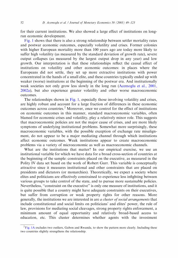
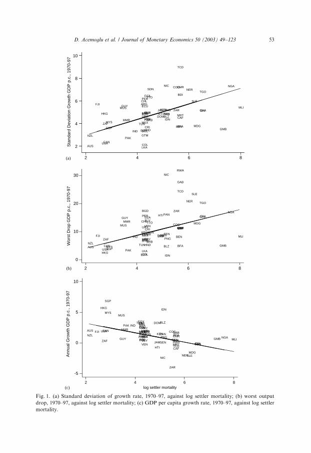
Fig. 1 shows that there is also a strong relationship between settler mortality ratesand postwar economic outcomes, especially volatility and crises. Former colonieswith higher European mortality more than 100 years ago are today more likely tosuffer high volatility (as measured by the standard deviation of growth rate), severeoutput collapses (as measured by the largest output drop in any year) and lowgrowth. Our interpretation is that these relationships reflect the causal effect ofinstitutions on volatility and other economic outcomes: in places where theEuropeans did not settle, they set up more extractive institutions with powerconcentrated in the hands of a small elite, and these countries typically ended up withweaker (worse) institutions at the beginning of the postwar era. And institutionallyweak societies not only grow less slowly in the long run (Acemoglu et al., 2001,2002a), but also experience greater volatility and other worse macroeconomicoutcomes.

The relationships shown in Fig. 1, especially those involving volatility and crises,are highly robust and account for a large fraction of differences in these economicoutcomes across countries.2 Moreover, once we control for the effect of institutionson economic outcomes in this manner, standard macroeconomic variables, oftenblamed for economic crises and volatility, play a relatively minor role. This suggeststhat macroeconomic policies are not the major cause of crises, and are more likelysymptoms of underlying institutional problems. Somewhat more surprisingly, thesemacroeconomic variables, with the possible exception of exchange rate misalign-ment, do not appear to be a major mediating channel through which institutionsaffect economic outcomes. Weak institutions appear to create macroeconomicproblems via a variety of microeconomic as well as macroeconomic channels.

What are the institutions that matter? In our empirical exercise, we use aninstitutional variable for which we have data for a broad cross-section of countries atthe beginning of the sample: constraints placed on the executive, as measured in thePolity IV data set based on the work of Robert Gurr. This variable is conceptuallyattractive since it measures institutional and other constraints that are placed onpresidents and dictators (or monarchies). Theoretically, we expect a society whereelites and politicians are effectively constrained to experience less infighting betweenvarious groups to take control of the state, and to pursue more sustainable policies.Nevertheless, ‘‘constraint on the executive’’ is only one measure of institutions, and itis quite possible that a country might have adequate constraints on their executives,but suffer from corruption or weak property rights for other reasons. Moregenerally, the institutions we are interested in are a cluster of social arrangements thatinclude constitutional and social limits on politicians’ and elites’ power, the rule oflaw, provisions for mediating social cleavages, strong property rights enforcement, aminimum amount of equal opportunity and relatively broad-based access toeducation, etc. This cluster determines whether agents with the investment

2Fig. 1A excludes two outliers, Gabon and Rwanda, to show the pattern more clearly. Including these

two countries slightly strengthens the relationship.


2 4 6 8

2

4

6

8

10

ARG

AUS

BDI

BENBFA

BGDBLZ

BOL

BRA

BRBCAF

CAN

CHL

CIV

CMRCOG

COL

CRI

DOM

DZA

ECU

EGY

FJI

GHA

GMB

GTM

GUY

HKG

HND

HTI

IDN

IND

JAMKEN

LKA

MAR

MDGMEX

MLI

MMR

MRT

MUS

MYS

NERNGANIC

NZLPAK

PAN

PER

PNG

PRY

SDN

SEN

SGP

SLE

SLV

TCD

TGO

TTO

TUN

URY

USA

VEN

ZAF

ZAR

Sta

ndar

d D

evia

tion

Gro

wth

GD

P p

.c.,

1970

-97

Wor

st D

rop

GD

P p

.c.,

1970

-97

2 4 6 8

0

10

20

30 NIC

MRTCOG

CMR

SLE

EGY

CIVNGA

NER

DZACHL

SDN

RWA

TCD

HND

BOL

GAB

BDI

GMB

CAF

SEN

BFA

SLV

ZARPAN

TGO

PER

JAM

MUS

KEN

AUS

MARARG

PRYBRADOM

TUN

GHA

NZL

HTI

VEN

BRBPNG

MDG

CRI

INDGTM

ECU

USA

URY

SGP

TTO

CAN

LKA

FJI

MYSPAK

IDNCOL

ZAFMEX

BGD

MLI

BLZ

HKG

MMR

BEN

GUY

(a)

(b)

Ann

ual G

row

th G

DP

p.c

., 19

70-9

7

log settler mortality2 4 6 8

-5

0

5

10

NIC

MRT

COG

CMR

SLE

EGY

CIV

NGA

NER

DZA

CHL

SDN

RWATCD

HNDBOL

GAB

BDI GMB

CAF

SEN

BFA

SLV

ZAR

PAN

TGO

PERJAM

MUS

KENAUS MAR

ARG

PRYBRA

DOMTUN

GHA

NZL

HTIVEN

BRB

PNG

MDG

CRI

IND

GTM

ECUUSA URY

SGP

TTOCAN

LKA

FJI

MYS

PAK

IDN

COL

ZAF

MEXBGD

MLI

BLZ

HKG

MMR

BENGUY

(c)

Fig. 1. (a) Standard deviation of growth rate, 1970–97, against log settler mortality; (b) worst output

drop, 1970–97, against log settler mortality; (c) GDP per capita growth rate, 1970–97, against log settler

mortality.


opportunities will undertake these investments, whether there will be significantswings in the political and social environment leading to crises, and whetherpoliticians will be induced to pursue unsustainable policies in order to remain inpower in the face of deep social cleavages. Therefore, we prefer to be relatively looseon what the fundamental institutional problems are, and instead try to isolate thehistorically determined component of these institutional differences.

How do we interpret these results? Our conclusion is that the large postwarcrosscountry differences in volatility, crises and growth performance haveinstitutional causes. Both poor macroeconomic performance and distortionarymacroeconomic policies are symptoms rather than causes, and the macroeconomicpolicies often blamed for crises do not appear to be the major mediating channel forthe impact of institutions on economic instability. This does not mean thatmacroeconomic policies do not matter for macroeconomic outcomes. Clearly,overvalued exchange rates or high inflation would discourage certain investments,and unsustainable policies will necessarily lead to some sort of crisis.3 Our mainargument is that in institutionally weak societies, elites and politicians will findvarious ways of expropriating different segments of the society, ranging frommacroeconomic to various macroeconomic policies. It is the presence of this type ofexpropriation and the power struggle to control the state to take advantage of theresulting rents that underlie bad macroeconomic outcomes and volatility.4 A logicalimplication of this view is a seesaw effect: if the elites are prevented from using oneparticular instrument, as long as institutional weaknesses remain, a likely outcome isthat they will pursue their objectives using other instruments. And this, we believe, isthe reason why none of the standard macroeconomic variables are the mainmediating channel for the effect of institutions on volatility and crises.

To improve our understanding of the relationship between institutions andvolatility, we also look at whether countries with weak institutions are unable to dealwith global crises, world economic slowdowns or other global developments, such asthe increase in the volume of international trade. Our results indicate that this is notan important channel via which weak institutions affect volatility and economicperformance. We also find that there is a very similar relationship between

3Moreover, the cause of the decline in U.S. output volatility over the past two decades is unlikely to be

institutional. Our focus here is not differences in output volatility between OECD countries, which all have

relatively good institutions, but the large cross-country differences in volatility across societies with very

different institutional structures.4There are a variety of reasons why weak constraints on executives and other institutional problems

might lead to volatility. For example, Acemoglu and Robinson (2001) show how ‘‘weak institutions’’

might encourage coups and revolutions, leading to political and economic instability. Alternatively,

institutional failures may also make economic adjustment difficult. In an important paper, Rodrik (1999)

suggests that countries with weak institutions are unable to deal with major economic shocks, and

identifies the major shocks with those taking place during the 1970s. Rodrik suggests that this inability to

deal with global economic changes underlies the disappointing growth performance of many less

developed countries (LDCs) during the 1980s and 1990s (see also Easterly, 2001). Similarly, Johnson et al.

(2000) show that among emerging markets open to capital flows, it was those with weaker political and

financial institutions that experienced more severe crises during the late 1990s, suggesting an important

interaction between global shocks and institutions (see also Eichengreen and Bordo, 2002).


institutions and volatility in every decade, and crises are spread across the variousdecades quite evenly.

These findings suggest that it is the inability of institutionally weak societies todeal with their own economic and political shocks that is of first-order importance.Moreover, this inability appears to be somewhat linked to ‘‘state failures’’ (civil wars,revolutions or periods of severe infighting). If we consider these state failures as thetip of the iceberg, it is a reasonable conjecture that many economic crises and a greatdeal of volatility happen amidst political problems. At some level, this is notsurprising. The problem of institutionally weak societies is to constrain thosecontrolling political power, and this lack of constraints on politicians and elitesincreases the willingness of various groups to fight in order to gain power, andenables them to exploit their position, sometimes with disastrous consequences,when they come to power. Nevertheless, that the greater instability faced byinstitutionally weak societies is linked to frequent political crises is for now only aconjecture, backed only with some circumstantial evidence.

There is now a large literature on economic volatility. Much of it focuses ondeveloped countries, and investigates why the business cycle has become less volatilein the U.S. and many OECD economies over the past 20 years (e.g., Blanchard andSimon, 2002; McConnell and Perez-Quiros, 2000; Stock and Watson, 2002). Thisliterature emphasizes technological factors (e.g., improved inventory management)and improvements in policy (e.g., better and more credible monetary policy, inflationtargeting, etc.). Our results can be interpreted as showing that these factors are muchless important in the very large cross-country differences in volatility than areinstitutional differences.

The literature on macroeconomic volatility among LDCs is also large, but focusesprimarily on macroeconomic problems (e.g., Krugman, 1979; Dornbusch et al.,1995; Kaminsky and Reinhart, 1999) and financial factors (e.g., Cabellero, 2001;Caballero and Krishnamurthy, 2000; Chang and Velasco, 2002; Denizer et al., 2001;Easterly et al., 2000; Voth, 2002; Raddatz, 2002). We are unaware of any studieslinking volatility to long-run institutional causes other than the paper by Rodrik(2002) which shows that democracies are less volatile than nondemocratic regimes.In addition, Acemoglu and Zilibotti (1997) show a strong relationship between initialincome and volatility: richer countries are less volatile. They interpret this asresulting from the fact that richer countries are able to achieve a more balancedsectoral distribution of output. Ramey and Ramey (1995) document a cross-countryrelationship between volatility and growth, and interpret it as due to the adverseeffects of volatility on growth. Finally, Kraay and Ventura (2000) develop a modelwhere trade between rich and poor countries can increase volatility in poorcountries, and provide some evidence consistent with this prediction.

In addition, our work relates to the large literature on the determinants of growth.Starting with the seminal work by Barro (1991), many economists have found avariety of important determinants of growth. While some of these determinants areoutcomes of previous investments, such as education, others are contemporarypolicy variables, such as government consumption or inflation. Although economicgrowth is not our main focus, our paper is clearly related to this literature since we


are trying to determine which of these macroeconomic policies matter for volatilityand crises (and also for growth), when we take the importance of institutions intoaccount.

Finally, this paper is most closely related to studies investigating the relationshipbetween institutions and economic performance. Many economists and socialscientists have argued that economic and political institutions are a majordeterminant of economic outcomes. Recent proponents of this view include, amongothers, Jones (1981), North and Thomas (1973), North (1981), and Olson (1982)—see also Acemoglu and Robinson (2000, 2002), Bardhan (1984), Benhabib andRustichini (1996), Krusell and R!ios-Rull (1996), Parente and Prescott (1999) andTornell and Velasco (1992) for attempts to model some of these issues. Acemogluet al. (2001, 2002a, b), Besley (1995), Johnson et al. (2002), Hall and Jones (1999), LaPorta et al. (1998) and Mauro (1995), among others, provide micro and macroevidence consistent with this notion. All of these studies focus on the effect ofinstitutions on economic growth, investment or the level of development. Thecurrent paper can be viewed as extending this literature by showing a robust andstrong effect of institutions on the volatility of economic activity.

The rest of the paper is organized as follows. In the next section, we document thecorrelation between a range of macroeconomic variables and volatility, which isconsistent with the standard view that macroeconomic policies have a causal effecton volatility. In Section 3, we discuss why we expect a relationship betweeninstitutions and volatility, and present two case studies, Argentina and Ghana, whereinstitutional weaknesses appear to have translated into macroeconomic problems. InSection 4, we explain our empirical strategy for distinguishing the effect ofinstitutions on volatility, crises and growth from the effect of macroeconomicpolicies. In Section 5, we review the source of variation in institutions that we willexploit for this exercise. In Section 6, we document the relationship betweeninstitutions and macroeconomic performance, and show how once we control for thecausal effect of institutions (or of the historically determined component ofinstitutions) on volatility and economic performance, macroeconomic policies donot appear to play a direct role. In Section 7, we investigate the robustness of theeffect of institutions on volatility, crises and growth, and explore variousmechanisms via which this effect might be working. Section 8 concludes.

2. Macroeconomic policies and economic performance

The standard macroeconomic view links economic volatility to bad macroeco-nomic policies. According to this view, large government sectors and budget deficits,high inflation, and misaligned exchange rates will result in macroeconomic crises. Inline with this standard view, many macroeconomists see a causal relationshipbetween the improved conduct of monetary policy of the past two decades and theincreased stability of U.S. output. Are there grounds to suspect that there is also arelationship between cross-country differences in volatility and macroeconomicpolicies? Again, the standard view among macroeconomists seems to be that the


answer is yes. For example, in its 1987 Development Report, the World Bank statesthat ‘‘high inflation increases uncertainty, discourages investment and technologicalchange, distorts relative prices, and stands in the way of sustainable growth’’. Indiscussing crises in Mexico and Argentina, Dornbusch et al. (1995, p. 220) write: ‘‘ythe real exchange it is a key relative price. When it becomes too high, it hurts growth,endangers financial stability, and ultimately comes crashing downy the realexchange is in many, though not all, instances a policy variabley’’

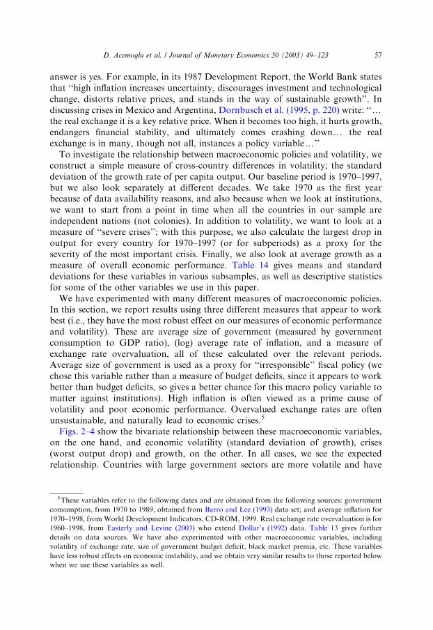
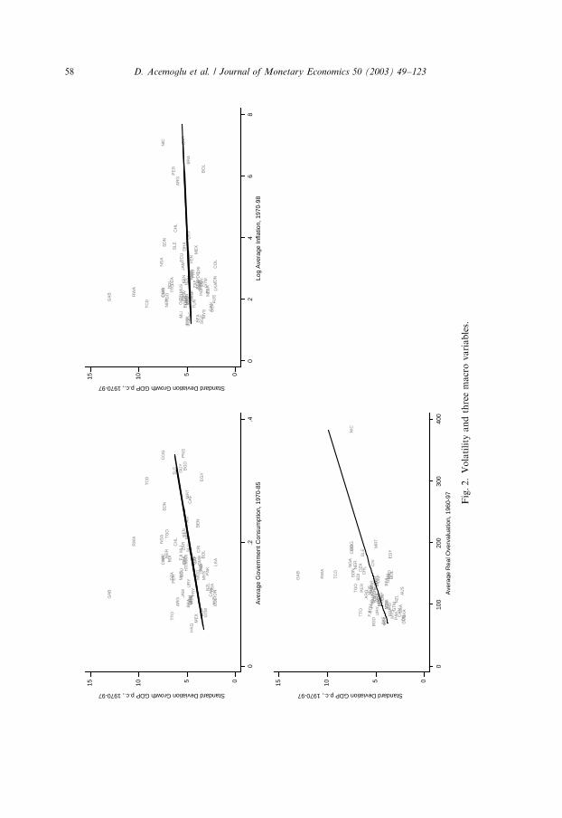
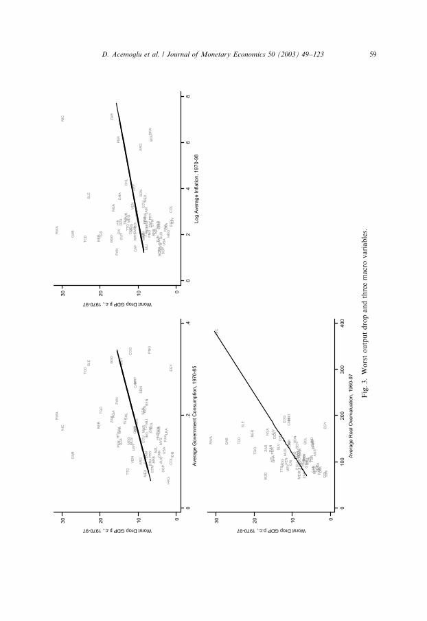
To investigate the relationship between macroeconomic policies and volatility, weconstruct a simple measure of cross-country differences in volatility; the standarddeviation of the growth rate of per capita output. Our baseline period is 1970–1997,but we also look separately at different decades. We take 1970 as the first yearbecause of data availability reasons, and also because when we look at institutions,we want to start from a point in time when all the countries in our sample areindependent nations (not colonies). In addition to volatility, we want to look at ameasure of ‘‘severe crises’’; with this purpose, we also calculate the largest drop inoutput for every country for 1970–1997 (or for subperiods) as a proxy for theseverity of the most important crisis. Finally, we also look at average growth as ameasure of overall economic performance. Table 14 gives means and standarddeviations for these variables in various subsamples, as well as descriptive statisticsfor some of the other variables we use in this paper.

We have experimented with many different measures of macroeconomic policies.In this section, we report results using three different measures that appear to workbest (i.e., they have the most robust effect on our measures of economic performanceand volatility). These are average size of government (measured by governmentconsumption to GDP ratio), (log) average rate of inflation, and a measure ofexchange rate overvaluation, all of these calculated over the relevant periods.Average size of government is used as a proxy for ‘‘irresponsible’’ fiscal policy (wechose this variable rather than a measure of budget deficits, since it appears to workbetter than budget deficits, so gives a better chance for this macro policy variable tomatter against institutions). High inflation is often viewed as a prime cause ofvolatility and poor economic performance. Overvalued exchange rates are oftenunsustainable, and naturally lead to economic crises.5

Figs. 2–4 show the bivariate relationship between these macroeconomic variables,on the one hand, and economic volatility (standard deviation of growth), crises(worst output drop) and growth, on the other. In all cases, we see the expectedrelationship. Countries with large government sectors are more volatile and have

5These variables refer to the following dates and are obtained from the following sources: government

consumption, from 1970 to 1989, obtained from Barro and Lee (1993) data set; and average inflation for

1970–1998, fromWorld Development Indicators, CD-ROM, 1999. Real exchange rate overvaluation is for

1960–1998, from Easterly and Levine (2003) who extend Dollar’s (1992) data. Table 13 gives further

details on data sources. We have also experimented with other macroeconomic variables, including

volatility of exchange rate, size of government budget deficit, black market premia, etc. These variables

have less robust effects on economic instability, and we obtain very similar results to those reported below

when we use these variables as well.


Standard Deviation Growth GDP p.c., 1970-97

Ave

rage

Gov

ernm

ent C

onsu

mpt

ion,

197

0-85

0.2

.4

051015

Standard Deviation Growth GDP p.c., 1970-97

Log

Ave

rage

Infla

tion,

197

0-98

02

46

8

051015

Standard Deviation GDP p.c., 1970-97

Ave

rage

Rea

l Ove

rval

uatio

n, 1

960-

97

010

020

030

040

0

051015

Fig.2.Volatility

andthreemacrovariables.


Worst Drop GDP p.c., 1970-97

Ave

rag

e G

ove

rnm

en

t C

on

su

mp

tio

n, 1

97

0-8

5

0.2

.4

0

10

20

30


Lo

g A

ve

rag

e In

fla

tio

n, 1

97

0-9

8

02

46

8

0

10

20

30


Ave

rag

e R

ea

l O

ve

rva

lua

tio

n, 1

96

0-9

7

0100

20

03

00

40

0

0

10

20

30

Fig.3.Worstoutputdropandthreemacrovariables.


Annual Growth GDP p.c., 1970-97

Ave

rag

e G

ove

rnm

en

t C

on

su

mp

tio

n, 1

97

0-8

5

0.2

.4

-.0

50

.05.1


Lo

g A

ve

rag

e In

fla

tio

n, 1

97

0-9

8

02

46

8

-.0

50

.05.1


Ave

rag

e R

ea

l O

ve

rva

lua

tio

n, 1

96

0-9

7

01

00

20

03

00

40

0

-.0

50

.05.1

Fig.4.Growth

andthreemacrovariables.


more severe crises. They also grow, on average, more slowly. The same is true forcountries with high inflation and overvalued exchange rates.

Do these correlations reflect the causal effect of bad macroeconomic policies oneconomic volatility and performance or are they capturing the effect of institutionalfactors on economic outcomes? This is the question we investigate in the next foursections.

3. Institutions and economic performance

Figs 2, 3 and 4 show a correlation between macroeconomic policies and outcomes,but they do not establish causality. Countries that pursue distortionary macro-economic policies are different in a number of dimensions; most importantly, theydiffer substantially in their ‘‘social organization’’. While some countries, such as theU.S., Australia or Canada, are democratic, relatively equal, suffer few radical socialcleavages and have a variety of checks and balances on politicians’ actions, others,such as Ghana, Nicaragua, or Nigeria, fluctuate between democracy and dictator-ship, are highly unequal, and lack effective constraints on politicians and elites. Werefer to this cluster of social arrangements as ‘‘institutions’’ and think of the lattergroup of countries as having ‘‘weak institutions’’.

It is quite reasonable to suspect that weak institutions will have a significantimpact on economic performance. In previous research, we documented a largeeffect of this type of institutions on economic development (Acemoglu et al., 2001,2002a; see also Knack and Keefer, 1995; Hall and Jones, 1999). There are alsonatural reasons for why institutionally weak countries might suffer substantialvolatility, which we discuss next.

3.1. Institutions and volatility: some theoretical ideas

Here we briefly discuss why we might expect greater economic instability ininstitutionally weak societies.6

1. In institutionally weak societies there are few constraints on rulers. Following achange in the balance of political power, groups that gain politically may thenattempt to use their new power to redistribute assets and income to themselves, inthe process creating economic turbulence. In contrast, this source of turbulencewould be largely absent in societies where institutions prevent this type ofredistribution.

2. Lack of effective constraints on politicians and politically powerful groups impliesthat there are greater gains from coming to power, and correspondingly, greaterlosses from not controlling political power—thus, overall greater ‘‘politicalstakes’’. Therefore, in institutionally weak societies, there will be greater infighting

6See the previous version of the paper where we provide a simple dynamic model formalizing the first

two ideas.


between various groups to come to power and enjoy these greater gains, andhence, greater political and economic turbulence.

3. With weak institutions, economic cooperation may have to rely on ‘‘trust’’ or,more explicitly, on cooperation supported by repeated games strategies. Shocksmay make it impossible to sustain cooperation, and lead to output collapses.

4. With weak institutions, contractual arrangements will be more imperfect, makingcertain economic relationships more susceptible to shocks.

5. In societies with institutional problems, politicians may be forced to pursueunsustainable policies in order to satisfy various groups and remain in power, andvolatility may result when these policies are abandoned.

6. With weak institutions, entrepreneurs may choose sectors/activities from whichthey can withdraw their capital more quickly, thus contributing to potentialeconomic instability.

Our empirical work will not be able to distinguish between these various channelslinking institutions to economic instability, though we believe that gaining a deeperunderstanding of the relative importance of various channels would be a majorcontribution to our understanding. We leave this as a potential area for futureresearch.

3.2. Sources of volatility in institutionally weak societies: two case studies

In this subsection, we briefly discuss the experiences of two institutionally weaksocieties with economic instability, Argentina and Ghana.

3.2.1. Ghana

Ghana was the first European colony in Africa to become independent in 1958 andat this time had roughly the same level of GDP per capita as South Korea. However,in 2000 GDP per capita had just about recovered to where it was in 1958 even after adecade and a half of relatively consistent of growth. The economic and politicalhistory of Ghana has been marred by severe instability with military coups in 1966,1972, 1978, 1979 and 1982 and re-democratizations in 1969, 1979 and 1996.

The anti-colonial movement was organized in Ghana by Kwame Nkrumah andhis Convention People’s Party (CPP) (see Austin, 1964; Apter, 1972). However, assoon as the promise of independence had been secured from the British the anti-colonial coalition in Ghana crumbled. Pellow and Chazan note (1986, p. 30) ‘‘by1951, with the British agreement in principle to grant independence to the colony,this stage of decolonization gave way to a period of domestic struggles for power onthe eve of independence. At this junction, the internal tensions that had beensomewhat in check erupted into an open clash over the control of the colonial state’’.This left Nkrumah (who was from a minor Akan ethnic group—the Nzima) with avery precarious political base. To compensate for this Nkrumah engaged in a ‘‘divideand rule’’ strategy with respect to the Ashanti (whose chiefs were one of his strongestopponents) by attempting to set different factions of commoners against the chiefs.


The chiefs and their National Liberation Movement (NLM) ‘‘met the nationalistappeal of the CPP with a rival nationalism of its own, through an impassioneddemand for recognition of the traditional unity of the Ashanti nation’’, Austin (1964,p. 250). This political strategy ensured Nkrumah’s power at independence in 1957.After the departure of the British, he moved to suppress the opposition and alteredthe Constitution (in a fraudulent plebiscite) to strengthen his powers. Pellow andChazan (1986, p. 41) argue that

‘‘The 1960 constitutional referendum y augmented the powers of the executivey Nkrumah was elected president of the First Republic, and thus, for all intentsand purposes, by 1960 Ghana had become a one-party state with Nkrumah as itsleader. The authoritarian tendencies apparent during decolonization wereofficially entrenched in the centralized and personalized pattern of governmentthat emerged at this juncture’’.

Despite the announced objectives of modernization, the need to stabilize politicalpower seems to have been the key determinant of economic policies. Pellow andChazan (1986, p. 45) argue that by 1964 the CPP had ‘‘reduced the role of the state tothat of a dispenser of patronage. By advocating the construction of a ramifiedbureaucracy, Nkrumah established a new social stratum directly dependent on thestate. By curtailing the freedom of movement of these state functionaries through thediversion of administrative tasks to political ends, the regime contributed directly toundermining their effective performance’’.

The disastrous economic impact of the CPP’s policies have been well analyzed byBates (1981) (see also Owusu, 1970; Leith and Lofchie, 1993). He showed that thegovernment used the state Cocoa marketing board and exchange rate policy tosystematically expropriate the coca farmers who dominated the economy andexports. The CPP transferred these rents to the urban and ethnic interests whichsupported them. The fact that this redistribution took such an inefficient form wasexplained both by the inability of the central state to control or raise taxes in thecountryside, and by the political rationality of redistributing in ways which could beselectively targeted. Bates (1981, p. 114) argues:

‘‘Were the governments of Africa to confer a price rise on all rural producers, thepolitical benefits would be low; for both supporters and dissidents would securethe benefits of such a measure, with the result that it would generate no incentivesto support the government in power. The conferral of benefits in the form ofpublic works projects, such as state farms, on the other hand, has the politicaladvantage of allowing the benefits to be selectively apportioned. The schemes canbe given to supporters and withheld from opponents’’.

Bates applied a similar argument to explain the overvaluation of the exchangerate. When the foreign exchange market does not clear, the government has to rationaccess to foreign exchange and can target allocations to supporters. In addition, andperhaps more important, overvalued exchange rates directly transfer resources fromthe rural sector to the urban sector, making it an attractive policy tool for thepolitical elites.


These distortionary policies did not stop when Nkrumah was deposed in 1966;they were in fact intensified right up until Rawlings’s policy changes of 1982 (seeHerbst, 1993, on these changes and the more recent economic and political history).

Ghana therefore provides a clear example of how a range of distortionary policies,including overvalued exchange rates, were motivated by the desire to redistributeincome. The bad effects were so severe and debilitating for the economy because theinstitutional environment inherited from Britain placed few, if any, constraints onwhat politicians could do. Nkrumah and the CPP were able to build a one-partystate, use the bureaucracy and economic policies for patronage and engage in masscorruption. The high political stakes that resulted made it very attractive to be inpower and induced intense political instability, as shown by the very frequent coups,and political instability translated into economic instability. Overall, it seems fairlyclear that in the Ghanaian case, economic instability was caused mainly byinstitutional weaknesses, which was mediated by a range of different macro andmicropolicies.

3.2.2. Argentina

In any discussion of crises and poor growth in developing countries Argentinatends to come near the top of anyone’s list. Argentina is the most famous case of acountry which ought to be relatively prosperous, and indeed was so until the 1920s.It is standard to blame poor economic performance and volatility in Argentina onbad economic policies. The usual candidate for low growth is inward-lookingindustrialization and irresponsible fiscal policy (Krueger, 1993; Taylor, 1998).

The traditional story for why Argentina pursued such policies is the adoption ofmisguided state-led development strategies as a result of the influence of economistssuch as Prebisch and the dependency theorists (Krueger, 1993). Yet Peronist policiespredated Prebisch’s seminal work in 1950,7 and the reality is that Per !on neverfollowed a coherent industrialization policy. Gerchunoff (1989) sums up Peronisteconomic policy in the following way:

‘‘there was no specific and unified Peronist economic policy, much less a long-term development strategy. In spite of official rhetoric about a plan, theobjective—and at times exclusive—priority was y an economic order capable ofmaintaining the new distributive model’’.

The first real statement of Prebisch’s views was in his famous work of 1950, and hehad no influence on policy in Argentina until 1955, when he was recalled from exilefollowing Per !on’s fall from power.

A second view sees the great depression and the Second World War as leading to aphase of ‘‘natural import substitution’’, which then created an industrial interestgroup. This interest group was sufficiently strong that it could induce state subsidiesand intervention (this view is developed in Frieden, 2001). Both this theory and theone emphasizing mistaken economic theories see bad industrial policies and state

7Per !on came to power in 1943 and indeed Prebisch was hounded from Argentina and into exile in Chile

by Per !on.


intervention leading also to unsustainable subsidization, fiscal insolvency, bank-ruptcy and hyperinflation.

A third view, popular in political science, sees the cause of the form of bothmacroeconomic and microeconomic policy in the rise and persistence of ‘‘populism’’and more specifically Peronism (Weisman, 1987, Collier and Collier, 1991, Roe,1998). This view tends to see structural changes in the economy, such as urbanizationand the rise of organized labor, as leading to particular sorts of political coalitions,favoring certain policies, and preventing economic development.

Although there are undoubtedly aspects of truth in these explanations, a moresatisfactory account of poor economic policies in Argentina situates them in theirinstitutional context. It seems that Per !on’s policies, and subsequent Argentinianpolicies, were not really a reflection of a ‘‘full-blown Peronist growth strategy’’ asargued by Shleifer (1997), or aimed at ‘‘the goal of rapid industrialization’’ and ‘‘theintent of building a domestic industrial base behind tariff rates,’’ as argued by Sachs(1990, p. 148). Instead, these were policies intended to transfer resources from onesegment of society to another, as well as a method of maintaining power bypoliticians with a weak social base in an institutionally-weak society (see,Gerchunoff, 1989; Mazzuca, 2001). In line with this view, D!iaz and Carlos (1970,p. 126) concludes that

‘‘Peronist policies present a picture of a government interested not so much inindustrialization as in a nationalistic and populist policy of increasing the realconsumption, employment, and economic security of the masses—and of the newentrepreneurs. It chose these goals even at the expense of capital formation and ofthe economy’s capacity to transform’’.

Where do the institutional weaknesses of the Argentine society come from?8 As aSpanish colony Argentina had low population density and was something of abackwater because of the focus on the mines of Peru and Bolivia. It thus avoidedmany of the worse colonial institutions, such as the encomienda and the mita.Nevertheless, after independence Argentina suffered from severe political instabilityas rival regional warlords and Caudillos vied for control of Buenos Aires and thecountry. An effective national state emerged only in the 1860s under the Presidencyof Mitre. In order to secure compliance, the constitutional settlement andinstitutions created then ceded large powers to the provinces. Crucially, the centralstate never imposed upon the regions the type of centralized institutions constructedhistorically in Europe. Mazzuca (2001) suggests, building on the work of Tilly (1990)and Herbst (2000), that this was because: (1) the Argentine regime did not faceexternal threats to its sovereignty and was therefore never forced to modernize; (2)both the expanding world commodity and financial markets gave the centralgovernments enough fiscal resources that they could use to avoid the costs ofdisciplining the provinces.9 Although this institutionalization of political power didnot impede the boom in Argentina up until 1920s, it left a legacy of political

8Our account here builds on Mazzuca (2001).9Rock (1987, p. 125) notes ‘‘Mitre became adept in the dispensation of subsidies to the provinces’’.


institutions which has had a crucial impact on policy over the last century. Ourargument is that in particular it has led to highly inefficient forms of redistributionaway from the most productive parts of the country (Buenos Aires and the littoral)towards the economically marginal, but politically salient provinces. Politiciansundertook this type of inefficient redistribution using a variety of tools, ranging fromfiscal policy and exchange rate policy to microeconomic policies.

A tangible manifestation of this perverse institutionalization of political power canbe seen from the malapportionment of the Argentine congress. Samuels and Snyder(2001, 2002) show that Argentina has the most malapportioned Senate in the worldand that the degree of malapportionment of Congress is about 2.5 times the worldaverage and 50% higher than the Latin America average.10 The four provinces ofBuenos Aires, Santa Fe, C !ordoba and Mendoza contain 78% of national industrialproduction and 70% of the total population, but control just 8 of the 48 seats in thesenate, and 48% of the seats in Congress. Gibson (1997) refers to these fourprovinces as the ‘core’ and the other provinces as the ‘periphery’ and shows thatpolitical support from the periphery has been crucial in Argentine politics (see alsoGermani, 1962; Mora y and Llorente, 1980). In particular, the Peronists, despite theconventional wisdom that they are the party of labor and urban interests, havealways relied heavily on this support.

Gibson et al. (2001, p. 11) argue that the importance of ‘‘overrepresentedperipheral region provinces in the national Peronist coalition has continued to thepresent day, and during President Menem’s first term they provided a major base ofsupport in the national legislature’’. The nature of this political coalition led Menemto insulate the periphery from most of his economic reforms. During his presidency,public sector employment and subsidies to the periphery increased despite rapidretrenchment and deregulation in Buenos Aires (Gibson et al., 2001, Table 6). Thisstructure of political institutions is important because it leads the peripheral regionsto be a crucial part of any political coalition and leads, as in Ghana, to the burden ofredistribution falling squarely on the most productive region of the country.

Nevertheless, political institutions such as these, while they may have large effectson policy, are not determined randomly. Indeed, malapportionment was intensifiedby Per !on in 1949 when he established a minimum of two deputies per provinceregardless of population (Sawers, 1996, p. 194). It was further increased by themilitary in 1972 and the early 1980s in an attempt to weaken the power of urbaninterests in democracy. This process was driven by the initial political equilibriumfavoring the periphery and thus further intensified the inherent institutionaldistortions.11

10Measuring malapportionment by the proportion of seats that are not allocated on the basis of one

person one vote, the Argentine Senate has a score of 0.49 and the Congress 0.14. The world and Latin

American averages are, respectively, 0.27 and 0.19 for Upper Chambers and 0.09 and 0.06 for lower

chambers. Note that while the U.S. Senate is malapportioned (score 0.36), the U.S. Congress is not

malapportioned. Gibson et al. (2001) provide evidence suggesting that it is malapportionment in the lower

chamber that is the main determinant of fiscal redistribution.11There are many ways in which malapportionment can affect the efficiency of economic policy. For

example, imagine that to put together a coalition, a President must give politicians enough redistribution


This perspective suggests that the repetitive nature of unsustainable andbad macroeconomic policies in Argentina stems from an underlying set ofweak institutions, which make massive redistribution of income feasibleand even politically rational. This analysis is rather different from much currentanalysis.

The recent crisis in Argentina has been explained by the collapse of anunsustainable economic model which involved tying the peso to the US dollar.This resulted in overvaluation, domestic recession and a current account deficit thathad to be funded by unsustainable international borrowing. The conventionalwisdom is that the adoption of this particular set of policies was an attempt to obtaincredibility with financial markets (e.g. Rodrik, 2002). Instead, our perspectivesuggests that, as in Bates’s (1981) analysis of the political economy of Africa, badeconomic policies should be understood as part of a package of often inefficientredistributive tools. The currency board adopted by Argentina also created clearwinners and losers. The economically poor but politically pivotal periphery gainedtransfers and was unthreatened by the adverse effects of a crisis that had greatereffects on the core and the middle classes (who are now being ‘‘expropriated’’ by avariety of methods).12 The persistent nature of crises and expropriation in Argentina,and the fact that the same set of macroeconomic policies continually recur andsubsequently collapse (see della Paolera and Taylor, 2001) are consistent with ourinterpretation.13

Some recent analyses (e.g. Caballero and Dornbusch, 2002) recognizethe existence of ‘‘political and social problems,’’ but still maintain the view thatbad policy in Argentina is either misguided or incompetent, and argue that thepolicy failures in Argentina can now only be solved by an internationaltakeover of fiscal and monetary policies. Our analysis here suggests that thissolution to instability and poor economic performance in Argentina may not besuccessful. If at root the problems are weak institutions leading to politicalconflict, highly inefficient redistribution and outright predation, then, withoutinstitutional change, distributional conflict is bound to resurface even if inter-national bankers are in control of monetary policy. There are always otherinstruments.

(footnote continued)

for them to be re-elected. In this case, it is cheaper to ‘‘buy’’ a politician from a peripheral province in

Argentina since he needs fewer votes to win. This ‘‘price’’ can influence the form that payment takes (see

the model by Lizzeri and Persico, 2001, for a formalization of a related idea). For example, when the price

is low it may be rational to buy politicians with private goods (income transfers), while when it is high (for

instance in Buenos Aires) it is cheaper to use public goods. Malapportionment can then lead to the

undersupply of public goods. Moreover, anticipating the cost of ‘buying’ power, a President may want to

create malapportionment because he has to redistribute less in total and keeps more of the rents from

power.12Undoubtedly the form of the monetary policy helped to bring down inflation, but this does not imply

that the main objective of the set of policies adopted was to promote development and stability.13A significant example of absence of constraints on the executive in Argentina is the ability of Menem

to re-write the Constitution in 1995 so that he could run for the presidency again.


4. Empirical strategy

The discussion so far illustrates how we might expect both institutional differencesand differences in macroeconomic policies to cause differences in macroeconomicperformance, especially in volatility and crises. We now discuss a simple empiricalstrategy to make progress in distinguishing between these two sources of differencesin volatility and crises.

Ignoring nonlinearities, the economic relationship we are interested in identifyingis:

Xc;t�1;t ¼ Q0c;t�1;t � aþ b � Ic;t¼0 þ Z0

c;t�1;t � gþ y � ln yc;t�1 þ Ec;t�1;t; ð1Þ

where Xc;t�1;t is the macroeconomic outcome of interest for country c between times t

and t � 1: The three outcomes that we will look at are overall volatility (standarddeviation of GDP per capita growth), severity of crises (worst output drop) andaverage per capita growth. In our baseline regressions, the basic time period will befrom 1970 to 1997 (this choice is dictated by data availability and our desire to startthe analysis at a point in time where the countries for which we have data are allindependent nation states). Q0

c;t�1;t is a vector of macroeconomic policies for countryc between times t and t � 1: The three measures of macroeconomic policies we willlook at are the ones shown in Section 2: average size of government consumption,inflation, and real exchange rate overvaluation.

Ic;t¼0 is our measure of institutions at the beginning of the sample. We will use theconstraint on the executive variable from the Polity IV dataset, which measures theextent of constitutional limits on the exercise of arbitrary power by the executive.The Polity dataset reports a qualitative score, between 1 and 7, for every independentcountry. In previous work (e.g., Acemoglu et al., 2001, 2002a), we showed that thismeasure is correlated with other measures of institutional quality and with economicdevelopment. As our baseline measure, we use the average value for this constraintfrom the Polity IV dataset for 1950, 1960 and 1970, assigning the lowest score tocountries that are not yet independent (and therefore not in the Polity IV dataset).14

This is reasonable since in a country still under colonial control there are typicallyfew real constraints on the power of the rulers. Appendix Tables 13, 14 and 15provide results using constraint on the executive in 1970 as an alternative measure ofinstitutions, with qualitatively and quantitatively very similar results.

In addition, in Eq. (1), Zc;t�1;t is a set of other controls, and ln yc;t�1 is the log ofinitial income per capita, which we include in some of the regressions. FollowingBarro (1991) this variable is included in most growth regressions to control forconvergence effects. It is also useful to include it in regressions of volatility or crises,

14We take these averages of 1950, 1960 and 1970 as our baseline measure, rather than simply use the

1970 value of the index, since we are interested in the long-run component of these constraints (not in the

year-to-year fluctuations) and also because the Polity dataset gives high scores to a number of former

colonies in 1970 that subsequently drop by a large amount. This reflects the fact that many of these

countries adopted the constitution of their former colonial powers, but did not really implement the

constitution or introduce effective checks.


since as shown in Acemoglu and Zilibotti (1997), poorer countries suffersubstantially more volatility.

The parameters that we are interested in identifying are a and b; the effect ofmacroeconomic policy variables and institutions.15 The simplest strategy is toestimate the model in equation (1) using ordinary least squares (OLS) regression.There are two distinct problems with this strategy:

1. Both institutions and macro policy variables are endogenous, so we may becapturing reverse causality, or the effect of some omitted characteristics(geography, culture, or other variables) on both policy (or institutions) andeconomic outcomes.

2. Both institutions and policy variables are measured with error, or in the case ofinstitutions, available measures correspond only poorly to the desired concept(more explicitly, while the institutions we have in mind are multi-dimensional,‘‘constraint on the executive’’ only measures one of these dimensions, and thatquite imperfectly).

Both of these concerns imply that OLS regressions will give results that do notcorrespond to the causal effect of institutions and policy variables on economicoutcomes. So we would like to estimate Eq. (1) using two-stage least squares (2SLS)with distinct and plausible instruments for both macro policy variables andinstitutions. These instruments should be correlated with the endogenous regressors,and they should be orthogonal to any other omitted characteristics and notcorrelated with the outcomes of interest through any other channel than their effectvia the endogenous regressors.

In this paper, we pursue the strategy of instrumenting for institutions using thehistorically determined component of institutions, arising from the colonialexperience of former colonies. The instrument will be discussed in detail in thenext section. To the extent that the instrument is valid, it will solve the endo-geneity, the omitted variables bias and the measurement error problems. Inparticular, if the instrument is valid, we can estimate the effect of institutions oneconomic outcomes, the b parameters, consistently in models that exclude the macropolicy variables.

When the macro policy variables are also included, the simplest strategy is to treatthem as exogenous. Ignoring the measurement error problem, the coefficients onthese policy variables, the a parameters, will be typically biased upwards. Theappendix of Acemoglu et al. (2001) shows that in this case there may also be adownward bias in b; the effect of institutions on outcomes. Therefore, our simpleststrategy of instrumenting for institutions and treating macro policy variables asexogenous is ‘‘conservative’’, in the sense that it stacks the cards against finding a

15 In addition it is interesting to look at whether there is an interaction between institutions and macro

policy variables. We can add the interaction term Q0c;t�1;t � Ic;t�1; and investigate whether there is a non-

monotonic relationship between institutions and volatility, i.e., add higher order terms Ic;t�1 to the

regression equation (1). In our empirical work, such interaction and higher order terms are never

significant, so we do not report them in the paper.


substantial role for institutions and in favor of finding an important role for macropolicy variables (unless measurement error in these policy variables is a majorproblem). Moreover, Eq. (1) shows that we are using contemporary averages of themacrovariables, while using lagged values of institutions. This is again in the spirit ofstacking the cards in favor of finding a significant role for macro variables. As itturns out almost all of our regressions will show a major role for institutions, andmore limited and less robust influence from the macro variables. So our conservativestrategy makes the interpretation of these results simpler.

A caveat for the above discussion is that if the measurement error in macrovariables is significant, their coefficients might be biased downward due toattenuation bias. Since we are taking 30-year averages of these variables, themeasurement error problem should not be too severe.16 As an alternative strategy fordealing both with attenuation bias and endogeneity of the macro variables, we alsoreport regressions where we instrument for the macro variables with their laggedvalues when available. We will see that these specifications give similar results tothose where these policy variables are treated as exogenous.

Another possible concern is that distortionary policy may matter for macro-economic variables, but we may be unable to detect this because we are takingaverages over thirty-year periods. This would be the case if, for example, some of thecountries go through a period of about 5–10 years of high inflation or an overvaluedexchange rate, causing major crises, but during other periods they have offsettinglow inflation and undervalued exchange rates, making their average policies similarto those in other countries. To deal with this problem, we estimate a variation on ourbasic regression using a panel of 5-year averages for each country between 1970 and1997 (or shorter periods for some of the macro variables), with the followingstructure:

Xc;t�1;t ¼ Q0c;t�1;t � aþ b � Ic;t¼0 þ Z0

c;t�1;t � gþ y � ln yc;t�1 þ dt�1;t þ Ec;t�1;t; ð2Þ

where all the variables are defined similarly to Eq. (1), except that we now have a fullset of time effects for every five-year episode, the dt�1;t terms. In addition, we still usethe institutions at the beginning of the sample, Ic;t¼0: Recall that our interest is in thehistorically determined component of institutions (that is more clearly exogenous),hence not in the variations in institutions from year-to-year. As a result, thisregression does not (cannot) control for a full set of country dummies. Since we havemore than one observation per country, but one of our key regressors only varies bycountry, we cluster the standard errors by country (using the Stata robust standarderrors). If some countries have volatile macroeconomic policies that matter onlywhen they reach very extreme values, this specification should show a greater role forpolicy variables than the cross-sectional regression (1). In practice, estimates of the

16Unless there is again attenuation bias caused by the variables in question not corresponding to the

conceptually appropriate policy variables. We believe this possibility is unlikely in the case of the policy

variables, since these are the variables emphasized in the policy discussions and the relevant literature, and

we have experimented with many other variables.


impact of policy variables on volatility, crises and growth from Eqs. (1) and (2) arequite similar.

5. Sources of variation in institutions

The empirical strategy outlined in Section 4 relies on a valid instrument forinstitutions. Our idea is to exploit the historically determined component ofinstitutions, or in other words, instrument for institutions with historical variables.This clearly solves the simple ‘‘reverse causality’’ problem, and to the extent that theinstrument is plausibly orthogonal to other omitted determinants of economicoutcomes, such as volatility, crises and growth, it also avoids the omitted variablebias. Also, the instrumentation strategy removes the attenuation bias (as long as the‘‘measurement error’’ or the conceptual discrepancy between our measure and thetrue concept can be approximated by classical measurement error).

5.1. Historical determinants of institutions among former European colonies

The set of former European colonies provides an attractive sample for isolatingthe historically determined component of institutions, since the institutions in almostall of the former colonies have been heavily influenced by their colonial experience(see Acemoglu et al., 2001, for a more detailed discussion on this point).

In Acemoglu et al. (2001, 2002a), we contrasted institutions of private property,which protect the property rights of a broad segment of society, and extractive

institutions, which lack constraints on elites and politicians. We argued thatinstitutions of private property, which correspond to effective constraints on elitesand rulers, were more likely to arise when Europeans settled in large numbers, andset up institutions protecting their own rights. The ‘‘Neo-Europes’’, the U.S.,Canada, Australia and New Zealand, are perhaps the best examples of the highEuropean settlement associated with the development of good institutions. Incontrast, extractive institutions emerged when Europeans pursued a strategy ofextracting resources from the colonies without settling and without developingparticipatory institutions. While there are many determinants of the exactcolonization strategy pursued by European powers, an important determinant isnaturally whether Europeans could settle or not, since where they could not settle,the extractive strategy was much more likely.17 Therefore, in places where the diseaseenvironment was not favorable to European health and settlement, we expect theformation of extractive states, and today the presence of weak institutions, as theseextractive institutions persist. This reasoning suggests that proxies for mortality ratesexpected by the first European settlers in the colonies could be an instrument for

17Another important determinant appears to be population density. Europeans were less likely to settle

in already densely settled areas, and more likely to pursue extractive strategies given the level of settlement

(Acemoglu et al., 2002a). We obtain similar results to those reported below if we use population density in

1500 as an additional instrument.


current institutions in these countries. Schematically, the reasoning underlying thisinstrumentation strategy is

ðpotentialÞ settler

mortality) settlements )

early

institutions)

current

institutions)

current

performance

Based on this reasoning, we use data on the mortality rates of soldiers, bishops, andsailors stationed in the colonies between the 17th and 19th centuries (Curtin, 1989,1998; Gutierrez, 1986). These give a good indication of the mortality rates faced bysettlers. Europeans were well informed about these mortality rates at the time, eventhough they did not know how to control the diseases that caused these highmortality rates, especially yellow fever and malaria (see the discussion in Acemogluet al., 2001).

A major concern is the validity of the exclusion restriction presumed by thisinstrumentation strategy—i.e., whether the mortality rates faced by the settlersbetween the 17th and 19th centuries could actually have an effect on currentoutcomes through another channel. Probably the most important threat to thevalidity of our instrument comes from the correlation between European mortalityrates over 100 years ago and the health of the current population or climate, and theeffect of current health and climate on current economic outcomes. We believe thatthis concern does not invalidate our approach and that our exclusion restriction isplausible. The majority of European deaths in the colonies were caused by malariaand yellow fever. Although these diseases were fatal to Europeans who had noimmunity, they had much more limited effects on indigenous adults who, over thecenturies, had developed various types of immunities. These diseases are thereforeunlikely to be the reason why many countries in Africa and Asia are very poor today.This notion is supported by the mortality rates of local people in high-settlermortality areas, which were comparable to the mortality rates of British troopsserving in Britain or in healthier colonies (see for example Curtin, 1998, Table 2). Tosubstantiate the validity of our instrumentation approach, in Acemoglu et al., (2001)we showed that the results are robust to controlling for climate, humidity, othergeographic variables, and current health conditions, and that we obtain very similarresults exploiting only differences in European mortality due to yellow fever, whichis an attractive source of variation, since yellow fever has been mostly eradicated. Onthe basis of these findings, we take mortality rates of European settlers between the17th and 19th centuries as an instrument for current institutions in the formercolonies.18

Fig. 5 shows the first-stage relationship between our constraint on the executivevariable (an average for 1950, 1960 and 1970) and the log of European settlermortality in annualized deaths per thousand mean strength. This measure reports thedeath rate among 1,000 soldiers where each death is replaced with a new soldier andwas the standard measure in army records, where much of the information comesfrom. We use logs rather than levels, since otherwise some of the African

18We also show in Acemoglu et al. (2001) that these mortality rates were a first-order determinant of

early institutions, and these institutional differences have persisted to the present.


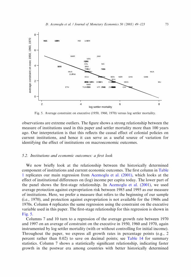
observations are extreme outliers. The figure shows a strong relationship between themeasure of institutions used in this paper and settler mortality more than 100 yearsago. Our interpretation is that this reflects the causal effect of colonial policies oncurrent institutions, and hence it can serve as a useful source of variation foridentifying the effect of institutions on macroeconomic outcomes.

5.2. Institutions and economic outcomes: a first look

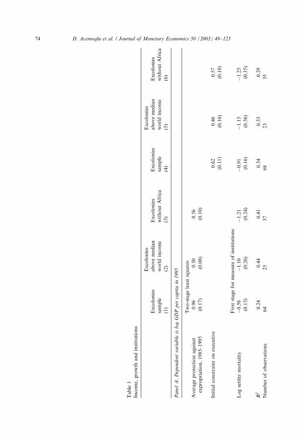
We now briefly look at the relationship between the historically determinedcomponent of institutions and current economic outcomes. The first column in Table1 replicates our main regression from Acemoglu et al. (2001), which looks at theeffect of institutional differences on (log) income per capita today. The lower part ofthe panel shows the first-stage relationship. In Acemoglu et al. (2001), we usedaverage protection against expropriation risk between 1985 and 1995 as our measureof institutions. Here, we prefer a measure that refers to the beginning of our sample(i.e., 1970), and protection against expropriation is not available for the 1960s and1970s. Column 4 replicates the same regression using the constraint on the executivevariable used in this paper. The first-stage relationship for this regression is shown inFig. 5.

Columns 7 and 10 turn to a regression of the average growth rate between 1970and 1997 on an average of constraint on the executive in 1950, 1960 and 1970, againinstrumented by log settler mortality (with or without controlling for initial income).Throughout the paper, we express all growth rates in percentage points (e.g., 2percent rather than 0.02) to save on decimal points; see Table 14 for summarystatistics. Column 7 shows a statistically significant relationship, indicating fastergrowth in the postwar era among countries with better historically determined

aver

age

cons

trai

nt o

n ex

ec 1

950,

196

0, 1

970

log settler mortality2 4 6 8

0

2

4

6

8

NGA

GHA

TZA

NER

ZAR

MRTCOG

DZA GIN

CMR

CIV

BOL

AGOGAB

EGY

BDIRWA

SDN

HND

CAF

UGA

GMBSEN

TCDPRY TGO

JAM

SLV

KENBFA

DOM

AUS

PAN

MLI

BEN

MUS

MARMDG

GUY

HTI

ECU

ARG

VEN

GTM

TUN

NIC

NZL

BRACHL

ETH

IDNTTO

IND

URY

CRIUSA

MMR

MYSSGPPER

CAN

COL

PAK

ZAF

MEX

BGD

LKA

GNB

AFG

PNG

VNMLAO

Fig. 5. Average constraint on executive (1950, 1960, 1970) versus log settler mortality.


Table

1

Income,

growth

andinstitutions

Excolonies

Excolonies

Excolonies

abovemedian

Excolonies

Excolonies

abovemedian

Excolonies

sample

worldincome

withoutAfrica

sample

worldincome

withoutAfrica

(1)

(2)

(3)

(4)

(5)

(6)

Pan

elA:

Dep

end

ent

vari

ab

leis

log

GD

Pp

erca

pit

ain

19

95

Two-stageleast

squares

Averageprotectionagainst

expropriation,1985–1995

0.96

0.50

0.56

(0.17)

(0.08)

(0.10)

Initialconstraintonexecutive

0.62

0.46

0.57

(0.11)

(0.16)

(0.18)

First

stageformeasure

ofinstitutions

Logsettlermortality

�0.58

�1.10

�1.21

�0.91

�1.15

�1.25

(0.13)

(0.26)

(0.24)

(0.16)

(0.36)

(0.35)

R2

0.24

0.44

0.41

0.34

0.33

0.29

Number

ofobservations

64

25

37

68

23

35


Excolonies

Excolonies

Excolonies

abovemedian

Excolonies

Excolonies

abovemedian

Excolonies

sample

worldincome

withoutAfrica

sample

worldincome

withoutAfrica

(7)

(8)

(9)

(10)

(11)

(12)

Pan

elB:

Dep

end

ent

vari

ab

leis

ave

rage

an

nu

al

gro

wth

of

GD

Pp

erca

pit

a,

19

70

–1

99

7

Tw

o-s

tag

ele

ast

squ

are

s

Initialconstrainton

executive

0.75

0.50

0.50

1.57

0.98

1.05

(0.22)

(0.32)

(0.31)

(0.71)

(0.60)

(0.58)

LogGDPper

capitain

1970

�1.58

�2.04

�1.42

(1.00)

(2.46)

(0.81)

Fir

stst

age

for

mea

sure

of

inst

ituti

ons

Logsettlermortality

�0.95

�1.35

�1.31

�0.54

�0.97

�0.98

(0.16)

(0.32)

(0.35)

(0.20)

(0.35)

(0.40)

LogGDPper

capitain

1970

0.84

1.21

0.63

(0.27)

(0.56)

(0.39)

R2

0.37

0.44

0.30

0.45

0.53

0.35

Number

ofobservations

63

25

35

61

25

34

Standard

errors

are

inparentheses.Allregressionsare

cross-sectionalwithoneobservationper

country.In

Panel

Athedependentvariable

isthelevel

oflog

GDPper

capitain

1995andin

Panel

Bitis

theaverageannualgrowth

rate

ofGDPper

capitafrom

1970to

1997;both

are

from

theWorldBank.The

independentvariable

incolumns1,2and3ofPanel

Ais

averageprotectionagainst

expropriationrisk,1985–1995,from

PoliticalRiskServices,asusedin

Acemoglu

etal.(2001);ahigher

score

indicatesmore

protection.In

allother

columnstheindependentvariable,initialconstraintonexecutive,

isaverage

constraintonexecutivein

1950,1960and1970,whichisanaverageofthePolity

score

ineach

year;countriesthatare

stillcoloniesin

aparticularyearare

assigned

ascore

of1.In

both

panelsthemeasure

ofinstitutionsisinstrumentedusinglogsettlermortality

before

1850(w

heremortality

isper

1000per

annum

withreplacement).The,

excoloniessampleincludes

allform

ercoloniesofEuropeanPowersforwhichAcemoglu

etal.(2001)report

data.Alternativesamples

are

excoloniesabovemedianworldper

capitaincomein

1970,asmeasuredbySummers–Hestonandreported

inBarroandLee

(1993),andwithoutGabon,and

excolonieswithoutanyAfricancountries.Formore

detailed

data

definitionsandsources

seeTable

13.


institutions. For example, the coefficient of 0.75 implies that a country like the U.S.,with a value of constraint on the executive of 7, is predicted to grow about 3 percenta year faster than a country like Nigeria, with a score of 3. The coefficient estimate ofthe effect of initial ‘‘constraint on the executive’’ on growth becomes larger when wecontrol for initial income in column 10, but also the standard error more than triples(though the coefficient is still statistically significant at the 5 percent level). This is apattern we see throughout the paper; regressions with economic growth as thedependent variable are less robust than regressions for volatility or largest outputdrop, especially when we control for initial income. At some level, it is not surprisingthat the relationship between the historically determined component of institutionsand postwar growth becomes substantially weaker when we control for initialincome: initial income is determined largely by institutions, so our measure ofinstitutions and initial income are highly correlated. In fact, much of the divergenceamong former colonies took place between 1750 and 1950, when countries with goodinstitutions took advantage of industrialization and modernization opportunities,and those with extractive institutions failed to do so (see Acemoglu et al., 2002a). Soour measure of institutions may be a much better determinant of the level of incomein 1970 than subsequent growth.

It is useful to know whether the relationship between the historically-determinedcomponent of institutions and economic outcomes is driven mainly by the contrastbetween rich and poor nations. Columns 2, 5, 8 and 11 report similar regressions forcountries above the median world per capita income in 1970 (using the Summers–Heston income per capita data for that year, from the Barro and Lee dataset). Inthese regressions, and all those in subsequent tables that use this subsample, we dropGabon, which is an outlier with high volatility (including Gabon in this subsampledoes not change the results). In Table 1, the estimates for this subsample are similarto, but slightly lower than, those for the sample of all excolonies. They continue to behighly significant in income level regressions (columns 2 and 5), but are onlysignificant at the 10 percent level in the growth regressions (columns 8 and 11).

Finally, columns 3, 6, 9 and 12 report regressions for excolonies without Africa, toshow that the effect of the historically-determined component of institutions onincome level and growth is not driven by a contrast between African and non-African nations. In this smaller sample, the 2SLS estimate of the effect of institutionson economic outcomes is again slightly lower than that for all excolonies.Nevertheless, this estimate is still significant at the 5 percent level in the incomelevel regressions, and significant at the 10 percent in the growth regressions. In thesubsequent analysis, we find that the results without Africa are similar to those thatjust use countries above median world per capita income, so we just report the latter.

6. Institutions, macroeconomic policies, macroeconomic outcomes

In this section we look at the effect of institutions and macroeconomic policies onvolatility, and also on the severity of crises and growth. We start with therelationship between institutions and macro variables, and then investigate their


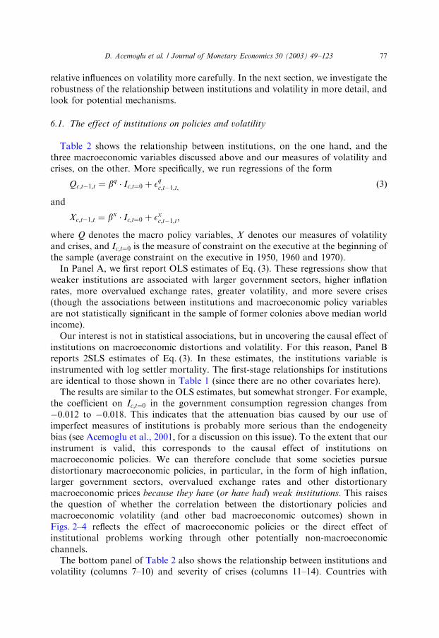
relative influences on volatility more carefully. In the next section, we investigate therobustness of the relationship between institutions and volatility in more detail, andlook for potential mechanisms.

6.1. The effect of institutions on policies and volatility

Table 2 shows the relationship between institutions, on the one hand, and thethree macroeconomic variables discussed above and our measures of volatility andcrises, on the other. More specifically, we run regressions of the form

Qc;t�1;t ¼ bq � Ic;t¼0 þ Eqc;t�1;t; ð3Þ

and

Xc;t�1;t ¼ bx � Ic;t¼0 þ Exc;t�1;t;

where Q denotes the macro policy variables, X denotes our measures of volatilityand crises, and Ic;t¼0 is the measure of constraint on the executive at the beginning ofthe sample (average constraint on the executive in 1950, 1960 and 1970).

In Panel A, we first report OLS estimates of Eq. (3). These regressions show thatweaker institutions are associated with larger government sectors, higher inflationrates, more overvalued exchange rates, greater volatility, and more severe crises(though the associations between institutions and macroeconomic policy variablesare not statistically significant in the sample of former colonies above median worldincome).

Our interest is not in statistical associations, but in uncovering the causal effect ofinstitutions on macroeconomic distortions and volatility. For this reason, Panel Breports 2SLS estimates of Eq. (3). In these estimates, the institutions variable isinstrumented with log settler mortality. The first-stage relationships for institutionsare identical to those shown in Table 1 (since there are no other covariates here).

The results are similar to the OLS estimates, but somewhat stronger. For example,the coefficient on Ic;t¼0 in the government consumption regression changes from�0:012 to �0:018: This indicates that the attenuation bias caused by our use ofimperfect measures of institutions is probably more serious than the endogeneitybias (see Acemoglu et al., 2001, for a discussion on this issue). To the extent that ourinstrument is valid, this corresponds to the causal effect of institutions onmacroeconomic policies. We can therefore conclude that some societies pursuedistortionary macroeconomic policies, in particular, in the form of high inflation,larger government sectors, overvalued exchange rates and other distortionarymacroeconomic prices because they have (or have had) weak institutions. This raisesthe question of whether the correlation between the distortionary policies andmacroeconomic volatility (and other bad macroeconomic outcomes) shown inFigs. 2–4 reflects the effect of macroeconomic policies or the direct effect ofinstitutional problems working through other potentially non-macroeconomicchannels.

The bottom panel of Table 2 also shows the relationship between institutions andvolatility (columns 7–10) and severity of crises (columns 11–14). Countries with


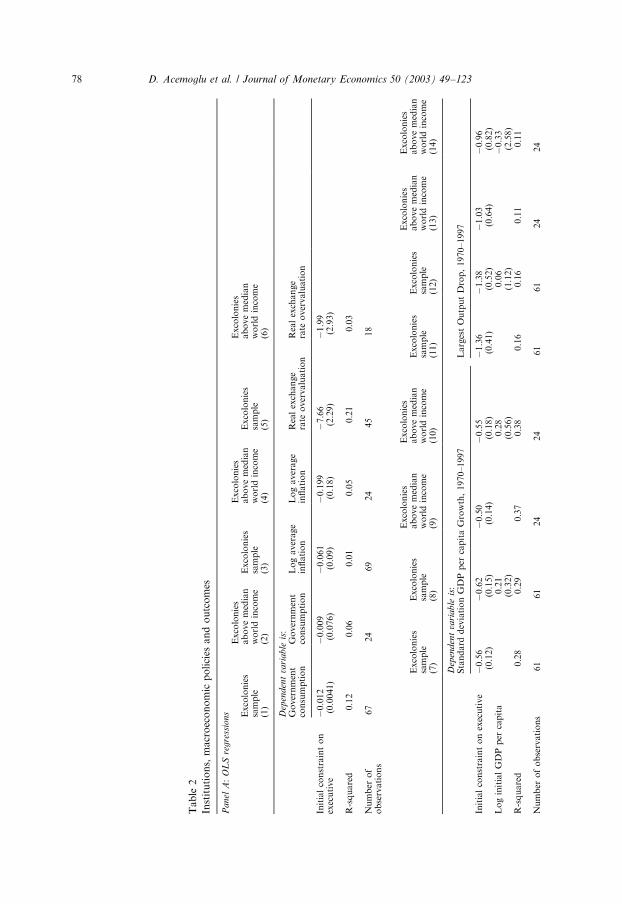
Table

2

Institutions,macroeconomic

policies

andoutcomes

Panel

A:

OL

Sre

gre

ssio

ns

Excolonies

Excolonies

Excolonies

Excolonies

abovemedian

Excolonies

abovemedian

Excolonies

abovemedian

sample

worldincome

sample

worldincome

sample

worldincome

(1)

(2)

(3)

(4)

(5)

(6)

Dep

enden

tva

riable

is:

Government

Government

Logaverage

Logaverage

Realexchange

Realexchange

consumption

consumption

inflation

inflation

rate

overvaluation

rate

overvaluation

Initialconstrainton

executive

�0.012

�0.009

�0.061

�0.199

�7.66

�1.99

(0.0041)

(0.076)

(0.09)

(0.18)

(2.29)

(2.93)

R-squared

0.12

0.06

0.01

0.05

0.21

0.03

Number

of

observations

67

24

69

24

45

18

Excolonies

Excolonies

Excolonies

Excolonies

Excolonies

Excolonies

abovemedian

abovemedian

Excolonies

Excolonies

abovemedian

abovemedian

sample

sample

worldincome

worldincome

sample

sample

worldincome

worldincome

(7)

(8)

(9)

(10)

(11)

(12)

(13)

(14)

Dep

enden

tva

riable

is:

Standard

deviationGDPper

capitaGrowth,1970–1997

LargestOutputDrop,1970–1997


�0.56

�0.62

�0.50

�0.55

�1.36

�1.38

�1.03

�0.96

(0.12)

(0.15)

(0.14)

(0.18)

(0.41)

(0.52)

(0.64)

(0.82)

LoginitialGDPper

capita

0.21

0.28

0.06

�0.33

(0.32)

(0.56)

(1.12)

(2.58)

R-squared

0.28

0.29

0.37

0.38

0.16

0.16

0.11

0.11

Number

ofobservations

61

61

24

24

61

61

24

24


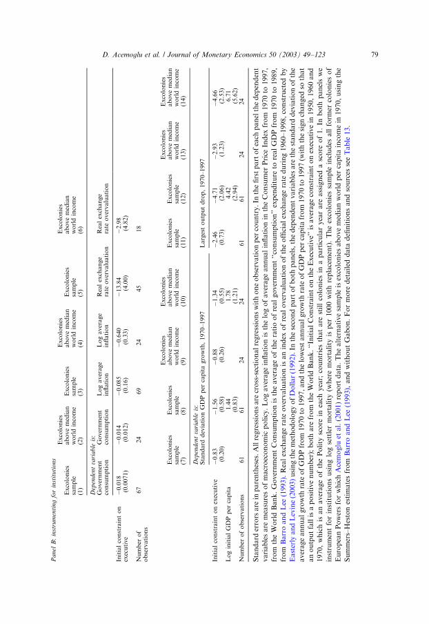
Panel

B:

inst

rum

enti

ng

for

inst

ituti

ons

Excolonies

Excolonies

Excolonies

Excolonies

abovemedian

Excolonies

abovemedian

Excolonies

abovemedian

sample

worldincome

sample

worldincome

sample

worldincome

(1)

(2)

(3)

(4)

(5)

(6)

Dep

enden

tva

riable

is:

Government

Government

Logaverage

Logaverage

Realexchange

Realexchange

consumption

consumption

inflation

inflation

rate

overvaluation

rate

overvaluation

Initialconstrainton

executive

�0.018

�0.014

�0.085

�0.640

�13.84

�2.98

(0.0071)

(0.012)

(0.16)

(0.33)

(4.00)

(4.82)

Number

of

observations

67

24

69

24

45

18

Excolonies

Excolonies

Excolonies

Excolonies

Excolonies

Excolonies

abovemedian

abovemedian

Excolonies

Excolonies

abovemedian

abovemedian

sample

sample

worldincome

worldincome

sample

sample

worldincome

worldincome

(7)

(8)

(9)

(10)

(11)

(12)

(13)

(14)

Dep

enden

tva

riable

is:

Standard

deviationGDPper

capitagrowth,1970–1997

Largestoutputdrop,1970–1997


�0.83

�1.56

�0.88

�1.34

�2.46

�4.71

�2.93

�4.66

(0.20)

(0.58)

(0.26)

(0.55)

(0.73)

(2.06)

(1.23)

(2.53)

LoginitialGDPper

capita

1.44

1.78

4.42

6.71

(0.83)

(1.21)

(2.94)

(5.62)

Number

ofobservations

61

61

24

24

61

61

24

24

Standard

errors

are


cross-sectionalregressionswithoneobservationper

country.In

thefirstpartofeach

panelthedependent

variablesare

measuresofmacroeconomic

policy.Logaverageinflationisthelogofaverageannualinflationin

theConsumer

Price

Index

from

1970to

1997,

from

theWorldBank.GovernmentConsumptionistheaverageoftheratioofrealgovernment‘‘consumption’’expenditure

torealGDPfrom

1970to

1989,

from

BarroandLee

(1993).Realexchangerate

overvaluationisanindex

ofrealovervaluationoftheofficialexchangerate

during1960–1998,constructed

by

Easterly

andLevine(2003)usingthemethodologyofDollar(1992).In

thesecondpartofboth

panels,thedependentvariablesare

thestandard

deviationofthe

averageannualgrowth

rate

ofGDPfrom

1970to

1997,andthelowestannualgrowth

rate

ofGDPper

capitafrom

1970to

1997(w

iththesignchanged

sothat

anoutputfallisapositivenumber);both

are

from

theWorldBank.‘‘InitialConstraintontheExecutive’’isaverageconstraintonexecutivein

1950,1960and

1970,whichis

anaverageofthePolity

score

ineach

year;

countriesthatare

stillcoloniesin

aparticularyearare

assigned

ascore

of1.In

both

panelswe

instrumentforinstitutionsusinglogsettlermortality

(wheremortality

isper

1000withreplacement).Theexcoloniessample

includes

allform

ercoloniesof

EuropeanPowersforwhichAcemoglu

etal.(2001)reportdata.Thealternativesampleisexcoloniesabovemedianworldper

capitaincomein

1970,usingthe

Summers–Hestonestimatesfrom

BarroandLee

(1993),andwithoutGabon.Formore

detailed

data


seeTable

13.


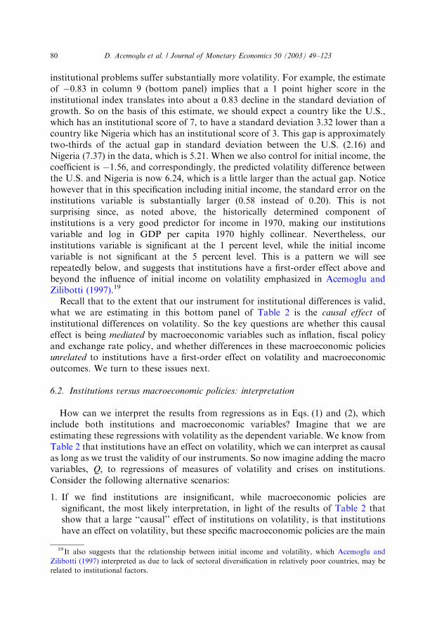
institutional problems suffer substantially more volatility. For example, the estimateof �0:83 in column 9 (bottom panel) implies that a 1 point higher score in theinstitutional index translates into about a 0.83 decline in the standard deviation ofgrowth. So on the basis of this estimate, we should expect a country like the U.S.,which has an institutional score of 7, to have a standard deviation 3.32 lower than acountry like Nigeria which has an institutional score of 3. This gap is approximatelytwo-thirds of the actual gap in standard deviation between the U.S. (2.16) andNigeria (7.37) in the data, which is 5.21. When we also control for initial income, thecoefficient is �1:56; and correspondingly, the predicted volatility difference betweenthe U.S. and Nigeria is now 6.24, which is a little larger than the actual gap. Noticehowever that in this specification including initial income, the standard error on theinstitutions variable is substantially larger (0.58 instead of 0.20). This is notsurprising since, as noted above, the historically determined component ofinstitutions is a very good predictor for income in 1970, making our institutionsvariable and log in GDP per capita 1970 highly collinear. Nevertheless, ourinstitutions variable is significant at the 1 percent level, while the initial incomevariable is not significant at the 5 percent level. This is a pattern we will seerepeatedly below, and suggests that institutions have a first-order effect above andbeyond the influence of initial income on volatility emphasized in Acemoglu andZilibotti (1997).19

Recall that to the extent that our instrument for institutional differences is valid,what we are estimating in this bottom panel of Table 2 is the causal effect ofinstitutional differences on volatility. So the key questions are whether this causaleffect is being mediated by macroeconomic variables such as inflation, fiscal policyand exchange rate policy, and whether differences in these macroeconomic policiesunrelated to institutions have a first-order effect on volatility and macroeconomicoutcomes. We turn to these issues next.

6.2. Institutions versus macroeconomic policies: interpretation

How can we interpret the results from regressions as in Eqs. (1) and (2), whichinclude both institutions and macroeconomic variables? Imagine that we areestimating these regressions with volatility as the dependent variable. We know fromTable 2 that institutions have an effect on volatility, which we can interpret as causalas long as we trust the validity of our instruments. So now imagine adding the macrovariables, Q; to regressions of measures of volatility and crises on institutions.Consider the following alternative scenarios:

1. If we find institutions are insignificant, while macroeconomic policies aresignificant, the most likely interpretation, in light of the results of Table 2 thatshow that a large ‘‘causal’’ effect of institutions on volatility, is that institutionshave an effect on volatility, but these specific macroeconomic policies are the main

19 It also suggests that the relationship between initial income and volatility, which Acemoglu and

Zilibotti (1997) interpreted as due to lack of sectoral diversification in relatively poor countries, may be

related to institutional factors.


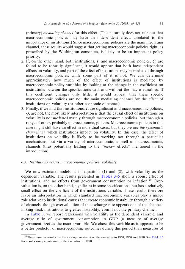
(primary) mediating channel for this effect. (This naturally does not rule out thatmacroeconomic policies may have an independent effect, unrelated to theimportance of institutions.) Since macroeconomic policies are the main mediatingchannel, these results would suggest that getting macroeconomic policies right, asprescribed by the Washington consensus, is likely to be an important policypriority.

2. If, on the other hand, both institutions, I ; and macroeconomic policies, Q; arefound to be robustly significant, it would appear that both have independenteffects on volatility, and part of the effect of institutions may be mediated throughmacroeconomic policies, while some part of it is not. We can determineapproximately how much of the effect of institutions is mediated bymacroeconomic policy variables by looking at the change in the coefficient oninstitutions between the specifications with and without the macro variables. Ifthis coefficient changes only little, it would appear that these specificmacroeconomic policies are not the main mediating channel for the effect ofinstitutions on volatility (or other economic outcomes).

3. Finally, if we find that institutions, I ; are significant and macroeconomic policies,Q; are not, the most likely interpretation is that the causal effect of institutions onvolatility is not mediated mainly through macroeconomic policies, but through arange of other, probably microeconomic, policies. Macroeconomic policies in thiscase might still have an effect in individual cases; but they are not the systematic

channel via which institutions impact on volatility. In this case, the effect ofinstitutions on volatility is likely to be working not through a particularmechanisms, but via a variety of microeconomic, as well as macroeconomic,channels (thus potentially leading to the ‘‘seesaw effects’’ mentioned in theintroduction).

6.3. Institutions versus macroeconomic policies: volatility

We now estimate models as in equations (1) and (2), with volatility as thedependent variable. The results presented in Tables 3–5 show a robust effect ofinstitutions, and no effects from government consumption or inflation.20 Over-valuation is, on the other hand, significant in some specifications, but has a relativelysmall effect on the coefficient of the institutions variable. These results thereforefavor an interpretation in which standard macroeconomic variables play a minorrole relative to institutional causes that create economic instability through a varietyof channels, though overvaluation of the exchange rate appears one of the channelslinking weak institutions to greater instability, even if not the primary channel.

In Table 3, we report regressions with volatility as the dependent variable, andaverage ratio of government consumption to GDP (a measure of averagegovernment size) as the macro variable. We chose this variable as it appears to bea better predictor of macroeconomic outcomes during this period than measures of

20These baseline results use the average constraint on the executive in 1950, 1960 and 1970. See Table 15

for results using constraint on the executive in 1970.


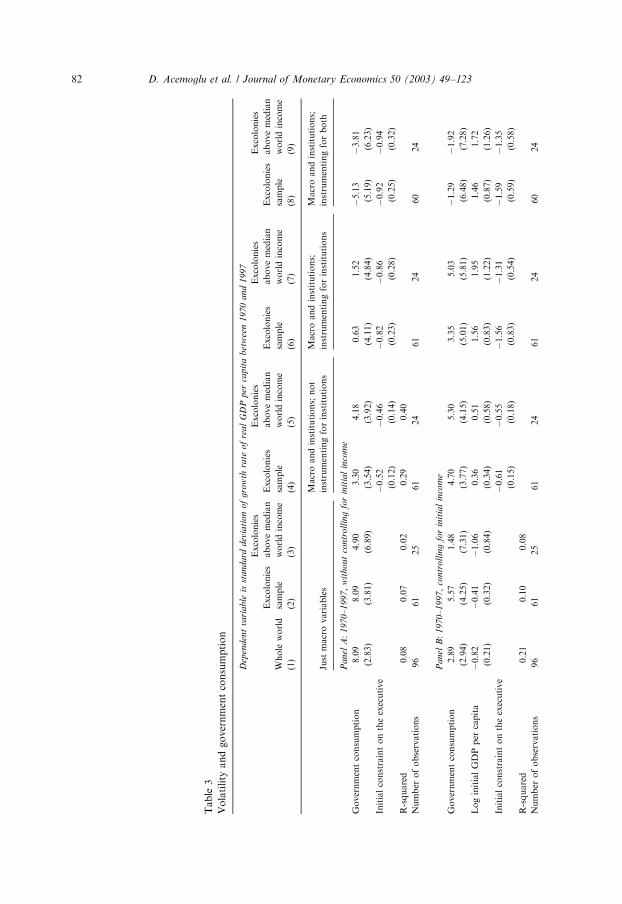
Table

3

Volatility

andgovernmentconsumption

Dep

enden

tva

riable

isst

andard

dev

iati

on

of

gro

wth

rate

of

real

GD

Pper

capit

abet

wee

n1970

and

1997

Excolonies

Excolonies

Excolonies

Excolonies

Excolonies

abovemedian

Excolonies

abovemedian

Excolonies

abovemedian

Excolonies

abovemedian

Whole

world

sample

worldincome

sample

worldincome

sample

worldincome

sample

worldincome

(1)

(2)

(3)

(4)

(5)

(6)

(7)

(8)

(9)

Macroandinstitutions;

not



Just

macrovariables

instrumentingforinstitutions


instrumentingforboth

Panel

A:

1970–1997,

wit

hout

contr

oll

ing

for

init

ial

inco

me

Governmentconsumption

8.09

8.09

4.90

3.30

4.18

0.63

1.52

�5.13

�3.81

(2.83)

(3.81)

(6.89)

(3.54)

(3.92)

(4.11)

(4.84)

(5.19)

(6.23)

Initialconstraintontheexecutive

�0.52

�0.46

�0.82

�0.86

�0.92

�0.94

(0.12)

(0.14)

(0.23)

(0.28)

(0.25)

(0.32)

R-squared

0.08

0.07

0.02

0.29

0.40

Number

ofobservations

96

61

25

61

24

61

24

60

24

Panel

B:

1970–1997,

contr

oll

ing

for

init

ial

inco

me


2.89

5.57

1.48

4.70

5.30

3.35

5.03

�1.29

�1.92

(2.94)

(4.25)

(7.31)

(3.77)

(4.15)

(5.01)

(5.81)

(6.48)

(7.28)

LoginitialGDPper

capita

�0.82

�0.41

�1.06

0.36

0.51

1.56

1.95

1.46

1.72

(0.21)

(0.32)

(0.84)

(0.34)

(0.58)

(0.83)

(1.22)

(0.87)

(1.26)


�0.61

�0.55

�1.56

�1.31

�1.59

�1.35

(0.15)

(0.18)

(0.83)

(0.54)

(0.59)

(0.58)

R-squared

0.21

0.10

0.08

Number

ofobservations

96

61

25

61

24

61

24

60

24


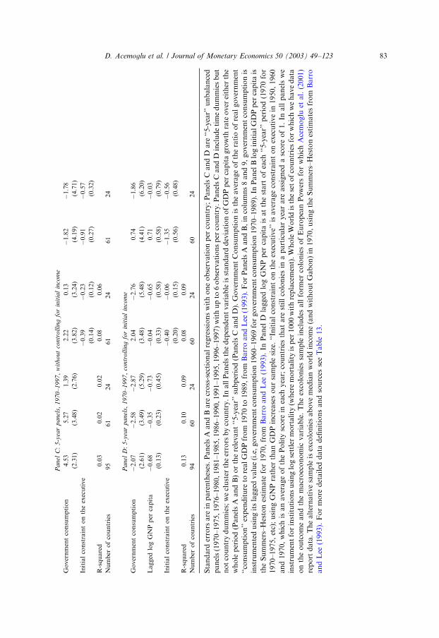
Panel

C:

5-y

ear

panel

s,1970–1997,

wit

hout

contr

oll

ing

for

init

ial

inco

me


4.53

5.27

1.39

2.22

0.13

�1.82

�1.78

(2.31)

(3.48)

(2.76)

(3.82)

(3.24)

(4.19)

(4.71)


�0.39

�0.23

�0.91

�0.57

(0.14)

(0.12)

(0.27)

(0.32)

R-squared

0.03

0.02

0.02

0.08

0.06

Number

ofcountries

95

61

24

61

24

61

24

Panel

D:

5-y

ear

panel

s,1970–1997,

contr

oll

ing

for

init

ial

inco

me


�2.07

�2.58

�2.87

2.04

�2.76

0.74

�1.86

(2.61)

(3.49)

(5.29)

(3.48)

(5.48)

(4.41)

(6.20)

Lagged

logGNPper

capita

�0.68

�0.35

�0.73

�0.04

�0.65

0.71

�0.03

(0.13)

(0.23)

(0.45)

(0.33)

(0.58)

(0.58)

(0.79)


�0.40

�0.06

�1.35

�0.56

(0.20)

(0.15)

(0.56)

(0.48)

R-squared

0.13

0.10

0.09

0.08

0.09

Number

ofcountries

94

60

24

60

24

60

24

Standard

errors

are

inparentheses.PanelsA

andBare


country;PanelsCandD

are

‘‘5-year’’unbalanced

panels(1970–1975,1976–1980,1981–1985,1986–1990,1991–1995,1996–1997)withupto

6observationsper

country.PanelsCandD

includetimedummiesbut

notcountrydummies;wecluster

theerrors

bycountry.In

allPanelsthedependentvariableisstandard

deviationofGDPper

capitagrowth

rate

over

either

the

wholeperiod(PanelsA

andB)ortherelevant‘‘5-year’’subperiod(PanelsCandD).GovernmentConsumptionistheaverageoftheratioofrealgovernment

‘‘consumption’’expenditure

torealGDPfrom

1970to

1989,from

BarroandLee

(1993).ForPanelsA

andB,in

columns8and9,governmentconsumptionis

instrumentedusingitslagged

value(i.e,governmentconsumption1960–1969forgovernmentconsumption1970–1989).In

PanelBloginitialGDPper

capitais

theSummers–Hestonestimate

for1970,from

BarroandLee

(1993).In

Panel

Dlagged

logGNPper

capitaisatthestart

ofeach

‘‘5-year’’period(1970for

1970–1975,etc);usingGNPrather

thanGDPincreasesoursample

size.‘‘Initialconstraintontheexecutive’’isaverageconstraintonexecutivein

1950,1960

and1970,whichisanaverageofthePolity

score

ineach


stillcoloniesin

aparticularyearare

assigned

ascore

of1.In

allpanelswe


(wheremortality

isper

1000withreplacement).WholeWorldisthesetofcountriesforwhichwehavedata

ontheoutcomeandthemacroeconomic

variable.Theexcoloniessample

includes

allform


etal.(2001)

report

data.Thealternativesampleisexcoloniesabovemedianworldincome(andwithoutGabon)in

1970,usingtheSummers–Hestonestimatesfrom

Barro

andLee

(1993).Formore

detailed

data


seeTable

13.


Table

4

Volatility

andinflation

Dep

enden

tva

riable

isst

andard

dev

iati

on

of

gro

wth

rate

of

real

GD

Pper

capit

a,

1970–1997

Whole

World

Excolonies

sample

Excolonies

above

median

world

income

Excolonies

sample

Excolonies

above

median

world

income

Excolonies

sample

Excolonies

above

median

world

income

Excolonies

sample

Excolonies

above

median

world

income

(1)

(2)

(3)

(4)

(5)

(6)

(7)

(8)

(9)

MacroandInstitutions;not

MacroandInstitutions;


Just

macrovariables

instrumentingfor

institutions

instrumentingfor

institutions


Panel

A:

1970–1997,

wit

hout

contr

oll

ing

for

init

ial

inco

me

Logaverageinflation

0.30

0.12

0.51

0.11

0.41

0.10

0.34

�0.14

0.42

(0.17)

(0.19)

(0.17)

(0.16)

(0.14)

(0.17)

(0.16)

(0.42)

(0.35)

Initialconstraintonthe

executive

�0.56

�0.42

�0.83

�0.66

�0.86

�0.62

(0.12)

(0.12)

(0.21)

(0.23)

(0.22)

(0.34)

R-squared

0.03

0.01

0.30

0.29

0.55

Number

ofobservations

96

61

24

61

24

61

24

48

19

Panel

B:

1970–1997,

contr

oll

ing

for

init

ial

inco

me

Logaverageinflation

0.21

0.17

0.48

0.09

0.41

�0.04

0.33

�0.07

0.25

(0.16)

(0.19)

(0.17)

(0.17)

(0.14)

(0.23)

(0.19)

(0.48)

(0.48)

LoginitialGDPper

capita

�0.88

�0.63

�0.55

0.19

0.33

1.47

1.29

1.25

1.35

(0.19)

(0.29)

(0.46)

(0.32)

(0.48)

(0.88)

(0.96)

(0.74)

(1.01)


executive

�0.62

�0.48

�1.57

�1.00

�1.45

�1.06

(0.15)

(0.16)

(0.61)

(0.45)

(0.51)

(0.63)

R-squared

0.22

0.08

0.35

0.29

0.56

Number

ofobservations

96

61

24

61

24

61

24

48

19


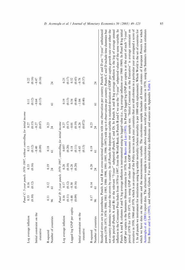
Panel

C:

5-y

ear

panel

s.1970–1997,

wit

hout

contr

oll

ing

for

init

ial

inco

me

Logaverageinflation

0.33

0.16

0.33

0.13

0.27

0.11

0.22

(0.10)

(0.12)

(0.16)

(0.12)

(0.15)

(0.12)

(0.16)


executive

�0.40

�0.27

�0.64

�0.47

(0.09)

(0.07)

(0.15)

(0.16)

R-squared

0.11

0.12

0.19

0.18

0.23

Number

ofcountries

96

61

24

61

24

61

24

Panel

D:

5-y

ear

panel

s.1970–1997,

contr

oll

ing

for

init

ial

inco

me

Logaverageinflation

0.16

0.17

0.28

0.057

0.27

0.19

0.25

(0.11)

(0.12)

(0.18)

(0.20)

(0.17)

(0.13)

(0.17)

Lagged

logGNPper

capita

�0.48

�0.30

�0.28

0.18

�0.01

0.54

0.52

(0.09)

(0.16)

(0.20)

(0.11)

(0.19)

(0.40)

(0.45)


executive

�0.43

�0.26

�1.04

�0.78

(0.13)

(0.072)

(0.40)

(0.37)

R-squared

0.17

0.14

0.20

0.19

0.23

Number

ofcountries

96

61

24

61

24

61

24

Standard

errors

are


andBare


country;PanelsC

andD

are


panels(1970–1975,1976–1980,1981–1985,1986–1990,1991–1995,1996–1997)withupto

6observationsper

country.PanelsCandD



theerrors

bycountry.In


deviationofGDPper

capitagrowth

rate

over

either

the

whole

period(PanelsA

andB)ortherelevant‘‘5-year’’subperiod(PanelsC

andD).In

PanelsA

andB

logaverageinflationis

thelogofaverageannual

inflationin

theConsumer

Price

Index

from

1970to

1997,from

theWorldBank;in

PanelsBandCweuse

the‘‘5-year’’subperiodvalues

ofthesamevariable.In

PanelsA

andB,columns8and9,logaverageinflationisinstrumentedusingitslagged

value(i.e.,logaverageinflationover

1960–1969).In

PanelBloginitial

GDPper

capitaistheSummers–Hestonestimate

for1970,from

BarroandLee

(1993).In

Panel

Dlagged

logGNPper

capitaisatthestart

ofeach

‘‘5-year’’

period(1970for1970–1975,etc);usingGNP

rather

thanGDP

increasesoursample

size.‘‘InitialConstraintontheExecutive’’is

averageconstrainton

executivein


score

ineach


stillcoloniesin

aparticularyearare

assigned

ascore

of

1.In

allpanelsweinstrumentforinstitutionsusinglogsettlermortality

(wheremortality

isper

1000withreplacement).WholeWorldisthesetofcountriesfor

whichwehavedata


variable.Theexcoloniessample

includes

allform

ercoloniesofEuropeanPowersforwhich

Acemoglu

etal.(2001)report

data.Thealternativesampleisexcoloniesabovemedianworldper

capitaincomein

1970,usingtheSummers–Hestonestimates

from

BarroandLee


detailed

data


seeAppendix

Table

1.


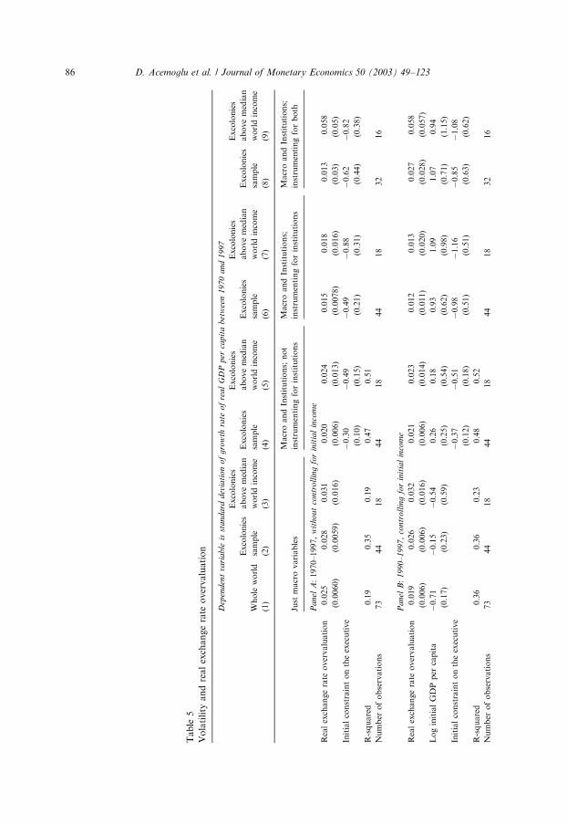
Table

5

Volatility

andrealexchangerate

overvaluation

Dep

enden

tva

riable

isst

andard

dev

iati

on

of

gro

wth

rate

of

real

GD

Pper

capit

abet

wee

n1970

and

1997

Excolonies

Excolonies

Excolonies

Excolonies

Excolonies

abovemedian

Excolonies

abovemedian

Excolonies

abovemedian

Excolonies

abovemedian

Whole

world

sample

worldincome

sample

worldincome

sample

worldincome

sample

worldincome

(1)

(2)

(3)

(4)

(5)

(6)

(7)

(8)

(9)


not



Just

macrovariables




Panel

A:1970–1997,

wit

hout

contr

oll

ing

for

init

ial

inco

me

Realexchangerate

overvaluation

0.025

0.028

0.031

0.020

0.024

0.015

0.018

0.013

0.058

(0.0060)

(0.0059)

(0.016)

(0.006)

(0.013)

(0.0078)

(0.016)

(0.03)

(0.05)


�0.30

�0.49

�0.49

�0.88

�0.62

�0.82

(0.10)

(0.15)

(0.21)

(0.31)

(0.44)

(0.38)

R-squared

0.19

0.35

0.19

0.47

0.51

Number

ofobservations

73

44

18

44

18

44

18

32

16

Panel

B:

1990–1997,

contr

oll

ing

for

init

ial

inco

me

Realexchangerate

overvaluation

0.019

0.026

0.032

0.021

0.023

0.012

0.013

0.027

0.058

(0.006)

(0.006)

(0.016)

(0.006)

(0.014)

(0.011)

(0.020)

(0.028)

(0.057)

LoginitialGDPper

capita

�0.71

�0.15

�0.54

0.26

0.18

0.93

1.09

1.07

0.94

(0.17)

(0.23)

(0.59)

(0.25)

(0.54)

(0.62)

(0.98)

(0.71)

(1.15)


�0.37

�0.51

�0.98

�1.16

�0.85

�1.08

(0.12)

(0.18)

(0.51)

(0.51)

(0.63)

(0.62)

R-squared

0.36

0.36

0.23

0.48

0.52

Number

ofobservations

73

44

18

44

18

44

18

32

16


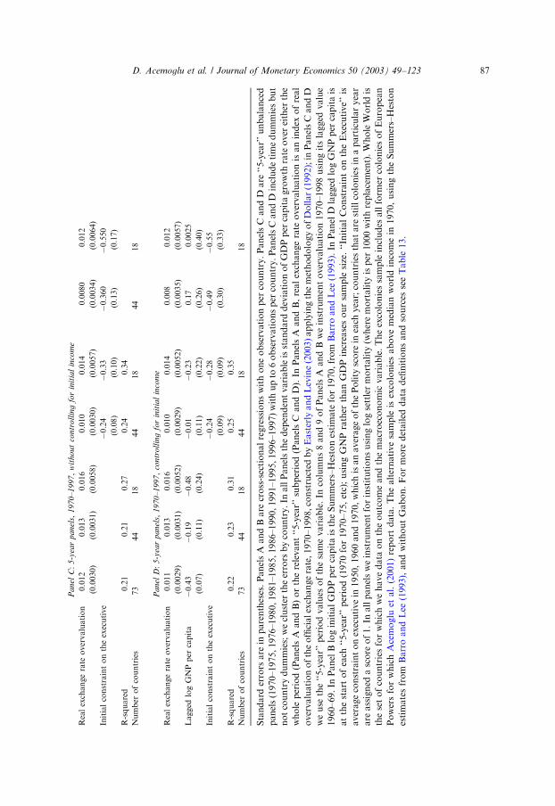
Panel

C:

5-y

ear

panel

s,1970–1997,

wit

hout

contr

oll

ing

for

init

ial

inco

me

Realexchangerate

overvaluation

0.012

0.013

0.016

0.010

0.014

0.0080

0.012

(0.0030)

(0.0031)

(0.0058)

(0.0030)

(0.0057)

(0.0034)

(0.0064)


�0.24

�0.33

�0.360

�0.550

(0.08)

(0.10)

(0.13)

(0.17)

R-squared

0.21

0.21

0.27

0.24

0.34

Number

ofcountries

73

44

18

44

18

44

18

Panel

D:

5-y

ear

panel

s,1970–1997,

contr

oll

ing

for

init

ial

inco

me

Realexchangerate

overvaluation

0.011

0.013

0.016

0.010

0.014

0.008

0.012

(0.0029)

(0.0031)

(0.0052)

(0.0029)

(0.0052)

(0.0035)

(0.0057)

Lagged

logGNPper

capita

�0.43

�0.19

�0.48

�0.01

�0.23

0.17

0.0025

(0.07)

(0.11)

(0.24)

(0.11)

(0.22)

(0.26)

(0.40)


�0.24

�0.28

�0.49

�0.55

(0.09)

(0.09)

(0.30)

(0.33)

R-squared

0.22

0.23

0.31

0.25

0.35

Number

ofcountries

73

44

18

44

18

18

Standard

errors

are


andBare


country.PanelsC

andD

are


panels(1970–1975,1976–1980,1981–1985,1986–1990,1991–1995,1996–1997)withupto

6observationsper

country.PanelsCandD



theerrors

bycountry.In


deviationofGDPper

capitagrowth

rate

over

either

the

whole

period(PanelsA

andB)ortherelevant‘‘5-year’’subperiod(PanelsC

andD).In

PanelsA

andB,realexchangerate

overvaluationisanindex

ofreal

overvaluationoftheofficialexchangerate,1970–1998,constructed

byEasterlyandLevine(2003)applyingthemethodologyofDollar(1992);in

PanelsCandD

weuse

the‘‘5-year’’periodvalues

ofthesamevariable.In

columns8and9ofPanelsA

andBweinstrumentovervaluation1970–1998usingitslagged

value

1960–69.In



for1970,from

BarroandLee

(1993).In

PanelD

lagged

logGNPper

capitais

atthestart

ofeach

‘‘5-year’’period(1970for1970–75,etc);usingGNPrather



averageconstraintonexecutivein


score

ineach


stillcoloniesin

aparticularyear

are

assigned

ascore

of1.In


(wheremortality

isper

1000withreplacement).WholeWorldis

thesetofcountriesforwhichwehavedata


variable.Theexcoloniessampleincludes

allform

ercoloniesofEuropean

PowersforwhichAcemoglu

etal.(2001)report

data.Thealternativesample

isexcoloniesabovemedianworldincomein

1970,usingtheSummers–Heston

estimatesfrom

BarroandLee


detailed

data


seeTable

13.


the budget deficit. The first three columns in the top panel document a strongrelationship between the size of government and volatility, without controlling forinstitutions, as already shown in Fig. 2. The second panel shows that a similar butweaker relationship applies when we control for initial income. Greater governmentsize is associated with greater instability. The rest of the table shows that addinginstitutions reduces the importance of the government size variable, which is neverfound to be significant.21

In columns 4 and 5, we start with OLS regressions, where institutions are treatedas exogenous. These regressions show a negative relationship between constraint onthe executive and volatility, both in the full excolonies sample and in the smallersample of excolonies above median world income. The correlation betweengovernment consumption and volatility is no longer significant. The results aresimilar when we control for initial income in Panel B: institutions continue to besignificant and government size is not.

In columns 6 and 7, we instrument for institutions using (potential) Europeansettler mortality, as in previous tables, and treat government size as exogenous. Theeffect of institutions on volatility is now stronger, and there is also no effect ofgovernment consumption (the coefficient is now almost zero down from 8.09).

Average size of government over the sample period may be correlated with otherdeterminants of volatility, and may also be measured with error. To deal with theseendogeneity and attenuation issues, columns 8 and 9 instrument for government sizeusing past government size. Now the government size variable has the opposite signto those in columns 1, 2 and 3 and is far from being significant. This is despite thefact that there is a good first-stage relationship for government size (the t-statistic onpast government consumption is over 10, and the R2 of the first-stage regression is0.69). Therefore, the cross-sectional regressions in Panels A and B suggest thatdifferences in government size are not a major determinant of the volatility over thethirty-year period we are looking at.

It is also worth noting that the (instrumented) effect of initial institutions onvolatility we estimate in these two panels are very similar to the estimates in Table 2.For example, in Table 2, the effect of initial constraint on the executive on volatilityis around �0:8 in models that do not control for initial income, and around �1:6 inmodels that control for initial income. When we also control for government size asin Table 3, the effect of initial institutions on volatility is very similar: the coefficientis now �0:82 without initial income and �1:56 with initial income.

The models reported in Panels A and B are based on the estimation of Eq. (1),which looks at the relationship between volatility and government size over thethirty-year period (1970–1997). As discussed above, some countries may experienceshort periods of large government spending, causing major crises, while during otherperiods they may have offsetting low spending, thus resulting in average governmentsize similar to that in other countries. To investigate this possibility, in Panels C and D,

21To save space we do not report the first-stage relationship for institutions, which is very similar to the

regressions reported in Table 2 (though not identical since other variables are now also included in the first

stage).


we estimate the panel regression equation (2). The first three columns show the effectof government size without controlling for institutions. When we add institutions,the government size variable is again found not to be a key determinant of volatility.Instead, there is a robust relationship between initial institutions and subsequentvolatility between 1970 and 1997.

Table 4 repeats the same exercise as Table 3, but using log inflation rather thangovernment consumption. We use the log of average inflation rather than the level ofinflation, since the relationship between volatility and inflation is stronger when weuse the log specification and less affected by outliers. Panels A and B estimateEq. (1), with and without initial income. The basic patterns are the same.Throughout, there is a robust effect of institutions on volatility, with very similarcoefficients to those found in Table 2 (in instrumented regressions using the fullsample, the coefficient is �0:83 without initial income and �1:57 with initial income).There is no evidence that inflation matters for volatility in the full sample of formercolonies, either in the cross-section or in the 5-year panel, although it is significant insome specifications for the sample of former colonies above median world income.

Table 5 turns to exchange rate overvaluation, and uses the index of exchange rateovervaluation constructed by David Dollar (1992) and updated by Easterly andLevine (2003).22 The first three columns show a strong relationship between realexchange rate overvaluation when the importance of institutions is not taken intoaccount. When the next column includes institutions in the regression, the effect ofovervaluation remains significant. Initial institutions also continue to have a largeand statistically-significant effect on volatility, with a coefficient about 1/4 less thanthe corresponding estimate without controlling for exchange rate overvaluation.23

When we also control for initial income per capita in Panel B, the effect ofovervaluation is still significant, and initial constraint on the executive is also highlysignificant, but with a smaller coefficient than our baseline estimates. These resultssuggest that misaligned exchange rates are a mediating channel for the effect ofinstitutions on volatility, but probably not the primary mediating channel.

Overall, the results presented in this subsection suggest that the historically-determined component of institutions has a first-order effect on volatility, andneither inflation nor government consumption (nor the other standard macrovariables we examined) seem to be the main mediating channel, though exchangerate overvaluation is typically correlated with volatility. Our interpretation of theseresults is that a fundamental determinant of thirty-year volatility differences isinstitutional differences across countries, and that institutional differences create

22Due to data availability, we use the average value of this overvaluation index from 1960 to 1998,

generously provided by Bill Easterly and Ross Levine. Because we only have an average value for the

entire period, we cannot instrument using lagged values as in Tables 3 and 4. We have also checked the

results using the variability of overvaluation from Dollar (1992), but as this does not change our results we

omit it here from the discussion.23The coefficient on institutions in Table 3 is �0:83; but once we limit the sample to the former colonies

for which we have data on real exchange rate overvaluation, the coefficient on institutions drops to �0:69:The coefficient in Table 5 is �0:49:


economic instability through a variety of microeconomic channels as well as theoften-emphasized macroeconomic channels.

6.4. Institutions versus macroeconomic policies: crises

Table 6 presents a number of specifications that look at the impact of macrovariables and institutions on the severity of crises, measured by the largest outputdrop during the sample. Each of the three different panels refers to one of the threemacro variables we considered so far. In all cases, our measure of institutions,average constraint on the executive in 1950, 1960 and 1970, is instrumented by settlermortality (See Table 17 for results using constraint on the executive in 1970).

The picture that emerges from this table is similar to that from Tables 3–5. In mostspecifications there is a substantial effect of initial constraint on the executive onseverity of crises, and this effect remains statistically significant at the conventionallevels even when we control for initial income. In most specifications, the effect ofinitial institutions is again comparable to the baseline results in Table 2 (in Table 2,the coefficient on institutions in the 2SLS regression on worst output performance isaround �2:5 when we do not control for initial income, and around �5 when wecontrol for initial income; the range of estimates in this table are tightly around thesevalues). We also find that government consumption and log average inflation do notappear to have an effect on the severity of crises when we take the influence ofinstitutions into account. In contrast to our results with volatility, the extent ofovervaluation of the real exchange rate is also insignificant, and only slightly reducesthe effect of institutions on the severity of crises.

These results confirm the conclusion of the previous section that there appears tobe a close a link between institutions and economic instability, most likely notmediated primarily through the standard macroeconomic variables.

6.5. Institutions versus macroeconomic policies: economic growth

Table 7 looks at the relationship between macroeconomic variables andinstitutions, on the one hand, and economic growth, on the other. As in Table 6,the three panels of the table refer to three different macro variables, and in all caseswe also include institutions, average constraint on the executive in 1950, 1960 and1970, instrumented by our historical instruments (See Table 17 for results usingconstraint on the executive in 1970).

In the full sample of excolonies (odd-numbered columns), we find a significanteffect of initial institutions on growth, no effects from government consumption,some effects from inflation, and stronger effects from overvaluation. When we limitthe sample to excolonies above median world income, and especially when we alsocontrol for initial income, the effect of institutions on growth is weaker. Ourinterpretation is the same as the one we offered above: much of the divergence inincome happened between 1750 and 1950, when countries with good institutionsgrew rapidly, and those with extractive institutions failed to do so (Acemoglu et al.,2002a). By 1970, much of this process of adjustment was complete, and the effect of


institutions on further growth is correspondingly weaker. Moreover, the sample offormer colonies above median world income is relatively small, and exhibits limitedvariation in growth. In this light, these weaker results may not be so surprising.

7. Institutions and volatility: robustness and mechanisms

The previous section documented a strong relationship between institutions andeconomic volatility, and presented evidence suggesting that this relationship was notmediated through any of the standard macroeconomic variables. In this section, weinvestigate the relationship between institutions and volatility further, and show thatit is robust to controlling for a variety of other potential determinants of economicinstability. We then investigate the empirical validity of some potential mechanismsvia which institutions might be affecting volatility.

7.1. Robustness

Table 8 reports regressions of volatility on institutions, while also controlling for anumber of potential determinants of volatility. In particular, in various columns, wecontrol for all the macro variables together, the initial level of education, theimportance of financial intermediation, the variability of terms of trade times theshare of exports, and we also estimate models excluding outliers.

In columns 1 and 2 of Panel A of Table 8, we add all the macro variables together,with or without initial income. Initial constraint on the executive has a negativeeffect on volatility. Without controlling for initial income, this effect is significant,but some what smaller than in Table 2. When we also control for initial income, thestandard error increases but the coefficient on institutions remains very similar in sizeto the coefficients reported in Table 2. The effect of initial income is not significant.Jointly, the macro variables are insignificant as shown by the p-value. In Panel B, werun the same regressions, but this time in a manner similar to the panel regression inequation (2), with each observation corresponding to a 5-year period. Now theeffects of the macro variables are even weaker, and the constraint on the executive isconsistently significant, with very similar coefficients to before (again the standarderrors in this lower panel are clustered by country).

In columns 3 and 4 we control for years of schooling in 1970 (from Barro and Lee,1993). This is a useful specification, since, as we argue in Acemoglu et al. (2001),historical institutions determined various components of investments, includinginvestments in human capital, so we expect education levels in 1970 to be correlatedwith the historically determined component of institutions. It is then important toknow whether the effect of institutions on volatility is working primarily throughsome educational mechanism. When we include human capital, constraint on theexecutive continues to have a negative effect, similar in magnitude to our previousresults, but it is no longer significant. This is because human capital and constrainton the executive are highly correlated. But, the years of schooling variable is very farfrom being significant, and in fact, it has the wrong sign. In the lower panel where we


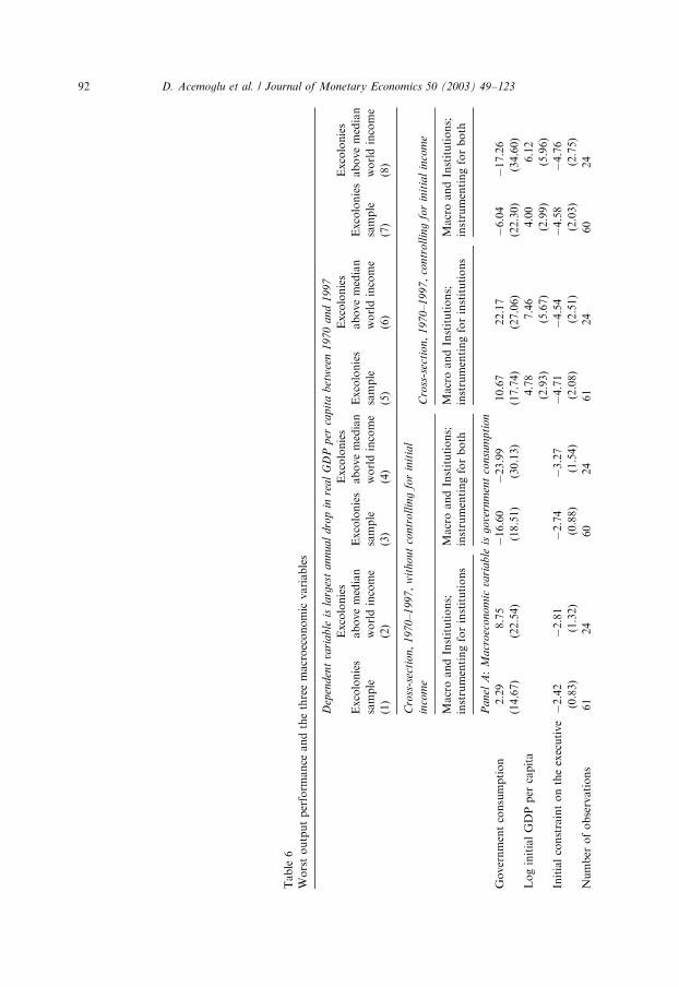
Table

6

Worstoutputperform

ance

andthethreemacroeconomic

variables

Dep

enden

tva

ria

ble

isla

rges

ta

nn

ua

ld

rop

inre

al

GD

Pp

erca

pit

ab

etw

een

19

70

an

d1

99

7

Excolonies

Excolonies

Excolonies

Excolonies

Excolonies

abovemedian

Excolonies

abovemedian

Excolonies

abovemedian

Excoloniesabovemedian

sample

worldincome

sample

worldincome

sample

worldincome

sample

worldincome

(1)

(2)

(3)

(4)

(5)

(6)

(7)

(8)

Cro

ss-s

ecti

on,

19

70

–1

99

7,

wit

hou

tco

ntr

oll

ing

for

init

ial

inco

me

Cro

ss-s

ecti

on,

19

70–

19

97,

con

tro

llin

gfo

rin

itia

lin

com

e









Pa

nel

A:

Ma

cro

eco

no

mic

vari

ab

leis

go

vern

men

tco

nsu

mpti

on


2.29

8.75

�16.60

�23.99

10.67

22.17

�6.04

�17.26

(14.67)

(22.54)

(18.51)

(30.13)

(17.74)

(27.06)

(22.30)

(34.60)

LoginitialGDPper

capita

4.78

7.46

4.00

6.12

(2.93)

(5.67)

(2.99)

(5.96)


�2.42

�2.81

�2.74

�3.27

�4.71

�4.54

�4.58

�4.76

(0.83)

(1.32)

(0.88)

(1.54)

(2.08)

(2.51)

(2.03)

(2.75)

Number

ofobservations

61

24

60

24

61

24

60

24


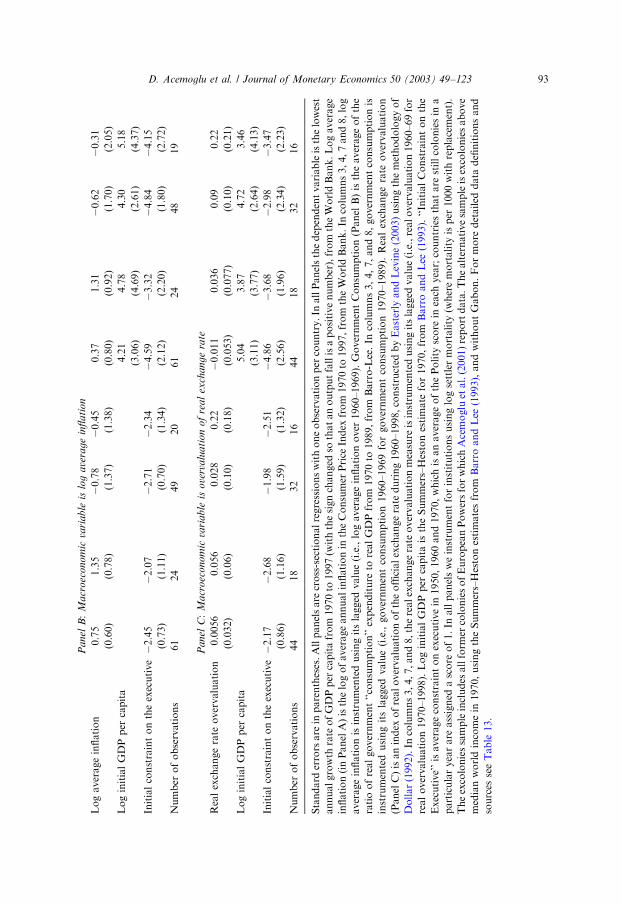
Pa

nel

B:

Ma

cro

eco

nom

icva

ria

ble

islo

ga

vera

ge

infl

ati

on

Logaverageinflation

0.75

1.35

�0.78

�0.45

0.37

1.31

�0.62

�0.31

(0.60)

(0.78)

(1.37)

(1.38)

(0.80)

(0.92)

(1.70)

(2.05)

LoginitialGDPper

capita

4.21

4.78

4.30

5.18

(3.06)

(4.69)

(2.61)

(4.37)


�2.45

�2.07

�2.71

�2.34

�4.59

�3.32

�4.84

�4.15

(0.73)

(1.11)

(0.70)

(1.34)

(2.12)

(2.20)

(1.80)

(2.72)

Number

ofobservations

61

24

49

20

61

24

48

19

Pa

nel

C:

Ma

cro

eco

no

mic

vari

ab

leis

ove

rva

lua

tio

no

fre

al

exch

an

ge

rate

Realexchangerate

overvaluation

0.0056

0.056

0.028

0.22

�0.011

0.036

0.09

0.22

(0.032)

(0.06)

(0.10)

(0.18)

(0.053)

(0.077)

(0.10)

(0.21)

LoginitialGDPper

capita

5.04

3.87

4.72

3.46

(3.11)

(3.77)

(2.64)

(4.13)


�2.17

�2.68

�1.98

�2.51

�4.86

�3.68

�2.98

�3.47

(0.86)

(1.16)

(1.59)

(1.32)

(2.56)

(1.96)

(2.34)

(2.23)

Number

ofobservations

44

18

32

16

44

18

32

16

Standard

errors

are

inparentheses.Allpanelsare


country.In

allPanelsthedependentvariableisthelowest

annualgrowth

rate

ofGDPper

capitafrom

1970to

1997(w

iththesignchanged

sothatanoutputfallisapositivenumber),from

theWorldBank.Logaverage

inflation(inPanelA)isthelogofaverageannualinflationin

theConsumer

Price

Index

from

1970to

1997,from

theWorldBank.In

columns3,4,7and8,log

averageinflationisinstrumentedusingitslagged


1960–1969).GovernmentConsumption(Panel

B)istheaverageofthe

ratioofrealgovernment‘‘consumption’’expenditure

torealGDPfrom

1970to

1989,from

Barro-Lee.In

columns3,4,7,and8,governmentconsumptionis


value(i.e.,governmentconsumption1960–1969forgovernmentconsumption1970–1989).Realexchangerate

overvaluation

(PanelC)isanindex



byEasterly

andLevine(2003)usingthemethodologyof

Dollar(1992).In

columns3,4,7,and8,therealexchangerate

overvaluationmeasure

isinstrumentedusingitslagged

value(i.e.,realovervaluation1960–69for

realovervaluation1970–1998).LoginitialGDPper


for1970,from

BarroandLee

(1993).‘‘InitialConstraintonthe

Executive’’isaverageconstraintonexecutivein


score

ineach


stillcoloniesin

a

particularyearare

assigned

ascore

of1.In


(wheremortality

isper

1000withreplacement).

Theexcoloniessampleincludes

allform


etal.(2001)reportdata.Thealternativesampleisexcoloniesabove

medianworldincomein


BarroandLee


detailed

data

definitionsand

sources

seeTable

13.


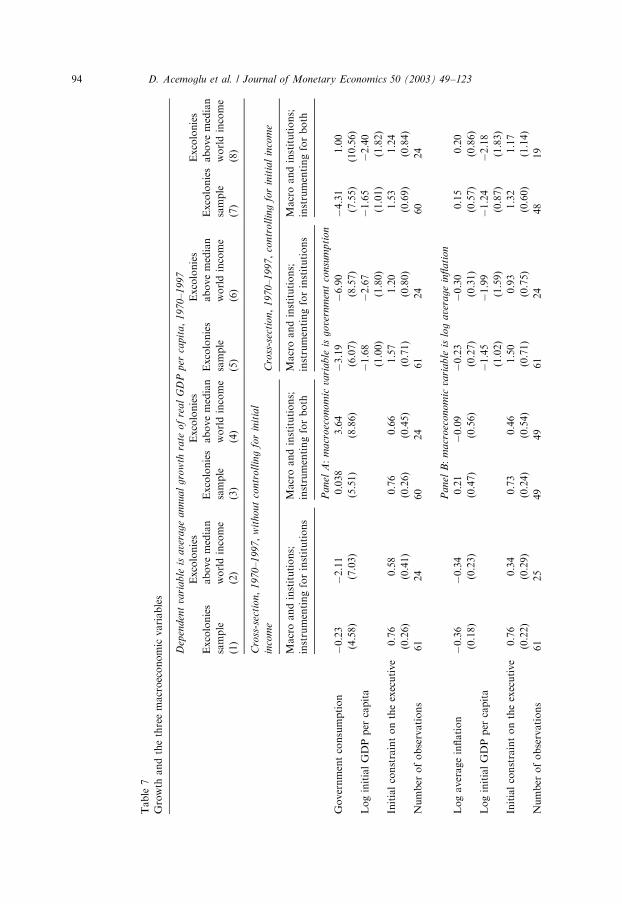
Table

7

Growth

andthethreemacroeconomic

variables

Dep

enden

tva

ria

ble

isa

vera

ge

an

nua

lg

row

thra

teo

fre

al

GD

Pp

erca

pit

a,

19

70–

19

97

Excolonies

Excolonies

Excolonies

Excolonies

Excolonies

abovemedian

Excolonies

abovemedian

Excolonies

abovemedian

Excoloniesabovemedian

sample

worldincome

sample

worldincome

sample

worldincome

sample

worldincome

(1)

(2)

(3)

(4)

(5)

(6)

(7)

(8)

Cro

ss-s

ecti

on,

19

70

–1

99

7,

wit

hou

tco

ntr

oll

ing

for

init

ial

inco

me

Cro

ss-s

ecti

on,

19

70–

19

97,

con

tro

llin

gfo

rin

itia

lin

com

e









Pa

nel

A:

ma

cro

eco

no

mic

vari

ab

leis

go

vern

men

tco

nsu

mp

tio

n


�0.23

�2.11

0.038

3.64

�3.19

�6.90

�4.31

1.00

(4.58)

(7.03)

(5.51)

(8.86)

(6.07)

(8.57)

(7.55)

(10.56)

LoginitialGDPper

capita

�1.68

�2.67

�1.65

�2.40

(1.00)

(1.80)

(1.01)

(1.82)


0.76

0.58

0.76

0.66

1.57

1.20

1.53

1.24

(0.26)

(0.41)

(0.26)

(0.45)

(0.71)

(0.80)

(0.69)

(0.84)

Number

ofobservations

61

24

60

24

61

24

60

24

Pa

nel

B:

ma

cro

eco

no

mic

vari

ab

leis

log

ave

rag

ein

flati

on

Logaverageinflation

�0.36

�0.34

0.21

�0.09

�0.23

�0.30

0.15

0.20

(0.18)

(0.23)

(0.47)

(0.56)

(0.27)

(0.31)

(0.57)

(0.86)

LoginitialGDPper

capita

�1.45

�1.99

�1.24

�2.18

(1.02)

(1.59)

(0.87)

(1.83)


0.76

0.34

0.73

0.46

1.50

0.93

1.32

1.17

(0.22)

(0.29)

(0.24)

(0.54)

(0.71)

(0.75)

(0.60)

(1.14)

Number

ofobservations

61

25

49

49

61

24

48

19


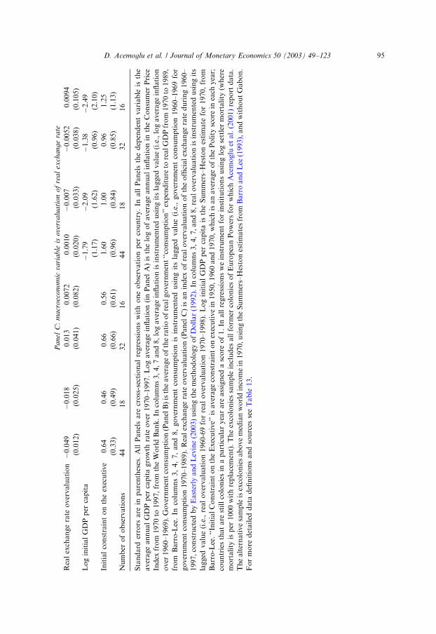
Pa

nel

C:

ma

cro

eco

no

mic

vari

ab

leis

ove

rvalu

ati

on

of

rea

lex

chan

ge

rate

Realexchangerate

overvaluation

�0.049

�0.018

0.013

0.0072

0.0010

�0.007

�0.0052

0.0094

(0.012)

(0.025)

(0.041)

(0.082)

(0.020)

(0.033)

(0.038)

(0.105)

LoginitialGDPper

capita

�1.79

�2.09

�1.38

�2.49

(1.17)

(1.62)

(0.96)

(2.10)


0.64

0.46

0.66

0.56

1.60

1.00

0.96

1.25

(0.33)

(0.49)

(0.66)

(0.61)

(0.96)

(0.84)

(0.85)

(1.13)

Number

ofobservations

44

18

32

16

44

18

32

16

Standard

errors

are

inparentheses.AllPanelsare


country.In

allPanelsthedependentvariable

isthe

averageannualGDPper

capitagrowth

rate

over

1970–1997.Logaverageinflation(inPanel

A)isthelogofaverageannualinflationin

theConsumer

Price

Index

from

1970to

1997,from

theWorldBank.In

columns3,4,7and8,logaverageinflationisinstrumentedusingitslagged

value(i.e.,logaverageinflation

over

1960–1969).Governmentconsumption(PanelB)istheaverageoftheratioofrealgovernment‘‘consumption’’expenditure

torealGDPfrom

1970to

1989,

from

Barro-Lee.In

columns3,4,7,and8,governmentconsumptionis


value(i.e.,governmentconsumption1960–1969for

governmentconsumption1970–1989).Realexchangerate

overvaluation(Panel

C)isanindex


during1960–

1997,constructed

byEasterly

andLevine(2003)usingthemethodologyofDollar(1992).In

columns3,4,7,and8,realovervaluationisinstrumentedusingits

lagged

value(i.e.,realovervaluation1960-69forrealovervaluation1970–1998).LoginitialGDPper


for1970,from

Barro-Lee.‘‘InitialConstraintontheExecutive’’isaverageconstraintonexecutivein


score

ineach

year;

countriesthatare

stillcoloniesin

aparticularyearare

assigned

ascore

of1.In

allregressionsweinstrumentforinstitutionsusinglogsettlermortality

(where

mortality

isper

1000withreplacement).Theexcoloniessampleincludes

allform


etal.(2001)reportdata.

Thealternativesampleisexcoloniesabovemedianworldincomein


BarroandLee

(1993),andwithoutGabon.

Formore

detailed

data


seeTable

13.


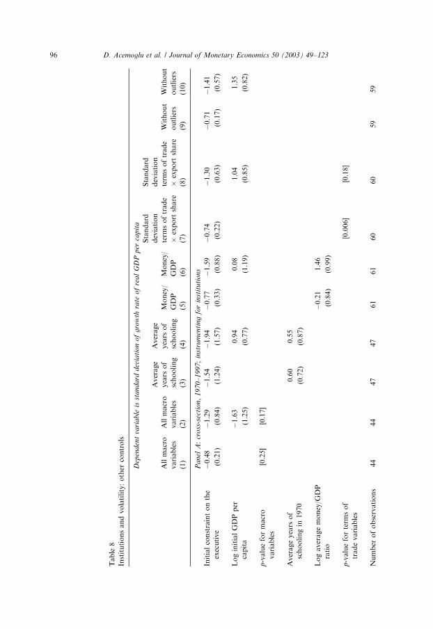
Table

8

Institutionsandvolatility:other

controls

Dep

end

ent

vari

ab

leis

sta

nd

ard

dev

iati

on

of

gro

wth

rate

of

rea

lG

DP

per

cap

ita

Allmacro

variables

Allmacro

variables

Average

years

of

schooling

Average

years

of

schooling

Money/

GDP

Money/

GDP

Standard

deviation

term

softrade

export

share

Standard

deviation

term

softrade

export

share

Without

outliers

Without

outliers

(1)

(2)

(3)

(4)

(5)

(6)

(7)

(8)

(9)

(10)

Pan

elA:

cro

ss-s

ecti

on,

19

70–

19

97;

inst

rum

enti

ng

for

inst

itu

tio

ns


executive

�0.48

�1.29

�1.54

�1.94

�0.77

�1.59

�0.74

�1.30

�0.71

�1.41

(0.21)

(0.84)

(1.24)

(1.57)

(0.33)

(0.88)

(0.22)

(0.63)

(0.17)

(0.57)

LoginitialGDPper

capita

�1.63

0.94

0.08

1.04

1.35

(1.25)

(0.77)

(1.19)

(0.85)

(0.82)

p-valueformacro

variables

[0.25]

[0.17]

Averageyears

of

schoolingin

1970

0.60

0.55

(0.72)

(0.87)

Logaveragemoney/G

DP

ratio

�0.21

1.46

(0.84)

(0.99)

p-valueforterm

sof

tradevariables

[0.006]

[0.18]

Number

ofobservations

44

44

47

47

61

61

60

60

59

59


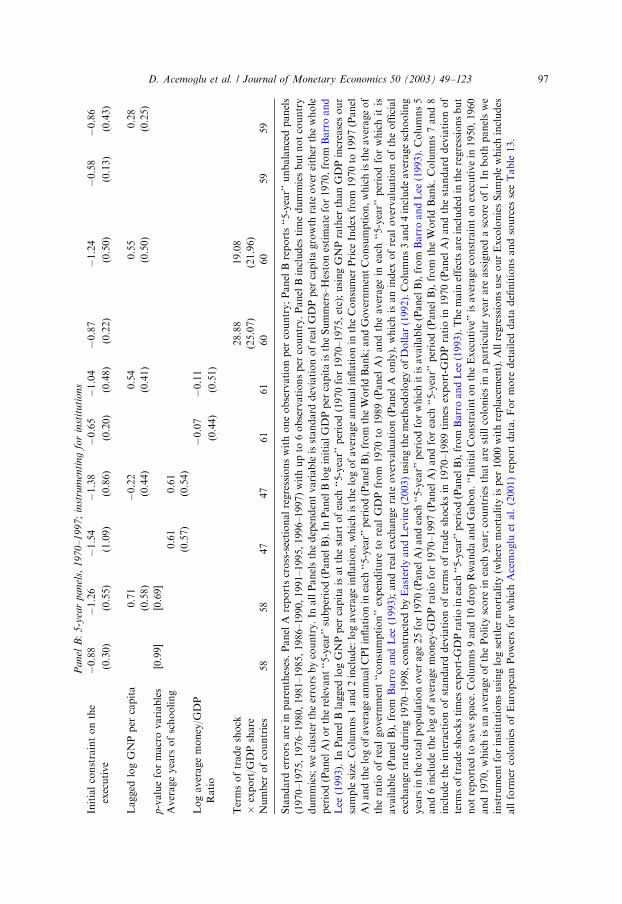
Pan

elB:

5-y

ear

pa

nel

s,1

97

0–

199

7;

inst

rum

enti

ng

for

inst

itu

tio

ns


executive

�0.88

�1.26

�1.54

�1.38

�0.65

�1.04

�0.87

�1.24

�0.58

�0.86

(0.30)

(0.55)

(1.09)

(0.86)

(0.20)

(0.48)

(0.22)

(0.50)

(0.13)

(0.43)

Lagged

logGNPper

capita

0.71

�0.22

0.54

0.55

0.28

(0.58)

(0.44)

(0.41)

(0.50)

(0.25)

p-valueformacrovariables

[0.99]

[0.69]

Averageyears

ofschooling

0.61

0.61

(0.57)

(0.54)

Logaveragemoney/G

DP

Ratio

�0.07

�0.11

(0.44)

(0.51)

Termsoftradeshock

28.88

19.08

export/G

DPshare

(25.07)

(21.96)

Number

ofcountries

58

58

47

47

61

61

60

60

59

59

Standard

errors

are

inparentheses.PanelA

reportscross-sectionalregressionswithoneobservationper

country;PanelBreports‘‘5-year’’unbalancedpanels

(1970–1975,1976–1980,1981–1985,1986–1990,1991–1995,1996–1997)withupto

6observationsper

country.PanelBincludes

timedummiesbutnotcountry

dummies;wecluster

theerrors

bycountry.In


deviationofrealGDPper

capitagrowth

rate

over

either

thewhole

period(PanelA)ortherelevant‘‘5-year’’subperiod(PanelB).In



for1970,from

Barroand

Lee

(1993).In

PanelBlagged

logGNPper

capitaisatthestart

ofeach


thanGDPincreasesour

samplesize.Columns1and2include:logaverageinflation,whichisthelogofaverageannualinflationin

theConsumer

Price

Index

from

1970to

1997(Panel

A)andthelogofaverageannualCPIinflationin

each

‘‘5-year’’period(PanelB),from

theWorldBank;andGovernmentConsumption,whichistheaverageof

theratioofrealgovernment‘‘consumption’’expenditure

torealGDPfrom

1970to

1989(Panel

A)andtheaveragein

each

‘‘5-year’’periodforwhichitis

available

(Panel

B),from

BarroandLee

(1993);andrealexchangerate

overvaluation(Panel

Aonly),whichisanindex

ofrealovervaluationoftheofficial

exchangerateduring1970–1998,constructed

byEasterly

andLevine(2003)usingthemethodologyofDollar(1992).Columns3and4includeaverageschooling

years

inthetotalpopulationover

age25for1970(PanelA)andeach

‘‘5-year’’periodforwhichitisavailable(PanelB),from

BarroandLee

(1993).Columns5

and6includethelogofaveragemoney-G

DPratiofor1970–1997(Panel

A)andforeach

‘‘5-year’’period(Panel

B),from

theWorldBank.Columns7and8

includetheinteractionofstandard

deviationofterm

softradeshocksin

1970–1989times

export-G

DPratioin

1970(Panel

A)andthestandard

deviationof

term

softradeshockstimes

export-G

DPratioin

each

‘‘5-year’’period(PanelB),from

BarroandLee

(1993).Themain

effectsare

included

intheregressionsbut

notreported

tosavespace.Columns9and10dropRwandaandGabon.‘‘InitialConstraintontheExecutive’’isaverageconstraintonexecutivein

1950,1960

and1970,whichisanaverageofthePolity

score

ineach


stillcoloniesin

aparticularyearare

assigned

ascore

ofl.In

both

panelswe


(wheremortality

isper

1000withreplacement).Allregressionsuse

ourExcoloniesSamplewhichincludes

allform


etal.(2001)report

data.Formore

detailed

data


seeTable

13.


run regressions for the 5-year panel, the human capital variable continues to beinsignificant, but now the initial constraint on the executive is significant at the 10percent level, with a similar coefficient to that found in Table 2. These results suggestthat the effect of initial constraint on the executive is not working through aneducational channel.

In columns 5 and 6 we add (log of) the ratio of real M2 to GDP as a measure ofthe importance of financial intermediation (see Easterly et al., 2000, for the use ofthis variable in this context). Many macroeconomists emphasize weak financialintermediation as a primary cause of economic volatility. Again we find no strongevidence supporting this claim. The financial intermediation variables are notsignificant, and initial constraint on the executive is significant in most specifica-tions.24

In columns 7 and 8, we control for other determinants of variability, includingterms of trade variability, the export share of the GDP, and the interaction betweenthese two variables. In columns 9 and 10 we also exclude some outliers. The resultsare very similar to our baseline results, showing that the effect of the historicallydetermined component of institutions on volatility is robust, and is not simply drivenby some other sources of output variability correlated with institutions.25

Table 9 further checks the robustness of our results in two ways: with additionalcontrol variables and by restricting the sample. Panel A adds additional controlvariables. La Porta et al. (1998) have argued for the importance of investorprotection, and Johnson et al. (2000) found that investor protection measures weresignificantly correlated with exchange rate depreciations and stock market declinesacross emerging markets in 1997–1998. In columns 1 and 2, we add the measure of dejure shareholders’ rights from La Porta et al. (1998).26 These de jure measures do notappear to be related to volatility (although the sample size is now quite small), whilethe coefficient on initial constraint on the executive is essentially the same as in Table2. Columns 3 and 4 show similar results for de jure creditors’ rights. The results aresimilar, but now when we also include log initial GDP per capita (column 4), thecoefficient on initial constraint on the executive is no longer significant at the 5percent level. Clearly investor protection and creditors’ rights are closely linked tooverall property rights enforcement and constraint on the executive. Nevertheless,they capture only one dimension of ‘‘institutional’’ differences, which we believe aremuch broader, and include various other aspects of the organization of society.

24This is consistent with the results in Johnson et al. (2002), who, in a different context, also find that

property rights appear to matter more than the availability of external finance.25We have also run the regressions as in Table 8 using a different measure of institutions, average

protection against expropriation risk, which was our main variable in Acemoglu et al. (2001). This variable

refers to a later period and hence is not ideal for our purposes here. However, as we are instrumenting for

institutions with historical variables, this may not matter too much. In any case, the results with this

alternative specification are very similar to those in Table 8, and show a robust effect of institutions on

volatility.26We refer to these as ‘‘de jure’’ measures, since these measures do not take into account how well these

legislated rights are enforced. Note also that these measures are only available for countries that are

relatively open to capital flows. For example, we do not have this information for many African countries.


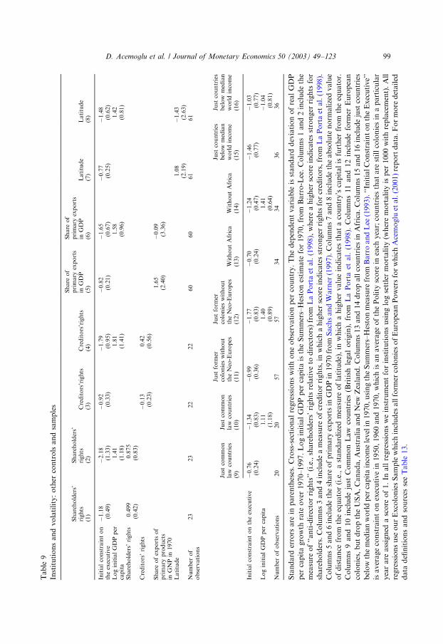
Table

9

Institutionsandvolatility:other

controlsandsamples

Share

of

Share

of

Shareholders’

Shareholders’

primary

exports

primary

exports

rights

rights

Creditors’rights

Creditors’rights

inGDP

inGDP

Latitude

Latitude

(1)

(2)

(3)

(4)

(5)

(6)

(7)

(8)

Initialconstrainton

theexecutive

�1.18

�2.18

�0.92

�1.79

�0.82

�1.65

�0.77

�1.48

(0.49)

(1.33)

(0.33)

(0.95)

(0.21)

(0.67)

(0.25)

(0.62)

LoginitialGDPper

capita

1.41

1.81

1.58

1.42

(1.18)

(1.41)

(0.96)

(0.81)

Shareholders’rights

0.499

0.875

(0.42)

(0.83)

Creditors’rights

�0.13

0.42

(0.23)

(0.56)

Share

ofexportsof

primary

products

1.65

�0.09

inGNPin

1970

(2.40)

(3.36)

Latitude

1.08

�1.43

(2.19)

(2.63)

Number

of

observations

23

23

22

22

60

60

61

61

Just

form

erJust

form

erJust

countries

Just

countries

Just

common

Just

common

colonieswithout

colonieswithout

below

median

below

median

law

countries

law

countries

theNeo-Europes

theNeo-Europes

WithoutAfrica

WithoutAfrica

worldincome

worldincome

(9)

(10)

(11)

(12)

(13)

(14)

(15)

(16)


�0.76

�1.34

�0.99

�1.77

�0.70

�1.24

�1.46

�1.03

(0.24)

(0.83)

(0.36)

(0.83)

(0.24)

(0.47)

(0.77)

(0.77)

LoginitialGDPper

capita

1.11

1.40

1.41

�1.04

(1.18)

(0.89)

(0.64)

(0.81)

Number

ofobservations

20

20

57

57

34

34

36

36

Standard

errors

are

inparentheses.Cross-sectionalregressionswithoneobservationper

country.Thedependentvariable

isstandard

deviationofrealGDP

per

capitagrowth

rate

over

1970–1997.LoginitialGDPper


for1970,from

Barro-Lee.Columns1and2includethe

measure

of‘‘anti-directorrights’’(i.e.,shareholders’rights

relativeto

directors)from

LaPortaet

al.(1998),whereahigher

score

indicatesstronger

rights

for

shareholders.Columns3and4includeameasure

ofcreditorrights,in

whichahigher

score

indicatesstronger

rightsforcreditors,from

LaPortaet

al.(1998).

Columns5and6includetheshare

ofprimary

exportsin

GDPin

1970from

SachsandWarner

(1997).Columns7and8includetheabsolute

norm

alizedvalue

ofdistance

from

theequator(i.e.,astandardized

measure

oflatitude),in

whichahigher

valueindicatesthatacountry’scapitalisfurther

from

theequator.

Columns9and10includejust

CommonLaw

countries(British

legalorigin),from

LaPortaet

al.(1998).Columns11and12includeform

erEuropean

colonies,butdroptheUSA,Canada,AustraliaandNew

Zealand.Columns13and14dropallcountriesin

Africa.Columns15and16includejustcountries

belowthemedianworldper

capitaincomelevelin

1970,usingtheSummers–Hestonmeasure

from

BarroandLee

(1993).‘‘InitialConstraintontheExecutive’’

isaverageconstraintonexecutivein


score

ineach


stillcoloniesin

aparticular

yearare

assigned

ascore

of1.In


(wheremortality

isper

1000withreplacement).All

regressionsuse

ourExcoloniesSamplewhichincludes

allform


etal.(2001)reportdata.Formore

detailed

data


seeTable

13.


These results therefore suggest that what is important for volatility (and moregenerally, for economic performance) is not simply de jure investor or creditorprotection, but a broader range of institutions, including property rights protectionfor a broader cross-section of society, constraints on politicians and elites,arrangements to manage social divisions and ensure political stability, and the ‘‘rulele of law’’, which determine whether these de jure rights are enforced.27

Columns 5 and 6 add the share of primary exports in GDP, a basic measure ofopenness and exposure to shocks, from Sachs and Warner (1997). This variable alsohas little effect on our main results. Similarly, including latitude, as a common proxyfor geographic influences on economic outcomes, has little impact on initialconstraint on the executive, and latitude itself is insignificant (see columns 7 and 8).

Panel B further checks our results by limiting the sample of countries underconsideration. Columns 9 and 10 report regressions using only Common Lawcountries, i.e., those that inherited or adopted a legal system based on Britishcommon law (see La Porta et al., 1998). Columns 11 and 12 run the regressions justfor former colonies, and drop the ‘‘Neo-Europes’’ (USA, Canada, Australia andNew Zealand). The results for these various subsamples are similar to our baselineresults.

One concern with our basic results is whether they simply reflect very large crisesand volatility in African or other poor nations which also have weak institutions. Ifthis were the case, one might think that institutions matter for differences involatility between poor (African) and rich (non-African) nations, but have less effecton volatility among richer (non-African) nations. The results so far show that thereis a strong relationship between the historically-determined component ofinstitutions and volatility even among nations above median world income (seeTables 1–7). Moreover, Table 1 showed that even excluding Africa, there is astatistical relationship between the historically determined component of institutionsand the level of income or economic growth. To investigate this issue further in thecontext of volatility, columns 13 and 14 drop all the African countries. Thecoefficient on initial constraint on the executive remains significant and similar in sizeto our baseline result in Table 3. This, together with the results reported so far,suggests that our results are not driven simply by the contrast between poor and richnations, and institutional differences even among relatively rich nations matter forvolatility. Finally, columns 15 and 16 report results just for countries below themedian world per capita income level, where we find a similar relationship,suggesting that the link between institutions and volatility is there both amongrelatively poor and relatively rich nations.

Another dimension of robustness is whether the relationship between institutionsand instability is being driven by events in some specific decades. To investigate thisissue, Table 10 looks at the relationship between our measure of institutions (whichrefers to the average constraint on the executive in 1950, 1960 and 1970), and the

27La Porta et al. (1998) also suggest that effective investor protection must be enforced through courts

or regulation, and Johnson et al. (2000) find significant effects for the rule of law both directly and in

interaction with de jure investor protection measures.


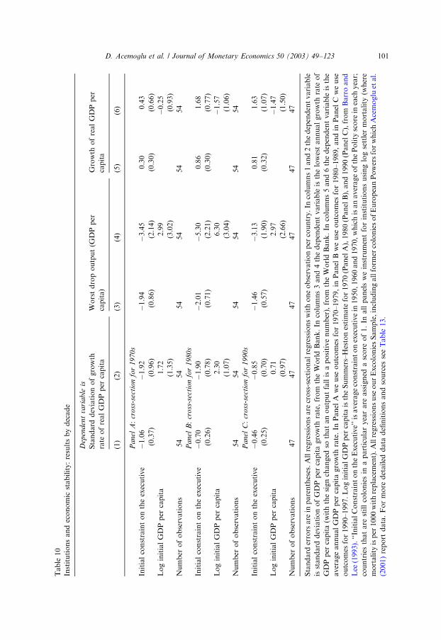
Table

10

Institutionsandeconomic

stability:resultsbydecade

Dep

enden

tva

ria

ble

is

Standard

deviationofgrowth

Worstdropoutput(G

DPper

Growth

ofrealGDPper

rate

ofrealGDPper

capita

capita)

capita

(1)

(2)

(3)

(4)

(5)

(6)

Pa

nel

A:

cro

ss-s

ecti

on

for

19

70s


�1.06

�1.92

�1.94

�3.45

0.30

0.43

(0.37)

(0.96)

(0.86)

(2.14)

(0.30)

(0.66)

LoginitialGDPper

capita

1.72

2.99

�0.25

(1.35)

(3.02)

(0.93)

Number

ofobservations

54

54

54

54

54

54

Pa

nel

B:

cro

ss-s

ecti

on

for

19

80s


�0.70

�1.90

�2.01

�5.30

0.86

1.68

(0.26)

(0.78)

(0.71)

(2.21)

(0.30)

(0.77)

LoginitialGDPper

capita

2.30

6.30

�1.57

(1.07)

(3.04)

(1.06)

Number

ofobservations

54

54

54

54

54

54

Pa

nel

C:

cro

ss-s

ecti

on

for

19

90s


�0.46

�0.85

�1.46

�3.13

0.81

1.63

(0.25)

(0.70)

(0.57)

(1.90)

(0.32)

(1.07)

LoginitialGDPper

capita

0.71

2.97

�1.47

(0.97)

(2.66)

(1.50)

Number

ofobservations

47

47

47

47

47

47

Standard

errors

are



country.In

columns1and2thedependentvariable

isstandard

deviationofGDPper

capitagrowth

rate,from

theWorldBank.In


isthelowestannualgrowth

rate

of

GDPper

capita(w

iththesignchanged


theWorldBank.In


isthe

averageannualGDPper

capitagrowth

rate.In

Panel

Aweuse

outcomes

for1970–1979,in

Panel

Bweuse

outcomes

for1980–1989,andin

Panel

Cweuse

outcomes

for1990–1997.LoginitialGDPper


for1970(PanelA),1980(PanelB),and1990(PanelC),from

Barroand

Lee

(1993).‘‘InitialConstraintontheExecutive’’isaverageconstraintonexecutivein


score

ineach

year;

countriesthatare

stillcoloniesin

aparticularyearare

assigned

ascore

of1.In


(where

mortality

isper


ourExcoloniesSample,includingallform


etal.

(2001)report

data.Formore

detailed

data


seeTable

13.


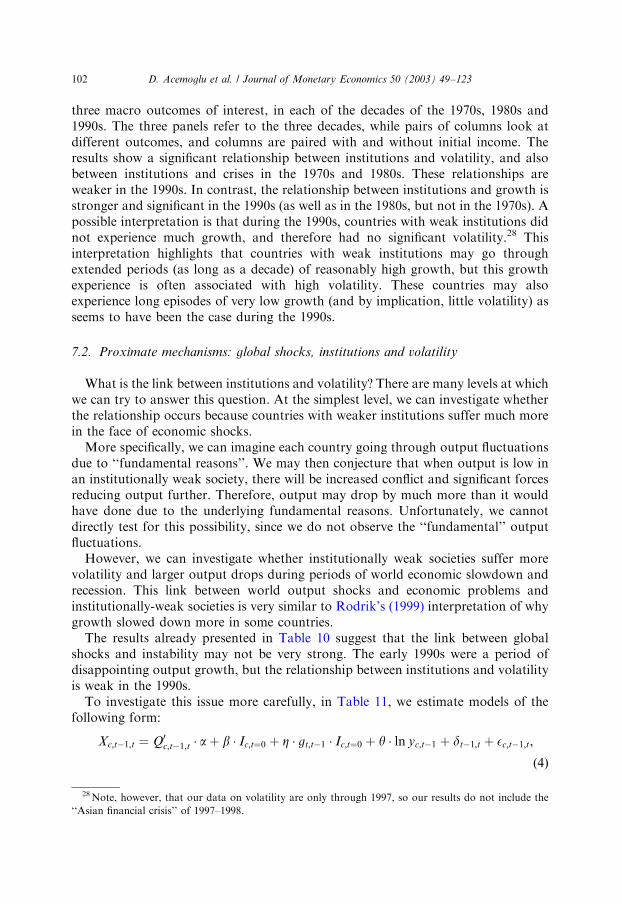
three macro outcomes of interest, in each of the decades of the 1970s, 1980s and1990s. The three panels refer to the three decades, while pairs of columns look atdifferent outcomes, and columns are paired with and without initial income. Theresults show a significant relationship between institutions and volatility, and alsobetween institutions and crises in the 1970s and 1980s. These relationships areweaker in the 1990s. In contrast, the relationship between institutions and growth isstronger and significant in the 1990s (as well as in the 1980s, but not in the 1970s). Apossible interpretation is that during the 1990s, countries with weak institutions didnot experience much growth, and therefore had no significant volatility.28 Thisinterpretation highlights that countries with weak institutions may go throughextended periods (as long as a decade) of reasonably high growth, but this growthexperience is often associated with high volatility. These countries may alsoexperience long episodes of very low growth (and by implication, little volatility) asseems to have been the case during the 1990s.

7.2. Proximate mechanisms: global shocks, institutions and volatility

What is the link between institutions and volatility? There are many levels at whichwe can try to answer this question. At the simplest level, we can investigate whetherthe relationship occurs because countries with weaker institutions suffer much morein the face of economic shocks.

More specifically, we can imagine each country going through output fluctuationsdue to ‘‘fundamental reasons’’. We may then conjecture that when output is low inan institutionally weak society, there will be increased conflict and significant forcesreducing output further. Therefore, output may drop by much more than it wouldhave done due to the underlying fundamental reasons. Unfortunately, we cannotdirectly test for this possibility, since we do not observe the ‘‘fundamental’’ outputfluctuations.

However, we can investigate whether institutionally weak societies suffer morevolatility and larger output drops during periods of world economic slowdown andrecession. This link between world output shocks and economic problems andinstitutionally-weak societies is very similar to Rodrik’s (1999) interpretation of whygrowth slowed down more in some countries.

The results already presented in Table 10 suggest that the link between globalshocks and instability may not be very strong. The early 1990s were a period ofdisappointing output growth, but the relationship between institutions and volatilityis weak in the 1990s.

To investigate this issue more carefully, in Table 11, we estimate models of thefollowing form:

Xc;t�1;t ¼ Q0c;t�1;t � aþ b � Ic;t¼0 þ Z � gt;t�1 � Ic;t¼0 þ y � ln yc;t�1 þ dt�1;t þ Ec;t�1;t;

ð4Þ

28Note, however, that our data on volatility are only through 1997, so our results do not include the

‘‘Asian financial crisis’’ of 1997–1998.


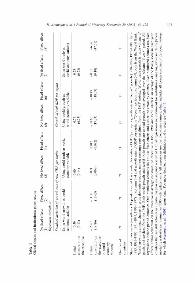
Table

11

Globalshocksandinstitutions:panel

results

Nofixed

effects

Fixed

effects

Nofixed

effects

Fixed

effects

Nofixed

effects

Fixed

effects

Nofixed

effects

Fixed

effects

(1)

(2)

(3)

(4)

(5)

(6)

(7)

(8)

Dep

enden

tva

ria

ble

is:

Sta

nd

ard

dev

iati

on

of

gro

wth

rate

of

rea

lG

DP

per

cap

ita

Gro

wth

of

rea

lG

DP

per

capit

a

Usingworldgrowth

asworld

Usingworldtradeasworld

Usingworldgrowth

as

Usingworldtradeas

economyvariable

economyvariable

worldeconomyvariable

worldeconomyvariable

Initial

constrainton

theexecutive

�0.59

�0.60

0.74

0.73

(0.13)

(0.14)

(0.23)

(0.23)

Initial

constrainton

theexecutive

�15.67

�11.11

0.021

0.012

�38.66

�40.19

�0.01

�6.36

world

economy

variable

(19.86)

(18.63)

(0.067)

(0.092)

(17.34)

(18.79)

(0.10)

(47.51)

Number

of

countries

71

71

71

71

71

71

71

71

Standard

errors

are

inparentheses.Dependentvariableisstandard

deviationofGDPper

capitagrowth

rate

in‘‘5-year’’periods(1970–1975,1976–1980,1981–

1985,1986–1990,1991–1995,1996–1997)in

columns1–4andgrowth

ratesofGDPper

capitain

‘‘5-year’’periodsin

columns5–8,both

from

theWorldBank.

Worldgrowth

isannualchangein

gross

domesticproduct,market

exchangerate

weighted,from

theIM

Fwebsite.Worldtradegrowth

istradevolumeof

goodsandservices,from

theIM

F.Both

worldgrowth

andworldtradegrowth

are

annualgrowth

ratesaveraged

over

therelevant‘‘5-year’’period.All

regressionsincludeperioddummies.

Oddnumbered

columnsdonotuse

fixed

effectsandcluster

theerrors

bycountry.Even

numbered

columnsuse

fixed

effects.

Initialconstraintontheexecutiveis


1950,1960and1970,whichis

anaverageofthePolity

score

ineach

year;

countriesthatare

stillcoloniesin

aparticularyearare

assigned

ascore

of1.In


(where

mortality

isdeathsper

annum

per


ourExcoloniesSample,whichincludes

allform

ercoloniesofEuropeanPowers

forwhichAcemoglu

etal.(2001)report

data.Formore

detailed

data


seeTable

13.


where all the variables are defined as before, and in particular, Xc;t�1;t refers to macrooutcomes between time t � 1 and t; and here time periods are taken to be five-yearperiods. The dt�1;t terms denote time effects, and Ic;t¼0 is our measure of initialinstitutions.

The variable of interest here is the interaction term between the world growth rate,gt;t�1; and country institutions. A significant effect from these interaction termswould indicate that institutionally weak societies have a greater propensity toexperience macro-economic problems (high volatility or low growth) during periodsof slow world growth. As before we instrument for institutions, Ic;t¼0; using ourhistorical instruments, and now we also instrument for the interaction betweeninstitutions and world aggregates, the gt;t�1 � Ic;t¼0 terms, using interactions betweenworld aggregates and our instruments. The variables are de-meaned, so the maineffect of institutions in this regression is evaluated at the mean value of the sample.We also cluster the standard errors by country.

As an alternative specification we estimate:

Xc;t�1;t ¼ Q0c;t�1;t � aþ Z � gt;t�1 � Ic;t¼0 þ y � ln yc;t�1 þ dc þ dt�1;t þ ec;t�1;t; ð5Þ

which replaces the main effect of institutions by a full set of country dummies.Table 11 focuses on two global variables: the growth rate of world output

and of world trade. The results show no evidence that there is a significantinteraction term indicating greater propensity of institutionally weak societiesto run into crises during periods of world economic slowdown (or expansion)or greater growth of world trade. The interaction terms are usually insignificantwhen the dependent variable is volatility of output. In contrast, in columns 5 and 6where the dependent variable is country growth, we find significant interactionsbetween world growth and initial institutions. This suggests that when the worldeconomy slows down, institutionally weak societies slow down more than others.But these growth effects do not translate into greater volatility for theseinstitutionally weak societies during periods of world economic slowdown (columns1, 2, 3 and 4).

We conclude that the proximate mechanism for the relationship betweeninstitutions and volatility is not primarily the propensity of institutionally-weaksocieties to run into crises during periods of world recession or other major globalevents. Instead it is likely that it is the inability of institutionally weak societies todeal with their own idiosyncratic economic and most likely political problems thatunderlies their economic instability. In the next subsection, we briefly look at apotential mechanism along these lines.

7.3. State failures and volatility

This subsection provides a preliminary investigation of whether political crisescould be a mediating mechanism for the impact of weak institutions on economicvolatility, as suggested by some of the theoretical ideas in subsection subsection 3.1.We believe that the link between political crises (state failures) and economicinstability is important to understand the relationship between institutions and


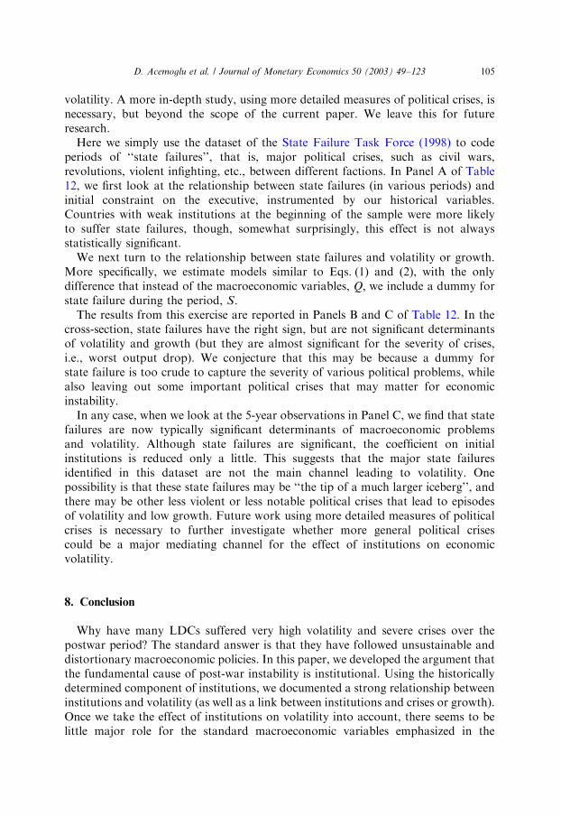
volatility. A more in-depth study, using more detailed measures of political crises, isnecessary, but beyond the scope of the current paper. We leave this for futureresearch.

Here we simply use the dataset of the State Failure Task Force (1998) to codeperiods of ‘‘state failures’’, that is, major political crises, such as civil wars,revolutions, violent infighting, etc., between different factions. In Panel A of Table12, we first look at the relationship between state failures (in various periods) andinitial constraint on the executive, instrumented by our historical variables.Countries with weak institutions at the beginning of the sample were more likelyto suffer state failures, though, somewhat surprisingly, this effect is not alwaysstatistically significant.

We next turn to the relationship between state failures and volatility or growth.More specifically, we estimate models similar to Eqs. (1) and (2), with the onlydifference that instead of the macroeconomic variables, Q; we include a dummy forstate failure during the period, S:

The results from this exercise are reported in Panels B and C of Table 12. In thecross-section, state failures have the right sign, but are not significant determinantsof volatility and growth (but they are almost significant for the severity of crises,i.e., worst output drop). We conjecture that this may be because a dummy forstate failure is too crude to capture the severity of various political problems, whilealso leaving out some important political crises that may matter for economicinstability.

In any case, when we look at the 5-year observations in Panel C, we find that statefailures are now typically significant determinants of macroeconomic problemsand volatility. Although state failures are significant, the coefficient on initialinstitutions is reduced only a little. This suggests that the major state failuresidentified in this dataset are not the main channel leading to volatility. Onepossibility is that these state failures may be ‘‘the tip of a much larger iceberg’’, andthere may be other less violent or less notable political crises that lead to episodesof volatility and low growth. Future work using more detailed measures of politicalcrises is necessary to further investigate whether more general political crisescould be a major mediating channel for the effect of institutions on economicvolatility.

8. Conclusion

Why have many LDCs suffered very high volatility and severe crises over thepostwar period? The standard answer is that they have followed unsustainable anddistortionary macroeconomic policies. In this paper, we developed the argument thatthe fundamental cause of post-war instability is institutional. Using the historicallydetermined component of institutions, we documented a strong relationship betweeninstitutions and volatility (as well as a link between institutions and crises or growth).Once we take the effect of institutions on volatility into account, there seems to belittle major role for the standard macroeconomic variables emphasized in the


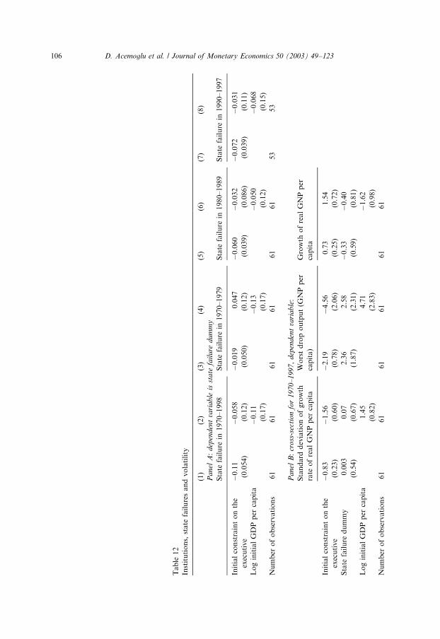
Table

12

Institutions,state

failuresandvolatility

(1)

(2)

(3)

(4)

(5)

(6)

(7)

(8)

Pa

nel

A:

dep

enden

tva

ria

ble

isst

ate

fail

ure

du

mm

y

State

failure

in1970–1998

State

failure

in1970–1979

State

failure

in1980–1989

State

failure

in1990–1997


executive

�0.11

�0.058

�0.019

0.047

�0.060

�0.032

�0.072

�0.031

(0.054)

(0.12)

(0.050)

(0.12)

(0.039)

(0.086)

(0.039)

(0.11)

LoginitialGDPper

capita

�0.11

�0.13

�0.050

�0.068

(0.17)

(0.17)

(0.12)

(0.15)

Number

ofobservations

61

61

61

61

61

61

53

53

Pa

nel

B:

cro

ss-s

ecti

on

for

19

70

–1

99

7,

dep

enden

tva

ria

ble:

Standard

deviationofgrowth

Worstdropoutput(G

NPper

Growth

ofrealGNPper

rate

ofrealGNPper

capita

capita)

capita


executive

�0.83

�1.56

�2.19

�4.56

0.73

1.54

(0.23)

(0.60)

(0.78)

(2.06)

(0.25)

(0.72)

State

failure

dummy

0.003

0.07

2.36

2.58

�0.33

�0.40

(0.54)

(0.67)

(1.87)

(2.31)

(0.59)

(0.81)

LoginitialGDPper

capita

1.45

4.71

�1.62

(0.82)

(2.83)

(0.98)

Number

ofobservations

61

61

61

61

61

61


Pa

nel

C:

5-y

ear

pa

nel

sfo

r1

97

0–

19

97,

dep

enden

tva

ria

ble:

Standard

deviationofgrowth

Worstdropoutput(G

NPper

Growth

ofrealGNPper

rate

ofrealGNPper

capita

capita)

capita


executive

�0.60

�1.06

�1.27

�2.32

0.66

1.05

(0.14)

(0.41)

(0.34)

(0.81)

(0.23)

(0.41)

State

failure

dummy

1.24

1.25

3.88

3.89

�2.28

�2.28

(0.70)

(0.73)

(1.20)

(1.33)

(0.63)

(0.67)

Lagged

logGNPper

capita

0.60

1.38

�0.51

(0.40)

(0.78)

(0.40)

Number

ofcountries

61

61

61

61

61

61

Standard

errors

are


andBare


country.Panel

Cis‘‘5-year’’unbalancedpanels

(1970–1975,1976–1980,1981–1985,1986–1990,1991–1995,1996–1997)withupto

6observationsper

country.PanelCincludes

timedummiesbutnotcountry

dummies;wecluster

theerrors

bycountry.In

PanelA

thedependentvariableisadummyvariableequalto

oneifthecountryexperience

a‘‘State

failure’’,i.e.,a

civilwar,breakdownofsocialorder,majorethnicconflictormajorregim

etransitionasdefined

bytheState

failure

project.ForPanelA,thedummyequalsone

iftherewasastate

failure

in1970–1998(columns1and2),in

1970–1979(columns3and4),in

1980–1989(columns5and6),andin

1990–1997(columns7and

8).In

PanelsBandC,columns1and2,thedependentvariable

isstandard

deviationofGDPper

capitagrowth

rate

in1970–1997(Panel

B)andin

each

‘‘5-

year’’period(PanelC),from

theWorldBank.In

PanelsBandC,columns3and4,thedependentvariableisthelowestannualgrowth

rate

ofGDPper

capita

(withthesignchanged

sothatanoutputfallisapositivenumber)in

1970–1997(PanelB)andeach

‘‘5-year’’period(PanelC),from

theWorldBank.In

Panels

BandC,columns5and6,thedependentvariableistheaverageannualGDPper

capitagrowth

rate

in1970–1997(PanelB)andeach

‘‘5-year’’period(PanelC).

LoginitialGDPper


for1970(PanelsA

andB),from

BarroandLee

(1993).In

PanelClagged

logGNPper

capitaisat

thestart

ofeach






score

ineach


stillcoloniesin

aparticularyear

are

assigned

ascore

of1.In

both

panelsweinstrumentforinstitutionsusinglogsettlermortality

(wheremortality

isper

1000withreplacement).Allregressions

use

ourexcoloniessample

whichincludes

allform

ercoloniesofEuropeanpowersforwhichAcemoglu

etal.(2001)report

data.Formore

detailed

data


seeTable

13.


literature and by the Washington consensus. The only ‘‘macro’’ variable whichappears to play an important mediating role is overvaluation of the realexchange rate, which is consistent with our discussion of the Ghanaian case,where real overvaluation was used as a method of expropropriation or re-distribution.

Overall, we interpret our findings as suggesting that the major causes of thelarge cross-country differences in volatility are institutional, and none of thestandard macroeconomic variables appear to be the primary mediating channelsthrough which institutional causes lead to economic instability. These macro-economic problems, just like the volatility and the disappointing macroeconomicperformance suffered by these countries, are symptoms of deeper institutionalcauses.

This perspective does not suggest that macroeconomic policies do not matter. Thepoint we believe and want to emphasize is that there are deeper institutional causesleading to economic instability, and these institutional causes lead to badmacroeconomic outcomes via a variety of mediating channels. Distortionarymacroeconomic policies are part of these channels, or in other words, they arepart of the ‘‘tools’’ that groups in power use in order to enrich themselves and toremain in power. But they are only one of many possible tools, and a variety ofcomplex factors, which we do not currently understand, determine which of thesetools get used in various circumstances. An interesting possibility implied by thisperspective is a seesaw effect: preventing the use of a specific macro distortion willnot necessarily cure the economic instability problems, since underlying institutionalproblems may manifest themselves in the use of some other tools by politicians andelites to achieve their objectives.

Our results also did not specifically pinpoint the exact mechanism via whichinstitutional weaknesses translate into economic instability. They are consistentwith the notion that political crises (‘‘state failures’’) may be important, but ourevidence here is more circumstantial. More research on these issues is clearlynecessary.


Table

13

Variable


Variable

Description

Source

LogGDPper

capita(PPP)in

1995

Logarithm

ofGDPper

capita,onpurchasing

power

parity

basis,in

1995.

WorldBank,WorldDevelopmentIndicators,

CD-R

om,1999.Data

onSurinameis

from

the2000versionofthissamesource.

LogGDPper

capitain

1970

Logarithm

ofrealGDPper

capita(1980

internationalprices)

from

Summers–Heston

datasetv.4.0.

Barro-Lee

dataset,usedin

BarroandLee

(1993)andavailable

from

theNBER

website:

www.nber.org.

LogGDPper

capitain

1980

Logarithm

ofrealGDPper

capita(1985


from

Summers–Heston

datasetv.5.5.

Barro-Lee

dataset.

LogGDPper

capitain

1990

Logarithm

ofrealGDPper

capita(1985


from

Summers–Heston

datasetv.5.5.

Barro-Lee

dataset.

Growth

rate

ofGDPper

capita,1970–1998

AnnualGDPgrowth

rate

minusannual

populationgrowth

rate.


CD-R

om,1999.

Standard

deviationofgrowth

Standard

deviationofGDPper

capitagrowth

rate.

Calculatedfrom

thegrowth

rate

ofGDPper

capita.From

theWorldBank,World

DevelopmentIndicators,CD-R

om,1999.

Worstoutputdrop

WorstannualGDPper

capitagrowth

rate.Sign

hasbeenchanged

sothatanegativegrowth

rate

is

apositive‘‘outputdrop’’.

Calculatedfrom

theGrowth

Rate

ofGDPper

capita.From

theWorldBank,World

DevelopmentIndicators,CD-R

om,1999.

Appen

dix

Variabledefinitionsandsources,Descriptivestatistics,Volatility

institutionsin

1970,worstoutputperform

ance

andgrowth

institutionsin

1970are

given

inTables13–17.


http://www.nber.org

LogGNPper

capita,1970,1975,1980,1985,1990,

1995

Logarithm

ofGNPper

capita


CD-R

om,1999.Data

onSurinameis

from

the2000versionofthissamesource.

Constraintonexecutivein

1950,1960,1970,1990

andinterveningyears.

Aseven

category

scale,from

1to

7,withahigher

score

indicatingmore

constraints.Score

of1

indicatesunlimited

authority;score

of3indicates

slightto

moderate

limitations;score

of5indicates

substantiallimitations;score

of7indicates

executiveparity

orsubordination.Scoresof2,4,

and6indicate

interm

ediate

values.

Polity

IVdataset,downloaded

from

Inter-

University

Consortium

forPoliticalandSocial

Research.Variable

described

inGurr,1997.

Averageprotectionagainst

expropriationrisk,

1985–1995

Riskofexpropriationofprivate

foreigninvestm

ent

bygovernment,from

0to

10,whereahigher

score

meansless

risk.Wecalculatedthemeanvaluefor

thescoresin

allyears

from

1985to

1995.

Datasetobtained

directlyfrom

politicalrisk

services,September

1999.Thesedata

were

previouslyusedbyKnack

andKeefer(1995)

andwereorganized

inelectronic

form

bythe

IRIS

Center(U

niversity

ofMaryland).The

originalcompilersofthisdata

are

Political

RiskServices.

Logaverageinflation

Logofaverageannualinflationin

theconsumer

price

index

from

1970to

1998.


CD-R

om,1999.


Averageoftheratioofrealgovernment

‘‘consumption’’expenditure

torealGDPfrom

1970to

1989.

Barro-Lee

dataset.

Realexchangerate

overvaluation

Anindex


exchangerate

in1960–1997.

Easterly

andLevine(2003)usingthe

methodologyofDollar(1992).

Variabilityofrealexchangerate

overvaluation

Standard

deviationofanindex

ofreal

overvaluationoftheofficialexchangerate

in1976–

1985.

Dollar(1992).

Averageyears

ofschooling

Averageschoolingyears

inthetotalpopulation

over

age25for1970

Barro-Lee

dataset.

Money/G

DP

LogofaverageMoney-G

DPratiofor1970–1997

(andsubperiodswherespecified)


CD-R

om,1999.

Table

13

(co

nti

nu

ed)

Variable

Description

Source


Shareholders’rights

Anindex

aggregatingtheshareholder

rights

which

LaPortaet

al.label

as‘‘anti-directorrights’’.The

index

isform

edbyadding1when:(1)thecountry

allowsshareholdersto

mailtheirproxyvote;(2)

shareholdersare

notrequired

todeposittheir

sharespriorto

thegeneralshareholders’meeting;

(3)cumulativevotingisallowed;(4)anoppressed

minorities

mechanism

isin

place;or(5)when

the

minim

um

percentageofshare

capitalthatentitles

a

shareholder

tocallforanextraordinary

shareholders’meetingisless

thanorequalto

10%

(thesamplemedian).Theindex

ranges

from

0to

5.

LaPortaet

al.,1998.

Creditors’rights

Anindex

aggregatingcreditorrights.Theindex

is

form

edbyadding1when:(1)thecountryim

poses

restrictions,such

ascreditors’consentorminim

um

dividends,to

file

forreorganization;(2)secured

creditors

are

able

togain

possessionoftheir

security

once

thereorganizationpetitionhasbeen

approved

(noautomaticstay);(3)thedebtordoes

notretain

theadministrationofitsproperty

pendingtheresolutionofthereorganization;(4)

securedcreditors

are

ranked

firstin

thedistribution

oftheproceedsthatresultfrom

thedispositionof

theassetsofabankruptfirm

.Theindex

ranges

from

0to

4.

LaPortaet

al.,1998.

Standard

deviationofterm

softradeshocks

Standard

deviationofanindex

ofterm

sshock,

1970–1989(andsubperiodswherespecified)

Barro-Lee

dataset.

Export/G

DP

Ratioofexportsto

GDPin

1970(andother

dates

wherespecified)

Barro-Lee

dataset.

Share

ofprimary

exportsin

GDP

Exportsofcommoditiesdivided

byGDPin

1970

Sachs-Warner

dataset,available

ontheweb.

Usedin

SachsandWarner

(1997).

State

Failure

Dummyequalto

oneiftherewasacivilwar,

breakdownofsocialorder,majorethnicconflictor

majorregim

etransitionasdefined

bythestate

failure

project.

State

Failure

Task

Force(1998)


Worldgrowth

Growth

rate

ofworldGDP

IMF(online)

Worldtradegrowth

Growth

rate

ofworldtrade

IMF(online)

Logsettlermortality

Logofestimatedmortality

forEuropeansettlers

duringtheearlyperiodofEuropeancolonization

(before

1850).Settler

mortality

iscalculatedfrom

themortality

ratesofEuropean-born

soldiers,

sailors

andbishopswhen

stationed

incolonies.It

measurestheeffectsoflocaldiseasesonpeople

withoutinherited

oracquired

imm

Acemoglu

etal.(2001),basedonCurtin

(1989)

andother

sources.

Table

13

(co

nti

nu

ed)

Variable

Description

Source


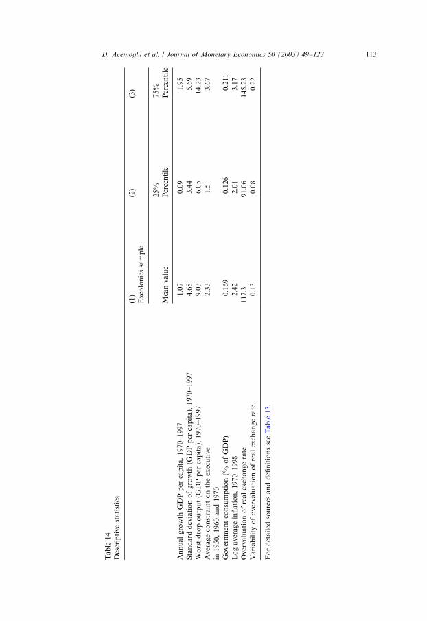
Table

14

Descriptivestatistics

(1)

(2)

(3)

Excoloniessample

25%

75%

Meanvalue

Percentile

Percentile

Annualgrowth

GDPper

capita,1970–1997

1.07

0.09

1.95

Standard

deviationofgrowth

(GDPper

capita),1970–1997

4.68

3.44

5.69

Worstdropoutput(G

DPper

capita),1970–1997

9.03

6.05

14.23

Averageconstraintontheexecutive

2.33

1.5

3.67

in1950,1960and1970

Governmentconsumption(%

ofGDP)

0.169

0.126

0.211

Logaverageinflation,1970–1998

2.42

2.01

3.17

Overvaluationofrealexchangerate

117.3

91.06

145.23

Variabilityofovervaluationofrealexchangerate

0.13

0.08

0.22

Fordetailed

sources

anddefinitionsseeTable

13.


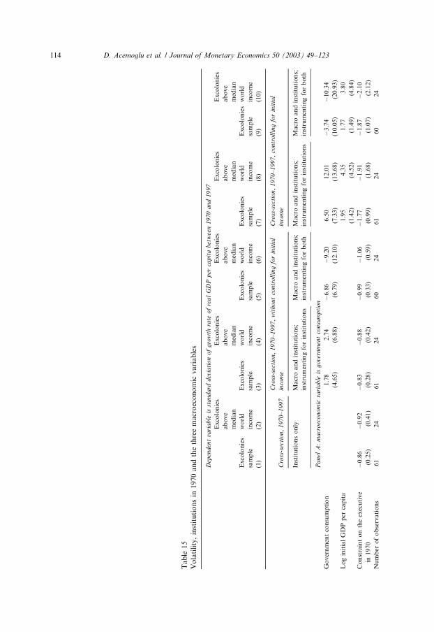
Table

15

Volatility,institutionsin

1970andthethreemacroeconomic

variables

Dep

enden

tva

riable

isst

andard

dev

iati

on

of

gro

wth

rate

of

real

GD

Pper

capit

abet

wee

n1970

and

1997

Excolonies

sample

Excolonies

above

median

world

income

Excolonies

sample

Excolonies

above

median

world

income

Excolonies

sample

Excolonies

above

median

world

income

Excolonies

sample

Excolonies

above

median

world

income

Excolonies

sample

Excolonies

above

median

world

income

(1)

(2)

(3)

(4)

(5)

(6)

(7)

(8)

(9)

(10)

Cro

ss-s

ecti

on,

1970–1997,

wit

hout

contr

oll

ing

for

init

ial

Cro

ss-s

ecti

on,

19

70

–1

99

7,

contr

oll

ing

for

init

ial

Cro

ss-s

ecti

on,

1970–1997

inco

me

inco

me

Institutionsonly









Pa

nel

A:

macr

oec

onom

icva

riable

isgove

rnm

ent

consu

mpti

on


1.78

2.74

�6.86

�9.20

6.50

12.01

�3.74

�10.34

(4.65)

(6.88)

(6.79)

(12.10)

(7.33)

(13.68)

(10.05)

(20.93)

LoginitialGDPper

capita

1.95

4.35

1.77

3.80

(1.42)

(4.52)

(1.49)

(4.84)

Constraintontheexecutive

in1970

�0.86

�0.92

�0.83

�0.88

�0.99

�1.06

�1.77

�1.91

�1.87

�2.10

(0.25)

(0.41)

(0.28)

(0.42)

(0.33)

(0.59)

(0.99)

(1.68)

(1.07)

(2.12)

Number

ofobservations

61

24

61

24

60

24

61

24

60

24


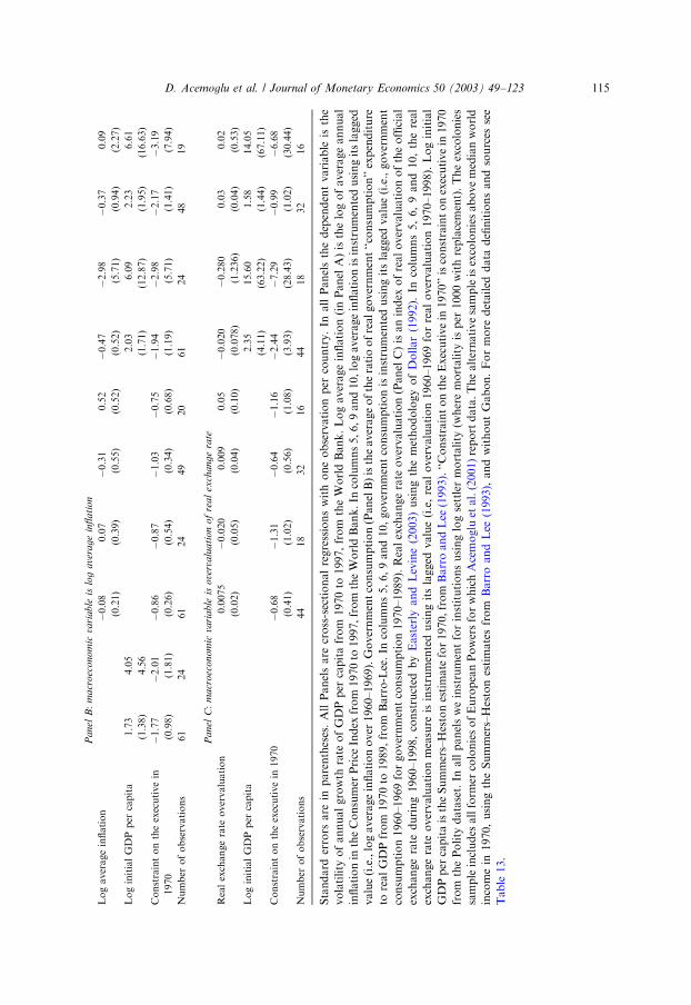
Pa

nel

B:

macr

oec

onom

icva

riable

islo

gave

rage

infl

ati

on

Logaverageinflation

�0.08

0.07

�0.31

0.52

�0.47

�2.98

�0.37

0.09

(0.21)

(0.39)

(0.55)

(0.52)

(0.52)

(5.71)

(0.94)

(2.27)

LoginitialGDPper

capita

1.73

4.05

2.03

6.09

2.23

6.61

(1.38)

4.56

(1.71)

(12.87)

(1.95)

(16.63)

Constraintontheexecutivein

1970

�1.77

�2.01

�0.86

�0.87

�1.03

�0.75

�1.94

�2.98

�2.17

�3.19

(0.98)

(1.81)

(0.26)

(0.54)

(0.34)

(0.68)

(1.19)

(5.71)

(1.41)

(7.94)

Number

ofobservations

61

24

61

24

49

20

61

24

48

19

Pa

nel

C:

macr

oec

onom

icva

riable

isove

rvalu

ati

on

of

real

exch

ange

rate

Realexchangerate

overvaluation

0.0075

�0.020

0.009

0.05

�0.020

�0.280

0.03

0.02

(0.02)

(0.05)

(0.04)

(0.10)

(0.078)

(1.236)

(0.04)

(0.53)

LoginitialGDPper

capita

2.35

15.60

1.58

14.05

(4.11)

(63.22)

(1.44)

(67.11)


1970

�0.68

�1.31

�0.64

�1.16

�2.44

�7.29

�0.99

�6.68

(0.41)

(1.02)

(0.56)

(1.08)

(3.93)

(28.43)

(1.02)

(30.44)

Number

ofobservations

44

18

32

16

44

18

32

16

Standard

errors

are



country.In


isthe

volatility

ofannualgrowth

rate

ofGDPper

capitafrom

1970to

1997,from

theWorldBank.Logaverageinflation(inPanel

A)isthelogofaverageannual

inflationin

theConsumer

Price

Index

from

1970to

1997,from

theWorldBank.In



1960–1969).Governmentconsumption(PanelB)istheaverageoftheratioofrealgovernment‘‘consumption’’expenditure

torealGDPfrom

1970to

1989,from

Barro-Lee.In

columns5,6,9and10,governmentconsumptionisinstrumentedusingitslagged

value(i.e.,government

consumption1960–1969forgovernmentconsumption1970–1989).Realexchangerate

overvaluation(PanelC)isanindex


exchangerate


byEasterly

andLevine(2003)usingthemethodologyofDollar(1992).

Incolumns5,6,9and10,thereal

exchangerate



value(i.e,realovervaluation1960–1969forrealovervaluation1970–1998).Loginitial

GDPper


for1970,from

BarroandLee

(1993).‘‘ConstraintontheExecutivein

1970’’isconstraintonexecutivein

1970

from

thePolity

dataset.In


(wheremortality

isper

1000withreplacement).Theexcolonies

sampleincludes

allform


etal.(2001)reportdata.Thealternativesampleisexcoloniesabovemedianworld

incomein


BarroandLee


detailed

data


see

Table

13.


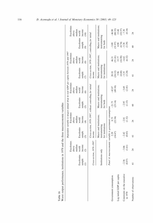
Table

16

Worstoutputperform

ance,institutionsin


variables

Dep

enden

tva

riable

isla

rges

tannual

dro

pin

real

GD

Pper

capit

abet

wee

n1970

and

1997

Excolonies

sample

Excolonies

above

median

world

income

Excolonies

sample

Excolonies

above

median

world

income

Excolonies

sample

Excolonies

above

median

world

income

Excolonies

sample

Excolonies

above

median

world

income

Excolonies

sample

Excolonies

above

median

world

income

(1)

(2)

(3)

(4)

(5)

(6)

(7)

(8)

(9)

(10)

Cro

ss-s

ecti

on,

1970–1997,

wit

hout

contr

oll

ing

for

init

ial

Cro

ss-s

ecti

on,

19

70

–1

99

7,

contr

oll

ing

for

init

ial

Cro

ss-s

ecti

on,

1970–1997

inco

me

inco

me





Institutionsonly

instrumenting

forinstitutions

instrumenting

forboth

instrumenting

forinstitutions

instrumenting

forboth

Panel

A:

macr

oec

onom

icva

riable

isgove

rnm

ent

consu

mpti

on


2.29

8.75

�21.75

�42.87

20.18

46.31

�3.09

�46.90

(14.67)

(22.54)

(23.14)

(49.10)

(24.12)

(51.41)

(31.97)

(80.32)

LoginitialGDPper

capita

5.96

15.77

4.90

13.44

(4.68)

(16.98)

(4.74)

(18.57)


in1970

�2.56

�3.06

�2.42

�2.81

�2.95

�3.69

�5.35

�6.62

�5.38

�7.38

(0.87)

(1.61)

(0.83)

(1.32)

(1.13)

(2.41)

(3.24)

(6.32)

(3.39)

(8.14)

Number

ofobservations

61

24

61

24

60

24

61

24

60

24


Panel

B:

macr

oec

onom

icva

riable

islo

gave

rage

infl

ati

on

Logaverageinflation

0.24

0.49

�1.38

0.79

�0.90

�1.92

�1.60

�0.91

(0.72)

(1.47)

(1.78)

(1.82)

(1.67)

(7.97)

(3.20)

(8.78)

LoginitialGDPper

capita

5.28

14.61

5.86

20.74

7.57

25.70

(4.54)

(17.17)

(5.50)

(45.29)

(6.64)

(64.21)


1970�5.35

�7.00

�2.56

�2.73

�3.30

�2.90

�5.67

�9.92

�7.26

�12.45

(3.24)

(6.82)

(0.88)

(2.07)

(1.10)

(2.39)

(3.82)

(20.10)

(4.81)

(30.66)

Number

ofobservations

61

24

61

24

49

20

61

24

48

19

Panel

C:

macr

oec

onom

icva

riable

isove

rvalu

ati

on

of

real

exch

ange

rate

Realexchangerate

overvaluation

�0.028

�0.064

0.017

0.21

�0.17

�0.897

0.09

0.10

(0.06)

(0.16)

(0.12)

(0.31)

(0.39)

(3.910)

(0.13)

(1.66)

LoginitialGDPper

capita

12.08

49.77

6.50

45.43

(20.40)

(200.22)

(4.95)

(212.81)


1970

�3.03

�3.98

�2.04

�3.55

�12.07

�23.06

�3.46

�21.38

(1.72)

(3.12)

(1.82)

(3.26)

(19.52)

(90.04)

(3.48)

(96.54)

Number

ofobservations

44

18

32

16

44

18

32

16

Standard

errors

are



country.In

allPanelsthedependentvariableisthelowest

annualgrowth

rate

ofGDPper

capitafrom

1970to

1997(w

iththesignchanged


theWorldBank.Logaverage

inflation(inPanelA)isthelogofaverageannualinflationin

theConsumer

Price

Index

from

1970to

1997,from

theWorldBank.In

columns5,6,9and10,log

averageinflationisinstrumentedusingitslagged


1960–1969).GovernmentConsumption(Panel

B)istheaverageofthe

ratioofrealgovernment‘‘consumption’’expenditure

torealGDPfrom

1970to

1989,from

Barro-Lee.In

columns5,6,9and10,governmentconsumptionis


value(i.e.,governmentconsumption1960–1969forgovernmentconsumption1970–1989).Realexchangerate

overvaluation

(PanelC)isanindex



byEasterly

andLevine(2003)usingthemethodologyof

Dollar(1992).In

columns5,6,9

and10,therealexchangerate



value(i.e,realovervaluation1960–1969

forrealovervaluation1970–1998).LoginitialGDPper

capitais

theSummers–Hestonestimate

for1970,from

BarroandLee

(1993).‘‘Constraintonthe

executivein

1970’’is

constraintonexecutivein

1970from

thePolity

dataset.In


(where

mortality

isper

1000withreplacement).Theexcoloniessampleincludes

allform


etal.(2001)reportdata.

Thealternativesampleisexcoloniesabovemedianworldincomein

1970,usingtheSummers–Hestonestimatesform

BarroandLee

(1993),andwithoutGabon.

Formore

detailed

data


seeTable

1.


Table

17

Growth,institutionsin


variables

Dep

enden

tva

riable

isave

rage

annual

gro

wth

of

real

GD

Pper

capit

abet

wee

n1970

and

1997

Excolonies

sample

Excolonies

above

median

world

income

Excolonies

sample

Excolonies

above

median

world

income

Excolonies

sample

Excolonies

above

median

world

income

Excolonies

sample

Excolonies

above

median

world

income

Excolonies

sample

Excolonies

above

median

world

income

(1)

(2)

(3)

(4)

(5)

(6)

(7)

(8)

(9)

(10)

Cro

ss-s

ecti

on,

1970–1997,

wit

hout

contr

oll

ing

for

init

ial

Cro

ss-s

ecti

on,

19

70

–1

99

7,

contr

oll

ing

for

init

ial

Cro

ss-s

ecti

on,

1970–1997

inco

me

inco

me

Macroandinstitutions:




Institutionsonly





Pa

nel

A:

macr

oec

onom

icva

riable

isgove

rnm

ent

consu

mpti

on


�1.31

�2.93

1.45

7.44

�6.35

�13.27

�1.97

8.74

(5.06)

(7.86)

(6.86)

(13.03)

(8.31)

(15.19)

(10.87)

(22.70)

LoginitialGDPper

capita

�2.08

�4.86

�1.95

�4.31

(1.61)

(5.02)

(1.61)

(5.25)


in1970

0.80

0.63

0.77

0.59

0.82

0.74

1.78

1.75

1.79

1.93

(0.28)

(0.47)

(0.30)

(0.48)

(0.33)

(0.64)

(1.12)

(1.87)

(1.15)

(2.30)

Number

ofobservations

61

24

61

24

60

24

61

24

60

24

Pa

nel

B:

macr

oec

onom

icva

riable

islo

gave

rage

infl

ati

on

Logaverageinflation

�0.20

�0.15

0.37

�0.16

0.19

0.60

0.42

0.37

(0.23)

(0.42)

(0.60)

(0.63)

(0.57)

(2.39)

(0.99)

(2.75)

LoginitialGDPper

capita

�1.86

�4.53

�1.98

�6.46

�2.13

�7.98

(1.56)

(5.06)

(1.87)

(13.58)

(2.05)

(20.08)


1970

1.78

1.85

0.79

0.54

0.89

0.57

1.85

2.78

1.98

3.52

(1.11)

(2.01)

(0.28)

(0.60)

(0.37)

(0.83)

(1.30)

(6.03)

(1.48)

(9.58)

Number

ofobservations

61

24

61

24

49

20

61

24

48

19


Pa

nel

C:

macr

oec

onom

icva

riable

isove

rvalu

ati

on

of

real

exch

ange

rate

Realexchangerate

overvaluation

0.0051

0.0029

0.017

0.01

0.053

0.250

�0.01

0.05

(0.02)

(0.05)

(0.05)

(1.05)

(0.130)

(1.130)

(0.05)

(0.62)

LoginitialGDPper

capita

�4.11

�14.52

�1.95

�17.60

(7.00)

(57.67)

(1.74)

(79.21)


1970

0.89

0.68

0.68

0.79

3.96

6.24

1.11

7.70

(0.61)

(0.94)

(0.75)

(1.10)

(6.69)

(25.93)

(1.23)

(35.93)

Number

ofobservations

44

18

32

16

44

18

32

16

Standard

errors

are



country.In


isthe

averageannualgrowth

rateofGDPper

capitafrom

1970to

1997,from

theWorldBank.Logaverageinflation(inPanelA)isthelogofaverageannualinflation

intheConsumer

Price

Index

from

1970to

1997,from

theWorldBank.In


value

(i.e.,logaverageinflationover

1960–1969).GovernmentConsumption(PanelB)istheaverageoftheratioofrealgovernment‘‘consumption’’expenditure

to

realGDPfrom

1970to

1989,from

Barro-Lee.In

columns5,6,9and10,governmentconsumptionisinstrumentedusingitslagged

value(i.e.,government

consumption1960–1969forgovernmentconsumption1970–1989).Realexchangerate

overvaluation(PanelC)isanindex


exchangerate


byEasterly

andLevine(2003)usingthemethodologyofDollar(1992).

Incolumns5,6,9and10,thereal

exchangerate



value(i.e.,realovervaluation1960–1969forrealovervaluation1970–1998).Loginitial

GDPper


for1970,from

BarroandLee

(1993).‘‘ConstraintontheExecutivein

1970’’isconstraintonexecutivein

1970

from

thePolity

dataset.In


(wheremortality

isper

1000withreplacement).Theexcolonies

sampleincludes

allform


etal.(2001)reportdata.Thealternativesampleisexcoloniesabovemedianworld

incomein


BarroandLee


detailed

data


see

Table

13.


References

Acemoglu, D., Robinson, J.A., 2000. Political losers as a barrier to economic development. American

Economic Review 90, 126–130.

Acemoglu, D., Robinson, J.A., 2001. A theory of political transitions. American Economic Review 91,

938–963.

Acemoglu, D., Robinson, J.A., 2002. Economic backwardness in political perspective. NBER Working

Paper No. 8831.

Acemoglu, D., Zilibotti, F., 1997. Was Prometheus Unbound by Chance? Risk, diversification and

growth. Journal of Political Economy 105, 1167–1200.

Acemoglu, D., Johnson, S., Robinson, J.A., 2001. Colonial origins of comparative development: an

empirical investigation. American Economic Review 91, 1369–1401.

Acemoglu, D., Johnson, S., Robinson, J.A., 2002a. Reversal of fortune: Geography and institutions in the

making of the modern world income distribution. Quarterly Journal of Economics, Forthcoming.

Acemoglu, D., Johnson, S., Robinson, J.A., 2002b. The Rise of Europe: Atlantic Trade, Institutional

Change and Economic Growth, Unpublished.

Apter, D.E., 1972. Ghana in Transition. Princeton University Press, Princeton.

Austin, D., 1964. Politics in Ghana, 1947–1960. Oxford University Press, Oxford, UK.

Bardhan, P., 1984. The Political Economy of Development in India. Basil Blackwell, Oxford.

Barro, R.J., 1991. Economic growth in a cross section of countries. Quarterly Journal of Economics 106,

407–433.

Barro, R.J., Lee, J.W., 1993. International comparisons of educational attainment. Journal of Monetary

Economics 32, 363–394.

Bates, R.H., 1981. Markets and States in Tropical Africa. University of California Press, Berkeley.

Benhabib, J., Rustichini, A., 1996. Social conflict and growth. Journal of Economic Growth 1, 125–142.

Besley, T., 1995. Property rights and investment incentives: theory and evidence from Ghana. Journal of

Political Economy 103, 903–937.

Blanchard, O.J., Simon, J., 2002. The long and large decline in US output volatility. Brookings Papers on

Economics Activity, Forthcoming.

Cabellero, R.J., 2001. Macroeconomic volatility in reformed Latin America: diagnosis and policy

proposals. Inter-American Development Bank, Washington.

Caballero, R.J., Dornbusch, R., 2002. A Plan for Argentina. http://web.mit.edu/caball/www/ARGEN-

TINA22802.pdf.

Caballero, R.J., Krishnamurthy, A., 2000. Emerging market crises; an asset markets perspective.

Department of Economics, MIT, Unpublished.

Chang, R., Velasco, A., 2002. A model of financial crisis in emerging markets. Quarterly Journal of

Economics, Forthcoming.

Collier, D., Collier, R.B., 1991. Shaping the Political Arena: Critical Junctures, the Labor Movement, and

Regime Dynamics in Latin America. Princeton University Press, Princeton.

Curtin, P.D., 1989. Death by Migration: Europe’s Encounter with the Tropical World in the 19th Century.

Cambridge University Press, New York.

Curtin, P.D., 1998. Disease and Empire: The Health of European Troops in the Conquest of Africa.

Cambridge University Press, New York.

Denizer, C., Iyigun, M., Owen, A., 2001. Finance and macroeconomic volatility. World Bank discussion

paper.

D!ıaz, A., Carlos, F., 1970. Essays on the Economic History of the Argentine Republic. Yale University

Press, New Haven, CT.

Dollar, D., 1992. Outward oriented developing economies really do grow more rapidly. Economic

Development and Cultural Change 40, 523–544.

Dornbusch, R., Goldfajn, I., Valdes, R., 1995. Currency crises and collapses. Brookings Papers on

Economic Activities, pp. 219–294.


http://web.mit.edu/caball/www/ARGENTINA22802.pdf

http://web.mit.edu/caball/www/ARGENTINA22802.pdf

Easterly, W., 2001. The lost decades: the developing countries stagnation in spite of policy reform. Journal

of Economic Growth 9, 135–157.

Easterly, W., Islam, R., Stiglitz, J., 2000. Shaken and stirred, explaining growth volatility. Annual Bank

Conference on Development Economics, The World Bank, April.

Easterly, W., Levine, R., 2003. Tropics, germs and crops: how endowments influence economic

development. Journal of Monetary Economics 50 (1), this issue.

Edwards, S., 1989. The international monetary fund and the developing countries: a critical evaluation. In:

Brunner, K., Meltzer, A.H. (Eds.), IMF Policy Advice, Market Volatility, Commodity Price Rules and

Other Essays. North-Holland, Amsterdam.

Eichengreen, B., Bordo, M.D., 2002. Crises then and now: what lessons from the last era of financial

globalization? NBER Working Paper 8716, January.

Frieden, J., 2001. The Modern World Economy; 1870–2000. Department of Government, Harvard

University, Unpublished Book manuscript.

Gerchunoff, P., 1989. Peronist economic policies, 1946–1955. In: Dornbusch, R., Tella, G.di. (Eds.),

The Political Economy of Argentina, 1946–1983. University of Pittsburg Press, Pittsburg,

PA.

Germani, G., 1962. Politica y Sociedad en una Epoca de Transicion, de la Sociedad Tradicional a la

Sociedad de Masas, Buenos Aires; Editorial Paidos.

Gibson, E.L., 1997. The populist road to market reform: policy and electoral coalitions in Mexico and

Argentina. World Politics 59.

Gibson, E.L., Calvo, E.F., Falleti, T.G., 2001. Reallocative federalism: overrepresentation and public

spending in the Western Hemisphere. Department of Political Science, Northwestern University,

Unpublished.

Gutierrez, H., 1986. La Mortalite des Eveques Latino-Americains aux XVIIe et XVIII Siecles. Annales de

Demographic Historique 29–39.

Hall, R.E., Jones, C.I., 1999. Why do some countries produce so much more output per worker than

others? Quarterly Journal of Economics 114, 83–116.

Herbst, J.I., 1993. The Politics of Reform in Ghana, 1982–1991. University of California Press,

Berkeley.

Herbst, J.I., 2000. States and Power in Africa: Comparative lessons in Authority and Control. Princeton

University Press, Princeton.

Johnson, S., Boone, P., Breach, A., Friedman, E., 2000. Corporate governance in the Asian financial crisis.

Journal of Financial Economics 58 (1–2), 141–186.

Johnson, S., McMillan, J., Woodruff, C., 2002. Property rights and finance. American Economic Review,

forthcoming.

Jones, E.L., 1981. The European Miracle: Environments, Economies and Geopolitics in the History of

Europe and Asia. Cambridge University Press, Cambridge, UK.

Kaminsky, G.L., Reinhart, C.M., 1999. The twin crises: the causes of banking and balance of payments

problems. American Economic Review 89, 473–500.

Knack, S., Keefer, P., 1995. Institutions and economic performance: cross-country tests using alternative

measures. Economics and Politics 7, 207–227.

Kraay, A., Ventura, J., 2000. Comparative advantage and the cross-section of business cycles. Department

of Economics, MIT, Cambridge, MA, Unpublished.

Krueger, A.O., 1993. Political Economy of Policy Reform in Developing Countries. MIT Press,

Cambridge.

Krugman, P., 1979. A model of balance of payments crises. Journal of Money Credit and Banking 11,

311–325.

Krusell, P., R!ios-Rull, J.V., 1996. Vested interests in a theory of growth and stagnation. Review of

Economic Studies 63, 301–329.

La Porta, R., Lopez-de-Silanes, F., Shleifer, A., Vishny, R.W., 1998. Law and finance. Journal of Political

Economy 106, 1113–1155.


Leith, J.C., Lofchie, M.F., 1993. The political economy of structural adjustment in Ghana. In: Robert,

H.B., Krueger, A.O. (Eds.), Political and Economic Interactions in Economics Policy Reform:

Evidence from Eight Countries. Basil Blackwell, Cambridge, MA.

Lizzeri, A., Persico, N., 2001. The provision of public goods under alternative electoral incentives.

American Economic Review 91, 225–245.

Mauro, P., 1995. Corruption and growth. Quarterly Journal of Economics CX, 681–712.

Mazzuca, S., 2001. Southern cone leviathans. State formation in Argentina, Brazil, Chile, and Uruguay.

Ph.D. Dissertation, Department of Political Science, Berkeley, Unpublished.

McConnell, M.M., Perez-Quiros, G., 2000. Output Fluctuations in the United States: What has Changed

since the Early 1980’s. American Economic Review 90, 1464–1476.

Mora y, A.M., Llorente, I., 1980. El Voto Peronista. Editorial Sudamericana, Buenos Aires.

North, D.C., 1981. Structure and Change in Economic History. W.W. Norton & Co., New York.

North, D.C., Thomas, P., 1973. The Rise of the Western World: A New Economic History. Cambridge

University Press, Cambridge, UK.

Olson, M.C., 1982. The Rise and Decline of Nations. Yale University Press, New Haven, CT.

Owusu, M., 1970. Use and Abuses of Power. A Case Study of Continuity and Change in the Politics of

Ghana. University of Chicago Press, Chicago, IL.

della Paolera, G., Taylor, A.M., 2001. Straining at the Anchor: The Argentine Currency Board and the

Search for Macroeconomic Stability 1880–1935. University of Chicago Press, Chicago.

Parente, S.L., Prescott, E.C., 1999. Monopoly rights: a barrier to riches. American Economic Review 89,

1216–1233.

Pellow, D., Chazan, N., 1986. Ghana: Coping with Uncertainty. Westview Press, Boulder, CO.

Raddatz, C., 2002. Liquidity Needs and Vulnerability to Financial Under-development. Unpublished,

Department of Economics, MIT, Cambridge, MA.

Ramey, G., Ramey, V., 1995. Cross-country evidence on the links between volatility and growth.

American Economic Review 85, 1138–1151.

Rock, D.J., 1987. Argentina 1516–1987: From Spanish Colonization to Alfonsin. University of California

Press, Berkeley.

Rodrik, D., 1999. Where did all the growth go? External shocks, social conflict and growth collapses.

Journal of Economic Growth 4 (4) (December), 385–412.

Rodrik, D., 2002. Reform in Argentina, take two: trade rout. The New Republic.

Roe, M.J., 1998. Essays: backlash. Columbia Law Review 98, 217–241.

Sachs, J.D., 1990. Social conflict and populist policies in Latin America. In: Brunetta, R., Dell’Aringa, C.

(Eds.), Labor Relations and Economic Performance. NYU Press, New York.

Sachs, J.D., Warner, A., 1997. Fundamental sources of long-run growth. American Economic Review,

Papers and Proceedings, May.

Samuels, D., Snyder, R., 2001. The value of a vote: malapportionment in comparative perspective. British

Journal of Political Science 31 (4), 651–671.

Samuels, D., Snyder, R., 2002. Legislative Malapportionment in Latin America: Historical and

Comparative Perspectives. Unpublished.

Sawers, L., 1996. The Other Argentina: The Interior and National Development. Westview Press, Boulder.

Shleifer, A., 1997. Government in transition. European Economic Review 41, 385–410.

State Failure Task Force, 1998. State Failure Task Force Report: Phase II Findings. Prepared by Esty,

D.C., Goldstone, J.A., Gurr, T.R., Huff, B., Levy, M., Dabelko, G.D., Surko, P.T., Unger, A.N., 31

July.

Stock, J., Watson, M., 2002. Has the Business Cycle Changed and Why? NBER Macroeconomic Annual,

Forthcoming.

Taylor, A.M., 1998. On the costs of inward looking development: price distortions, growth and divergence

in Latin America. Journal of Economic History 57, 147–184.

Tornell, A., Velasco, A., 1992. The tragedy of the commons and economic growth: why does capital flow

from poor to rich countries? Journal of Political Economy 100, 1208–1231.


Voth, H.J., 2002. Why was stock market volatility so high during the Great Depression? Evidence from 10

countries during the interwar period. CEPR Discussion Paper, DP3254.

Weisman, C., 1987. The Reversal of Development in Argentina. Princeton University Press, Princeton.

Williamson, J., 1990. Latin American Adjustment: How Much Has Happened? Institute for International

Economics, Washington, DC.


institutional causes, macroeconomic symptoms: volatility, crises and

Documents