Institutional Corruption and Election Fraud: Evidencefrom a Field Experiment in Afghanistan∗

Michael Callen† and James D. Long‡

June 14, 2014

Abstract

We investigate the relationship between political networks, weak institutions, and electionfraud during the 2010 parliamentary election in Afghanistan combining: (i) data on politicalconnections between candidates and election officials; (ii) a nationwide controlled evaluationof a novel monitoring technology; and (iii) direct measurements of aggregation fraud. Wefind considerable evidence of aggregation fraud in favor of connected candidates and that theannouncement of a new monitoring technology reduced theft of election materials by about60 percent and vote counts for connected candidates by about 25 percent. The results haveimplications for electoral competition and are potentially actionable for policymakers.

JEL codes: P16, D72, D73

Keywords: Election Fraud, Corruption

∗Authors’ Note: We are grateful to Glenn Cowan, Jed Ober, Eric Bjornlund, Evan Smith, and JonGatto at Democracy International (DI) and Nader Nadery, Jandad Spinghar, and Una Moore at the Freeand Fair Elections Foundation of Afghanistan (FEFA). We acknowledge the support of USAID DevelopmentInnovation Ventures (DIV), DI, and grant #FA9550-09-1-0314 from the Air Force Office of Scientific Research(Callen). We are indebted to James Andreoni, Luke Condra, Gordon Dahl, Daniel Egel, Col. Joseph H.Felter, Ray Fisman, Tarek Ghani, Susan Hyde, Radha Iyengar, Danielle Jung, Asim Ijaz Khwaja, DavidLaitin, David Lake, Edward Miguel, Karthik Muralidharan, Paul Niehaus, Gerard Padro-i-Miquel, RohiniPande, Ngoc Anh Tran, Maura O’Neill, Shanker Satyanath, Jacob Shapiro, Romain Wacziarg, Scott Worden,Christopher Woodruff and seminar participants at the NBER Political Economy Meeting, the 2011 NEUDCconference, George Mason University, the Development and Conflict Research (DACOR) conference, the2011 Institute on Global Conflict and Cooperation (IGCC) conference, UC San Diego, Yale, the Center forGlobal Development (CGD), and USAID for extremely helpful comments. We are particularly indebtedto Eli Berman, Clark Gibson, and Craig McIntosh for advice and support at all stages of the project.This project would not have been possible without the dedicated research assistance of Randy Edwards,Mohammad Isaqzadeh, Shahim Kabuli, and Arman Rezaee. Mistakes remain with the authors.†University of California Los Angeles. Department of Political Science. 4289 Bunche Hall, Los

Angeles, CA 90095. email: mjcallen@ucsd.edu‡Harvard Academy for International and Area Studies and University of Washington. Depart-

ment of Political Science.

1

1 Introduction

Many governments are not responsive to their citizens. Fair elections provide an important means

of improving responsiveness by making elected officials accountable to voters.1 However, election

fraud undermines this critical function in many young democracies, often at the hands of tightly

networked groups of political elites. This paper examines whether candidates exploit connections

to elections officials to add fraudulent votes during the aggregation process. We study this problem

in Afghanistan, a country where democratic institutions are struggling to develop after the last

three decades of continuous conflict.2

There are many ways to manipulate elections, including voter intimidation, ballot box stuffing,

and changing vote totals after ballots are cast. We study the manipulation of vote totals during

the aggregation process, which we henceforth call “aggregation fraud”. We are interested in this

particular type of fraud because it is likely to involve collusion between candidates and election

officials. We collect novel data on aggregation fraud by photographing provisional vote tally sheets

at individual polling centers before the aggregation process and comparing these counts to the

corresponding numbers after aggregation is completed.3 This technique, which we call “photo

quick count”, records the same vote totals both before and after aggregation. In a clean election,

these numbers should be identical. We find differences at 78 percent of the polling locations in our

observed sample. Additionally, candidates connected to officials in charge of aggregation receive

an average of 3.5 fraudulent votes per polling station (about 13.7 percent of their polling station

average).

Given that fraud affects many elections in developing countries, there is reason to study the

effects of election monitoring both for the design of policy and for understanding the mechanics of

1There is substantial empirical documentation of the benefits of improving political accountability (Besleyand Burgess 2002; Besley, Pande and Rao 2005; Chattopadhyay and Duflo 2004; Ferraz and Finan 2008;2011; Fujiwara 2013; Pande 2003; Martinez-Bravo et al. 2013). Additionally, in countries experiencing violentcontests for state control, such as Afghanistan, fair elections may also undermine popular support for insur-gents by promoting an accountable and legitimate government and by providing a forum for reconciliation(Berman, Shapiro and Felter 2011; Besley and Persson 2011; McChrystal 2009; United States Army 2006;World Bank 2011).

2Rashid (2009) provides an authoritative account of how the patronage networks of Afghan warlords haveundermined political development in Afghanistan.

3In many countries, it is standard for election officials to record vote totals at a particular polling centeron an election returns form and then post the form on the outside of the polling center, indicating vote totalsat the polling centers to local residents.

2

election fraud. We therefore implement an experiment both to estimate the causal effect of photo

quick count on aggregation fraud and to provide more general evidence on the response of fraud to

the credible threat of discovery through monitoring. Specifically, we test whether announcing photo

quick count measurements to election officials reduces fraud. We deliver a letter to a randomly

selected set of polling center managers in 238 polling centers from an experimental sample of

471 polling centers.4 The letter explains how photo quick count works and announces that the

measurement will be taken. Our nationwide experimental sample comprises 7.8 percent of polling

centers operating on election day and spans 19 of Afghanistan’s 34 provinces.

This experiment produces four main results. First, the photo quick count announcement re-

duced damaging of election materials by candidate representatives from 18.9 to 8.1 percent (a

reduction of about 60 percent). Second, it reduced votes for politically powerful candidates at

a given polling location from about 21 to about 15 (a reduction of about 25 percent).5 Treat-

ment effects are also larger for candidates connected to officials in charge of aggregation in their

constituency.6 These candidates lost about 6.5 votes as a result of the intervention.7 Third, the in-

tervention impacts fraud measured directly using photo quick count. Point estimates for this effect

range between 9.37 and 17.17 fewer votes changed during aggregation for candidates connected to

the provincial aggregator.8 Last, we find that having a neighbor treated within one kilometer is

associated with an additional reduction of about seven votes, suggesting our estimates may slightly

understate the true effect.

Our results relate to empirical findings in four strands of literature on the economics of cor-

ruption. First, as in the important examples provided by Bertrand et al. (2007) and Olken and

Barron (2009), we find that corruption limits the ability of governments to correct externalities.

4Polling center managers are election officials tasked with managing the voting process on election dayand overseeing the counting of votes at the end of the day in their assigned polling center.

5The mean number of votes cast for a candidate at a given polling substation in our control sample is1.410, reflecting the fact that many candidates receive no votes in many locations. The mean number ofvotes cast for all candidates at a given polling location is 269.

6As we describe in Section 3, we observe these connections only for 57 candidates, a small subset ofcandidates running in the election. In Table A2, however, we find that treatment effects are localized toconnected candidates, even controlling for whether they were investigated.

7Correspondingly, these candidates receive enough votes to rank among winning candidates at 49.7 percentof the polling substations in our control sample. Our treatment reduces this share to 38.2 percent of pollingsubstations.

8These large bounds on the estimated treatment effect are due to substantial treatment-related attritionin this measure. We calculate these bounds using the trimming method of Lee (2009).

3

The purpose of electoral law is to ensure that election outcomes reflect the will of the electorate.

We show that this function is undermined by a faulty aggregation process. Second, the effects of

announcing photo quick count depend on pre-existing connections between candidates and election

officials. Fragile democracies provide many examples of elected officials sharing rents with their

networks (Fisman 2001; Khwaja and Mian 2005). Free and fair elections may place limits on this

(see, for example, Ferraz and Finan 2008; 2011), and so patronage networks might have incen-

tives to coordinate when capturing elections. This suggests the possibility of multiple equilibria in

corruption as discussed in Olken and Pande (2011); the same intervention can have very different

effects depending on pre-existing political relationships. Third, we examine the determinants of

equilibrium patterns of corruption (Shleifer and Vishny 1993; Cadot 1987; Rose-Ackerman 1975;

Svensson 2003), focusing on the role of candidate connections. Last, our experiment relates to the

growing body of experimental and quasi-experimental assessments of initiatives to improve elec-

tions (Aker, Collier and Vicente 2013; Fujiwara 2013; Hyde 2007; Ichino and Schundeln 2012). Our

project also draws direct inspiration from work in development economics on efforts to improve

transparency and accountability (Atanassova, Bertrand and Niehaus 2013; Duflo, Hanna and Ryan

2012; Di Tella and Schargrodsky 2003; Ferraz and Finan 2008; Olken 2007; Yang 2008).9

We point to three implications for policies aimed at strengthening democratic institutions.

First, aggregation fraud was a serious problem in this election. When electoral institutions are

weak, candidates may be able to leverage their ties to officials to distort electoral outcomes in their

favor. Second, we find a substantial response of fraud to monitoring, suggesting that monitoring

can increase fairness in elections. Third and relatedly, our results provide promise for photo quick

count as a means of both precisely measuring and of reducing aggregation fraud. This approach can

increase precision beyond existing forensic tests which compare realized vote distributions with the-

oretical distributions that should occur in a fair election.10 Moreover, such checks can be subverted

by competent manipulators by ensuring that rigged values follow the test distributions. The tech-

nology is also highly compatible with implementation via Information Communications Technology.

9Research on the role of monitoring and anti-corruption efforts in development is advancing rapidly; wedirect readers to Olken and Pande (2011) and McGee and Gaventa (2011) for excellent reviews of researchin this field.

10Myagkov, Ordeshook and Shakin (2009), Mebane (2008), and Beber and Scacco (2012) describe forensicmethods of detecting election fraud.

4

The cost of recording and centralizing information on diffuse illegal behavior is now nominal. The

rapid increase in cellular connectivity and in smartphone usage in developing countries allows the

possibility that this technology might also be adapted to citizen-based implementation.

We structure the rest of the paper as follows. Section 2 describes our experimental setting

and relevant features of electoral institutions in Afghanistan. Section 3 presents results using data

on directly measured aggregation fraud. Section 4 describes our experimental evaluation of photo

quick count. Section 5 provides results from the experiment and Section 6 concludes.

2 Institutional Background

2.1 Post-Invasion Democracy in Afghanistan

After the invasion by the United States and fall of the Taliban in 2001, a coalition of international

armed forces helped to empanel a Constitutional Loya Jirga to establish democratic institutions

in Afghanistan after decades of internecine conflict, civil war, and Taliban rule. In 2004, popular

elections validated the Loya Jirga’s choice of Hamid Karzai as president, and in 2005, Afghans

voted in the first elections for the lower house of parliament (Wolesi Jirga). In 2009, Karzai was re-

elected amid claims of rampant election fraud, which largely discredited the government.11 Afghans

returned to the polls in September 2010 to elect members of parliament amid a growing insurgency

and a US commitment to begin withdrawing troops in July 2011. The international community

viewed these elections as a critical benchmark in the consolidation of democratic institutions given

doubts about the Karzai government’s ability to exercise control in much of the country. Despite

lingering memories of violence and widespread fraud from the 2009 election, roughly 5 million voters

cast ballots in the 2010 Wolesi Jirga elections.12

11Karzai initially won 53 percent of the vote, above the 50 percent threshold necessary to avoid a run-off. After an independent investigation based on physical inspections of a random subsample of ballots,Karzai’s share was reduced to 47 percent. Karzai finally won re-election when his main competitor, AbdullahAbdullah, refused to participate in the run-off.

12The Independent Electoral Commission projected this number out of what it believes are 11 millionlegitimate registered voters. Afghanistan has never had a complete census so population estimates varywidely. The total population is estimated at roughly 30 million and the voting age population is roughly 16million.

5

2.2 Electoral Institutions

Three features of the parliamentary election system in Afghanistan make it particularly vulnerable

to fraud. First, many seats are available within a single constituency, creating thin victory margins

for a large number of positions. This both makes fraudulent votes potentially highly valuable and

also increases the number of potential manipulators. Second, electoral institutions in Afghanistan

are just beginning to develop and remain weak. Finally, the state exercises incomplete territorial

control, leaving polling centers in contested regions vulnerable to closure or capture. We discuss

each of these three features in this section.

Afghanistan’s 34 provinces serve as multi-member districts that elect members to the Wolesi

Jirga. Each province serves as a single electoral district and the number of seats it holds in

parliament is proportional to its estimated population. Candidates run “at large” within a province

without respect to any smaller constituency boundaries. Voters cast a Single Non-Transferable Vote

(SNTV) for individual candidates, nearly all of whom run as independents.13 The rules declare

winning candidates as those who receive the most votes relative to each province’s seat share. For

example, Kabul province elects the most members to Parliament (33), Ghor province elects the

median number of candidates in our sample (6), and Panjsher the fewest (2). The candidates who

rank 1 to 33 in Kabul, 1 to 6 in Ghor, and 1 to 2 in Panjsher win seats.14

This method for allocating seats in parliament for winning candidates provides incentives for

fraud. Because many seats are available within a single province, a large number of candidates

gain office with thin victory margins. SNTV with large district magnitudes and a lack of political

parties also disperses votes across many candidates. The vote margin separating the lowest winning

candidate from the highest losing candidate is often small. This creates a high expected return

for even small manipulation for many candidates. In contrast, electoral systems with established

parties and with small district magnitude tend to produce larger victory margins, so non-viable

13SNTV systems provide voters with one ballot that they cast for one candidate when multiple candidatesrun for multiple seats. If a voter’s ballot goes towards a losing candidate, the vote is not re-apportioned. Al-though this electoral system is rare, former U.S. Ambassador to Afghanistan Zalmay Khalilzad and PresidentHamid Karzai promoted SNTV during the first parliamentary elections in 2005 to marginalize warlords andreduce the likelihood they obtained parliamentary seats. As a corollary, Karzai also decreed that politicalparties should not be allowed to form.

14There are 249 seats in the Wolesi Jirga. Ten seats are reserved for the nomadic Kuchi population andthe remaining seats are allocated in proportion to the estimated population of the province.

6

candidates may be less likely to rig. Because each province contains multiple seats, it remains

possible for election officials involved in vote aggregation to rig votes on behalf of multiple officials

simultaneously.

Electoral malfeasance in Afghanistan may also be partly due to the weak institutions tasked

with managing elections. The Independent Election Commission serves as the main electoral body

responsible for polling, counting votes, aggregation, and certifying winning candidates. Histori-

cally, the Independent Election Commission has proven susceptible to influence by corrupt agents.

We review specific features of the aggregation process which conduce to fraud and considerable

photographic evidence of fraud in Section 3 below.15

Informal networks also play an important role in determining political outcomes in Afghanistan.

Despite attempts to promote democratic institutions, pre-existing power structures remain highly

relevant.16 For example, several of the main candidates in the 2010 election and a number of

current government officials were warlords prior to the U.S.-led invasion. Former warlords also

had considerable influence during the drafting of the Bonn Agreement, which provides the basis

for Afghanistan’s current political institutions. Along these lines, Karzai enjoys strong links with

government officials in Southern Afghanistan given his family roots in that part of the country.

Former warlords fighting in the Northern Alliance against the Taliban exert strong control in

Northern Afghanistan and have played a key role in the US-backed government.

Despite weak electoral institutions, candidates and officials face some possibility of punishment

for rigging. The Electoral Complaints Commission, which is backed by the United Nations, exists

as a separate and independent body from the Independent Elections Commission. The Electoral

Complaints Commission investigates complaints against polling officials, candidates, or citizens.

Any Afghan can lodge such a complaint. Based on the seriousness of a complaint and its likelihood

of affecting the election’s outcome, the Electoral Complaints Commission may decide to cancel all

of the votes at a given polling location, all of the votes for a particular candidate at a polling loca-

tion, or the total votes for a candidate across their entire constituency. The Electoral Complaints

15Similarly, Callen and Weidmann (2013) find that fraud was sufficiently severe to be detected by relativelyinsensitive forensic techniques in about 20 percent of the 398 districts in Afghanistan.

16For example, the Afghan Attorney General, Ishaq Malako alleged in an address to parliament, broadcaston Afghan nation television, that election outcomes were heavily influenced by well-connected Afghansthrough secret dealings in Dubai, and claimed to have evidence to that effect.

7

Commission over-turned some 25 percent of the ballots in this process in the 2010 election. This

resulted in 30 seats changing hands (National Democratic Institute 2010). Additionally, under its

purview of fighting corruption, the Attorney General’s office may prosecute specific individuals,

including election officials and candidates, it believes to have participated in election fraud and

levy fines or prison sentences against them if found guilty.17

3 Aggregation Fraud

There are many ways to rig an election such as buying votes, intimidating voters, and stuffing

ballot boxes. We focus on fraud which happens during the aggregation process. This type of fraud

typically involves adjusting votes in favor of a particular candidate and usually happens at a central

aggregation center.

We capture vote totals both immediately before and directly after the aggregation process,

which took roughly one month. These data directly measure votes added or subtracted during

aggregation for each candidate at each polling location in our observed sample. To our knowledge,

these are the first direct measurements of aggregation fraud. We begin by examining which types

of candidates benefit from aggregation fraud and summarize a few basic patterns.

3.1 Vote Aggregation

Aggregation takes place in three stages. First, after voting concludes, election staff count votes at

individual polling centers. Polling centers contain several polling substations. There are typically

four substations in a polling center. For example, a polling center might be a school, and polling

substations are classrooms set up as polling locations inside of the school.18 Counting is overseen

17To our knowledge, no candidates received criminal penalties for committing election fraud. However,during the month-long aggregation process, the Attorney General attempted to suspend the heads of boththe Independent Election Commission and the Electoral Complaints Commission.

18Analysis in this paper is done at the level of the polling substation. In particular, we use votes for agiven candidates at single polling substation as a main outcome. We had several options in terms of thelevel of aggregation to select as the unit of analysis. The candidate-polling substation is the most basicconstitutive unit. We use this as the unit of analysis because polling substation outcomes range much lesswidely than polling center outcomes. This allows us to estimate treatment effects across fairly similar units.In our data, there are between 1 and 11 polling substations in a given polling center. The number of votescast at a polling substation varies between 0 and 599, reflecting a law that when 600 votes are cast, a new

8

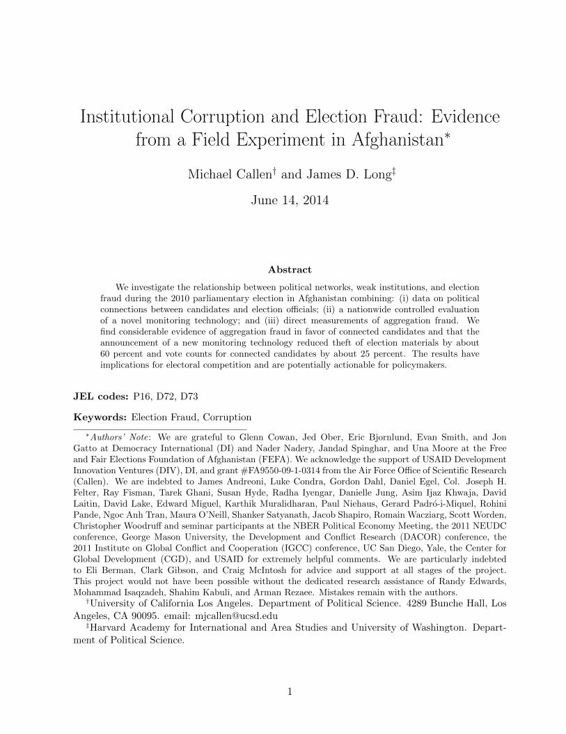
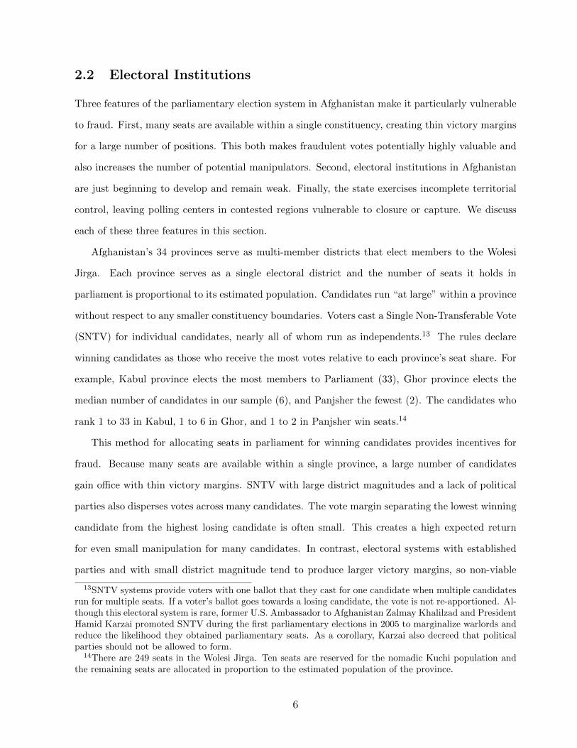
Presiding Official: Polling Center Manager Total Number: 6,038 Period of Operation: 7AM – 4PM on election day

Polling Center Provincial Aggregation

Center National Aggregation

Center

Presiding Official: Provincial Elections Officer Total Number: 36 Period of Operation: ~1 month after election

Presiding Official: Chairman Total Number: 1 Period of Operation: ~3 months after election

Figure 1: The Aggregation Process

at each polling center by a Polling Center Manager. The candidate totals for each substation are

recorded on a single Declaration of Results form. Second, copies of the results forms are then

sealed in a tamper-evident bag and sent to a Provincial Aggregation Center. After the count, the

ballots are returned to the boxes, and the boxes are stored locally and are not transmitted to the

Provincial Aggregation Center.19 Changing the Declaration of Results forms is therefore all that

is necessary to manipulate the aggregation process. Separate copies of each Declaration of Results

form are also posted on the outside of the polling center for public viewing. One Declaration of

Results form is posted for each polling substation. In the final stage, results forms are collected

at the National Aggregation Center in Kabul and combined to produce a national total. Figure 1

summarizes the aggregation process.

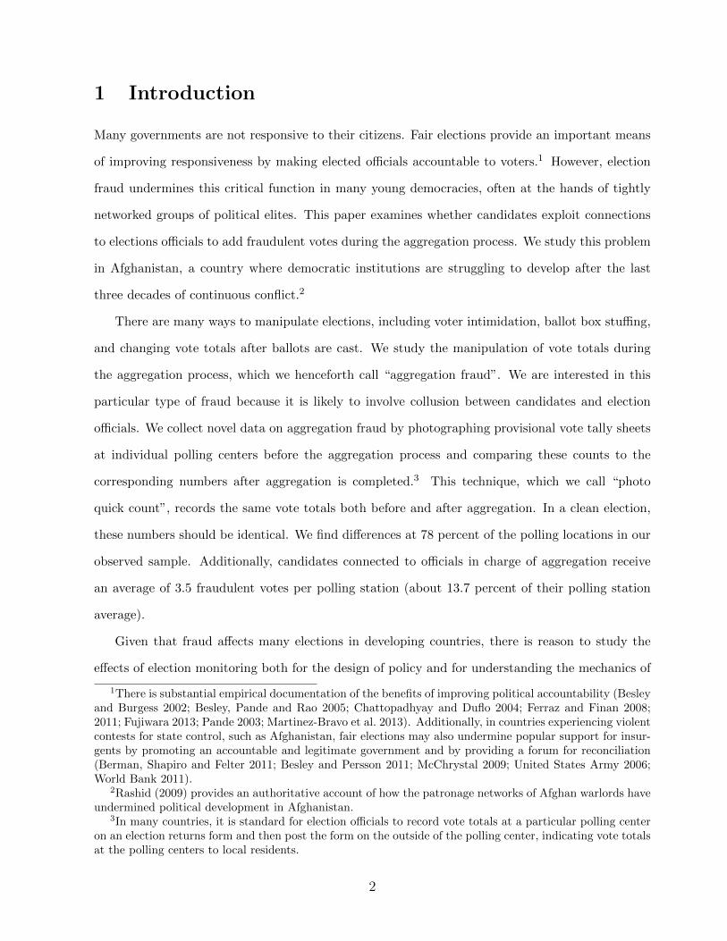
3.2 Measuring Fraud

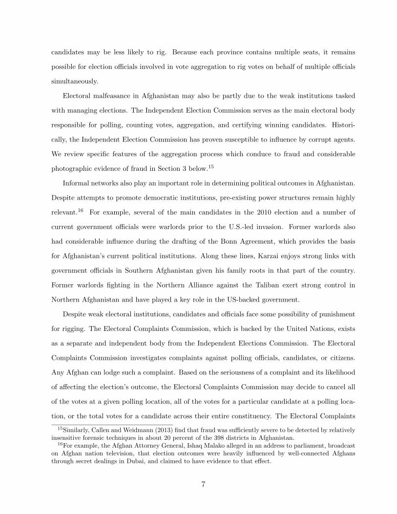
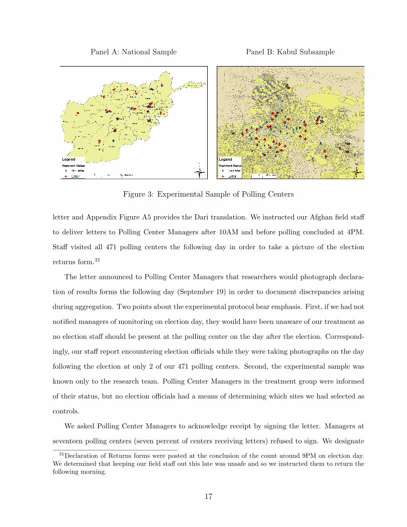
We measure fraud by taking photographs of the Declaration of Results form posted for public

viewing prior to aggregation and comparing this record to the corresponding vote total after aggre-

gation. We compare at the level of individual candidates at specific polling substations. Figure 2

illustrates the method. Our research team took the picture on the left at a polling center in the

field the morning after election day. The scan on the right was taken at the national aggregation

substation must be opened. By contrast, the number of votes cast at a polling center in our data rangesfrom 0 to 5526. Appendix Table A8 reports results aggregating to the candidate - polling center level.

19In most cases, boxes are stored at one pre-designated site in each of the 398 districts across Afghanistan.

9

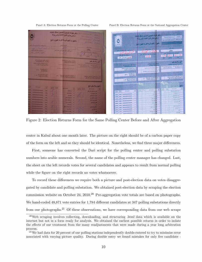
Panel A: Election Returns Form at the Polling Center Panel B: Election Returns Form at the National Aggregation Center

Figure 2: Election Returns Form for the Same Polling Center Before and After Aggregation

center in Kabul about one month later. The picture on the right should be of a carbon paper copy

of the form on the left and so they should be identical. Nonetheless, we find three major differences.

First, someone has converted the Dari script for the polling center and polling substation

numbers into arabic numerals. Second, the name of the polling center manager has changed. Last,

the sheet on the left records votes for several candidates and appears to result from normal polling

while the figure on the right records no votes whatsoever.

To record these differences we require both a picture and post-election data on votes disaggre-

gated by candidate and polling substation. We obtained post-election data by scraping the election

commission website on October 24, 2010.20 Pre-aggregation vote totals are based on photographs.

We hand-coded 48,871 vote entries for 1,784 different candidates at 347 polling substations directly

from our photographs.21 Of these observations, we have corresponding data from our web scrape

20Web scraping involves collecting, downloading, and structuring .html data which is available on theinternet but not in a form ready for analysis. We obtained the earliest possible returns in order to isolatethe effects of our treatment from the many readjustments that were made during a year long arbitrationprocess.

21We had data for 20 percent of our polling stations independently double-entered to try to minimize errorassociated with varying picture quality. During double entry we found mistakes for only five candidate -

10

for 48,018 entries at 346 polling substations. These 346 polling substations were contained in 149

distinct polling centers in our experimental sample.22

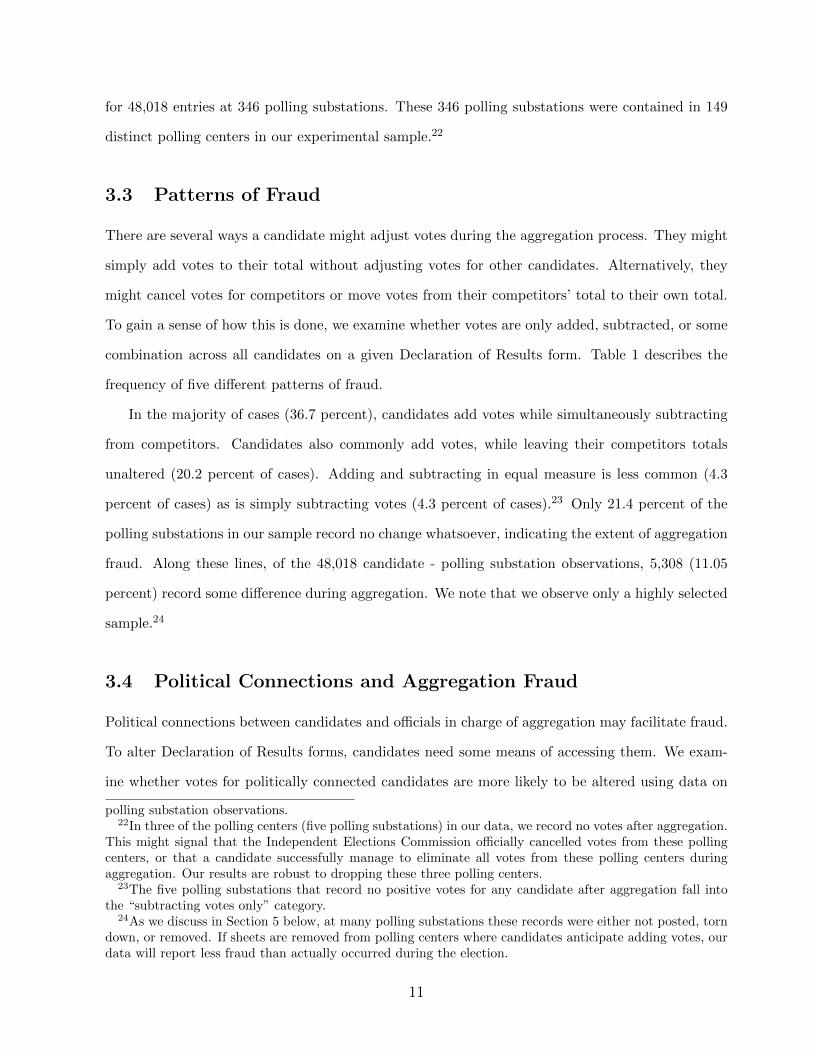
3.3 Patterns of Fraud

There are several ways a candidate might adjust votes during the aggregation process. They might

simply add votes to their total without adjusting votes for other candidates. Alternatively, they

might cancel votes for competitors or move votes from their competitors’ total to their own total.

To gain a sense of how this is done, we examine whether votes are only added, subtracted, or some

combination across all candidates on a given Declaration of Results form. Table 1 describes the

frequency of five different patterns of fraud.

In the majority of cases (36.7 percent), candidates add votes while simultaneously subtracting

from competitors. Candidates also commonly add votes, while leaving their competitors totals

unaltered (20.2 percent of cases). Adding and subtracting in equal measure is less common (4.3

percent of cases) as is simply subtracting votes (4.3 percent of cases).23 Only 21.4 percent of the

polling substations in our sample record no change whatsoever, indicating the extent of aggregation

fraud. Along these lines, of the 48,018 candidate - polling substation observations, 5,308 (11.05

percent) record some difference during aggregation. We note that we observe only a highly selected

sample.24

3.4 Political Connections and Aggregation Fraud

Political connections between candidates and officials in charge of aggregation may facilitate fraud.

To alter Declaration of Results forms, candidates need some means of accessing them. We exam-

ine whether votes for politically connected candidates are more likely to be altered using data on

polling substation observations.22In three of the polling centers (five polling substations) in our data, we record no votes after aggregation.

This might signal that the Independent Elections Commission officially cancelled votes from these pollingcenters, or that a candidate successfully manage to eliminate all votes from these polling centers duringaggregation. Our results are robust to dropping these three polling centers.

23The five polling substations that record no positive votes for any candidate after aggregation fall intothe “subtracting votes only” category.

24As we discuss in Section 5 below, at many polling substations these records were either not posted, torndown, or removed. If sheets are removed from polling centers where candidates anticipate adding votes, ourdata will report less fraud than actually occurred during the election.

11

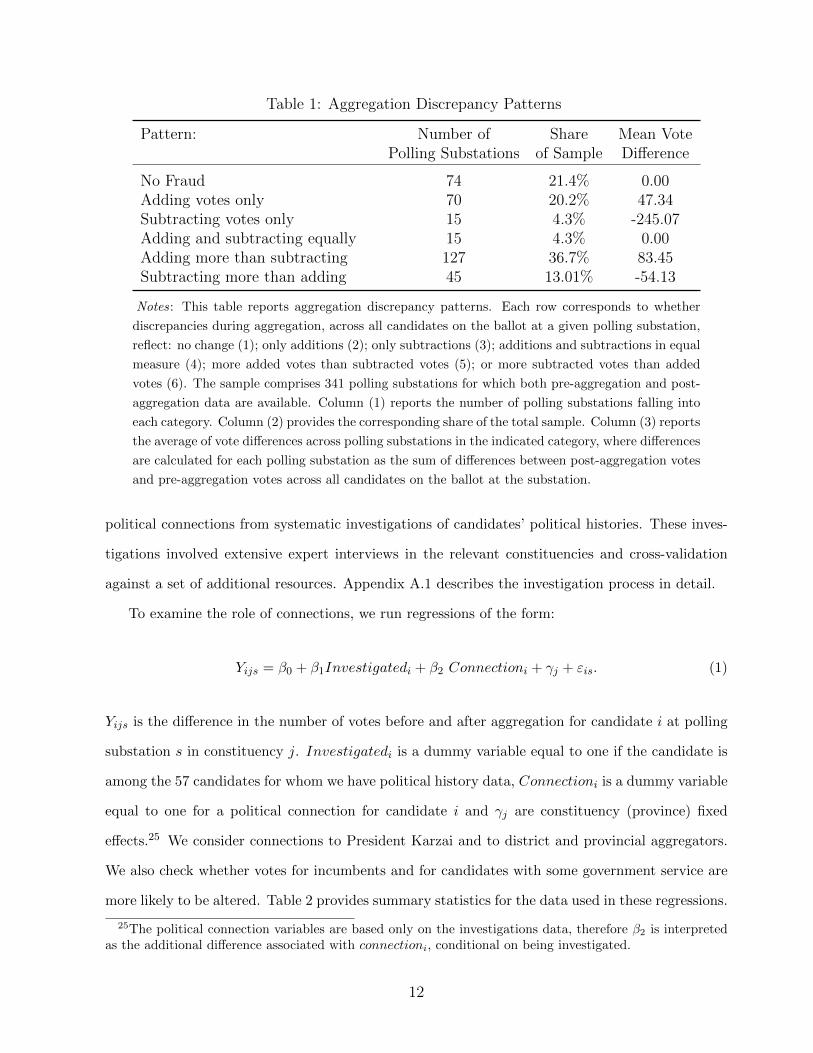
Table 1: Aggregation Discrepancy Patterns

Pattern: Number of Share Mean VotePolling Substations of Sample Difference

No Fraud 74 21.4% 0.00Adding votes only 70 20.2% 47.34Subtracting votes only 15 4.3% -245.07Adding and subtracting equally 15 4.3% 0.00Adding more than subtracting 127 36.7% 83.45Subtracting more than adding 45 13.01% -54.13

Notes: This table reports aggregation discrepancy patterns. Each row corresponds to whether

discrepancies during aggregation, across all candidates on the ballot at a given polling substation,

reflect: no change (1); only additions (2); only subtractions (3); additions and subtractions in equal

measure (4); more added votes than subtracted votes (5); or more subtracted votes than added

votes (6). The sample comprises 341 polling substations for which both pre-aggregation and post-

aggregation data are available. Column (1) reports the number of polling substations falling into

each category. Column (2) provides the corresponding share of the total sample. Column (3) reports

the average of vote differences across polling substations in the indicated category, where differences

are calculated for each polling substation as the sum of differences between post-aggregation votes

and pre-aggregation votes across all candidates on the ballot at the substation.

political connections from systematic investigations of candidates’ political histories. These inves-

tigations involved extensive expert interviews in the relevant constituencies and cross-validation

against a set of additional resources. Appendix A.1 describes the investigation process in detail.

To examine the role of connections, we run regressions of the form:

Yijs = β0 + β1Investigatedi + β2 Connectioni + γj + εis. (1)

Yijs is the difference in the number of votes before and after aggregation for candidate i at polling

substation s in constituency j. Investigatedi is a dummy variable equal to one if the candidate is

among the 57 candidates for whom we have political history data, Connectioni is a dummy variable

equal to one for a political connection for candidate i and γj are constituency (province) fixed

effects.25 We consider connections to President Karzai and to district and provincial aggregators.

We also check whether votes for incumbents and for candidates with some government service are

more likely to be altered. Table 2 provides summary statistics for the data used in these regressions.

25The political connection variables are based only on the investigations data, therefore β2 is interpretedas the additional difference associated with connectioni, conditional on being investigated.

12

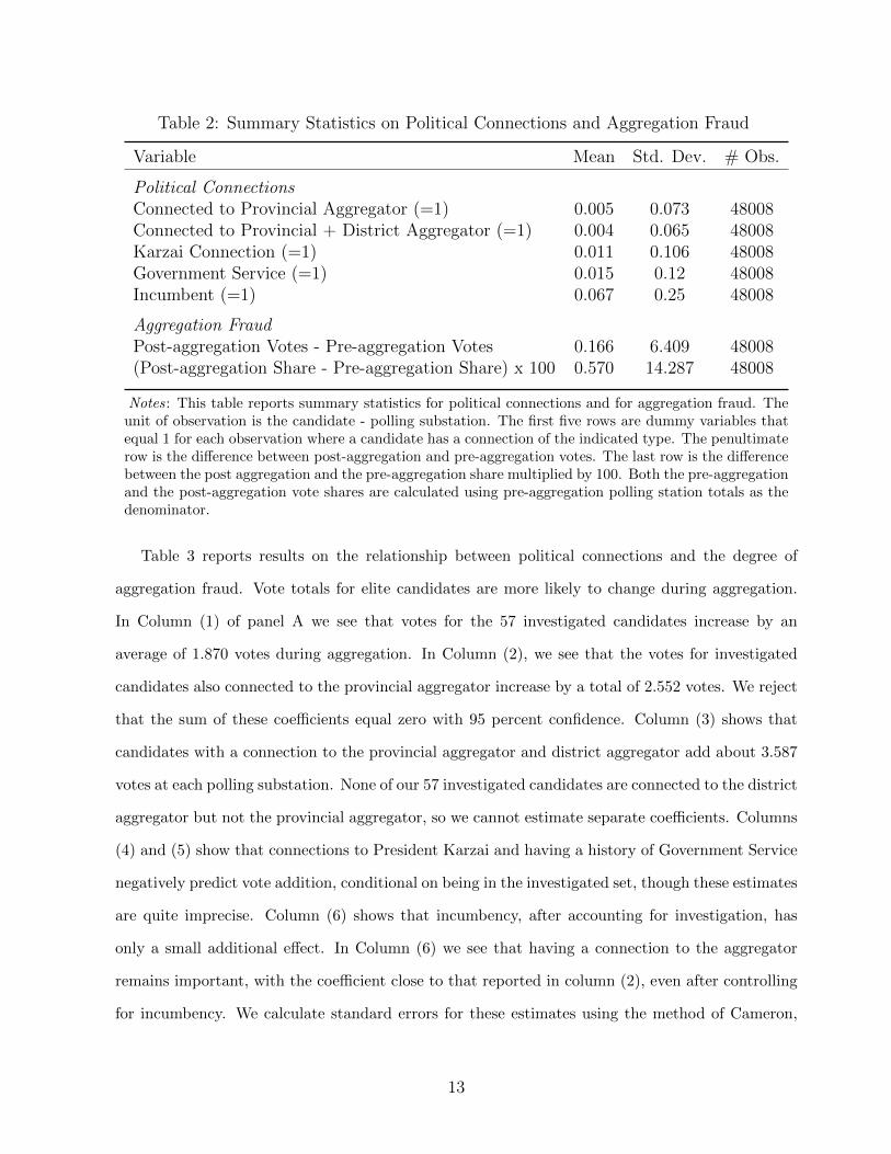
Table 2: Summary Statistics on Political Connections and Aggregation Fraud

Variable Mean Std. Dev. # Obs.

Political ConnectionsConnected to Provincial Aggregator (=1) 0.005 0.073 48008Connected to Provincial + District Aggregator (=1) 0.004 0.065 48008Karzai Connection (=1) 0.011 0.106 48008Government Service (=1) 0.015 0.12 48008Incumbent (=1) 0.067 0.25 48008

Aggregation FraudPost-aggregation Votes - Pre-aggregation Votes 0.166 6.409 48008(Post-aggregation Share - Pre-aggregation Share) x 100 0.570 14.287 48008

Notes: This table reports summary statistics for political connections and for aggregation fraud. Theunit of observation is the candidate - polling substation. The first five rows are dummy variables thatequal 1 for each observation where a candidate has a connection of the indicated type. The penultimaterow is the difference between post-aggregation and pre-aggregation votes. The last row is the differencebetween the post aggregation and the pre-aggregation share multiplied by 100. Both the pre-aggregationand the post-aggregation vote shares are calculated using pre-aggregation polling station totals as thedenominator.

Table 3 reports results on the relationship between political connections and the degree of

aggregation fraud. Vote totals for elite candidates are more likely to change during aggregation.

In Column (1) of panel A we see that votes for the 57 investigated candidates increase by an

average of 1.870 votes during aggregation. In Column (2), we see that the votes for investigated

candidates also connected to the provincial aggregator increase by a total of 2.552 votes. We reject

that the sum of these coefficients equal zero with 95 percent confidence. Column (3) shows that

candidates with a connection to the provincial aggregator and district aggregator add about 3.587

votes at each polling substation. None of our 57 investigated candidates are connected to the district

aggregator but not the provincial aggregator, so we cannot estimate separate coefficients. Columns

(4) and (5) show that connections to President Karzai and having a history of Government Service

negatively predict vote addition, conditional on being in the investigated set, though these estimates

are quite imprecise. Column (6) shows that incumbency, after accounting for investigation, has

only a small additional effect. In Column (6) we see that having a connection to the aggregator

remains important, with the coefficient close to that reported in column (2), even after controlling

for incumbency. We calculate standard errors for these estimates using the method of Cameron,

13

Table 3: Vote Changes During Aggregation by Candidate Type

Dependent Variable: Post-aggregation Votes - Pre-aggregation VotesPanel A - Votes (1) (2) (3) (4) (5) (6) (7)

Investigated (=1) 1.870* 1.610 1.380 2.328 3.149** 1.764* 3.385**(0.980) (1.208) (1.176) (2.169) (1.415) (1.013) (1.713)

Provincial Aggregator Connection (=1) 0.942(1.651)

Prov. + District Aggregator Connection (=1) 2.207 2.553(1.848) (1.807)

Karzai Connect. (=1) -0.745 -1.005(2.216) (2.153)

Government Service (=1) -1.634 -2.038(1.918) (1.996)

Incumbent (=1) 0.245 0.302(0.238) (0.226)

Constant 0.104*** 0.105*** 0.106*** 0.105*** 0.105*** 0.094** 0.096***(0.037) (0.037) (0.037) (0.036) (0.037) (0.037) (0.037)

R-Squared 0.013 0.013 0.014 0.013 0.013 0.013 0.015# Candidates 1783 1783 1783 1783 1783 1783 1783#Polling Stations 149 149 149 149 149 149 149# Candidate - Polling Station Observations 48008 48008 48008 48008 48008 48008 48008Connection(s) + Investigated = 0 (p-value) 0.056 0.038 0.009 0.029 0.212 0.035 0.032Mean for Candidates Not Investigated 0.131 0.131 0.131 0.131 0.131 0.131 0.131

Dependent Variable: (Post-aggregation Share - Pre-aggregation Share) x 100Panel B - Vote Shares (1) (2) (3) (4) (5) (6) (7)

Investigated (=1) 2.978** 3.069* 2.905* 2.054* 0.756 2.928** 0.051(1.316) (1.708) (1.588) (1.208) (0.864) (1.330) (1.271)

Provincial Aggregator Connection (=1) -0.325(1.810)

Prov. + District Aggregator Connection (=1) 0.328 -0.215(1.828) (2.005)

Karzai Connect. (=1) 1.500 1.343(1.227) (1.263)

Government Service (=1) 2.838 2.744(2.263) (2.486)

Incumbent (=1) 0.115 -0.000(0.198) (0.207)

Constant 0.247* 0.247* 0.248* 0.246* 0.246* 0.243* 0.244*(0.132) (0.132) (0.132) (0.132) (0.132) (0.131) (0.131)

R-Squared 0.008 0.009 0.009 0.009 0.009 0.009 0.009# Candidates 1784 1784 1784 1784 1784 1784 1784#Polling Stations 149 149 149 149 149 149 149# Candidate - Polling Station Observations 48008 48008 48008 48008 48008 48008 48008Connection(s) + Investigated = 0 (p-value) 0.024 0.008 0.009 0.024 0.042 0.020 0.003Mean for Candidates Not Investigated 0.503 0.503 0.503 0.503 0.503 0.503 0.503

Notes: This table reports on political connections and the degree of aggregation fraud. The unit of observation is the candidate - polling substation.Each column in Panel A reports results from an OLS regression using the difference between post-aggregation and pre-aggregation votes as thedependent variable and a dummy variable that equals one if a candidate - polling substation observation records the indicated connection(s) as anindependent variable and an additional dummy that equals one if that observation has any background investigation data. Note that we observeconnections only for investigated candidates. Panel B repeats these specifications using the difference between pre-aggregation and post-aggregationvote shares (multiplied by 100) as a dependent variable. Both pre-aggregation and post-aggregation vote shares are calculated using pre-electionpolling station vote totals as the denominator. All specifications in both panels include province fixed effects and drop the five largest and fivesmallest observations of the dependent variable. No candidates record a connection to the district aggregator and not to the provincial aggregatorso these coefficients cannot be estimated separately. Sample: treatment and control polling centers for which complete vote difference data areavailable. Table A7 reports corresponding results for the control sample only. Levels of significance: *p < 0.1, **p < 0.05, ***p < 0.01. Standarderrors clustered by candidate and by polling center using the method of Cameron, Gelbach and Miller (2011) are reported in parentheses.

14

Gelbach and Miller (2011), which allows for arbitrary correlation for a given candidate across polling

centers and across candidates within a given polling center.26

Panel B repeats this analysis replacing the dependent variable with the change in vote shares

during aggregation.27 Being in the set of elite candidates with a political history investigation

predicts the a roughly 3 percent increase in vote share across specifications. To provide a sense of

the magnitude, if a candidate moved from a 0.5 percent vote share (the mean among un-investigated

candidates) to a 3.5 percent vote share, they would move from the seventh percentile to the 79th

percentile of candidates receiving positive votes.28

While there is evidence that political strength predicts adding votes during aggregation, we

treat this exercise speculatively for three reasons. First, we have data on connections only for

the most powerful candidates. Political power is likely to be highly asymmetrically distributed

across candidates and is concentrated in the subsample of 57 that we observe, making it difficult to

determine precisely which type of connection is most important for rigging an election.29 Second,

connections are likely correlated with other candidate attributes that facilitate fraud, and we observe

only a very limited number of candidate characteristics making it difficult to rule out omitted

variables. Last, we omit the five largest and smallest observations off the left-hand side variable.

These results are robust to dropping all but the three most negative observations, which are all

at least 28.5 standard deviations away from the mean, but break down if these three outliers are

included.

Our results, to this point, are based on a comparison of independent photographic records of

election returns forms prior to aggregation and ex post results.30 This approach uncovers a type of

26In this case, these standard errors are more conservative than those clustered only at the candidate oronly at the polling substation level.

27For both the pre-aggregation and post-aggregation vote share, we normalize votes by the total numberof votes cast at the substation prior to election. We do this to isolate vote changes that are sure to benefitthe candidate in question.

28On average, there are 483 candidates listed at each of the polling substations in our sample and 93candidates listed if we exclude Kabul from the sample. At a given polling substation, on average 267.701votes are cast (standard deviation = 175.410). Excluding Kabul from the sample, on average 293.683 votesare cast (standard deviation = 178.285).

29Table A6 reports regressions of vote changes during aggregation on specific connections only within thesample of investigated candidates.

30This design builds on Parallel Vote Tabulations (PVTs), which have been in use since the 1980s. Throughrepresentative sampling and recording of ballots by field staff, PVTs predict national totals within a smallmargin of error (Cowan, Estok and Nevitte 2002), but do not make polling center specific comparisons. Two

15

fraud which is usually largely hidden, suggesting that it might also be used to deter manipulation.

We now turn from a descriptive analysis of the dynamics of aggregation fraud to an examination

of whether awareness of photo quick count can be used to reduce fraud.

4 Experiment

This section reports results from an experiment that randomly informed election officials about

photo quick count measurements in order to assess potential impacts on fraud. This section de-

scribes the experimental setting, the information intervention used to manipulate the awareness of

polling officials, and provides details of our treatment assignment protocol. Section 5 describes our

measures of election fraud and provides results.

4.1 Experimental Setting

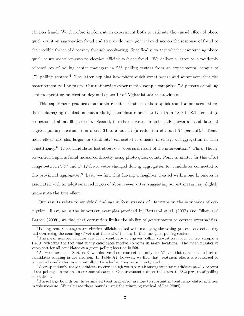
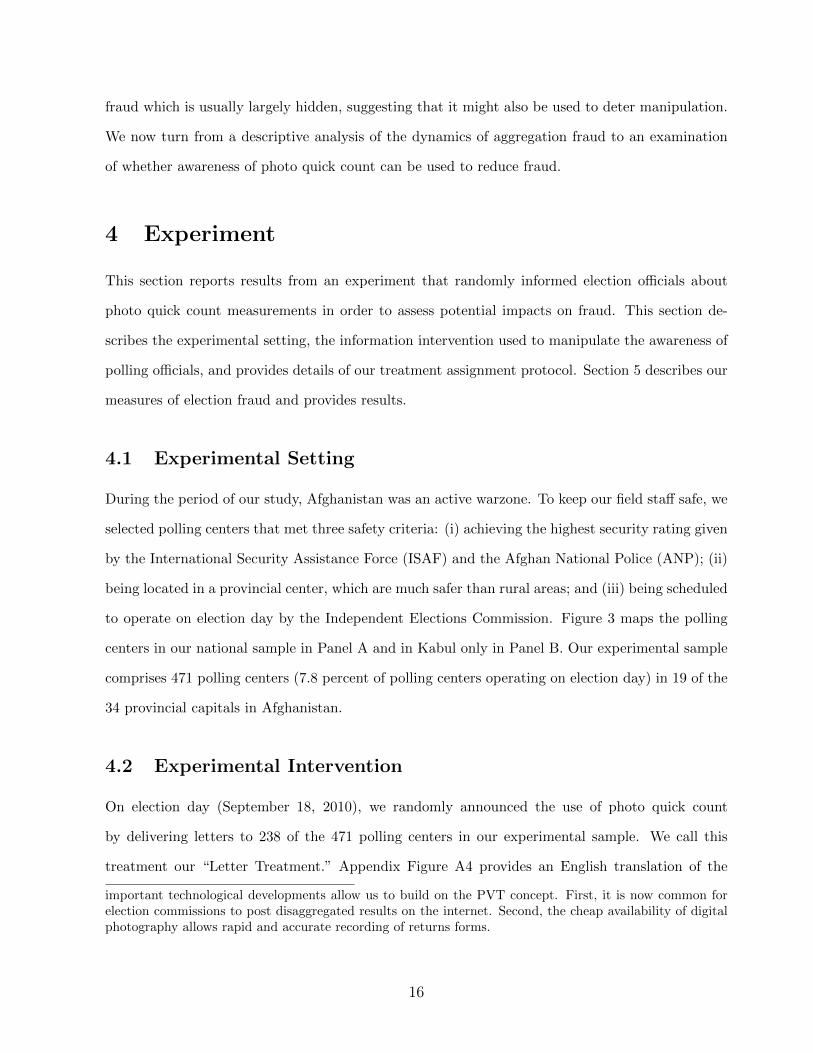
During the period of our study, Afghanistan was an active warzone. To keep our field staff safe, we

selected polling centers that met three safety criteria: (i) achieving the highest security rating given

by the International Security Assistance Force (ISAF) and the Afghan National Police (ANP); (ii)

being located in a provincial center, which are much safer than rural areas; and (iii) being scheduled

to operate on election day by the Independent Elections Commission. Figure 3 maps the polling

centers in our national sample in Panel A and in Kabul only in Panel B. Our experimental sample

comprises 471 polling centers (7.8 percent of polling centers operating on election day) in 19 of the

34 provincial capitals in Afghanistan.

4.2 Experimental Intervention

On election day (September 18, 2010), we randomly announced the use of photo quick count

by delivering letters to 238 of the 471 polling centers in our experimental sample. We call this

treatment our “Letter Treatment.” Appendix Figure A4 provides an English translation of the

important technological developments allow us to build on the PVT concept. First, it is now common forelection commissions to post disaggregated results on the internet. Second, the cheap availability of digitalphotography allows rapid and accurate recording of returns forms.

16

Panel A: National Sample Panel B: Kabul Subsample

Figure 3: Experimental Sample of Polling Centers

letter and Appendix Figure A5 provides the Dari translation. We instructed our Afghan field staff

to deliver letters to Polling Center Managers after 10AM and before polling concluded at 4PM.

Staff visited all 471 polling centers the following day in order to take a picture of the election

returns form.31

The letter announced to Polling Center Managers that researchers would photograph declara-

tion of results forms the following day (September 19) in order to document discrepancies arising

during aggregation. Two points about the experimental protocol bear emphasis. First, if we had not

notified managers of monitoring on election day, they would have been unaware of our treatment as

no election staff should be present at the polling center on the day after the election. Correspond-

ingly, our staff report encountering election officials while they were taking photographs on the day

following the election at only 2 of our 471 polling centers. Second, the experimental sample was

known only to the research team. Polling Center Managers in the treatment group were informed

of their status, but no election officials had a means of determining which sites we had selected as

controls.

We asked Polling Center Managers to acknowledge receipt by signing the letter. Managers at

seventeen polling centers (seven percent of centers receiving letters) refused to sign. We designate

31Declaration of Returns forms were posted at the conclusion of the count around 9PM on election day.We determined that keeping our field staff out this late was unsafe and so we instructed them to return thefollowing morning.

17

a polling center as treated if the manager received a letter (Letter Treatment = 1). Our results

remain robust to redefining treatment as both receiving and signing a letter.

4.3 Assigning Treatment

To inform our treatment assignment, we fielded a baseline survey of households living in the imme-

diate vicinity of 450 of the polling centers in our experimental sample a month before the election

(August 2010). On election day, we added 21 polling centers in Kabul after obtaining additional

funding.32 We do not have baseline survey data for these 21 polling centers and so place them all

in a single strata when assigning treatment.33

To ensure balance, we stratify treatment on province. In the 450 polling centers for which we

have baseline data, we also stratify on the share of respondents from the baseline survey reporting

at least occasional access to electricity and on respondents reporting that the district governor

carries the most responsibility for keeping elections fair. We estimate all core specifications both

with and without stratum fixed effects.34 Table 4 reports summary statistics and verifies balance

and Table A5 provides summary statistics for the remaining variables used in the analysis.35

5 Data and Results

We examine the impact of announcing photo quick count on four outcomes. The first is the direct

aggregation fraud measure discussed in Section 3, which we construct as the absolute value of

the difference between votes before and after the aggregation process. This measure is subject to

substantial non-random attrition, potentially biasing our estimated treatment effect. We therefore

32The survey contained 2,904 respondents. To attempt to obtain a representative sample of respondentsliving near polling centers, enumerators employed a random walk pattern starting at the polling center, withrandom selection of every fourth house or structure. Respondents within households are randomly selectedusing Kish grid. The survey had 50 percent male and female respondents each and enumerators conductedinterviews in either Dari or Pashto.

33An alternative is to drop these 21 polling centers from specifications with district fixed effects reflectingthe lack of baseline survey data to stratify them on. Results are robust to this change.

34Bruhn and McKenzie (2009) suggest stratifying treatment assignment on baseline measurements of keyoutcomes to increase power. Because measures of fraud are unavailable prior to the election, we select ourstratifying variables by identifying measures most highly correlated with fraud during the 2009 presidentialelection in a national sample.

35Estimates in column (1) of Table 7 additionally indicate that treatment did not affect turnout.

18

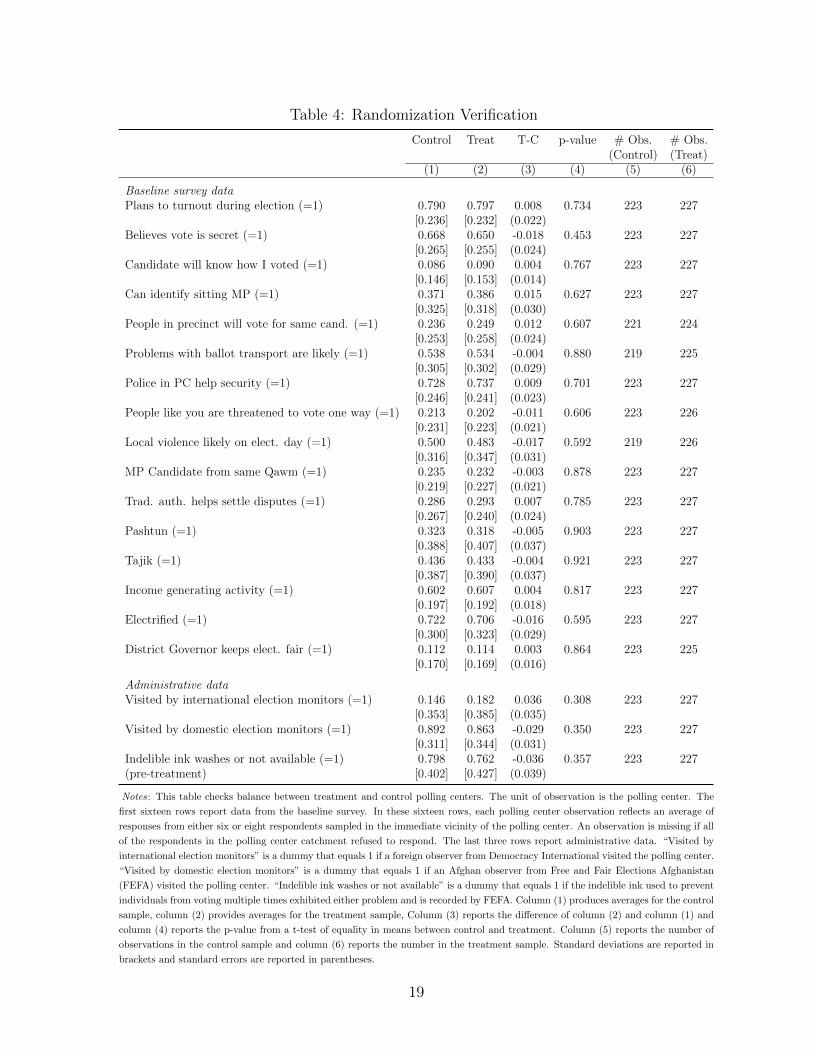
Table 4: Randomization Verification

Control Treat T-C p-value # Obs. # Obs.(Control) (Treat)

(1) (2) (3) (4) (5) (6)

Baseline survey dataPlans to turnout during election (=1) 0.790 0.797 0.008 0.734 223 227

[0.236] [0.232] (0.022)Believes vote is secret (=1) 0.668 0.650 -0.018 0.453 223 227

[0.265] [0.255] (0.024)Candidate will know how I voted (=1) 0.086 0.090 0.004 0.767 223 227

[0.146] [0.153] (0.014)Can identify sitting MP (=1) 0.371 0.386 0.015 0.627 223 227

[0.325] [0.318] (0.030)People in precinct will vote for same cand. (=1) 0.236 0.249 0.012 0.607 221 224

[0.253] [0.258] (0.024)Problems with ballot transport are likely (=1) 0.538 0.534 -0.004 0.880 219 225

[0.305] [0.302] (0.029)Police in PC help security (=1) 0.728 0.737 0.009 0.701 223 227

[0.246] [0.241] (0.023)People like you are threatened to vote one way (=1) 0.213 0.202 -0.011 0.606 223 226

[0.231] [0.223] (0.021)Local violence likely on elect. day (=1) 0.500 0.483 -0.017 0.592 219 226

[0.316] [0.347] (0.031)MP Candidate from same Qawm (=1) 0.235 0.232 -0.003 0.878 223 227

[0.219] [0.227] (0.021)Trad. auth. helps settle disputes (=1) 0.286 0.293 0.007 0.785 223 227

[0.267] [0.240] (0.024)Pashtun (=1) 0.323 0.318 -0.005 0.903 223 227

[0.388] [0.407] (0.037)Tajik (=1) 0.436 0.433 -0.004 0.921 223 227

[0.387] [0.390] (0.037)Income generating activity (=1) 0.602 0.607 0.004 0.817 223 227

[0.197] [0.192] (0.018)Electrified (=1) 0.722 0.706 -0.016 0.595 223 227

[0.300] [0.323] (0.029)District Governor keeps elect. fair (=1) 0.112 0.114 0.003 0.864 223 225

[0.170] [0.169] (0.016)

Administrative dataVisited by international election monitors (=1) 0.146 0.182 0.036 0.308 223 227

[0.353] [0.385] (0.035)Visited by domestic election monitors (=1) 0.892 0.863 -0.029 0.350 223 227

[0.311] [0.344] (0.031)Indelible ink washes or not available (=1) 0.798 0.762 -0.036 0.357 223 227(pre-treatment) [0.402] [0.427] (0.039)

Notes: This table checks balance between treatment and control polling centers. The unit of observation is the polling center. The

first sixteen rows report data from the baseline survey. In these sixteen rows, each polling center observation reflects an average of

responses from either six or eight respondents sampled in the immediate vicinity of the polling center. An observation is missing if all

of the respondents in the polling center catchment refused to respond. The last three rows report administrative data. “Visited by

international election monitors” is a dummy that equals 1 if a foreign observer from Democracy International visited the polling center.

“Visited by domestic election monitors” is a dummy that equals 1 if an Afghan observer from Free and Fair Elections Afghanistan

(FEFA) visited the polling center. “Indelible ink washes or not available” is a dummy that equals 1 if the indelible ink used to prevent

individuals from voting multiple times exhibited either problem and is recorded by FEFA. Column (1) produces averages for the control

sample, column (2) provides averages for the treatment sample, Column (3) reports the difference of column (2) and column (1) and

column (4) reports the p-value from a t-test of equality in means between control and treatment. Column (5) reports the number of

observations in the control sample and column (6) reports the number in the treatment sample. Standard deviations are reported in

brackets and standard errors are reported in parentheses.

19

rely on three additional proxy measures less subject to this concern: (i) the number of votes cast

for elite candidates; (ii) a dummy variable that equals 1 in every case where a candidate records

enough votes to rank among the winning candidates at the polling substation, which we report in

Appendix A.2; and (iii) primary reports that materials were stolen or damaged by local candidate

representatives.36

5.1 Aggregation Fraud

The purpose of our treatment was to provide incentives to election officials to ensure that no

discrepancies arose during aggregation. Given this objective and our finding in Section 3 that

votes are both commonly added and subtracted, we examine impacts on the absolute value of vote

differences between pre-aggregation and post-aggregation vote totals.37 This measure exhibited a

large degree of treatment-related attrition. We turn to a discussion of how we address this issue in

our analysis.

Addressing Attrition

Treatment significantly increased the availability of photographic records (p = 0.064), potentially

biasing mean difference estimators of the treatment effect.38 In general, with substantial treatment-

related attrition, the effect of treatment on fraud will be confounded with its effect on the availability

of photographic records. The mean difference may only reflect treatment revealing an additional

part of the fraud distribution, while there is no actual effect on the outcome of interest. To address

this, we use the method provided in Lee (2009), which estimates bounds on the effect of treatment

in the presence of non-random attrition. The purpose of this method is to trim observations that

36The number of votes cast for elite candidates is available for 461 of our 471 polling centers. Baselinecovariates are not available for 21 of the 461 polling centers with vote outcome data. Specifications aretherefore estimated on samples corresponding to 461 polling centers when control variables are not includedand 440 when control variables are included. Specifications in Table 9 are estimated on one less polling centerwhich we drop when trimming the top percentile of results. Only one polling center is dropped (rather thanfour), because there can be several powerful candidates in a given polling center.

37In Appendix A.4 we provide evidence that both vote additions and subtractions are especially large forpowerful candidates, motivating our use of the absolute value measure for these subsamples.

38We collected pictures of 204 (20 percent) of the 1,020 Declarations of Results forms that should havebeen posted at treatment polling centers and 143 (14.77 percent) of the 968 forms that should have beenposted at control polling centers. The treatment effect is therefore -0.052 (standard error = 0.028).

20

report outcomes only under treatment from the estimation sample, allowing impacts to be estimated

using only units where outcomes would be observed irrespective of treatment assignment.39

This method relies fundamentally on the monotonicity assumption.40 In this setting, there

are two ways that the attrition process could be monotonic. Both regard polling officials who

would post Declarations of Results forms under treatment, but not otherwise. In the first instance,

these marginal officials might respond to the treatment notification letter by posting results only in

cases when doing so does not reveal fraud during the aggregation process. This would imply that

trimming the corresponding marginal polling substations from the bottom of the treatment sample

would provide the correct estimate. In the second, these officials might respond to treatment by

posting results only in locations where there is substantial fraud.41 In this case, trimming the

corresponding portion at the top of the treatment distribution would provide the correct estimate.

An intermediate scenario would arise if low-level polling center managers are unaware of aggregation

fraud that takes place later in the aggregation process. In this case, the true effect would lie between

the two bounds.

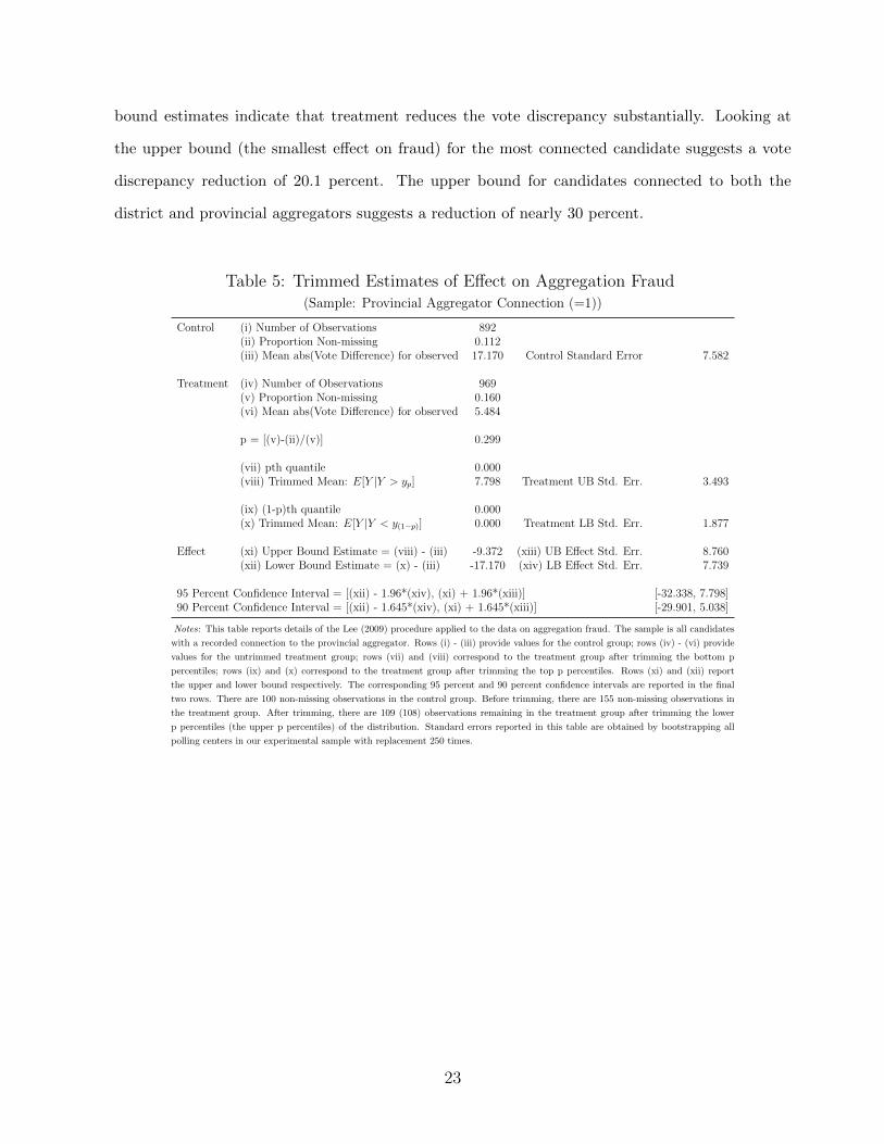
To illustrate this method, Table 5 applies the method to the absolute vote difference for can-

didates connected to the provincial aggregator. Of the 892 polling substations where we could

potentially observe this measure in our control sample, we successfully measure 100 (11.2 percent).

In this sample, the average absolute vote difference is 17.170. Turning to our treatment sample,

there are 969 potential observations, of which we successfully measure 155 (16 percent). In this

sample, the average absolute vote difference is 5.484.

To bound the treatment effect, we remove the part of the treatment group induced to reveal

outcomes by treatment. We calculate the share to remove, the “trimming ratio”, as 16%−11.2%16% =

29.9%. Under the monotonicity assumption, we can estimate the upper bound of the treatment

effect (i.e. the smallest fraud reducing effect) by removing the bottom 29.9 percentiles in terms of

39These estimands are therefore different from the average treatment effect across the entire experimentalsample. We point interested readers to the Gerber and Green (2012) text, which provides a clear descriptionof the Lee (2009) method.

40Let ri(T ) denote whether an outcome is reported as a function of treatment status (T ∈ {0, 1}). Whenri(T ) = 1 the outcome is observed and when ri(T ) = 0 it is not. The monotonicity assumption statesri(1) ≥ ri(0) or ri(1) ≤ ri(0) for all i.

41This could happen if polling center managers in the most fraud-affected polling centers are not afraid ofrevealing fraud.

21

absolute vote differences from the treatment sample and taking the difference between the trimmed

treatment mean and the control mean. This yields an estimate of 7.798 - 17.170 = -9.372 votes. To

obtain the lower bound of the treatment effect (i.e. the largest fraud reducing effect), we remove

the top 29.9 percentiles in terms of absolute vote differences. This yields an estimate of 0 - 17.170

= -17.170 votes.42

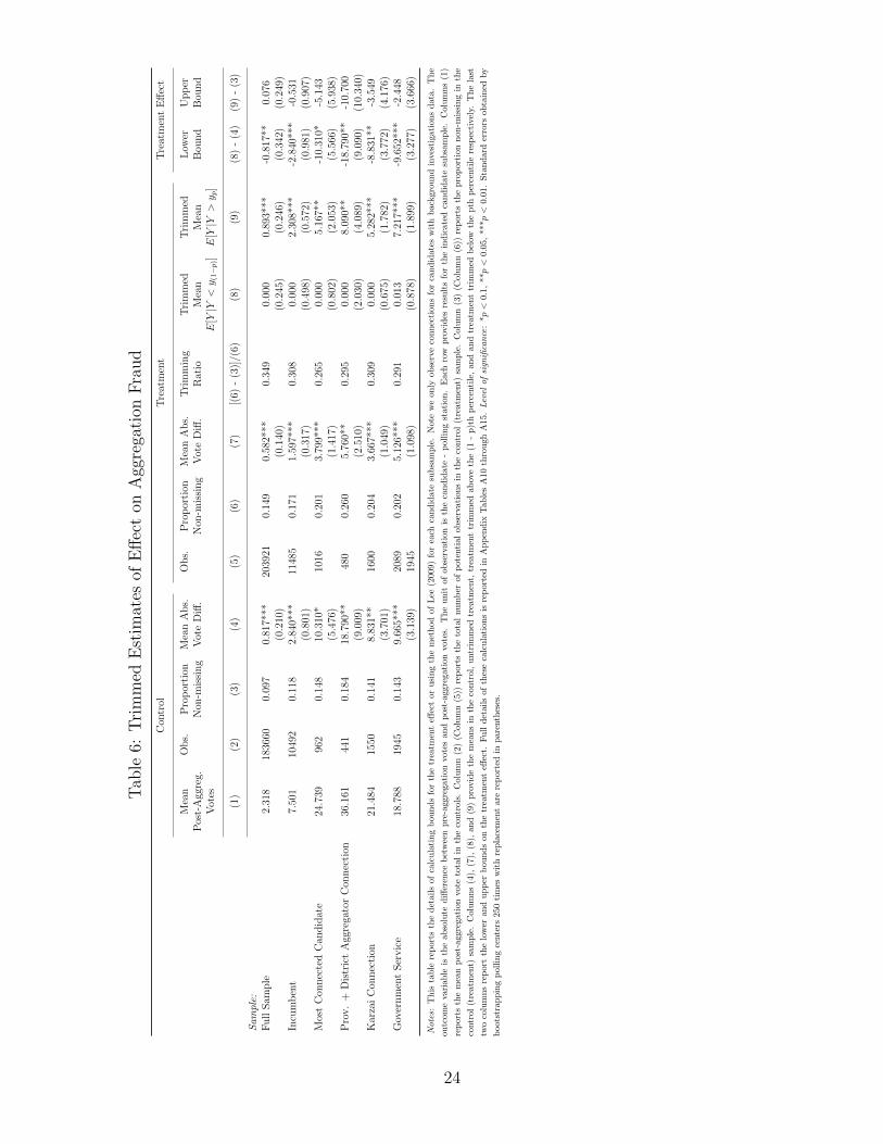
Table 6 summarizes estimates from the same exercise performed on the full sample, and for

each of the remaining five candidate type subsamples.43 To provide a basis of comparison for the

estimated effect sizes, column (1) reports the mean post-aggregation vote-total across candidate-

polling substations for the controlling polling substations within the candidate subsample. Columns

(2) and (3) report the number of observations that would be observed in the control sample with

complete data and the non-missing proportion, respectively. Column (4) reports the mean vote

difference in the observed control sample. These estimates are consistent with our finding in

Table 3 above that observations corresponding to connected candidates are more likely to exhibit

discrepancies. Columns (5) through (7) provide the analogues to columns (2) through (4) for

the treatment sample. The next column provides the trimming ratio p. Column (8) provides the

trimmed mean in the control sample trimming above the (1−p)th percentile and column (9) reports

the trimmed mean eliminating the bottom p percentiles. The final two columns report the lower

bound and the upper bound, respectively. In eleven of the twelve cases, the estimated upper bound

is below zero. In no cases, however, can we statistically reject that the upper bound is different

from zero.

Using the post-aggregation total in column (1) as a point of reference, the upper and lower

42To construct confidence intervals, we estimate standard errors for both upper and lower bounds. Lee(2009) shows that the asymptotic variance of the trimming estimator depends on: (i) the variance of thetrimmed outcome variable; (ii) the trimming threshold value, which is a quantile that must be estimated;and (iii) the corresponding trimming ratio, which is also estimated. Lee (2009), provides expressions for theasymptotic standard errors only for the i.i.d. case. Our treatment is administered at the cluster (pollingcenter) level. Therefore, as in Vogl (forthcoming), we block-bootstrap the bounds estimator at the pollingcenter level.

43In Table A4, we perform the same exercise using the simple vote difference as an outcome. We findno evidence of a mean effect on this outcome. In Appendix A.4, we argue that this is because photo quickcount appears to reduce rigging both for and against powerful candidates in roughly equal measure. We alsoprovide evidence that the reason we find a post-aggregation reduction in Table 7 while finding no effect onvote differences may be because treatment affected the number of votes posted immediately after treatment.This is necessarily speculative because of the limited sample with vote difference data. Tables A10 throughA15 replicate Table 5 for each of the five remaining subsamples.

22

bound estimates indicate that treatment reduces the vote discrepancy substantially. Looking at

the upper bound (the smallest effect on fraud) for the most connected candidate suggests a vote

discrepancy reduction of 20.1 percent. The upper bound for candidates connected to both the

district and provincial aggregators suggests a reduction of nearly 30 percent.

Table 5: Trimmed Estimates of Effect on Aggregation Fraud(Sample: Provincial Aggregator Connection (=1))

Control (i) Number of Observations 892(ii) Proportion Non-missing 0.112(iii) Mean abs(Vote Difference) for observed 17.170 Control Standard Error 7.582

Treatment (iv) Number of Observations 969(v) Proportion Non-missing 0.160(vi) Mean abs(Vote Difference) for observed 5.484

p = [(v)-(ii)/(v)] 0.299

(vii) pth quantile 0.000(viii) Trimmed Mean: E[Y |Y > yp] 7.798 Treatment UB Std. Err. 3.493

(ix) (1-p)th quantile 0.000(x) Trimmed Mean: E[Y |Y < y(1−p)] 0.000 Treatment LB Std. Err. 1.877

Effect (xi) Upper Bound Estimate = (viii) - (iii) -9.372 (xiii) UB Effect Std. Err. 8.760(xii) Lower Bound Estimate = (x) - (iii) -17.170 (xiv) LB Effect Std. Err. 7.739

95 Percent Confidence Interval = [(xii) - 1.96*(xiv), (xi) + 1.96*(xiii)] [-32.338, 7.798]90 Percent Confidence Interval = [(xii) - 1.645*(xiv), (xi) + 1.645*(xiii)] [-29.901, 5.038]

Notes: This table reports details of the Lee (2009) procedure applied to the data on aggregation fraud. The sample is all candidates

with a recorded connection to the provincial aggregator. Rows (i) - (iii) provide values for the control group; rows (iv) - (vi) provide

values for the untrimmed treatment group; rows (vii) and (viii) correspond to the treatment group after trimming the bottom p

percentiles; rows (ix) and (x) correspond to the treatment group after trimming the top p percentiles. Rows (xi) and (xii) report

the upper and lower bound respectively. The corresponding 95 percent and 90 percent confidence intervals are reported in the final

two rows. There are 100 non-missing observations in the control group. Before trimming, there are 155 non-missing observations in

the treatment group. After trimming, there are 109 (108) observations remaining in the treatment group after trimming the lower

p percentiles (the upper p percentiles) of the distribution. Standard errors reported in this table are obtained by bootstrapping all

polling centers in our experimental sample with replacement 250 times.

23

Tab

le6:

Tri

mm

edE

stim

ates

ofE

ffec

ton

Agg

rega

tion

Fra

ud

Con

trol

Tre

atm

ent

Tre

atm

ent

Eff

ect

Mea

nO

bs.

Pro

por

tion

Mea

nA

bs.

Ob

s.P

rop

orti

onM

ean

Ab

s.T

rim

min

gT

rim

med

Tri

mm

edL

ower

Up

per

Pos

t-A

ggre

g.N

on-m

issi

ng

Vot

eD

iff.

Non

-mis

sin

gV

ote

Diff

.R

atio

Mea

nM

ean

Bou

nd

Bou

nd

Vot

esE

[Y|Y

<y (

1−p)]

E[Y|Y

>y p

]

(1)

(2)

(3)

(4)

(5)

(6)

(7)

[(6)

-(3

)]/(

6)(8

)(9

)(8

)-

(4)

(9)

-(3

)

Sam

ple:

Fu

llS

amp

le2.

318

1836

600.

097

0.81

7***

2039

210.

149

0.58

2***

0.34

90.

000

0.89

3***

-0.8

17**

0.07

6(0

.210

)(0

.140

)(0

.245

)(0

.246

)(0

.342

)(0

.249

)In

cum

ben

t7.

501

1049

20.

118

2.84

0***

1148

50.

171

1.59

7***

0.30

80.

000

2.30

8***

-2.8

40**

*-0

.531

(0.8

01)

(0.3

17)

(0.4

98)

(0.5

72)

(0.9

81)

(0.9

07)

Mos

tC

onn

ecte

dC

and

idat

e24

.739

962

0.14

810

.310

*10

160.

201

3.79

9***

0.26

50.

000

5.16

7**

-10.

310*

-5.1

43(5

.476

)(1

.417

)(0

.802

)(2

.053

)(5

.566

)(5

.938

)P

rov.

+D

istr

ict

Agg

rega

tor

Con

nec

tion

36.1

6144

10.

184

18.7

90**

480

0.26

05.

760*

*0.

295

0.00

08.

090*

*-1

8.79

0**

-10.

700

(9.0

09)

(2.5

10)

(2.0

30)

(4.0

89)

(9.0

90)

(10.

340)

Kar

zai

Con

nec

tion

21.4

8415

500.

141

8.83

1**

1600

0.20

43.

667*

**0.

309

0.00

05.

282*

**-8

.831

**-3

.549

(3.7

01)

(1.0

49)

(0.6

75)

(1.7

82)

(3.7

72)

(4.1

76)

Gov

ernm

ent

Ser

vic

e18

.788

1945

0.14

39.

665*

**20

890.

202

5.12

6***

0.29

10.

013

7.21

7***

-9.6

52**

*-2

.448

(3.1

39)

1945

(1.0

98)

(0.8

78)

(1.8

99)

(3.2

77)

(3.6

66)

Note

s:T

his

tab

lere

port

sth

ed

etai

lsof

calc

ula

tin

gb

oun

ds

for

the

trea

tmen

teff

ect

or

usi

ng

the

met

hod

of

Lee

(2009)

for

each

can

did

ate

sub

sam

ple

.N

ote

we

on

lyob

serv

eco

nn

ecti

on

sfo

rca

nd

idate

sw

ith

back

gro

un

din

vest

igati

on

sd

ata

.T

he

ou

tcom

eva

riab

leis

the

abso

lute

diff

eren

ceb

etw

een

pre

-agg

rega

tion

vote

san

dp

ost

-aggre

gati

on

vote

s.T

he

un

itof

obse

rvati

on

isth

eca

nd

idate

-p

oll

ing

stati

on.

Each

row

pro

vid

esre

sult

sfo

rth

ein

dic

ate

dca

nd

idate

sub

sam

ple

.C

olu

mn

s(1

)

rep

orts

the

mea

np

ost-

aggr

egat

ion

vote

tota

lin

the

contr

ols.

Col

um

n(2

)(C

olu

mn

(5))

rep

ort

sth

eto

tal

nu

mb

erof

pote

nti

al

ob

serv

ati

on

sin

the

contr

ol

(tre

atm

ent)

sam

ple

.C

olu

mn

(3)

(Colu

mn

(6))

rep

ort

sth

ep

rop

ort

ion

non

-mis

sin

gin

the

contr

ol

(tre

atm

ent)

sam

ple

.C

olu

mn

s(4

),(7

),(8

),an

d(9

)p

rovid

eth

em

ean

sin

the

contr

ol,

untr

imm

edtr

eatm

ent,

trea

tmen

ttr

imm

edab

ove

the

(1-

p)t

hp

erce

nti

le,

an

dan

dtr

eatm

ent

trim

med

bel

owth

ep

thp

erce

nti

lere

spec

tivel

y.T

he

last

two

colu

mn

sre

por

tth

elo

wer

and

up

per

bou

nd

son

the

trea

tmen

teff

ect.

Fu

lld

etail

sof

thes

eca

lcu

lati

ons

isre

port

edin

Ap

pen

dix

Tab

les

A10

thro

ugh

A15.

Lev

elof

sign

ifica

nce

:*p<

0.1,

**p

<0.

05,

***p

<0.0

1.

Sta

nd

ard

erro

rsob

tain

edby

boot

stra

pp

ing

pol

lin

gce

nte

rs25

0ti

mes

wit

hre

pla

cem

ent

are

rep

orte

din

pare

nth

eses

.

24

5.2 Votes for Elite Candidates:

We next estimate the impact of photo quick count on votes for elite candidates. This measure has

the benefit of much less treatment-related attrition, but provides a less precise reflection of fraud

than our picture-based measure.44 We obtained data on votes disaggregated by candidate and

polling substation from a scrape of the election commission website on October 24, 2010. During

the scrape, 98 of the 1,977 polling substations in our experimental sample (4.96 percent) had not

yet posted returns. These 98 polling substations were contained within ten polling centers. Missing

data are not predicted by treatment status (p = 0.439).45

We run regressions of the form:

Yis = β1 + β2Treats + β3Treats ∗ Connectioni + β4Treats ∗ Investigatedi + β′7Xis + εis, (2)

where Yis is votes cast for candidate i in polling substation s, Connectioni is a dummy variable equal

to one for candidates with a specific type of political connection, Investigatedi is a dummy variable

equal to one for candidates with investigations data, and Xis is a matrix containing covariates from

our baseline survey, the Investigatedi and Connectedi dummies, and a set of stratum fixed effects.

To succinctly summarize impact, we also identify highly influential candidates using an index

based on our political connections data. We identify one elite candidate in each of the 19 political

constituencies by constructing the following index from the data on political connections described

in Section 3:

Indexi = Karzaii +Governmenti +DEOi + PEOi.

Karzaii equals 1 for a candidate i with an indirect connection to Karzai (e.g., through a relative)

and 2 for a direct connection (e.g., serving directly with the president), Governmenti equals 1 for

holding a minor government post since 2001 (e.g., teacher) and 2 for holding a major government

post (e.g., parliamentarian), DEOi equals 1 when connected to the District Elections Officer, and

44This approach follows the existing literature on the impact of election monitoring (Hyde 2007).45Regressions reported in Table 7 and 8 are estimated on a sample of 461 polling centers when control

variables are not included and 440 polling centers when control variables are included. The reason for thisis that we could not obtain voting outcomes for 10 of our 471 polling centers during the web scrape and welack control variables for an additional 21 polling centers.

25

PEOi equals 1 when connected to the Provincial Elections Officer. We term the candidate with

highest index score who is also among the top 10 vote recipients in control polling centers as

the“most connected candidate.” Figure A3 depicts average votes in treatment and control polling

centers for each type of candidate connection.

Column (1) Panel A of Table 7 reports the impact on treatment for all candidates, finding no

evidence of effect across all candidates. Columns (2) - (5) provide estimated effects from regressions

interacting treatment with an dummy variable equal to 1 for the most connected candidate using

several different specifications. For all of these specifications, we find that the most connected

candidate obtains about 17 to 20 votes at a given polling substation. In columns (2) - (4) we see

that treatment reduced votes for most connected candidates from an average of about 21 votes to

about 15 votes (a reduction of about 25 percent). Column (5) reports estimates trimming the top

percentile of votes for the interacted candidate type. The most connected candidates are typically

among the very highest vote recipients. We trim to ensure that our effects are not driven by a few

extreme outliers. Removing these observations both lowers the number of votes powerful candidates

received in controls and reduces the estimated treatment effect by about one vote, though effects

remain significant. As in column (1), there is no evidence of effect on the remaining candidates

without recorded connections. This provides some evidence that the effect is localized to elite

candidates, consistent with political connections playing a role in facilitating access to aggregation

fraud.

Panel B of Table 7 reports results from regressions interacting treatment with specific candidate

categories and a dummy for whether they are among the set of 57 candidates with background

investigations data. The point estimates suggest a negative effect for all investigated candidates.

The estimated joint effect of being investigated and having a connection are statistically different

from zero at the 95 percent level for candidates with a provincial aggregator connection in column

(1) and for candidates with a history of government service in column (3). As in Panel A, there

appears to be no effect on candidates without recorded connections and connected candidates obtain

higher vote totals.

To benchmark the size of the impacts estimated in Table 7, Section A.2 examines the impact

of treatment on whether candidates score enough votes at a given polling substation to be ranked

26

above the threshold required to obtain office in their constituency. Specifically, we estimate the

effect of treatment on a dummy variable that equals 1 for every candidate - polling substation

observation recording enough votes to rank among the winning candidates at the polling station.

The largest effects are for candidates connected to the provincial aggregator (column (2) of of Table

A2). These candidates have a 57 percent chance of ranking above the victory threshold in control

polling stations. Point estimates indicate that treatment reduced the probability of winning by 11.5

percentage points. The degree of the reduction suggests that, for powerful candidates, aggregation

fraud is severe enough to play a meaningful role in determining final election outcomes.

5.3 Theft and Damaging of Forms:

On the day after the election, our field staff visited all 471 operating polling centers in the ex-

perimental sample. During the visit, they attempted to photograph returns forms. If the forms

were missing, they investigated whether any of the materials had been stolen or damaged during

the night of the election.46 Investigations involved interviewing residents living in the immediate

vicinity of polling centers.47 In this section, we estimate impacts on forms reported as stolen or

damaged by candidate agents, who are candidate proxies legally permitted to observe polling and

are typically present at most polling centers in their candidate’s constituency. Candidate agents

are supporters of the candidate who play a crucial role assisting candidates at all stages of the

campaign. Candidate agents stole or damaged materials at 62 (13.16 percent) of the 471 operating

polling centers.

There are several reasons that stealing or damaging forms may reflect an intention to change vote

totals during aggregation. Records of citizen and candidate complaints provided by the Electoral

Complaints Commission indicate that the purpose of stealing forms was to take them to a separate

46These investigations produce 44 reports of candidate agents stealing the returns form along with theballot boxes and other election materials, 18 reports of candidate agents merely tearing down the returnsform, 15 reports of citizens stealing returns forms, 17 reports of citizens tearing down returns forms, and 28reports of security officials stealing materials or denying our interviewers access to photograph them.

47While election commission staff should have vacated the polling center at the end of election day, wetrained our staff to investigate by only interviewing local community members and not to engage commissionstaff so as to not create a measurement effect. While this would not affect the internal validity of our estimatesof program effect, our aim was to minimize the additional monitoring effect for the entire sample. Resultsobtained with these data merit some caution as our field staff could only rely on reports of nearby citizensto determine the reason that Declaration of Results forms are missing.

27

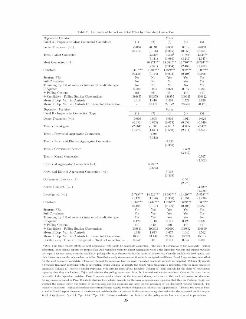
Table 7: Estimates of Impact on Total Votes by Candidate Connection

Dependent Variable: VotesPanel A - Impacts on Most Connected Candidates (1) (2) (3) (4) (5)

Letter Treatment (=1) -0.066 -0.034 0.030 0.019 -0.033(0.212) (0.196) (0.045) (0.056) (0.054)

Treat x Most Connected -5.430* -5.392* -5.780* -4.634**(3.111) (3.080) (3.245) (2.347)

Most Connected (=1) 20.871*** 18.604*** 19.746*** 16.794***(2.391) (2.364) (2.489) (1.787)

Constant 1.410*** 1.301*** 1.279*** 1.952*** 1.808***(0.156) (0.144) (0.032) (0.108) (0.106)

Stratum FEs No No Yes Yes YesFull Covariates No No No Yes YesTrimming top 1% of votes for interacted candidate type No No No No YesR-Squared 0.000 0.024 0.079 0.077 0.094# Polling Centers 461 461 461 440 440# Candidate - Polling Station Observations 386855 386855 386855 309947 309822Mean of Dep. Var. in Controls 1.410 1.410 1.410 1.724 1.629Mean of Dep. Var. in Controls for Interacted Connection - 22.172 22.172 23.516 20.170

Dependent Variable: VotesPanel B - Impacts by Connection Type (1) (2) (3) (4) (5)

Letter Treatment (=1) -0.010 0.005 0.010 -0.011 -0.029(0.052) (0.053) (0.053) (0.052) (0.049)

Treat x Investigated -2.864* -1.583 -2.831* -1.065 -2.472(1.473) (1.641) (1.680) (2.711) (1.851)

Treat x Provincial Aggregator Connection -4.896(3.312)

Treat x Prov. and District Aggregator Connection -3.293(4.368)

Treat x Government Service -2.399(3.142)

Treat x Karzai Connection 0.567(2.302)

Provincial Aggregator Connection (=1) 5.930**(2.635)

Prov. and District Aggregator Connection (=1) 5.168(3.539)

Government Service (=1) -0.541(2.276)

Karzai Connect. (=1) -3.323*(1.786)

Investigated (=1) 15.788*** 14.524*** 15.993*** 16.429*** 15.958***(1.122) (1.186) (1.300) (1.951) (1.436)

Constant 1.667*** 1.732*** 1.726*** 1.669*** 1.536***(0.105) (0.107) (0.106) (0.105) (0.097)

Stratum FEs Yes Yes Yes Yes YesFull Covariates Yes Yes Yes Yes YesTrimming top 1% of votes for interacted candidate type Yes Yes Yes Yes NoR-Squared 0.123 0.118 0.117 0.123 0.131# Polling Centers 440 440 440 440 440# Candidate - Polling Station Observations 309843 309893 309900 309852 309699Mean of Dep. Var. in Controls 1.639 1.673 1.677 1.646 1.562Mean of Dep. Var. in Controls for Interacted Connection 18.713 24.147 24.834 18.723 15.312P-Value - H0 : Treat x Investigated + Treat x Connection = 0 0.052 0.031 0.141 0.047 0.201

Notes: This table reports effects on post-aggregation vote totals by candidate connection. The unit of observation is the candidate - polling

substation. Each column reports the results of an OLS regression where total post-aggregation votes is the dependent variable and dummy variables

that equal 1 for treatment, when the candidate - polling substation observation has the indicated connection, when the candidate is investigated, and

their interactions are the independent variables. Note that we only observe connections for investigated candidates. Panel A reports treatment effect

for the most connected candidate. Please see the text for details on how the most connected candidate variable is computed. Column (1) reports

a bivariate treatment regression with no interaction terms; Column (2) reports the results when treatment is interacted with the most connected

candidate; Column (3) reports a similar regression with stratum fixed effects included; Column (4) adds controls for the share of respondents

reporting that they are Pashtun, Tajik, and whether the polling center was visited by international election monitors; Column (5) trims the top

percentile of the dependent variable. Panel B reports results interacting the treatment dummy with each of the candidate connection dummies.

All regressions reported in Panel B include stratum fixed effects, controls for the share of respondents reporting that they are Pashtun, Tajik, and

whether the polling center was visited by international election monitors; and have the top percentile of the dependent variable trimmed. The

number of candidate - polling substations observations change slightly because of duplicates values at the top percentile. The final two rows in Panel

A and in Panel B report the mean of the dependent variable in the controls and in the controls among observations for the interacted candidate type.

Level of significance: *p < 0.1, **p < 0.05, ***p < 0.01. Robust standard errors clustered at the polling center level are reported in parentheses.

28

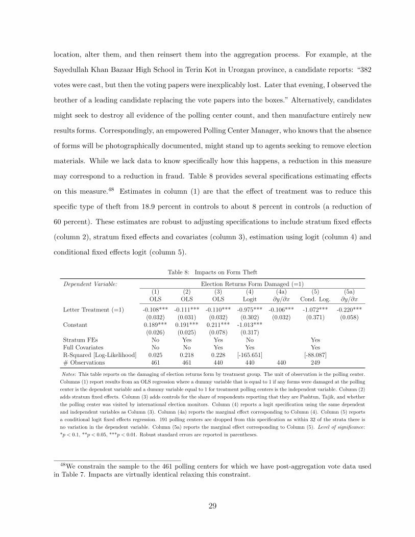
location, alter them, and then reinsert them into the aggregation process. For example, at the

Sayedullah Khan Bazaar High School in Terin Kot in Urozgan province, a candidate reports: “382

votes were cast, but then the voting papers were inexplicably lost. Later that evening, I observed the

brother of a leading candidate replacing the vote papers into the boxes.” Alternatively, candidates

might seek to destroy all evidence of the polling center count, and then manufacture entirely new

results forms. Correspondingly, an empowered Polling Center Manager, who knows that the absence

of forms will be photographically documented, might stand up to agents seeking to remove election

materials. While we lack data to know specifically how this happens, a reduction in this measure

may correspond to a reduction in fraud. Table 8 provides several specifications estimating effects

on this measure.48 Estimates in column (1) are that the effect of treatment was to reduce this

specific type of theft from 18.9 percent in controls to about 8 percent in controls (a reduction of

60 percent). These estimates are robust to adjusting specifications to include stratum fixed effects

(column 2), stratum fixed effects and covariates (column 3), estimation using logit (column 4) and

conditional fixed effects logit (column 5).

Table 8: Impacts on Form Theft

Dependent Variable: Election Returns Form Damaged (=1)(1) (2) (3) (4) (4a) (5) (5a)

OLS OLS OLS Logit ∂y/∂x Cond. Log. ∂y/∂x

Letter Treatment (=1) -0.108*** -0.111*** -0.110*** -0.975*** -0.106*** -1.072*** -0.220***(0.032) (0.031) (0.032) (0.302) (0.032) (0.371) (0.058)

Constant 0.189*** 0.191*** 0.211*** -1.013***(0.026) (0.025) (0.078) (0.317)

Stratum FEs No Yes Yes No YesFull Covariates No No Yes Yes YesR-Squared [Log-Likelihood] 0.025 0.218 0.228 [-165.651] [-88.087]# Observations 461 461 440 440 440 249

Notes: This table reports on the damaging of election returns form by treatment group. The unit of observation is the polling center.

Columns (1) report results from an OLS regression where a dummy variable that is equal to 1 if any forms were damaged at the polling

center is the dependent variable and a dummy variable equal to 1 for treatment polling centers is the independent variable. Column (2)

adds stratum fixed effects. Column (3) adds controls for the share of respondents reporting that they are Pashtun, Tajik, and whether

the polling center was visited by international election monitors. Column (4) reports a logit specification using the same dependent

and independent variables as Column (3). Column (4a) reports the marginal effect corresponding to Column (4). Column (5) reports

a conditional logit fixed effects regression. 191 polling centers are dropped from this specification as within 32 of the strata there is

no variation in the dependent variable. Column (5a) reports the marginal effect corresponding to Column (5). Level of significance:

*p < 0.1, **p < 0.05, ***p < 0.01. Robust standard errors are reported in parentheses.

48We constrain the sample to the 461 polling centers for which we have post-aggregation vote data usedin Table 7. Impacts are virtually identical relaxing this constraint.

29

5.4 Tests for spatial externalities

We next test for spatial externalities. We do this for four reasons. First, treatment externalities

may confound our estimates of program effect, leading us to overstate impact if fraud is merely

displaced and to understate impact if fraud is reduced in neighboring polling centers because of a

“chilling effect” (Miguel and Kremer 2004).49 Second, displacement effects and “chilling effects”

should be factored in when considering the efficacy of photo quick count.50 Third, tests for spatial

externalities can provide some information about how aggregation fraud is perpetrated. Fourth,

the estimated externalities, which indicate that monitoring announcements have negative effects on

fraud in neighboring polling centers, provide additional evidence of a high elasticity of fraud with

respect to the threat of monitoring.

The tests in this section are necessarily speculative. An ideal design allows an explicit com-

parison between various treatment densities against a set of pure controls. We could not achieve

this for several reasons. For example, we could not treat rural polling centers, which comprise the

majority of polling centers, due to safety concerns.51

A simple, but imperfect, test for externalities is to compare votes for the most connected

candidate in control polling substations which have no treated neighbors within a two kilometer

halo (N = 196) and in the remaining set of controls which have some treated neighbors within two

kilometers (N = 704). We find that the average number of votes for the most connected candidates

in the first group (42.939) is much larger than in the remaining controls (17.784) and that this

difference is statistically significant (p = 0.004, clustering standard errors at the polling center

level). This suggests a negative treatment externality.

49Because candidates run “at large” within a province, they may attempt substitution of legitimate andfake ballots anywhere within a province. Announcing monitoring in any polling center may therefore createtreatment externalities for other polling centers in a province. In practice, however, candidates may facelimits to displacing votes across polling substations within a province. Candidates mostly garner theirvotes in their home districts or towns where they remain popular, or from pockets of spatially clusteredfamily members. For example, given the extreme ethnic segregation of neighborhoods in Afghanistan, aTajik candidate receiving a considerable number of votes in a solidly Pashtun part of a province could raiseimmediate suspicions of fraud.

50Ichino and Schundeln (2012) find evidence that domestic observers monitoring the voter registrationprocess during the 2008 election in Ghana displaced some irregularities to unmonitored electoral areas.

51Additionally, with only 34 electoral constituencies, the Afghan electoral system affords limited power fortests at the constituency level.

30

To examine this further, we estimate treatment externalities with the specification:

Yics = ϕ1 + ϕ2Letter Treatmentc + ϕ3Treated1kmc + ϕ4Total

1kmc

+ ϕ5Treated1−2kmc + ϕ6Total

1−2kmc +ϕ′7Xc + ηics. (4)

Yics is the number of votes for the most connected candidate i in polling substation s in polling

center c, Treated1kmc is a dummy equal to 1 if any neighbors of polling center c within 1 km are

treated, Total1kmc is the total number of polling centers within a one kilometer halo, and variables

are similarly defined for polling centers between one and two kilometers away. As in Miguel and

Kremer (2004), our identifying assumption is that, conditional on the number of polling centers

within a fixed halo, the number treated is random. Table A9 reports tests verifying this identifying

assumption.52 We additionally estimate several variants of Specification 4, providing the full set

of interactions with Letter Treatment and separating Treated1kmc into a set of 5 dummy variables

to test for nonlinear effects in local treatment saturations.53 Table A5 provides summary statistics

for the data used in this analysis.

To assess the extent to which externalities confound our estimates of program effect, the first

column of Table 9 estimates impact only for the most connected candidate for comparison with

columns (2) - (4), which control for spatial externalities. The estimate increases slightly when

controlling for spatial externalities, but remains around four fewer votes for the most connected

candidate.54 Column (2) provides evidence of a negative externality, consistent with a “chilling

effect.” The estimates in column (3) suggest that having a neighbor treated within one kilometer

has a stronger negative externality (-6.74 votes) than having a neighbor treated between one and

two kilometers away (-4.74 votes). Column (4) separates out the effects by the number of neigh-

52We check this assumption by estimating Specification 4, replacing the dependent variable with the samebaseline variables that we use to test for treatment assignment balance in Table 4.

53In our data, the maximum number of polling centers within a one kilometer radius is five, so we createcategorical dummies for one treatment polling center within one kilometer, two treatment polling centerswithin one kilometer, and so on.

54The small change in the estimates of core impact despite large negative externalities in neighboringpolling centers may be because own-treatment status is weakly correlated with the treatment status ofnearby polling centers. To see this, imagine we estimate only yc = βT own

c + ηc, when yc = βT ownc +

γTneighborc + εc is the true model and cov(T own

c , Tneighborc ) ≈ 0. Then, since by a standard result E[β] =

β+ cov(T ownc , Tneighbor

c )γ, E[β] ≈ β, even when γ is large. Intuitively, this is equivalent to saying that thereare a large number of valid controls mixed in with the contaminated controls.

31

Table 9: Spatial Treatment Externalities

Dependent Variable: Votes for theMost Connected Candidate

(1) (2) (3) (4)

Letter Treatment (=1) -4.080** -4.183** -4.290** -4.159**(2.009) (1.982) (1.956) (1.980)

Any PCs treated within 1km (=1) -6.877* -6.742*(3.512) (3.486)

Total PCs within 1km -0.597 -0.499 -1.256(0.566) (0.564) (0.806)

Any PCs treated within 1-2km (=1) -4.738 -4.681(4.244) (4.240)

Total PCs within 1-2km 0.103 0.223(0.378) (0.392)

1 treated PC within 1km (=1) -6.457*(3.613)

2 treated PCs within 1km (=1) -5.831(3.882)

3 treated PCs within 1km (=1) -3.007(4.858)

4 treated PCs within 1km (=1) 1.459(5.620)

5 treated PCs within 1km (=1) -1.334(6.929)

Constant 28.064*** 30.543*** 32.378*** 32.697***(6.017) (6.043) (7.004) (6.987)

R-Squared 0.276 0.290 0.292 0.294Trimming top 1% of votes for interacted candidate type Yes Yes Yes Yes# Polling Centers 439 439 439 439# Candidate - Polling Substation Observations 1841 1841 1841 1841Mean Dep. Var. control +

no treated PCs 0-2km 42.939 42.939 42.939 42.939

Notes: Each column provides results from an OLS regression of the post-aggregation vote total for the most connected candidate

on a treatment dummy and variables to account for the number of neighboring polling centers that received treatment. These

are: Any PCs treated within 1km (2km) is a dummy variable that equals 1 if polling center within a 1 kilometer (2 kilometers)

radius received a treatment notification letter; Any PCs within 1km (1-2km) is a variable equal to the number of polling centers

within a 1 kilometer radius (1 to 2 kilometer radius) received a treatment notification letter; 1 treated PC within 1km is a dummy

that equals 1 if 1 polling center within a 1 km radius was treated and so on for 2 to 5 polling centers. The maximum number

of polling centers treated within a kilometer in our sample is 5. The unit of observation is the candidate - polling substation.

The sample is restricted to the most connected candidate only. The most connected candidate is identified using the procedure

described in Section 5. The top percentile is trimmed and stratum fixed effects and controls for the share of respondents reporting

that they are Pashtun, Tajik, and whether the polling center was visited by international election monitors are included in all

specifications. Level of significance: *p < 0.1, **p < 0.05, ***p < 0.01. Robust standard errors clustered at the polling center

level reported in parentheses.

bors treated. Estimates here are imprecise, but they are consistent with treatment externalities

decreasing in the number of neighbors treated.55

55This pattern suggests that polling center managers both actively communicate with one another aboutexternal monitoring and that they may be sensitive to changes in the degree of monitoring. These commu-nications may play some role in shaping managers’ beliefs about the probability that their results will beaudited. The diminishing pattern is consistent with updating being greatest in response to the arrival of thefirst letter in a neighborhood.

32

6 Conclusion

Our results demonstrate that aggregation fraud represents a threat to electoral fairness and that

photo quick count provides a means of addressing this problem. Our data provide, to our knowledge,

the first direct measurement of aggregation fraud and also the first systematic evidence of candidates

using their political networks to infiltrate electoral institutions. We discuss three direct policy

implications and three broader implications for electoral competition. We conclude with directions

for future research.

Our data yield three actionable policy results. First, photo quick count is effective, scalable,

well-suited to citizen-based implementation and “viral” adoption, and is cost-effective relative to

traditional international election monitoring.56 We successfully visited 471 polling centers, with a

total budget of just over 100,000 USD.57 By contrast, the largest foreign mission during this election

reached about 85 polling centers, spanning a smaller physical area than in our sample, with a budget

of approximately 10 million USD.58 Moreover, as cellular networks densify and bandwidth increases,

the potential for photo quick count to scale should expand and costs should decrease. Importantly,

this approach may also be sustainable with limited international support. The need for similar

interventions is likely to increase as developed countries transition to a “light footprint” approach

to international engagement. Second, no matter how it is addressed, aggregation fraud appears

to be a serious problem. Estimating the impact of aggregation fraud relative to other types of

fraud lies beyond our data. Nonetheless, the sheer magnitude of the problem and the centrality

of vote aggregation to the electoral process suggest that future efforts to improve elections should

target this problem. Last, improving the independence of electoral institutions and ensuring that

candidates cannot infiltrate them is necessary to achieve fair elections.

56Viral adoption refers to the adoption of new technology by independent actors based on widely availableinformation. Since completing our study, civil society groups in several countries have begun to implementphoto quick count. For example, during the 2014 Afghan Presidential Election, the method was used tomeasure aggregation fraud at 80 percent of active polling centers.

57Costs were contained primarily because we used local staff. Photo quick count can be implemented aseffectively by local staff without any special training by international election monitoring experts.

58Along these lines, the European Union spends approximately 4 million USD on an average electionobservation mission (European Union 2006). During the 2003 Cambodian National Assembly election, theEuropean Union spent approximately 1.5 million USD to deploy 120 observers (Lopez-Pintor and Fischer2006). To our knowledge, the European Union and the Asia Foundation are the only major internationalelection monitoring organizations that publish data on the cost of their missions.

33

Aggregation fraud, in our data, is both prevalent and disproportionately beneficial to connected

candidates. This has at least three negative implications for electoral competition. First, this

creates a substantial barrier to entry for unconnected candidates. We find evidence that powerful

candidates can both add votes for themselves and subtract votes for contenders. In this situation,

competitors without connections may be at a serious disadvantage. In extreme cases, they may not

be able to win at all without these connections, regardless of their competence. Second, candidates

have incentives to cultivate connections in order to win elections. This may create reasons for

candidates to favor clientielistic strategies relative to programmatic ones. Last, the prevalence of

aggregation fraud fundamentally limits the ability of voters to express their preferences through

the ballot. The candidate who wins may be the one with the strongest connections, not the one

preferred by voters. This would limit the disciplining role of elections.

Our findings produce a set of questions for future research. First, do informal connections

between state actors explain corruption and accountability failures in other settings, such as state

service provision? Second, a natural extension of this research involves investigating the longer

term effects of fraud reduction on the effectiveness of government in improving social welfare and

on citizens’ attitudes toward government—an important consideration in states where government

legitimacy is contested. Third, our paper suggests further work on institutional reforms that

might improve the effectiveness and sustainability of government monitoring efforts. Finally, and

perhaps more practically, our results suggest that identifying and operationalizing innovative uses

of technology to quickly gather information on corruption, waste, and abuse is a promising direction

for research and for policy.

34

References

Aker, Jenny, Paul Collier, and Pedro C. Vicente. 2013. “Is Information Power: Using

Cellphones During an Election in Mozambique.” Oxford University Working Paper.

Atanassova, Antonia, Marianne Bertrand, and Paul Niehaus. 2013. “Targeting with

Agents.” American Economic Journal: Economic Policy, 5(1): 206 – 238.

Beber, Bernd, and Alexandra Scacco. 2012. “What the Numbers Say: A Digit-Based Test for

Election Fraud Using New Data from Nigeria.” Political Analysis, 20(2): 211–234.

Berman, Eli, Jacob N. Shapiro, and Joseph H. Felter. 2011. “Can Hearts and Minds

Be Bought? The Economics of Counterinsurgency in Iraq.” Journal of Political Economy,

119(4): 766 – 819.

Bertrand, Marianne, Simeon Djankov, Rema Hanna, and Sendhil Mullainathan. 2007.

“Obtaining a Driver’s License in India: An Experimental Approach to Studying Corruption.”

The Quarterly Journal of Economics, 122(4): 1639–1676.

Besley, Timothy, and Robin Burgess. 2002. “The Political Economy of Government Respon-

siveness: Theory and Evidence from India.” Quarterly Journal of Economics, 117(4): 1415–1452.

Besley, Timothy, and Torsten Persson. 2011. “The Logic of Political Violence.” Quarterly

Journal of Economics, 126(3): 1411 – 1445.

Besley, Timothy, Rohini Pande, and Vijayendra Rao. 2005. “Participatory Democracy in

Action: Survey Evidence from South India.” Journal of the European Economic Association,

3(2-3): 648–657.

Bruhn, Miriam, and David McKenzie. 2009. “In Pursuit of Balance: Randomization in

Practice in Development Field Experiments.” American Economic Journal: Applied Economics,

1(4): 200–232.

Cadot, Olivier. 1987. “Corruption as a Gamble.” Journal of Public Economics, 33(2): 223–244.

35

Callen, Michael, and Nils Weidmann. 2013. “Violence and Election Fraud: Evidence from

Afghanistan.” British Journal of Political Science, 43(1): 53 – 75.

Cameron, A. Colin, Jonah B. Gelbach, and Douglas L. Miller. 2011. “Robust Inference

With Multiway Clustering.” Journal of Business & Economic Statistics, 29(2): 238–249.

Chattopadhyay, Raghabendra, and Esther Duflo. 2004. “Women as Policy Makers: Evidence

from a Nationwide Randomized Experiment in India.” Econometrica, 72(5): 1409–1443.

Cowan, Glenn, Melissa Estok, and Neil Nevitte. 2002. The Quick Count and Election Ob-

servation. National Democratic Institute for International Affairs.

Di Tella, Rafael, and Ernesto Schargrodsky. 2003. “The Role of Wages and Auditing during

a Crackdown on Corruption in the City of Buenos Aires.” Journal of Law and Economics,

46(1): 269–292.

Duflo, Esther, Rema Hanna, and Stephen Ryan. 2012. “Incentives Work: Getting Teachers

to Come to School.” American Economic Review, 102(4): 1241 – 1278.

European Union. 2006. “European Union: External Action FAQ.”

Ferraz, Claudio, and Frederico Finan. 2008. “Exposing Corrupt Politicians: The Effects of

Brazil’s Publicly Released Audits on Electoral Outcomes.” The Quarterly Journal of Economics,

123(2): 703–745.

Ferraz, Claudio, and Frederico Finan. 2011. “Electoral Accountability and Corruption: Evi-

dence from the Audits of Local Governments.” American Economic Review, 101: 1274–1311.

Fisman, Raymond. 2001. “Estimating the Value of Political Connections.” American Economic

Review, 91(4): 1095–1102.

Fujiwara, Thomas. 2013. “Voting Technology, Political Responsiveness, and Infant Health: Evi-

dence from Brazil.” Mimeo, Princeton University.

Gerber, Alan S., and Donald P. Green. 2012. Field Experiments: Design, Analysis, and

Interpretation. W.W. Norton.

36

Hyde, Susan D. 2007. “The Observer Effect in International Politics: Evidence from a Natural

Experiment.” World Politics, 60(1): 37–63.

Ichino, Nahomi, and Matthias Schundeln. 2012. “Deterring or Displacing Electoral Irregular-

ities? Spillover Effects of Observers in a Randomized Field Experiment in Ghana.” The Journal

of Politics, 74: 292–307.

Khwaja, Asim Ijaz, and Atif Mian. 2005. “Do Lenders Favor Politically Connected

Firms? Rent Provision in an Emerging Financial Market.” Quarterly Journal of Economics,

120(4): 1371–1411.

Lee, David S. 2009. “Training, Wages, and Sample Selection: Estimating Sharp Bounds on

Treatment Effects.” Review of Economic Studies, 76(3): 1071 – 1102.

Lopez-Pintor, Rafael, and Jeff Fischer. 2006. “Cost of Registration and Elections (CORE)

Project.” Center for Transitional and Post-Conflict Governance.

Martinez-Bravo, Monica, Gerard Padro i Miquel, Nancy Qian, and Yang Yao. 2013.

“Elections and Economic Policy: Evidence from Rural China.”

McChrystal, Stanley. 2009. “COMISAF’s Initial Assessment to the Secretary of Defense.”

McGee, Rosie, and John Gaventa. 2011. “Shifting Power? Assessing the Impact of Trans-

parency and Accountability Initiatives.” Institute of Development Studies Working Paper.

Mebane, Walter R. Jr. 2008. “Election Forensics: The Second-Digit Benford’s Law Test and

Recent American Presidential Elections.” In Election Fraud: Detecting and Deterring Electoral

Manipulation. , ed. R. Michael Alvarez, Thad E. Hall and Susan D. Hyde, 162–181. Washington,

DC:Brookings Institution Press.

Miguel, Edward, and Michael Kremer. 2004. “Worms: Identifying Impacts on Education and

Health in the Presence of Treatment Externalities.” Econometrica, 72(1): 159–217.

Myagkov, Mikhail, Peter C. Ordeshook, and Peter Shakin. 2009. The Forensics of Election

Fraud: Russia and Ukraine. New York:Cambridge University Press.

37

National Democratic Institute. 2010. “Afghanistan Election Data.” http: // 2010.

afghanistanelectiondata. org/ .

Olken, Benjamin A. 2007. “Monitoring Corruption: Evidence from a Field Experiment in In-

donesia.” Journal of Political Economy, 115(2): 200–249.

Olken, Benjamin A., and Patrick Barron. 2009. “The Simple Economics of Extortion: Evi-

dence from Trucking in Aceh.” Journal of Political Economy, 117(3): 417–452.

Olken, Benjamin A., and Rohini Pande. 2011. “Corruption in Developing Countries.” National

Bureau of Economic Research (NBER) Working Paper No. W17398.

Pande, Rohini. 2003. “Can Mandated Political Representation Increase Policy Influence for Disad-

vantaged Minorities? Theory and Evidence from India.” American Economic Review, 93(4): 1132

– 1151.

Rashid, Ahmed. 2009. Descent into Chaos: The U.S. and the Disaster in Pakistan, Afghanistan,

and Central Asia. London:Penguin.

Rose-Ackerman, Susan. 1975. “The Economics of Corruption.” Journal of Public Economics,

4(2): 187 – 203.

Shleifer, Andrei, and Robert W. Vishny. 1993. “Corruption.” Quarterly Journal of Eco-

nomics, 108(3).

Svensson, Jakob. 2003. “Who Must Pay Bribes and How Much? Evidence from A Cross Section

of Firms.” Quarterly Journal of Economics, 118(1): 207–230.

United States Army. 2006. “Field Manual 3-24: Counterinsurgency.”

Vogl, Tom S. forthcoming. “Marriage Institutions and Sibling Competition: Evidence from South

Asia.” Quarterly Journal of Economics.

World Bank. 2011. World Development Report 2011: Conflict, Security, and Development. WDR.

38

Yang, Dean. 2008. “Can Enforcement Backfire? Crime Displacement in the Context of Customs

Reform in the Philippines.” The Review of Economics and Statistics, 90(1): 1–14.

39

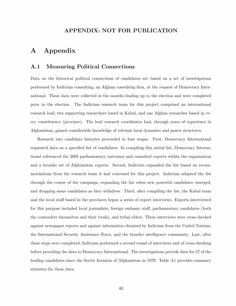
APPENDIX: NOT FOR PUBLICATION

A Appendix

A.1 Measuring Political Connections

Data on the historical political connections of candidates are based on a set of investigations

performed by Indicium consulting, an Afghan consulting firm, at the request of Democracy Inter-

national. These data were collected in the months leading up to the election and were completed

prior to the election. The Indicium research team for this project comprised an international

research lead, two supporting researchers based in Kabul, and one Afghan researcher based in ev-

ery constituency (province). The lead research coordinator had, through years of experience in

Afghanistan, gained considerable knowledge of relevant local dynamics and power structures.

Research into candidate histories proceeded in four stages. First, Democracy International

requested data on a specified list of candidates. In compiling this initial list, Democracy Interna-

tional referenced the 2005 parliamentary outcomes and consulted experts within the organization

and a broader set of Afghanistan experts. Second, Indicium expanded the list based on recom-

mendations from the research team it had convened for this project. Indicium adapted the list

through the course of the campaign, expanding the list when new powerful candidates emerged,

and dropping some candidates as they withdrew. Third, after compiling the list, the Kabul team

and the local staff based in the provinces began a series of expert interviews. Experts interviewed

for this purpose included local journalists, foreign embassy staff, parliamentary candidates (both

the contenders themselves and their rivals), and tribal elders. These interviews were cross-checked

against newspaper reports and against information obtained by Indicium from the United Nations,

the International Security Assistance Force, and the broader intelligence community. Last, after

these steps were completed, Indicium performed a second round of interviews and of cross-checking

before providing the data to Democracy International. The investigations provide data for 57 of the

leading candidates since the Soviet Invasion of Afghanistan in 1979. Table A1 provides summary

statistics for these data.

40

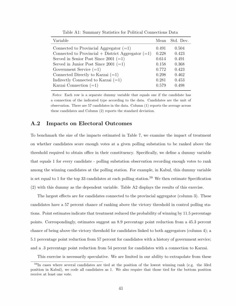
Table A1: Summary Statistics for Political Connections Data

Variable Mean Std. Dev.

Connected to Provincial Aggregator (=1) 0.491 0.504Connected to Provincial + District Aggregator (=1) 0.228 0.423Served in Senior Post Since 2001 (=1) 0.614 0.491Served in Junior Post Since 2001 (=1) 0.158 0.368Government Service (=1) 0.772 0.423Connected Directly to Karzai (=1) 0.298 0.462Indirectly Connected to Karzai (=1) 0.281 0.453Karzai Connection (=1) 0.579 0.498

Notes: Each row is a separate dummy variable that equals one if the candidate has

a connection of the indicated type according to the data. Candidates are the unit of

observation. There are 57 candidates in the data. Column (1) reports the average across

these candidates and Column (2) reports the standard deviation.

A.2 Impacts on Electoral Outcomes

To benchmark the size of the impacts estimated in Table 7, we examine the impact of treatment

on whether candidates score enough votes at a given polling substation to be ranked above the

threshold required to obtain office in their constituency. Specifically, we define a dummy variable

that equals 1 for every candidate - polling substation observation recording enough votes to rank

among the winning candidates at the polling station. For example, in Kabul, this dummy variable

is set equal to 1 for the top 33 candidates at each polling station.59 We then estimate Specification

(2) with this dummy as the dependent variable. Table A2 displays the results of this exercise.

The largest effects are for candidates connected to the provincial aggregator (column 3). These

candidates have a 57 percent chance of ranking above the victory threshold in control polling sta-

tions. Point estimates indicate that treatment reduced the probability of winning by 11.5 percentage

points. Correspondingly, estimates suggest an 8.9 percentage point reduction from a 45.3 percent

chance of being above the victory threshold for candidates linked to both aggregators (column 4); a

5.1 percentage point reduction from 57 percent for candidates with a history of government service;

and a .3 percentage point reduction from 54 percent for candidates with a connection to Karzai.

This exercise is necessarily speculative. We are limited in our ability to extrapolate from these

59In cases where several candidates are tied at the position of the lowest winning rank (e.g. the 33rdposition in Kabul), we code all candidates as 1. We also require that those tied for the bottom positionreceive at least one vote.

41

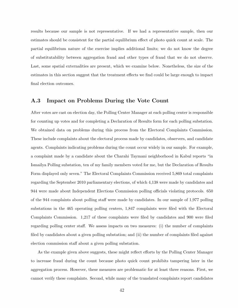
results because our sample is not representative. If we had a representative sample, then our

estimates should be consistent for the partial equilibrium effect of photo quick count at scale. The

partial equilibrium nature of the exercise implies additional limits; we do not know the degree

of substitutability between aggregation fraud and other types of fraud that we do not observe.

Last, some spatial externalities are present, which we examine below. Nonetheless, the size of the

estimates in this section suggest that the treatment effects we find could be large enough to impact

final election outcomes.

A.3 Impact on Problems During the Vote Count

After votes are cast on election day, the Polling Center Manager at each polling center is responsible

for counting up votes and for completing a Declaration of Results form for each polling substation.

We obtained data on problems during this process from the Electoral Complaints Commission.

These include complaints about the electoral process made by candidates, observers, and candidate

agents. Complaints indicating problems during the count occur widely in our sample. For example,

a complaint made by a candidate about the Charahi Taymani neighborhood in Kabul reports “in

Ismailya Polling substation, ten of my family members voted for me, but the Declaration of Results

Form displayed only seven.” The Electoral Complaints Commission received 5,869 total complaints

regarding the September 2010 parliamentary elections, of which 4,138 were made by candidates and

944 were made about Independent Elections Commission polling officials violating protocols. 650

of the 944 complaints about polling staff were made by candidates. In our sample of 1,977 polling

substations in the 465 operating polling centers, 1,847 complaints were filed with the Electoral

Complaints Commission. 1,217 of these complaints were filed by candidates and 900 were filed

regarding polling center staff. We assess impacts on two measures: (i) the number of complaints

filed by candidates about a given polling substation; and (ii) the number of complaints filed against

election commission staff about a given polling substation.

As the example given above suggests, these might reflect efforts by the Polling Center Manager

to increase fraud during the count because photo quick count prohibits tampering later in the

aggregation process. However, these measures are problematic for at least three reasons. First, we

cannot verify these complaints. Second, while many of the translated complaints report candidates

42

Table A2: Estimates of Impact on Whether a Candidate Receives Enough Votes to Win

Dependent Variable: Received Enough Votes to be in a Winning Rank Position (=1)Impacts by Connection Type (1) (2) (3) (4) (5) (6)

Letter Treatment (=1) 0.001 0.001 0.001 0.001 0.001 0.001(0.002) (0.002) (0.002) (0.002) (0.002) (0.002)

Treat x Most Connected -0.051(0.039)

Treat x Investigated -0.040 0.004 -0.029 0.001 -0.020(0.026) (0.030) (0.027) (0.053) (0.041)

Treat x Provincial Aggregator Connection -0.115***(0.044)

Treat x Prov. and District Aggregator Connection -0.060(0.051)

Treat x Government Service -0.051(0.059)

Treat x Karzai Connection -0.030(0.049)

Most Connected (=1) 0.473***(0.028)

Provincial Aggregator Connection (=1) -0.106***(0.032)

Prov. and District Aggregator Connection (=1) -0.140***(0.039)

Government Service (=1) -0.019(0.043)

Karzai Connect. (=1) -0.053(0.036)

Investigated (=1) 0.481*** 0.521*** 0.508*** 0.496*** 0.508***(0.018) (0.021) (0.019) (0.038) (0.030)

Constant 0.088*** 0.083*** 0.083*** 0.083*** 0.083*** 0.082***(0.004) (0.004) (0.004) (0.004) (0.004) (0.004)

Stratum FEs Yes Yes Yes Yes Yes YesFull Covariates Yes Yes Yes Yes Yes YesTrimming top 1% of votes for interacted candidate type Yes Yes Yes Yes Yes NoR-Squared 0.026 0.050 0.051 0.051 0.050 0.049# Polling Centers 440 440 440 440 440 440# Candidate - Polling Station Observations 309822 309843 309893 309900 309852 309699Mean of Dep. Var. in Controls 0.091 0.091 0.091 0.091 0.091 0.090Mean of Dep. Var. in Controls for Interacted Connection 0.582 0.571 0.497 0.453 0.565 0.540P - Value: Treat x Investigated + Treat x Connection = 0 0.190 0.128 0.002 0.051 0.078 0.112

Notes: This table reports effects on whether candidates receive enough votes to be in the set of winning candidates at a given polling substation. The

unit of observation is the candidate - polling substation. Each column reports the results of an OLS regression where a dummy variable that equals

1 for every candidate - polling substation observation recording enough votes to rank among the winning candidates at the polling substation is the

dependent variable. Columns (2) through (6) report results from regressions interacting the treatment dummy with each candidate connection type

dummy and a dummy for being investigated. Note we observe connections data only for investigated candidates. All regressions include stratum fixed

effects and controls for the share of respondents reporting that they are Pashtun, Tajik, and whether the polling center was visited by international

election monitors. The final two rows report the mean of the dependent variable in the controls and in the controls among observations for the interacted

candidate type. Level of significance: *p < 0.1, **p < 0.05, ***p < 0.01. Robust standard errors clustered at the polling center level are reported in

parentheses.

43

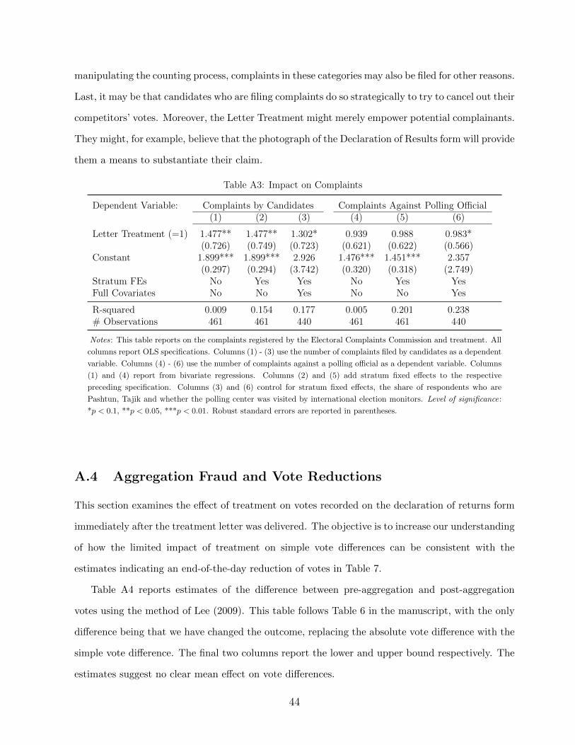
manipulating the counting process, complaints in these categories may also be filed for other reasons.

Last, it may be that candidates who are filing complaints do so strategically to try to cancel out their

competitors’ votes. Moreover, the Letter Treatment might merely empower potential complainants.

They might, for example, believe that the photograph of the Declaration of Results form will provide

them a means to substantiate their claim.

Table A3: Impact on Complaints

Dependent Variable: Complaints by Candidates Complaints Against Polling Official(1) (2) (3) (4) (5) (6)

Letter Treatment (=1) 1.477** 1.477** 1.302* 0.939 0.988 0.983*(0.726) (0.749) (0.723) (0.621) (0.622) (0.566)

Constant 1.899*** 1.899*** 2.926 1.476*** 1.451*** 2.357(0.297) (0.294) (3.742) (0.320) (0.318) (2.749)

Stratum FEs No Yes Yes No Yes YesFull Covariates No No Yes No No Yes

R-squared 0.009 0.154 0.177 0.005 0.201 0.238# Observations 461 461 440 461 461 440

Notes: This table reports on the complaints registered by the Electoral Complaints Commission and treatment. All

columns report OLS specifications. Columns (1) - (3) use the number of complaints filed by candidates as a dependent

variable. Columns (4) - (6) use the number of complaints against a polling official as a dependent variable. Columns

(1) and (4) report from bivariate regressions. Columns (2) and (5) add stratum fixed effects to the respective

preceding specification. Columns (3) and (6) control for stratum fixed effects, the share of respondents who are

Pashtun, Tajik and whether the polling center was visited by international election monitors. Level of significance:

*p < 0.1, **p < 0.05, ***p < 0.01. Robust standard errors are reported in parentheses.

A.4 Aggregation Fraud and Vote Reductions

This section examines the effect of treatment on votes recorded on the declaration of returns form

immediately after the treatment letter was delivered. The objective is to increase our understanding

of how the limited impact of treatment on simple vote differences can be consistent with the

estimates indicating an end-of-the-day reduction of votes in Table 7.

Table A4 reports estimates of the difference between pre-aggregation and post-aggregation

votes using the method of Lee (2009). This table follows Table 6 in the manuscript, with the only

difference being that we have changed the outcome, replacing the absolute vote difference with the

simple vote difference. The final two columns report the lower and upper bound respectively. The

estimates suggest no clear mean effect on vote differences.

44

This contrasts with Table 6, which reports negative effects for the absolute vote difference. To

understand why we find reductions for the absolute vote difference but not for the simple vote

difference, we plot the densities of the vote addition measures by treatment status for each of the

candidate subsamples in Figure A1. The figures suggests that one of the principal consequences of

treatment for powerful candidates is to increase the frequency with which the pre-aggregation total

perfectly matches the post-aggregation total (i.e., the vote difference equals zero). The densities

depicted in Figure A1 suggest that we observe no effect on the vote difference measure because

treatment reduces rigging both for and against powerful candidates in a way that is roughly sym-

metric.

We next consider how treatment reduced votes for powerful candidates, while having mainly

offsetting effects in terms of rigging both for and against the candidate. Figure A2 depicts Lee

(2009) bounds for pre-aggregation votes, post-aggregation votes, and their difference. Recall that

these are all post-treatment measures. Based on this figure, it appears that treatment operated by

first creating a reduction in votes for powerful candidates in the pre-aggregation number, and then

by creating greater fidelity between the pre-aggreagtion and post-aggregation totals.

The treatment letter indicated that we would be taking pictures of the results and then posting

them on a website accessible to “the people of Afghanistan, the international community, and local

and international media.” This makes clear that the technique would create broader awareness of

the vote numbers on the declaration of results form. We speculate that the reduction at this stage

may be because treatment reinforced the deterrent effect of posting the form at the polling center

in the first place.

To summarize our findings in this section, we find that treatment both reduced votes recorded

on the declaration of results form at the polling center and reduced rigging both for and against

powerful candidates in roughly equal measure. As a result, treatment diminished the absolute

difference between pre-aggregation and post-aggregation votes and decreased votes for powerful

candidates at the end of the election.

We treat these results speculatively mainly due to data limitations. The estimand in this

case is the treatment effect on polling centers that would report results irrespective of treatment.

This is about 9.7 percent of the total number of candidate polling substation observations in our

45

0.0

1.0

2.0

3.0

4.0

5D

ensi

ty

−200 −100 0 100 200Vote Difference During Aggregation

Provincial Aggregator Connection (=1)

0.0

1.0

2.0

3.0

4D

ensi

ty

−200 −100 0 100 200Vote Difference During Aggregation

Prov. + Dist. Aggregator Connection (=1)

0.0

2.0

4.0

6.0

8D

ensi

ty

−100 0 100 200Vote Difference During Aggregation

Karzai Connection (=1)

0.0

2.0

4.0

6D

ensi

ty

−100 0 100 200Vote Difference During Aggregation

Government Connection (=1)

0.0

2.0

4.0

6D

ensi

ty

−100 0 100 200Vote Difference During Aggregation

Incumbent (=1)

0.0

2.0

4.0

6D

ensi

ty

−100 0 100 200Vote Difference During Aggregation

Investigated (=1)

Treatment Control

Figure A1: Vote Difference Densities by Treatment GroupNotes: This figure depicts the kernel density estimates of the distribution of vote differences during aggregation. The vote

difference during aggregation is created by subtracting the number of votes recorded on pictures of the declaration of results

forms from the number of votes for the same candidate polling-station observation reported on the website of the Independent

Elections Commission (IEC). The maximum number of votes that can be cast a polling station is 600 votes. We therefore drop

one observation recoding -800 votes. Section A.1 describes the candidate connections data used to define candidate subsamples.

experimental sample and the behavior of the polling center managers that are always willing to

report may be different. Specifically, polling center managers who are willing to post declaration

of results forms irrespective of treatment may use the letter as an excuse not to record fake votes

for candidates on the declaration of returns form. The behavior could be different in our general

sample.

46

votes diff votes after votes before

Investigated

votes diff votes after votes before

Incumbent

votes diff votes after votes before

Government Service

votes diff votes after votes before

Karzai Connection

votes diff votes after votes before

Dist. Aggr. Connection

votes diff votes after votes before

Prov. Aggr. Connection

votes diff votes after votes before

Full Sample

Sam

ple

−30 −20 −10 0 10Estimated Treatment Effect (Votes)

Figure A2: Trimmed Estimates of Effect on Three MeasuresNotes: This error bars depict the upper and lower Lee (2009) bound estimates for votes recorded on the declaration of results

form at the polling center prior to aggregation (votes before), votes scraped from the Independent Elections Commission (IEC)

on its website (votes after) and the difference between votes after and votes before (votes diff). The dots correspond to the point

estimate, ignoring attrition. The maximum number of votes that can be cast a polling station is 600 votes. We therefore drop

one observation recoding -800 votes. Section A.1 describes the candidate connections data used to define candidate subsamples.

47

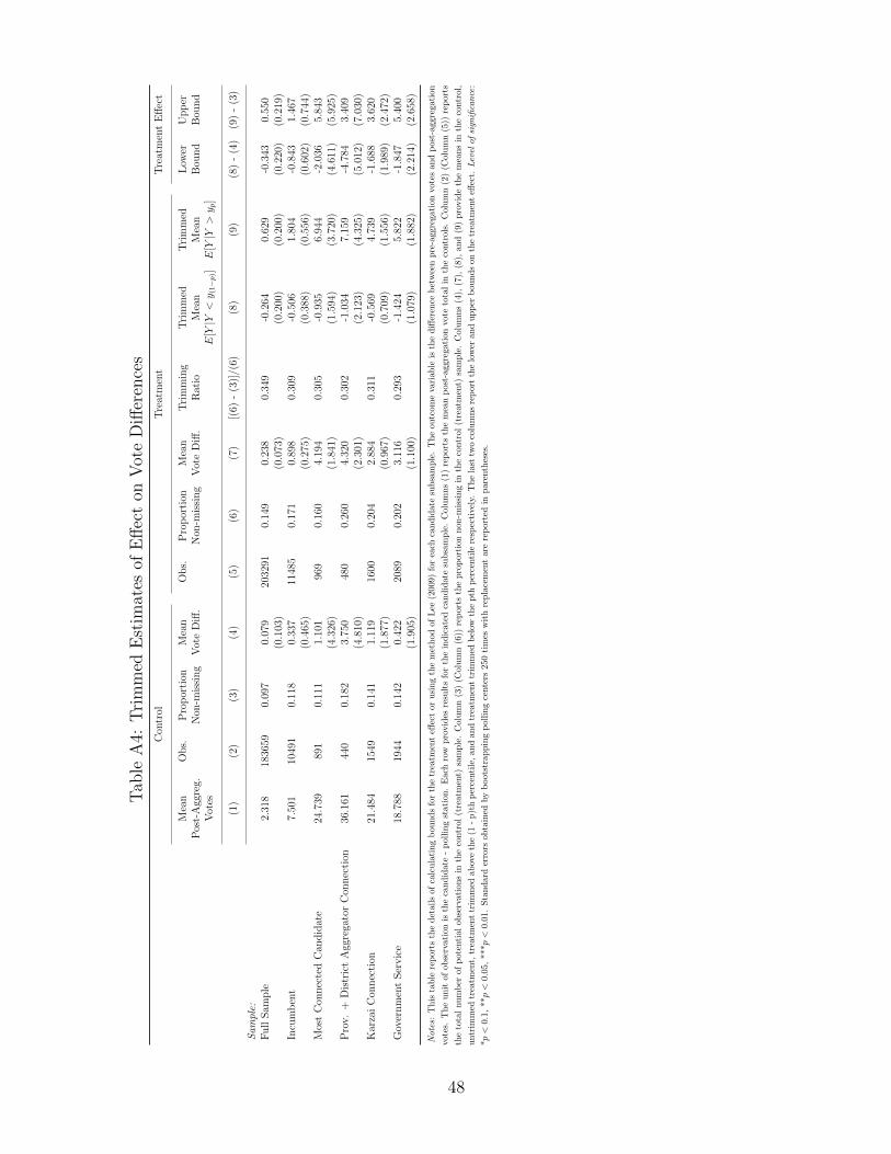
Tab

leA

4:T

rim

med

Est

imat

esof

Eff

ect

onV

ote

Diff

eren

ces

Con

trol

Tre

atm

ent

Tre

atm

ent

Eff

ect

Mea

nO

bs.

Pro

por

tion

Mea

nO

bs.

Pro

por

tion

Mea

nT

rim

min

gT

rim

med

Tri

mm

edL

ower

Up

per

Pos

t-A

ggre

g.N

on-m

issi

ng

Vot

eD

iff.

Non

-mis

sin

gV

ote

Diff

.R

atio

Mea

nM

ean

Bou

nd

Bou

nd

Vot

esE

[Y|Y

<y (

1−p)]

E[Y|Y

>y p

]

(1)

(2)

(3)

(4)

(5)

(6)

(7)

[(6)

-(3

)]/(

6)(8

)(9

)(8

)-

(4)

(9)

-(3

)

Sam

ple:

Fu

llS

amp

le2.

318

1836

590.

097

0.07

920

3291

0.14

90.

238

0.34

9-0

.264

0.62

9-0

.343

0.55

0(0

.103

)(0

.073

)(0

.200

)(0

.200

)(0

.220

)(0

.219

)In

cum

ben

t7.

501

1049

10.

118

0.33

711

485

0.17

10.

898

0.30

9-0

.506

1.80

4-0

.843

1.46

7(0

.465

)(0

.275

)(0

.388

)(0

.556

)(0

.602

)(0

.744

)M

ost

Con

nec

ted

Can

did

ate

24.7

3989

10.

111

1.10

196

90.

160

4.19

40.

305

-0.9

356.

944

-2.0

365.

843

(4.3

26)

(1.8

41)

(1.5

94)

(3.7

20)

(4.6

11)

(5.9

25)

Pro

v.

+D

istr

ict

Agg

rega

tor

Con

nec

tion

36.1

6144

00.

182

3.75

048

00.

260

4.32

00.

302

-1.0

347.

159

-4.7

843.

409

(4.8

10)

(2.3

01)

(2.1

23)

(4.3

25)

(5.0

12)

(7.0

30)

Kar

zai

Con

nec

tion

21.4

8415

490.

141

1.11

916

000.

204

2.88

40.

311

-0.5

694.

739

-1.6

883.

620

(1.8

77)

(0.9

67)

(0.7

09)

(1.5

56)

(1.9

89)

(2.4

72)

Gov

ernm

ent

Ser

vic

e18

.788

1944

0.14

20.

422

2089

0.20

23.

116

0.29

3-1

.424

5.82

2-1

.847

5.40

0(1

.905

)(1

.100

)(1

.079

)(1

.882

)(2

.214

)(2

.658

)

Note

s:T

his

table

rep

orts

the

det

ails

ofca

lcu

lati

ng

bou

nd

sfo

rth

etr

eatm

ent

effec

tor

usi

ng

the

met

hod

of

Lee

(2009)

for

each

can

did

ate

subsa

mp

le.

Th

eou

tcom

eva

riab

leis

the

diff

eren

ceb

etw

een

pre

-aggr

egati

on

vote

san

dp

ost

-agg

regati

on

vote

s.T

he

un

itof

obse

rvat

ion

isth

eca

nd

idat

e-

pol

lin

gst

atio

n.

Eac

hro

wp

rovid

esre

sult

sfo

rth

ein

dic

ate

dca

nd

idate

sub

sam

ple

.C

olu

mn

s(1

)re

port

sth

em

ean

post

-aggre

gati

on

vote

tota

lin

the

contr

ols

.C

olu

mn

(2)

(Colu

mn

(5))

rep

ort

s

the

tota

lnu

mb

erof

pot

enti

alob

serv

atio

ns

inth

eco

ntr

ol(t

reat

men

t)sa

mp

le.

Colu

mn

(3)

(Colu

mn

(6))

rep

ort

sth

ep

rop

ort

ion

non

-mis

sin

gin

the

contr

ol

(tre

atm

ent)

sam

ple

.C

olu

mn

s(4

),(7

),(8

),an

d(9

)p

rovid

eth

em

ean

sin

the

contr

ol,

untr

imm

edtr

eatm

ent,

trea

tmen

ttr

imm

edab

ove

the

(1-

p)t

hp

erce

nti

le,

and

and

trea

tmen

ttr

imm

edb

elow

the

pth

per

centi

lere

spec

tive

ly.

Th

ela

sttw

oco

lum

ns

rep

ort

the

low

eran

du

pp

erb

ou

nd

son

the

trea

tmen

teff

ect.

Lev

elof

sign

ifica

nce

:

*p<

0.1,

**p<

0.05

,**

*p<

0.0

1.S

tan

dar

der

rors

obta

ined

by

boot

stra

pp

ing

poll

ing

cente

rs250

tim

esw

ith

rep

lace

men

tar

ere

port

edin

pare

nth

eses

.

48

A.5 Data Appendix

We use the following administrative data: (i) systematic political background investigations of

the main candidates; (ii) geographic coordinates and security assessments of polling substations

provided by ISAF; (iii) complaints about illegal election activities filed at the Electoral Complaints

Commission; (iv) disaggregated vote counts from the Independent Elections Commission; and (v)

data on adherence to electoral protocols from the Free and Fair Elections Foundation of Afghanistan

(FEFA). Additionally, we fielded a baseline survey of households living in the immediate vicinity

of 450 of the 471 polling centers in our experimental sample a month before the election (August

2010). The 21 polling centers in the experimental sample not surveyed at baseline are in Kabul.

We subsequently added these using additional funding made available after the baseline. The

survey contained 2,904 respondents. To attempt to obtain a representative sample of respondents

living near polling centers, enumerators employed a random walk pattern starting at the polling

center, with random selection of every fourth house or structure. Respondents within households

are randomly selected using Kish grid. The survey had 50 percent male and female respondents

each and enumerators conducted it in either Dari or Pashto. Last, we obtain a primary measure

of returns form manipulation by sending field staff to investigate whether election materials were

stolen or damaged the day following the election (September 19), which we describe in section 3.

49

A.6 Additional Figures and Tables

Table A5: Additional Summary Statistics

Variable Mean Std. Dev. # Observations

Additional Fraud MeasuresElection returns form manipulation (=1) 0.134 0.342 461Number of Electoral Complaints Commission complaints by candidate 2.649 7.9 461Number of Electoral Complaints Commission complaints against polling official 1.952 6.724 461

Geospatial MeasuresPolling Centers treated within 1km (=1) 0.505 0.501 461Total Polling Centers treated within 1km 1.089 1.354 461Total Polling Centers within 1km 2.219 2.508 461Polling Centers treated within 1-2km (=1) 0.636 0.482 461Total Polling Centers treated within 1-2km 2.362 2.473 461Total Polling Centers within 1-2km 4.731 4.677 461

Notes: The first three rows are variables based on complaints data from the Electoral Complaints Commission. All three variables are the

total number of complaints pertaining to the station. The last six rows are computed using GIS based on geographic coordinates for the

polling substations in our sample provided by the International Security Assistance Force (ISAF). The first column reports the mean, the

second column reports the standard deviation, and the third reports the number of observations.

50

Table A6: Vote Changes During Aggregation by Candidate Type

(Sample: Only Candidates with Investigations Data)

Dependent Variable: Post-aggregation Votes - Pre-aggregation VotesPanel A - Votes (1) (2) (3) (4) (5) (6) (7)

Provincial Aggregator Connection (=1) 1.160(1.746)

Prov. + District Aggregator Connection (=1) 2.510 2.727 2.900(1.910) (1.736) (1.772)

Karzai Connect. (=1) -0.758 -0.970(2.317) (1.801)

Government Service (=1) -1.577 -1.879(2.038) (2.834)

Incumbent (=1) -0.570 -0.991 0.005(1.850) (1.646) (1.981)

Constant 1.768 1.525 2.559 3.330** 2.382 1.971 3.496**(1.269) (1.241) (2.264) (1.476) (1.746) (1.870) (1.678)

R-Squared 0.001 0.004 0.000 0.001 0.000 0.004 0.006# Candidates 56 56 56 56 56 56 56#Polling Stations 149 149 149 149 149 149 149# Candidate - Polling Station Observations 891 891 891 891 891 891 891

Dependent Variable: (Post-aggregation Share - Pre-aggregation Share) x 100Panel B - Vote Shares (1) (2) (3) (4) (5) (6) (7)

Provincial Aggregator Connection (=1) 0.384(2.393)

Prov. + District Aggregator Connection (=1) 1.171 1.499 1.149(2.385) (2.201) (2.239)

Karzai Connect. (=1) 0.513 1.537(2.097) (2.736)

Government Service (=1) 3.294 4.936(2.485) (4.344)

Incumbent (=1) -1.240 -1.476 -3.735(2.457) (2.317) (4.066)

Constant 4.004 3.844* 3.799 1.535** 4.736 4.510 0.921(2.450) (2.280) (2.420) (0.653) (2.884) (3.017) (1.668)

R-Squared 0.000 0.000 0.000 0.001 0.000 0.001 0.003# Candidates 57 57 57 57 57 57 57#Polling Stations 149 149 149 149 149 149 149# Candidate - Polling Station Observations 892 892 892 892 892 892 892

Notes: This table reports on political connections and the degree of aggregation fraud restricting the sample only to the 57 candidateswith connections data. The unit of observation is the candidate - polling substation. Each column in Panel A reports results froman OLS regression using the difference between post-aggregation and pre-aggregation votes as the dependent variable and a dummyvariable that equals one if a candidate - polling substation observation records the indicated connection(s) as an independent variable.Panel B repeats these specifications using the difference between pre-aggregation and post-aggregation vote shares (multiplied by 100)as a dependent variable. Both pre-aggregation and post-aggregation vote shares are calculated using pre-election polling station votetotals as the denominator. All specifications in both panels include province fixed effects and drop the five largest and five smallestobservations of the dependent variable. No candidates record a connection to the district aggregator and not to the provincial aggregatorso these coefficients cannot be estimated separately. Sample: treatment and control polling centers for which complete vote differencedata are available. Levels of significance: *p < 0.1, **p < 0.05, ***p < 0.01. Standard errors clustered by candidate and by pollingcenter using the method of Cameron, Gelbach and Miller (2011) are reported in parentheses.

51

Table A7: Vote Changes During Aggregation by Candidate Type

(Sample: Control Polling Stations)

Dependent Variable: Post-aggregation Votes - Pre-aggregation VotesPanel A - Votes (1) (2) (3) (4) (5) (6) (7)

Investigated (=1) 0.506 0.370 -0.224 1.089 2.985 0.479 3.267(1.319) (1.354) (1.549) (2.088) (2.393) (1.316) (2.262)

Provincial Aggregator Connection (=1) 0.522(2.209)

Prov. + District Aggregator Connection (=1) 3.499 4.320*(2.444) (2.250)

Karzai Connect. (=1) -0.967 -1.518(1.973) (1.949)

Government Service (=1) -3.260 -3.707(2.817) (2.778)

Incumbent (=1) 0.072 0.187(0.251) (0.233)

Constant 0.085*** 0.085*** 0.087*** 0.086*** 0.087*** 0.082*** 0.084**(0.030) (0.030) (0.031) (0.032) (0.031) (0.031) (0.033)

R-Squared 0.016 0.017 0.018 0.017 0.018 0.016 0.021# Candidates 1537 1537 1537 1537 1537 1537 1537#Polling Stations 67 67 67 67 67 67 67# Candidate - Polling Station Observations 17779 17779 17779 17779 17779 17779 17779Connection(s) + Investigated = 0 (p-value) 0.701 0.691 0.070 0.923 0.860 0.681 0.076Mean for Candidates Not Investigated 0.036 0.036 0.036 0.036 0.036 0.036 0.036

Dependent Variable: (Post-aggregation Share - Pre-aggregation Share) x 100Panel B - Vote Shares (1) (2) (3) (4) (5) (6) (7)

Investigated (=1) 3.703 4.397 3.968 1.198 -0.471 3.748 -2.416(2.740) (3.646) (3.412) (1.794) (1.646) (2.781) (1.942)

Provincial Aggregator Connection (=1) -2.605(2.965)

Prov. + District Aggregator Connection (=1) -1.234 -2.879(2.669) (3.737)

Karzai Connect. (=1) 4.147** 4.388**(1.672) (1.814)

Government Service (=1) 5.482 5.568(4.788) (5.422)

Incumbent (=1) -0.118 -0.393(0.261) (0.469)

Constant 0.210** 0.208** 0.209** 0.205** 0.206** 0.215** 0.215***(0.085) (0.085) (0.085) (0.085) (0.085) (0.086) (0.083)

R-Squared 0.014 0.014 0.014 0.014 0.014 0.014 0.014# Candidates 1538 1538 1538 1538 1538 1538 1538#Polling Stations 67 67 67 67 67 67 67# Candidate - Polling Station Observations 17778 17778 17778 17778 17778 17778 17778Connection(s) + Investigated = 0 (p-value) 0.177 0.226 0.119 0.120 0.189 0.176 0.087Mean for Candidates Not Investigated 0.751 0.751 0.751 0.751 0.751 0.751 0.751

Notes: This table reports on political connections and the degree of aggregation fraud in the control sample. The unit of observation is thecandidate - polling substation. Each column in Panel A reports results from an OLS regression using the difference between post-aggregation andpre-aggregation votes as the dependent variable and a dummy variable that equals one if a candidate - polling substation observation records theindicated connection(s) as an independent variable and an additional dummy that equals one if that observation has any background investigationdata. Panel B repeats these specifications using the difference between pre-aggregation and post-aggregation vote shares (multiplied by 100) asa dependent variable. Both pre-aggregation and post-aggregation vote shares are calculated using pre-election polling station vote totals as thedenominator. All specifications in both panels include province fixed effects and drop the five largest and five smallest observations of the dependentvariable. No candidates record a connection to the district aggregator and not to the provincial aggregator so these coefficients cannot be estimatedseparately. Sample: treatment and control polling centers for which complete vote difference data are available. Levels of significance: *p < 0.1,**p < 0.05, ***p < 0.01. Standard errors clustered by candidate and by polling center using the method of Cameron, Gelbach and Miller (2011)are reported in parentheses.

52

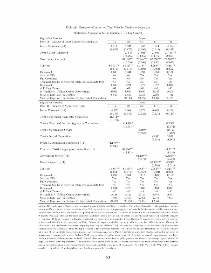
Table A8: Estimates of Impact on Total Votes by Candidate Connection

(Estimates Aggregating to the Candidate - Polling Center)

Dependent Variable: VotesPanel A - Impacts on Most Connected Candidates (1) (2) (3) (4) (5)

Letter Treatment (=1) 0.214 0.335 0.282 0.224 -0.024(0.942) (0.875) (0.290) (0.349) (0.331)

Treat x Most Connected -21.656 -21.935* -23.053* -25.751***(13.285) (13.233) (13.793) (9.863)

Most Connected (=1) 87.828*** 79.144*** 82.750*** 74.585***(10.026) (9.960) (10.361) (8.023)

Constant 6.539*** 6.035*** 6.113*** 8.760*** 7.521***(0.672) (0.619) (0.192) (0.882) (0.657)

R-Squared 0.000 0.031 0.093 0.089 0.101Stratum FEs No No Yes Yes YesFull Covariates No No No Yes YesTrimming top 1% of votes for interacted candidate type No No No No YesR-Squared 0.000 0.024 0.079 0.077 0.094# Polling Centers 461 461 461 440 440# Candidate - Polling Center Observations 80060 80060 80060 66137 66108Mean of Dep. Var. in Controls 6.539 6.539 6.539 7.660 7.401Mean of Dep. Var. in Controls for Interacted Connection - 93.863 93.863 98.073 88.991

Dependent Variable: VotesPanel B - Impacts by Connection Type (1) (2) (3) (4) (5)

Letter Treatment (=1) -0.027 0.008 0.071 -0.009 0.259(0.336) (0.349) (0.325) (0.321) (0.345)

Treat x Provincial Aggregator Connection -21.474**(10.018)

Treat x Prov. and District Aggregator Connection -26.688* -13.561(15.791) (23.674)

Treat x Government Service -15.389** -12.725(6.550) (18.707)

Treat x Karzai Connection -9.913 3.959(6.381) (18.967)

Provincial Aggregator Connection (=1) 71.140***(7.939)

Prov. and District Aggregator Connection (=1) 82.906*** 43.531**(12.852) (18.450)

Government Service (=1) 64.459*** 77.828***(5.079) (12.258)

Karzai Connect. (=1) 50.969*** -19.332(4.792) (12.321)

Constant 7.595*** 8.145*** 7.166*** 7.084*** 8.229***(0.661) (0.677) (0.657) (0.624) (0.881)

R-Squared 0.099 0.084 0.117 0.109 0.114Stratum FEs Yes Yes Yes Yes YesFull Covariates Yes Yes Yes Yes YesTrimming top 1% of votes for interacted candidate type Yes Yes Yes Yes NoR-Squared 0.091 0.078 0.108 0.103 0.098# Polling Centers 440 440 440 440 440# Candidate - Polling Center Observations 66118 66127 66116 66077 66137Mean of Dep. Var. in Controls 7.508 7.556 7.463 7.079 7.660Mean of Dep. Var. in Controls for Interacted Connection 84.798 98.928 76.144 62.673 -

Notes: This table reports effects on post-aggregation vote totals by candidate connection. The unit of observation is the candidate - polling

substation.Each column reports the results of an OLS regression where total post-aggregation votes is the dependent variable and a dummy

variable that equals 1 when the candidate - polling substation observation has the indicated connection is the independent variable. Panel

A reports treatment effect for the most connected candidate. Please see the text for details on how the most connected candidate variable

is computed. Column (1) reports a bivariate treatment regression with no interaction terms; Column (2) reports the results when treatment

is interacted with the most connected candidate; Column (3) reports a similar regression with stratum fixed effects included; Column (4)

adds controls for the share of respondents reporting that they are Pashtun, Tajik, and whether the polling center was visited by international

election monitors; Column (5) trims the top percentile of the dependent variable. Panel B reports results interacting the treatment dummy

with each of the candidate connection dummies. All regressions reported in Panel B include stratum fixed effects, controls for the share of

respondents reporting that they are Pashtun, Tajik, and whether the polling center was visited by international election monitors; and have

the top percentile of the dependent variable trimmed. The number of candidate - polling substations observations change slightly because of

duplicates values at the top percentile. The final two rows in Panel A and in Panel B report the mean of the dependent variable in the controls

and in the controls among observations for the interacted candidate type. Level of significance: *p < 0.1, **p < 0.05, ***p < 0.01. Robust

standard errors clustered at the polling center level are reported in parentheses.

53

Table A9: Validation Tests the Randomization to Test for Spatial Externalities

Transport Expects Vote Can TraditionalProblems Violence is Secret Identify MP Authority

Panel A (1) (2) (3) (4) (5)Received Letter (=1) 0.009 0.001 -0.018 0.014 0.017

(0.026) (0.026) (0.022) (0.020) (0.021)Any PCs treated within 1km (=1) 0.015 0.096** -0.040 0.019 0.023

(0.050) (0.042) (0.035) (0.035) (0.036)Total PCs within 1km (0-5) -0.010 -0.005 0.014* 0.000 0.009

(0.010) (0.009) (0.009) (0.007) (0.008)Any PCs treated within 1-2km (=1) 0.054 -0.002 0.030 0.021 0.070*

(0.047) (0.049) (0.038) (0.042) (0.041)Total PCs within 1-2km (0-24) 0.003 -0.003 0.001 -0.008** -0.011***

(0.006) (0.006) (0.005) (0.004) (0.004)Constant 0.499*** 0.471*** 0.634*** 0.390*** 0.256***

(0.033) (0.034) (0.030) (0.036) (0.030)# Observations 436 436 440 440 440R-Squared 0.332 0.434 0.340 0.641 0.370

Pashtun Income Electrified District Gov. Visited byKeeps Fair Int’l Monitors

Panel B (1) (2) (3) (4) (5)Received Letter (=1) -0.010 -66.909 -0.010 0.005 0.035

(0.018) (480.913) (0.016) (0.012) (0.035)Any PCs treated within 1km (=1) -0.007 487.848 0.030 0.019 0.068

(0.028) (721.844) (0.026) (0.022) (0.053)Total PCs within 1km (0-5) 0.005 -145.416 0.002 -0.006 0.021*

(0.007) (218.328) (0.005) (0.005) (0.012)Any PCs treated within 1-2km (=1) 0.014 -245.542 0.030 -0.024 0.004

(0.028) (724.078) (0.031) (0.023) (0.058)Total PCs within 1-2km (0-24) -0.006 144.201 0.002 -0.002 0.015*

(0.004) (131.907) (0.003) (0.003) (0.008)Constant 0.339*** 10167.997*** 0.674*** 0.139*** -0.006

(0.022) (569.063) (0.023) (0.018) (0.049)# Observations 440 435 440 438 440R-Squared 0.817 0.301 0.778 0.502 0.226

Notes: Each column provides results from an OLS regression of the indicated dependent variable on a treatmentdummy and variables to account for the number of neighboring polling centers that received treatment. Dependentvariables are computed as averages of answers from respondents near the polling center in the baseline survey.These are: Any PCs treated within 1km (2km) is a dummy variable that equals 1 if a polling center within a 1kilometer (2 kilometers) radius received a treatment notification letter; Any PCs within 1km (1-2km) is a variableequal to the number of polling centers within a 1 kilometer radius (1 to 2 kilometer radius) received a treatmentnotification letter; 1 treated PC within 1km is a dummy that equals 1 if 1 polling center within a 1 km radius wastreated and so on for 2 to 5 polling centers. The maximum number of polling centers treated within a kilometer inour sample is 5. The unit of observation is the candidate - polling substation. The sample is restricted to the mostconnected candidate only. The most connected candidate is identified using the procedure described in Section 5.The top percentile is trimmed and stratum fixed effects and controls for the share of respondents reporting thatthey are Pashtun, Tajik, and whether the polling center was visited by international election monitors are includedin all specifications. Level of significance: *p < 0.1, **p < 0.05, ***p < 0.01. Robust standard errors clustered atthe the polling center level reported in parentheses.

54

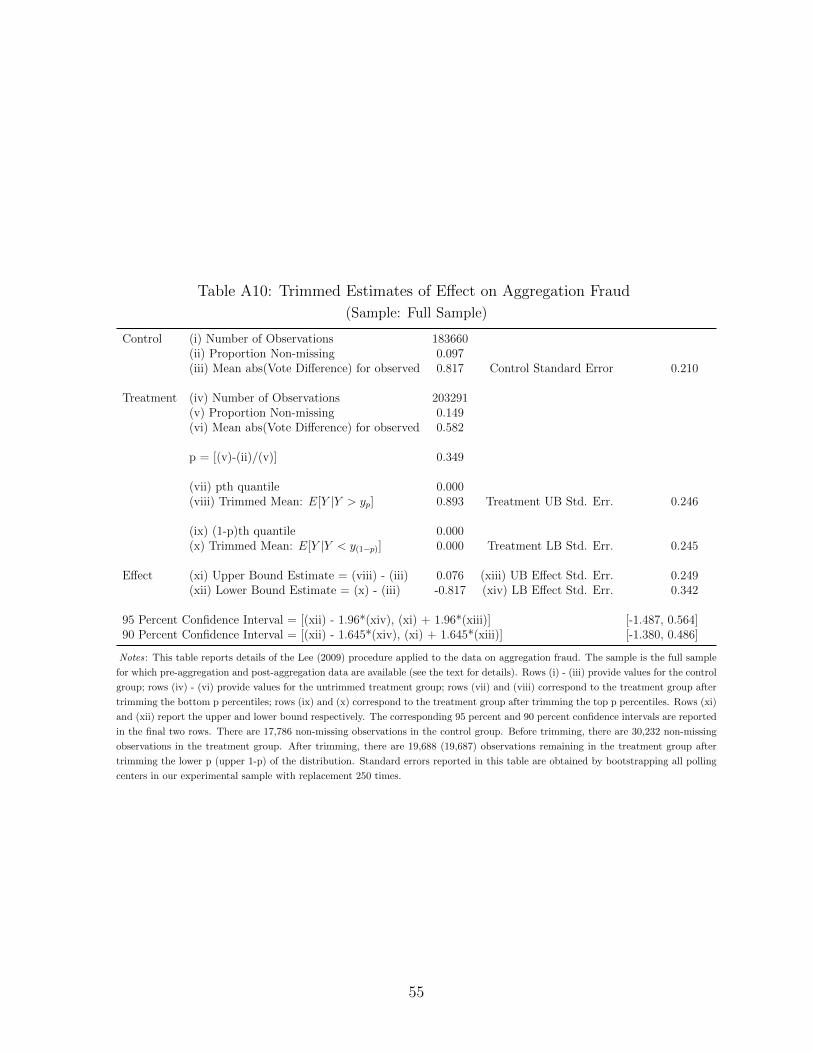
Table A10: Trimmed Estimates of Effect on Aggregation Fraud

(Sample: Full Sample)

Control (i) Number of Observations 183660(ii) Proportion Non-missing 0.097(iii) Mean abs(Vote Difference) for observed 0.817 Control Standard Error 0.210

Treatment (iv) Number of Observations 203291(v) Proportion Non-missing 0.149(vi) Mean abs(Vote Difference) for observed 0.582

p = [(v)-(ii)/(v)] 0.349

(vii) pth quantile 0.000(viii) Trimmed Mean: E[Y |Y > yp] 0.893 Treatment UB Std. Err. 0.246

(ix) (1-p)th quantile 0.000(x) Trimmed Mean: E[Y |Y < y(1−p)] 0.000 Treatment LB Std. Err. 0.245

Effect (xi) Upper Bound Estimate = (viii) - (iii) 0.076 (xiii) UB Effect Std. Err. 0.249(xii) Lower Bound Estimate = (x) - (iii) -0.817 (xiv) LB Effect Std. Err. 0.342

95 Percent Confidence Interval = [(xii) - 1.96*(xiv), (xi) + 1.96*(xiii)] [-1.487, 0.564]90 Percent Confidence Interval = [(xii) - 1.645*(xiv), (xi) + 1.645*(xiii)] [-1.380, 0.486]

Notes: This table reports details of the Lee (2009) procedure applied to the data on aggregation fraud. The sample is the full sample

for which pre-aggregation and post-aggregation data are available (see the text for details). Rows (i) - (iii) provide values for the control

group; rows (iv) - (vi) provide values for the untrimmed treatment group; rows (vii) and (viii) correspond to the treatment group after

trimming the bottom p percentiles; rows (ix) and (x) correspond to the treatment group after trimming the top p percentiles. Rows (xi)

and (xii) report the upper and lower bound respectively. The corresponding 95 percent and 90 percent confidence intervals are reported

in the final two rows. There are 17,786 non-missing observations in the control group. Before trimming, there are 30,232 non-missing

observations in the treatment group. After trimming, there are 19,688 (19,687) observations remaining in the treatment group after

trimming the lower p (upper 1-p) of the distribution. Standard errors reported in this table are obtained by bootstrapping all polling

centers in our experimental sample with replacement 250 times.

55

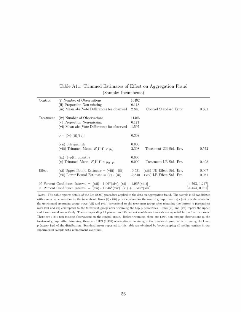
Table A11: Trimmed Estimates of Effect on Aggregation Fraud

(Sample: Incumbents)

Control (i) Number of Observations 10492(ii) Proportion Non-missing 0.118(iii) Mean abs(Vote Difference) for observed 2.840 Control Standard Error 0.801

Treatment (iv) Number of Observations 11485(v) Proportion Non-missing 0.171(vi) Mean abs(Vote Difference) for observed 1.597

p = [(v)-(ii)/(v)] 0.308

(vii) pth quantile 0.000(viii) Trimmed Mean: E[Y |Y > yp] 2.308 Treatment UB Std. Err. 0.572

(ix) (1-p)th quantile 0.000(x) Trimmed Mean: E[Y |Y < y(1−p)] 0.000 Treatment LB Std. Err. 0.498

Effect (xi) Upper Bound Estimate = (viii) - (iii) -0.531 (xiii) UB Effect Std. Err. 0.907(xii) Lower Bound Estimate = (x) - (iii) -2.840 (xiv) LB Effect Std. Err. 0.981

95 Percent Confidence Interval = [(xii) - 1.96*(xiv), (xi) + 1.96*(xiii)] [-4.763, 1.247]90 Percent Confidence Interval = [(xii) - 1.645*(xiv), (xi) + 1.645*(xiii)] [-4.454, 0.961]

Notes: This table reports details of the Lee (2009) procedure applied to the data on aggregation fraud. The sample is all candidates

with a recorded connection to the incumbent. Rows (i) - (iii) provide values for the control group; rows (iv) - (vi) provide values for

the untrimmed treatment group; rows (vii) and (viii) correspond to the treatment group after trimming the bottom p percentiles;

rows (ix) and (x) correspond to the treatment group after trimming the top p percentiles. Rows (xi) and (xii) report the upper

and lower bound respectively. The corresponding 95 percent and 90 percent confidence intervals are reported in the final two rows.

There are 1,241 non-missing observations in the control group. Before trimming, there are 1,964 non-missing observations in the

treatment group. After trimming, there are 1,359 (1,358) observations remaining in the treatment group after trimming the lower

p (upper 1-p) of the distribution. Standard errors reported in this table are obtained by bootstrapping all polling centers in our

experimental sample with replacement 250 times.

56

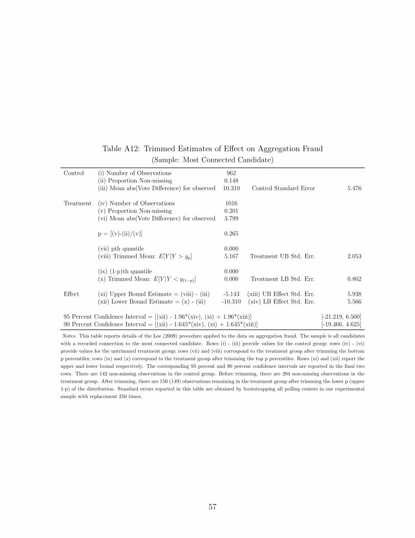
Table A12: Trimmed Estimates of Effect on Aggregation Fraud

(Sample: Most Connected Candidate)

Control (i) Number of Observations 962(ii) Proportion Non-missing 0.148(iii) Mean abs(Vote Difference) for observed 10.310 Control Standard Error 5.476

Treatment (iv) Number of Observations 1016(v) Proportion Non-missing 0.201(vi) Mean abs(Vote Difference) for observed 3.799

p = [(v)-(ii)/(v)] 0.265

(vii) pth quantile 0.000(viii) Trimmed Mean: E[Y |Y > yp] 5.167 Treatment UB Std. Err. 2.053

(ix) (1-p)th quantile 0.000(x) Trimmed Mean: E[Y |Y < y(1−p)] 0.000 Treatment LB Std. Err. 0.802

Effect (xi) Upper Bound Estimate = (viii) - (iii) -5.143 (xiii) UB Effect Std. Err. 5.938(xii) Lower Bound Estimate = (x) - (iii) -10.310 (xiv) LB Effect Std. Err. 5.566

95 Percent Confidence Interval = [(xii) - 1.96*(xiv), (xi) + 1.96*(xiii)] [-21.219, 6.500]90 Percent Confidence Interval = [(xii) - 1.645*(xiv), (xi) + 1.645*(xiii)] [-19.466, 4.625]

Notes: This table reports details of the Lee (2009) procedure applied to the data on aggregation fraud. The sample is all candidates

with a recorded connection to the most connected candidate. Rows (i) - (iii) provide values for the control group; rows (iv) - (vi)

provide values for the untrimmed treatment group; rows (vii) and (viii) correspond to the treatment group after trimming the bottom

p percentiles; rows (ix) and (x) correspond to the treatment group after trimming the top p percentiles. Rows (xi) and (xii) report the

upper and lower bound respectively. The corresponding 95 percent and 90 percent confidence intervals are reported in the final two

rows. There are 142 non-missing observations in the control group. Before trimming, there are 204 non-missing observations in the

treatment group. After trimming, there are 150 (149) observations remaining in the treatment group after trimming the lower p (upper

1-p) of the distribution. Standard errors reported in this table are obtained by bootstrapping all polling centers in our experimental

sample with replacement 250 times.

57

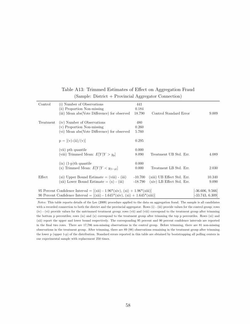
Table A13: Trimmed Estimates of Effect on Aggregation Fraud

(Sample: District + Provincial Aggregator Connection)

Control (i) Number of Observations 441(ii) Proportion Non-missing 0.184(iii) Mean abs(Vote Difference) for observed 18.790 Control Standard Error 9.009

Treatment (iv) Number of Observations 480(v) Proportion Non-missing 0.260(vi) Mean abs(Vote Difference) for observed 5.760

p = [(v)-(ii)/(v)] 0.295

(vii) pth quantile 0.000(viii) Trimmed Mean: E[Y |Y > yp] 8.090 Treatment UB Std. Err. 4.089

(ix) (1-p)th quantile 0.000(x) Trimmed Mean: E[Y |Y < y(1−p)] 0.000 Treatment LB Std. Err. 2.030

Effect (xi) Upper Bound Estimate = (viii) - (iii) -10.700 (xiii) UB Effect Std. Err. 10.340(xii) Lower Bound Estimate = (x) - (iii) -18.790 (xiv) LB Effect Std. Err. 9.090

95 Percent Confidence Interval = [(xii) - 1.96*(xiv), (xi) + 1.96*(xiii)] [-36.606, 9.566]90 Percent Confidence Interval = [(xii) - 1.645*(xiv), (xi) + 1.645*(xiii)] [-33.743, 6.309]

Notes: This table reports details of the Lee (2009) procedure applied to the data on aggregation fraud. The sample is all candidates

with a recorded connection to both the district and the provincial aggregator. Rows (i) - (iii) provide values for the control group; rows

(iv) - (vi) provide values for the untrimmed treatment group; rows (vii) and (viii) correspond to the treatment group after trimming

the bottom p percentiles; rows (ix) and (x) correspond to the treatment group after trimming the top p percentiles. Rows (xi) and

(xii) report the upper and lower bound respectively. The corresponding 95 percent and 90 percent confidence intervals are reported

in the final two rows. There are 17,786 non-missing observations in the control group. Before trimming, there are 81 non-missing

observations in the treatment group. After trimming, there are 89 (88) observations remaining in the treatment group after trimming

the lower p (upper 1-p) of the distribution. Standard errors reported in this table are obtained by bootstrapping all polling centers in

our experimental sample with replacement 250 times.

58

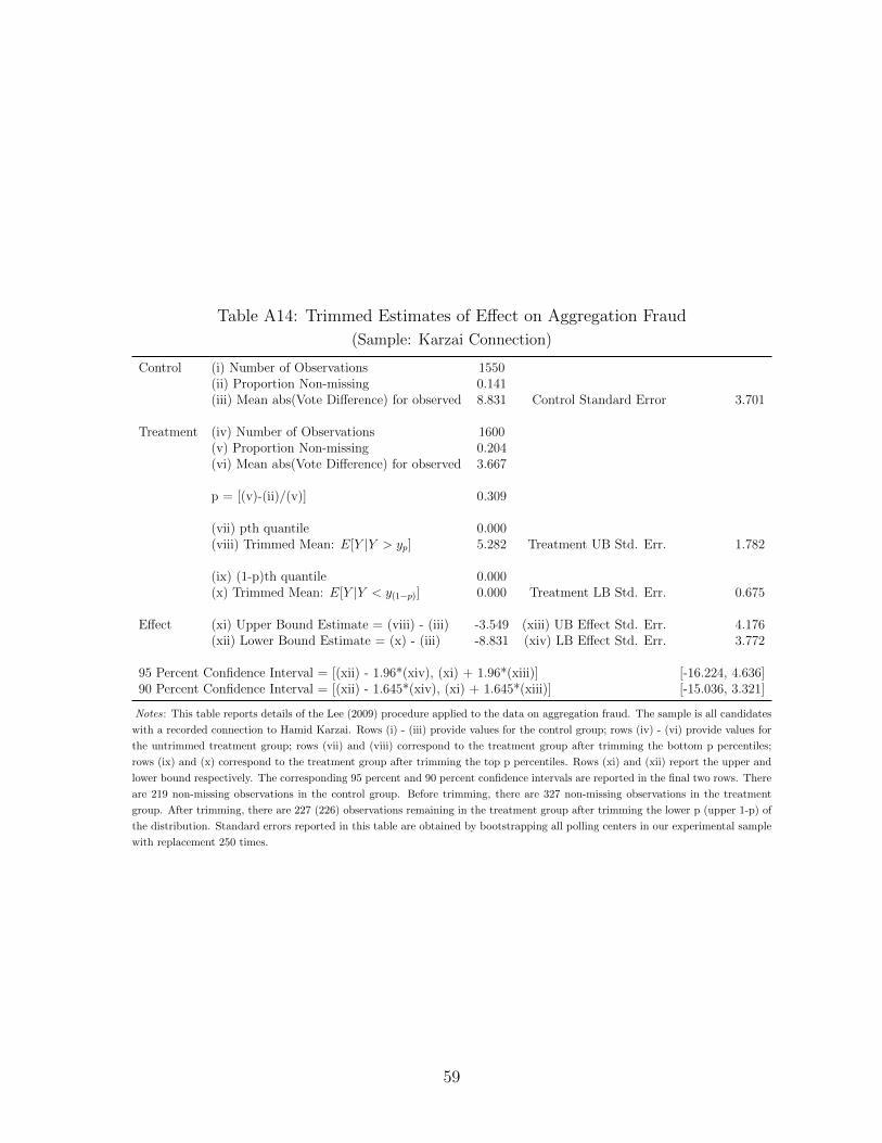
Table A14: Trimmed Estimates of Effect on Aggregation Fraud

(Sample: Karzai Connection)

Control (i) Number of Observations 1550(ii) Proportion Non-missing 0.141(iii) Mean abs(Vote Difference) for observed 8.831 Control Standard Error 3.701

Treatment (iv) Number of Observations 1600(v) Proportion Non-missing 0.204(vi) Mean abs(Vote Difference) for observed 3.667

p = [(v)-(ii)/(v)] 0.309

(vii) pth quantile 0.000(viii) Trimmed Mean: E[Y |Y > yp] 5.282 Treatment UB Std. Err. 1.782

(ix) (1-p)th quantile 0.000(x) Trimmed Mean: E[Y |Y < y(1−p)] 0.000 Treatment LB Std. Err. 0.675

Effect (xi) Upper Bound Estimate = (viii) - (iii) -3.549 (xiii) UB Effect Std. Err. 4.176(xii) Lower Bound Estimate = (x) - (iii) -8.831 (xiv) LB Effect Std. Err. 3.772

95 Percent Confidence Interval = [(xii) - 1.96*(xiv), (xi) + 1.96*(xiii)] [-16.224, 4.636]90 Percent Confidence Interval = [(xii) - 1.645*(xiv), (xi) + 1.645*(xiii)] [-15.036, 3.321]

Notes: This table reports details of the Lee (2009) procedure applied to the data on aggregation fraud. The sample is all candidates

with a recorded connection to Hamid Karzai. Rows (i) - (iii) provide values for the control group; rows (iv) - (vi) provide values for

the untrimmed treatment group; rows (vii) and (viii) correspond to the treatment group after trimming the bottom p percentiles;

rows (ix) and (x) correspond to the treatment group after trimming the top p percentiles. Rows (xi) and (xii) report the upper and

lower bound respectively. The corresponding 95 percent and 90 percent confidence intervals are reported in the final two rows. There

are 219 non-missing observations in the control group. Before trimming, there are 327 non-missing observations in the treatment

group. After trimming, there are 227 (226) observations remaining in the treatment group after trimming the lower p (upper 1-p) of

the distribution. Standard errors reported in this table are obtained by bootstrapping all polling centers in our experimental sample

with replacement 250 times.

59

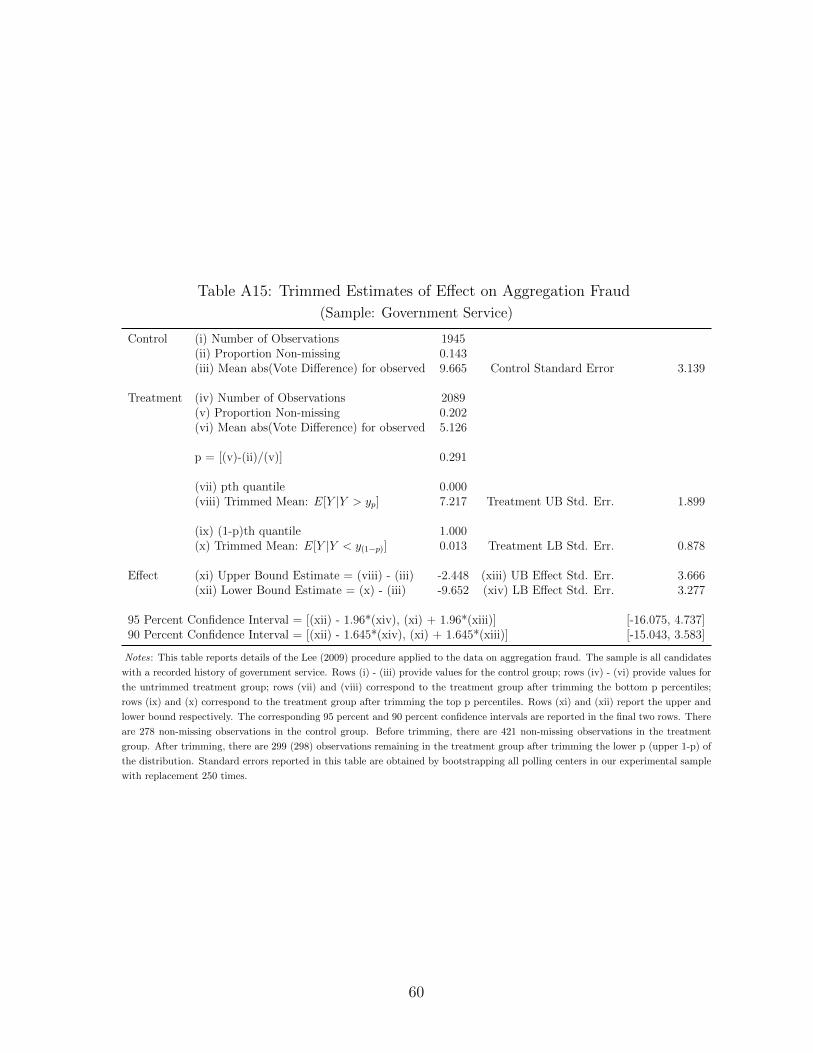
Table A15: Trimmed Estimates of Effect on Aggregation Fraud

(Sample: Government Service)

Control (i) Number of Observations 1945(ii) Proportion Non-missing 0.143(iii) Mean abs(Vote Difference) for observed 9.665 Control Standard Error 3.139

Treatment (iv) Number of Observations 2089(v) Proportion Non-missing 0.202(vi) Mean abs(Vote Difference) for observed 5.126

p = [(v)-(ii)/(v)] 0.291

(vii) pth quantile 0.000(viii) Trimmed Mean: E[Y |Y > yp] 7.217 Treatment UB Std. Err. 1.899

(ix) (1-p)th quantile 1.000(x) Trimmed Mean: E[Y |Y < y(1−p)] 0.013 Treatment LB Std. Err. 0.878

Effect (xi) Upper Bound Estimate = (viii) - (iii) -2.448 (xiii) UB Effect Std. Err. 3.666(xii) Lower Bound Estimate = (x) - (iii) -9.652 (xiv) LB Effect Std. Err. 3.277

95 Percent Confidence Interval = [(xii) - 1.96*(xiv), (xi) + 1.96*(xiii)] [-16.075, 4.737]90 Percent Confidence Interval = [(xii) - 1.645*(xiv), (xi) + 1.645*(xiii)] [-15.043, 3.583]

Notes: This table reports details of the Lee (2009) procedure applied to the data on aggregation fraud. The sample is all candidates

with a recorded history of government service. Rows (i) - (iii) provide values for the control group; rows (iv) - (vi) provide values for

the untrimmed treatment group; rows (vii) and (viii) correspond to the treatment group after trimming the bottom p percentiles;

rows (ix) and (x) correspond to the treatment group after trimming the top p percentiles. Rows (xi) and (xii) report the upper and

lower bound respectively. The corresponding 95 percent and 90 percent confidence intervals are reported in the final two rows. There

are 278 non-missing observations in the control group. Before trimming, there are 421 non-missing observations in the treatment

group. After trimming, there are 299 (298) observations remaining in the treatment group after trimming the lower p (upper 1-p) of

the distribution. Standard errors reported in this table are obtained by bootstrapping all polling centers in our experimental sample

with replacement 250 times.

60

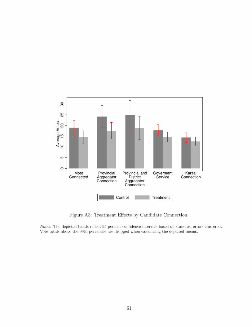
05

1015

2025

30Av

erag

e Vo

tes

MostConnected

ProvincialAggregatorConnection

Provincial andDistrict

AggregatorConnection

GovermentService

KarzaiConnection

Control Treatment

Figure A3: Treatment Effects by Candidate Connection

Notes: The depicted bands reflect 95 percent confidence intervals based on standard errors clustered.Vote totals above the 99th percentile are dropped when calculating the depicted means.

61

Polling Center Name: …………………..

Polling Center Code:…………………….

Date: ………………………………………

Dear Sir or Madam-

Greetings! I am an official election observer with the Opinion Research Center of Afghanistan (ORCA). My organization is providing this letter to collect some important information about your polling center and share it with our main office. Your polling center has been randomly selected from among polling centers in this province.

In our attempts to help Afghanistan have free and fair elections, I will return to this polling center tomorrow morning in order to take pictures of the results for every candidate in every station on the tally sheets after they have been posted.

The information will be posted on a website that belongs to local and international election observers so that it will be used by the people of Afghanistan, the international community, and local and international media. We will also compare the photos taken with the tally certified by the IEC in Kabul.

As recognition that you have read and understood this letter, please sign here: ___________

Thank you kindly for your help and cooperation.

Sincerely,

Haj Abdul Nabi Barakzai

Deputy Head of ORCA

Name and Signature of manager of polling station:………………………………………

Figure A4: Letter Delivered to Polling Center Managers

62

نام مرکز رائ دهی: _________________ تاریخ: ________________ ___ مرکز رائ دهی: _____________کود

به حضور محترم آقای / خانم

مسئولیت نظارت 472 مراکز رائ برحسب توافقنامه کمیسیون مستقل انتخابات دفتر اورکا دهی را بر عهده دارد.

میباشد و برای او (ORCA) دفتربه مربوطیک تن از نظارت کننده گان رسمیدارنده مکتوب معلومات تا بتواند مرکز رای دهی تسلیم نمودهدراین تا این مکتوب را وظیفه سپرده شده است. این مرکز دفتر مرکزی شریک بسازدجمع آوری نموده و با مرکز رای دهی این و دقیق را ازموثقاین ولایت تمام مراکز رای دهی میانبه صورت تصادفی از گر به شمول چندین مراکز دیرای دهی انتخاب شده است.

فردا صبح . ناظر ما یک انتخابات آزاد و مشروع در افغانستان کمک خواهیم کرد تقویتبرایما . نصب میگردد اخذ نمایدمرکز رای دهیاین که در را نتایج کاندیدان لست آمد تا تصاویر از دخواه

گذاشته مربوط به ناظرین انتخاباتی داخلی و خارجی این نتایج در سایت انترنتی تصاویر از این نتایج ، موسسات خارجی، و مطبوعات داخلی و خارجیخواهد شد تا تمام مردم افغانستان نتایج را با نتایج که از طرف اینتصاویر حاصله از ناظرحیث مناستفاده کنند. و همچنان ما انتخابات در کابل نشر میشود مقایسه خواهیم کرد. مستقلکمیسیون

در پائین ایدبرای تائید اینکه این مکتوب بدسترس شما قرار گرفته و شما انرا مطالعه نموده مضا نمائید. لطف نموده ا

از همکاری شما قبلا اظهار سپاس.

بااحترام

حاجی عبدالنبی بارکزی

معاون دفتر اورکا

آمر محترم مرکزرائ دهی: _______________ یامضااسم و

Figure A5: Dari Translation of Letter Delivered to Polling Center Managers

63