instruction formats - personal.kent.eduaguercio/cs35101slides/tanenbaum/ca_ch0… · instruction...

Instruction Formats

• An instruction consists of an opcode, usually with some additional information such as where operands come from, and where results go.

• The general subject of specifying where the operands are is called addressing.

• Several possible formats for level 2 instructions are shown on the next slide.

Common Instruction Formats

Four common instruction formats: (a) Zero-address instruction. (b) One-address instruction (c) Two-address instruction. (d) Three-address instruction

Instruction Formats

• On some machines, all instructions have the same length; on others there may be many different lengths.

• Instructions may be shorter than, the same length as, or longer than the word length. Having a single instruction length is simpler

and makes decoding easier, but is less efficient.

Common Instruction Formats

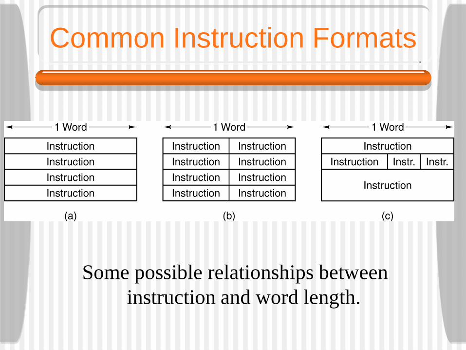
Some possible relationships between instruction and word length.

Expanding Opcodes

We will now examine tradeoffs involving both opcodes and addresses. Consider an (n + k) bit instruction with a k-bit

opcode and a single n-bit address.• This instruction allows 2k different operations and 2n

addressable memory cells.• Alternatively, the same n + k bits could be broken

up into a (k - 1) bit opcode and an (n + 1) bit address, meaning half as many instructions and either twice as much addressable memory or the same amount of memory with twice the resolution.

Expanding Opcodes

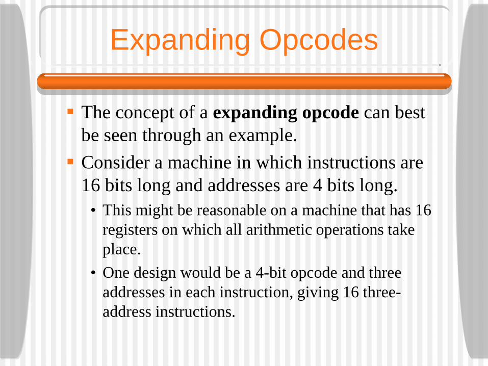
The concept of a expanding opcode can best be seen through an example. Consider a machine in which instructions are

16 bits long and addresses are 4 bits long.• This might be reasonable on a machine that has 16

registers on which all arithmetic operations take place.

• One design would be a 4-bit opcode and three addresses in each instruction, giving 16 three-address instructions.

Expanding Opcodes

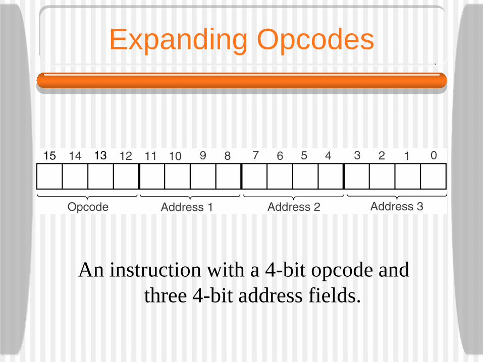
An instruction with a 4-bit opcode and three 4-bit address fields.

Expanding Opcodes

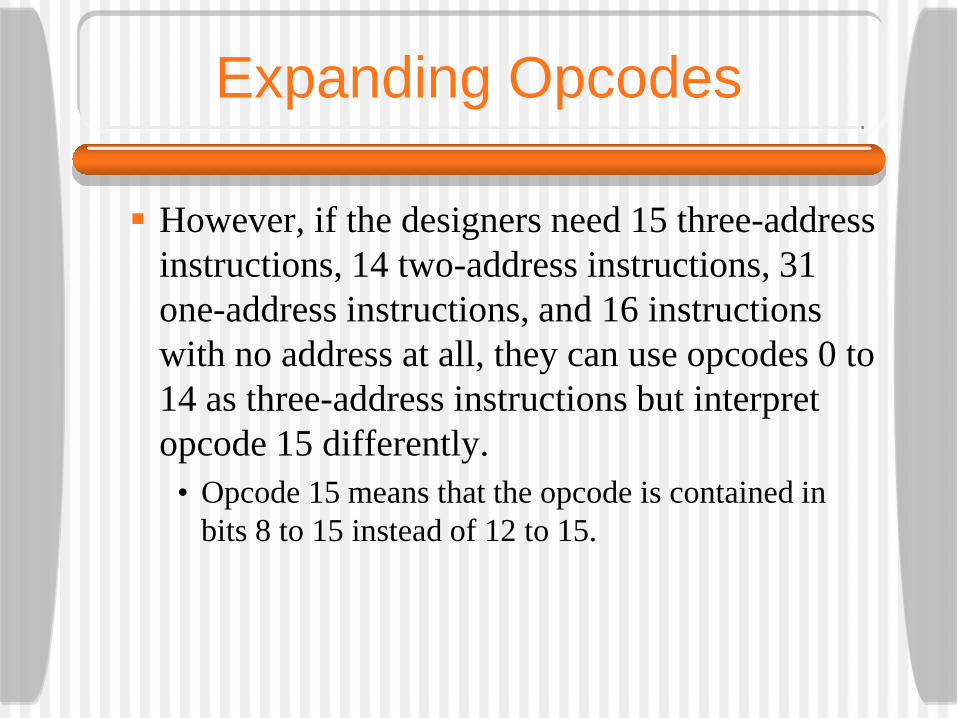
However, if the designers need 15 three-address instructions, 14 two-address instructions, 31 one-address instructions, and 16 instructions with no address at all, they can use opcodes 0 to 14 as three-address instructions but interpret opcode 15 differently.

• Opcode 15 means that the opcode is contained in bits 8 to 15 instead of 12 to 15.

Expanding Opcodes

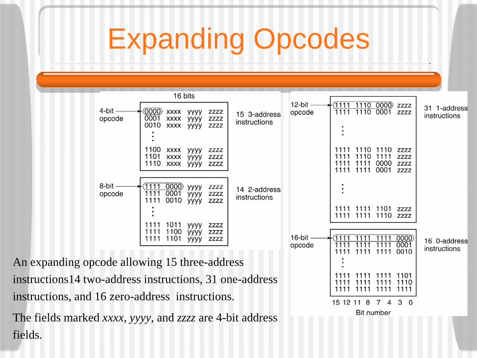
An expanding opcode allowing 15 three-address instructions14 two-address instructions, 31 one-address instructions, and 16 zero-address instructions.

The fields marked xxxx, yyyy, and zzzz are 4-bit address fields.

UltraSPARC III Instruction Formats

The original SPARC instruction formats.

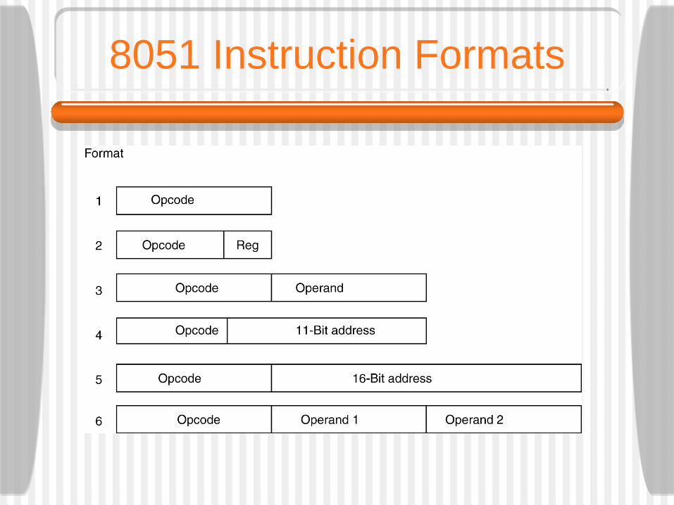
8051 Instruction Formats

Addressing

A large portion of the bits in a program are used to specify where the operands come from rather than what operations are being performed on them.

• An ADD instruction requires the specification of three operands: two sources and a destination.

• If memory addresses are 32 bits, the instruction takes three 32-bit addresses in addition to the opcode.

Two general methods are used to reduce the size of the specification

Addressing

• If an operand is to be used several times, it can be moved to a register. To do this, we must perform a LOAD (which includes the

full memory address).• A second method is to specify one or more

addresses implicitly. Use a two-address instruction, for example. The Pentium 4 uses two-address instructions while the

UltraSPARC III uses three-address instructions. If we have instructions which can work with only one

register, we can have one-address instructions. Finally, using a stack we can have zero-address

instructions (the JVM IADD, for example).

Addressing Modes

There are many different ways we can specify addresses. These are called addressing modes. The simplest way for an instruction to specify

an operand is to include the operand rather than an address or some other information describing where the operand is. This is called immediate addressing and the operand is called an immediate operand.

• This only works with constants.• The number of values is limited by the size of the

field.

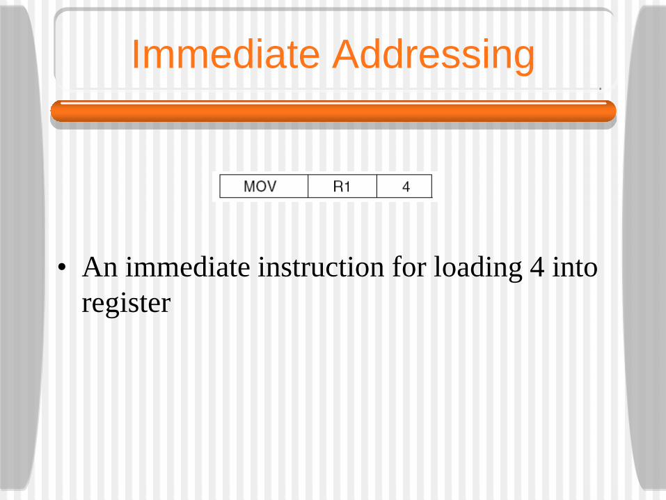
Immediate Addressing

• An immediate instruction for loading 4 into register

Direct Addressing

A method for specifying an operand in memory is just to give its full address. This is called direct addressing. The instruction will always access exactly the

same memory location.• Thus direct addressing can only be used to access

global variables whose address is known at compile time.

• Many programs have global variables so this method is widely used.

Register Addressing

Register addressing is conceptually the same as direct addressing but specifies a register rather than a memory location.

• Because registers are so important this addressing mode is the most common one on most computers.

• Many compilers determine the most frequently used variables and place them in registers.

• This addressing mode is known as register mode.• In load/store architectures such as the UltraSPARC

III, nearly all instructions use this addressing mode exclusively.

Register Indirect Addressing

In this mode, the operand being specified comes from memory or goes to memory, but its address is not hardwired into the instruction, as in direct addressing. Instead the address is contained in a register. When an address is used in this manner it is

called a pointer. Register indirect addressing can reference

memory without having a full memory address in the instruction.


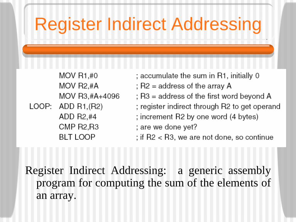
Register Indirect Addressing: a generic assemblyprogram for computing the sum of the elements ofan array.


The previous program used several addressing modes.

• The first three instructions use register mode for the first operand, and immediate mode for the second operand (a constant indicated by the # sign).

• The body of the loop itself does not contain any memory addresses. It uses register and register indirect mode in the fourth instruction.

• The BLT might use a memory address, but most likely it specifies the address to branch to with an 8-bit offset relative to the BLT instruction itself.

Indexed Addressing

It is frequently useful to be able to reference memory words at a known offset from a register. (Remember in IJVM we referenced local variables by giving their offset from LV). Addressing memory by giving a register

(explicit or implicit) plus a constant offset is called indexed addressing.

• We can also give a memory pointer in the instruction and a small offset in the register

Indexed Addressing

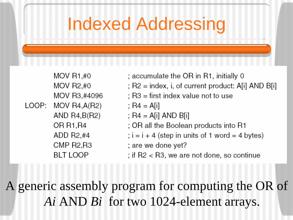
A generic assembly program for computing the OR of Ai AND Bi for two 1024-element arrays.

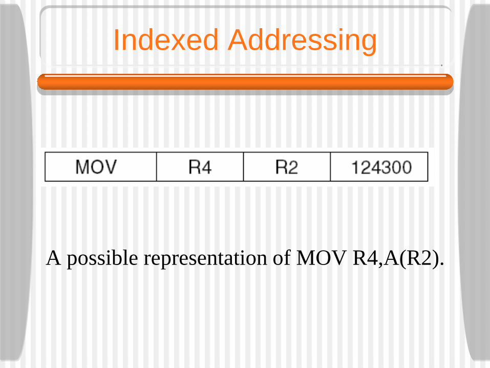
Indexed Addressing

A possible representation of MOV R4,A(R2).

Based Indexed Addressing

Some machines have an addressing mode in which the memory address is computed by adding up two registers plus an (optional) offset. Sometimes this mode is called based-indexed

addressing.• One of the registers is the base and the other is the

index.• We could have used this mode in the previous

program to write:LOOP: MOV R4, (R2+R5)

AND R4, (R2+R6)

Stack Addressing

We have noted that it is desirable to make machine instructions as short as possible.

• The ultimate limit in reducing address lengths is having no addresses at all.

• As we have seen, zero-address instructions, such as IADD are possible in conjunction with a stack.

• It is traditional in mathematics to put the operator between the operands (x + y), rather than after the operands (x y +).

• Between the operands is called infix notation.• After the operands is called postfix or reverse Polish notation.

Reverse Polish Notation

Reverse Polish notation has a number of advantages over infix for expressing algebraic formulas.

• Any formula can be expressed without parentheses.• It is convenient for evaluating expressions on

computers with stacks.• Infix operators have precedence, which is arbitrary

and undesirable.• There are several algorithms for converting infix

formulas into Polish notation. This one is by Dijkstra.


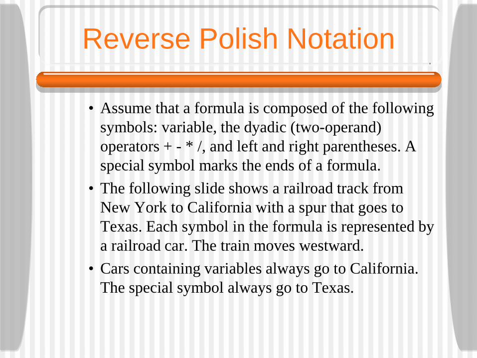
• Assume that a formula is composed of the following symbols: variable, the dyadic (two-operand) operators + - * /, and left and right parentheses. A special symbol marks the ends of a formula.

• The following slide shows a railroad track from New York to California with a spur that goes to Texas. Each symbol in the formula is represented by a railroad car. The train moves westward.

• Cars containing variables always go to California. The special symbol always go to Texas.


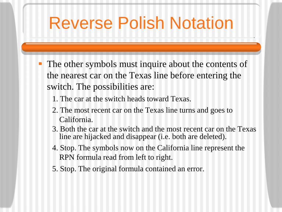
The other symbols must inquire about the contents of the nearest car on the Texas line before entering the switch. The possibilities are:

1. The car at the switch heads toward Texas.2. The most recent car on the Texas line turns and goes to

California.3. Both the car at the switch and the most recent car on the Texas

line are hijacked and disappear (i.e. both are deleted).4. Stop. The symbols now on the California line represent the

RPN formula read from left to right.5. Stop. The original formula contained an error.


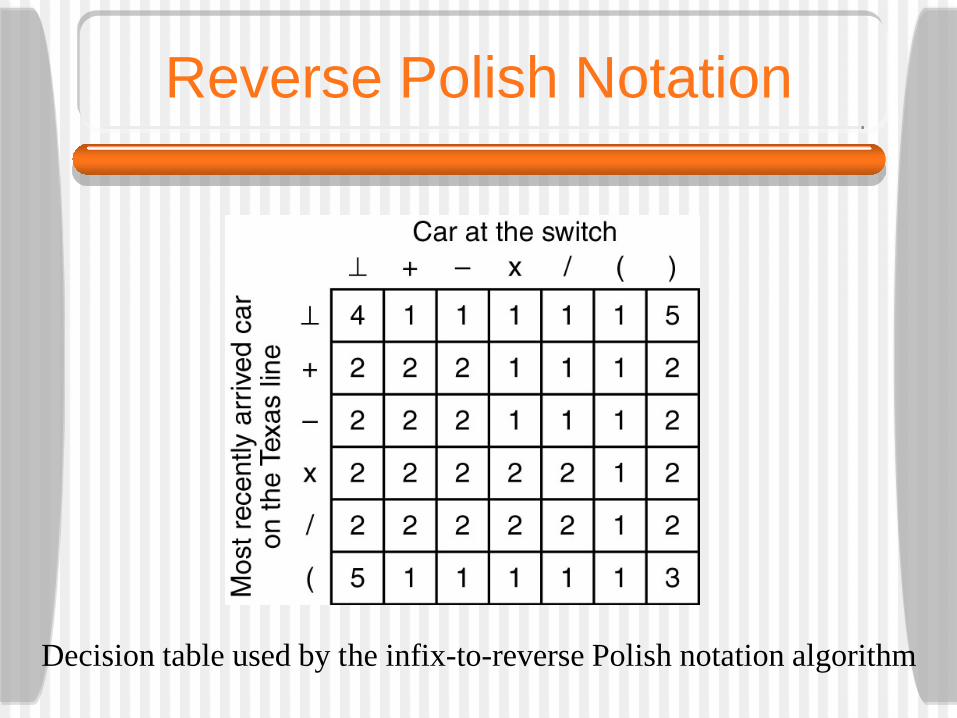
Decision table used by the infix-to-reverse Polish notation algorithm


Some examples of infix expressions and their reverse Polish notation equivalents.


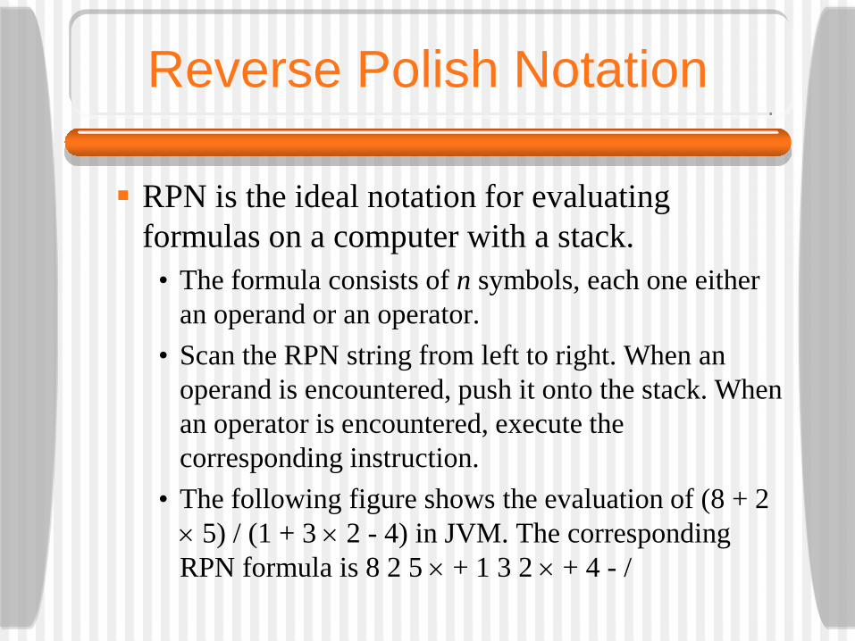
RPN is the ideal notation for evaluating formulas on a computer with a stack.

• The formula consists of n symbols, each one either an operand or an operator.

• Scan the RPN string from left to right. When an operand is encountered, push it onto the stack. When an operator is encountered, execute the corresponding instruction.

• The following figure shows the evaluation of (8 + 2 × 5) / (1 + 3 × 2 - 4) in JVM. The corresponding RPN formula is 8 2 5 × + 1 3 2 × + 4 - /


Use of a stack to evaluate a reverse Polish notation formula.

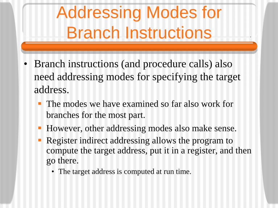
Addressing Modes for Branch Instructions

• Branch instructions (and procedure calls) also need addressing modes for specifying the target address. The modes we have examined so far also work for

branches for the most part. However, other addressing modes also make sense. Register indirect addressing allows the program to

compute the target address, put it in a register, and then go there.

• The target address is computed at run time.

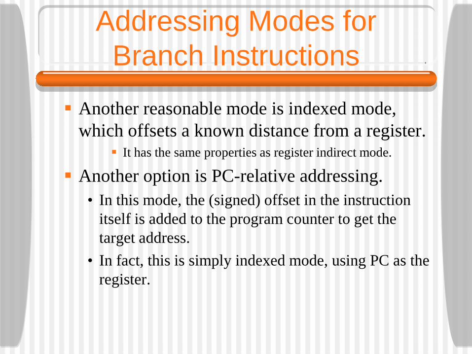
Addressing Modes for Branch Instructions

Another reasonable mode is indexed mode, which offsets a known distance from a register.

It has the same properties as register indirect mode.

Another option is PC-relative addressing. • In this mode, the (signed) offset in the instruction

itself is added to the program counter to get the target address.

• In fact, this is simply indexed mode, using PC as the register.

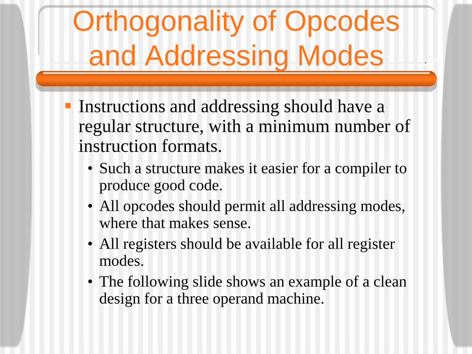
Orthogonality of Opcodes and Addressing Modes

Instructions and addressing should have a regular structure, with a minimum number of instruction formats.

• Such a structure makes it easier for a compiler to produce good code.

• All opcodes should permit all addressing modes, where that makes sense.

• All registers should be available for all register modes.

• The following slide shows an example of a clean design for a three operand machine.


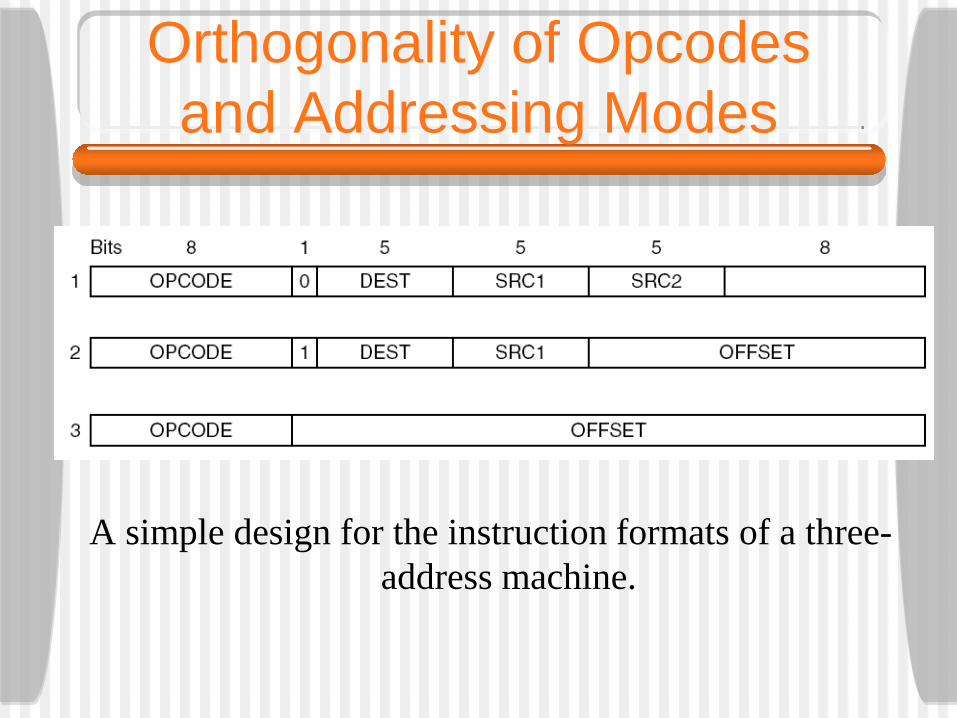
A simple design for the instruction formats of a three-address machine.


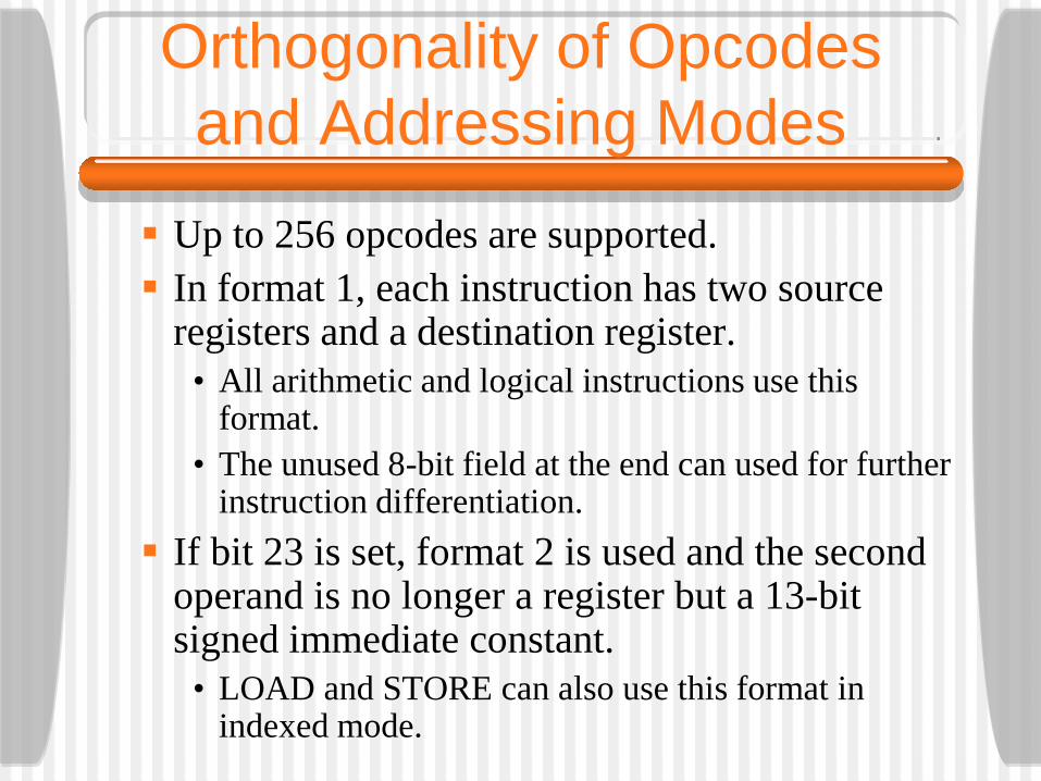
Up to 256 opcodes are supported. In format 1, each instruction has two source

registers and a destination register.• All arithmetic and logical instructions use this

format.• The unused 8-bit field at the end can used for further

instruction differentiation. If bit 23 is set, format 2 is used and the second

operand is no longer a register but a 13-bit signed immediate constant.

• LOAD and STORE can also use this format in indexed mode.


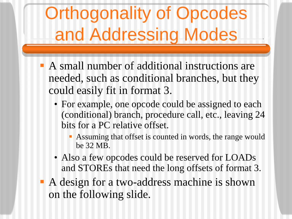
A small number of additional instructions are needed, such as conditional branches, but they could easily fit in format 3.

• For example, one opcode could be assigned to each (conditional) branch, procedure call, etc., leaving 24 bits for a PC relative offset. Assuming that offset is counted in words, the range would

be 32 MB.• Also a few opcodes could be reserved for LOADs

and STOREs that need the long offsets of format 3. A design for a two-address machine is shown

on the following slide.

Comparison of Addressing Modes

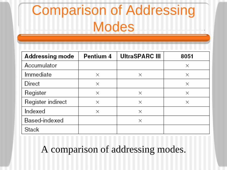
A comparison of addressing modes.

Instruction Types

• There are several groups of instruction types: Data Movement Instructions Dyadic Operations Monadic Operations Comparison and Conditional Branches Procedure Call Instructions Loop Control Input/Output

Instruction Types

• Data Movement Instructions Might better be called data duplication

instructions. LOAD - memory to register STORE - register to memory MOVE - register to register

Instruction Types

• Dyadic Operations Addition/Subtraction Multiplication/Division Boolean Operations: AND, OR, XOR, NOR,

NAND.• AND can be used to extract bits from a word by

ANDing together the word with a constant mask.• The result is shifted to obtain the correct bits.

Instruction Types

• Monadic Operations SHIFT and ROTATE

• Can be used to implement multiplication and division by powers of 2.

INCREMENT and DECREMENT NEG

Instruction Types

• Comparison and Conditional Branches We may need to test a condition before

branching to a statement beginning with a LABEL. Some machines have condition bits that are

used to indicate specific conditions.• Carry bit, for example.

Branch if a word is zero is an important instruction.

• Can also compare two words - a comparison bit is set.

Instruction Types

• Loop control The need to execute a group of instructions a

fixed number of times occurs frequently and thus some machines have instructions to facilitate this.

• All the schemes involve a counter that is increased or decreased by some constant once each time though the loop.

• The counter is also tested once each time through the loop.

• If a certain condition holds, the loop is terminated.

Instruction Types

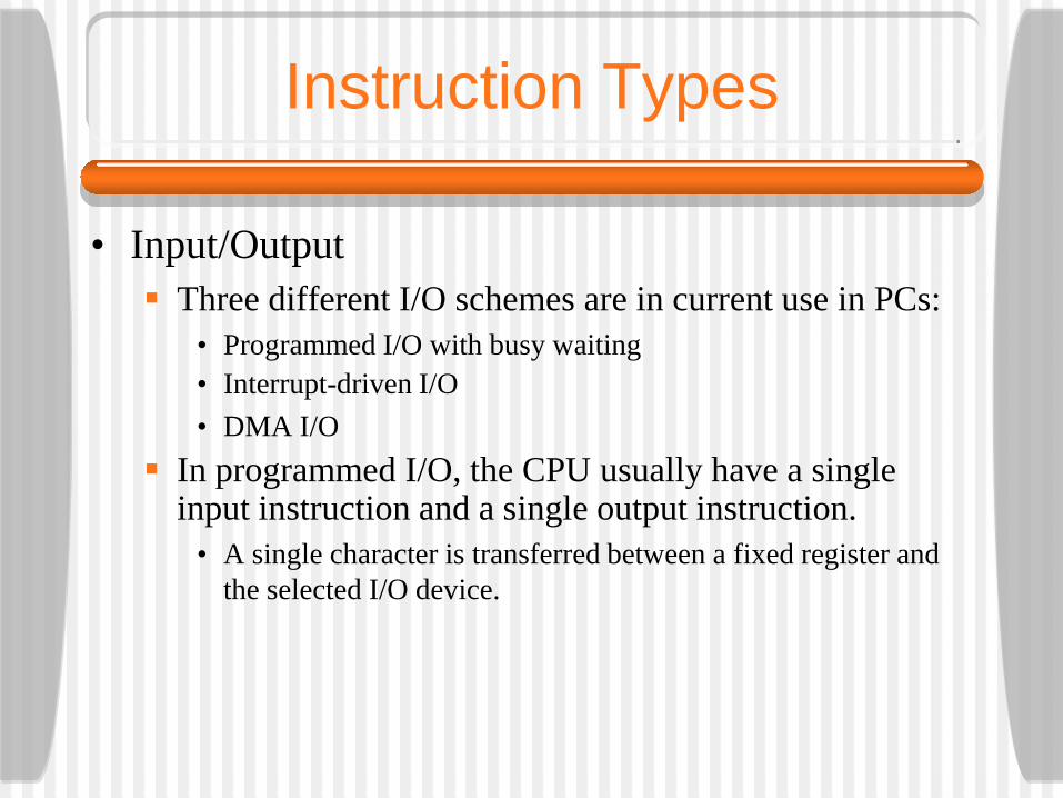
• Input/Output Three different I/O schemes are in current use in PCs:

• Programmed I/O with busy waiting• Interrupt-driven I/O• DMA I/O

In programmed I/O, the CPU usually have a single input instruction and a single output instruction.

• A single character is transferred between a fixed register and the selected I/O device.

Instruction Types

Device registers for a simple terminal.

Instruction Types

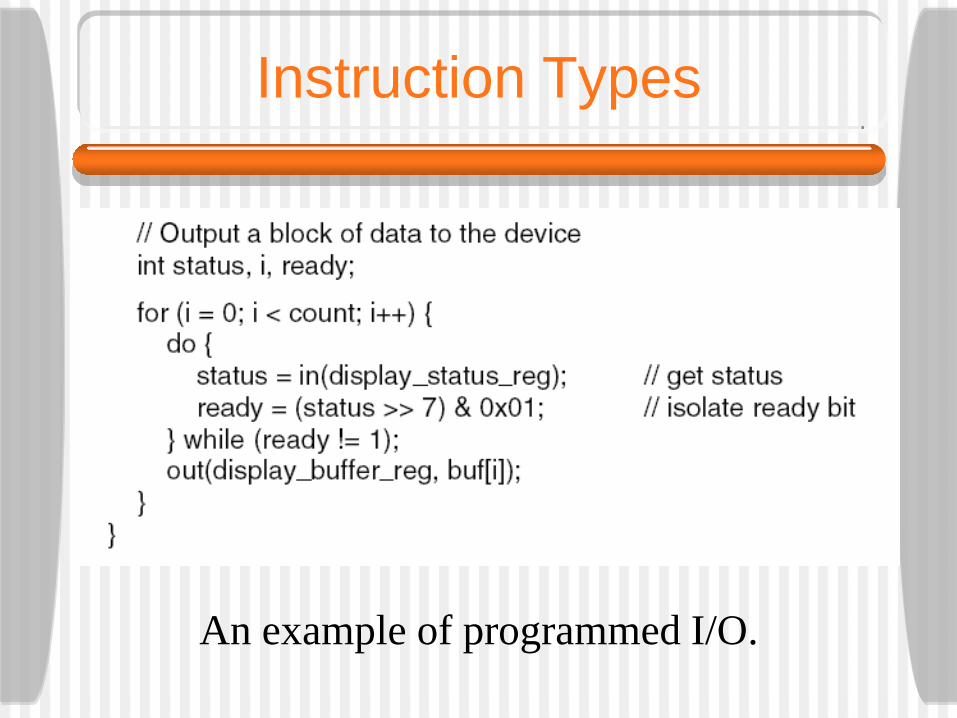
An example of programmed I/O.

Instruction Types

The primary disadvantage of programmed I/O is that the CPU wastes time in a tight loop.

• This is called busy waiting.• This is OK in embedded processors, but not in a

multitasking machine. We can avoid this problem by starting the I/O

and telling the I/O device to generate an interrupt when it is done. In Direct Memory Access (DMA), a chip

connected directly to the bus relieves the CPU of processing the interrupts.

Instruction Types

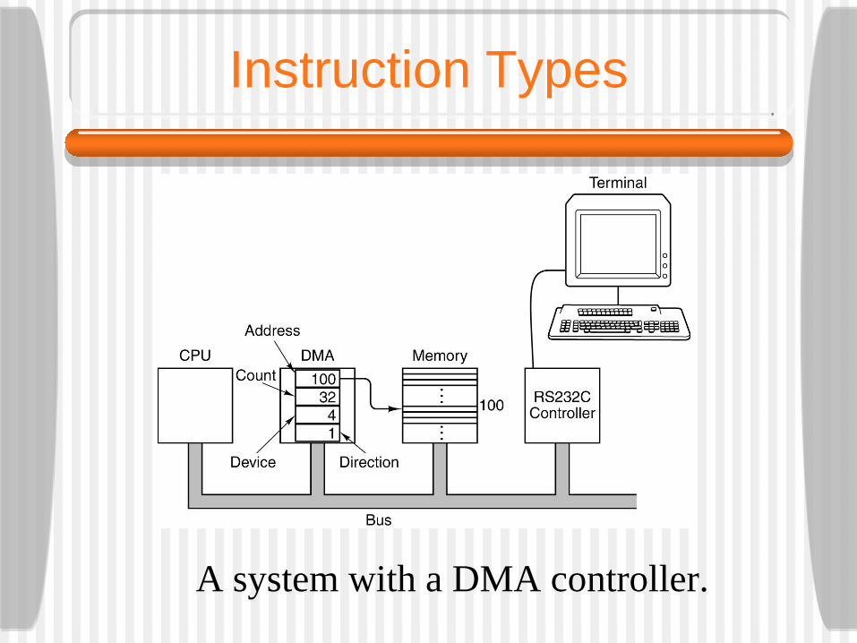
A system with a DMA controller.

instruction formats - personal.kent.eduaguercio/cs35101slides/tanenbaum/ca_ch0… · instruction...

Documents