instructional workshop on openfoam ... - github...
TRANSCRIPT

Instructional workshop on OpenFOAMprogramming
LECTURE # 7
Pavanakumar Mohanamuraly
May 10, 2014

Outline
gaussLaplacianScheme - walk through
Introduction to flux limiters
Limiters in OpenFOAM
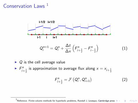
Conservation Laws 1
i
i+1/2i-1/2
i-1 i+1
Qn+1i = Qn
i +∆t
∆x
(F ni+ 1
2− F n
i− 12
)(1)
I Q is the cell average value
I F ni+ 1
2
is approximation to average flux along x = xi+ 12
F ni+ 1
2= F
(Qn
i ,Qni+1
)(2)
1Reference: Finite-volume methods for hyperbolic problems, Randall J. Leveque, Cambridge press

Method of Godunov
I Reconstruct a piecewise polynomial function qn(x , tn) definedfor all x , from the cell averages Qn
i .
I In the simplest case this is a piecewise constant function thattakes the value Qn
i in the i th grid cell, i.e.,
qn(x , tn) = Qni for all x ∈ Ci (3)
I Evolve the hyperbolic equation exactly (or approximately)with this initial data to obtain qn(x , tn+1) a time ∆t later.
I Average this function over each grid cell to obtain new cellaverages
Qn+1i =
1
∆x
∫Ci
qn(x , tn+1)dx (4)

High resolution finite volume schemes
I Assuming constant cell variation leads to O(∆x) error
i
i+1/2i-1/2
I Linear variation of values in cell leads to O(∆x2) error
i
i+1/2i-1/2
i-1 i+1
I Reconstruct slopes from cell centroid values
I Extrapolate to faces to get L/R states

Piecewise linear reconstruction
I To achieve better than first-order accuracy need better thanpiecewise constant function
I Construct a piecewise linear function using Qni
qn(x , tn+1) = Qni + σni (x − xi ) for xi− 1
2≤ x ≤ xi+ 1
2(5)
and
xi = xi− 12
+1
2∆x (6)
I σni is the function slope of the i th cell

Problems with linear reconstruction
I Consider a distribution of Qni as shown below (J is some
arbitrary cell)
Qni =
{1 if i ≤ J0 if i > J
(7)
108 6 High-Resolution Methods
6.6 Oscillations
As we have seen in Figure 6.1, second-order methods such as the Lax–Wendroff or Beam–Warming (and also Fromm’s method) give oscillatory approximations to discontinuoussolutions. This can be easily understood using the interpretation of Algorithm 4.1.
Consider the Lax–Wendroff method, for example, applied to piecewise constant datawith values
Qni =
!1 if i ! J,
0 if i > J.
Choosing slopes in each grid cell based on the Lax–Wendroff prescription (6.16) gives thepiecewise linear function shown in Figure 6.4(a). The slope ! n
i is nonzero only for i = J .The function qn(x, tn) has an overshoot with a maximum value of 1.5 regardless of "x .
When we advect this profile a distance u "t , and then compute the average over the J th cell,we will get a value that is greater than 1 for any "t with 0 < u "t < "x . The worst case iswhen u "t = "x/2, in which case qn(x, tn+1) is shown in Figure 6.4(b) and Qn+1
J = 1.125.In the next time step this overshoot will be accentuated, while in cell J " 1 we will nowhave a positive slope, leading to a value Qn+1
J"1 that is less than 1. This oscillation then growswith time.
The slopes proposed in the previous section were based on the assumption that thesolution is smooth. Near a discontinuity there is no reason to believe that introducing thisslope will improve the accuracy. On the contrary, if one of our goals is to avoid nonphysicaloscillations, then in the above example we must set the slope to zero in the J th cell. Any! n
J < 0 will lead to Qn+1J > 1, while a positive slope wouldn’t make much sense. On the
other hand we don’t want to set all slopes to zero all the time, or we simply have thefirst-order upwind method. Where the solution is smooth we want second-order accuracy.Moreover, we will see below that even near a discontinuity, once the solution is somewhatsmeared out over more than one cell, introducing nonzero slopes can help keep the solutionfrom smearing out too far, and hence will significantly increase the resolution and keepdiscontinuities fairly sharp, as long as care is taken to avoid oscillations.
This suggests that we must pay attention to how the solution is behaving near the i thcell in choosing our formula for ! n
i . (And hence the resulting updating formula will benonlinear even for the linear advection equation). Where the solution is smooth, we want tochoose something like the Lax–Wendroff slope. Near a discontinuity we may want to limitthis slope, using a value that is smaller in magnitude in order to avoid oscillations. Methodsbased on this idea are known as slope-limiter methods. This approach was introduced by van
(a)
QnJ
(b)
Fig. 6.4. (a) Grid values Qn and reconstructed qn(·, tn) using Lax–Wendroff slopes. (b) After advectionwith u "t = "x/2. The dots show the new cell averages Qn+1. Note the overshoot.(a) Linear reconstruction for f (x) using cell averages Qn
i
(b) Simple linear advection of reconstructed values to tn+1
Under/Overshoot in solution

The remedy
I Introduce a function φ(θni ) to limit the slope of the functionas shown below,
qn(x , tn+1) = Qni + φ(θni )︸ ︷︷ ︸
limiter
σni︸︷︷︸slope
(x − xi ) for xi− 12≤ x ≤ xi+ 1
2
(8)
I θni is a measure of the variation of the function Qni in cell i
I φ = 0 is piecewise constant reconstruction
I φ = 1 is piecewise linear reconstruction
I 0 < φ < 1 is piecewise linear reconstruction (with loss ofaccuracy)

Variation measure θni
I Many ways to obtain θ
I Implementation dependent function
I An example upwind version
θni =∆Qn
I− 12
∆Qni− 1
2
(9)
where,∆Qn
i− 12
= Qni − Qn
i−1 (10)
and
I =
{i − 1 if a > 0i + 1 if a < 0
(11)
where, a is the wave speed (advection)

Limiter function φ 2
I Many choices available and no-universal choice
I Can be differentiable or non-differentiable
I Differentiable limiter = smoother convergence
the differentiable Venkatakirhsnan limiter outperforms the min-max limiter and enables computation using higher CFL values. The Mach contour over the wing has been plotted in figure (3) and the chordwise non-dimensional pressure coefficient variation at three span location of the wing are plotted in figure (4). The results look quite similar for all the CFL numbers and limiters except for the min-max limiter with a CFL value of 1.5
Figure (2) Residual plot for CFL (i) 0.9, (ii) 1.2 and (iii) 1.5
I Min-Max is non-differentiable
I Venkatakishnan is differentiable
2Pavanakumar et al, NCAE 2012

Higher than 2nd order
I Is it possible to go higher than second order ?
I Can we use higher-order (> 1) polynomials to reconstruct ?
I There are two main problems discussed in the next two slides

Curse of polynomial interpolationFit a polynomial over functions
I Runge phenomena
f (x) =1
1 + x2for − 1 ≤ x ≤ 1 (12)

Curse of polynomial interpolationFit a polynomial over functions
I Gibbs oscillation
f (x) =
{0 if x ≤ 0.51 if x > 0.5
for 0 ≤ x ≤ 1 (13)
0 0.1 0.2 0.3 0.4 0.5 0.6 0.7 0.8 0.9 1−0.2
0
0.2
0.4
0.6
0.8
1
1.2
Student Version of MATLAB

Higher order polynomial
At steep gradients
I Suffer from under-shoot and over-shoot
I Violation of bounds
I Monotonic solution can become non-monotonic
Remedy
I Use orthogonal polynomial like Chebyshev, Legendre, etc
I ENO or WENO type limited polynomials
Beyond the scope of OpenFOAM
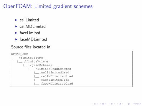
OpenFOAM: Limited gradient schemes
I cellLimited
I cellMDLimited
I faceLimited
I faceMDLimited
Source files located in
$FOAM_SRC|__ /finiteVolume
|__ /finiteVolume|__ /gradSchemes
|__ /limitedGradSchemes|__ cellLimitedGrad|__ cellMDLimitedGrad|__ faceLimitedGrad|__ faceMDLimitedGrad

cellLimited gradient scheme - Some notationsI Let the face neighbouring cells of cell i be j ∈ Cij
I Let the faces of cell i be o ∈ Cio
I rio is the line joining cell i ’s centroid to its face centroidsI rij is the line joining cell i ’s centroid to its face neighbouring
cell j ’s centroids
3 Spatial Discretization
The weighted least-squares procedure is used to evaluate the derivatives of the fluxes.Since, upwinding is necessary to stabilize the scheme we evaluate the mid-point flux at theedge connecting the point i with its neighbor j. We refer to the figure (1) for convention.
i
j
o
LR
rio
nio
rij
Support/Connectivity : C(i)Mid-Point Node : oUpwind Direction : nioLeft State : LRight State : R
Figure 1: Least-square procedure for flux derivative evaluation
A local Riemann problem is solved in the interface o to yield the interfacial flux Fio.The left L and right R states are obtained by appropriate reconstruction procedure. Inthe present work, two types of reconstructions are implemented, namely,
• Zeroth order reconstruction
• Gradient based first order reconstruction with slope limiting
We now formulate the least-squares problem for evaluating this mid-point flux Fio. Thevector joining node i to its neighbor mid-point o is defined as rio(∆xio,∆yio,∆zio). Onecan formulate the weighted least-squares problem for the derivatives in two different ways,
• Taylor Series Extrapolation
• Polynomial Interpolation
The former satisfies the so called delta property, i.e. the function value at the evaluationpoint is exactly satisfied but the later does not satisfy this property.
2

cellLimited gradient scheme
I Find maximum and minimum values of all cell (face)neighbours (Cij)
qmaxi = max
j∈Cij
qij (14)
qmini = min
j∈Cij
qij (15)
I ij is the cell i ’s j th face-cell neighbour
I io is the cell i ’s oth face
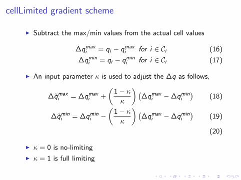
cellLimited gradient scheme
I Subtract the max/min values from the actual cell values
∆qmaxi = qi − qmax
i for i ∈ Ci (16)
∆qmini = qi − qmin
i for i ∈ Ci (17)
I An input parameter κ is used to adjust the ∆q as follows,
∆qmaxi = ∆qmax
i +
(1− κκ
)(∆qmax
i −∆qmini
)(18)
∆qmini = ∆qmin
i −(
1− κκ
)(∆qmax
i −∆qmini
)(19)
(20)
I κ = 0 is no-limiting
I κ = 1 is full limiting

cellLimited gradient scheme
I Calculate gradient ∇qi using a suitable gradScheme
I Set the cell limiter values φi as follows, (loop over all faces ofcell)
φi =
min
[1, min
o∈Cio
(∆qmax
i∇qi ·rio
)]if ∆qmax
i < ∇qi · rio
min
[1, min
o∈Cio
(∆qmin
i∇qi ·rio
)]if ∆qmin
i > ∇qi · rio
(21)
I Now the limited gradient value is φi∇qi
This is the min/max limiter and remember the same φi value isused for all components of ∇qi
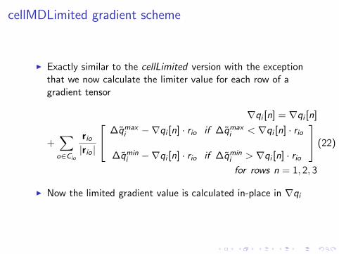
cellMDLimited gradient scheme
I Exactly similar to the cellLimited version with the exceptionthat we now calculate the limiter value for each row of agradient tensor
∇qi [n] = ∇qi [n]
+∑o∈Cio
rio|rio |
∆qmaxi −∇qi [n] · rio if ∆qmax
i < ∇qi [n] · rio
∆qmini −∇qi [n] · rio if ∆qmin
i > ∇qi [n] · rio
(22)
for rows n = 1, 2, 3
I Now the limited gradient value is calculated in-place in ∇qi

faceLimited gradient scheme
I Max/min values calculated using local face owner/neighbourcell values
qmaxio = max(qownio , qneiio ) (23)
qminio = min(qownio , qneiio ) (24)
I Correct max/min face values using input parameter κ
qmaxio = qmax
io +
(1− κκ
)(qmax
io − qminio ) (25)
qminio = qmin
io −(
1− κκ
)(qmax
io − qminio ) (26)

faceLimited gradient scheme
I Let ∇qi be the gradient obtained from gradScheme
I Limiter function φi is calculated as follows,
φi =
min
[1, min
o∈Cio
(∆qmax
io∇qi ·rio
)]if ∆qmax
io < ∇qi · rio
min
[1, min
o∈Cio
(∆qmin
io∇qi ·rio
)]if ∆qmin
io > ∇qi · rio
(27)
where, ∆qmax/minio = qi − q
max/minio
I Now the limited gradient value is φi∇qi
More dissipative than cellLimited version but cheapercomputationally (2X faster)
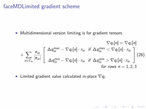
faceMDLimited gradient scheme
I Multidimensional version limiting is for gradient tensors
∇qi [n] = ∇qi [n]
+∑o∈Cio
rio|rio |
∆qmaxio −∇qi [n] · rio if ∆qmax
io < ∇qi [n] · rio
∆qminio −∇qi [n] · rio if ∆qmin
io > ∇qi [n] · rio
(28)
for rows n = 1, 2, 3
I Limited gradient value calculated in-place ∇qi

End of Week 3 Day 2