instructors solutions to assignment 3 - york university · instructors solutions to assignment 3...

Instructors Solutions to Assignment 3 Problem 4.6

(a) By inspection, we note that the time period T0 = 2π, which implies that the fundamental frequency ω0 = 1.

Since the CTFS coefficient a0 represents the average value of the signal, therefore, a0 = 3/2.

Using Eq. (4.31), the CTFS cosine coefficients an’s, for (n ≠ 0), are given by

[ ] [ ]

0

0 0 00 0 0

0

2 1 1

3 3

1( )cos( ) 3cos( ) 3cos( )

sin( ) sin( ) 0 0

T

n T

n n

a x t n t dt n t dt nt dt

nt n

π π

ππ

π π

π

ω ω

π

= = =

= = − =

∫ ∫ ∫

Using Eq. (4.32), the CTFS sine coefficients bn’s are given by

[ ] [ ]0

0 0 00 0

3 3 32 1

6

1( )sin( ) 3sin( ) cos( ) cos( ) cos(0) 1 ( 1)

0

Tn

n n n nT

n

b x t n t dt nt dt nt n

n odd

n even

ππ

ππ π π

π

ω π ⎡ ⎤= = = − = − + = − −⎣ ⎦

⎧ =⎪= ⎨=⎪⎩

∫ ∫

(c) By inspection, we note that the time period T0 = T, which implies that the fundamental frequency ω0 = 2π/T.

Since the CTFS coefficient a0 represents the average value of the signal, therefore, a0 = 1/2.

Since the function [x3(t) − 0.5] is odd, therefore, the CTFS cosine coefficients an = 0, for (n ≠ 0).


( )

π=

ω=

⎥⎥⎦

⎤

⎢⎢⎣

⎡

ω×⎟

⎠⎞⎜

⎝⎛−+

ωω×⎟

⎠⎞⎜

⎝⎛−

ω−×−=

⎥⎥⎦

⎤

⎢⎢⎣

⎡

ωω−×⎟

⎠⎞⎜

⎝⎛−−

ωω−×⎟

⎠⎞⎜

⎝⎛ −=

ω⎟⎠⎞⎜

⎝⎛ −= ∫

nTn

nTnTn

TnT

ntn

Tntn

Tt

T

dttnTt

Tb

T

T

n

12

)()0sin(1

)()sin(1

)(1102

)()sin(1

)()cos(12

)sin(12

0

20

20

0

0

02

0

0

0

0

00

(e) By inspection, we note that the time period T0 = 2T, which implies that the fundamental frequency ω0 = π/T.

Using Eq. (4.30), the CTFS coefficient T0 is given by

( ) ( )

[ ]

2

00 0 0 0

0

2 2 2 4

2 4 2 4 2 2 2/

1 1 1 1

11 1 1 1 1 1 1

( ) 1 0.5sin sin

cos( ) cos( ) cos(0)

T T T Tt tT T

TtT

T T T T

T T

a x t dt dt dt dtπ π

ππ π ππ

ππ −

⎡ ⎤= = − = −⎣ ⎦

= + × = + − = − =⎡ ⎤⎣ ⎦

∫ ∫ ∫ ∫

Assignment 2 CSE3451: Signals and Systems 2

Using Eq. (4.31), the CTFS cosine coefficients an’s, for (n ≠ 0), are given by

( ) ( )0 0 00 0 0

2 22 1 11 0.5sin cos( ) cos( ) sin cos( )T T T

t tn T T

A B

TT Ta n t dt n t dt n t dtπ πω ω ω

= =

⎡ ⎤= − = −⎣ ⎦∫ ∫ ∫1 4 4 2 4 43 1 4 4 44 2 4 4 4 43

where Integrals A and B are simplified as

[ ] [ ] [ ]0 0001 1 1sin( ) sin( ) 0 sin( ) 0 0T

n nn TA n t n T nπ πω ω ω π= = − = − =

and

( ) ( ) ( ) ( )

[ ][ ]

00 0 0

0 0

2 2 4

4 4( 1)/ ( 1)/

4 ( 1)

1 1 1

1 1 1 1

1 1

sin cos( ) sin cos sin ( 1) sin ( 1)

cos ( 1) cos ( 1) for 1

1 cos ( 1)

T T Tt t n t t tT T T T T

T Tt tT T

T T T

T Tn T n T

n

B n t dt dt n n dt

n n n

n

π π π π π

π ππ π

π

ω

π+ −

+

−

⎡ ⎤= = = + − −⎣ ⎦

= × + + × − ≠⎡ ⎤ ⎡ ⎤⎣ ⎦ ⎣ ⎦

= − + −

∫ ∫ ∫

[ ]

2

4 ( 1)

4 ( 1) 4 ( 1) ( 1)12 2

1 cos ( 1)

0 10 1n

n n n

n

n oddn odd

n evenn even

π

π π π

π−

+ − −

− −

≠ =≠ = ⎧⎧⎪ ⎪= =⎨ ⎨− =− =⎪ ⎪⎩ ⎩

For [ ]2 20

04 4 82 /1 1 1 11, sin cos 1 cos2 0T

Tt tT TT T Tn B dtπ π

ππ π−= = = × = − =⎡ ⎤⎣ ⎦∫ .

In other words, 2( 1)1

0

n

n oddB

n evenπ −

=⎧⎪= ⎨− =⎪⎩

which implies that

2( 1)1

0n

n

n odda A B

n evenπ −

=⎧⎪= − = ⎨ =⎪⎩


bn =22T 1− 0.5sin π t

T( )⎡⎣ ⎤⎦sin(nω0t)dt0

T

∫ = 1T sin(nω0t)dt0

T

∫=C

− 12T sin π t

T( )sin(nω0t)dt0

T

∫=D

where Integrals C and D are simplified as

[ ] [ ] [ ]0 0001 1 1

2

0cos( ) cos( ) cos(0) 1 cos( )T

n nn Tn

n evenC n t n T n

n oddπ πωπ

ω ω π=⎧⎪= − = − + = − = ⎨=⎪⎩

and

Assignment 2 CSE3451: Signals and Systems

3

( ) ( ) ( )

[ ][ ]

0 0

0 0

2 4

4 4( 1)/ ( 1)/

4 ( 1) 4 ( 1)

1 1

1 1 1 1

1 1

sin sin cos ( 1) cos ( 1)

sin ( 1) sin ( 1) for 1

sin ( 1) sin(0) sin ( 1) sin

T Tt n t t tT T T T

T Tt tT T

T T

T Tn T n T

n n

D dt n n dt

n n n

n n

π π π π

π ππ π

π ππ π− +

− +

⎡ ⎤= = − − +⎣ ⎦

= × − − × + ≠⎡ ⎤ ⎡ ⎤⎣ ⎦ ⎣ ⎦

= − − − + −

∫ ∫

[ ][ ]

(0)

0 for 1n= ≠

For (n = 1),

D = 12T sin2 π t

T( )dt0

T

∫ = 14T 1− cos 2π t

T( )⎡⎣ ⎤⎦dt0

T

∫ = 14 −

14T×2π /T sin

2π tT⎡⎣ ⎤⎦0

T

=0

⎛

⎝⎜⎜

⎞

⎠⎟⎟= 14 .

In other words, 14 1

0 1

nD

n

=⎧⎪= ⎨>⎪⎩

.

Therefore, 4

2 1

2

0

1

1 .n

n

n even

b C D n

n oddπ

π

=⎧⎪⎪= − = − =⎨⎪

≠ =⎪⎩

▌

Problem 4.11

(a) By inspection, we note that the time period T0 = 2π, which implies that the fundamental frequency ω0 = 1. Using Eq. (4.44), the DTFS coefficients Dn’s are given by

( )⎪⎩

⎪⎨⎧

≠−

==

π== π−

π

π−

−

ω− ∫∫ .01

0,3

21)(1

23

23

0

2

20

0

0

0

ne

ndtedtetx

TD jn

nj

jntT

T

tjnn

or, ( )⎪⎪⎩

⎪⎪⎨

⎧

≠

=

=−−π

=

π n

nn

n

njD

jn

nn

odd

.0,even 0

0

)1(123

3

23

The magnitude and phase spectra are given by

Magnitude Spectrum: ⎪⎩

⎪⎨

⎧

≠=

=

π . odd,.0,even ,0

0,

3

23

nnn

nD

n

n

Phase Spectrum: ⎪⎩

⎪⎨

⎧

<>−=

π

π

.0, odd,0, odd,

even ,0

2

2nnnnn

Dn

The magnitude and phase spectra are shown in row 1 of the subplots included in Fig. S4.11.

(c) By inspection, we note that the time period T0 = Τ, which implies that the fundamental frequency ω0 = 2π/T. Using Eq. (4.44), the DTFS coefficients Dn’s are given by


( )( )⎪

⎪

⎩

⎪⎪

⎨

⎧

≠−

==×

=−==

∫∫∫

ω−

ω−ω−

.011

0,11)(1

0

21

21

00 0

00

ndteT

ndte

Tdtetx

TD T

tjnTt

TTT

tjnTt

Ttjn

n

For (n ≠ 0), the DTFS coefficients are given by

( ) ( ) ( )Ttjn

T

tjn

Tt

Ttjn

Tt

n jne

jnedte

TD

02

0

1

00 )()(111 00

0

⎥⎥⎦

⎤

⎢⎢⎣

⎡

ω−−−

ω−−=−=

ω−ω−ω−∫ ,

which reduces to

π

=⎥⎥⎦

⎤

⎢⎢⎣

⎡

ω−−

ω−+

ω−−=

ω−

njjnjne

jnD

T

T

Tjn

TTn 21

)(1

)()(10

02

0

12

0

1

0

10

.

Combining the two cases, we get

⎪⎩

⎪⎨⎧

≠

==

π .0,

0,

2121

n

nD

njn

The magnitude and phase spectra are given by

Magnitude Spectrum: ⎪⎩

⎪⎨⎧

≠

==

π.0,

0,

2121

n

nD

nn

Phase Spectrum: ⎪⎩

⎪⎨⎧

>π−<π=

=.0,5.00,5.00,0

nnn

Dn

The magnitude and phase spectra are shown in row 3 of the subplots included in Fig. S4.11.

(e) By inspection, we note that the time period T0 = 2Τ, which implies that the fundamental frequency ω0 = π/T. For (n = 0), the exponential DTFS coefficients is given by

( ) ( )

[ ]

2

00 0 0 0

0

2 2 2 4

2 4 2 4 2 2/

1 1 1 1

1 1 1 1 1 1 1

( ) 1 0.5sin sin

cos( ) cos( ) cos(0)

T T T Tt tT T

TtT

T T T T

T T

D x t dt dt dt dtπ π

ππ ππ π

⎡ ⎤= = − = −⎣ ⎦

= + × = + − = −⎡ ⎤⎣ ⎦

∫ ∫ ∫ ∫

For (n = 0), the exponential DTFS coefficients is given by

Dn =12T 1− 0.5sin π t

T( )⎡⎣ ⎤⎦e− jnω0t dt =

0

T

∫ 12T e− jnω0t dt

0

T

∫=A

− 14T sin π t

T( )e− jnω0t dt0

T

∫=B

.

Solving for Integrals A and B, we get


5

0 0

000

2 2 2 21 1 1 11 1 ( 1)T

Tjn t jn t jn nT j n T j n j nA e dt e eω ω π

ω π π− − −

− −⎡ ⎤ ⎡ ⎤ ⎡ ⎤= = = − = − −⎣ ⎦ ⎣ ⎦⎣ ⎦∫

and

( )

( )

( 1) ( 1)

( 1) ( 1)

0 0 0

( 1) ( 1)0

( 1)1 1( 1)

4 8 8

8

8

1 1 1

1

1

sin

for 1

1

jn t j t j t jn t j n t j n tT T T T T T

j n t j n tT T

T T TtT

TT T

j n j n

j nn

T j T j T

j T

B e dt e e e dt e e dt

e e n

e

π π π π π π

π π

π

π π

ππ

− − − − − − +

− − − +

− − +

− −−

⎡ ⎤ ⎡ ⎤= = − = −⎣ ⎦ ⎣ ⎦

⎡ ⎤= + ≠ ±⎣ ⎦

= − −

∫ ∫ ∫

( )2

2

( 1)( 1)

( 1) ( 1)1 1 1( 1) ( 1) 4 ( 1)

14 ( 1)

81

1

( 1) 1 1 ( 1)

1 ( 1)

j nn

n nn n n

nn

e ππ

π

π

π

− ++

− −−− + −

−−

⎡ ⎤−⎣ ⎦⎡ ⎤ ⎡ ⎤ ⎡ ⎤= − − − = − −⎣ ⎦ ⎣ ⎦⎣ ⎦

⎡ ⎤= + −⎣ ⎦

For n = ± 1, Integral B reduces to

2 2

200

8 8 8 81 1 1For 1, 1 = =

j t j tT T

T TTjj T j T j T j

Tn B e dt t eπ π

π

− −⎡ ⎤ ⎡ ⎤= = − = +⎣ ⎦ ⎣ ⎦∫

and 2 2

200

8 8 8 81 1 1For 1, 1 = =

j t j tT T

T TTjj T j T j T j

Tn B e dt e tπ π

π

− − −⎡ ⎤ ⎡ ⎤= − = − = − − −⎣ ⎦ ⎣ ⎦∫ .

In other words, 2

18

14 ( 1)

1

1 ( 1) j

nn

nB

otherwiseπ

−−

± = ±⎧⎪= ⎨ ⎡ ⎤+ −⎪ ⎣ ⎦⎩

Combining, the above cases, the CTFS coefficients can be expressed as

2

1 12 2

18

14 ( 1)

12

2

2

1

1

0

1 ( 1) 1

1 ( 1) 1 ( 1)

1

nn j

n nn

j n

j n

n

D n

otherwise

π

π

π

π −

⎧ − =⎪⎪ ⎡ ⎤= − − = ±⎨ ⎣ ⎦⎪ ⎡ ⎤ ⎡ ⎤− − + + −⎪ ⎣ ⎦ ⎣ ⎦⎩

−

=

m

( )( )

( )2

1

18

14 ( 1)

1 12

2

1

1

0

1

1 ( 1) 1 ( 1)

1

n nn j n

n

j n

otherwise

π

π

π

π

π−

⎧ =⎪⎪ − = ±⎨⎪ ⎡ ⎤ ⎡ ⎤+ − + − −⎪ ⎣ ⎦ ⎣ ⎦⎩

−

=

m

( )2

18

12 ( 1)

1

1

0

1

0

1n

jn

n

j n

n even

n oddπ

π

π

−

⎧ =⎪

− = ±⎪⎪⎨

≠ =⎪⎪ ± ≠ =⎪⎩

m

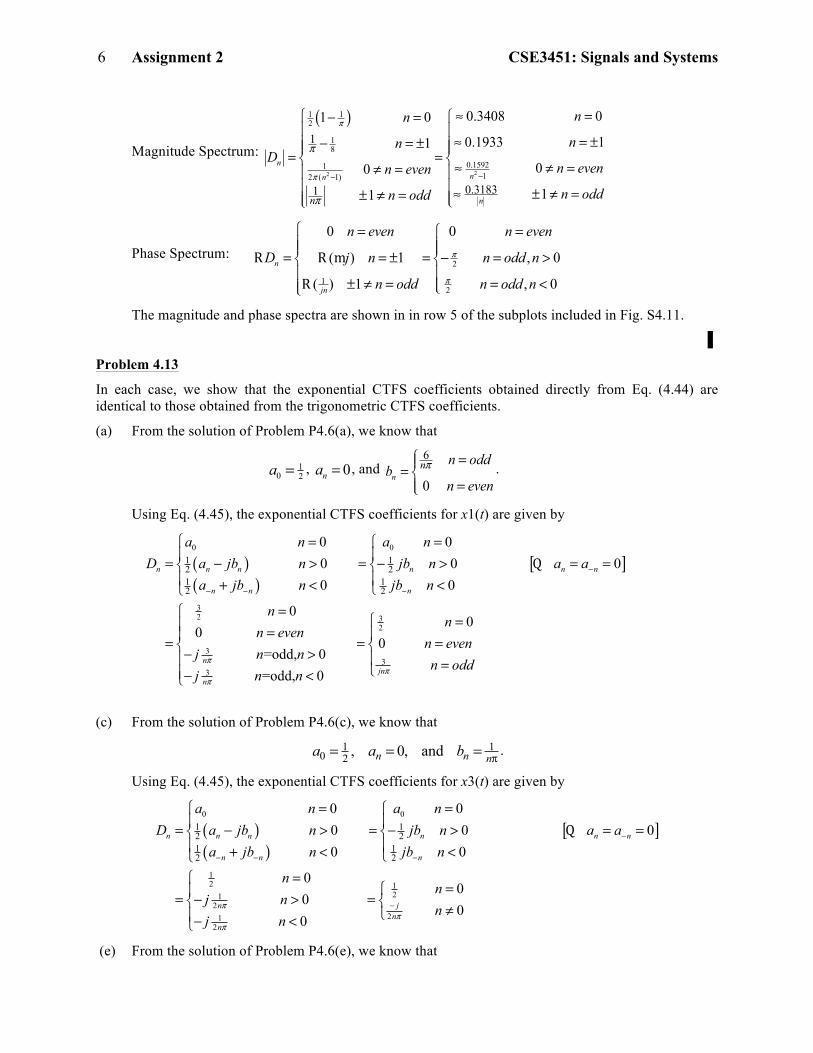
The expressions for the magnitude and phase spectra are given by


Magnitude Spectrum:

( )

22

1 12

18

0.1592112 ( 1)

1

0.31831

0.3408 01 0

0.1933 1 1

0 0

1 1

nnn

nn

nn

nnD

n evenn even

n oddn odd

π

π

π

π

−−

≈ =⎧ ⎧− =⎪ ⎪

≈ = ±− = ±⎪ ⎪⎪ ⎪= =⎨ ⎨≈ ≠ =≠ =⎪ ⎪⎪ ⎪≈ ± ≠ =± ≠ = ⎪⎪ ⎩⎩

Phase Spectrum: 2

12

0 0

( ) 1 , 0

( ) 1 , 0n

jn

n even n even

D j n n odd n

n odd n odd n

π

π

⎧ = =⎧⎪ ⎪⎪ ⎪= = ± = − = >⎨ ⎨⎪ ⎪

± ≠ = = <⎪⎪ ⎩⎩

R R m

R

The magnitude and phase spectra are shown in in row 5 of the subplots included in Fig. S4.11.

▌

Problem 4.13

In each case, we show that the exponential CTFS coefficients obtained directly from Eq. (4.44) are identical to those obtained from the trigonometric CTFS coefficients.

(a) From the solution of Problem P4.6(a), we know that

10 2a = , 0na = , and

6

0n

n n oddb

n evenπ⎧ =⎪= ⎨

=⎪⎩.

Using Eq. (4.45), the exponential CTFS coefficients for x1(t) are given by

( )( )

[ ]0 0

32

3

3

1 12 21 12 2

0 0 0 0 0

0 0

00

=odd, 0

n n n n n n

n n n

n

n

a n a nD a jb n jb n a a

a jb n jb n

nn even

j n nj

π

π

−

− − −

= =⎧ ⎧⎪ ⎪= − > = − > = =⎨ ⎨⎪ ⎪+ < <⎩⎩

==

=− >−

Q

32

3

0 0

=odd, 0 jn

nn evenn odd

n n π

⎧ ⎧ =⎪ ⎪⎪ = =⎨ ⎨⎪ ⎪ =⎩⎪ <⎩

(c) From the solution of Problem P4.6(c), we know that

π=== nnn baa 121

0 and,0, .


( )( )

[ ]0 0

12

12

12

1 12 21 12 2

0 0 0 0 0

0 0

0 0

n n n n n n

n n n

n

n

a n a nD a jb n jb n a a

a jb n jb n

nj nj

π

π

−

− − −

= =⎧ ⎧⎪ ⎪= − > = − > = =⎨ ⎨⎪ ⎪+ < <⎩⎩

== − >

−

Q

12

2

0

0 0

jn

nn

n π−

⎧=⎧⎪ =⎨ ⎨ ≠⎩⎪ <⎩

(e) From the solution of Problem P4.6(e), we know that


7

0 2 21 1a π= − ,

2( 1)1

0n

n

n odda

n evenπ −

=⎧⎪= ⎨ =⎪⎩, and

42 1

2

0

1

1n n

n

n even

b n

n oddπ

π

=⎧⎪⎪= − =⎨⎪

≠ =⎪⎩


(n = 0): 0 2 21 1D π= −

(n = 1): ( ) ( ) ( )1 1 112 2 4 8

2 1 1 1jD a jb jπ π= − = − − = −

(n = −1): ( ) ( ) ( )1 1 112 2 4 8

2 1 1 1jD a jb jπ π− = + = − = − −

(n > 1): ( )22

1

112 ( 1)2 ( 1)

12

jjnn

n n nnn

n oddn oddD a jb

n evenn evenππ

ππ −−

⎧ =⎧− =⎪ ⎪= − = =⎨ ⎨ ==⎪ ⎪⎩⎩

(n < −1): ( )( )

22

122

112 ( 1)2 ( 1)

12

jjnn

n n nnn

n oddn oddD a jb

n evenn evenππ

ππ

−− −

−−

⎧ =⎧=⎪ ⎪= + = =⎨ ⎨ ==⎪ ⎪⎩⎩

Combining the above results, we obtain

( )( )2

1 12

18

12 ( 1)

1

1

1 0

1

0

1 .

n

n

jn

n

j nD

n even

n odd

π

π

π

π

−

⎧ − =⎪± − = ±⎪⎪= ⎨

≠ =⎪⎪ ± ≠ =⎪⎩

Problem 5.2

(a) By definition,

[ ] [ ] [ ]

[ ] [ ] [ ]).2/(sinc3

66)2/sin(2

133)(

2/

2/)2/sin(

/212/)2/sin(2/2/3

0

2/2/2/330)(1

ωπ=

×==ωπ−−=

−−=−−===ω

ωπ−

ωπωπ

πωπ−

ωωπωπ−ωπ−

ω

πωπωπ−ωπ−

ωωπ−

ωπ

ω−ω−∫

ω−

j

jjjj

jjjj

jjj

etj

e

eeje

eeeedteXtj

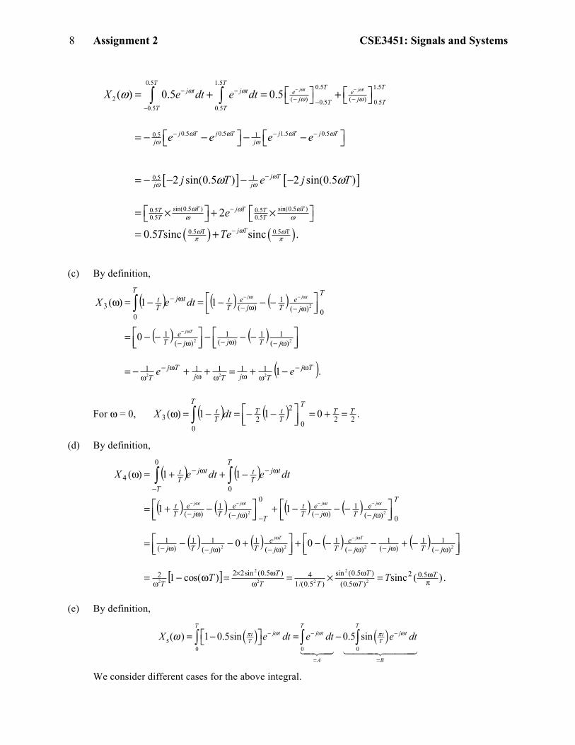
(b) By definition,


[ ] [ ]

0.5 1.5 0.5 1.5

2 ( ) ( )0.5 0.50.5 0.5

0.5 0.5 1.5 0.50.5 1

0.5 1

sin0.50.5

( ) 0.5 0.5

2 sin(0.5 ) 2 sin(0.5 )

j t j tT T T Tj t j t e e

j jT TT T

j T j T j T j Tj j

j Tj j

TT

X e dt e dt

e e e e

j T e j T

ω ωω ωω ω

ω ω ω ωω ω

ωω ω

ω

ω ω

− −− −− −−

−

− − −

−

⎡ ⎤ ⎡ ⎤= + = +⎣ ⎦ ⎣ ⎦

⎡ ⎤ ⎡ ⎤= − − − −⎣ ⎦ ⎣ ⎦

= − − − −

= ×

∫ ∫

( ) ( )

(0.5 ) sin(0.5 )0.50.5

0.5 T 0.5 T

2

0.5 sinc sinc .

T Tj T TT

j T

e

T Te

ω ωωω ω

ωω ωπ π

−

−

⎡ ⎤ ⎡ ⎤+ ×⎣ ⎦ ⎣ ⎦= +

(c) By definition,

( ) ( ) ( )

( ) ( )

( ).1

0

11)(

222

22

2

11111

)(11

)(1

)(1

0)(1

)(0

3

TjTjTj

TjT

jTjje

T

T

je

Tje

Tt

Ttj

Tt

ee

dteX

Tj

tjtj

ω−ωωωω

ω−ω

ω−ω−ω−

ω−ω−ω−

−+=++−=

⎥⎦⎤

⎢⎣⎡ −−−⎥⎦

⎤⎢⎣⎡ −−=

⎥⎦⎤

⎢⎣⎡ −−−=−=ω

ω−

ω−ω−

∫

For ω = 0, ( ) ( ) 220

22

03 011)( TT

T

TtT

T

Tt dtX =+=⎥⎦

⎤⎢⎣⎡ −−=−=ω ∫ .

(d) By definition,

( ) ( )

( ) ( ) ( ) ( )

( ) ( ) ( ) ( )

[ ] .)(sinc)cos(1

00

11

11)(

5.02)5.0()5.0(sin

)5.0/(14)5.0(sin222

)(11

)(1

)(1

)(1

)(11

)(1

0)(1

)(

0

)(1

)(

0

0

4

2

2

22

2

2

2222

22

πω

ωω

ωω×

ω

ω−ω−ω−ω−ω−ω−

ω−ω−−ω−ω−

ω−

−

ω−

=×==ω−=

⎥⎦⎤

⎢⎣⎡ −+−−−+⎥⎦

⎤⎢⎣⎡ +−−=

⎥⎦⎤

⎢⎣⎡ −−−+⎥⎦

⎤⎢⎣⎡ −+=

−++=ω

ω−ω

ω−ω−ω−ω−

∫∫

TTT

TTT

T

jTjje

Tje

TjTj

T

je

Tje

Tt

Tje

Tje

Tt

Ttj

Tt

T

tjTt

TT

dtedteX

TjTj

tjtjtjtj

(e) By definition,

X 5(ω ) = 1− 0.5sin π tT( )⎡⎣ ⎤⎦e

− jωt dt =0

T

∫ e− jωt dt0

T

∫=A

− 0.5 sin π t

T( )e− jωt dt0

T

∫=B

We consider different cases for the above integral.


9

Case I: ( ω = 0)

( ) ( )

[ ]

50 0

0 2/0.5 1

(0) ( ) 1 0.5sin 0.5 sin

cos( ) cos( ) cos(0) (1 )

T Tt tT T

TtTT

T T

X x t dt dt dt dt

T T T T

π π

ππ πππ π

−∞ ∞

∞ −∞

⎡ ⎤= = − = −⎣ ⎦

= + = + − = − = −⎡ ⎤⎣ ⎦

∫ ∫ ∫ ∫

Case II: ( ω ≠ 0, ω ≠ π/T):

[ ]0

0

1 1 11 1 0T

Tj t j t j T j Tj j jA e dt e e eω ω ω ωω ω ω ω− − − −

− −⎡ ⎤ ⎡ ⎤ ⎡ ⎤= = = − = − ≠⎣ ⎦ ⎣ ⎦ ⎣ ⎦∫

B = 0.5 e− jωtπ2

T2−ω 2

− jω sin π tT( )− π

T cosπ tT( ){ }⎡

⎣⎢

⎤

⎦⎥0

T

for ω ≠ 0,± πT

= 0.5T 2

π 2−ω 2T 2e− jωt jω sin π t

T( )=0 at t=0,T

+ πT cos

π tT( )

⎧⎨⎪

⎩⎪

⎫⎬⎪

⎭⎪

⎡

⎣

⎢⎢⎢

⎤

⎦

⎥⎥⎥0

T

= 0.5T 2

π 2−ω 2T 2− πT e

− jωT − πT

⎡⎣ ⎤⎦ =0.5πT

π 2−ω 2T 21+ e− jωT⎡⎣ ⎤⎦

Case III: ( ω = π/T):

( )

2

2

2

( ) ( )0.5 0.52 2

0 0 0

0.52

0

0.52

0

0.5 sin

1

,

1

t tT T T T

tT

j tT

tT

T T Tj j j t j tj t j tt

T j j

Tj

j

Tj

j

T

T

B e dt e e e dt e e dt

e dt

As e is periodic with period T e

e dt

π π π π

π

π

π

ω ωω ωπ

π

π

ω

ω

− − − − +− −

−

± ±

⎡ ⎤ ⎡ ⎤= = − = −⎣ ⎦ ⎣ ⎦

⎧ ⎡ ⎤− =⎪ ⎣ ⎦⎪= ⎨⎪ ⎡ ⎤− − = −⎪ ⎣ ⎦⎩

∫ ∫ ∫

∫

∫

[ ]

2

0

0.5 0.52 20

0j tT

T

T Tj j

dt

t

π⎡ ⎤=⎢ ⎥

⎣ ⎦

= ± = ±

∫

Combining, the above results, the CTFT can be expressed as

2 2 2

1

0.55 2

0.5

1

1

(1 ) 0

( ) 1

1 1

j T Tj T

j T j TTT

j

j

T

X e

e e

π

ω π

ω ωππ ω

ω

ω

ω

ω ω−

− −−

− =

⎡ ⎤= − = ±⎣ ⎦⎡ ⎤ ⎡ ⎤− − +⎣ ⎦ ⎣ ⎦

m

2 2 2

1

4

0.5

2

1

(1 ) 0

1 1

Tj T

j T j TTT

j

j

T

otherwise

T

e e

π

π

ω ωππ ω

π

ω

ω

ω− −

−

⎧⎪⎪⎨⎪⎪⎩

− =

= ± = ±

⎡ ⎤ ⎡ ⎤− − +⎣ ⎦ ⎣ ⎦

m

otherwise

⎧⎪⎪⎨⎪⎪⎩

▌

Problem 5.4

(a) The partial fraction expansion is given by


)3(

2)2(

1)3)(2(

)1()(1 ω++

ω+−≡

ω+ω+ω+=ω

jjjjjX

Calculating the inverse CTFT, we obtain

)(2)()( 321 tuetuetx tt −− +−= .

(b) The partial fraction expansion is given by

)3(

5.0)2(

1)1(

5.0)3)(2)(1(

1)(2 ω++

ω+−+

ω+≡

ω+ω+ω+=ω

jjjjjjX


)(5.0)()(5.0)( 322 tuetuetuetx ttt −−− +−= .

(c) The partial fraction expansion is given by

)3(5.0

)2(1

)2(0

)1(5.0

)3()2)(1(1)( 223 ω+

−+ω+

−+ω+

+ω+

≡ω+ω+ω+

=ωjjjjjjj

X


)(5.0)()(5.0)( 323 tuetutetuetx ttt −−− +−= . ▌

Problem 5.9

(a) Applying the linearity property,

( ) { } {} { } { })()3sin(7)10cos(315)()3sin(7)10cos(35 221 tutettutetX tt −− ℑ−ℑ+ℑ=−+ℑ=ω .

By selecting the appropriate CTFT pairs from Table 5.2, we get

( ) {}2213)2(

21)10(3)10(31)(10+ω+

−−ωπδ+−ωπδ+ℑωδ=ωj

X .

(b) Entry (8) of Table 5.2 provides the CTFT pair

ω⎯⎯ →← jt 2CTFT)sgn( .

Using the duality property, )sgn(2CTFT2 ω−π⎯⎯ →←jt ,

or, )sgn(CTFT1 ω−⎯⎯ →←π jt .

(c) Entry (7) of Table 5.2 provides the CTFT pair

ω+− ⎯⎯ →← jte 4

8CTFT4 .

Using the time shifting property, ω−ω+

−− ⎯⎯ →← 548CTFT54 jj

t ee .

Using the frequency differentiation property,

{ }ω+ω−

ω−− ⎯⎯ →← j

jddt ejet 4

852CTFT5422

2)(


11

or, 3)4(15

415CTFT542 16200

ω+ω−

ω+ω−−− +⎯⎯ →←

jj

jjt eeet .

(d) Entry (17) of Table 5.2 provides the CTFT pair

( )πωππ ⎯⎯ →←= 6

CTFT3

)3sin( rect3)3(sinc3 ttt

and ( )πωππ ⎯⎯ →←= 10

CTFT5


Using the multiplication property

( ) ( )[ ]πω

πω

ππ

ππ

ππ ∗⎯⎯ →←××π 1062

CTFT)5sin()3sin(2 rectrect2

tt

tt

or, ( ) ( )[ ]πω

πωπππ ∗⎯⎯ →← 1062

CTFT)5sin()3sin( rectrect2ttt ,

or, ( ) ( )2sin(3 )sin(5 ) CTFT 5

2 6 105 rect rectt tt

π π π ω ωπ π⎡ ⎤←⎯⎯→ ∗⎣ ⎦ ,

where * is the convolution operation.

(e) Entry (17) of Table 5.2 provides the CTFT pair

( )πωππ ⎯⎯ →←= 6

CTFT3


and ( )πωππ ⎯⎯ →←= 8

CTFT4

)4sin( rect4)4(sinc4 ttt .

Using the time differentiation property,

( )πωππ ω⎯⎯ →← 8

CTFT)4sin(1 rect)( jtt

dtd .

Using the convolution property

( ) ( )[ ]πω

πω

πππ

πππ ω×⎯⎯ →←∗×π 862

CTFT)4sin(1)3sin(2 rectrect2

jtt

dtd

tt

or, ( ) ( )[ ]πω

πωπππ ω×⎯⎯ →←∗ 862

CTFT)4sin()3sin( rectrect jtt

dtd

tt ,

or, ( )πωππ π⎯⎯ →←∗ 6CTFT)4sin()3sin( rect24 jt

tdtd

tt . ▌

Problem 5.15

(a) Using the time scaling property, ( ) ( )221CTFT2 ω⎯⎯⎯ →← Xtx .

Using the frequency shifting property, ( ) ( )25

21CTFT5 2 +ω− ⎯⎯ →← Xtxe tj .

Substituting the value of X(ω), we obtain


{ }5

5 1 32

1112112

1 5 3(2 )0 elsewhere

11 55 1

0 elsewhere.

j te x tω

ω

ω

ω

ωω

+−

+

−

⎧ − + ≤⎪ℑ = ⎨⎪⎩

− ≤ ≤ −⎧⎪= − ≤ ≤ −⎨⎪⎩

(b) Using the frequency differentiation property,

( ) 2

2CTFT2)(ω

⎯⎯ →←dXdtxjt ,

or, ( ) 2

2CTFT2ω

−⎯⎯ →←dXdtxt .

The CTFT of t2 x(t) is given by

{ } ( )[ ] ( )[ ] [ ] [ ])3()3()3()3(rect)( 332

2

2+ωδ−−ωδ=−ωδ−+ωδ−=−=Δ−= ω

ωω

ω dd

ddtxtF .

(c) Express ( ) dtdx

dtdx

dtdx tt 55 +=+ .

Using the time differentiation property, the CTFT of dxdt is given by

)(CTFT ωω⎯⎯ →← Xjdtdx .

Applying the frequency differentiation property to the above CTFT pair, gives

[ ] ωω ω−ω−=ωω⎯⎯⎯ →← ddX

dd

dtdx XXjjt )()(CTFT .

The CTFT of ( )5 dxdtt + is given by

( ){ } )(5)(5 ωω+ω−ω−=+ℑ ω XjXt ddX

dtdx .

Substituting the value of X(ω), we obtain

( ){ }( ) ( )( ) ( )

⎪⎩

⎪⎨

⎧≤ω≤−+−+ω≤ω≤−−−ω

=+ℑ ωω

ωω

elsewhere.00311530115

5 32

3

32

3jj

t dtdx

(d) Using the time multiplication property,

( ) ( ) ( ) ( )[ ]ω∗ω⎯⎯ →←⋅ π XXtxtx 21CTFT ,

which implies that

{ } ( ) ( )[ ]3321)()( ωωπ Δ∗Δ=⋅ txtxF .

(e) Using the time convolution property,

Error! Objects cannot be created from editing field codes.,

which reduces to


13

{ }⎪⎩

⎪⎨⎧ ≤ω−+

=

⎪⎪⎩

⎪⎪⎨

⎧≤ω⎥⎦

⎤⎢⎣⎡ −

=∗ωω

ω

elsewhere.0

31

elsewhere0

31)()( 3

29

2

32

txtxF

(f) Using the time multiplication property,

( ) ( ) ( ) ( ) ( )021

021CTFT

0cos ω+ωπδ∗ω+ω−ωπδ∗ω⎯⎯ →←ω⋅ ππ XXttx ,

or, ( ) ( ) ( )021

021CTFT

0cos ω+ω+ω−ω⎯⎯ →←ω⋅ XXttx

Case I: For ω0 = 3/2, we obtain

( ) ( ) ( )2321

23

21CTFT)2/3cos( +ω+−ω⎯⎯ →←⋅ XXttx .

The two replicas overlap over (−3/2 ≤ ω < 3/2), therefore,

{ }⎪⎪⎩

⎪⎪⎨

⎧

≤ω≤+≤ω≤−−≤ω≤−+

= −ω

+ω

elsewhere.0

1)2/3cos()(

29

23

62/3

21

23

23

23

29

62/3

21

ttxF

Case II: For ω0 = 3, we obtain

( ) ( ) ( )333cos 21

21CTFT +ω+−ω⎯⎯ →←⋅ XXttx .

Since there is no overlap between the two shifted replicas,

{ }⎪⎪⎩

⎪⎪⎨

⎧

≤−ω−

≤+ω−

= −ω

+ω

elsewhere.0

331

331

3cos)( 3333

21ttxF

or, { }⎪⎪⎩

⎪⎪⎨

⎧

<ω≤−

<ω≤−−

= −ω

+ω

elsewhere.0

60

06

3cos)( 63

21

63

21

ttxF

Case III: For ω0 = 6, we obtain

( ) ( ) ( )666cos 21

21CTFT +ω+−ω⎯⎯ →←⋅ XXttx .

Since there is no overlap between the two shifted replicas,

{ }⎪⎪⎩

⎪⎪⎨

⎧

≤−ω−

≤+ω−

= −ω

+ω

elsewhere.0

361

361

3cos)( 3636

21ttxF


or, { }⎪⎪⎩

⎪⎪⎨

⎧

<ω≤−

−<ω≤−−

= −ω

+ω

elsewhere.0

93

39

3cos)( 66

21

66

21

ttxF ▌

Problem 5.20

(a) Calculating the CTFT of both sides and applying the time differentiation property, yields

( ) ( ) ( ) ( ) ( ) ( ) ( ) ( )ω=ω+ωω+ωω+ωω XYYjYjYj 6115 23 ,

or, ( ) ( ) ( )( ) ( ) ( )ω=ω+ω+ω+ω XYjjj 6115 23 ,

or, ( ) ( )( ) ( ) ( ) ( ) 6115

123 +ω+ω+ω

=ωω=ω

jjjXYH .

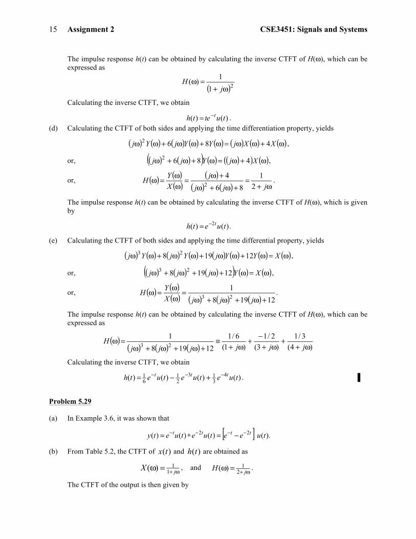
The impulse response h(t) can be obtained by calculating the inverse CTFT of H(ω), which can be expressed as

)3(

5.0)2(

1)1(

5.0)3)(2)(1(

1)(ω+

+ω+

−+ω+

≡ω+ω+ω+

=ωjjjjjj

H


)(5.0)()(5.0)( 32 tuetuetueth ttt −−− +−= . (b) Calculating the CTFT of both sides and applying the time differential property, yields

( ) ( ) ( ) ( ) ( ) ( )ω=ω+ωω+ωω XYYjYj 232 ,

or, ( ) ( )( ) ( ) ( )ω=ω+ω+ω XYjj 232 ,

or, ( ) ( )( ) ( ) ( ) 23

12 +ω+ω

=ωω=ω

jjXYH .


( ) ( ) )2(

1)1(

123

1)( 2 ω+−

ω+≡

+ω+ω=ω

jjjjH


)()()( 2 tuetueth tt −− −= .

(c) Calculating the CTFT of both sides and applying the time differentiation property, yields

( ) ( ) ( ) ( ) ( ) ( )ω=ω+ωω+ωω XYYjYj 22 ,

or, ( ) ( )( ) ( ) ( )ω=ω+ω+ω XYjj 112 ,

or, ( ) ( )( ) ( ) ( ) 12

12 +ω+ω

=ωω=ω

jjXYH .


15


( )211)(ω+

=ωj

H


)()( tuteth t−= . (d) Calculating the CTFT of both sides and applying the time differentiation property, yields

( ) ( ) ( ) ( ) ( ) ( ) ( ) ( )ω+ωω=ω+ωω+ωω XXjYYjYj 4862 ,

or, ( ) ( )( ) ( ) ( )( ) ( )ω+ω=ω+ω+ω XjYjj 4862 ,

or, ( ) ( )( )

( )( ) ( ) ω+

=+ω+ω

+ω=ωω=ω

jjjj

XYH

21

864

2.

The impulse response h(t) can be obtained by calculating the inverse CTFT of H(ω), which is given by

)()( 2 tueth t−= .

(e) Calculating the CTFT of both sides and applying the time differential property, yields

( ) ( ) ( ) ( ) ( ) ( ) ( ) ( )ω=ω+ωω+ωω+ωω XYYjYjYj 12198 23 ,

or, ( ) ( ) ( )( ) ( ) ( )ω=ω+ω+ω+ω XYjjj 12198 23 ,

or, ( ) ( )( ) ( ) ( ) ( ) 12198

123 +ω+ω+ω

=ωω=ω

jjjXYH .


( )( ) ( ) ( ) )4(

3/1)3(2/1

)1(6/1

12198123 ω+

+ω+

−+ω+

≡+ω+ω+ω

=ωjjjjjj

H


)()()()( 4313

21

61 tuetuetueth ttt −−− +−= . ▌

Problem 5.29

(a) In Example 3.6, it was shown that

[ ] ).()()()( 22 tueetuetuety tttt −−−− −=∗=

(b) From Table 5.2, the CTFT of ( )x t and ( )h t are obtained as

ω+=ω jX 11)( , and

ω+=ω jH 21)( .

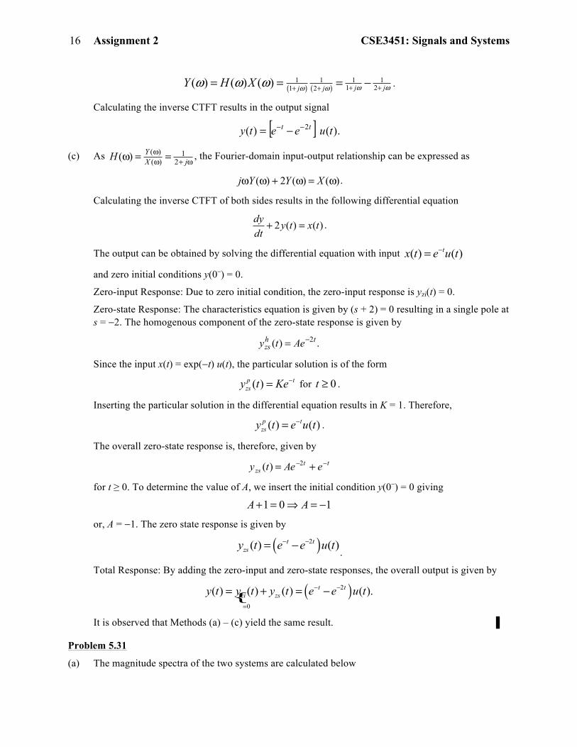
The CTFT of the output is then given by


( ) ( )1 1 1 1

1 21 2( ) ( ) ( ) j jj jY H X ω ωω ωω ω ω + ++ += = = − .

Calculating the inverse CTFT results in the output signal

[ ] ).()( 2 tueety tt −− −=

(c) As ω+ω

ω ==ω jXYH 2

1)()()( , the Fourier-domain input-output relationship can be expressed as

)()(2)( ω=ω+ωω XYYj .

Calculating the inverse CTFT of both sides results in the following differential equation

)()(2 txtydtdy =+ .

The output can be obtained by solving the differential equation with input ( ) ( )tx t e u t−=

and zero initial conditions y(0−) = 0.

Zero-input Response: Due to zero initial condition, the zero-input response is yzi(t) = 0.

Zero-state Response: The characteristics equation is given by (s + 2) = 0 resulting in a single pole at s = −2. The homogenous component of the zero-state response is given by

.)( 2thzs Aety −=

Since the input x(t) = exp(−t) u(t), the particular solution is of the form

( )p tzsy t Ke−= for 0t ≥ .

Inserting the particular solution in the differential equation results in K = 1. Therefore,

( ) ( )p tzsy t e u t−= .

The overall zero-state response is, therefore, given by

ttzs eAety −− += 2)(

for t ≥ 0. To determine the value of A, we insert the initial condition y(0−) = 0 giving

1 0 1A A+ = ⇒ = −

or, A = −1. The zero state response is given by

( )2( ) ( )t tzsy t e e u t− −= −

.

Total Response: By adding the zero-input and zero-state responses, the overall output is given by

{ ( )20

( ) ( ) ( ) ( ).t tzi zsy t y t y t e e u t− −

=

= + = −

It is observed that Methods (a) – (c) yield the same result. ▌

Problem 5.31

(a) The magnitude spectra of the two systems are calculated below


17

( ) 12

2

400400

1 ==ωω+ω+H

( )⎩⎨⎧ ≥ω=ω

elsewhere.0201

2H

The magnitude spectra are plotted in Fig. S5.31). From Fig. S5.31(a), we observe that the magnitude |H1(ω)| is 1 at all frequencies. Therefore, System H1(ω) is an all pass filter.

From Fig. S5.31(b), we observe that the magnitude |H2(ω)| is zero at frequencies below 20 radians/s. At frequencies above 20 radians/s, the magnitude is 1. Therefore, System H2(ω) is a highpass filter.

ω0

1( )ω1H

cωcω−ω

0

1( )ω1H

cωcω− ω

0

1( )ω2H

2020−ω

0

1( )ω2H

2020− (a) (b)

Fig. S5.31: Magnitude Spectra for Problem 5.31.

(b) Calculating the inverse CTFT, the impulse response of the two systems is given by

{ } { } { } )()(401)( 20120401

2020401

1 ttueth tjj

j δ−=ℑ−ℑ=ℑ= −−ω+

−ω+ω−−− .

{ } { } { }1 1 1 20 202 40 40( ) 1 rect( ) 1 rect( ) ( ) sinc( )th t tω ω

π πδ− − −=ℑ − =ℑ −ℑ = − . ▌

Problem 5.32

The transfer functions for the three LTIC systems are given by

System (a): 21 )1(2)(ω+

=ωj

H .

System (b): ω

+ωπδ=ωj

H 1)()(2 .

System (c): ω+ω−=

ω++−=ω

jj

jH

221

252)(3

The following Matlab code generates the magnitude and phase spectra of the three LTIC systems.

%MATLAB Program for Problem P5.32

%System (a)

clear; % clear the MATLAB environment

num_coeff = [2]; % NUM coeffs. in decreasing powers of s

denom_coeff = [1 2 1]; % DEN coeffs. in decreasing powers of s


sys = tf(num_coeff,denom_coeff); % specify the transfer function

figure(1)

bode(sys,{0.02,100}); grid; % sketch the Bode plots

title('Bode Plot for System-1')

%System (b)


num_coeff = [1]; % NUM coeffs. in decreasing powers of s

denom_coeff = [1 0]; % DEN coeffs. in decreasing powers of s


figure(2)



%System (vc)


num_coeff = [-2 1]; % NUM coeffs. in decreasing powers of s

denom_coeff = [1 2]; % DEN coeffs. in decreasing powers of s


figure(3)



The resulting Bode plots are shown in Fig. S5.32.

Calculating Output:

System (a): Using the modulation property, the output of system (a) is given by

[ ] ( )[ ]

2 21 1

1 2 (1 1) (1 1)

2( ) ( 1) ( 1) 2 ( 1) ( 1)(1 )

( 1) ( 1) .

j jY

jj

ω π δ ω δ ω π δ ω δ ωω

π δ ω δ ω

+ −= × − + + = − + +

+= − − − +


tty sin)(1 = .

System (b): Using the modulation property, the output of system (a) is given by

[ ]

[ ]

1 12

1( ) ( ) ( 1) ( 1) ( 1) ( 1)

( 1) ( 1) .

j jYj

j

ω πδ ω π δ ω δ ω π δ ω δ ωω

π δ ω δ ω

−⎡ ⎤ ⎡ ⎤= + × − + + = − + +⎢ ⎥ ⎣ ⎦⎣ ⎦

= − − − +


tty sin)(2 = .


19

-80

-60

-40

-20

0

20

Mag

nitu

de (d

B)

10-1 100 101 102-180

-135

-90

-45

0

Phas

e (d

eg)

Bode Plot for System-1

Frequency (rad/sec) (a)

-40

-20

0

20

40

Mag

nitu

de (d

B)

10-1 100 101 102-91

-90.5

-90

-89.5

-89

Phas

e (d

eg)


Frequency (rad/sec)

-10

-5

0

5

10

Mag

nitu

de (d

B)

10-1 100 101 102180

225

270

315

360

Phas

e (d

eg)


Frequency (rad/sec) (b) (c)

Figure S5.32. Magnitude and phase spectra for systems in Problem 5.32.

System (c): Using the modulation property, the output of system (a) is given by

[ ]

[ ]

2

1 2 1 22 2

1 2( ) ( 1) ( 1)2

( 1) ( 1)

( 1) ( 1) .

j jj j

jYj

j

ωω π δ ω δ ωω

π δ ω δ ω

π δ ω δ ω

− ++ −

−= × − + ++

⎡ ⎤= − + +⎣ ⎦= − − − +


tty sin)(3 = .

To explain why the three systems produce the same output for input x(t) = cost, consider Eq. (5.77), which for ω0 = 1 is given by

( ) ( ))1(cos)1(cos 0)( SymmetricHermitian HtHt H <+ω⎯⎯⎯⎯⎯⎯⎯⎯⎯ →⎯ ω .


In other words, the output for x(t) = cos(t) depends only on the magnitude and phase of the system at ω = 1. For the three systems, we note that

1)1()1()1( 321 === HHH

and

2321 )1()1()1( π−===< HHH .

Since the magnitudes and phases of the three systems at ω = 1 are the same, the three systems produce the same output ( ) siny t t= for x(t) = cos(t). ▌

instructors solutions to assignment 3 - york university · instructors solutions to assignment 3...

Documents