instrument control for beam position monitor...

INSTRUMENT CONTROL FOR BEAM POSITION MONITOR CALIBRATION AND DIAGNOSTICS USING MATLAB

A Design Project Report

Presented to the School of Electrical and Computer Engineering of Cornell University

in Partial Fulfillment of the Requirements for the Degree of

Master of Engineering, Electrical and Computer Engineering

Submitted by

Samuel Fanfan

MEng Field Advisor: Dr. Bruce R. Land

MEng Outside Advisor: Kurt Vetter

Degree Date: May 2013

Abstract

Master of Engineering Program

School of Electrical and Computer Engineering

Cornell University

Design Project Report

Project Title:

Instrument Control for Beam Position Monitor Calibration and Diagnostics Using MATLAB

Author:

Samuel Fanfan

Abstract:

This paper presents a project done in collaboration with Brookhaven National Laboratory for the application of Radio Frequency Beam Position Monitors (RF BPM). These Radio Frequency Beam Position Monitors are to be utilized in the National Synchrotron Light Source II particle accelerator facility post construction. The purpose of the RF BPM is to detect transverse beam position with sub-micron resolution and stability under normal operating conditions. In order to accurately measure the beam’s position it is crucial for the BPM’s four input channel receivers to be matched properly. Traditional calibration schemes comprise of manually adjusting a signal generator coupled to the RF BPM unit under test and recording the receiver signal strength for various power level settings. A MATLAB “RF BPM CalTool” has been developed to automate the process.

The tool interfaces with the instruments by means of Instrument Control and was developed utilizing the MathWorks Instrument Control Toolbox. Remote control of the signal generator is executed using the VISA-TCP protocol in conjunction with SCPI commands. Information exchange with the BPM is established using the ModBus-TCP protocol and the raw data is read and handled by the CalTool. A graphical user interface implements the aforementioned functionality along with a post-processing step. Testing of the tool was executed via simulation and trial-and-error exercises.

Executive Summary Brookhaven National Laboratory (BNL) is a multipurpose research institution located on

the center of Long Island, NY. The laboratory is home to the National Synchrotron Light Source, a photon-generating particle accelerator facility soon to be succeeded by the National Synchrotron Light Source II complex in 2015. For the purpose of research endeavors the detection of the live electron beam is a necessity, a task handled by Radio Frequency Beam Position Monitors. The primary purpose of the RF BPM is to detect the transverse beam position with a resolution of approximately 200nm.

In order to accurately measure the beam’s position it is crucial for the BPM’s four input channel receivers to be matched properly. Traditional calibration schemes comprise of manually adjusting a signal generator coupled to the RF BPM unit under test and recording the receiver signal strength for various power level settings. Automation of the calibration process is explored via Instrument Control.

The developed Radio Frequency Beam Position Monitor Calibration Tool (RF BPM CalTool) interfaces with the instruments by means of Instrument Control and was developed utilizing the MathWorks Instrument Control Toolbox. The tool controls the signal generator and communicates with the BPM unit, both over TCP/IP, and was developed utilizing the MathWorks Instrument Control Toolbox. Remote control of the signal generator is executed using the VISA-TCP protocol in conjunction with SCPI commands. Communication with the BPM is established using the ModBus-TCP protocol and the raw data is read and handled by the CalTool.

A created graphical user interface implements the aforementioned functionality. A final post-processing step is implemented in the GUI and exports the calculated systematic gain coefficients to a user-specified filed to be used for further verification. Calibration of the hardware is achieved within seventeen hours. The time required for calibration is affected by the granularity of the signal sweep executed by the signal generator. The source code was later optimized to obtain the desired result within three hours.

Additionally a Real-Time Plotting Tool (RTP Tool) was engineered as a diagnostics tool, complete with its own graphical user interface. Whereas the CalTool is used to analyze steady-state responses the RTP Tool enables monitoring of transient dynamic responses. This tool provides real-time feedback for input stimuli and allows collected data records to be saved for post-hoc analysis.

Table of Contents INTRODUCTION...........................................................................................................................5

DESIGN REQUIREMENTS...........................................................................................................7

INTERFACE AND COMMUNICATION PROTOCOLS............................................................13

VISA..........................................................................................................................................9

Modbus-TCP/IP.........................................................................................................................9

SCPI...........................................................................................................................................9

HIGH LEVEL OPERATION........................................................................................................10

IMPLEMENTATION....................................................................................................................12

Signal Generator Communication............................................................................................12

Beam Position Monitor Communication.................................................................................13

Graphical User Interface..........................................................................................................17

TESTING.......................................................................................................................................18

RESULTS......................................................................................................................................19

Real-Time Plotting Tool..........................................................................................................19

Calibration Tool.......................................................................................................................20

EVALUATION..............................................................................................................................24

CONCLUSION..............................................................................................................................25

ACKNOWLEDGEMENTS...........................................................................................................26

REFERENCES..............................................................................................................................27

APPENDIX....................................................................................................................................27

INTRODUCTION Brookhaven National Laboratory (BNL) is a multipurpose research institution located on the center of Long Island, NY. Functioning under the U.S. Department of Energy’s Office of Science, the laboratory operates cutting-edge large-scale facilities for studies in physics, chemistry, biology, medicine applied science and a wide range of advanced technologies. The lab is also home to the National Synchrotron Light Source (NSLS), one of the world’s most widely used scientific facilities. Each year its bright beams of x-rays, ultraviolet light, and infrared light are used by researchers worldwide for experiments in diverse fields.

To meet the critical scientific challenges surrounding the energy future a new facility – NSLS-II – is nearing completion, slated to go online in 2015. This new light source will utilize a medium-energy electron storage ring capable of producing x-rays 10,000 brighter than the current NSLS. The NSLS-II facility produces “bright” light (photon) sources by means of a particle accelerator. For the purposes of the various experiments it is necessary to have accurate readings and measurements of the beam (the accelerating particle). Various devices are incorporated into the accelerator facility for this purpose, with one being the Radio Frequency Beam Position Monitor (RF BPM). The primary purpose of the RF BPM is to detect the transverse beam position with a resolution of approximately 200nm. The RF BPM is also required to support turn-by-turn measurements primarily for beam dynamic studies, and single pass beam position.

Though different BPM platforms are available commercially few meet the aforementioned resolution requirement. The engineers at Brookhaven opted to design their own custom hardware platform. The realized system is depicted below. From a high level of abstraction, the BPM can be described as a state-of-the-art calculator comprised of an Analog Front End (AFE) and Digital Front End (DFE). The AFE receives analog signals from pickup electrodes placed through the accelerator complex which are converted to digital signals after being conditioned. The DFE then performs the actual calculations to obtain the desired measurement and position results. More information on the BPM’s functionality is detailed in the following section.

Before being placed into commission each BPM must be properly calibrated. As depicted above, the hardware harbors four input channels. The calibration process entails setting the channel gains such that the proper result is produced across the four channels. Performing this task manually can take many hours per device. Considering hundreds of these devices are to be installed in the NSLS-II facility, such work would prove impractical for an individual let alone being prone to human error. Automation of the calibration process is explored via means of Instrument Control.

Figure 1. Brookhaven National Laboratory’s realized RF Beam Position Monitor, chassis cover removed.

Instrument Control is the practice of connecting a test instrument to a computer and taking measurements. Moreover instrument control allows for general communication with a test device. To achieve this goal the MathWorks’ MATLAB software is used. MATLAB contains the Instrument Control Toolbox add-on which allows one to directly connect MATLAB to instruments using various drives to support various communication interfaces. In addition to providing out-of-the-box support for some of the more widely-adapted protocols the toolbox also provides utilities for most other protocols. In this case the user must write code for proper functionality.

DESIGN REQUIREMENTS As mentioned above, calibration of the BPM hardware requires adjusting the channel gains accordingly. There are two primary components to channel-to-channel gain variation. The first is time-varying variations induced from factors including temperature variation, externally coupled noise, and intrinsic noise. The second source is systematic gain variations which are defined as the static gain differences of each channel when measured at an operational ambient temperature. Correcting the dynamic gain variations involves work with the AFE and is a task left to the engineers of Brookhaven National Lab. Systematic gain variations may be removed in a lab setting by calibrating the RF BPM devices.

Traditional calibration schemes comprise of manually adjusting a signal generator coupled to the RF BPM unit under test and recording the receiver signal strength for various power level settings. Aside from being a time-consuming process manual calibration may also be prone to human error. In order to automate this process and achieve uniform correctness a calibration tool was proposed. Calibration instruments consists of a Rhode & Schwartz SMA 100A Signal Generator, the proposed “RF CalTool,” and the RF BPM Unit Under Test (UUT). The RF CalTool is to utilize a Graphical User Interface (GUI) in addition to providing a timely result. The following illustration depicts the architecture and high-level functionality of the tool.

Figure 2. High level architecture of RF CalTool.

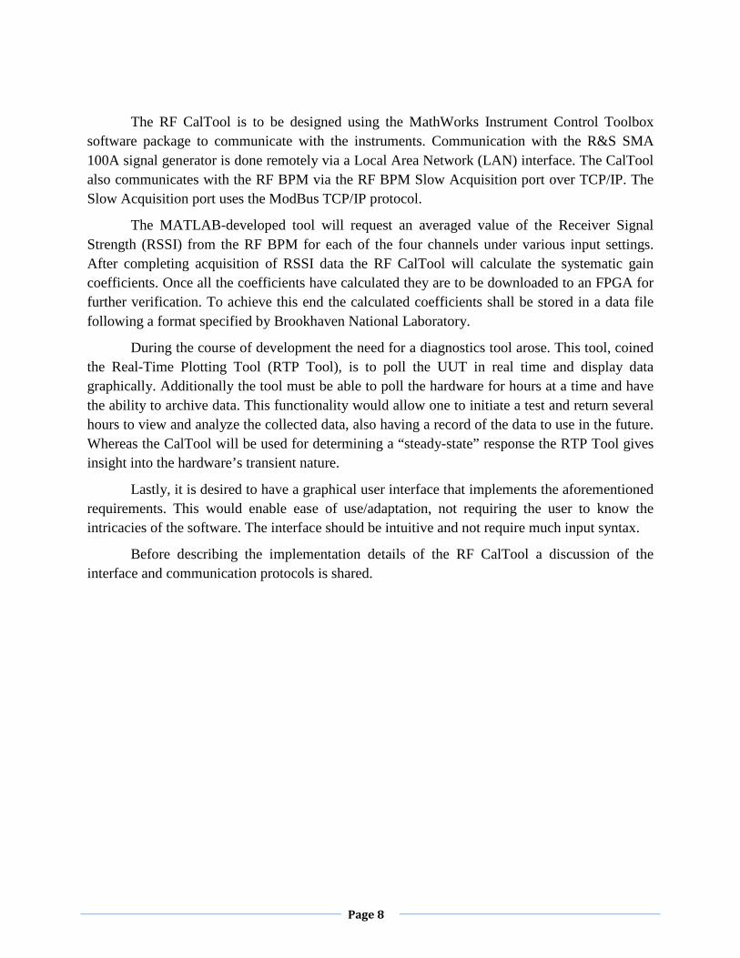
The RF CalTool is to be designed using the MathWorks Instrument Control Toolbox software package to communicate with the instruments. Communication with the R&S SMA 100A signal generator is done remotely via a Local Area Network (LAN) interface. The CalTool also communicates with the RF BPM via the RF BPM Slow Acquisition port over TCP/IP. The Slow Acquisition port uses the ModBus TCP/IP protocol.

The MATLAB-developed tool will request an averaged value of the Receiver Signal Strength (RSSI) from the RF BPM for each of the four channels under various input settings. After completing acquisition of RSSI data the RF CalTool will calculate the systematic gain coefficients. Once all the coefficients have calculated they are to be downloaded to an FPGA for further verification. To achieve this end the calculated coefficients shall be stored in a data file following a format specified by Brookhaven National Laboratory.

During the course of development the need for a diagnostics tool arose. This tool, coined the Real-Time Plotting Tool (RTP Tool), is to poll the UUT in real time and display data graphically. Additionally the tool must be able to poll the hardware for hours at a time and have the ability to archive data. This functionality would allow one to initiate a test and return several hours to view and analyze the collected data, also having a record of the data to use in the future. Whereas the CalTool will be used for determining a “steady-state” response the RTP Tool gives insight into the hardware’s transient nature.

Lastly, it is desired to have a graphical user interface that implements the aforementioned requirements. This would enable ease of use/adaptation, not requiring the user to know the intricacies of the software. The interface should be intuitive and not require much input syntax.

Before describing the implementation details of the RF CalTool a discussion of the interface and communication protocols is shared.

INTERFACE AND COMMUNICATION PROTOCOLS VISA

Virtual Instrument Software Architecture (VISA) is a widely used I/O Application Programming Interface in the Test & Measurement industry for communicating with instruments from a PC. VISA is an industry standard implemented by several Test & Measurement companies such as Tektronix, Kikusui, Agilent Technologies and National Instruments.

The VISA standard includes specifications for communication with resources (usually, but not limited to, instruments) over Test & Measurement-specific I/O interfaces such as General Purpose Interface Bus (GPIB) and VME Extensions for Instrumentation (VXI). There are also some specifications for Test & Measurement-specific protocols over PC-standard I/O, such as VXI-11 (over TCP/IP) and USB Test & Measurement Class (over USB).

ModBus TCP/IP

ModBus is a serial commutations protocol. Given its simple and robust implementation it became a de facto standard communication protocol for connection industrial electronic devices. This open-source protocol was developed with industrial applications in mind and is easy to deploy and maintain. Generally it is used to transfer discrete/analog I/O and register data (raw bits/words) between control devices.

To move ModBus into the 21st century the ModBus TCP/IP was developed. This new protocol combines the versatility & scalability of Ethernet networks (TCP/IP) with a vendor-neutral data representation. ModBus TCP/IP is implementable for any device that supports TCP/IP sockets.

SCPI

The Standard Commands for Programmable Instruments (SCPI, pronounced “skippy”) defines a standard for syntax and commands to for use in controlling programmable test and measurement devices. SCPI syntax is ASCII text, allowing it to be attached to any computer test language or used with test application environments (MATLAB). SCPI is hardware independent and its strings can be sent over any instrument interface. Being an industry standard SCPI enables one to communicate with a variety of supported devices using a common platform.

HIGH LELVEL OPERATION This section focuses solely on the internal operation of the RTP and CalTools. Details concerning the communication interface are described in the following section. The following figure depicts internal functionality of the calibration tool.

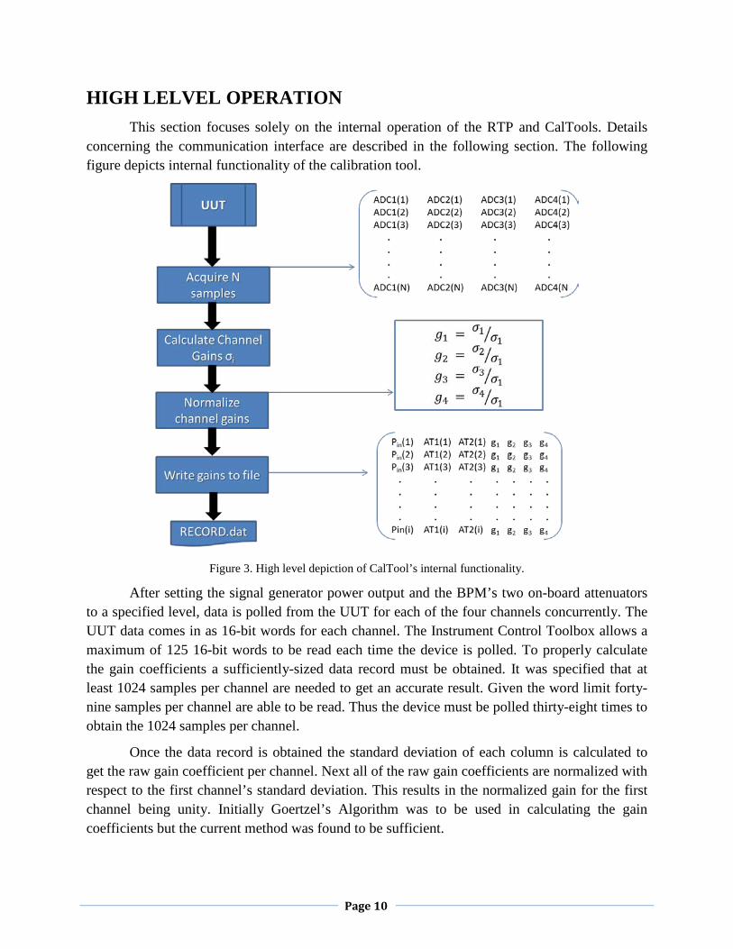
Figure 3. High level depiction of CalTool’s internal functionality.

After setting the signal generator power output and the BPM’s two on-board attenuators to a specified level, data is polled from the UUT for each of the four channels concurrently. The UUT data comes in as 16-bit words for each channel. The Instrument Control Toolbox allows a maximum of 125 16-bit words to be read each time the device is polled. To properly calculate the gain coefficients a sufficiently-sized data record must be obtained. It was specified that at least 1024 samples per channel are needed to get an accurate result. Given the word limit forty-nine samples per channel are able to be read. Thus the device must be polled thirty-eight times to obtain the 1024 samples per channel.

Once the data record is obtained the standard deviation of each column is calculated to get the raw gain coefficient per channel. Next all of the raw gain coefficients are normalized with respect to the first channel’s standard deviation. This results in the normalized gain for the first channel being unity. Initially Goertzel’s Algorithm was to be used in calculating the gain coefficients but the current method was found to be sufficient.

After the normalized gain coefficients are found the information is recorded along with the power and attenuator settings leading to said values. The signal generator or attenuator is then adjusted and the process repeats. Once the desired set of gain coefficients are found the resultant I/O record is saved as a comma-delimited .dat file. This format is utilized by the onboard FPGA which uses the record to verify the gain coefficients.

Similarly for the plotting tool the diagram below depicts internal functionality (communication aside) at a high level.

Figure 4. High level depiction of RTP Tool’s internal functionality.

The Real-Time Plotting Tool is built off the CalTool’s platform but is not as computation-heavy, especially considering it must provide real-time feedback. Its main functionality lies in collecting and displaying data in real time along with functionality to save data records. This latter feature is very useful in the cases in the cases where one wants initiate a test and collect the data record at a later period in time and also for maintaining a record when improper functionality is observed.

The RTP Tool first polls the BPM device and records a data sample for each channel. Once ten samples per channel are recorded an on-screen plot is updated with the values. Ten more samples per channel are collected and the plot is updated after every cycle. This process continues as long as desired.

It should be noted two plots are managed simultaneously by the tool. One plot contains RSSI data doe the four channels, similar to the CalTool. The second plot displays position data polled from the slow acquisition port. Once the desired amount of data samples are collected the user has the option to save the data record to a user-specified file-type (.dat default).

IMPLEMENTATION Signal Generator Communication

The Rhode & Schwartz SMA100A signal generator is equipped with several interfaces for remote control. The Network Interface Card for the LAN interface uses 10/100/1000Mbps Ethernet IEEE 802.3u standard and provides support for the VISA protocol. The Virtual Instrument Software Architecture (VISA) protocol is a widely used I/O API in industry for communicating with instruments from a PC. One of VISA's advantages is that it uses many of the same operations to communicate with instruments regardless of the interface type. This allows for interchangeability among instruments.

Since the VISA protocol is being used, a VISA-TCP object is constructed in MATLAB. For this to work an active installation of the VISA API from any of the vendor companies must be installed. The National Instruments API was used throughout the design process. In addition to specifying the API vendor one must also specify the resource string in the command in MATLAB. The format of the visa command is as follows:

obj = visa(‘vendor’, ‘resourcename’, …),

where the ellipse indicates the option of additional property names and values that may be initialized. The resource name provides the created object with the information necessary for locating and connecting to the instrument. For a TCP/IP interface the resource name is a string with the format

TCPIP::ipaddress::inst0::INSTR

It should be noted that the “TCPIP” header of the resource name is all that lets the object know the VISA protocol will be used over TCP/IP. Specifying use of VISA over a different interface is simply a matter of choosing the appropriate header. After substituting the instrument’s IP address into the resource name, the VISA-TCP object is ready for communication. Once the MATLAB host computer is connected to the signal generator via Ethernet, the connection can be opened using the fopen command.

Though the connection with the instrument has been established an instruction signaling to switch the signal generator to remote control mode must be sent before the instrument can be controlled remotely. Following the standardized VISA protocol for instrument automation is the Standard Commands for Programmable Instruments (SCPI) command set, an industry standard for controlling programmable test and measurement instruments. SCPI specifies a common syntax, command structure, and data formats, to be used with all instruments (R&S SMA100A manual). SCPI commands are ASCII textual strings and may comprise a series of one or more keywords, many of which take parameters.

Commands are sent to the signal generator over the physical layer. In the MATLAB workspace this is done by creating the string command and then sending using either the fprintf or query functions. The fprintf function is used to write text to the instrument; query is used to

read from the instrument. Query string commands must end with ‘?’ to designate the instruction as a request for information from the client (MATLAB). Responses to queries may be stored to a variable name in the MATLAB workspace for future use (i.e. iden = query(obj1,‘*idn?’); ). Similar to all commands, responses to queries are formatted as ASCII textual strings. These strings may be reformatted upon receipt for desired use.

The signal generator can be switched from manual to remote control by sending the ‘&GTR’ string over an open connection (using fprintf). While the remote control session is active the device’s physical input interface (buttons/knobs) is disabled. From here on all of the signal generator’s many functions maybe be invoked or statuses checked by use of the proper SCPI command/query. The R&S SMA100A product manual details all the allowed functions. Once a remote control session is completed, the instrument can be switched to manual control from MATLAB using the ‘GTL’ command. It is recommended that the device be reset before switching back to local mode.

After successfully establishing the VISA-TCP connection through MATLAB the remainder of the script executes the functionality outlined in the design requirements. This entails setting the signal generator to a specified frequency, setting the output waveform to continuous mode, and sweeping the RF output power in 1 dB increments from -100 dBm to +10 dBm (decibels (dB) of the measured power referenced to one milliwatt).

Beam Position Monitor Communication

Following the specifications set forth by Brookhaven National Laboratory, the RF CalTool communicates with the RF BPM via the RF BPM Slow Acquisition port using the TCP/IP interface. The BPM Slow Acquisition Port uses the ModBus TCP/IP Protocol (Vetter et all). The RF CalTool requests an averaged value of the Receiver Signal Strength (RSSI) for each of the four channels for each input setting of the signal generator. The MATLAB Instrument Control Toolbox software does not provide direct support for the ModBus-TCP protocol so much time was spent understanding the dynamics of the standard.

ModBus is an application layer messaging protocol intended for supervision and control of automation equipment. Published as a ‘de-facto’ industry standard, ModBus is a vendor neutral communication protocol most commonly found in use with Programmable Logic Controllers, I/O modules, and gateways to other simple field buses or I/O networks. By definition ModBus is a request/reply messaging system and offers services specified by function codes.

ModBus-TCP/IP (MB-TCP) is a variation of the ModBus family of protocols for use over a TCP/IP interface. The listening TCP port 502 is reserved for MB-TCP communications, although another port may be dedicated to ModBus over TCP based on the specific application. The ModBus messaging service is provided using a Client/Server model to facilitate communication between devices connected on an Ethernet network. The original ModBus protocol defines a simple Protocol Data Unit (PDU) independent of the underlying

communication layers. The mapping of ModBus protocol on specific buses or networks introduces additional fields on the Application Data Unit (ADU). The figure below depicts the structure of a typical ModBus frame.

Figure 5. Standard ModBus frame structure.

The client that initiates the ModBus transaction builds the ModBus ADU before communicating with the ModBus device. The function code indicates to the server which kind of action to perform. ModBus uses ‘big-endian’ representation for addresses and data items so that when a numerical quantity larger than a single byte is transmitted, the most significant byte is sent first.

ModBus-TCP exhibits near-identical functionality as the standard ModBus protocol except for changes to the frame structure. For ModBus-TCP, the ModBus frame is encapsulated in an Ethernet frame’s Data/Payload field before transmission. Since the TCP/IP protocol incorporates its own means for error correction and the Ethernet frame contains a destination address, the Application Data Unit of the ModBus frame contains a different structure, depicted in the following figure.

Figure 6. ModBus-TCP frame structure.

When ModBus is carried over TCP, additional length information is carried in the prefix to allow the recipient to recognize message boundaries even if the message had to be split into multiple packets for transmission. The existence of explicit and implicit length rules, and the use of a CRC-32 error check code (on Ethernet), results in an infinitesimal chance of undetected corruption for a request or response message. A dedicated header is used on TCP/IP to identify the ModBus Application Data Unit(ADU). The actual byte structure of the ADU is described as follows:

Figure 7. Byte structure of ModBus-TCP frame.

• Two byte Transaction Identifier used to identify a ModBus request/response action. This field is initialized by the client in a request and copied by the server for the response. Comparing the transaction IDs of the response to a specific request is used for error checking.

• Two byte Protocol Identifier. Per the ModBus standard this field is always initialized to 0 by the client and copied by the server for the response message.

• Two bytes (upper and lower) denoting the length field that represents the number of bytes following (i.e. Unit ID + Function Code + Data). This field is initialized by the client for a request and by the server for a response. Some functions utilize a variable data field while others do not.

• One byte specifying the Unit Identifier used to identify the remote server device. This field is initialized by the client and recopied by the server. Request made where the Unit Identifier field does not match that of the slave device are ignored by the server.

• The 1 byte Function Code field specifying the function to be executed. This field is also initialized by the client and recopied by the server.

• The variable-byte Data field contains information related to a request or response. The structure of this filed may be dependent on the function being used.

ModBus bases its data model on a series of tables, each of which having unique characteristics. The four primary tables are input discretes (single bit, read only), output discretes (single bit, alterable by an application program with read/write capabilities), input registers (16-bit quantity, read only) and output registers (16-bit quantity, alterable by an application program). For each of the primary tables the protocol allows individual selection of 216 - 65536 data items. Read/write operations of those items are designed to span multiple consecutive data items up to a data size limit which is dependent on the transaction function code.

One potential source of confusion was the relationship between the index parameter used in MATLAB and ModBus. In MATLAB indexes are expressed as decimal numbers with a starting offset of 1. However ModBus uses the more natural software interpretation of an unsigned integer index starting at zero.

It should be noted MATLAB has limitations with the ModBus-TCP protocol. The Instrument Control Toolbox only includes support for client functionality, so trying to develop a ModBus server using the MATLAB environment is not doable.

The process for establishing communication with a ModBus-TCP device using MATLAB is now detailed. The instrument control toolbox is designed to handle TCP/IP communication, so interfacing with a ModBus-TCP is boils down to properly parsing and interpreting the ModBus frame in the data field of the received Ethernet frame. For requests, the frame must be created in MATLAB before being encapsulated in a TCP/IP message and sent to the ModBus device.

A TCP/IP object is created using the tcpip function, making sure to specify the remote host address and port number (default port for ModBus-TCP is 502). Next the ADU header field is constructed - segments of the header field are initialized as a vector in the MATLAB workspace. By default variables declared in the MATLAB environment are of type double, with each element requiring 8 bytes for representation. For proper communication over ModBus-TCP each element of a vector must occupy 1 byte. This is achieved by use of MATLAB’s uint8 function which converts any type to an unsigned 8-bit (1 byte) integer. So after the request has been constructed in MATLAB it is converted to an unsigned 8-bit type to assure proper reception on the server end.

Construction of the data field is dependent on the function being performed. For the output register read function (FC = 3), the data field need only contain two bytes denoting the reference address to be read and a following two bytes denoting the word count (number of registers to be read). Once the data field is constructed, the header, function code, and data field are concatenated into the variable req which is the completed request. The request is transformed using the uint8 command before being written to the ModBus TCP/IP object.

The TCP/IP object is opened using the fopen command to establish a connection with the BPM. A connection timeout is typically due to either an incorrect remote host address or firewall settings (when communicating with the UUT from a remote workstation). The fwrite command is used to send the request as binary data to the server. A one-second pause is implemented before reading the BPM’s response to ensure ample time for creation and receipt of the response. The fread command is used to read the server’s response stored in the TCP/IP object’s BytesAvailable parameter. The ‘uint8’ format option is used to ensure the incoming binary data is read properly. This raw response is the actual ModBus frame from the BPM. The header of the response is removed before handling response’s data field.

After successfully receiving the response the connection is closed before parsing the binary data into decimal format. Handling of the response is dependent on the given function, so separate scripts are written for the RTP and CalTools. The above processed may be altered in future implementations to improve efficiency handling the ModBus response.

Graphical User Interface

The final requirement of the RF CalTool is to have all the aforementioned functionality accessible by way of a Graphical User Interface (GUI). MATLAB provides the option of creating a GUI programmatically or by using their GUIDE (GUI Design Environment) tool, an interactive GUI construction kit. Though use of GUIDE simplifies the visual layout process, M-file source code generated by the tool possesses a cumbersome and sloppy format. Designing the GUI programmatically takes a bit more time but offers the user more control of the overall design and insight on the functionality of the GUI components.

The typical process for GUI design is followed. After sketching the desired design on paper, the GUI is programmed one component at a time with frequent references to the MATLAB GUI documentation. Several user input fields are implemented in the layout design to give the tools varying degrees of freedom (and in turn more practicality & control over the instruments).

After successfully laying out the structure of the GUI, labels are added to each different control object. Spacing/positioning of the items is handled using the Position property for each of the different user interface controls/panels. Tooltip messages are added to most fields providing the user with help/direction if needed.

The source code for the GUI is divided into 5 sections (using MATLAB’s cell break feature): Pre-initialization Tasks, Construction Tasks, Post-initialization Tasks, Callbacks, and Utility Functions. The pre-initialization tasks section initializes global variables that are used throughout the GUI layout process. The construction tasks area contains code responsible for the physical appearance of the GUI. Post-Initialization Tasks initializes variables that will be used in subsequent callback and subfunction definitions. The Callbacks section contains code for the given callbacks implemented. Lastly the Utility Functions region contains subfunctions.

TESTING During the early stages of this project the BPM hardware was merely a prototype with a

specification. Initial design and testing for the communication interface was performed using a ModBus-TCP simulator to emulate the BPM interface. “ModBus Slave” is a program used for simulating up to 32 slave/server devices using a variety of interface options (Serial, GPIB, TCP/IP, etc.). It was specifically created to provide developers with a realistic platform for programming and testing while their target ModBus hardware was still being manufactured. The program provides support for the most common ModBus functions, mainly register and input read/write functions.

Once the BPM units were available direct testing with the hardware was carried out. With the communication mechanism mostly figured out via the Modbus Slave program an iterative trial-and-error tactic was invoked until proper communication could be established. From there on an incremental design approach was used to gradually implement functionality, one function at a time.

RESULTS Real-Time Plotting Tool

As mentioned above the RTP Tool came about during the development of the CalTool. As such it was built upon the CalTool’s communication framework, varying only in functionality. A depiction of the end result is below.

Figure 8. RTP Tool’s main window.

Upon launch the RPT Tool starts as just the console window depicted above. The user must select the proper communication port to be used with the radio buttons. Unlike the CalTool this tool does not communicate with the signal generator. The command line allows the user to issue individual ModBus commands to the BPM hardware; after typing the ASCII command the ‘Set’ button must be asserted. The BPM Response window is updated with response, request, and error messages as made available. Clicking ‘Save’ records the messages in the response window. Upon pressing the ‘Collect data’ button channel and position plot windows spawn and data collection begins.

Figure 9. Screenshot of RPT Tool’s live capture plots.

The above illustration is a sample depiction of the real time plots. As can be seen, in this example approximately 4000 data samples have been collected and displayed. Data collection may be halted with the ‘Stop’ button in the console window. Stopping then collecting data results in the plots being reset and the initial data being lost. The ‘Save data to file’ button initiates a prompt asking the user for a save location, file name and type. Doing so resets the workspace and data record after being saved.

Calibration Tool

The CalTool is more involved due to it interfacing with two devices over separate interfaces and protocols. Transliteration between the signal generator and BPM messages had its initial difficulty until the mechanisms were well understood. Pictured below is the CalTool’s main console window.

As can be seen in the screenshot below, the GUI is separated into three regions. The “Generator Options” region provides options for control of the signal generator. The user may select one of two test instruments and provide the devices IP address for connection. Device parameters such as the desired RF output frequency, power level sweep start and end points and sweep step size time may be specified. The “Connection Status” and “Device Identity” fields are static text fields altered by the RF CalTool and not the user.

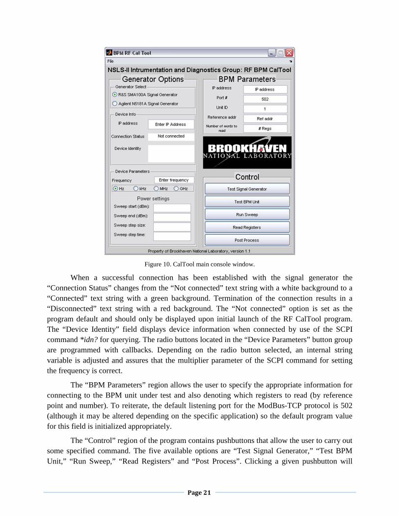
Figure 10. CalTool main console window.

When a successful connection has been established with the signal generator the “Connection Status” changes from the “Not connected” text string with a white background to a “Connected” text string with a green background. Termination of the connection results in a “Disconnected” text string with a red background. The “Not connected” option is set as the program default and should only be displayed upon initial launch of the RF CalTool program. The “Device Identity” field displays device information when connected by use of the SCPI command *idn? for querying. The radio buttons located in the “Device Parameters” button group are programmed with callbacks. Depending on the radio button selected, an internal string variable is adjusted and assures that the multiplier parameter of the SCPI command for setting the frequency is correct.

The “BPM Parameters” region allows the user to specify the appropriate information for connecting to the BPM unit under test and also denoting which registers to read (by reference point and number). To reiterate, the default listening port for the ModBus-TCP protocol is 502 (although it may be altered depending on the specific application) so the default program value for this field is initialized appropriately.

The “Control” region of the program contains pushbuttons that allow the user to carry out some specified command. The five available options are “Test Signal Generator,” “Test BPM Unit,” “Run Sweep,” “Read Registers” and “Post Process”. Clicking a given pushbutton will

execute a script coded into the “Utility Functions” section of the source code. Before describing functionality it should be noted that an additional utility function for reading the inputs is utilized by the “Run Sweep” and “Read Registers” controls. The first two buttons test the connection with either of the devices to ensure communication is possible based off the user’s input.

The function ReadInputs, written as a subfunction of the GUI M-file, reads the user inputs from the graphical user interface and stores them in variables within the source code for use in other subfunctions. Values that are to be used within SCPI string commands are stored as character strings. The input values for “Sweep start”, “Sweep end” and “Sweep step size” are stored as integers using MATLAB’s str2num command for use as indexes for loops described in the following subfunctions.

Another subfunction, MB_RegRead, is used communicate with the BPM device. Note that the ModBus-TCP object must be open before calling this function or else an error will occur. Each time it is called, the MB_RegRead function sends the pre-constructed request to the ModBus-TCP device and receives the response. A one second pause is implemented using the pause function to ensure ample time for reception of data. An error checking feature is also implemented to further ensure proper reception of the data. After receiving the response from the BPM, the received ModBus frame is parsed and the headers of the given request and response are compared. If the two are the same, functionality continues on. If the two are different, an error message is triggered and an error dialog appears on screen to notify the user. The epilogue of this subfunction converts the raw binary data received from the BPM unit into decimal units for viewing and analysis and returns these values.

The “Run Sweep” control is used to collect Receiver Signal Strength (RSSI) samples from the BPM unit under test for a sweep of the signal generator specified by the start/end points and the sweep step size. Clicking “Run Sweep” pushbutton executes the subfunction ReadInputs which reads the user inputs using the predefined subfunction. Device objects are then created for the signal generator’s VISA-TCP and the BPM unit’s ModBus-TCP protocols using the inputted IP addresses. The buffer input size parameter for the ModBus-TCP object is increased to facilitate any needs for a large transfer of data. Before opening either of the interface connections the ModBus frame for the request is constructed using more of the input data read by means of the ReadInputs function. Once construction of the frame is completed the communication channels are opened and the signal generator is set to remote control mode. The frequency and sweep settings of the instrument are set according to the user inputs before sending the first request to the ModBus device. To achieve proper sweep functionality a loop is used. The declaration of the loop follows:

for i = Sweep_start : Sweep_step_size : Sweep_end

Within the body of the loop the MB_RegRead function is called and the request/response transaction occurs. After reading the RSSI data for the initial setting, the current value of the signal generator’s level setting is adjusted by the sweep step size, the request is resent, and new RSSI data for the new setting are received. This loop continues until the sweep end value is

reached. The PP matrix stores successive RSSI readings by declaring it as PP = [PP; MB_RegRead] (note that PP is initialized as an empty array) within the body of the loop. Upon exiting the loop the signal generator is reset, switched back to local mode, and both channel connections are closed.

The “Read Registers” control functions similarly to the “Run Sweep” function, except it only collects one sample of RSSI data. The signal generator is set to the level specified by “Sweep start” and the ModBus response is retrieved for this one setting before closing the interface connections and parsing the received data.

The “Post Process” pushbutton runs the script (subfunction) for calculating the systematic gain coefficients from PP and saves the results to a user specified output file. Upon execution, the user is prompted with a question dialog warning that collected data will be deleted after saving to the output file. This is done to reset the PP matrix in preparation of a new collection of data. If the user selects “No” when prompted to save, the PP variable is maintained at its current state. When the “Yes” option is selected for saving, the PP matrix is copied to a local variable output to ensure that no data is lost should an error occur during execution. The function proceeds to operate on output and normalize the channel readings, row by row, by the reading for the first channel.

Once completed, a save dialog box (identical to the typical system file save prompt) prompts the user for a location and filename save the output file as. The default file type for the output file is set .dat (data file), but the user may alter this simply by including the file type extension when naming the output. The filename and save location are stored into the MATLAB environment. The fopen function is used to create a new file in the location specified using the write-mode option (‘w’) to denote we will be writing to this created file. A textual header (format provided by Brookhaven) is first written to the file. Following this a for loop is used to write the calculated gain coefficients row by row to the output file, making use of a line break between each write for legibility. Once the final line is written the loop exits and the file is closed. The PP matrix is reinitialized as an empty matrix to collect new data and the function exits.

The final steps of the GUI design entailed adding features for ease of use. This is implemented by the use of tool tip strings. Whenever the user positions the mouse over a given input field or interactive user input control (radio buttons) a message appears above the mouse cursor providing some information or insight regarding what should be entered. Additionally a simple menu is added to the design. The only parent element in the menu is the “File” label with two submenus: “File Help” and “File Close.” Selecting the help menu displays a message box containing brief information about the purpose and creation of the tool. Selecting the close menu option prompts the user with a question dialog. Using this dialog the user can choose to terminate the program or continue execution.

EVALUATION RPT Tool

The RPT Tool was desired to observe transient dynamics in real-time and save a data record collected over a given duration. As such the realized tool met all the design requirements. Given that the Slow Acquisition data is provided at a frequency of 10 Hz the plots are updated roughly every second.

CalTool

The CalTool met all of the design requirements in terms of functionality. One cause of contention though is the amount of time taken to complete the calibration process. Though automated the code takes roughly 17 hours to collect all the samples and perform post processing. This is mainly due to the program collecting 1024 samples for each step in the sweep. The finer the granularity of the step size the longer the overall process takes.

Another issue is the lack of parallelism in the design. When the design specifications were initially declared, processing time was not mentioned until towards the end of the project. Therefore the tool was designed for functionality. Fortunately once the software platform was functional the engineers at Brookhaven were able to optimize the code, bringing the total calibration time down to three hours. As of today all 246 BPM devices have been successfully calibrated, programmed and installed into the NSLS-II facility.

CONCLUSION The purpose of the RF Beam Position Monitor is to detect transverse beam position with

sub-micron resolution and stability for normal operation conditions. The most crucial parameter of the BPM to accurately measure the position is for the gains of the four channels to be matched. The RF Calibration Tool presented in this work has proven to provide such functionality. Though the initial design takes 17 hours for calibration the code has been optimized to get the time down to a tolerable level. The developed Real-Time Plotting Tool provides an effective means for monitoring and archiving transient response dynamics. Both of these developed tools demonstrate MATLAB as a suitable platform for Instrument Control given its versatility. As of today all of the Beam Position Monitors for the National Synchrotron Light Source II have been calibrated and installed successfully.

ACKNOWLEDGEMENTS I’d like to extend special thanks to Bruce Land for the continuous encouragement when

times were difficult and for the weekly check-ins and conversations; to Clifford Pollock, the MEng Board, and the ECE Department for allowing this project to happen; to Kurt Vetter for appointing me to this project and the ongoing education in the realm Electron Beam Detection; to Terrence Buck for his support and representation, working behind the scenes to make this collaboration with BNL possible; to the GEM National Consortium for my placement with Brookhaven National Lab, without whom none of this would be possible; to Brookhaven National Laboratory for providing me with an opportunity to apply skills I’ve learned in the classroom to a practical design problem; and to the MathWorks for providing lots of documentation online and also being available via their Customer Support hotline to clarify a few misconceptions about the Instrument Control Toolbox.

REFERENCES Vetter, Kurt. NSLS-II RF BPM Systematic Gain Calibration – “RF BPM CalTool”. Brookhaven

National Laboratory (March 1, 2010). PDF file.

ModBus Application Protocol Specification V1.1b, The ModBus Organization (December 28,

2006). <www.modbus-IDA.org>

ModBus Messaging on TCP/IP Implementation Guide. The ModBus Organization (October 24,

2006). <www.modbus-IDA.org >

Swales, Andy. Open ModBus/TCP Specification. Schneider Electric Company (March 1999).

PDF file

Rohde & Schwarz GmbH & Co. KG. (2008). Publication Manual for the Rhode & Schwartz

SMA100A Signal Generator. Munich.

The MathWorks. MATLAB: Creating Graphical User Interfaces. PDF File.

<www.mathworks.com/access/helpdesk/help/pdf_doc/matlab/buildgui.pdf>

The MathWorks. MATLAB: Instrument Control Toolbox 2 User’s Guide. PDF File.

<www.mathworks.com/access/helpdesk/help/pdf_doc/instrument/instrument.pdf>

The MathWorks. MATLAB 7: Programming Fundamentals. PDF File.

<www.mathworks.com/access/helpdesk/help/pdf_doc/matlab/matlab_prog.pdf>

The MathWorks. MATLAB 7: Programming Tips. PDF File.

<www.mathworks.com/access/helpdesk/help/pdf_doc/matlab/programming_tips.pdf>

APPENDIX See website for source code.

http://www.modbus-ida.org/

http://www.modbus-ida.org/

http://www.mathworks.com/access/helpdesk/help/pdf_doc/matlab/buildgui.pdf

instrument control for beam position monitor...

Documents