Instrument Science Report ACS 2020-08

Update of the Photometric Calibration of the ACS CCD Cameras

Ralph C. Bohlin, Jenna E. Ryon, Jay Anderson

ABSTRACT

The spectral energy distributions of the three primary standard stars that are the basis for the

HST absolute fluxes are improved by a few percent, which requires an update to the instrumental

calibrations in order to retain our precision goal of 1%. In addition, analysis of the perennial monitoring

observations of the primary White Dwarf (WD) standard stars provides a better correction for the

loss of sensitivity with time for recent CCD data from the Advanced Camera for Surveys/Wide Field

Camera (ACS/WFC). The ACS encircled energy fractions are also updated for the CCD cameras.

Keywords: stars:fundamental parameters (absolute flux) — techniques:photometry

1. INTRODUCTION

The flux calibrations for the ACS filters in the CCD (charge coupled device) modes were last updated by Bohlin

(2016), who included charge transfer efficiency (CTE) corrections, encircled energy (EE) corrections, changes in sensi-

tivity with time, and the absolute flux calibration itself. However, new calibrations are required, because Bohlin et al.

(2020) has established new spectral energy distributions (SEDs) for the primary flux reference standards, as based on

improved agreement between NLTE grids of pure hydrogen hot WD model grids made by I. Hubeny and T. Rauch.

The new reference SEDs are all in the CALSPEC database1.

ACS has two CCD channels, a Wide Field Channel (WFC) and a High Resolution Channel (HRC), both of which

require a new flux calibration. Updates to the MAMA Solar Blind Channel SBC throughput curves were made using

the same methodology as Avila et al. (2019), but using the updated STIS SEDs as inputs. Please consult that reference

for details. The main goal of this work is to establish this flux calibration with better than a 1% precision at the

WFC1-1K reference point for the heavily used CCD broadband filters. See Bohlin (2016) for details of the methodology

used to derive the quantities presented here. The bulk of the recent data is processed with CALACS version 10.2.1.

Section 2 reviews the procedure for extracting the stellar photometry in electrons s−1 from the ACS images. Section

3 covers the changing sensitivity with time, including a discussion of a small problem with recent monitor observations

that have an added post-flash background. Section 4 reviews the encircled energy (EE) fractions for apertures of radii

from 0.05–2′′, i.e. 1–40 WFC pixels. Section 5 covers the absolute flux calibration.

2. THE PHOTOMETRY

1 https://www.stsci.edu/hst/instrumentation/reference-data-for-calibration-and-tools/astronomical-catalogs/calspec

2

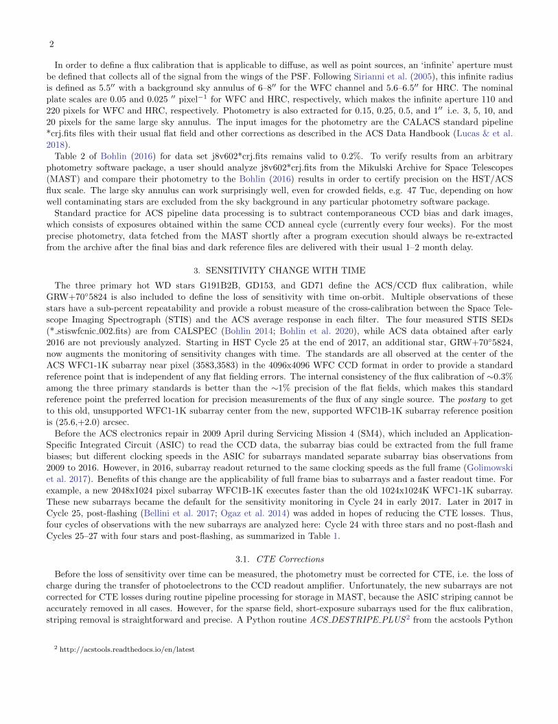
In order to define a flux calibration that is applicable to diffuse, as well as point sources, an ‘infinite’ aperture must

be defined that collects all of the signal from the wings of the PSF. Following Sirianni et al. (2005), this infinite radius

is defined as 5.5′′ with a background sky annulus of 6–8′′ for the WFC channel and 5.6–6.5′′ for HRC. The nominal

plate scales are 0.05 and 0.025 ′′ pixel−1 for WFC and HRC, respectively, which makes the infinite aperture 110 and

220 pixels for WFC and HRC, respectively. Photometry is also extracted for 0.15, 0.25, 0.5, and 1′′ i.e. 3, 5, 10, and

20 pixels for the same large sky annulus. The input images for the photometry are the CALACS standard pipeline

*crj.fits files with their usual flat field and other corrections as described in the ACS Data Handbook (Lucas & et al.

2018).

Table 2 of Bohlin (2016) for data set j8v602*crj.fits remains valid to 0.2%. To verify results from an arbitrary

photometry software package, a user should analyze j8v602*crj.fits from the Mikulski Archive for Space Telescopes

(MAST) and compare their photometry to the Bohlin (2016) results in order to certify precision on the HST/ACS

flux scale. The large sky annulus can work surprisingly well, even for crowded fields, e.g. 47 Tuc, depending on how

well contaminating stars are excluded from the sky background in any particular photometry software package.

Standard practice for ACS pipeline data processing is to subtract contemporaneous CCD bias and dark images,

which consists of exposures obtained within the same CCD anneal cycle (currently every four weeks). For the most

precise photometry, data fetched from the MAST shortly after a program execution should always be re-extracted

from the archive after the final bias and dark reference files are delivered with their usual 1–2 month delay.

3. SENSITIVITY CHANGE WITH TIME

The three primary hot WD stars G191B2B, GD153, and GD71 define the ACS/CCD flux calibration, while

GRW+70◦5824 is also included to define the loss of sensitivity with time on-orbit. Multiple observations of these

stars have a sub-percent repeatability and provide a robust measure of the cross-calibration between the Space Tele-

scope Imaging Spectrograph (STIS) and the ACS average response in each filter. The four measured STIS SEDs

(* stiswfcnic 002.fits) are from CALSPEC (Bohlin 2014; Bohlin et al. 2020), while ACS data obtained after early

2016 are not previously analyzed. Starting in HST Cycle 25 at the end of 2017, an additional star, GRW+70◦5824,

now augments the monitoring of sensitivity changes with time. The standards are all observed at the center of the

ACS WFC1-1K subarray near pixel (3583,3583) in the 4096x4096 WFC CCD format in order to provide a standard

reference point that is independent of any flat fielding errors. The internal consistency of the flux calibration of ∼0.3%

among the three primary standards is better than the ∼1% precision of the flat fields, which makes this standard

reference point the preferred location for precision measurements of the flux of any single source. The postarg to get

to this old, unsupported WFC1-1K subarray center from the new, supported WFC1B-1K subarray reference position

is (25.6,+2.0) arcsec.

Before the ACS electronics repair in 2009 April during Servicing Mission 4 (SM4), which included an Application-

Specific Integrated Circuit (ASIC) to read the CCD data, the subarray bias could be extracted from the full frame

biases; but different clocking speeds in the ASIC for subarrays mandated separate subarray bias observations from

2009 to 2016. However, in 2016, subarray readout returned to the same clocking speeds as the full frame (Golimowski

et al. 2017). Benefits of this change are the applicability of full frame bias to subarrays and a faster readout time. For

example, a new 2048x1024 pixel subarray WFC1B-1K executes faster than the old 1024x1024K WFC1-1K subarray.

These new subarrays became the default for the sensitivity monitoring in Cycle 24 in early 2017. Later in 2017 in

Cycle 25, post-flashing (Bellini et al. 2017; Ogaz et al. 2014) was added in hopes of reducing the CTE losses. Thus,

four cycles of observations with the new subarrays are analyzed here: Cycle 24 with three stars and no post-flash and

Cycles 25–27 with four stars and post-flashing, as summarized in Table 1.

3.1. CTE Corrections

Before the loss of sensitivity over time can be measured, the photometry must be corrected for CTE, i.e. the loss of

charge during the transfer of photoelectrons to the CCD readout amplifier. Unfortunately, the new subarrays are not

corrected for CTE losses during routine pipeline processing for storage in MAST, because the ASIC striping cannot be

accurately removed in all cases. However, for the sparse field, short-exposure subarrays used for the flux calibration,

striping removal is straightforward and precise. A Python routine ACS DESTRIPE PLUS 2 from the acstools Python

2 http://acstools.readthedocs.io/en/latest

3

Table 1. Observations with New 2048x1024 Subarrays

Star Date Cycle Proposal Flashed?

G191B2B 2017-01-20 24 14863 No

GD153 2017-01-19 24 14863 No

GD71 2017-02-08 24 14863 No

G191B2B 2017-12-14 25 14956 Yes

GD153 2018-02-04 25 14956 Yes

GD71 2017-11-23 25 14956 Yes

GRW+70◦5824 2017-11-28 25 14956 Yes

G191B2B 2018-11-28 26 15529 Yes

GD153 2018-12-30 26 15529 Yes

GD71 2018-11-01 26 15529 Yes

GRW+70◦5824 2018-11-15 26 15529 Yes

G191B2B 2019-10-13 27 15767 Yes

GD153 2019-11-29 27 15767 Yes

GD71 2019-09-03 27 15767 Yes

GRW+70◦5824 2019-09-10 27 15767 Yes

KF08T3 2017a 24 14863 No

aThree visits in March, April, and June of 2017

package produces uncorrected and CTE-corrected images ( crj and crc files), both of which are de-striped. The CTE

correction is defined as photometry from the crj divided by photometry from the crc images.

The photometry from the flashed data is ∼0.6% higher than from unflashed observations, which seemed perfect,

as flashing should lessen CTE losses and reduce CTE corrections. However, both the unflashed and flashed data

have the same <0.1% CTE correction for results from the software package ACS DESTRIPE PLUS (Grogin et al.

2011). Furthermore, the amount of CTE losses of <0.1% from ACS DESTRIPE PLUS agrees with predictions of

the Bohlin & Anderson (2011) algorithm for the unflashed, new subarray data. The CTE corrections in both Bohlin

& Anderson (2011) and in ACS DESTRIPE PLUS are based on the algorithm of Anderson & Bedin (2010) and

Anderson & Ryon (2018). Bohlin & Anderson (2011) used data from 2009 obtained with the SM4 ASIC to define their

correction algorithm, which is a parameterization of a set of results from typical flux calibration observations with

high signal and near zero background that are reduced with the Anderson pixel-based correction. The parameterized

fits are free of the noise associated with the pixel-based correction itself, which makes Bohlin & Anderson (2011) the

preferred CTE correction algorithm for the flux calibration observations given its validation by agreement with the

ACS DESTRIPE PLUS results for the modern subarray style that began in 2017.

Thinking that there still might be ACS DESTRIPE PLUS errors or possible inadequacy in the pixel based cor-

rection for the bright standard stars, the CTE corrections predicted by the Chiaberge (2012)3 algorithm for five-

pixel radius photometry with a 13-18 pixel background annulus is also compared to the CTE loss results from

ACS DESTRIPE PLUS with the same background annulus. Again, the Chiaberge (2012) CTE corrections of <0.1%

are in agreement with ACS DESTRIPE PLUS for the flashed data with its ∼32 electrons of added background, which

still leaves the ∼0.6% higher signal unexplained for the flashed exposures. While this check is valid for five-pixel radius

photometry, there is no Chiaberge (2012) CTE correction for the flux calibration photometry with 20 pixel radius and

6–8′′ sky annulus.

3.2. Excess Signal for Flashed Data

With doubts dispelled about the precision of CTE corrections, questions about the exposure time of flashed data

arise. Ogaz et al. (2014) discuss the details of post-flashing observations and explain that shutter B is always used for

3 https://acsphotometriccte.stsci.edu/

4

the science exposures, while Gilliland & Hartig (2003) say: ”... exposure times are shorter when terminated by the A

shutter” but are not quantitative, except for suggesting that 1% B/A timing errors exist for exposure times of 0.7–2s.

However, if the shutter B exposures used for the flashed data are actually 12ms longer than nominal, i.e. 0.6% larger

for the commonly used 4s CR-split=2 exposures, then Figure 1 shows that everything makes sense. A corollary is that

flashing does not reduce either the predicted or actual observed CTE losses for the bright standards and should be

dropped for future cycles.

Analysis of the ratio B/A exposure times for unflashed data supports only a 3ms excess for shutter B. The results of

Ryon & Grogin (2018) for illumination of the whole shutter by the tungsten lamp imply that the average transmission

of the closed shutter is too low to explain the apparent extra 9 ms of exposure time that explains the discrepancy of the

flashed data. Furthermore, the excess signal from any light leak would vary with the time that the stellar image sits on

the shutter, which is not the case. The unlikely possibility that the shutter B slowed with the advent of post-flashing

is ruled out by the fact that the Cycle 28 data have no excess signal, even though flashing is omitted. Whether the

excess exposure time for the flashed data is caused by a subtlety of the new flash commanding procedure or some

other reason is not important. Simply increasing the effective exposure time by 12ms brings the three years of flashed

data into line with the unflashed observation and makes the flashed data useful for defining ACS calibrations.

3.3. Sensitivity Losses

This work updates the results of Bohlin (2016), where more details about the analysis are provided. The reference

positions for the flux calibration are at the center of the HRC CCD and at the center of the currently unsupported

WFC1-1K subarray at pixel (3583,1535) of chip-1; and the change in sensitivity is determined by the 1′′ radius

photometry that has the best repeatability, according to table 3 of Bohlin (2016). This 1′′ photometry of the four

monitor stars with the eight most important broadband filters is shown in Figure 2 and is corrected only for CTE,

for the discontinuity due to the change in the WFC CCD set-point temperature from -77C to -81C on 2006 July

6 (2006.50), and for the 12ms extra exposure time for flashed data. The sub-percent CTE corrections of Bohlin &

Anderson (2011) are applied for WFC and should be negligible for the early HRC data, which is heavily exposed. The

HRC and WFC photometry are in red and black, respectively.

To reduce measurement noise and enforce the prior of the expected smooth change with wavelength, the slopes of

the linear fits from Figure 2 are fit with a polynomial as a function of the filter pivot wavelengths, as shown in Figure 3

for the eight broadband filters available to both WFC and HRC and for the three UV filters of HRC. For the pre-SM4

ACS epoch, the data are rather sparse, because the policy of the once per year monitoring of the sensitivity changes

at the WFC1-1K reference point with the three primary standard stars had not yet been established. Both the WFC

and HRC data points in Figure 2 agree with the dotted lines, which are the fits of the slopes from Figure 3. F475W

is a worst case deviation between the solid and dotted lines, where a dominant constraint on the rate of sensitivity

loss is the lone WFC GD153 point at 2007.0 from program 11054. The planned observations of G191B2B in that

cycle 15 were not executed because of the ACS failure at 2007.1. Given the scatter in the data, the fitted loss rate is

uncertain but would coincide with the slope from the fitted results (dotted line), if the lone 2007.0 point were ∼2σ

lower. Statistically, the best result is from accepting both the WFC and HRC measures and adopting the fitted mean

for F475W.

For the later years of ACS after SM4 at 2009.4, the eight WFC broadband filters are well monitored over 10 annual

cycles; and all show a consistent sensitivity loss. This average post-SM4 loss rate is 0.000574 per year, i.e. 0.0574%/yr

with an error-in-the-mean of 0.0066%/yr and an rms scatter of 0.0188%/yr. The largest deviation is for F555W where

the measured rate is < 2σ from the mean. The average loss rate of 0.0574%/yr is adopted for all WFC data after

2009.4 and is within 1σ of the 0.061%/yr found by Bohlin (2016). The general trends of reduced loss rates with

time and increased loss rates toward UV wavelengths are the expected behavior for a gradually slowing of outgassing

hydrocarbons and their polymerization on the optical surfaces in spacecrafts Bohlin (2014). The observed trends in

STIS (dashed line) follow this model.

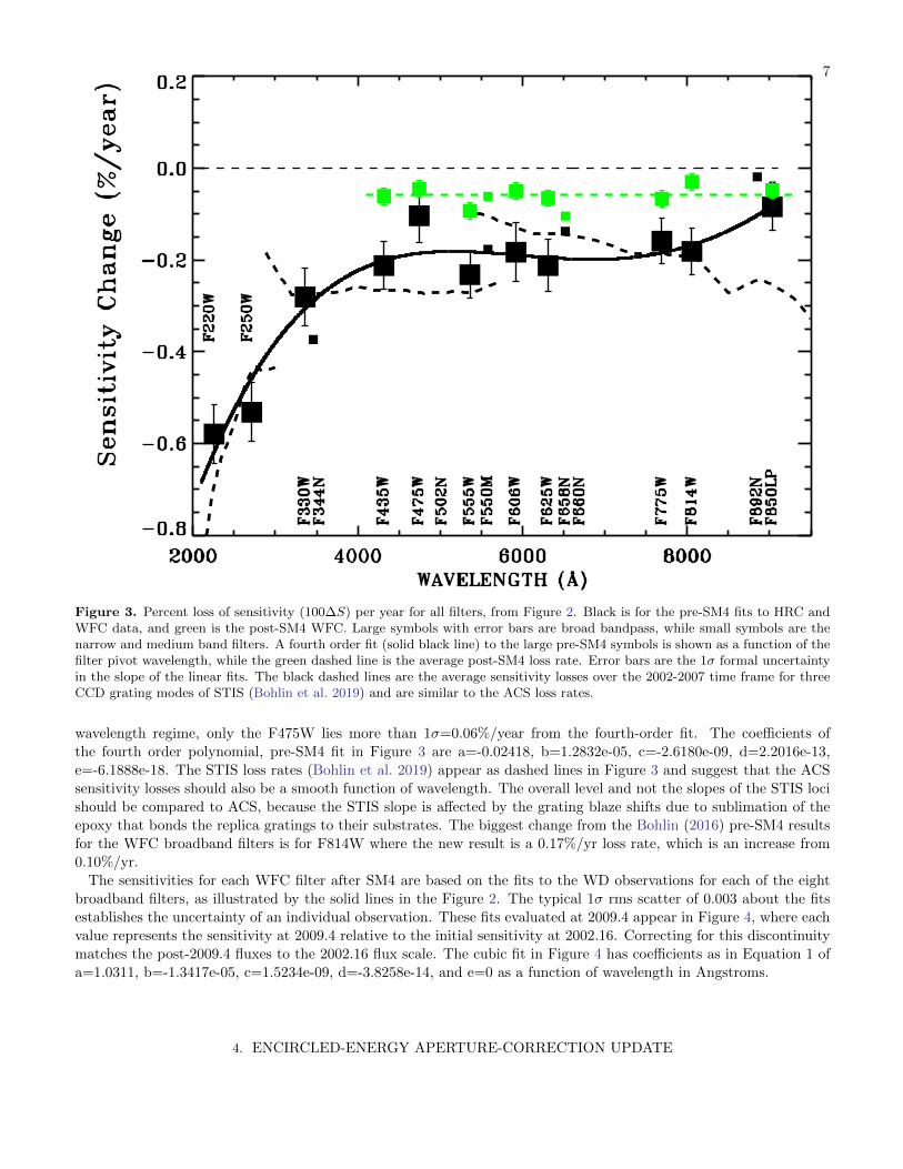
Following Bohlin (2016), Figure 3 shows the slope of the rates of sensitivity loss (∆S) for each filter and a fourth-order

polynomial fit to the pre-SM4 data for both cameras as a function of the pivot wavelength (λ).

∆S = a+ bλ+ cλ2 + dλ3 + eλ4 (1)

The medium and narrow band data are shown but are omitted in the fitting procedure because of the minimal ACS

observation sets and also because of the finite STIS resolution that affects the predicted count rate P. In the WFC

5

Figure 1. Ratio of flashed to unflashed photometry for the Table 1 observations, which are corrected for the loss of sensitivitywith time and for CTE losses. The abscissa represents the total electron signal for 1′′ photometry of a single exposure frame.In the bottom panel, the ratios show a systematic offset of 0.57±0.05%, while the top panel documents the improved ratioswith a 12ms increase of exposure time per frame for 36 flashed observations of 2–3s total exposure time. Typical error bars of0.002–0.003 are defined by the rms scatter of the data points.

6

Figure 2. Relative sensitivity vs. time for the eight most heavily used broadband filters. The OBServed count rates are dividedby the predicted SYNTHetic photometry from STIS SEDs that is a constant for each filter over time, in order to place all starson the same scale. Symbols are square, circle, triangle, and X for G191B2B, GD153, GD71, and GRW+70◦5824 respectively.Solid lines are fits to the one arcsec photometry ratios that are corrected for CTE losses and for the sensitivity loss at 2006.5when the WFC CCD temperature was lowered from -77C to -81C (Mack et al. 2007), while the dotted lines represent the finalloss rates from Figure 3. The individual and average loss rates agree within the 2σ uncertainty of the individual slopes. Redsymbols are for HRC before its death; and black symbols are the WFC, which was resurrected in 2009. The straight line fits tothe pre-SM4 data are normalized to unity at 2002.16 when ACS on-orbit operation began. Both pre- and post-SM4 data arenormalized with this same fit value to maintain the relative sensitivity measures over the complete WFC lifetime.

7

Figure 3. Percent loss of sensitivity (100∆S) per year for all filters, from Figure 2. Black is for the pre-SM4 fits to HRC andWFC data, and green is the post-SM4 WFC. Large symbols with error bars are broad bandpass, while small symbols are thenarrow and medium band filters. A fourth order fit (solid black line) to the large pre-SM4 symbols is shown as a function of thefilter pivot wavelength, while the green dashed line is the average post-SM4 loss rate. Error bars are the 1σ formal uncertaintyin the slope of the linear fits. The black dashed lines are the average sensitivity losses over the 2002-2007 time frame for threeCCD grating modes of STIS (Bohlin et al. 2019) and are similar to the ACS loss rates.

wavelength regime, only the F475W lies more than 1σ=0.06%/year from the fourth-order fit. The coefficients of

the fourth order polynomial, pre-SM4 fit in Figure 3 are a=-0.02418, b=1.2832e-05, c=-2.6180e-09, d=2.2016e-13,

e=-6.1888e-18. The STIS loss rates (Bohlin et al. 2019) appear as dashed lines in Figure 3 and suggest that the ACS

sensitivity losses should also be a smooth function of wavelength. The overall level and not the slopes of the STIS loci

should be compared to ACS, because the STIS slope is affected by the grating blaze shifts due to sublimation of the

epoxy that bonds the replica gratings to their substrates. The biggest change from the Bohlin (2016) pre-SM4 results

for the WFC broadband filters is for F814W where the new result is a 0.17%/yr loss rate, which is an increase from

0.10%/yr.

The sensitivities for each WFC filter after SM4 are based on the fits to the WD observations for each of the eight

broadband filters, as illustrated by the solid lines in the Figure 2. The typical 1σ rms scatter of 0.003 about the fits

establishes the uncertainty of an individual observation. These fits evaluated at 2009.4 appear in Figure 4, where each

value represents the sensitivity at 2009.4 relative to the initial sensitivity at 2002.16. Correcting for this discontinuity

matches the post-2009.4 fluxes to the 2002.16 flux scale. The cubic fit in Figure 4 has coefficients as in Equation 1 of

a=1.0311, b=-1.3417e-05, c=1.5234e-09, d=-3.8258e-14, and e=0 as a function of wavelength in Angstroms.

4. ENCIRCLED-ENERGY APERTURE-CORRECTION UPDATE

8

Figure 4. The WFC sensitivity correction at 2009.4 relative to the initial sensitivity at 2002.16 as based on fitting the post-SM4observations of the four WD standard stars. The filled squares are the eight WFC broadband filters, while the smooth curve isa cubic fit to these eight points. The open diamonds are the medium and a narrow band filter.

The encircled energy (EE) in the infinite aperture defines the diffuse source calibration, but the point source flux

calibration in the smaller apertures is unaffected by excess noise in the large infinite aperture, as long as the proper

EE factor is used. The average 20-pixel EE value is used to convert the 20 pixel photometry to the infinite values.

Plots of the aperture photometry vs. time illustrate the reproducibility and determine the best reference aperture

for the absolute flux calibration. For example, Figure 5 compares the measured WFC F606W fractional encircled

energy for the most relevant photometry apertures from three to 110 pixel radii. The rms scatter is tabulated for all

eight of the WFC broadband filters in Table 2. There are no obvious trends with time or with stellar color in Figure 5.

For the bright, isolated standard stars, the 20 pixel (1′′) aperture generally has the best photometric repeatability

at σ20=0.29–0.47%, although there is little loss in precision with an aperture as small as five pixels, where 0.39%<

σ5 <0.85%. While the infinite 5.5′′ radius aperture contains all the signal by definition, there is more scatter because

of the excess sky noise in that large 5.5′′ aperture. The three pixel radius aperture has 3–6 times the uncertainty of a

1′′ aperture; and if possible, the use of a three pixel radius should be avoided because of exact centering uncertainties

and focus variations that could be systematic over an entire image.

EE values are the smaller aperture photometry divided by the noisy large 110 pixel radius values; and the fitting

technique of Bohlin (2016) is required to lower the uncertainties. While the large 110 pixel infinite aperture should

recapture all the trapped and re-emitted charge, the smaller aperture data require a CTE correction. The pipeline

processing now supplies the Anderson & Ryon (2018) CTE corrected full frame 4096x4096 pixel images; but CTE

corrected subarrays are not provided, so that the subarrays used here must be corrected for CTE losses in the post-

pipeline processing. A fit as a function of wavelength for the broad filters of Table 2 reduces the uncertainty, while at

the same time providing fitted values for the problematic narrower filters (Bohlin 2012). For hot stars to K stars, the

EE for 12 aperture sizes appear in Table 3, where typical uncertainties in the EE fits for WFC and the 0.15, 0.25, 0.5,

9

Figure 5. Fractional encircled energy for seven stars from spectral type K to hot WDs, i.e. the ratio of actual photometry tosynthetic photometry for an infinite 110 pixel radius. The gap in time from 2007-2009 is when ACS/WFC was not operational.The low point for the three pixel radius GD71 at 2012.8 is not caused by any saturated pixel falling outside the three pixelradius, which suggests that the occasional image has a 3σ error (5% here) for three pixel photometry.

10

Table 2. Photometric rms Scatter vs. Radius

Filter σ3(%) σ5(%) σ10(%) σ20(%) σ110(%)

F435W 0.94 0.43 0.35 0.34 0.97

F475W 1.25 0.39 0.33 0.31 0.49

F555W 1.08 0.40 0.38 0.39 0.76

F606W 1.43 0.44 0.38 0.37 0.70

F625W 1.72 0.48 0.29 0.29 0.57

F775W 1.92 0.54 0.48 0.48 0.93

F814W 1.43 0.40 0.32 0.30 0.73

F850LP 1.83 0.83 0.57 0.43 0.92

Table 3. WFC Encircled Energy Fractions for K and Hotter Stars

Filter 1 pix 2 pix 3 pix 4 pix 5 pix 6 pix 7 pix 8 pix 9 pix 10 pix 20 pix 40 pix

F435W 0.330 0.665 0.793 0.838 0.862 0.876 0.887 0.895 0.901 0.907 0.941 0.979

F475W 0.328 0.670 0.794 0.841 0.867 0.881 0.891 0.900 0.906 0.911 0.943 0.978

F502N 0.327 0.671 0.795 0.841 0.867 0.883 0.893 0.901 0.908 0.913 0.944 0.977

F555W 0.328 0.670 0.796 0.840 0.867 0.883 0.894 0.902 0.909 0.914 0.945 0.976

F550M 0.329 0.669 0.796 0.840 0.866 0.883 0.894 0.902 0.909 0.914 0.945 0.975

F606W 0.331 0.665 0.796 0.839 0.865 0.883 0.895 0.903 0.910 0.915 0.946 0.974

F625W 0.332 0.660 0.797 0.839 0.864 0.883 0.895 0.903 0.910 0.915 0.947 0.973

F658N 0.333 0.656 0.797 0.839 0.863 0.883 0.896 0.904 0.910 0.916 0.948 0.973

F660N 0.333 0.655 0.797 0.839 0.863 0.883 0.896 0.904 0.910 0.916 0.948 0.972

F775W 0.327 0.626 0.783 0.836 0.859 0.877 0.894 0.903 0.910 0.916 0.949 0.972

F814W 0.319 0.610 0.770 0.830 0.854 0.872 0.889 0.900 0.907 0.914 0.949 0.972

F892N 0.279 0.547 0.706 0.788 0.818 0.840 0.859 0.877 0.888 0.897 0.942 0.970

F850LP 0.271 0.534 0.693 0.777 0.810 0.832 0.852 0.871 0.884 0.892 0.940 0.970

and 1 arcsec radii are 0.3, 0.2, 0.3, and 0.1%, respectively. The ACS CCDs are linear through saturation, as long as

all of the saturated signal is included in the aperture (Gilliland 2004; Cohen & Grogin 2020), which means that some

of the smaller aperture measures of BD+17◦4708 and G191B2B with excessive saturation are omitted. The largest

deviations from the values of Bohlin (2016) are only 0.2% for the one arcsec radius and 0.3% for the three pixel EE.

There are no new data for HRC or for stars cooler than K type, so the EE results of Bohlin (2016) are still valid.

5. ABSOLUTE FLUX CALIBRATION

5.1. Procedure

The ACS instrumental calibration constants S, i.e. the PHOTFLAM values that appear in the ACS data headers,

are the ratio of the photon-weighted STIS spectral energy distribution (SED) over the ACS bandpass, i.e. mean flux

〈F 〉 from synthetic photometry, divided by the measured instrumental count rate C in photoelectrons s−1 in the ACS

’infinite’ 5.5′′ radius aperture Bohlin (2016). To define an ACS flux calibration, the predicted synthetic count rate P,

i.e. the integral of the photon-weighted STIS SED over the wavelength range of the ACS filter bandpass, is matched

to the observed rate C by adjusting the ACS throughput function of quantum efficiency vs wavelength, as detailed in

Bohlin (2016) and Bohlin et al. (2014). The filter throughput functions include the updates to the shapes of F435W

and F814W for WFC; however, Bohlin (2016) neglected to include these filter shifts for HRC, which uses the same

11

Table 4. Filter Transmission Updates

Residuals

Filter WFC 3σa HRC 3σa

F220W ... ... 1.000 0.004

F250W ... ... 1.000 0.004

F330W ... ... 1.000 0.004

F344N ... ... 1.000 0.006

F435W 1.000 0.002 0.982 0.004

F475W 1.000 0.002 1.000 0.004

F502N 1.002 0.005 1.001 0.006

F555W 1.000 0.002 1.000 0.004

F550M 1.001 0.002 1.001 0.005

F606W 1.000 0.002 1.000 0.004

F625W 1.000 0.001 1.000 0.004

F658N 0.995 0.003 0.995 0.009

F660N 0.996 0.008 0.995 0.007

F775W 1.000 0.002 1.000 0.003

F814W 1.001 0.001 0.989 0.003

F892N 1.000 0.004 1.002 0.005

F850LP 1.001 0.001 1.000 0.004

a The 3σ uncertainties of the residuals areerrors-in-the-mean.

physical filter as the WFC. Thus, updated HRC filter shapes for F435W and F814W are included here for the first

time.

For the reference STIS spectra, both the models and the calibrated STIS SEDs are in CALSPEC. No model is

perfect; and the fitting of smooth splines to the STIS sensitivity interpolates over model errors, which are mostly in

the line profiles and at the Balmer confluence near 3800 A. The calibrated STIS SEDs are comprised of a minimum

of 13 independent observations for each of the three primary WDs per grating mode and have negligible uncertainty

from photon statistics. In this case, the STIS SEDs are slightly more precise than the models in the regions of the

flux distribution that are bootstrapped from the assumption of a smooth sensitivity curve. Consequently, the ACS

flux calibration is based on the CALSPEC files * stiswfcnic 002.fits rather than the NLTE models that must be used

for STIS flux calibration.

5.2. Results

Figure 6 shows the ratios of observed count rate C to synthetic photometry P vs. pivot wavelength for WFC.

The heavy solid line is a quartic polynomial fit to the filled squares for the eight primary WDs with coefficients

7.942e-01, 1.290e-04, -3.150e-08, 3.371e-12, -1.320e-16. The fit for HRC is similar. These quartic fits are within 0.1%

of the filled squares and define the required updates to the detector QEs. Residual deviations of the black squares are

as large as 0.5% for the narrow band filters as shown in Table 4.

After updating the ACS flux-calibration QE for the smooth fit vs. wavelength and for the individual filter residuals,

Figure 7 demonstrates agreement of the ACS photometry of the three WDs (black squares) with the STIS synthetic

photometry to 0.1% for all 13 WFC filters. HRC also has similar residuals of ≤ 0.1% for all 17 filters. These new

fully corrected filter throughputs are then propagated to the final PHOTFLAM values, as tabulated for select dates

in Table 5. The dates in Table 5 for the times of major change are used in the routine data processing to determing

the header PHOTFLAM values by linear interpolation between the pairs of dates.

The corrected average photometry for the other four stars in Figure 7 is within the goal of 1% agreement for the

eight broadbands, except for the KF08T3 measures in F775W and F850LP (upside-down purple triangles). Because

12

Figure 6. Ratios of observed count rate C to synthetic photometry P vs. pivot wavelength for WFC. The black squares andtheir 3σ errors-in-the-mean represent the average of the three prime WDs, while the averages are shown for the G star P330E(green circle), K stars KF06T2 (purple star) and KF08T3 (inverted purple triangle), and GRW+70◦5824 (red cross). The lessprecise results for the sparsely observed primary WD with the narrow and medium band filters are the open black squares.Typically, the filled square averages of the primary WDs have about 10 times as many observations as the single-star averages.The observations are all corrected for CTE losses, time-dependent sensitivity, the change in CCD temperature at 2006.5, thepixel-area maps, and encircled energy for the 1′′radius photometry.

all three observation that comprise each of these two discrepant points agree to 0.1–0.2%, a likely explanation is that

the filter bandpass function is slightly too low at the longer wavelengths where these cool K stars are relatively much

brighter than the hot WDs. Similarly, the discrepant photometry for the cool stars in F550M is likely due to an error

in the F550M filter throughput function.

6. DRZ PHOTOMETRY

In principle, extracting photometry from the geometrically corrected drizzled * drc.fits files is more straightforward

than using the * crj.fits files. There is no need to apply PAMs, the plate scale is constant at exactly 0.05′′ per pixel

for WFC (0.025′′ for HRC), and a CTE correction is included. However, figure 13 of Bohlin (2016) illustrated poor

photometry from the pipeline drizzled files. Subsequently, Hoffmann & Avila (2017) improved the parameters of the

drizzle algorithm; and a new evaluation of the MAST DRZ photometry is required, even though MAST drizzled

products are only provided for quick looks.

The second extension of the drz product is the weight (WHT) image, which offers clues to the drizzle validity. If the

pair of * flt.fits images that are combined into the drz have slightly different or misaligned PSFs or even mis-matched

backgrounds (Avila et al. 2015), a reduced WHT coincident with the core of the star usually indicates improper results.

A data quality (Q) parameter can be defined as the percent drop from maximum to minimum WHT weight in the 3x3

13

Figure 7. Count rate ratios vs. pivot wavelength for the stars observed with WFC after making the corrections for the smoothfit in Figure 6 and for the Table 4 filter transmission residuals. The black squares and their 3σ errors-in-the-mean for the averageof the three prime WDs are now all within 0.001 of unity, while the averages are also shown for the WD GRW+70◦5824 (redcross), the G star P330E (green circle), and the K standards KF06T2 and KF08T3 (purple). The less precise results for thesparsely observed narrow and medium band filters are the open black squares.

set of pixels centered on the star. Bohlin (2016) set a Q=13.1% limit to provide a fairly good dividing line between

good and bad drz photometry for pairs of images; and most of the poor drz measures are flagged as bad without

flagging too many of the valid drz results. The crj photometry is validated by the small rms σ20 <0.5% in Table 2 for

the baseline 20 pixel photometry.

Figure 8, compares the WFC drz with the baseline crj 1′′ photometry of the standard stars as a function of the

response in the peak pixel of each observation. There are 469 unflagged comparisons shown as the filled circles and

only 23 (5%) drz photometry comparisons are flagged as bad Q and shown as open circles, in contrast to the 28% with

bad Q in 2016. Three of the 23 open circles are off-scale in Figure 8. Only 10 (2%) of the 469 unflagged points differ

by more than 1% from unity.

Thus, the drz files are now often correct, but for the most precise photometry or for cases where the photometry for

a particular star is important, the crj or crc files are preferred, even when the WHT drizzle extension is considered.

Further study would be valuable, but for now the pipeline drz photometry should still be considered a quick look

product.

7. CONCLUSIONS AND SCHEDULE

14

Table 5. ACS infinite aperture calibration constants photflam, i.e. S in units of erg s−1 cm−2 A−1/(e s−1)

WFC HRC

Filter MJD52334 MJD53919 MJD53920 MJD54976 MJD54977 MJD62502 MJD52334 MJD54136

2002.16 2006.5 2006.5 2009.4 2009.4 2030.0 2002.16 2007.1

-77C -77C -81C -81C -81C -81C

F220W 8.210e-18 8.466e-18

F250W 4.707e-18 4.815e-18

F330W 2.239e-18 2.273e-18

F344N 2.228e-17 2.261e-17

F435W 3.095e-19 3.122e-19 3.196e-19 3.215e-19 3.173e-19 3.211e-19 5.319e-19 5.373e-19

F475W 1.799e-19 1.813e-19 1.849e-19 1.859e-19 1.838e-19 1.860e-19 2.914e-19 2.941e-19

F502N 5.169e-18 5.210e-18 5.300e-18 5.328e-18 5.273e-18 5.336e-18 8.049e-18 8.122e-18

F550M 3.938e-19 3.970e-19 4.023e-19 4.045e-19 4.003e-19 4.051e-19 5.845e-19 5.899e-19

F555W 1.938e-19 1.953e-19 1.982e-19 1.993e-19 1.972e-19 1.996e-19 3.013e-19 3.041e-19

F606W 7.732e-20 7.796e-20 7.893e-20 7.937e-20 7.846e-20 7.941e-20 1.269e-19 1.281e-19

F625W 1.178e-19 1.188e-19 1.201e-19 1.207e-19 1.193e-19 1.208e-19 1.958e-19 1.977e-19

F658N 1.965e-18 1.982e-18 2.003e-18 2.014e-18 1.990e-18 2.014e-18 3.363e-18 3.396e-18

F660N 5.138e-18 5.182e-18 5.235e-18 5.265e-18 5.201e-18 5.263e-18 8.866e-18 8.953e-18

F775W 9.877e-20 9.954e-20 1.008e-19 1.013e-19 9.994e-20 1.011e-19 1.937e-19 1.954e-19

F814W 6.972e-20 7.019e-20 7.128e-20 7.160e-20 7.064e-20 7.149e-20 1.284e-19 1.293e-19

F850LP 1.498e-19 1.505e-19 1.540e-19 1.545e-19 1.525e-19 1.544e-19 2.260e-19 2.271e-19

F892N 1.482e-18 1.488e-18 1.519e-18 1.523e-18 1.505e-18 1.522e-18 2.443e-18 2.454e-18

Note—The applicable dates are listed as MJD and as fractional year, along with the WFC CCD set point temperature.The S at any date is the linear interpolation between pairs of columns.

The values tabulated here should be used for flux calibration of all ACS CCD photometry and are scheduled to be

incorporated in the ACS data reduction pipeline on 2020 October 12 for repopulating the header values in the MAST

calibrated data files and for all PYSYNPHOT calculations.

8. ACKNOWLEDGEMENTS

The full ACS team provided suggestions and comments that improved this ISR. Support for this work was provided

by NASA through the Space Telescope Science Institute, which is operated by AURA, Inc., under NASA contract

NAS5-26555. This research has made use of the SIMBAD database, operated at CDS, Strasbourg, France. Wayne

Landsman provided the IDL photometry routine apphot.pro.

ORCID IDs

Ralph C. Bohlin https://orcid.org/0000-0001-9806-0551

15

Figure 8. Comparison of 20 pixel photometry from crj and drz files for the WFC standard star observations. The 469 filledblack circles are the ratios for drz photometry with good weight (WHT) arrays, while the open black circles represent the sameratio but with a WHT Q parameter of greater than 0.131.

REFERENCES

Anderson, J., & Bedin, L. R. 2010, PASP, 122, 1035

Anderson, J., & Ryon, J. E. 2018, Improving the

Pixel-Based CTE-correction Model for ACS/WFC,

Instrument Science Report ACS 2018-04

Avila, R. J., Bohlin, R., Hathi, N., et al. 2019, SBC

Absolute Flux Calibration, Instrument Science Report

ACS 2019-5

Avila, R. J., Hack, W., Cara, M., et al. 2015, in

Astronomical Society of the Pacific Conference Series,

Vol. 495, Astronomical Data Analysis Software an

Systems XXIV (ADASS XXIV), ed. A. R. Taylor &

E. Rosolowsky, 281

Bellini, A., Grogin, N. A., Lim, P. L., & Golimowski, D.

2017, Post-Flash Validation of the new ACS/WFC

Subarrays, Instrument Science Report ACS 2017-6

Bohlin, R. C. 2012, Flux Calibration of the ACS CCD

Cameras IV. Absolute Fluxes, Instrument Science

Report, ACS 2012–01, (Baltimore: STScI), Tech. rep.

—. 2014, AJ, 147, 127

—. 2016, AJ, 152, 60

Bohlin, R. C., & Anderson, J. 2011, Flux Calibration of the

ACS CCD Cameras I. CTE Correction, Instrument

Science Report, ACS 2011–01, (Baltimore: STScI), Tech.

rep.

Bohlin, R. C., Deustua, S. E., & de Rosa, G. 2019, The

Astronomical Journal, 158, 211

Bohlin, R. C., Gordon, K. D., & Tremblay, P.-E. 2014,

PASP, 126, 711

Bohlin, R. C., Hubeny, I., & Rauch, T. 2020, AJ, 160, 21

16

Bohlin, R. C., Mack, J., Hartig, G., & Sirianni, M. 2005,

Earth Flats, Instrument Science Report ACS 2005-12,

(Baltimore: STScI), Tech. rep.

Chiaberge, M. 2012, A new accurate CTE photometric

correction formula for ACS/WFC, Instrument Science

Report, ACS 2012–05, (Baltimore: STScI), Tech. rep.

Cohen, Y., & Grogin, N. A. 2020, Unusual Horizontal

Charge Overflow from Saturated CCD Pixels in the ACS

WFC: Discovery and Remediation, Instrument Science

Report ACS 2020-07, (Baltimore: STScI), Tech. rep.

Gilliland, R. L. 2004, ACS CCD Gains, Full Well Depths,

and Linearity up to and Beyond Saturation, Instrument

Science Report ACS 2004–01, (Baltimore: STScI), Tech.

rep.

Gilliland, R. L., & Hartig, G. 2003, Stability and Accuracy

of HRC and WFC Shutters, Instrument Science Report

ACS 2003-03

Golimowski, D., Anderson, J., Arslanian, S., et al. 2017,

New Subarray Readout Patterns for the ACS Wide Field

Channel, Instrument Science Report, ACS 2017–03,

(Baltimore:STScI), Tech. rep.

Grogin, N. A., Lim, P. L., Maybhate, A., Hook, R. N., &

Loose, M. 2011, Post-SM4 ACS/WFC Bias Striping:

Characterization and Mitigation, Instrument Science

Report ACS 2011-05

Hoffmann, S. L., & Avila, R. J. 2017, Updated MDRIZTAB

Parameters for ACS/WFC, Instrument Science Report

ACS 2017-2

Lucas, R., & et al. 2018, ACS Data Handbook v.9.0

Mack, J., Gilliland, R. L., Anderson, J., & Sirianni, M.

2007, WFC Zeropoints at -80C, Instrument Science

Report, ACS 2007–02, (Baltimore:STScI), Tech. rep.

Ogaz, S., Chiaberge, M., & Grogin, N. A. 2014, Post-Flash

Capabilities of the Advanced Camera for Surveys Wide

Field Channel (ACS/WFC), Instrument Science Report

ACS 2014-01

Ryon, J. E., & Grogin, N. A. 2018, ACS/WFC Parallel

CTE from EPER Tests, Instrument Science Report, ACS

2018–09, (Baltimore: STScI), Tech. rep.

Sirianni, M., Jee, M. J., Benıtez, N., et al. 2005, PASP,

117, 1049 (S05)