instrumentation and axial load testing of displacement piles

Purdue UniversityPurdue e-PubsLyles School of Civil Engineering FacultyPublications Lyles School of Civil Engineering

2-20-2013

Instrumentation and Axial Load Testing ofDisplacement PilesAdriano V.D. Bica

Monica PrezziPurdue University, [email protected]

Hoyoung SeoTexas Tech University

Rodrigo SalgadoPurdue University, [email protected]

Daehyeon KimChosun University

Follow this and additional works at: http://docs.lib.purdue.edu/civeng

Part of the Civil and Environmental Engineering Commons

This document has been made available through Purdue e-Pubs, a service of the Purdue University Libraries. Please contact [email protected] foradditional information.

Bica, Adriano V.D.; Prezzi, Monica; Seo, Hoyoung; Salgado, Rodrigo; and Kim, Daehyeon, "Instrumentation and Axial Load Testing ofDisplacement Piles" (2013). Lyles School of Civil Engineering Faculty Publications. Paper 6.http://docs.lib.purdue.edu/civeng/6

http://docs.lib.purdue.edu?utm_source=docs.lib.purdue.edu%2Fciveng%2F6&utm_medium=PDF&utm_campaign=PDFCoverPages

http://docs.lib.purdue.edu/civeng?utm_source=docs.lib.purdue.edu%2Fciveng%2F6&utm_medium=PDF&utm_campaign=PDFCoverPages


http://docs.lib.purdue.edu/civl?utm_source=docs.lib.purdue.edu%2Fciveng%2F6&utm_medium=PDF&utm_campaign=PDFCoverPages


http://network.bepress.com/hgg/discipline/251?utm_source=docs.lib.purdue.edu%2Fciveng%2F6&utm_medium=PDF&utm_campaign=PDFCoverPages

Proceedings of the Institution of Civil Engineers

http://dx.doi.org/10.1680/geng.12.00080

Paper 1200080

Received 30/06/2012 Accepted 11/09/2012

Keywords: field testing & monitoring/foundations/piles & piling

ICE Publishing: All rights reserved

Geotechnical Engineering

Instrumentation and axial load testing ofdisplacement pilesBica, Prezzi, Seo, Salgado and Kim

Instrumentation and axial loadtesting of displacement pilesAdriano V. D. Bica PhDAssociate Professor, Department of Civil Engineering, Universidade FederalDo Rio Grande Do Sul, Porto Alegre, Brazil

Monica Prezzi PhDProfessor, School of Civil Engineering, Purdue University, West Lafayette,IN, USA

Hoyoung Seo PEAssistant Professor, Department of Civil and Environmental Engineering,Texas Tech University, Lubbock, TX, USA

Rodrigo Salgado PhDProfessor, School of Civil Engineering, Purdue University, West Lafayette,IN, USA

Daehyeon Kim PhDAssistant Professor, Department of Civil Engineering, Chosun University,Gwangju, Korea

Despite the fact that results of many instrumented pile load tests have been reported in the literature, it is difficult

to find well-documented instrumentation procedures that can be used when planning a load testing programme. A

load test programme designed to investigate various aspects of the design and behaviour of driven steel piles is

discussed in the present paper. Although the literature contains information on load testing of instrumented piles

driven in either sand or clay, limited information is available regarding their axial load response in transitional soils

(soils composed of various amounts of clay, silt and sand). Results are presented for fully instrumented axial load

tests performed on an H pile and a closed-ended pipe pile driven into a multilayered soil profile consisting of

transitional soils. In addition, the load testing planning, the instrumentation of the piles, the testing methods and

the interpretation of the pile testing data are discussed in detail in the context of this and other load testing

programmes described in the literature, in order to illustrate the various steps.

NotationAb area of pile base

Asi pile shaft area interfacing with layer i

A1, A2 fitting parameters for the equation to estimate qbL

when the pile base is embedded in a strong layer

overlying a weak layer

Bo outer pile diameter

C1, C2 slope and intercept of the axial load–settlement curve

in the 1/Q against w space

Ht distance from the pile base to the interface of the

weak/strong layers

L pile length

n number of soil layers

Q axial load applied to the pile head

QsL limit shaft resistance

QbL,ult ultimate base resistance

Qult ultimate axial load-bearing capacity

qb,ult ultimate unit base resistance

qc,strong cone resistance of strong layer

qc,weak cone resistance of weak layer

qsLi limit unit shaft resistance for soil layer i

w settlement at the pile head corresponding to the axial

load Q

z pile depth

1. IntroductionSteel H piles and steel pipe piles are used worldwide for the

foundations of a variety of structures. These piles are manufac-

tured in a wide range of dimensions and lengths, providing for

both small and large axial and lateral load capacities. Steel piles

offer significant advantages over other types of piles as they are

easy to handle, splice and drive into the ground. The possibility

of applying axial loads soon after installation can also be

advantageous, particularly for underpinning works. Despite the

fact that driven piles are often used in practice because of the

many advantages they offer, there are still knowledge gaps in

their design, particularly when they are installed in non-textbook

soils. In addition, although results of instrumented pile load tests

are available in the literature, it is difficult to find well-

documented discussions of instrumentation procedures that can

be referred to when planning a load testing programme.

Before a load testing programme is undertaken, a thorough

review of the literature is always recommended so that mistakes

and problems faced by previous researchers can be avoided at the

planning stages. It is not uncommon for load tests to fail to

achieve their goals because of faulty planning.

The type and number of instruments used in a given pile load test

programme depend on its goals. For example, in the case of

verification or proof load tests, only an axial load cell and an

axial displacement instrument, installed at the pile head, may be

sufficient. However, if investigation of other aspects of the pile–

soil interaction problem is required, then other instruments are

needed as well. Figure 1 summarises the measurements and

instruments typically used in pile load test programmes.

1

Axial load tests have been performed on instrumented full-scale

piles mainly for determining the load–settlement and the load–

transfer relationships and for comparing measured data with

corresponding values predicted by pile design methods. In this

paper, a detailed description is presented of the procedures

required for successful pile instrumentation and data acquisition

and the results of four high-quality instrumented pile load tests

performed on steel piles driven in a mixed soil profile.

2. Pile load responseThe ultimate axial load-bearing capacity Qult of a single pile is

expressed as the sum of the ultimate base resistance Qb,ult and the

limit shaft resistance QsL

Qult ¼ Qb,ult þ QsL ¼ (qb,ultAb)þXn

i¼1

qsLiAsi

1:

where qb,ult is the ultimate unit base resistance; qsLi is the limit

unit shaft resistance for soil layer i; Ab is the area of pile base;

Asi is the pile shaft area interfacing with layer i; n is the number

of soil layers.

Only small pile displacements (typically of the order of 1% of

the pile diameter) are required for complete mobilisation of QsL:

The value of Qult adopted in practice based on pile load test

results usually corresponds to a pile displacement equal to 10%

of the pile diameter, so QsL is fully mobilised when the applied

axial load Q ¼ Qult: Both QsL and Qb,ult are affected by

(a) the degree of soil displacement during pile installation

(b) soil type and stress state

(c) installation method

(d ) degree of ‘soil plugging’ developed during installation

(e) pile size and shape

( f ) the presence of residual loads after installation

(g) set-up and other time-related effects.

Both soil type and stress state influence pile behaviour signifi-

cantly. For sand, available data by Lehane et al. (1993) and

analyses by Salgado (2006a, 2006b); Loukidis and Salgado

(2008) and Basu et al. (2011) suggest that qsL depends on the

mobilisation of critical-state shear strength in a very narrow shear

band surrounding the pile. Changes in radial effective stresses

caused by pile installation at a sand element at depth z down a

pile of length L depend on z, the relative density of the element,

and the ratio of the vertical distance L–z from the element to the

base of the pile to the pile radius. However, changes in radial

effective stresses during axial loading of the pile depend mainly

on local interface dilation and principal stress rotation. Both of

these factors affect the value of qsL that is in fact mobilised. For

clay, qsL depends instead on the mobilisation of residual shear

strength (Coop and Wroth, 1989; Salgado, 2006b; Chakraborty et

al., 2012).

Residual loads, which are compressive axial loads that are locked

in the pile as a result of pile driving, need to be carefully

evaluated when interpreting pile load test results (Alawneh and

Malkawi, 2000; Briaud and Tucker, 1984). During driving, the

pile undergoes elastic compression. After driving, the pile tries to

rebound to recover its initial length, moving upwards. The soil

below the pile base, compressed during driving, also tends to

push the pile upwards. However, because interface shear resis-

tance is mobilised between the pile shaft and the surrounding soil

as the pile rebounds, qsL reverses direction (from an upward

direction to a downward direction), at least in the upper portion

of the pile. Therefore, measurement of the residual load distribu-

Basicmeasurements

Complementarymeasurements

Advancedmeasurements

• Load–displacement– ALC, ADILoad–transfer– ALC, SG

•

• Pore pressure change– PPTGround heave– SDPile driving analysis– ACC, SG

•

•

• Stress change in the soil– RSCDynamic testing– ACC, SGPile base load– OCUnit shaft friction– SFC

•

•

•

Pile load test

Figure 1. Measurements and instruments in pile load test

programmes (ALC: axial load cell; ADI: axial displacement

instrument; SG: strain gauge; PPT: pore pressure transducer;

SD: surveying device; ACC: accelerometer; RSC: radial stress cell;

OC: Osterberg cell; SFC: shaft friction cell)

2

Geotechnical Engineering Instrumentation and axial load testing ofdisplacement pilesBica, Prezzi, Seo, Salgado and Kim

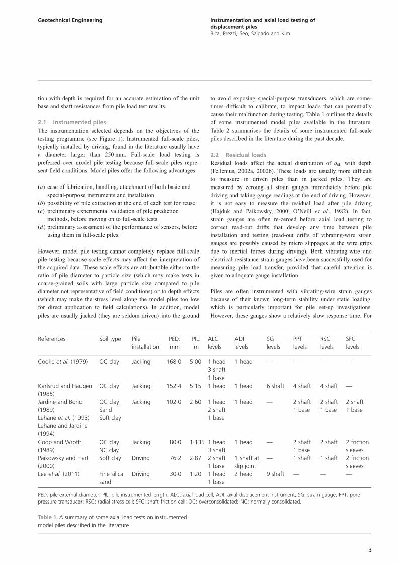
tion with depth is required for an accurate estimation of the unit

base and shaft resistances from pile load test results.

2.1 Instrumented piles

The instrumentation selected depends on the objectives of the

testing programme (see Figure 1). Instrumented full-scale piles,

typically installed by driving, found in the literature usually have

a diameter larger than 250 mm. Full-scale load testing is

preferred over model pile testing because full-scale piles repre-

sent field conditions. Model piles offer the following advantages

(a) ease of fabrication, handling, attachment of both basic and

special-purpose instruments and installation

(b) possibility of pile extraction at the end of each test for reuse

(c) preliminary experimental validation of pile prediction

methods, before moving on to full-scale tests

(d ) preliminary assessment of the performance of sensors, before

using them in full-scale piles.

However, model pile testing cannot completely replace full-scale

pile testing because scale effects may affect the interpretation of

the acquired data. These scale effects are attributable either to the

ratio of pile diameter to particle size (which may make tests in

coarse-grained soils with large particle size compared to pile

diameter not representative of field conditions) or to depth effects

(which may make the stress level along the model piles too low

for direct application to field calculations). In addition, model

piles are usually jacked (they are seldom driven) into the ground

to avoid exposing special-purpose transducers, which are some-

times difficult to calibrate, to impact loads that can potentially

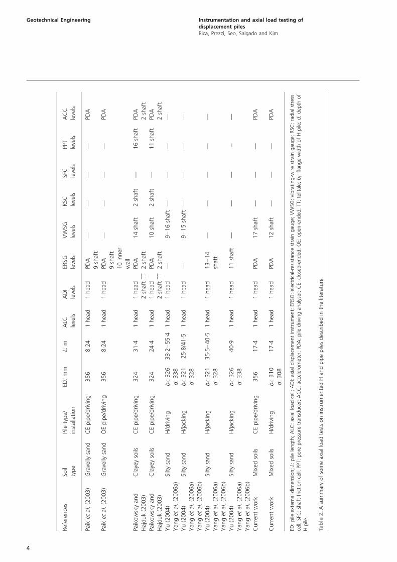
cause their malfunction during testing. Table 1 outlines the details

of some instrumented model piles available in the literature.

Table 2 summarises the details of some instrumented full-scale

piles described in the literature during the past decade.

2.2 Residual loads

Residual loads affect the actual distribution of qsL with depth

(Fellenius, 2002a, 2002b). These loads are usually more difficult

to measure in driven piles than in jacked piles. They are

measured by zeroing all strain gauges immediately before pile

driving and taking gauge readings at the end of driving. However,

it is not easy to measure the residual load after pile driving

(Hajduk and Paikowsky, 2000; O’Neill et al., 1982). In fact,

strain gauges are often re-zeroed before axial load testing to

correct read-out drifts that develop any time between pile

installation and testing (read-out drifts of vibrating-wire strain

gauges are possibly caused by micro slippages at the wire grips

due to inertial forces during driving). Both vibrating-wire and

electrical-resistance strain gauges have been successfully used for

measuring pile load transfer, provided that careful attention is

given to adequate gauge installation.

Piles are often instrumented with vibrating-wire strain gauges

because of their known long-term stability under static loading,

which is particularly important for pile set-up investigations.

However, these gauges show a relatively slow response time. For

References Soil type Pile

installation

PED:

mm

PIL:

m

ALC

levels

ADI

levels

SG

levels

PPT

levels

RSC

levels

SFC

levels

Cooke et al. (1979) OC clay Jacking 168.0 5.00 1 head

3 shaft

1 base

1 head — — — —

Karlsrud and Haugen

(1985)

OC clay Jacking 152.4 5.15 1 head 1 head 6 shaft 4 shaft 4 shaft —

Jardine and Bond

(1989)

Lehane et al. (1993)

Lehane and Jardine

(1994)

OC clay

Sand

Soft clay

Jacking 102.0 2.60 1 head

2 shaft

1 base

1 head — 2 shaft

1 base

2 shaft

1 base

2 shaft

1 base

Coop and Wroth

(1989)

OC clay

NC clay

Jacking 80.0 1.135 1 head

3 shaft

1 head — 2 shaft

1 base

2 shaft 2 friction

sleeves

Paikowsky and Hart

(2000)

Soft clay Driving 76.2 2.87 2 shaft

1 base

1 shaft at

slip joint

— 1 shaft 1 shaft 2 friction

sleeves

Lee et al. (2011) Fine silica

sand

Driving 30.0 1.20 1 head

1 base

2 head 9 shaft — — —

PED: pile external diameter; PIL: pile instrumented length; ALC: axial load cell; ADI: axial displacement instrument; SG: strain gauge; PPT: porepressure transducer; RSC: radial stress cell; SFC: shaft friction cell; OC: overconsolidated; NC: normally consolidated.

Table 1. A summary of some axial load tests on instrumented

model piles described in the literature

3


Ref

eren

ces

Soil

type

Pile

type/

inst

alla

tion

ED:

mm

L:m

ALC

leve

ls

AD

I

leve

ls

ERSG

leve

ls

VW

SG

leve

ls

RSC

leve

ls

SFC

leve

ls

PPT

leve

ls

AC

C

leve

ls

Paik

etal

.(2

003)

Gra

velly

sand

CE

pip

e/drivi

ng

356

8. 2

41

hea

d1

hea

dPD

A

9sh

aft

——

——

PDA

Paik

etal

.(2

003)

Gra

velly

sand

OE

pip

e/drivi

ng

356

8. 2

41

hea

d1

hea

dPD

A

9sh

aft

10

inner

wal

l

——

——

PDA

Paik

ow

sky

and

Haj

duk

(2003)

Cla

yey

soils

CE

pip

e/drivi

ng

324

31. 4

1hea

d1

hea

d

2sh

aft

TT

PDA

2sh

aft

14

shaf

t2

shaf

t—

16

shaf

tPD

A

2sh

aft

Paik

ow

sky

and

Haj

duk

(2003)

Cla

yey

soils

CE

pip

e/drivi

ng

324

24. 4

1hea

d1

hea

d

2sh

aft

TT

PDA

2sh

aft

10

shaf

t2

shaf

t—

11

shaf

tPD

A

2sh

aft

Yu

(2004)

Yan

get

al.

(2006a)

Silty

sand

H/d

rivi

ng

bf:

326

d:

338

33. 2

–55. 4

1hea

d1

hea

d—

9–

16

shaf

t—

——

—

Yu

(2004)

Yan

get

al.

(2006a)

Yan

get

al.

(2006b)

Silty

sand

H/ja

ckin

gb

f:321

d:

328

25. 8

/41. 5

1hea

d1

hea

d—

9–

15

shaf

t—

——

—

Yu

(2004)

Yan

get

al.

(2006a)

Yan

get

al.

(2006b)

Silty

sand

H/ja

ckin

gb

f:321

d:

328

35. 5

–40. 5

1hea

d1

hea

d13

–14

shaf

t

——

——

—

Yu

(2004)

Yan

get

al.

(2006a)

Yan

get

al.

(2006b)

Silty

sand

H/ja

ckin

gb

f:326

d:

338

40. 9

1hea

d1

hea

d11

shaf

t—

——

�—

Curr

ent

work

Mix

edso

ilsC

Epip

e/drivi

ng

356

17. 4

1hea

d1

hea

dPD

A17

shaf

t—

——

PDA

Curr

ent

work

Mix

edso

ilsH

/drivi

ng

bf:

310

d:

308

17. 4

1hea

d1

hea

dPD

A12

shaf

t—

——

PDA

ED:

pile

exte

rnal

dim

ensi

on;

L:pile

length

;A

LC:

axia

llo

adce

ll;A

DI:

axia

ldis

pla

cem

ent

inst

rum

ent;

ERSG

:el

ectr

ical

-res

ista

nce

stra

ingau

ge;

VW

SG:

vibra

ting-w

ire

stra

ingau

ge;

RSC

:ra

dia

lst

ress

cell;

SFC

:sh

aft

fric

tion

cell;

PPT:

pore

pre

ssure

tran

sduce

r;A

CC

:ac

cele

rom

eter

;PD

A:

pile

drivi

ng

anal

yser

;C

E:cl

ose

d-e

nded

;O

E:open

-ended

;TT

:te

lltal

e;b

f:flan

ge

wid

thof

Hpile

;d:

dep

thof

Hpile

.

Tab

le2.A

sum

mar

yof

som

eax

iallo

adte

sts

on

inst

rum

ente

dH

and

pip

epile

sdes

crib

edin

the

liter

ature

4


measurements during pile driving, faster-response electrical-

resistance strain gauges are often preferred, together with

accelerometers. Furthermore, because the masses of electrical-

resistance strain gauges are very small compared to those of

vibrating-wire strain gauges, electrical-resistance strain gauges

are less sensitive to the inertial forces resulting from pile driving

and, hence, are less likely to drift after pile driving. This means

that electrical-resistance strain gauges are more suitable for

measuring residual loads than vibrating-wire strain gauges,

which are subject to possibly significant drifting; however,

electrical-resistance strain gauges do not normally survive in the

long term because they are more sensitive to humidity and other

weather-related effects. Therefore, pile instrumentation combin-

ing both electrical-resistance gauges, whose most important goal

would be that of obtaining residual loads after driving, and

vibrating-wire strain gauges, whose major goal would be that of

long-term monitoring, may be a better option. This may also be

a more cost-effective solution because the cost of acquisition

and installation of a reasonable number of electrical-resistance

strain gauges is lower than that of vibrating-wire strain gauges.

3. Pile load testing programmeIn the context of the present research, instrumented axial load tests

were performed on an H pile and a closed-ended pipe pile, both

driven into a multilayered soil profile in Indiana. The objective of

these tests was to determine, for each pile, the following

(a) load–settlement curve

(b) Qult

(c) load–transfer relationship

(d ) QsL and Qb,ult

(e) qsLi for each soil layer crossed

( f ) qb,ult:

The pile load test results are compared with predictions by soil

property based and in situ test based design methods in Seo et al.

(2009) and Kim et al. (2009). Pile set-up effects are discussed by

Lee et al. (2010).

3.1 Site investigation

The test site is located on State Road 49 (on the north side of

Oliver Ditch) in Jasper County, Indiana. Four standard penetration

tests (SPTs) and four cone penetration tests (CPTs) were

performed before driving the piles into the ground. The ground-

water level and bedrock were found at a depth of 1 m and 26 m,

respectively. Two of the CPTs near the location of the test H pile

were terminated at a depth of about 18 m, about 1 m into an

extremely dense non-plastic silt layer with an average qc of

50 MPa. Below this silt layer, there exists a relatively soft, thick

clay layer with an average qc of 1.5 MPa. The soil profile consists

of 11 soil layers, starting from the ground surface to the pile

base. Figure 2 shows the surface layout of sampling boreholes, in

situ tests, test piles, reaction piles and extra piles. Figure 3 shows

the soil profile and the results of SPTs and CPTs. Results of

laboratory tests performed on soil samples obtained from these

boreholes are reported by Seo et al. (2009) and Kim et al.

(2009).

3.2 Pile instrumentation

It is well known that pile capacities are affected by the degree of

soil displacement during pile installation. Typically, ultimate pile

capacities are greater for displacement piles than for partial or

non-displacement piles because of the stiffer response of displa-

cement piles, which can be attributed to the significant amount of

soil preloading during their installation (Salgado, 2008). In order

to compare the load–settlement and load–transfer behaviours of

partial and full displacement piles, an H pile (partial displace-

3660 mm3660 mm

1830 mm

1830 mm

C4S4C3

S3

CPT

SPT

Closed-ended pipe pile

H pile

3660 mm3660 mm3660 mm

ECEP

EHP RCEP 1-

RHP 1-

RHP-2

MCEP

RHP 3-

RHP 4-

RHP 5-

MHP

RCEP 2-

RHP 6-

RHP-7

C2

S2

C1

S1

Figure 2. Layout of pile load tests and in situ tests (MCEP: main

closed-ended pipe pile; MHP: main H pile; RHP: reaction H pile;

RCEP: reaction closed-ended pipe pile; ECEP: extra closed-ended

pipe pile; EHP: extra H pile)

5


ment pile) and a closed-ended pipe pile (full displacement pile)

were selected in the present study.

The H pile had 310 mm of flange width, 308 mm of web

depth and 15 mm of thickness (HP 310 3 110). The spiral-

welded pipe pile, which was closed by a 25.4 mm thick steel

plate welded to the base, had 356 mm outer diameter and

12.7 mm wall thickness. Both piles were driven to a depth of

17.4 m within the dense silt layer (i.e. both piles were

embedded inside this layer at least 1.5 times the outer

0

2

4

6

8

10

12

14

16

18

20

22

24

26

Depth:m Soil layers

0 50 100 150 200

Blow counts, NSPT

0 10 20 30 40 50 60

Cone resistance, : MPaqc

0 500 10001500

Sleeve friction: kPa

�200 200 600 1000

Pore waterpressure: kPa

S3

S4

C3

C4

C3

C4

C3

C4

(a)

Organicclay (OH)

Silty sand(SP - SM)

Clayeysandy silt

(CL)Silty/clayeysandSandy

silty clay(SM)Silty/clayeysand

Silty clay(CL)

Clayeysilt (CL)Silty clay

(CL)Clayeysilt (CL)

Verydense silt

0

2

4

6

8

10

12

14

16

18

20

22

24

26

Depth:m Soil layers

0 50 100 150 200

Blow counts, NSPT

0 10 20 30 40 50 60

Cone resistance, : MPaqc

0 500 10001500

Sleeve friction: kPa

�200 200 600 1000

Pore waterpressure: kPa

S1

S2

C1

C2

C1

C2

C1

C2

(b)

Organicclay (OH)

Silty sand(SP - SM)Clayey

sandy silt(CL)Silty/clayeysandSandy

silty clay(SM)Silty/clayeysand

Silty clay(CL)

Clayeysilt (CL)Silty clay

(CL)Clayeysilt (CL)

Verydense silt

Silty clay(CL)

Silty clay(CL)

Figure 3. Soil profile and results of in situ tests at (a) H pile

location, (b) pipe pile location

6


diameter of the pipe pile or the flange width of the H pile).

Their final lengths, including the portion above the ground

surface, were 18.5 m.

Twenty-four vibrating-wire strain gauges (Geokon Model 4150)

were attached to the outside of the two flanges of the H pile, at

12 levels. Thirty-two vibrating-wire strain gauges (also Geokon

Model 4150) were attached to the outer surface of the pipe pile,

at 16 levels. All gauges were spot-welded to the pile surface,

covered with a semicircular plate and sealed with silicone rubber.

Care was taken to install these gauges away from the spiral

welding joints of the pipe pile, where the pipe wall thickness may

be slightly different. To avoid damage during driving, the gauges

on both piles were covered with steel angle channels (76 mm

wide and 6 mm thick), welded to the pile surface. These channels

ran from the base to near the head of the piles. The lower end of

each channel was closed by welding a tapered cover to prevent

the entrance of soil during pile driving. Gauge cables were routed

to the ground surface inside the channels. The cables were

wrapped with aluminium tape to protect them from the heat

generated by welding. The strain values obtained from the

vibrating-wire strain gauges installed above the ground level were

used to calculate the Young’s modulus values for both piles.

Although other instrumentation techniques – such as electrical-

resistance strain gauges – could have been used for measuring

axial strains in these test piles, the spot-welded vibrating-wire

strain gauge was selected because of its

(a) small size

(b) ruggedness

(c) ease of installation

(d ) moisture resistance

(e) long-term stability (required for evaluating pile set-up)

( f ) possibility of using long instrument cables without significant

loss of accuracy

(g) ease of connection to a field data acquisition system (with a

built-in plucking circuit).

The operation of the vibrating-wire type of strain gauge is based

on changes of the natural frequency of a tensioned wire. A small

relative movement of the fixed ends of the wire, which is vibrated

by the input pluck pulse, will alter the tension of the wire and

hence cause a change in its natural frequency. This change in

natural frequency is measured by means of an electromagnetic

coil positioned next to the wire. Although vibrating-wire strain

gauges, in contrast with electric-resistance strain gauges, are

durable and have minimal lead-wire effect, they are very sensitive

to wire tension and have limited range of measurable strains

(usually up to 3000 microstrains). Therefore, much care is needed

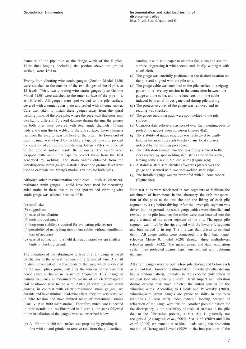
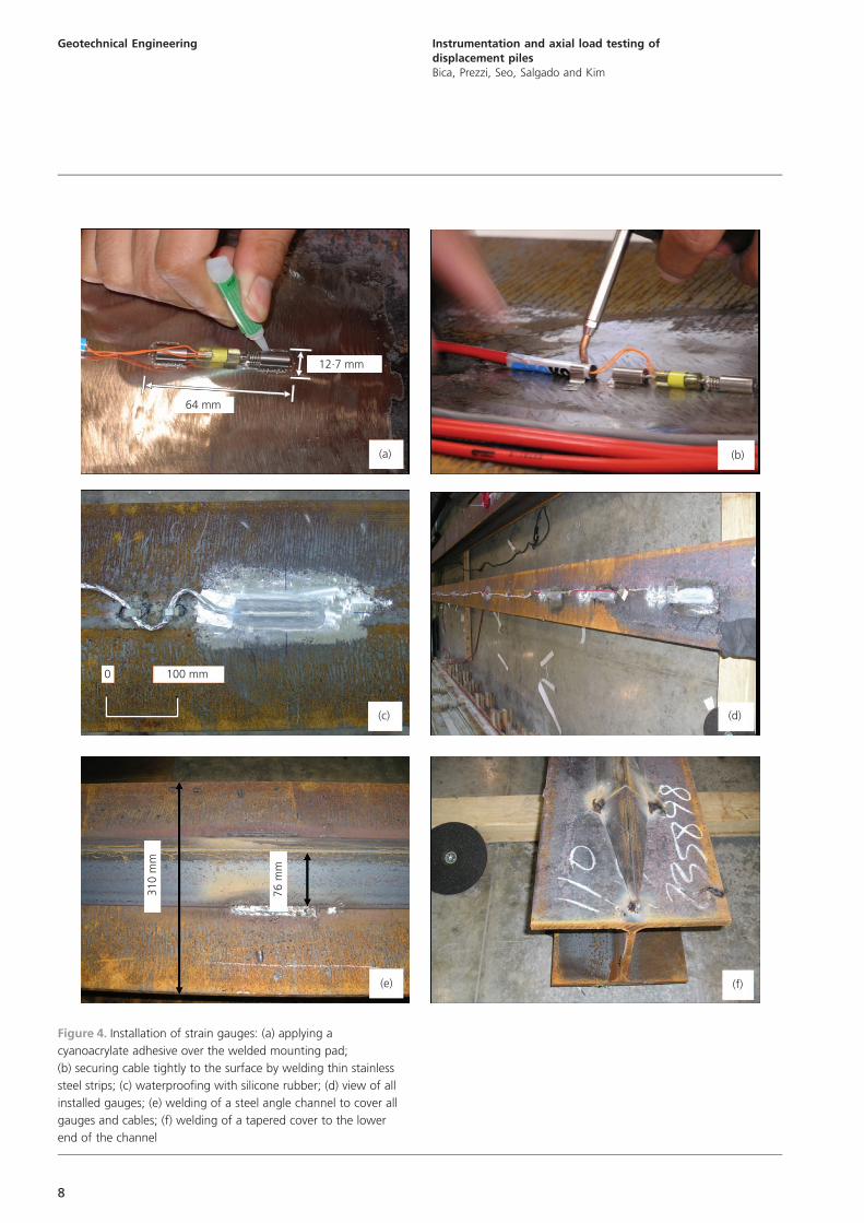
in their installation. As illustrated in Figure 4, the steps followed

in the installation of the gauges were as described below.

(a) A 150 mm 3 100 mm surface was prepared by grinding it

first with a hand grinder to remove rust from the pile surface,

sanding it with sand paper to obtain a flat, clean and smooth

surface, degreasing it with acetone and, finally, wiping it with

a soft cloth.

(b) The gauge was carefully positioned at the desired location on

the pile and aligned with the pile axis.

(c) The gauge cable was anchored to the pile surface in a zigzag

pattern to relieve any tension in the connection between the

gauge and the cable, and to reduce tension in the cable

induced by inertial forces generated during pile driving.

(d ) The protective cover of the gauge was removed and its

reading was checked.

(e) The gauge mounting pads were spot welded to the pile

surface.

( f ) Cyanoacrylate adhesive was spread over the mounting pads to

protect the gauges from corrosion (Figure 4(a)).

(g) The stability of gauge readings was rechecked by gently

tapping the mounting pads to relieve any local stresses

induced by the welding procedure.

(h) The cable-to-lead-wire junction was firmly secured to the

steel surface by spot welding steel strips around the cable,

leaving some slack in the lead wires (Figure 4(b)).

(i) A stainless steel semicircular cover was placed over the

gauge and secured with two spot-welded steel strips.

( j) The installed gauge was waterproofed with silicone rubber

(Figure 4(c)).

Both test piles were fabricated in two segments to facilitate the

attachment of instruments in the laboratory, the safe transporta-

tion of the piles to the test site and the lifting of each pile

segment by a rig before driving. After the lower pile segment was

driven into the ground, the strain gauge cables were identified and

rewired at the pile junction; the cables were then inserted into the

angle channel of the upper segment of the pile. The upper pile

segment was lifted by the rig, aligned with the lower pile segment

and butt welded to its top. The pile was then driven to its final

depth. All gauge cables were connected to a field data logger

(Geokon Micro-10, model 8020) through three multiplexers

(Geokon model 8032). The measurement and data acquisition

system was protected against harsh environment and lightning

damage.

All strain gauges were zeroed before pile driving and before each

axial load test. However, readings taken immediately after driving

had a random pattern, unrelated to the expected distribution of

residual load along the pile shaft. Harsh impact and vibration

during driving may have affected the initial tension of the

vibrating wires. According to Hajduk and Paikowsky (2000),

vibrating-wire strain gauges are prone to shifts in the zero

readings (i.e. zero drift) under dynamic loading because of

relaxation of the gauge wire tension. Another possible reason for

the discrepancy is the possibility of residual stresses in the pile

due to the fabrication process, a fact that is generally not

recognised (Akutagawa et al., 2005). Seo et al. (2009) and Kim

et al. (2009) estimated the residual loads using the prediction

method of Darrag and Lovell (1989) in the interpretation of the

7


64 mm

12·7 mm

(a) (b)

0 100 mm

(c) (d)

(e)

310

mm

76 m

m

(f)

Figure 4. Installation of strain gauges: (a) applying a

cyanoacrylate adhesive over the welded mounting pad;

(b) securing cable tightly to the surface by welding thin stainless

steel strips; (c) waterproofing with silicone rubber; (d) view of all

installed gauges; (e) welding of a steel angle channel to cover all

gauges and cables; (f) welding of a tapered cover to the lower

end of the channel

8


results of the axial load tests, and the estimated residual loads

were small compared with the loads carried by the piles.

The details of the pile instrumentation and the location of the

strain gauges along the length of each pile are shown in Figure 5.

The large number of strain gauges in these piles allowed for a

better correlation between qsL and soil type along the pile shaft.

This dense gauge layout provided enough redundancy to compen-

sate for eventual gauge losses during pile driving and to ensure

reliable strain measurements without installing backup instru-

ments (such as rod extensometers). Four strain gauges did not

survive driving and load testing.

3.3 Pile loading

Figure 6 shows the pile axial load testing layout. A 500 mm wide

and 50.8 mm thick square steel plate was welded to the head of

each test pile for distributing the applied axial load evenly. A

hydraulic jack was placed over this plate. A 400 mm wide and

76.2 mm thick square steel plate was placed over the jack ram. A

load cell was then placed over this steel plate. Another 400 mm

wide and 76.2 mm thick square steel plate and a spherical seat

were inserted between the load cell and the reaction beam

situated above it to maintain the verticality of the load. All these

components were carefully aligned and levelled before pile

testing. The settlement of each test pile was measured by two dial

gauges (one on each side of the pile shaft) attached to two

reference beams by magnetic clamps. The spindle of each dial

gauge rested on a steel bracket welded to the pile shaft. The

supports of each reference beam were placed at least 6.8 pile

diameters away from the test piles.

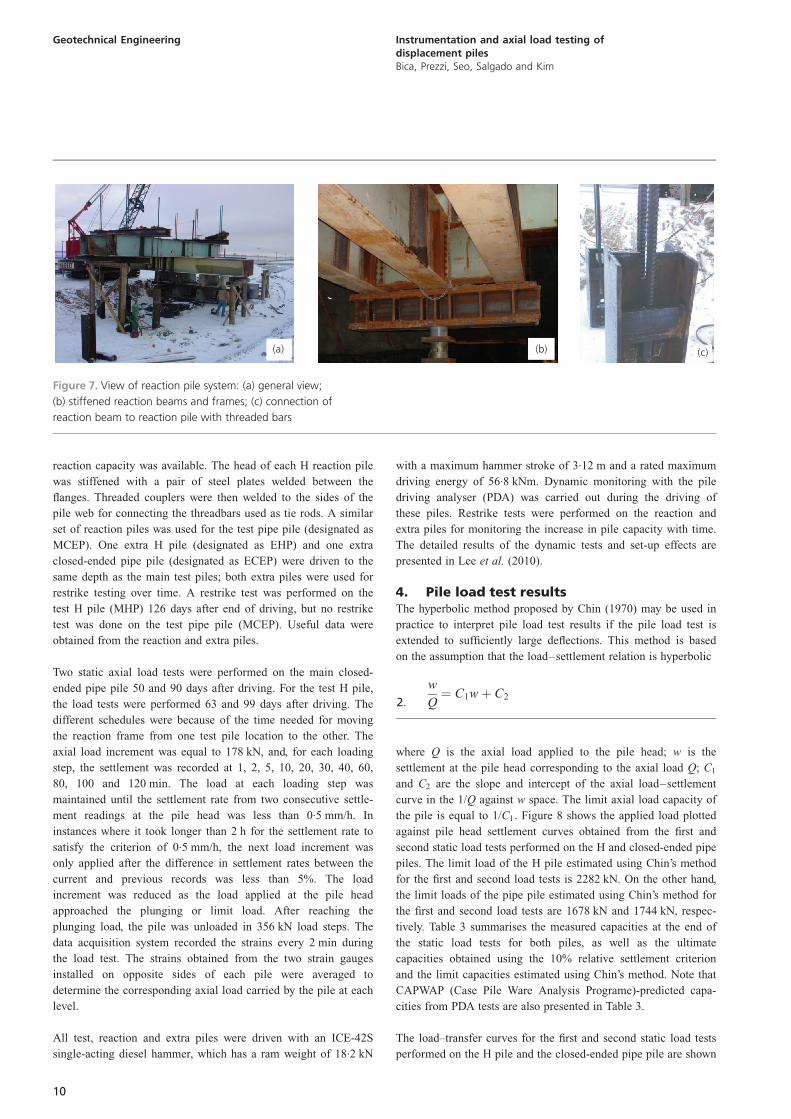
Figure 7(a) shows a general view of the reaction system. It was

designed in such a way that the reaction frame could be

reassembled from one test pile location to the other. The reaction

beam was a wide-flange I steel beam, 4.2 m long and 406 mm

deep. Both flanges of this beam were heavily stiffened by welding

steel plates along its whole length. Vertical web stiffeners were

also welded to this beam, particularly above the pile–jack–load

cell assembly. The reaction beam was attached to a heavy

reaction frame assembled with steel plate girders to distribute the

applied load among six reaction piles (Figure 7(b)). The weight

of the reaction frame was supported by a stack of concrete beams

bearing on the ground surface. Vertical threadbars connected to

each reaction pile were tied to the reaction frame (Figure 7(c)).

As shown in the test layout of Figure 2, one closed-ended pipe

pile (designated as RCEP) and five H piles (designated as RHP)

were used as reaction piles for the instrumented test H pile

(designated as MHP). To compare the pile capacities obtained

from dynamic restrike tests with those obtained from the static

axial load tests, one of the reaction H piles (RHP-6) was driven

to the same depth as the instrumented H test pile. All other

reaction H piles were driven to 24.4 m to make sure the necessary

18500

5005005001500

2000

2000

2000

2000

2000

2000

2000400500Ground surface

17400

Angle for protection ofstrain gauges and cables

Strain gauges

310

308

15

15

76 6

(a)

356

12·7

76

2000

2000

2000

1000600300

18500

17400

10001000100013001000100010001000

500500500

Ground surface

Angle for protection ofstrain gauges and cables

Strain gauges

6

(b)

Figure 5. Instrumentation details: (a) H pile; (b) closed-ended pipe

pile (dimensions in mm)

Load cellReaction frames

Test pile

Dial gauges

Reference beams

Reaction beam

Spherical seat

Hydraulic jack

Figure 6. View of axial pile load testing layout

9


reaction capacity was available. The head of each H reaction pile

was stiffened with a pair of steel plates welded between the

flanges. Threaded couplers were then welded to the sides of the

pile web for connecting the threadbars used as tie rods. A similar

set of reaction piles was used for the test pipe pile (designated as

MCEP). One extra H pile (designated as EHP) and one extra

closed-ended pipe pile (designated as ECEP) were driven to the

same depth as the main test piles; both extra piles were used for

restrike testing over time. A restrike test was performed on the

test H pile (MHP) 126 days after end of driving, but no restrike

test was done on the test pipe pile (MCEP). Useful data were

obtained from the reaction and extra piles.

Two static axial load tests were performed on the main closed-

ended pipe pile 50 and 90 days after driving. For the test H pile,

the load tests were performed 63 and 99 days after driving. The

different schedules were because of the time needed for moving

the reaction frame from one test pile location to the other. The

axial load increment was equal to 178 kN, and, for each loading

step, the settlement was recorded at 1, 2, 5, 10, 20, 30, 40, 60,

80, 100 and 120 min. The load at each loading step was

maintained until the settlement rate from two consecutive settle-

ment readings at the pile head was less than 0.5 mm/h. In

instances where it took longer than 2 h for the settlement rate to

satisfy the criterion of 0.5 mm/h, the next load increment was

only applied after the difference in settlement rates between the

current and previous records was less than 5%. The load

increment was reduced as the load applied at the pile head

approached the plunging or limit load. After reaching the

plunging load, the pile was unloaded in 356 kN load steps. The

data acquisition system recorded the strains every 2 min during

the load test. The strains obtained from the two strain gauges

installed on opposite sides of each pile were averaged to

determine the corresponding axial load carried by the pile at each

level.

All test, reaction and extra piles were driven with an ICE-42S

single-acting diesel hammer, which has a ram weight of 18.2 kN

with a maximum hammer stroke of 3.12 m and a rated maximum

driving energy of 56.8 kNm. Dynamic monitoring with the pile

driving analyser (PDA) was carried out during the driving of

these piles. Restrike tests were performed on the reaction and

extra piles for monitoring the increase in pile capacity with time.

The detailed results of the dynamic tests and set-up effects are

presented in Lee et al. (2010).

4. Pile load test resultsThe hyperbolic method proposed by Chin (1970) may be used in

practice to interpret pile load test results if the pile load test is

extended to sufficiently large deflections. This method is based

on the assumption that the load–settlement relation is hyperbolic

w

Q¼ C1wþ C2

2:

where Q is the axial load applied to the pile head; w is the

settlement at the pile head corresponding to the axial load Q; C1

and C2 are the slope and intercept of the axial load–settlement

curve in the 1/Q against w space. The limit axial load capacity of

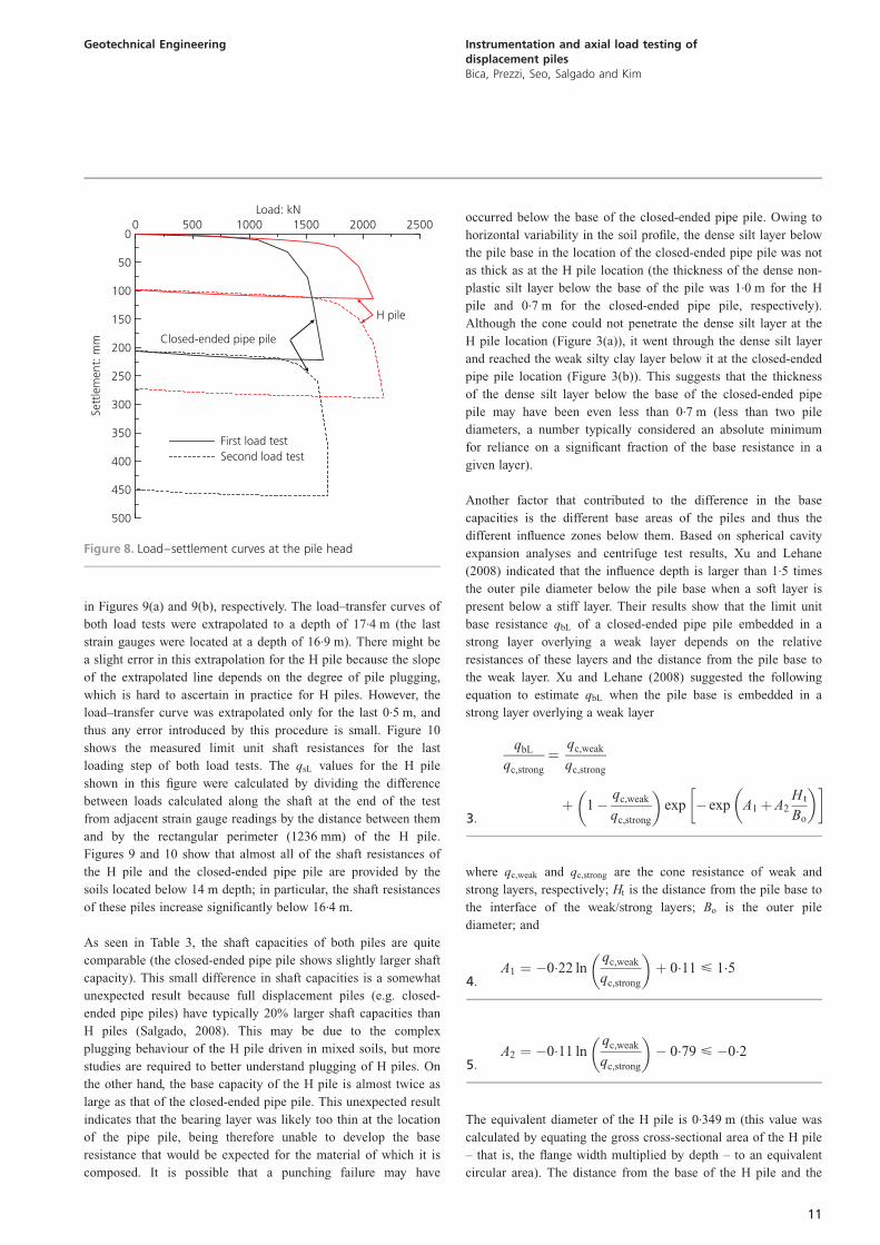
the pile is equal to 1/C1: Figure 8 shows the applied load plotted

against pile head settlement curves obtained from the first and

second static load tests performed on the H and closed-ended pipe

piles. The limit load of the H pile estimated using Chin’s method

for the first and second load tests is 2282 kN. On the other hand,

the limit loads of the pipe pile estimated using Chin’s method for

the first and second load tests are 1678 kN and 1744 kN, respec-

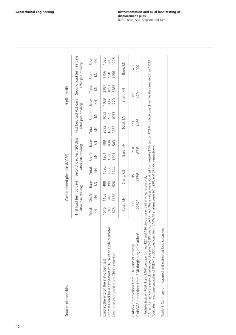
tively. Table 3 summarises the measured capacities at the end of

the static load tests for both piles, as well as the ultimate

capacities obtained using the 10% relative settlement criterion

and the limit capacities estimated using Chin’s method. Note that

CAPWAP (Case Pile Ware Analysis Programe)-predicted capa-

cities from PDA tests are also presented in Table 3.

The load–transfer curves for the first and second static load tests

performed on the H pile and the closed-ended pipe pile are shown

(a) (b) (c)

Figure 7. View of reaction pile system: (a) general view;

(b) stiffened reaction beams and frames; (c) connection of

reaction beam to reaction pile with threaded bars

10


in Figures 9(a) and 9(b), respectively. The load–transfer curves of

both load tests were extrapolated to a depth of 17.4 m (the last

strain gauges were located at a depth of 16.9 m). There might be

a slight error in this extrapolation for the H pile because the slope

of the extrapolated line depends on the degree of pile plugging,

which is hard to ascertain in practice for H piles. However, the

load–transfer curve was extrapolated only for the last 0.5 m, and

thus any error introduced by this procedure is small. Figure 10

shows the measured limit unit shaft resistances for the last

loading step of both load tests. The qsL values for the H pile

shown in this figure were calculated by dividing the difference

between loads calculated along the shaft at the end of the test

from adjacent strain gauge readings by the distance between them

and by the rectangular perimeter (1236 mm) of the H pile.

Figures 9 and 10 show that almost all of the shaft resistances of

the H pile and the closed-ended pipe pile are provided by the

soils located below 14 m depth; in particular, the shaft resistances

of these piles increase significantly below 16.4 m.

As seen in Table 3, the shaft capacities of both piles are quite

comparable (the closed-ended pipe pile shows slightly larger shaft

capacity). This small difference in shaft capacities is a somewhat

unexpected result because full displacement piles (e.g. closed-

ended pipe piles) have typically 20% larger shaft capacities than

H piles (Salgado, 2008). This may be due to the complex

plugging behaviour of the H pile driven in mixed soils, but more

studies are required to better understand plugging of H piles. On

the other hand, the base capacity of the H pile is almost twice as

large as that of the closed-ended pipe pile. This unexpected result

indicates that the bearing layer was likely too thin at the location

of the pipe pile, being therefore unable to develop the base

resistance that would be expected for the material of which it is

composed. It is possible that a punching failure may have

occurred below the base of the closed-ended pipe pile. Owing to

horizontal variability in the soil profile, the dense silt layer below

the pile base in the location of the closed-ended pipe pile was not

as thick as at the H pile location (the thickness of the dense non-

plastic silt layer below the base of the pile was 1.0 m for the H

pile and 0.7 m for the closed-ended pipe pile, respectively).

Although the cone could not penetrate the dense silt layer at the

H pile location (Figure 3(a)), it went through the dense silt layer

and reached the weak silty clay layer below it at the closed-ended

pipe pile location (Figure 3(b)). This suggests that the thickness

of the dense silt layer below the base of the closed-ended pipe

pile may have been even less than 0.7 m (less than two pile

diameters, a number typically considered an absolute minimum

for reliance on a significant fraction of the base resistance in a

given layer).

Another factor that contributed to the difference in the base

capacities is the different base areas of the piles and thus the

different influence zones below them. Based on spherical cavity

expansion analyses and centrifuge test results, Xu and Lehane

(2008) indicated that the influence depth is larger than 1.5 times

the outer pile diameter below the pile base when a soft layer is

present below a stiff layer. Their results show that the limit unit

base resistance qbL of a closed-ended pipe pile embedded in a

strong layer overlying a weak layer depends on the relative

resistances of these layers and the distance from the pile base to

the weak layer. Xu and Lehane (2008) suggested the following

equation to estimate qbL when the pile base is embedded in a

strong layer overlying a weak layer

qbL

qc,strong

¼qc,weak

qc,strong

þ 1�qc,weak

qc,strong

� �exp � exp A1þA2

H t

Bo

� �� 3:

where qc,weak and qc,strong are the cone resistance of weak and

strong layers, respectively; Ht is the distance from the pile base to

the interface of the weak/strong layers; Bo is the outer pile

diameter; and

A1 ¼ �0:22 lnqc,weak

qc,strong

� �þ 0:11 < 1:5

4:

A2 ¼ �0:11 lnqc,weak

qc,strong

� �� 0:79 < �0:2

5:

The equivalent diameter of the H pile is 0.349 m (this value was

calculated by equating the gross cross-sectional area of the H pile

– that is, the flange width multiplied by depth – to an equivalent

circular area). The distance from the base of the H pile and the

2500200015001000500

500

450

400

350

300

250

200

150

100

50

0

Sett

lem

ent:

mm

0Load: kN

First load testSecond load test

H pile

Closed-ended pipe pile

Figure 8. Load–settlement curves at the pile head

11


Sourc

esof

capac

itie

sC

lose

d-e

nded

pip

epile

(MC

EP)

Hpile

(MH

P)

Firs

tlo

adte

st(5

0day

s

afte

rpile

drivi

ng)

Seco

nd

load

test

(90

day

s

afte

rpile

drivi

ng)

Firs

tlo

adte

st(6

3day

s

afte

rpile

drivi

ng)

Seco

nd

load

test

(99

day

s

afte

rpile

drivi

ng)

Tota

l:

kN

Shaf

t:

kN

Bas

e:

kN

Tota

l:

kN

Shaf

t:

kN

Bas

e:

kN

Tota

l:

kN

Shaf

t:

kN

Bas

e:

kN

Tota

l:

kN

Shaf

t:

kN

Bas

e:

kN

Load

atth

een

dof

the

stat

iclo

adte

st1646

1158

488

1690

1201

489

2092

1053

1039

2181

1156

1025

Ultim

ate

load

for

ase

ttle

men

tof

10%

of

the

pile

dia

met

er1345

946

399

1500

1066

434

1839

933

906

1851

958

893

Lim

itlo

ades

tim

ated

from

Chin

’scr

iter

ion

1678

1158

520

1744

1201

543

2282

1053

1229

2282

1156

1126

Tota

l:kN

Shaf

t:kN

Bas

e:kN

Tota

l:kN

Shaf

t:kN

Bas

e:kN

CA

PWA

Ppre

dic

tions

from

EOD

(end

of

drivi

ng)

905

195

710

990

311

679

CA

PWA

Ppre

dic

tions

from

BO

R(b

egin

nin

gof

rest

rike

)a2252

b1379

b873

b1486

479

1007

aRes

trik

ete

sts

on

RC

EP-1

and

MH

Pw

ere

per

form

ed127

and

126

day

saf

ter

end

of

drivi

ng,

resp

ective

ly.

bA

rest

rike

test

on

the

mai

ncl

ose

d-e

nded

pip

epile

(MC

EP)

was

not

per

form

ed.

Thes

eva

lues

wer

eobta

ined

from

rest

rike

PDA

test

on

RC

EP-1

,w

hic

hw

asdrive

nto

the

sam

edep

thas

MC

EP.

Tota

l,sh

aft,

and

bas

eca

pac

itie

sof

RC

EP-1

atEO

Dpre

dic

ted

from

CA

PWA

Pan

alys

esw

ere

961,

290,

and

671

kN,

resp

ective

ly.

Tab

le3.Su

mm

ary

of

mea

sure

dan

des

tim

ated

load

capac

itie

s

12


closed-ended pipe pile to the top of the clay layer underneath the

very dense silt layer in which the pile was embedded was

assumed to be equal to 1 m and 0.7 m, respectively. This

corresponds to 2.9 times the equivalent circular H pile diameter

(0.349 m) and 2 times the outer diameter of the pipe pile. Using

qc ¼ 50 MPa for the dense silt layer and qc ¼ 1.5 MPa for the

soft clay layer, the estimated qbL values at the H pile and the pipe

pile base according to Equation 3 are 24.3 MPa and 17.8 MPa,

respectively. Note that the equivalent outer diameter of the H pile

was calculated assuming that its gross rectangular area was

operative at the pile base. This assumption is only valid when the

H pile is fully plugged. In reality, the H pile base was most likely

partially plugged and hence the operative base area may be in

between the actual H pile cross-sectional area and the gross

rectangular area. This indicates that qbL may have been higher

than 24.3 MPa for the H pile because the equivalent outer

diameter Bo would have been smaller than 0.349 m for partially

plugged conditions. On the other hand, CPT results indicated that

the thickness of the dense silt layer below the base of the closed-

ended pipe pile may have been even less that 0.7 m, as mentioned

previously. If this is indeed the case, qbL of the closed-ended pipe

pile would have been smaller than 17.8 MPa. This may partially

explain why the base capacity of the H pile is almost twice as

large as that of the closed-ended pipe pile.

5. Summary and conclusionThe literature contains a limited number of well-documented

cases of instrumented pile load tests in which loading was

extended to large enough displacements, load was applied at rates

that may be related to situations of practical interest and for

which also complete soil characterisation was done at the location

of the pile load test. This has an important consequence:

researchers attempting to develop new analyses or methods of

design have little to no access to quality data to validate their

research. One of the aims of this paper was to show very

specifically what must be done to obtain information that is

complete and that will thus be useful for researchers in the

future.

The planning of a pile load testing programme, the principles of

operation of the vibrating-wire strain gauges and the procedures

required for their successful installation on steel piles have been

discussed in detail. In this discussion, the results were used from

static instrumented axial load tests performed on an H pile and a

closed-ended pipe pile, both driven into a multilayered soil

profile. For the test piles, several levels of strain gauges were

2500200015001000500

2000160012008004000Load: kN

20

18

16

14

12

10

8

6

4

2

0

Dep

th: m

0Load: kN


(a)

20

18

16

14

12

10

8

6

4

2

0

Dep

th: m


(b)

Figure 9. Load–transfer curves: (a) H pile; (b) closed-ended pipe pile

Limit unit shaft resistance, : kPaqsL

45040035030025020015010050

qsL (first load test)

qsL (second load test)

20

18

16

14

12

10

8

6

4

2

0

Dep

th: m

0

H pileClosed-ended pipe pile

Figure 10. Distribution of limit unit shaft resistances

13


attached along their length in order to achieve accurate measure-

ments of the load transferred to each soil layer. The vertical

spacing between adjacent strain gauges was reduced near the base

of each pile, as a high rate of load transfer was expected to occur

at this depth (a very dense silty layer is present at the base of the

piles). Ultimate loads corresponding to a settlement of 10% of

the pile diameter (1839 kN for the H pile and 1345 kN for the

closed-ended pipe pile according to the first loading test) and

limit loads according to Chin’s criterion (2282 kN for the H pile

and 1678 kN for the closed-ended pipe pile according to the first

loading test) were determined for both piles. The measured shaft

capacities of the closed-ended pipe pile and the H pile were very

similar (the closed-ended pipe pile showed a slightly larger shaft

capacity). The measured load–transfer curves showed that a

substantial portion of QsL was mobilised in the lower third of

each pile. However, the base capacity of the H pile was about

twice that of the closed-ended pipe pile. This was attributed to

the different influence zones below the base of the piles and the

smaller thickness of the bearing layer at the location of the pipe

pile, which allowed less base resistance to develop at the location

of the closed-ended pipe pile.

REFERENCES

Akutagawa S, Ota M, Yasuhara K et al. (2005) Use of magnetic

anisotropy sensor for stress measurement of steel ribs used

for NATM tunnel. Proceedings of Japan Society of Civil

Engineers 805: 117–130 (in Japanese with English abstract).

Alawneh AS and Malkawi AIH (2000) Estimation of post-driving

residual stresses along driven piles in sand. Geotechnical

Testing Journal, ASTM 23(3): 313–326.

Basu P, Loukadis D, Prezzi M and Salgado R (2011) Analysis of

shaft resistance of jacked piles in sands. International

Journal for Numerical and Analytical Methods in

Geomechanics 35(15): 1605–1635.

Briaud JL and Tucker L (1984) Piles in sand: a method including

residual stresses. Journal of Geotechnical Engineering, ASCE

110(11): 1666–1680.

Chakraborty T, Salgado R, Basu P and Prezzi M (2012). The Shaft

Resistance of Drilled Shafts in Clay. Journal of Geotechnical

and Geoenvironmental Engineering, ASCE, doi: 10.1061/

(ASCE)GT.1443-5606.0000803.

Chin FV (1970) Estimation of the ultimate load of piles not carried

to failure. Proceedings of the 2nd Southeast Asian Conference

on Soil Engineering, Singapore, vol. 1, pp. 81–90.

Cooke RW, Price G and Tarr K (1979) Jacked piles in London

Clay: a study of load transfer and settlement under working

conditions. Geotechnique 29(2): 113–147.

Coop MR and Wroth CP (1989) Field studies of an instrumented

model pile in clay. Geotechnique 39(4): 679–696.

Darrag AA and Lovell CW (1989) A simplified procedure for

predicting residual stresses for piles. Proceedings of the 12th

International Conference on Soil Mechanics and Foundation

Engineering, Rio de Janeiro, Brazil, vol. 2, pp. 1127–1130.

Fellenius BH (2002a) Determining the resistance distribution in

piles. Part 1: Notes on shift of no-load reading and residual

load. Geotechnical News Magazine 20(2): 35–38.

Fellenius BH (2002b) Determining the resistance distribution in

piles. Part 2: Method for determining the residual load.

Geotechnical News Magazine, 20(3): 25–29.

Hajduk EL and Paikowsky SG (2000) Performance evaluation of an

instrumented test pile cluster. Proceedings of ASCE Specialty

Conference, Performance Verification of Constructed

Geotechnical Facilities, Amherst, MA, USA (Lutenegger AJ

and DeGroot DJ (eds)). ASCE, Reston, VA, USA, ASCE

Geotechnical Special Publication No. 94, pp. 124–147.

Jardine R and Bond AJ (1989) Behaviour of displacement piles in

a heavily overconsolidated clay. Proceedings of the 12th

International Conference on Soil Mechanics and Foundation

Engineering, Rio de Janeiro, Brazil, vol. 2, pp. 1147–1152.

Karlsrud K and Haugen T (1985) Axial static capacity of steel

model piles in overconsolidated clay. Proceedings of the

11th International Conference on Soil Mechanics and

Foundation Engineering, San Francisco, CA, USA, vol. III,

pp. 1401–1406.

Kim D, Bica AVD, Salgado R, Prezzi M and Lee W (2009) Load

testing of a closed-ended pipe pile driven in multilayered soil.

Journal of Geotechnical and Geoenvironmental Engineering

135(4): 463–473.

Lee J, Prezzi M and Salgado R (2011) Experimental investigation

of the combined load response of model piles driven in sand.

Geotechnical Testing Journal 34(6): 653–667.

Lee W, Kim D, Salgado R and Zaheer M (2010) Setup of driven

piles in layered soils. Soils and Foundations 50(5): 585–598.

Lehane BM and Jardine RJ (1994) Displacement-pile behavior in

a soft marine clay. Canadian Geotechnical Journal 31(2):

181–191.

Lehane BM, Jardine RJ, Bond AJ and Frank R (1993) Mechanisms

of shaft friction in sand from instrumented pile tests. Journal

of Geotechnical and Geoenvironmental Engineering, ASCE

119(1): 19–35.

Loukidis D and Salgado R (2008) Analysis of the shaft resistance

of nondisplacement piles in sand. Geotechnique 58(4): 283–

296.

O’Neill MW, Hawkins MA and Audibert JME (1982) Installation of

pile group in overconsolidation clay. Journal of Geotechnical

Engineering Division, ASCE 108(11): 1369–1386.

Paik K, Salgado R, Lee J and Kim B (2003) Behavior of open- and

closed-ended piles driven into sands. Journal of Geotechnical

and Geoenvironmental Engineering, ASCE 129(4): 296–306.

Paikowsky SG and Hajduk EL (2003) Design and construction of

three instrumented test piles to examine time dependent pile

capacity gain. Geotechnical Testing Journal, ASTM 27(6):

1–17.

Paikowsky SG and Hart L (2000) Development and Field Testing

of Multiple Deployment Model Pile. Federal Highway

Administration, McLean, VA, USA, FHWA Publication No.

FHWA-RD-99–194.

Salgado R (2006a) Analysis of the axial response of non-

displacement piles in sand. In Geomechanics II: Testing,

14


Modeling and Simulation. Proceedings of the 2nd Japan–US

Workshop. ASCE, Reston, VA, USA, Geotechnical Special

Publication No. 143, pp. 427–439.

Salgado R (2006b) The role of analysis in non-displacement pile

design. Modern Trends in Geomechanics, Springer

Proceedings in Physics 106: 521–540.

Salgado R (2008) The Engineering of Foundations. McGraw Hill,

New York, NY, USA.

Seo H, Yildirim IZ and Prezzi M (2009) Assessment of the axial

load response of an H pile driven in multilayered soil.

Journal of Geotechnical and Geoenvironmental Engineering

135(12): 1789–1804.

Xu X and Lehane M (2008) Pile and penetrometer end bearing

resistance in two-layered soil profiles. Geotechnique 58(3):

187–197.

Yang J, Tham LG, Lee PKK, Chan ST and Yu F (2006a) Behavior

of jacked and driven piles in sandy soil. Geotechnique 56(4):

245–259.

Yang J, Tham LG, Lee PKK and Yu F (2006b) Observed

performance of long H-piles jacked into sandy soils. Journal

of Geotechnical and Geoenvironmental Engineering, ASCE

132(1): 24–35.

Yu F (2004) Behavior of Large Capacity Jacked Piles. PhD thesis,

University of Hong Kong, Hong Kong, PR China.

WHAT DO YOU THINK?

To discuss this paper, please email up to 500 words to the

editor at [email protected]. Your contribution will be

forwarded to the author(s) for a reply and, if considered

appropriate by the editorial panel, will be published as a

discussion in a future issue of the journal.

Proceedings journals rely entirely on contributions sent in

by civil engineering professionals, academics and students.

Papers should be 2000–5000 words long (briefing papers

should be 1000–2000 words long), with adequate illustra-

tions and references. You can submit your paper online via

www.icevirtuallibrary.com/content/journals, where you

will also find detailed author guidelines.

15


instrumentation and axial load testing of displacement piles

Documents