Instrumentation for millimeter wave tests and measurements

Tomasz Waliwander1, Michael Crowley1, 1Farran Technology, Cork, Ireland, www.farran.com

1.1 Abstract There has been a vast research effort and academic development in the past three decades in millimeter wave (mm-wave) technology. Such an effort has been corresponding steadily in the growth in customer demand for mm-wave components and systems which has in turn created a need for a cost effective test and measurement solutions for high frequency applications. There is a large number of test instrumentation already available in the field as well as new developments coming on-stream to the engineers ranging from signal generators, spectrum analyzers to network and noise figure analyzers to choose from to fulfill test and evaluation duties. The choice of instrumentation as well as ways of extending their measurement capabilities will be discussed in this article.

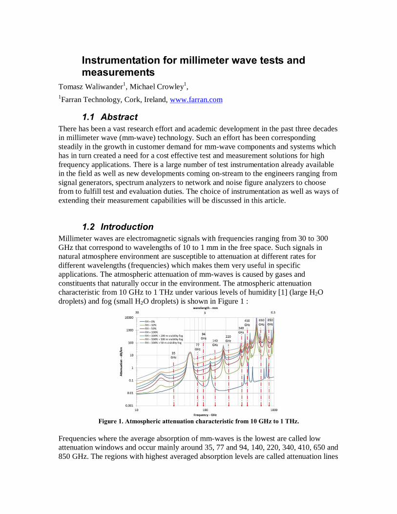
1.2 Introduction Millimeter waves are electromagnetic signals with frequencies ranging from 30 to 300 GHz that correspond to wavelengths of 10 to 1 mm in the free space. Such signals in natural atmosphere environment are susceptible to attenuation at different rates for different wavelengths (frequencies) which makes them very useful in specific applications. The atmospheric attenuation of mm-waves is caused by gases and constituents that naturally occur in the environment. The atmospheric attenuation characteristic from 10 GHz to 1 THz under various levels of humidity [1] (large H2O droplets) and fog (small H2O droplets) is shown in Figure 1 :

Figure 1. Atmospheric attenuation characteristic from 10 GHz to 1 THz.

Frequencies where the average absorption of mm-waves is the lowest are called low attenuation windows and occur mainly around 35, 77 and 94, 140, 220, 340, 410, 650 and 850 GHz. The regions with highest averaged absorption levels are called attenuation lines

and can be seen around 22, 60, 118, 183, 320, 380, 450, 560, 750 GHz. It is the oxygen molecules that are responsible for high attenuation at 60, 118 and 560 and 750 GHz. The rest of the attenuation lines are caused mainly by water droplets of various diameter sizes as well as other chemical species (CO2, N2O, NO, SO2 and SH2) at submillimeter wavelengths. Due to different properties of mm-waves at different frequencies and environmental conditions the applications of mm-waves vary largely from communications, imaging and security applications, radar, radiometry and atmospheric sensing. All the applications mentioned, at some stage of their development, need to employ a mm-wave measurement system for component and system level testing and evaluation.

1.3 Mm-wave Applications The mm-wave applications correlate closely with how such signals propagate in the atmosphere. The frequencies for which atmospheric attenuation is low (44, 86, 94, 140 GHz) are particularly useful in communication system operating at long ranges such as: satellite communications, backhaul mm-wave radios and point to multi-point radio links. For short range communications the 60 GHz band provides enough range where only a local area, short distance transmission is required. Other application benefiting from low atmospheric attenuation would include automotive radars at 24, 77 and 94 GHz where a long range transmission and reception is possible [2]. Imaging and security utilizes a mixture of high and low attenuations bands for passive and active systems. These use 77, 94 and 183 GHz frequencies as these signals present good properties to penetrate many materials (i.e. clothing) and see through the fog and rain. For those materials that can not be penetrated the atmospheric environment provides a good thermal contrast from which images can be synthesized at post processing level (see Figure 2).

Figure 2. Typical human body image obtained with mm-wave imaging system.

Other applications include scientific research as well as radiometry and ground based astronomy. These applications would mainly concentrate at 183 and 220 GHz as well as higher frequencies.

Rectangular waveguide due to its inherently low loss properties is the medium that is most frequently used in mm-wave applications. Under normal conditions the electromagnetic field propagates through the waveguide in transverse electrical dominant mode TE10 and has a cut off point below which it does not propagate in any form or mode. Millimeter wave waveguide bands are shown in Table 1 and contain band designation, internal waveguide dimensions as well as cut off frequency. Table 1. Waveguide band designations.

Band Designation Frequency range [GHz]

Cut off Frequency

[GHz]

Dimensions [mm]

WR-19 U 40 – 60 31.4 4.755 x 2.388 WR-15 V 50 – 75 39.9 3.759 x 1.88 WR-12 E 60 – 90 48.4 3.099 x 1.549 WR-10 W 75 – 110 59 2.54 x 1.27 WR-08 F 90 – 140 73.8 2.032 x 1.016 WR-06 D 110 – 170 90.8 1.651 x 0.826 WR-05 G 140 – 220 116 1.295 x 0.648 WR-04 Y 170 – 260 137 1.092 x 0.546 WR-03 J 220 – 325 174 0.864 x 0.432

1.4 Mm-wave Frequency Extensions The mm-wave frequencies can be generated in general using two methods: up conversion by means of solid state devices such as Schottky diodes, or down conversion using optical and quasi optical methods. It is the former method that is used predominantly in millimeter wave range and thus will be discussed here. The mm-wave signals are created with either multiplying or mixing lower frequency signals (<30 GHz). This is achieved by using active (requiring DC biasing) MMIC based multipliers or mixers at the lower end of mm-wave band (<80 GHz typically) and devices built with Schottky diode devices for higher end of mm-wave spectrum. To reach frequencies beyond 110 GHz harmonic mixers (mixers utilizing a n-th harmonic of the LO signal) or chain of multipliers (lower frequency modules driving the input of higher frequency ones – i.e. a doubler driving a tripler) are most commonly used. Due to conversion efficiency constraints in general those devices would be limited to doublers and triplers only. Most commonly purchased and used test and measurements instruments operate below 20 GHz. Such operating range is adequate to fulfill the evaluation and test purposes in most cases. However with the advent of mm-wave applications, more so than ever before, there is a need for measurement systems operating at frequencies above 20 GHz and very often beyond 110 GHz. Such systems in principle are thought to extend the range of standard instruments beyond their range by means of frequency multiplication or mixing.

In general there are 4 groups of test and measurement equipment commonly used in component and system evaluation by engineers. These include: signal generators, spectrum and signal analyzers, vector network analyzers and noise figure analyzers.

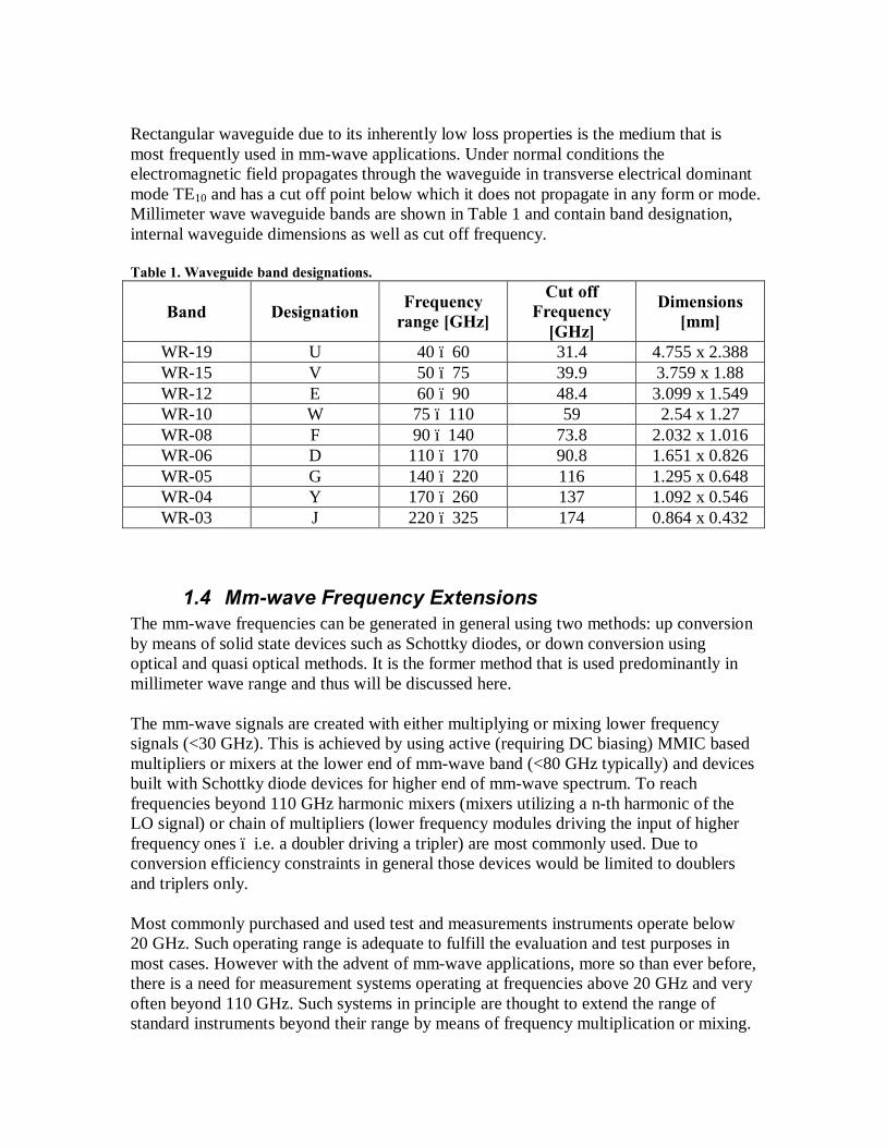
1.4.1 Signal Generators Frequency Extension Sources – FES In most cases the mm-wave users already own a microwave signal generators that are capable of supplying frequencies up to 20 GHz. For scalar measurements and modulation the frequency extension can be achieved by a frequency multiplication. The generator is used as a driver for a amplifier-multiplier chain where the input signal is firstly multiplied and then amplified by an active MMIC module and used internally to drive a stand alone passive multiplier – usually a doubler or a tripler. To reach the higher end of mm-wave spectrum a chain of passive multipliers might have to be used to achieve best output power and frequency coverage. Farran Technology offers a full range of Frequency Extension Sources (FES) for extending the coverage of microwave signal sources. These modules operate on principle of frequency multiplication and amplification to offer best performance on the market. In the Figure 3 a typical block diagram of such modules is shown:

x2 X2 orx3

FES-19FES-15FES-12FES-10

Fin=10-15 GHzFin=12.5-18.75 GHzFin=10-15 GHzFin=12.5-18.33 GHz

x2x2x3x3

Fout=40-60 GHzFout=50-75 GHzFout=60-90 GHzFout=75-110 GHz

x2 X2 orx3

FES-06FES-05FES-03

Fin=9.16-14.16 GHzFin=11.67-18.33 GHzFin=12.22-18.05 GHz

x2x2x3

Fout=110-170 GHzFout=140-220 GHzFout=220-325 GHz

x3

Figure 3. Block diagrams of Frequency Extension Sources for signal generators. Modern test laboratories require high stablility signal sources that can be applied as local oscillators in mixer applications or as an RF sources in antenna and receiver applications. Also mm-wave on wafer device testing requires a repeatable, as well as compact, extension source that can be easily mounted on wafer probing station positioners close to a DUT reducing therefore unnecessary losses associated with long cables at high frequencies. Farran Technology’s (FTL) signal generator frequency extenders (FESs) provide unparalleled in industry performance that will fulfill the requirements needed at

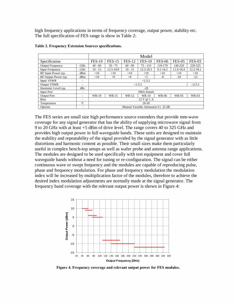
high frequency applications in terms of frequency coverage, output power, stability etc. The full specification of FES range is show in Table 2: Table 2. Frequency Extension Sources specifications.

Model Specification FES-19 FES-15 FES-12 FES-10 FES-06 FES-05 FES-03 Output Frequency GHz 40 - 60 50 - 75 60 - 90 75 - 110 110-170 140-220 220-325 Input Frequency GHz 10 - 15 12.5-18.8 10 - 15 12.5-18.3 9.1-14.2 11.6-18.4 12.2-18.1 RF Input Power typ. dBm +10 +10 +10 +10 +10 +10 +10 RF Output Power typ. dBm +10 +9 +6 +5 -8 -10 -12 Input VSWR - <1.5:1 Output VSWR - <1.5:1 <2.5:1 Harmonic Level typ. dBc -20 Input Port - SMA female Output Port - WR-19 WR-15 WR-12 WR-10 WR-06 WR-05 WR-03 Bias - 12 V @ 1 A Temperature °C 20-30 Options - Manual Variable Attenuator 0 – 25 dB

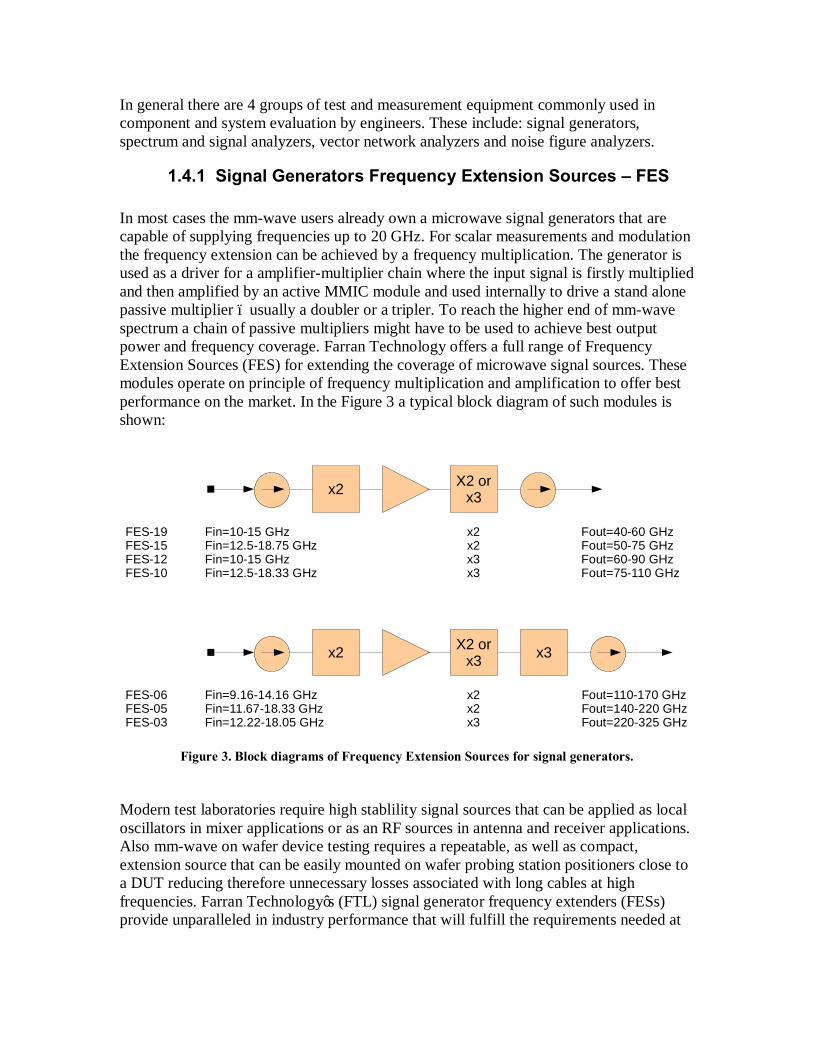
The FES series are small size high performance source extenders that provide mm-wave coverage for any signal generator that has the ability of supplying microwave signal from 9 to 20 GHz with at least +5 dBm of drive level. The range covers 40 to 325 GHz and provides high output power in full waveguide bands. These units are designed to maintain the stability and repeatability of the signal provided by the signal generator with as little distortions and harmonic content as possible. Their small sizes make them particularly useful in complex bench-top setups as well as wafer probe and antenna range applications. The modules are designed to be used specifically with test equipment and cover full waveguide bands without a need for tuning or re-configuration. The signal can be either continuous wave or swept frequency and the modules are capable of reproducing pulse, phase and frequency modulation. For phase and frequency modulation the modulation index will be increased by multiplication factor of the modules, therefore to achieve the desired index modulation adjustments are normally made at the signal generator. The frequency band coverage with the relevant output power is shown in Figure 4:

-15

-10

-5

0

5

10

15

20 40 60 80 100 120 140 160 180 200 220 240 260 280 300 320 340

Output Frequency [GHz]

Out

put P

ower

[dB

m]

Figure 4. Frequency coverage and relevant output power for FES modules.

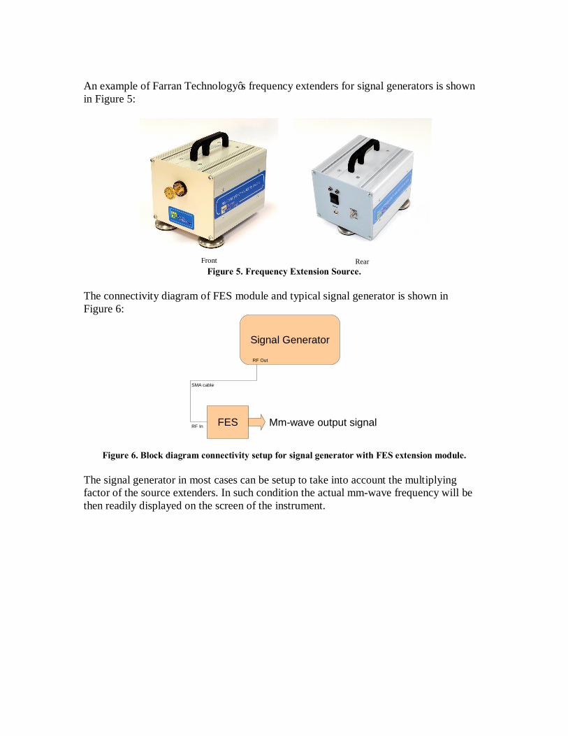
An example of Farran Technology’s frequency extenders for signal generators is shown in Figure 5:

Front

Rear

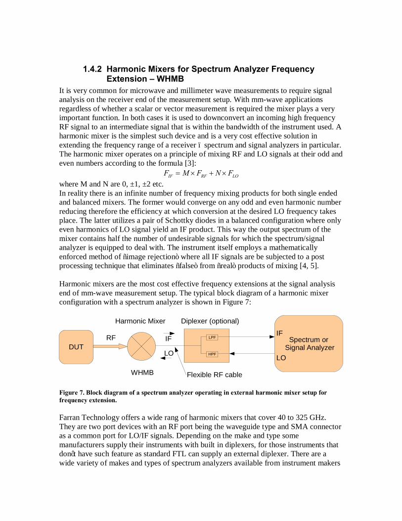
Figure 5. Frequency Extension Source. The connectivity diagram of FES module and typical signal generator is shown in Figure 6:

Signal Generator

FES

RF Out

RF In Mm-wave output signal

SMA cable

Figure 6. Block diagram connectivity setup for signal generator with FES extension module. The signal generator in most cases can be setup to take into account the multiplying factor of the source extenders. In such condition the actual mm-wave frequency will be then readily displayed on the screen of the instrument.

1.4.2 Harmonic Mixers for Spectrum Analyzer Frequency Extension – WHMB

It is very common for microwave and millimeter wave measurements to require signal analysis on the receiver end of the measurement setup. With mm-wave applications regardless of whether a scalar or vector measurement is required the mixer plays a very important function. In both cases it is used to downconvert an incoming high frequency RF signal to an intermediate signal that is within the bandwidth of the instrument used. A harmonic mixer is the simplest such device and is a very cost effective solution in extending the frequency range of a receiver – spectrum and signal analyzers in particular. The harmonic mixer operates on a principle of mixing RF and LO signals at their odd and even numbers according to the formula [3]:

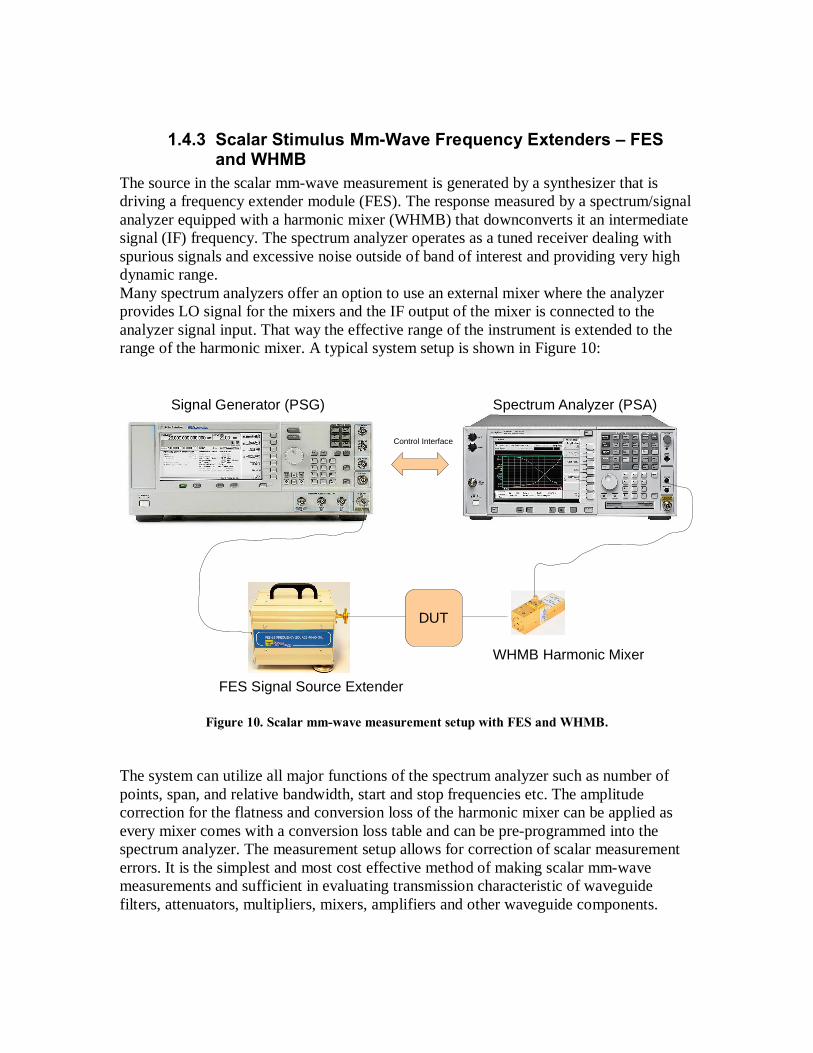
LORFIF FNFMF ×+×= where M and N are 0, ±1, ±2 etc. In reality there is an infinite number of frequency mixing products for both single ended and balanced mixers. The former would converge on any odd and even harmonic number reducing therefore the efficiency at which conversion at the desired LO frequency takes place. The latter utilizes a pair of Schottky diodes in a balanced configuration where only even harmonics of LO signal yield an IF product. This way the output spectrum of the mixer contains half the number of undesirable signals for which the spectrum/signal analyzer is equipped to deal with. The instrument itself employs a mathematically enforced method of “image rejection” where all IF signals are be subjected to a post processing technique that eliminates “false” from “real” products of mixing [4, 5]. Harmonic mixers are the most cost effective frequency extensions at the signal analysis end of mm-wave measurement setup. The typical block diagram of a harmonic mixer configuration with a spectrum analyzer is shown in Figure 7:

DUTHPF

LPF

Harmonic Mixer

WHMB

RF

Diplexer (optional)

Spectrum or Signal Analyzer

LO

IF

LO

IF

Flexible RF cable Figure 7. Block diagram of a spectrum analyzer operating in external harmonic mixer setup for frequency extension. Farran Technology offers a wide rang of harmonic mixers that cover 40 to 325 GHz. They are two port devices with an RF port being the waveguide type and SMA connector as a common port for LO/IF signals. Depending on the make and type some manufacturers supply their instruments with built in diplexers, for those instruments that don’t have such feature as standard FTL can supply an external diplexer. There are a wide variety of makes and types of spectrum analyzers available from instrument makers

such as Agilent, Rohde & Schwarz, Tektronix, Advantest and Anritsu to name just a few. Farran Technology’s Harmonic Mixers can be configured to work with any spectrum analyzer that has the external mixer option. The specifications of Farran Technology’s spectrum analyzer harmonic balanced mixer extensions are given in Table 3. Table 3. WHMB harmonic mixer range specification. Model Specification WHMB-

19 WHMB-

15 WHMB-

12 WHMB-

10 WHMB-

06 WHMB-

05 WHMB-

03 RF Frequency GHz 40 - 60 50 - 75 60 - 90 75 - 110 110-170 140-220 220-325 LO Frequency Agilent * GHz 4 – 10 3.6 – 5.4 3.75-5.63 4.2 – 6.1 5 – 7.7 4.67-7.33 4.78-7.06 LO Frequency R&S * GHz 10 - 15 12.5-18.8 10 - 15 12.5-18.3 9.1-14.2 11.6-18.4 12.2-18.1 Harmonic Number Agilent - 10 14 16 18 22 30 46 Harmonic Number R&S - 4 6 6 8 10 12 18 Conversion Loss Agilent typ. dB 30 32 40 42 45 50 60 Conversion Loss R&S typ. dB 20 25 32 30 35 40 45 Max RF Input Power typ. dBm +10 +10 +10 0 0 0 0 LO Drive Level yup. dBm +15 IF Frequency MHz 5 - 1000 RF VSWR - <3.5:1 LO/IF Port - SMA female RF Port - WR-19 WR-15 WR-12 WR-10 WR-06 WR-05 WR-03 Temperature °C 20-30 Options - Diplexer

Note:

* LO signal frequencies are approximate values – do not take the actual IF frequency selected into account. Due to their balanced configuration all the mixers operate on even LO harmonics without a need of a bias. The mixer is connected to the analyzer with a flexible cable and its operation setup is fully visible to the user through the instrument interface. Its frequency range (waveguide type) and conversion loss can be setup in the analyzer for accurate measurements. The analyzer uses the external mixer as a part of its own receiver circuit. The LO harmonic number, RF frequency range with its corresponding conversion loss values can be loaded up onto the instrument from the data supplied with the harmonic mixer. That way the actual display of the instrument will reflect the actual results in a real time manner. Figure 8 shows the WHMB-10 (top) and WHMB-03 (bottom) products:

Figure 8. WHMB-10 and WHMB-03 harmonic mixers.

Figure 9 shows a typical measurement result of a 67 GHz mm-wave signal:

Figure 9. Typical real time measurement result with WHMB-12. The desired signal is centered at 67 GHz and the instrument is using full WR-12 waveguide band. The “image resolution” option at the instrument reduces significantly the spectrum clutter and as it can be seen in Figure 9 in the vicinity of the RF signal all other spurious are suppressed more than 50 dBc. Such operation allows for a unambiguous mm-wave measurements in the given RF range. The only visible spurious signals in the band are positioned at 89 GHz and are typically 20 dB below the level of the desired signal. For some instruments there is a need for an external diplexer that would provide signal filtration of IF and LO and ensure single port connectivity with the harmonic mixer when the spectrum analyzer does not have a diplexer functionality built in as a standard. Farran Technology can supply diplexers for various analyzer types and manufacturers.

1.4.3 Scalar Stimulus Mm-Wave Frequency Extenders – FES and WHMB

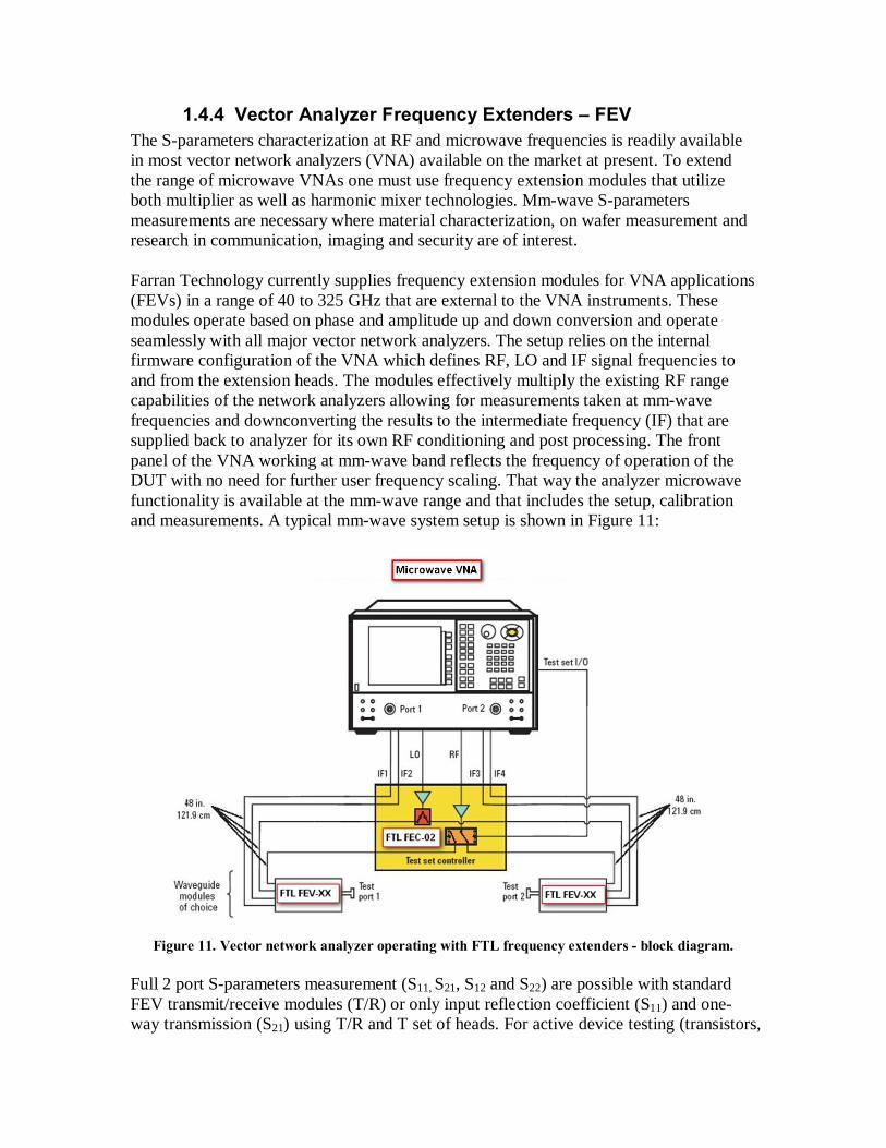
The source in the scalar mm-wave measurement is generated by a synthesizer that is driving a frequency extender module (FES). The response measured by a spectrum/signal analyzer equipped with a harmonic mixer (WHMB) that downconverts it an intermediate signal (IF) frequency. The spectrum analyzer operates as a tuned receiver dealing with spurious signals and excessive noise outside of band of interest and providing very high dynamic range. Many spectrum analyzers offer an option to use an external mixer where the analyzer provides LO signal for the mixers and the IF output of the mixer is connected to the analyzer signal input. That way the effective range of the instrument is extended to the range of the harmonic mixer. A typical system setup is shown in Figure 10:

DUT

Control Interface

Signal Generator (PSG) Spectrum Analyzer (PSA)

WHMB Harmonic Mixer

FES Signal Source Extender

Figure 10. Scalar mm-wave measurement setup with FES and WHMB. The system can utilize all major functions of the spectrum analyzer such as number of points, span, and relative bandwidth, start and stop frequencies etc. The amplitude correction for the flatness and conversion loss of the harmonic mixer can be applied as every mixer comes with a conversion loss table and can be pre-programmed into the spectrum analyzer. The measurement setup allows for correction of scalar measurement errors. It is the simplest and most cost effective method of making scalar mm-wave measurements and sufficient in evaluating transmission characteristic of waveguide filters, attenuators, multipliers, mixers, amplifiers and other waveguide components.

1.4.4 Vector Analyzer Frequency Extenders – FEV The S-parameters characterization at RF and microwave frequencies is readily available in most vector network analyzers (VNA) available on the market at present. To extend the range of microwave VNAs one must use frequency extension modules that utilize both multiplier as well as harmonic mixer technologies. Mm-wave S-parameters measurements are necessary where material characterization, on wafer measurement and research in communication, imaging and security are of interest. Farran Technology currently supplies frequency extension modules for VNA applications (FEVs) in a range of 40 to 325 GHz that are external to the VNA instruments. These modules operate based on phase and amplitude up and down conversion and operate seamlessly with all major vector network analyzers. The setup relies on the internal firmware configuration of the VNA which defines RF, LO and IF signal frequencies to and from the extension heads. The modules effectively multiply the existing RF range capabilities of the network analyzers allowing for measurements taken at mm-wave frequencies and downconverting the results to the intermediate frequency (IF) that are supplied back to analyzer for its own RF conditioning and post processing. The front panel of the VNA working at mm-wave band reflects the frequency of operation of the DUT with no need for further user frequency scaling. That way the analyzer microwave functionality is available at the mm-wave range and that includes the setup, calibration and measurements. A typical mm-wave system setup is shown in Figure 11:

Figure 11. Vector network analyzer operating with FTL frequency extenders - block diagram. Full 2 port S-parameters measurement (S11, S21, S12 and S22) are possible with standard FEV transmit/receive modules (T/R) or only input reflection coefficient (S11) and one-way transmission (S21) using T/R and T set of heads. For active device testing (transistors,

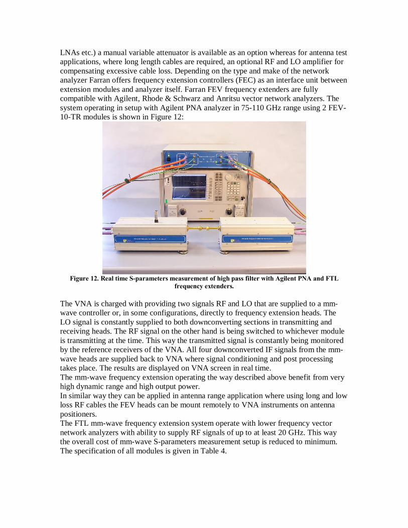
LNAs etc.) a manual variable attenuator is available as an option whereas for antenna test applications, where long length cables are required, an optional RF and LO amplifier for compensating excessive cable loss. Depending on the type and make of the network analyzer Farran offers frequency extension controllers (FEC) as an interface unit between extension modules and analyzer itself. Farran FEV frequency extenders are fully compatible with Agilent, Rhode & Schwarz and Anritsu vector network analyzers. The system operating in setup with Agilent PNA analyzer in 75-110 GHz range using 2 FEV-10-TR modules is shown in Figure 12:

Figure 12. Real time S-parameters measurement of high pass filter with Agilent PNA and FTL

frequency extenders. The VNA is charged with providing two signals RF and LO that are supplied to a mm-wave controller or, in some configurations, directly to frequency extension heads. The LO signal is constantly supplied to both downconverting sections in transmitting and receiving heads. The RF signal on the other hand is being switched to whichever module is transmitting at the time. This way the transmitted signal is constantly being monitored by the reference receivers of the VNA. All four downconverted IF signals from the mm-wave heads are supplied back to VNA where signal conditioning and post processing takes place. The results are displayed on VNA screen in real time. The mm-wave frequency extension operating the way described above benefit from very high dynamic range and high output power. In similar way they can be applied in antenna range application where using long and low loss RF cables the FEV heads can be mount remotely to VNA instruments on antenna positioners. The FTL mm-wave frequency extension system operate with lower frequency vector network analyzers with ability to supply RF signals of up to at least 20 GHz. This way the overall cost of mm-wave S-parameters measurement setup is reduced to minimum. The specification of all modules is given in Table 4.

Table 4. Specification of Frequency Extension Heads for VNAs. Model Specification FEV-19 FEV-15 FEV-12 FEV-10 FEV-06 FEV-05 FEV-03 RF Frequency GHz 40 - 60 50 - 75 60 - 90 75 - 110 110-170 140-220 220-325 LO Input Frequency GHz 10 - 15 8.33-12.5 10 -15 9.4-13.75 11-17 11.7-18.3 9.16-13.5 RF Input Frequency GHz 10 - 15 12.5-18.8 10 - 15 12.5-18.3 9.1-14.2 11.6-18.4 12.2-18.1 LO Harmonic Number - 4 6 6 8 10 12 24 RF Multiplier Factor - 4 4 6 6 12 12 18 RF Output Power typ. dBm +9 +7 +4 +4 -10 -12 -15 Dynamic Range typ. (1) dB 120 120 110 110 100 90 80 Raw Coupler Directivity typ. dB 45 45 45 45 40 35 30 Trace Stability (2) ±dB /

±° 0.1 1

0.1 1

0.1 1

0.2 2

0.4 4

0.6 6

0.8 8

Optional Variable Attenuator dB 25 RF/LO Drive Level typ. dBm +5 to +10 IF Frequency MHz 5 - 300 RF/LO Port - 3.5 mm female IF Port - SMA female RF Port - WR-19 WR-15 WR-12 WR-10 WR-06 WR-05 WR-03 Temperature °C 20-30 DC Power Requirements - +6 V at 1.5 A Weight kg 3.5 Dimensions (L x W x H) mm 290 x 130 x 85 Optional Controllers - FEC-02 and FEC-03 for a 2-port mm-wave measurement, FEC-04 for 4-port setup

Notes: (1) – Measured with PNA-X at 10 Hz IF bandwidth (2) – Tested at ambient temperature with ideal RF and LO cables. Tested after 2h of warm-up and calibration.

There are many different vector network analyzer types equipped with various options. Please check with Farran’s factory before placing an order. Figure 13 presents most common VNA with frequency extenders configurations:

FEVs with Agilent 4 port PNA-X

FEVs with R&S ZVA

FEVs in 4 port setup with PNA-X and FEC-04 controller

FEVs with PNA-X with an active DUT (LNA) under test

Figure 13. FTL vector network analyzer frequency modules in various configurations.

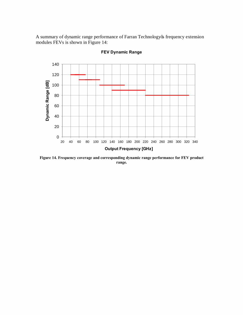
A summary of dynamic range performance of Farran Technology’s frequency extension modules FEVs is shown in Figure 14:

FEV Dynamic Range

0

20

40

60

80

100

120

140

20 40 60 80 100 120 140 160 180 200 220 240 260 280 300 320 340

Output Frequency [GHz]

Dyn

amic

Ran

ge [d

B]

Figure 14. Frequency coverage and corresponding dynamic range performance for FEV product

range.

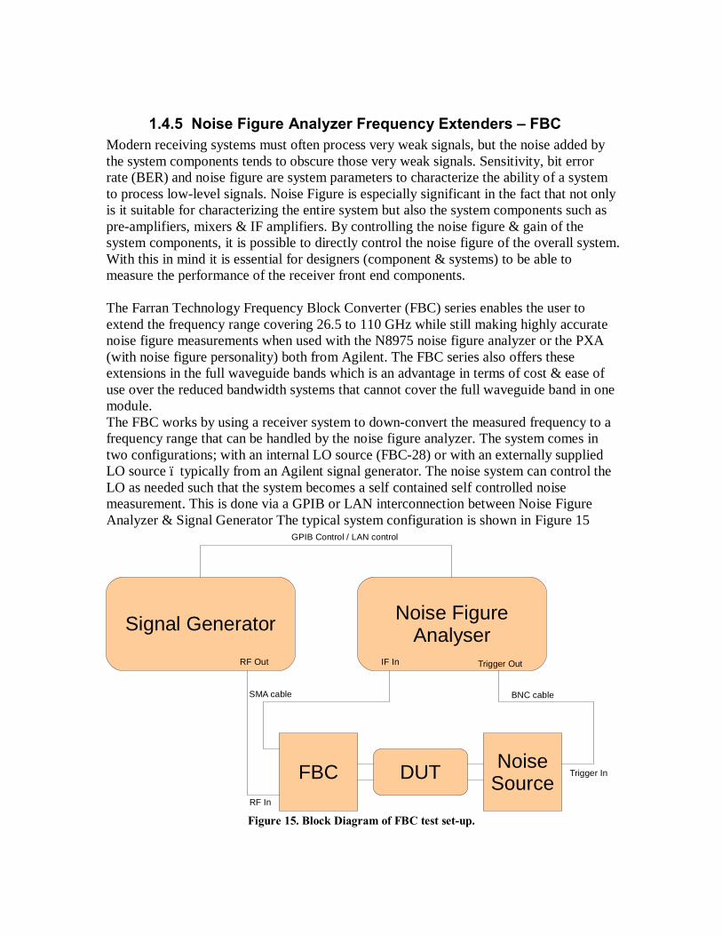
1.4.5 Noise Figure Analyzer Frequency Extenders – FBC Modern receiving systems must often process very weak signals, but the noise added by the system components tends to obscure those very weak signals. Sensitivity, bit error rate (BER) and noise figure are system parameters to characterize the ability of a system to process low-level signals. Noise Figure is especially significant in the fact that not only is it suitable for characterizing the entire system but also the system components such as pre-amplifiers, mixers & IF amplifiers. By controlling the noise figure & gain of the system components, it is possible to directly control the noise figure of the overall system. With this in mind it is essential for designers (component & systems) to be able to measure the performance of the receiver front end components. The Farran Technology Frequency Block Converter (FBC) series enables the user to extend the frequency range covering 26.5 to 110 GHz while still making highly accurate noise figure measurements when used with the N8975 noise figure analyzer or the PXA (with noise figure personality) both from Agilent. The FBC series also offers these extensions in the full waveguide bands which is an advantage in terms of cost & ease of use over the reduced bandwidth systems that cannot cover the full waveguide band in one module. The FBC works by using a receiver system to down-convert the measured frequency to a frequency range that can be handled by the noise figure analyzer. The system comes in two configurations; with an internal LO source (FBC-28) or with an externally supplied LO source – typically from an Agilent signal generator. The noise system can control the LO as needed such that the system becomes a self contained self controlled noise measurement. This is done via a GPIB or LAN interconnection between Noise Figure Analyzer & Signal Generator The typical system configuration is shown in Figure 15

Signal Generator

FBC

RF Out

RF In

SMA cable

Noise FigureAnalyser

IF In

DUT NoiseSource

BNC cable

Trigger Out

Trigger In

GPIB Control / LAN control

Figure 15. Block Diagram of FBC test set-up.

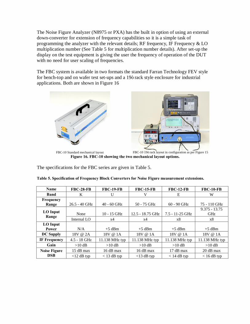
The Noise Figure Analyzer (N8975 or PXA) has the built in option of using an external down-converter for extension of frequency capabilities so it is a simple task of programming the analyzer with the relevant details; RF frequency, IF Frequency & LO multiplication number (See Table 5 for multiplication number details). After set-up the display on the test equipment is giving the user the frequency of operation of the DUT with no need for user scaling of frequencies. The FBC system is available in two formats the standard Farran Technology FEV style for bench-top and on wafer test set-ups and a 19” rack style enclosure for industrial applications. Both are shown in Figure 16

FBC-10 Standard mechanical layout

FBC-10 19” rack layout in configuration as per Figure 15

Figure 16. FBC-10 showing the two mechanical layout options. The specifications for the FBC series are given in Table 5. Table 5. Specification of Frequency Block Converters for Noise Figure measurement extensions.

Name FBC-28-FB FBC-19-FB FBC-15-FB FBC-12-FB FBC-10-FB Band K U V E W

Frequency Range 26.5 - 40 GHz 40 - 60 GHz 50 - 75 GHz 60 - 90 GHz 75 - 110 GHz

None 10 - 15 GHz 12.5 - 18.75 GHz 7.5 - 11-25 GHz 9.375 - 13.75

GHz LO Input Range

Internal LO x4 x4 x8 x8 LO Input

Power N/A +5 dBm +5 dBm +5 dBm +5 dBm DC Supply 18V @ 2A 18V @ 1A 18V @ 1A 18V @ 1A 18V @ 1A

IF Frequency 4.5 - 18 GHz 11.138 MHz typ 11.138 MHz typ 11.138 MHz typ 11.138 MHz typ Gain >10 dB >10 dB >10 dB >10 dB >10 dB

15 dB max 16 dB max 16 dB max 17 dB max 20 dB max Noise Figure DSB <12 dB typ < 13 dB typ <13 dB typ < 14 dB typ < 16 dB typ

1.5 Conclusion In this article we have outlined some of the reasons why it is now necessary to have test and measurement facilities up to mm-wave frequencies and beyond. We have presented example of the applications that are now becoming more common areas for research & development. Also presented were some of the potential methods for performing these tests & measurements at mm-wave frequencies. Finally we have given examples of the technology developed by Farran Technology to enable these measurements to be performed.

1.6 References [1] Richard Martin, Christopher Schuetz, Thomas Dillon, Daniel Mackrides, Peng

Yao, Kevin Shreve, Charles Harrity, Alicia Zablocki, Brock Overmiller, Petersen Curt, James Bonnett, Andrew Wright, John Wilson, Shouyaun Shi and Dennis Prather, “Optical up-conversion enables capture of millimeter-wave video with an IR camera”, SPIE, August 2012

[2] Mohamed M. Sayed, “Millimeter Wave Test and Instrumentation”, Millimeter Wave Solutions

[3] R. J. Matreci and F. K. David, IEEE/MTT-S International Microwave Symposium Digest, 1983, pp 130-132

[4] Agilent Technologies, Inc., Palo Alto, CA, US, www.agilent.com [5] Rohde & Schwarz, Munich, Germany, www.rohde-schwarz.com