Integrated Feature Selection and Higher-order Spatial FeatureExtraction for Object Categorization

David Liu1, Gang Hua2, Paul Viola2, Tsuhan Chen1

Dept. of ECE, Carnegie Mellon University1 and Microsoft Live Labs2

dliu@cmu.edu, {ganghua,viola}@microsoft.com, tsuhan@cmu.edu

Abstract

In computer vision, the bag-of-visual words imagerepresentation has been shown to yield good results.Recent work has shown that modeling the spatial re-lationship between visual words further improves per-formance. Previous work extracts higher-order spatialfeatures exhaustively. However, these spatial featuresare expensive to compute. We propose a novel methodthat simultaneously performs feature selection and fea-ture extraction. Higher-order spatial features are pro-gressively extracted based on selected lower order ones,thereby avoiding exhaustive computation. The methodcan be based on any additive feature selection algorithmsuch as boosting. Experimental results show that themethod is computationally much more efficient thanprevious approaches, without sacrificing accuracy.

1. Introduction

The traditional pipeline of pattern recognition sys-tems consists of three stages: feature extraction, fea-ture selection, and classification. These stages are nor-mally conducted in independent steps, lacking an inte-grated approach. The issues are as follows: 1. Speed:Feature extraction can be time consuming. Featuresthat require extensive computation should be gener-ated only when needed. 2. Storage: Extracting all fea-tures before selecting them can be cumbersome whenthey don’t fit into the random access memory.

Many object recognition problems involve a pro-hibitively large number of features. It is not uncom-mon that computing the features is the bottleneck ofthe whole pipeline. Techniques such as “classifier cas-cade” [17] reduce the amount of computation for fea-ture extraction in run time (in testing), while the aimhere is to improve the feature extraction and selectionprocedure in training.

In this work, we focus on the bag-of-local feature

1st Order

Feature Pool

1st Order

Feature Pool

2nd Order

Feature Pool

2nd Order

Feature Pool

1st Order

Feature Pool

1st Order

Feature PoolSelectionSelection

SelectionSelection

Extracted 2nd-order Features

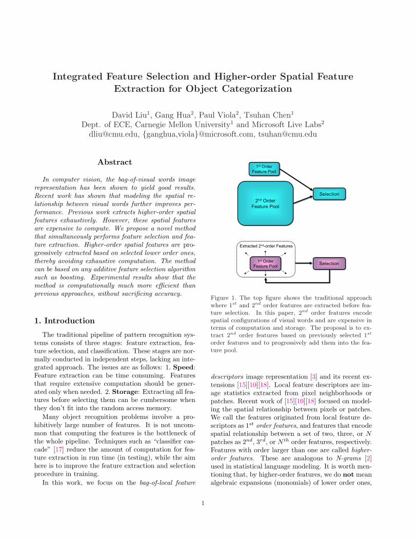
Figure 1. The top figure shows the traditional approachwhere 1st and 2nd order features are extracted before fea-ture selection. In this paper, 2nd order features encodespatial configurations of visual words and are expensive interms of computation and storage. The proposal is to ex-tract 2nd order features based on previously selected 1st

order features and to progressively add them into the fea-ture pool.

descriptors image representation [3] and its recent ex-tensions [15][10][18]. Local feature descriptors are im-age statistics extracted from pixel neighborhoods orpatches. Recent work of [15][10][18] focused on model-ing the spatial relationship between pixels or patches.We call the features originated from local feature de-scriptors as 1st order features, and features that encodespatial relationship between a set of two, three, or Npatches as 2nd, 3rd, or N th order features, respectively.Features with order larger than one are called higher-order features. These are analogous to N-grams [2]used in statistical language modeling. It is worth men-tioning that, by higher-order features, we do not meanalgebraic expansions (monomials) of lower order ones,

1

such as cross terms (x1x2), squares or cubes (x31).

In the recent works of [15][10][18], higher-orderfeatures are extracted exhaustively. However, thesehigher-order features are prohibitively expensive tocompute: first, their number is combinatorially explod-ing with the number of pixels or patches; second, ex-tracting them requires expensive nearest neighbor ordistance computations in image space [4]. It is the ex-pensive nature of higher-order features that motivatesour work.

Instead of exhaustively extracting all higher-orderfeatures before feature selection begins, we propose toextract them progressively during feature selection, asillustrated in Fig. 1. We start the feature selectionprocess as early as when the feature pool consists onlyof 1st order features. Subsequently, features that havebeen selected are used to create higher-order features.This process dynamically enlarges the feature pool ina greedy fashion so that we don’t need to exhaustivelycompute and store all higher-order features.

A comprehensive review of feature selection methodsis given by [8]. Our method can be based on any addi-tive feature selection algorithm such as boosting [20] orCMIM [7][16]. Boosting was originally proposed as aclassifier and has also been used as a feature selectionmethod [17] due to its good performance, simplicityin implementation, and ease of extension to multiclassproblems [20]. Another popular branch of feature selec-tion methods is based on information-theoretic criteriasuch as maximization of conditional mutual informa-tion [7][16].

2. Integrated feature selection and ex-traction

Each image is represented as a feature vector whichdynamically increases in the number of dimensions.Initially, each feature corresponds to a distinct code-word. The feature values are the normalized histogrambin counts of the visual words. These features are the1st order features, and this is the bag-of-visual wordsimage representation [3]. Visual words, with textons[9] as a special case, have been used in various applica-tions. A dictionary of codewords refers to the clustersof local feature descriptors extracted from pixel neigh-borhoods or patches, and a visual word refers to aninstance of a codeword.

Our method maintains a ‘feature pool’ which ini-tially consists only of 1st order features. Subsequently,instead of exhaustively building all higher-order fea-tures, the process of feature selection and higher-orderfeature extraction are run alternately. At each round,feature selection picks a feature, and feature extraction

Round 2

Round 2’

Round 1

1st order features Higher order features

Figure 2. The ‘feature pool’ is dynamically built by alter-nating between feature selection and feature extraction.

pairs this feature with each of the previously selectedfeatures. The pairing process can be generic, and wewill explain the implementation in Sec. 3. The pairingprocess creates new features which are concatenated tothe feature vector of each image. In the next round offeature selection, this enlarged ‘feature pool’ providesthe features to be selected from.

In Fig. 2, we illustrate this process for the first fewrounds. In the first round, feature selection picks afeature (the light gray squares) from the ‘feature pool’and puts it in a 1st order list (not shown in Fig. 2) thatholds all previous selected 1st order features. Since thelist was empty, we continue to the second round. Inthe second round, feature selection picks a feature (thedark gray squares) from the ‘feature pool’ and placesit in the 1st order list. At the same time, feature ex-traction pairs this newly selected feature with the pre-viously selected feature (the light gray square) and cre-ates new features (the diagonally patterned squares).These 2nd order features are then augmented into the‘feature pool’. In general, we may maintain 1st, ..., Lth-order lists instead of only 1st order lists. If a selectedfeature has order L1, then it was originated from L1

codewords, and pairing it with another feature of or-der L2 means that we can create new features thatoriginate from a set of L1 + L2 codewords.

In Algorithm 1 we detail the procedure of computingfeatures up to the 2nd order. We use Discrete AdaBoostwith decision stumps for feature selection as in [17],although other feature selection methods could be usedas well. AdaBoost maintains a set of sample weights,{vn}, n = 1, ..., N , on the N training images (Line 1).At each round, a decision stump tries to minimize theweighted error rate by picking an optimal feature andthreshold (Line 4). The selected feature could be a1st or 2nd order feature. If it is a 1st order feature, itis placed in the 1st-order list z(.) (Line 8), and thenpaired with all previous members in the 1st-order listto generate new 2nd order features (Line 11). The new

Building

Grass

Sky

Cow

1st order

2nd order

1st order

2nd order

1st order

2nd order

1st order

2nd orderNumber of features

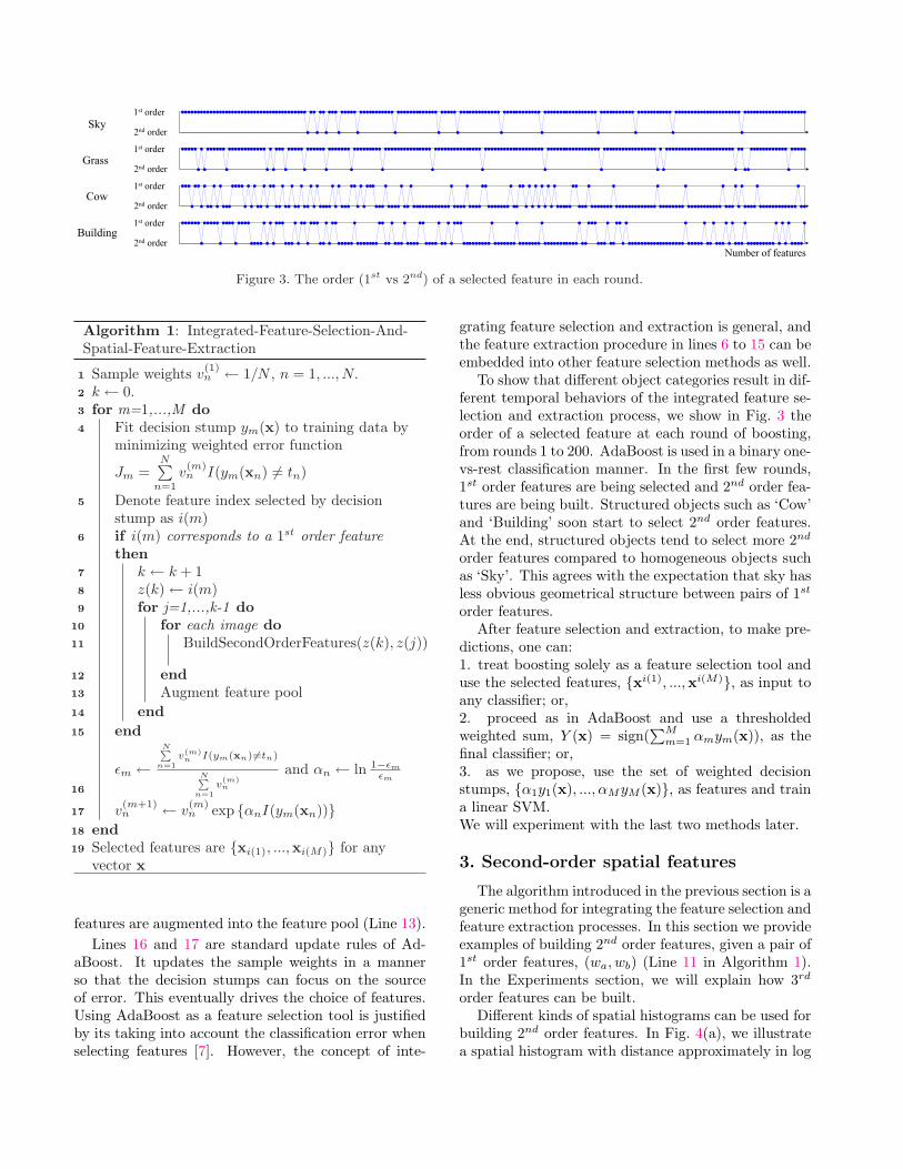
Figure 3. The order (1st vs 2nd) of a selected feature in each round.

Algorithm 1: Integrated-Feature-Selection-And-Spatial-Feature-Extraction

Sample weights v(1)n ← 1/N , n = 1, ..., N.1

k ← 0.2

for m=1,...,M do3

Fit decision stump ym(x) to training data by4

minimizing weighted error function

Jm =N∑

n=1v(m)n I(ym(xn) 6= tn)

Denote feature index selected by decision5

stump as i(m)if i(m) corresponds to a 1st order feature6

thenk ← k + 17

z(k) ← i(m)8

for j=1,...,k-1 do9

for each image do10

BuildSecondOrderFeatures(z(k), z(j))11

end12

Augment feature pool13

end14

end15

εm ←N∑

n=1v(m)

n I(ym(xn)6=tn)

N∑n=1

v(m)n

and αn ← ln 1−εm

εm

16

v(m+1)n ← v

(m)n exp {αnI(ym(xn))}17

end18

Selected features are {xi(1), ...,xi(M)} for any19

vector x

features are augmented into the feature pool (Line 13).Lines 16 and 17 are standard update rules of Ad-

aBoost. It updates the sample weights in a mannerso that the decision stumps can focus on the sourceof error. This eventually drives the choice of features.Using AdaBoost as a feature selection tool is justifiedby its taking into account the classification error whenselecting features [7]. However, the concept of inte-

grating feature selection and extraction is general, andthe feature extraction procedure in lines 6 to 15 can beembedded into other feature selection methods as well.

To show that different object categories result in dif-ferent temporal behaviors of the integrated feature se-lection and extraction process, we show in Fig. 3 theorder of a selected feature at each round of boosting,from rounds 1 to 200. AdaBoost is used in a binary one-vs-rest classification manner. In the first few rounds,1st order features are being selected and 2nd order fea-tures are being built. Structured objects such as ‘Cow’and ‘Building’ soon start to select 2nd order features.At the end, structured objects tend to select more 2nd

order features compared to homogeneous objects suchas ‘Sky’. This agrees with the expectation that sky hasless obvious geometrical structure between pairs of 1st

order features.After feature selection and extraction, to make pre-

dictions, one can:1. treat boosting solely as a feature selection tool anduse the selected features, {xi(1), ...,xi(M)}, as input toany classifier; or,2. proceed as in AdaBoost and use a thresholdedweighted sum, Y (x) = sign(

∑Mm=1 αmym(x)), as the

final classifier; or,3. as we propose, use the set of weighted decisionstumps, {α1y1(x), ..., αMyM (x)}, as features and traina linear SVM.We will experiment with the last two methods later.

3. Second-order spatial features

The algorithm introduced in the previous section is ageneric method for integrating the feature selection andfeature extraction processes. In this section we provideexamples of building 2nd order features, given a pair of1st order features, (wa, wb) (Line 11 in Algorithm 1).In the Experiments section, we will explain how 3rd

order features can be built.Different kinds of spatial histograms can be used for

building 2nd order features. In Fig. 4(a), we illustratea spatial histogram with distance approximately in log

Figure 5. Second-order features. These are best viewed in color.

(a) (b)

Figure 4. Examples of spatial histograms.

scale, similar to the shape context histogram [1]. Thelog scale tolerates larger uncertainties of bin countsin longer ranges. The four directional bins are con-structed to describe the semantics ‘above’, ‘below’, ‘tothe left’, and ‘to the right’. In Fig. 4(b), directions areignored in order to describe how the co-occurrence of(wa, wb) varies in distance. In [15], squared regions areused to approximate the circular regions in Fig. 4(b)in order to take advantage of the integral histogrammethod [14]. Of course, squared regions and integralhistogram can be used in our work as well.

The goal is to build a descriptor that describes howwb is spatially distributed relative to wa. Let us firstsuppose that there is only a single instance of wa inan image, but multiple wb’s. Using this instance ofwa as a reference center of the spatial histogram, wecount how many instances of wb fall into each bin. Thebin counts form the descriptor. Since there are usuallymultiple instances of wa in an image, we build a spatialhistogram for each instance of wa, and then normalizeover all spatial histograms; the normalization is doneby summing the counts of corresponding bins, and di-viding the counts by the number of instances of wa.This takes care of the case when multiple instances ofan object appear in an image. The whole process issummarized in Algorithm 2.

The spatial histograms yield translation invariant

descriptors, since the reference center is always in re-spect to the center word wa, and describes the relativeposition of instances of wb. The descriptors can alsobe (quasi-)scale invariant. This can be achieved by de-termining the normalized distance between instancesof wa and wb, where the normalization is done by con-sidering the geometric mean of the scale of the twopatches. To make the descriptor in Fig. 4(a) rotationinvariant, we can take into account the dominant ori-entation of a patch [19]. However, rotation invariancemay diminish discriminative power and hurt perfor-mance [19] in object categorization.

Algorithm 2: BuildSecondOrderFeaturesGoal: create feature descriptor given a word pair1

Input: codeword pair (wa, wb)2

Output: a vector of bin counts3

Suppose there are Na instances of wa, and Nb4

instances of wb in the imageInitialize Na spatial histograms, using each5

instance of wa as a reference centerfor i=1,...,Na do6

Count the number of instances of wb falling in7

each binend8

Sum up corresponding bins over the Na spatial9

histogramsDivide bin counts by Na10

In Fig. 5, red circles indicate words used as referencecenter. The red-green pairs correspond to a highly dis-criminative 2nd order feature that has been selected inearly rounds of boosting. The images are those thatare incorrectly classified when only 1st order featuresare used for training a classifier. We can see that 2nd

order features can detect meaningful patterns in theseimages. As a result, most of these images are correctly

0 500 1000 1500 20000.6

0.7

0.8

0.9

1

Number of features

Acc

ura

cy

Number of features

Ela

pse

d t

ime

(sec

)

0 500 1000 1500 20000

0.5

1

1.5

2

2.5x 10

4

0 1000 20000

500

1000

1500

0 1000 20000

2

4

6

8x 10

4

Number of features

Cu

mu

lati

ve

# e

xtr

acte

d 2

nd

ord

er f

eat

Number of features

Cu

mu

lati

ve

# s

elec

ted

2n

do

rder

fea

t

proposed

proposed

baseline

baseline

Number of features

Rat

io o

f sh

ared

wo

rds

+ w

ord

pai

rs

0 1000 20000

0.2

0.4

0.6

0.8

1

proposed

baseline

proposed

baseline

(a) (b)

(c) (d) (e)

Figure 6. Integrated vs separated: After around 800 rounds of boosting, the proposed method outperforms baseline both in(a) testing accuracy and (b) required training time.

classified by a classifier using both 1st and 2nd orderfeatures.

4. Experiments

We use three datasets in the experiments: the PAS-CAL VOC2006 dataset [5], the Caltech-4 plus back-ground dataset used in [6], and the MSRC-v2 15-classdataset used in [15]. We used the same training-testingexperiment setups as in these respective references.

For each dataset we use different local feature de-scriptors to show the generality of our approach. Forthe PASCAL dataset, we adopt the popular choice offinding a set of salient image regions using the Harris-Laplace interest point detectors [5]. Another scheme isto abandon the use of interest point detectors [13] andsample image patches uniformly from the image. Weadopt this approach for the Caltech-4 dataset. Eachregion or patch is then converted into a 128-D SIFT[12] descriptor. For the MSRC dataset, we follow thecommon approach [15] of computing dense filter-bank(3 Gaussians, 4 Laplacian of Gaussians, 4 first orderderivatives of Gaussians) responses for each pixel.

The local feature descriptors are then collected fromthe training images and vector quantized using K-

means clustering. The resulting cluster centers formthe dictionary of codewords, {w1, ..., wJ}. We useJ = 100 for the MSRC dataset, and J = 1000 for theother two datasets; these are common choices for thesedatasets. Each local feature descriptor is then assignedto the closest codeword and forms a visual word.

For the MSRC dataset, we used the spatial his-togram in Fig. 4(b), in order to facilitate comparisonwith the recent work of [15]. We followed the specs in[15] with 15 distance bins of equal spacing, the out-ermost bin with a radius of 80 pixels, and no scalenormalization being performed. For the Caltech andPASCAL datasets, we used the spatial histogram inFig. 4(a), where the scale is normalized according tothe patch size or interest point size as explained ear-lier, and the outermost bin has a radius equal to 15times the normalized patch size. The scale invariancecan be observed in Fig. 5 from the different distancesbetween red-green word pairs.

4.1. Integrated vs Separated

Here we present the main result of this paper. InFig. 6 we show the experiment on the 15-class MSRCdataset. We use a multiclass version of AdaBoost [20]for feature selection, and linear SVM for classification

as explained in Sec. 2. In Fig. 6(a), we see that the ac-curacy settles down after about 800 rounds of boosting.Accuracy is calculated as the mean over the diagonalelements of the 15-class confusion matrix. In Fig. 6(b),we see the integrated feature selection and extractionscheme requires only about 33% of training time com-pared to the canonical approach where feature extrac-tion and selection are two separate processes.

Surprisingly, we can see in Fig. 6(a) that, in addi-tion to being more efficient, the proposed scheme alsoachieves better accuracy in spite of its greedy nature.This can be explained by the fact that 2nd order fea-tures are sparser than 1st order features and hence sta-tistically less reliable; the integrated scheme starts withthe pool of first order features and gradually adds in2nd order features, hence it spends more quality timewith more reliable 1st order features.

In Fig. 6(c)-(e) we examine some temporal behaviorsof the two methods. In Fig. 6(c), we show the cumu-lative number of 2nd order features being extracted ateach round of feature selection. While the canonicalprocedure extracts all features before selection starts,the proposed scheme aggressively extracts 2nd orderfeatures in earlier rounds and then slows down. Thislogarithmic type of curve signifies the coupling betweenthe feature extraction and the feature selection pro-cesses; if they weren’t coupled, features would havebeen extracted at a constant (linear) speed instead ofa logarithmic.

In Fig. 6(c), we also noticed that at 800 rounds ofboosting, only about half of all possible 2nd order fea-tures were extracted. This implies less computation interms of feature extraction, as well as more efficientfeature selection, as the feature pool is much smaller.

In Fig. 6(d), it appears that the canonical approachselects 2nd order features at roughly the same pace asthe integrated scheme, both selecting on average 0.7second-order features per round of boosting. But infact, as shown in Fig. 6(e), the overlap between theselected features of the two methods is small; at 800rounds of boosting, the share ratio is only 0.14. Theshare ratio is the intersection of the shared visual wordsand visual word pairs of the two methods divided bythe union. This means that the two methods have verydifferent temporal behaviors.

4.2. Importance of feature selection

Here we compare with the recent work of [15], wherefeature selection is not performed, but first and second-order features are quantized separately into dictionar-ies of codewords. A histogram of these codewords isused as a feature vector. In Table 1, all three methodsuse the nearest neighbor classifier as in [15] for fair com-

parison 1. We see that our method yields state-of-the-art performance, compared to the quantized (Method2) and non-quantized (Method 1) versions. In addition,since the 2nd order features need not be exhaustivelycomputed and also no vector quantization on 2nd or-der features is required, our method is also much fasterthan the method in [15].

Proposed Method 1 Method 2 [15]

Feature selection √ × ×

Quantization × × √

Accuracy 75.9% 71.3% 74.1%

Table 1. Importance of feature selection.

4.3. Linear SVM on weighted decision stumps

As explained in Sec. 2, we propose to concate-nate the weighted output of all weak classifiers,{α1y1(x), ..., αMyM (x)}, from AdaBoost as a featurevector and then run a linear SVM. Results are shown inTable 2. The superior result over AdaBoost comes froma re-weighting of the terms {α1y1(x), ..., αMyM (x)}.

PASCAL(EER)

MSRC(1-accuracy)

AdaBoost classifier (1st order feat) 13.4% 24.1%

AdaBoost classifier (1st & 2nd order) 12.1% 21.2%

Linear SVM on weighted decision stumps 10.9% 16.9%

Table 2. Performance on the PASCAL car-vs-rest andMSRC 15-class datasets.

The best results [5] reported on the PASCALVOC2006 and VOC2007 datasets employ the SpatialPyramid [11] technique on top of the bag of words rep-resentation. The Spatial Pyramid technique is orthog-onal to the proposed method and combining them isexpected to yield even better results.

4.4. Increasing the order

In Fig. 7, we experiment on the MSRC dataset andsee that the classification accuracy obtained from usinga feature pool of 1st and 2nd order features is higherthan using 1st order features alone. Including 3rd orderfeatures does not improve accuracy. We generated 3rd

order features by counting the number of times threecodewords (wa, wb, wc) fall within a radius of 30 pix-els, i.e., the spatial histogram has only one bin. Third

1We re-implemented the work of [15], because they used anuntypical quantization scheme to generate 1st order codewords,and results are not comparable; also, their spatial histogram issquare-shaped.

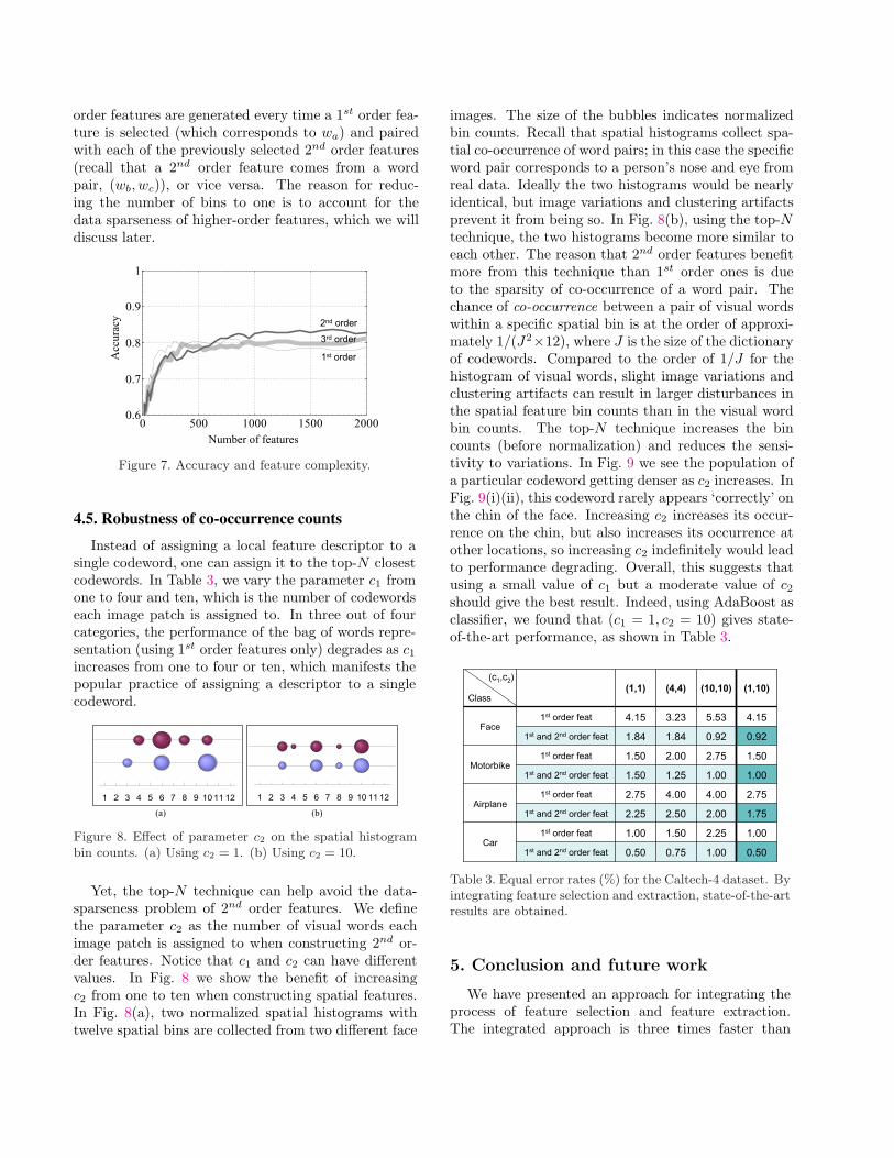
order features are generated every time a 1st order fea-ture is selected (which corresponds to wa) and pairedwith each of the previously selected 2nd order features(recall that a 2nd order feature comes from a wordpair, (wb, wc)), or vice versa. The reason for reduc-ing the number of bins to one is to account for thedata sparseness of higher-order features, which we willdiscuss later.

0 500 1000 1500 20000.6

0.7

0.8

0.9

1

Number of features

Acc

ura

cy

1st order

2nd order

3rd order

Figure 7. Accuracy and feature complexity.

4.5. Robustness of co-occurrence counts

Instead of assigning a local feature descriptor to asingle codeword, one can assign it to the top-N closestcodewords. In Table 3, we vary the parameter c1 fromone to four and ten, which is the number of codewordseach image patch is assigned to. In three out of fourcategories, the performance of the bag of words repre-sentation (using 1st order features only) degrades as c1

increases from one to four or ten, which manifests thepopular practice of assigning a descriptor to a singlecodeword.

0 1 2 3 4 5 6 7 8 9 1011 12 130 1 2 3 4 5 6 7 8 9 10 11 12 13

(a) (b)

Figure 8. Effect of parameter c2 on the spatial histogrambin counts. (a) Using c2 = 1. (b) Using c2 = 10.

Yet, the top-N technique can help avoid the data-sparseness problem of 2nd order features. We definethe parameter c2 as the number of visual words eachimage patch is assigned to when constructing 2nd or-der features. Notice that c1 and c2 can have differentvalues. In Fig. 8 we show the benefit of increasingc2 from one to ten when constructing spatial features.In Fig. 8(a), two normalized spatial histograms withtwelve spatial bins are collected from two different face

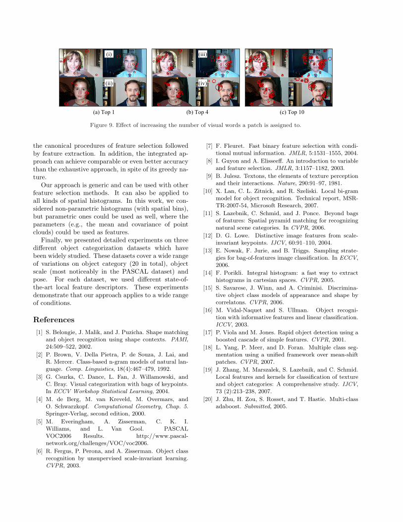
images. The size of the bubbles indicates normalizedbin counts. Recall that spatial histograms collect spa-tial co-occurrence of word pairs; in this case the specificword pair corresponds to a person’s nose and eye fromreal data. Ideally the two histograms would be nearlyidentical, but image variations and clustering artifactsprevent it from being so. In Fig. 8(b), using the top-Ntechnique, the two histograms become more similar toeach other. The reason that 2nd order features benefitmore from this technique than 1st order ones is dueto the sparsity of co-occurrence of a word pair. Thechance of co-occurrence between a pair of visual wordswithin a specific spatial bin is at the order of approxi-mately 1/(J2×12), where J is the size of the dictionaryof codewords. Compared to the order of 1/J for thehistogram of visual words, slight image variations andclustering artifacts can result in larger disturbances inthe spatial feature bin counts than in the visual wordbin counts. The top-N technique increases the bincounts (before normalization) and reduces the sensi-tivity to variations. In Fig. 9 we see the population ofa particular codeword getting denser as c2 increases. InFig. 9(i)(ii), this codeword rarely appears ‘correctly’ onthe chin of the face. Increasing c2 increases its occur-rence on the chin, but also increases its occurrence atother locations, so increasing c2 indefinitely would leadto performance degrading. Overall, this suggests thatusing a small value of c1 but a moderate value of c2

should give the best result. Indeed, using AdaBoost asclassifier, we found that (c1 = 1, c2 = 10) gives state-of-the-art performance, as shown in Table 3.

(1,1) (4,4) (10,10) (1,10)

Face1st order feat 4.15 3.23 5.53 4.15

1st and 2nd order feat 1.84 1.84 0.92 0.92

Motorbike1st order feat 1.50 2.00 2.75 1.50

1st and 2nd order feat 1.50 1.25 1.00 1.00

Airplane1st order feat 2.75 4.00 4.00 2.75

1st and 2nd order feat 2.25 2.50 2.00 1.75

Car1st order feat 1.00 1.50 2.25 1.00

1st and 2nd order feat 0.50 0.75 1.00 0.50

Class

(c1,c2)

Table 3. Equal error rates (%) for the Caltech-4 dataset. Byintegrating feature selection and extraction, state-of-the-artresults are obtained.

5. Conclusion and future work

We have presented an approach for integrating theprocess of feature selection and feature extraction.The integrated approach is three times faster than

(a) Top 1 (b) Top 4 (c) Top 10

(i)

(ii)

(iii)

(iv)

Figure 9. Effect of increasing the number of visual words a patch is assigned to.

the canonical procedures of feature selection followedby feature extraction. In addition, the integrated ap-proach can achieve comparable or even better accuracythan the exhaustive approach, in spite of its greedy na-ture.

Our approach is generic and can be used with otherfeature selection methods. It can also be applied toall kinds of spatial histograms. In this work, we con-sidered non-parametric histograms (with spatial bins),but parametric ones could be used as well, where theparameters (e.g., the mean and covariance of pointclouds) could be used as features.

Finally, we presented detailed experiments on threedifferent object categorization datasets which havebeen widely studied. These datasets cover a wide rangeof variations on object category (20 in total), objectscale (most noticeably in the PASCAL dataset) andpose. For each dataset, we used different state-of-the-art local feature descriptors. These experimentsdemonstrate that our approach applies to a wide rangeof conditions.

References

[1] S. Belongie, J. Malik, and J. Puzicha. Shape matchingand object recognition using shape contexts. PAMI,24:509–522, 2002.

[2] P. Brown, V. Della Pietra, P. de Souza, J. Lai, andR. Mercer. Class-based n-gram models of natural lan-guage. Comp. Linguistics, 18(4):467–479, 1992.

[3] G. Csurka, C. Dance, L. Fan, J. Willamowski, andC. Bray. Visual categorization with bags of keypoints.In ECCV Workshop Statistical Learning, 2004.

[4] M. de Berg, M. van Kreveld, M. Overmars, andO. Schwarzkopf. Computational Geometry, Chap. 5.Springer-Verlag, second edition, 2000.

[5] M. Everingham, A. Zisserman, C. K. I.Williams, and L. Van Gool. PASCALVOC2006 Results. http://www.pascal-network.org/challenges/VOC/voc2006.

[6] R. Fergus, P. Perona, and A. Zisserman. Object classrecognition by unsupervised scale-invariant learning.CVPR, 2003.

[7] F. Fleuret. Fast binary feature selection with condi-tional mutual information. JMLR, 5:1531–1555, 2004.

[8] I. Guyon and A. Elisseeff. An introduction to variableand feature selection. JMLR, 3:1157–1182, 2003.

[9] B. Julesz. Textons, the elements of texture perceptionand their interactions. Nature, 290:91–97, 1981.

[10] X. Lan, C. L. Zitnick, and R. Szeliski. Local bi-grammodel for object recognition. Technical report, MSR-TR-2007-54, Microsoft Research, 2007.

[11] S. Lazebnik, C. Schmid, and J. Ponce. Beyond bagsof features: Spatial pyramid matching for recognizingnatural scene categories. In CVPR, 2006.

[12] D. G. Lowe. Distinctive image features from scale-invariant keypoints. IJCV, 60:91–110, 2004.

[13] E. Nowak, F. Jurie, and B. Triggs. Sampling strate-gies for bag-of-features image classification. In ECCV,2006.

[14] F. Porikli. Integral histogram: a fast way to extracthistograms in cartesian spaces. CVPR, 2005.

[15] S. Savarese, J. Winn, and A. Criminisi. Discrimina-tive object class models of appearance and shape bycorrelatons. CVPR, 2006.

[16] M. Vidal-Naquet and S. Ullman. Object recogni-tion with informative features and linear classification.ICCV, 2003.

[17] P. Viola and M. Jones. Rapid object detection using aboosted cascade of simple features. CVPR, 2001.

[18] L. Yang, P. Meer, and D. Foran. Multiple class seg-mentation using a unified framework over mean-shiftpatches. CVPR, 2007.

[19] J. Zhang, M. Marszalek, S. Lazebnik, and C. Schmid.Local features and kernels for classification of textureand object categories: A comprehensive study. IJCV,73 (2):213–238, 2007.

[20] J. Zhu, H. Zou, S. Rosset, and T. Hastie. Multi-classadaboost. Submitted, 2005.