integrated model for production planning in a large iron and steel manufacturing environment
TRANSCRIPT
This article was downloaded by: [Linnaeus University]On: 16 October 2014, At: 13:52Publisher: Taylor & FrancisInforma Ltd Registered in England and Wales Registered Number: 1072954Registered office: Mortimer House, 37-41 Mortimer Street, London W1T3JH, UK
International Journal ofProduction ResearchPublication details, including instructions forauthors and subscription information:http://www.tandfonline.com/loi/tprs20
Integrated model forproduction planning in a largeiron and steel manufacturingenvironmentHong Li & J. ShangPublished online: 14 Nov 2010.
To cite this article: Hong Li & J. Shang (2001) Integrated model for productionplanning in a large iron and steel manufacturing environment, International Journalof Production Research, 39:9, 2037-2062, DOI: 10.1080/00207540110035200
To link to this article: http://dx.doi.org/10.1080/00207540110035200
PLEASE SCROLL DOWN FOR ARTICLE
Taylor & Francis makes every effort to ensure the accuracy of all theinformation (the “Content”) contained in the publications on our platform.However, Taylor & Francis, our agents, and our licensors make norepresentations or warranties whatsoever as to the accuracy, completeness,or suitability for any purpose of the Content. Any opinions and viewsexpressed in this publication are the opinions and views of the authors, andare not the views of or endorsed by Taylor & Francis. The accuracy of theContent should not be relied upon and should be independently verified withprimary sources of information. Taylor and Francis shall not be liable for anylosses, actions, claims, proceedings, demands, costs, expenses, damages,and other liabilities whatsoever or howsoever caused arising directly orindirectly in connection with, in relation to or arising out of the use of theContent.
This article may be used for research, teaching, and private study purposes.Any substantial or systematic reproduction, redistribution, reselling, loan,sub-licensing, systematic supply, or distribution in any form to anyone is

expressly forbidden. Terms & Conditions of access and use can be found athttp://www.tandfonline.com/page/terms-and-conditions
Dow
nloa
ded
by [
Lin
naeu
s U
nive
rsity
] at
13:
53 1
6 O
ctob
er 2
014

int. j. prod. res., 2001, vol. 39, no. 9, 2037 ± 2062
Integrated model for production planning in a large iron and steelmanufacturing environment
HONG LIy and J. SHANGz*
The authors have developed a production-planning model for a large steel cor-poration in China. Large systems normally require decomposition and module-interfaces, yet complicated interfaces often result in system breakdown and pre-vent it from reaching its full potential. To overcome di� culties of the linkageproblem and to synchronize the production of main products and by-products,the input-output (I± O) model was looked at. The proposed optimization model,based on the I± O concept, is capable of coordinating large number of variableswith minimum interfaces. It provides a comprehensive production managementframework. Owing to the generality of the model structure, the authors believe itis useful for both the studied company and for many other organizations.
1. Introduction
High productivity and energy e� ciency are the main objectives of today’ s iron
and steel manufacturing. The present research addresses the problem of coordinating
multiple plants in a large iron and steel complex in China. The goal is to maximizeiron and steel production while at the same time minimizing by-product gas emis-
sions. In fact, energy consumption accounts for a major part of a steel company’s
expenses. Considerable eŒorts have been undertaken to discover energy-saving alter-
natives. One of the main methods is to maximize utilization of by-product gas, which
in turn reduces gas release and related pollution. To achieve these goals one has to
manage eŒectively the operations of the production system; in the present case thismust occur through the coordination of various factories within the company.
To date, many researchers and practitioners have studied iron and steel produc-
tion management issues with varied success. The literature contains assorted tech-
niques. For example, Sato et al. (1977) applied mathematical programming to
production scheduling. Mackulak et al. (1980) and Box and Herbe (1988) developedcomputer control schemes for production planning. The system developed by Assaf
et al. (1997) was based on an implicit enumeration procedure, while Lin and Moodie
(1989) proposed a hierarchical scheduling strategy. Others such as Sztrimbely et al.
(1989), Numao and Morishita (1988) and Jimichi et al. (1990) recommended expert
systems.Owing to the need to coordinate multiplants and to synchronize steel production
with gas generation, this study forgoes the traditional planning and scheduling
International Journal of Production Research ISSN 0020± 7543 print/ISSN 1366± 588X online # 2001 Taylor & Francis Ltd
http://www.tandf.co.uk/journals
DOI: 10.1080/00207540110035200
Revision received October 2000.{ Complete Business Solutions, Inc., 111 Liberty Street, Columbus, OH 43215, USA.{ 254 Mervis Hall, Katz Graduate School of Business, University of Pittsburgh,
Pittsburgh, PA 15260, USA.* To whom correspondence should be addressed. e-mail: [email protected]
Dow
nloa
ded
by [
Lin
naeu
s U
nive
rsity
] at
13:
53 1
6 O
ctob
er 2
014
approach. Instead, Leontif’s Input± Output (I± O) model (1966) is investigated for its
application potential. The I± O model is predominantly concerned with the activity ofindustry sectors that consume products from other industries (inputs) while generat-
ing their own goods (outputs). Each factory site in a manufacturing system resembles
a region in the I± O model. DiŒerent factories are interdependent, just like various
regions. Based on this concept, Leontif ’s model is revised here and a dynamicoptimal plan for steel production is devised.
2. Problem description and hierarchical planningThe following subsections describe manufacturing facilities, traditional produc-
tion management approaches and limitations of the hierarchical planning systems.
2.1. Integrated manufacturing company
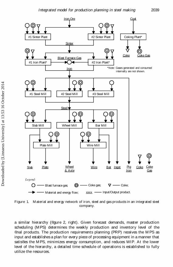
This study is based on Maanshan Iron and Steel Company, the ® fth largest
corporation of its kind in China. The company has multiplant sites: one cokingplant, two sinters, two iron plants, three steel rolling mills, one power plant and
more (® gure 1). DiŒerent factories have diŒerent e� ciencies, producing various
products and consuming a variety of materials. The interplant material ¯ ows are
determined by the availability of the supply and the corporation’ s dispatcher. Inputs
needed for producing a particular product are normally supplied by several factories.
This is a multi-input, -output, -stage and -site manufacturing environment.The 14 factories are connected through the interaction of steel production and
gas generation. Typically, by-product gas is generated in the processes of coke-
making, iron-making and steel-making and also is consumed in the processes. The
by-product gas generation depends on the amount and type of main products pro-
duced, whereas by-product gas supply dictates the amount of iron and steel produc-tion. As a result, gas is an output (by-product) as well as an input (fuel), and iron/
steel is a ® nal product (output) as well as an input for gas generation. E� cient use of
energy such as gas and electricity is an important steel industry objective (Cho 1981,
Lin and Moodie 1985). Currently, the steel industry consumes ¹15% of China’s
energy and is one of the largest energy consumers.Two of the main energy-saving ideas are direct rolling (DR) and hot charging
(HC), which totally or partially eliminate reheating requirements (Assaf et al. 1997).
Such approaches are suitable for mini-mills, where all the production processes are
nearby. The Japanese steel industry has successfully implemented such practices.
Yet, in the studied system, the production stream is established through a series of
factories, each of which completes only one major function. Various plants aredistributed over a large geographical area. Both DR and HC require that slabs
coming directly from the slabbing mill be inspected and charged immediately to
the hot strip mill without a cooling down cycle. With limited budget for equipment
upgrades, the modern techniques of DR and HC are not applicable to the present
problem. Adequate coordination among diŒerent production functions and pro-cesses becomes critical for the success of this integrated system.
2.2. Hierarchical production planning for steel manufacturing
Conventionally, a hierarchical approach is employed for complex problems. A
popular steel manufacturing hierarchy (® gure 2, left) relevant to our research isestablished by Purdue Laboratory for Applied Industrial Control (PLAIC)
(Williams 1985). Lin and Moodie (1989) developed a production strategy based on
2038 H. Li and J. Shang
Dow
nloa
ded
by [
Lin
naeu
s U
nive
rsity
] at
13:
53 1
6 O
ctob
er 2
014
a similar hierarchy (® gure 2, right). Given forecast demands, master production
scheduling (MPS) determines the weekly production and inventory level of the
® nal products. The production requirements planning (PRP) receives the MPS as
input and establishes a plan for every piece of processing equipment in a manner that
satis® es the MPS, minimizes energy consumption, and reduces WIP. At the lower
level of the hierarchy, a detailed time schedule of operations is established to fully
utilize the resources.
2039Integrated model for production planning in steel making
Slab
#3 Steel Mill
Sinter
Iron Ore Coal
Coke Coke Gas
Coking Plant*
Blast Furnace Gas
#1 Iron Plant* #2 Iron Plant*
Iron
#1 Steel Mill #2 Steel Mill
Steel
Slab Mill Wheel Mill Bar Mill
Bar Wheel & Axle
Wire Ingot Pig Iron
Coke Coke Gas
Plate
#1 Sinter Plant #2 Sinter Plant
Plate Mill Wire Mill
*Note: Gases generated and consumed internally are not shown.
Legend:
Blast furnace gas;
Material and energy flow;
Coke gas; Coke;
Input/Output product. xxxx
Figure 1. Material and energy network of iron, steel and gas products in an integrated steelcompany.
Dow
nloa
ded
by [
Lin
naeu
s U
nive
rsity
] at
13:
53 1
6 O
ctob
er 2
014

Many researchers directly addressed the level two optimal sequencing and sched-
uling problem in the PLAIC’s hierarchy (Box and Herbs 1988, Jacobs et al. 1988,Petermen et al. 1992). Hax and Meal (1975) introduced a widely adopted hierarchical
production planning (HPP) approach, which is based on tactical and operational
decisions in a batch production environment. Since steel manufacturing is usually
not a batch process, its discussion is omitted here.
2.3. Comments on current practice
A hierarchical approach like Lin and Moodie’s (1989) easily ® ts into the plant
management and control structure. However, there is no detailed guideline as to
product aggregation and disaggregation and for multiple-site coordination. On the
other hand, Bitran and Hax’s framework (1977) is well suited for product aggrega-
tion and disaggregation. Yet its focus on parts and assembly makes it mainly suitablefor discrete manufacturing, not for steel manufacturing, which consists of both
continuous and discrete processes.
A major weakness of the hierarchical approach lies in its interface. In dealing
with hierarchy, each individual level is decomposed into functional units so that the
burden of planning and scheduling can be shared. Though functional decomposition
is eŒective in taking on hard problems, the modules that carry out diŒerent functions
inevitably require communication, thus, interface. The more modules a hierarchyhas, the more interfaces are needed. Excess interface causes communication break-
down and hinders system performance. To overcome such di� culties, a model which
reduces the need for interface and provides an e� cient solution procedure is
proposed. The model is capable of integrating large number of variables withoutaggregation or losing any individual information. The only interfaces required are
short-term operational scheduling and long-term strategic planning. Details are
described in Sections 3 and 4.
2040 H. Li and J. Shang
LEVEL 4B
MANAGEMENT DATA
REPRESENTATION
« FORECAST DEMANDS & ORDERS
¯
LEVEL 4A
OVERALL PRODUCTION
PLANNING
« MASTER
PRODUCTION SCHEDULING (MPS)
®
¯
LEVEL 3
DETAILED PRODUCTION SCHEDULING
« PRODUCTION
REQUIREMENTS PLANNING (PRP)
®
¯
LEVEL 2
OPTIMIZATION
«
PRODUCTION SEQUENCING AND SCHEDULING (PSS)
®
¯
LEVEL 1
DIRECT DIGITAL CONTROL
Figure 2. Correspondence between PLAIC and Lin and Moodie’s hirarchy.
Dow
nloa
ded
by [
Lin
naeu
s U
nive
rsity
] at
13:
53 1
6 O
ctob
er 2
014

3. Input± output model
Leontief ’s Input± Output (I± O) model (1966) is modi® ed here to address themultisite coordination problem encountered by Maanshan Iron and Steel
Company. Although the model was originally developed to examine the interdepen-
dence among various producing and consuming sectors within a national economy,
great similarities have been observed between the structure of a ® rm and that of aneconomy. In both the national economy and the production environment, the fun-
damental problem makeup is the same: the interdependence among individual sec-
tors of an economy (or of a ® rm) can be described by a set of linear equations, and
the characteristics of such a system can be re¯ ected in the values of the linear
equations derived from empirical data.
3.1. Applying the input-outpu t model to manufacturing environmentThe information for the I± O model is contained in an interindustry transactions
table (table 1), which is the statistical basis of the I± O system. Output of each process
is distributed along a column, while the corresponding rows record the inputs. Its
application to production planning can be described as follows. Each row describes
how a particular material or semi-product is consumed by various semi- or ® nal-
products in the column. The internal ¯ ows, xij ’ s, form a square matrix. The addi-
tional column labelled `Final Demand’ records the sales of corresponding rows’products to outside markets. At the bottom of the table are the resources, such as
electricity, labour and equipment directly purchased from outside markets. These
resources are not part of the output of current production and are called primary
inputs.
The relationships between inputs (rows) and outputs (columns) can be repre-sented by the following ¯ ow balance equation:
Pnjˆ1 xij ‡ yi ˆ xi i ˆ 1; 2; . . . ; n;
Pnjˆ1 zkj ˆ zk k ˆ 1; 2; . . . ; m;
(…3:1†
where
xij amount of material or semi-product i consumed in the production of semi-
or ® nal-product j; j ˆ 1; 2; . . . ; n,yi amount of ® nal product i produced for external consumption, or available
for sale, i ˆ 1; 2; . . . ; n,
2041Integrated model for production planning in steel making
Output Intermediate demandFinal Total
Input 1 2 ¢ ¢ ¢ n demand output
Consumption 1 x11 x12 ¢ ¢ ¢ x1n y1 x1
2 x21 x22 ¢ ¢ ¢ x2n y2 x2
¢ ¢ ¢ ¢ ¢ ¢ ¢ ¢ ¢ ¢ ¢ ¢ ¢ ¢ ¢ ¢ ¢ ¢ ¢ ¢ ¢n xn1 xn2 ¢ ¢ ¢ xnn yn xn
Purchase 1 z11 z12 ¢ ¢ ¢ z1n z1
2 z21 z22 ¢ ¢ ¢ z2n z2
¢ ¢ ¢ ¢ ¢ ¢ ¢ ¢ ¢ ¢ ¢ ¢ ¢ ¢ ¢ ¢ ¢ ¢m zm1 zm2 ¢ ¢ ¢ zmm zm
Table 1. Input± output transaction table for material ¯ ows.
Dow
nloa
ded
by [
Lin
naeu
s U
nive
rsity
] at
13:
53 1
6 O
ctob
er 2
014

xi amount of product i produced, i ˆ 1; 2; . . . ; n,
zkj amount of resource k purchased for producing product j; k ˆ 1; 2; . . . ; m,zk total amount of resource k purchased, k ˆ 1; 2; . . . ; m.
(Those interested can write to the authors to obtain complete numerical information
for the studied problem.) For the sake of brevity and clarity, only part of the
complete numerical table is explained. Table 2 displays a small section of the com-
plete Xij table. The value under the title of each column is the amount of productsproduced (Xj) in the corresponding factory. Going down vertically, the table shows
how various inputs in each row are needed to produce the speci® c semi- or ® nal-
product in the column. For example, cell (9, 17) indicates 674,438 GJ of blast furnace
gas is needed to produce 88,781 tons of iron in the 1_Iron factory.
The technical coeYcient aij is de® ned as:
aij ˆxij
xj
i; j ˆ 1; 2; . . . ; n;
which is the amount of material or semi-product i directly consumed in the produc-
tion of a unit of product j. The value depends on the technical capability of each
factory, thus the name technical coe� cient. See table 3 for part of the aij ’ s.
Similarly, the purchase coe� cient dkj can be de® ned as:
dkj ˆzkj
xj
k ˆ 1; 2; . . . ; m; j ˆ 1; 2; . . . ; n;
which indicates the amount of purchased material k directly consumed in the pro-
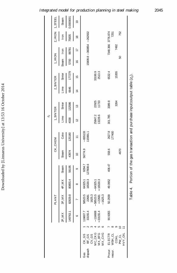
duction of a unit of product j. See table 4 for part of the zkj ’ s and table 5 for part ofthe dkj ’ s.
Because of the interaction between the company’ s diŒerent factories (diŒerent
sites), a change in the ® nal demand for the products of one factory causes repercus-
sions throughout the whole production system. Changes in ® nal product demand not
only change the output quantity of the factory concerned, but also they impact many
of the other factories within the production system. One goal of our productionanalysis is to study the eŒects of these changes. Unfortunately, the technical coe� -
cients only show the direct (® rst-order) eŒects of changes in ® nal demand. The total
eŒects of ® rst-, second- and higher-orders can actually be summarized in the inter-
dependence coe� cients, which are derived in the following. First, (3.1) is converted
into matrix form:
AX ‡ Y ˆ X
DX ˆ Z;
¼…3:2†
where
A direct input coe� cient matrix, A ˆ …aij†n¤n,
X total product vector, X ˆ …x1; x2; . . . ; xn†T,
Y ® nal demand vector, Y ˆ …y1; y2; . . . ; yn†T,
D purchase coe� cient matrix, D ˆ …dkj†m¤n,
Z vector of purchased resources, Z ˆ …z1; z2; . . . ; zm†T.
Matrices (3.2) may be rewritten as
2042 H. Li and J. Shang
Dow
nloa
ded
by [
Lin
naeu
s U
nive
rsity
] at
13:
53 1
6 O
ctob
er 2
014

2043Integrated model for production planning in steel making
Xij
CH
_C
HE
M1_
SIN
TE
R2_
SIN
TE
R1_
IRO
N2_
IRO
N1_
ST
EE
L2_
ST
EE
L
Ste
am
Co
ke
Lim
eS
inte
rL
ime
Sin
ter
Iro
nIr
on
Ste
am
OP
_S
TL
Lim
eC
V_
ST
LE
L_
ST
L
10
11
12
13
14
15
17
18
19
20
21
22
23
43
97
412
518
04
038
13
258
66
64
61
7727
988
781
75
83
50
335
41
26
07
255
59
529
4
CK
_C
HE
MC
K_
GS
110
119
88
.3S
tea
m2
25
88
41
170
1_S
INT
ER
MX
33
90
75
.834
657
.9C
ok
e4
58
45
.6L
ime
523
52
2_S
INT
ER
MX
635
704
.2C
ok
e7
55
2L
ime
84
59
.5
1_IR
ON
BF
_G
S9
67
44
38
Ste
am
10
57
00
Co
ke
11
486
98
Sin
ter
12
14
34
76
2_IR
ON
BF
_G
S1
35
26
125
Ste
am
14
18
65
0C
ok
e1
535
71
1S
inte
r1
61
25
460
1_S
TE
EL
MX
17
28
10
0.5
Ste
am
18
10
10
7L
ime
19
257
8Ir
on
20
26
16
8
2_S
TE
EL
Ste
am
21
20
50
Co
ke
22
79
5L
ime
23
20
96
27
iro
n2
43
05
22
72
0
Tab
le2.
Po
rtio
no
fth
ein
pu
t±o
utp
ut
tab
le…X
ij†.
Dow
nloa
ded
by [
Lin
naeu
s U
nive
rsity
] at
13:
53 1
6 O
ctob
er 2
014

2044 H. Li and J. Shang
Aij
CH
_C
HE
M1_
SIN
TE
R2_
SIN
TE
R1_
IRO
N2_
IRO
N1_
ST
EE
L2_
ST
EE
L
439
74
12
51
80
40
38
132
58
666
46
177
27
988
78
17
58
35
033
541
260
72
55
59
529
4
CK
_C
HE
MC
K_
GS
10
8.0
84
26
51
00
00
00
00
00
0S
team
20
.05
88
53
0.3
28
88
64
00
00
00
00
00
0
1_S
INT
ER
MX
30
09.6
770
20.2
61
40
00
00
00
00
Co
ke
40
00
0.0
44
09
00
00
00
00
0L
ime
50
00
0.0
17
74
00
00
00
00
0
2_S
INT
ER
MX
60
00
00
0.2
014
01
00
00
00
0C
ok
e7
00
00
0.0
830
60
00
00
00
0L
ime
80
00
00
0.0
251
55
00
00
00
0
1_IR
ON
GF
_G
S9
00
00
00
7.5
966
50
00
00
0S
team
10
00
00
00
0.0
642
00
00
00
Co
ke
11
00
00
00
0.5
485
20
00
00
0S
inte
r1
20
00
00
01
.72
87
00
00
00
2_IR
ON
BF
_G
S1
30
00
00
00
69
377
60
00
00
Ste
am
14
00
00
00
00
.245
93
00
00
0C
ok
e1
50
00
00
00
0.4
70
90
00
00
Sin
ter
16
00
00
00
01
.654
38
00
00
0
1_S
TE
EL
MX
17
00
00
00
00
00
.83
78
00
0S
team
18
00
00
00
00
00
.30
13
30
00
Lim
e1
90
00
00
00
00
0.0
768
60
00
Iro
n2
00
00
00
00
00
0.8
398
10
00
2_S
TE
EL
Ste
am
21
00
00
00
00
00
00
.08
02
10
Co
ke
22
00
00
00
00
00
0.3
049
50
0L
ime
23
00
00
00
00
00
00
.08
20
10
.00
51
iro
n2
40
00
00
00
00
00
1.1
941
80.1
36
Tab
le3
.P
ort
ion
of
the
tech
nic
al
coe�
cien
tta
ble
…aij
ˆx
ij=x
i†.
Dow
nloa
ded
by [
Lin
naeu
s U
nive
rsity
] at
13:
53 1
6 O
ctob
er 2
014
2045Integrated model for production planning in steel making
z ij
PL
AN
TC
K_
CH
EM
1_S
INT
ER
2_S
INT
ER
1_IR
ON
2_IR
ON
1_S
TE
EL
2P_
MX
3P
_M
X4P
_M
XS
tea
mS
tea
mC
ok
eL
ime
Sin
ter
Lim
eS
inte
rS
team
Iro
nIr
on
Ste
am
1497
63.1
828
29.8
8085
5.4
561
954
3974
125
180
403
813
2586
6646
177
279
5700
88
781
7583
50
.000
000
1
67
89
101
112
1314
151
617
1819
Ga
sC
K_
GS
111
6607
.758
523
.564
325.
19
294.
75
6774
.965
5133
dis
pa
chB
F_
GS
23
3155
.42
2681
1653
0.3
1278
08.6
115
991.
11
5909
.83
6085
42
6293
2
CV
_G
S3
162
5.3
MC
_C
KG
41
1660
858
523
.564
325.
12
584
7.2
2292
53
3190
.9
MX
_B
FG
53
3155
.42
2681
1653
0.3
13
228.
611
733
2513
.3
MX
_C
VG
61
625.
3
Pro
cur.
EL
EC
TR
79
0.9
355
50.2
939
49.0
952
408
.47
558
.62
627.
83
01.
785
3389
.865
32.4
7348
.36
637
76.8
74
reso
ur.
WS
H_
CL
817
7400
725
1
CO
AL
93
264
1535
57
492
PW
_C
L1
04
670
50
752
HV
Y_
OIL
11
Ta
ble
4.
Po
rtio
no
fth
ega
str
an
sact
ion
an
dp
urc
hase
inp
ut±
ou
tpu
tta
ble
(zij).
Dow
nloa
ded
by [
Lin
naeu
s U
nive
rsity
] at
13:
53 1
6 O
ctob
er 2
014

2046 H. Li and J. Shang
Dij
PL
AN
TC
K_
CH
EM
1_S
INT
ER
2_S
INT
ER
1_IR
ON
2_IR
ON
1_S
TE
EL
2P
_M
X3
P_
MX
4P
_M
XS
team
Ste
am
Co
ke
Lim
eS
inte
rL
ime
Sin
ter
Ste
amIr
on
Iro
nS
team
149
763.
182
829
.88
0855
.456
195
439
741
2518
040
3813
258
666
461
7727
95
700
8878
175
835
0.0
000
001
67
89
10
11
12
1314
151
617
18
19
Ga
sC
K_
GS
10.
778
614
0.70
655
10
.79
5557
0.1
654
011.
291
102
5.2
3353
00
00
00
00
dis
pac
hB
F_
GS
20.
221
386
0.27
382
70
.20
4443
2.2
743
770
0.9
265
950
00
02.
791
193
4.0
645
53.
4671
60
CV
_G
S3
00.
019
622
00
00
00
00
00
00
MC
_C
KG
40
.77
861
0.7
0655
0.7
9556
00
06
.40
0991
0.1
729
00.
187
224
00
00
MX
_B
FG
50
.22
139
0.2
7383
0.2
0444
00
03
.27
6028
0.0
885
00.
014
177
00
00
MX
_C
VG
60
0.0
1962
00
00
00
00
00
00
Pro
cur.
EL
EC
TR
70.
000
607
0.00
060
70
.00
0607
0.0
072
690.
012
703
0.0
209
920
.07
4736
0.0
256
00.
036
848
00
.08
277
0.0
498
040
reso
ur.
WS
H_
CL
80
00
00
1.4
171
590
00
00
00
.09
5615
0
CO
AL
90
00
00
00
0.0
246
00.
086
615
00.
084
387
00
PW
_C
L10
00
00
0.1
0619
90
00
00
0.0
0877
20
0.0
099
160
HV
Y_
OIL
110
00
00
00
00
00
00
0
Ta
ble
5.
Po
rtio
no
fth
ete
chn
ica
lco
e�ci
ents
for
ga
str
an
sact
ion
an
dp
urc
ha
sed
mate
rials
(dij
ˆz i
j=x
i).
Dow
nloa
ded
by [
Lin
naeu
s U
nive
rsity
] at
13:
53 1
6 O
ctob
er 2
014

Y ˆ …I-A†XZ ˆ DX :
¼…3:3†
In I± O analysis, the vector of Y’s (® nal demand) is usually assumed to be exogenous,
and the goal is to determine the vector of the X’s needed. Matrices (3.3) can be
reorganized into
X ˆ …I-A† 1Y
Z ˆ D…I-A† 1Y :
(…3:4†
The coe� cients …I-A† 1 are the interdependence coeYcients. Matrix (3.4) indicatesthat if market demand Y is known, both the corresponding total output X to be
produced and the related resources Z to be purchased can be easily determined. The
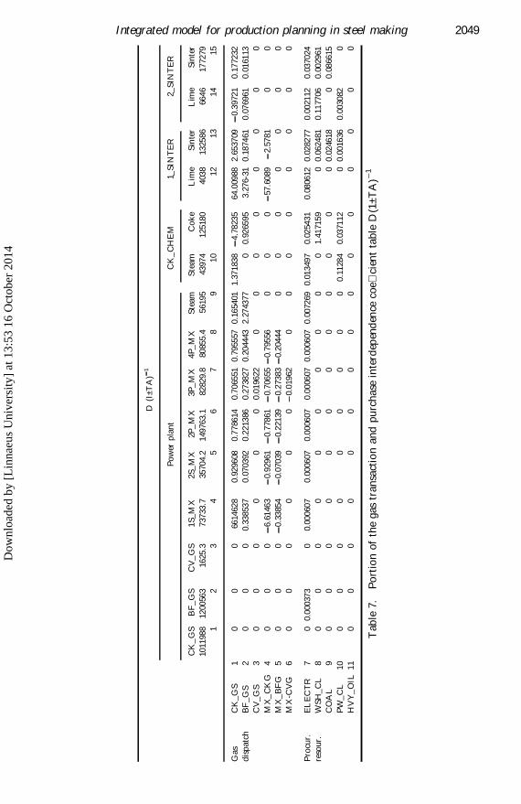
numerical example of the interdependence coe� cients is in table 6. Table 7 shows
part of the interdependence coe� cients for purchased materials and gas dispatching.
Both tables involve the T matrix (see below).
3.2. Use of multiregional I± O model to coordinate multisites
Each plant in a distributed production environment is comparable to a region in
a larger economy. In this subsection, we modify the Multi-regional Chenery± Moses
I± O model and adapt it to the multiplant production environment.
3.2.1. Modifying the Chenery± Moses model for multisited production planning and
scheduling
Given that the manufacturing system has s factories, and there are m…q† types of
inputs consumed, and n…q† types of output produced by factory q, the local technical
coe� cient a…q†ij for factory q can be de® ned as:
a…q†ij ˆ
x…q†ij
x…q†j
i ˆ 1; 2; . . . ; m…q†j ˆ 1; 2; . . . ; n…q†q ˆ 1; 2; . . . ; s;
…3:7†
where
x…q†ij amount of material or semi-product i consumed by semi-product or ® nal
product j in plant q; and
x…q†j amount of semi-product or ® nal product j produced by plant q.
The dispatch coe� cient tpq
l…p†k…q†, known as the trade coe� cient in Chenery± Moses
model, can be computed by the following formula:
tpq
l…p†k…q† ˆrpqk…q†
rqk…q†
l…p† ˆ k…q†
0 l…p† 6ˆ k…q†
l…p† ˆ 1; 2; . . . ; n…p†k…q† ˆ 1; 2; . . . ; m…q†p; q ˆ 1; 2; . . . ; s;
8><
>:…3:8†
where
l…p†; k…q† subscripts denoting the products made by plants p and q respectively,
where l…p† ˆ k…q† indicates the same product from diŒerent plants,and l…p† 6ˆ k…q† otherwise;
rpqk…q† amount of item k supplied by plant p to plant q; and
2047Integrated model for production planning in steel making
Dow
nloa
ded
by [
Lin
naeu
s U
nive
rsity
] at
13:
53 1
6 O
ctob
er 2
014
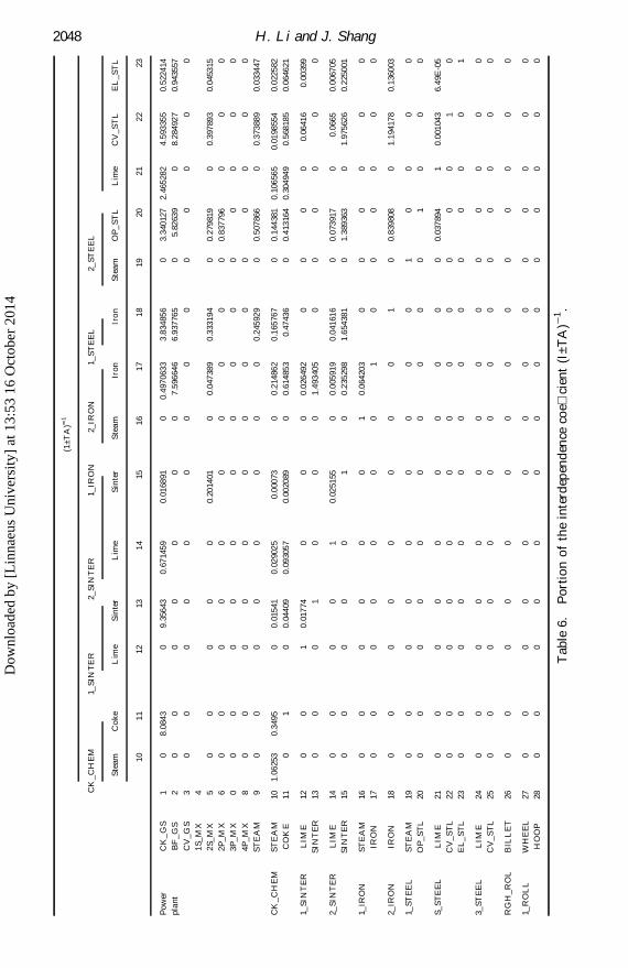
2048 H. Li and J. Shang
(1±
TA
)1
CK
_C
HE
M1_
SIN
TE
R2_
SIN
TE
R1
_IR
ON
2_IR
ON
1_
ST
EE
L2_
ST
EE
L
Ste
am
Co
ke
Lim
eS
inte
rL
ime
Sin
ter
Ste
am
Iro
nIr
on
Ste
am
OP
_S
TL
Lim
eC
V_
ST
LE
L_
ST
L
10
11
12
13
14
15
16
17
18
19
20
21
22
23
Po
wer
CK
_G
S1
08
.084
30
9.3
56
43
0.6
714
59
0.0
16
89
10
0.4
97
06
33
3.8
34
85
60
3.3
40
127
2.4
65
28
24
.59
33
55
0.5
22
41
4
pla
nt
BF
_G
S2
00
00
00
07
.59
66
46
6.9
37
76
50
5.8
26
39
08
.28
49
27
0.9
43
55
7
CV
_G
S3
00
00
00
00
00
00
00
1S_
MX
4
2S_
MX
50
00
00
0.2
01
40
10
0.0
47
38
90
.33
31
94
00
.27
98
19
00
.39
78
93
0.0
45
31
5
2P
_M
X6
00
00
00
00
00
0.8
37
796
00
0
3P
_M
X0
00
00
00
00
00
00
00
4P
_M
X8
00
00
00
00
00
00
00
ST
EA
M9
00
00
00
00
0.2
45
92
90
0.5
07
866
00
.37
38
89
0.0
33
44
7
CK
_C
HE
MS
TE
AM
10
1.0
62
53
0.3
49
50
0.0
15
41
0.0
290
25
0.0
00
73
00
.21
48
62
0.1
65
76
70
0.1
44
381
0.1
06
56
50
.01
98
55
40
.02
25
82
CO
KE
11
01
00
.04
40
90
.09
30
57
0.0
02
08
90
0.6
14
85
30
.47
43
60
0.4
13
164
0.3
04
94
90
.56
81
85
0.0
64
62
1
1_S
INT
ER
LIM
E12
00
10
.01
77
40
00
0.0
26
49
20
00
00
.06
41
60
.00
39
9
SIN
TE
R13
00
01
00
01
.49
34
05
00
00
00
2_S
INT
ER
LIM
E14
00
00
10
.02
51
55
00
.00
59
19
0.0
41
61
60
0.0
73
917
00
.06
65
0.0
06
70
5
SIN
TE
R15
00
00
01
00
.23
52
98
1.6
54
38
10
1.3
89
363
01
.97
56
26
0.2
25
00
1
1_IR
ON
ST
EA
M16
00
00
00
10
.06
42
03
00
00
00
IRO
N17
00
00
00
01
00
00
00
2_IR
ON
IRO
N18
00
00
00
00
10
0.8
39
808
01
.19
41
78
0.1
36
00
3
1_S
TE
EL
ST
EA
M19
00
00
00
00
01
00
00
OP
_S
TL
20
00
00
00
00
00
10
00
S_
ST
EE
LL
IME
21
00
00
00
00
00
0.0
37
894
10
.00
10
43
6.4
9E
-05
CV
_S
TL
22
00
00
00
00
00
00
10
EL
_S
TL
23
00
00
00
00
00
00
01
3_S
TE
EL
LIM
E24
00
00
00
00
00
00
00
CV
_S
TL
25
00
00
00
00
00
00
00
RG
H_
RO
LB
ILL
ET
26
00
00
00
00
00
00
00
1_R
OL
LW
HE
EL
27
00
00
00
00
00
00
00
HO
OP
28
00
00
00
00
00
00
00
Ta
ble
6.
Po
rtio
no
fth
ein
terd
epen
den
ceco
e�ci
ent
(I±
TA
)1.
Dow
nloa
ded
by [
Lin
naeu
s U
nive
rsity
] at
13:
53 1
6 O
ctob
er 2
014
2049Integrated model for production planning in steel making
D(I
±TA
)1
Po
wer
pla
nt
CK
_C
HE
M1_
SIN
TE
R2_
SIN
TE
R
CK
_G
SB
F_
GS
CV
_G
S1
S_M
X2S
_M
X2P
_M
X3P
_M
X4
P_
MX
Ste
amS
team
Co
ke
Lim
eS
inte
rL
ime
Sin
ter
1011
988
1200
563
1625
.37
3733
.735
704.
21
4976
3.1
8282
9.8
8085
5.4
56
195
4397
41
2518
04
038
1325
86
664
617
7279
12
34
56
78
91
01
21
31
41
5
Ga
sC
K_
GS
10
00
6614
628
0.9
296
080
.77
8614
0.7
065
510
.79
5557
0.1
654
011.
371
838
4.7
823
56
4.0
0988
2.6
537
090
.39
721
0.1
772
32
dis
pa
tch
BF
_G
S2
00
00.
338
537
0.0
703
920
.22
1386
0.2
738
270
.20
4443
2.2
743
770
0.92
659
53
.27
6-31
0.1
874
610
.07
6961
0.0
161
13
CV
_G
S3
00
00
00
0.0
196
220
00
00
00
0
MX
_C
KG
40
00
6.6
146
30.
929
610.
778
610.
706
550.
795
560
00
57.6
089
2.57
810
0
MX
_B
FG
50
00
0.3
385
40.
070
390.
221
390.
273
830.
204
440
00
00
00
MX
-CV
G6
00
00
00
0.0
1962
00
00
00
00
Pro
cur.
EL
EC
TR
70
0.0
0037
30
0.00
060
70
.00
0607
0.0
006
070
.00
0607
0.0
006
070
.00
7269
0.01
349
70.
0254
31
0.0
806
120
.02
8277
0.0
021
120
.03
7024
reso
ur.
WS
H_
CL
80
00
00
00
00
01.
4171
59
00
.06
2481
0.1
177
060
.00
2961
CO
AL
90
00
00
00
00
00
00
.02
4618
00
.08
6615
PW
_C
L1
00
00
00
00
00
0.1
128
40.
0371
12
00
.00
1636
0.0
030
820
HV
Y_
OIL
11
00
00
00
00
00
00
00
0
Tab
le7.
Po
rtio
no
fth
eg
as
tra
nsa
ctio
na
nd
pu
rch
ase
inte
rdep
end
ence
coe�
cien
tta
ble
D(1
±T
A)
1
Dow
nloa
ded
by [
Lin
naeu
s U
nive
rsity
] at
13:
53 1
6 O
ctob
er 2
014

rq
k…q† amount of product k needed by plant q, including both the internal
consumption and the ® nal demand (external sales).
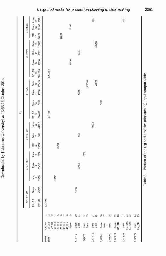
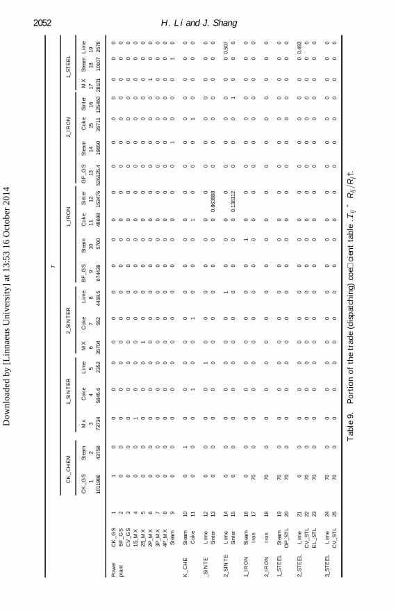
Part of R and T matrices can be found in tables 8 and 9.
Based on equation (3.8), the local supply function, from plant p to q, can be
written in a matrix form as:
R…pq† ˆ T …pq†R…q† p; q ˆ 1; 2; . . . ; s; …3:9†
where
R…pq† ˆ …r…pq†1 ; r
…pq†2 ; . . . ; r
…pq†n…p††
T
and
R…q† ˆ …r…q†1 ; r
…q†2 ; . . . ; r
…q†m…q††
T:
In equation (3.9), matrix T…pq† is not a squared one (36*47 in our case) like its
counterpart in the original Chenery± Moses model. Its row catalogue is the sameas the product catalogue of plant p, and its column catalogue is equivalent to the
consumption catalogue of plant q. That is:
T …pq† ˆ
t…pq†11 t
…pq†12 ¢ ¢ ¢ t
…pq†lm…q†
t…pq†21 t
…pq†22 ¢ ¢ ¢ t
…pq†2m…q†
..
. ... ..
.
t…pq†n…p†1
t…pq†n…p†2 ¢ ¢ ¢ t
…pq†n…p†m…q†
0
BBBBBB@
1
CCCCCCAˆ …t…pq†
t…p†k…q††n…p†¤m…q†: …3:10†
By using equation (3.7) for local technical coe� cient a…q†ij , the local net demand
function in matrix form becomes:
R…q† ˆ A…q†Z…q† q ˆ 1; 2; . . . ; s; …3:11†
where
A…q† ˆ
a…q†11 a
…q†12 ¢ ¢ ¢ a
…q†ln…q†
a…q†21 a
…q†22 ¢ ¢ ¢ a
…q†2n…q†
..
. ... ..
.
a…q†m…q†1 a
…q†m…q†2 ¢ ¢ ¢ a
…q†m…q†n…q†
0
BBBBBB@
1
CCCCCCA;
X …q† ˆ …X …q†1 ; X
…q†2 ; . . . ; X
…q†n…q††
T:
Note, the local transactions matrix A…q† is not a square matrix either (47*36 in our
case). The ® nal products of the plant from its plant p are counted in the local
production function, which is:
X …p† ˆXs
qˆ1
R…pq† ‡ Y …p† p ˆ 1; 2; . . . ; s; …3:12†
where Y…p† is plant p’ s ® nal product demand vector, and
2050 H. Li and J. Shang
Dow
nloa
ded
by [
Lin
naeu
s U
nive
rsity
] at
13:
53 1
6 O
ctob
er 2
014
2051Integrated model for production planning in steel making
Rij
CK
_C
HE
M1
_S
INT
ER
2_
SIN
TE
R1_
IRO
N2_
IRO
N1_
ST
EE
L
CK
_G
SS
team
Mx
Co
ke
Lim
eM
XC
ok
eL
ime
BF
_G
SS
tea
mC
ok
eS
inte
rG
F_
GS
Ste
am
Co
ke
Sin
ter
MX
Ste
am
Lim
e
12
34
56
78
91
01
11
21
31
41
51
61
71
81
9
10
11
98
64
37
58
73
73
45
84
5.6
23
52
35
70
45
52
445
9.5
67
44
38
57
00
48
69
81
53
47
65
26
12
5.4
18
65
03
57
11
12
54
60
28
10
11
01
07
25
78
Po
wer
CK
_G
S1
10
11
98
8
pla
nt
BF
_G
S2
67
44
38
52
61
25
.4
CV
_G
S3
1S
_M
X4
73
73
4
2S
_M
X5
35
70
4
2P
_M
X6
28
10
1
3P
_M
X7
4P
_M
X8
Ste
am
91
86
50
10
10
7
K_
CH
ES
team
10
43
75
8
Co
ke
11
58
45
.65
52
48
69
83
57
11
_S
INT
EL
ime
12
23
52
Sin
ter
13
13
25
86
2_S
INT
EL
ime
14
445
9.5
13
07
Sin
ter
15
20
89
01
25
46
0
1_IR
ON
Ste
am
16
57
00
Iro
n1
7
2_IR
ON
Iro
n1
8
1_S
TE
EL
Ste
am
19
OP
_S
TL
20
2_S
TE
EL
Lim
e2
11
27
1
CV
_S
TL
22
EL
_S
TL
23
3_S
TE
EL
Lim
e2
4
CV
_S
TL
25
Ta
ble
8.
Po
rtio
no
fth
ere
gio
na
ltr
an
sfer
(dis
pa
tch
ing
)in
pu
t±o
utp
ut
tab
le.
Dow
nloa
ded
by [
Lin
naeu
s U
nive
rsity
] at
13:
53 1
6 O
ctob
er 2
014
2052 H. Li and J. Shang
T
CK
_C
HE
M1_
SIN
TE
R2
_S
INT
ER
1_
IRO
N2_
IRO
N1
_S
TE
EL
CK
_G
SS
tea
mM
xC
ok
eL
ime
MX
Co
ke
Lim
eB
F_
GS
Ste
am
Co
ke
Sin
ter
GF
_G
SS
tea
mC
ok
eS
inte
rM
XS
tea
mL
ime
12
34
56
78
91
01
11
21
31
41
51
61
71
81
9
10
11
98
64
37
58
737
34
58
45
.62
35
23
57
04
55
24
45
9.5
67
44
38
57
00
48
69
81
53
47
65
26
12
5.4
18
65
03
57
11
12
54
60
28
10
11
01
07
25
78
Po
wer
CK
_G
S1
10
00
00
00
00
00
00
00
00
0
pla
nt
BF
_G
S2
00
00
00
00
00
00
00
00
00
0
CV
_G
S3
00
00
00
00
00
00
00
00
00
0
1S
_M
X4
00
10
00
00
00
00
00
00
00
0
2S
_M
X5
00
00
01
00
00
00
00
00
00
0
2P
_M
X6
00
00
00
00
00
00
00
00
10
0
3P
_M
X7
00
00
00
00
00
00
00
00
00
0
4P
_M
X8
00
00
00
00
00
00
00
00
00
0
Ste
am
90
00
00
00
00
00
00
10
00
10
K_
CH
ES
tea
m1
00
10
00
00
00
00
00
00
00
00
Co
ke
11
00
01
00
10
00
10
00
10
00
0
_S
INT
EL
ime
12
00
00
10
00
00
00
00
00
00
0
Sin
ter
13
00
00
00
00
00
00
.86
38
88
00
00
00
0
2_S
INT
EL
ime
14
00
00
00
01
00
00
00
00
00
0.5
07
Sin
ter
15
00
00
00
00
00
00
.13
61
12
00
01
00
0
1_IR
ON
Ste
am
16
00
00
00
00
01
00
00
00
00
0
Iro
n1
77
00
00
00
00
00
00
00
00
00
0
2_IR
ON
Iro
n1
87
00
00
00
00
00
00
00
00
00
0
1_S
TE
EL
Ste
am
19
70
00
00
00
00
00
00
00
00
00
OP
_S
TL
20
70
00
00
00
00
00
00
00
00
00
2_S
TE
EL
Lim
e2
10
00
00
00
00
00
00
00
00
00
.49
3
CV
_S
TL
22
70
00
00
00
00
00
00
00
00
00
EL
_S
TL
23
70
00
00
00
00
00
00
00
00
00
3_S
TE
EL
Lim
e2
47
00
00
00
00
00
00
00
00
00
0
CV
_S
TL
25
70
00
00
00
00
00
00
00
00
00
Ta
ble
9.
Po
rtio
no
fth
etr
ad
e(d
isp
atc
hin
g)
coe�
cien
tta
ble
…Tij
ˆR
ij=R
j†.
Dow
nloa
ded
by [
Lin
naeu
s U
nive
rsity
] at
13:
53 1
6 O
ctob
er 2
014

Y …p† ˆ …y…p†1 ; y
…p†2 ; . . . ; y
…p†n…p††
T;
By combining equations (3.9), (3.11) and (3.12), the global production function can
be obtained as follows:
X …p† ˆXs
qˆ1
T …pq†A…q†X …q† ‡ Y …p† p ˆ 1; 2; . . . ; s: …3:13†
Note that inconsistencies, gaps and redundancies in statistical system of a plant can
easily be revealed in the process of compiling the above table. The creation of I± O
tables has no doubt led to improved statistics in the entire company where such
tables are prepared.
Equation (3.13) indicates that products X …p† of plant p will satisfy materialrequirements,
Psqˆ1 T …pq†A…q†X …q†, from all plants including its own, and also provide
the company with its ® nal (external) demand, Y …p†. Equation (3.13) can be reorga-
nized as:
X ˆ TAAX ‡ Y ; …3:14†
where
T ˆ
T …11† T …12† ¢ ¢ ¢ T …1s†
T …21† T …22† ¢ ¢ ¢ T …2s†
..
. ... ..
.
T …s1† T …s2† ¢ ¢ ¢ T …ss†
0
BBBB@
1
CCCCA
AA ˆ diag …A…1†; A…2†; . . . ; A…s††;
X ˆ …X …1†; X …2†; . . . ; X …s††T
and
Y ˆ …Y …1†; Y …2†; . . . ; Y …s††T:
Matrix (3.14) provides an e� cient production planning and scheduling model that
possesses the following edges.
(1) The I± O model is capable of dealing with interplant material ¯ ows. It caneffectively coordinate all factories and products and ensure overall system
equilibrium.
(2) It acknowledges the fact that corporate’s material dispatching practice
(matrix T) is independent of the production planning procedure exercised
at the individual factory level.
(3) It offers a handy link for bridging both the corporate and the factory man-
agement.(4) It possesses a compact and standard structure that can be easily adjusted.
(5) If local production costs and material handling costs are available, one can
easily calculate the total product (X) costs and the ® nal product (Y) costs.
In the original Chenery± Moses Model, both diagonal matrix A…q† in A and block
matrix T …pq† in T are square matrices (Sohn 1986, Miller 1989), which expands the
matrix dimension swiftly at the rise of factory sites or product types. By using model
2053Integrated model for production planning in steel making
Dow
nloa
ded
by [
Lin
naeu
s U
nive
rsity
] at
13:
53 1
6 O
ctob
er 2
014

(3.14), the complete model technical structure for plant q, any changes in a plant will
not aŒect the remaining plants. As a result, if the number of the product typesincreases by n, the overall matrix dimension will increase by `n’ instead of
`n £ ñ total number of plants’ . Therefore, model (3.14) is more practical and man-
ageable.
3.3. Modify the negative input method for by-produc t management
Coordination between the production of main products and their by-products is
a very critical issue. O’ Conner (1975) presented a specially structured transactionstable where he lists negative values of by-products on the column of its associated
main products. By introducing a negative I± O technical coe� cient into the direct
input coe� cient matrix, he quanti® ed the relationship between the main product and
its by-product. However, it results in a coe� cient matrix that no longer preserves the
non-negative property of the original structure of the I± O matrix, A. As a result, the
non-singularity of the matrix (I± A) is no longer guaranteed, and the interdependencecoe� cient (I-A† 1 matrix is not attainable. (Note: a matrix can only be inverted if it
is non-singular. Chen and Li (1985) showed that a necessary condition for a matrix
to be non-singular is when the matrix’s coe� cients are non-negative. ) In modelling
the relationship between iron/steel products and their by-products, we modify the
original negative input method to ensure the non-negativity of matrix (I± A), and
maintain the true relationship between the main products and their by-products.The `modi® ed negative input method’ in this subsection is illustrated through the
numerical example in table 10. In table 10a, we record the by-product gas volume at
the intersection of the by-product rows and the main product columns. For example,
the numerical value 674 437.8 GJ in cell (9, 17) is the total output of blast furnace gas
(BFG) generated during iron-making in the 1_Iron factory. In cell (2, 17) the nega-tive number -360 854 GJ shows the net BFG output from iron making in 1_Iron
factory. This is less than the total gas 674 437.8 GJ generated since iron production
consumes BFG during its own production processes. The positive numbers in table
10b represent gas consumed while making the product in the speci® c column. For
example, the mixed-gas station consumes 33 155.4, 22 681 and 16 530.3 GJ (see cells(2,6), (2,7), and (2,8)) of BFG to produce the mixed BFG in cells (5,6), (5,7), (5,8)).
Factories 1_Sinter and 2_Sinter consume speci® c amount of mixed BFG in its pro-
duction process as seen in cells (5,12), (5,13) and (5, 15). Such an arrangement makes
it possible to handle each gas-mixing station independently. In summary, the by-
product gases in Xij table are always positive, and they are the outputs from the
corresponding columns. In Zij table, the positive numbers are the inputs to thecorresponding column production. The negative numbers in the gas dispatching
area are the net outputs from the corresponding columns.
Now return to table 3 to examine the meaning of the technical coe� cients of the
by-product gas. The technical coe� cients aij ’ s are the direct output coeYcients.
For example, 7.59665 [5 674 437.8/88 781] in cell (9,17)] is the direct outputcoeYcients of BFG when producing iron in 1_Iron. In cell (2,17) of table 5,
the -4.06455 (-360 854/88 781) is the net output coeYcients of the BFG, which
is the result of [ (674 437.8 internal consumption)/(88 781)]. The I± O tables
and their derivations in our ® nal table (not given) provide complete technical
description of the integrated steel plant. Owing to the use of the negative inputmethod, we can manage the main products and the by-product gas operations
simultaneously, making synchronization planning possible.
2054 H. Li and J. Shang
Dow
nloa
ded
by [
Lin
naeu
s U
nive
rsity
] at
13:
53 1
6 O
ctob
er 2
014

2055Integrated model for production planning in steel making
(a)
Xij
Pla
nt
CH
_C
HE
M1_
SIN
TE
R2_
SIN
TE
R1_
IRO
N1_
IRO
N2_
IRO
N
2P_
MX
3P
_M
X4P
_M
XS
tea
mS
tea
mC
ok
eL
ime
Sin
ter
Lim
eS
inte
rS
tea
mIr
on
Iro
n6
78
91
011
1213
141
51
61
71
814
976
3.1
828
29.8
8085
5.4
561
954
3974
125
180
403
813
2586
664
617
7279
5700
8878
17
5835
CK
_C
HE
MC
K_
GS
11
0119
88.3
Ste
am2
2588
4117
0
1_S
INT
ER
MX
33
9075
.83
4657
.9C
ok
e4
5845
.6L
ime
52
352
2_S
INT
ER
MX
635
704.
2C
ok
e7
552
Lim
e8
445
9.5
1_IR
ON
BF
_G
S9
6744
37.
8S
team
105
700
Co
ke
1148
698
Sin
ter
121
5347
6
2_IR
ON
BF
_G
S13
526
125.
4S
team
141
8650
Co
ke
153
5711
Sin
ter
1612
5460
(b)
Zij
Pla
nt
CH
_C
HE
M1_
SIN
TE
R2_
SIN
TE
R1_
IRO
N1_
IRO
N2_
IRO
N
2P_
MX
3P
_M
X4P
_M
XS
tea
mS
tea
mC
ok
eL
ime
Sin
ter
Lim
eS
inte
rS
tea
mIr
on
Iro
n14
976
3.1
828
29.8
8085
5.4
561
954
3974
125
180
403
813
2586
664
617
7279
5700
8878
17
5835
67
89
10
1112
1314
15
16
17
18
Gas
CK
_G
S1
1166
07.
75
8523
.564
325.
19
294.
756
774.
965
5133
.4d
isp
ach
BF
_G
S2
331
55.4
2268
116
530.
31
2780
8.6
1159
91.1
1590
9.8
360
854
262
932.
3C
V_
GS
316
25.3
MX
_C
KG
411
660
7.7
585
23.5
6432
5.1
258
47.2
229
24.9
3319
0.9
MX
_B
FG
53
3155
.422
681
1653
0.3
132
28.6
11
733
251
3.3
MX
_C
VG
616
25.3
Pro
cur.
EL
EC
TR
79
0.9
355
50.
293
949
.09
524
08.4
755
8.6
2627
.83
01.7
85
3389
.78
96
532.
473
48.3
66
377
6.8
74re
sou
rW
SH
_C
L8
177
400
7251
CO
AL
93
264
153
557
492
Tab
le1
0.
Illu
stra
tio
no
fth
en
ega
tiv
ein
pu
tm
eth
od
.
Dow
nloa
ded
by [
Lin
naeu
s U
nive
rsity
] at
13:
53 1
6 O
ctob
er 2
014
4. Input± output model for dynamic production planning and scheduling
We have established a quantitative basis for production planning. However, themodel so far is static. A practical system must be dynamic and its problem size does
not grow exponentially with the number of product types or factory sites. This
section presents a dynamic model based on the techniques discussed above.
4.1. Dynamic approach for daily production planning and scheduling
The idea of having products consumed later than they were produced indicates
that the production system needs dynamic balance, both horizontally (i.e. within 1
day if daily production is in question) and vertically (i.e. a stretch of many days). To
solve the dynamic problems, we allow the variables of current ® nal products (Yt) to
be negative when current demand exceeds current supply and then establish balancedproduction relations for diŒerent time periods. A dynamic model with the I± O
matrix as its main component is introduced below:
TtAAtXt ‡ Yt ˆ XtPt½ˆ1 Y½ ‡ So ¶ 0;
t ˆ 1; 2; . . . ; T ;
(…4:1†
where
t; ½; T time parameters,Tt; At dispatch matrix and technical matrix in time t respectively,
Xt; Yt total product vector (total production) and ® nal product (external
demand) vector in time t respectively,
So inventory vector at time 0 (at the beginning of the planning horizon).
The ® rst equation in (4.1) shows the balanced relationship at time t, while the secondequation ensures the balanced relationship of each time period. The second equation
guarantees that the amount of the shortage occurring at time t can be satis® ed by
previous supplies, including the beginning inventory. This implies that the system
does not allow backorder.
A typical dynamic I-O model uses diŒerence equations to describe the verticalrelationships across diŒerent time periods in question (Chen and Li 1985, Miller
1989). Consequently, complicated modelling structures and numerous variables
are inevitable. Developing a model for on-line management, (4.1) not only prevents
a dynamic model from becoming a ® nite diŒerence equation, but also it helps reduce
new variables and coe� cients. It lays a solid foundation for constructing the optimal
model below.
4.2. Dynamic and optimal planning model
Through the combination of a multiregional column model, negative input
method and dynamic balance concepts, we form a dynamic optimum model.Management at the Iron and Steel Complex has chosen two objectives for the
production system: (1) maximizing the ® nal products’ daily production value and
(2) minimizing the daily release of gases in an eŒort to reduce pollution. The ® rst
goal of maximizing the production objective can be expressed as:
max Z ˆXT
½ˆ1
Y½ ¢ p½ ; …4:2†
2056 H. Li and J. Shang
Dow
nloa
ded
by [
Lin
naeu
s U
nive
rsity
] at
13:
53 1
6 O
ctob
er 2
014

where p½ is the price vector of the ® nal products at time ½ . The second objective is the
gas release control and is de® ned as follows:
min Z ˆXT
½ˆ1
…CR½ ‡ BR½†; …4:3†
where
½; T time indicator and its upper limit; and
CR½ ; BR½ the amount of coke oven gas and blast furnace gas released duringtime ½ .
Among the constraints of the model, the daily production capacity can be expressed
as:
XLt µ …I-TtAAt† 1Yt µ XHt: t ˆ 1; 2; . . . ; T ; …4:4†
where
XLt; XHt lower and upper capacity limits at time t;Tt dispatch matrix at time t; and
AAt technical matrix at time t.
The lower limit XLt above is set for technical and/or economical reasons. In the steel
plant, every large piece of equipment has a break-even point. Any amount less than
the break-even point (lower limit) is unacceptable. XLt and XHt are also used tosignify the direct in¯ uence of equipment maintenance or machine breakdown.
The equilibrium condition of gas generation and consumption is established by
using the interdependence coe� cients …I-TA† 1, and the equilibrium coe� cients
D…1-TA† 1. According to the interdependence structure of the I± O table in tables
6 and 7, the constraint can be presented as:
Dg;t…I-TtAAt†1Yt ‡ Yg;t ‡ GRt ‡ »»g;t…I-TtAAt†
1g Yt ˆ 0; t ˆ 1; 2; . . . ; T ; …4:5†
where
Dg;t technical coe� cient matrix of gases (such as those in ® rst tosixth rows in table 5);
Dg;t…I-TtAAt† 1 equilibrium matrix of the by-product gases (such as those in
® rst to sixth rows in table 7);
Yg;t gas supply to outside customers at time t;GRt amount of released gas vector at time t, GRt ˆ …CRt; BRt†T;
…I-TtAAt†1
g block matrix of …I-TtAAt†1, which consists of the rows of the
total output coe� cients of the by-product gases; and
»»g;t error control diagonal matrix which re¯ ects the percentage of
gas losses on the network and measurement errors, etc. »»g;t
re¯ ects the actual circumstances of a gas-dispatching opera-
tion.
The constraint for purchased electricity is:
De;t…I-TtAAt† 1Yt µ …1-»»e;t†EHt -Yet t ˆ 1; 2; . . . ; T ; …4:6†
where
2057Integrated model for production planning in steel making
Dow
nloa
ded
by [
Lin
naeu
s U
nive
rsity
] at
13:
53 1
6 O
ctob
er 2
014

De;t technical coe� cient matrix of purchased electricity at time t;
De;t…I-TtAAt† 1 total input coe� cients of electricity;
»»e;t error control percentage of electricity dispatching operation;EHt electricity peak limit at time t; and
ye;t electricity supply to outside systems.
Since coal can be stored, its constraint may be computed directly for the entire
planning horizon:
XT
½ˆ1
Dc;½ …I-T½ AA½†1Y½ µ CH; …4:7†
where
Dc;½ technical coe� cient matrix of purchased coal at time ½ ;
Dc;½ …I-T½ AA½ † 1 total input coe� cients of coal; and
CH supply or storage limit for coal during the planning period.
The constraint of the ® nal products is:
XT
½ˆ1
Y½ ¶ YM ‡ ST‡1-So; …4:8†
where
YM demand matrix for the semi- or ® nal-products during the planning
horizon, ½ ˆ 1; 2; . . . ; T ; and
ST‡1; So amount of inventory required for the next planning period, and the
inventory remaining from the last planning period, respectively.
The dynamic constraint is:
Xt
½ˆ1
Yt ¶ -So t ˆ 1; 2; . . . ; T : …4:9†
Using equations (4.2) and (4.4± 4.9), we establish a dynamic optimum model as
follows:
MaxXT
½ˆ1
Y½p½
S.t.
…I-TtAAt† 1Yt ¶ XLt
…I-TtAAt† 1Yt µ XHt
‰…Dg;t…I-TtAAt† 1 ‡ »»g;t…I-TtAAt† 1g ŠYt-GRt ˆ Yg;t
De;t…I-TtAAt† 1Yt µ …1-»e;t†EHt ye;tPT
½ˆ1 Dc;½ …I-T½ AA½† 1Y½ µ CHPT
½ˆ1 Y½ > YM ‡ ST‡1 SoPT½ˆ1 Y½ ¶ So
GRt ¶ 0 t ˆ 1; 2; . . . ; T :
9>>>>>>>>>>>>>>>>=
>>>>>>>>>>>>>>>>;
…4:10†
2058 H. Li and J. Shang
Dow
nloa
ded
by [
Lin
naeu
s U
nive
rsity
] at
13:
53 1
6 O
ctob
er 2
014
The model described here takes the ® nal products as variables and the by-product
equilibrium coe� cients as parameters. After solving (4.10), we use the objective
function and its optimal value as an additional constraint and solve (4.10) againby replacing the objective function with (4.3): min
PT½ˆ1…CR½ ‡ BR½†, to minimize
the by-product gas discharge.
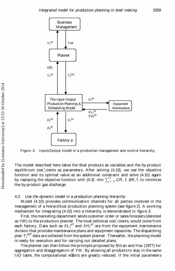
4.3. Use the dynamic model in a production planning hierarchyModel (4.10) provides communication channels for all parties involved in the
management of a hierarchical production planning system (see ® gure 2). A working
mechanism for integrating (4.10) into a hierarchy is demonstrated in ® gure 3.
First, the marketing department sends customer order or sales forecasts (denoted
as YM) to the production planner. The local technical coe� cients, would come fromeach factory. Data such as XL
…p†t and XH
…p†t are from the equipment maintenance
division that provides maintenance plans and equipment capacities. The dispatching
plan T…pq†t data are collected from the system planner. Thereafter, the planning model
is ready for execution and for carrying out detailed plans.
The planner can then follow the principle proposed by Bitran and Hax (1977) foraggregation and disaggregation of YM. By allowing all products to stay in the same
I± O table, the computational eŒorts are greatly reduced. If the initial parameters
2059Integrated model for production planning in steel making
Business Management Yt
(p) YM
Planner GRt
Yt(p) Tt
(pq)
The Input-Output Xt(p)
Production Planning & Equipment
Scheduling Model Maintenance XLt
(p) XHt
(p) Dt
(p) Xt
(p)
At(p)
Factory p
Figure 3. Input± Output model in a production management and control hierarchy.
Dow
nloa
ded
by [
Lin
naeu
s U
nive
rsity
] at
13:
53 1
6 O
ctob
er 2
014
result in infeasible solution, the planner could provide adjustments on the initial
parameters. It is possible that a bottleneck exists in the current system and achange in XL
…p†t and XH
…p†t becomes necessary. The planner may ask the factory
involved to rearrange its operational procedure so as to ease the bottleneck, where
the detailed plans will be decided according to particular circumstances.
5. Model evaluation
The proposed model was constructed with the historical data supplied by
Maanshan Iron and Steel Complex. Other sets of data were later obtained from
the organization to validate the proposed procedure. The model’s capability was
tested based on the plant’ s normal daily operation. Overall, the proposed modelincreases Maanshan’ s energy savings by almost 24% . As a result, the iron and
steel production rate increases by ¹20% due to the additional supply of the by-
product gas energy.
In other situation when set-up times and costs are involved, the zij table (table 4)
can record the amount of the time (or resource) needed to set up a machine fromproducing product i to product j. To calculate the costs of direct input, either
material or semi-product, the I± O model only needs to measure them by their
dollar values, instead of physical measurement, in formulating technical coe� cient,
aij . It is important to understand that the I-O model by itself is a balanced design. It
only discloses whether each constituent in the table maintains a su� cient amount.The optimization model is the very one that helps adequately allocate the excess gas
to various production units, thus enhancing overall system e� ciency.
Through the experiments, we found that the proposed model not only meets the
requirements of the hierarchical planning and control in Maanshan, but it is also
capable of identifying the bottleneck of the operational structure, including a feasi-
bility study of the long-run production plan. It provides, within a very reasonablecomputation time, comprehensive and optimal results in terms of iron and steel
production, by-product gas utilization and equipment maintenance plans.
6. Summary and conclusionThe major contributions of this research can be summarized as follows.
(1) It improves performance. Since the proposed model is capable of unifying
both global and local prospects within one integrated structure, complex
interactions and iterations between various levels as seen in conventional
decompositions are eliminated. Therefore, the model not only improvescomputational ef® ciency, but also helps obtaining global optimum.
(2) It provides a useful communication tool. Since the proposed model consis-
tently preserves the global view, it closely mimics the reality. Such ability
helps management of the company understand the model structure. As a
result, management is more willing to accept the proposed model.(3) It identi® es bottlenecks. The calculation as seen in constraint (4.4),
ZHt …I TtAAt† 1Yt, helps identify bottlenecks. By using market demand
Yt, and system capacity XHt, the negative difference found above will reveal
that bottlenecks are present in the system. (Positive outcome indicates suf® -
cient system capacity.) This approach is demand driven and only involvesstandard matrix calculation. No optimization procedure is needed prior to
the identi® cation of bottlenecks.
2060 H. Li and J. Shang
Dow
nloa
ded
by [
Lin
naeu
s U
nive
rsity
] at
13:
53 1
6 O
ctob
er 2
014
Models developed based on the speci® c structures of the manufacturing facility
signi® cantly increase overall system e� ciency. In conducting this research, we spenta large amount of time identifying the problem and de® ning the data before the I± O
model was chosen. The approach takes account of the geographically dispersed
situation and the need to synchronize the production of main products and by-
product gas. The dispatch matrix, Tt, and technical matrix, AA can capture andmodel both the individual and the global aspects of the problem without arti ® cially
decompose a system. Since this modelling approach preserves the `global view’,
physical ¯ ow in the network is well represented. It not only maximizes system
output and minimizes environmental pollution, but also provides resource consump-
tion information. Hence, it adds to the accuracy of product cost calculation. As a
consequence, it is eŒective in addressing practical and complicated manufacturing
management issues.The model itself is easy to implement and guarantees good results. Although the
procedure presented in this paper was developed speci® cally for Maanshan, due to
its general structure, we believe the proposed framework is useful for managing
systems involving by products. In particular, it is suitable for managing various
centralized and decentralized supply chain networks, due to their similarity in struc-ture to the studied problem. Bene® ts of the model may be best observed when
members of the manufacturing network play the role of the supplier and consumer
simultaneously. For example, the proposed framework is useful in modelling the
problem of Ford Explorer’s recall of Firestone tires. The returned tires will be
recycled and part of the recycled materials may later become inputs. This turnsthe supplier of the output (tires) into the consumer of its own product (recycled
tires). Traditional production management approach is incapable of handling such
loop situations, while the proposed model could analyse such supply-demand rela-
tionships e� ciently.
Despite similarity between the structure of ® rms and the composition of indus-
tries in an economy, no researchers have thus far taken advantage of I± O analysisand applied it to production/operations management domain. This research pro-
mises to be an innovative application of economics theory, and hopefully it will
provide a new and useful tool for researchers in the area of production and opera-
tions management.
Acknowledgement
This research was partially supported by an Institute for IndustrialCompetitiveness grant.
References
ASSAF, I., CHEN, M. and KATZBERG, J., 1997, Steel production schedule generation.International Journal of Production Research, 35, 467± 477.
BITRAN, G. and HAX, A., 1977, On the design of hierarchical production planning systems.Decision Sciences, 8, 25± 55.
BOX, R. and HERBE, D., JR, 1988, A scheduling model for LTV Steel’s Cleveland Works’ twinstrand continuous slab caster. Interfaces, 18, 42± 56.
CHEN, X. and LI, B., 1985, Economic-Mathematic Methods and Models (PR China: Financeand Economics Press).
CHO, C. H., 1981, Energy Management Applications for the Steel Industry, Iron and SteelEngineer, 8, 54± 60.
2061Integrated model for production planning in steel making
Dow
nloa
ded
by [
Lin
naeu
s U
nive
rsity
] at
13:
53 1
6 O
ctob
er 2
014

HAX, A. and MEAL, H., 1975, Hierarchical Integration of Production and Scheduling. In M.A. Geisler (ed.), Studies in the Management Sciences, 1, Logistics (Amsterdam: North-Holland and American Elsevier), pp. 53± 69.
JACOBS, T., WRIGHT, J. and COBBS, E., 1988, Optimal inter-process steel production sched-uling. Computers and Operations Research, 15, 497± 507.
JIMICHI, Y., HORI, A., ISHIHARA, H. and ODAIRA, T., 1990, An expert system of automaticslab assignment for hot strip mill. ISIJ International, 30, 155± 160.
LEONTIF, W., 1966, Input± Output Economics (New York: Oxford University Press).LIN, C. W. and MOODIE, C. L., 1985, An Energy-EVective Production Scheduling Strategy for
Hierarchical Control of Steel Manufacture. PLAIC Report no. 147 (West Lafayette:Purdue Laboratory for Applied Industrial Control, Purdue University).
LIN, C. W. and MOODIE, C. L., 1989, Hierarchical production planning for a model steelmanufacturing system. International Journal of Production Research, 27, 613± 628.
MACKULAK, G. T., MOODIE, C. L. and WILLIAMS, T. J., 1980, Computerized hierarchicalproduction control in steel manufacture. International Journal of Production Research,18, 455± 465.
MILLER, R. E., POLENSKE, K. R. and ROSE, A. Z. (eds), 1989, Frontiers of Input± OutputAnalysis (New York: Oxford University Press).
NUMAO, M. and MORISHITA, S., 1988, Scheplan Ð a scheduling expert for steel-making pro-cess. Proceedings of the International Workshop on ArtiWcial Intelligence for IndustrialApplications, 25± 28 May, Hitachi, pp. 467± 472.
O’ CONNOR, R. and HENRY, E. W., 1975, Input-output analysis and its applications. InGriYn’ s Statistical Monographs and Courses, 36 (Hafner).
PETERMEN, C. SORENSEN, K. and VIDAL, R., 1992, Inter-process synchronization in steelproduction. International Journal of Production Research, 30, 1415± 1425.
SATO, S., YAMAOKA, T., AOKI, Y. and UEDA, T., 1977, Development of integrated productionscheduling system for iron and steel works. International Journal of ProductionResearch, 15, 539± 552.
SOHN, I. (ed.), 1986, Readings in Input± Output Analysis, Theory and Applications (New York:Oxford University Press).
SZTRIMBELY, W., WEYMOUTH, P. and PONZO, T., 1989, An expert systems approach to rule-based dynamic process plant scheduling. In M. Y. Demeri (ed.), Expert SystemApplications in Materials Processing and Manufacturing (Minerals, Metals &Materials Society).
WILLIAMS, T. J. (ed.), 1985, Design of Hierarchical Control Systems: With Special Reference toSteel Plant Operations (PLAIC and Elsevier).
2062 Integrated model for production planning in steel making
Dow
nloa
ded
by [
Lin
naeu
s U
nive
rsity
] at
13:
53 1
6 O
ctob
er 2
014