integrated modelling of river management and ... · integrated modelling of river management and...
TRANSCRIPT
Integrated modelling of river management and infrastructure options to improve environmental outcomes in the Lower River Murray IC Overton, BA Bryan, AJ Higgins, K Holland, D King, RE Lester, M Nolan, D Hatton MacDonald, R Oliver, Z Lorenz and JD Connor
Report prepared for South Australian Department of Water, Land and Biodiversity Conservation
20 October 2010

Water for a Healthy Country Flagship Report series ISSN: 1835-095X
Australia is founding its future on science and innovation. Its national science agency, CSIRO, is a powerhouse of ideas, technologies and skills.
CSIRO initiated the National Research Flagships to address Australia’s major research challenges and opportunities. They apply large scale, long term, multidisciplinary science and aim for widespread adoption of solutions. The Flagship Collaboration Fund supports the best and brightest researchers to address these complex challenges through partnerships between CSIRO, universities, research agencies and industry.
The Water for a Healthy Country Flagship aims to achieve a tenfold increase in the economic, social and environmental benefits from water by 2025.
For more information about Water for a Healthy Country Flagship or the National Research Flagship Initiative visit www.csiro.au/org/HealthyCountry.html
Enquiries should be addressed to:
Ian Overton CSIRO Water for a Healthy Country PMB No. 2, Glen Osmond, SA, 5064
Citation: Overton IC, Bryan BA, Higgins AJ, Holland K, King D, Lester RE, Nolan M, Hatton MacDonald D, Oliver R, Lorenz Z, and Connor JD (2010) Integrated modelling of river management and infrastructure options to improve environmental outcomes in the Lower River Murray. CSIRO: Water for a Healthy Country National Research Flagship. Technical report prepared for the South Australian Department of Water, Land and Biodiversity Conservation. 121 pp.
Copyright and Disclaimer
© 2010 CSIRO To the extent permitted by law, all rights are reserved and no part of this publication covered by copyright may be reproduced or copied in any form or by any means except with the written permission of CSIRO.
Important Disclaimer
CSIRO advises that the information contained in this publication comprises general statements based on scientific research. The reader is advised and needs to be aware that such information may be incomplete or unable to be used in any specific situation. No reliance or actions must therefore be made on that information without seeking prior expert professional, scientific and technical advice. To the extent permitted by law, CSIRO (including its employees and consultants) excludes all liability to any person for any consequences, including but not limited to all losses, damages, costs, expenses and any other compensation, arising directly or indirectly from using this publication (in part or in whole) and any information or material contained in it.
Cover image CSIRO staff discuss management options with officers from the South Australian Murray Darling Basin Natural Resource Management Board, 2005 on the Chowilla Floodplain. Photograph by Ian Overton.

Integrated Modelling of the Lower River Murray iii
EXECUTIVE SUMMARY Water dependent ecosystems of the Lower River Murray in South Australia are highly stressed, primarily due to river regulation and drought causing river flows that lack appropriate magnitude, frequency, duration, and timing to support ecological functions. Low river flows are predicted to increase in frequency into the future under climate change predictions. In combination with increased environmental flows, the ecological health of these water dependent ecosystems can be enhanced by the operation of existing and new flow-control infrastructure (weirs and regulators) to return more natural environmental flow regimes to specific areas. However, determining the optimal investment and operation strategies over time is a complex task due to several factors including the multiple environmental, economic, and social values attached to wetlands, spatial and temporal heterogeneity and dependencies, non-linearity, and time dependent decisions. This makes for a very large number of decision variables over a long planning horizon. To assess ecological benefit of flow manipulation two approaches have been developed. Firstly the range of habitats derived by a series of hydrological variables has been compared to historical conditions. The benefit of a similar range of habitats is that biodiversity is likely to be similar to historical conditions while allowing for ecological adaption. Secondly the health of current vegetation, fish and bird habitats has been assessed using a range of ecological response curves. Ecological response models were developed to link three aspects of environmental flows (flood duration, timing, and interflood period) to the health responses of ecosystem components. The infrastructure investments (flow-control regulators and irrigation pump relocation) were sited by interpreting high resolution LiDAR elevation data, digital orthophotography, and wetland mapping information; and their costs were quantified using a spreadsheet-based model. Social values were also estimated using a choice model quantifying willingness to pay for various ecosystem components and these were also included in the model. These diverse datasets and models were integrated in a decision support tool based on non-linear integer programming to investigate the cost-effectiveness of alternative flow levels and timing, existing flow-control infrastructure operation, and new infrastructure investment alternatives, given wider system constraints. The decision support tool can identify a suite of cost-effective infrastructure investments and a plan for their operation specifying where and when to capture and release water in water dependent ecosystems. Outputs include a ranking of investment alternatives and operational rules for managing flow-control infrastructure to achieve ecological and social values at minimum economic cost. The results have provided a priority listing of investments under three scenarios which were compared to the baseline (do-nothing) scenario:
Firstly using new regulators on wetlands and pump relocations only (infrastructure investment);
Secondly using infrastructure investments and weir manipulation through raising and lowering; and
Thirdly using infrastructure investments and weir raising only. The ecological benefits from the range of investments identified are seen in improvements in the flood duration brought about through wetland regulation. The river flow history is the most important component of the modelling. Two hydrographs from a period of 1895 to 2006 were available that represented current and natural conditions. Current flow was modelled by using climate data over the time period and current (2009) river abstraction rules. The natural flow data was modelled using actual climate data and no water abstraction rules.

Integrated Modelling of the Lower River Murray iv
For model runs that only used infrastructure investments (scenario 1) the improvements to aquatic vegetation, bird breeding, fish and floodplain vegetation habitats was 56%, 39%, 48% and 10% respectively. The best outcome was achieved when weir raising, lowering and investments were introduced (scenario 3). The overall benefit improved with improvements to aquatic vegetation, bird breeding, fish and floodplain vegetation habitats increasing by 54%, 40%, 51% and 22% respectively. The reduction in the benefits to aquatic vegetation with the introduction of weir manipulation is because the approach was to optimise the outcome of all four components. The above results incorporate flood timing, interflood periods and flood duration. Greater ecosystem benefits have been identified coming from the duration changes rather than the flood timing and interflood periods. This may be a factor of the ecosystem response curves used or their integration, however, these hydrological variables are less influenced by small regulators and more influenced by changing the timing and frequency of floods coming into South Australia. At sites permanently below that of the pool levels changing the timing, frequency and magnitudes of floods to SA will have limited impacts because they are permanently drowned/inundated due to the operation of the weirs. Simplifying the problem facing management of the SA River Murray in returning “natural” conditions or at least a representative mosaic of the/a “natural” state there are two issues for management those areas that receive too much water (below pool) & those that receive too little (above pool). Different approaches are needed to ensure that both these issues are addressed. For the permanent wetlands the flood timing, interflood and duration are all unchanged if no wetting or drying can be implemented. Hence the need for investment in wetland regulators to gain ecological benefits at these below pool sites. The project did not consider the removal of any existing inappropriate regulatory structures. This option would affect the wetlands and would likely improve the overall results. The model results assume no changes to water across the border into South Australia. The model could be extended to consider operational rules that could show benefits from environmental flows into South Australia.

Integrated Modelling of the Lower River Murray v
ACKNOWLEDGEMENTS We gratefully acknowledge the financial and technical support of the SA Department of Water, Land, and Biodiversity Conservation, especially the project Directors Rajiv Mouveri and Judy Goode. We are also grateful for the support of CSIRO’s Water for a Healthy Country National Research Flagship.
Integrated Modelling of the Lower River Murray vi
CONTENTS
Executive Summary .................................................................................................... iii
Acknowledgements ...................................................................................................... v
1. Introduction ......................................................................................................... 1 1.1. Background ............................................................................................................... 1
1.2. Project objectives ...................................................................................................... 3
1.3. Project method .......................................................................................................... 5
2. Ecological Objectives ......................................................................................... 7 2.1. Landscape approach .............................................................................................. 10
2.2. Health approach ...................................................................................................... 12
3. Ecohydrological Classification ........................................................................ 13 3.1. Wetlands and watercourses .................................................................................... 13
3.2. Floodplains .............................................................................................................. 18
4. River Hydrology and Floodplain Mapping ...................................................... 24 4.1. River hydrology ....................................................................................................... 24
4.2. Wetland and floodplain inundation .......................................................................... 24
5. Infrastructure and Weir Operation ................................................................... 27 5.1. Infrastructure ........................................................................................................... 27
5.1.1. Regulators and cost estimates ............................................................................ 27 5.1.2. Pump relocations and cost estimates .................................................................. 29 5.1.3. Infrastructure cost estimates ............................................................................... 31
5.2. Weir operations ....................................................................................................... 33
6. Assessing Likely Ecological Response .......................................................... 37 6.1. Ecological response models for the Lower Murray ................................................. 37
6.2. Linking ecological response and ecohydrological units .......................................... 39
6.3. Combining ecological response models ................................................................. 40
7. Social Values Incorporated in the Model ........................................................ 42 7.1. Stated preference values ........................................................................................ 42
7.2. Mapped community values ..................................................................................... 43
8. Integrated Modelling and Analysis .................................................................. 44 8.1. Mathematical model ................................................................................................ 44
8.1.1. Decision variables ............................................................................................... 44 8.1.2. Constraints .......................................................................................................... 44 8.1.3. Objective function ................................................................................................ 45
8.2. Solution method ...................................................................................................... 45
9. Results ............................................................................................................... 47 9.1. Scenarios ................................................................................................................ 47
9.2. Investment results ................................................................................................... 47 9.2.1. Scenario 2 – Infrastructure but no weir manipulation .......................................... 47 9.2.2. Scenario 3 – Infrastructure and weir raising and lowering ................................... 50 9.2.3. Scenario 4 – Infrastructure and weir raising only ................................................ 53
9.3. Ecological Results ................................................................................................... 56 9.3.1. Scenario 2 – Infrastructure but no weir manipulation .......................................... 56 9.3.2. Scenario 3 – Infrastructure and weir raising and lowering ................................... 61 9.3.3. Scenario 4 – Infrastructure and weir raising only ................................................ 65

Integrated Modelling of the Lower River Murray vii
10. Discussion ......................................................................................................... 70 10.1. Ecological benefits .................................................................................................. 70
10.2. Priority investments ................................................................................................. 71
10.3. Limitations of the ecological response models ....................................................... 71
10.4. Further analysis and refinements............................................................................ 72
10.5. Conclusion .............................................................................................................. 73
References .................................................................................................................. 75
Appendix A. Investment Locations .......................................................................... 79
Appendix B. Ecological Responses by Ecohydrological Types ............................ 96
Appendix C. Ecological Responses ....................................................................... 100
Appendix D. Ecological Response Curves ............................................................ 102
Appendix E. Mathematical Programming Model ................................................... 113

Integrated Modelling of the Lower River Murray viii
LIST OF FIGURES
Figure 1. South Australian River Murray floodplain. ................................................................. 2
Figure 2. Method adopted for the project. ................................................................................ 6
Figure 3. Landscape approach showing the area of floodplain and wetlands over a range of percentage of time inundated. Four scenarios are presented including historic, current, a management strategy and an investment scenario. ............................................................... 11
Figure 4. Two examples of species response curves for flood duration and interflood dry period (Young et al. 2003). The response curves used in this project are shown in Appendix C. ............................................................................................................................................ 12
Figure 5. Relationship between River Murray flow (ML d-1) and SAAE wetland type area (ha). ............................................................................................................................................... 14
Figure 6. Distribution of SAAE wetland type area (ha) through River Murray flows (ML d-1). 14
Figure 7. A portion of the South Australian River Murray floodplain showing the Ecohydrological types for watercourses. ................................................................................ 15
Figure 8. A portion of the South Australian River Murray floodplain showing the Ecohydrological types for wetlands. ....................................................................................... 17
Figure 9. Relationship between River Murray flow (ML d-1) and floodplain EH type area (ha) and as a proportion of total EH type area (%). ....................................................................... 19
Figure 10. Relationship between River Murray flow (ML d-1) and floodplain EH type area (ha). ............................................................................................................................................... 20
Figure 11. A portion of the South Australian River Murray floodplain showing the Ecohydrological types for floodplains. .................................................................................... 21
Figure 12. A portion of the South Australian River Murray floodplain showing the Ecohydrological types. ........................................................................................................... 23
Figure 13. The hydrographs used in the project. The Natural hydrograph is estimated from actual climate data with no water abstraction. The Current hydrograph is modelled with actual climate and current (2009) abstraction rules. Data provided by the CSIRO MDBSY project. .................................................................................................................................... 24
Figure 14. Cross section of the River Murray showing the different commence to fill levels needed to over top the sill levels. ........................................................................................... 25
Figure 15. Commence to fill values for different wetland and floodplain features. ................. 26
Figure 16. Regulators positioned to enable isolation of wetland from river as determined by LiDAR data ............................................................................................................................. 28
Figure 17. Many wetlands along the River Murray have very large connection with the River channel making regulators too large to be an option. ............................................................ 29
Figure 18. An example of new pipes to relocate pumps for irrigation use. Pumps (in red) have in these cost estimates been calculated based on distances to the nearest part of channel. What is required is better planned infrastructure investment that delivers water to multiple customers along common pipelines. This is not possible to automate and requires the interpretation of each individual wetland to calculate required pipe lengths to move pumps. 30
Figure 19. Portion of the River Murray showing the locations of regulators and pump relocation pipes. The full range of investments have been mapped in Appendix A. .............. 33

Integrated Modelling of the Lower River Murray ix
Figure 20. An example of a backwater graph for one of the weir reaches showing the different river heights achieved from different flows. These curves and those for different weir levels are used within the RiM-FIM model to predict wetland connectivity. ........................... 36
Figure 21. Example of an ecological response function for the health of colonial nesting water birds against inter-flood duration from Young et al. [2003]. .................................................... 37
Figure 22. Graph of wetland/floodplain area improved versus investment cost. .................... 50
Figure 23. Weir regulation used in the optimum solution for investment and weir operation in Scenario 3. The operating regime is a result of the model optimising outcomes. .................. 53
Figure 24. Weir regulation used in the optimum solution for investment and weir operation in Scenario 4 Compared to scenario 3, only weir heights of >0cm were allowed, thus leading to a cycle variation compared to Figure 22. ............................................................................... 56
Figure 25.. Summary of ecological benefits from Scenario 2. Red indicates the area of the floodplain that achieved a good ecological score under base scenario (current conditions). Blue shows the area that used to occur under natural conditions. Green shows the area that has been improved as a result of the scenario across all hydrographs combinations. Note the term terrestrial vegetation here refers to floodplain vegetation. ............................................. 58
Figure 26. Graphs showing the floodplain and wetland areas in good ecological health under base case (current), natural and model scenario 2 for flood timing. ...................................... 59
Figure 27. Graphs showing the floodplain and wetland areas in good ecological health under base case (current), natural and model scenario 2 for interflood period. ............................... 60
Figure 28. Graphs showing the floodplain and wetland areas in good ecological health under base case (current), natural and model scenario 2 for flood duration. ................................... 61
Figure 29. Summary of ecological benefits from Scenario 3. Red indicates the area of the floodplain that achieved a good ecological score under base scenario (current conditions). Blue shows the area that used to occur under natural conditions. Green shows the area that has been improved as a result of the scenario. Note the term terrestrial vegetation here refers to floodplain vegetation. ............................................................................................... 62
Figure 30. Graphs showing the floodplain and wetland areas in good ecological health under base case (current), natural and model scenario 3 for flood timing. ...................................... 63
Figure 31. Graphs showing the floodplain and wetland areas in good ecological health under base case (current), natural and model scenario 3 for interflood period. ............................... 64
Figure 32. Graphs showing the floodplain and wetland areas in good ecological health under base case (current), natural and model scenario 3 for flood duration. ................................... 65
Figure 33. Summary of ecological benefits from Scenario 4. Red indicates the area of the floodplain that achieved a good ecological score under base scenario (current conditions). Blue shows the area that used to occur under natural conditions. Green shows the area that has been improved as a result of the scenario. Note the term terrestrial vegetation here refers to floodplain vegetation. ............................................................................................... 66
Figure 34. Graphs showing the floodplain and wetland areas in good ecological health under base case (current), natural and model scenario 4 for flood timing. ...................................... 67
Figure 35. Graphs showing the floodplain and wetland areas in good ecological health under base case (current), natural and model scenario 4 for interflood period. ............................... 68
Figure 36. Graphs showing the floodplain and wetland areas in good ecological health under base case (current), natural and model scenario 4 for flood duration. ................................... 69
Figure C.37. Response of adult floodplain river red gums to: a) flood duration (days); b) flood timing; and c) interflood period (months) .............................................................................. 102

Integrated Modelling of the Lower River Murray x
Figure C.38. Response of floodplain river red gum seedlings to: a) flood duration (days); and b) flood timing ....................................................................................................................... 102
Figure C.39. Response of adult floodplain river red gums to: a) flood duration (days); and b) interflood period (months) .................................................................................................... 103
Figure C.40. Response of adult black box to: a) flood duration (days); b) flood timing; and c) interflood period (months) .................................................................................................... 103
Figure C.41. Response of black box seedlings to: a) flood duration (days); and b) flood timing ............................................................................................................................................. 103
Figure C.42. Response of adult lignum to: a) flood duration (days); b) flood timing; and c) interflood period (months) .................................................................................................... 104
Figure C.43. Response of lignum seedlings to: a) flood duration (days); and b) flood timing ............................................................................................................................................. 104
Figure C.44. Response of adult salt-tolerant woodland vegetation to: a) flood duration (days); and b) interflood period (months) ......................................................................................... 105
Figure C.45. Response of adult chenopods to: a) flood duration (days); and b) interflood period (months) .................................................................................................................... 105
Figure C.46. Response of adult Phragmites australis to: a) flood duration (days); b) flood timing; and c) interflood period (months) .............................................................................. 106
Figure C.47. Response of black box seedlings to flood timing ............................................. 106
Figure C.48. Response of adult ribbonweed to: a) flood duration (days); and b) flood timing ............................................................................................................................................. 106
Figure C.49. Response of ribbonweed seedlings to flood timing ......................................... 106
Figure C.50. Response of colonial nesting waterbird breeding to: a) flood duration (days); and c) interflood period (months) ......................................................................................... 107
Figure C.51. Response of waterfowl and grebe habitat to: a) flood duration (days); and c) interflood period (months) .................................................................................................... 107
Figure C.52. Response of adult main channel specialists to: a) flood duration (days); b) flood timing; and c) interflood period (months) .............................................................................. 108
Figure C.53. Response of main channel specialist spawning to: a) flood duration (days); and b) likely spawning timing ...................................................................................................... 108
Figure C.54. Response of flood spawners to: a) flood duration (days); b) flood timing; and c) interflood period (months) .................................................................................................... 108
Figure C.55. Likely spawning timing for flood spawners ...................................................... 109
Figure C.56. Response of adult wetland specialists to: a) flood duration (days); b) flood timing; and c) interflood period (months) .............................................................................. 109
Figure C.57. Likely spawning timing for wetland specialists ................................................ 109
Figure C.58. Response of adult freshwater catfish to: a) flood duration (days); b) flood timing; and c) interflood period (months) ......................................................................................... 110
Figure C.59. Response of freshwater catfish spawning to: a) flood duration (days); and b) likely spawning timing ........................................................................................................... 110
Figure C.60. Response of adult main channel generalists to: a) flood duration (days); b) flood timing; and c) interflood period (months) .............................................................................. 111
Figure C.61. Response of main channel generalist spawning to: a) flood duration (days); and b) likely spawning timing ...................................................................................................... 111

Integrated Modelling of the Lower River Murray xi
Figure C.62. Response of adult low flow specialists to: a) flood timing; and b) interflood period (months) .................................................................................................................... 111
Figure C.63. Response of low flow specialist spawning to: a) flood duration (days); and b) likely spawning timing ........................................................................................................... 112
LIST OF TABLES
Table 1: Floodplain ecohydrological types. ............................................................................ 18
Table 2: Areas of each Ecohydrological types in South Australia. ......................................... 22
Table 3. Investments considered in the model, ordered by decreasing cost. ........................ 31
Table 4: River Murray locks and weirs ................................................................................... 34
Table 5. Weir raising constraints in South Australia (SA Water). ........................................... 35
Table 6. Biotic communities described by MFAT for Zones E and G (Young et al. 2003) ..... 38
Table 7. Area weighted mean River Murray flow (GL d-1), flood duration (days) and interflood period (months) for each EH type and total floodplain area. Area weighted standard deviations are also shown. ..................................................................................................... 39
Table 8. Attribute levels used in the choice sets. ................................................................... 42
Table 9: Investment ranking lists as a result of Scenario 2 showing the percentage of time in optimal solutions for all hydrographs and for the 1986-2006 (most recent) period and the area of impact. ........................................................................................................................ 48
Table 10: Investment ranking lists as a result of Scenario 3 showing the percentage of time in optimal solutions for all hydrographs and for the 1986-2006 (most recent) period and the area of impact. ........................................................................................................................ 50
Table 11: Investment ranking lists as a result of Scenario 4 showing the percentage of time in optimal solutions for all hydrographs and for the 1986-2006 (most recent) period and the area of impact. ........................................................................................................................ 53
Table 12: Summarised ecological score of Scenario 2 versus Base and Natural for each ecological component. ............................................................................................................ 57
Table 13: Total scores (areas) for base case and natural case for ecological components. . 57
Table 14: Summarised ecological score of Scenario 3 versus Base and Natural for each ecological component. ............................................................................................................ 62
Table 15: Summarised ecological score of Scenario 4 versus Base and Natural for each ecological component. ............................................................................................................ 65

Integrated Modelling of the Lower River Murray 1
1. INTRODUCTION
1.1. Background The riverine environment of the River Murray in South Australia (Figure 1) is suffering due to long-term over-allocation of river water, regulation and reduced flows caused by drought. Many riparian, wetland, and floodplain ecosystems are highly stressed, primarily due to a lack of environmental flows at the quantity, timing, duration, frequency, rate of change, and quality required to sustain these ecosystems (Kingsford 2000, Bunn and Arthington 2002, Poff et al. 2007, Acreman and Ferguson 2010, Palmer et al. 2010, Poff and Zimmerman 2010). In highly regulated river systems, infrastructure such as dams, weirs, and regulators used to store and release water for consumptive purposes can also be used to return natural environmental flows (Poff et al. 1997) of appropriate quantity, timing, duration, frequency, and quality to enhance ecological health (Galat and Lipkin 2000, Bednarek and Hart 2005, Harman and Stewardson 2005, Lind et al. 2007, Holland et al. 2009, Poff et al. 2010). One proven management option being considered is the further construction of flow regulating structures across wetlands and the relocating of pumps accessing water from these wetlands to the main river channel. This will enable the re-introduction of wetting and drying cycles and a reduction in evaporation from wetlands permanently inundated as a consequence of regulating the river with weirs. A second option that is being considered is the operation of the weirs within South Australia to improve environmental outcomes. Of the six weirs along the river only three are currently being considered for manipulation, however in this project we modelled the manipulation of all six weirs in case this was an option later. Some ecological processes and species diversity are threatened by water availability and land management. These threats may result in a change of ecosystem state to a different type of ecosystem, for example from a floodplain vegetation community to a terrestrial vegetation community, that may be irreversible. There is a need to identify the critical ecosystem components that must be maintained, at a sustainable level, to ensure that the ecosystem can recover from this and future drought periods. The hydrological management issues for this river reach include a disproportionate number of permanent wetlands that have drowned riparian/floodplain areas. Most of these areas used to be ephemerally inundated under natural conditions but the installation of the weirs has increased river levels that have resulted in many permanent wetlands that no longer have natural flood frequencies or durations. The weirs and river extraction have reduced the frequency of floods causing a reduction in the frequency of flood events, a prolonging of the Interflood period and a decrease in the duration of flood events. In the upper reaches of the River Murray the flood timing has altered from natural conditions as a result of irrigation water transference, however this has less of an impact in the lower reaches.

Integrated Modelling of the Lower River Murray 2
Figure 1. South Australian River Murray floodplain.
Under the Australian Government’s $12.9B Water for the Future program the South Australian Government’s Murray Futures program is charged with making investments in water infrastructure. Part of this program aims to enhance the ecological health of water dependent ecosystems along the River Murray through investment in infrastructure such as flow regulation structures and weirs to enhance the ecological health of priority wetlands and floodplains while improving security for irrigation water users. The system is severely degraded as a result of the extended drought period and there is concern that critical ecosystem components, key species and ecosystem functions, may be irreversibly lost. It is essential to identify the critical elements of the ecosystem that can be allowed to be scaled down during dry years but in such a condition that it is able to be revived during wet years. It is therefore a requirement to understand the important ecosystems of the South Australian River Murray, which areas and species are critical, and what infrastructure could be invested in to protect these. Getting better environmental health outcomes requires consideration of associated issues especially how flow can be managed in concert with infrastructure investment to improve environmental outcomes. Additionally it is important to consider how infrastructure investment and flow management strategies are likely to impact local community economic and social well being. Some environmental assets may be more valued by local communities for aesthetic, recreational amenity and cultural reasons than others. There may be opportunities to offset some adverse regional economic, social impacts with investment. Notably, some of the important environmental assets in the region may be close to thresholds, beyond which, in absence of appropriate flow management in the near future, they will be irreversibly lost or so degraded that they will be difficult and expensive to restore. Planning for the return of environmental flows through infrastructure operation is a complex task. Riparian systems have spatially-heterogeneous ecological, economic, and social values, and are dominated by spatial dependencies and temporally dynamic hydrological and ecological processes. Decisions on where to locate significant investments in flow-control

Integrated Modelling of the Lower River Murray 3
infrastructure (or removal), and how to best operate this infrastructure over time to achieve multiple objectives are hard and involve multiple spatio-temporal decisions and trade-offs. Arthington et al. (2006) states that the increasing tendency of water managers to favour simplistic and static rules for governing environmental flows is misguided and is likely to lead to the further degradation of water dependent ecosystems. Arthington et al. (2010) called for a renewed focus on modelling the full complexity of eco-hydrological systems to find more acceptable and robust ways to manage environmental flows for water dependent ecosystems. The literature is rich with methodologies to optimally alter river flow to improve environmental or agricultural objectives. Previously, similar spatial, multi-period problems have been addressed through a variety of operations research techniques including stochastic dynamic programming (Tilmant et al. 2007), fuzzy logic (Abolpour and Javan 2007), meta-modelling (Mousavi and Shourian 2010), goal programming (Xevi and Khan 2005), and elitist-mutated particle swarm optimization (Reddy and Kumar 2007). Suen and Eheart (2006) used a genetic algorithm to quantify flow regimes that balanced ecological and human needs. Stewart-Koster et al. (2010) used Bayesian networks to guide investments in flow and catchment restoration for enhancing riparian ecosystem health. The River Murray in South Australia contains 9280 individual water course, floodplain, and wetland polygons along the 650km portion of the river (Figure 1). These were classified into 18 ecohydrological units based on vegetation mapping and commence-to-fill flow values (Overton 2005). A total of 16 ecosystem components were identified for the study area including vegetation communities, water bird habitat, and fish species. Many of these included separate response functions for adult and juvenile life stages totalling 27 individual response functions. Six weirs are located along the river with a range of operating height ranges. A total of 357 wetlands can be controlled by 125 regulators as wetland complexes, of which 43 of them are existing 82 are eligible to be built. The term regulator complex is used since a complex contains one or more wetlands controlled by one or more regulators. Regulators within a complex are operated simultaneously. There is a cost associated with building each of these 82 regulators to manage the wetland complexes (including moving irrigation pumps from wetlands). If all 82 regulators were built, the total cost would be $118 million. A planning horizon of 20 years (240 months) was used for the analysis in this project, with the natural and current hydrographs of 1986 to 2006.
1.2. Project objectives The primary objective of the project was to decide on the most appropriate investments that can enhance the ecological health of SA River Murray water dependent ecosystems, improving security of water for irrigation and prioritising investments that improve socio-economic outcomes. The main objectives can be summarised as:
Improve environmental health
Improve socio-economic outcomes
Reduce water losses from evaporation
Increase water access security for irrigation
In many cases these objectives can be complimentary. For example moving irrigation pumps to the main river channel from a back water wetland improves the water access security

Integrated Modelling of the Lower River Murray 4
while allowing a wet and dry cycle to be established in the back water, reducing evaporation losses and producing a more natural flow regime for the wetland, potentially increasing environmental health and social aesthetic values. However, there are costs associated with wetland and floodplain management decisions. Costs include the upfront infrastructure investments, follow-on cost associated with changes in system ecological health and water quality changes from changed flow management, employment and population impacts and less tangible costs such as the impacts on families and communities. Investment in environmental flow management for enhancing wetland health along the SA River Murray is a complex problem with complexity arising from at least the following characteristics: Spatial heterogeneity – Ecological values and asset conditions vary across floodplains and wetlands along the river. So too does the environmental water requirement to provide improvement in ecological health, and the capacity to enhance ecological benefits of flow with infrastructure investment. Key elements of this heterogeneity include: (a) differences in the extent to which area of floodplains and wetland contain important ecological assets, (b) elevations of floodplains and wetlands which influence the level of flow required to inundate, (c) differences across asset types in the duration, timing and return intervals required to achieve desired ecological outcomes, (d) differences in the structure of channels and geomorphology of floodplains and wetlands that influence the feasibility of infrastructure to enhance ecological impacts of flows, (e) differences in the degree of impact of salinisation related to surface water and groundwater interactions. Spatial interdependence – Some ecological outcomes depend not only on the pattern of flow on individual units but on the extent of flows across the system in total and on connectivity through flow between units. Many ecological benefits are derived at a landscape scale such as fish passage and bird breeding and foraging habitats. In many cases flows of sufficient magnitude to influence ecological health on a particular targeted asset will have some benefits for other ecological and water quality outcomes elsewhere. However, flow patterns most desirable for one ecological outcome often don’t completely correspond to those most desirable for other ecological outcomes. Inter-temporal dependence and future flow uncertainty – The overall level of flow that will be available in the future is uncertain and to a large extent beyond the control of decision makers in South Australia. Flow that will be available for the environment is largely determined by how future climate influences overall inflows to the system and on how decisions at a system level to allocate available flows to multiple in some case competing uses are made by the Murray-Darling Basin Authority. However, the one component of River Murray flow within South Australia that has high levels of certainty is the maintenance of relatively stable weir pools in particular those above Lock 1. Diverse values – Different people value different type of environmental assets at different locations differently. Results of a purely scientifically ecological prioritisation of where to invest may not correspond perfectly with results of prioritisation driven by other fields of study or elements of society such as local social or cultural values. The overall scarcity of water in the system leads to a need to consider trade-offs over time in choices to allocate water for the environment. An adequate decision support framework will need to consider trade-offs between more extensive flooding in one year and less potential to provide environmental flows in future years whilst being mindful of political/legal constraints of the water allocation system., and where to invest and allocate water from a ecological, indigenous, and non-indigenous local social / cultural perspectives.

Integrated Modelling of the Lower River Murray 5
Given the nature of the problem described above, it is evident that a decision support tool is needed that is capable of answering the following questions:
Determine objectives. Which wetlands / floodplains do we target for management to ensure that critical species and ecosystem functions can recover in wetter years?
What management investments do we make to maximise use of available water? (e.g. flow control, supporting infrastructure such as fish passages, walkways etc.)
What is the best way to manage environmental flow regimes for managing high priority floodplains and wetlands? (how much water, where, when, and in what order?)
What is the appropriate landscape configuration/mosaic of water dependent ecosystems across the landscape?
1.3. Project method The project method needed to provide an approach for three main objectives of improving ecological benefit while providing water savings and considering impact on social values. The project needed to involve:
Hydrology - Development of river system hydrology modelling capacity to use flows over the SA border, predict inundation of floodplains and wetlands, and predict return flows to the river following environmental watering; Infrastructure – Development of impacts and costs for a range of investments including new regulators, moving irrigation pumps and operation of the main River Murray weirs; Ecology - Development and application of ecosystem responses to changes in flood duration and frequency to maximise environmental benefit from a range of investments and influence infrastructure operation; Socio-economics - Development of modelling capacity to estimate socio-economic impacts of infrastructure investment and flow management options including: infrastructure investment costs, and economic benefits from enhanced environmental flows such as improved tourism opportunities, and reduced municipal industrial water treatment costs; Integration – Development of a decision support tool to rank possible investments and combine weir operation scenarios to derive a short list of investments to be further considered for implementation.
Figure 2 shows the analytical steps involved in the project. The steps involved are further explained below.

Integrated Modelling of the Lower River Murray 6
Figure 2. Method adopted for the project.

Integrated Modelling of the Lower River Murray 7
2. ECOLOGICAL OBJECTIVES A key objective of the Project is to improve the environmental condition of the river and its associated water dependent ecosystems. This requires describing an acceptable and attainable environmental outcome, or a set of alternative outcomes, that could be achieved by managed water delivery to the interconnected water dependent ecosystems that make up the SA River Murray environment. As future water availability is uncertain, the target conditions need to be flexible and scalable within the capacity of the ecosystems to respond to change and our ability to manage them. A key question is how to determine the environmental targets that flow management should aim to achieve. This is not a simple question, or a new one. The river system is made up of the river channel, riparian zone, floodplain, and alluvial aquifer. Consequently, not only is longitudinal connectivity important but also lateral and vertical connections (Ward 1989). However, much of the discussion and effort around defining environmental flows for rivers has been focussed on in-stream conditions (Richter et al. 1996; Poff et al. 1997; Arthington et al. 2006) rather than the entire system. Several hundreds of methods have been devised for environmental flow assessment with a focus on different characteristics of the river condition including hydrological rules, hydraulic rating methods, habitat simulation methods and holistic methods (see reviews by Tharme 2003; Arthington et al. 2006). Attempts have been made to encapsulate these various approaches into the “natural flow regime” paradigm (Richter et al. 1996; Poff et al. 1997), which recognises the importance of flow patterns in creating and maintaining riverine habitats and biodiversity. It proposes that to sustain ecological conditions, management strategies must reproduce characteristic river flow patterns, including the magnitude, frequency, timing, duration, rate of change, and predictability of events such as floods and base flows (Richter et al. 1996; Poff et al. 1997). Application of this approach in the “Range of Variability” method relies on 32 different hydrological parameters to characterise the stream flow record (Richter et al. 1997). The RVA method recommends that managed flows should attempt to be within one standard deviation of the mean of each of the hydrological indicators obtained under a reference condition. This can be a difficult task for those managing flows in regulated systems with alternative requirements for water delivery to support agricultural, industrial and urban uses. A limitation of the flow pattern approaches is that they do not explicitly relate ecological responses to hydrological changes, making it difficult to assess the environmental benefits arising from the flow management (Stewardson and Gippel 2003). Some methods have attempted to identify the ecological significance of hydrological changes by relating them to specific flow habitat niches required by aquatic biota such as fish, macroinvertebrates and aquatic vegetation (Bovee and Milhous 1978; Stewardson and Cottingham 2002; Lytle and Poff 2004). A difficulty with this approach is quantifying the connections between hydrological characteristics and the desired ecological outcomes. In some cases specific niche requirements for particular organisms have been identified and used to indicate the overall condition of a system (Bovee and Milhous 1978). In other cases more general physical responses, such as mean depth over riffle zones or illuminated area of sediments, have been included to broaden and generalise the description of habitat conditions (Stewardson and Cottingham 2002; Stewardson and Gippel 2003; Cottingham et al. in press). These more holistic approaches are often applied in conjunction with expert panels and underpin approaches such as the Victorian Environmental Flows Monitoring and Assessment Program (Cottingham et al. 2005). Despite the continuing development in environmental flows assessment techniques, there remains considerable debate over the appropriateness of the different methods and their mode of application. The most difficult problem is still to quantify the connections between altered flow characteristics and the myriad of ecological responses that determine the

Integrated Modelling of the Lower River Murray 8
ecological outcomes. Yet this quantification is necessary so that environmental flow requirements can be predicted and the potential benefits of environmental flow allocations estimated. Although considerable effort has gone into developing environmental flow methods for rivers, surprisingly little has included explicit assessment of floodplain connections. In situations where the floodplain has been included, analyses have generally relied on hydrological approaches quantifying the magnitude and occurrence of flood peaks. Occasionally the periods of inundation of specific floodplain habitats such as wetlands or forested areas have been assessed. However, holistic analyses of the interconnected floodplain ecosystems over whole, or even significant parts of river valleys, are rare. Part of the difficulty is the need for a spatially explicit floodplain inundation model that describes the connection between discharge height and flood extent. Although flood modelling is well established for many rivers in the developed world, these models are mostly aimed at providing flood damage forecasting for built infrastructure. They are less often created for assessing ecological connectivity in areas where more natural floodplain conditions may still prevail. The Murray Flows Assessment Tool (MFAT) is a decision support system that was developed to describe the ecological implications of modifying flows within the Murray River (Young et al. 2003). It can be applied either to regions or to the length of the Murray River, and makes an assessment of the impacts of flow changes to both in-stream and floodplain areas. The basis of the modelling relies on specific ecological response functions determined for a range of key organisms from published information, or in the many cases where this was not available, from expert opinion and consensus. The ecological responses are functions of hydrological characteristics of the channel and floodplain. As a flood model was not available, modelling of the connectivity between river and floodplain is dependent on a user developed “pipe and pond” description of the floodplain in the area of interest. Indices of suitability for a given river hydrograph are calculated based on the occurrence of the conditions required to support particular organisms. These indices are usually combined across organisms to give a single parameter that integrates the effects of river flow. Indices derived from hydrographs representing different flow management strategies are then compared to the indices obtained using modelled, pre-development, river flows to asses the impact of changes. MFAT represents the most advanced attempt at environmental flows modelling for the River Murray, but it has not been extensively used, probably because of the difficulty representing floodplain connections, uncertainties regarding the ecological response functions that it relies on, and the abstract nature of the condition indices that make it difficult to envisage the resulting landscape outcomes. The use of flood inundation modelling and LiDAR in this project is seen as a progressive step forward in the application of response curves to landscape scale habitat modelling. However, the MFAT does describe an approach that is likely to prove useful to new model development and it provides some of the most considered ecological response functions currently available. This project has adopted two approaches to investigating ecological benefits. These are:
Landscape - Improving hydrological habitat diversity through improving the
duration and frequency of flooding across the range of natural flow extents.
This approach supports biodiversity through prioritising investments that lead
to increased diversity of habitats in a similar proportion to what occurred
naturally using a natural flow run as a baseline.

Integrated Modelling of the Lower River Murray 9
Health - Improving the overall scores of species response curves for a range
of iconic species (Appendix B). This approach supports species health and
productivity in those habitats where these species currently occur.
The method for modelling flow related ecological outcomes draws on the strengths of the various different environmental flow analyses that have been published previously. The project combined hydrological characteristics, ecohydrological habitat descriptions, biotic distributions and statistical spatial analyses of floodplain units to develop a detailed understanding of flow connections and influences across the floodplain. The approach uses a floodplain inundation model based on satellite imagery of flood extents and river flows (Overton et al. 2006). The model predicted inundation of 30 m by 30 m pixels across the floodplain for every 1 GL/day flow step in the river at the South Australian border. Linking of flow and inundation enabled hydrological characteristics of ecological significance to be estimated for each pixel across the floodplain. These included the following metrics:
• Flood magnitude which defines the flooded area; • Flooding frequency; • Food duration; • Flood timing (seasonality); and • Interflood period (dry period).
Three premises underpin the analyses that were used to determine the ecological effects of changed flow conditions and to set environmental targets. The first was that the frequency and spatial distribution of hydrological units under pre-regulation flow conditions determined and supported the original water dependent ecosystems. This distribution of hydrological units was considered to be the primary target for ecosystem maintenance, although in some circumstances this target was rephrased so that a reference or historical flow condition was considered to determine and support a particular mix of water dependent ecosystems. The project established natural flow regimes for all wetlands by using commence to fill thresholds for ephemeral wetlands. For permanent wetlands, where the commence to fill heights are below pool level which occurs in the upper pool reaches, the commence to fill values were estimated to give a range of values in a similar distribution to those in the lower pool reaches where the commence to fill values are above pool level. In both cases the target was to maintain the lateral and longitudinal distribution of hydrological habitats across the floodplain. Aiming for natural wet/dry cycles in all wetlands would not be achievable given the high degree of groundwater connectivity which is likely to fill low lying wetlands even if they were disconnected from the river. While the natural distribution of hydrological units was used as the target for ecosystem maintenance, it was used to inform the range and relative proportions of each hydrological unit, rather than as an absolute goal. It would not be possible to return the Lower Murray to natural conditions without restoring natural flow conditions, but it is possible to achieve a more-natural distribution of water dependent ecosystems through the use of regulators, weir pool operations and environmental flows. The second premise was that sustaining the same distribution of hydrological habitats across a floodplain would support the same ecosystem diversity and provide the myriad of biotic links that determine foodweb structures and ecosystem resilience. This premise implies that the floodplain size could be reduced and provided the distribution of habitats remained similar it would still contain the same ecological structure and function. However there is no evidence that this would occur. It assumes that creating suitable habitat is sufficient to ensure the development of particular ecological systems. This may not always be the case, for example if propagules of organisms cannot move into newly created areas because of

Integrated Modelling of the Lower River Murray 10
distance or lack of connection, then those organisms will be absent. Restoration activities can assist with some of these problems, but this assumption will need to be kept in mind. The third premise was that the total area of the various habitats was critical to ensuring there are sufficient resources to sustain populations of organisms. An example of this is the area required for successful breeding by aquatic birds. Too small an area will not provide the nesting and feeding sites that are necessary to sustain the bird populations even if the distribution of the required habitats was suitable.
2.1. Landscape approach These three premises provided the framework for developing environmental targets for flow management. An example of this is shown in Figure 3 where the historic flow sets a reference distribution of inundation areas while the current flow shows the change in distribution resulting from flow modification. The strategy was to redistribute the current distribution of hydrological habitats to match more closely the historical pattern. This is shown diagrammatically as being attained using a combination of environmental flows, weir raising and engineering strategies. A particular set of ecosystems, those required for bird breeding, are indicated to show how particular habitats or organisms can be linked into the assessment. This link was also made for areas considered to be environmental assets on other grounds, such as community composition or habitat types. The landscape approach has the objective to mimic the natural hydrological habitat diversity. Figure 3 shows the landscape approach as it would apply to one hydrological parameter. Four scenarios are presented including historic (the distribution that would have occurred in the last 100 years with no regulation), current (the distribution seen in the last 80 years), a strategy showing what could happen by targeting environmental flows and weir operation, and finally investment which shows how infrastructure could be used to target a particular percentage of time inundated that is required for bird breeding in a particular size wetland. Note that this diagram is hypothetical and the actual distribution of wetlands under different scenarios has not been evaluated for the reach.

Integrated Modelling of the Lower River Murray 11
Figure 3. Landscape approach showing the area of floodplain and wetlands over a range of percentage of time inundated. Four scenarios are presented including historic, current, a management strategy and an investment scenario.
The approach is to create a database that contains the ecohydrological conditions for each pixel on the floodplain in response to different river hydrographs. Software will enable rapid updating of the data set with new hydrographs as required. Distributions of habitat types are then compared using spatial statistics. The database will also be linked to GIS so that the distributions of habitat types can be displayed. The primary target for environmental flows will be to maintain the distribution of ecohydrological units across the floodplain in patterns consistent with pre-regulation or other historical conditions. Multi-criteria analyses will compare the costs and likelihood of meeting these targets, or components of targets, to help select suitable flow management strategies. This approach has been chosen as it is more tenable to describe the hydrological conditions across the floodplain than to determine the required hydrological habitats for particular organisms and then use this to create target flow patterns. Groundwater intrusion into the wetlands was not modelled and therefore has not been considered in this analysis. Firstly, there are very many organisms reliant on the water dependent ecosystems, ranging from microbes to vertebrates. The specific habitat requirements of most are unknown, and even if they were known, the task of providing sufficient suitable habitat for each organism in order to build the target ecosystem would be a difficult task. In fact it could be argued that this should necessarily result in the distribution of hydrological habitats that were originally present in the ecosystem. Despite this, it will be necessary to build the requirements of specific organisms into this decision framework as it is uncertain whether it will always be possible to create the appropriate distributions of hydrological habitats with the water resources and management strategies available. In such cases preference may be given to species that are considered critical to ecosystem structure and function or organisms that require enhanced support, at the cost of others, because of their public or threatened status.
Integrated Modelling of the Lower River Murray 12
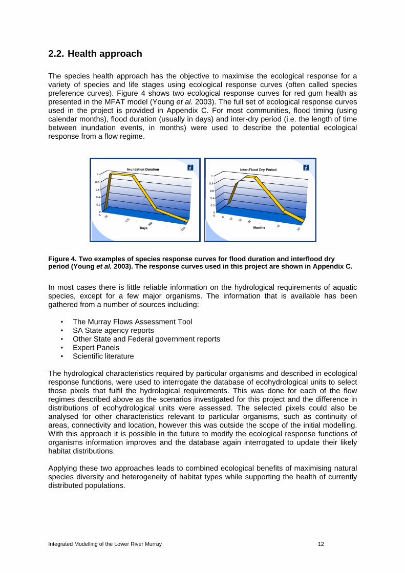
2.2. Health approach The species health approach has the objective to maximise the ecological response for a variety of species and life stages using ecological response curves (often called species preference curves). Figure 4 shows two ecological response curves for red gum health as presented in the MFAT model (Young et al. 2003). The full set of ecological response curves used in the project is provided in Appendix C. For most communities, flood timing (using calendar months), flood duration (usually in days) and inter-dry period (i.e. the length of time between inundation events, in months) were used to describe the potential ecological response from a flow regime.
Figure 4. Two examples of species response curves for flood duration and interflood dry period (Young et al. 2003). The response curves used in this project are shown in Appendix C.
In most cases there is little reliable information on the hydrological requirements of aquatic species, except for a few major organisms. The information that is available has been gathered from a number of sources including:
• The Murray Flows Assessment Tool • SA State agency reports • Other State and Federal government reports • Expert Panels • Scientific literature
The hydrological characteristics required by particular organisms and described in ecological response functions, were used to interrogate the database of ecohydrological units to select those pixels that fulfil the hydrological requirements. This was done for each of the flow regimes described above as the scenarios investigated for this project and the difference in distributions of ecohydrological units were assessed. The selected pixels could also be analysed for other characteristics relevant to particular organisms, such as continuity of areas, connectivity and location, however this was outside the scope of the initial modelling. With this approach it is possible in the future to modify the ecological response functions of organisms information improves and the database again interrogated to update their likely habitat distributions. Applying these two approaches leads to combined ecological benefits of maximising natural species diversity and heterogeneity of habitat types while supporting the health of currently distributed populations.

Integrated Modelling of the Lower River Murray 13
3. ECOHYDROLOGICAL CLASSIFICATION In order to determine the effectiveness of the operation of wetland regulators and weir pool manipulation, the River Murray floodplain, wetlands and watercourses needed to be separated into consistent habitats to which ecological response functions could be applied spatially. Certain EH types include those adjacent habitat attributes that are impacted by the local hydrology as in the case of fringing vegetation (red gums) being supported by lateral recharge. Red gums have been divided into two groups. Firstly the red gums that occur on the floodplain are mapped into the riparian unit. These red gums have their own response curve with a negative response to long flood durations. The second group of red gums is the fringing red gums that are associated with channels and wetlands. Their response curves do not have a negative response to prolonged inundation as they are fringing the water body and are not within it.
3.1. Wetlands and watercourses To do this, wetland and watercourse areas were separated based on key functional differences by Jones and Miles (2009) using the South Australian Aquatic Ecosystems (SAAE) classification (Fee and Sholz, 2009). Watercourses were separated based on permanence of the water regime (permanent, seasonal or ephemeral). Wetlands were separated based on permanence of the water regime (permanent or temporary), vegetation presence (wetland, swamp or lake), wetland surface water hydrology (overbank flow, throughflow, terminal branch) and presence of salt tolerant vegetation (saline swamp). The area weighted mean flow from the RiM-FIM was used to determine when the wetlands and watercourses were inundated by river flows. Backwater curves in the RiM-FIM were used to determine commence to fill values for each of the ephemeral wetlands and watercourses. These values were used to determine whether inundation occurred through natural flooding, operation of wetland regulators or weir pool manipulation. The weir pools mainly affect the part of the reach directly upstream of the weir. In this region the wetlands are permanently inundated and there was no data to identify their natural commence to fill heights. The range of commence to fill heights for temporary wetlands in the lower pool reaches was used as a natural distribution and commence to fill heights of permanent wetlands were assigned so that a similar range occurred. Bathymetry data for the permanent wetlands would improve the results of the project as it would remove the need for this estimation. Watercourse reaches covered 11,112 ha of the River Murray floodplain in SA. Permanent watercourses were the dominant watercourse (97%). Wetlands covered 16,682 ha of the River Murray floodplain in SA. Over two thirds of the total wetland area (87%) was classed as permanently inundated terminal wetlands (31%) and throughflow wetlands (38%) (Figure 5). Most of the wetlands (84%) were inundated at the average pool level flow of 5,000 ML d-1. Therefore permanent wetlands now make up 84% of wetlands in the lower River Murray, a large overrepresentation of this wetland type. Similarly, a medium sized flood of 70,000 ML d-1 flow covered 95% of all mapped wetlands. Only 6 ha (0.038%) of wetland area is classified as floodplain wetlands. This was identified as a limitation of the SAAE mapping by Jones and Miles (2009). Floodplain types were not adequately mapped as part of the SAAE process.

Integrated Modelling of the Lower River Murray 14
Figure 5. Relationship between River Murray flow (ML d-1) and SAAE wetland type area (ha).
Figure 6 shows that distribution of wetland types against their commence to inundation flow values. Terminal wetlands had the greatest number of commence to inundate discharges at higher flow rates with most wetland types occurring at 5,000 ML d-1, representing pool level flow in the RiM-FIM model.
Figure 6. Distribution of SAAE wetland type area (ha) through River Murray flows (ML d-1).
Figure 7 shows a portion of the River Murray and the spatial distribution of different watercourse ecohydrological types. The different ecohydrological types for wetlands are shown in Figure 8.
All wetland areas
River Murray flow (ML d-1)
2000
0
4000
0
6000
0
8000
0
1000
00
1200
00
Wetla
nd a
rea
(ha)
0
5000
10000
15000
TerminalThroughflow Overbank Flow Saline Swamp Floodplain Total wetland area (ha) Limit of RiM FiM
Terminal
0
500
2500
5000
Throughflow
Wet
land
are
a (h
a)
0
500
2500
5000
Overbank
River Murray flow (ML d-1)
0
2000
0
4000
0
6000
0
8000
0
1000
00
1200
00
0
500
2500
5000
Saline swamp
0
500
2500
5000
Total wetland area
River Murray flow (ML d-1)
0
2000
0
4000
0
6000
0
8000
0
1000
00
1200
00
0
500
2500
5000
7500
10000
12500

Integrated Modelling of the Lower River Murray 15
Figure 7. A portion of the South Australian River Murray floodplain showing the Ecohydrological types for watercourses.

Integrated Modelling of the Lower River Murray 16

Integrated Modelling of the Lower River Murray 17
Figure 8. A portion of the South Australian River Murray floodplain showing the Ecohydrological types for wetlands.

Integrated Modelling of the Lower River Murray 18
3.2. Floodplains The floodplain areas of the River Murray floodplain were separated based on the dominant vegetation community composition described by the SA River Murray DEH vegetation mapping (2003). The 72 vegetation communities described in the DEH mapping were formed into six ecohydrological (EH) types based on (Table 1). The rationale for the floodplain EH classes was that the vegetation represent the long term plant water availability of an area, i.e. an integrated measure of the soil properties, water table depth, groundwater salinity and flooding regime. The vegetation communities were grouped based on the functional plant classification based on water regime preferences modified by Nicol (2009) from Brock and Casanova (1997) for the Chowilla understorey vegetation. Table 1: Floodplain ecohydrological types.
Ecohydrological type Water Regime Examples
1 Emergent Static shallow water <1 m or permanently saturated soil. Flooding frequency <1 year
Typha spp., Phragmites australis
Amphibious fluctuation tolerators emergent Flooding frequency <1 year
Cyperus gymnocaulos, Juncus usitatus
2 Lignum Fluctuation tolerator, woody Flooding frequency 1-5 years
Muehlenbeckia florulenta
3 Riparian Fluctuation tolerators, woody Flooding frequency 1-5 years
Eucalyptus camaldulensis, Eucalyptus largiflorens, Acacia stenophylla,
4 High floodplain Fluctuation tolerators woody Flooding frequency >5 years
Eucalyptus largiflorens, Acacia stenophylla
5 Salt tolerant Tolerant of high soil or water salinity Flooding frequency >1 year
Halosarcia pergranulata, Pachycornia triandra,
6 Terrestrial dry Will not tolerate inundation and tolerates low soil moisture for extended periods Flooding frequency >5 years
Atriplex vesicaria, Rhagodia spinescens, Enchylaena tomentosa
The floodplain EH types covered 69,637 ha of the River Murray floodplain in SA. Almost all (94%) of the floodplain areas were above the floodplain overbank flow threshold of 35,000 ML d-1. This may represent the spatial accuracy of the RiM-FIM mapping. The dominant tree species covered 36,048 ha or 52% of the total floodplain area in SA, which was split evenly between the riparian (18,664 ha or 27%) and floodplain (also referred to as terrestrial vegetation) (17,384 ha or 25%) EH types. The lignum EH type covered 11,297 ha or 16%, the salt tolerant EH type covered 9,378 ha or 13%, the terrestrial dry EH type covered 8,597 ha or 12% and the emergent EH type covered 4,317 ha or 6% of the total floodplain area in SA. The emergent EH type shows inconsistencies between its frequency of inundation of less than one year and the majority of area having greater than 60,000 ML/d commence-to-fill. This is a factor of the resolution of inundation mapping and vegetation mapping. This may have implications on the results of achieving a natural distribution for this EH type. The spread of EH type area with River Murray flow is greatest in the riparian EH type, with riparian areas occurring in all flow bands from 5,000 ML d-1 to the limit of the RiM-FIM mapping (Figure 9). The cause of this is probably as a result of the mixed species including red gum, black box and river cooba which have a range of tolerances and requirements. The
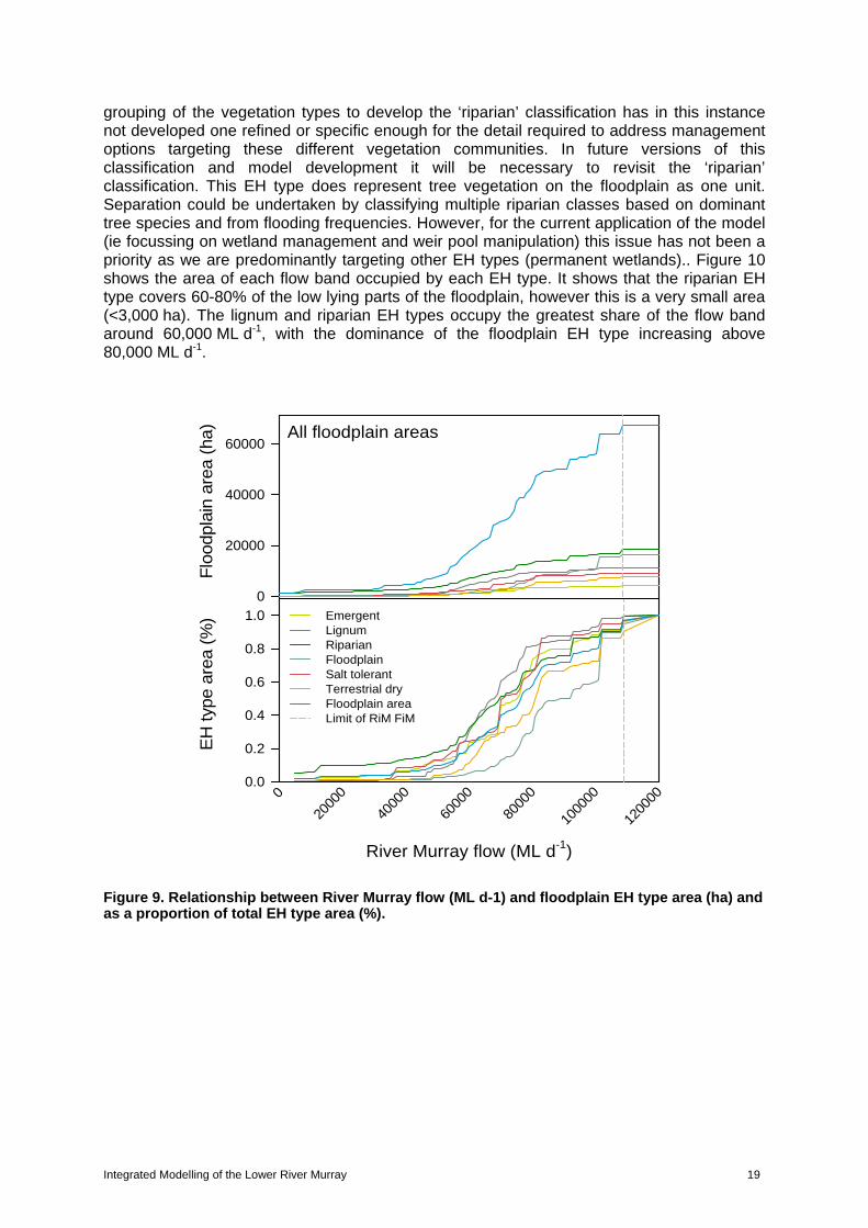
Integrated Modelling of the Lower River Murray 19
grouping of the vegetation types to develop the ‘riparian’ classification has in this instance not developed one refined or specific enough for the detail required to address management options targeting these different vegetation communities. In future versions of this classification and model development it will be necessary to revisit the ‘riparian’ classification. This EH type does represent tree vegetation on the floodplain as one unit. Separation could be undertaken by classifying multiple riparian classes based on dominant tree species and from flooding frequencies. However, for the current application of the model (ie focussing on wetland management and weir pool manipulation) this issue has not been a priority as we are predominantly targeting other EH types (permanent wetlands).. Figure 10 shows the area of each flow band occupied by each EH type. It shows that the riparian EH type covers 60-80% of the low lying parts of the floodplain, however this is a very small area (<3,000 ha). The lignum and riparian EH types occupy the greatest share of the flow band around 60,000 ML d-1, with the dominance of the floodplain EH type increasing above 80,000 ML d-1.
Figure 9. Relationship between River Murray flow (ML d-1) and floodplain EH type area (ha) and as a proportion of total EH type area (%).
River Murray flow (ML d-1)
0
2000
0
4000
0
6000
0
8000
0
1000
00
1200
00
EH
type a
rea (
%)
0.0
0.2
0.4
0.6
0.8
1.0
All floodplain areas
Flo
odpla
in a
rea (
ha)
0
20000
40000
60000
Emergent Lignum Riparian Floodplain Salt tolerant Terrestrial dry Floodplain areaLimit of RiM FiM

Integrated Modelling of the Lower River Murray 20
Figure 10. Relationship between River Murray flow (ML d-1) and floodplain EH type area (ha).
Emergent
0
2500
5000
Lignum
Flo
odpla
in a
rea (
ha)
0
2500
5000
Riparian
River Murray flow (ML d-1)
0
2000
0
4000
0
6000
0
8000
0
1000
00
1200
000
2500
5000
Salt tolerant
Floodplain
Terrestrial dry
0
2000
0
4000
0
6000
0
8000
0
1000
00
1200
00

Integrated Modelling of the Lower River Murray 21
Figure 11. A portion of the South Australian River Murray floodplain showing the Ecohydrological types for floodplains.
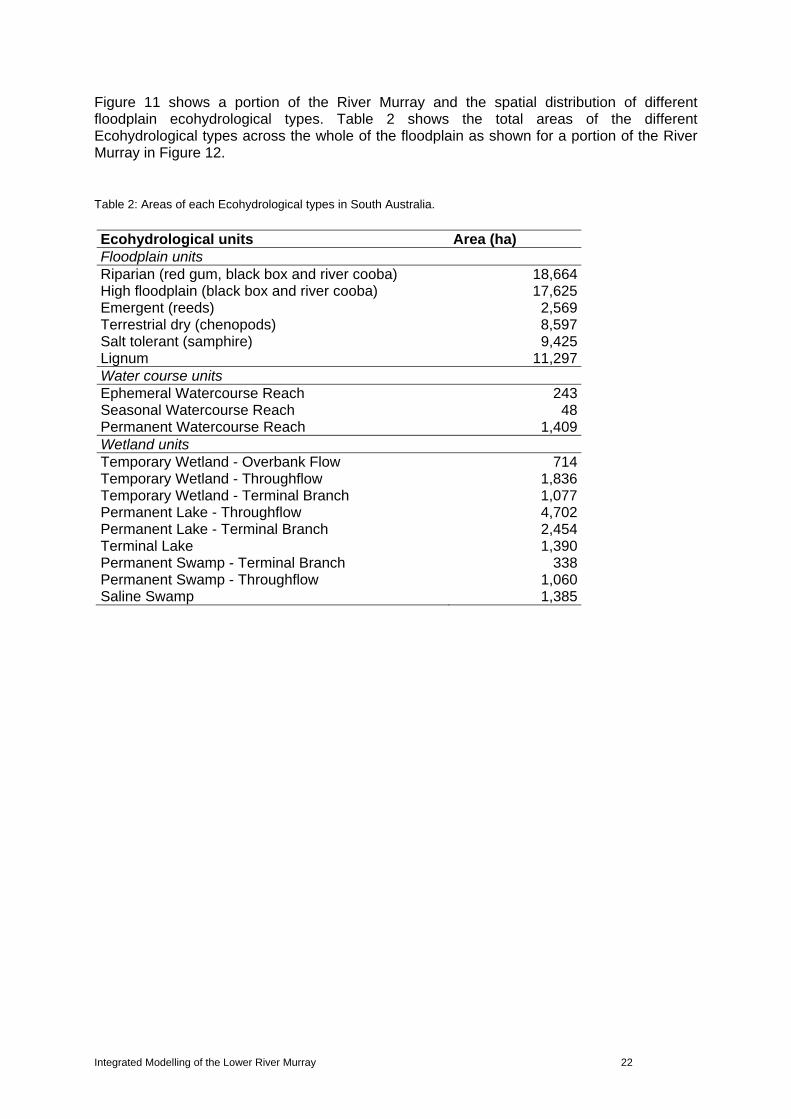
Integrated Modelling of the Lower River Murray 22
Figure 11 shows a portion of the River Murray and the spatial distribution of different floodplain ecohydrological types. Table 2 shows the total areas of the different Ecohydrological types across the whole of the floodplain as shown for a portion of the River Murray in Figure 12.
Table 2: Areas of each Ecohydrological types in South Australia.
Ecohydrological units Area (ha) Floodplain units Riparian (red gum, black box and river cooba) 18,664 High floodplain (black box and river cooba) 17,625 Emergent (reeds) 2,569 Terrestrial dry (chenopods) 8,597 Salt tolerant (samphire) 9,425 Lignum 11,297 Water course units Ephemeral Watercourse Reach 243 Seasonal Watercourse Reach 48 Permanent Watercourse Reach 1,409 Wetland units Temporary Wetland - Overbank Flow 714 Temporary Wetland - Throughflow 1,836 Temporary Wetland - Terminal Branch 1,077 Permanent Lake - Throughflow 4,702 Permanent Lake - Terminal Branch 2,454 Terminal Lake 1,390 Permanent Swamp - Terminal Branch 338 Permanent Swamp - Throughflow 1,060 Saline Swamp 1,385

Integrated Modelling of the Lower River Murray 23
Figure 12. A portion of the South Australian River Murray floodplain showing the Ecohydrological types.

Integrated Modelling of the Lower River Murray 24
4. RIVER HYDROLOGY AND FLOODPLAIN MAPPING
4.1. River hydrology The river flow history is the most important component of the modelling. For this project we used two hydrographs from a period of 1895 to 2006 obtained from the Murray-Darling Basin Sustainable Yields project (CSIRO 2009). Two hydrographs were available for this period for current and natural conditions. Current flow was modelled using climate data over the time period and current (2009) river abstraction rules. The natural flow data was modelled using actual climate data and no water abstraction rules. For the purposes of keeping model run time to an achievable duration the hydrograph was broken up into smaller 20 year periods. The most recent period is shown in Figure 13 for 1986 to 2006. Natural flows have typically had a larger magnitude (covering a larger area) and had a longer duration.
Figure 13. The hydrographs used in the project. The Natural hydrograph is estimated from actual climate data with no water abstraction. The Current hydrograph is modelled with actual climate and current (2009) abstraction rules. Data provided by the CSIRO MDBSY project.
4.2. Wetland and floodplain inundation Wetland mapping was provided by the South Australian Department of Environment and Heritage. A digital elevation model (DEM) was available for the River Murray floodplain in South Australia. The model was used for mapping the extent of new infrastructure required to regulate wetlands. The River Murray Floodplain Inundation Model (RiM-FIM) (Overton et al. 2006) has been developed for the River Murray from Hume Dam to the Lower Lakes. RiM-FIM was developed from a combination of satellite derived inundation extents, a digital elevation model and a river hydrology model to predict river heights from the manipulation of weir heights and river discharge at the South Australian border. In this project RiM-FIM was used to predict areas of inundation and wetland connectivity from various scenarios of river flows and weir operation.
0
20000
40000
60000
80000
100000
120000
140000
160000
198
6
198
7
198
7
198
8
198
9
199
0
199
0
199
1
199
2
199
3
199
3
199
4
199
5
199
6
199
6
199
7
199
8
199
9
199
9
200
0
200
1
200
2
200
2
200
3
200
4
200
5
200
5
ML
/day
Date
Natural
Current

Integrated Modelling of the Lower River Murray 25
Figure 14. Cross section of the River Murray showing the different commence to fill levels needed to over top the sill levels.
The RiM-FIM model provides commence-to-fill levels for each floodplain and wetland area. The commence-to-fill is described by a flow but also by a river height. The model is then able to indicate inundation areas with weir operations that change the river height without changing the river discharge. Figure 14 shows a schematic cross section of the floodplain with wetlands having different commence-to-fills. Figure 15 shows the spatial distribution of commence-to-fill values for a portion of the River Murray floodplain. Permanent wetland commence to fills could not be determined from RiM-FIM but had to be estimated in the absence of bathymetry.

Integrated Modelling of the Lower River Murray 26
Figure 15. Commence to fill values for different wetland and floodplain features.

Integrated Modelling of the Lower River Murray 27
5. INFRASTRUCTURE AND WEIR OPERATION
5.1. Infrastructure Infrastructure models developed by Tonkin Consulting and Aquaterra (Aquaterra 2010) for the RRP were employed to calculate indicative economic costs of installing regulators and for relocation of pumps on wetlands in the South Australian River Murray floodplain. Pump surveys also have information about pump relocation costs but these were not used in this project. A desktop analysis in a GIS environment, using the best available data, was undertaken to provide the required input into these models. Further consultation with engineers and detailed costing would be required if construction is to be considered. Ongoing maintenance and operation responsibilities/costs will also need to be determined.
5.1.1. Regulators and cost estimates
The first step in estimating regulator costs was to identify which wetlands could be regulated. Each polygon in the wetland/watercourse dataset was visually assessed along with LiDAR elevation data and aerial imagery to determine the dimensional requirements of regulating. Initially wetlands were not considered feasible if they are already adequately regulated, have inlets/outlets greater than 200 metres or are filled from overbank flow. These sites were reviewed by DWLBC staff with some regulators being moved and additional regulators positioned on other wetlands. The regulator infrastructure model required the width of channel opening and depth of channel as inputs. Positioning of regulators, and consequently width, was determined in order to maintain a level of water as defined, in most cases, by the wetland polygon (Figure 16). Some wetland polygons are under/over-representative according to the LiDAR or aerial imagery and consequently do not connect to the regulators. Depth of channel was estimated using LiDAR and baseline survey data when available. For permanent wetlands where no data was available the depth was assumed to be 2 m as this was the average for known wetlands. In many cases permanent wetlands occur along the edge of the River Murray. These wetlands could benefit from new regulators which could restore a natural wet and dry cycle. However, some of these wetlands have a very large connection with the river which makes a regulator unviable (Figure 17). The list of regulators width and depth was provided to Tonkin Consulting for entering into the infrastructure model developed for the RRP. The resulting cost estimates were grouped into investment complexes according to which wetland or wetlands the regulators influenced, e.g. a group of wetlands that are hydrologically connected. The regulators considered under the RRP infrastructure model are compliant with SA MDB NRM Board ‘Design and Construction of Wetland Regulating Structures – Engineering Guidelines’ Tonkin Engineering 2008. There were a number of assumptions relating to regulator options that were made to enable a large standardised run of the cost model to be made. These assumptions were that all regulating structures:
type was set to “embankment with box culvert and flow control”; all box culverts were square; an overshot gate included on one culvert opening; if multiple culvert openings, stop logs included on all remaining openings (excluding
the one with overshot gate); the maximum width of culverts was limited to 10m; single vehicle passage across both embankment and structure;

Integrated Modelling of the Lower River Murray 28
guardrail and handrail across structure; GCL for seepage control through embankment; fish screens on all culvert openings; no fish cages; skylight on one culvert run; rock base for fish passage on one culvert run; 10m of rubble access track; all structures within 50km of a major regional town; no security fencing; no gates and signs.
Figure 16. Regulators positioned to enable isolation of wetland from river as determined by LiDAR data
Elevation
Wetland polygon
Proposed Regulator
High
Low

Integrated Modelling of the Lower River Murray 29
Figure 17. Many wetlands along the River Murray have very large connection with the River channel making regulators too large to be an option.
The interface of the main channel with wetland/watercourse is not necessarily the optimal position for regulation. These examples highlight the uncertainty of required regulator length as demonstrated by differences between the LiDAR DEM and the digitised wetland. Positioning of regulators required individual assessment using best available data. Therefore an automated approach to creating and measuring lengths of regulators was not possible.
5.1.2. Pump relocations and cost estimates
In order to estimate the cost of relocating pumps it was first necessary to identify the location of the pumps on the wetlands to be regulated. They were determined between Locks 1 and Lock 3 and Lock 5 to the border from pump survey data and between Wellington and Lock 1 and Lock 3 to Lock 5 from meter locations as a surrogate for pump locations as pump survey data has not been completed. There were 84 pumps and 74 meter locations identified for relocating. The cost of relocating the pumps required the use of a pump relocation infrastructure model. A pump survey report had been produced that estimated costs from pump relocation but this was for relocating pumps to higher ground and not to the main channel. The pump relocation infrastructure model required 5 inputs:
Relocation pipeline length – divided into length along road verge and length through existing vegetation where applicable;
Existing pump flow in L/s; Existing pump head in metres ; and Length of ETSA infrastructure extension.
The best path for a pipeline was drawn to connect pump/meter locations to the river channel. These pipelines followed roads/paths when possible, avoiding vegetation and steep incline/declines, as assessed by aerial imagery and LiDAR. The length of pipeline along the road verge and length of pipeline through vegetation was recorded. Only 43 of the 84 pumps had flow and head data recorded in the pump surveys. When this information was not available an estimate was made based on the recorded values. These estimates were:
Domestic: Flow – 2 L/s and head – 50m
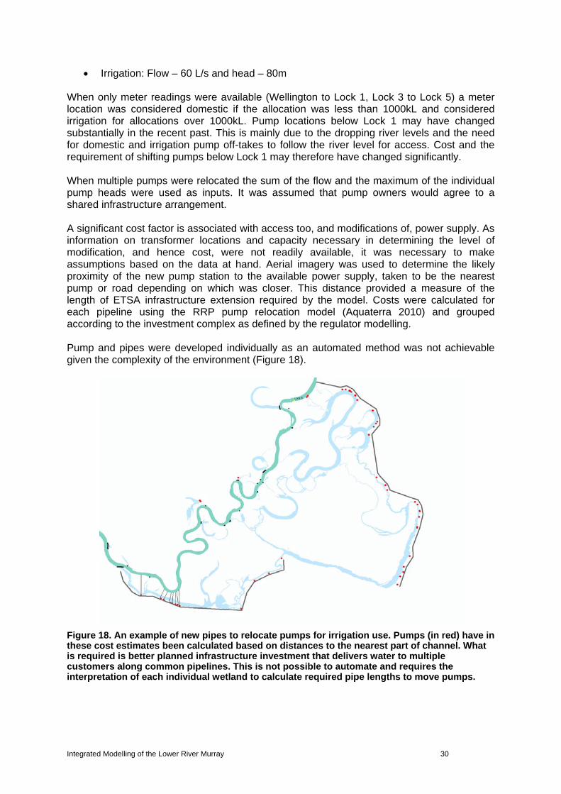
Integrated Modelling of the Lower River Murray 30
Irrigation: Flow – 60 L/s and head – 80m When only meter readings were available (Wellington to Lock 1, Lock 3 to Lock 5) a meter location was considered domestic if the allocation was less than 1000kL and considered irrigation for allocations over 1000kL. Pump locations below Lock 1 may have changed substantially in the recent past. This is mainly due to the dropping river levels and the need for domestic and irrigation pump off-takes to follow the river level for access. Cost and the requirement of shifting pumps below Lock 1 may therefore have changed significantly. When multiple pumps were relocated the sum of the flow and the maximum of the individual pump heads were used as inputs. It was assumed that pump owners would agree to a shared infrastructure arrangement. A significant cost factor is associated with access too, and modifications of, power supply. As information on transformer locations and capacity necessary in determining the level of modification, and hence cost, were not readily available, it was necessary to make assumptions based on the data at hand. Aerial imagery was used to determine the likely proximity of the new pump station to the available power supply, taken to be the nearest pump or road depending on which was closer. This distance provided a measure of the length of ETSA infrastructure extension required by the model. Costs were calculated for each pipeline using the RRP pump relocation model (Aquaterra 2010) and grouped according to the investment complex as defined by the regulator modelling. Pump and pipes were developed individually as an automated method was not achievable given the complexity of the environment (Figure 18).
Figure 18. An example of new pipes to relocate pumps for irrigation use. Pumps (in red) have in these cost estimates been calculated based on distances to the nearest part of channel. What is required is better planned infrastructure investment that delivers water to multiple customers along common pipelines. This is not possible to automate and requires the interpretation of each individual wetland to calculate required pipe lengths to move pumps.

Integrated Modelling of the Lower River Murray 31
5.1.3. Infrastructure cost estimates
The wetland/watercourse polygons, uniquely identified by WETLANDID, were assigned an investment identifier, INVEST_ID, which identifies a single wetland/watercourse polygon, or group of wetland/watercourse polygons, for which an infrastructure investment influences. A total of 80 infrastructure investments were identified influencing 172 wetland/watercourse polygons with a total area of 5,536 hectares. The total estimated infrastructure cost was $117,215,797 (including GST) being $51,957,400 for the cost of constructing regulators and $65,258,397 for pump relocation. Table 3 lists the investments ordered by decreasing cost. A list of the investments, their common names and the cost of establishment is provided in Table 3. Table 3. Investments considered in the model, ordered by decreasing cost.
INVEST_ID INVEST_NAME COST ($)
14 DEVON DOWNS 9,895,69621 MARKS LANDING 6,838,57460 PYAP COMPLEX 5,831,80578 328 4,849,7517 CAURNAMONT 4,668,4006 SALTBUSH FLAT 4,136,479
48 BIG TOOLUNKA FLAT 4,108,01135 MURBKO FLAT COMPLEX 3,897,00474 WOOLENOOK BEND COMPLEX 3,674,204
103 ARLUNGA 3,625,71011 WALKER FLAT LAKES COMPLEX 2,794,80733 DONALD FLAT LAGOON 2,694,54419 PUNYELROO 2,673,63826 PORTEE COMPLEX 2,656,84547 LITTLE TOOLUNKA FLAT 2,630,1133 LAKE CARLET 2,530,750
62 GURRA GURRA LAKES 2,489,07712 FORSTER LAGOON 2,469,99261 AJAX ACHILLIES LAKE 2,367,13958 NOCKBURRA AND CHAMBER CREEK 2,197,59113 WONGULLA LAGOON 1,990,26534 IRWIN FLAT 1,868,46053 YARRA COMPLEX 1,780,05023 SWAN REACH COMPLEX 1 1,754,50032 SINCLAIR FLAT 1,731,95371 RAL RAL COMPLEX 1,688,50017 BIG BEND 1 1,511,08715 PRIESS LANDING 1,491,57228 ROONKA 1,349,70077 BIG HUNCHEE, LITTLE HUNCHEE AND AMAZON CREEKS 1,328,80076 2825 1,314,50031 MCBEAN POUND NORTH 1,082,70416 HENLEY PARK 1,060,371
100 GERARD SWAMPS 1,048,30079 MURTHO PARK COMPLEX 935,000

Integrated Modelling of the Lower River Murray 32
36 WOMBAT REST BACKWATER 889,70529 REEDY ISLAND FLAT 854,70042 WESTON FLAT LAGOON 849,20055 WOOLPUNDA 849,20068 1193 843,70070 GOAT ISLAND AND PARINGA PADDOCK 607,20072 528 583,00059 BELDORA WETLANDS 572,000
104 YOUNGHUSBAND 557,70038 NORTH WEST BEND 523,60044 QUALCO SWAMP 520,300
102 KROEHNS LANDING 510,40069 NELWART SWAMP 507,1001 JURY SWAMP (JAENSCHS BEACH) 487,300
39 NIKALAPKO 476,300106 TEAL FLAT 475,200105 TEAL HUT 471,900
75 1108 459,80022 SWAN REACH FERRY 454,30046 NIGRA LAGOON 429,00054 DELVINS POUND 423,50081 1245 418,00041 MOLO FLAT 407,00049 ROSS LAGOON 403,70030 MCBEAN POUND SOUTH 382,80080 NELWOOD 367,40050 JAESCHKE LAGOON 349,80064 LYRUP EAST 334,4009 NORTH CAURNAMONT 331,100
56 GLEN DEVLIN COMPLEX 277,20073 BULYONG ISLAND BASIN 273,90045 BOGGY FLAT 266,20020 1644 262,90067 1192 256,3008 NORTH PURNONG 255,2005 CRAIGNOOK 253,000
63 LYRUP CAUSEWAY WEST 253,00037 MORGAN EAST 239,80051 MAIZE ISLAND COMPLEX 234,30057 PARCOOLA WEST 228,80010 SCRUBBY FLAT 226,6004 MAIDMENT LAGOON 198,000
18 BIG BEND 2 198,0002 POMPOOTA 189,200
52 PASCHKES FLAT 174,900101 1541 174,900
24 SWAN REACH COMPLEX 2 171,600 It is expected that the number of domestic pumps needing relocation has been under-estimated between Wellington and Lock 1 and Lock 3 and Lock 5. This being due to the reliance on meter locations rather than pump locations and it is likely that domestic pumps

Integrated Modelling of the Lower River Murray 33
which are not metered are not accounted for. The majority of flow and head values are estimated due to the incomplete nature of the pump survey data thus introducing even more uncertainty. The lack of data on pump locations and power requirements is a significant hurdle in providing accurate infrastructure cost estimates. The estimates of regulator costs are based on up to date valuation however, better bathymetric detail would improve the calculation of regulator cost as depth of channel, and hence height of regulator, has a significant contribution to cost. These indicative economic cost estimates provided the data to measure the level of investment required in infrastructure for wetland management across the South Australian Murray-Darling basin floodplain once the optimisation model was completed. The current estimates provide a consistent high level approach to direct further on-ground investigations to refine cost estimates. Consultation with wetland managers and the consideration of local variables in the application of both regulator and pump relocation cost models would help to improve these estimates by filling in some of the identified data gaps. Figure 19 shows a portion of the river with a range of regulator and pump relocation investments. Maps of all the potential investments are provided in Appendix A.
Figure 19. Portion of the River Murray showing the locations of regulators and pump relocation pipes. The full range of investments have been mapped in Appendix A.
5.2. Weir operations There are six weirs that control the flow of the River Murray in South Australia (Table 4).

Integrated Modelling of the Lower River Murray 34
Table 4: River Murray locks and weirs
River Murray Lock/Weir
No. 1 No. 2 No. 3 No. 4 No. 5 No. 6
Date constructed
1922 1928 1925 1929 1927 1930
River distance (km from mouth)
274.3 362.1 431.4 516.2 562.4 619.8
Length of pool (river km)
87.8 69.3 84.8 46.2 57.4 76.8
Normal upper pool level (m AHD)
3.20 6.10 9.80 13.20 16.30 19.25
Lower pool level at 5 000 ML/d (m AHD)
0.75 3.25 6.25 10.25 13.35 16.43
Lower pool level at 30 000 ML/d (m AHD)
1.90 5.10 7.95 12.20 14.70 18.40
The manipulation of the pool height by raising and lowering the weir level is considered to have a range of environmental benefits. These include (based on Aquaterra, 2004): Weir raising benefits are:
Reconnection of the dynamic interactions between the floodplain and the river; Benefit vegetation, waterbirds and invertebrates by emulating hydrological variability; Improve vegetation and macro invertebrate communities by improving seed bank
viability; Reducing water stress in floodplain vegetation; Improve biofilm community heterogeneity, thereby increasing their value as a food
source; and Improve vegetation coverage and recruitment.
Weir lowering benefits are:
Increases distribution of amphibious plants; Improves biofilm heterogeneity; Dries inundated sediments, thereby consolidating them; Desiccates soil bacteria and allows nitrification process to occur removing this as a limiting factor; and Provides positive impact for flowing water habitats.
Not all of these benefits are explicitly modelled in this project. The six weirs have constraints on weir manipulation. The primary constraint on the extent of weir pool raising is the lock and weir structures themselves (Table 5). Weir pool drawdown is limited by the potential impact upon pumping infrastructure. Other potential issues caused by weir manipulations include (listed after Cooling et al. 2010):
undesirable flooding (caravan parks, roads, shacks, pump off-takes); ferry operations; houseboats, water skiing and other recreational boating;

Integrated Modelling of the Lower River Murray 35
salinity; raised groundwater levels; acid sulphate soils; loss of boat access to floodplain watercourses; and, fishway function in the weirs.
The operational rules provided by the SA MDB NRM Board used in this project include:
height of each weir above or below pool level; maximum change in weir height from one month to the next; height differences between weirs; and maximum number of times a weir is raised or lowered per year.
Table 5. Weir raising constraints in South Australia (SA Water).
Weir 1
Weir 2 Weir 3 Weir 4 Weir 5 Weir 6
Max raising (m) at 5 000 ML/day
1.06 1.10 0.59 1.14 0.50 0.62
Max raising (m) at 10 000 ML/day
1.06 0.7 0.59 1.14 0.50 0.62
Max raising (m) at 15 000 ML/day
1.06 0.65 0.59 1.14 0.50 0.62
Max raising (m) at 20 000 ML/day
1.06 0.35 0.59 1.14 0.50 0.62
Max raising at (m) 30 000 ML/day
1.06 0 0.59 0 0.50 0
Max raising at (m) 40 000 ML/day
0 0 0.40 0 0.50 0
Max raising at (m) 50 000 ML/day
0 0 0.25 0 0.50 0
The impact of raising or lowering a weir is to change the river height without necessarily changing the river discharge. Figure 20 shows backwater curves from the RiM-FIM with different river heights achieved from increasing river flow. These curves, and those that model weir operations, are used to identify floodplain inundation extent. Weir raising has been trialled before and is seen as a feasible method of increasing the area of inundation from low flows. The weirs are removed at river flows of approximately 50,000 ML/day and above (depending on the weir). At flows near this the weirs cannot be raised. Weir raising involves a change in river management and this may not be feasible at all times or in all reaches. For this reason Scenario 2 has been developed that involved no weir operations. Weir lowering could be used to dry out some wetlands and thereby improve their ecological condition, although a lack bathymetry has impeded the understanding of what permanent

Integrated Modelling of the Lower River Murray 36
wetlands disconnect at specific river heights. Scenario 3 has been developed to include investments and weir raising and lowering. There are some concerns over weir lowering and raising that include isolation or drowning of irrigation pumps and the discharge of saline groundwater into the river as the river is lowered below the groundwater level or raised to connect to the groundwater and discharge when lowered. For this reason a fourth scenario is used that includes investments and weir raising only.
Figure 20. An example of a backwater graph for one of the weir reaches showing the different river heights achieved from different flows. These curves and those for different weir levels are used within the RiM-FIM model to predict wetland connectivity.

Integrated Modelling of the Lower River Murray 37
6. ASSESSING LIKELY ECOLOGICAL RESPONSE One method for objectively assessing the performance of proposed regulators is to determine their likely ecological response. Ecological response models provide a mechanism to objectively compare the effect of different combinations of regulators on wetland and floodplain habitats.
6.1. Ecological response models for the Lower Murray The Murray Flow Assessment Tool (MFAT; Young et al. 2003) is the most comprehensive set of ecological response curves that have been generated for the Lower Murray. The system was developed in 2003 as a decision support system to predict the ecological benefits (or otherwise) of different flow scenarios along the River Murray. MFAT has response curves for floodplain and wetland vegetation, waterbird habitat and native fish habitat that are tailored for each of nine zones along the River Murray and its tributaries. Two of those zones are relevant to this study; Zone E which covers the River Murray stretch from Lock 11 at Mildura to Lock 3 and Overland Corner; and Zone G, covering the remainder of the South Australian River Murray, from Overland Corner to Wellington. For each of the biotic communities present in either Zone E or G (Table 6), response curves were extracted from MFAT for those parameters which were able to be predicted by the integrated mathematical model described later. For most communities, this included flood timing (using calendar months), flood duration (usually in days) and inter-dry period (i.e. the length of time between inundation events, in months). Where relevant, separate response curves were included for different life stages (e.g. seedlings and adults for vegetation and spawning, juveniles and adults for fish). Ecological responses quantified the health of the ecological features on a scale from 0 - 1 as a function of environmental flow characteristics (Figure 21). Appendix D presents all the response curves used.
Figure 21. Example of an ecological response function for the health of colonial nesting water birds against inter-flood duration from Young et al. [2003].
Where different response curves had been generated for Zones E and G, the response curve with the highest level of confidence was used (Young et al. 2003). Where the response curves differed, but the same level of confidence was given to both, the curve for Zone G was used, as this covered the majority of the South Australian River Murray. Where biotic communities had response curves in one Zone, but not the other (i.e. had been deemed irrelevant by the researchers who developed MFAT), the curves for the one extant Zone were included. Further analysis could apply different response curves in different river reaches.
0
0.2
0.4
0.6
0.8
1
0 10 20 30 40
Number of months
Hea
lth

Integrated Modelling of the Lower River Murray 38
Table 6. Biotic communities described by MFAT for Zones E and G (Young et al. 2003)
Community Community type Zone E Zone G
River Red Gum woodland Floodplain vegetation
Black Box woodland Floodplain vegetation
Lignum shrubland Floodplain vegetation
Rats tail couch grassland* Floodplain vegetation
Ribbon weed herbland Wetland vegetation
Phragmites australis Wetland vegetation
Colonial nesting waterbirds Waterbird habitat
Waterfowl and grebes Waterbird habitat
Flood spawners Native fish habitat
Wetland specialists Native fish habitat
Freshwater catfish Native fish habitat
Main channel generalists Native fish habitat
Main channel specialists Native fish habitat
Low flow specialists Native fish habitat
* Note that no instances of rats tail couch grassland were found in the ecohydrological units, so this community has been excluded from the modelling. Source: Young et al. (2003). As MFAT was developed approximately seven years ago, and questions have been raised as to the accuracy of some of the responses documented (Nick Bond, Monash University, pers. comm., Brenton Zampatti, SARDI Aquatic Sciences, pers. comm.), additional information was used to modify the responses where available. Additional information was included drawn from Overton et al. (2009) and Ecological Associates (2010). This information has been incorporated into the response curves illustrated in Appendix D, with the exact source of each curve listed in Appendix C. Response curves for vegetation communities relating to flood duration and inter-dry period were modified using an analysis of the current extent of vegetation. The floodplain EH type data was used to make estimates of the minimum inundation duration and maximum interflood periods that the vegetation experienced under a natural hydrograph. The natural hydrograph is considered sufficient to support adult health as most of the long lived vegetation are likely to be hundreds of years old, indicating that it wasn’t just recruitment, but adult survival, that the natural hydrograph provided. An estimate of the area weighted mean flow to inundate each EH type within one area weighted standard deviation shows that the mean flow to inundate each EH type ranges from 68,000 ML d-1 for riparian EH type to 87,000 ML d-1 for the floodplain EH type (Table 5). This equates to a range in minimum flood duration of 62 days for riparian EH type areas and 41 days for floodplain EH type areas. Similarly, the maximum interflood period ranges from 15 months for the riparian EH type to 20 months for the floodplain EH type. These average maximum interflood periods appear low and are likely to be influenced by inundation areas fringing mapping units. These vegetation types are known to exist in habitats with much longer Interflood periods.

Integrated Modelling of the Lower River Murray 39
Table 7. Area weighted mean River Murray flow (GL d-1), flood duration (days) and interflood period (months) for each EH type and total floodplain area. Area weighted standard deviations are also shown.
All floodplain areas Over bank flows (>35 GL d-1) -SD Mean +SD -SD Mean +SD River Murray flow (ML d-1) Emergent 52,000 72,000 92,000 58,000 74,000 91,000 High floodplain 70,000 87,000 104,000 73,000 88,000 103,000 Lignum 53,000 70,000 86,000 55,000 70,000 86,000 Riparian 41,000 68,000 95,000 57,000 76,000 94,000 Salt tolerant 53,000 71,000 89,000 55,000 72,000 88,000 Terrestrial dry 61,000 79,000 97,000 64,000 80,000 96,000 Total floodplain area 53,000 75,000 97,000 60,000 78,000 95,000 Flood duration (days) Emergent 82 54 44 78 52 43 Floodplain 56 41 41 55 40 41 Lignum 81 56 41 82 56 41 Riparian 96 62 39 80 50 43 Salt tolerant 87 56 39 82 54 39 Terrestrial dry 76 46 39 67 45 39 Total floodplain area 87 52 39 77 47 39 Interflood period (months) Emergent 10 15 28 12 16 26 Floodplain 15 20 45 16 21 43 Lignum 10 14 20 11 15 20 Riparian 7 15 29 12 16 30 Salt tolerant 11 15 21 11 15 21 Terrestrial dry 13 17 30 13 17 29 Total floodplain area 11 16 30 13 17 29 * Note that no instances of rats tail couch grassland were found in the ecohydrological units, so this community has been excluded from the modelling. It is also worth noting the high river flow mean for emergent vegetation. This is not typical of this vegetation type and is being influenced by the spatial accuracy of the vegetation and flood mapping. A final modification was to only use responses of zero when it was likely that populations would become locally extinct. Thus, habitats deemed simply unsuitable were given a low value (0.05) rather than the zero that appeared in MFAT, while likely population limits (e.g. appropriate conditions for reproduction occurring less frequently than the life span of the organism) were allocated a zero response.
6.2. Linking ecological response and ecohydrological units Ecological response curves were linked to the various ecohydrological units in order to relate biota to the habitat in which it was most likely to be found (Appendex B). Floodplain ecohydrological units were defined based on their vegetation communities, and these definitions were used to relate the response curves for the respective community. Riparian and wetland vegetation communities and faunal communities were linked based on the habitat preference information found in MFAT reference, Overton et al. (2009) and Ecological Associates (2010). Expert opinion (which included Brenton Zampatti (SARDI), Dan Rogers

Integrated Modelling of the Lower River Murray 40
(DENR), Nick Bond (Monash), Paul Close (UWA), Ian Overton (CSIRO) and Kate Holland (CSIRO)) was also sought to verify the faunal community associations, for which the least South Australian-specific information was available in the literature. Each community was given a rating for each of the ecohydrological unit types. This rating ranged between 0, if a community was not likely to utilise the habitat described by the ecohydrological unit (e.g. fish that are main channel specialists are not likely to use the floodplain even when it is inundated), to 1 if the ecohydrological unit was likely to be core habitat (e.g. watercourse reaches for fish that are main channel specialists). Scores of 0.5 were allocated for marginal habitat, or if there was a moderate possibility that the habitat would be used, and 0.25 if it was unlikely, but possible, that the habitat would be used. It was possible that more than one ecohydrological unit could be associated with each community and for some communities, life history stages were differentially assigned. This was the case where larvae or juveniles tend to utilise different habitat types from adults of the same community. Different ecological response curves for red gum were applied to red gum communities in the different ecohydrological units. This was necessary as interaction with nearby water bodies can influence the health of established red gum trees.. In floodplain areas the red gums respond to flooding periods and can be negatively impacted by prolonged inundation. On watercourse and wetlands the red gums occur adjacent to the water body and prolonged inundation of the adjacent water body supports their health by providing a water source either direct to their roots or through lateral recharge of the banks.
6.3. Combining ecological response models More than one ecological response curve existed for all of the biotic communities assessed. The general lack of information regarding the relative importance of each response curve meant that there was little basis upon which to weight the various responses (e.g. MFAT used an arithmetic mean (Young et al. 2003)). Thus, multiple ecological responses were multiplied to give an overall response for each habitat unit. This means that the maximum value is not comparable across biotic communities, which should be considered when interpreting the results. Indices to summarise ecological responses In order to summarise the predicted ecological response within each individual wetland, and each ecohydrological type, summary indices were developed. Information upon which to base a more-complex set of composite indices was not available. Thus, the indices were an average of values for individual biotic communities, grouped according to type. A diversity value would be an useful addition to look at in future work . Four summary indices were developed. These were: floodplain vegetation, which averaged response for the floodplain and riparian river
red gums, black box woodlands, lignum shrublands, salt-tolerant woodlands and chenopod woodlands biotic communities (including both adults and seedlings);
aquatic vegetation, which averaged responses for the Phragmites australis and ribbonweed herbland biotic communities;
waterbirds, which averaged responses for colonial nesting waterbird breeding and waterfowl and grebe habitat; and
fish, which average responses across main channel specialists, flood-spawning fish, wetland specialists, freshwater catfish, main channel generalists and low-flow specialist fish communities.

Integrated Modelling of the Lower River Murray 41
A limitation of this approach is the diversity of biotic responses was not represented in the scoring. In future work to address this issue an index could be developed that considered the number ecological responses, by….

Integrated Modelling of the Lower River Murray 42
7. SOCIAL VALUES INCORPORATED IN THE MODEL
7.1. Stated preference values In 2009, a major national survey of willingness to pay for improving the quality of the River Murray and the Coorong was undertaken. A random sample of 1000 SA households from the Australian Post database was asked to participate in a survey and 63.6% responded. Survey respondents were asked about their knowledge and experience with the River Murray and the Coorong. Using a stated preference technique (Hensher, Rose and Greene, 2005), survey respondents were asked to consider a choice experiment where they were offered the status quo health of the Murray River and Coorong as well as two options which involved different levels of health of particular assets and different costs. Table 8 outlines the levels used in the experiment. By presenting different combination of the attributes and different household costs, respondents face different trade-offs. Respondents were quizzed on the information in survey and reminded about the cost to their household. Table 8. Attribute levels used in the choice sets.
Attributes Current Situation Levels in Options B and C
Waterbird breeding along the River Murray
Every ten years 10, 7, 4, 1
Native fish in the River Murray
30% of original population
30%, 40%, 50%,60%
Healthy vegetation along the River Murray
50% of original area 50%, 60%, 70%, 80%
Waterbird habitat in the Coorong
Poor quality Poor quality, Good quality
Household Cost per year for 10 years
$0 $20, $50, $75, $100, $125, $150, 200, $250
Willingness to pay values are calculated from models of choice, specifically the probability of choosing the status quo or one of the two other options. Willingness to pay is expressed as an amount per household per year for ten years:
to decrease the interval between bird breeding events by 1 year; to increase the proportion of native fish by 1%; to increase the proportion of healthy native vegetation by 1%; and to improve the health of the waterbird habitat of the Coorong.
These values were tested and found to be statistically higher than Victoria, lower than the ACT but found to be no different from rest of Australia. More on these values can be found in Hatton MacDonald et al. forthcoming.

Integrated Modelling of the Lower River Murray 43
These values represent some of the recreational use values and the “intrinsic” values that people assign to environmental quality. Respondents were asked about their experience of the river including sight-seeing, boating, fishing etc. However not everyone travels to the river or the Coorong and these people assign a value based on their desire for these natural assets “to exist” and to be there for future generations.
7.2. Mapped community values In 2008, as part of a study of community leaders in the SAMB, 56 participants were asked to undertake a mapping task as part of larger interview. Participants were asked to locate and describe places of value and threat by first arranging plastic dots (moveable plastic discs about 10 mm in diameter) on a 1:325,000 scale A0 (841 × 1189 mm) size topographic map of the SAMDB NRM region (Raymond et al. 2009). To create scarcity and value, participants were given a maximum of 40 green dots to assign positive value and 10 red dots to assign negative values. Participants were encouraged to view value on a continuum from red dots (= ‘negative value’) to green dots (= ‘positive value’). The green dots enabled the spatial representation of value intensities. A set of maps and supporting transcripts were produced which identify the natural assets and ecosystem services that people value across the landscape. This information provides a relative local ranking of priorities for NRM purposes. A set of transcripts of discussion around the mapping exercise are useful for providing context around the personal stories and history that local people associate with the SAMDB region. Participants assigned value to the rangeland areas, national parks, built infrastructure (schools, footie clubs, their local community), and sites of cultural, historical significance across the landscape. Participants assigned value to the River Murray, the Lower Lakes, Coorong generically in some cases. Some participants assigned value to specific locations on the river such as Chowilla. Water was an important natural asset to study participants but it ranked among a number of other important topics including food production, built infrastructure, etc. The mapped values and the interviews and the stories in particular provide context on what local people value in the region.

Integrated Modelling of the Lower River Murray 44
8. INTEGRATED MODELLING AND ANALYSIS Since the 1940’s, operations research methods in optimisation have successfully provided decision makers with best bet options of planning and operating infrastructure. With advances in mathematical methods and computing power over the past two decades, we now have the opportunity to optimise infrastructure planning in much more complex systems such as the River Murray. A benefit of applying mathematical optimisation is that we take a whole-of-system approach to modelling the eco-hydrological functionality of the River Murray, in the context of decisions made in investment in regulators. This means a set of new regulators can be identified that is optimal with regards to budget, ecological response, and optimal in relation to the way the infrastructure is best operated. The project has produced innovative model for supporting these decisions, and the remainder of this section describes the model itself and how it is solved. For a thorough description of the mathematical model and solution method see Appendix E.
8.1. Mathematical model In formulating a mathematical model of the River Murray, we identified parameters, decision variables, an objective function and constraints that represented the system.
8.1.1. Decision variables
Three decision variables were used:
1) a yes/no decision whether each eligible new investment complex (regulators + moving of pumps) is built;
2) the operation of the regulators in each investment complex (+ existing regulators) in each month- that is whether it is opened or closed. All regulators within an investment complex will be opened or closed simultaneously;
3) the height (cm) of each weir in each month.
The second and third decision variables are at monthly time steps, with an optimisation horizon of 20 years to accommodate the representation of wet and dry years. For the first decision variable, there were 80 eligible new investments, which if all were built would cost $117,215,797. However, given an estimated budget of $60,000,000 on which to base investment decisions, not all eligible regulators can be built and an optimal selection needs to be made that does not exceed the budget.
8.1.2. Constraints
Several constraints are mathematically implemented in the model, which serve the purpose of representing the dynamics of the River Murray system, enforce restrictions on the decisions made, and provide mathematical sensibility. These constraints are described as follows:
Cost budget of new investment complexes (regulators and movement of existing pumps)
The amount of water absorbed by wetlands and floodplains in a given month does not exceed the amount of water available at the border in that month
Amount of water in each wetland/floodplain in each month, which depends on commence-to-fill, weir height, water losses and whether the regulator is opened or closed.
Integrated Modelling of the Lower River Murray 45
Weir operating rules – maximum change in weir height from one month to the next, height differences between weirs, and maximum number of times a weir is raised or lowered per year
Regulator operating rules – maximum number of times a regulator is opened or closed per year
Calculation of ecological response functions for each species at each river reach, based on MFAT suitability. Three indicator distributions are calculated to represent the ecological responses- flood timing, flood duration and interflood period. These indicators are calculated for: the current hydrograph with the model decisions on weirs and regulators; and the natural hydrograph with no infrastructure present.
Soft constraints (or penalties were also incorporated) and other considerations are as follows:
Ability to implement an investment due to landholder index. 3 freehold, 2 leasehold, 1 unallocated crown land or reserve. As index 3 is the most difficult, the ecological benefits were penalised 20%. For 2, the benefits were penalised 10%. This was done to put greater emphasis on investments where the wetlands were category 1.
8.1.3. Objective function
The goal is to achieve ecological responses for each species (represented across the eco-hydrological units) under a current hydrograph that are proportionally as close as possible as the ecological responses under a natural hydrograph. Whilst the current hydrograph has much less water than the natural, the impact of this deficiency will be reduced by optimising the infrastructure to provide timing of water and directing it to wetlands/floodplains that have the best ecological outcome. We use compromise programming (or least squares differences) to ensure that the representation of species progresses towards that of the natural hydrograph without unwanted over or under representation of some species. This unwanted outcome may be unavoidable if it is not possible to water key wetlands/floodplains under a current hydrograph. The objective function also has flexibility to put higher priorities on some species to represent conservation priorities. Social values are incorporated into the objective function by one of two approaches. The first is incorporating a social value (based on willingness to pay) on species, as per the “Improving the quality of the River Murray and the Coorong – A survey of community attitudes” study by Darla Hatton MacDonald and described in Section 6.1. The second approach is to use a social value for every wetland and floodplain, using data from as per Mapping Community Values for Natural Capital and Ecosystem Services work done by Raymond et al. (2009). Social and ecological goals can be traded off against one another in the objective function. We have integrated both approaches. To include both ecological and social objectives within a single objective function, they needed to be weighted against one another. We felt a weighting ratio of 5:1 for ecological versus social objectives was suitable for the analysis. It allowed the optimisation to achieve some social benefits in the investment selection without a significant detriment to the ecological outcome.
8.2. Solution method The formulated model is classed as a non-linear integer programming problem. With an optimisation horizon of 240 months and 123 regulators (including 80 new investments) and 7 weirs, there are nearly 25,000 decision variables. In operations research terms, the problem is regarded as NP-Hard, which means the optimal solution cannot be guaranteed without evaluating a large proportion of the 225000 decision variable combinations. This means finding

Integrated Modelling of the Lower River Murray 46
an optimal solution is impossible and a near optimal solution needs to be sought using heuristic methods. Since the problem formulation is complex, the use of a commercial software package such as GAMS will be impractical. For the project, we develop tailored solution algorithms using state-of-the-art meta-heuristics. We apply the tabu search meta-heuristic (Glover, 1993) due to its ability to incorporate complex problem structures and overcome local optimal solutions. Modern meta-heuristics such as tabu search or simulated annealing are usually able to converge close to the optimal solution due to algorithm features that allow it to escape from poor sub-optimal solutions in search for better solutions. Three tabu search algorithms were created, one for each set of decisions variables. These algorithms are applied recursively until convergence to a near optimal solution is achieved. Full mathematical details and pseudo codes are contained in Appendix E. We coded the algorithms using Lahey Fortran 95 on multi-core processor PC’s and 4 gigabytes of RAM. Since the algorithms usually generate a slightly different near optimal solution each time they are executed, we ran the overall model 5 times for each hydrograph, with each run taking 6 hours of CPU time. From these solutions, we identified: the regulators that were always selected to be part of the optimal solution; regulators that are sometimes selected; and the regulators that are never selected.

Integrated Modelling of the Lower River Murray 47
9. RESULTS
9.1. Scenarios Three alternative scenarios were considered and compared to the baseline scenario.
1a) Baseline with current hydrograph: this is the do nothing scenario where the infrastructure (existing weirs or regulators) use is not altered. It uses the current hydrograph that is used for scenarios 2, 3 and 4. 1b) Baseline with natural hydrograph: this is the do nothing scenario where the infrastructure (existing weirs or regulators) are not used. It uses the natural hydrograph as the target for manipulation. 2) Infrastructure but no weir manipulation: all weirs are set to 0 cm and only new or existing wetland regulators are operated. Pumps are relocated in the managed wetlands. Investment selections presented in this report are based on this scenario. 3) Infrastructure and weir raising and lowering: new and existing regulators are operated along with weir raising and lowering. Pumps are relocated in the managed wetlands. This is the best case scenario where all infrastructure is optimised. 4) Infrastructure and weir raising only: same as scenario 3 except weirs are not lowered to below normal pool level.
To accommodate long term climate variability, we performed each scenario on five hydrograph periods: 1906-1926, 1926-1946, 1946-1966, 1966-1986, 1986-2006. If an investment is always or mostly selected across all these hydrographs, the ecological benefits from the investment are considered to be significant across future climate variability. The scenarios produce an ecological outcome, and depending on the scenario, produces a weir and regulator manipulation regime. Rerunning the scenarios when improved mapping, investment cost and ecological response data becomes available will increase the confidence in the optimal list of investments.
9.2. Investment results
9.2.1. Scenario 2 – Infrastructure but no weir manipulation
Amongst the five model runs for each hydrograph (50 model runs in total and the five best scenarios out of ten selected), we produced a list of the percentage of time that each investment complex was selected in the near optimal solution. In Table 9, the investments are sorted in descending order of this percentage (column 4). Investments in Table 9 that were selected 100 percent of the time are the most eligible investments, and the least eligible were selected 0 percent of the time. The last column shows the cumulative cost going from the most eligible candidate down to the least eligible. An optimal selection for a given budget is achieved by progressing down the list until the cumulative cost reaches the budget amount. There may be additional variables (beyond those accommodated in this report) that would make an investment infeasible (e.g. not recommended for hydrological manipulation due to salinisation). There is a strong overlap between the results for all hydrographs and 1986-2006. For example, over about 90% of the top 30 investments in the 1986 hydrograph overlapped the top 30 across all hydrographs. This suggests a high robustness of these investments being the best selection given the variability of climate over the next 20 years.
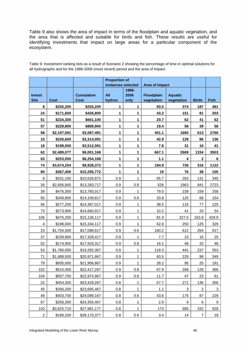
Integrated Modelling of the Lower River Murray 48
Table 9 also shows the area of impact in terms of the floodplain and aquatic vegetation, and the area that is affected and suitable for birds and fish. These results are useful for identifying investments that impact on large areas for a particular component of the ecosystem. Table 9: Investment ranking lists as a result of Scenario 2 showing the percentage of time in optimal solutions for all hydrographs and for the 1986-2006 (most recent) period and the area of impact.
Proportion of instances selected Area of Impact
Invest Site Cost
Cumulative Cost
All hydros
1986-2006 only
Floodplain vegetation
Aquatic vegetation Birds Fish
8 $255,200 $255,200 1 1 93.5 374 187 491
24 $171,600 $426,800 1 1 43.2 151 81 203
51 $234,300 $661,100 1 1 20.7 62 41 62
57 $228,800 $889,900 1 1 19.4 58 39 58
58 $2,197,591 $3,087,491 1 1 451.1 1660 613 2766
10 $226,600 $3,314,091 1 1 42.9 129 86 136
18 $198,000 $3,512,091 1 1 7.8 31 16 41
62 $2,489,077 $6,001,168 1 1 667.1 2669 1334 3503
63 $253,000 $6,254,168 1 1 1.1 4 2 6
74 $3,674,204 $9,928,372 1 1 194.9 726 316 1122
80 $367,400 $10,295,772 1 1 19 76 38 100
9 $331,100 $10,626,872 0.9 1 65.7 263 131 345
26 $2,656,845 $13,283,717 0.9 0.8 526 1963 941 2723
39 $476,300 $13,760,017 0.9 1 79.5 239 159 258
50 $349,800 $14,109,817 0.9 0.6 33.8 125 68 154
56 $277,200 $14,387,017 0.9 1 38.5 116 77 125
73 $273,900 $14,660,917 0.9 1 10.2 41 20 54
106 $475,200 $15,136,117 0.9 1 81.9 327.5 163.8 429.9
4 $198,000 $15,334,117 0.9 1 62.6 250 125 329
23 $1,754,500 $17,088,617 0.9 0.6 160.2 612 264 917
37 $239,800 $17,328,417 0.9 1 7.7 23 15 25
52 $174,900 $17,503,317 0.9 0.8 16.1 48 32 48
53 $1,780,050 $19,283,367 0.9 1 118.3 441 237 553
71 $1,688,500 $20,971,867 0.9 1 60.5 229 98 349
79 $935,000 $21,906,867 0.9 1 28.2 95 25 191
102 $510,400 $22,417,267 0.9 0.8 67.9 268 128 366
104 $557,700 $22,974,967 0.9 0.8 11.7 47 23 61
22 $454,300 $23,429,267 0.8 1 67.7 271 136 356
45 $266,200 $23,695,467 0.8 1 1.1 3 2 3
49 $403,700 $24,099,167 0.8 0.6 43.6 175 87 229
67 $256,300 $24,355,467 0.8 1 2.9 9 6 9
103 $3,625,710 $27,981,177 0.8 1 173 685 332 928
2 $189,200 $28,170,377 0.8 0.6 3.4 14 7 18
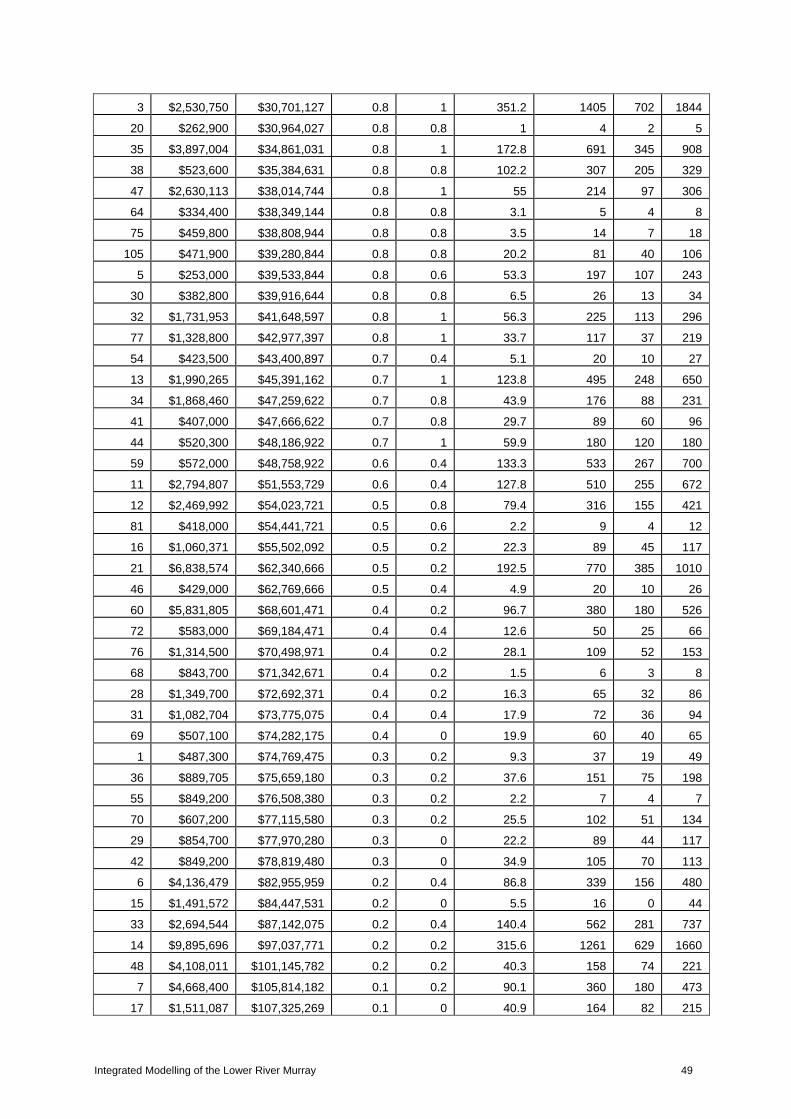
Integrated Modelling of the Lower River Murray 49
3 $2,530,750 $30,701,127 0.8 1 351.2 1405 702 1844
20 $262,900 $30,964,027 0.8 0.8 1 4 2 5
35 $3,897,004 $34,861,031 0.8 1 172.8 691 345 908
38 $523,600 $35,384,631 0.8 0.8 102.2 307 205 329
47 $2,630,113 $38,014,744 0.8 1 55 214 97 306
64 $334,400 $38,349,144 0.8 0.8 3.1 5 4 8
75 $459,800 $38,808,944 0.8 0.8 3.5 14 7 18
105 $471,900 $39,280,844 0.8 0.8 20.2 81 40 106
5 $253,000 $39,533,844 0.8 0.6 53.3 197 107 243
30 $382,800 $39,916,644 0.8 0.8 6.5 26 13 34
32 $1,731,953 $41,648,597 0.8 1 56.3 225 113 296
77 $1,328,800 $42,977,397 0.8 1 33.7 117 37 219
54 $423,500 $43,400,897 0.7 0.4 5.1 20 10 27
13 $1,990,265 $45,391,162 0.7 1 123.8 495 248 650
34 $1,868,460 $47,259,622 0.7 0.8 43.9 176 88 231
41 $407,000 $47,666,622 0.7 0.8 29.7 89 60 96
44 $520,300 $48,186,922 0.7 1 59.9 180 120 180
59 $572,000 $48,758,922 0.6 0.4 133.3 533 267 700
11 $2,794,807 $51,553,729 0.6 0.4 127.8 510 255 672
12 $2,469,992 $54,023,721 0.5 0.8 79.4 316 155 421
81 $418,000 $54,441,721 0.5 0.6 2.2 9 4 12
16 $1,060,371 $55,502,092 0.5 0.2 22.3 89 45 117
21 $6,838,574 $62,340,666 0.5 0.2 192.5 770 385 1010
46 $429,000 $62,769,666 0.5 0.4 4.9 20 10 26
60 $5,831,805 $68,601,471 0.4 0.2 96.7 380 180 526
72 $583,000 $69,184,471 0.4 0.4 12.6 50 25 66
76 $1,314,500 $70,498,971 0.4 0.2 28.1 109 52 153
68 $843,700 $71,342,671 0.4 0.2 1.5 6 3 8
28 $1,349,700 $72,692,371 0.4 0.2 16.3 65 32 86
31 $1,082,704 $73,775,075 0.4 0.4 17.9 72 36 94
69 $507,100 $74,282,175 0.4 0 19.9 60 40 65
1 $487,300 $74,769,475 0.3 0.2 9.3 37 19 49
36 $889,705 $75,659,180 0.3 0.2 37.6 151 75 198
55 $849,200 $76,508,380 0.3 0.2 2.2 7 4 7
70 $607,200 $77,115,580 0.3 0.2 25.5 102 51 134
29 $854,700 $77,970,280 0.3 0 22.2 89 44 117
42 $849,200 $78,819,480 0.3 0 34.9 105 70 113
6 $4,136,479 $82,955,959 0.2 0.4 86.8 339 156 480
15 $1,491,572 $84,447,531 0.2 0 5.5 16 0 44
33 $2,694,544 $87,142,075 0.2 0.4 140.4 562 281 737
14 $9,895,696 $97,037,771 0.2 0.2 315.6 1261 629 1660
48 $4,108,011 $101,145,782 0.2 0.2 40.3 158 74 221
7 $4,668,400 $105,814,182 0.1 0.2 90.1 360 180 473
17 $1,511,087 $107,325,269 0.1 0 40.9 164 82 215

Integrated Modelling of the Lower River Murray 50
19 $2,673,638 $109,998,907 0.1 0 125.1 500 250 657
78 $4,849,751 $114,848,658 0.1 0 14.5 58 29 76
61 $2,367,139 $117,215,797 0 0 21.8 87 44 115
Figure 22 shows the total area benefited versus cumulative investment costs, where the x axis represents the cumulative investments from best to worst in Table 9. It highlights a diminishing marginal return of benefit versus cost. That is, spending 50% of the budget optimally ($60M) leads to over 75% of the possible area benefited if $120M was spent.
Figure 22. Graph of wetland/floodplain area improved versus investment cost.
9.2.2. Scenario 3 – Infrastructure and weir raising and lowering
This scenario incorporated new regulator structure, pump relocation and weir raising and lowering of all six weirs. Table 10 shows the ranking of investments for scenario 3. Whilst the rank order is different to those of scenario 2 in Table 9, there is a 68% overlap in the top 30 investments.
Table 10: Investment ranking lists as a result of Scenario 3 showing the percentage of time in optimal solutions for all hydrographs and for the 1986-2006 (most recent) period and the area of impact.
Scenario 2
Investment cost
$0M $20M $40M $60M $80M $100M $120M
Flo
odpl
ain
area
(ha
)
0
5000
10000
15000
20000
25000
30000
35000
Terrestrial vegetation Aquatic vegetation Bird habitat Fish habitat
Scenario 2
Investment cost
$0M $20M $40M $60M $80M $100M $120M
Flo
odpl
ain
area
(ha
)
0
5000
10000
15000
20000
25000
30000
35000
Terrestrial vegetation Aquatic vegetation Bird habitat Fish habitat

Integrated Modelling of the Lower River Murray 51
Proportion of instances selected Area
Invest Cost Cumulative Cost
All hydros
1986-2006 only
Floodplain vegetation
Aquatic vegetation Birds Fish
102 $510,400 $510,400 1 1 67.9 267.8 128.4 366.3
74 $3,674,204 $4,184,604 1 1 194.9 726 315.7 1121.7
24 $171,600 $4,356,204 1 1 43.2 151.2 81 202.5
106 $475,200 $4,831,404 1 1 81.9 327.5 163.8 429.9
62 $2,489,077 $7,320,481 1 1 667.1 2668.6 1334.3 3502.5
26 $2,656,845 $9,977,326 1 0.8 526 1963.2 940.7 2722.9
80 $367,400 $10,344,726 0.9 1 19 76 38 99.7
58 $2,197,591 $12,542,317 0.9 1 451.1 1659.8 613 2765.8
13 $1,990,265 $14,532,582 0.9 1 123.8 495 247.5 649.7
71 $1,688,500 $16,221,082 0.9 1 60.5 228.5 98.4 348.6
47 $2,630,113 $18,851,195 0.9 1 55 213.8 97.4 306.2
8 $255,200 $19,106,395 0.9 1 93.5 374.2 187.1 491.1
53 $1,780,050 $20,886,445 0.8 1 118.3 440.6 236.6 552.9
105 $471,900 $21,358,345 0.8 1 20.2 80.7 40.4 106
104 $557,700 $21,916,045 0.8 1 11.7 46.8 23.4 61.4
64 $334,400 $22,250,445 0.8 0.4 3.1 4.8 4.3 7.8
51 $234,300 $22,484,745 0.8 0.8 20.7 62.1 41.4 62.1
23 $1,754,500 $24,239,245 0.8 0.8 160.2 611.6 263.8 916.9
22 $454,300 $24,693,545 0.8 1 67.7 271 135.5 355.7
52 $174,900 $24,868,445 0.8 0.8 16.1 48.4 32.2 48.4
50 $349,800 $25,218,245 0.8 0.8 33.8 125 67.7 154.3
39 $476,300 $25,694,545 0.8 0.8 79.5 238.5 159 258.3
32 $1,731,953 $27,426,498 0.8 0.8 56.3 225.3 112.7 295.8
18 $198,000 $27,624,498 0.8 0.6 7.8 31 15.5 40.7
11 $2,794,807 $30,419,305 0.8 0.6 127.8 510.2 254.6 672.4
103 $3,625,710 $34,045,015 0.7 0.8 173 684.9 331.7 927.9
73 $273,900 $34,318,915 0.7 0.8 10.2 40.8 20.4 53.6
49 $403,700 $34,722,615 0.7 0.6 43.6 174.5 87.2 229
37 $239,800 $34,962,415 0.7 0.6 7.7 23 15.3 24.9
3 $2,530,750 $37,493,165 0.7 0.8 351.2 1404.6 702.3 1843.6
79 $935,000 $38,428,165 0.7 0.8 28.2 95.2 25.2 191.3
77 $1,328,800 $39,756,965 0.7 0.2 33.7 117.2 36.6 219.2
45 $266,200 $40,023,165 0.7 0.6 1.1 3.3 2.2 3.3
10 $226,600 $40,249,765 0.7 0.8 42.9 128.8 85.9 136.4
54 $423,500 $40,673,265 0.6 1 5.1 20.4 10.2 26.7
16 $1,060,371 $41,733,636 0.6 0.8 22.3 89.3 44.6 117.2
12 $2,469,992 $44,203,628 0.6 1 79.4 315.8 155.4 421.3
63 $253,000 $44,456,628 0.6 1 1.1 4.2 2.1 5.5
38 $523,600 $44,980,228 0.6 1 102.2 306.7 204.5 328.7

Integrated Modelling of the Lower River Murray 52
30 $382,800 $45,363,028 0.6 0.4 6.5 26.1 13 34.2
21 $6,838,574 $52,201,602 0.6 0.8 192.5 769.8 384.9 1010.4
75 $459,800 $52,661,402 0.6 0 3.5 13.8 6.9 18.1
59 $572,000 $53,233,402 0.6 0.8 133.3 533.2 266.6 699.8
57 $228,800 $53,462,202 0.6 0.4 19.4 58.2 38.8 58.2
44 $520,300 $53,982,502 0.6 1 59.9 179.6 119.7 179.6
6 $4,136,479 $58,118,981 0.6 0.6 86.8 338.5 156 480.2
67 $256,300 $58,375,281 0.5 0.2 2.9 8.6 5.8 9.3
35 $3,897,004 $62,272,285 0.5 0.6 172.8 690.8 345 907.8
34 $1,868,460 $64,140,745 0.5 0.8 43.9 175.8 87.9 230.7
4 $198,000 $64,338,745 0.5 0.6 62.6 250.3 125.1 328.5
2 $189,200 $64,527,945 0.5 0.4 3.4 13.7 6.9 18
76 $1,314,500 $65,842,445 0.5 0 28.1 109 52 153.3
28 $1,349,700 $67,192,145 0.4 0.6 16.3 64.6 32 86.4
20 $262,900 $67,455,045 0.4 0.4 1 3.9 2 5.1
56 $277,200 $67,732,245 0.4 0.4 38.5 115.5 77 125.2
41 $407,000 $68,139,245 0.4 0.4 29.7 89.2 59.5 95.6
31 $1,082,704 $69,221,949 0.4 0.6 17.9 71.7 35.8 94.1
9 $331,100 $69,553,049 0.4 0.2 65.7 262.8 131.4 344.9
81 $418,000 $69,971,049 0.4 0 2.2 8.8 4.4 11.5
42 $849,200 $70,820,249 0.4 0.2 34.9 104.7 69.8 113.4
5 $253,000 $71,073,249 0.4 0 53.3 196.7 106.6 242.8
60 $5,831,805 $76,905,054 0.3 0.2 96.7 380.1 179.9 526.2
48 $4,108,011 $81,013,065 0.3 0.4 40.3 157.7 73.6 221.4
33 $2,694,544 $83,707,609 0.3 0.2 140.4 561.6 280.8 737.1
1 $487,300 $84,194,909 0.3 0.4 9.3 37 18.5 48.6
70 $607,200 $84,802,109 0.3 0.2 25.5 102.2 51.1 134.1
36 $889,705 $85,691,814 0.3 0.2 37.6 150.5 75.2 197.5
29 $854,700 $86,546,514 0.3 0.2 22.2 88.7 44.4 116.5
68 $843,700 $87,390,214 0.2 0.4 1.5 5.9 2.9 7.7
55 $849,200 $88,239,414 0.2 0 2.2 6.6 4.4 6.5
46 $429,000 $88,668,414 0.2 0.2 4.9 19.5 9.8 25.7
14 $9,895,696 $98,564,110 0.2 0 315.6 1261.3 628.8 1660.2
69 $507,100 $99,071,210 0.2 0.2 19.9 59.8 39.9 64.8
78 $4,849,751 $103,920,961 0.2 0 14.5 57.8 28.9 75.9
72 $583,000 $104,503,961 0.2 0 12.6 50.3 25.1 66
15 $1,491,572 $105,995,533 0.2 0 5.5 16 0 43.9
17 $1,511,087 $107,506,620 0.1 0.4 40.9 163.7 81.9 214.9
61 $2,367,139 $109,873,759 0 0.2 21.8 87.3 43.6 114.6
7 $4,668,400 $114,542,159 0 0 90.1 360.3 180.2 472.9
19 $2,673,638 $117,215,797 0 0 125.1 500.3 250.1 656.6
The scenarios incorporates the lowering and raising of the six weirs in South Australia. As mentioned before only three weirs are currently being considered and if this was the case

Integrated Modelling of the Lower River Murray 53
then the optimal investment rankings would change. Figure 23 shows the operational regime of the six weirs to achieve the outcomes over the model time period.
Figure 23. Weir regulation used in the optimum solution for investment and weir operation in Scenario 3. The operating regime is a result of the model optimising outcomes.
9.2.3. Scenario 4 – Infrastructure and weir raising only
Scenario 4 is the same as scenario 3 but the weirs are not manipulated below pool level. Table 9 contains the optimal rank order based on Scenario 4. Whilst the rank order is different to those of scenario 2 in Table 9, there is a 76% overlap in the top 30 investments.
Table 11: Investment ranking lists as a result of Scenario 4 showing the percentage of time in optimal solutions for all hydrographs and for the 1986-2006 (most recent) period and the area of impact.
Proportion of instances selected Area
Invest Cost Cumulative Cost
All hydros
1986-2006 only
Floodplain vegetation
Aquatic vegetation Birds Fish
8 $255,200 $255,200 1 1 93.5 374.2 187.1 491.1
23 $1,754,500 $2,009,700 1 1 160.2 611.6 263.8 916.9
26 $2,656,845 $4,666,545 1 1 526 1963.2 940.7 2722.9
47 $2,630,113 $7,296,658 1 1 55 213.8 97.4 306.2
52 $174,900 $7,471,558 1 1 16.1 48.4 32.2 48.4
74 $3,674,204 $11,145,762 1 1 194.9 726 315.7 1121.7
80 $367,400 $11,513,162 1 1 19 76 38 99.7
102 $510,400 $12,023,562 1 1 67.9 267.8 128.4 366.3
106 $475,200 $12,498,762 1 1 81.9 327.5 163.8 429.9
10 $226,600 $12,725,362 0.9 1 42.9 128.8 85.9 136.4
Lock 1-2
Wei
r he
ight
(cm
)
-25
0
25
50
Lock 2-3
Wei
r he
ight
(cm
)
-25
0
25
50
Lock 3-4
Months
0 50 100 150 200 250
Wei
r he
ight
(cm
)
-25
0
25
50
Lock 4-5
Lock 5-6
Lock 6 - SA border
Months
0 50 100 150 200 250
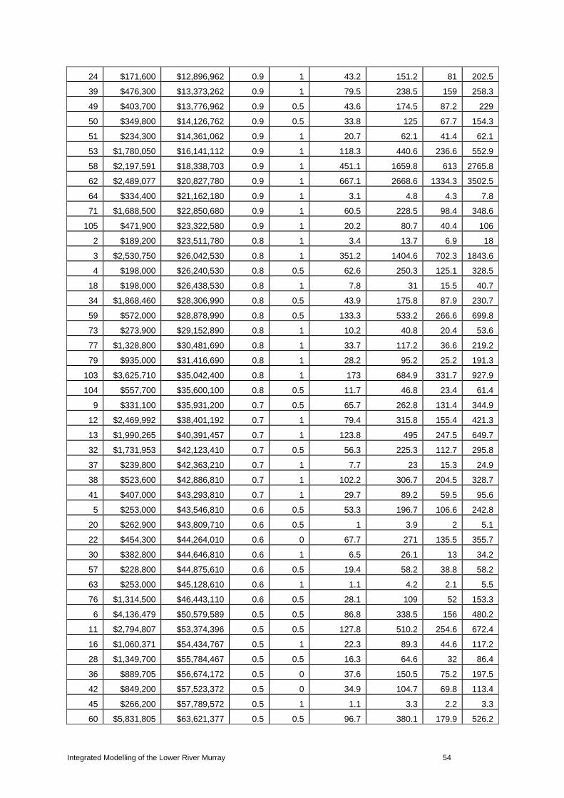
Integrated Modelling of the Lower River Murray 54
24 $171,600 $12,896,962 0.9 1 43.2 151.2 81 202.5
39 $476,300 $13,373,262 0.9 1 79.5 238.5 159 258.3
49 $403,700 $13,776,962 0.9 0.5 43.6 174.5 87.2 229
50 $349,800 $14,126,762 0.9 0.5 33.8 125 67.7 154.3
51 $234,300 $14,361,062 0.9 1 20.7 62.1 41.4 62.1
53 $1,780,050 $16,141,112 0.9 1 118.3 440.6 236.6 552.9
58 $2,197,591 $18,338,703 0.9 1 451.1 1659.8 613 2765.8
62 $2,489,077 $20,827,780 0.9 1 667.1 2668.6 1334.3 3502.5
64 $334,400 $21,162,180 0.9 1 3.1 4.8 4.3 7.8
71 $1,688,500 $22,850,680 0.9 1 60.5 228.5 98.4 348.6
105 $471,900 $23,322,580 0.9 1 20.2 80.7 40.4 106
2 $189,200 $23,511,780 0.8 1 3.4 13.7 6.9 18
3 $2,530,750 $26,042,530 0.8 1 351.2 1404.6 702.3 1843.6
4 $198,000 $26,240,530 0.8 0.5 62.6 250.3 125.1 328.5
18 $198,000 $26,438,530 0.8 1 7.8 31 15.5 40.7
34 $1,868,460 $28,306,990 0.8 0.5 43.9 175.8 87.9 230.7
59 $572,000 $28,878,990 0.8 0.5 133.3 533.2 266.6 699.8
73 $273,900 $29,152,890 0.8 1 10.2 40.8 20.4 53.6
77 $1,328,800 $30,481,690 0.8 1 33.7 117.2 36.6 219.2
79 $935,000 $31,416,690 0.8 1 28.2 95.2 25.2 191.3
103 $3,625,710 $35,042,400 0.8 1 173 684.9 331.7 927.9
104 $557,700 $35,600,100 0.8 0.5 11.7 46.8 23.4 61.4
9 $331,100 $35,931,200 0.7 0.5 65.7 262.8 131.4 344.9
12 $2,469,992 $38,401,192 0.7 1 79.4 315.8 155.4 421.3
13 $1,990,265 $40,391,457 0.7 1 123.8 495 247.5 649.7
32 $1,731,953 $42,123,410 0.7 0.5 56.3 225.3 112.7 295.8
37 $239,800 $42,363,210 0.7 1 7.7 23 15.3 24.9
38 $523,600 $42,886,810 0.7 1 102.2 306.7 204.5 328.7
41 $407,000 $43,293,810 0.7 1 29.7 89.2 59.5 95.6
5 $253,000 $43,546,810 0.6 0.5 53.3 196.7 106.6 242.8
20 $262,900 $43,809,710 0.6 0.5 1 3.9 2 5.1
22 $454,300 $44,264,010 0.6 0 67.7 271 135.5 355.7
30 $382,800 $44,646,810 0.6 1 6.5 26.1 13 34.2
57 $228,800 $44,875,610 0.6 0.5 19.4 58.2 38.8 58.2
63 $253,000 $45,128,610 0.6 1 1.1 4.2 2.1 5.5
76 $1,314,500 $46,443,110 0.6 0.5 28.1 109 52 153.3
6 $4,136,479 $50,579,589 0.5 0.5 86.8 338.5 156 480.2
11 $2,794,807 $53,374,396 0.5 0.5 127.8 510.2 254.6 672.4
16 $1,060,371 $54,434,767 0.5 1 22.3 89.3 44.6 117.2
28 $1,349,700 $55,784,467 0.5 0.5 16.3 64.6 32 86.4
36 $889,705 $56,674,172 0.5 0 37.6 150.5 75.2 197.5
42 $849,200 $57,523,372 0.5 0 34.9 104.7 69.8 113.4
45 $266,200 $57,789,572 0.5 1 1.1 3.3 2.2 3.3
60 $5,831,805 $63,621,377 0.5 0.5 96.7 380.1 179.9 526.2

Integrated Modelling of the Lower River Murray 55
69 $507,100 $64,128,477 0.5 1 19.9 59.8 39.9 64.8
72 $583,000 $64,711,477 0.5 1 12.6 50.3 25.1 66
75 $459,800 $65,171,277 0.5 0.5 3.5 13.8 6.9 18.1
81 $418,000 $65,589,277 0.5 0.5 2.2 8.8 4.4 11.5
31 $1,082,704 $66,671,981 0.4 1 17.9 71.7 35.8 94.1
35 $3,897,004 $70,568,985 0.4 0.5 172.8 690.8 345 907.8
44 $520,300 $71,089,285 0.4 0.5 59.9 179.6 119.7 179.6
46 $429,000 $71,518,285 0.4 0 4.9 19.5 9.8 25.7
48 $4,108,011 $75,626,296 0.4 0.5 40.3 157.7 73.6 221.4
54 $423,500 $76,049,796 0.4 0.5 5.1 20.4 10.2 26.7
56 $277,200 $76,326,996 0.4 0.5 38.5 115.5 77 125.2
1 $487,300 $76,814,296 0.3 0.5 9.3 37 18.5 48.6
21 $6,838,574 $83,652,870 0.3 0 192.5 769.8 384.9 1010.4
55 $849,200 $84,502,070 0.3 0.5 2.2 6.6 4.4 6.5
67 $256,300 $84,758,370 0.3 0.5 2.9 8.6 5.8 9.3
14 $9,895,696 $94,654,066 0.2 0 315.6 1261.3 628.8 1660.2
15 $1,491,572 $96,145,638 0.2 0.5 5.5 16 0 43.9
33 $2,694,544 $98,840,182 0.2 0 140.4 561.6 280.8 737.1
68 $843,700 $99,683,882 0.2 0.5 1.5 5.9 2.9 7.7
70 $607,200 $100,291,082 0.2 0.5 25.5 102.2 51.1 134.1
7 $4,668,400 $104,959,482 0.1 0 90.1 360.3 180.2 472.9
29 $854,700 $105,814,182 0.1 0 22.2 88.7 44.4 116.5
78 $4,849,751 $110,663,933 0.1 0 14.5 57.8 28.9 75.9
17 $1,511,087 $112,175,020 0 0 40.9 163.7 81.9 214.9
19 $2,673,638 $114,848,658 0 0 125.1 500.3 250.1 656.6
61 $2,367,139 $117,215,797 0 0 21.8 87.3 43.6 114.6
The operational regime of the weirs is presented in Figure 24. The operation only includes weir raising. Note that the weirs are raised more times in the model run time period than they are in scenario 3 when weir lowering is allowed.

Integrated Modelling of the Lower River Murray 56
Figure 24. Weir regulation used in the optimum solution for investment and weir operation in Scenario 4 Compared to scenario 3, only weir heights of >0cm were allowed, thus leading to a cycle variation compared to Figure 22.
9.3. Ecological Results
9.3.1. Scenario 2 – Infrastructure but no weir manipulation
Summarised ecological scores (aggregated from ecohydrological units) were generated for each ecological component category by flood timing (FT), flood duration (FD) and interflood period (IP). The values in Table 12 represent the summarised scores for the Model, which is an aggregation of FT, FD, IP curves over all ecological functions and river weir reaches. Instead of showing the aggregated scores for Base (current flows with current infrastructure and no weir manipulation), Model (current flows with new infrastructure, pump relocation and weir manipulation depending on the scenario) and Natural (natural flows before river regulation and extraction), results in Table 12 represent the values for the Model in terms of distance between 0 (Base) and 1 (Natural) for scenario 2. The closer the value is to 1 the better. A negative score means that the Model produced a weaker response than the Base solution for that category which can occur if the flood timing, flood duration or Interflood period is less beneficial. This is possible because the model is an optimisation of many factors. This means that in some scenarios, for some variables, the optimal result may be lower than the current value. By operating the flow control infrastructure, the Model produced significant improvements in FD compared to the FT and IP indicators for non-permanent wetlands. This is not surprising since regulators are an effective means of holding water in non-permanent wetlands or holding water out of permanent wetlands to achieve desirable FD’s. To substantially improve FT and IP for all wetlands we need to be able to strategically modify the hydrograph in conjunction with the investments and optimising the regulator operations. FT and IP are impacted for local wetlands by their regulators. Table 13 shows the areas of good condition derived by multiplying the area of the floodplain, as represented by EH mapping, by its ecological condition, based individual MFAT responses or the average aggregates. The total area can be seen as higher under natural
Lock 1-2W
eir
heig
ht (
cm)
-25
0
25
50
Lock 2-3
Wei
r he
ight
(cm
)
-25
0
25
50
Lock 3-4
Months
0 50 100 150 200 250
Wei
r he
ight
(cm
)
-25
0
25
50
Lock 4-5
Lock 5-6
Lock 6 - SA border
Months
0 50 100 150 200 250

Integrated Modelling of the Lower River Murray 57
conditions than base case. The scenario model results in Table 12 are based on the amount of area that has moved from the base case towards the natural case. Table 12: Summarised ecological score of Scenario 2 versus Base and Natural for each ecological component.
1986-2006
Floodplain vegetation Aquatic vegetation Bird habitat Fish habitat
Flood timing 0.0035 0.2925 0.0633 0.1277
Interflood period 0.0175 0.1599 0.0252 0.1418
Flood duration 0.0975 0.5622 0.3872 0.4788
Table 13: Total scores (areas) for base case and natural case for ecological components.
Total score (Base) Area multiplied by ecological condition
Total score (Natural) Area multiplied by ecological condition
Floodplain vegetation
Aquatic vegetation
Bird habitat
Fish habitat
Floodplain vegetation
Aquatic vegetation
Bird habitat
Fish habitat
Flood timing 326,852 624,412 354,910 1,414,350 406,147 576,355 448,075 1,417,731Interflood period 31,425 36,814 29,881 49,696 54,421 43,387 55,493 77,384Flood duration 31,425 34,712 25,330 58,181 54,421 39,213 40,463 82,344
Note that the area of aquatic vegetation under the base case is higher than under natural and the increased area of permanent wetlands has created a larger area suitable for fringing aquatic vegetation. This may not be the case in reality as a natural wet/dry cycle is likely to produce greater areas of suitable aquatic vegetation habitat including the wetland beds when dry, the variable fringing habitats and enhanced light penetration from clearer water due to the consolidation of sediments. This is a limitation of the model and could be addressed in future work by creating new MFAT responses (such as an interflood period for ribbonweed herblands), refining existing MFAT responses and reassigning the habitat scores detailed in Appendix B for these two functional groups across the wetland types. Figure 25 summarises the difference between base case, scenario 2 and natural conditions for each ecological component for the three hydrological parameters. The graph is best interpreted by a gain (green bar) achieved by scenario 2 versus the base (red) and natural (blue). A large green bar compared to the blue bar means scenario 2 achieves significant progress towards the score of the natural hydrograph for that indicator. The most visually noticeable impacts for scenario 2 are for FD. The only limitation of Figure 25 is that it does not show the higher score for the base for aquatic vegetation in flood timing (Table 13).

Integrated Modelling of the Lower River Murray 58
Figure 25.. Summary of ecological benefits from Scenario 2. Red indicates the area of the floodplain that achieved a good ecological score under base scenario (current conditions). Blue shows the area that used to occur under natural conditions. Green shows the area that has been improved as a result of the scenario across all hydrographs combinations. Note the term terrestrial vegetation here refers to floodplain vegetation.
The model shows estimates of the area of suitable habitat (Figure 25) but a number of factors could alter the actual vegetation extent. These include:
The vegetation data is 10 years old and transitions to other habitats could have already commenced;
The condition of the vegetation is too poor or old to respond resulting in suitable habitat but not the tree response until recruitment occurs;
Inappropriate soils to produce the results shown; and Insufficient seed banks or dispersal to generate the response.
Figure 26 to Figure 28 show the detailed distribution of flood timing, interflood period and flood duration for different ecological components and for each of the 7 river reaches. The graphs are in the form of histograms (like Figure 3). The graphs show which parts of the flood duration, flood timing and interflood period does the scenario 2 (green line) improve upon most, versus the base case. The bar chart at the top of each graph shows the ecological suitability for each ecological function, which acts like a priority weighting in the model. Where the bars are higher (e.g. certain months suited for flood timing), it is more preferable to achieve a gain for the scenario 2 versus the base. In most cases, there was not a significant visible difference between the base and scenario 2. There were instances in aquatic vegetation (Figure 26) where there was a visible benefit for flood timing. For flood
Terrestrial vegetationE
colo
gica
l sco
re
0
20000
40000
60000
80000
100000
120000Natural hydrograph
Scenario 2
Base scenario
Aquatic vegetation
Bird habitat
Flood
timing
Inte
rfloo
d pe
riod
Flood
dura
tion
Total
Eco
logi
cal s
core
0
20000
40000
60000
80000
100000
120000Fish habitat
Flood
timing
Inte
rfloo
d pe
riod
Flood
dura
tion
Total

Integrated Modelling of the Lower River Murray 59
duration (Figure 27), the graphs for scenario 2 were very close to those of the natural hydrograph across all river reaches for aquatic vegetation.
Figure 26. Graphs showing the floodplain and wetland areas in good ecological health under base case (current), natural and model scenario 2 for flood timing.
Eco
logi
cal
suita
biliity
0
1
Aquatic vegetationFloodplain trees Bird habitat Fish habitat
Wellington - Lock 1
0
2500
5000
Lock 1 - Lock 2
0
1000
2000
3000
Lock 2 - Lock 3
0
1000
2000
3000
Lock 3 - Lock 4
Flo
odp
lain
and
wetla
nd
are
a (h
a)
0
2500
5000
7500
10000
Lock 4 - Lock 5
0
2500
5000
Lock 5 - Lock 6
0
2500
5000
7500
Lock 6 - SA border
Jan
Feb
Mar Ap
rMay Ju
nJu
lAu
gSe
pOct
Nov
Dec
0
2500
5000
Flood timingJa
nFe
bMar Ap
rMay Ju
nJu
lAu
gSe
pOct
Nov
Dec Ja
nFe
bMar Ap
rMay Ju
nJu
lAu
gSe
pOct
Nov
Dec Ja
nFe
bMar Ap
rMay Ju
nJu
lAu
gSe
pOct
Nov
Dec
Base scenario Scenario 2Natural hydrograph

Integrated Modelling of the Lower River Murray 60
Figure 27. Graphs showing the floodplain and wetland areas in good ecological health under base case (current), natural and model scenario 2 for interflood period.
Eco
logical
suita
biliity
0
1
Aquatic vegetationFloodplain trees Bird habitat Fish habitat
Wellington - Lock 1
0
1000
2000
Lock 1 - Lock 2
0
500
1000
Lock 2 - Lock 3
0
500
1000
Lock 3 - Lock 4
Flo
odpla
in a
nd w
etla
nd
are
a (h
a)
0
1000
2000
3000
4000
Lock 4 - Lock 5
0
1000
2000
3000
Lock 5 - Lock 6
0
1000
2000
3000
Lock 6 - SA border
0 20 40 60 80 100
120
140
160
0
1000
2000
3000
Inter flood duration (months)
0 20 40 60 80 100
120
140
160 0 20 40 60 80 10
012
014
016
0 0 20 40 60 80 100
120
140
160
Base scenario Scenario 2Natural hydrograph

Integrated Modelling of the Lower River Murray 61
Figure 28. Graphs showing the floodplain and wetland areas in good ecological health under base case (current), natural and model scenario 2 for flood duration.
A further extension of the project would be to report on the ecological results for each EH type looking at ecological components and the different ID, FT, IP factors. This would provide an idea of representiveness in terms of EH type the investment outcomes will deliver upon and provide insight into which EH types are being targeted to the hydrological scenario.
9.3.2. Scenario 3 – Infrastructure and weir raising and lowering
The results for scenario 3 are presented in the same way as for scenario 2 in Table 14 and Figure 29 to Figure 32. One would expect the score for scenario 3 to be a slight improvement over scenario 2 (Table 10). In this case it was mixed, where some scores improved whilst others didn’t. The results on optimal investments in Tables 7-9 were based on the best five model runs for each of the five hydrographs. Results in Tables 10, 12 and 14 are based on one hydrograph which is why there is some variation in these results. Figures 29-32 are interpreted in the same way as Figures 25-28 for Scenario 2. It is hard to compare the results
Eco
logical
suita
biliity
0
1
Aquatic vegetationFloodplain trees Bird habitat Fish habitat
Wellington - Lock 1
0
500
1000
Lock 1 - Lock 2
0
500
1000
Lock 2 - Lock 3
0
500
1000
Lock 3 - Lock 4
Flo
odpla
in a
nd w
etla
nd a
rea (ha
)
0
1000
2000
3000
Lock 4 - Lock 5
0
1000
2000
Lock 5 - Lock 6
0
1000
2000
3000
Lock 6 - SA border
1 2 3 4 5 6 7 8 9101112131415161718
19-49>4
90
1000
2000
Inundation duration (months)
1 2 3 4 5 6 7 8 9101112131415161718
19-49>4
9 1 2 3 4 5 6 7 8 9101112131415161718
19-49>4
9 1 2 3 4 5 6 7 8 9101112131415161718
19-49>4
9
Base scenario Scenario 2Natural hydrograph
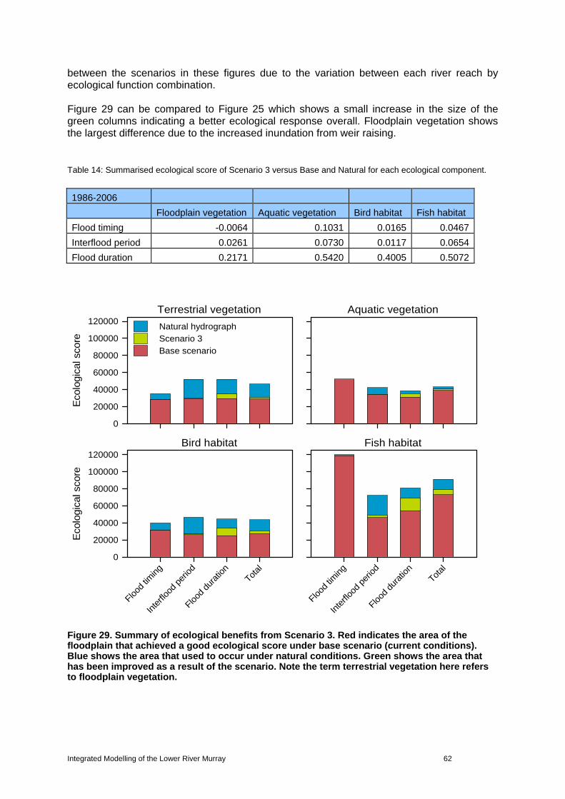
Integrated Modelling of the Lower River Murray 62
between the scenarios in these figures due to the variation between each river reach by ecological function combination. Figure 29 can be compared to Figure 25 which shows a small increase in the size of the green columns indicating a better ecological response overall. Floodplain vegetation shows the largest difference due to the increased inundation from weir raising.
Table 14: Summarised ecological score of Scenario 3 versus Base and Natural for each ecological component.
1986-2006
Floodplain vegetation Aquatic vegetation Bird habitat Fish habitat
Flood timing -0.0064 0.1031 0.0165 0.0467
Interflood period 0.0261 0.0730 0.0117 0.0654
Flood duration 0.2171 0.5420 0.4005 0.5072
Figure 29. Summary of ecological benefits from Scenario 3. Red indicates the area of the floodplain that achieved a good ecological score under base scenario (current conditions). Blue shows the area that used to occur under natural conditions. Green shows the area that has been improved as a result of the scenario. Note the term terrestrial vegetation here refers to floodplain vegetation.
Terrestrial vegetation
Eco
logi
cal s
core
0
20000
40000
60000
80000
100000
120000Natural hydrographScenario 3 Base scenario
Aquatic vegetation
Bird habitat
Flood
timing
Inte
rfloo
d pe
riod
Flood
dura
tion
Total
Eco
logi
cal s
core
0
20000
40000
60000
80000
100000
120000Fish habitat
Flood
timing
Inte
rfloo
d pe
riod
Flood
dura
tion
Total

Integrated Modelling of the Lower River Murray 63
Figure 30. Graphs showing the floodplain and wetland areas in good ecological health under base case (current), natural and model scenario 3 for flood timing.
Eco
logic
al
suita
biliity
0
1
Aquatic vegetationFloodplain trees Bird habitat Fish habitat
Wellington - Lock 1
0
2500
5000
Lock 1 - Lock 2
0
1000
2000
3000
Lock 2 - Lock 3
0
1000
2000
3000
Lock 3 - Lock 4
Flo
odpla
in a
nd w
etla
nd
are
a (ha
)
0
2500
5000
7500
10000
Lock 4 - Lock 5
0
2500
5000
Lock 5 - Lock 6
0
2500
5000
7500
Lock 6 - SA border
Jan
Feb
Mar Ap
rMay Ju
nJu
lAu
gSep O
ctNov
Dec
0
2500
5000
Flood timingJa
nFe
bMar Ap
rMay Ju
nJu
lAu
gSep O
ctNov
Dec Ja
nFe
bMar Ap
rMay Ju
nJu
lAug Se
pOct
Nov
Dec Ja
nFe
bMar Apr
May Ju
nJu
lAu
gSe
pOct
Nov
Dec
Base scenario Scenario 3Natural hydrograph

Integrated Modelling of the Lower River Murray 64
Figure 31. Graphs showing the floodplain and wetland areas in good ecological health under base case (current), natural and model scenario 3 for interflood period.
Eco
logical
suita
biliity
0
1
Aquatic vegetationFloodplain trees Bird habitat Fish habitat
Wellington - Lock 1
0
1000
2000
Lock 1 - Lock 2
0
500
1000
Lock 2 - Lock 3
0
500
1000
Lock 3 - Lock 4
Flo
odpla
in a
nd w
etla
nd
are
a (h
a)
0
1000
2000
3000
4000
Lock 4 - Lock 5
0
1000
2000
3000
Lock 5 - Lock 6
0
1000
2000
3000
Lock 6 - SA border
0 20 40 60 80 100
120
140
160
0
1000
2000
3000
Inter flood duration (months)
0 20 40 60 80 100
120
140
160 0 20 40 60 80 10
012
014
016
0 0 20 40 60 80 100
120
140
160
Base scenario Scenario 3Natural hydrograph

Integrated Modelling of the Lower River Murray 65
Figure 32. Graphs showing the floodplain and wetland areas in good ecological health under base case (current), natural and model scenario 3 for flood duration.
9.3.3. Scenario 4 – Infrastructure and weir raising only
The results for scenario 4 are presented in the same way as for scenarios 2 and 3 in Table 15 and Figure 33 to Figure 36. From these graphs and tables, it is difficult to make comparisons between scenario 2, 3 and 4 due to the variability across ecological functions and river reaches. We would expect the overall ecological score for scenario 4 to be in between scenario 2 and 3 since only weir raising was allowed. Comparing scenario 3 (29) with scenario 4 (Figure 33) the differences are very small. Scenario 4 (Figure 33) shows the improved terrestrial vegetation (floodplain vegetation) response over scenario 2 (Figure 25).
Table 15: Summarised ecological score of Scenario 4 versus Base and Natural for each ecological component.
1986-2006
Eco
logical
suita
biliity
0
1
Aquatic vegetationFloodplain trees Bird habitat Fish habitat
Wellington - Lock 1
0
500
1000
Lock 1 - Lock 2
0
500
1000
Lock 2 - Lock 3
0
500
1000
Lock 3 - Lock 4
Flood
plain a
nd w
etland
area
(ha
)
0
1000
2000
3000
Lock 4 - Lock 5
0
1000
2000
Lock 5 - Lock 6
0
1000
2000
3000
Lock 6 - SA border
1 2 3 4 5 6 7 8 9101112131415161718
19-49>4
90
1000
2000
Inundation duration (months)
1 2 3 4 5 6 7 8 9101112131415161718
19-49>4
9 1 2 3 4 5 6 7 8 9101112131415161718
19-49>4
9 1 2 3 4 5 6 7 8 9101112131415161718
19-49>4
9
Base scenario Scenario 3Natural hydrograph

Integrated Modelling of the Lower River Murray 66
Floodplain vegetation Aquatic vegetation Bird habitat Fish habitat
Flood timing 0.0099 0.2085 0.0344 0.0998
Interflood period 0.0283 0.1112 0.0204 0.1106
Flood duration 0.1976 0.5305 0.4064 0.4677
Figure 33. Summary of ecological benefits from Scenario 4. Red indicates the area of the floodplain that achieved a good ecological score under base scenario (current conditions). Blue shows the area that used to occur under natural conditions. Green shows the area that has been improved as a result of the scenario. Note the term terrestrial vegetation here refers to floodplain vegetation.
Terrestrial vegetation
Eco
logi
cal s
core
0
20000
40000
60000
80000
100000
120000Natural hydrographScenario 4Base scenario
Aquatic vegetation
Bird habitat
Flood
timing
Inte
rfloo
d pe
riod
Flood
dura
tion
Total
Eco
logi
cal s
core
0
20000
40000
60000
80000
100000
120000Fish habitat
Flood
timing
Inte
rfloo
d pe
riod
Flood
dura
tion
Total

Integrated Modelling of the Lower River Murray 67
Figure 34. Graphs showing the floodplain and wetland areas in good ecological health under base case (current), natural and model scenario 4 for flood timing.
Eco
logical
suita
biliity
0
1
Aquatic vegetationFloodplain trees Bird habitat Fish habitat
Wellington - Lock 1
0
2500
5000
Lock 1 - Lock 2
0
1000
2000
3000
Lock 2 - Lock 3
0
1000
2000
3000
Lock 3 - Lock 4
Flo
odpla
in a
nd w
etla
nd a
rea (ha)
0
2500
5000
7500
10000
Lock 4 - Lock 5
0
2500
5000
Lock 5 - Lock 6
0
2500
5000
7500
Lock 6 - SA border
Jan
Feb
Mar Ap
rMay Ju
nJu
lAu
gSe
pOct
Nov
Dec
0
2500
5000
Flood timingJa
nFe
bMar Ap
rMay Ju
nJu
lAu
gSe
pOct
Nov
Dec Ja
nFe
bMar Ap
rMay Ju
nJu
lAu
gSe
pOct
Nov
Dec Ja
nFe
bMar Ap
rMay Ju
nJu
lAu
gSe
pOct
Nov
Dec
Base scenario Scenario 4Natural hydrograph
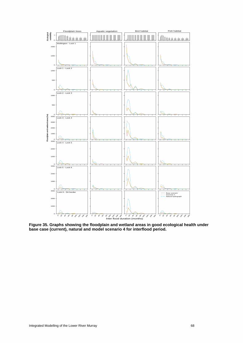
Integrated Modelling of the Lower River Murray 68
Figure 35. Graphs showing the floodplain and wetland areas in good ecological health under base case (current), natural and model scenario 4 for interflood period.
Eco
logical
suita
biliity
0
1
Aquatic vegetationFloodplain trees Bird habitat Fish habitat
Wellington - Lock 1
0
1000
2000
Lock 1 - Lock 2
0
500
1000
Lock 2 - Lock 3
0
500
1000
Lock 3 - Lock 4
Flo
odpla
in a
nd w
etla
nd
are
a (h
a)
0
1000
2000
3000
4000
Lock 4 - Lock 5
0
1000
2000
3000
Lock 5 - Lock 6
0
1000
2000
3000
Lock 6 - SA border
0 20 40 60 80 100
120
140
160
0
1000
2000
3000
Inter flood duration (months)
0 20 40 60 80 100
120
140
160 0 20 40 60 80 10
012
014
016
0 0 20 40 60 80 100
120
140
160
Base scenario Scenario 4Natural hydrograph
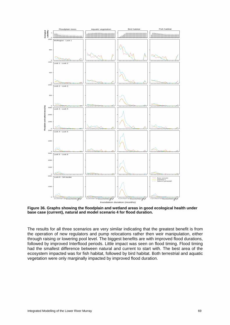
Integrated Modelling of the Lower River Murray 69
Figure 36. Graphs showing the floodplain and wetland areas in good ecological health under base case (current), natural and model scenario 4 for flood duration.
The results for all three scenarios are very similar indicating that the greatest benefit is from the operation of new regulators and pump relocations rather then weir manipulation, either through raising or lowering pool level. The biggest benefits are with improved flood durations, followed by improved Interflood periods. Little impact was seen on flood timing. Flood timing had the smallest difference between natural and current to start with. The best area of the ecosystem impacted was for fish habitat, followed by bird habitat. Both terrestrial and aquatic vegetation were only marginally impacted by improved flood duration.
Eco
logical
suita
biliity
0
1
Aquatic vegetationFloodplain trees Bird habitat Fish habitat
Wellington - Lock 1
0
500
1000
Lock 1 - Lock 2
0
500
1000
Lock 2 - Lock 3
0
500
1000
Lock 3 - Lock 4
Flood
plain
and
wetla
nd
are
a (ha)
0
1000
2000
3000
Lock 4 - Lock 5
0
1000
2000
Lock 5 - Lock 6
0
1000
2000
3000
Lock 6 - SA border
1 2 3 4 5 6 7 8 9101112131415161718
19-49>4
90
1000
2000
Inundation duration (months)
1 2 3 4 5 6 7 8 9101112131415161718
19-49>4
9 1 2 3 4 5 6 7 8 9101112131415161718
19-49>4
9 1 2 3 4 5 6 7 8 9101112131415161718
19-49>4
9
Base scenario Scenario 4Natural hydrograph

Integrated Modelling of the Lower River Murray 70
10. DISCUSSION The approach used here takes a substantial step forward over past research by addressing a river system where there are multiple infrastructures (weirs and regulators) to be optimised simultaneously to achieve ecological and social benefits across a range of spatial and temporal scales. The model addresses the real world planning question of the selection of a cost-effective suite of investments in establishing new flow-control infrastructure given a limited budget. It also identifies the optimal operation of this infrastructure to control flows in watercourse, floodplain, and wetland ecosystems (see Appendix E for full details of the optimisation model) with the aim of returning natural environmental flows in terms of flood timing, duration, and interflood period. It is a complex, non-linear problem, since investment and operating decisions in one site affect investment and management decisions and their ecological and social consequences in other sites. The increase from 84% of wetlands being permanent to inundating 95% with a medium size flood highlights that wetland management in SA should predominately focus on reducing permanent wetlands (through either regulators or weir pool lowering) to maximise effectiveness, rather than looking at increased flows, whilst the management method of increased flows relates more to the critical needs of the floodplain ecosystems
10.1. Ecological benefits The investments have been shown to produce a large, over 50%, improvement in the area of good condition for aquatic vegetation and fish passage for flood duration as the regulators can hold water in and out of wetlands for the targeted duration. The flood duration, timing and the Interflood period can be manipulated with the control structures. The results for scenario 2 (no weirs) shows an improvement of 56% of the gap between base case and natural for the area of good condition for aquatic vegetation and 48% for fish habitat in regards to flood duration (Figure 25 and Table 12). The result for bird breeding is 39% improvement which is still a significant gain. Floodplain vegetation shows an improvement of 10% to the fringing vegetation. For Interflood period the results for aquatic vegetation, birds, fish and floodplain vegetation are 16%, 3%, 14% and 2% respectively. For flood timing the results are 29%, 6%, 13% and 0%. It is not surprising that flood timing has not been altered for broad floodplain vegetation areas high on the floodplain from investments in wetland regulators only. Less improvement for floodplain vegetation and bird breeding habitat occurs because these have a different ecosystem requirement that cannot be met by regulators. The results for scenario 3 (investments and weir raising and lowering) show improvements similar to scenario 2 (Table 14). Results for scenario 4 (weir raising only) are between scenario 2 and 3 (Table 15). The regulators are likely to provide less benefit in terms of flood timing and interflood period as these need larger changes in the occurrence of floods over the South Australian border. Though this would be different for the management of permanent wetlands. Adding weir operations only marginally improves the benefits obtained from the regulator investments. To benefit ecohydrological types associated with the mid to high elevation areas floodplain these results support the widely acknowledged fact there is a need to impact large changes in the occurrence of floods over the South Australian border. For these ecohydrological classification types it can be concluded, largely, that management solutions other than wetland regulators and weir pool manipulation are required. The results show that flood duration, and to a lesser extent flood timing and interflood period, for aquatic vegetation, fish habitat and bird habitat can be improved though manipulation of wetland regulators. The scale of investments considered here have a large impact on the

Integrated Modelling of the Lower River Murray 71
habitats for these two ecological components in the Lower River Murray in South Australia. As expected the wetland regulators have less impact on bird and floodplain vegetation habitats but do still show improvements over current conditions when compared to areas under natural conditions. The investments considered have less of an impact on flood timing and interflood periods for all ecological types for non-permanent wetlands. To target these EH types changes to the flow regime across the South Australian border are one option to potentially further improve these hydrological parameters for floodplains and non-permanent wetlands, especially for bird and floodplain vegetation habitats. To optimally achieve this the following management options could be investigated, increasing the environmental water reserve, gain more understanding around optimal timing of e-flows, improve ability to utilise/call upon multiple storages in unison, improve release capacities of storages etc.
10.2. Priority investments The analysis for this report has maximised ecological outcomes through the optimal selection of new investments and the optimal operation of weir and regulator infrastructure. It is based on no change in water availability at the South Australian border or any additional storage of water. Building and operating the suggested new investments and operating the weirs and existing regulators in accordance with the optimal model runs will provide improved ecological and social benefits. The list of investments and the order they appear in the results is different for the three scenarios presented. This shows that a different combination of regulators is needed depending on whether the weirs are not used, are raised or are allowed to be raised and lowered. This is also true for the operation of only three of the weirs due to salinity issues. There are a lot of common investments to all three lists and these investments are seen as the safest investments to make regardless of other management options being available as highlighted in Section 9.2.
10.3. Limitations of the ecological response models There are a number of limitations associated with the ecological response models used in this study. These limitations should be acknowledged to ensure that appropriate caution is used when interpreting the results from those models. For the most part, the information used was based on the ecological response curves used in MFAT (Young et al. 2003). A number of limitations associated with the information included in MFAT have been identified (Nick Bond, Monash University, Brenton Zampatti, SARDI Aquatic Sciences, Dan Rogers, SA Department for Environment and Heritage, personal communication). Where scientific evidence or expert opinion was available, it was used to update MFAT curves, or develop new curves. These changes have been documented as per the MFAT method to ensure transparency and robustness of the assessments. One relevant limitation with MFAT is whether fish communities in the Lower River Murray respond in the manner described therein. There is a view that fish communities in the River were poorly understood in 2003, and that the curves included should be treated with caution, despite being best-available science at the time (Nick Bond, Monash University, Brenton Zampatti, SARDI Aquatic Sciences, personal communication). To date, however, no replacement curves have been developed. Another concern is that not all biotic groups are evenly distributed throughout the Lower River Murray, and that the curves may give a misleading picture of the likely biotic response. For example, it is recognised that colonial nesting waterbirds are unlikely to breed in the large accumulations common upstream in the lower reaches of the River, regardless of the types of habitat present. A biogeographic constraint that was able to reflect these limitations would be a potential improvement solution

Integrated Modelling of the Lower River Murray 72
as a further development of this model. As well as increased number of MFAT curves used when compared to other ecosystem components. Another limitation related to this study (but also potentially MFAT) relates to how ecological response curves are combined. Multiple curves exist for most communities, although not all and especially not for every lifestage (e.g. for flood timing, interflood periods and inundation durations). MFAT used an arithmetic mean to combine multiple curves, but little justification exists for this choice. There is limited understanding how the choice of method for combining curves is likely to affect the outcomes of the modelling. Also, not all of the curves in MFAT were able to be incorporated in this work (e.g. the numerical model did not predict rates of rise and fall of flood waters, so responses to these variables could not be included). It is unclear how the exclusion of these curves affects the modelling outcomes. The analysis considered the sensitivity of optimal investments due to uncertainty in the hydrograph. It showed about a 90% overlap between optimal investments in regulators across the hydrographs which gives confidence in the optimal investments being robust across the possible future hydrographs. This is not all that surprising as the wetland regulator management option primarily focuses on returning the disproportionate number of permanent wetlands to a more temporary hydrological regime. It is perhaps this permanency (relative certainty) of localised hydrology that has resulted in the overlap of optimal mosaics of investment sites, which also fosters confidence in investment choices. There is a further need to understand the sensitivity of the numerical model and the selection of regulators to uncertainties with the ecological response models. If the outcome is relative insensitive to the values in each individual response curve, the limitations highlighted here may have a very small impact on the outcomes of this study. Given the low sensitivity of regulator investment to hydrograph, would give us confidence of low sensitivity to ecological response. Particularly as variations in hydrographs impact all ecohydrological units whereas variations in response curves will have a smaller impact to a limited number of eco-hydrological units. The exception may be if there was a major bias in response curves across a large number of species or ecological functions, or for those functional groups that only have a relatively small number of total response curves. Some additional work is required to analyse these sensitivities.
10.4. Further analysis and refinements There are additional analysis that can be conducted to explore further opportunities for increased ecological benefits or saving of water. These are identified as:
Improved response models, sensitivity testing, make sure that the eco-hydro types are reflected (changed) with management, i.e.
wetland goes from permanent to temporary with different response curves and will therefore better reflect the response expected through the investment…
how best to use the 15GL from RRP Or how best to use water buyback associated e.g. through Water for the Future
1) Purchasing of additional water entitlements versus additional infrastructure. We can simulate the ecological benefits of investing in $X of new regulators versus $X of additional water entitlements and their associated allocations over Y years for ecological use. The additional purchased water entitlements and their associated allocations could be added to the hydrograph in ecologically ideal time periods keeping in mind both operational and statutory constraints. Under both scenarios, the operational use of infrastructure would be optimised. Another way to look at the issue is if there is a budget of $Z in total, optimise the

Integrated Modelling of the Lower River Murray 73
amount of the budget used for additional infrastructure ($X) versus purchasing additional water ($Y) where X+Y=Z. The problem with this approach/suggestion is that it compares two different management objectives that target two different problems for different ecosystems. Namely ecosystems with too much water to sustain natural function and ecosystems with too little water to sustain natural function. 2) Hold back water at storages and release when ecologically suitable. In this scenario, there is no increase in water, but it is released at the border at optimal times according to ecological outcomes. We could also turn the scenario around to minimise the amount of water required to achieve the same ecological outcome as the current hydrograph, by optimising its timing. Whilst the best available information up to April 2010 was used in the model, the following could be refined further for future analysis:
Costs of regulator investments. Also, Investment_ID’s 100 and 101 had costs associated with them but did not have wetlands linked to them.
Commence to fill values; Ecohydrological category of each floodplain and wetland. Currently 18 categories are
used, which can be aggregated or dis-aggregated further; Ecological response functions for each species/functional group and indicators used; Assumptions on the downstream use of water released on wetlands and floodplains,
along with evaporative/loss effects; Include surface area and depth relationships to allow more MFAT responses (rate of
rise and fall etc.) to be incorporated along with more accurate water accounting and spatial articulation of responses;
Allow spatial variation of EH types based on recruitment MFAT responses and hydrology;
Provide indices for different life stages and ecohydrological types; Apply weightings to MFAT response curves to address limitations in science or other
factors as described in the MFAT Technical Manual (Young et al 2003); and Social values of species and individual wetlands.
We don’t expect the above refinements would have a significant impact on the optimal selection of investments, but would further the model towards an ongoing operational model rather than investment selection model. The only exception would be if there are major refinements required to the investment costs. Further research could focus on refining the science where gaps are identified, development of a decision support tool documentation and training sufficient to allow further applications by the SA Government, and further assessment of investment and flow management options with updated underpinning science and economics and social survey data.
10.5. Conclusion Achieving better ecological health outcomes for highly regulated rivers such as the South Australian River Murray requires consideration of how natural environmental flows can be returned through the management of existing and new flow-control infrastructure. Additionally, it is important to consider how infrastructure investment and flow management strategies are likely to impact upon social values for these systems. Investment in water infrastructure and management can enhance the ecological health of water dependent ecosystems along highly regulated rivers. Investment in new flow-control infrastructure and management of both existing and new infrastructure can help return natural environmental flows to achieve healthy and representative areas of river ecosystems.

Integrated Modelling of the Lower River Murray 74
This report developed an integrated model to cost-effectively restore environmental flows and ecosystem health in the River Murray in South Australia. The model integrates a range of hydrological, ecological, economic, and social components. A hydrological model is used to identify spatial and temporal inundation dynamics given flow rates and weir operation. Ecological response models were developed to link three aspects of environmental flows (flood duration, flood timing, and interflood period) to the health responses of ecosystem components. The infrastructure investments (flow-control regulators and irrigation pump relocation) were sited by interpreting high resolution LiDAR elevation data, digital orthophotography, and wetland mapping information; and their costs were quantified using a spreadsheet-based model. Social values were also estimated using a choice model quantifying willingness to pay for various ecosystem components and these were also included in the model. These diverse datasets and models were integrated in a decision support tool based on non-linear integer programming to investigate the cost-effectiveness of alternative flow levels and timing, existing flow-control infrastructure operation, and new infrastructure investment alternatives, given wider system constraints. The decision support tool can identify a suite of cost-effective infrastructure investments and a plan for their operation specifying where and when to capture and release water in riparian ecosystems. Outputs include a ranking of investment alternative and rules for managing flow-control infrastructure to achieve ecological and social values at minimum economic cost. This report has assembled a variety of hydrological, ecological, social and economic information and integrated this to inform cost-effective investment and management decisions for river ecosystems over time. River ecosystems and water resources management involve complex spatial and temporal processes. The integration of hydrological, ecological, social and economic information in a decision analysis model was essential for identifying cost-effective solutions for managing the health of river ecosystems so they can continue producing the many services that society relies on. Future work needs to consider the potential ecological and social benefits achieved by increasing flows over the South Australian border. By purchasing additional water on the market and by the strategic timing and delivery of that water through the operation of upstream storages, we can effectively modify environmental flows (current hydrograph). This can be done strategically to complement the operation of existing and new infrastructure in restoring natural flows to the full gamut of ecohydrological units.

Integrated Modelling of the Lower River Murray 75
REFERENCES Abolpour, B., Javan, M., 2007. Optimization model for allocating water in a river basin, during a
drought. Journal of Irrigation and Drainage Engineering-Asce. 133(6), 559-572. Acreman, M.C., Ferguson, A.J.D., 2010. Environmental flows and the european water framework
directive. Freshwater Biology. 55(1), 32-48. Amini, MM., Racer M., 1995. A hybrid heuristic for the generalised assignment problem. European
Journal of Operational Research. 88, 343-348. Arthington, A.H., Naiman, R.J., McClain M.E., Nilsson, C., 2010. Preserving the biodiversity and
ecological services of rivers: New challenges and research opportunities. Freshwater Biology. 55(1), 1-16.
Arthington, A.H., Bunn, S.E., Poff, N.L., Naiman, R.J., 2006. The challenge of providing environmental
flow rules to sustain river ecosystems. Ecological Applications. 16(4), 1311-1318. Aquaterra, 2009. South Australia Weir Pool Manipulation Compilation Report. Report prepared for the
South Australian Murray-Darling Basin Natural Resource Management Board. Aquaterra, 2010. Wetland infrastructure options. Report to the Environmental Water Management
Program, Department of Water, Land and Biodiversity Conservation. Bednarek, A.T., Hart, D.D., 2005. Modifying dam operations to restore rivers: Ecological responses to
tennessee river dam mitigation. Ecological Applications. 15(3), 997-1008. Bramel J, Simchi-Levi D., 1997. The Logic of Logistic, Springer Series in Operation Research. Bunn, S.E., Arthington, A.H., 2002. Basic principles and ecological consequences of altered flow
regimes for aquatic biodiversity. Environmental Management. 30(4), 492-507. Cardwell, H., Jager, H., Sale, M., 1996. Designing instream flows to satisfy fish and human water
needs. Journal of Water Resource Planning and Management. 122(5), 356-363. Christofides, N., Beasley, J.E., 1983. Extensions to a Lagrangean relaxation approach for the
capacitated warehouse location problem. European Journal of Operational Research. 12, 19–28.
Chu, P.C., Beasley, J.E., 1996. A genetic algorithm for the generalised assignment problem.
Computers and Operations Research. 24, 17-23. Cooling, M.P., Lloyd, L.N. and Walker, K.F. 2010. SA River Murray Weir Operating Strategy. Lloyd
Environmental report to SA Murray-Darling Basin NRM Board, Syndal, Victoria. CSIRO (2009). Murray-Darling Basin Sustainable Yields. Report to the National Water Commission. Debecker, A., Goethals, P., D’heygere, T., Pauw, N. 2006. Development of an in-stream migration
model for Gammarus pules L. (Crustacea, Amphipoda) as a tool in river restoration management. Aquatic Ecology. 40, 249-261.
Ecological Associates (2010). The environmental water requirements of the South Australian River
Murray – draft report. Ecological Associates report AQ010-1-A prepared for the South Australian Murray-Darling Basin Natural Resource Management Board, Adelaide.
Fisher, M.L., Jaaikumar, R., Van Wassenhove, L. 1986. A multiplier adjustment method for the
generalised assignment problem. Management Science. 32, 1095-1103.
Integrated Modelling of the Lower River Murray 76
Galat, D.L., Lipkin R. 2000. Restoring ecological integrity of great rivers: Historical hydrographs aid in
defining reference conditions for the missouri river. Hydrobiologia. 422, 29-48. Ghiani, G., Guerriero, F., Musmanno, R. 2002. The capacitated plant location problem with multiple
facilities in the same site. Computers and Operations Research. 29, 1903-1912. Glover F (1993). A user's guide to tabu search. Annals of Operations Research 41, 3-28. Harman, C., Stewardson, M., 2005. Optimizing dam release rules to meet environmental flow targets.
River Research and Applications. 21(2-3), 113-129, 2005. Hatton MacDonald D, Morrison M, Rose J, Boyle K (under review). Valuing a Multi-State River: The
Case of the River Murray. Australian Journal of Agricultural Economics. Hensher D, Rose J and Greene W (2005). Applied Choice Analysis. Cambridge University Press,
Cambridge. Higgins, A.J. 2001. A dynamic tabu search for large scale generalised assignment problems.
Computers and Operations Research. 28, 1039 - 1048. Higgins, A.J., Bryan, B.A., Overton, I.C., Holland, K., Lester, R.E., King, D., Nolan, M., Hatton
MacDonald, D., Oliver, R.L., Lorenz, Z. and Connor, J.D. (2010). Integrated modelling of cost-effective siting and operation of flow-control infrastructure for river ecosystem conservation. In preparation for submission as a journal paper.
Hughes, D., Ziervogel, G., 1998. The inclusion of operating rules in a daily reservoir simulation model
to determine ecological reserve releases for river maintenance. Water SA. 24(4), 293-302. Holland, K.L., Charles, A.H., Jolly, I.D., Overton, I.C., Gehrig S., Simmons, C.T., 2009. Effectiveness
of artificial watering of a semi-arid saline wetland for managing riparian vegetation health. Hydrological Processes. 23(24), 3474-3484.
Kingsford, R.T., 2000. Ecological impacts of dams, water diversions and river management on
floodplain wetlands in australia. Austral Ecology. 25(2), 109-127. Laguna, M., Kelly, J.P., Velarde J,L., Glover F. 1995. Tabu search for the multilevel generalised
assignment problem. European Journal of Operational Research. 82, 176-189. Lind, P.R., Robson, B.J., Mitchell, B.D. 2007. Multiple lines of evidence for the beneficial effects of
environmental flows in two lowland rivers in Victoria, Australia. River Research and Applications. 23(9), 933-946.
Morrison M (2000). Aggregation Biases in Stated preference Studies. Australian Economic Papers 39:
215-230. Mousavi, S.J., Shourian, M., 2010. Adaptive sequentially space-filling metamodeling applied in optimal
water quantity allocation at basin scale. Water Resources Research. 46. Osman, I. H., 1995. Heuristics for the generalised assignment problem: simulated annealing and tabu
search approaches. OR Spektrum. 17, 211-225. Overton IC, Colloff MJ, Doody TM, Henderson B and Cuddy SM (eds). (2009). Ecological Outcomes
of Flow Regimes in the Murray-Darling Basin. Report prepared for the National Water Commission by CSIRO Water for a Healthy Country Flagship. CSIRO, Canberra.
Overton IC, McEwan K, Gabrovsek C and Sherrah J (2006). The River Murray Floodplain Inundation
Model (RiM-FIM). CSIRO Water for a Healthy Country Technical Report. pp. 127.
Integrated Modelling of the Lower River Murray 77
Palmer, M.A., Menninger H.L., Bernhardt, E., 2010. River restoration, habitat heterogeneity and
biodiversity: A failure of theory or practice?. Freshwater Biology. 55, 205-222. Poff, N.L., Zimmerman, J., 2010. Ecological responses to altered flow regimes: A literature review to
inform the science and management of environmental flows. Freshwater Biology. 55(1), 194-205.
Poff, N.L., Richter, B.D., Arthington, A.H., Bunn, S.E., Naiman, R.J., Kendy, E., Acreman, M., Apse,
C., Bledsoe, B.P., Freeman, M.C., Henriksen, J., Jacobson, R.B., Kennen, J.G., Merritt, D.M., O'Keeffe, J.H., Olden, J.D., Rogers, K., Tharme., R.E., Warner A., 2010. The ecological limits of hydrologic alteration (eloha): A new framework for developing regional environmental flow standards. Freshwater Biology. 55(1), 147-170.
Poff, N.L., Olden, J.D., Merritt D.M., Pepin, D.M., 2007. Homogenization of regional river dynamics by
dams and global biodiversity implications. Proceedings of the National Academy of Sciences of the United States of America. 104(14), 5732-5737.
Raymond CM, Bryan BA, Hatton MacDonald D, Cast A, Strathearn S, Grandgirard A, Kalivas T
(2009). Mapping community values for natural capital and ecosystem services. Ecological Economics 68, 1301-1315.
Reddy, M.J., Kumar, D.N., 2007. Optimal reservoir operation for irrigation of multiple crops using
elitist-mutated particle swarm optimization. Hydrological Sciences Journal-Journal Des Sciences Hydrologiques. 52(4), 686-701.
Raymond,. C.M, Bryan, B.A., Hatton MacDonald, D., Cast, A., Strathearn, S., Grandgirard, A., Kalivas,
T., 2009. Mapping community values for natural capital and ecosystem services. Ecological Economics. 68, 1301-1315.
Richter, B.D., Thomas, G.A., 2007. Restoring environmental flows by modifying dam operations,
Ecology and Society, 12(1), 26. Rood, S.B., Samuelson, G.M., Braatne, J.H., Gourley, C.R., Hughes F.M., Mahoney, J.M., 2005.
Managing river flows to restore floodplain forests. Frontiers in Ecology and the Environment. 3(4), 193-201.
Schluter, M., Savitsky, A., McKinner, D., Lieth, H., 2005. Optimising long term water allocation in the
Amudarya river delta – A water management model for ecological impact assessment. Environmental Modelling & Software. 20, 529-545.
Schluter, M., Ruger, N., Savitsky, A., Novikova, N., Matthies, M., 2006. TUGAI: An integrated
simulation tool for ecological assessment of alternative water management strategies in a degraded river Delta. Environmental Management. 38, 638-653.
Shiau, J., Wu, F., 2009. Regionalisation of natural flow regime: Application to environmental flow
optimisation at ungauged sites. River Research and Applications. 25, 1071-1089. Shiah, J., Wu, F., 2007. Pareto-optimal solutions for environmental flow schemes incorporating the
intra-annual and interannual variability of the natural flow regime. Water Resources Research. 43.
Stewart-Koster, B., Bunn, S.E., MacKay, S.J., Poff, N.L., Naiman R.J., Lake, P.S., 2010. The use of
bayesian networks to guide investments in flow and catchment restoration for impaired river ecosystems. Freshwater Biology. 55(1), 243-260.
Suen, J., Eheart, .J, 2006. Reservoir management to balance ecosystem and human needs:
Incorporating the paradigm of the ecological flow regime. Water Resources Research. 42.

Integrated Modelling of the Lower River Murray 78
Tilmant, A., van der Zaag, P., Fortemps, P., 2007. Modeling and analysis of collective management of
water resources. Hydrology and Earth System Sciences. 11(2), 711-720. Tonkin Engineering, 2008. Design and Construction of Wetland Regulating Structures – Engineering
Guidelines. Report to the South Australian Murray Darling Basin Natural Resource Management Board.
Tu, M., Hsu, N., Yeh, W., 2003. Optimisation of reservoir management and operation with hedging
rules. Journal of Water Resources Planning and Management. 129(2), 86-97. Xevi, E., Khan, S., 2005. A multi-objective optimisation approach to water management. Journal of
Environmental Management. 77(4), 269-277. Young W.J., Scott, A.C., Cuddy, S.M., Rennie, B.A., 2003. Murray Flow Assessment Tool – a
technical description. Client Report, CSIRO Land and Water, Canberra. Walker, K.F., Thoms, M.C., 1993. Environmental-effects of flow regulation on the lower river murray,
Australia. Regulated Rivers-Research & Management. 8(1-2), 103-119.

Integrated Modelling of the Lower River Murray 79
APPENDIX A. INVESTMENT LOCATIONS

Integrated Modelling of the Lower River Murray 80

Integrated Modelling of the Lower River Murray 81

Integrated Modelling of the Lower River Murray 82

Integrated Modelling of the Lower River Murray 83
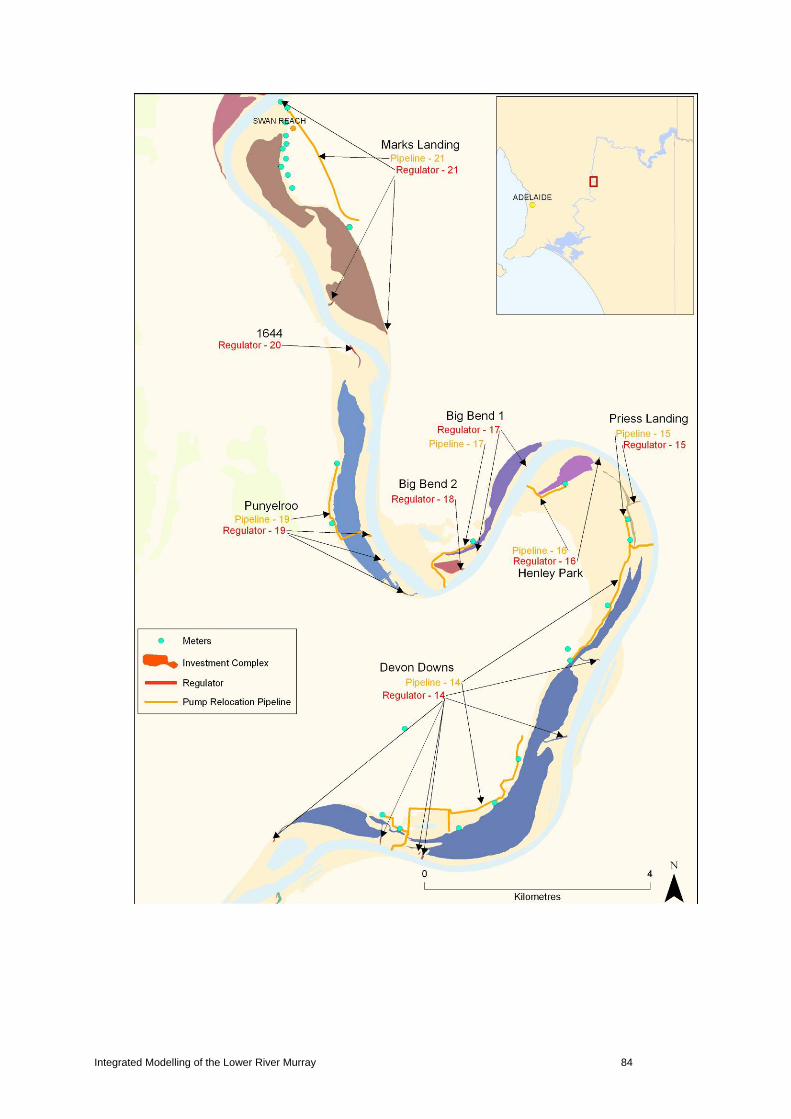
Integrated Modelling of the Lower River Murray 84

Integrated Modelling of the Lower River Murray 85

Integrated Modelling of the Lower River Murray 86

Integrated Modelling of the Lower River Murray 87

Integrated Modelling of the Lower River Murray 88

Integrated Modelling of the Lower River Murray 89

Integrated Modelling of the Lower River Murray 90
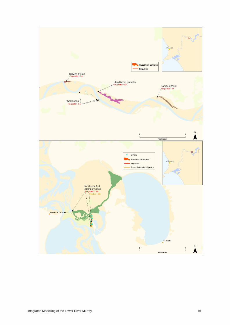
Integrated Modelling of the Lower River Murray 91

Integrated Modelling of the Lower River Murray 92

Integrated Modelling of the Lower River Murray 93

Integrated Modelling of the Lower River Murray 94
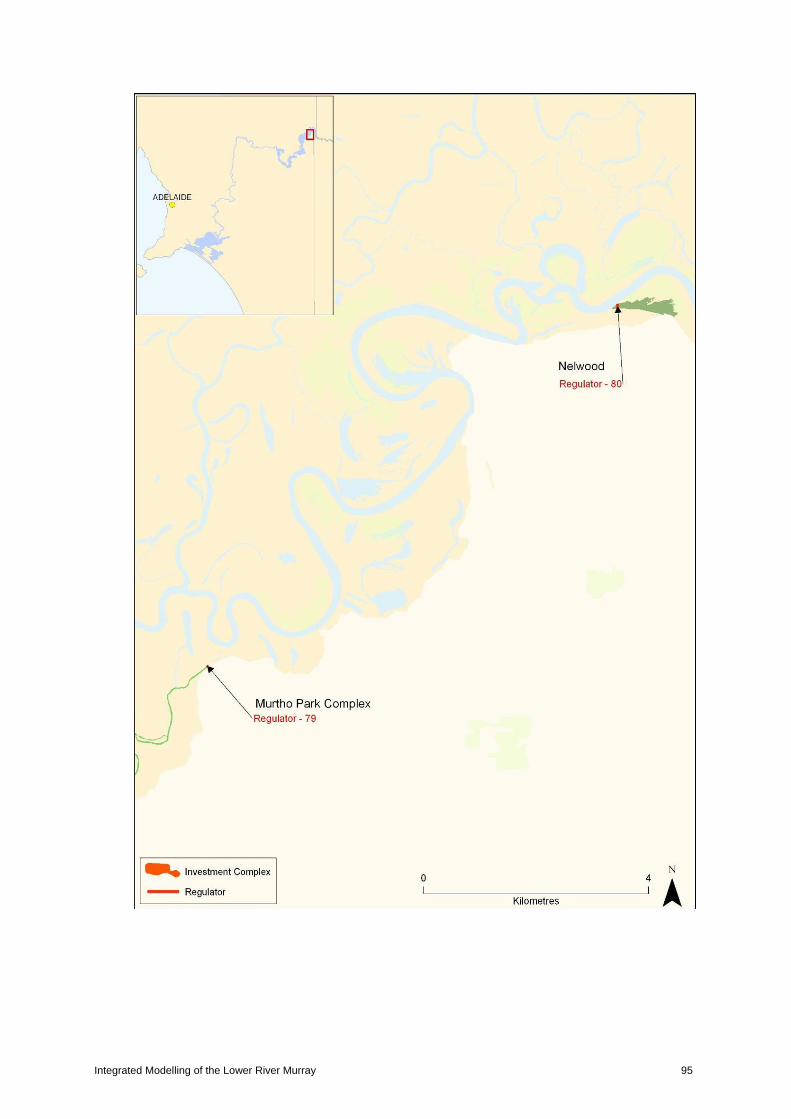
Integrated Modelling of the Lower River Murray 95

APPENDIX B. ECOLOGICAL RESPONSES BY ECOHYDROLOGICAL TYPES Table B.1. Links between ecohydrological units and vegetation communities. A score of 1 indicates that an ecohydrological unit is likely to be good potential habitat, a score of 0 indicates that it is not likely to be good habitat and a score of 0.5 means that it may be used as habitat (or may be marginal habitat). Life stage abbreviations are: A – adult, S – seedling. NB – Rats tail couch grassland was not identified for this region. Note the names of the Ecohydrological units are labels for the mapping unit and not descriptions of the type of habitat. For example chenopds have been mapped into the Terrestrial dry unit although they can be salt tolerant and Lignum has been mapped in the lignum unit even though it occupies habitats that can be described as riparian or floodplain.
Bla
ck b
ox
Red
gum
(F
lood
plai
n)
Red
gum
(F
ringi
ng)
Lign
um
Che
nopo
d
Sal
t-to
lera
nt
Phr
agm
ites
aust
ralis
Rib
bon
wee
d
Life stage A S A S A A S A A A S A S
Floodplain
Riparian 0 0 1 1 0 0 0 0 0 0 0 0 0
High floodplain 1 1 0 0 0 0 0 0 0 0 0 0 0
Emergent 0 0 0 0 0 0 0 0 0 1 1 0 0
Terrestrial dry 0 0 0 0 0 0 0 1 0 0 0 0 0
Salt tolerant 0 0 0 0 0 0 0 0 1 0 0 0 0
Lignum 0 0 0 0 0 1 1 0 0 0 0 0 0
In-channel
Ephemeral 0 0 0 0 1 0 0 0 0 1 1 0 0
Seasonal 0 0 0 0 1 0 0 0 0 1 1 0 0
Permanent 0 0 0 0 1 0 0 0 0 1 1 0.5 0.5
Wetland Temporary (Overbank Flow) 0 0 0 0 1 0 0 0 0 1 1 0.5 0.5 Temporary (Through-flow) 0 0 0 0 1 0 0 0 0 1 1 0.5 0.5 Temporary (Terminal) 0 0 0 0 1 0 0 0 0 1 1 0.5 0.5 Permanent Lake (Terminal) 0 0 0 0 1 0 0 0 0 1 1 1 1 Permanent Lake (Through-flow) 0 0 0 0 1 0 0 0 0 1 1 1 1
Terminal Lake 0 0 0 0 1 0 0 0 0 1 1 1 1 Permanent Swamp (Terminal) 0 0 0 0 1 0 0 0 0 1 1 1 1 Permanent Swamp (Through-flow) 0 0 0 0 1 0 0 0 0 1 1 1 1

Integrated Modelling of the Lower River Murray 97
Bla
ck b
ox
Red
gum
(F
lood
plai
n)
Red
gum
(F
ringi
ng)
Lign
um
Che
nopo
d
Sal
t-to
lera
nt
Phr
agm
ites
aust
ralis
Rib
bon
wee
d
Life stage A S A S A A S A A A S A S
Saline Swamp 0 0 0 0 0 0 0 0 0 0 0 0 0

Integrated Modelling of the Lower River Murray 98
Table B.2. Links between ecohydrological units and faunal communities. A score of 1 indicates that an ecohydrological unit is likely to be good potential habitat, a score of 0 indicates that it is not likely to be good habitat, a score of 0.5 means that it may be used as habitat (or may be marginal habitat) and a score of 0.25 indicates that it is unlikely, but could possibly be used as a habitat. Life stage abbreviations are: A – adult, B – breeding event, L&J – larval and juvenile. Note the names of the Ecohydrological units are labels for the mapping unit and not descriptions of the type of habitat.
Col
onia
l ne
stin
g w
ater
bird
s
Wat
erfo
wl
and
greb
e
Mai
n ch
anne
l sp
ecia
list
Flo
od
spaw
ners
Wet
land
sp
ecia
list
Fre
shw
ater
ca
tfish
Mai
n ch
anne
l ge
nera
lists
Low
flow
sp
ecia
lists
Life stage B B A
L&J A
L&J A
L&J A
L&J A
L&J A
L&J
Floodplain
Riparian 1 1 0 0 0.25
0.25
0.25
0.25 0 0
0.25
0.25
0.25
0.25
High floodplain 1 1 0 0
0.25
0.25
0.25
0.25 0 0
0.25
0.25
0.25
0.25
Emergent 1 1 0 0 0.25
0.25
0.25
0.25 0 0
0.25
0.25
0.25
0.25
Terrestrial dry 1 1 0 0
0.25
0.25 0 0 0 0 0 0 0 0
Salt tolerant 0.5 0.5 0 0 0.25
0.25 0 0 0 0 0 0 0 0
Lignum 1 1 0 0 0.25
0.25
0.25
0.25 0 0
0.25
0.25
0.25
0.25
In-channel
Ephemeral 0 0 1 1 1 1 1 1 1 1 1 1 1 1
Seasonal 0 0 1 1 1 1 1 1 1 1 1 1 1 1
Permanent 0 0 1 1 1 1 1 1 1 1 1 1 1 1
Wetland Temporary (Overbank Flow) 1 1 0 0
0.25
0.25 0.5 0.5
0.25
0.25 0.5 0.5 0.5 0.5
Temporary (Through-flow) 1 1 0.5 0.5
0.25
0.25 0.5 0.5
0.25
0.25 0.5 0.5 0.5 0.5
Temporary (Terminal) 1 1
0.25
0.25
0.25
0.25 0.5 0.5
0.25
0.25 0.5 0.5 0.5 0.5
Permanent Lake (Terminal) 1 1
0.25
0.25
0.25
0.25 1 1 0.5 0.5 1 1 1 1
Permanent Lake (Through-flow) 1 1
0.25
0.25
0.25
0.25 1 1 0.5 0.5 1 1 1 1
Terminal Lake 1 1
0.25
0.25
0.25
0.25 1 1 0.5 0.5 1 1 1 1
Permanent 1 1 0.2 0.2 0.2 0.2 1 1 0.5 0.5 1 1 1 1

Integrated Modelling of the Lower River Murray 99
C
olon
ial
nest
ing
wat
erbi
rds
Wat
erfo
wl
and
greb
e
Mai
n ch
anne
l sp
ecia
list
Flo
od
spaw
ners
Wet
land
sp
ecia
list
Fre
shw
ater
ca
tfish
Mai
n ch
anne
l ge
nera
lists
Low
flow
sp
ecia
lists
Life stage B B A
L&J A
L&J A
L&J A
L&J A
L&J A
L&J
Swamp (Terminal)
5 5 5 5
Permanent Swamp (Through-flow) 1 1
0.25
0.25
0.25
0.25 1 1 0.5 0.5 1 1 1 1
Saline Swamp 0.5 0.5 0 0 0 0 0 0 0 0 0 0 0 0
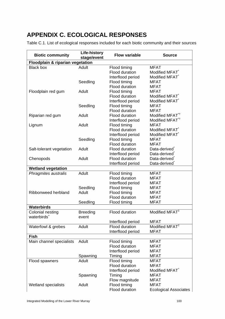
Integrated Modelling of the Lower River Murray 100
APPENDIX C. ECOLOGICAL RESPONSES Table C.1. List of ecological responses included for each biotic community and their sources
Biotic community Life-history stage/event
Flow variable Source
Floodplain & riparian vegetation Black box Adult Flood timing MFAT Flood duration Modified MFAT* Interflood period Modified MFAT* Seedling Flood timing MFAT Flood duration MFAT Floodplain red gum Adult Flood timing MFAT Flood duration Modified MFAT* Interflood period Modified MFAT* Seedling Flood timing MFAT Flood duration MFAT Riparian red gum Adult Flood duration Modified MFAT*† Interflood period Modified MFAT*† Lignum Adult Flood timing MFAT Flood duration Modified MFAT* Interflood period Modified MFAT* Seedling Flood timing MFAT Flood duration MFAT Salt-tolerant vegetation Adult Flood duration Data-derived* Interflood period Data-derived* Chenopods Adult Flood duration Data-derived* Interflood period Data-derived* Wetland vegetation Phragmites australis Adult Flood timing MFAT Flood duration MFAT Interflood period MFAT Seedling Flood timing MFAT Ribbonweed herbland Adult Flood timing MFAT Flood duration MFAT Seedling Flood timing MFAT Waterbirds Colonial nesting waterbirds+
Breeding event
Flood duration Modified MFAT‡
Interflood period MFAT Waterfowl & grebes Adult Flood duration Modified MFAT‡ Interflood period MFAT Fish Main channel specialists Adult Flood timing MFAT Flood duration MFAT Interflood period MFAT Spawning Timing MFAT Flood spawners Adult Flood timing MFAT Flood duration MFAT Interflood period Modified MFAT^ Spawning Timing MFAT Flow magnitude MFAT Wetland specialists Adult Flood timing MFAT Flood duration Ecological Associates

Integrated Modelling of the Lower River Murray 101
Biotic community Life-history stage/event
Flow variable Source
(2010) Interflood period Ecological Associates
(2010) Spawning Timing Overton et al. (2009) Freshwater catfish Adult Flood timing MFAT Flood duration MFAT Interflood period MFAT Spawning Timing MFAT Flow magnitude MFAT Main channel generalists
Adult Flood timing MFAT
Flood duration MFAT Interflood period Modified MFAT‡ Spawning Timing MFAT Low flow specialists Adult Flood timing MFAT Interflood period MFAT Spawning Timing MFAT
* Modifications to MFAT (or data-derived relationships) were based on relationships derived from the current location of vegetation communities. † Further modifications were made based to remove the negative response to permanent inundation, as these trees are assumed to be on the edges of channels and wetlands, not on the floodplain. + Colonial nesting waterbirds are less likely to breed in the Lower Murray and are more likely to be of importance near the SA border. ‡ Modifications to MFAT were based on information contained in Ecological Associates (2010). ^ Modifications to MFAT were based on information contained in Overton et al. (2009). Note that for all MFAT-derived curves, responses listed by MFAT as 0 were altered to 0.05 due to the difference in the interpretation of a 0 response (i.e. unfavourable habitat versus irreparable harm) between MFAT and this project. Refer to the Methods for further information.
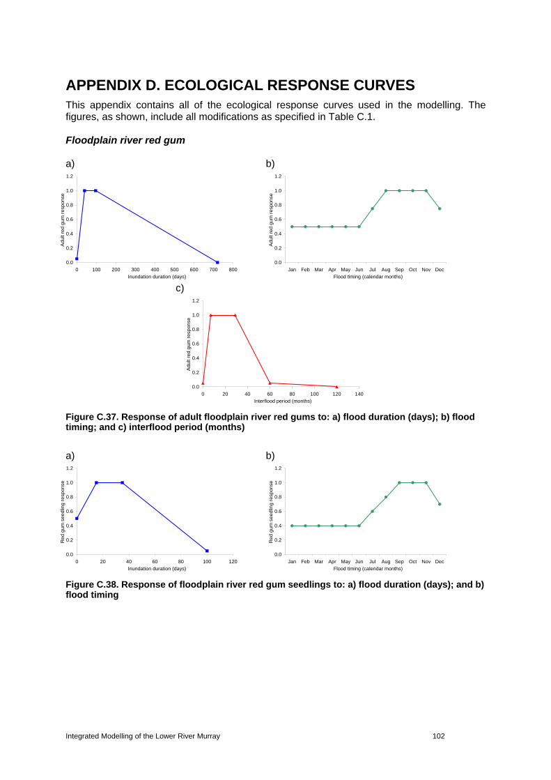
Integrated Modelling of the Lower River Murray 102
APPENDIX D. ECOLOGICAL RESPONSE CURVES This appendix contains all of the ecological response curves used in the modelling. The figures, as shown, include all modifications as specified in Table C.1. Floodplain river red gum a) b)
c)
Figure C.37. Response of adult floodplain river red gums to: a) flood duration (days); b) flood timing; and c) interflood period (months)
a) b)
Figure C.38. Response of floodplain river red gum seedlings to: a) flood duration (days); and b) flood timing
0.0
0.2
0.4
0.6
0.8
1.0
1.2
0 100 200 300 400 500 600 700 800
Inundation duration (days)
Adu
lt re
d gu
m r
espo
nse
0.0
0.2
0.4
0.6
0.8
1.0
1.2
Jan Feb Mar Apr May Jun Jul Aug Sep Oct Nov Dec
Flood timing (calendar months)A
dult
red
gum
res
pon
se
0.0
0.2
0.4
0.6
0.8
1.0
1.2
0 20 40 60 80 100 120 140
Interflood period (months)
Adu
lt re
d gu
m r
espo
nse
0.0
0.2
0.4
0.6
0.8
1.0
1.2
0 20 40 60 80 100 120
Inundation duration (days)
Red
gu
m s
eedl
ing
res
pons
e
0.0
0.2
0.4
0.6
0.8
1.0
1.2
Jan Feb Mar Apr May Jun Jul Aug Sep Oct Nov Dec
Flood timing (calendar months)
Red
gu
m s
eedl
ing
res
pons
e

Integrated Modelling of the Lower River Murray 103
Fringing river red gum a) b)
Figure C.39. Response of adult floodplain river red gums to: a) flood duration (days); and b) interflood period (months)
Black box woodland a) b)
c)
Figure C.40. Response of adult black box to: a) flood duration (days); b) flood timing; and c) interflood period (months)
a) b)
Figure C.41. Response of black box seedlings to: a) flood duration (days); and b) flood timing
0.0
0.2
0.4
0.6
0.8
1.0
1.2
0 100 200 300 400 500 600 700 800
Inundation duration (days)
Adu
lt re
d gu
m r
espo
nse
0.0
0.2
0.4
0.6
0.8
1.0
1.2
0 20 40 60 80 100 120 140
Interflood period (months)
Adu
lt re
d gu
m r
espo
nse
0.0
0.2
0.4
0.6
0.8
1.0
1.2
0 50 100 150 200 250 300 350 400
Inundation duration (days)
Adu
lt bl
ack
bo
x re
spon
se
0.0
0.2
0.4
0.6
0.8
1.0
1.2
Jan Feb Mar Apr May Jun Jul Aug Sep Oct Nov Dec
Flood timing (calendar months)
Adu
lt bl
ack
bo
x re
spon
se
0.0
0.2
0.4
0.6
0.8
1.0
1.2
0 20 40 60 80 100
Interflood period (months)
Adu
lt bl
ack
bo
x re
spon
se
0.0
0.2
0.4
0.6
0.8
1.0
1.2
0 20 40 60 80 100 120
Inundation duration (days)
Bla
ck b
ox s
eedl
ing
res
pons
e
0.0
0.2
0.4
0.6
0.8
1.0
1.2
Jan Feb Mar Apr May Jun Jul Aug Sep Oct Nov DecFlood timing (calendar months)
Bla
ck b
ox s
eed
ling
resp
onse

Integrated Modelling of the Lower River Murray 104
Lignum shrubland a) b)
c)
Figure C.42. Response of adult lignum to: a) flood duration (days); b) flood timing; and c) interflood period (months)
a) b)
Figure C.43. Response of lignum seedlings to: a) flood duration (days); and b) flood timing
Salt-tolerant woodland
0.0
0.2
0.4
0.6
0.8
1.0
1.2
0 50 100 150 200 250 300 350 400
Inundation duration (days)
Adu
lt lig
num
res
pons
e
0.0
0.2
0.4
0.6
0.8
1.0
1.2
Jan Feb Mar Apr May Jun Jul Aug Sep Oct Nov Dec
Flood timing (calendar months)
Adu
lt re
d gu
m r
espo
nse
0.0
0.2
0.4
0.6
0.8
1.0
1.2
0 20 40 60 80 100 120 140
Interflood period (months)
Adu
lt lig
num
res
pons
e
0.0
0.2
0.4
0.6
0.8
1.0
1.2
0 20 40 60 80 100 120 140
Inundation duration (days)
Lign
um s
eedl
ing
res
pon
se
0.0
0.2
0.4
0.6
0.8
1.0
1.2
Jan Feb Mar Apr May Jun Jul Aug Sep Oct Nov Dec
Flood timing (calendar months)
Lign
um s
eedl
ing
res
pon
se

Integrated Modelling of the Lower River Murray 105
a) b)
Figure C.44. Response of adult salt-tolerant woodland vegetation to: a) flood duration (days); and b) interflood period (months)
Chenopod woodland a) b)
Figure C.45. Response of adult chenopods to: a) flood duration (days); and b) interflood period (months)
Phragmites australis a) b)
c)
0.0
0.2
0.4
0.6
0.8
1.0
1.2
0 100 200 300 400 500 600 700 800
Inundation duration (days)
Ad
ult s
alt-
tole
rant
res
pons
e
0.0
0.2
0.4
0.6
0.8
1.0
1.2
0 100 200 300 400 500 600 700 800
Interflood period (months)
Ad
ult s
alt-
tole
rant
res
pons
e
0.0
0.2
0.4
0.6
0.8
1.0
1.2
0 100 200 300 400 500 600 700 800
Inundation duration (days)
Adu
lt ch
enop
od r
esp
onse
0.0
0.2
0.4
0.6
0.8
1.0
1.2
0 5 10 15 20 25 30 35
Interflood period (months)
Adu
lt ch
enop
od r
esp
onse
0.0
0.2
0.4
0.6
0.8
1.0
1.2
0 50 100 150 200 250 300 350 400
Inundation duration (days)
Adu
lt P
hrag
mite
s r
espo
nse
0.0
0.2
0.4
0.6
0.8
1.0
1.2
Jan Feb Mar Apr May Jun Jul Aug Sep Oct Nov Dec
Flood timing (calendar months)
Adu
lt P
hrag
mite
s r
espo
nse

Integrated Modelling of the Lower River Murray 106
Figure C.46. Response of adult Phragmites australis to: a) flood duration (days); b) flood timing; and c) interflood period (months)
Figure C.47. Response of black box seedlings to flood timing
Ribbonweed herbland a) b)
Figure C.48. Response of adult ribbonweed to: a) flood duration (days); and b) flood timing
Figure C.49. Response of ribbonweed seedlings to flood timing
Colonial nesting waterbird breeding
0.0
0.2
0.4
0.6
0.8
1.0
1.2
0 50 100 150 200 250 300 350 400
Interflood period (months)
Adu
lt P
hrag
mite
s r
espo
nse
0.0
0.2
0.4
0.6
0.8
1.0
1.2
Jan Feb Mar Apr May Jun Jul Aug Sep Oct Nov Dec
Flood timing (calendar months)
Phr
agm
ites
see
dlin
g re
spon
se
0.0
0.2
0.4
0.6
0.8
1.0
1.2
0 50 100 150 200 250 300
Inundation duration (days)
Adu
lt rib
bon
wee
d r
espo
nse
0.0
0.2
0.4
0.6
0.8
1.0
1.2
Jan Feb Mar Apr May Jun Jul Aug Sep Oct Nov Dec
Flood timing (calendar months)
Adu
lt rib
bon
wee
d r
espo
nse
0.0
0.2
0.4
0.6
0.8
1.0
1.2
Jan Feb Mar Apr May Jun Jul Aug Sep Oct Nov Dec
Flood timing (calendar months)
Rib
bon
wee
d s
eedl
ing
res
pons
e

Integrated Modelling of the Lower River Murray 107
a) b)
Figure C.50. Response of colonial nesting waterbird breeding to: a) flood duration (days); and c) interflood period (months)
Waterfowl and grebe habitat a) b)
Figure C.51. Response of waterfowl and grebe habitat to: a) flood duration (days); and c) interflood period (months)
Main channel specialist fish a) b)
c)
0.0
0.2
0.4
0.6
0.8
1.0
1.2
0 50 100 150 200
Inundation duration (days)
Co
loni
al n
estin
g w
ater
bird
bre
edi
ng
resp
onse
0.0
0.2
0.4
0.6
0.8
1.0
1.2
0 10 20 30 40Interflood period (months)
Co
loni
al n
estin
g w
ater
bird
bre
edi
ng
resp
ons
e
0.0
0.2
0.4
0.6
0.8
1.0
1.2
0 50 100 150 200
Inundation duration (days)
Wat
erfo
wl a
nd
greb
e h
abita
t res
pon
se
0.0
0.2
0.4
0.6
0.8
1.0
1.2
0 5 10 15 20 25 30 35 40
Interflood period (months)
Wat
erfo
wl a
nd
greb
e h
abita
t res
pon
se
0.0
0.2
0.4
0.6
0.8
1.0
1.2
0 50 100 150 200 250 300 350 400Inundation duration (days)
Adu
lt m
ain
cha
nne
l spe
cia
list r
esp
onse
0.0
0.2
0.4
0.6
0.8
1.0
1.2
Jan Feb Mar Apr May Jun Jul Aug Sep Oct Nov DecFlood timing (calendar months)
Adu
lt m
ain
chan
nel s
pec
ialis
t re
spon
se

Integrated Modelling of the Lower River Murray 108
Figure C.52. Response of adult main channel specialists to: a) flood duration (days); b) flood timing; and c) interflood period (months)
a) b)
Figure C.53. Response of main channel specialist spawning to: a) flood duration (days); and b) likely spawning timing
Flood spawning fish a) b)
c)
Figure C.54. Response of flood spawners to: a) flood duration (days); b) flood timing; and c) interflood period (months)
0.0
0.2
0.4
0.6
0.8
1.0
1.2
0 5 10 15 20 25 30 35 40Interflood period (months)
Adu
lt m
ain
cha
nne
l spe
cia
list r
esp
onse
0.0
0.2
0.4
0.6
0.8
1.0
1.2
0 5 10 15 20 25Inundation duration (days)
Mai
n ch
ann
el s
peci
alis
t sp
awni
ng
resp
onse
0.0
0.2
0.4
0.6
0.8
1.0
1.2
Jan Feb Mar Apr May Jun Jul Aug Sep Oct Nov Dec
Spawning timing (calendar months)
Mai
n ch
anne
l spe
cial
ist s
paw
nin
g re
spo
nse
0.0
0.2
0.4
0.6
0.8
1.0
1.2
0 50 100 150 200 250 300 350 400Inundation duration (days)
Adu
lt flo
od s
paw
ner
resp
ons
e
0.0
0.2
0.4
0.6
0.8
1.0
1.2
Jan Feb Mar Apr May Jun Jul Aug Sep Oct Nov DecFlood timing (calendar months)
Ad
ult f
loo
d sp
awne
r re
spon
se
0.0
0.2
0.4
0.6
0.8
1.0
1.2
0 50 100 150 200 250 300Interflood period (months)
Adu
lt flo
od s
paw
ner
resp
ons
e
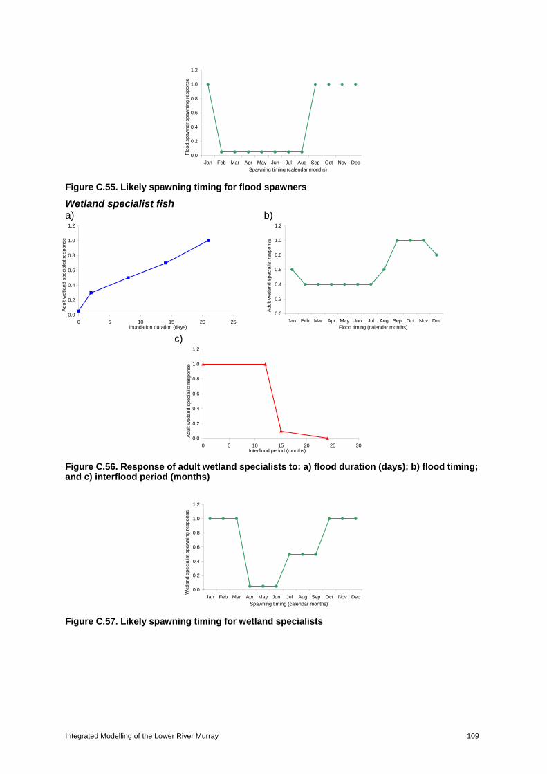
Integrated Modelling of the Lower River Murray 109
Figure C.55. Likely spawning timing for flood spawners
Wetland specialist fish a) b)
c)
Figure C.56. Response of adult wetland specialists to: a) flood duration (days); b) flood timing; and c) interflood period (months)
Figure C.57. Likely spawning timing for wetland specialists
0.0
0.2
0.4
0.6
0.8
1.0
1.2
Jan Feb Mar Apr May Jun Jul Aug Sep Oct Nov Dec
Spawning timing (calendar months)
Flo
od s
paw
ner
spa
wni
ng r
espo
nse
0.0
0.2
0.4
0.6
0.8
1.0
1.2
0 5 10 15 20 25Inundation duration (days)
Adu
lt w
etla
nd
spec
ialis
t res
pons
e
0.0
0.2
0.4
0.6
0.8
1.0
1.2
Jan Feb Mar Apr May Jun Jul Aug Sep Oct Nov DecFlood timing (calendar months)
Adu
lt w
etla
nd s
peci
alis
t res
pons
e
0.0
0.2
0.4
0.6
0.8
1.0
1.2
0 5 10 15 20 25 30Interflood period (months)
Adu
lt w
etla
nd
spec
ialis
t res
pons
e
0.0
0.2
0.4
0.6
0.8
1.0
1.2
Jan Feb Mar Apr May Jun Jul Aug Sep Oct Nov Dec
Spawning timing (calendar months)
Wet
land
spe
cial
ist s
paw
nin
g re
spo
nse

Integrated Modelling of the Lower River Murray 110
Freshwater catfish a) b)
c)
Figure C.58. Response of adult freshwater catfish to: a) flood duration (days); b) flood timing; and c) interflood period (months)
a) b)
Figure C.59. Response of freshwater catfish spawning to: a) flood duration (days); and b) likely spawning timing
Main channel generalist fish a) b)
c)
0.0
0.2
0.4
0.6
0.8
1.0
1.2
0 50 100 150 200 250 300 350 400Inundation duration (days)
Ad
ult c
atfis
h re
spon
se
0.0
0.2
0.4
0.6
0.8
1.0
1.2
Jan Feb Mar Apr May Jun Jul Aug Sep Oct Nov DecFlood timing (calendar months)
Adu
lt ca
tfish
res
pons
e
0.0
0.2
0.4
0.6
0.8
1.0
1.2
0 5 10 15 20 25 30 35 40Interflood period (months)
Ad
ult c
atfis
h re
spon
se
0.0
0.2
0.4
0.6
0.8
1.0
1.2
0 5 10 15 20 25Inundation duration (days)
Cat
fish
spaw
nin
g re
spon
se
0.0
0.2
0.4
0.6
0.8
1.0
1.2
Jan Feb Mar Apr May Jun Jul Aug Sep Oct Nov Dec
Spawning timing (calendar months)
Cat
fish
spa
wn
ing
resp
onse
0.0
0.2
0.4
0.6
0.8
1.0
1.2
0 100 200 300 400Inundation duration (days)
Adu
lt m
ain
cha
nnel
gen
eral
ist
resp
onse
0.0
0.2
0.4
0.6
0.8
1.0
1.2
Jan Feb Mar Apr May Jun Jul Aug Sep Oct Nov DecFlood timing (calendar months)
Adu
lt m
ain
chan
nel g
ene
ralis
t re
spon
se
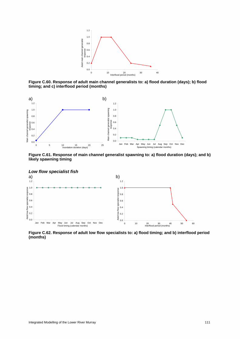
Integrated Modelling of the Lower River Murray 111
Figure C.60. Response of adult main channel generalists to: a) flood duration (days); b) flood timing; and c) interflood period (months)
a) b)
Figure C.61. Response of main channel generalist spawning to: a) flood duration (days); and b) likely spawning timing
Low flow specialist fish a) b)
Figure C.62. Response of adult low flow specialists to: a) flood timing; and b) interflood period (months)
0.0
0.2
0.4
0.6
0.8
1.0
1.2
0 10 20 30 40Interflood period (months)
Adu
lt m
ain
cha
nnel
gen
eral
ist
resp
onse
0.0
0.2
0.4
0.6
0.8
1.0
1.2
0 5 10 15 20 25Inundation duration (days)
Mai
n ch
anne
l gen
era
list s
paw
ning
re
spon
se
0.0
0.2
0.4
0.6
0.8
1.0
1.2
Jan Feb Mar Apr May Jun Jul Aug Sep Oct Nov Dec
Spawning timing (calendar months)
Mai
n c
hann
el g
ener
alis
t spa
wni
ng
resp
onse
0.0
0.2
0.4
0.6
0.8
1.0
1.2
Jan Feb Mar Apr May Jun Jul Aug Sep Oct Nov DecFlood timing (calendar months)
Ad
ult l
ow
flow
spe
cial
ist r
espo
nse
0.0
0.2
0.4
0.6
0.8
1.0
1.2
0 10 20 30 40 50 60Interflood period (months)
Adu
lt lo
w fl
ow s
peci
alis
t res
pons
e

Integrated Modelling of the Lower River Murray 112
a) b)
Figure C.63. Response of low flow specialist spawning to: a) flood duration (days); and b) likely spawning timing
0.0
0.2
0.4
0.6
0.8
1.0
1.2
0 5 10 15 20 25Inundation duration (days)
Low
flow
spe
cial
ist s
paw
nin
g re
spon
se
0.0
0.2
0.4
0.6
0.8
1.0
1.2
Jan Feb Mar Apr May Jun Jul Aug Sep Oct Nov Dec
Spawning timing (calendar months)
Low
flow
spe
cia
list s
paw
ning
res
pons
e

Integrated Modelling of the Lower River Murray 113
APPENDIX E. MATHEMATICAL PROGRAMMING MODEL In this appendix, we formulate a mathematical programming model to optimise the operations of regulator and weir infrastructure in a river system over a pre-defined planning horizon, to maximise ecological and social outcomes. The model will be published in Higgins et al (2010). It accommodates operational rules of infrastructure along with temporal features of water flow in the river system and multiple ecological indicators. The resulting model has a large number of parameter and variable definitions. Input Parameters The fundamental spatial decision-making for investment and operation of regulators unit is the regulated wetland complex {1,..., , ...., }i I n n . The set I includes both existing
regulated wetland complexes n and potential new ones n n . Wetland complexes usually contain multiple regulators. All regulators within a complex are operated simultaneously. These regulators control the opening and closing that provide water to eco-hydrological polygons linked to that regulated complex. Usually only wetlands have regulators (i.e. as opposed to floodplain units), though not all wetlands are regulated. Let:
iC = cost of building a new regulators for wetland complex i I ; and
B = budget for building new regulator investments. Investment in wetland complexes includes the construction cost for new regulators as well as the upfront costs of relocating irrigation off-take pumps from the wetland to the main river channel so that the re-introduction of wetting and drying regimes to wetlands does not impinge on the water security of irrigators Let j J represent the set of individual and spatially distinct areas (polygons) of a specific eco-hydrological unit. These polygons represent water course, wetland, and floodplain ecosystems, which are located along the river channel. The inundation regimes of ecohydrological unit polygons are impacted by the water flow (ML/day), where increased water flow leads to increased water height. Inundation regimes are also impacted by the operation of flow-control structures (regulators and weirs), where weirs manipulate the water height for a given water flow. Let:
ja = area of eco-hydrological polygon j J , measured in hectares;
1 if eco-hydrological polygon is linked to regulated complex
0 otherwise j
i
j J i If
;
k K = the set of ecological components which occur in specific ecohydrological polygons where k {black box woodland, river red gum woodland, colonial nesting waterbirds, etc};
probability of ecohydrological polygon containing component kjq j J k K ; and
l L be the set of weirs. Along the South Australian River Murray L = 6 (number of weirs), which also represent the set of river zones of interest across the Murray catchment. Let:
1 if eco-hydrological polygon is linked to weir
0 otherwise lj
j J l Lb

Integrated Modelling of the Lower River Murray 114
The eco-hydrological polygon is linked at a weir if it is upstream to the weir and the inundation of the polygon is influenced by the raising or lowering of the weir. Let:
whjc = commence-to-fill flow rate (ML/day) required to start filling eco-hydrological polygon
j J , when the weir height is at height wh. This is the flow rate either from the water source (e.g. dam) or at the most upstream point of the river system under consideration. The weir height is measured in centimetres, and based on existing weir operation rules, weir heights can be set at levels wh WH . The commence-to-fill values are lower for higher weir heights since a raised weir require a lower main channel flow rate to achieve flooding into the eco-hydrological polygon. Eco-hydrological polygon j J can only be affected by the immediate
downstream weir as per ljb .
The model runs over an arbitrarily-long planning horizon with monthly units
{1,...., }m M HO where HO = number of temporal units in the planning horizon. Several parameters are used to define the water supply for current and natural hydrographs:
mr = average water supply (ML/day) in month m M that can be made available for all eco-
hydrological polygons, under a current hydrograph. This is the water supply from the dams or at the most upstream point of the river system under consideration.
mp = peak daily water supply (ML/day) in month m M that can be made available for all
eco-hydrological polygons, under a current hydrograph.
me = water allocation (ML) to be reserved for other purposes (e.g. for environmental flows to the Lower Lakes and Coorong estuary) in month m M .
jw = volume of water (ML) required to fill eco-hydrological polygon j J from empty.
mjo = the expected water lost (ML) from eco-hydrological polygon j J from leakage and
evaporation. Decision Variables We specified three sets of decision variables in this study. The first set of decision variables is binary and defines the eligible wetland complexes for investment in regulators:
1 if regulators are constructed for wetland complex
0 otherwise i
i Iy
1for 'iy i n
The second set of decision variables is also binary and defines how existing and new regulators are operated in wetland complexes:
1 if regulators in complex are open in month
0 otherwise mi
i I m Mx

Integrated Modelling of the Lower River Murray 115
We assume that new regulators are operational at the beginning of the planning horizon, though this assumption can be relaxed by forcing 0m
ix for the months prior to construction.
The third set of decision variables governs the height for each weir. We use integer increments (e.g. cm) rather than continuous such that:
mlh height of weir l L in month m M .
The decision variables , m
i iy x , mlh are optimised simultaneously within the solution
methodology. Let X, H, Y represent vectors of the decision variables mix , m
lh , iy ,
respectively. To reduce the number of decision variable categories, selection of new regulators for wetland complex iy are controlled by its operation m
ix . That is, iy is set to 1
automatically if the regulators in the complex are operated. Other Variables The following variables are dependent on the decision variables defined above.
mjs = stock of water (ML) in each eco-hydrological unit polygon j J at the end of month
m M .
1 if flow into eco-hydrological polygon in month is achievable
0 otherwise mj
j J m Md
mjd = 1 where the flow rate along the river is greater than the commence-to-fill flow value of
eco-hydrological unit polygon j J , subject to the regulators in complex i I being open. If mjd = 0 water will drain from the eco-hydrological polygon (reverse flow), unless the
regulators in the complex are closed.
1 eco-hydrological polygon in month is inundated with water
0 otherwise mj
j J m Mg
For the scenarios in this project, we assume mjg = 1 if eco-hydrological polygon j J is
more than 80% full ( 0.8mj js w ), though this percentage can be changed.
Constraints A constraint was set on the total available budget for new flow control infrastructure investment:
i ii I
i n
C y B
(1)

Integrated Modelling of the Lower River Murray 116
The following constraints are used to automatically set mjd =1 if the peak daily water supply
is greater than the commence-to-fill flow value for the polygon j J :
(1 )mlhm m
j jp c d N , , 1ljj J m M b (2)
mlhm m
j jp c d N , , 1ljj J m M b (3)
where N is a big number (e.g. 10e9). If the commence-to-fill flow value was less than the
peak daily water supply, mjd would have to equal 1 for both constraints to be satisfied.
The next constraint ensures the total amount of water entering the eco-hydrological unit polygon in month m M must be less than or equal to the available water in month m M , accommodating water set aside for other uses.
1 1(1 ) ( )j m m m mi i i j j j
i I j J
f x x w s d
+ 1( )m m m m mj j j
j J
d w s e r t
m M (4)
where mt = number of days in month m M . The first double summation refers to the filling of wetlands through the opening of the regulator(‘s), when the regulator(‘s) was closed in the previous month. The second summation component refers to the filling of eco-hydrological unit polygons (unregulated
wetlands and floodplains) influenced by the raising of the associated weir. The term 1mj jw s
in both summations refers to the water that is added (or topped up to full) in the eco-hydrological unit polygon, allowing for the fact it may not be empty to begin with. Only existing regulators or regulators in selected new wetland complexes can be operated:
mi ix y ,m M i I (5)
Next is the balance equation for water volume flow in each eco-hydrological unit polygon. It calculates the amount of water in polygon j J in month m M as equal to the amount of
water in month 1m M minus the water losses in month m M plus the amount of water that enters through inundation minus the amount of water that is released:
1 1 1(1 ) ( )m m m m m j m mj j j i i i j j j
i I
s s o x x f w s d
+ 1( )m mj j jw s d
1 1( ) (1 ) (1 )m m m m j mj j i i i j
i I
s o x x f d
1( )m m mj j js o d ,j J m M (6)
Water enters or is released from the eco-hydrological polygon as a function of the commence-to-fill flow value and river flow rates, as well as weir and regulator operations. As with equation (4), the components in equation (6) refer to the filling of the eco-hydrological
polygon via the regulator or weir (not simultaneously). The term 1mj jw s in the first and
second summations refers to the amount of water being added to fill it. The second half of equation (6) refers to emptying of the polygons when either the regulator is opened when river flows are less than the polygon’s commence-to-fill flow values, or the weir is lowered.
The term 1( )m mj js o refers to the amount of water removed to empty it. If emptied, we
assume it is emptied completely (i.e. mjs =0). For the current version of the model, water that
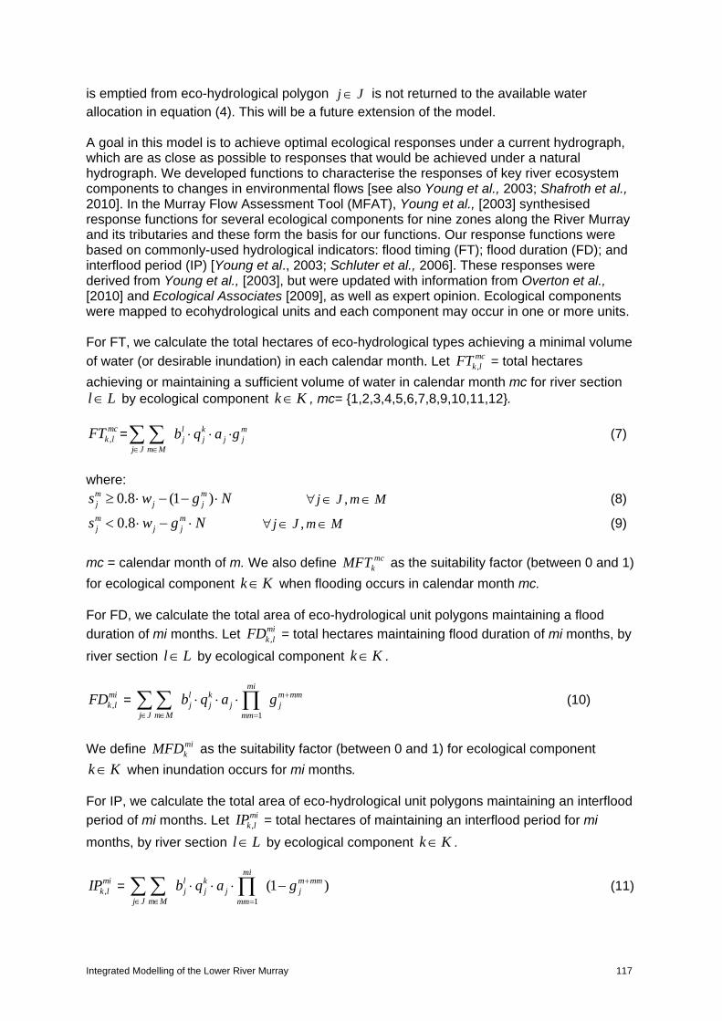
Integrated Modelling of the Lower River Murray 117
is emptied from eco-hydrological polygon j J is not returned to the available water allocation in equation (4). This will be a future extension of the model. A goal in this model is to achieve optimal ecological responses under a current hydrograph, which are as close as possible to responses that would be achieved under a natural hydrograph. We developed functions to characterise the responses of key river ecosystem components to changes in environmental flows [see also Young et al., 2003; Shafroth et al., 2010]. In the Murray Flow Assessment Tool (MFAT), Young et al., [2003] synthesised response functions for several ecological components for nine zones along the River Murray and its tributaries and these form the basis for our functions. Our response functions were based on commonly-used hydrological indicators: flood timing (FT); flood duration (FD); and interflood period (IP) [Young et al., 2003; Schluter et al., 2006]. These responses were derived from Young et al., [2003], but were updated with information from Overton et al., [2010] and Ecological Associates [2009], as well as expert opinion. Ecological components were mapped to ecohydrological units and each component may occur in one or more units. For FT, we calculate the total hectares of eco-hydrological types achieving a minimal volume
of water (or desirable inundation) in each calendar month. Let ,mc
k lFT = total hectares
achieving or maintaining a sufficient volume of water in calendar month mc for river section l L by ecological component k K , mc= {1,2,3,4,5,6,7,8,9,10,11,12}.
,mc
k lFT = l k mj j j j
j J m M
b q a g
(7)
where:
0.8 (1 )m mj j js w g N ,j J m M (8)
0.8m mj j js w g N ,j J m M (9)
mc = calendar month of m. We also define mc
kMFT as the suitability factor (between 0 and 1)
for ecological component k K when flooding occurs in calendar month mc. For FD, we calculate the total area of eco-hydrological unit polygons maintaining a flood
duration of mi months. Let ,mik lFD = total hectares maintaining flood duration of mi months, by
river section l L by ecological component k K .
,mik lFD =
1
mil k m mmj j j j
j J m M mm
b q a g
(10)
We define mi
kMFD as the suitability factor (between 0 and 1) for ecological component
k K when inundation occurs for mi months. For IP, we calculate the total area of eco-hydrological unit polygons maintaining an interflood
period of mi months. Let ,mi
k lIP = total hectares of maintaining an interflood period for mi
months, by river section l L by ecological component k K .
,mi
k lIP = 1
(1 )mi
l k m mmj j j j
j J m M mm
b q a g
(11)

Integrated Modelling of the Lower River Murray 118
We define mikMIP as the suitability factor (between 0 and 1) for ecological component k K
when an interflood period occurs for mi months.
,mc
k lFT , ,mik lFD and ,
mik lIP are calculated based on the current hydrograph ,m mr p . Let ,
mck lNFT ,
,mik lNFD and ,
mik lNIP corresponding indicators calculated for the natural hydrograph. The
indicators for the natural hydrograph are not dependent upon the decision variables and are calculated prior to initiating the optimisation algorithm. Operations of the Weirs Operational rules on weirs were also required to manage water stress levels between upstream and downstream weirs, and meet safety requirements of moving the structures within a given month. . No more than a cm change in weir height between months:
1m ml lh h (12)
1m ml lh h (13)
No more than a cm difference between neighbouring weirs:
1m ml lh h (14)
1m ml lh h (15)
Objective Function
The objective function aims to keep the ecological response indicators ,mc
k lFT , ,mik lFD and ,
mik lIP
proportionally as close as possible to the corresponding indicators ,mc
k lNFT , ,mik lNFD and
,mi
k lNIP based on a natural hydrograph. To achieve this, we implemented a minimised least-
squares type approach, as follows: Min Z1 =
2 2, , , ,( ) ( )mc mc mc mi mi mi
k k l k l k k l k lmc k K l L mi k K l L
MFT FT NFT MFD FD NFD
2, ,( )mi mi mi
k k l k lmi k K l L
MIP IP NIP
(16)
where the least-squares difference for FT, FD and IP are multiplied together due to the general lack of information regarding the relative importance of each response indicator. An additional objective function can be added to maximise the total social value from the system. Social values can be placed on ecological components or individual eco-hydrological polygons. Let:
jS = social priority of eco-hydrological unit polygons j J if it is in an acceptable healthy
state. It can be a normalised value of between 0 and 1.

Integrated Modelling of the Lower River Murray 119
An eco-hydrological unit polygon j J can be considered to have social value if it is ecologically healthy or is inundated (fishing, water sports). For this project, we assume the latter, and the objective function can be formulated as follows: Max Z2 = m
j jj J m M
S g
(17)
An aggregated objective is: Min Z = 1 1 2 2W Z W Z (18)
Where weights W1 and W2 were chosen so that the ecological objective was 5:1 priority compared to the social objective, based on expert opinion.
Solution Method The model represented by equations (1) to (18) is a non-linear integer programming problem. By considering variables iy , it is an extension of the capacitated P-median problem, with
additional decision variables mix , m
lh . This is very difficult to solve using commercial software
packages for real-world problems of reasonable size. By solving only for m
ix and mlh the model is similar to an assignment problem, in terms of
assigning the operations of the regulators/weirs to each month in the planning horizon with some regulators/weirs being assigned to multiple months. However, the assignment problem is subject to dynamic constraints represented by constraint (4,6,10,11). Such a problem has been shown to be NP-Hard, but solvable to optimality for small instances. There are a large range of methods that have been applied for finding near optimal solutions to models like the generalised assignment problem in the presence of additional constraints. To accommodate the different decision variables m
ix , mlh , iy , we apply a 2-stage recursive
heuristic method that exploits this structure. Two-stage or nested methods are suitable for solving problems with more than one type of decision variable. To avoid solving a P-median problem for iy and reduce the amount of solution method nesting, we can solve for iy
implicitly. This is done by solving for mix assuming all regulated wetland complexes are
available, and enforcing constraint (1) to limit the number of new ones used. The solution method is best described using the following algorithm: Algorithm 1
, ,best best bestX H Z = 0 Initialise X=0, H = mid-point weir heights REPEAT
Solve for X using Algorithm 2 Solve for H using Algorithm 3
UNTIL There is no further improvement in the solution There are a wide range of suitable meta-heuristics for solving the sub-problems for m
ix and mlh , including simulated annealing and tabu search, genetic algorithms and hybrid heuristics.
An important consideration is that the selected method needs to have fast convergence,

Integrated Modelling of the Lower River Murray 120
particularly as the sub-problems will need to be repeatedly solved for mix and m
lh . In this
study, we used the tabu search method. The general tabu search heuristic is based on the establishment of moves so as to transform a current solution to one of the neighbouring solutions. The tabu search escapes local optimal solutions by allowing up-hill (non-improving) moves to be performed when no down-hill (improving) moves are available. At each iteration of the tabu search, the neighbourhood (or a sample of it) is explored. The best non-tabu move found in the search is applied. A move is tabu if it is one of the TL (tabu list) most-recent moves implemented. If this tabu list size TL is too small, the heuristic will cycle through a series of solutions. The tabu status is over-ridden if the solution satisfies an aspiration criteria function. Four neighbourhoods are applied, two for each of the decision variables: Neighbourhood 1: Open or close the regulator(s) in a wetland complex – If m
ix =1, then let mix
=0. If mix =0, then let m
ix =1.
Neighbourhood 2: Open regulator(s) in one complex and close another - If m
ix =1 and mix = 0
then let mix =0 and m
ix = 1.
Neighbourhood 3: Raise or lower a weir - If m
lh =wh1, then let mlh =wh2, where wh1, wh2
WH . Neighbourhood 4: Raise one weir and lower another - If m
lh =wh1 and ''mlh =wh2 then let m
lh
=wh2 and ''mlh =wh1.
The two neighbourhoods for each of the decision variables, m
ix and mlh , compliment one
another during the tabu search routine. Neighbourhoods 2 and 4 are applied more frequently
when it is difficult to improve the solution due to constraints (1,4). After ' continuous iterations where the best solution is not improved, the search is intensified by replacing the current solution with the best so far. The tabu search strategies used are described by Algorithm 2 and 3. Algorithm 2 Set =0
Let Z’=Z, iZ =Z, X’=X, iX =X,
REPEAT
APPENDIX 1. REPEAT Obtain a sample of moves from neighbourhoods 1 and 2 of X’, and let X be the move in the sample that produced the maximum objective function value Z. IF Z< Z’ and the move is not tabu and constraints (1) to (10) are satisfied, SET Z’ = Z, X’=X
IF Z< iZ SET iZ =Z, Z’ = Z, X’=X, iX =X, =0 UPDATE the tabu list with the reverse move ADD 1 to
UNTIL = '
Z’= iZ , X’= iX

Integrated Modelling of the Lower River Murray 121
UNTIL convergence criteria is achieved. Algorithm 3 Set =0
Let Z’=Z, iZ =Z, H’=H, iH =H.
REPEAT
APPENDIX 2. REPEAT Obtain a sample of moves from neighbourhoods 3 and 4 of H’ and let H be the move in the sample that produced the maximum objective function value Z. IF Z< Z’ and the move is not tabu and constraints (1) to (10) are satisfied, SET Z’ = Z, H’=H
IF Z< iZ SET iZ =Z, Z’ = Z, H’=H, iH =H, =0 UPDATE the tabu list with the reverse move ADD 1 to
UNTIL = '
Z’= iZ , H’= iH UNTIL convergence criteria is achieved. In Algorithm 2, the best values found of ' and the TL were 50 and 15, respectively. We experimented with the neighbourhood sample sizes and found the following to work well for Neighbourhoods 1 to 4 respectively: 200, 100, 30, 50. The performance of algorithms 2 and 3 were not sensitive to small changes in the chosen neighbourhood sample sizes.
