UH54 I1.5F60,6 1'no. 5

OREGON STATE UNIVERSITY LIBRARIES

Integrated Research In The

Coniferous Forest Biome

12 0009035011

COMPACT

R:: L

.5.

INTEGRATED RESEARCH IN THE CONIFEROUS FOREST BIOME

R. H. Waring and R. L. Edmonds (editors)

Bulletin No. 5Coniferous Forest Biome

Ecosystem Analysis Studies

U.S./International Biological Program

The work reported in this publication was supported by the NationalScience Foundation under grants no. GB-20963 and GB-36810X1 to theConiferous Forest Biome, Ecosystem Analysis Studies, U.S./InternationalBiological Program. Contributions 59 through 66 of the ConiferousForest Biome are contained herein. Any portion of this publicationmay be reproduced for purposes of the U.S. Government. Copies areavailable from the Coniferous Forest Biome, University of WashingtonAR-10, Seattle, Washington 98195.

September 1974

iii

FOREWORD

Before embarking on the third year of field research, the ConiferousForest Biome presented an initial synthesis of its major programs atthe national meeting of the American Institute of Biological Sciencesheld on 21 June 1973 in Amherst, Massachusetts.

Integration is still incomplete, but major strides have been made. Thecoupling of processes and development of a system viewpoint has emerged.This publication is thus a contribution of all Biome participants. It

is dedicated to Dr. Jerry F. Franklin, present director of ecosystemprograms for the National Science Foundation and past deputy directorof our Biome. It was through his effort, more than that of any otherone person, that the idea of integrating ecosystem research passed froma vision to reality.

R. H. Waring

Iv

CONTENTS

R. H. Waring:Structure and function of the ConiferousForest Biome organization . . . . . . . . . . . . . . . . . .

P. Sollins, R. H. Waring, and D. W. Cole:A systematic framework for modeling and studying thephysiology of a coniferous forest ecosystem . . . . . . . 7

C. C. Grier, D. W. Cole, C. T. Dyrness, and R. L. Fredriksen:Nutrient cycling in 37- and 450-year-old Douglas-firecosystems . . . . . . . . . . . . . . . . . . . . . . . . 21

L. J. Fritschen, L. W. Gay, and H. R. Holbo:Estimating evapotranspiration from forests by meteorologicaland lysimetric methods . . . . . . . . . . . . . . . . . . . 35

M. A. Strand:Canopy food chain in a coniferous forest watershed . . . . 41

D. B. Zobel, W. A. McKee, G. M. Hawk, and C. T. Dyrness:Correlation of forest communities with environment andphenology on the H. J. Andrews Experimental Forest,Oregon . . . . . . . . . . . . . . . . . . . . . . . . . . . 48

J. R. Sedell, F. J. Triska, J. D. Hall, N. H. Anderson,and J. H. Lyford:Sources and fates of organic inputs in coniferous foreststreams . . . . . . . . . . . . . . . . . . . . . . . . . . . 57

R. C. Wissmar, D. M. Eggers, and N. W. Bartoo:Analysis of lake ecosystems: Lake Washington drainagebasin . . . . . . . . . . . . . . . . . . . . . . . . . . . 70

.

.

STRUCTURE AND FUNCTION OF THECONIFEROUS FOREST BIOME ORGANIZATION'

R. H. Waring

Oregon State University

ABSTRACT

Integrating the research effort for an analysis of ecosystems requiresastrong but flexible organization. The Coniferous Forest Biome's researchgroups reflect our changing perception of the major processes operating inboth terrestrial and aquatic systems. They also reflect changing goals asour understanding increases and wider application and longer range predic-tions are desired. In addition, there is a geographic perspective express-ing the concentration of effort on different processes and systems acrossthe Biome.

The evolution of field research and modeling are intimately linked. Directorsand research committee chairmen take leading roles in designing and coordi-nating the research with the aid of workshops to measure progress, modifymodel structure, and identify critical data needs. Often a small task forceis appointed to address particular problems that require shifting resourcesand personnel to meet a critical need. A key group of integrators hasdeveloped, consisting of people who have an ecosystem perspective and train-ing in more than one discipline. Their contributions to the program areessential and their experience and talents make them capable of leading thenext generation of ecosystem studies.

INTRODUCTION

The kind of science that can be accomplished by large integrated researchdiffers from that which can be done by individuals or small groups. Thestructure of large scientific programs, although more formal than smallerones, need not be less efficient. Integrated research, however, requiresa special structure and a special kind of people to accomplish its task.This paper explains how integrated research has evolved in the ConiferousForest Biome.

The Coniferous Forest Biome was initiated in September 1970 as one of thefive programs in the Ecosystem Analysis Studies sponsored by the NationalScience Foundation as part of the U.S./International Biological Programeffort. The general research objectives are to increase the understandingof whole ecosystems with special emphasis on land-water interactions. To

keep track of details, help organize the research, and test the validity ofcertain assumptions, we make use of computers and system modeling.

Our general research philosophy is that knowledge of the internal structureand function of ecosystems comes from understanding basic processes thatoperate across a biome. Coupling these processes into subsystems and link-ing these into terrestrial and aquatic ecosystems provide a hierarchical

'This is contribution no. 59 from the Coniferous Forest Biome.

2

means of understanding the internal structure and function of these complex

systems. With this general philosophy, the structure for conducting theresearch and administering the program was developed.

STRUCTURE OF THE CONIFEROUS FOREST BIOME

Geographic Structure

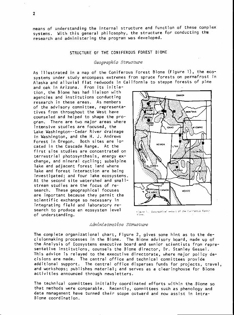
As illustrated in a map of the Coniferous Forest Biome (Figure 1), the eco-systems under study encompass extremes from spruce forests on permafrost inAlaska and alluvial flat redwoods in California to steppe forests of pineand oak in Arizona. From its initia-tion, the Biome has had liaison withagencies and institutions conductingresearch in these areas. As membersof the advisory committee, representa-tives from throughout the West havecounseled and helped to shape the pro-gram. There are two major areas whereintensive studies are focused, theLake Washington--Cedar River drainagein Washington, and the H. J. AndrewsForest in Oregon. Both sites are lo-cated in the Cascade Range. At thefirst site studies are concentrated onterrestrial photosynthesis, energy ex-change, and mineral cycling; subalpinelake and adjacent forest land wherelake and forest interaction are beinginvestigated; and four lake ecosystems.At the second site watershed and small-stream studies are the focus of re-search. These geographical focusesare important because they permit thescientific exchange so necessary inintegrating field and laboratory re-search to produce an ecosystem levelof understanding.

Figure 1. Geographical extent of the Coniferous Forest

Biome.

Administrative Structure

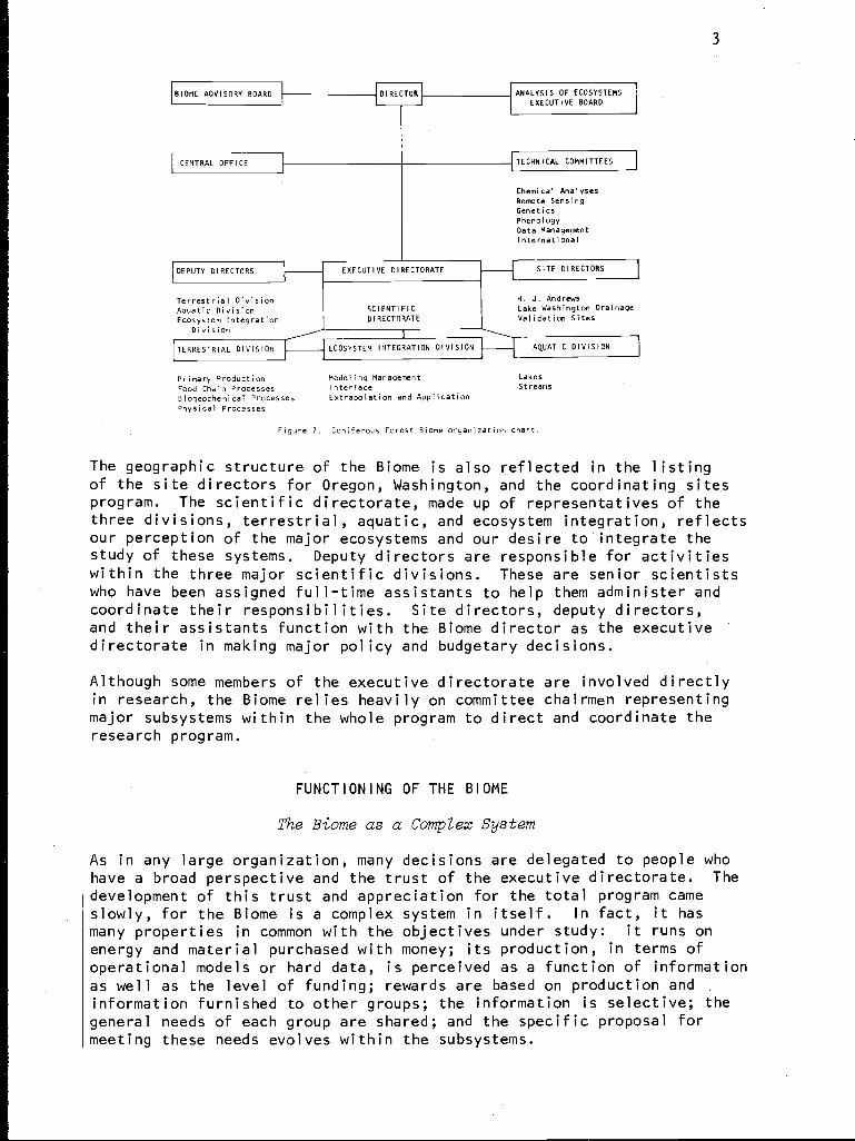
The complete organizational chart, Figure 2, gives some hint as to the de-cisionmaking processes in the Biome. The Biome advisory board, made up ofthe Analysis of Ecosystems executive board and senior scientists from repre-sentative institutions, counsels the Biome director, Dr. Stanley Gessel.This advice is relayed to the executive directorate, where major policy de-cisions are made. The central office and technical committees provideadditional support. The central office disperses funds for projects, travel,and workshops; publishes material; and serves as a clearinghouse for Biomeactivities announced through newsletters.

The technical committees initially coordinated efforts within the.Biome sothat methods were comparable. Recently, committees such as phenology anddata management have turned their scope outward and now assist in intra-Biome coordination.

3

BIOME ADVISORY BOARD

CENTRAL OFFICE

DEPUTY DIRECTORS

Terrestrial DivisionAquatic DivisionEcosystem Integration

Division

TERRESTRIAL DIVISION

DIRECTOR

EXECUTIVE DIRECTORATE

SCIENTIFICDIRECTORATE

ANALYSIS OF ECOSYSTEMSEXECUTIVE BOARD

TECHNICAL COMMITTEES

Chemical AnalysesRemote SensingGeneticsPhenologyData ManagementInternational

SITE DIRECTORS

H. J. AndrewsLake Washington DrainageValidation Sites

ECOSYSTEM INTEGRATION DIVISION AQUATIC DIVISION

Primary Production Modeling Management LakesFood Chain Processes Interface StreamsBiogeochemical Processes Extrapolation and Application

Physical Processes

Figure 2. Coniferous Forest Biome organization chart.

The geographic structure of the Biome is also reflected in the listingof the site directors for Oregon, Washington, and the coordinating sitesprogram. The scientific directorate, made up of representatives of thethree divisions, terrestrial, aquatic, and ecosystem integration, reflectsour perception of the major ecosystems and our desire to'integrate thestudy of these systems. Deputy directors are responsible for activitieswithin the three major scientific divisions. These are senior scientistswho have been assigned full-time assistants to help them administer andcoordinate their responsibilities. Site directors, deputy directors,and their assistants function with the Biome director as the executivedirectorate in making major policy and budgetary decisions.

Although some members of the executive directorate are involved directlyin research, the Biome relies heavily on committee chairmen representingmajor subsystems within the whole program to direct and coordinate theresearch program.

FUNCTIONING OF THE BIOME

The Biome as a Complex System

As in any large organization, many decisions are delegated to people whohave a broad perspective and the trust of the executive directorate. Thedevelopment of this trust and appreciation for the total program cameslowly, for the Biome is a complex system in itself. In fact, it hasmany properties in common with the objectives under study: it runs onenergy and material purchased with money; its production, in terms ofoperational models or hard data, is perceived as a function of informationas well as the level of funding; rewards are based on production and ,

information furnished to other groups; the information is selective; thegeneral needs of each group are shared; and the specific proposal formeeting these needs evolves within the subsystems.

4

Formulation of Specific Tasks

From counsel with the scientific directorate, a series of tasks are for-mulated by the executive directorate and these serve as the focus foroverall synthesis and direction for a one- or two-year period. Forexample, one of the eight tasks defined for 1973-1974 (Gessel 1972) wasto complete initial nutrient water and energy models for unit watershedsand to begin their refinement with particular attention to simplifyingprocess models describing the behavior of large drainages and stronglycontrasting coniferous ecosystems across the Biome. Each task is scru-tinized and responsibility for various components is assigned to appro-priate site directors and committee and subcommittee chairmen.

Design of Specific Research Proposals

Initially, the Biome accepted proposals written by individual scientists.These proposals were modified and assembled into categories more repre-sentative of classical disciplines than Biome objectives. The committeeand subcommittee chairmen, at that early stage in our development, pre-sided over the editing and coordination of these research proposals.Those projects that were funded generally depended upon graduate studentsfor their implementation.

As the conceptual models for ecosystems developed, notable gaps in theprogram were identified. Because of the almost full commitment to con-tract research, there was little flexibility for correcting these defi-ciencies until the following year. The acceptable approach for doingresearch within an academic structure simply did not meet the objectivesof our integrated program.

Coordination and Synthesis through Research Committees

Two major changes have helped correct the deficiency and assure coordi-nated field measurements and synthesis. One was a decision to entrustcommittee and subcommittee chairmen with the additional responsibilityof managing and coordinating research proposals within their area ofresponsibility. The second was the addition of full-time coordinatorpositions with needed technical assistance to assure more complete inte-gration and additional flexibility. In reality, this means individualresearch proposals are now rare. Committee chairmen have available acertain amount of resource to provide information for other groups andaid in better understanding the internal operation of the particularsubsystem or area of responsibility.

Computer Simulation Workshops

Workshops are among the most valuable tools aiding assemblage of dataand identifying important assumptions. With the introduction of ageneral computer processor developed by our central modeling group underthe direction of Scott Overton, we now have a system that permits us tohave an efficient and common means of studying subsystems and also tocouple these subsystems to one another at mixed resolutions of time.This major breakthrough has increased the value of workshops even moreby permitting scientists working in the program or consultants fromother Biomes to join in explicitly questioning assumptions incorporatedin the models. As a result of these workshops we gain a better under-

5

standing of the subsystems, and are able to identify specific deficienciesthat can be corrected during the oncoming field season with resourceskept available for such needs.

Integration by Task Force

The process of integration requires a full commitment. Chemical analyses,storage of data in the information bank, and modeling must all receiveattention to assure that the assembling of ecosystem models is accomplishedefficiently. Setting priorities is a function of the site director or amodeling coordinator. The site directors, as members of the executivedirectorate, have direct access to personnel throughout the Biome and,by invitation, to specialists throughout the world. To accomplish oneof the integration tasks, such as the assemblage of a watershed ecosystem,a site director forms his own team, usually consisting of some of thecommittee and subcommittee chairmen. At each site the director has acoordinating group representing various specialties and service groupsfrom the information bank and chemical laboratories. These usually meetmonthly to assess progress and resolve problems.

The task forces are usually divided into smaller groups with specificresponsibilities that can be accomplished within a time span of two orthree months. These latter groups meet at least weekly to assess theirown progress. The chairmen of these smaller task forces can change asthe synthesis proceeds. Often special reports are assembled and dataare forwarded to the information bank. At the monthly site coordinatingmeetings, special workshops, or seminars, the results of this intensiveeffort is shared with others. Eventually, material is assembled ininternal reports and presented to a wider audience at national andinternational meetings.2

The Integrator

Often in this kind of large research program, time, not money, is limit-ing. The time of dedicated, informed, and competent people is alwaysvaluable, but in a large integrated research program using models, bothas goals and as an aid in directing the program, the contributions ofthese people cannot be overstressed.

Probably the most valuable product of the International Biological Pro-gram in the United States will not be the systems models that will aid

2Following the success of the task force approach and the completion ofconceptual models in 1973, the Biome administrative structure has evolvedto recognize integrated research at the stand, watershed, land-waterinteractions, aquatic, and regional levels. At each level an integratedteam was established. A full-time Biome researcher leads each team,which includes a modeler and programer. This reorganization has eliminatedthe formal role of site directors although coordination of research atdifferent institutions is still of concern.

6

in making decisions concerning land and water management, but the train-ing of people able to bridge the communication gap between disciplinesand institutions. Such people chair the committees and subcommittees;coordinate the field programs at the intensive sites; and grapple withbiology, mathematics, and personalities in serving the information banksand central laboratories of the Biomes. All exhibit special traits,which include competence in more than one discipline, interest in anddedication to the synthesis of knowledge at a level higher than theirown specialties, and a willingness to sacrifice their time and talentsto such a joint effort.

Only these kinds of people, fully committed, if not fully funded by theBiome, make the synthesis possible. It is an honor, as well as a neces-sity, to have such talented people. The extent of their contributionsto ecosystem studies should be formally recognized.

REFERENCES

GESSEL, S. P. 1972. Organization and research program of the ConiferousForest Biome (An integrated research component of the IBP). IN: J. F.Franklin, L. J. Dempster, and R. H. Waring (eds.), Proceedings--Researchon coniferous forest ecosystems--A symposium, p. 7-14. USDA For. Serv.,Portland, Oreg.

7

A SYSTEMATIC FRAMEWORK FOR MODELING AND STUDYINGTHE PHYSIOLOGY OF A CONIFEROUS FOREST ECOSYSTEM'

P. Sollins, R. H. Waring, and D. W. Cole

University of Washington, Oregon State University,and University of Washington

ABSTRACT

A coupled set of models of carbon, water, and mineral element processesis being developed as part of the Coniferous Forest Biome terrestrialresearch program. In this paper we present the rationale and objectives,a summary description of the structure and method of implementation, anda statement of progress as of November 1973. Objectives of the modelinginclude presentation of hypotheses concerning system behavior, researchcoordination, identification of information voids, and study of systemresponse to perturbations. Perturbations of interest include climaticchange, defoliation, fire, thinning, fertilization, and irrigation.Responses of interest include growth of trees, runoff volume and pattern,and nutrient concentrations in the runoff.

Implementation is by means of a coupled set of nonlinear differenceequations, about 80 i,n all. The equations are divided into six groupsof processes (modules): carbon, water, cationic elements except H+, H+,anionic elements, and HC03. Documentation accompanies conceptualizationand precedes programing. Both documentation and code use a consistentnotation reflecting what we believe to be structure inherent in thenatural system. The notation permits identification of state variables,and parameters. Mnemonics are not used. Extensive written descriptionof each variable, function, and parameter is included in the documentation.Only minimal written "comments" appear in the code.

Model parameters for processes that have not been studied extensivelyare calculated from annual budgets of transfer and accumulation of carbon,water, and the four "nutrient" element groups. Material balance andelectrical neutrality are principles assumed in calculating these budgets.Function forms for processes that are not well understood are usuallypostulated to be linear and donor-controlled although they often includeeffects of driving variables such as air or litter temperature. Ulti-mately we wish each process to be described by a function of comparablecomplexity and realism. Current information precludes this and we feelthat the most important task at present is identification of processesand construction of an adequate framework for analysis of ecosystemresponse.

'This is contribution no. 60 from the Coniferous Forest Biome.

8

INTRODUCTION

Early in their history each of the US/IBP Ecosystem Analysis Studiesprojects decided to develop some sort of overall ecosystem model. Some

later abandoned the project as unrealistic, others pursued the goal withlittle success or created models too large and complex to be of generaluse. The IBP Grasslands model, for example, is difficult to comprehendor modify because of the lack of any consistent notational scheme,particularly one reflecting the structure inherent in the model and thereal system.

The Coniferous Forest Biome was a latecomer to this endeavor and, althoughdesiring an ecosystem model of coniferous forests, was determined not toproduce a white elephant. In this effort we developed a series of objec-tives and a sequence of tasks. We agreed to model the ecosystem as aset of coupled difference equations describing flow of materials betweencompartments representing storages in various substrates, positions, andspecies groups. The methodology has been applied widely to ecologicalproblems. It is described by Reichle et al. (1974) and Sollins et al.(1974) and is an outgrowth of earlier work by Olson (1965) and Odum (1971).

As our first task we attempted to list the important processes and theirinteractions. From such a table we then constructed box-and-arrow dia-grams to aid communication and research design. Next we used these dia-grams to display the properties of the ecosystems under study. Thus,

annual budgets of accumulation and transfer among different componentsof the system were used to locate data voids and inconsistencies and todocument our progress in data synthesis. Many unmeasured transfers werecalculated by assuming material balance. From the budget data and infor-mation on factors affecting rates of processes we began to constructdynamic simulation models that would enable us both to study the eco-systems further and to solve real-life problems related to their

behavior.

Profiting by the experience of the other Biomes, we recognized the needto impose constraints on the development of our ecosystem model. First,our objectives had to be realistically narrowed. We chose as outputsof primary interest the growth of primary producers, water runoff fromthe ecosystem, and nutrient loss in the runoff. The susceptibilities ofthe ecosystem to fire and to insect outbreaks were desired but notrequired model products.

Second, we felt that we had to define beforehand the perturbations thatwe wanted to study. We chose fertilization, defoliation, fire, thinning(including clearcut), and climatic changes. We recognized that themodel structure would reflect the perturbations and outputs we had chosen,and that the structure might well be inappropriate for other studies.We realized that the degree of detail included in each part of the modelwould be a tacit statement of our estimate of the importance of thatpart. We agreed that we could not omit processes felt to be importantsimply because they were difficult to measure or model.

Third, we recognized that the model had to be operational before theBiome project ended and in a format understandable by ecologists if it

9

were to serve its first two objectives of increasing communication andimproving research design and coordination. To accomplish the lastobjective of increasing our understanding of the functioning of thesystem, the model had to be used in a large variety of situations and,where possible, compared with the. behavior of real systems.

Fourth, we recognized that our modeling approach restricted us to areasof land that could be assumed homogeneous with respect to their soils,topography, and climate, and with respect to the species compositionand age of the vegetation. We expected to be able to model spatialheterogeneity by operating in parallel models of hydrologic or vegeta-tional subunits. There were still, however, many problems that couldnot be studied with a whole-system compartment model and we realizedthat alternative modeling approaches were necessary. Detailed modelsof individual processes were of interest to Biome scientists and arebeing developed (K. L. Reed and co-workers, MS in prep., Hatheway et al.1972, Strand 1974). Study of spatial variation within a stand and long-term processes of species succession seemed more appropriately consideredin a "tree-by-tree" model in which empirical equations are used to pre-dict establishment, growth, and mortality. Such a model is also underdevelopment (K. L. Reed et al., MS in prep.).

Finally, all of these constraints and objectives demanded that the modelbe kept simple, that it be constructed modularly, that the couplingsbetween modules be defined early in the modeling, and that a consistentmodeling paradigm be adopted for the duration of the project.

This report was written at the point at which we had defined the outputs,adopted a paradigm, constructed the box-and-arrow diagrams, and deter-mined most of the budgets. We are in the process of testing or construct-ing the various modules. The first two objectives have been accomplished;however, we require at least another year before we can assess our abilityto meet the third objective of predicting patterns of ecosystem response.

OVERALL MODEL STRUCTURE

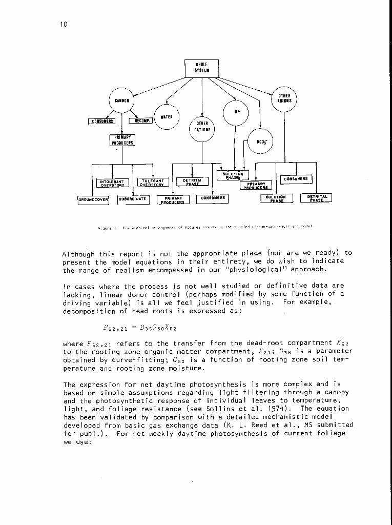
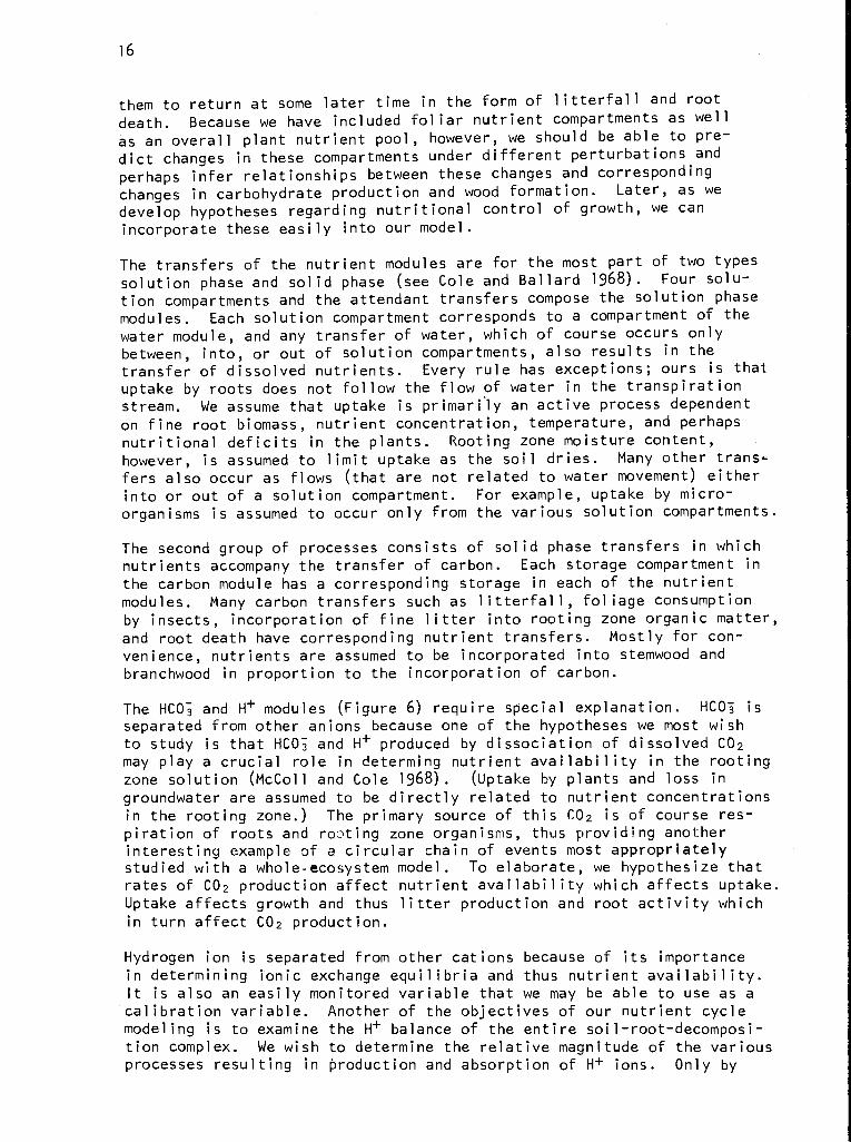
Our ecosystem model is conceived as a hierarchical structure in whichthe first level consists of six modules for different substances. Theseare carbon, water, and four groups of other elements, namely, H+ (hydro-gen ions), other cationic elements, HCO3 (bicarbonate ions), and otheranionic elements (Figure 1). For lack of a better term these lastfour will be referred to as the nutrient modules although neither H+nor HCO3 is nutritionally significant.

Material balance is maintained strictly in all except the H+ and HC03modules (see below). Driving variables of the model consist of airtemperature, precipitation, dew point, incident shortwave radiation, daylength, and concentrations of the four nutrient groups in precipitation.Soil and litter moisture and temperature are state variables calculateddynamically. Transfers are calculated at intervals of one day for thewater module and one week for the carbon module. Nutrient transfers are

computed at daily or weekly intervals depending on whether they are cal-culated as part of a water or a carbon transfer, respectively.

10

WHOLE

SYSTEM

OTHER

ANIONS

PRIMARY

PRODUCERS

INTOLERANTOVER TORY

DECOMP.

TOLERANTV

OTHER

CATIONS

DETRITALPHASE

HCO3

SOLUTIONPHAS

GROUNDCOVER lSUBORDINATEPRIMARY CONSUMERS

PRIMARYCONSUMERS

SOLUTION DETRITALH

Figure 1. Hierarchical arrangement of modules composing the coupled carbon-water-nutrient model.

Although this report is not the appropriate place (nor are we ready) to

present the model equations in their entirety, we do wish to indicate

the range of realism encompassed in our ''physiological'' approach.

In cases where the process is not well studied or definitive data arelacking, linear donor control (perhaps modified by some function of adriving variable) is all we feel justified in using. For example,

decomposition of dead roots is expressed as:

F62,21 = B38G50X62

where F62,21 refers to the transfer from the dead-root compartment X62to the rooting zone organic matter compartment, X21; B38 is a parameterobtained by curve-fitting; G50 is a function of rooting zone soil tem-perature and rooting zone moisture.

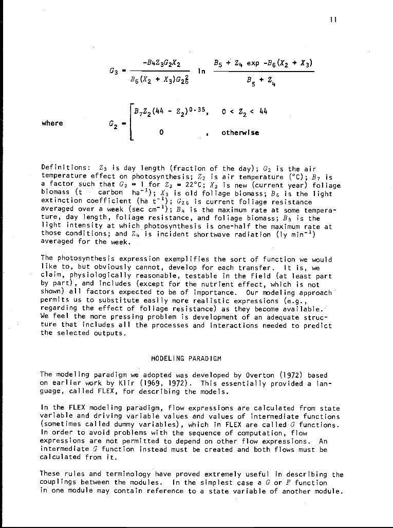
The expression for net daytime photosynthesis is more complex and isbased on simple assumptions regarding light filtering through a canopyand the photosynthetic response of individual leaves to temperature,light, and foliage resistance (see Sollins et al. 1974). The equationhas been validated by comparison with a detailed mechanistic modeldeveloped from basic gas exchange data (K. L. Reed et al., MS submittedfor pub].). For net weekly daytime photosynthesis of current foliagewe use:

11

where

-B4Z3G2X2 B5 + Z4 exp -B6(X2 + X3)G3 = In

B6(X2 + X3)G2226 B5 + z4

G2 =

B7z2(44 - z2)0.35, 0 < Z2 < 44

,0 otherwise

Definitions: Z3 is day length (fraction of the day); G2 is the airtemperature effect on photosynthesis; Z2 is air temperature (°C); B7 isa factor such that G2 = 1 for Z2 = 22°C; X2 is new (current year) foliagebiomass (t carbon ha-1); X3 is old foliage biomass; B6 is the lightextinction coefficient (ha t-1); G26 is current foliage resistanceaveraged over a week (sec cm-1); B4 is the maximum rate at some tempera-ture, day length, foliage resistance, and foliage biomass; B5 is thelight intensity at which photosynthesis is one-half the maximum rate atthose conditions; and Z4 is incident shortwave radiation (ly min-1)averaged for the week.

The photosynthesis expression exemplifies the sort of function we wouldlike to, but obviously cannot, develop for each transfer. It is, weclaim, physiologically reasonable, testable in the field (at least partby part), and includes (except for the nutrient effect, which is notshown) all factors expected to be of importance. Our modeling approachpermits us to substitute easily more realistic expressions (e.g.,regarding the effect of foliage resistance) as they become available.We feel the more pressing problem is development of an adequate struc-ture that includes all the processes and interactions needed to predictthe selected outputs.

MODELING PARADIGM

The modeling paradigm we adopted was developed by Overton (1972) basedon earlier work by Klir (1969, 1972). This essentially provided a lan-guage, called FLEX, for describing the models.

In the FLEX modeling paradigm, flow expressions are calculated from statevariable and driving variable values and values of intermediate functions(sometimes called dummy variables), which in FLEX are called G functions.In order to avoid problems with the sequence of computation, flowexpressions are not permitted to depend on other flow expressions. Anintermediate G function instead must be created and both flows must becalculated from it.

These rules and terminology have proved extremely useful in describing thecouplings between the modules. In the simplest case a G or F functionin one module may contain reference to a state variable of another module.

12

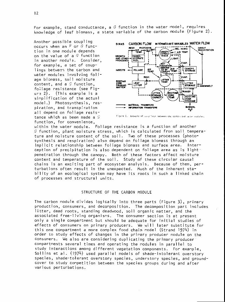
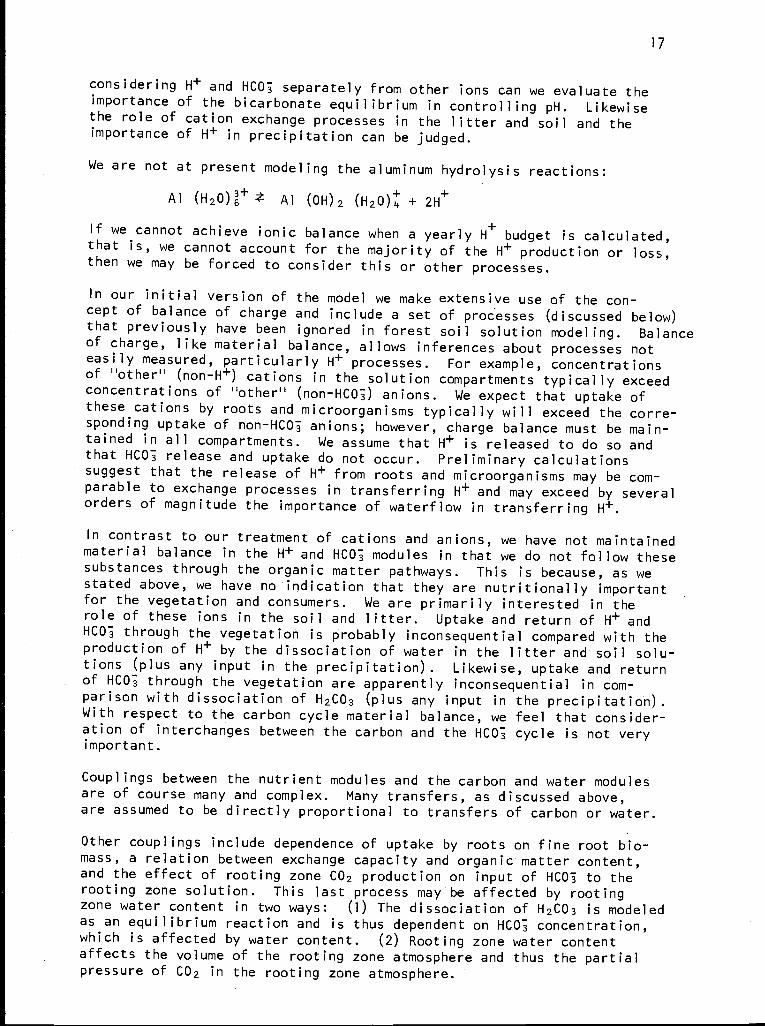
For example, stand conductance, a G function in the water model, requiresknowledge of leaf biomass, a state variable of the carbon module (Figure 2).

Another possible couplingSINKS CARBON FLOW INTERMEDIATE VARIABLES WATER FLOW

occurs when an F or G func- -----+--------- DIRECTRESP.AIR IPHOTOSYN ; Rtion in one module depends AIRMID.PRECIPITATION

I TEMP. CANOPY AIR TEMP

on the value of a G function GROWTH I CARGO TANCE --AND OTHER HYDRATE I \, LIGHT Iin another modula. Consider, PROCESSES POOL i i

for exam le a set of coup NET'p , p - ----* RADIATION___

l in s between the carbon and INSECTS FOLIAGE AIR SORB LAIR -I CANOPYg TEMP. CANOPY TEMP. I STORAGE

water modules involving fol i-RESP i -'±EVAP.age biomass, soil moisture

ROOTING -__ LITTER j__content, and a G function, ZONE

ORGANICLEAF TEMP. LITTERLITTER STORAGE NOW MELT

foliage resistance (see Fig- MATTER

ANSPure 2) . (This example is a UTTER ' Roan !STORAGE ZONE

simplification of the actual CAPACITY TEMP. ROOTINGZONE

model.) Photosynthesis, res-MATERIAL TRANSFERS

L- STORAGE-+p i r a t i o n , and t r a n s p i r a t i o n --- INFORMATION TRANSFERS SUBSOIL

H20

all depend on foliage resis-tance which as been made a Gfunction, for convenience,

Figure 2. Example of couplings between the carbon and water modules.

within the water module. Foliage resistance is a function of anotherG function, plant moisture stress, which is calculated from soil tempera-ture and moisture content of the soil. Two of these processes (photo-synthesis and respiration) also depend on foliage biomass through animplicit relationship between foliage biomass and surface area. Inter-ception of precipitation is also dependent on foliage area as is lightpenetration through the canopy. Both of these factors affect moisturecontent and temperature of the soil. Study of these circular causalchains is an exciting part of ecosystem analysis. Because of them, per-turbations often result in the unexpected. Much of the inherent sta-bility of an ecological system may have its roots in such a linked chainof processes and structural units.

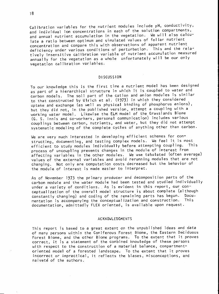
STRUCTURE OF THE CARBON MODULE

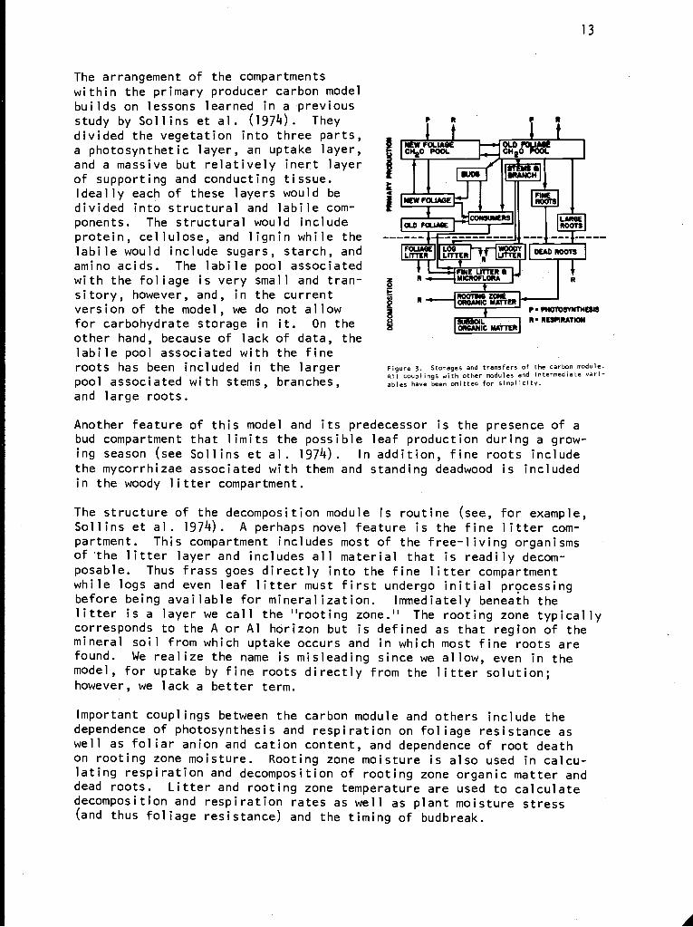
The carbon module divides logically into three parts (Figure 3), primaryproduction, consumers, and decomposition. The decomposition part includeslitter, dead roots, standing deadwood, soil organic matter, and theassociated free-living organisms. The consumer section is at presentonly a single compartment but should be adequate for initial studies ofeffects of consumers on primary producers. We will later substitute forthis one compartment a more complex food chain model (Strand 1974) inorder to study effects of changes in the primary producer module on theconsumers. We also are considering duplicating the primary producercompartments several times and operating the modules in parallel tostudy interactions among different vegetation components. For example,Sollins et al. (1974) used parallel models of shade-intolerant overstoryspecies, shade-tolerant overstory species, understory species, and ground-cover to study competition between the species groups during and aftervarious perturbations.

I

13

The arrangement of the compartmentswithin the primary producer carbon modelbuilds on lessons learned in a previousstudy by Sollins et al. (1974). Theydivided the vegetation into three parts,a photosynthetic layer, an uptake layer,and a massive but relatively inert layerof supporting and conducting tissue.Ideally each of these layers would bedivided into structural and labile com-

Ili

NEW FOLIAGE

ponents The structural would include f CONSUMERSau

protein, cellulose, and lignin while thelabile would include sugars, starch, andamino acids. The labile pool associatedwith the foliage is very small and tran-sitory, however, and, in the currentversion of the model, we do not allowfor carbohydrate storage in it. On theother hand, because of lack of data, thelabile pool associated with the fineroots has been included in the largerpool associated with stems, branches,and large roots.

FOLIAGE Los 1M000Y OHO ROOTSLITTER LITTER R LITTER

FINE LITTERMICROFLORA

OR"NICROOTING ZONE

P PHOTOSYNTHESIS

SOIL R RESPIRATIONORGANIC MATTER

Figure 3. Storages and transfers of the carbon module.All couplings with other modules and intermediate vari-ables have been omitted for simplicity.

Another feature of this model and its predecessor is the presence of abud compartment that limits the possible leaf production during a grow-ing season (see Sollins et al. 1974). In addition, fine roots includethe mycorrhizae associated with them and standing deadwood is includedin the woody litter compartment.

The structure of the decomposition module is routine (see, for example,Sollins et al. 1974). A perhaps novel feature is the fine litter com-partment. This compartment includes most of the free-living organismsof'the litter layer and includes all material that is readily decom-posable. Thus frass goes directly into the fine litter compartmentwhile logs and even leaf litter must first undergo initial processingbefore being available for mineralization. Immediately beneath thelitter is a layer we call the "rooting zone." The rooting zone typicallycorresponds to the A or Al horizon but is defined as that region of themineral soil from which uptake occurs and in which most fine roots arefound. We realize the name is misleading since we allow, even in themodel, for uptake by fine roots directly from the litter solution;however, we lack a better term.

Important couplings between the carbon module and others include thedependence of photosynthesis and respiration on foliage resistance aswell as foliar anion and cation content, and dependence of root deathon rooting zone moisture. Rooting zone moisture is also used in calcu-lating respiration and decomposition of rooting zone organic matter anddead roots. Litter and rooting zone temperature are used to calculatedecomposition and respiration rates as well as plant moisture stress(and thus foliage resistance) and the timing of budbreak.

4

14

Variables against which the behavior of the carbon module will be com-

pared (calibration variables) are growth of woody tissues (stems and

branches) and seasonal patterns of foliage biomass, forest floor respira-

tion, and fine root biomass.

STRUCTURE OF THE WATER MODULE

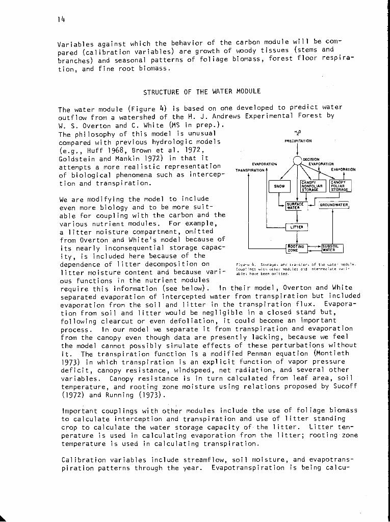
The water module (Figure 4) is based on one developed to predict water

outflow from a watershed of the H. J. Andrews Experimental Forest by

W. S. Overton and C. White (MS in prep.).

The philosophy of this model is unusual HQ

d with revi-ur- h drologic modelsare PRECIPITATIONp ycomp(e.g., Huff 1968, Brown et al. 1972,Goldstein and Mankin 1972) in that it DECISION

attempts a more realistic representation EVAPORATION EVAPORATION

TRANSPIRATION EVAPORATION

of biological phenomena such as intercep-tion and transpiration. SNOW

tNONFOLIAR FOLIARCANOPY

I 'STORAGE

We are modifying the model to includeeven more biology and to be more suit-able for coupling with the carbon and thevarious nutrient modules. For example,

a litter moisture compartment, omittedLITTER

from Overton and White's model because of

GROUNDWATER

NEING WATERILits nearly inconsequential storage capac- ZODOT

ity, is included here because of thedependence of litter decomposition on Figure 4. Storages and transfers of the water module.

Couplin with other modules and intermediate vari-litter moisture content and because var i - ableshgsave been omitted

ous functions in the nutrient modulesrequire this information (see below). In their model, Overton and Whiteseparated evaporation of intercepted water from transpiration but includedevaporation from the soil and litter in the transpiration flux. Evapora-

tion from soil and litter would be negligible in a closed stand but,following clearcut or even defoliation, it could become an important

process. In our model we separate it from transpiration and evaporationfrom the canopy even though data are presently lacking, because we feelthe model cannot possibly simulate effects of these perturbations withoutit. The transpiration function is a modified Penman equation (Montieth1973) in which transpiration is an explicit function of vapor pressuredeficit, canopy resistance, windspeed, net radiation, and several othervariables. Canopy resistance is in turn calculated from leaf area, soiltemperature, and rooting zone moisture using relations proposed by Sucoff(1972) and Running (1973).

Important couplings with other modules include the use of foliage biomassto calculate interception and transpiration and use of litter standingcrop to calculate the water storage capacity of the litter. Litter tem-perature is used in calculating evaporation from the litter; rooting zonetemperature is used in calculating transpiration.

Calibration variables include streamflow, soil moisture, and evapotrans-piration patterns through the year. Evapotranspiration is being calcu-

15

lated independently for the site on the H. J. Andrews Experimental Forestbased on energy balance considerations that do not depend on measurementsof dewpoint temperature. This may provide an additional check on thebehavior of the water module.

In addition, the weighing lysimeter tree (Fritschen 1972) will providedata on the change in weight of a representative portion of a stand.Since CO2 fixation is negligible any changes must be due to changes inthe water content of the system, thus providing a continuous record ofevapotranspiration against which to check the model.

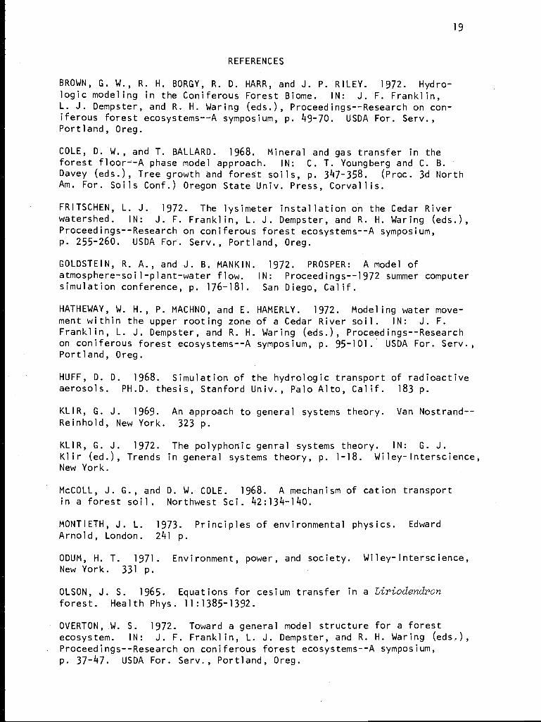
STRUCTURE OF THE NUTRIENT MODULES

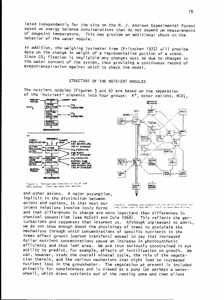
The nutrient modules (Figures 5 and 6) are based on the separationof the "nutrient" elements into four groups: H+, other cations, HC03,

PRECIPI- SNO ELT CANOPY DRIPNTERCEPTETATIONPNECIRTATIO

Lf1TERON DHC03 SOLUTI DISSOLVING

SOL UTIION

GROUNDWATER-------------------------H+

DIRECTSNOWMELT M`Aunov

ROOTINGZONESOLUTION

CO2DISSOLVING

PRECIPITATION, I i-DRIP i7nnc ul IcnLITTEREXCHANGESITES

ZZOONEINO

EXCHANGE

AND MICROFLORAI- L (NO H4 STORAGE)LITTERSOLUTION

ZRINGSOLUTION

CDR DISSOLVING

FINE ROOTS(NO IN STORAGE)CO, DISSOLVING

ROOTING ZONEORGANIC MATTERAND MICROFLORA(NO H STORAGE)

MINERALFORMS SUBSOIL

SOLUTION

GROUNDWATERf

Figure 5. Storages and transfers of the H+ andHCO3 modules. Couplings have been omitted.

90NMELT

LITTEREXCINNOESITES

DIRECT

LITTEISOLN

r

ROOTING ROOTINGZONE EXC ZONESITES SOLN.

SUBSOILSOLN

CANOPYSOL N

FIXATION

FINELITTER

WOODY

LITTER

LOGLITTER

0N

A

JFIXATION

OLD

.

LEAFLITTER

NUTPOOL

ROOTINGZONEORG MAT

STEM BBRANCHES

FINEROOTS

ROOTTS Y

SUBSOILORG MA

INSECTS

CLRRENTFOL

LARGEROOTS

and other anions. A major assumption,implicit in the distinction betweenanions and ca t i o n s , is that most n u - Figure 6. Storages and transfers of the cation and anion mod-t r i e n t relations involve i on i c forms o'P5 (other than II and HEO,). Conpl ^gs have been omitted.

and that differences in charge are more important than differences inchemical composition (see McColl and Cole 1968). This reflects the per-turbations and responses that interest us. Although unpleasant to admit,we do not know enough about the physiology of trees to postulate themechanisms through which concentrations of specific nutrients in thetrees affect growth (carbon transfers) except to say that increasedfoliar nutrient concentrations cause an increase in photosyntheticefficiency and thus leaf area. We are thus seriously constrained in ourability to predict, for example, effects of fertilization on growth. We

can, however, study the overall mineral cycle, the role of the vegeta-tion therein, and the various mechanisms that might lead to increasednutrient loss in the groundwater. The vegetation at present is includedprimarily for completeness and is viewed as a pump (or perhaps a water-wheel), which draws nutrients out of the rooting zone and then allows

16

them to return at some later time in the form of litterfall and root

death. Because we have included foliar nutrient compartments as well

as an overall plant nutrient pool, however, we should be able to pre-

dict changes in these compartments under different perturbations and

perhaps infer relationships between these changes and corresponding

changes in carbohydrate production and wood formation. Later, as we

develop hypotheses regarding nutritional control of growth, we canincorporate these easily into our model.

The transfers of the nutrient modules are for the most part of two types

solution phase and solid phase (see Cole and Ballard 1968). Four solu-

tion compartments and the attendant transfers compose the solution phase

modules. Each solution compartment corresponds to a compartment of thewater module, and any transfer of water, which of course occurs only

between, into, or out of solution compartments, also results in thetransfer of dissolved nutrients. Every rule has exceptions; ours is thatuptake by roots does not follow the flow of water in the transpirationstream. We assume that uptake is primarily an active process dependenton fine root biomass, nutrient concentration, temperature, and perhaps

nutritional deficits in the plants. Rooting zone moisture content,however, is assumed to limit uptake as the soil dries. Many other trans.

fers also occur as flows (that are not related to water movement) eitherinto or out of a solution compartment. For example, uptake by micro-organisms is assumed to occur only from the various solution compartments.

The second group of processes consists of solid phase transfers in whichnutrients accompany the transfer of carbon. Each storage compartment inthe carbon module has a corresponding storage in each of the nutrientmodules. Many carbon transfers such as litterfall, foliage consumptionby insects, incorporation of fine litter into rooting zone organic matter,and root death have corresponding nutrient transfers. Mostly for con-

venience, nutrients are assumed to be incorporated into stemwood andbranchwood in proportion to the incorporation of carbon.

The HCO3 and H+ modules (Figure 6) require special explanation. HCO3 isseparated from other anions because one of the hypotheses we most wishto study is that HCO3 and H+ produced by dissociation of dissolved CO2may play a crucial role in determing nutrient availability in the rootingzone solution (McColl and Cole 1968). (Uptake by plants and loss in

groundwater are assumed to be directly related to nutrient concentrationsin the rooting zone.) The primary source of this C02 is of course res-piration of roots and rooting zone organisms, thus providing anotherinteresting example of a circular chain of events most appropriatelystudied with a whole-ecosystem model. To elaborate, we hypothesize thatrates of C02 production affect nutrient availability which affects uptake.Uptake affects growth and thus litter production and root activity whichin turn affect CO2 production.

Hydrogen ion is separated from other cations because of its importancein determining ionic exchange equilibria and thus nutrient availability.It is also an easily monitored variable that we may be able to use as acalibration variable. Another of the objectives of our nutrient cyclemodeling is to examine the H+ balance of the entire soil-root-decomposi-tion complex. We wish to determine the relative magnitude of the variousprocesses resulting in production and absorption of H+ ions. Only by

17

considering H+ and HCO3 separately from other ions can we evaluate theimportance of the bicarbonate equilibrium in controlling pH. Likewisethe role of cation exchange processes in the litter and soil and theimportance of H+ in precipitation can be judged.

We are not at present modeling the aluminum hydrolysis reactions:

Al (H2O)6+ - Al (OH)2 (H20)4 + 2H+

If we cannot achieve ionic balance when a yearly H+ budget is calculated,that is, we cannot account for the majority of the H+ production or loss,then we may be forced to consider this or other processes.

In our initial version of the model we make extensive use of the con-cept of balance of charge and include a set of processes (discussed below)that previously have been ignored in forest soil solution modeling. Balanceof charge, like material balance, allows inferences about processes noteasily measured, particularly H+ processes. For example, concentrationsof "other" (non-H+) cations in the solution compartments typically exceedconcentrations of "other" (non-HCO3) anions. We expect that uptake ofthese cations by roots and microorganisms typically will exceed the corre-sponding uptake of non-HCO3 anions; however, charge balance must be main-tained in all compartments. We assume that H+ is released to do so andthat HCO3 release and uptake do not occur. Preliminary calculationssuggest that the release of H+ from roots and microorganisms may be com-parable to exchange processes in transferring H+ and may exceed by severalorders of magnitude the importance of waterflow in transferring H+.

In contrast to our treatment of cations and anions, we have not maintainedmaterial balance in the H+ and HCO3 modules in that we do not follow thesesubstances through the organic matter pathways. This is because, as westated above, we have no indication that they are nutritionally importantfor the vegetation and consumers. We are primarily interested in therole of these ions in the soil and litter. Uptake and return of H+ andHCO3 through the vegetation is probably inconsequential compared with theproduction of H+ by the dissociation of water in the litter and soil solu-tions (plus any input in the precipitation). Likewise, uptake and returnof HCO3 through the vegetation are apparently inconsequential in com-parison with dissociation of H2CO3 (plus any input in the precipitation).With respect to the carbon cycle material balance, we feel that consider-ation of interchanges between the carbon and the HCO3 cycle is not veryimportant.

Couplings between the nutrient modules and the carbon and water modulesare of course many and complex. Many transfers, as discussed above,are assumed to be directly proportional to transfers of carbon or water.

Other couplings include dependence of uptake by roots on fine root bio-mass, a relation between exchange capacity and organic matter content,and the effect of rooting zone C02 production on input of HCOj to therooting zone solution. This last process may be affected by rootingzone water content in two ways: (1) The dissociation of H2CO3 is modeledas an equilibrium reaction and is thus dependent on HCO3 concentration,which is affected by water content. (2) Rooting zone water contentaffects the volume of the rooting zone atmosphere and thus the partialpressure of CO2 in the rooting zone atmosphere.

18

Calibration variables for the nutrient modules include pH, conductivity,

and individual ion concentrations in each of the solution compartments,

and annual nutrient accumulation in the vegetation. We will also calcu-

late a ratio between optimum and simulated values of foliar nutrient

concentration and compare this with observations of apparent nutrient

deficiency under various conditions of perturbation. This and the rela-

tively insensitive calibration variable of nutrient accumulation measured

annually for the vegetation as a whole unfortunately will be our only

vegetation calibration variables.

DISCUSSION

To our knowledge this is the first time a nutrient model has been designed

as part of a hierarchical structure in which it is coupled to water and

carbon models. The soil part of the cation and anion modules is similar

to that constructed by Ulrich et al. (1973) in which they considered

uptake and exchange (as well as physical binding of phosphorus anions),

but they did not, in the published version, attempt a coupling with a

working water model. Likewise the ELM model of the Grasslands Biome

(G. S. Innis and co-workers, personal communication) includes various

couplings between carbon, nutrients, and water, but they did not attemptsystematic modeling of the complete cycles of anything other than carbon.

We are very much interested in developing efficient schemes for con-

structing, documenting, and testing complex models. We feel it is most

efficient to study modules individually before attempting coupling. This

process of uncoupling prevents changes in the module of interest from

affecting variables in the other modules. We use tabulated (often average)values of the external variables and avoid rerunning modules that are notchanging. Not only are computation costs decreased but the behavior ofthe module of interest is made easier to interpret.

As of November 1973 the primary producer and decomposition parts of thecarbon module and the water module had been tested and studied individuallyunder a variety of conditions. As is evident in this report, our con-ceptualization of the overall model structure is about complete (although

constantly changing) and coding of the remaining parts has begun. Docu-

mentation is accompanying the conceptualization and construction. This

documentation, admittedly FLEX oriented, is available upon request.

ACKNOWLEDGMENTS

This report is based to a great extent on the unpublished ideas and dataof many persons within the Coniferous Forest Biome, the Eastern DeciduousForest Biome, and the other Biome programs. To the extent that it proves

correct, it is a statement of the combined knowledge of these personswith respect to the construction of a material balance, compartment-oriented model of a forested landscape. To the extent that it provesincorrect or impractical, it reflects the biases, misconceptions, andnaivete of the authors.

19

REFERENCES

BROWN, G. W., R. H. BORGY, R. D. HARR, and J. P. RILEY. 1972. Hydro-logic modeling in the Coniferous Forest Biome. IN: J. F. Franklin,L. J. Dempster, and R. H. Waring (eds.), Proceedings--Research on con-iferous forest ecosystems--A symposium, p. 49-70. USDA For. Serv.,Portland, Oreg.

COLE, D. W., and T. BALLARD. 1968. Mineral and gas transfer in theforest floor--A phase model approach. IN: C. T. Youngberg and C. B.Davey (eds.), Tree growth and forest soils, p. 347-358. (Proc. 3d NorthAm. For. Soils Conf.) Oregon State Univ. Press, Corvallis.

FRITSCHEN, L. J. 1972. The lysimeter installation on the Cedar Riverwatershed. IN: J. F. Franklin, L. J. Dempster, and R. H. Waring (eds.),Proceedings--Research on coniferous forest ecosystems--A symposium,p. 255-260. USDA For. Serv., Portland, Oreg.

GOLDSTEIN, R. A., and J. B. MANKIN. 1972. PROSPER: A model ofatmosphere-soil-plant-water flow. IN: Proceedings--1972 summer computersimulation conference, p. 176-181. San Diego, Calif.

HATHEWAY, W. H., P. MACHNO, and E. HAMERLY. 1972. Modeling water move-ment within the upper rooting zone of a Cedar River soil. IN: J. F.Franklin, L. J. Dempster, and R. H. Waring (eds.), Proceedings--Researchon coniferous forest ecosystems--A symposium, p. 95-101. USDA For. Serv.,Portland, Oreg.

HUFF, D. D. 1968. Simulation of the hydrologic transport of radioactiveaerosols. PH.D. thesis, Stanford Univ., Palo Alto, Calif. 183 p.

KLIR, G. J. 1969. An approach to general systems theory. Van Nostrand--Reinhold, New York. 323 p.

KLIR, G. J. 1972. The polyphonic genral systems theory. IN: G. J.Klir (ed.), Trends in general systems theory, p. 1-18. Wiley-Interscience,New York.

McCOLL, J. G., and D. W. COLE. 1968. A mechanism of cation transportin a forest soil. Northwest Sci. 42:134-140.

MONTIETH, J. L. 1973. Principles of environmental physics. EdwardArnold, London. 241 p.

ODUM, H. T. 1971. Environment, power, and society. Wiley-Interscience,New York. 331 p.

OLSON, J. S. 1965. Equations for cesium transfer in a Liriodendronforest. Health Phys. 11:1385-1392.

OVERTON,.W. S. 1972. Toward a general model structure for a forestecosystem. IN: J. F. Franklin, L. J. Dempster, and R. H. Waring (eds.),Proceedings--Research on coniferous forest ecosystems--A symposium,p. 37-47. USDA For. Serv., Portland, Oreg.

20

REICHLE, D. E., R. V. O'NEILL, S. V. KAYE, P. SOLLINS, and R. S. BOOTH.

1974. Systems analysis as applied to modeling ecological processes.Oikos (in press).

RUNNING, S. W. 1973. Leaf resistance responses in selected conifersinterpreted with a model simulating transpiration. M.S. thesis, Oregon

State Univ., Corvallis. 87 p.

SOLLINS, P., W. F. HARRIS, and N. T. EDWARDS. 1974. Simulating thephysiology of a temperate deciduous forest. IN: B. C. Patten (ed.),Systems analysis and simulation in ecology, Vol. 4. Academic Press,New York (in press).

STRAND, M. A. 1974. Canopy food chain in a coniferous forest water-shed. IN: R. H. Waring and R. L. Edmonds (eds.), Integrated researchin the Coniferous Forest Biome, p. 41-47 (this volume). Conif. For.Biome Bull. no. 5 (Proc. AIBS Symp. Conif. For. Ecosyst.). Univ.Washington, Seattle.

SUCOFF, E. 1972. Water potential in red pine: soil moisture, evapo-transpiration, crown position. Ecology 53:681-686.

ULRICH, B., R. MAYER, P. K. KHANNA, and J. PRENZEL. 1973. Modeling ofbioelement cycling in a beech forest of Solling district. GottingerBodenkundliche Berichte 29:1-54.

21

NUTRIENT CYCLING IN 37- AND 450-YEAR-OLDDOUGLAS-FIR ECOSYSTEMS'

C. C. Grier, D. W. Cole, C. T. Dyrness, and R. L. Fredriksen

Oregon State University, University of Washington, and USDA Forest Service

ABSTRACT

Biomass and nitrogen, phosphorus, potassium, and calcium distribution,and biogeochemical and stand nitrogen, phosphorus, potassium, and calciumbudgets were determined for 37- and 450-year-old Pseudotsuga menziesii(Mirb.) Franco stands in the U.S. Pacific Northwest. Biomass of the450-year-old stand is greater, but annual growth is less than that ofthe 37-year-old stand. About 50% of the annual growth and over 50% ofthe nutrient uptake and return in the 450-year-old stand occurs in sub-ordinate vegetation compared with less than 15% in the 37-year-old stand.Chemical differences in soil parent material between the two stands arereflected in both the biogeochemical and stand nutrient cycles.

INTRODUCTION

Coniferous forests of the U.S. Pacific Northwest are among the mostproductive forests in the world. In the Douglas-fir region, for example,stands often reach 1000 metric tons ha-' of standing biomass in 100 years.Because nutrients are involved in almost all ecosystem processes, studiesof nutrient movement and accumulation yield a great deal of informationabout factors affecting productivity of these forests. Further, studiesof nutrient cycling contribute much to understanding overall behaviorof coniferous forest ecosystems.

In general terms, the objectives of nutrient cycling research of theConiferous Forest Biome are: (1) to study the role of nutrients inecosystem function; (2) to develop conceptual and simulation modelsrepresenting our understanding of nutrient cycling; and (3) to use thosemodels both to extend our understanding of ecosystems and to evaluatethe effects of various perturbations on ecosystem processes and entireecosystems.

This paper is intended as an overview of current nutrient cycling researchin the Coniferous Forest Biome. The discussion here emphasizes researchdirected toward meeting the first two of the above objectives with theresearch reported by comparing nutrient cycling between two intensiveresearch sites. A comparison of nutrient cycling rates and processesbetween the 37- and 450-year-old stands on these sites should increaseour understanding of some of the broader aspects of ecosystem behavior.

'This is contribution no. 61 from the Coniferous Forest Biome.

22

RESEARCH AREAS

Thompson Research Center, Washington

The Allan E. Thompson Research Center is a research area developed forstudy of nutrient cycling in second-growth Douglas-fir stands. It islocated about 64 km southeast of Seattle, Washington, at an elevation of215 m in the foothills of the Washington Cascades. A full descriptionof the geology, soils, vegetation, and climate is given by Cole and Gessel0968).

The study site is located on a glacial outwash terrace along the CedarRiver. This outwash terrace was formed during the recessing of the Pugetlobe of the Fraser ice sheet about 12,000 years ago.

The soil underlying the research plot described in this paper is classi-fied as a Typic Haplorthod (U.S. Department of Agriculture 1960, 1972)and is mapped as Everett gravelly sand loam. This soil contains lessthan 5% silt plus clay and normally contains gravel amounting to 50%-80%of the soil volume. The forest floor is classified as a duff-mull(Hoover and Lunt 1952) and ranges from 1 cm to 3 cm thick. This forestfloor represents the accumulation since 1931 when the present stand wasestablished following logging (around 1915) and repeated fires.

The present overstory vegetation is a planted stand of Douglas-fir(Pseudotsuga menziesii [Mirb.] Franco) which was established about 1931.Currently, the trees average about 19 m high with a crown density ofabout 85%.

The principal understory species are salal (GauZtheria shaZZon Pursh.),Oregon grape (Berberis nervosa [Pursh] Nutt.), red huckleberry (VacciniumparvifoZium Smith), and twinflower (Linnaea borealis L. ssp. americana[Forbes] Rehder). Various mosses are the principal understory vegetationbeneath the denser portions of the canopy.

The climate is typical of foothill conditions in the Puget Sound basin.Temperatures have ranged from -18°C to 38°C, but these extremes are sel-dom reached. The average temperature for July is 16.7°C and for Januaryis 2.8°C. The average annual precipitation is 136 cm, almost all fallingas rain. Precipitation rates are generally less than 0.25 cm hr-1 andover 70% of precipitation falls between October and March.

Watershed 10, H. J. Andrews Experimental Forest, Oregon

Watershed 10 is a 10.24-ha watershed located in the western CascadeRange about 70 km east of Eugene, Oregon. Elevations on the watershedrange from 430 m at the stream gaging station to about 670 m at thehighest point. Slopes on the watershed average about 45% but frequentlyexceed 100%.

The study site is located in an area underlain by volcanic tuff andbreccia. Soils of the watershed are derived from these materials.Soils of the watershed are classified as Typic Dystrochrepts (Inceptisols;U.S. Department of Agriculture, 1960, 1972) and range from gravelly,

23

silty clay loam to very gravelly clay loam. The <2-mm fraction of thesesoils ranges from 20% to 50% clay and contains gravel amounting to 30%-50%of the soil volume. The forest floor ranges from 3 to 5 cm thick and isclassified as a duff-mull (Hoover and Lunt 1952).

The present overstory vegetation is dominated by a 60- to 80-m-tall,450-year-old stand of Douglas-fir (Pseudotsuga menziesii) containingsmall islands of younger age classes. Distribution of understory vegeta-tion reflects topography and slope-aspect on this watershed. Dry ridge-tops and south-facing slopes have an understory composed primarily ofchinkapin (Castanopsis chrysophyZZa), Pacific rhododendron (RhododendronmacrophylLum), and salal. More mesic parts of the watershed support anunderstory of vine maple (Acer circinatum), rhododendron, and Oregongrape, with a well developed intermediate canopy of Tsuga heterophyZZa.Subordinate vegetation of the moist areas along the stream and on north-facing slopes is primarily vine maple and sword fern (PoZystichum munitum).

The climate of watershed 10 is typical for the western Oregon Cascades.Average annual precipitation is 230 mm per year with over 75% of theprecipitation falling as rain between October and March. Snow accumula-tions on the watershed are not uncommon, but seldom last more than twoweeks. Based on two years' data, the average daytime temperature forJuly is 21°C and for January is 0°C. Observed extremes have ranged froma high of 41°C in August to a low of -20°C in December.

METHODS

Mapping of Watershed 10

A 25-m by 25-m grid system, corrected to horizontal distance, was estab-lished on watershed 10. All mapping used this grid system for reference.Soils were mapped on the basis of depth, stone and gravel content, andwater storage in the upper 100 cm of profile. Subordinate vegetationwas mapped using methods outlined by G. M. Hawk (pers. commun., 1973).Diameter, species, and location of all living and standing dead trees onthe watershed greater than 15 cm dbh (diameter breast height) were mapped.These data were punched on computer cards. Trees less than 15 cm dbhwere considered to be understory vegetation.

Organic Matter and Nutrient Distribution

Biomass, nutrient capital, and productivity of the overstory vegetationof the Thompson site were estimated from destructive analysis of treesfrom that area (Dice 1970). Overstory biomass and nutrient distributionon watershed 10 were estimated from regression equations using diameterand species data compiled for the stem map. The regression equationswere based on data from destructive analysis of the major overstoryspecies on the watershed based on a modification of the fixed-internalstratification method outlined by Monsi and Saeki (1953). The modifi-cation used consisted of dividing both the branchless stem and the canopyof each felled sample tree into three equal segments and weighing andsampling component mass in each of these segments.

24

Annual growth of stands on watershed 10 was estimated as follows: Average

diameter increment over the past five years was determined for 10-cm-

diameter classes for each species on the watershed. This increment was

added to recorded tree diameters according to species and diameter class

and overstory biomass was recomputed using the new diameters. Productivity

was then estimated as the difference between the first and second biomass

estimates. Nutrient distribution in overstory biomass and nutrientsincorporated in new growth were estimated by sampling and analyzing newgrowth and older plant components during the sampling for biomassestimation.

Understory biomass and nutrient distribution on watershed 10 were esti-mated by regression methods based on destructive sampling for largerunderstory species, while the mass of smaller shrubs and herbs was deter-mined by total harvest. Methods used in understory biomass estimatesare described by Russel (1973). Understory biomass and nutrient capitalof the Thompson site was determined by harvest of small plots.

Litter layer mass on watershed 10 was determined by sampling the litterlayer in two areas representative of the entire watershed. Total andexchangeable nutrients; water storage; depth of L, F, and H layers; andlitter mass were determined using methods outlined by Youngberg (1966).

Litter layer mass and nutrient capital at the Thompson site were deter-mined using methods reported by Grier and McColl (1971).

The mass of standing and down dead trees on watershed 10 was estimatedfrom data gathered during stem mapping. Heights of standing dead treeswere estimated and diameters were measured. Length and diameter of allrecognizable fallen trees were measured. Similar methods were used forthe Thompson site. Mass of standing and down dead was computed from theSmalian volume of logs and standing dead, assuming a density of 0.3 anda uniform taper of 2%.

Soil nutrient and organic matter content of watershed 10 were determinedby sampling of soil in the areas where litter mass was determined. Total

and exchangeable nutrients and organic matter were determined by methodsoutlined by R. B. Brown and R. B. Parsons (pers. commun., 1973). Methodsused for soil analysis at the Thompson site are outlined by Grier andCole (1972).

Epiphyte standing crop and nitrogen content in the overstory of watershed10 were determined by methods reported by Pike et al. (1972). Epiphytesare a negligible component of the stand at the Thompson site.

Organic Matter and Nutrient Fluxes

Litterfall at both sites is collected on screens placed approximately15 cm above the soil surface. Eight 0.21-m2 screens are used in theplot at the Thompson site. On watershed 10, litter is collected from75 0.26-m2 screens located randomly within each of the 15 soil-vegetationunits with approximately the same area sampled in each unit. Total areasampled is 0.41% for the Thomson site and 0.02% on watershed 10. Litteris collected monthly, dried at 70°C, and sorted into the following cate-gories: conifer foliage, hardwood foliage, woody material, reproductive

25

parts, living foliage and twigs, and "other material." Nutrient contentof each of these categories is determined.

Throughfall at both sites is collected in 20-cm-diameter polyethylenefunnels having a neck screen of the same mesh as the litter screens.The funnels are inserted in 20-liter polyethylene bottles and the assemblyis placed immediately adjacent to each litter screen. Eight collectorsare used at the Thompson site and 75 are used on watershed 10. Litteris allowed to collect in the funnels so that nutrients leached from thelitter are collected in throughfall. Collections are made monthly andanalyses are performed on unfiltered samples. Chloroform is added tothe collectors to retard microbial effects on water chemistry.

Stemflow on watershed 10 is collected on fifteen 10-m by 10-m plots inwhich all trees >5 cm dbh are fitted with polyurethane foam collars atbreast height (Likens and Eaton 1970). On each plot, water is pipedfrom the sampled trees to a group of opaque 125-liter polyethylene trashcans fitted with tight lids. Collections are made as necessary to avoidoverflow, with a maximum interval of one month. At the Thompson site,stemflow is diverted from six representative trees into opaque 160-litertrash cans by rubber collars at breast height (130 cm).

Litter decomposition studies based on litterbags filled with specificsubstrates are in progress on watershed 10. Methods used are reportedby Cromack (1973). Mineralization and leaching of nutrients from thelitter layer are directly measured at both sites using tension lysimeters(Cole 1968).

Nutrient leaching in the soil profile at the Thompson site is measuredwith tension lysimeters placed at the lower boundaries of the Al and B2horizons and at 1 m in the C horizon to collect percolating soil water.On watershed 10, Soiltest soil solution extractors are placed at the baseof the rooting zone (1 m) and at different depths in the subsoil todetermine nutrient concentrations in the subsoil water.

Incorporation of nutrients into growth by overstory and understory vege-tation was estimated by sampling and analysis of new growth at the endof the growing season and using nutrient concentrations and annual growthestimates to compute nutrient content of new growth.

Annual biogeochemical nutrient budgets for watershed 10 were preparedfrom measurements of quantity and chemistry of input and outflow water.Methods used are reported by Fredriksen (1972). Annual budgets for theThompson site are based on data from the lysimeter installation (Coleet al. 1968). Chemical analyses of plant tissue and water were doneusing methods outlined by Grier and Cole (1972) and Fredriksen (1972).

RESULTS AND DISCUSSION

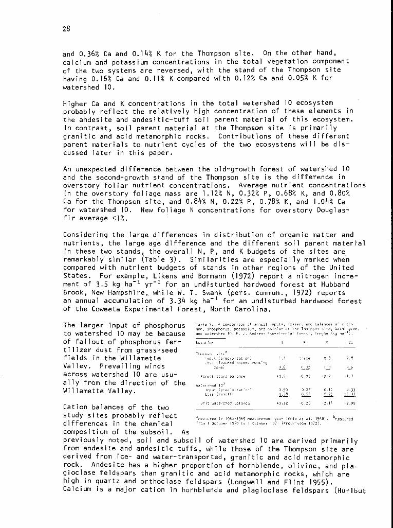
As would.be expected, there are large differences in distribution oforganic matter, nitrogen, phosphorus, potassium, and calcium between the37-year-old stand of the Thompson site and 450-year-old stand on water-shed 10 (Tables 1 and 2). These differences reflect not only the age

26

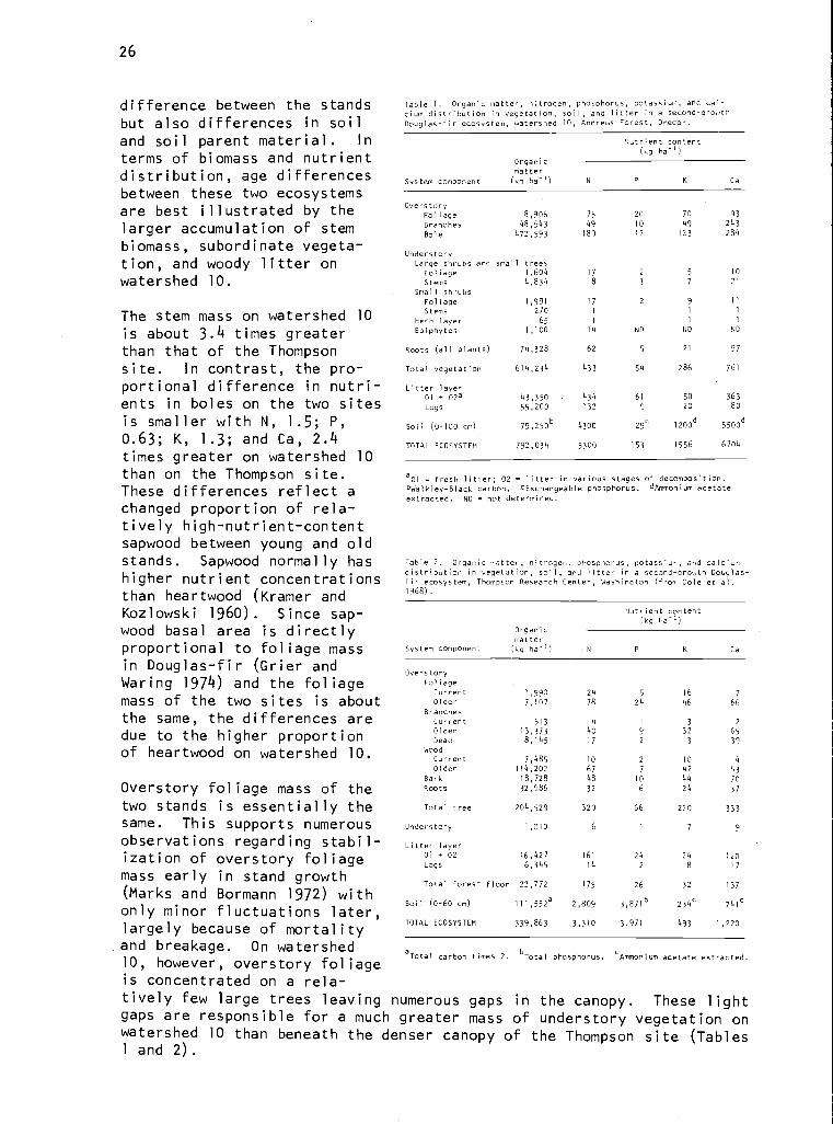
difference between the standsbut also differences in soiland soil parent material. In

terms of biomass and nutrientdistribution, age differencesbetween these two ecosystemsare best illustrated by thelarger accumulation of stembiomass, subordinate vegeta-tion, and woody litter onwatershed 10.

The stem mass on watershed 10is about 3.4 times greaterthan that of the Thompsonsite. In contrast, the pro-portional difference in nutri-ents in boles on the two sitesis smaller with N, 1.5; P,0.63; K, 1.3; and Ca, 2.4times greater on watershed 10than on the Thompson site.These differences reflect achanged proportion of rela-tively high-nutrient-contentsapwood between young and oldstands. Sapwood normally hashigher nutrient concentrationsthan heartwood (Kramer andKozlowski 1960). Since sap-wood basal area is directlyproportional to foliage massin Douglas-fir (Grier andWaring 1974) and the foliagemass of the two sites is aboutthe same, the differences aredue to the higher proportionof heartwood on watershed 10.

Overstory foliage mass of thetwo stands is essentially thesame. This supports numerousobservations regarding stabil-ization of overstory foliagemass early in stand growth(Marks and Bormann 1972) withonly minor fluctuations later,largely because of mortalityand breakage. On watershed10, however, overstory foliageis concentrated on a rela-

Table 1. Organic matter, nitrogen, phosphorus, potassium, and cal-cium distribution in vegetation, soil, and litter in a second-growthDouglas-fir ecosystem, watershed 10, Andrews Forest, Oregon.

Organicmatter

System component (kq ha-')

Ove rstoryFoliage 8,906

Branches 48,543

Bole 472,593

UnderstoryLarge shrubs and small trees

Foliage 1,604

Stems 4,834

Small shrubsFoliage 1,991

Stems 270

Herb layer 65

Epiphytes 1,100

Roots (all plants) 74,328

Total vegetation 614,234

Litter layer01 + 02a 43,350

Logs 55,200

soil (0-100 cm) 79,250b

TOTAL ECOSYSTEM 792,034

Nutrient content(kg ha-')

-

N P K Ca

75 20 70 93

49 10 49 243

189 12 123 284

17 2 5 10

8 3 7 21

17 2 9 11

1 I 1

1 I 1

14 ND ND ND

62 5 21 97

433 54 286 761

434 61 50 363

132 9 20 80

4300 29c 1200d 5500d

5300 153 1556 6704

a01 = fresh litter; 02 = litter in various stages of decomposition.

bWalkley-Black carbon. cExchangeable phosphorus. dAmmonium acetateextracted. ND = not determined.

Table 2. Organic matter, nitrogen, phosphorus, potassium, and calciumdistribution in vegetation, soil, and litter in a second-growth Douglas-fir ecosystem, Thompson Research Center, Washington (from Cole et al.1968).

Organicmatter

System component (kg ha-')

Nutrient content(kg ha-1)

P K Ca

OverstoryFoliageCurrent 1,990 24 5 16 7

Older 7,107 78 24 46 66Branches

Current 513 4 1 3 2

Older 13,373 40 9 32 65

Dead 8,145 17 2 3 39Wood

Current 7,485 IO 2 10 4

Older 114,202 67 7 42 43

Bark 18,728 48 10 44 70Roots 32,986 32 6 24 37

Total tree 204,529 320 66 220 333

Understory 1,010 6 1 7 9

Litter layer01 + 02 16,427 161 24 24 120Logs 6,345 14 2 8 17

Total forest floor 22,772 175 26 32 137

Soil (0-60 cm) 11552a 2,809 3 8716 234c 741c

TOTAL ECOSYSTEM 339,863 3,310 3 ,971 493 1,220

aTotal carbon times 2bTotal phosphorus. cAmmonium acetate extracted.

tively few large trees leaving numerous gaps in the canopy. These lightgaps are responsible for a much greater mass of understory vegetation onwatershed 10 than beneath the denser canopy of the Thompson site (Tables1 and 2).

-N

27

The large mass of understory vegetation on watershed 10, relative to theThompson site, implies major differences in nutrient cycling pathwaysbetween young- and old-growth stands. Calculations, based on averagefoliage turnover rates for understory and overstory species of the twosites, indicate that between 40% and 60% of leaf litterfall on watershed10 is contributed by understory compared with about 15% for the Thompsonsite. The large litter input from understory vegetation on watershed 10is confirmed by litterfall data indicating that from 10% to 70% of annualleaf litter input on individual litter screens is hardwood foliage (C. C.Grier, unpublished data).

Generally, nutrient return by foliage of understory vegetation should beproportionally greater than.overstory foliage. return because of thegenerally higher nutrient content of hardwood foliage. For example,hardwood litter from watershed 10 has 15%, 28%, 32%, and 55% higherrespective N, K, Ca, and Mg concentrations than does conifer litter,while P concentrations in understory litterfall are 22% lower than inoverstory litter (Abee and Lavender 1972).

These data indicate that in the 450-year-old stand of watershed 10, amajor portion of the nutrient cycling is taking place through subordinatevegetation. In contrast, the major nutrient pathway in the young standof the Thompson site is through the overstory.

Litter layer mass and nutrient capital also reflect the large age dif-ference between these two stands (Tables 1 and 2). Standing crop of the01 and 02 layers of the forest floor is 2.6 times greater on watershed10 than at the Thompson site. This difference reflects in part the largeinput of woody material from the decadent overstory vegetation of water-shed 10. Abee and Lavender (1972) found that 47% of litterfall in twoplots on watershed 10 was woody material. This is in contrast to theapproximately 30% reported by Bray and Gorham (1964) for cool-temperateforests of the world and the 33% woody material in litterfall of theThompson site.

Mass of standing and down dead trees is substantially greater on water-shed 10 than at the Thompson site. The stand at the Thompson site hashad little mortality since it was established in 1931 and forest floorlogs here are remnants of the former stand. In contrast, tree mortalityin the stand of watershed 10 is high, estimated at 2% per year currently.In addition, much of the mortality on watershed 10 is of larger trees.

The litter layer, including logs, of both sites constitutes a substantialpool of potentially available nutrients. About 11% N, 4.5% K, and 6.6%Ca are in the litter out of the total amounts of these elements in thewatershed 10 ecosystem, in comparison with 5.2% N, 6% K, and 11% Ca inthe litter layer of the Thompson site. Phosphorus values for the twosites (Tables 1 and 2) are not directly comparable because of the dif-ferent extraction procedures used for soil phosphorus.

Soil parent material differences between the two sites may be reflectedin the higher total concentrations of Ca and K in the watershed 10 eco-system. Total ecosystem Ca and K (Table 1), expressed as percentages oftotal ecosystem organic matter, are 0.85% Ca and 0.2% K for watershed 10

28

and 0.36% Ca and 0.14% K for the Thompson site. On the other hand,calcium and potassium concentrations in the total vegetation componentof the two systems are reversed, with the stand of the Thompson sitehaving 0.16% Ca and 0.11% K compared with 0.12% Ca and 0.05% K forwatershed 10.

Higher Ca and K concentrations in the total watershed 10 ecosystemprobably reflect the relatively high concentration of these elements inthe andesite and andesitic-tuff soil parent material of this ecosystem.In contrast, soil parent material at the Thompson site is primarilygranitic and acid metamorphic rocks. Contributions of these differentparent materials to nutrient cycles of the two ecosystems will be dis-cussed later in this paper.

An unexpected difference between the old-growth forest of watershed 10and the second-growth stand of the Thompson site is the difference inoverstory foliar nutrient concentrations. Average nutrient concentrationsin the overstory foliage mass are 1.12% N, 0.32% P, 0.68% K, and 0.80%Ca for the Thompson site, and 0.84% N, 0.22% P, 0.78% K, and 1.04% Cafor watershed 10. New foliage N concentrations for overstory Douglas-fir average <1%.

Considering the large differences in distribution of organic matter andnutrients, the large age difference and the different soil parent materialin these two stands, the overall N, P, and K budgets of the sites areremarkably similar (Table 3). Similarities are especially marked whencompared with nutrient budgets of stands in other regions of the UnitedStates. For example, Likens and Bormann (1972) report a nitrogen incre-ment of 3.5 kg ha-1 yr-1 for an undisturbed hardwood forest at HubbardBrook, New Hampshire,. while W. T. Swank (pers. commun., 1972) reportsan annual accumulation of 3.34 kg ha-1 for an undisturbed hardwood forestof the Coweeta Experimental Forest, North Carolina.

The larger input of phosphorusto watershed 10 may be becauseof fallout of phosphorus fer-tilizer dust from grass-seedfields in the WillametteValley. Prevailing windsacross watershed 10 are usu-ally from the direction of theWillamette Valley.

Table 3. A comparison of annual inputs, losses, and balances of nitro-gen, phosphorus, potassium, and calcium at the Thompson site, Washington,and watershed 10, H. J. Andrews taper i,en tat Forest, Oregon (kg ha r

Location P K Ca

Thompson siteaInput (precipitation) 1.1 trace 0.8 2.8Loss (leached beyond rooting

zone) 0.6 0.02 1.0 4.5

Forest stand balance +0.5 -0.02 -0.2 -1.7

Watershed 106Input (precipitation) 0.90 0.27 0.11 2.33

Loss (runoff) 0.38 0.52 2.25 50.32

Cation balances of the twostudy sites probably reflectdifferences in the chemical

Unit watershed balance +0,52 -0.25 -2.14 47.99

Measured in 1964-1965 measurement year (Cole et al. 1968). bMeasuredfrom I October 1970 to I October 1971 (Fredriksen 1972).

composition of the subsoil. As

previously noted, soil and subsoil of watershed 10 are derived primarilyfrom andesite and andesitic tuffs, while those of the Thompson site arederived from ice- and water-transported, granitic and acid metamorphicrock. Andesite has a higher proportion of hornblende, olivine, and pla-gioclase feldspars than granitic and acid metamorphic rocks, which arehigh in quartz and orthoclase feldspars (Longwell and Flint 1955).Calcium is a major cation in hornblende and plagioclase feldspars (Hurlbut

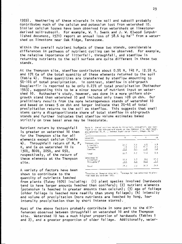
29

1959). Weathering of these minerals in the soil and subsoil probablycontributes much of the calcium and potassium lost from watershed 10.Similar calcium losses have been observed from watersheds on limestone-derived soil-subsoil. For example, W. T. Swank and J. W. Elwood (unpub-lished document, 1971) report an annual loss of 58.6 kg ha-1 from a water-shed on limestone near Oak Ridge, Tennessee.

Within the overall nutrient budgets of these two stands, considerabledifferences in pathways of nutrient cycling can be observed. For example,

the relative importance of litterfall, throughfall, and stemflow inreturning nutrients to the soil surface are quite different in these twostands.

At the Thompson site, stemflow contributes about 0.9% N, 14% P, 12.5% K,and 17% Ca of the total quantity of these elements returned to the soil(Table 4). These quantities are transferred by stemflow amounting to5%-100 of total precipitation. In contrast, stemflow in old-growthDouglas-fir is reported to be only 0.27% of total precipitation (Rothacher1963), suggesting this to be a minor source of nutrient input on water-shed 10. Rothacher's study, however, was done in a more uniform old-growth stand than watershed 10 and included only trees >28 cm dbh. Our

preliminary results from the more heterogeneous stands of watershed 10and based on trees 5 cm dbh and larger indicate that 2%-4% of totalprecipitation returns to the soil as stemflow. This suggests that smallstems carry a disproportionate share of total stemflow in old-growthstands and further indicates that stemflow volume estimates basedstrictly on tree basal area may be inaccurate.

Nutrient return by throughfallis greater on watershed 10 thanfor the Thompson site for allelements except calcium (Table4). Throughfall return of N, PK, and Ca on watershed 10 is130%, 800%, 205%, and 65%,respectively, of the return ofthese elements at the Thompsonsite.

f

Table 4. Annual nutrient return by Litterfall, throughfail, and stem-flowa in 43- and 450-year-old stands at the Thompson site, Washington,and watershed 10, H. J. Andrews Experimental Forest, Oregon (kg hayr-').

Location N P K Ca

Thompson siteLitterfallThroughfaIiStemf low

Total

Watershed 10LitterfallThroughfall6

Total

21.0 0.3 0.5 1.8

1.5 0.3 10.7 3.5

0.2 0.1 1.6 1.1

22.7 0.7 12.8 6.4

27.3 4.7 8.0 67.3

2.0 2_5 22,0 2.3

29.3 7.2 20.0 29.6

A variety of factors have beenshown to contribute to the aStemflow at Thompson site only. 6Average for two watershed 10 plots

from Abee and Lavender 1972.

quantity of nutrients leachedfrom plants (Tukey 1970) including: (1) plant species involved (hardwoodstend to have larger amounts leached than conifers); (2) nutrient elements(potassium is leached in greater amounts than calcium); (3) age of foliage(older foliage is leached more readily than young foliage); (4) intensity

and volume of precipitation (more nutrients are leached by long, low-intensity precipitation than by short intense storms).

Most of the above factors probably contribute in some part to the dif-ferences observed between throughfall on watershed 10 and the Thompsonsite. Watershed 10 has a much higher proportion of hardwoods (Tables 1

and 2), and a greater proportion of older foliage. Additionally, water-

30

shed 10 has 170% greater precipitation, which falls at about the samerate as at the Thompson site, and greater total foliage and branch massexposed to leaching (Tables 1 and 2).

In combination, these factors probably account for the major differencesobserved in leaching of N, K, and Ca. The factors responsible for the800% greater return of P on watershed 10 cannot be satisfactorily explainedat present, especially since P is usually leached from plants in rela-tively small amounts (Tukey 1970). Further research is proposed toexamine this phenomenon.

Organic matter and nutrient transfers by litterfall also reflect thedifferences between the two sites. Annual litterfall in the 37-year-oldstand of the Thompson site is currently about 2900 kg ha-1 compared with5900 ka ha-1 on watershed 10. Annual foliage litterfall, however, issimilar for the two sites, with 2200 kg ha- and 2800 kg ha-1 for theThompson site and watershed 10, respectively. The larger amount forwatershed 10 is due to the large mass of hardwoods in the understory.

Of total nutrients returned in litterfall for the two research sites(Table 4), about 90% are returned in the foliage component of the litterat the Thompson site. In contrast, 48% N, 69% P, 61% K, and 70% Ca arereturned annually in foliage litter on watershed 10; the remainingnutrients are returned in woody material, reproductive parts, epiphytes,microlitter, and other minor categories.

Nutrients returned in epiphyte- and microlitter make a measurable con-tribution to the annual nutrient cycle on watershed 10. In this old-growth stand, epiphytes on branches alone amount to a dry weight of800-1600 kg ha-1 and contain about 13.5 kg ha-1 N (Pike et al. 1972).Many lichens fix atmospheric N and, because of this and their possiblerole in adsorbing and desorbing nutrients in precipitation and through-fall, further studies of the role of epiphytes in nutrient cycling areplanned. Annual nutrient by epiphyte-fall on watershed 10 is 6.7% N,3.6% P, 5.6% K, and 0.7% Ca of total nutrients in litterfall (Abee andLavender 1972). Epiphytes are a negligible component of litterfall atthe Thompson site.

A portion of nutrient return by litterfall is in the form of fine organicmatter such as insect frass, spores, pollen, and dust. This materialis overlooked in many nutrient cycling studies in spite of nutrient con-centrations such as 2% N in pollen and 7.8% N in some insect bodies(Stark 1973). This microlitter is a strongly seasonal input to thelitter layer. Studies of microlitter input and turnover are currentlyin progress on watershed 10.

As previously mentioned, over 80% N, 30% P, 20% K, and 70% Ca reachingthe soil surface of these two research sites do so by litterfall. Researchis currently in progress at both sites to determine factors involved inmaking nutrients returned by litterfall available for plant uptake,including studies of the relation between climate and litter decomposition,the relation between decomposition and mineralization, and ion leachingin the soil.

31

Data on nutrient mineralization during decomposition are being providedfor both sites from two sources, tension lysimetry (Cole 1968) and analysisof litterbags (Cromack 1973). Tension lysimetry provides integratedmineralization data for the total litter mass and data of nutrient fluxin the soil, while litterbag studies provide mineralization data forspecific organic substrates. Preliminary results of litterbag studiesindicate that in the first six months of decomposition, weight loss ofgreen needle litter was 17%, while potassium, magnesium, and calciumconcentrations decreased by 75%, 75%, and 15% respectively, and nitrogenand phosphorus concentration showed no change (K. Cromack and R. Fogel,unpublished). Similar data are now available for a wide variety ofsubstrates. For example, weight loss of fallen conifer needles and moss(Isothecium stoZoniferum) is 10% in the first year (K. Cromack and R.Fogel, unpublished), while nitrogen-rich lichens lose 50% to 60% of theirweight in one year (Rossman, unpublished).

Overstory vegetation of the Thompson site is currently over four timesmore productive than that of watershed 10 (Table 5). Over 40% of annualgrowth on watershed 10 is in the understory vegetation, however, sototal production on watershed 10 is actually about one-half that of theThompson site. The values given in Table 5 do not include mortality;doing so would probably reduce the overstory growth value for watershed10 considerably. Nutrient utilization by understory of watershed 10should nearly equal that of the overstory because of higher nutrientconcentrations in new hardwood growth (Russel 1973). Onsite observa-tions indicate mortality is high for watershed 10 and negligible for theThompson site, but long-term data will be needed to establish mortalityat both sites.

Table 5. Net' annual organic matter and nutrient accumulation by vege-N u t r i e n t accumulation in new tat ion of 37- and 450-year-old Douglas-fir standsb on the Thompson site,

growth i n t he ov e r s to r y is 1 owWashington, and the H. J. Andrews Experimental Forest, Oregon (kg ha-').

for both sites compared with Organic

stands in other parts of the Location matter N P K Ca

world. For example, Nelson et al. Thompson Site (43 years old)

(1970) report 34.3 kg/ha N, 4.7 Total all vegetation 9988 23.6 6.6 14,4 8.7

d 1d)ry0

(450 years of23625.0 1.1 4.4 4.3kg ha-1 P, 18.9 kg ha-1 K, and Watersheo

22.0 kg ha-1 Ca accumulated by understoryc 1840 d d d d

5-year-old loblolly pine (Pinus Total all vegetation 4202

taeda L.) in producing 9400 kgh a- 1 of o r g a n i c matter d u r i n g one aHortalitycnot deducted from agove figures. bDoes not include root pro-

duction. From Russel 1973. Not available at time of writing.

year. Annual nutrient accumula-tions in new tissue of the old-growth forest are substantially belowthose of the 37-year-old stand of the Thompson intensive site in spiteof the threefold greater biomass accumulation on watershed 10. The lowerdemand for nutrients by the old-growth forest may indicate a successionalpattern of reduced nutrient utilization that will be continued into climaxTsuga heterophylla stands typical of this area.

SUMMARY

Biomass and nutrient distribution and nutrient cycling process in 37- and450-year-old Douglas-fir stands of the Thompson site in Washington andwatershed 10 in Oregon reflect both the differences in age and soil and

32

soil parent material. total biomass of the older stand is greater.Overstory foliage mass of the two sites is the same. In the 450-year-oldstand, foliage is concentrated on fewer stems causing light gaps in thecanopy. The greater light penetration through the older canopy promotesdense understory vegetation. Litter accumulation is fourfold greaterin the older stand because of larger input of slowly decomposing woodymaterial. Nutrient concentrations are generally lower in the less physio-logically active 450-year-old overstory.

Input-output nutrient budgets for the two stands are relatively similarexcept for calcium. The large calcium output from watershed 10 is probablydue to subsoil weathering.

Annual return of nutrients to the litter layer is greater in the 450-year-old stand, with approximately half this annual return contributedby understory vegetation. In contrast, less than 15% of annual returnis contributed by understory in the 37-year-old stand.

The greater nutrient return by throughfall on watershed 10 is probablyexplained by the greater precipitation, larger amounts of older foliage,greater foliage and branch mass, and the larger mass of hardwoods in thisstand. Nutrient return by stemflow is significant in the 43-year-oldstand of the Thompson site. Stemflow is less important in the olderstand but comparable data are not yet available.

Annual incorporation of nutrients in overstory growth is 4.7, 6, 3.3,and 2 times greater for N, P, K, and Ca, respectively, in the 43-year-oldstand. Including the understory, nutrient incorporation in growth shouldbe at least twice the above figures, since understory production is nearlyequal that of the overstory.

REFERENCES

ABEE, A., and D. P. LAVENDER. 1972. Nutrient cycling in throughfalland litterfall in 450-year-old Douglas-fir stands. IN: J. F. Franklin,L. J. Dempster, and R. H. Waring (eds.), Proceedings--Research on conif-erous forest ecosystems--A symposium, p. 133-143. USDA For. Serv.,Portland, Oreg.

BRAY, J. R., and E. GORHAM. 1964. Litter production in forests of theOld World. IN: J. B. Craig (ed.), Advances in ecological research,p. 101-157. Academic Press, New York.

COLE, D. W. 1968. A system for measuring conductivity, acidity andrate of flow in a forest soil. Water Resour. Res. 4:1127-1136.

COLE, D. W., and S. P. GESSEL. 1968. Cedar River research--A programfor studying pathways, rates and processes of elemental cycling in aforest ecosystem. Univ. Washington, Coll. For. Resour., For. Resour.Monogr. Contrib. no. 4. Univ. Washington, Seattle. 53 p.

COLE, D. W., S. P. GESSEL, and S. F. DICE. 1968. Distribution andcycling of nitrogen, phosphorus, potassium and calcium in a second-

33

growth Douglas-fir ecosystem. IN: H. E. Young (ed.), Primary productivityand mineral cycling in natural ecosystems, p. 197-233. (AAAS Symp.) Univ.Maine Press, Orono.

CROMACK, K., Jr. 1973. Litter production and decomposition in a mixedhardwood watershed and a white pine watershed at Coweeta HydrologicStation, North Carolina. Ph.D. dissertation, Univ. Georgia, Athens.160 p.

DICE, S. F. 1970. The biomass and nutrient flux in a second-growthDouglas-fir ecosystem (A study in quantitative ecology). Ph.D. disser-tation, Univ.. Washington, Seattle. 166 p.

FREDRIKSEN, R. L. 1972. Nutrient budget of a Douglas-fir forest on anexperimental watershed in western Oregon. IN: J. F. Franklin, L. J.Dempster, and R. H. Waring (eds.), Proceedings--Research on coniferousforest ecosystems--A symposium, p. 115-131. USDA For. Serv., Portland,Oreg.

GRIER, C. C., and D. W. COLE. 1972. Elemental transport changes occur-ring during development of a second-growth Douglas-fir ecosystem. IN:J. F. Franklin, L. J. Dempster, and R. H. Waring (eds.) Proceedings--Research on coniferous forest ecosystems--A symposium, p. 103-113.USDA For. Serv., Portland, Oreg.

GRIER, C. C., and J. G. McCOLL. 1971. Forest floor characteristicswithin a small plot in Douglas-fir in western Washington. Soil Sci. Soc.Am. Proc. 35:988-991.

GRIER, C. C., and R. H. WARING. 1974. Coniferous foliage mass relatedto sapwood area. For. Sci. (in press).

HOOVER, M. D., and A. H. LUNT. 1952. A key for the classification offorest humus types. Soil Sci. Soc. Am. Proc. 16:368-370.

HURLBUT, C. S., Jr. 1959. Dana's manual of mineralogy. Wiley, NewYork. 609 p.

KRAMER, P. J., and T. T. KOZLOWSKI. 1960. Physiology of trees. McGraw-

Hill, New York. 642 p.

LIKENS, G. E., and F. H. BORMANN. 1972. Nutrient cycling in ecosystems.IN: J. A. Wiens (ed.), Ecosystem structure and function, p. 25-67.Oregon State Univ. Press, Corvallis.

LIKENS, G. E., and J. S. EATON. 1970. A polyurethane stemflow collectorfor trees and shrubs. Ecology 51:938-939.

LONGWELL, C. R., and R. F. FLINT. 1955. Introduction to physicalgeology. Wiley, New York. 432 p.

MARKS, P. L., and F. H. BORMANN. 1972. Revegetation following forestcutting: Mechanisms for return to steady-state nutrient cycling.Science 176:914-915.

34

MONSI, M., and T. SAEKI. 1953. Uber den Lichtfaktor in denPflanzengesellschaften and seine Bedeutung fur die Stoffproduktion.Jap. J. Bot. 14:22-52.

NELSON, L. E., G. L. SWITZER, and W. H. SMITH. 1970. Dry matter andnutrient accumulation in young loblolly pine (Pinus taeda L.). IN:C. T. Youngberg and C. B. Davey (eds.), Tree growth and forest soils,p. 261-273. Oregon State Univ. Press, Corvallis.

PIKE, L. H., D. M. TRACY, M. A. SHERWOOD, and D. NIELSEN. 1972.Estimates of biomass and fixed nitrogen of epiphytes from old-growthDouglas-fir. IN: J. F. Franklin, L. J. Dempster, and R. H. Waring(eds.), Proceedings--Research on coniferous forest ecosystems--A sym-posium, p. 177-187. USDA For. Serv., Portland, Oreg.

ROTHACHER, J. 1963. Net precipitation under a Douglas-fir forest.For. Sci. 9:423-429.

RUSSEL, D. W. 1973. The life history of vine maple on the H. J. AndrewsExperimental Forest. M.S. thesis, Oregon State Univ., Corvallis. 167 p.

STARK, N. 1973. Nutrient cycling in a Jeffrey pine ecosystem. MontanaForest and Conservation Exp. Stn., Univ. Montana, Missoula. 389 p.

TUKEY, H. B., Jr. 1970. The leaching of substances from plants. Ann.Rev. Plant Physiol. 21:305-324.

U.S. DEPARTMENT OF AGRICULTURE. 1960. Soil classification: A compre-hensive system--7th approximation. U.S. Gov. Print. Office, Washington,D.C. 265 p.

USDA SOIL CONSERVATION SERVICE, SOIL SURVEY STAFF. 1972. Soil series ofthe United States, Puerto Rico, and the Virgin Islands: Their taxonomicclassification. U.S. Government Printing Office, Washington, D.C. 377 p.

YOUNGBERG, C. T. 1966. Forest floors in Douglas-fir forests. I. Dryweight and chemical properties. Soil Sci. Soc. Am. Proc. 30:406-409.

35

ESTIMATING EVAPOTRANSPIRATION FROM FORESTSBY METEOROLOGICAL AND LYSIMETRIC METHODS'

L. J. Fritschen, L. W. Gay, and H. R. Holbo

University of Washington, Oregon State University,and University of Washington

ABSTRACT

The development of meteorological models (Bowen ratio, aerodynamic, andeddy correlation) for short-term prediction of fluxes of latent heat isdiscussed. Evapotranspiration of a Douglas-fir (Pseudotsuga menziesii[Mirb.] Franco) tree in a weighing lysimeter, located on the Cedar Riverwatershed near Seattle, Washington, was determined during the summer andfall of 1972 and 1973. Details are given on the installation of thelysimeter, on methods, and on the lysimetric measurements of latentenergy. Results from the lysimeter tree are compared with meteorologicalmodel results.

INTRODUCTION

Meteorological models have been developed from physical theory to pre-dict the fluxes of momentum, sensible heat, latent heat, and carbondioxide for short periods. These models have several advantages fordetermining the fluxes of momentum and matter from natural surfaces.The flux of water vapor (evapotranspiration), for example, can be deter-mined with meteorological models. The instruments needed to sample theinput variables can be constructed so that the models can be used with

a great deal of transferability, and assumptions concerning the wetnessof the surface or the status of soil moisture are not required.

Meteorological models also have disadvantages. The most serious of theseis the assumption that the fluxes are vertical (i.e., no horizontaladvection). This assumption is not always met under the conditions ofinterest. The second disadvantage is two of these models, the energybalance and aerodynamic models, require vertical gradients of inputparameters. Vertical gradients exist in most ecosystems under forcedconvection conditions. In many localities, however, free convectionprevails more often than forced convection. The meteorological modelnot requiring vertical gradients, which operates under free convectionconditions, is the eddy correlation model.

Additional testing of meteorological models is needed before they canbe used widely in forestry. This testing can be accomplished only bycomparing the results of evaporative fluxes determined with a weighinglysimeter with meteorological model outputs. The objectives of themeteorological program were to (1) construct a weighing lysimeter;(2) test the meteorological models; and (3) evaluate the fluxes oflatent and sensible heat, carbon dioxide, and momentum.

'This is contribution no. 62 from the Coniferous Forest Biome.

36

WEIGHING LYSIMETER METHODS AND RESULTS

Details of design, construction, and use of lysimeters are described inmany articles and need not be discussed here. An excellent review byTanner (1967) lists criteria for good agricultural lysimetry. To ensurethat a lysimeter is representative of the surrounding area the followingcriteria must be met: (1) similar water availability, (2) similar soilaeration, (3) similar thermal regime, (4) similar soil porosity andtexture, and (5) similar vegetation density per unit area. In addition,(6) the lysimeter surface should be large compared with the wall area,(7) aboveground structures and paths should be minimized, (8) chemical

balance should be maintained, and (9) condensation and evaporation fromtanks should be avoided.

The greatest lysimetric problem in forestry is the scaling of data froma single tree to a representative unit area. Ideally, more than onetree should be installed in a lysimeter, but this is difficult toaccomplish in tall forest stands. In addition, it is also very difficultto select a single tree in a naturally regenerated stand that is repre-sentative of the local forested area because of the variation in sizeand location of trees with respect to each other and to holes in thecanopy.

Determination of the absolute volume of evapotranspiration is straight-forward with the lysimeter. Interpretation of the water balance, however,which includes interception and throughfall, becomes difficult when thetree crown extends beyond the lysimeter surface. All of the interception,but only a portion of the throughfall, is recorded as a weight increaseon the lysimeter. Evaluation of these components of the water balancerequires minute scrutiny of the weight records. In practice, a weightedpercentage of the total rainfall can be used to minimize this problem.

The effect of wind upon the lysimeter signal is far more serious inforestry than in agriculture. When strong winds occur, only dailyevapotranspiration can be resolved.

At the A. E. Thompson Research Center in the Cedar River watershed nearSeattle, Washington, a codominant Douglas-fir (Pseudotsuga nanziesii)was installed in a weighing lysimeter during the spring of 1971 (Fritschenet al. 1973). The salient features of the weighing lysimeter are: thesoil container is 3.7 m in diameter, 1.2 m deep; the soil container isresting on 165.5 m of 6.4-cm butyl rubber tubing filled with water; thesoil container was constructed around the root ball of a 28-m-high,38-cm-dbh tree in a 45-year-old naturally regenerated stand; the con-tainer, soil, and tree weigh 28,900 kg; weight changes are detected bymeasuring the differential pressure between an active and a dummy stand-pipe. The sensitivity of the system is 6.3 g, which is equivalent to0.06 mm of water.

Vegetation surrounding the lysimeter tree consists mostly of Douglas-firand a few western hemlock and maple. Average tree spacing is 5.8 m(vegetation density is 472 trees per hectare), and the average diameterat breast height (dbh) is 20 cm. The soil on the site is a Barnestongravelly loamy sand originating from glacial outwash laid down at theend of the Vashon glacial period (Paulson and Miller 1952).

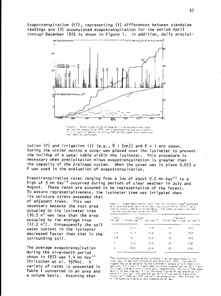
37

Evapotranspiration (ET), representing (1) differences between standpipereadings and (2) accumulated evapotranspiration for the period Aprilthrough December 1972 is shown in Figure 1. In addition, daily precipi-

PRECIPITATION (mm)

20

ACCUIMULATED ET or P.I (cmcm2)

4OF

'COVER ONLYSI METER

nti H H

EVAPOTRANSPIRATION (mm cm2)1 ET

5

-77

Figure I. Evapotranspiration of Douglas-fir as averages over shortperiods and accumulation (ET), daily precipitation and accumulation(P + I), and irrigation (I) during 1972 on the Cedar River watershednear Seattle, Washington.

tation (P) and irrigation (I) (e.g., 8 I [mm]) and P + I are shown.During the winter months a cover was placed over the lysimeter to preventthe buildup of a water table within the lysimeter. This procedure isnecessary when precipitation minus evapotranspiration is greater thanthe capacity of the drainage system. When the coverP was used in the evaluation of evapotranspiration.

was in place 0.075 x

Evapotranspiration rates ranging from a low of about 0.2 mm day-1to a

high of 3 mm day-1 occurred during periods of clear weather in July andAugust. These rates are assumed to be representative of the forest.To assure representativeness, the lysimeter tree was irrigated whenits moisture stress exceeded thatof adjacent trees. This wasnecessary because the root areaoccupied by the lysimeter tree(10.5 m2 was less than the areaoccupied by the average tree(17.5 m2). Consequently the soilwater content in the lysimeterdecreased faster than that in thesurrounding soil.

The average evapotranspirationduring the nine-month periodshown in 1972 was 1.4 mm day-1

(Fritschen et al. 1974b). Avariety of rates is presented inTable 1 converted to an area anda volume basis. Assuming that

Table I. Evapotranspiration rates from the lysimeter treea expressedon a rate and area basis using the crown projection of 29.5 m' as ascaling factor, and on a volume basis. The rates represent low andhigh and intermediate values for 1972.

Rate Volume Area basis(mm day-) (liters day-) (gal day-') (kl ha-'day-`) (gal Ac' da

1

1.4

1.8

29.5

41.3

53.1

7.8

10.9

14.0

14

I OF9

1497

2

3

18 1925

59.0 15.6 20 2138

88.5 23.4 30 3208

aThe hydrologic balance of the lysimeter tree was determined for twoclear days in May 1972 (Fritschen and Doraiswamy 1973). The resultssuggest dew as an addition to the hydrologic balance of 6.4 liters (1.7gal) and 10.9 liters (2.9 gal) when the total evaporation was 42.5 liters(11.2 gal) and 55.2 liters (14.6 gal), respectively. By use of the standdensity of one tree per 17.5 m2 the above figures of dew amount to 3.7and 6.3 liters ha-' (393 and 670 gal Ac"') of dew and 24.3 and 31.6liters ha-' (2587 and 3373 gal Ac-') of evaporation. Thus 15% and 195of the hydrologic balance were evaporation of dew.

UN

P.

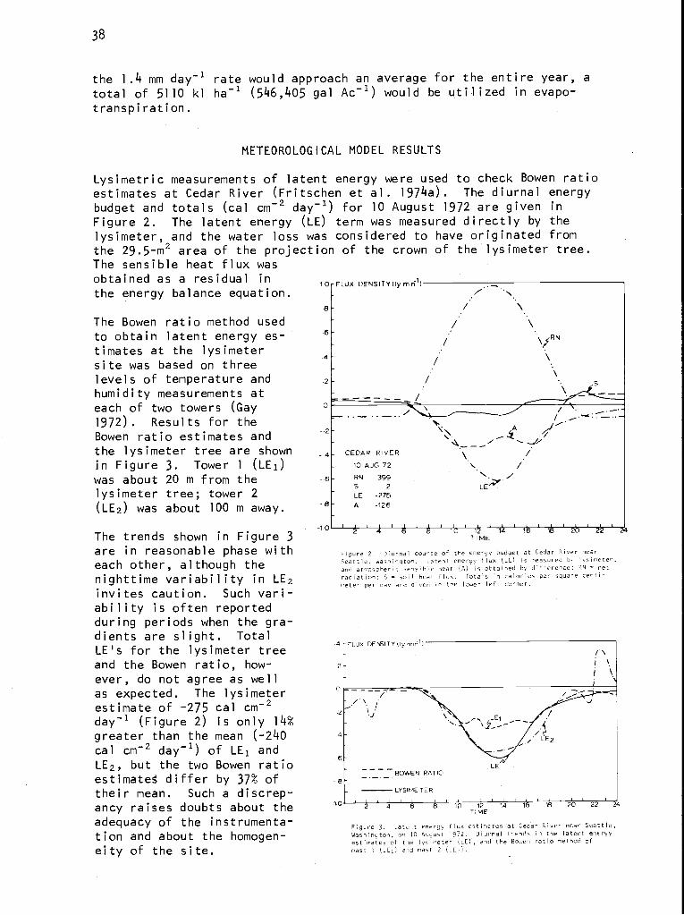
38

the 1.4 mm day-1 rate would approach an average for the entire year, atotal of 5110 kl ha-1 (546,405 gal Ac-1) would be utilized in evapo-transpiration.

METEOROLOGICAL MODEL RESULTS

Lysimetric measurements of latent energy were used to check Bowen ratioestimates at Cedar River (Fritschen et al. 1974a). The diurnal energybudget and totals (cal cm-2 day-1) for 10 August 1972 are given inFigure 2. The latent energy (LE) term was measured directly by thelysimeter, and the water loss was considered to have originated fromthe 29.5-m2 area of the projection of the crown of the lysimeter tree.The sensible heat flux wasobtained as a residual in 10FFLUX DENSITY (lymin )the energy balance equation.

The Bowen ratio method usedto obtain latent energy es-timates at the lysimetersite was based on threelevels of temperature andhumidity measurements ateach of two towers (Gay1972). Results for theBowen ratio estimates andthe lysimeter tree are shownin Figure 3. Tower 1 (LE1)was about 20 m from thelysimeter tree; tower 2(LE2) was about 100 m away.

The trends shown in Figure 3are in reasonable phase witheach other, although thenighttime variability in LE2invites caution. Such vari-ability is often reportedduring periods when the gra-dients are slight. TotalLE's for the lysimeter treeand the Bowen ratio, how-ever, do not agree as wellas expected. The lysimeterestimate of -275 cal cm 2

day-1 (Figure 2) is only 14%greater than the mean (-240cal cm-2 day-1) of LE1 andLE2, but the two Bowen ratioestimated differ by 37% oftheir mean. Such a discrep-ancy raises doubts about theadequacy of the instrumenta-tion and about the homogen-eity of the site.

Figure 2. Diurnal course of the energy budget at Cedar River nearSeattle, Washlgtne. Latent energy flux (LE) is measured by Ivsimeter.

and atmospheric sensible heat (A) is obtained by difference; RN = netradiation; S soil heat flux. Totals in calories per square centi-npeter per day are given in the lower left corner.

4 FLUX DENSITY(ly mint)

2 J

BOWEN RATIO

LYSIME TER

4 6 B 10 12 14 16 1B 20 22 24TIME

Figure 3. Latent energy flux estimates at Cedar River near Seattle,Washington, on 10 August 1972. Diurnal trends in the latent energyestimates of the lysimeter (LE), and the Bowen ratio method ofmast 1 (LEt) and mast 2 (CE.).

=

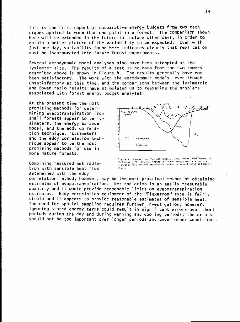
39

This is the first report of comparative energy budgets from two tech-niques applied to more than one point in a forest. The comparison shownhere will be extended in the future to include other days, in order toobtain a better picture of the variability to be expected. Even withjust one day, variability found here indicates clearly that replicationmust be incorporated into future forest experiments.

Several aerodynamic model analyses also have been attempted at thelysimeter site. The results of a test using data from the two towersdescribed above is shown in Figure 4. The results generally have notbeen satisfactory. The work with the aerodynamic models, even thoughunsatisfactory at this time, and the comparisons between the lysimetricand Bowen ratio results have stimulated us to reexamine the problemsassociated with forest energy budget analyses.

At the present time the mostpromising methods for deter-mining evapotranspiration fromsmall forests appear to be ly-simeters, the energy balancemodel, and the eddy correla-tion technique. Lysimetersand the eddy correlation tech-nique appear to be the mostpromising methods for use inmore mature forests.

Combining measured net radia-tion with sensible heat fluxdetermined with the eddy

10 AUG 7210 12 14 16 10 20

Figure 4, Latent heat flux estimates at Cedar River, Washington, on10 August 1972. Diurnal trends in latent energy estimates of theIysimetei (LE) and the aerodynamic method on mast 1 (LEI) and mast 2(LE ).

correlation method, however, may be the most practical method of obtainingestimates of evapotranspiration. Net radiation is an easily measurablequantity and it would provide reasonable limits on evapotranspirationestimates. Eddy correlation equipment of the "Fluxatron" type is fairlysimple and it appears to provide reasonable estimates of sensible heat.The need for spatial sampling requires further investigation, however.Ignoring stored energy terms could result in significant errors over shortperiods during the day and during warming and cooling periods; the errorsshould not be too important over longer periods and under other conditions.

40

REFERENCES

FRITSCHEN, L. J., L. COX, and R. KINERSON. 1973. A 28-m Douglas-firin a weighing lysimeter. For. Sci. 19:256-261.

FRITSCHEN, L. J., and P. DORAIWSWAMY. 1973. Dew: An addition to thehydrologic balance of Douglas-fir. Water Resour. Res. 9:891-894.

FRITSCHEN, L. J., L. GAY, and R. HOLBO. 1974a. Estimation of evapo-transpiration from forests by meteorological and lysimetric methods.Water Resour. Res. (in press).

FRITSCHEN, L. J., J. HSIA, and P. DORAIWSWAMY. 1974b. Evapotranspira-tion of Douglas-fir determined with a weighing lysimeter. Water Resour.Res. (in press).

GAY, L. W. 1972. Energy flux studies in a coniferous forest ecosystem.IN: J. F. Franklin, L. J. Dempster, and R. H. Waring (eds.) Proceedings--Research on coniferous forest ecosystems--A symposium, p. 243-253. USDAFor. Serv., Portland, Oreg.

PAULSON, E. N., and J. T. MILLER. 1952. Soil survey of King County,Washington, No. 31. USDA Soil Series 19393. U.S. Government PrintingOffice, Washington, D.C.

TANNER, C. B. 1967. Measurement of evapotranspiration. IN: R. M. Hagen,H. R. Haise, and T. W. Edminister (eds.), Irrigation of Agricultural Lands,p. 534-574. Amer. Soc. Agron. Monogr. 11.

41

CANOPY FOOD CHAININ A CONIFEROUS FOREST WATERSHED'

Mary Ann Strand2

Oregon State University

ABSTRACT

The internal structure and external couplings of the canopy food chainare examined to quantify the pattern of energy distribution in an old-growth Douglas-fir watershed. The-food chain has been divided into ninefunctional groups: grazing vertebrates, grazing insects, sucking insects,seed and cone insects, predaceous birds, parasitic invertebrates, pre-daceous invertebrates, omnivorous birds, and nest predators. Surveys ofthe watershed fauna have shown that these functional groups are complexand may contain large numbers of species. For example, the five inverte-brate groups may include as many as 450 species.

Modeling techniques are employed to compute total annual consumption andsecondary production for two functional groups, grazing insects and omniv--orous birds. The estimates are based on field density records, publisheddata, and simplifying assumptions. The annual consumption by grazinginsects on the watershed is estimated to be 42.5 kg/ha or about 1.6% oftotal primary production. The omnivorous bird population consumes6.2 kg/ha while on the watershed; about 75% of their diet consists ofinsects. The consumption rates and mean standing crop values are similarto those reported for other forests. At current population levels, thisfood chain represents only a minor pathway in the total watershed energyflux.

INTRODUCTION

The canopy food chain is a subsystem within the forest ecosystem. Theinternal structure and external couplings of this subsystem have beenexamined as part of an integrated research effort to quantify the patternof energy distribution in an old-growth Douglas-fir watershed. Thiswatershed is designated number 10 in USDA Forest Service studies and islocated at the H. J. Andrews Experimental Forest on the west side of theCascade Range in Oregon. The distribution of biomass within the vegeta-tion subsystems is described by Grier et al. (1974) in this volume. Otherdescriptions have been made by Fredriksen (1972). This paper discussesthe role of the canopy food chain as a user of energy.

'This is contribution no. 63 from the Coniferous Forest Biome.

2Present address: Boyce Thompson Institute for Plant Research, Inc.,Yonkers, NY 10703.

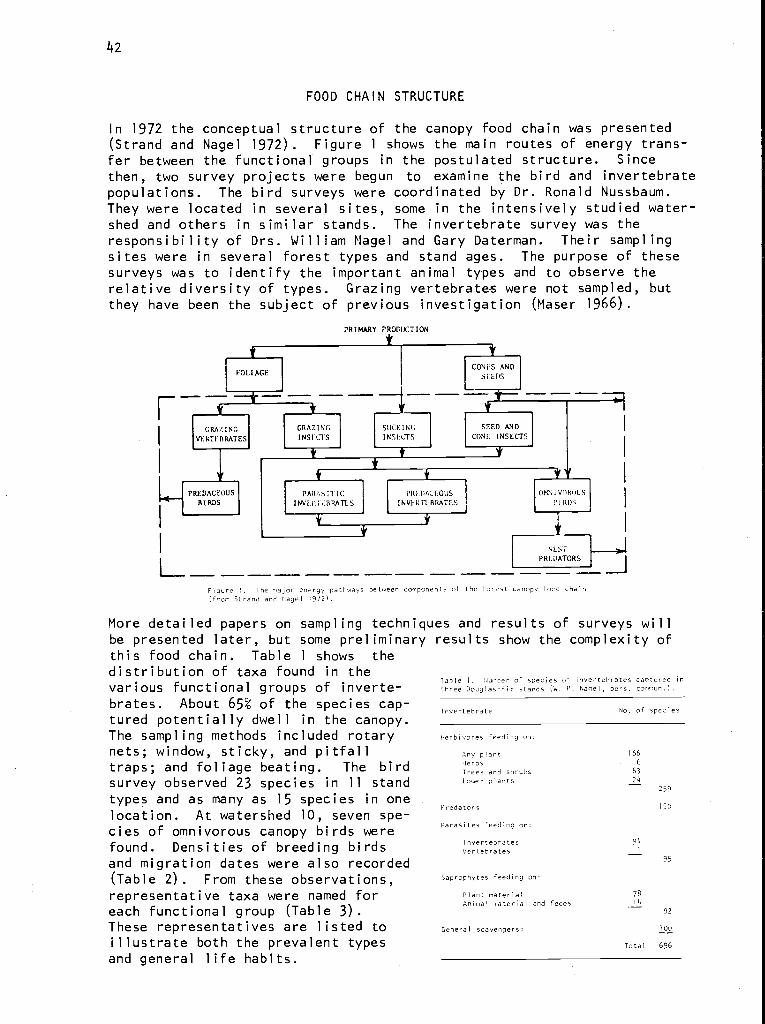
42

In 1972 the conceptual structure of the canopy food chain was presented(Strand and Nagel 1972). Figure 1 shows the main routes of energy trans-fer between the functional groups in the postulated structure. Sincethen, two survey projects were begun to examine the bird and invertebratepopulations. The bird surveys were coordinated by Dr. Ronald Nussbaum.They were located in several sites, some in the intensively studied water-shed and others in similar stands. The invertebrate survey was theresponsibility of Drs. William Nagel and Gary Daterman. Their samplingsites were in several forest types and stand ages. The purpose of thesesurveys was to identify the important animal types and to observe therelative diversity of types. Grazing vertebrates were not sampled, butthey have been the subject of previous investigation (Maser 1966).

PRIMARY PRODUCTION

IOLI AGE

FOOD CHAIN STRUCTURE

I I VERTIRRATESI I INS I'.CTS

L

PREDACEOUSBIRDS

PAR' IT ICI N%'I L';, RRATES

S IIC K I NC

I NSILTS

I'RILACEOUSINVERTI BRATEN

CCONI..S AND

SfIE DS

SEED ANDCONE INSECTS

Figure !. The "ajor energy pathways between components of the forest canop(from Strand and Nagel 1972).

OK': I Vf1ROUS

TlRDS

NESS

PREDATORS

food chain

More detailed papers on sampling techniques and results of surveys willbe presented later, but some preliminary results show the complexity ofthis food chain. Table 1 shows the

distribution of taxa found in theNumber of species of invertebrates captured inTable I .various functional groups of inverte- three Douglas-fir stands (W. P. Nagel, pers. cor:"iun.).

brates. About 65% of the species cap- Invertebrate No. of speciestured potentially dwell in the canopy.The sampling methods included rotary Herbivores feeding on:

nets; window, sticky, and pitfall Any plant 166

traps; and foliage beating. The bird Trees 6Trees and shrubs 63

survey observed 23 species in 11 stand Lover plants 24 259

types and as many as 15 species in onePPredators 150

location. At watershed 10, seven spe-Parasites feeding on:

cies of omnivorous canopy birds werefound. Densities of breeding birds 'oratesveerrtteebbrrates

and migration dates were also recorded 95

(Table 2). From these observations, Saprophytes feeding on:

representative taxa were named for Plant material 7s

each functional group (Table 3). Animal material and feces 14

92

These representatives are listed to General scavengers: 1D0

illustrate both the prevalent types Total 696

and general life habits.

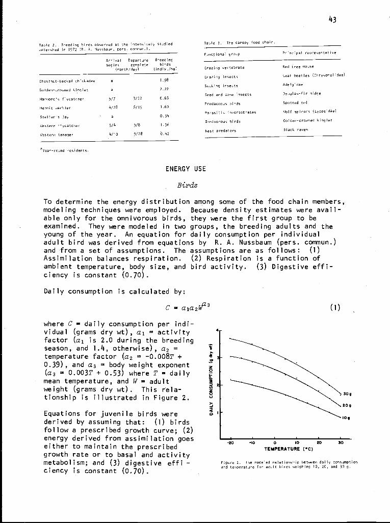
43

Table 2. Breeding birds observed at the intensively studiedwatershed in 1972 (R. A. Nussbaum, pers. commun.).

Arrivalbegins

Departurecomplete

Breedingbirds

(month/day) (in div./ha)

Chestnut-backed chickadee a 1.98

Golden-crowned kinglet a 2.22

Hammond's flycatcher 5/7 9/22 0.68

Hermit warbler 4/28 8/15 1.60

Steller's jay a 0.34

Western flycatcher 5/4 9/8 1.36

Western tanager 4/10 9/28 0.42

ayear-round residents.

Table 3. The canopy food chain.

Functional group

Grazing vertebrate

Grazing insects

Sucking insects

Seed and cone insects

Predaceous birds

Parasitic invertebrates

Omnivorous birds

Nest predators

ENERGY USE

Birds

Principal representative

Red tree mouse

Leaf beetles (Chrysomel idae)

Adel gidae

Douglas-fir midge

Spotted owl

Wolf spiders (Lycosidae)

Golden-crowned kinglet

Black raven

To determine the energy distribution among some of the food chain members,modeling techniques were employed. Because density estimates were avail-able only for the omnivorous birds, they were the first group to beexamined. They were modeled in two groups, the breeding adults and theyoung of the year. An equation for daily consumption per individualadult bird was derived from equations by R. A. Nussbaum (pers. commun.)and from a set of assumptions. The assumptions are as follows: (1)Assimilation balances respiration. (2) Respiration is a function ofambient temperature, body size, and bird activity. (3) Digestive effi-ciency is constant (0.70).

Daily consumption is calculated by:(

C = ala2fv 3

where C = daily consumption per indi-vidual (grams dry wt), al = activityfactor (al is 2.0 during the breedingseason, and 1.4, otherwise), a2 =temperature factor (a2 = -0.008T +0.39), and a3 = body weight exponent(a3 = 0.003T + 0.53) where T = dailymean temperature, and W = adultweight (grams dry wt). This rela-tionship is illustrated in Figure 2.

Equations for juvenile birds werederived by assuming that: (1) birdsfollow a prescribed growth curve; (2)energy derived from assimilation goeseither to maintain the prescribedgrowth rate or to basal and activitymetabolism; and (3) digestive effi -ciency is constant (0.70).

4

309

209

log

-20 -10 0 10 20 30

TEMPERATURE (C)

Figure 2. The modeled relationship between daily consumptionand temperature for adult birds weighing 10, 20, and 30 g.

(1)

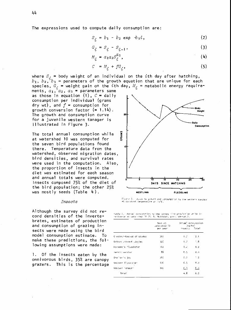
44

The expressions used to compute daily consumption are:

Si = b1 - b2 exp -b3i,

20

G. = Si - S. (3)-M. = a1a2Sa3, (4)

C = M. + fGi, (5)

where S. = body weight of an individual on the ith day after hatching,b1, b2,Zb3 = parameters of the growth equation that are unique for eachspecies, G. = weight gain on the ith day, M. = metabolic energy require-

Zments, a1,a2, a3 = parameters sameas those in equation (1), C = dailyconsumption per individual (gramsdry wt), and f = consumption forgrowth conversion factor (= 1.14).The growth and consumption curvefor a juvenile western tanager isillustrated in Figure 3.

The total annual consumption whileat watershed 10 was computed forthe seven bird populations foundthere. Temperature data from thewatershed, observed migration dates,bird densities, and survival rateswere used in the computation. Also,the proportion of insects in thediet was estimated for each seasonand annual totals were computed.Insects composed 75% of the diet ofthe bird population; the other 25%was mostly seeds (Table 4).

Insects

Although the survey did not re-

to2

10

5 10 Is 20 25

DAYS SINCE MATCHING

NESTLING FLEDGLING

(2)

30

Figure 3. Juvenile growth and consumption by the western tanagerat constant temperature of 16 `C.

bird population while inTable A Annual consumption b the canopy y.cord densities of the i n v e r t e - residence at watershed 10 (R. A. 1,ussbaum, pers. commun.).

brates, estimates of productionand consumption of grazing in-sects were made using the bird

Annual consumption(kg/ha)

Insects Total

Days atwatershed 10

per year

model consumption estimate. To Chestnut-backed chickadee 365 1.7 2.1

make these predictions, the fol- golden-crowned kinglet 365 1.7 1.8

lowing assumptions were made: Hammond's flycatcher 112 0.2 0.2

Hermit warbler 88

1. Of the insects eaten by the 0.3 0.3

1 2365 02S e er s ;ayt .omnivorous birds, 35% are canopygrazers. This is the percentage CLe`° "y`d1fef 'us

Western tanager 145 0.3 0.3

Total 4.8 6.2

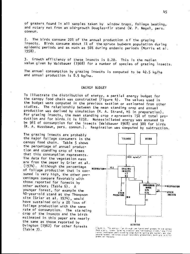
45

of grazers found in all samples taken by window traps, foliage beating,and rotary net from an old-growth Douglas-fir stand (W. P. Nagel, pers.commun.

2. The birds consume 20% of the annual production of the grazinginsects. Birds consume about 1% of the spruce budworm population duringepidemic periods and as much as 50% during endemic periods (Morris et al.1958).

3. Growth efficiency of these insects is 0.20. This is the medianvalue given by Waldbauer (1968) for a number of species of grazing insects.

The annual consumption by grazing insects is computed to be 42.5 kg/haand annual production is 8.5 kg/ha.

ENERGY BUDGET

To illustrate the distribution of energy, a partial energy budget forthe canopy food chain was constructed (Figure 4). The values used inthe budget were computed in the previous section or estimated from otherstudies. The relationship between the mean standing crop and annualproduction was derived by simulation (M. A. Strand, MS in preparation)..For grazing insects, the mean standing crop represents 15% of total pro-duction and for birds,it is 125%. Nonassimilated energy was assumed tobe 56% of consumption for the insects (Waldbauer 1968) and 30% for birds(R. A. Nussbaum, pers. commun.). Respiration was computed by subtraction.

The grazing insects are probablythe major foliage consumers in thecanopy food chain. Table 5 showsthe percentage of annual produc-tion and standing crop of treesthat this consumption represents.The data for the vegetation massare from the paper by Grier et al.

---------------------

.F0LIAOE

42.5 kghalyil

(1974). Although the percentageRESPIRATION 10.2f f lo o iage production that is con-

sumed is very high, the other per-centages compare favorably withthose reported for forests byother authors (Table 6). Ayounger forest, for example the40-year-old stand at the Thompsonsite (Grier et al. 1974), wouldhave sustained only a 2% loss offoliage production with the samerate of consumption. The sta ndingcrop of the insects and the birdsestimated in this paper are nearly

GRAZINGINSECTS

4.31.5

1.7

OTHERPREDATORS

1.7

21.0

SEEDS

1-----------.4 1

14.1 '

RESPIRATIONOMNIVOROUSBIRDS

0.250.20 OTHER

INSECTS

2.1

I--------- ----------------------- ---------------------

the same as those reported by0vington (1962) for other forests DETRITUS

Figure 4. The energy flux through two functional groups in the canopy(Tab 1 e 7). food chain. Under 'grazing insects' and ''omnivorous birds,'' the firstnumber indicates mean standing crop during spring and summer, and thesecond number indicates annual secondary production; both are in kilo-grams per hectare.

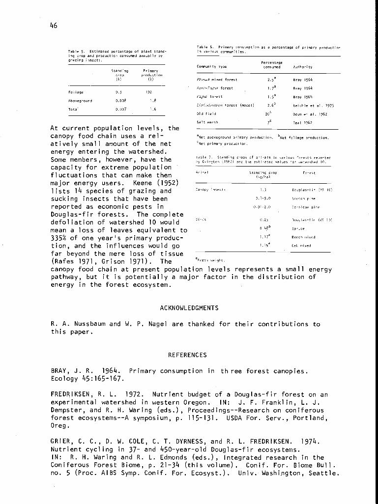
46

Table 6. Primary consumption as a percentage of primary productionTable 5. Estimated percentage of plant stand- in various communities.ing crop and production consumed annually bygrazing insects. Percentage

Standing PrimaryCommunity type consumed Authority

crop production

(i) (3) Prunus mixed forest 2.5a Bray 1964

Acer-Fagus forest 1.7a Bray 1964Foliage 0.5 102

Fagius forest 1.5a Bray 1964Aboveground 0.008 1.8

Liriodendron forest (model) 2.6b Reichle et al. 1973Total 0.007 1.6

At current population levels, the

Odum et al. 1962Old field

Salt marsh

20

7c Teal 1962

canopy food chain uses a r e l - aNet aboveground primary production. bNet foliage production.

at i ve l y small amount of the net cNet primary production.

energy entering the watershed.Some members howe v e r have t he Table 7. Standing crops of animals in various forests reported

,f by Ovin9 ton (1962) and the estimated values for watershed 10.

capacity for extreme populationfluctuations that can make them " °'n9 crop oresc

(kg/ha)

major energy users. Keene (1952)lists 14 species of grazing andsucking insects that have beenreported as economic pests inDouglas-fir forests. The completedefoliation of watershed 10 wouldmean a loss of leaves equivalent to335% of one year's primary produc-t i on , and the influences would gofar beyond the mere loss of tissue

Canopy insects 1.3 Douglas-fir (l6 10)

0.1-5.0 Scotch pine

0.01-2.0 Corsican pine

u.[2 uouglas-tlr Il/S IU)

0.4ea Spruce

1.17a Beech mixed

1.15a Oak mixed

(Rafes 1971, Gr i son 1971). The aFresh weight.

canopy food chain at present population levels represents a small energypathway, but it is potentially a major factor in the distribution ofenergy in the forest ecosystem.

ACKNOWLEDGMENTS

R. A. Nussbaum and W. P. Nagel are thanked for their contributions tothis paper.

REFERENCES

BRAY, J. R. 1964. Primary consumption in th ree forest canopies.Ecology 45:165-167.

FREDRIKSEN, R. L. 1972. Nutrient budget of a Douglas-fir forest on anexperimental watershed in western Oregon. IN: J. F. Franklin, L. J.Dempster, and R. H. Waring (eds.), Proceedings--Research on coniferousforest ecosystems--A symposium, p. 115-131. USDA For. Serv., Portland,Oreg.

GRIER, C. C., D. W. COLE, C. T. DYRNESS, and R. L. FREDRIKSEN. 1974.

Nutrient cycling in 37- and 450-year-old Douglas-fir ecosystems.IN: R. H. Waring and R. L. Edmonds (eds.), Integrated research in theConiferous Forest Biome, p. 21-34 (this volume). Conif. For. Biome Bull.no. 5 (Proc. AIBS Symp. Conif. For. Ecosyst.). Univ. Washington, Seattle.

47

GRISON, P. 1971. Observations sur l'impact des insectes defoliateurssur la productivite primaire. IN: P. Duvigneud (ed.), Productivity offorest ecosystems, p. 369-375. (Proc. Brussels Symp., 1969.) UNESCO.

KEENE, F. P. 1952. Insect enemies of western forests. U.S. Dep. Agric.Misc. Publ. 273. 280 p.

MASER, C. 0. 1966. Life histories and ecology of Phenacomys albipes,Phenacomys Zongicaudus, Phenacomys siZvicoZa. M.S. thesis, Oregon StateUniv., Corvallis.

MORRIS, R. F., W. F. CHESHIRE, C. A. MILLER, and D. G. MOTT. 1958. Thenumerical response of avian and mammalian predators during a gradation ofthe spruce budworm. Ecology 39:487-494.

ODUM, E. P., C. E. CONNELL, and L. B. DAVENPORT. 1962. Populationenergy flow of three primary consumer components of old-field ecosystems.Ecology 43:88-96.

OVINGTON, J. D. 1962. Quantitative ecology and the woodland ecosystemconcept. Adv. Ecol. Res. 1:103-192.

RAFES, P. M. 1971. Pests and the damage which they cause to forests..IN: P. Duvigneud (ed.), Productivity of forest ecosystems, p. 357-367.(Proc. Brussels Symp., 1969.) UNESCO.

REICHLE, D. E., R. A. GOLDSTEIN, R. I. VAN HOOK, JR., and G. J. DODSON.1973. Analysis of insect consumption in a forest canopy. Ecology54:1076-1084.

STRAND, M. A., and W. P. NAGEL. 1972. Preliminary considerations ofthe forest canopy consumer subsystem. IN: J. F. Franklin, L. J. Dempster,and R. H. Waring (eds.), Proceedings--Research on coniferous forest eco-systems--A symposium, p. 71-77, USDA For. Serv., Portland, Oreg.

TEAL, J. M. 1962. Energy flow in the salt marsh ecosystem of Georgia.Ecology 43:614-624.

WALDBAUER, G. P. 1968. The consumption and utilization of food byinsects. Adv. Insect Physiol. 5:229-288.

48

CORRELATION OF FOREST COMMUNITIES WITH ENVIRONMENTAND PHENOLOGY ON THE H. J. ANDREWS

EXPERIMENTAL FOREST, OREGON1

D. B. Zobel, W. A. McKee,G. M. Hawk, and C. T. Dyrness

Oregon State University and USDA Forest Service

ABSTRACT

Air and soil temperature, leaf nutrient content, late summer plant mois-ture stress, and phenology were meas ured on 14 of the 23 forest communi-ties recognized in the study area. The three vegetation zones identifieddiffer considerably in a temperature index. Comparisons of an existingvegetation ordination with ordinations made using the results of thisstudy showed that the x axis of the vegetation ordination represents amoisture axis. Although both temperature and nutrition correlate tosome extent with the y axis of the ordination, it is not simply a re-

sponse to any one or two factors studied. Yearday of selected pheno-logical stages is well correlated with the temperature index used, but

not with ordination axes.

The maximum predawn moisture stress and the calculated temperature indexeffectively separate the previously classified communities in the studyarea. The range of the environmental indexes measured in this area isvery similar to that in the eastern Siskiyou Mountain forests.

INTRODUCTION

The Oregon intensive study site of the Coniferous Forest Biome is theH. J. Andrews Experimental Forest. A considerable diversity of forestcommunities is included in this 6000-ha watershed, which extends from450 to 1600 m elevation (Dyrness et al. 1974). Available resources allowonly a small part of this area to be studied, requiring results to beextrapolated to the unsampled portion of the watershed. To extrapolate

results in describing the area, and in modeling the processes occurringthere, some meaningful method of stratification must be employed. The

plant community is being used as a primary unit of stratification, asvegetation has long been considered to represent an integration of thetotal environment (Billings 1952).

For a stratification system to serve the needs of workers in severalfields, more information about the stratification units than simply theirspecies composition is necessary. To increase the usefulness of thecommunity stratification, several environmental variables and plant phe-nology were measured on stands representing the more common and contrast-ing plant communities. These measurements were intended to provide datafor use by other investigators, as well as being of interest in examin-ing vegetation-environment relationships.

'This is contribution no. 64 from the Coniferous Forest Biome.

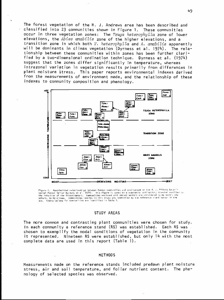
49

The forest vegetation of the H. J. Andrews area has been described andclassified into 23 communities shown in Figure 1. These communitiesoccur in three vegetation zones: The Tsuga heterophyZZa zone of lowerelevations, the Abies amabiZis zone of the higher elevations, and atransition zone in which both T. heterophyZZa and A. amabiZis apparentlywill be dominants in climax vegetation (Dyrness et al. 1974). The rela-tionship between these communities within zones has been further clari-fied by a two-dimensional ordination technique. Dyrness et al. (1974)suggest that the zones differ significantly in temperature, whereasintrazonal variation in vegetation results primarily from differences inplant moisture stress. This paper reports environmental indexes derivedfrom the measurements of environment made, and the relationship of theseindexes to community composition and phenology.

HOT

Tsha /Pomp

TMM/Ate//

Pimo-

Cooma

Psme/Nod/

TSUGA HETEROPHYLLAZONE

TRANSITION ZONE

COL

Chino/Opho

MOIST

I Abpr/ IAelr

Abom/Actr

DECREASING MOISTURE

TaM/Coth

Abom/Vomo /X la

-)DRY

Figure 1. Hypothesized relationships between forest communities and environment on the H. J. Andrews Experi-mental Forest (after Dyrness et al. 1974). This figure is based on a vegetation ordination, somewhat modified bythe intuition of the investigators. Communities enclosed with dashed borders are considered to be seral; theothers, to be climax. Communities sampled in this study are identified by the reference stand num her in thebox. Abbreviations for communities are identified in Table 1.

STUDY AREAS

The more common and contrasting plant communities were chosen for study.In each community a reference stand (RS) was established. Each RS waschosen to exemplify the modal conditions of vegetation in the communityit represented. Nineteen RS were established, but only 14 with the mostcomplete data are used in this report (Table 1).

METHODS

ARIES AMABILISZONE

Abom-Tsma/

Measurements made on the reference stands included predawn plant moisturestress, air and soil temperature, and foliar nutrient content. The phe-nology of selected species was observed.

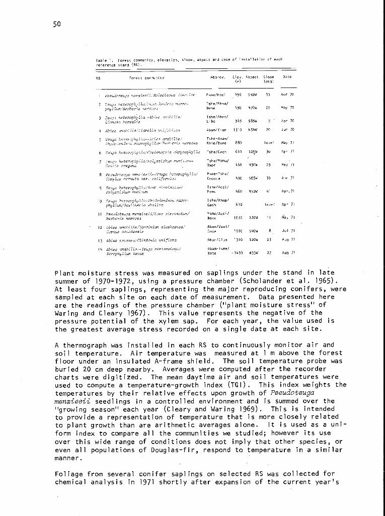
50

Table 1. Forest community, elevation, slope, aspect and date of installation of each

reference stand (RS).

RS Forest community Abbrev. Elev. Aspect(m)

Slope(deg)

Date

1 Pseudotsuga menzies i i,Ho lodi:scus discolor Psme/Hodi 490 S4014 30 Apr 70

2 Tsuaa heterophulla; iihododen<Zro: macro- Tshe/Rhma/

phyZZwn/Berrberis nervosa Bene 490 N70W 21 May 70

3 Tsuga heterophylla--Abies amabzais/ Tshe/Abam/

Linnaea borealis Libo 945 S85W 5 Apr 70

4 Abies mnabilis,,Tiareliia unifoliata Abam/Tiun 1310 N54W 20 Jun 70

5 Tsuga he terophy Zla--Abies avoidlie Tshe-Abam/

Rhododendron maeronhyhZum Berberis nervosa Rhma/Bene 880 level May 71

6 Tsuga heterophy Zla/c'as tanopsis chrysophuZZa Tshe/Cach 610 S25W 30 Apr 71

7 Tsuga heterophylla/Polystiehum munitum-- Tshe/Pomu/oxalis oregano Oxor 460 N30W 29 may 71

8 Pseudotsuga menziesii--Tsuga heterophylla/ Psme-Tshe/Corylus cornuta var. californica Cococa 490 S85W 39 Apr 71

9 Tsuga heterophyZZa,'Acer eireinatum/ Tshe/Acci/

PoZustichum munitum Pomu 460 N50W 41 Apr.71

10 Tsuga heterophylla/.Rhododendron macro- Tshe/Rhma/phyZZum/Gaultheria shaZZon Gash 610 level Apr 71

11 Pseudotsuga menziesii/Acer circinatwn/ Psme/Acci/Berberis nervosa Bene 1010 S20W 11 May 71

12 Abies amabilis/Vaccinium alaskaense/ Abam/Vaal/Corpus canadensis Coca 1010 54014 8 Jul 71

13 Abies procera/Clintonia unifZora Abpr/Clun 1310 S20W 23 Aug 71

14 Abies amabiZis--Tsuga mertensiana/ Abam-Tsme/Xerophy ZZwm tenor Xete .1430 N33W 27 Aug 71

Plant moisture stress was measured on saplings under the stand in latesummer of 1970-1972, using a pressure chamber (Scholander et al. 1965).At least four saplings, representing the major reproducing conifers, weresampled at each site on each date of measurement. Data presented hereare the readings of the pressure chamber ("plant moisture stress" ofWaring and Cleary 1967). This value represents the negative of thepressure potential of the xylem sap. For each year, the value used isthe greatest average stress recorded on a single date at each site.

A thermograph was installed in each RS to continuously monitor air andsoil temperature. Air temperature was measured at 1 m above the forestfloor under an insulated A-frame shield. The soil temperature probe wasburied 20 cm deep nearby. Averages were computed after the recordercharts were digitized. The mean daytime air and soil temperatures wereused to compute a temperature-growth index (TGI). This index weights thetemperatures by their relative effects upon growth of Pseudotsugamenziesii seedlings in a controlled environment and is summed over the"growing season" each year (Cleary and Waring 1969). This is intendedto provide a representation of temperature that is more closely relatedto plant growth than are arithmetic averages alone. It is used as a uni-form index to compare all the communities we studied; however its useover this wide range of conditions does not imply that other species, oreven all populations of Douglas-fir, respond to temperature in a similarmanner.

Foliage from several conifer saplings on selected RS was collected forchemical analysis in 1971 shortly after expansion of the current year's

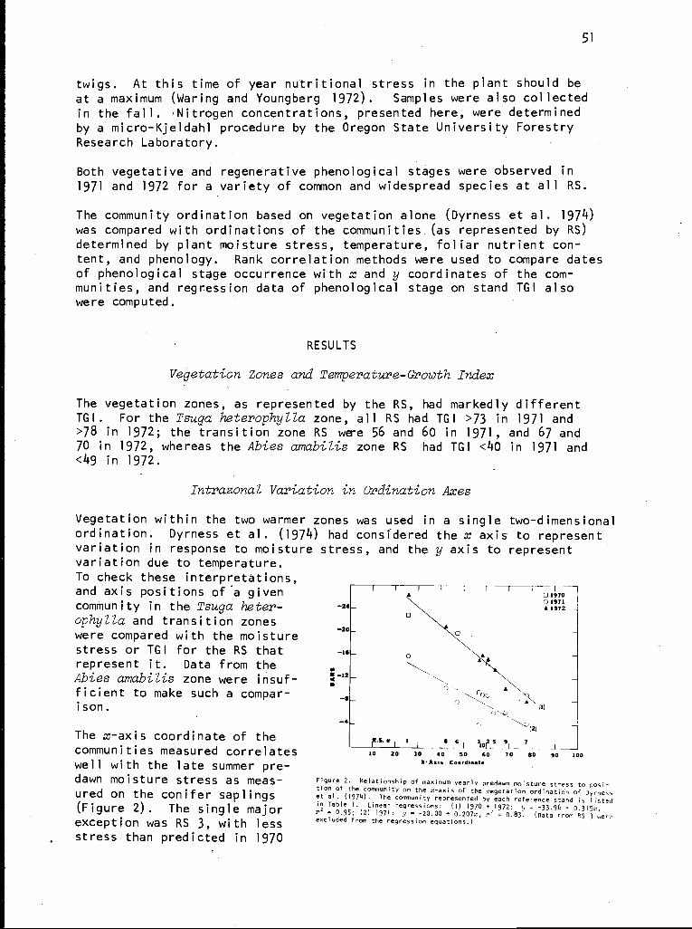
51

twigs. At this time of year nutritional stress in the plant should beat a maximum (Waring and Youngberg 1972). Samples were also collected

in the fall. Nitrogen concentrations, presented here, were determinedby a micro-Kjeldahl procedure by the Oregon State University ForestryResearch Laboratory.

Both vegetative and regenerative phenological stages were observed in1971 and 1972 for a variety of common and widespread species at all RS.

The community ordination based on vegetation alone (Dyrness et al. 1974)was compared with ordinations of the communities.(as represented by RS)determined by plant moisture stress, temperature, foliar nutrient con-tent, and phenology. Rank correlation methods were used to compare datesof phenological stage occurrence with x and y coordinates of the com-munities, and regression data of phenological stage on stand TGI alsowere computed.

RESULTS

Vegetation Zones and Temperature-Growth Index

The vegetation zones, as represented by the RS, had markedly differentTGI. For the Tsuga heterophyZZa zone, all RS had TGI >73 in 1971 and>78 in 1972; the transition zone RS were 56 and 60 in 1971, and 67 and70 in 1972, whereas the Abies amabiZis zone RS had TGI <40 in 1971 and<49 in 1972.

IntrazonaZ Variation in Ordination Axes

Vegetation within the two warmer zones was used in a single two-dimensionalordination. Dyrness et al. (1974) had considered the x axis to representvariation in response to moisture stress, and the y axis to representvariation due to temperature.To check these interpretations,and axis positions of a givencommunity in the Tsuga heter-ophyZZa and transition zoneswere compared with the moisture

-24

-20

stress or TGI for the RS that -10represent it. Data from theAbies amabiZis zone were insuf-ficient to make such a compar-ison.

The x-axis coordinate of thecommunities measured correlateswell with the late summer pre-dawn moisture stress as meas-ured on the conifer saplings(Figure 2). The single majorexception was RS 3, with lessstress than predicted in 1970

00-12

-s

-4

T I T 1 T

1970U 1971

1972

(1)

11.S. OF I 1 1 _L, 6 1 3102 5 9 7LL - 1 - I 1

10 20 30 40 50 60 70 so 90 100X-ARi5 Ceo,dle.te

Figure 2. Relationship of maximum yearly predawn moisture stress to posi-tion of the community on the x-axis of the vegetation ordination of Dyrnesset al. (1974). The community represented by each reference stand is listedin Table I. Linear regressions: (I) 1970 + 1972: y = -33.96 + 0.319.x,r2 = 0.95; (2) 1971: y = -20.00 + 0.207x, rz = 0.83. (Data from RS 3 wereexcluded from the regression equations.)

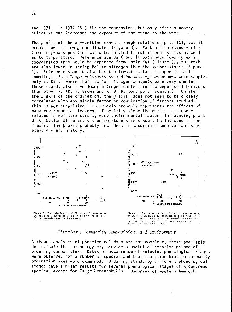
52

and 1971. In 1972 RS 3 fit the regression, but only after a nearbyselective cut increased the exposure of the stand to the west.

The y axis of the communities shows a rough relationship to TGI, but itbreaks down at low y coordinates (Figure 3) Part of the stand varia-tion in y-axis position could be related to nutritional status as wellas to temperature. Reference stands 6 and 10 both have lower y-axiscoordinates than would be expected from their TGI (Figure 3), but bothare also lower in spring foliar nitrogen than the other stands (Figure4). Reference stand 6 also has the lowest foliar nitrogen in fallsampling. Both Tsuga heterophyZZa and Pseudotsuga menziesii were sampledonly at RS 6, where their foliar nitrogen contents were very similar.These stands also have lower nitrogen content in the upper soil horizonsthan other RS (R. B. Brown and R. B. Parsons pers. commun.). Unlikethe x axis of the ordination, the y axis does not seem to be closelycorrelated with any single factor or combination of factors studied.This is not surprising. The y axis probably represents the effects ofmany environmental factors. Especially since the x axis is closelyrelated to moisture stress, many environmental factors influencing plantdistribution differently than moisture stress would be included in they axis. The y axis probably includes, in a ddition, such variables asstand age and history.

33

X100W

2= 90

r

n_ 1971

50

11

11

11

9

Ref. Stand No. 6 10 8 1 2 1157 3I 1 I I I 1

10 30 50Y - AXIS COORDINATE

47

00° days sincebud burst

0.8

0.7

25

32171.36

19 13

28 9Ref. Stand No. 6 10 81 1 2 Ill57 3

10 30 50Y -AXIS COORDINATE

Figure 3. The relationship of TGI of a reference standand the y-axis coordinate, in a vegetation ordination,

of the community the stand represents.

Figure 4. The relationship of foliar nitrogen contentof year-old needles after budbreak in the spring (1971)to the -axis coordinate of the community representedby each reference stand. Time since budbreak islisted with each point (days).

PhenoZogy, Community Composition, and Environment

Although analyses of phenological data are not complete, those availabledo indicate that phenology may provide a useful alternative method ofordering communities. Dates of occurrence of selected phenological stageswere observed for a number of species and their relationships to communityordination axes were examined. Ordering stands by different phenologicalstages gave similar results for several phenological stages of widespreadspecies, except for Tsuga heterophyZZa. Budbreak of western hemlock

1.2

1.0

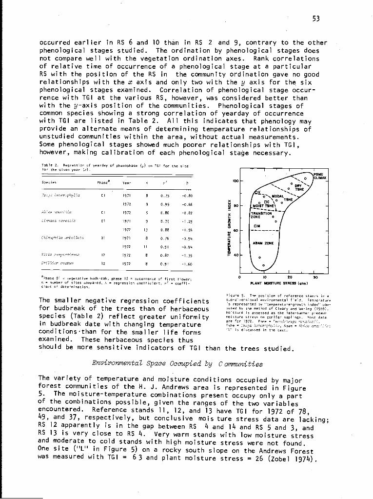
53

occurred earlier in RS 6 and 10 than in RS 2 and 9, contrary to the otherphenological stages studied. The ordination by phenological stages doesnot compare well with the vegetation ordination axes. Rank correlationsof relative time of occurrence of a phenological stage at a particularRS with the position of the RS in the community ordination gave no goodrelationships with the x axis and only two with the y axis for the sixphenological stages examined. Correlation of phenological stage occur-rence with TGI at the various RS, however, was considered better thanwith the y-axis position of the communities. Phenological stages ofcommon species showing a strong correlation of yearday of occurrencewith TGI are listed in Table 2. All this indicates that phenology mayprovide an alternate means of determining temperature relationships ofunstudied communities within the area, without actual measurements.Some phenological stages showed much poorer relationships with TGI,however, making calibration of each phenological stage necessary.

Table 2. Regression of yearday of phenophase (y) on TGI for the sitefor the given year (x).

Species Phasea Year n b

i'suga heterophylla 01 1971 8 0.75 -0.80

1972 9 0.95 -0.66

A S 01 1972 5 0.86 -0.82

Linnaea borealis 01 1971 9 0.75 -1.29

1972 13 0.88 -1.56

Chimaphila umbeZlata 01 1971 8 0.76 -0.94

1972 11 0.91 -0.94

Viola sempervirens 12 1972 8 0.82 -1.35

TrilZiaim ovatum 12 1972 8 0.91 -1.60

aPhase 01 = vegetative budbreak, phase 12 = occurrence of first flower;n = number of sites compared, b = regression coefficient, r2 = coeffi-cient of determination.

The smaller negative regression coefficientsfor budbreak of the trees than of herbaceousspecies (Table 2) reflect greater uniformityin budbreak date with changing temperatureconditions than for the smaller life formsexamined. These herbaceous species thus

100

0

` 00DRT"

0 TSHE

o s, MODAL \\ ,, TSMEO - \ 0MOIST TSME\

TRANSITIONZONE 0

1 1

10 20 30

PLANT MOISTURE STRESS (atm)

Figure 5. The position of reference stands in atwo-dimensional environmental field. Temperatureis represented by ''temperature-growth index'com-puted by the method of Cleary and Waring (1969).Moisture is assessed as the late-summer predawnmoisture stress on conifer saplings. Most dataare for 1972. Psme = Pocudotsuna rrenzies:Tshe = 's upa hoterophiZ la, Abam = Abies nmaid' ,

"L" is discussed in the text.

should be more sensitive indicators of TGI than the trees studied.

Environmental Space Occupied by Communities

The variety of temperature and moisture conditions occupied by majorforest communities of the H. J. Andrews area is represented in Figure5. The moisture-temperature combinations present occupy only a partof the combinations possible, given the ranges of the two variablesencountered. Reference stands 11, 12, and 13 have TGI for 1972 of 78,49, and 37, respectively, but conclusive mois ture stress data are lacking;RS 12 apparently is in the gap between RS 4 and 14 and RS 5 and 3, andRS 13 is very close to RS 4. Very warm stands with low moisture stressand moderate to cold stands with high moisture stress were not found.One site (IILII in Figure 5) on a rocky south slope on the Andrews Forestwas measured with TGI = 6 3 and plant moisture stress = 26 (Zobel 1974).

ADAM ZONE

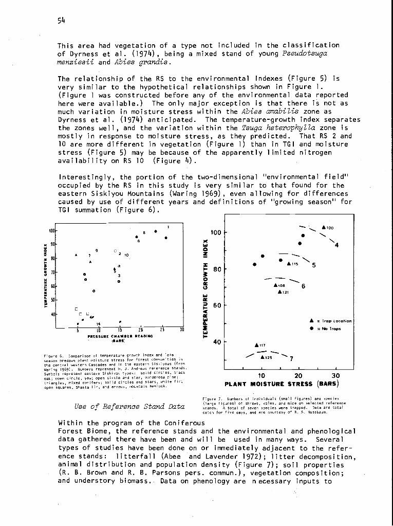
54

This area had vegetation of a type not included in the classificationof Dyrness et al. (1974), being a mixed stand of young Pseudotsugamenziesii and Abies grandis.

The relationship of the RS to the environmental indexes (Figure 5) is

very similar to the hypothetical relationships shown in Figure 1.(Figure 1 was constructed before any of the environmental data reportedhere were available.) The only major exception is that there is not asmuch variation in moisture stress within the Abies amabilis zone asDyrness et al. (1974) anticipated. The temperature-growth index separatesthe zones well, and the variation within the Tsuga heterophyZZa zone is

mostly in response to moisture stress, as they predicted. That RS 2 and10 are more different in vegetation (Figure 1) than in TGI and moisturestress (Figure 5) may be because of the apparently limited nitrogenavailability on RS 10 (Figure 4).

Interestingly, the portion of the two-dimensional "environmental field"occupied by the RS in this study is very similar to that found for theeastern Siskiyou Mountains (Waring 1969), even allowing for differencescaused by use of different years and definitions of "growing season" forTGI summation (Figure 6).

100

9 0A 7 2 10

A

so 30 0

0

s

10 15 20 25 30

PRESSURE CHAMBER READING(BARS)

Figure 6. Comparison of temperature growth index and lateseason predawn plant moisture stress for forest communities in

the central western Cascades and in the eastern Siskiyous (from

Waring 1969) Numbers represent H. J. Andrews reference stands.Symbols represent eastern Siskiyou types: solid circles, black

oak; open circle, yew; open circle and star, ponderosa pine;

triangles, mixed conifers; solid circles and stars, white fir;

open squares, Shasta fir; and arrows, mountain hemlock.

Use of Reference Stand Data

2

H40

A too

\4,1-Ails 5

Aloe 6£121

A117

£125

£ c ]rap location= No Traps

1

10 20 30PLANT MOISTURE STRESS (BARS)

Figure 7. Numbers of individuals (small figures) and species(large figures) of shrews, voles, and mice on selected referencestands. A total of seven species were trapped. Data are totalcatch for five days, and are courtesy of R. A. Nussbaum.

Within the program of the ConiferousForest Biome, the reference stands and the environmental and phenologicaldata gathered there have been and will be used in many ways. Severaltypes of studies have been done on or immediately adjacent to the refer-ence stands: litterfall (Abee and Lavender 1972); litter decomposition,animal distribution and population density (Figure 7); soil properties(R. B. Brown and R. B. Parsons pers. commun.), vegetation composition;and understory biomass. Data on phenology are necessary inputs to

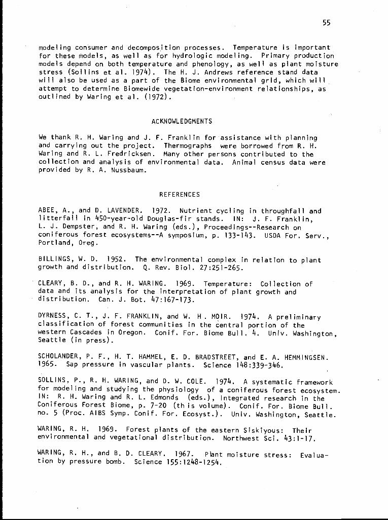
55

modeling consumer and decomposition processes. Temperature is importantfor these models, as well as for hydrologic modeling. Primary productionmodels depend on both temperature and phenology, as well as plant moisturestress (Sollins et al. 1974). The H. J. Andrews reference stand datawill also be used as a part of the Biome environmental grid, which willattempt to determine Biomewide vegetation-enviro-nment relationships, asoutlined by Waring et al. (1972).

ACKNOWLEDGMENTS

We thank R. H. Waring and J. F. Franklin for assistance with planningand carrying out the project. Thermographs were borrowed from R. H.Waring and R. L. Fredricksen. Many other persons contributed to thecollection and analysis of environmental data. Animal census data wereprovided by R. A. Nussbaum.

REFERENCES

ABEE, A., and D. LAVENDER. 1972. Nutrient cycling in throughfall andlitterfall in 450-year-old Douglas-fir stands. IN: J. F. Franklin,L. J. Dempster, and R. H. Waring (eds.), Proceedings--Research onconiferous forest ecosystems--A symposium, p. 133-143. USDA For. Serv.,Portland, Oreg.

BILLINGS, W. D. 1952. The environmental complex in relation to plantgrowth and distribution. Q. Rev. Biol. 27:251-265.

CLEARY, B. D., and R. H. WARING. 1969. Temperature: Collection ofdata and its analysis for the interpretation of plant growth anddistribution. Can. J. Bot. 47:167-173.

DYRNESS, C. T., J. F. FRANKLIN, and W. H . MOIR. 1974. A preliminaryclassification of forest communities in the central portion of thewestern Cascades in Oregon. Conif. For. Biome Bull. 4. Univ. Washington,Seattle (in press).

SCHOLANDER, P. F., H. T. HAMMEL, E. D. BRADSTREET, and E. A. HEMMINGSEN.1965. Sap pressure in vascular plants. Science 148:339-346.

SOLLINS, P., R. H. WARING, and D. W. COLE. 1974. A systematic frameworkfor modeling and studying the physiology of a coniferous forest ecosystem.IN: R. H. Waring and R. L. Edmonds (eds.), Integrated research in theConiferous Forest Biome, p. 7-20 (th is volume). Conif. For. Biome Bull.no. 5 (Proc. AIBS Symp. Conif. For. Ecosyst.). Univ. Washington, Seattle.

WARING, R. H. 1969. Forest plants of the eastern Siskiyous: Theirenvironmental and vegetational distribution. Northwest Sci. 43:1-17.

WARING, R. H., and B. D. CLEARY. 1967. Plant moisture stress: Evalua-tion by pressure bomb. Science 155:1248-1254.

56

WARING, R. H., K. L. REED, and W. H. EMMINGHAM. 1972. An environmental

grid for classifying coniferous forest ecosystems. IN: J. F. Franklin,

L. J. Dempster, and R. H. Waring (eds.), Proceedings--Research on coniferousforest ecosystems--A symposium, p. 79-91. USDA For. Serv., Portland, Oreg.

WARING, R. H., and C. T. YOUNGBERG. 1972. Evaluating forest sites forpotential growth response of trees to fertilizer. Northwest Sci. 46:67-75.

ZOBEL, D. B. 1974. Local variation in intergrading Abies grandis--Abies concoZor populations in the central Oregon Cascades. II. Stomatalreaction to moisture stress. Bot. Gaz. 135 (in press).

r

57

SOURCES AND FATES OF ORGANIC INPUTSIN CONIFEROUS FOREST STREAMS'

J. R. Sedell, F. J. Triska, J. D. Hall,N. H. Anderson, and J. H. Lyford

Oregon State University

ABSTRACT

A study of the quality and magnitude of particulate organic inputs wasundertaken in two streams in the Oregon Cascades. Objectives includedestimation of litterfall and lateral movement of organic debris into astream, estimation of litter breakdown rates, and construction of afirst-approximation organic material budget.

In this study, approximately 65% of the litterfall input consisted ofDouglas-fir and hemlock needles, which fall throughout the year. Decid-

uous inputs occurred primarily mid-October through November and consistedprincipally of vine maple and bigleaf maple. Preliminary lateral movementdata indicated that organic material entering watershed 10 from the bankwas 1.5 times the litterfall. The total estimate of litter input isapproximately 2.5 g m-2 day-'. Both streams have the capacity to processall types of leaf litter within a year. Needles, the most refractoryleaf litter, are processed by microbes and, once conditioned, are con-sumed readily by invertebrate shredders. Thus the large amounts ofneedle litter that enter the stream in late summer and fall constitutea food source usable by stream detritivores after deciduous litter hasdecomposed.

Leaf-pack experiments have revealed the danger of extrapolation of bio-logical information from smaller to larger streams. Faster processingtimes for larger streams have been suggested by information on weightloss, invertebrate biomass, and leaf quality. Changes in litter qualitywere determined by increases in the percentage of lignin content. In-creases in lignin composition were compared with decreases in non-cell-wall constituents to obtain an estimate of microbial activity.

Information on litterfall and lateral movement, in conjunction withpreviously collected data, led to a first-approximation particulateorganic matter budget for watershed 10. When compared with a similarbudget from a very different stream system, processing capabilities ofthe-two streams were remarkably similar. In both streams almost 990 ofthe particulate organic material entered from terrestrial systems. Abouttwo-thirds of the organic inputs entering each stream were processedwithin the system, indicating the processing role of small forest streams.

'This is contribution no. 65 from the Coniferous Forest Biome.

58

INTRODUCTION

The idea that most streams not significantly altered by man are predom-inantly heterotrophic has been well substantiated by stream biologistsover the past few years. That is, the maintenance of stream communitystructure and function is dependent upon the import of organic matterfrom autotrophically dominated terrestrial communities. Woodland streamscan be compared to soil litter communities and the benthic communitiesof lakes in that they are detritus based and dependent upon export ofproduction from other systems.

Part of the work under way in Oregon under the Coniferous Biome programis designed to study the interrelations between the terrestrial andaquatic components of small watersheds. Under investigation in thestream ecosystem are the rates of production of aquatic plants, insects,and fish, along with the input of particulate organic material and theprocessing of it by microorganisms and invertebrates. The work reported

in this paper represents a part of that research, with emphasis on thefate of the particulate organic material.

Some of the mechanisms involved in the degradation of vascular planttissue in stream environments have been the subject of recent studies(Kaushik and Hynes 1971, Vannote 1970, Triska 1970, Cummins et al. 1972,1973, Fisher and Likens 1972). The functional relationships among vas-cular plant tissue, dissolved organic matter, microbial organisms (fungiand bacteria), and animals have not been clearly defined, however.

The present study assessed the sources and magnitude of various particu-late organic matter inputs and their fates in two Cascade Range streams.Three main objectives of this study were: (1) to estimate litterfallbiomass and lateral movement of detritus into a stream running throughan old-growth forest; (2) to estimate the rates of litter breakdown intwo coniferous forest streams of different flow; and (3) to obtain adata base for construction of an organic material budget and for latersystems modeling of energy or mineral cycling.

Study Area

The study was conducted in the H. J. Andrews Experimental Forest, a6000-ha watershed in the western Cascades of Oregon. The drainage ischaracterized by steep topography, with about one-fifth of the studyarea consisting of more gentle slopes or benches. Elevation variesfrom 457 m to more than 1523 m. Mean forest air temperature variesfrom 2°C in January to 18°C during the summer months. Annual precipi-tation ranges from 225 cm at lower elevations to 350 cm at the highestridges. Highest elevations are characterized by extensive snowpackduring the winter, while rain predominates at lower elevations (Berntsenand Rothacher 1959). M ack Creek and the stream draining watershed 10were the two streams in t he drainage basin that were studied intensively.

Watershed 10 (WS 10) covers 10.1 ha and rises from 430 m at the outletstream gaging station to 670 m at the highest point. The overall slopeof the stream channel is 45%. Side slopes and headwall, however, rangeup to 90% because o f the deep incision of the basin into the main ridge.

59

Stream discharge varies from around 0.23 liter/sec in the summer to about140 liters/sec during winter freshets. The uppermost forks are intermittentduring the summer months. Mean width of the stream channel ranges from0.25 m in the upper reaches to 0.75-1.0 m at the base of the watershed.

Streambed morphology is best described as a "stairstep" series of smallpools connected by free-fall zones or riffles running on bedrock. Poolsare formed mainly by accumulations of organic debris. The substrateconsists of loose rocks and gravel from weathered tuff and brecciamaterial and bedrock of unweathered tuff and breccia.

Mack Creek is one of the three major streams that drain the entire AndrewsExperimental Forest. The area being studied is between 700 m and 900 min elevation and drains approximately 650 ha. The watershed slope inthis area is 440. Stream discharge at the study area is estimated between100-140 liters/sec in late summer and 1500-1800 liters/sec during winterfreshets. The stream morphology is a stairstep of gouged pools, free-fallzones, and fast water around large boulders. The substrate ranges fromlarge boulders to fine silt. Unlike WS 10, Mack Creek has a well-developedarmor layer on the bottom, which prevents all but the largest winterstorms from moving large particles of sediment. Watershed 10 has nosuch layer and only the organic debris dams act as protection from stream-bed erosion during winter storms. In WS 10 even small winter stormscause extensive substrate movement in the pools.

Both streams have comparable water chemistry and temperature regimesranging from 0°C to 15°C, with a mean of approximately 8°C. Water chem-istry has been extensively investigated on WS 10 and preliminary resultswere reported by Fredriksen (1972). The streams are low in dissolvedmaterials, carrying an a verage concentration of total dissolved solidsof 40 mg/liter (Fredriksen 1971).

MATERIALS AND METHODS

Particulate organic material input and export was studied intensivelyon WS 10 only. The investigation to determine rates of litter breakdownwas conducted on both WS 10 and Mack Creek. Litterfall input to theWS 10 stream system was sampled with eleven 1 .0-m2 litter traps placedrandomly over the stream. The traps stand on angle iron legs about 0.5 mabove the water. Traps are 15 cm deep and each has a removable muslininsert with a mesh opening of 500-800 um. Litterfall was sampled monthlyfrom March 1972 to March 1973. Litter was sorted into eight categories:cones, leaves, needles, twigs, wood, frass, bark, and fruit; it was driedat 50°C and weighed.

Since WS 10 is at the bottom of a deeply incised basin, organic materialalso enters by.sliding down the bank slope and into the stream. Thislateral movement across the forest floor is being sampled by 30 randomlyplaced, rectangular boxes (0.1 m high by 0.3 deep by 0.5 m wide) withaluminum tray inserts. Traps are placed on the forest floor adjacentto the streambed with the open end (0.5 m) oriented parallel to the streamand facing upslope. Lateral movement is collected monthly. Litter issorted into categories as above, dried, and weighed.

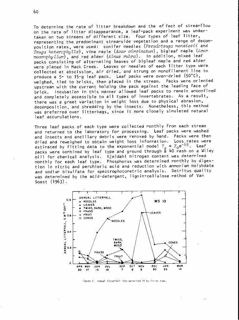
60

To determine the rate of litter breakdown and the of fect of streamflowon the rate of litter disappearance, a leaf-pack experiment was under-taken on two streams of different size. Four types of leaf litter,representing the predominant streamside vegetation and a range of decom-position rates, were used: conifer needles (Pseudotsuga menziesii and

Tsuga heterophyZZa), vine maple (Acer circinatum), bigleaf maple (AcermacrophyZZum), and red alder (AZnus rubra). In addition, mixed leafpacks consisting of alternating leaves of bigleaf maple and red alderwere placed in Mack Creek. Leaves or needles of each litter type werecollected at abscission, air dried, and strung on monofilament line toproduce a 5- to 15-g leaf pack. Leaf packs were oven-dried (50°C),weighed, tied to bricks, then placed in the stream. Packs were orientedupstream with the current holding the pack against the leading face ofbrick. Incubation in this manner allowed leaf packs to remain unconfinedand completely accessible to all types of invertebrates. As a result,there was a great variation in weight loss due to physical abrasion,decomposition, and shredding by the insects. Nonetheless, this methodwas preferred over litterbags, since it more closely simulated naturalleaf accumulations.

Three leaf packs of each type were collected monthly from each streamand returned to the laboratory for processing. Leaf packs were washedand insects and ancillary debris were removed by hand. Packs were thendried and reweighed to obtain weight loss information. Loss rates wereestimated by fitting data to the exponential model Y = Yoe-kt. Leafpacks were combined by leaf type and ground through a 40 mesh on a Wileymill for chemical analysis. Kjeldahl nitrogen content was determinedmonthly for each leaf type. Phosphorus was determined monthly by diges-tion in nitric and perchloric acid and reduction with ammonium molybdateand sodium bisulfate for spectrophotometric analysis. Detritus qualitywas determined by the acid-detergent, lignin-cellulose method of VanSoest (1963).

0.8

T I

24

ANNUAL LITTERFALLNEEDLESLEAVESTWIGS, BARK, WOOD

O FRASSo FRUITo CONES

APR MAY JUN JUL20 17 16 19

SEP OCT NOV8

WS 10

DEC20

JAN23

MAR10

Figure I. Annual litterfall into watershed 10 by Ii ter type.

7

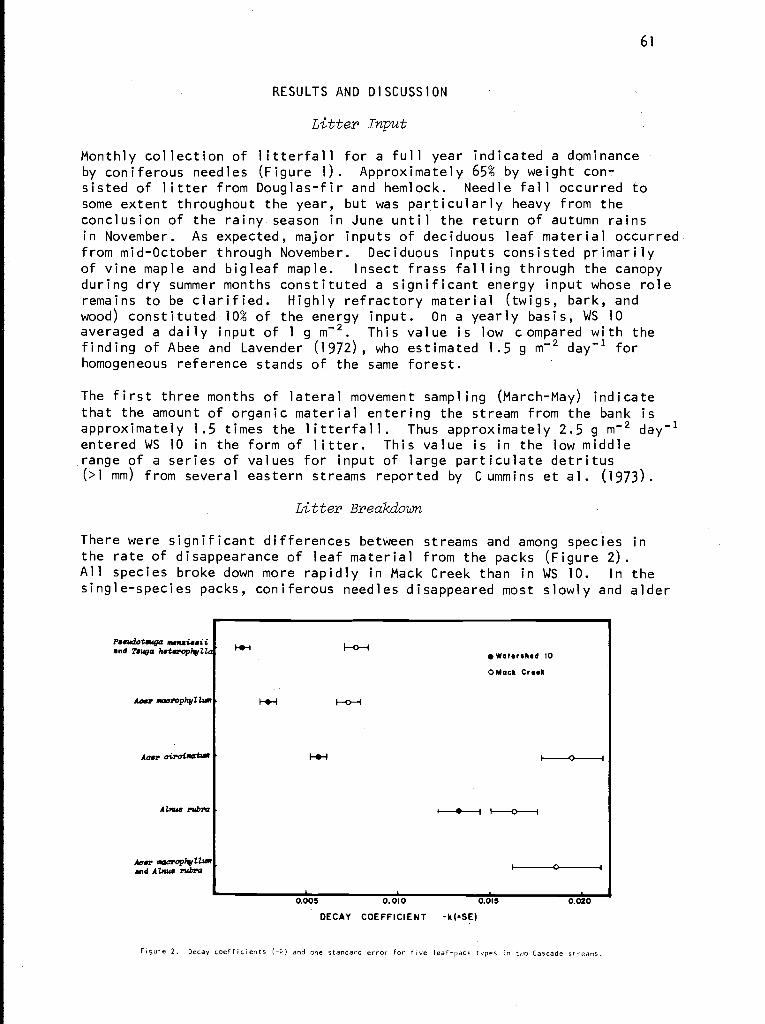
61

RESULTS AND DISCUSSION

Litter Input

Monthly collection of litterfall for a full year indicated a dominanceby coniferous needles (Figure 1). Approximately 65% by weight con-sisted of litter from Douglas-fir and hemlock. Needle fall occurred tosome extent throughout the year, but was particularly heavy from theconclusion of the rainy season in June until the return of autumn rainsin November. As expected, major inputs of deciduous leaf material occurredfrom mid-October through November. Deciduous inputs consisted primarilyof vine maple and bigleaf maple. Insect frass falling through the canopyduring dry summer months constituted a significant energy input whose roleremains to be clarified. Highly refractory material (twigs, bark, andwood) constituted 10% of the energy input. On a yearly basis, WS 10averaged a daily input of 1 g

m-2 This value is low compared with thefinding of Abee and Lavender (1972), who estimated 1.5 g m-2 day-1 forhomogeneous reference stands of the same forest.

The first three months of lateral movement sampling (March-May) indicatethat the amount of organic material entering the stream from the bank isapproximately 1.5 times the litterfall. Thus approximately 2.5 g m-2 day-1entered WS 10 in the form of litter. This value is in the low middlerange of a series of values for input of large particulate detritus(>1 mm) from several eastern streams reported by C ummins et al. (1973).

Litter Breakdown

There were significant differences between streams and among species inthe rate of disappearance of leaf material from the packs (Figure 2).All species broke down more rapidly in Mack Creek than in WS 10. In thesingle-species packs, coniferous needles disappeared most slowly and alder

Pasudotauga aansiasiiand Tauga hatarophyZZ*

9 Watershed 10

0Mack Creak

Aoar saarophyZZuer

Agar 0iroinatrw

AZrms ruby

Ac.r nnorophyZZuuand AZnus rubra

0.005 0.010

DECAY COEFFICIENT -k(SE)

1S I 1

0.015

o-

0.020

Figure 2. Decay coefficients (-k) and one standard error for five leaf-pack types in two Cascade streams.

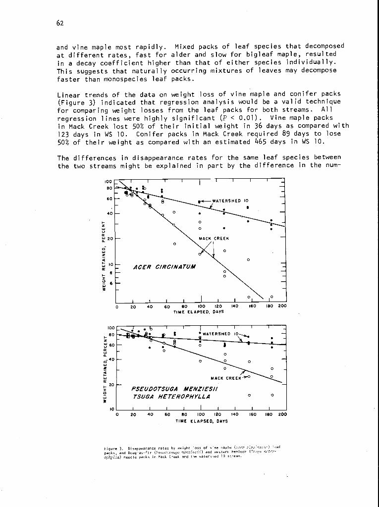
62

and vine maple most rapidly. Mixed packs of leaf species that decomposedat different rates, fast for alder and slow for bigleaf maple, resulted

in a decay coefficient higher than that of either species individually.This suggests that naturally occurring mixtures of leaves may decomposefaster than monospecies leaf packs.

Linear trends of the data on weight loss of vine maple and conifer packs(Figure 3) indicated that regression analysis would be a valid techniquefor comparing weight losses from the leaf packs for both streams. All

regression lines were highly significant (P < 0.01). Vine maple packs

in Mack Creek lost 50% of their initial weight in 36 days as compared with123 days in WS 10. Conifer packs in Mack Creek required 89 days to lose50% of their weight as compared with an estimated 465 days in WS 10.

The differences in disappearance rates for the same leaf species betweenthe two streams might be explained in part by the difference in the num-

0 20 40 60 80 100 120 140

TIME ELAPSED, DAYS160 180 200

Figure 3. Disappearance rates by weight loss of vine maple (leer cire Lnaturc) leaf

packs, and Douglas-fir (Pseudotsuga menziesii) and western hemlock (Teen heter-ophyZla) needle packs in Mack Creek and the watershed 10 stream.

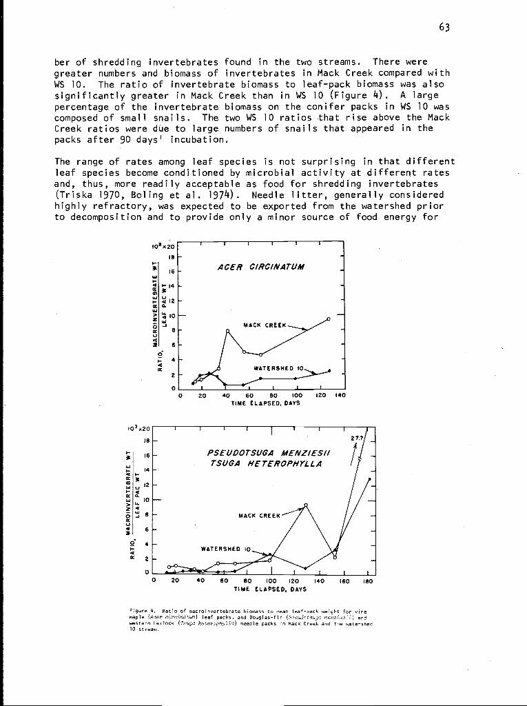
63

ber of shredding invertebrates found in the two streams. There weregreater numbers and biomass of invertebrates in Mack Creek compared withWS 10. The ratio of invertebrate biomass to leaf-pack biomass was alsosignificantly greater in Mack Creek than in WS 10 (Figure 4). A largepercentage of the invertebrate biomass on the conifer packs in WS 10 wascomposed of small snails. The two WS 10 ratios that rise above the MackCreek ratios were due to large numbers of snails that appeared in thepacks after 90 days' incubation.

The range of rates among leaf species is not surprising in that differentleaf species become conditioned by microbial activity at different ratesand, thus, more readily acceptable as food for shredding invertebrates(Triska 1970, Boling et al. 1974). Needle litter, generally consideredhighly refractory, was expected to be exported from the watershed priorto decomposition and to provide only a minor source of food energy for

103x20

al

103 x20

18

16

0

00

00

20

20

40

40 60 80 100TIME ELAPSED, DAYS

120 140

60 80 100 120 140

TIME ELAPSED, DAYS160 180

Figure 4. Ratio of macroinvertebrate biomass to mean leaf-pack weight for vinemaple (Aeer eireinatum) leaf packs, and Douglas-fir (Pseudotsuga nenziesi) andwestern hemlock (Tsuga heterephyZla) needle packs in Mack Creek and the watershed10 stream.

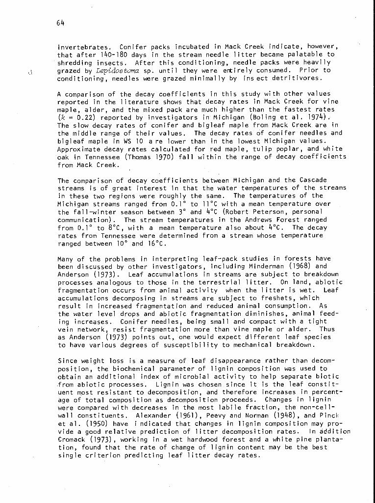
64

0

invertebrates. Conifer packs incubated in Mack Creek indicate, however,that after 140-180 days in the stream needle litter became palatable toshredding insects. After this conditioning, needle packs were heavilygrazed by Lepidostoma sp. until they were entirely consumed. Prior toconditioning, needles were grazed minimally by ins ect detritivores.

A comparison of the decay coefficients in this study with other valuesreported in the literature shows that decay rates in Mack Creek for vinemaple, alder, and the mixed pack are much higher than the fastest rates(k = 0.22) reported by investigators in Michigan (Boling et al. 1974).The slow decay rates of conifer and bigleaf maple from Mack Creek are inthe middle range of their values. The decay rates of conifer needles andbigleaf maple in WS 10 a re lower than in the lowest Michigan values.Approximate decay rates calculated for red maple, tulip poplar, and whiteoak in Tennessee (Thomas 1970) fall within the range of decay coefficientsfrom Mack Creek.

The comparison of decay coefficients between Michigan and the Cascadestreams is of great interest in that the water temperatures of the streamsin these two regions were roughly the same. The temperatures of theMichigan streams ranged from 0.10 to 11°C with a mean temperature overthe fall-winter season between 3° and 4°C (Robert Peterson, personalcommunication). The stream temperatures in the Andrews Forest rangedfrom 0.1° to 8°C, with a mean temperature also about 4°C. The decayrates from Tennessee were determined from a stream whose temperatureranged between 10° and 16°C.

Many of the problems in interpreting leaf-pack studies in forests havebeen discussed by other investigators, including Minderman (1968) andAnderson (1973). Leaf accumulations in streams are subject to breakdownprocesses analogous to those in the terrestrial litter. On land, abioticfragmentation occurs from animal activity when the litter is wet. Leafaccumulations decomposing in streams are subject to freshets, whichresult in increased fragmentation and reduced animal consumption. Asthe water level drops and abiotic fragmentation diminishes, animal feed-ing increases. Conifer needles, being small and compact with a tightvein network, resist fragmentation more than vine maple or alder. Thusas Anderson (1973) points out, one would expect different leaf speciesto have various degrees of susceptibility to mechanical breakdown.

Since weight loss is a measure of leaf disappearance rather than decom-position, the biochemical parameter of lignin composition was used toobtain an additional index of microbial activity to help separate biotic-from abiotic processes. Lignin was chosen since it is the leaf constit-uent most resistant to decomposition, and therefore increases in percent-age of total composition as decomposition proceeds. Changes in ligninwere compared with decreases in the most labile fraction, the non-cell-wall constituents. Alexander (1961), Peevy and Norman (1948), and Pincket al. (1950) have indicated that changes in lignin composition may pro-vide a good relative prediction of litter decomposition rates. In additionCromack (1973), working in a wet hardwood forest and a white pine planta-tion, found that the rate of change of lignin content may be the bestsingle criterion predicting leaf litter decay rates.

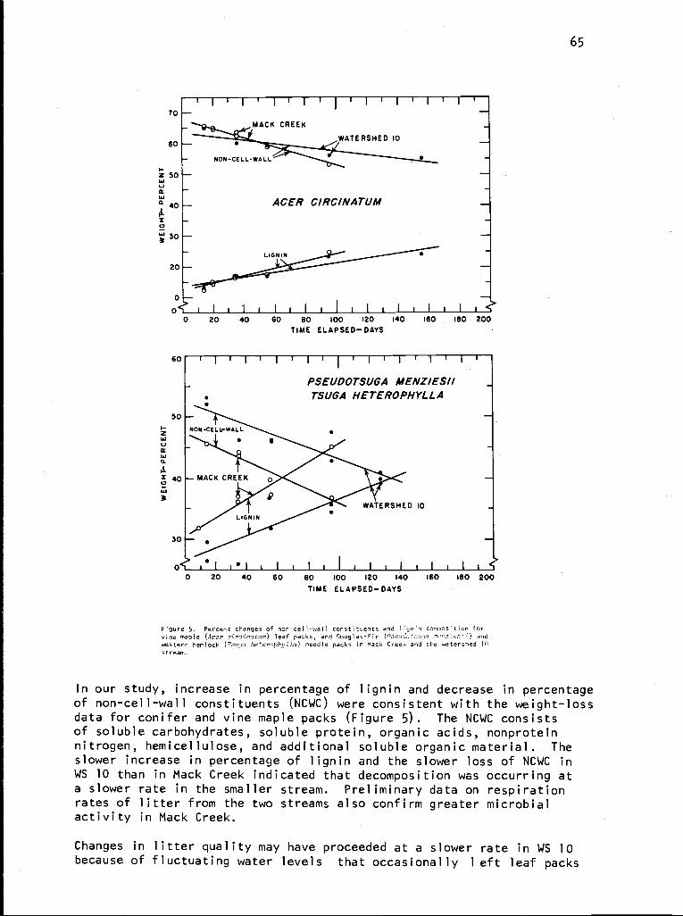
65

0 I I I I I I I I I I I I I I I I I I 1

0

60

50

1!40

W

20 40 60 80 100 120 140 160 180 200TIME ELAPSED-DAYS

I F 1I

11

WATERSHED 10

30

LIGNIN

o 1 0 I I 1 1 1 1 1 1 I 1 1 1 1 1 1 1 I 1

0 20 40 60 80 100 120 140 160 180 200TIME ELAPSED-DAYS

Figure 5. Percent changes of non-cell-wall constituents and lignin composition forvine maple (Acer circinatum) leaf packs, and Douglas-fir (Pseud;tauna msnzie^-'i) and

western hemlock (Tsuga heterophylla) needle packs in Mack Creek and the watershed ID

stream.

In our study, increase in percentage of lignin and decrease in percentageof non-cell-wall constituents (NCWC) were consistent with the weight-lossdata for conifer and vine maple packs (Figure 5). The NCWC consistsof soluble carbohydrates, soluble protein, organic acids, nonproteinnitrogen, hemicellulose, and additional soluble organic material. Theslower increase in percentage of lignin and the slower loss of NCWC inWS 10 than in Mack Creek indicated that decomposition was occurring ata slower rate in the smaller stream. Preliminary data on respirationrates of litter from the two streams also confirm greater microbialactivity in Mack Creek.

PSEUDOTSUGA MENZ/ES//TSUGA HETEROPHYLLA

Changes in litter quality may have proceeded at a slower rate in WS 10because of fluctuating water levels that occasionally 1 eft leaf packs

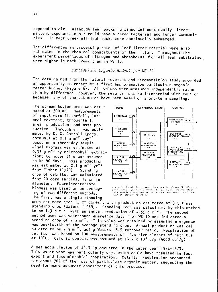
66

exposed to air. Although leaf packs remained wet continually, inter-mittent exposure to air could have altered bacterial and fungal communi-ties. In Mack Creek all leaf packs were continually submerged.

The differences in processing rates of leaf litter material were alsoreflected in the chemical constituents of the litter. Throughout theexperiment percentages of nitrogen and phosphorus for all leaf substrateswere higher in Mack Creek than in WS 10.

Particulate Organic Budget for WS 10

The data gained from the lateral movement and decomposition study providedan opportunity to construct a first-approximation particulate organicmatter budget (Figure 6). All values were measured independently ratherthan by difference; however, the results must be interpreted with cautionbecause many of the estimates have been based on short-term sampling.

The stream bottom area was esti- INPUT STANDING CROP OUTPUTmated at 300 m2. Measurementsof input were 1 i tterfa l 1 , lat- LITTEREALL 38.0%I

era) movement, throughfal l , PAFXPCn1ATE z0.,%

algal production, and moss pro-duction. Throughfall was esti- THROUGH

FALL 2.3%mated by G. C. Carroll (pers. DETRITUS(

commun.) at 0.1 g m-2 day-' 324

based on a three-day sample. LATERAL ,% I MACRO-I INVERTEBRATE

32

DETRITUSRESPIRATION

es

/Algal biomass was estimated at ee 0.5 MACRO- 'INVERTEBRATE

ATION0.33 g m-2 by chlorophyll extrac- JPR RIMARY RESPIR'eO DUCERStion; turnover time was assumed

'AL o'6%

t o be 40 days. Moss production PRIMARYETIONPRODUCERSwas estimated at 2.1 g

m-yr

from Fisher (1970). Standingcrop of detritus was calculatedfrom 20 core samples, 15 cm indiameter. Macroinvertebrate

I

S,.e

MOSSPRODUCT ION I I

0.7

biomass was based on an averag- Figp-e:). Annual flux particulate ''a`er'a' h'°,ays ('n k'Iogransper streari per year) 1 .atersh.d 10 0972-1q73). The percentage

i n g of two differentf f methods .

value associated 0ith each vector indicates the proportion of totald

The first was a single standingm pj Ur output rpresente .

crop estimate (ten 15-cm cores), with production estimated at 3.5 timesstanding crop (Waters 1 969). Standing crop was calculated by this methodto be 1.3 g m-2, with an annual production of 4.55 g m-2. The secondmethod used was year-round emergence data from WS 10 and indicated astanding crop of 2 g m-2. This value was obtained by assuming emergencewas one-fourth of the average standing crop. Annual production was cal-culated to be 7 g m-2, using Waters' 3.5 turnover ratio. Respiration ofdetritus was based on 100 measurements of five size classes of detritusat 10°C. Caloric content was assumed at 16.7 x 103 J/g (4000 cal/g).

A net accumulation of 24.3 kg occurred in the water year 1972-1973.This water year was particularly dry, which could have resulted in lessexport and less microbial respiration. Detrital respiration accountedfor about 70% of the loss of particulate organic matter, suggesting theneed for more accurate assessment of this process.

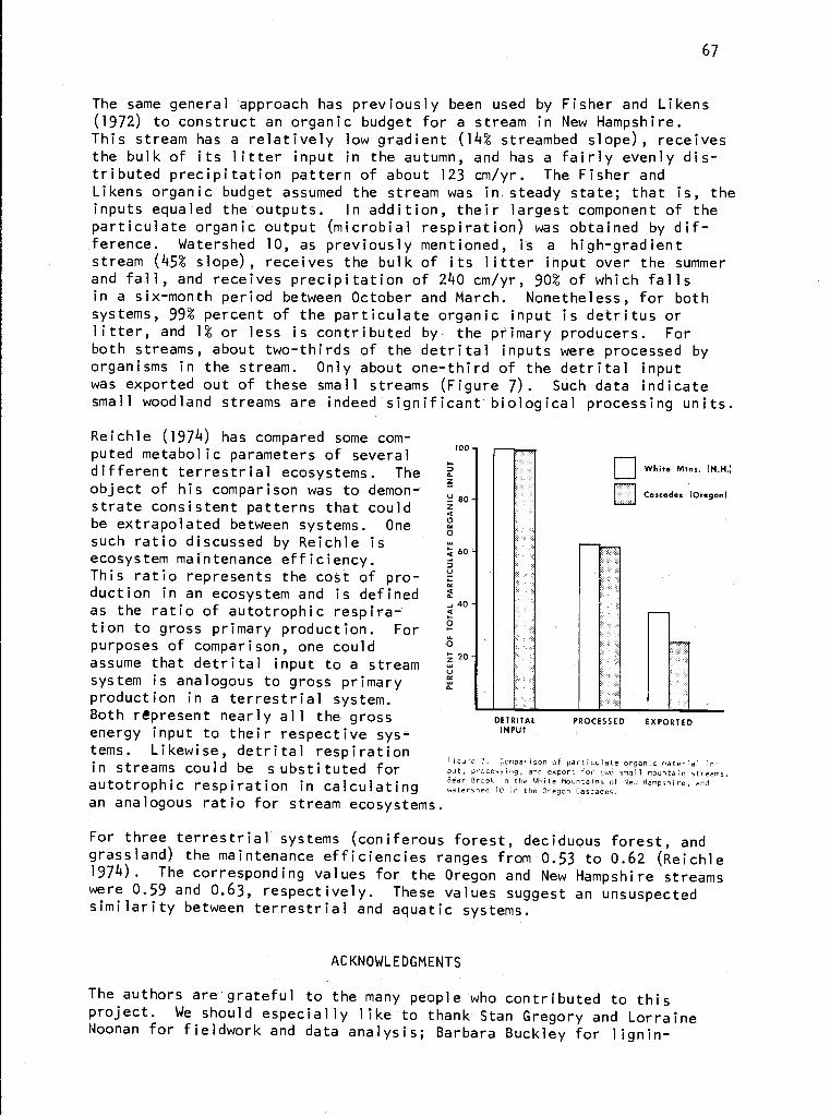
67

The same general approach has previously been used by Fisher and Likens(1972) to construct an organic budget for a stream in New Hampshire.This stream has a relatively low gradient (14o streambed slope), receivesthe bulk of its litter input in the autumn, and has a fairly evenly dis-tributed precipitation pattern of about 123 cm/yr. The Fisher andLikens organic budget assumed the stream was in steady state; that is, theinputs equaled the outputs. In addition, their largest component of theparticulate organic output (microbial respiration) was obtained by dif-ference. Watershed 10, as previously mentioned, is a high-gradientstream (45o slope), receives the bulk of its litter input over the summerand fall, and receives precipitation of 240 cm/yr, 90% of which fallsin a six-month period between October and March. Nonetheless, for bothsystems, 99% percent of the particulate organic input is detritus orlitter, and l% or less is contributed by the primary producers. Forboth streams, about two-thirds of the detrital inputs were processed byorganisms in the stream. Only about one-third of the detrital inputwas exported out of these small streams (Figure 7). Such data indicatesmall woodland streams are indeed significant biological processing units.

Reichle (1974) has compared some com-puted metabolic parameters of severaldifferent terrestrial ecosystems. Theobject of his comparison was to demon-strate consistent patterns that couldbe extrapolated between systems. Onesuch ratio discussed by Reichle isecosystem maintenance efficiency.This ratio represents the cost of pro-duction in an ecosystem and is definedas the ratio of autotrophic respira-tion to gross primary production. Forpurposes of comparison, one couldassume that detrital input to a streamsystem is analogous to gross primaryproduction in a terrestrial system.Both represent nearly all the grossenergy input to their respective sys-tems. Likewise, detrital respirationin streams could be substituted forautotrophic respiration in calculatingan analogous ratio for stream ecosystems.

White Mtns. (N.H.)

Cascades (Oregon)

DETRITAL PROCESSED EXPORTEDINPUT

Figure 7. Comparison of particulate organic material in-put, processing, a-id export for two small mountain streams,Bear Brool in the White Mountains of 11e, Hampshire, andwatershed 10 in the Oregon Cascades.

For three terrestrial systems (coniferous forest, deciduous forest, andgrassland) the maintenance efficiencies ranges from 0.53 to 0.62 (Reichle1974). The corresponding values for the Oregon and New Hampshire streamswere 0.59 and 0.63, respectively. These values suggest an unsuspectedsimilarity between terrestrial and aquatic systems.

ACKNOWLEDGMENTS

The authors are grateful to the many people who contributed to thisproject. We should especially like to thank Stan Gregory and LorraineNoonan for fieldwork and data analysis; Barbara Buckley for lignin-

80

0

60

40

68

cellulose analysis; Nancy Triska for leaf-pack processing; Dick Aho,Ken Brophy, and Ed Grafius for field sampling and sorting; and EllenSedell and Bonnie Hall for the line drawings.

REFERENCES

ABEE, A., and D. LAVENDER. 1972. Nutrient cycling in throughfall andlitterfall in 450-year-old Douglas-fir stands, IN: J. F. Franklin,L. J. Dempster, and R. H. Waring (eds.), Proceedings--Research onconiferous forest ecosystems--A symposium, p. 133-143. USDA For. Serv.,Portland, Oreg.

ALEXANDER, M. 1961. Introduction to s oil microbiology. John Wiley andSons, New York. 472 p.

ANDERSON, J. M. 1973. The breakdown and decomposition of sweet chestnut(Castanea sativa Mill.) and beech (Fagus syZvatica L.) leaf litter intwo deciduous woodland soils. I. Breakdown, leaching, and decomposition.Oecologia 12:251-274.

BERNTSEN, C. M., and J. ROTHACHER. 1959. A guide to the H. J. AndrewsExperimental Forest. USDA For. Serv. Pacific Northwest Forest and RangeExperiment Station. 21 p.

BOLING, R. H., R. C. PETERSEN, and K. W. CUMMINS. 1974. Ecosystemmodeling for small woodland streams. IN: B. C. Patten (ed.), Systemsanalysis and simulation in ecology, vol. 3 (in press).

CROMACK, K., Jr. 1973. Litter production and litter decomposition in amixed hardwood watershed and in a white pine watershed at CoweetaHydrologic Station, North Carolina. Ph.D. thesis, Univ. Georgia, Athens.160 p.

CUMMINS, K. W., J. J. KLUG, R. G. WETZEL, R. C. PETERSON, K. F. SUBERKROPP,B. A. MANNY, J. C. WUYCHECK, and F. 0. HOWARD. 1972. Organic enrichmentwith leaf leachate in experimental lotic systems. BioScience 22:719-722.

CUMMINS, K. W., R. C. PETERSEN, F. 0. HOWARD, J. C. WUYCHEK, and V. I.

HOLT. 1973. The utilization of leaf litter by stream detritivores.Ecology 54:336-345.

FISHER, S. G. 1970. Annual energy budget for a small forest streamecosystem: Bear Brook, West Thornton, New Hampshire. Ph.D. thesis,Dartmouth Coll., Hanover, N.H. 97 p.

FISHER, S. G., and G. E. LIKENS. 1972. Stream ecosystem: Organic energybudget. BioScience 22:33-35.

FREDRIKSEN, R. L. 1971. Comparative chemical quality--Natural anddisturbed streams following logging and slash burning. IN: J. T. Krygierand J. D. Hall, (eds.), Symposium on forest land use and the streamenvironment. Oregon State Univ., Corvallis.

69

FREDRIKSEN, R. L. 1972. Nutrient budget of a Douglas-fir forest on anexperimental watershed in western Oregon. IN: J. F. Franklin, L. J.Dempster, and R. H. Waring (eds.), Proceedings--Research on coniferousforest ecosystems--A symposium, p. 115-131. USDA For. Serv., Portland,Oreg.

KAUSHIK, N. K., and H. B. N. HYNES. 1971. The fate of dead leaves thatfall into streams. Arch. Hydrobiol. 68:465-515.

MINDERMAN, G. 1968. Addition, decomposition, and accumulation of organicmatter in forests. J. Ecol. 56:355-362.

OLSON, J. S. 1963. Energy storage and the balance of producers anddecomposers in ecological systems. Ecology 44:322-331.

PEEVY, W. J., and A. G. NORMAN. 1948. Influence of composition of plantmaterials on properties of decomposed residues. Soil Sci. 65:209-226.

PINCK, L. A., F. E. ALLISON, and M. S. SHERMAN. 1950. Maintenance ofsoil organic matter. II. Losses of carbon and nitrogen from young andmature plant materials during decomposition in soil. Soil Sci. 69:391-401.

REICHLE, D. E. 1974. Advances in ecosystem science. BioScience (inpress).

THOMAS, W. A. 1970. Weight and calcium losses from decomposing treeleaves on land and in water. J. Appl. Ecol. 7:237-241.

TRISKA, F. J. 1970. Seasonal distribution of aquatic hyphomycetes inrelation to the disappearance o f leaf litter from a woodland stream.Ph.D. thesis, Univ. Pittsburgh. 189 p.

VANNOTE, R. L. 1970. Detrital consumers in natural systems. IN: K. W.Cummins (ed.), The stream ecosystem, p. 20-23. AAAS symposium. Tech.Rep. Mich. State Univ. Inst. Water Res. 7:1-42.

VAN SOEST, P. J. 1963. Rapid method for determination of celluloseand lignin. J. Assoc. Off. Agric. Chem. 46:829-835.

WATERS, T. F. 1969. The turnover ratio in production ecology of fresh-water invertebrates. Am. Nat. 103:173-185.

70

ANALYSIS OF LAKE ECOSYSTEMS: LAKE WASHINGTON DRAINAGE BASIN'

R. C. Wissmar, D. M. Eggers, and N. W. Bartoo

University of Washington

ABSTRACT

Research on four lake ecosystems of the Lake Washington drainage basinis discussed using a hierarchical design depicting the system componentsnested in four levels: drainage basin, lakes, limnetic and littoralzones, and process models. Comparisons are made of these lakes of dif-ferent trophic states using parameters inherent to process models. Dy-

namic processes of the fourth level include phytoplankton, zooplankton,benthos, and fish. Related research activities and information on theCedar River and Fern and Castle Lakes are discussed.

INTRODUCTION

Analysis of lake ecosystems in the Coniferous Forest Biome encompassesresearch programs on four lakes of varying trophic states in the LakeWashington drainage basin near Seattle, Washington. This paper presentsa systems organization for the lakes within the drainage basin and asummary of research activities for 1972 and 1973. The hierarchicalclassification incorporates influences of developed and undevelopedwatersheds, the trophic conditions of lakes, and detailed process modelsfor food chains and nutrient cycles within each lake.

The principal question addressed by the Coniferous Biome lake programis: If research and theory are combined with mathematical modeling,can a better understanding of the acute and chronic behavior of ecosys-tems be obtained by studying lakes of different environments and bio-logical communities? Our approach follows the concept that productivityand maintenance of biological structure within lakes is at least partlydependent upon the form, quantity, and flux of organic matter and nutrientsfrom different terrestrial sources and upon internal variations of car-bon and nutrient cycles for each lake type. Some of the studies includethe assessment of interrelationships between plankton production andnutrient cycles, the effect of organic matter supply on benthic metab-olism, and responses of fish populations to the composition and magnitudeof food resources. Research and modeling programs are intended to simu-late responses of lakes to natural and cultural effects. Such simulationsare useful in studying changes in lakes due to thermal discharges, damconstruction, dredging, alteration of organic and nutrient loading byindustrial and urban development, agricultural practices, navigationalmanagement, and logging activities.

'This is contribution no. 66 from the Coniferous Forest Biome and con-tribution no. 393 from the College of Fisheries, Univ. Washington. Seemethods section for list of contributors.

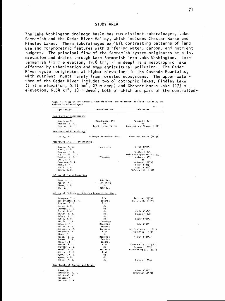
71

The Lake Washington drainage basin has two distinct subdrainages, LakeSammamish and the Cedar River Valley, which includes Chester Morse andFindley Lakes. These subdrainages exhibit contrasting patterns of landuse and morphometric features with differing water, carbon, and nutrientbudgets. The principal flow of the Sammamish system originates at a lowelevation and drains through Lake Sammamish into Lake Washington. LakeSammamish (12 m elevation, 19.8 km2, 31 m deep) is a mesotrophic lakeaffected by urbanization and some agricultural pollution. The CedarRiver system originates at higher elevations in the Cascade Mountains,with nutrient inputs mainly from forested ecosystems. The upper water-shed of the Cedar River includes two oligotrophic lakes, Findley Lake(1131 m elevation, 0.11 km2, 27 m deep) and Chester Morse Lake (473 melevation, 6.54 km2, 38 m deep), both of which are part of the controlled-

Table I. Research contributors, determinations, and references for lake studies by theUniversity of Washington.

Contributors Determinations

Department of Oceanography

Devol , A. H. Respiratory ETS Packard (1971)Packard, T. T. do doPamatmat, 11. M. Benthic respiration Pamatmat and Bhagwat (1973)

STUDY AREA

References

Department of Microbiology

Staley, J. T. Nitrogen transformations Mague and Barris (1973)

Department of Civil Engineering

Barnes, R. S.Birch, P. B.Monahan, F. C.Spyridakis, D. E.

Hendrey, G. R.Litt, A. H.Pederson, G. L.Rock, C. A.Stoll, R. K.Welch, E. B.

Sediments

Plankton

Birch (1974)do

Monahan (1974)Welch and Spyridakis (1972)

Hendrey (1973)do

Pederson (1974)Emery (1972)Stoll (1973)

Welch et al. (1974)

College of Forest Resources

Sara, R. I.Jensen, A.Olson, P. R.Rau, G.

DetritusLogistics

do

Detritus

College of Fisheries, Fisheries Research Institute

Berggren, T. J. FishBissonnette, P. A. BenthosBurgner, R. L. FishCasne, S. R. doChapman, D. G. doCosta, H. H. doDawson, J. J. doDelacy, A. C. doDoble, D. D. doKittle, L. J. LimnologyMale, L. M . ModelingMalick, J. G. Bent hosMatches, J . R. BacteriaNishimoto, M. FishOlney, F. doRichey, J. E. ModelingStoberQ. J. BenthosTaub, F. . B. BenthosThorne, B. E. FishTraynor, J. J. doWekell, M. M. BacteriaWhitney, B. R. FishWydoski, R. S. doWyman, K. H. do

Hansen, B. G. do

Departments of Zoology and Botany

Adams, D.Edmondson, W. T.Del Moral, R.Tsukada, M.

Paulson, D. R.

Berggren (1974)Bissonnette (1974)

Noble (1972)Dawson (1972)

Doble (1974)

Male (1973)

Harrison et al. (1971)Nishimoto (1973)

Richey (1974a)

Thorne et al. (1974)

Traynor (1973)Harrison et al. (1971)

Hansen (1974)

Adams (1973)Edmondson (1972)

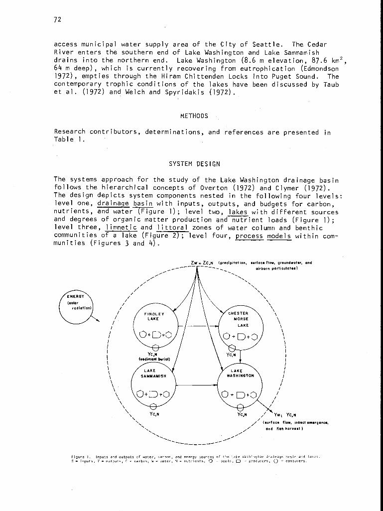
72

access municipal water supply area of the City of Seattle. The CedarRiver enters the southern end of Lake Washington and Lake Sammamishdrains into the northern end. Lake Washington (8.6 m elevation, 87.6 km2,64 m deep), which is currently recovering from eutrophication (Edmondson1972), empties through the Hiram Chittenden Locks into Puget Sound. Thecontemporary trophic conditions of the lakes have been discussed by Taubet al. (1972) and Welch and Spyridakis (1972).

METHODS

Research contributors, determinations, and references are presented inTable 1.

SYSTEM DESIGN

The systems approach for the study of the Lake Washington drainage basinfollows the hierarchical concepts of Overton (1972) and Clymer (1972).The design depicts system components nested in the following four levels:level one, drainage basin with inputs, outputs, and budgets for carbon,nutrients, and water Figure 1); level two, lakes with different sourcesand degrees of organic matter production and nutrient loads (Figure 1);level three, limnetic and littoral zones of water column and benthiccommunities of a lake (Figure 2); level four, process models within com-munities (Figures 3 and 4).

ZW+ZC,N (precipitation, surface flow, groundwater, andticulates)n arair or p

Yc,N // -YW; YC,N(surface flow, insect emergence,

and fish harvest )

Figure I. Inputs and outputs of water, carbon, and energy sources of the Lake Washington drainage basin and lakes.Z = inputs, Y = outputs, C = carbon, W = water, N = nutrients, 0 = pools, D = producers, n = consumers.

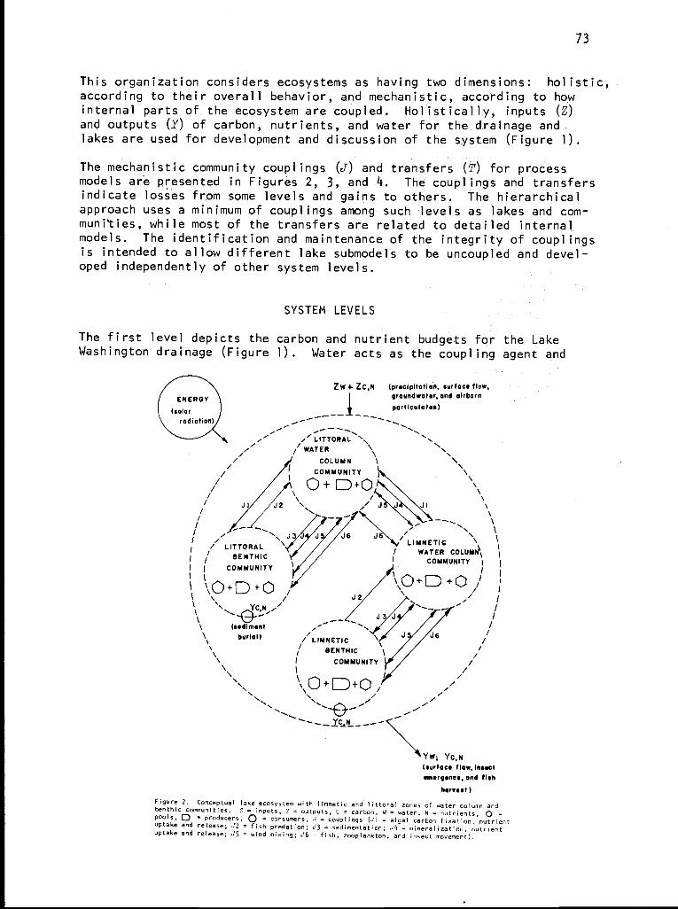
73

This organization considers ecosystems as having two dimensions: holistic,according to their overall behavior, and mechanistic, according to howinternal parts of the ecosystem are coupled. Holistically, inputs (Z)

and outputs (Y) of carbon, nutrients, and water for the. drainage andlakes are used for development and discussion of the system (Figure 1).

The mechanistic community couplings (J) and transfers (T) for processmodels are presented in Figures 2, 3, and 4. The couplings and transfersindicate losses from some levels and gains to others. The hierarchicalapproach uses a minimum of couplings among such levels as lakes and com-munities, while most of the transfers are related to detailed internalmodels. The identification and maintenance of the integrity of couplingsis intended to allow different lake submodels to be uncoupled and devel-oped independently of other system levels.

SYSTEM LEVELS

The first level depicts the carbon and nutrient budgets for the LakeWashington drainage (Figure 1). Water acts as the coupling agent and

ENERGY

(solarradiation)

LITTORAL

Z W + z C,N (precipitation, surface flow,

1groundwater, and airbernparticulates)

-__ Yc1rr ___

Yw; YC,N(surface flow, insectemergence, and fish

harvest)Figure 2. Conceptual lake ecosystem with limnetic and littoral zones of water column andbenthic communities. Z - inputs, Y = outputs, C = carbon, W = water, N nutrients, 0 =pools, J - producers, Q = consumers, .7 = couplings (JI = alga) carbon fixation, nutrientuptake and release; .72 = fish predation; J3 = sedimentation; J4 = mineralization, nutrientuptake and release; 75 = wind mixing; 76 = fish, zooplankton, and insect movement).

=

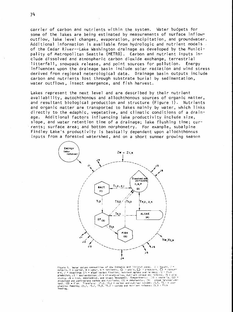
74

carrier of carbon and nutrients within the system. Water budgets forsome of the lakes are being estimated by measurements of surface inflow-outflow, lake level changes, evaporation, precipitation, and groundwater.Additional information is available from hydrologic and nutrient modelsof the Cedar River--Lake Washington drainage as developed by the Munici-pality of Metropolitan Seattle (METRO). Carbon and nutrient inputs in-clude dissolved and atmospheric carbon dioxide exchange, terrestriallitterfall, snowpack release, and point sources for pollution. Energyinfluences upon the drainage basin include solar radiation and wind stressderived from regional meterological data. Drainage basin outputs includecarbon and nutrients lost through substrate burial by sedimentation,water outflows, insect emergence, and fish harvest.

Lakes represent the next level and are described by their nutrientavailability, autochthonous and allochthonous sources of organic matter,and resultant biological production and structure (Figure 1). Nutrientsand organic matter are transported to lakes mainly by water, which linksdirectly to the edaphic, vegetative, and climatic conditions of a drain-age. Additional factors influencing lake productivity include size,slope, and water retention time of a drainage; lake flushing time; cur-rents; surface area; and bottom morphometry. For example, subalpineFindley Lake's productivity is basically dependent upon allochthonousinputs from a forested watershed, and on a short summer growing season

ENERGY(solar

radiation)

J4

ZW + ZC,N

4

J4

Dissolved andparticulateC,N,P

r

Figure 3. Water column communities of the limnetic and littoral zones. Z = inputs, 7 =

outputs, C = carbon, W = water, N = nutrients, i = pools, D = producers, Q = consum-ers, J - couplings (JI = algal carbon fixation, nutrient uptake and release; 72 = fish

predation; J3 = sedimentation; J4 = mineralization, nutrient uptake and release; --15 = wind

mixing; J6 = fish, zooplankton, and insect movement). Compartments: (1) = bacteria, (2)

dissolved and particulate carbon and nutrients, (3) = zooplankton, (4) = algae (phytoplank-

ton), (5) = fish. Transfers: T4,2, T1,2 = carbon and nutrient uptake; 3,4, T3,1 = zoo-

plankton feeding; T3,2, T5,2, T2,4, T2,1 = carbon and nutrient release; 15,3 = fishfeeding.

JI

R /J3

16

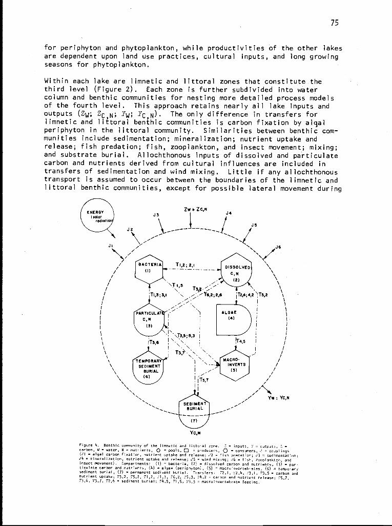
75

for periphyton and phytoplankton, while productivities of the other lakesare dependent upon land use practices, cultural inputs, and long growingseasons for phytoplankton.

Within each lake are limnetic and littoral zones that constitute thethird level (Figure 2). Each zone is further subdivided into watercolumn and benthic communities for nesting more detailed process modelsof the fourth level. This approach retains nearly all lake inputs and

outputs (ZW; ZC,N; 1W; YC,N) The only difference in transfers forlimnetic and littoral benthic communities is carbon fixation by algalperiphyton in the littoral community. Similarities between benthic com-munities include sedimentation; mineralization; nutrient uptake andrelease; fish predation; fish, zooplankton, and insect movement; mixing;and substrate burial. Allochthonous inputs of dissolved and particulatecarbon and nutrients derived from cultural influences are included intransfers of sedimentation and wind mixing. Little if any allochthonoustransport is assumed to occur between the boundaries of the limnetic andlittoral benthic communities, except for possible lateral movement during

ENERGYDolor

radiation

ZW + ZC,NJ3 J4

JS

JI J6

/ 1BACrERIA]hTI2;2i4 DISSOLVED \\\N

\

\T I,sT3,2-

/ 7I,3;3,1 T2,4;4,2\T5,2

I i'/ \ I 11I oennew AT - 1 ALGAE( C N { (4) I

I I

Tassa i

TEMPORAR MACRO- /\1 -- INVERTS /\ SEDIMENT

\ BURIAL I i (S)

\\\ l6)j Ts,T

Figure 4. Benthic community of the limnetic and littoral zone. Z = inputs, 1 outputs, C =carbon; ,W = water, N = nutrients, 0 = pools, = producers, 0 = consumers, .7 = couplings(JI - algal carbon fixation, nutrient uptake and release; J2 = fish predation; .73 = sedimentation;

J4 mineralization, nutrient uptake and release; .15 wind mixing; .16 = fish, zooplankton, andinsect movement). Compartments: (I) = bacteria,

(2)=

= dissolved carbon and nutrients, (3) - par-ticulate carbon and nutrients, (4) = algae (periphyton), (5) = macroinvertebrates, (6) = temporarysediment burial, (7) = permanent sediment burial. Transfers: T2,1, T2,4, T3,1, T3,5 = carbon andnutrient uptake; T3,2, T5,2, T1,2, T1,3, T6,2, T5,3, T4,2 = carbon and nutrient release; 15,7,T3,6, T3,7, T2,6 - sediment burial; T4,5, TI,5, T3,5 = macroinvertebrate feeding.

\

;

=

76

sedimentation. Limnetic and littoral communities exist in all lakesexcept Findley Lake, where the littoral community predominates throughoutthe growing season (July to October).

Process research and models constitute the fourth level and involve thetransfer of carbon and nutrients between pools, processes, and consumers(Figures 3 and 4). Fourth-level processes include simulation of growthand feeding for limnetic fish, distribution of benthic-littoral fish andplankton production, benthic metabolism, and nutrient interactions. The

plankton and nutrient modeling is scheduled to be expanded by an approachdeveloped by Richey (1974a). Model expansion for limnetic fish includesoptimal foraging, schooling behavior, and distribution in the water column.Benthic-littoral fish models are currently being constructed for growth,feeding, and competition. Benthic modeling is conceptual and awaitsfurther analysis of data sets.

PROCESS MODELING

Primary production by phytoplankton is the principal source of organicmatter formation in many lakes. The amount of carbon fixed or the re-sponse of algal photosynthesis to natural and cultural inputs of nutrientsand carbon provides a means for initial and long-term assessment of theeffects of eutrophication and consequent management of water quality.Modeling activities during 1971 to 1973 attempted to simulate quantitativerelationship between nutrient concentrations and differences in phytoplanktonutilization rates, as well as phytoplankton biomass changes, nutrientsupply, and nutrient cycling dynamics of various lakes. The primaryproduction nutrient cycling submodel (Male 1973) incorporates in situand in vitro nutrient experiments, field data, and a system of partialdifferential equations for evaluating both the temporal and spatialdynamics of phytoplankton production.

Process models are constructed such that transfer coefficients can beformulated from field and laboratory data. For example, a normalizedproductivity index (production per biomass per insolation, [P/BI/I)can be obtained by dividing productivity by an estimate of the carbonbiomass and by daily insolation. The (P/B)/I values tend to increaseover time following an actual production peak, so that a (P/B)/I peakusually occurred later in the growing season. The effect of lightintensity and nutrient availability on the production/biomass quotientcan be examined by the function

u = um k + S RRexp (1 - R/Ro) (1)

t o

where -p is P/B, u is maximum P/B, S is inorganic phosphate concentration,kt is S at 1/2 um, R is lux, and Ro is optimum lux, was found to describeexperimental results at the 0.05 level of significance, with a highdegree of correlation. It was initially hypothesized that the kt values

of natural phytoplankton populations were related to the productivityof the ambient waters in such a fashion that as productivity increasesso does kt. The half-saturation constant kt reflects the relative

77

ability of phytoplankton to use low levels of nutrients. The kt valuesobtained were 0.17, 0.36, 0.42, and 2.84 ug P/liter for Findley, ChesterMorse, Sammamish, and Washington, respectively. By comparing these ktvalues for the four lakes, the direct correlation between the trophic

status and kt confirms this hypothesis for natural phytoplanktoncommunities in lacustrine environments (Hendrey 1973).

Zooplankton models are still at the conceptual stage; however activelaboratory and field research is being conducted (see Research Activities)-

At present, the limnetic fish model consists of a feeding dynamics andenergy budget model for sockeye salmon in Lake Washington. Other majorlimnetic fish such as stickleback and smelt will be included after com-pletion of successful simulations for sockeye. Emphasis is placed onsockeye because of its unique feeding behavior, "entirely" on zooplankton.This model provides a useful structure for analysis of growth in sockeyesalmon and relates to other sockeye salmon producing systems with widelydiffering zooplankton population characteristics.

Earlier biological studies (Woodey 1972, Dryfoos 1966) have contributedinformation regarding feeding behavior (food selectivity, verticalmigration, feeding period) for sockeye salmon, and to a limited extentfor longfin smelt, in Lake Washington. Woodey (1972), Traynor (1973),and Dawson (1972) have provided information on population density,production, biomass, and patterns of horizontal movement for all threemajor limnetic fish species (sockeye salmon, longfin smelt, and three-spine stickleback) in Lake Washington. Berggren (1974) has providedsimilar but less complete information regarding Lake Sammamish sockeye.D. M. Eggers has constructed a process-oriented model for the limneticgrowth of sockeye salmon, consistent with behavioral patterns observedin the above studies. The effects of the external variables such aslight and water temperature are provided in the model. These allow usto study energetic implications of the observed feeding behavior ofsalmon, which include diel vertical migration and the limitation offeeding to hours of dusk and dawn. The model is tied to the widerecosystem structure through two major couplings. These are species-specific grazing rates on zooplankton and release of carbon, nitrogen,and phosphorus through excretion of metabolic wastes (Figure 3). Thepresent limnetic growth model utilizes the Holling (1966) concept ofpredation extended to a multiple-prey situation. Optimal foraging theorycombined with specific rates of prey size encounter and prey speciescapture success allows one to predict that component of the total zoo-plankton population encountered which is utilized by the predator. Thepredator's strategy of prey utilization changes seasonally. The abovemodel gives us the potential ability to study successional changesexerted on the zooplankton population by limnetic fish predators, whichwill be realized only when the model is coupled with the model of thezooplankton population dynamics incorporating selecting predation.

The present model incorporates a single predator, with five species ofzooplankton prey. The zooplankton population density and size distri-bution by species are inputs, together with the environmental variablesof light intensity and temperature. There exist three components of themodel: predator-prey interactions, other predator behavioral processes,and growth of the predator. They are discussed below.

78

The predator-prey interaction model component relates quantity of preyconsumed by the predator and is an extension of earlier work by Charnov(1973) and Werner (1972). The general form of the model is:

iEA Ji Xi (E)Ni ( ) ISi (C)C (E) - E . ( ) ] dE

(2)CT

1 + ieA Ji X.( )N.( )Hi( ) d2

where CT is net carbon consumed, (Li, Ui) is size interval of preyspecies i that are pursued when encountered by the predator, A is a setof prey species available to the predator, ai(d) is a function thatyields encounter rate for a given size C of the ith prey species, Si(d)is function that yields the proportion of prey successfully capturedwhen pursued for a given size E of the ith prey species, Hi(E), is afunction that yields the total time needed to pursue, capture, and eatan individual size E of the ith prey species, Ci() is carbon content ofan individual of size i of the ith prey species, Ei(C) is expected carbonexpended by the predator per pursuit of an individual of size E of theith species, and Ni(i;) is density of prey size of the ith prey species.

The feeding behavior model simulates sockeye salmon encountering a numberof prey species, consisting of individuals of varying size. Becauseencounter rate increases with size of the prey, larger individuals of agiven species are encountered more frequently than smaller individualsof the same population density. Hence they occur more frequently in thediet. Even if the predator is taking all prey as encountered, there isa difference between the size distribution of the prey in the stomachsand prey in the water column.

To illustrate this point, the model was used in simulating the resultsof an experiment conducted by Brooks (1968). Here, 65 AZosa pseudoharenguswere put in a 250-liter aquarium. At the outset of the experiment theaquarium contained a known density of five size classes of Diaptomusminutus, together with incidental Epischura nordenskioZdi and Daphniacatawba. These large prey disappeared quickly and are ignored inapplication of the model. The effect of the predation by AZosa wasmeasured by following the density of the five size classes over thecourse of the experiment. The density of the larger size classes declinedmuch faster than the density of the smaller size classes.

In the application of the model, the predator exploited five prey typesof constant size. Encounter is a Poisson process, where the expectednumber of encounters is simply the product of volume searched in a unitof time and the prey density. The volume searched depends upon a con-stant parameter that is a property of the predator. The parameter isthe minimum angle of visual perception. Hence prey of different sizesare perceived at varying distances, with larger individuals seen atgreater distances than smaller individuals. Handling time was assumedto be constant for each of the given size classes. A minimum angle ofvision of 0.02088 radian with the predator searching at one length persec, and with 1.84 sec to pursue, capture, and eat a prey once that preyis encountered, generated and predicted densities presented in Figure 5.

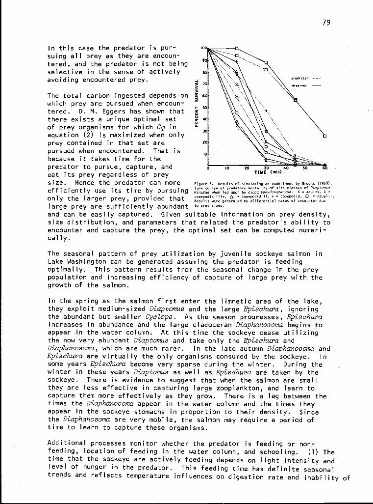
79

In this case the predator is pur- loo

suing all prey as they are encoun-tered, and the predator is not being

90

selective in the sense of actively so

predicted --avo i d i ng encountered prey. <.,;'.,a.,

TO %4 observed

60The total carbon ingested depends on Cr

which prey are pursued when encoun- N

tered. D. M. Eggers has shown that W 30

there exists a unique optimal set Cr 40

of prey organisms for which CT in30

equation (2) is maximized when onlyprey contained in that set are to

pursued when encountered. That is 10

because it takes time for thepredator to pursue, capture, and o to zo 30 io 50 60

eat its prey regardless of prey TIME (min)

size. Hence the predator can more Figure 5. Results of simulating an experiment by Brooks (1968).

efficiently i its time bTime course of predatory mortality of size classes of Diaptomus

use by pursuing minutus when fed upon by AZosa pseudoharengus. X = adults, 0 =

only t he larger prey, that copepodid 111+, Q= copepodid ii, + = copepodid, = nauplii.provided Results were generated by differential rates of encounter due

large prey are sufficiently abundant to prey sizes.

and can be easily captured. Given suitable information on prey density,size distribution, and parameters that related the predator's ability toencounter and capture the prey, the optimal set can be computed numeri-cally.

The seasonal pattern of prey utilization by juvenile sockeye salmon inLake Washington can be generated assuming the predator is feedingoptimally. This pattern results from the seasonal change in the preypopulation and increasing efficiency of capture of large prey with thegrowth of the salmon.

In the spring as the salmon first enter the limnetic area of the lake,they exploit medium-sized Diaptomus and the large Epischura, ignoringthe abundant but smaller Cyclops. As the season progresses, Epischuraincreases in abundance and the large cladoceran Diaphanosoma begins toappear in the water column. At this time the sockeye cease utilizingthe now very abundant Diaptomus and take only the Epischura andDiaphanosoma, which are much rarer. In the late autumn Diaphanosoma andEpischura are virtually the only organisms consumed by the sockeye. In

some years Epischura become very sparse during the winter. During thewinter in these years Diaptomus as well as Epischura are taken by thesockeye. There is evidence to suggest that when the salmon are smallthey are less effective in capturing large zooplankton, and learn tocapture them more effectively as they grow. There is a lag between thetimes the Diaphanosoma appear in the water column and the times theyappear in the sockeye stomachs in proportion to their density. Sincethe Diaphanosoma are very mobile, the salmon may require a period oftime to learn to capture these organisms.

Additional processes monitor whether the predator is feeding or non-feeding, location of feeding in the water column, and schooling. (1) Thetime that the sockeye are actively feeding depends on light intensity andlevel of hunger in the predator. This feeding time has definite seasonaltrends and reflects temperature influences on digestion rate and inability of

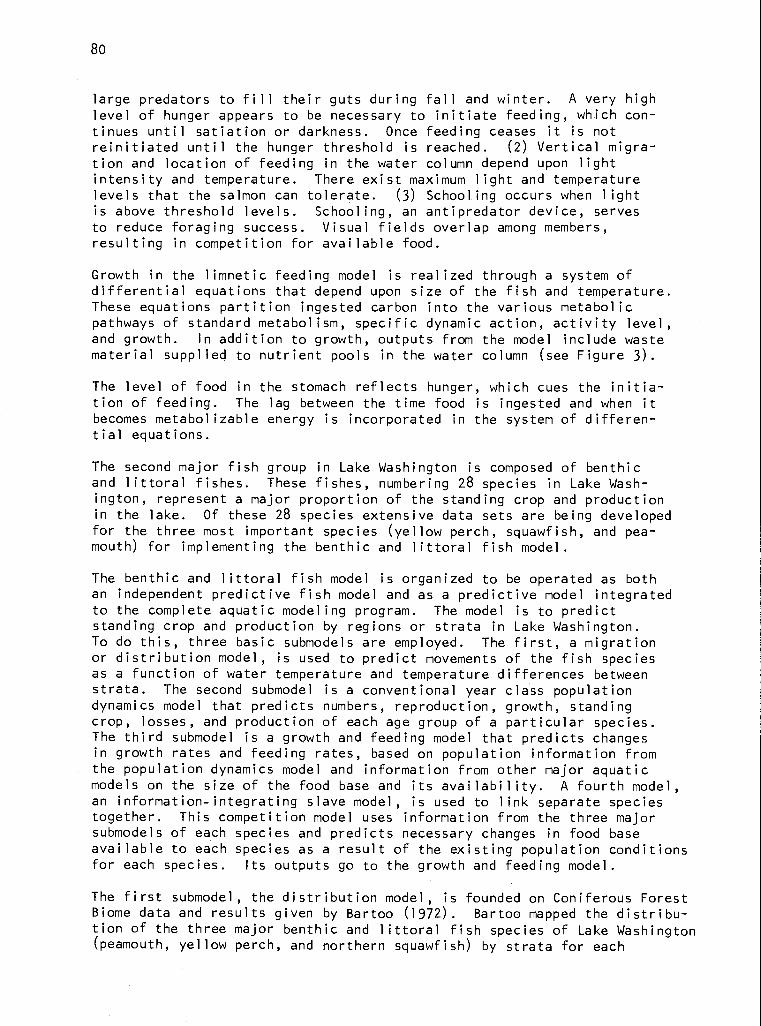
80

large predators to fill their guts during fall and winter. A very highlevel of hunger appears to be necessary to initiate feeding, which con-tinues until satiation or darkness. Once feeding ceases it is not

reinitiated until the hunger threshold is reached. (2) Vertical migra-tion and location of feeding in the water column depend upon lightintensity and temperature. There exist maximum light and temperaturelevels that the salmon can tolerate. (3) Schooling occurs when lightis above threshold levels. Schooling, an antipredator device, servesto reduce foraging success. Visual fields overlap among members,resulting in competition for available food.

Growth in the limnetic feeding model is realized through a system ofdifferential equations that depend upon size of the fish and temperature.These equations partition ingested carbon into the various metabolicpathways of standard metabolism, specific dynamic action, activity level,and growth. In addition to growth, outputs from the model include wastematerial supplied to nutrient pools in the water column (see Figure 3).

The level of food in the stomach reflects hunger, which cues the initia-tion of feeding. The lag between the time food is ingested and when itbecomes metabolizable energy is incorporated in the system of differen-tial equations.

The second major fish group in Lake Washington is composed of benthicand littoral fishes. These fishes, numbering 28 species in Lake Wash-ington, represent a major proportion of the standing crop and productionin the lake. Of these 28 species extensive data sets are being developedfor the three most important species (yellow perch, squawfish, and pea-mouth) for implementing the benthic and littoral fish model.

The benthic and littoral fish model is organized to be operated as bothan independent predictive fish model and as a predictive model integratedto the complete aquatic modeling program. The model is to predictstanding crop and production by regions or strata in Lake Washington.To do this, three basic submodels are employed. The first, a migrationor distribution model, is used to predict movements of the fish speciesas a function of water temperature and temperature differences betweenstrata. The second submodel is a conventional year class populationdynamics model that predicts numbers, reproduction, growth, standingcrop, losses, and production of each age group of a particular species.The third submodel is a growth and feeding model that predicts changesin growth rates and feeding rates, based on population information fromthe population dynamics model and information from other major aquaticmodels on the size of the food base and its availability. A fourth model,an information-integrating slave model, is used to link separate speciestogether. This competition model uses information from the three majorsubmodels of each species and predicts necessary changes in food baseavailable to each species as a result of the existing population conditionsfor each species. Its outputs go to the growth and feeding model.

The first submodel, the distribution model, is founded on Coniferous ForestBiome data and results given by Bartoo (1972). Bartoo mapped the distribu-tion of the three major benthic and littoral fish species of Lake Washington(peamouth, yellow perch, and northern squawfish) by strata for each

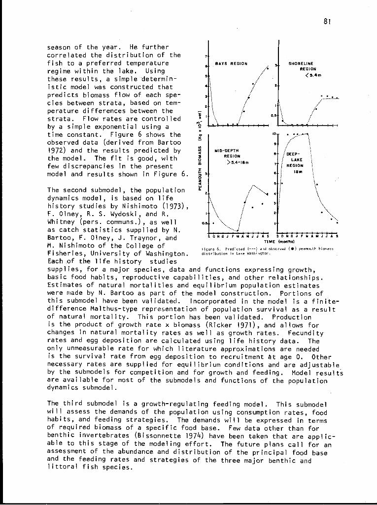
81

season of the year. He furthercorrelated the distribution of the Jfish to a preferred temperatureregime within the lake. Usingthese results, a simple determin-istic model was constructed thatpredicts biomass flow of each spe-cies between strata, based on tem-perature differences between thestrata. Flow rates are controlledby a simple exponential using atime constant. Figure 6 shows theobserved data (derived from Bartoo1972) and the results predicted bythe model. The fit is good, withfew discrepancies in the presentmodel and results shown in Figure 6.

The second submodel, the populationdynamics model, is based on lifehistory studies by Nishimoto (1973),F. Olney, R. S. Wydoski, and R.Whitney (pers. communs.), as wellas catch statistics supplied by N.Bartoo, F. Olney, J. Traynor, andM. Nishimoto of the College ofFisheries, University of Washington.Each of the life history studies

BAYS REGION

3+

2+

Y

Na MID-DEPTH

0REGION

>5.4-18m

3O

G

2

I +

o.u It

SHORELINEREGION

<5.4m

0 N D J F M A M J J A S S O N D J F M A M J J A STIME (months)

Figure 6. Predicted (---) and observed (0) peamouth biomass

distribution in Lake Washington.

supplies, for a major species, data and functions expressing growth,basic food habits, reproductive capabilities, and other relationships.Estimates of natural mortalities and equilibrium population estimateswere made by N. Bartoo as part of the model construction. Portions ofthis submcdel have been validated. Incorporated in the model is a finite-difference Malthus-type representation of population survival as a resultof natural mortality. This portion has been validated. Productionis the product of growth rate x biomass (Ricker 1971), and allows forchanges in natural mortality rates as well as growth rates. Fecundityrates and egg deposition are calculated using life history data. Theonly unmeasurable rate for which literature approximations are neededis the survival rate from egg deposition to recruitment at age 0. Othernecessary rates are supplied for equilibrium conditions and are adjustableby the submodels for competition and for growth and feeding. Model resultsare available for most of the submodels and functions of the populationdynamics submodel.

The third submodel is a growth-regulating feeding model. This submodelwill assess the demands of the population using consumption rates, foodhabits, and feeding strategies. The demands will be expressed in termsof required biomass of a specific food base. Few data other than forbenthic invertebrates (Bissonnette 1974) have been taken that are applic-able to this stage of the modeling effort. The future plans call for anassessment of the abundance and distribution of the principal food baseand the feeding rates and strategies of the three major benthic andlittoral fish species.

82

The fish feeding studies will function as the basis for linkages betweenthe three principal fish species. The competition model, as formulated,takes the projected required food base needs for each species, computesthe total demand for a given food base, and compares the total demandfor the available biomass. In case of marked competition, the demandfor the available food base may exceed 100% of the base. Based onobserved feeding strategies and expected success in the face of increasedcompetition, each species will be allotted less of the food base thanrequired for continued maximum growth, thus the growth and survival rateswill be modified. In order that the several benthic and littoral fishpopulations can be linked together and to allow for competition andchanges in population parameters, the necessary feeding data are beingestimated.

The benthic and littoral fish model, in addition to acting as a submodelof the general aquatic model, will be independently able to address thefollowing principal types of questions: (1) What relationships existbetween production and nutrient pools and the recycling of nutrients tothe other aquatic processes? (2) What is the relative importance of thespatial distribution of benthic and littoral fishes relative to theireffects on distribution of food organisms and nutrient recycling intodifferent strata? (3) How much energy is transferred to and from thebenthic and littoral fish populations? (4) How do the benthic andlittoral fish populations behave with changes in competition from otherspecies? (5) How do the benthic and littoral fish populations and theirdistributions respond to perturbations of the aquatic system such aschanges in water temperatures caused by localized water heating, fishharvests, selective fish eradications, changes in food bases, and intro-duction of competing fish species?

RESEARCH ACTIVITIES

Plankton-nutrient cycling research on the four lakes includes seasonalpatterns of phytoplankton productivity, biomass, respiration, growthkinetics, cell size, composition, light conditions, and nutrient supply;and zooplankton populations and grazing rates; and uses modeling tosimulate and evaluate the temporal-spatial. dynamics of plankton production.A comparison of several trophic status indicators in these four lakesis presented in Table 2.

Experiments have shown that the phytoplankton, from oligotrophic tomesotrophic lakes and under varying light conditions, were all stimulated

Table 2. Comparison of trophic status of four lakes in the Lake Washington drainage basin (averageyearly values).

Chloro-Produc-tivity ETS N

Total P PO4-P N03-N phyll a (mg C Secchl (mg 02 fixa-Lake 09/0 (ug/t) (u9/0 (ug/t) m-2 day-1) (m)

m 2 hr-1) kt(P04) tion

Findley 11.4 3.1 5.41 0.6 220 16.4 9 0.17 insig

ChesterMorse 6.9 2.1 9.36 1.1 262 8.3 13 0.36 insig

Sanmamish 48.0 7.0 86.0 7.11 499 3.5 2 0.42 sigWashington 18.7 1.1 56.5 9.5 1070 2.3 55 2.84 sig

83

by phosphorus concentrations as low as 1 pg P/liter. The light treatmentshad less effect than was anticipated; the greatest response to lightintensity was found at the lowest nutrient concentrations. It appearsthat cells grown at higher nutrient concentrations achieve their maximumgrowth response regardless of light intensity because of light adaptation,while cells at lower nutrient concentrations, being relatively nutrientstarved, are unable to make physiological adaptations to varying lightregimes.

Concurrent investigations included the relative contributions of threesize classes of the phytoplankton to lake productivity in four lakes ofcontrasting trophic state. Some of the routine in situ carbon-14 pro-ductivity samples were fractioned by selective filtration into net,nanno-, and ultraplankton by passing the carbon-14-labeled sample througha stacked series of three filters of 50, 5, and 0.45 um nominal porosity.The results for the ultraplankton were not entirely successful becauseof filtering characteristics of the 5-pm filter (E. B. Welch and G. R.Hendrey, pers. communs.). Except in Findley Lake, the contribution ofthe net plankton to that of the total community increased in a nearlylinear fashion with lake productivity. The discrepancies in Findleymay result from a lack of disruptive circulation, allowing the inclusionin the net plankton of cells that in the other lakes would have passedinto the nannoplankton. In all four lakes the relative contributionsof the net plankton to productivity were at a maximum early in thegrowing season in response to increased temperature during a period ofrelatively high nutrient concentration (Hendrey and Welch 1974). Thehypothesis that the relative contributions of the various size classesof the phytoplankton communities are related to the overall productivityof the lake is supported by observations both in nature and experimentalresearch (Hendrey 1973).

Growth kinetics of the net and nannoplankton were studied in conjunctionwith the nutrient enrichment experiments on Lake Washington. The half-saturation constants and optimal light intensities were, for the netplankton, kt = 4.6 pg P/liter, Ro = 4329 lux, and um = 0.135/hr. For thenannoplankton the values were kt = 2.8 ug P/liter, Ro = 1585 lux, andum = 0.167/hr. These results indicate that the nannoplankton cells wereable to maintain a higher maximum specific growth rate at lower levelsof available nutrients than were the net plankton. This extends to lakesthe conclusions of other investigators in marine waters (Dugdale 1967)that competition for available nutrients in oligotrophic waters wouldresult in the dominance of species with low kt values (Hendrey 1973).

Plankton research has included estimates of the seasonal distributionof the respiratory electron transport (ETS) activity and nitrogen fixationin the four lakes (Table 2). Respiration and nutrient regeneration ratesfor net plankton in the euphotic zone have been calculated from ETSactivities (A. Devol, pers. commun.; Packard et al. 1974, Conover andCorner 1968, Beers 1964). Nitrogen fixation rates were determinedperiodically by the acetylene reduction technique at three depths ineach of the lakes. Fixation began in June in Lakes Washington andSammamish and peaked during July and August. Chester Morse and FindleyLakes did not exhibit acetylene reduction activity until August and therates encountered were much lower than in the other two lakes.

84

Zooplankton grazing rates and life history stage densities for secondaryproduction estimates were determined in 1972 and 1973. Eight copepod,seven cladoceran, and nine rotifer species were identified. No onespecies of cladoceran or copepod occurred in all the lakes, but the roti-

fers are common throughout. Copepods in the lakes showed no clear dielvertical migration, while two cladocerans did migrate. Copepods weremost important numerically in the lakes. Some principal members wereDiaptomus ashZandi, which reached a seasonal maximum adult density of11/liter (mean of water column) in Lake Sammamish, and Limnocalanus in

Chester Morse, which reached a maximum of 0.7/liter. Two Diaptomusspecies are important in Findley Lake. Densities averaged about 10 timesgreater in Sammamish than in the two oligotrophic lakes.

Grazing rates of zooplankton (in situ) were partitioned for threephytoplankton size classes (same sizes as previously described) to assessthe effect of feeding on particle size and to relate to concurrent studieson fractioned phytoplankton productivity and nutrient responses.Zooplankton grazing appeared to account for a considerable proportionof the loss of nannoplankton in all lakes except for more eutrophicLake Sammamish, where blue-greens and net plankton are more frequentand detritus feeders are favored. Grazing of phytoplankton by zooplanktonstimulated photosynthetic carbon uptake in the light in excess of 200%over ungrazed populations. Phytoplankton loss rates from grazing rangedfrom 0.002 to 0.268 jig chlorophyll a per animal per day. Feeding wasfound to be maximum at low concentrations of algae. These rates accountfor from 2% to 247% of the average growing season productivity in thelakes. Net plankton (>50 um) were seldom grazed and, since that sizefraction and algal mass in general increased with mean productivity andnutrient content in the lakes, such decreasing efficiency in food transferis seen as a major effect of eutrophication (Stoll 1973).

The major limnetic fishes of Lake Washington (juvenile sockeye salmon,smelt, stickleback), Lake Sammamish (juvenile sockeye, kokanee, chinooksalmon), and Chester Morse Lake (pigmy whitefish, Dolly Varden, rainbowtrout) are being studied to develop data sets for implementation oflimnetic fish models. Estimates of population abundance, biomass,production, mortality, and growth for each major pelagic fish populationhave been completed in Lake Washington and Lake Sammamish and will beincluded in models after completion of successful simulations forjuvenile sockeye salmon. In addition, a bimonthly field study of sockeyefeeding on zooplankton has been completed in Lake Washington. Emphasisis placed on juvenile sockeye salmon because it is the predominant speciesfeeding on zooplankton, and zooplankton constitute the major link with

primary producers. This information, together with zooplankton communitystudies of Lake Washington by W. T. Edmondson of the University ofWashington, provides a basis for models of trophic relations of limneticfish.

Investigations of the limnetic fish populations of Lake Washington werecontinued through 1973. Population estimates were established throughthe acoustical procedures developed under the Sea Grant program and wereused in conjunction with biological information obtained from midwaternet sampling to obtain point estimates of abundance and biomass. Fromthese, growth rates and production of the different species were deter-

85

mined. Seasonal patterns in population parameters and changes in thehorizontal and vertical distributions of the major pelagic species andyear classes in the lake were analyzed also. A high correlation wasfound between the distribution of densities of the 1971 year classes ofsockeye salmon and longfin smelt, and was hypothesized to be due tophysical factors acting simultaneously on the two species. A comparisonof the vertical distributions of the major pelagic species provided ahighly significant multiple correlation coefficient, perhaps indicatingthat the same factors controlled the vertical distribution of each species.

Periodic monitoring of the size of the adult sockeye salmon populationin Lake Washington by acoustical methods is being continued through 1973and 1974. A series of 11 surveys over an identical transect pattern wascompleted during the months of June through November for estimation ofthe time and rate of movement into the lake, the total adult sockeyesalmon escapement, and the rate of migration up the Cedar River. Theestimate of escapement was similar to the estimate based on counts atthe Chittenden Locks by the Washington State Department of Fisheries.

Estimates of the abundance of presmolt sockeye salmon in the lake wereused in conjunction with estimates of adult escapement for further defini-tion of the spawner-recruit relationship for the Lake Washington sockeyesalmon run. A major goal in the continuing work on the spawner-recruitmodel is to develop the capability to predict escapement accurately fromacoustic estimates of smolts prior to outmigration (Traynor 1973).

Studies on the feeding ecology of fish have been continued with theobjective of determining the quantity of food consumed each day by juvenilesockeye salmon (Oncorhynchus nerka) in the limnetic zone of Lake Wash-ington to better understand the elements of the trophic level next beyondthe zooplankton. This information is essential to the current compre-hensive modeling studies of energy transfer in the Lake Washingtonecosystem.

Die] sampling of the 1971 year class was conducted in February and April1973; however, the presmolts were unavailable to the sampling gear inApril. Previously, successful diet sampling had been conducted in June,August, October, and December 1972. The first three of these dates coin-cided with the primary lacustrine growing period of the juvenile sockeyesalmon. A 5.5-m herring trawl was fished from the research vessel RVCommando, and echo-sounding gear was used to help locate the fish anddetermine depths to be sampled. Miller high-speed plankton nets weresent down with some of the trawl hauls to secure simultaneous planktonsamples.

The amount of food consumed, size of fish, and time of year were noted.Estimates of the rate of gastric evacuation were made by length group offish from nighttime samples. Inherent in the procedure was the assump-tion that no feeding occurs at night and that the volume of stomach con-tents decreases with time. The results indicated a decrease in a rateof gastric evacuation with increasing size of fish and with advancingtime of year, the latter probably as a result of decreasing night tem-perature of residence. The daily ration was computed by length group offish from samples collected throughout the 24-hr sampling period. The

86

procedures assumed that on the average the rate of food consumptionequals the absolute value of the rate of gastric evacuation. The amount

of food consumed increased with increasing size of fish; however, expresse,as a percentage of body weight, it decreased. Food consumption reacheda peak in autumn. Comparisons of stomach contents with the simultaneouslycollected plankton samples indicated selection of the larger prey species.Some differences in diet with respect to size of fish were noted in sum-mer (Doble 1974).

Seasonal abundance estimates of the 1971 year class of sockeye salmonhave been made on Lake Sammamish. These estimates incorporate age 0kokanee along with age 0 migratory sockeye. Seasonal abundance estimatesof resident kokanee and residual (age 1+) chinook also have been com-pleted. Catch data indicated that the 1970 year class of fall chinook,which entered the pelagic zone at least by July, constituted a majorproportion of the large fish targets enumerated acoustically throughoutthe remainder of the year (Berggren 1974).

Estimates of biomass and production, distribution, and food habits ofthe 1971 year class of sockeye and other limnetic fish were made for LakeSammamish. The resulting biomass and production per hectare were greaterthan in Lake Washington (Traynor 1973), indicating a large 1971 year classof sockeye in Lake Sammamish. The population approached approximatelyone-half the density per unit volume of the 1969 year class of sockeyesalmon in Lake Washington, the largest year class observed since 1969when monitoring of the lake began. Horizontal and vertical distributionsreflected the effects of limitation of habitat by oxygen deficiency inthe hypolimnion. Minimum differential feedings of juvenile sockeye sal-mon were observed between 10-mm length groups. Daphnia was the predomi-nant food item during most of the year although ostracods were utilizedduring the winter at a time when feeding was reduced.

The Chester Morse Lake study is designed to determine the populationsizes, age and growths, length-weight relationships, fecundity, sexratios, mortality rates, and feeding habits of rainbow trout (SaZmogairdneri) and Dolly Varden (SaZveZinus malma). Biomass and productionof the two species are being estimated from this information. Petersonestimates from the August data result in population estimates of4650 <8138 <15,752 rainbows and 1684 13015 16147 (a = 0.05) Dolly Varden.A Schnabel estimate over the eight-month sample period results in popu-lation estimates of 9830 rainbows and 1305 Dolly Varden. Age determina-tions are being completed to calculate age distributions of sampledpopulations. The feeding habits of pygmy whitefish, Prosopium couZteri,and the age, growth, and fecundity are being incorporated in the dis-cussion of this significant food item of Dolly Varden. Rainbow datawill be used in the basic population dynamics model.

Development of studies on benthic processes is based on distinct transferswith the plankton community and between internal compartments of benthiccommunities. The benthic community of a lake is being considered asdependent upon transfers of energy, carbon, and nutrients from sedimentedorganic and inorganic matter into paths of substrate burial, chemicaloxidation, microbial-macroinvertebrate metabolism, fish predation, andinsect emergence. Sedimentation; exchange of carbon, nitrogen, and

87

phosphorus; and carbon fixed by periphyton are linked to the availablecarbon, nitrogen, phosphorus, and microflora-mesofauna components of thebenthic community. Sedimentation measurements include inputs of majorcations, heavy metals, and dissolved and particulate carbon, nitrogen,and phosphorus from endogenous organic matter production, and organics andinorganics from exogenous sources. Exchange of carbon, nitrogen, phos-phorus, and oxygen by the benthic community occurs during chemicaloxidation, oxygen consumption, microbial mineralization, and macro-invertebrate respiration (Figure 4).

Sedimentation patterns were measured in the four lakes of the LakeWashington drainage basin. More extensive treatment of sediment fluxeswere made in Findley Lake and sediment nutrient regeneration from insitu Lake Sammamish experiments. Sediment aliquots were analyzed fortotal carbon (990 organic carbon), phosphorus, nitrogen, and iron anda number of trace metals. Basic differences in the lakes have beenassessed by elemental fluxes, percent contents, and ratios of carbon:nitrogen, nitrogen:phosphorus, and carbon:phosphorus. The sedimenttrap data indicate that a major input to Findley Lake is allochthonousorganic while in Chester Morse Lake inorganic inputs from either bottomsediment resuspension or from allochthonous sources are predominating.The sedimentation data from Lake Sammamish indicate the relative impor-tance of inputs, especially of phosphorus and iron, from sediments broughtabout by the reduction of Fe3+ and dissolution of phosphorus in theoxygen-depleted sediment-water interface. Seasonal plankton sedimenta-tion data rank the lakes in the same order relative to productivity asmeasured by carbon-14 assimilation: Lake Washington > Lake Sammamish> Chester Morse > Findley Lake (D. Spyridakis pers. commun., Birch1974). Physical and chemical characteristics of the lake sediments havebeen measured by Bauer (1971) and Horton (1972).

Research on the contribution of allochthonous inputs to the particulatecarbon and nutrient pools of the benthic community are being conductedat Findley Lake. Particulate carbon enters the lake by litterfall, surfacerunoff, and snowmelt, and is composed mainly of needles of western hemlock(Tsuga heterophyZZa) and silver fir (Abies amabiZis). Litterbags ofconifer needles are being used in decomposition studies by measuringweight loss and changes in nutrient content (G. Rau pers. commun.).

Pollen, diatom, and sedimentary chlorophyll analysis of Findley Lakeindicates distinct relationships between the aquatic and terrestrialenvironments. Any severe disturbance of the terrestrial environmentcaused shifts in the aquatic ecosystem. These changes often involveda sequence of changes in the dominant diatom present. Further, thepattern of changes in the aquatic ecosystem tended to be related to thetype of disturbance in the surrounding watershed, for example, forestfires. Sedimentary chlorophyll either did not change significantly orvaried in relation to changes in the number of conifer needles in thesediment (Adams 1973).

The sediment nutrient regeneration studies in Lake Sammamish involvedthe incubation of six sediment-water columns in enclosed cylinders.Starting in the fall of 1972, water samples were removed from the columnsand analyzed for total phosphorous and total soluble phosphorus, total

88

and soluble iron, dissolved oxygen, and alkalinity. Specific conduc-

tance, pH, temperature, total nitrogen, total soluble nitrogen,N03-plus-N02-N and HH4-N were also monitored. This experiment wasrepeated in the spring of 1973 employing the same methods. Differences

in the rates of phosphorus and iron release as well as oxygen depletionare easily attributable to the distinct temperature regimes observed inthe lake water during the winter and spring incubations. The loss ofoxygen was accompanied by increases in phosphorus, iron, and nitrogencontents. Conductivity and alkalinity increased while pH decreased to6.8 in most cases.

Total phosphorus increased in most of the columns to about 200 ± 20 jig/liter, while soluble phosphorus increased to 140 ± 10 ug/liter. Total

iron increased in most of the columns to 2.1 ± 0.2 mg/liter, while solubleiron increased to 1.50 ± 0.1 mg/liter. Generally, the total phosphorusand total soluble phosphorus curves paralleled each other, coincidingwith reduction of Fe3+. Purging the columns with N2 affected the rateof oxygen depletion and subsequent rate of release of nutrients but notthe magnitude of release. The high iron content measured in the columnsunder nearly complete anoxic conditions increased the sensitivity of thesystems to any possible oxygen intrusion. Thus, in some of the columnsystems, iron and phosphorus were found to decrease following their peakconcentrations as a result of the precipitation of ferric hydroxy and/orferric hydroxyphosphate compounds.

With respect to nitrogen, N03-plus-N02-N generally decreased in thecolumns but did not disappear. In most cases NH4 -N was initiallyincreased to between 150 and 180 pg/liter before decreasing to values lessthan 100 pg/liter. In general it was found that total inorganic nitrogenincreased 20%-25% above the initial levels followed by a marked decreasein the later stages of incubation. This decrease represented a 40%-50%loss of the initial inorganic nitrogen contents. It appeared that asthe anoxic conditions became more pronounced there was a loss of nitrogenfrom the system by biological or chemical denitrification, or both.

The maximum rates of phosphorus release were from 4 to 6 mg m-2 day-1at temperatures between 6° and 10°C and increased to 11-15 mg m-2 day-1at temperatures between 10° and 18°C. The maximum amount released wasnot a function of temperature. The release of phosphorus in the columnsincreased to a maximum between 550 and 600 mg/m2 for total phosphorusand 350 and 400 mg/m2 for total soluble phosphorus. These values comparedwell with those obtained for the lake but were 50%-60° lower than thosein a laboratory experiment conducted at 25°C under completely mixed andanaerobic conditions. Comparison of the maximum amounts of phosphorusin the in situ column and in 30-m-deep lake water column with the surface(10-cm-deep) sediment phosphorus contents revealed that as much as 19%-20oof the sediment phosphorus was released in both cases. The correspondingmaximum iron values in the water columns represented 4%-5i of the amountof iron in the surface sediments.

It can be concluded that sediment phosphorus release is a primary inputfactor in the dynamics of phosphorus in the lake. The release of phos-phorus from the sediments could supply enough phosphorus to supportsummer production in Lake Sammamish provided that a lake mixing mechanism

89

were available to supply hypolimnetic phosphorus to the photic zone.About 75% of the total phosphorus released into the hypolimnion of thelake is supplied by the sediments, on the basis of the in situ columnstudy results. The lack of response in the trophic status of LakeSammamish following sewage diversion in 1968 could very well be attributedto this demonstrated ability of lake sediments to supply large amountsof nutrients to the lake water column. It will be difficult to anticipateany changes in the nutrient status of the lake within a time period com-parable to that observed in Lake Washington case, as long as hypolimneticoxygen deficits continue during stratified periods (D. Spyridakis pers.commun., Monahan 1974).

The measurement of sediment metabolism in Lake Washington was performedby Pamatmat and Bhagwat (1973). They reported that the rate of totaloxygen uptake by the sediment represents the sum of aerobic plus anaerobicmetabolism in a surface layer of indeterminate thickness. In situ ratesof anaerobic metabolism in the sediment column can be determined by meansof a triphenyltetrazolium chloride (TTC) method of total de.hydrogenaseassay. In Lake Washington, which has had a long and well-documentedhistory of eutrophication and deposition of sewage effluent, anaerobicmetabolism by bacteria alone in the sediment column far exceeds totalmetabolism as estimated by the rate of total oxygen uptake by undisturbedcores. The total oxygen uptake (biological and chemical) ranged from0.16 to 0.45 calorie per core per hour while the dehydrogenase activity(TTC) ranged from 0.37 to 4.7 calories per core per hour.

Mineralization of organic compounds in the benthic community by bacteriahas been assessed by [14C]glucose uptake. Sediment samples have beencollected and analyzed from the four lakes. The rate of glucose mineral-ization bY4 the bacteria was measured by incubating sediment and uniformlylabeled [ C]glucose at the in situ temperature. In each lake sampled, thebacteria associated with the shore sediment were more numerous andexhibited a higher rate of glucose mineralization than those found inthe sediment of deepwater stations. In all lakes the glucose mineraliza-tion rate was greater in summer, decreased in fall, and attained a minimumvalue in winter and early spring. Sediment samples collected in winterwere incubated at the in situ temperatures prevailing at other seasons ofthe year. The rate of glucose utilization or turnover time fell very closeto the rates obtained at the different seasons. Samples collected duringthe summer and tested under conditions prevailing during colder periodsalso gave excellent results. These data indicate that the temperaturein the environment has a great influence on the activity of the bacteriaresponsible for mineralization.

Aerobic and anaerobic bacterial plate counts were run on the sedimentscollected. Counts obtained with anaerobic incubation, which enumeratesanaerobes and facultative anaerobes, were one order of magnitude lowerthan aerobic counts. Sediment samples collected from deep water werealso about one order of magnitude lower than those obtained from shallowor shore stations. In addition, the numbers of organisms capable ofdigesting chitin or cellulose were estimated by adding reprecipitatedchitin (0.6?) or reprecipitated cellulose (0.1%) to the medium. Chitino-clastic or cellulolytic bacteria were easily detected on the medium bya clear zone or plaque that appeared around the colonies hydrolyzing

90

the complex molecules. The highest bacterial counts were obtained withaerobic incubation. Bacteria capable of digesting chitin were found inall stations sampled in the four lakes. All but one chitinoclast testedwere obligate aerobes. As with total bacterial counts, the totalchitinoclast biomass and the percentage of total aerobic chitinoclastscounted were higher for shallow or shore samples than for the deeperstations. There appeared to be an increase in numbers of chitinoclastsin the winter months over the summer months. Studies on the four lakesshowed that the highest numbers of chitinoclasts were found in the shorestations of Chester Morse and Findley Lakes; however those organismsisolated from Lakes Washington and Sammamish were more rapid inhydrolyzing chitin.

Cellulolytic bacteria have been isolated from Lakes Sammamish andWashington and no doubt play a part in the role of cellulose decompositionin the lake systems. The strains of cellulolytic bacteria isolated areobligate anaerobes; however, they have not been identified.

Through expansion of the above research on bacteria and subsequentmodeling, we plan to address such questions as: What changes occur inmineralization rates with different temperatures and sedimentation rateswithin and between lakes? If mineralization rates of organics differfor lakes but not for temperatures and sediments, will the variation berelated to proportions and differences in availability of carbon, nitro-gen, and phosphorus in various organic substrates? Or, more specifically,how does the availability of organic nutrients limit utilization of carboncompounds?

The macroinvertebrate populations of the benthic community are beingdefined. The objective is to measure energy and carbon flow with fieldestimates of biomass, density, species composition, life cycles, andliterature values for assimilation, mortality, and respiration. The

research includes assessing the relationship between macroinvertebratebiomass, density, and distribution and the standing crop and distributionof detritus. Preliminary information indicates that the major standingcrop of detritus and benthic organisms is at the mouths of inlet streamsand rivers of all four lakes. A concurrent study of aquatic insectshas found the highest emergence for insects in Findley Lake near inletareas of high detrital standing crops (T. Sherk pers. commun.). Thesedata will be used to evaluate the hypothesis that a significant portionof fish production is supported by the detrital food chain. In addition,this information will serve as input to a model on overall lake pro-ductivity.

Chironomid larvae are the predominant organisms in the profundal areasof all lakes but Chester Morse, where Pontoporeia affinis is the pre-dominant species. Other groups found commonly in the profundal zone areoligochaetes and sphaerids. Of lesser importance are ceratopogonids,gastropods, and leeches. Littoral areas show increased species diversityas expected with sialids, tricopterans, ephemeropterans, and water mites,in addition to the groups mentioned above.

A length-weight relationship has been established for chironomids andsimilar relationships for P. affinis, oligochaetes, and sphaerids are

91

being explored. Preliminary estimates of chironomid larval mortalityand growth rates show predation pressure in the spring and fall coinci-dent with their primary growth periods. Stratification over the summerlimits predation and growth because of lack of oxygen on the bottom.Temperature drops over the winter reduce metabolic activity of bothpredator and prey, with mortality and growth leveling off. Emergenceoccurs in the spring, and very high mortality in the pupal stage is dueto increased visibility during migrations to the surface.

Fish-feeding on benthic organisms has been shown to be selective. Pre-liminary evidence indicates a preference for chironomid larvae and pupae.Chironomids in the lakes studied have a nutritional makeup of approximately60% protein, loo ash, 22% carbohydrate, and 8% fat. Whether they arepreferred as a food type because of greater availability to the predatoror nutritional value is unknown.

The productivity of benthic organisms has been shown to depend heavilyon primary production, allochthonous input, lake sedimentation rates,fish feeding, and several physical properties (temperature, mixing,depth, oxygen concentration, etc.; Johnson and Brinkhurst 1971). Cor-relations with these parameters are planned when the data becomeavailable.

The production of macroinvertebrates and fish in the Cedar River isunder investigation as part of the studies of streams in the ConiferousForest Biome. The Cedar River system is unique by virtue of its multipleuse. The free-flowing river is divided into three rather discretereaches. The upper reach, immediately above Chester Morse Reservoir,is relatively unaffected by man's activities except for well-controlledlogging. The middle reach, immediately below the dam, is directlyinfluenced by the reservoir and fluctuating discharge due to hydro-electric generation. The lower reach, extending to Lake Washington, isdelineated by the City of Seattle water supply diversion at Landsburg.This diversion limits the upstream extent of migration of anadromousfish, of which sockeye salmon are the most numerous. The watershedabove the diversion is a source of municipal and industrial water supplyfor metropolitan Seattle, and has unexploited resident fish populations.

Initially, quantitative macroinvertebrate and water quality sampleswere collected from the three river reaches over a 17-month period.This is being followed by a quantitative study of the fish populationsthrough electrofishing methods. Preliminary estimates of the fish popu-lations indicate a general increase in biomass downstream and a pre-dominance of rainbow trout or rainbow-steelhead trout (Salmo gairdneri)at each station during the summer sampling period. Significant numbersof chinook (Oncorhynchus tshcaaytseha) and coho (0. kisutch) salmon werealso found below the Landsburg diversion. Water quality analysis wasalso conducted, and an increase was found in total alkalinity, pH, con-ductivity, hardness, and temperature from upstream to downstream. Thecontribution of plankton from Chester Morse Reservoir to the river insectcommunity is reflected in increased abundance of Hydropsyche and Simuliidae.The production of Simuliidae was estimated to increase by about twoorders of magnitude immediately below the reservoir. Further work isbeing devoted to production estimates of Plecoptera (with the assistance

92

of Dr. Arden Gaufin, University of Utah), Ephemeroptera, Trichoptera,and Diptera, as well as the input of allochthonous material in the stream

system (J. Malick pers. commun.).

FUTURE RESEARCH AND MODEL VERIFICATION

Research on the trophic dynamics of lakes in 1974 will concentrate onsynthesis of past data into general models and on using these modelsto guide extensive diel and bloom period sampling. This sampling will beconcentrated on Lake Washington, with synoptic type measurements inthe other lakes. These data will be incorporated into a finer resolution.model of a Lake Washington water column and will be used to update thecomparative, cross-lake model. The sampling will help in elucidatingseveral of the key mechanisms regulating lakes. Thus research willconcentrate on the quantitative relations between nutrient cycling andproduction, and factors affecting material and energy transfers betweentrophic levels, population dynamics of some aquatic organisms, importanceof physical transport processes, and the response of an aquatic system toexogenous perturbations. Couplings to higher trophic levels will beprovided by several fish studies.

LAKE RESEARCH AT FERN AND CASTLE LAKES

Lake research outside the Lake Washington drainage basin but supportedby the Coniferous Forest Biome has been completed (Olsen and Chapman1972). Results of the Fern Lake research by the College of Fisherieswere synthesized into an ecosystem model during 1973 (Fowler 1973).Submodels for hydrology, nutrients, phytoplankton, and zooplankton werecombined into a simulation model that uses temperature and climatologicaldata as driving variables to predict the levels of various other com-ponents of the ecosystem. Predictions from all portions of the modelhave been compared with those observed in data collected at Fern Lake,Washington.

Modeling and research on the phosphorus dynamics (Richey 1974b) and heatbudgets in Castle Lake, California, were completed in 1973. This studyidentified important phosphorus parameters and developed a methodologyto measure them in the lake. Expected rates of phosphorus fluxes wereestimated by the use of. isotope measurements, and phosphorus pool sizeswere assessed through chemical determinations and from calculations ofphytoplankton, bacteria, and zooplankton carbon masses and transfers.The heat budget of Castle Lake was considered as an accounting systemfor energy flux and a physical framework that governs a majority ofbiological processes. The heat budget encompasses the important abioticphenomena of lake stratification, absorption of net radiation, heatstorage and loss, net advection of energy into and out of a lake, turbu-lence, and light regimes (J. E. Richey pers. commun.).

93

REFERENCES

ADAMS, D. 1973. The paleoecology of two lakes in western Washington.M.S. thesis, Univ. Washington, Seattle. 58 p.

BARTOO, N. W. 1972. The vertical and horizontal distributions of northernsquawfish (Ptychocheilus oregonensis), peamouth (MyZocheilus caurinus),yellow perch (Perca flavescens), and adult sockeye salmon (Oneorhynehusnerka) in Lake Washington. M.S. thesis, Univ. Washington, Seattle. 60 p.

BAUER, D. H. 1971. Carbon and nitrogen in the sediments of selectedlakes in the Lake Washington drainage. M.S. thesis, Univ. Washington,Seattle. 91 p.

BEERS, J. R. 1964. Ammonia and inorganic phosphorus excretion by theplanktonic chaetognath, Sagitta hispida (Conat.). J. Conseil, ConseilPerm. Int. Explor. Mer. 24:123-129.

BERGGREN, T. 1974. Seasonal changes in the abundance, biomass, production,distribution, and feeding of the 1971 year class of sockeye salmon in LakeSammamish. M.S. thesis, Univ. Washington, Seattle. 80 p.

BIRCH, P. B. 1974. Sedimentation of C, N, P and Fe in four lakes ofthe Lake Washington drainage basin. M.S. thesis, Univ. Washington,Seattle. 163 p.

BISSONNETTE, P. A. 1974. Extent of mercury and lead uptake from lakesediments by Chironomidae. M.S. thesis, Univ. Washington, Seattle. 96 p.

BROOKS, J. L. 1968. The effects of prey size selection by lakeplanktivores. Syst. Zool. 17:272-291.

CHARNOV, E. L. 1973. Optimal foraging: Some theoretical explorations.Ph.D. thesis, Univ. Washington, Seattle. 95 p.

CLYMER, A. B. 1972. Next-generation models in ecology. IN: B. C.Patten (ed.), Systems analysis and simulation in ecology, p. 533-569.Academic Press, New York.

CONOVER, R. J., and E. D. S. CORNER. 1968. Respiration and nitrogenexcretion by some marine zooplankton in relation to their life cycles.J. Mar. Biol. Assoc. U.K. 48:49-75.

DAWSON, J. J. 1972. Determination of seasonal distribution of juvenilesockeye salmon in Lake Washington by means of acoustics. M.S. thesis,Univ. Washington, Seattle. 112 p.

DOBLE, D. D. 1974. Diel feeding periodicity, instantaneous rate ofgastric evacuation, and daily zooplankton ration of juvenile sockeyesalmon (Oncorhynchus nerka) in Lake Washington. M.S. thesis, Univ.Washington, Seattle. 79 p.

DRYFOOS, R. L. 1966. The life history and ecology of the longfin smeltin Lake Washington. Ph.D. thesis, Univ. Washington, Seattle. 229 p.

96

L. J. Dempster, and R. H. Waring (eds.), Proceedings--Research on con-iferous forest ecosystems--A symposium, p. 301-315. USDA For. Serv.,Portland, Oreg.

WERNER, E. E. 1972. On the breadth of diet in fishes. Ph.D. thesis,Michigan State Univ., East Lansing.

WOODEY, J. C. 1972. Distribution, feeding, and growth of juvenilesockeye salmon in Lake Washington. Ph.D. thesis, Univ. Washington,Seattle. 207 p.