integrated simulation and model-checking for the analysis of biochemical systems

Integrated Simulation and Model-Checkingfor the Analysis of Biochemical Systems

Federica Ciocchettaa,1, Stephen Gilmorea,2,Maria Luisa Guerrieroa,3, Jane Hillstona,b,4

a Laboratory for Foundations of Computer Science, The University of Edinburgh, EH8 9AB Edinburgh,Scotland

b Centre for Systems Biology at Edinburgh (CSBE), Edinburgh, Scotland 5

Abstract

Model-checking can provide valuable insight into the behaviour of biochemical systems, answering quantita-tive queries which are more difficult to answer using stochastic simulation alone. However, model-checkingis a computationally intensive technique which can become infeasible if the system under consideration istoo large. Moreover, the finite nature of the state representation used means that a priori bounds must beset for the numbers of molecules of each species to be observed in the system.

In this paper we present an approach which addresses these problems by using stochastic simulation andthe PRISM model checker in tandem. The stochastic simulation identifies reasonable bounds for molecularpopulations in the context of the considered experiment. These bounds are used to parameterise the PRISMmodel and limit its state space. A simulation pre-run identifies interesting time intervals on which model-checking should focus, if this information is not available from experimental data.

Keywords: Systems biology, process algebra, model-checking, stochastic simulation

1 Introduction

Model-checking and stochastic simulation techniques have both been applied to thestudy of biochemical systems, and both allow researchers to make predictions andtest hypotheses. The questions which they answer can be different and complemen-tary.

The stochastic simulation approach allows modellers to analyse the time evo-lution of all species composing a system at the same time. However, since one

1 Email: [email protected] Email: [email protected] Email: [email protected] Email: [email protected] The Centre for Systems Biology at Edinburgh is a Centre for Integrative Systems Biology (CISB) fundedby the BBSRC and EPSRC in 2006

Electronic Notes in Theoretical Computer Science 232 (2009) 17–38

1571-0661/$ – see front matter © 2009 Elsevier B.V. All rights reserved.

www.elsevier.com/locate/entcs

doi:10.1016/j.entcs.2009.02.048

mailto:[email protected]




http://www.elsevier.com/locate/entcs

simulation run generates a single trajectory out of all the possible behaviours ofsystems, usually average values among several runs need to be considered to achievethe necessary level of confidence in the results obtained.

Probabilistic model-checking instead answers quantitative temporal queries byperforming an exhaustive exploration of all the possible paths through the system.Model-checking requires both the model and the specification of the system understudy to be formally specified: this allows the user to detect possible errors in themodel or the presence of deadlock states, and to automatically verify whether or notrelevant properties are satisfied by the model. For these reasons, when analysingbiochemical systems, it is often more desirable to perform model-checking thansimulation. Unfortunately, model-checking has one major problem, the state-spaceexplosion: a system with too many states becomes intractable and needs to beconstrained.

The aim of the present work is to investigate how combined use of stochasticsimulation and model-checking can lead to a better understanding of biochemicalsystems. In particular, we investigate how to exploit the knowledge acquired fromthe simulation to make the model-checking feasible. Specifically, the simulationresults are used to establish reasonable lower and upper bounds for the moleculecounts of the species involved. We show with a simple example how, by usingthe bounds estimated by our approach, we are able to substantially speed up themodel-checking without introducing significant error.

We use the high-level modelling language Bio-PEPA [6,7], a timed process al-gebra designed specifically for the description of biological phenomena and theiranalysis through quantitative methods such as stochastic simulation and model-checking. Several alternative representations can be automatically generated froma Bio-PEPA specification, allowing us to perform different kinds of analyses on thesame model. In particular, we consider here two generated models: one suitable forstochastic simulation using Dizzy [18], the other suitable for model-checking usingPRISM [17].

The novel contribution offered by the present paper is the use of simulationand model-checking conjoined in two ways. Firstly, we use simulation to boundthe model-checking problem and later we compare model-checking results obtainedthrough both exact and approximate probabilistic model-checking. The formermethod elaborates the full state-space of the model and uses linear algebra to solvethe underlying Markov chain. The latter uses simulation to answer the model-checking problem, up to a satisfactory confidence interval.

The rest of the paper is structured as follows. In Sect. 2 we discuss some moti-vations of our work and we illustrate them by means of a simple example. Sect. 3is devoted to the description of the background. In Sect. 4 we present our approachand in the following Sect. 5 we apply it to two biochemical networks. Some relatedwork is reported in Sect. 6 and finally, some concluding remarks are presented inSect. 7.

F. Ciocchetta et al. / Electronic Notes in Theoretical Computer Science 232 (2009) 17–3818

2 Motivation

Analysing models of biological processes via probabilistic model-checking has con-siderable appeal. As with stochastic simulation the answers which are returned frommodel-checking give a thorough stochastic treatment of the small-scale phenomenawhich are of greatest interest to computational biologists today. However, in con-trast to a simulation run which generates just one of many possible trajectories, theanalysis results computed by probabilistic model-checking give a definitive answer.That is, it is not necessary to re-run the analysis repeatedly and compute ensembleaverages of the results. Further, by building a reward structure over the model it ispossible to express complex analysis questions and evaluate these through model-checking. This form of analysis has the power to expose of the system under studysignificant temporal behaviour which could not be appreciated from simple inspec-tion of the species time-series generated by simulation runs (see for example [10]).

Set against this, the probabilistic model-checking approach faces the well-knownproblem of state-space explosion where, as the complexity of the system under studyincreases, there is an exponential growth in the state-space of the underlying model.The use of an exact discrete-state representation of the state-space of the modelrestricts the use of probabilistic model-checking to the analysis of problems whereall of the species are available in low copy numbers. Multi-scale models (where somespecies are in plentiful supply and others have very low molecule counts) generallygive rise to discrete-state problems whose numerical solution is infeasible.

Even in the case where all of the chemical species involved are present only in lowcopy numbers it is still necessary to place a bound on the maximum molecule countwhich each species will attain. For models involving biochemical processes such assynthesis, no such bounds can be established. In the present paper we describethe application of stochastic simulation to the problem of bounding discrete-statemodels allowing us to convert an unbounded model-checking problem into a boundedone.

To illustrate the problem which we are discussing here consider a simple modelof the Michaelis-Menten reactions involving four chemical species: an enzyme E,a substrate S, a compound E:S and a product P . The species react over threereaction channels: r1 converting E and S to E:S , the backward reaction r−1 takingE:S to E and S, and the reaction r2 converting the compound E:S into productP and releasing the enzyme E. The reaction rates are governed by kinetic lawsinvolving rate constants (k1, k−1 and k2) and the molecular counts of the speciesinvolved.

The chemical equation describing Michaelis-Menten reactions is

E + Sk1

k−1

E:Sk2

E + P .

In the Bio-PEPA language the notation fri is used to indicate the rate associatedwith the reaction ri.

F. Ciocchetta et al. / Electronic Notes in Theoretical Computer Science 232 (2009) 17–38 19

fr1 = k1 × E × S

fr−1 = k−1 × E:Sfr2 = k2 × E:S

When initiated with low molecule counts (E,S,E:S , P ) = (5, 5, 0, 0) this modelgives rise to a state space of very modest size, as indicated in Fig. 1. Starting in

(5, 5, 0, 0)

(4, 4, 1, 0) (5, 4, 0, 1)

(2, 2, 3, 0) (3, 2, 2, 1) (4, 2, 1, 2) (5, 2, 0, 3)

(3, 3, 2, 0) (4, 3, 1, 1) (5, 3, 0, 2)

(1, 1, 4, 0) (2, 1, 3, 1) (3, 1, 2, 2) (4, 1, 1, 3) (5, 1, 0, 4)

(0, 0, 5, 0) (1, 0, 4, 1) (2, 0, 3, 2) (3, 0, 2, 3) (4, 0, 1, 4) (5, 0, 0, 5)

r1r−1

r1r−1 r1r−1

r1r−1

r1r−1 r1r−1 r1r−1

r1r−1r1r−1

r1r−1

r1r−1 r1r−1 r1r−1 r1r−1 r1r−1

r2

r2 r2

r2 r2 r2

r2 r2 r2 r2

r2 r2 r2 r2 r2

Fig. 1. Discrete state-space representation of the Michaelis-Menten reactions.

the state (5, 5, 0, 0) each of the four species E, S, E:S and P can achieve molecularcounts in the bounded integer range 0 to 5. Of the 6×6×6×6 = 1296 potential statesin the full product state space of this model only 21 of these are actually reachableby any sequence of reactions. One reachable state, (5, 0, 0, 5), is a “deadlock” statewith no outgoing transitions. Reaction r1 is prevented because S = 0 and reactionsr−1 and r2 are prevented because E:S = 0.

However, if we consider an extension of the model with an additional reactionr0 which synthesises the compound E:S

∅k0

E:S

with the synthesis occurring at a constant rate fr0 = k0 then this additional reac-tion channel changes the analysis of the model dramatically. The state which waspreviously a deadlock state now admits an r0 reaction which leads it to a previ-ously unreachable state, (5, 0, 1, 5). The reactions r−1, r1 and r2 can occur in statesreachable from that one as shown in Fig. 2.

Each of these states, and every other state, now allows an r0 reaction, takingthem to previously unreachable states each of which allows r0 and reactions r−1, r1

and r2 subsequent to that. The effect of introducing this single synthesis reactionis that we now cannot find any upper bound N such that the molecular speciescounts are guaranteed to lie in the bounded integer range 0 to N . In general, if weare unable to bound the reachable state-space then we cannot analyse our model


(5, 0, 0, 5) (6, 1, 0, 5)

(5, 0, 1, 5) (6, 0, 0, 6)r0

r1r−1r2

Fig. 2. Synthesis of the compound adds further states.

by probabilistic model-checking.Here we seek to bring the unbounded state-space back within bounds by exploit-

ing the following observations.

(i) The generation of the derivation graph of the underlying state-space does nottake into account the numerical values assigned to the rate constants, and thepropensity functions which depend on those. This means that the derivationgraph may include many states which the system is almost sure not to reachwithin a particular time bound.

(ii) Most chemical systems involve several widely varying time scales, so such sys-tems are nearly always stiff [19]. A consequence of this is that the first passagetime to many states is likely to be long and truncation of the state-space usinga time-bounded reachability metric is likely to be productive.

(iii) Many of the logical formulae which we wish to check involve reaching within afixed time bound model states which satisfy a given predicate.

(iv) Stochastic simulation methods such as Gillespie’s Direct Method [9] gener-ate exact stochastic simulations of trajectories from the initial state to statesreachable within a given time bound.

3 Background

The context of application we consider is that of biochemical networks. A bio-chemical network is composed of n species which interact through m reactions; thedynamics of reaction j is described by a kinetic law fj . The quantitative behaviourof a biochemical network depends on the initial values of the involved species andon the kinetic parameters.

In the following, we distinguish between structurally bounded and structurallyunbounded biochemical networks. A biochemical network is (structurally) boundedif for each species Si (i ∈ {1, . . . , n}) there exists a value Maxi ∈ N such thatXi(t) < Maxi ∀t, where Xi(t) is the amount of species i at time t. The values Maxi

for a generic biochemical network, if they exist, depend on the kind of reactionsinvolved, on their kinetic laws and constants, and on the initial state of the system.If, instead, the amount of one or more species has the potential to grow withoutbound, the network is structurally unbounded.

If we assume a finite number of molecules for each species in the initial state,and we do not consider reactions which can increase the amount of any species,then we have structurally bounded networks. If instead, we consider synthesis


reactions (e.g. ∅ → A, C → C +A) or arbitrary split reactions, we have structurallyunbounded networks. In many cases a structurally unbounded network may havea pragmatic bound because of the quantitative relations between the moleculesand the reactions composing the network. Specifically, even though some synthesisreactions are present, the average value of each species can be bounded.

Note that, in the real world, biochemical networks are generally bounded: degra-dation, for instance, is an important mechanism cells use to avoid an uncontrolledincrease of molecules. However, structurally unbounded networks are interestingbecause an anomalous behaviour of some biological entity could trigger such anuncontrolled growth. Moreover, biological models are often limited to particularsub-systems, in which the bounding reaction might not be included.

3.1 Bio-PEPA

The Bio-PEPA language [7,6] allows us to explicitly represent some features of bio-chemical models, such as the stoichiometry of reactions and the role of each speciesin a given reaction, and allows the definition of general kinetic laws. Bio-PEPA mod-els can be analysed by different techniques (stochastic simulation, analysis basedon ODEs, numerical solution of the continuous-time Markov chain (CTMC), andprobabilistic model-checking), since the mappings of Bio-PEPA models into speci-fications for those approaches have been defined [6].

The language is based on discrete levels of parameterised species: each compo-nent represents a species and its parameter may be interpreted as the number ofmolecules or discrete levels of concentration depending on the type of analysis to beapplied. Parametric levels are considered for the definition of the transition systemand for the derivation of a CTMC whose states represent the concentration levelsof the species.

The syntax of Bio-PEPA is defined as:

S ::= (α, κ) op S | S + S | C P ::= P ��L P | S(l)

where op = ↓ | ↑ | ⊕ | | .The component S is called a sequential component (or species component) and

represents the species whereas the component P , called a model component, de-scribes the system and the interactions among components. The parameter l ∈ N

represents the discrete level of concentration. The prefix term (α, κ) op S containsinformation about the role of the species in the reaction associated with the actiontype α: κ is the stoichiometry coefficient of the species and the prefix combinator“op” represents the role of the element in the reaction. Specifically, ↓ indicates areactant, ↑ a product, ⊕ an activator, an inhibitor and a generic modifier. Theoperator “+” expresses the choice between possible actions and the constant C isdefined by an equation C

def= S. Finally, the process P ��L Q denotes the cooperation

between components: the set L determines those activities on which the operandsare forced to synchronise.

In order to specify a model in Bio-PEPA, in addition to the definition of the


species and model components, we need to define a set of functional rates F ex-pressing the kinetic laws of the reactions, a set of constant parameters K and thecompartment size (in the set V). For discrete state space analysis the behaviour ofthe system is defined in terms of an operational semantics. The rules are reportedin [6]. In the following we indicate a Bio-PEPA model with M.

The Bio-PEPA language is supported by software tools which automaticallyprocess Bio-PEPA models and generate other representations in forms suitable forsimulation and model-checking. The generated simulation model can be executedusing the Dizzy stochastic simulator [18]. The representation which is used fordiscrete state-space generation and analysis by numerical solution of the underlyingCTMC is expressed in the reactive modules language supported by the PRISMmodel-checker. In addition the Bio-PEPA tools generate reward structures andcommon CSL formulae used in model-checking.

In this paper we consider only numbers of molecules, therefore the CTMCsobtained from our Bio-PEPA models are in terms of number of molecules as well.

3.2 Model Analysis

Both stochastic simulation and the probabilistic model-checking that we consider arebased on an underlying mathematical model which is a CTMC. A continuous-timeMarkov chain is a discrete-state process whose evolution is governed by exponentialdistributions, giving the stochastic process the memoryless or Markovian property.

Gillespie’s stochastic simulation algorithm [9] is a widely-used method for thesimulation of biochemical systems. It applies to homogeneous, well-stirred systemsin thermal equilibrium and constant volume. Broadly speaking, the goal is to de-scribe the evolution of the system X(t), described in terms of the number of elementsof each species, starting from an initial state.

PRISM [17] is a probabilistic model checker, which can be used to check prop-erties of discrete-time Markov chains and Markov decision processes, in additionto CTMCs. It has been used to analyse systems from a wide range of applicationdomains. Models are described using the state-based PRISM language and for aCTMC model it is possible to specify quantitative properties of the system using atemporal logic, called CSL [1,2] (Continuous Stochastic Logic).

The PRISM language is composed of modules and variables. A model is com-posed of a number of modules which can interact with each other. From a Bio-PEPAmodel there will be one module for each species. A module contains a number oflocal variables. The values of these variables at any given time constitute the stateof the module. Such a variable will be used to record the number of moleculeswhich are currently present in the system. The global state of the whole modelis determined by the local state of all modules. This corresponds to X(t) in thestochastic simulation. The behaviour of each module is described by a set of guardedcommands. Each command describes a transition which the module can make ifthe guard is true. A command includes an update which gives new values to thevariables. In the mapping from a Bio-PEPA model the transitions correspond tothe activities of the Bio-PEPA model and the updates take the stoichiometry into


account. Transition rates are specified in an auxiliary module which defines thefunctional rates corresponding to all the reactions.

The well-formed formulae of CSL are made up of state formulae φ and pathformulae ψ. The syntax of CSL is below.

φ ::= true | false | a | φ ∧ φ | φ ∨ φ | ¬φ | P��p[ψ] | S��p[φ]

ψ ::= Xφ | φ UI φ | φ U φ

Here a is an atomic proposition, �� ∈ {<,≤, >,≥} is a relational parameter, p ∈[0, 1] is a probability, and I is an interval of R

+. The operator P��p[ψ] is used toexpress transient properties (i.e. dependent on time) whereas the operator S��p[φ] isused to express steady state properties (i.e. hold in the long run). The operators Xand U are used to express neXt and Until properties, respectively. Time-boundedUntil formulae UI are indexed by an interval I. Derived logical operators such asimplication (⇒) can be encoded in the usual way.

3.3 Model-checking with PRISM

PRISM [17] includes support for the specification and analysis of properties based onrewards: real values are associated with certain states or transitions of the model.In this way it is possible to reason about various quantitative measures such as“expected number of processes/proteins” or “expected number of reactions”. ThePRISM reward language allows the expression of both instantaneous and cumulativerewards.

PRISM supports both exact and approximate probabilistic model-checking (inthe style of the APMC tool [13,14]). In approximate model-checking Monte-Carlosimulation is used together with the theory of randomised approximation schemesto give accurate approximations of satisfaction probabilities. Properties of largediscrete-state systems can be checked using very little memory but in practice therun-times of such simulations can be very long. In our experience a simulation pre-run followed by exact probabilistic model-checking is less costly than computing thesame results using approximate model-checking alone. We will compare the resultsobtained from the two methods.

4 Estimating Lower and Upper Bounds on Molecules

As mentioned above, from a Bio-PEPA system M we can generate a Dizzy model forstochastic simulation and a PRISM model for model-checking. The initial amountof each species, stoichiometric information and the kinetic laws with the associatedparameters are needed for the simulation model. This information can be collectedfrom M. In addition, the lower and upper bounds for each species are also neededin the PRISM model in order to build a finite CTMC and, hence, to make theanalysis by means of CTMC feasible. Especially in the case of unbounded networksit is essential to define an upper bound that makes the analysis feasible but still is


able to capture the behaviours of interest of the system.The main issue we investigate in this work is: how to specify the minimum and

maximum amount of each involved species? In principle, in some networks, boundson the number of molecules can be obtained from pre-existing biological knowledgeabout the system and from experimental data. However, this information is of-ten incomplete, we could have only little pre-existing knowledge of the (normal andanomalous) behaviour of the system and there can be a high variability among differ-ent experiments. In these cases the derivation of the bounds is particularly hard toface. Furthermore, the bound values are tightly dependent on the initial conditionsand on the parameter values; since wet experiments are generally time-consumingand costly, assuming that such bounds are known for each relevant parameter setis not realistic.

Even in the complete absence of experimental data it is possible for a struc-turally bounded network to derive theoretically both lower and upper bounds forthe number of molecules. For instance, in the simple case with stoichiometry equalto one and no arbitrary split of molecules/complexes, the lower bound can be fixedto 0, while an upper bound is given by the sum of the initial amount of each species.

However, in general, for real life complex systems, it is hard to derive this infor-mation and, depending on the relative rates of the reactions, the theoretical boundscould be practically unreachable. Unfortunately, bounds calculated in this way arevery loose and the system is almost always intractable for model-checking if thesebounds are used. Furthermore, when unbounded networks are considered it is noteven possible to derive these loose theoretical bounds.

Here we use stochastic simulation to estimate the minimum and maximum num-ber of molecules for each species. We run a number of simulation experiments anduse the output results as a rule of thumb for selecting lower and upper bounds formodel-checking. The number of simulation runs should be chosen depending onthe variability of the specific system under study. Due to the nature of stochasticsimulation, the more simulation experiments we perform, the higher will be ourconfidence in the derived bounds. This approach is the sole way of deriving boundsif the total number of molecules present in the system can increase compared to theinitial state.

In the case of structurally bounded networks, the species can assume values be-tween a minimum and a maximum value. From the simulation results, we can derivean estimate of the maximum value for each species Si as Maxi = max{Xj

i (t), j =1, . . . , Nruns, t ∈ [0, T ]}, where Xj

i (t) is the amount of the species i, in the simu-lation j at time t, Nruns is the number of simulation runs and T is the simulationstop-time, which depends on the specific network and is usually defined accordingto experimental data or set to some time of interest. A similar approach is used toderive the minimum value Mini.

In structurally unbounded networks it is possible that a species does not havean upper bound on the number of molecules on the long run. However here weare interested in the behaviour of the system until a fixed time T of interest andtherefore we consider the maximum value for each species in the interval [0, T ]. By


considering the simulation results, we can derive an estimate of the maximum and ofthe minimum value as before. It is worth noting that, by this approach, we imposesome bounds on systems which are not bounded. As a consequence, we can onlyverify time-bounded formulae over the interval [0, T ]. In practice this is not a severerestriction because almost all of the formulae which we use are time-bounded Untilformulae.

A final observation is about the time interval [0, T ]. In our experience tran-sient properties (i.e. dependent on time) are of greatest interest to biologists, notsteady-state behaviour. Generally, the time bound considered is the one used in theexperimental work. When analysing models, therefore, we are interested in checkingproperties within that time bound, as these can be validated against the availableexperimental data. However, when experimental data is not available or is par-tial or incomplete, the time bound needs to be arbitrarily defined. Since checkingproperties can be very time-consuming for models representing real life systems, itis desirable to focus on the shortest time interval which allows us to capture theinteresting behaviour. For example, if a steady state exists, it is pointless to con-sider a time longer than the one at which the steady state is reached. On the otherhand, one might not be interested in the very first time steps. Again, the time-seriesgenerated by a simulation pre-run can provide a good estimate of the time intervalto choose for the verification of transient properties.

5 Application and Results

We consider here two simple models in order to illustrate our approach, to show thecomputational advantage of using the estimated bounds in model-checking, and todiscuss the error which is introduced by truncating the state space. These models areabstract representations, under different assumptions, of a general genetic networkwith a negative feedback. An example of this kind of network is the control circuitfor the λ repressor protein CI of λ-phage in E.Coli, modelled in [3].

A schema of the general network is reported in Fig. 3. We have four biochemicalentities that interact with each other through six reactions. The biochemical entitiesare the DNA (D), the mRNA (M ), a protein in monomeric form (P) and a proteinin dimeric form (P2 ). The first reaction in the network is the transcription of themRNA from the DNA. The protein in dimeric form, which is the final productof the network, has an inhibitory effect on the transcription process. The secondreaction is the translation of the protein from the mRNA. Reactions degradation Mand degradation P represent the possible degradation of mRNA and of the protein,respectively. Finally, dimerization and monomerization are the protein dimerizationand its inverse reaction. All reactions are described by mass-action kinetics, apartfrom transcription, which follows Michaelis-Menten kinetics.

The network is structurally unbounded, since both transcription and translationlead to the creation of new molecules. However, the two degradation reactions andthe transcription inhibition by means of the dimeric protein have a regulatory effecton the protein synthesis and therefore, under some conditions, all the species reach


DNA (D)

degradation _P

degradation_M mRNA (M)

Protein (P)

Dimer Protein (P2)

transcription

translation

dimerization monomerization

Fig. 3. Genetic network model.

a finite average value.Our two models represent the network described above with two different sets

of parameters and a different assumption on the degradation of the protein. Theset of parameters used in the first model makes the protein degradation fast enoughto yield to a pragmatically bounded system (on average). In the second model,instead, we consider different values for some of the parameters and the completeabsence of protein degradation. These assumptions have a dramatic effect on thesystems behaviour: it makes the amount of protein increase indefinitely.

5.1 Specification of the Networks in Bio-PEPA

5.1.1 The Network with Protein Degradation (M1)In the following we define the Bio-PEPA system M1 representing the first network.

The set of species components and the model component are defined as follows.

Ddef= (transcription, 1) D;

Mdef= (transcription, 1)↑M + (translation, 1) M + (degradation M, 1)↓M ;

Pdef= (translation, 1)↑P + (dimerization, 2)↓P + (monomerization, 2)↑P+

(degradation P, 1)↓P ;

P2 def= (transcription, 1) P2 + (dimerization, 1)↑P2 + (monomerization, 1)↓P2;

Res def= (degradation M, 1) Res + (degradation P, 1) Res;

(((D(1) ��{transcription} M(0)) ��

{translation} P (0)) ��{dimerization,monomerization} P2(0)) ��

{degradation M,degradation P} Res(1)

All the species are in the same compartment, defined as vcell : 1 nM−1. Initiallywe have one molecule of DNA and one molecule of the generic modifier Res. Weomit the information about levels, since in this work we consider the molecular level,as usual in stochastic simulation. The set of functional rates FR and stochasticparameters K are reported below.


ftranscription =v × D

KM + P2; ftranslation = k2 × M ;

fdegradation M = k3 × M ; fdegradation P = k4 × P ;

fdimerization =k5 × P × (P − 1)

2; fmonomerization = k−5 × P2;

KM = 356 molecules; v = 2.19 s−1; k2 = 0.043 s−1;

k3 = 0.039 s−1; k4 = 0.0007 s−1;

k5 = 0.025 s−1; k−5 = 0.5 s−1 .

5.1.2 The Network Without Protein Degradation (M2)The definition of the Bio-PEPA system M2 representing the second network is verysimilar to the case of the first network. Below we report only the parts of thespecification of M2 that differ from M1. The changes concern the definition of thespecies components P and Res (the term for protein degradation is removed), theelimination of the functional rate fdegradation P (representing the kinetic law for theprotein degradation), and some parameter values in the set K.

Pdef= (translation, 1)↑P + (dimerization, 2)↓P + (monomerization, 2)↑P ;

Res def= (degradation M, 1) Res;

(((D(1) ��{transcription} M(0)) ��

{translation} P (0)) ��{dimerization,monomerization} P2(0)) ��

{degradation M} Res(1)

The new set of parameters K′ is:

KM = 356 molecules; v = 2.19 s−1; k2 = 0.03 s−1;

k3 = 0.039 s−1; k5 = 0.06 s−1; k−5 = 0.5 s−1 .

With respect to M1, the rate of dimerization (k5) is increased, the rate oftranslation (k2) is decreased, and k4 is removed as we assume that there is noprotein degradation.

5.2 Simulation and Model-Checking

Here we apply our approach to both M1 and M2. Notice that since both describean unbounded network, it is not possible to calculate even loose theoretical boundsfrom the initial conditions.

5.2.1 Network M1

We focus first on M1. We perform 1000 independent stochastic simulation runsusing Gillespie’s Direct Method [9]. The chosen number of runs is large enough totake into account the variability of the system, but still makes the total simulationtime reasonable (in the order of minutes). We used T = 20000 s as a simulation


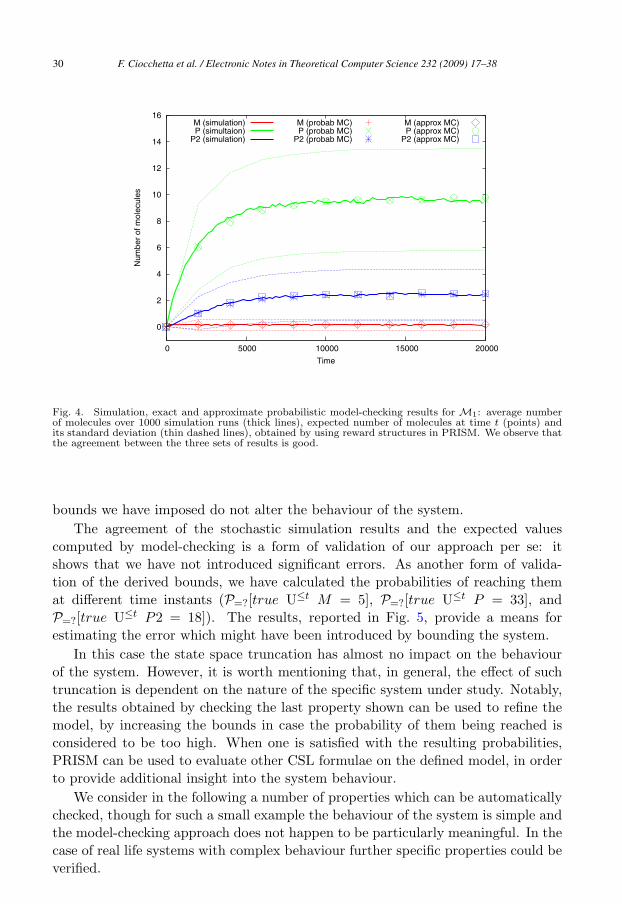
stop-time: by that time the system has reached a stable state.The simulation results are reported in Fig. 4, which shows the average values

obtained over all the runs. As the figure shows, both the monomeric protein P andthe dimeric protein P2 rapidly increase until they reach levels which remain stablewithin the considered time bound.

This simple network is an interesting example because, despite being structurallyunbounded, a stable behaviour is observed by looking at the average values ofmultiple runs: the amount of all the species is not unbounded.

We can estimate the upper bounds for the amounts of each species as the max-imum values obtained in any run at any time instant,

MaxM = 5; MaxP = 33; MaxP2 = 18

and we can use these values in the PRISM model. The amounts of the otherspecies, D and Res, are not affected by the reactions in which they are involvedand, therefore, they are constant at value 1.

In this example, the lower bounds for all the interesting species are 0, since theyare not present at system initialisation.

In Fig. 4 we also report the expected values for the amounts of the interestingspecies (M , P and P2) obtained by PRISM using the derived bounds. The resultsare in agreement with the average values calculated from the simulation runs. Thesevalues have been obtained by checking the instantaneous reward properties

RM=?[I = t], RP

=?[I = t], RP2=?[I = t]

varying the time t ∈ [0, T ], where M , P and P2 are reward structures associatingwith each state the current number of molecules of each species. In the same Fig. 4we consider the standard deviation of the number of molecules for the PRISMmodel. Specifically, we define reward structures associating with each state thesquare of the number of molecules of each species and the standard deviation isthen calculated as the square root of the variance E(Y )2 − E(Y 2), where Y is therandom variable representing a species in the network, whereas E(Y ) and E(Y 2)indicate the expected values for the amount of the species Y and for its squarevalue.

In order to confirm the belief that the choice of the bounds is crucial for havingthe right compromise between correctness and efficiency, we performed a few moreexperiments, both with smaller and with bigger upper bounds. The result is that, ifthe selected bounds are too low, the obtained behaviour is not in agreement with theaverage simulation result. On the other hand, using bounds which are too high hasthe effect of dramatically increasing the state space and, thus, it makes the model-checking much slower. For instance, the verification of the next set of properties ina model where the bounds for the three species are doubled is over 20 times slower,while verifying the previously-used CSL formulae (with no increase in the bound tobe reached to satisfy the formula) produces the very same values reported in Fig. 5.All values are equal up to the fifth decimal digit at least. This confirms that the


0

2

4

6

8

10

12

14

16

0 5000 10000 15000 20000

Num

ber

of m

olec

ules

Time

M (simulation)P (simultaion)

P2 (simulation)

M (probab MC)P (probab MC)

P2 (probab MC)

M (approx MC)P (approx MC)

P2 (approx MC)

Fig. 4. Simulation, exact and approximate probabilistic model-checking results for M1: average numberof molecules over 1000 simulation runs (thick lines), expected number of molecules at time t (points) andits standard deviation (thin dashed lines), obtained by using reward structures in PRISM. We observe thatthe agreement between the three sets of results is good.

bounds we have imposed do not alter the behaviour of the system.The agreement of the stochastic simulation results and the expected values

computed by model-checking is a form of validation of our approach per se: itshows that we have not introduced significant errors. As another form of valida-tion of the derived bounds, we have calculated the probabilities of reaching themat different time instants (P=?[true U≤t M = 5], P=?[true U≤t P = 33], andP=?[true U≤t P2 = 18]). The results, reported in Fig. 5, provide a means forestimating the error which might have been introduced by bounding the system.

In this case the state space truncation has almost no impact on the behaviourof the system. However, it is worth mentioning that, in general, the effect of suchtruncation is dependent on the nature of the specific system under study. Notably,the results obtained by checking the last property shown can be used to refine themodel, by increasing the bounds in case the probability of them being reached isconsidered to be too high. When one is satisfied with the resulting probabilities,PRISM can be used to evaluate other CSL formulae on the defined model, in orderto provide additional insight into the system behaviour.

We consider in the following a number of properties which can be automaticallychecked, though for such a small example the behaviour of the system is simple andthe model-checking approach does not happen to be particularly meaningful. In thecase of real life systems with complex behaviour further specific properties could beverified.


0

0.005

0.01

0.015

0.02

0.025

0.03

0.035

0 5000 10000 15000 20000

Pro

babi

lity

Time

M at maxP at max

P2 at max

Fig. 5. Model-checking results for M1: probability of each species reaching its upper bound.

As a first example we consider the cumulative reward property

R〈react〉=? [C ≤ t]

where 〈react〉 is a reaction name (e.g. “transcription”, “translation”, “degrada-tion M”, etc.), with which a transition reward is associated. These properties,analysed at different time instants t ∈ [0, T ] return the expected number of occur-rences of a reaction by that time (see Fig. 6, where we have separated slow and fastreactions in two different graphs for the sake of readability because of their verydifferent scales).

0

20

40

60

80

100

120

140

0 5000 10000 15000 20000

Exp

ecte

d nu

mbe

r of

occ

urre

nces

Time

transcriptiontranslation

degradationMdegradationP

(a) slow reactions

0

5000

10000

15000

20000

25000

0 5000 10000 15000 20000

Exp

ecte

d nu

mbe

r of

occ

urre

nces

Time

dimerizationmonomerization

(b) fast reactions

Fig. 6. Model-checking results for M1: expected number of occurrences of reactions by time t.

Fig. 7 shows the expected amounts of monomers (P ) compared to the totalamount of proteins (P + P2) present at time t. Specifically, it refers to the formulaRratio

=? [I = t] where “ratio” is a reward structure which associates the reward PP+P2


with each state.

0

0.2

0.4

0.6

0.8

1

0 5000 10000 15000 20000

Pro

babi

lity

Time

P / (P + P2)

Fig. 7. Model-checking results for M1: expected ratio between protein monomers and total proteins attime t.

We point out that properties such as the ones just mentioned and many others(e.g. the expected time at which a protein dimer is first produced, the probabilityof having more dimers than monomers at some time t, etc.) can be evaluated in aprobabilistically precise manner by model-checking: all the user needs to do is toprovide the model-checker with the CSL specification of the desired property andwait for the definitive answer. On the other hand, the analysis of these properties bysimulation, if possible, requires the use of reward-based simulation tools in whichthe user often needs to implement the reward functions themselves; in addition,the answers regarding the satisfaction of properties obtained by simulation couldonly be up to some confidence interval and, often, an extremely high number ofsimulation runs would be required to achieve a satisfactory confidence.

In this example, we have checked all properties at time instants in the interval[0, T ]. However, as one can easily see from Fig. 4, the system reaches a stablebehaviour much before time T . In cases like this, and if the time required formodel-checking experiments is long, the number of experiments to run could bereduced by considering this further information from the simulation results.

5.2.2 Network M2

We consider here M2. The simulation results reported in Fig. 8 show that thesystem does not reach a stable (average) state within the simulation time in whichwe are interested (T = 20000s): since in the model there is no protein degradation,both the monomeric protein P and the dimeric protein P2 increase without limit.

Again, we estimate the upper bounds for the amounts of each species as themaximum values obtained in any run at any time instant up to the simulation


stop-time,MaxM = 5; MaxP = 51; MaxP2 = 64

and we use these values in the PRISM model. The amounts of D and Res areconstant in this case, too.

In Fig. 8 we report the expected values (and their standard deviation) of theamounts of the interesting species obtained by PRISM, which are in agreementwith the average values calculated from the simulation runs. These values havebeen obtained by checking the instantaneous reward properties

RM=?[I = t], RP

=?[I = t], RP2=?[I = t] .

Fig. 9 reports on the probabilities of reaching the upper bounds at different timeinstants (P=?[true U≤t M = 5], P=?[true U≤t P = 51], and P=?[true U≤t P2 =64]).

The occurrences of each reaction by time t are reported in Fig. 10, while Fig. 11shows the expected amounts of monomers (P ) compared to the total amount ofproteins (P +P2) present at time t (they refer to the same properties described forM1).

Finally, Fig. 12 shows the probability of the amount of P2 being greater than theamount of P at different time instants (P=?[true U[t,t] P2 > P ]). As expected, thisprobability increases as time increases. However, it does not reach 1. Indeed, even if

0

5

10

15

20

25

30

35

40

0 5000 10000 15000 20000

Num

ber

of m

olec

ules

Time

M (simulation)P (simulation)

P2 (simulation)

M (probab MC)P (probab MC)

P2 (probab MC)

M (approx MC)P (approx MC)

P2 (approx MC)

Fig. 8. Simulation, exact and approximate probabilistic model-checking results for M2: average numberof molecules over 1000 simulation runs (thick lines), expected number of molecules at time t (points) andits standard deviation (thin dashed lines) obtained by using reward structures in PRISM. We observe thatthe agreement in all three cases is good but that the strongest agreement is between the average simulationresults and the probabilistic model-checking results. The results obtained by approximate model-checkingappear to indicate higher numbers of both monomers and dimers than the other two methods.


0

0.005

0.01

0.015

0.02

0.025

0.03

0.035

0 5000 10000 15000 20000

Pro

babi

lity

Time

M at maxP at max

P2 at max

Fig. 9. Model-checking results for M2: probability of each species reaching its upper bound.

0

20

40

60

80

100

120

140

0 5000 10000 15000 20000

Exp

ecte

d nu

mbe

r of

occ

urre

nces

Time

transcriptiontranslation

degradationM

(a) slow reactions

0

20000

40000

60000

80000

100000

120000

140000

160000

0 5000 10000 15000 20000

Exp

ecte

d nu

mbe

r of

occ

urre

nces

Time

dimerizationmonomerization

(b) fast reactions

Fig. 10. Model-checking results for M2: expected number of occurrences of reactions by time t.

the average behaviour shows that in the long run the amount of P2 is greater thanthe amount of P (see Fig. 8), this is not generally true for all possible behaviours:the system is highly variable, and there can be some paths in which P2 < P evenwhen approaching the simulation stop-time. This is not very surprising because theconfidence intervals around the times series for P and P2 are still overlapping up tothe stop time of 20000 seconds (see Fig. 8). The formal confirmation of this remarkis given by the fact that the probability of P2 being greater than P in every stateafter time t (P=?[G[t,T ] P2 > P ]) is 0 for any t ∈ [0, T ).

6 Related Work

In this work, as in our earlier work [4], we are concerned with obtaining the exactprobability distribution across all of the states of the reachable state-space of a


0

0.2

0.4

0.6

0.8

1

0 5000 10000 15000 20000

Pro

babi

lity

Time

P / (P + P2)

Fig. 11. Model-checking results for M2: expected ratio between protein monomers and total proteins attime t.

0

0.2

0.4

0.6

0.8

1

0 5000 10000 15000 20000

Pro

babi

lity

Time

P2 > P

Fig. 12. Model-checking results for M2: expected probability of P2 > P at time t.

network of chemical reactions. In our earlier work we used the stochastic processalgebra PEPA [16,15] to express the model and applied numerical linear algebrato solve the underlying Markov chain. In this paper we are using the Bio-PEPAlanguage and applying model-checking to obtain our results.

The use of probabilistic model-checking for the analysis of models of biologicalphenomena is already well established. In [5] the authors consider signal trans-duction in the RKIP-inhibited ERK pathway and manage the state-space explosionproblem by using approximate techniques where concentrations are modelled by dis-


crete abstract quantities. In [10] the authors apply model-checking to the complexFGF (Fibroblast Growth Factor) signalling pathway.

Another programme of work bringing together the analysis methods of stochasticsimulation and the numerical solution of the Markov chain is perfect sampling [11].This work joins the “Dominated Coupling From The Past” Algorithm from Monte-Carlo Markov Chain theory with Gillespie’s Stochastic Simulation Algorithm inthe DCFTP-SSA [12]. The DCFTP-SSA guarantees sampling from the stationaryprobability distribution of the Chemical Master Equation and can be used to studysteady-state properties of a broad class of stochastic biochemical networks. Ourwork guarantees that we are using the transient probability distribution of the CMEand can be used to study time-dependent properties of a broad class of stochasticbiochemical networks up to the stop-time of the simulation pre-run.

We have focused here on relating different stochastic approaches to the analysisof biochemical systems. Much work remains still to be done in relating discretestochastic models and continuous sure models [8] and understanding when each ofthese is the appropriate model to use [20].

7 Conclusions

Summing up, our approach is the following:

• We consider a Bio-PEPA system M representing a biochemical network, andwe automatically derive from it a model specification to be used for stochasticsimulation (by Dizzy) and one to be used for model-checking (by PRISM).

• We set the simulation time T and the number of simulation runs.• We pick as bound for a species the largest number of molecules which that species

has obtained in any simulation run within time T .• We update the PRISM model derived from the Bio-PEPA model with the es-

timated bounds, and we validate this model by comparing the expected valuescalculated by PRISM with the average values obtained by simulation.

• We use PRISM to analyse the model by verifying specific CSL properties.

In addition to the fact that simulation allows us to set some bounds whichmake model-checking feasible, the combination of those two analysis techniques isitself advantageous. Simulation and model-checking are complementary techniquesand they can be used to investigate different properties of the same system inorder to give a more complete understanding. Moreover, since the Dizzy modeland the PRISM model are equivalent, we expect the results obtained with thetwo approaches to be in agreement. If this is the case, that can give us staunchconfidence about the correctness of the results. If, instead, we get different results,that means there is some mistake in either approach (e.g. more simulation runsneed to be performed, the chosen bounds are too low, or the simulation stop-time istoo small), and this information could be used to refine the model or the simulationsettings.


We have automated the generation of the simulation model and the model-checker input from a model expressed in the Bio-PEPA process algebra. We haveautomated the repeated execution of a set of independent simulation runs andthe identification of the maximum and minimum values of each species from thesimulation results. The user then only needs to load the PRISM model, supplythe identified parameters and execute it. However, the choice of the number ofsimulation runs to be performed remains in the hands of the modeller.

We point out that the upper bounds estimated by using this approach are ap-proximate because, given the stochastic nature of the simulation, we can have gen-uine confidence in the chosen bounds only if we run a suitably large number ofsimulations. However, this issue is not specific to this approach. The choice of thenumber of simulation runs is needed for any stochastic simulation experiment; ontop of that, we use the simulation just as a supporting technique to the model-checking, and we believe that the combined use of the two approaches helps tominimize the uncertainty due to the stochastic simulation.

The good agreement between the results obtained by simulation and by model-checking on the presented example makes us confident that, provided an adequatenumber of simulation runs is performed, then our approach does not introducesignificant errors. However, we stress again the fact that the sensitivity to thetruncation of the state space is strongly dependent on the system itself; therefore,in order to assess the correctness of the estimated bounds for a specific system,the results obtained by model-checking should be validated against the behaviourobtained by simulation and against previous experimental and computational data,if there is any available.

Acknowledgement

The authors thank the anonymous reviewers of this paper for their insightful com-ments on the work. Federica Ciocchetta and Jane Hillston are supported by theU.K. Engineering and Physical Sciences Research Council (EPSRC) Advanced Re-search Fellowship and research grant EP/C543696/1 “Process Algebra Approachesto Collective Dynamics”. Stephen Gilmore and Maria Luisa Guerriero are supportedby the EPSRC grant EP/E031439/1 “Stochastic Process Algebra for BiochemicalSignalling Pathway Analysis”.

References

[1] Baier, C., B. Haverkort, H. Hermanns and J.-P. Katoen, Model-checking algorithms for continuous-timeMarkov chains, IEEE Trans. Software Eng. 29 (2003), pp. 1–18.

[2] Baier, C., J.-P. Katoen and H. Hermanns, Approximate Symbolic Model Checking of Continuous-TimeMarkov Chains, in: Proceedings of CONCUR’99, LNCS 1664, 1999, pp. 146–161.

[3] Bundschuh, R., F. Hayot and C. Jayaprakash, Fluctuations and Slow Variables in Genetic Networks,Biophys. J. 84 (2003), pp. 1606–1615.

[4] Calder, M., S. Gilmore and J. Hillston, Modelling the influence of RKIP on the ERK signalling pathwayusing the stochastic process algebra PEPA, Transactions on Computational Systems Biology VII 4230(2006), pp. 1–23.


[5] Calder, M., V. Vyshemirsky, D. Gilbert and R. Orton, Analysis of signalling pathways using continuoustime Markov chains, Transactions on Computational Systems Biology VI 4220 (2006), pp. 44–67,springer.

[6] Ciocchetta, F. and J. Hillston, Bio-PEPA: a framework for the modelling and analysis of biologicalsystems (2008), School of Informatics University of Edinburgh Technical Report EDI-INF-RR-1231.

[7] Ciocchetta, F. and J. Hillston, Bio-PEPA: an extension of the process algebra PEPA for biochemicalnetworks, in: Proc. of FBTC 2007, Electronic Notes in Theoretical Computer Science 194, 2008, pp.103–117.

[8] Geisweiller, N., J. Hillston and M. Stenico, Relating continuous and discrete PEPA models of signallingpathways, Theoretical Computer Science 404 (2008), pp. 97–111.

[9] Gillespie, D., Exact stochastic simulation of coupled chemical reactions, Journal of Physical Chemistry81 (1977), pp. 2340–2361.

[10] Heath, J., M. Kwiatkowska, G. Norman, D. Parker and O. Tymchyshyn, Probabilistic Model Checkingof Complex Biological Pathways, Theoretical Computer Science 319 (2008), pp. 239–257, special Issueon Converging Sciences: Informatics and Biology.

[11] Hemberg, M. and M. Barahona, Perfect sampling of the master equation for gene regulatory networks,Biophys J. 93 (2007), pp. 401–10.

[12] Hemberg, M. and M. Barahona, A Dominated Coupling From The Past algorithm for the stochasticsimulation of networks of biochemical reactions, BMC Syst Biol. 2 (2008), pp. 401–10.

[13] Herault, T., R. Lassaigne, F. Magniette and S. Peyronnet, Approximate probabilistic model checking,in: Proceedings of the 5th Verification, Model Checking and Abstract Interpretation (VMCAI 2004),LNCS 2937, Venice, Italy, 2004, pp. 73–84.

[14] Herault, T., R. Lassaigne and S. Peyronnet, APMC 3.0: Approximate Verification of Discreteand Continuous Time Markov Chains, in: Proceedings of the 3rd International Conference on theQuantitative Evaluation of SysTems (QEST’06), California, USA, 2006.

[15] Hillston, J., Process algebras for quantitative analysis, in: Proceedings of the 20th Annual IEEESymposium on Logic in Computer Science (LICS’ 05) (2005), pp. 239–248.

[16] Hillston, J., Tuning systems: From composition to performance, The Computer Journal 48 (2005),pp. 385–400, the Needham Lecture paper.

[17] Hinton, A., M. Kwiatkowska, G. Norman and D. Parker, PRISM: A tool for automatic verification ofprobabilistic systems, in: H. Hermanns and J. Palsberg, editors, Proc. 12th International Conference onTools and Algorithms for the Construction and Analysis of Systems (TACAS’06), LNCS 3920 (2006),pp. 441–444.

[18] Ramsey, S., D. Orrell and H. Bolouri, Dizzy: stochastic simulation of large-scale genetic regulatorynetworks, J. Bioinf. Comp. Biol. 3 (2005), pp. 415–436.

[19] Rathinam, M., L. Petzold, Y. Cao and D. Gillespie, Stiffness in stochastic chemically reacting systems:The implicit tau-leaping method, Journal of Chemical Physics 119 (2003), pp. 12784–12794.

[20] Wolkenhauer, O., M. Ullah, W. Kolch and K. H. Cho, Modelling and Simulation of IntraCellularDynamics: Choosing an Appropriate Framework, IEEE Transactions on NanoBioScience 3 (2004),pp. 200–207.


integrated simulation and model-checking for the analysis of biochemical systems

Documents