Western Washington University Western Washington University

Western CEDAR Western CEDAR

WWU Graduate School Collection WWU Graduate and Undergraduate Scholarship

2012

Integrating ensemble species distribution modeling and statistical Integrating ensemble species distribution modeling and statistical

phylogeography to inform projections of climate change impacts phylogeography to inform projections of climate change impacts

on species distributions on species distributions

Brenna R. Forester Western Washington University

Follow this and additional works at: https://cedar.wwu.edu/wwuet

Part of the Environmental Sciences Commons

Recommended Citation Recommended Citation Forester, Brenna R., "Integrating ensemble species distribution modeling and statistical phylogeography to inform projections of climate change impacts on species distributions" (2012). WWU Graduate School Collection. 202. https://cedar.wwu.edu/wwuet/202

This Masters Thesis is brought to you for free and open access by the WWU Graduate and Undergraduate Scholarship at Western CEDAR. It has been accepted for inclusion in WWU Graduate School Collection by an authorized administrator of Western CEDAR. For more information, please contact westerncedar@wwu.edu.

INTEGRATING ENSEMBLE SPECIES DISTRIBUTION MODELING AND

STATISTICAL PHYLOGEOGRAPHY TO INFORM PROJECTIONS

OF CLIMATE CHANGE IMPACTS ON SPECIES DISTRIBUTIONS

By

Brenna R. Forester

Accepted in Partial Completion

Of the Requirements for the Degree

Master of Science

Kathleen L. Kitto, Dean of the Graduate School

ADVISORY COMMITTEE

Chair, Dr. Andrew G. Bunn

Dr. Eric G. DeChaine

Dr. David O. Wallin

MASTER’S THESIS

In presenting this thesis in partial fulfillment of the requirements for a master’s degree at

Western Washington University, I grant to Western Washington University the non‐exclusive royalty‐free right to archive, reproduce, distribute, and display the thesis in any and

all forms, including electronic format, via any digital library mechanisms maintained by

WWU.

I represent and warrant this is my original work, and does not infringe or violate any rights of

others. I warrant that I have obtained written permissions from the owner of any third party

copyrighted material included in these files.

I acknowledge that I retain ownership rights to the copyright of this work, including but not

limited to the right to use all or part of this work in future works, such as articles or books.

Library users are granted permission for individual, research and non‐commercial

reproduction of this work for educational purposes only. Any further digital posting of this

document requires specific permission from the author.

Any copying or publication of this thesis for commercial purposes, or for financial gain, is

not allowed without my written permission.

Brenna R. Forester

April 23, 2012

INTEGRATING ENSEMBLE SPECIES DISTRIBUTION MODELING AND

STATISTICAL PHYLOGEOGRAPHY TO INFORM PROJECTIONS

OF CLIMATE CHANGE IMPACTS ON SPECIES DISTRIBUTIONS

A Thesis

Presented to

The Faculty of

Western Washington University

In Partial Fulfillment

Of the Requirements for the Degree

Master of Science

by

Brenna R. Forester

April 2012

iv

ABSTRACT

Species distribution models (SDMs) are commonly used to forecast climate change

impacts on species and ecosystems. These models, however, are subject to important

assumptions and limitations. By integrating two independent but complementary methods,

ensemble SDMs and statistical phylogeography, I was able to address key assumptions and

create robust assessments of climate change impacts on species’ distributions while

improving the conservation value of these projections.

This approach was demonstrated using Rhodiola integrifolia, an alpine-arctic plant

distributed at high elevations and latitudes throughout the North American cordillera. SDMs

for R. integrifolia were fit to current and past climates using eight model algorithms, two

threshold methods, and between one and three climate data sets (downscaled from general

circulation models, GCMs). This ensemble of projections was combined using consensus

methods to create a map of stable climate (refugial habitat) since the Last Interglacial

(124,000 years before present).

Four biogeographic hypotheses were developed based on the configuration of refugial

habitat and were tested using a statistical phylogeographic approach. Statistical

phylogeography evaluates the probability of alternative models of population history given

uncertainty about past population parameters, such as effective population sizes and the

timing of divergence events. The multiple-refugia hypothesis was supported by both

methods, validating the assumption of niche conservatism in R. integrifolia, and justifying

the projection of SDMs onto future climates.

v

SDMs were projected onto two greenhouse gas scenarios (A1B and A2) for 2085

using climate data downscaled from five GCMs. Ensemble and consensus methods were

used to illustrate variability across these GCMs. Projections at 2085 showed substantial

losses of climatically suitable habitat for R. integrifolia across its range. Southern

populations had the greatest losses, though the biogeographic scale of modeling may

overpredict extinction risks in areas of topographic complexity. Finally, past and future

SDM projections were assessed for novel values of climate variables; projections in areas of

novel climate were flagged as having higher uncertainty.

Integrating molecular approaches with spatial analyses of species distributions under

global change has great potential to improve conservation decision-making. Molecular tools

can support and improve current methods for understanding species vulnerability to climate

change, and provide additional data upon which to base conservation decisions, such as

prioritizing the conservation of areas of high genetic diversity in order to build evolutionary

resiliency within populations.

vi

ACKNOWLEDGEMENTS

Thank you to Andy Bunn for his expertise, advice and good humor. Thanks to Eric

DeChaine for collaborating on this project, and for serving on my committee. Thanks as well

to committee member David Wallin for his assistance and feedback. This project benefited

greatly from those who facilitated climate data access and helped with troubleshooting,

especially Gavin Schmidt, Joy Singarayer and Michel Crucifix. Many thanks to Wilfried

Thuiller, for his gracious assistance with modeling questions. Special acknowledgement to

members of the Huxley College Graduate Research Working Group.

vii

TABLE OF CONTENTS

Abstract.................................................................................................................................iv

Acknowledgements...............................................................................................................vi

List of Figures and Tables...................................................................................................viii

Introduction.............................................................................................................................1

Methods.................................................................................................................................10

Results...................................................................................................................................26

Discussion.............................................................................................................................42

References.............................................................................................................................56

Appendix A...........................................................................................................................65

Appendix B...........................................................................................................................72

viii

LIST OF FIGURES AND TABLES

Figure 1: Methods for ensemble species distribution modeling of refugial areas for R.

integrifolia since the Last Interglacial; use of the refugial model to develop

biogeographic hypotheses for phylogeographic analysis; projection of verified

models onto future climate, using an ensemble of GCMs.......................................14

Figure 2: Boxplots for sensitivity and AUC scores for 10 cross-validation runs on test

data. The consensus model does not include ANN................................................29

Figure 3: Consensus refugial model indicating areas of suitable habitat for R. integrifolia

across four time slices: current conditions, mid-Holocene, LGM, and LIG...........30

Figure 4: Biogeographic hypotheses tested using statistical phylogeography. Each

hypothesis represents a different model of effective population sizes (Ne) and

divergence times: panmixia; northward colonization from a southern refugium;

southward colonization from a northern refugium; colonization from northern

and southern refugia with divergence at the LGM and Illinoian Glacial Period....33

Figure 5: Current, A1B scenario, and A2 scenario consensus probability maps. Change

in suitable habitat from current to future for the A1B and A2 scenarios, based

on a cutoff of 50% of the models indicating suitable habitat..................................36

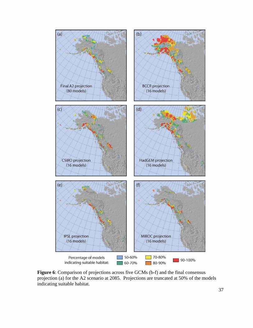
Figure 6: Comparison of projections across five GCMs and the final consensus projection

for the A2 scenario at 2085. Projections are truncated at 50% of the models

indicating suitable habitat........................................................................................37

Figure 7: Geographic distribution of novel values of climate variables over seven GCMs

used to project the refugial consensus map..............................................................40

Figure 8: Geographic distribution of novel values of climate variables for the A1B scenario

and the A2 scenario..................................................................................................41

Table 1: Climate data used to model the distribution of suitable habitat for R. integrifolia...13

Table 2: Predictor variables used to model the distribution of suitable habitat for R.

integrifolia.................................................................................................................27

Table 3: Mean AUC and sensitivity of 10 cross-validation runs on test data for nine single

models and the final consensus model (does not include ANN)..............................28

Table 4: Changes in climatically suitable habitat for R. integrifolia from current conditions

to future climate scenarios for 2085.........................................................................35

Introduction

Anthropogenic climate change is impacting ecosystems worldwide, generating a

global signal of climate-induced range shifts and phenological responses crossing all

ecosystems and taxonomic groups (Hughes 2000; Parmesan and Yohe 2003; Root et al.

2003; Parmesan 2006, 2007; Chen et al. 2011). Forecasting impacts on species distributions

has important conservation implications, as scientists and managers try to determine the best

strategies for preserving habitat for imperiled species and maintaining ecosystem

functioning. Species distribution models (SDMs) have become one of the most accessible

and widely used tools to develop these forecasts (Franklin 2009; Zimmermann et al. 2010).

Correlative SDMs are based on the principle that climate constrains species’

distributions within their biogeographic and evolutionary history (Woodward 1987; Webb

and Bartlein 1992). They are created by extracting a relationship between a species’

observed distribution and climate and environmental variables. That relationship can then be

projected onto models of current climate to determine the geographic distribution of

climatically suitable habitat. Predictive distributions are created by projecting that same

relationship onto models of past or future climate.

SDMs are also known as niche models, reflecting their foundation in the fundamental

and realized niche concepts first described by Hutchinson (1957). There is a growing

literature dedicated to understanding which parts of the niche are being modeled with SDMs

(Araújo and Guisan 2006; Kearney 2006; Soberón 2007, 2010; Colwell and Rangel 2009),

however this debate is far from consensus. I favor the interpretation of Soberón (2007, 2010)

who recognizes three primary factors affecting the distribution of species: (1) the spatial

distribution of favorable environmental conditions, (2) the biotic environment, including

2

predators, competitors, facilitators, etc., and (3) the dispersal capability of the species. He

terms the first of these factors the Grinnellian niche (operating at broad geographic scales),

the second the Eltonian niche (operating at local scales), while the third introduces the

potential for metapopulation structure and source-sink dynamics. In this interpretation,

SDMs at biogeographic scales are representations of the Grinnellian niche (niche as habitat

rather than function), which interacts at finer scales with both the Eltonian niche and

dispersal capability/source-sink dynamics. Because of these interactions, correlative SDMs

based on climate variables potentially model both Hutchinson’s realized niche (Hutchinson

1957) and sink habitats that are accessible because of dispersal capabilities.

Under this framework, SDM output at biogeographic scales is best described as the

distribution of climatically suitable habitat for a species, rather than a representation of a

species’ niche. While the inclusion of occurrence records from sink populations will

introduce error in correlative models, the assumed small number of these records relative to

source records and the coarse scale (and broad extent) of modeling are generally thought to

minimize their contribution to overall error rates (Franklin 2009).

Despite their widespread use, SDMs have many technical limitations, including

problems handling historical demographic signals, biotic interactions, and changing

combinations of climate variables, and theoretical assumptions, such as species-climate

equilibrium and niche conservatism (Jackson et al. 2009; Wiens et al. 2009). Furthermore,

recent papers have argued that SDMs provide only a starting point for understanding species’

responses to climate change and planning adaptive management strategies to conserve

biodiversity (Franklin 2010; Scoble and Lowe 2010; Dawson et al. 2011).

3

One proposal for the improvement of SDMs is to integrate phylogeography, which

examines the current geographic distribution of genetic variation within and between

populations to infer demographic history and how paleoclimatic events may have impacted

population divergence (Avise 2000). For example, Pleistocene glacial cycles generated

periods of expansion and contraction of species ranges, leaving a genetic fingerprint on

current populations (Davis and Shaw 2001). The geographic distribution of current genetic

variation depends on how species responded to these climate oscillations, the number,

location, and size of refugia, the connectivity among populations, dispersal capabilities, and

rates of recolonization (Hewitt 2000).

Phylogeography is most often used to determine the impact of Pleistocene glacial

cycles on genetic variation within species or among groups of species, including the

identification of migration barriers, long-term refugia (areas where species persist for at least

an entire glacial-interglacial cycle), and suture zones (regions where lineages that were

isolated in the past now meet) (Scoble and Lowe 2010). Phylogeographers have started to

use SDMs to generate paleodistribution models, with which they develop spatially explicit

biogeographic hypotheses which can be tested using statistical phylogeographic methods

(Carstens and Richards 2007; Richards et al. 2007). Statistical phylogeography evaluates the

probability of alternative models of population history given uncertainty about past

population parameters, such as effective population size. The outcome of these efforts

includes an improved understanding of the mechanisms creating patterns of biodiversity, as

well as the patterns and timing of divergence and speciation events (Hugall et al. 2002;

Knowles et al. 2007; Waltari et al. 2007; Dépraz et al. 2008; Chan et al. 2011).

4

Ecologists looking to model future impacts of climate change on species distributions

can integrate phylogeographic approaches to address one of the fundamental problems with

SDM projections: the assumption that these models can accurately project species

distributions over time. For many reasons, an SDM that performs well on current data

cannot be presumed to perform well on projected climate data (Heikkinen et al. 2011),

though this assumption is routinely made. Reciprocal inferences derived from SDMs and

statistical phylogeography can be used to provide support for a model’s ability to accurately

project distributions over time.

Phylogeographic analyses can help address other important SDM assumptions and

limitations, including niche conservatism and dispersal capability. Niche conservatism is the

tendency of a species to retain its climatic niche over time (Wiens et al. 2010). This is a

fundamental assumption of projecting SDMs, since projection of a labile species-climate

relationship into the future (or past) would be inappropriate. Dispersal capability is another

limiting factor; SDM projections usually assume either unlimited dispersal or none at all. In

some cases, the differences between these projections can be significant, contributing to

uncertainty (for example, Thomas et al. 2004; Engler and Guisan 2009). Phylogeographic

analyses can provide a species-specific metric of dispersal capability with which SDM

projections can be constrained.

Finally, the detection of refugia and past barriers to dispersal has important

conservation applications. Long-term refugia tend to be geographic locations with high

levels of allelic diversity (Stewart et al. 2010). Locating past barriers can result in the

identification of suture zones, which have been shown to support high levels of

5

diversification and speciation (Hewitt 1996; Moritz et al. 2009). Including these locations in

conservation planning can help build evolutionary resiliency within populations, mediating

extinction risks (Klein et al. 2009; Sgro et al. 2011).

Only a few studies have used the combination of SDMs and phylogeography to both

understand the impact of paleoclimatic events on species distributions and assess future

climate change impacts (Cordellier and Pfenninger 2009; Galbreath et al. 2009). These

authors typically employ accessible and user-friendly approaches to species distribution

modeling, such as Maxent modeling software (Phillips et al. 2006; Phillips and Dudik 2008)

and interpolated climate data from WorldClim (Hijmans et al. 2005). However, the growing

literature devoted to improving SDMs has indicated that the two greatest sources of

uncertainty in SDM projections are the choice of model algorithm and the general circulation

model (GCM) used for climate forecasting (Diniz-Filho et al. 2009; Buisson et al. 2010). For

this reason, the use of a single model algorithm and a single GCM to project changes in

species’ distributions has been critiqued (Nogués-Bravo 2009).

A recent approach to addressing this uncertainty is ensemble modeling combined

with consensus projections, for example, taking the mean of projections, or using a model

“voting” approach (Araújo and New 2007; Marmion et al. 2009). Ensemble modeling is

based on the idea that different combinations of initial conditions, model algorithms, and

GCMs represent alternate possible states of the system being modeled (Araújo and New

2007). When these are combined using consensus methods (such as the mean of all models),

they can form a more accurate projection, outperforming single models (Marmion et al.

2009; Grenouillet et al. 2011). This assumes that the included models meet some standard of

6

“good” performance, since increased accuracy would not be expected simply by combining

poor models (Araújo et al. 2005).

Ensemble modeling and consensus projections are particularly well-suited to

temporal and spatial projection of SDMs. Research has indicated that single models that

have the best performance on current data will not necessarily provide the most accurate

future projections, and that consensus projections can more effectively model observed range

shifts (Thuiller 2004; Araújo et al. 2005). Furthermore, some algorithms are better at

extrapolation modeling, where variables are outside the range used to build the models

(Marmion et al. 2009; Heikkinen et al. 2011). While projection of SDMs onto these “novel

climates” is discouraged (Fitzpatrick and Hargrove 2009; Elith et al. 2010), it is usually

unavoidable since novel combinations of temperature and precipitation are highly likely over

forecast periods (~100 years) on the spatial scale of most SDM studies (Williams et al.

2007). Detecting areas of non-analog climates and indicating larger levels of uncertainty in

those areas is essential to producing robust projections of climate change impacts.

Another important component of improving SDMs (ensemble or otherwise) is

incorporation of an ecological understanding of how the environment shapes patterns of

species distributions. The selection of biologically appropriate, functionally-relevant

predictor variables has been emphasized by many authors (for example, Guisan and

Zimmermann 2000; Austin 2002; Lookingbill and Urban 2005; Austin and Van Niel 2011).

For example, these include “plant-relevant variables” such as radiation, temperature and soil

moisture, as opposed to their “physical proxy variables” like aspect, elevation and

topographic convergence (Lookingbill and Urban 2005). Unfortunately, selection of

7

ecologically relevant predictors is not addressed by many SDM practitioners. Part of this is a

consequence of the easy availability of pre-calculated gridded predictor variables (for

example, the 19 bioclimatic variables that make up the online WorldClim database (Hijmans

et al. 2005)), as well as an assumption that the model algorithm will choose the most

important predictive variables. This last assumption is particularly problematic, since

including multiple correlated predictors (for example, mean temperatures for each month)

can result in serious errors, including a bias for autocorrelated variables and coarse-scale over

fine-scale predictors (Franklin 2009).

In this study, I combined ensemble modeling and consensus projections with

statistical phylogeographic analyses to assess past and future climate change impacts on the

geographic distribution of an alpine-arctic plant. Alpine and arctic species have responded to

climate oscillations throughout their evolutionary history. However, the speed of

anthropogenic climate change will challenge species responses through migration, dispersal,

and genetic adaptation, by shifting habitat conditions more rapidly than in the past (Davis

and Shaw 2001). Alpine species, with distributions defined by steep climatic gradients, are

being disproportionately impacted by these changes (Nogués-Bravo et al. 2007; Lenoir et al.

2008; Engler et al. 2009; Dirnbock et al. 2011). In alpine and arctic systems, these range

shifts will likely result in increasingly fragmented and reduced habitat as species move

higher in elevation and latitude. The consequence for many local populations will be

extirpation as they run out of high elevation and high latitude habitat.

For this analysis, I modeled the distribution of suitable habitat for Rhodiola

integrifolia Raf. (Crassulaceae), roseroot or king’s crown. R. integrifolia is a succulent,

8

perennial alpine-arctic specialist. It has a widespread, patchy distribution at high altitudes

and latitudes throughout the North American Cordillera, from the Sierra Nevada Mountains

in California, east to the Rocky Mountains, and north to the alpine tundra of Alaska and

Siberia (Clausen 1975). Habitats include rocky slopes, alpine meadows and arctic tundra,

with plants rooting in rock crevices or in shallow soil and gravel (Clausen 1975). This

species reproduces by wind-dispersed seeds and can also propagate vegetatively at the root

stock (Clausen 1975). I chose this species for analysis because of its widespread spatial

distribution and climatic restriction to alpine and arctic areas.

The purpose of this research was to illustrate how the integration of ensemble SDMs

and phylogeography can yield robust assessments of climate change impacts on species’

distributions and provide additional information important for conservation. These

reciprocally inferential approaches were used to model the effect of past and future climate

change on the geographic distribution and genetic variability of R. integrifolia. My

objectives were to:

1. Develop a model of climatically stable refugial areas in western North America for R.

integrifolia over the last 124 kya (kya, thousand years ago).

a. Determine the geographic distribution of climatically suitable habitat using an

ensemble modeling approach at four time periods: current, mid-Holocene (6 kya),

Last Glacial Maximum (21 kya), and Last Interglacial (124 kya).

b. Establish the locations of potential refugia (areas of stable climate) over the past

124 kya.

c. Assess the impact of novel values of climate variables on this refugial model.

9

2. Evaluate the level of agreement between the SDM refugial model and empirical

genetic data using a statistical phylogeographic approach.

a. Develop biogeographic hypotheses (models of population history) based on the

geographic distribution of potential refugial habitat.

b. Test these alternate hypotheses using statistical phylogeography; determine which

hypothesis is best supported by the genetic data.

c. If phylogeographic analyses and SDM projections disagree, assess the potential

for dispersal barriers, lack of niche conservatism, and/or modeling errors.

d. If phylogeographic analyses and SDM projections agree, the ability of the SDMs

to project over time and changing climates is supported; SDMs can be projected

onto future climates.

3. Assess the impact of future climate change scenarios on the geographic distribution of

climatically suitable habitat for R. integrifolia in western North America.

a. Project the impact of future climate change on suitable habitat using multiple

general circulation models and greenhouse gas scenarios.

b. Assess the impact of novel values of climate variables on future projections.

Statistical phylogeography in combination with ensemble SDMs has great potential for

improving our understanding of how species will respond to ongoing climate change.

Including molecular approaches allows us to better understand how species have responded

to past climate fluctuations and plan more effective conservation strategies for the future.

10

Methods

Spatial and temporal scales

The spatial extent of this analysis was the North American Cordillera, extending from

approximately 30°N to 80°N, and -180°W to -99°E. This extent includes the entire

latitudinal distribution of R. integrifolia and a large part of its longitudinal distribution, an

important means of minimizing bias in model projections (Barbet-Massin et al. 2010).

Spatial resolution was 0.5°. This relatively coarse pixel size was chosen to balance

“resolution with realism” (Daly 2006) when downscaling climate data from general

circulation models (GCMs). At scales finer than 0.5°, complex physiographic factors impact

climate, including elevation, terrain features, cold air drainage, and coastal influences (Daly

2006). It is very difficult to account for these impacts when interpolating climate data from

GCMs (typically generated at 2 to 3° resolution) to resolutions finer than 0.5°. Furthermore,

coarse spatial resolutions minimize the effects of biotic interactions and source-sink

dynamics, which typically occur at finer scales (Pearson and Dawson 2003; Soberón 2010).

The tradeoff with this approach is that resolution is lost in complex terrain, such as mountain

ranges, since the 0.5° pixel size averages climate over these heterogeneous areas. This must

be taken into consideration when interpreting results.

Past, current and future distribution models were created for R. integrifolia (see

below). Paleodistributions were created for the Mid-Holocene (6 kya), the Last Glacial

Maximum (LGM, 21 kya), and the Last Interglacial (LIG, 124 kya). Current distributions

were based on mean climatology from 1971-2000. Future distributions were based on mean

11

climate values projected for 2071-2100 (hereafter referred to as “2085”) under two

greenhouse gas scenarios.

Occurrence records

Georeferenced occurrence records for R. integrifolia (including ssp. integrifolia, ssp.

procera, and ssp. neomexicana) and its taxonomic synonyms were collected from six online

herbarium databases: Arctos (http://arctos.database.museum/), the Oregon Flora Project

(www.oregonflora.org), the Consortium of California Herbaria (www.ucjeps.berkeley.edu/

consortium), the Rocky Mountain Herbarium (www.rmh.uwyo.edu), the University of British

Columbia Herbarium (www.beatymuseum.ubc.ca/ herbarium), and the University of

Washington Herbarium (www.washington.edu/burkemuseum/collections/herbarium).

Records were plotted on topographic maps in ArcMap (ESRI 2010) and visually inspected

for obvious georeferencing errors. Georeferencing was evaluated and modified, if needed,

on a subset of the records, yielding 554 total records. For modeling, one record was used per

pixel, producing a final data set of 269 records (Figure 1a).

Phylogenetic analysis of all R. integrifolia subspecies by DeChaine et al. (in prep)

showed a deep divergence (dating to approximately 500 kya) between the clade located in

Colorado and New Mexico (currently represented as R. integrifolia ssp. integrifolia, ssp.

procera, and ssp. neomexicana) and all other populations of R. integrifolia. Because of this

deep divergence and the limitation of SDM paleodistributions to the LIG, records from

Colorado and New Mexico were excluded from this analysis. Additionally, this analysis did

not include ssp. leedyi, a relict subspecies confined to cold air seeps located along dolomite

cliffs in Minnesota and New York. The extremely small range and microhabitat

12

specialization of this subspecies is not conducive to the spatial scale used in this analysis.

The leedyi subspecies is included in the phylogenetic analysis (DeChaine et al. in prep).

Climate data and interpolation

Eight climate models were used in this analysis, covering five time periods (Table 1).

When available, monthly global data were accessed for the following variables: total

precipitation rate, mean surface air temperature, maximum surface air temperature, and

minimum surface air temperature. Standard deviations of climate variables were also

calculated. Detailed information on climate data sets and processing are available in

Appendix A.

Anomalies were calculated for past and future climate data. Absolute anomalies

(past-present and future-present) were calculated for temperature variables, while relative

anomalies were calculated for precipitation (past/present and future/present). Anomalies

were interpolated globally to a 0.5° pixel size using ordinary cokriging in ArcMap (ESRI

2010). CRU TS 2.1 climate data were used as the secondary cokriging dataset. The

“Optimize Model” setting was used for each layer (minimizing the mean square error), and

the search neighborhood for the climate layer was set to 12 maximum and 2 minimum

neighbors with semiaxes settings of 20. The CRU dataset was set to a search neighborhood

of 5 maximum and 2 minimum neighbors, with semiaxes set to 20. These settings were

chosen to minimize error rates. Interpolated anomalies were applied to CRU climate data to

create the final normalized climate layers for each time slice. Negative precipitation values

were set equal to zero. Cokriging root mean square errors are reported in Appendix B. The

13

LGM ice layer is from Dyke et al. (2003) and corresponds well with the coarse ice sheet data

provided with the LGM climate models (not shown).

Table 1: Climate data used to model the distribution of suitable habitat for R. integrifolia.

Time period Model Reference Source

Current

(1971-2000) CRU TS 2.1 Mitchell and Jones 2005

University of East

Anglia Climatic

Research Unit

Mid Holocene

(6 kya)

CCSM 3 Otto-Bliesner et al. 2006

Paleoclimate Modelling

Intercomparison

Project Phase 2

(Braconnot et al. 2007)

HadCM3 UBRIS Gordon et al. 2000

MIROC 3.2 K-1 model developers 2004

Last Glacial

Maximum

(21 kya)

CCSM 3 Otto-Bliesner et al. 2006

HadCM3 Gordon et al. 2000

MIROC 3.2 K-1 model developers 2004

Last

Interglacial

(124 kya)

HadCM3 Gordon et al. 2000

Bristol Research

Initiative for the

Dynamic Global

Environment

Future

(2071-2100)

BCCR BCM 2.0 www.bjerknes.uib.no Coupled Model

Intercomparison

Project Phase 3

(Meehl et al. 2007)

World Data Center for

Climate, Hamburg,

Germany

CSIRO Mk3.5 Gordon et al. 2002

HadGEM1 Johns et al. 2006

IPSL CM4 Marti et al. 2009

MIROC 3.2 K-1 model developers 2004

14

Figure 1: Methods for ensemble species distribution modeling of refugial areas for R.

integrifolia since the Last Interglacial (a-g); use of the refugial model to develop

biogeographic hypotheses for phylogeographic analysis (h); projection of verified models

onto future climate, using an ensemble of GCMs (i).

15

Predictor variables

In this study, 60 potential predictor variables were calculated that are relevant to plant

life generally and alpine species in particular. These included growing degree days, chilling

period, seasonal snowpack, and annual and seasonal indices of precipitation and temperature.

Snowpack was calculated using methods developed by Lutz and colleagues (2010). Recent

research has shown that including measures of extreme climate events, as opposed to just

climate variability, can greatly improve the prediction of species distributions, especially at

range limits (Zimmermann et al. 2009). To incorporate measures of climate extremes, the

standard deviations of temperature and precipitation were calculated, based on methods used

by Zimmermann and colleagues (2009). Unfortunately calculation of actual

evapotranspiration and water deficit, which account for the seasonal timing of water supply

and energy input (Stephenson 1998) could not be calculated due to a lack of required inputs

from paleoclimate data sets.

Of the 60 calculated predictor variables, the most relevant were identified using the

randomForest package (Liaw and Wiener 2002) in R (R Development Core Team 2011).

Random forest is an ensemble modeling approach based on classification and regression

trees; it builds multiple trees using random subsets of the observations and predictor

variables and then averages (regression) or tallies (classification) them. Random forest

incorporates measures of variable importance that are increasingly being used for variable

selection in a wide variety of applications because of their flexibility (e.g. variables are

assessed both independently and using a multivariate approach among variables, Strobl et al.

2008). However, correlation between predictor variables can impact random forest variable

16

importance measures, so recommendations to address this problem by Strobl and colleagues

(2008) were followed, including using multiple values of mtry (the number of variables

randomly sampled at each split) as well as a large number of trees (5000). Absences were

chosen at random to equal the number of presence records. Random forest was run 100

times with 5000 trees at the following values of mtry: 5, 10, 20, 30, 40, 50, 55, and 60. Gini

importance and mean decrease accuracy scores were output and averaged over 100 runs for

each value of mtry. Variables were chosen based on variable importance scores as compared

across mtry values. Spearman’s correlation was used to remove variables that were

correlated at rho values greater than |0.8|. Of the 60 potential predictor variables, eight were

chosen for modeling (Figure 1c, Results: Table 2).

Species distribution modeling and evaluation

Modeling was conducted using the BIOMOD package (Thuiller et al. 2009) in R and

Maxent, v. 3.3.3 (Phillips et al. 2006; Phillips and Dudik 2008). Nine model algorithms were

run, representing three types of analysis: (1) regression methods, including generalized linear

models (GLM), generalized additive models (GAM), and multivariate adaptive regression

splines (MARS); (2) classification methods, including classification tree analysis (CTA) and

flexible discriminant analysis (FDA); and (3) machine learning methods, including artificial

neural networks (ANN), generalized boosted models (GBM, also called boosted regression

trees), random forest (RF), and maximum entropy (Maxent). All models except Maxent were

run using BIOMOD.

GLMs were run with a binomial error distribution with logit link and were fitted with

17

linear and quadratic terms; stepwise AIC criteria were used for model selection. GAMs were

run with a binomial error distribution with logit link and were fitted with nonparametric

smoothing splines (four degrees of smoothing). MARS models were fit with a maximum

interaction degree of two on the forward stepwise pass, with backward stepwise pruning of

these models based on generalized cross-validation. CTA models were run with 50 cross-

validations. FDA was run using the MARS regression method for optimal scaling. ANN

models used five cross-validation runs. GBM models were run using a Bernoulli distribution

(logistic regression for binary data), 5000 trees, and five cross-validation runs. RF models

were run with 750 trees and an mtry value of four.

Independent validation data are required to assess the predictive performance of

models. In the absence of independent data, data partitioning can be used to assess model

stability and the sensitivity of the model results to initial conditions (Araújo and Guisan

2006; Thuiller et al. 2009). Data were partitioned using the heuristic reported in Fielding and

Bell (1997): [1 + (p – 1)1/2

]-1

, where p is the number of predictor variables. This

corresponded to a calibration data set using 70% of the original data, with 30% reserved for

verification. For models run in BIOMOD, ten data partitions were run for each model using

random selections (with replacement) for calibration and verification (Figure 1e). Because

the removal of presence records has a negative effect on model projections, final consensus

models were built using 100% of the available data (Araújo et al. 2005).

Maxent was run twice. The first run included ten bootstrapped replicates using a

random test percentage of 30% of the sample records and the random seed setting (ensuring

different random partitions for testing and training). These runs were used to calculate test

18

statistics (AUC and sensitivity, see below). The second run used all of the presence records

to train the model; this run was used in model ensembles. In both runs, the number of

maximum iterations was 500 and the convergence threshold was 0.00001 (following

recommendations by Phillips and Dudik 2008).

For all models, the entire background of the study area was used to create pseudo-

absence points (6539 background points, Figure 1b). The entire area was chosen to ensure

complete sampling of environmental conditions in the study area. By training the model on a

broad combination of predictor variables, climatic extrapolation is minimized when

projecting onto different climates. For all models, background records were weighted to

maintain the number of presence records equal to the number of background records

(prevalence = 0.5). Weighting pseudo-absence records to maintain equal prevalence has

been found to maximize model performance using simulated species distributions (Barbet-

Massin et al. 2012).

The area under the curve of the receiver operating characteristic (AUC, Fielding and

Bell 1997) and sensitivity (also known as true positive fraction) were used to assess model

accuracy and stability. When using true absence data, AUC quantifies the ability of a model

to discriminate presence from absence (Fielding and Bell 1997). When using pseudo-

absence data, AUC instead determines if the model can classify presence records more

accurately than random prediction (Phillips et al. 2006). AUC is a threshold-independent

measure with values that range from 1 (perfect classification) to 0.5 (no better than random).

Maxent uses a slightly different approach to calculating AUC compared to BIOMOD,

which may result in marginally inflated AUC values. Sensitivity was calculated to compare

19

all models using identical methods. Sensitivity is a threshold-dependent measure; it requires

that probabilistic output be converted to presence/absence data in order to calculate the

proportion of observed occurrences that are correctly predicted (true positives / (true

positives + false negatives)). To convert probabilities to presence/absence, the mean

probability value across model output was used; this is a simple threshold method that has

been shown to be robust in threshold comparisons (Liu et al. 2005). Because high sensitivity

can be achieved simply by predicting suitability across large parts of the study area,

sensitivity values must be tested for statistical significance. An exact one-tailed binomial test

was used to calculate the probability of obtaining sensitivity values by chance. Significant

tests (p < 0.05) indicate that the model is classifying presence better than a random

expectation, given the proportion of pixels predicted present (Anderson et al. 2002).

Evaluation statistics were averaged across the ten cross-validation runs and used to

assess the internal consistency of the models, and determine if models should be removed

from the consensus analysis. Models with mean AUC and mean sensitivity > 0.7 were

determined to be useful and were kept in the consensus analysis (Figure 1d). Model

projections were also inspected individually to ensure they were ecologically realistic.

Evaluation statistics were calculated for the current consensus model (an ensemble of 16

binary models, see below) to compare the performance of the consensus model against the

single models.

20

Paleodistributions and the refugial model

Models for R. integrifolia were projected onto current climate and models of past

climate, including three GCMs each for the Mid-Holocene and LGM, and one GCM for the

LIG (Figure 1f). Model output is probabilistic, indicating the probability of suitable habitat

in a given pixel. These probabilities were converted to presence/absence predictions in order

to assess the presence or absence of suitable habitat across all time slices in each pixel. Two

thresholds were used: a threshold that minimizes the absolute value of sensitivity minus

specificity (minSeSp), and the mean probability value across model output (mean). Both of

these methods have been shown to perform well in threshold comparisons (Liu et al. 2005).

For each time period (current, Mid-Holocene, LGM, and LIG), consensus probability

maps were created, indicating the percentage of models showing the presence of suitable

habitat at each pixel. For the current and LIG, these consensus probabilities were composed

of 16 models: eight model algorithms (one algorithm was discarded, see Results) using each

of two threshold methods (minSeSp and mean). For the Mid-Holocene and LGM, consensus

probabilities each consisted of 48 models: eight model algorithms using two threshold

methods for three GCMs. The consensus probability map for each time period was

converted to a binary map based on four thresholds: 30, 50, 70, and 90% probability of

suitable habitat. Maps based on these thresholds for each time period were stacked to show

agreement on suitable habitat across all four time slices. The final refugial map therefore

indicates pixels classified as suitable habitat across all four time slices, based on the four

thresholds of suitable habitat for each time period: 30, 50, 70 and 90%. The LGM ice layer

(Dyke et al. 2003) was overlaid (to exclude potential suitable habitat under the ice sheet) to

21

create a final map of potential refugial habitat for R. integrifolia since the Last Interglacial

(Figure 1g).

Biogeographic hypothesis development and testing

Biogeographic hypotheses consist of models of population history that indicate the

branching patterns, timing of divergence events, and effective population size (Ne) of

populations of a species. Generally, hypotheses should contain enough parameters to

distinguish between alternate models, but be simple enough to be addressed with the genetic

material available and method of analysis employed (Knowles 2004). Alternate

biogeographic hypotheses for R. integrifolia were based on the configuration of potential

refugia as identified by the refugial model:

1. Panmixia (no genetic differentiation between populations).

2. Northward colonization from a southern refugium after the LGM.

3. Southward colonization from a northern refugium after the LGM.

4. Colonization from multiple refugia (north and south).

The fourth hypothesis was tested using two divergence times and two levels of Ne.

Hypotheses are presented in more detail in Results.

Alternative biogeographic hypotheses were tested using a statistical phylogeographic

approach (described below) to determine the extent to which the empirical genetic data

supported each hypothesis (Figure 1h). Statistical phylogeography evaluates the probability

of alternative models of population history given uncertainty about past population

parameters, such as effective population sizes (Ne) and the timing of divergence events. The

22

genetic data set employed for this study was analyzed by Dr. Eric DeChaine (WWU, Biology

Department) using coalescent simulations (see below). The coalescent is a model of

population genetics that takes into account the stochasticity of the genetic process when

modeling different mechanisms of population history within a species (Rosenberg and

Nordborg 2002).

Agreement between the biogeographic hypothesis supported by the SDMs

(hypothesis 4) and the genetic data would corroborate the ability of the SDMs to effectively

project the distribution of suitable habitat over time. Agreement would also support niche

conservatism in R. integrifolia. A lack of agreement between the SDM and the genetic data

could occur for several reasons, including a lack of niche conservatism in the species,

barriers to dispersal (areas indicated as suitable habitat by the SDMs but not actually

occupied by the species), and/or errors in the SDMs or genetic analyses.

Statistical phylogeography (contributed by E. DeChaine)

The sampling scheme and molecular approaches are described in detail elsewhere

(DeChaine et al. in prep). In brief: (i) genomic DNA was extracted from individuals of R.

integrifolia sampled throughout their range; (ii) five anonymous nuclear loci were sequenced

for each individual; (iii) phylogenies were estimated for each locus in Garli v. 0.951 (Zwickl

2006) and used as ‘observed’ trees for testing the models of divergence based on hypotheses

developed from the SDMs; and (iv) population genetic parameters (i.e., TMRCA, Ne) were

estimated in BEAST v. 1.6.2 (Drummond and Rambaut 2007) and LAMARC v. 2.1.6

(Kuhner 2006).

23

Coalescent simulations of genealogies constrained within models of population

divergence were performed with MESQUITE 2.75 (Maddison and Maddison 2011). Each

population model is comprised of the tree topology, estimates of effective population size for

each population, and time (in generations) given as branch lengths. Four models were tested:

(1) panmixia, (2) recent colonization of the north from the south, (3) recent colonization of

the south from the north, and (4) colonization from northern and southern refugia. Gene

trees were simulated by constraining the coalescence of lineages within the topology, branch

lengths, and Ne for a given model. This yielded 1000 simulated gene trees within each model

of divergence, over a range of branch lengths (times).

The expected distribution of discordance between gene trees and the population

model was measured by deep coalescences (DC; Maddison 1997) by counting the number of

extra gene lineages per population, assuming incomplete lineage sorting accounts for all

discordance. The DC from the observed gene trees were averaged across loci (DC = 18.8)

and compared with the null distribution from the simulations to test statistically whether the

observed tree could have been generated under the expected distribution for the population

model. If the observed DC did not fit the expected distribution (α = 0.05) for a given model,

that model was rejected. If the observation fell within the expected distribution for a model

of population divergence, that model was accepted as a possible scenario that could have led

to the distribution of genetic variation observed today.

Future projections

Models for R. integrifolia were projected onto models of future climate, including

two greenhouse gas scenarios (A1B and A2) for each of five downscaled GCMs for 2085

24

(Figure 1i). This time period was chosen as it represents the maximum temporal coverage of

future projections provided by the IPCC. The A2 (“business as usual”) scenario is

considered a high-range scenario by the IPCC, with an average temperature increase of 3.4°C

by 2100 (Meehl et al. 2007). The A1B scenario is a mid-high scenario involving eventual

atmospheric CO2 stabilization, with an average temperature increase of 2.8°C by 2100

(Meehl et al. 2007). Lower emissions scenarios (B1 and B2) were not considered in this

analysis, since recent projections indicate that current global emissions are on track to

surpass these more conservative scenarios (Sokolov et al. 2009).

As with the paleodistribution model, probabilistic output was converted to

presence/absence predictions using two thresholds: minimizing the absolute value of

sensitivity minus specificity, and the mean probability value. Consensus probability maps

for each greenhouse gas scenario consist of a total of 80 models (8 algorithms using 2

threshold methods for 5 GCM projections). These maps indicate the percentage of models

showing the presence of suitable habitat, truncated at 50% and more of the models indicating

suitable habitat.

Novel values of climate variables

Analysis of the spatial distribution of novel values of climate variables was conducted

using Maxent, v. 3.3.3 (Phillips et al. 2006; Phillips and Dudik 2008). For each climate data

set, Maxent calculates a multivariate environmental similarity surface (MESS), which

indicates how similar a point is to a set of reference points across multiple predictor variables

(Elith et al. 2010, especially Appendix S3). Negative values indicate that at least one

predictor variable is outside the range used to train the model (the reference set).

25

Combinations of predictor variables that are within the range of the reference set can be

distinguished by low positive values (indicating unusual climatic environments) and high

positive values (indicating common climatic environments). MESS values are determined by

the variable that has a value most different from the reference set (the most dissimilar

variable, MoD). MESS and MoD maps were created for each past and future climate data

set, with the reference set being current climate conditions.

MESS maps were simplified to binary values by setting all negative values equal to

one (novel values), with zero and positive values equal to zero (not novel). Binary MESS

maps were combined for all paleodistribution climate layers (LIG, three 21k GCM layers,

three 6k GCM layers) creating a single map indicating the number of GCMs with novel

values of climate variables. For each of the two future climate scenarios (A1B and A2),

binary MESS maps were combined (five GCM layers per scenario) to form single maps

indicating the number of climate layers with novel values. Each of these maps was combined

with its respective consensus projection (refugial, A1B, and A2 models) to determine which

areas were subject to projections based on novel values of climate variables.

Area calculations

In order to calculate area from raster layers, raster data was projected using the

following settings: coordinate system: North America Albers Equal Area Conic; geographic

transformation: NAD83 to WGS84_1; resampling technique: nearest neighbor assignment;

output cell size: 50,000 meters. Areas were calculated to determine changes in available

habitat under future climate change scenarios.

26

Results

Climate data interpolation

Interpolation errors were reported as root mean square error (RMSE), which

quantifies the difference between predicted and measured values (reported in Appendix B).

RMSE can be sensitive to outliers (Hernandez-Stefanoni and Ponce-Hernandez 2006), but is

considered one of the better measures of overall model performance (Willmott 1982). Small

values of RMSE indicate good agreement between predicted and measured values.

Overall RMSE values for temperature climate variables were small, with 91% of 636

RMSE values less than one, and only four RMSE values greater than three (Appendix B,

Tables B1-B4). Temperature climate variables from GCM data were surface air temperature,

maximum surface temperature, minimum surface temperature, and the standard deviation of

minimum surface temperature.

Values of RMSE for total precipitation rate were more variable, with 77% of 204

RMSE values less than one, and 11% of values greater than three (Appendix B, Table B5).

Adjustments made to precipitation data with very large RMSE are detailed in Appendix B.

Generally, the higher variability of GCM data for precipitation in comparison to temperature

is expected. GCMs can quite accurately simulate seasonal temperatures, since the large scale

factors controlling temperature (insolation patterns and the configuration of continents) are

well understood (Randall et al. 2007). Factors controlling precipitation are more numerous

and complex, and can be difficult to evaluate at large scales (Randall et al. 2007). While

GCM ensembles (model means) show skill at global simulations of annual mean

precipitation, individual models can show “substantial precipitation biases” (Randall et al.

27

2007). These biases may account for the larger RMSE errors found in precipitation vs.

temperature variable datasets. They also illustrate why SDMs should be based on more than

one GCM data set.

Predictor variables

Of the 60 calculated predictor variables, eight were chosen to model suitable habitat

for R. integrifolia (Table 2). These variables correspond to climatic factors that are relevant

to alpine and arctic plants, including measures of spring snowpack, summer temperatures,

and summer temperature variability, as indexed by standard deviation (Körner 2003).

Table 2: Predictor variables used to model the distribution of suitable habitat for R.

integrifolia.

Variable Description

Annual temperature range

maximum temperature of the warmest month –

minimum temperature of the coldest month,

calculated per pixel

Isothermality a measure of temperature seasonality; mean diurnal

range / annual temperature range

Summer minimum temperature mean of minimum temperatures for June, July and

August

Standard deviation of summer

minimum temperature

mean of standard deviations of minimum

temperatures for June, July and August

Cumulative spring snowpack sum of snowpack for March, April and May

Annual precipitation range precipitation of the wettest month – precipitation of

the driest month, calculated per pixel

Precipitation of the driest month precipitation of the driest month, calculated per pixel

Mean spring precipitation mean of precipitation for March, April and May

28

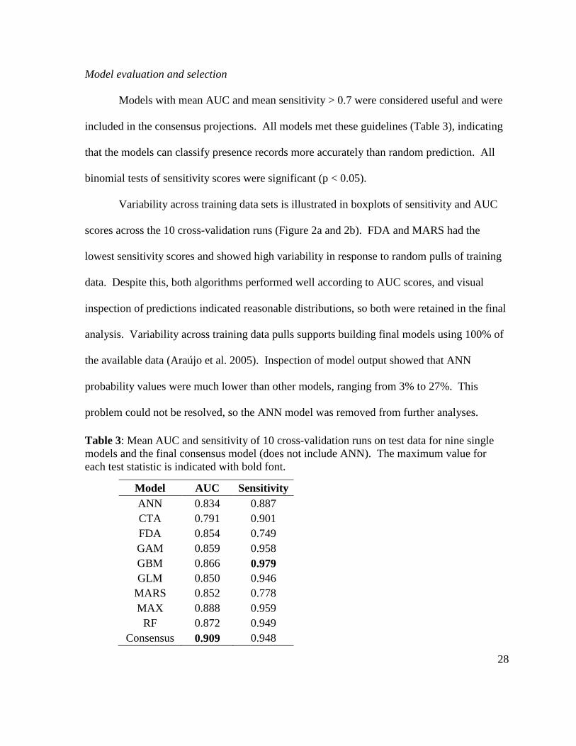
Model evaluation and selection

Models with mean AUC and mean sensitivity > 0.7 were considered useful and were

included in the consensus projections. All models met these guidelines (Table 3), indicating

that the models can classify presence records more accurately than random prediction. All

binomial tests of sensitivity scores were significant (p < 0.05).

Variability across training data sets is illustrated in boxplots of sensitivity and AUC

scores across the 10 cross-validation runs (Figure 2a and 2b). FDA and MARS had the

lowest sensitivity scores and showed high variability in response to random pulls of training

data. Despite this, both algorithms performed well according to AUC scores, and visual

inspection of predictions indicated reasonable distributions, so both were retained in the final

analysis. Variability across training data pulls supports building final models using 100% of

the available data (Araújo et al. 2005). Inspection of model output showed that ANN

probability values were much lower than other models, ranging from 3% to 27%. This

problem could not be resolved, so the ANN model was removed from further analyses.

Table 3: Mean AUC and sensitivity of 10 cross-validation runs on test data for nine single

models and the final consensus model (does not include ANN). The maximum value for

each test statistic is indicated with bold font.

Model AUC Sensitivity

ANN 0.834 0.887

CTA 0.791 0.901

FDA 0.854 0.749

GAM 0.859 0.958

GBM 0.866 0.979

GLM 0.850 0.946

MARS 0.852 0.778

MAX 0.888 0.959

RF 0.872 0.949

Consensus 0.909 0.948

29

Figure 2: Boxplots for sensitivity (a) and AUC (b) scores for 10 cross-validation runs on test data. The boxes represent the range of half of the scores, with the median represented by the black line. The whiskers represent the minimum and maximum score values. The consensus model does not include ANN. Note difference in y-axis scaling between (a) and (b).

ANN CTA FDA GAM GBM GLM MARS MAX RF Consensus

0.65

0.70

0.7

50

.80

0.8

50.

90

0.95

1.0

0

Model

Sen

siti

vity

(a)

ANN CTA FDA GAM GBM GLM MARS MAX RF Consensus

0.75

0.80

0.85

0.90

0.95

Model

AU

C

(b)

30

Refugial model, biogeographic hypotheses, and phylogeographic results

The refugial model shows potential refugial habitat to the north, south, and west of

the LGM ice sheet (Figure 3). South of the ice sheet, the strongest support for refugial areas

is found in the Oregon Cascades, Klamath, and Sierra Nevada Mountain ranges. North of the

ice sheet, the strongest support for refugial habitat is located in the Aleutian Islands and

southwest Alaska.

Figure 3: Consensus refugial model indicating areas of suitable habitat for R. integrifolia

across four time slices: current conditions, mid-Holocene, LGM, and LIG. Ice sheet layer is

from Dyke et al. 2003.

31

Potential coastal refugia in Haida Gwaii and the Alexander Archipelago (west coast

of British Columbia and Alaska) are indicated as well. The presence of exposed land in this

area during the LGM (now under water) likely provided additional habitat during the LGM

(Shafer et al. 2010, and references therein). Unfortunately, a test of this west coast refugium

could not be included in this analysis due to a lack of R. integrifolia tissue samples from that

region. However, previous examination of the distribution of R. integrifolia haplotypes has

provided support for a refugium in Haida Gwaii (Guest 2009).

Based on the configuration of refugial habitat in the SDM model and the availability

of genetic samples, four alternate biogeographic hypotheses (Figure 4) were tested for R.

integrifolia using a statistical phylogeographic approach:

1. Panmixia: no genetic differentiation between populations. This represents a null

hypothesis that an individual has an equal probability of being found anywhere in its

geographic range.

2. Northward colonization from a southern refugium after the LGM. This population

model is defined by expansion out of a southern refugial area, likely in the southern

Oregon Cascades or Sierra Nevada Mountains. This hypothesis predicts decreasing

genetic diversity with increasing latitude, and lineage coalescence dating to, or prior

to, the LGM. This model was parameterized with 90% of Ne located in the south and

10% of Ne located in the north.

3. Southward colonization from a northern refugium after the LGM. This population

model is defined by expansion out of a northern refugial area, likely centered in

southwestern Alaska. This hypothesis predicts increasing genetic diversity with

32

increasing latitude, and lineage coalescence dating to, or prior to, the LGM. This

model was parameterized with 90% of Ne located in the north and 10% of Ne located

in the south.

4. Colonization from multiple refugia (north and south). This population model is

defined by expansion out of northern and southern refugial areas after the LGM. This

hypothesis predicts no relationship between latitude and genetic diversity, and lineage

coalescence dating prior to the LGM. This model was parameterized with a range of

values of Ne (50,000 to 500,000) and two population divergence times: the LGM and

mid-Pleistocene (Illinoian Glacial Period, 120-180 kya).

The SDM refugial model would be best supported by the multiple refugia hypothesis.

Genetic support for the single refugium or panmixia models would not invalidate the SDM

projections, but would not exclude other possible explanations, such as mistakes in the

modeling process, barriers to dispersal, or a lack of niche conservatism.

33

Figure 4: Biogeographic hypotheses tested using statistical phylogeography. Each

hypothesis represents a different model of effective population sizes (Ne) and divergence

times: (a) panmixia; (b) northward colonization from a southern refugium; (c) southward

colonization from a northern refugium; (d) colonization from northern and southern refugia

with divergence at the LGM (left) and Illinoian Glacial Period (right).

34

The first three biogeographic hypotheses (panmixia and colonization from single

refugia) were not supported by the genetic data; the observed number of deep coalescences

did not meet the expected distribution for these population models (α = 0.05). The multiple

refugia hypothesis was supported (p < 0.05), meaning the observed number of deep

coalescences fell within the expected distribution for this model of population divergence.

The currently observed distribution of genetic variation for R. integrifolia can therefore be

explained by a model of population divergence in which northern and southern clades

diverged at or prior to the LGM. Divergence between these clades is supported both at the

LGM (where Ne = 50,000 to 100,000) and the mid-Pleistocene (Illinoian Glacial where Ne =

300,000 to 500,000). Additional phylogenetic analyses has further explored the timing of

this divergence (DeChaine et al. in prep).

Future projections

With phylogeographic support for the multiple refugia hypothesis, niche conservatism

in R. integrifolia was demonstrated across the modeled time period. Furthermore, the ability

of the SDMs to accurately project the climate-habitat relationship through time was

supported. Reciprocal inferences from both the refugial model and genetic data support the

use of the SDMs to assess future climate change impacts.

SDMs were used to project the geographic distribution of suitable habitat for R.

integrifolia in 2085 using five GCMs and two climate change scenarios. Consensus

projections were truncated at values of 50% or more of the models predicting suitable

habitat. Future consensus probability maps (Figure 5b and 5c) are based on five GCM

35

projections for each scenario (A1B and A2), and represent the consensus output from 80

models (eight model algorithms using two cutoff methods for each of five GCMs).

Projections for the A1B and A2 scenarios did not differ substantially, with both

indicating a significant reduction in suitable habitat (63 to 67%) by 2085 (Table 4, Figure 5d

and 5e). Both projections show a northward latitudinal shift in suitable habitat, with habitat

losses represented by upward elevational shifts and/or contractions of suitable habitat (Figure

5d and 5e). Relative to habitat loss, habitat expansion was minimal, with the largest gains in

the Brooks Range and north coast of Alaska. Both scenarios show dramatic loss of habitat in

the southern part of the range, including the Sierra Nevada, Cascade, and Northern Rocky

Mountains.

Though not explicitly quantified in this analysis, there were considerable differences

across the five GCM projections for both the A1B and A2 scenarios. To illustrate these

differences, projections from the five separate GCM projections and the final consensus

projection for the A2 scenario are presented in Figure 6.

Table 4: Changes in climatically suitable habitat for R. integrifolia from current conditions to

future climate scenarios for 2085.

A1B Scenario A2 Scenario

Loss 63% 67%

Stable 25% 22%

Gain 12% 11%

36

Figure 5: Current (a), A1B scenario (b), and A2 scenario (c) consensus probability maps.

Change in suitable habitat from current to future for the A1B (d) and A2 (e) scenarios, based

on a cutoff of 50% of the models indicating suitable habitat; black dots (a, d, e) indicate

pixels with current populations of R. integrifolia (based on herbarium searches).

37

Figure 6: Comparison of projections across five GCMs (b-f) and the final consensus

projection (a) for the A2 scenario at 2085. Projections are truncated at 50% of the models

indicating suitable habitat.

38

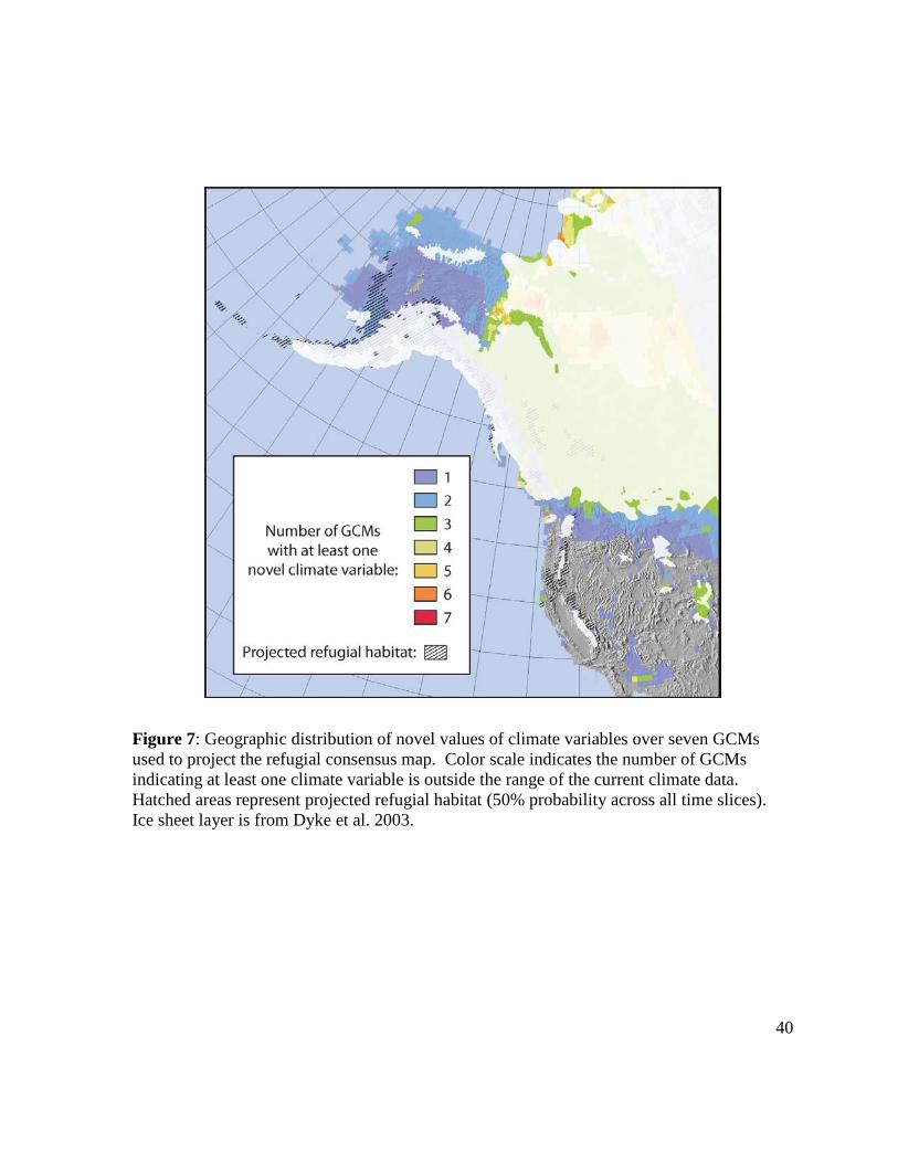
Novel values of climate variables

For the refugial model, novel values of climate variables were present mainly to the

north of the LGM ice sheet (Figure 7). In this area, suitable habitat and novel climate

variables coincided for one to two of the seven GCMs. The most dissimilar variables

(MoDs) north of the ice sheet were the standard deviation of summer minimum temperature

(tmnSD.JJA) and annual temperature range, both of which were found in climate data from

the LGM. For two of the GCMs (CCSM 3 and MIROC 3.2), novel values did not overlap

north of the ice sheet.

South of the LGM ice sheet, the main MoDs were tmnSD.JJA and annual temperature

range (again, all in the LGM data sets). The southern Rockies were of particular note, with

all three LGM climate data sets indicating summer minimum temperature as the MoD.

Overall, novel values of climate variables were more extensive in LGM climate data,

compared to mid-Holocene and LIG data sets. This is not surprising, given the large

differences between LGM and current climate.

For both the A1B and A2 projections, the overlap of future novel values of climate

variables with projected suitable habitat is limited mainly to northwestern Alaska (Figure 8a

and 8b). For both scenarios and across all GCMs, the MoD in this area is tmnSD.JJA. In

both scenarios, there is at least one GCM that does not have novel values in this region.

Future consensus projections do not show a gain of suitable habitat along the arctic coast;

however novel values of climate variables in this region indicate that this is an area of

uncertainty in model projections, and the potential for climatically suitable habitat in this

region should not be dismissed.

39

In both future projections, the areas to the north (arctic coast) and south (northwestern

Mexico) with high novel climates but no predicted habitat suitability have consistent MoDs.

In the arctic, the MoD is tmnSD.JJA, while in Mexico the MoD is summer minimum

temperature. These areas have novel climate values for these variables across all five GCMs,

which is not surprising given that these regions represent the extremes of temperature

variables in the climate data used to train the models. Coastal novel values are mainly

contributed by annual precipitation range; this is consistent across both scenarios and all

GCMs.

40

Figure 7: Geographic distribution of novel values of climate variables over seven GCMs

used to project the refugial consensus map. Color scale indicates the number of GCMs

indicating at least one climate variable is outside the range of the current climate data.

Hatched areas represent projected refugial habitat (50% probability across all time slices).

Ice sheet layer is from Dyke et al. 2003.

41

Figure 8: Geographic distribution of novel values of climate variables for the A1B scenario (a) and the A2 scenario (b). Color

scale indicates the number of GCMs indicating at least one climate variable is outside the range of the current climate data.

Hatched areas represent projected suitable habitat.

42

Discussion

Biogeographic hypothesis testing and niche conservatism

There is agreement between the refugial model, developed using SDMs, and the

phylogeographic analysis, conducted using simulations and empirical genetic data. Support

for the same hypothesis from these two independent data sets strengthens the inferences from

each, and indicates that there are two main lineages of R. integrifolia (north and south) that

have persisted at least since the LIG, and likely since the mid-Pleistocene.

The match between refugia identified by the SDMs and the phylogeographic analysis

supports niche conservatism in R. integrifolia, and justifies projection of the SDMs onto

future climates. This finding of niche conservatism is consistent with previous work on plant

responses to Quaternary climate change. Plants have a rich late-Quaternary paleoecological

record in North America and Europe due to an abundance of palynological analyses.

Research in this area, supported by phylogenetic work, has generally agreed that the

fundamental response of most temperate plant taxa to Quaternary climate changes was

migration, rather than adaptation (Huntley 1991; Prinzing et al. 2001; Ackerly 2003). Niche

conservatism should not be assumed for all plants however; rapid adaptive capacity has been

found for specific traits in some species (for example, changes in flowering time of Brassica

rapa, an annual plant studied in southern California, in response to climate fluctuations,

Franks et al. 2007).

The use of static SDMs to project future distributions is only appropriate for species

where the climate-distribution relationship is stable. Though niche conservatism is usually

assumed (or not addressed at all) in most SDM studies, genetic analyses have shown the

43

potential for rapid adaptation in some taxa, especially insects (Parmesan 2006; Reusch and

Wood 2007) and invasive species (Broennimann et al. 2007). Additionally, a study of 23

mammal species suggested a lack of niche conservatism in five, though other explanations

could not explicitly be ruled out (Martinez-Meyer et al. 2004). For some species

evolutionary responses will be more nuanced, with adaptation occurring at species range

limits, especially “trailing-edge” populations (Ackerly 2003; Hampe and Petit 2005;

Parmesan 2006). With this diversity of species-specific responses to climate change, it is

important to test the assumption of niche conservatism before projecting species distributions

into the future, since projection of species with labile niches would lead to erroneous results.

Especially for studies modeling at fine resolutions (e.g. 1-km pixel sizes), the potential for

rapid adaptation at species range limits should give modelers pause, in addition to other

concerns at these fine scales, such as changing biotic interactions and potential errors in

climate data downscaling.

It is important to note that phylogeographic support for the alternate hypotheses of a

single R. integrifolia refugium to the south or north of the LGM ice sheet would not have

invalidated the SDM refugial model. The SDMs in this study model the distribution of

climatically suitable habitat, but habitat suitability should not be equated with habitat

occupation. In this case, phylogeographic support for a single refugium model could have

multiple explanations, including: (1) long-term barriers to dispersal, such as sufficiently large

distances between habitat patches during the LIG that prevented colonization of climatically

suitable habitat; (2) adaptation (niche evolution or a lack of niche conservatism); (3) errors in

SDMs or climate data; and (4) errors in the phylogeographic modeling. One previous study

44

disentangled these explanations, finding support for niche evolution in a land snail (genus

Candidula) (Pfenninger et al. 2007) and further illustrating that the assumption of niche

conservatism in SDM studies should be tested.

Additionally, support for the multiple-refugia hypothesis is limited to the context of

the four models tested in this study. These models represent relatively simplistic hypotheses

regarding the structuring of genetic diversity in this widely distributed species. Given the

results of the SDMs, more sophisticated hypotheses could be tested in the future, including

the potential for cryptic refugia (e.g. a west coast refugium) and “refugia within refugia”

(isolation within major refugia, Shafer et al. 2010).

An interesting result of the refugial modeling was the indication of suitable habitat in

the Alexander Archipelago and Haida Gwaii, to the west of the LGM ice sheet (Figure 3a).

The presence of ice-free refugial areas on the west coast of British Columbia during the

LGM has been established in previous studies (Warner et al. 1982; Cook et al. 2006; Shafer

et al. 2010, and references therein), indicating that much of this suitable habitat was likely

ice-free. Unfortunately, genetic samples were not available from R. integrifolia populations

in this area, preventing a test of this west-coast refugial hypothesis. The presence of this

refugium is supported, however, by previous analyses of haplotype distributions for R.

integrifolia (Guest 2009). This illustrates how models derived from SDMs can be used to not

only develop biogeographic hypotheses but also direct appropriate sampling strategies to

better target specific phylogeographic questions. A test of this west coast hypothesis would

contribute to our understanding of the role of cryptic refugia in structuring current patterns of

genetic diversity, as well as improve estimates of dispersal and recolonization rates after the

45

LGM. Additionally, because refugia harbor high levels of genetic diversity (Hewitt 1996),

confirmation of a west coast R. integrifolia clade would lend support to efforts to recognize

and conserve the unique biota of these islands (Cook et al. 2006).

Future projections: the value of ensemble methods and genetic data, and a few caveats

Future projections of habitat suitability for R. integrifolia show substantial losses of

climatically suitable habitat across the range. Overall differences between greenhouse gas

scenarios were minimal (Figure 5, Table 4), while differences in projections across GCMs

were quite large (Figure 6). This indicates that less focus should be placed on modeling

alternate scenarios, with more effort directed toward sampling different GCM projections.

This coincides with previous work by Buisson et al. (2010), who found that up to 19% of

uncertainty in future model projections was due to the choice of GCM alone. Differences in

model algorithms accounted for even more of the uncertainty in future projections (29% to

51%), while greenhouse gas scenarios explained little of the variability (less than 10%).

In the southern part of the range, there is an almost complete loss of climatically

suitable habitat. Habitat persists at greatly reduced levels in the Sierra Nevada Mountains in

both the A1B and A2 scenarios, while only the A1B scenario retains any suitable habitat by

2085 in the Northern Rocky Mountains. The central and northern parts of the range also

show large losses of suitable habitat. Habitat gains in southeast Alaska may facilitate

population connectivity (Figure 5d and 5e) between central and northern populations. The

development of climatically suitable habitat in the Brooks Range of Alaska may also allow

for population expansion in that area.

46

Dispersal estimates are lacking in most SDM studies; projections usually assume

either unlimited dispersal, representing an optimistic scenario where species can colonize all

climatically suitable habitat, or no dispersal, representing a more conservative scenario in

which species can only persist in areas of stable climate. The difference between projections

using these alternate scenarios can be significant, contributing to uncertainty (for example,

Thomas et al. 2004; Engler and Guisan 2009). Phylogeography can provide a species-

specific metric of dispersal capability with which SDM projections can be constrained,

although these metrics are dependent upon the hypotheses tested (e.g. migration rates can be

overestimated if cryptic refugia are not included, Shafer et al. 2010). However, even rough

estimates of dispersal capability have been shown to greatly reduce this component of

projection uncertainty in SDMs (Engler and Guisan 2009).

Although phylogeographic analysis can provide a dispersal metric, an assessment of

dispersal capacity for R. integrifolia was outside the scope of this analysis. Based on future

projections, however, it appears unlikely that dispersal limitations will prevent colonization

of newly suitable habitat, since these areas are near currently established populations. Biotic

interactions and/or fine-scale climate variability (which are not addressed at the coarse scale

of this analysis) may prove to be greater determinants of successful population expansion.

An additional component of dispersal capability is the potential for populations to maintain

gene flow. Southern populations (Sierra Nevada and Rocky Mountains) are geographically

isolated, so dispersal between these populations is highly unlikely. The more closely located

west coast and southern Alaskan populations, however, have the potential to maintain gene

flow, since many of these populations are separated by only one or two pixels (approximately

47

50 to 100 km). Additional genetic analyses would allow an assessment of the potential for

increased connectivity or isolation of populations under future climates.

The ability to identify past refugia is an important benefit of phylogeography.

Because glacial-interglacial refugia tend to harbor high levels of allelic diversity (Hewitt

1996; Stewart et al. 2010), these regions have implications for conserving the genetic

structure of current and future populations. The refugial model indicates discrete southern

refugia in the southern Oregon Cascades, Klamath, and Sierra Nevada Mountain ranges

(Figure 3a). Populations in the Oregon Cascades are predicted to be extirpated by 2085,

though the potential for persistence in microclimate refugia should not be discounted (see

below). The Sierra Nevada population is likely to persist but will be further isolated under

both future climate change scenarios. The persistence of these populations will be important

to the maintenance of overall levels of genetic diversity in this species. Further analysis of

genetic data can corroborate this interpretation, by providing indices that quantify neutral

genetic diversity within these populations. Overlap between northern (Alaskan) refugia and

future distributions of suitable habitat are not as clear; further analysis of relative levels of

genetic diversity within and between populations in Alaska would be helpful to better

understand the potential genetic impacts of population losses, especially in southwestern

Alaska and the Aleutian Islands. Additionally, populations currently located in the

Alexander Archipelago and Haida Gwaii are forecast to lose all suitable habitat under both

future scenarios. This should encourage efforts to assess the genetic support for this region

as a cryptic refugia for R. integrifolia, and a possible area of unique genetic diversity for the

species.

48

Although these projections appear dire, it is important to recognize that the coarse

grain of this biogeographic analysis can overpredict the loss of climatically suitable habitat.

Especially in mountainous regions, coarse SDMs are likely to underestimate the potential for

suitable habitat under future climate change (Randin et al. 2009; Barbet-Massin et al. 2010).

At landscape to local scales topography has important impacts on the distribution of alpine

plants. This is mainly due to the influence of topography on the distribution of microclimate

refugia in mountainous terrain (Dobrowski 2010). In these areas of topographic complexity,

climate patterns at fine scales are influenced by spatially varying elevation relationships,

terrain barriers, terrain-induced climate transitions, cold air drainage patterns, inversions, and

coastal effects (Daly 2006). Because coarse climatic data average out these complexities, the

most likely outcome is underestimation of potential habitat, though one study has shown the

opposite effect (Trivedi et al. 2008).

This suggests some important limitations in the use of SDMs to predict climate

change impacts. First, modelers need to balance “resolution with realism” (Daly 2006) when

downscaling projections from GCMs, although the improved availability of regional climate

models may help with this limitation (at least for future climate projections). The common

use of gridded climate data that are interpolated to ~1-km pixel sizes from very large scale

GCM runs (e.g. 2 by 3°) should be questioned. A second consideration is that at fine

(landscape to local) scales, climatic controls over species distributions breaks down. Biotic

interactions, range dynamics, demographic processes, topography and microclimate are

extremely important. At these scales, the use of SDMs alone is not suitable; SDMs

49

integrated with mechanistic models is a more appropriate approach (for example, Keith et al.

2008; Brook et al. 2009).

Predictor variable selection and SDMs

The importance of using predictor variables in correlative SDMs that are biologically

appropriate and functionally-relevant to the species being modeled has been stressed by

many authors (for example, Guisan and Zimmermann 2000; Austin 2002; Lookingbill and

Urban 2005). Less commonly emphasized is how the selection of appropriate variables

interacts with scale (both extent and pixel size); for example, climate-related variables are

most applicable at global to regional scales, with topography, land use and soil type more

relevant at landscape to site-level scales (Pearson and Dawson 2003). As mentioned above,

biotic interactions and source-sink dynamics also become extremely important at landscape

and site-level scales. Unfortunately, many SDM studies still rely exclusively on pre-

calculated biogeographic-scale abiotic variables (e.g. WorldClim data), even when modeling

at fine spatial scales. Difficulties in compiling gridded data sets (e.g. workload, access,

feasibility) will prevent many SDM practitioners from using ecologically-based, scale-

appropriate predictor variables. On the other hand, the removal of highly correlated predictor

variables is becoming more common in SDM studies. This is a positive development, since

highly correlated variables can cause serious prediction errors in some model algorithms

(Franklin 2009). Overall, ecologists using SDMs need to be aware of these limitations and

plan the scale (extent and grain) of their studies based on what is logistically feasible and

ecologically appropriate.

50

In this study, the final choice of predictor variables clearly relates to the ecology and

distribution of alpine and arctic plants at biogeographic scales. Spring snowpack, summer

temperatures, and summer temperature extremes (as indexed by standard deviation) are

particularly relevant to alpine-arctic plants (Körner 2003). These factors interact, especially

at the beginning of the growing season when the start of plant growth is triggered by

photoperiod, temperature, and snowpack depth (Körner 2003). Plants must strike a balance

between warming temperatures, diminishing snowpack, and the potential for extreme cold

events that could cause frost damage to sensitive tissues (Inouye 2008). Research on

herbaceous plants and shrubs in the alpine has shown that the negative impact of early season

low-temperature events on bud mortality outweighed the positive effects of longer growing

seasons (Inouye 2008; Wipf et al. 2009). Reduced snowpack in spring resulted in increased

exposure of leaf and flower buds to early spring frost events, reducing seed production and

impacting demographic recruitment (Inouye 2008).

Methods to select relevant predictor variables from a potentially large, correlated list

of possibilities have not been addressed specifically in the SDM literature. In this study, the

random forest algorithm was successfully used to select the most relevant predictor variables

for R. integrifolia, while controlling for the highly correlated nature of these predictors

(Strobl et al. 2008). To my knowledge, this multivariate approach to variable selection has

not been used in SDM studies. It should be considered, as it provides a simple and intuitive

method to filter highly correlated predictors and select the most species-relevant variables.

51

Ensemble modeling and novel climates

In addition to support from genetic analyses, species distribution projections were

made more robust through the use of an ensemble and consensus approach to modeling. The

consensus model of current R. integrifolia distribution had a higher predictive capacity based

on AUC scores than any of the single SDMs alone (Figure 2b, Table 3), and was among the

highest scoring based on sensitivity scores (Figure 2a, Table 3). This is in agreement with

previous work indicating that consensus models outperform individual models, providing

more robust projections of habitat distribution (Marmion et al. 2009; Grenouillet et al. 2011).

The use of multiple model algorithms in studies that project species distributions is also

supported by recent work showing that models with the highest accuracy on current climate

data may not be the best at projecting onto new areas or climate conditions (Heikkinen et al.

2011).

The ensemble and consensus approach also allows a spatial depiction of agreement

across model algorithms, by showing areas of consensus among models and areas of

disagreement. Current and future projections for R. integrifolia (Figure 5) show the

percentage of models “voting” for suitable habitat for a given pixel. Areas of agreement are

regions of greater confidence in the model projections, while areas of disagreement (e.g. at

the low end of the 50% cutoff) indicate areas of lower confidence. The combined output of

model algorithms, threshold methods and GCM conditions helps delimit a range of

uncertainties associated with projecting the distribution of suitable habitat (Araújo and New

2007). For example, rather than basing an analysis spanning 124 kya on the output from one

model algorithm and one GCM projection, I combined output from 8 model algorithms on

52

anywhere from one to five GCMs. Using this ensemble and consensus approach, my final

maps indicate agreement across many model projections (from 16 to 128 models). As each

of these indicates possible states of the system being modeled, this approach allows for

greater confidence in model output, especially when projecting across temporal scales.

Despite its advantages, ensemble modeling should be used with caution. Naïve use of

model algorithms can result in poor parameterization and poorly performing models.

Ensemble approaches also greatly magnify the work-load associated with modeling species

distributions. Despite these drawbacks, ensemble approaches appear to be an effective way

to create robust projections that include a depiction of variability and uncertainty.

As mentioned above, the use of multiple GCMs is an especially important component

of the ensemble approach when projecting species distributions. I found substantial

variability across the five GCMs used for future projections (Figure 6). By combining these

projections and showing areas of consensus and disagreement among models, I can indicate

areas of higher and lower confidence in projected distributions. This analysis only takes a

small sample of available projections; the IPCC’s Fourth Assessment Report included 23

GCMs. However, most SDM studies use one or at most two GCMs for future projections;

there is certainly room for improvement in this component of projecting climate change

impacts. Modelers are limited by the availability of interpolated climate data from these

GCMs, and so often focus their efforts on including multiple greenhouse gas scenarios,

despite the fact that these contribute very little to sampling the variability in future

projections (Buisson et al. 2010).

53

Novel climate variable analysis also illustrates why it is important to use multiple

GCMs. While GCMs can sometimes be spatially coherent in their novel climates across

variables (e.g. different GCMs predicting areas of novel climate in similar locations based on

the same variable), many times GCMs differ in their spatial prediction of novel values of

climate variables. For example, in the A1B and A2 projections, areas of novel climate are

seen in the northwestern part of Alaska and along the arctic coast (Figure 8a and 8b). For

both scenarios, there are GCMs without novel values in these regions. If this were an area of

potential conservation concern, those GCM projections without novel values could be

individually inspected to avoid the uncertainties associated with projecting models onto

novel climates.

For future projections, most of the novel values of climate variables are found at the

latitudinal limits of the projected study area. This is expected, since these regions represent

the extremes of temperature variables in the climate data used to train the models. In both

paleoclimatic and future climate data sets, the possibility of encountering novel climates is

minimized by training the current model on the entire latitudinal range of the species,

ensuring that all current values and combinations of climate variables are included in creation

of response curves.

The very real possibility of projecting SDMs onto novel climates is frequently

mentioned in the literature, but rarely addressed. The MESS analysis included with the most

recent versions of Maxent is an excellent tool to help modelers consider the impact of novel

values of climate variables on their projections. This technique, however, does not consider

novel combinations of climate variables. This analysis is equally important because models

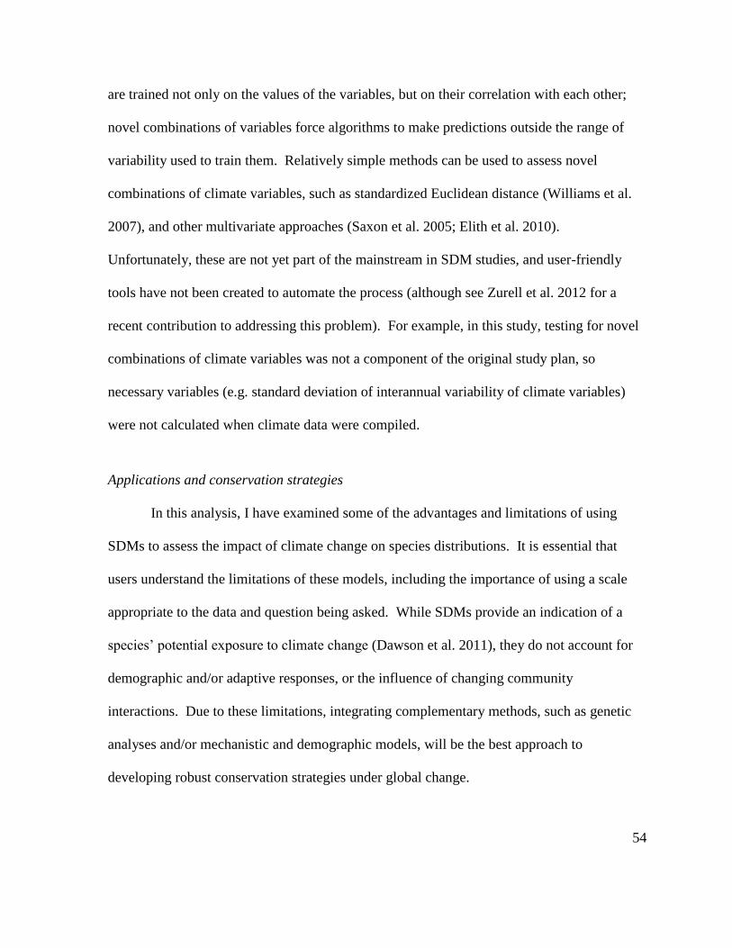
54

are trained not only on the values of the variables, but on their correlation with each other;

novel combinations of variables force algorithms to make predictions outside the range of

variability used to train them. Relatively simple methods can be used to assess novel

combinations of climate variables, such as standardized Euclidean distance (Williams et al.

2007), and other multivariate approaches (Saxon et al. 2005; Elith et al. 2010).

Unfortunately, these are not yet part of the mainstream in SDM studies, and user-friendly

tools have not been created to automate the process (although see Zurell et al. 2012 for a

recent contribution to addressing this problem). For example, in this study, testing for novel

combinations of climate variables was not a component of the original study plan, so

necessary variables (e.g. standard deviation of interannual variability of climate variables)

were not calculated when climate data were compiled.

Applications and conservation strategies

In this analysis, I have examined some of the advantages and limitations of using

SDMs to assess the impact of climate change on species distributions. It is essential that

users understand the limitations of these models, including the importance of using a scale

appropriate to the data and question being asked. While SDMs provide an indication of a

species’ potential exposure to climate change (Dawson et al. 2011), they do not account for

demographic and/or adaptive responses, or the influence of changing community

interactions. Due to these limitations, integrating complementary methods, such as genetic

analyses and/or mechanistic and demographic models, will be the best approach to

developing robust conservation strategies under global change.

55

In this study, SDMs were coupled with phylogeographic analyses, providing a more

comprehensive assessment of climate change impacts that addresses both exposure and past

responses to climate change, as well as identification of areas of potentially high genetic

diversity (past refugia). Genetic analyses can also provide measures of neutral (and

increasingly, adaptive) genetic diversity, population differentiation, and dispersal capability.

The use of molecular data to improve conservation responses to global change will continue

to increase as the costs of obtaining genetic data decline. The explicit incorporation of

“evolutionary resilience” (Sgro et al. 2011) in conservation planning has become feasible

with rapid developments in sequencing and analytic tools. These approaches are especially

important for proactive conservation actions since research indicates that wild populations

are more susceptible to extinction in the absence of genetic variation (Spielman et al. 2004).

I agree with Dawson and colleagues (2011) that efforts to conserve biodiversity and

improve ecosystem functioning need to move beyond predictions of climate change impacts

and toward an integrated effort to address solutions. SDMs will be only one component of

that effort. Practitioners should continue to develop a more sophisticated understanding of

the advantages, limitations and appropriate uses of SDMs, while working with colleagues to

incorporate alternate and complementary analyses. This integrated approach will be the most

effective way to develop robust conservation strategies for species and ecosystems in the face

of the interacting stressors of climate change, land-use change, habitat destruction, invasive

species, pollution, and other anthropogenic influences.

56

References:

Ackerly D (2003) Community assembly, niche conservatism, and adaptive evolution in

changing environments. International Journal of Plant Sciences 164:S165-S184

Anderson RP, Gómez‐Laverde M, Peterson AT (2002) Geographical distributions of spiny

pocket mice in South America: insights from predictive models. Global Ecology and

Biogeography 11:131–141

Araújo MB, Guisan A (2006) Five (or so) challenges for species distribution modelling.

Journal of Biogeography 33:1677–1688

Araújo MB, New M (2007) Ensemble forecasting of species distributions. Trends in Ecology

& Evolution 22:42–47

Araújo MB, Whittaker RJ, Ladle RJ, Erhard M (2005) Reducing uncertainty in projections of

extinction risk from climate change. Global Ecology and Biogeography 14:529–538

Austin M (2002) Spatial prediction of species distribution: an interface between ecological

theory and statistical modelling. Ecological Modelling 157:101–118

Austin MP, Van Niel KP (2011) Improving species distribution models for climate change

studies: variable selection and scale. Journal of Biogeography 38:1–8

Avise JC (2000) Phylogeography: The History and Formation of Species. Harvard University

Press, Cambridge, MA

Barbet-Massin M, Jiguet F, Albert CH, Thuiller W (2012) Selecting pseudo‐absences for

species distribution models: how, where and how many? Methods in Ecology and

Evolution

Barbet‐Massin M, Thuiller W, Jiguet F (2010) How much do we overestimate future local

extinction rates when restricting the range of occurrence data in climate suitability

models? Ecography 33:878–886

Brook BW, Akçakaya HR, Keith DA, Mace GM, Pearson RG, Araújo MB (2009) Integrating

bioclimate with population models to improve forecasts of species extinctions under

climate change. Biology Letters

Buisson L, Thuiller W, Casajus N, Lek S, Grenouillet G (2010) Uncertainty in ensemble

forecasting of species distribution. Global Change Biology 16:1145–1157

Carstens BC, Richards CL (2007) Integrating coalescent and ecological niche modeling in

comparative phylogeography. Evolution 61:1439–1454

Chan LM, Brown JL, Yoder AD (2011) Integrating statistical genetic and geospatial methods

brings new power to phylogeography. Molecular Phylogenetics and Evolution

59:523–537

57

Chen I-C, Hill JK, Ohlemüller R, Roy DB, Thomas CD (2011) Rapid range shifts of species

associated with high levels of climate warming. Science 333:1024–1026

Clausen R (1975) Sedum of North America North of the Mexican Plateau. Cornell University

Press, Ithaca, NY

Colwell RK, Rangel TF (2009) Hutchinson’s duality: the once and future niche. Proceedings

of the National Academy of Sciences

Cook JA, Dawson NG, MacDonald SO (2006) Conservation of highly fragmented systems:

the north temperate Alexander Archipelago. Biological Conservation 133:1–15

Cordellier M, Pfenninger M (2009) Inferring the past to predict the future: climate modelling

predictions and phylogeography for the freshwater gastropod Radix balthica

(Pulmonata, Basommatophora). Molecular Ecology 18:534–544

Daly C (2006) Guidelines for assessing the suitability of spatial climate data sets.

International Journal of Climatology 26:707–721

Davis MB, Shaw RG (2001) Range shifts and adaptive responses to Quaternary climate

change. Science 292:673–679

Dawson TP, Jackson ST, House JI, Prentice IC, Mace GM (2011) Beyond predictions:

biodiversity conservation in a changing climate. Science 332:53–58

DeChaine EG, Forester BR, Schaefer H, Davis CC (in prep) The Return of the King! Cryptic

lineages hidden among disjunct refugia in the arctic-alpine plant Rhodiola integrifolia

(Crassulaceae).

Dépraz A, Cordellier M, Hausser J, Pfenninger M (2008) Postglacial recolonization at a

snail’s pace (Trochulus villosus): confronting competing refugia hypotheses using

model selection. Molecular Ecology 17:2449–2462

Diniz-Filho JAF, Mauricio Bini L, Fernando Rangel T, Loyola RD, Hof C, Nogués‐Bravo D,

Araújo MB (2009) Partitioning and mapping uncertainties in ensembles of forecasts

of species turnover under climate change. Ecography 32:897–906

Dirnbock T, Essl F, Rabitsch W (2011) Disproportional risk for habitat loss of high-altitude

endemic species under climate change. Global Change Biology 17:990–996

Dobrowski SZ (2010) A climatic basis for microrefugia: the influence of terrain on climate.

Global Change Biology:1–14

Drummond AJ, Rambaut A (2007) BEAST: Bayesian evolutionary analysis by sampling

trees. BMC Evolutionary Biology 7:214

Dyke AS, Moore A, Robertson L (2003) Deglaciation of North America; Geological Survey

of Canada Open File 1547.

58

Elith J, Kearney M, Phillips S (2010) The art of modelling range-shifting species. Methods in

Ecology and Evolution 1:330–342

Engler R, Guisan A (2009) MigClim: predicting plant distribution and dispersal in a

changing climate. Diversity and Distributions 15:590–601

Engler R, Randin CF, Vittoz P, Czáka T, Beniston M, Zimmermann NE, Guisan A (2009)

Predicting future distributions of mountain plants under climate change: does

dispersal capacity matter? Ecography 32:34–45

ESRI (Environmental Systems Resource Institute) (2010) ArcMap 10.0. Redlands, California

Fielding A, Bell J (1997) A review of methods for the assessment of prediction errors in

conservation presence/absence models. Environmental Conservation 24:38–49

Fitzpatrick M, Hargrove W (2009) The projection of species distribution models and the

problem of non-analog climate. Biodiversity and Conservation 18:2255–2261

Franklin J (2009) Mapping Species Distributions: Spatial Inference and Prediction.

Cambridge University Press, Cambridge, UK

Franklin J (2010) Moving beyond static species distribution models in support of

conservation biogeography. Diversity and Distributions 16:321–330

Franks SJ, Sim S, Weis AE (2007) Rapid evolution of flowering time by an annual plant in

response to a climate fluctuation. Proceedings of the National Academy of Sciences

104:1278 –1282

Galbreath KE, Hafner DJ, Zamudio KR (2009) When cold is better: climate-driven elevation

shifts yield complex patterns of diversification and demography in an alpine specialist

(American pika, Ochotona princeps). Evolution 63:2848–2863

Gordon C, Cooper C, Senior CA, Banks H, Gregory JM, Johns TC, Mitchell JFB, Wood RA

(2000) The simulation of SST, sea ice extents and ocean heat transports in a version

of the Hadley Centre coupled model without flux adjustments. Climate Dynamics

16:147–168

Gordon H, Rotstayn L, McGregor J, Dix M, Kowalczyk E, O’Farrell S, Waterman L, Hirst

A, Wilson S, Collier M, Watterson I, Elliott T (2002) The CSIRO Mk3 Climate

System Model. CSIRO Atmospheric Research, Aspendale, Victoria, Australia

Grenouillet G, Buisson L, Casajus N, Lek S (2011) Ensemble modelling of species

distribution: the effects of geographical and environmental ranges. Ecography 34:9–

17

Guest HJ (2009) Systematic and phylogeographic implications of molecular variation in the

western North American roseroot Rhodiola integrifolia (Crassulaceae). Master's

thesis, University of Victoria, British Columbia, Canada

59

Guisan A, Zimmermann N (2000) Predictive habitat distribution models in ecology.

Ecological Modelling 135:147–186

Hampe A, Petit R (2005) Conserving biodiversity under climate change: the rear edge

matters. Ecology Letters 8:461–467

Heikkinen RK, Marmion M, Luoto M (2011) Does the interpolation accuracy of species

distribution models come at the expense of transferability? Ecography:1–13

Hernandez-Stefanoni JL, Ponce-Hernandez R (2006) Mapping the spatial variability of plant

diversity in a tropical forest: comparison of spatial interpolation methods.

Environmental Monitoring and Assessment 117:307–334

Hewitt G (1996) Some genetic consequences of ice ages, and their role in divergence and

speciation. Biological Journal of the Linnean Society 58:247–276

Hewitt G (2000) The genetic legacy of the Quaternary ice ages. Nature 405:907–913

Hijmans R, Cameron S, Parra J, Jones P, Jarvis A (2005) Very high resolution interpolated

climate surfaces for global land areas. International Journal of Climatology 25:1965–

1978

Hugall A, Moritz C, Moussalli A, Stanisic J (2002) Reconciling paleodistribution models and

comparative phylogeography in the Wet Tropics rainforest land snail Gnarosophia

bellendenkerensis (Brazier 1875). Proceedings of the National Academy of Sciences

99:6112–6117

Hughes L (2000) Biological consequences of global warming: is the signal already apparent?

Trends in Ecology & Evolution 15:56–61

Hutchinson GE (1957) Concluding remarks. Cold Spring Harbor Symposia on Quantitative

Biology 22:415–427

Inouye DW (2008) Effects of climate change on phenology, frost damage, and floral

abundance of montane wildflowers. Ecology 89:353–362

Jackson ST, Betancourt JL, Booth RK, Gray ST (2009) Ecology and the ratchet of events:

climate variability, niche dimensions, and species distributions. Proceedings of the

National Academy of Sciences 106:19685–19692

Johns TC, Durman CF, Banks HT, Roberts MJ, McLaren AJ, Ridley JK, Senior CA,

Williams KD, Jones A, Rickard GJ, Cusack S, Ingram WJ, Crucifix M, Sexton DMH,

Joshi MM, Dong B-W, Spencer H, Hill RSR, Gregory JM, Keen AB, Pardaens AK,

Lowe JA, Bodas-Salcedo A, Stark S, Searl Y (2006) The new Hadley Centre climate

model (HadGEM1): Evaluation of coupled simulations. Journal of Climate 19:1327–

1353

60

K-1 model developers (2004) K-1 coupled GCM (MIROC) description (H Hasumi and S

Emori, Eds.). Center for Climate System Research, University of Tokyo

Kearney M (2006) Habitat, environment and niche: what are we modelling? Oikos 115:186–

191

Keith DA, Akçakaya HR, Thuiller W, Midgley GF, Pearson RG, Phillips SJ, Regan HM,

Araújo MB, Rebelo TG (2008) Predicting extinction risks under climate change:

coupling stochastic population models with dynamic bioclimatic habitat models.

Biology Letters 4:560–563

Klein C, Wilson K, Watts M, Stein J, Berry S, Carwardine J, Smith M, Mackey B,

Possingham H (2009) Incorporating ecological and evolutionary processes into

continental-scale conservation planning. Ecological Applications 19:206–217

Knowles LL (2004) The burgeoning field of statistical phylogeography. Journal of

Evolutionary Biology 17:1–10

Knowles L, Carstens B, Keat M (2007) Coupling genetic and ecological-niche models to

examine how past population distributions contribute to divergence. Current Biology

17:940–946

Körner C (2003)Alpine Plant Life: Functional Plant Ecology of High Mountain Ecosystems,

2nd ed. Springer, Berlin

Kuhner MK (2006) LAMARC 2.0: maximum likelihood and Bayesian estimation of

population parameters. Bioinformatics 22:768–770

Lenoir J, Gegout JC, Marquet PA, de Ruffray P, Brisse H (2008) A significant upward shift

in plant species optimum elevation during the 20th century. Science 320:1768–1771

Liaw A, Wiener M (2002) Classification and regression by randomForest. R News 2:18–22

Liu C, Berry P, Dawson T, Pearson R (2005) Selecting thresholds of occurrence in the

prediction of species distributions. Ecography 28:385–393

Lookingbill T, Urban D (2005) Gradient analysis, the next generation: towards more plant-

relevant explanatory variables. Canadian Journal of Forest Research 35:1744–1753

Lutz J, van Wagtendonk J, Franklin J (2010) Climatic water deficit, tree species ranges, and

climate change in Yosemite National Park. Journal of Biogeography 37:936–950

Maddison WP (1997) Gene trees in species trees. Systematic Biology 46:523–536

Maddison WP, Maddison DR (2011) Mesquite: a modular system for evolutionary analysis.

Marmion M, Parviainen M, Luoto M, Heikkinen R, Thuiller W (2009) Evaluation of

consensus methods in predictive species distribution modelling. Diversity and

Distributions 15:59–69

61

Marti O, Braconnot P, Dufresne J-L, Bellier J, Benshila R, Bony S, Brockmann P, Cadule P,

Caubel A, Codron F, Noblet N, Denvil S, Fairhead L, Fichefet T, Foujols M-A,

Friedlingstein P, Goosse H, Grandpeix J-Y, Guilyardi E, Hourdin F, Idelkadi A,

Kageyama M, Krinner G, Lévy C, Madec G, Mignot J, Musat I, Swingedouw D,

Talandier C (2009) Key features of the IPSL ocean atmosphere model and its

sensitivity to atmospheric resolution. Climate Dynamics 34:1–26

Meehl G, et al. (2007) 2007: Global Climate Projections. In: S. Solomon et al. (ed) Climate

Change 2007: The Physical Science Basis. Contribution of Working Group I to the

Fourth Assessment Report of the Intergovernmental Panel on Climate Change.

Cambridge University Press, Cambridge, UK and New York, NY, USA

Mitchell TD, Jones PD (2005) An improved method of constructing a database of monthly

climate observations and associated high-resolution grids. International Journal of

Climatology 25:693–712

Moritz C, Hoskin C., MacKenzie J., Phillips B., Tonione M, Silva N, VanDerWal J,

Williams S., Graham C. (2009) Identification and dynamics of a cryptic suture zone

in tropical rainforest. Proceedings of the Royal Society B: Biological Sciences

276:1235 –1244

Nogués-Bravo D (2009) Predicting the past distribution of species climatic niches. Global

Ecology and Biogeography 18:521–531

Nogués-Bravo D, Araújo MB, Errea MP, Martínez-Rica JP (2007) Exposure of global

mountain systems to climate warming during the 21st Century. Global Environmental

Change 17:420–428

Otto-Bliesner BL, Brady EC, Clauzet G, Tomas R, Levis S, Kothavala Z (2006) Last Glacial

Maximum and Holocene climate in CCSM3. Journal of Climate 19:2526–2544

Parmesan C (2006) Ecological and evolutionary responses to recent climate change. Annual

Review of Ecology, Evolution, and Systematics 37:637–669

Parmesan C (2007) Influences of species, latitudes and methodologies on estimates of

phenological response to global warming. Global Change Biology 13:1860–1872

Parmesan C, Yohe G (2003) A globally coherent fingerprint of climate change impacts

across natural systems. Nature 421:37–42

Pearson RG, Dawson TP (2003) Predicting the impacts of climate change on the distribution

of species: are bioclimate envelope models useful? Global Ecology and Biogeography

12:361–371

Pfenninger M, Nowak C, Magnin F (2007) Intraspecific range dynamics and niche evolution

in Candidula land snail species. Biological Journal of the Linnean Society 90:303–

317

62

Phillips SJ, Anderson RP, Schapire RE (2006) Maximum entropy modeling of species

geographic distributions. Ecological Modelling 190:231–259

Phillips S, Dudik M (2008) Modeling of species distributions with Maxent: new extensions

and a comprehensive evaluation. Ecography 31:161–175

R Development Core Team (2011) R: a language and environment for statistical computing.

R Foundation for Statistical Computing, Vienna, Austria

Randin C, Engler R, Normand S, Zappa M, Zimmermann N, Pearman P, Vittoz P, Thuiller

W, Guisan A (2009) Climate change and plant distribution: local models predict high-

elevation persistence. Global Change Biology 15:1557–1569

Reusch TB, Wood TE (2007) Molecular ecology of global change. Molecular Ecology

16:3973–3992

Richards CL, Carstens BC, Lacey Knowles L (2007) Distribution modelling and statistical

phylogeography: an integrative framework for generating and testing alternative

biogeographical hypotheses. Journal of Biogeography 34:1833–1845

Root TL, Price JT, Hall KR, Schneider SH, Rosenzweig C, Pounds JA (2003) Fingerprints of

global warming on wild animals and plants. Nature 421:57–60

Rosenberg N, Nordborg M (2002) Genealogical trees, coalescent theory and the analysis of

genetic polymorphisms. Nature Reviews Genetics 3:380–390

Saxon E, Baker B, Hargrove W, Hoffman F, Zganjar C (2005) Mapping environments at risk

under different global climate change scenarios. Ecology Letters 8:53–60

Scoble J, Lowe A (2010) A case for incorporating phylogeography and landscape genetics

into species distribution modelling approaches to improve climate adaptation and

conservation planning. Diversity and Distributions 16:343–353

Sgro C, Lowe A, Hoffmann A (2011) Building evolutionary resilience for conserving

biodiversity under climate change. Evolutionary Applications 4:326–337

Shafer ABA, Cullingham CI, Côté SD, Coltman DW (2010) Of glaciers and refugia: a

decade of study sheds new light on the phylogeography of northwestern North

America. Molecular Ecology 19:4589–4621

Soberón J (2007) Grinnellian and Eltonian niches and geographic distributions of species.

Ecology Letters 10:1115–1123

Soberón JM (2010) Niche and area of distribution modeling: a population ecology

perspective. Ecography 33:159–167

Sokolov A, Stone P, Forest C, Prinn R, Sarofim M, Webster M, Paltsev S, Schlosser C,

Kicklighter D, Dutkiewicz S, Reilly J, Wang C, Felzer B, Melillo J, Jacoby H (2009)

63

Probabilistic forecast for twenty-first-century climate based on uncertainties in

emissions (without policy) and climate parameters. Journal of Climate 22:5175–5204

Spielman D, Brook BW, Frankham R (2004) Most species are not driven to extinction before

genetic factors impact them. Proceedings of the National Academy of Sciences

101:15261 –15264

Stephenson N (1998) Actual evapotranspiration and deficit: biologically meaningful

correlates of vegetation distribution across spatial scales. Journal of Biogeography

25:855–870

Stewart J, Lister A, Barnes I, Dalen L (2010) Refugia revisited: individualistic responses of

species in space and time. Proceedings of the Royal Society B: Biological Sciences

277:661–671

Strobl C, Boulesteix A-L, Kneib T, Augustin T, Zeileis A (2008) Conditional variable

importance for random forests. BMC Bioinformatics 9:307

Thomas CD, Cameron A, Green RE, Bakkenes M, Beaumont LJ, Collingham YC, Erasmus

BFN, de Siqueira MF, Grainger A, Hannah L, Hughes L, Huntley B, van Jaarsveld

AS, Midgley GF, Miles L, Ortega-Huerta MA, Townsend Peterson A, Phillips OL,

Williams SE (2004) Extinction risk from climate change. Nature 427:145–148

Thuiller W (2004) Patterns and uncertainties of species’ range shifts under climate change.

Global Change Biology 10:2020–2027

Thuiller W, Lafourcade B, Engler R, Araujo M (2009) BIOMOD - a platform for ensemble

forecasting of species distributions. Ecography 32:369–373

Trivedi M, Berry P, Morecroft M, Dawson T (2008) Spatial scale affects bioclimate model

projections of climate change impacts on mountain plants. Global Change Biology

14:1089–1103

Waltari E, Hijmans R, Peterson A, Nyari A, Perkins S, Guralnick R (2007) Locating

Pleistocene refugia: comparing phylogeographic and ecological niche model

predictions. PLoS ONE 2:e563

Warner BG, Mathewes RW, Clague JJ (1982) Ice-free conditions on the Queen Charlotte

Islands, British Columbia, at the height of late Wisconsin glaciation. Science 218:675

–677

Webb TI, Bartlein PJ (1992) Global changes during the last 3 million years: climatic controls

and biotic responses. Annual Review of Ecology and Systematics 23:141–173

Wiens J, Ackerly D, Allen A, Anacker B, Buckley L, Cornell H, Damschen E, Davies T,

Grytnes J, Harrison S, Hawkins B, Holt R, McCain C, Stephens P (2010) Niche

conservatism as an emerging principle in ecology and conservation biology. Ecology

Letters 13:1310–1324

64

Wiens J, Stralberg D, Jongsomjit D, Howell C, Snyder M (2009) Niches, models, and climate

change: assessing the assumptions and uncertainties. Proceedings of the National

Academy of Sciences 106:19729–19736

Williams J, Jackson S, Kutzbacht J (2007) Projected distributions of novel and disappearing

climates by 2100 AD. Proceedings of the National Academy of Sciences 104:5738–

5742

Willmott CJ (1982) Some comments on the evaluation of model performance. Bulletin of the

American Meteorological Society 63:1309–1313

Wipf S, Stoeckli V, Bebi P (2009) Winter climate change in alpine tundra: plant responses to

changes in snow depth and snowmelt timing. Climatic Change 94:105–121

Woodward F (1987) Climate and Plant Distribution. Cambridge University Press,

Cambridge, UK

Zimmermann NE, Edwards Jr TC, Graham CH, Pearman PB, Svenning J (2010) New trends

in species distribution modelling. Ecography 33:985–989

Zimmermann N, Yoccoz N, Edwards T, Meier E, Thuiller W, Guisan A, Schmatz D,

Pearman P (2009) Climatic extremes improve predictions of spatial patterns of tree

species. Proceedings of the National Academy of Sciences 106:19723–19728

Zurell D, Elith J, Schröder B (2012) Predicting to new environments: tools for visualizing

model behaviour and impacts on mapped distributions. Diversity and Distributions

Zwickl D (2006) Genetic algorithm approaches for the phylogenetic analysis of large

biological sequence datasets under the maximum likelihood criterion. Ph.D.

Dissertation, The University of Texas at Austin

65

Appendix A: Climate data processing

When available, global monthly layers were downloaded from climate databases for

the following four climate variables: total precipitation rate (pr), surface (2m) air temperature

(tas), maximum surface temperature (tasmax), and minimum surface temperature (tasmin).

Current climate data are based on a 30-year mean (1971-2000). Mid Holocene (6 kya) and

LGM (21 kya) climate data are 100-year means, except as indicated below. LIG (124 kya)

climate data are 30-year means. Future climate data are 30-year (2071-2100) or 29-year

(2071-2099) means.

All monthly climate data files for pr, tas, tasmin, and tasmax were plotted as

histograms and inspected visually for problems. All models passed this inspection except

specific months in two future climate models for variable pr (see Future Data below).

Current Data:

CRU TS 2.1 model (Mitchell and Jones 2005): Global monthly values for all four

variables representing current global climate (mean of 1971-2000) were downloaded from

the Climate Research Unit TS 2.1 model. The native resolution of this data is 0.5°. Standard

deviations of the four variables were calculated by taking the standard deviation of monthly

data over 30 years (1971-2000). These standard deviations were used in variable selection

(see main text). For past and future climate data, standard deviations were calculated for

tasmin alone, since this variable was chosen during variable selection.

66

Paleoclimate Data for Mid-Holocene (6 kya) and Last Glacial Maximum (21 kya):

These data were downloaded from the Paleoclimatic Modelling Intercomparison

Project Phase 2 (PMIP 2) database (Braconnot et al. 2007). I would like to acknowledge the

international modeling groups for providing their data for analysis, the Laboratoire des

Sciences du Climat et de l'Environnement (LSCE) for collecting and archiving the model

data, and individual members of the modeling groups who assisted with questions. The PMIP

2 Data Archive is supported by CEA, CNRS and the Programme National d'Etude de la

Dynamique du Climat (PNEDC). Data were downloaded from the database between

1/15/2011 and 2/26/2011. More information is available at http://pmip2.lsce.ipsl.fr/.

CCSM 3 model (Otto-Bliesner et al. 2006): Global monthly values for all four

variables were downloaded from the PMIP 2 database for 0, 6, and 21 kya. The native

resolution of this data is 2.8125°. The standard deviation of tasmin was calculated by taking

the standard deviation of monthly data over 100 years. Some CCSM precipitation anomalies

showed extreme values (e.g. 3e14); to correct for these extremes, the 0.5th

and 99.5th

quantiles of the CCSM precipitation anomalies were changed to the closest (lowest or

highest) value prior to interpolation.

HadCM3 UBRIS and HadCM3 models (Gordon et al. 2000): The 6 kya and 21 kya

data from this model were produced on different computers using different compilers, so are

treated separately; each time slice (6 and 21 kya) has its own 0 kya set from which anomalies

were calculated (Michel Crucifix, pers. comm., February 2011). The native resolution of the

6 and 21 kya datasets is 3.75° (longitude) x 2.5° (latitude).

67

For 6 kya data, global monthly values for all four variables were downloaded from the PMIP

2 database. The standard deviation of tasmin was calculated by taking the standard deviation

of monthly data over 100 years. For 21 kya data, global monthly values for pr and tas were

downloaded from the PMIP 2 database. Monthly data for tasmin and tasmax were not

available for the 21 kya model run, so daily tasmin and tasmax data (over 20 years) were

downloaded. These data were processed to create 20-year mean monthly data sets for tasmin

and tasmax. The standard deviation of tasmin was calculated by taking the standard deviation

of monthly data over 20 years.

MIROC 3.2 model (K-1 model developers 2004): Global monthly values for all four

variables were downloaded from the PMIP 2 database for 0, 6, and 21 kya. The native

resolution of this data is 2.8125°. The standard deviation of tasmin was calculated by taking

the standard deviation of monthly data over 100 years.

Paleoclimate Data for the Last Interglacial (124 kya):

I would like to acknowledge the assistance of Dr. Joy Singarayer in obtaining access

to these data.

HadCM3 model (Gordon et al. 2000): Global monthly values for pr and tas were

downloaded from the Bristol Research Initiative for the Dynamic Global Environment

(BRIDGE) database for 0 and 124 kya. The native resolution of this data is 3.75° (longitude)

x 2.5° (latitude). Model data for tasmin and tasmax were not available. Assuming similar

variability in temperature between the LIG and current interglacial conditions, offsets

between current (CRU) mean temperature (tas) and minimum and maximum temperature

68

(tasmin and tasmax) were calculated. These offsets were applied to LIG mean temperature

values to create LIG tasmin and tasmax data sets. The standard deviation of tasmin was

therefore identical to that for the current period.

Future Data:

These data were downloaded from the Coupled Model Intercomparison Project Phase

3 (CMIP 3) database (Meehl et al. 2007), and the World Data Center for Climate’s CERA

database (Hamburg Germany). Scenarios downloaded include 20C3M (simulation of 20th

century climate), A1B, and A2.

BCCR BCM 2.0 model (www.bjerknes.uib.no): Global monthly values for all four

variables were downloaded from the CERA database for the 20C3M, A1B, and A2 scenarios.

The native resolution of this data is 2.8125° and the model has been run through 2099 (29-

year mean). The standard deviation of tasmin was calculated by taking the standard

deviation of monthly data over 29 years.

CSIRO Mk3.5 model (Gordon et al. 2002): Global monthly values for all four

variables were downloaded from the CMIP 3 database for the 20C3M, A1B, and A2

scenarios. The native resolution of this data is 1.875° and the model has been run through

2100 (30-year mean). The standard deviation of tasmin was calculated by taking the

standard deviation of monthly data over 30 years.

HadGEM1 model (Johns et al. 2006): Global monthly values for pr and tas were

downloaded from the CERA database for the 20C3M, A1B, and A2 scenarios. The native

resolution of this data is 1.875° (longitude) x 1.24° (latitude) and the model has been run

69

through 2099 (29-year mean). The exception is the A2 scenario, which was has been run

through November 2099. In order to maintain the full 29-year mean, A2 means were

calculated from December 2070 through November 2099.

Monthly data for tasmin and tasmax were not available, so daily data were

downloaded. These data were processed to create 29-year mean monthly data sets for tasmin

and tasmax. The standard deviation of tasmin was calculated by taking the standard deviation

of monthly data over 29 years.

Visual inspection of histograms for monthly data indicated non-climatic patterns in

the A2 January pr file. The problem was not resolved by working back through the data file,

so an A2 January pr file was produced for the HadGEM1 data set by averaging the A2

January pr files from the other four future data sets.

IPSL CM4 model (Marti et al. 2009): Global monthly values for pr and tas were

downloaded from the CMIP 3 database for the 20C3M, A1B, and A2 scenarios. The native

resolution of this data is 3.75° (longitude) x 2.5° (latitude) and the model has been run

through 2100 (30-year mean).

Monthly data for tasmin and tasmax were not available, so daily data were

downloaded from the CERA database. These data were processed to create 30-year mean

monthly data sets for tasmin and tasmax. The standard deviation of tasmin was calculated by

taking the standard deviation of monthly data over 30 years.

Visual inspection of histograms for monthly data indicated non-climatic patterns in

the A1B March, November, and December pr files as well as the A2 November and

December pr files. The problems were not resolved by working back through the data files,

70

so alternate pr files were produced by averaging the appropriate pr files from the other four

future data sets.

MIROC 3.2 model, run 1 (K-1 model developers 2004): Global monthly values for

all four variables were downloaded from the CERA database for the 20C3M, A1B, and A2

scenarios. The native resolution of this data is 2.8125° and the model has been run through

2100 (30-year mean). The standard deviation of tasmin was calculated by taking the

standard deviation of monthly data over 30 years.

71

References:

Braconnot P, Otto-Bliesner B, Harrison S, Joussaume S, Peterchmitt J-Y, Abe-Ouchi A,

Crucifix M, Driesschaert E, Fichefet T, Hewitt CD, Kageyama M, Kitoh A, Laîné A,

Loutre M-F, Marti O, Merkel U, Ramstein G, Valdes P, Weber SL, Yu Y, Zhao Y

(2007) Results of PMIP2 coupled simulations of the Mid-Holocene and Last Glacial

Maximum – Part 1: experiments and large-scale features. Climates of the Past 3:261-

277

Gordon C, Cooper C, Senior CA, Banks H, Gregory JM, Johns TC, Mitchell JFB, Wood RA

(2000) The simulation of SST, sea ice extents and ocean heat transports in a version

of the Hadley Centre coupled model without flux adjustments. Climate Dynamics

16:147-168

Gordon H, Rotstayn L, McGregor J, Dix M, Kowalczyk E, O’Farrell S, Waterman L, Hirst

A, Wilson S, Collier M, Watterson I, Elliott T (2002) The CSIRO Mk3 Climate

System Model. CSIRO Atmospheric Research, Aspendale, Victoria, Australia

Johns TC, Durman CF, Banks HT, Roberts MJ, McLaren AJ, Ridley JK, Senior CA,

Williams KD, Jones A, Rickard GJ, Cusack S, Ingram WJ, Crucifix M, Sexton DMH,

Joshi MM, Dong B-W, Spencer H, Hill RSR, Gregory JM, Keen AB, Pardaens AK,

Lowe JA, Bodas-Salcedo A, Stark S, Searl Y (2006) The new Hadley Centre climate

model (HadGEM1): Evaluation of coupled simulations. Journal of Climate 19:1327-

1353

K-1 model developers (2004) K-1 coupled GCM (MIROC) description (H Hasumi and S

Emori, Eds.). Center for Climate System Research, University of Tokyo

Marti O, Braconnot P, Dufresne J-L, Bellier J, Benshila R, Bony S, Brockmann P, Cadule P,

Caubel A, Codron F, Noblet N, Denvil S, Fairhead L, Fichefet T, Foujols M-A,

Friedlingstein P, Goosse H, Grandpeix J-Y, Guilyardi E, Hourdin F, Idelkadi A,

Kageyama M, Krinner G, Lévy C, Madec G, Mignot J, Musat I, Swingedouw D,

Talandier C (2009) Key features of the IPSL ocean atmosphere model and its

sensitivity to atmospheric resolution. Climate Dynamics 34:1-26

Meehl GA, Covey C, Taylor KE, Delworth T, Stouffer RJ, Latif M, McAvaney B, Mitchell

JFB (2007) THE WCRP CMIP3 multimodel dataset: A new era in climate change

research. Bulletin of the American Meteorological Society 88:1383-1394

Mitchell TD, Jones PD (2005) An improved method of constructing a database of monthly

climate observations and associated high-resolution grids. International Journal of

Climatology 25:693-712

Otto-Bliesner BL, Brady EC, Clauzet G, Tomas R, Levis S, Kothavala Z (2006) Last Glacial

Maximum and Holocene climate in CCSM3. Journal of Climate 19:2526-2544

72

Appendix B: Interpolation Errors

Interpolation errors are reported as root mean square error (RMSE), which quantifies

the difference between predicted and measured values. It can be sensitive to outliers

(Hernandez-Stefanoni and Ponce-Hernandez 2006), but is considered one of the better

measures of overall model performance (Willmott 1982). Small values of RMSE indicate

good agreement between predicted and measured values.

For temperature climate variables, all RMSE values were small. Values of RMSE for

surface air temperature (Table B1), maximum surface temperature (Table B2), minimum

surface temperature (Table B3), and the standard deviation of minimum surface temperature

(Table B4) are presented below. Of these RMSE values, 9% (57 values) had errors greater

than 1, and less than 1% (4 values) had errors greater than 3. Of the errors greater than 1, all

but one were found in 21 kya data sets.

Values of RMSE for total precipitation rate were more variable (Table B5). Of the

204 RMSE values for precipitation, 23% (47 values) were greater than 1, 11% (22 values)

were greater than 3, and 7% (14 values) were greater than 10. Some of these had values

much larger than 10 (see Table B5). Precipitation datasets with RMSE values greater than 10

were inspected visually using histograms and mapped monthly data. Six of these 14 monthly

datasets were found to have non-climatic patterns: HadGem1 A2 January; IPSL CM4 A1B

March, November, and December; and IPSL CM4 A2 November and December. Problems

with these files were not resolved by working back through the data files, so alternate

precipitation files for these months were calculated by averaging the monthly precipitation

files from the remaining four future data sets in each case (see Appendix A). The remaining

73

datasets with RMSE values greater than 10 were within normal precipitation ranges for the

study area and were not altered.

References:

Hernandez-Stefanoni JL, Ponce-Hernandez R (2006) Mapping the spatial variability of plant

diversity in a tropical forest: Comparison of spatial interpolation methods.

Environmental Monitoring and Assessment 117:307-334

Willmott CJ (1982) Some comments on the evaluation of model performance. Bulletin of the

American Meteorological Society 63:1309-1313

74

Table B1: Values of RMSE for surface air temperature. Values greater than 3 are shaded grey.

Model Time Jan Feb Mar Apr May Jun Jul Aug Sep Oct Nov Dec

CCSM 3 6 kya 0.063 0.062 0.060 0.051 0.055 0.053 0.099 0.124 0.092 0.081 0.073 0.069

21 kya 0.520 0.306 0.332 0.321 0.280 0.278 0.259 0.327 0.309 0.302 0.492 0.509

HadCM3 UBRIS 6 kya 0.268 0.299 0.310 0.284 0.234 8.270 0.348 0.395 0.356 0.324 0.307 0.265

HadCM3 21 kya 2.735 2.501 2.299 2.058 1.742 1.968 2.058 1.853 1.858 2.232 2.656 2.907

LIG 0.428 0.468 0.483 0.415 0.328 0.411 0.632 0.617 0.479 0.434 0.462 0.393

MIROC 3.2 6 kya 0.100 0.094 0.088 0.071 0.075 0.070 0.084 0.111 0.152 0.148 0.123 0.101

21 kya 0.857 0.666 0.755 0.679 0.617 0.591 0.605 0.607 0.626 0.630 0.833 0.844

BCCR BCM 2.0 A1 0.210 0.198 0.239 0.269 0.328 0.351 0.356 0.294 0.231 0.245 0.224 0.219

A2 0.217 0.215 0.272 0.310 0.352 0.393 0.411 0.346 0.275 0.271 0.240 0.239

CSIRO Mk 3.5 A1 0.162 0.158 0.141 0.151 0.222 0.257 0.217 0.108 0.092 0.143 0.173 0.175

A2 0.187 0.178 0.150 0.177 0.259 0.259 0.222 0.116 0.084 0.149 0.185 0.199

HadGEM1 A1 0.315 0.358 0.381 0.348 0.319 0.343 0.313 0.296 0.236 0.251 0.263 0.283

A2 0.340 0.377 0.402 0.376 0.354 0.377 0.314 0.311 0.254 0.266 0.278 0.303

IPSL CM4 A1 0.230 0.224 0.204 0.199 0.242 0.226 0.234 0.186 0.173 0.191 0.248 0.244

A2 0.234 0.226 0.208 0.196 0.244 0.217 0.240 0.198 0.173 0.193 0.242 0.237

MIROC 3.2 A1 0.166 0.178 0.190 0.179 0.153 0.154 0.146 0.161 0.212 0.196 0.176 0.162

A2 0.168 0.181 0.195 0.196 0.168 0.168 0.166 0.175 0.213 0.197 0.175 0.160

75

Table B2: Values of RMSE for maximum surface temperature. All values were less than 3.

Model Time Jan Feb Mar Apr May Jun Jul Aug Sep Oct Nov Dec

CCSM 3 6 kya 0.163 0.181 0.219 0.247 0.197 0.220 0.345 0.433 0.266 0.172 0.158 0.158

21 kya 0.905 1.069 1.036 1.040 1.034 1.086 1.200 1.132 0.985 0.893 0.892 0.885

HadCM3 UBRIS 6 kya 0.395 0.422 0.445 0.471 0.433 0.370 0.460 0.551 0.570 0.480 0.460 0.421

HadCM3 21 kya 2.440 2.344 2.162 1.945 1.755 2.106 2.360 1.934 1.853 2.148 2.530 2.754

LIG -- -- -- -- -- -- -- -- -- -- -- --

MIROC 3.2 6 kya 0.095 0.100 0.107 0.094 0.107 0.101 0.123 0.131 0.148 0.131 0.109 0.097

21 kya 0.542 0.508 0.478 0.555 0.602 0.582 0.592 0.554 0.495 0.469 0.508 0.729

BCCR BCM 2.0 A1 0.207 0.198 0.246 0.279 0.334 0.311 0.363 0.300 0.241 0.246 0.219 0.213

A2 0.213 0.216 0.280 0.308 0.357 0.392 0.421 0.352 0.292 0.272 0.235 0.232

CSIRO Mk 3.5 A1 0.141 0.133 0.117 0.101 0.215 0.227 0.214 0.160 0.083 0.114 0.144 0.147

A2 0.164 0.145 0.123 0.107 0.226 0.236 0.223 0.125 0.087 0.120 0.153 0.165

HadGEM1 A1 0.353 0.381 0.408 0.372 0.368 0.398 0.363 0.319 0.269 0.248 0.267 0.301

A2 0.358 0.397 0.441 0.438 0.417 0.328 0.352 0.348 0.331 0.336 0.342 0.335

IPSL CM4 A1 0.286 0.283 0.293 0.341 0.349 0.373 0.400 0.363 0.268 0.260 0.293 0.288

A2 0.324 0.297 0.300 0.365 0.389 0.405 0.406 0.337 0.292 0.272 0.295 0.316

MIROC 3.2 A1 0.170 0.174 0.209 0.235 0.228 0.204 0.194 0.212 0.226 0.191 0.162 0.161

A2 0.187 0.193 0.221 0.256 0.238 0.224 0.221 0.226 0.237 0.199 0.165 0.170

76

Table B3: Values of RMSE for minimum surface temperature. Values greater than 3 are shaded grey.

Model Time Jan Feb Mar Apr May Jun Jul Aug Sep Oct Nov Dec

CCSM 3 6 kya 0.302 0.302 0.300 0.277 0.220 0.192 0.201 0.279 0.354 0.333 0.372 0.302

21 kya 1.629 1.775 1.611 1.346 1.212 1.125 1.123 1.301 1.407 1.603 1.581 1.538

HadCM3 UBRIS 6 kya 0.363 0.355 0.403 0.412 0.378 0.314 0.375 0.437 0.440 0.453 0.401 0.374

HadCM3 21 kya 3.001 2.775 2.585 2.374 1.978 2.073 2.275 2.060 2.152 2.511 3.098 3.929

LIG -- -- -- -- -- -- -- -- -- -- -- --

MIROC 3.2 6 kya 0.120 0.115 0.101 0.089 0.081 0.067 0.083 0.144 0.196 0.170 0.154 0.121

21 kya 1.020 0.980 0.961 0.889 0.725 0.704 0.715 0.755 0.822 0.818 0.905 0.988

BCCR BCM 2.0 A1 0.221 0.207 0.242 0.275 0.324 0.337 0.350 0.287 0.230 0.249 0.235 0.231

A2 0.229 0.224 0.273 0.306 0.339 0.342 0.403 0.341 0.275 0.277 0.252 0.253

CSIRO Mk 3.5 A1 0.207 0.207 0.197 0.227 0.226 0.277 0.145 0.140 0.102 0.214 0.220 0.216

A2 0.235 0.233 0.209 0.250 0.230 0.261 0.150 0.111 0.139 0.222 0.237 0.247

HadGEM1 A1 0.423 0.470 0.503 0.458 0.403 0.477 0.370 0.360 0.331 0.338 0.344 0.362

A2 0.414 0.462 0.504 0.517 0.467 0.380 0.378 0.374 0.377 0.406 0.393 0.390

IPSL CM4 A1 0.308 0.305 0.285 0.315 0.367 0.356 0.435 0.337 0.305 0.294 0.344 0.324

A2 0.347 0.314 0.301 0.330 0.365 0.372 0.367 0.330 0.329 0.324 0.358 0.353

MIROC 3.2 A1 0.206 0.227 0.232 0.199 0.172 0.149 0.149 0.189 0.266 0.238 0.216 0.198

A2 0.208 0.228 0.234 0.210 0.187 0.161 0.163 0.210 0.264 0.238 0.219 0.197

77

Table B4: Values of RMSE for the standard deviation of minimum surface temperature. All values were less than 3. This

variable was only calculated for summer (June-July-August) minimum temperatures.

Model Time Jun Jul Aug

CCSM 3 6 kya 0.135 0.133 0.152

21 kya 0.278 0.256 0.297

HadCM3 UBRIS 6 kya 0.272 0.271 0.283

HadCM3 21 kya 0.825 0.759 0.696

LIG -- -- --

MIROC 3.2 6 kya 0.041 0.039 0.059

21 kya 0.123 0.126 0.136

BCCR BCM 2.0 A1 0.146 0.112 0.085

A2 0.158 0.105 0.126

CSIRO Mk 3.5 A1 0.056 0.060 0.050

A2 0.060 0.061 0.051

HadGEM1 A1 0.169 0.169 0.178

A2 0.173 0.183 0.171

IPSL CM4 A1 0.158 0.177 0.171

A2 0.175 0.175 0.174

MIROC 3.2 A1 0.063 0.063 0.090

A2 0.071 0.066 0.088

78

Table B5: Values of RMSE for total precipitation rate. Values greater than 10 are shaded light grey. Precipitation files shaded

dark grey showed non-climatic patterns and were replaced (see text).

Model Time Jan Feb Mar Apr May Jun Jul Aug Sep Oct Nov Dec

CCSM 3 6 kya 0.069 0.073 0.068 0.075 0.085 0.090 0.231 0.469 0.173 0.062 0.068 0.056

21 kya 0.116 0.129 0.112 0.126 0.130 0.126 0.158 0.139 0.101 0.077 0.088 0.106

HadCM3

UBRIS 6 kya 0.131 0.150 0.143 0.202 0.127 0.131 1.422 2.643 0.387 0.158 0.119 0.126

HadCM3 21 kya 0.320 0.305 0.227 0.205 0.412 1.383 2.366 3.236 2.755 2.336 0.584 0.371

LIG 0.333 0.389 0.457 0.209 0.552 0.372 11.75 6.083 4.188 0.593 0.304 0.270

MIROC 3.2 6 kya 0.035 0.035 0.043 0.027 0.027 0.041 0.046 0.054 0.039 0.045 0.068 0.031

21 kya 0.114 0.125 0.088 0.045 0.058 0.197 0.438 0.175 0.091 0.054 0.056 0.056

BCCR BCM 2.0 A1 2.013 0.516 0.246 0.165 0.287 0.140 1.987 0.307 1.095 3.295 1.842 1.213

A2 1.720 1.513 0.481 0.145 0.214 4.247 1.073 0.792 0.724 1.065 0.441 6.964

CSIRO Mk 3.5 A1 0.459 0.234 0.102 0.078 0.100 0.787 0.560 0.388 1.284 0.141 0.123 0.172

A2 0.269 0.170 0.215 0.088 0.120 0.345 0.466 0.747 0.418 0.124 0.116 0.372

HadGEM1 A1 1.709 33.51 0.207 0.086 0.096 0.095 2.001 0.553 3.840 0.128 0.697 4.897

A2 76.49 132.5 0.138 0.091 0.116 0.131 1.962 1.364 1.276 0.148 0.348 248.1

IPSL CM4 A1 156.0 0.732 4041.4 0.176 0.085 0.138 1.870 0.691 0.251 1.028 78.13 12572.4

A2 18.77 42.72 44.01 0.157 0.087 0.174 1.238 0.377 0.305 1.009 76.02 14973.0

MIROC 3.2 A1 0.095 0.116 0.083 0.055 0.062 0.082 0.074 0.075 0.070 0.070 0.079 0.078

A2 0.306 0.173 0.087 0.058 0.080 0.073 0.091 0.079 0.075 0.089 0.103 0.122