integrating identification and qualitative analysis …mocenni/mocenni-ijbc.pdf · integrating...

International Journal of Bifurcation and Chaos, Vol. 13, No. 2 (2003) 357–374c© World Scientific Publishing Company

INTEGRATING IDENTIFICATION AND QUALITATIVE

ANALYSIS FOR THE DYNAMIC MODEL

OF A LAGOON

A. GARULLI∗, C. MOCENNI† and A. VICINO‡

Dipartimento di Ingegneria dell’Informazione,Centro per lo Studio dei Sistemi Complessi,

Universita di Siena, Via Roma 56, 53100 Siena, Italy∗[email protected]†[email protected]‡[email protected]

A. TESIDipartimento di Sistemi e Informatica, Universita di Firenze

Via di S. Marta 3, 50139 Firenze, [email protected]

Received July 11, 2001; Revised February 13, 2002

This paper deals with the identification and the qualitative analysis of a dynamic model of ashallow lagoon. The model describes the relations between biotic (phytoplankton, zooplankton)and abiotic (oxygen, nutrients) components of a lagoon. The first step of the paper is to deriveestimates for the model parameters through an identification procedure using real data. Thesecond step is to perform a qualitative analysis of the model dynamics, via the introductionof a parameterized reduced order model. The main contribution of the paper is to make aneffort in the direction of synergyzing the identification stage with the qualitative analysis of themodel dynamics, in order to gain a better understanding of the system behavior and obtainmore reliable estimates for the model parameters and exogenous inputs.

Keywords : Biological processes; lagoon; dynamic model; identification; qualitative analysis.

1. Introduction

The dynamic model presented in this paper de-scribes biotic and abiotic processes in a shallowsaltmarsh coastal lagoon. Several models have beenproposed for phytoplankton-zooplankton-nutrientsdynamics [Childers & McKellar, 1987; Franks et al.,1986; Kremer & Nixon, 1978] and dissolved oxygenconcentration in marine and freshwater environ-ment [Ginot & Herve, 1994; Van Duin & Lijklema,1989]. The model considered in the paper concernstwo trophic levels and it stems from a more gen-eral lagoon model introduced in [Hull et al., 2000;

Mocenni et al., 1999]. These levels refer to a pro-ducer (phytoplankton) and a herbivore consumer(zooplankton). Two other components enrich thepicture of the ecosystem: dissolved inorganic nu-trients in water column involved in photosynthe-sis and regenerated by bacterial populations, anddissolved oxygen content in water column. Themodel includes also the effect of exogenous environ-mental factors acting on the ecosystem processes,such as light [Childers & McKellar, 1987; Eilers &Peeters, 1988], temperature [Kremer & Nixon, 1978;Norberg & Angelis, 1997] and wind [Van Duin &Lijklema, 1989]. These driving inputs play a key

357

358 A. Garulli et al.

role in the model analysis and identification devel-oped in the paper.

The aim of the paper is to derive estimates forthe nonlinear model parameters through an identi-fication procedure using real data. In this respect,a lot of work has been devoted to the identificationof black-box nonlinear models for the analysis ofasymptotic properties of real data, when physicalmodels are not available [Aguirre & Billing, 1994;Coca & Billings, 1997]. This approach has been suc-cessfully applied for modeling biological processes(see, e.g. [Coca et al., 2000]). On the other hand,qualitative analysis of ecological systems is a pow-erful tool for the investigation and prediction ofthe behavior of systems subject to exogenous in-puts (see e.g. [Kuznetsov, 1995; Kuznetsov et al.,1992; Strogatz, 1994]).

The main contribution of this paper is that ofsynergyzing the identification stage with the qual-itative analysis of the dynamics of the model, inorder to gain a better understanding of the sys-tem behavior and obtain more reliable estimatesfor the model parameters and exogenous inputs.In particular, the complete model is reduced to asecond order model, which depends on two biologi-cally meaningful parameters. These parameters areused to perform the bifurcation analysis on the re-duced model. The analysis of the system qualita-tive behavior in the two parameter plane allows oneto improve the results of the parameter estimationprocedure. This approach may prove useful in con-texts where the a priori information on the systemstructure and the available data do not allow forsufficiently accurate model identification.

The paper is organized as follows. Section 2introduces the model describing the main biochemi-cal and biological processes as well as the exogenousinputs acting on the system. In Sec. 3 an ap-propriate tuning procedure based on least squaresoptimization for the estimation of the model pa-rameters is performed, with reference to the spe-cific case study of the Caprolace lagoon, located inthe Parco Nazionale del Circeo (Italy). In Sec. 4the essence of the nonlinear dynamics of the modelis captured in the formulation of a reduced ordermodel. A qualitative analysis of the dynamical be-havior of the system is performed, via a suitableparameterization of the reduced order model. InSec. 5 the information provided by the qualitativeanalysis is exploited to improve the performance ofthe identification procedure, through a proper se-lection of the starting point in the least squares

estimation optimization procedure. Finally, someconcluding remarks are drawn in Sec. 6.

2. Model Formulation

2.1. Driving environmentalfunctions

The exogenous inputs to the lagoon system de-scribed in this subsection are light, wind andtemperature. Such inputs usually show an an-nual periodicity, inducing seasonal phenomena inecosystems [Kremer & Nixon, 1978]. The month isassumed as sampling time for our analysis.

Based on references [Childers & McKellar,1987; Eilers & Peeters, 1988; Hull et al., 1991; Kre-mer & Nixon, 1978; Van Duin & Lijklema, 1989],we assume the following equations for describing theamount of light time per month u1(t), the temper-ature u2(t) and the average wind intensity u3(t):

u1(t) = µ11 + µ12 sin

(

2π

12(t + µ13)

)

, (1)

u2(t) = µ21 + µ22 sin

(

2π

12(t + µ23)

)

, (2)

u3(t) = µ31 + µ32 cos

(

2π

12(t + µ33)

)

, (3)

where µij , i, j = 1, 2, 3 are parameters to be fixedon the basis of the available data (see Sec. 3.1).

An additional variable playing an importantrole in the model is the limiting factor of tem-perature on the growth of phytoplankton biomass.According to the analysis proposed in [Kremer &Nixon, 1978], this limiting factor u4 can be ex-pressed by the following equation:

u4(t) = γeδu2(t). (4)

The values of the constants γ and δ are reported inTable 2.

2.2. State variable equations

In this subsection, the dynamic state equationsrepresenting the mathematical model will be in-troduced. The model parameters, denoted by ki,i = 0, 1, . . . , 16, kP , kT , kX , kAE and kAN , are all

Integrating Identification and Qualitative Analysis for the Dynamic Model of a Lagoon 359

Table 1. Definition of state variables of the model.

Variable Biological Meaning Units

x1 phytoplankton biomass mg m−3

x2 zooplankton biomass mg m−3

x3 dissolved oxygen concentration mg l−1

x4 nutrients mg m−3

non-negative. Table 1 reports the state variablesneeded to construct the mathematical model.

Phytoplankton. This population represents theproducer (in forms of Diatoms, Peridenes andMicroflagelates), i.e. the set of vegetal speciesperforming carbon fixation, measured in terms ofbiomass. The dynamic equation describing theevolution of the phytoplankton x1 is

x1 = k1u1u4x1x4

k0 + x4− k2x

21

− k3x2x1

kP + x1. (5)

The first term in Eq. (5) accounts for the photosyn-thetic activity, which produces oxygen leading toan increase of phytoplankton biomass. The processis influenced by light intensity and limited by tem-perature and nutrient concentration. The secondterm of the equation represents the natural mortal-ity that is assumed to be proportional to the squareof phytoplankton biomass itself. The formulationof the first two terms is based on the logistic equa-tion [Murray, 1993], which is the best known modelof population dynamics for the vegetation microor-ganisms. The third term accounts for losses due tograzing of zooplankton.

Note that kP represents the half saturationvalue, since if x1 = kP , then x1/(kP + x1) = 0.5,thus producing a reduction of 50% of the grazingand growth of zooplankton (see Eq. (6) below).

Zooplankton. The variable x2 is the biomass of her-bivore consumers (mainly copepods as some speciesof Acartia). The zooplankton evolution equation is

x2 = k4x2x1

(kP + x1)− k5x2 . (6)

The dynamics of this variable is regulated by agrowth due to grazing on phytoplankton and bythe losses for natural mortality. Here, it is assumedthat there is no interspecific competition between

zooplankters, as it can be checked in the mortalityterm.

Dissolved oxygen. The equation describing thedynamics of dissolved oxygen x3 is

x3 = k6u3 + k7u1u4x1x4

k0 + x4− k8fα(x3)

− k9fβ(x3) + k10[CS(u2) − x3]

kT + u2

− k11x1x3 − k12x2x3, (7)

where

fα(x3) =x2

3

kAE + x23

fβ(x3) =x3

kAN + x23

. (8)

The first two terms of Eq. (7) account for windreaeration and photosynthesis oxygen production.The third and fourth terms represent the losses dueto the bacterial activity, while the last two termsshow the decrease of oxygen content due to thephytoplankton and zooplankton respiration. Thefifth term accounts for the equilibrium physical–chemical reaction between gaseous oxygen and dis-solved oxygen. The rate of this process is globallyinfluenced by water temperature: the higher thetemperature, the lower is the probability that the

Table 2. Estimated parameters of the environ-mental exogenous inputs.

Parameter Value Units

µ11 0.5 t (month)

µ12 0.125 t (month)

µ13 5.7 t (month)

µ21 17.5 ◦C

µ22 11 ◦C

µ23 3 t (month)

µ31 1.8 m s−1

µ32 0.8 m s−1

µ33 10 t (month)

γ 0.59 [t (month)]−1

δ 0.0633 [◦C]−1

c1 14.6 mg l−1

c2 −0.4 mg l−1 [◦C]−1

c3 0.008 mg l−1 [◦C]−2


exchange occurs from air to water. The parame-ter kT represents the temperature limiting factor.Furthermore, since the rate k10 is always positive,the direction of the chemical reaction [CS(u2)−x3]is related to the over/under saturated level of oxy-gen concentration x3 in the water. For temperatureranges between 7◦C and 28◦C, the saturation valueCS(u2) changes according to the following equation[Van Duin & Lijklema, 1989] (see Table 2 for thevalues of the constants ci, i = 1, 2, 3):

CS(u2) = c1 + c2u2 + c3u22 . (9)

Finally, the functions fα and fβ, described inEq. (8), represent the dependence of aerobic andanaerobic activities on dissolved oxygen concentra-tion, respectively. Indeed, the degradation of or-ganic matter performed by anaerobic bacterial pool(in water and sediments) is a very important pro-cess responsible for about 50% of the mineralizationof organic matter [Izzo & Hull, 1991]. This processalways occurs under environmental conditions thatcause the amount of dissolved oxygen to be insuf-ficient for complete mineralization. If the matterundergoes anaerobic breakdown, the result is fer-mentation leading to sulphate reduction [Jørgensen,1977]. Bacterial sulphate reduction indirectly con-sumes the oxygen available in the water column,since the hydrogen sulfide produced as a reaction toanaerobic respiration is reoxidized chemically usinga double amount of oxygen compared to the require-ments of the aerobic process, thus exacerbating theoxygen shortage.

Note that kAE and kAN define the shape offα and fβ, respectively, and they will be fixed onthe basis of availability of oxygen in the consideredlagoon.

Nutrients. The nutrient variable x4 refers to the ni-trogen and phosphorus compounds in water andsediments. There is evidence from field experi-ments [Hull et al., 1991] that in coastal shallowwater lagoons (and in particular in the Caprolacelagoon) the main source of nutrients for phyto-plankton growth must come from recycling due tobacterial activity and sediment release, while thelosses are due to the photosynthetic activity, outgo-ing flows of water and material and retaining fromsediment. We model nutrients dynamics accordingto the following equation:

x4 = k13fα(x3) + k14fβ(x3)

− k15u1u4x1x4

k0 + x4− k16

x4

kX + x4, (10)

where fα(x3) and fβ(x3) are given in (8) andkX represents the nutrient fixation half saturationconstant.

The first two terms of Eq. (10) account for theaerobic and anaerobic production of nutrients bymineralization of organic matter, respectively. Theconsumption terms are due to the photosyntheticactivity of phytoplankton species and the fixationin the sediment.

3. Experimental Results

3.1. Estimation techniques andexperimental data

The parametric identification has been performedfor the model introduced in the previous section.The identification technique is based on the mini-mization of the cost function F (θ), representing themean square error between simulated and experi-mental data [Ljung, 1999; Garulli et al., 1999]

F (θ) =N∑

i=1

e2(ti) =N∑

i=1

(φ(θ, ti)

−φ(ti))T Wi(φ(ti))(φ(θ, ti) −φ(ti)) , (11)

where φ(ti) is the measurement vector at time ti,φ(θ, ti) is the vector of corresponding values pro-vided by the model at time ti, θ is the vectorof model parameters, and Wi(φ(ti)) is a suitableweighting matrix (see the next subsection for moredetails).

The set of real data used for parameter iden-tification refers to experiments performed by theLaboratorio Centrale di Idrobiologia of Rome [Hullet al., 1991] and ENEA [1995]. These experimentalstudies concern the research about two saltmarshcoastal ecosystems situated in the Parco Nazionaledel Circeo (Italy): the Fogliano and Caprolace la-goons.

The data collected consists of

1. Average monthly values of the biomasses of themost important vegetal and animal species andof the dissolved oxygen, over a period of threeyears. In particular, as usually done, the data re-lated to the phytoplankton biomass are assumedproportional to the Chlorophyll “a” contained inthe water.


2. Average daily measurements of environmentalfactors like photoperiod, water temperature, andwind stress. These data have been used to esti-mate the parameters of the driving functions u1,u2, u3 in (1)–(3) as reported in Table 2.

3.2. Numerical results

Parametric identification of the model has been per-formed using three sets of data: phytoplankton (x1)and zooplankton (x2) biomasses and oxygen con-centration (x3). Following the notation adopted forthe cost function (11), we have

θ = (k0, . . . , k12)′,

φ(ti) = (x1(ti), x2(ti), x3(ti))′,

Wi = diag{x−2j (ti)}, j = 1, 2, 3 .

(12)

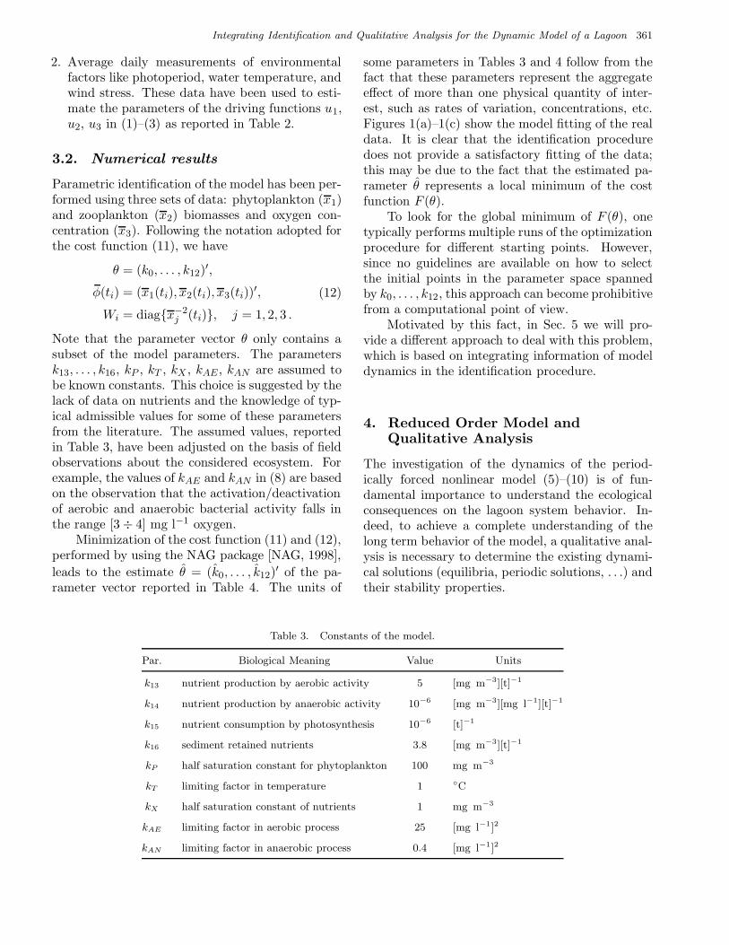
Note that the parameter vector θ only contains asubset of the model parameters. The parametersk13, . . . , k16, kP , kT , kX , kAE , kAN are assumed tobe known constants. This choice is suggested by thelack of data on nutrients and the knowledge of typ-ical admissible values for some of these parametersfrom the literature. The assumed values, reportedin Table 3, have been adjusted on the basis of fieldobservations about the considered ecosystem. Forexample, the values of kAE and kAN in (8) are basedon the observation that the activation/deactivationof aerobic and anaerobic bacterial activity falls inthe range [3 ÷ 4] mg l−1 oxygen.

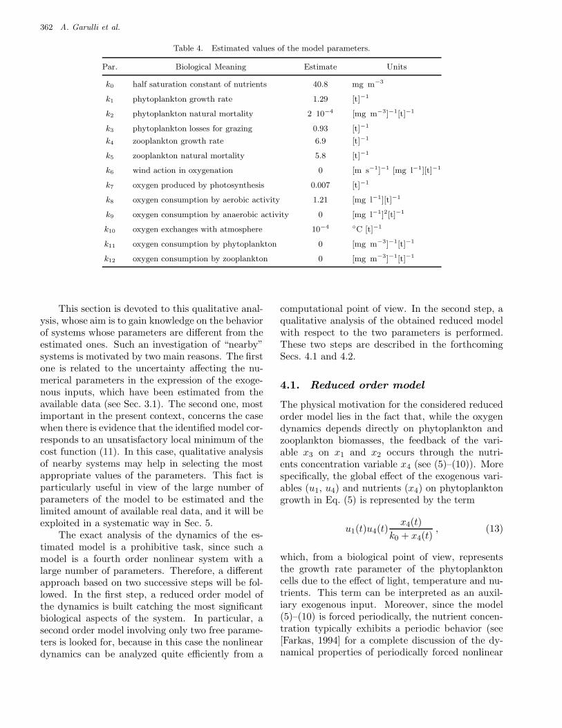
Minimization of the cost function (11) and (12),performed by using the NAG package [NAG, 1998],

leads to the estimate θ = (k0, . . . , k12)′ of the pa-

rameter vector reported in Table 4. The units of

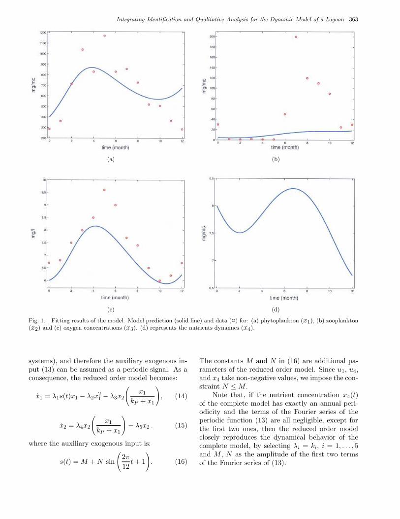
some parameters in Tables 3 and 4 follow from thefact that these parameters represent the aggregateeffect of more than one physical quantity of inter-est, such as rates of variation, concentrations, etc.Figures 1(a)–1(c) show the model fitting of the realdata. It is clear that the identification proceduredoes not provide a satisfactory fitting of the data;this may be due to the fact that the estimated pa-rameter θ represents a local minimum of the costfunction F (θ).

To look for the global minimum of F (θ), onetypically performs multiple runs of the optimizationprocedure for different starting points. However,since no guidelines are available on how to selectthe initial points in the parameter space spannedby k0, . . . , k12, this approach can become prohibitivefrom a computational point of view.

Motivated by this fact, in Sec. 5 we will pro-vide a different approach to deal with this problem,which is based on integrating information of modeldynamics in the identification procedure.

4. Reduced Order Model andQualitative Analysis

The investigation of the dynamics of the period-ically forced nonlinear model (5)–(10) is of fun-damental importance to understand the ecologicalconsequences on the lagoon system behavior. In-deed, to achieve a complete understanding of thelong term behavior of the model, a qualitative anal-ysis is necessary to determine the existing dynami-cal solutions (equilibria, periodic solutions, . . .) andtheir stability properties.

Table 3. Constants of the model.

Par. Biological Meaning Value Units

k13 nutrient production by aerobic activity 5 [mg m−3][t]−1

k14 nutrient production by anaerobic activity 10−6 [mg m−3][mg l−1][t]−1

k15 nutrient consumption by photosynthesis 10−6 [t]−1

k16 sediment retained nutrients 3.8 [mg m−3][t]−1

kP half saturation constant for phytoplankton 100 mg m−3

kT limiting factor in temperature 1 ◦C

kX half saturation constant of nutrients 1 mg m−3

kAE limiting factor in aerobic process 25 [mg l−1]2

kAN limiting factor in anaerobic process 0.4 [mg l−1]2


Table 4. Estimated values of the model parameters.

Par. Biological Meaning Estimate Units

k0 half saturation constant of nutrients 40.8 mg m−3

k1 phytoplankton growth rate 1.29 [t]−1

k2 phytoplankton natural mortality 2 10−4 [mg m−3]−1[t]−1

k3 phytoplankton losses for grazing 0.93 [t]−1

k4 zooplankton growth rate 6.9 [t]−1

k5 zooplankton natural mortality 5.8 [t]−1

k6 wind action in oxygenation 0 [m s−1]−1 [mg l−1][t]−1

k7 oxygen produced by photosynthesis 0.007 [t]−1

k8 oxygen consumption by aerobic activity 1.21 [mg l−1][t]−1

k9 oxygen consumption by anaerobic activity 0 [mg l−1]2[t]−1

k10 oxygen exchanges with atmosphere 10−4 ◦C [t]−1

k11 oxygen consumption by phytoplankton 0 [mg m−3]−1[t]−1

k12 oxygen consumption by zooplankton 0 [mg m−3]−1[t]−1

This section is devoted to this qualitative anal-ysis, whose aim is to gain knowledge on the behaviorof systems whose parameters are different from theestimated ones. Such an investigation of “nearby”systems is motivated by two main reasons. The firstone is related to the uncertainty affecting the nu-merical parameters in the expression of the exoge-nous inputs, which have been estimated from theavailable data (see Sec. 3.1). The second one, mostimportant in the present context, concerns the casewhen there is evidence that the identified model cor-responds to an unsatisfactory local minimum of thecost function (11). In this case, qualitative analysisof nearby systems may help in selecting the mostappropriate values of the parameters. This fact isparticularly useful in view of the large number ofparameters of the model to be estimated and thelimited amount of available real data, and it will beexploited in a systematic way in Sec. 5.

The exact analysis of the dynamics of the es-timated model is a prohibitive task, since such amodel is a fourth order nonlinear system with alarge number of parameters. Therefore, a differentapproach based on two successive steps will be fol-lowed. In the first step, a reduced order model ofthe dynamics is built catching the most significantbiological aspects of the system. In particular, asecond order model involving only two free parame-ters is looked for, because in this case the nonlineardynamics can be analyzed quite efficiently from a

computational point of view. In the second step, aqualitative analysis of the obtained reduced modelwith respect to the two parameters is performed.These two steps are described in the forthcomingSecs. 4.1 and 4.2.

4.1. Reduced order model

The physical motivation for the considered reducedorder model lies in the fact that, while the oxygendynamics depends directly on phytoplankton andzooplankton biomasses, the feedback of the vari-able x3 on x1 and x2 occurs through the nutri-ents concentration variable x4 (see (5)–(10)). Morespecifically, the global effect of the exogenous vari-ables (u1, u4) and nutrients (x4) on phytoplanktongrowth in Eq. (5) is represented by the term

u1(t)u4(t)x4(t)

k0 + x4(t), (13)

which, from a biological point of view, representsthe growth rate parameter of the phytoplanktoncells due to the effect of light, temperature and nu-trients. This term can be interpreted as an auxil-iary exogenous input. Moreover, since the model(5)–(10) is forced periodically, the nutrient concen-tration typically exhibits a periodic behavior (see[Farkas, 1994] for a complete discussion of the dy-namical properties of periodically forced nonlinear


(a) (b)

(c) (d)

Fig. 1. Fitting results of the model. Model prediction (solid line) and data (◦) for: (a) phytoplankton (x1), (b) zooplankton(x2) and (c) oxygen concentrations (x3). (d) represents the nutrients dynamics (x4).

systems), and therefore the auxiliary exogenous in-put (13) can be assumed as a periodic signal. As aconsequence, the reduced order model becomes:

x1 = λ1s(t)x1 − λ2x21 − λ3x2

(

x1

kP + x1

)

, (14)

x2 = λ4x2

(

x1

kP + x1

)

− λ5x2 . (15)

where the auxiliary exogenous input is:

s(t) = M + N sin

(

2π

12t + 1

)

. (16)

The constants M and N in (16) are additional pa-rameters of the reduced order model. Since u1, u4,and x4 take non-negative values, we impose the con-straint N ≤ M .

Note that, if the nutrient concentration x4(t)of the complete model has exactly an annual peri-odicity and the terms of the Fourier series of theperiodic function (13) are all negligible, except forthe first two ones, then the reduced order modelclosely reproduces the dynamical behavior of thecomplete model, by selecting λi = ki, i = 1, . . . , 5and M , N as the amplitude of the first two termsof the Fourier series of (13).


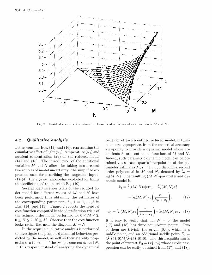
Fig. 2. Residual cost function values for the reduced order model as a function of M and N .

4.2. Qualitative analysis

Let us consider Eqs. (13) and (16), representing thecumulative effect of light (u1), temperature (u4) andnutrient concentration (x4) on the reduced model(14) and (15). The introduction of the additionalvariables M and N allows for taking into accounttwo sources of model uncertainty: the simplified ex-pression used for describing the exogenous inputs(1)–(4); the a priori knowledge exploited for fixingthe coefficients of the nutrient Eq. (10).

Several identification trials of the reduced or-der model for different values of M and N havebeen performed, thus obtaining the estimates ofthe corresponding parameters λi, i = 1, . . . , 5 inEqs. (14) and (15). Figure 2 reports the residualcost function computed in the identification trials ofthe reduced order model performed for 0 ≤ M ≤ 2,0 ≤ N ≤ 2, N ≤ M . Observe that the cost functionlooks rather flat near the diagonal M = N .

In the sequel a qualitative analysis is performedto investigate the possible dynamical behaviors pre-dicted by the model, as well as their stability prop-erties as a function of the two parameters M and N .In this respect, instead of analyzing the dynamical

behavior of each identified reduced model, it turnsout more appropriate, from the numerical accuracyviewpoint, to provide a dynamic model whose co-efficients λi are continuous functions of M and N .Indeed, such parametric dynamic model can be ob-tained via a least squares interpolation of the pa-rameter estimates λi, i = 1, . . . , 5 through a secondorder polynomial in M and N , denoted by λi =λi(M,N). The resulting (M,N)-parameterized dy-namic model is:

x1 = λ1(M,N)s(t)x1 − λ2(M,N)x21

− λ3(M,N)x2

(

x1

kP + x1

)

, (17)

x2 = λ4(M,N)x2

(

x1

kP + x1

)

−λ5(M,N)x2 . (18)

It is easy to verify that, for N = 0, the model(17) and (18) has three equilibrium points. Twoof them are trivial: the origin (0, 0), which is asaddle point, and an additional saddle point E1 =(λ1(M, 0)M/λ2(M, 0), 0). The third equilibrium isthe point of interest E2 = (x∗

1, x∗2) whose explicit ex-

pression can be easily obtained from (17) and (18).


The following considerations can be made on theproperties of the equilibrium point E2.

N = 0. The equilibrium point E2 is stable forM > 0.5; for M = 0.5 one of the two eigenval-ues vanishes; for M < 0.5 the model shows a saddlepoint.

N > 0. For small values of N , the periodicallyforced model retains the stability properties of theunforced system. In particular, the stable equilibriagive rise to stable periodic solutions of period T =12 months (see [Farkas, 1994] for a theoretical ex-planation). As N increases, such periodic solutionmay undergo some bifurcation, thus generating dif-ferent solutions [Kuznetsov, 1995; Strogatz, 1994].Clearly, the detection of bifurcations is importantfor understanding the system behavior especiallyfor larger values of N (see also [Kremer & Nixon,1978]). In the following, (F ) denotes a flip bifur-cation, (N − S) a Neimark–Sacker bifurcation and(T ) a tangent or fold bifurcation.

The bifurcations can be studied via the Poincaremap [Kuznetsov, 1995; Strogatz, 1994] which can

be computed using suitable software packages (inour case, LOCBIF (Interactive Local BifurcationAnalyzer [Khibnik et al., 1992]) and WINPP(The Dynamical Systems Tool [Ermentrout, 1999])have been used). These packages perform bothsimulations of dynamical systems and numerical bi-furcation analysis.

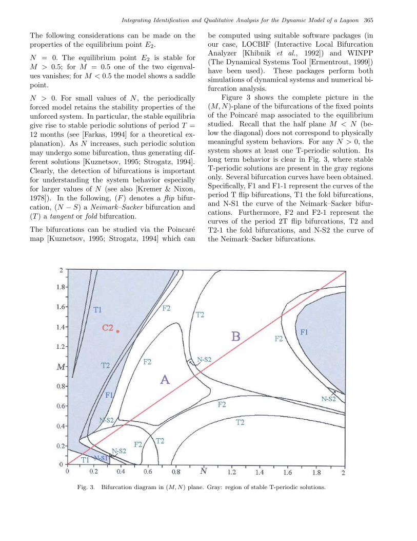
Figure 3 shows the complete picture in the(M,N)-plane of the bifurcations of the fixed pointsof the Poincare map associated to the equilibriumstudied. Recall that the half plane M < N (be-low the diagonal) does not correspond to physicallymeaningful system behaviors. For any N > 0, thesystem shows at least one T-periodic solution. Itslong term behavior is clear in Fig. 3, where stableT-periodic solutions are present in the gray regionsonly. Several bifurcation curves have been obtained.Specifically, F1 and F1-1 represent the curves of theperiod T flip bifurcations, T1 the fold bifurcations,and N-S1 the curve of the Neimark–Sacker bifur-cations. Furthermore, F2 and F2-1 represent thecurves of the period 2T flip bifurcations, T2 andT2-1 the fold bifurcations, and N-S2 the curve ofthe Neimark–Sacker bifurcations.

Fig. 3. Bifurcation diagram in (M, N) plane. Gray: region of stable T-periodic solutions.


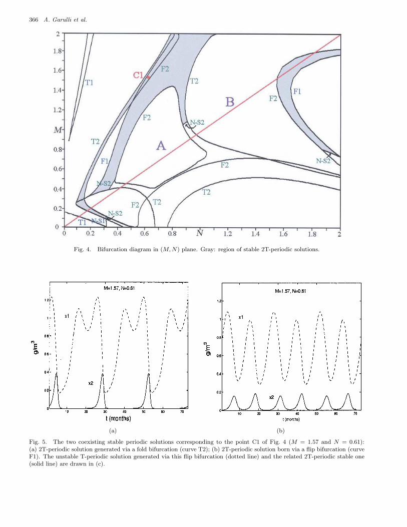
Fig. 4. Bifurcation diagram in (M, N) plane. Gray: region of stable 2T-periodic solutions.

(a) (b)

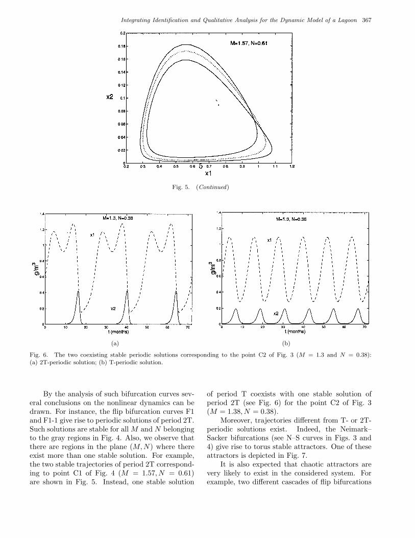
Fig. 5. The two coexisting stable periodic solutions corresponding to the point C1 of Fig. 4 (M = 1.57 and N = 0.61):(a) 2T-periodic solution generated via a fold bifurcation (curve T2); (b) 2T-periodic solution born via a flip bifurcation (curveF1). The unstable T-periodic solution generated via this flip bifurcation (dotted line) and the related 2T-periodic stable one(solid line) are drawn in (c).


Fig. 5. (Continued)

(a) (b)

Fig. 6. The two coexisting stable periodic solutions corresponding to the point C2 of Fig. 3 (M = 1.3 and N = 0.38):(a) 2T-periodic solution; (b) T-periodic solution.

By the analysis of such bifurcation curves sev-eral conclusions on the nonlinear dynamics can bedrawn. For instance, the flip bifurcation curves F1and F1-1 give rise to periodic solutions of period 2T.Such solutions are stable for all M and N belongingto the gray regions in Fig. 4. Also, we observe thatthere are regions in the plane (M,N) where thereexist more than one stable solution. For example,the two stable trajectories of period 2T correspond-ing to point C1 of Fig. 4 (M = 1.57, N = 0.61)are shown in Fig. 5. Instead, one stable solution

of period T coexists with one stable solution ofperiod 2T (see Fig. 6) for the point C2 of Fig. 3(M = 1.38, N = 0.38).

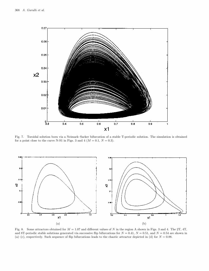
Moreover, trajectories different from T- or 2T-periodic solutions exist. Indeed, the Neimark–Sacker bifurcations (see N–S curves in Figs. 3 and4) give rise to torus stable attractors. One of theseattractors is depicted in Fig. 7.

It is also expected that chaotic attractors arevery likely to exist in the considered system. Forexample, two different cascades of flip bifurcations


Fig. 7. Toroidal solution born via a Neimark–Sacker bifurcation of a stable T-periodic solution. The simulation is obtainedfor a point close to the curve N-S1 in Figs. 3 and 4 (M = 0.1, N = 0.3).

(a) (b)

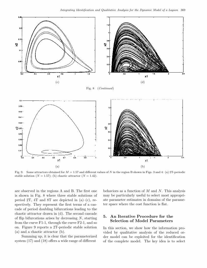
Fig. 8. Some attractors obtained for M = 1.07 and different values of N in the region A shown in Figs. 3 and 4. The 2T, 4T,and 8T-periodic stable solutions generated via successive flip bifurcations for N = 0.41, N = 0.51, and N = 0.54 are shown in(a)–(c), respectively. Such sequence of flip bifurcations leads to the chaotic attractor depicted in (d) for N = 0.88.


(c) (d)

Fig. 8 (Continued)

(a) (b)

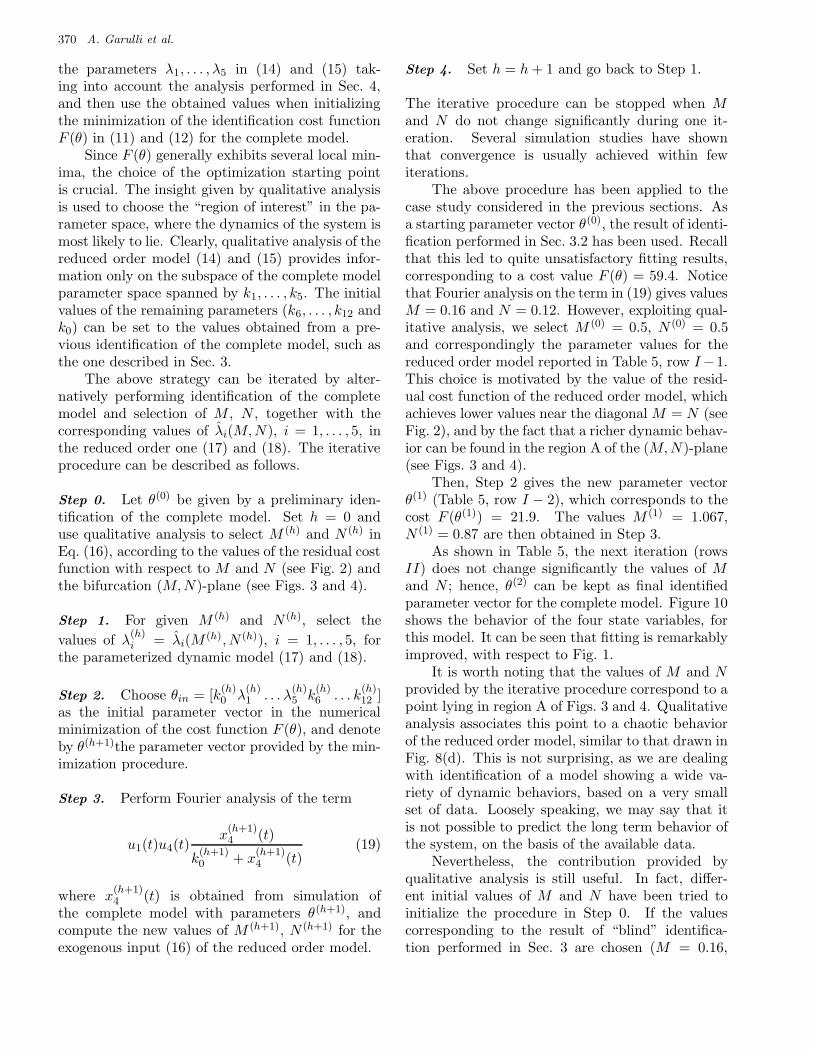
Fig. 9. Some attractors obtained for M = 1.57 and different values of N in the region B shown in Figs. 3 and 4: (a) 2T-periodicstable solution (N = 1.57); (b) chaotic attractor (N = 1.42).

are observed in the regions A and B. The first oneis shown in Fig. 8 where three stable solutions ofperiod 2T, 4T and 8T are depicted in (a)–(c), re-spectively. They represent the first terms of a cas-cade of period doubling bifurcations leading to thechaotic attractor drawn in (d). The second cascadeof flip bifurcations arises by decreasing N , startingfrom the curve F1-1, through the curve F2-1, and soon. Figure 9 reports a 2T-periodic stable solution(a) and a chaotic attractor (b).

Summing up, it is clear that the parameterizedsystem (17) and (18) offers a wide range of different

behaviors as a function of M and N . This analysismay be particularly useful to select most appropri-ate parameter estimates in domains of the parame-ter space where the cost function is flat.

5. An Iterative Procedure for theSelection of Model Parameters

In this section, we show how the information pro-vided by qualitative analysis of the reduced or-der model can be exploited for the identificationof the complete model. The key idea is to select


the parameters λ1, . . . , λ5 in (14) and (15) tak-ing into account the analysis performed in Sec. 4,and then use the obtained values when initializingthe minimization of the identification cost functionF (θ) in (11) and (12) for the complete model.

Since F (θ) generally exhibits several local min-ima, the choice of the optimization starting pointis crucial. The insight given by qualitative analysisis used to choose the “region of interest” in the pa-rameter space, where the dynamics of the system ismost likely to lie. Clearly, qualitative analysis of thereduced order model (14) and (15) provides infor-mation only on the subspace of the complete modelparameter space spanned by k1, . . . , k5. The initialvalues of the remaining parameters (k6, . . . , k12 andk0) can be set to the values obtained from a pre-vious identification of the complete model, such asthe one described in Sec. 3.

The above strategy can be iterated by alter-natively performing identification of the completemodel and selection of M , N , together with thecorresponding values of λi(M,N), i = 1, . . . , 5, inthe reduced order one (17) and (18). The iterativeprocedure can be described as follows.

Step 0. Let θ(0) be given by a preliminary iden-tification of the complete model. Set h = 0 anduse qualitative analysis to select M (h) and N (h) inEq. (16), according to the values of the residual costfunction with respect to M and N (see Fig. 2) andthe bifurcation (M,N)-plane (see Figs. 3 and 4).

Step 1. For given M (h) and N (h), select the

values of λ(h)i = λi(M

(h), N (h)), i = 1, . . . , 5, forthe parameterized dynamic model (17) and (18).

Step 2. Choose θin = [k(h)0 λ

(h)1 . . . λ

(h)5 k

(h)6 . . . k

(h)12 ]

as the initial parameter vector in the numericalminimization of the cost function F (θ), and denoteby θ(h+1)the parameter vector provided by the min-imization procedure.

Step 3. Perform Fourier analysis of the term

u1(t)u4(t)x

(h+1)4 (t)

k(h+1)0 + x

(h+1)4 (t)

(19)

where x(h+1)4 (t) is obtained from simulation of

the complete model with parameters θ(h+1), andcompute the new values of M (h+1), N (h+1) for theexogenous input (16) of the reduced order model.

Step 4. Set h = h + 1 and go back to Step 1.

The iterative procedure can be stopped when Mand N do not change significantly during one it-eration. Several simulation studies have shownthat convergence is usually achieved within fewiterations.

The above procedure has been applied to thecase study considered in the previous sections. Asa starting parameter vector θ(0), the result of identi-fication performed in Sec. 3.2 has been used. Recallthat this led to quite unsatisfactory fitting results,corresponding to a cost value F (θ) = 59.4. Noticethat Fourier analysis on the term in (19) gives valuesM = 0.16 and N = 0.12. However, exploiting qual-itative analysis, we select M (0) = 0.5, N (0) = 0.5and correspondingly the parameter values for thereduced order model reported in Table 5, row I −1.This choice is motivated by the value of the resid-ual cost function of the reduced order model, whichachieves lower values near the diagonal M = N (seeFig. 2), and by the fact that a richer dynamic behav-ior can be found in the region A of the (M,N)-plane(see Figs. 3 and 4).

Then, Step 2 gives the new parameter vectorθ(1) (Table 5, row I − 2), which corresponds to thecost F (θ(1)) = 21.9. The values M (1) = 1.067,N (1) = 0.87 are then obtained in Step 3.

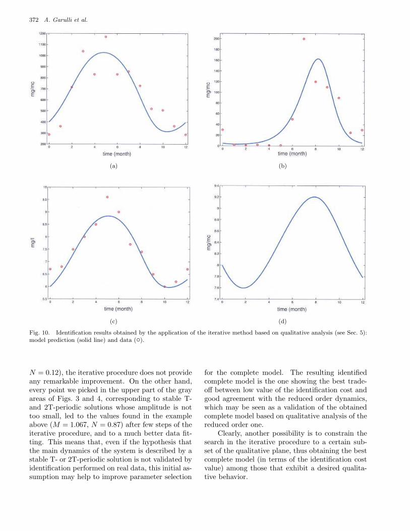
As shown in Table 5, the next iteration (rowsII) does not change significantly the values of Mand N ; hence, θ(2) can be kept as final identifiedparameter vector for the complete model. Figure 10shows the behavior of the four state variables, forthis model. It can be seen that fitting is remarkablyimproved, with respect to Fig. 1.

It is worth noting that the values of M and Nprovided by the iterative procedure correspond to apoint lying in region A of Figs. 3 and 4. Qualitativeanalysis associates this point to a chaotic behaviorof the reduced order model, similar to that drawn inFig. 8(d). This is not surprising, as we are dealingwith identification of a model showing a wide va-riety of dynamic behaviors, based on a very smallset of data. Loosely speaking, we may say that itis not possible to predict the long term behavior ofthe system, on the basis of the available data.

Nevertheless, the contribution provided byqualitative analysis is still useful. In fact, differ-ent initial values of M and N have been tried toinitialize the procedure in Step 0. If the valuescorresponding to the result of “blind” identifica-tion performed in Sec. 3 are chosen (M = 0.16,

Integ

ratin

gId

entifi

catio

nand

Qualita

tive

Analy

sisfo

rth

eD

ynam

icM

odelofa

Lagoon

371

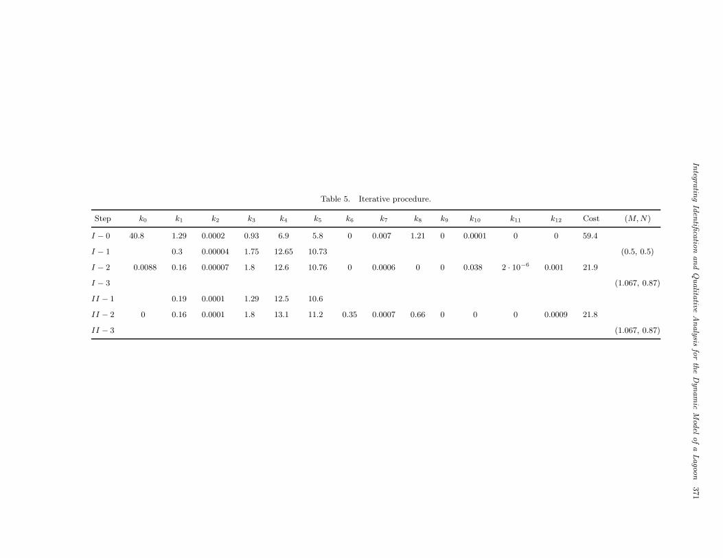
Table 5. Iterative procedure.

Step k0 k1 k2 k3 k4 k5 k6 k7 k8 k9 k10 k11 k12 Cost (M, N)

I − 0 40.8 1.29 0.0002 0.93 6.9 5.8 0 0.007 1.21 0 0.0001 0 0 59.4

I − 1 0.3 0.00004 1.75 12.65 10.73 (0.5, 0.5)

I − 2 0.0088 0.16 0.00007 1.8 12.6 10.76 0 0.0006 0 0 0.038 2 · 10−6 0.001 21.9

I − 3 (1.067, 0.87)

II − 1 0.19 0.0001 1.29 12.5 10.6

II − 2 0 0.16 0.0001 1.8 13.1 11.2 0.35 0.0007 0.66 0 0 0 0.0009 21.8

II − 3 (1.067, 0.87)


(a) (b)

(c) (d)

Fig. 10. Identification results obtained by the application of the iterative method based on qualitative analysis (see Sec. 5):model prediction (solid line) and data (◦).

N = 0.12), the iterative procedure does not provideany remarkable improvement. On the other hand,every point we picked in the upper part of the grayareas of Figs. 3 and 4, corresponding to stable T-and 2T-periodic solutions whose amplitude is nottoo small, led to the values found in the exampleabove (M = 1.067, N = 0.87) after few steps of theiterative procedure, and to a much better data fit-ting. This means that, even if the hypothesis thatthe main dynamics of the system is described by astable T- or 2T-periodic solution is not validated byidentification performed on real data, this initial as-sumption may help to improve parameter selection

for the complete model. The resulting identifiedcomplete model is the one showing the best trade-off between low value of the identification cost andgood agreement with the reduced order dynamics,which may be seen as a validation of the obtainedcomplete model based on qualitative analysis of thereduced order one.

Clearly, another possibility is to constrain thesearch in the iterative procedure to a certain sub-set of the qualitative plane, thus obtaining the bestcomplete model (in terms of the identification costvalue) among those that exhibit a desired qualita-tive behavior.


6. Conclusions

In this paper a procedure for identifying the dy-namic model of a lagoon by using real data has beenproposed. The new approach relies on the system-atic use of the information on the model dynamicsin the identification procedure. More specifically, inorder to understand the dynamical behavior of thecomplete model on the basis of real data, a suitablereduced order model is introduced and its quali-tative analysis is performed as a function of twovariables. These variables are instrumental for theiterative procedure designed for parameter estima-tion of the complete model. Indeed, the qualita-tive analysis of the reduced order model providesuseful information for picking the starting parame-ter vector in the estimation nonconvex optimizationprogram.

From a biological point of view, it has beenobserved that a model describing the dynamics ofa lagoon exhibits a richness of possible behaviors,depending on the model parameters, in agreementwith theoretical and experimental biological knowl-edge. In this respect, the application to the Capro-lace lagoon provides satisfactory results.

The proposed identification procedure may alsobe useful when more complicated models are con-sidered, which is often the case when modelingenvironmental systems. Further testing of thewhole identification scheme in more general con-texts is under investigation and it will be the objectof future work.

ReferencesAguirre, L. A. & Billings, S. A. [1994] “Validating iden-

tified nonlinear models with chaotic dynamics,” Int.

J. Bifurcation and Chaos 4(1), 109–125.Childers, D. L. & McKellar, H. N. [1987] “A simulation

of saltmarsh water column dynamics,” Ecol. Model.

36, 211–238.Coca, D. & Billings, S. A. [1997] “Continous-time system

identification for linear and nonlinear systems us-ing wavelet decompositions,” Int. J. Bifurcation and

Chaos 7(1), p. 87.Coca, D., Zheng, Y., Mayhew, J. W. & Billings, S. A.

[2000] “Nonlinear system identification and analysisof complex dynamical behavior in reflected light mea-surements of vasomotion,” Int. J. Bifurcation and

Chaos 10(2), 461–476.Eilers, P. H. C. & Peeters, J. C. H. [1988] “A model for

the relationship between light intensity and the rateof photosynthesis in phytoplanktan,” Ecol. Model. 42,199–215.

ENEA [1995] “Ricerca e sviluppo di modelli ed indicatoriecologici e di sistemi esperti di monitoraggio ambien-tale per la gestione delle zone umide e salmastre aifini dell’acquacoltura,” Ente per le Nuove technologie,

l’Energie e l’Ambiente (Research Project).Ermentrout, G. B. [1999] WINPP: The Dynamical

Systems Tool.Farkas, M. [1994] Periodic Motions (Springer-Verlag,

NY).Franks, P. J. S., Wroblewski, J. S. & Flierl, G. R. [1986]

“Behaviour of a simple plankton model with food-levelacclimation by herbivores,” Marine Biol. 91, 121–129.

Garulli, A., Tesi, A. & Vicino, A. (eds.) [1999] Robust-

ness in Identification and Control, Lecture Notes inControl and Information Sciences, Vol. 245 (Springer-Verlag).

Ginot, V. & Herve, J. C. [1994] “Estimating the param-eters of dissolved oxygen dynamics in shallow ponds,”Ecol. Model. 73, 169–187

Hull, V., Falcucci, M. & Cignini, I. [1991] Indagine am-

bientale sulla laguna di Caprolace, Parco Nazinale del

Circeo. ed. Ministero Agricoltura e Foreste.Hull, V., Mocenni, C. Falcucci, M. & Marchettini, N.

[2000] “A trophodynamic model for the lagoon ofFogliano (Italy) with ecological modifying parame-ters,” Ecol. Model. 134, 153–167.

Izzo, G. & Hull, V. [1991] “The anoxyc crises indistrophic processes of coastal lagoons: An ener-getic explanation,” Ecological Physical Chemistry, eds.Rossi, C. & Tiezzi, E. (Elsevier), pp. 559–572.

Jørgensen, B. B. [1977] “The sulfur cycle of a coastalmarine sediment,” Limnol. Oceanogr. 22(5), 814–832.

Khibnik, A., Kuznetsov, Y., Levitin, V. & Nikolaev,E. [1992] LOCBIF: Interactive Local Bifurcation An-

alyzer, Version 2.2. Research Computing Centre,Russian Academy of Sciences, Puschchino, MoscowRegion 142292, Russia.

Kremer, J. N. & Nixon, S. W. [1978] A Coastal Ma-

rine Ecosystem. Simulation and Analysis (Springer-Verlag).

Kuzentsov, Y., Muratori, S. & Rinaldi, S. [1992] “Bifur-cations and chaos in a periodic predator–prey model,”Int. J. Bifurcation and Chaos 2, 117–128.

Kuznetsov, Y. [1995] Elements of Applied Bifurcation

Theory (Springer-Verlag).Ljung, L. [1999] System Identification, 2nd edition

(Prentice-Hall).Mocenni, C., Garulli, A. & Vicino, A. [1999] “Identi-

fication of simplified biological models of a lagoon,”Proc. 14th IFAC World Congress, Beijing, China,pp. 151–156.

Murray, J. D. [1993] Mathematical Biology (Springer-Verlag).

NAG [1998] Numerical Algorithms Group, NAG founda-tion toolbox for MATLAB 6.


Norberg, J. & De Angelis, D. [1997] “Temperatureeffects on stocks and stability of a phytoplankton–zooplankton model and the dependence on light andnutrients,” Ecol. Model. 95, 75–86.

Strogatz, S. H. [1994] Nonlinear Dynamics and Chaos

(Addison-Wesley).

Van Duin, E. H. S. & Lijklema, L. [1989] “Modellingphotosynthesis and oxygen in a shallow, hypertrophiclake,” Ecol. Model. 45(4), 243–260.

integrating identification and qualitative analysis …mocenni/mocenni-ijbc.pdf · integrating...

Documents