integrating maintenance planning and production scheduling ... · integrating maintenance planning...
TRANSCRIPT
IntegratingMaintenance Planning and Production Scheduling: MakingOperational Decisions with a Strategic Perspective
by
Maliheh Aramon Bajestani
A thesis submitted in conformity with the requirementsfor the degree of Doctor of Philosophy
Graduate Department of Mechanical & Industrial EngineeringUniversity of Toronto
© Copyright 2014 by Maliheh Aramon Bajestani
Abstract
Integrating Maintenance Planning and Production Scheduling: MakingOperational Decisions with a Strategic Perspective
Maliheh Aramon Bajestani
Doctor of Philosophy
Graduate Department of Mechanical & Industrial Engineering
University of Toronto
2014
In today’s competitive environment, the importance of continuous production, quality improvement, and
fast delivery has forced production and delivery processes to become highly reliable. Keeping equip-
ment in good condition through maintenance activities can ensure a more reliable system. However,
maintenance leads to temporary reduction in capacity that could otherwise be utilized for production.
Therefore, the coordination of maintenance and production is important to guarantee good system per-
formance. The central thesis of this dissertation is that integrating maintenance and production decisions
increases efficiency by ensuring high quality production, effective resource utilization, and on-time de-
liveries.
Firstly, we study the problem of integrated maintenance and production planning where machines
are preventively maintained in the context of a periodic review production system with uncertain yield.
Our goal is to provide insight into the optimal maintenance policy, increasing the number of finished
products. Specifically, we prove the conditions that guarantee the optimal maintenance policy has a
threshold type.
Secondly, we address the problem of integrated maintenance planning and production scheduling
where machines are correctively maintained in the context of a dynamic aircraft repair shop. To solve
the problem, we view the dynamic repair shop as successive static repair scheduling sub-problems over
shorter periods. Our results show that the approach that uses logic-based Benders decomposition to
solve the static sub-problems, schedules over longer horizon, and quickly adjusts the schedule increases
the utilization of aircraft in the long term.
Finally, we tackle the problem of integrated maintenance planning and production scheduling where
machines are preventively maintained in the context of a multi-machine production system. Depending
on the deterioration process of machines, we design decomposed techniques that deal with the stochastic
ii
and combinatorial challenges in different, coupled stages. Our results demonstrate that the integrated
approaches decrease the total maintenance and lost production cost, maximizing the on-time deliveries.
We also prove sufficient conditions that guarantee the monotonicity of the optimal maintenance policy
in both machine state and the number of customer orders.
Within these three contexts, this dissertation demonstrates that the integrated maintenance and pro-
duction decision-making increases the process efficiency to produce high quality products in a timely
manner.
iii
Acknowledgements
This dissertation marks the end of my PhD journey– one of the most challenging, though illuminating,
periods of my life. There are many people who have contributed, both directly and indirectly, to the
work recorded herein. I would like to take this opportunity to recognize them.
First, I would like to thank the sources that provided funding to me throughout my studies, including
the Discovery Grants Program of the Natural Sciences and Engineering Research Council of Canada, the
consortium members of Centre for Maintenance Optimization & Reliability Engineering (C-MORE),
the Canadian Foundation for Innovation, the Ontario Research Fund, the Ontario Ministry for Research
and Innovation, IBM ILOG, the University of Toronto Doctoral Completion Award, and the Department
of Mechanical & Industrial Engineering.
Of course, I thank my supervisor, Professor J. Christopher Beck, who has contributed immeasurably
to my development as a researcher. You have been a dedicated, patient, and insightful advisor who taught
me the importance of good research and hard work. I could not have completed this work without your
support and guidance. Thank you for everything, working with you has been an invaluable experience.
I am grateful to Professor Andrew K. S. Jardine for giving me the chance to pursue my PhD studies
and providing excellent support and advice along the way.
I would like to extend my sincere gratitude to Dr. Dragan Banjevic who has contributed much to the
quality of my research. I am thankful for your exceptional willingness and time helping me to work out
the details.
I would also like to thank my committee members Professor Mark S. Fox, Professor Chelliah
Sriskandarajah, and Professor Chi-Guhn Lee for their time, cogent comments and suggestions.
I feel fortunate to have been a student at the Department of Mechanical & Industrial Engineering
and acknowledge the help of all faculty and staff throughout my coursework and research. I thank Dr.
Elizabeth Thompson for her encouragement and editorial help, Brenda Fung for patiently answering all
my administrative questions, and Oscar del Rio for retrieving the very important files that I mistakenly
deleted.
I am honored to have had great friends during my graduate studies. I thank all my friends at the
Toronto Intelligent Decision Engineering Laboratory (TIDEL) and C-MORE for sharing conversations,
laughs, and good times.
I am indebted to Lei Duan for his invaluable advice on managing my PhD work. Thank you for
highlighting the importance of taking initiative in research, which helped me a lot along the course of
my PhD.
I would also like to thank Dr. Reza Samavi for useful advice and support in both academic and non-
academic subjects. I really appreciate the time you spent discussing different aspects of life overseas
with me, which helped me to go through the cultural transition easier.
I am pleased to have made an amazing friend during my years of PhD study, Dr. Daria Terekhov. I
am thankful to you for encouraging me to always be positive and kindly supporting me in so many ways.
iv
The fact that our countless discussions of everything academic and non-academic are always endless is
an indication of our great friendship. I value this friendship and wish for it to continue for years to come.
Thank you to my great friends Professor Vahideh Abedi, Leyla Kermanshah, Samira Karimelahi,
and Masumeh Kalantari, who always found time to share their friendship and support. A special thank
you to Vahideh for helping me through the difficult moments of graduate school and for being like a
sister to me.
Thank you to my brother, Mohammad, for showing me that he is much more independent than what
I could have imagined. It is still unbelievable that my little brother turned into a young man during my
years of being away from home. Although I missed so many moments while you were growing up, I
am happy that I have a strong supporter like you now.
Thanks to my sister, Maryam, for being my best friend all my life. You have always inspired me to
do my best and reminded me that I am capable of doing whatever I wish.
Last and most, thanks to my parents, whose love, kindness, and compassion gave me the confidence
and strength to complete this work. Thanks Dad for your belief in me and your extraordinary support
of me in going after what I want. Thanks Mom for always being there for me and teaching me to never
give up, no matter how hard the challenges are.
v
Contents
1 Introduction 11.1 Dissertation Outline . . . . . . . . . . . . . . . . . . . . . . . . . . . . . . . . . . . . 3
1.2 Summary of Contributions . . . . . . . . . . . . . . . . . . . . . . . . . . . . . . . . 5
2 Integrated Maintenance & Production: A Literature Review 72.1 Classification Scheme . . . . . . . . . . . . . . . . . . . . . . . . . . . . . . . . . . . 7
2.2 Long-term Perspective . . . . . . . . . . . . . . . . . . . . . . . . . . . . . . . . . . 9
2.2.1 Maintenance Fundamentals . . . . . . . . . . . . . . . . . . . . . . . . . . . 9
2.2.1.1 Failure rate . . . . . . . . . . . . . . . . . . . . . . . . . . . . . . . 10
2.2.1.2 Repair . . . . . . . . . . . . . . . . . . . . . . . . . . . . . . . . . 10
2.2.1.3 Maintenance Policies . . . . . . . . . . . . . . . . . . . . . . . . . 11
2.2.1.4 Solution Techniques . . . . . . . . . . . . . . . . . . . . . . . . . . 13
2.2.2 Random Yield without Maintenance . . . . . . . . . . . . . . . . . . . . . . . 16
2.2.2.1 Periodic Review Models . . . . . . . . . . . . . . . . . . . . . . . . 16
2.2.2.2 Continuous Review Models . . . . . . . . . . . . . . . . . . . . . . 18
2.2.3 Random Yield with Maintenance . . . . . . . . . . . . . . . . . . . . . . . . . 19
2.2.3.1 Periodic Review Models . . . . . . . . . . . . . . . . . . . . . . . . 20
2.2.3.2 Continuous Review Models . . . . . . . . . . . . . . . . . . . . . . 22
2.2.4 Maintenance & Production Sequencing/Scheduling . . . . . . . . . . . . . . . 24
2.2.5 Summary . . . . . . . . . . . . . . . . . . . . . . . . . . . . . . . . . . . . . 25
2.3 Short-term Perspective . . . . . . . . . . . . . . . . . . . . . . . . . . . . . . . . . . 26
2.3.1 Scheduling Fundamentals . . . . . . . . . . . . . . . . . . . . . . . . . . . . 26
2.3.1.1 Mixed integer Programming . . . . . . . . . . . . . . . . . . . . . . 28
2.3.1.2 Constraint Programming . . . . . . . . . . . . . . . . . . . . . . . 29
2.3.1.3 Hybrid Optimization Methods . . . . . . . . . . . . . . . . . . . . . 30
2.3.2 Stochastic Sequencing/Scheduling . . . . . . . . . . . . . . . . . . . . . . . . 33
2.3.3 Dynamic Sequencing/Scheduling . . . . . . . . . . . . . . . . . . . . . . . . 35
2.3.4 Sequencing/Scheduling with Availability Constraints . . . . . . . . . . . . . . 37
2.3.5 Summary . . . . . . . . . . . . . . . . . . . . . . . . . . . . . . . . . . . . . 39
2.4 Conclusion . . . . . . . . . . . . . . . . . . . . . . . . . . . . . . . . . . . . . . . . 39
vi
3 Maintenance & Production Planning with Partial Control over Machine Conditions 403.1 Problem Definition . . . . . . . . . . . . . . . . . . . . . . . . . . . . . . . . . . . . 42
3.2 Single Period Analysis . . . . . . . . . . . . . . . . . . . . . . . . . . . . . . . . . . 44
3.2.1 Sufficient Conditions for the Existence of Derivatives . . . . . . . . . . . . . . 44
3.2.2 Single Period Optimal Policy . . . . . . . . . . . . . . . . . . . . . . . . . . . 44
3.2.3 Insights . . . . . . . . . . . . . . . . . . . . . . . . . . . . . . . . . . . . . . 48
3.2.4 Numerical Example . . . . . . . . . . . . . . . . . . . . . . . . . . . . . . . 50
3.2.5 Summary of Single Period Analysis . . . . . . . . . . . . . . . . . . . . . . . 50
3.3 Multiple Period Analysis . . . . . . . . . . . . . . . . . . . . . . . . . . . . . . . . . 52
3.3.1 Multiple Period Optimal Policy . . . . . . . . . . . . . . . . . . . . . . . . . 52
3.3.2 Insights . . . . . . . . . . . . . . . . . . . . . . . . . . . . . . . . . . . . . . 54
3.3.3 Summary of Multiple Period Analysis . . . . . . . . . . . . . . . . . . . . . . 55
3.4 Conclusion . . . . . . . . . . . . . . . . . . . . . . . . . . . . . . . . . . . . . . . . 55
4 Maintenance Planning & Production Scheduling with No Control over Machine Condi-tions 574.1 Background . . . . . . . . . . . . . . . . . . . . . . . . . . . . . . . . . . . . . . . . 59
4.1.1 Problem Definition . . . . . . . . . . . . . . . . . . . . . . . . . . . . . . . . 59
4.1.2 Literature Review . . . . . . . . . . . . . . . . . . . . . . . . . . . . . . . . . 60
4.1.2.1 Repair Shop Scheduling . . . . . . . . . . . . . . . . . . . . . . . . 60
4.2 The Complexity of the Static Repair Shop Problem . . . . . . . . . . . . . . . . . . . 62
4.3 Solution Approach . . . . . . . . . . . . . . . . . . . . . . . . . . . . . . . . . . . . 63
4.3.1 Scheduling Techniques . . . . . . . . . . . . . . . . . . . . . . . . . . . . . . 63
4.3.1.1 Mixed Integer Programming . . . . . . . . . . . . . . . . . . . . . 63
4.3.1.2 Constraint Programming . . . . . . . . . . . . . . . . . . . . . . . 66
4.3.1.3 Logic-based Benders Decomposition . . . . . . . . . . . . . . . . . 67
4.3.1.4 A Dispatching Heuristic . . . . . . . . . . . . . . . . . . . . . . . . 70
4.3.1.5 Hybrid Heuristic-Complete Approaches . . . . . . . . . . . . . . . 71
4.3.1.6 Theoretical Results . . . . . . . . . . . . . . . . . . . . . . . . . . 71
4.3.2 Rescheduling Strategies . . . . . . . . . . . . . . . . . . . . . . . . . . . . . 71
4.3.3 Modeling the Aircraft Failures . . . . . . . . . . . . . . . . . . . . . . . . . . 72
4.4 Computational Experiments . . . . . . . . . . . . . . . . . . . . . . . . . . . . . . . 73
4.4.1 Experimental Results on Scheduling Techniques . . . . . . . . . . . . . . . . 73
4.4.1.1 Experimental Setup . . . . . . . . . . . . . . . . . . . . . . . . . . 73
4.4.1.2 Experimental Results . . . . . . . . . . . . . . . . . . . . . . . . . 74
4.4.2 Experimental Results on Rescheduling Strategies . . . . . . . . . . . . . . . . 78
4.4.2.1 Experimental Setup . . . . . . . . . . . . . . . . . . . . . . . . . . 78
4.4.2.2 Experimental Results . . . . . . . . . . . . . . . . . . . . . . . . . 79
4.5 Discussion . . . . . . . . . . . . . . . . . . . . . . . . . . . . . . . . . . . . . . . . . 84
4.6 Conclusion . . . . . . . . . . . . . . . . . . . . . . . . . . . . . . . . . . . . . . . . 85
vii
5 Maintenance Planning & Production Scheduling with Partial Control over Machine Con-ditions: Deterministic Deterioration 875.1 Problem Definition . . . . . . . . . . . . . . . . . . . . . . . . . . . . . . . . . . . . 88
5.2 Solution Approaches . . . . . . . . . . . . . . . . . . . . . . . . . . . . . . . . . . . 91
5.2.1 The Integrated Approach . . . . . . . . . . . . . . . . . . . . . . . . . . . . . 92
5.2.1.1 The Maintenance Planning Problem (MPP) . . . . . . . . . . . . . . 93
5.2.1.2 The Production Scheduling Problem (PSP) . . . . . . . . . . . . . . 94
5.2.1.3 The MPP Cuts . . . . . . . . . . . . . . . . . . . . . . . . . . . . . 95
5.2.1.4 Relaxation of the PSP in the MPP . . . . . . . . . . . . . . . . . . . 96
5.2.2 The Non-integrated Approach . . . . . . . . . . . . . . . . . . . . . . . . . . 97
5.2.3 The Short-term Approach . . . . . . . . . . . . . . . . . . . . . . . . . . . . 97
5.2.4 Heuristic Approaches . . . . . . . . . . . . . . . . . . . . . . . . . . . . . . . 97
5.2.4.1 A Heuristic for the PSP . . . . . . . . . . . . . . . . . . . . . . . . 98
5.2.4.2 A Heuristic for the MPSP . . . . . . . . . . . . . . . . . . . . . . . 98
5.3 Empirical Study . . . . . . . . . . . . . . . . . . . . . . . . . . . . . . . . . . . . . . 98
5.3.1 Experimental Setup . . . . . . . . . . . . . . . . . . . . . . . . . . . . . . . . 98
5.3.2 Computational Results . . . . . . . . . . . . . . . . . . . . . . . . . . . . . . 100
5.4 Discussion . . . . . . . . . . . . . . . . . . . . . . . . . . . . . . . . . . . . . . . . . 101
5.4.1 The Extended Integrated Approach . . . . . . . . . . . . . . . . . . . . . . . 103
5.5 Conclusion . . . . . . . . . . . . . . . . . . . . . . . . . . . . . . . . . . . . . . . . 104
6 Maintenance Planning & Production Scheduling with Partial Control over Machine Con-ditions: Markovian Deterioration 1066.1 Problem Definition . . . . . . . . . . . . . . . . . . . . . . . . . . . . . . . . . . . . 107
6.2 Decomposing the Problem . . . . . . . . . . . . . . . . . . . . . . . . . . . . . . . . 112
6.2.1 The Maintenance Planning Problem (MPP) . . . . . . . . . . . . . . . . . . . 112
6.2.2 The Production Scheduling Problem (PSP) . . . . . . . . . . . . . . . . . . . 115
6.3 Solving the Decomposed Problem . . . . . . . . . . . . . . . . . . . . . . . . . . . . 115
6.3.1 MPP . . . . . . . . . . . . . . . . . . . . . . . . . . . . . . . . . . . . . . . 116
6.3.1.1 MDP Approach . . . . . . . . . . . . . . . . . . . . . . . . . . . . 116
6.3.1.2 Heuristic Approach . . . . . . . . . . . . . . . . . . . . . . . . . . 124
6.3.2 PSP . . . . . . . . . . . . . . . . . . . . . . . . . . . . . . . . . . . . . . . . 124
6.3.2.1 MIP Approach . . . . . . . . . . . . . . . . . . . . . . . . . . . . . 124
6.3.2.2 CP Approach . . . . . . . . . . . . . . . . . . . . . . . . . . . . . 126
6.3.2.3 Heuristic Approach . . . . . . . . . . . . . . . . . . . . . . . . . . 127
6.4 Execution of the Planned Schedule . . . . . . . . . . . . . . . . . . . . . . . . . . . . 127
6.5 Computational Study . . . . . . . . . . . . . . . . . . . . . . . . . . . . . . . . . . . 129
6.5.1 Experimental Setup . . . . . . . . . . . . . . . . . . . . . . . . . . . . . . . . 129
6.5.2 Experimental Results . . . . . . . . . . . . . . . . . . . . . . . . . . . . . . . 130
6.6 Discussion . . . . . . . . . . . . . . . . . . . . . . . . . . . . . . . . . . . . . . . . . 133
viii
6.6.1 Real Failure Rate Data . . . . . . . . . . . . . . . . . . . . . . . . . . . . . . 133
6.6.2 Practical Relevance of the Experimental Results . . . . . . . . . . . . . . . . 134
6.7 Conclusion . . . . . . . . . . . . . . . . . . . . . . . . . . . . . . . . . . . . . . . . 136
7 Future Work 1387.1 Maintenance & Production Planning with Partial Control over Machine Conditions . . 138
7.1.1 Different Assumptions . . . . . . . . . . . . . . . . . . . . . . . . . . . . . . 138
7.1.2 Efficient Algorithms . . . . . . . . . . . . . . . . . . . . . . . . . . . . . . . 140
7.2 Maintenance Planning & Production Scheduling with No Control over Machine Condi-
tions . . . . . . . . . . . . . . . . . . . . . . . . . . . . . . . . . . . . . . . . . . . . 141
7.2.1 Competitive Ratios of the Developed Algorithms . . . . . . . . . . . . . . . . 141
7.2.2 Scheduling Horizon and Rescheduling Frequency . . . . . . . . . . . . . . . . 142
7.3 Maintenance Planning & Production Scheduling with Partial Control over Machine
Conditions . . . . . . . . . . . . . . . . . . . . . . . . . . . . . . . . . . . . . . . . . 143
7.3.1 Extensions of Chapter 5 . . . . . . . . . . . . . . . . . . . . . . . . . . . . . 143
7.3.1.1 The Length of the Maintenance Planning Horizon . . . . . . . . . . 143
7.3.1.2 Developing Efficient Algorithms for the Production Scheduling Problem144
7.3.1.3 Modeling Machine Failures . . . . . . . . . . . . . . . . . . . . . . 144
7.3.2 Extensions of Chapter 6 . . . . . . . . . . . . . . . . . . . . . . . . . . . . . 145
7.3.2.1 Different Assumptions . . . . . . . . . . . . . . . . . . . . . . . . . 145
7.3.2.2 Different Modeling Approaches . . . . . . . . . . . . . . . . . . . . 145
7.4 General Future Research Directions on Integrated Maintenance and Production Decision 146
7.4.1 Conceptual Directions . . . . . . . . . . . . . . . . . . . . . . . . . . . . . . 146
7.4.2 Theoretical Directions . . . . . . . . . . . . . . . . . . . . . . . . . . . . . . 148
7.5 Toward Integrated Decision Making . . . . . . . . . . . . . . . . . . . . . . . . . . . 149
7.6 Conclusion . . . . . . . . . . . . . . . . . . . . . . . . . . . . . . . . . . . . . . . . 150
8 Conclusion 1518.1 Maintenance & Production Planning with Partial Control over Machine Conditions . . 152
8.2 Maintenance Planning & Production Scheduling with No Control over Machine Condi-
tions . . . . . . . . . . . . . . . . . . . . . . . . . . . . . . . . . . . . . . . . . . . . 153
8.3 Maintenance Planning & Production Scheduling with Partial Control over Machine
Conditions . . . . . . . . . . . . . . . . . . . . . . . . . . . . . . . . . . . . . . . . . 153
8.4 Summary of Contributions . . . . . . . . . . . . . . . . . . . . . . . . . . . . . . . . 155
8.5 Conclusion . . . . . . . . . . . . . . . . . . . . . . . . . . . . . . . . . . . . . . . . 156
Appendices 156
A Proofs of Some Propositions in Chapter 3 157A.1 Proofs of the Single Period Propositions . . . . . . . . . . . . . . . . . . . . . . . . . 157
ix
A.1.1 Proof of Proposition 3.1 . . . . . . . . . . . . . . . . . . . . . . . . . . . . . 157
A.1.2 Proof of Proposition 3.2 . . . . . . . . . . . . . . . . . . . . . . . . . . . . . 158
A.1.3 Supermodularity of the Total Expected Cost over One Period . . . . . . . . . . 159
A.1.4 Proof of Proposition 3.3 . . . . . . . . . . . . . . . . . . . . . . . . . . . . . 160
A.1.5 Proof of Proposition 3.4 . . . . . . . . . . . . . . . . . . . . . . . . . . . . . 161
A.2 Proofs of the Multiple Period Propositions . . . . . . . . . . . . . . . . . . . . . . . . 161
A.2.1 Proof of Proposition 3.5 . . . . . . . . . . . . . . . . . . . . . . . . . . . . . 161
A.2.2 Proof of Proposition 3.6 . . . . . . . . . . . . . . . . . . . . . . . . . . . . . 162
A.2.3 Supermodularity of the Total Discounted Expected Cost over Multiple Periods 163
B Structural Properties of the Production Scheduling Problem 165B.1 Dominance Properties . . . . . . . . . . . . . . . . . . . . . . . . . . . . . . . . . . . 165
B.2 Empirical Study . . . . . . . . . . . . . . . . . . . . . . . . . . . . . . . . . . . . . . 168
B.2.1 Experimental Setup . . . . . . . . . . . . . . . . . . . . . . . . . . . . . . . . 168
B.2.2 Computational Results . . . . . . . . . . . . . . . . . . . . . . . . . . . . . . 168
B.3 Conclusion . . . . . . . . . . . . . . . . . . . . . . . . . . . . . . . . . . . . . . . . 169
C Approximating the Average Production Rate 171C.1 Exact Method . . . . . . . . . . . . . . . . . . . . . . . . . . . . . . . . . . . . . . . 171
C.1.1 Machine m does not Need Maintenance . . . . . . . . . . . . . . . . . . . . . 171
C.1.1.1 Solving Equation (C.2) . . . . . . . . . . . . . . . . . . . . . . . . 173
C.1.2 Machine m Needs Maintenance . . . . . . . . . . . . . . . . . . . . . . . . . 174
C.2 Error of the Approximation Method . . . . . . . . . . . . . . . . . . . . . . . . . . . 174
C.2.1 Machine m does not Need Maintenance . . . . . . . . . . . . . . . . . . . . . 175
C.2.2 Machine m Needs Maintenance . . . . . . . . . . . . . . . . . . . . . . . . . 176
C.3 Numerical Example . . . . . . . . . . . . . . . . . . . . . . . . . . . . . . . . . . . . 176
D Experimental Setup of Chapter 6 179D.1 Time Periods . . . . . . . . . . . . . . . . . . . . . . . . . . . . . . . . . . . . . . . 179
D.2 Machines . . . . . . . . . . . . . . . . . . . . . . . . . . . . . . . . . . . . . . . . . 179
D.3 Jobs . . . . . . . . . . . . . . . . . . . . . . . . . . . . . . . . . . . . . . . . . . . . 182
Bibliography 182
x
List of Tables
4.1 Summary of notation; the decision variables and inferred variables for the MIP model. 64
4.2 The mean run-time, the mean (median) number of master problem iterations, the mean
(median) percentage of run-time spent solving the master problem and the sub-problems,
and the percentage of problems solved to optimality for all approaches. . . . . . . . . 76
4.3 The mean (variance) of observed coverage up to flight 28 (O28[var(.)]) and the mean
percentage of available aircraft for the first flight (ρ). . . . . . . . . . . . . . . . . . . 79
5.1 Extra decision variables for maintenance/production scheduling in period k. . . . . . . 90
5.2 The speed of a machine at each state in different deterioration processes. . . . . . . . . 99
5.3 The mean and the standard deviation (std) of the normalized total cost, the number of
instances for which the best known solution is found (best), and the number of timed-out
instances. . . . . . . . . . . . . . . . . . . . . . . . . . . . . . . . . . . . . . . . . . 101
5.4 The mean and the standard deviation (std) of the total run-time of each period problem,
the mean percentage of run-time spent solving MPPs and PSPs in each period. . . . . . 101
5.5 The difference between the means of normalized total costs for different algorithms and
different ρ values. . . . . . . . . . . . . . . . . . . . . . . . . . . . . . . . . . . . . . 103
6.1 Extra decision variables for maintenance/production scheduling in period k. . . . . . . 110
6.2 The range of mean time to failure (MTTF) for different deterioration factors. . . . . . . 130
6.3 The mean and the standard deviation (std) of the difference between the normalized total
discounted costs. . . . . . . . . . . . . . . . . . . . . . . . . . . . . . . . . . . . . . 131
6.4 The mean and the standard deviation (std) of the PSP run-time (sec) per period and the
percentage of timed-out periods in the MDP-MIP approach for ρ = 0.2 and ρ = 0.5. . . 132
6.5 The mean and the standard deviation (std) of the PSP run-time (sec) per period and the
percentage of timed-out periods in the MDP-MIP approach for ρ = 0.8 and ρ = 0.95. . 132
6.6 The mean per-period maintenance cost (maintenance) and the mean per-period lost pro-
duction cost (lost) for different approaches, different deterioration factors, and discount
factors 0.2 and 0.5. . . . . . . . . . . . . . . . . . . . . . . . . . . . . . . . . . . . . 133
6.7 The mean per-period maintenance cost (maintenance) and the mean per-period lost pro-
duction cost (lost) for different approaches, different deterioration factors, and discount
factors 0.8 and 0.95. . . . . . . . . . . . . . . . . . . . . . . . . . . . . . . . . . . . . 133
xi
6.8 MTTF of different components in quarter hour time units (Green, 1969; Wright, 1984;
Smith, 1985; Bently, 1999). . . . . . . . . . . . . . . . . . . . . . . . . . . . . . . . . 134
6.9 MTTF of different engineering items summarized from Figure 6.10 in quarter hour time
units (Carter, 1986). . . . . . . . . . . . . . . . . . . . . . . . . . . . . . . . . . . . . 136
B.1 The mean run-time and the percentage of unsolved problems. . . . . . . . . . . . . . . 168
C.1 The average production rate of machine m given its initial state is i, ∀i ∈ {0, 1, 2, 3, 4}
and it does not need maintenance using the approximation and the exact methods. . . . 177
C.2 The average production rate of machine m given its initial state is i, ∀i ∈ {0, 1, 2, 3, 4}
and it needs maintenance using approximation and the exact methods. . . . . . . . . . 177
D.1 The range of the data related to time periods where M is the number of machines. . . . 179
xii
List of Figures
2.1 Different literature on addressing the relation between maintenance and production tak-
ing a long-term perspective. . . . . . . . . . . . . . . . . . . . . . . . . . . . . . . . . 8
2.2 Different literature on addressing the relation between maintenance and production tak-
ing a short-term perspective. . . . . . . . . . . . . . . . . . . . . . . . . . . . . . . . 9
2.3 Different literature on addressing the relation between maintenance and production tak-
ing a short-term perspective. . . . . . . . . . . . . . . . . . . . . . . . . . . . . . . . 26
2.4 Time-indexed mixed integer programming model. . . . . . . . . . . . . . . . . . . . . 29
2.5 The constraint programming model. . . . . . . . . . . . . . . . . . . . . . . . . . . . 30
2.6 The master problem formulation. . . . . . . . . . . . . . . . . . . . . . . . . . . . . . 33
2.7 The sub-problem formulation. . . . . . . . . . . . . . . . . . . . . . . . . . . . . . . 33
3.1 Changes in the inventory threshold value, x1(u, y), according to the changes in the pro-
duction quantity, u, when maintenance is positive. . . . . . . . . . . . . . . . . . . . . 50
3.2 The optimal amount of investment is non-increasing in the initial inventory for different
production quantities and K = 100. . . . . . . . . . . . . . . . . . . . . . . . . . . . . 51
3.3 The non-monotonicity of production quantity with respect to the inventory threshold
value for different K values. . . . . . . . . . . . . . . . . . . . . . . . . . . . . . . . 51
4.1 Aircraft flow among waves, checks, and the repair shop over a long horizon. . . . . . 58
4.2 Snapshot of the problem at time 0 over a long horizon. . . . . . . . . . . . . . . . . . 59
4.3 The global MIP model for the static repair shop scheduling problem. . . . . . . . . . . 65
4.4 The CP model for the static repair shop scheduling problem. . . . . . . . . . . . . . . 67
4.5 The rescheduling policies. . . . . . . . . . . . . . . . . . . . . . . . . . . . . . . . . 73
4.6 Run-times (seconds) of the six complete models. . . . . . . . . . . . . . . . . . . . . 75
4.7 Mean run-time vs. number of aircraft per wave (|W | = 3). . . . . . . . . . . . . . . . . 77
4.8 Mean observed coverage for three different policies using Benders-MIP-T. . . . . . . . 80
4.9 Mean observed coverage for three different policies using MIP. . . . . . . . . . . . . . 80
4.10 Mean observed coverage for three different policies using the dispatching heuristic. . . 80
4.11 The percentage of flights with a coverage less than or equal to ω, where ω denotes the
values on the x-axis. . . . . . . . . . . . . . . . . . . . . . . . . . . . . . . . . . . . . 82
5.1 Maintenance/production scheduling constraints in period k. . . . . . . . . . . . . . . . 90
xiii
5.2 The non-linear mixed integer programming model. . . . . . . . . . . . . . . . . . . . 91
5.3 The schematic representation of the logic-based Benders decomposition approach. . . 92
5.4 The schematic representation of the Integrated approach. . . . . . . . . . . . . . . . . 92
5.5 The MPP model. . . . . . . . . . . . . . . . . . . . . . . . . . . . . . . . . . . . . . 94
5.6 The PSP model. . . . . . . . . . . . . . . . . . . . . . . . . . . . . . . . . . . . . . . 95
5.7 The optimal schedules for Example 1. . . . . . . . . . . . . . . . . . . . . . . . . . . 96
5.8 The schematic representation of the Non-integrated approach. . . . . . . . . . . . . . 97
5.9 The schematic representation of the Short-term approach. . . . . . . . . . . . . . . . . 97
5.10 The MPSP model. . . . . . . . . . . . . . . . . . . . . . . . . . . . . . . . . . . . . . 98
5.11 The mean and the standard deviation of the normalized total cost for different algorithms
and different number of jobs. . . . . . . . . . . . . . . . . . . . . . . . . . . . . . . . 100
5.12 The mean and the standard deviation of the normalized total cost for different algorithms
and different ρ values. . . . . . . . . . . . . . . . . . . . . . . . . . . . . . . . . . . . 102
6.1 Snapshot of the problem at time 0. . . . . . . . . . . . . . . . . . . . . . . . . . . . . 108
6.2 Maintenance/production scheduling constraints in period k for Zk = |Jk|. . . . . . . . . 111
6.3 The optimization model. . . . . . . . . . . . . . . . . . . . . . . . . . . . . . . . . . 111
6.4 Schematic representation of the decomposition approach. . . . . . . . . . . . . . . . . 112
6.5 The PSP model for time period k. . . . . . . . . . . . . . . . . . . . . . . . . . . . . . 115
6.6 An example of a switching curve policy for a machine with six states. . . . . . . . . . 117
6.7 Three examples of maintenance probability matrices. . . . . . . . . . . . . . . . . . . 117
6.8 The CP model of the PSP for time period k. . . . . . . . . . . . . . . . . . . . . . . . 126
6.9 The mean and the standard deviation of the difference between the normalized total
discounted costs for different deterioration factors and discount factors. . . . . . . . . 131
6.10 MTTF for parts, equipments, and systems in quarter hour time units (Green, 1969). . . 135
B.1 An example of Property 1. . . . . . . . . . . . . . . . . . . . . . . . . . . . . . . . . 166
B.2 Run-times of the PSP model with and without the dominance properties (DP). . . . . . 169
B.3 Run-times of the PSP model with and without the dominance properties (DP) for differ-
ent ρ values. . . . . . . . . . . . . . . . . . . . . . . . . . . . . . . . . . . . . . . . . 170
B.4 Difference between mean run-times of the PSP models with and without the dominance
properties for different ρ values. . . . . . . . . . . . . . . . . . . . . . . . . . . . . . 170
D.1 Transition Rate Matrix . . . . . . . . . . . . . . . . . . . . . . . . . . . . . . . . . . 181
xiv
Chapter 1
Introduction
In many industries the conditions of the systems used to produce goods or deliver services are major
determinants of the efficiency of the production or service delivery process (Wang, 2002; Sloan, 2008).
For example, delayed repair of an expensive asset like a fighter aircraft can translate to costly under-
use of a valuable resource, a dull drill-bit in manufacturing can significantly slow down production,
and contaminated equipment in the pharmaceutical industry can dramatically increase the number of
defective products. In these three examples, keeping excess inventory of aircraft, finished products,
or drugs on hand is not a practical approach to maintain high system performance due to economic
pressure, rapid technological advancements, highly customized products, and/or regulations.
An alternative strategy is to ensure a reliable system where equipment always operates at the highest
speed, never breaks-down, and never produces defective products (Waeyenbergh et al., 2000). While
such an ideal system is not achievable in reality, investment in properly performed maintenance can
result in a more reliable system with less variance in machine speed, fewer breakdowns, and higher
yield. However, since maintenance results in temporary production interruptions, treating maintenance
as a function separate from production does not guarantee good system performance, especially the
ability to produce the required quantity of high quality products in a timely manner. Instead, one should
seek to harmonize maintenance with production to ensure process efficiency.
The central thesis of this dissertation is that integrating maintenance and production
decisions increases efficiency by ensuring high quality production, effective resource uti-
lization, and on-time deliveries.
The challenges for coordination of maintenance and production depend on the type of maintenance
strategy. The general maintenance strategy of a production system can be one of the following:
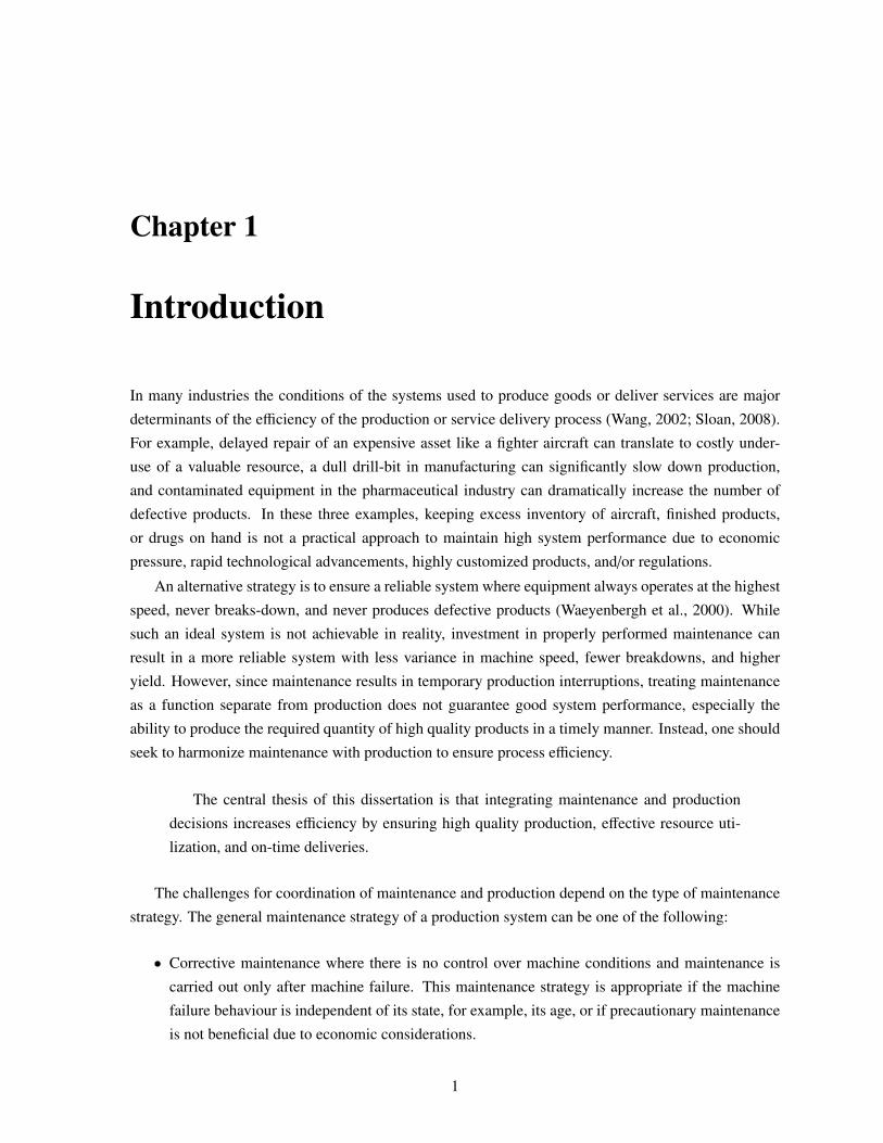
• Corrective maintenance where there is no control over machine conditions and maintenance is
carried out only after machine failure. This maintenance strategy is appropriate if the machine
failure behaviour is independent of its state, for example, its age, or if precautionary maintenance
is not beneficial due to economic considerations.
1
Chapter 1. Introduction 2
• Preventive maintenance where machine conditions can be partially controlled by performing
maintenance both before and at failures to decrease the number of breakdowns. This mainte-
nance strategy is applicable if the frequency of machine failure changes depending on its state or
there is a measurable condition which can signal incipient failures.
When the maintenance plan is corrective, there is no explicit decision on when to schedule main-
tenance and machines are maintained reactively upon failure. The only decision is about production.
Since each machine failure interrupts the system, ignoring the possibility of machine breakdowns in
determining production decisions leads to an imprecise estimate of the production capacity, and the pro-
duction plan and schedule1 will likely be inaccurate. It is desirable to make planning and scheduling
decisions that are optimal for the particular machine failures that are actually going to happen. Clearly,
this ideal situation is not achievable since information on machine breakdowns and, consequently, the
production unavailability periods are not known in advance. Therefore, a realistic research challenge
is to construct a production plan and schedule which perform well for the majority of scenarios of ma-
chine breakdowns and are flexible enough to be adjusted as new information on unavailable production
periods becomes known.
In the case of a preventive maintenance strategy, both maintenance and production decisions are
relevant. Determining maintenance decisions individually based only on the state of machines, such as
their age and failure characteristics, results in a static rule (Dijkhuizen and Harten, 1998): Machine X
should be maintained after Y hours of operations. However, static rules are indifferent to fluctuations
that might happen over time in a production system. For example, if the production system is heavily
loaded, there is an opportunity for significant financial gains by delaying maintenance (Kaufman and
Lewis, 2007). As another example, if there is large inventory on hand, it intuitively makes sense to ben-
efit from the reduced need for production by scheduling maintenance earlier. Therefore, incorporating
the operational state of the production system such as inventory, workload, and due dates into main-
tenance decisions leads to better allocation of resources to maintenance and production. Furthermore,
in a system with partial control over machine conditions, performing preventive maintenance, though
decreasing the number of breakdowns, will result in planned periods of process unavailability that could
be otherwise allocated to production. Thus, the desirable production plan and schedule are not only
hedged against various unplanned interventions; they also include the minimum number of planned un-
availability periods while ensuring a highly reliable system. The research challenge in this case is to
utilize both the available information on machine conditions and the operational state of the process to
simultaneously make maintenance and production decisions.
This dissertation develops models and optimization techniques that integrate maintenance and pro-
duction decisions, addressing the challenges noted above. To create a framework capturing possible
interdependencies between production problems and maintenance strategies, we divide the production
problems into planning and scheduling and the maintenance strategies into corrective and preventive.
1In this dissertation we distinguish between production plans and schedules as follows. A production plan evaluates ca-pacity needs and determines the optimal production quantities (Nahmias, 2005). A production schedule allocates the availablecapacity to competing customer orders over time (Pinedo, 2005).
Chapter 1. Introduction 3
The investigation of our thesis focuses on three areas.
1. Integrated maintenance and production planning with partial control over machine conditions in
the context of a periodic review production system. The goal is to determine the optimal amount
of investment in maintenance for a given production quantity considering the inventory on hand.
2. Integrated maintenance planning and production scheduling with no control over machine condi-
tions in the context of a dynamic military aircraft repair shop. The goal is to create the optimal
production schedule considering the uncertainty on machine conditions and due dates of products.
3. Integrated maintenance planning and production scheduling with partial control over machine
conditions in the context of a multi-machine production system. The goal is to simultaneously
find the maintenance plan and determine the optimal maintenance and production schedules con-
sidering the available information on machine conditions, planned production interruptions, and
product due dates.
In the first area of our study, we use stochastic optimization techniques to make integrated mainte-
nance and production planning decisions since both decisions are long-term and are based on stochastic
and aggregate information. For example, the production process is abstracted as a single-stage pro-
cess and all customer orders are considered similar, requiring the same production capacity and due
at the same time. In the last two areas of our study, to make integrated maintenance and production
scheduling decisions, both stochastic and complex combinatorial properties must be properly modeled.
Production scheduling decisions are addressed by combinatorial optimization tools since, in contrast to
maintenance decisions, they are short-term and are based on combinatorial information. The existence
of different customer orders with various requirements and multiple machines with complex interde-
pendencies is, for example, taken into account. For making integrated maintenance and scheduling
decisions, we develop decomposition techniques that deal with stochastic and combinatorial challenges
in different, coupled stages. These techniques combine the ideas of stochastic optimization tools such
as dynamic programming (Puterman, 1994) with those of combinatorial optimization techniques such
as mixed integer programming (Queyranne and Schulz, 1994), constraint programming (Baptiste et al.,
2006), and logic-based Benders decomposition (Hooker and Yan, 1995; Hooker and Ottosson, 2003).
1.1 Dissertation Outline
Chapter 2 provides a review of the literature on the interdependencies of maintenance and production
problems. It presents a novel framework with three axes: the type of production problem, the mainte-
nance strategy, and the length of the decision horizon. Production problems are divided into planning
and scheduling, maintenance strategies into corrective and preventive, and the length of the decision
horizons into long- and short-term. The combinations of different problems on the three axes indicate
the areas where maintenance and production can be integrated. A thorough review of the formulations
and the solution methodologies in each area is provided. The review forms a foundation where possible
Chapter 1. Introduction 4
relationships between maintenance and production are presented in a principled and intuitive structure.
Finally, the chapter identifies the dissertation’s three main areas of investigation: integrated maintenance
and production planning with partial control over machine conditions, integrated maintenance planning
and production scheduling with no control over machine conditions, and integrated maintenance plan-
ning and production scheduling with partial control over machine conditions.
Chapter 3 addresses the integrated maintenance and production planning problem with partial con-
trol over machine conditions in the context of a periodic review production system. It considers a firm
that produces a single product in a single-stage process. Due to machine deterioration and unexpected
failures, the quantity produced (yield) is random and the firm decides to invest in preventive maintenance
to increase the number of finished high quality products. The problem at the beginning of each period is
to simultaneously determine the production quantity and the amount of investment in maintenance. We
use stochastic dynamic programming to identify the optimal policy such that the discounted expected
total cost is minimized over multiple periods. However, due to the non-convexity of the cost function,
we analyze a simpler problem where the production quantity is fixed. Our goal is to characterize the
structure of the optimal maintenance policy. The results show that the optimal maintenance investment
policy is a threshold policy if the yield linearly changes in the amount of money invested and there is a
strong condition on the expected value of yield such that the marginal yield is always positive. If invest-
ment does not always increase the yield, by using Chebyshev’s other inequality, we provide insight into
the optimal threshold investment policy. Finally, we provide several managerial insights by comparing
different problem parameters.
Assuming that the production quantity and the amount of maintenance investment are known, Chap-
ter 4 studies the relationship between maintenance and production from an operational perspective. The
problem of integrated maintenance planning and production scheduling where machines are only cor-
rectively maintained is investigated in the context of a dynamic military aircraft repair shop. The set of
production activities (flights) is already scheduled, with each flight requiring a certain number and type
of machines (aircraft). The machines might unexpectedly break-down, limiting their availability for pro-
duction. Maintenance on failed machines must be scheduled to ensure that the production activities are
carried out as scheduled. To solve the problem, we view the dynamic repair shop as successive static re-
pair scheduling sub-problems over shorter time periods where the uncertainty about machine failures is
incorporated in the repair schedule. We propose a complete approach based on the logic-based Benders
decomposition to solve the static sub-problems and design different rescheduling policies to schedule
the dynamic repair shop. Computational experiments demonstrate that the Benders model is able to
find and prove optimal solutions on average four times faster than a mixed integer programming model.
The rescheduling approach that can schedule over a longer horizon and quickly adjust the schedule in-
creases the number of machines available for production in the long term by 10% over the approaches
using only one aspect.
Continuing the study of integration of maintenance planning and production scheduling, Chapter 5
assumes that machines can be maintained both before and at failure. A multi-machine production sys-
tem over multiple periods is considered where different customer orders must be processed on each
Chapter 1. Introduction 5
machine and are due at different times. Each machine deteriorates as it is used for production, and the
production capacity decreases as a result. Maintaining machines before failure improves their conditions
but interrupts production. The challenge is to simultaneously determine the allocation of maintenance
to machines and time periods and to schedule maintenance and production in each period, utilizing the
available information on machine conditions. The deterioration of each machine is modeled assuming
that its speed decreases deterministically as the number of time periods since maintenance increases. To
solve the problem, motivated by logic-based Benders decomposition, we design an integrated two-stage
algorithm. The first stage assigns maintenance to machines and time periods, abstracting the scheduling
problem, while the second stage creates a schedule for the current time period. The first stage is then
re-solved using feedback from the schedule. This iteration between maintenance planning and schedul-
ing continues until the solution costs in two stages converge. Our results demonstrate that the benefit
of integrated decision making increases when maintenance is less expensive relative to lost production
cost and that a longer horizon for maintenance planning is beneficial when maintenance cost increases.
Chapter 6 addresses the same problem as Chapter 5, using a more sophisticated and realistic model
of stochastic machine deterioration. A set of discrete states represents different machine conditions and
the deterioration process follows a continuous time Markov chain. Similar to Chapter 5, we design a
two-stage algorithm to solve the problem. In the first stage, we formulate a Markov decision process
model to determine the maintenance policy where the scheduling constraints are abstracted. The main-
tenance policy defines a decision rule for performing maintenance. We also derive sufficient conditions
guaranteeing the monotonicity of the maintenance policy in both machine state and demand. In the sec-
ond stage, we formulate a mixed integer programming model to find the maintenance and the production
schedule in the current period incorporating all scheduling combinatorics. Our computational results
demonstrate that exploiting machine condition information in maintenance and production scheduling
decisions leads to 21% cost savings on average. Furthermore, the benefit of integrating maintenance
reasoning in production scheduling decisions is higher for high discount factors and for industries with
medium mean time to failure.
Chapter 7 outlines future work extending the problems studied in Chapters 3 to 6 and suggests
two general directions to better model realistic problems which are both stochastic and combinatorially
complex. Finally, it discusses the relevance of our approach to other integrated decisions in supply chain
management.
Chapter 8 summarizes the contributions of the dissertation and provides a conclusion.
Appendix A includes the proofs of the propositions in Chapter 3. Several structural properties of the
production scheduling problem in Chapter 5 are given in Appendix B. The exact method for calculating
the average production rate used in the production scheduling problem and the detailed experimental
setup of Chapter 6 are presented in Appendices C and D, respectively.
1.2 Summary of Contributions
The main contributions of this dissertation are summarized below.
Chapter 1. Introduction 6
• We are the first to theoretically identify the set of conditions that guarantee the existence of an
optimal threshold type maintenance policy in a periodic review production system with random
yield. The results will help managers to decide how much money should be invested to improve
the state of the production system.
• We provide several managerial insights, including how the amount of investment in maintenance
changes as the inventory or the total available budget increases. Understanding these relationships
is useful to coordinate maintenance and production planning decisions.
• We are the first to develop optimization techniques that can effectively reason about both stochas-
tic and combinatorial challenges in the context of maintenance and production scheduling deci-
sions over a long-time horizon. Our techniques are all based on the idea of decomposition where
the stochastic and the combinatorial challenges are addressed in different, coupled stages.
• We design an integrated technique to create a repair schedule for a dynamic military aircraft repair
shop problem and show that adjusting the repair schedule as new short-term information becomes
known significantly increases flight coverage. The integrated technique is based on a novel logic-
based Benders decomposition approach which is four times faster than a novel mixed integer
programming model on average which in turn is two orders of magnitude faster than an existing
mixed integer programming model in the literature.
• We are the first to explicitly model the effect of machine deterioration and restoration on the
processing times of customer orders in integrated maintenance and scheduling decisions.
• To precisely model the production capacity as a function of both machine state and the operational
state of the system in a multi-machine production environment, we design appropriate solution
techniques that depend on the deterioration process of machines. More specifically,
– if machines deteriorate as the number of time periods since maintenance increases, we de-
sign a coupled two-stage integrated approach inspired by the idea of logic-based Benders
decomposition; and
– if machines deteriorate following a continuous Markov chain, we design a two-stage decom-
posed approach combining Markov decision process and mixed integer programming.
• We are the first to prove the conditions guaranteeing the monotonicity of a maintenance policy
on both machine state and the number of customer orders when the effect of performing pre-
ventive maintenance on the production is not certain. More specifically, we consider preventive
maintenance does not necessarily make the machine as good as new.
Chapter 2
Integrated Maintenance & Production: ALiterature Review
Changing trends in production including the introduction of “just-in-time” inventory management in
the past few decades has increased the importance of timely and continuous production (Dekker et al.,
1997; Waeyenbergh et al., 2000). Keeping large inventories of finished products does not ensure cus-
tomer satisfactions anymore because of the fast technological changes (Waeyenbergh et al., 2000). As a
consequence, to cope with the current competitive environment where customers expect higher product
quality, on-time deliveries, and a higher degree of customization, a production system is forced to be
highly reliable (Waeyenbergh et al., 2000). However, a real-world production system is dynamic and un-
certain where machine breakdowns make the production capacity unavailable and imperfect processes
produce defective products. Deteriorating machine condition is one of the main sources of uncertainty
in both machine breakdowns and imperfect processes. Maintenance, on the contrary, improves machine
conditions, but it uses the potential production time that could be otherwise allocated to production.
Therefore, the interdependency between maintenance and production and their conflicts in the short
term have necessitated developing models and techniques that integrate maintenance reasoning into
production problems. The goal of the integrated techniques is to guarantee the continuous functionality
of the production system to produce the required quantity of the products with the required quality in a
timely manner (Ben-Daya and Rahim, 2001; Pintelon and Parodi-Herz, 2008).
In this chapter, we review the literature addressing the interdependency between maintenance and
production. We first define our framework for classification of this relationship, we then provide an
overview of each area of our classification in detail and state the connection between the relevant litera-
ture and the corresponding contributions of this dissertation.
2.1 Classification Scheme
A production system deals with two different problems:
• Production planning: Production planning determines the optimal production quantities, also
7
Chapter 2. IntegratedMaintenance & Production: A Literature Review 8
known as lot-sizing, and evaluates the required production capacity (Nahmias, 2005).
• Production sequencing/scheduling: Production sequencing/scheduling addresses the problem of
allocating the available production capacity and assigning start times to production jobs (Pinedo,
2002).
Maintenance reasoning in a production system is mainly addressed in two situations in which there
is either no control or partial control over machine conditions. The former situation includes correc-
tive maintenance, i.e., machines are maintained only at failure while the latter includes both corrective
and preventive maintenance (Wang, 2002), machines can be maintained to prevent incipient failures.
The combination of two different production problems and two different maintenance situations defines
different problems where maintenance and production decisions are interdependent.
We further classify the literature addressing the interdependency between maintenance and produc-
tion into two categories based on the length of the decision horizon.
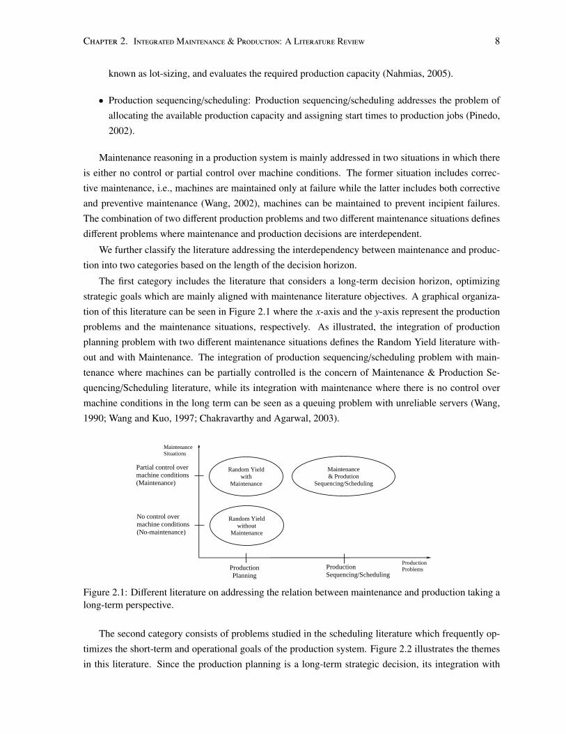
The first category includes the literature that considers a long-term decision horizon, optimizing
strategic goals which are mainly aligned with maintenance literature objectives. A graphical organiza-
tion of this literature can be seen in Figure 2.1 where the x-axis and the y-axis represent the production
problems and the maintenance situations, respectively. As illustrated, the integration of production
planning problem with two different maintenance situations defines the Random Yield literature with-
out and with Maintenance. The integration of production sequencing/scheduling problem with main-
tenance where machines can be partially controlled is the concern of Maintenance & Production Se-
quencing/Scheduling literature, while its integration with maintenance where there is no control over
machine conditions in the long term can be seen as a queuing problem with unreliable servers (Wang,
1990; Wang and Kuo, 1997; Chakravarthy and Agarwal, 2003).
Partial control over
machine conditions
(Maintenance)
No control over
machine conditions
(No-maintenance)
Production
Planning
Production
Sequencing/Scheduling
Production
Problems
Random Yield
without
Maintenance
Random Yield
with
Maintenance
Maintenance
& Prodution
Sequencing/Scheduling
Maintenance
Situations
Figure 2.1: Different literature on addressing the relation between maintenance and production taking along-term perspective.
The second category consists of problems studied in the scheduling literature which frequently op-
timizes the short-term and operational goals of the production system. Figure 2.2 illustrates the themes
in this literature. Since the production planning is a long-term strategic decision, its integration with
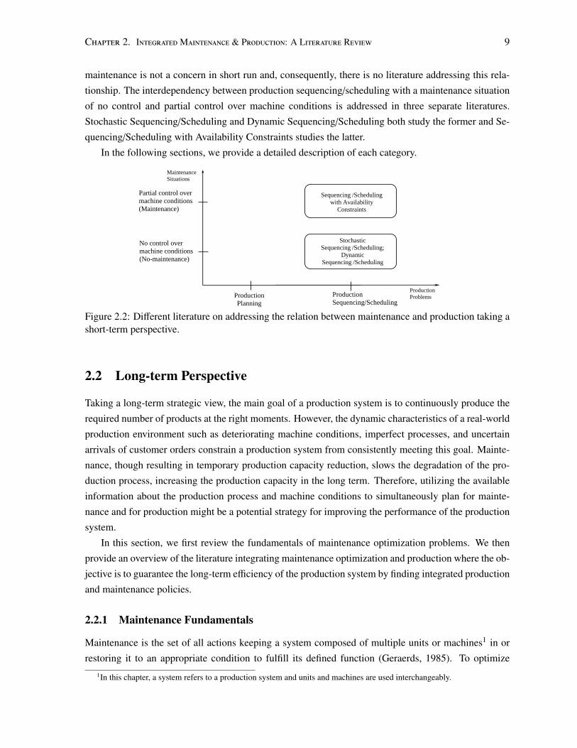
Chapter 2. IntegratedMaintenance & Production: A Literature Review 9
maintenance is not a concern in short run and, consequently, there is no literature addressing this rela-
tionship. The interdependency between production sequencing/scheduling with a maintenance situation
of no control and partial control over machine conditions is addressed in three separate literatures.
Stochastic Sequencing/Scheduling and Dynamic Sequencing/Scheduling both study the former and Se-
quencing/Scheduling with Availability Constraints studies the latter.
In the following sections, we provide a detailed description of each category.
Partial control over
machine conditions
(Maintenance)
No control over
machine conditions
(No-maintenance)
Production
Planning
Production
Sequencing/Scheduling
Production
Problems
Sequencing /Scheduling
with Availability
Constraints
Maintenance
Situations
Stochastic
Sequencing /Scheduling;
Dynamic
Sequencing /Scheduling
Figure 2.2: Different literature on addressing the relation between maintenance and production taking ashort-term perspective.
2.2 Long-term Perspective
Taking a long-term strategic view, the main goal of a production system is to continuously produce the
required number of products at the right moments. However, the dynamic characteristics of a real-world
production environment such as deteriorating machine conditions, imperfect processes, and uncertain
arrivals of customer orders constrain a production system from consistently meeting this goal. Mainte-
nance, though resulting in temporary production capacity reduction, slows the degradation of the pro-
duction process, increasing the production capacity in the long term. Therefore, utilizing the available
information about the production process and machine conditions to simultaneously plan for mainte-
nance and for production might be a potential strategy for improving the performance of the production
system.
In this section, we first review the fundamentals of maintenance optimization problems. We then
provide an overview of the literature integrating maintenance optimization and production where the ob-
jective is to guarantee the long-term efficiency of the production system by finding integrated production
and maintenance policies.
2.2.1 Maintenance Fundamentals
Maintenance is the set of all actions keeping a system composed of multiple units or machines1 in or
restoring it to an appropriate condition to fulfill its defined function (Geraerds, 1985). To optimize1In this chapter, a system refers to a production system and units and machines are used interchangeably.
Chapter 2. IntegratedMaintenance & Production: A Literature Review 10
maintenance, a mathematical model in which both costs and benefits of maintenance are quantified is
constructed and an optimum balance is achieved (Dekker et al., 1996). The cost and benefit of main-
tenance are dependent on the maintenance policy, a mapping from the system states (breakdown, age,
etc.) to maintenance actions (inspection, repair, replacement) (McCall, 1965; Dekker et al., 1996). One
example of a maintenance policy is the age replacement policy where a unit is replaced at age T or at
failure, whichever occurs first. Maintenance optimization models usually assume that the maintenance
policy is known in advance, for example, it is the age replacement policy. Their focus is then on de-
termining the optimal values for the policy parameters, i.e., finding the optimal value of T in the age
replacement policy.
Since the literature on maintenance optimization problems is extensive and independent of pro-
duction problems, we only review its main concepts to provide the reader with understanding of the
maintenance terms used in this dissertation. Interested readers are referred to the books by Ebeling
(1997), Jardine and Tsang (2006), and Nakagawa (2005; 2010; 2011). A detailed survey on the mainte-
nance models can be found in papers by Cho and Parlar (1991), Dekker et al. (1997), Wang (2002), and
Nicolai and Dekker (2008).
In this section, we first formally define the most important quantity of the maintenance theory, failure
rate, we then provide an explanation for the most general maintenance action, repair, and recapitulate
the four most widely used maintenance policies in their simplest form (Pintelon and Parodi-Herz, 2008).
We finally briefly describe the common techniques for solving the maintenance optimization problems.
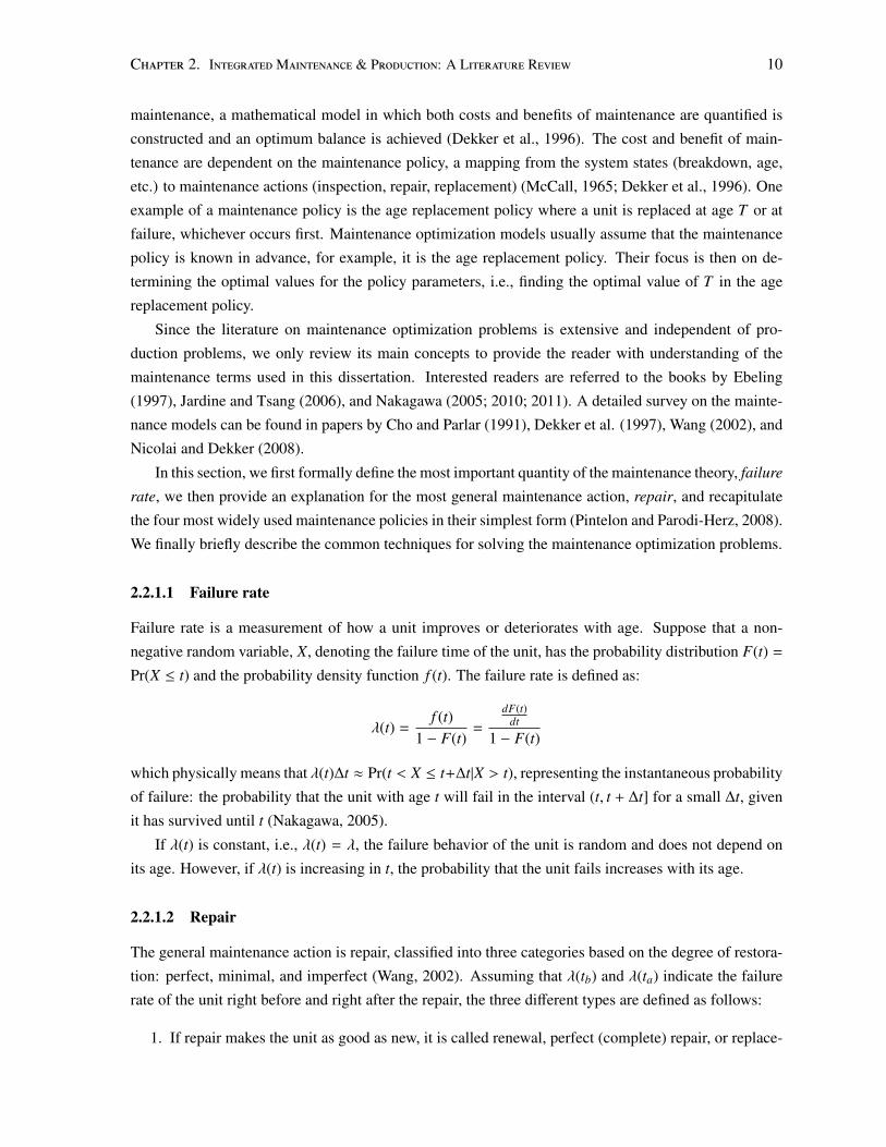
2.2.1.1 Failure rate
Failure rate is a measurement of how a unit improves or deteriorates with age. Suppose that a non-
negative random variable, X, denoting the failure time of the unit, has the probability distribution F(t) =
Pr(X ≤ t) and the probability density function f (t). The failure rate is defined as:
λ(t) =f (t)
1 − F(t)=
dF(t)dt
1 − F(t)
which physically means that λ(t)∆t ≈ Pr(t < X ≤ t+∆t|X > t), representing the instantaneous probability
of failure: the probability that the unit with age t will fail in the interval (t, t + ∆t] for a small ∆t, given
it has survived until t (Nakagawa, 2005).
If λ(t) is constant, i.e., λ(t) = λ, the failure behavior of the unit is random and does not depend on
its age. However, if λ(t) is increasing in t, the probability that the unit fails increases with its age.
2.2.1.2 Repair
The general maintenance action is repair, classified into three categories based on the degree of restora-
tion: perfect, minimal, and imperfect (Wang, 2002). Assuming that λ(tb) and λ(ta) indicate the failure
rate of the unit right before and right after the repair, the three different types are defined as follows:
1. If repair makes the unit as good as new, it is called renewal, perfect (complete) repair, or replace-
Chapter 2. IntegratedMaintenance & Production: A Literature Review 11
ment. Specifically, the failure rate of the unit after repair equals its failure rate at age 0, i.e.,
λ(ta) = λ(0).
2. If repair makes the unit as good as right before it fails, it is called minimal repair. In this case,
λ(ta) = λ(tb).
3. If repair makes the unit better than right before its failure, but worse than new, it is called imperfect
(incomplete) repair. In this case, λ(0) < λ(ta) < λ(tb).
2.2.1.3 Maintenance Policies
The four policies that we review are: failure-based maintenance (FBM), preventive-based maintenance
(PBM), condition-based maintenance (CBM), and opportunity-based maintenance (OBM) (Pintelon and
Parodi-Herz, 2008).
Failure-based Maintenance: Maintenance is carried out only after breakdowns. This policy is typically
used in case of constant failure rate (random failure behavior) and low breakdown cost. For example,
general machine-repairman problem has a set of workers and a set of machines that are subject to fail-
ures and therefore need repair. As the number of workers is typically less than the number of machines,
several optimization problems can be defined in order to minimize the average cost per time unit: op-
timizing the repair rate, i.e., number of workers and number of repair facilities; optimizing the number
of spare machines; and optimizing the repair scheduling policy.2 A detailed survey of the first two op-
timization problems is provided by Haque and Armstrong (2007) and Cho and Parlar (1991), while the
latter is comprehensively reviewed by Iravani et al. (2007).
The maintenance policy used in Chapter 4 is a failure-based maintenance policy where aircraft are
minimally repaired upon failure.
Preventive-based Maintenance: Maintenance is carried out after a specified amount of time. The main
assumptions of this policy are:
1. A unit fails gradually with time, i.e., its failure rate is increasing in time. Therefore, performing
maintenance can change the failure time distribution of the unit, decreasing the expected number
of failures in future.
2. The cost of preventive maintenance, repairing the unit before it fails is less than the cost of correc-
tive maintenance, repairing the unit at failure. This assumption is essential to make the problem
non-trivial; otherwise, the optimal decision is always to let the system operate until failure.
Three examples of PBM policies are as follows:
• Age replacement: The age replacement policy completely repairs (or replaces) a unit at age T or
at failure, whichever occurs first. The age of a unit corresponds to its total up-time. The decision
2The problem of finding the repair scheduling policy can be seen as a problem of integrated production sequenc-ing/scheduling with maintenance where there is no control over machines with a long-term perspective. This problem isaddressed in queuing theory literature (Wang, 1990; Wang and Kuo, 1997; Chakravarthy and Agarwal, 2003).
Chapter 2. IntegratedMaintenance & Production: A Literature Review 12
is to find the optimal T . This policy is appropriate for a unit with catastrophic failure mode, where
its failure is very serious and incurs a significant loss and, therefore, replacement at each failure
is required (Nakagawa, 2005).
• Periodic replacement: Under this policy, a unit is completely repaired (replaced) at periodic times,
kT, k ∈ {1, 2, ...}, independent of its age and failure history and is minimally repaired at its failures.
If the unit is also replaced at failure times, the periodic replacement is called block replacement.
The main advantage of this policy is that there is no necessity to record the age of the unit. This
policy is reasonably applicable for units in complex systems when it is costly to replace a unit in
operation (Wang, 2002; Nakagawa, 2005).
• Repair number counting: This policy replaces a unit at its k-th failure and the first (k − 1) failures
are fixed by minimal repair. This policy finds the optimal k and its main difference with the age
and the periodic replacement policies is that the time of performing preventive maintenance is
random, being equal to the time of the k-th failure (Wang, 2002).
The maintenance model studied in Chapter 5 is a PBM policy where the number of time periods
between consecutive maintenance on a machine is optimized.
Condition-based Maintenance: Maintenance is carried out after the values of one or several system
parameters exceed predetermined values. As in PBM, the cost of preventive maintenance is assumed
to be less than the cost of corrective maintenance, but the failure rate of the unit does not necessarily
increase in time. CBM is becoming a common approach in industries because the investment in under-
lying techniques such as vibration analysis and oil spectrometry is economically justified (Pintelon and
Parodi-Herz, 2008).
In Chapter 6, a CBM policy is developed to perform maintenance on a machine each time its degra-
dation level exceeds a threshold value.
Opportunity-based Maintenance: The OBM policy is defined for a multi-unit system with dependency
among its units. The optimal maintenance policy of each unit, therefore, depends on the state of the other
units: the failure of one unit results in a potential opportunity to perform maintenance on some of the
other units (Wang, 2002). One of the main interactions between components is economic where the cost
of joint maintenance of a group of components is not equal to the total cost of individual maintenance of
each component: it can be either lower (positive economic dependence) or higher (negative economic
dependence) (Nicolai and Dekker, 2008).3
The maintenance policies in Chapters 5 and 6 are developed for a multi-machine production system
where there is negative economic dependency between machines. More specifically, there is a limit on
the available maintenance capacity, implying that more than a specified number of machines cannot be
maintained at the same time.
3An opportunity-based maintenance policy is also applicable for a single-unit system with different failure modes wherebreakdown as a result of one failure mode is an opportunity for performing maintenance to decrease the probability of failuredue to other failure modes (Jhang and Sheu, 1999).
Chapter 2. IntegratedMaintenance & Production: A Literature Review 13
2.2.1.4 Solution Techniques
There are two typical forms of maintenance optimization problems. The first form assumes that the
maintenance policy is known and finds the optimal values of the given policy parameters. For example,
with a periodic replacement policy, the maintenance optimization problem is to find the optimal T to
perform complete repair at periodic times of kT, k ∈ {1, 2, ...}. Renewal theory is the usual solution
technique for this form of maintenance optimization problems with the typical objective of minimizing
the total expected cost per time unit. The second form aims to find the optimal maintenance policy, i.e.,
the optimal mapping between system states and maintenance actions and its primary solution technique
is dynamic programming (McCall, 1965; Dohi et al., 2000).
In this section, we briefly describe each solution technique.
Renewal Theory: The renewal process can be formally defined as follows (Nakagawa, 2005; Ross,
2010):
Renewal Process: Consider a sequence of independent and non-negative random variables {X1, X2, ...}
where Pr(Xi = 0) < 1, ∀i, to avoid triviality. Suppose that X2, X3, ... have an identical distribution of F(t)
with finite mean µ and X1 possibly has a different distribution of F1(t) with mean µ1. Three different
renewal processes can be defined depending on the following types of F1(t).
1. If F1(t) = F(t), i.e., all random variables are identically distributed, the process is called an
ordinary renewal process or a renewal process.4
2. If F1(t) and F(t) are not the same, the process is called a modified or a delayed renewal process.
3. If F1(t) is defined as F1(t) =
∫ t0 [1−F(u)]du
µ , the process is an equilibrium or a stationary process.
The following example makes the above definitions clearer. Consider a unit with the maintenance
policy of replacing it with a new one upon failure. Further assume that the time of replacing the unit
is negligible such that the unit starts operating immediately after replacement. Assume that X1 and
Xi, ∀i > 1, are random variables representing the time to the first failure and the time between the
(i − 1)- and the i-th failures with distributions F1(t) and F(t), respectively. If the unit is installed at time
t = 0, then all the failure times have the same distribution representing an ordinary renewal process.
If the unit is in use at time t = 0, X1 is the residual time to the first failure and could have a different
distribution from the failure time of a new unit. The sequence of time to failures, therefore, represents
a delayed renewal process. If the observed time origin is sufficiently long after the installation of the
unit and X1 has the distribution of F1(t) =
∫ t0 [1−F(u)]du
µ , the sequence of time to failures then denotes an
equilibrium (a stationary) renewal process. Under both ordinary and stationary renewal processes, the
expected number of failures in the interval of [t1, t2] depends on the length of the interval, (t2 − t1), and
the mean time to failure for a new unit, µ, being equal to t2−t1µ (Barlow and Proschan, 1996).
The fundamental theorem in minimizing the cost function in the first forms of maintenance opti-
mization problems is the renewal reward theorem. Before stating the theorem, we define some notation.
4The ordinary renewal process is the most common process used in the maintenance optimization models.
Chapter 2. IntegratedMaintenance & Production: A Literature Review 14
Since at each failure, the unit is renewed and Xi corresponds to the time between the (i − 1)- and the
i-th renewals, S n =∑n
i=1 Xi represents the time of the n-th renewal and N(t) = max{n : S n ≤ t} de-
notes the number of renewals during (0, t]. Assuming that Ri is the reward earned at the i-th renewal,
R(t) =∑N(t)
i=1 Ri represents the total reward during (0, t]. Now, we state the theorem below (Nakagawa,
2005; Ross, 2010).
Renewal Reward Theorem: Assuming that E[R] = E[Ri] and E[X] = E[Xi]
a) with probability 1, limt→∞R(t)
t =E[R]E[X]
b) limt→∞E[R(t)]
t =E[R]E[X]
Letting the time between renewals represent one cycle, the renewal reward theorem shows that the
expected reward per unit of time for an infinite time span equals the expected reward per one cycle
divided by the mean time of one cycle.
To show the application of the renewal reward theorem in maintenance models, consider the age
replacement policy as defined earlier where the goal is to find the optimal T such that the expected
maintenance cost per time unit is minimized. We define Cr and Cp as the cost of replacing the unit at
failure and the cost of replacing the unit at time T before failure. Under the age replacement policy,
the unit is replaced at the first failure denoted by random variable X with failure distribution F(x) or at
time T , whichever occurs first. Therefore, the length of each renewal cycle equals min(X,T ) with the
expected value E[min(X,T )]. The cost of each renewal cycle is equal to CrI(X ≤ T ) + CpI(X > T )
where I is an indicator function. The expected cost per cycle is then equal to CrF(T ) + Cp(1 − F(T )).
Using the renewal reward theorem, the optimal T minimizes the expected cost per cycle divided by the
expected length of the cycle, i.e., CrF(T )+Cp(1−F(T ))E[min(X,T )] .
Dynamic Programming: The dynamic programming framework provides an opportunity for the deci-
sion maker to influence the behavior of a probabilistic system through choosing a sequence of actions
which causes the system to perform optimally with respect to some predetermined performance crite-
rion (Puterman, 1994). There are five elements to almost any dynamic programming model: decision
epochs, states, actions, rewards, and transition probabilities. Each element is briefly described below ac-
companied with maintenance related examples. Unless otherwise indicated, the details of the following
are from the book by Puterman (1994).
Decision Epochs: Decisions are made at points of time called decision epochs. The set of decision
epochs, T , can be classified as either a discrete or a continuous set and as either a finite or an infinite
set. In a discrete time problem, time is divided into periods and the decision epochs correspond to
the beginning of each period denoted as t ∈ {1, 2, ...}. In continuous time problems, the decision time
points are random points of time denoted as t ∈ [0,∞); for example, the breakdown of a machine or the
completion time of a repair corresponds to a potential continuous decision epoch.
States: At each decision epoch, the probabilistic system is in a state. The set of all possible system states
is denoted by S where S t = s corresponds to the system state at decision epoch t. The set S can have
several dimensions and can be finite or infinite. For example, the age of a machine can represent the
Chapter 2. IntegratedMaintenance & Production: A Literature Review 15
machine state at every decision time epoch. However, the most common approach in the maintenance
literature is to represent the state of the machine using a finite discrete set, i.e., {0, 1, ...,N} where 0 and
N indicate the new and the failed conditions of the machine and the middle states represent intermediate
levels of machine health.
Actions: At each decision time epoch, t, after observing the state of the system, S t = s, the decision
maker chooses an action at from the non-empty set of all possible actions at state s, at ∈ As where
A = ∪s∈SAs is the action space. The common actions in maintenance models at each decision time
epoch, independent of the state of the system, are “no repair” and “repair”.
Rewards: As a result of performing action at at state S t at decision time point t, the decision maker pays
cost Ct(S t, at). For example, if the chosen action is to perform repair, the decision maker pays the cost
of repair plus the other related operational costs such as lost production cost.
Transition Probabilities: The system state at next decision epoch is determined by the probability dis-
tribution pt(.|S t, at). For example, let’s divide the time into equal time periods with length T where the
beginning of each period represents a decision epoch. If the decision maker replaces the machine with
a new one at the beginning of the n-th period, the transition probability that the machine is in a failed
state at the next decision epoch, the beginning of the (n + 1)-th period, equals Pr(X ≤ T ) = F(T ) where
F(x) is the failure distribution of the new unit.
Given the above five elements, the main goal of a dynamic programming model is to find a decision
rule, or a policy, prescribing a procedure for choosing the actions at each state of the system at any
decision time point such that a predetermined objective, for example, the expected sum of costs over
finite decision epochs t ∈ T , is minimized. Formally, the Markov5 policy π, chooses action Aπt (S t)
at time t if the system state is S t. If the selection of actions does not depend on time, the policy is a
stationary policy. The goal is then to find the optimal policy π ∈ Π, minimizing the expected sum of
costs over the finite set of decision epochs t ∈ T denoted as minπ∈ΠE[
∑t∈T C(S t, Aπt (S t))]. For example,
representing the possible states of the machine as {0, 1, ...,N} and the possible actions at each state as
“no repair” and “repair”, the stationary policy π divides the state space into two sub-sets I and II: sub-set
I includes the states in which it is optimal to perform repair and sub-set II includes the remaining states
where it is always optimal not to perform repair.
The stochastic dynamic programming methods such as policy iteration, value iteration, and modified
policy iteration are the common algorithms used to find the optimal policy (Heyman and Sobel, 1984;
Puterman, 1994). However, the majority of literature has focused on characterizing the structure of
the optimal maintenance policy. Interested readers are referred to the books by Bertsekas (2007) and
Puterman (1994) for an extensive coverage on dynamic programming models and their applications.
In Chapter 6, we use Markov decision process to find the optimal maintenance policy.
In the next three sub-sections, we review the literature that integrate maintenance and production
taking a long-term decision horizon.
5The policy is Markovian since it depends on the previous system states and actions only through the current state of thesystem (Puterman, 1994).
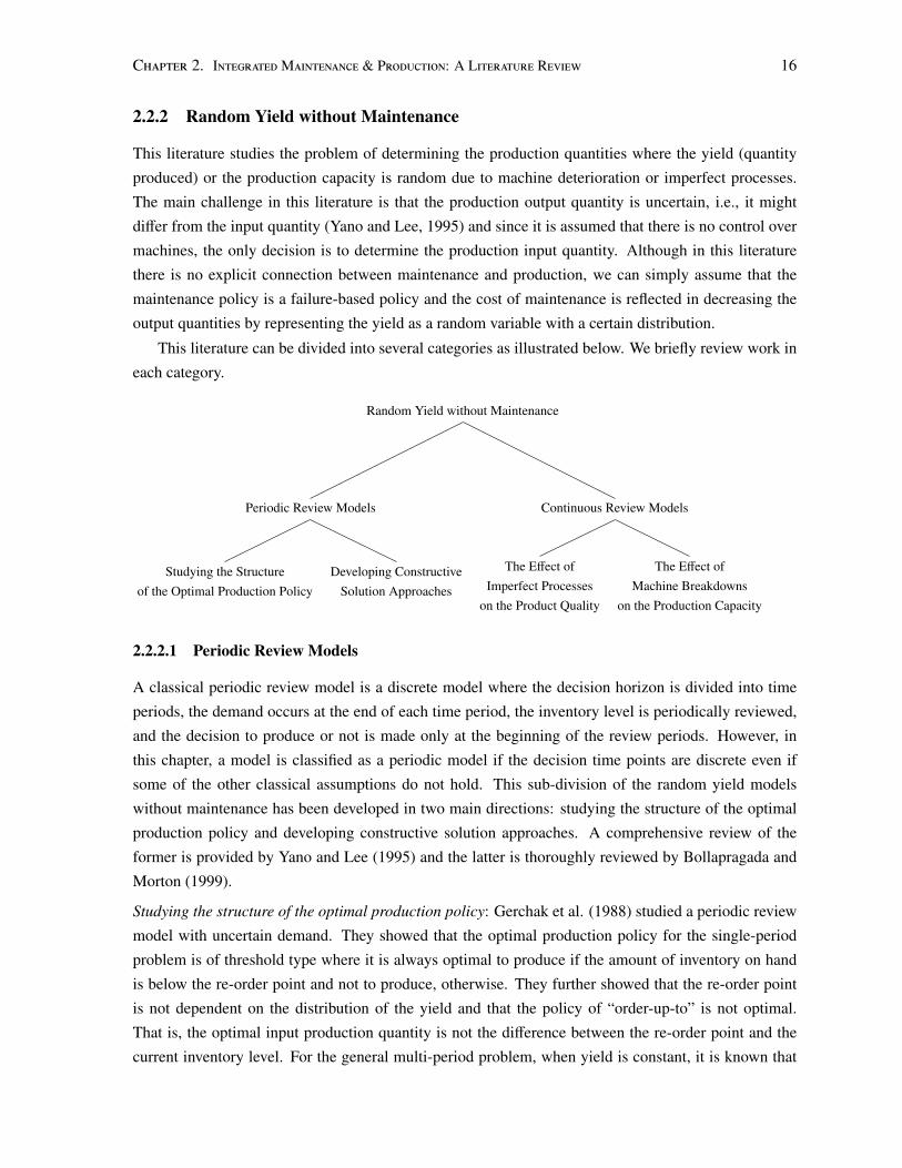
Chapter 2. IntegratedMaintenance & Production: A Literature Review 16
2.2.2 Random Yield without Maintenance
This literature studies the problem of determining the production quantities where the yield (quantity
produced) or the production capacity is random due to machine deterioration or imperfect processes.
The main challenge in this literature is that the production output quantity is uncertain, i.e., it might
differ from the input quantity (Yano and Lee, 1995) and since it is assumed that there is no control over
machines, the only decision is to determine the production input quantity. Although in this literature
there is no explicit connection between maintenance and production, we can simply assume that the
maintenance policy is a failure-based policy and the cost of maintenance is reflected in decreasing the
output quantities by representing the yield as a random variable with a certain distribution.
This literature can be divided into several categories as illustrated below. We briefly review work in
each category.
Random Yield without Maintenance
Periodic Review Models
Studying the Structureof the Optimal Production Policy
Developing ConstructiveSolution Approaches
Continuous Review Models
The Effect ofImperfect Processes
on the Product Quality
The Effect ofMachine Breakdowns
on the Production Capacity
2.2.2.1 Periodic Review Models
A classical periodic review model is a discrete model where the decision horizon is divided into time
periods, the demand occurs at the end of each time period, the inventory level is periodically reviewed,
and the decision to produce or not is made only at the beginning of the review periods. However, in
this chapter, a model is classified as a periodic model if the decision time points are discrete even if
some of the other classical assumptions do not hold. This sub-division of the random yield models
without maintenance has been developed in two main directions: studying the structure of the optimal
production policy and developing constructive solution approaches. A comprehensive review of the
former is provided by Yano and Lee (1995) and the latter is thoroughly reviewed by Bollapragada and
Morton (1999).
Studying the structure of the optimal production policy: Gerchak et al. (1988) studied a periodic review
model with uncertain demand. They showed that the optimal production policy for the single-period
problem is of threshold type where it is always optimal to produce if the amount of inventory on hand
is below the re-order point and not to produce, otherwise. They further showed that the re-order point
is not dependent on the distribution of the yield and that the policy of “order-up-to” is not optimal.
That is, the optimal input production quantity is not the difference between the re-order point and the
current inventory level. For the general multi-period problem, when yield is constant, it is known that
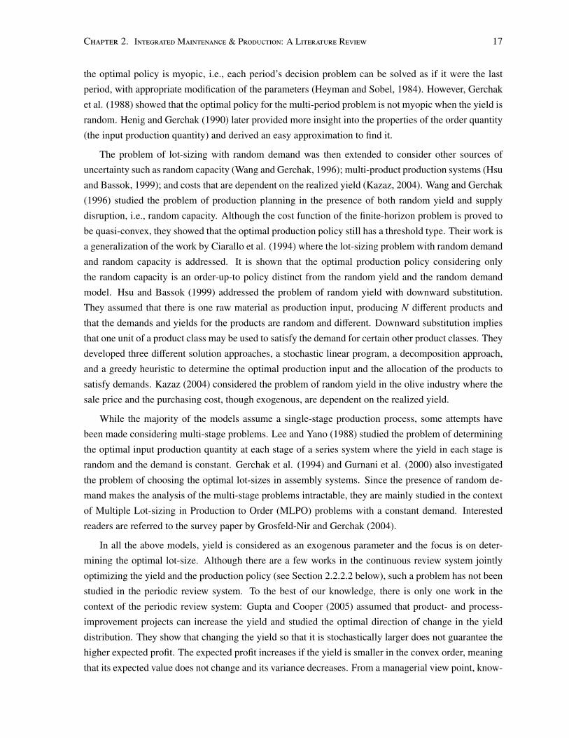
Chapter 2. IntegratedMaintenance & Production: A Literature Review 17
the optimal policy is myopic, i.e., each period’s decision problem can be solved as if it were the last
period, with appropriate modification of the parameters (Heyman and Sobel, 1984). However, Gerchak
et al. (1988) showed that the optimal policy for the multi-period problem is not myopic when the yield is
random. Henig and Gerchak (1990) later provided more insight into the properties of the order quantity
(the input production quantity) and derived an easy approximation to find it.
The problem of lot-sizing with random demand was then extended to consider other sources of
uncertainty such as random capacity (Wang and Gerchak, 1996); multi-product production systems (Hsu
and Bassok, 1999); and costs that are dependent on the realized yield (Kazaz, 2004). Wang and Gerchak
(1996) studied the problem of production planning in the presence of both random yield and supply
disruption, i.e., random capacity. Although the cost function of the finite-horizon problem is proved to
be quasi-convex, they showed that the optimal production policy still has a threshold type. Their work is
a generalization of the work by Ciarallo et al. (1994) where the lot-sizing problem with random demand
and random capacity is addressed. It is shown that the optimal production policy considering only
the random capacity is an order-up-to policy distinct from the random yield and the random demand
model. Hsu and Bassok (1999) addressed the problem of random yield with downward substitution.
They assumed that there is one raw material as production input, producing N different products and
that the demands and yields for the products are random and different. Downward substitution implies
that one unit of a product class may be used to satisfy the demand for certain other product classes. They
developed three different solution approaches, a stochastic linear program, a decomposition approach,
and a greedy heuristic to determine the optimal production input and the allocation of the products to
satisfy demands. Kazaz (2004) considered the problem of random yield in the olive industry where the
sale price and the purchasing cost, though exogenous, are dependent on the realized yield.
While the majority of the models assume a single-stage production process, some attempts have
been made considering multi-stage problems. Lee and Yano (1988) studied the problem of determining
the optimal input production quantity at each stage of a series system where the yield in each stage is
random and the demand is constant. Gerchak et al. (1994) and Gurnani et al. (2000) also investigated
the problem of choosing the optimal lot-sizes in assembly systems. Since the presence of random de-
mand makes the analysis of the multi-stage problems intractable, they are mainly studied in the context
of Multiple Lot-sizing in Production to Order (MLPO) problems with a constant demand. Interested
readers are referred to the survey paper by Grosfeld-Nir and Gerchak (2004).
In all the above models, yield is considered as an exogenous parameter and the focus is on deter-
mining the optimal lot-size. Although there are a few works in the continuous review system jointly
optimizing the yield and the production policy (see Section 2.2.2.2 below), such a problem has not been
studied in the periodic review system. To the best of our knowledge, there is only one work in the
context of the periodic review system: Gupta and Cooper (2005) assumed that product- and process-
improvement projects can increase the yield and studied the optimal direction of change in the yield
distribution. They show that changing the yield so that it is stochastically larger does not guarantee the
higher expected profit. The expected profit increases if the yield is smaller in the convex order, meaning
that its expected value does not change and its variance decreases. From a managerial view point, know-
Chapter 2. IntegratedMaintenance & Production: A Literature Review 18
ing the optimal direction of change in yield is not enough for initiating process improvement projects
such as maintenance. A manager needs to know the optimal amount of money that should be allocated
to maintenance, and our work in Chapter 3 is a step in this direction.
Developing Constructive Solution Approaches: Since the structure of the optimal production policy with
random yield is not myopic, the literature on developing efficient solution approaches has focused on
when a myopic policy can be a good approximation to the optimal policy and has devised efficient algo-
rithms to find the optimal production quantity at the beginning of each review period. Baker and Erhardt
(1995) proposed a heuristic policy in the form of order-up-to policy where the demand and the yield are
random. Their simulation study showed that ignoring the random yield does not result in a significant
increase in the cost unless the service level is high or the process is extremely random. Bollapragada
and Morton (1999) considered the problem with random yield where the demand is random but not sta-
tionary. Three heuristics are developed to solve the problem based on the position of the inventory at the
end of the time period. The solutions of the heuristics are then compared with the optimal solution of a
dynamic programming approach and it is experimentally shown that the best heuristic has the worst-case
error of 3% and 5% for the infinite and finite cases. Li et al. (2008) based their work on the papers by
Henig and Gerchak (1990) and by Bollapragada and Morton (1999) to find more insight to the values of
order quantity and the re-order point. They derived upper and lower bounds for both the optimal order
quantity and the order threshold and used the derived bounds to construct efficient heuristics.
2.2.2.2 Continuous Review Models
The classical continuous review model is the economic manufacturing quantity (EMQ) problem where
the goal is to find the production up-time or alternatively the production quantity that minimizes the
production and inventory costs assuming that the production and the demand rates are constant, that
there is a single machine processing the products, that the inventory level is continuously monitored, that
the product quality is always acceptable, and that the production capacity is always at its maximum limit
(Nahmias, 2005). Relaxing the last two assumptions to explicitly model the effect of machine conditions
on the product quality or on the production capacity is the focus of the random yield literature without or
with maintenance in continuous review models. Continuous review models have been mainly used for
the joint optimization of maintenance and production policies, described in Section 2.2.3.2. However,
they were initially used to extend the EMQ models to address the uncertainty in the production process
without explicitly considering maintenance.
To address the effect of imperfect processes on the product quality, Rosenblatt and Lee (1986) stud-
ied the effect of an imperfect production process assuming two states: “in-control” and “out-of-control”.
The time that the process shifts between two states is exponentially distributed and the product quality
is determined only after production. They showed that the production run is shorter than that of the
classical EMQ formula and that it decreases as the defective rate or the cost of defective items increases.
Their analysis is further extended to incorporate the dynamic nature of deterioration processes, i.e., the
proportion of defective items is not constant. Porteus (1986) studied the same problem assuming that
the system incurs an extra cost for rework of each defective piece that it produces. Thus, there is an in-
Chapter 2. IntegratedMaintenance & Production: A Literature Review 19
centive to produce smaller lots, and have a smaller fraction of defective units. He also introduced three
options for investing in quality improvements: (i) reducing the probability that the process moves out
of control; (ii) reducing setup cost; and (iii) simultaneously using the two previous options. By assum-
ing a specific form of the investment cost function for each option, he explicitly obtained the optimal
investment strategy. Porteus (1986) motivated later work on jointly optimizing the yield variability and
lot-sizing: Gerchak and Parlar (1990) where the yield variability can be affected by investment and Lin
and Hou (2005) where the set-up cost and yield variability can be reduced through capital investment
are two examples.
Groenevelt et al. (1992b) addressed the effect of machine breakdowns on the production capacity in
the EMQ model. They studied the problem under two production policies: no-resumption and resume
(abort). Under the no-resumption policy, the production of the interrupted lot is not resumed after a
breakdown. The on-hand inventory is used before a new cycle is initiated. Under the resume policy,
production is immediately resumed after a breakdown if the current on-hand inventory is below a certain
threshold level. They showed that under both policies, the optimal lot-size will be always bigger than
the one in the corresponding deterministic cases, and that the optimal lot-size increases with the failure
rate. This paper has initiated a large amount of work discussed in Section 2.2.3.2.
To address both effects of an imperfect production process on the product quality and the machine
breakdowns on the production capacity, Boon et al. (2000) used the no-resumption policy of Groenevelt
et al. (1992b) such that two different probability distributions for time to transition from the in-control
state to the out-of-control state and time to breakdown are considered.
2.2.3 Random Yield with Maintenance
The main assumptions of the Random Yield with Maintenance literature are similar to those in the
literature reviewed in Section 2.2.2. The key difference is that maintenance and production decisions
are both addressed because machine conditions can be partially controlled. Therefore, it is generally
assumed that the production process deteriorates with time, i.e., the distribution of time to failure is
considered to result in an increasing failure rate.
As shown below, we review this literature in two main categories of periodic review and continu-
ous review models similar to the previous section. Budai et al. (2006) have classified the integrated
maintenance and production models where both decisions are relevant into four categories: conceptual
and process design models, economic manufacturing quantity models, production systems with buffer
capacity models, and production and maintenance rate optimization models. Their classification can
be considered as an alternative classification of our Random Yield with Maintenance category where
our periodic review and continuous review sub-categories include the production systems with buffer
capacity and the economic manufacturing quantity models of Budai et al. (2006), respectively. Our
classification allows a better description of the similarities and the differences in Random Yield litera-
ture with and without maintenance.
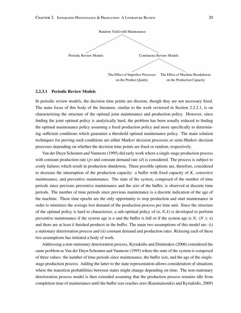
Chapter 2. IntegratedMaintenance & Production: A Literature Review 20
Random Yield with Maintenance
Periodic Review Models Continuous Review Models
The Effect of Imperfect Processeson the Product Quality
The Effect of Machine Breakdownson the Production Capacity
2.2.3.1 Periodic Review Models
In periodic review models, the decision time points are discrete, though they are not necessary fixed.
The main focus of this body of the literature, similar to the work reviewed in Section 2.2.2.1, is on
characterizing the structure of the optimal joint maintenance and production policy. However, since
finding the joint optimal policy is analytically hard, the problem has been usually reduced to finding
the optimal maintenance policy assuming a fixed production policy and more specifically to determin-
ing sufficient conditions which guarantee a threshold optimal maintenance policy. The main solution
techniques for proving such conditions are either Markov decision processes or semi-Markov decision
processes depending on whether the decision time points are fixed or random, respectively.
Van der Duyn Schouten and Vanneste (1995) did early work where a single-stage production process
with constant production rate (p) and constant demand rate (d) is considered. The process is subject to
costly failures which result in production shutdowns. Three possible options are, therefore, considered
to decrease the interruption of the production capacity: a buffer with fixed capacity of K, corrective
maintenance, and preventive maintenance. The state of the system, composed of the number of time
periods since previous preventive maintenance and the size of the buffer, is observed at discrete time
periods. The number of time periods since previous maintenance is a discrete indication of the age of
the machine. These time epochs are the only opportunity to stop production and start maintenance in
order to minimize the average lost demand of the production process per time unit. Since the structure
of the optimal policy is hard to characterize, a sub-optimal policy of (n,N, k) is developed to perform
preventive maintenance if the system age is n and the buffer is full or if the system age is N, (N ≥ n)
and there are at least k finished products in the buffer. The main two assumptions of this model are: (i)
a stationary deterioration process and (ii) constant demand and production rates. Relaxing each of these
two assumptions has initiated a body of work.
Addressing a non-stationary deterioration process, Kyriakidis and Dimitrakos (2006) considered the
same problem as Van der Duyn Schouten and Vanneste (1995) where the state of the system is composed
of three values: the number of time periods since maintenance, the buffer size, and the age of the single-
stage production process. Adding the latter to the state representation allows consideration of situations
where the transition probabilities between states might change depending on time. The non-stationary
deterioration process model is then extended assuming that the production process remains idle from
completion time of maintenance until the buffer size reaches zero (Karamatsoukis and Kyriakidis, 2009)
Chapter 2. IntegratedMaintenance & Production: A Literature Review 21
and that the repair time is increasing in the number of previous repairs (Dehayem Nodem et al., 2011).
To address random demand and production rates, Das and Sarkar (1999) did the early work studying
a problem with an application in discrete manufacturing industries. The production time of each product
is generally distributed, the production process is prone to failures where the time to failure and the time
to repair are generally distributed, and the inventory system is controlled using a (S , s) policy. Under this
inventory policy, the production stops when the buffer inventory reaches S and the production resumes
when the inventory drops to s. Decision epochs in this model are random, equivalent to completion
times of products. When processing of a product is finished, the state of the system, a vector of the
number of products produced since previous maintenance and the buffer size, is observed. The decision
on whether to continue production or to stop it for maintenance is then made. Since decision epochs
are random times, a semi-Markov decision process framework is developed to solve the problem using
a numerical search technique.
While in the model of Das and Sarkar (1999) the production policy is defined as a (S , s) policy,
Iravani and Duenyas (2002) focused on the joint characterization of maintenance and production policies
where the general distributions of time to produce, time to failure, and time to repair in the model by Das
and Sarkar (1999) are replaced by exponential distributions. However, using a semi-Markov decision
process, the structure of the optimal policy is shown to be complex. Utilizing several properties of the
optimal joint policy, a heuristic policy with two threshold values for stopping the production and for
undertaking maintenance is numerically investigated. Yao et al. (2005) further relaxed several other
assumptions and under some conditions, such as high positive or negative inventory levels, showed that
the maintenance policy has a control-limit structure.
In the models addressing the relationship between maintenance and production with random de-
mand and production rates, it is assumed that time to produce a final product is random. However,
Sloan (2004) took a different modeling approach and assumed that the number of acceptable final prod-
ucts, i.e., yield, produced in a given time period is random and has a binomial distribution. He showed
that under some reasonable conditions regarding the yield and machine deterioration, threshold mainte-
nance and threshold production policies exist, but the production policy is not monotone in the machine
state. A numerical investigation resulted in 18% cost savings of the integrated solution approach over a
sequential one where the maintenance and the production policies are independently determined.
Keeping inventory in stock to satisfy customer orders at process failures is considered as a strategy
in all the previous models. Kaufman and Lewis (2007), however, considered the problem of integrated
maintenance and production excluding this strategy. They studied the problem for a single server queue
where the deterioration process of the server is described by decreasing service rates. The production
policy is first-come, first-served and the maintenance policy is considered to be dependent on both
the number of customers in the queue and the deterioration level of the server. It is shown that the
maintenance policy has a switching curve structure6 which is monotone in the service rate and is non-
6A deterministic stationary policy is a switching curve policy if it can be described by a curve in state space X thatseparates X into two connected regions. In one region the policy calls for action “no repair” to be used, while in the otherregion action “repair” is used. Furthermore, a switching curve policy is called monotone if the curve dividing X into tworegions is monotone.
Chapter 2. IntegratedMaintenance & Production: A Literature Review 22
monotone in the number of customers in the queue.
In all the above models, it is assumed that the state of the machine is fully observable. However, to
gain insight into conditions where it is beneficial to invest in sensor technologies, Gilbert and Bar (1999)
addressed the problem of determining the optimal maintenance policy in a small lot production setting
considering two different models. In the first model, they assumed that the technology is available to
observe the true state of the machine and in the second model they assumed that the state of the machine
can be inferred from the quality of its previous outputs. For each of the models, it is shown that the
optimal maintenance policy is a threshold type. Furthermore, using a set of numerical studies, three
parameters are identified, contributing to the value of information of the true state of the machine. The
three parameters are the rate at which the machine goes out of control, the ratio between the cost of
repairing the machine and the cost of producing a defective product, and the probability with which the
machine produces a defective product.
While all the papers reviewed above are developed for a single-product system, there are several
papers addressing a multi-product system. For example, Aghezzaf et al. (2007) and Najid et al. (2011)
presented a non-linear mixed integer programming model to address the problem of simultaneous de-
termination of production quantities and the maintenance schedule in a single machine, multi-product
system. They defined the maintenance policy such that the system is periodically renewed and it is min-
imally repaired when failure happens. Aghezzaf and Najid (2008) later extended the model to address
a parallel machine production system where a noncyclic preventive maintenance policy is allowed. The
differences of these models with the previous models of single-product systems are: the maintenance
policy is assumed fixed, the production policy is instead optimized, and the solution approach is changed
from dynamic programming to mathematical programming where there is a finite decision horizon as
opposed to infinite one.
2.2.3.2 Continuous Review Models
In this section, we review the relevant work in the context of EMQ models where both the production
policy and the maintenance policy are to be determined. The common theme of this sub-category of
the literature is that a preventive-based maintenance policy is defined and its parameters are jointly
optimized with the production input quantity. The main features of this literature distinct from the
periodic review models reviewed in Section 2.2.3.1 are: instead of a fixed production policy, a fixed
maintenance policy is considered, and the main solution technique is changed from Markov decision
processes to renewal theory.
Similar to Section 2.2.2.2, we divide this sub-category into two streams: the effect of imperfect
processes on the product quality and the effect of machine breakdowns on the production capacity.
To model the effect of imperfect processes on the product quality, Lee and Rosenblatt (1987) ex-
tended their previous work (Rosenblatt and Lee, 1986) by relaxing the assumption that the product
quality is determined at the end of the production process. They assumed that the product quality can
be determined during production by inspection. The problem of joint control of production cycles or
manufacturing quantities and maintenance by inspection is considered for the first time in their work.
Chapter 2. IntegratedMaintenance & Production: A Literature Review 23
When maintenance by inspection is adopted, it is shown that the optimal inspection schedule is equally-
spaced throughout the production run. The problem is then solved by using an approximation of the
cost function. This model has later extensively studied, generalizing some of its assumptions. Porteus
(1990) considered that the inspection model is a delay model: whenever a product is inspected, there is
a delay for the outcome of the inspection to be revealed. Tseng (1996) extended the model assuming
that the process lifetime has a general distribution with an increasing failure rate rather than an exponen-
tial distribution. Wang and Sheu (2003) extended the model addressing imperfect periodic inspections
and used a Markov chain to jointly determine the production cycle, process inspection intervals, and
maintenance level. Wang (2006) extended his previous work to derive some structural properties for the
optimal production and preventive maintenance policy under the assumption that the sufficient condi-
tions for the optimality of the equal-interval preventive maintenance schedule hold.
Although the demand in EMQ models is usually considered constant, the second stream, modeling
the effect of machine breakdowns on the production capacity, studies both constant and random demand
models. The constant demand models were initiated by Groenevelt et al. (1992a) where the problem
of selecting the economic lot-size for an unreliable manufacturing facility with a constant failure rate
and general distributed repair times is studied. They assumed that during each production run, a certain
fraction, β, of the products is diverted to a separate stock, called safety stock, while the rest of products
are considered as running stock and are used to meet customer demand. The safety stocks are used after
each breakdown to satisfy demand while the machine under goes corrective maintenance. However, at
the end of each production cycle, when machine under goes preventive maintenance, the running stock
is used to meet the demand. It is further assumed that lost sales occur when the machine is broken
and safety stocks are depleted, regardless of the running stock level. A closed form expression is then
derived to determine the optimal lot-size. Cheung and Hausman (1997) considered the same problem for
a manufacturing facility with an increasing failure rate where the preventive maintenance is performed
every m time periods. Dohi et al. (2001) later revised the model of Cheung and Hausman (1997) to
relax the strong assumption that the production process does not fail if the amount of stock is less than
s. While all the previous work assumes that the duration of preventive maintenance is constant, Chelbi
and Ait-Kadi (2004) considered a random duration for preventive maintenance.
To address models with random demand, Srinivasan and Lee (1996) extended the EMQ model
assuming a (S , s) production policy where demand occurs according to a Poisson process and the pro-
duction facility deteriorates in time. The maintenance policy minimally repairs the facility upon failure
during operations and initiates preventive maintenance as soon as the inventory level increases to a cer-
tain prespecified value, S . After the preventive maintenance operation, the facility is restored to as good
as new condition and the production resumes when the inventory level drops down to another prespec-
ified value, s. Under a cost structure that includes preventive maintenance cost, repair cost, setup cost,
holding cost, and backorder cost, an expression for the expected cost per time unit is obtained for a
given policy. Some properties of the cost functions are developed and on the basis of these properties,
an efficient algorithm is presented to find the optimal values of the given policy.
Makis and Fung (1996) and later Chakraborty et al. (2009) presented a model for joint determination
Chapter 2. IntegratedMaintenance & Production: A Literature Review 24
of the lot-size, inspection intervals and preventive replacement time, addressing both machine failure
and imperfect process.
2.2.4 Maintenance & Production Sequencing/Scheduling
This literature addresses the problem of production sequencing/scheduling when machines can be par-
tially controlled. The majority of this literature is defined for a single-stage (or a single machine)
production process and, therefore, the problem reduces to product sequencing since there is no decision
regarding the allocation of products to machines. The differences between sequencing and scheduling
are explained in detail in Section 2.3.1.
The work in this area assumes that the lot-size is already determined and addresses the problem of
which product to process next given that the machine deteriorates over time. The quality of a product
depends on the machine condition and maintenance actions can improve machine conditions. The prob-
lem is formulated as a periodic review model with discrete decision time points. In the simplest version
of the problem, the sequence of the events at the beginning of each time period is as follows: the con-
dition of the machine is observed, then the decision either “to maintain” or “to produce” is made. If the
decision is made to do maintenance, it is assumed that the whole period is taken by maintenance and the
production is 0. If the decision is “to produce”, the single product to be produced during the time period
is selected. In different problem variations, maintenance and production times may be random (Sloan,
2008) or constant (Sloan and Shanthikumar, 2000; Kazaz and Sloan, 2008); there might be one (Sloan
and Shanthikumar, 2000, 2002) or multiple maintenance actions (Sloan, 2008); the effect of mainte-
nance on machine conditions might be probabilistic (Sloan, 2008) or certain (Sloan and Shanthikumar,
2000; Kazaz and Sloan, 2008).
Markov decision processes are the main solution approaches used to find the optimal solution min-
imizing the expected maintenance and production costs over infinite horizon. The focus of the solution
approaches, similar to the periodic models reviewed in earlier sections, is on determining when a par-
ticular type of policy such as a monotone policy is optimal rather than finding the optimal values for a
predefined policy.
Sloan and Shanthikumar (2000) did early work in a single-stage production process where all prod-
ucts have the same processing times, there is one maintenance operation, making the machine as good as
new, and the machine deterioration process is independent of the products produced. The machine con-
dition, which deteriorates over time, is represented by a value drawn from a discrete set. The problem of
integrated production and maintenance is formulated as a constrained Markov decision process model
where product mix constraints require that γk × 100% of the total production must consist of product k.
Sloan and Shanthikumar (2000) derived analytical conditions to have a control-limit maintenance policy
and used linear programming to compare their proposed integrated approach with traditional sequential
approaches. They also experimentally showed that the integrated production and maintenance policy
has a substantial gain over traditional first-come, first-served (FCFS) production policy and fixed-time
maintenance policy such as periodic maintenance. Recently, Batun and Maillart (2012) reassessed the
numerical results of Sloan and Shanthikumar (2000) and concluded that the previous work overestimates
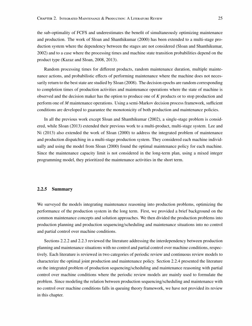
Chapter 2. IntegratedMaintenance & Production: A Literature Review 25
the sub-optimality of FCFS and underestimates the benefit of simultaneously optimizing maintenance
and production. The work of Sloan and Shanthikumar (2000) has been extended to a multi-stage pro-
duction system where the dependency between the stages are not considered (Sloan and Shanthikumar,
2002) and to a case where the processing times and machine state transition probabilities depend on the
product type (Kazaz and Sloan, 2008, 2013).
Random processing times for different products, random maintenance duration, multiple mainte-
nance actions, and probabilistic effects of performing maintenance where the machine does not neces-
sarily return to the best state are studied by Sloan (2008). The decision epochs are random corresponding
to completion times of production activities and maintenance operations where the state of machine is
observed and the decision maker has the option to produce one of K products or to stop production and
perform one of M maintenance operations. Using a semi-Markov decision process framework, sufficient
conditions are developed to guarantee the monotonicity of both production and maintenance policies.
In all the previous work except Sloan and Shanthikumar (2002), a single-stage problem is consid-
ered, while Sloan (2013) extended their previous work to a multi-product, multi-stage system. Lee and
Ni (2013) also extended the work of Sloan (2000) to address the integrated problem of maintenance
and production dispatching in a multi-stage production system. They considered each machine individ-
ually and using the model from Sloan (2000) found the optimal maintenance policy for each machine.
Since the maintenance capacity limit is not considered in the long-term plan, using a mixed integer
programming model, they prioritized the maintenance activities in the short term.
2.2.5 Summary
We surveyed the models integrating maintenance reasoning into production problems, optimizing the
performance of the production system in the long term. First, we provided a brief background on the
common maintenance concepts and solution approaches. We then divided the production problems into
production planning and production sequencing/scheduling and maintenance situations into no control
and partial control over machine conditions.
Sections 2.2.2 and 2.2.3 reviewed the literature addressing the interdependency between production
planning and maintenance situations with no control and partial control over machine conditions, respec-
tively. Each literature is reviewed in two categories of periodic review and continuous review models to
characterize the optimal joint production and maintenance policy. Section 2.2.4 presented the literature
on the integrated problem of production sequencing/scheduling and maintenance reasoning with partial
control over machine conditions where the periodic review models are mainly used to formulate the
problem. Since modeling the relation between production sequencing/scheduling and maintenance with
no control over machine conditions falls in queuing theory framework, we have not provided its review
in this chapter.
Chapter 2. IntegratedMaintenance & Production: A Literature Review 26
2.3 Short-term Perspective
Taking an operational view, after the production quantities and the preventive maintenance activities
are determined, one of the main short-term goals of the production process is to optimize the time and
sequence of maintenance and production operations. Because of the preventive maintenance activities
and unexpected breakdowns, the resources are not available all the times. Therefore, the main challenge
is to allocate the right resource to the right operation, either maintenance or production, such that the
products are ready at the right time or completed as soon as possible. The scheduling literature is the
area that deals with this challenge.
In this section, we first provide the necessary background on scheduling problems, particularly on
their solution approaches. We then review the literature addressing the relationship between mainte-
nance and production where the short-term performance measures are to be optimized. Recall that
in our classification scheme, we have considered two different production problems, planning and se-
quencing/scheduling, and two maintenance situations, no control and partial control over machine con-
ditions. Four different problems can be defined in different intersections of production and maintenance
problems. However, since production planning is not a short-term decision, we review the literature
addressing the integrated problem of production sequencing/scheduling with two different maintenance
situations of no control and partial control over machine conditions. As shown in Figure 2.3 which is
repeated from Section 2.1, there are two separate literatures studying the former relationship and one
dealing with the latter interdependency.
Partial control over
machine conditions
(Maintenance)
No control over
machine conditions
(No-maintenance)
Production
Planning
Production
Sequencing/Scheduling
Production
Problems
Sequencing /Scheduling
with Availability
Constraints
Maintenance
Situations
Stochastic
Sequencing /Scheduling;
Dynamic
Sequencing /Scheduling
Figure 2.3: Different literature on addressing the relation between maintenance and production taking ashort-term perspective.
2.3.1 Scheduling Fundamentals
Scheduling is the allocation of the available resources (machines) to competing tasks (jobs) over time
with the goal of optimizing one or a set of predetermined objectives such as finishing all the jobs as early
as possible or finishing as many jobs as possible within a given interval (Pinedo, 2002). Depending on
the application, the machines and the jobs can refer to different things. In this dissertation, in Chapter
4 where a problem is studied in a military application, the aircraft and the flights correspond to the
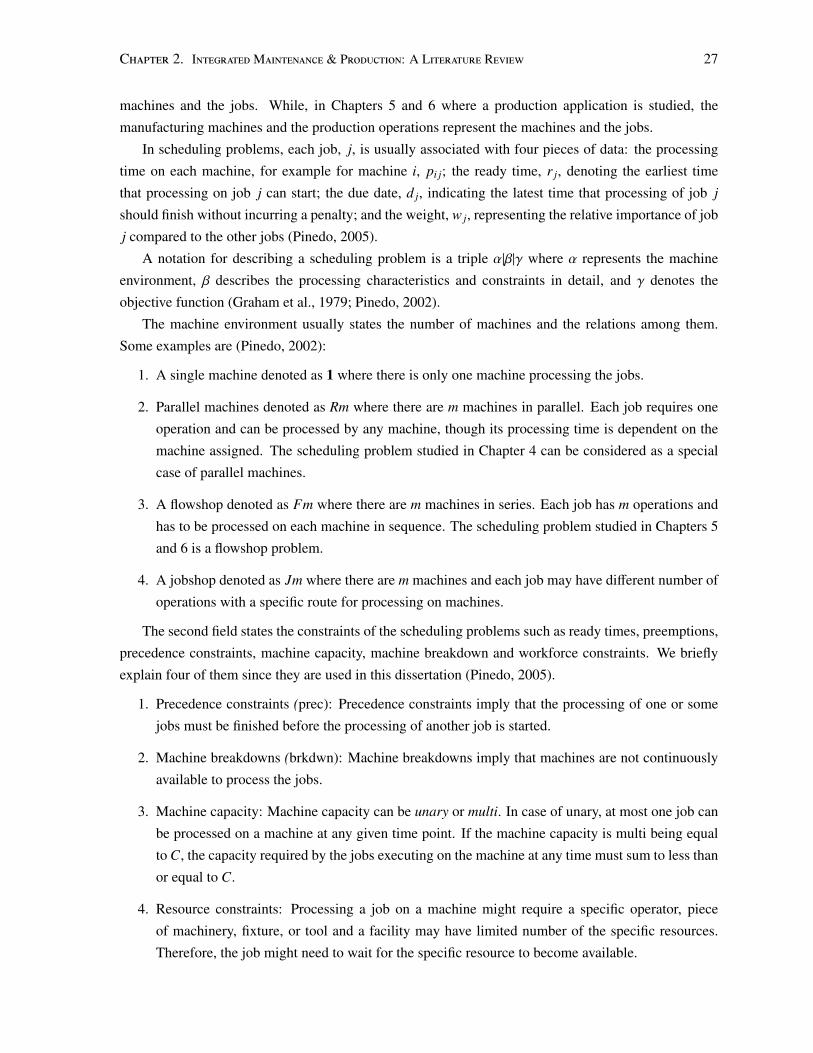
Chapter 2. IntegratedMaintenance & Production: A Literature Review 27
machines and the jobs. While, in Chapters 5 and 6 where a production application is studied, the
manufacturing machines and the production operations represent the machines and the jobs.
In scheduling problems, each job, j, is usually associated with four pieces of data: the processing
time on each machine, for example for machine i, pi j; the ready time, r j, denoting the earliest time
that processing on job j can start; the due date, d j, indicating the latest time that processing of job j
should finish without incurring a penalty; and the weight, w j, representing the relative importance of job
j compared to the other jobs (Pinedo, 2005).
A notation for describing a scheduling problem is a triple α|β|γ where α represents the machine
environment, β describes the processing characteristics and constraints in detail, and γ denotes the
objective function (Graham et al., 1979; Pinedo, 2002).
The machine environment usually states the number of machines and the relations among them.
Some examples are (Pinedo, 2002):
1. A single machine denoted as 1 where there is only one machine processing the jobs.
2. Parallel machines denoted as Rm where there are m machines in parallel. Each job requires one
operation and can be processed by any machine, though its processing time is dependent on the
machine assigned. The scheduling problem studied in Chapter 4 can be considered as a special
case of parallel machines.
3. A flowshop denoted as Fm where there are m machines in series. Each job has m operations and
has to be processed on each machine in sequence. The scheduling problem studied in Chapters 5
and 6 is a flowshop problem.
4. A jobshop denoted as Jm where there are m machines and each job may have different number of
operations with a specific route for processing on machines.
The second field states the constraints of the scheduling problems such as ready times, preemptions,
precedence constraints, machine capacity, machine breakdown and workforce constraints. We briefly
explain four of them since they are used in this dissertation (Pinedo, 2005).
1. Precedence constraints (prec): Precedence constraints imply that the processing of one or some
jobs must be finished before the processing of another job is started.
2. Machine breakdowns (brkdwn): Machine breakdowns imply that machines are not continuously
available to process the jobs.
3. Machine capacity: Machine capacity can be unary or multi. In case of unary, at most one job can
be processed on a machine at any given time point. If the machine capacity is multi being equal
to C, the capacity required by the jobs executing on the machine at any time must sum to less than
or equal to C.
4. Resource constraints: Processing a job on a machine might require a specific operator, piece
of machinery, fixture, or tool and a facility may have limited number of the specific resources.
Therefore, the job might need to wait for the specific resource to become available.
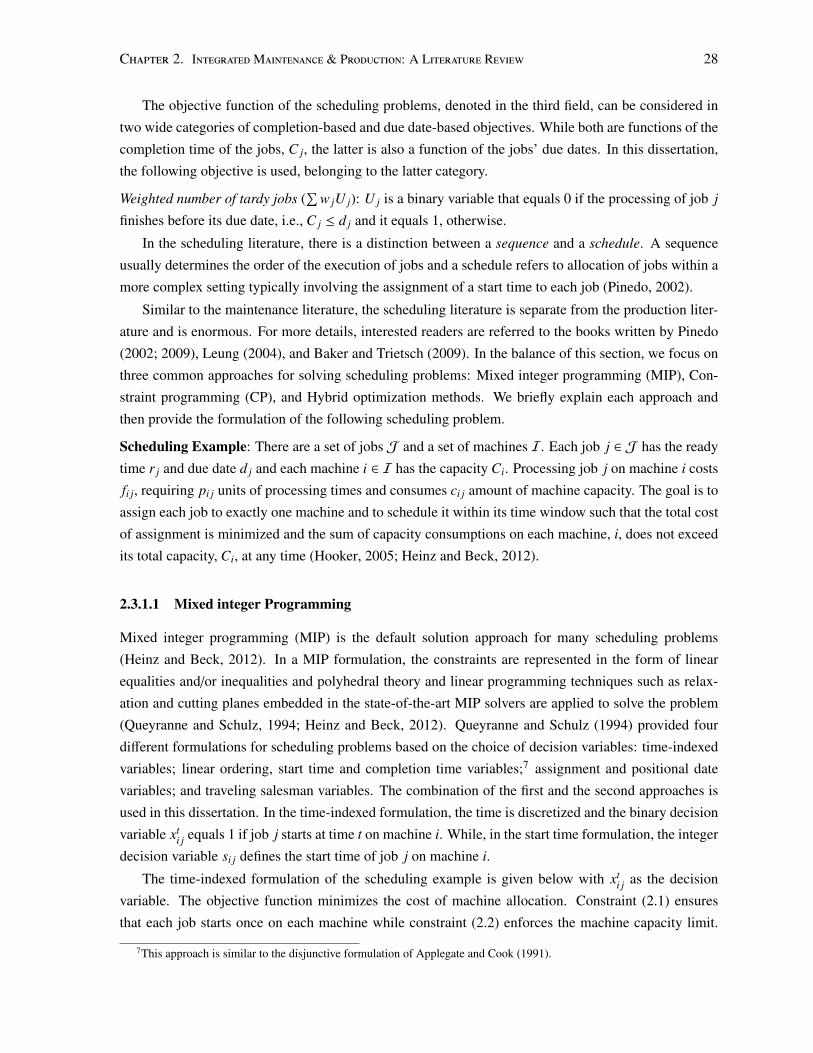
Chapter 2. IntegratedMaintenance & Production: A Literature Review 28
The objective function of the scheduling problems, denoted in the third field, can be considered in
two wide categories of completion-based and due date-based objectives. While both are functions of the
completion time of the jobs, C j, the latter is also a function of the jobs’ due dates. In this dissertation,
the following objective is used, belonging to the latter category.
Weighted number of tardy jobs (∑
w jU j): U j is a binary variable that equals 0 if the processing of job j
finishes before its due date, i.e., C j ≤ d j and it equals 1, otherwise.
In the scheduling literature, there is a distinction between a sequence and a schedule. A sequence
usually determines the order of the execution of jobs and a schedule refers to allocation of jobs within a
more complex setting typically involving the assignment of a start time to each job (Pinedo, 2002).
Similar to the maintenance literature, the scheduling literature is separate from the production liter-
ature and is enormous. For more details, interested readers are referred to the books written by Pinedo
(2002; 2009), Leung (2004), and Baker and Trietsch (2009). In the balance of this section, we focus on
three common approaches for solving scheduling problems: Mixed integer programming (MIP), Con-
straint programming (CP), and Hybrid optimization methods. We briefly explain each approach and
then provide the formulation of the following scheduling problem.
Scheduling Example: There are a set of jobs J and a set of machines I. Each job j ∈ J has the ready
time r j and due date d j and each machine i ∈ I has the capacity Ci. Processing job j on machine i costs
fi j, requiring pi j units of processing times and consumes ci j amount of machine capacity. The goal is to
assign each job to exactly one machine and to schedule it within its time window such that the total cost
of assignment is minimized and the sum of capacity consumptions on each machine, i, does not exceed
its total capacity, Ci, at any time (Hooker, 2005; Heinz and Beck, 2012).
2.3.1.1 Mixed integer Programming
Mixed integer programming (MIP) is the default solution approach for many scheduling problems
(Heinz and Beck, 2012). In a MIP formulation, the constraints are represented in the form of linear
equalities and/or inequalities and polyhedral theory and linear programming techniques such as relax-
ation and cutting planes embedded in the state-of-the-art MIP solvers are applied to solve the problem
(Queyranne and Schulz, 1994; Heinz and Beck, 2012). Queyranne and Schulz (1994) provided four
different formulations for scheduling problems based on the choice of decision variables: time-indexed
variables; linear ordering, start time and completion time variables;7 assignment and positional date
variables; and traveling salesman variables. The combination of the first and the second approaches is
used in this dissertation. In the time-indexed formulation, the time is discretized and the binary decision
variable xti j equals 1 if job j starts at time t on machine i. While, in the start time formulation, the integer
decision variable si j defines the start time of job j on machine i.
The time-indexed formulation of the scheduling example is given below with xti j as the decision
variable. The objective function minimizes the cost of machine allocation. Constraint (2.1) ensures
that each job starts once on each machine while constraint (2.2) enforces the machine capacity limit.
7This approach is similar to the disjunctive formulation of Applegate and Cook (1991).
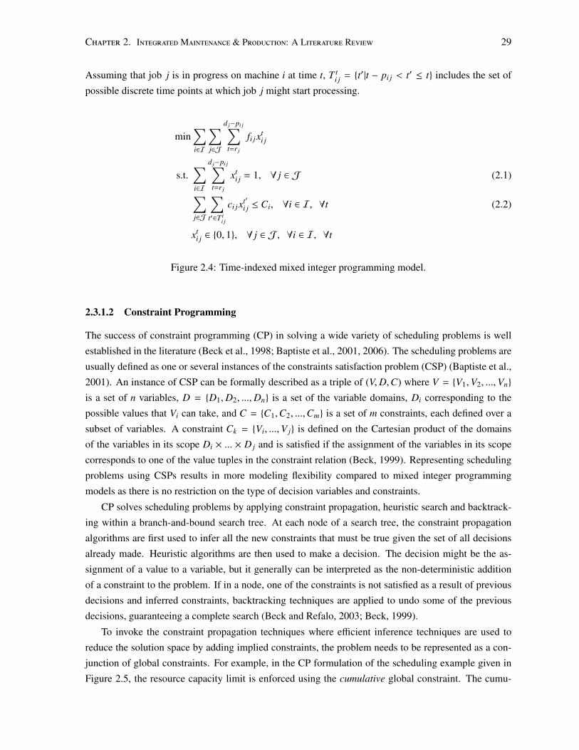
Chapter 2. IntegratedMaintenance & Production: A Literature Review 29
Assuming that job j is in progress on machine i at time t, T ti j = {t′|t − pi j < t′ ≤ t} includes the set of
possible discrete time points at which job j might start processing.
min∑i∈I
∑j∈J
d j−pi j∑t=r j
fi jxti j
s.t.∑i∈I
d j−pi j∑t=r j
xti j = 1, ∀ j ∈ J (2.1)∑
j∈J
∑t′∈T t
i j
ci jxt′i j ≤ Ci, ∀i ∈ I, ∀t (2.2)
xti j ∈ {0, 1}, ∀ j ∈ J , ∀i ∈ I, ∀t
Figure 2.4: Time-indexed mixed integer programming model.
2.3.1.2 Constraint Programming
The success of constraint programming (CP) in solving a wide variety of scheduling problems is well
established in the literature (Beck et al., 1998; Baptiste et al., 2001, 2006). The scheduling problems are
usually defined as one or several instances of the constraints satisfaction problem (CSP) (Baptiste et al.,
2001). An instance of CSP can be formally described as a triple of (V,D,C) where V = {V1,V2, ...,Vn}
is a set of n variables, D = {D1,D2, ...,Dn} is a set of the variable domains, Di corresponding to the
possible values that Vi can take, and C = {C1,C2, ...,Cm} is a set of m constraints, each defined over a
subset of variables. A constraint Ck = {Vi, ...,V j} is defined on the Cartesian product of the domains
of the variables in its scope Di × ... × D j and is satisfied if the assignment of the variables in its scope
corresponds to one of the value tuples in the constraint relation (Beck, 1999). Representing scheduling
problems using CSPs results in more modeling flexibility compared to mixed integer programming
models as there is no restriction on the type of decision variables and constraints.
CP solves scheduling problems by applying constraint propagation, heuristic search and backtrack-
ing within a branch-and-bound search tree. At each node of a search tree, the constraint propagation
algorithms are first used to infer all the new constraints that must be true given the set of all decisions
already made. Heuristic algorithms are then used to make a decision. The decision might be the as-
signment of a value to a variable, but it generally can be interpreted as the non-deterministic addition
of a constraint to the problem. If in a node, one of the constraints is not satisfied as a result of previous
decisions and inferred constraints, backtracking techniques are applied to undo some of the previous
decisions, guaranteeing a complete search (Beck and Refalo, 2003; Beck, 1999).
To invoke the constraint propagation techniques where efficient inference techniques are used to
reduce the solution space by adding implied constraints, the problem needs to be represented as a con-
junction of global constraints. For example, in the CP formulation of the scheduling example given in
Figure 2.5, the resource capacity limit is enforced using the cumulative global constraint. The cumu-
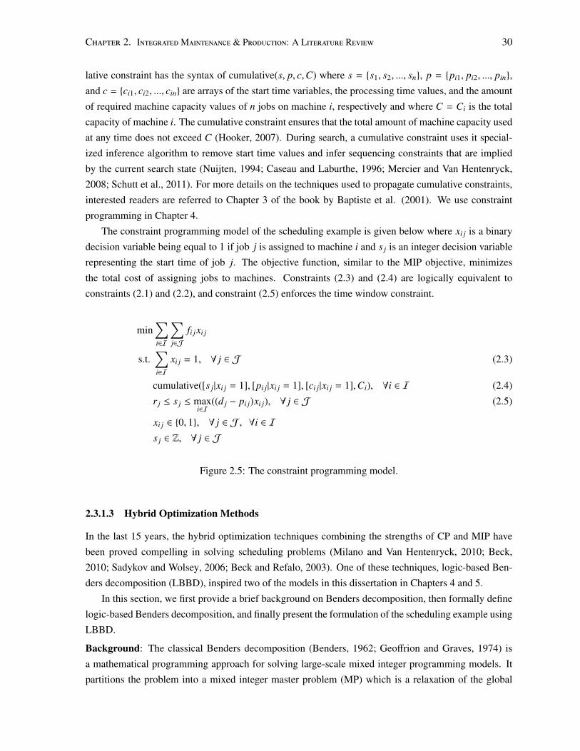
Chapter 2. IntegratedMaintenance & Production: A Literature Review 30
lative constraint has the syntax of cumulative(s, p, c,C) where s = {s1, s2, ..., sn}, p = {pi1, pi2, ..., pin},
and c = {ci1, ci2, ..., cin} are arrays of the start time variables, the processing time values, and the amount
of required machine capacity values of n jobs on machine i, respectively and where C = Ci is the total
capacity of machine i. The cumulative constraint ensures that the total amount of machine capacity used
at any time does not exceed C (Hooker, 2007). During search, a cumulative constraint uses it special-
ized inference algorithm to remove start time values and infer sequencing constraints that are implied
by the current search state (Nuijten, 1994; Caseau and Laburthe, 1996; Mercier and Van Hentenryck,
2008; Schutt et al., 2011). For more details on the techniques used to propagate cumulative constraints,
interested readers are referred to Chapter 3 of the book by Baptiste et al. (2001). We use constraint
programming in Chapter 4.
The constraint programming model of the scheduling example is given below where xi j is a binary
decision variable being equal to 1 if job j is assigned to machine i and s j is an integer decision variable
representing the start time of job j. The objective function, similar to the MIP objective, minimizes
the total cost of assigning jobs to machines. Constraints (2.3) and (2.4) are logically equivalent to
constraints (2.1) and (2.2), and constraint (2.5) enforces the time window constraint.
min∑i∈I
∑j∈J
fi jxi j
s.t.∑i∈I
xi j = 1, ∀ j ∈ J (2.3)
cumulative([s j|xi j = 1], [pi j|xi j = 1], [ci j|xi j = 1],Ci), ∀i ∈ I (2.4)
r j ≤ s j ≤ maxi∈I
((d j − pi j)xi j), ∀ j ∈ J (2.5)
xi j ∈ {0, 1}, ∀ j ∈ J , ∀i ∈ I
s j ∈ Z, ∀ j ∈ J
Figure 2.5: The constraint programming model.
2.3.1.3 Hybrid Optimization Methods
In the last 15 years, the hybrid optimization techniques combining the strengths of CP and MIP have
been proved compelling in solving scheduling problems (Milano and Van Hentenryck, 2010; Beck,
2010; Sadykov and Wolsey, 2006; Beck and Refalo, 2003). One of these techniques, logic-based Ben-
ders decomposition (LBBD), inspired two of the models in this dissertation in Chapters 4 and 5.
In this section, we first provide a brief background on Benders decomposition, then formally define
logic-based Benders decomposition, and finally present the formulation of the scheduling example using
LBBD.
Background: The classical Benders decomposition (Benders, 1962; Geoffrion and Graves, 1974) is
a mathematical programming approach for solving large-scale mixed integer programming models. It
partitions the problem into a mixed integer master problem (MP) which is a relaxation of the global
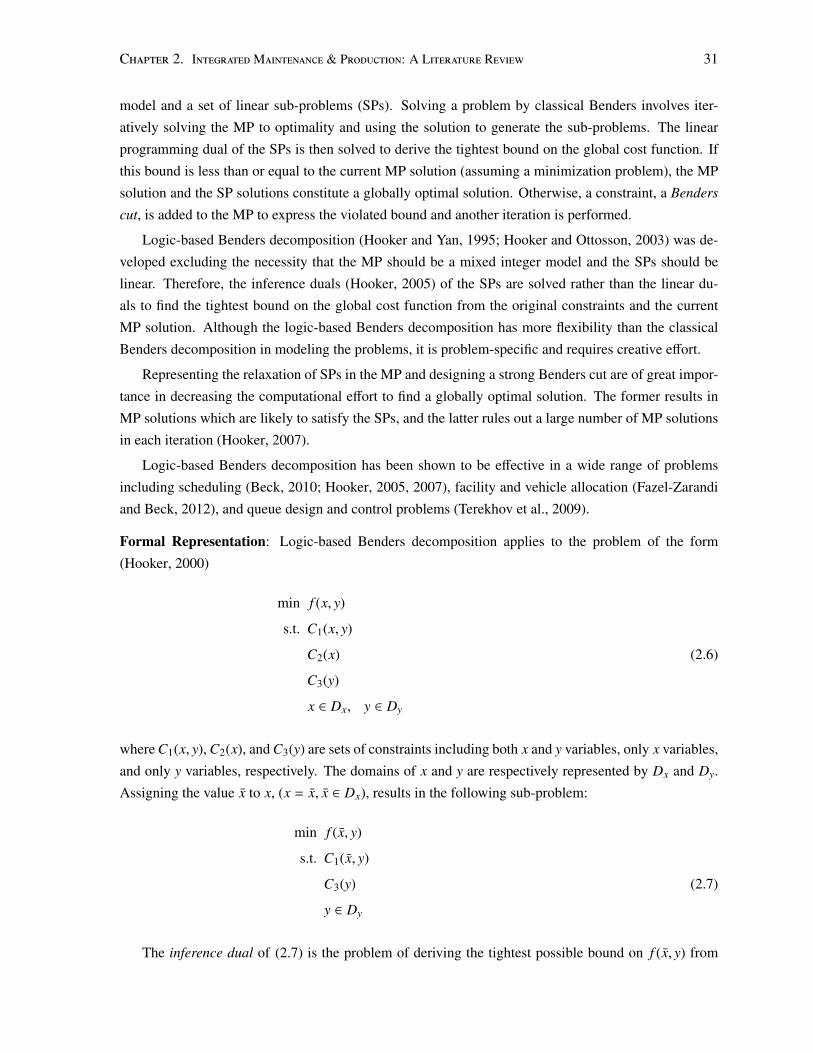
Chapter 2. IntegratedMaintenance & Production: A Literature Review 31
model and a set of linear sub-problems (SPs). Solving a problem by classical Benders involves iter-
atively solving the MP to optimality and using the solution to generate the sub-problems. The linear
programming dual of the SPs is then solved to derive the tightest bound on the global cost function. If
this bound is less than or equal to the current MP solution (assuming a minimization problem), the MP
solution and the SP solutions constitute a globally optimal solution. Otherwise, a constraint, a Benders
cut, is added to the MP to express the violated bound and another iteration is performed.
Logic-based Benders decomposition (Hooker and Yan, 1995; Hooker and Ottosson, 2003) was de-
veloped excluding the necessity that the MP should be a mixed integer model and the SPs should be
linear. Therefore, the inference duals (Hooker, 2005) of the SPs are solved rather than the linear du-
als to find the tightest bound on the global cost function from the original constraints and the current
MP solution. Although the logic-based Benders decomposition has more flexibility than the classical
Benders decomposition in modeling the problems, it is problem-specific and requires creative effort.
Representing the relaxation of SPs in the MP and designing a strong Benders cut are of great impor-
tance in decreasing the computational effort to find a globally optimal solution. The former results in
MP solutions which are likely to satisfy the SPs, and the latter rules out a large number of MP solutions
in each iteration (Hooker, 2007).
Logic-based Benders decomposition has been shown to be effective in a wide range of problems
including scheduling (Beck, 2010; Hooker, 2005, 2007), facility and vehicle allocation (Fazel-Zarandi
and Beck, 2012), and queue design and control problems (Terekhov et al., 2009).
Formal Representation: Logic-based Benders decomposition applies to the problem of the form
(Hooker, 2000)
min f (x, y)
s.t. C1(x, y)
C2(x) (2.6)
C3(y)
x ∈ Dx, y ∈ Dy
where C1(x, y), C2(x), and C3(y) are sets of constraints including both x and y variables, only x variables,
and only y variables, respectively. The domains of x and y are respectively represented by Dx and Dy.
Assigning the value x to x, (x = x, x ∈ Dx), results in the following sub-problem:
min f (x, y)
s.t. C1(x, y)
C3(y) (2.7)
y ∈ Dy
The inference dual of (2.7) is the problem of deriving the tightest possible bound on f (x, y) from
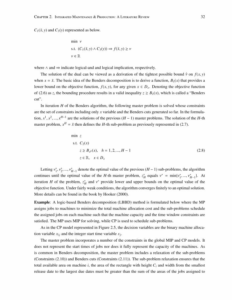
Chapter 2. IntegratedMaintenance & Production: A Literature Review 32
C1(x, y) and C3(y) represented as below.
min ν
s.t. (C1(x, y) ∧C3(y))⇒ f (x, y) ≥ ν
ν ∈ R
where ∧ and⇒ indicate logical-and and logical implication, respectively.
The solution of the dual can be viewed as a derivation of the tightest possible bound ν on f (x, y)
when x = x. The basic idea of the Benders decomposition is to derive a function, Bx(x) that provides a
lower bound on the objective function, f (x, y), for any given x ∈ Dx. Denoting the objective function
of (2.6) as z, the bounding procedure results in a valid inequality z ≥ Bx(x), which is called a “Benders
cut”.
In iteration H of the Benders algorithm, the following master problem is solved whose constraints
are the set of constraints including only x variable and the Benders cuts generated so far. In the formula-
tion, x1, x2, ..., xH−1 are the solutions of the previous (H − 1) master problems. The solution of the H-th
master problem, xH = x then defines the H-th sub-problem as previously represented in (2.7).
min z
s.t. C2(x)
z ≥ Bxh(x), h = 1, 2, ...,H − 1 (2.8)
z ∈ R, x ∈ Dx
Letting ν∗1, ν∗2, ..., ν
∗H−1 denote the optimal value of the previous (H − 1) sub-problems, the algorithm
continues until the optimal value of the H-th master problem, z∗H equals ν∗ = min{ν∗1, ..., ν∗H−1}. At
iteration H of the problem, z∗H and ν∗ provide lower and upper bounds on the optimal value of the
objective function. Under fairly weak conditions, the algorithm converges finitely to an optimal solution.
More details can be found in the book by Hooker (2000).
Example: A logic-based Benders decomposition (LBBD) method is formulated below where the MP
assigns jobs to machines to minimize the total machine allocation cost and the sub-problems schedule
the assigned jobs on each machine such that the machine capacity and the time window constraints are
satisfied. The MP uses MIP for solving, while CP is used to schedule sub-problems.
As in the CP model represented in Figure 2.5, the decision variables are the binary machine alloca-
tion variable xi j and the integer start time variable s j.
The master problem incorporates a number of the constraints in the global MIP and CP models. It
does not represent the start times of jobs nor does it fully represent the capacity of the machines. As
is common in Benders decomposition, the master problem includes a relaxation of the sub-problems
(Constraints (2.10)) and Benders cuts (Constraints (2.11)). The sub-problem relaxation ensures that the
total available area on machine i, the area of the rectangle with height Ci and width from the smallest
release date to the largest due dates must be greater than the sum of the areas of the jobs assigned to
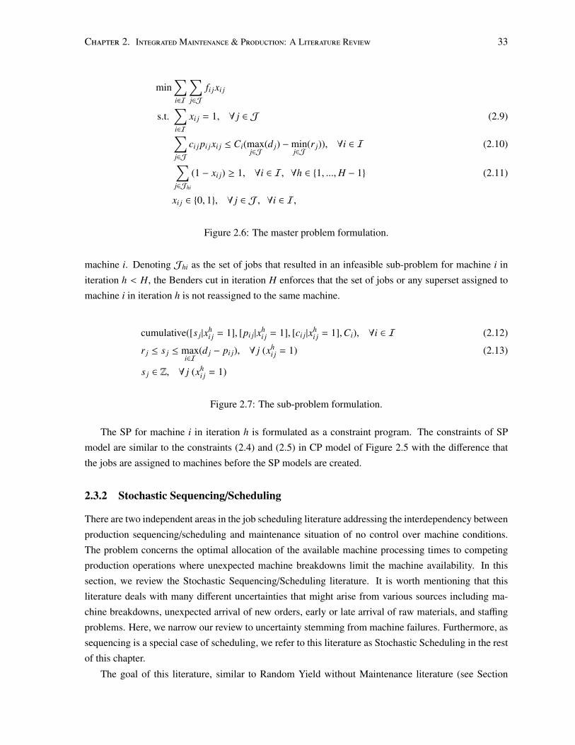
Chapter 2. IntegratedMaintenance & Production: A Literature Review 33
min∑i∈I
∑j∈J
fi jxi j
s.t.∑i∈I
xi j = 1, ∀ j ∈ J (2.9)∑j∈J
ci j pi jxi j ≤ Ci(maxj∈J
(d j) −minj∈J
(r j)), ∀i ∈ I (2.10)∑j∈Jhi
(1 − xi j) ≥ 1, ∀i ∈ I, ∀h ∈ {1, ...,H − 1} (2.11)
xi j ∈ {0, 1}, ∀ j ∈ J , ∀i ∈ I,
Figure 2.6: The master problem formulation.
machine i. Denoting Jhi as the set of jobs that resulted in an infeasible sub-problem for machine i in
iteration h < H, the Benders cut in iteration H enforces that the set of jobs or any superset assigned to
machine i in iteration h is not reassigned to the same machine.
cumulative([s j|xhi j = 1], [pi j|xh
i j = 1], [ci j|xhi j = 1],Ci), ∀i ∈ I (2.12)
r j ≤ s j ≤ maxi∈I
(d j − pi j), ∀ j (xhi j = 1) (2.13)
s j ∈ Z, ∀ j (xhi j = 1)
Figure 2.7: The sub-problem formulation.
The SP for machine i in iteration h is formulated as a constraint program. The constraints of SP
model are similar to the constraints (2.4) and (2.5) in CP model of Figure 2.5 with the difference that
the jobs are assigned to machines before the SP models are created.
2.3.2 Stochastic Sequencing/Scheduling
There are two independent areas in the job scheduling literature addressing the interdependency between
production sequencing/scheduling and maintenance situation of no control over machine conditions.
The problem concerns the optimal allocation of the available machine processing times to competing
production operations where unexpected machine breakdowns limit the machine availability. In this
section, we review the Stochastic Sequencing/Scheduling literature. It is worth mentioning that this
literature deals with many different uncertainties that might arise from various sources including ma-
chine breakdowns, unexpected arrival of new orders, early or late arrival of raw materials, and staffing
problems. Here, we narrow our review to uncertainty stemming from machine failures. Furthermore, as
sequencing is a special case of scheduling, we refer to this literature as Stochastic Scheduling in the rest
of this chapter.
The goal of this literature, similar to Random Yield without Maintenance literature (see Section
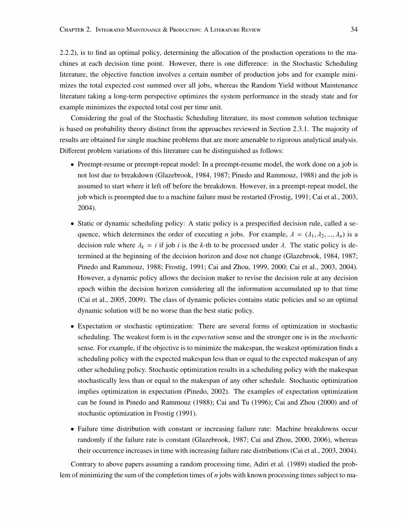
Chapter 2. IntegratedMaintenance & Production: A Literature Review 34
2.2.2), is to find an optimal policy, determining the allocation of the production operations to the ma-
chines at each decision time point. However, there is one difference: in the Stochastic Scheduling
literature, the objective function involves a certain number of production jobs and for example mini-
mizes the total expected cost summed over all jobs, whereas the Random Yield without Maintenance
literature taking a long-term perspective optimizes the system performance in the steady state and for
example minimizes the expected total cost per time unit.
Considering the goal of the Stochastic Scheduling literature, its most common solution technique
is based on probability theory distinct from the approaches reviewed in Section 2.3.1. The majority of
results are obtained for single machine problems that are more amenable to rigorous analytical analysis.
Different problem variations of this literature can be distinguished as follows:
• Preempt-resume or preempt-repeat model: In a preempt-resume model, the work done on a job is
not lost due to breakdown (Glazebrook, 1984, 1987; Pinedo and Rammouz, 1988) and the job is
assumed to start where it left off before the breakdown. However, in a preempt-repeat model, the
job which is preempted due to a machine failure must be restarted (Frostig, 1991; Cai et al., 2003,
2004).
• Static or dynamic scheduling policy: A static policy is a prespecified decision rule, called a se-
quence, which determines the order of executing n jobs. For example, λ = (λ1, λ2, ..., λn) is a
decision rule where λk = i if job i is the k-th to be processed under λ. The static policy is de-
termined at the beginning of the decision horizon and dose not change (Glazebrook, 1984, 1987;
Pinedo and Rammouz, 1988; Frostig, 1991; Cai and Zhou, 1999, 2000; Cai et al., 2003, 2004).
However, a dynamic policy allows the decision maker to revise the decision rule at any decision
epoch within the decision horizon considering all the information accumulated up to that time
(Cai et al., 2005, 2009). The class of dynamic policies contains static policies and so an optimal
dynamic solution will be no worse than the best static policy.
• Expectation or stochastic optimization: There are several forms of optimization in stochastic
scheduling. The weakest form is in the expectation sense and the stronger one is in the stochastic
sense. For example, if the objective is to minimize the makespan, the weakest optimization finds a
scheduling policy with the expected makespan less than or equal to the expected makespan of any
other scheduling policy. Stochastic optimization results in a scheduling policy with the makespan
stochastically less than or equal to the makespan of any other schedule. Stochastic optimization
implies optimization in expectation (Pinedo, 2002). The examples of expectation optimization
can be found in Pinedo and Rammouz (1988); Cai and Tu (1996); Cai and Zhou (2000) and of
stochastic optimization in Frostig (1991).
• Failure time distribution with constant or increasing failure rate: Machine breakdowns occur
randomly if the failure rate is constant (Glazebrook, 1987; Cai and Zhou, 2000, 2006), whereas
their occurrence increases in time with increasing failure rate distributions (Cai et al., 2003, 2004).
Contrary to above papers assuming a random processing time, Adiri et al. (1989) studied the prob-
lem of minimizing the sum of the completion times of n jobs with known processing times subject to ma-
Chapter 2. IntegratedMaintenance & Production: A Literature Review 35
chine breakdown. Assuming known processing times adds to the combinatorial part of the problem and
consequently obtaining general results is challenging. Considering a single breakdown, i.e., machine
breakdown occurs only once during the processing of all n jobs and assuming the preempt-repeat model,
they showed: (1) the Shortest Processing Time (SPT) dispatching rule stochastically minimizes the sum
of completion times if the failure time distribution is concave.8 SPT is the most famous dispatching rule
in the scheduling literature which processes the jobs in non-decreasing order of their processing times.
It is known that SPT minimizes the sum of job completion times in a single machine problem with no
breakdown if all jobs are ready at time 0 (Pinedo, 2002), (2) the problem of deciding whether there is a
schedule with sum of completion times less than a given value is NP-complete assuming that the time
of single breakdown is known, and (3) the maximum relative error of the SPT dispatching policy for
the problem with the deterministic single breakdown is 25% from the optimal scheduling policy. Adiri
et al. (1991) then extended their results to the problem with the objective of stochastically minimiz-
ing the number of tardy jobs. Under certain conditions on processing times and due dates, the optimal
scheduling policies are derived for both the preempt-repeat and the preempt-resume models.
Birge et al. (1990) also assumed known processing times and focused on deriving a bound on the
difference between the performance of the optimal static policy and the Weighted Shortest Processing
Time (WSPT)9 dispatching rule assuming both the preempt-resume and the preempt-repeat models.
Although the majority of the Stochastic Scheduling literature is devoted to single machine problems,
Allahverdi and Mittenthal (1995) studied the problem of stochastically minimizing makespan in a two-
machine flowshop assuming unexpected machine breakdowns and the preempt-resume model. They
first showed that the optimal scheduling policy is a permutation schedule, i.e., the sequence of the jobs
is the same on both machines, as in the deterministic counterpart. Second, they characterized specific
conditions on the breakdown process for which Johnson’s algorithm10 stochastically minimizes the
makespan as in the deterministic problem. Allahverdi and Mittenthal (1994) studied the problem of
stochastically minimizing the makespan and minimizing the expected sum of the completion times in a
sub-category of the flowshop problems, i.e., a two-machine ordered11 flowshop problem. Three other
papers of Allahverdi (1995; 1996; 1997) studied different two-machine stochastic flowshop problems,
focusing on deriving sufficient conditions that guarantee the optimality of specific scheduling policies.
2.3.3 Dynamic Sequencing/Scheduling
Dynamic Scheduling12 is a methodology developed in the scheduling literature to find the allocation
of operations to machines where operational uncertainties like machine breakdowns or the unexpected
arrival of new orders prevent the execution of the schedule as planned (Aytug et al., 2005; O’Donovan
et al., 1999).8A concave failure time distribution includes distributions with decreasing and constant failure rates (Adiri et al., 1989).9The Weighted Shortest Processing Time (WSPT) dispatching rule minimizes the sum of the weighted completion times
in a deterministic single machine problem by processing the jobs in non-decreasing order of p jw j
ratio (Pinedo, 2002).10For the description of Johnson’s rule, readers are referred to Chapter 6 of Pinedo’s book (Pinedo, 2002).11For the definition of an ordered flowshop problem, interested readers are referred to the paper by Allahverdi and Mittenthal
(1994).12Since scheduling includes sequencing, we refer to Dynamic Sequencing/Scheduling as Dynamic Scheduling.
Chapter 2. IntegratedMaintenance & Production: A Literature Review 36
At the highest level, Dynamic Scheduling is based on the combination of reactive and predictive
generation of a schedule. In reactive scheduling, all decisions are usually made without anticipation and
online, while in predictive scheduling, decisions are made offline. For the surveys of the literature, see
the work of Bidot et al. (2009), Thomas and Szczerbicka (2007), Herroelen and Leus (2005), Aytug et
al. (2005), and Davenport and Beck (2000).
In a completely reactive approach, all decision are made in the real time usually using one of the
following techniques:
• Dispatching rules: Dispatching rules usually make decisions based on a priority index calculated
from job and machine attributes (O’Donovan et al., 1999). Although priority dispatching rules
are the best solution approach for the dynamic problems in the presence of limited computational
power (Thomas and Szczerbicka, 2007) or quick and drastic changes in the problem parameters
(Branke and Mattfeld, 2005), they lack the ability to optimize a global objective function (Branke
and Mattfeld, 2005) or to plan into future (Thomas and Szczerbicka, 2007). Discussions on
dispatching rules and their applicability for various uncertainty situations can be found in papers
by Panwalkar and Iskander (1977), Haupt (1989), and Morton and Pentico (1993).
• Online stochastic optimization: The online stochastic optimization (OSCO) (Van Hentenryck and
Bent, 2006) framework combines the online algorithms and stochastic programming. OSCO
makes decisions one at a time by first sampling the distribution of future events and then solving
deterministic problems, each representing a possible realization of the uncertain future.
In a completely predictive approach, the known statistics on uncertainty are usually used to make
offline decisions. Two techniques of this category are:
• Redundancy-based techniques: The main characteristic of redundancy-based techniques is the
allocation of extra time and/or resources so that the unexpected events during execution can be
dealt with using some of this reserved time and resources (Davenport and Beck, 2000; Beck and
Wilson, 2007). Several examples of this approach are: inserting idle time into the schedule to
cope with machine disruptions where the idle time is calculated based on the failure rate and
the expected repair time (Mehta and Uzsoy, 1998, 1999; O’Donovan et al., 1999); extending the
duration of the critical jobs considering the expected up-time and the expected repair time (Gao,
1995); forcing any solution to respect constraints on the slack13 of the jobs (Davenport et al.,
2001); and modifying the objective function to be a linear combination of the expected makespan
and expected delay (Leon et al., 1994).
• Probabilistic techniques: Probabilistic techniques, similar to approaches in Stochastic Scheduling
literature (see Section 2.3.2), use representations of uncertainty to reason about the possible out-
comes when the schedule is executed (Beck and Wilson, 2007). The work of Leon et al. (1994) is
an example of this technique where the jobshop scheduling problem in the presence of machine
13The slack of a job is the time that it can be delayed without breaking any constraints and increasing the cost of theschedule.
Chapter 2. IntegratedMaintenance & Production: A Literature Review 37
disruption is represented as a discrete stochastic control problem and a game-theoretic approach
minimizing the expected makespan and deviations from an offline schedule is developed to solve
the problem.
Predictive-reactive approaches are based on the idea of rolling horizon where the predictive com-
ponent generates a schedule in advance over a short time period considering the known information
about uncertainty, for example, the distributions of failure and repair times. The constructed schedule is
then executed and whenever disruptions occur, the reactive component modifies the schedule to either
permit the execution or to improve the quality of the schedule considering the observed information.
The dynamic problem is viewed as a collection of linked static sub-problems where the myriad of algo-
rithms developed for the static scheduling problems (see Section 2.3.1) are applicable in the predictive
phase. Connecting the static sub-problems using rescheduling strategies is done in the reactive phase
where the previous schedule is modified. The rescheduling might be as simple as the Right Shift rule
or might construct a new schedule for all the activities that have not yet executed. Some examples of
rescheduling strategies are: Sadeh et al. (1993) where a set of control rules such as WSPT and Apparent
Tardiness Cost (ATC) are used either to choose the next job to schedule or to identify the set of jobs
which need to be fully rescheduled; El Sakkout and Wallace (2000) where a full rescheduling of the jobs
is performed such that the absolute difference between the start times of the jobs in the revised schedule
and the original start times is minimized; and Bean et al. (1991) and Akturk and Gorgulu (1999) where
the rescheduling is performed such that the revised schedule matches the original one after a certain
time. We use a predictive-reactive approach in Chapter 4 of this dissertation.
2.3.4 Sequencing/Scheduling with Availability Constraints
Addressing the problem of scheduling planned maintenance activities along with production jobs is the
concern of Sequencing/Scheduling with Availability Constraints literature.14 More specifically, there
are a number of maintenance activities that must be inserted into the schedule among the regular pro-
duction jobs such that a given operational performance measure is optimized. This problem has been
studied from two perspectives. The first deals only with the fact that a machine undergoing maintenance
is unavailable for production jobs (Schmidt, 2000; Lee, 2004; Ma et al., 2010). The second perspective
models different processing times for a production job depending on whether it is scheduled before or
after maintenance (Lee and Leon, 2001). Both perspectives typically focus on analyzing the computa-
tional complexity of the problems and/or deriving the properties of the optimal schedules. The derived
properties are used to develop polynomial time approximation algorithms or efficient heuristics, or are
modeled as constraints to reduce the computational effort.
The problem of the first category can be defined as follow. A set of jobsJ = {Ji|i = 1, ..., n} and a set
of machinesM = {M j| j = 1, ...,m} are given. Machine M j is not available for processing the jobs within
S j time intervals [Bsj, F
sj], s = 1, ..., S j where Bs
j and F sj denote the start time and the finish time of the
s-th unavailability interval (Ma et al., 2010). The goal of the problem is to pack the jobs into the gaps
14We refer to this literature as Scheduling with Availability Constraints literature.
Chapter 2. IntegratedMaintenance & Production: A Literature Review 38
created between unavailability intervals, optimizing an operational performance measure such as finish-
ing all the jobs as soon as possible. In different problem variations, jobs may be resumable (Lee, 1996),
non-resumable (Lee, 1996), and semi-resumable (i.e., the disrupted job has to partially re-start when
the machine becomes available again) (Lee, 1999). Furthermore, one or several unavailability intervals
(maintenance periods) might be considered where their start and end times are either known or decision
variables. A number of different combinations of the unavailability intervals and job characteristics have
been studied (Lee, 1996; Liao and Chen, 2003; Akturk et al., 2004; Chen, 2006; Ji et al., 2007; Kovacs
and Beck, 2007). While the majority of this literature deals with deterministic problems where limited
availabilities of machines only result from planned maintenance, Cassady and Kutanoglu (2003; 2005)
and Kuo and Chang (2007) studied a single machine scheduling problem assuming that the machine is
not continuously available due to both planned maintenance and random machine breakdowns.
The above scheduling problems have no correlation between machine conditions and processing
times, ignoring the practical relevance of maintenance on machine deterioration and restoration pro-
cesses (Kellerer et al., 2012; Rustogi and Strusevich, 2012). Lee and Leon (2001) were the first to
introduce such maintenance considerations into the scheduling literature, initiating the study of the sec-
ond category of problems. More specifically, the authors represented maintenance as a rate-modifying
activity that changes the processing times of production jobs scheduled after maintenance to λ j p j where
0 < λ j < 1 and p j represents the processing time of job j before maintenance. In the work of Lee and
Leon and many subsequent models (e.g., Mosheiov and Sarig (2009); Mosheiov and Sidney (2010))
only a single rate-modifying activity is considered and the processing time of a job does not depend
on its position in the schedule or its start time, only whether it comes before or after maintenance.
However, recent work has studied the problem of dividing the jobs into groups where the number of
groups indicates the number of maintenance activities and the processing time of each job depends both
on its assigned group and its position within the group (Kuo and Yang, 2008; Yang and Yang, 2010;
Lodree and D., 2010; Rustogi and Strusevich, 2012; Kellerer et al., 2012). The focus of this work is the
development of polynomial-time algorithms when the problem is limited to the single machine.
Some other works incorporating practical maintenance considerations in production scheduling
problems include: Kubzin and Strusevich (2006) where delaying the maintenance activity increases
the time needed to perform it; and Xu et al. (2008; 2010) where the concept of ε-almost periodic
maintenance is defined to account for non-periodic maintenance.
The review of this literature indicates there exists no work that reasons with an explicit represen-
tation of machine condition or the effect of machine deterioration and restoration on processing times.
Furthermore, unlike the broader maintenance literature (Dekker et al., 1996; Wang, 2002; Nicolai and
Dekker, 2008; Pintelon and Parodi-Herz, 2008), maintenance is considered as a short-term decision
when reasoning about it in combination with production scheduling. That is, the problem is defined
over a fixed horizon where maintenance and machine deterioration act on the same time scale as the
production jobs. In practice, a machine does not deteriorate as fast as the production jobs are processed
and so maintenance decisions are naturally made over longer time horizons than detailed scheduling de-
cisions (Cassady and Kutanoglu, 2005; Budai et al., 2006; Grigoriev et al., 2006; Aghezzaf and Najid,
Chapter 2. IntegratedMaintenance & Production: A Literature Review 39
2008). In Chapter of 5 and 6 of this dissertation, we extend this literature using techniques reviewed
in Section 2.2 to integrate maintenance planning with production and maintenance scheduling where
maintenance is considered as a long-term decision and where there is an explicit model representing
the deterioration processes of machines and their effects on the processing times. This perspective on
the problem takes into account common conceptualizations of maintenance as they appear in that area
of the research literature (McCall, 1965; Dekker et al., 1997; Wang, 2002; Pintelon and Parodi-Herz,
2008) and introduce them to the scheduling literature.
2.3.5 Summary
We reviewed the literature addressing the relationship between production problems and maintenance
situations with the goal of optimizing the operational and short-term objectives of the production pro-
cess. First, the common concepts and solution approaches of scheduling literature were reviewed. Then,
in Sections 2.3.2 and 2.3.3, two separate areas of Stochastic Sequencing/Scheduling and Dynamic Se-
quencing/Scheduling that study the problem of integrated production sequencing/scheduling and the
maintenance situation of no control over machine conditions were reviewed. Finally, Section 2.3.4 pre-
sented the literature studying the interdependency between production sequencing/scheduling and the
maintenance situation of partial control over machine conditions.
2.4 Conclusion
In this chapter, we surveyed the literature integrating maintenance and production reasoning in two main
streams with long-term and short-term decision horizons. We divided the production decisions into two
problems of lot-sizing and sequencing/scheduling and the maintenance situations into two categories of
no control or partial control over machine conditions. In each category, we provided a review of the
literature integrating one of the two production decisions with one of the two maintenance situations.
In this dissertation, we contribute to three of these areas: the integration of production planning
and maintenance assuming partial control over machine conditions; the integration of production se-
quencing/scheduling and maintenance with no control over machine conditions; and the integration of
production sequencing/scheduling and maintenance with partial control over machine conditions. In the
following chapters, we present each of our contributions in more detail.
Chapter 3
Maintenance & Production Planning withPartial Control over Machine Conditions
In many manufacturing industries, the quantity produced (yield) is uncertain, i.e., it might be less
than the input production quantity due to imperfect processes, machine deteriorations and breakdowns.
Adopting a reactive approach to the failures of the production process where machines, for example, are
only maintained at breakdowns might result in significant production loss. Therefore, many manufac-
turing firms have initiatives to invest in process improvement projects such as preventive maintenance
to increase the yield and minimize total cost (Gerchak and Parlar, 1990; Lin and Hou, 2005; Gupta and
Cooper, 2005). To initiate improvement, a firm needs to decide the amount of resource (e.g. money)
that should be allocated to a project, for example, preventive maintenance.
In this chapter, we consider a firm that manufactures one product with a single-stage process over
multiple time periods to meet customer demand at the end of each period. The main causes of yield
losses include machine deterioration and machine breakdowns that are internal to the production pro-
cess. Therefore, investing in an improvement project such as preventive maintenance can increase the
quantity produced. The problem at the beginning of each time period is to determine the production
quantity and to decide whether to invest in an improvement project and if so, the amount of investment.
This is an example of an integrated maintenance and production planning problem with partial con-
trol over machine conditions in a periodic review system where preventive maintenance represents the
improvement project.
The ultimate goal in addressing the interdependency between maintenance and production planning
where machines can be partially controlled is to determine the joint optimal maintenance and produc-
tion policy. The production policy defines the production quantity (or lot-size) and the maintenance
policy determines the amount of investment in maintenance to change the yield. However, as stated in
Section 2.2.3.1, since characterizing the joint optimal policy is analytically hard, it is usually assumed
that the production policy is fixed and the optimal maintenance policy is determined. Following the
same approach, in this chapter we introduce a combined model where the production policy is predeter-
mined, i.e., no decision is made about the production quantities. Our goal is to provide insight into the
40
Chapter 3. Maintenance & Production Planning with Partial Control 41
optimal decision on the level of yield alteration by investing in maintenance. However, our modeling
approach has two differences with the majority of the models reviewed in Section 2.2.3.1. First, the
usual assumption of the literature is that the production time of a product is random, but, like Sloan
(2004), we assume that the number of acceptable products is random. Second, unlike the models in
the literature, we do not include an explicit representation of machine deterioration. In the literature,
the random time to produce a product or the random number of acceptable products are dependent on
machine conditions. However, we take more strategic modeling approach where the machine condition
information is not available and we assume that the random number of acceptable products is dependent
on the amount of money committed to perform maintenance or any other improvement projects. The
decisions, therefore, in our model generally correspond to any costly improvement projects that affect
yield.
The assumption that yield changes through investment in process improvement projects without
explicitly modeling the machine deterioration is considered in continuous review models (Gerchak and
Parlar, 1990; Lin and Hou, 2005) as explained in Section 2.2.2.2. This assumption, though, has not
been studied in a periodic review system. To the best of our knowledge, only Gupta and Cooper (2005)
studied the optimal direction of change in the yield distribution in a periodic review system; more details
on their work are provided in Section 2.2.2.1. However, knowing the optimal direction of change is not
enough to initiate a process improvement such as preventive maintenance. We need to know the optimal
amount of money that should be allocated to maintenance. We address this question here.
In this chapter, we determine the structure and the properties of the optimal maintenance (invest-
ment) policy. We characterize when a threshold maintenance policy is optimal. We analyze both single
period and multiple period problems. The results that apply to both cases are summarized as below:
• We prove that if the yield changes linearly in the amount of investment and the budget available
for making an investment at the beginning of each period is fixed a priori, then the cost function
is convex in the amount of money invested in maintenance and therefore the first-order condition
provides the global optimal solution.
• Given a linear yield function and a fixed budget at the beginning of each period, we show that
the threshold maintenance policy is optimal if yield does not decrease as the invested money
increases. If the effect of maintenance on the process is such that the expected yield is non-
decreasing, using Chebyshev’s other inequality, we provide insight into the existence of an opti-
mal threshold maintenance policy. To the best of our knowledge, Chebyshev’s other inequality
has not previously been used in the literature of production and inventory models.
• Given a linear yield function and a fixed budget at the beginning of each period, if yield is non-
decreasing in the investment value, the optimal amount of investment does not increase as the
amount of inventory on hand increases.
• Given a linear yield function which is non-decreasing in the investment value, the inventory
threshold value does not decrease as the budget available at the beginning of the period increases.
Chapter 3. Maintenance & Production Planning with Partial Control 42
We also provide some structural results on the relationship between different problem parameters for
both single period and multiple period problems and on the structure of the optimal policy when the
yield is not a linear function for the single period problem.
This chapter is organized as follows. Firstly, the problem of interest and our assumptions are defined.
Section 3.2 discusses our results for the single period problem. The analysis over multiple periods is
given in Section 3.3. We conclude the chapter in Section 3.4. Some of the proofs are provided in
Appendix A.
3.1 Problem Definition
We consider a manufacturing firm producing a single product with a single-stage process over n dis-
crete time periods. Let Zi be the random demand of time period i, we assume that Z1,Z2, . . . ,Zn are
independent and identically distributed (i.i.d) with distribution Q(.) and density q(.). At the beginning
of time period i, the manufacturer receives a certain amount of raw material to produce u units of pro-
duction. For example, one could imagine that the raw material has a long lead time and therefore was
ordered previously based on a forecast of the demand. As the yield (the number of acceptable products)
is random, the manufacturer decides to increase it through investing money in preventive maintenance.
Assuming that the manufacturer has a budget of yi at the beginning of time period i, the decision is to
determine the amount of money invested in period i denoted as ai, (ai ≤ yi).
As stated previously, we assume that the main causes of yield losses are internal to production
process such as machine deterioration. The proportion of acceptable products is therefore dependent on
the production quantity. We do not use the common stochastically proportional yield model (Yano and
Lee, 1995) to describe the random yield since it is appropriate in situations where the yield losses mainly
occur due to random environmental changes and variations in raw materials (Yano and Lee, 1995). We
consider a more general form Yai = f (ai,Y0, u) for the random yield of period i which is a function of the
money invested, ai, the initial yield (the quantity produced without investment), Y0, and the production
quantity, u, with two boundary conditions: f (0,Y0, u) = Y0 and f (yi,Y0, u) ≤ u. Note that Y0 and Yai are
random variables with values over the interval [0, u]. Letting Yai =∂ f (ai,Y0,u)
∂aiand Yai =
∂2 f (ai,Y0,u)∂a2
ifor a
given random variable Y0 and production quantity u, we further assume that:
i) the random yield, Yai , is increasing in the initial yield, Y0,
ii) the random yield, Yai , is increasing and concave in the production quantity, u: we expect the yield
to be higher if there is more production quantity, but its marginal value is non-increasing, and
iii) the marginal yield, Yai , is non-increasing in the initial yield, Y0: when the initial yield is high,
investment in maintenance does not increase the number of acceptable products as much as when
the initial yield is low.
To model the effect of investment in maintenance on the random yield, we introduce two different
cases:
Chapter 3. Maintenance & Production Planning with Partial Control 43
• Positive maintenance: The yield is non-decreasing in ai, i.e., Yai ≥ 0: the number of acceptable
products does not decrease as the amount of investment increases.
• Expected positive maintenance: The expected yield is non-decreasing in ai, i.e., E[Yai] ≥ 0: the
number of acceptable products might increase or decrease as the amount of investment increases;
however, the expected number of acceptable products does not decrease.
At the beginning of period i, the initial inventory, xi, and the total available budget, yi, are observed.
The decision on the amount of money invested in maintenance, ai, is then made to minimize the total
discounted expected cost over the remaining (n − i + 1) periods from period i to n, Φ(n−i+1)(xi, yi), given
by the following recursive equation:
Φ(n−i+1)(xi, yi) = min0≤ai≤yi
{π(xi, ai) + ρE[Φn−i(xi + Yai − Zi, yi+1)]}, (3.1)
where ρ ∈ [0, 1) is a discount factor, π(xi, ai) is the expected total cost of period i (Equation 3.3),
xi+1 = xi + Yai − Zi is the initial inventory for period (i + 1) and Φ0(., .) = 0. Note that we can either
assume that the budget available at the beginning of each period is determined a priori or that there
is a total budget available for investment over all time periods. In both assumptions, the investment
decision in a period affects the yield and consequently the initial inventory for the next period, while in
the latter assumption it also affects the total budget available for making investment in the next period,
i.e., yi+1 = yi − ai. Since characterizing the structure of the optimal solution with the latter assumption
is hard, in this chapter we only address the problem assuming that the budget for each time period is
previously determined and does not carry over time periods. Therefore, Equation (3.1) is modified as:
Φ(n−i+1)(xi, yi, . . . , yn) = min0≤ai≤yi
{π(xi, ai) + ρE[Φn−i(xi + Yai − Zi, yi+1, . . . , yn)]}, (3.2)
where yi is the pre-determined available budget for period i.
Let c, p, h ≥ 0 denote the per-item production, backlog, and holding costs. In Equation (3.3), the
respective terms represent the production cost, the money invested in maintenance, expected holding
cost and expected backlog cost.
π(xi, ai) = cu + ai + hE[(xi + Yai − Zi)+] + pE[(Zi − x − Yai)+].1 (3.3)
In Equation (3.3), the money not used in period i, i.e., (yi−ai), does not count negatively toward the total
cost. For example, it is assumed that at each period, the firm only has access to the part of the budget
which is spent on improvement projects and the firm cannot save the extra money. This assumption is
realistic where each firm is a branch of a bigger company and the budget allocation decision is made
centrally in the head company. If the firm can save the remaining budget, the expected total cost of
1The per-period expected total cost equation is different from the well-known newsvendor problem (periodic review in-ventory problem with random demand, perfect yield, full backlogging, linear ordering, holding, and penalty costs) becauseyield is random and dependent on the investment decision. An idea for representing the per-period expected total cost as anewsvendor equation is discussed in Section 7.1.2.
Chapter 3. Maintenance & Production Planning with Partial Control 44
period i equals cu + ai + hE[(xi + Yai − Zi)+] + pE[(Zi − x − Yai)+] − (yi − ai).
We use Equation (3.3) in our analysis assuming that the firm cannot save the remaining budget of
each period. However, unless otherwise indicated, our results hold true in case the firm can save the
money.
Assuming the initial inventory of x1 and the budget of y1, . . . , yn available for period 1 to n, the goal
of the problem is to determine the investment in each period such that the total discounted expected cost
from period 1 to period n, Φn(x1, y1, . . . , yn), is minimized.
3.2 Single Period Analysis
In this section, we analyze the problem over single time period. Since our analysis is mainly based
on differentiation, we first present two propositions which provide sufficient conditions for most of the
functions used in the chapter to be differentiable rather than simply assuming that the derivative exists.
We then derive the optimal policy, provide some insights to the problem, and finally present a numerical
study illustrating some of the results.
3.2.1 Sufficient Conditions for the Existence of Derivatives
Propositions 3.1 and 3.2, stated below, provide sufficient conditions such that derivatives exist for func-
tions of the form that are used in this chapter.
Proposition 3.1. If g(t) = E[(V + Ut)+] where V and U are random variables, E[|U |] < ∞, and
Pr(V + Ut = 0) = 0, then g′(t) = E[UI(V + Ut > 0)]. Note that x+ = max(0, x).
Proof. See Section A.1.1. �
Proposition 3.2. Let g(t) = E[Q(V + Ut)] where V and U are random variables, E[|U |] < ∞, Pr(V +
Ut = 0) = 0, and Q(x) is a CDF such that Q(x) = 0, ∀x < 0. Assume also, for simplicity, that
|Q(x + h) − Q(x)| ≤ C|h| where C is a positive constant. Then g′(t) = E[UQ′(V + Ut)].
Proof. See Section A.1.2. �
3.2.2 Single Period Optimal Policy
Let us denote the initial inventory, the budget available, and the amount of investment as x, y, and a,
respectively. The random variable W(x, a), given below, represents the cost over one time period where
Y = x + Ya.2
W(x, a) = cu + a + h(Y − Z)+ + p(Z − Y)+.
2In this section, we exclude the subscript that indicates the period number from most of notation since we only have oneperiod. We however include the subscript in some notation to make it easier to compare with their counterparts in multipleperiod problem of Section 3.3. Furthermore, since the demands of all periods are independent and identically distributedrandom variables, we use Z to refer to the demand of any period in the rest of the chapter.
Chapter 3. Maintenance & Production Planning with Partial Control 45
Knowing that (Y − Z)+ − (Z − Y)+ = Y − Z, we have
W(x, a) = cu + a + h(Y − Z)+ + p[(Y − Z)+ − (Y − Z)]
= cu + a + (h + p)(Y − Z)+ − pY + pZ.
The expected value of W(x, a) gives the cost over one period, π(x, a), as below:
π(x, a) = E[W(x, a)] = cu + a + (h + p)E[(Y − Z)+] − pE[Y] + pE[Z]
= cu + a + (h + p)E[(x + Ya − Z)+] + p(E[Z] − x − E[Ya]).
The optimization problem over one time period can be written as follows where Φ1(x, y) denotes the
optimal expected cost over one time period:
Φ1(x, y) = min0≤a≤y
(π(x, a)).
We denote g(a) = π(x, a) and B = (h + p).
Lemma 3.1. The expected cost over one time period, g(a), is convex in a if the yield, Ya, is
(i) linear in a, or
(ii) concave in a and there is no holding cost, h = 0.
Proof. Using Propositions 3.1 and 3.2, g′(a) and g′′(a) are given as below:
g′(a) = 1 + BE[YaI(x + Ya − Z)+] − pE[Ya]
= 1 + BE[E[YaI(x + Ya − Z)+|Ya]] − pE[Ya]
= 1 + BE[YaE[I(x + Ya − Z)+|Ya]] − pE[Ya]
= 1 + BE[YaPr(x + Ya − Z > 0)] − pE[Ya]
= 1 + BE[YaPr(Z < x + Ya)] − pE[Ya]
= 1 + BE[YaQ(x + Ya)] − pE[Ya],
g′′(a) = BE[YaQ(x + Ya) + Y2a q(x + Ya)] − pE[Ya].
To prove the convexity of g(a), it is enough to show that g′′(a) ≥ 0. We have the following two cases:
1. If yield is linear in a, then Ya = 0 and we have:
g′′(a) = BE[Y2a q(x + Ya)] ≥ 0.
Chapter 3. Maintenance & Production Planning with Partial Control 46
2. If yield is concave in a and h = 0, then Ya ≤ 0 and we have:
g′′(a) = pE[YaQ(x + Ya) + Y2a q(x + Ya)] − pE[Ya]
= pE[Ya(Q(x + Ya) − 1) + Y2a q(x + Ya)] ≥ 0.
The inequality follows since Q(.) ≤ 1.
In each of the above cases, we showed that g′′(a) ≥ 0 which completes the proof. �
Theorem 3.1. The optimal policy, given a production quantity u, is a threshold policy if one of the
following conditions holds true:
(i) Ya is linear in a and maintenance is positive;
(ii) Ya is linear in a, q(.) is non-increasing, and maintenance is expected positive;
(iii) Ya is concave in a, h = 0, and maintenance is positive;
(iv) Ya is concave in a, h = 0, q(.) is non-increasing, and maintenance is expected positive.
Proof. Given Lemma 3.1, g(a) is convex in all four stated conditions. Denoting the optimal amount of
investment when one period is remaining as a∗1, it will solve g′(a∗1) = 0 for a given x. We need to first
show that the solution exists. To have a feasible solution in the interval [0, y], the following conditions
need to be true:
L1(0) > 1,
L1(y) < 1,
where L1(a) = pE[Ya(1 − Q(x + Ya))] − hE[YaQ(x + Ya)] denotes the marginal yield saving where
the first and the second terms are equal to the marginal backlog saving and the marginal holding cost,
respectively. If the above conditions are not true, we have the following cases for the optimal amount of
investment, a∗1:
1. If L1(0) ≤ 1, then a∗1 = 0.
2. If L1(y) ≥ 1, then a∗1 = y.
Now, we assume that the solution exists. Let x1(u, y) denote the inventory level for the production
quantity u and the budget y where the optimal investment is 0 and one time period is remaining, it solves
1 + BE[Y0Q(x1(u, y) + Y0)] − pE[Y0] = 0.
Further, using Proposition 3.2, we have
∂g′(a)∂x
= BE[Yaq(x + Ya)].
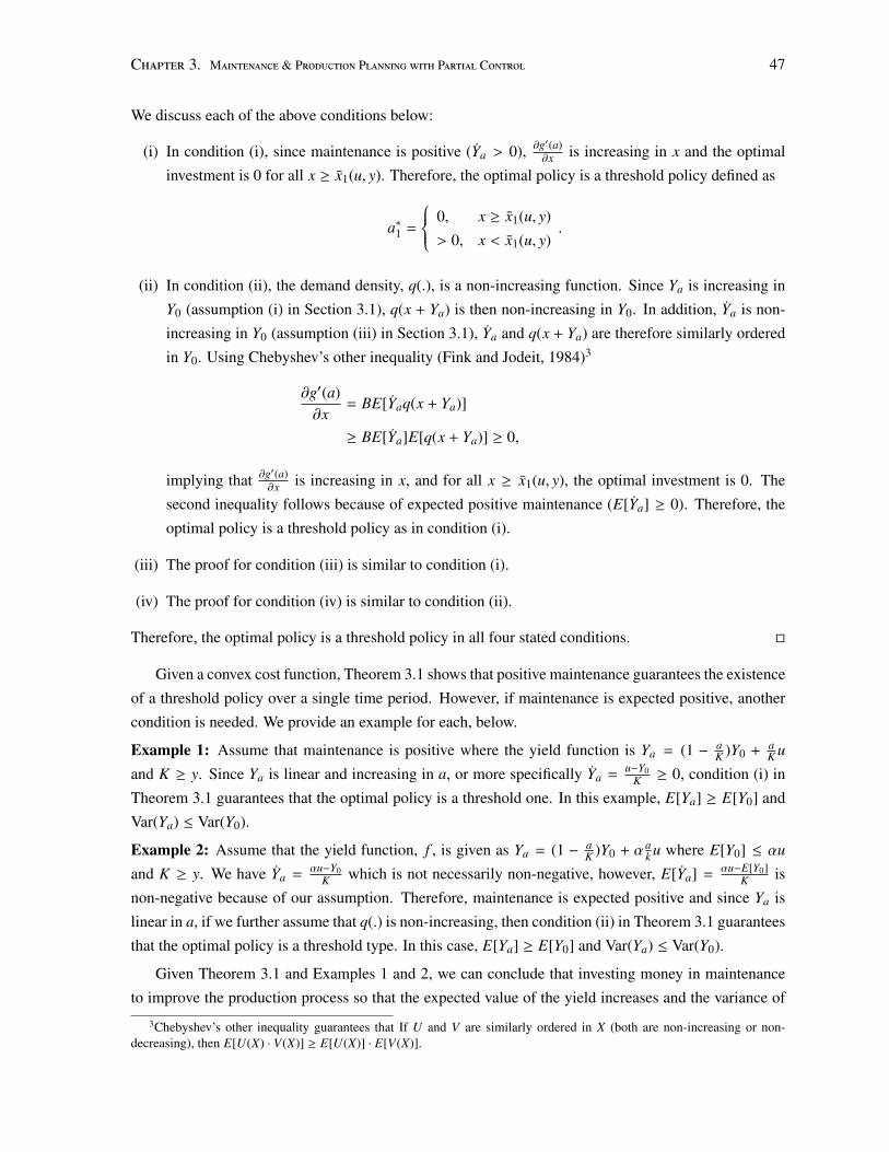
Chapter 3. Maintenance & Production Planning with Partial Control 47
We discuss each of the above conditions below:
(i) In condition (i), since maintenance is positive (Ya > 0), ∂g′(a)∂x is increasing in x and the optimal
investment is 0 for all x ≥ x1(u, y). Therefore, the optimal policy is a threshold policy defined as
a∗1 =
0, x ≥ x1(u, y)
> 0, x < x1(u, y).
(ii) In condition (ii), the demand density, q(.), is a non-increasing function. Since Ya is increasing in
Y0 (assumption (i) in Section 3.1), q(x + Ya) is then non-increasing in Y0. In addition, Ya is non-
increasing in Y0 (assumption (iii) in Section 3.1), Ya and q(x + Ya) are therefore similarly ordered
in Y0. Using Chebyshev’s other inequality (Fink and Jodeit, 1984)3
∂g′(a)∂x
= BE[Yaq(x + Ya)]
≥ BE[Ya]E[q(x + Ya)] ≥ 0,
implying that ∂g′(a)∂x is increasing in x, and for all x ≥ x1(u, y), the optimal investment is 0. The
second inequality follows because of expected positive maintenance (E[Ya] ≥ 0). Therefore, the
optimal policy is a threshold policy as in condition (i).
(iii) The proof for condition (iii) is similar to condition (i).
(iv) The proof for condition (iv) is similar to condition (ii).
Therefore, the optimal policy is a threshold policy in all four stated conditions. �
Given a convex cost function, Theorem 3.1 shows that positive maintenance guarantees the existence
of a threshold policy over a single time period. However, if maintenance is expected positive, another
condition is needed. We provide an example for each, below.
Example 1: Assume that maintenance is positive where the yield function is Ya = (1 − aK )Y0 + a
K u
and K ≥ y. Since Ya is linear and increasing in a, or more specifically Ya =u−Y0
K ≥ 0, condition (i) in
Theorem 3.1 guarantees that the optimal policy is a threshold one. In this example, E[Ya] ≥ E[Y0] and
Var(Ya) ≤ Var(Y0).
Example 2: Assume that the yield function, f , is given as Ya = (1 − aK )Y0 + α a
k u where E[Y0] ≤ αu
and K ≥ y. We have Ya =αu−Y0
K which is not necessarily non-negative, however, E[Ya] =αu−E[Y0]
K is
non-negative because of our assumption. Therefore, maintenance is expected positive and since Ya is
linear in a, if we further assume that q(.) is non-increasing, then condition (ii) in Theorem 3.1 guarantees
that the optimal policy is a threshold type. In this case, E[Ya] ≥ E[Y0] and Var(Ya) ≤ Var(Y0).
Given Theorem 3.1 and Examples 1 and 2, we can conclude that investing money in maintenance
to improve the production process so that the expected value of the yield increases and the variance of
3Chebyshev’s other inequality guarantees that If U and V are similarly ordered in X (both are non-increasing or non-decreasing), then E[U(X) · V(X)] ≥ E[U(X)] · E[V(X)].
Chapter 3. Maintenance & Production Planning with Partial Control 48
the yield decreases does not necessarily guarantee that a threshold policy is optimal. Even if we set α in
Example 2 such that we have necessary conditions for Ya to be smaller than Y0 in the convex order, i.e.,
E[Ya] = E[Y0] and Var(Ya) ≤ Var(Y0), the optimal policy is not necessarily a threshold type. Recalling
from Section 2.2.2.1, Gupta and Cooper (2005) showed that if the yield after a process improvement
project is smaller than the initial yield in the convex order, the expected profit increases. However, as
already discussed, the same condition does not guarantee an optimal threshold type policy. To have
an optimal threshold policy, we need a stronger condition on the expected value of the yield: it should
increase up to a certain level so that the marginal yield (Ya) is positive, i.e., investing more money in
maintenance does not decrease the number of acceptable products. However, the stated condition is
not a necessary condition to have a threshold investment policy. Example 2 represents a yield function
where the marginal yield is not positive, but the expected marginal yield is positive, i.e., investing more
money does not decrease the number of acceptable products on average. As previously mentioned, if
we assume that the demand density function is non-increasing, for example, having an exponential or a
uniform distribution, then the threshold policy is optimal.
3.2.3 Insights
In this section, we provide some insights to the single period problem comparing the relationships
between problem parameters.
Total Budget and Optimal Investment: If the budget allocated for investing in maintenance, y, in-
creases, the solution space, a ≤ y, is a superset of the previous solution space. Therefore, as stated in
Remark 3.1, the optimal investment, a∗1, does not decrease.
Remark 3.1. For a given inventory level, the optimal investment, a∗1, is non-decreasing in the budget, y.
It is worth mentioning that Remark 3.1 does not hold true if the firm saves the remaining budget
where it counts negatively toward the total cost. More specifically, let assume that a∗1(y1) and a∗1(y2)
indicate the optimal amount of investment for the budget y1 and y2, respectively. If y2 ≥ y1, it is
straightforward to show that a∗1(y2) − a∗1(y1) ≥ −(y2 − y1).
Inventory Level and Optimal Investment: The optimal investment in a period depends on both the
total available budget and the available inventory. If the inventory on hand increases, the firm has more
acceptable finished products to satisfy demand. The need for investment in maintenance to increase the
number of acceptable products therefore decreases and the optimal investment consequently does not
increase. Proposition 3.3 states the conditions where this relationship between inventory level and the
optimal investment exists. It is worth mentioning that in case of multiple period problem, it might be
beneficial to invest more in maintenance when the need for production is reduced (see Section 3.3.2).
Proposition 3.3. For a given budget y, if one of the following conditions holds true, then the optimal
investment, a∗1, is non-increasing in the inventory level, x.
(i) Maintenance is positive.
(ii) Maintenance is expected positive and the demand density is non-increasing.
Chapter 3. Maintenance & Production Planning with Partial Control 49
Proof. See Section A.1.4. �
Note that in Remark 3.1 and Proposition 3.3, the yield function can be any general function in the
investment value.
Inventory Threshold Value and Total Budget: When the total budget increases, the firm has more
resources to commit to maintenance to increase the number of acceptable finished products. Therefore, it
would make sense to invest in maintenance even if the amount of inventory on hand is large. Proposition
3.4 states the situations when the inventory threshold value does not decrease as the total budget for
investment increases.
Proposition 3.4. For a given production quantity u, if the conditions of Theorem 3.1 hold true, then the
inventory threshold value, x1(u, y), is non-decreasing in the total budget, y.
Proof. See Section A.1.5. �
Inventory Threshold Value and Production Quantity: We intuitively expect that as production quan-
tity, u, increases, the number of acceptable finished products increases and the threshold value, x1(u, y),
decreases for a given y: the firm initiates preventive maintenance if the amount of inventory at the be-
ginning of the time period is low because it needs more product at the end of the period and wants
to achieve this by increasing the yield. However, Remark 3.2 shows that there is a non-monotonic
relationship between the production quantity and the inventory level for starting maintenance.
In the following remark, we assume that the conditions of Lemma 3.1 hold true on the yield function.
Remark 3.2. If maintenance is positive, Ya ≥ 0, then the inventory threshold value, x1(u, y), is non-
monotonic in the production quantity, u.
We know that x1(u, y) solves
1 + BE[Y0Q(x1(u, y) + Y0)] − pE[Y0] = 0.
Denoting g(x1(u, y), u) = BE[Y0Q(x1(u, y) + Y0)] and J(u) = pE[Y0] − 1, we then have
g(x1(u, y), u) = J(u).
As we assumed in Section 3.1, Ya is increasing in u. If Ya ≥ 0 (as stated in Remark 3.2), we conclude that
Ya is also increasing in u. Therefore, both g(x1(u, y), u) and J(u) are increasing functions of u. Then,
as shown in Figure 3.1, if the production quantity denoted as u0 increases to u1 or u2, the threshold
value does not necessarily decrease. For u1, (u1 > u0) as shown in Figure 3.1, the threshold value
decreases, i.e., x1(u1, y) < x1(u0, y). However, for u2, (u2 > u0), the threshold value increases, i.e.,
x1(u2, y) > x1(u0, y).
Chapter 3. Maintenance & Production Planning with Partial Control 50
Figure 3.1: Changes in the inventory threshold value, x1(u, y), according to the changes in the productionquantity, u, when maintenance is positive.
3.2.4 Numerical Example
In this section, we provide a numerical example illustrating some of the results in the previous section.
We assume that the demand has an exponential distribution with a mean of 100, the initial yield has a
uniform distribution, the holding and the backlog costs equal 1 and 6, respectively, and the total available
budget is 90. Further we assume the random yield function is represented as Ya = (1 − aK )Y0 + a
K u.
Figure 3.2 illustrates the results of Proposition 3.3 that the optimal amount of investments, a∗1, does
not increase as the amount of initial inventory, x, increases for different production quantities and K =
100. Figure 3.3 shows that the production quantity, u, is not monotone with respect to the inventory
threshold value, x1(u, y) = x1(u, 90), for both values of K = 100 and K = 150 as stated in Remark 3.2.
One observation in Figure 3.3 is that the inventory threshold value, x1(u, 90), decreases for higher values
of K. Increasing the number of acceptable products is more expensive when K is higher. Intuitively,
when process improvement projects are costly, the firm does not make an investment unless the inventory
on hand is low.
3.2.5 Summary of Single Period Analysis
The summary of the results by analyzing the single time period problem is provided below.
• If the yield is a linear function of the amount of investment or is a concave function of the invest-
ment value with a zero holding cost, we have:
– The investment policy is a threshold policy for a given production policy if investing more
money in maintenance never decreases the number of acceptable products (positive mainte-
nance).
– In a practical situation, it seems more reasonable that the marginal yield is not positive,
but the expected marginal yield is positive (expected positive maintenance). Investing in
maintenance might decrease or increase the number of acceptable products, but the expected
number of acceptable products does not decrease. Our analysis shows that the investment
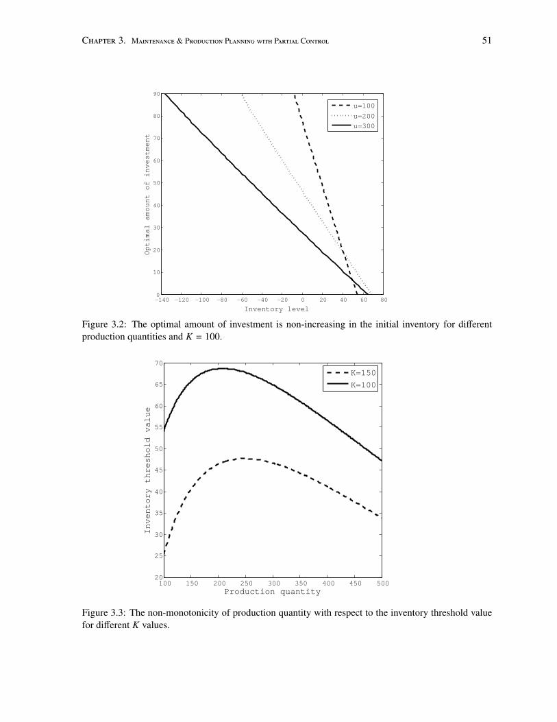
Chapter 3. Maintenance & Production Planning with Partial Control 51
−140 −120 −100 −80 −60 −40 −20 0 20 40 60 800
10
20
30
40
50
60
70
80
90
Inventory level
Op
tima
l am
ou
nt o
f in
vest
me
nt
u=100
u=200
u=300
Figure 3.2: The optimal amount of investment is non-increasing in the initial inventory for differentproduction quantities and K = 100.
100 150 200 250 300 350 400 450 50020
25
30
35
40
45
50
55
60
65
70
Production quantity
Inventory threshold value
K=150
K=100
Figure 3.3: The non-monotonicity of production quantity with respect to the inventory threshold valuefor different K values.
Chapter 3. Maintenance & Production Planning with Partial Control 52
policy in this situation is a threshold policy if the demand density function is non-increasing,
for example, having an exponential or a uniform distribution.
– Increasing the production quantity does not necessarily decrease the threshold on the inven-
tory level.
– The inventory threshold value does not decrease if the budget increases in both cases of pos-
itive maintenance and expected positive maintenance with non-increasing demand density.
• In both cases of positive maintenance and expected positive maintenance with non-increasing
demand density, the optimal amount of investment does not increase if more inventory is on hand.
• The optimal amount of investment does not decrease if more budget is available.
3.3 Multiple Period Analysis
In this section, we address the multiple period problem. First, we derive the multiple period optimal
policy and we then provide some insights to the problem.
3.3.1 Multiple Period Optimal Policy
Assuming x and yi as the initial inventory and the budget for the i-th period,4 the optimization problem
over n time periods is given below. Recall that we assume the budget available for each period is
previously determined and the money does not carry over the periods.
Φn(x, y1, . . . , yn) = min0≤a≤y1
{π(x, a) + ρE[Φn−1(x + Ya − Z, y2, . . . , yn)]}.
Proposition 3.5. The expected cost over one time period, π(x, a), is a jointly convex function given the
conditions of Lemma 3.1 hold true on the yield function.
Proof. See Section A.2.1. �
Proposition 3.6. Φ1(x, yn) is convex in x given the conditions of Lemma 3.1 hold true on the yield
function.
Proof. See Section A.2.2. �
Proposition 3.7. Φn(x, y1, . . . , yn) is convex in x if Ya is linear in a.
Proof. We use induction to show the convexity of Φn in x. In Proposition 3.6, we have shown that
Φ1(x, yn) is convex in x. Assuming that Φn−1(x, y2, . . . , yn) is convex in x and knowing that Ya is linear
in a, Φn−1(x + Ya − Z, y2, . . . , yn) is convex in (x, a) as x + Ya − Z is a linear function of x and a
(Theorem 5.7 of Rockafellar (1970)). Since π(x, a) is convex in (x, a) (Proposition 3.5); therefore,
4Since in this section we do not explicitly refer to the initial inventory level of any other period except period i, we excludethe subscript that represents the period number.
Chapter 3. Maintenance & Production Planning with Partial Control 53
π(x, a) + ρE[Φn−1(x + Ya − Z, y2, . . . , yn)] is convex in (x, a). Using the same reasoning as used in the
proof of Proposition 3.6 (see Section A.2.2.) results in the convexity of Φn(x, y1, . . . , yn) in x. �
Theorem 3.2. The optimal policy over n time periods, given a production quantity u, is a threshold
policy if the yield is linear in the investment value and maintenance is positive.
Proof. We re-write the optimal expected discounted cost over n periods as
Φn(x, y1, . . . , yn) = min0≤a≤y1
{Jn(x, a, y2, . . . , yn)},
where,
Jn(x, a, y2, . . . , yn) = π(x, a) + ρE[Φn−1(x + Ya − Z, y2, . . . , yn)].
Assuming that derivatives of Φn(x, y1, . . . , yn) in x exist and that Ya is linear in a, we have
∂Jn
∂a= 1 + BE[YaQ(x + Ya)] − pE[Ya] + ρE[Ya
∂Φn−1(x + Ya − Z, y2, . . . , yn)∂x
],
∂2Jn
∂a2 = BE[Y2a q(x + Ya)] + ρE[Y2
a∂2Φn−1(x + Ya − Z, y2, . . . , yn)
∂x2 ].
Using Proposition 3.7, ∂2 Jn∂a2 ≥ 0 and the optimal solution will solve
∂Jn
∂a= 0.
The reasoning on the existence of optimal solution is the same as in Theorem 3.1 with the only difference
that Ln(a), given below, replaces L1(a):
Ln(a) = pE[Ya(1 − Q(x + Ya))] − hE[YaQ(x + Ya)] − ρE[Ya∂Φn−1(x + Ya − Z, y2, . . . , yn)
∂x].
Denote the optimal amount of investment when n periods are remaining by a∗n and the inventory level
for which the optimal investment is 0 by xn(u, y1). We have
∂Jn
∂a∂x= BE[Yaq(x + Ya)] + ρE[Ya
∂2Φn−1(x + Ya − Z, y2, . . . , yn)∂x2 ].
As Proposition 3.7 and positive maintenance guarantee that ∂Jn(x,a,y2,...,yn)∂a∂x is increasing in x, the
optimal investment is 0 for all x ≥ xn(u, y1) which completes the proof. �
Theorem 3.2 shows that condition (i) of Theorem 3.1, i.e., a linear yield in the amount of invest-
ment and positive maintenance, guarantees the existence of the threshold policy over multiple periods.
If maintenance is expected positive, which is more likely in the real situation, to have a threshold opti-
Chapter 3. Maintenance & Production Planning with Partial Control 54
mal policy over n periods, we need three conditions to guarantee ∂Jn(x,a,y2,...,yn)∂a∂x is increasing in x using
Chebyshev’s other inequality. The conditions are:
(i) yield is linear in the investment,
(ii) the demand density function is non-increasing, and
(iii) the second derivative of the optimal total discounted expected cost over (n−1) periods, Φ′′n−1(x, y1, . . . , yn),
is non-increasing in x.
Therefore, the conditions that make the threshold policy optimal over one time period, Conditions
(i) and (ii), are not sufficient to guarantee the existence of a threshold policy over n periods in case of
expected positive maintenance. Condition (iii) should also hold true to have a threshold optimal policy,
however, this condition is not verifiable and useful in practice since it is stated on the cost function, not
on the problem parameters.
3.3.2 Insights
Similar to Section 3.2.3, in this section, we present several insights to the multiple period problem
comparing the relationships between problem parameters.
Total Budget and Optimal Investment: If the firm allocates more budget for investment in the first
period, it has more resources for increasing the production quantity. In the other words, the solution
space, a ≤ y1, becomes larger and since it includes the solution space before budget increase, the
optimal investment when n periods are remaining, a∗n, does not decrease.
Remark 3.3. For a given inventory level, the optimal investment when n periods are remaining, a∗n, is
non-decreasing in the total budget available at the beginning of the first period, y1.5
Inventory Level and Optimal Investment: When n periods are remaining, Proposition 3.8 states that
if the inventory on hand increases in case of positive maintenance, the need for increasing the yield
decreases. Thus, the firm does not increase the optimal amount of investment in maintenance.
If maintenance takes the potential production capacity, resulting in periods of process unavailability,
it might be optimal to invest more in maintenance when the inventory level on hand is high and there is
a reduced need for production. Performing maintenance will likely increase the initial inventory level
for the next periods, increasing the holding cost, but it will also decrease the backlog cost. It is worth
mentioning that the expected positive maintenance situation can be considered as an example where
maintenance takes the potential production capacity since investing more money does not guarantee
an increase in the production quantity. Therefore, it might be optimal to increase the investment in
maintenance even if the current inventory on hand is high enough in order to ensure a high inventory
level in future periods. The possibility of being optimal to increase the investment for high inventory
levels in the expected positive maintenance case further implies that the threshold policy is not necessary
optimal without some additional assumptions as discussed in Section 3.3.1.5This remark does not hold true if the firm saves the remaining budget where it counts negatively toward the total cost of
one period.
Chapter 3. Maintenance & Production Planning with Partial Control 55
Proposition 3.8. For a given budget y1, the optimal investment, a∗n, is non-increasing in the inventory
level, x, if maintenance is positive and the yield is linear in the investment value.
Proof. The proof is the same as the proof of Proposition 3.3 where Jn(x, a, y2, . . . , yn) and a∗n(x, y1)
replace π(x, a) and a∗1(x, y). Note that, we first need to prove that Jn(x, a, y2, . . . , yn) is supermodular in
(x, a) which is shown in Section A.2.3. �
Inventory Threshold Value and Total Budget: The following proposition states the same result as
Proposition 3.4 for n periods. If the budget at the beginning of the period increases, the firm has more
resources to improve the production process and invests in maintenance even if the inventory on hand is
high enough.
Proposition 3.9. For a given production quantity u, the inventory threshold value, xn(u, y1), is non-
decreasing in the budget y1 if maintenance is positive and the yield is linear in the investment value.
Proof. The proof is similar to the proof of Proposition 3.4. Note that the supermodularity of Φn(x, y1, . . . , yn)
in (x, y1) is proved in Section A.2.3. �
It is worth mentioning that Propositions 3.8 and 3.9 correspond to Propositions 3.3 and 3.4 in Sec-
tion 3.2.3. However, if one period is remaining, the properties hold true in more general cases where
maintenance can be also expected positive.
3.3.3 Summary of Multiple Period Analysis
The summary of our results for multiple period problem is:
• If the yield is a linear function of the amount of investment and maintenance is positive:
– The optimal investment policy is a threshold type policy.
– The optimal amount of investment in maintenance does not increase if there is more inven-
tory on hand.
– The inventory threshold value does not decrease if the budget for investing in maintenance
increases.
• If the budget increases, the optimal amount of investment does not decrease.
3.4 Conclusion
Uncertainties in production systems resulting in a random yield can be due to internal causes such
as machine deterioration and machine breakdowns. Therefore, there is an interest to invest in process
improvement projects such as preventive maintenance to increase the yield. A firm must jointly optimize
the production quantity and invest in maintenance. In this chapter, we study this problem, addressing
the integration of maintenance and production planning with partial control over machine conditions in
Chapter 3. Maintenance & Production Planning with Partial Control 56
a periodic review system. However, because of the non-convexity of the cost function, we analyze the
problem by fixing the production quantities to gain insight into the structure of optimal maintenance
policy. As mentioned by Gupta and Cooper (2005), the assumption of fixed production quantities is
reasonable when the firm is committed to them ahead of time.
We have mainly focused on understanding the structure of the optimal maintenance policy. If the
yield is a linear function of the amount of money invested in maintenance and the marginal yield is
positive, our results show that:
• the optimal policy is a single critical level type of the inventory level. At the beginning of each
time period, a firm must observe the inventory level and if it is below a certain amount, it is
optimal to invest in maintenance,
• the optimal amount of investment does not increase if the available inventory increases, and
• the inventory threshold value does not decrease if the firm has more budget to invest in mainte-
nance.
However, in a real situation, the marginal yield is not always positive. It is more likely that the
expected yield will not decrease as the amount of money invested in maintenance increases, i.e., the
expected marginal yield is positive. Our analysis shows that if the demand probability density function
is non-increasing, the threshold maintenance policy is optimal, though, only over a single time period.
We have also provided some structural results when the yield is not a linear function of the investment
value which are only valid for the single period problem.
Furthermore, we have discussed the technical problem of providing sufficient conditions, albeit very
general ones, such that the derivatives exist for the functions commonly used in the production and
inventory literature.
In this chapter, we took a strategic perspective and addressed the interdependency between produc-
tion planning and maintenance where the goal is to find the optimal production quantity and investment
in maintenance increasing the number of acceptable finished products. In the next chapter, we assume
that the production quantity and the amount of investment are determined and therefore study the rela-
tionship between production and maintenance taking an operational view. Our goal in the next chapter
is to determine the optimal allocation of resources to either production or maintenance to maximize the
number of acceptable finished products by their due dates.
Chapter 4
Maintenance Planning & ProductionScheduling with No Control over MachineConditions
Production scheduling concerns the optimal allocation of machines to competing customer orders to
maximize customer satisfaction. However, unexpected machine breakdowns might result in periods of
unavailability where machines are under repair and no orders can be processed. Performing preventive
maintenance on machines can partially control their conditions, decreasing the number of failures. In
some production systems, it is, however, not justifiable to preventively maintain machines for example
because of the random deterioration processes of machines1 or higher cost of preventive maintenance
than corrective maintenance. Therefore, the maintenance policy is the failure-based policy where there is
no control over machine conditions and machines are maintained only at failures (see Section 2.2.1.3). In
these production systems, utilizing the available information on machine breakdowns and incorporating
them into the production schedule to hedge against failures is a challenging problem. In this chapter, we
address this challenge in the context of an aircraft fleet management problem where the flights and the
aircraft correspond to the production activities and the machines, respectively and where the aircraft are
maintained only at failures because of high preventive maintenance cost.
Motivated by the work of Safaei et al. (2010; 2011), we study the problem of scheduling a military
aircraft repair shop, where a number of flights are planned over a long horizon. Every flight, also
called a wave, has requirements for a specific number of aircraft of different types. Flights might be
partially carried out without their requirements. Aircraft are checked for failures before and after each
flight: if an aircraft is diagnosed as failed, it enters the repair shop and is minimally repaired. Aircraft
flow over a long horizon is illustrated in Figure 4.1. The goal is to determine the optimal assignment
of aircraft to waves and a schedule of aircraft repairs that will maximize the flight coverage, that is,
the extent to which the aircraft requirements of the flights are met. This problem is an example of an
1If a machine has a random deterioration process, its failure rate is constant and does not increase as the age of the machineincreases.
57
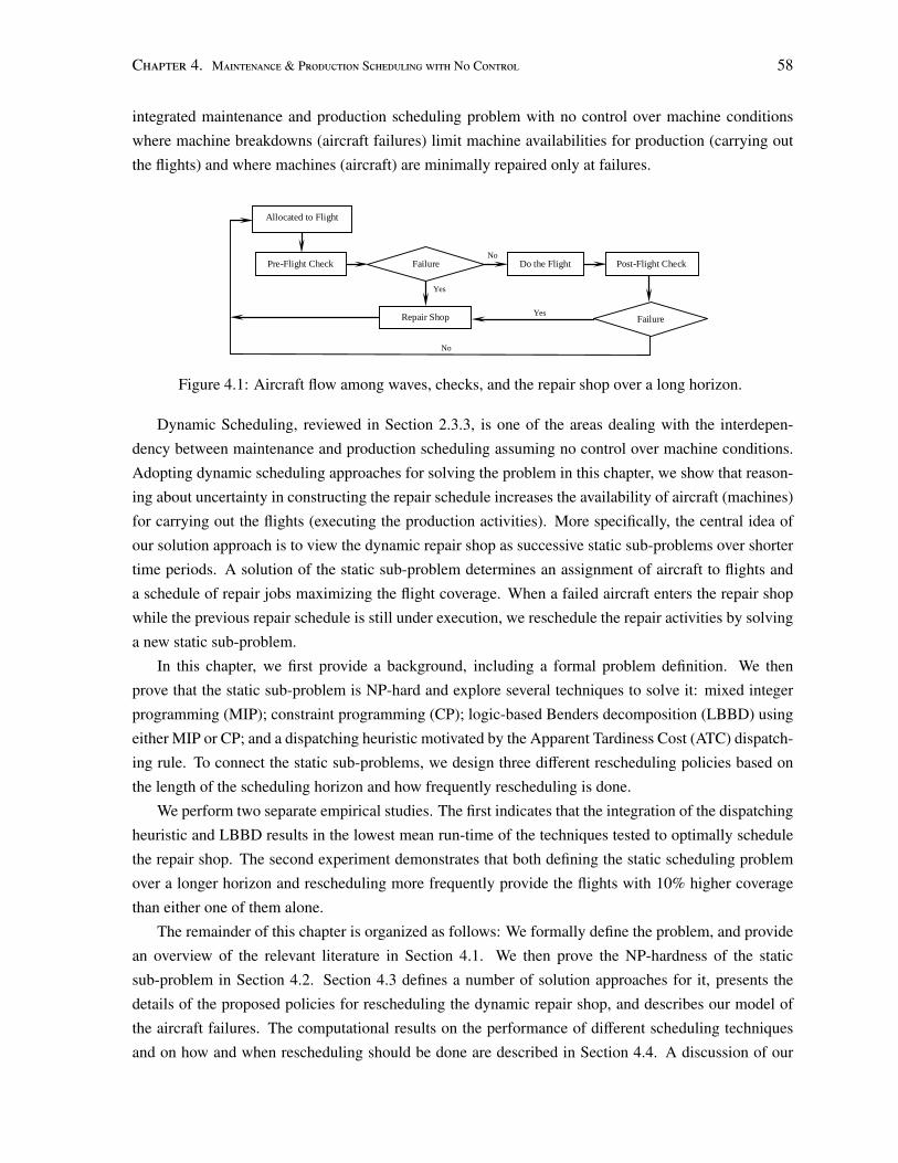
Chapter 4. Maintenance & Production Scheduling with No Control 58
integrated maintenance and production scheduling problem with no control over machine conditions
where machine breakdowns (aircraft failures) limit machine availabilities for production (carrying out
the flights) and where machines (aircraft) are minimally repaired only at failures.
No
Yes
Do the Flight Failure Pre-Flight Check
Allocated to Flight
Failure
Yes
No
Repair Shop
Post-Flight Check
Figure 4.1: Aircraft flow among waves, checks, and the repair shop over a long horizon.
Dynamic Scheduling, reviewed in Section 2.3.3, is one of the areas dealing with the interdepen-
dency between maintenance and production scheduling assuming no control over machine conditions.
Adopting dynamic scheduling approaches for solving the problem in this chapter, we show that reason-
ing about uncertainty in constructing the repair schedule increases the availability of aircraft (machines)
for carrying out the flights (executing the production activities). More specifically, the central idea of
our solution approach is to view the dynamic repair shop as successive static sub-problems over shorter
time periods. A solution of the static sub-problem determines an assignment of aircraft to flights and
a schedule of repair jobs maximizing the flight coverage. When a failed aircraft enters the repair shop
while the previous repair schedule is still under execution, we reschedule the repair activities by solving
a new static sub-problem.
In this chapter, we first provide a background, including a formal problem definition. We then
prove that the static sub-problem is NP-hard and explore several techniques to solve it: mixed integer
programming (MIP); constraint programming (CP); logic-based Benders decomposition (LBBD) using
either MIP or CP; and a dispatching heuristic motivated by the Apparent Tardiness Cost (ATC) dispatch-
ing rule. To connect the static sub-problems, we design three different rescheduling policies based on
the length of the scheduling horizon and how frequently rescheduling is done.
We perform two separate empirical studies. The first indicates that the integration of the dispatching
heuristic and LBBD results in the lowest mean run-time of the techniques tested to optimally schedule
the repair shop. The second experiment demonstrates that both defining the static scheduling problem
over a longer horizon and rescheduling more frequently provide the flights with 10% higher coverage
than either one of them alone.
The remainder of this chapter is organized as follows: We formally define the problem, and provide
an overview of the relevant literature in Section 4.1. We then prove the NP-hardness of the static
sub-problem in Section 4.2. Section 4.3 defines a number of solution approaches for it, presents the
details of the proposed policies for rescheduling the dynamic repair shop, and describes our model of
the aircraft failures. The computational results on the performance of different scheduling techniques
and on how and when rescheduling should be done are described in Section 4.4. A discussion of our
Chapter 4. Maintenance & Production Scheduling with No Control 59
solution approach and results are presented in Section 4.5. We end with conclusion in Section 4.6.
4.1 Background
In this section, the formal definition of the problem is given and the relevant literature on repair shop
scheduling is reviewed.
4.1.1 Problem Definition
Figure 4.2 is a snapshot of the problem at time 0, where circles represent aircraft. A number of flights
(five are shown) and their corresponding pre- and post-flight checks are already scheduled over a long
horizon. It is assumed that the total number of aircraft is constant over a long horizon. A number of
aircraft (three in the diagram) are ready for the pre-flight check while others are currently in the shop
awaiting repair before they can proceed to a pre-flight check. Failure is only detected during a check
and we assume that a check will always correctly assess the status of an aircraft at negligible cost and
that the duration of a check is incorporated in the length of the corresponding wave.
Repair Shop
...
Wave-5
st5 et5
Wave-1 Wave-2
Wave-3
st1 et1 st2 st3
et2 et3
Wave-4
st4 et4
0
...
Checks
Figure 4.2: Snapshot of the problem at time 0 over a long horizon.
The goal is to assign aircraft to waves to maximize coverage while at the same time creating a
feasible repair schedule. The scheduling problem is under the constraints that the repair shop has limited
capacity and the aircraft are subject to breakdown. We assume that once an aircraft fails, it goes to the
repair shop and waits until its repair operations are performed.
We use the following notation to represent the problem.
• N is the set of aircraft. λn is the failure rate of the aircraft n ∈ N denoting the frequency of failure
per time unit. For example if the failure rate is 0.2 per day, it means that the mean time to aircraft
failure is 5 days.
• K is the set of aircraft types. Ik denotes the set of aircraft type k ∈ K where ηk aircraft are ready
(i.e., not in the repair shop at time 0). Let |Ik| denote the number of aircraft of type k, |Ik| − ηk
aircraft of type k are then in the repair shop at time 0. λk is the mean failure rate over all aircraft
of type k.
• R is the set of repair resources (called trades). The maximum capacity of trade r ∈ R is Cr which
is the maximum number of units of trade r that can be used at any one time point.
Chapter 4. Maintenance & Production Scheduling with No Control 60
• W is the set of waves. Each wave, w ∈ W, has a start-time, stw, and an end-time, etw. Each wave
requires at most akw aircraft of type k.
• J is the set of existing jobs in the repair shop. Each job is associated with a specific aircraft
type. Mr is the set of jobs requiring trade r. Each job might require more than one trade to be
completed. The processing time of job j on trade r is p jr and c jr is the capacity of trade r required
by job j.
To model the deterioration of an aircraft, each time it flies a wave its failure rate, λn, increases by
γ percent, i.e., its failure rate is (1 + 0.01 × γ)λn after the flight. If an aircraft fails, its failure rate after
repair returns to what it was just before the failure. In the other words, as in one of the standard repair
models in the maintenance literature, repair is minimal (Wang, 2002). The probability of diagnosing
aircraft n as failed in pre- and post-flight checks is a function of its failure rate right before the checks
denoted as f pre(λn) and f post(λn). The probability of failure detection in pre-flight checks is smaller
than the post-flight checks because an aircraft is either just released from the repair shop or has already
passed a previous post-flight check successfully (Safaei et al., 2011).
To find the probability of failure of an aircraft in pre- and post-flight checks for a specific wave,
we need to track the complete history of the aircraft. For example, if we assume that a given aircraft
is repaired and assigned to the first wave, then there are three paths: the aircraft fails the pre-flight
check; the aircraft passes the pre-flight check, flies the wave, and fails the post-flight check; or the
aircraft passes the pre-flight check, flies the wave, and passes the post-flight check. Therefore, the
availability of the aircraft for the second wave can be represented as a random variable whose expected
value depends on the probability of these three different paths and the scheduling decisions to repair the
failed aircraft before the second wave. Similarly the availability of the aircraft for subsequent waves
depends on its entire path through the checks, repair shop, and waves. As the number of waves and
aircraft increase, the size of the state space will become prohibitive. Furthermore, the repair scheduling
decisions themselves impact the aircraft histories: the probability that an aircraft is available for the
third wave is different depending on if it was repaired in time for the first wave or only for the second
wave. The details on approximating the failure probabilities are presented in Section 4.3.1.1.
As the complexity of the problem has not been shown, we prove that it is NP-hard in Section 4.2.
4.1.2 Literature Review
As already mentioned, the problem of this chapter is an example of integrated maintenance and produc-
tion scheduling problem assuming no control over machine conditions which is reviewed in detail in
Sections 2.3.2 and 2.3.3. In this section, we provide necessary background on repair shop scheduling
problem, the context of our example problem.
4.1.2.1 Repair Shop Scheduling
Repair shops have been mainly studied as a machine-repairman problem (Haque and Armstrong, 2007;
Stecke, 1992) which has a set of workers and a set of machines that are subject to failures and therefore
Chapter 4. Maintenance & Production Scheduling with No Control 61
need repair. Workers and machines respectively correspond to trades and aircraft, in our problem. As
the number of workers is less than the number of machines, it is necessary to allocate the repair jobs to
the workers with the goal of optimizing a given performance measure (e.g., the total expected machine
downtime) over the long term. Derman et al. (1980) did the early work on solving the scheduling
problem of a repair shop with a single repairman. They showed that repairing the failed machines in
non-decreasing order of failure rate stochastically maximizes the number of working machines. The
literature on the scheduling of a repair shop was then extended by considering multiple repairmen,
preemptive and non-preemptive repair, and different failure and repair distributions. A comprehensive
review of the literature on the scheduling of a repair system is provided by Iravani et al. (2007).
The analytical models in the literature are mainly developed using Markov Decision Processes (dy-
namic programming) and guarantee the optimality of a given performance measure in the long term.
These models often do not consider the combinatorics of the real scheduling problems such as different
repair capacity limits, different due dates, and different resource and processing requirements. There-
fore, they typically result in a static dispatching-type repair policy similar to that found by Derman et
al. (1980). However, in our problem, the waves have different plane requirements and the processing
times and the resource requirements of the repair activities become known when they enter the repair
shop. Therefore, we believe that a better performance can be achieved by dealing directly with the
combinatorics and explicitly scheduling the repair shop to meet the waves. To handle the uncertain
and combinatorial structure of the scheduling problems, our solution approach is based on the ideas of
dynamic scheduling algorithms reviewed in Section 2.3.3.
Other areas of literature with similarities to our static problem are the operational level maintenance
scheduling problem, in general, and the flight and maintenance planning problem of military aircraft,
specifically. The former literature addresses the problem of finding a schedule for given maintenance
activities such that the sum of maintenance costs is minimized. The focus is on the operational level,
determining the maintenance activities performed in each time period (Budai et al., 2006). Starting with
the early work of Wagner et al. (1964), this literature was extended through developing mathematical
models and effective solution approaches for a variety of applications (Frost and Dechter, 1998; Haghani
and Shafahi, 2002; Budai et al., 2006; Grigoriev et al., 2006). The latter literature studies the problem
of maintenance planning and mission assignment of military aircraft where the goal is to decide which
aircraft to fly and which one to perform maintenance, maximizing their long-term availability. Similar
to the maintenance scheduling literature, mathematical programming is the common approach to solve
the problems of this literature. Kozanidis et al. (2012) recently proposed a mixed integer non-linear
programming model to optimize the joint flight and maintenance plan of mission aircraft.
Safaei et al. (2010) modeled the static problem addressed here as an operational level maintenance
scheduling problem using MIP. Their MIP includes an assignment problem and two network problems:
the former assigns the aircraft to the waves and the latter calculates the expected number of available
aircraft for the waves as well as the expected number of available workers for the repair jobs. They later
extended their work by using slightly different MIP model where the time-indexed approach is used to
enforce the workforce availability constraint and they verified the validity of their model by a number
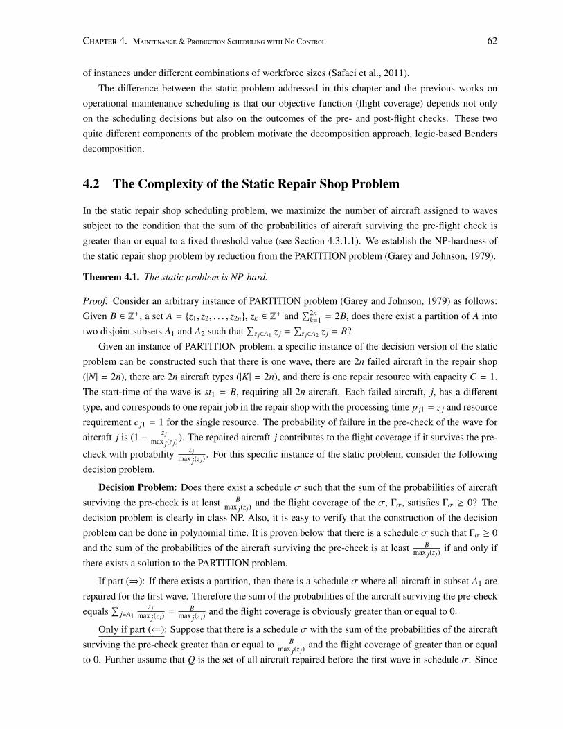
Chapter 4. Maintenance & Production Scheduling with No Control 62
of instances under different combinations of workforce sizes (Safaei et al., 2011).
The difference between the static problem addressed in this chapter and the previous works on
operational maintenance scheduling is that our objective function (flight coverage) depends not only
on the scheduling decisions but also on the outcomes of the pre- and post-flight checks. These two
quite different components of the problem motivate the decomposition approach, logic-based Benders
decomposition.
4.2 The Complexity of the Static Repair Shop Problem
In the static repair shop scheduling problem, we maximize the number of aircraft assigned to waves
subject to the condition that the sum of the probabilities of aircraft surviving the pre-flight check is
greater than or equal to a fixed threshold value (see Section 4.3.1.1). We establish the NP-hardness of
the static repair shop problem by reduction from the PARTITION problem (Garey and Johnson, 1979).
Theorem 4.1. The static problem is NP-hard.
Proof. Consider an arbitrary instance of PARTITION problem (Garey and Johnson, 1979) as follows:
Given B ∈ Z+, a set A = {z1, z2, . . . , z2n}, zk ∈ Z+ and
∑2nk=1 = 2B, does there exist a partition of A into
two disjoint subsets A1 and A2 such that∑
z j∈A1 z j =∑
z j∈A2 z j = B?
Given an instance of PARTITION problem, a specific instance of the decision version of the static
problem can be constructed such that there is one wave, there are 2n failed aircraft in the repair shop
(|N | = 2n), there are 2n aircraft types (|K| = 2n), and there is one repair resource with capacity C = 1.
The start-time of the wave is st1 = B, requiring all 2n aircraft. Each failed aircraft, j, has a different
type, and corresponds to one repair job in the repair shop with the processing time p j1 = z j and resource
requirement c j1 = 1 for the single resource. The probability of failure in the pre-check of the wave for
aircraft j is (1 − z jmax j(z j)
). The repaired aircraft j contributes to the flight coverage if it survives the pre-
check with probability z jmax j(z j)
. For this specific instance of the static problem, consider the following
decision problem.
Decision Problem: Does there exist a schedule σ such that the sum of the probabilities of aircraft
surviving the pre-check is at least Bmax j(z j)
and the flight coverage of the σ, Γσ, satisfies Γσ ≥ 0? The
decision problem is clearly in class NP. Also, it is easy to verify that the construction of the decision
problem can be done in polynomial time. It is proven below that there is a schedule σ such that Γσ ≥ 0
and the sum of the probabilities of the aircraft surviving the pre-check is at least Bmax j(z j)
if and only if
there exists a solution to the PARTITION problem.
If part (⇒): If there exists a partition, then there is a schedule σ where all aircraft in subset A1 are
repaired for the first wave. Therefore the sum of the probabilities of the aircraft surviving the pre-check
equals∑
j∈A1
z jmax j(z j)
= Bmax j(z j)
and the flight coverage is obviously greater than or equal to 0.
Only if part (⇐): Suppose that there is a schedule σ with the sum of the probabilities of the aircraft
surviving the pre-check greater than or equal to Bmax j(z j)
and the flight coverage of greater than or equal
to 0. Further assume that Q is the set of all aircraft repaired before the first wave in schedule σ. Since
Chapter 4. Maintenance & Production Scheduling with No Control 63
the start time of the first wave is B, then∑
j∈Q z j ≤ B. Furthermore, the sum of the probabilities of the
aircraft surviving the pre-check equals∑
j∈Qz j
max j(z j)which is greater than or equal to B
max j(z j). Therefore,
we can conclude that∑
j∈Q z j = B meaning that there is a solution to the PARTITION problem. �
4.3 Solution Approach
The main idea of our solution approach is to view the dynamic problem as linked successive static
sub-problems which is a common approach in dynamic scheduling. This view results in a rescheduling
strategy based on scheduling static sub-problems over shorter time periods. Therefore, we have two sub-
goals: how to solve and how to connect the static sub-problems. In this section, we first present different
solution techniques for solving the static sub-problems and then define three rescheduling strategies
designed to connect them. Finally, we describe our approach for modeling the dynamic events, i.e.,
aircraft failures.
4.3.1 Scheduling Techniques
We investigate a number of approaches to solve the repair shop scheduling problem including mixed
integer programming, constraint programming, logic-based Benders decomposition, a dispatch rule,
and a simple hybrid approach. Each of the approaches is described in detail in this section.
4.3.1.1 Mixed Integer Programming
We propose a novel mixed integer programming model where the uncertainty in the outcome of the
checks is modeled as expectation. This model is different from and, as we show below in Section
4.4.1.2, significantly faster than those of Safaei et al. (2010; 2011). Table 4.1 summarizes the notation
defined in Section 4.1.1 and defines the decision variables of the MIP model.
In this section, without loss of generality, we interpret W as the set of waves in the current static
sub-problem and consider the start-times of the waves as due dates to finish the repair of the aircraft.
Therefore, we define D = {di|i = 1, 2, ..., |W |, |W | + 1} to be an ordered set of due dates consisting of
the wave start-times plus a big value, B, sorted in ascending order. More specifically, di equals to the
start-time of the i-th wave, sti. Because of the limited repair capacity, it is possible that some of the
failed aircraft cannot be repaired in time for any of the waves. In such a case, the due date of the repair
job is assigned to d|W |+1 = B. In our model, B equals the sum of the start-time of the last wave and the
maximum processing times of all the jobs over all the trades, i.e., d|W | + maxj,r
(p jr) and we do not enforce
the repair resource capacity after d|W |.
As explained in Section 4.1.1, the exact calculation of the aircraft failure probability and conse-
quently the expected number of available aircraft is intractable since it depends on the complete aircraft
histories. Therefore, we distinguish aircraft based on their type and use a recursive equation (Equation
4.4) to approximate the expected number of available aircraft. The details of Equation (4.4) are provided
later in this section. For each aircraft type of k, the average failure rate, λk, is used to calculate the prob-
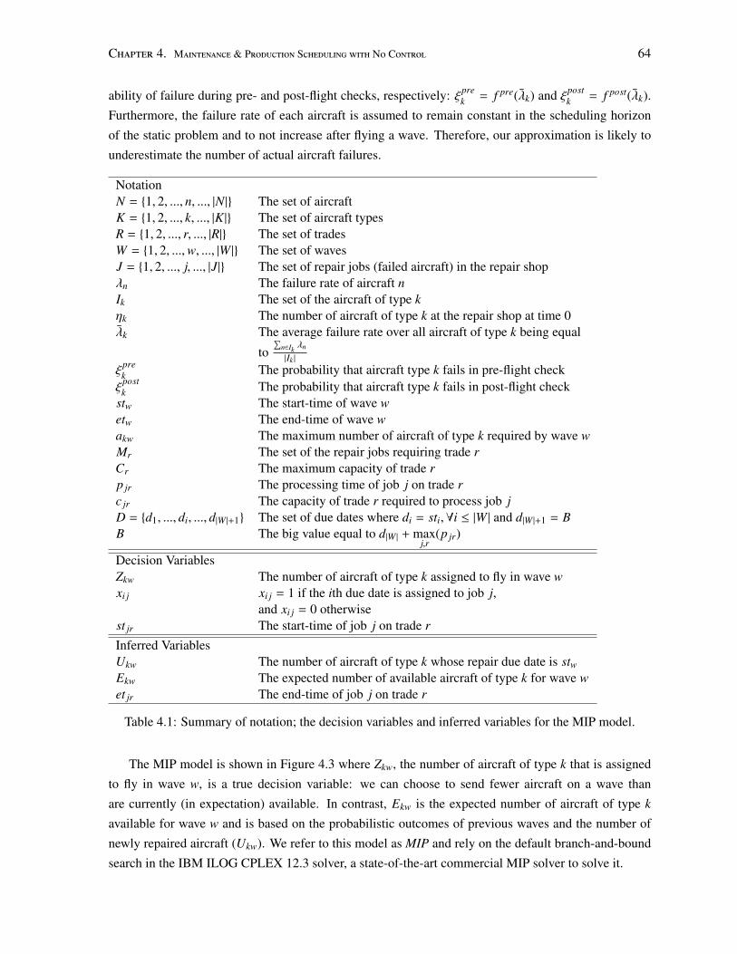
Chapter 4. Maintenance & Production Scheduling with No Control 64
ability of failure during pre- and post-flight checks, respectively: ξprek = f pre(λk) and ξpost
k = f post(λk).
Furthermore, the failure rate of each aircraft is assumed to remain constant in the scheduling horizon
of the static problem and to not increase after flying a wave. Therefore, our approximation is likely to
underestimate the number of actual aircraft failures.
NotationN = {1, 2, ..., n, ..., |N |} The set of aircraftK = {1, 2, ..., k, ..., |K|} The set of aircraft typesR = {1, 2, ..., r, ..., |R|} The set of tradesW = {1, 2, ...,w, ..., |W |} The set of wavesJ = {1, 2, ..., j, ..., |J|} The set of repair jobs (failed aircraft) in the repair shopλn The failure rate of aircraft nIk The set of the aircraft of type kηk The number of aircraft of type k at the repair shop at time 0λk The average failure rate over all aircraft of type k being equal
to∑
n∈Ikλn
|Ik |
ξprek The probability that aircraft type k fails in pre-flight checkξ
postk The probability that aircraft type k fails in post-flight check
stw The start-time of wave wetw The end-time of wave wakw The maximum number of aircraft of type k required by wave wMr The set of the repair jobs requiring trade rCr The maximum capacity of trade rp jr The processing time of job j on trade rc jr The capacity of trade r required to process job jD = {d1, ..., di, ..., d|W |+1} The set of due dates where di = sti,∀i ≤ |W | and d|W |+1 = BB The big value equal to d|W | + max
j,r(p jr)
Decision VariablesZkw The number of aircraft of type k assigned to fly in wave wxi j xi j = 1 if the ith due date is assigned to job j,
and xi j = 0 otherwisest jr The start-time of job j on trade r
Inferred VariablesUkw The number of aircraft of type k whose repair due date is stwEkw The expected number of available aircraft of type k for wave wet jr The end-time of job j on trade r
Table 4.1: Summary of notation; the decision variables and inferred variables for the MIP model.
The MIP model is shown in Figure 4.3 where Zkw, the number of aircraft of type k that is assigned
to fly in wave w, is a true decision variable: we can choose to send fewer aircraft on a wave than
are currently (in expectation) available. In contrast, Ekw is the expected number of aircraft of type k
available for wave w and is based on the probabilistic outcomes of previous waves and the number of
newly repaired aircraft (Ukw). We refer to this model as MIP and rely on the default branch-and-bound
search in the IBM ILOG CPLEX 12.3 solver, a state-of-the-art commercial MIP solver to solve it.
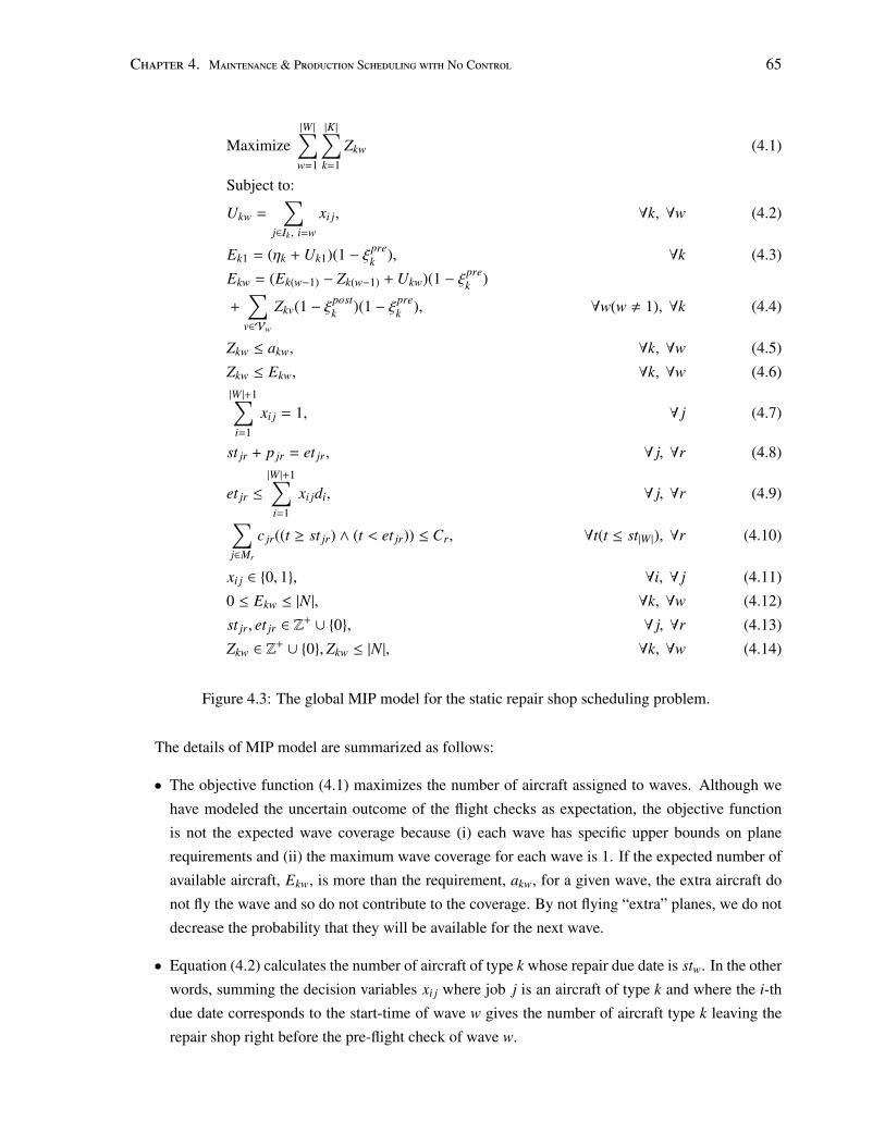
Chapter 4. Maintenance & Production Scheduling with No Control 65
Maximize|W |∑w=1
|K|∑k=1
Zkw (4.1)
Subject to:
Ukw =∑
j∈Ik , i=w
xi j, ∀k, ∀w (4.2)
Ek1 = (ηk + Uk1)(1 − ξprek ), ∀k (4.3)
Ekw = (Ek(w−1) − Zk(w−1) + Ukw)(1 − ξprek )
+∑
v∈Vw
Zkv(1 − ξpostk )(1 − ξpre
k ), ∀w(w , 1), ∀k (4.4)
Zkw ≤ akw, ∀k, ∀w (4.5)
Zkw ≤ Ekw, ∀k, ∀w (4.6)|W |+1∑
i=1
xi j = 1, ∀ j (4.7)
st jr + p jr = et jr, ∀ j, ∀r (4.8)
et jr ≤
|W |+1∑i=1
xi jdi, ∀ j, ∀r (4.9)∑j∈Mr
c jr((t ≥ st jr) ∧ (t < et jr)) ≤ Cr, ∀t(t ≤ st|W |), ∀r (4.10)
xi j ∈ {0, 1}, ∀i, ∀ j (4.11)
0 ≤ Ekw ≤ |N |, ∀k, ∀w (4.12)
st jr, et jr ∈ Z+ ∪ {0}, ∀ j, ∀r (4.13)
Zkw ∈ Z+ ∪ {0},Zkw ≤ |N |, ∀k, ∀w (4.14)
Figure 4.3: The global MIP model for the static repair shop scheduling problem.
The details of MIP model are summarized as follows:
• The objective function (4.1) maximizes the number of aircraft assigned to waves. Although we
have modeled the uncertain outcome of the flight checks as expectation, the objective function
is not the expected wave coverage because (i) each wave has specific upper bounds on plane
requirements and (ii) the maximum wave coverage for each wave is 1. If the expected number of
available aircraft, Ekw, is more than the requirement, akw, for a given wave, the extra aircraft do
not fly the wave and so do not contribute to the coverage. By not flying “extra” planes, we do not
decrease the probability that they will be available for the next wave.
• Equation (4.2) calculates the number of aircraft of type k whose repair due date is stw. In the other
words, summing the decision variables xi j where job j is an aircraft of type k and where the i-th
due date corresponds to the start-time of wave w gives the number of aircraft type k leaving the
repair shop right before the pre-flight check of wave w.
Chapter 4. Maintenance & Production Scheduling with No Control 66
• Equation (4.3) calculates the expected number of available aircraft of type k for the first wave.
• Equation (4.4) calculates the expected number of available aircraft of type k for the other waves.
The first term includes those aircraft available but not used for the previous wave, i.e., (Ek(w−1) −
Zk(w−1)), and those newly arrived from the repair shop, i.e., Ukw. The second term sums over all
aircraft that become available because they have completed waves since the previous wave started
whereVw = {v|v ∈ W, stw−1 < etv ≤ stw}.
• Constraints (4.5) and (4.6) ensure that the number of aircraft that is assigned to fly in each wave
is less than or equal to the number of aircraft required and the expected number available.
• Constraint (4.7) assigns exactly one due date to each job.
• Equation (4.8) calculates the end-time of the jobs.
• Constraint (4.9) guarantees that the end-time of each job is less than or equal to its assigned due
date.
• Constraint (4.10) is a logical-and constraint enforcing the capacity limit of trade r by summing
over the capacity required by the set of jobs under repair at time t. Since the jobs after the start-
time of the last wave do not contribute to the coverage, the capacity constraint is enforced only
until the start-time of the last wave, i.e., st|W |. The logical “∧” constraint evaluates to 1 if and
only if its two component constraints both evaluate to 1 and to 0 otherwise. A logical inequality
evaluates to 1 if and only if it is true and 0 otherwise. For example, if job j is under repair at time
t, both logical inequalities, (st jr ≤ t) and (t < et jr) evaluate to 1 and the logical-and constraint,
therefore, evaluates to 1. To linearize this constraint, we rely on the default approaches in IBM
ILOG CPLEX for handling logical constraints. These approaches translate the logical constraints
into their equivalent linear counterparts by creation of new variables and constraints (CPLEX,
2011).
• Constraints (4.11) to (4.14) define the domains of the decision variables.
4.3.1.2 Constraint Programming
To formulate the problem using CP, we use the same decision variables as in Table 4.1. However, instead
of xi j, we define D j corresponding to the assigned due date for job j. The CP model differs from MIP
in several constraints defined below.
The global cardinality constraint (gcc) has the syntax of gcc(card, value, base) where card, value,
and base are arrays of variables, values, and variables, respectively. The gcc constraint is satisfied if
value[i] is taken by card[i] elements of base. In our CP model, for each aircraft type k, Constraint (4.15)
enforces that Ukw counts the number of times that the start-time of wave w is assigned as a due date to
the jobs associated with a failed aircraft of type k.
The cumulative constraint ensures that the total amount of resource capacity used at any time on
machine r does not exceed its total capacity, Cr.
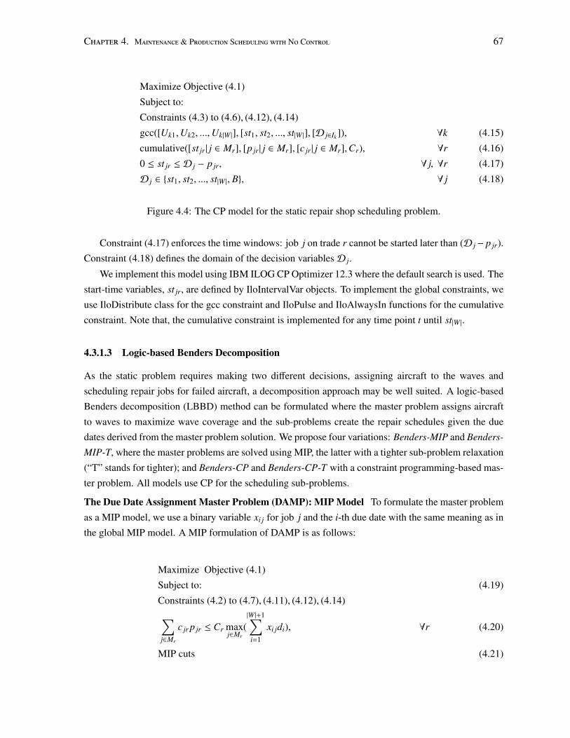
Chapter 4. Maintenance & Production Scheduling with No Control 67
Maximize Objective (4.1)
Subject to:
Constraints (4.3) to (4.6), (4.12), (4.14)
gcc([Uk1,Uk2, ...,Uk|W |], [st1, st2, ..., st|W |], [D j∈Ik ]), ∀k (4.15)
cumulative([st jr | j ∈ Mr], [p jr | j ∈ Mr], [c jr | j ∈ Mr],Cr), ∀r (4.16)
0 ≤ st jr ≤ D j − p jr, ∀ j, ∀r (4.17)
D j ∈ {st1, st2, ..., st|W |, B}, ∀ j (4.18)
Figure 4.4: The CP model for the static repair shop scheduling problem.
Constraint (4.17) enforces the time windows: job j on trade r cannot be started later than (D j− p jr).
Constraint (4.18) defines the domain of the decision variablesD j.
We implement this model using IBM ILOG CP Optimizer 12.3 where the default search is used. The
start-time variables, st jr, are defined by IloIntervalVar objects. To implement the global constraints, we
use IloDistribute class for the gcc constraint and IloPulse and IloAlwaysIn functions for the cumulative
constraint. Note that, the cumulative constraint is implemented for any time point t until st|W |.
4.3.1.3 Logic-based Benders Decomposition
As the static problem requires making two different decisions, assigning aircraft to the waves and
scheduling repair jobs for failed aircraft, a decomposition approach may be well suited. A logic-based
Benders decomposition (LBBD) method can be formulated where the master problem assigns aircraft
to waves to maximize wave coverage and the sub-problems create the repair schedules given the due
dates derived from the master problem solution. We propose four variations: Benders-MIP and Benders-
MIP-T, where the master problems are solved using MIP, the latter with a tighter sub-problem relaxation
(“T” stands for tighter); and Benders-CP and Benders-CP-T with a constraint programming-based mas-
ter problem. All models use CP for the scheduling sub-problems.
The Due Date Assignment Master Problem (DAMP): MIP Model To formulate the master problem
as a MIP model, we use a binary variable xi j for job j and the i-th due date with the same meaning as in
the global MIP model. A MIP formulation of DAMP is as follows:
Maximize Objective (4.1)
Subject to: (4.19)
Constraints (4.2) to (4.7), (4.11), (4.12), (4.14)∑j∈Mr
c jr p jr ≤ Cr maxj∈Mr
(|W |+1∑
i=1
xi jdi), ∀r (4.20)
MIP cuts (4.21)
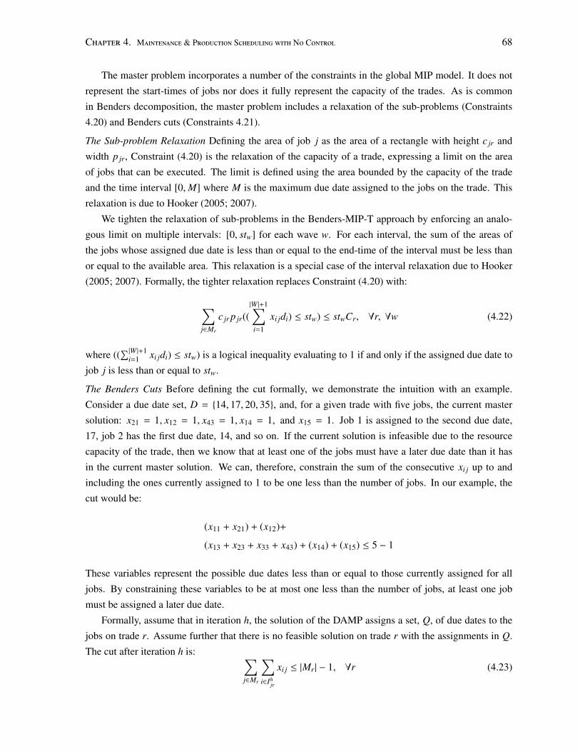
Chapter 4. Maintenance & Production Scheduling with No Control 68
The master problem incorporates a number of the constraints in the global MIP model. It does not
represent the start-times of jobs nor does it fully represent the capacity of the trades. As is common
in Benders decomposition, the master problem includes a relaxation of the sub-problems (Constraints
4.20) and Benders cuts (Constraints 4.21).
The Sub-problem Relaxation Defining the area of job j as the area of a rectangle with height c jr and
width p jr, Constraint (4.20) is the relaxation of the capacity of a trade, expressing a limit on the area
of jobs that can be executed. The limit is defined using the area bounded by the capacity of the trade
and the time interval [0,M] where M is the maximum due date assigned to the jobs on the trade. This
relaxation is due to Hooker (2005; 2007).
We tighten the relaxation of sub-problems in the Benders-MIP-T approach by enforcing an analo-
gous limit on multiple intervals: [0, stw] for each wave w. For each interval, the sum of the areas of
the jobs whose assigned due date is less than or equal to the end-time of the interval must be less than
or equal to the available area. This relaxation is a special case of the interval relaxation due to Hooker
(2005; 2007). Formally, the tighter relaxation replaces Constraint (4.20) with:
∑j∈Mr
c jr p jr((|W |+1∑
i=1
xi jdi) ≤ stw) ≤ stwCr, ∀r, ∀w (4.22)
where ((∑|W |+1
i=1 xi jdi) ≤ stw) is a logical inequality evaluating to 1 if and only if the assigned due date to
job j is less than or equal to stw.
The Benders Cuts Before defining the cut formally, we demonstrate the intuition with an example.
Consider a due date set, D = {14, 17, 20, 35}, and, for a given trade with five jobs, the current master
solution: x21 = 1, x12 = 1, x43 = 1, x14 = 1, and x15 = 1. Job 1 is assigned to the second due date,
17, job 2 has the first due date, 14, and so on. If the current solution is infeasible due to the resource
capacity of the trade, then we know that at least one of the jobs must have a later due date than it has
in the current master solution. We can, therefore, constrain the sum of the consecutive xi j up to and
including the ones currently assigned to 1 to be one less than the number of jobs. In our example, the
cut would be:
(x11 + x21) + (x12)+
(x13 + x23 + x33 + x43) + (x14) + (x15) ≤ 5 − 1
These variables represent the possible due dates less than or equal to those currently assigned for all
jobs. By constraining these variables to be at most one less than the number of jobs, at least one job
must be assigned a later due date.
Formally, assume that in iteration h, the solution of the DAMP assigns a set, Q, of due dates to the
jobs on trade r. Assume further that there is no feasible solution on trade r with the assignments in Q.
The cut after iteration h is: ∑j∈Mr
∑i∈Ih
jr
xi j ≤ |Mr | − 1, ∀r (4.23)
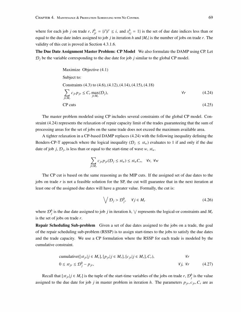
Chapter 4. Maintenance & Production Scheduling with No Control 69
where for each job j on trade r, Ihjr = {i′|i′ ≤ i, and xh
i j = 1} is the set of due date indices less than or
equal to the due date index assigned to job j in iteration h and |Mr | is the number of jobs on trade r. The
validity of this cut is proved in Section 4.3.1.6.
The Due Date Assignment Master Problem: CP Model We also formulate the DAMP using CP. Let
D j be the variable corresponding to the due date for job j similar to the global CP model.
Maximize Objective (4.1)
Subject to:
Constraints (4.3) to (4.6), (4.12), (4.14), (4.15), (4.18)∑j∈Mr
c jr p jr ≤ Cr maxj∈Mr
(D j), ∀r (4.24)
CP cuts (4.25)
The master problem modeled using CP includes several constraints of the global CP model. Con-
straint (4.24) represents the relaxation of repair capacity limit of the trades guaranteeing that the sum of
processing areas for the set of jobs on the same trade does not exceed the maximum available area.
A tighter relaxation in a CP-based DAMP replaces (4.24) with the following inequality defining the
Benders-CP-T approach where the logical inequality (D j ≤ stw) evaluates to 1 if and only if the due
date of job j,D j, is less than or equal to the start-time of wave w, stw.∑j∈Mr
c jr p jr(D j ≤ stw) ≤ stwCr, ∀r, ∀w
The CP cut is based on the same reasoning as the MIP cuts. If the assigned set of due dates to the
jobs on trade r is not a feasible solution for the SP, the cut will guarantee that in the next iteration at
least one of the assigned due dates will have a greater value. Formally, the cut is:∨D j > D
hj , ∀ j ∈ Mr (4.26)
whereDhj is the due date assigned to job j in iteration h,
∨represents the logical-or constraints and Mr
is the set of jobs on trade r.
Repair Scheduling Sub-problem Given a set of due dates assigned to the jobs on a trade, the goal
of the repair scheduling sub-problem (RSSP) is to assign start-times to the jobs to satisfy the due dates
and the trade capacity. We use a CP formulation where the RSSP for each trade is modeled by the
cumulative constraint.
cumulative([st jr | j ∈ Mr], [p jr | j ∈ Mr], [c jr | j ∈ Mr],Cr), ∀r
0 ≤ st jr ≤ Dhj − p jr, ∀ j, ∀r (4.27)
Recall that [st jr | j ∈ Mr] is the tuple of the start-time variables of the jobs on trade r,Dhj is the value
assigned to the due date for job j in master problem in iteration h. The parameters p jr, c jr,Cr are as
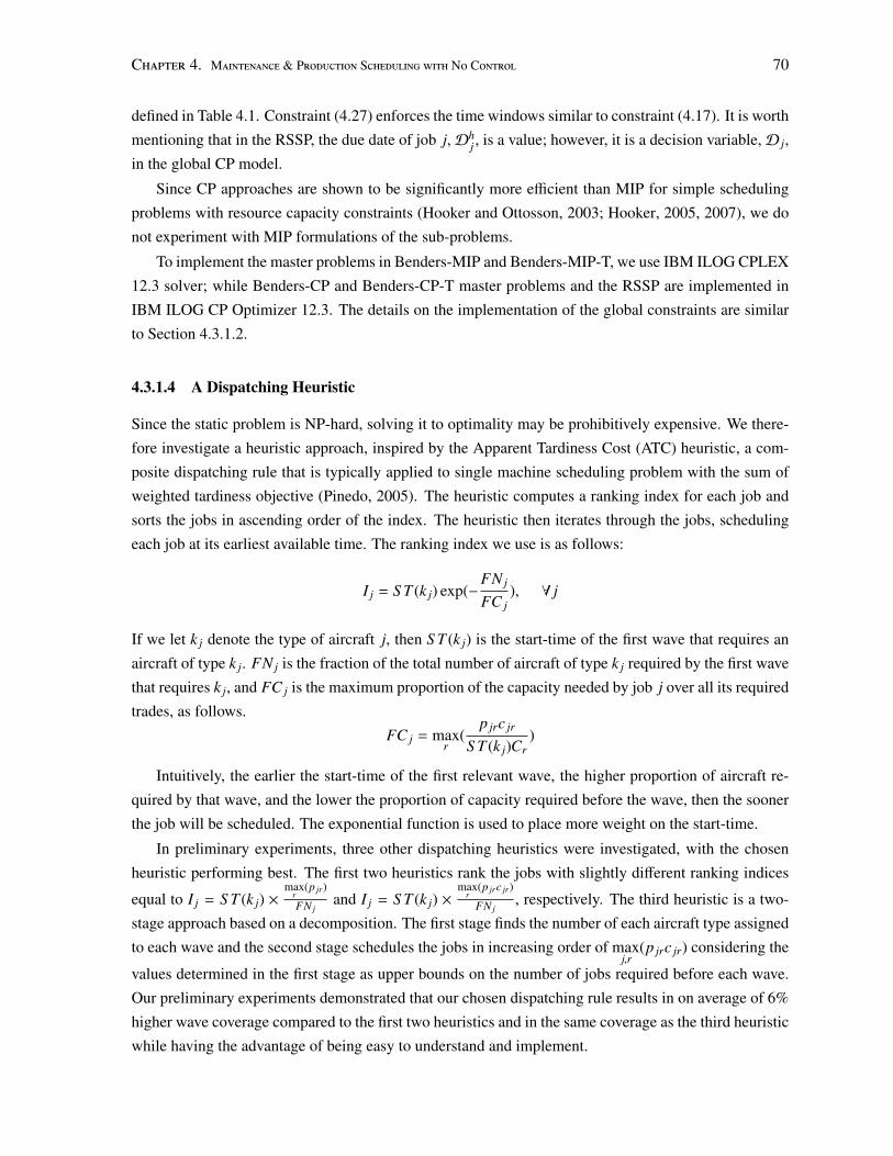
Chapter 4. Maintenance & Production Scheduling with No Control 70
defined in Table 4.1. Constraint (4.27) enforces the time windows similar to constraint (4.17). It is worth
mentioning that in the RSSP, the due date of job j,Dhj , is a value; however, it is a decision variable,D j,
in the global CP model.
Since CP approaches are shown to be significantly more efficient than MIP for simple scheduling
problems with resource capacity constraints (Hooker and Ottosson, 2003; Hooker, 2005, 2007), we do
not experiment with MIP formulations of the sub-problems.
To implement the master problems in Benders-MIP and Benders-MIP-T, we use IBM ILOG CPLEX
12.3 solver; while Benders-CP and Benders-CP-T master problems and the RSSP are implemented in
IBM ILOG CP Optimizer 12.3. The details on the implementation of the global constraints are similar
to Section 4.3.1.2.
4.3.1.4 A Dispatching Heuristic
Since the static problem is NP-hard, solving it to optimality may be prohibitively expensive. We there-
fore investigate a heuristic approach, inspired by the Apparent Tardiness Cost (ATC) heuristic, a com-
posite dispatching rule that is typically applied to single machine scheduling problem with the sum of
weighted tardiness objective (Pinedo, 2005). The heuristic computes a ranking index for each job and
sorts the jobs in ascending order of the index. The heuristic then iterates through the jobs, scheduling
each job at its earliest available time. The ranking index we use is as follows:
I j = S T (k j) exp(−FN j
FC j), ∀ j
If we let k j denote the type of aircraft j, then S T (k j) is the start-time of the first wave that requires an
aircraft of type k j. FN j is the fraction of the total number of aircraft of type k j required by the first wave
that requires k j, and FC j is the maximum proportion of the capacity needed by job j over all its required
trades, as follows.
FC j = maxr
(p jrc jr
S T (k j)Cr)
Intuitively, the earlier the start-time of the first relevant wave, the higher proportion of aircraft re-
quired by that wave, and the lower the proportion of capacity required before the wave, then the sooner
the job will be scheduled. The exponential function is used to place more weight on the start-time.
In preliminary experiments, three other dispatching heuristics were investigated, with the chosen
heuristic performing best. The first two heuristics rank the jobs with slightly different ranking indices
equal to I j = S T (k j) ×max
r(p jr)
FN jand I j = S T (k j) ×
maxr
(p jrc jr)
FN j, respectively. The third heuristic is a two-
stage approach based on a decomposition. The first stage finds the number of each aircraft type assigned
to each wave and the second stage schedules the jobs in increasing order of maxj,r
(p jrc jr) considering the
values determined in the first stage as upper bounds on the number of jobs required before each wave.
Our preliminary experiments demonstrated that our chosen dispatching rule results in on average of 6%
higher wave coverage compared to the first two heuristics and in the same coverage as the third heuristic
while having the advantage of being easy to understand and implement.
Chapter 4. Maintenance & Production Scheduling with No Control 71
4.3.1.5 Hybrid Heuristic-Complete Approaches
A hybrid heuristic-complete approach in which the heuristic solution provides a lower bound for the
maximization objective (Equation 4.1) may improve the performance of the complete approaches.
Therefore, a simple hybrid first runs the dispatching heuristic and then uses the objective value as a
starting lower bound for the complete approaches. Assume that the heuristic finds a solution, S , with
f (S ) as the number of aircraft assigned to waves. Any of the complete approaches can now be modified
by adding the following constraint:|W |∑w=1
|K|∑k=1
Zkw ≥ f (S )
For LBBD variations, the above constraint is added to the master problem.
4.3.1.6 Theoretical Results
To guarantee the finite convergence of a LBBD model to a globally optimal solution, the Benders cuts
must be valid and the master decision variables must have finite domains. A Benders cut is valid in a
given iteration, h, if and only if (1) it excludes the current globally infeasible assignment in the master
problem without (2) removing any globally optimal assignments (Chu and Xia, 2004). The former
guarantees the finite convergence and the latter guarantees the optimality. As the decision variables in
DAMP have a finite domain, it is sufficient to prove the satisfaction of the two conditions.
Theorem 4.2. Cut (4.23) is valid.
Proof. For condition (1), for the sub-problem in iteration h on trade r, by definition:∑j∈Mr
∑i∈Ih
jr
xi j = |Mr |
Consequently, cut (4.23) excludes the current assignment of master problem.
For condition (2), consider a global optimal solution S that does not satisfy cut (4.23) as generated
in iteration h. As the cut states that at least one job must have a greater due date than it had in h, to
violate the cut, all jobs in S must have equal or lesser due dates than they had in iteration h. However,
because the sub-problem was infeasible in iteration h, any sub-problem with only equal or lesser due
dates must also be infeasible as the available capacity on the trade is the same or less. Therefore, S must
be infeasible and we contradict the assumption that S is globally optimal.
Therefore, the cut is valid. �
An analogous argument holds for cut (4.26).
4.3.2 Rescheduling Strategies
The dynamic repair shop problem over the long horizon can be viewed as static scheduling sub-problems
over successive time periods. Let’s assume that we start repairing the failed aircraft and assigning them
Chapter 4. Maintenance & Production Scheduling with No Control 72
to the waves based on the computed schedule at time 0. A wave might start while a repair is under way in
the repair shop. If some aircraft fails the pre-flight check, it goes to the repair shop. Each failed aircraft
requires a set of independent repair activities with known processing times and resource requirements.
At the repair shop, some of the previously failed aircraft might be already repaired, some might be under
repair, and others might be awaiting repair. Once the failed aircraft enters the repair shop, we have a
new static repair scheduling sub-problem where the set of existing jobs (J), the number of aircraft not
in the repair shop for each aircraft type (ηk), and the failure rates of the aircraft (λn) are updated. The
set of existing jobs includes the recently failed aircraft and the previously failed aircraft whose repairs
are still under way or are not yet started. The new static sub-problem has an added constraint, namely
that the repairs currently under way cannot be disrupted.
We connect the static sub-problems using three different policies denoted as Pi j where i and j define
the length of scheduling horizon and the frequency of rescheduling in number of waves, respectively. In
all three policies, we schedule the repair activities, observe the aircraft failures, and respond to failures
by rescheduling the repair activities.
The three policies discussed here are as follows:
• P11: In Figure 4.5, we show that P11 schedules one wave at a time (i = 1) and reschedules after
each wave ( j = 1). P11 is a myopic policy aiming at providing the next first wave with the highest
possible coverage.
• P31: In contrast to P11, for P31 (Figure 4.5), the scheduling horizon is three waves but rescheduling
is still done after each wave. P31 with a longer scheduling horizon than P11 trades-off the coverage
among the next three waves. It is worth mentioning that we have chosen three as the length of the
scheduling horizon because three waves are usually scheduled daily based on the real data (Safaei
et al., 2011).
• P33: This policy has a scheduling horizon with a length of three waves and reschedules after every
third wave (Figure 4.5). P33 might trade-off the lower coverage of the next first wave for higher
coverages of the second and the third waves; however, it has a lower frequency of rescheduling.
4.3.3 Modeling the Aircraft Failures
To model the dynamic events, we simulate the aircraft failures in pre- and post-flight checks. Every
aircraft either passes or fails each check. If the aircraft fails, a new set of repair activities with known
processing times and resource requirements is added to the repair shop. If the aircraft passes, it flies the
wave if required. As mentioned in Section 4.1.1, after repair the failure rate of the aircraft returns to
what it was before the failure and it increases by γ percent each time it flies a wave due to deterioration.
If λn is the initial failure rate of the aircraft n ∈ N, its failure rate after flying w waves without failure
will be λn(1 + 0.01 × γ)w.
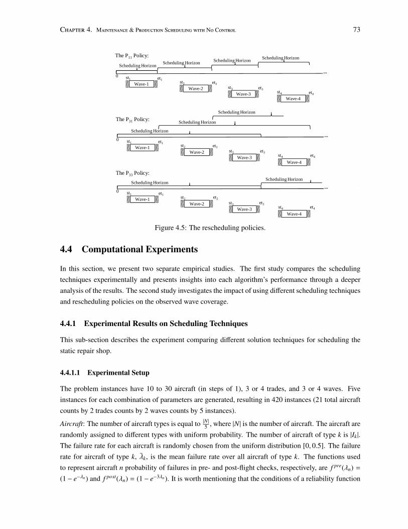
Chapter 4. Maintenance & Production Scheduling with No Control 73
Wave-1Wave-2
Wave-3
st1 et1 st2st3
et2et3
Wave-4st4 et4
0
Scheduling Horizon ...
Scheduling Horizon Scheduling Horizon Scheduling Horizon
Wave-1Wave-2
Wave-3
st1 et1 st2st3
et2et3
Wave-4st4 et4
0
Scheduling Horizon ...
Scheduling Horizon
The P31 Policy:
The P11 Policy:
The P33 Policy:
Wave-1Wave-2
Wave-3
st1 et1 st2st3
et2et3
Wave-4st4 et4
0
Scheduling Horizon ...
Scheduling Horizon
Scheduling Horizon
Figure 4.5: The rescheduling policies.
4.4 Computational Experiments
In this section, we present two separate empirical studies. The first study compares the scheduling
techniques experimentally and presents insights into each algorithm’s performance through a deeper
analysis of the results. The second study investigates the impact of using different scheduling techniques
and rescheduling policies on the observed wave coverage.
4.4.1 Experimental Results on Scheduling Techniques
This sub-section describes the experiment comparing different solution techniques for scheduling the
static repair shop.
4.4.1.1 Experimental Setup
The problem instances have 10 to 30 aircraft (in steps of 1), 3 or 4 trades, and 3 or 4 waves. Five
instances for each combination of parameters are generated, resulting in 420 instances (21 total aircraft
counts by 2 trades counts by 2 waves counts by 5 instances).
Aircraft: The number of aircraft types is equal to |N|5 , where |N | is the number of aircraft. The aircraft are
randomly assigned to different types with uniform probability. The number of aircraft of type k is |Ik|.
The failure rate for each aircraft is randomly chosen from the uniform distribution [0, 0.5]. The failure
rate for aircraft of type k, λk, is the mean failure rate over all aircraft of type k. The functions used
to represent aircraft n probability of failures in pre- and post-flight checks, respectively, are f pre(λn) =
(1 − e−λn) and f post(λn) = (1 − e−3λn). It is worth mentioning that the conditions of a reliability function
Chapter 4. Maintenance & Production Scheduling with No Control 74
in the extreme values of failure rates hold true for the functions used. If the failure rate goes to 0, the
probability of failure equals 0, and if the failure rate goes to∞, the probability of failure equals 1.
Waves: The plane requirement of each aircraft type for each wave is randomly generated from the integer
uniform distribution [1, |Ik|]. The length of each wave is drawn with uniform probability from [3, 5]. To
make an instance loose enough to permit feasible solutions yet tight enough to be challenging, a lower
bound on the length of the scheduling horizon (H) is needed. The sum of the processing areas of the
jobs in each trade, r, divided by the trade capacity is denoted by S r. LB = maxr
(S r) is a lower bound
on the time required to schedule all jobs and we use H = 1.2 × LB. The end-time for each wave, etw, is
generated as et|W | = H − rand[0, 3] for the final wave, |W |, and etw = stw+1 − rand[0, 3] for w < |W |.
Trades: The capacity limit for each trade is set at Cr = 10.
Repair Jobs: Eighty percent of the aircraft are in the repair shop at the beginning, resulting in |J| = 0.8|N |
repair jobs. The jobs are randomly assigned to the trades with replacement such that the number of jobs
per trade is equal to |J|/2. Each job requires at least one trade and some require more than one trade.
The capacity of trade r used by job j, c jr, is drawn from [1, 10] while the processing time, p jr, is drawn
from [r, 10r]: jobs on trades with lower indices have shorter processing times than those on trades with
higher indices.
Though our problem instances are generated randomly, the setting of our experiment includes three
numerical examples of Safaei et al. (2011) which are based on the real data. Furthermore, our setting
consists of more instances and results in problem instances which are one and a half times bigger than
the examples used in the literature (Safaei et al., 2011) where the number of aircraft is 10, 15, or 20; the
number of waves is 3 or 4; and the number of trades and aircraft types are equal to 3 and 2.
All experiments were run with a 7200-second time limit on an AMD 270 CPU with 1 MB cache per
core, 4 GB of main memory, running Red Hat Enterprise Linux 4.
4.4.1.2 Experimental Results
Figure 4.6 shows scatter-plots of run-times of the six complete approaches. Both axes are log-scale, and
the points below the line y = x indicate a lower run-time for the algorithm on the y-axis. The numbers
in the boxes indicate the number of points below or above the line. Run-times are counted as equal if
they differ less than 10%.
The graphs indicate a benefit for MIP over CP, for Benders-CP over MIP, for Benders-MIP over
Benders-CP and MIP, for Benders-MIP-T over Benders-MIP, and for Benders-CP-T over Benders-CP.
Table 4.2 presents further data, sorted in descending percentage of problems solved to optimality, for all
algorithms.
The mean run-time of the MIP model given in Safaei et al. (2011) over eight scenarios with 10
aircraft and 3 waves is 294.75 seconds. However, our proposed MIP model has the run-time of 2.64
seconds on average over ten of the instances with the same number of aircraft and waves, indicating that
it is significantly faster than Safaei et al.’s model.
MIP vs. CP The MIP approach has a clear superiority over the CP, achieving a lower run-time on
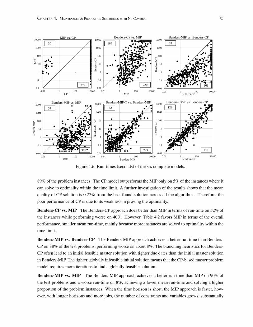
Chapter 4. Maintenance & Production Scheduling with No Control 75
0.01
0.1
1
10
100
1000
10000
0.01 1 100 10000
MIP
CP
MIP vs. CP
23
0.01
0.1
1
10
100
1000
10000
0.01 1 100 10000B
ende
rs-C
PMIP
Benders-CP vs. MIP
0.01
0.1
1
10
100
1000
10000
0.01 1 100 10000
Ben
ders
-MIP
Benders-CP
Benders-MIP vs. Benders-CP
1000
10000Benders-MIP vs. MIP
1000
10000 Benders-MIP-T vs. Benders-MIP
20
372 220
169 35
368
34 1621000
10000 Benders-CP-T vs. Benders-CP122
0.01
0.1
1
10
100
1000
0.01 1 100 10000
Ben
ders
-MIP
MIP
0.01
0.1
1
10
100
1000
0.01 1 100 10000
Ben
ders
-MIP
-T
Benders-MIP
34 162
2293780.01
0.1
1
10
100
1000
0.01 1 100 10000B
ende
rs-C
P-T
Benders-CP
122
161
Figure 4.6: Run-times (seconds) of the six complete models.
89% of the problem instances. The CP model outperforms the MIP only on 5% of the instances where it
can solve to optimality within the time limit. A further investigation of the results shows that the mean
quality of CP solution is 0.27% from the best found solution across all the algorithms. Therefore, the
poor performance of CP is due to its weakness in proving the optimality.
Benders-CP vs. MIP The Benders-CP approach does better than MIP in terms of run-time on 52% of
the instances while performing worse on 40%. However, Table 4.2 favors MIP in terms of the overall
performance, smaller mean run-time, mainly because more instances are solved to optimality within the
time limit.
Benders-MIP vs. Benders-CP The Benders-MIP approach achieves a better run-time than Benders-
CP on 88% of the test problems, performing worse on about 8%. The branching heuristics for Benders-
CP often lead to an initial feasible master solution with tighter due dates than the initial master solution
in Benders-MIP. The tighter, globally infeasible initial solution means that the CP-based master problem
model requires more iterations to find a globally feasible solution.
Benders-MIP vs. MIP The Benders-MIP approach achieves a better run-time than MIP on 90% of
the test problems and a worse run-time on 8%, achieving a lower mean run-time and solving a higher
proportion of the problem instances. When the time horizon is short, the MIP approach is faster, how-
ever, with longer horizons and more jobs, the number of constraints and variables grows, substantially
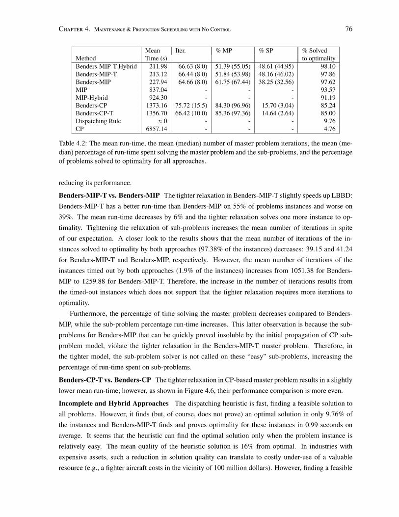
Chapter 4. Maintenance & Production Scheduling with No Control 76
Mean Iter. % MP % SP % SolvedMethod Time (s) to optimalityBenders-MIP-T-Hybrid 211.98 66.63 (8.0) 51.39 (55.05) 48.61 (44.95) 98.10Benders-MIP-T 213.12 66.44 (8.0) 51.84 (53.98) 48.16 (46.02) 97.86Benders-MIP 227.94 64.66 (8.0) 61.75 (67.44) 38.25 (32.56) 97.62MIP 837.04 - - - 93.57MIP-Hybrid 924.30 - - - 91.19Benders-CP 1373.16 75.72 (15.5) 84.30 (96.96) 15.70 (3.04) 85.24Benders-CP-T 1356.70 66.42 (10.0) 85.36 (97.36) 14.64 (2.64) 85.00Dispatching Rule ≈ 0 - - - 9.76CP 6857.14 - - - 4.76
Table 4.2: The mean run-time, the mean (median) number of master problem iterations, the mean (me-dian) percentage of run-time spent solving the master problem and the sub-problems, and the percentageof problems solved to optimality for all approaches.
reducing its performance.
Benders-MIP-T vs. Benders-MIP The tighter relaxation in Benders-MIP-T slightly speeds up LBBD:
Benders-MIP-T has a better run-time than Benders-MIP on 55% of problems instances and worse on
39%. The mean run-time decreases by 6% and the tighter relaxation solves one more instance to op-
timality. Tightening the relaxation of sub-problems increases the mean number of iterations in spite
of our expectation. A closer look to the results shows that the mean number of iterations of the in-
stances solved to optimality by both approaches (97.38% of the instances) decreases: 39.15 and 41.24
for Benders-MIP-T and Benders-MIP, respectively. However, the mean number of iterations of the
instances timed out by both approaches (1.9% of the instances) increases from 1051.38 for Benders-
MIP to 1259.88 for Benders-MIP-T. Therefore, the increase in the number of iterations results from
the timed-out instances which does not support that the tighter relaxation requires more iterations to
optimality.
Furthermore, the percentage of time solving the master problem decreases compared to Benders-
MIP, while the sub-problem percentage run-time increases. This latter observation is because the sub-
problems for Benders-MIP that can be quickly proved insoluble by the initial propagation of CP sub-
problem model, violate the tighter relaxation in the Benders-MIP-T master problem. Therefore, in
the tighter model, the sub-problem solver is not called on these “easy” sub-problems, increasing the
percentage of run-time spent on sub-problems.
Benders-CP-T vs. Benders-CP The tighter relaxation in CP-based master problem results in a slightly
lower mean run-time; however, as shown in Figure 4.6, their performance comparison is more even.
Incomplete and Hybrid Approaches The dispatching heuristic is fast, finding a feasible solution to
all problems. However, it finds (but, of course, does not prove) an optimal solution in only 9.76% of
the instances and Benders-MIP-T finds and proves optimality for these instances in 0.99 seconds on
average. It seems that the heuristic can find the optimal solution only when the problem instance is
relatively easy. The mean quality of the heuristic solution is 16% from optimal. In industries with
expensive assets, such a reduction in solution quality can translate to costly under-use of a valuable
resource (e.g., a fighter aircraft costs in the vicinity of 100 million dollars). However, finding a feasible
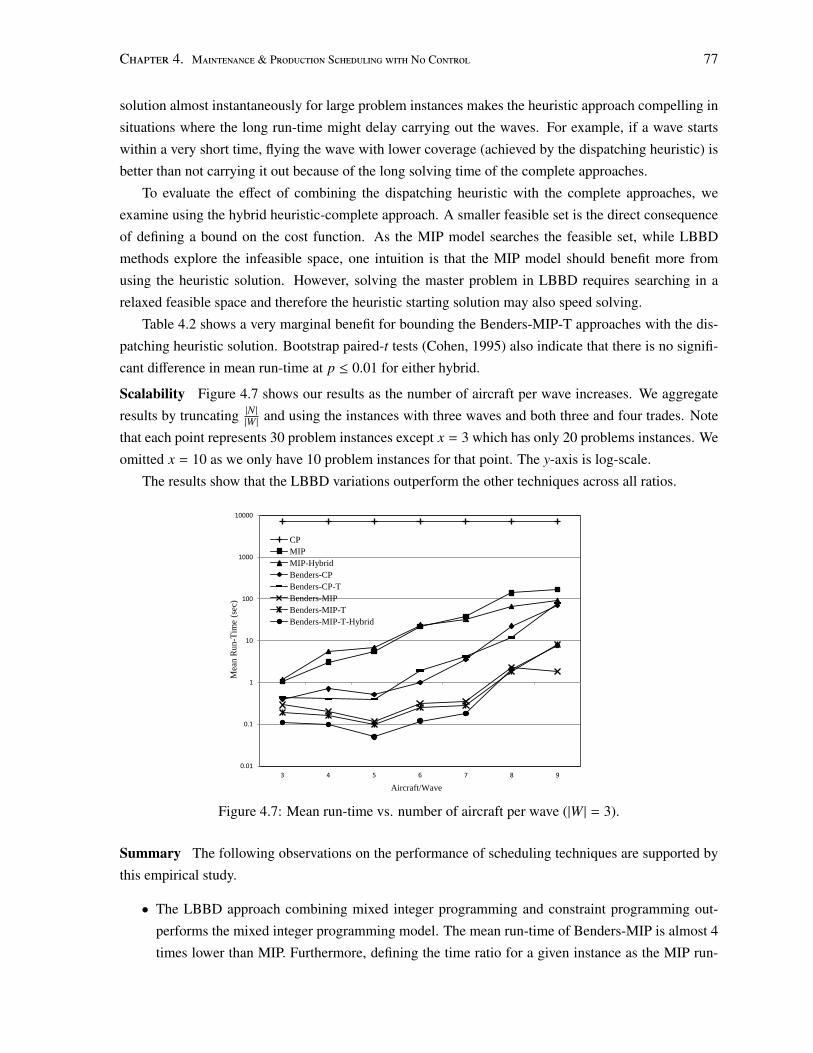
Chapter 4. Maintenance & Production Scheduling with No Control 77
solution almost instantaneously for large problem instances makes the heuristic approach compelling in
situations where the long run-time might delay carrying out the waves. For example, if a wave starts
within a very short time, flying the wave with lower coverage (achieved by the dispatching heuristic) is
better than not carrying it out because of the long solving time of the complete approaches.
To evaluate the effect of combining the dispatching heuristic with the complete approaches, we
examine using the hybrid heuristic-complete approach. A smaller feasible set is the direct consequence
of defining a bound on the cost function. As the MIP model searches the feasible set, while LBBD
methods explore the infeasible space, one intuition is that the MIP model should benefit more from
using the heuristic solution. However, solving the master problem in LBBD requires searching in a
relaxed feasible space and therefore the heuristic starting solution may also speed solving.
Table 4.2 shows a very marginal benefit for bounding the Benders-MIP-T approaches with the dis-
patching heuristic solution. Bootstrap paired-t tests (Cohen, 1995) also indicate that there is no signifi-
cant difference in mean run-time at p ≤ 0.01 for either hybrid.
Scalability Figure 4.7 shows our results as the number of aircraft per wave increases. We aggregate
results by truncating |N||W | and using the instances with three waves and both three and four trades. Note
that each point represents 30 problem instances except x = 3 which has only 20 problems instances. We
omitted x = 10 as we only have 10 problem instances for that point. The y-axis is log-scale.
The results show that the LBBD variations outperform the other techniques across all ratios.
0.01
0.1
1
10
100
1000
10000
3 4 5 6 7 8 9
Mea
n R
un-T
ime
(sec
)
Aircraft/Wave
CP
MIP
MIP-Hybrid
Benders-CP
Benders-CP-T
Benders-MIP
Benders-MIP-T
Benders-MIP-T-Hybrid
Figure 4.7: Mean run-time vs. number of aircraft per wave (|W | = 3).
Summary The following observations on the performance of scheduling techniques are supported by
this empirical study.
• The LBBD approach combining mixed integer programming and constraint programming out-
performs the mixed integer programming model. The mean run-time of Benders-MIP is almost 4
times lower than MIP. Furthermore, defining the time ratio for a given instance as the MIP run-
Chapter 4. Maintenance & Production Scheduling with No Control 78
time divided by Benders-MIP run-time, the Benders-MIP is almost 32 times faster than MIP, on
average, with a geometric mean time ratio of 31.56. The time ratios range is [0.01, 94132.67] with
a median of 38.32.
• A tighter relaxation slightly speeds up LBBD. Benders-MIP-T and Benders-CP-T, both, have a
run-time about 1.2 times faster than Benders-MIP and Benders-CP, respectively.
• A dispatching heuristic can provide the optimal solution for the easy problem instances. However,
the mean percent relative error of heuristic is almost 16% overall, indicating that the dispatching
rule by itself is not effective enough for industries with high equipment cost.
• The simple hybridization of the complete approaches with the dispatching heuristic does not result
in a statistically significant difference in run-time.
4.4.2 Experimental Results on Rescheduling Strategies
This sub-section describes experiment investigating the impact of applying different scheduling tech-
niques and rescheduling policies in a dynamic repair shop.
4.4.2.1 Experimental Setup
For our problem instances, the number of aircraft, the number of trades, and the total number of waves
are set to {10, 15, 20, 25, 30}, {4}, and {30} respectively. Each combination has 5 instances for a total
of 25 instances. Each instance is simulated 20 times. The parameters of the problem instances are
generated as in Section 4.4.1 with the following modifications:
Aircraft: The failure rate of an aircraft is increased by γ = 5 percent each time it is used.
Repair Jobs: Repair jobs that entered repair shop after time 0 are randomly assigned to the trades. The
probability of assigning a job to each trade is considered as 0.5.
Waves: The start-time of each wave is generated as st1 = rand[ H3 ,
H2 ] for the first wave, and stw =
etw−1 + rand(0, 40) for 1 < w ≤ 30. As mentioned earlier the total number of waves is 30. The value of
H is calculated as in Section 4.4.1.
Dynamic events: To simulate an aircraft failure, we generate a random value from the uniform distribu-
tion [0, 1] for each aircraft at each check. If the random value is less than the aircraft’s probability of
failure, the aircraft fails; otherwise, it passes. The aircraft’s probability of failure in pre- and post-flight
checks are calculated using (1 − e−λn) and (1 − e−3λn), respectively. Recall that, λn is the failure rate
of aircraft, n ∈ N, which increases by γ = 5 percent each time the aircraft flies a wave. Note that
passing the pre-flight check of a wave does not necessarily mean that the aircraft flies the wave. If the
number of available aircraft is more than the requirements, the aircraft that fly are randomly selected
from those that passed the pre-flight check to meet the requirements. Our latter assumption implies that
all aircraft ready at the beginning of a wave are checked regardless of the wave requirements. Since
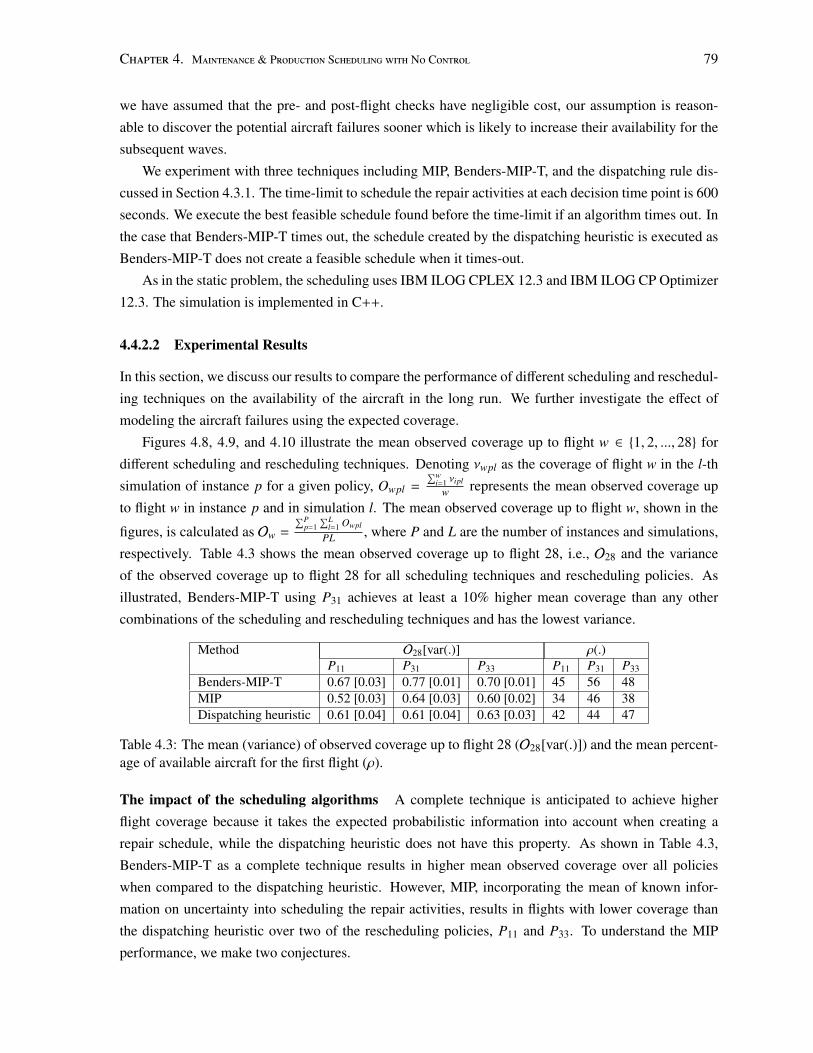
Chapter 4. Maintenance & Production Scheduling with No Control 79
we have assumed that the pre- and post-flight checks have negligible cost, our assumption is reason-
able to discover the potential aircraft failures sooner which is likely to increase their availability for the
subsequent waves.
We experiment with three techniques including MIP, Benders-MIP-T, and the dispatching rule dis-
cussed in Section 4.3.1. The time-limit to schedule the repair activities at each decision time point is 600
seconds. We execute the best feasible schedule found before the time-limit if an algorithm times out. In
the case that Benders-MIP-T times out, the schedule created by the dispatching heuristic is executed as
Benders-MIP-T does not create a feasible schedule when it times-out.
As in the static problem, the scheduling uses IBM ILOG CPLEX 12.3 and IBM ILOG CP Optimizer
12.3. The simulation is implemented in C++.
4.4.2.2 Experimental Results
In this section, we discuss our results to compare the performance of different scheduling and reschedul-
ing techniques on the availability of the aircraft in the long run. We further investigate the effect of
modeling the aircraft failures using the expected coverage.
Figures 4.8, 4.9, and 4.10 illustrate the mean observed coverage up to flight w ∈ {1, 2, ..., 28} for
different scheduling and rescheduling techniques. Denoting νwpl as the coverage of flight w in the l-th
simulation of instance p for a given policy, Owpl =∑w
i=1 νipl
w represents the mean observed coverage up
to flight w in instance p and in simulation l. The mean observed coverage up to flight w, shown in the
figures, is calculated as Ow =
∑Pp=1
∑Ll=1 Owpl
PL , where P and L are the number of instances and simulations,
respectively. Table 4.3 shows the mean observed coverage up to flight 28, i.e., O28 and the variance
of the observed coverage up to flight 28 for all scheduling techniques and rescheduling policies. As
illustrated, Benders-MIP-T using P31 achieves at least a 10% higher mean coverage than any other
combinations of the scheduling and rescheduling techniques and has the lowest variance.
Method O28[var(.)] ρ(.)P11 P31 P33 P11 P31 P33
Benders-MIP-T 0.67 [0.03] 0.77 [0.01] 0.70 [0.01] 45 56 48MIP 0.52 [0.03] 0.64 [0.03] 0.60 [0.02] 34 46 38Dispatching heuristic 0.61 [0.04] 0.61 [0.04] 0.63 [0.03] 42 44 47
Table 4.3: The mean (variance) of observed coverage up to flight 28 (O28[var(.)]) and the mean percent-age of available aircraft for the first flight (ρ).
The impact of the scheduling algorithms A complete technique is anticipated to achieve higher
flight coverage because it takes the expected probabilistic information into account when creating a
repair schedule, while the dispatching heuristic does not have this property. As shown in Table 4.3,
Benders-MIP-T as a complete technique results in higher mean observed coverage over all policies
when compared to the dispatching heuristic. However, MIP, incorporating the mean of known infor-
mation on uncertainty into scheduling the repair activities, results in flights with lower coverage than
the dispatching heuristic over two of the rescheduling policies, P11 and P33. To understand the MIP
performance, we make two conjectures.
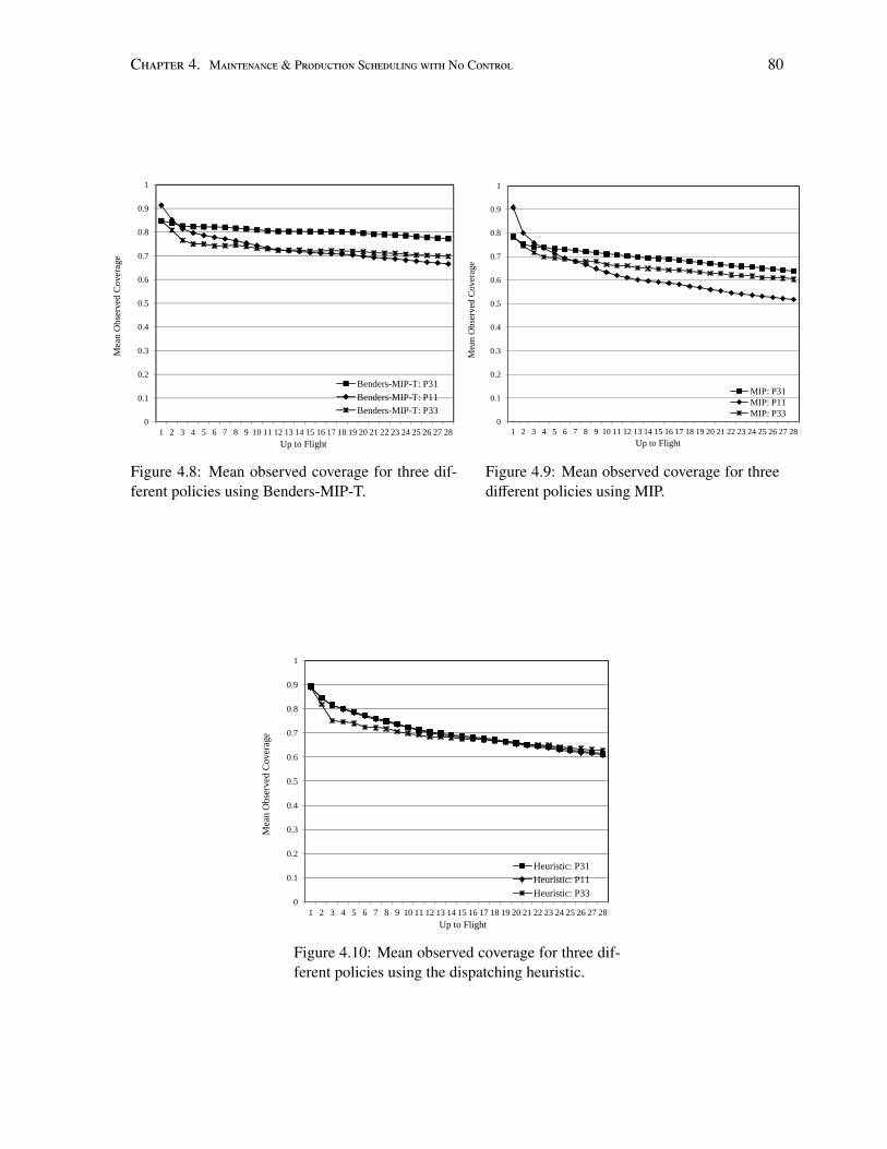
Chapter 4. Maintenance & Production Scheduling with No Control 80
0
0.1
0.2
0.3
0.4
0.5
0.6
0.7
0.8
0.9
1
1 2 3 4 5 6 7 8 9 10 11 12 13 14 15 16 17 18 19 20 21 22 23 24 25 26 27 28
Mea
n O
bser
ved
Cov
erag
e
Up to Flight
Benders-MIP-T: P31
Benders-MIP-T: P11
Benders-MIP-T: P33
Figure 4.8: Mean observed coverage for three dif-ferent policies using Benders-MIP-T.
0
0.1
0.2
0.3
0.4
0.5
0.6
0.7
0.8
0.9
1
1 2 3 4 5 6 7 8 9 10 11 12 13 14 15 16 17 18 19 20 21 22 23 24 25 26 27 28
Mea
n O
bse
rved
Co
ver
age
Up to Flight
MIP: P31
MIP: P11
MIP: P33
Figure 4.9: Mean observed coverage for threedifferent policies using MIP.
0
0.1
0.2
0.3
0.4
0.5
0.6
0.7
0.8
0.9
1
1 2 3 4 5 6 7 8 9 10 11 12 13 14 15 16 17 18 19 20 21 22 23 24 25 26 27 28
Mea
n O
bse
rved
Co
ver
age
Up to Flight
Heuristic: P31
Heuristic: P11
Heuristic: P33
Figure 4.10: Mean observed coverage for three dif-ferent policies using the dispatching heuristic.
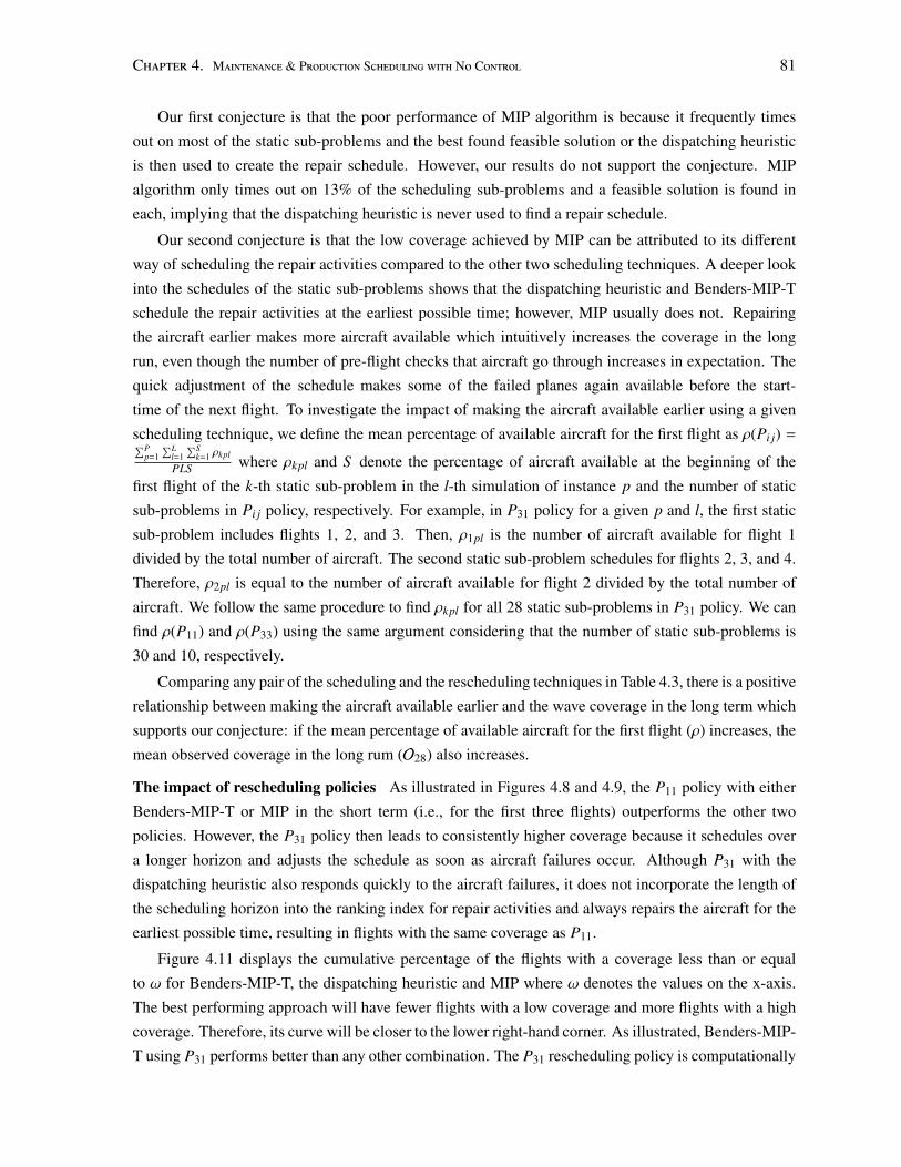
Chapter 4. Maintenance & Production Scheduling with No Control 81
Our first conjecture is that the poor performance of MIP algorithm is because it frequently times
out on most of the static sub-problems and the best found feasible solution or the dispatching heuristic
is then used to create the repair schedule. However, our results do not support the conjecture. MIP
algorithm only times out on 13% of the scheduling sub-problems and a feasible solution is found in
each, implying that the dispatching heuristic is never used to find a repair schedule.
Our second conjecture is that the low coverage achieved by MIP can be attributed to its different
way of scheduling the repair activities compared to the other two scheduling techniques. A deeper look
into the schedules of the static sub-problems shows that the dispatching heuristic and Benders-MIP-T
schedule the repair activities at the earliest possible time; however, MIP usually does not. Repairing
the aircraft earlier makes more aircraft available which intuitively increases the coverage in the long
run, even though the number of pre-flight checks that aircraft go through increases in expectation. The
quick adjustment of the schedule makes some of the failed planes again available before the start-
time of the next flight. To investigate the impact of making the aircraft available earlier using a given
scheduling technique, we define the mean percentage of available aircraft for the first flight as ρ(Pi j) =∑Pp=1
∑Ll=1
∑Sk=1 ρkpl
PLS where ρkpl and S denote the percentage of aircraft available at the beginning of the
first flight of the k-th static sub-problem in the l-th simulation of instance p and the number of static
sub-problems in Pi j policy, respectively. For example, in P31 policy for a given p and l, the first static
sub-problem includes flights 1, 2, and 3. Then, ρ1pl is the number of aircraft available for flight 1
divided by the total number of aircraft. The second static sub-problem schedules for flights 2, 3, and 4.
Therefore, ρ2pl is equal to the number of aircraft available for flight 2 divided by the total number of
aircraft. We follow the same procedure to find ρkpl for all 28 static sub-problems in P31 policy. We can
find ρ(P11) and ρ(P33) using the same argument considering that the number of static sub-problems is
30 and 10, respectively.
Comparing any pair of the scheduling and the rescheduling techniques in Table 4.3, there is a positive
relationship between making the aircraft available earlier and the wave coverage in the long term which
supports our conjecture: if the mean percentage of available aircraft for the first flight (ρ) increases, the
mean observed coverage in the long rum (O28) also increases.
The impact of rescheduling policies As illustrated in Figures 4.8 and 4.9, the P11 policy with either
Benders-MIP-T or MIP in the short term (i.e., for the first three flights) outperforms the other two
policies. However, the P31 policy then leads to consistently higher coverage because it schedules over
a longer horizon and adjusts the schedule as soon as aircraft failures occur. Although P31 with the
dispatching heuristic also responds quickly to the aircraft failures, it does not incorporate the length of
the scheduling horizon into the ranking index for repair activities and always repairs the aircraft for the
earliest possible time, resulting in flights with the same coverage as P11.
Figure 4.11 displays the cumulative percentage of the flights with a coverage less than or equal
to ω for Benders-MIP-T, the dispatching heuristic and MIP where ω denotes the values on the x-axis.
The best performing approach will have fewer flights with a low coverage and more flights with a high
coverage. Therefore, its curve will be closer to the lower right-hand corner. As illustrated, Benders-MIP-
T using P31 performs better than any other combination. The P31 rescheduling policy is computationally
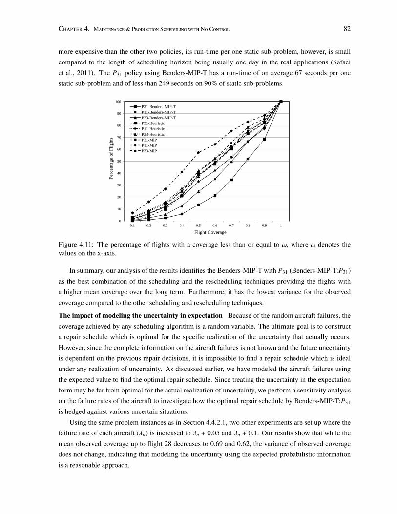
Chapter 4. Maintenance & Production Scheduling with No Control 82
more expensive than the other two policies, its run-time per one static sub-problem, however, is small
compared to the length of scheduling horizon being usually one day in the real applications (Safaei
et al., 2011). The P31 policy using Benders-MIP-T has a run-time of on average 67 seconds per one
static sub-problem and of less than 249 seconds on 90% of static sub-problems.
0
10
20
30
40
50
60
70
80
90
100
0.1 0.2 0.3 0.4 0.5 0.6 0.7 0.8 0.9 1
Per
centa
ge
of
Fli
ghts
Flight Coverage
P31-Benders-MIP-T
P11-Benders-MIP-T
P33-Benders-MIP-T
P31-Heuristic
P11-Heuristic
P33-Heuristic
P31-MIP
P11-MIP
P33-MIP
Figure 4.11: The percentage of flights with a coverage less than or equal to ω, where ω denotes thevalues on the x-axis.
In summary, our analysis of the results identifies the Benders-MIP-T with P31 (Benders-MIP-T:P31)
as the best combination of the scheduling and the rescheduling techniques providing the flights with
a higher mean coverage over the long term. Furthermore, it has the lowest variance for the observed
coverage compared to the other scheduling and rescheduling techniques.
The impact of modeling the uncertainty in expectation Because of the random aircraft failures, the
coverage achieved by any scheduling algorithm is a random variable. The ultimate goal is to construct
a repair schedule which is optimal for the specific realization of the uncertainty that actually occurs.
However, since the complete information on the aircraft failures is not known and the future uncertainty
is dependent on the previous repair decisions, it is impossible to find a repair schedule which is ideal
under any realization of uncertainty. As discussed earlier, we have modeled the aircraft failures using
the expected value to find the optimal repair schedule. Since treating the uncertainty in the expectation
form may be far from optimal for the actual realization of uncertainty, we perform a sensitivity analysis
on the failure rates of the aircraft to investigate how the optimal repair schedule by Benders-MIP-T:P31
is hedged against various uncertain situations.
Using the same problem instances as in Section 4.4.2.1, two other experiments are set up where the
failure rate of each aircraft (λn) is increased to λn + 0.05 and λn + 0.1. Our results show that while the
mean observed coverage up to flight 28 decreases to 0.69 and 0.62, the variance of observed coverage
does not change, indicating that modeling the uncertainty using the expected probabilistic information
is a reasonable approach.
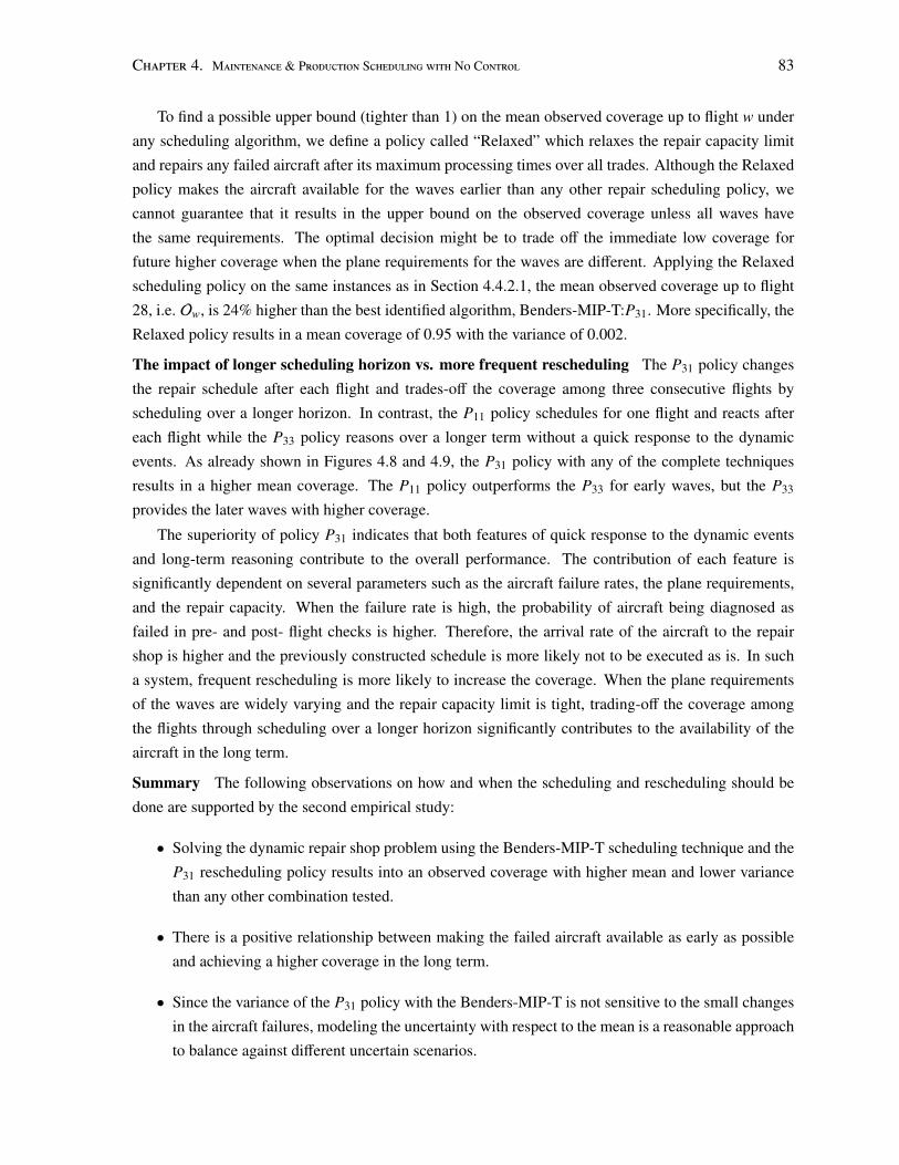
Chapter 4. Maintenance & Production Scheduling with No Control 83
To find a possible upper bound (tighter than 1) on the mean observed coverage up to flight w under
any scheduling algorithm, we define a policy called “Relaxed” which relaxes the repair capacity limit
and repairs any failed aircraft after its maximum processing times over all trades. Although the Relaxed
policy makes the aircraft available for the waves earlier than any other repair scheduling policy, we
cannot guarantee that it results in the upper bound on the observed coverage unless all waves have
the same requirements. The optimal decision might be to trade off the immediate low coverage for
future higher coverage when the plane requirements for the waves are different. Applying the Relaxed
scheduling policy on the same instances as in Section 4.4.2.1, the mean observed coverage up to flight
28, i.e. Ow, is 24% higher than the best identified algorithm, Benders-MIP-T:P31. More specifically, the
Relaxed policy results in a mean coverage of 0.95 with the variance of 0.002.
The impact of longer scheduling horizon vs. more frequent rescheduling The P31 policy changes
the repair schedule after each flight and trades-off the coverage among three consecutive flights by
scheduling over a longer horizon. In contrast, the P11 policy schedules for one flight and reacts after
each flight while the P33 policy reasons over a longer term without a quick response to the dynamic
events. As already shown in Figures 4.8 and 4.9, the P31 policy with any of the complete techniques
results in a higher mean coverage. The P11 policy outperforms the P33 for early waves, but the P33
provides the later waves with higher coverage.
The superiority of policy P31 indicates that both features of quick response to the dynamic events
and long-term reasoning contribute to the overall performance. The contribution of each feature is
significantly dependent on several parameters such as the aircraft failure rates, the plane requirements,
and the repair capacity. When the failure rate is high, the probability of aircraft being diagnosed as
failed in pre- and post- flight checks is higher. Therefore, the arrival rate of the aircraft to the repair
shop is higher and the previously constructed schedule is more likely not to be executed as is. In such
a system, frequent rescheduling is more likely to increase the coverage. When the plane requirements
of the waves are widely varying and the repair capacity limit is tight, trading-off the coverage among
the flights through scheduling over a longer horizon significantly contributes to the availability of the
aircraft in the long term.
Summary The following observations on how and when the scheduling and rescheduling should be
done are supported by the second empirical study:
• Solving the dynamic repair shop problem using the Benders-MIP-T scheduling technique and the
P31 rescheduling policy results into an observed coverage with higher mean and lower variance
than any other combination tested.
• There is a positive relationship between making the failed aircraft available as early as possible
and achieving a higher coverage in the long term.
• Since the variance of the P31 policy with the Benders-MIP-T is not sensitive to the small changes
in the aircraft failures, modeling the uncertainty with respect to the mean is a reasonable approach
to balance against different uncertain scenarios.
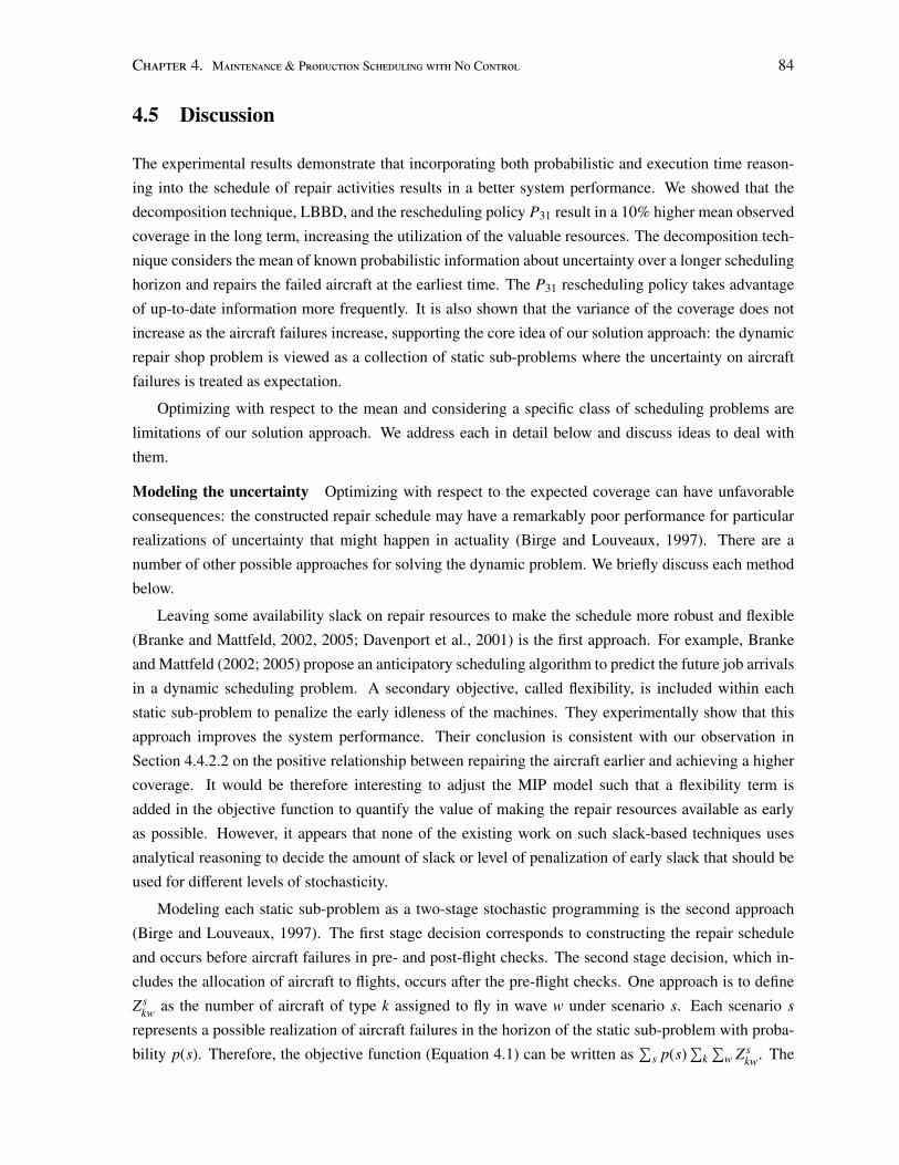
Chapter 4. Maintenance & Production Scheduling with No Control 84
4.5 Discussion
The experimental results demonstrate that incorporating both probabilistic and execution time reason-
ing into the schedule of repair activities results in a better system performance. We showed that the
decomposition technique, LBBD, and the rescheduling policy P31 result in a 10% higher mean observed
coverage in the long term, increasing the utilization of the valuable resources. The decomposition tech-
nique considers the mean of known probabilistic information about uncertainty over a longer scheduling
horizon and repairs the failed aircraft at the earliest time. The P31 rescheduling policy takes advantage
of up-to-date information more frequently. It is also shown that the variance of the coverage does not
increase as the aircraft failures increase, supporting the core idea of our solution approach: the dynamic
repair shop problem is viewed as a collection of static sub-problems where the uncertainty on aircraft
failures is treated as expectation.
Optimizing with respect to the mean and considering a specific class of scheduling problems are
limitations of our solution approach. We address each in detail below and discuss ideas to deal with
them.
Modeling the uncertainty Optimizing with respect to the expected coverage can have unfavorable
consequences: the constructed repair schedule may have a remarkably poor performance for particular
realizations of uncertainty that might happen in actuality (Birge and Louveaux, 1997). There are a
number of other possible approaches for solving the dynamic problem. We briefly discuss each method
below.
Leaving some availability slack on repair resources to make the schedule more robust and flexible
(Branke and Mattfeld, 2002, 2005; Davenport et al., 2001) is the first approach. For example, Branke
and Mattfeld (2002; 2005) propose an anticipatory scheduling algorithm to predict the future job arrivals
in a dynamic scheduling problem. A secondary objective, called flexibility, is included within each
static sub-problem to penalize the early idleness of the machines. They experimentally show that this
approach improves the system performance. Their conclusion is consistent with our observation in
Section 4.4.2.2 on the positive relationship between repairing the aircraft earlier and achieving a higher
coverage. It would be therefore interesting to adjust the MIP model such that a flexibility term is
added in the objective function to quantify the value of making the repair resources available as early
as possible. However, it appears that none of the existing work on such slack-based techniques uses
analytical reasoning to decide the amount of slack or level of penalization of early slack that should be
used for different levels of stochasticity.
Modeling each static sub-problem as a two-stage stochastic programming is the second approach
(Birge and Louveaux, 1997). The first stage decision corresponds to constructing the repair schedule
and occurs before aircraft failures in pre- and post-flight checks. The second stage decision, which in-
cludes the allocation of aircraft to flights, occurs after the pre-flight checks. One approach is to define
Z skw as the number of aircraft of type k assigned to fly in wave w under scenario s. Each scenario s
represents a possible realization of aircraft failures in the horizon of the static sub-problem with proba-
bility p(s). Therefore, the objective function (Equation 4.1) can be written as∑
s p(s)∑
k∑
w Z skw. The
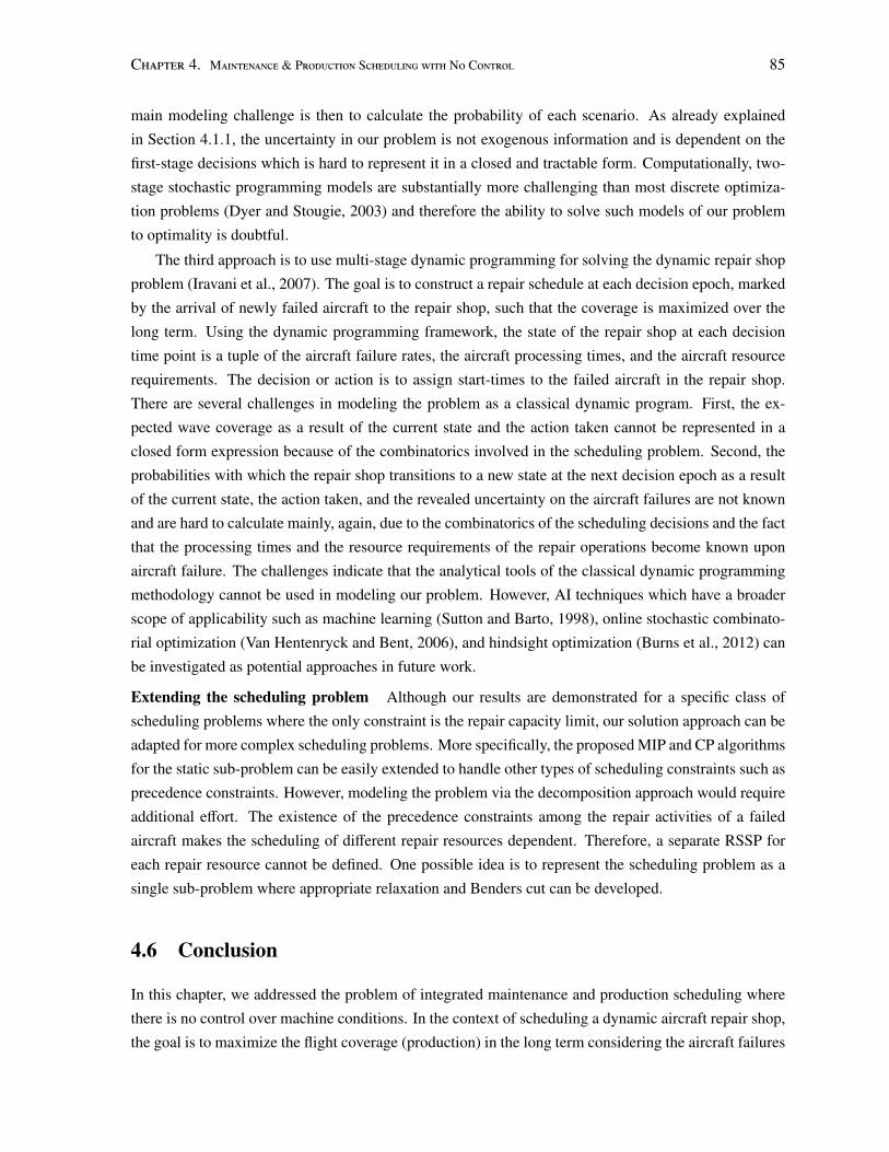
Chapter 4. Maintenance & Production Scheduling with No Control 85
main modeling challenge is then to calculate the probability of each scenario. As already explained
in Section 4.1.1, the uncertainty in our problem is not exogenous information and is dependent on the
first-stage decisions which is hard to represent it in a closed and tractable form. Computationally, two-
stage stochastic programming models are substantially more challenging than most discrete optimiza-
tion problems (Dyer and Stougie, 2003) and therefore the ability to solve such models of our problem
to optimality is doubtful.
The third approach is to use multi-stage dynamic programming for solving the dynamic repair shop
problem (Iravani et al., 2007). The goal is to construct a repair schedule at each decision epoch, marked
by the arrival of newly failed aircraft to the repair shop, such that the coverage is maximized over the
long term. Using the dynamic programming framework, the state of the repair shop at each decision
time point is a tuple of the aircraft failure rates, the aircraft processing times, and the aircraft resource
requirements. The decision or action is to assign start-times to the failed aircraft in the repair shop.
There are several challenges in modeling the problem as a classical dynamic program. First, the ex-
pected wave coverage as a result of the current state and the action taken cannot be represented in a
closed form expression because of the combinatorics involved in the scheduling problem. Second, the
probabilities with which the repair shop transitions to a new state at the next decision epoch as a result
of the current state, the action taken, and the revealed uncertainty on the aircraft failures are not known
and are hard to calculate mainly, again, due to the combinatorics of the scheduling decisions and the fact
that the processing times and the resource requirements of the repair operations become known upon
aircraft failure. The challenges indicate that the analytical tools of the classical dynamic programming
methodology cannot be used in modeling our problem. However, AI techniques which have a broader
scope of applicability such as machine learning (Sutton and Barto, 1998), online stochastic combinato-
rial optimization (Van Hentenryck and Bent, 2006), and hindsight optimization (Burns et al., 2012) can
be investigated as potential approaches in future work.
Extending the scheduling problem Although our results are demonstrated for a specific class of
scheduling problems where the only constraint is the repair capacity limit, our solution approach can be
adapted for more complex scheduling problems. More specifically, the proposed MIP and CP algorithms
for the static sub-problem can be easily extended to handle other types of scheduling constraints such as
precedence constraints. However, modeling the problem via the decomposition approach would require
additional effort. The existence of the precedence constraints among the repair activities of a failed
aircraft makes the scheduling of different repair resources dependent. Therefore, a separate RSSP for
each repair resource cannot be defined. One possible idea is to represent the scheduling problem as a
single sub-problem where appropriate relaxation and Benders cut can be developed.
4.6 Conclusion
In this chapter, we addressed the problem of integrated maintenance and production scheduling where
there is no control over machine conditions. In the context of scheduling a dynamic aircraft repair shop,
the goal is to maximize the flight coverage (production) in the long term considering the aircraft failures
Chapter 4. Maintenance & Production Scheduling with No Control 86
(machine breakdowns). Minimal repair on failed aircraft should be scheduled to ensure that the flights,
each requiring a certain number and type of aircraft, are carried out with their full aircraft requirement.
Our proposed solution approach solves the dynamic problem as successive static scheduling prob-
lems over shorter time periods. Several scheduling algorithms and different rescheduling policies are
proposed to schedule the repair activities online with dynamic reaction to the aircraft failures. The
length of the scheduling horizon and the frequency of rescheduling are the features defining our three
policies.
The computational results show that an optimization approach using logic-based Benders decom-
position, scheduling over a longer horizon, incorporating the mean of known information on aircraft
failures, and adjusting the repair schedule as soon as new jobs enter the repair shop yields higher mean
coverage and is a reasonable approach to balance against different uncertain scenarios.
To address the relationship between maintenance and production scheduling in this chapter, we as-
sumed that machines are maintained only at failures. In the next chapter, we address the same relation-
ship in the context of manufacturing industries, where there is partial control over machine conditions.
Machines are maintained not only at failures but they are also preventively maintained before failures to
decrease the number of breakdowns.
Chapter 5
Maintenance Planning & ProductionScheduling with Partial Control overMachine Conditions: DeterministicDeterioration
In the previous chapter, we addressed the interdependency between maintenance and production schedul-
ing where machines were only correctively maintained at failures in a repair shop scheduling problem.
In this chapter, we study the same relationship assuming that machines can also be preventively main-
tained before failures.
In many industries, when machines are used for production, their condition changes as parts wear.
Such wear can lead to a decrease in the speed at which operations (e.g., drilling with a dull drill-bit) can
be done, thereby decreasing the available production capacity. However, preventive maintenance im-
proves machine conditions, restoring the production capacity, while using potential production time that
could be otherwise allocated to processing the customer orders. Therefore, scheduling maintenance to
minimize the disruption of the production process is a challenging problem. In this chapter, we explore
how information about machine conditions can be utilized to simultaneously schedule maintenance and
production activities, maximizing customer satisfaction.
The problem of integrated maintenance and production scheduling with partial control over ma-
chine conditions was reviewed in Section 2.3.4. As already mentioned, the following three maintenance
concepts are not considered in the scheduling literature:
• the effect of maintenance on machines, i.e., improving machine conditions (Ma et al., 2010),
• the explicit connection between processing times and machine conditions, and
• the decision regarding planning maintenance since the time windows for maintenance are typi-
cally given (e.g., Kuo and Yang (2008); Kellerer et al. (2012); Mosheiov and Sidney (2010)).
87
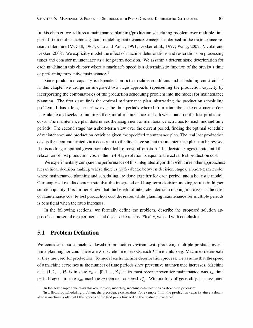
Chapter 5. Maintenance & Production Scheduling with Partial Control: Deterministic Deterioration 88
In this chapter, we address a maintenance planning/production scheduling problem over multiple time
periods in a multi-machine system, modeling maintenance concepts as defined in the maintenance re-
search literature (McCall, 1965; Cho and Parlar, 1991; Dekker et al., 1997; Wang, 2002; Nicolai and
Dekker, 2008). We explicitly model the effect of machine deteriorations and restorations on processing
times and consider maintenance as a long-term decision. We assume a deterministic deterioration for
each machine in this chapter where a machine’s speed is a deterministic function of the previous time
of performing preventive maintenance.1
Since production capacity is dependent on both machine conditions and scheduling constraints,2
in this chapter we design an integrated two-stage approach, representing the production capacity by
incorporating the combinatorics of the production scheduling problem into the model for maintenance
planning. The first stage finds the optimal maintenance plan, abstracting the production scheduling
problem. It has a long-term view over the time periods where information about the customer orders
is available and seeks to minimize the sum of maintenance and a lower bound on the lost production
costs. The maintenance plan determines the assignment of maintenance activities to machines and time
periods. The second stage has a short-term view over the current period, finding the optimal schedule
of maintenance and production activities given the specified maintenance plan. The real lost production
cost is then communicated via a constraint to the first stage so that the maintenance plan can be revised
if it is no longer optimal given more detailed lost cost information. The decision stages iterate until the
relaxation of lost production cost in the first stage solution is equal to the actual lost production cost.
We experimentally compare the performance of this integrated algorithm with three other approaches:
hierarchical decision making where there is no feedback between decision stages, a short-term model
where maintenance planning and scheduling are done together for each period, and a heuristic model.
Our empirical results demonstrate that the integrated and long-term decision making results in higher
solution quality. It is further shown that the benefit of integrated decision making increases as the ratio
of maintenance cost to lost production cost decreases while planning maintenance for multiple periods
is beneficial when the ratio increases.
In the following sections, we formally define the problem, describe the proposed solution ap-
proaches, present the experiments and discuss the results. Finally, we end with conclusion.
5.1 Problem Definition
We consider a multi-machine flowshop production environment, producing multiple products over a
finite planning horizon. There are K discrete time periods, each T time units long. Machines deteriorate
as they are used for production. To model each machine deterioration process, we assume that the speed
of a machine decreases as the number of time periods since preventive maintenance increases. Machine
m ∈ {1, 2, ...,M} is in state sm ∈ {0, 1, ...,Sm} if its most recent preventive maintenance was sm time
periods ago. In state sm, machine m operates at speed νmsm
. Without loss of generality, it is assumed
1In the next chapter, we relax this assumption, modeling machine deteriorations as stochastic processes.2In a flowshop scheduling problem, the precedence constraints, for example, limit the production capacity since a down-
stream machine is idle until the process of the first job is finished on the upstream machines.
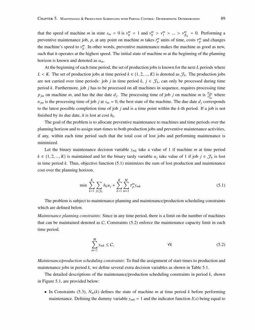
Chapter 5. Maintenance & Production Scheduling with Partial Control: Deterministic Deterioration 89
that the speed of machine m in state sm = 0 is νm0 = 1 and νm
0 > νm1 > ... > νm
Sm= 0. Performing a
preventive maintenance job, p, at any point on machine m takes tmp units of time, costs τm
p and changes
the machine’s speed to νm0 . In other words, preventive maintenance makes the machine as good as new,
such that it operates at the highest speed. The initial state of machine m at the beginning of the planning
horizon is known and denoted as αm.
At the beginning of each time period, the set of production jobs is known for the next L periods where
L < K. The set of production jobs at time period k ∈ {1, 2, ...,K} is denoted as Jk. The production jobs
are not carried over time periods: job j in time period k, j ∈ Jk, can only be processed during time
period k. Furthermore, job j has to be processed on all machines in sequence, requires processing time
p jm on machine m, and has the due date d j. The processing time of job j on machine m is n jmνm
smwhere
n jm is the processing time of job j at sm = 0, the best state of the machine. The due date d j corresponds
to the latest possible completion time of job j and is a time point within the k-th period. If a job is not
finished by its due date, it is lost at cost hk.
The goal of the problem is to allocate preventive maintenance to machines and time periods over the
planning horizon and to assign start-times to both production jobs and preventive maintenance activities,
if any, within each time period such that the total cost of lost jobs and performing maintenance is
minimized.
Let the binary maintenance decision variable ymk take a value of 1 if machine m at time period
k ∈ {1, 2, ...,K} is maintained and let the binary tardy variable u j take value of 1 if job j ∈ Jk is lost
in time period k. Thus, objective function (5.1) minimizes the sum of lost production and maintenance
cost over the planning horizon.
minK∑
k=1
∑j∈Jk
hku j +
K∑k=1
M∑m=1
τmp ymk (5.1)
The problem is subject to maintenance planning and maintenance/production scheduling constraints
which are defined below.
Maintenance planning constraints: Since in any time period, there is a limit on the number of machines
that can be maintained denoted as C, Constraints (5.2) enforce the maintenance capacity limit in each
time period.
M∑m=1
ymk ≤ C, ∀k (5.2)
Maintenance/production scheduling constraints: To find the assignment of start-times to production and
maintenance jobs in period k, we define several extra decision variables as shown in Table 5.1.
The detailed descriptions of the maintenance/production scheduling constraints in period k, shown
in Figure 5.1, are provided below:
• In Constraints (5.3), Nm(k) defines the state of machine m at time period k before performing
maintenance. Defining the dummy variable ym0 = 1 and the indicator function I(x) being equal to
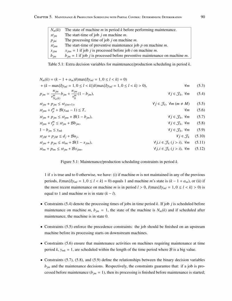
Chapter 5. Maintenance & Production Scheduling with Partial Control: Deterministic Deterioration 90
Nm(k) The state of machine m in period k before performing maintenance.st jm The start-time of job j on machine m.p jm The processing time of job j on machine m.stpm The start-time of preventive maintenance job p on machine m.x jim x jim = 1 if job j is processed before job i on machine m.b jm b jm = 1 if job j is processed before preventive maintenance on machine m.
Table 5.1: Extra decision variables for maintenance/production scheduling in period k.
Nm(k) = (k − 1 + αm)I(max{l|yml = 1, 0 ≤ l < k} = 0)
+ (k −max{l|yml = 1, 0 ≤ l < k})I(max{l|yml = 1, 0 ≤ l < k} > 0), ∀m (5.3)
p jm =n jm
νmNm(k)
b jm +n jm
νm0
(1 − b jm), ∀ j ∈ Jk, ∀m (5.4)
st jm + p jm ≤ st j(m+1), ∀ j ∈ Jk, ∀m (m , M) (5.5)
stpm + tmp + B(ymk − 1) ≤ T, ∀m (5.6)
st jm + p jm ≤ stpm + B(1 − b jm), ∀ j ∈ Jk, ∀m (5.7)
stpm + tmp ≤ st jm + Bb jm, ∀ j ∈ Jk, ∀m (5.8)
1 − b jm ≤ ymk ∀ j ∈ Jk, ∀m (5.9)
st jM + p jM ≤ d j + Bu j, ∀ j ∈ Jk (5.10)
st jm + p jm ≤ stim + B(1 − x jim), ∀ j, i ∈ Jk ( j > i), ∀m (5.11)
stim + pim ≤ st jm + Bx jim, ∀ j, i ∈ Jk ( j > i), ∀m (5.12)
Figure 5.1: Maintenance/production scheduling constraints in period k.
1 if x is true and to 0 otherwise, we have: (i) if machine m is not maintained in any of the previous
periods, I(max{l|yml = 1, 0 ≤ l < k} = 0) equals 1 and machine m’s state is (k − 1 + αm), or (ii) if
the most recent maintenance on machine m is in period l > 0, I(max{l|yml = 1, 0 ≤ l < k} > 0) is
equal to 1 and machine m is in state (k − l).
• Constraints (5.4) denote the processing times of jobs in time period k. If job j is scheduled before
maintenance on machine m, b jm = 1, the state of the machine is Nm(k) and if scheduled after
maintenance, the machine is in state 0.
• Constraints (5.5) enforce the precedence constraints: the job should be finished on an upstream
machine before its processing starts on downstream machines.
• Constraints (5.6) ensure that maintenance activities on machines requiring maintenance at time
period k, ymk = 1, are scheduled within the length of the time period where B is a big value.
• Constraints (5.7), (5.8), and (5.9) define the relationships between the binary decision variables
b jm and the maintenance decisions. Respectively, the constraints guarantee that: if a job is pro-
cessed before maintenance (b jm = 1), then its processing is finished before maintenance is started;
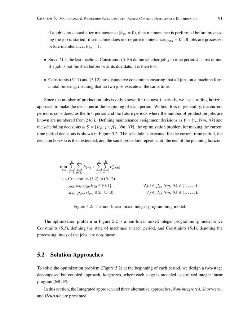
Chapter 5. Maintenance & Production Scheduling with Partial Control: Deterministic Deterioration 91
if a job is processed after maintenance (b jm = 0), then maintenance is performed before process-
ing the job is started; if a machine does not require maintenance, ymk = 0, all jobs are processed
before maintenance, b jm = 1.
• Since M is the last machine, Constraints (5.10) define whether job j in time period k is lost or not.
If a job is not finished before or at its due date, it is then lost.
• Constraints (5.11) and (5.12) are disjunctive constraints ensuring that all jobs on a machine form
a total ordering, meaning that no two jobs execute at the same time.
Since the number of production jobs is only known for the next L periods, we use a rolling horizon
approach to make the decisions at the beginning of each period. Without loss of generality, the current
period is considered as the first period and the future periods where the number of production jobs are
known are numbered from 2 to L. Defining maintenance assignment decisions as Y = {ymk|∀m, ∀k} and
the scheduling decisions as S = {st jm| j ∈ Jk, ∀m, ∀k}, the optimization problem for making the current
time period decisions is shown in Figure 5.2. The schedule is executed for the current time period, the
decision horizon is then extended, and the same procedure repeats until the end of the planning horizon.
minY,S
L∑k=1
∑j∈Jk
hku j +
L∑k=1
M∑m=1
τmp ymk
s.t. Constraints (5.2) to (5.12)
ymk, u j, x jim, b jm ∈ {0, 1}, ∀ j, i ∈ Jk, ∀m, ∀k ∈ {1, . . . , L}
st jm, p jm, stpm ∈ Z+ ∪ {0}, ∀ j ∈ Jk, ∀m, ∀k ∈ {1, . . . , L}
Figure 5.2: The non-linear mixed integer programming model.
The optimization problem in Figure 5.2 is a non-linear mixed integer programming model since
Constraints (5.3), defining the state of machines at each period, and Constraints (5.4), denoting the
processing times of the jobs, are non-linear.
5.2 Solution Approaches
To solve the optimization problem (Figure 5.2) at the beginning of each period, we design a two-stage
decomposed but coupled approach, Integrated, where each stage is modeled as a mixed integer linear
program (MILP).
In this section, the Integrated approach and three alternative approaches, Non-integrated, Short-term,
and Heuristic are presented.
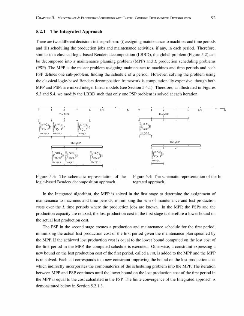
Chapter 5. Maintenance & Production Scheduling with Partial Control: Deterministic Deterioration 92
5.2.1 The Integrated Approach
There are two different decisions in the problem: (i) assigning maintenance to machines and time periods
and (ii) scheduling the production jobs and maintenance activities, if any, in each period. Therefore,
similar to a classical logic-based Benders decomposition (LBBD), the global problem (Figure 5.2) can
be decomposed into a maintenance planning problem (MPP) and L production scheduling problems
(PSP). The MPP is the master problem assigning maintenance to machines and time periods and each
PSP defines one sub-problem, finding the schedule of a period. However, solving the problem using
the classical logic-based Benders decomposition framework is computationally expensive, though both
MPP and PSPs are mixed integer linear models (see Section 5.4.1). Therefore, as illustrated in Figures
5.3 and 5.4, we modify the LBBD such that only one PSP problem is solved at each iteration.
...
... The PSP_1 The PSP_2 The PSP_L
0 1 2 L
The MPP
MP
P S
olu
tion
Cut
0 1 2 L
MP
P S
olu
tion
Cut
MP
P S
olu
tion
Cut
0 1 2 ... L L+1 K
The PSP_1 The PSP_2 The PSP_L
0 1 2 L
The MPP
MP
P S
olu
tion
Cut
0 1 2 L
MP
P S
olu
tion
Cut
MP
P S
olu
tion
Cut
...
...
...
Figure 5.3: The schematic representation of thelogic-based Benders decomposition approach.
...
The PSP_1
0 1 2 L
The MPP
MP
P S
olu
tion
Cut
0 1
0 1 2 ... L L+1 K
The PSP_1
0 1 2 L
The MPP
MP
P S
olu
tion
Cut
0 1 ...
...
Figure 5.4: The schematic representation of the In-tegrated approach.
In the Integrated algorithm, the MPP is solved in the first stage to determine the assignment of
maintenance to machines and time periods, minimizing the sum of maintenance and lost production
costs over the L time periods where the production jobs are known. In the MPP, the PSPs and the
production capacity are relaxed, the lost production cost in the first stage is therefore a lower bound on
the actual lost production cost.
The PSP in the second stage creates a production and maintenance schedule for the first period,
minimizing the actual lost production cost of the first period given the maintenance plan specified by
the MPP. If the achieved lost production cost is equal to the lower bound computed on the lost cost of
the first period in the MPP, the computed schedule is executed. Otherwise, a constraint expressing a
new bound on the lost production cost of the first period, called a cut, is added to the MPP and the MPP
is re-solved. Each cut corresponds to a new constraint improving the bound on the lost production cost
which indirectly incorporates the combinatorics of the scheduling problem into the MPP. The iteration
between MPP and PSP continues until the lower bound on the lost production cost of the first period in
the MPP is equal to the cost calculated in the PSP. The finite convergence of the Integrated approach is
demonstrated below in Section 5.2.1.3.
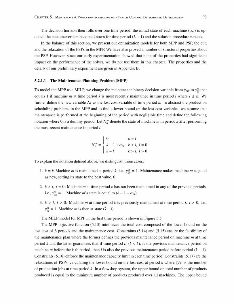
Chapter 5. Maintenance & Production Scheduling with Partial Control: Deterministic Deterioration 93
The decision horizon then rolls over one time period, the initial state of each machine (αm) is up-
dated, the customer orders become known for time period (L + 1) and the solution procedure repeats.
In the balance of this section, we present our optimization models for both MPP and PSP, the cut,
and the relaxation of the PSPs in the MPP. We have also proved a number of structural properties about
the PSP. However, since our early experimentation showed that none of the properties had significant
impact on the performance of the solver, we do not use them in this chapter. The properties and the
details of our preliminary experiment are given in Appendix B.
5.2.1.1 The Maintenance Planning Problem (MPP)
To model the MPP as a MILP, we change the maintenance binary decision variable from ymk to ymlk that
equals 1 if machine m at time period k is most recently maintained in time period l where l ≤ k. We
further define the new variable Λk as the lost cost variable of time period k. To abstract the production
scheduling problems in the MPP and to find a lower bound on the lost cost variables, we assume that
maintenance is performed at the beginning of the period with negligible time and define the following
notation where 0 is a dummy period. Let Nmlk denote the state of machine m in period k after performing
the most recent maintenance in period l.
Nmlk =
0 k = l
k − 1 + αm k > l, l = 0
k − l k > l, l > 0
To explain the notation defined above, we distinguish three cases:
1. k = l: Machine m is maintained at period k, i.e., ymkk = 1. Maintenance makes machine m as good
as new, setting its state to the best value, 0.
2. k > l, l = 0: Machine m at time period k has not been maintained in any of the previous periods,
i.e., ym0k = 1. Machine m’s state is equal to (k − 1 + αm).
3. k > l, l > 0: Machine m at time period k is previously maintained at time period l, l > 0, i.e.,
ymlk = 1. Machine m is then at state (k − l).
The MILP model for MPP in the first time period is shown in Figure 5.5.
The MPP objective function (5.13) minimizes the total cost composed of the lower bound on the
lost cost of L periods and the maintenance cost. Constraints (5.14) and (5.15) ensure the feasibility of
the maintenance plan where the former defines the previous maintenance period on machine m at time
period k and the latter guarantees that if time period l, (l < k), is the previous maintenance period on
machine m before the k-th period, then l is also the previous maintenance period before period (k − 1).
Constraints (5.16) enforce the maintenance capacity limit in each time period. Constraints (5.17) are the
relaxations of PSPs, calculating the lower bound on the lost cost at period k where |Jk| is the number
of production jobs at time period k. In a flowshop system, the upper bound on total number of products
produced is equal to the minimum number of products produced over all machines. The upper bound
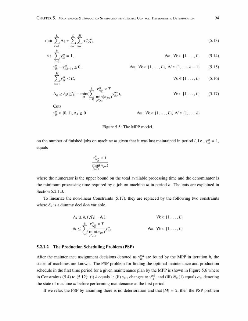
Chapter 5. Maintenance & Production Scheduling with Partial Control: Deterministic Deterioration 94
minL∑
k=1
Λk +
L∑k=1
M∑m=1
τmp ym
kk (5.13)
s.t.k∑
l=0
ymlk = 1, ∀m, ∀k ∈ {1, . . . , L} (5.14)
ymlk − ym
l(k−1) ≤ 0, ∀m, ∀k ∈ {1, . . . , L}, ∀l ∈ {1, . . . , k − 1} (5.15)M∑
m=1
ymkk ≤ C, ∀k ∈ {1, . . . , L} (5.16)
Λk ≥ hk(|Jk| −minm
(k∑
l=0
νmNm
lk× T
minj∈Jk
(n jm)ym
lk)), ∀k ∈ {1, . . . , L} (5.17)
Cuts
ymlk ∈ {0, 1},Λk ≥ 0 ∀m, ∀k ∈ {1, . . . , L}, ∀l ∈ {1, . . . , k}
Figure 5.5: The MPP model.
on the number of finished jobs on machine m given that it was last maintained in period l, i.e., ymlk = 1,
equals
νmNm
lk× T
minj∈Jk
(n jm)
where the numerator is the upper bound on the total available processing time and the denominator is
the minimum processing time required by a job on machine m in period k. The cuts are explained in
Section 5.2.1.3.
To linearize the non-linear Constraints (5.17), they are replaced by the following two constraints
where δk is a dummy decision variable.
Λk ≥ hk(|Jk| − δk), ∀k ∈ {1, . . . , L}
δk ≤
k∑l=0
νmNm
lk× T
minj∈Jk
(n jm)ym
lk, ∀m, ∀k ∈ {1, . . . , L}
5.2.1.2 The Production Scheduling Problem (PSP)
After the maintenance assignment decisions denoted as ymhlk are found by the MPP in iteration h, the
states of machines are known. The PSP problem for finding the optimal maintenance and production
schedule in the first time period for a given maintenance plan by the MPP is shown in Figure 5.6 where
in Constraints (5.4) to (5.12): (i) k equals 1; (ii) ym1 changes to ymh11 , and (iii) Nm(1) equals αm denoting
the state of machine m before performing maintenance at the first period.
If we relax the PSP by assuming there is no deterioration and that |M| = 2, then the PSP problem
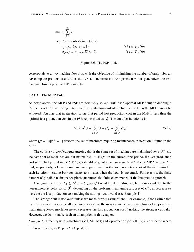
Chapter 5. Maintenance & Production Scheduling with Partial Control: Deterministic Deterioration 95
min h1
|J1 |∑j=1
u j
s.t. Constraints (5.4) to (5.12)
u j, x jim, b jm ∈ {0, 1}, ∀ j, i ∈ J1, ∀m
st jm, p jm, stpm ∈ Z+ ∪ {0}, ∀ j ∈ J1, ∀m
Figure 5.6: The PSP model.
corresponds to a two machine flowshop with the objective of minimizing the number of tardy jobs, an
NP-complete problem (Lenstra et al., 1977). Therefore the PSP problem which generalizes the two
machine flowshop is also NP-complete.
5.2.1.3 The MPP Cuts
As noted above, the MPP and PSP are iteratively solved, with each optimal MPP solution defining a
PSP and each PSP returning cuts if the lost production cost of the first period from the MPP cannot be
achieved. Assume that in iteration h, the first period lost production cost in the MPP is less than the
optimal lost production cost in the PSP, represented as Λh1. The cut after iteration h is:
Λ1 ≥ Λh1(1 −
∑m∈Qh
(1 − ym11) −
∑m<Qh
ym11) (5.18)
where Qh = {m|ymh11 = 1} denotes the set of machines requiring maintenance in iteration h found in the
MPP.
The cut is a no-good cut guaranteeing that if the same set of machines are maintained (m ∈ Qh) and
the same set of machines are not maintained (m < Qh) in the current first period, the lost production
cost of the first period in the MPP (Λ1) should be greater than or equal to Λh1. As the MPP and the PSP
find, respectively, a lower bound and an upper bound on the lost production cost of the first period in
each iteration, iterating between stages terminates when the bounds are equal. Furthermore, the finite
number of possible maintenance plans guarantees the finite convergence of the Integrated approach.
Changing the cut to Λ1 ≥ Λh1(1 −
∑m<Qh ym
11) would make it stronger, but is unsound due to the
non-monotonic behavior of Qh: depending on the problem, maintaining a subset of Qh can decrease or
increase the lost production cost making the stronger cut invalid (see Example 1).
The stronger cut is not valid unless we make further assumptions. For example, if we assume that
the maintenance duration of all machines is less than the increase in the processing times of all jobs, then
maintaining fewer machines never decreases the lost production cost,3 making the stronger cut valid.
However, we do not make such an assumption in this chapter.
Example 1: A facility with 3 machines (M1, M2, M3) and 2 production jobs (J1, J2) is considered where
3For more details, see Property 2 in Appendix B.
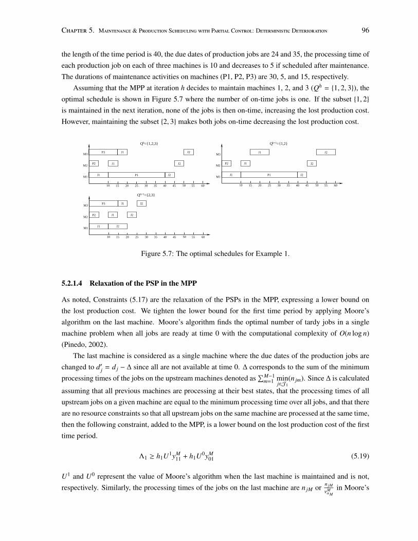
Chapter 5. Maintenance & Production Scheduling with Partial Control: Deterministic Deterioration 96
the length of the time period is 40, the due dates of production jobs are 24 and 35, the processing time of
each production job on each of three machines is 10 and decreases to 5 if scheduled after maintenance.
The durations of maintenance activities on machines (P1, P2, P3) are 30, 5, and 15, respectively.
Assuming that the MPP at iteration h decides to maintain machines 1, 2, and 3 (Qh = {1, 2, 3}), the
optimal schedule is shown in Figure 5.7 where the number of on-time jobs is one. If the subset {1, 2}
is maintained in the next iteration, none of the jobs is then on-time, increasing the lost production cost.
However, maintaining the subset {2, 3} makes both jobs on-time decreasing the lost production cost.
P2
J1 J2
M1
M2
M3
10 20 15 25 35
J1 J2
J1 J2
Qh={1,2,3}
30 40 45 50 55
P1
60
P3
P2
J1 J2
M1
M2
M3
10 20 15 25 35
J1 J2
J1 J2
Qh+1={2,3}
30 40 45 50 55 60
J1 J2
M1
M2
M3
10 20 15 25 35
J1 J2
J1 J2
Qh+1={1,2}
30 40 45 50 55
P1
60
P2
P3
Figure 5.7: The optimal schedules for Example 1.
5.2.1.4 Relaxation of the PSP in the MPP
As noted, Constraints (5.17) are the relaxation of the PSPs in the MPP, expressing a lower bound on
the lost production cost. We tighten the lower bound for the first time period by applying Moore’s
algorithm on the last machine. Moore’s algorithm finds the optimal number of tardy jobs in a single
machine problem when all jobs are ready at time 0 with the computational complexity of O(n log n)
(Pinedo, 2002).
The last machine is considered as a single machine where the due dates of the production jobs are
changed to d′j = d j − ∆ since all are not available at time 0. ∆ corresponds to the sum of the minimum
processing times of the jobs on the upstream machines denoted as∑M−1
m=1 minj∈J1
(n jm). Since ∆ is calculated
assuming that all previous machines are processing at their best states, that the processing times of all
upstream jobs on a given machine are equal to the minimum processing time over all jobs, and that there
are no resource constraints so that all upstream jobs on the same machine are processed at the same time,
then the following constraint, added to the MPP, is a lower bound on the lost production cost of the first
time period.
Λ1 ≥ h1U1yM11 + h1U0yM
01 (5.19)
U1 and U0 represent the value of Moore’s algorithm when the last machine is maintained and is not,
respectively. Similarly, the processing times of the jobs on the last machine are n jM or n jM
νMαM
in Moore’s
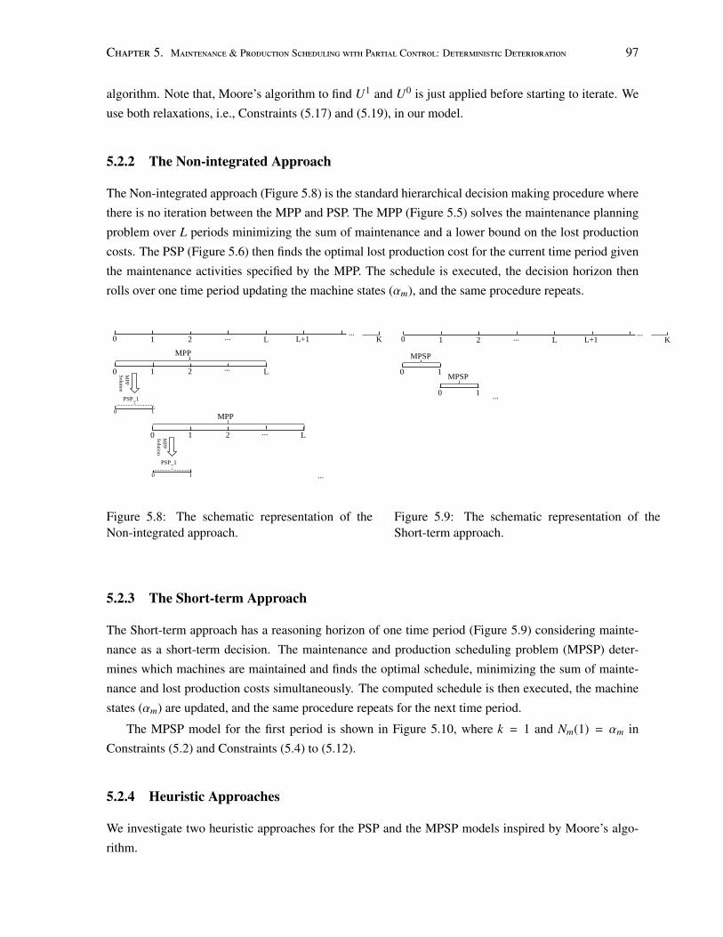
Chapter 5. Maintenance & Production Scheduling with Partial Control: Deterministic Deterioration 97
algorithm. Note that, Moore’s algorithm to find U1 and U0 is just applied before starting to iterate. We
use both relaxations, i.e., Constraints (5.17) and (5.19), in our model.
5.2.2 The Non-integrated Approach
The Non-integrated approach (Figure 5.8) is the standard hierarchical decision making procedure where
there is no iteration between the MPP and PSP. The MPP (Figure 5.5) solves the maintenance planning
problem over L periods minimizing the sum of maintenance and a lower bound on the lost production
costs. The PSP (Figure 5.6) then finds the optimal lost production cost for the current time period given
the maintenance activities specified by the MPP. The schedule is executed, the decision horizon then
rolls over one time period updating the machine states (αm), and the same procedure repeats.
PSP_1
0 1 2 L
MPP
MP
P
So
lutio
n
0 1
PSP_1
0 1 2 L
MPP
MP
P
So
lutio
n
0 1 ...
...
...
0 1 2 ... L L+1 K ...
Figure 5.8: The schematic representation of theNon-integrated approach.
0 1
MPSP
... 0 1
MPSP
0 1 2 ... L L+1 K ...
Figure 5.9: The schematic representation of theShort-term approach.
5.2.3 The Short-term Approach
The Short-term approach has a reasoning horizon of one time period (Figure 5.9) considering mainte-
nance as a short-term decision. The maintenance and production scheduling problem (MPSP) deter-
mines which machines are maintained and finds the optimal schedule, minimizing the sum of mainte-
nance and lost production costs simultaneously. The computed schedule is then executed, the machine
states (αm) are updated, and the same procedure repeats for the next time period.
The MPSP model for the first period is shown in Figure 5.10, where k = 1 and Nm(1) = αm in
Constraints (5.2) and Constraints (5.4) to (5.12).
5.2.4 Heuristic Approaches
We investigate two heuristic approaches for the PSP and the MPSP models inspired by Moore’s algo-
rithm.
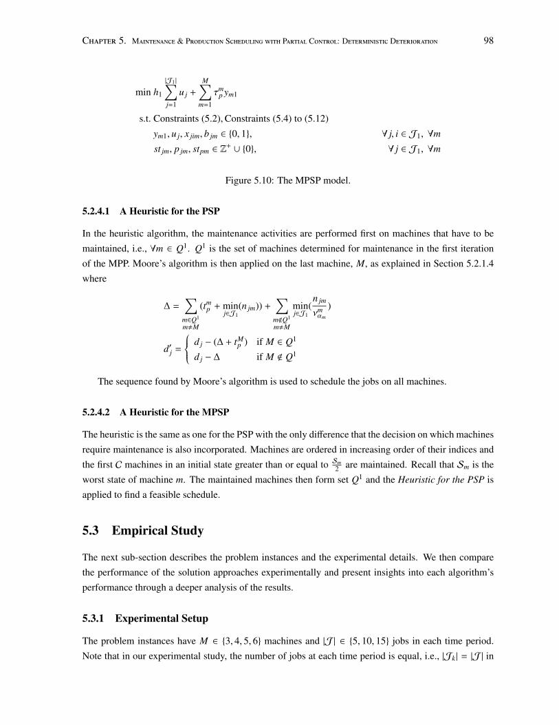
Chapter 5. Maintenance & Production Scheduling with Partial Control: Deterministic Deterioration 98
min h1
|J1 |∑j=1
u j +
M∑m=1
τmp ym1
s.t. Constraints (5.2),Constraints (5.4) to (5.12)
ym1, u j, x jim, b jm ∈ {0, 1}, ∀ j, i ∈ J1, ∀m
st jm, p jm, stpm ∈ Z+ ∪ {0}, ∀ j ∈ J1, ∀m
Figure 5.10: The MPSP model.
5.2.4.1 A Heuristic for the PSP
In the heuristic algorithm, the maintenance activities are performed first on machines that have to be
maintained, i.e., ∀m ∈ Q1. Q1 is the set of machines determined for maintenance in the first iteration
of the MPP. Moore’s algorithm is then applied on the last machine, M, as explained in Section 5.2.1.4
where
∆ =∑
m∈Q1
m,M
(tmp + min
j∈J1(n jm)) +
∑m<Q1
m,M
minj∈J1
(n jm
νmαm
)
d′j =
d j − (∆ + tMp ) if M ∈ Q1
d j − ∆ if M < Q1
The sequence found by Moore’s algorithm is used to schedule the jobs on all machines.
5.2.4.2 A Heuristic for the MPSP
The heuristic is the same as one for the PSP with the only difference that the decision on which machines
require maintenance is also incorporated. Machines are ordered in increasing order of their indices and
the first C machines in an initial state greater than or equal to Sm2 are maintained. Recall that Sm is the
worst state of machine m. The maintained machines then form set Q1 and the Heuristic for the PSP is
applied to find a feasible schedule.
5.3 Empirical Study
The next sub-section describes the problem instances and the experimental details. We then compare
the performance of the solution approaches experimentally and present insights into each algorithm’s
performance through a deeper analysis of the results.
5.3.1 Experimental Setup
The problem instances have M ∈ {3, 4, 5, 6} machines and |J| ∈ {5, 10, 15} jobs in each time period.
Note that in our experimental study, the number of jobs at each time period is equal, i.e., |Jk| = |J| in
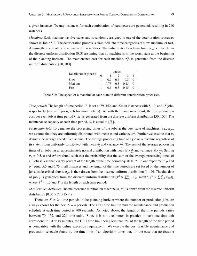
Chapter 5. Maintenance & Production Scheduling with Partial Control: Deterministic Deterioration 99
a given instance. Twenty instances for each combination of parameters are generated, resulting in 240
instances.
Machines Each machine has five states and is randomly assigned to one of the deterioration processes
shown in Table 5.2. The deterioration process is classified into three categories of slow, medium, or fast,
defining the speed of the machine in different states. The initial state of each machine, αm, is drawn from
the discrete uniform distribution [0, 3] assuming that no machine is in the worst state at the beginning
of the planning horizon. The maintenance cost for each machine, τmp , is generated from the discrete
uniform distribution [50, 100].
Deterioration process States0 1 2 3 4
Slow 1 0.9 0.6 0.3 0Medium 1 0.75 0.5 0.25 0Fast 1 0.6 0.3 0.15 0
Table 5.2: The speed of a machine at each state in different deterioration processes.
Time periods The length of time period, T , is set at 79, 152, and 224 in instances with 5, 10, and 15 jobs,
respectively (see next paragraph for more details). As with the maintenance cost, the lost production
cost per each job at time period k, hk, is generated from the discrete uniform distribution [50, 100]. The
maintenance capacity at each time period, C, is equal to bM2 c.
Production jobs To generate the processing times of the jobs at the best state of machines, i.e., n jm,
we assume that they are uniformly distributed with mean µ and variance σ2. Further we assume that νa
denotes the average speed of a machine. The average processing time of a job on a machine regardless of
its state is then uniformly distributed with mean µνa
and variance σ2
ν2a
. The sum of the average processing
times of all jobs has an approximately normal distribution with mean |J|× µνa
and variance |J|×σ2
ν2a
. Setting
νa = 0.5, µ and σ2 are found such that the probability that the sum of the average processing times of
all jobs is less than eighty percent of the length of the time period equals 0.75. In our experiment, µ and
σ2 equal 5.5 and 6.75 in all instances and the length of the time periods are set based on the number of
jobs, as described above. n jm is then drawn from the discrete uniform distribution [1, 10]. The due date
of job j is generated from the discrete uniform distribution [ f d ×∑M
m=1 n jm,max(T, f d ×∑M
m=1 n jm)],
where f d = 1.5 and T is the length of each time period.
Maintenance Activities The maintenance duration on machine m, tmp , is drawn from the discrete uniform
distribution [0.05 × T, 0.15 × T ].
There are K = 24 time periods in the planning horizon where the number of production jobs are
always known for the next L = 4 periods. The CPU time limit to find the maintenance and production
schedule at each time period is 900 seconds. As noted above, the length of the time periods varies
between 79, 152, and 224 time units. Since it is not uncommon in practice to have one time unit
correspond to 10 or 15 minutes, the CPU time limit being less than 2% of the length of the time period
is compatible with the online execution requirement. We execute the best feasible maintenance and
production schedule found by the time-limit if an algorithm times out. In the case that no feasible
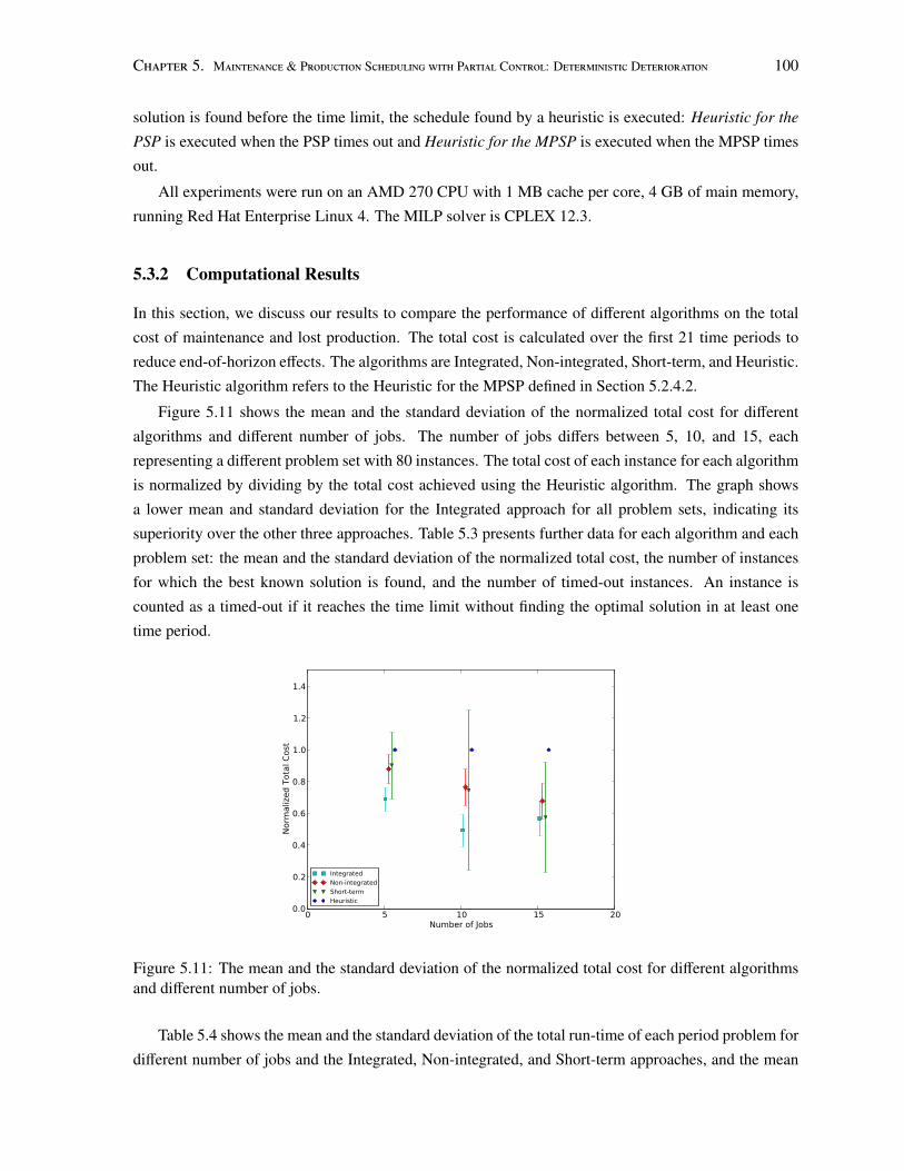
Chapter 5. Maintenance & Production Scheduling with Partial Control: Deterministic Deterioration 100
solution is found before the time limit, the schedule found by a heuristic is executed: Heuristic for the
PSP is executed when the PSP times out and Heuristic for the MPSP is executed when the MPSP times
out.
All experiments were run on an AMD 270 CPU with 1 MB cache per core, 4 GB of main memory,
running Red Hat Enterprise Linux 4. The MILP solver is CPLEX 12.3.
5.3.2 Computational Results
In this section, we discuss our results to compare the performance of different algorithms on the total
cost of maintenance and lost production. The total cost is calculated over the first 21 time periods to
reduce end-of-horizon effects. The algorithms are Integrated, Non-integrated, Short-term, and Heuristic.
The Heuristic algorithm refers to the Heuristic for the MPSP defined in Section 5.2.4.2.
Figure 5.11 shows the mean and the standard deviation of the normalized total cost for different
algorithms and different number of jobs. The number of jobs differs between 5, 10, and 15, each
representing a different problem set with 80 instances. The total cost of each instance for each algorithm
is normalized by dividing by the total cost achieved using the Heuristic algorithm. The graph shows
a lower mean and standard deviation for the Integrated approach for all problem sets, indicating its
superiority over the other three approaches. Table 5.3 presents further data for each algorithm and each
problem set: the mean and the standard deviation of the normalized total cost, the number of instances
for which the best known solution is found, and the number of timed-out instances. An instance is
counted as a timed-out if it reaches the time limit without finding the optimal solution in at least one
time period.
0 5 10 15 20Number of Jobs
0.0
0.2
0.4
0.6
0.8
1.0
1.2
1.4
Norm
aliz
ed T
otal
Cos
t
IntegratedNon-integratedShort-termHeuristic
Figure 5.11: The mean and the standard deviation of the normalized total cost for different algorithmsand different number of jobs.
Table 5.4 shows the mean and the standard deviation of the total run-time of each period problem for
different number of jobs and the Integrated, Non-integrated, and Short-term approaches, and the mean
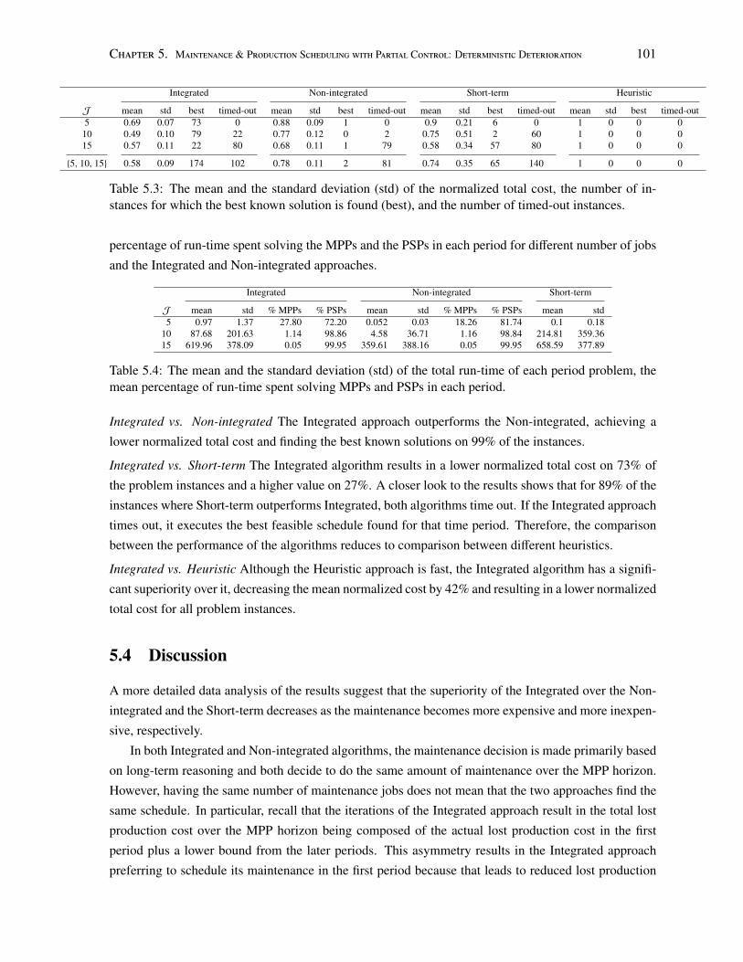
Chapter 5. Maintenance & Production Scheduling with Partial Control: Deterministic Deterioration 101
Integrated Non-integrated Short-term Heuristic
J mean std best timed-out mean std best timed-out mean std best timed-out mean std best timed-out5 0.69 0.07 73 0 0.88 0.09 1 0 0.9 0.21 6 0 1 0 0 010 0.49 0.10 79 22 0.77 0.12 0 2 0.75 0.51 2 60 1 0 0 015 0.57 0.11 22 80 0.68 0.11 1 79 0.58 0.34 57 80 1 0 0 0
{5, 10, 15} 0.58 0.09 174 102 0.78 0.11 2 81 0.74 0.35 65 140 1 0 0 0
Table 5.3: The mean and the standard deviation (std) of the normalized total cost, the number of in-stances for which the best known solution is found (best), and the number of timed-out instances.
percentage of run-time spent solving the MPPs and the PSPs in each period for different number of jobs
and the Integrated and Non-integrated approaches.
Integrated Non-integrated Short-term
J mean std % MPPs % PSPs mean std % MPPs % PSPs mean std5 0.97 1.37 27.80 72.20 0.052 0.03 18.26 81.74 0.1 0.18
10 87.68 201.63 1.14 98.86 4.58 36.71 1.16 98.84 214.81 359.3615 619.96 378.09 0.05 99.95 359.61 388.16 0.05 99.95 658.59 377.89
Table 5.4: The mean and the standard deviation (std) of the total run-time of each period problem, themean percentage of run-time spent solving MPPs and PSPs in each period.
Integrated vs. Non-integrated The Integrated approach outperforms the Non-integrated, achieving a
lower normalized total cost and finding the best known solutions on 99% of the instances.
Integrated vs. Short-term The Integrated algorithm results in a lower normalized total cost on 73% of
the problem instances and a higher value on 27%. A closer look to the results shows that for 89% of the
instances where Short-term outperforms Integrated, both algorithms time out. If the Integrated approach
times out, it executes the best feasible schedule found for that time period. Therefore, the comparison
between the performance of the algorithms reduces to comparison between different heuristics.
Integrated vs. Heuristic Although the Heuristic approach is fast, the Integrated algorithm has a signifi-
cant superiority over it, decreasing the mean normalized cost by 42% and resulting in a lower normalized
total cost for all problem instances.
5.4 Discussion
A more detailed data analysis of the results suggest that the superiority of the Integrated over the Non-
integrated and the Short-term decreases as the maintenance becomes more expensive and more inexpen-
sive, respectively.
In both Integrated and Non-integrated algorithms, the maintenance decision is made primarily based
on long-term reasoning and both decide to do the same amount of maintenance over the MPP horizon.
However, having the same number of maintenance jobs does not mean that the two approaches find the
same schedule. In particular, recall that the iterations of the Integrated approach result in the total lost
production cost over the MPP horizon being composed of the actual lost production cost in the first
period plus a lower bound from the later periods. This asymmetry results in the Integrated approach
preferring to schedule its maintenance in the first period because that leads to reduced lost production
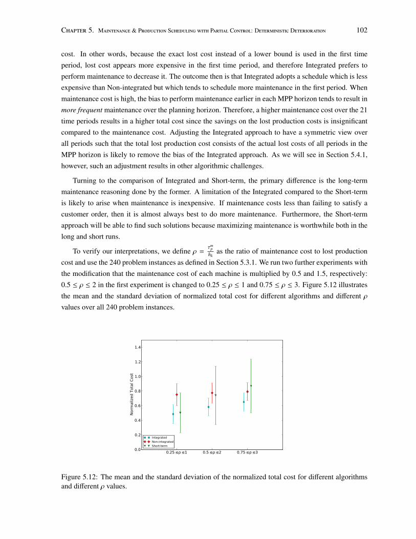
Chapter 5. Maintenance & Production Scheduling with Partial Control: Deterministic Deterioration 102
cost. In other words, because the exact lost cost instead of a lower bound is used in the first time
period, lost cost appears more expensive in the first time period, and therefore Integrated prefers to
perform maintenance to decrease it. The outcome then is that Integrated adopts a schedule which is less
expensive than Non-integrated but which tends to schedule more maintenance in the first period. When
maintenance cost is high, the bias to perform maintenance earlier in each MPP horizon tends to result in
more frequent maintenance over the planning horizon. Therefore, a higher maintenance cost over the 21
time periods results in a higher total cost since the savings on the lost production costs is insignificant
compared to the maintenance cost. Adjusting the Integrated approach to have a symmetric view over
all periods such that the total lost production cost consists of the actual lost costs of all periods in the
MPP horizon is likely to remove the bias of the Integrated approach. As we will see in Section 5.4.1,
however, such an adjustment results in other algorithmic challenges.
Turning to the comparison of Integrated and Short-term, the primary difference is the long-term
maintenance reasoning done by the former. A limitation of the Integrated compared to the Short-term
is likely to arise when maintenance is inexpensive. If maintenance costs less than failing to satisfy a
customer order, then it is almost always best to do more maintenance. Furthermore, the Short-term
approach will be able to find such solutions because maximizing maintenance is worthwhile both in the
long and short runs.
To verify our interpretations, we define ρ =τm
phk
as the ratio of maintenance cost to lost production
cost and use the 240 problem instances as defined in Section 5.3.1. We run two further experiments with
the modification that the maintenance cost of each machine is multiplied by 0.5 and 1.5, respectively:
0.5 ≤ ρ ≤ 2 in the first experiment is changed to 0.25 ≤ ρ ≤ 1 and 0.75 ≤ ρ ≤ 3. Figure 5.12 illustrates
the mean and the standard deviation of normalized total cost for different algorithms and different ρ
values over all 240 problem instances.
0.25 1 0.5 2 0.75 30.0
0.2
0.4
0.6
0.8
1.0
1.2
1.4
Norm
aliz
ed T
otal
Cos
t
IntegratedNon-integratedShort-term
Figure 5.12: The mean and the standard deviation of the normalized total cost for different algorithmsand different ρ values.
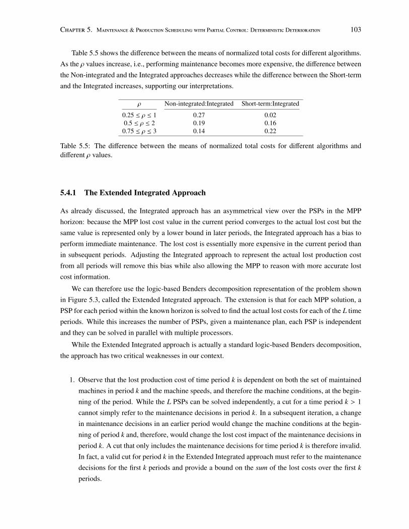
Chapter 5. Maintenance & Production Scheduling with Partial Control: Deterministic Deterioration 103
Table 5.5 shows the difference between the means of normalized total costs for different algorithms.
As the ρ values increase, i.e., performing maintenance becomes more expensive, the difference between
the Non-integrated and the Integrated approaches decreases while the difference between the Short-term
and the Integrated increases, supporting our interpretations.
ρ Non-integrated:Integrated Short-term:Integrated
0.25 ≤ ρ ≤ 1 0.27 0.020.5 ≤ ρ ≤ 2 0.19 0.16
0.75 ≤ ρ ≤ 3 0.14 0.22
Table 5.5: The difference between the means of normalized total costs for different algorithms anddifferent ρ values.
5.4.1 The Extended Integrated Approach
As already discussed, the Integrated approach has an asymmetrical view over the PSPs in the MPP
horizon: because the MPP lost cost value in the current period converges to the actual lost cost but the
same value is represented only by a lower bound in later periods, the Integrated approach has a bias to
perform immediate maintenance. The lost cost is essentially more expensive in the current period than
in subsequent periods. Adjusting the Integrated approach to represent the actual lost production cost
from all periods will remove this bias while also allowing the MPP to reason with more accurate lost
cost information.
We can therefore use the logic-based Benders decomposition representation of the problem shown
in Figure 5.3, called the Extended Integrated approach. The extension is that for each MPP solution, a
PSP for each period within the known horizon is solved to find the actual lost costs for each of the L time
periods. While this increases the number of PSPs, given a maintenance plan, each PSP is independent
and they can be solved in parallel with multiple processors.
While the Extended Integrated approach is actually a standard logic-based Benders decomposition,
the approach has two critical weaknesses in our context.
1. Observe that the lost production cost of time period k is dependent on both the set of maintained
machines in period k and the machine speeds, and therefore the machine conditions, at the begin-
ning of the period. While the L PSPs can be solved independently, a cut for a time period k > 1
cannot simply refer to the maintenance decisions in period k. In a subsequent iteration, a change
in maintenance decisions in an earlier period would change the machine conditions at the begin-
ning of period k and, therefore, would change the lost cost impact of the maintenance decisions in
period k. A cut that only includes the maintenance decisions for time period k is therefore invalid.
In fact, a valid cut for period k in the Extended Integrated approach must refer to the maintenance
decisions for the first k periods and provide a bound on the sum of the lost costs over the first k
periods.
Chapter 5. Maintenance & Production Scheduling with Partial Control: Deterministic Deterioration 104
Formally, the cuts after iteration h are:
k∑i=1
Λi ≥(k∑
i=1
Λhi )(1 −
k∑i=1
∑m∈Qh
i
(1 − ymii ) −
k∑i=1
∑m<Qh
i
ymii ),∀k ∈ {1, . . . , L} (5.20)
Qhk indicates the set of machines maintained in period k in iteration h. The iterations between
the MPP and the PSPs continue until the total lost cost over L time periods is equal to the one
computed in the MPP.
2. At each iteration of the MPP, the PSPs return cuts until the convergence criterion is achieved.
The maximum number of iterations therefore equals the maximum number of times that the PSPs
might return cuts to the MPP. Since the cuts in the Integrated approach (Equations (5.18)) involve
only the lost production cost variable for the first period, the maximum number of iterations is∑Ci=0
(Mi
)enumerating all possible ways of assigning maintenance to i machines and the first period
considering the maintenance capacity limit of C. However, the cuts in the Extended Integrated
approach (Equations (5.20)) involve the lost production cost variables for all L periods. The
maximum number of iterations consequently increases to (∑C
i=0
(Mi
))L. The Extended Integrated
approach will then be expected to have an extremely high computational expense not because of
the linear increase in the number of PSPs in each MPP iteration (i.e., solving (L − 1) more PSPs),
but because of the exponential increase in the number of MPP iterations.
These weaknesses make the Extended Integrated model unlikely to be successful. To confirm this
analysis, we ran it on the 240 problem instances of Section 5.3 where 0.5 ≤ ρ ≤ 2 and where the CPU
time limit is 900 seconds for each period. As expected, it times out on 198 problem instances and the
mean of the normalized total cost over all instances marginally increases to 0.59 compared to 0.58 for
the Integrated approach in Table 5.3.
5.5 Conclusion
In this chapter, we studied an integrated maintenance planning and production scheduling problem in a
multi-machine and multi-period production system where machine conditions are partially controlled.
At the beginning of each time period, two decisions are made: which machines are to be maintained, if
any, and when each production and each maintenance activity should be executed in order to minimize
the total maintenance and lost production costs over the planning horizon.
To precisely model the production capacity as a function of both machine states and scheduling
combinatorics, we propose an integrated two-stage algorithm. In the first stage of the algorithm, main-
tenance planning is done over time periods where the customer orders are known. The production
scheduling problem and production capacity are abstracted in the first stage and the objective is to find a
maintenance plan for each machine, minimizing the sum of maintenance cost and a lower bound on lost
production cost. The second stage then schedules maintenance and production activities in the current
Chapter 5. Maintenance & Production Scheduling with Partial Control: Deterministic Deterioration 105
period, minimizing the actual lost production cost assuming the given maintenance plan. The iteration
between two stages continues, with feedback, until the lower bound and the actual lost production cost
of the current period converge.
The computational results demonstrate that the Integrated approach yields lower total cost than three
other approaches tested: a Non-integrated approach, a Short-term, integrated approach, and a Heuris-
tic approach. The benefit for Integrated decision making over Non-integrated, furthermore, increases
for lower maintenance cost relative to lost production cost. Finally, the benefit of long-term decision
making in the Integrated approach over a myopic, Short-term approach increases with higher relative
maintenance cost. These observations suggest that at extreme low or high relative maintenance cost,
Short-term and Non-integrated approaches should be adopted. However, for a broad range of interme-
diate relative costs, Integrated provides superior quality solutions.
To model each machine deterioration in this chapter, we assumed that the speed of a machine is a
deterministic function of the number of time periods since preventive maintenance. This assumption
might be a plausible approximation for modeling machine conditions where the production process is
smooth and machines do not go under dramatic load fluctuations. In the next chapter, we generalize
this assumption modeling each machine deterioration as a stochastic process covering a wider range of
manufacturing industries.
Chapter 6
Maintenance Planning & ProductionScheduling with Partial Control overMachine Conditions: MarkovianDeterioration
In this chapter we continue studying the interdependency between maintenance planning and production
scheduling where machines are maintained both correctively and preventively.
Machine deterioration is one of the main causes of production capacity reduction in many manufac-
turing industries (Kaufman and Lewis, 2007; Sloan, 2008). Maintenance operations improve machine
conditions, but also occupy potential production time, possibly delaying the customer orders. There-
fore, the challenge is to determine the maintenance and the production schedule to maximize customer
satisfaction. In the previous chapter, we motivated this challenge from the perspective of the schedul-
ing literature and introduced common maintenance conceptualizations as they appear in maintenance
research area to scheduling literature. More specifically, we modeled machine deterioration as a de-
terministic function of the number of time periods since previous maintenance and considered a finite,
though long, decision horizon. In this chapter, we study the same challenge but from the perspective of
the research on maintenance.
In the maintenance literature, the problem of integrated maintenance and production scheduling
utilizing machine condition information has mainly been addressed on the tactical level, adopting a
long-term decision horizon. It has been developed in two directions. The first stream assumes that all
customer orders are similar and addresses the problem of production planning: how much to produce
(see Section 2.2.3 for review of this literature). The second stream assumes different customer orders,
but a single machine and addresses the problem of product dispatching: which product to produce next
(see Section 2.2.4 for review of this literature). In this chapter, we address the problem of integrated
maintenance and production scheduling on the operational level assuming a multi-machine production
environment where different customer orders have to be scheduled on machines in sequence and are due
106
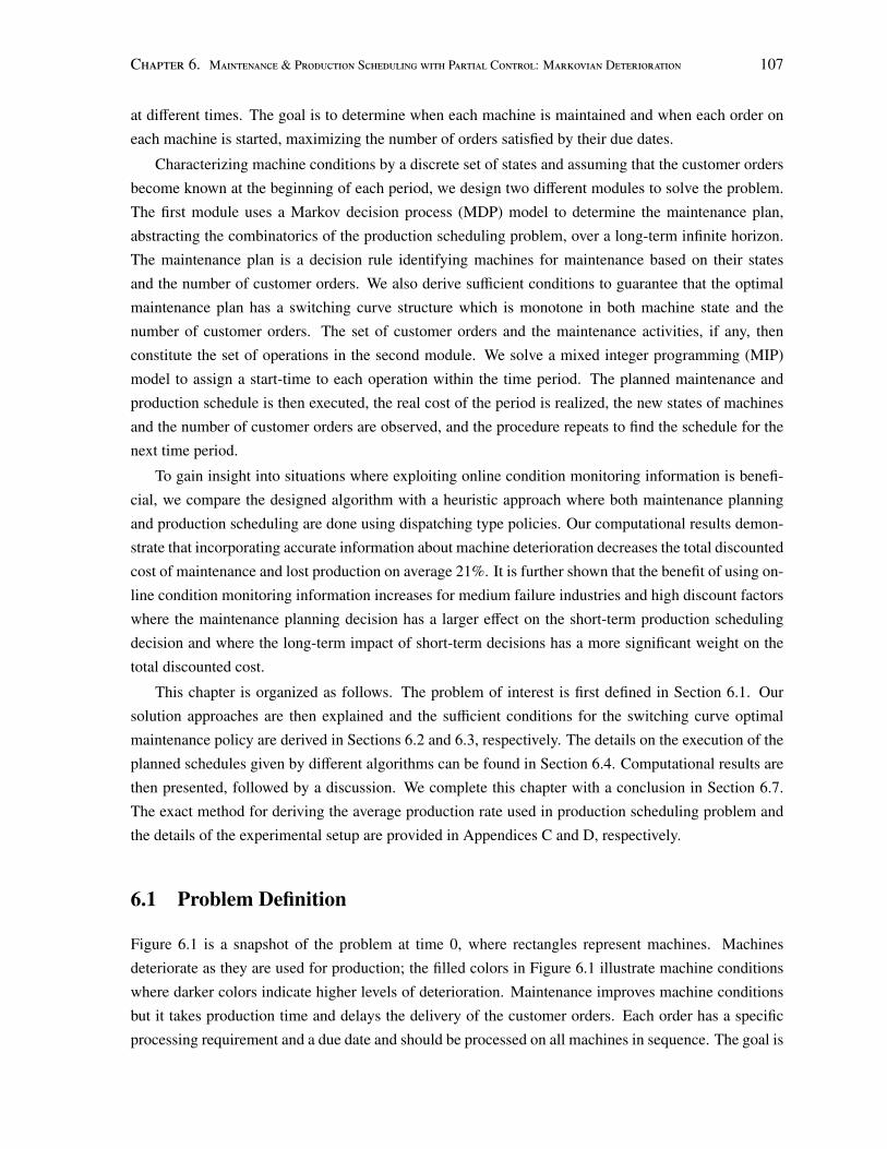
Chapter 6. Maintenance & Production Scheduling with Partial Control: Markovian Deterioration 107
at different times. The goal is to determine when each machine is maintained and when each order on
each machine is started, maximizing the number of orders satisfied by their due dates.
Characterizing machine conditions by a discrete set of states and assuming that the customer orders
become known at the beginning of each period, we design two different modules to solve the problem.
The first module uses a Markov decision process (MDP) model to determine the maintenance plan,
abstracting the combinatorics of the production scheduling problem, over a long-term infinite horizon.
The maintenance plan is a decision rule identifying machines for maintenance based on their states
and the number of customer orders. We also derive sufficient conditions to guarantee that the optimal
maintenance plan has a switching curve structure which is monotone in both machine state and the
number of customer orders. The set of customer orders and the maintenance activities, if any, then
constitute the set of operations in the second module. We solve a mixed integer programming (MIP)
model to assign a start-time to each operation within the time period. The planned maintenance and
production schedule is then executed, the real cost of the period is realized, the new states of machines
and the number of customer orders are observed, and the procedure repeats to find the schedule for the
next time period.
To gain insight into situations where exploiting online condition monitoring information is benefi-
cial, we compare the designed algorithm with a heuristic approach where both maintenance planning
and production scheduling are done using dispatching type policies. Our computational results demon-
strate that incorporating accurate information about machine deterioration decreases the total discounted
cost of maintenance and lost production on average 21%. It is further shown that the benefit of using on-
line condition monitoring information increases for medium failure industries and high discount factors
where the maintenance planning decision has a larger effect on the short-term production scheduling
decision and where the long-term impact of short-term decisions has a more significant weight on the
total discounted cost.
This chapter is organized as follows. The problem of interest is first defined in Section 6.1. Our
solution approaches are then explained and the sufficient conditions for the switching curve optimal
maintenance policy are derived in Sections 6.2 and 6.3, respectively. The details on the execution of the
planned schedules given by different algorithms can be found in Section 6.4. Computational results are
then presented, followed by a discussion. We complete this chapter with a conclusion in Section 6.7.
The exact method for deriving the average production rate used in production scheduling problem and
the details of the experimental setup are provided in Appendices C and D, respectively.
6.1 Problem Definition
Figure 6.1 is a snapshot of the problem at time 0, where rectangles represent machines. Machines
deteriorate as they are used for production; the filled colors in Figure 6.1 illustrate machine conditions
where darker colors indicate higher levels of deterioration. Maintenance improves machine conditions
but it takes production time and delays the delivery of the customer orders. Each order has a specific
processing requirement and a due date and should be processed on all machines in sequence. The goal is
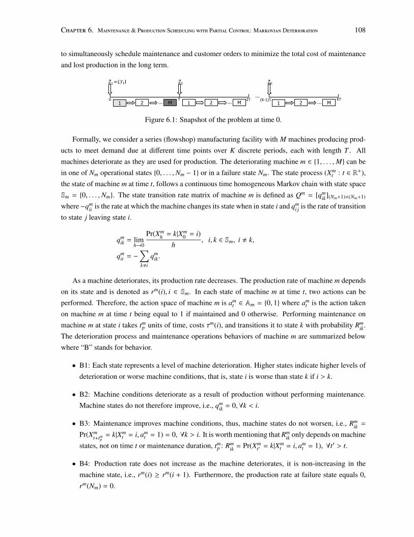
Chapter 6. Maintenance & Production Scheduling with Partial Control: Markovian Deterioration 108
to simultaneously schedule maintenance and customer orders to minimize the total cost of maintenance
and lost production in the long term.
T 2T 0 1 2 M ... 1 2 M ...
Z2
(K-1)T KT 1 2 M ...
...
ZK Z1 =
Figure 6.1: Snapshot of the problem at time 0.
Formally, we consider a series (flowshop) manufacturing facility with M machines producing prod-
ucts to meet demand due at different time points over K discrete periods, each with length T . All
machines deteriorate as they are used for production. The deteriorating machine m ∈ {1, . . . ,M} can be
in one of Nm operational states {0, . . . ,Nm − 1} or in a failure state Nm. The state process (Xmt : t ∈ R+),
the state of machine m at time t, follows a continuous time homogeneous Markov chain with state space
Sm = {0, . . . ,Nm}. The state transition rate matrix of machine m is defined as Qm = [qmik](Nm+1)×(Nm+1)
where −qmii is the rate at which the machine changes its state when in state i and qm
i j is the rate of transition
to state j leaving state i.
qmik = lim
h→0
Pr(Xmh = k|Xm
0 = i)h
, i, k ∈ Sm, i , k,
qmii = −
∑k,i
qmik.
As a machine deteriorates, its production rate decreases. The production rate of machine m depends
on its state and is denoted as rm(i), i ∈ Sm. In each state of machine m at time t, two actions can be
performed. Therefore, the action space of machine m is amt ∈ Am = {0, 1} where am
t is the action taken
on machine m at time t being equal to 1 if maintained and 0 otherwise. Performing maintenance on
machine m at state i takes tmp units of time, costs τm(i), and transitions it to state k with probability Rm
ik.
The deterioration process and maintenance operations behaviors of machine m are summarized below
where “B” stands for behavior.
• B1: Each state represents a level of machine deterioration. Higher states indicate higher levels of
deterioration or worse machine conditions, that is, state i is worse than state k if i > k.
• B2: Machine conditions deteriorate as a result of production without performing maintenance.
Machine states do not therefore improve, i.e., qmik = 0,∀k < i.
• B3: Maintenance improves machine conditions, thus, machine states do not worsen, i.e., Rmik =
Pr(Xmt+tmp
= k|Xmt = i, am
t = 1) = 0, ∀k > i. It is worth mentioning that Rmik only depends on machine
states, not on time t or maintenance duration, tmp : Rm
ik = Pr(Xmt′ = k|Xm
t = i, amt = 1), ∀t′ > t.
• B4: Production rate does not increase as the machine deteriorates, it is non-increasing in the
machine state, i.e., rm(i) ≥ rm(i + 1). Furthermore, the production rate at failure state equals 0,
rm(Nm) = 0.
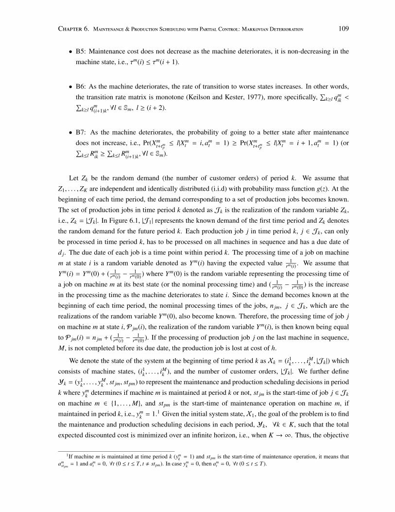
Chapter 6. Maintenance & Production Scheduling with Partial Control: Markovian Deterioration 109
• B5: Maintenance cost does not decrease as the machine deteriorates, it is non-decreasing in the
machine state, i.e., τm(i) ≤ τm(i + 1).
• B6: As the machine deteriorates, the rate of transition to worse states increases. In other words,
the transition rate matrix is monotone (Keilson and Kester, 1977), more specifically,∑
k≥l qmik <∑
k≥l qm(i+1)k,∀l ∈ Sm, l ≥ (i + 2).
• B7: As the machine deteriorates, the probability of going to a better state after maintenance
does not increase, i.e., Pr(Xmt+tmp≤ l|Xm
t = i, amt = 1) ≥ Pr(Xm
t+tmp≤ l|Xm
t = i + 1, amt = 1) (or∑
k≤l Rmik ≥
∑k≤l Rm
(i+1)k,∀l ∈ Sm).
Let Zk be the random demand (the number of customer orders) of period k. We assume that
Z1, . . . ,ZK are independent and identically distributed (i.i.d) with probability mass function g(z). At the
beginning of each time period, the demand corresponding to a set of production jobs becomes known.
The set of production jobs in time period k denoted as Jk is the realization of the random variable Zk,
i.e., Zk = |Jk|. In Figure 6.1, |J1| represents the known demand of the first time period and Zk denotes
the random demand for the future period k. Each production job j in time period k, j ∈ Jk, can only
be processed in time period k, has to be processed on all machines in sequence and has a due date of
d j. The due date of each job is a time point within period k. The processing time of a job on machine
m at state i is a random variable denoted as Ym(i) having the expected value 1rm(i) . We assume that
Ym(i) = Ym(0) + ( 1rm(i) −
1rm(0) ) where Ym(0) is the random variable representing the processing time of
a job on machine m at its best state (or the nominal processing time) and ( 1rm(i) −
1rm(0) ) is the increase
in the processing time as the machine deteriorates to state i. Since the demand becomes known at the
beginning of each time period, the nominal processing times of the jobs, n jm, j ∈ Jk, which are the
realizations of the random variable Ym(0), also become known. Therefore, the processing time of job j
on machine m at state i, P jm(i), the realization of the random variable Ym(i), is then known being equal
to P jm(i) = n jm + ( 1rm(i) −
1rm(0) ). If the processing of production job j on the last machine in sequence,
M, is not completed before its due date, the production job is lost at cost of h.
We denote the state of the system at the beginning of time period k as Xk = (i1k , . . . , iMk , |Jk|) which
consists of machine states, (i1k , . . . , iMk ), and the number of customer orders, |Jk|. We further define
Yk = (y1k , . . . , y
Mk , st jm, stpm) to represent the maintenance and production scheduling decisions in period
k where ymk determines if machine m is maintained at period k or not, st jm is the start-time of job j ∈ Jk
on machine m ∈ {1, . . . ,M}, and stpm is the start-time of maintenance operation on machine m, if
maintained in period k, i.e., ymk = 1.1 Given the initial system state, X1, the goal of the problem is to find
the maintenance and production scheduling decisions in each period, Yk, ∀k ∈ K, such that the total
expected discounted cost is minimized over an infinite horizon, i.e., when K → ∞. Thus, the objective
1If machine m is maintained at time period k (ymk = 1) and stpm is the start-time of maintenance operation, it means that
amstpm
= 1 and amt = 0, ∀t (0 ≤ t ≤ T, t , stpm). In case ym
k = 0, then amt = 0, ∀t (0 ≤ t ≤ T ).
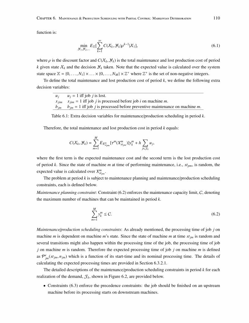
Chapter 6. Maintenance & Production Scheduling with Partial Control: Markovian Deterioration 110
function is:
minY1,Y2,...
EX[∞∑
k=1
C(Xk,Yk)ρk−1|X1], (6.1)
where ρ is the discount factor and C(Xk,Yk) is the total maintenance and lost production cost of period
k given state Xk and the decision Yk taken. Note that the expected value is calculated over the system
state space X = {0, . . . ,N1} × . . . × {0, . . . ,NM} × Z+ where Z+ is the set of non-negative integers.
To define the total maintenance and lost production cost of period k, we define the following extra
decision variables:
u j u j = 1 iff job j is lost.x jim x jim = 1 iff job j is processed before job i on machine m.b jm b jm = 1 iff job j is processed before preventive maintenance on machine m.
Table 6.1: Extra decision variables for maintenance/production scheduling in period k.
Therefore, the total maintenance and lost production cost in period k equals:
C(Xk,Yk) =
M∑m=1
EXmstpm
[τm(Xmstpm
)]ymk + h
∑j∈Jk
u j,
where the first term is the expected maintenance cost and the second term is the lost production cost
of period k. Since the state of machine m at time of performing maintenance, i.e., stpm, is random, the
expected value is calculated over Xmstpm
.
The problem at period k is subject to maintenance planning and maintenance/production scheduling
constraints, each is defined below.
Maintenance planning constraint: Constraint (6.2) enforces the maintenance capacity limit, C, denoting
the maximum number of machines that can be maintained in period k.
M∑m=1
ymk ≤ C. (6.2)
Maintenance/production scheduling constraints: As already mentioned, the processing time of job j on
machine m is dependent on machine m’s state. Since the state of machine m at time st jm is random and
several transitions might also happen within the processing time of the job, the processing time of job
j on machine m is random. Therefore the expected processing time of job j on machine m is defined
as Pejm(st jm, n jm) which is a function of its start-time and its nominal processing time. The details of
calculating the expected processing times are provided in Section 6.3.2.1.
The detailed descriptions of the maintenance/production scheduling constraints in period k for each
realization of the demand, Jk, shown in Figure 6.2, are provided below.
• Constraints (6.3) enforce the precedence constraints: the job should be finished on an upstream
machine before its processing starts on downstream machines.
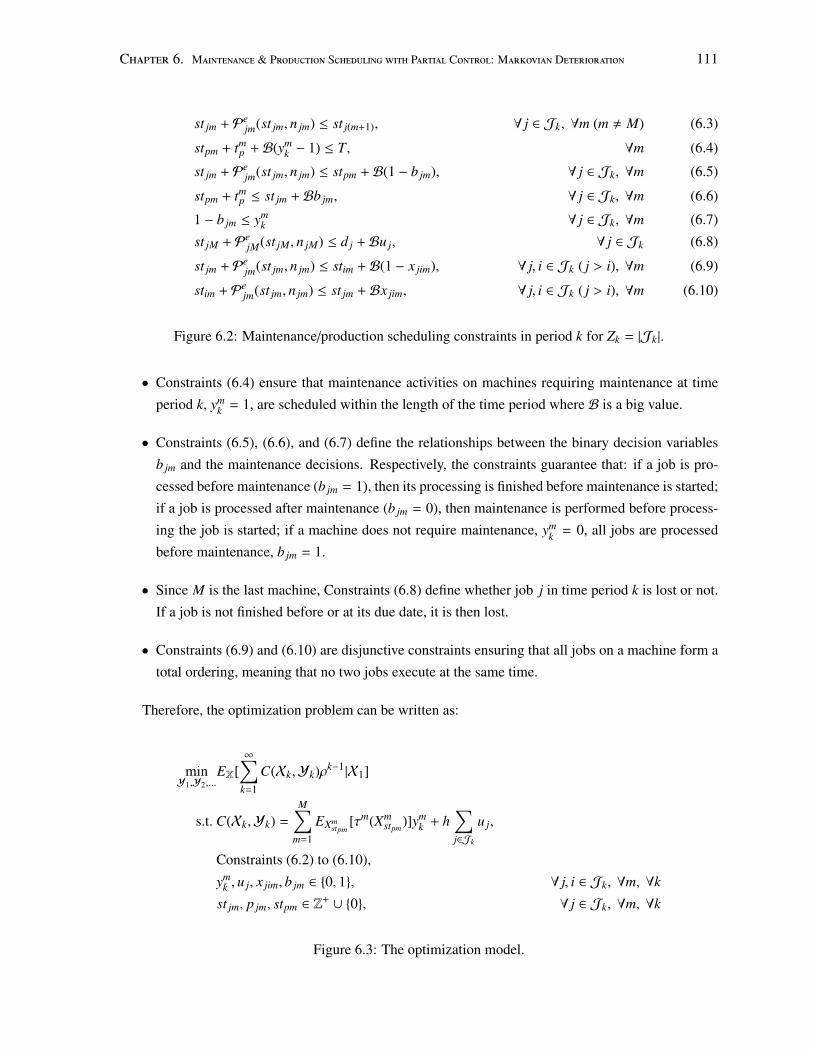
Chapter 6. Maintenance & Production Scheduling with Partial Control: Markovian Deterioration 111
st jm + Pejm(st jm, n jm) ≤ st j(m+1), ∀ j ∈ Jk, ∀m (m , M) (6.3)
stpm + tmp + B(ym
k − 1) ≤ T, ∀m (6.4)
st jm + Pejm(st jm, n jm) ≤ stpm + B(1 − b jm), ∀ j ∈ Jk, ∀m (6.5)
stpm + tmp ≤ st jm + Bb jm, ∀ j ∈ Jk, ∀m (6.6)
1 − b jm ≤ ymk ∀ j ∈ Jk, ∀m (6.7)
st jM + PejM(st jM, n jM) ≤ d j + Bu j, ∀ j ∈ Jk (6.8)
st jm + Pejm(st jm, n jm) ≤ stim + B(1 − x jim), ∀ j, i ∈ Jk ( j > i), ∀m (6.9)
stim + Pejm(st jm, n jm) ≤ st jm + Bx jim, ∀ j, i ∈ Jk ( j > i), ∀m (6.10)
Figure 6.2: Maintenance/production scheduling constraints in period k for Zk = |Jk|.
• Constraints (6.4) ensure that maintenance activities on machines requiring maintenance at time
period k, ymk = 1, are scheduled within the length of the time period where B is a big value.
• Constraints (6.5), (6.6), and (6.7) define the relationships between the binary decision variables
b jm and the maintenance decisions. Respectively, the constraints guarantee that: if a job is pro-
cessed before maintenance (b jm = 1), then its processing is finished before maintenance is started;
if a job is processed after maintenance (b jm = 0), then maintenance is performed before process-
ing the job is started; if a machine does not require maintenance, ymk = 0, all jobs are processed
before maintenance, b jm = 1.
• Since M is the last machine, Constraints (6.8) define whether job j in time period k is lost or not.
If a job is not finished before or at its due date, it is then lost.
• Constraints (6.9) and (6.10) are disjunctive constraints ensuring that all jobs on a machine form a
total ordering, meaning that no two jobs execute at the same time.
Therefore, the optimization problem can be written as:
minY1,Y2,...
EX[∞∑
k=1
C(Xk,Yk)ρk−1|X1]
s.t. C(Xk,Yk) =
M∑m=1
EXmstpm
[τm(Xmstpm
)]ymk + h
∑j∈Jk
u j,
Constraints (6.2) to (6.10),
ymk , u j, x jim, b jm ∈ {0, 1}, ∀ j, i ∈ Jk, ∀m, ∀k
st jm, p jm, stpm ∈ Z+ ∪ {0}, ∀ j ∈ Jk, ∀m, ∀k
Figure 6.3: The optimization model.
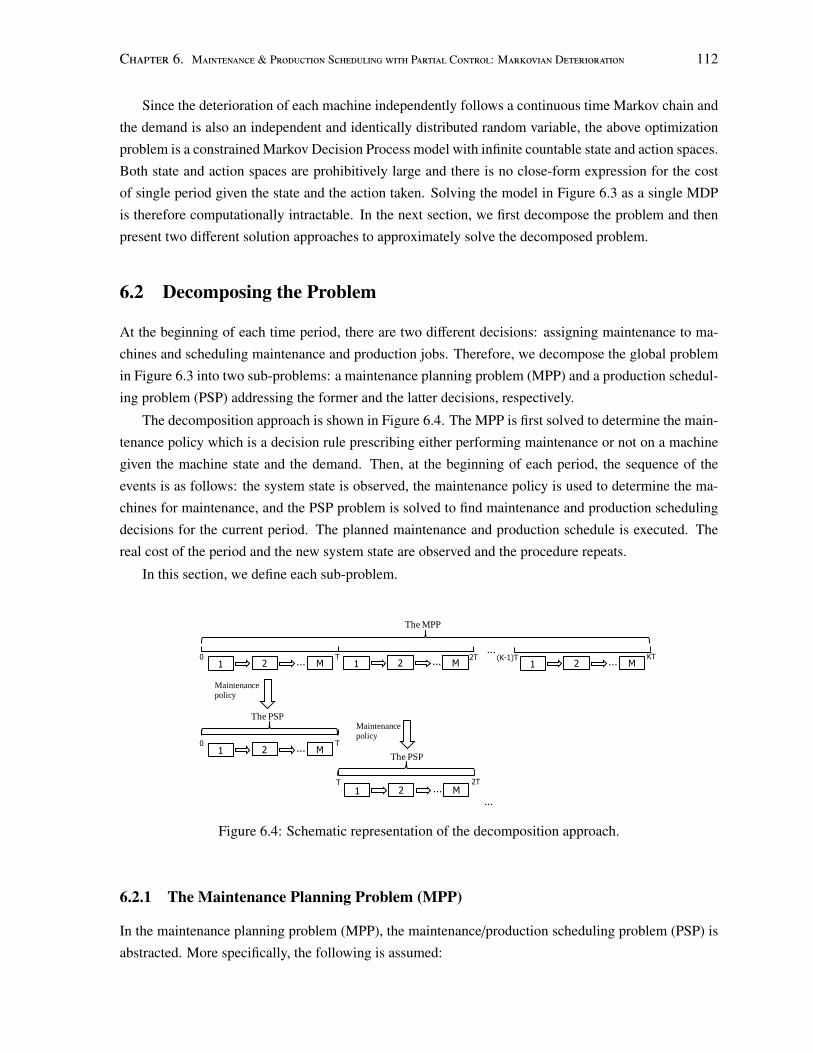
Chapter 6. Maintenance & Production Scheduling with Partial Control: Markovian Deterioration 112
Since the deterioration of each machine independently follows a continuous time Markov chain and
the demand is also an independent and identically distributed random variable, the above optimization
problem is a constrained Markov Decision Process model with infinite countable state and action spaces.
Both state and action spaces are prohibitively large and there is no close-form expression for the cost
of single period given the state and the action taken. Solving the model in Figure 6.3 as a single MDP
is therefore computationally intractable. In the next section, we first decompose the problem and then
present two different solution approaches to approximately solve the decomposed problem.
6.2 Decomposing the Problem
At the beginning of each time period, there are two different decisions: assigning maintenance to ma-
chines and scheduling maintenance and production jobs. Therefore, we decompose the global problem
in Figure 6.3 into two sub-problems: a maintenance planning problem (MPP) and a production schedul-
ing problem (PSP) addressing the former and the latter decisions, respectively.
The decomposition approach is shown in Figure 6.4. The MPP is first solved to determine the main-
tenance policy which is a decision rule prescribing either performing maintenance or not on a machine
given the machine state and the demand. Then, at the beginning of each period, the sequence of the
events is as follows: the system state is observed, the maintenance policy is used to determine the ma-
chines for maintenance, and the PSP problem is solved to find maintenance and production scheduling
decisions for the current period. The planned maintenance and production schedule is executed. The
real cost of the period and the new system state are observed and the procedure repeats.
In this section, we define each sub-problem.
T 2T 0 1 2 M ... 1 2 M ...
(K-1)T KT 1 2 M ...
...
The MPP
T 0 1 2 M ...
The PSP
2T T
1 2 M ...
The PSP
...
Maintenance policy
Maintenance policy
Figure 6.4: Schematic representation of the decomposition approach.
6.2.1 The Maintenance Planning Problem (MPP)
In the maintenance planning problem (MPP), the maintenance/production scheduling problem (PSP) is
abstracted. More specifically, the following is assumed:
Chapter 6. Maintenance & Production Scheduling with Partial Control: Markovian Deterioration 113
1. All production jobs on machine m ∈ {1, . . . ,M} are assumed to have the same processing time
equal to 1rm(im) where im is the state of machine m at the beginning of the period. It is further
assumed that all production jobs are due at the end of the time period (d j = T ).
2. Maintenance, if any, is performed at the beginning of the time period and it has a negligible
duration (tmp = 0). More specifically, the action performed on machine m at time 0, am
0 , equals 1 if
maintained (ymk = 1) and equals 0, otherwise (ym
k = 0). Therefore, ymk = am
0 .
Although there is negative economic dependency between machines, implying that there is a limit
on the number of machines maintained in each time period, in the MPP machines are considered inde-
pendently. A Markov decision process (MDP) model is used for each machine independently to find the
optimal maintenance policy over an infinite horizon such that the total expected discounted cost of main-
tenance and a lower bound on the lost production is minimized. In the MDP model of each machine, one
decision is made at the beginning of each period: whether to maintain the machine or not. To consider
the maintenance capacity limit in the MDP, the conditions of the machines should be represented as a
vector of size M with its elements being the state of machines which results in∏M
m=1(Nm + 1) different
levels of system deterioration. Therefore, solving one MDP to make the maintenance decisions of all
machines is computationally intractable due to the size of the state space. In this section, the index of
machine, i.e., m, is excluded from the notation for ease of reading.
In the MDP, the following information is required: the production rate of a machine at each state,
r(i); the maintenance cost of a machine at each state, τ(i); the transition probability that a machine
changes its state in a time interval with length T ; and the demand distribution.
The machine transition probability, pa0ik , represents the probability that the machine is in state k at
the beginning of next time period given its current state is i and action a0 is taken at the beginning of
the current period. Since the deterioration process of the machine follows a homogeneous continuous
time Markov chain, the transition probabilities do not vary in time. Taking the behavior of deterioration
process into account, we have:
p0ik = Pr(XT = k|X0 = i, a0 = 0) =
pik 0 ≤ i ≤ k ≤ N,
1 i = N, k = N,
0 0 ≤ k < i ≤ N,
p1ik = Pr(XT = k|X0 = i, a0 = 1) =
N∑l=0
Pr(X0+ = l|X0 = i, a0 = 1) · Pr(XT = k|X0+ = l, a0+ = 0)
=
N∑l=0
Ril p0lk,
where pik is the probability of changing the state from i to k as a result of production within a period of
T time units. Using matrix notation, P0 = [p0ik] = eQT and P1 = [p1
ik] = R × P0 where R = [Rik].
Chapter 6. Maintenance & Production Scheduling with Partial Control: Markovian Deterioration 114
We define the maintenance cost, τ(i, a0), and the production rate, r(i, a0), when machine is in state i
and action a0 is taken as follows.
τ(i, 0) = 0, τ(i, 1) = τ(i),
r(i, 0) = r(i), r(i, 1) =
N∑l=0
Rilr(l).
Assuming the machine is in state i, demand is z, and action a0 is taken, the total maintenance and lost
production cost of a single period, C(i, z, a0), is defined below where the first and the second terms
denote maintenance cost and lost production cost, respectively. The number of products produced by
the machine equals Tr(i, a0), and since in a series manufacturing all demand needs to be produced by
each machine, (z − Tbr(i, a0))+ = max(0, z − Tr(i, a0)) denotes the number of lost products.
C(i, z, a0) = τ(i, a0) + h(z − Tr(i, a0))+.
We define Vn(i, z, a0) as the total discounted expected maintenance and lost production cost when the
machine state is i, the demand is z, action a0 is taken at the beginning of the period, and n time periods
are remaining. Vn(i, z), the minimal discounted cost, Vn(i, z) = mina0∈{0,1}
(Vn(i, z, a0)), can be found by
solving the following recursive equation.
Vn(i, z) = mina0∈{0,1}
[C(i, z, a0) + ρ
N∑k=0
pa0ik
∞∑δ=0
g(δ)Vn−1(k, δ)]. (6.11)
where V0(i, z) = 0, ∀i, z. Recall that ρ is the discount factor and g(δ) is the probability that the demand
in the next period equals δ. For the optimality Equation (6.11), Theorem 6.2.10 in Puterman (1994,
p. 154) guarantees that there exists an optimal stationary policy because the state space is countable,
the costs are bounded and stationary, i.e., they do not change from one decision point to another, the
transition probabilities are stationary, and the action space for each state is finite.
The infinite-horizon equivalent of Equation (6.11) can be written as:
V(i, z) = mina0∈{0,1}
[C(i, z, a0) + ρ
N∑k=0
pa0ik
∞∑δ=0
g(δ)V(k, δ)]. (6.12)
The following Lemma shows that there is a solution to Equation (6.12).
Lemma 6.1. V(i, z) = limn→∞ Vn(i, z) exists for ∀i, ∀z.
Proof. Consider π as a policy and let Wπ(i, z) denote the expected value of this policy when the initial
machine state is i and the demand is z. Based on Theorem 8-13 in Heyman and Sobel (1984), if Wπ(i, z) <
∞ for ∀i, ∀z, then V(i, z) = limn→∞ Vn(i, z) exists for ∀i, ∀z. We consider π as a policy where we always
maintain the machine. Since single period value function, V1(i, z) = C(i, z, 1), is bounded and the
discount factor, ρ, is less than 1, Wπ(i, z) < ∞ for ∀i, ∀z which completes the proof. �
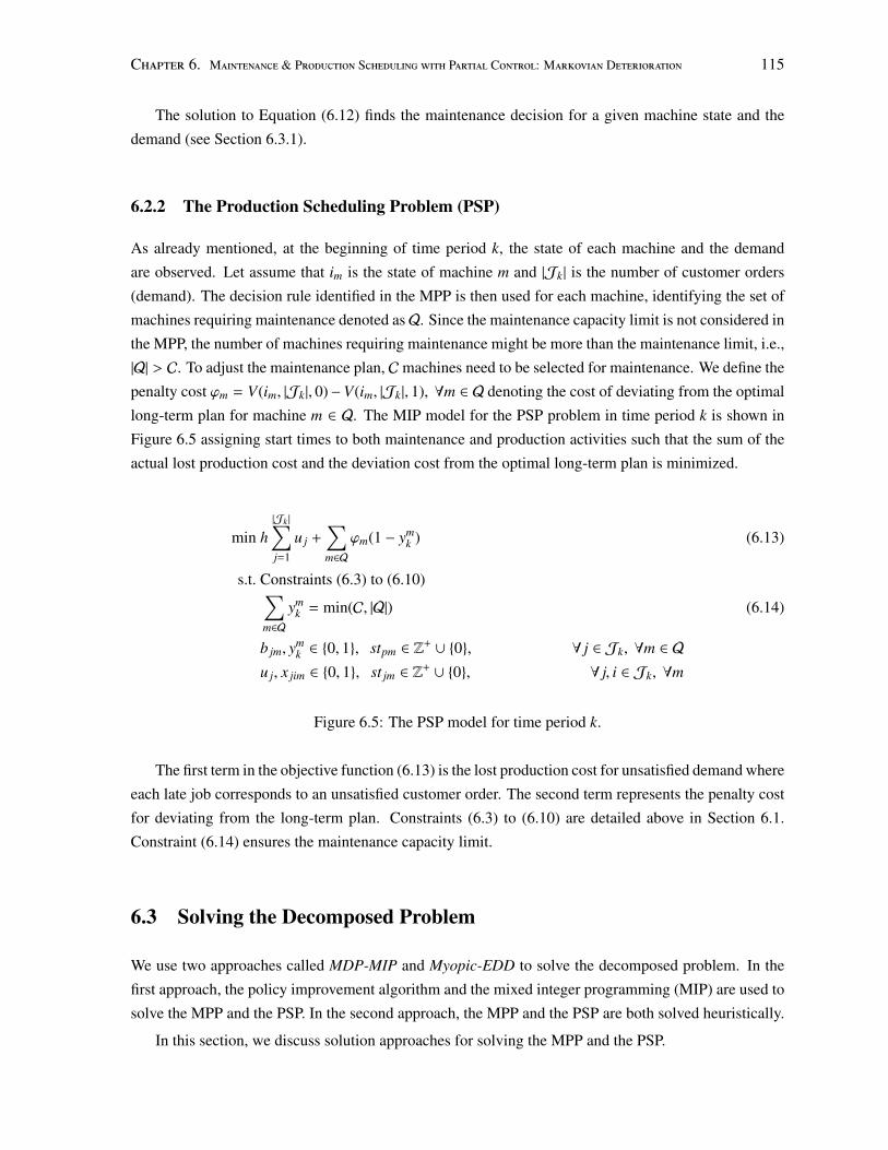
Chapter 6. Maintenance & Production Scheduling with Partial Control: Markovian Deterioration 115
The solution to Equation (6.12) finds the maintenance decision for a given machine state and the
demand (see Section 6.3.1).
6.2.2 The Production Scheduling Problem (PSP)
As already mentioned, at the beginning of time period k, the state of each machine and the demand
are observed. Let assume that im is the state of machine m and |Jk| is the number of customer orders
(demand). The decision rule identified in the MPP is then used for each machine, identifying the set of
machines requiring maintenance denoted asQ. Since the maintenance capacity limit is not considered in
the MPP, the number of machines requiring maintenance might be more than the maintenance limit, i.e.,
|Q| > C. To adjust the maintenance plan, Cmachines need to be selected for maintenance. We define the
penalty cost ϕm = V(im, |Jk|, 0)−V(im, |Jk|, 1), ∀m ∈ Q denoting the cost of deviating from the optimal
long-term plan for machine m ∈ Q. The MIP model for the PSP problem in time period k is shown in
Figure 6.5 assigning start times to both maintenance and production activities such that the sum of the
actual lost production cost and the deviation cost from the optimal long-term plan is minimized.
min h|Jk |∑j=1
u j +∑m∈Q
ϕm(1 − ymk ) (6.13)
s.t. Constraints (6.3) to (6.10)∑m∈Q
ymk = min(C, |Q|) (6.14)
b jm, ymk ∈ {0, 1}, stpm ∈ Z
+ ∪ {0}, ∀ j ∈ Jk, ∀m ∈ Q
u j, x jim ∈ {0, 1}, st jm ∈ Z+ ∪ {0}, ∀ j, i ∈ Jk, ∀m
Figure 6.5: The PSP model for time period k.
The first term in the objective function (6.13) is the lost production cost for unsatisfied demand where
each late job corresponds to an unsatisfied customer order. The second term represents the penalty cost
for deviating from the long-term plan. Constraints (6.3) to (6.10) are detailed above in Section 6.1.
Constraint (6.14) ensures the maintenance capacity limit.
6.3 Solving the Decomposed Problem
We use two approaches called MDP-MIP and Myopic-EDD to solve the decomposed problem. In the
first approach, the policy improvement algorithm and the mixed integer programming (MIP) are used to
solve the MPP and the PSP. In the second approach, the MPP and the PSP are both solved heuristically.
In this section, we discuss solution approaches for solving the MPP and the PSP.
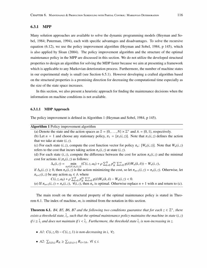
Chapter 6. Maintenance & Production Scheduling with Partial Control: Markovian Deterioration 116
6.3.1 MPP
Many solution approaches are available to solve the dynamic programming models (Heyman and So-
bel, 1984; Puterman, 1994), each with specific advantages and disadvantages. To solve the recursive
equation (6.12), we use the policy improvement algorithm (Heyman and Sobel, 1984, p 145), which
is also applied by Sloan (2004). The policy improvement algorithm and the structure of the optimal
maintenance policy in the MPP are discussed in this section. We do not utilize the developed structural
properties to design an algorithm for solving the MDP faster because we aim at presenting a framework
which is applicable to any Markovian deterioration process. Furthermore, the number of machine states
in our experimental study is small (see Section 6.5.1). However developing a crafted algorithm based
on the structural properties is a promising direction for decreasing the computational time especially as
the size of the state space increases.
In this section, we also present a heuristic approach for finding the maintenance decisions when the
information on machine conditions is not available.
6.3.1.1 MDP Approach
The policy improvement is defined in Algorithm 1 (Heyman and Sobel, 1984, p 145).
Algorithm 1 Policy improvement algorithm(a) Denote the state and the action spaces as S = {0, . . . ,N} × Z+ and A = {0, 1}, respectively.(b) Let n = 1 and choose any stationary policy, π1 = [π1(i, z)]. Note that π1(i, z) defines the actionthat we take at state (i, z).(c) For each state (i, z), compute the cost function vector for policy πn: [Wn(i, z)]. Note that Wn(i, z)refers to the cost that incurs taking action πn(i, z) at state (i, z).(d) For each state (i, z), compute the difference between the cost for action πn(i, z) and the minimalcost for actions A\πn(i, z) as follows:
∆n(i, z) = mina0∈{A\πn(i,z)}
(C(i, z, a0) + ρ∑N
k=0 pa0ik
∑∞δ=0 g(δ)Wn(k, δ)) −Wn(i, z),
if ∆n(i, z) ≥ 0, then πn(i, z) is the action minimizing the cost, so let πn+1(i, z) = πn(i, z). Otherwise, letπn+1(i, z) be any action a0 ∈ A where
C(i, z, a0) + ρ∑N
k=0 pa0ik
∑∞δ=0 g(δ)Wn(k, δ) −Wn(i, z) < 0.
(e) If πn+1(i, z) = πn(i, z), ∀(i, z), then πn is optimal. Otherwise replace n + 1 with n and return to (c).
The main result on the structural property of the optimal maintenance policy is stated in Theo-
rem 6.1. The index of machine, m, is omitted from the notation in this section.
Theorem 6.1. B4, B5, B6, B7 and the following two conditions guarantee that for each z ∈ Z+, there
exists a threshold state, iz, such that the optimal maintenance policy maintains the machine in state (i, z)
if i ≥ iz and does not maintain if i < iz. Furthermore, the threshold state iz is non-increasing in z.
• A1: C(i, z, 0) −C(i, z, 1) is non-decreasing in i, ∀z.
• A2:∑
l≤k≤i Rik ≥∑
l≤k≤i+1 R(i+1)k, ∀l ≤ i.
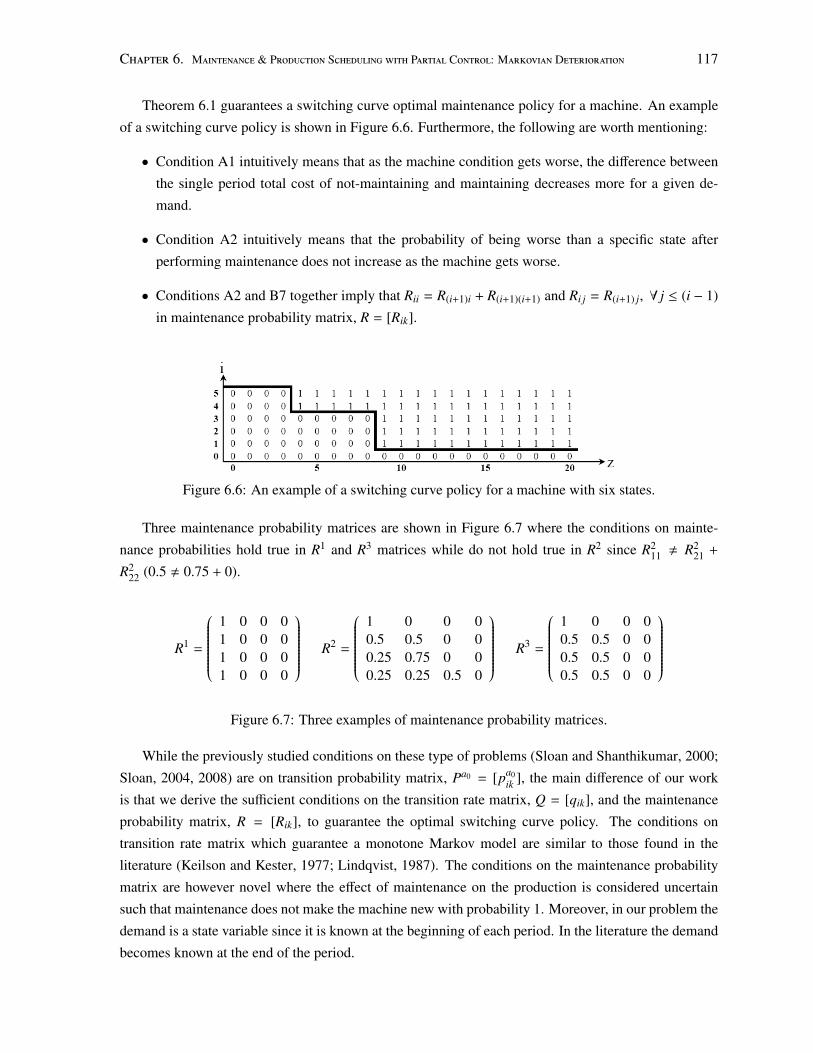
Chapter 6. Maintenance & Production Scheduling with Partial Control: Markovian Deterioration 117
Theorem 6.1 guarantees a switching curve optimal maintenance policy for a machine. An example
of a switching curve policy is shown in Figure 6.6. Furthermore, the following are worth mentioning:
• Condition A1 intuitively means that as the machine condition gets worse, the difference between
the single period total cost of not-maintaining and maintaining decreases more for a given de-
mand.
• Condition A2 intuitively means that the probability of being worse than a specific state after
performing maintenance does not increase as the machine gets worse.
• Conditions A2 and B7 together imply that Rii = R(i+1)i + R(i+1)(i+1) and Ri j = R(i+1) j, ∀ j ≤ (i − 1)
in maintenance probability matrix, R = [Rik].
Figure 6.6: An example of a switching curve policy for a machine with six states.
Three maintenance probability matrices are shown in Figure 6.7 where the conditions on mainte-
nance probabilities hold true in R1 and R3 matrices while do not hold true in R2 since R211 , R2
21 +
R222 (0.5 , 0.75 + 0).
R1 =
1 0 0 01 0 0 01 0 0 01 0 0 0
R2 =
1 0 0 00.5 0.5 0 00.25 0.75 0 00.25 0.25 0.5 0
R3 =
1 0 0 00.5 0.5 0 00.5 0.5 0 00.5 0.5 0 0
Figure 6.7: Three examples of maintenance probability matrices.
While the previously studied conditions on these type of problems (Sloan and Shanthikumar, 2000;
Sloan, 2004, 2008) are on transition probability matrix, Pa0 = [pa0ik ], the main difference of our work
is that we derive the sufficient conditions on the transition rate matrix, Q = [qik], and the maintenance
probability matrix, R = [Rik], to guarantee the optimal switching curve policy. The conditions on
transition rate matrix which guarantee a monotone Markov model are similar to those found in the
literature (Keilson and Kester, 1977; Lindqvist, 1987). The conditions on the maintenance probability
matrix are however novel where the effect of maintenance on the production is considered uncertain
such that maintenance does not make the machine new with probability 1. Moreover, in our problem the
demand is a state variable since it is known at the beginning of each period. In the literature the demand
becomes known at the end of the period.
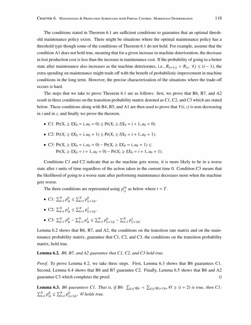
Chapter 6. Maintenance & Production Scheduling with Partial Control: Markovian Deterioration 118
The conditions stated in Theorem 6.1 are sufficient conditions to guarantee that an optimal thresh-
old maintenance policy exists. There might be situations where the optimal maintenance policy has a
threshold type though some of the conditions of Theorem 6.1 do not hold. For example, assume that the
condition A1 does not hold true, meaning that for a given increase in machine deterioration, the decrease
in lost production cost is less than the increase in maintenance cost. If the probability of going to a better
state after maintenance also increases as the machine deteriorates, i.e., R(i+1) j > Ri j, ∀ j ≤ (i − 1), the
extra spending on maintenance might trade off with the benefit of probabilistic improvement in machine
conditions in the long term. However, the precise characterization of the situations where the trade-off
occurs is hard.
The steps that we take to prove Theorem 6.1 are as follows: first, we prove that B6, B7, and A2
result in three conditions on the transition probability matrix denoted as C1, C2, and C3 which are stated
below. These conditions along with B4, B5, and A1 are then used to prove that V(i, z) is non-decreasing
in i and in z, and finally we prove the theorem.
• C1: Pr(Xt ≥ l|X0 = i, a0 = 0) ≤ Pr(Xt ≥ l|X0 = i + 1, a0 = 0).
• C2: Pr(Xt ≥ l|X0 = i, a0 = 1) ≤ Pr(Xt ≥ l|X0 = i + 1, a0 = 1).
• C3: Pr(Xt ≥ l|X0 = i, a0 = 0) − Pr(Xt ≥ l|X0 = i, a0 = 1) ≤
Pr(Xt ≥ l|X0 = i + 1, a0 = 0) − Pr(Xt ≥ l|X0 = i + 1, a0 = 1).
Conditions C1 and C2 indicate that as the machine gets worse, it is more likely to be in a worse
state after t units of time regardless of the action taken in the current time 0. Condition C3 means that
the likelihood of going to a worse state after performing maintenance decreases more when the machine
gets worse.
The three conditions are represented using pa0i j as below where t = T .
• C1:∑N
k=l p0ik ≤
∑Nk=l p0
(i+1)k.
• C2:∑N
k=l p1ik ≤
∑Nk=l p1
(i+1)k.
• C3:∑N
k=l p0ik −
∑Nk=l p1
ik ≤∑N
k=l p0(i+1)k −
∑Nk=l p1
(i+1)k.
Lemma 6.2 shows that B6, B7, and A2, the conditions on the transition rate matrix and on the main-
tenance probability matrix, guarantee that C1, C2, and C3, the conditions on the transition probability
matrix, hold true.
Lemma 6.2. B6, B7, and A2 guarantee that C1, C2, and C3 hold true.
Proof. To prove Lemma 6.2, we take three steps. First, Lemma 6.3 shows that B6 guarantees C1.
Second, Lemma 6.4 shows that B6 and B7 guarantee C2. Finally, Lemma 6.5 shows that B6 and A2
guarantee C3 which completes the proof. �
Lemma 6.3. B6 guarantees C1. That is, if B6:∑
k≥l qik <∑
k≥l q(i+1)k,∀l ≥ (i + 2) is true, then C1:∑Nk=l p0
ik ≤∑N
k=l p0(i+1)k, ∀l holds true.
Chapter 6. Maintenance & Production Scheduling with Partial Control: Markovian Deterioration 119
Proof. The proof is based on induction.
The first step is to show Pr(X∆ ≥ l|X0 = i, a0 = 0) ≤ Pr(X∆ ≥ l|X0 = i + 1, a0 = 0), ∀l for a small
∆ ≥ 0. We discuss the following two cases:
1. If l ≤ i + 1, then Pr(X∆ ≥ l|X0 = i + 1, a0 = 0) = 1 and the inequality is obvious.
2. If l ≥ i + 2, then
Pr(X∆ ≥ l|X0 = i + 1, a0 = 0) − Pr(X∆ ≥ l|X0 = i, a0 = 0) =∑k≥l
(q(i+1)k∆ + o(i+1)k(∆)) −∑k≥l
(qik∆ + oik(∆)) =
∆[∑k≥l
q(i+1)k −∑k≥l
qik +oi+1(∆) − oi(∆)
∆],
where∑
k≥l o(i+1)k(∆) = oi+1(∆) and∑
k≥l oik(∆) = oi(∆). Since as ∆ → 0, oi+1(∆)−oi(∆)∆
→ 0 and∑k≥l q(i+1)k −
∑k≥l qik > 0, there exists a small ∆0 such that ∀∆ ≤ ∆0, Pr(X∆ ≥ l|X0 = i + 1, a0 =
0) − Pr(X∆ ≥ l|X0 = i, a0 = 0) ≥ 0.
We choose K > 0 and big such that ∆ = tK is very small. Therefore, given 1 and 2 we have shown the
first step which is
Pr(X∆ ≥ l|X0 = i, a0 = 0) ≤ Pr(X∆ ≥ l|X0 = i + 1, a0 = 0), ∀l.
The induction assumption is Pr(X( j−1)∆ ≥ l|X0 = i, a0 = 0) ≤ Pr(X( j−1)∆ ≥ l|X0 = i + 1, a0 = 0), ∀l.
The last step is to show Pr(X j∆ ≥ l|X0 = i, a0 = 0) ≤ Pr(X j∆ ≥ l|X0 = i + 1, a0 = 0), ∀l.
We have
Pr(X j∆ ≥ l|X0 = i, a0 = 0) =
N∑k=0
Pr(X∆ = k|X0 = i, a0 = 0) · Pr(X j∆ ≥ l|X∆ = k, a∆ = 0),
Pr(X j∆ ≥ l|X0 = i + 1, a0 = 0) =
N∑k=0
Pr(X∆ = k|X0 = i + 1, a0 = 0) · Pr(X j∆ ≥ l|X∆ = k, a∆ = 0).
Defining f (k) = Pr(X j∆ ≥ l|X∆ = k, a∆ = 0) and Pr(Yi = k) = Pr(X∆ = k|X0 = i, a0 = 0), we have
Pr(X j∆ ≥ l|X0 = i, a0 = 0) = E[ f (Yi)],
Pr(X j∆ ≥ l|X0 = i + 1, a0 = 0) = E[ f (Yi+1)].
In the first step, we showed that
Pr(X∆ ≥ l|X0 = i, a0 = 0) ≤ Pr(X∆ ≥ l|X0 = i + 1, a0 = 0), ∀l.
Chapter 6. Maintenance & Production Scheduling with Partial Control: Markovian Deterioration 120
Using the definition of Pr(Yi = k), we have
Pr(Yi ≥ l) ≤ Pr(Yi+1 ≥ l),
meaning that Yi is stochastically smaller than Yi+1, Yi ≤st Yi+1. Since f (k) is non-decreasing in k because
of the induction assumption, E[ f (Yi)] ≤ E[ f (Yi+1)].2 Letting K = j and t = T where K∆ = t, the proof
is complete. �
Lemma 6.4. B6 and B7 guarantee C2. That is, if
(i) B6:∑
k≥l qik <∑
k≥l q(i+1)k, ∀l ≥ i + 2, and
(ii) B7:∑
k≤l Rik ≥∑
k≤l R(i+1)k, ∀l are true,
then C2:∑N
k=l p1ik ≤
∑Nk=l p1
(i+1)k, ∀l holds true.
Proof. We have
Pr(Xt ≥ l|X0 = i, a0 = 1) =
N∑k=0
Pr(X0+ = k|X0 = i, a0 = 1) · Pr(Xt ≥ l|X0+ = k, a0+ = 0)
=
N∑k=0
RikPr(Xt ≥ l|X0+ = k, a0+ = 0) = E[ f (Yi)],
Pr(Xt ≥ l|X0 = i + 1, a0 = 1) =
N∑k=0
Pr(X0+ = k|X0 = i + 1, a0 = 1) · Pr(Xt ≥ l|X0+ = k, a0+ = 0)
=
N∑k=0
R(i+1)kPr(Xt ≥ l|X0+ = k, a0+ = 0) = E[ f (Xi+1)],
where Rik = Pr(Yi = k) = Pr(X0+ = k|X0 = i, a0 = 1) and f (k) = Pr(Xt ≥ l|X0+ = k, a0+ = 0). Since
B7 indicates that Pr(Yi ≤ l) ≥ Pr(Yi+1 ≤ l), we conclude that Yi ≤st Yi+1. Furthermore, in the proof
of Lemma 6.3, it is shown that f (k) is non-decreasing in k. Therefore, E[ f (Yi)] ≤ E[ f (Yi+1)]. Letting
t = T , the proof is complete. �
Lemma 6.5. B6 and A2 guarantee C3. That is, if
(i) B6:∑
k≥l qik <∑
k≥l q(i+1)k, ∀l ≥ i + 2, and
(ii) A2:∑
l≤k≤i Rik ≥∑
l≤k≤i+1 R(i+1)k, ∀l ≤ i are true,
then C3:∑N
k=l p0ik −
∑Nk=l p1
ik ≤∑N
k=l p0(i+1)k −
∑Nk=l p1
(i+1)k, ∀l holds true.
2A real random variable, A, is stochastically smaller than a random variable, B, if and only if for all non-decreasingfunctions u, E[u(A)] ≤ E[u(B)].
Chapter 6. Maintenance & Production Scheduling with Partial Control: Markovian Deterioration 121
Proof. The proof is based on induction.
The first step is to show that:
Pr(X∆ ≥ l|X0 = i, a0 = 0) − Pr(X∆ ≥ l|X0 = i, a0 = 1) ≤
Pr(X∆ ≥ l|X0 = i + 1, a0 = 0) − Pr(X∆ ≥ l|X0 = i + 1, a0 = 1), ∀l.
To do so, we first need to prove
Pr(X0+ ≥ l|X0 = i, a0 = 0) − Pr(X0+ ≥ l|X0 = i, a0 = 1) ≤
Pr(X0+ ≥ l|X0 = i + 1, a0 = 0) − Pr(X0+ ≥ l|X0 = i + 1, a0 = 1), ∀l. (6.15)
Let us discuss the following two cases:
1. if l ≥ i + 1, then the inequality (6.15) is obvious as 0 − 0 ≤ 1 − c where 0 ≤ c ≤ 1.
2. if l ≤ i, based on A2, we have
Pr(X0+ ≥ l|X0 = i, a0 = 1) ≥ Pr(X0+ ≥ l|X0 = i + 1, a0 = 1).
By adding Pr(X0+ ≥ l|X0 = i, a0 = 0) to the above inequality, we have:
Pr(X0+ ≥ l|X0 = i, a0 = 0) − Pr(X0+ ≥ l|X0 = i, a0 = 1) ≤
Pr(X0+ ≥ l|X0 = i, a0 = 0) − Pr(X0+ ≥ l|X0 = i + 1, a0 = 1). (6.16)
In the proof of Lemma 6.3, we have shown Pr(X0+ ≥ l|X0 = i, a0 = 0) ≤ Pr(X0+ ≥ l|X0 = i+1, a0 =
0); therefore, we can write (6.16) as:
Pr(X0+ ≥ l|X0 = i, a = 0) − Pr(X0+ ≥ l|X0 = i, a = 1) ≤
Pr(X0+ ≥ l|X0 = i + 1, a = 0) − Pr(X0+ ≥ l|X0 = i + 1, a = 1).
Given 1 and 2, we have shown that the inequality (6.15) holds true. Then, we have
Pr(X∆ ≥ l|X0 = i, a0 = 0) − Pr(X∆ ≥ l|X0 = i, a0 = 1)
=
N∑k=0
Pr(X0+ = k|X0 = i, a0 = 0) · Pr(X∆ ≥ l|X0+ = k, a0+ = 0)
−
N∑k=0
Pr(X0+ = k|X0 = i, a0 = 1) · Pr(X∆ ≥ l|X0+ = k, a0+ = 0).
Chapter 6. Maintenance & Production Scheduling with Partial Control: Markovian Deterioration 122
Defining f (k) = Pr(X∆ ≥ l|X0+ = k, a0+ = 0), Pr(Yi = k) = Pr(X0+ = k|X0 = i, a0 = 0), and Pr(Zi = k) =
Pr(X0+ = k|X0 = i, a0 = 1), we have
Pr(X∆ ≥ l|X0 = i, a0 = 0) − Pr(X∆ ≥ l|X0 = i, a0 = 1) = E[ f (Yi)] − E[ f (Zi)].
Following the same as above, we have
Pr(X∆ ≥ l|X0 = i + 1, a0 = 0) − Pr(X∆ ≥ l|X0 = i + 1, a0 = 1) = E[ f (Yi+1)] − E[ f (Zi+1)].
Knowing that E[ f (Y)] = f (0) +∑
j≥1( f ( j) − f ( j − 1)) · Pr(Y ≥ j), we then have
E[ f (Yi)] − E[ f (Zi)] =∑j≥1
( f ( j) − f ( j − 1)) · (Pr(Yi ≥ j) − Pr(Zi ≥ j)),
E[ f (Yi+1)] − E[ f (Zi+1)] =∑j≥1
( f ( j) − f ( j − 1)) · (Pr(Yi+1 ≥ j) − Pr(Zi+1 ≥ j)).
Based on inequality (6.15), we have
Pr(Yi ≥ j) − Pr(Zi ≥ j) ≤ Pr(Yi+1 ≥ j) − Pr(Zi+1 ≥ j).
Considering that f is non-decreasing based on the proof of Lemma 6.3, we have
E[ f (Yi)] − E[ f (Zi)] ≤ E[ f (Yi+1)] − E[ f (Zi+1)].
which completes the proof of the first step. Let us choose j > 0 and big such that ∆ = Tj is small
enough. The induction assumption is Pr(X( j−1)∆ ≥ l|X0 = i, a0 = 0) − Pr(X( j−1)∆ ≥ l|X0 = i, a0 = 1) ≤
Pr(X( j−1)∆ ≥ l|X0 = i + 1, a0 = 0) − Pr(X( j−1)∆ ≥ l|X0 = i + 1, a0 = 1), ∀l. The last step is to show
Pr(X j∆ ≥ l|X0 = i, a0 = 0) − Pr(X j∆ ≥ l|X0 = i, a0 = 1) ≤ Pr(X j∆ ≥ l|X0 = i + 1, a0 = 0) − Pr(X j∆ ≥
l|X0 = i + 1, a0 = 1), ∀l where T = j∆.
The proof of the last step is similar to the first step where ∆ and j∆ replace 0+ and ∆, respectively. �
In the following, we use three conditions C1, C2, and C3 with B4 and B5 to show that the value
function V(i, z) is non-decreasing in i and in z.
Lemma 6.6. V(i, z) is non-decreasing in i for ∀z ∈ Z+.
Proof. We use the induction to show the lemma. We first show that the single period value function,
V1(i, z) is non-decreasing in i for ∀z.
Based on B5, the maintenance cost τ(i, a0) is non-decreasing in i for ∀a0 ∈ {0, 1}. B4 ensures that
r(i, 0) = r(i) is non-increasing in i. B4 and B7 also guarantee that r(i, 1) =∑N
k=0 Rikr(k) is non-increasing
in i (the proof is exactly the same as Lemma 6.4 with the only difference that f (k) = r(k) is non-
increasing in k, consequently r(i, 1) is non-increasing). Therefore, lost production cost, h(z− Tr(i, a0))+
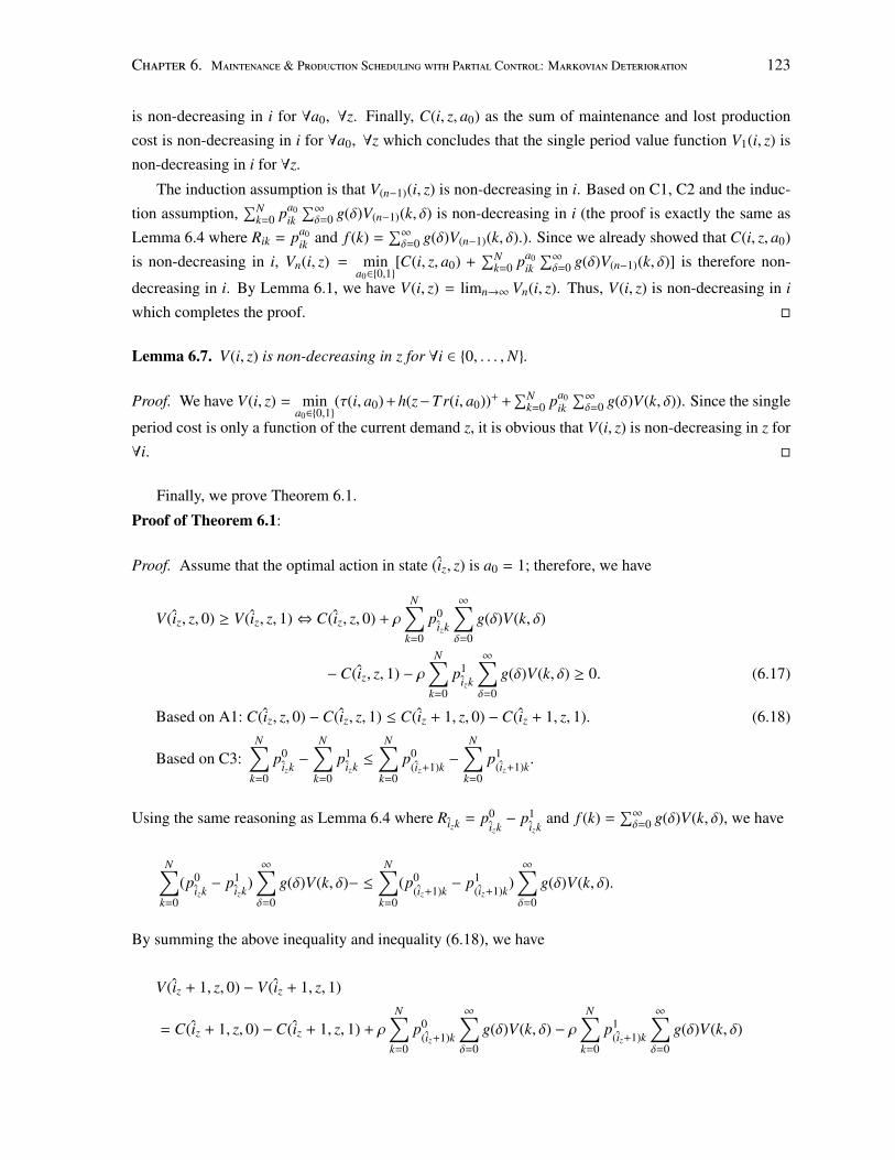
Chapter 6. Maintenance & Production Scheduling with Partial Control: Markovian Deterioration 123
is non-decreasing in i for ∀a0, ∀z. Finally, C(i, z, a0) as the sum of maintenance and lost production
cost is non-decreasing in i for ∀a0, ∀z which concludes that the single period value function V1(i, z) is
non-decreasing in i for ∀z.
The induction assumption is that V(n−1)(i, z) is non-decreasing in i. Based on C1, C2 and the induc-
tion assumption,∑N
k=0 pa0ik
∑∞δ=0 g(δ)V(n−1)(k, δ) is non-decreasing in i (the proof is exactly the same as
Lemma 6.4 where Rik = pa0ik and f (k) =
∑∞δ=0 g(δ)V(n−1)(k, δ).). Since we already showed that C(i, z, a0)
is non-decreasing in i, Vn(i, z) = mina0∈{0,1}
[C(i, z, a0) +∑N
k=0 pa0ik
∑∞δ=0 g(δ)V(n−1)(k, δ)] is therefore non-
decreasing in i. By Lemma 6.1, we have V(i, z) = limn→∞ Vn(i, z). Thus, V(i, z) is non-decreasing in i
which completes the proof. �
Lemma 6.7. V(i, z) is non-decreasing in z for ∀i ∈ {0, . . . ,N}.
Proof. We have V(i, z) = mina0∈{0,1}
(τ(i, a0) + h(z−Tr(i, a0))+ +∑N
k=0 pa0ik
∑∞δ=0 g(δ)V(k, δ)). Since the single
period cost is only a function of the current demand z, it is obvious that V(i, z) is non-decreasing in z for
∀i. �
Finally, we prove Theorem 6.1.
Proof of Theorem 6.1:
Proof. Assume that the optimal action in state (iz, z) is a0 = 1; therefore, we have
V(iz, z, 0) ≥ V(iz, z, 1)⇔ C(iz, z, 0) + ρ
N∑k=0
p0izk
∞∑δ=0
g(δ)V(k, δ)
−C(iz, z, 1) − ρN∑
k=0
p1izk
∞∑δ=0
g(δ)V(k, δ) ≥ 0. (6.17)
Based on A1: C(iz, z, 0) −C(iz, z, 1) ≤ C(iz + 1, z, 0) −C(iz + 1, z, 1). (6.18)
Based on C3:N∑
k=0
p0izk−
N∑k=0
p1izk≤
N∑k=0
p0(iz+1)k
−
N∑k=0
p1(iz+1)k
.
Using the same reasoning as Lemma 6.4 where Rizk = p0izk− p1
izkand f (k) =
∑∞δ=0 g(δ)V(k, δ), we have
N∑k=0
(p0izk− p1
izk)∞∑δ=0
g(δ)V(k, δ)− ≤N∑
k=0
(p0(iz+1)k
− p1(iz+1)k
)∞∑δ=0
g(δ)V(k, δ).
By summing the above inequality and inequality (6.18), we have
V(iz + 1, z, 0) − V(iz + 1, z, 1)
= C(iz + 1, z, 0) −C(iz + 1, z, 1) + ρ
N∑k=0
p0(iz+1)k
∞∑δ=0
g(δ)V(k, δ) − ρN∑
k=0
p1(iz+1)k
∞∑δ=0
g(δ)V(k, δ)
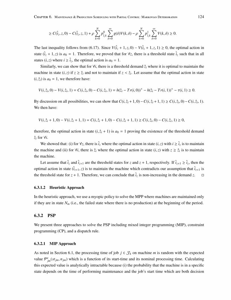
Chapter 6. Maintenance & Production Scheduling with Partial Control: Markovian Deterioration 124
≥ C(iz, z, 0) −C(iz, z, 1) + ρ
N∑k=0
p0izk
∞∑δ=0
g(δ)V(k, δ) − ρN∑
k=0
p1izk
∞∑δ=0
V(k, δ) ≥ 0.
The last inequality follows from (6.17). Since V(iz + 1, z, 0) − V(iz + 1, z, 1) ≥ 0, the optimal action in
state (iz + 1, z) is a0 = 1. Therefore, we proved that for ∀z, there is a threshold state iz such that in all
states (i, z) where i ≥ iz, the optimal action is a0 = 1.
Similarly, we can show that for ∀i, there is a threshold demand zi where it is optimal to maintain the
machine in state (i, z) if z ≥ zi and not to maintain if z < zi. Let assume that the optimal action in state
(i, zi) is a0 = 1, we therefore have:
V(i, zi, 0) − V(i, zi, 1) = C(i, zi, 0) −C(i, zi, 1) = h(zi − Tr(i, 0))+ − h(zi − Tr(i, 1))+ − τ(i, 1) ≥ 0.
By discussion on all possibilities, we can show that C(i, zi + 1, 0)−C(i, zi + 1, 1) ≥ C(i, zi, 0)−C(i, zi, 1).
We then have:
V(i, zi + 1, 0) − V(i, zi + 1, 1) = C(i, zi + 1, 0) −C(i, zi + 1, 1) ≥ C(i, zi, 0) −C(i, zi, 1) ≥ 0,
therefore, the optimal action in state (i, zi + 1) is a0 = 1 proving the existence of the threshold demand
zi for ∀i.
We showed that: (i) for ∀z, there is iz where the optimal action in state (i, z) with i ≥ iz is to maintain
the machine and (ii) for ∀i, there is zi where the optimal action in state (i, z) with z ≥ zi is to maintain
the machine.
Let assume that iz and iz+1 are the threshold states for z and z + 1, respectively. If iz+1 ≥ iz, then the
optimal action in state (iz+1, z) is to maintain the machine which contradicts our assumption that iz+1 is
the threshold state for z + 1. Therefore, we can conclude that iz is non-increasing in the demand z. �
6.3.1.2 Heuristic Approach
In the heuristic approach, we use a myopic policy to solve the MPP where machines are maintained only
if they are in state Nm (i.e., the failed state where there is no production) at the beginning of the period.
6.3.2 PSP
We present three approaches to solve the PSP including mixed integer programming (MIP), constraint
programming (CP), and a dispatch rule.
6.3.2.1 MIP Approach
As noted in Section 6.1, the processing time of job j ∈ Jk on machine m is random with the expected
value Pejm(st jm, n jm) which is a function of its start-time and its nominal processing time. Calculating
this expected value is analytically intractable because (i) the probability that the machine is in a specific
state depends on the time of performing maintenance and the job’s start time which are both decision
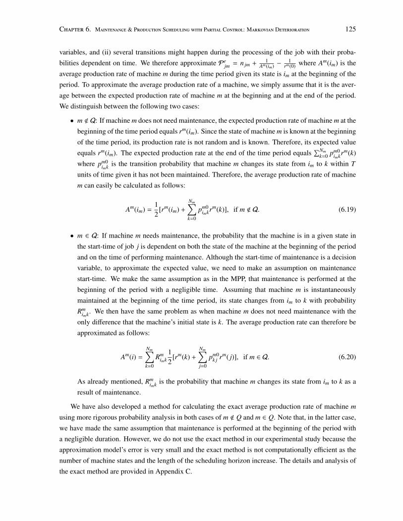
Chapter 6. Maintenance & Production Scheduling with Partial Control: Markovian Deterioration 125
variables, and (ii) several transitions might happen during the processing of the job with their proba-
bilities dependent on time. We therefore approximate Pejm = n jm + 1
Am(im) −1
rm(0) where Am(im) is the
average production rate of machine m during the time period given its state is im at the beginning of the
period. To approximate the average production rate of a machine, we simply assume that it is the aver-
age between the expected production rate of machine m at the beginning and at the end of the period.
We distinguish between the following two cases:
• m < Q: If machine m does not need maintenance, the expected production rate of machine m at the
beginning of the time period equals rm(im). Since the state of machine m is known at the beginning
of the time period, its production rate is not random and is known. Therefore, its expected value
equals rm(im). The expected production rate at the end of the time period equals∑Nm
k=0 pm0imkrm(k)
where pm0imk is the transition probability that machine m changes its state from im to k within T
units of time given it has not been maintained. Therefore, the average production rate of machine
m can easily be calculated as follows:
Am(im) =12
[rm(im) +
Nm∑k=0
pm0imkrm(k)], if m < Q. (6.19)
• m ∈ Q: If machine m needs maintenance, the probability that the machine is in a given state in
the start-time of job j is dependent on both the state of the machine at the beginning of the period
and on the time of performing maintenance. Although the start-time of maintenance is a decision
variable, to approximate the expected value, we need to make an assumption on maintenance
start-time. We make the same assumption as in the MPP, that maintenance is performed at the
beginning of the period with a negligible time. Assuming that machine m is instantaneously
maintained at the beginning of the time period, its state changes from im to k with probability
Rmimk. We then have the same problem as when machine m does not need maintenance with the
only difference that the machine’s initial state is k. The average production rate can therefore be
approximated as follows:
Am(i) =
Nm∑k=0
Rmimk
12
[rm(k) +
Nm∑j=0
pm0k j rm( j)], if m ∈ Q. (6.20)
As already mentioned, Rmimk is the probability that machine m changes its state from im to k as a
result of maintenance.
We have also developed a method for calculating the exact average production rate of machine m
using more rigorous probability analysis in both cases of m < Q and m ∈ Q. Note that, in the latter case,
we have made the same assumption that maintenance is performed at the beginning of the period with
a negligible duration. However, we do not use the exact method in our experimental study because the
approximation model’s error is very small and the exact method is not computationally efficient as the
number of machine states and the length of the scheduling horizon increase. The details and analysis of
the exact method are provided in Appendix C.
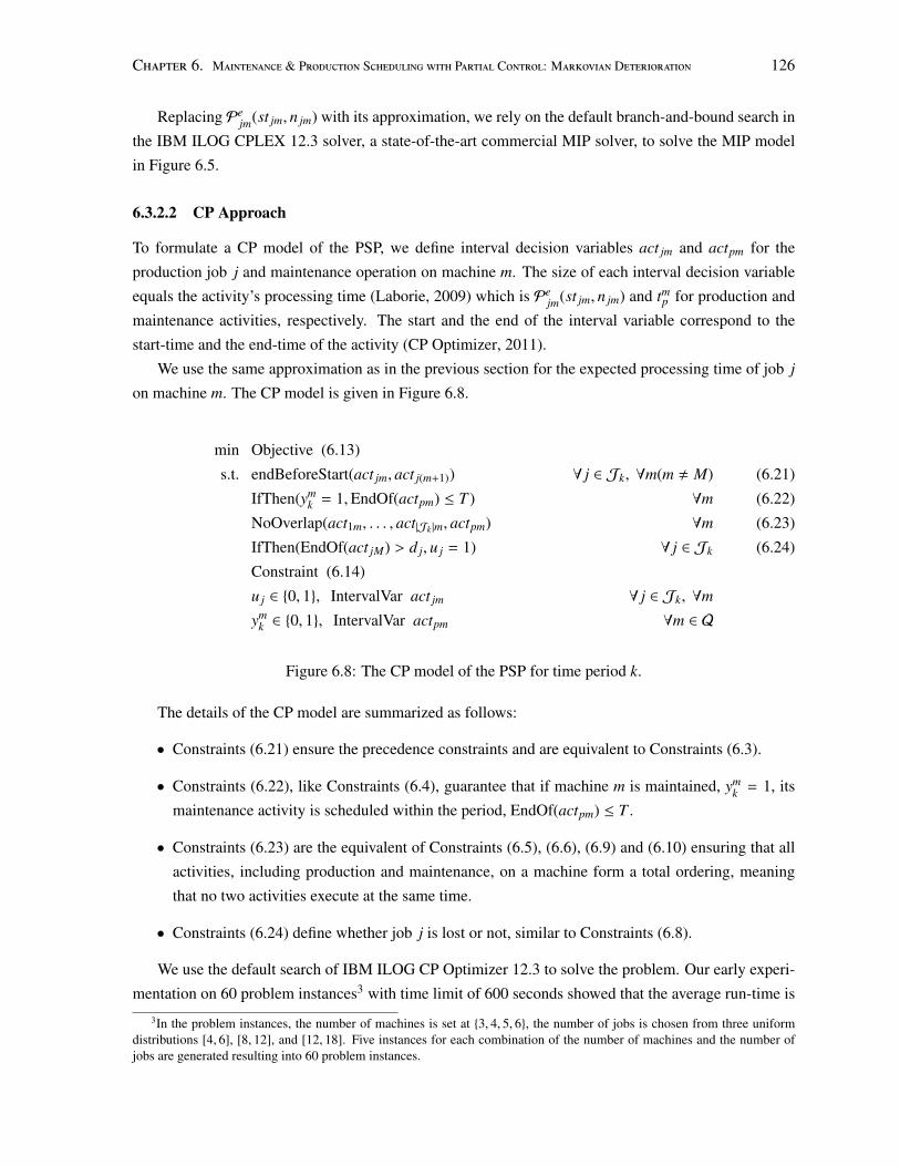
Chapter 6. Maintenance & Production Scheduling with Partial Control: Markovian Deterioration 126
Replacing Pejm(st jm, n jm) with its approximation, we rely on the default branch-and-bound search in
the IBM ILOG CPLEX 12.3 solver, a state-of-the-art commercial MIP solver, to solve the MIP model
in Figure 6.5.
6.3.2.2 CP Approach
To formulate a CP model of the PSP, we define interval decision variables act jm and actpm for the
production job j and maintenance operation on machine m. The size of each interval decision variable
equals the activity’s processing time (Laborie, 2009) which is Pejm(st jm, n jm) and tm
p for production and
maintenance activities, respectively. The start and the end of the interval variable correspond to the
start-time and the end-time of the activity (CP Optimizer, 2011).
We use the same approximation as in the previous section for the expected processing time of job j
on machine m. The CP model is given in Figure 6.8.
min Objective (6.13)
s.t. endBeforeStart(act jm, act j(m+1)) ∀ j ∈ Jk, ∀m(m , M) (6.21)
IfThen(ymk = 1,EndOf(actpm) ≤ T ) ∀m (6.22)
NoOverlap(act1m, . . . , act|Jk |m, actpm) ∀m (6.23)
IfThen(EndOf(act jM) > d j, u j = 1) ∀ j ∈ Jk (6.24)
Constraint (6.14)
u j ∈ {0, 1}, IntervalVar act jm ∀ j ∈ Jk, ∀m
ymk ∈ {0, 1}, IntervalVar actpm ∀m ∈ Q
Figure 6.8: The CP model of the PSP for time period k.
The details of the CP model are summarized as follows:
• Constraints (6.21) ensure the precedence constraints and are equivalent to Constraints (6.3).
• Constraints (6.22), like Constraints (6.4), guarantee that if machine m is maintained, ymk = 1, its
maintenance activity is scheduled within the period, EndOf(actpm) ≤ T .
• Constraints (6.23) are the equivalent of Constraints (6.5), (6.6), (6.9) and (6.10) ensuring that all
activities, including production and maintenance, on a machine form a total ordering, meaning
that no two activities execute at the same time.
• Constraints (6.24) define whether job j is lost or not, similar to Constraints (6.8).
We use the default search of IBM ILOG CP Optimizer 12.3 to solve the problem. Our early experi-
mentation on 60 problem instances3 with time limit of 600 seconds showed that the average run-time is
3In the problem instances, the number of machines is set at {3, 4, 5, 6}, the number of jobs is chosen from three uniformdistributions [4, 6], [8, 12], and [12, 18]. Five instances for each combination of the number of machines and the number ofjobs are generated resulting into 60 problem instances.
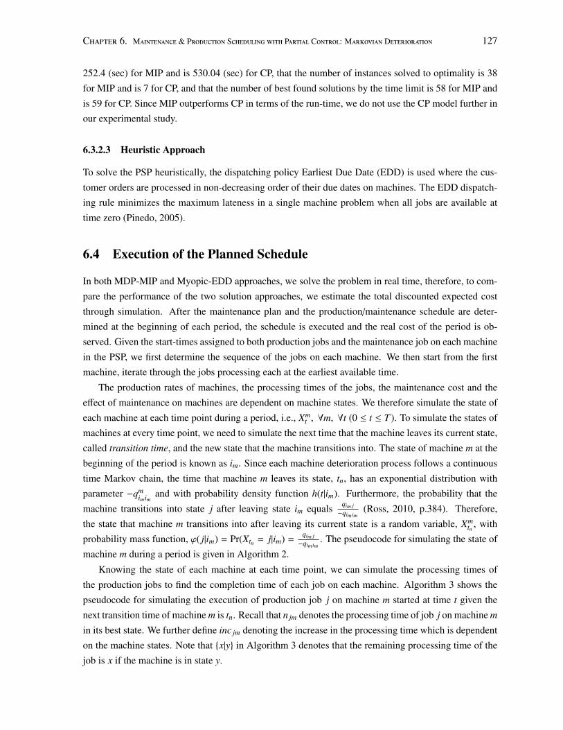
Chapter 6. Maintenance & Production Scheduling with Partial Control: Markovian Deterioration 127
252.4 (sec) for MIP and is 530.04 (sec) for CP, that the number of instances solved to optimality is 38
for MIP and is 7 for CP, and that the number of best found solutions by the time limit is 58 for MIP and
is 59 for CP. Since MIP outperforms CP in terms of the run-time, we do not use the CP model further in
our experimental study.
6.3.2.3 Heuristic Approach
To solve the PSP heuristically, the dispatching policy Earliest Due Date (EDD) is used where the cus-
tomer orders are processed in non-decreasing order of their due dates on machines. The EDD dispatch-
ing rule minimizes the maximum lateness in a single machine problem when all jobs are available at
time zero (Pinedo, 2005).
6.4 Execution of the Planned Schedule
In both MDP-MIP and Myopic-EDD approaches, we solve the problem in real time, therefore, to com-
pare the performance of the two solution approaches, we estimate the total discounted expected cost
through simulation. After the maintenance plan and the production/maintenance schedule are deter-
mined at the beginning of each period, the schedule is executed and the real cost of the period is ob-
served. Given the start-times assigned to both production jobs and the maintenance job on each machine
in the PSP, we first determine the sequence of the jobs on each machine. We then start from the first
machine, iterate through the jobs processing each at the earliest available time.
The production rates of machines, the processing times of the jobs, the maintenance cost and the
effect of maintenance on machines are dependent on machine states. We therefore simulate the state of
each machine at each time point during a period, i.e., Xmt , ∀m, ∀t (0 ≤ t ≤ T ). To simulate the states of
machines at every time point, we need to simulate the next time that the machine leaves its current state,
called transition time, and the new state that the machine transitions into. The state of machine m at the
beginning of the period is known as im. Since each machine deterioration process follows a continuous
time Markov chain, the time that machine m leaves its state, tn, has an exponential distribution with
parameter −qmimim
and with probability density function h(t|im). Furthermore, the probability that the
machine transitions into state j after leaving state im equals qim j−qimim
(Ross, 2010, p.384). Therefore,
the state that machine m transitions into after leaving its current state is a random variable, Xmtn , with
probability mass function, ϕ( j|im) = Pr(Xtn = j|im) =qim j−qimim
. The pseudocode for simulating the state of
machine m during a period is given in Algorithm 2.
Knowing the state of each machine at each time point, we can simulate the processing times of
the production jobs to find the completion time of each job on each machine. Algorithm 3 shows the
pseudocode for simulating the execution of production job j on machine m started at time t given the
next transition time of machine m is tn. Recall that n jm denotes the processing time of job j on machine m
in its best state. We further define inc jm denoting the increase in the processing time which is dependent
on the machine states. Note that {x|y} in Algorithm 3 denotes that the remaining processing time of the
job is x if the machine is in state y.
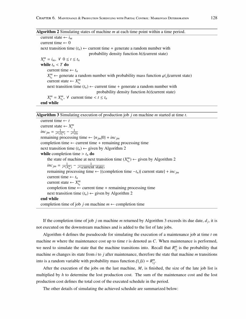
Chapter 6. Maintenance & Production Scheduling with Partial Control: Markovian Deterioration 128
Algorithm 2 Simulating states of machine m at each time point within a time period.current state← imcurrent time← 0next transition time (tn)← current time + generate a random number with
probability density function h(t|current state)Xm
t = im, ∀ 0 ≤ t ≤ tnwhile tn < T do
current time← tnXm
tn ← generate a random number with probability mass function ϕ( j|current state)current state← Xm
tnnext transition time (tn)← current time + generate a random number with
probability density function h(t|current state)Xm
t = Xmtn , ∀ current time < t ≤ tn
end while
Algorithm 3 Simulating execution of production job j on machine m started at time t.current time← tcurrent state← Xm
tinc jm = 1
rm(Xmt ) −
1rm(0)
remaining processing time← {n jm|0} + inc jm
completion time← current time + remaining processing timenext transition time (tn)← given by Algorithm 2while completion time > tn do
the state of machine at next transition time (Xmtn )← given by Algorithm 2
inc jm = 1rm(Xm
tn ) −1
rm(current state)remaining processing time← {(completion time −tn)| current state} + inc jm
current time← tncurrent state← Xm
tncompletion time← current time + remaining processing timenext transition time (tn)← given by Algorithm 2
end whilecompletion time of job j on machine m← completion time
If the completion time of job j on machine m returned by Algorithm 3 exceeds its due date, d j, it is
not executed on the downstream machines and is added to the list of late jobs.
Algorithm 4 defines the pseudocode for simulating the execution of a maintenance job at time t on
machine m where the maintenance cost up to time t is denoted as C. When maintenance is performed,
we need to simulate the state that the machine transitions into. Recall that Rmi j is the probability that
machine m changes its state from i to j after maintenance, therefore the state that machine m transitions
into is a random variable with probability mass function ξ( j|i) = Rmi j.
After the execution of the jobs on the last machine, M, is finished, the size of the late job list is
multiplied by h to determine the lost production cost. The sum of the maintenance cost and the lost
production cost defines the total cost of the executed schedule in the period.
The other details of simulating the achieved schedule are summarized below:
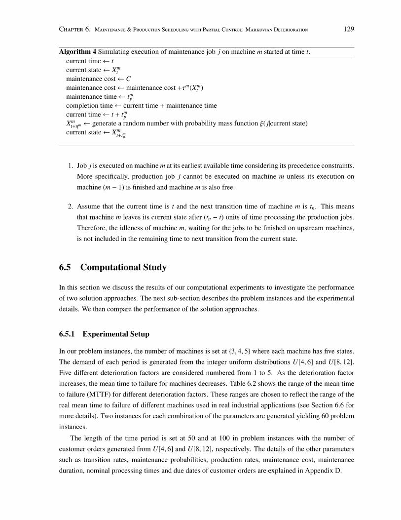
Chapter 6. Maintenance & Production Scheduling with Partial Control: Markovian Deterioration 129
Algorithm 4 Simulating execution of maintenance job j on machine m started at time t.current time← tcurrent state← Xm
tmaintenance cost← Cmaintenance cost← maintenance cost +τm(Xm
t )maintenance time← tm
pcompletion time← current time + maintenance timecurrent time← t + tm
pXm
t+ηm ← generate a random number with probability mass function ξ( j|current state)current state← Xm
t+tmp
1. Job j is executed on machine m at its earliest available time considering its precedence constraints.
More specifically, production job j cannot be executed on machine m unless its execution on
machine (m − 1) is finished and machine m is also free.
2. Assume that the current time is t and the next transition time of machine m is tn. This means
that machine m leaves its current state after (tn − t) units of time processing the production jobs.
Therefore, the idleness of machine m, waiting for the jobs to be finished on upstream machines,
is not included in the remaining time to next transition from the current state.
6.5 Computational Study
In this section we discuss the results of our computational experiments to investigate the performance
of two solution approaches. The next sub-section describes the problem instances and the experimental
details. We then compare the performance of the solution approaches.
6.5.1 Experimental Setup
In our problem instances, the number of machines is set at {3, 4, 5} where each machine has five states.
The demand of each period is generated from the integer uniform distributions U[4, 6] and U[8, 12].
Five different deterioration factors are considered numbered from 1 to 5. As the deterioration factor
increases, the mean time to failure for machines decreases. Table 6.2 shows the range of the mean time
to failure (MTTF) for different deterioration factors. These ranges are chosen to reflect the range of the
real mean time to failure of different machines used in real industrial applications (see Section 6.6 for
more details). Two instances for each combination of the parameters are generated yielding 60 problem
instances.
The length of the time period is set at 50 and at 100 in problem instances with the number of
customer orders generated from U[4, 6] and U[8, 12], respectively. The details of the other parameters
such as transition rates, maintenance probabilities, production rates, maintenance cost, maintenance
duration, nominal processing times and due dates of customer orders are explained in Appendix D.
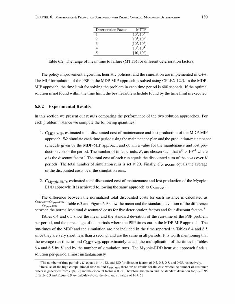
Chapter 6. Maintenance & Production Scheduling with Partial Control: Markovian Deterioration 130
Deterioration Factor MTTF1 [105, 107]2 [104, 106]3 [103, 105]4 [102, 104]5 [10, 103]
Table 6.2: The range of mean time to failure (MTTF) for different deterioration factors.
The policy improvement algorithm, heuristic policies, and the simulation are implemented in C++.
The MIP formulation of the PSP in the MDP-MIP approach is solved using CPLEX 12.3. In the MDP-
MIP approach, the time limit for solving the problem in each time period is 600 seconds. If the optimal
solution is not found within the time limit, the best feasible schedule found by the time limit is executed.
6.5.2 Experimental Results
In this section we present our results comparing the performance of the two solution approaches. For
each problem instance we compute the following quantities:
1. CMDP-MIP, estimated total discounted cost of maintenance and lost production of the MDP-MIP
approach: We simulate each time period using the maintenance plan and the production/maintenance
schedule given by the MDP-MIP approach and obtain a value for the maintenance and lost pro-
duction cost of the period. The number of time periods, K, are chosen such that ρK > 10−4 where
ρ is the discount factor.4 The total cost of each run equals the discounted sum of the costs over K
periods. The total number of simulation runs is set at 20. Finally, CMDP-MIP equals the average
of the discounted costs over the simulation runs.
2. CMyopic-EDD, estimated total discounted cost of maintenance and lost production of the Myopic-
EDD approach: It is achieved following the same approach as CMDP-MIP.
The difference between the normalized total discounted costs for each instance is calculated asCMDP-MIP−CMyopic-EDD
CMyopic-EDD. Table 6.3 and Figure 6.9 show the mean and the standard deviation of the difference
between the normalized total discounted costs for five deterioration factors and four discount factors.5
Tables 6.4 and 6.5 show the mean and the standard deviation of the run-time of the PSP problem
per period, and the percentage of the periods where the PSP times out in the MDP-MIP approach. The
run-times of the MDP and the simulation are not included in the time reported in Tables 6.4 and 6.5
since they are very short, less than a second, and are the same in all periods. It is worth mentioning that
the average run-time to find CMDP-MIP approximately equals the multiplication of the times in Tables
6.4 and 6.5 by K and by the number of simulation runs. The Myopic-EDD heuristic approach finds a
solution per-period almost instantaneously.
4The number of time periods , K, equals 6, 14, 42, and 180 for discount factors of 0.2, 0.5, 0.8, and 0.95, respectively.5Because of the high computational time to find CMDP-MIP, there are no results for the case where the number of customer
orders is generated from U[8, 12] and the discount factor is 0.95. Therefore, the mean and the standard deviation for ρ = 0.95in Table 6.3 and Figure 6.9 are calculated over the demand situation of U[4, 6].
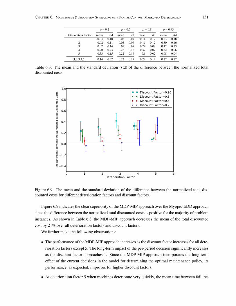
Chapter 6. Maintenance & Production Scheduling with Partial Control: Markovian Deterioration 131
ρ = 0.2 ρ = 0.5 ρ = 0.8 ρ = 0.95
Deterioration Factor mean std mean std mean std mean std1 -0.03 0.10 0.05 0.07 0.14 0.12 0.23 0.182 -0.02 0.11 0.05 0.07 0.16 0.12 0.30 0.163 0.02 0.14 0.09 0.08 0.24 0.09 0.42 0.134 0.20 0.23 0.26 0.16 0.32 0.07 0.32 0.065 0.33 0.15 0.22 0.14 0.1 0.02 0.08 0.04
{1,2,3,4,5} 0.14 0.32 0.22 0.19 0.24 0.14 0.27 0.17
Table 6.3: The mean and the standard deviation (std) of the difference between the normalized totaldiscounted costs.
0 1 2 3 4 5 6Deterioration Factor
0.4
0.2
0.0
0.2
0.4
0.6
0.8
1.0
The
Diff
eren
ce b
etw
een
the
Norm
aliz
ed T
otal
Dis
coun
ted
Cost
s Discount Factor=0.95Discount Factor=0.8Discount Factor=0.5Discount Factor=0.2
Figure 6.9: The mean and the standard deviation of the difference between the normalized total dis-counted costs for different deterioration factors and discount factors.
Figure 6.9 indicates the clear superiority of the MDP-MIP approach over the Myopic-EDD approach
since the difference between the normalized total discounted costs is positive for the majority of problem
instances. As shown in Table 6.3, the MDP-MIP approach decreases the mean of the total discounted
cost by 21% over all deterioration factors and discount factors.
We further make the following observations:
• The performance of the MDP-MIP approach increases as the discount factor increases for all dete-
rioration factors except 5. The long-term impact of the per-period decision significantly increases
as the discount factor approaches 1. Since the MDP-MIP approach incorporates the long-term
effect of the current decisions in the model for determining the optimal maintenance policy, its
performance, as expected, improves for higher discount factors.
• At deterioration factor 5 when machines deteriorate very quickly, the mean time between failures
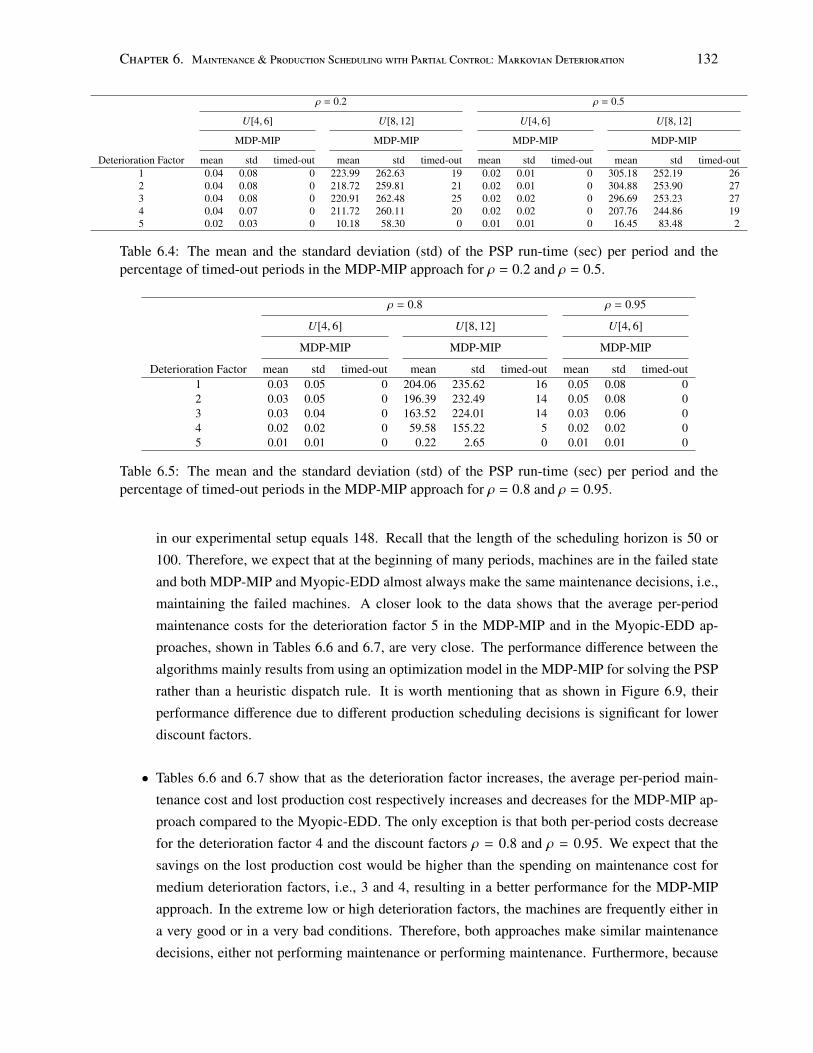
Chapter 6. Maintenance & Production Scheduling with Partial Control: Markovian Deterioration 132
ρ = 0.2 ρ = 0.5
U[4, 6] U[8, 12] U[4, 6] U[8, 12]
MDP-MIP MDP-MIP MDP-MIP MDP-MIP
Deterioration Factor mean std timed-out mean std timed-out mean std timed-out mean std timed-out1 0.04 0.08 0 223.99 262.63 19 0.02 0.01 0 305.18 252.19 262 0.04 0.08 0 218.72 259.81 21 0.02 0.01 0 304.88 253.90 273 0.04 0.08 0 220.91 262.48 25 0.02 0.02 0 296.69 253.23 274 0.04 0.07 0 211.72 260.11 20 0.02 0.02 0 207.76 244.86 195 0.02 0.03 0 10.18 58.30 0 0.01 0.01 0 16.45 83.48 2
Table 6.4: The mean and the standard deviation (std) of the PSP run-time (sec) per period and thepercentage of timed-out periods in the MDP-MIP approach for ρ = 0.2 and ρ = 0.5.
ρ = 0.8 ρ = 0.95
U[4, 6] U[8, 12] U[4, 6]
MDP-MIP MDP-MIP MDP-MIP
Deterioration Factor mean std timed-out mean std timed-out mean std timed-out1 0.03 0.05 0 204.06 235.62 16 0.05 0.08 02 0.03 0.05 0 196.39 232.49 14 0.05 0.08 03 0.03 0.04 0 163.52 224.01 14 0.03 0.06 04 0.02 0.02 0 59.58 155.22 5 0.02 0.02 05 0.01 0.01 0 0.22 2.65 0 0.01 0.01 0
Table 6.5: The mean and the standard deviation (std) of the PSP run-time (sec) per period and thepercentage of timed-out periods in the MDP-MIP approach for ρ = 0.8 and ρ = 0.95.
in our experimental setup equals 148. Recall that the length of the scheduling horizon is 50 or
100. Therefore, we expect that at the beginning of many periods, machines are in the failed state
and both MDP-MIP and Myopic-EDD almost always make the same maintenance decisions, i.e.,
maintaining the failed machines. A closer look to the data shows that the average per-period
maintenance costs for the deterioration factor 5 in the MDP-MIP and in the Myopic-EDD ap-
proaches, shown in Tables 6.6 and 6.7, are very close. The performance difference between the
algorithms mainly results from using an optimization model in the MDP-MIP for solving the PSP
rather than a heuristic dispatch rule. It is worth mentioning that as shown in Figure 6.9, their
performance difference due to different production scheduling decisions is significant for lower
discount factors.
• Tables 6.6 and 6.7 show that as the deterioration factor increases, the average per-period main-
tenance cost and lost production cost respectively increases and decreases for the MDP-MIP ap-
proach compared to the Myopic-EDD. The only exception is that both per-period costs decrease
for the deterioration factor 4 and the discount factors ρ = 0.8 and ρ = 0.95. We expect that the
savings on the lost production cost would be higher than the spending on maintenance cost for
medium deterioration factors, i.e., 3 and 4, resulting in a better performance for the MDP-MIP
approach. In the extreme low or high deterioration factors, the machines are frequently either in
a very good or in a very bad conditions. Therefore, both approaches make similar maintenance
decisions, either not performing maintenance or performing maintenance. Furthermore, because
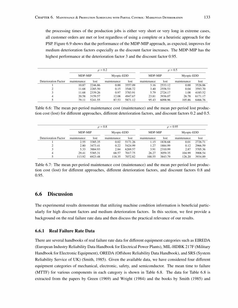
Chapter 6. Maintenance & Production Scheduling with Partial Control: Markovian Deterioration 133
the processing times of the production jobs is either very short or very long in extreme cases,
all customer orders are met or lost regardless of using a complete or a heuristic approach for the
PSP. Figure 6.9 shows that the performance of the MDP-MIP approach, as expected, improves for
medium deterioration factors especially as the discount factor increases. The MDP-MIP has the
highest performance at the deterioration factor 3 and the discount factor 0.95.
ρ = 0.2 ρ = 0.5
MDP-MIP Myopic-EDD MDP-MIP Myopic-EDD
Deterioration Factor maintenance lost maintenance lost maintenance lost maintenance lost1 10.87 2246.86 0.00 3557.09 3.16 2533.12 0.00 3526.062 11.68 2285.50 0.15 3548.72 3.40 2558.53 0.04 3593.703 11.68 2339.26 0.97 3783.91 5.79 2724.17 1.08 4185.524 20.58 3159.57 12.08 4947.67 23.81 3936.07 26.78 6171.175 79.11 5241.55 87.53 5871.12 95.43 6098.96 105.86 6466.76
Table 6.6: The mean per-period maintenance cost (maintenance) and the mean per-period lost produc-tion cost (lost) for different approaches, different deterioration factors, and discount factors 0.2 and 0.5.
ρ = 0.8 ρ = 0.95
MDP-MIP Myopic-EDD MDP-MIP Myopic-EDD
Deterioration Factor maintenance lost maintenance lost maintenance lost maintenance lost1 2.55 3385.35 0.02 5171.26 1.15 1838.68 0.01 2726.712 2.80 3473.41 0.22 5424.99 1.27 1884.99 0.12 2966.593 5.33 3884.93 2.84 6269.57 3.91 2310.99 2.87 3705.364 29.41 5385.31 68.57 7017.75 26.27 3059.35 104.99 3908.545 113.92 6923.48 118.35 7072.82 100.55 3843.79 126.20 3934.89
Table 6.7: The mean per-period maintenance cost (maintenance) and the mean per-period lost produc-tion cost (lost) for different approaches, different deterioration factors, and discount factors 0.8 and0.95.
6.6 Discussion
The experimental results demonstrate that utilizing machine condition information is beneficial partic-
ularly for high discount factors and medium deterioration factors. In this section, we first provide a
background on the real failure rate data and then discuss the practical relevance of our results.
6.6.1 Real Failure Rate Data
There are several handbooks of real failure rate data for different equipment categories such as EIREDA
(European Industry Reliability Data Handbook for Electrical Power Plants), MIL-HDBK 217F (Military
Handbook for Electronic Equipment), OREDA (Offshore Reliability Data Handbook), and SRS (System
Reliability Service of UK) (Smith, 1985). Given the available data, we have considered four different
equipment categories of mechanical, electronic, safety, and semiconductor. The mean time to failure
(MTTF) for various components in each category is shown in Table 6.8. The data for Table 6.8 is
extracted from the papers by Green (1969) and Wright (1984) and the books by Smith (1985) and
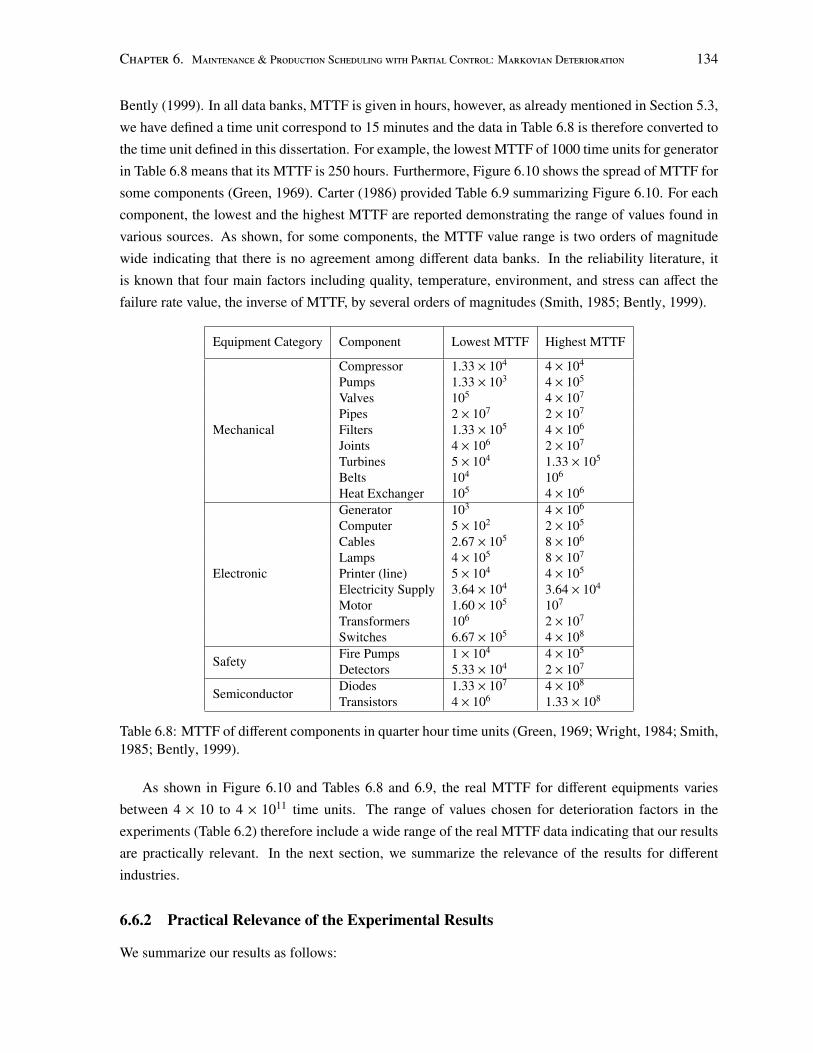
Chapter 6. Maintenance & Production Scheduling with Partial Control: Markovian Deterioration 134
Bently (1999). In all data banks, MTTF is given in hours, however, as already mentioned in Section 5.3,
we have defined a time unit correspond to 15 minutes and the data in Table 6.8 is therefore converted to
the time unit defined in this dissertation. For example, the lowest MTTF of 1000 time units for generator
in Table 6.8 means that its MTTF is 250 hours. Furthermore, Figure 6.10 shows the spread of MTTF for
some components (Green, 1969). Carter (1986) provided Table 6.9 summarizing Figure 6.10. For each
component, the lowest and the highest MTTF are reported demonstrating the range of values found in
various sources. As shown, for some components, the MTTF value range is two orders of magnitude
wide indicating that there is no agreement among different data banks. In the reliability literature, it
is known that four main factors including quality, temperature, environment, and stress can affect the
failure rate value, the inverse of MTTF, by several orders of magnitudes (Smith, 1985; Bently, 1999).
Equipment Category Component Lowest MTTF Highest MTTF
Mechanical
Compressor 1.33 × 10⁴ 4 × 10⁴
Pumps 1.33 × 10³ 4 × 10⁵
Valves 105 4 × 10⁷
Pipes 2 × 10⁷ 2 × 10⁷
Filters 1.33 × 10⁵ 4 × 10⁶
Joints 4 × 10⁶ 2 × 10⁷
Turbines 5 × 10⁴ 1.33 × 10⁵
Belts 104 106
Heat Exchanger 105 4 × 10⁶
Electronic
Generator 103 4 × 10⁶
Computer 5 × 10² 2 × 10⁵
Cables 2.67 × 10⁵ 8 × 10⁶
Lamps 4 × 10⁵ 8 × 10⁷
Printer (line) 5 × 10⁴ 4 × 10⁵
Electricity Supply 3.64 × 10⁴ 3.64 × 10⁴
Motor 1.60 × 10⁵ 107
Transformers 106 2 × 10⁷
Switches 6.67 × 10⁵ 4 × 10⁸
Safety Fire Pumps 1 × 10⁴ 4 × 10⁵
Detectors 5.33 × 10⁴ 2 × 10⁷
Semiconductor Diodes 1.33 × 10⁷ 4 × 10⁸
Transistors 4 × 10⁶ 1.33 × 10⁸
Table 6.8: MTTF of different components in quarter hour time units (Green, 1969; Wright, 1984; Smith,1985; Bently, 1999).
As shown in Figure 6.10 and Tables 6.8 and 6.9, the real MTTF for different equipments varies
between 4 × 10 to 4 × 10¹¹ time units. The range of values chosen for deterioration factors in the
experiments (Table 6.2) therefore include a wide range of the real MTTF data indicating that our results
are practically relevant. In the next section, we summarize the relevance of the results for different
industries.
6.6.2 Practical Relevance of the Experimental Results
We summarize our results as follows:
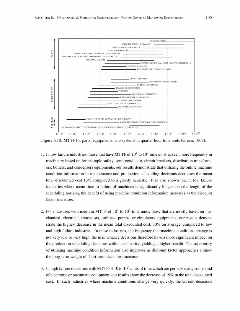
Chapter 6. Maintenance & Production Scheduling with Partial Control: Markovian Deterioration 135
4 × 101 4 × 10² 4 × 10³ 4 × 10⁴ 4 × 10⁵ 4 × 10⁶ 4 × 10⁷ 4 × 10⁸ 4 × 10⁹ 4 × 10¹⁰ 4 × 10¹¹
SYST
EMS
EQU
IPM
ENTS
PA
RTS
SOLDERED JOINTS (AUTOMATIC)
CRIMPED AND WELDED JOINTS
HAND SOLDERED JOINTS
SEMICONDUCTORS, MICROELECTRONIC CIRCUTS
DISCRETE ELECTRONIC PARTS (RESISTORS, CAPACITORS, ...)
MECHANICAL PARTS
ELECTRO MECHANICAL PARTS (RELAYS, SYMTCHES, ...)
ELECTRONIC VALVES
PNEUMATIIC AND HYDRAULIC PARTS
CIRCUIT BREAKERS
DISTRIBUTION TRANSFORMERS
BOILERS, CONDENSERS
TRANSISTOR EQUIPMENTS
TURBINES
MECHANICAL EQUIPMENTS
LARGE ELECTRICAL MACHINES
ELECTRONIC VALVE EQUIPMENTS
PUMPS, CIRCULATORS
PNEUMATIC EQUIPMENTS
LARGE ELECTRONIC SYSTEMS (NO REDUNDENCY)
LARGE ELECTRONIC SYSTEMS (WITH REDUNDENCY)
AUTOMATIC PROTECTIVE SYSTEMS (WITH REDUNDENCY & DIVERSITY) (ESTIMATED)
WRAPPED JOINTS
Figure 6.10: MTTF for parts, equipments, and systems in quarter hour time units (Green, 1969).
1. In low failure industries, those that have MTTF of 104 to 107 time units as seen more frequently in
machinery based on for example safety, semi-conductor, circuit breakers, distribution transform-
ers, boilers, and condensers equipments, our results demonstrate that utilizing the online machine
condition information in maintenance and production scheduling decisions decreases the mean
total discounted cost 13% compared to a greedy heuristic. It is also shown that in low failure
industries where mean time to failure of machines is significantly longer than the length of the
scheduling horizon, the benefit of using machine condition information increases as the discount
factor increases.
2. For industries with medium MTTF of 102 to 105 time units, those that are mostly based on me-
chanical, electrical, transistors, turbines, pumps, or circulators equipments, our results demon-
strate the highest decrease in the mean total discounted cost, 30% on average, compared to low
and high failure industries. In these industries, the frequency that machine conditions change is
not very low or very high, the maintenance decisions therefore have a more significant impact on
the production scheduling decisions within each period yielding a higher benefit. The superiority
of utilizing machine condition information also improves as discount factor approaches 1 since
the long-term weight of short-term decisions increases.
3. In high failure industries with MTTF of 10 to 103 units of time which are perhaps using some kind
of electronic or pneumatic equipment, our results show the decrease of 19% in the total discounted
cost. In such industries where machine conditions change very quickly, the current decisions
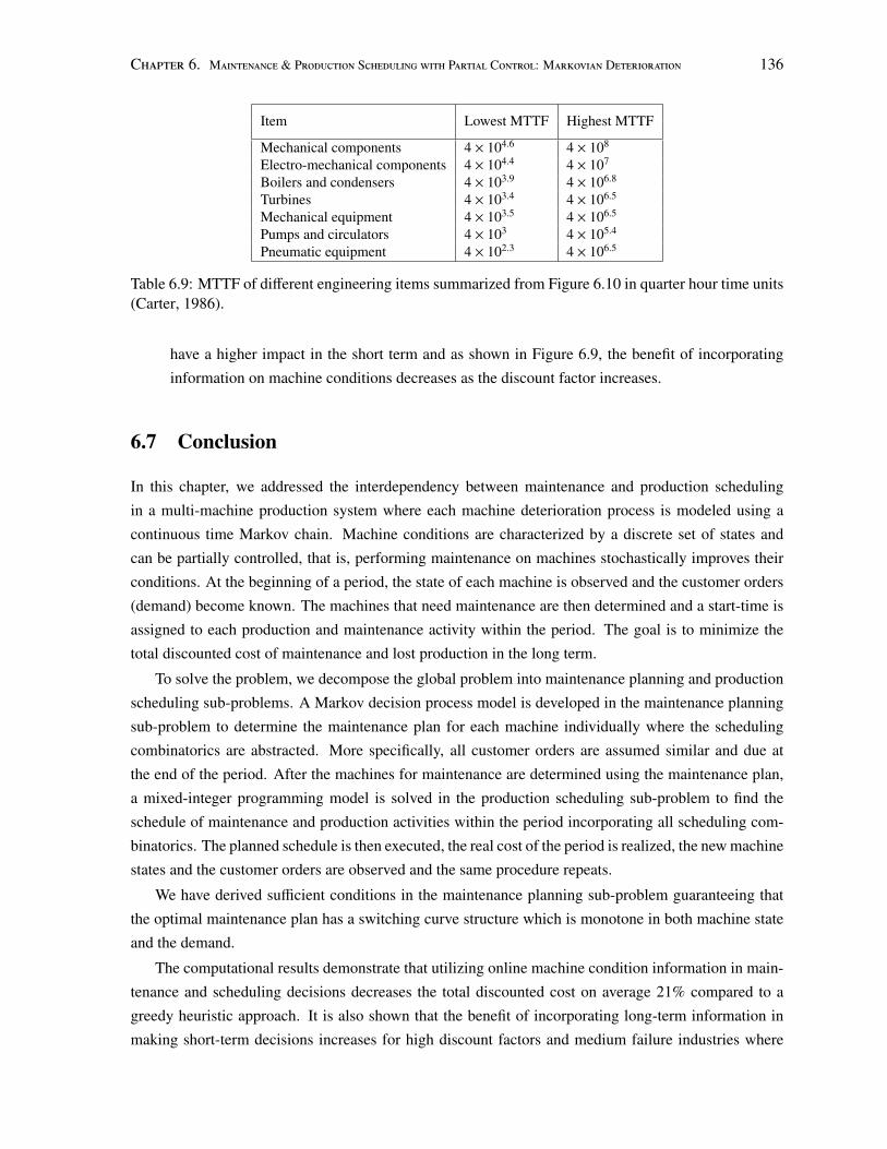
Chapter 6. Maintenance & Production Scheduling with Partial Control: Markovian Deterioration 136
Item Lowest MTTF Highest MTTF
Mechanical components 4 × 104.6 4 × 10⁸
Electro-mechanical components 4 × 104.4 4 × 10⁷
Boilers and condensers 4 × 103.9 4 × 106.8
Turbines 4 × 103.4 4 × 106.5
Mechanical equipment 4 × 103.5 4 × 106.5
Pumps and circulators 4 × 10³ 4 × 105.4
Pneumatic equipment 4 × 102.3 4 × 106.5
Table 6.9: MTTF of different engineering items summarized from Figure 6.10 in quarter hour time units(Carter, 1986).
have a higher impact in the short term and as shown in Figure 6.9, the benefit of incorporating
information on machine conditions decreases as the discount factor increases.
6.7 Conclusion
In this chapter, we addressed the interdependency between maintenance and production scheduling
in a multi-machine production system where each machine deterioration process is modeled using a
continuous time Markov chain. Machine conditions are characterized by a discrete set of states and
can be partially controlled, that is, performing maintenance on machines stochastically improves their
conditions. At the beginning of a period, the state of each machine is observed and the customer orders
(demand) become known. The machines that need maintenance are then determined and a start-time is
assigned to each production and maintenance activity within the period. The goal is to minimize the
total discounted cost of maintenance and lost production in the long term.
To solve the problem, we decompose the global problem into maintenance planning and production
scheduling sub-problems. A Markov decision process model is developed in the maintenance planning
sub-problem to determine the maintenance plan for each machine individually where the scheduling
combinatorics are abstracted. More specifically, all customer orders are assumed similar and due at
the end of the period. After the machines for maintenance are determined using the maintenance plan,
a mixed-integer programming model is solved in the production scheduling sub-problem to find the
schedule of maintenance and production activities within the period incorporating all scheduling com-
binatorics. The planned schedule is then executed, the real cost of the period is realized, the new machine
states and the customer orders are observed and the same procedure repeats.
We have derived sufficient conditions in the maintenance planning sub-problem guaranteeing that
the optimal maintenance plan has a switching curve structure which is monotone in both machine state
and the demand.
The computational results demonstrate that utilizing online machine condition information in main-
tenance and scheduling decisions decreases the total discounted cost on average 21% compared to a
greedy heuristic approach. It is also shown that the benefit of incorporating long-term information in
making short-term decisions increases for high discount factors and medium failure industries where
Chapter 6. Maintenance & Production Scheduling with Partial Control: Markovian Deterioration 137
the long-term impact of short-term decisions is higher and where the maintenance decisions effect on
short-term production scheduling decisions is more significant.
In this chapter, we continued addressing the interdependency between maintenance and production
scheduling where there is a partial control over machine conditions and where each machine deteriora-
tion is modeled using a stochastic process. In the next chapter, we discuss future directions for studying
the interdependency between maintenance and production problems.

Chapter 7
Future Work
In this dissertation, we addressed the interdependency between production and maintenance in the fol-
lowing three areas:
• maintenance and production planning with partial control over machine conditions,
• maintenance planning and production scheduling with no control over machine conditions, and
• maintenance planning and production scheduling with partial control over machine conditions.
In this chapter, we first present future research directions to extend the work in Chapters 3 to 6. We
then discuss two general directions for further progress in studying the relationship between mainte-
nance and production in real-world applications. We finally explain the relevance of our results to other
integrated decisions in supply chain management and indicate broader areas for future work.
7.1 Maintenance & Production Planning with Partial Control over Ma-chine Conditions
The problem of integrated maintenance and production planning where machines can be maintained be-
fore failure focuses on determining the optimal joint production and maintenance policies. In Chapter 3,
we studied a simpler combined problem in the context of a periodic review production system assuming
that the production policy is fixed. We analyzed the problem, determining the optimal maintenance
policy.
In this section, we outline possible extensions of the problem studied in Chapter 3.
7.1.1 Different Assumptions
Non-stationary Demand: As mentioned in Section 3.1, we have assumed that the demand of each period
is independent of the other periods. However, in real applications, the demand is affected by prevailing
business environment (Papachristos and Katsaros, 2008). For example, the demand of a product could
138
Chapter 7. FutureWork 139
be dependent on the technology status, society status, consumer wealth, and weather conditions. As-
suming a non-stationary demand allows the modeling of period to period variation and a more informed
maintenance policy can be, therefore, found. Given the fixed production quantity assumption, we would
intuitively expect that the firm invests more money in maintenance in a period where the demand is
stochastically larger. It would also be interesting to derive conditions that guarantee the optimality of a
threshold maintenance policy. The threshold value is likely to be a function of the inventory level, the
expected demand, and the variance of the demand.
Advanced Demand Information: In Chapter 3, investing in process improvement projects such as preven-
tive maintenance is introduced as a strategy for partially controlling the sources of uncertainty internal
to the production process. However, external sources of uncertainty like demand also exist in a pro-
duction system. Advanced demand information strategies where the firm uses information technologies
and sale techniques to collect accurate information about customer orders is shown to be effective in
better management of external uncertainties (Ozer and Wei, 2004). Studying the problem of Chapter 3
assuming both strategies of investing in process improvement projects and investing in obtaining more
accurate demand information is a promising future research direction. More specifically, at the begin-
ning of each period, the firm determines the amount of investment in each strategy. Modeling the effect
of investing in information technologies on demand is challenging. One possible idea is to assume that
the demand of period i, i.e., Zi, is a stochastic function of the amount of investment. For example, there
are several possible investment options where each results in a specific distribution for the demand. The
mean of the demand is identical across all investment options, however, the variance of the demand is
lower in an option with higher investment. Analyzing the problem in the presence of investing in both
process improvement projects and demand information technologies would be harder than the problem
of Chapter 3 since the demand distribution of each period is dependent on the investment in information
technologies. We would intuitively expect that there exists a threshold value such that if the amount of
inventory on hand is bigger, it is optimal not to invest in any of the investment strategies. Characterizing
the optimal investment decisions in case of lower inventory on hand would be however challenging.
Multi-product Production Systems: We studied a single product system in Chapter 3. One direction for
extending the problem is to consider a multi-product system following the paper by Hsu and Bassok
(1999). They assumed that there is one raw material as input, producing N different products where the
demands and the yields of the products are random and different. Addressing a multi-product system in
the context of the problem in Chapter 3 means that the firm should make two decisions at the beginning
of each period: (i) how to optimally allocate the given production quantity among different products and
(ii) how much to invest in maintenance. Since it is hard to analytically deal with allocation decisions in
the framework of Markov decision process, exploring mathematical programming approaches such as
stochastic programming, also used by Hsu and Bassok (1999), is more appropriate to solve the problem.
Multi-stage Production Systems: As indicated in Section 2.2.2.1, the majority of the models integrating
maintenance and production planning decisions are developed for single-stage production processes.
The results on multi-stage systems which consist of M machines in series are scarce and mostly limited
to M = 2. Extending the problem of Chapter 3 to a multi-stage setting is one possible future direction
Chapter 7. FutureWork 140
where the fixed production quantity u is the input to the first stage and the random yield of stage k is
then the input to the (k + 1)-th stage. The decisions of the firm at the beginning of each period include
the amount of investment in maintenance and its division among different stages.
Carry-over of the Budget: The problem of Chapter 3 is studied assuming that the total budget available
at the beginning of each period is determined a priori and the remaining budget of a period cannot
carry over to the next period. This assumption provides a sub-optimal solution for the case where the
allocation of the total budget available at the beginning of the planning horizon to n periods is also a
decision variable. In Section 3.1, we mentioned that analyzing the problem in this case is hard, however,
it is interesting to investigate the validity of the results obtained in Chapter 3. Particularly, the following
questions can be investigated:
1. Does the money invested in maintenance decrease if more inventory is available at the beginning
of a period?
2. Does the amount of investment increase as the number of remaining periods decreases?
7.1.2 Efficient Algorithms
In this section, we discuss algorithmic ideas for solving the multiple period problem of Chapter 3 and
for solving the original problem of integrated maintenance and production planning where the goal is to
simultaneously determine the amount of investment and the production quantities.
Multiple Period Problem of Chapter 3: In Section 2.2.2, we reviewed a body of work focused on un-
derstanding when a myopic policy results in a solution that is close to optimal for general random yield
problems and on designing efficient algorithms to solve the multiple period problem. The main idea in
the majority of the techniques is to transfer the random yield problem to a newsvendor problem which
has a myopic optimal base stock policy. Under a myopic policy, the optimal solution of the multiple pe-
riod problem is equal to the optimal solution of several single period problems. Therefore, the problem
can be solved easily without knowledge about future periods. Bollapragada and Morton (1999) studied
the single item periodic review inventory problem with random yield and demand. They represented the
cost function in terms of the inventory position at the end of the period and showed that the random yield
problem is identical to the newsvendor problem with a demand distribution dependent on the quantity
ordered. They then developed heuristic approaches to calculate the optimal production quantity. Li et al.
(2008) studied the same problem where they derived upper and lower bounds for both the optimal order
quantity and the order threshold value by solving various newsvendor problems. They used the bounds
to design a heuristic approach. It is interesting to represent the problem of Chapter 3 in terms of the end
of period inventory position or to investigate deriving bounds. However, since we have not considered
a stochastically proportional yield model, it seems that the transformation or finding bounds would be
difficult. The easiest next step would be to adopt the existing heuristics and compare them experimen-
tally with the optimal solution of the backward dynamic programming procedure. The experimental
evaluation can then provide insight in the promising heuristic to pursue theoretically.
Chapter 7. FutureWork 141
Joint Maintenance and Production Policies: One idea to address the original single period problem is
to use an iterative two-step approach. First, the production quantity u1 is chosen based on the historical
data, and the optimal amount of investment a1 is found by the techniques discussed in Section 3.2.2.
Second, the techniques in random yield literature reviewed in Section 2.2.2 are used to find a new
production quantity u2 where the yield distribution is fixed at a1.1 For the new production quantity u2,
a new investment value a2 is found and the procedure repeats until the total cost converges. The main
challenge of using such a technique is proving its convergence.
7.2 Maintenance Planning & Production Scheduling with No Controlover Machine Conditions
To address the relationship between maintenance planning and production scheduling where machines
are only maintained at failure, a technique that can efficiently incorporate the known stochastic informa-
tion about machine conditions into scheduling decisions needs to be developed. In Chapter 4, we dealt
with this challenge in the context of a military repair shop scheduling problem and developed a dynamic
scheduling technique to solve the problem. In Section 4.5, we discussed a number of future research
directions to better model the uncertainty on aircraft failures including leaving some availability slack
on repair resources, two-stage stochastic programming, and multi-stage dynamic programming. We also
presented some ideas for studying a more complex scheduling problem. In this section, we present two
other ideas for extending the work in Chapter 4.
7.2.1 Competitive Ratios of the Developed Algorithms
Based on the definition given by Hall et al. (2009), in a semi-online scheduling problem, the data for the
currently available jobs is known and new jobs might arrive only at known discrete future times. The
dynamic repair shop scheduling problem of Chapter 4 is therefore a semi-online scheduling problem
where the pre-flight and the post-flight checks are the discrete times at which new jobs might arrive to
the repair shop. A semi-online scheduling problem interpolates between the classical offline scheduling
where all the data on jobs is known at the beginning of the scheduling horizon and the classical online
scheduling where jobs may arrive at any time and their data becomes known only on arrival (Hall et al.,
2009).
The common performance measure in online or semi-online scheduling problems is the competitive
ratio which informally implies how much one loses by not knowing the complete information in the
worst case (Vestjens, 1997). To formally define the competitive ratio, let Z∗(P) denote the optimal
solution of instance P given by an offline algorithm where all data on jobs is known in advance. Further
assume that ZA(P) is the solution achieved by the online algorithm A. In a maximization problem, the
competitive ratio of algorithm A equals RA = inf{ZA(P)
Z∗(P) |∀P, Z∗(P) > 0} (Hoogeveen et al., 2000). To
calculate the competitive ratio of any online algorithms for the dynamic repair shop scheduling problem,
1The optimal policy in this case is a base stock policy where the production quantity equals the difference between theinventory threshold value and the inventory on hand.
Chapter 7. FutureWork 142
assume that there is one aircraft ready for the pre-flight check and there is no aircraft in the repair shop.
The number of waves already scheduled is W, each requiring one aircraft to carry the flight. Consider
a situation where an online algorithm A assigns the aircraft to the first wave, the aircraft fails in the
pre-flight check, the new job arriving to the repair shop has a very long processing time that cannot
be processed before other waves. If no failures happen in the future pre- and post-flight checks, the
coverage of algorithm A and the optimal coverage equals 0 and (W−1), respectively, resulting in RA = 0.
On the other hand, assume that algorithm A waits and does not assign the aircraft to the first wave. If
failure is not detected in the first pre-flight check and is detected in all future checks, the coverage of
the algorithm A equals 0 while the optimal coverage equals 1 and RA = 0, again. Therefore, any online
algorithms can perform very poorly in the worst case for the dynamic repair shop problem.
The drawback of using competitive ratio to measure the quality of an algorithm is that it focuses
on the worst-case instance and so fails to find online algorithms that work well in practice (Vestjens,
1997). One approach to deal with this issue is to use probabilistic analysis to characterize the average-
case performance of the algorithm assuming certain distributions of the problem data (Vestjens, 1997).
However, Coffman and Lueker (1991) mentioned that the probabilistic analysis of an algorithm, even a
simple one, is very challenging and usually asymptotic. In other words, the average-case performance
can be found when the problem size is very large. For the dynamic repair shop scheduling problem, the
experimental results on the mean observed coverage up to flight 28 in Table 4.3 showed that the average
performance of the three online algorithms is in range of [0.52, 0.77]. Performing probabilistic analysis
to theoretically quantify the average-case performance measure for any of the three approaches would
be however extremely challenging.
One possible idea to provide theoretical insight is to consider quantifying the average-case per-
formance measure of a simple dispatching heuristic for a simple version of the repair shop scheduling
problem. An example of a simple problem can be the one that reduces from a single machine scheduling
problem with the objective of maximizing the weighted number of early jobs and with a common due
date (see Section 4.2). A dispatching heuristic that processes the jobs in non-decreasing order of p jc j
can
be considered as a simple algorithm.2 The literature on the average-case performance of bin-packing
problem can be the starting point (Simchi-Levi et al., 2005).
7.2.2 Scheduling Horizon and Rescheduling Frequency
All three rescheduling policies for the dynamic repair shop scheduling problem in Section 4.3.2 are
characterized by the length of the scheduling horizon and the frequency of rescheduling. Our experi-
mental results showed that the P31 policy yields a higher mean observed coverage using both complete
approaches for scheduling the static problem. As noted in Section 4.3.2, three is chosen as the length of
the scheduling horizon since three waves are usually scheduled daily in the real-world application of the
problem. However, the optimal length of the scheduling horizon i∗ is the minimum number of waves
2 p j and c j are the processing time and the capacity requirement of job j, respectively.
Chapter 7. FutureWork 143
where the data on the waves after wave i∗ has no effect on the optimal decisions for the current wave.3
The frequency of rescheduling has the highest possible value in the P31 policy since the rescheduling
is done after each wave. Making a new schedule after each wave is computationally expensive, therefore,
accounting the computational cost, it might not be optimal to revise the schedule at the earliest possible
time.
As a future research direction, it is interesting to develop an optimization model where the length
of the scheduling horizon and the frequency of rescheduling are also decision variables. Bidot (2005)
and Bidot et al. (2009) consider these two challenges in studying scheduling problems under uncer-
tainty. More specifically, they propose different algorithmic frameworks that incrementally generate
the complete schedule by generating and maintaining robust4 partial and flexible schedules. However,
their study is done on a conceptual level providing a basis for combining the predictive and reactive
approaches to construct the schedule in real time. We believe that dynamic programming and optimal
control frameworks are the tools to theoretically determine the length of the scheduling horizon and the
rescheduling frequency, however, solving the models resulting from these tools is challenging due to
very large state and action spaces.
7.3 Maintenance Planning & Production Scheduling with Partial Con-trol over Machine Conditions
Integrated maintenance planning and production scheduling where machines can be preventively main-
tained considers the conflict of maintenance and production in the short term and addresses the problem
of simultaneously scheduling maintenance and production to minimize the total maintenance and lost
production cost in the long run. In Chapters 5 and 6, we tackled this interdependency in a multi-machine
production system where two different approaches are used to model machine deterioration. In Chapter
5, we assumed that the speed of the machine is a deterministic function of the number of periods since
maintenance and in Chapter 6, we characterized machine conditions by a set of discrete numbers where
machines stochastically degrade.
In this section, we first list some ideas for extending the work in Chapter 5 and then for Chapter 6.
7.3.1 Extensions of Chapter 5
In this section, we outlines several ideas for extending the work in Chapter 5.
7.3.1.1 The Length of the Maintenance Planning Horizon
In Section 5.1, we assumed that at the beginning of each period, the set of production jobs is known for
the next L periods and L is a known parameter. One possible extension of the problem is to consider
that the set of production jobs is only known for the current period and the firm has the option of buying
3The question of how far into the future the decision maker should forecast to make the optimal current decision is theconcern of the horizon and forecast research literature (Sethi and Sorger, 1991; Chand et al., 2002).
4A robust schedule is a schedule whose quality is maintained during the execution (Bidot, 2005).
Chapter 7. FutureWork 144
information for future periods. Therefore, the firm needs to also decide whether to pay for information
in future periods and for how many periods. This extension of the problem in Chapter 5 is similar to
the idea discussed in Section 7.2.2. Our computational experiments in Section 5.3.2 showed that the
Short-term approach with L = 1 outperforms the Integrated approach with L = 4 on a small number of
problem instances even in case that there is no cost associated with the information in future periods.
Therefore, reasoning for a longer future is not always beneficial and it is interesting to consider the
length of the maintenance planning horizon as a decision variable.
7.3.1.2 Developing Efficient Algorithms for the Production Scheduling Problem
Our computational results in Section 5.3.2 and the discussion in Section 5.4 provided evidence that
solving the production scheduling problem (PSP) of each period to optimality can improve the perfor-
mance of the Integrated approach. The existing literature on the flowshop scheduling problem with the
objective of minimizing the number of tardy jobs (Ho and Gupta, 1995; Jr et al., 2004; Bulbul et al.,
2004; Gupta and Jr, 2006; Shabtay, 2012) can be investigated to tighten the relaxation of the PSP in
the maintenance planning problem, to design a stronger cut, and to develop more efficient dominance
properties decreasing the run-time of the PSP.
7.3.1.3 Modeling Machine Failures
In Chapter 5, machine deterioration is modeled as a deterministic function of the number of time periods
since maintenance. Adopting this approach does not model random machine breakdowns, therefore an
interesting extension of the problem is to incorporate machine failures in the model.
Besides the deterioration over time modeled in Chapter 5, assume that machine m is subject to
random breakdowns where the probability of failure increases as the machine age increases. The age
of the machine equals the sum of its total up-times since previous maintenance. Time to failures of
machine m are random variables. At each failure, machine m is minimally repaired where the repair
times are also random variables. Minimal repair makes the machine as good as right before the failure,
that is, the speed of the machine after repair is exactly the same as it was before failure.
Given the machine breakdown within a period, machine m is not continuously available during the
whole period to process the jobs. Let Vm(T, x0) denote the expected up-time of machine m in a period
with length T and an initial age of x0 at the beginning of the period. One approach to consider machine
failures is to replace T withVm(T, x0) in the models of maintenance planning and production scheduling
problems in Figures 5.5 and 5.6. To find the expected up-time for machine m, the model presented by
Dagpunar and Jack (1993) can be extended. The drawback of this approach is modeling the uncertainty
on machine conditions in the weakest form, as expectation.5 To deal with this weakness and build a
solution that is hedged against various uncertain situations, the same idea as proposed by Beck and
Wilson (2007) can be investigated in future work.
Beck and Wilson (2007) studied the problem of minimizing makespan in a jobshop scheduling
5For a discussion on weaknesses of modeling the uncertainty as expectation, see Section 4.5.
Chapter 7. FutureWork 145
problem where the processing time of each job on each machine is represented by an independent
random variable with a known mean and variance. They defined the best solutions as ones which have
a high probability of achieving a good makespan. Following the same idea, we can defineHm(c; T, x0)
as the probability that the up-time of machine m in a period with length T and the initial age of x0 is
greater than c. Therefore, the goal of the problem is not only minimizing the total cost of maintenance
and lost production, but also constructing a schedule where the probability of the up-time being greater
than c is high.
7.3.2 Extensions of Chapter 6
In this section, we discuss extensions of the problem studied in Chapter 6.
7.3.2.1 Different Assumptions
The Start-Time and the Duration of Maintenance: In Section 6.2.1, it is assumed that maintenance is
performed at the beginning of a period and is instantaneous. Relaxing this assumption to represent the
time of performing maintenance as a random variable over the interval [0,T ] with a general probability
distribution and/or to consider the maintenance duration of tmp > 0 is a challenging setting to investigate
the existence of the switching curve maintenance policy. More specifically, it is interesting to char-
acterize the set of the probability distributions for maintenance start-time that guarantees a monotone
maintenance policy.
Non-stationary Demand: In Section 6.1, it is assumed that the demands of the time periods are identi-
cally distributed random variables. Relaxing this assumption where the demand of period i is a function
of time can capture prevailing business environment as explained in Section 7.1.1. Understanding the
structure of the optimal maintenance policy in this case is a direction to pursue in the future.
7.3.2.2 Different Modeling Approaches
We discuss two different approaches for modeling the problem of Chapter 6, below. The first approach
is to model the maintenance planning problem (MPP) as a restless bandit problem and the second one
is to incorporate the decision about when to perform maintenance into the MPP.
Modeling the MPP as a Restless Bandit Problem: We first define the classical restless bandit problem.
Assume that there are a set of N projects. Project n ∈ {1, . . . ,N} can be in one of a finite number of
states in ∈ Sn where Sn is the state space of project n. At the beginning of each period k ∈ {1, 2, . . .},
exactly M projects (M < N) must be set active. If project n in state in is set active, an active reward R1in
is earned and the project state changes to jn with probability p1in jn
at the beginning of the next period.
If the project in state in is set passive, a passive reward R0in
is received and the state changes to jn with
probability p0in jn
. The challenge is to find a Markovian scheduling policy that sets projects either active
or passive at the beginning of each period such that the total expected discounted reward is maximized
over an infinite horizon (Bertsimas and Nino-Mora, 2000).
Chapter 7. FutureWork 146
The maintenance planning problem in Section 6.2.1 can be modeled as a restless bandit problem
where the machines represent the projects and performing maintenance or not on a machine corresponds
to setting a project active or passive. The maintenance capacity limit, C, is the equivalent of the number
of active projects, M, in each period. However there is a subtle difference. In a restless bandit problem,
the number of active projects must be M at each time period, in the maintenance planning problem,
however, the number of machines that are maintained must be at most C.
Bertsimas and Nino-Mora (2000) used a mathematical programming approach called performance
region to formulate a series of N linear programming relaxations for the restless bandit problem. They
then developed a priority-index heuristic in terms of the optimal dual variables of the first-order relax-
ation and experimentally showed that the heuristic is significantly accurate. One possible future research
direction is to formulate the first-order linear relaxation of the maintenance planning problem determin-
ing the priority-index heuristic. It is interesting to compare the performance of an approach where the
maintenance decisions are found using the priority-index heuristic with the other two approaches dis-
cussed in Section 6.3.1 where the policy improvement algorithm and the myopic heuristic are used to
determine the maintenance decisions.
Incorporating the Decision about When to Perform Maintenance into the MPP: The MPP in Chapter 6
determines whether a machine needs maintenance or not. The exact time of maintenance is then de-
termined in the production scheduling problem along with the schedule of the production activities. It
would be interesting to change the MPP such that it determines both decisions on whether the machine
needs maintenance and if so, the exact time of performing maintenance. In this case, the scheduling
horizon with length T is discretized and the action space on machine m equals {00, 01, 1, 2, . . . ,T − tp}
where 00, 01 and i > 0 mean that machine m is not maintained, is maintained at time 0, and is maintained
at time i > 0, respectively. Note that tp is the duration of maintenance activity. The disadvantage of this
approach is that the solution space increases from (Nm + 1)2 to (Nm + 1)2+(T−tp) and solving the MPP
problem using the policy improvement algorithm would be more challenging. Recall that (Nm + 1) is
the number of machine m’s states.
7.4 General Future Research Directions on Integrated Maintenance andProduction Decision
In this section, we first present conceptual and theoretical general future research directions on integrated
maintenance and production decisions.
7.4.1 Conceptual Directions
In Chapters 5 and 6, we considered a production system composed of M machines where customers
place their orders at the beginning of each period. Each order should be processed on each machine in
sequence and has a specific due date. One of our decisions, which is also of concern in the maintenance
literature, is to determine the optimal time to perform preventive maintenance on each machine.
Chapter 7. FutureWork 147
To find the time to perform preventive maintenance, a typical maintenance model considers each of
M machines independently and develops an optimization model based on the state of the machine, for
example, its age or its deterioration level. In such a model, it is assumed that there is no limit on main-
tenance resources such as spares and manpower and that the time to perform maintenance is negligible.
Furthermore, the effect of maintenance on temporary production capacity reduction is presented in terms
of expected preventive and corrective maintenance costs which do not depend on the operational state
of the system such as due dates of customer orders. The model then results in a static control rule that
connects the maintenance decision to the state of the machine. This model has the following drawbacks:
1. The interactions between machines are not considered. For example, it is assumed that there is
no limit on maintenance resources. However, in real-world setting, there are restrictions on the
number of available spares and maintenance staff. Therefore, additional labor or spares might be
required, incurring significant cost by considering each machine independently.
2. Maintenance decisions are represented as static rules dependent only on the state of the machine.
However, in real applications, the state of production system is dynamic and new opportunities
happen in real time. For example, delaying maintenance on a machine might result in satisfying
the order of a customer resulting in significant gains.
3. The effect of maintenance on production system capacity is represented only in terms of machine
state. The available information on the number of orders, their processing requirements and their
due dates are not considered in maintenance decisions resulting in a less informed maintenance
decision.
We took the initial steps in Chapters 5 and 6 addressing all three mentioned drawbacks and simulta-
neously determined the allocation of production capacity to maintenance and production activities. We
believe in order to ensure the reliability of production systems to have three features of quality, on-time
delivery, and safety, future research should focus on incorporating maintenance reasoning in operational
scheduling decisions. More specifically, maintenance decisions based on the stationary information on
machine conditions should be used only as a guide line. The exact time of performing maintenance
should be determined considering the workload on each machine, the due dates, and the restrictions on
available maintenance resources.
It would be interesting to quantify the benefit of adjusting maintenance decisions based on real-time
changes. One idea is to consider a production system consisted of multiple machines, either flowshop or
jobshop. Assume that the maintenance rule for each machine is available based on the recommendation
given by the manufacturer of the machine. For example, machine i should be maintained after x hours
of operations. The goal is to maximize the number of customer orders satisfied by their due dates
ensuring the maintenance requirements of each machine. There are two different approaches to deal
with maintenance rules. The first approach treats them as hard constraints while the second approach
allows maintenance happen between (x − ∆x) and (x + ∆x) hours of operations where the exact time
depends on the operational state of the production system. The experimental comparison of these two
Chapter 7. FutureWork 148
approaches would be a solution for calculating the benefit of having flexibility on the exact time of
performing maintenance.
7.4.2 Theoretical Directions
In this dissertation, we classified the production problems to production planning and production schedul-
ing. We then studied the relationship between maintenance and production planning decisions in Chap-
ter 3 and between maintenance and production scheduling decisions in Chapters 4, 5, and 6. In this
section, we discuss future research directions on combining maintenance reasoning with production
decisions.
As noted in Chapters 2 and 3, the problem of integrated maintenance and production planning aims
at determining the optimal joint maintenance and production policies. Since both maintenance and pro-
duction planning decisions are long-term and based on aggregate and stochastic information, stochastic
optimization techniques such as dynamic programming are the primary approach for modeling these
problems. The resulting models are usually prohibitively large and solving them is challenging. This
research area has therefore mainly focused on developing heuristic approaches generally in three steps
which are very problem-specific: simplifying the problem by relaxing the assumptions, deriving several
structural properties to gain insight into the optimal solution of the simplified problem, and finally uti-
lizing the derived properties to develop a heuristic approach for the real problem. The success of this
research area in solving real-world integrated maintenance and production planning problems therefore
appears to be dependent on developing techniques that can deal with the curse of dimensionality in
dynamic programming techniques. Investigating the applicability of artificial intelligence techniques
such as machine learning (Sutton and Barto, 1998) and approximate dynamic programming techniques
(Powell, 2011) is an interesting direction to pursue in future. These techniques combine the ideas from
dynamic programming, mathematical programming, simulation and statistics.
In Chapters 4, 5, and 6, we dealt with the interdependency between maintenance and production
scheduling decisions. We focused on developing algorithmic techniques to incorporate maintenance
reasoning in short-term combinatorial production scheduling decisions and showed that such techniques
led to higher system performance. The examples are the scheduling-rescheduling approach in Chapter
4, the Integrated approach in Chapter 5, and the MDP-MIP approach in Chapter 6. As this dissertation
represents the first work on integrated maintenance planning and combinatorial scheduling for a long-
term horizon, the investigation of real-world maintenance planning and scheduling problems in future
work is likely to inspire a variety of problem definitions, formulations, and solution approaches that may
be complementary to and extend the work presented in this dissertation. As noted earlier, maintenance
planning decisions are stochastic in nature and are the concern of stochastic optimization techniques.
The scheduling decisions are however deterministic and combinatorial in nature and are modeled using
mathematical programming approaches. The efficiency of the future work in addressing the real-world
problems that are both stochastic and combinatoric in nature is then strongly tied to developing solution
frameworks that can efficiently integrate stochastic and combinatorial optimization techniques.
In summary, to further progress on addressing realistic integrated maintenance and production prob-
Chapter 7. FutureWork 149
lems whether planning or scheduling, the future work focus should be on developing algorithmic tech-
niques that can unify the ideas of dynamic programming and mathematical programming.
7.5 Toward Integrated Decision Making
Utilizing both long-term and short-term information to make integrated maintenance and scheduling
decisions is the central challenge addressed in this dissertation. In order to make decisions to determine
which machines need maintenance and the time to perform maintenance, the detailed objective infor-
mation such as the lost production cost from the solution to the scheduling problem is required. The
common approach in the literature is to approximate the objective based on stochastic and aggregate in-
formation about machine conditions, production rates, and due dates. However, the true objective value
depends on the short-term and combinatorial scheduling decisions including the allocation of machines
to jobs. At the same time, scheduling decisions require the information about which machines are under
maintenance and the maintenance duration. A similar relationship exists in other integrated decision-
making problems such as inventory allocation and routing (Dror et al., 1985; Dror and Ball, 1987; Moin
and Salhi, 2007); facility location-allocation and routing (Fazel-Zarandi and Beck, 2012; Fazel-Zarandi
et al., 2013); inventory management and scheduling (Terekhov et al., 2012; Terekhov, 2013); lot-sizing
and scheduling (Mateus et al., 2010); and capacity planning and scheduling (Megow et al., 2011).
Inventory Allocation and Routing: Inventory allocation decisions determine which customers to serve
and the amount of inventory allocated to each customer. To make these decisions, an estimate of the
delivery cost for each customer is used even though its exact value depends on short-term decisions of
the vehicle routes. However, information about customer selection and inventory allocation is required
to find the optimal route for each vehicle and to calculate the exact delivery cost (Dror et al., 1985; Dror
and Ball, 1987; Moin and Salhi, 2007).
Facility Location-Allocation and Routing: The objective of the location-allocation problem is to select
a set of facilities to open and to allocate customers to facilities. The cost of serving a client from a
facility is usually abstracted as a known parameter, despite the fact that its exact value is a function
of short-term decisions such as the type of vehicle assigned to the customer and the vehicle route. In
contrast, the allocation of clients to facilities should be known to make routing decisions and to find the
accurate cost of serving a customer from a facility (Fazel-Zarandi and Beck, 2012; Fazel-Zarandi et al.,
2013).
Inventory Management and Scheduling: Inventory management addresses the decisions on the quantity
delivered to a manufacturing facility and on the timing of this delivery. The inventory models discard
the details of a production process and make decisions based on fixed production, holding and backlog
costs. Due to abstraction, the delivery plan might lead to an infeasible production schedule where, for
example, there are not enough components to produce the customer orders by their due dates. To find the
inventory replenishment policy, the scheduling constraints such as the processing requirements and the
due dates of the customer orders should be therefore considered. On the other hand, scheduling models
assume a given delivery plan and construct the optimal schedule using the concepts of completion time,
Chapter 7. FutureWork 150
earliness, and tardiness which can represent the cost of producing a product, the inventory cost of a
finished product, and the cost of delay in delivery of a product (Terekhov et al., 2012; Terekhov, 2013).
Capacitated Lot-sizing and Scheduling: An estimate of the available production capacity is considered
in lot-sizing models to find the production quantities. The exact capacity, however, is dependent on ma-
chine utilization which is determined by scheduling decisions. Production lots nevertheless constitute
the jobs for scheduling and therefore are inputs to scheduling models (Mateus et al., 2010). An op-
portunity for investigating this interdependency is to extend the paper by Duan et al. (2012) where the
challenge of applying automated negotiation between two self-interested agents (a manufacturer and a
supplier), each solving their lot-sizing problems locally is studied. The goal for two agents is to achieve
an agreement while optimizing their own objective functions. A fixed and known production capacity is
considered in the lot-sizing problems of both agents that is private to the two agents. One does not know
the others capacity. Representing the production capacity as a function of local scheduling problems of
each agent is an interesting extension to pursue. More specifically, the research question is on how the
final agreement changes with an accurate representation of the production capacity in local optimization
problems of both agents.
Capacity Planning and Scheduling: In order to quantify the number of workers and other resources
for a turnaround project in a power plant, the project duration information is required. While the exact
duration of the project depends on the scheduling decisions considering all side constraints such as
working shifts, resource capacities, and due dates, the number of available workers and resources is
required to make detailed scheduling decisions (Megow et al., 2011).
The main idea of this dissertation for addressing this relationship is based on decomposition where
long-term and short-term decisions are tackled in different, coupled stages. Investigating the applica-
bility of the approach of this dissertation in other problem settings with a similar interdependency is a
promising future direction.
7.6 Conclusion
In this chapter, we presented ideas for extensions of the work in Chapter 3 addressing the integrated
maintenance and production planning with partial control over machine conditions, in Chapter 4 study-
ing the interdependency between maintenance planning and production scheduling where machines
are only correctively maintained, and in Chapters 5 and 6 tackling the maintenance planning rela-
tionship with production scheduling decisions where machines are both correctively and preventively
maintained. We then discussed general ideas to further progress on solving the real-world integrated
maintenance and production problems. Finally, we noted the relevance of the ideas developed in this
dissertation to other integrated decision making problems.
In the next chapter, we summarize the contributions of this dissertation and conclude.
Chapter 8
Conclusion
The importance of timely and continuous production, quality improvement, and fast delivery has forced
production and delivery processes to be highly reliable. Maintenance improves the reliability by reduc-
ing the occurrence of breakdowns, however, it results in planned periods of process unavailability that
could be otherwise utilized for production. Therefore, the coordination of maintenance and production
decisions is necessary to trade off the increase in planned production capacity reduction for the decrease
in the number of unexpected interruptions. In this dissertation, we created a novel framework based on
the type of production decision, maintenance strategy and the length of decision horizon to capture pos-
sible interdependencies between maintenance and production. More specifically, different combinations
of two production decisions of planning and scheduling with two maintenance strategies of corrective
and preventive over a short- or long-term decision horizon define the possible relationships between
maintenance and production. In three of these relationships within the contexts of a periodic review
production system, a dynamic military aircraft repair shop, and a multi-machine production system,
we showed that integrating maintenance and production decisions enhances efficiency by increasing the
yield, the utilization of resources, and the on-time deliveries. The integrated decisions addressed in each
context are as follows:
• Periodic review production system: integrated maintenance and production planning with partial
control over machine conditions.
• Dynamic military aircraft repair shop: integrated maintenance planning and production schedul-
ing with no control over machine conditions.
• Multi-machine production system: integrated maintenance planning and production scheduling
with partial control over machine conditions.
In this chapter, we summarize the work in each area and re-state the contributions of this dissertation.
151
Chapter 8. Conclusion 152
8.1 Maintenance & Production Planning with Partial Control over Ma-chine Conditions
In Chapter 3, we considered a production system which produces one product in a single-stage pro-
cess over multiple periods to meet customer demands at the end of each period. Due to the internal
causes including machine deteriorations and breakdowns, the quantity produced is not equal to the input
production quantity. The firm has an interest to commit resources for improving machine conditions
and consequently increasing the yield. The problem at the beginning of each time period is to simul-
taneously determine the input production quantity and the investment in maintenance to minimize the
total discounted expected cost over multiple periods. This is an example of an integrated maintenance
and production planning problem where machine conditions can be partially controlled by performing
maintenance.
Because analyzing the problem with joint decisions is intractable due to the non-convexity of the
cost function, we studied a simpler problem where the input production quantity is fixed. Since yield
losses are due to internal causes, the output production quantity is not proportional to the input. To model
the random yield of each period, we assumed a more general form than the stochastically proportional
yield model (Yano and Lee, 1995). Further, we introduced two different cases of positive and expected
positive maintenance to model the effect of investment in maintenance on the random yield. In case
of positive maintenance, the yield does not decrease as the amount of investment increases. In case
of expected positive maintenance, the expected yield does not decrease as more money is invested in
maintenance. Finally, we assumed that the budget available for making an investment at the beginning
of each period is determined a priori.
We focused on understanding the structure and the properties of the optimal maintenance (invest-
ment) policy. Our main results in case of positive maintenance are summarized below:
• If yield is a linear function of the amount of investment, the optimal maintenance policy over
multiple periods is a single critical level type of the inventory level.
• The optimal amount of investment in maintenance does not increase as the inventory on hand
increases.
• The inventory threshold value does not decrease if there is more budget for investment at the
beginning of the period.
If maintenance is expected positive, our analysis shows that the threshold maintenance policy is
optimal, though only over single period, if the yield is linear in investment value and the demand density
function is non-increasing, having, for example, an exponential or a uniform distribution. However, the
maintenance policy over multiple periods does not necessarily have a threshold structure. It is also
shown that all single-period results hold true when yield is concave in the investment value and there is
no holding cost.
We had a strategic perspective for studying the relationship between maintenance and production
in Chapter 3 where both decisions of production quantity and maintenance investment are long-term.
Chapter 8. Conclusion 153
Assuming that long-term decisions are determined, we took an operational view in Chapters 4 to 6 to
determine the optimal allocation of resources to either production or maintenance.
8.2 Maintenance Planning & Production Scheduling with No Controlover Machine Conditions
In Chapter 4, we studied a dynamic military aircraft repair shop where a number of flights, each with
a requirement for a specific number and type of aircraft, are scheduled over a long horizon. Aircraft
are checked for failure before and after each flight: if failure is detected in an aircraft, it enters the
repair shop and waits until its repair operations are performed. The goal is to assign aircraft to flights
and schedule repair activities while considering the flight requirements, repair capacity, and aircraft
failures to maximize the flight coverage. This problem is an example of an integrated maintenance and
production scheduling problem with no control over machine conditions where machine failures (aircraft
breakdowns) limit their availabilities for production (undertaking the flights) and where machines are
only reactively maintained upon failures.
To solve the problem, we viewed the dynamic repair shop as linked static repair scheduling sub-
problems. The solution of the static problem allocates the aircraft to flights and constructs the repair
schedule maximizing the flight coverage. When a failed aircraft enters the repair shop while the previ-
ous repair schedule is still under execution, we reschedule the repair activities by solving a new static
sub-problem. We designed five different approaches including mixed integer programming, constraint
programming, logic-based Benders decomposition, a dispatching heuristic, and a simple hybrid to solve
the static sub-problems. We then defined three rescheduling policies, distinguished based on the length
of the scheduling horizon and the frequency of rescheduling, to connect the static sub-problems.
Computational experiments demonstrate that the approach that uses logic-based Benders decompo-
sition to solve the static sub-problems, incorporates the known information on aircraft failures into the
repair schedule, schedules over a longer horizon, and reschedules as soon as a failed aircraft enters the
repair shop increases the flight coverage on average 10% compared to the other approaches tested. It is
also shown that this approach balances against different uncertain scenarios of aircraft breakdowns.
8.3 Maintenance Planning & Production Scheduling with Partial Con-trol over Machine Conditions
We continued addressing the integration of maintenance planning and production scheduling in Chap-
ters 5 and 6 where machines can be partially controlled by performing maintenance both before and at
failure. We considered a multi-machine flowshop production system that produces multiple products
over multiple periods. As machines are used for production, they deteriorate and the production capac-
ity therefore decreases. Maintenance improves machine conditions and restores the production capacity
but results in temporary production unavailability. The challenge is how to use the available informa-
tion on machine conditions to simultaneously schedule maintenance and production activities. At the
Chapter 8. Conclusion 154
beginning of each time period, two decisions are made: which machines are maintained, if any, and
when each maintenance and each production activity start on each machine to minimize the total cost
of maintenance and lost production. We addressed this problem from the perspective of the scheduling
and the maintenance research literatures in Chapters 5 and 6, respectively.
In Chapter 5, we assumed that a machine’s speed deterministically decreases as the number of
periods since maintenance increases. To precisely model the production capacity as a function of both
machine conditions and scheduling constraints, we designed a coupled two-stage algorithm. The first
stage contains the abstraction of the scheduling problem where all customer orders are considered to
require the same production capacity and to be due at the same time. It determines the assignment
of maintenance to machines and time periods minimizing the sum of maintenance cost and the lower
bound on the lost production cost over multiple periods. The second stage finds the maintenance and the
production schedule of the current period given the specified maintenance plan. The real lost production
cost of the current period is then communicated to the first stage by a constraint. The solution of the
first stage can then be revised if it is no longer optimal given more detailed lost cost information. The
iteration between two stages continues until the lower bound and the actual lost production cost of the
current period converges.
We compared the integrated approach experimentally with three other approaches: a hierarchical
approach where there is no feedback between two stages, an integrated short-term approach where
maintenance planning and production scheduling are done together for each period, and a heuristic
approach. The computational results demonstrate that the integrated approach yields lower total cost. It
is also shown that the benefit of integrated decision making and long-term reasoning increases for lower
and higher maintenance cost relative to lost production cost.
In Chapter 6, we studied the same problem as Chapter 5 from the perspective of maintenance re-
search literature. We assumed that a set of discrete states characterizes machine conditions and each
machine deteriorates stochastically following a continuous time Markov chain. To find the maintenance
plan and the schedule of maintenance and production activities, we decomposed the global problem into
two sub-problems. The first sub-problem utilizes a Markov decision process model to find the opti-
mal decision rule for performing maintenance, abstracting the scheduling combinatorics. The decision
rule identifies machines for maintenance based on their states and the number of customer orders. The
sufficient conditions are also derived to prove that the optimal decision rule has a switching curve struc-
ture which is monotone in both machine state and the number of customer orders. After the machines
for maintenance are determined using the decision rule, the second sub-problem uses mixed integer
programming model to schedule maintenance, if any, and production activities in the current period, in-
corporating scheduling combinatorics. The planned maintenance and production schedule is executed,
the real maintenance and lost production cost is realized, the new machine states and the number of
customer orders are observed, and the same procedure repeats.
We experimentally compared the designed algorithm with a heuristic approach where both main-
tenance planning and production scheduling sub-problems are solved using dispatching policies. Our
results show that incorporating accurate information on machine deterioration into maintenance and
Chapter 8. Conclusion 155
production scheduling decisions decreases the total discounted maintenance and lost production cost on
average 21% over the heuristic approach. It is further shown that the benefit of integrated maintenance
and production scheduling decisions increases for high discount factors and industries with moderate
mean time to failures.
8.4 Summary of Contributions
The main contributions of this dissertation are:
• We are the first to theoretically identify the set of conditions that guarantee the existence of an
optimal threshold type maintenance policy in a periodic review production system with random
yield. The results will help managers to decide how much money should be invested to improve
the state of the production system.
• We provide several managerial insights, including how the amount of investment in maintenance
changes as the inventory or the total available budget increases. Understanding these relationships
is useful to coordinate maintenance and production planning decisions.
• We are the first to develop optimization techniques that can effectively reason about both stochas-
tic and combinatorial challenges in the context of maintenance and production scheduling deci-
sions over a long-time horizon. Our techniques are all based on the idea of decomposition where
the stochastic and the combinatorial challenges are addressed in different, coupled stages.
• We design an integrated technique to create a repair schedule for a dynamic military aircraft repair
shop problem and show that adjusting the repair schedule as new short-term information becomes
known significantly increases flight coverage. The integrated technique is based on a novel logic-
based Benders decomposition approach which is four times faster than a novel mixed integer
programming model on average which in turn is two orders of magnitude faster than an existing
mixed integer programming model in the literature.
• We are the first to explicitly model the effect of machine deterioration and restoration on the
processing times of customer orders in integrated maintenance and scheduling decisions.
• To precisely model the production capacity as a function of both machine state and the operational
state of the system in a multi-machine production environment, we design appropriate solution
techniques that depend on the deterioration process of machines. More specifically,
– if machines deteriorate as the number of time periods since maintenance increases, we de-
sign a coupled two-stage integrated approach inspired by the idea of logic-based Benders
decomposition; and
– if machines deteriorate following a continuous Markov chain, we design a two-stage decom-
posed approach combining Markov decision process and mixed integer programming.
Chapter 8. Conclusion 156
• We are the first to prove the conditions guaranteeing the monotonicity of a maintenance policy
on both machine state and the number of customer orders when the effect of performing pre-
ventive maintenance on the production is not certain. More specifically, we consider preventive
maintenance does not necessarily make the machine as good as new.
8.5 Conclusion
The central thesis of this dissertation is that integrating maintenance and production decisions increases
efficiency by ensuring high quality production, effective resources utilization, and on-time deliveries. In
this dissertation, we created a novel framework with three axes of the type of production problem, the
maintenance strategy, and the length of decision horizon to capture possible interdependencies between
maintenance and production. In our framework, different combinations of two production problems
of planning and scheduling with two maintenance strategies of corrective and preventive over a short-
or long-term decision horizon define areas where maintenance and production are interrelated. We
investigated our thesis in three areas.
Firstly, we addressed the integrated problem of maintenance and production planning in the context
of a periodic review production system where machines can be preventively maintained. Our analysis
shows that the integrated decision-making ensures high quality production.
Secondly, we dealt with the problem of integrated maintenance planning and production scheduling
with no control over machine conditions in the context of a dynamic military aircraft repair shop. Our
results demonstrate that incorporating the known information on machine conditions into the repair
schedule leads to the effective utilization of the valuable resources, i.e., aircraft.
Finally, we studied the integration of maintenance planning and production scheduling where ma-
chines can be maintained both before and at failure in the context of a multi-machine production system.
It is shown that the precise representation of the production capacity as a function of both machine states
and scheduling constraints decreases the total maintenance and lost production cost, increasing the num-
ber of on-time deliveries.
Appendix A
Proofs of Some Propositions in Chapter 3
In this appendix, the proofs of some propositions in Chapter 3 are provided.
A.1 Proofs of the Single Period Propositions
The proofs of several propositions discussed in Section 3.2 are given below.
A.1.1 Proof of Proposition 3.1
As stated in Section 3.2.1, Proposition 3.1 provides sufficient conditions such that the derivative of the
function g(t) = E[(V + Ut)+] exists.
Proposition 3.1: If g(t) = E[(V + Ut)+] where V and U are random variables, E[|U |] < ∞, and
Pr(V + Ut = 0) = 0, then g′(t) = E[UI(V + Ut > 0)]. Note that x+ = max(0, x).
Proof. We need to show that g′(t) = lim∆→0g(t+∆)−g(t)
∆exists. Therefore, we have
g′(t) = lim∆→0
E[(V + Ut + U∆)+ − (V + Ut)+]∆
.
Defining Z∆ =(V+Ut+U∆)+−(V+Ut)+
∆, we have with probability 1
lim∆→0
Z∆ = I(V + Ut > 0) lim∆→0
Z∆ + I(V + Ut < 0) lim∆→0
Z∆ + I(V + Ut = 0) lim∆→0
Z∆
= I(V + Ut > 0) lim∆→0
Z∆ + I(V + Ut < 0) lim∆→0
Z∆ .
1. For V + Ut > 0 and |∆| , 0 small, we have V + Ut + U∆ > 0; therefore,
I(V + Ut > 0) lim∆→0
Z∆ = I(V + Ut > 0) lim∆→0
[V + Ut + U∆ − V − Ut
∆] = UI(V + Ut > 0).
157
Appendix A. Proofs of Some Propositions in Chapter 3 158
2. For V + Ut < 0 and |∆| , 0 small, we have V + Ut + U∆ < 0; therefore,
I(V + Ut < 0) lim∆→0
Z∆ = I(V + Ut < 0) lim∆→0
[0 − 0
∆] = 0.
Putting 1 and 2 together, we have with probability 1
lim∆→0
Z∆ = UI(V + Ut > 0).
Knowing that ∀X,Y ∈ R, |(X + Y)+ − X+| ≤ |Y |, we have |Z∆| ≤ |U |. We can therefore use the dominated
convergence theorem and
g′(t) = lim∆→0
E[(V + Ut + U∆)+ − (V + Ut)+]∆
= lim∆→0
E[Z∆]
= E[ lim∆→0
Z∆] = E[UI(V + Ut > 0)].
which completes the proof. �
A.1.2 Proof of Proposition 3.2
Proposition 3.2 presented in Section 3.2.1 states the sufficient conditions such that the derivative of the
function g(t) = E[Q(V + Ut)] exists.
Proposition 3.2: Let g(t) = E[Q(V + Ut)] where V and U are random variables, E[|U |] < ∞, Pr(V +
Ut = 0) = 0, and Q(x) is a CDF such that Q(x) = 0, ∀x < 0. Assume also, for simplicity, that
|Q(x + h) − Q(x)| ≤ C|h| where C is a positive constant. Then g′(t) = E[UQ′(V + Ut)].
Proof. The proof is similar to Proposition 3.1. We have
g′(t) = lim∆→0
E[Q(V + Ut + U∆) − Q(V + Ut)]∆
.
Defining Z∆ =Q(V+Ut+U∆)−Q(V+Ut)
∆, we have
lim∆→0
Z∆ = lim∆→0
[Q(V + Ut + U∆) − Q(V + Ut)
∆]I(V + Ut > 0)
+ lim∆→0
[0 − 0
∆]I(V + Ut < 0) = UQ′(V + Ut).
From the condition stated in the proposition, we have |Z∆| = |Q(V+Ut+U∆)−Q(V+Ut)
∆| ≤ C|U |. This condition
guarantees that Q(x) is Lipschitz continuous on R and is the common simplest assumption that allows
applying the dominated convergence theorem as below:
g′(t) = lim∆→0
E[Q(V + Ut + U∆) − Q(V + Ut)]∆
= lim∆→0
E[Z∆]
= E[ lim∆→0
Z∆] = E[UQ′(V + Ut)],
Appendix A. Proofs of Some Propositions in Chapter 3 159
which completes the proof. �
A.1.3 Supermodularity of the Total Expected Cost over One Period
To prove Propositions 3.3 and 3.4 in Section 3.2.3, we need to first prove the supermodularity of both
π(x, a) and Φ1(x, y).
We first define the sumpermodular function and then prove the supermodularity of both the total
expected cost, π(x, a), and the optimal total expected cost, Φ1(x, y) over single period.
Definition A.1. Let f , f : Rk → R, be a real-valued function. f is supermodular if
f (x ∧ y) + f (x ∨ y) ≥ f (x) + f (y) ∀x, y ∈ Rk,
where x ∧ y and x ∨ y respectively denote the minimum and maximum of x and y componentwise (Def-
inition 8-5 of Heyman and Sobel (1984)). If f is twice continuously differentiable, based on Topkis’s
Characterization Theorem (Milgrom and Roberts, 1990), f is supermodular if and only if ∀x ∈ Rk, and
∀i , j, ∂2 f∂xi∂x j
≥ 0.
Proposition A.1. π(x, a) and Φ1(x, y) are supermodular functions if
(i) maintenance is positive, or
(ii) maintenance is expected positive and the demand density is non-increasing.
Proof. Given Propositions 3.1 and 3.2, we have
∂2π
∂a∂x= BE[Yaq(x + Ya)] ≥ 0,
in both cases as discussed in proof of Theorem 3.1. Therefore π(x, a) is a supermodular function.
Letting x1 ≤ x2 and y1 ≤ y2, we define
Φ1(x1, y1) = mina≤y1
(π(x1, a)) = π(x1, a1),
Φ1(x2, y2) = mina≤y2
(π(x2, a)) = π(x2, a2).
Based on the above definition, a1 ≤ y1 and a2 ≤ y2. Therefore, Φ1(x2, y1) ≤ π(x2, a1) and Φ1(x1, y2) ≤
π(x1, a2). We discuss the following two cases:
• If a1 ≤ a2, by supermodularity of π(x, a) we have
Φ1(x1, y1) + Φ1(x2, y2) = π(x1, a1) + π(x2, a2)
≥ π(x1, a2) + π(x2, a1)
≥ Φ1(x1, y2) + Φ2(x2, y1),
which proves the supermodularity of Φ1(x, y).
Appendix A. Proofs of Some Propositions in Chapter 3 160
• If a1 ≥ a2, then y2 ≥ y1 ≥ a1 ≥ a2 and we have Φ1(x1, y2) ≤ π(x1, a1) and Φ1(x2, y1) ≤ π(x2, a2).
Therefore, we have
Φ1(x1, y1) + Φ1(x2, y2) = π(x1, a1) + π(x2, a2)
≥ Φ1(x1, y2) + Φ2(x2, y1),
which proves the supermodularity of Φ1(x, y)
Therefore, we prove that π(x, a) and Φ1(x, y) are supermodular functions in (x, a) and (x, y), respectively.
�
A.1.4 Proof of Proposition 3.3
Proposition 3.3 in Section 3.2.3 states the relationship between the optimal investment and the inventory
level.
Proposition 3.3: For a given budget y, if one of the following conditions holds true, then the optimal
investment, a∗1, is non-increasing in the inventory level, x.
(i) Maintenance is positive.
(ii) Maintenance is expected positive and the demand density is non-increasing.
Proof. Letting a∗1(x, y) be the optimal amount of investment with initial inventory x and the budget y
and x2 ≥ x1, we have
a∗1(x1, y) = arg mina≤y
(π(x1, a)),
a∗1(x2, y) = arg mina≤y
(π(x2, a)).
To show a∗1(x2, y) ≤ a∗1(x1, y), we need to show π(x2, a) ≥ π(x2, a∗1(x1, y)), ∀a ≥ a∗1(x1, y). Let consider
(x1, a) and (x2, a∗1(x1, y)) where x2 ≥ x1 and a ≥ a∗1(x1, y). Since π is supermodular in both conditions
(i) and (ii) (Proposition A.1), we have
π(x1, a∗1(x1, y)) + π(x2, a) ≥ π(x1, a) + π(x2, a∗1(x1, y)).
Furthermore, since π(x1, a) ≥ π(x1, a∗1(x1, y)), we then have
π(x1, a∗1(x1, y)) + π(x2, a) ≥ π(x1, a∗1(x1, y)) + π(x2, a∗1(x1, y)).
Therefore,
π(x2, a) ≥ π(x2, a∗1(x1, y)),
which proves that a∗1(x2, y) ≤ a∗1(x1, y). �
Appendix A. Proofs of Some Propositions in Chapter 3 161
A.1.5 Proof of Proposition 3.4
Proposition 3.4 given in Section 3.2.3 shows how the inventory threshold value changes as the total
budget increases.
Proposition 3.4: For a given production quantity u, if the conditions of Theorem 3.1 hold true, then the
inventory threshold value, x1(u, y), is non-decreasing in the total budget, y.
Proof. In all four stated conditions of Theorem 3.1, the inventory threshold value exists. Assuming that
y2 ≥ y1, we define
Φ1(x1(u, y1), y1) = π(x1(u, y1), 0),
Φ1(x1(u, y2), y2) = π(x1(u, y2), 0).
To show that x1(u, y2) ≥ x1(u, y1), it is enough to show that π(x, 0) ≥ Φ(x, y2), ∀x ≤ x1(u, y1).
Let consider (x, y2) and (x1(u, y1), 0) where x ≤ x1(u, y1) and 0 ≤ y2. Using Remark 3.1, we have
Φ1(x1(u, y1), y2) ≤ π(x1(u, y1), 0). Therefore,
Φ1(x, 0) + π(x1(u, y1), 0) ≥ Φ1(x, 0) + Φ1(x1(x, y1), y2).
Further, since Φ1 is a supermodular function, we have:
Φ1(x, 0) + Φ(x1(u, y1), y2) ≥ Φ1(x, y2) + Φ1(x1(u, y1), 0).
The above two inequalities result in
Φ1(x, 0) + π(x1(u, y1), 0) ≥ Φ1(x, y2) + Φ1(x1(u, y1), 0).
Since Φ1(x, 0) = π(x, 0) and Φ1(x1(u, y1), 0) = π(x1(u, y1), 0), we have
π(x, 0) ≥ Φ1(x, y2),
which completes the proof that x1(u, y1) ≤ x1(u, y2). �
A.2 Proofs of the Multiple Period Propositions
In this section, we present the proofs of several propositions discussed in Section 3.3.1.
A.2.1 Proof of Proposition 3.5
Proposition 3.5 of Section 3.3.1 shows the convexity of total expected cost over one period.
Proposition 3.5: The expected cost over one time period, π(x, a), is a jointly convex function given the
conditions of Lemma 3.1 hold true on the yield function.
Appendix A. Proofs of Some Propositions in Chapter 3 162
Proof. We discuss two cases:
1. If Ya is linear in a, we have
∂2π
∂x2 = BE[q(x + Ya)] ≥ 0.
∂2π
∂a2 = BE[YaQ(x + Ya) + (Ya)2q(x + Ya)] − pE[Ya] = BE[(Ya)2q(x + Ya)] ≥ 0.
∂2π
∂a∂x=
∂2π
∂x∂a= BE[Yaq(x + Ya)].
∂2π
∂x2 ×∂2π
∂a2 − (∂2π
∂a∂x)2 = B2E[q(x + Ya)]E[YaQ(x + Ya)] + B2E[q(x + Ya)]E[(Ya)2q(x + Ya)]
− pBE[q(x + Ya)]E[Ya] − B2(E[Yaq(x + Ya)])2
= B2E[q(x + Ya)]E[(Ya)2q(x + Ya)] − B2(E[Yaq(x + Ya)])2 ≥ 0,
the last inequality follows from applying the Chauchy-Schwartz inequality in the integral form
|∫
( f (x)g(x)dx)|2 ≤∫| f (x)|2dx×
∫|g(x)|2dx where f (x) = B
√q(x + Ya) and g(x) = Ya
√q(x + Ya).
The above inequalities prove the convexity of π in (x, a).
2. If Ya is concave in a and h = 0, we have
∂2π
∂x2 = pE[q(x + Ya)] ≥ 0.
∂2π
∂a2 = pE[YaQ(x + Ya) + (Ya)2q(x + Ya)] − pE[Ya]
= pE[Ya(Q(x + Ya) − 1) + (Ya)2q(x + Ya)] ≥ 0.
∂2π
∂a∂x=
∂2π
∂x∂a= pE[Yaq(x + Ya)].
∂2π
∂x2 ×∂2π
∂a2 − (∂2π
∂a∂x)2 = p2E[q(x + Ya)]E[YaQ(x + Ya)] + p2E[q(x + Ya)]E[(Ya)2q(x + Ya)]
− p2E[q(x + Ya)]E[Ya] − p2(E[Yaq(x + Ya)])2
= p2E[q(x + Ya)]E[(Ya)2q(x + Ya)] − p2(E[Yaq(x + Ya)])2
+ p2E[q(x + Ya)]E[Ya(Q(x + Ya) − 1)] ≥ 0,
the last inequality follows from applying the Chauchy-Schwartz inequality as stated above. The
above inequalities prove the convexity of π in (x, a).
Given 1 and 2, we complete the proof. �
A.2.2 Proof of Proposition 3.6
Proposition 3.6 in Section 3.3.1 proves the convexity of the optimal total expected cost over one period.
Proposition 3.6: Φ1(x, yn) is convex in x given the conditions of Lemma 3.1 hold true on the yield
function.
Appendix A. Proofs of Some Propositions in Chapter 3 163
Proof. We prove this proposition applying the same idea as Proposition B-4 of Heyman and Soble
(1984). Recall that
Φ1(x, yn) = min0≤a≤yn
(π(x, a)).
Let (x, a) = λ(x1, a1) + (1 − λ)(x2, a2). For ∀δ > 0 and small, there is ai ≤ yn such that Φ1(xi, yn) + δ ≥
π(xi, ai). we have
λΦ1(x1, yn) + (1 − λ)Φ1(x2, yn) ≥ λπ(x1, a1) + (1 − λ)π(x2, a2) − δ.
Since π is convex in (x, a) (Proposition 3.5), we have
≥ π(x, a) − δ
≥ Φ1(x, yn) − δ.
Letting δ→ 0 proves the convexity of Φ1(x, yn) in x. �
A.2.3 Supermodularity of the Total Discounted Expected Cost over Multiple Periods
The next proposition shows that both Jn(x, a, y2, . . . , yn) and Φn(x, y1, . . . , yn) are supermodular func-
tions in (x, a) and in (x, y1), respectively. This proposition is used in the proof of Propositions 3.8 and
3.9 in Section 3.3.2.
Proposition A.2. J(x, a, y2, . . . , yn) and Φn(x, y1, . . . , yn) are, respectively, supermodular functions in
(x, a) and in (x, y1) if maintenance is positive and the yield is linear in the investment value.
Proof. To prove this proposition, we first state one property of a convex function.
Let consider u1, u2, u3, u4 where u2 ≥ u4 and u1 − u2 = u3 − u4 ≥ 0. If f (u) is a convex function,
then we have f (u1) − f (u2) ≥ f (u3) − f (u4).
Now, let x2 ≥ x1 and a2 ≥ a1. Since maintenance is positive, i.e., Ya2 ≥ Ya1 and Φn−1(x, y2, . . . , yn)
is convex in x (Proposition 3.7), using the stated property of the convex function, we have
Φn−1(x2 + Ya2 − Z, y2, . . . , yn) − Φn−1(x1 + Ya2 − Z, y2, . . . , yn) ≥
Φn−1(x2 + Ya1 − Z, y2, . . . , yn) − Φn−1(x1 + Ya1 − Z, y2, . . . , yn), (A.1)
where u1 = x2 + Ya2 − Z, u2 = x1 + Ya2 − Z, u3 = x2 + Ya1 − Z, and u4 = x1 + Ya1 − Z. Further we have
Jn(x1, a1, y2, . . . , yn) + Jn(x2, a2, y2, . . . , yn) = π(x1, a1) + ρE[Φn−1(x1 + Ya1 − Z, y2, . . . , yn)]
+ π(x2, a2) + ρE[Φn−1(x2 + Ya2 − Z, y2, . . . , yn)],
Appendix A. Proofs of Some Propositions in Chapter 3 164
since π(x, a) is supermodular when maintenance is positive (Proposition A.1), we have
≥ π(x1, a2) + π(x2, a1)
+ ρE[Φn−1(x1 + Ya1 − Z, y2, . . . , yn)]
+ ρE[Φn−1(x2 + Ya2 − Z, y2, . . . , yn)],
applying the inequality (A.1), we can write
≥ π(x1, a2) + π(x2, a1)
+ ρE[Φn−1(x1 + Ya2 − Z, y2, . . . , yn)]
+ ρE[Φn−1(x2 + Ya1 − Z, y2, . . . , yn)],
≥ Jn(x1, a2, y2, . . . , yn) + Jn(x2, a1, y2, . . . , yn),
which completes the proof for supermodularity of Jn(x, a, y2, . . . , yn) in (x, a). Following the same proof
as in Proposition A.1, the supermodularity of Φn(x, y1, . . . , yn) in (x, y1) follows. �
Appendix B
Structural Properties of the ProductionScheduling Problem
In this appendix, we prove a number of dominance properties for the production scheduling problem
(PSP) defined in Section 5.2.1.2. Our computational results show that the dominance properties do not
have a significant impact on decreasing the run-time of the PSP problem.
The appendix is organized as follows: We first describe the dominance properties, and then present
our experiments. We end with a conclusion.
B.1 Dominance Properties
Four dominance properties of an optimal production and maintenance schedule are proved in this section
as conditional statements. If the predicate of the statement is true, the consequent is added as a new
constraint to the PSP model. The PSP model refers to the model given in Figure 5.6 in Section 5.2.1.2.
Property 1: If the duration of maintenance (tmp ) on a given machine is less than or equal to the sum of the
minimum possible processing times of the jobs on the upstream machines (∑m−1
l=1 minj
(p jl)), it is always
best to schedule maintenance first on the machine. Note that p jl =n jl
νlsl, ∀l < Q, and p jl = n jl, ∀l ∈ Q.
if tmp ≤
m−1∑l=1
minj
(p jl) then stpm = 0, ∀m ∈ Q,m , 1.
We perform maintenance on machine m during the otherwise idle time while it is waiting for the
first job to be executed on the upstream machines, {1, 2, ...,m − 1}. An example of this property is
shown in Figure B.1 where there are three machines, each shown in one row, where the solid and dashed
rectangles represent the production and maintenance jobs, respectively and where the numbers inside
the rectangles indicate the duration of the jobs. As illustrated, it is best to perform maintenance on the
third machine while waiting for the first job to be processed on the first two machines.
165
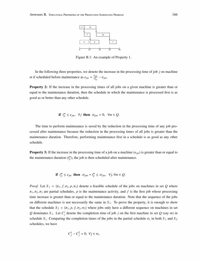
Appendix B. Structural Properties of the Production Scheduling Problem 166
12 4
7 14
9 8 7
0 10 20 30 40
Figure B.1: An example of Property 1.
In the following three properties, we denote the increase in the processing time of job j on machine
m if scheduled before maintenance as ε jm =n jmνm
sm− n jm.
Property 2: If the increase in the processing times of all jobs on a given machine is greater than or
equal to the maintenance duration, then the schedule in which the maintenance is processed first is as
good as or better than any other schedule.
if tmp ≤ ε jm, ∀ j then stpm = 0, ∀m ∈ Q.
The time to perform maintenance is saved by the reduction in the processing time of any job pro-
cessed after maintenance because the reduction in the processing times of all jobs is greater than the
maintenance duration. Therefore, performing maintenance first in a schedule is as good as any other
schedule.
Property 3: If the increase in the processing time of a job on a machine (ε jm) is greater than or equal to
the maintenance duration (tmp ), the job is then scheduled after maintenance.
if tmp ≤ ε jm then stpm + tm
p ≤ st jm, ∀ j,∀m ∈ Q.
Proof. Let S 1 = {π1, f , π2, p, π3} denote a feasible schedule of the jobs on machines in set Q where
π1, π2, π3 are partial schedules, p is the maintenance activity, and f is the first job whose processing
time increase is greater than or equal to the maintenance duration. Note that the sequence of the jobs
on different machines is not necessarily the same in S 1. To prove the property, it is enough to show
that the schedule S 2 = {π1, p, f , π2, π3} where jobs only have a different sequence on machines in set
Q dominates S 1. Let Cij denote the completion time of job j on the first machine in set Q (say m) in
schedule S i. Comparing the completion times of the jobs in the partial schedule π1 in both S 1 and S 2
schedules, we have
C1j −C2
j = 0, ∀ j ∈ π1.
Appendix B. Structural Properties of the Production Scheduling Problem 167
Letting |π1| denote the index of the last job in π1, we have
C1f −C2
f = (C1|π1 |
+ n f m + ε f m) − (C2|π1 |
+ tmp + n f m) ≥ 0.
The above inequality follows because of our assumption on the increase in the processing time of pro-
duction job f . Assuming that l, j represent the indices of the jobs in π2, we have
C1j −C2
j = (C1f +
l= j∑l=1
(nlm + εlm)) − (C2f +
l= j∑l=1
nlm) ≥ 0, ∀ j ∈ π2.
Denoting |π2| as the index of the last job in π2 and l, j as the indices of the jobs in π3, we have
C1j −C2
j = (C1|π2 |
+ tmp +
l= j∑l=1
nlm) − (C2|π2 |
+
l= j∑l=1
nlm) ≥ 0, ∀ j ∈ π3.
As shown, the completion time of each job on machine m in schedule S 2 is smaller than or equal to
its corresponding in schedule S 1. The same argument can be used to show that schedule S 2 finishes
the processing of any job on any downstream machine, i.e., {m + 1, ...,M}, no later than schedule S 1.
Therefore, in schedule S 2, the number of lost jobs is less than or equal to the one in schedule S 1 which
completes the proof. �
Property 4: If the maintenance duration on a given machine (tmp ) is greater than the sum of the in-
crease in the processing times of all possible combinations of l out of |J| jobs, the schedule in which
maintenance is scheduled after |J| − s jobs such that 0 < s ≤ l is not optimal.
if tmp >
i=l∑i=1
ε jim, ∀ j1, j2, ..., jl then
|J|∑j=1
b jm ≤ (|J| − l − 1)w + |J|(1 − w), ∀m ∈ Q,
|J|∑j=1
b jm ≥ |J|(1 − w), ∀m ∈ Q.
Note that |J| is the number of jobs in the PSP and w is a binary variable. The consequence guarantees
that maintenance is either scheduled last or scheduled after at most (|J| − l − 1) jobs.
Proof. Following the same reasoning as Property 3 where {π1, p, π2} and {π1, π2, p} represent the se-
quence of the jobs on machines m ∈ Q in schedules S 1 and S 2, respectively, the property follows. Note
that the number of jobs in partial schedule π2 is equal to s. �
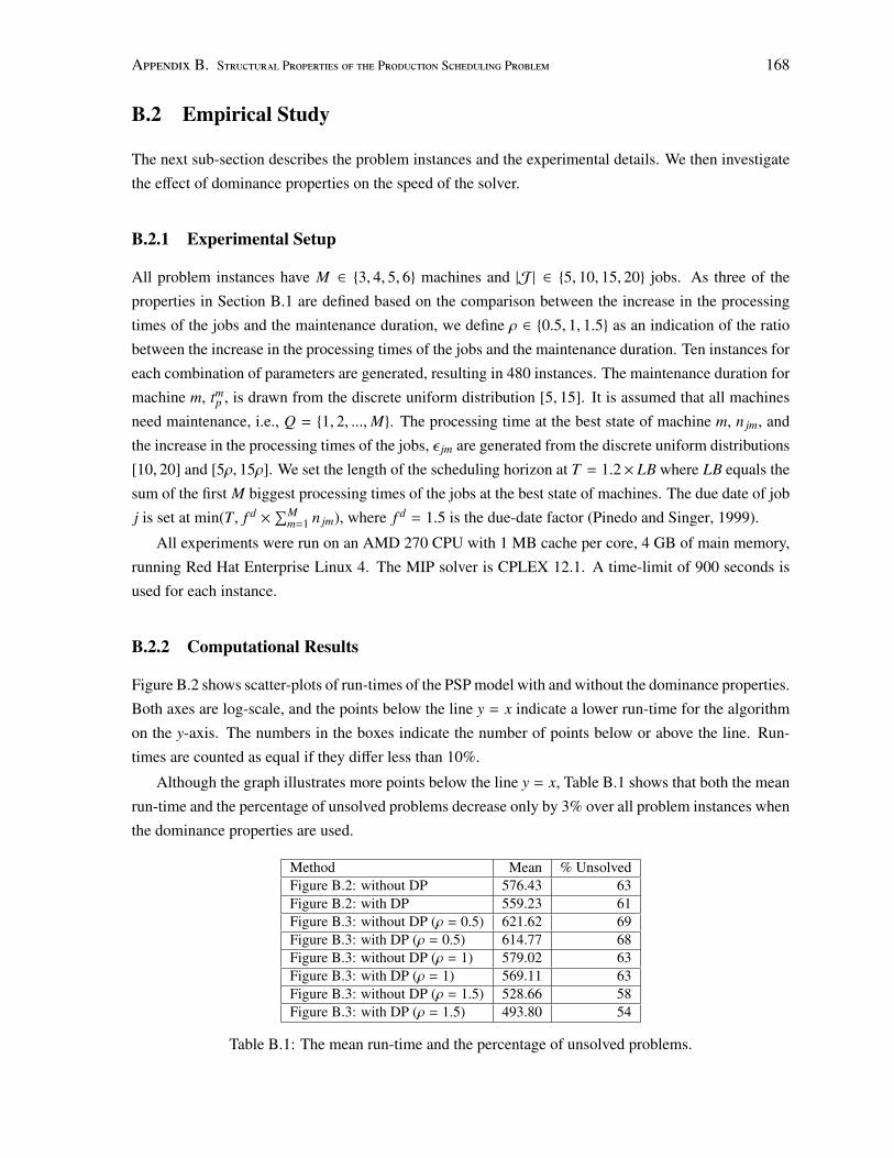
Appendix B. Structural Properties of the Production Scheduling Problem 168
B.2 Empirical Study
The next sub-section describes the problem instances and the experimental details. We then investigate
the effect of dominance properties on the speed of the solver.
B.2.1 Experimental Setup
All problem instances have M ∈ {3, 4, 5, 6} machines and |J| ∈ {5, 10, 15, 20} jobs. As three of the
properties in Section B.1 are defined based on the comparison between the increase in the processing
times of the jobs and the maintenance duration, we define ρ ∈ {0.5, 1, 1.5} as an indication of the ratio
between the increase in the processing times of the jobs and the maintenance duration. Ten instances for
each combination of parameters are generated, resulting in 480 instances. The maintenance duration for
machine m, tmp , is drawn from the discrete uniform distribution [5, 15]. It is assumed that all machines
need maintenance, i.e., Q = {1, 2, ...,M}. The processing time at the best state of machine m, n jm, and
the increase in the processing times of the jobs, ε jm are generated from the discrete uniform distributions
[10, 20] and [5ρ, 15ρ]. We set the length of the scheduling horizon at T = 1.2× LB where LB equals the
sum of the first M biggest processing times of the jobs at the best state of machines. The due date of job
j is set at min(T, f d ×∑M
m=1 n jm), where f d = 1.5 is the due-date factor (Pinedo and Singer, 1999).
All experiments were run on an AMD 270 CPU with 1 MB cache per core, 4 GB of main memory,
running Red Hat Enterprise Linux 4. The MIP solver is CPLEX 12.1. A time-limit of 900 seconds is
used for each instance.
B.2.2 Computational Results
Figure B.2 shows scatter-plots of run-times of the PSP model with and without the dominance properties.
Both axes are log-scale, and the points below the line y = x indicate a lower run-time for the algorithm
on the y-axis. The numbers in the boxes indicate the number of points below or above the line. Run-
times are counted as equal if they differ less than 10%.
Although the graph illustrates more points below the line y = x, Table B.1 shows that both the mean
run-time and the percentage of unsolved problems decrease only by 3% over all problem instances when
the dominance properties are used.
Method Mean % UnsolvedFigure B.2: without DP 576.43 63Figure B.2: with DP 559.23 61Figure B.3: without DP (ρ = 0.5) 621.62 69Figure B.3: with DP (ρ = 0.5) 614.77 68Figure B.3: without DP (ρ = 1) 579.02 63Figure B.3: with DP (ρ = 1) 569.11 63Figure B.3: without DP (ρ = 1.5) 528.66 58Figure B.3: with DP (ρ = 1.5) 493.80 54
Table B.1: The mean run-time and the percentage of unsolved problems.
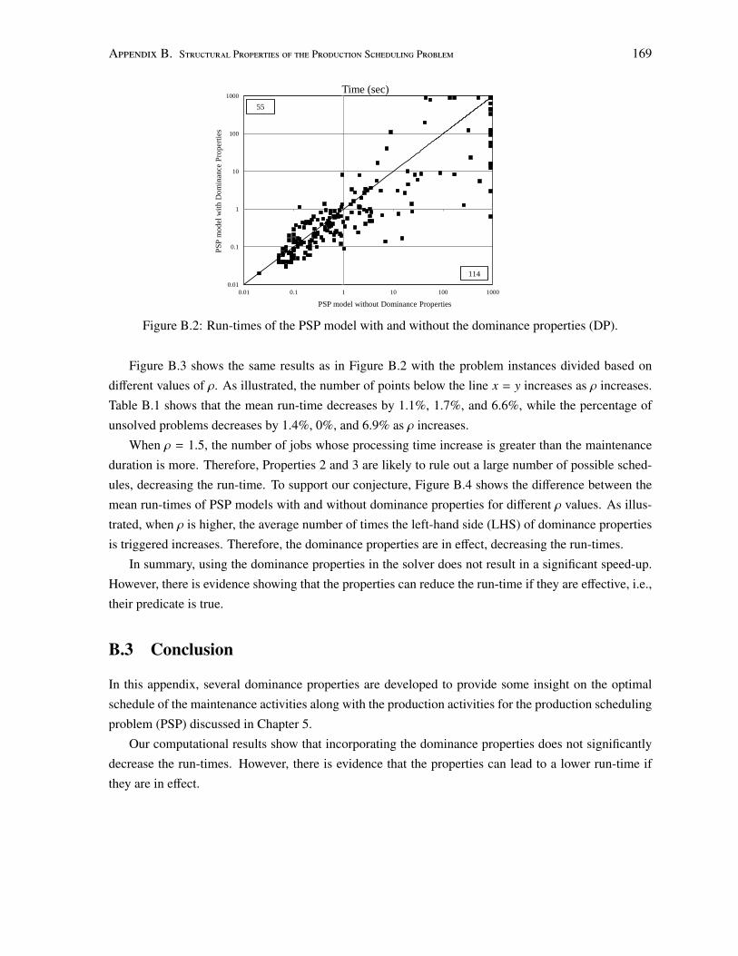
Appendix B. Structural Properties of the Production Scheduling Problem 169
0.01
0.1
1
10
100
1000
0.01 0.1 1 10 100 1000
PS
P m
od
el w
ith D
om
inan
ce P
rop
erti
es
PSP model without Dominance Properties
Time (sec)
55
114
Figure B.2: Run-times of the PSP model with and without the dominance properties (DP).
Figure B.3 shows the same results as in Figure B.2 with the problem instances divided based on
different values of ρ. As illustrated, the number of points below the line x = y increases as ρ increases.
Table B.1 shows that the mean run-time decreases by 1.1%, 1.7%, and 6.6%, while the percentage of
unsolved problems decreases by 1.4%, 0%, and 6.9% as ρ increases.
When ρ = 1.5, the number of jobs whose processing time increase is greater than the maintenance
duration is more. Therefore, Properties 2 and 3 are likely to rule out a large number of possible sched-
ules, decreasing the run-time. To support our conjecture, Figure B.4 shows the difference between the
mean run-times of PSP models with and without dominance properties for different ρ values. As illus-
trated, when ρ is higher, the average number of times the left-hand side (LHS) of dominance properties
is triggered increases. Therefore, the dominance properties are in effect, decreasing the run-times.
In summary, using the dominance properties in the solver does not result in a significant speed-up.
However, there is evidence showing that the properties can reduce the run-time if they are effective, i.e.,
their predicate is true.
B.3 Conclusion
In this appendix, several dominance properties are developed to provide some insight on the optimal
schedule of the maintenance activities along with the production activities for the production scheduling
problem (PSP) discussed in Chapter 5.
Our computational results show that incorporating the dominance properties does not significantly
decrease the run-times. However, there is evidence that the properties can lead to a lower run-time if
they are in effect.
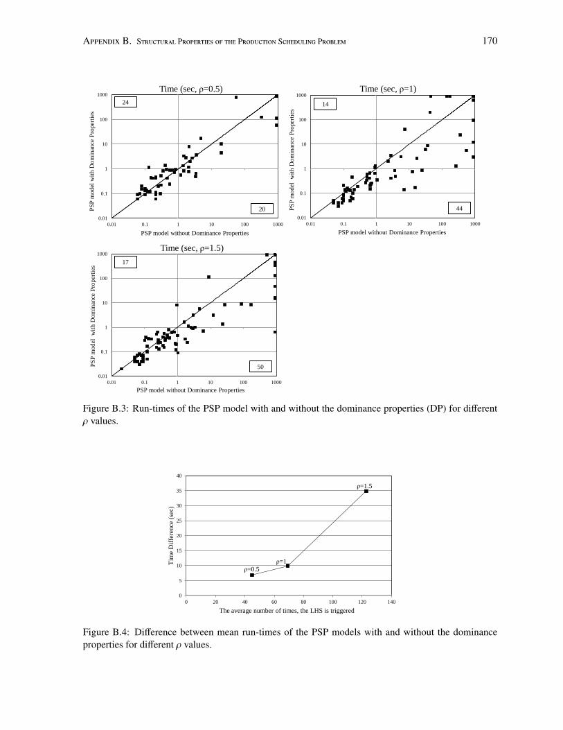
Appendix B. Structural Properties of the Production Scheduling Problem 170
0.01
0.1
1
10
100
1000
0.01 0.1 1 10 100 1000
PS
P m
od
el w
ith D
om
inan
ce P
rop
erti
es
PSP model without Dominance Properties
Time (sec, ρ=0.5)
24
20
0.01
0.1
1
10
100
1000
0.01 0.1 1 10 100 1000
PS
P m
od
el
wit
h D
om
inan
ce P
rop
erti
es
PSP model without Dominance Properties
Time (sec, ρ=1)
14
44
0.01
0.1
1
10
100
1000
0.01 0.1 1 10 100 1000
PS
P m
od
el
wit
h D
om
inan
ce P
rop
erti
es
PSP model without Dominance Properties
Time (sec, ρ=1.5)
17
50
Figure B.3: Run-times of the PSP model with and without the dominance properties (DP) for differentρ values.
ρ=0.5
ρ=1
ρ=1.5
0
5
10
15
20
25
30
35
40
0 20 40 60 80 100 120 140
Tim
e D
iffe
rence
(se
c)
The average number of times, the LHS is triggered
Figure B.4: Difference between mean run-times of the PSP models with and without the dominanceproperties for different ρ values.
Appendix C
Approximating the Average ProductionRate
In Section 6.3.2.1, we discussed a simple approach to approximate the average production rate of a
machine. In this appendix, we discuss an exact approach.
This appendix is organized as follows. We first present the exact method for calculating the average
production rate of machine m within the time period. We then discuss the error of the approximation
approach presented in Section 6.3.2.1. In Section C.3, we solve a numerical example to compare the
two approaches and explain the reasons for using the approximation method in the experimental study
of Section 6.5.2.
C.1 Exact Method
The main idea of the exact method is to define the production quantity (the number of products produced
within the time period) as a random variable and to find its expected value. The average production rate
then equals the expected production quantity per time unit.
In this section, we first calculate the average production rate of machine m in a time period with
length t assuming that it does not need maintenance and then extend the result to the case when ma-
chine m needs maintenance. In the latter case we need to make an assumption on the time at which
maintenance is performed. Similar to Section 6.3.2.1, we assume that maintenance is performed at the
beginning of the interval and that maintenance duration is negligible.
C.1.1 Machine m does not Need Maintenance
In this section, we assume that machine m does not need maintenance. We do not include the index of
machine in the notation for ease of reading. We use the following notation.
• [0, t): The time period starting at time 0 and ending at time t.
• Xt: The state of machine m at time t.
171
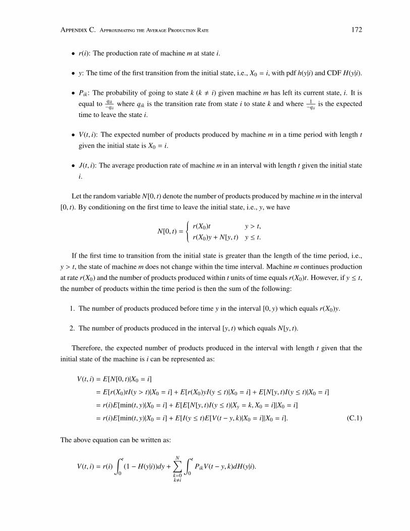
Appendix C. Approximating the Average Production Rate 172
• r(i): The production rate of machine m at state i.
• y: The time of the first transition from the initial state, i.e., X0 = i, with pdf h(y|i) and CDF H(y|i).
• Pik: The probability of going to state k (k , i) given machine m has left its current state, i. It is
equal to qik−qii
where qik is the transition rate from state i to state k and where 1−qii
is the expected
time to leave the state i.
• V(t, i): The expected number of products produced by machine m in a time period with length t
given the initial state is X0 = i.
• J(t, i): The average production rate of machine m in an interval with length t given the initial state
i.
Let the random variable N[0, t) denote the number of products produced by machine m in the interval
[0, t). By conditioning on the first time to leave the initial state, i.e., y, we have
N[0, t) =
r(X0)t y > t,
r(X0)y + N[y, t) y ≤ t.
If the first time to transition from the initial state is greater than the length of the time period, i.e.,
y > t, the state of machine m does not change within the time interval. Machine m continues production
at rate r(X0) and the number of products produced within t units of time equals r(X0)t. However, if y ≤ t,
the number of products within the time period is then the sum of the following:
1. The number of products produced before time y in the interval [0, y) which equals r(X0)y.
2. The number of products produced in the interval [y, t) which equals N[y, t).
Therefore, the expected number of products produced in the interval with length t given that the
initial state of the machine is i can be represented as:
V(t, i) = E[N[0, t)|X0 = i]
= E[r(X0)tI(y > t)|X0 = i] + E[r(X0)yI(y ≤ t)|X0 = i] + E[N[y, t)I(y ≤ t)|X0 = i]
= r(i)E[min(t, y)|X0 = i] + E[E[N[y, t)I(y ≤ t)|Xy = k, X0 = i]|X0 = i]
= r(i)E[min(t, y)|X0 = i] + E[I(y ≤ t)E[V(t − y, k)|X0 = i]|X0 = i]. (C.1)
The above equation can be written as:
V(t, i) = r(i)∫ t
0(1 − H(y|i))dy +
N∑k=0k,i
∫ t
0PikV(t − y, k)dH(y|i).
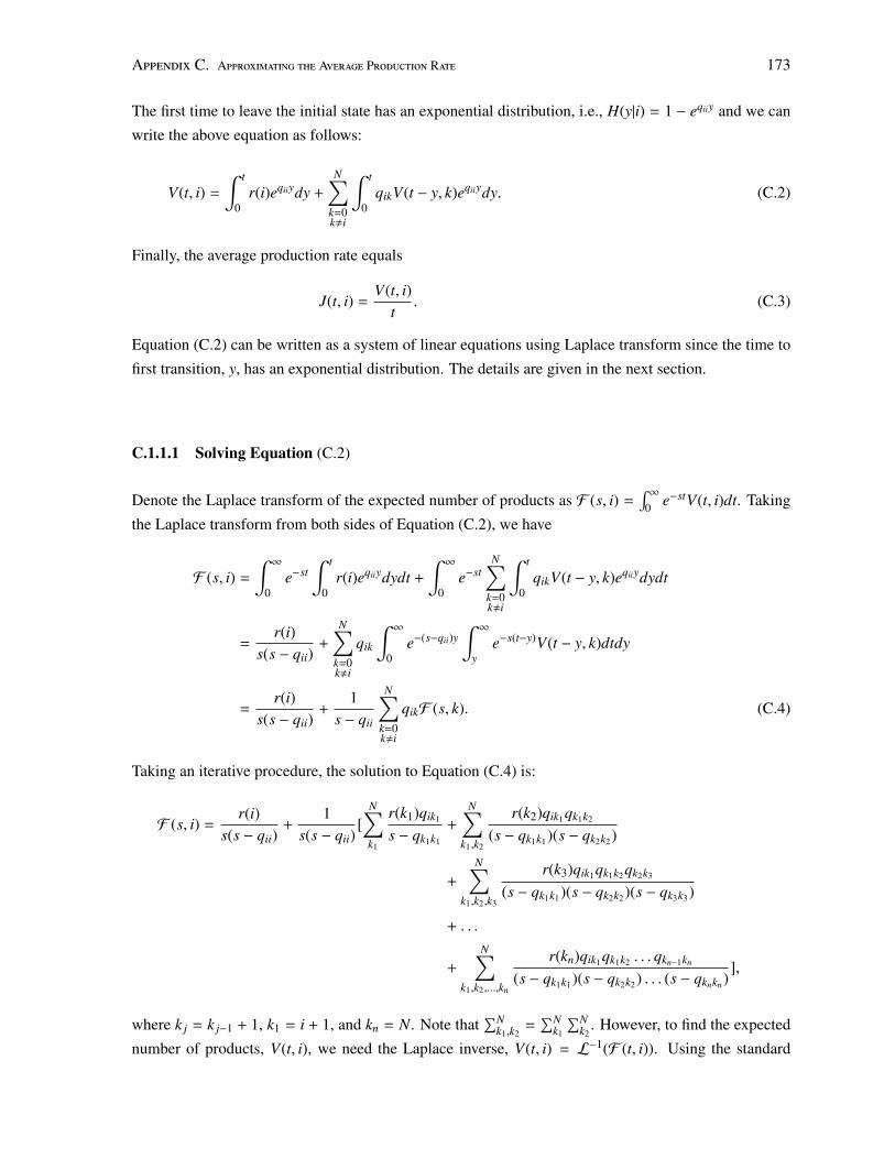
Appendix C. Approximating the Average Production Rate 173
The first time to leave the initial state has an exponential distribution, i.e., H(y|i) = 1 − eqiiy and we can
write the above equation as follows:
V(t, i) =
∫ t
0r(i)eqiiydy +
N∑k=0k,i
∫ t
0qikV(t − y, k)eqiiydy. (C.2)
Finally, the average production rate equals
J(t, i) =V(t, i)
t. (C.3)
Equation (C.2) can be written as a system of linear equations using Laplace transform since the time to
first transition, y, has an exponential distribution. The details are given in the next section.
C.1.1.1 Solving Equation (C.2)
Denote the Laplace transform of the expected number of products as F (s, i) =∫ ∞
0 e−stV(t, i)dt. Taking
the Laplace transform from both sides of Equation (C.2), we have
F (s, i) =
∫ ∞
0e−st
∫ t
0r(i)eqiiydydt +
∫ ∞
0e−st
N∑k=0k,i
∫ t
0qikV(t − y, k)eqiiydydt
=r(i)
s(s − qii)+
N∑k=0k,i
qik
∫ ∞
0e−(s−qii)y
∫ ∞
ye−s(t−y)V(t − y, k)dtdy
=r(i)
s(s − qii)+
1s − qii
N∑k=0k,i
qikF (s, k). (C.4)
Taking an iterative procedure, the solution to Equation (C.4) is:
F (s, i) =r(i)
s(s − qii)+
1s(s − qii)
[N∑k1
r(k1)qik1
s − qk1k1
+
N∑k1,k2
r(k2)qik1qk1k2
(s − qk1k1)(s − qk2k2)
+
N∑k1,k2,k3
r(k3)qik1qk1k2qk2k3
(s − qk1k1)(s − qk2k2)(s − qk3k3)
+ . . .
+
N∑k1,k2,...,kn
r(kn)qik1qk1k2 . . . qkn−1kn
(s − qk1k1)(s − qk2k2) . . . (s − qknkn)],
where k j = k j−1 + 1, k1 = i + 1, and kn = N. Note that∑N
k1,k2=
∑Nk1
∑Nk2
. However, to find the expected
number of products, V(t, i), we need the Laplace inverse, V(t, i) = L−1(F (t, i)). Using the standard
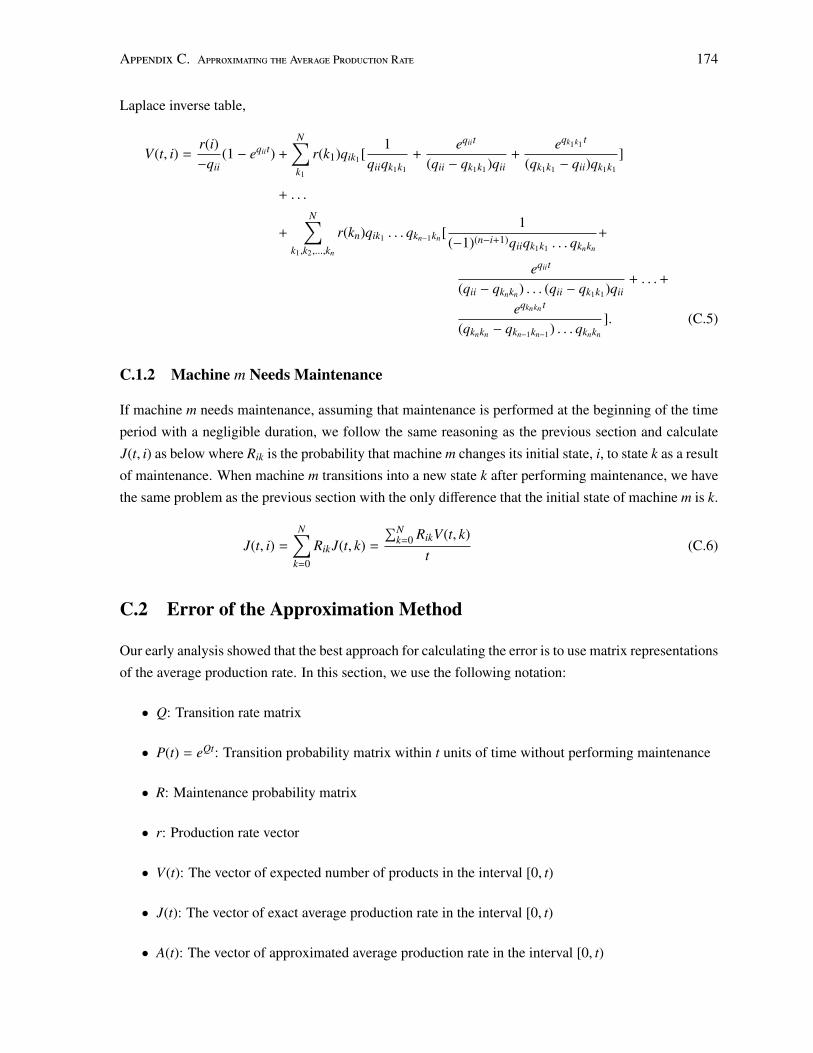
Appendix C. Approximating the Average Production Rate 174
Laplace inverse table,
V(t, i) =r(i)−qii
(1 − eqiit) +
N∑k1
r(k1)qik1[1
qiiqk1k1
+eqiit
(qii − qk1k1)qii+
eqk1k1 t
(qk1k1 − qii)qk1k1
]
+ . . .
+
N∑k1,k2,...,kn
r(kn)qik1 . . . qkn−1kn[1
(−1)(n−i+1)qiiqk1k1 . . . qknkn
+
eqiit
(qii − qknkn) . . . (qii − qk1k1)qii+ . . .+
eqknkn t
(qknkn − qkn−1kn−1) . . . qknkn
]. (C.5)
C.1.2 Machine m Needs Maintenance
If machine m needs maintenance, assuming that maintenance is performed at the beginning of the time
period with a negligible duration, we follow the same reasoning as the previous section and calculate
J(t, i) as below where Rik is the probability that machine m changes its initial state, i, to state k as a result
of maintenance. When machine m transitions into a new state k after performing maintenance, we have
the same problem as the previous section with the only difference that the initial state of machine m is k.
J(t, i) =
N∑k=0
RikJ(t, k) =
∑Nk=0 RikV(t, k)
t(C.6)
C.2 Error of the Approximation Method
Our early analysis showed that the best approach for calculating the error is to use matrix representations
of the average production rate. In this section, we use the following notation:
• Q: Transition rate matrix
• P(t) = eQt: Transition probability matrix within t units of time without performing maintenance
• R: Maintenance probability matrix
• r: Production rate vector
• V(t): The vector of expected number of products in the interval [0, t)
• J(t): The vector of exact average production rate in the interval [0, t)
• A(t): The vector of approximated average production rate in the interval [0, t)
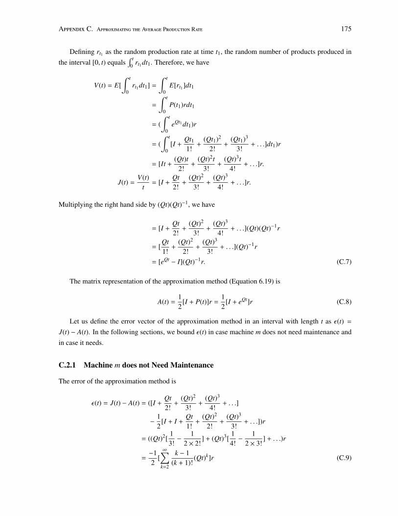
Appendix C. Approximating the Average Production Rate 175
Defining rt1 as the random production rate at time t1, the random number of products produced in
the interval [0, t) equals∫ t
0 rt1dt1. Therefore, we have
V(t) = E[∫ t
0rt1dt1] =
∫ t
0E[rt1]dt1
=
∫ t
0P(t1)rdt1
= (∫ t
0eQt1dt1)r
= (∫ t
0[I +
Qt11!
+(Qt1)2
2!+
(Qt1)3
3!+ . . .]dt1)r
= [It +(Qt)t
2!+
(Qt)2t3!
+(Qt)3t
4!+ . . .]r.
J(t) =V(t)
t= [I +
Qt2!
+(Qt)2
3!+
(Qt)3
4!+ . . .]r.
Multiplying the right hand side by (Qt)(Qt)−1, we have
= [I +Qt2!
+(Qt)2
3!+
(Qt)3
4!+ . . .](Qt)(Qt)−1r
= [Qt1!
+(Qt)2
2!+
(Qt)3
3!+ . . .](Qt)−1r
= [eQt − I](Qt)−1r. (C.7)
The matrix representation of the approximation method (Equation 6.19) is
A(t) =12
[I + P(t)]r =12
[I + eQt]r (C.8)
Let us define the error vector of the approximation method in an interval with length t as ε(t) =
J(t) − A(t). In the following sections, we bound ε(t) in case machine m does not need maintenance and
in case it needs.
C.2.1 Machine m does not Need Maintenance
The error of the approximation method is
ε(t) = J(t) − A(t) = ([I +Qt2!
+(Qt)2
3!+
(Qt)3
4!+ . . .]
−12
[I + I +Qt1!
+(Qt)2
2!+
(Qt)3
3!+ . . .])r
= ((Qt)2[13!−
12 × 2!
] + (Qt)3[14!−
12 × 3!
] + . . .)r
=−12
[∞∑
k=2
k − 1(k + 1)!
(Qt)k]r (C.9)
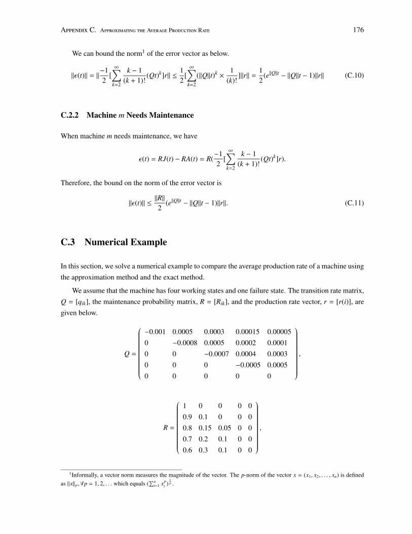
Appendix C. Approximating the Average Production Rate 176
We can bound the norm1 of the error vector as below.
‖ε(t)‖ = ‖−12
[∞∑
k=2
k − 1(k + 1)!
(Qt)k]r‖ ≤12
[∞∑
k=2
(‖Q‖t)k ×1
(k)!]‖r‖ =
12
(e‖Q‖t − ‖Q‖t − 1)‖r‖ (C.10)
C.2.2 Machine m Needs Maintenance
When machine m needs maintenance, we have
ε(t) = RJ(t) − RA(t) = R(−12
[∞∑
k=2
k − 1(k + 1)!
(Qt)k]r).
Therefore, the bound on the norm of the error vector is
‖ε(t)‖ ≤‖R‖2
(e‖Q‖t − ‖Q‖t − 1)‖r‖. (C.11)
C.3 Numerical Example
In this section, we solve a numerical example to compare the average production rate of a machine using
the approximation method and the exact method.
We assume that the machine has four working states and one failure state. The transition rate matrix,
Q = [qik], the maintenance probability matrix, R = [Rik], and the production rate vector, r = [r(i)], are
given below.
Q =
−0.001 0.0005 0.0003 0.00015 0.00005
0 −0.0008 0.0005 0.0002 0.0001
0 0 −0.0007 0.0004 0.0003
0 0 0 −0.0005 0.0005
0 0 0 0 0
,
R =
1 0 0 0 0
0.9 0.1 0 0 0
0.8 0.15 0.05 0 0
0.7 0.2 0.1 0 0
0.6 0.3 0.1 0 0
,
1Informally, a vector norm measures the magnitude of the vector. The p-norm of the vector x = (x1, x2, . . . , xn) is definedas ‖x‖p,∀p = 1, 2, . . . which equals (
∑ni=1 xp
i )1p .
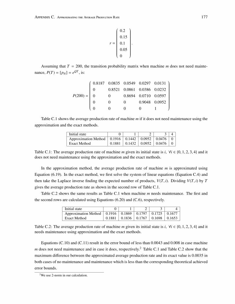
Appendix C. Approximating the Average Production Rate 177
r =
0.2
0.15
0.1
0.05
0
.
Assuming that T = 200, the transition probability matrix when machine m does not need mainte-
nance, P(T ) = [pik] = eQT , is:
P(200) =
0.8187 0.0835 0.0549 0.0297 0.0131
0 0.8521 0.0861 0.0386 0.0232
0 0 0.8694 0.0710 0.0597
0 0 0 0.9048 0.0952
0 0 0 0 1
Table C.1 shows the average production rate of machine m if it does not need maintenance using the
approximation and the exact methods.
Initial state 0 1 2 3 4Approximation Method 0.1916 0.1442 0.0952 0.0476 0Exact Method 0.1881 0.1432 0.0952 0.0476 0
Table C.1: The average production rate of machine m given its initial state is i, ∀i ∈ {0, 1, 2, 3, 4} and itdoes not need maintenance using the approximation and the exact methods.
In the approximation method, the average production rate of machine m is approximated using
Equation (6.19). In the exact method, we first solve the system of linear equations (Equation C.4) and
then take the Laplace inverse finding the expected number of products, V(T, i). Dividing V(T, i) by T
gives the average production rate as shown in the second row of Table C.1.
Table C.2 shows the same results as Table C.1 when machine m needs maintenance. The first and
the second rows are calculated using Equations (6.20) and (C.6), respectively.
Initial state 0 1 2 3 4Approximation Method 0.1916 0.1869 0.1797 0.1725 0.1677Exact Method 0.1881 0.1836 0.1767 0.1698 0.1653
Table C.2: The average production rate of machine m given its initial state is i, ∀i ∈ {0, 1, 2, 3, 4} and itneeds maintenance using approximation and the exact methods.
Equations (C.10) and (C.11) result in the error bound of less than 0.0043 and 0.008 in case machine
m does not need maintenance and in case it does, respectively.2 Table C.1 and Table C.2 show that the
maximum difference between the approximated average production rate and its exact value is 0.0035 in
both cases of no maintenance and maintenance which is less than the corresponding theoretical achieved
error bounds.2We use 2-norm in our calculation.
Appendix C. Approximating the Average Production Rate 178
The main question of our interest is to decide which method is appropriate to calculate the average
production rate. We use the approximation method in our experimental study (Section 6.5.2) mainly
because of the following:
• In our experimental setup (see Appendix D), the transition rate and the maintenance probability
matrices have small norms. Equations (C.10) and (C.11) therefore result in error bounds close to
0 implying that the approximated average production rate is very close to the exact value.
• As the number of states increases, Equation (C.5) is not computationally efficient since the de-
nominators of the fractions in the sums tend to 0. The alternative approach is to solve the inte-
gral Equation (C.2) using successive approximation procedure (Pogorzelski, 1966; Keffer, 1999).
However, our previous experiment on the successive approximation procedure shows that its con-
vergence speed is very slow specially as t increases. It is also worth mentioning that we do not use
the matrix representation of the exact average production rate (Equation C.7) for calculation since
the transition rate matrix Q is singular in the majority of our problem instances and the inverse
matrix Q−1 does not exist.
• The approximated procedure is simple requiring less information and is fast.
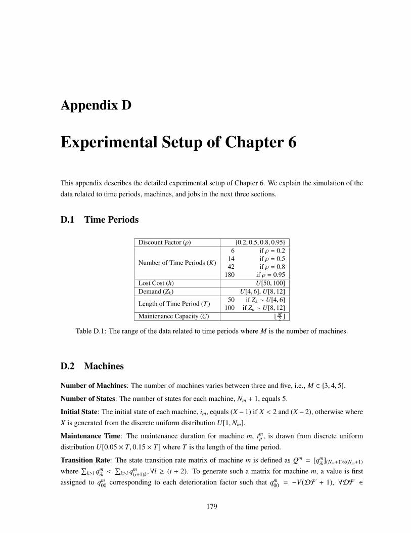
Appendix D
Experimental Setup of Chapter 6
This appendix describes the detailed experimental setup of Chapter 6. We explain the simulation of the
data related to time periods, machines, and jobs in the next three sections.
D.1 Time Periods
Discount Factor (ρ) {0.2, 0.5, 0.8, 0.95}
Number of Time Periods (K)
6 if ρ = 0.214 if ρ = 0.542 if ρ = 0.8
180 if ρ = 0.95Lost Cost (h) U[50, 100]Demand (Zk) U[4, 6], U[8, 12]
Length of Time Period (T ) 50 if Zk ∼ U[4, 6]100 if Zk ∼ U[8, 12]
Maintenance Capacity (C) bM2 c
Table D.1: The range of the data related to time periods where M is the number of machines.
D.2 Machines
Number of Machines: The number of machines varies between three and five, i.e., M ∈ {3, 4, 5}.
Number of States: The number of states for each machine, Nm + 1, equals 5.
Initial State: The initial state of each machine, im, equals (X − 1) if X < 2 and (X − 2), otherwise where
X is generated from the discrete uniform distribution U[1,Nm].
Maintenance Time: The maintenance duration for machine m, tmp , is drawn from discrete uniform
distribution U[0.05 × T, 0.15 × T ] where T is the length of the time period.
Transition Rate: The state transition rate matrix of machine m is defined as Qm = [qmik](Nm+1)×(Nm+1)
where∑
k≥l qmik <
∑k≥l qm
(i+1)k,∀l ≥ (i + 2). To generate such a matrix for machine m, a value is first
assigned to qm00 corresponding to each deterioration factor such that qm
00 = −V(DF + 1), ∀DF ∈
179
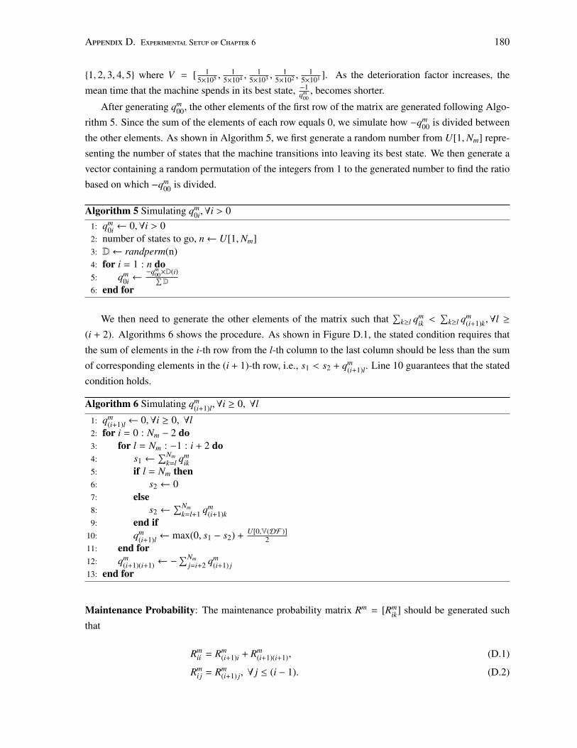
Appendix D. Experimental Setup of Chapter 6 180
{1, 2, 3, 4, 5} where V = [ 15×105 ,
15×104 ,
15×103 ,
15×102 ,
15×101 ]. As the deterioration factor increases, the
mean time that the machine spends in its best state, −1qm
00, becomes shorter.
After generating qm00, the other elements of the first row of the matrix are generated following Algo-
rithm 5. Since the sum of the elements of each row equals 0, we simulate how −qm00 is divided between
the other elements. As shown in Algorithm 5, we first generate a random number from U[1,Nm] repre-
senting the number of states that the machine transitions into leaving its best state. We then generate a
vector containing a random permutation of the integers from 1 to the generated number to find the ratio
based on which −qm00 is divided.
Algorithm 5 Simulating qm0i,∀i > 0
1: qm0i ← 0,∀i > 0
2: number of states to go, n← U[1,Nm]3: D← randperm(n)4: for i = 1 : n do5: qm
0i ←−qm
00×D(i)∑D
6: end for
We then need to generate the other elements of the matrix such that∑
k≥l qmik <
∑k≥l qm
(i+1)k,∀l ≥
(i + 2). Algorithms 6 shows the procedure. As shown in Figure D.1, the stated condition requires that
the sum of elements in the i-th row from the l-th column to the last column should be less than the sum
of corresponding elements in the (i + 1)-th row, i.e., s1 < s2 + qm(i+1)l. Line 10 guarantees that the stated
condition holds.
Algorithm 6 Simulating qm(i+1)l,∀i ≥ 0, ∀l
1: qm(i+1)l ← 0,∀i ≥ 0, ∀l
2: for i = 0 : Nm − 2 do3: for l = Nm : −1 : i + 2 do4: s1 ←
∑Nmk=l qm
ik5: if l = Nm then6: s2 ← 07: else8: s2 ←
∑Nmk=l+1 qm
(i+1)k9: end if
10: qm(i+1)l ← max(0, s1 − s2) +
U[0,V(DF )]2
11: end for12: qm
(i+1)(i+1) ← −∑Nm
j=i+2 qm(i+1) j
13: end for
Maintenance Probability: The maintenance probability matrix Rm = [Rmik] should be generated such
that
Rmii = Rm
(i+1)i + Rm(i+1)(i+1), (D.1)
Rmi j = Rm
(i+1) j, ∀ j ≤ (i − 1). (D.2)
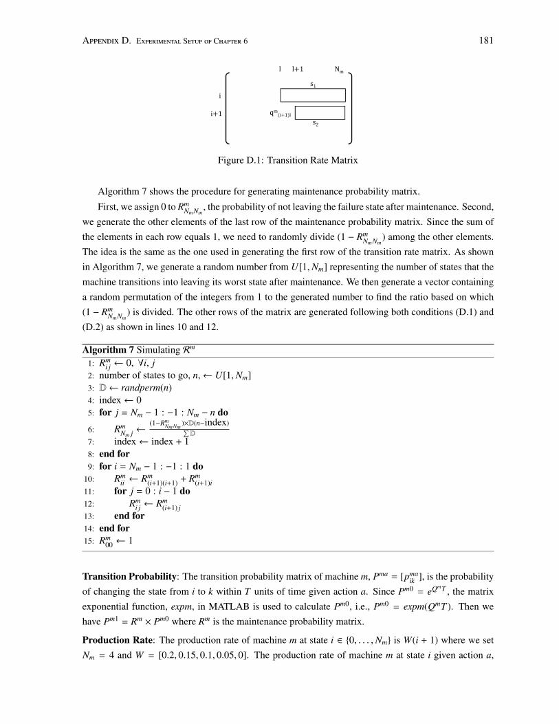
Appendix D. Experimental Setup of Chapter 6 181
i
i 1
l Nm
s1
s2qm i 1 l
l 1
Figure D.1: Transition Rate Matrix
Algorithm 7 shows the procedure for generating maintenance probability matrix.
First, we assign 0 to RmNmNm
, the probability of not leaving the failure state after maintenance. Second,
we generate the other elements of the last row of the maintenance probability matrix. Since the sum of
the elements in each row equals 1, we need to randomly divide (1 − RmNmNm
) among the other elements.
The idea is the same as the one used in generating the first row of the transition rate matrix. As shown
in Algorithm 7, we generate a random number from U[1,Nm] representing the number of states that the
machine transitions into leaving its worst state after maintenance. We then generate a vector containing
a random permutation of the integers from 1 to the generated number to find the ratio based on which
(1 − RmNmNm
) is divided. The other rows of the matrix are generated following both conditions (D.1) and
(D.2) as shown in lines 10 and 12.
Algorithm 7 Simulating Rm
1: Rmi j ← 0, ∀i, j
2: number of states to go, n,← U[1,Nm]3: D← randperm(n)4: index← 05: for j = Nm − 1 : −1 : Nm − n do
6: RmNm j ←
(1−RmNmNm
)×D(n−index)∑D
7: index← index + 18: end for9: for i = Nm − 1 : −1 : 1 do
10: Rmii ← Rm
(i+1)(i+1) + Rm(i+1)i
11: for j = 0 : i − 1 do12: Rm
i j ← Rm(i+1) j
13: end for14: end for15: Rm
00 ← 1
Transition Probability: The transition probability matrix of machine m, Pma = [pmaik ], is the probability
of changing the state from i to k within T units of time given action a. Since Pm0 = eQmT , the matrix
exponential function, expm, in MATLAB is used to calculate Pm0, i.e., Pm0 = expm(QmT ). Then we
have Pm1 = Rm × Pm0 where Rm is the maintenance probability matrix.
Production Rate: The production rate of machine m at state i ∈ {0, . . . ,Nm} is W(i + 1) where we set
Nm = 4 and W = [0.2, 0.15, 0.1, 0.05, 0]. The production rate of machine m at state i given action a,
Appendix D. Experimental Setup of Chapter 6 182
rm(i, a), is calculated as below where Rmil is the maintenance probability.
rm(i, 0) = W(i + 1), rm(i, 1) =
Nm∑l=0
Rmil W(l + 1).
Maintenance Cost: We need to generate maintenance cost of machine m at state i, τm(i), such that
condition (D.3) holds true.
τm(i + 1) − τm(i) ≤ h(z − Trm(i + 1, 0))+ − h(z − Trm(i + 1, 1))+
− h(z − Trm(i, 0))+ + h(z − Trm(i, 1))+, ∀i, ∀z (D.3)
Moreover, τm(i + 1) ≥ τm(i) implying that the left-hand side of condition (D.3) is greater than 0.
Algorithm 8 shows the procedure that we use to generate the maintenance cost at each state for each
machine where a and b are the lower and the upper bounds for demand. First maintenance cost at the
worst state is generated from the uniform distribution U[50, 100]. As shown in Line 6 of Algorithm
8, if the right-hand side of condition (D.3) is less than 0, the required condition does not hold and
we re-initiate the procedure of generating the data from the beginning. Otherwise, as line 9 shows in
Algorithm 8, τm(i) is generated such that condition (D.3) holds true.
Algorithm 8 Simulating τm(i), ∀i1: τm(Nm)← U[50, 100]2: for i = Nm − 1 : −1 : 0 do3: for z = a : b do4: c← h(z − Trm(i + 1, 0))+ − (z − Trm(i + 1, 1))+ − h(z − Trm(i, 0))+ + (z − Trm(i, 1))+
5: if c < 0 then6: re-initiate simulating the data7: end if8: end for9: τm(i)← τm(i + 1)
10: end for
D.3 Jobs
Nominal Processing Time: The nominal processing time of the production activity j on machine m,
n jm, is drawn from the discrete uniform distribution U[1, 9]. It is worth mentioning that the nominal
processing time distribution is chosen such that its mean equals 1rm(0) = 5.
Due date: The due date of production activity j is set at min(T, f d ×∑M
m=1 n jm) where f d, the due-date
factor, is 2.5 and 3 for T = 50 and T = 100, respectively.
Bibliography
Adiri, I., J. Bruno, E. Frostig, A. H. G. Rinnooy Kan. 1989. Single machine flow-time scheduling with
a single breakdown. Acta Informatica 26 679–696.
Adiri, I., E. Frostig, A. H. G. Rinnooy Kan. 1991. Scheduling on a single machine with a single
breakdown to minimize stochastically the number of tardy jobs. Naval Research Logistics 38 261–
271.
Aghezzaf, E., N. M. Najid. 2008. Integrated production planning and preventive maintenance in deteri-
orating production systems. Information Sciences 178 3382–3392.
Aghezzaf, E. H., M. A. Jamali, D. Ait-Kadi. 2007. An integrated production and preventive maintenance
planning model. European Journal of Operational Research 181 679–685.
Akturk, M. S., J. B. Ghosh, E. D. Gunes. 2004. Scheduling with tool changes to minimize total com-
pletion time: Basic results and SPT performance. European Journal of Operational Research 157784–790.
Akturk, S. M., E. Gorgulu. 1999. Match-up scheduling under a machine breakdown. European Journal
of Operational Research 112 81–97.
Allahverdi, A. 1995. Two-stage production scheduling with separated setup times and stochastic break-
downs. Journal of the Operational Research Society 46 896–904.
Allahverdi, A. 1996. Two-machine proportionate flowshop scheduling with breakdowns to minimize
the maximum lateness. Computers & Operations Research 23 909–916.
Allahverdi, A. 1997. Scheduling in stochastic flowshop with independent setup, processing and removal
times. Computers & Operations Research 24 955–960.
Allahverdi, A., J. Mittenthal. 1994. Two-machine ordered flowshop scheduling under random break-
downs. Mathematical and Computer Modeling 20 9–17.
Allahverdi, A., J. Mittenthal. 1995. Scheduling on a two-machine flowshop subject to random break-
downs with a makespan objective function. European Journal of Operational Research 81 376–387.
183
BIBLIOGRAPHY 184
Applegate, D., W. Cook. 1991. A computational study of the jobshop scheduling problem. ORSA
Journal on Computing 3 149–156.
Aytug, H., M Lawley, K. McKay, S. Mohan, R. Uzsoy. 2005. Executing production schedules in the
face of uncertainties: A review and future directions. European Journal of Operational Research 16186–110.
Baker, H., R. Ehrhardt. 1995. A dynamic inventory model with random replenishment quantities. Omega
23 109–116.
Baker, K. R., D. Trietsch. 2009. Principles of Sequencing and Scheduling. John Wiley & Sons.
Baptiste, P., P. Laborie, C. Pape, W. Nuijten. 2006. Constraint-Based Scheduling and Planning. F. Rossi,
P. Beek, T. Walsh, eds., Handbook of Constraint Programming. Elsevier.
Baptiste, P., C. L. Pape, W. Nuijten. 2001. Constraint-based Scheduling. Kluwer Academic Publishers.
Barlow, R. E., F. Proschan. 1996. Mathematical Theory of Reliability. SAIM.
Batun, S., L. M. Maillart. 2012. Reassessing tradeoffs inherent to simultaneous maintenance and pro-
duction planning. Production and Operations Management 21 396–403.
Bean, J. C., J. R. Birge, J. Mittenthal, C. E. Noon. 1991. Match-up scheduling with multiple resources,
release dates and disruptions. Operations Research 39 470–483.
Beck, J. C. 1999. Texture measurements as a basis for heuristic commitment techniques in constraint-
directed scheduling. Ph.D. thesis, Department of Computer Science, University of Toronto.
Beck, J. C. 2010. Checking-up on branch-and-check. Proceedings of the Sixteenth International Con-
ference on Principles and Practice of Constraint Programming (CP2010). 84–98.
Beck, J. C., A. J. Davenport, E. D. Davis, M. S. Fox. 1998. The ODO project: Toward a unified basis
for constraint-directed scheduling. Journal of Scheduling 1 89–125.
Beck, J. C., P. Refalo. 2003. A hybrid approach to scheduling with earliness and tardiness costs. Annals
of Operations Research 118 49–71.
Beck, J. C., N. Wilson. 2007. Proactive algorithms for jobshop scheduling with probabilistic durations.
Journal of Artificial Intelligence Research 28 183–232.
Ben-Daya, M., M. A. Rahim. 2001. Integrated Production, Quality & Maintenance Models: An
Overview. M. Ben-Daya, M. A. Rahim, eds., Integrated Models in Production Planning, Inventory,
Quality, and Maintenance. Kluwer Academic Publisher.
Benders, J. 1962. Partitioning procedures for solving mixed-variables programming problems. Nu-
merische Mathematik 4 238–252.
BIBLIOGRAPHY 185
Bently, J. P. 1999. Reliability and Quality Engineering. 2nd ed. Addison Wesley Longman.
Bertsekas, D. P. 2007. Dynamic Programming and Optimal Control, vol. II. 3rd ed. Athena Scientific.
Bertsimas, D., J. Nino-Mora. 2000. Restless bandits, linear programming relaxations, and a primal-dual
index heuristic. Operations Research 48 80–90.
Bidot, J. 2005. A general framework integrating techniques for scheduling under uncertainty. Ph.D.
thesis, Institut National Polytechnique de Toulouse, France.
Bidot, J., T. Vidal, P. Laborie, J. C. Beck. 2009. A theoretical and practical framework for scheduling in
a stochastic environment. Journal of Scheduling 12 315–344.
Birge, J., J. B. G. Frenk, J. Mittenthal, A. H. G. Rinnooy Kan. 1990. Single machine scheduling subject
to stochastic breakdowns. Naval Research Logistics 37 661–677.
Birge, J. R., F. Louveaux. 1997. Introduction to Stochastic Programming. Springer Verlag.
Bollapragada, S., T. E. Morton. 1999. Myopic heuristics for the random yield problem. Operations
Research 47 713–722.
Boone, T., R. Ganeshan, Y. Guo, J. Ord. 2000. The impact of imperfect processes on production run
times. Decision Sciences 31 777–783.
Branke, J., D. C. Mattfeld. 2002. Anticipatory scheduling for dynamic jobshop problems. Proceedings
of the ICAPS’02 Workshop on Online Planning and Scheduling. 3–10.
Branke, J., D. C. Mattfeld. 2005. Anticipation and flexibility in dynamic scheduling. International
Journal of Production Research 43 3103–3129.
Budai, G., D. Huisman, R. Dekker. 2006. Scheduling preventive railway maintenance activities. Journal
of the Operational Research Society 57 1035–1044.
Bulbul, K., P. Kaminsky, C. Yano. 2004. Flowshop scheduling with earliness, tardiness, and intermedi-
ate inventory holding costs. Naval Research Logistics 51 407–445.
Burns, E., J. Benton, W. Ruml, S. Yoon, M. B. Do. 2012. Anticipatory online planning. Proceedings
of the Twenty-Second International Conference on Automated Planning and Scheduling (ICAPS’12).
333–337.
Cai, X., A. Sun, X. Zhou. 2003. Stochastic scheduling with preemptive-repeat machine breakdowns to
minimize the expected weighted flow time. Probability in the Engineering and Information Sciences
17 467–485.
Cai, X., X. Sun, X. Zhou. 2004. Stochastic scheduling subject to machine breakdowns: The preemptive-
repeat model with discounted reward and other criteria. Naval Research Logistics 51 800–817.
BIBLIOGRAPHY 186
Cai, X., F. S. Tu. 1996. Scheduling jobs with random processing times on a single machine subject to
stochastic breakdowns to minimize early-tardy penalties. Naval Research Logistics 43 1127–1146.
Cai, X., X. Wu, X. Zhou. 2005. Dynamically optimal policies for stochastic scheduling subject to
preemptive-repeat machine breakdowns. IEEE Transactions on Automation Science and Engineering
2 158–172.
Cai, X., X. Wu, X. Zhou. 2009. Stochastic scheduling subject to preemptive-repeat breakdowns with
incomplete information. Operations Research 57 1–14.
Cai, X., S. Zhou. 1999. Stochastic scheduling on parallel machines subject to random breakdowns to
minimize expected costs for earliness and tardy jobs. Operations Research 47 422–437.
Cai, X., X. Zhou. 2000. Asymmetric earliness and tardiness scheduling with exponential processing
times on an unreliable machine. Annals of Operations Research 98 313–331.
Cai, X., X. Zhou. 2006. Stochastic scheduling with asymmetric earliness and tardiness penalties under
random machine breakdowns. Probability in the Engineering and Information Sciences 20 635–654.
Carter, A. D. S. 1986. Mechanical Reliability. 2nd ed. Mechanical Education Ltd.
Caseau, Y., F. Laburthe. 1996. Cumulative scheduling with task intervals. Proceedings of the 1996 Joint
International Conference and Symposium on Logic Programming. MIT, 363–377.
Cassady, C. R., E. Kutanoglu. 2003. Minimizing job tardiness using integrated preventive maintenance
planning and production scheduling. IIE Transactions 35 503–513.
Cassady, C. R., E. Kutanoglu. 2005. Integrating preventive maintenance planning and production
scheduling for a single machine. IEEE Transactions on Reliability 54 304–309.
Chakraborty, T., B. C. Giri, K. S. Chaudhuri. 2009. Production lot-sizing with process deterioration and
machine breakdown under inspection schedule. Omega 37 257–271.
Chakravarthy, S. R., A. Agarwal. 2003. Analysis of a machine repair problem with an unreliable server
and phase type repairs and services. Naval Research Logistics 50 462–480.
Chand, S., V. N. Hsu, S. Sethi. 2002. Forecast, solution, and rolling horizons in operations management
problems: A classified bibliography. Manufacturing & Service Operations Management 4 25–43.
Chelbi, A., D. Ait-Kadi. 2004. Analysis of a production/inventory system with randomly failing pro-
duction unit submitted to regular preventive maintenance. European Journal of Operational Research
156 712–718.
Chen, J. S. 2006. Single machine scheduling with flexible and periodic maintenance. Journal of the
Operational Society 57 703–710.
BIBLIOGRAPHY 187
Cheung, K. L., W. H. Hausman. 1997. Joint determination of preventive maintenance and safety stocks
in an unreliable production environment. Naval Research Logistics 44 257–272.
Cho, I. D., M. Parlar. 1991. A survey of maintenance models for multi-unit systems. European Journal
of Operational Research 51 1–23.
Chu, Y., Q. Xia. 2004. Generating Benders cuts for a general class of integer programming problems.
Proceedings of the First International Conference on the Integration of AI and OR Techniques in
Constraint Programming (CPAIOR04). 127–136.
Ciarallo, F. W., R. Akella, T. E. Morton. 1994. A periodic review, production planning model with un-
certain capacity and uncertain demand-Optimality of extended myopic policies. Management Science
40 320–332.
Coffman, E. G. Jr., G. S. Lueker. 1991. Probabilistic Analysis of Packing and Partitioning Algorithms.
John Wiley & Sons Ltd.
Cohen, P. R. 1995. Empirical Methods for Artificial Intelligence. The MIT Press.
CP Optimizer. 2011. IBM ILOG CP Optimizer User’s Manual. IBM ILOG. Available at http:
//pic.dhe.ibm.com/infocenter/cosinfoc/v12r3/index.jsp.
CPLEX. 2011. IBM ILOG CPLEX 12.3 User’s Manual. IBM ILOG. Available at http://pic.dhe.
ibm.com/infocenter/cosinfoc/v12r3/index.jsp.
Dagpunar, J. S., N. Jack. 1993. Optimizing system availability under minimal repair with non-negligible
repair and replacement times. Journal of Operational Research Society 44 1097–1103.
Das, T. K., S. Sarkar. 1999. Optimal preventive maintenance in a production inventory system. IIE
Transactions 31 537–555.
Davenport, A., J. C. Beck. 2000. A survey of techniques for scheduling with uncertainty. Available at
http://www.tidel.mie.utoronto.ca/publications.php.
Davenport, A. J., C. Gefflot, J. C. Beck. 2001. Slack-based techniques for robust schedules. Proceedings
of the Sixth European Conference on Planning (ECP-2001).
Dehayem Nodem, F. I., J. P. Kenne, A. Gharbi. 2011. Simultaneous control of production, re-
pair/replacement and preventive maintenance of deteriorating manufacturing systems. International
Journal of Production Economics 134 271–282.
Dekker, R., R. E. Wildeman, F. A. van der Duyn Schouten. 1997. A review of multi-component main-
tenance models with economic dependence. Mathematical Methods of Operations Research 45 411–
435.
Dekker, R., R. E. Wildeman, R. van Egmond. 1996. Joint replacement in an operational planning phase.
European Journal of Operational Research 91 74–88.
BIBLIOGRAPHY 188
Derman, C., Lieberman G. J., S. M. Ross. 1980. On the optimal assignment of servers and a repairman.
Journal of Applied Probabilities 19 577–581.
Dijkhuizen, G. C. van, A. van Harten. 1998. Two-stage generalized age maintenance of a queue-like
production system. European Journal of Operational Research 108 363–378.
Dohi, T., N. Kaio, S. Osaki. 2000. Basic Preventive Maintenance Policies and their Variations. M. Ben-
Daya, S. O. Duffuaa, R. Abdul, eds., Maintenance, Modeling and Optimization. Kluwer Academic
Publisher.
Dohi, T., H. Okamura, S. Osaki. 2001. Optimal control of preventive maintenance schedule and safety
stocks in an unreliable manufacturing environment. International Journal of Production Economics
74 147–155.
Dror, M., M. Ball. 1987. Inventory/routing: Reduction from an annual to short period problem. Naval
Research Logistics 34 891–905.
Dror, M., M. Ball, B. Golden. 1985. Computational comparisons of algorithms for inventory routing.
Annals of Operations Research 4 3–23.
Duan, L., M. K. Dogru, U. Ozen, J. C. Beck. 2012. A negotiation framework for linked combinatorial
optimization problems. Journal of Autonomous Agents and Multi-Agent Systems 25 158–182.
Dyer, M., L. Stougie. 2003. Computational complexity of stochastic programming problems. SPOR-
Report 2003-20, Department of Mathematics and Computer Science, Eindhoven Technical Univer-
sity, Eindhoven.
Ebeling, C. E. 1997. An Introduction to Reliability and the Maintainability Engineering. Mcgraw-Hill
College Division.
El Sakkout, H., M. Wallace. 2000. Probe backtrack search for minimal perturbation in dynamic schedul-
ing. Constraints 5 359–388.
Fazel-Zarandi, M. M., J. C. Beck. 2012. Using logic-based Benders decomposition to solve the capacity
and distance constrained plant location problem. INFORMS Journal on Computing 24 399–415.
Fazel-Zarandi, M. M., O. Berman, J. C. Beck. 2013. Solving a stochastic facility location/fleet manage-
ment problem with logic-based Benders decomposition. IIE Transactions 45 896–911.
Fink, A. M., Max Jodeit. 1984. On Chebyshev’s other inequality. Inequalities in Statistics and Proba-
bility 5 115–120.
Frost, D., R. Dechter. 1998. Optimizing with constraints: A case study in scheduling maintenance of
electric power units. Lecture Notes in Computer Science 1520 469–488.
Frostig, E. 1991. A note on stochastic scheduling on a single machine subject to breakdown: The
preemptive repeat model. Probability in the Engineering and Informational Sciences 5 349–354.
BIBLIOGRAPHY 189
Gao, H. 1995. Building robust schedules using temporal protection-An empirical study of constraint
based scheduling under machine failure uncertainty. Master’s thesis, Department of Mechanical &
Industrial Engineering, University of Toronto.
Garey, M. R., D. S. Johnson. 1979. Computers and intractability: A guide to the theory of NP-
completeness. San Francisco: W.H. Freeman.
Geoffrion, A. M., G. W. Graves. 1974. Multicommodity distribution system design by Benders decom-
position. Management Science 20 822–844.
Geraerds, W. M. J. 1985. The cost of downtime for maintenance: Preliminary consideration. Mainte-
nance Management International 5 13–21.
Gerchak, Y., M. Parlar. 1990. Yield variability, cost tradeoffs and diversification in the EOQ model.
Naval Research Logistics 37 341–354.
Gerchak, Y., R. G. Vickson, M. Parlar. 1988. Periodic review production models with variable yield and
uncertain demand. IIE Transactions 20 144–150.
Gerchak, Y., Y. Wang, C. A. Yano. 1994. Lot-sizing in assembly systems with random component
yields. IIE Transactions 26 19–24.
Gilbert, S. M., H. M. Bar. 1999. The value of observing the condition of a deteriorating machine. Naval
Research Logistics 46 790–807.
Glazebrook, K. D. 1984. Scheduling stochastic jobs on a single machine subject to breakdowns. Naval
Research Logistics Quarterly 31 251–264.
Glazebrook, K. D. 1987. Evaluating the effects of machine breakdowns in stochastic scheduling prob-
lems. Naval Research Logistics 34 319–335.
Graham, R. L., E. L. Lawler, J. K. Lenstra, A. H. G. Rinnooy Kan. 1979. Optimization and approx-
imation in deterministic sequencing and scheduling: A survey. Annals of Discrete Mathematics 5287–326.
Green, A. E. 1969. Reliability prediction. Conference on Safety and Failure of Components. Institution
of Mechanical Engineers, Sussex.
Grigoriev, A., J. van de Klundert, F. C. R. Spieksma. 2006. Modeling and solving the periodic mainte-
nance problem. European Journal of Operational Research 172 783–797.
Groenevelt, H., L. Pintelon, A. Seidmann. 1992a. Production batching with machine breakdowns and
safety stocks. Operations Research 40 959–971.
Groenevelt, H., L. Pintelon, A. Seidmann. 1992b. Production lot-sizing with machine breakdowns.
Management Science 38 104–123.
BIBLIOGRAPHY 190
Grosfeld-Nir, A., Y. Gerchak. 2004. Multiple lot-sizing in production to order with random yields:
Review of recent advances. Annals of Operations Research 126 43–69.
Gupta, D., W. Cooper. 2005. Stochastic comparisons in production yield management. Operations
Research 53 377–384.
Gupta, J. N. D., E. F. S. Jr. 2006. Flowshop scheduling research after five decades. European Journal
of Operational Research 169 699–711.
Gurnani, H., R. Akellas, J. Lehoczky. 2000. Supply management in assembly systems with random
yield and random demand. IIE Transactions 32 701–714.
Haghani, A., Y. Shafahi. 2002. Bus maintenance systems and maintenance scheduling: Model formula-
tions and solutions. Transportation Research Part A 36 453–482.
Hall, N. G., M. E. Posner, C. N. Potts. 2009. Online scheduling with known arrival times. Mathematics
of Operations Research 34 92–102.
Haque, L., M. J. Armstrong. 2007. A survey of the machine interference problem. European Journal of
Operational Research 179 469–482.
Haupt, R. 1989. A survey of priority rule-based scheduling. OR Spectrum 11 3–16.
Heinz, S., J. C. Beck. 2012. Reconsidering mixed integer programming and MIP-based hybrids for
scheduling. Proceedings of the Ninth International Conference on Integration of AI and OR Tech-
niques in Constraint Programming for Combinatorial Optimization Problems (CPAIOR2012). 211–
227.
Henig, M., Y. Gerchak. 1990. The structure of periodic review policies in the presence of random yield.
Operations Research 38 634–643.
Herroelen, W., R. Leus. 2005. Project scheduling under uncertainty: Survey and research potentials.
European Journal of Operational Research 165 289–306.
Heyman, D. P., M. J. Sobel. 1984. Stochastic Models in Operations Research, vol. II. McGraw-Hill.
Ho, J. C., J. N. D. Gupta. 1995. Flowshop scheduling with dominant machines. Computers & Operations
Research 22 237–246.
Hoogeveen, H., C. N. Potts, G. J. Woeginger. 2000. Online scheduling on a single machine: Maximizing
the number of early jobs. Operations Research Letters 27 193–197.
Hooker, J. 2005. A hybrid method for planning and scheduling. Constraints 10 385–401.
Hooker, J. 2007. Planning and scheduling by logic-based Benders decomposition. Operations Research
55 588–602.
BIBLIOGRAPHY 191
Hooker, J., G. Ottosson. 2003. Logic-based Benders decomposition. Mathematical Programming 9633–60.
Hooker, J., H. Yan. 1995. Logic circuit verification by Benders decomposition. V. Saraswat, P. Van Hen-
tenryck, eds., Principles and Practice of Constraint Programming: The Newport Papers. MIT Press,
267–288.
Hooker, J. N. 2000. Logic-Based Methods for Optimizations: Combining Optimization and Constraint
Satisfaction. John Wiley & Sons.
Hsu, A., Y. Bassok. 1999. Random yield and random demand in a production system with downward
substitution. Operations Research 47 277–290.
Iravani, S. M. R., I. Duenyas. 2002. Integrated maintenance and production control of a deteriorating
production system. IIE Transactions 34 423435.
Iravani, S. M. R., V. Krishnamurthy, G. H. Chao. 2007. Optimal server scheduling in nonpreemptive
finite-population queueing systems. Queueing System 55 95–105.
Jardine, A. K. S., A. H. C. Tsang. 2006. Maintenance, Replacement, and Reliability: Theory and
Application. CRC Press of Taylor & Francis.
Jhang, J. P., S. H. Sheu. 1999. Opportunity-based age replacement policy with minimal repair. Relia-
bility Engineering and System Safety 64 339–344.
Ji, M., Y. He, T. C. E. Cheng. 2007. Single machine scheduling with periodic maintenance to minimize
makespan. Computers & Operations Research 34 1764–1770.
Jr, E. L., W. Jang, C. M. Klein. 2004. A new rule for minimizing the number of tardy jobs in dynamic
flowshops. European Journal of Operational Research 159 258–263.
Karamatsoukis, C. C., E. G. Kyriakidis. 2009. Optimal maintenance of a production-inventory system
with idle periods. European Journal of Operational Research 196 744–751.
Kaufman, D. L., M. E. Lewis. 2007. Machine maintenance with workload considerations. Naval
Research Logistics 54 750–766.
Kazaz, B. 2004. Production planning under yield and demand uncertainty with yield-dependent cost
and price. Manufacturing & Service Operations Management 6 209–224.
Kazaz, B., T. W. Sloan. 2008. Production policies under deteriorating process conditions. IIE Transac-
tions 40 187–205.
Kazaz, B., T. W. Sloan. 2013. The impact of process deterioration on production and maintenance
policies. European Journal of Operational Research 227 88–100.
BIBLIOGRAPHY 192
Keffer, D. 1999. Advance Analytical Techniques for the Solution of Single- and Multi-Dimensional
Integral Equations. University of Tennessee, Department of Chemical Engineering. Available at
http://utkstair.org/clausius/docs/che505/pdf/IE_1_A_vol1.pdf.
Keilson, J., A. Kester. 1977. Monotone matrices and monotone Markov processes. Stochastic Processes
and their Applications 5 231–241.
Kellerer, H., K. Rustogi, A. Strusevich. 2012. Approximation schemes for scheduling on a single
machine subject to cumulative deterioration and maintenance. Journal of Scheduling In press.
Kovacs, A., J. C. Beck. 2007. Single machine scheduling with tool changes: A constraint-based ap-
proach. Proceedings of the 26th Workshop of the UK Planning and Scheduling Special Interest
Group. 71–78.
Kozanidis, G., A. Gavranis, E. Kostarelou. 2012. Mixed integer least squares optimization for flight and
maintenance planning of mission aircraft. Naval Research Logistics 59 212–229.
Kubzin, M. A., V. A. Strusevich. 2006. Planning machine maintenance in two-machine shop scheduling.
Operations Research 54 789–800.
Kuo, W. H., D. L. Yang. 2008. Minimizing the makespan in a single machine scheduling problem with
the cyclic process of an aging effect. Journal of the Operational Research Society 59 416–420.
Kuo, Y., Z. Chang. 2007. Integrated production scheduling and preventive maintenance planning for a
single machine under a cumulative damage failure process. Naval Research Logistics 54 602–614.
Kyriakidis, E. G., T. D. Dimitrakos. 2006. Optimal preventive maintenance of a production system with
an intermediate buffer. European Journal of Operational Research 168 86–99.
Laborie, P. 2009. IBM ILOG CP Optimizer for detailed scheduling illustrated on three problems. Pro-
ceedings of the Sixth International Conference on Integration of AI and OR Techniques in Constraint
Programming for Combinatorial Optimization Problems (CPAIOR2009). 148–162.
Lee, C. Y. 1996. Machine scheduling with an availability constraint. Journal of Global Optimization 9395–416.
Lee, C. Y. 1999. Two-machine flowshop scheduling with availability constraints. European Journal of
Operational Research 114 420–429.
Lee, C-Y. 2004. Machine scheduling with availability constraints. JY-T Leung, ed., Handbook of
scheduling: Algorithms, Models and Performance Analysis. Chapman & Hall/CRC.
Lee, C. Y., V. J. Leon. 2001. Machine scheduling with a rate-modifying activity. European Journal of
Operational Research 128 119–128.
Lee, H. L., M. J. Rosenblatt. 1987. Simultaneous determination of production cycle and inspection
schedules in a production system. Management Science 33 1125–1136.
BIBLIOGRAPHY 193
Lee, H. L., C. A. Yano. 1988. Production control in multi-stage systems with variable yield losses.
Operations Research 36 269–278.
Lee, S., J. Ni. 2013. Joint decision making for maintenance and production scheduling of production
systems. International Journal of Advanced Manufacturing Technology 66 1135–1146.
Lenstra, J. K., A. H. G. Rinnooy Kan, P. Brucker. 1977. Complexity of machine scheduling problems.
Annals of Discrete Mathematics 1 342–362.
Leon, V. J., S. D. Wu, R. H. Storer. 1994. A game-theoretic control approach for jobshops in the
presence of disruptions. International Journal of Production Research 32 1451–1476.
Leung, J. Y.-T. 2004. Handbook of Scheduling: Algorithms, Models, and Performance Analysis. 1st ed.
CRC Press.
Li, Q., H. Xu, S. Zheng. 2008. Periodic-review inventory systems with random yield and demand:
Bounds and heuristics. IIE Transactions 40 434–444.
Liao, C. J., W. J. Chen. 2003. Single machine scheduling with periodic maintenance and non-resumable
jobs. Computers and Operations Research 30 1335–1347.
Lin, L-C, K-L Hou. 2005. An inventory system with investment to reduce yield variability and setup
cost. Journal of the Operational Research Society 56 67–74.
Lindqvist, B. H. 1987. Monotone Markov models. Reliability Engineering 17 47–58.
Lodree, Jr. E. J., Geiger C. D. 2010. A note on the optimal sequence position for a rate-modifying
activity under simple linear deterioration. European Journal of Operational Research 201 644–648.
Ma, Y., C. Chu, Zuo C. 2010. A survey of scheduling with deterministic machine availability constraints.
Computers and Industrial Engineering 58 199–211.
Makis, V., J. Fung. 1996. Optimal preventive replacement, lot-sizing and inspection policy for a deteri-
orating production system. Journal of Quality in Maintenance Engineering 1 41–55.
Mateus, G. R., M. G. Ravetti, M. C. de Souza, T. M. Valeriano. 2010. Capacitated lot-sizing and
sequence dependent setup scheduling: An iterative approach for integration. Journal of Scheduling
13 245–259.
McCall, J. J. 1965. Maintenance policies for stochastically failing equipment. Management Science 11493–524.
Megow, N., R. H. Mohring, J. Schulz. 2011. Decision support and optimization in shutdown and
turnaround scheduling. INFORMS Journal on Computing 23 189–204.
Mehta, S., R. Uzsoy. 1998. Predictable scheduling of a jobshop subject to breakdowns. IIE Transactions
on Robotics and Automation 14 365–378.
BIBLIOGRAPHY 194
Mehta, S., R. Uzsoy. 1999. Predictable scheduling of a single machine subject to breakdowns. Interna-
tional Journal of Computer-Integrated Manufacturing 12 15–38.
Mercier, L., P. Van Hentenryck. 2008. Edge finding for cumulative scheduling. INFORMS Journal on
Computing 20 143–153.
Milano, M., P. Van Hentenryck. 2010. Hybrid Optimization: The Ten Years of CPAIOR. Springer.
Milgrom, P., J. Roberts. 1990. Rationalizability, learning, and equilibrium in games with strategic
complementarities. Econometrica 58 1255–1277.
Moin, N. H., S. Salhi. 2007. Inventory routing problems: A logistical overview. The Journal of the
Operational Research Society 58 1185–1194.
Morton, T. E., D. W. Pentico. 1993. Heuristic Scheduling Systems. Wiley.
Mosheiov, G., A. Sarig. 2009. Scheduling a maintenance activity and due-window assignment on a
single machine. Computers and Operational Research 36 2541–2545.
Mosheiov, G., J. B. Sidney. 2010. Scheduling a deteriorating maintenance activity on a single machine.
Journal of the Operational Research Society 61 882–887.
Nahmias, S. 2005. Production and Operation Analysis. 5th ed. McGraw-Hill.
Najid, N. M., M. Alaoui-Selsouli, A. Mohafid. 2011. An integrated production and maintenance plan-
ning model with time windows and shortage cost. International Journal of Production Research 492265–2283.
Nakagawa, T. 2005. Maintenance Theory of Reliability. Springer-Verlag.
Nakagawa, T. 2010. Advanced Reliability Models and Maintenance Policies. Springer-Verlag.
Nakagawa, T. 2011. Stochastic Processes with Applications to Reliability Theory. Springer-Verlag.
Nicolai, R. P., R. Dekker. 2008. Optimal Maintenance of Multi-Component Systems: A Review.
K. A. H. Kobbacy, D. N. P. Murthy, eds., Complex System Maintenance Handbook. Springer Series
in Reliability Engineering.
Nuijten, W. P. M. 1994. Time and resource constrained scheduling. Ph.D. thesis, Eindhoven, University
of Technology.
O’Donovan, R., R. Uzsoy, K. N. McKay. 1999. Predictable scheduling of a single machine with break-
downs and sensitive jobs. International Journal of Production Research 37 4217–4233.
Ozer, O., W. Wei. 2004. Inventory control with limited capacity and advanced demand information.
Operations Research 52 988–1000.
Panwalkar, S. S., W. Iskander. 1977. A survey of scheduling rules. Operations Research 25 45–61.
BIBLIOGRAPHY 195
Papachristos, S., A. Katsaros. 2008. A periodic-review inventory model in a fluctuating environment.
IIE Transactions 40 356–366.
Pinedo, M. 2002. Scheduling, Theory, Algorithms, and Systems. 2nd ed. Prentice Hall.
Pinedo, M., E. Rammouz. 1988. A note on stochastic scheduling on a single machine subject to break-
down and repair. Probability in the Engineering and Informational Sciences 2 41–49.
Pinedo, M., M. Singer. 1999. A shifting bottleneck heuristic for minimizing the total weighted tardiness
in a jobshop. Naval Research Logistics 46 1–17.
Pinedo, M. L. 2005. Planning and Scheduling in Manufacturing and Services. Springer Series in
Operations Research, Springer.
Pinedo, M. L. 2009. Planning and Scheduling in Manufacturing and Services. Springer.
Pintelon, L., A. Parodi-Herz. 2008. Maintenance: An Evolutionary Perspective. K. A. H. Kobbacy,
D. N. P. Murthy, eds., Complex System Maintenance Handbook. Springer Series in Reliability Engi-
neering.
Pogorzelski, W. 1966. Integral Equations and their Applications, vol. I. Polish Scientific Publish-
ers/Pergamon Press.
Porteus, E. L. 1986. Optimal lot-sizing, process quality improvement and setup cost reduction. Opera-
tions Research 34 137–144.
Porteus, E. L. 1990. The impact of inspection delay on process and inspection lot-sizing. Management
Science 36 999–1007.
Powell, W. B. 2011. Approximate Dynamic Programming: Solving the Curses of Dimensionality. 2nd
ed. Wiley Series in Probability and Statistics.
Puterman, M. L. 1994. Markov Decision Processes: Discrete Stochastic Dynamic Programming. John
Wiley & Sons, Inc.
Queyranne, M., A. Schulz. 1994. Polyhedral approaches to machine scheduling problems. Tech. Rep.
408/1994, Department of Mathematics, Technische Universitat Berlin, Germany. Revised in 1996.
Rockafellar, R. T. 1970. Convex Analysis. Princeton University Press.
Rosenblatt, M. J., H. L. Lee. 1986. Economic production cycles with imperfect production processes.
IIE Transactions 18 48–54.
Ross, S. M. 2010. Introduction to Probability Models. Academic Press.
Rustogi, K., A. Strusevich. 2012. Single machine scheduling with general positional deterioration and
rate-modifying maintenance. Omega 40 791–804.
BIBLIOGRAPHY 196
Sadeh, S., N. M. Otsuka, R. Schnelbach. 1993. Predictive and reactive scheduling with the Micro-Boss
production scheduling and control system. In Working notes of the IJCAI93 workshop on knowledge-
based production planning, scheduling, and control. Chambry, France, 293–306.
Sadykov, R., L. A. Wolsey. 2006. Integer programming and constraint programming in solving a multi-
machine assignment scheduling problem with deadlines and release dates. INFORMS Journal on
Computing 18 209–217.
Safaei, N., D. Banjevic, A. K. S. Jardine. 2010. Workforce constrained maintenance scheduling for air-
craft fleet: A case study. Proceedings of the Sixteenth ISSAT International Conference on Reliability
and Quality in Design. 291–297.
Safaei, N., D. Banjevic, A. K. S. Jardine. 2011. Workforce-constrained maintenance scheduling for
military aircraft fleet: A case study. Annals of Operations Research 186 295–316.
Schmidt, G. 2000. Scheduling with limited machine availability. European Journal of Operational
Research 121 1–15.
Schutt, A., T. Feydy, P. J. Stuckey, M. G. Wallace. 2011. Explaining the cumulative propagator. Con-
straints 16 250–282.
Sethi, S., G. Sorger. 1991. A theory of rolling horizon decision making. Annals of Operations Research
29 387–416.
Shabtay, D. 2012. The just-in-time scheduling problem in a flowshop scheduling system. European
Journal of Operational Research 216 521–532.
Simchi-Levi, D., X. Chen, J. Bramel. 2005. The Logic of Logistics: Theory, Algorithms, and Appli-
cations for Logistics and Supply Chain Management. Springer Series in Operations Research and
Financial Engineering.
Sloan, T. W. 2004. A periodic review production and maintenance model with random demand, deteri-
orating equipment, and Binomial yield. Journal of Operational Research Society 55 647–656.
Sloan, T. W. 2008. Simultaneous determination of production and maintenance schedules using in-line
equipment condition and yield information. Naval Research Logistics 55 117–129.
Sloan, T. W. 2013. Yield-based production and maintenance scheduling of multi-product, multi-stage
manufacturing systems Under review.
Sloan, T. W., J. G. Shanthikumar. 2000. Combined production and maintenance scheduling for a
multiple-product, single machine production system. Production and Operations Management 9379–399.
Sloan, T. W., J. G. Shanthikumar. 2002. Using in-line equipment condition and yield information for
maintenance scheduling and dispatching in semiconductor wafer fabs. IIE Transactions 34 191–209.
BIBLIOGRAPHY 197
Smith, D. J. 1985. Reliability and Maintainability in Perspective. 2nd ed. John Wiley & Sons.
Srinivasan, M., H. Lee. 1996. Production-inventory systems with preventive maintenance. IIE Transac-
tions 28 879–890.
Stecke, K. E. 1992. Machine Interference: Assignment of Machines to Operators. Handbook of Indus-
trial Engineering. 2nd ed. John Wiley & Sons.
Sutton, R. S., A. G. Barto. 1998. Reinforcement Learning: An Introduction. MIT Press.
Terekhov, D. 2013. Integrating combinatorial scheduling with inventory management and queueing
theory. Ph.D. thesis, Department of Mechanical & Industrial Engineering, University of Toronto.
Terekhov, D., J. C. Beck, K. N. Brown. 2009. A constraint programming approach for solving a queue-
ing design and control problem. INFORMS Journal on Computing 21 546–561.
Terekhov, D., M. K. Dogru, U. Ozen, J. C. Beck. 2012. Solving two-machine assembly scheduling
problems with inventory constraints. Computers and Industrial Engineering 63 120–134.
Thomas, M., H. Szczerbicka. 2007. Evaluating online scheduling techniques in uncertain environments.
Proceedings of the Third Multidisciplinary International Scheduling Conference (MISTA07).
Tseng, S. 1996. Optimal preventive maintenance policy for deteriorating production systems. IIE
Transactions 28 687–694.
Van der Duyn Schouten, F. A., S. G. Vanneste. 1995. Maintenance optimization of a production system
with buffer capacity. European Journal of Operational Research 82 323–338.
Van Hentenryck, P., R. Bent. 2006. Online Stochastic Combinatorial Optimization. MIT Press.
Vestjens, A. P. A. 1997. Online machine scheduling. Ph.D. thesis, Eindhoven University of Technology,
Eindhoven, The Netherlands.
Waeyenbergh, L., L. Pintelon, L. Gelders. 2000. JIT and Maintenance. M. Ben-Daya, S. O. Duffuaa,
R. Abdul, eds., Maintenance, Modeling and Optimization. Kluwer Academi.
Wagner, H. M., R. J. Giglio, R. G. Glaser. 1964. Preventive maintenance scheduling by mathematical
programming. Management Science 10 316–334.
Wang, C. 2006. Optimal production and maintenance policy for imperfect production systems. Naval
Research Logistics 53 151–156.
Wang, C., S. Sheu. 2003. Determining the optimal production-maintenance policy with inspection
errors: Using a Markov chain. Computers and Operations Research 30 1–17.
Wang, H. 2002. A survey of maintenance policies of deteriorating systems. European Journal of
Operational Research 139 469–489.
BIBLIOGRAPHY 198
Wang, K. H. 1990. Profit analysis of the machine-repair problem with a single service station subject to
breakdowns. Journal of the Operational Research Society 41 1153–1160.
Wang, K. H., M. Y. Kuo. 1997. Profit analysis of the M\Ek\1 machine repair problem with a non-reliable
service station. Computers and Industrial Engineering 32 587–594.
Wang, Y., Y. Gerchak. 1996. Periodic review production models with variable capacity, random yield,
and uncertain demand. Management Science 42 130–137.
Wright, R. I. 1984. Instrument reliability. Instrument Science and Technology 82–92.
Xu, D., K. Sun, H. Li. 2008. Parallel machine scheduling with almost periodic maintenance and non-
preemptive jobs to minimize makespan. Computers and Operations Research 35 1344–1349.
Xu, D., Y. Yin, H. Li. 2010. Scheduling jobs under increasing linear machine maintenance time. Journal
of Scheduling 13 443–449.
Yang, S. J., D. L. Yang. 2010. Minimizing the makespan single machine scheduling with aging effects
and variable maintenance activities. Omega 38 528–533.
Yano, C. A., H. L. Lee. 1995. Lot-sizing with random yields: A review. Operations Research 43311–331.
Yao, X., X. Xie, M. C. Fu, S. I. Marcus. 2005. Optimal joint preventive maintenance and production
policies. Naval Research Logistics 52 668–681.