integration by parts for heat kernel measures revisited · integration by parts for heat kernel...

.I. Math. Pures Appl., 16, 1991, p. 103-131

INTEGRATION BY PARTS FOR HEAT KERNEL MEASURES REVISITED

By Bruce K. DRIVER (*)

ABSTRACT. - Stochastic calculus proofs of the integration by parts formula for cylinder functions of parallel translation on the Wiener space of a compact Riemannian manifold (M) are given. These formulas are used to prove a new probabilistic formula for the logarithmic derivative of the heat kernel on M. This new formula is well suited for generalizations to infinite dimensional manifolds.

Contents

1. Introduction ..................................

2. The Euclidean Prototypes ..........................

2.1. Cameron’s Integration by Parts Formula ..............

2.2. Notation .................................

2.3. Heat Kernel Integration by Parts ...................

3. Integration by Parts for “Curved” Wiener Space .............

3.1, Differential Geometric Preliminaries .................

3.2. The Basic Processes ..........................

3.3. Another Integration by Parts Argument ...............

4. Consequences for Heat Kernel Measures on M .............

4.1. Backwards Integrals ..........................

5. Bismut’s formula ...............................

6. Applications to Compact Lie Groups with Left Invariant Metrics

7. Appendix: Geometric Identities .......................

704

705

706

706

709

710

710

712

713

721

725

726

728

733

(*) This research was partially supported by NSF Grant nos. DMS 92 - 23177 and DMS 96-12651. AMS 1991 Mathematics Subject Classification. Primary 60 H 07, 60 H 30; Secondary 58 D 20.

JOURNAL DE MATHBMATIQUES PURES ET APPLIQUkES. - 0021-7824/1997/08/$ 7.00 0 Gauthier-Villars

704 B. K. DRIVER

1. Introduction

Let (Md? (.;),V.o) b e tven, where M is either W or a compact connected manifold g’ (without boundary) of dimension d, (.. .) is a Riemannian metric on M. V is a metric- compatible covariant derivative, and o is a fixed base point in M. Let T = Tr and R = RT: denote the torsion and curvature of V respectively. If M = I@, we take (.. .) to be the usual dot product on Iw” and V to be the Levi Civita covariant derivative. In all cases we will assume that TJ is Torsion Skew Symmetric or TSS for short, i.e. that (T(X.Y):Y) E 0 f or all vector fields X and Y on M. Let {Ct}t20, {//t}t20, and {b(t)}t2~ be th ree adapted continuous processes on a filtered probability space such that C is an M-valued Brownian motion, // is stochastic parallel translation along C. and b(t) = & //;lSC, - a TOM-valued Brownian motion. See sections 3.1 and 3.2 for more details on this notation.

For any finite dimensional inner product space V, let H(V) denote the Cameron-Martin Hilbert space of paths h : [O: m) + V which are absolutely continuous and satisfy

(h. h) E 1% lit>(t)l’dt < 30. . (1

Given h E H(TO M) let X” denote the Cameron-Martin vector jkld on W(M) given by X:, = /l&(t). It was shown in [7] that X’” may indeed be considered as a vector field on W(M) in the sense that Xh generates a quasi-invariant flow, at least when h is Ct. This theorem was extended by Hsu [21, 221 to include all h E H(T,M). Also see Norris [33], Enchev and Stroock [17], and Lyons and Qian [29] for other approaches.

It was also shown in [7] (see Theorem 9.1 on p. 363 where Xh was written as &) that Xh may be viewed as a densely defined closed operator on the path space of M. This last result relies on an integration by parts formula which, in the special case of Xh acting on functions of the form ,f(n) = F(a(t)), is due to Bismut [4]. Moreover, by Proposition 4.10 in Driver [8] (also see Enchev and Stroock [ 17]), it was shown that these integration by parts formula extend to cylinder functions of the parallel translation process, //. In this paper we will give another elementary proof of the integration by parts formula for cylinder functions of //. As a corollary (see Theorem 4.1 and Corollary 4.3 below) we find the following integration by parts formula. Let Y be a smooth vector field on M and 1 : [0, T] + IF! be an absolutely continuous function such that I(0) = 0, 1(T) = 1; and ./aT i’(t) dt < x. then

(1.1) E[(V Y)(C,)] = E [ ( //;lY(CT), iT (i(t) - $(t)Ric,,;) z(t))]. In this formula V. Y is the divergence of Y, Ric 11, = //;lRic //+: Ric is the Ricci tensor

and % denotes the backwards It8 differential. There have been numerous proofs and extensions of integration by parts formulas on

W(M). See, for example, [l, 2, 15, 18, 19, 20, 27, 28, 30, 31, 331 and the references therein for some of the more recent articles. Moreover, there are many results in the literature closely related to Eq. (l.l), see for example [3, 4, 12, 14, 15, 20, 23, 32, 34, 35, 36, 371 and the references therein.

TOME 76 - 1997 - No 8

INTEGRATION BY PARTS FOR HEAT KERNEL MEASURES 705

In order to explain the relationship of Eq. (1.1) to the current literature it is useful to rewrite the left hand side of this equation. Let o = Co and pt(n:, 9) denote the heat kernel on M, then:

E[(V . Y)(C,)] = Z)T(O, x)V . Y(x) drr:

where Of is used to denote the gradient of f. Therefore, if we were to “condition” Eq. (1.1) on the set where CT = z (X E n/l is a fixed point), we would learn that

where II = Y (CT) E T,M. Hence, we see that Eq. (1.1) gives a probabilistic representation for the logarithmic derivative, in the second variable, of the heat kernel pT (., .). Whereas Bismut’ s [4] formula (see Theorem 5.1 below and literature cited above) gives a similar representation for the logarithmic derivative, in the first variable, of the heat kernel. Of course, since pr(o, z) is symmetric in o and 2, one may obviously obtain a probabilistic formula for V, lnpT(o, X) from Bismut’ s formula.

As the above discussion indicates, when M is a finite dimensional Riemannian manifold there is no advantage of Eq. (1.2) over Bismut’s formula, Eq. (4.17) below. However, Eq. (1.1) is better suited for the purpose of generalization to the case where the finite dimensional manifold A4 is to be replaced by an infinite dimensional manifold. Indeed, if M is infinite dimensional one can no longer hope to write the law of CT as a density times “Lebesgue” measure because Lebesgue measure will not exist. Thus for each o E M, we must view pT(o, .) as a measure and here we will lose the symmetry between the two arguments in PT.

In fact, the results in this paper were motivated by the desire to find integration by parts formulas for the heat kernel measures on (infinite dimensional) spaces of loops into a compact Lie group. For applications of the results in this paper to loop groups the reader is referred to Driver [lo].

2. The Euclidean Prototypes

As a warm up for the next two sections, we will recall Cameron’s integration by parts formula on classical Wiener space along with an “elementary” stochastic calculus proof. The method of proof used here and the next section has already been described by Elton Hsu [24].

JOURNAL DE MATHBMATIQUES PURES ET APPLlQUtiES

706 0. K. DRIVER

2.1. Cameron’s Integration by Parts Formula

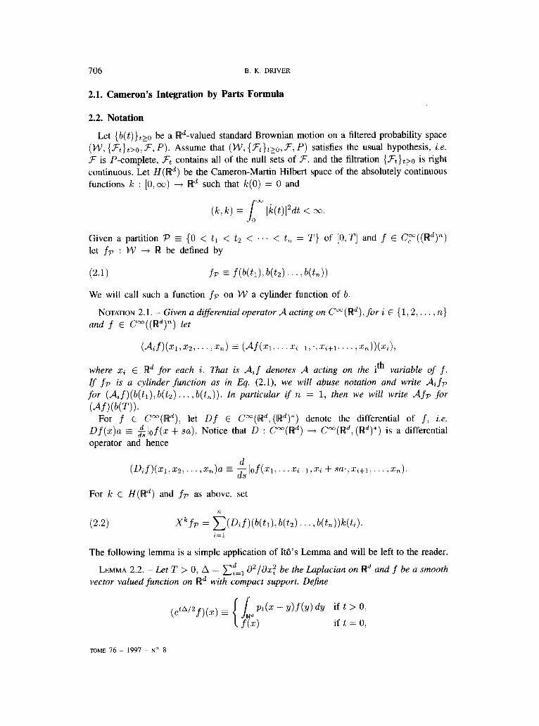
2.2. Notation

Let {b(t)}tzo be a @-valued standard Brownian motion on a filtered probability space (W, {Ft}tk~, F’, P). Assume that (W, {.Tt)t~o, F, P) satisfies the usual hypothesis, i.e. F is P-complete, Ft contains all of the null sets of .T, and the filtration {Ft}t20 is right continuous. Let H(Rd) be the Cameron-Martin Hilbert space of the absolutely continuous functions k : [0, oo) + Rd such that k(0) = 0 and

Given a partition P s (0 < tl < t2 < . . . < t,, = T} of [0, T] and f E Cy ( (R’)‘L) let fp : W --+ W be defined by

We will call such a function fp on W a cylinder function of b.

NOTATION 2.1. - Given a differentiaz operator A acting on C”(W”), for i E { 1,2, . . . , rb} and f E CW((Rd)n) let

(W(a,Z2,... rx,) = (df(xl,...xi-l:.rxi+l!...,x,))(xi)!

where xi E Wd for each i. That is dif denotes A acting on the 1 ‘th variable of f. I” fp is a cylinder function as in Eq. (2.1), we will abuse notation and write Aifp for (Af)(b(h), b(h) . . . , b(t,)). In particzdar if n = 1, then we will write dfp for

Vf)(b(TW For f E Cm(Wd), let Df E C”(Rd, (Wd)*) denote the differential of f, i.e.

of( E &lof(z + su). Notice that D : Cm(Rd) + C”(Rd,(Rd)*) is a differential operator and hence

d (Dif)(X1,52,. . . ,X,)U E -ll)f(Xl,~. .Xi-ljXi + SU’,Xi+l,. . TX,).

ds

For k E H(Wd) and fp as above, set

(2.2) Xkfp = $J(Dif)(b(tl)> b(b) . . .> b(h))k(G). r=l

The following lemma is a simple application of ItB’s Lemma and will be left to the reader.

LEMMA 2.2. - Let T > 0, A = ~~=, a’/axq be the Laplacian on Rd and f be a smooth vector valued function on Rd with compact support. Dejine

if t > 0,

if t = 0,

TOME 76 - 1997 - No 8

INTEGRATION BY PARTS FOR HEAT KERNELMEASURES 707

andfor all t E [O,T], Nt z (e(‘-“)“l”f)(b(t)) and

W, E (De(T-“)A’“f)(b(t)) = (e(T-“)A’“Df)(b(t)).

(Here p&) = (27rt)-d/2 exp( -Izl”/2t) is the convolution heat kernel on Rd.) Then Nt and W, are L2-martingales for t E [0, T] and dN, = Wtdb(t).

The following theorem is well known, see Cameron [5]. In order to illustrate the methods to be used in the next section we will not give Cameron’s original proof which is based on the Cameron-Martin theorem but instead give a (harder) “stochastic calculus” proof.

THEOREM 2.3. - Let k E If(@) and fp b e a cylinder function as in Eq. (2.1), then

(2.3)

Moreover, if fp and yp are two cylinder functions,

(2.4) EKX%)gpl = E f [ p(-X’gi.+~T(k:,db)gp)].

Proof. - Let us first notice that Eq. (2.4) is a consequence of Eq. (2.3) with fp replaced by fpgp = (fg)p and the product rule, X’(fpgp) = (Xkfp)gp + fp(XkgP). Therefore we need only consider the proof of Eq. (2.3). Since the proof here is to illustrate the ideas to come, let us only prove Eq. (2.3) for partitions of the form P = (0 < T} and 7’ = (0 < u < T}.

Case 1. - Suppose f E Cp(Rd), fp = f( b(T)), and Nt and W, are defined as in Lemma 2.2. Then X’fp = Df(b(T))k(T) = WTk(T), so that

T

(2.5) EIXlcfp] = E[WTk(T)] = E {dWk + Wdk} ] = E [lT W&(t) dt] >

wherein the last equality we used the fact that W is an L2-martingale and k is bounded on [0, T]. Using the L2-isometry property of the It8 integral and Lemma 2.2,

(2.6) E[iT W&(&j = E[lTWdblT(IE;db)]

= E[(NT - No)iT(“&)]= E[ir~T(~,db~]~

since NO = Efp is a constant and NT = f p. Combining Eq. (2.5) and (2.6) proves Eq. (2.3) in the case that P = (0 < T}.

Case 2. - Suppose P = (0 < u < T}, f E Cc((W”)“), and fp = f(b(u), b(T)). Now let

fT(t, 2, y) e ev f(GY) z .I,d P(T-t)(~ - z)f(z> z)dz,

Nt = fr(t, b(u), b(t)) for all t E [u, T]

JOURNAL DE MATHeMATIQUES PURES ET APPLIQUfiES

708 B. K. DRIVER

and Wt E D2fr(tr6(~~),b(l;)), h w ere O2 denote the differential of fr (t, x, y) in the y-variable. Again a short computation with ho’s lemma shows that W, and N+ are L2-martingales for t E [u,T] and that dN+ = W,&(t).

Now

so that

X”f7-J = hf(q?l,), wq)&) + D2f(b(7j), W))W) = Dlf(b(U), b(T))k:(u) + WyvqT),

E[Pfp] = E[Dlf(b(lL). b(T))k(u) + WTk(T)]

= E[&f(b(u).b(T))k(u)] + E W k( ) + [ I!. ?I. ~i(dwi:+ Mm)]

= EIDlfT(u. h(u). b(u))k(u)] + E W k( ) + [ (, > 11 /Irw+n(i)di].

wherein we have used the fact the W, is L2-martingale and the Markov property to show EIDlf(b(u), b(T))k(u)] = EIDlfT(u, b(u), b(u))k(u)]. As in Eq. (2.6),

Since W,,~(U) = Dzfr(u, b(~), b(u))k(u), combining the two above displayed equations gives: (2.7)

E[XkfF] = E[D&+, b(u), b(u))k(u) + Dzf~(u, b(u). b(us))k:(u)] + E fs [ p@w.

Letting f E fr(~, b(u), b(u.)) and noting that

xkf = DlfT(U, b(u): h(u))k:(u) + D2f7416, b(U)), h(?L))k(U),

Eq. (2.7) may be written as

(2.8) E[X”f?] = E[X”f] + E f. [ FIf,i(i-.W],

By case 1) already proved,

(2.9) E[X”f] = E [j I”(& r(h)] = E [f&u> b(v), b(u)) I”‘(& dh)]

= E[f(b(,fL),h(l.)) p:+ E[f? &dh)].

wherein the third inequality we have used the Markov property of b. Combining equations (2.8) and (2.9) gives (2.3). The general case can be proved similarly using induction on the number of partition points in P. Q.E.D.

TOME76- 1997-No8


2.3. Heat Kernel Integration by Parts

Let Y : R” -+ Wd be a smooth vector field on Rd and V . Y be its divergence. Assume for simplicity that Y has compact support. A simple integration by parts shows that

/ (V . Y)(Z)PT(Z) dx = - / Dp7+)Y(x) dn: = + ld p,(~)(Y(L+L~) dx 1 R” w

or equivalently that,

In Section 4 we will derive an analogous formula in the case where Rd is replaced by a compact manifold M. In order to illustrate the proofs that will be given in section 4, I will give two alternate (harder) proofs of Eq. (2.10).

First Alternative Proof of Equation (2.10). - Choose an orthonormal basis S for Wd and for c E S set h,(t) = $c, XF = Xt’ = h,(t), and

2; E /

t(h,l dbj = f(c: b(i)), v’t E [O, co). -0

Let 1 denote the constant cylinder function “one” of the Brownian motion h. Since X’l = 0.

0 = c Jww(x~, Jv~~)N = c Jww*(X;, wGw1 CES CGS

= c q-xc + 4(G Y(V)))1 CES

= c E[-X”(c, Y(b(T)))] + $E(Y(b(T), b(T)): c6S

wherein the second equality we have used Eq. (2.4). This proves Eq. (2.10), since after unwinding the definitions we have that

c XC(c, W(T))) = (V . Y)(W)). CES

Q.E.D.

Second Alternative Proof of Equation (2.10). - For t E [0, T], set

K(x) = (eVAY)(x) = J’ pp-q(x - y)Y(y)dy Wd

JOURNAL DE MATHtiMATlQUES PURE.7 ET APPLIQ&ES

710 ES. K. DRIVER

and

(2.11) Qt = t(V . Y,)(W)) - (b(t)? K(b(t))).

Using i3Y,/i3t = -iAx, iJ(V . Y,)/at = -$A(V &) (I), and Ito’s lemma, we hnd

dQt = (V . Y,)(w))dt + Wd,(,)V . Y&b(t)) - (db(t).Y,(b(t))) - ((d db(t)Yt)(b(t)). b(t)) - @b(t). (&,(,)Y,)(b(t)))

= wdb(t)v . Y,)(b(t)) - (W). Y,(W)) - ((4fb(*)K)(b(t))> b(t)).

Therefore, Qt is an L”-martingale and in particular EQT = EQ,. This proves Eq. (2. IO), since QT = T(V Y)(B(T)) - h(T) Y(b(T)) while Q. = 0. Q.E.D.

3. Integration by Parts for “Curved” Wiener Space

3.1. Differential Geometric Preliminaries

Let (Md,(.;),V.o) b e g’ tven, where M is a compact connected manifold (without boundary) of dimension d, (.. .) is a Riemannian metric on M, V is a (.. .)-compatible covariant derivative, and o is a fixed base point in M. Let T = TG and R = Rr. denote the torsion and curvature of V respectively. So

and T(X,Y) s VeyY - VI-X - [X-Y]

for all smooth vector fields X. Y, and Z on M.

Standing Assumption: The covariant derivative (V) is assumed to be Torsion Skew Symmetric or TSS for short. That is to say (T(X;Y). Y) E 0 for all vector fields X and Y on M.

The Laplacian (A) with respect to (V) is the second order differential operator acting on the smooth functions f E C”(M) g iven by Af 3 trVdf z C:4,{EiEif - df (VEtEi)}, where {Ei}rzL=l is a local orthonormal frame. We recall from Driver [6] that this Laplacian is the same as the Levi-Civita Laplacian due to the TSS condition on (V).

For ~TL E M, let O,,,(M) denote the collection of linear isometries of T,M to T,,,M. O(M) = UmEnlM, and 7r : O(M) + M denote the projection map, -/r(O,,(M)) = {n%} for all m E M. The principal bundle 7r : O(M) + M is a convenient representation for the orthogonal frame bundle over M. The structure group of this bundle is the group O(T,M) of isometries of T,M. Let so(T,M) be the Lie algebra of O(TOM) consisting of skew-symmetric linear transformations on T,M.

(‘) We have used the fact that the Laplacian and the divergence operator commute on R”. For general Riemannian manifolds this is not the case. It is at this point that the geometry enters into the argument.

TOME 76 - 1997 ~ No 8

INTEGRATION BY PARTS FORHEATKERNEL MEASURES 711

Given smooth paths u in O(M) and c in M such that U(S) E O,(,)(M), let V,u(s)/ds : T,M -+ T,(,) M denote the linear operator defined by (VU(S)/&)U = V(u(s)a)/ds for all a E T,M. Notice that V(s) E u( ) s a is a vector field along a so that VV(s)/ds = V(u(s)a)/ds makes sense.

DEFINITION 3.1 (Canonical l-form). - Let 0 be the T,M-valued l-form on O(M) given by 19(l) E (7r(<))-ln*<. In particular, if s -+ u(s) E O(M) is a smooth path and c(s) = T(u(s)) then e(u’(s)) = G(S)-‘a’(s).

DEFINITION 3.2 (Connection l-form). - Let w be the so(T,M)-valued connection Z-form on O(M) given by w(u’(0)) z U(O)-lV~(s)/ds\,=a, where s --+ u(s) is any smooth curve in O(M). Notice that a path u is parallel or horizontal in O(M) ijffw(u’) E 0.

DEFINITION 3.3 (Horizontal Vector Fields). - For a E T,M and u E O(M) let B,(u) E T,O(M) be dejined by w(BLL(u)) = 0 ( i.e. B,(u) is horizontal) and 7r*BL1(u) = uu.

Let S be an orthonormal basis for T,M. Let C denote the flat or Bochner Laplacian on O(M), C - CcES Bz. A key fact about the Bochner Laplacian is that for all f E C==(M), C(f o 7r) = (Af) o x.

Given a complete vector field 2 on a manifold Q, let et2 denote the flow of 2. So for each t E Iw, etz : Q --t Q is diffeomorphism and if g(t) = et’(q) for some 9 E Q, then da(t)/& = Z(cr(t)) with a(0) = y.

NOTATION 3.4. - For n, b E T,M and an isometty u : T,M * T,M (i.e. u E O,(M)), define

&&,b) G u -lRV(uu, ub)u E so(T,M),

Ric,u z c flU(u, c)c CES

O&z> b) E u -lTv(uu,ub) E T&t

and %JL - a&, c)),

CES

where

(&@),(u, c) = 1) %+)(a, c). 0

So R, Ric , and 0 are the equi-invariant forms of the curvature tensor, the Ricci tensor, and the torsion tensor respectively. Similarly, 6, is the equi-invariant form of a contraction of VT”. It is well known that the Ricci tensor, Ric , is symmetric if V is the Levi-Civita covariant derivative on M, i.e. TV E 0. More generally we have the following lemma.

LEMMA 3.5. - Suppose that V is torsion skew symmetric, then

(3.1) RicZ = Ric,+G,.

Proof - By Theorem 9.4 of [8] for any u,b,c E T,M,

(3.2) (R(b,u)c,b) - (R(b,c)u, b) - (B@(u,c),b) = 0.

JOURNAL DE MATHBMATIQUES PURES ET APPLlQLJkES

712 B. K. DRIVER

Using fl(11, a) = -!A(a, b), (O(u! c), b) = -(@(CL, c), 0)) (since V is TSS), and the fact that R,,(n,b) E so(T,M), Eq. (3.2) may be written as,

(O(a, b)b, c) - (qc. b)h, a) + (R&3(n, b)> r) = 0.

Summing the above equation over h E S yields.

(Ric CL, c) - (Ric c, CL) + (&L, c) = 0

from which Eq. (3.1) follows. Q.E.D.

3.2. The Basic Processes

NOTATION 3.6. - Given a (vector valued) semi-martingale X, ?IX will denote the Strutonovich differential of X while dX will denote the Itii differential of X.

Let (W, {Ft}t>0, F’, P) be a filtered probability space satisfying the usual hypothesis, i.e. F is P-complete, 3t contains all of the null sets of 3, and the filtration {3+}t2~j is right continuous. We also assume that there are three adapted continuous processes {G}tz~), {//t}t2~, and {b(t)}+20 on (W, {3t}t>0,3. P) with v&es in M, O(M), and

T,M respectively such that C is a M-valued Brownian motion, // is parallel translation along C, and b(t) is the “undevelopment” of C. To be more precise, we are assuming:

1. Co = o and C is a diffusion process on M with generator iA, i.e. for all f E C”(M),

is a martingale. 2. //O = IT&, r o /lt = C, for all t 2 0, and .I;:w(/~//~) is the zero process. 3. 11 is an TOM-valued Brownian motion,

(3.3)

and /lt solves the Stratonovich stochastic differential equation,

where b,(t) z (b(t),c). The fact that such processes exist is well known by the works of Eells and Elworthy and

Malliavin, see for example Elworthy 1131, Kunita [Ku], Malliavin [MO, Ml], Emery [ 161, Theorem 3.3, p. 297 in [7], and also [9]. For later purposes, recall that a process satisfying item 2 above is called stochastic parallel translation along C and that stochastic parallel translation exists uniquely along any M-valued semi-martingale C.

Now let W(M) denote the space of continuous paths (T : [O, CG) --+ M such that ~(0) = o and H(T,M) be the Cameron-Martin space:

TOME~~-1997-N’ 8


Given Ic in the Cameron-Martin space H(T,AJ), let X” denote the Cameron-Martin vector field given by X,” = /ltlc(t). (Notice that {Xf} tko is a TM-valued process on W.) It was shown in [D5]: if W = W(M), C is the canonical process (i.e. &(a) = g(t) for t E [O,oo) and a E W(M)), P is Wiener measure on W(M) and Ic is Cl, then Xk may be considered as a vector field on W(M) which generates a quasi-invariant flow. This theorem was extended by Hsu [21, 221 to include all Ic E H(TOM). Also see Norris [33], Enchev and Stroock [17], and Lyons and Qian [29] for other approaches.

It was also shown in [7] (where X” was written as &), Theorem 9.1, p. 363 , that X” may be viewed as a densely defined closed operator on L’(W(n/l), P). This last result relies on an integration by parts formula which in the special case of X” acting on functions of the form S(c) = F(a(t)) is due to Bismut [4]. There have been numerous proofs and extensions of integration by parts formulas on W(M), see for example [ 1, 2, 8, 15, 18, 19, 20, 27, 28, 30, 31, 331 and the references therein for some of the more recent articles. In the next subsection, we will give an alternate proof of this integration by parts formula. The method to be used here has also been discussed by Elton Hsu [24]. My motivation for developing this method stems from its application to the situation where M is replaced by an (infinite dimensional) loop group, see Driver [lo].

3.3. Another Integration by Parts Argument

NOTATION 3.7. - Suppose that k E H(T,M) is given, let

where

(3.6)

n NOTATION 3.8. - To each A E C”(O(M) --f so(T,M)), let A denote the vertical vector

field on 0( A4) dejined by

@F)(u) s $1 F(u&“)) 0

for all F E Cw(O(M)). An important special case is when A E so(T,M) is a constant function.

DEFINITION 3.9 (Cylinder Function). - Given T > 0, a partition P - (0 < tl < tz < ... < t,, = T} of [O,T], and F E C”( O(M)“) let Fp denote the function on W dejined by,

(3.8) FF = W/t, > lltz . . . > //t,t 1

Anyfunction FF of the form given in Eq. (3.8) will be called a cylinder function of parallel translation or more simply a cylinder function of //. When given a cylinder function f of // which may be written in the form FF, we will say that f is based on P and the degree of f is less than or equal to n.

JOURNAL DE MATHBMATIQUES PURES ET APPLlQUkES

714 B. K. DRIVER

NOTATION 3.10. - Given a differential operator A acting on C”(O(M)), for % E {1,2,. . ,n} and F E C-(0(M)“) let

(AiF) ( ~l,wz,.. .1 *au,,) 3 (dF(u,, . . %I,,-~> ., u~+~, . . . , U,))(U),

where Ui E O(M) f or each i. That is AiF denotes A acting on the i-th variable of F. Zf FF is a cylinder function as in Eq. (3.8), we will abuse notation and write d;FF for (diF)(//tl, /lt2 . . , /lt,). In particular ifn, = 1. then dFF = (dF)(//T).

Let D : C”(0(M)) --) C”(O(AI) + (T,fV$so(5!‘,M))*) be the first order differential operator given by

DF(u)(~ + A) = ((B,. + A)F)(u).

Hence by the above notation, D;F? : W + (TJ4 $ so(TJU))* is defined by:

(3.9) D&a = g W/t,, . 1 l/t,-, , Pa C//t, 1, //L+], . . l/t,, ) and ’ 0

(3.10) QFPA = $1 W/t, 3 ’ . . l/t,-, , llt,~~? l/t,+1 3 . . . > l/t, ), 0

where a E T,M and A E so(TOM).

DEFINITION 3.11. - Given k in the Cameron-Martin space H (T, M) , let X” denote the Cameron-Martin vector field on W(M) given by X,” = /l&(t). We let XL act on the cylinder function Fp given in (3.8) via

(3.11) i=l

To motivate this definition, suppose for the moment that W = W(M) and P is Wiener measure on W. Recall that XL should be thought of as a vector field on W(M). Noting that parallel translation // t is an almost everywhere defined function from W to O(M), it makes sense to try to compute the differential (/lt)*Xk of //t in the direction determined by the vector field X”. The result is

(3.12) (//t)*x” = Bk(t)(//t) - @(//t).

see Theorem 2.2 on p. 282 of [7] for a proof of (3.12) for smooth paths and the proof of Theorem 5.1 on p. 320 of [7] for the stochastic version. So if F E C”(O(M)):

(3.13) XkWId) = W&X”)F = (DF)(IIT)(J~T) - ~$1.

Clearly, Eq. (3.11) is the natural generalization of Eq. (3.13) to cylinder functions of // of degree greater than one.

The main result of this section is the following integration by parts theorem (see Theorem 9.1 in [7]) which will be proved at the end of this section.

TOME 76 - 1997 - No 8

INTEGRATION BY PARTS FOR HEAT KERNEL MEASURES 71.5

THEOREM 3.12. - Let k E H(T,M) and Fp be a cylinderfinction of //, as in Eq. (3.8), then

(3.14) E[X”FrJ = E[zrF&

where

(3.15) zt - I’( { k:(r) + ~Ric~,7k(r)},dh(r)). . 0

Let & be the a-subalgebra of .Fr which is the completion of the a-algebra generated by {//t}tEIO,T1. Note that one would get the same a-algebras if /lt was replaced by b(t) or Ct above.

COROLLARY 3.13. - For each T > 0 and k E H(T,M), X” may be considered to be a densely defined closable operator on L2(W, GT, I’) with domain V(Xk) consisting of the cylinderfunctions based on [0, T]. Moreover, -Xk’ + ZT C (X”)“, where (X”)” denotes the L’(W, &-, I’)-adjoint of X”.

Proof. - Let FF and Gp be two cylinder functions of //. Upon noting that X’(FPGp) = (XkFp)Gp + FFXkGp, Theorem 3.12 with F? replaced by (F?GT) implies

(3.16) E[(XkFF)Gp] = E[F?(-X” + zT)Gp].

Suppose that FF and H p, are two cylinder functions based on [0, T] (P’ is possibly another partition of [0, T]) such that FF = HFf a.e. Let P be any partition of [O. T] such that P U P’ c P and G+ be any cylinder function of // based on 9. Then by Eq. (3.16) with FP replaced by FJJ - HFl and Gp replaced by G,,

(3.17) E[(X”FF - XkHp,)G,] = E[(F~J - HF,)(-Xk + z~)G.~] = 0.

Since (X”F? - XkHF,) is &- measurable and the collection of cylinder functions G, as above are dense in L’(W,&-:I’), it follows that X”FF - XkH,, = 0 a.e. This shows that X” is well defined as an operator on L2( W, &-. P) with domain D(X’). Given this, the assertion that -Xk + zT c (X”)” follows directly from Eq. (3.16). This in turn shows that (X”)” is densely defined which implies that X’” is closable. Q.E.D.

Before beginning the proof of Theorem 3.12, let us recall some facts about the degenerate parabolic partial differential equation,

(3.18) dG(t, u)/i)t = $C(t. l,,) with G(O: .) = F(,),

where F E C-(0(M)). The following theorem is a restatement of Theorem 3.1, p. 259 in Ikeda and Watanabe [25] specialized to the setting of this paper.

THEOREM 3.14. - To each F E C-(0(M)), there is a unique function G E C([O>ca) x O(M)), such that G E C”((0. cc) x O(M)) and G solves Eq. (3.18).

JOURNAL DE MATHEMATIQUES PURES ET APPLlQ&ES

716 B. K. DRIVER

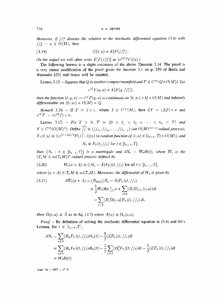
Moreover, if //y d enotes the solution to the stochastic differential equation (3.4) with //;I = u E O(M), then

(3.19) qt. u) = E[F(//,“)].

(In the sequel we will often write E[F(//y)] as (e”c/2F)(zt).) The following lemma is a slight extension of the above Theorem 3.14. The proof is

a very minor modification of the proof given for theorem 3.1 on p. 259 of Ikeda and Watanabe [25] and hence will be omitted.

LEMMA 3.15. - Suppose that Q is another compact manifold and F E C” (Q x O(M)). Let

etLF(q, u) = JW’(CI, //,“>I,

then thefunction (t, q! U) --f et’F(q, U) is c ontinuous on [0, m) x Q x O(M) and infinitely differentiable on (0, KJ) x O(M) x Q.

Remark 3.16. - If F = f o 7r. where f E C”(M), then LF = (Af) o 7r and etLF = (etAf) o r.

LEMMA 3.17. - Fix T > 0, P = (0 < tl < t2 < . .. < t,, = T} and

F E C-(O(M)n). Dejine 2 2 (//r,. /lt2,. . . , //t,,-l) (an O(M)(“-I)-valued process),

FT(t! ?L) - ((e(‘-“)‘/“F(z, .))(u) ( a random function of (t, U) E [&- 1, T] x 0 (M)) ) and

N+ SE FT(t,/lt) for t E [tlL--l,T],

then {N, : t E [&-I, T]} . ts a martingale and dN, = W,db(t), where Wt is the (T,M @ so(T,M))* -valued process dejned by

(3.20) Wt(a + A) = ((B, + a)FT)(t, /lt) for all t E [t+-l, T].

where (a + A) E T, M $ so( T, M) . Moreover, the differential of W, is given by

(3.21) dWt(u + A) = (&&L + -b%)(t, l/t)

+ iWt(Rici,ta + x(K-fl),,, (c! u))dt CES

- ~(B,$(c. u)FT)(t, //t) dt. L-ES

Here fi(c,u) G A as in Eq. (3.7) where A(u) G &(~!a).

Proof. - By definition of solving the stochastic differential equation in (3.4) and M’s Lemma, for t E [tnel,T],

dNt = ~(BaF,)@, l/t)~b,(t) - ;(LFT)(t: //,)dt aES

= ~(&FT)(t, //t)db&) + ; x(&%)(4 /l&t - &W(t; /l&t aES QES

= W,db(t).

TOME 76 - 1997 - No 8


A similar computation shows that

(3.22) dWt(a + A) = ~(B,(&x + &%)(t, //t)db,. C-ES

Using the commutator formulas in Lemma 7.3 of the Appendix, Eq. (3.22) may be expressed as

dWt(a + A) = I(&(& + @‘d(t, //t)& CES

+ i ~({-%fi(C,a) -t&c*, + (B,ll(C:a)j}F~-l)(lit)dt,

CES

from which Eq. (3.21) follows. Q.E.D. The following corollary is a special case of the above lemma.

COROLLARY 3.18. - Let P = (0 < T}, Fp = f&) = F(//T), where f E C-(M) and F z f o r, DeJine

~~ f @W*l:’ f)(E,) fur aE1 t E [0, T].

Then Nt is a martingale and dN, = W,db(t), w h ere W, is the (TOM)*-valued process dejned by

(3.23) Wta f P//,,e (T-t)A/2f)(Ct) for all t E [0, T].

Moreover, the differential of W, is given by

(3.24) dwta = F’:,tca(t)~,,tae (T-t)A’2f)(Ct) + kW&cjita dt,

where for f E C”(M), V2 f is the tensor jield dejined by

V&f = X(YP) - (Ymf.

Here X and Y are arbitrary vector fields on M.

Proof. - This is a straight forward application of Lemma 3.17 using the following remarks. For F = for, (iiF) = 0, (&F)(u) = V,,f, (B,B,F)(u) = VtaBubf, and etCF = (e”“f) o 7r. Q.E.D.

The proof of Theorem 3.12 is slightly cumbersome. So before proving it, let us practice with the following special case which already contains the main ideas.

THEOREM 3.19. - Let k E H(TOM), f E C-(M), and Fp = f(&), then

(3.25) W~“FPI = E[&%J],

where z is dejned in (3.15).

JOURNAL DE MATHBMATIQUES PURES ET APPLlQU6ES

718 B. K. DRIVER

Proof. - Let

(3.26)

so that

t K(t) = #k(t) + 1

s 2 0 Ric */,T k(7)&,

k(t) = k(t) + :Ric */,, k(t) with K(0) = 0.

Let W, be defined as in Eq. (3.23) and notice that

X”F7, = (&(qF)(//T) = W,k(T)

1 = Wdlc + ZWRic iltkdt +

wherein the last equality we have used Eq. (3.24) of Corollary 3.18. Taking expectations of this identity gives:

(3.27) E[X”F?] = E 1

T

Wdk+ 5WRicT,lkdt = E, o W,K(t)dt. > I

Since NT = No + JOT W,db(t), Eq. (3.27) and the L2-isometry properties of the Ito’s integral implies

I T

E W&t) dt = E 1 0

(lT WtWt), ~i(H.:db))

Q.E.D.

Proof of Theorem 3.12. - Let Fp be a cylinder function of // as in Eq. (3.8)

K(t) be as in Eq. (3.26) W, as in (3.23), and 2 z (/lt,,/ltl,. . ,/It,-,). Since WT(U + A) = (&F + ~F)(//T)

(3.28) EXkb = 2 WW(fl, IIT) - &)I i=l n-l

= ~E[QE'(Tj:/l~)(k.(ti) - AtJ]+WG-@CT)- AT)], i=l

where A, = At as in Notation 3.7.

TOME76- 1997-No8

INTEGRATION BY PARTS FOR HEAT KERNEL MEASURES

Now by M’s Lemma, Eq. (3.26), Len-ma 3.17 and Eq. (3.5),

E[WT(~(T) - Ad] = E[Wt,-, @(L-d - &-,)I + TI + T2 + T3,

where

T1=E T J T

Wd(k - A) = E W L-1 s( L-1 dk - ; c(&O),,t (k(t), c)dt

05s >

J T

T2 3 E dW(k - A) G-1

T

= -E ic V%fk W)UW@, l/t) dt * h-1 &S

+fE .I

T Wt(Ric ilt k(t) + ~(&fl),,, (c, k(t)))dt h-1 CES

and

J T

T3--E dWdA t,-1

(&~FT)(t, //t)(~=~q,,(k(t),c) dt

(@fin>//, (k(t), ‘$bT)@> l/t) dt

(Wt((&W//, (W), 4) dt.

Therefore, we obtain

Tl + Tz = E J

’ {W&K - (&9)//t (W&W} t,-1

-E -

(Bcfk +))FT)(t, l/t)&

719

JOURNAL DE MATHBMATIQUES PURES ET APPLlQU6ES

720

and

8. K. DRIVER

.T

Tl + Tz + Ts = E .I WdK f,L 1

where we have used dM = Wdb in the third equality and

and NT = Fp in the last. Hence

-W%@(T) - AT)] = E[W,-, (W-I) - At,,-, ,I + E ( PTdb))

FP

which combined with Eq. (3.28) gives 7-k-l

(3.29) EX”FP = c E[DiF(z, //d(Wi) - Ad] + E[W,~-,(W,-I) - 4-J i=l

The rest of the proof will now proceed by induction on ‘II. The case 12 = 1 follows directly by taking t,-r = 0 in Eq. (3.29).

Now suppose that Eq. (3.14) holds for all cylinder functions Fp of degree n - 1 or less. We wish to show that it holds for a cylinder function of degree n. To simplify notation, let

F(ul,. . . ,u,-~) E (e(T-t~~-‘)~-‘“F)((ul,. . . , u,el, u,,-1))

= E[F(u1,u2,... 1 %-l, //‘(;-,,_,,)I

(see Theorem 3.14 and Lemma 3.15) and Fp denote the cylinder function of // given by

Fp=F(&=( e(T-t~+)r,~2F)(~, l/t,-J.

Notice that n-2

(3.30) xkFp = C(D.ie (T-t”L)Ln/2F)(~, //t,m,)(k(t;) - Atz) i=l

+ (D,,-le(T-t”-‘)L’1’2F)(~? //t,-l)(k(L~) - Atnml)

+ (D,,e(‘-t~‘~‘)~~‘2F)(~, //t,,-l)(k(tn--l) - A,,-,).

TOME 76 - 1997 - No 8


By the Markov property or by Ito’s Lemma, for any i < ‘IZ, (X31)

E[QP.(z, lld(Wi) - AdI = W e(T-f”-‘)~,,/2U1F)(7j, //t,-J(k(ti) - A,,)).

Therefore n-l

n-2

= c q@T-t-- ‘)L7L’2W(z, l/t,-J@(h) - Ad)

i=l

+ )73((ew-‘)w2~ nJ(Tj> l/t,-JWn-I) - At,-,)) + q~,(e(T-t”-‘w2 F)(fi> lltn-1 )@&-I) - 4-l 1).

Using the fact that Di commutes with L, for 1; < n, this last expression combined with Eq. (3.30) and the definition of W, in Eq. (3.20) shows:

n-1

(3.32) c w477, //T)(Wi) - AL)] + JWL, (W-1) - AtJ = E[X”G4 i=l

So by Eq. (3.32) and Eq. (3.29)

(3.33) EXkFp = E[X”&] + E F ( r~n~l~hW).

Applying the induction hypothesis, this gives

EX”Fp = E(~~~..-‘~~,db))+E(Fr~~~-,(Icl.db))

= E(F~~7’-‘(i;db))+E(F~~,~l(li.db))

wherein the second equality we have again used the Markov property to replace F? by FF. Q.E.D.

4. Consequences for Heat Kernel Measures on AI.

The notation of Section 3 will be use in this section as well. Also if Y is a smooth vector field on A&, let V s Y denote the divergence of Y i.e.

(4.1) (V . Y)(m) 2 trVY = $(VE,Y, E;), i=l

where {Ei}$=, is any orthonormal basis for T,,M.

JOURNAL DE MATH6MATIQUES PURES ET APPLIQU6ES

722 B. K. DRIVER

THEOREM 4.1. - Let T > 0 and 1 E H(W) such that l(T) = 1. Then for all smooth vector jields Y on M; (4.2) E[(V.Y)(CT)] = E[(,,,'Y(C,).ln7(iit)- ;l(t)Ric+t)-; ~h.l’l&)].

where for u E O(M),

(4.3) J, = x(B,Ric (.)c)u = i xRicetn,(U)c CES o&s

_ -1 u C( V,,Ric)uc.

CES

COROLLARY 4.2. - If Y is a smooth vector$eld on M and f E C-(M), then

(4.4)

and

(4.5) E[V . I] = E //TlY(&), y - & /T t(Ric,,,db(t) + ~,,;dt))] 0

Proof. - Because V 9 (fY) = Yf + fV . Y, Eq. (4.4) follows by replacing Y by fY in Eq. (4.2). Taking l(t) E t/T in Eq. (4.2) proves Eq. (4.5). Q.E.D.

First proof of Theorem 4.1. - This proof is modeled on the first proof of Theorem 2.3. Choose an orthonormal basis S for T,M and for c E S set h,(t) = 1 (t)c and Xi f X,“c E //,h,(t) for t E [0,x1). Th en using the integration by parts Theorem 3.19,

0 = c E(x”l)(X;, Y(G)) = 1 qX”)*(X;,Y(CT))] CES 4s

= c E[(-X” + z;)( x;, Y(C,))] =: E(-I + II), CES

where

I- ~xc(x;.,Y(&)) and II z ~z$(X;,Y(&-)), CES CES

TOME76-1997-N’s


and

T W) = J ([ 2Ric ilt + i(t) c, db@) 0 1 >

T 1 I ([ TRic,;, + i(t) . 0

Notice that g E (X;,Y(&)) = F(/IT), where F(u) = (c,c’Y(TI-(IA))). Hence 9 = (x;,mT)) is a cylinder function of // as defined in Section 3 and moreover by Eq. (3.1 l),

(4.6) X”g = DF(//T)(-A$ + h,(T)). Note

(4.7) DF(u)A = f 1 (c, eCAupl Y@(u))) = -(c,Au-‘Y@(u))), QA E so(T,M) 0

and

(4.8) DF(u)a = (c, u-l &Y) = (UC, VuaY) QA E TX.

Using equations (4.6-4.8) and Eq. (3.59,

I= ~{(//TC,v//,.cY) + (CP+//,~Y(~T))) CES

(J T

= (v ' y)(k) + @Pic//,W), //TIJ'(C~) 0 >

= (v ’ y)(cT) + 0

I(t)Ric,,,db(t) + i J T

~(t)J//,& //;ly(cT) > 0 >

where we have used (I

T

(4.9) Ric ,,t t%(t) = Ric ,,t db(t) + i x(B,Ric ‘:)/It dt CES

1 = Ric ,,,db(t) + 2 J/itdt.

Similarly, we have

11 = c +(//Tc, y(cT)) CES

= Z’C: //~ly(~T)) ( IT [ +iC ,,* + i(t)] db(t), c)

. = yRlC//, + i(t) Wt), //&+y(cT) 1 > .

JOURNAL DE MATHeMATIQUES PURES ET APPLIQ&ES

724 6. K. DRIVER

Combining the above expressions shows

0 = E[-I + II]

1 (1 1.

= E -(V . Y)(C,) + i(t)db(t), //pY(cT) 0

- AE .T

(.I /

T

2 0 l(t)Ric l,,&(t) + W)J,,&, //;ly(&-) .

. 0 >

This finishes the first proof of the Theorem. Q.E.D.

Second proof of Theorem 4.1. - This proof will follow the strategy of the second proof of Eq. (2.10) of Section 2. To simplify notation, we will write dQ+ Z dV, if Q and V are semi-martingales such that Qt - V, is a martingale.

Let F(u) = u- ‘Y(x(u)) and set Y,(u) E (e CT-tWlzyj(,) = cc (T-t)C12Y) (u) . Define

13 Yt s C(Bc.Y*, c) = c B,(Y,, c) f-ES C-ES

and set

By ItB’s Lemma, as in the proof of Lemma 3.17,

@x//t)] = ~(BcY,)(//t)dh(t) = &#t)(//t) I-ES

and

Therefore, we obtain

dQt g i(W . Y,>Wd dt + YirC. W’t)(//t) dt - ((&&X//t), i(t)W)) l(f) = { i(W W//t) + ,([G W’i)(I/t) - ~((BcK)(//t), c)i(t) dt

6s

= F([G B+‘i)(//t) dt

= -y{(V,(//t), J/i,) + C((B,k;)(//,),Ric,,,c))}dt? CES

TOME76- 1997-No8


wherein the last equality we have used the commutator formula in Eq. (7.6) of Corollary 7.4 from the Appendix below.

Unlike the proof of Eq. (2.10), Q, is not a martingale and hence we will have to modify Q. Set N+ G Qt + V, where

Notice that

w dV+ ” -$.J,,, , KC//t)) dt + F(Ric,,,dVt)7 (Qt)K)(//t))

= F(.J,,,, K(//t)) dt + F x(Ric,,,c, (B,Y,)(//,)) dt cts

z -dQ+.

Hence we have shown that dNt = dQt + dV, Z 0; that is N is a martingale. Therefore we conclude that EN, = EN” = 0, since No = &a + V, = 0. Since B. Y = (V . Y) o K, and l(T)(B. %)(/IT) = (B. F)(//T) = (V. Y)(~T),

NT = QT + VT

b(7){eJ//T d7 + Ric /IT db(r)}: Yd//T)

= (v . Y)(&-) - ( ,,;lY(&): IT i(t)db(t)) 0

+; (I

T

l(t){.J//, dt + Ric//, Wt)}, //TIYT(C~) . * 0 >

It is now clear the statement ENT = 0 is equivalent to Eq. (4.2). Q.E.D.

4.1. Backwards Integrals

The “J” term in Eq. (4.2) is somewhat undesirable, since it involves derivatives of the Ricci tensor. This is in contrast with Bismut’s formula which is reviewed in the next section. Before ending this section I would like to point out that by using a “backwards” Ito’s integral, we may eliminate the “.I” term.

Let K = (0 = to < tl < tz < ... < t, -+ co} denote a partition of [0, co), 1~1 = maxi Itl+l - ti(. For r = ti E r, let r+ = t(i+l) be the successor to 7 in 7r. Suppose that V is a finite dimensional vector space, X is a V-valued continuous semi-martingale and A is a End(V)-valued continuous semi-martingale. Then the backwards stochastic integral of A relative to X is

(4.10) .+

.!- AdX z lirn C( A t A -r+)(X(t A (T+)) - X(7 A t)), 0 1~1-0 rev

JOllRNAL DE MATHCMATIQUES PURES ET APPLiQU6ES

726 B. K. DRIVER

where the limit exists in probability uniformly for t in compact subset of that the forward and Stratonovich integrals may be defined similarly as

(4.11)

[O! CG). Recall

and

(4.12) t .I 0

ASX E ,$yk& ;(A(t A T+) + A(~))(x(t A (T+)) - X(7- A t)) 7ET

respectively. We also know that the joint quadratic variation “.I’ dAdX” is given by

(4.13) .I

‘dAdX = ,;ynx(A(t A T+) - A(~))(x(t ri (it)) - x(7 A t)). TEX

It is a trivial exercise to prove that

(4.14)

and

From the computation given for Eq. (4.9) we know that

(4.16) d(Ric l,,)&(t) = .J,,, dt.

Using this equation and Eq. (4.14) we find that Theorem 4.1 may be written as:

COROLLARY 4.3. - Let T > 0 and 1 E H(W) such that l(T) = 1. Then for all smooth vector fields Y on M,

(4.17) E[(O . Y)(C,)] = E [ (//;‘Y&), liT (i(t) - +(t)k;lt) Z(t))].

5. Bismut’s formula

For the sake of comparison and completeness, let us include Bismut’s formula, see Eq. (2.77) in [4]. (Note: Bismut uses 6 for the Ito’s differential and d for the Stratonovich differential.)

THEOREM 5.1 (Bismut). - Let f : M --+ R be a smooth function, then for any 0 < t 5 ‘I’,

t;(e ‘“‘“f)(o) = t-ll3 [ (.I’ Q&b-)) ((-12fi(z,)]

TOME76- 1997-No8


where Qt is the unique solution to the d@erential equation:

(5.1) dQ,/dt = -iQ,Ric;,t with Qo = I.

Proof. - The proof given here is modeled on Remark 6 on p. 84 in Bismut [4] and the proof of Theorem 2.1 in Elworthy and Li [ 141. Also see Norris 1331.

For (t,m) E [O,T] x M let

F(t, m) G (e”-““‘“f)(m).

Also let Qt E End(T,M) be an adapted continuous process to be chosen later. Consider zt E (J;Q,.db(r))F(t,C,). W e wish to compute the differential of zt. First notice that dF(t,C+) = (V ,,,db(t)F(t, .))(C,) and therefore:

dzt = Q,db(t) . F(t, C,) + (l Q&r)) P,,,~~(t)W; NG)

+ c(Qtc. P//J% 3(G)) dt. CES

From this we conclude that:

Qrc(V//,cF(r, .))(G) d7

Q&, //,l$F(r, C,)) dr

Suppose that we can choose Qr such that Q,.//;‘eF(r, C,.) is a martingale and Qo = 1. For such a Q,

.I’

t Ezt = E Qo//ileF(O, Co) dr = t?$?A’2f)(o).

0

That is to say

*(e “““f)(o) = t-lE [ (.I’ Q&(d) (~‘““/2.f)(c,)]

=t-‘E[(~Q~db(r))F(~7)],

wherein the second inequality we have used the Markov property of Ct.

JOURNAL DE MATH’iMATIQUES PURES ET APPLIQUBES

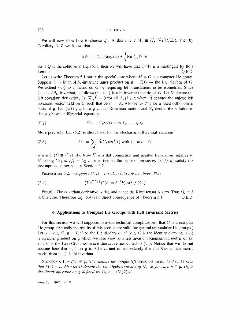
728 B. K. DKlVER

We will now show how to choose C),. To this end let r/ii, = //,lVF(t, C,). Then by Corollary 3.18 we know that

1 clw+ = cl(martingale) + ?RIC i,, lY&.

So if & is the solution to Eq. (5.1), then we will have that C),W, is a martingale by ho’s Lemma. Q.E.D.

Let us write Theorem 5.1 out in the special case where M = G is a compact Lie group. Suppose (., .) is an A&-invariant inner product on g = T,G - the Lie algebra of G. We extend (., .) to a metric on G by requiring left translations to be isometries. Since (.. .) is A&-invariant, it follows that (.> .) is a bi-invariant metric on G. Let V denote the left covariant derivative, i.e. V;, B = 0 for all A, n E g where A denotes the unique left invariant vector field on G such that a((:) = A. Also let 5’ c g be a fixed orthonormal basis of g. Let {b(t)} t>O be a g-valued Brownian motion and Ct denote the solution to the stochastic differential equation:

(5.2) hII+ = C,hb(t) with Co = (2 E G.

More precisely, Eq. (5.2) is short hand for the stochastic differential equation

(x3)

where b”(t) - (b(t),A). N ow V is a flat connection and parallel translation (relative to V) along C(.) is /lt = LX,,. In particular, the triple of processes (C, //. b) satisfy the assumptions described in Section 3.2.

PROPOSITION 5.2. - S~qyose (G. (.. .). C, C, //. 6) ore as above. Then

(5.4) (f,,TW f)(c) = t-lE,[b(t)f(xT)]

Proof. - The covariant derivative is flat, and hence the Ricci tensor is zero. Thus CJ, = I in this case. Therefore Eq. (5.4) is a direct consequence of Theorem 5.1. Q.E.D.

6. Applications to Compact Lie Groups with Left Invariant Metrics

For this section we will suppose, to avoid technical complications, that G is a compact Lie group. (Actually the results of this section are valid for general unimodular Lie groups.) Let o = e E G, g = T,G be the Lie algebra of G (f$ E G is the identity element), (.> .) is an inner product on g which we also view as a left invariant Riemannian metric on G, and V is the Levi-Civita covariant derivative associated to (., .). Notice that we do not assume here that (., .) on g is Ad-invariant or equivalently that the Riemannian metric made from (., .) is bi-invariant.

NOTATION 6.1. - (f h, E g. let h denote the unique left invariant vector,field on G such that g,(e) = h. Also let D denote the Lie algebrcl version of 0. i.e. ,filr each h E g, Dh is the linear operator on g defined by II,, X: E (Vi, k:)(e).

TOME76- 1997-N’??


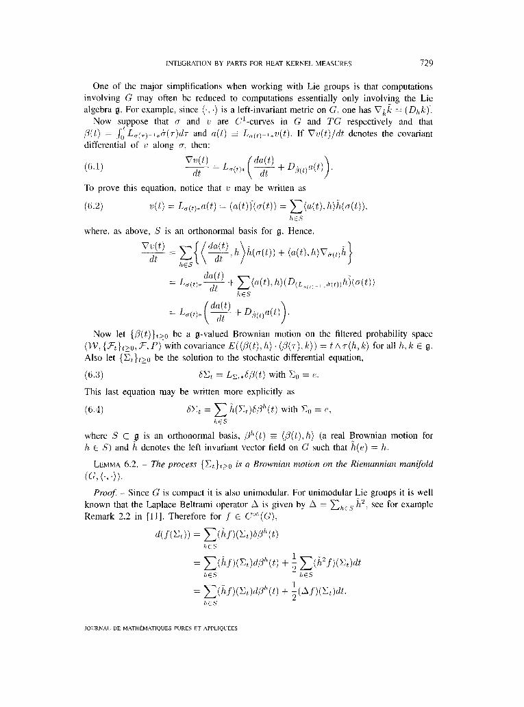
One of the major simplifications when working with Lie groups is that computations involving G may often be reduced to computations essentially only involving the Lie algebra g. For example, since (., .) is a left-invariant metric on G, one has Oil = (Dhlc j.

Now suppose that (7 and u are Cl-curves in G and TG respectively and that P(t) = .I;:Lflc,,-l.6(r)d~ and cl(t) 3 L rr(t)mi*v(t). If VU(~)/& denotes the covariant differential of ‘11 along c, then:

(6.1)

To prove this equation, notice that 0 may be written as

(6.2) u(t) = Lrr(t)*a(t) = (a@)j(@)) = C(n(t), h)k(u(t)), 11 ES

where, as above, S is an orthonormal basis for g. Hence,

hES

= -L(t)* dn(t)

( ’ dt + q(f)“(t)

Now let {B(t)} t20 be a g-valued Brownian motion on the filtered probability space (W, {.%~O, 3, P) with covariance E((P(i), h) . (P(r), k)) = t A r(h, k) for all h, k: E g. Ah let {G}t,~ be the solution to the stochastic differential equation,

(6.3) bC, = Lx,*6[j(t) with Co = e

This last equation may be written more explicitly as

(6.4)

where S c _B is an orthonormal basis, ,0’“(t) E (ii)(t), h) (a real Brownian motion for r%. E S) and h denotes the left invariant vector field on G such that h(e) = II.

LEMMA 6.2. - The process {Ct}lzo is a Browniun motion on the Riemannian manifold (C, (., .)).

Proof. - Since G is compact it is also unimodular. For unimodular Lie groups it is well known that the Laplace Beltrami operator A is given by A = CILES jL2, see for example Remark 2.2 in [ll]. Therefore for f E C”(G).

W(G)) = ~hf)(W~/J’L(f) hES

= x(jLf)(C&jjA(t) + f x(h’f)(C,)dt h ES h E s

= ~(jlf)(E,)d/+(t) + ;(A.f)(Et)dt. 11 ES

JOiJRNAL DE MATHBMATIQUES PURES ET APPLlQUdES

730 B. K. DRIVER

which shows that C satisfies the martingale characterization of a Brownian motion, see Section 3.2. Q.E.D.

Continuing the notation of Section 3.2, let // denote stochastic parallel translation (for the Levi-Civita covariant derivative V) along C and h be the g-valued Brownian motion defined in Eq. (3.3). In the next theorem we will give a more concrete description of the processes // and b.

THEOREM 6.3. - Let /j, C, //. and b be the processes described above and set

(6.5) U(f) E Lqt)-l*//t.

Then U(t) is the O(g)-valued adapted and continuous process satisfying the stochastic differential equation

(6.6) dU(f) + Dh:,(t~Ci(l;) = 0 with U(0) = I,,

(6.7)

and also

(6.8)

.t b(t) z I u(T)yf5p(T).

* I)

I

.t l,(f) = u(T)ydp(T).

. 0 Proof. - The proof of Eq. (6.7) is easy:

Ml(f) = //,‘oc* = //,‘L,+*Sg(t) = u(t)-‘rig(t).

We now will show that Eq. (6.6) holds. Define F : O(G) + O(g) by F(p) s L,(,)m~,p, where x : O(G) + G is the fiber projection map. (Recall that O(G) = USE~Og(G) and O,(G) is the set of isometries from g = T,,G to TqG.) Since U(f) = F(//+), in order to find the equation satisfied by U(t) we will need the horizontal derivative of F.

CLAIM. - For h E JJ, let B3h be the associated horizontal vector field on O(G) defined in Definition 3.3. Then (BhF)(p) = -DT,~,,,, , ,llhF(l~).

To prove this claim let y(t) b e a curve in G such that 9(O) = X(J)) and 9(O) = ph. Define O(t) E O(g) to be the solution the ordinary differential equation

(6.9) do(t)/& + D,,(+,O(f) = 0 with O(0) = L,g(o)m~ +y.

where o(t) = L ,(t,-l*9(t) E 8. (Notice that (w(O) = L T(pj ~,ph.) Let p(.) be the curve in O(G) defined by p(t) = L,ct)* O(t) E O(G). By Eq. (6.1), Or)(t)/& = 0 sop is horizontal. Also we have p(O) = p, and r,$(O) = g(O) = ;r,h and hence 6(O) = L3h (11). Therefore:

= g o(t) = -D,,,,O(O) ’ 0

= -DI, ,,,,,-,.PhFW

TOME76-1997-No8


This proves the claim. Because of the claim, we now know that

which in view of Eq. (6.7) proves Eq. (6.6). To complete the proof we need only verify Eq. (6.8). Now

(6.10) .t t

b(t) = I

U(t)-%[qt) = I’

u(r)-‘dp(t) + v,. . 0 . 0

where V is the process of bounded variation given by

Using Levy’s criteria, it is easily checked that s,” U(t)-‘d/j(t) is a Brownian motion. But we know a priori that b(t) is also a Brownian motion on 8. In order for these statements to be consistent with Eq. (6.10) is is necessary for V = 0: i.e. Eq. (6.8) is valid. Q.E.D.

As a bi-product of the proof we have shown that

(li.11) c D/,/l = 0. h E s

We could also verify this equation more directly as follows. For k: E g let

then et’ is the flow of i. Because G is compact and hence unimodular, the Riemannian volume form on G which is a left invariant volume form is also a right invariant volume form. Therefore right translation preserve the Riemannian volume form and hence the flow et’ preserves the Riemannian volume form. Consequently, the divergence of i is zero. On the other hand, we may also compute the divergence of ,& using the Levi-Civita covariant derivative V via,

(13.12) V .k: = trvi = C(V,i,i) = C(D&,h) = - C(k,D,,h), hES hE.S hES

wherein the last equality we have used the metric compatibility of V to conclude that 111, is skew adjoint on 8. Since, as already noted, V . ,& = 0 for all k: E g, Eq. (6.11) follows from Eq. (6.12).

JOURNAL DE MATHriMATlQUES PURES ET APPLIQUBES

732 B. K. DRIVER

We now wish to write down Theorem 4.1 in the context of this section.

COROLLARY 6.4. - Let (G, (.. .), 0) b e as above. Also let f E C”(G). h E g, T > 0. and 1 E H(R) such that l(T) = 1, then

where Ric. is the Ricci tensor restricted to g = T,G and .J is dgjined in Eq. (4.3).

Proof. - Applying Theorem 4.1 with Y = f h, using the fact that V. ( fi,) = hf’+.fC .ib = i&f, shows that

(6.14) EK&~‘PT)I = E f(&)//;'k(&), l!(t) - il(t)Ric,,

Since (., .) is left invariant, it follows that Ric and VRic are also left invariant, i.e. L,;:Ric L,, = Ric and L$ (V L,+lrRic)Lg,k = (VhRic)k for all 9 E G, therefore,

Ric,,, = RicLX,wU(t) = UP1(t)RicLc,,U(t) = V’(t)Ric,,li(t),

and fJ/,, = J~x:,,u(t) = C(LC,.u(t))-l(VL,,.I’(t)hRic)LC,*U(t)h

he.5

= c U-l(t)(b(t)h Ric)U(t)h = U-‘(t)<J,,. !&ES

Also notice that

//$i&) = li’jT)L,;$h(&) = Ii-‘(T)h.

Using these last three equalities and Eq. (6.8) in Eq. (6.14), one finds that:

E[(kf)(&)l = E [fCW( i;‘jl.)h.~T( i(t) - ACT:-‘(t)Ric.,li(ij)rr’(tj,l:i(r))]

- i~[([ili~)h.[ ~p(t)'./,dt)].

from which Eq. (6.13) clearly follows. Q.E.D.

COROLLARY 6.5. - Let (G, (...),V), f E C”(G), h E g. T > 0, and 1 E H(W) such that l(T) = 1 be as in Corollary 6.4. Then

(6.15) E[(jlf)(&)] = E f(C ) U(T)-% [. T ( ..lT’is’(t)(i(t) - ii(i)Rk.,)

(6.16) = E[f(&-) lr(r:(t,T)i,, (i(t) - &t)Ric,)&(ti)]q

TOME 76 - 1997 - No 8


where zj denotes the backwards ItG’s differential and cJ(t. T) G U(t)U(T)-1 for 0 < i’ 5 T.

Remark 6.6. - Notice that the process U(t, T)h is not adapted to the forward filtration. The stochastic integral in Eq. (6.16) is to be interpreted as a limit in probability of Riemann sums of the form in Eq. (4.10) with A(t) = (i(7) - +1(T)Ricz)U(t, T)h and X(t) = p(t). The convergence (in probability uniformly on compact subsets of [O. x)) of these sums follows from the corresponding convergence of the Riemann sums defining the stochastic integral in Eq. (6.15). In fact U(t, T) solves the (non-adapted to the forward filtration) Stratonovich differential equation,

dU(t;T) + Dsqt)U(t,T) = 0 with U(T,T) = lg.

From this it follows that U(t, T) may be chosen to be a(,/-l(r) - /j(T) : t < 7 5 T)- adapted. Hence the backward ItG’s integral is an adapted integral when “run” in reverse time. This fact will be exploited in Section 6 in Driver [IO] where the reader may find more details on this remark.

Proof of Corollary 6.5. - Equation (6.16) follows directly from (6.15) and the proof of Eq. (6.15) is basically the same as the proof of Corollary 4.3. Just apply Eq. (4.14) to Eq. (6.13) using

d(U-‘(t)Ric,)@(t) = (U-‘(t)Dda(t~Ric.)ng(t)

= c U-l(t)(DhRic,)hdt = Upl(t)Jdt hES

and d(U-yt))dp(t) = U-yt)D&&[qt) = c U-yt)D& dt = 0.

l&S wherein the last equality we used Eq. (6.11). Q.E.D.

7. Appendix: Geometric Identities

The purpose of this Appendix is to recall some basic commutator formulas for the operators used in the body of the paper. First recall that if A : O(M) + so(T,M) is a smooth function let a denote the vertical vector field on O(M) defined as: (A.f)(u) E -&f(uP(“) ). Let h(a, b) denote the vertical vector field 2. where A(u) = !&(a,b). Similarly, let B- o((~,~) denote the horizontal vector field on O(M) defined by u E O(M) -+ BO,(a,b) (u) E TO(M). The following lemma is standard, for a proof see Kobayshi and Nomizu [26] or Lemma 9.2 in [8] for example.

LEMMA 7.1. - Let a,b E TOM and AIC E so(T,M), then I. [.d,6’] = [A, Cj, and 2. [&,&I = -Qa,b) - &i~(~,b), 3. [&Ll = BAa.

JOIJRNAL DE MATHliMATIQUES PURES ET APPLIQUfiES

734 B. K. DRIVER

Remark 7.2. - The last commutator formula easily generalizes to

(7.1) [A, B,,] = B.&l - a

when A : O(M) + ,so(T,M) is a non-constant smooth function.

LEMMA 7.3. - Let n E T,,M and A E so(T,M). then [G.a] = 0 and

Proqfl - We compute,

which is zero, since (Aa. 1.) is skew symmetric in (I, and c while {BaB,, + B,.B,} is symmetric. Similarly,

Now

since ( B,Bb + Bb B,) is symmetric in b and c while (O(c, (I). h) is anti-symmetric in b

and c because of the TSS assumption. Also

= -BRic, - ~(BJ(fz, f~s)j} - BG,

= - B(Ric a+~rL) - C(BJ(fC. fh) j 4s

= -BRic CL - ~(B,Q(f;, fL)j.

Assembling the last three displayed equations proves Eq. (7.2) Q.E.D.

TOME 76 - 1997 - I? 8

INTEGRATION By PARTS FOR HEAT KERNEL MEASURES 735

We now apply the formula for [C, B,] to functions on O(M) coming from functions and vector fields on M. To state the next result, if 2 : O(M) + T,,M is a smooth function, let

(7.4) B. 2 E C(B,Z./r) = ~B,(Z.n). oE.5 OES

COROLLARY 7.4. - Suppose that F E C” (O(M)) and 2 E C”(O(M) + TOM) such that F(lry) = F(u) and Z(ug) = f’Z(u) for all y E O(TOM). i.e. F = f o 7r and Z(u) = 71,-lY(7r(lL)), where f (Y) is a smooth function (vector,field) on M, then,

(7.5) [.C, B,]F = BRic .,,F

and

(7.6)

n3here

[C. B.12 z L(B . 2) - B . CZ = -(Z, .J) - x(B,Z.Riu). (I ES

(7.7) .I E c B, Ric (I,. “ES

Remark 7.5. - The commutator formula in Eq. (7.6) may be written directly for the vector field Y as,

[A,V.]Y z A(V . Y) - V. AY = -(Y,j) - (VY,Ric),

where j is the vector field on M such that j(n~) = CC,,s(V,Ric)c for all II), E A4 and any orthonormal basis S of T,M.

Proo$ - Suppose that p : G = SO(r),) + A&(V) is a representation, A : O(M) + so(T,M), and W : O(M) -+ V are smooth functions and that W(U~) = [I(~-~)W(U) for all u E O( AI) and 9 E G. then

(~W)(TL) = ;I W(d’(“)) = $1 p(e-tA”“‘)W(u) = -&4(u))W(u). ’ 0 ’ 0

where p*(A) = 6 ],,/)* (et-‘). In particular,

(h)(u,) = $1 Z(uefA(“)) = $1 e-“~(“)l~-‘Y(~(ls)) = -A(u)Z(u). ‘I 0 ’ 0

which we abbreviate as: AZ’ = -AZ. We then have the following important commutator formula:

= C{P*(B~Q(C, u))W + 2/1*(!2(~, ~L))B,.W} + BRic .,W: CES

JCWRNAL DE MATHBMATIQUES PUKES ET APPLtQlJfiES

736 B. K. DRIVER

Eq. (7.5) follows by taking W’ = E’, in which case p* = 0. If W = % in the above equation (in which case p* = ld). then

[L. B,,]Z = I{ (B,.12(C. fl,))Z + 262(C. U)B,,Z} + BRic ,,Z. es

Hence, we have

C([c.B,]Z.U) = C {((B,.62(c.U))Z.f~,) + a(n(c:n)~,Z.n)} + C~Ric .,,(2.(1) (1 ES fl.4.s ,I ES

= 1 {-(Z. (B,.O(c. u))u) - 2(B,.Z. I2(c, u)u) + (El,.%. (i)(Ric *(IL c)}

= -~{(Z.I3,.Ricc) +2(B,Z,Ricc) - (B,,Z,Ricc+)}

= -(Z, .J) - ~(O,J’. Rice)}. CES

which is Eq. (7.6). Acknowledgments

Q.E.D.

I would like to thank David Elworthy for illuminating discussions on topics related to this work.

REFERENCES

[ I] S. AIDA, On the irreducibility of certain Dirichlet @wu on loop spaces over compact homogeneous .rpaw.s, in the Proceedings of the 1994 Taniguchi Symposium in “New Trends in Stochastic Analysis” (K. D. Elworthy, S. Kusuoka, I. Shigekawa Eds.), World Scientific, New Jersey 1997, pp. 3-42.

[21 H. AIRAUL~ and P. MALLIAVIN, Integration by parts formulas and dilatation vector fields on elliptic probability spaces, Prob. Theory Related Fields, 106, 1996, no. 4, pp. 447-494.

[3] J.-M. BISMUT, Martingales, the Malliavin calculus and hypoellipticity under general HSrmander’s conditions. 2. Wahrsch. Vew. Gebiete, 56, no. 4, 1981, pp. 469-505.

[4] J.-M. BISMUT, “Large Deviations and the Malliavin Gtlculus”, Birkhauser, Boston/Basel/Stuttgart, 1984. 151 R. H. CAMERON, The first variation of an indefinite Wiener integral, Proc. A.M.,?, 2, 1951, pp. 914.924. (61 B. K. DRIVER, I-.\Iz,: Continuum expectations, lattice convergence, and lassos, Comm. Math. Phys.. 12.3. 1989,

pp. 575-616. 171 B. K. DRIVER, A Cameron-Martin type quasi-invariance theorem for Brownian motion on a compact Riemannian

manifold, .I. of Func. Anal.. 110. 1992, pp. 272-376. 181 B. K. DRIVER, The Lie bracket qfadapted ~~ectorfields on Wiener spaces, UCSD preprint, 1995. To appear in

Applied Mathematics and Optimization. [9] B. K. DRIVER, A primer OII Riemannian gemnett:y rind stochastic analysis on path spaces, ETH (Ziirich.

Switzerland) preprint series. 1 IO] B. K. DRIVER, Integration by parts and quasi-invariance for heat kernel measures on loop groups, December

1996, UCSD preprint, 64 pages. To appear in J. of Funct. Awl. [ I I ] B. K. DRIVER and L. GROSS, Hilbert spaces of/?olomorphicfunctions on complex Lie groups, in the Proceedings

of the 1994 Taniguchi Symposium in “New Trends in Stochastic Analysis” (K. D. Elworthy. S. Kusuoka, 1. Shigekawa Eds.), World Scientific. New Jersey 1997, pp. 76-106.

[ 121 R. J. ELLIOTT and M. KOHLMANN. Integration by parts. homogeneous chaos expansions and smooth densities. Ann. Prohab., 17, no. I, 1989, pp. 194-207.

[ 131 K. D. ELWORTHY, “Stochastic differential equations on manifolds.” London Mathematical Society Lecture note Series 70. Cambridge Univ. Press, London, 1982.

1141 K. D. ELWORTHY and Xue-Mei LI. Formulae for the derivatives of heat semigroups, J. of Furzc. Anal., 12.5, 1994, pp. 252-286.

[ISI K. D. ELWORTHY and Xue-Mei LI, A class of integration by parts formulae in stochastic analysis 1, pp. 15-30, in “It6 Stochastic Calculus and Probability Theory,” N. Ikeda, S. Watanabe, M. Fukushima, and H. Kunita (Eds.), Springer Verlag, Tokyo, 1996.

rOME76- 1997-No8


1161 M. EMERY, “Stochastic Calculus in Manifolds,” Springer, Berlin/Heidelberg/New York, 1989. [ 171 0. ENCHEV and D. W. STROOCK, Towards a Riemannian geometry on the path space over a Riemannian

manifold. .I. Funct. Ann/., 134, 1995, no. 2, pp. 392.416. [ IX] S. FANG, InCgalitC du type de Poincare sur l’espace des chemins riemanniens. (French) [P&care-type inequality

on a Riemannian path space] C. R. Acad. SC;. Paris S&r. I Math., 318, 1994, no. 3, pp. 257-260. [ 191 S. FANG, Stochastic anticipative integrals on a Riemannian manifold. ./. Funct. Anal., 131, 1995, no. I,

pp. 228-253. 1201 S. FANG and P. MALLIAVIN, Stochastic analysis on the path space of a Riemannian manifold. 1. Markovian

stochastic calculus, J. Funct. Ann/., 118, no. 1, 1993, pp. 249-274. 12 11 E. P. Hsu, Quasi-invariance of the Wiener measure on the path space over a compact Riemannian manifold.

J. Funct. Anal., 134, no. 2, 1995, pp. 417-450. (221 E. P. HSU, Flows and quasi-invariance of the Wiener measure on path spaces. Stochastic analysis (Ithaca, NY,

1993). 265-279, Proc. Swnpos. Puve Math., 57, Amer. Math. Sot., Providence, RI, 1995. 1231 E. P. HSLJ, InCgalitCa de Sobolev logarithmiques sur un espace de chemina. (French) [Logarithmic Sobolev

inequalities on path spaces] C. R. Acad. Sci. Pm?.\ Sr’r. I Math., 320, no. 8, 1995, pp. 1009-1012. 1211 E. P. Hsu, Lectures given at the IAS/Park City Mathematica Institute, Summer Session, held June 23-July 13,

1996 at the Institute for Advanced Study. [ai] N. IKEDA and S. WATANABE, “Stochastic differential equations and diffusion processes,” North-Holland

Mathematical Library, 24. North-Holland Publishing Co., Amsterdam-New York: Kodansha, L.~d., Tokyo. 1981.

1261 KOBAYASH~ and NOMIZIJ, “Foundations of differential geometry, Vols. I.,” Interscience Publishers (John Wiley and Sons), New York/London, 1963.

1271 R. LEANDRE, Integration by parts formulas and rotationally invariant Sobolev calculus on free loop spaces, .J. of

Geometry and Physics. I I, 1993, pp. 5 17-528. [2X] R. LEANDRE and J. R. NORRIS, Integration by parts Cameron-Martin formulas for the free path space of a

compact Riemannian manifold, Warwick Univ. preprint, January 1995. 1291 T. LYONS and Z. QIAN, Stochastic Jacobi fields and vector fields induced by varying area on path spaces,

Preprint, 1996 Imperial College of Science, London England. 1301 M.-P. MALLIAVIN and P. MALLIAVI~, Integration on loop groups. I. Quasi invariant measures, Quasi invariant

integration on loop groups, J. of’ Fu‘unct. Anal., 93, 1990, pp. 207-237. 13 I] M.-P. MALLIAVIN and P. MALLIAVIN, Integration on loop group III, Asymptotic Peter-Weyl orthogonality. J. of

Funct. Am/., IO& 1992, pp. 13-46. 1321 J. R. NORRIS, Simplified Malliavin calculus, Seminaire de Probabilites XX 1984/85 (ed. par J. Azema et M. Yor),

Lect. Notes in Muth., 1204, Springer-Verlag, Berlin, 1986, pp. 101-l 30. [33] J. R. NORRIS, Twisted Sheets, J. Funct. Anal., 132, 1995, pp. 273-334. 1331 D. W. STROOCK, An estimate on the Hessian of the heat kernel, pp. 355-372 in “It8 Stochastic Calculus and

Probability Theory.” Ikeda, Watanabe, Fukushima, and Kunita (Eds.), Springer-Verlag. Berlin/Heidelberg/New York. 1996.

1351 D. W. STROOCK and J. TIIRETSKY, Upper bounds on derivatives of the logarithm of the heat kernel, M.I.T. preprint, July 1996.

1361 D. W. STROOCK and J. TURETSKY, Short time behavior of logarithmic derivatives of the heat kernel, M.I.T. preprint, December 1996.

1371 D. W. STROO(.K and 0. ZEI~UUNI, Variations on a theme by Bismut, AstCrisyue, 236, 1996, pp. 291.301. [KU] H. K~INITA, Stochtrstic Flows md Stnchastic Djflerenticrl Equcrtims. Cambridge University Press, Cambridge,

1990. [MO] P. MALLIAVIN, GkmCtrie d(@rentiel/e stochastique, MontrCal: Presses de I’Universite de Montreal, 1978. [Ml] P. MALLIAVIN, Stochcrstic calculus ofwriation and hyppoelliptic operators, Proc. Int. Symp. S.D.E. Kyoto, 1976,

pp. 195-264. Wiley and Sons, New York, 1978.

(Manuscript received December 30. 1996.)

B. K. DRIVER Department of Mathematics, 0 112

University of California, San Diego La Jolla, CA 92093-0112

Email: [email protected]

JOURNAL DE MATHBMATIQUES PURES ET APPLIQUBES

integration by parts for heat kernel measures revisited · integration by parts for heat kernel...

Documents