USDOT Region V Regional University Transportation Center Final Report

IL IN

WI

MN

MI

OH

NEXTRANS Project No. 073IY03

Integration of Pavement Cracking Prediction Model with Asset Management and Vehicle-Infrastructure Interaction Models

By

William G. Buttlar, Ph.D Principal Investigator

University of Illinois Urbana-Champaign Professor of Civil and Environmental Engineering

buttlar@uiuc.edu

Glaucio H. Paulino, Ph.D Co-Principal Investigator

Professor of Civil and Environmental Engineering University of Illinois, Urbana-Champaign

paulino@uiuc.edu

DISCLAIMER

Funding for this research was provided by the NEXTRANS Center, Purdue University under Grant No. DTRT07-G-005 of the U.S. Department of Transportation, Research and Innovative Technology Administration (RITA), University Transportation Centers Program. The contents of this report reflect the views of the authors, who are responsible for the facts and the accuracy of the information presented herein. This document is disseminated under the sponsorship of the Department of Transportation, University Transportation Centers Program, in the interest of information exchange. The U.S. Government assumes no liability for the contents or use thereof.

i

ACKNOWLEDGMENTS

The authors acknowledge the assistance and feedback from the members of the

study advisory committee.

ii

TABLE OF CONTENTS

Page

LIST OF FIGURES ........................................................................................................... iv

LIST OF TABLES ............................................................................................................. iv

CHAPTER 1. INTRODUCTION ....................................................................................... 1

1.1 Background and motivation .................................................................................1

1.2 Problem statement ...............................................................................................2

1.3 Study objectives ...................................................................................................2

1.4 Organization of the research ................................................................................3

CHAPTER 2. PAVEMENT DISTRESS AND RELATED COSTS .................................. 5

2.1 Introduction ..........................................................................................................5

2.2 Pavement cracking prediction using MEPDG .....................................................5

2.3 Pavement agency costs ........................................................................................6

2.4 Pavement user costs .............................................................................................6

2.4.1 Fuel cost ...................................................................................................... 6

2.4.2 Repair and maintenance costs ..................................................................... 8

2.4.3 Depreciation costs ....................................................................................... 9

2.4.4 Tire costs ................................................................................................... 11

CHAPTER 3. PAVEMENT DISTRESS AND DRIVING CONFORT PREDICTION .. 13

3.1 Introduction ........................................................................................................13

3.2 Pavement cracking prediction ............................................................................13

iii

3.3 Pavement roughness prediction example ...........................................................17

CHAPTER 4. ESTIMATION OF COSTS DUE TO PAVEMENT ROUGHNESS ........ 20

4.1 Pavement user costs with conventional M&R ...................................................20

4.2 Pavement users costs with enhanced M&R .......................................................27

4.3 Environmental impacts of M&R activities ........................................................30

4.3.1 Pollution damage cost rates ...................................................................... 30

4.4 Emission costs due to M&R activities ...............................................................31

4.4.1 Emission calculation ................................................................................. 32

CHAPTER 5. RESULTS AND DISSCUSSION.............................................................. 38

5.1 Agency investment, users, and emission costs ..................................................38

5.2 Importance of pavement smoothness .................................................................39

CHAPTER 6. SUMMARY, CONCLUSION, AND RECOMMENDATION ................. 41

6.1 Summary ............................................................................................................41

6.2 Conclusion .........................................................................................................42

6.3 Recommendation ...............................................................................................43

REFERENCES ................................................................................................................. 44

iv

LIST OF FIGURES

Figure Page

Figure 1.1 An approach to make pavement design and maintenance decision .................. 3 Figure 4.1 Comparison between agency costs and user costs related to pavement roughness .......................................................................................................................... 24 Figure 4.2 Present worth of agency costs and user costs related to roughness over 35-year analysis period of pavement (initial IRI = 63 inch/mile) .................................................. 25 Figure 4.3 Present worth of agency costs and user costs related to roughness over 35-year analysis period of pavement (initial IRI = 70 inch/mile) .................................................. 26 Figure 4.4 Emission of alternative approach for urban area over 35-year pavement service life: (a) initial construction, (b) maintenance, (c) emission due to pavement roughness, and (d) total emission ........................................................................................................ 34 Figure 5.1 Agency costs, emission costs, and user costs due to roughness ...................... 39 Figure 5.2 Motorists cost for vehicle repair and maintenances per year .......................... 40

LIST OF TABLES

Table Page Table 2.1 Multiplying factors (MF) for repair and maintenance costs generated from Zaniewski et al. (1982) ....................................................................................................... 8 Table 2.2 Multiplying factor for depreciation cost based IRI and Zaniewski et al. (1982)........................................................................................................................................... 10 Table 2.3 Multiplying factor for tire cost based on IRI and Zaniewski et al. (1982) ....... 11 Table 3.1 Comparison of MEPDG pavement cracking prediction of Level 3 and Level 1........................................................................................................................................... 14 Table 3.2 MEPDG Level 1 pavement cracking prediction analysis results ..................... 15 Table 3.3 Prediction of IRI using M-E PDG software program ....................................... 18 Table 4.1 Total user cost increased due to pavement roughness ...................................... 21 Table 4.2 Pavement maintenance and rehabilitation (M&R) strategies (1-mile) ............. 23 Table 4.3 Sensitivity Analysis for Traffic Level and Analysis Period ............................. 27

v

Table 4.4 An example of an enhanced maintenance and rehabilitation strategy for a 1-mile section of roadway .................................................................................................... 28 Table 4.5 User Costs for the Enhanced M&R Strategy .................................................... 29 Table 4.6 Emission cost rates (Kendall et al. (2008)) ....................................................... 31 Table 4.7 Details of material quantities, process, and equipment used for CMR............. 32 Table 4.8 Emissions by category and associated environmental cost: basic approach - Urban area ......................................................................................................................... 35 Table 4.9 Emissions by category and associated environmental cost: alternative approach - Urban area....................................................................................................................... 36

1

CHAPTER 1. INTRODUCTION

1.1 Background and motivation

Not long after the construction of a pavement or a new pavement surface, various

forms of deterioration begin to accumulate due to the harsh effects of traffic loading

combined with weathering action. In a recent NEXTRANS project, a pavement cracking

prediction tool is developed, which can predict fundamental material fracture response

and is capable of performing thermal cracking simulations. This deteriorated pavement

condition, which is the sum effect of a number of distinct deterioration modes or

‘distresses,’ increases not only agency costs but also user costs. It is required to consider

both users and agency investments while making decision for pavement maintenance and

rehabilitation for better financial management. The material selection process can be

optimized by incorporating user costs via pavement life-cycle analysis and maintaining

pavement distress levels using the pavement cracking prediction tool. Pavement

condition has significant impacts on user costs. There are many indices that represent

pavement condition. International Roughness Index (IRI) is widely used to quantify

pavement smoothness. From the driving comfort viewpoint, smoothness is considered as

the most important aspect of pavement condition, and it is especially important for

pavements with elevated speed limits. Highway agencies generally have their own

specifications of IRI level for different classes of roadways. Roughness increases user

costs including fuel, repair and maintenance, depreciation, and tire costs. User costs

across a vehicle fleet resulting from increased roughness is undoubtedly significant, but

has not been well quantified in light of newly available prediction tools.

2

1.2 Problem statement

Very little research has been undertaken to integrate fundamental predictions of

pavement deterioration with pavement roughness and its effect on vehicles maintenance

and driver safety. In a current NEXTRANS project, a pavement cracking prediction tool

is developed, which can predict fundamental material fracture response utilizing a

cohesive zone model within a finite element framework. A newly developed graphical

user interface (GUI) for the simulation software has been demonstrated at a recent

NEXTRANS summit. This tool is capable of performing thermal cracking simulations

and is expected to be widely utilized by State Department of Transportation (DOT)

engineers as well as other transportation agency engineers (county, city, federal etc.) for

the design of asphalt pavements and overlays that are resistant against thermally induced

cracking. Integration with more general asset management system is currently underway.

1.3 Study objectives

The main objective of this study is to develop an integrated framework that allows

for linking of pavement simulation software (such as, pavement cracking prediction

software developed under a previous NEXTRANS project) with actual pavement

cracking, distress and roughness, and to develop a framework that links the pavement

roughness and distress information with vehicle maintenance and driver comfort.

The objectives of this study are to: (1) prediction of pavement distress such as low

temperature cracking, (2) estimate different types of user costs incurred by pavement

roughness resulting from distresses, (3) compare agency investments for different

maintenance and rehabilitation strategies and associated roughness-related user costs, (4)

analyze environmental impacts of construction, maintenance, and rehabilitation (CMR)

activities used in pavement engineering, (5) estimate and compare agency costs, user

costs due to roughness, and emission costs due to CMR activities, and; (6) estimate

emission costs associated with pavement roughness. By considering the cost associated

with the environmental impact of CMR activities, a more realistic estimate of the ROI

associated with maintaining relatively smooth pavement throughout its service life was

assessed.

3

This presents a holistic approach to pavement design and maintenance, with the

ultimate goal of providing the USDOT with a tool to decrease life cycle costs of a

pavement system in a much broader sense, and moreover, to enhance safety through

scientifically informed design and maintenance decisions.

1.4 Organization of the research

This study is mainly focused on pavement cracking prediction, resulting driving

discomfort which is measured by roughness, incurred users costs, and recommendations

to adjust initial pavement design and maintenance and rehabilitations activities. The

entire process is illustrated in Figure 1.

Figure 1.1 An approach to make pavement design and maintenance decision

Chapter two discusses pavement cracking prediction using M-E PDG software

program where different levels of analysis were performed with different asphalt binder.

It also discusses agency costs such as initial construction, maintenance, and

4

rehabilitations costs for 35 years of pavement life. As pavement roughness increases user

costs such as fuel, tire, depreciation, and maintenance costs, models to estimate these

parameters are also discussed in Chapter two.

Chapter three includes pavement cracking prediction with different kinds of

asphalt binder. It also discusses estimation pavement roughness because of pavement

cracking.

Chapter four discusses user costs associated with four alternative maintenance and

rehabilitation activities over 35 years of pavement design life. It includes estimation of

fuel costs, tire costs, depreciation costs, and repair costs. It also discusses environmental

impacts of maintenance and rehabilitation activities in conjunction to reduce pavement

roughness.

Chapter five discusses overall agency, users, and environmental costs associates

with pavements. It also summarizes motorists extra vehicle repair and maintenance costs

across the US as a result of poor pavement condition.

Chapter six summarizes the project work and findings. It also provides

recommendations to further extend this study.

5

CHAPTER 2. PAVEMENT DISTRESS AND RELATED COSTS

2.1 Introduction

Pavement cracking prediction ahead of pavement construction is an important

input for a comprehensive pavement management system. This kind of prediction can

help to modify pavement materials selection, effective planning of maintenance and

rehabilitation activities, and investment decisions. Although agency costs for a given

pavement facility are very significant at the time of initial construction and when major

rehabilitation activities performed, pavement user costs may also be significant when the

total fleet using those facilities is considered. Pavement agency costs include initial

construction, maintenance, rehabilitation, and engineering administration. Pavement user

costs include fuel, oil, tire repair and replacement, vehicle maintenance and repair,

depreciation, travel time delay, and driver discomfort/injury.

2.2 Pavement cracking prediction using MEPDG

In a recent NexTrans project, a pavement cracking prediction tool has been

developed. In this study, pavement cracking prediction of MEPDG software program has

been evaluated. In particular, the predicted amounts of thermal cracking were examined.

For the first portion of the research program, the goal was to find which asphalt binders

reach the threshold of thermal cracking within one winter in a given climate. The

threshold of thermal cracking was set as 200 feet of transverse cracking per 500 feet of

pavement. Several different climates were examined, each with a different length and

severity of winter season. After examining the predicted amount of thermal cracking,

appropriate asphalt binders could be selected for use in new pavement structures.

6

“Softer” binders, which are graded for better performance in low temperatures, would be

expected to crack less under thermal stresses.

2.3 Pavement agency costs

Various DOT’s have their own unique pavement rehabilitation and maintenance

(R&M) strategies. In this study, four alternative strategies have been considered. Cost

information for different rehabilitation and maintenance techniques was collected from

DOT’s as retrieved from the literature. As these data were collected from different

sources, data was inflated using the relevant Consumer Price Index (CPI) and expressed

in 2011 dollars. According to FHWA (2011), “the Consumer Price Index (CPI) measures

the changes in the cost of purchasing products and services”. FHWA also maintains a

similar cost index for highway construction activities. According to FHWA (2011), the

Federal-aid highway Construction Index (CI) is computed based on the unit costs of

excavation, resurfacing, and construction, and reflects cost changes for materials such as

reinforcing steel, bituminous concrete, Portland cement and other ingredients for highway

projects across the country. As CI is not available for most recent years, CPI was used in

this study.

2.4 Pavement user costs

2.4.1 Fuel cost

Fuel is an important component of pavement user costs, and has been reported to

account for as much as 50-75% of total pavement user costs (Sinha and Labi 2007). Fuel

consumption depends on vehicle class, and factors that affect fuel consumption include

vehicle type, class, age, vehicle technology, pavement surface type, pavement condition,

speed, roadway geometry, environment, etc. According to the American Automobile

Association (2011), the composite national average driving cost per-mile for 2010 was

58.5 cents, based on $2.88 per gallon fuel cost. Fuel consumption is directly related to

forces acting on the vehicle, including aerodynamic, rolling resistance, gradient,

curvature, and inertial forces. Zaniewski (1989) reported that fuel consumption of

automobiles is not dependent on pavement surface type. Lu (1985) reported that

7

pavement rolling resistance depends on pavement roughness, and that an IRI reduction of

129 inch/mile will result in a 10% drop in rolling resistance. A decrease in rolling

resistance by 10% increases fuel economy by 1% to 2%, according to TRB Special

Report 286. This increase in fuel economy would save about 1.75 to 3.5 billion gallons of

fuel per year of the 175.2 billion gallon consumed by the total highway fleet in the year

2008 (FHWA 2011), if this improvement in rolling resistance could be attained. Thus,

maintaining pavement surface smoothness could potentially save billions of dollars

annually in the US.

There are many models available to estimate vehicular fuel consumption, which

are often termed as vehicle operating cost (VOC) models. The models include: (a) Texas

Research and Development Foundation (TRDF) model; (b) World Bank’s HDM-4

model; (c) Saskatchewan models; (d) ARFCOM: Australian Road Fuel Consumption

model; (e) New Zealand VOC model; (f) South African VOC models, and; (g) Swedish

mechanistic model for simulations on road traffic (VETO). HDM-4, the most recent

VOC model, clearly shows that pavement roughness affects fuel consumption. As the

HDM-4 model was developed based upon data from developing countries, Zaabar and

Chatti (2010) calibrated the model to consider US conditions. They estimated the

increase in fuel consumption based on pavement roughness for different types of

vehicles, which was converted into equation form for the purposes of this study:

% Increase in Fuel Consumption = 𝟎𝟎.𝟎𝟎𝟎𝟎𝟎𝟎𝟎𝟎 × 𝑰𝑰𝑰𝑰𝑰𝑰 − 𝟎𝟎.𝟗𝟗𝟗𝟗𝟗𝟗 ⋯ ⋯ (𝟎𝟎)

Here, IRI is pavement roughness expressed in units of inches/mile. This above equation

was used to estimate increase in pavement user costs, as described later in this paper.

The Environmental Protection Agency (EPA) estimates annual fuel costs for different

types of vehicle. For this study, arbitrarily, a mid-sized Honda Accord M-6 car was

selected. According to EPA (2010), fuel cost for this car is 15.12 cents/mile considering

15000 miles driven per year (55% city, 45% highway) and a fuel price of $3.78/gal.

8

2.4.2 Repair and maintenance costs

Repair and maintenance includes user costs (parts and labor) required because of

vehicular wear and tear. Zaniewski et al. (1982) developed the only model found in the

literature based on US conditions. The World Bank’s recent HDM-4 model is based on

data from developing countries (Bennett and Greenwood 2003); however, Zaabar and

Chatti (2010) reported repair and maintenance cost predictions by the HDM-4 model is

reasonable for US conditions. According to HDM-4, the effect of pavement roughness on

repair and maintenance cost is negligible at low (193 inch/mile) IRI. However, Zaniewski

et al. (1982) modified a World Bank study which was based on data from Brazil to

investigate the effect of roughness on repair and maintenance costs and proposed

adjustment factors based on the present serviceability index (PSI) parameter, which

provides a numeric rating of current pavement condition. According to the authors, the

multiplying factor for repair and maintenance cost would be 1.00 at a PSI value of 3.5.

Later PSI values were converted to IRI (Table 2.1) using a transfer equation generated by

Hall and Correa (1999).

Table 2.1 Multiplying factors (MF) for repair and maintenance costs generated from

Zaniewski et al. (1982)

PSI (IRI), inch/mile

MF for Passenger Car

and Pickup Trucks

Vehicle Class

Average Cost, $/1000-mile

Zaniewski et al. (1982)

2007 Value, Zaabar and Chatti

(2010) 2011 Cost

4.5 40 0.83 Small Car 34.50 64.73 69.77 4.0 63 0.90 Medium Car 41.84

3.5 84 1.00 Large Car 48.33 3.0 123 1.15 Pick Up 53.12 83.31 89.81 2.5 180 1.37 Light Truck 99.59 148.24 159.80

2.0 320 1.71 Medium Truck 140.82 190.83 205.71

1.5 610 1.98 Heavy Truck 140.82 191.95 206.92

9

The following equation was fitted to find a relationship between IRI and repair and

maintenance (R&M) cost.

Multiplying Factor (MF) for R&M = −𝟎𝟎 × 𝟎𝟎𝟎𝟎−𝟗𝟗 × 𝑰𝑰𝑰𝑰𝑰𝑰𝟐𝟐 + 𝟎𝟎.𝟎𝟎𝟎𝟎𝟎𝟎𝟗𝟗 × 𝑰𝑰𝑰𝑰𝑰𝑰 +

𝟎𝟎.𝟗𝟗𝟐𝟐𝟔𝟔𝟗𝟗 ⋯ ⋯ (𝟐𝟐)

R2 = 0.9986

Where, IRI is in inch/mile

Zaniewski et al. (1982) proposed repair and maintenance costs for different types of

vehicles and Zaabar and Chatti (2010) updated this cost to 2007 dollar value. In this

study, cost information was updated to 2011 dollar value to estimate additional user costs

incurred as a result of pavement roughness.

2.4.3 Depreciation costs

Chesher et al. (1981) reported, from a study performed based on developing

countries data, that vehicular depreciation rate is dependent on pavement roughness.

Studies performed in developed countries have also shown that roughness affects

depreciation costs. Vehicle depreciation cost depends on mileage driven and age of

vehicle. According to Haugodegard et al. (1994), a major part (70%) of depreciation cost

depends on vehicle age and a minor part (30%) on mileage. They also observed that

mileage-related depreciation depends on pavement roughness. Zaniewski et al. (1982)

studied depreciation cost based on a survey and vehicle registration data. They proposed

adjustment factors based on a PSI of 3.5. Table 2.2 represents multiplying factor for

depreciation cost.

10

Table 2.2 Multiplying factor for depreciation cost based IRI and Zaniewski et al. (1982)

Present Serviceability Index (PSI)

International Roughness Index (IRI), inch/mile

MF for Passenger Car and Pickup Trucks

4.5 40 0.98

4.0 63 0.99

3.5 84 1.00

3.0 123 1.02

2.5 180 1.04

2.0 320 1.06

1.5 610 1.09

The following equation was developed using data reported in Table 3 to establish a

formulaic relationship between IRI and depreciation cost.

Multiplying Factor (MF) for Depreciation =−𝟎𝟎 × 𝟎𝟎𝟎𝟎−𝟗𝟗 × 𝑰𝑰𝑰𝑰𝑰𝑰𝟐𝟐 + 𝟎𝟎.𝟎𝟎𝟎𝟎𝟎𝟎𝟎𝟎 × 𝑰𝑰𝑰𝑰𝑰𝑰 +

𝟎𝟎.𝟗𝟗𝟎𝟎𝟔𝟔𝟎𝟎 ⋯ ⋯ (𝟔𝟔)

R2 = 0.9983

where, IRI is in units of inches/mile. This equation was used in this study to

estimate depreciation cost at different levels of IRI.

FHWA (2002) reported average vehicle depreciation cost of different types

vehicles. This study found that mileage related depreciation costs for a medium or large

sized auto is 9.8 cents/mile in 1995 dollars. According to Barnes and Langworthy (2004),

a baseline depreciation cost of an automobile in highway and smooth pavement condition

is 6.2 cents/mile in 2003 dollars. Applying the CPI, this depreciation cost would be 7.53

cents/mile in 2011 dollars, which has been subsequently used in this paper to estimate

additional cost incurred by pavement roughness.

11

2.4.4 Tire costs

Zaniewski et al. (1982) developed an adjustment factor to estimate tire cost as a

function of pavement condition, using a PSI of 3.5 as reference, where tire cost increases

with pavement roughness (Papagiannakis and Delwar 1999). The effect of distance

traveled and tire load are greater than that of pavement roughness on tire wear

(Papagiannakis and Delwar 1999). Tire wear depends on roughness, and highly abrasive

aggregate has an effect on tire wear (Papagiannakis and Delwar 1999). Haugodegard et al

(1994) showed, based on a Norwegian study, a definite increasing trend of tire wear with

pavement roughness. Table 2.3 presents multiplying factors for tire cost.

Table 2.3 Multiplying factor for tire cost based on IRI and Zaniewski et al. (1982)

Present Serviceability Index (PSI)

International Roughness Index (IRI), inch/mile

MF for Passenger Car and Pickup Trucks

4.5 40 0.76 4.0 63 0.86 3.5 84 1.00 3.0 123 1.16 2.5 180 1.37 2.0 320 1.64 1.5 610 1.97

The following equation was fitted from Table 4 to find a relationship between IRI and

tire cost.

Multiplying Factor (MF) for Tire Cost = −𝟗𝟗 × 𝟎𝟎𝟎𝟎−𝟗𝟗 × 𝑰𝑰𝑰𝑰𝑰𝑰𝟐𝟐 + 𝟎𝟎.𝟎𝟎𝟎𝟎𝟗𝟗𝟎𝟎 × 𝑰𝑰𝑰𝑰𝑰𝑰 +

𝟎𝟎.𝟎𝟎𝟎𝟎𝟔𝟔𝟔𝟔 ⋯ ⋯ (𝟎𝟎)

R2 = 0.9989

Where, IRI is in inch/mile. This equation was used in this study to estimate tire cost at

different levels of IRI.

According to Barnes and Langworthy (2003), baseline tire cost for an automobile

operated on a highway with a smooth pavement condition is 0.9 cents/mile in 2003

12

dollars. By using CPI, this tire cost is 1.1 cents/mile in 2011 dollar which has been later

used to estimate additional cost incurred due to pavement roughness.

13

CHAPTER 3. PAVEMENT DISTRESS AND DRIVING CONFORT PREDICTION

3.1 Introduction

Pavement cracking and other distresses are the main attributes which affect

driving comforts. In this study, pavement cracking was predicted with help of MEPDG

program for different asphalt binders, and resulting pavement roughness was also

estimated.

3.2 Pavement cracking prediction

The MEPDG program produces monthly data for pavement distresses. From this

data, the amount of thermal cracking at several different years (typically 1, 5, 10, 15, and

20) was recorded for analysis in this project. If the pavement reached the maximum level

of cracking before the end of the design life, the time to failure was recorded. The

thermal cracking data was recorded for each asphalt binder in each of the three climates

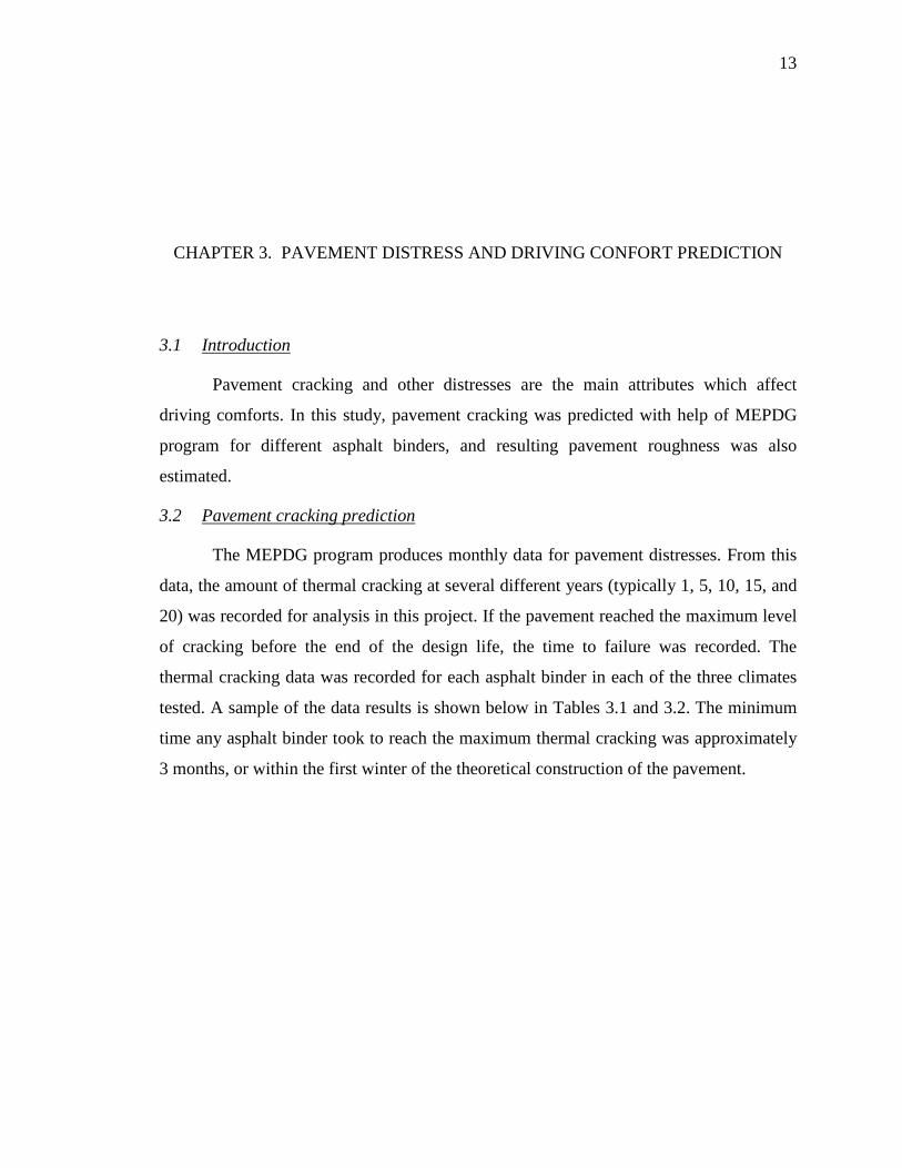
tested. A sample of the data results is shown below in Tables 3.1 and 3.2. The minimum

time any asphalt binder took to reach the maximum thermal cracking was approximately

3 months, or within the first winter of the theoretical construction of the pavement.

14

Table 3.1 Comparison of MEPDG pavement cracking prediction of Level 3 and Level 1

Level 3 Analysis

Climate Binder Cracking @ 5 Years

Cracking @ 10 Years

Cracking @ 15 Years

Cracking @ 20 Years

Intermediate

PG 64-22 0.245 4.077 12.572 23.917

PG 70-22 0.072 1.212 3.735 7.290

PG 76-22 0.019 0.337 1.022 1.972

PG 64-28 0.002 0.028 0.079 0.149

PG 70-28 0.000 0.009 0.026 0.050

PG 76-28 0.000 0.004 0.013 0.024

Level 1 Analysis

Climate Binder Cracking @

5 Years Cracking @

10 Years Cracking @

15 Years Cracking @

20 Years

Intermediate

PG 64-22 38.199 145.688 172.767 177.920

PG 70-22 Max cracking: 200 @ 15.3 mo. -

PG 76-22 - - - -

PG 64-28 0.000 0.001 0.002 0.004

PG 70-28 - - - -

PG 76-28 - - - -

Note 1: IDT data not available for PG 76-22, PG 70-28, and PG 76-28 asphalt binders

Note 2: Cracking shown in terms of feet per 500 feet (200 ft. maximum) Pavement Structure: 5” HMA, 8” crushed stone base, A-7-6 subgrade

15

Table 3.2 MEPDG Level 1 pavement cracking prediction analysis results

Cold Climate (International Falls, MN)

Binder Cracking @ 5 Years Cracking@10 Years Cracking@15

Years Cracking@20

Years PG 64-22 157.8 177.0 180.1 182.8

PG 70-22 Maxed out: 200 @ 3.4 mo. PG 64-28 0.04 2.5 9.2 22.9

Intermediate Climate (Champaign, IL)

Binder Cracking @ 5 Years

Cracking @10 Years

Cracking @15 Years

Cracking @20 Years

PG 64-22 11.067 67.022 83.291 87.552

PG 70-22 Maxed out: 200 @ 15.3 mo. PG 64-28 0.000 0.001 0.002 0.004

Warm Climate (Flagstaff, AZ)

Binder Cracking @ 5 Years

Cracking @ 10 Years

Cracking @15 Years

Cracking @20 Years

PG 64-22 0.004 0.04 0.2 0.4

PG 70-22 72.2 92.2 96.7 102.5

PG 64-28 0.0 0.0 0.0 0.0

With the University of Illinois IDT data, the weakest binder, in regards to thermal

cracking, was seen to be PG 70-22, regardless of climate. The most effective binder

against thermal cracking was seen to be PG 64-28. However, it must be noted that the

Level 1 analysis was performed using the data from just a single IDT. Additional IDT

results were not available for the PG 64-28 binder during this study.

The trends of thermal cracking for the various binders were consistent across the

three climates. The only difference among the climates was the degree of thermal

cracking that occurred. For the sake of space in this report, only the results from the full

depth pavement set are shown in Table 3.2. Sets 2, 3, and 4 yielded similar trends in

thermal cracking. As the thickness of the asphalt concrete layer decreased, the amount of

thermal cracking increased uniformly, regardless of climate. As expected, thermal

cracking was greatest in the cold climate of International Falls, MN, and least in the

warm climate of Flagstaff, AZ. However, the binders showed similar trends in thermal

cracking relative to other binders. The weakest binder always experienced the most

16

thermal cracking, while the most effective binder showed the least thermal cracking, or

no thermal cracking at all.

With the MEPDG default data, the most cracking susceptible binder was found to

be PG 70-16. The most effective binder for thermal cracking was PG 46-40. The IDT

database did not have data for those binders, as they are not typically used in the State of

Illinois. The asphalt binder grades chosen for Level 3 analysis were chosen to show

sequential differences in maximum and minimum design temperature from PG 64-22, the

typical binder used in Illinois. One of the unexpected results of the level 3 analysis was

that the PG 70-16 binder consistently performed worse than the PG 76-10 binder. The PG

76-10 binder should have experienced the most predicted thermal cracking, since it had

the highest minimum temperature grade. However, these are seldom used grades.

As part of this research project, the differences in results between pavements with

the default MEPDG data and the IDT data from the University of Illinois were examined.

The discrepancies between the Level 1 and Level 3 analyses conducted with the MEPDG

are shown in Table 3.1 below. For PG 64-22, over a design life of 20 years, 87.6 feet of

transverse cracking per 500 feet of pavement was predicted to occur by MEPDG using

IDT data (Level 1 analysis). Using the default MEPDG data, only 23.9 feet of transverse

cracking per 500 feet of pavement was predicted (Level 3 analysis). The results of the

MEPDG testing with the IDT creep compliance and tensile strength data showed a

consistently higher level of thermal cracking. Overall, the results of this research show

that the default creep compliance and tensile strength data for the asphalt binders in the

MEPDG may need to be updated in order to achieve more reasonable results.

The calibration factors used for thermal cracking were adjusted so that MEPDG

predictions would match an expert’s predictions. For the level 3 analysis in Champaign,

IL, the ideal calibration factor was found to be 1.73. For the level 1 analysis in

Champaign, IL, the ideal calibration factor was found to be approximately 0.97. The

difference in these regional calibration factors further demonstrates the disparity between

the level 1 and level 3 analysis results.

17

3.3 Pavement roughness prediction example

Pavements begin deteriorating after construction due to traffic loads and

environmental factors. Pavement surface roughness increases with the extent and severity

of various distresses, which affects ride quality, safety, travel speed, and vehicle

operating costs. There are many pavement roughness models which were developed

using different distresses for new and overlaid pavements (Von Quintus et al. 2001). In

this study, the IRI model that appears on the M-E PDG (AASHTO 2008) was used to

predict pavement roughness:

IRI = IRI0 + 0.0150*SF + 0.400*FCTotal + 0.0080*TC + 40*RD

Where, IRI0 = Initial IRI, inch/mile

SF = Site Factor

FCTotal = Area of fatigue cracking (combined alligator, longitudinal, and reflection

cracking under the wheel path), in percentage of total lane area

TC = Length of transverse cracking in feet per mile

RD = Average rut depth measured in inches

The following inputs were used for MEPDG analysis of 12-inch full depth asphalt

pavement, along with program default values:

AADT = 10000

Asphalt Binder = PG 64-22

Asphalt creep and strength data: University of Illinois, Buttlar group database

Initial IRI = 63 inch/mile and 70 inch/mile

Climate: Champaign, IL

Design life: 20 years

Table 3.3 shows the predicted IRI of a 12-inch, full-depth asphalt pavement.

18

Table 3.3 Prediction of IRI using M-E PDG software program

Year Transverse Cracking (ft./mi)

IRI (When Initial IRI = 63 inch/mile)

IRI (When Initial IRI = 70 inch/mile)

1 0 76.3 83.3 2 12.3 80.1 87.1 3 39.8 83 90 4 111 86.6 93.6 5 117 89.6 96.6 6 315 93.5 100.5 7 599 98.5 105.5 8 604 101.4 108.4 9 606 104.3 111.3 10 708 108.3 115.3 11 729 111.2 118.2 12 756 114.6 121.6 13 757 117.8 124.8 14 798 121.2 128.2 15 880 124.9 131.9 16 881 128.3 135.3 17 882 131.6 138.6 18 908 135.4 142.4 19 915 138.8 145.8 20 925 142.5 149.5

Perera and Kohn (2006) reported that, for pavement sections with IRI greater than

97 inch/mile before applying an overlay, the IRI after placing the overlay was reduced to

between 52 to 76 inch/mile. They also reported that IRI values would be less than 64

inch/mile after the application of an overlay when pre-overlay IRI values of less than 97

inch/mile were present. Thus, for roughness prediction of pavement following

rehabilitation, an IRI level of (63 inch/mile) was assumed in this study. Maintenance

represents pavement improvement activities which are performed when pavement is in a

structurally sound, good condition. Al-Mansour et al. (1994) studied the effect of crack

sealing, chip seal, and sand seal on roughness in flexible pavements used on interstate

and state highways. They reported low benefits in roughness reduction due to

19

maintenance activities in the case of new pavements and increased benefit in roughness

reduction for maintenance applied to aged pavements. Hall et al. (2002) studied the effect

of various maintenance activates, including slurry seal, chip seal, crack seal, and thin

overlays on pavement roughness. Based upon a statistical analysis, they reported that the

effect of chip seals, crack seals, and slurry seals were not significant compared to a

control section which did not receive a maintenance treatment. However, thin overlays

were found to reduce pavement roughness significantly. In this study, no improvement in

IRI was considered for pavements undergoing chip seals, slurry seals, and crack seals,

while a roughness reduction resulting in a restored IRI level of 63 inch/mile was assumed

following the application of an overlay. Although rate of change of IRI for overlays is

higher than new pavement IRI deterioration, the same rate was considered for simplicity

of calculation in this study.

20

CHAPTER 4. ESTIMATION OF COSTS DUE TO PAVEMENT ROUGHNESS

Chapter 4 presents an analysis of user costs resulting from pavement roughness.

In Chapter two and Chapter three, pavement cracking prediction along with resulting

roughness and methods of user costs estimation were presented. In this section, total user

cost per 1-mile pavement section has been estimated for an assumed vehicle fleet.

4.1 Pavement user costs with conventional M&R

Different types of pavement user costs were estimated by using the equations and

user cost data provided in the above sections. Table 4.1 shows increases in user costs i.e.

fuel consumption, repair and maintenance, depreciation, and tire cost, at different levels

of IRI as predicted by the AASHTO Mechanistic Empirical Pavement Design Guide

(MEPDG) software program. Total roughness-related user costs are also shown in Table

4.1 for a fleet of 10,000 vehicles, assumed to travel an average of 12,000 miles per year.

From Table 4.1, it can be seen that a vehicle owner will incur an additional $129/year for

a vehicle driven on road with an IRI of 110 inch/mile, which is considered to be an

adequate smoothness level for a primary road. This additional user cost would be higher

($478/year) if the same vehicle were driven on road with an IRI of 200 inch/mile, which

is the highest acceptable IRI level for a primary road.

21

Table 4.1 Total user cost increased due to pavement roughness

IRI, inch/mile

Increase in Fuel Cost, $/mile from Eq. (1)

Increase in R&M Cost by Eq. (2), $/mile

Increase in Depreciation Cost by Eq.(3), $/mile

Increase in Tire Cost by Eq. (4), $/mile

Total Increase in User Cost, $/mile

Total Cost per Year for 10,000 vehicle, $

Total Cost per Year per vehicle, $

63.00 0.00000 0 0 0 0.00000 - -

76.3 0.00031 0 0.00008 0 0.00039 $46,428 $5

80.1 0.00040 0 0.00024 0 0.00063 $75,841 $8

83 0.00046 0 0.00035 0 0.00082 $98,113 $10

86.6 0.00055 0.000742 0.00050 0 0.00179 $214,581 $21

89.6 0.00062 0.001575 0.00061 0.00016 0.00297 $356,126 $36

93.5 0.00071 0.002648 0.00077 0.00036 0.00449 $538,386 $54

98.5 0.00083 0.004009 0.00096 0.00061 0.00641 $769,284 $77

101.4 0.00090 0.00479 0.00106 0.00076 0.00751 $901,780 $ 90

104.3 0.00097 0.005565 0.00117 0.00090 0.00861 $1,033,230 $103

108.3 0.00106 0.006625 0.00132 0.00110 0.01011 $1,212,824 $121

1001 0.00087 0.004413 0.00101 0.00069 0.00698 $837,947 $84

1102 0.00111 0.007072 0.00138 0.00118 0.01074 $1,288,548 $129

1253 0.00146 0.010931 0.00190 0.00188 0.01618 $1,941,125 $194

1754 0.00265 0.022673 0.00340 0.00390 0.03262 $3,914,234 $391

2005 0.00324 0.027896 0.00401 0.00472 0.03987 $4,784,164 $478

2506 0.00443 0.037047 0.00495 0.00600 0.05242 $6,290,776 $629

1 IRI level for adequate smooth pavement of Interstate highways 2 IRI level for adequate smooth pavement of Primary roads 3 IRI level for adequate smooth pavement of Secondary roads 4 IRI level for inadequate smooth pavement of Interstate highways 5 IRI level for inadequate smooth pavement of Primary roads 6 IRI level for inadequate smooth pavement of Secondary roads

22

Agency costs for four different maintenance and rehabilitation (M&R) strategies were

estimated. The effects of M&R activities on pavement roughness were estimated from

data found through literature review (Hall et al. 2002). Table 4.2 shows agency costs for

four alternative M&R strategies. To calculate life-cycle cost of pavement, a 35 year

analysis period and a 3% discount rate was considered. A comparison was then made

between agency costs and costs related to pavement roughness, as shown in Figure 4.1.

23

Table 4.2 Pavement maintenance and rehabilitation (M&R) strategies (1-mile)

Alternative 1 Alternative 2 Year Action Cost Year Action Cost

0 New Pavement $206,712 0 New Pavement $206,712

3 Crack Seal (4 yrs) $1,500 3 Crack Seal (4 yrs) $1,500 7 Crack Seal (4 yrs) $1,500 7 Mill & Patch 20%

Spot Repair $18,050

10 2" Overlay (10 yrs) $92,810 15 2" Mill & 2" Overlay $94,090 13 Crack Seal (4 yrs) $1,500 18 Crack Seal (4 yrs) $1,500 16 Slurry Seal (4 yrs) $11,265 20 Mill & Patch 20%

Spot Repair $18,050

20 2" Mill & 2" Overlay $94,090 27 1.5" Mill & 3" Overlay

$110,860

23 Crack Seal (4 yrs) $1,500 30 Crack Seal (4 yrs) $1,500 26 Chip Seal (5 yrs) $12,530 35 Salvage Value -$33,258 30 2" Mill & 2" Overlay $94,090 35 Salvage Value -$47,045

Present Worth = $367,115 Present Worth = $332,735 EUAC = $ 17,085 EUAC = $ 15,485

Alternative 3 Alternative 4 Year Action Cost Year Action Cost

0 New Pavement $206,712 0 New Pavement $206,712 3 Crack Seal (4 yrs) $1,500 3 Crack Seal (4 yrs) $1,500 5 Chip Seal (5 yrs) $12,530 5 Crack Seal (4 yrs) $1,500 10 1.5" Overlay (10 yrs) $77,585 9 Mill & Patch 20%

Spot Repair $18,050

14 Crack Seal (4 yrs) $1,500 12 Chip Seal (5 yrs) $12,530 17 Slurry Seal (4 yrs) $11,265 17 2" Mill & 2" Overlay $94,090 20 2" Mill & 2" Overlay $94,090 20 Crack Seal (4 yrs) $1,500 23 Crack Seal (4 yrs) $1,500 23 Slurry Seal (4 yrs) $11,265 26 Fog Seal (2 yrs) $9,700 27 1.5" Overlay (10 yrs) $77,585 30 1.5" Overlay (10 yrs) $77,585 30 Crack Seal (4 yrs) $1,500 35 Salvage Value -$38,792 35 Salvage Value -$15,517

Present Worth = $359,962 Present Worth = $325,497 EUAC = $ 16,752 EUAC = $ 15,148

24

Figure 4.1 Comparison between agency costs and user costs related to pavement roughness

In Figure 4.1, roughness cost was calculated assuming 12,000 mile/year and a

10,000 annual average daily traffic (AADT) level. It can be seen that the present worth

(PW) of the pavement from the LCCA was found to be about $350,000, whereas cost

related to roughness was about $9,910,000 to $15,460,000 depending on the initial

roughness of the pavement. This finding suggests that highway agencies only expend

about 2.3% to 3.6% of the amount that is spent by users as a result of pavement

roughness over the period of the LCC.

In this study, agency costs and costs incurred because of pavement roughness

were considered, not total vehicle operating cost. Figures 4.2 and 4.3 show that vehicle

-200

0

200

400

600

800

1000

1200

1400

1600

0 1 2 3 4 5 6 7 8 9 1011121314151617181920212223242526272829303132333435

1522

1522

543

682

Cos

t, $/

mile

(T

hous

ads)

Time (Years)

Alt. 1 AgencyExpenditure

Alt. 2 AgencyExpenditure

Alt. 3 AgencyExpenditure

Alt. 4 AgencyExpenditure

UserCost_Roughness_InitialIRI=63 inch/mileUserCost_Roughness_InitialIRI=70 inch/mile

25

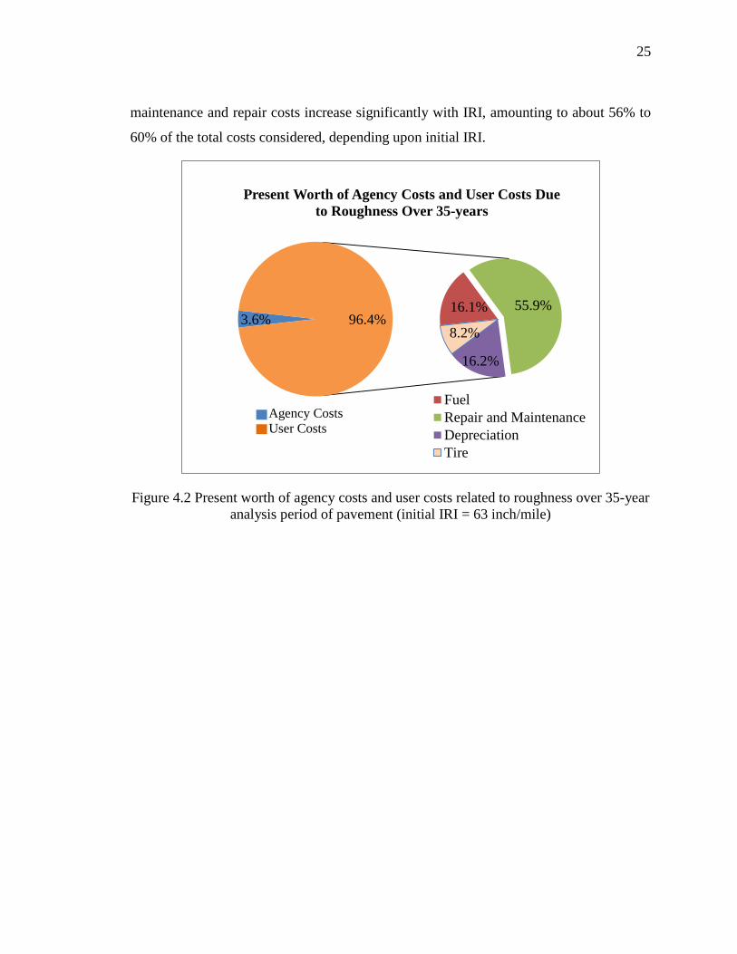
maintenance and repair costs increase significantly with IRI, amounting to about 56% to

60% of the total costs considered, depending upon initial IRI.

Figure 4.2 Present worth of agency costs and user costs related to roughness over 35-year analysis period of pavement (initial IRI = 63 inch/mile)

3.6% 16.1% 55.9%

16.2%

8.2% 96.4%

Present Worth of Agency Costs and User Costs Due to Roughness Over 35-years

FuelRepair and MaintenanceDepreciationTire

Agency Costs User Costs

26

Figure 4.3 Present worth of agency costs and user costs related to roughness over 35-year analysis period of pavement (initial IRI = 70 inch/mile)

The present analysis strongly suggests that increased investment in pavement

maintenance and rehabilitation activities aimed at reducing pavement roughness could

result in a many-fold savings in user costs. It is acknowledged that the typical values,

models and other assumptions used in this study will vary from region to region, and will

change with time (e.g., with changes in fuel, material, and vehicle maintenance costs,

changes in transportation policies, etc.). A spreadsheet-based program is currently being

developed to facilitate the LCCA analysis performed herein, which will allow this model

to be readily applied in various regions across the US and abroad. Table 4.3 provides a

sensitivity analysis comparing agency vs. user costs for differing average daily traffic

(ADT) levels and analysis periods. It was assumed that agency cost would be 10% less

and 10% more for 8,000 ADT and 12,000 ADT, respectively compared to 10,000 ADT,

to account for full-depth asphalt design pavement thickness variation as a function of

design traffic. Although these two variables clearly affect agency and user costs, the

overall conclusion of the study (users bear the bulk of the financial burden when

pavements become rough) is unchanged.

2.3% 13.2% 60.4%

14.7%

9.3% 97.6%

Present Worth of Agency Costs and User Costs Due to Roughness Over 35-years

FuelRepair and MaintenanceDepreciationTire

Agency Costs User Costs

27

Table 4.3 Sensitivity Analysis for Traffic Level and Analysis Period

Average Daily Traffic Level and Yearly User Cost Traffic Level (ADT) Agency Cost User Cost

Initial IRI =63 inch/mile

Initial IRI = 70 inch/mile

8,000 $330,400 $7,928,341 $12,368,748 10,000 $367,115 $9,910,426 $15,460,936 12,000 $403,825 $11,892,512 $18,553,123

Analysis Period and Yearly User Cost Analysis Period (years) Agency Cost User Cost

Initial IRI =63 inch/mile

Initial IRI = 70 inch/mile

35 $367,115 $9,910,426 $15,460,936 40 $388,723 $11,345,212 $17,409,807 45 $405,547 $11,561,089 $17,929,249

4.2 Pavement users costs with enhanced M&R

A final analysis is now presented to further demonstrate that increased pavement

maintenance activities will be paid off many times over in reduced user costs. Table 4.4

shows the maintenance and rehabilitation strategy used to conduct this analysis. Table 4.5

shows increases in user costs.

28

Table 4.4 An example of an enhanced maintenance and rehabilitation strategy for a 1-mile section of roadway

Year Action Cost

0 New Pavement $206712 Present of Worth of Alternative 1 $367,115

3 Crack Seal (4 yrs) $1,500 Present Worth of this M&R $475,325

7 2" Mill & 2" Overlay $94,090 Additional

Investment $108,209 10 Crack Seal (4 yrs) $1,500

13 2" Mill & 2" Overlay $94,090

Roughness related user costs for

Alternative 1 with initial IRI 63 in/mile

$9,910,426

16 Slurry Seal (4 yrs) $11,265

Roughness related user costs for this

M&R with initial IRI 63 in/mile

$4,740,484

20 2" Mill & 2" Overlay $94,090 Reduction of user

costs $5,169,943 23 Crack Seal (4 yrs) $1,500

26 2" Mill & 2" Overlay $94,090

Roughness related user costs for

Alternative 1 with initial IRI 70 in/mile

$15,460,936

30 2" Mill & 2" Overlay $94,090

Roughness related user costs for this

M&R with initial IRI 70 in/mile

$9,725,724

35 Salvage Value -$47,045 Reduction of user costs

$5,735,212

Present Worth (PW) = $475,325 EUAC = $22,121

29

Table 4.5 User Costs for the Enhanced M&R Strategy

Initial IRI of Pavement = 63 inch/mile Initial IRI of Pavement = 70 inch/mile

Year IRI, Inch/mile

Total Increase in User Cost, $/mile

Total Cost per year for 10,000 vehicle, $

Total Cost per Year per vehicle, $

IRI, Inch/mile

Total Increase in User Cost, $/mile

Total Cost per year for 10,000 vehicle, $

0 63 0 $ - $ - 70 0 $ - 1 76.3 0.000386899 $ 46,428 $ 5 83.3 0.000481 $ 57,709 2 80.1 0.000632008 $ 75,841 $ 8 87.1 0.001986 $ 238,297 3 83 0.000817608 $ 98,113 $ 10 90 0.003124 $ 374,906 4 86.6 0.001788174 $ 214,581 $ 21 93.6 0.004525 $ 543,034 5 89.6 0.002967715 $ 356,126 $ 36 96.6 0.005683 $ 681,909 6 93.5 0.004486547 $ 538,386 $ 54 100.5 0.007173 $ 860,773 7 76.3 0.000386899 $ 46,428 $ 5 83.3 0.000481 $ 57,709 8 80.1 0.000632008 $ 75,841 $ 8 87.1 0.001986 $ 238,297 9 83 0.000817608 $ 98,113 $ 10 90 0.003124 $ 374,906

10 86.6 0.001788174 $ 214,581 $ 21 93.6 0.004525 $ 543,034 11 89.6 0.002967715 $ 356,126 $ 36 96.6 0.005683 $ 681,909 12 93.5 0.004486547 $ 538,386 $ 54 100.5 0.007173 $ 860,773 . . . . . . . . . . . . . . . . . . . . . . . . 34 86.6 0.001788174 $ 214,581 $ 10 90 0.003124 $ 374,906 35 89.6 0.002967715 $ 356,126 $ 21 93.6 0.004525 $ 543,034

Present Worth (PW) = $4,740,484 Present Worth (PW) = $9,725,724

If the enhanced M&R strategy shown in Table 4.4 is used, it would require an

additional transportation agency expenditure in terms of present worth of $108,209 more

over the 35-year analysis period. According to Table 4.4, this would save a whopping

$5,169,943 to $5,735,212 (52% to 37%) of user costs over the 35-year life cycle

depending on the initial roughness of the pavement. Stated otherwise, increased

maintenance activities resulting in smoother pavement condition over the life of the

pavement will have about a 50-fold return on investment in terms of reduced user costs.

Additional justification for the increased maintenance expenditures can be argued from a

sustainability standpoint; increased pavement maintenance activities will significantly

reduce fuel consumption and tire wear over the life of the pavement, and will extend the

overall life of pavement system (the enhanced M&R strategy results in a higher salvage

value and therefore a higher remaining life in the pavement section at the end of the 35-

year analysis period, thereby delaying reconstruction). It is hoped that the present

30

analysis will provide compelling information that can be used by transportation policy

makers to make a strong case for increased maintenance and rehabilitation activities to

help reduce the financial burden carried by users resulting from rough pavement.

4.3 Environmental impacts of M&R activities

According to the National Asphalt Pavement Association (NAPA), annual hot-mix

asphalt production in the US is about 500 million tons. About 90% roads and highways

are constructed with asphalt concrete (Hansen and Newcomb 2007). According to the

Federal Highway Administration (Harrington 2005), annual production of aggregate is

about 2 billion tons, but the demand will increase to 2.5 billion tons by 2020. The amount

of resources and investment needed to keep the transportation network in good condition,

and methods to go about this in a sustainable manner, need to be thoroughly analyzed.

Life cycle cost analysis (LCCA) and life cycle assessment (LCA) are powerful tools that

can be used to assess economic and environmental impacts associated with resource

usage and infrastructure investments. An ideal LCA considers five phases of pavement

life, including: materials; construction; use; maintenance and rehabilitation (M&R), and;

end-of-life.

Brillet et al. (2006) reported that construction and maintenance of roadways and

vehicle operation are not independent. This is because while pavement M&R activities

improve the smoothness of roads and, therefore; consumption related to use is decreased,

the additional M&R activities required to improve smoothness result in extra

consumption and emission. It is evident from a review of the literature that long term

assessment of pavement using LCCA-LCA and including agency costs, user costs, and

environmental costs is necessary to obtain a holistic evaluation of rehabilitation strategies

and sustainable construction approaches.

4.3.1 Pollution damage cost rates

Although no standard monetary value has been assigned to various pollutants,

many existing studies considered different values for each pollutant. Unit costs of

pollutants are estimated based on their impacts on health. Unit cost of pollutants and

greenhouse gases depends on population density and land cover of the construction site

31

(Malela and Sadasivam 2011). It is assumed that the emission of these pollutants and

greenhouse gases have a substantial adverse effect on health in metropolitan areas with

higher population densities. Thus, unit costs associated with emissions is higher in urban

areas than rural areas. Tol (2005) reported that damage cost of carbon dioxide (CO2)

varies in the range of $5-125 per ton, and reported that most estimates are in the lower

range. Tol et al. (2001) stated that “estimates [of carbon dioxide emission cost] in excess

of $50/ton requires relatively unlikely scenario of climate change, impact sensitivity, and

economic values”. Emission damage costs were collected from Kendall et al. (2008) and

adjusted to 2011 dollar using consumer price index (CPI). Damage cost was reported by

Tol (2003) based on cost effectiveness and cost benefit of various emission and climatic

scenarios. In this study, emission damage costs of pollutants and greenhouse gases were

obtained from a recent (2011) FHWA report (Mallela and Sadasivam 2011) and Kendall

et al. (2008) report (Table 4.6).

Table 4.6 Emission cost rates (Kendall et al. (2008))

CO2, tons

NOX, tons

PM10, tons

SO2, tons

CO, tons

Pb, tons

Rural Cost Rate, $/ton 26 8712 980 26 0 588 Urban Cost Rate, $/ton 26 8712 7526 208 2 4845

4.4 Emission costs due to M&R activities

Environmental Costs were estimated from emissions generated by various activities

related to pavement such as pavement materials production, transportation, and

equipments used during construction. Pavement Life-cycle Assessment Tool for

Environmental and Economic Effects (PaLATE) provides emissions of five criteria-

pollutants defined by Environmental Protection Agency (EPA) and major greenhouse

(CO2) gas (Horvath 2004). The criteria-pollutants include carbon monoxide (CO),

nitrogen oxides (NOX), sulfur dioxide (SO2), lead (Pb), and particulate matter (PM10).

The PaLATE program estimates emissions resulting from the production of pavement

materials, transportation of those materials to the site, and construction processes.

32

4.4.1 Emission calculation

Life cycle cost analysis and life cycle assessment (LCCA-LCA) were applied to a

1-mile, 1-lane asphalt pavement section. In this study, emissions due to material

production, transportation to the construction site, and construction process was obtained

by PaLATE. Table 4.7 describes materials, processes, and equipment considered in this

study for the CMR activities in the two different approaches investigated.

Table 4.7 Details of material quantities, process, and equipment used for CMR

Stage Item

Quantity, yd3 Material Source to

Site Distance,

mile

Transportation Mode Basic

Approach Alternative Approach

Initial Construction

Virgin Aggregate 2206 2206 20 Dump Truck

Bitumen 141 141 30 Tanker Truck Gravel (Base) 98 98 20 Dump Truck

Maintenance and

Rehabilitation

Virgin Aggregate 1256 1917 20 Dump Truck

Bitumen 70.4 117 30 Tanker Truck Asphalt

Emulsion 35 17.4 30 Tanker Truck

RAP Material 782 1955 - Hot-in-Place

Recycling (HIPR)

782 1955 -

Crack Sealing 0.26 0.19 30 Tanker Truck Process Equipment Used HMA Production Asphalt Mixing in Batch Plant Asphalt Paving Paver, Pneumatic Roller, Tandem Roller Milling Milling Machine Crushing Plant Excavator, Wheel Load, Dozer, Generator HIPR Heating Machine, Asphalt Mixer, Pneumatic Roller,

Tandem Roller

The PaLATE program accounts for emissions due to all phases of material

production. For asphalt production, this includes extraction, transportation/storage,

heating, distillation, cooling, and final processing. Emission due to the traffic use phase

33

was estimated by MOVES, which was developed by EPA. Two different traffic levels

(10,000 and 15,000 AADT) were considered in both the basic and alternative M&R

approaches. Figure 4.4 shows emissions generated by 15,000 passenger cars over 35

years in an urban area along with pavement construction emissions. As initial

construction is identical in both basic and alternative approaches, emission is also same.

In maintenance phase, CO2 emission is about 115 tons/mile and 191 tons/mile in the

basic and alternative approaches, respectively. Because of the heavier rehabilitation

associated with the alternative approach, emissions are higher than those associated with

the basic approach. However, CO2 emissions related to pavement roughness is actually

predicted to be less in the alternative approach (240 tons/mile) than the basic approach

(325 tons/mile) because of the reduction in vehicle emissions associated with maintaining

smoother pavement throughout the analysis period investigated.

34

Figure 4.4 Emission of alternative approach for urban area over 35-year pavement service life: (a) initial construction, (b) maintenance, (c) emission due to pavement roughness,

and (d) total emission

Zaabar and Chatti (2011) studied the effect of roughness on fuel consumption of

vehicles, and reported that fuel consumption increases with pavement roughness and can

increase as high as 4 percent depending on IRI level. In the current study, their model

was used to estimate additional fuel resulting from pavement roughness. The MOVES

program was to calculate rate of emission of air pollutants and greenhouse gases (EPA

2012). This rate was used to estimate emission due to fuel utilized by vehicles due to

roughness and is reported in this paper as roughness-related emissions. Pollution damage

costs were estimated using rates reported by Kendall et al. (2008). Tables 4.8 and 4.9

35

show emissions and cost data for urban area for basic and alternative approaches using

15,000 AADT.

Table 4.8 Emissions by category and associated environmental cost: basic approach - Urban area

Emissions Category CO2, tons NOx, tons PM10, tons SO2, tons CO, tons Pb, tons

Initial Construction 204 2 1 49 1 0.0002 Maintenance 115 1 1 45 0 0.0002

Vehicles - 35years 87764 292 588 3 4391 11 Roughness Related 325 1 2 0 16 0.04

Total Emissions 88408 296 592 97 4409 11 Est. Envir. Cost, $/ton 26 8712 7526 208 2 4845 Total Environmental

Cost, $ $2,274,301 $2,581,150 $4,453,547 $20,261 $10,802 $51,089

Total = $9,391,150 Portion of Emissions due to

Init. Constr. and Maint. 319 3 2 94 1 0.0004

Est. Envir. Cost, $/ton 26 8712 7526 208 2 4845 Cost, $ $8,206 $27,243 $12,095 $19,602 $3 $2

Total = $67,151 Portion of Emissions due to

Roughness 325 1 2 0 16 0.04

Est. Envir. Cost, $/ton 26 8712 7526 208 2 4845 Cost, $ $8,360 $9,421 $13,503 $2 $40 $188

Total = $31,514

36

Table 4.9 Emissions by category and associated environmental cost: alternative approach - Urban area

Emissions Category CO2, tons NOx, tons PM10, tons SO2, tons CO, tons Pb, tons

Initial Construction 204 2 1 49 1 0.0002 Maintenance 191 2 1 83 1 0.0002

Vehicles - 35years 87764 292 588 3 4391 10.5058 Roughness Related 241 1 2 0 12 0.0288

Total Emissions 88400 297 592 136 4405 10.5350 Est. Envir. Cost, $/ton 26 8712 7526 208 2 4845 Total Environmental

Cost, $ $2,274,092 $2,587,036 $4,454,407 $28,301 $10,792 $51,041

Total = $9,405,669 Portion of Emissions due to

Init. Constr. and Maint. 395 4 2 133 1 0.0004

Est. Envir. Cost, $/ton 26 8712 7526 208 2 4845

Cost, $ $10,162 $35,569 $14,307 $27,643 $3 $2 Total = $87,686

Portion of Emissions due to Roughness 240.82 0.80 1.61 0.01 12.05 0.03

Est. Envir. Cost, $/ton 26 8712 7526 208 2 4845 Cost, $ $6,195 $6,982 $12,150 $2 $30 $140

Total = $25,498

From Table 4.8 and 4.9, it can be seen that emission of air-pollutants and

greenhouse gases in an urban setting are predicted to be higher in the alternate M&R

approach than that of the basic approach. Carbon dioxide (CO2) emission is same for the

initial construction phase but higher for alternative approach in maintenance phases and

roughness related emission. As more major rehabilitation and maintenance activities were

applied in alternative approach, as shown in Table 4.4, emissions are higher in this case.

Increases in carbon dioxide and sulfur dioxide emissions in maintenance activities are

significant, about 66% and 84%, respectively. But roughness-emission was reduced in the

alternative approach as pavement was kept smoother via additional rehabilitation. From

Table 4.8 and 4.9, it can be seen that both carbon dioxide and carbon monoxide emissions

related to pavement roughness were reduced by 25% in the alternative approach. Vehicle

37

emissions for 15,000 AADT was also estimated over the 35-year analysis period and

reported in Tables 4.8 and 4.9. Emissions due to construction and maintenance of

pavement are quite low compared to vehicle emissions. Costs associated with emissions

were also reported in Table 4.8 and 4.9. Emission costs in the alternative approach due to

maintenance and rehabilitation is 30% higher than that of the basic approach over the 35

year service life of the pavement, but roughness-emission cost is about 20% less than that

of the basic approach. As a result, it can be seen that pavement smoothness tends to

reduce the costs associated with emissions that are generated as a result of the additional

rehabilitation required to maintain the higher level of smoothness by about two thirds.

38

CHAPTER 5. RESULTS AND DISSCUSSION

This chapter summarizes the research, highlights its contributions, and proposes

directions for future research.

5.1 Agency investment, users, and emission costs

Agency costs, user costs due to pavement roughness, and emission costs due CRM

and roughness are shown in Figure 5.1. From Figure 5.1, it can be seen that emissions

cost due to CRM and roughness is only about 1% and 0.3%, respectively, whereas

agency cost and user costs are about 5% and 94%. After splitting the user costs, it can be

seen that about 54% of these costs are related to vehicle repair and maintenance. As

mentioned earlier, an additional agency investment of $108,209 over 35 years can reduce

user costs from $9.9 million to $4.7 million with an ROI of about 48-to-1. As a result of

these additional agency M&R activities, extra emissions with a cost of about $20,535 are

generated, however; the achieved smoothness reduces the roughness emission cost by an

amount of $6,016. Clearly, from a user cost standpoint, it is good policy to maintain

roads at a high level of smoothness, as millions of dollars are saved for users over the 35

year analysis period, as compared to the very modest additional environmental cost

required to maintain the pavement in a smooth condition (difference between $20,535

and & $6,016, or about $14,500). Although the environmental costs associated with the

two M & R strategies considered were relatively small as compared to user costs, it was

nevertheless important to conduct a thorough LCA to demonstrate that the results

presented by Islam and Buttlar (2012) were still applicable when environmental effects

were considered. Whereas the study by Islam and Buttlar (2012) reported a potential 50-

to-1 ROI as a result of maintaining pavement in a smooth condition, the current study,

39

which includes LCA along with LCCA, indicates that a 48-to-1 ROI can be realized by

maintaining smooth pavement.

Figure 5.1 Agency costs, emission costs, and user costs due to roughness

5.2 Importance of pavement smoothness

Pavement smoothness is very important not only to reduce vehicle repair and

maintenance costs but also for safety. Motorists pay significant amount of money because

of poor pavement condition. It is a common trend that motorists choose to ride on

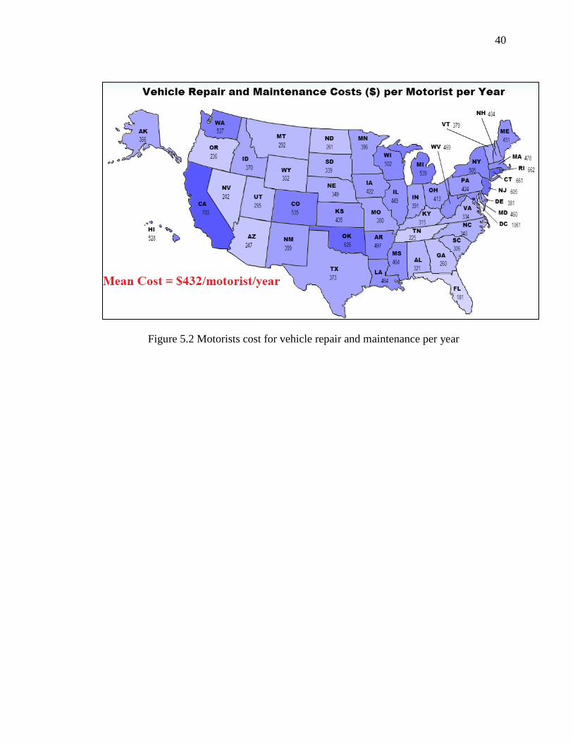
smoother pavement even if it requires a long detour. Motorists extra expenditure for

vehicle repair and maintenances are shown in a map (Figure 5.2), and these data were

collected from ASCE report cards.

40

Figure 5.2 Motorists cost for vehicle repair and maintenance per year

41

CHAPTER 6. SUMMARY, CONCLUSION, AND RECOMMENDATIONS

6.1 Summary

Roughness is an important aspect of pavement condition which significantly affects

driver comfort, and moreover, user costs. A comprehensive investigation was conducted

to study the effect of pavement roughness on agency and user costs. Some unique

features of the research conducted include: (1) A comprehensive array of user costs

related to roughness were considered; (2) fuel consumption was computed using a

calibrated HDM-4 model; (3) total user costs for a single vehicle and 10,000 AADT was

considered for Interstate, primary, and secondary roads; (4) a functional relationship

between IRI level and user costs was developed; (5) agency costs were simultaneously

considered and compared with user costs in the context of pavement roughness, (6) the

newly released MEPDG program was used to predict IRI at different traffic levels and

weather condition and with different initial IRI level, and; (7) environmental costs of

CMR activities were also considered. The analysis conducted demonstrated that user

costs including fuel consumption, repair and maintenance, depreciation, and tire costs

dramatically increase with increased pavement roughness, which far outweigh agency

costs associated with the construction and maintenance of the facility itself. For the two

main examples presented, agency costs based upon typical maintenance practices by state

DOTs were in the range of 2.3 to 3.6% of the combined costs (agency plus user)

associated with a unit section of roadway.

42

6.2 Conclusions

It is critically important to maintain pavement in good condition, otherwise,

significant user-related costs can be incurred, along with other costs such as those

associated with vehicle emissions. From this study, the following conclusions can be

drawn:

(a) By investing in additional maintenance (resurfacing every 7 years instead of every 10

years, on average) would save a whopping $5.1 M to $5.7 M (52% to 37%) of user costs

over the 35-year life cycle depending on the initial roughness of the pavement, as

compared to the additional $108,000.00 agency investment required for this additional

rehabilitation step. This equates to a 50-fold return on investment in terms of reduced

user costs.

(b) An additional agency investment of $108,209 over a 35-year design period for one

mile/one lane of roadway can provide a 48-to-1 return on investment in terms of reduced

user costs, when environmental costs are included in the analysis. Still, it can be

concluded that maintaining pavement in a smooth condition is an excellent value

proposition for the traveling public.

(c) Emission costs associated with additional rehabilitation (maintaining a smooth

pavement throughout service life) in the alternative approach were very low compared to

savings in user costs that would be realized as a result of maintaining the pavement in a

smooth condition.

(d) In the basic approach (pavement allowed to become rough during service life), user

costs due to roughness is about $9.9 million (94%) whereas costs to the agency, emission

costs due to CMR, and emission costs due to roughness were about $545,491 (5%),

$67,151 (1%), and $31,514 (0.3%), respectively, over the 35 year analysis period.

(e) In the alternative approach, which requires an additional $108,210 investment in M &

R over the 35 year analysis period, user costs associated with roughness is about $4.7

million (about 52% less than that associated with the basic approach), whereas agency

43

costs, emissions costs due to CMR, and emissions costs due to roughness were calculated

as $653,701, $87,686, and $25,498, respectively.

Additional justification for the increased maintenance expenditures can be argued

from a sustainability standpoint; increased pavement maintenance activities will

significantly reduce fuel consumption and tire wear over the life of the pavement, and

will extend the overall life of pavement system.

6.3 Recommendation

Driving comfort and safety are the two most important things that matter for

motorists. Pavement roughness in terms of IRI has been widely using in the US as an

indicator of driving comfort. It is also an important parameter in pavement design,

maintenance, and management decision making process. Pavement materials selection,

maintenance and rehabilitation strategies can be modified using roughness information.

Currently, a high speed inertial profiler (laser and accelerometer based) system is widely

used to collect pavement roughness. This system requires a specialized vehicle with very

expensive equipment and trained personnel (sometimes termed “million dollar vans”).

Most transportation agencies collect pavement roughness data biennial basis; therefore,

pavement maintenance and rehabilitation decisions are made based on a scarcity of

current data. With the mobile device revolution, smartphones are equipped with an

integrated accelerometer array which can be utilized to estimate pavement roughness by

developing a data collection application and analysis scheme. This system can collect

data by crowdsourcing, which will provide and up-to-date assessment of pavement

conditions, at a lower cost, along with the ability to detect bump features (potholes and

buckles or blow-ups) and vehicle swerve maneuvers. We propose this to be the subject

of a follow-up NexTrans project.

44

REFERENCES

AAA Association Communication. Your Driving Costs. AAA, Heathrow, Florida, 2011.

http://www.aaaexchange.com/main/Default.asp?CategoryID=16&SubCategoryID=76&C

ontentID=353. DrivingCosts2011.pdf. Accessed July 15, 2011.

AASHTO. Mechanistic-Empirical Pavement Design Guide. A Manual of Practice,

American Association of State Highway Officials, Highway Research Board.

Washington, D.C., 2008.

Al-Mansour, A., Sinha, K. C., and Kuczek, T. Effects of Routine Maintenance on

Flexible Pavement Condition. Journal of Transportation Engineering, ASCE, Volume

120, Issue 1, 1994.

Barnes, G., and Langworthy, P. Per Mile Costs of Operating Automobiles and Trucks. In

Transportation Research Record: Journal of the Transportation Research Board, No.

1824, Transportation Research Board of the National Academies, Washington, D.C.,

2004, pp. 71-77.

Bennett, C. R., and Greenwood, I. D. Volume 7: Modeling Road User and Environmental

Effects in HDM-4, Version 3.0. International Study of Highway Development and

Management Tools (ISOHDM), World Road Association (PIARC), 2003.

Brillet, F., A. Jullien, and S. Sayagh. Assessment of Consumptions and Emissions during

Pavement Lifetime. In Transport Research Arena Europe 2006, TRA, Gotenborg,

Sweden, 2006.

45

Chatti, K., and I. Zaabar. New Mechanistic-Empirical Approach for Estimating the Effect

of Roughness on Vehicle Durability Transportation Research Record: Journal of the

Transportation Research Board, Vol. 2227, 2011, pp. 180-188.

Chesher, A., Harrison, R., and Swait, J. D. Vehicle Depreciation and Interest Costs: Some

Evidence from Brazil. Proceedings of the Second World Conference on Transport

Research, London, England, 1981.

Federal Highway Administration (FHWA). Highway Finance Data Collection, Our

Nation's Highways: 2010.

http://www.fhwa.dot.gov/policyinformation/pubs/hf/pl10023/fig5_1.cfm. Accessed July

20, 2011.

Federal Highway Administration (FHWA). Our Nation's Highways: 2008. Figure 6-7.

Highway Construction Price Trends and Consumer Price Index. U.S. Department of

Transportation, 2011.

http://www.fhwa.dot.gov/policyinformation/pubs/pl08021/fig6_7.cfm. Accessed July15,

2011.

Federal Highway Administration (FHWA). Highway Economic Requirements System

Technical Manual, U.S. Department of Transportation, Washington, D.C., 2002.

Hall, K. T., Correa, C. E., and Simpson, A. L. LTPP Data Analysis: Effectiveness of

Maintenance and Rehabilitation Options. NCHRP Project 20-50[3/4], 2002.

Hall, K. T., and Correa, C. E. Estimation of Present Serviceability Index from

International Roughness Index. In Transportation Research Record: Journal of the

Transportation Research Board, No. 1655, Transportation Research Board of the National

Academies, Washington, D.C., 1999, pp. 93–99.

Hansen, K., and D. Newcomb. RAP Usage Survey. National Asphalt Pavement

Association, Lanham, MD, 2007.

46

Haugodegard, T., Johansen, J., Bertelsen, D., and Gabestad, K. Norwegian Public Roads

Administration: A Complete Pavement Management System in Operation. Proceedings

of Third International Conference on Managing Pavements, Volume 2, San Antonio,

Texas, May 22-26, 1994.

Harrington, J. Recycled Roadways. Public Roads, Vol. 68, No. 4, 2005, pp. FHWA-

HRT-05-003.

Horvath, A. Life-Cycle Analysis Model and Decision-Support Tool for Selecting

Recycled Versus Virgin Materials for Highway Applications. RMRC Research Project

No. 23, Recycled Materials Resource Center, Durham, New Hampshire, 2004.

Islam, S., and W. Buttlar. Effect of Pavement Roughness on User Costs. Transportation

Research Record: Journal of the Transportation Research Board, Vol. 2285, 2012, pp. 47-

55.

Kendall, A., G. A. Keoleian, and G. E. Helfand. Integrated Life-Cycle Assessment and

Life-Cycle Cost Analysis Model for Concrete Bridge Deck Applications. Journal of

Infrastructure Systems, Vol. 14, No. 3, 2008, pp. 214-222.

Lu, X. P. Effects of Road Roughness on Vehicular Rolling Resistance. Measuring Road

Roughness and Its Effects on User Cost and Comfort (T. D. Gillespie and M. Sayers,

eds.), ASTM Special Technical Publication 884. American Society for Testing and

Materials, Philadelphia, Pa., 1985, pp. 143–161.

Mallela, J., and S. Sadasivam. Work Zone Road User Costs. FHWA-DTFH61-06-D-

00004, Federal Highway Administration, Washington, DC, 2011.

Papagiannakis, A. T., and M. Delwar. Methodology to Improve Pavement-Investment

Decisions. Final Report to National Cooperative Highway Research Program for Study 1-

33, Transportation Research Board, Washington, D.C., 1999.

47

Perera, R. W., and Kohn, S.D. Ride Quality Performance of Asphalt Concrete Pavements

Subjected to Different Rehabilitation Strategies. ASCE Proceedings of 2006 Airfield and

Highway Pavements Specialty Conference, Atlanta, Georgia, April 30 – May 3, 2006.

Sinha, K. C. and Labi, S. Transportation Decision Making: Principles of Project

Evaluation and Programming. John Wiley & Sons, Inc., New York, 2007.

Tol, R. S. J. The Marginal Damage Costs of Carbon Dioxide Emissions: An Assessment

of the Uncertainties. Energy Policy, Vol. 33, No. 16, 2005, pp. 2064-2074.

Tol, R. S. J. Is the Uncertainty about Climate Change Too Large for Expected Cost-

Benefit Analysis. Climatic Change, Vol. 56, 2003, pp. 265-289.

Tol, R. S. J., T. E. Downing, S. Fankhauser, R. G. Richels, and J. B. Smith. Progress in

Estimating the Marginal Costs of Greenhouse Gas Emissions. Research unit

Sustainability and Global Change, Hamburg University, 2001.

Transportation Research Board Special Report 286. Tires and Passenger Vehicle Fuel

Economy - Informing Consumers, Improving Performance. Transportation Research

Board, Washington, D.C., 2006.

U.S. Environmental Protection Agency. Motor Vehicle Emisiion Simulator (MOVES). ,

Vol. MOVES2010b, 2012.

U.S. Environmental Protection Agency (EPA). Fuel Economy Guide – Model Year 2010.

Retrieved From: http://www.fueleconomy.gov/feg/pdfs/guides/FEG2011.pdf. Accessed

April 15, 2011.

Von Quintus, H. L., Eltahan, A., and Yau, A. Smoothness Models for Hot-Mix Asphalt–

Surfaced Pavements Developed from Long-Term Pavement Performance Program Data.

In Transportation Research Record 1764, TRB, National Research Council, Washington,

D.C., 2001, pp. 139–156.

48

Zaabar, I., and K. Chatti. Calibration of HDM4 Models for Estimating the Effect of

Pavement Roughness on Fuel Consumption for US Conditions. In Transportation

Research Record: Journal of the Transportation Research Board, No. 2155,

Transportation Research Board of the National Academies, Washington, D.C., 2010, pp.

105–116.

Zaniewski, J.P. Effect of Pavement Surface Type on Fuel Consumption; Portland Cement

Association: Skokie, IL, 1989.

Zaniewski, J. P., Butler, B. C., Cunningham, G., Elkins, E., Paggi, M. S., and

Machemehl, R. Vehicle Operating Costs, Fuel Consumption, and Pavement Type and

Condition Factors. FHWA-PL-82-001. FHWA, U.S. Department of Transportation, 1982.