integration of wave and tidal power into the haida gwaii
TRANSCRIPT

Integration of Wave and Tidal Power into the Haida Gwaii
Electrical Grid
by
Susan Margot Boronowski
B.A.Sc., University of British Columbia, 2007
A Thesis Submitted in Partial Fulfillment
of the Requirements for the Degree of
MASTER OF APPLIED SCIENCE
in the Department of Mechanical Engineering
© Susan Margot Boronowski, 2009
University of Victoria
All rights reserved. This thesis may not be reproduced in whole or in part, by photocopy
or other means, without the permission of the author.

ii
Supervisory Committee
Integration of Wave and Tidal Power into the Haida Gwaii Electrical Grid
by
Susan Margot Boronowski B.A.Sc., University of British Columbia, 2007
Supervisory Committee Dr. Andrew Rowe, (Department of Mechanical Engineering) Supervisor Dr. Peter Wild, (Department of Mechanical Engineering) Supervisor Dr. Brad Buckham, (Department of Mechanical Engineering) Departmental Member

iii
Abstract
Supervisory Committee Dr. Andrew Rowe, (Department of Mechanical Engineering) Supervisor Dr. Peter Wild, (Department of Mechanical Engineering) Supervisor Dr. Brad Buckham, (Department of Mechanical Engineering) Departmental Member
Rising energy demand, fossil fuel costs, and greenhouse gas emissions have led to a
growing interest in renewable energy integration. Remote communities, often
accompanied by high energy costs and abundant renewable energy resources, are ideal
cases for renewable energy integration. The Queen Charlotte Islands, also known as
Haida Gwaii, are a remote archipelago off the northwest coast of British Columbia,
Canada that relies heavily on diesel fuel for energy generation. An investigation is done
into the potential for electricity generation using both tidal stream and wave energy in
Haida Gwaii. A mixed integer optimization network model is developed in a Matlab and
GAMS software environment, subject to set of system constraints including minimum
operational levels and transmission capacities. The unit commitment and economic
dispatch decisions are dynamically solved for four periods of 336 hours, representing the
four annual seasons. Optimization results are used to develop an operational strategy
simulation model, indicative of realistic operator behaviour. Results from both models
find that the tidal stream energy resource in Haida Gwaii has a larger potential to reduce
energy costs than wave energy; however, tidal steam energy is more difficult to integrate
from a system operation point of view and, in the absence of storage, would only be
practical at power penetration levels less than 20%.
iv
Table of Contents Supervisory Committee .................................................................................................... ii Abstract............................................................................................................................. iii Table of Contents ............................................................................................................. iv List of Tables .................................................................................................................... vi List of Figures.................................................................................................................. vii Nomenclature .................................................................................................................... x Acknowledgments .......................................................................................................... xiv Chapter 1 Introduction..................................................................................................... 1
1.1 Energy System Modeling.......................................................................................... 2 1.2 Integration of Renewable Energy into Electrical Grids............................................ 4 1.3 Thesis Objective and Outline.................................................................................... 7
Chapter 2 Potential for Tidal Stream Power in Haida Gwaii ...................................... 8
2.1 Background ............................................................................................................... 8 2.2 Resource Assessment.............................................................................................. 10
Chapter 3 Potential for Wave Power in Haida Gwaii ................................................. 12
3.1 Wave Energy Background ...................................................................................... 12
3.1.1 Classification.................................................................................................... 12 3.1.2 Power Extraction from Waves ......................................................................... 14
3.2 Wave Energy Conversion Devices ......................................................................... 15 3.2.1 AquaBuOY ...................................................................................................... 16 3.2.2 Pelamis............................................................................................................. 18 3.2.3 Wave Dragon ................................................................................................... 20
3.3 Resource Assessment.............................................................................................. 21 Chapter 4 Modeling the Haida Gwaii Network ........................................................... 26
4.1 Existing Network .................................................................................................... 26 4.2 Network Optimization Model ................................................................................. 28 4.3 Model Parameterization .......................................................................................... 34 4.4 Model Input Data .................................................................................................... 35
4.4.1 Load Data......................................................................................................... 35 4.4.2 Tidal Power Data ............................................................................................. 37
v4.4.3 Wave Power Data ............................................................................................ 37
Chapter 5 Optimization Results .................................................................................... 39
5.1 Linking the Grids .................................................................................................... 39 5.2 Integrating Tidal Power .......................................................................................... 41 5.3 Integrating Wave Power ......................................................................................... 48
Chapter 6 Developing an Operational Strategy........................................................... 54
6.1 A Simulation Model................................................................................................ 54 6.2 The Effects of Tidal Power Addition...................................................................... 57 6.3 The Effects of Wave Power Addition..................................................................... 61 6.4 Comparison of Wave and Tidal Power................................................................... 65
Chapter 7 Conclusions.................................................................................................... 69
7.1 Key Findings........................................................................................................... 69 7.2 Recommendations................................................................................................... 71
Bibliography .................................................................................................................... 73 Appendix A – Theoretical Wave Power Calculations ................................................. 77

vi
List of Tables
Table 1: Basic types of surface waves according to period [24] ...................................... 13
Table 2: AquaBuOY output power for varying sea states (kW) [40] ............................... 23
Table 3: Pelamis output power for varying sea states (kW) [35] ..................................... 23
Table 4: Wave Dragon output power for varying sea states (kW) [39]............................ 24
Table 5: Wave energy potential by location ..................................................................... 25
Table 6: Average hour-to-hour wave power output fluctuation, West Moresby location 25
Table 7: Diesel generating units in Haida Gwaii [3] ........................................................ 28
Table 8: Haida Gwaii transmission line information (data from [3]) ............................... 28
Table 9: Generator dispatch order..................................................................................... 55

vii
List of Figures
Figure 1: AquaBuOY operating principle [32]................................................................. 17
Figure 2: Pelamis device [35] ........................................................................................... 19
Figure 3: Wave Dragon operating principle [37].............................................................. 20
Figure 4: Wave buoy locations [41].................................................................................. 21
Figure 5: Haida Gwaii electricity system (data from [3])................................................. 27
Figure 6: Network Diagram.............................................................................................. 29
Figure 7: Power Balance of the link between bus i and n (modified from [42]) .............. 30
Figure 8: Total production cost curve for a 1 MW capacity diesel generator .................. 32
Figure 9: Incremental production cost curve for a 1 MW capacity diesel generator........ 32
Figure 10: Diesel generator emissions for a 1 MW capacity unit..................................... 34
Figure 11: Sensitivity results for linked grids case, month of January data ..................... 35
Figure 12: Masset DGS Jan-05 maximum and minimum load [3]................................... 36
Figure 13: Diesel generator duty cycle, no renewable power.......................................... 40
Figure 14: Average number of diesel generator cycles, no renewable power .................. 40
Figure 15: Typical generation, 5 MW installed tidal capacity.......................................... 42
Figure 16: Diesel generator duty cycle vs. installed tidal capacity, non-linked case ...... 43
Figure 17: Diesel generator duty cycle vs. installed tidal capacity, linked case............... 43
Figure 18: Energy contribution by source vs. installed tidal capacity.............................. 45
Figure 19: Optimized annual tidal plant capacity factor................................................... 45
Figure 20: Average line power flow vs. installed tidal capacity, linked case................... 47
Figure 21: Average CO2 emissions vs. installed tidal capacity ........................................ 47
Figure 22: Annual operational cost of energy vs. installed tidal capacity ........................ 47
Figure 23: Break even project cost vs. installed tidal capacity......................................... 47
Figure 24: Energy contribution by source vs. installed wave capacity, CD location ....... 49
Figure 25: Energy contribution by source vs. installed wave capacity, WM location ..... 49
Figure 26: Generator duty cycles vs. installed wave capacity, CD location, non-linked
case.................................................................................................................................... 50
Figure 27: Generator duty cycles vs. installed wave capacity, CD location, linked case. 50
viiiFigure 28: Generator duty cycles vs. installed wave capacity, WM location, non-linked
case.................................................................................................................................... 51
Figure 29: Generator duty cycles vs. installed wave capacity, WM location, linked case51
Figure 30: Optimized annual wave plant capacity factor ................................................. 52
Figure 31: Average CO2 emissions vs. installed wave capacity....................................... 52
Figure 32: Annual operational cost of energy vs. installed wave capacity....................... 53
Figure 33: Break even project cost vs. installed wave capacity ....................................... 53
Figure 34: Operational strategy ........................................................................................ 56
Figure 35: Simulation diesel generator duty cycle vs. installed tidal capacity, non-linked
case.................................................................................................................................... 58
Figure 36: Simulation diesel generator duty cycle vs. installed tidal capacity, linked case
........................................................................................................................................... 58
Figure 37: Simulation energy contribution by source vs. installed tidal capacity ............ 59
Figure 38: Simulation average tidal plant capacity factor ................................................ 59
Figure 39: Curtailed tidal energy vs. installed tidal capacity............................................ 60
Figure 40: Total number of diesel generator cycles vs. installed tidal capacity ............... 60
Figure 41: Simulation average CO2 emissions vs. installed tidal capacity...................... 61
Figure 42: Simulation break even project cost vs. installed tidal capacity...................... 61
Figure 43: Annual operational cost of energy vs. installed tidal capacity, all cases......... 61
Figure 44: Simulation energy contribution by source vs. installed wave capacity, CD
location.............................................................................................................................. 63
Figure 45: Simulation energy contribution by source vs. installed wave capacity, WM
location.............................................................................................................................. 63
Figure 46: Simulation wave plant annual CF ................................................................... 64
Figure 47: Simulation total number of cycles vs. installed wave capacity....................... 64
Figure 48: Simulation annual operational cost of energy vs. installed wave capacity .... 65
Figure 49: Simulation break even project cost vs. installed wave capacity...................... 65
Figure 50: Diesel energy generated with all renewable options, linked grid with
operational strategy........................................................................................................... 66
Figure 51: Total number of diesel generator cycles with all renewable options, linked grid
with operational strategy................................................................................................... 66

ixFigure 52: Annual operational cost of energy with all renewable options, linked grid with
operational strategy........................................................................................................... 67
Figure 53: Break even project cost with all renewable options, linked grid with
operational strategy........................................................................................................... 67
Figure 54: Annual operational cost of energy with all renewable options, non-linked grid
with operational strategy................................................................................................... 68
Figure 55: Break even project cost with all renewable options, non-linked grid with
operational strategy........................................................................................................... 68
Figure 56: West Dixon Entrance hourly theoretical wave power for 2000 ...................... 77
Figure 57: Central Dixon Entrance hourly theoretical wave power for 2005................... 77
Figure 58: North Hecate Strait hourly theoretical wave power for 2005 ......................... 78
Figure 59: South Moresby hourly theoretical wave power for 2005 ................................ 78
Figure 60: West Moresby hourly theoretical wave power for 2004 ................................. 79
x
Nomenclature
Tidal Energy a amplitude of dominant tidal constituent outside channel in open ocean [m]
A swept area of turbine [m2]
c channel geometry term [m-1]
g acceleration due to gravity [ms-2]
N number of tidal stream turbines
P power [W]
Q volume flow rate through channel [m3s-1]
Qo volume flow rate in undisturbed state [m3s-1]
u flow velocity [ms-1]
η coefficient of performance of turbine
ρ density of fluid [kgm-3]
λ1 turbine drag parameter
ω frequency of dominant tidal constituent outside channel in open ocean [s-1]
Wave Energy a wave amplitude [m]
arms root mean square of displacement of water surface of wave from mean
position [m]
c wave speed [ms-1]
cg wave group velocity [ms-1]
d wave depth [m]
E total energy of a wave [J]
h displacement of water surface of wave from mean position [m]
H wave height [m]
H1/3 “one third” significant wave height [m]
Hs significant wave height [m]
Nc total number of wave crests
P wave power [Wm-1]
xiT wave period [s-1]
Tc mean crest period [s-1]
Te wave energy period [s-1]
Tp peak wave period [s-1]
Tz mean zero crossing wave period [s-1]
λ wavelength [m]
ζ coverage factor
Network Model c cost [CAD]
e CO2 emissions from generation [kgCO2MWh-1]
E total generation of CO2 emissions for period T [kgCO2]
g incremental production cost [$MWh-1]
G power generation at a bus [MW]
K number of cost levels
KS Kolmogorov-Smirnov test statistic
L power consumption at a bus [MW]
Loss power loss across a bus connector [MW]
M incremental generation for a cost level [MW]
P power entering or leaving a bus connector [MW]
Pop population of a network
R resistance of a bus connector [Ω]
Sink power sink at a bus [MW]
V voltage of a bus connector [V]
w variable indicating a diesel generating unit started up
x state variable of a diesel generating unit
y percent of incremental generation used for a set cost level
z variable indicating a diesel generating unit shut down

xii
Superscripts * non-dimensional value
Subscripts cap nameplate capacity of a generator
d dispatchable generator index
i,n bus indices
j bus connector index
k cost level index
loc location
m month
maint maintenance
max maximum
min minimum
sd diesel generating unit is shut-down
su diesel generating unit is start-up
t discrete time index
T total time steps
Tot total
y year
Abbreviations CD Central Dixon Entrance buoy location
CDF cumulative distribution function
CF capacity factor
CPUC California Public Utilities Commission
EMEC European Marine Energy Test Centre
EPRI Electric Power Research Institute
FERC Federal Energy Regulatory commission
GAMS General Algebraic Modeling System

xiiiIPP independent power producer
MEDS Marine Environmental Data Services
O&M operation and maintenance
PG&E Pacific Gas and Electric Company
PPA power purchase agreement
SCDF empirical cumulative distribution function
TE tidal energy
TP tidal plant
WEC wave energy converter
WM West Moresby buoy location

xiv
Acknowledgments
First and foremost, I would like to thank my supervisors, Drs. Andrew Rowe and Peter
Wild, for their support, guidance, and contributions to this work. A special thank you is
owed to Dr. G. Cornelis van Kooten, Jesse Maddaloni, and Justin Blanchfield for all of
their much appreciated assistance, expertise, and patience. Additionally, thank you to my
fellow graduate students, Torsten Broeer, Scott Beatty, and Clayton Hiles, who were
always there to offer help and encouragement when needed.

Chapter 1
Introduction Electricity generation is an issue of increasing interest due to growing energy
demand, fossil fuel costs, and greenhouse gas emissions. This issue is of particular
concern to remote communities, where the cost of electricity is generally higher than the
norm [1]. The Queen Charlotte Islands, also known as Haida Gwaii, are a remote
archipelago off the northwest coast of British Columbia, Canada with an isolated
electricity generation system that is heavily dependent on diesel fuel for operation [2].
Currently, there are two separate grids on Haida Gwaii, north and south, each supplying
approximately 1500 customers [2]. The peak load for the north grid in 2005 was roughly
4.8 MW, just under 1 MW less than that of the south grid [3]. A small hydro power
facility, sized at 5.7 MW, exists in conjunction with two diesel generation systems, sized
at 9.15 and 11.4 MW [3], resulting in a system average cost of electricity production in
2006 of 0.26 $/kWh [2].
A potential option to reduce the cost of electricity for the region, as well as
greenhouse gas emissions, is to incorporate some form of renewable energy into the
system. A resource of particular interest to jurisdictions along a shoreline is ocean
energy. Haida Gwaii is strategically located with lengthy coastlines that offer generous
amounts of wave and tidal energy. Estimates from the National Research Council
suggest the mean annual wave power available near the western shore of Haida Gwaii to
be on the order of 45 kW/m, while estimates for exposed sites in deep water are even
higher at approximately 54 kW/m [4]. Triton Consultants, who were commissioned by
the National Research Council, estimate the mean potential tidal current energy in the
Haida Gwaii region to be 81 MW. This tidal current energy potential is distributed
among 9 different sites, the largest of which is Masset Sound with a 21 MW potential [5].
Renewable energy sources including wind, solar, wave, tidal stream, and run-of-
river hydroelectric are considered non-dispatchable as they cannot be called upon to
increase their output if needed. However, energy output from these sources can be
curtailed. Traditional generators, such as diesel, thermal and large scale hydroelectric

2plants, are considered dispatchable due to the fact that output can be increased at the
system operator’s command.
A major issue with renewable energy sources is their intermittent nature. Short term
fluctuations in power from these sources, combined with fluctuations in demand, create a
difficult environment for the generation system to meet the load [1]. Renewable energy
is often considered must-take, indicating that if it is available it must be used by the
system [6]. Sudden fluctuations in renewable energy cause traditional dispatchable
generators to ramp up or down quickly to meet the load. Furthermore, these generators
are forced to be ready to meet the load in the case of a drop in renewable power, thereby
increasing system balancing reserve [7]. Another impact is the reduction of generator
efficiency as a result of often being forced to operate at lower part loads [1]. Tidal stream
power has the advantage of being completely predictable due to the cyclical nature of the
tides; however, it is still intermittent. Waves, on the other hand, are only predictable on
the short term, although seasonal variability can be predicted long in advance [4].
In order to understand the impact of incorporating renewable energy into the
generation system in Haida Gwaii, from system operation, cost, and emissions
perspectives, it was necessary to build a network model. This type of energy system
modeling is well developed with many papers discussing supply and demand analysis,
new energy sources integration, as well as energy transmission [8]. The following section
will review the area of energy system modeling, followed by a discussion of studies
considering the impacts of integrating renewable energy. Finally, the objective and scope
of this thesis will be defined.
1.1 Energy System Modeling Energy system modeling is a broad, well developed field, from which many
different types of models have emerged. Some of the main types include energy planning
models, energy supply-demand models, forecasting models, neural network models and
emission reduction models. Jebaraj and Iniyan [8] present an extensive review of such
models.
Energy planning models, also referred to as integrated energy system models, often
incorporate optimization techniques in order to find the lowest cost solution. Such
models include that developed by Joshi, where a schedule for a supply system consisting

3of a mix of energy sources and conversion devices for a typical village in India was
developed with the goal of minimizing cost [9]. Malik similarly designed a planning
approach for the Wardha district in India, using a mix of new and conventional energy
technologies in a mixed integer linear optimization model [10]. Other models include
multi-objective, quadratic and linear programming methods [8].
Energy planning models can obviously include renewable energy in the system that
is being analyzed. Iniyan and Sumathy built such a model, where the cost/efficiency ratio
was minimized while determining the optimum allocation of different renewable energy
sources for various end uses. Constraints in their analysis included energy demand,
potential of renewable energy sources, and reliability and acceptance of renewable energy
systems [11]. A wind-hydro system model, which determined the optimal configuration
of a proposed renewable energy development for several typical Agean Sea Island cases,
was developed by Kaldellis and Kavadis. Long term wind speed measurements,
electrical load demand and system operational characteristics were included in the
analysis [12].
Energy system planning often means the scheduling of fossil-fuel power generation
systems. The two main decisions that a system operator must make include the unit-
commitment and economic dispatch decisions. The unit-commitment decision, which
decides if a generating unit will be in operation at each point in time, must consider
generator capacity requirements such as minimum and maximum operational levels and
the cost of starting up or shutting down a generating unit. The economic dispatch
decision ensures that load is met by some configuration of generating unit operation,
which depends on relative efficiencies of the units. Therefore, scheduling of an energy
system to minimize cost must be done by simultaneously considering the unit
commitment and economic dispatch decisions. This is done at once for all time periods
analyzed, usually sized at 1 hour. This is known as dynamic optimization, which enables
the system to look forward and backward in time when deciding which generating units
to operate. [13]
Economics are the basis of supply-demand models, where the impacts on energy
supply and demand are considered in conjunction with other factors. An example of this

4is a study done by Uri (1985) in which the impact that prices and economic activity have
on demand for gasoline in the US was analyzed [14].
Forecasting models, used to determine future energy distribution patterns, include
variables such as population, income, price, growth factors, and technology. These
models can be developed for commercial, as well as renewable, energy systems. Uri
(1978) developed an econometric time series forecasting model that predicted monthly
peak system load [15], and Wisser predicted the wind energy potential of Grenada based
on historic readings of mean hourly wind velocity [16].
Other energy models include those based on neural networks and emission
reduction. Neural network models utilize fuzzy logic to rank the relative importance
between supply and demand determinants [8]. Emission reduction models include
climate system models and individual energy system models where the impact on
emission reduction is the focus [8]. An example of an emission reduction model is a
multi-objective optimization model built by Hsu and Chou to determine the impact of
energy conversion policy on the cost of reducing carbon dioxide emissions in Taiwan
[17].
1.2 Integration of Renewable Energy into Electrical Grids The issue of intermittency is of significant concern for widespread adoption of
renewable power. Fluctuations in power output due to changing resources can have a
negative impact on system operation as well as power quality [1]. To maintain power
quality, traditional generation is forced to match the power fluctuations from renewable
sources through increased ramping, leading to lower overall fuel efficiencies and
increased maintenance. Generation responsiveness and grid strength determine the viable
level of intermittent capacity that can be installed in a grid [1].
A report by Gross et al. [7] showed that system balancing reserves and system
margin are two areas where the effect of intermittent renewable energy can also be seen.
System balancing reserves deal with unexpected short term fluctuations on the order of
seconds to hours. Sized on a statistical basis according to the expected range of
unpredictable variation in demand, reliability of generators and scale of a potential fault,
their purpose is to maintain a low risk of demand being unmet. System margin is the
difference between installed generation capacity and peak demand. It is sized according

5to the number of, and reliability of, generators as well as variability in demand.
Intermittent renewable energy sources increase the supply uncertainty and therefore both
system balancing reserves and system margin requirements also increase, adding to the
cost of electricity generation for the system.
Autonomous systems greater than 1 kV and less than 50 kV have been shown to
successfully absorb instantaneous wind power penetration up to 40% without special
control measures [1]. This means that at a specific point in time 40% of the load is being
met by wind power. Due to their small scale, autonomous grids do not benefit from
geographically distributed wind. Where distributed wind acts to smooth overall wind
power in a large system, no smoothing occurs in an autonomous system. This
intermittency, combined with system operating constraints, can limit the possible
penetration of wind power without control mechanisms in place. However, the need for
control can be minimized with the use of rapid response complementary power plants,
such as gas or hydro. Multiple measures can be taken to further increase wind
penetration including grid reinforcement, inclusion of storage, wind velocity forecasting,
and voltage-controlled power production, whereby power spikes are mitigated via
thyristors that gradually connect the turbines to the grid [1]. This method of voltage
control has been shown to achieve 100% wind penetration at times while maintaining
voltage stability of the grid [1].
Autonomous grids with wind-diesel systems are seen throughout the world. One
such example is Cape Verde, where grid control is performed manually by diesel plant
operators for instantaneous power penetration levels up to 35% with no serious technical
problems. Ten Mile Lagoon, Australia is another example, where a 33 kV grid has nine
225kW wind turbines that contribute 10% of the annual energy demand. Instantaneous
wind power penetration is kept below 40% at all times by feathering the blades of the
turbines. However, under test conditions, penetration was allowed to reach 60% and
showed no adverse effects on system stability. This level of instantaneous power
penetration cannot be maintained because stability cannot be guaranteed. In 2005, wind
power in Crete, Greece, another autonomous grid, contributed approximately 10% of the
electricity demand with maximum instantaneous power penetration reaching 40%. [1]

6Wind-diesel systems for remote communities in Canada have been implemented
since the 1980s [18]. Unfortunately, these systems have been largely unsuccessful due to
cost overruns linked to operation and maintenance of the wind generators [18]. A study
done by Weis and Ilinca [18] considered typical small and medium remote Canadian
communities where the maximum loads were 260 kW and 700 kW, respectively. They
found that without storage the optimal number of turbines, sized at 65 kW each, was 5 for
the small and 10 for the medium community. This corresponds to power penetration
levels of 125% and 93%, respectively, where power penetration is defined as installed
wind capacity divided by peak load. Due to issues with intermittency, the optimum
number of turbines did not increase indefinitely with increasing wind speeds. However,
including idealized energy storage doubled the optimal number of turbines in both cases.
Kaldellis [19] studied the maximum wind energy penetration in the Aegean
Archipelago, where multiple autonomous island grids exist. There is excellent wind
potential in this area, with the annual mean wind speed exceeding 5.5m/s. Additionally,
the electricity production cost is extremely high with insufficient power supply problems
often encountered. Kaldellis found that the maximum wind energy contribution for
excellent wind potential areas was 20%, with this value dropping to 15% for average
wind potential areas. Only with the addition of storage would the level of wind energy
input be able to increase above these levels, despite the abundant wind resource.
Another major barrier for adoption of renewable power is capital cost. Maddaloni et
al. [20] built a load balance model where wind was integrated into three different
generation mixtures, all with the same load profile. They considered a hydro dominated
mix, coal dominated mix, and an equal parts hydro and natural gas mix. The cost of
electricity was found to increase for all cases due to the high capital cost of wind power.
More importantly, it was found to increase the most for the hydro dominated mix and the
least for the equal part hydro and natural gas mix. This was due to low fuel costs being
mitigated in the hydro case as opposed to relatively high costs in the natural gas case.
Bakos [21] considered a hybrid wind/hydro power system for the island of Ikaria,
Greece where the maximum and minimum demands were 4020 kW and 800 kW,
respectively. The power for the isolated grid on Ikaria is currently generated through the
use of diesel and mazut. The proposed hybrid system would combine a wind farm with a

7reversible-hydro power station and a parallel water pump station. The study found that
the cost of electricity could drop 0.05 $/kWh from 0.17 $/kWh to 0.12 $/kWh with the
installation of 14 wind turbines, although no mention of capital cost is included.
1.3 Thesis Objective and Outline The objective of the following research was to analyze the effects on the Haida
Gwaii generation system when highly variable wave and tidal stream power were added
to the existing dispatchable generation system. A mixed integer optimization model was
built to determine the minimum cost solution, results from which were used to develop a
more realistic operational policy. Constraints such as generator response time, part-load
efficiencies, capacities, and minimum operational level, as well as transmission line
capacities, were included with the aim of realistically representing the network. The
existing grid was modeled along with a proposed linked grid structure, where the two
grids are linked at their nearest point. The effects on system operation, cost and
emissions for both grid structures with varying levels of installed wave and tidal capacity
were determined.
This thesis will begin by reviewing the resource potential of both tidal and wave
power in the Haida Gwaii region. The theory behind tides and tidal stream power will be
reviewed, along with its potential in Haida Gwaii. This will be followed by a detailed
discussion of wave power and its potential in the region as well. Following the wave
resource quantification for Haida Gwaii, the existing network will be introduced and the
optimization network model that was built will be discussed. All aspects of the
optimization model will be detailed, including constraints, costs, input data and model
parameterization. Optimization model results for linking the grids, as well as integrating
tidal and wave power, will be presented and discussed, from which a simulation model
outlining an operational control strategy for the system will be developed. The effects of
integrating tidal and wave power into a system controlled by such an operational strategy
will be analyzed in order to represent more realistic operator behaviour and system
impacts. Finally, simulation results for both tidal and wave power integration will be
compared to one another, helping to determine the best renewable energy option for
Haida Gwaii.

8
Chapter 2
Potential for Tidal Stream Power in Haida Gwaii The high cost of electricity in Haida Gwaii has led to significant interest in
incorporating renewable energy into the generation mix. One resource that has been
considered is tidal power, with several reports investigating the tidal stream power
potential in the area [5, 22]. The following chapter will review the theory behind ocean
tides and several studies that have estimated the potential tidal stream power available in
the Haida Gwaii region.
2.1 Background Tides are generated from the gravitational forces of over 400 celestial bodies. Of
those bodies, the sun and moon are the most important. Although the mass of the sun is
far greater, the tide generating force from the moon is twice that of the sun. This occurs
because the tide generating force is inversely proportional to the cube of the distance
from the center of the earth to the center of the tide generating object. It follows,
therefore, that the tidal pattern is primarily a result of the rotation of the earth and the
moon about their common center of mass, located 1600 km beneath the surface of the
earth. Gravitational forces and the centripetal force acting on all particles of the earth
combine to produce a net force that creates two tidal bulges, one towards the moon and
the other away from the moon. This bulge shifts its position on the surface of the earth as
it rotates about its axis. Since the earth-moon system is rotating about each other while
the earth is rotating about its axis, the moon moves 12.2 east of a stationary observer on
the surface of the earth after a solar day of 24 hours. An extra 50 minutes is required to
match the location of the observer directly in line with the moon, thereby identifying the
lunar day of 24 hours and 50 minutes. [23]
Tides follow the same time period as a lunar day; however, tides are further
complicated by the sun’s gravitational force. When the moon is between the earth and
the sun, it is said to be in conjunction; when it is on the opposite side of the earth from
the sun, it is said to be in opposition. If the moon is at a right angle to the sun relative to
the earth it is said to be in quadrature. When the moon is in either conjunction or
opposition, the gravitational forces from the sun and moon combine, thereby producing

9maximum tidal ranges. These tides are referred to as spring tides. When the moon is in
quadrature, the gravitational forces from the sun and moon are at right angles to each
other. This results in the minimum tidal range, referred to as a neap tide. The earth
moon system is in the same phase with respect to the sun every 29.5 days, resulting in a
15 day cycle of spring and neap tides. [23]
The declination of both the earth and moon are another aspect affecting the tides.
As the earth revolves around the sun, its axis of rotation is tilted 23.5 from vertical
relative to its orbital path, creating the four seasons. Furthermore, the moon’s orbit is at
an angle of 5 relative to the earth’s orbital path. This means the tidal bulges are rarely
aligned with the equator, but rather lie at any latitude from the equator to 28.5 on either
side. In most cases, successive high and low tides have different amplitudes, called the
diurnal inequality. In fact, the tides are only further complicated by the many other tide
generating variables called partial tides. All of these celestial forcings combined cause
the tides to repeat themselves every 18.6 years. [23]
Equilibrium theory of tides, as described above, assumes the earth has a smooth
surface completely covered with water. In reality, tides are altered by the presence of
continents and ocean basins of varying depths, sizes and shapes. Tides are classified as
diurnal, semi-diurnal, or mixed. Diurnal indicates a single high and low tide each lunar
day, while semi-diurnal refers to two high and two low tides of approximately the same
amplitude each lunar day. A mixed tide combines aspects from both diurnal and semi-
diurnal tides. They most commonly have a semi-diurnal period, although that is not
always the case, and often have large variation in amplitude of successive high and low
tides. This type of tide is the most common tide seen throughout the world and also
Haida Gwaii. [23]
Tidal streams are horizontal currents created from the motion of the tides. Tidal
streams associated with the rising and falling of the tide are referred to as the flood and
ebb, and have an almost uniform velocity throughout the entire depth of water. Slack
water occurs during the short time interval between the end of the flood and the
beginning of the ebb, or vice versa, when there is no horizontal motion of the water.
Tidal stream velocities measured along the British Columbia coast range from 0.5 m/s in
the open ocean to approximately 8 m/s at Nakwakto rapids. Although tidal streams are

10directly related to the tides, the strength of the current does not necessarily coincide with
the amplitude of the corresponding vertical change. Tidal stream power uses these tidal
streams to turn a turbine, much in the same way that wind is used to power a wind
turbine. [24]
2.2 Resource Assessment Tidal stream resources are often reported according to the average output power
over temporal fluctuations, known as the mean power. The annual mean power is,
therefore, the average value of output power over an entire year. Another common way
of characterizing a potential site is to calculate its mean power density, the mean power
per unit area. While mean power represents the total power potential of a site, the mean
power density represents the power intensity of the flow. [4]
A recent study undertaken by Hatch Energy [22] estimates the mean potential tidal
power available in Haida Gwaii to be 88.7 MW. Of the 88.7 MW estimated, 21.5 MW of
that is assumed to be from a site located in Masset Sound. Triton Consultants [5]
similarly estimates the mean potential power of the region to be 81 MW, with 14 – 27
MW of that value coming from a site also selected in Masset Sound. Both of these
estimates were based on the energy flux method:
312 turbP N A uηρ= , (1)
where P is power available in watts, N is the number of turbines present, η is the
coefficient of performance of the turbine unit, ρ is the density of the fluid (kg/m3), Aturb is
the swept area of the turbine blades (m2), and u is the velocity of the fluid (m/s) [5].
However, it has been shown that the maximum extractable power is not directly related to
the undisturbed kinetic energy flux of the flow as assumed by this method [25]. In fact,
Triton admits that “…kinetic energy is only loosely related to the extractable power since
extractable power is highly dependent on the physical characteristics of the site…” [5].
Recent work by Garret and Cummins [26] has considered a channel linking two
large basins while including the effects of flow acceleration, bottom drag and exit
separation that were previously neglected. This work was furthered by Blanchfield et al.
[27] who analyzed the case of a bay linked to the open ocean by a channel, using Masset

11Sound, Haida Gwaii as a case study for the model. Blanchfield et al. found that the
maximum average extractable power in Masset Sound, Pmax, can be expressed as
max 00.21P gaQρ= , (2) where ρ is the water density, g is acceleration due to gravity, Q0 is the maximum volume
flow rate in the undisturbed state, and a is the amplitude of the dominant tidal constituent
outside the channel in the open ocean. Instantaneous power was expressed as
2
* ( ) ,gaP Pc
ρω
= (3)
where c is the channel geometry term and ω is the frequency of the dominant tidal
constituent. P* is the non-dimensional extractable power, expressed as a function of the
turbine drag parameter λ1* and non-dimensional flow rate Q* as
* * *2 *1P Q Qλ= . (4)
Results from this case study suggest a maximum average extractable power of 87
MW is available in Masset Sound; however, extraction of this amount would reduce the
volume flow rate through the channel to approximately 58% of the undisturbed state. It
was found that limiting the average power extracted to approximately 37 MW would
reduce the volume flow rate through the channel by 10%, a more acceptable level. These
values represent the maximum average extractable power and are, therefore, significantly
higher than estimates based on the energy flux method. [27]

12
Chapter 3
Potential for Wave Power in Haida Gwaii Another resource that has been considered for integration into the Haida Gwaii grid
is wave power. In order to determine a typical annual hourly wave power profile, data
from buoys in the ocean surrounding Haida Gwaii was analyzed; however, the theory
behind wave energy first needs to be understood in order to utilize the buoy data. The
next section briefly outlines the theory behind wave energy, followed by a review of
three wave energy conversion devices currently being developed. Wave data from five
buoys is analyzed, theoretical wave power is determined, and the buoy data is combined
with power capture matrices from the wave devices analyzed to determine hourly wave
energy available in a given year for each device. Each location is then assessed
according to the average annual capacity factor and location relative to the grid.
3.1 Wave Energy Background Waves are generated when a disturbance, such as wind or a passing boat, forces
particles of water out of their equilibrium state. In response, gravity acts to restore
equilibrium, but overshoots due to the inertia of the water and must correct again. Once
again the correction is overshot, and the cycle continues at regular intervals of time. This
behaviour is very similar to the swinging of a pendulum. [24]
Free surface waves are characterized by certain properties: wave period, wave
speed, wavelength, and wave height. Wave period, T, is the time it takes two successive
crests to pass a fixed point, whereas wave speed, c, is the speed of the wave relative to a
fixed point [24]. Wavelength, λ, is the distance from one crest to the next, and wave
height, H, is the distance from trough to crest of the wave [24]. Other well known
properties include wave amplitude, a, and water depth, d. Wave amplitude is the distance
from the mean water line level to the trough or crest of a sinusoidal wave, equal to half
the wave height, whereas water depth is the distance from the mean water line level to the
base of the column of fluid.
3.1.1 Classification Waves are often classified as deep, intermediate or shallow. Deep water waves are
characterized by a water depth greater than ¼ of their wavelength. These types of waves

13are usually wind waves or swell in the open ocean and are not affected by the bottom
topography. Intermediate water waves occur when the water depth is between ¼ and
1/20 of their wavelength. A common intermediate water wave is swell at the continental
shelf from the open ocean. These waves are only partially affected by the bottom
topography. Shallow water waves occur when the water depth is less than 1/20 of their
wavelength and they are strongly influenced by bottom topography. Shallow water
waves include tides and tsunamis as these both have very long wavelengths. [24]
Water particle motion differs for deep, intermediate and shallow water waves.
Particles in a deep water wave move in a circular motion with a radius of motion that
deceases exponentially with depth. Shallow water wave particles move in ellipses near
the surface, flattening to straight lines near the bottom. Unlike deep water waves, where
particle movement degrades to zero with depth, the horizontal movements of shallow
water waves decrease only slightly with depth. This is seen practically in tidal currents in
open water, a classic shallow water wave, where velocity is almost uniform throughout
the column of water. [24]
Waves can also be classified according to their period. Table 1 shows various
types of waves described by their primary generating and restoring mechanisms. Gravity
waves are the type of wave focused on for wave energy production.
Table 1: Basic types of surface waves according to period [24]
Name Periods Wavelengths Generating Mechanism
Restoring Mechanism
Capillary waves (ripples, wavelets)
Less than 0.1s Less than 2 cm Wind, pressure
fluctuations Surface tension
Gravity waves (chop, sea, swell) 0.5 – 30 s 10 cm – 1000 m Wind Gravity
Infragravity waves Minutes
Hundreds of meters to
hundreds of kilometers
Storm systems Gravity
Tsunamis Tens of
minutes to 1 h
Hundreds of kilometers
Submarine earthquakes,
shoreline slumping Gravity
Tides Mainly 12.5 and 25 h
Thousands of kilometers
Gravitational attraction of sun and
moon
Gravity and coriolis force

143.1.2 Power Extraction from Waves
Elementary theory of deep water waves starts by considering a regular wave of
sinusoidal shape. Wave theory is complex and it is not the intention of this report to
delve into theory, but to extract and present the pertinent details. Energy of a wave is
found by summing the kinetic and potential energy contained in each particle of the
wave. Power in that wave, P, is represented in terms of kW per meter of wave crest
width by
gP Ec= , (5)
where E is the total energy of the wave and cg is the velocity at which the energy of the
group of waves moves forward, known as group velocity [28]. In deep water, group
velocity is equal to ½ the individual wave speed [24]. In terms of wave properties, power
is equal to
2 2
8g a TP ρπ
= , (6)
where ρ is density of the fluid, g is gravitational acceleration, a is wave amplitude, and T
is wave period [28].
In reality, wave systems are made up of multiple waves with varying amplitude,
period and direction. Swell, a commonly used term, refers to wave trains in a preferred
direction with a long period, generated by a continuous wind [24]. Inconsistent winds
lead to shorter period waves with erratic motion, called a sea [24]. In order to
understand the wave environment in a particular location, data must be collected over
many different sea states or a long period of time. When doing so, certain values are
tracked including: Nc, H1/3, Hs, Hmax, Tz, Tp and Tc. In a set time period, Nc represents the
total number of crests, H1/3 the ‘one third’ significant wave height (average height of the
highest 1/3 of the waves), and Hs the ‘true’ significant wave height represented by
12
2
14 4
n
is rms
hH a
n=
⎡ ⎤⎛ ⎞⎢ ⎥⎜ ⎟⎝ ⎠⎢ ⎥= =⎢ ⎥⎢ ⎥⎣ ⎦
∑, (7)
where arms is the root mean square of the displacement of the water surface from the
mean position (h), calculated from n measurements at equal time intervals [28]. Hmax is

15the maximum height of a wave; Tz is the mean zero crossing period, calculated by
dividing the total time of the record by the number of upward crossings of the mean water
level; Tp is the peak period, or most energetic wave period at a specific point; and Tc is
the mean crest period, or duration of record divided by Nc. [28]
Power from real waves is often represented in terms of Hs and the energy period, Te.
The energy period is the period of a single sinusoidal wave with the same energy as the
sea state [4, 28]. Power from a wave is represented by
2 2
64s eg H TP ρπ
= . (8)
The energy period is rarely specified; however, for many seas Te = 1.12 Tz [28]. If Tp is
known, it is assumed that Te = αTp, where α = 0.86 for a Pierson-Moskowitz spectrum
and increases towards unity with decreasing spectral width [4].
3.2 Wave Energy Conversion Devices As wave energy conversion is a developing industry, many wave energy converters
(WEC) exist in the pre-commercial phase. A common way of classifying WEC devices
is according to their alignment to oncoming waves. Three types of devices exist: point
absorbers, terminators, and attenuators. Point absorbers are devices similar to buoys in
that they are usually axisymmetric about a vertical axis and have a small horizontal
dimension compared to the wavelength of incoming waves. These devices are able to
absorb energy from a large range of wavelengths with any directionality, limited only by
the allowable magnitude of device oscillations. Attenuators and terminators, on the other
hand, have one dominant horizontal dimension. Attenuators are aligned with the
incoming wave direction so their beam is much smaller than their length. Terminators
are the opposite of attenuators and have their dominant direction perpendicular to the
incoming waves, meaning their beam is much larger than their length. Although similar
in design, mooring forces are much larger for terminators than attenuators due to their
alignment relative to incoming waves. [29]
Further device classification is often done according to location of the device and
form of energy conversion. Device location is categorized as offshore, onshore or
nearshore, with offshore indicating depths greater than 50 m. Wave energy can be
converted to hydraulic, pneumatic or mechanical energy, or converted directly to

16electricity. Hydrualic energy is the pressurization of a liquid, typically water or oil, via
wave driven pumping. This pressurized fluid is sent to a tank or reservoir from which it
exits at a constant rate to drive a turbine or other hydraulic motor. This way the output
power can be smoothed and controlled according to the rate of fluid leaving the tank. In
the case that the fluid is sea water an open loop system is possible. Pneumatic systems
pressurize a gas rather than a liquid, with air being the typical gas used. Conversion
directly to mechanical energy was typical of 19th century WEC devices; however, this
type of energy conversion system is not seen anymore. Direct conversion to electricity,
although possible, is often considered undesirable due to the fluctuating output from the
wave motion. [29]
The focus of this report will be on offshore WEC devices. Three devices have been
chosen: a point absorber, attenuator and terminator. The chosen point absorber,
attenuator and terminator are AquaBuOY, Pelamis and Wave Dragon, respectively.
AquaBuOY is owned by Finavera Renewables Ltd., Pelamis by Pelamis Wave Power
Ltd., and Wave Dragon by Wave Dragon Ltd.
3.2.1 AquaBuOY AquaBuOY, as the name sounds, is a floating buoy structure categorized as an
offshore point absorber with hydraulic energy conversion. The AquaBuOY device
contains four main elements: buoy, acceleration tube, piston and hose pump (Figure 1).
A cylindrical buoy, 6 m in diameter [30], acts as a float, or wave follower. Rigidly
attached to the underside of the buoy is a vertical hollow cylinder 30 m in length [30] that
is open to the water on both ends, allowing water to pass back and forth as the float
follows the surface. Midway in the tube is a neutrally buoyant piston that moves up and
down due to the water moving through the tube. The hose pump is a steel reinforced
rubber hose whose internal volume is reduced when the hose stretches. Two hose pumps
are used in the design, each attaching from one end of the acceleration tube to the piston.
When the piston moves within the tube the hoses stretch and compress. The stretching
hose pressurizes the sea water within it, which is then fed to a high pressure accumulator.
Pressurized seawater from the accumulator is subsequently fed through a turbine that
drives a generator. Electricity from that generator is brought to shore via a standard
submarine cable. [31]

17Survivability of devices in extreme weather is a main concern for wave device
developers. This issue is often referred to as the end-stop problem. In the case of
extreme weather, the piston assembly in the AquaBuOY will move into an area where the
hose pump will widen. This enables the water inside the tube to bypass the piston
assembly, effectively discharging the fluid without putting stress on the system. [31]
Figure 1: AquaBuOY operating principle [32]
Sea trials of AquaBuOY’s predecessor, the IPS buoy, were performed in the North
Sea in 1981 [30]. The IPS buoy has the same hydrodynamic design but a different power
take off system [30]. Numerical modeling was carried out by AquaEnergy, the first
developers of AquaBuOY, in 2003 along with initial planning for a pilot plant in Makah
Bay, Washington that included wave tank testing at Aalborg University [30]. June 2006
saw the acquisition of AquaEnergy by Finavera Renewables Ltd [33]. This was followed
by the deployment of AquaBuOY 2.0 on September 6, 2007 3.5 miles off the coast of
Newport, Oregon [33]. AquaBuOY 2.0 was the first installation of a WEC of this scale
on the west coast of North America [33]. However, on October 27, 2007 the prototype
that had been designed to last three months sank, one day before it was scheduled to be
removed from the water [34]. Throughout the period the prototype was being tested,
mathematical and power output modeling was verified [33].
Following the deployment of AquaBuOY 2.0, Finavera Renewables focused on a
third generation buoy, AquaBuOY 3.0, while narrowing their focus to the west coast of

18North America and South Africa. Additionally, they signed a long term power purchase
agreement (PPA) with Pacific Gas and Electric (PG&E) for a 2 MW project off the coast
of California, scheduled to be the first commercial PPA for wave energy in North
America. However, in October 2008 the California Public Utilities Commission (CPUC)
denied PG&E’s application for a PPA. In February 2009 Finavera Renwables announced
it was surrendering its Federal Energy Regulatory Commission (FERC) licence for the
Makah Bay wave energy pilot project in Washington and was focusing solely on wind
project development. [33]
3.2.2 Pelamis The Pelamis device is a floating structure composed of multiple cylindrical sections
linked together, giving it the semblance of a snake. Classified as an attenuator and
offshore device, it is held in place by a mooring system that allows it to align itself
parallel to the direction of travel of oncoming waves. The hinged joints linking the
sections of the device together flex as a wave travels down the length of the device and it
heaves and sways. This motion of the joints drives hydraulic rams that pump high
pressure biodegradable hydraulic fluid to an accumulator. From there it is run through a
hydraulic motor at a constant rate that in turn drives an electrical generator. Should a
leak occur, the hydraulic fluid is able to decompose completely within a few days.
The accumulators are sized in order to provide continuous, smooth output power
comparable to that of a conventional generator. Power from all joints in the device is
sent down a single cable to the seabed where it meets up with power from other devices
and is sent to shore via a seabed cable. In the event of extreme weather or loss of the
grid, excess power can be dumped via a heat exchanger included in each device.
Mechanical to electrical power conversion efficiency ranges from 70 – 80% depending
on the sea state, where maximum efficiency is achieved at rated capacity. [29]
The Pelamis can be installed in a range of water depths and bottom conditions,
allowing for site variability. The device is constructed and assembled on land from “off
the shelf” components and towed to the desired location. Once on location, rapid
attachment/detachment electrical and mooring connections minimize set-up costs.
Additionally, it can be moved easily for future maintenance. These design features are
intended to keep operational costs low. [29]

19
Figure 2: Pelamis device [35]
A full scale pre-commercial prototype rated at 750 kW was first deployed in early
2004 in the North Sea where it underwent sea trials. In August of 2004 the prototype was
towed to the European Marine Energy Test Centre (EMEC) in Orkney, Scotland, where
power produced was supplied to the local grid. Following this success, the Electric
Power Research Institute (EPRI) reported that Pelamis was the only WEC technology
suitable for immediate deployment [30]. In 2006 the prototype was removed from EMEC
to check for any problems and to upgrade the device to the newest design, the P1A
Pelamis. Further sea tests were subsequently carried out on the upgraded prototype
before it was reinstalled at EMEC in March of 2007. [29]
In 2005, three P1A machines were ordered by a Portuguese Consortium led by
Enersis for the world’s first multi-unit wave farm [29]. This was also the world’s first
commercial order for WECs [36]. The wave farm, Aguҫadoura, was to be located 5 km
offshore on the north coast of Portugal [29]. Additionally, Enersis issued a letter of intent
for purchases of another 20 MW of Pelamis devices [36]. Following this initial
agreement, in December 2008 Enersis was purchased by Babcock and Brown, an
Australian infrastructure company [36]. The wave farm continued to be supported and in
September 2008 Pelamis Wave Power successfully commissioned the first three units
[36]. The machines were later removed to resolve engineering related issues with regards

20to the location of the machine’s bearings in their housings [36]. In late 2008, Babcock
and Brown encountered financial trouble and the project stalled while waiting for a new
partner [36]. It is the view of Pelamis Wave Power that the machines will be ready for
redeployment when a new partner is found [36].
3.2.3 Wave Dragon Wave Dragon is a floating, terminator type, overtopping device (Figure 3).
Designed for water depths greater than 20 m it can be classified as a nearshore or
offshore device. Two arms focus the waves towards a double curved ramp and increase
the wave height substantially in doing so. Once the water moves up the ramp it spills into
the overtopping basin, a concrete reservoir. Water exits the reservoir through multiple
low head propeller turbines and returns to the ocean. EPRI reports that modified Kaplan-
Turbines are used with permanent magnet generators to generate electricity [30]. In the
case of extreme weather the water will simply wash over the platform harmlessly once
the reservoir is full. The front of the device will have catenary anchored leg mooring and
the rear a single mooring to allow the device to always turn into the wave direction. [29]
The Wave Dragon is the largest wave energy converter design today. Each unit will
have a rated capacity between 4 and 11 MW, or more, depending on the wave climate.
Since it is so large and stable it will likely be possible for maintenance to be done
onboard the device, reducing O&M costs and downtime. [29]
Figure 3: Wave Dragon operating principle [37]
Wave Dragon has tested a prototype rated at 20 kW in northern Denmark for over
20,000 operational hours. The prototype was deployed in March 2003 at the Danish
Wave Energy Test Center in Nissum Bredning, a sheltered inland sea. The device was
tested continuously until January 2005. In 2006 the modified prototype was re-deployed

21to another more energetic wave site. Results of the testing outlined wave energy
absorption performance, verified system performance, and led to the redesign of some
components as well as improvement of almost all subsystems. [37]
In April 2006 Wave Dragon was awarded an R&D contract with the European
Commission to finalize the design and construction of a multi-MW WEC. They are now
in the process of developing a pilot test zone in the Irish Sea, close to Milford Haven,
Pembrokeshire, Wales. They intend to deploy a 4 to 7 MW device and test it for 3-5
years to prove its commercial viability. Following initial testing, the device will be
moved to a more energetic site approximately 19 km offshore. [29]
3.3 Resource Assessment Archived wave data from the Marine Environmental Data Services (MEDS) of the
Department of Fisheries and Oceans Canada was downloaded for five locations near
Haida Gwaii [38]. Data for all five locations was provided by buoys operated by the
Meteorological Service of Canada. The locations of these buoys can be seen in Figure 4,
where the buoys are represented by teardrop shape markers. Measurements of Hs and Tp
were reported hourly from January 2000 until June 2009. Only data classified as good or
acceptable by MEDS was kept.
Figure 4: Wave buoy locations [41]

22
Theoretical wave power based on equation (8) was calculated for each buoy
location. Typical years of this theoretical wave power are shown in Appendix A, where
it can be seen that annual mean wave power is significantly higher for the buoys located
on the west coast of Haida Gwaii. The annual mean theoretical wave power was found to
be on the order of 40 kW/m for the West Dixon Entrance, South Moresby, and West
Moresby locations, while it was found to be on the order of 10 kW/m for the Central
Dixon Entrance and North Hecate Strait locations. These findings are supported by
Andrew Cornett’s Inventory of Canada’s Marine Renewable Energy Resources [4].
Following this, buoy data was sorted according to month, day, hour and year, and
classified by month. A coverage value was calculated for each month as many months
had hours of missing data; this was done using a method adopted from Dunnett [39].
This coverage value, ζ, represents the percentage of available data in each month,
, ,, ,
, 24loc m y
loc m ym y
hd
ς = , (9)
where h represents the total hours of available buoy data at a given location and dm,y
represents the number of days in month m and year y. Months with coverage values
below 90% were excluded from the analysis, while hourly wave power was calculated for
the rest.
To convert hourly wave data to output power from each WEC, device performance
data reported by the manufacturer was found for all three converters discussed in the
previous section. Performance data for the AquaBuOY (Table 2), sized at 250 kW
capacity, is reported to have been calculated based on a frequency domain numerical
model of the device, where power values represent the upper theoretical fluid power
available [40]. According to Pelamis Wave Power, specifications for the Pelamis device
(Table 3), sized at 750 kW, were derived using an experimentally verified numerical
model [35] that assumed a two parameter Pierson-Moskowitz spectra as input and took
into account design constraints and machine efficiency. Period was presented in the form
of Tpow and it was assumed that Tpow = Te [39] and Tp = αTe, where the value α = 0.9 was
chosen for this study [4]. Little is known of the derivation of the Wave Dragon
performance data for a 7 MW capacity unit reported by Dunnett (Table 4 [39]). It is
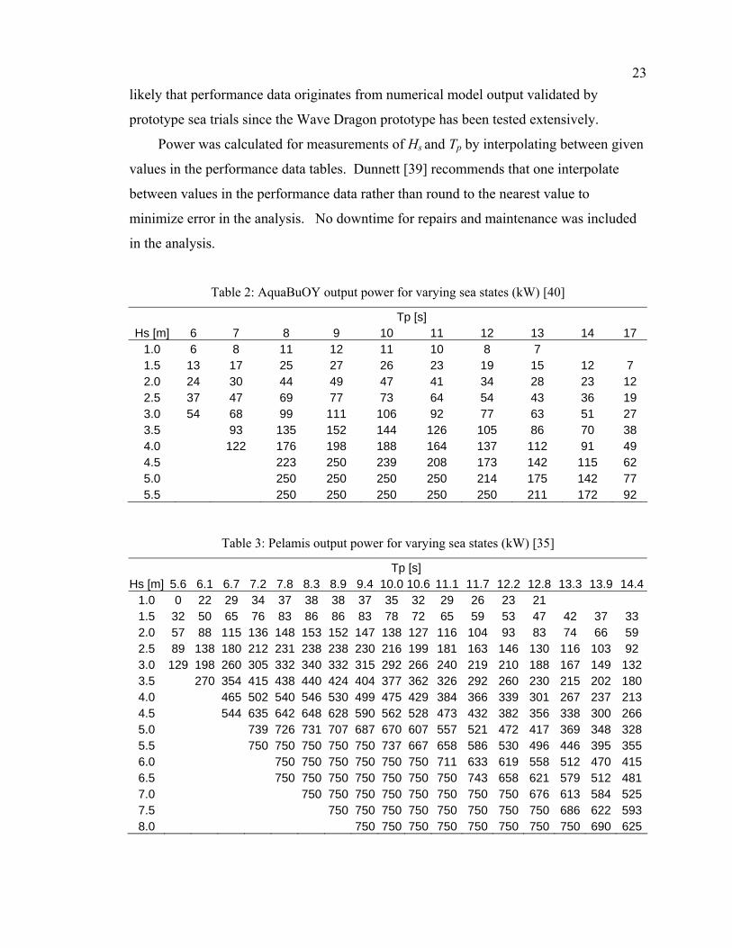
23likely that performance data originates from numerical model output validated by
prototype sea trials since the Wave Dragon prototype has been tested extensively.
Power was calculated for measurements of Hs and Tp by interpolating between given
values in the performance data tables. Dunnett [39] recommends that one interpolate
between values in the performance data rather than round to the nearest value to
minimize error in the analysis. No downtime for repairs and maintenance was included
in the analysis.
Table 2: AquaBuOY output power for varying sea states (kW) [40]
Tp [s] Hs [m] 6 7 8 9 10 11 12 13 14 17
1.0 6 8 11 12 11 10 8 7 1.5 13 17 25 27 26 23 19 15 12 7 2.0 24 30 44 49 47 41 34 28 23 12 2.5 37 47 69 77 73 64 54 43 36 19 3.0 54 68 99 111 106 92 77 63 51 27 3.5 93 135 152 144 126 105 86 70 38 4.0 122 176 198 188 164 137 112 91 49 4.5 223 250 239 208 173 142 115 62 5.0 250 250 250 250 214 175 142 77 5.5 250 250 250 250 250 211 172 92
Table 3: Pelamis output power for varying sea states (kW) [35]
Tp [s] Hs [m] 5.6 6.1 6.7 7.2 7.8 8.3 8.9 9.4 10.0 10.6 11.1 11.7 12.2 12.8 13.3 13.9 14.4
1.0 0 22 29 34 37 38 38 37 35 32 29 26 23 21 1.5 32 50 65 76 83 86 86 83 78 72 65 59 53 47 42 37 33 2.0 57 88 115 136 148 153 152 147 138 127 116 104 93 83 74 66 59 2.5 89 138 180 212 231 238 238 230 216 199 181 163 146 130 116 103 92 3.0 129 198 260 305 332 340 332 315 292 266 240 219 210 188 167 149 1323.5 270 354 415 438 440 424 404 377 362 326 292 260 230 215 202 1804.0 465 502 540 546 530 499 475 429 384 366 339 301 267 237 2134.5 544 635 642 648 628 590 562 528 473 432 382 356 338 300 2665.0 739 726 731 707 687 670 607 557 521 472 417 369 348 3285.5 750 750 750 750 750 737 667 658 586 530 496 446 395 3556.0 750 750 750 750 750 750 711 633 619 558 512 470 4156.5 750 750 750 750 750 750 750 743 658 621 579 512 4817.0 750 750 750 750 750 750 750 750 676 613 584 5257.5 750 750 750 750 750 750 750 750 686 622 5938.0 750 750 750 750 750 750 750 750 690 625

24
Table 4: Wave Dragon output power for varying sea states (kW) [39]
Tp [s] Hs [m] 5 6 7 8 9 10 11 12 13 14 15 16 17
1.0 150 250 360 360 360 360 360 360 320 280 250 220 180 2.0 640 700 840 900 1190 1190 1190 1190 1070 950 830 710 590 3.0 1450 1610 1750 2000 2620 2620 2620 2360 2100 1840 1570 13104.0 2840 3220 3710 4200 5320 5320 4430 3930 3440 2950 24605.0 4610 5320 6020 7000 7000 6790 6090 5250 3950 33006.0 6720 7000 7000 7000 7000 7000 6860 5110 42007.0 7000 7000 7000 7000 7000 7000 6650 5740
Potential locations for a WEC device were assessed based on their average annual
capacity factor (CF) and relative proximity to the existing grid. CF is defined as the total
output energy from a device over a period of time divided by the potential output energy
if the device had been operating at full capacity the entire time. This represents average
expected output energy for each device with respect to each unit of capacity installed, and
is important considering the high capital cost of devices. A high CF reduces the number
of devices required to reach a certain level of energy output, therefore resulting in a lower
capital cost. Hourly output wave power was used to determine monthly CF for each
device at each location for all years of data. From this the average monthly CF was
determined for each device at each site, leading to an average annual CF (Table 5), with
the highest capacity factors seen at the South Moresby, West Moresby, and West Dixon
Entrance locations. Additionally, the highest capacity factors were seen with the Wave
Dragon device.
An analysis of the distance from the buoy location to shore, as well as the distance
on shore to the nearest grid connection point, was done via Google Maps [41]. It can be
seen that the distance for the West Dixon Entrance and South Moresby locations are
significantly larger than the other locations. Note that it was assumed that no over land
transmission lines would be allowed in the Gwaii Haanas National Park Reserve.
The West Moresby location appears to be an interesting option as the distance to the
grid is much smaller and it also has a high CF. It is likely that other locations along the
west coast of Moresby Island closer to the Moresby Lake Hydro facility, where power
can be transmitted to the grid, have a similar wave climate. Therefore, the transmission
distance could be even less than stated. Although the CF for the Central Dixon Entrance
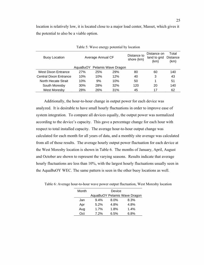
25location is relatively low, it is located close to a major load center, Masset, which gives it
the potential to also be a viable option.
Table 5: Wave energy potential by location
Buoy Location Average Annual CF Distance to shore (km)
Distance on land to grid
(km)
Total Distance
(km)
AquaBuOY Pelamis Wave Dragon West Dixon Entrance 27% 25% 29% 80 60 140
Central Dixon Entrance 10% 10% 12% 40 3 43 North Hecate Strait 10% 9% 10% 50 1 51
South Moresby 30% 28% 32% 120 20 140 West Moresby 28% 26% 31% 45 17 62
Additionally, the hour-to-hour change in output power for each device was
analyzed. It is desirable to have small hourly fluctuations in order to improve ease of
system integration. To compare all devices equally, the output power was normalized
according to the device’s capacity. This gave a percentage change for each hour with
respect to total installed capacity. The average hour-to-hour output change was
calculated for each month for all years of data, and a monthly site average was calculated
from all of those results. The average hourly output power fluctuation for each device at
the West Moresby location is shown in Table 6. The months of January, April, August
and October are shown to represent the varying seasons. Results indicate that average
hourly fluctuations are less than 10%, with the largest hourly fluctuations usually seen in
the AquaBuOY WEC. The same pattern is seen in the other buoy locations as well.
Table 6: Average hour-to-hour wave power output fluctuation, West Moresby location
Month Device AquaBuOY Pelamis Wave Dragon
Jan 9.4% 8.0% 8.3% Apr 5.2% 4.8% 4.8% Aug 1.7% 1.8% 1.4% Oct 7.2% 6.5% 6.8%

26
Chapter 4
Modeling the Haida Gwaii Network In order to predict the impact of integrating intermittent tidal and wave power into
the Haida Gwaii generation system, an energy system model was built. This chapter
outlines the existing network and the mixed integer optimization model that was built to
simulate the network, including model parameterizations and input data.
4.1 Existing Network Haida Gwaii is an archipelago made up of approximately 150 islands off the
northwest coast of British Columbia (BC), Canada. Dominated by two main islands,
Graham to the north and Moresby to the south, Haida Gwaii stretches for approximately
300 km. According to the 2006 Statistics Canada census, the population of Haida Gwaii
was 5063 [2] with the majority of the population living on Graham Island in the towns of
Masset, Old Masset, Port Clements, Tlell, Skidegate and Queen Charlotte City, and on
Moresby Island in the community of Sandspit.
The two independent generation distribution systems on Haida Gwaii are referred to
as North and South and are only 10 km apart at their nearest point [2]. The north system,
or grid, serves approximately 1400 customers in the towns of Masset, Old Masset, and
Port Clements, and the south grid serves 1600 customers in Tlell, Skidegate, Queen
Charlotte City and Sandspit [2]. Each customer can represent a household or more than
one person. The north grid is powered solely by Masset Diesel Generation Station (DGS)
which has a capacity of 11.4 MW and is composed of 7 separate generation units of
varying size [3, 22]. Its peak load and total generation in 2005 were 4.8 MW and 25.5
GWh respectively [3, 22]. The south grid is powered primarily by an independent power
producer (IPP) hydro electric power plant with a capacity of 5.7 MW [2, 22]. This
facility, owned and operated by EPCOR Power L.P., uses Moresby Lake on Moresby
Island as its reservoir. There is also a BC Hydro owned backup diesel generation system
at Sandspit with a capacity of 9.15 MW, composed of 7 separate generation units of
varying size [3, 22]. In 2005, the peak load of the south grid was 5.6 MW with BC
Hydro generating a total of 8.2 GWh from Sandspit DGS and buying 18.2 GWh, equal to
70% of annual demand, from the IPP [3, 22].

27Figure 5 shows the geographical layout of the generation systems. Individual
generation units at each DGS are detailed in Table 7. Transmission of electricity is
generally done via 25 kV 3-phase transmission lines; however, there are several
exceptions including the submarine cable linking Graham Island to Moresby Island via
Skidegate Inlet and the IPP owned 69 kV line linking the Moresby Lake hydro facility to
the southern grid [3]. Transmission line details are provided in Table 8 below. Note that
the transmission system is simplified for this analysis.
Figure 5: Haida Gwaii electricity system (data from [3])

28Table 7: Diesel generating units in Haida Gwaii [3]
Masset DGS Sandspit DGS
Unit Size (kW) Unit Size (kW)MASG1 2108 M124G1 2500 MASG2 2108 M178G1 1600 MASG3 2108 M167G1 850 M125G1 2500 SPTG1 1600 M172G1 850 SPTG2 1600 M174G1 850 SPTG3 1000
M165 1000 SPTG4 1000
Table 8: Haida Gwaii transmission line information (data from [3])
Link Assigned
Label Bus
connections Voltage
(kV) Length (km)
Resistance [43]
(Ohms/km)
Current Carrying
Capacity [44] (A) Notes
a 1-2 25 50 0.1688 460 3 phase, 336.4
kcmil conductor size, ASC type
c 3-4 25 40 0.3368 295 3/0 AWG, single phase, ASC
d 4-5 25 5 0.5351 225 1/0 AWG submarine cable
e 5-6 69 49 0.3368 295 3/0 AWG, single phase, ASC*
* Assumed line type
4.2 Network Optimization Model To study the economic and technical implications of integrating tidal power and
linking the two grids, a network model that minimizes cost subject to a set of constraints
was constructed. The model consists of six buses representing transmission substations
with five links connecting them. The north grid is represented by bus 1 and 2, where 1
represents the town of Masset and 2 Port Clements. For the south grid, bus 3 represents
Tlell, bus 4 Skidegate and Queen Charlotte City, bus 5 Sandspit, and bus 6 Moresby Lake
hydro facility. Each bus can include power contributions from generators and other
buses, as well as power leaving for other buses and local demand. Note that bus 1
includes a sink where energy can be dumped as needed and any of these variables can be
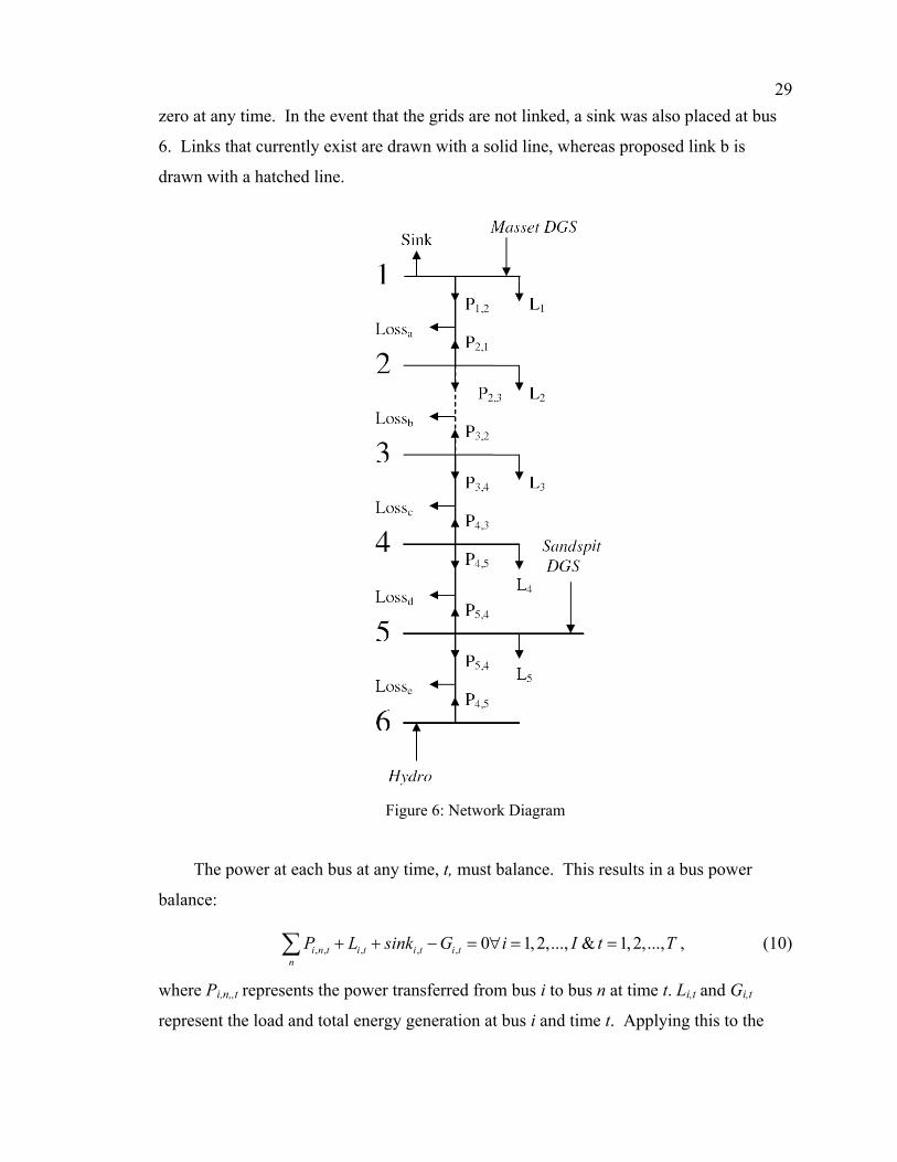
29zero at any time. In the event that the grids are not linked, a sink was also placed at bus
6. Links that currently exist are drawn with a solid line, whereas proposed link b is
drawn with a hatched line.
Figure 6: Network Diagram
The power at each bus at any time, t, must balance. This results in a bus power
balance:
, , , , , 0 1, 2,..., & 1,2,...,i n t i t i t i tn
P L sink G i I t T+ + − = ∀ = =∑ , (10)
where Pi,n,,t represents the power transferred from bus i to bus n at time t. Li,t and Gi,t
represent the load and total energy generation at bus i and time t. Applying this to the

30above network gives six equations, one for each bus, which are used as constraints in the
model. Note the non-negativity of load, energy generated, and energy sent to the sink,
, , ,, , 0 1,2,..., & 1,2,...,i t i t i tL G sink i I t T≥ ∀ = = , (11) Transmission line constraints include line losses and current carrying capacity.
Since power leaving a bus is defined as positive, power is entering the link from opposite
directions. Figure 7 below shows the power balance on each link. This results in one of
the power terms being negative. Furthermore, one of the power terms must be smaller
than the other to make up for the transmission losses which are determined from the
following equation,
2 2
, , , ,, 2
max( , )1, 2,..., & 1, 2,...,i n t n i t j
j tj
P P RLoss j N t T
V= ∀ = = , (12)
where Rj and Vj represent the resistance and voltage of link j, and N represents the total
number of links. The current on each line is constrained so that the maximum allowable
current, or current carrying capacity, is not exceeded. Table 8 outlines the reported
voltages, lengths, and type of each existing line. Resistances and current carrying
capacity were estimated from the type of line [43, 44]. The link from bus 2 to 3 is
assumed to be 20 km in length, 25 kV, 3/0 AWG, single phase, ASC type, where length
and voltage were estimated based on the Haida Gwaii Community Electricity Plan
released in April 2008 [2].
Figure 7: Power Balance of the link between bus i and n (modified from [42])
Multiple constraints exist due to the nature of each generator. For dispatchable
generators, where output can be increased or decreased as desired, generation cannot
exceed capacity
, , 1, 2,..., & 1,2,...,d t d capG G d D t T≤ ∀ = = , (13)

31where Gd,t is output from dispatchable generator d at time t and Gd,cap is the capacity of
generator d. Generators must also stay within ramping rate limits dependent on the type
of generator. Diesel generators in the Haida Gwaii network are capable of ramping up to
their full capacity from zero output within the one-hour time step used in this model [45].
Similarly, ramping down can be done within a period of one hour, indicating that
ramping rate constraints are, in fact, not needed in this case. BC Hydro’s preference is to
operate all diesel generation units at a minimum output level of 50% part load [3, 22].
For example, this means that a 1 MW unit can operate at a minimum level of 0.5 MW
while on. This led to the inclusion of a binary variable, xd,t,, that indicates whether a unit
is operating during a specific time period, where xd,t, is equal to 1 if the unit is on and 0 if
the unit is off.
In reality, hydro power generation is limited by reservoir volume. Unfortunately
temporal data on reservoir volume were unavailable; however, actual hourly power
generated in 2006 from the hydro facility was available [3]. Therefore, hourly generation
from the hydro facility was used as a direct input to the model and assumed must-take to
match the current operating strategy [3].
Operating costs have been assigned to each diesel generating unit at Masset and
Sandspit DGS. The fuel costs of the diesel generating units were determined from
industry-reported fuel consumption values (gal/hr) as a function of part load [46] and a
cost of 1$/L for diesel fuel [22]. A second order polynomial curve was fit to the data for
each size of generator and plotted in a total production cost curve (Figure 8). The cost of
operating each unit at the minimum operational level of 50% part load was determined
from the total production cost curve. The incremental cost of increasing the output power
another unit was determined by calculating the slope of the total production curve at 10
different power levels (Figure 9). This approach is taken from Muckstadt [13] and allows
the objective function to be linear, thereby greatly reducing the computational
complexity. The number of cost levels for each generator is represented by Kd and in this
case is set at 10 for all generators. The incremental generation for each cost level is
represented by Md,k. In Figure 9, Md,k is equal to 0.05 MW for all cost levels, or 5% of
the total generator capacity. Incremental generation levels were kept at 5% of total
generator capacity for all generators.

32
y = 63.504x2 + 168.89x + 35.91
0
50
100
150
200
250
300
0.2 0.4 0.6 0.8 1Power (MW)
Tota
l Pro
duct
ion
Cos
t ($/
hr)
Figure 8: Total production cost curve for a 1
MW capacity diesel generator
200
225
250
275
300
0.2 0.4 0.6 0.8 1
Power (MW)
Incr
emen
tal P
rdn
Cos
t ($/
MW
-hr)
Figure 9: Incremental production cost curve for
a 1 MW capacity diesel generator
Costs were also applied to maintenance and cycling of diesel generators. The cost
associated with maintenance for the diesel generation units, cmaint, was calculated based
on an overhaul life estimate of 30,000 hours in operation and overhaul cost of $200,000,
resulting in a cost of $6.67 per hour in operation [45]. Cycling of diesel generators leads
to an increased rate of degradation of the unit over time [47]. As a result, operators avoid
constantly shutting down and starting up units. To mimic this behaviour, a cost was
applied to the action of starting up and shutting down a generator where csu,d is the start-
up cost and csd,d, is the shut-down cost of generator d.
The objective of the model is to minimize total system operating cost subject to the
constraints outlined in equations (10), (11), (12) and those shown below in equations (15)
through (20). Note that equation (13) is implicit in the objective function. The problem
statement, modified from [13], is as follows:
, , , , , , , , , ,mingensT K
su d d t sd d d t min d d t d k t d k d k t maint d tt d k
c w c z h c x M h g y c x⎡ ⎤+ + + +⎢ ⎥⎣ ⎦∑∑ ∑ (14)
s.t. , , ,0 d k t d ty x≤ ≤ (15) , , , 1d t d t d tw x x −≥ − (16) , , 1 ,d t d t d tz x x−≥ − (17) , ,, 0d t d tw z ≥ (18)

33 ,d tx binary≡ (19)
, ,i n tP LineCapacity≤ , (20) where cmin,d is the cost in dollars of operating generator d at its minimum capacity for 1
hour, ht is the number of hours in period t, gd,k is the incremental production cost of
operating generator d at cost level k, and yd,k,t is the percent of available capacity, Md,k,
that is used in period t. Equation (15) illustrates that yd,k,t can only be greater than zero if
xd,t is 1, indicating that the unit is on. It can also be seen from equation (16) that wd,t
equals 1 if unit d is started in period t and zero otherwise. Likewise, equation (17) shows
that zd,t equals 1 if unit d is shut down in period t and zero otherwise. Equation (20)
indicates that the power along a line cannot exceed the capacity of that line determined
from rated voltage and current carrying capacity.
Since both hydro and tidal power are considered non-dispatchable in the model,
costs associated with them were not optimized. Rather, fixed costs associated with hydro
and tidal power can be added to the optimized solution to find the total system cost.
Total carbon dioxide emissions were calculated for each case based on fuel
consumption of the diesel generators and 10.1kg CO2/gal(US) of diesel fuel [48] such
that
, ,E=genT
d t d tt d
e G∑∑ , (21)
where E is total CO2 emissions in time period T and ed,t is kg CO2 per MWh for generator
d at time t. To find ed,t, industry-reported diesel fuel consumption data (gal/hr) as a
function of output [46] was converted to kg CO2/MWh and a quadratic equation was fit
to the data (Figure 10).
The model was built using a Matlab (The MathWorks Inc.)/General Algebraic
Modeling System (GAMS Development Corp.) environment, where data was input into
Matlab and GAMS solved the optimization through a call from Matlab. GAMS solved
the problem with the Cplex solver, which utilizes a branch and cut algorithm to solve a
series of linear subproblems and converge on a solution for the mixed integer linear
program [49].
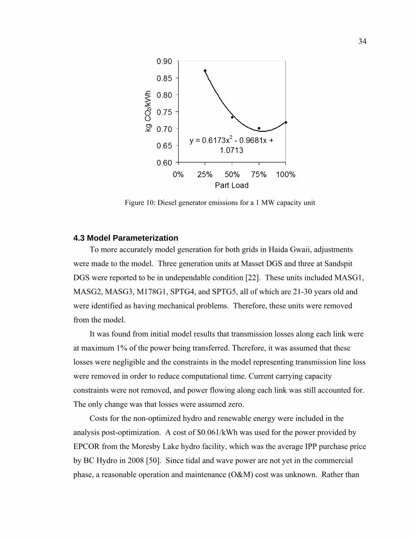
34
Figure 10: Diesel generator emissions for a 1 MW capacity unit
4.3 Model Parameterization To more accurately model generation for both grids in Haida Gwaii, adjustments
were made to the model. Three generation units at Masset DGS and three at Sandspit
DGS were reported to be in undependable condition [22]. These units included MASG1,
MASG2, MASG3, M178G1, SPTG4, and SPTG5, all of which are 21-30 years old and
were identified as having mechanical problems. Therefore, these units were removed
from the model.
It was found from initial model results that transmission losses along each link were
at maximum 1% of the power being transferred. Therefore, it was assumed that these
losses were negligible and the constraints in the model representing transmission line loss
were removed in order to reduce computational time. Current carrying capacity
constraints were not removed, and power flowing along each link was still accounted for.
The only change was that losses were assumed zero.
Costs for the non-optimized hydro and renewable energy were included in the
analysis post-optimization. A cost of $0.061/kWh was used for the power provided by
EPCOR from the Moresby Lake hydro facility, which was the average IPP purchase price
by BC Hydro in 2008 [50]. Since tidal and wave power are not yet in the commercial
phase, a reasonable operation and maintenance (O&M) cost was unknown. Rather than

35speculating on a cost, no O&M cost was included and the maximum economically viable
cost for the project was determined, which includes the project’s O&M costs.
Since the actual cost of starting-up or shutting down a unit can not easily be
determined, and estimates for these costs vary widely [45, 47], it was decided to keep the
values of csu,d and csd,d, low to mimic the behaviour of reduced cycling while not affecting
overall cost. A sensitivity study was done for the linked grids case (Figure 11) as well as
the separate north and south grids case. A value of $200 was chosen for both csu,d and
csd,d as it reduced the number of start-ups by 50% while only increasing the total
operational cost of the system by 2%.
Figure 11: Sensitivity results for linked grids case, month of January data
The model was validated through several means. It was tested with multiple simple
cases to confirm that it provided the least cost solution and no constraints were violated.
Furthermore, the problem was solved with three different solvers including Cplex,
Coincbc and Coinglpk, all of which provided the same solution.
4.4 Model Input Data
4.4.1 Load Data Load data was supplied by BC Hydro. For the south grid, hourly generation data for
both the IPP facility and Sandspit DGS were provided for 2007. It was assumed that the
combination of these two generation loads at each hour was equal to the south grid’s

36demand. For the north grid, actual hourly load data was not available; rather, the
maximum and minimum demand day in a given month was provided for 2005 (Figure
12). To manufacture daily load data for the north, a distribution profile of data for each
hour was needed.
Figure 12: Masset DGS Jan-05 maximum and minimum load [3]
Since the only extensive data available were from the south grid, load data
categorized by hour for each month from the south grid were analysed with a Lilliefors
test and found to follow a normal distribution 82% of the time at a significance level of
1%. Each hour in the months of January, April, August and October was analyzed,
resulting in 96 different test results. The Lilliefors test, similar to the Kolmogorov–
Smirnov test, uses the test statistic
max ( ) ( )KS SCDF x CDF x= − , (22) where SCDF is the empirical cumulative distribution function (CDF) estimated from the
sample and CDF is the normal CDF with mean and standard deviation equal to the mean
and standard deviation of the sample [51]. The data were also tested for other
distributions and were found to fit the normal distribution the best. The load for each
hour in a given month in the north grid was assumed to follow a normal distribution
similar to that of the south. Based on this assumption, multiple days of data were
randomly generated for each month, resulting in a year of hourly north load data.

37Another problem arose in that load is distributed throughout the grid, but only total
load for each grid was known. Therefore, load at each bus was calculated based on the
population at each bus:
ii tot
tot
popL Lpop
⎡ ⎤= ⎢ ⎥⎣ ⎦
, (23)
where Li represents load at bus i, popi represents the population at bus i, poptot represents
the total population of the grid in which bus i is located, and Ltot represents the total load
of that grid. Individual community populations were provided by the 2006 Statistics
Canada census [2].
4.4.2 Tidal Power Data Hourly tidal power data for Masset Sound was calculated for an entire year using the
model developed by Blanchfield [27]. Turbine drag factors varying from 0.001 to 0.046
at increments of 0.001 were used, resulting in 46 different levels of tidal input. This
corresponded to a maximum of 0.22 to 9.85 MW of tidal power available in a given hour.
It is assumed that the maximum tidal power available is equal to the installed tidal
capacity. Tidal power penetration is the level of installed capacity over peak demand.
Given that the maximum load was 4.79 MW for the north grid and 9.85 MW for both
grids combined, this represents maximum power penetration levels of 206% for the north
grid alone and 100% for the linked grid case.
Another way of evaluating the level of tidal input is the ratio of total tidal energy
produced to the total energy demand, often referred to as energy penetration. In the case
of the linked grid system this level increases from 1% to 55%, and for the non-linked
system it ranges from 3% to130%. This level of input in the north grid, although much
higher than what is realistically expected, is informative as it allows direct comparison
between the two options; however, if installed, excess power could be used for residential
heating or stored for later use.
4.4.3 Wave Power Data Two locations were considered for a wave power plant: Central Dixon Entrance
(CD) and West Moresby (WM). Although CD has a low annual capacity factor, its
location relative to a major load center, Masset, potentially makes it a more viable option.
The WM location was more promising, with an annual capacity factor of 26-31%

38depending on the device used, although farther from major load centers. The Pelamis
device was selected as it is the most advanced device having undergone significant sea
trials as mentioned before. Installed capacity ranged from one to thirteen devices, each
sized at 750 kW. This corresponds to a maximum installation of 9.75 MW, or a
maximum power penetration of 99% and 204% for the linked and non-linked grid cases,
respectively.
Hourly wave power from the Pelamis WEC was manufactured for all years of
available data using the technique described in Section 3.3. Each month was analysed
and an individual year was selected that had a monthly CF closest to the average monthly
CF for that site. This meant that data from different years were used for each month.
The average annual energy penetration with 13 Pelamis devices installed for the CD
location is 14% for the linked grid and 34% for the non-linked grid. The same values for
the WM location are 37% and 86%, reflecting the higher CF available at the WM
location.

39
Chapter 5
Optimization Results The following chapter discusses the results from the optimization model. First, the
effect of linking the grids is analyzed. Second, integrating tidal power from Masset
sound is considered, and, third, integrating wave power from both the CD and WM
locations is reviewed. To do this, the models were initially run with no renewable energy
input, followed by incremental levels of renewable capacity installed. Tidal energy was
assumed to be input directly into the Masset bus, as was wave energy from the CD
location. This meant that when the grids were not linked, renewable energy contributed
to the north grid alone. However, wave energy from the WM location was input into the
Moresby Lake bus, thereby contributing solely to the south grid when the grids were not
linked.
To represent variation among seasons, four separate two week time periods were
modeled. These two week periods were selected from January, April, August and
October. Annual results presented below are based on an average of the four time
periods analyzed.
5.1 Linking the Grids One of the immediate concerns with linking the grids is the resulting effect on
system operation. The duty cycle of each generating unit, defined as the percent of time
in operation, was determined when the grids were both linked and not linked (Figure 13).
Linking the grids appears to reduce the number of generating units required. This can be
seen in Figure 13, where duty cycles for two of the units, M174G1 and M165G1, are zero
for the linked case. Conversely, the non-linked case requires all generators to operate at
some point, and in all but one case the generators are used more often. An example of
this is M172G1, the 0.85 MW capacity unit in Masset, which has a duty cycle of 75%
when the grids are separate and 14% when they are linked. The exception to this rule is
M124G1, the 2.5 MW capacity unit in Sandspit, whose duty cycle increases from 10%
when the grids are not linked to 97% when they are linked. These results indicate that
linking the grids would lead to heavy use of the 2.5 MW units and very light use of the
other smaller units.

40Furthermore, fewer start-ups and shut-downs are required for the linked case than
the non-linked case. The average number of cycles, where a cycle represents a generator
turning on and off, over a two week period for each generator was 5 or less for the linked
case and 7 for the non-linked case (Figure 14). In fact, the number of cycles for most
generators is well below BC Hydro’s operational policy of cycling each generator no
more than once a day [3, 22], or a maximum of 14 cycles for each generator for the two
week period.
Figure 13: Diesel generator duty cycle, no
renewable power
Figure 14: Average number of diesel generator
cycles, no renewable power
Less than 1% of the energy produced was sent to the sink in all cases analyzed. This
excess energy is due to the minimum operational level constraints placed on the
generators, as well as the decision to run a larger unit than is required, and dump excess
energy, rather than shut the unit down for a short period of time. Energy sent to the sink
is always higher for the non-linked grid than the linked one.
The average power sent along proposed line b (Figure 6) was 1.1MW. Although
power travels in both directions, it traveled most often in the south to north direction,
indicating that power was being transferred from the south to the north grid. This is
largely due to the extra power generated by M124G1, which is sent to the north grid and
makes M174G1 in Masset redundant (shown in Figure 13).

41The only line that reached its carrying capacity, and therefore limited generator
operation, was line d, the underwater cable linking Graham and Moresby Islands. This
capacity was reached only when the grids were linked. Most of the population, and
therefore also the energy demand, is located on Graham Island [2]. Figure 13 illustrates
that when the grids are linked the optimal solution is to reduce generation from Masset
DGS and increase output from Sandspit DGS. This increase in power from Sandspit
DGS must be sent along line d in order to be delivered to the main load center. In the
non-linked grids case, the south grid load never exceeded the carrying capacity of line d,
so it was a non-issue. However, in the linked grids case, the low carrying capacity of line
d acted as a bottleneck in the network and restricted how much power could be sent from
Sandspit DGS and Moresby Lake Hydro Facility to the north grid.
Carbon dioxide emissions were reduced only slightly for the linked grid over the
non-linked grid. Average annual emissions were 0.435 kg/kWh for the current non-
linked case and 0.434 kg/kWh for the linked case. The most notable difference in
emissions was an increase in emissions during August, when hydro output is at its lowest.
The total cost of generation for each time period was determined by adding the set
cost of hydro to the minimized diesel cost. To find the optimal average cost of electricity
for the year, the costs of the four periods analyzed were combined and divided by the
total energy consumption. This resulted in a cost of 0.194 $/kWh and 0.191 $/kWh for
the non-linked and linked cases respectively. Given the average cost of electricity and
total annual consumption [22], the total savings due to linking the grids in one year of
operation was calculated as $178,000 CAN. Estimates for the capital cost of linking the
grid range from $10-15M CAN [52].
5.2 Integrating Tidal Power The addition of tidal power to the system increases the complexity of system
operation. A typical snapshot of diesel generator output with 5 MW of tidal capacity
installed is shown in Figure 15. This is from the non-linked grids case and shows only
those generators in the north grid affected by the tidal addition. It can be seen that diesel
generating units must cycle and ramp up and down more often to compensate for the
varying tidal energy. Furthermore, decisions on when to cycle generating units become
more complex when tidal power is added to the system. For example, at hour 27 the

42level of tidal energy input exceeds the load; however, M174G1 continues to run. This
decision is made because it is cheaper to keep the unit running at its minimum
operational level and curtail tidal energy than to shut the unit down and start it up again
in the following hour.
Figure 15: Typical generation, 5 MW installed tidal capacity
As installed tidal capacity increases, the duty cycle of those diesel units most often
operated declines for both the linked and non-linked cases. Optimization results indicate
that the largest units available should be used the most often. For the non-linked case, the
only generators affected were, of course, those in the north grid (shown in Figure 16).
The duty cycle for M125G1, the 2.5 MW unit in Masset, was initially at 100% with no
tidal input, but declined to 56% with 5 MW of tidal capacity installed. Similarly, the
duty cycle for M165, the 1 MW unit in Masset, decreased from 100% with no tidal input
to 37% with 5 MW installed. It is interesting to note that the duty cycle of these two
generators does not begin to decrease until installed tidal capacity reaches 2.3 MW.
Rather, before 2.3 MW of tidal capacity is installed the duty cycle of the smaller diesel
unit, M172G1, decreases 50%, showing that diesel generation is first replaced from the
smaller generators.

43Figure 17 depicts the change in duty cycle for each diesel generating unit as installed
tidal capacity increases for the linked case. It was previously noted that linking the grids
would eliminate the use of generators M174G1 and M167G1, and increase the use of the
two 2.5 MW capacity units, M125G1 and M124G1, so that they were used far more often
than the rest. When tidal power was added to the linked system M174G1 and M167G1
maintained a duty cycle of 0% until installed tidal capacity exceeded 2 MW. Likewise,
M172G1, the other 0.85 MW capacity unit in Masset DGS, dropped from 14% to 0%
duty cycle when tidal power was input and stayed out of use until 2.3 MW of tidal
capacity was installed. Unlike the non-linked case, the duty cycle of the larger units
decreased quickly as tidal capacity increased for approximately the first 5 MW of tidal
capacity installed. For example, the duty cycle for M124G1 decreased 76% when 5 MW
of tidal capacity was installed. It appears that initially diesel generation from the larger
units is being replaced by tidal energy and generation from several smaller units.
However, after approximately 5 MW of tidal capacity is installed the duty cycle for the
smaller units begins to decrease and the duty cycle of the larger units levels off. This
shows that there is a minimum duty cycle required for the larger units due to the cyclic
nature of tidal power.
Figure 16: Diesel generator duty cycle vs.
installed tidal capacity, non-linked case
Figure 17: Diesel generator duty cycle vs.
installed tidal capacity, linked case

44As installed tidal capacity increased, the cyclical nature of the tidal power was
amplified, resulting in an increase in the number of cycles for each diesel generating unit.
The most significant increase for both the linked and non-linked cases was seen in
M125G1, which reached its maximum allowable number of cycles for the non-linked
case when installed tidal capacity was 2.5 MW. Likewise, M125G1 reached its
maximum allowable number of cycles for the linked case when installed tidal capacity
was 3.2 MW. This indicates that above these levels of installed tidal capacity the
minimum cost schedule determined from optimization cannot be followed.
Average diesel generation, as well as tidal energy used and curtailed tidal energy, is
shown in Figure 18 for the non-linked and linked cases with varying tidal capacity. All
values have been normalized by total diesel generation from the case with no tidal energy
input, which represents the total load minus the must-take hydro input. Diesel generation
is always lower for the linked case than the non-linked case with the same level of tidal
capacity installed, indicating tidal energy can replace more diesel generation in the linked
case. Consequently, there is more curtailed tidal energy in the non-linked case. Levelling
off of diesel energy generated as tidal capacity increases can also be seen, showing that
increasing tidal capacity beyond a certain level provides less benefit as less diesel
generation can be replaced. It also shows that excess tidal energy begins to grow quickly
above 4 MW of tidal capacity installed, indicating that storage, or allowing hydro to vary,
would be beneficial above this level.
The average CF of the tidal power plant, CFplant, was determined as shown:
usedplant
cap
TECF
TP T= ∑ , (24)
where TEused represent the total tidal energy absorbed by the grid, TPcap represents the
tidal plant installed capacity, and T represents the total number hours in the time period
analyzed. CFplant is never 100% due to the cyclic nature of the tides. In fact, assuming
all tidal energy produced could be absorbed by the grid, the average annual plant CF for
the Masset Sound site was 39%. This represents the upper CF limit possible for the tidal
plant and is henceforth referred to as the resource CF.
The tidal plant CF with increasing installed capacity is shown in Figure 19 for both
the linked and non-linked cases. An interesting behaviour is the increase in plant CF for

45the non-linked case between 2.3 and 4 MW of tidal capacity installed. This occurs
because at this point tidal energy begins to replace significant amounts of diesel
generation from M125G1 and M165. This can be seen in Figure 16 where the duty cycle
of M125G1 drops from 95% at 2.3 MW installed to 60% at 4 MW installed. Likewise
the duty cycle of M165 drops from 98% to 34% over the same period. Above 4 MW of
installed tidal capacity, tidal energy cannot replace diesel generation at the same rate due
to diesel generation constraints and curtailed tidal energy grows (also shown in Figure
18). This leads to the subsequent decrease in CF shown.
Figure 18: Energy contribution by source vs.
installed tidal capacity
Figure 19: Optimized annual tidal plant capacity
factor
Average power flowing along each line for the linked case is shown in Figure 20. In
addition to the average power, the mean power on each line was found, indicating the
most frequent direction of power flow. Power on proposed line b flowed primarily in the
south to north grid direction until installed tidal capacity reached 5 MW, at which point
power flowed from north to south grid more often. The carrying capacity of line d was
reached in the linked case, leading to limits on diesel generation from Sandspit DGS. It
is clear from Figure 20 that link d, which is also the most heavily constrained line, has the
highest level of power flowing along it. This is also true for the non-linked case,
although it never reaches its capacity when separate grids are in place. No other lines
reached their carrying capacity for either the linked or non-linked cases. For the non-
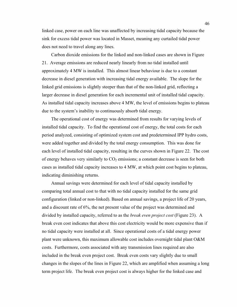
46linked case, power on each line was unaffected by increasing tidal capacity because the
sink for excess tidal power was located in Masset, meaning any curtailed tidal power
does not need to travel along any lines.
Carbon dioxide emissions for the linked and non-linked cases are shown in Figure
21. Average emissions are reduced nearly linearly from no tidal installed until
approximately 4 MW is installed. This almost linear behaviour is due to a constant
decrease in diesel generation with increasing tidal energy available. The slope for the
linked grid emissions is slightly steeper than that of the non-linked grid, reflecting a
larger decrease in diesel generation for each incremental unit of installed tidal capacity.
As installed tidal capacity increases above 4 MW, the level of emissions begins to plateau
due to the system’s inability to continuously absorb tidal energy.
The operational cost of energy was determined from results for varying levels of
installed tidal capacity. To find the operational cost of energy, the total costs for each
period analyzed, consisting of optimized system cost and predetermined IPP hydro costs,
were added together and divided by the total energy consumption. This was done for
each level of installed tidal capacity, resulting in the curves shown in Figure 22. The cost
of energy behaves very similarly to CO2 emissions; a constant decrease is seen for both
cases as installed tidal capacity increases to 4 MW, at which point cost begins to plateau,
indicating diminishing returns.
Annual savings were determined for each level of tidal capacity installed by
comparing total annual cost to that with no tidal capacity installed for the same grid
configuration (linked or non-linked). Based on annual savings, a project life of 20 years,
and a discount rate of 6%, the net present value of the project was determined and
divided by installed capacity, referred to as the break even project cost (Figure 23). A
break even cost indicates that above this cost electricity would be more expensive than if
no tidal capacity were installed at all. Since operational costs of a tidal energy power
plant were unknown, this maximum allowable cost includes overnight tidal plant O&M
costs. Furthermore, costs associated with any transmission lines required are also
included in the break even project cost. Break even costs vary slightly due to small
changes in the slopes of the lines in Figure 22, which are amplified when assuming a long
term project life. The break even project cost is always higher for the linked case and

47low levels of installed tidal capacity, therefore making it more economical to integrate
tidal power when the grids are connected and at low penetration levels. Overnight
capital cost estimates from the US Energy Information Administration, in terms of 2007
US dollars, are on the order of 2000 $/kW for onshore wind, 3800 $/kW for offshore
wind, 2300 $/kW for hydroelectric, and 5500 $/kW for photovoltaic [53]. These
estimates do not include O&M or transmission line costs however.
Figure 20: Average line power flow vs.
installed tidal capacity, linked case
Figure 21: Average CO2 emissions vs. installed
tidal capacity
Figure 22: Annual operational cost of energy
vs. installed tidal capacity
Figure 23: Break even project cost vs. installed
tidal capacity

48It is apparent from this analysis of the technical and economic impacts of tidal
power integration into the Haida Gwaii grid that tidal power is feasible at low levels of
installation. A similar analysis will now be done on the impacts of wave power
integration.
5.3 Integrating Wave Power
The effects of integrating wave energy into the Haida Gwaii system are largely
dependent on energy penetration levels. The average annual CF of the wave resource in
the CD location for the Pelamis device was found to be 10% (Table 5). This meant that
wave power input had little impact on the system at low levels of installed capacity. In
fact, wave energy penetration did not reach 10% of total linked system load until installed
capacity reached 6.75 MW. Figure 24 shows total diesel generation, as well as wave
energy used and curtailed, normalized by total diesel generation with no renewable input.
Normalized diesel generation and wave energy used represent the percent contributions
of each that meet the remaining load after hydro power has been used. It can be seen that
wave power does not replace significant amounts of diesel generation in the CD location
for either the linked or non-linked grids case.
The WM location benefits from a higher annual wave resource CF than the CD
location, namely 26% for the Pelamis device (Table 5), indicating larger effects on
system operation. It can be expected that wave power would replace more diesel
generation; however, in the non-linked grids case, wave power is contributing to the
south grid, which already benefits from significant hydro power. This means that there is
not much diesel generation to displace when the grids are not linked, especially in the
winter months when hydro output is at its peak.
Figure 25 shows the normalized average diesel generation, wave energy used and
wave energy curtailed as was done for the CD location in Figure 24. A significant
difference between the linked and non-linked cases is seen, with far more diesel
generation being replaced and wave energy being used in the linked case. As mentioned
before, this is due to the abundant must-take hydro power already present in the south
grid. However, wave energy is still significantly limited in the linked case as installed

49capacity increases due to the carrying capacity constraint of line d, the submarine cable
linking Moresby and Graham Islands. This line was found to reach its carrying capacity
when the grids were linked with no renewable installed at all, limiting the power that
could be generated by Sandspit DGS and the Moresby Lake Hydro Facility; therefore, it
is evident that it will only become a more significant bottleneck as wave energy
generation capacity is installed on Moresby Island, resulting in curtailment of wave
energy from the WM location.
Figure 24: Energy contribution by source vs.
installed wave capacity, CD location
Figure 25: Energy contribution by source vs.
installed wave capacity, WM location
Diesel generator duty cycle varied only slightly with increasing installed wave
capacity for the CD location. This effect was seen for both the linked and non-linked
grids cases (Figure 26 and Figure 27). In both cases, the larger capacity generation units
were used the most often and the smaller units used less. In the linked grids case, the
duty cycle of the two largest units, both sized at 2.5 MW capacity, decreased 20% and
50% with 9.75 MW of wave capacity installed. In the non-linked grids case, where the
north grid was the only grid affected, the duty cycle of the two largest units only began to
decrease when installed wave capacity reached approximately 4 MW. Rather, the duty
cycle of the two smaller units decreased initially.

50
Figure 26: Generator duty cycles vs. installed
wave capacity, CD location, non-linked case
Figure 27: Generator duty cycles vs. installed
wave capacity, CD location, linked case
The duty cycle of the diesel generating units behaved similarly in the WM location,
however duty cycle decreased more (Figures 28 and 29). The largest change is seen in
the linked case where the two largest units decrease 45% and 70% with 9.75 MW of
wave capacity installed. The effect on the non-linked grids is much smaller, expressing
no clear pattern. In both the linked and non-linked cases, it is evident that the duty cycles
of diesel generating units plateau as installed wave capacity increases, indicating that
diesel generation cannot be completely replaced with wave energy. This indicates that no
further wave energy can be absorbed and, in turn, leads to a steady increase in curtailed
wave energy at higher installation levels.

51
Figure 28: Generator duty cycles vs. installed
wave capacity, WM location, non-linked case
Figure 29: Generator duty cycles vs. installed
wave capacity, WM location, linked case
Cycling of the diesel generating units never exceeded the allowable limit of one
cycle per day for each unit in either location and either grid configuration. M125G1, the
2.5 MW capacity unit in Masset DGS, cycled most often when the grids were linked for
both locations. The maximum number of cycles reached in two weeks for M125G1 was
7 for the CD location and 6 for the WM location when the grids were linked. When the
grids were not linked in the CD location, the maximum number of cycles for a generator
in the north grid was 5, far below the allowable limit. For the WM location, when the
grids were not linked the maximum number of cycles for a generator in the south grid
was 3. These results suggest that intermittency of wave energy is not significant enough
to drastically increase generator cycling.
The CF of the wave plant was determined in the same manner as that of the tidal
plant; the total wave energy used over the two week time period was divided by the
theoretical output of the wave plant assuming it had operated at maximum capacity for
the entire time. Figure 30 shows the CF for each location and each case. It can be seen
that the highest CF is reached for the WM location linked case. Since some wave power
is curtailed, the actual CF is slightly lower than the resource CF. Additionally, the
resource CF is less than 100% because the device is not always operating at its maximum
capacity. It was found that the maximum instantaneous power output that the Pelamis

52device reached was 100% of its rated capacity at the WM location and 84% at the CD
location. Wave plant CF levels for the WM location non-linked case are far below the
resource CF. This is directly a result of the high curtailment of wave energy in that case,
which is in turn due to a hydro energy saturated system.
The carbon dioxide emissions of the system with increasing installed wave capacity
are shown in Figure 31. Clearly the largest reduction in emissions is seen in the WM
location when the grids are linked. Although reductions are seen in the non-linked grids
cases, they are always less than if the grids were linked. Nevertheless, emissions for the
CD location are not significantly lower for the linked case than the non-linked case,
indicating that from an emissions perspective linking the grids will lead to only a slight
improvement.
Figure 30: Optimized annual wave plant
capacity factor
Figure 31: Average CO2 emissions vs. installed
wave capacity
The resulting operational cost of energy for the system with wave power input was
determined for each location and each grid configuration (Figure 32). The cost with no
installed wave capacity was the same for wave energy input from both locations of
course, but as installed wave capacity increased it became clear that the WM location
with linked grids has the largest potential to reduce costs. Integrating wave power while
not linking the grids had a smaller effect on system cost; however, cost was still reduced
for both locations.

53The break even project cost was determined from the total annual savings (Figure
33). Once again a project lifetime of 20 years was assumed with a discount rate of 6%.
This project cost, although reported in terms of installed wave capacity, encompasses all
project costs including capital costs for the wave devices and transmission lines to link
the device to the grid, as well as all O&M costs. In the case of wave energy, the capital
cost for transmission lines could be quite significant. It is clear that the most economical
option is to install WEC devices at the WM location while linking the grids. However, in
the event that the grids are not linked, the most economical option would be to install
WEC devices at the CD location.
Figure 32: Annual operational cost of energy
vs. installed wave capacity
Figure 33: Break even project cost vs. installed
wave capacity

54
Chapter 6
Developing an Operational Strategy Although optimization results represent the lowest cost solution, they do not
necessarily represent the most realistic way of operating the system. It was desired to
model a more practical operating scheme based on guidance from optimization results. A
major change in the control strategy from the optimization model was making the
renewable power must-take by the system. This meant that if renewable power was
available, the system must use it before it used diesel generation, a commonly used
operational strategy. Curtailment of renewable power was only allowed if it exceeded the
remaining load after hydro power had been accounted for or if line constraints were
encountered. This chapter outlines the operational strategy developed, as well as system
impacts due to the addition of both tidal and wave power.
6.1 A Simulation Model An operation strategy for energy generation was developed to model operator
behaviour realistically. Based on optimization results, strategies were developed for both
the linked and non-linked cases. Hydro and renewable power were assumed must-take,
with diesel generators meeting the remaining load. Generators were constrained to
operate at a minimum of 50% of their rated capacity with no dumping of power allowed.
To meet the load at times when the remaining load was less than the minimum
operational level of the smallest generator, the smallest generator was allowed to operate
below this threshold. Transmission line carrying capacity was included for line d only, as
it was found from optimization results to be the only line that constrained the operation of
the system. All costs remained the same as those used in the optimization model, and the
exact same scenarios were analyzed.
Duty cycle results from optimization determined the order in which generation units
would be used. Those with high duty cycles were selected first and those with low duty
cycles were selected last. The dispatch order of generators varied for each season
analyzed and for the linked versus non-linked cases. Since the largest units were the
most often used in all optimization cases, the large units were the first to be selected. The
first two generators were base loaded at their minimum operational levels and

55subsequently ramped up and down to meet fluctuations in the load. This technique
helped limit cycling of generators and most accurately matched the average generation
levels from optimization. Following the base loading of the first two units, the rest of the
generators were operated at their rated capacity when needed, with the third generator
selected before the fourth and so on. A flow chart of the operational policy used is shown
in Figure 34 where G1, G2, and G3 represent the first, second, and third generators
selected respectively. Table 9 shows the generator dispatch order for each case.
The simulation makes a distinction between all units of the same size. However, in
practice these units can be used interchangeably. Therefore, rather than limiting the
number of cycles of each individual generator, the total number of cycles for all units of
one size were considered. For example, in the case of the linked grid the total number of
cycles for SPTG1 and SPTG2 should be restricted to be 2 or below for every day, which
is equal to cycling once a day each. Including this constraint in the model led to
problems with meeting the load with increasing installed renewable capacity. In order to
avoid this problem, and gather results for all levels of installed renewable capacity
considered, this constraint was not applied to the model. Rather, results were analyzed to
see at what level of installed renewable capacity the cycling limit of each generator size
group was exceeded.
Table 9: Generator dispatch order
Linked Case Non-linked case Dispatch
order Generator
(all seasons) Size (MW)
North Grid (Jan & Oct)
North Grid (Apr & Aug)
South Grid (Jan, Apr, Oct)
South Grid (Aug)
1 M125G1 2.5 M125G1 M125G1 SPTG1 M124G1 2 M124G1 2.5 M165 M172G1 SPTG2 SPTG1 3 SPTG1 1.6 M172G1 M174G1 M124G1 SPTG2 4 SPTG2 1.6 M174G1 M165 M167G1 M167G1 5 M165 1 6 M172G1 0.85 7 M174G1 0.85 8 M167G1 0.85

56Remove must take power (i.e. hydro & wave/tidal) from load.
Check if remaining load
> 0
Base load generator at minimum operational level.
Curtail excess wave/tidal
power
Meet remaining load with G1 and/or G2
Turn on generator and increase generation until
capacity is reached or generation = remaining load.
Load is met
Yes
No
No
Yes
Check if remaining load
> 0
No
Yes
Check if remaining load can
be met by unused capacity of G1 and/or
G2
Yes
Check if remaining load >=
minimum operational level of selected
generator
No
No
Yes
Check if remaining load
> 0
Yes
Check if remaining load >=
minimum operational level of selected
generator
No
Load is metCheck
if selected generator is
G2
Select next generator
Yes
No
Select G1
Select next generator
Figure 34: Operational strategy

576.2 The Effects of Tidal Power Addition
Operational strategy simulations were done for both the linked and non-linked cases
with zero to 5 MW of installed tidal capacity. Installed tidal capacity was limited to 5
MW as it was felt that this range captured the realistic installation range. In fact, tidal
power began to exceed load with 2.2 and 2.8 MW of installed tidal capacity for the non-
linked and linked cases respectively. In the absence of storage or curtailment of tidal
power, installations above these levels are unlikely.
Duty cycles of the generators show the effects of linking the grid and increasing
tidal capacity installed on the operation of each generator (Figure 35 and Figure 36).
Linking the grids eliminates the need for the last two generators listed in the linked case
dispatch order, M174G1 and M167G1. SPTG2 and M172G1, although not completely
out of use, could also likely be removed from operation as they have duty cycles of 1 and
2% respectively. Other generators with higher duty cycles could likely run instead of
these units, thereby eliminating the need for four diesel generators if the grids were to be
linked. Similar to the optimization results, as installed tidal capacity increased the duty
cycle of the larger units decreased. The duty cycle of M125G1 decreased from 100%
with no installed tidal capacity to 62% and 47% for the linked and non-linked cases
respectively with 5 MW of installed tidal capacity. For the linked case, duty cycles of
smaller units held fairly steady with increasing tidal capacity at low values (<10%). In
the non-linked case, the duty cycle of M174G1 similarly remained low and the southern
grid generators were not affected by increasing installed tidal capacity.

58
Figure 35: Simulation diesel generator duty
cycle vs. installed tidal capacity, non-linked case
Figure 36: Simulation diesel generator duty
cycle vs. installed tidal capacity, linked case
The main difference in results between the linked and non-linked cases was the
number of cycles for the diesel generating units. It was found that the non-linked system
cycled far more, with the two 850 kW units located at Masset DGS exceeding the
maximum number of allowable cycles when installed tidal capacity equalled 1 MW. On
the other hand, the generating units in the linked case did not exceed the allowable
number of cycles until installed tidal capacity reached 1.7 MW, at which point the two
2.5 MW units cycled more than allowed. This situation could likely be avoided through a
change of dispatch order, extending the allowable installed tidal capacity. In the non-
linked case, the north grid has fewer generators to choose from and as a result exceeded
allowable cycling for all generators when installed tidal capacity equalled 2 MW. The
same point is never reached for the linked case. This suggests that from an operational
perspective no more than 2 MW can be installed in the non-linked system with such an
operating strategy. On the other hand, if the grids were linked this feasible level of
installed tidal capacity could rise to 5 MW.
Since no dumped power is allowed, and tidal power is considered must-take, diesel
generation is equal for the linked and non-linked cases until tidal power begins to exceed
the north grid load. Similarly, tidal energy used is equal for both cases until it exceeds
the load. At that point, less tidal energy can be absorbed by the separate grid system than

59the linked system. Figure 37 shows diesel generation, tidal energy used, and curtailed
tidal energy normalized by total diesel generation with no renewable input, as was done
previously for the optimization results. Generation for the two cases does not noticeably
deviate until installed tidal capacity exceeds 3 MW. Average annual tidal plant CF is,
likewise, the same for both cases until tidal power begins to exceed load. As mentioned
before, this occurs at 2.2 and 2.8 MW installed capacity for the non-linked and linked
cases respectively. Figure 38 illustrates the decrease in CF at these points.
Figure 37: Simulation energy contribution by
source vs. installed tidal capacity
Figure 38: Simulation average tidal plant
capacity factor
Comparing simulation to optimization results shows the effects of the operational
strategy on tidal energy absorbed and diesel generator cycling. Tidal power was not
considered must-take in the optimization, therefore leading to higher curtailed tidal
energy values. Figure 39 shows curtailed tidal energy in the linked and non-linked cases
for both the optimization and simulation normalized by total diesel generation with no
renewable input. Curtailed tidal energy is always higher in the optimization. On the
other hand, Figure 40 shows the total number of cycles in both cases for the optimization
and simulation, and it can be seen that the number of diesel generating unit cycles is far
higher for the simulation. This indicates that curtailing a bit of tidal energy leads to less
cycling of diesel generators.
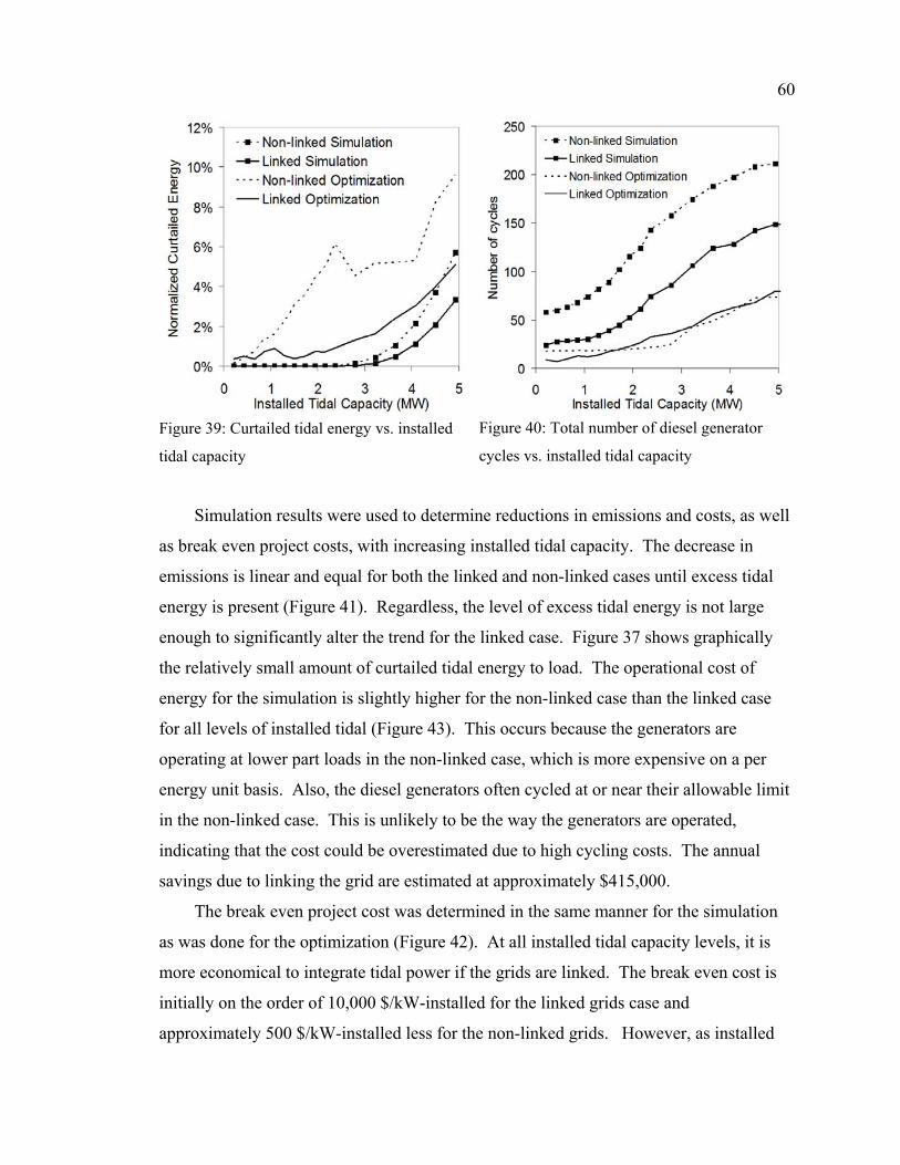
60
Figure 39: Curtailed tidal energy vs. installed
tidal capacity
Figure 40: Total number of diesel generator
cycles vs. installed tidal capacity
Simulation results were used to determine reductions in emissions and costs, as well
as break even project costs, with increasing installed tidal capacity. The decrease in
emissions is linear and equal for both the linked and non-linked cases until excess tidal
energy is present (Figure 41). Regardless, the level of excess tidal energy is not large
enough to significantly alter the trend for the linked case. Figure 37 shows graphically
the relatively small amount of curtailed tidal energy to load. The operational cost of
energy for the simulation is slightly higher for the non-linked case than the linked case
for all levels of installed tidal (Figure 43). This occurs because the generators are
operating at lower part loads in the non-linked case, which is more expensive on a per
energy unit basis. Also, the diesel generators often cycled at or near their allowable limit
in the non-linked case. This is unlikely to be the way the generators are operated,
indicating that the cost could be overestimated due to high cycling costs. The annual
savings due to linking the grid are estimated at approximately $415,000.
The break even project cost was determined in the same manner for the simulation
as was done for the optimization (Figure 42). At all installed tidal capacity levels, it is
more economical to integrate tidal power if the grids are linked. The break even cost is
initially on the order of 10,000 $/kW-installed for the linked grids case and
approximately 500 $/kW-installed less for the non-linked grids. However, as installed
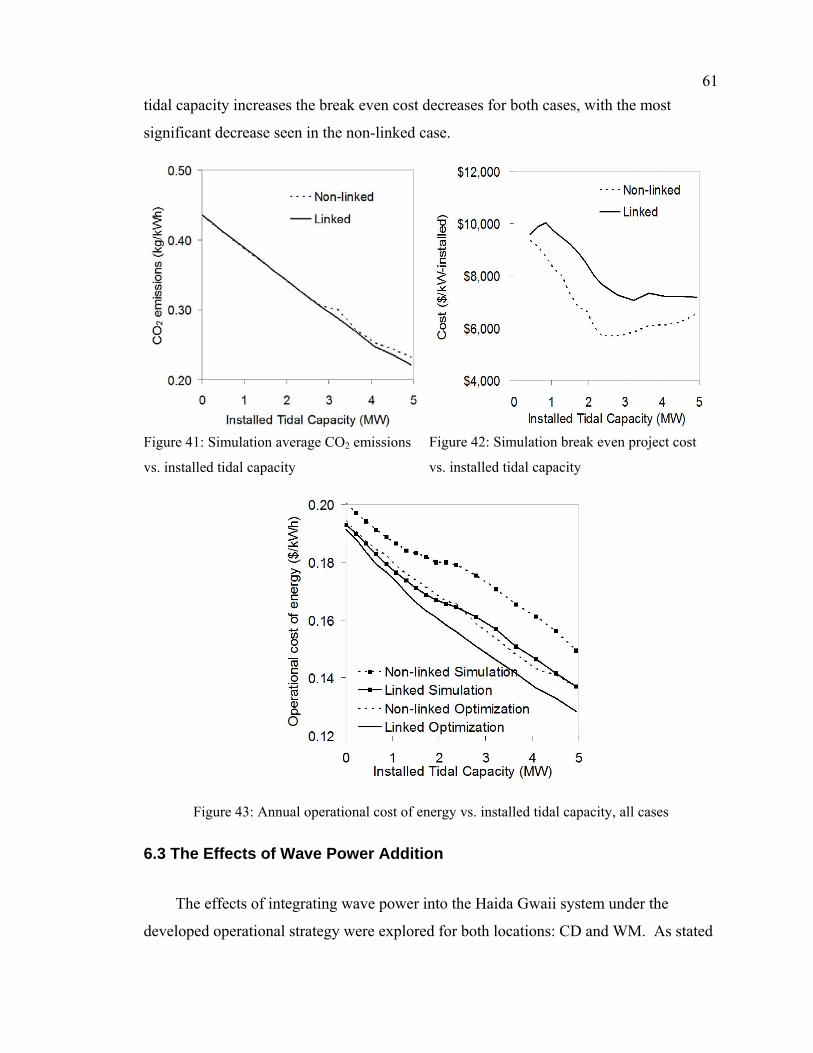
61tidal capacity increases the break even cost decreases for both cases, with the most
significant decrease seen in the non-linked case.
Figure 41: Simulation average CO2 emissions
vs. installed tidal capacity
Figure 42: Simulation break even project cost
vs. installed tidal capacity
Figure 43: Annual operational cost of energy vs. installed tidal capacity, all cases
6.3 The Effects of Wave Power Addition
The effects of integrating wave power into the Haida Gwaii system under the
developed operational strategy were explored for both locations: CD and WM. As stated
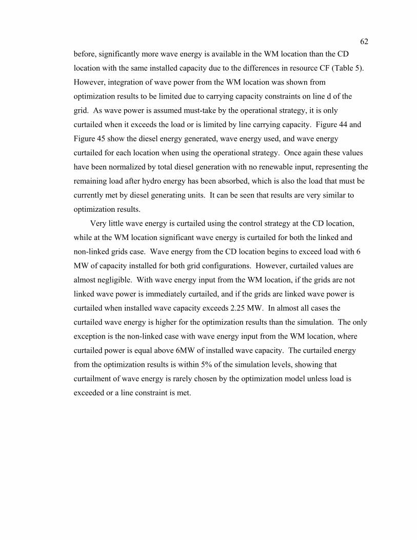
62before, significantly more wave energy is available in the WM location than the CD
location with the same installed capacity due to the differences in resource CF (Table 5).
However, integration of wave power from the WM location was shown from
optimization results to be limited due to carrying capacity constraints on line d of the
grid. As wave power is assumed must-take by the operational strategy, it is only
curtailed when it exceeds the load or is limited by line carrying capacity. Figure 44 and
Figure 45 show the diesel energy generated, wave energy used, and wave energy
curtailed for each location when using the operational strategy. Once again these values
have been normalized by total diesel generation with no renewable input, representing the
remaining load after hydro energy has been absorbed, which is also the load that must be
currently met by diesel generating units. It can be seen that results are very similar to
optimization results.
Very little wave energy is curtailed using the control strategy at the CD location,
while at the WM location significant wave energy is curtailed for both the linked and
non-linked grids case. Wave energy from the CD location begins to exceed load with 6
MW of capacity installed for both grid configurations. However, curtailed values are
almost negligible. With wave energy input from the WM location, if the grids are not
linked wave power is immediately curtailed, and if the grids are linked wave power is
curtailed when installed wave capacity exceeds 2.25 MW. In almost all cases the
curtailed wave energy is higher for the optimization results than the simulation. The only
exception is the non-linked case with wave energy input from the WM location, where
curtailed power is equal above 6MW of installed wave capacity. The curtailed energy
from the optimization results is within 5% of the simulation levels, showing that
curtailment of wave energy is rarely chosen by the optimization model unless load is
exceeded or a line constraint is met.

63
Figure 44: Simulation energy contribution by
source vs. installed wave capacity, CD location
Figure 45: Simulation energy contribution by
source vs. installed wave capacity, WM location
Figure 46 shows the CF of the wave plant for all situations, and it can be seen that
results are slightly higher than those from the optimization (shown in Figure 30). This, of
course, occurs due to the must-take strategy imposed on wave power, leading to higher
plant CF values at equal levels of installed wave capacity. Reductions in CF are seen
with increasing installed capacity due to the increased curtailment of wave power. The
point where wave energy exceeds load can be seen in Figure 46 as well, as the plant CF
deviates from the resource CF. As mentioned previously, this occurs with 6 MW of wave
capacity installed for input from the CD location for both grid configurations. Wave
input from the WM location immediately exceeds the load when the grids are not linked
and does so with 2.25 MW installed for the linked grid configuration.
Cycling of the diesel generators, although not an issue for the optimized results,
became a problem when utilizing the control strategy. Figure 47 shows the total number
of cycles for all diesel generating units when wave energy was input from both the CD
and WM location. When wave power was input from the CD location, no cycling limits
were exceeded for the linked case, but were exceeded when installed wave capacity
reached 8.25 MW for the non-linked case. Wave power input from the WM location
never led to over cycling of the diesel generating units for either the linked or non-linked
case. In fact, cycling was actually reduced for the non-linked case as duty cycles of

64generating units tended towards zero with increasing installed wave capacity. It is clear
that increasing installed wave capacity tends to increase the number of cycles.
Furthermore, the non-linked case usually has a higher number of cycles than the linked
case.
Figure 46: Simulation wave plant annual CF
Figure 47: Simulation total number of cycles vs.
installed wave capacity
The operational cost of energy with increasing wave capacity while using the
operational strategy is shown in Figure 48. The largest savings can clearly be achieved
for the linked grid case with wave energy input from the WM location. Cost for the non-
linked case with input from the WM location shows that cost plateaus and only slight
savings can be achieved above 3.75 MW of wave capacity installed. Steady cost
decreases are seen for both linked and non-linked grids with input from the CD location
due to the low curtailment of wave energy. Carbon dioxide emissions follow the same
pattern since fuel consumption, cost and emissions are all directly related. Costs for the
simulation are all higher than energy costs from the optimization.
The project break even cost in terms of kW of wave power installed is shown in
Figure 49. It indicates that the most economical option would be installation of wave
power in the WM location to a linked grid system. The maximum break even cost occurs
with 2.25 MW of wave capacity installed from the WM location at a level of 5,900 $/kW-
installed. In the situation where the grids are not linked, it appears that installation of
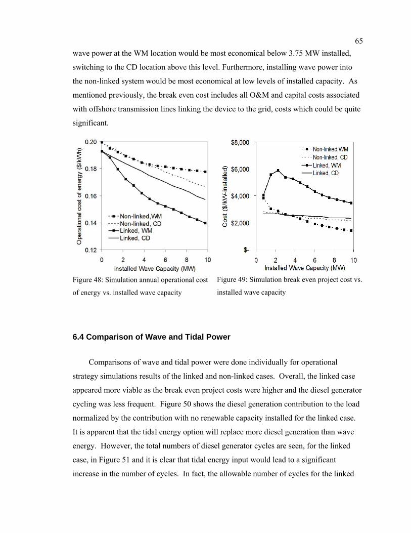
65wave power at the WM location would be most economical below 3.75 MW installed,
switching to the CD location above this level. Furthermore, installing wave power into
the non-linked system would be most economical at low levels of installed capacity. As
mentioned previously, the break even cost includes all O&M and capital costs associated
with offshore transmission lines linking the device to the grid, costs which could be quite
significant.
Figure 48: Simulation annual operational cost
of energy vs. installed wave capacity
Figure 49: Simulation break even project cost vs.
installed wave capacity
6.4 Comparison of Wave and Tidal Power
Comparisons of wave and tidal power were done individually for operational
strategy simulations results of the linked and non-linked cases. Overall, the linked case
appeared more viable as the break even project costs were higher and the diesel generator
cycling was less frequent. Figure 50 shows the diesel generation contribution to the load
normalized by the contribution with no renewable capacity installed for the linked case.
It is apparent that the tidal energy option will replace more diesel generation than wave
energy. However, the total numbers of diesel generator cycles are seen, for the linked
case, in Figure 51 and it is clear that tidal energy input would lead to a significant
increase in the number of cycles. In fact, the allowable number of cycles for the linked

66case with tidal input is exceeded with 1.7 MW installed. The maximum number of
allowable cycles is never exceeded when wave energy is input from the WM location.
On the other hand, curtailed energy is always higher for the case of wave energy input
from the WM location than tidal energy input, a finding which is directly due to the
limited carrying capacity of line d.
Figure 50: Diesel energy generated with all
renewable options, linked grid with operational
strategy
Figure 51: Total number of diesel generator
cycles with all renewable options, linked grid
with operational strategy
Operational cost of energy and break even project cost for all renewable energy
options with a linked grid are shown in Figure 52 and Figure 53. Tidal energy appears to
be the lowest cost option and Figure 53 follows this by showing tidal to have the highest
project break even cost at approximately 10,000 $/kW-installed. The maximum break
even project cost for wave energy input from the WM location is 5,900 $/kW-installed,
considerably lower than tidal energy. In the event that the carrying capacity on line d
was increased to the point where it no longer affected system operation, meaning no
wave energy was curtailed unless it exceeded the load, the maximum break even cost of
wave energy from the WM location increased to 6,800 $/kW-installed. This value is still
lower than that of tidal energy due to the lower resource CF available. Furthermore, the
additional capital cost required for transmission for the offshore wave plant will likely be
higher than transmission costs for the tidal plant as it will be farther offshore. This

67results in an even larger gap between maximum allowable capital costs of the devices
alone.
Figure 52: Annual operational cost of energy
with all renewable options, linked grid with
operational strategy
Figure 53: Break even project cost with all
renewable options, linked grid with operational
strategy
Results from the non-linked cases clearly show that tidal power would be the lowest
cost option and wave power would likely not be suitable if the grids were not linked
(Figure 54 and Figure 55). A low CF for the CD location and a south grid already
saturated with cheap hydro power contribute to this result. Levels of diesel generation
are 11% lower when tidal power is input rather than wave power at a level of 1.5 MW of
renewable capacity installed, and 33% lower with 5 MW installed. However, tidal power
proves to be more problematic for generator cycling when the grids are not linked,
causing them to cycle more than their limit with only 1 MW installed. Wave energy, on
the other hand, does not cause generating units to exceed their allowable number of
cycles until 8.25 MW is installed in the CD location, and never does so for the WM
location.

68
Figure 54: Annual operational cost of energy
with all renewable options, non-linked grid with
operational strategy
Figure 55: Break even project cost with all
renewable options, non-linked grid with
operational strategy

69
Chapter 7
Conclusions The issue of integration of renewable power is of significant interest for remote
communities with high costs of electricity. Haida Gwaii, a remote archipelago off the
northwest coast of British Columbia, Canada, faces a rising cost of electricity due to its
dependence on fossil fuels for energy generation. To understand the impact of renewable
energy integration, with regards to cost, emissions, and system operation, an optimization
network model was built. GAMS was used to develop a linear mixed integer model
which was accompanied by a Matlab interface. The current generation system on Haida
Gwaii consists of two separate grids, north and south, each supplying a peak load on the
order of 5 MW. The option of linking the grids was analyzed along with the impact of
integrating both tidal and wave energy. An operational strategy simulation model for the
generation system was developed based on the optimization results in order to model
more realistic practices, in which renewable power was considered must-take.
7.1 Key Findings Linking the grids was found to reduce the number of diesel generators in operation,
frequency of cycling the diesel generators in operation, system emissions, and cost of
electricity. The optimal average annual cost of electricity dropped from 0.194 $/kWh to
0.191 $/kWh by linking the grids. From this, annual savings from the optimization
model were found to be on the order of $175,000 CAN. Operational strategy model
results found the average annual cost of electricity to be slightly higher than that from the
optimization model at 0.200 $/kWh for the non-linked case and 0.193 $/kWh for the
linked case, resulting in annual savings of $415,000 CAN.
Tidal energy integration from Masset Sound was analyzed for installed capacities of
0.22 MW to 9.85 MW, or power penetration levels of 2.2% to 100% for the linked grids
case and 4.6% to 206% for the non-linked grids case. These levels corresponded to
maximum energy penetration values of 55% and 130%, respectively. Tidal power input
was found to increase the number of diesel generating units in operation as well as the
frequency of cycling of the units. Due to an operational policy of not cycling each diesel
generating unit more than once a day, it was found that the minimum cost solution from

70the optimization model results could not be followed above 2.5 MW of tidal capacity
installed for the non-linked case and 3.2 MW for the linked case. Following an
operational policy further reduced this feasible operating limit to be 1 MW and 1.7 MW
of tidal capacity installed for the non-linked and linked cases, respectively.
Carbon dioxide emissions and cost of electricity decreased almost linearly as
installed tidal capacity increased from 0 to 4 MW for the optimization model, resulting in
savings of 0.054 and 0.051 $/kWh for the linked and non-linked cases respectively.
Above this level of tidal capacity installed, diminishing returns were seen. Slightly lower
savings of 0.046 and 0.039 $/kWh were determined from the simulation model for the
linked and non-linked cases respectively with 4 MW of tidal capacity installed.
Project break even costs for a tidal plant, calculated based on a 20 year project life,
6% discount rate, and including all operational and maintenance and transmission costs,
were constantly higher for the linked case than the non-linked case. The maximum
break-even cost for the linked case from the optimization model was found with 0.65MW
of tidal capacity installed at 11,500 $/kW-installed, and at 0.86 MW installed and 10,000
$/kW-installed from the simulation model. Such findings suggest that it is both
economically and technically beneficial to link the grids before integrating tidal power
while maintaining low levels of installed tidal capacity.
The impacts of wave energy integration were explored for two different locations,
Central Dixon Entrance and West Moresby. Central Dixon Entrance, located 40 km
offshore from the town of Masset, had an average annual resource capacity factor of 10%
when using the Pelamis device selected. West Moresby was located more remotely, 45
km off the western shore of Moresby Island, but benefitted from an average annual
resource capacity factor of 26% with the Pelamis device. Installation levels investigated
included 1 – 13 Pelamis devices sized at 750 kW each, resulting in maximum power
penetrations of 99 and 204% for the linked and non-linked grids respectively.
Integration of wave energy was found to increase the number of diesel generating unit
cycles, however never caused a single unit to cycle more than its allowable daily limit, a
positive result from the system operation point of view. Optimization and simulation
results found that integration of wave energy from the West Moresby location to a linked
grid would be the most economical option. Maximum project break even costs for such a
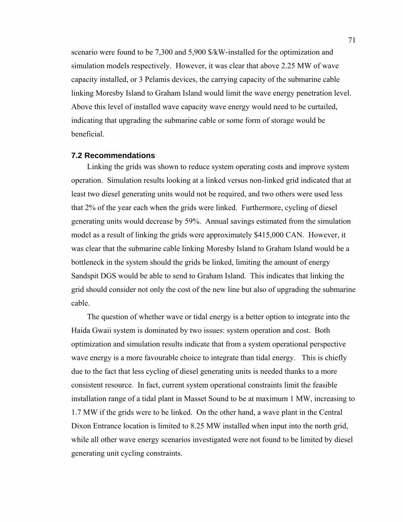
71scenario were found to be 7,300 and 5,900 $/kW-installed for the optimization and
simulation models respectively. However, it was clear that above 2.25 MW of wave
capacity installed, or 3 Pelamis devices, the carrying capacity of the submarine cable
linking Moresby Island to Graham Island would limit the wave energy penetration level.
Above this level of installed wave capacity wave energy would need to be curtailed,
indicating that upgrading the submarine cable or some form of storage would be
beneficial.
7.2 Recommendations Linking the grids was shown to reduce system operating costs and improve system
operation. Simulation results looking at a linked versus non-linked grid indicated that at
least two diesel generating units would not be required, and two others were used less
that 2% of the year each when the grids were linked. Furthermore, cycling of diesel
generating units would decrease by 59%. Annual savings estimated from the simulation
model as a result of linking the grids were approximately $415,000 CAN. However, it
was clear that the submarine cable linking Moresby Island to Graham Island would be a
bottleneck in the system should the grids be linked, limiting the amount of energy
Sandspit DGS would be able to send to Graham Island. This indicates that linking the
grid should consider not only the cost of the new line but also of upgrading the submarine
cable.
The question of whether wave or tidal energy is a better option to integrate into the
Haida Gwaii system is dominated by two issues: system operation and cost. Both
optimization and simulation results indicate that from a system operational perspective
wave energy is a more favourable choice to integrate than tidal energy. This is chiefly
due to the fact that less cycling of diesel generating units is needed thanks to a more
consistent resource. In fact, current system operational constraints limit the feasible
installation range of a tidal plant in Masset Sound to be at maximum 1 MW, increasing to
1.7 MW if the grids were to be linked. On the other hand, a wave plant in the Central
Dixon Entrance location is limited to 8.25 MW installed when input into the north grid,
while all other wave energy scenarios investigated were not found to be limited by diesel
generating unit cycling constraints.

72From a cost perspective it is clear that integrating tidal energy is a better option.
Additionally, it is clear that it is more economical to integrate renewable power if the
grids are linked and installed levels remain low. Break even project cost estimates from
the simulation model for the tidal plant with a linked grid were on the order of 10,000
$/kW-installed for 1 MW installed. The highest break even project costs for a wave plant
were for the West Moresby location with a linked grid and were on the order of
6,000$/kW-installed for 2.25 MW installed. The discrepancy between the two values is
largely due to the lower annual capacity factor of the wave power resource as compared
to the tidal power resource, namely 26% as opposed to 39%. Furthermore, the break
even project cost includes the cost associated with transmission of the power to shore,
and since the wave plant is likely to the farther offshore that capital cost will be higher.
This, in turn, increases the gap between maximum allowable capital cost for the tidal and
wave energy devices alone.
Further development of the network model should be done to fully understand the
possible impact of renewable power integration. Up to this point, hydro power from
Moresby Lake Hydro Facility has been assumed must-take with no storage capabilities.
A dynamic reservoir model should be developed for the facility, from which the option of
including storage could be explored. Other storage options could also be considered,
such as pumped hydro or battery storage. The information provided with regards to
transmission lines was limited, therefore resulting in a simplified grid. More detailed
information on the transmission lines would allow for a more complete representation of
the network. Furthermore, a full AC power analysis of the grid would provide a more
realistic solution as reactive power, voltage fluctuations, and phase angles would be
accounted for. Although it is unlikely that an optimization model will be able to solve for
a period of one year, the simulation model could be run for an entire year rather than four
separate two week periods. Possible future costs relating to the production of carbon
dioxide emissions could also be included in the model, an interesting consideration for
future policy makers. Finally, other renewable energy options, such as wind or biomass,
could be similarly analyzed with the model and compared.

73
Bibliography 1. Weisser, Daniel, and Raquel S. Garcia. "Instantaneous Wind Energy Penetration
in Isolated Electricity Grids: Concepts and Review." Renewable Energy 30.8 (2005): 1299-308.
2. Sheltair Group. Haida Gwaii Community Electricity Plan. April 2008. 3. BC Hydro. Personal Communication. June 2008.
4. Cornett, A. Inventory of Canada’s Marine Renewable Energy Resources.
Canadian Hydraulics Centre, National Research Council of Canada; April 2006. CHC-TR-041.
5. Triton Consultants Ltd. Canada Ocean Energy Atlas (Phase 1) Potential Tidal
Current Energy Resources Analysis Background. Prepared for the Canadian Hyrdaulics Centre, May 2006.
6. Government of Germany. “Amendment of the Act on Granting Priority to
Renewable Energy Sources: English Edition.” April 2, 2004. 7. Gross, R., et al. "Renewables and the Grid: Understanding Intermittency."
Proceedings of the Institution of Civil Engineers. Engineering sustainability 33 (2007): 31-41.
8. Jebaraj, S., and S. Iniyan. "A Review of Energy Models." Renewable and
Sustainable Energy Reviews 10.4 (2006): 281-311.
9. Joshi, Bharati, T. S. Bhatti, and N. K. Bansal. "Decentralized Energy Planning Model for a Typical Village in India." Energy 17.9 (1992): 869-76.
10. Malik, B., et al. "Mathematical Model for Energy Planning of Rural India."
International journal of energy research 18.4 (1994): 469-82.
11. Iniyan, S., and K. Sumathy. "An Optimal Renewable Energy Model for various End-Uses." Energy 25.6 (2000): 563-75.
12. Kaldellis, J. K., and K. A. Kavadias. "Optimal Wind-Hydro Solution for Aegean
Sea Islands' Electricity-Demand Fulfilment." Applied Energy 70.4 (2001): 333-54.
13. Muckstadt, John A., and Sherri A. Koenig. "An Application of Lagrangian
Relaxation to Scheduling in Power-Generation Systems." Operations research 25.3 (1977): 387.

7414. Uri, N. D., and S. Hassanein. "Modeling the High Frequency Demand for
Energy." Applied Energy 19.1 (1985): 49-59.
15. Uri, N. D. "Forecasting Peak System Load using a Combined Time Series and Econometric Model." Applied Energy 4 (1978): 219-27.
16. Weisser, D. "A Wind Energy Analysis of Grenada: An Estimation using the
‘Weibull’ Density Function." Renewable Energy 28.11 (2003): 1803-12.
17. Hsu, George J. Y., and Feng-Ying Chou. "Integrated Planning for Mitigating CO2 Emissions in Taiwan: A Multi-Objective Programming Approach." Energy Policy 28.8 (2000): 519-23.
18. Weis, Timothy M., and Adrian Ilinca. "The Utility of Energy Storage to Improve
the Economics of wind–diesel Power Plants in Canada." Renewable Energy 33.7 (2008): 1544-57.
19. Kaldellis, J. K. "The Wind Potential Impact on the Maximum Wind Energy
Penetration in Autonomous Electrical Grids." Renewable Energy 33.7 (2008): 1665-77.
20. Maddaloni, Jesse D., Andrew M. Rowe, and G. Cornelis van Kooten. "Wind
Integration into various Generation Mixtures." Renewable Energy 34.3 (2009): 807-14.
21. Bakos, George C. "Feasibility Study of a Hybrid wind/hydro Power-System for
Low-Cost Electricity Production." Applied Energy 72.3-4 (2002): 599-608. 22. Hatch Energy. Haida Gwaii/Queen Charlotte Islands Demonstration Tidal Power
Plant Feasibility Study. March 2008. 23. Thurman, Harold V. Introductory Oceanography. 8th ed. Upper Saddle River, NJ:
Prentice Hall, 1997. 24. Thomson, Richard E. Oceanography of the British Columbia Coast. Ottawa, Ont:
Canada Dept. of Fisheries and Oceans, 1981. 25. Garrett, Chris, and Patrick Cummins. "Generating Power from Tidal Currents."
Journal of Waterway, Port, Coastal & Ocean Engineering 130.3 (2004): 114-8. 26. Garrett, Chris, and Patrick Cummins. "The Power Potential of Tidal Currents in
Channels." Proceedings of the Royal Society 461 (2005): 2563-72. 27. Blanchfield, J., C. Garrett, and A. Rowe. "Tidal Stream Power Resource
Assessment for Masset Sound, Haida Gwaii." Proceedings of the Institution of Mechanical Engineers Part A Journal of Power and Energy 222.A5 (2008): 485.

75
28. Twidell, John, and Anthony D. Weir. Renewable Energy Resources. 2nd ed. London; New York: Taylor & Francis, 2006.
29. Cruz, João. Ocean Wave Energy: Current Status and Future Perspectives.
Illustrated ed. Springer, 2008. 30. EPRI. E2I EPRI Assessment. Offshore Wave Energy Conversion Devices. 2004. 31. Finavera Renewables. "Wave Tech: System Configuration." 2007.
<http://www.finavera.com/en/wavetech/configuration>. 32. Weinstein, Alla. AquaEnergy Group Ltd. "AquaBuOY in Portugal."
<http://ec.europa.eu/research/energy/pdf/gp/gp_events/ocean_energy/1145_aquabuoy_demo_plant_en.pdf>.
33. Finavera Renewables. "Press Room." 2009. < http://www.finavera.com/en/press>. 34. Renewable Energy World. “While Finavera’s Buoy Sinks, Hopes of Harnessing
Ocean Energy Survive” November 8, 2007. <http://www.renewableenergyworld.com/rea/news/article/2007/11/while-finaveras-buoy-sinks-hopes-of-harnessing-ocean-energy-survive-50510>
35. Pelamis Wave Power. "Pelamis P-750 Wave Energy Converter Brochure."
<http://www.pelamiswave.com/content.php?id=161>. 36. Pelamis Wave Power. 2009 < http://www.pelamiswave.com/index.php> 37. Wave Dragon. 2009 <http://www.wavedragon.net/> 38. Marine Environmental Data Services, Department of Fisheries and Oceans
Canada. "IdxMap - SVG Data Search." 2008-06-12 2008. <http://www.meds-sdmm.dfo-mpo.gc.ca/meds/Databases/WAVE/idxMAP/idxMapQbasic_e.asp>.
39. Dunnett, David, and James S. Wallace. "Electricity Generation from Wave Power
in Canada." Renewable Energy 34.1 (2009): 179-95. 40. Weinstein, A., et al. “AquaBuOY - the Offshore Wave Energy Converter
Numerical Modeling and Optimization.” Oceans ’04. MTTS/IEEE Techno-ocean ’04, 4 (2004): 1854-1859.
41. Google. "Google Maps Canada." 2009. <http://maps.google.ca/maps?tab=ml>. 42. Maddaloni, Jesse D. Techno-Economic Optimization of Integrating Wind Power
into Constrained Electric Networks. Master of Applied Science University of Victoria, 2007.

76 43. Alcan Cable. “Bare Overhead Cable. Canadian Product Catalogue.”
<http://www.cable.alcan.com/alcancable/en-US/Products/Canada/Bare+Overhead+Conductors/Bare+Overhead+Conductor.htm>
44. Aluminum Association. “Aluminum Electrical Conductor Handbook.” New York
(1971). 45. Matt Clare. Finning (Canada) Inc. Personal Communication. December 2008. 46. Diesel Service and Supply Inc. Approximate Fuel Consumption Chart. 2008
<www.diselserviceandsupply.com>. 47. Lefton S.A., Besuner P.M., Grimsrud G.P., “Managing utility power plant assets
to economically optimize power plant cycling, costs, life, and reliability,” Proceedings of the 4th IEEE Conference on Control Applications (Cat. No.95CH35764) (1995): 195-208.
48. US Environmental Protection Agency. “Emission Facts: Average Carbon Dioxide
Emissions Resulting from Gasoline and Diesel Fuel.” 2008 <http://www.epa.gov/OTAQ/climate/420f05001.htm>.
49. Brooke, A., et al. "GAMS: The Solver Manuals." Washington, DC: GAMS
Development Corporation (2005). 50. BC Hydro and Power Authority. “BC Hydro 2008 Annual report.” March 2009:
<http://www.bchydro.com/about/company_information/reports/2008annualreport/intro.html>.
51. Lilliefors, H.W., "On the Komogorov-Smirnov test for normality with mean and
variance unknown," Journal of the American Statistical Association, 62 (1967): 399-402.
52. Lial, Kelly. EPCOR. Personal communication. September 2008.
53. US Energy Information Administration. “Assumptions to the Annual Energy
Outlook 2009. Report #: DOE/EIA-0554(2009).” March 2009. http://www.eia.doe.gov/oiaf/aeo/assumption/index.html
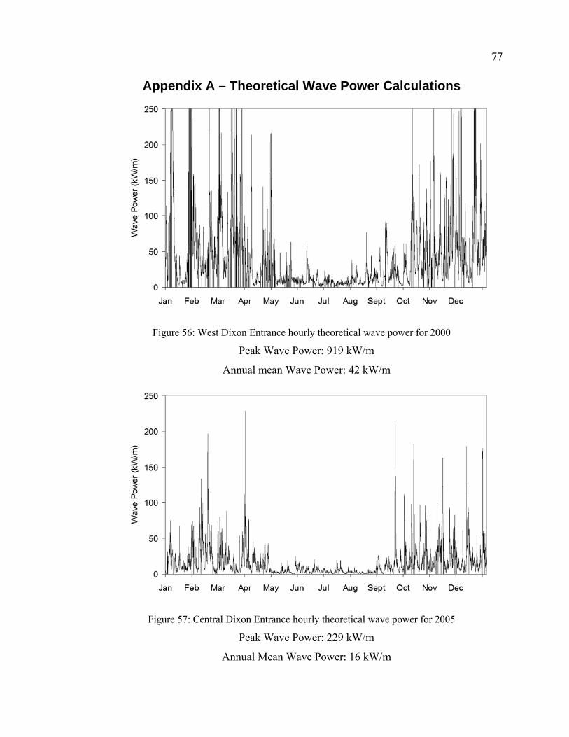
77
Appendix A – Theoretical Wave Power Calculations
Figure 56: West Dixon Entrance hourly theoretical wave power for 2000
Peak Wave Power: 919 kW/m
Annual mean Wave Power: 42 kW/m
Figure 57: Central Dixon Entrance hourly theoretical wave power for 2005
Peak Wave Power: 229 kW/m
Annual Mean Wave Power: 16 kW/m

78
Figure 58: North Hecate Strait hourly theoretical wave power for 2005
Peak Wave Power: 240 kW/m
Annual Mean Wave Power: 11 kW/m
Figure 59: South Moresby hourly theoretical wave power for 2005
Peak Wave Power: 681 kW/m
Annual Mean Wave Power: 43 kW/m

79
Figure 60: West Moresby hourly theoretical wave power for 2004
Peak Wave Power: 752 kW/m
Annual Mean Wave Power: 42 kW/m