University of Wollongong University of Wollongong

Research Online Research Online

University of Wollongong Thesis Collection 1954-2016 University of Wollongong Thesis Collections

2005

Intelligent automated drilling and reaming of carbon composites Intelligent automated drilling and reaming of carbon composites

Marta A. Fernandes martaf@uow.edu.au

Follow this and additional works at: https://ro.uow.edu.au/theses

University of Wollongong University of Wollongong

Copyright Warning Copyright Warning

You may print or download ONE copy of this document for the purpose of your own research or study. The University

does not authorise you to copy, communicate or otherwise make available electronically to any other person any

copyright material contained on this site.

You are reminded of the following: This work is copyright. Apart from any use permitted under the Copyright Act

1968, no part of this work may be reproduced by any process, nor may any other exclusive right be exercised,

without the permission of the author. Copyright owners are entitled to take legal action against persons who infringe

their copyright. A reproduction of material that is protected by copyright may be a copyright infringement. A court

may impose penalties and award damages in relation to offences and infringements relating to copyright material.

Higher penalties may apply, and higher damages may be awarded, for offences and infringements involving the

conversion of material into digital or electronic form.

Unless otherwise indicated, the views expressed in this thesis are those of the author and do not necessarily Unless otherwise indicated, the views expressed in this thesis are those of the author and do not necessarily

represent the views of the University of Wollongong. represent the views of the University of Wollongong.

Recommended Citation Recommended Citation Fernandes, Marta, Intelligent automated drilling and reaming of carbon composites, PhD thesis, School of Electrical, Computer and Telecommunications Engineering, University of Wollongong, 2005. http://ro.uow.edu.au/theses/477

Research Online is the open access institutional repository for the University of Wollongong. For further information contact the UOW Library: research-pubs@uow.edu.au

NOTE

This online version of the thesis may have different page formatting and pagination from the paper copy held in the University of Wollongong Library.

UNIVERSITY OF WOLLONGONG

COPYRIGHT WARNING

You may print or download ONE copy of this document for the purpose of your own research or study. The University does not authorise you to copy, communicate or otherwise make available electronically to any other person any copyright material contained on this site. You are reminded of the following: Copyright owners are entitled to take legal action against persons who infringe their copyright. A reproduction of material that is protected by copyright may be a copyright infringement. A court may impose penalties and award damages in relation to offences and infringements relating to copyright material. Higher penalties may apply, and higher damages may be awarded, for offences and infringements involving the conversion of material into digital or electronic form.

Intelligent Automated Drilling and Reaming of Carbon Composites

A thesis submitted in fulfilment of the requirements for the award of the degree

Doctor of Philosophy

from

University of Wollongong

by

Marta Fernandes, Eng., ME (Hons)

School of Electrical, Computer and Telecommunications Engineering

2005

Acknowledgements

First, and furthermost, I would like to thank my supervisor Professor Chris Cook for giving me the

opportunity to work in this research project and for being an endless source of encouragement and

support. His expert advice and resourcefulness were invaluable.

I would also like to thank Dr. Friso De Boer who introduced me to research and was my mentor for

many years. Unfortunately he was not able to be my supervisor until the end but his priceless help is

most acknowledged.

Many thanks to Dr Gursel Alici, my second supervisor, who joined us close to the end of the study

but nevertheless brought much insight to the research. His expertise and friendly availability were

essential for the successful completion of this thesis.

I would like to thank all general staff that through these years helped me reaching my goal. Special

thanks to Mr. Brian Webb for building my test rig and to Mr. Joe Abbot and Mr. Greg Tillman for

helping me use various equipment.

To my colleagues, I would like to thank them for their help and advice as well as their friendship. In

particular I would like to thank Mr Steve Van Duin for making the drawings of my test rig and Dr

John Simpson for his invaluable advice and help on setting up all the hardware.

To all my family and friends, at the university and at home, in Portugal and in Australia, which are

too many to name, thank you for living through my distance, moods and complaints. Your patience

and belief it is most appreciated.

I would also like to thank my dear husband Greg and son Miguel for their unconditional love and

support. They lived with me through the ups and downs of the past years and it is thanks to their

patience and sacrifice that I have been able to finish this thesis.

CERTIFICATION

I, Marta Alexandra Ribeiro Fernandes, declare that this thesis, submitted in partial

fulfilment of the requirements for the award of Doctor of Philosophy, in the school of

Electrical, Computer and Telecommunications Engineering, University of Wollongong, is

wholly my work unless otherwise referenced or acknowledged. The document has not been

submitted for qualifications at any other academic institution.

Marta Fernandes

6 March 2005

1

ABSTRACT

This thesis describes research in intelligent automated drilling of carbon fibre

composites. This work has been motivated by the aircraft industry where there is a

significant interest in automating part of the production process to improve productivity

and consistency. The requirements for automated drilling as well as problems inherent

in drilling composites are addressed.

Drilling Forces and moments are investigated and used to model the drilling process. A

mathematical model is developed to represent the thrust forces and this model also

accounts for aging of the tool. The quality of the holes produced was investigated and

parameters such as surface finish, break outs and size of the holes were related to the

drilling parameters and forces generated.

A decision making algorithm has been designed to enable parameters to be varied

during the drilling operation to maintain optimum conditions. This decision making

algorithm takes into account inherent system limits and uses information such as age of

the tool and maximum force allowed to provide the spindle speed and feed rate to be

used at each stage of the drilling process. The aim of this algorithm is to choose the

parameters which will minimize drilling time and tool wear while maintaining quality of

the holes and respecting the initial conditions of maximum thrust force.

The developed system has been implemented and shown to successfully drill holes of

acceptable quality despite inherent aging of drill bits while maximising productivity.

2

Published or Accepted Papers Arising From This Thesis

• Fernandes, M., Cook, C., Alici, G., “Investigation of hole quality on drilling

carbon composites with a ‘one shot’ drill bit”, Aerospace Manufacturing and

Automated Fastening Conference & Exhibition, Dallas, 2005

• Fernandes, M., Cook, C., Alici, G., “Empirical modeling of force profiles during

drilling of carbon composites”, 8th CIRP International Workshop on Modelling

of Machining Operations, Chemnitz, Germany, 2005

• Fernandes, M. and Cook, C., "Drilling of Carbon Composites Using a one shot

drill bit. Part 1: 5 stage representation of drilling factors affecting maximum

force and Torque," International Journal of Machine Tools & Manufacture,

2005.

• Fernandes, M. and Cook, C., "Drilling of Carbon composites using a one shot

drill bit. Part II: Empirical modelling of maximum thrust force," International

Journal of Machine Tools & Manufacture, 2005

• Fernandes, M., Gower, S., De Boer, F., and Cook, C., "Robotic Drilling of

Carbon Fibre", Proceedings of the ACUN-3 International Composite

Conference, Technology convergence in composite applications, Sydney,

Australia, 2001.

• Fernandes, M., Gower, S., and Zealey, J., "Preliminary Experiments in Robotic

Drilling of Composites", Proceedings of the 2nd International Conference on

Mechanics of Structures, Materials and Systems, Wollongong, Australia, 2001.

3

Table of contents

Chapter 1 Introduction and Literature Review .....................................................6 1.1 Background .......................................................................................................6

1.2 Carbon Composites ...........................................................................................8

1.3 Drilling Process .................................................................................................9

1.3.1 One Shot Drill Bit ...................................................................................13

1.3.2 Modelling Drilling Process .....................................................................15

1.4 Automated Drilling of Carbon Composites ....................................................18

1.4.1 Positioning of End Effector.....................................................................18

1.4.2 Tool Conditioning Monitoring................................................................19

1.4.3 Hole Quality ............................................................................................22

1.4.4 Optimization and Control of the Drilling Process...................................26

1.5 Discussion and Summary of Literature Review..............................................29

1.6 Problem Formulation ......................................................................................31

1.7 Outline of the Thesis .......................................................................................32

Chapter 2 Experimental Setup...............................................................................34 2.1 Drilling Rig .....................................................................................................34

2.1.1 Motors .....................................................................................................36

2.1.2 6 axis Force Sensor .................................................................................37

2.1.3 Data Acquisition and Control of the Test Rig.........................................38

2.1.4 Calibration Procedures ............................................................................40

2.2 Drill bits ..........................................................................................................41

2.3 Carbon Composite Samples ............................................................................43

4

Chapter 3 Modelling Thrust Force and Torque...................................................44 3.1 Introduction .....................................................................................................44

3.2 Description of Experiments.............................................................................44

3.3 Typical Thrust Force and Torque....................................................................46

3.4 Effect of Drilling Parameters on Thrust Force and Torque ............................51

3.5 Effect of Tool Age on Thrust Force and Torque.............................................57

3.6 Lateral Forces and Torques .............................................................................65

3.7 Frequency Content of Thrust Force and Torque .............................................69

3.8 Conclusions .....................................................................................................71

Chapter 4 Maximum Thrust Force and Torque Estimation...............................73 4.1 Introduction .....................................................................................................73

4.2 Using Shaw’s simplified equations .................................................................73

4.2.1 Estimating Torque at Break-Through .....................................................76

4.2.2 Estimating Maximum Thrust Force ........................................................77

4.3 Estimation of Thrust Force In Relation to Time .............................................82

4.3.1 Estimation of Thrust force at Position ‘A’ ..............................................83

4.3.2 Estimation of Thrust force at position ‘C’ ..............................................86

4.3.3 Estimation of Thrust force at position ‘D’ ..............................................88

4.3.4 Mathematical Representation of Thrust Force in Relation to Time........90

4.4 Conclusion.......................................................................................................94

Chapter 5 Analysing Quality of Holes ...................................................................96 5.1 Introduction .....................................................................................................96

5.2 Description of Experiments.............................................................................97

5.3 Analysing Hole Quality.................................................................................100

5.3.1 Visual Inspection...................................................................................101

5

5.3.2 Discussion of Results ............................................................................104

5.3.3 Microscope............................................................................................110

5.3.4 Pin Gages ..............................................................................................112

5.3.5 Coordinate Measurements.....................................................................116

5.4 Relating Quality of Holes to Drilling Force and Torque ..............................132

5.5 Relating Drilling Stages to Quality ...............................................................135

5.6 Conclusion.....................................................................................................139

Chapter 6 Automated Drilling and Reaming......................................................143 6.1 Introduction ...................................................................................................143

6.2 Optimising Drilling Time..............................................................................145

6.2.1 Stage I....................................................................................................146

6.2.2 Stage II ..................................................................................................149

6.2.3 Stage III .................................................................................................149

6.2.4 Stage IV and V ......................................................................................150

6.3 Implementation of Automated Drilling- Experiments and Results...............151

6.3.1 Maximum thrust force of 100N.............................................................152

6.3.2 Maximum thrust force of 200N.............................................................161

6.3.3 Discussion of Results ............................................................................166

6.4 Conclusion.....................................................................................................166

Chapter 7 Conclusions and Recommendations for Future Research ..............168 7.1 Conclusions ...................................................................................................168

7.2 Recommendations for Future Research ........................................................172

References ....................................................................................................................174 List of Figures ..............................................................................................................190 Appendixes...................................................................................................................195

6

Chapter 1 Introduction and Literature Review

1.1 Background

This thesis work has been motivated by the aircraft industry where there is a significant

interest in automating the process of assembling aeroplane components involving the

drilling of large numbers of holes into carbon fibre composite materials for later

fastening to alloy structures. Current methods are time consuming, costly and often

involve the use of large dedicated assembly jigs or substantial manual labour. The

advantages of automating the manufacture of these parts using commercially available

robots include increased productivity and flexibility and reduced investment costs over

dedicated automation methods. However, successful automation of hole drilling using

such ‘lean automation’ techniques requires a better understanding of the forces, torques,

feed rates and other parameters required to maintain hole quality.

The development of such an automated system includes the study of many different

sub- sub-systems; examples include the fixture of the parts being assembled, the

accurate positioning of the robot and the control of the hole drilling process. Parts are

commonly assembled by mechanically holding them together, drilling, disassembly and

cleaning, and then reassembly and fastening using rivets. It has been reported in the

literature that 40 million holes are drilled annually just for the manufacturing of

aeroplane wings [1] in one assembly line.

7

The drilling operation is most critical due to the characteristics of the composites, and

the reaction forces produced during drilling which might provoke deflections in the

manipulator and consequently loss of accuracy. Poor fixture design accounts for nearly

40% of part rejections [2], while poor hole drilling has been reported to account for 60%

of all part rejections [3]. Because drilling is performed on nearly completed parts, such

defects are very costly. Also the quality of the holes drilled on carbon composite has

been linked to the strength of the joint being assembled [4] and fatigue life of the parts

[5-7].

New technologies have emerged in the market, such as laser drilling, ultrasonic[8],

water jet, electrochemical spark machining [9], vibration [10, 11] or orbital drilling [12].

The high cost of these techniques allied to a limited range of applications have meant

that conventional drilling still remains the dominant process for making holes [13].

The research work in this thesis concentrates on studying the conventional drilling of

holes in carbon composites to assist in implementing an automated solution. At the heart

of any automated hole drilling system is a sufficiently good understanding of the hole

drilling process to enable it to be conducted automatically whilst retaining or improving

hole quality, and the research work presented here contributes to this understanding.

8

1.2 Carbon Composites

Carbon composite is one of the most advanced and adaptable engineering material

known today [14]. Its use has revolutionised several industries, from sporting goods to

car industry, aerospace and construction such as bridges. The popularity and success of

carbon composite in these industries is largely due to the high strength and stiffness in

relation to its weight. Other advantages are that composites are corrosion resistant,

electrically insulating, show good damping properties and tailorability allowing for a

reduction in tooling and assembly costs [10, 14].

The constituents of a composite are its matrix and its reinforcement. The reinforcement

is responsible for its strength and macroscopic stiffness carrying most of the structural

loads. The matrix binds the reinforcement together, introducing the external loads

effectively and protecting it from environmental effects. The matrix is therefore

responsible for the shape, surface appearance, environmental tolerance and durability

[14]. Matrices can be metal, ceramic or polymeric while the reinforcement can be

carbon fibre, glass fibre and polymers. The arrangement of the reinforcement within the

composite varies from randomly oriented to aligned, continuous or discontinuous

configurations. The characteristics and properties of the composite depend on its

constituents and the way they are aligned. The materials need to be chosen for each

application to provide the necessary mechanical properties.

9

Composites can outperform many engineering materials although there are

disadvantages too, such as poor temperature performance, high raw material cost, lack

of knowledge and know-how, and difficulty in machining [14].

During the last fifty years, composites have been used as substitutes for other traditional

materials such as wood, steel, aluminium, plastic and concrete, and new applications are

continuously arising. However, new machining techniques are needed in order to

expand the successful application of this promising material.

1.3 Drilling Process

Drilling is a common process used for unwanted material removal from the workpiece.

The drilling of metal has been studied, analysed and optimised since the beginning of

the 20th century. Although carbon composite is not metal, for many years industry has

applied the theory: “cut it like metal”. The results of this theory were often poor finish

quality and excessive tool wear. In this thesis, the vast knowledge of drilling metals is

used but adapted for the drilling of carbon composites.

The drilling process is a complex 3 dimensional process and is affected by numerous

variables. The cutting speed or spindle speed and the feed rate are the basic parameters

governing the drilling operation [15]. Other independent variables are the tool (material

and geometry), the workpiece material and thickness, coolant, etc. The resultant

variables are the forces and torques generated, the temperature, the type of chip, the

quality of the hole and the tool wear rate.

10

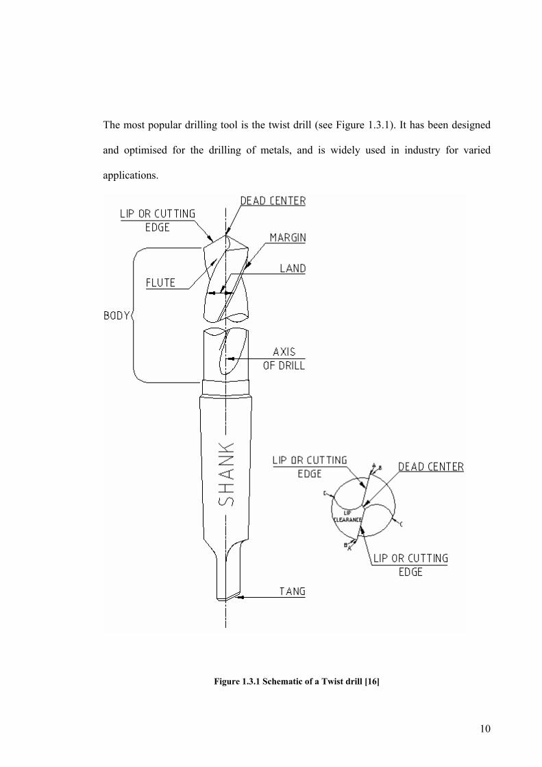
The most popular drilling tool is the twist drill (see Figure 1.3.1). It has been designed

and optimised for the drilling of metals, and is widely used in industry for varied

applications.

Figure 1.3.1 Schematic of a Twist drill [16]

11

The web of the drill bit pierces the workpiece, chips are produced by the web and

evacuated by the flutes, and finally the drill is guided in the hole already produced by

the margins [17]. The requirements for the shape of the drill bit are usually conflicting,

for example:

• While a small web will reduce thrust force, a larger web will provide better

resistance to chipping and give torsional rigidity.

• Large flutes provide larger space for chip transport, while smaller flutes allow

better rigidity.

• An increase in the helix angle allows a faster removal of chips but reduces the

strength of the cutting edges.

It is possible to find in the market twist drills of varied geometry ideal for particular

applications. Common twist drills are made of High Speed Steel (HSS), but this is not

suitable for the drilling of composites because it wears so rapidly that even after only a

few holes the quality is not acceptable. Tungsten Carbide and PCD (polycrystalline

diamond) are, therefore, usually adopted to drill composites. While PCD shows better

performance in relation to tool wear rate, the price is much higher than Tungsten

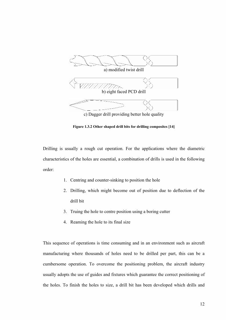
carbide. Other shaped drill bits have also been designed for the drilling of composites.

Figure 1.3.2 shows some examples of these drill bits.

12

a) modified twist drill

b) eight faced PCD drill

c) Dagger drill providing better hole quality

Figure 1.3.2 Other shaped drill bits for drilling composites [14]

Drilling is usually a rough cut operation. For the applications where the diametric

characteristics of the holes are essential, a combination of drills is used in the following

order:

1. Centring and counter-sinking to position the hole

2. Drilling, which might become out of position due to deflection of the

drill bit

3. Truing the hole to centre position using a boring cutter

4. Reaming the hole to its final size

This sequence of operations is time consuming and in an environment such as aircraft

manufacturing where thousands of holes need to be drilled per part, this can be a

cumbersome operation. To overcome the positioning problem, the aircraft industry

usually adopts the use of guides and fixtures which guarantee the correct positioning of

the holes. To finish the holes to size, a drill bit has been developed which drills and

13

reams in one go, hence called a ‘one shot’ drill bit. The time savings of using this tool

are evidently high compared to the traditional method of drilling and reaming in

separate operations.

1.3.1 One Shot Drill Bit For the application of drilling carbon composites, aircraft manufacturers commonly use

a one shot drill bit which has specific characteristics ideal for carbon composites:

• The web of the drill bit is very small to reduce the amount of thrust force and

therefore avoid delamination.

• Straight flutes are used to allow for the quick evacuation of the chips produced

and for cooling of the cutting area. This characteristic is particularly important

due to the highly abrasive nature of the chips which if not removed promptly

will wear the drill bit prematurely. Keeping the temperature generated low is

also very important due to the low thermal tolerance of the carbon composite.

• Two distinct cutting angles, for drilling and reaming in one operation.

A schematic figure of a typical one-shot drill bit can be seen in Figure 1.3.3.

14

Figure 1.3.3 Schematic of one shot drill bit

15

The drawback of the shape of this drill bit is the lower rigidity due to the small web and

large flutes. This means that it might be prone to break and chip if the drilling

conditions are not ideal. Another disadvantage of this design is the chances of vibrating

and chattering during the reaming process because of the decreased rigidity of the

coupling between cutting face and workpiece. Nevertheless, this shaped drill bit is

widely used for manual drilling of composites, and studies have found that this drill bit

is economical, and produces good quality holes when compared to other shaped drill

bits [14, 18] for the drilling of carbon composites.

1.3.2 Modelling Drilling Process

The relation between the drilling process variables has been studied for many years.

Several models have been developed to estimate the thrust force and torque [12, 17, 19-

31]. These models range from mechanistic approaches [19, 26, 27], to neural networks

[25, 32]. Orthogonal cutting is a common approach for the modelling of carbon

composites[17, 28, 29, 33, 34]. These models and are usually developed for a twist drill

bit and do not take in account drill bit wear or ageing.

From all the drilling models available, Shaw’s and Oxford’s models are very popular.

From Oxford’s experiments in 1955 [31], the drilling process was divided into three

components: extrusion under the chisel edge, secondary cutting along the chisel edge

and primary cutting along the cutting edges. Later in 1957, Shaw and Oxford found the

influence of the chisel edge on the total thrust force used and developed semi-empirical

16

equations for predicting the thrust force and torque in the drilling process. These

equations (developed for the twist drill) are still used by many researchers [17, 35] due

to their simplicity and have been shown to apply to the drilling of carbon composites

[15, 36]. A brief explanation of Shaw’s equations will follow; for more details please

refer to [31].

Shaw’s equations

The specific cutting energy ū (equation 1.1) or cutting energy per unit volume is

developed to apply to a two dimensional cutting model of a single point tool.

ū= 28FdT (1.1)

where T is the torque in Nm, F is the Force in N and d the diameter in mm. This cutting

energy was found to be directly related to the hardness of the material being cut, HB,

and therefore considered as the cutting hardness value.

A dimensional analysis is used to represent thrust force and torque, taking into

consideration the mechanics of the twist drill. It is also considered in this work that

changes to the flutes would not influence the results because the flutes are used for chip

evacuation only, and unless there are jammed chips on the flutes, their action can be

ignored. From this study, the following equations emerge (equation 1.2 and equation

1.3)

17

+

+

+

−=

−

+

−

23

1

21

1

12

1

1

dcK

dcK

dcdc

dfK

HdF a

aa

a

B

(1.2)

+

+

−=

−

+

− a

aa

a

B dcK

dcdc

dfK

HdT 2

51

1

43

1

1 (1.3)

where,

F Thrust force (N)

T Torque (Nm-1)

a, Ki (i=1,5) Constants to be determined experimentally

d Drill diameter (mm)

f Feed (mm/rev)

c Length of chisel edge (mm)

HB Hardness of the material

Ū Specific cutting energy

For a given drill bit, c/d is constant, and therefore it is possible to simplify the equations

1.2 and 1.3 which become equation 1.4.

18

( )

=

+=⇔

=

+=

−−

−

+

−

+

−

aa

a

a

a

B

a

a

B

dfKT

dKfdKF

dfK

HdT

KdfK

HdF

2111

210

19

1

1

83

71

1

62

(1.4)

where the parameters K9-11 are determined experimentally. It is therefore concluded that

for a given drill bit and workpiece material, the thrust force and torque depend on the

feed (mm/rev) and the diameter of the drill bit.

1.4 Automated Drilling of Carbon Composites

The manufacturing operation of drilling composites is commonly carried out manually.

When it is not possible to use a CNC machine for drilling (because of the size of the

workpiece or location of the holes), the best choice of performance versus cost is

usually a manual operator. To develop an automated system with the flexibility of an

operator while maintaining performance and precision, the following requirements have

to be built into the system, as they will not be provided by an operator:

1.4.1 Positioning of End Effector

The manipulator or robot must resist the reaction forces originating from the drill

against the workpiece. Previous research in this area has addressed the problem of

deformation of the robot in the presence of reaction forces [37-40]. The success and

flexibility of the developed systems is unclear and does not account for problems such

as deformation of the workpiece [2] and the drill bit.

19

The drill must be perpendicular to the work-piece during the drilling process. Systems

previously developed for robotic drilling usually “clamp” the drill to the right position

and angle before the start of drilling [41]. By doing this, the flexibility of the system is

reduced. Force controllers have been developed which maintain the drill perpendicular

to the workpiece by changing the position of the end effector through drilling[37, 39,

40]. This solution maintains the flexibility of the system but the effect such techniques

will have on the quality of the holes and tool life has not been established. More

recently other techniques have emerged to solve this problem. An example is a

configurable tooling system using a metrology system and tooling [42]. In this work, the

equipment holding the workpiece is positioned and calibrated by a robot to an accuracy

of 50µm. The workpiece is firmly clamped while machining but the clamping system

maintains the flexibility desired.

The research reported in this thesis does not include end effector positioning; however,

the force and torque modelling results will assist in the design of such end effectors.

1.4.2 Tool Conditioning Monitoring

The control system must be able to detect problems in the process such as tool wear and

tool breakage. Several sensors and signals have been used attempting to monitor the

drilling process, such as spindle motor power [41, 43], vibration[44-46], acoustic

vibrations [47-49], and thrust forces [50]. These studies usually consist of finding a

signature signal and the problems are detected when the signal varies from the

20

signature. The success of such technique relies on the need to maintain all drilling

parameters constant so that the signature can be used. The same principle is found on

more modern approaches such as neural networks [51] and artificial intelligence [52].

Tool condition monitoring is an extensively researched area and publications can be

found which summarise the work done to date on this area [53, 54].

Tool Wear

Detecting tool wear is particularly important for the drilling of carbon composites due to

the excessive tool wear rate usually encountered allied to the quality problems caused

by worn drill bits. The abrasive nature of the chips, the temperatures generated, and the

low heat conductivity of the material make the wear of the drill bit an essential factor to

take into consideration. Tool wear also affects the forces generated while drilling,

which in turn can cause defects such as delamination and unacceptable hole size

variations. Many authors have reported hole quality problems related to the wear of the

drill bit [22, 55-57].

For an automated drilling system, determining when to change the drill bit is important,

but it is also important to understand how tool wear is affecting the process and the

quality of the holes produced. The study of tool wear is essential for an automated

system for drilling carbon composites. Tool wear cannot be avoided altogether, but if

better understood, its consequences on the process can be minimized.

21

Wear of the drill bit is usually measured with a microscope but can also be accurately

determined by components of the force generated [35, 58, 59].

The extent and location of wear in the tool depends on the material of the tool and

workpiece as well as the settings used. The wear mechanism for composites is usually

abrasive wear [60] (due to the cutting action of hard particles) and both wear of the nose

[58, 59] and flank [35, 61] have been reported in the literature.

In relation to the drilling settings, it is generally accepted that tool wear increases

substantially with increasing temperature and cutting speed [60-65]. The same

conclusion was found by Taylor as early as 1907 which proposes a relation between tool

life and wear [17].

It is believed that the wear of the drill causes a loss of clearance and an increase in

frictional resistance. The wear rate will rise abruptly when the temperature reaches the

thermal softening point of the work material [17].

Tool wear and tool age are directly related but are not necessarily the same thing. Tool

wear represents the change of geometry of the drill bit as it ages. Tool life, on the other

hand corresponds to how many holes can be drilled before the drill bit can no longer

make holes of acceptable quality. In a manufacturing context, this is a very important

distinction, as tool age is the relevant factor. Minimizing the effect of tool wear will

increase the life of the tool which is obviously desirable, but tool life can be expanded

further if more holes can be produced with an aged or worn drill bit. There are,

22

therefore, two distinct goals: take measures that minimise the appearance of tool wear

and measures which minimise the effect tool wear has on the quality of the holes

produced. Wear may not be the dominating criterion for determining tool life; instead,

the hole quality parameters such as surface finish of loose fibres may become the

governing factor [66].

1.4.3 Hole Quality

The quality of the holes produced is an extremely important indicator of a successful

drilling operation. Researchers have addressed the importance of hole quality on the

strength and fatigue life of carbon composites [5, 6]. Factors such as tool life can also be

determined by the number of holes of acceptable quality the drill bit can make. For the

aerospace industry where the hole tolerances are very tight, an understanding of hole

quality parameters is essential. Hence, for an automated solution it is mandatory to use

hole quality as a governing factor.

Acceptable hole quality consists of a collection of indicators whose priorities will

depend on the application. Diametric tolerance is the most common factor taken into

consideration. This consists of a permissible variation in dimensions such as the height,

width, depth, diameter and angle of the hole. But there are others too, such as surface

roughness of the edges and the appearance of burrs. In industry, it is common practice

to use visual inspection and pin gages to verify if a hole is within diametric tolerance.

Two pin gages are used, GO and NOT GO. The pin GO has the minimum size allowed

23

for the application while the NOT GO is over that size. This procedure is defined in

standards for limits and fits (eg Australian Standard AS 1654.1-1995 and 1654.2-1995).

The tolerance of the hole is dictated by the fit needed for an application.

The following defects are directly related to the characteristics of the composite:

Delamination

Delamination is often regarded as the biggest and most frequent hole defect found in

the drilling of carbon composites. Delamination usually occurs on the top and bottom

layer of the sample. At the entrance, this phenomenon is called peel up and occurs as the

drill bit enters the material and the upper most layer of laminate separates from the rest

of the body. The delamination of the bottom layer of the sample occurs as the tip of the

drill bit pushes the last layers of the laminate. Figure 1.4.1 shows a schematic of this

phenomenon.

(a) (b)

Figure 1.4.1 Schematics of delamination caused by drilling; a) top Layer b) bottom layer

The causes for delamination are well known, as there are numerous studies and

publications dedicated to it [13-15, 18, 36, 55-57, 63, 65, 67-83]. Height feed rate and

24

high thrust force are the main causes of delamination. Delamination of the last plies

occurs when the last layers cannot withstand the thrust force generated by the web of

the drill bit. Delamination not only reduces the structural integrity of the material, but

also induces poor assembly and increased fatigue [79]. For an automated drilling

solution, avoiding delamination and or detecting when it occurs is therefore essential.

Much work has been done on this. Delamination is usually avoided by limiting the feed

rate which in turn reduces the thrust force and minimises the chances of delamination

occurring. Hocheng and Dharan, in 1990, have developed a delamination model which

allows the estimation of which force a laminate can withstand before delamination [71,

73]. It uses a linear-elastic fracture mechanics approach and is a very popular model, as

many other researchers have used it to estimate the critical force and control the actual

force maintaining it under the calculated critical value, hence avoiding delamination

[36, 67, 70, 84].

Other delamination models have been proposed in the literature, such as using an

adhesion model together with finite element method analysis [68], or analytical models

[75, 77].

Appearance of delamination is also linked to tool wear. Several authors have reported

that as the drill bit wears out, the appearance of delamination is more frequent and

sometimes catastrophic [18, 36]. This is caused by the higher forces generated by a

worn out drill bit. A way of counteracting this effect would be to take measures to

reduce the thrust force, for example reducing the feed rate. Hence, to avoid

25

delamination in the drilling of carbon composites, measures which minimize thrust are

necessary.

Thermal induced defects

Thermally induced defects have also been reported in the literature[14, 18, 82]. Holes

can present a damaged area around the edges where the stability of the matrix is

compromised [79]. Composites are prone to melting and scorching of the surface

around the hole. This is due to the high temperatures generated due to the low heat

conductivity of the composite. It has been reported that the tool absorbs 50% of the heat

generated, while the chips and workpiece absorb 25% each [14]. For the drilling of

metals, the workpiece only takes 7% of the heat generated. This problem is combined

with the low thermal tolerance of the matrix in composites.

The high temperatures generated will also affect the chip produced. The chips are

usually a dry dust, or sand. With the high temperatures generated it becomes sticky and

can stick to the tool and clog the evacuation system [57].

Thermal deformations along the walls of the hole have been reported [85], where the

heat is generated by the friction between the fibres and the cutting edges of the drill

[77].

26

Studies have been made where drilling was performed at cryogenic temperatures (using

liquid nitrogen) and shown that although the forces increase, the holes produced showed

better diametric tolerance, surface finish and tool life[66].

From the literature found on this matter, it can be concluded that measures which will

keep the temperatures low are very desirable. The use of coolant is extensively used in

drilling of metals, but for carbon composites most coolants are not acceptable because

moisture is easily absorbed and affects the performance of the part [3]. For that reason it

is common to limit the maximum drilling speed to that which produces an acceptable

temperature.

Fibre pull outs

The appearance of a rough cut and loose fibres on the edges of the holes is common in

the drilling of composites. In the aircraft industry, after drilling the holes, and before

fastening, the holes need to be de-burred and all the loose fibres removed. The

appearance of these loose fibres is linked to the age of the drill bit and to the thrust force

generated [64]. Despite the time consuming task of cleaning the holes after drilling, not

many studies have been carried out dedicated to this matter.

1.4.4 Optimization and Control of the Drilling Process

Finally, in an automated system, the drilling process itself needs to be controlled and

ideally optimized. Existing practices typically decide on the feeds and speeds used

27

taking into consideration the drill bit used and the thickness and material of the

workpiece. For the drilling of metal, it is common to use the spindle speed advised by

the tool designer, while the feed is found in tables according to the workpiece material

and diameter of the hole [86]. These tables are obtained by machinability tests, where

thousands of holes are drilled and the best set of parameters found by trial and error.

The task of updating these tables is therefore a very time consuming process, but the use

of the generated tables is a practical and quick procedure. With the constant

development of new composite materials, performing machinability tests for each type

of composite and drill bit would be a very time consuming and expensive task.

Many researchers have considered this problem in a more analytical way in order to

optimize the drilling process [3, 19, 43, 51, 55, 60, 63-67, 69-71, 74, 83, 87-95]. To find

the ideal drilling parameters, researchers usually relate the drilling settings to the quality

of the holes, the drilling force and torque and the tool wear rate. Factors such as surface

roughness and delamination are the most common hole quality parameters analysed. It

is generally accepted that better hole quality is obtained for lower feeds and speeds.

Higher feeds generate higher forces, and consequently delamination, while higher

spindle speeds affect the surface finish of the hole. The ideal drilling parameters are

usually a compromise between the need to minimise drilling time, forces and tool wear

while maintaining quality. The actual ideal parameters found vary substantially

accordingly to the drill bit used, the composite, thickness and diameter of the hole.

Most of the optimization work described uses twist drills and drilling with constant

settings. Although the drilling process will have different characteristics as the drill bit

28

enters and cuts the hole, this is ignored by most researchers optimising the drilling

process. The feed and speed are optimized from an overall perspective, not taking into

account the time varying characteristics of the drilling process.

Some work has also been done using force control [32, 37, 67, 69]. These researchers

do not use constant feed rate, but vary the feed in order to control the thrust force

generated. This is a very useful approach for drilling carbon composites because it can

be used to avoid excessive forces which would cause delamination and undesirable

deflections and loss of accuracy. The disadvantage of these controllers lies in the need

to use a force sensor which in many manufacturing environments would be difficult to

implement and could also contribute to deflection on the system and consequent loss in

accuracy. For the cases where open loop force control is used, which does not

necessarily need the use of a force sensor, the drilling models developed do not account

for tool wear even though in a manufacturing environment tool wear will be

unavoidable.

Optimisation of the drill bit shape has also been studied [81, 91]. The relation between

the hole quality and the type of drill [72, 80, 85], cutting edges, [76, 77, 96], chisel edge

[20, 76, 78] and even the symmetry between the cutting edges[97] have all been

examined. The chisel edge is directly related to the thrust forces; hence the bigger the

web the higher the forces and delamination. The angle between the cutting edges and

the fibres also relate to delamination and to fibre pull-outs.

29

1.5 Discussion and Summary of Literature Review

With the growing number of applications for carbon composites, the development of

machining ‘know how’ for this material is essential. In today’s competitive market,

industries such as aircraft manufacturing have the need for fast, lean, flexible and

adaptable manufacturing processes in order to survive. Drilling of holes in carbon

composites is a most time consuming task and so any time savings in this operation are

very desirable.

Much research work has been done on several aspects of the lean automation of the

drilling operation, including:

• Positioning of the end effector, control of reaction forces and angle of attack

during drilling,

• Optimisation of the drill bit for carbon composites,

• Tool condition monitoring, including the study of tool wear,

• Optimization of the drilling process taking into consideration tool wear rate and

hole quality for various composite structures,

From the literature review carried out it is possible to conclude that due to the high

number of variables affecting the drilling process, optimisation is usually dependent on

the particular conditions used for testing, and therefore for each new material and or

application new studies are necessary.

30

Tool wear is a recognized problem or a limitation in the drilling of carbon composites

for three main reasons: the cost of the drill bits, the time delay due to changing drill bits

and the adverse effect of tool wear on the quality of the holes. Tool wear has been

extensively studied in the literature. The causes and effects of tool wear on the drilling

of carbon composites are all very well known. Regardless of all these studies, there are

a few aspects that still need to be addressed:

Due to the very high rates of tool wear most drilling models ignore it and are developed

for new drill bits only. This simplifies the task of modelling, but in practice is not

applicable, as most holes are not drilled by new drill bits. A drilling model which

accounts for tool wear is therefore necessary.

Similarly most optimisation of the parameter settings for the drilling process does not

take into consideration the unavoidable wearing out of the tool. Most work described

above finds the ideal settings which as a whole will minimise tool wear, but do not

adjust the drilling parameters to compensate for the tool wear. Some other researchers

control the feed to monitor the high forces created by tool wear, but often ignore other

hole quality issues affected by tool wear.

Another aspect not taken into consideration in the literature is to optimise the drilling

process using variable settings throughout the drilling of a hole. Using constant settings

is a simple and practical approach but does not use the capabilities of an automated

approach to its full potential. It is expected that much improvement could be made to

the drilling times if the drilling settings were to vary through the drilling process.

31

One last consideration is the drill bit used for drilling carbon composites. Although it is

well recognised that the shape of the twist drill is not ideal for drilling composites, most

work developed uses this drill bit. There is work showing the advantages of other

shaped drill bits but most optimisation work still used the common twist drill. PCD

(polycrystalline diamond) is usually the best material for drilling composites, but its

price is prohibitive in many applications. The ‘one shot’ tungsten carbide drill bit is

commonly used in the aircraft industry. This has a very effective shape for drilling

composites and also saves time by finishing the hole to its final size as it drills and

reams in one operation. No published optimisation work is available using this drill bit.

1.6 Problem Formulation

The aim of this research work is to develop an intelligent automated drilling system

capable of drilling carbon fibre composites with a one shot drill bit producing high

quality holes while maximising productivity. The novelty of this system will be to take

into consideration the age of the drill bit and to drill with variable settings.

There will be two main outcomes of this research:

1. Analyses, evaluation and modelling of the drilling of carbon composites using a

one shot drill bit;

2. Development and implementation of an intelligent automated drilling system for

drilling carbon composites using a “one shot” drill bit.

32

It is expected that the system developed in this thesis would be practical to implement in

a manufacturing environment and will potentially save time in the drilling operation.

1.7 Outline of the Thesis

In this chapter, the goals and scope of this thesis have been described and a literature

review of the work relevant to the area has been presented. The remainder of the thesis

is structured as follows:

The experimental setup used for this thesis is described in Chapter 2. A dedicated

instrumented test rig has been designed and built for drilling carbon composites. This

test rig consists of two motors and one 6-axis force sensor and considerable signal

conditioning and data acquisition equipment. Details of the carbon composite and drill

bits used for the experiments are also described in Chapter 2.

The forces and torques produced while drilling are investigated in Chapter 3. A five

stage model is used to describe the drilling and reaming process. The relation between

maximum thrust force, torque and several process variables is developed in Chapter 3.

The results obtained are used in the subsequent chapters.

Chapter 4 is dedicated to the mathematical modelling of thrust force and torque. Firstly,

Shaw’s and Oxford’s simplified equations are used to estimate the maximum thrust

force and torque for holes drilled by a new drill bit. Secondly, a tool age factor is used

to compensate for the age of the drill bit. Finally, the thrust force is also estimated as a

33

function of time by estimating the thrust force for each of the stages as described in

Chapter 3. The estimation model developed in this Chapter is used for the automated

drilling developed in Chapter 6.

The quality of the holes drilled is investigated in Chapter 5. Several quality parameters

are measured and related to the drilling parameters used. The holes were analysed by

visual inspection, microscope, pin gages and a coordinate measurement machine.

The outcomes of Chapter 5 are used in the decision making algorithm developed in

Chapter 6 to develop an intelligent, automated drilling system. In this system, the

spindle speed and feed are not constant through the drilling process. A decision making

algorithm is developed to find the drilling parameters for each stage for a given

situation. This algorithm uses information such as the age of the drill bit and the

maximum thrust force allowed in order to calculate the spindle speed and feed to be

used. The objective of this intelligent drilling system is to minimise drilling time and

maximise hole quality while satisfying the system constraints of feeds, spindle speeds

and forces.

In Chapter 7, the conclusions of the work developed in this thesis are given and

discussed. The advantages and possible applications of such a system are pointed out as

well as the limitations of the current work. Suggestions for further studies in this area

are given in the second part of Chapter 7.

34

Chapter 2 Experimental Setup

An automated instrumented test rig has been designed, built and commissioned for the

experiments undertaken in this thesis. In this chapter a description of this test bed as

well as of the drill bits and carbon composite samples used is given.

2.1 Drilling Rig

Figure 2.1.1 shows the schematic of the drill rig. The feed rate is achieved by means of

a motor coupled to a gear box (ratio10:1) and a ball screw linear table (5mm screw

pitch). The force sensor and workpiece holder are attached to the sliding table and fed to

the drill bit (which is stationary). The spindle speed is generated by a stationary motor.

Figure 2.1.1Test rig schematic

Spindle motor (stationary)

Feed rate motor

Gear box

Sliding linear table holding the force sensor

Force sensor

Workpiece holder

Z

YX

35

The following figure (Figure 2.1.2) shows photos of the completed test rig

Figure 2.1.2 Photo of test bed

The test rig was fully controlled by a Pentium III computer running Windows 2000. A

manually held air vacuum is used to vacuum the chips after drilling.

A photo of the full setup can be seen in Figure 2.1.3 and details of all the equipment are

described in the following sections.

36

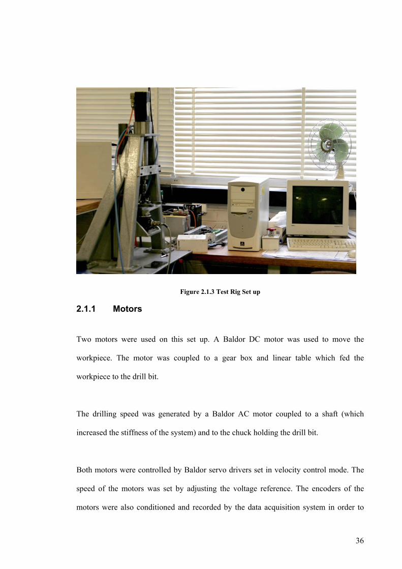
Figure 2.1.3 Test Rig Set up

2.1.1 Motors

Two motors were used on this set up. A Baldor DC motor was used to move the

workpiece. The motor was coupled to a gear box and linear table which fed the

workpiece to the drill bit.

The drilling speed was generated by a Baldor AC motor coupled to a shaft (which

increased the stiffness of the system) and to the chuck holding the drill bit.

Both motors were controlled by Baldor servo drivers set in velocity control mode. The

speed of the motors was set by adjusting the voltage reference. The encoders of the

motors were also conditioned and recorded by the data acquisition system in order to

37

measure the actual speed and or position of the system. Details of the motors’ ratings

can be found in Appendix A.

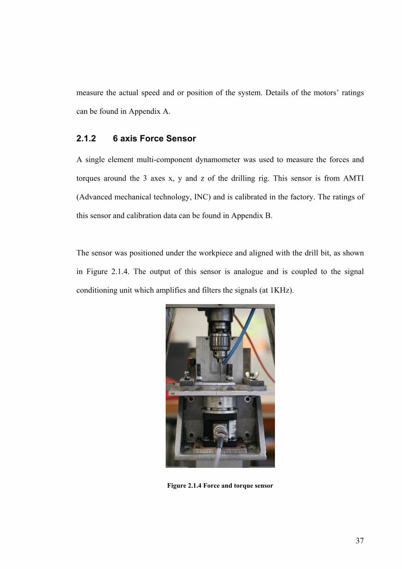
2.1.2 6 axis Force Sensor A single element multi-component dynamometer was used to measure the forces and

torques around the 3 axes x, y and z of the drilling rig. This sensor is from AMTI

(Advanced mechanical technology, INC) and is calibrated in the factory. The ratings of

this sensor and calibration data can be found in Appendix B.

The sensor was positioned under the workpiece and aligned with the drill bit, as shown

in Figure 2.1.4. The output of this sensor is analogue and is coupled to the signal

conditioning unit which amplifies and filters the signals (at 1KHz).

Figure 2.1.4 Force and torque sensor

38

An AMTI 6 channel strain gage amplifier was used to amplify and condition the signals

produced by the force sensor. Gain and filtering is set individually for each channel and

the output can be analogue or digital. The ratings of this amplifier and calibration data

can be found in Appendix B. In the current application, the analogue output was used

and coupled to the data acquisition board described in the next section.

2.1.3 Data Acquisition and Control of the Test Rig Two E series multifunction National Instruments data acquisition boards were used in

this test bed:

• PCI-6030E is a real time board with its own microprocessor. This board was

used to control the drilling process. It measured the encoders from the motors

and set the reference voltage. It was also used to measure the thrust force (force

in the Z axis) and determine the point of contact. This board has real time

capabilities, but the memory in the board is limited and therefore communication

with the computer, although possible, does not allow for large amounts of data

to transfer in real time. For this reason this board was not used to save the data

from the force sensor.

• PCI-6023E uses the computer processor and was used to acquire the data from

the force sensors.

Figure 2.1.5 shows a schematic of how the test rig was connected to the data acquisition

boards and computer.

39

Figure 2.1.5 Drilling rig connections scheme

LabView® was the language used to control the test bed. Two separate programs were

used running in two platforms and communicating with each other. The user interface

and data acquisition were running on the computer processor while the controller was

running on the real time board. The user could choose all the drilling parameters on the

user interface panel which would be passed to the controller program automatically.

This was a convenient and user friendly setup. Drilling time was controlled by

controlling the displacement of the workpiece from the moment of contact. The drilling

parameters chosen by the user were: displacement, spindle speed and feed rate. The user

could also define data acquisition frequency and variables to be measured, i.e. forces,

torques, motor encoder signals.

Spindle motor

Feed motor

Force sensor

Encoder signal

Reference Voltage

Fz Fy Fx Ty Ty Tz

DRILLING RIG

Sig

nal c

ondi

tion

ing

Encoder (speed & position) Feed Reference Fz Encoder (speed) Spindle Speed Reference

Fz Fy Fx Ty Ty Tz

DAQ RT

DAQ

DATA ACQUISITION & CONTROL

Encoder signal

Reference Voltage

40

2.1.4 Calibration Procedures

To calibrate and commission the test bed a series of test procedures was undertaken as

described below.

The force sensor signal conditioning unit has a zeroing button which was pressed before

drilling every time. This procedure ensured that all forces and torques were zero before

drilling started.

To calibrate the spindle speed, a tachometer was used to measure the speed output of the

spindle motor for a range of input voltages and the software used to adjust the

calibration. The encoder signals generated by the motor were also recorded and

compared to the set speed and tachometer readings. The speed generated was found to

be within 98.75% of the set speed.

To calibrate the feed rate and positioning, both the time and position of the workpiece

were observed. A program was used which moved the workpiece 10mm at constant

speed. The displacement was measured and compared to the input value and to the

encoder signals generated. A stop watch was used to measure the time it took to run the

program and that value was compared to the expected time for the given feed rate. The

feed rate was within 95% of the set value, while the positioning accuracy was found to

be 0.5mm.

41

Finally, the encoder’s data from both motors was recorded while drilling and compared

to the set speed and feed rate. The feed rate and spindle speed were found to be constant

before, during and after drilling, which means that both motors can develop the

necessary torque without losing performance.

2.2 Drill bits

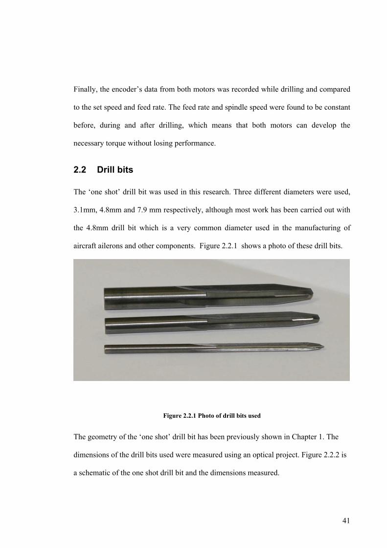
The ‘one shot’ drill bit was used in this research. Three different diameters were used,

3.1mm, 4.8mm and 7.9 mm respectively, although most work has been carried out with

the 4.8mm drill bit which is a very common diameter used in the manufacturing of

aircraft ailerons and other components. Figure 2.2.1 shows a photo of these drill bits.

Figure 2.2.1 Photo of drill bits used

The geometry of the ‘one shot’ drill bit has been previously shown in Chapter 1. The

dimensions of the drill bits used were measured using an optical project. Figure 2.2.2 is

a schematic of the one shot drill bit and the dimensions measured.

42

A Chisel edge AD Cutting lips D to end Reaming fultes

Figure 2.2.2 ‘One shot” Drill bit schematic

The measured dimensions can be seen in table 2.1.

Table 2.1 ‘One shot’ Drill Bit Dimensions

Diameter AB AC AD

3.1mm 0.6mm 1.9mm 6.2mm

4.8mm 1.1mm 2.1mm 8.2mm

7.9mm 1.4mm 3.1mm 15.1mm

43

2.3 Carbon Composite Samples

Two samples of laminated carbon composites have been used in this study, 2.2 and

5.2mm thick. They consisted of 90° angle carbon fibre reinforcement with resin epoxy

bond, each ply 0.2mm thick. The per ply area weight is 193 grams per square meter.

The resin formulation, fabric type and style can be found in Appendix C for product

designation F593-18 (manufactured by Hexcel), 3K-70-PW and Carbon T300. This data

sheet also gives information on the cure cycle and material properties.

These samples are representative of a common layout used in the skins of aircraft

components. The sheets manufactured were 1x0.5m and had to be cut to 7x5cm in order

to fit the experimental setup.

44

Chapter 3 Modelling Thrust Force and Torque

3.1 Introduction

The thrust force and torque produced during drilling contain important information

related to the quality of the hole and the wear of the drill bit [1]. The forces produced

during drilling of metal and composites using a twist drill have been extensively

described in the literature, as discussed in Chapter 1. The ‘one shot’ drill bit used in this

study has been designed to drill carbon fibre. In this chapter, the force and torque

produced during drilling of carbon fibre using a “one shot” drill bit is analysed. The

understanding of these forces plays a very important role in the optimisation of the

drilling process.

The experiments undertaken during the course of this study are described in Section 3.1.

In Section 3.2, the typical thrust force and torque are shown and a 5 stage model is used

to describe the drilling and reaming process. The effect the drilling parameters have on

the thrust force is derived in Section 3.4. The relation between tool age and the forces

generated is looked at in Section 3.5. Lateral forces and frequency content are

investigated in Section 3.6 and 3.7. Finally, conclusions are drawn in Section 3.8

3.2 Description of Experiments

The experimental data used in this chapter was collected from around 300 holes drilled

using a range of settings and workpiece layouts. The spindle speed (rpm) and feed rate

(mm/s) were varied but kept constant at each run (each hole was drilled at constant

45

spindle speed and feed rate). Table 3.1 shows the drilling parameters used where can be

seen that the feed (mm/rev) ranged from 0.02mm/rev to 0.12mm/rev.

Table 3.1 Drilling Parameters

Feed [mm/rev] Feed rate [mm/s] Spindle speed [rpm]

0.06 0.75 750

0.08 1 750

0.12 1.5 750

0.045 0.75 1000

0.06 1 1000

0.09 1.5 1000

0.03 0.75 1500

0.04 1 1500

0.06 1.5 1500

0.06 0.75 750

This range of feeds is fairly conservative to avoid chatter problems that might arise for

high spindle speeds. Three different diameter one shot drill bits were used to find the

influence of diameter on the drilling forces. The diameters were 3.1mm, 4.8mm and

7.9mm.

Three different layouts were used in these experiments: 2mm sample, 5.2mm sample

and a sample composed of two carbon fibre layers each 2mm thick. This variety of

samples was chosen in order to represent common layouts found in industry. The double

layer sample represents many practical applications where two parts are drilled together

to be fastened afterwards.

46

Each combination of feed and workpiece was repeated many times. The same sequence

of experiments was repeated over time using the same 4.9mm drill bit in order to study

the effect of tool age on the drilling forces.

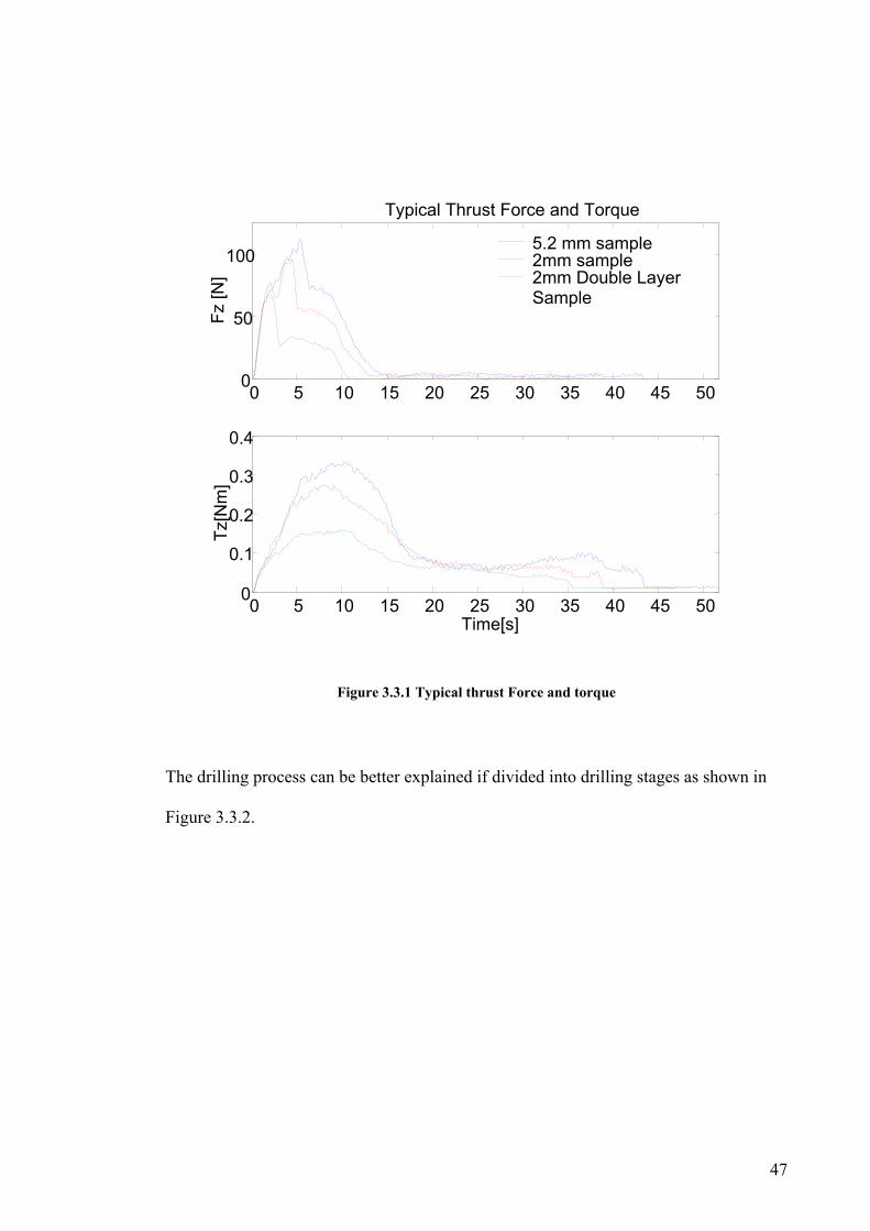
3.3 Typical Thrust Force and Torque

The typical thrust forces and spindle torques produced during drilling of carbon fibre

using the ‘one shot’ drill bit (Figure 1.3.3 and Figure 2.2.2) can be seen in Figure 3.3.1.

The z axis is defined as the axis along which the holes are drilled. The shape of these

forces relates to the shape of the drill bit and the thickness of the workpiece. Different

feed rates do not alter the shape but they do alter the magnitude of thrust force and

torque. The thickness of the workpiece also affects the value of the thrust force.

47

Figure 3.3.1 Typical thrust Force and torque

The drilling process can be better explained if divided into drilling stages as shown in Figure 3.3.2.

0 5 10 15 20 25 30 35 40 45 50 0

50

100

Typical Thrust Force and Torque Fz

[N]

5.2 mm sample 2mm sample 2mm Double Layer Sample

0 5 10 15 20 25 30 35 40 45 50 0

0.1

0.2

0.3

0.4

Tz[N

m]

Time[s]

48

Figure 3.3.2 Drilling Stages

The drill bit approaches the workpiece along the z-axis. In Stage I, the chisel edge

makes contact with the workpiece and “punches” its way into the sample. During this

stage, the thrust force increases very rapidly mostly because of the “extrusion” action of

the chisel edge. The torque also increases but at a much slower rate than the thrust force.

The slow increase of the torque relates to the small diameter of the drill bit at the tip. At

this stage, the drill bit is not yet drilling. A sharp decrease in the thrust force in the first

moments of contact has been reported in the literature [1]. That is because of the peel up

of the top layer of the laminate. Other possible problems that might arise during stage I

are skidding, wandering or deflecting of the drill bit, all of which affect the size of the

hole.

distance

Fz

Stage I Stage II Stage III Stage IV Stage V

Tz

0

0

49

The drilling process starts at Stage II as the cutting lips engage the workpiece. During

this stage, the thrust force increases steadily but at a slower rate as the cutting lips work

their way in. The torque increases steadily throughout this stage. In Figure 3.3.1 a

sudden drop of thrust force could be seen on the 2mm double layer sample. This is

related to the passage from one layer of material to the other. Although the layers are

attached together, the bottom surface of the top layer is fairly rough creating an air gap

between layers. Due to the air gap, the thrust force created by the extrusion action of the

chisel edge momentarily disappears, but its value picks up quickly as the drill bit

encounters the second layer. It is expected that the thrust force will drop more or less

depending on the size of the air gap. The passage from one layer to the other does not

affect the torque and does not affect the drilling process substantially. For simplicity of

the model being developed this drop in thrust force will be ignored. Delamination and

tool wear are commonly associated with stage II due to the high values of thrust force

and torque. The risk of delamination is especially high at the end of this stage as the last

plies of material are pushed by the chisel edge.

Stage III starts when the chisel edge reaches the bottom surface of the workpiece. The

thrust force suddenly drops when the chisel edge comes out of the workpiece. As the

drill bit makes its way through the hole, the cutting lips come out of the hole and the

reaming flutes enter the workpiece. Hence, the drilling is replaced by the reaming

action. The thrust force decreases until the cutting lips are out of the hole. The torque

increases very slightly during this stage. The maximum torque is attributed [1] to high

frictional forces between the lands of the drill and the wall of the hole. Theoretically,

50

the torque should reach its peak value when the cutting lips are fully engaged because

the diameter is at its highest value and the area of the drill in contact with the surface of

the hole is higher too (higher torque due to friction). With high temperatures, the

friction would also increase because of the thermal expansion of the composite which

would squeeze the drill. In the present situation, the chisel edge extrudes from the

workpiece before complete penetration making the prediction of when the maximum

torque should occur harder to accomplish. During the experiments, it was observed that

the peak torque occurred at any time during stage III, including at the very beginning.

To simplify the model, the torque in this stage is represented by a straight line. This is a

fair approximation taking into consideration that in most cases, the torque varies only

very slightly. This stage combines both drilling and reaming, and therefore problems

associated with both cutting processes can happen. Delamination is possible as the last

plies are drilled to the final size although the risk is smaller than the previous stage since

the thrust force is lower. Surface finish problems can arise in this stage as the transition

in the cutting surfaces might cause some vibration or even chatter.

Stage IV relates to the reaming process. The drilling has finished and the drill bit is

reaming the hole to its final size. Problems occurring in this section are related to the

final size and finish of the hole (reaming is more prone to vibrations and chattering than

drilling because of the reduced stiffness).

The drill bit backs out of the workpiece in Stage V. Reaming continues while there is

contact between the workpiece and the drill bit, altering the size and finish of the hole.

During this stage both thrust force and torque maintain the same values of the previous

51

stage. In practice, the only difference between stage III and stage IV is the direction of

movement, as the cutting action and possible problems arising are the same.

3.4 Effect of Drilling Parameters on Thrust Force and

Torque

In the previous section, the thrust force and torque produced while drilling carbon

composite is analysed in respect to displacement. This section focuses on the maximum

thrust force and torque, and the effect that some drilling parameters have on those

peaks.

Figure 3.4.1 and Figure 3.4.2 show an example of the maximum thrust force and torque

obtained drilling 5.2mm carbon composite using a 4.8mm diameter drill bit. It is clear

from the figure that thrust force and torque are proportional to the feed used to drill.

The most common measure of drilling settings is the feed [rev/mm] i.e. how much the

drill bit is fed to the sample (or the sample is fed to the drill) at each revolution of the

drill bit. This means that the feed can be maintained constant for a range of spindle

speeds and feed rates used. For example, drilling at 0.75mm/s and 750rpm, 1mm/s and

1000rpm or 1.5mm/s and 1500rpm all result in a 0.06mm/rev feed.

From the experiments undertaken, it was seen that the maximum thrust force and torque

do not remain constant if the spindle speed and feed rate vary, even when the resultant

feed used is the same. This discrepancy can be seen in Figure 3.4.1 and Figure 3.4.2

52

where at 0.06mm/rev the thrust force increased by about 10N and the torque by 0.1Nm

for lower spindle speeds. It can, therefore, be concluded that the thrust force and torque

are directly proportional to the feed rate and inversely proportional to the spindle speed.

5.2 mm Sample, 4.8mm Drill Bit

50

70

90

110

130

150

170

0 0.05 0.1 0.15

Feed [mm/rev]

Thru

st F

orce

[N]

750 RPM1000 RPM1500 RPM

Figure 3.4.1 Plot of maximum thrust force against feed for various spindle speeds

53

5.2 mm Sample, 4.8 mm Drill Bit

0

0.1

0.2

0.3

0.4

0.5

0.6

0 0.05 0.1 0.15

Feed [mm/rev]

Torq

ue [N

m]

750 RPM100 RPM1500

Figure 3.4.2 Plot of maximum torque against feed for various spindle speeds

The following figures show how the thickness of the workpiece affects the maximum

thrust force and torque. From observing Figure 3.4.3 and Figure 3.4.4 it can be

concluded that drilling thicker samples will produce higher thrust force and torque. This

is mainly due to the higher values of friction inside of the hole and larger surfaces in

contact while drilling.

Comparing the thrust force produced by drilling 2.1mm and 5.2mm samples, it can be

seen that the thrust force doubled (for the range of feeds tested). The torque produced

drilling different thicknesses also changed, but differently for different feeds. For lower

feeds, the torque had just a marginal increase when drilling thicker samples. For higher

feeds, the torque produced drilling thicker samples is over double the torque needed to

drill the thinner samples. A possible explanation for this is that at lower feeds, the chips

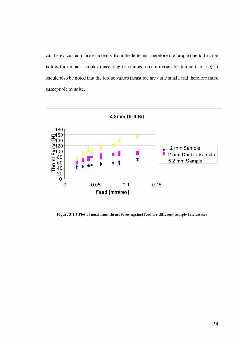
54

can be evacuated more efficiently from the hole and therefore the torque due to friction

is less for thinner samples (accepting friction as a main reason for torque increase). It

should also be noted that the torque values measured are quite small, and therefore more

susceptible to noise.

Figure 3.4.3 Plot of maximum thrust force against feed for different sample thicknesses

4.8mm Drill Bit

0 20406080

100 120 140 160 180

0 0.05 0.1 0.15Feed [mm/rev]

Thru

st F

orce

[N]

2 mm Sample2 mm Double Sample5.2 mm Sample

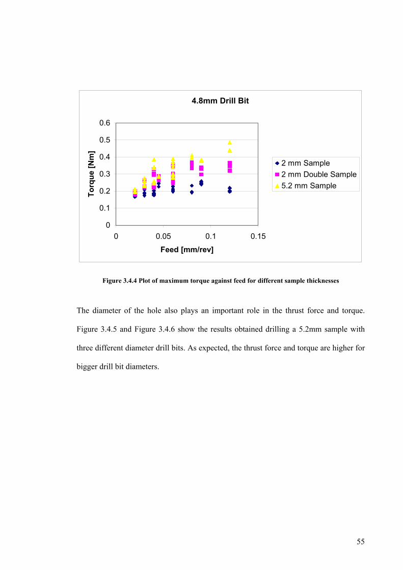
55

4.8mm Drill Bit

0

0.1

0.2

0.3

0.4

0.5

0.6

0 0.05 0.1 0.15

Feed [mm/rev]

Torq

ue [N

m]

2 mm Sample2 mm Double Sample5.2 mm Sample

Figure 3.4.4 Plot of maximum torque against feed for different sample thicknesses

The diameter of the hole also plays an important role in the thrust force and torque.

Figure 3.4.5 and Figure 3.4.6 show the results obtained drilling a 5.2mm sample with

three different diameter drill bits. As expected, the thrust force and torque are higher for

bigger drill bit diameters.

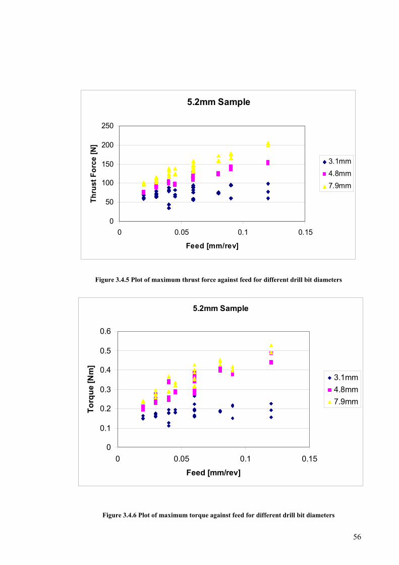
56

5.2mm Sample

0

50

100

150

200

250

0 0.05 0.1 0.15

Feed [mm/rev]

Thru

st F

orce

[N]

3.1mm4.8mm7.9mm

Figure 3.4.5 Plot of maximum thrust force against feed for different drill bit diameters

5.2mm Sample

0

0.1

0.2

0.3

0.4

0.5

0.6

0 0.05 0.1 0.15

Feed [mm/rev]

Torq

ue [N

m]

3.1mm4.8mm7.9mm

Figure 3.4.6 Plot of maximum torque against feed for different drill bit diameters

57

3.5 Effect of Tool Age on Thrust Force and Torque

High tool wear rates are a major concern in drilling carbon composites and the increase

of thrust force due to wear has been widely reported in the literature. In this section, the

effect of tool wear on thrust force and torque is studied. Initially, it is shown how tool

wear affects thrust force and torque in the time domain. Secondly, only peak values of

thrust and torque are analysed to show how tool wear affected the thrust force at

different feeds.

Tool wear is directly related to drilling time, and consequently to the number of holes

drilled with a given drill bit [4, 5]. The thrust force and torque produced by a drill bit at

different stages of the drill bit life are compared. In order to allow comparison, holes

drilled with the same settings and sample thickness were used. Figure 3.5.1, Figure

3.5.2, and Figure 3.5.3 show typical examples of thrust force and torque produced at

different stages of the drill bit life for each sample thickness tested.

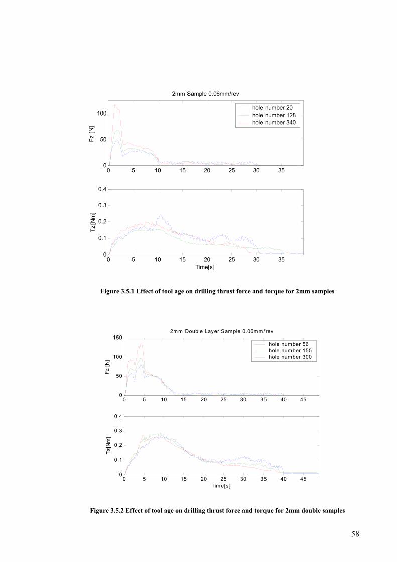
58

0 5 10 15 20 25 30 350

50

100

2mm Sample 0.06mm/revFz

[N]

hole number 20hole number 128hole number 340

0 5 10 15 20 25 30 350

0.1

0.2

0.3

0.4

Tz[N

m]

Time[s]

Figure 3.5.1 Effect of tool age on drilling thrust force and torque for 2mm samples

0 5 10 15 20 25 30 35 40 450

50

100

1502mm Double Layer Sample 0.06mm/rev

Fz [N

]

hole number 56hole number 155hole number 300

0 5 10 15 20 25 30 35 40 450

0.1

0.2

0.3

0.4

Tz[N

m]

Time[s]

Figure 3.5.2 Effect of tool age on drilling thrust force and torque for 2mm double samples

59

0 5 10 15 20 25 30 35 40 45 500

50

100

150

5.2mm Layer Sample 0.06mm/rev

Fz [N

]hole number 92hole number 174hole number 250

0 5 10 15 20 25 30 35 40 45 500

0.1

0.2

0.3

0.4

Tz[N

m]

Time[s]

Figure 3.5.3 Effect of tool age on drilling thrust force and torque for 5.2mm samples

From the experiments, it can be seen that thrust force increases with the number of holes

drilled. Although the thrust force has increased throughout the course of the drilling

process, the increase is more noticeable just before breaking through, which suggests

that the primary cutting surfaces of the drill bit might be wearing out more that the rest

of the body of the drill bit. This agrees with the work published by Lin [4] which reports

that when drilling composites the drill wears first in the outer cutting edges. Comparing

Figure 3.5.1, Figure 3.5.2 and Figure 3.5.3, it can be seen that the effect of tool wear is

more prominent when drilling thinner samples. A possible explanation for this is that for

thicker samples the total thrust force produced is a sum of the thrust force from affected

and non affected areas of the drill bit, and therefore the overall thrust force increase is

not as pronounced as for thinner samples.

60

The torque produced did not show significant changes over the range of number of

holes analysed. This was true for all the samples tested. The same findings have also

been reported by others[6].

The previous analysis looked at the thrust force increase in the time domain. Another

way of analysing the data is to plot the maximum thrust force and torque against the

feed to find the effect of tool wear for different feeds.

2mm sample

020

40

6080

100

120

140160

0 0.05 0.1 0.15

Feed [mm/rev]

Thru

st F

orce

[N]

holes 1-36holes 115-141holes 324-358

Figure 3.5.4 Plot of maximum thrust force against feed for 2mm sample

61

2mm sample

0

0.05

0.1

0.15

0.2

0.25

0.3

0 0.05 0.1 0.15

Feed [mm/rev]

Torq

ue [N

m]

holes 1-36holes 114-140holes 324-358

Figure 3.5.5 Plot of maximum torque against feed for 2mm sample

Figure 3.5.4 and Figure 3.5.5 show the maximum thrust force and torque, respectively,

produced while drilling a 2mm sample at different feeds and at different stages of the

drill bit life. From analysing Figure 3.5.4, it can be concluded that the maximum thrust

force doubled during the number of holes studied. This increase is mainly constant for

all feeds used. The maximum torque shown in Figure 3.5.5 generally increases with

feed used (with a few exceptions for the first holes drilled at higher feed) but does not

seem to be particularly related to tool wear.

62

2mm Double Sample

0

50

100

150

200

250

0 0.05 0.1 0.15

Feed [mm/rev]

Thru

st F

orce

[N]

holes 37-72holes 141-167holes 286-321

Figure 3.5.6 Plot of maximum thrust force against feed for 2mm double sample

2mm Double Sample

00.05

0.10.15

0.20.25

0.30.35

0.40.45

0 0.05 0.1 0.15

Feed [mm/rev]

Torq

ue [N

m]

holes 37-72holes 141-168holes 286-321

Figure 3.5.7 Plot of maximum torque against feed for 2mm double sample

63

In Figure 3.5.6 and Figure 3.5.7, the maximum thrust force and torque produced while

drilling a 2mm double sample at different feeds and at different stages of the drill bit life

can be seen. The maximum thrust force increases with feed and number of holes drilled

(due to tool wear); however this increase is not consistent for all feeds used. For lower

feeds, the maximum thrust force increases only slightly due to tool wear, while for the

higher feeds, the thrust force doubled (as for the 2mm sample). The maximum torque

shown in Figure 3.5.7 increased with feed (again a few exceptions for the higher feeds)

but is not related to tool wear.

For the case of drilling a 5.2mm sample, the results can be seen in Figure 3.5.8 and

Figure 3.5.9. Again, the thrust force increases with the feed used and with number of

holes drilled. The influence of tool wear on the thrust force is more accentuated for

higher feeds but not as much as when drilling thinner samples. The maximum torque is

proportional to the feed used but is not affected by tool wear.

64

5.2 mm sample

0

50

100

150

200

250

300

0 0.05 0.1 0.15

Feed [mm/rev]

Thru

st F

orce

[N]

holes 73-108holes 168-191holes 250-285

Figure 3.5.8 Plot of maximum thrust force against feed for 5.2mm sample

5.2mm Sample

0

0.1

0.2

0.3

0.4

0.5

0.6

0 0.05 0.1 0.15

Feed [mm/rev]

Torq

ue [N

m]

holes 73-108holes 168-193holes 251-285

Figure 3.5.9 Plot of maximum torque against feed for 5.2mm sample

65

From the experiments undertaken it can be concluded that the thrust force increases

with number of holes drilled while torque is not particularly affected. It has also been

shown that the effect of tool wear on maximum thrust force varies with the thickness of

the workpiece and the feed used for drilling.

3.6 Lateral Forces and Torques

The forces produced during drilling are commonly associated with the thrust force and

torque. The lateral forces, in theory, should be zero. Each cutting edge produces a force

in the direction of the cutting direction, but being in pairs, the cutting edge on the

opposite side will produce an equivalent force in the opposite direction with the

resultant force zero. In practice, the cutting edges do not produce exactly the same force

and a resultant lateral force can be generated. Researchers have used this lateral force as

an indication of the angle of attack [2]. It is assumed that if there is a lateral force, it

means the end effector is not perpendicular to the workpiece and needs to be adjusted to

produce no forces on the lateral plane. Other published work[3] has shown a relation

between the frequency content of such forces and the angle of attack. It is, therefore, of

relevance to study these forces and torques.

Figure 3.6.1 shows an example of the forces and torques produced while drilling in the

X and Y axis. It can be seen that these forces indeed are not zero and that the torque

around the axis X is a mirror of the force in Y, and the torque around axis Y is a mirror

66

of the force in X. This is expected as each torque is produced by the force on the other

axis.

Figure 3.6.1 Forces and torques produced while drilling

In previous sections, it has been shown how the thrust force and torque vary with

settings used and with age of the drill bit. Such relationships are not found for the lateral

forces. Both in amplitude and direction, no typical shape of signal and could be found.

The variation of these forces did not relate to the settings or tool age either. Holes

drilled consecutively by the same drill bit and settings would often produce forces in the

x and y directions different in amplitude and direction. Figure 3.6.2 shows such an

67

example. It can be seen that although the settings used are the same, the amplitude and

direction of the lateral forces varied.

Figure 3.6.2 Holes drilled consecutively by the same drill bit and settings

An example of holes drilled by three drill bits at different age stages is shown in Figure

3.6.3.

68

Figure 3.6.3 Holes drilled by differently aged drill bits

A possible explanation for this observed phenomenon is the non homogeneity of the

sample being drilled. As the drill bit pushes through the workpiece, the fibres that are on

the way are likely to “push” the tip of the drill bit to the side. The direction and

amplitude of such forces would therefore be related to the position of the tip of the drill

in relation to the nodes of fibres it encounters. This would explain the fact that these

lateral forces may vary in direction during drilling but tend to be constant or at least in

just one direction during reaming. The position of the drill bit in relation to the fibres

could not be measured in this research and so further study of this lateral forces is

outside the scope of this thesis.

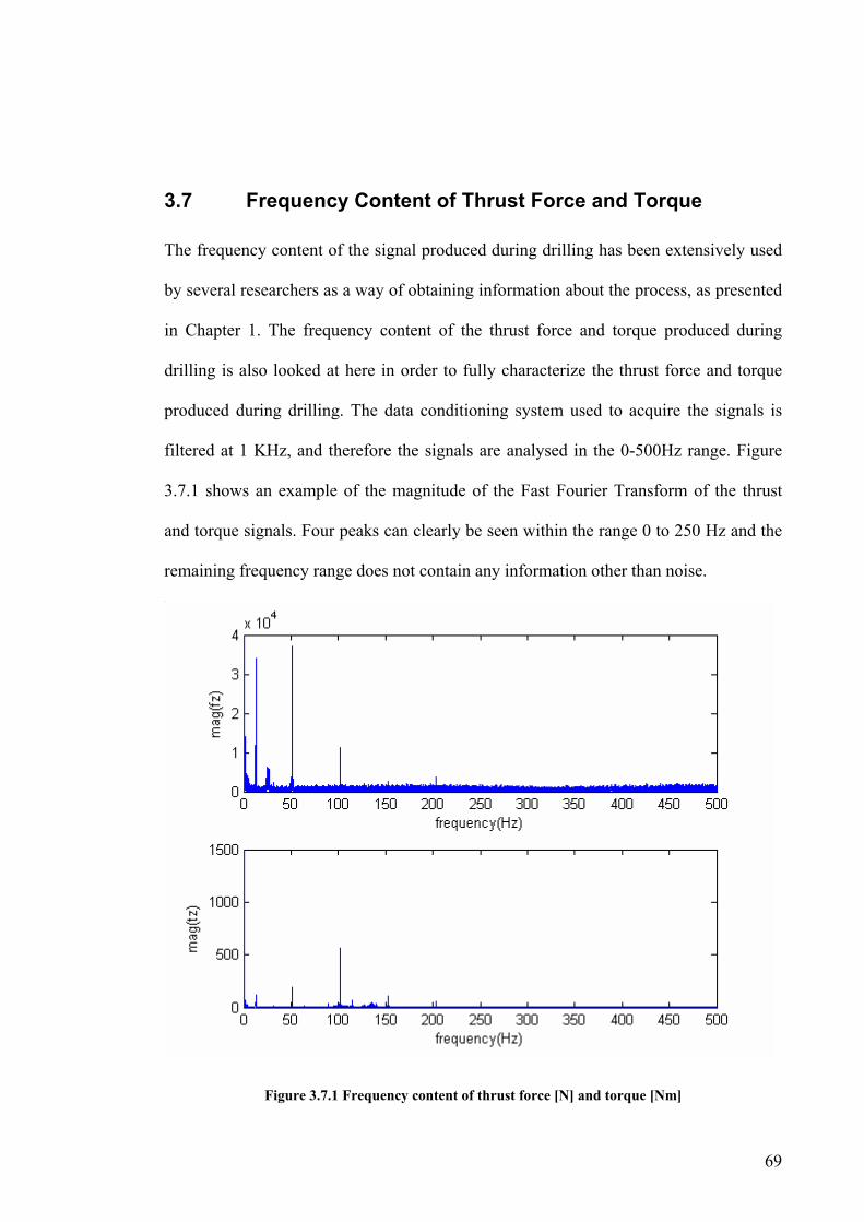
69

3.7 Frequency Content of Thrust Force and Torque

The frequency content of the signal produced during drilling has been extensively used

by several researchers as a way of obtaining information about the process, as presented

in Chapter 1. The frequency content of the thrust force and torque produced during

drilling is also looked at here in order to fully characterize the thrust force and torque

produced during drilling. The data conditioning system used to acquire the signals is

filtered at 1 KHz, and therefore the signals are analysed in the 0-500Hz range. Figure

3.7.1 shows an example of the magnitude of the Fast Fourier Transform of the thrust

and torque signals. Four peaks can clearly be seen within the range 0 to 250 Hz and the

remaining frequency range does not contain any information other than noise.

Figure 3.7.1 Frequency content of thrust force [N] and torque [Nm]

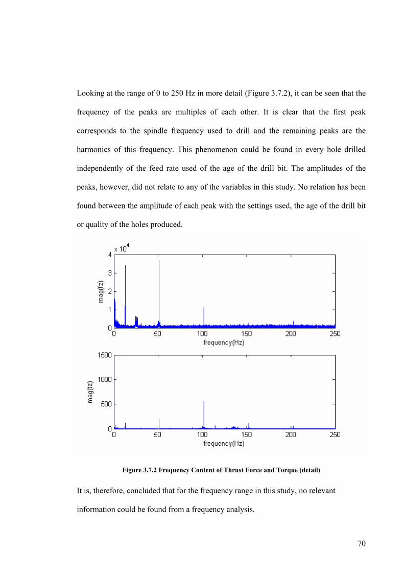
70

Looking at the range of 0 to 250 Hz in more detail (Figure 3.7.2), it can be seen that the

frequency of the peaks are multiples of each other. It is clear that the first peak

corresponds to the spindle frequency used to drill and the remaining peaks are the

harmonics of this frequency. This phenomenon could be found in every hole drilled

independently of the feed rate used of the age of the drill bit. The amplitudes of the

peaks, however, did not relate to any of the variables in this study. No relation has been

found between the amplitude of each peak with the settings used, the age of the drill bit

or quality of the holes produced.

Figure 3.7.2 Frequency Content of Thrust Force and Torque (detail)

It is, therefore, concluded that for the frequency range in this study, no relevant

information could be found from a frequency analysis.

71

3.8 Conclusions

In this chapter, the thrust force and torque produced during drilling of carbon composite

using a ‘one shot’ drill bit have been analysed.

The large number of experiments conducted show that the drilling process with the one

shot drill can be modelled as a 5 step process with each step directly related physically

to the various drilling and reaming processes. This is shown to be the case irrespective

of the feed rates for different thicknesses of material and also for a two layer stack. This

model depends on the position of the drill bit in relation to the workpiece. It can also be

concluded that the thrust force increases with number of holes drilled with a given drill

bit, while torque is not particularly affected. It has been shown that the effect of tool

wear on thrust force varies throughout the different stages, with the increase in thrust

force being more noticeable just before breaking through. The thickness of the

workpiece also plays a role in the effect of tool wear on the thrust force; the thinner the

workpiece, the bigger the increase of thrust force due to wear. The feeds used to drill

also affect the increase of thrust force due to tool wear: the higher is the feed, the bigger

the effect the tool wear has on the thrust force produced by worn drill bits. Therefore the

thrust force and torque are a function of feed, drill bit, thickness of the workpiece, and

tool wear (defined as the number of holes previously drilled).

The frequency content of the thrust force and torque has been studied and related to the

spindle speed used, but this study showed that no useful information was available over

the frequency range considered.

72

The lateral forces produced during drilling have been measured and it has been

concluded that they vary independently of the settings used and age of the drill bit. It is

suggested that they are most affected by the orientation and ratio of the workpiece and

other factors not related to drilling parameters.

The findings of this chapter enable the development of a mathematical model of the

thrust force as described in Chapter 4. This model can then be used to extend and /or

predict drill life and improve productivity and quality of hole drilling for industries such

as aerospace, in which the drilling of composites is an important manufacturing process.

73

Chapter 4 Maximum Thrust Force and Torque Estimation

4.1 Introduction

To estimate the maximum thrust force and torque, an empirical model will be

developed. Shaw’s simplified equations (see 1.3.2) have been successfully used by

several authors to predict thrust force and torque for drilling carbon composites with

new twist drills [6, 7]. For the current work, Shaw’s simplified equations will be

adapted in order to accommodate for tool wear and used to predict thrust force and

torque in the drilling of carbon composite with a ‘one shot’ drill bit.

Initially, in section 4.2, the maximum thrust force and torque will be estimated using

Shaw’s equations. The initial value of thrust force is at its maximum value, being

directly related to the occurrence of delamination and problems such as deflection of the

manipulator, occurrence of chatter, etc. In a second stage, section 4.3, the thrust force at

other stages of the drilling process will be modelled.

4.2 Using Shaw’s simplified equations

Shaw’s equations have been introduced and described in Chapter 1, where the

simplified equations are:

74

( )

=

+=−−

−

aa

a

dfKTorque

dKfdKForce21

22

11

3 (4.1)

Where f is the feed (mm/rev), d is the diameter (mm) and ‘a’ and ‘K’1-3 are obtained

experimentally.

The thrust force and torque estimated by Shaw’s equations are average values during

full engagement of the drill bit, called the steady state region. In the present application

the drill bit breaks through before full engagement and therefore the process does not

reach the steady state described in Shaw’s model.

The thrust force is at a maximum just before the drill bit breaks through, and assuming

this happens just after the drill bit fully engages the workpiece (illustrated below in

Figure 4.2.1 ), the thrust/torque calculated by Shaw would be a fair approximation of

the maximum thrust force obtained in the experiments described here.

Figure 4.2.1 Analogy from current thrust force and Shaw’s thrust force

Typical Thrust from current experiments

Typical thrust curve used by Shaw [1]

Steady state

Thrust Force

distance

Max Thrust force

75

This scenario implies that the full diameter of the drill bit is engaged. In other words,

the values of thrust and torque obtained by Shaw’s model can relate to the maximum

thrust force of the present process if the diameter used is the diameter of the of the part

of the bit which is fully engaged. Hence, the diameter used for calculating here is not

the diameter of the drill bit, but the diameter of the drill bit at the time of maximum

thrust/torque. The diameter will be related to the thickness of the workpiece as shown in

Figure 4.2.2.

Figure 4.2.2 Drill bit diameter at ‘break-through’

As previously explained, Shaw’s equations can be greatly simplified if the relation c/d

remains constant. The diameter being used varies for the same chisel edge, but the

chisel edge of the drill bit being used is only 0.2mm and therefore the ratio c/d is so

small that the variation can be ignored. Hence, Shaw’s simplified equation will be used

to estimate thrust force.

As explained and shown in the first sections of this chapter, the torque remains fairly

constant throughout the cutting process; hence Shaw’s simplified equations will also be

used to estimate the torque.

76

The first step will be to calculate the value of ‘a’ using the specific cutting energy based

on the measured torque and the diameter related to the thickness of the sample as

previously explained. The value of ‘a’ is dependent on the combination drill bit and

material of the workpiece and is directly related to the torque produced during drilling.

It has been previously shown that the torque produced during drilling is not significantly

affected by tool wear and therefore it will be assumed that the drill bit /material

relationship will not change due to tool wear (for the range of settings used); hence ‘a’

will be constant. By plotting log(fd) against log(u) a value for a of 0.603 is obtained as

shown in Figure 4.2.3.

y = -0.5847x - 0.1247

-0.1

0

0.1

0.2

0.3

0.4

0.5

0.6

-1.2 -1 -0.8 -0.6 -0.4 -0.2 0

log (fd)

log

(u)

Figure 4.2.3 Plot of log(u) against log(fd)

4.2.1 Estimating Torque at Break-Through

Using ‘a’ above, Shaw’s simplified equation to estimate torque becomes,

39..139.0 dkfT = (4.2)

Fitting experimental data to Equation 4.2 and averaging the resultant value of k,

77

39..139.013.0 dfT ×= (4.3)

The results obtained by using equation 4.3 to estimate the torque can be seen in Figure

4.2.4. The estimated values agree fairly well with the measured values. A few

discrepancies can be seen for some holes but taking into consideration that the torque is

a very small signal (easily perturbed by noise) the results are satisfactory.

0

0.1

0.2

0.3

0.4

0.5

0.6

1 19 37 55 73 91 109 127 145 163 181 199 217 235 253 271 289

Hole Number

Torq

ue [N

m]

Measured TzEstimated Tz

Figure 4.2.4 Measured and estimated torque using Shaw’s equations

4.2.2 Estimating Maximum Thrust Force

The following equation (Shaw’s simplified equation) will be used to estimate the

maximum thrust force,

2)1(

1 )( kfdkF a += − (4.4)

The maximum thrust force is strongly affected by tool wear and therefore Shaw’s model

has to be adapted in order to accommodate tool wear. Initially, only data from the first

holes drilled by a drill bit was used in order to calculate K1=76.56 and K2 =1.04 (using

the least squares method), giving:

78

239.0),( 04.1)(56.76 dfdF df += (4.5)

As seen in Figure 4.2.5, the estimated values agree with the measured values for the first

holes drilled. It can also be seen that the estimated values have the same trend as the

measured values for later holes, but the difference in amplitude increases with the

number of holes drilled.

0

50

100

150

200

250

300

1 27 53 79 105 131 157 183 209 235 261 287

Hole number

Thru

st fo

rce

[N]

Measured Thust Force

Estimated Thrust forceusing Shaw's equations

Figure 4.2.5 Measured and estimated thrust force using Shaw’s equations

This shows that although Shaw’s model can be used to estimate thrust force on drilling

of carbon composites using a new “one-shot” drill bit, the model needs to be adjusted

for tool wear. For example, consider:

)047.156.76( 239.0),,( dfdffToolAgeCoeF agedf +×= (4.6)

where the tool wear coefficient will be dependent on the number of holes drilled by the

drill bit. It is also expected that tool wear will affect the thrust force differently for each

of the different thicknesses of workpiece being tested, so that:

21),( knkffToolAgeCoe thickn +×= (4.7)

79

k1 and k2 were calculated using experimental data for each thickness of workpiece. The

estimated thrust force calculated from Equation 4.5 was divided by the measured thrust

force to give the tool wear coefficient for each sample. Plotting the tool wear coefficient

against the respective hole number, and fitting a line of best fit, the parameters k1 and k2

from Equation 4.7 can be found. The following figures show the results obtained for a

2mm sample, a 2mm double sample and a 5.4mm respectively.

y = 0.0036x + 0.98

0

0.5

1

1.5

2

2.5

3

0 100 200 300 400

Hole number

Age

coe

ffici

ent

Figure 4.2.6 Tool wear rate for 2mm sample

80

y = 0.0036x + 1.2128

0

0.5

1

1.5

2

2.5

3

3.5

0 50 100 150 200 250 300 350Hole number

Age

Coe

ffici

ent

Figure 4.2.7 Tool Wear Rate for 2mm Double Layer Sample

y = 0.0035x + 1.4925

0

0.5

1

1.5

2

2.5

3

3.5

0 50 100 150 200 250 300

Hole number

Age

coe

ffici

ent

Figure 4.2.8 Tool wear rate for 5.4mm sample

81

Hence the maximum thrust force will be:

)047.1)(56.76(*)5159.10035.0(

)047.1)(56.76(*)2128.10036.0(

)047.1)(56.76(*)0467.1003.0(

239.05

239.04

239.02

dfdnThrust

dfdnThrust

dfdnThrust

mmsample

mmsample

mmsample

++=

++=

++=

(4.8)

The following Figure shows the estimated thrust force calculated using Equation 4.8

against the measured values of maximum thrust force for each sample tested.

0

50

100

150

200

250

300

1 27 53 79 105 131 157 183 209 235 261 287

Hole Number

Thru

st F

orce

[N]

max Fzmax Fz estimate

Figure 4.2.9 measured and estimated maximum thrust force

As seen in Figure 4.2.9, the new model represents the drilling process very well. Some

discrepancies between the estimated and measured values would be expected to result

from noise on the measured values, and also from the approximation in the tool wear

model. Although wear is dependent on spindle speed and drilling time (number of

holes), on this model it was assumed that the rate of tool wear was constant for the

range of drilling parameters used.

82

4.3 Estimation of Thrust Force In Relation to Time

Figure 4.3.1 shows a representation of the typical thrust force produced during drilling.

The corners marked as ‘A’, ‘B’, ‘C’, ‘D’ and ‘E’, were used to represent the signal.

0 2 4 6 8 10 12

0

20

40

60

80

100

120

140

fz [N

] A

B

C D

E

Time[s]

Figure 4.3.1 Typical thrust force represented by corners

Using experimental data, the thrust force was measured for each corner shown in Figure

4.3.1 and used to model the drilling process. If force is plotted as a function of

displacement rather than time, the position of each corner is related to the thickness of

the workpiece. For the drill bits used here, A always occurs at 1.1mm of displacement.

The corner B represents the maximum thrust force, which occurs just before the break

through point and therefore equals the thickness of the workpiece. Corner C follows

corner B. Its position is 0.9mm after break through. D is the moment when the reaming

section of the drill bit enters the material and therefore is constant for all thicknesses at

83

8.41mm (distance from the tip to the reaming section of the drill bit). Corner E

represents the moment when the drill finishes cutting and the cutting lips leave the

workpiece, and hence its position is dependent on the thickness of the sample being

drilled.

The thrust force at ‘B’ has been successfully estimated in the previous section. In this

section the forces at ‘A’, ‘C’, ‘D’ and ‘E’ will be estimated.

4.3.1 Estimation of Thrust force at Position ‘A’

From the experimental data it was possible to see that the thrust force at ‘A’ was related

to the value of maximum thrust force. Figure 4.3.2 shows thrust force at A and at B. It

can be seen that the thrust force at A follows the same trend as the maximum thrust

force (or thrust force at B). It can also be noted that although the trend is the same, the

difference increases with number of holes drilled, suggesting that tool wear might affect

the thrust force at point A differently from the thrust force at point B.

84

0

50

100

150

200

250

1 16 31 46 61 76 91 106 121 136 151 166 181Sample Number

Forc

e [N

]

Thrust at BThrust at A

Figure 4.3.2 Plot of thrust force at ‘A’ and ‘B’

The thrust force at ‘A’ is therefore estimated using Equation 4.8 but with a different tool

wear coefficient. This means that tool wear impacts the thrust force differently at

different points of the drilling process.

In the previous Chapter it was shown that for the same feed and tool wear rate, the

thrust force at ‘A’ (Stage I) is independent of the thickness of the workpiece. Hence, the

tool wear coefficient suggested here will also be independent of the workpiece

thickness. Following the same procedure as before, the thrust force at ‘A’ was estimated

using Equation 4.5 where the diameter is the same for all thicknesses (3.26mm). The

estimated force is then divided by the measured thrust force and the results plotted

against the respective hole number. Figure 4.3.3 shows the results obtained.

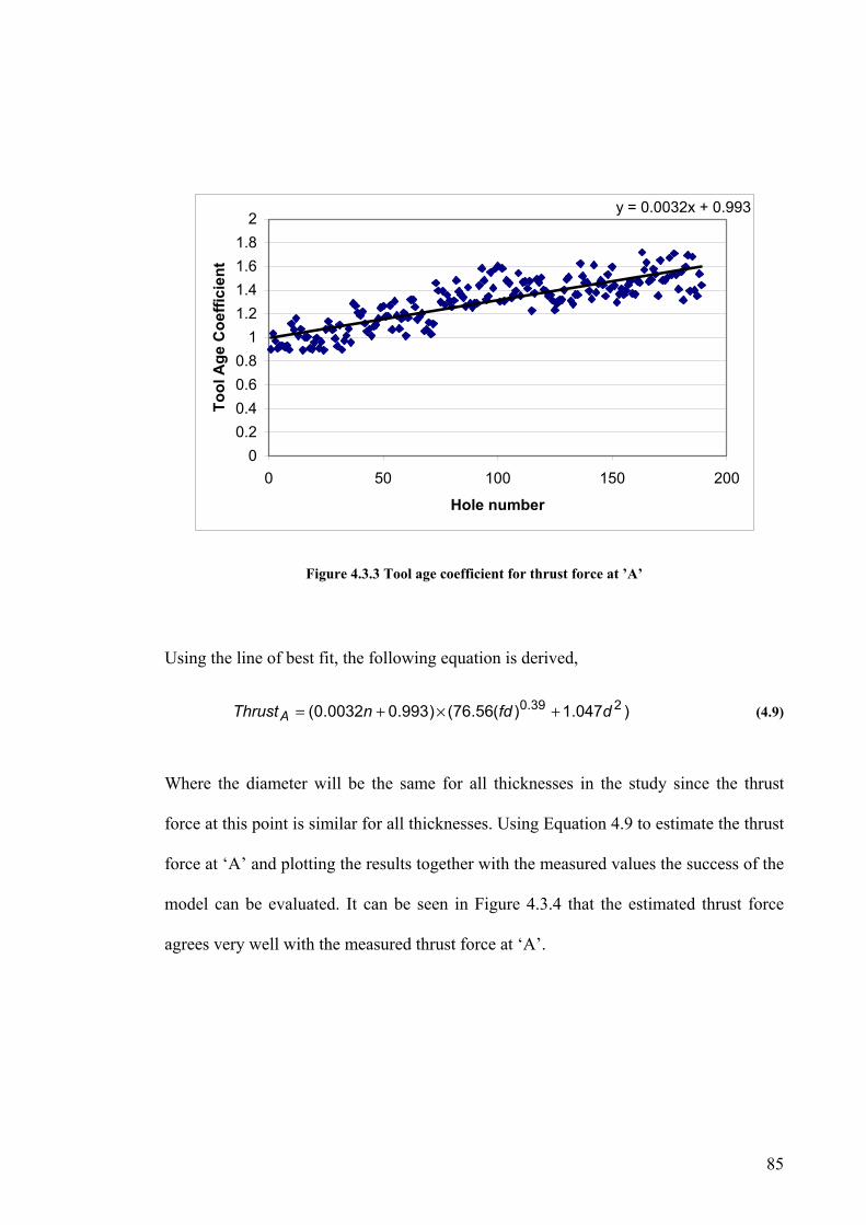
85

y = 0.0032x + 0.993

00.20.40.60.8

11.21.41.61.8

2

0 50 100 150 200

Hole number

Tool

Age

Coe

ffici

ent

Figure 4.3.3 Tool age coefficient for thrust force at ’A’

Using the line of best fit, the following equation is derived,

)047.1)(56.76()993.00032.0( 239.0 dfdnThrustA +×+= (4.9)

Where the diameter will be the same for all thicknesses in the study since the thrust

force at this point is similar for all thicknesses. Using Equation 4.9 to estimate the thrust

force at ‘A’ and plotting the results together with the measured values the success of the

model can be evaluated. It can be seen in Figure 4.3.4 that the estimated thrust force

agrees very well with the measured thrust force at ‘A’.

86

0

20

40

60

80

100

120

1 18 35 52 69 86 103 120 137 154 171 188

Sample Number

Forc

e [N

]

AA estimate

Figure 4.3.4 Estimated and measured thrust force at ‘A’

4.3.2 Estimation of Thrust force at position ‘C’

The thrust force at ‘C’ is also dependent on the maximum value of Fz and the thickness

of the sample. As shown in Figure 4.3.5, the Thrust force at ‘C’ follows the same trend

as the force at B (or maximum thrust force) but is consistently smaller. This suggests

that thrust force at C is a percentage of the thrust force at B and that tool wear affects

both equally.

87

020406080

100120140160180200

1 17 33 49 65 81 97 113 129 145 161 177

Sample Number

Forc

e [N

]

Max FzThrust at C

Figure 4.3.5 Estimated and Measured Thrust Force at ‘A’

Dividing the thrust force at ‘C’ by the thrust force at ‘B’ and averaging the resulting

ratios separately for each thickness, the following model for the Thrust Force at C is

obtained,

FzThrustC

FzThrustC

FzThrustC

mmsample

mmsample

mmsample

max56.0

max58.0

max40.0

5

4

2

×=

×=

×=

(4.10)

The following figure shows the results obtained when plotting the measured thrust force

at “C” and the thrust force calculated using Equation 4.10.

88

0

20

40

60

80

100

120

1 18 35 52 69 86 103 120 137 154 171 188

Sample Number

Forc

e [N

]

CC estimate

Figure 4.3.6 Estimated and Measured Thrust Force at ‘C’

As seen in Figure 4.3.6 the estimated force at ‘C’ agrees fairly well with the measured

thrust force. It is important to note that although the thrust force at ‘C’ could be

estimated using the model for estimating the maximum thrust force at B (as previously

done when estimating A), the results shown here used the measured values of the thrust

force at ‘B’. This avoids the errors in calculating thrust at B being amplified when

estimating thrust at ‘C’.

4.3.3 Estimation of Thrust force at position ‘D’

The thrust force decreases slightly from ‘C’ to ‘D’, as the cutting lips finish drilling the

hole. Plotting the thrust force measured at both ‘C’ and ‘D’ (see Figure 4.3.7) the

similarity in amplitude is remarkable for most holes.

89

0

20

40

60

80

100

120

1 14 27 40 53 66 79 92 105 118 131 144 157 170 183

Sample Number

Forc

e [N

]

Thrust at CThrust at D

Figure 4.3.7 Measured Thrust Force at ‘C’ and ‘D’

Calculating the ratio between both amplitudes and taking the average, it was concluded

that the thrust force at ‘D’ is on average 10% less than the thrust force at ‘C’. Hence the

model for the thrust force at ‘D’ is:

90.0×= estimatedThrustCThrustD (4.11)

Figure 4.3.8 shows the results obtained using Equation 4.11 to estimate the thrust force

at ‘D’. For most samples, the estimated value of thrust force agreed well with measured

values.

90

0

20

40

60

80

100

120

1 18 35 52 69 86 103 120 137 154 171 188

Sample Number

Forc

e [N

]

DD estimate

Figure 4.3.8 Estimated and measured thrust force at ‘D’

4.3.4 Mathematical Representation of Thrust Force in Relation to

Time

Using the value of thrust force estimated for each point, or corner, it is possible to

predict the thrust force throughout the drilling process (in the time domain). The

position of each corner in the time domain will be dependent on the thickness of the

workpiece and the feed rate (mm/s) used to drill. To model the thrust force in the time

domain it is first necessary to define the time for each corner:

91

]/[][41.8

]/[41.8

]/[9.0][

]/[][

][1.1

smmfeedratemmorkpieceThicknessWt

smmfeedratet

smmfeedratemmorkpieceThicknessWt

smmfeedratemmorkpieceThicknessWt

mmfeedratet

E

D

C

B

A

+=

=

+=

=

=

(4.12)

Combining the time and amplitude of each corner it is possible to derive the thrust force

in the time domain,

=

×−

−=

×−

=

×−

+−×=

×−

+−=

×+×

=

≥

≤<

≤<

≤<≤<

≤<

≤<

3

3

1.0

)047.1)(56.76()max(

)047.1)(56.76)((

)047.1)(56.76(

239.00

239.0

239.0

0

E

DED

CDC

cCB

BA

A

tt

DE

tttt

CD

tttt

Bc

Bttratiottt

AB

ABttt

A

Att

F

ttt

FF

ttt

FF

ttt

dfdfToolAgeCoeFcF

ttt

dfdefToolWearCofToolAgeCoeF

tt

dfdfToolAgeCoeF

(4.13)

Where,

ToolAgeCoeffA =(0.0032n+0.993) (4.14)

+×=+×=

+×=

)5159.10035.0(2.5)2128.10036.0(1.4

)0467.1003.0(1.2

nmmnmmnmm

fToolAgeCoe B (4.15)

92

The results obtained using this model can be seen in the following figures where the

estimated thrust force is plotted against the thrust force measured during the

experiments.

Figure 4.2.6, Figure 4.2.7, and Figure 4.2.8 show examples of holes drilled in 2mm,

2mm double layer and 5.2 mm samples respectively. Although the estimate fits fairly

well the measured thrust force, the thrust force at ‘C’ was over estimated in amplitude

and it has a small lag. A possible explanation for this would be the delamination of the

last plies of the sample which will cause the thrust force to drop before the drill bit

reaches the end of the workpiece.

Figure 4.3.9 Thrust force estimation for 2mm sample

93

Figure 4.3.10 Thrust force estimation for 2mm double layer sample

Figure 4.3.11 Thrust force estimation for 5.2mm sample

94

The model developed and used for this simulation had a few simplifications and

assumptions (previously explained) which might be the cause of some inaccuracies in

the overall result. For example, the assumption that the ratio c/d in Shaw’s equations

remains constant for all experiments (and thickness of sample). Also the equations use

feed [mm/rev] to represent the drilling speed but it has been shown that the thrust force

and torque will not always remain constant for different spindle speeds.

The tool wear rate coefficient could also be improved. The model used to represent tool

wear was linearly related to the number of holes drilled by the drill bit. However it is

known that the tool will wear differently for different feeds used and it has been shown

that the thrust force is affected by tool wear differently at different feeds.

It is important to note that all these simplifications and assumptions were made taking

into consideration the range of feeds and samples used. Although the drilling models

developed here could be further improved, the results are very satisfactory for the range

of settings in this research.

4.4 Conclusion

In this Chapter, the thrust force and torque produced during drilling of carbon fibre

using a “one shot” drill bit have been estimated.

It has been shown in this chapter that Shaw’s simplified equations can be used to

estimate maximum thrust force and torque for drilling of carbon composites using a new

95

‘one shot’ drill bit. It has also been shown that Shaw’s equation for thrust force does not

hold true for older drill bits and has to be corrected for the effect of tool wear.

Furthermore, the tool wear correction is dependent on the thickness of the workpiece.

The Thrust force in relation to time has been successfully estimated. The signal can be

represented by 5 points (or ‘corners’) joined by straight lines. The position of each

corner was found to be governed by the drill bit shape in relation to the material

thickness. Hence, the drilling force was found to be position dependent. The amplitude

of the thrust force was estimated in relation to the maximum thrust force referred to

above. Applications for this model include: Finding the feed which will keep the thrust

force under a pre-determined value; Estimating tool life for a certain application by

relating the force produced to the quality of the holes produced; Enabling defects to be

detected when actual forces exceed modelled limits.

It is shown later that being able to estimate the thrust force will be very useful for

optimising the drilling process at every stage of the drilling and reaming section.

96

Chapter 5 Analysing Quality of Holes

5.1 Introduction

The importance of hole quality in industries such as aerospace and others has been

stressed and discussed in Chapter 1. One of the objectives of this thesis is to improve

the quality of the holes drilled and minimize the number of defects. The quality

parameters used in this study are fibre pull up, break outs, surface texture, diameter and

roundness. In this chapter, the relation between some drilling parameters and hole

quality is investigated.

The experiments carried out are described in Section 5.2, where the format of the

experiments and drilling parameters used are defined. Section 5.3 is dedicated to

analysing the quality of the holes and discussing the results. Visual inspection

(subsection 5.3.1), microscope (subsection 5.3.3), Go/NoGo gages (subsection 5.3.4),

and a coordinate measurement machine (subsection 5.3.5) are the methods used to

measure the quality parameters. In section 5.4, the hole quality parameters are related to

the thrust force and torque produced during drilling. In section 5.5, another set of

experiments is carried out and the drilling stages are investigated in relation to quality.

Section 5.6 gives the conclusions where the outcomes of this chapter are discussed and

summarised.

97

5.2 Description of Experiments

Several series of holes were drilled with different drilling parameters in order to analyse

the effect drilling parameters have on the hole quality. Three 4.85mm drill bits were

used for these experiments and the thickness of the samples was 5.2mm. These

parameters were kept constant to limit the number of variables. The drilling parameters

varied were spindle speed [rpm], feed rate [mm/s], depth of drilling (displacement of the

tip of the drill bit from the first instant of contact), and tool age (number of holes

previously drilled by the drill bit).

Nine hole sets were drilled, each set consisting of 29 to 31 holes drilled with the same

drill bit and depth of drilling. Each combination of the parameters was repeated three

times. The feed and spindle parameters varied in accord with table 5.1.

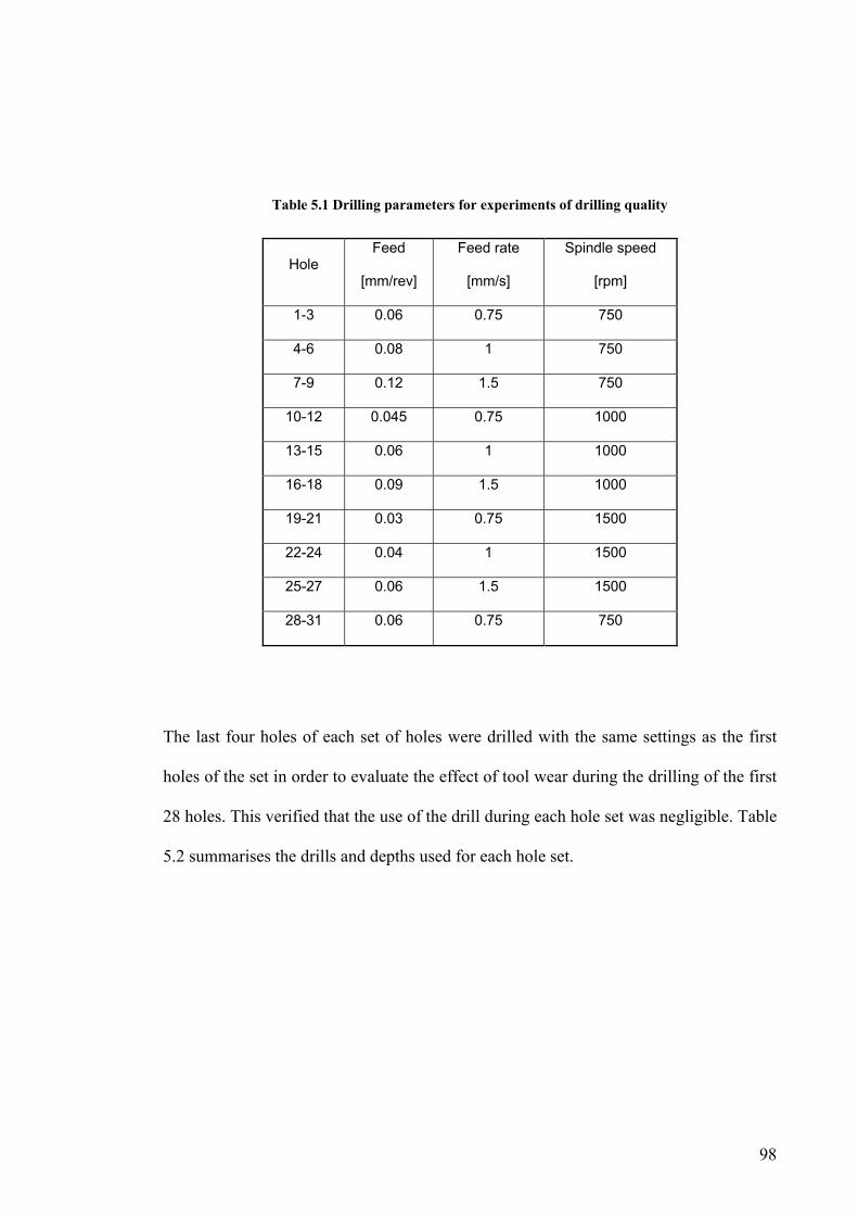
98

Table 5.1 Drilling parameters for experiments of drilling quality

Hole Feed

[mm/rev]

Feed rate

[mm/s]

Spindle speed

[rpm]

1-3 0.06 0.75 750

4-6 0.08 1 750

7-9 0.12 1.5 750

10-12 0.045 0.75 1000

13-15 0.06 1 1000

16-18 0.09 1.5 1000

19-21 0.03 0.75 1500

22-24 0.04 1 1500

25-27 0.06 1.5 1500

28-31 0.06 0.75 750

The last four holes of each set of holes were drilled with the same settings as the first

holes of the set in order to evaluate the effect of tool wear during the drilling of the first

28 holes. This verified that the use of the drill during each hole set was negligible. Table

5.2 summarises the drills and depths used for each hole set.

99

Table 5.2 Drilling Parameters

Hole set Drill bit Depth [mm]

1 drill #1

2 drill #2

3 drill #3

13.4

(drill depth)

4 drill #1

5 drill #2

6 drill #3

18

(drill & limited

drilling)

7 drill #1

8 drill #2

9 drill #3

23

(drill & max

reaming)

The first three hole sets were drilled with a new drill bit (drill #1), a drill bit which had

drilled 100 holes (drill #2) and a drill bit which had previously drilled 300 holes (drill

#3) respectively. All holes on the first three sets were drilled for a depth of 13.4mm

which is the displacement necessary for the cutting lips to reach the bottom of the

workpiece (5.2mm+8.2mm). This means that the direction of the tool travel was

reversed and the drill removed out of the hole at that depth. This distance of travel was

chosen because it was the transition from drilling to reaming and drilling stages, where

the thrust force dropped to zero. Hence, the hole was drilled but not reamed. The same

experiments were repeated for 18mm travel (Hole sets 4-6). At this depth reaming of the

hole was performed. The amount of time the hole is reamed is dependent on the travel

speed being used. A third series of experiments was also carried out, using 23 mm travel

100

(Hole sets 7-9). The aim of this last series of experiments is to study the effect of extra

reaming time on the quality of the holes.

5.3 Analysing Hole Quality

As previously described at the beginning of this chapter, hole quality includes several

parameters and there are numerous ways of measuring them. In this study, visual

inspection, pin gages, CMM (coordinates measurement machine) and microscope will

be used to measure or classify some of those quality parameters. The aim is not to

quantify hole quality but to detect the existence of hole defects. For this study, defects

will be considered undesirable characteristics of holes such as break outs, surface

texture, delamination and shape of the hole.

After drilling, each hole was analysed and the existence of any visual defects was

recorded. The parameters recorded by visual inspection were fibre break outs, surface

texture and delamination. The type of chip produced was also noted. Figure 5.3.1 shows

a photo of a hole and drill bit just after drilling with the chips still on the sample and on

the drill bit.

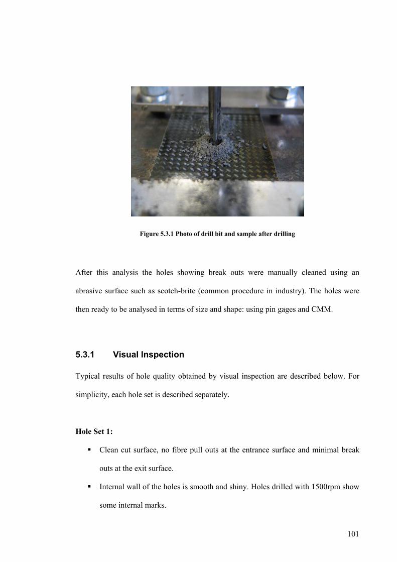
101

Figure 5.3.1 Photo of drill bit and sample after drilling

After this analysis the holes showing break outs were manually cleaned using an

abrasive surface such as scotch-brite (common procedure in industry). The holes were

then ready to be analysed in terms of size and shape: using pin gages and CMM.

5.3.1 Visual Inspection

Typical results of hole quality obtained by visual inspection are described below. For

simplicity, each hole set is described separately.

Hole Set 1:

Clean cut surface, no fibre pull outs at the entrance surface and minimal break

outs at the exit surface.

Internal wall of the holes is smooth and shiny. Holes drilled with 1500rpm show

some internal marks.

102

Chips produced are black and dry (sugar like).

The last two holes look the same as first holes drilled.

Hole Set 2:

The edges of the holes on the top surface are slightly raised; there are no loose

fibres at the entrance but some at the exit of the hole. The amount of break out is

the same for all holes, hence they are independent of the settings used.

The internal surface texture of the holes is not as smooth and shiny as the

surface shown for the holes drilled in the previous hole set. Circular marks can

be seen in most holes. The holes drilled with higher spindle speed show a

substantial increase in surface marks.

The chips produced are of lighter colour than hole set 1 and it can be seen that

some of the chips are ‘lumpier’.

The last two holes look similar to first holes drilled.

Hole Set 3:

The edges of the holes on the top surface are slightly raised, showing fibre

break outs at the entrance and the exit surface. The amount of break out is

independent of the settings used.

The internal surface of the holes shows circular marks. The holes drilled with

higher spindle speed show an increase in scorch marks.

The chips produced are lighter in colour and lumpier than hole set 2.

The last two holes look similar to first holes drilled.

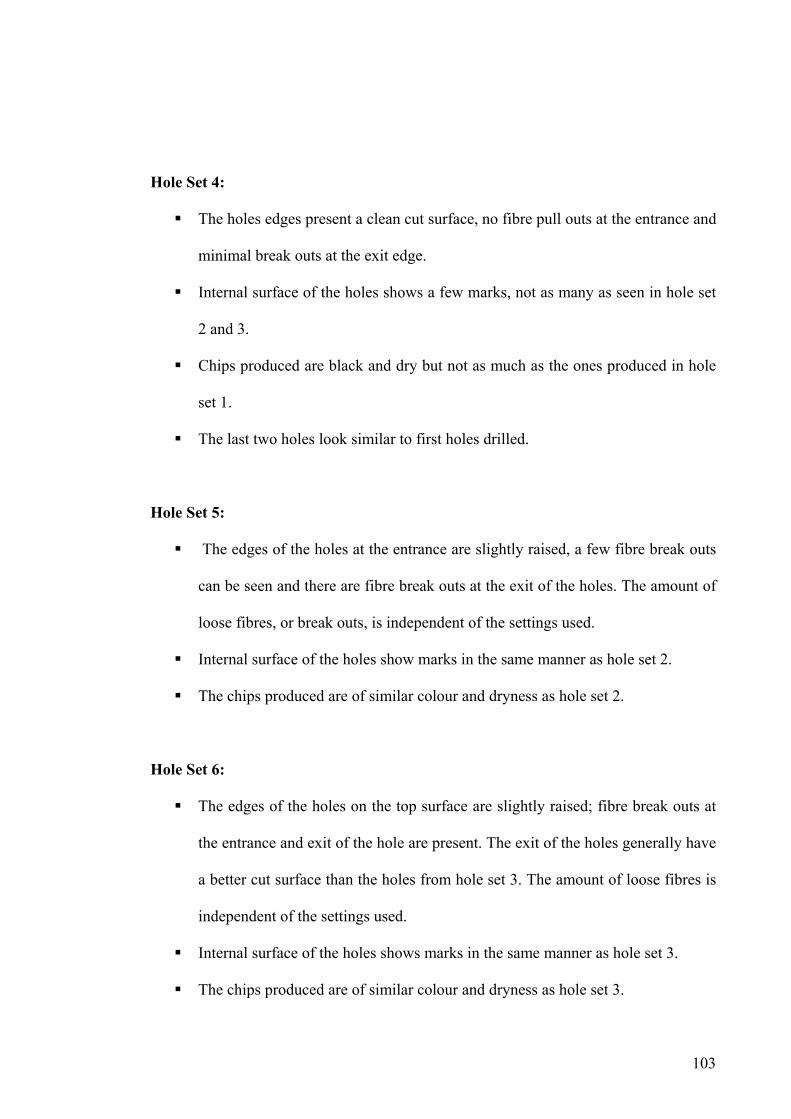
103

Hole Set 4:

The holes edges present a clean cut surface, no fibre pull outs at the entrance and

minimal break outs at the exit edge.

Internal surface of the holes shows a few marks, not as many as seen in hole set

2 and 3.

Chips produced are black and dry but not as much as the ones produced in hole

set 1.

The last two holes look similar to first holes drilled.

Hole Set 5:

The edges of the holes at the entrance are slightly raised, a few fibre break outs

can be seen and there are fibre break outs at the exit of the holes. The amount of

loose fibres, or break outs, is independent of the settings used.

Internal surface of the holes show marks in the same manner as hole set 2.

The chips produced are of similar colour and dryness as hole set 2.

Hole Set 6:

The edges of the holes on the top surface are slightly raised; fibre break outs at

the entrance and exit of the hole are present. The exit of the holes generally have

a better cut surface than the holes from hole set 3. The amount of loose fibres is

independent of the settings used.

Internal surface of the holes shows marks in the same manner as hole set 3.

The chips produced are of similar colour and dryness as hole set 3.

104

Hole Set 7:

The holes present a clean cut surface; few fibre break outs at the entrance

surface and minimal break outs at the exit surface.

Internal surface of the holes show a few marks, not as many as in the hole sets

drilled by the other drill bits.

The chips produced are black and dry but not as much as the ones produced in

hole sets 1 and 4.

The last two holes look similar to first holes drilled.

Hole Set 8:

The appearance of these holes is similar to the ones described for hole set 5

Hole Set 9:

The appearance of these holes is similar to the ones described for hole set 6.

5.3.2 Discussion of Results

A few conclusions can be drawn from the results described. First, the holes’

characteristics were directly related to the drill bit used. The new drill bit produced far

better looking holes than the other two drills. Fibre and scorching marks were directly

related to the age of the drill bit.

105

hole #1 hole #50 hole #150

Figure 5.3.2 Typical Surface texture of holes drilled by the same drill bit of different ages (same

drilling parameters)

The older the drill, the greater is the number of marks and scorching in the internal

surface of the holes. Figure 5.3.2 shows photos of cross sections of holes where this

phenomenon is evident.

High spindle speeds leave more scorch marks in the internal surface of the holes. Figure

5.3.3 shows an example of holes drilled consecutively by the same drill bit at different

spindle speeds.

(a) (b)

Figure 5.3.3 Internal surface of holes for a) High spindle speeds b) Low Spindle Speed

106

The heat generated by the higher spindle speed and/or the wear of the drill bit will

accumulate around the tool edge destroying the matrix stability [1]. With the damaged

matrix at the edges of the holes, fibres can be pulled out [2], producing the scorching

marks and rough cuts. As other researchers have explained, when the tool does not

successfully cut the fibres, the tensile and compressive forces generated by the tool

rotation cause the fibres and matrix to be torn out from the hole surface [3].

The colour and dryness of the chips changes with the number of holes drilled. Figure

5.3.4 shows an example of holes drilled with the same parameters using drill bits of

different ages. The colour of the chip produced gets lighter with the number of holes

drilled by the drill bit, possibly due to the higher temperatures generated with older drill

bits. The chips also become lumpier and more spread out.

new drill used drill older drill new drill used drill older drill

Figure 5.3.4 Photos of Typical Chips generated by drill bits of different ages

107

With the increase in thrust force due to wear of the drill, friction between the tool and

composite generates heat which damages the matrix, softening it. The chips form lumps

and can even clog the tool making further machining difficult [3].

In Figure 5.3.5, the difference in the amount of pulled or uncut fibres (so called break-

outs) produced for different age drill bits can be clearly seen. Newer drill bits produce

better-cut holes.

Hole Set 1 Hole Set 2 Hole Set 3

Figure 5.3.5 Typical Examples of Hole entrance for Hole Set 1, 2 and 3

The typical examples of exit surface of the holes is shown in Figure 5.3.6. As the

number of previously drilled holes increases, the drill bit produces more breakouts as

well as some burn marks around the edges.

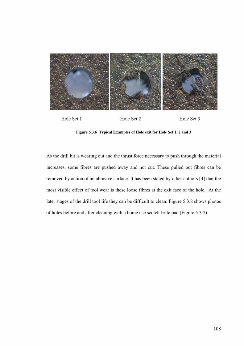
108

Hole Set 1 Hole Set 2 Hole Set 3

Figure 5.3.6 Typical Examples of Hole exit for Hole Set 1, 2 and 3

As the drill bit is wearing out and the thrust force necessary to push through the material

increases, some fibres are pushed away and not cut. These pulled out fibres can be

removed by action of an abrasive surface. It has been stated by other authors [4] that the

most visible effect of tool wear is these loose fibres at the exit face of the hole. At the

later stages of the drill tool life they can be difficult to clean. Figure 5.3.8 shows photos

of holes before and after cleaning with a home use scotch-brite pad (Figure 5.3.7).

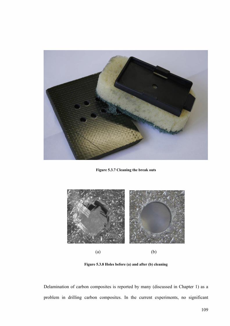
109

Figure 5.3.7 Cleaning the break outs

(a) (b)

Figure 5.3.8 Holes before (a) and after (b) cleaning

Delamination of carbon composites is reported by many (discussed in Chapter 1) as a

problem in drilling carbon composites. In the current experiments, no significant

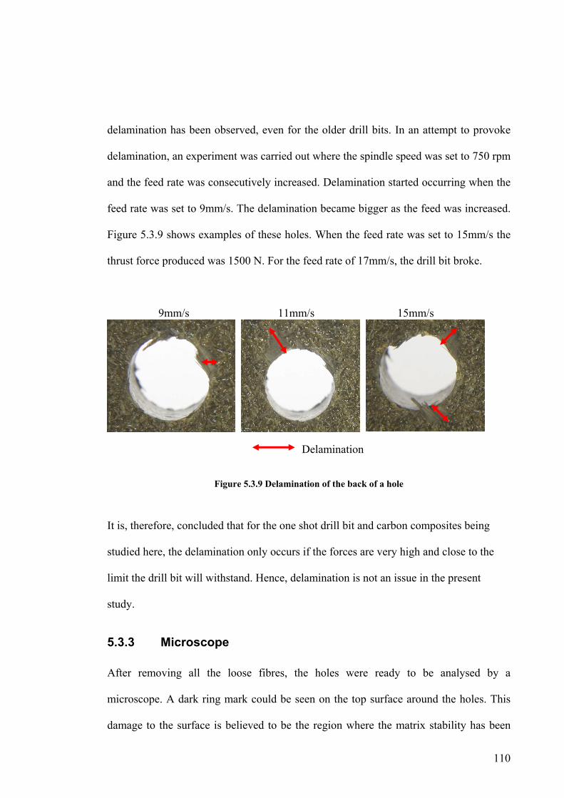
110

delamination has been observed, even for the older drill bits. In an attempt to provoke

delamination, an experiment was carried out where the spindle speed was set to 750 rpm

and the feed rate was consecutively increased. Delamination started occurring when the

feed rate was set to 9mm/s. The delamination became bigger as the feed was increased.

Figure 5.3.9 shows examples of these holes. When the feed rate was set to 15mm/s the

thrust force produced was 1500 N. For the feed rate of 17mm/s, the drill bit broke.

9mm/s 11mm/s 15mm/s

Figure 5.3.9 Delamination of the back of a hole

It is, therefore, concluded that for the one shot drill bit and carbon composites being

studied here, the delamination only occurs if the forces are very high and close to the

limit the drill bit will withstand. Hence, delamination is not an issue in the present

study.

5.3.3 Microscope

After removing all the loose fibres, the holes were ready to be analysed by a

microscope. A dark ring mark could be seen on the top surface around the holes. This

damage to the surface is believed to be the region where the matrix stability has been

Delamination

111

affected by temperature. The shaded area increased steadily with the number of holes

drilled as shown in Figure 5.3.10, Figure 5.3.11 and Figure 5.3.12. No relation could be

found between the extent of damage and the parameter settings used (spindle speed,

feed rate or depth of drilling).

Figure 5.3.10 Hole entrance Damage by drill #1 (Hole Set 1)

Figure 5.3.11 Hole entrance Damage by drill #2 (Hole Set 2)

Hole 1 Hole 8

Hole 14 Hole 20

Hole 102 Hole 125

112

Figure 5.3.12 Hole entrance Damage by drill #3 (Hole Set 3)

5.3.4 Pin Gages

Pin gages or Go NoGo gages are commonly used in industry to check if a hole is within

the size tolerance given to the application. For a hole to be within tolerance, the smaller

gage (go) has to enter the hole and the bigger (no go) cannot fit the hole. The same

procedure was used in this research to find the diameter of the holes. The drill bit

diameter was 4.85mm and the pin gages used ranged from 4.78mm to 4.95mm with

25.4µm steps, giving sizes: 4.80, 4.83mm, 4.85mm, 4.88mm, 4.9mm 4.93mm and

4.95mm. Aerospace industry applications where this drill bit is used commonly set the

size tolerance at 7µm: 4.83mm (go) to 4.90mm (no go). A hole that does not fit a

4.83mm gage is too small and a hole fitting a 4.90mm gage is too big.

All holes drilled in these experiments were tested using the pin gages. The gages were

introduced to each hole starting with the smallest one and going up in size until the gage

did not fit. Hence, the diameter of the hole is the size of the biggest gage fitting into the

hole.

Hole 300 Hole 315

113

Figure 5.3.13 shows the results obtained for the holes drilled by drill #1 (new drill bit).

Figure 5.3.13 Hole Diameters for Drill #1

It can be seen that all holes passed the size tolerance test. The holes drilled for 13.4mm

(Set 1) are generally smaller than the holes drilled and reamed for longer (18mm and

23mm). It is also observed that there is no difference in size between the holes

drilled/reamed for 18mm (set 4) and 23mm (set 7).

The diameter of the holes drilled with drill #2 can be seen in Figure 5.3.14. For this

drill, the depth of drilling is directly related to the size of the final holes. The longer it

drills, the bigger is the hole. It is also seen that the holes drilled for 13.4mm are too

small and would not pass the tolerance test.

drill #1

4.8 4.81 4.82 4.83 4.84 4.85 4.86 4.87 4.88 4.89

1 3 5 7 9 11 13 15 17 19 21 23 25 27 hole

diam

eter

[mm

]

13.4mm18mm23mm

Drilling depth

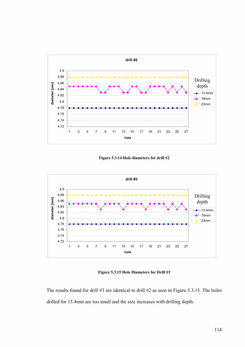
114

Figure 5.3.14 Hole diameters for drill #2

Figure 5.3.15 Hole Diameters for Drill #3

The results found for drill #3 are identical to drill #2 as seen in Figure 5.3.15. The holes

drilled for 13.4mm are too small and the size increases with drilling depth.

drill #2

4.72 4.74 4.76 4.78

4.8 4.82 4.84 4.86 4.88

4.9

1 3 5 7 9 11 13 15 17 19 21 23 25 27 hole

diam

eter

[mm

]

13.4mm

18mm

23mm

Drilling depth

drill #3

4.72 4.74 4.76 4.78

4.8 4.82 4.84 4.86 4.88

4.9

1 3 5 7 9 11 13 15 17 19 21 23 25 27 hole

diam

eter

[mm

]

13.4mm18mm23mm

Drilling depth

115

Figure 5.3.16 Hole Diameters for all holes

It is noted that the holes can be smaller than the size of the drill bit. This is a problem

usually associated with the material being drilled [5]. The elastic deformation of the

fibre, akin to buckling, causes a facet along the cut fibre inclined in relation to the

cutting edges. After being cut, the fibres return to the initial position, causing tightening

around the hole [6]. This effect will also increase the friction between the tool and the

composite, generating higher temperatures. The problem is compounded by the

insulating characteristics of the carbon composite, increasing the local temperature to

values that can damage the matrix. This heat damage is the reason for other problems

and or defects, one of them being the tapered shape of the holes [7]. It has been

suggested that this happens because of cutting at the margins on the thermally deformed

workpiece [8].

The use of pin gages to measure size is very quick and practical, and although it is

widely used in industry it has some limitations. The measurement of the hole is

4.72

4.74

4.76

4.78

4.8

4.82

4.84

4.86

4.88

4.9

1 4 7 10 13 16 19 22 25 28 31 34 37 40 43 46 49 52 55 58 61 64 67 70 73 76 79 82 85

hole

diam

eter

[mm

]

drill #1drill #2drill #3

Drilling depth

116

governed by its smallest diameter and it gives no indication about the possible variation

in diameter. Problems such as tapered holes, out of shape or angled holes are not

detected by the pin gages. Figure 5.3.17 represents some of these problems.

Figure 5.3.17 Examples of hole defects missed the gages

5.3.5 Coordinate Measurements

A coordinate measuring machine was used to measure the dimension of the holes.

Figure 5.3.18 shows a photo of a hole set.

Figure 5.3.18 Photo of a Hole Set

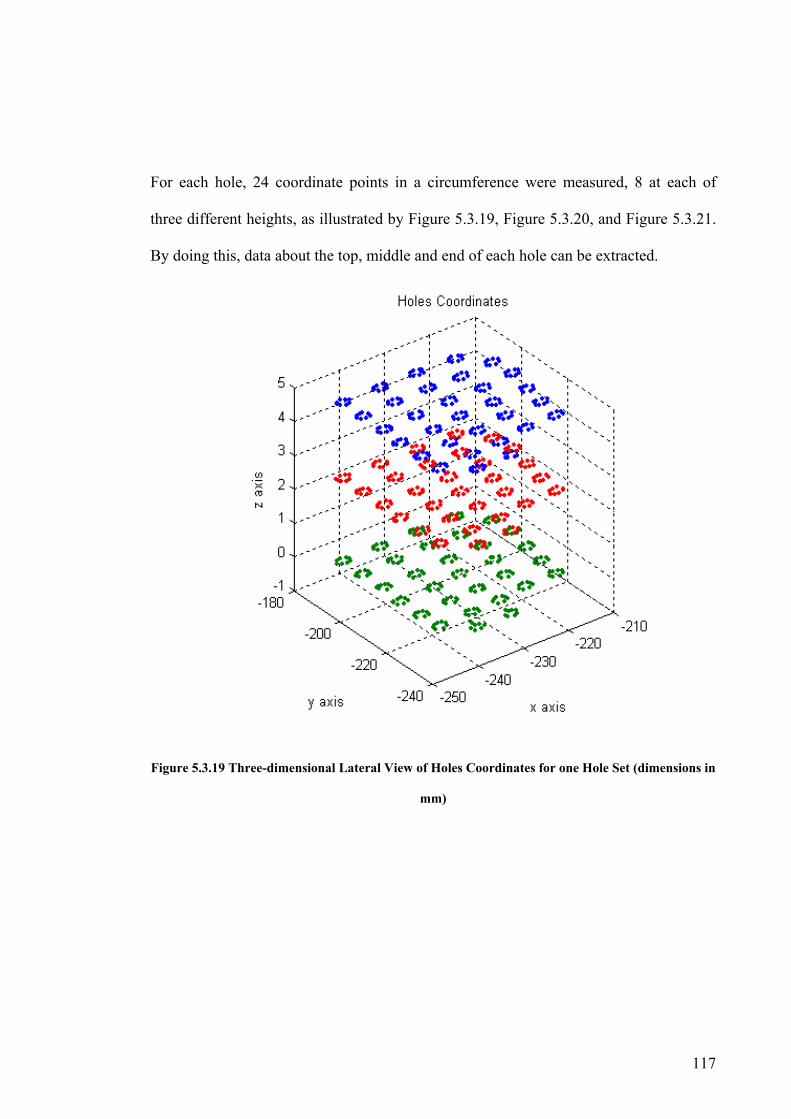
117

For each hole, 24 coordinate points in a circumference were measured, 8 at each of

three different heights, as illustrated by Figure 5.3.19, Figure 5.3.20, and Figure 5.3.21.

By doing this, data about the top, middle and end of each hole can be extracted.

Figure 5.3.19 Three-dimensional Lateral View of Holes Coordinates for one Hole Set (dimensions in

mm)

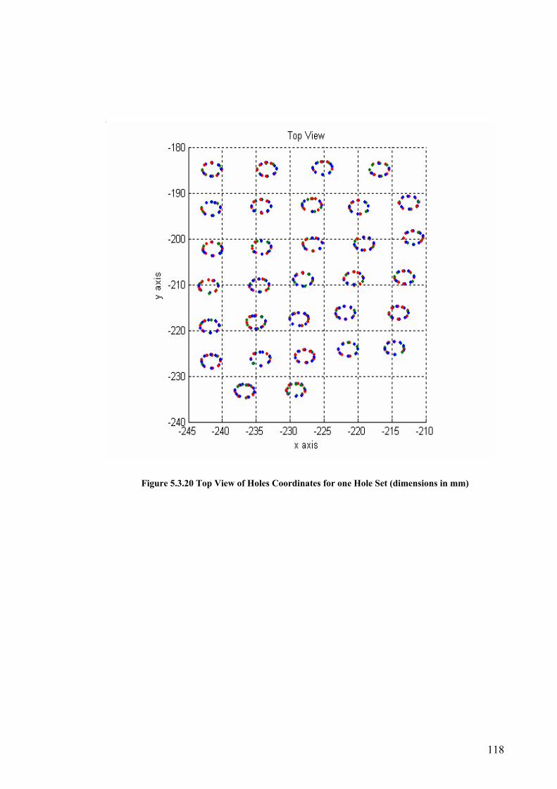
118

Figure 5.3.20 Top View of Holes Coordinates for one Hole Set (dimensions in mm)

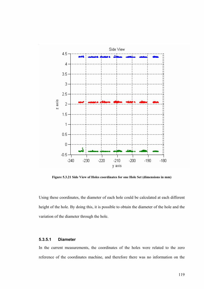
119

Figure 5.3.21 Side View of Holes coordinates for one Hole Set (dimensions in mm)

Using these coordinates, the diameter of each hole could be calculated at each different

height of the hole. By doing this, it is possible to obtain the diameter of the hole and the

variation of the diameter through the hole.

5.3.5.1 Diameter

In the current measurements, the coordinates of the holes were related to the zero

reference of the coordinates machine, and therefore there was no information on the

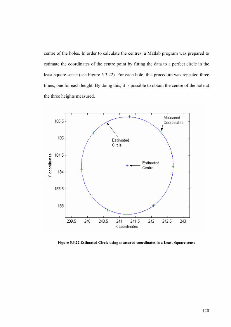
120

centre of the holes. In order to calculate the centres, a Matlab program was prepared to

estimate the coordinates of the centre point by fitting the data to a perfect circle in the

least square sense (see Figure 5.3.22). For each hole, this procedure was repeated three

times, one for each height. By doing this, it is possible to obtain the centre of the hole at

the three heights measured.

Figure 5.3.22 Estimated Circle using measured coordinates in a Least Square sense

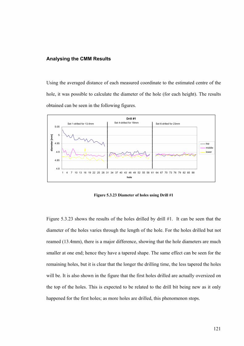
121

Analysing the CMM Results

Using the averaged distance of each measured coordinate to the estimated centre of the

hole, it was possible to calculate the diameter of the hole (for each height). The results

obtained can be seen in the following figures.

Figure 5.3.23 Diameter of holes using Drill #1

Figure 5.3.23 shows the results of the holes drilled by drill #1. It can be seen that the

diameter of the holes varies through the length of the hole. For the holes drilled but not

reamed (13.4mm), there is a major difference, showing that the hole diameters are much

smaller at one end; hence they have a tapered shape. The same effect can be seen for the

remaining holes, but it is clear that the longer the drilling time, the less tapered the holes

will be. It is also shown in the figure that the first holes drilled are actually oversized on

the top of the holes. This is expected to be related to the drill bit being new as it only

happened for the first holes; as more holes are drilled, this phenomenon stops.

Drill #1

4.8

4.85

4.9

4.95

5

5.05

1 4 7 10 13 16 19 22 25 28 31 34 37 40 43 46 49 52 55 58 61 64 67 70 73 76 79 82 85 88

hole

diam

eter

[mm

]

top

middle

lower

Set 1-drilled for 13.4mm Set 4-drilled for 18mm Set 6-drilled for 23mm

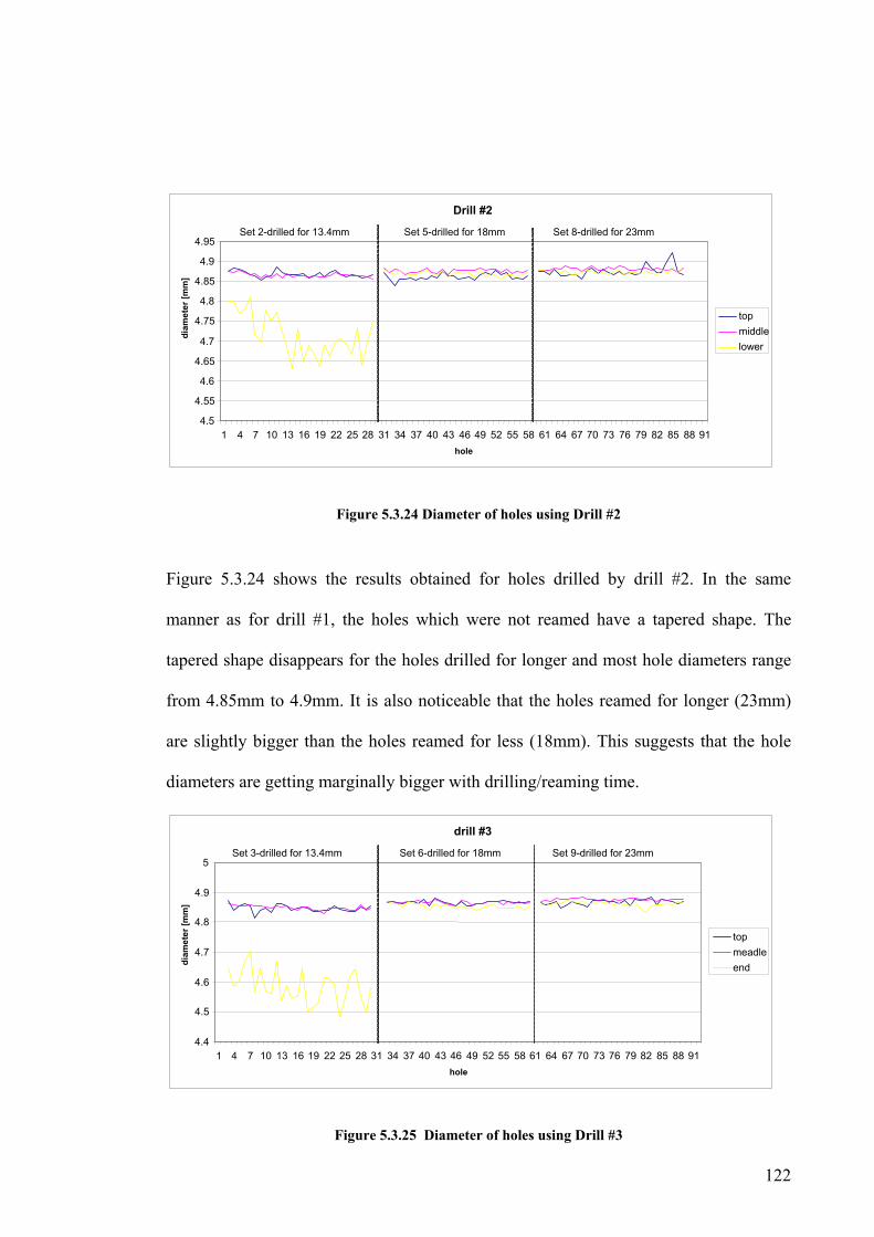
122

Figure 5.3.24 Diameter of holes using Drill #2

Figure 5.3.24 shows the results obtained for holes drilled by drill #2. In the same

manner as for drill #1, the holes which were not reamed have a tapered shape. The

tapered shape disappears for the holes drilled for longer and most hole diameters range

from 4.85mm to 4.9mm. It is also noticeable that the holes reamed for longer (23mm)

are slightly bigger than the holes reamed for less (18mm). This suggests that the hole

diameters are getting marginally bigger with drilling/reaming time.

Figure 5.3.25 Diameter of holes using Drill #3

Drill #2

4.5

4.55

4.6

4.65

4.7

4.75

4.8

4.85

4.9

4.95

1 4 7 10 13 16 19 22 25 28 31 34 37 40 43 46 49 52 55 58 61 64 67 70 73 76 79 82 85 88 91hole

diam

eter

[mm

]

topmiddlelower

Set 2-drilled for 13.4mm Set 5-drilled for 18mm Set 8-drilled for 23mm

drill #3

4.4

4.5

4.6

4.7

4.8

4.9

5

1 4 7 10 13 16 19 22 25 28 31 34 37 40 43 46 49 52 55 58 61 64 67 70 73 76 79 82 85 88 91hole

diam

eter

[mm

]

topmeadle end

Set 3-drilled for 13.4mm Set 6-drilled for 18mm Set 9-drilled for 23mm

123

The results obtained for the holes drilled by drill #3 can be seen in Figure 5.3.25. In the

same manner as for drill #2, the holes not reamed have a tapered shape which is not

seen on the remaining samples. The diameter of the holes also increases slightly with

drilling/reaming time.

Figure 5.3.26 Hole Diameters for all Samples

Comparing the diameters of the holes drilled by all drill bits (see Figure 5.3.26), it can

be seen that drill #2 makes holes slightly smaller than drill #1, but bigger than drill #3.

Hence, the older the drill bit, the smaller are the holes produced.

Figure 5.3.27, Figure 5.3.28, and Figure 5.3.29 show the relation between the diameter

of the holes and the settings used for drilling. For this analysis, the diameter of each

hole is an average of the diameters at each height of the hole.

The spindle speed slightly affects diameter, as shown in Figure 5.3.27. For higher

spindle speeds, the hole diameter is slightly smaller. This happens for all drill bits.

Diameter of holes at each high

4.4

4.5

4.6

4.7

4.8

4.9

5

5.1

1 11 21 31 41 51 61 71 81 91 101111 121131 141151161 171181191 201211 221231241 251261hole

diam

eter

[mm

]

topmiddlelower

Set 1 Set 2 Set 3 Set 4 Set 5 Set 6 Set 7 Set 8 Set 9

124

Figure 5.3.27 Relation between Spindle Speed and hole Diameter

Figure 5.3.28 shows the relation between the feed rate (mm/s) used and the hole

diameter. No trend emerges from this analysis. For holes drilled by drill#3, the

diameters are slightly smaller for higher feeds, but the difference is so small (and not for

all holes) that no conclusion can be drawn. Hence, within the range of feed rates used,

the diameter of the holes has not been affected by the feed rate.

4.7

4.75

4.8

4.85

4.9

4.95

5

0 200 400 600 800 1000 1200 1400 1600

spindle speed [rpm]

aver

age

diam

eter

[mm

]

drill #1drill #2drill #3

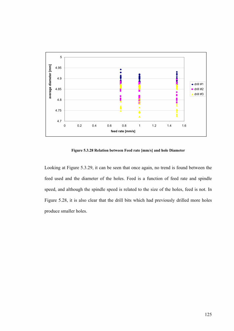
125

Figure 5.3.28 Relation between Feed rate [mm/s] and hole Diameter

Looking at Figure 5.3.29, it can be seen that once again, no trend is found between the

feed used and the diameter of the holes. Feed is a function of feed rate and spindle

speed, and although the spindle speed is related to the size of the holes, feed is not. In

Figure 5.28, it is also clear that the drill bits which had previously drilled more holes

produce smaller holes.

4.7

4.75

4.8

4.85

4.9

4.95

5

0 0.2 0.4 0.6 0.8 1 1.2 1.4 1.6 feed rate [mm/s]

aver

age

diam

eter

[mm

]

drill #1drill #2drill #3

126

Figure 5.3.29 Relation between Feed [mm/rev] and hole Diameter

5.3.5.3 Roundness

The roundness of the holes can be calculated using the coordinates measured by the

CMM and the line of best fit estimated above. Two reference circles are calculated,

which are concentric to the best fit circle and enclose all data points. Roundness consists

of the distance D between these two circles, as represented in Figure 5.3.30.

4.7

4.75

4.8

4.85

4.9

4.95

5

0 0.02 0.04 0.06 0.08 0.1 0.12 0.14 feed [mm/rev]

aver

age

diam

eter

[mm

]

drill #1drill #2drill #3

127

Figure 5.3.30 Defining Roundness

This procedure was used to calculate the roundness of each hole at each of the three

different heights measured. Hence, for every hole, there were three roundness results.

Figure 5.3.31 shows the results obtained for the holes drilled with the new drill (drill

#1).

Figure 5.3.31 Roundness of Holes for Drill #1

drill #1

0 0.05

0.1

0.15

0.2

0.25

0.3

0.35

0.4

1 4 7 10 13 16 19 22 25 28 31 34 37 40 43 46 49 52 55 58 61 64 67 70 73 76 79 82 85 88

hole

roun

dnes

s [m

m]

top middlelower

Hole Set 1-drilled for 13.4mm Hole Set 4-drilled for 18mm Hole Set 6-drilled for 23mm

128

For most holes, roundness was under 0.1mm. There is not a significant variance on the

roundness values for each height of the hole (with one exception, possibly due to

chatter). This means that the holes analysed have approximately the same roundness

throughout the hole. It can also be seen that the roundness values are decreased for the

sample reamed longer. Hence, when drilling with a new drill bit, the longer it reams, the

rounder the holes will be.

Figure 5.3.32 shows the results obtained for the holes drilled by drill #2, which had

previously drilled 100 holes. It can be seen that the roundness values are around

0.05mm with few exceptions. For this drill bit, the holes drilled for 13.4mm show a

significant difference in roundness throughout the hole. The lower level of the holes

presents a much higher value; hence the end of the holes is not as round. The same

phenomenon is not observed for the holes reamed for longer, where the roundness of the

holes is fairly constant through the hole and for all the settings tested.

Figure 5.3.32 Roundness of Holes for Drill #2

drill #2

00.050.1

0.150.2

0.250.3

0.350.4

0.450.5

1 4 7 10 13 16 19 22 25 28 31 34 37 40 43 46 49 52 55 58 61 64 67 70 73 76 79 82 85 hole

roun

dnes

s [m

m]

top middlelower

Hole Set 2-drilled for 13.4mm Hole Set 5-drilled for 18mm Hole Set 8-drilled for 23mm

129

Figure 5.3.33 shows the results obtained for the holes drilled with drill #3, which had

previously drilled the most number of holes. The results shown in this figure are very

similar to the results from drill #2. The roundness values average 0.05mm for most

holes, with the exception of the bottom layer of the holes drilled for 13.4mm where the

roundness values are much higher (the holes are not as round).

Figure 5.3.33 Roundness of Holes for Drill #3

By plotting all the results together, as depicted in Figure 5.3.33, it can be seen that for

hole sets 4, 5, 6, 7, 8 and 9, the roundness is constant throughout the holes, which means

that as long as the holes are reamed, the holes will be round throughout. For the holes

drilled but not reamed (13.4mm), there are two outcomes: hole sets 2 and 3 show the

lower end of the holes less round than the top and middle. The same effect is not seen

for hole set 1 which means that for the new drill bit, the hole is fairly round throughout.

As shown before, the roundness of the holes from drill #1 improves with reaming time,

but the difference is not as evident as it is for older drill bits.

drill #3

0

0.1

0.2

0.3

0.4

0.5

0.6

0.7

1 4 7 10 13 16 19 22 25 28 31 34 37 40 43 46 49 52 55 58 61 64 67 70 73 76 79 82 85 88

hole

roun

dnes

s [m

m]

top

middle

lower

Hole Set 3-drilled for 13.4mm Hole Set 6-drilled for 18mm Hole Set 9-drilled for 23mm

130

Figure 5.3.34 Roundness for all Samples

From Figure 5.3.34, it can also be concluded that hole roundness is better for the drill

#1, but when drilling for 18mm or more, the difference is very small.

Figure 5.3.35, Figure 5.3.36 and Figure 5.3.37 show the relation between the roundness

of the holes and the settings used for drilling. For this analysis, the roundness of each

hole is an average of the roundness at each height of the hole.

Roundness of holes at each height

0 0.1

0.2

0.3

0.4

0.5

0.6

0.7

1 11 21 31 41 51 61 71 81 91 101 111121 131 141151 161 171181 191 201211 221 231241 251 261

hole

roun

dnes

s [m

m]

topmiddlelower

Set 1 Set 2 Set 3 Set 4 Set 5 Set 6 Set 7 Set 8 Set 9

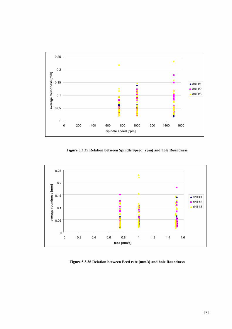
131

Figure 5.3.35 Relation between Spindle Speed [rpm] and hole Roundness

Figure 5.3.36 Relation between Feed rate [mm/s] and hole Roundness

0

0.05

0.1

0.15

0.2

0.25

0 200 400 600 800 1000 1200 1400 1600 Spindle speed [rpm]

aver

age

roun

dnes

s [m

m]

drill #1drill #2drill #3

0

0.05

0.1

0.15

0.2

0.25

0 0.2 0.4 0.6 0.8 1 1.2 1.4 1.6 feed [mm/s]

aver

age

roun

dnes

s [m

m]

drill #1drill #2drill #3

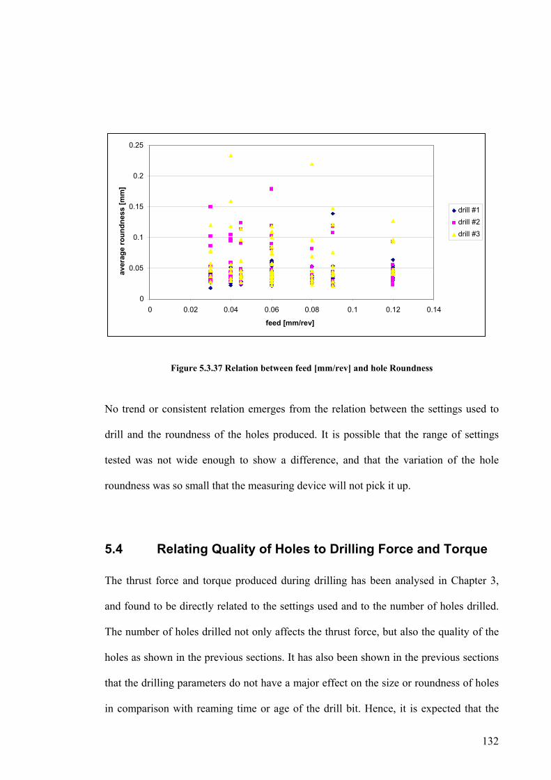
132

Figure 5.3.37 Relation between feed [mm/rev] and hole Roundness

No trend or consistent relation emerges from the relation between the settings used to

drill and the roundness of the holes produced. It is possible that the range of settings

tested was not wide enough to show a difference, and that the variation of the hole

roundness was so small that the measuring device will not pick it up.

5.4 Relating Quality of Holes to Drilling Force and Torque

The thrust force and torque produced during drilling has been analysed in Chapter 3,

and found to be directly related to the settings used and to the number of holes drilled.

The number of holes drilled not only affects the thrust force, but also the quality of the

holes as shown in the previous sections. It has also been shown in the previous sections

that the drilling parameters do not have a major effect on the size or roundness of holes

in comparison with reaming time or age of the drill bit. Hence, it is expected that the

0

0.05

0.1

0.15

0.2

0.25

0 0.02 0.04 0.06 0.08 0.1 0.12 0.14 feed [mm/rev]

aver

age

roun

dnes

s [m

m]

drill #1drill #2drill #3

133

thrust force will relate to the quality of holes only when and if it is also related to drill

bit age, not the drilling settings.

Figure 5.4.1 Relation between Thrust Force and Roundness

Figure 5.4.2 Relation between Thrust Force and Roundness

0

0.05

0.1

0.15

0.2

0.25

0 50 100 150 200 250 300

Thrust Force [N]

aver

age

roun

dnes

s [m

m]

0

0.05

0.1

0.15

0.2

0.25

0 0.1 0.2 0.3 0.4 0.5 0.6

Torque [Nm]

aver

age

roun

dnes

s [m

m]

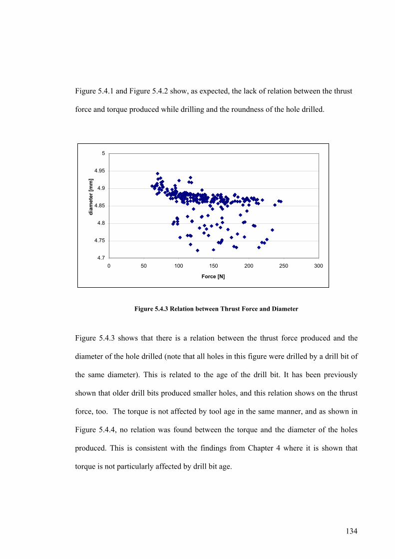
134

Figure 5.4.1 and Figure 5.4.2 show, as expected, the lack of relation between the thrust

force and torque produced while drilling and the roundness of the hole drilled.

Figure 5.4.3 Relation between Thrust Force and Diameter

Figure 5.4.3 shows that there is a relation between the thrust force produced and the

diameter of the hole drilled (note that all holes in this figure were drilled by a drill bit of

the same diameter). This is related to the age of the drill bit. It has been previously

shown that older drill bits produced smaller holes, and this relation shows on the thrust

force, too. The torque is not affected by tool age in the same manner, and as shown in

Figure 5.4.4, no relation was found between the torque and the diameter of the holes

produced. This is consistent with the findings from Chapter 4 where it is shown that

torque is not particularly affected by drill bit age.

4.7

4.75

4.8

4.85

4.9

4.95

5

0 50 100 150 200 250 300 Force [N]

dia

met

er [m

m]

135

Figure 5.4.4 Relation between Torque and Diameter

5.5 Relating Drilling Stages to Quality

The previous sections have described how some drilling parameters affect hole quality.

However, due to the nature of the experiments, it is not possible to know when the

damage to the holes’ quality occurs. The aim of this section is to investigate the relation

between hole quality and the stages of the drilling process.

It has previously been shown that for the range of settings used, the most important

factor affecting hole quality is tool age, or number of holes previously drilled.

Therefore, the tool age is chosen as the factor to be used in order to relate hole quality to

the drilling stages. To investigate this further, a series of experiments was carried out

where drill bits were changed at specific positions of the drilling process (see Figure

5.5.1). Two drill bits were used for this experiment; Drill A is a new drill bit while Drill

4.7

4.75

4.8

4.85

4.9

4.95

5

0 0.1 0.2 0.3 0.4 0.5 0.6 Torque [Nm]

diam

eter

[mm

]

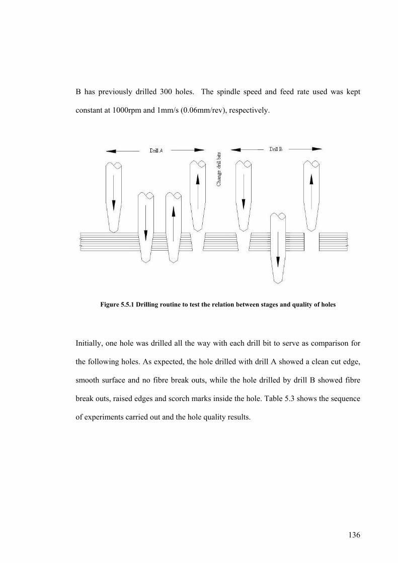
136

B has previously drilled 300 holes. The spindle speed and feed rate used was kept

constant at 1000rpm and 1mm/s (0.06mm/rev), respectively.

Figure 5.5.1 Drilling routine to test the relation between stages and quality of holes

Initially, one hole was drilled all the way with each drill bit to serve as comparison for

the following holes. As expected, the hole drilled with drill A showed a clean cut edge,

smooth surface and no fibre break outs, while the hole drilled by drill B showed fibre

break outs, raised edges and scorch marks inside the hole. Table 5.3 shows the sequence

of experiments carried out and the hole quality results.

137

Table 5.3 Drilling in stages experiments and Results

Stage I

entrance

Stage

II

drilling

Stage

III

reaming

and

drilling

Stage

IV and

V

reaming

Quality of Hole

#1 drill A clean cut edge, smooth internal surface,

no fibre break outs

#2 drill B fibre break outs, raised edges, scorch

marks inside the hole

#3 drill A drill B fibre break outs, raised edges, scorch

marks inside the hole

#4 drill B drill A clean cut edge, smooth internal surface,

no fibre break outs

#5 drill A drill B fibre break outs, raised edges, scorch

marks inside the hole

#6 drill B drill A clean cut edge, smooth internal surface,

no fibre break outs

#7 drill A drill B clean cut edge, smooth internal surface,

no fibre break outs

#8 drill B drill A fibre break outs, raised edges, scorch

marks inside the hole

During setting #3, a new drill bit was used for the entrance only and most of the hole

was drilled by an old drill bit. The resulting hole quality is comparable to that of the

138

setting #2, where an old drill bit was used all the way. This result was expected, as

most of the hole was drilled by drill B. In the same manner, setting #4 produced a hole

comparable to setting #1, where a new drill bit was used.

Setting #5 used both drill bits for the drilling part; it starts with drill A and when the

reaming section is going to enter the material, the drill bits were swapped. Note that the

reaming section initiates as the drilling is still going (as explained in Chapter 3). The

quality of the hole produced is comparable to #2, showing signs of poor quality. This

suggests that the drilling and reaming stage are more important to quality than the

drilling only stage. The opposite scenario is seen in setting #6, where the hole finished

drilling and reaming with a new drill bit. The hole quality compares to #1.

In setting #7 and #8, the holes were drilled with one drill bit and reamed with the other.

The hole quality corresponded to the drill bit used for the drilling stage. The hole drilled

with drill A and reamed with drill B showed better hole quality than the opposite

scenario. This suggests that if damage is caused during drilling, the reaming section is

not sufficient to hide it.

Analysing these results as a whole, it can be concluded that in the current experiments,

the drilling and reaming stage (Stage III) is the most important stage relating to the hole

quality. An explanation for this is that any possible damage occurring before the last

portion of drilling (Stage I and II) will be repaired by Stage III which is the stage where

the widest section of the drill bit enters the hole. On the other hand, damage occurring

during this stage will still be seen after reaming. This is not to say that reaming is not

139

necessary. As shown in previous sections, reaming finishes the hole to size, but does not

affect problems such as fibre break outs, scorch marks and raised edges.

Another possible explanation for the results presented is that the drill bit is worn on the

outer edge of the cutting edges, and therefore only the portion of the hole machined by

this section shows the effects of tool age. This explanation is unlikely because, as

shown in Chapter 3, the effect of wear on thrust force is present for all stages (but

reaming). This suggests that the drill bit was worn in the cutting edges which machined

other stages, in particular, before break through. It was also concluded in Chapter 3 that

the effect of wear was prominent during drilling, particularly just before breakthrough.

The present experiments show that the final visible damage occurs after breakthrough

(during stage III – drilling and reaming).

5.6 Conclusion

In this chapter, the quality of holes is analysed. Defects and quality parameters are

defined and ways of measuring them are investigated. Several experiments were carried

out with varying drilling parameters: spindle speed, feed rate, reaming time and age of

drill bit.

The holes produced were studied and several quality parameters were measured and

recorded. These consisted of: fibre break outs, scorching of material, chip size and

coloration, diameter and roundness of the holes. Various methods and equipment were

used for this study: visual inspection, microscope, pin gages and coordinate

140

measurement machine (CMM). The results obtained allowed the following conclusions

to be drawn:

• Holes that have been drilled but not reamed for long will have a tapered shape

and might have smaller diameter than the drill bit.

• Older drill bits produce smaller holes than new ones, possibly because the

cutting edge is not sharp enough; i.e., for the same amount of machining time,

less material is removed. The problem can be minimised by reaming for longer

with older drill bits. Reaming time can improve size tolerances, although this is

also known to increase temperature and tool wear.

• The chips produced by older drill bits show a lighter colour and bigger size than

the chips produced by newer drill bits.

• The damage to the surface is directly related to the age of the drill bit. New drill

bits produce shiny clean surfaces while older drill bits scorch the surface. This

problem can be marginally improved by using lower spindle speeds. Lowering

of the spindle speed is usually avoided because this increases the thrust force

and potentially increases the possibility of delamination. However, if the spindle

speed is decreased after break through, when the thrust force is already much

lower, but the widest section of the drill bit is outside the workpiece,

delamination can be avoided. This would also mean that reaming would be

141

performed at a slower speed than drilling which is the advice usually given for

reaming in general.

• Problems such as surface damage and breakouts occur while the widest section

of the drill bit enters and makes its way through the material (Stage III drilling

and reaming). This can be expected in the sense that any damage occurring

before Stage III will be drilled out, and the reaming action occurring afterwards

does not remove enough material to make the defect disappear.

• The Stage V (reaming) finishes the hole to size tolerance. It has been shown that

holes reamed for longer have better roundness and size tolerance. It has also

been shown that if drilling is stopped just as the cutting edges are through the

hole, the holes have a tapered shape. This problem is more pronounced for older

drill bits.

• It has been shown that the drilling and reaming stages are responsible for the

effects of tool wear on the surface finish of the hole; in particular the cutting

carried out by the widest section of the drill bit cutting edges. This is an

interesting finding because it disagrees with the common assumption that the

moment just before breakthrough is the most important section of the drilling

process. It is true that just before breaking through is the point where the thrust

force is at its higher value and delamination is possible. Although delamination

has not been observed in the current experiments, it is possible that it did occur,

142

but the extension of the delamination was within the diameter of the drill bit, and

therefore drilled out. It is expected that if more thrust force could have been used

without breaking drills the extension of delamination might not have been

compensated by the remaining drilling.

• The tool wear rate when drilling carbon composites is very high and, is the

major factor affecting hole quality. Factors such as drilling time, spindle speed

or feed rate can influence hole quality but on a smaller scale. Measures which

decrease the tool wear rate or maximise hole quality are therefore very desirable.

Such measures include choosing drilling parameters which would decrease the

time of drilling and the temperature generated. Unfortunately, many of these

measures might also bring adverse results, for example:

Increasing feed rate decreases drilling time, but increases thrust force

(enhancing the chances of delamination and increasing tool wear).

Increasing spindle speed decreases thrust force (and therefore the possibility

of delamination and tool wear), but increases temperature and possibility of

vibration or chattering.

Decreasing feed rate decreases thrust force but increases drilling time and

temperature generated.

Decreasing spindle speed will increase the thrust force generated.

The findings of this chapter will be used as input information for the design of an

automated drilling system described in the next chapter.

143

Chapter 6 Automated Drilling and Reaming

6.1 Introduction

The optimisation of machining has been the focus of many researchers as discussed in

Chapter 1. The most common approach is to define the limits and variables and use a

mathematical method to find the best solution for a particular application. This usually

involves undertaking several machinability tests where thousands of holes are drilled

and many drill bits used. The tool wear rate is established for each of the settings used

and this information is used to make the final decision. Although this is a costly and

slow procedure, it can be cost-effective for applications where many thousands of holes

need to be drilled for the same application. But most of these optimisation techniques do

not consider the possibility of using variable feeds and speeds during the drilling of

holes or of compensating for the inevitable wear of the drill bit.

The time it takes to drill a hole is directly related to the feed rate used. Since time is

such an expensive variable (in particularly in industries like the aerospace industry,

where several thousands of holes have to be machined per part), it is logical to

maximise the feed rate. Hence the maximum feed rates possible and the maximum

speed with which holes can be drilled before the quality of the holes and/or the

equipment suffers are all areas of considerable interest.

Finding the best settings for an application is a cumbersome problem and always a

matter of compromising. Limits of the system need to be established and the cost of

144

changing drill bits due to tool wear has to be measured against the savings generated by

drilling in shorter times.

The aim of this chapter in not to find the best feed rate and spindle speed for any

particular application, but to demonstrate that a better knowledge of the drilling process

and use of variable settings will allow faster drilling without losing quality.

The age of the drill bit has been shown to be the most important factor for hole quality.

Although this cannot be avoided (i.e. holes cannot be drilled with a new drill bit every

time) , the adverse effect tool age has on the quality of the holes can be minimized by

adjusting the drilling parameters for the age of the drill.

The work developed and described in the previous chapters will now be used to make

decisions about which settings are most apropriate during the course of the drilling

process.

In Chapter 3, the thrust force and torque are divided into sections which represent the

different machining stages. Now, these stages will serve as basis of defining a

controller. For each hole, drilling feed and speed will vary acordingly to the stage. The

hole quality information obtained in Chapter 5 will be used in the decision making

algorithm. The mathematical model developed in Chapter 4 will be used to find which

parameters to use for a given force so that open loop force control can be implemented.

145

It is important to note that the experiments undertaken in the previous chapters were

necessarily within a limited range of settings. Therefore, all the quality parameters

considered and the mathematical model developed here should only be used for the

range of settings used to develop it. In this chapter, the drilling settings will be

maintained within the range of settings tested to ensure accuracy and repeatibility of

results. In principle, it is possible that a different range of settings is also practical, but

the ones chosen here are widely used for industrial applications.

In section 6.2, an algorithm is developed in order to generate the best settings for each

stage of the drilling process by taking into consideration the age of the drill bits. This

algorithm is then tested in Section 6.3. Two given scenarios are used to calculate the

best settings and to drill holes. The results obtained are compared to those found by

drilling at constant settings in order to evaluate the success of the new automated

system. In Section 6.4, conclusions are drawn.

6.2 Optimising Drilling Time

From all the limitations in an application, the range of feeds and spindle speeds which

the equipment can develop is an obvious limitation. But there are others too. The forces

generated during the drilling process increase proportionally to the feed (mm/rev) and

usually limit the maximum feed rate. These forces are particularly important for the

drilling of carbon composites where accelerated tool wear will increase the thrust force

and where delamination is also a threat. Also, higher forces will affect the accuracy,

usually related to the load applied, of positioning systems.

146

The spindle speed also plays a role in this; the feed (mm/rev) increases proportionally

to the feed rate but inversely proportionally to the spindle speed. Theoretically, feed

rates could be maintained high without creating higher forces by increasing the spindle

speed. In this case, the spindle speed would be the limiting factor. But increasing the

spindle speed will bring other problems such as likelihood of vibrations (or even

chatter) and the increase of temperature and tool wear. In the drilling of carbon

composites where its abrasive nature already induces very high wear rates, increasing

the spindle speed would aggravate this problem. The temperature generated during

drilling not only will affect the tool wear rate but can also damage the workpiece as the

resin in the composites is particularly sensitive to temperatures.

The thrust force allowed by the system is therefore the most common limiting factor on

the minimisation of drilling time. Ideally, the feed rate should be as high as possible to

decrease drilling time while the spindle speed should be low to decrease temperature

and tool wear rate.

6.2.1 Stage I

Stage I represents the entrance of the drilling process. During this stage, problems such

as wandering and deflexion of the drill bit could be an issue. Peel-up has also been a

problem discussed in the literature [1]. In the experimental work presented here, peel-up

was not observed and no significant wandering of the drill bit or miss-positioning of the

hole could be measured. Furthermore, extensive testing discussed previously lead to the

conclusion that whatever happened during this stage was not affecting the final quality

of the holes. Therefore, the drilling parameters used during this stage will here only be

147

limited by the thrust force they generate. In Chapter 5, it was shown that the thrust force

at this stage started from 0 and increased steadily until it reached a value estimated by

the force model developed. Now, the force model can be used in the inverse model; for

a given thrust force, drill bit and thickness of material, the feed [mm/rev] can be

obtained from the following equation:

d

dn

thrustA

feed67698

047.1993.00032.0

39.01

2

−

+= Equation 6-1

where n is the number of holes previously drilled, thrustA [N] the thrust force and d

[mm] is the widest diameter of the drill bit in contact with the workpiece at position A

(as described in Chapter 5).

After obtaining the feed, a decision in terms of feed rate and spindle speed can be made.

The spindle speed used during this stage has been shown not to affect the quality of the

final holes. Therefore, the feed rate will be set to its maximum (allowed by the system)

and the resultant spindle speed calculated. If the spindle speed calculated is higher than

consistent with the findings from previous chapters, than the spindle speed can be set to

the maximum value allowed and the new feed rate calculated. If the spindle speed is

lower than the minimum allowed, the thrust force will just be less than the maximum

thrust force. If the new feed rate is considered too low, it means that the drill bit is too

old and needs to be changed.

The following chart represents the decision making process to calculate the feed rate

and spindle speed used in stage I.

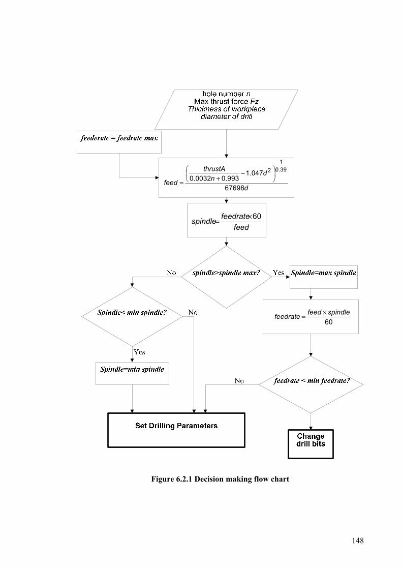
148

d

dn

thrustA

feed67698

047.1993.00032.0

39.01

2

−

+=

feedfeedratespindle 60×=

60spindlefeedfeedrate ×=

Figure 6.2.1 Decision making flow chart

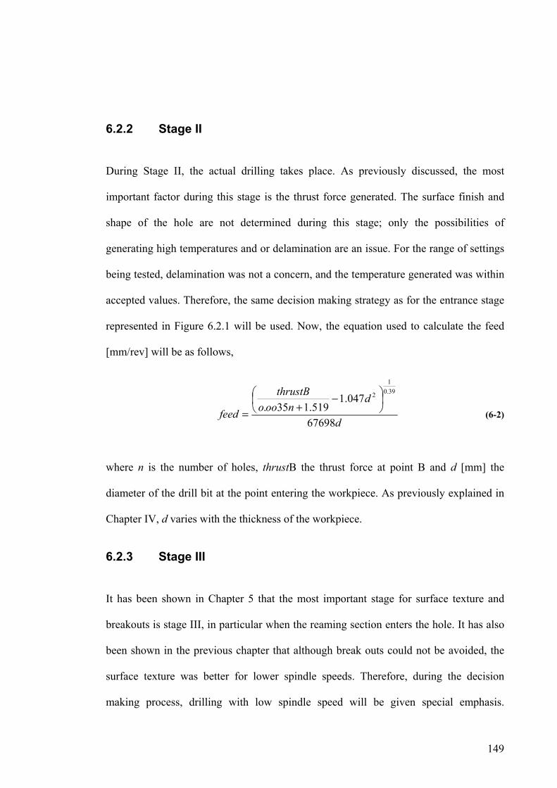
149

6.2.2 Stage II

During Stage II, the actual drilling takes place. As previously discussed, the most

important factor during this stage is the thrust force generated. The surface finish and

shape of the hole are not determined during this stage; only the possibilities of

generating high temperatures and or delamination are an issue. For the range of settings

being tested, delamination was not a concern, and the temperature generated was within

accepted values. Therefore, the same decision making strategy as for the entrance stage

represented in Figure 6.2.1 will be used. Now, the equation used to calculate the feed

[mm/rev] will be as follows,

d

dnooo

thrustB

feed67698

047.1519.135.

39.01

2

−

+= (6-2)

where n is the number of holes, thrustB the thrust force at point B and d [mm] the

diameter of the drill bit at the point entering the workpiece. As previously explained in

Chapter IV, d varies with the thickness of the workpiece.

6.2.3 Stage III

It has been shown in Chapter 5 that the most important stage for surface texture and

breakouts is stage III, in particular when the reaming section enters the hole. It has also

been shown in the previous chapter that although break outs could not be avoided, the

surface texture was better for lower spindle speeds. Therefore, during the decision

making process, drilling with low spindle speed will be given special emphasis.

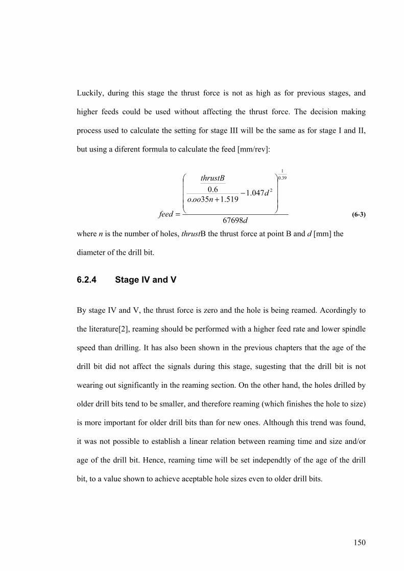
150

Luckily, during this stage the thrust force is not as high as for previous stages, and

higher feeds could be used without affecting the thrust force. The decision making

process used to calculate the setting for stage III will be the same as for stage I and II,

but using a diferent formula to calculate the feed [mm/rev]:

d

dnooo

thrustB

feed67698

047.1519.135.

6.039.01

2

−+

= (6-3)

where n is the number of holes, thrustB the thrust force at point B and d [mm] the

diameter of the drill bit.

6.2.4 Stage IV and V

By stage IV and V, the thrust force is zero and the hole is being reamed. Acordingly to

the literature[2], reaming should be performed with a higher feed rate and lower spindle

speed than drilling. It has also been shown in the previous chapters that the age of the

drill bit did not affect the signals during this stage, sugesting that the drill bit is not

wearing out significantly in the reaming section. On the other hand, the holes drilled by

older drill bits tend to be smaller, and therefore reaming (which finishes the hole to size)

is more important for older drill bits than for new ones. Although this trend was found,

it was not possible to establish a linear relation between reaming time and size and/or

age of the drill bit. Hence, reaming time will be set independtly of the age of the drill

bit, to a value shown to achieve aceptable hole sizes even to older drill bits.

151

Other quality parameters affected by the reaming section such as roundness and surface

finish are also shown to be within good tolerance values for the range of settings used

(as long as the hole is reamed). For these reasons, reaming and back out will be set to

high values of feed rate, and low values of spindle speed. For consistency the values of

feed rate and spindle speed used will be within the range tested, although it is reasonble

to believe that during this section, those values could be much different ( feed rates

much higher and spindle speeds much lower) without affecting the overall performance

of the system. Although such a perspective is attractive considering the potential time

savings, such a possibility is beyond the scope of the work in this thesis.

6.3 Implementation of Automated Drilling- Experiments and Results

A computer program was developed to drill in stages. The passage from one stage to the

next was controlled by position of the drill bit in relation to the workpiece. The values

of feed rate and spindle speed to be used at each stage were generated off-line by using

the decision method described above.

Three 4.9mm one shot drill bits were used for the experiments; Drill A had previously

drilled 35 holes, drill B 118 holes and drill C 420 holes. By using these drill bits, the

response of the new controller system to tool age could be evaluated. The workpiece

was 5.2mm thick. When the one shot drill bit is used by manual operators it can drill

around 100-150 holes before resharpening. From the experiments previously

undertaken, after drilling 150 holes without resharpening, the maximum thrust force

produced would vary from 70N to 200N depending on the settings used. The holes

152

produced were of acceptable quality and so 100N will be used as a maximum thrust

force reference; this, is a value which most robots used in this application will be able to

withstand. A second set of experiments was carried out for a maximum force of 200N in

order to show how the maximum thrust force allowed can influence the results.

Using the decision making algorithm described above, the settings used for each stage

were calculated. After each hole drilled with variable settings, a hole would be drilled

with a constant feed rate and spindle set to the most limiting value, in order to compare

them.

During the experimental trials undertaken to study the drilling in stages, it was found

that the drill bit did not withstand the sudden increase of the spindle speed during the

drilling process. Changes during stage III and IV did not cause any problems but from

stage I to stage II sometimes the drill bit would break. For this reason, it was decided

that the spindle speed found for stage II (which is the limiting stage) would also be used

for stage I.

6.3.1 Maximum thrust force of 100N

The settings found for drill A (Table 6.1) demonstrate that in order to maintain the

thrust force under 100N, drilling can be performed at the optimal settings for stage III,

while in stage I and II, the spindle speed had to be at its maximum and the feed rate

decreased slightly in Stage II. If the drilling was to be performed at constant settings and

with the same force constrains, the drilling time would have to be much higher and

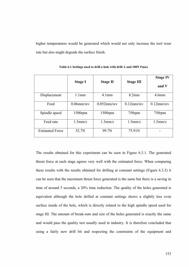
153

higher temperatures would be generated which would not only increase the tool wear

rate but also might degrade the surface finish.

Table 6.1 Settings used to drill a hole with drill A and 100N Fmax

Stage I Stage II Stage III Stage IV

and V

Displacement 1.1mm 4.1mm 8.2mm 4.6mm

Feed 0.06mm/rev 0.052mm/rev 0.12mm/rev 0.12mm/rev

Spindle speed 1500rpm 1500rpm 750rpm 750rpm

Feed rate 1.5mm/s 1.3mm/s 1.5mm/s 1.5mm/s

Estimated Force 52.7N 99.7N 75.91N -

The results obtained for this experiment can be seen in Figure 6.3.1. The generated

thrust force at each stage agrees very well with the estimated force. When comparing

these results with the results obtained for drilling at constant settings (Figure 6.3.2) it

can be seen that the maximum thrust force generated is the same but there is a saving in

time of around 5 seconds, a 20% time reduction. The quality of the holes generated is

equivalent although the hole drilled at constant settings shows a slightly less even

surface inside of the hole, which is directly related to the high spindle speed used for

stage III. The amount of break-outs and size of the holes generated is exactly the same

and would pass the quality test usually used in industry. It is therefore concluded that

using a fairly new drill bit and respecting the constraints of the equipment and

154

maximum force allowed, the hole drilled using variable settings saved time and had a

slight increase in hole quality.

Figure 6.3.1 Drill A variable settings (max Thrust =100N)

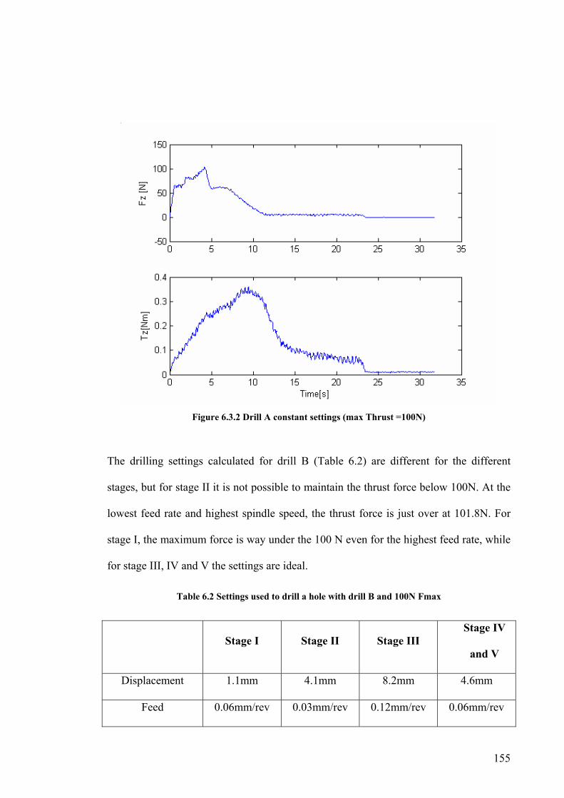
155

Figure 6.3.2 Drill A constant settings (max Thrust =100N)

The drilling settings calculated for drill B (Table 6.2) are different for the different

stages, but for stage II it is not possible to maintain the thrust force below 100N. At the

lowest feed rate and highest spindle speed, the thrust force is just over at 101.8N. For

stage I, the maximum force is way under the 100 N even for the highest feed rate, while

for stage III, IV and V the settings are ideal.

Table 6.2 Settings used to drill a hole with drill B and 100N Fmax

Stage I Stage II Stage III Stage IV

and V

Displacement 1.1mm 4.1mm 8.2mm 4.6mm

Feed 0.06mm/rev 0.03mm/rev 0.12mm/rev 0.06mm/rev

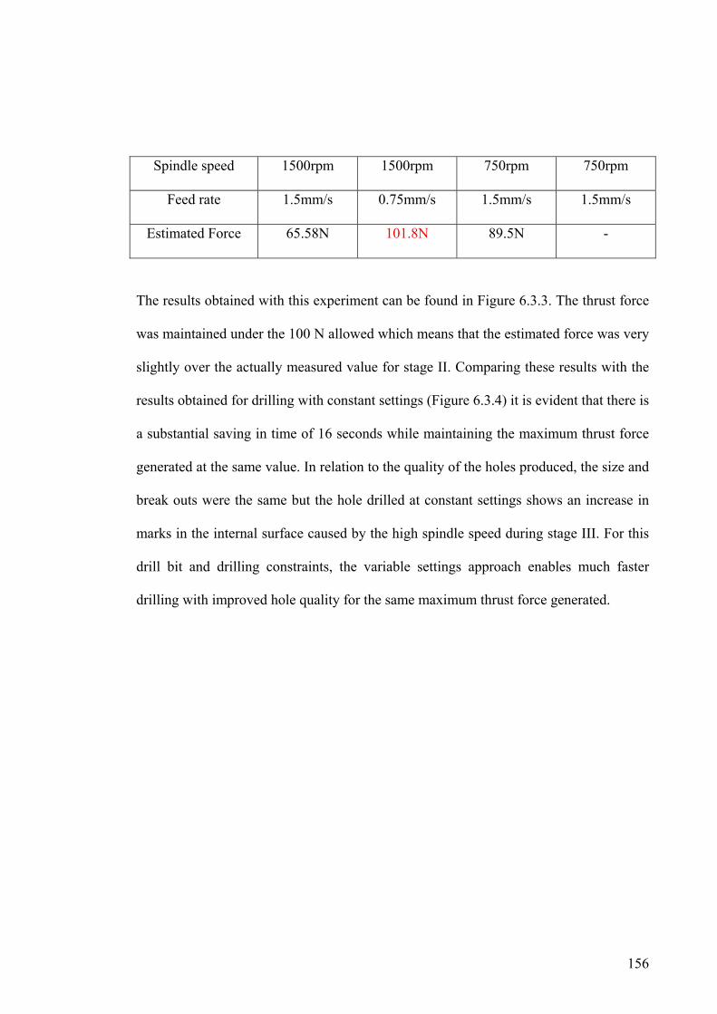
156

Spindle speed 1500rpm 1500rpm 750rpm 750rpm

Feed rate 1.5mm/s 0.75mm/s 1.5mm/s 1.5mm/s

Estimated Force 65.58N 101.8N 89.5N -

The results obtained with this experiment can be found in Figure 6.3.3. The thrust force

was maintained under the 100 N allowed which means that the estimated force was very

slightly over the actually measured value for stage II. Comparing these results with the

results obtained for drilling with constant settings (Figure 6.3.4) it is evident that there is

a substantial saving in time of 16 seconds while maintaining the maximum thrust force

generated at the same value. In relation to the quality of the holes produced, the size and

break outs were the same but the hole drilled at constant settings shows an increase in

marks in the internal surface caused by the high spindle speed during stage III. For this

drill bit and drilling constraints, the variable settings approach enables much faster

drilling with improved hole quality for the same maximum thrust force generated.

157

Figure 6.3.3 Drill B variable settings (max Thrust = 100N)

Figure 6.3.4 Drill B constant settings (max Thrust = 100N)

158

For drill C, which is the drill bit that performed the most number of holes, the

parameters calculated for each stage are also different (table 6.3). For stage II, it was not

possible to maintain the thrust force under the 100N using the range of settings

available. This means that to maintain the thrust force under 100N, a newer drill bit was

needed, or a different range of feed rate and/or spindle speed would have to be used.

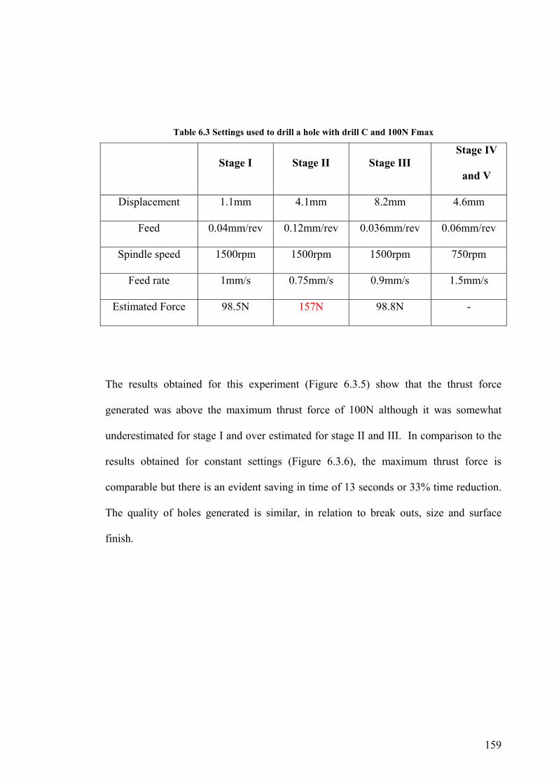
159

Table 6.3 Settings used to drill a hole with drill C and 100N Fmax

Stage I Stage II Stage III Stage IV

and V

Displacement 1.1mm 4.1mm 8.2mm 4.6mm

Feed 0.04mm/rev 0.12mm/rev 0.036mm/rev 0.06mm/rev

Spindle speed 1500rpm 1500rpm 1500rpm 750rpm

Feed rate 1mm/s 0.75mm/s 0.9mm/s 1.5mm/s

Estimated Force 98.5N 157N 98.8N -

The results obtained for this experiment (Figure 6.3.5) show that the thrust force

generated was above the maximum thrust force of 100N although it was somewhat

underestimated for stage I and over estimated for stage II and III. In comparison to the

results obtained for constant settings (Figure 6.3.6), the maximum thrust force is

comparable but there is an evident saving in time of 13 seconds or 33% time reduction.

The quality of holes generated is similar, in relation to break outs, size and surface

finish.

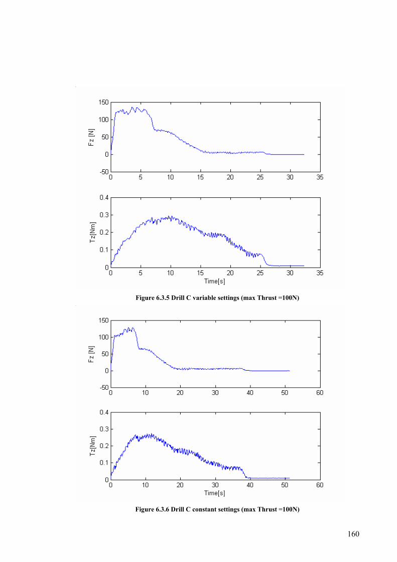
160

Figure 6.3.5 Drill C variable settings (max Thrust =100N)

Figure 6.3.6 Drill C constant settings (max Thrust =100N)

161

6.3.2 Maximum thrust force of 200N

If the maximum thrust force is set to higher values, the settings found will be quite

different. For drill A, the settings are all the same at maximum feed and lowest spindle

speed (Table 6.4). For this scenario, drilling in stages would not bring an advantage, as

the settings are the same for all stages and therefore the drilling is performed at constant

settings.

Table 6.4Settings used to drill a hole with drill A and 200N Fmax

Stage I Stage II Stage III Stage IV

and V

Displacement 1.1mm 4.1mm 8.2mm 4.6mm

Feed 0.12mm/rev 0.12mm/rev 0.12mm/rev 0.12mm/rev

Spindle speed 750rpm 750rpm 750rpm 750rpm

Feed rate 1.5mm/s 1.5mm/s 1.5mm/s 1.5mm/s

Estimated Force 66.59N 127N 66.59N -

The thrust force produced by these settings agree fairly well with the estimated values

as shown in Figure 6.3.7.

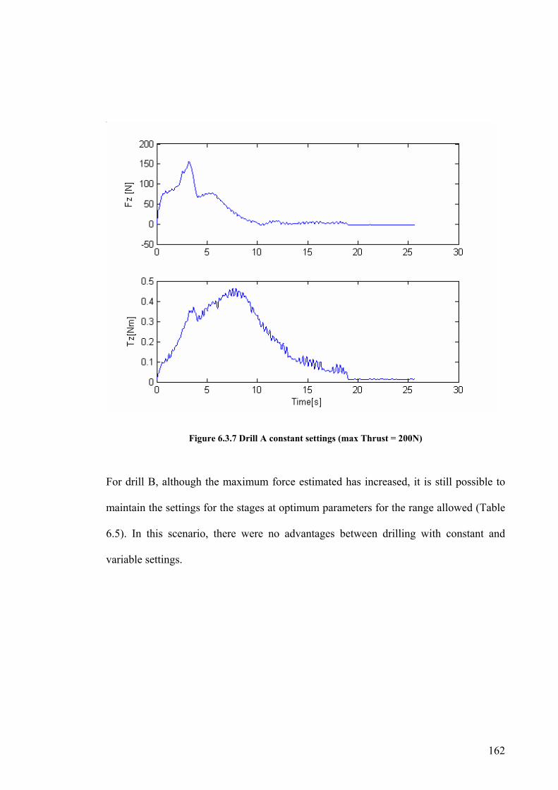
162

Figure 6.3.7 Drill A constant settings (max Thrust = 200N)

For drill B, although the maximum force estimated has increased, it is still possible to

maintain the settings for the stages at optimum parameters for the range allowed (Table

6.5). In this scenario, there were no advantages between drilling with constant and

variable settings.

163

Table 6.5 Settings used to drill a hole with drill B and 200N Fmax

Stage I Stage II Stage III Stage IV

and V

Displacement 1.1mm 4.1mm 8.2mm 4.6mm

Feed 0.12mm/rev 0.12mm/rev 0.12mm/rev 0.12mm/rev

Spindle speed 750rpm 750rpm 750rpm 750rpm

Feed rate 1.5mm/s 1.5mm/s 1.5mm/s 1.5mm/s

Estimated Force 82.88N 149N 89.9N -

In the same manner as for drill A, the thrust force produced agrees with the estimated

values (Figure 6.3.8).

Figure 6.3.8 drill B variable settings (max thrust = 200N)

164

For drill C, in order to maintain maximum force under 200N, the spindle speed had to

be increased from the ideal low value (Table 6.6). In this case, there is not an advantage

in terms of saving time by drilling in stages; the only advantage lies in being able to

reduce the spindle speed during drilling Stage II. If the drill bit were to drill with

constant settings higher temperatures would be generated and this would possibly

damage the surface of the hole. It has been previously shown in chapter 5 that for older

drill bits, the spindle speed used in stage III will affect the surface quality.

Table 6.6 Settings used to drill a hole with drill C and 200N Fmax

Stage I Stage II Stage III Stage IV

and V

Displacement 1.1mm 4.1mm 8.2mm 4.6mm

Feed 0.069mm/rev 0.035mm/rev 0.12mm/rev 0.12mm/rev

Spindle speed 1300rpm 1300rpm 750rpm 750rpm

Feed rate 1.5mm/s 1.5mm/s 1.5mm/s 1.5mm/s

Estimated Force 117N 198N 140.6N -

The results obtained using these setting are shown in Figure 6.3.9. As expected, the

thrust force was maintained under the 200N limit. Comparing this result to the one

obtained with constant settings (Figure 6.3.10), the only difference lies in stage III,

where the thrust force is lower for constant settings due to the higher spindle speed. In

terms of quality, the holes are comparable in terms of break outs and size. As expected,

the surface produced with the variable settings is slightly better.

165

Figure 6.3.9 Drill C variable settings (max Thrust = 200N)

Figure 6.3.10 Drill C constant settings (max Thrust = 200N)

166

6.3.3 Discussion of Results

It can be concluded from the previous experiments that the advantages of a variable

parameter drilling system vary for the different scenarios. The higher the allowed thrust

force, the less the advantage available. The age of the drill bit also affects the results; for

newer drill bits the improvements are not as evident as for older drill bits. The reason

for this difference is amplified by the limitations of the parameters that can be used. For

many cases, it was necessary to keep the feed rate and or the spindle speed at maximum

and/or minimum values which made the use of the variable system redundant. For an

application with a wider range of allowed settings, it is expected that the advantages of

this algorithm would be much higher. Nevertheless, for many scenarios shown, the

advantages of this automated system are evident.

The age of the drill bit has been taken into consideration and the drilling parameters

calculated adjusted. In practical terms, this is very important because the drill bit wears

out at such an accelerated rate that it would be impossible to tune any system without

considering tool wear. It has also been shown in these experiments that the developed

algorithm is of particular advantage for older drill bits.

6.4 Conclusion

In this chapter, the advantages of drilling with variable drilling parameters have been

shown. A decision making algorithm has been designed to select the ideal parameters

for a given aplication. This algorithm uses the limits of the system in terms of the

spindle speed and the feed rate, the maximum thrust force allowed and the age of the

drill bit to calculate the ideal parameters for each of the drilling stages.

167

The algorithm was implemented and tested for three drill bits at diferent ages and two

maximum thrust forces allowed, 100N and 200N respectively. The results obtained

were then compared to drilling at constant parameters using the parameters calculated

for stage II (which is the stage where the thrust force reaches its highest values).

It has been shown that using variable settings, the holes can be drilled at higher feed

rates, hence reducing the time necessary to drill. Time reductions of up to 33% were

achieved with this intelligent automated system. The quality of the holes was also

improved in some cases. There were situations where the settings calculated by the

algorithm were constant for all stages, meaning that there were scenarios where there

would be no advantage in drilling with variable settings. On the other hand, there was

not any scenario were the automated drilling system developed in this chapter would

yield worse results than drilling with constant settings.

The advantages of drilling with variable settings have been shown to increase with the

age of the drill bit and for lower forces. As the drill bit ages, the developed system

yields substantial advantages compared with drilling with constant settings. It is

therefore concluded that drilling with variable settings has been sucessfully shown to

improve drilling time and surface quality of the holes drilled for aging drill bits.

168

Chapter 7 Conclusions and Recommendations for

Future Research

7.1 Conclusions

In this Thesis, an automated drilling system has been developed and successfully

implemented for the intelligent drilling of carbon composites using a one shot drill bit.

In Chapter 1 the importance and need for this research is established. A literature review

on several aspects related to the drilling of carbon composites is carried out.

An instrumented drilling ring was designed, built and commissioned for the experiments

necessary to develop the automated system. This test rig is described in Chapter 2.

The forces and torques developed during drilling were studied and characterised in

Chapter 3. The thrust force and torque were divided into stages and the drilling and

reaming process at each of these stages described. Over 300 holes were drilled in order

to study the characteristics of these signals. The relationship between the maximum

thrust force and torque and drilling parameters was extracted. It was found that the

maximum thrust force and torque vary with the feed, the diameter of the drill bit, the

thickness of the workpiece and the age of the drill bit. The lateral forces produced

during drilling were also analysed as well as the frequency content of the thrust force

169

and torque, but no relevant results emerged from such analysis. The experiments and

findings from Chapter 3 are used in Chapter 4.

In Chapter 4 a mathematical model is developed to estimate thrust force. This model

was based on Shaw’s simplified equations, but several modifications were necessary in

order for it to be valid for the current application. Shaw’s model is developed for

estimating the steady state of the drilling process for a common twist drill. In the current

application, such a steady state never occurs due to the shape of the drill bit being used

and the thickness of samples being drilled. To overcome such limitations, the diameter

used for the model was not the diameter of the drill bit but a relationship between the

diameter of the drill bit and the thickness of the sample being drilled. This alteration

was proved to work and maximum thrust force and torque could be successfully

estimated for the holes drilled with a new drill bit. As the drill bit aged, Shaw’s

simplified equations did not hold and a tool age coefficient was introduced to

compensate for it. As a result, maximum thrust force and torque were successfully

estimated for over 300 holes drilled, which for this drill bit is over double its usual life

expectancy.

The Thrust force in relation to time has also been successfully estimated in Chapter 4.

The signal was represented by 5 points (or ‘corners’) joined by straight lines. The

position of each corner was found to be governed by the drill bit shape in relation to the

material thickness. Hence, the drilling force was found to be position dependent. The

amplitude of the thrust force was estimated in relation to the maximum thrust force

referred to above. Applications for this model include: finding the feed which will keep

170

the thrust force under a pre-determined value; estimating tool life for a certain

application by relating the force produced to the quality of the holes produced; enabling

defects to be detected when actual forces exceed modelled limits. This mathematical

model is used for the automated system developed in Chapter 6.

Chapter 5 is dedicated to studying the quality of the holes. The relation between many

hole quality parameters and the drilling settings was established. It was found in this

Chapter that older drill bits produce smaller holes than new drill bits, although the

problem can be minimised by reaming for longer with older drill bits. Reaming time can

improve size tolerances (although is also known to increase temperature and tool wear).

It was also found in this chapter that the surface finish of the hole is directly related to

the age of the drill bit, and to a lesser extent by the spindle speed.

The reaming section finishes the hole to size tolerance. It has been shown in Chapter 5

that holes reamed for longer presented better roundness and size tolerance. It has also

been shown that if drilling is stopped just as the cutting edges are through the hole, the

holes have a tapered shape. This problem is more pronounced for older drill bits.

It has concluded in chapter 5 that the drilling and reaming stage (Stage III) is

responsible for the effects of tool wear on the surface finish of the hole. Although

delamination is commonly considered a major problem in the drilling of carbon

composites, delamination was not observed for the range of parameters available for

this research.

171

Hence, it is concluded that the age of the drill bit is the most important factor affecting

the quality of the holes and that within the range of settings tested this can not be

avoided, though it can be minimized.

The findings from Chapter 5 are used in the design of the automated system developed

in Chapter 6.

An automated drilling system for variable drilling of carbon composites with the a shot

drill bit is developed and successfully implemented in Chapter 6. Using the results from

Chapter 3, Chapter 4 and Chapter 5, a decision making algorithm was designed which

calculated the best settings for each drilling and reaming stage in a given situation. The

inputs for this algorithm are: the constraints of the system (maximum thrust force

allowed, range of spindle speeds and feed rates), the thickness of the workpiece, the

diameter of the holes and the number of holes previously drilled by the drill bit. The

settings calculated were used to drill in stages and the results compared to the results

obtained if drilled with constant feed. It was shown in this Chapter that the developed

drilling system could improve substantially the time needed to drill the holes while

respecting all predetermined constraints. The surface finish of the holes was also

improved in many cases. The advantages of this system are particularly great for drill

bits which are not new. Taking into consideration that in a manufacturing scenario most

holes will be drilled with aging drill bits, the developed automated system has the

potential to bring substantial time savings. A further advantage is that the system

developed does not require a force sensor, though prior to characterisation of the

process for the particular drills and workpiece used is necessary.

172

7.2 Recommendations for Future Research There are various areas of work that could further improve the system developed in this

thesis, as discussed below.

The mathematical model developed in this work used a linear model for the age of the

drill bit, which was dependent on the number of holes drilled. Although this solution

yielded satisfactory results, the tool age should be dependent not only on the number of

holes drilled but also which settings were used on those drilled holes. Another way of

making the estimation more robust without having to remodel the tool age coefficient,

would be to implement “on line” variation of n (number of holes previously drilled).

This would mean that after each hole is drilled, instead of incrementing n by one, n

would be calculated taking into consideration the thrust force generated in the previous

hole drilled. The n used in the tool age coefficient would therefore be a function of the

thrust force generated in the previous hole instead of the actual number of holes drilled.

All the results found on this thesis are only valid for the range of settings used in the

experiments. A wider range of settings would therefore allow for a more robust

solution, and as discussed in Chapter 6, would probably increase the advantages of

using an automated system with variable settings.

Shaw’s simplified equation were successfully adapted for the current application, but

improvements could be made if the thrust force estimated did not depend on the feed

173

only (mm/rev), because as shown in Chapter 3 the thrust force varies for the same feed

(mm/rev) depending on the spindle speed used. If a wider range of spindle speeds and

feed rates (mm/s) were to be used, it is expected that this discrepancy might cause

problems. A more complex model for the thrust force would be necessary to overcome

this problem.

174

References [1] Latger, F., Harris, T., and Bjorklund, S., "Drilling Cost Model," presented at

2002 SAE Automated Fastening Conference & Exhibition, Chester, UK, 2002.

[2] Wardak, K., Tasch, U., and Charalambides, P. G., "Modeling and Simulations of

Optimal Drilling Through Elastically Deformation Workpieces," presented at

2001 IEEE/ASME International Conference on Advanced Intelligent

Mechatronics, Como, Italy, 2001.

[3] Abrate, S. and Walton, D. A., "machining of composite materials. Part I:

traditional methods," Composites Manufacturing, vol. 3, pp. 75-83, 1992.

[4] Lawlor, V. P., McCarthy, M. A., and Stanley, W. F., "An Experimental Study of

Bolt-Hole Clearance Effects in Double-lap, Multi-bolt Composite Joints,"

Composite Structures, 2004.

[5] Johansson, S., Ossbahr, G., and Harris, T., "A Study of the Influence of Drilling

Method and hole Quality on Static Strengh and Fatigue Life of Carbon-Fibre-

Reinforced Plastic aircraft Material"," presented at 2002 SAE Automated

Fastening Conference & Exhibition, Chester, U.K., 2002.

[6] Persson, E., Eriksson, I., Zackrisson, L., "Effects Of Hole Machining Defects On

Strength and Fatigue Life Of Composite Laminates," Composites: Part A, vol.

28A, pp. 141-151, 1997.

175

[7] Lin, H. J. and Tsai, C. C., "Failure Analysis Of Bolted Connections of

Composite With Drilled And Moulded-In Hole," Composite Structures, vol. 30,

pp. 159-168, 1995.

[8] Hocheng, H., Tai, N. H., and Liu, C. S., "Assessment of ultrasonic drilling of

C/SiC composite material," Composites Part A: Applied Science and

Manufacturing, vol. 31, pp. 133-142, 2000.

[9] Gautam, N. and Jain, V. K., "Experimental investigations into ECSD process

using various tool kinematics," International Journal of Machine Tools &

Manufacture, vol. 38, pp. 15-27, 1998.

[10] Ramkumar, J., Malhotra, S. K., and Krishnamurthy, K., "Effect of workpiece

vibration on drilling of GFRP laminates," Journal of Materials Processing

Technology, vol. 152, pp. 329-332, 2004.

[11] Zhang, L. B., Wang, L. J., Liu, X. Y., Zhao, H. W., Wang, X., and Luo, H. Y.,

"mechanical model for predicting thrust and torque in vibration drilling fibre-

reinforced composite materials," International Journal of Machine Tools &

Manufacture, vol. 41, pp. 641-657, 2001.

[12] Kihlman, H. and Lindqvist, R., "Orbital Drilling - Implementation and

Evaluation," presented at 2004 Aerospace Manufacturing and Automated

Fastening Conference & Exhibition, St Loius, Missouri, 2004.

176

[13] Chen, Y., "Drilling Process Modeling For New Drilling Process Development,"

in Mechanical Engineering Department. Michigan: University of Michigan,

1999, pp. 143.

[14] Astrom, B. T., Manufacturing of Polymer Composites: Chapman & Hall, 1997.

[15] Won, M., "Machining of Fiber-Reinforced Composite Laminates," in

Mechanical Engineering. Berkeley: University of California, 1999, pp. 158.

[16] DeGarmo, E. P., Materials and Processes in Manufacturing: The Macmillan

Company, 1962.

[17] Shaw, M. C., Metal Cutting Principals: Oxford Science Publications, 1984.

[18] Sprakel, M., "Drill Bit Investigation," in School of Mechanical Engineering.

Sydney: University of Technology, 1997, pp. 98.

[19] Strenkowski, J. S., Hsieh, C. C., and Shih, A. J., "An analytical finite element

technique for predicting thrust force and torque in drilling," International

Journal of Machine Tools & Manufacture, vol. 44, pp. 1413-1421, 2004.

[20] Xia, R. S. and Mahdavian, S. M., "Experimental studies of step drills and

establishment of empirical equations for the drilling process," International

Journal of Machine Tools & Manufacture, vol. 45, pp. 235-240, 2004.

177

[21] Langella, A., Nele, L., and Maio, A., "A Torque and Thrust Prediction Model

for Drilling of Composite Materials," Composite: Part A, vol. 36, pp. 83-93,

2005.

[22] Shatla, M. and Atlan, T., "Analytical Modeling of Drilling and Ball end

Milling," Journal of Materials Processing Technology, vol. 98, pp. 125-133,

2000.

[23] Shatla, M., "Prediction of Forces, Stresses, Temperatures and Tool Wear in

Metal Cutting," in Mechanical Engineering: Ohio State University, 1999, pp.

292.

[24] Yang, J. A., Jaganathan, V., and Du, R., "A new dynamic model for drilling and

reaming processes," International Journal of Machine Tools and Manufacture,

vol. 42, pp. 299-311, 2002.

[25] Karri, V., "RBF Neural Network for Thrust and Torque Predictions in Drilling

Operations," presented at Third International Conference on Computational

Intelligence and Multimedia Applications. ICCIMA '99, 1999.

[26] Elhachimi, M., Torbaty, S., and Joyot, P., "Mechanical Modelling of High Speed

Drilling.

1: Predicting Torque and Thrust," International Journal of Machine Tools &

Manufacture, vol. 39, pp. 553-568, 1999.

178

[27] Elhachimi, M., Torbaty, S., Joyot, P., "Mechanical Modelling of High Speed

Drilling. 2: Predicted and Experimental Results," International Journal of

Machine Tools & Manufacture, vol. 39, pp. 569-581, 1999.

[28] Arola, D. and Ramulu, M., "Orthogonal cutting of fiber-reinforced composites: a

finite element analysis," International Journal of Mechanical Sciences, vol. 39,

pp. 597-613, 1997.

[29] Arola, D., Ramulu, M., and D., H. W., "Chip formation in orthogonal trimming

of graphite/epoxy composite," Composites Part A: Applied Science and

Manufacturing, vol. 27, pp. 121-133, 1996.

[30] Wang, Z. M., Ezugwu, E. O., and Su, D., "advances in the precision machining

of small deep holes," Journal of Materials Processing Technology, vol. 68, pp.

257-261, 1997.

[31] Shaw, M. C. and Oxford, C. J., "On the Drilling of Metals 2-The Torque and

Thrust in Drilling," Transactions Of The ASME, pp. 139-148, 1957.

[32] Kawaji, S., Arao, M., and Chen, Y., "Thrust Force Control Of Drilling System

Using Neural Network," presented at 2001 IEEE/ASME International

Conference on Advanced Intelligent Mechatronics, Italy, 2001.

179

[33] Ramulu, M., Arola, D., and D., H. W., "Orthogonal cutting mechanisms of

Graphite/Epoxy composite. Part I: Unidirectional laminate," International

Journal of Machine Tools and Manufacture, vol. 35, pp. 1623-1638, 1995.

[34] Ramulu, M., Arola, D., and D., H. W., "Orthogonal cutting mechanisms of

Graphite/Epoxy composite. Part II: Multi-directional laminate," International

Journal of Machine Tools and Manufacture, vol. 35, pp. 1639-1648, 1995.

[35] Morin, E., Masounave, J., and Laufer, E. E., "Effect of Drill Wear on Cutting

Forces in The Drilling of Metal-Matrix Composites," Wear, vol. 184, pp. 11-16,

1995.

[36] Ozaki, M., "Supervisory Control of Drilling of Composite Materials," in

Mechanical Engineering. Berkeley: University of California, 2000.

[37] Alici, G. and Daniel, R. W., "Robotic drilling under force control: execution of a

task," presented at IEEE/RSJ/GI International Conference on Intelligent Robots

and Systems '94. 'Advanced Robotic Systems and the Real World', IROS '94.,

1994.

[38] Degoulange, E., Dauchez, P., Pierrot, F., and Prat, P., "Determination of a

Reference Model for Controlling The Deformation of an Industrial Robot.

Aplication to Riveting in Aeronautics," presented at IEEE/RSJ/GI International

180

Conference on Intelligent Robots and Systems '94. 'Advanced Robotic Systems

and the Real World', IROS '94, 1994.

[39] Alici, G. and Daniel, R. W., "Importance of Resolution of Joint Encoders During

Robotic Hard-on-Hard Tasks." IEE Colloquium on Precision Motion Control in

Robotics and Machine Drives, 1994, pp. 6/1-6/5.

[40] Alici, G. and Daniel, R. W., "Development and Experimental Verification of a

Mathematical Model for Robot Force Control Design," presented at 1993

IEEE/RSJ International Conference on Intelligent Robots and Systems,

Yokohama, Japan, 1993.

[41] Schimmels, J., "The Use of Complience and Constrain for Improved Robotic

Material Removal Processes," presented at 1994 IEEE International Conference

on Robotics and Automation, 1994.

[42] Kihlman, H., Ossbahr, G., Engstrom, M., and Anderson, J., "Low-cost

Automation for Aircraft Assembly," presented at 2004 Aerospace

Manufacturing and Automated Fastening Conference & Exhibition, St. Louis,

Missouri, 2004.

[43] Furness, R. J., Tsao, T., Rankin, J. S., II, Muth, M. J., and Manes, K. W.,

"Torque Control for a Form Tool Drilling Operation," vol. 7. IEEE Transactions

on Control Systems Technology, 1999, pp. 22-30.

181

[44] EL-Wardany, T. I., Gao, D., and Elbestawi, M. A., "Tool Condition Monitoring

in Drilling Using Vibration Signature Analysis," International Journal of

Machine Tools & Manufacture, vol. 36, pp. 687-711, 1996.

[45] Jaume, D., Verge, M., and Bernede, D., "Monitoring Drilling Wear State Using

Vibration Based Diagnosis," presented at International Conference on Systems,

Man and Cybernetics 'Systems Engineering in the Service of Humans', 1993.

[46] Li, X., "On-Line Detection of the Breakage of Small Diameter Drills Using

Current signature Wavelet Transform," International Journal of Machine Tools

& Manufacture, vol. 39, pp. 157-164, 1997.

[47] Narayanan, S. B., Fang, J., Bernard, G., and Atlas, L., "Feature Representations

for Monitoring of Tool Wear," presented at 1994 IEEE International Conference

on Acoustics, Speech, and Signal Processing. ICASSP-94, 1994.

[48] Ravishankar, S. R. and Murthy, C. R. L., "Characteristics Of AE Signals

Obtained During Drilling Composite Laminates," NDT&E International, vol.

33, pp. 341-348, 2000.

[49] Ravishankar, S. R. and Murthy, C. R. L., "Application Of Acoustic Emission In

Drilling Of Composite Laminates," NDT&E International, vol. 33, pp. 429-435,

2000.

182

[50] Mori, K., Kasashima, N., Fu, J. C., and Muto, K., "Prediction of Small Drill

Brakage by Wavelet Transforms and Linear Discriminant Functions,"

International Journal of Machine Tools & Manufacture, vol. 39, pp. 1471-1484,

1999.

[51] Raj, K. H., Sharma, R. S., Srivastava, S., and Patvardhan, "Modeling of

Manufaturing Processes With ANNs for Intelligent Manufacturing,"

International Journal of Machine Tools & Manufacture, vol. 40, pp. 851-868,

2000.

[52] Liu, T. I., Chen, W. Y., and Anatharaman, K. S., "Intelligent Detection of Drill

Wear," Mechanical Systems and Signal Processing, vol. 12, pp. 863-873, 1998.

[53] Jantunen, E., "A summary of methods applied to tool condition monitoring in

drilling," International Journal of Machine Tools and Manufacture, vol. 42, pp.

997-1010, 2002.

[54] Rehorn, A. G., Jiang, J., and Orban, P. E., "State-of-the-art methods and results

in tool conditioning monitoring: a review," International Journal Advance

Manufacture and Technology, 2004.

[55] Caprino, G. and Tagliaferri, V., "Damage development in drilling glass fibre

reinforced plastics," International Journal of Machine Tools & Manufacture,

vol. 35, pp. 817-829, 1995.

183

[56] Inoue, H., Aoyama, E., Hirogaki, T., Ogawa, K., Matsushita, H., Kitahara, Y.,

and Katayama, T., "Influence of tool wear on internal damage in small diameter

drilling in GFRP," Composite Structures, vol. 39, pp. 55-62, 1997.

[57] Piquet, R., Ferret, B., Lachaud, F., and Swider, P., "Experimental Analysis of

Drilling Damage in Thin Carbon/Epoxy Plate Using Special Drills,"

Composites: Part A, vol. 31, pp. 1107-1115, 2000.

[58] Caprino, G., De Iorio, I., Nele, L., and Santo, L., "Effect of Tool Wear on

cutting forces in the orthogonal cutting of unidirectional glass fibre-reinforced

plastics," Composite: Part A, vol. 27A, pp. 409-415, 1996.

[59] Oraby, S. E. and Hayhurst, D. R., "Tool Life Determination based on the

measurement of wear and tool force ratio variation," International Journal of

Machine Tools & Manufacture, vol. 44, pp. 1261-1269, 2004.

[60] Davim, J. P. and Antonio, C. C., "Optimal drilling of particulate metal matrix

composites based on experimental and numerical procedures," International

Journal of Machine Tools & Manufacture, vol. 41, pp. 21-23, 2001.

[61] Davim, J. P. and Conceicao Antonio, C. A., "Relationship Between Cutting

Force and PCD Cutting Tool Wear in Machining Silicon Carbide Reinforced

Aluminium," Journal of Materials Processing Technology, vol. 103, pp. 417-

423, 2000.

184

[62] Lin, S. C., Chen, I. K., "Drilling carbon fiber-Reinforced Composite Material at

High Speed," Wear, vol. 194, pp. 156-162, 1996.

[63] Kim, D. and Rumalu, M., "Drilling process optimization for

graphite/bismaleimide-titatium alloy stacks," Composite Structures, vol. 63, pp.

101-114, 2004.

[64] Ramulu, M., Branson, T., and Kim, D., "A study on the drilling of composite

and titanium stacks," Composite Structures, vol. 54, pp. 67-77, 2001.

[65] Chen, W., "Some Experimental Investigations in The Drilling of Fibre-

Reinforced Plastic (CFRP) Composite Laminates," International Journal of

Machine Tools & Manufacture, vol. 37, pp. 1097-1108, 1997.

[66] Bhattacharyya, D. and Horrigan, D. P. W., "A Study of Hole Drilling in Kevlar

Composites," Composites Science and Thecnology, vol. 58, pp. 267-283, 1998.

[67] Stone, R. and Krishnamurthy, K., "A Neural Network Thrust Force Controller to

Minimize Delamination During Drilling of Graphite-Epoxy Laminates,"

International Journal of Machine Tools & Manufacture, vol. 36, pp. 985-1003,

1996.

[68] Point, N. and Sacco, E., "A delamination model for laminated composites,"

International Journal of Solids and Structures, vol. 33, pp. 483-509, 1996.

185

[69] Sheng, Y., Tomizuka, M., and Osaki, M., "Dynamic Modeling and Adaptive

Predictive Control (APC) of Drilling of Composite Materials," presented at

American Control Conference, Chicago, Illinois, 2000.

[70] Mathew, J., Ramakrishnan, N., and Naik, N. K., "Trepanning on unidirectional

composites: delamination studies," Composites: Part A, vol. 30, pp. 951-959,

1999.

[71] HoCheng, H. and Tsao, C., "Analysis of delamination in drilling composite

materials using core drill," Australian Journal of Mechanical Engineering, pp.

49-53, 2003.

[72] Hocheng, H. and Tsao, C., "Comprehensive analysis of delamination in drilling

of composite materials with various drill bits," Journal of Processing

Technology, vol. 140, pp. 335-339, 2003.

[73] Hocheng, H., Yen, S. B., Ishihara, T., and Yen, B. K., "Fundamental turning

characteristics of a tribology-favored graphite/aluminum alloy composite

material," Composites Part A: Applied Science and Manufacturing, vol. 28, pp.

883-890, 1997.

[74] Won, M. and Dharan, C. K. H., "Drilling of Aramid and carbon fibre polymer

composites," Journal of Manufacturing Science and Engineering, vol. 124, pp.

778-783, 2002.

186

[75] Tsao, C. and Chen, W., "prediction of the location of delamination in the drilling

of composite laminates," Journal of Materials Processing Technology, vol. 70,

pp. 185-189, 1997.

[76] Tsao, C. and Ho-Cheng, H., "The effect of chisel length and associated pilot

hole on delamination when drilling composite materials," International Journal

of Machine Tools & Manufacture, vol. 43, pp. 1087-1092, 2003.

[77] Lachaud, F., Piquet, R., Collombet, F., and Surcin, L., "drilling of composite

structures," Composite Structures, vol. 52, pp. 511-516, 2001.

[78] Won, M. and Dharan, C. K. H., "Chisel Edge and Pilot Hole Effects in Drilling

Composite Laminates," Journal of Manufacturing Science and Engineering, vol.

124, pp. 242-247, 2002.

[79] Khashaba, U. A., "Delamination in drilling GFR-thermoset composites,"

Composite Structures, vol. 63, pp. 313-327, 2004.

[80] Tsao, C. and Hocheng, H., "Taguchi analysis of delamination associated with

various drill bits in drilling of composite material," International Journal of

Machine Tools & Manufacture, vol. 44, pp. 1085-1090, 2004.

187

[81] Zhang, H., Chen, W., Chen, d., and Zhang, L. B., "Assessment of the exit

defects in carbon fibre-reinforced plastic plates caused by drilling," Key

Engineering Materials, vol. 196, pp. 43-52, 2001.

[82] Bhrara, R. S., "On Drilling of Advanced Aerospace composites," in Aerospace

engineering. Melbourne: Royal Melbourne Institute of Technology, 1991.

[83] Tosun, G. and Muratoglu, M., "The drilling of Al/SiCCp metal-matrix

composites. Part II: Workpiece surface integrity," Composite Science and

Thecnology, vol. 64, 2004.

[84] Dharan, C. K. H., Won, M. S., "Machining Parameters for an Intelligent

Machining System for Composite laminates," International Journal of Machine

Tools & Manufacture, vol. 40, pp. 415-426, 2000.

[85] Kalidas, S., DeVor, R. E., and Kapoor, S. G., "Experimental investigation of the

effect of drill coatings on hole quality under dry and wet drilling conditions,"

Surface and Coatings Technology, vol. 148, pp. 117-128, 2001.

[86] Altintas, Manufacturing Automation: Cambridge University Press, 2000.

[87] Davim, J. P., Conceicao Antonio, C. A., "Optimisation of cutting conditions in

machining of aluminium matrix composites using a numerical and experimental

model," Journal of Materials Processing Technology, pp. 78-82, 2001.

188

[88] Kim, J., SangkeeMin, Dornfeld, D.A., "Optimization and control of drilling burr

formation of AISI 304L and AISI 4118 based on drilling burr control charts,"

International Journal of Machine Tools & Manufacture, vol. 41, pp. 923-936,

2000.

[89] El-Tammimi, A. and Darwish, S. M., "Geometric accuracies of NC and

conventionally drilled holes," Journal of Materials Processing Technology, vol.

75, pp. 111-116, 1998.

[90] Kalidas, S., Kapoor, S. G., and DeVor, R. E., "Influence of thermal effects on

hole quality in dry drilling, Part 2: thermo-elastic effects on hole quality,"

Journal of Manufacturing Science and Engineering, vol. 124, pp. 267-273,

2002.

[91] Ramulu, M., Rao, P. N., and Kao, H., "Drilling of (Al2O3)p/6061 metal matrix

composites," Journal of Materials Processing Technology, vol. 124, pp. 244-

254, 2002.

[92] Ramulu, M., Young, P., and Kao, H., "Drilling of Graphite/Bismaleimide

Composite Material," Journal of Materials Engineering and Performance, vol.

8, pp. 330-338, 1999.

[93] Mathew, J., Ramakrishnan, N., and Naik, N. K., "Investigations into the effect of

geometry of a trepanning tool on thrust and torque during drilling of GFRP

189

composites," Journal of Materials Processing Technology, vol. 91, pp. 1-11,

1999.

[94] Hashmi, K., Graham, I. D., and Mills, B., "Fuzzy Logic Based Data Selection

for the Drilling Process," Journal of Materials Processing Technology, vol. 108,

pp. 55-61, 2000.

[95] Meng, Q., Arsecularatne, J. A., and Mathew, P., "Calculation of Optimum

Cutting Conditions for Turning Operations Using a Machining Theory,"

International Journal of Machine Tools & Manufacture, vol. 40, pp. 1709-1733,

2000.

[96] Everson, C. E. and Cheraghi, S. H., "The application of acoustic emission for

precision drilling process monitoring," International Journal of Machine Tools

& Manufacture, vol. 39, pp. 371-387, 1998.

[97] Tsao, C. and Ho-Cheng, H., "Effect of eccentricity of twist drill and candle stick

drill on delamination in drilling composite materials," International Journal of

Machine Tools & Manufacture, pp. 1-6, 2004.

190

List of Figures

Figure 1.3.1 Schematic of a Twist drill [16] ...................................................................10

Figure 1.3.2 Other shaped drill bits for drilling composites [14]....................................12

Figure 1.3.3 Schematic of one shot drill bit ....................................................................14

Figure 1.4.1 Schematics of delamination caused by drilling; a) top Layer b) bottom

layer.................................................................................................................................23

Figure 2.1.1Test rig schematic ........................................................................................34

Figure 2.1.2 Photo of test bed .........................................................................................35

Figure 2.1.3 Test Rig Set up............................................................................................36

Figure 2.1.4 Force and torque sensor ..............................................................................37

Figure 2.1.5 Drilling rig connections scheme .................................................................39

Figure 2.2.1 Photo of drill bits used................................................................................41

Figure 2.2.2 ‘One shot” Drill bit schematic ....................................................................42

Figure 3.3.1 Typical thrust Force and torque..................................................................47

Figure 3.3.2 Drilling Stages ............................................................................................48

Figure 3.4.1 Plot of maximum thrust force against feed for various spindle speeds ......52

Figure 3.4.2 Plot of maximum torque against feed for various spindle speeds ..............53

Figure 3.4.3 Plot of maximum thrust force against feed for different sample thicknesses

.........................................................................................................................................54

Figure 3.4.4 Plot of maximum torque against feed for different sample thicknesses .....55

Figure 3.4.5 Plot of maximum thrust force against feed for different drill bit diameters

.........................................................................................................................................56

Figure 3.4.6 Plot of maximum torque against feed for different drill bit diameters .......56

191

Figure 3.5.1 Effect of tool age on drilling thrust force and torque for 2mm samples.....58

Figure 3.5.2 Effect of tool age on drilling thrust force and torque for 2mm double

samples ............................................................................................................................58

Figure 3.5.3 Effect of tool age on drilling thrust force and torque for 5.2mm samples..59

Figure 3.5.4 Plot of maximum thrust force against feed for 2mm sample......................60

Figure 3.5.5 Plot of maximum torque against feed for 2mm sample..............................61

Figure 3.5.6 Plot of maximum thrust force against feed for 2mm double sample..........62

Figure 3.5.7 Plot of maximum torque against feed for 2mm double sample..................62

Figure 3.5.8 Plot of maximum thrust force against feed for 5.2mm sample...................64

Figure 3.5.9 Plot of maximum torque against feed for 5.2mm sample...........................64

Figure 3.6.1 Forces and torques produced while drilling................................................66

Figure 3.6.2 Holes drilled consecutively by the same drill bit and settings....................67

Figure 3.6.3 Holes drilled by differently aged drill bits..................................................68

Figure 3.7.1 Frequency content of thrust force [N] and torque [Nm].............................69

Figure 3.7.2 Frequency Content of Thrust Force and Torque (detail) ............................70

Figure 4.2.1 Analogy from current thrust force and Shaw’s thrust force .......................74

Figure 4.2.2 Drill bit diameter at ‘break-through’ ..........................................................75

Figure 4.2.3 Plot of log(u) against log(fd).......................................................................76

Figure 4.2.4 Measured and estimated torque using Shaw’s equations............................77

Figure 4.2.5 Measured and estimated thrust force using Shaw’s equations ...................78

Figure 4.2.6 Tool wear rate for 2mm sample..................................................................79

Figure 4.2.7 Tool Wear Rate for 2mm Double Layer Sample........................................80

Figure 4.2.8 Tool wear rate for 5.4mm sample...............................................................80

Figure 4.2.9 measured and estimated maximum thrust force .........................................81

192

Figure 4.3.1 Typical thrust force represented by corners................................................82

Figure 4.3.2 Plot of thrust force at ‘A’ and ‘B’...............................................................84

Figure 4.3.3 Tool age coefficient for thrust force at ’A’.................................................85

Figure 4.3.4 Estimated and measured thrust force at ‘A’................................................86

Figure 4.3.5 Estimated and Measured Thrust Force at ‘A’.............................................87

Figure 4.3.6 Estimated and Measured Thrust Force at ‘C’ .............................................88

Figure 4.3.7 Measured Thrust Force at ‘C’ and ‘D’........................................................89

Figure 4.3.8 Estimated and measured thrust force at ‘D’................................................90

Figure 4.3.9 Thrust force estimation for 2mm sample....................................................92

Figure 4.3.10 Thrust force estimation for 2mm double layer sample .............................93

Figure 4.3.11 Thrust force estimation for 5.2mm sample...............................................93

Figure 5.3.1 Photo of drill bit and sample after drilling................................................101

Figure 5.3.2 Typical Surface texture of holes drilled by the same drill bit of different

ages (same drilling parameters).....................................................................................105

Figure 5.3.3 Internal surface of holes for a) High spindle speeds b) Low Spindle Speed

.......................................................................................................................................105

Figure 5.3.4 Photos of Typical Chips generated by drill bits of different ages ............106

Figure 5.3.5 Typical Examples of Hole entrance for Hole Set 1, 2 and 3 ....................107

Figure 5.3.6 Typical Examples of Hole exit for Hole Set 1, 2 and 3 ...........................108

Figure 5.3.7 Cleaning the break outs.............................................................................109

Figure 5.3.8 Holes before (a) and after (b) cleaning .....................................................109

Figure 5.3.9 Delamination of the back of a hole...........................................................110

Figure 5.3.10 Hole entrance Damage by drill #1 (Hole Set 1)......................................111

Figure 5.3.11 Hole entrance Damage by drill #2 (Hole Set 2)......................................111

193

Figure 5.3.12 Hole entrance Damage by drill #3 (Hole Set 3)......................................112

Figure 5.3.13 Hole Diameters for Drill #1 ....................................................................113

Figure 5.3.14 Hole diameters for drill #2......................................................................114

Figure 5.3.15 Hole Diameters for Drill #3 ....................................................................114

Figure 5.3.16 Hole Diameters for all holes ...................................................................115

Figure 5.3.17 Examples of hole defects missed the gages ............................................116

Figure 5.3.18 Photo of a Hole Set ................................................................................116

Figure 5.3.19 Three-dimensional Lateral View of Holes Coordinates for one Hole Set

(dimensions in mm).......................................................................................................117

Figure 5.3.20 Top View of Holes Coordinates for one Hole Set (dimensions in mm).118

Figure 5.3.21 Side View of Holes coordinates for one Hole Set (dimensions in mm) .119

Figure 5.3.22 Estimated Circle using measured coordinates in a Least Square sense..120

Figure 5.3.23 Diameter of holes using Drill #1.............................................................121

Figure 5.3.24 Diameter of holes using Drill #2.............................................................122

Figure 5.3.25 Diameter of holes using Drill #3............................................................122

Figure 5.3.26 Hole Diameters for all Samples ..............................................................123

Figure 5.3.27 Relation between Spindle Speed and hole Diameter ..............................124

Figure 5.3.28 Relation between Feed rate [mm/s] and hole Diameter..........................125

Figure 5.3.29 Relation between Feed [mm/rev] and hole Diameter .............................126

Figure 5.3.30 Defining Roundness................................................................................127

Figure 5.3.31 Roundness of Holes for Drill #1 ............................................................127

Figure 5.3.32 Roundness of Holes for Drill #2 .............................................................128

Figure 5.3.33 Roundness of Holes for Drill #3 ............................................................129

Figure 5.3.34 Roundness for all Samples......................................................................130

194

Figure 5.3.35 Relation between Spindle Speed [rpm] and hole Roundness .................131

Figure 5.3.36 Relation between Feed rate [mm/s] and hole Roundness .......................131

Figure 5.3.37 Relation between feed [mm/rev] and hole Roundness ...........................132

Figure 5.4.1 Relation between Thrust Force and Roundness........................................133

Figure 5.4.2 Relation between Thrust Force and Roundness........................................133

Figure 5.4.3 Relation between Thrust Force and Diameter ..........................................134

Figure 5.4.4 Relation between Torque and Diameter ...................................................135

Figure 5.5.1 Drilling routine to test the relation between stages and quality of holes..136

Figure 6.2.1 Decision making flow chart......................................................................148

Figure 6.3.1 Drill A variable settings (max Thrust =100N).....................................154

Figure 6.3.2 Drill A constant settings (max Thrust =100N) .........................................155

Figure 6.3.3 Drill B variable settings (max Thrust = 100N)........................................157

Figure 6.3.4 Drill B constant settings (max Thrust = 100N) ........................................157

Figure 6.3.5 Drill C variable settings (max Thrust =100N)..........................................160

Figure 6.3.6 Drill C constant settings (max Thrust =100N) .........................................160

Figure 6.3.7 Drill A constant settings (max Thrust = 200N) ........................................162

Figure 6.3.8 drill B variable settings (max thrust = 200N) ...........................................163

Figure 6.3.9 Drill C variable settings (max Thrust = 200N).........................................165

Figure 6.3.10 Drill C constant settings (max Thrust = 200N) ......................................165

195

Appendixes

A 1

APPENDIX A

Motor Ratings

Spindle Motor AC Baldor Motor (BSM 63A- 333AA)

Torque continuos 2.09Nm

Current continuos 6.43ARMS

Rated Speed 6000Rpm

Peak Current 24ARMS

Motion Motor DC Baldor Motor (IM-2250-B14-A23)

Torque Stall 0.35Nm

Maximum Speed 5000Rpm

Maximum Voltage 60VDC

Voltage Constant Ke = 12 V/KRpm

Current continuos 3.42 A

Current Peak 18.5 A

Tachometer 7 V/KRpm

encoder 500L

B 1

APENDIX B

Force Sensor

Single Element Multi-Component Dynamometer

MC3A-6-1000

Rated Maximum Loads

Fz 4450 N

Fx,Fy 2225 N

Mz 56.5 Nm

Mx,My 113 Nm

Typical Sensitivity

Fz 0.17 µV/(V-N)

Fx,Fy 0.67 µV/(V-N)

Mz 33.2 µV/(V-N-m)

Mx,My 33.2 µV/(V-N-m)

Stiffness

Fz 31.54 x 106 N/m

Fx, Fy 2.12 x 106 N/m

B 2

Mz 2.26 x 104 N-m/radian

Non-Linearity

Fx,Fy,Fz 0.20 ±% FSO

Hysteresis

Fx,Fy,Fz 0.20% FSO

Resonant Frequency

Mx,My 1000 Hertz

Calibration Loading Diagram Values of coordinates correspond to Figures 1 and 2.

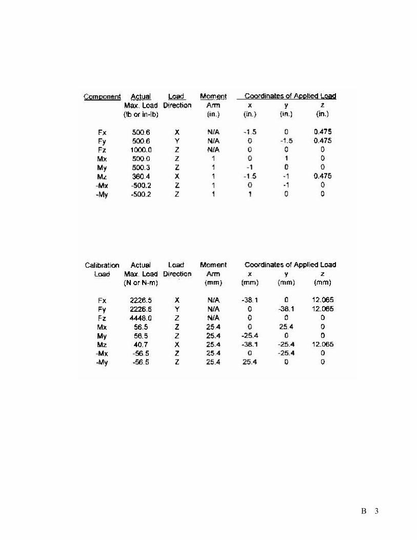
B 3

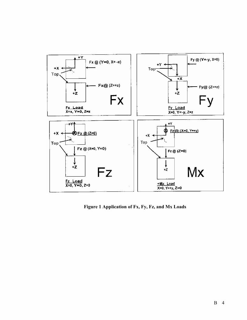
B 4

Figure 1 Application of Fx, Fy, Fz, and Mx Loads

B 5

Figure 2 Application of My, Mz, -Mx, and –My Loads

B 6

MSA -6 Strain Gage Amplifier

Inputs: Six four-arm Wheatstone Bridges (350Ώ)

Bridge Excitation: 2.5VDC, 5VDC, or 10VDC, jumper selected

Gain: 1000,2000, and 4000, jumper selectable

Auto-Zero: Push button

Filter: Two pole low-pass 1000 Hz filter

Output: +/- 10VDC into a minimum 10K ohm load

Operating Temperature: 0-125 deg F (-18 to 52deg C)

Power Supply: 15VDC, 110-250 VAC 50/60 Hz input

B 7

Calibration Record Sheet

C 1

APENDIX C

Product data sheet for F593 prepeg

(www.hexcelcomposites.com)

Product Data

F593™

Resin Systems for Advanced Composites

™ F593 is a trademark of Hexcel Corporation, Pleasanton, California.® HRH, Hexcel, and the Hexcel logo are registered trademarks of Hexcel Corporation, Pleasanton, California.

Description

F593 is a modified 350°F (177°C) curing epoxy system with very low flow for carbon fabric and tape applicationsthat provides excellent laminate and honeycomb sandwich properties. As a low flow resin, F593 lends itself to netresin, zero bleed applications. F593’s adhesive properties allow for the elimination of adhesive layers in co-curingsandwich structures. F593’s low flow minimizes sandwich part porosity.

Features

Uncured

■ Good Tack and Drape for Layup and Assembly■ Elevated Viscosity During Cure■ Simple Cure Cycle for Autoclave and Press■ Available on Various Fiber and Weave

Combinations

Neat Resin PropertiesSpecific gravity 1.22Tg dry 341°F (172°C)Tg wet 268°F (131°C)Equilibrium moisture absorption 4.2%Linear coefficient of thermal expansion 3.0 x 10–5 in/in/°F (5.4 x 10–5 cm/cm/°C)Tensile strength 8.76 ksi (60.4 MPa)Tensile modulus 0.43 msi (2.96 GPa)Tensile strain 2%Fracture toughness, K1C 1.11 ksi in (1.22 MPa m )Strain energy release rate, G1C 2.42 in-lb/in2 (0.42 kJ/m2)Volatiles after 30 minutes @ 350°F (177°C) 3.92%Poisson’s ratio 0.35Gel time @ 350°F (177°C) 9–17 min

Cured

■ Excellent K1C and G1C

■ Good Environment and Impact Resistance■ Flame-Retardant Version Available

To Meet FAR 25.853■ Good Sandwich Panel and Laminate Properties

375(191)

350(177)

325(163)

300(149)

275(135)

Temperature – ¡F (¡C)

100

101

102

Gel Time vs Temperature

103

Gel

Tim

e (m

in)

0

1

101

102

103

104

105

160(71)

240(116)

320(160)

400(204)

81oF (27oC)

248oF(120oC)

345oF(174oC)

Temperature – oF (oC)

ETA

(P

oise

)

Rheometrics Curve of F5934¡F (2¡C)/min, 50% Strain, 10 rad/sec,RDS-7700, 50 mm Plates 0.4 mm Gap

149oF(65oC)

10–1

97HXKB-865 F593.v16 3/29/99 10:48 AM Page 2

Property Carbon Fabrics Carbon Tapes

Prepreg Material description W3T282 F3T584 95 g/m2 145 g/m2 190 g/m2

% Resin content (dry) 38–46 38–46 36–40 36–40 36–40

% Volatiles @ 350°F (177°C) 1–6 1–6 1–4 1–4 1–4

% Flow @ 350°F (177°C) 4.5 Max. 4.5 Max. 13–25 13–25 13–25

100 psi (689 kPa)

LaminateCured thickness per ply – in (cm)

0.0081–0.0096 0.0155–0.018 0.0038–0.0042 0.0059–0.0063 0.0077–0.0083(0.021–0.024) (0.039–0.046) (0.0097–0.011) (0.015–0.016) (0.020–0.021)

% Fiber volume 45–53 45–53 50–55 50–55 50–55

Hexcel Fiber Areal Count Available WidthsForm

DesignationFiber

Wt. g/m2Weave

Warp x Fill Standard Width, in (cm)

Carbon W3T282-42"-F593

Toray 193 Plain 12.5 x 12.5

42", 60"Fabrics T-300/3k (106.7, 152.4)

W3G282-42"-F593Amoco

193 Plain 12.5 x 12.542", 60"

T-300/3k (106.7, 152.4)

W3C282-42"-F593Toho

193 Plain 12.5 x 12.542", 60"

G-30/500/3k (106.7, 152.4)

F3T584-42"-F593Toray

3708 Harness

24 x 2442", 60"

T-300/3k Satin (106.7, 152.4)

F3G584-42"-F593Amoco

3708 Harness

24 x 2442", 60"

T-300/3k Satin (106.7, 152.4)

F3C584-42"-F593Toho

3708 Harness

24 x 2442", 60"

G-30/500/3k Satin (106.7, 152.4)

Carbon T2TXXX-12"-F593

Toray 095, 145, 190 n/a n/a

12", 3"–24"Tapes T-300/12k (30.5, 7.6–61)

T2GXXX-12"-F593Amoco

095, 145, 190 n/a n/a12", 3"–24"

T-300/12k (30.5, 7.6–61)

Note: F593 carbon tapes and fabrics may be produced with various carbon fiber types and tow sizes. In designating tapes and fabrics, the second digit represents the towsize and the third digit represents the fiber type. Consult your nearest Hexcel Representative for additional information.

Availability

Physical Properties

F593™ Product Data

97HXKB-865 F593.v16 3/29/99 10:48 AM Page 3

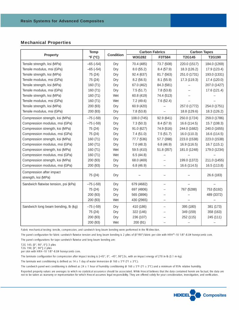
PropertyTemp

ConditionCarbon Fabrics Carbon Tapes

°F (°C) W3G282 F3T584 T2G145 T2G190

Tensile strength, ksi (MPa) –65 (–54) Dry 70.4 (485) 73.7 (508) 220.0 (1517) 184.0 (1269)

Tensile modulus, msi (GPa) –65 (–54) Dry 8.0 (55.2) 8.4 (57.9) 18.3 (126.2) 17.9 (123.4)

Tensile strength, ksi (MPa) 75 (24) Dry 92.4 (637) 81.7 (563) 251.0 (1731) 193.0 (1331)

Tensile modulus, msi (GPa) 75 (24) Dry 8.2 (56.5) 8.1 (55.9) 17.3 (119.3) 17.4 (120.0)

Tensile strength, ksi (MPa) 160 (71) Dry 67.0 (462) 84.3 (581) – 207.0 (1427)

Tensile modulus, msi (GPa) 160 (71) Dry 7.5 (51.7) 7.8 (53.8) – 17.6 (121.4)

Tensile strength, ksi (MPa) 160 (71) Wet 60.8 (419) 74.4 (513) – –

Tensile modulus, msi (GPa) 160 (71) Wet 7.2 (49.6) 7.6 (52.4) – –

Tensile strength, ksi (MPa) 200 (93) Dry 60.9 (420) – 257.0 (1772) 254.0 (1751)

Tensile modulus, msi (GPa) 200 (93) Dry 7.8 (53.8) – 18.8 (129.6) 18.3 (126.2)

Compression strength, ksi (MPa) –75 (–59) Dry 108.0 (745) 92.9 (641) 250.0 (1724) 259.0 (1786)

Compression modulus, msi (GPa) –75 (–59) Dry 7.3 (50.3) 8.4 (57.9) 16.6 (114.5) 15.7 (108.3)

Compression strength, ksi (MPa) 75 (24) Dry 91.0 (627) 74.9 (516) 244.0 (1682) 240.0 (1655)

Compression modulus, msi (GPa) 75 (24) Dry 7.4 (51.0) 7.5 (51.7) 16.0 (110.3) 16.6 (114.5)

Compression strength, ksi (MPa) 160 (71) Dry 77.7 (536) 57.7 (398) 223.0 (1538) 223.0 (1538)

Compression modulus, msi (GPa) 160 (71) Dry 7.0 (48.3) 6.8 (46.9) 16.9 (116.5) 16.7 (115.1)

Compression strength, ksi (MPa) 160 (71) Wet 59.5 (410) 51.8 (357) 181.0 (1248) 179.0 (1234)

Compression modulus, msi (GPa) 160 (71) Wet 6.5 (44.8) – – –

Compression strength, ksi (MPa) 200 (93) Dry 68.0 (469) – 199.0 (1372) 211.0 (1455)

Compression modulus, msi (GPa) 200 (93) Dry 6.8 (46.9) – 16.6 (114.5) 16.5 (113.8)

Compression after impact

strength, ksi (MPa)75 (24) Dry – – – 26.6 (183)

Sandwich flatwise tension, psi (kPa) –75 (–59) Dry 679 (4682) – – –

75 (24) Dry 697 (4806) – 767 (5288) 753 (5192)

200 (93) Dry 565 (3896) – – 489 (3372)

200 (93) Wet 430 (2965) – – –

Sandwich long beam bending, lb (kg) –75 (–59) Dry 410 (186) – 395 (180) 381 (173)

75 (24) Dry 322 (146) – 349 (159) 358 (163)

200 (93) Dry 236 (107) – 252 (115) 245 (111)

200 (93) Wet 200 (91) – – –

Fabric mechanical testing: tensile, compression, and sandwich long beam bending were performed in the fill direction.

The panel configuration for fabric sandwich flatwise tension and long beam bending is 2 plies of (0°/90°) fabric per skin with HRH®–10 1/8"–8.0# honeycomb core.

The panel configurations for tape sandwich flatwise and long beam bending are:

T2G 145; [0°, 90°, 0°]; 3 plies T2G 190; [0°, 90°]; 2 plies per skin with HRH–10 1/8"–8.0# honeycomb core.

The laminate configuration for compression after impact testing is [+45°, 0°, –45°, 90°] 3s, with an impact energy of 270 in-lb (3.1 m-kg).

The laminate wet conditioning is defined as 14 ± 1 day of water immersion @ 160 ± 5°F (71 ± 3°C).

The sandwich panel wet conditioning is defined as 24 ± 1 hour of humidity conditioning @ 160 ± 5°F (71 ± 3°C) and a minimum of 95% relative humidity.

Reported property values are averages to which no statistical assurance should be associated. While Hexcel believes that the data contained herein are factual, the data arenot to be taken as warranty or representation for which Hexcel assumes legal responsibility. They are offered solely for your consideration, investigation, and verification.

Mechanical Properties

Resin Systems for Advanced Composites

97HXKB-865 F593.v16 3/29/99 10:48 AM Page 4

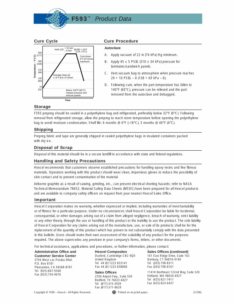
F593™ Product Data

Cure Cycle Cure Procedure

Storage

F593 prepreg should be sealed in a polyethylene bag and refrigerated, preferably below 32°F (0°C). Followingremoval from refrigerated storage, allow the prepreg to reach room temperature before opening the polyethylenebag to avoid moisture condensation. Shelf life: 6 months @ 0°F (–18°C), 3 months @ 40°F (4°C).

Shipping

Prepreg fabric and tape are generally shipped in sealed polyethylene bags in insulated containers packed with dry ice.

Disposal of Scrap

Disposal of this material should be in a secure landfill in accordance with state and federal regulations.

Handling and Safety Precautions

Hexcel recommends that customers observe established precautions for handling epoxy resins and fine fibrousmaterials. Operators working with this product should wear clean, impervious gloves to reduce the possibility ofskin contact and to prevent contamination of the material.

Airborne graphite as a result of sawing, grinding, etc., can present electrical shorting hazards; refer to NASATechnical Memorandum 78652. Material Safety Data Sheets (MSDS) have been prepared for all Hexcel productsand are available to company safety officers on request from your nearest Hexcel Sales Office.

Important

Hexcel Corporation makes no warranty, whether expressed or implied, including warranties of merchantability or of fitness for a particular purpose. Under no circumstances shall Hexcel Corporation be liable for incidental,consequential, or other damages arising out of a claim from alleged negligence, breach of warranty, strict liabilityor any other theory, through the use or handling of this product or the inability to use the product. The sole liabilityof Hexcel Corporation for any claims arising out of the manufacture, use, or sale of its products shall be for thereplacement of the quantity of this product which has proven to not substantially comply with the data presentedin this bulletin. Users should make their own assessment of the suitability of any product for the purposesrequired. The above supercedes any provision in your company’s forms, letters, or other documents.

For technical assistance, applications and procedures, or further information, please contact:

Administrative Office and Customer Service Center5794 West Las Positas Blvd.P.O. Box 8181Pleasanton, CA 94588-8781Tel (925) 847-9500Fax (925) 734-9676

Hexcel CompositesDuxford, Cambridge CB2 4QDUnited KingdomTel 44 (0) 1223 833141Fax 44 (0) 1223 838808

Sales Offices2350 Airport Fwy., Suite 550Bedford, TX 76022-6027Tel (817) 315-3939Fax (817) 571-8629

Sales Offices (continued)101 East Ridge Drive, Suite 102Danbury, CT 06810-4140Tel (203) 798-8311Fax (203) 798-8161

11410 Northeast 122nd Way, Suite 320Kirkland, WA 98034-6927Tel (425) 821-7411Fax (425) 823-6437

Autoclave

A. Apply vacuum of 22 in (74 kPa) Hg minimum.

B. Apply 45 ± 5 PSIG (310 ± 34 kPa) pressure forlaminates/sandwich panels.

C. Vent vacuum bag to atmosphere when pressure reaches 20 + 10 PSIG – 0 (138 + 69 kPa – 0).

D. Following cure, when the part temperature has fallen to140°F (60°C), pressure can be relieved and the part removed from the autoclave and debagged.

70(21)

140(60)

210(99)

280(158)

350(177)

Time

Tem

per

atur

e – ¡F

(¡C

)

Average Heat-up1–5¡F (0.6–3¡C)/min

@ 355 ± 10¡FHold 120+ 15 min– 0 min

Below 140¡F (60¡C)release pressure andremove panels

Cool-down5¡F (3¡C)/min maximum

(179 ± 6¡C)

(12/98)Copyright © 1998 – Hexcel – All Rights Reserved. Printed on recycled paper.

97HXKB-865 F593.v16 3/29/99 10:47 AM Page 1