26/10/09 1

Dr. Shubhi Purwar

DEPARTMENT OF ELECTRICAL ENGG.MOTILAL NEHRU NATIONAL INSTITUTE OF TECHNOLOGY

ALLAHABAD 211004

INTELLIGENT CONTROL OF NONLINEAR SYSTEMS

INDIA

26/10/09 2

OutlineMotivation Mathematical modelingNonlinear Control methodsIntelligent ControlFeedback LinearizationBackstepping ControlSliding mode ControlConclusion

26/10/09 3

Virtually all physical systems are nonlinear in nature. Because of the powerful tools established in linear systems, a first step in analyzing the nonlinear system is to linearize it about some nominal operating point.

However linearization alone will not be sufficient as nonlinear control analysis and design provides sharper understanding of the real system.

Motivation

26/10/09 4

Limitations of Linearization:

Approximation in the neighbourhood of operating point, it can predict only local behaviour.

Dynamics have essentially nonlinear phenomena due to the presence of nonlinearity

Finite escape time Multiple isolated equilibria Limit cycles

26/10/09 5

As we move from linear to nonlinear systems, we are faced with a more difficult situation

• The superposition principle does not hold.

• Analysis tools involve more advanced mathematics.

26/10/09 6

The difficulties of complex nonlinear systems can be classified into the following categories-

Presence of nonlinearities

Uncertainty

Computational complexity

26/10/09 7

Mathematical Modeling

• For designing a controller, we first need to analyze the plant quantitatively.

• The analysis requires a mathematical description of the interrelations between # system quantities themselves.

# system quantities & system I/P’s.

26/10/09

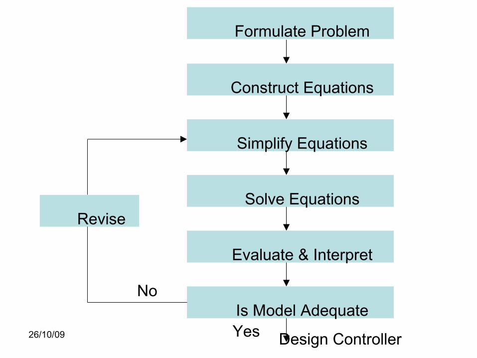
Formulate Problem

Construct Equations

Simplify Equations

Solve Equations

Evaluate & Interpret

Is Model Adequate

Revise

No

Yes Design Controller

26/10/09 9

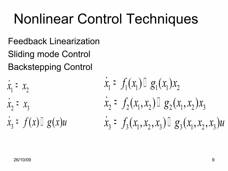
Nonlinear Control TechniquesFeedback LinearizationSliding mode ControlBackstepping Control

1 1 1 1 1 2

2 2 1 2 2 1 2 3

3 3 1 2 3 3 1 2 3

( ) ( )( , ) ( , )( , , ) ( , , )

x f x g x xx f x x g x x xx f x x x g x x x u

= += += +

˙˙˙

1 2

2 3

3 ( ) ( )

x xx xx f x g x u

=== +

˙˙˙

26/10/09 10

Intelligent Control Ability to deal with unknown system

parameters/unknown nonlinearities

Reduce the uncertainty

Plan, generate & execute control action

26/10/09 11

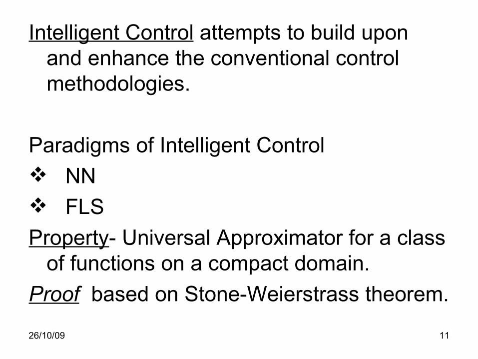
Intelligent Control attempts to build upon and enhance the conventional control methodologies.

Paradigms of Intelligent Control NN FLSProperty- Universal Approximator for a class

of functions on a compact domain.Proof based on Stone-Weierstrass theorem.

26/10/09 12

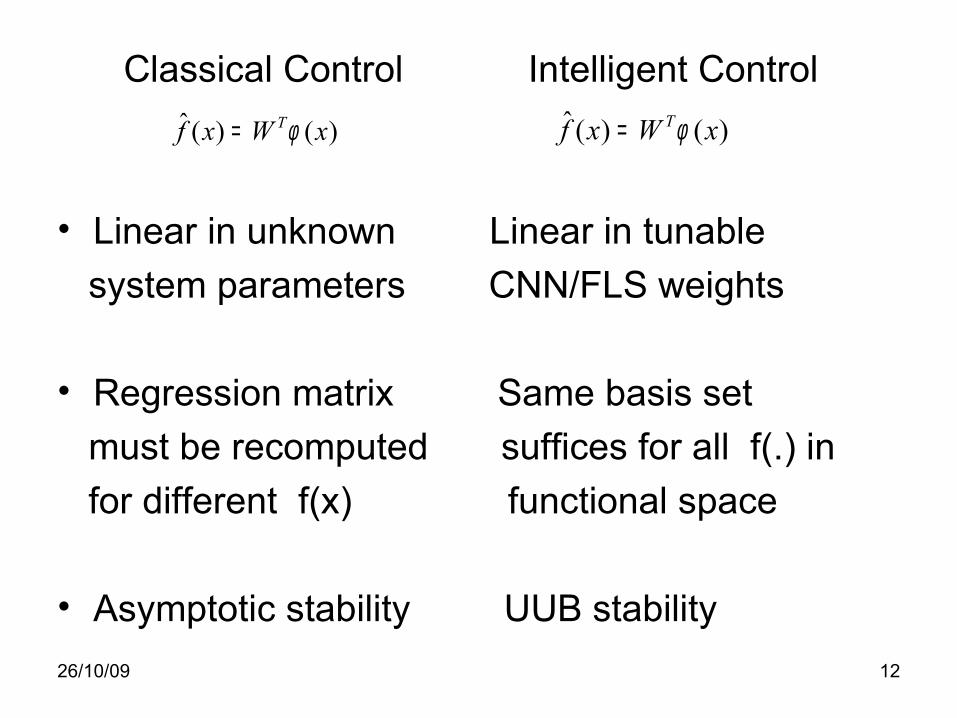
Classical Control Intelligent Control

• Linear in unknown Linear in tunable system parameters CNN/FLS weights

• Regression matrix Same basis set must be recomputed suffices for all f(.) in for different f(x) functional space

• Asymptotic stability UUB stability

ˆ ( ) ( )Tf x W xφ=ˆ ( ) ( )Tf x W xφ=

26/10/09 13

Asymptotic Stability (AS): Classical Adaptive Control

An equilibrium point xe is locally asymptotically stable at t0 if there exists a compact set S such that for every initial condition x0 in S, ║x(t)-xe║→0 as t → ∞.

26/10/09 14

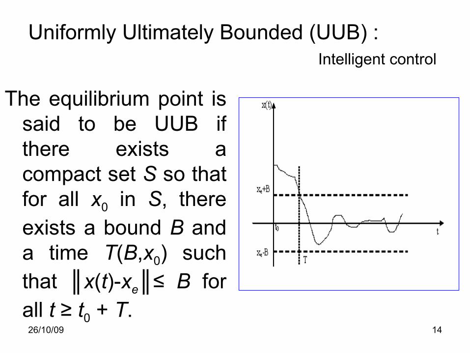
Uniformly Ultimately Bounded (UUB) : Intelligent control

The equilibrium point is said to be UUB if there exists a compact set S so that for all x0 in S, there exists a bound B and a time T(B,x0) such that ║x(t)-xe║≤ B for all t ≥ t0 + T.

26/10/09 15

Feedback Linearization

The idea of feedback linearization is to algebraically transform a nonlinear system dynamics into a linear one so that linear control techniques can be applied.

Input-State LinearizationInput-Output Linearization

26/10/09 16

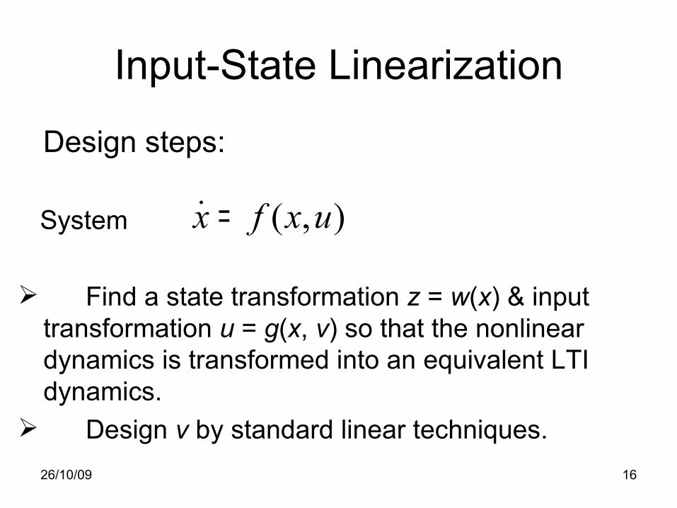
Input-State Linearization

Design steps:

System

Find a state transformation z = w(x) & input transformation u = g(x, v) so that the nonlinear dynamics is transformed into an equivalent LTI dynamics.

Design v by standard linear techniques.

( , )x f x u=˙

26/10/09 17

0_

Pole placement loop

Linearization loop

z = w(x)

v = -kTz u = g(x,v) ( , )x f x u=˙x

Inner loop: Linearization of input-state relation

Outer loop: Stabilization of closed loop dynamics

26/10/09 18

MATHEMATICAL TOOLS

•Lie algebra

•Frobenius Theorem

Control laws derived are often complex due to the need to determine nonlinear state space transformations.

26/10/09 19

Control design based on input-output linearization is done in 3 steps:

• Differentiate the output y until the input u appears

• Choose u to cancel the nonlinearities and guarantee tracking convergence

• Study the stability of the internal dynamics

Input-Output Linearization

26/10/09 20

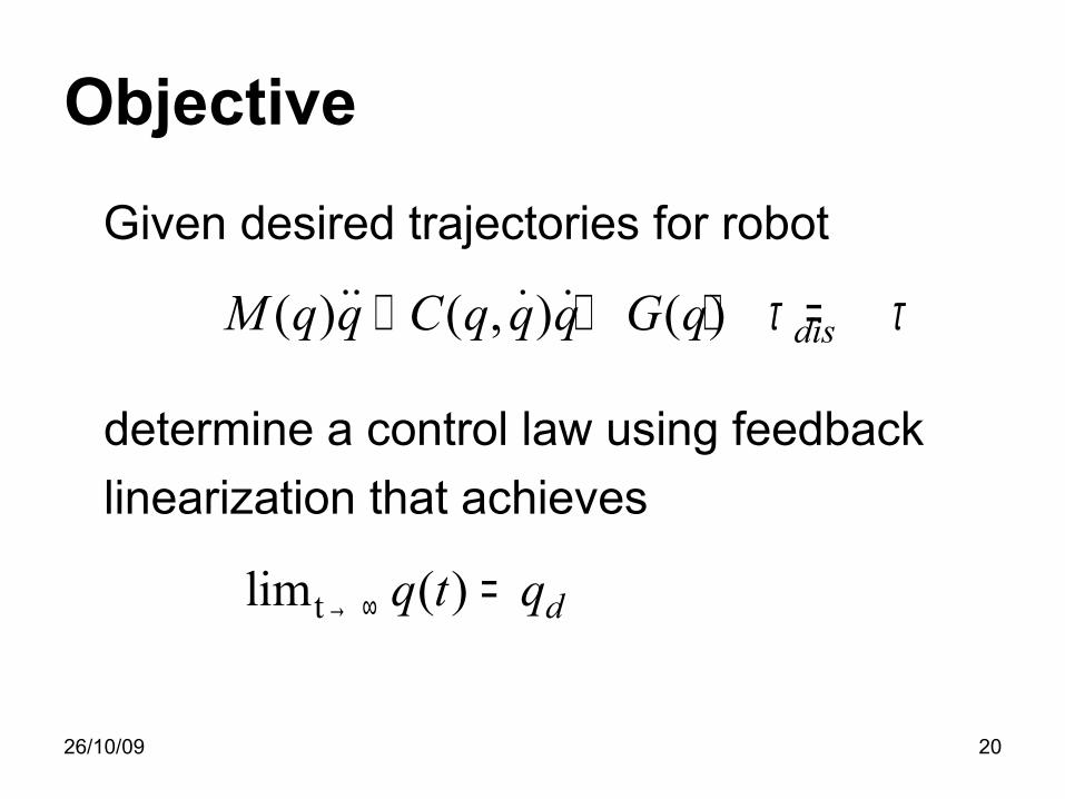
Objective

Given desired trajectories for robot

determine a control law using feedback linearization that achieves

tlim ( ) dq t q→ ∞ =

( ) ( , ) ( ) disM q q C q q q G q τ τ+ + + =˙̇ ˙ ˙

26/10/09 21

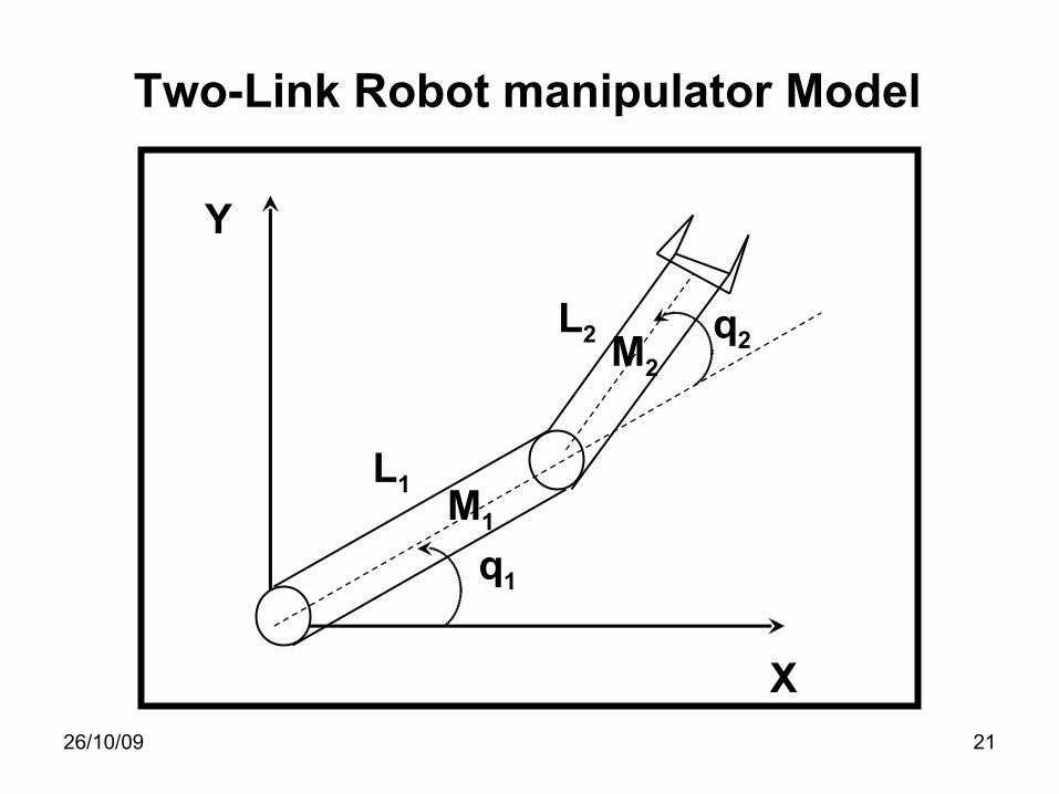
X

Y

q2

q1

M2

M1

L2

L1

Two-Link Robot manipulator Model

26/10/09 22

1

d( ) [ , y ,.... ]n Td d d

dT

x t y yE X Xr E

−== −

= Λ

˙

1

11

( ) ( )

dn

nd d i i

i

r f X g X u d Y

Y y eλ−

+=

= + + +

≡ − + ∑˙

[ ]1 ( )( ) v du f X K r Y d

g X= − − − −

max2

1 ˆ ˆ[ ( , ) ]( )

ˆ( )

c r

v d

r z

u f W X v ug X

v K r Y d

u K W W

= − + +

= − − −

= − +

2ˆ ˆ( )W M X r kM r Wφ= −˙

ˆ ˆ( ) ( )Tf X W Xφ=UXXGXXFX

XX),(),( 211212

21

+=

=˙

˙

26/10/09 23

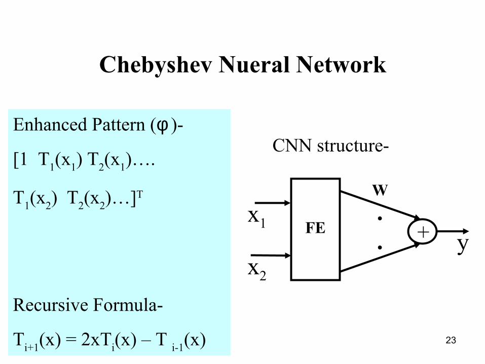
Chebyshev Nueral Network

Enhanced Pattern (φ )-

[1 T1(x1) T2(x1)….

T1(x2) T2(x2)…]T

Recursive Formula-

Ti+1(x) = 2xTi(x) – T i-1(x)

CNN structure-

.

.

.FE

x1

x2

+ y

W

26/10/09 24

Joint Tracking (CNN)

Solid – DesiredDashed - Actual

Time(sec)

0 1 2 3 4 5 6 7 8 9 10-1.5

-1

-0.5

0

0.5

1

1.5

RadiansSolid – DesiredDashed - Actual

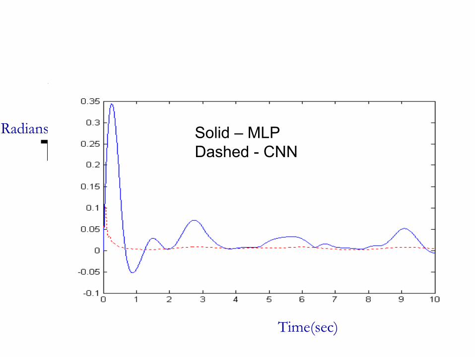
Tracking error (Joint 1)

Time(sec)

Radians Solid – MLPDashed - CNN

26/10/09 26

Tracking error (Joint 2)

Solid – MLPDashed - CNN

Radians

26/10/09 27

Conclusions

Can be applied forStabilization & Tracking controlSISO & MIMO systems

LimitationsCannot be applied to all nonlinear systemsFull state has to be measured

26/10/09 28

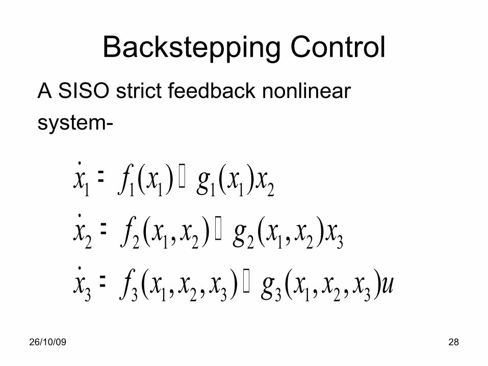
Backstepping ControlA SISO strict feedback nonlinear system-

1 1 1 1 1 2

2 2 1 2 2 1 2 3

3 3 1 2 3 3 1 2 3

( ) ( )( , ) ( , )( , , ) ( , , )

x f x g x xx f x x g x x xx f x x x g x x x u

= += += +

˙˙˙

26/10/09 29

1 1 1 1 1 2

2 2 1 2 2 1 2 3

3 3 1 2 3 3 1 2 3

( ) ( )( , ) ( , )( , , ) ( , , )

x f x g x xx f x x g x x xx f x x x g x x x u

= += += +

˙˙˙ ( )

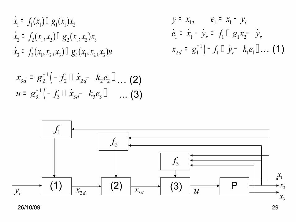
1 1 1

1 1 1 1 21

2 1 1 1 1

, r

r r

d r

y x e x ye x y f g x yx g f y k e−

= = −= − = + −

= − + −

˙ ˙ ˙ ˙

˙

( )( )

13 2 2 2 2 2

13 3 3 3 3

d d

d

x g f x k e

u g f x k e

−

−

= − + −

= − + −

˙

˙

… (1)

… (2) ... (3)

1f2f

3f

ry 2dx 3dx u1x

2x

3x(1) (2) (3) P

26/10/09 30

11

11

( )

( )

li

li

Mn li i jA

lj M

ni iA

l

x yy

x

µ

µ

==

==

Π=

Π

∑

∑

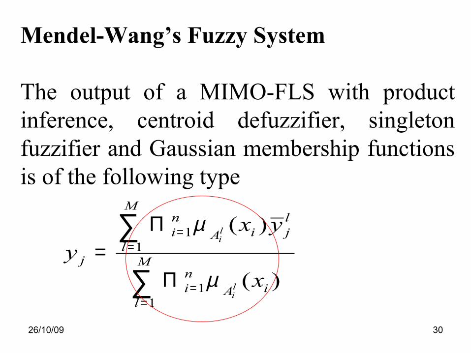
Mendel-Wang’s Fuzzy System

The output of a MIMO-FLS with product inference, centroid defuzzifier, singleton fuzzifier and Gaussian membership functions is of the following type

26/10/09 31

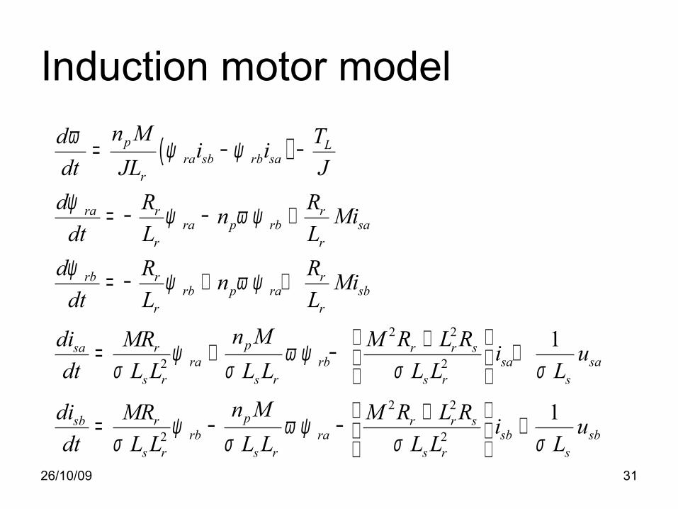
Induction motor model

( )

2 2

2 2

2 2

2

1

p Lra sb rb sa

r

ra r rra p rb sa

r r

rb r rrb p ra sb

r r

psa r r srra rb sa sa

s r s r s r s

psb r r srrb ra

s r s r

n Md Ti idt JL Jd R Rn Mi

dt L Ld R Rn Mi

dt L Ln Mdi M R L RMR i u

dt L L L L L L L

n Mdi M R L RMRdt L L L L

ω ψ ψ

ψ ψ ω ψ

ψ ψ ω ψ

ψ ω ψσ σ σ σ

ψ ω ψσ σ σ

= − −

= − − +

= − + +

+= + − +

+= − − 2

1sb sb

s r s

i uL L Lσ

+

26/10/09 32

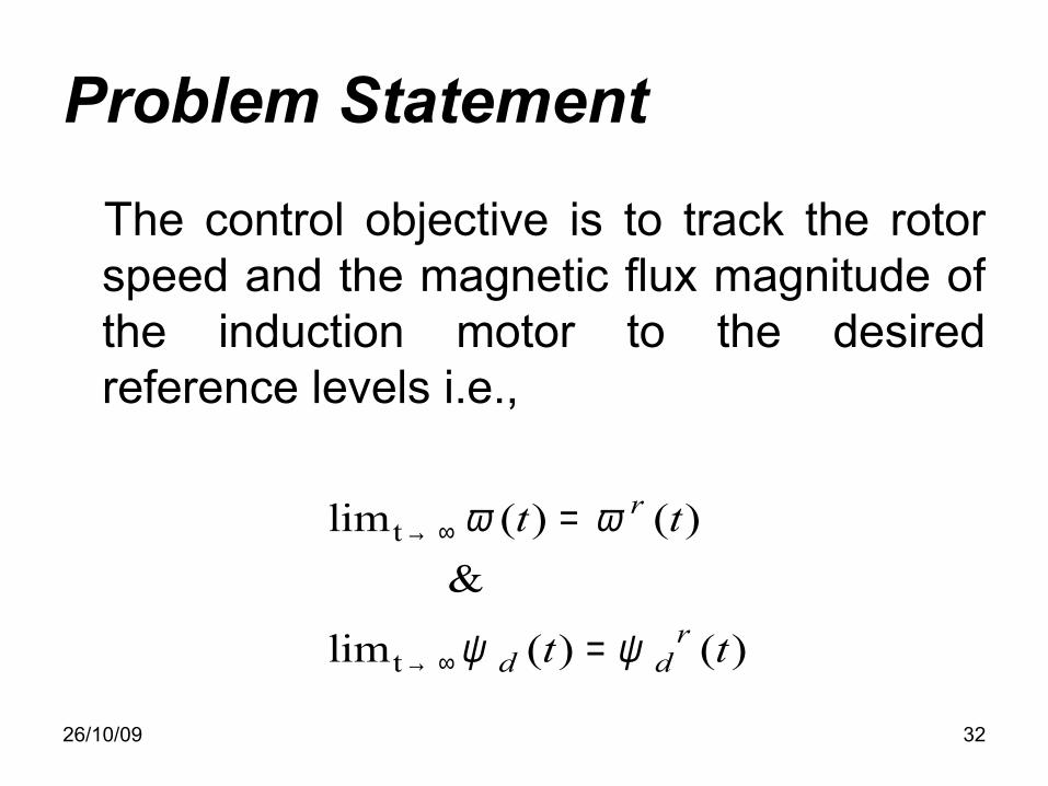
Problem Statement

The control objective is to track the rotor speed and the magnetic flux magnitude of the induction motor to the desired reference levels i.e.,

t

t

lim ( ) ( ) &

lim ( ) ( )

r

rd d

t t

t t

ω ω

ψ ψ

→ ∞

→ ∞

=

=

26/10/09 33

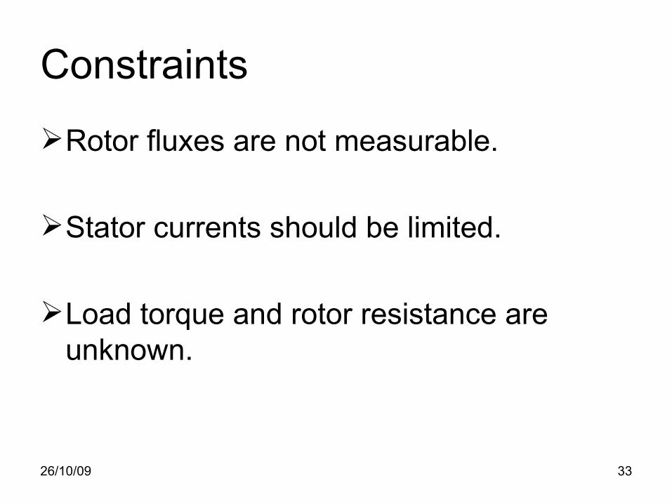
Constraints

Rotor fluxes are not measurable.

Stator currents should be limited.

Load torque and rotor resistance are unknown.

26/10/09 34

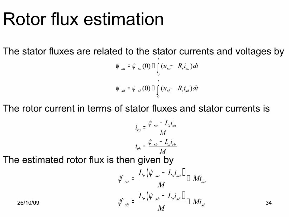
Rotor flux estimation

0

0

(0) ( )

(0) ( )

t

sa sa sa s sa

t

sb sb sb s sb

u R i dt

u R i dt

ψ ψ

ψ ψ

= + −

= + −

∫

∫

sa s sara

sb s sbrb

L iiM

L iiM

ψ

ψ

−=

−=

( )

( )

ˆ

ˆ

r sa s sara sa

r sb s sbrb sb

L L iMi

ML L i

MiM

ψψ

ψψ

−= +

−= +

The stator fluxes are related to the stator currents and voltages by

The rotor current in terms of stator fluxes and stator currents is

The estimated rotor flux is then given by

26/10/09 35

Stator current limitation

*1si

*2 si

sin θ

Is Is*

2*1si

2*2 si

cos θ i1*

i2*

+

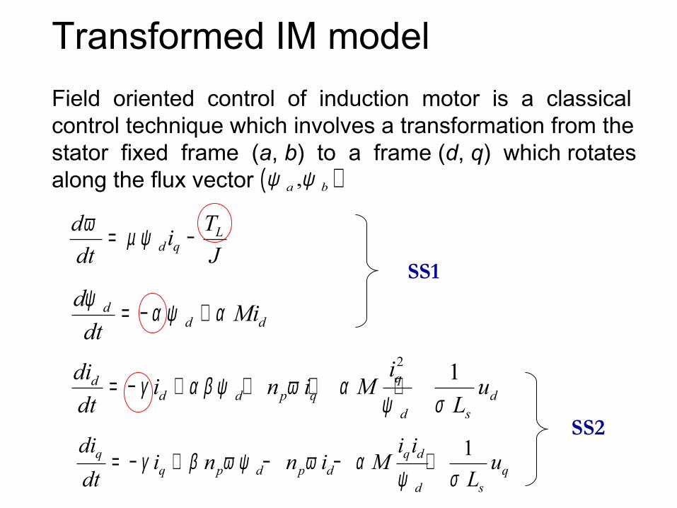
Transformed IM modelField oriented control of induction motor is a classical control technique which involves a transformation from the stator fixed frame (a, b) to a frame (d, q) which rotatesalong the flux vector

dd d

d Midtψ α ψ α= − +

2 1qdd d p q d

d s

idi i n i M udt L

γ α β ψ ω αψ σ

= − + + + +

1q q dq p d p d q

d s

di i ii n n i M u

dt Lγ β ω ψ ω α

ψ σ= − + − − +

( ),a bψ ψ

Ld q

d Tidt Jω µ ψ= −

SS1

SS2

26/10/09 37

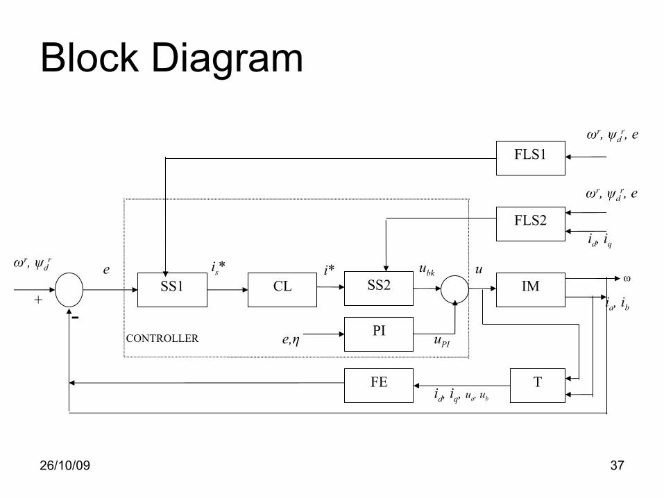
Block Diagram

ωr, ψdr is* i*

PICONTROLLER

SS2u

e,η

ubk

uPI

FE Tid, iq, ua, ub

FLS1

FLS2

SS1 CL IM

ωr, ψdr, e

e

ωr, ψdr, e

id, iq

ia, ib+

-ω

26/10/09 38

Controller design

11 1De = F +F + G iknown˙ ˆ* -1s 1 1 1 1i = G -F -F -K eknown

2 2 2η = F +F + G uknown˙

2

ˆ ˆ

ˆ ˆ1 1 1

2 2

F = Wφ

F = Wφ

T

T

ˆ ˆ

ˆ ˆ1 1 1 1 1 1

2 2 2 2 2 2

W = Γ φ e - Γ E W

W = Γ φ η - Γ E W

κ

κ

˙

˙

FLS1 - ωr, ψdr, e1, e2 - (20x1) and - (20x2)⇒ 1φ ˆ

1W

FLS2 - ωr, ψdr, e1, e2, id, iq - (30x1) and - (30x2)⇒ 2φ ˆ

2W

26/10/09 39

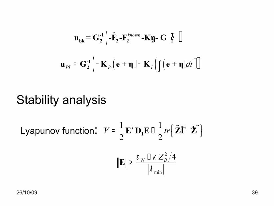
Stability analysis

{ }1 12 2

-11E D E ZΓ ZT TV tr= +

2

min

4N BZε κλ

+>E

( )2ˆ-1 T

bk 2 2 2 1u = G -F -F -Kη- G eknown

( ) ( )( )( )-12u G K e + η K e + ηPI P I dt= − − ∫

Lyapunov function:

26/10/09 40

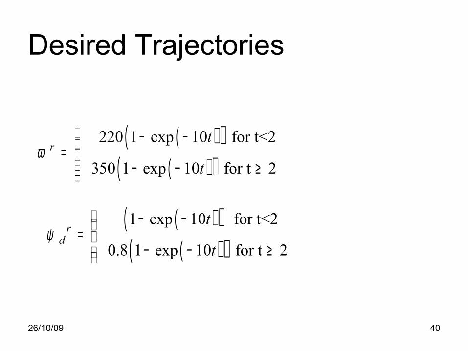
Desired Trajectories

( )( )( )( )

220 1 exp 10 for t<2

350 1 exp 10 for t 2 r

t

tω

− −= − − ≥

( )( )( )( )

1 exp 10 for t<2

0.8 1 exp 10 for t 2 r

d

t

tψ

− −= − − ≥

26/10/09 41

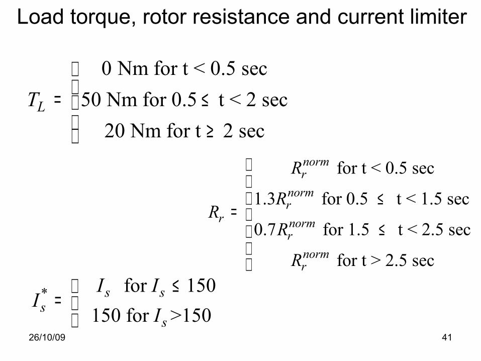
Load torque, rotor resistance and current limiter

0 Nm for t < 0.5 sec50 Nm for 0.5 t < 2 sec

20 Nm for t 2 secLT

= ≤ ≥

* for 150 150 for >150

s ss

s

I II

I≤

=

for t < 0.5 sec

1.3 for 0.5 t < 1.5 sec

0.7 for 1.5 t < 2.5 sec

for t > 2.5 sec

normr

normr

r normr

normr

R

RR

R

R

≤=

≤

26/10/09 42

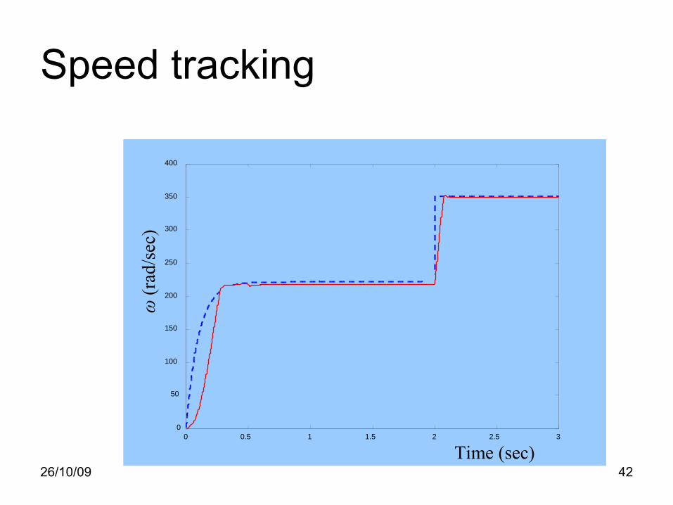
Speed tracking

0 0.5 1 1.5 2 2.5 30

50

100

150

200

250

300

350

400ω

(rad

/sec

)

Time (sec)

26/10/09 43

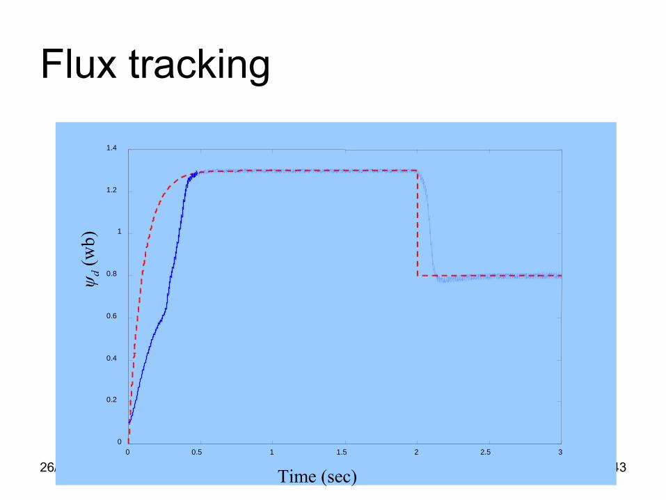
Flux tracking

0 0.5 1 1.5 2 2.5 30

0.2

0.4

0.6

0.8

1

1.2

1.4

Time (sec)

ψ d (w

b)

26/10/09 44

Current waveform

0 0.5 1 1.5 2 2.5 3

-150

-100

-50

0

50

100

150

Time (sec)

i a (am

p)

26/10/09 45

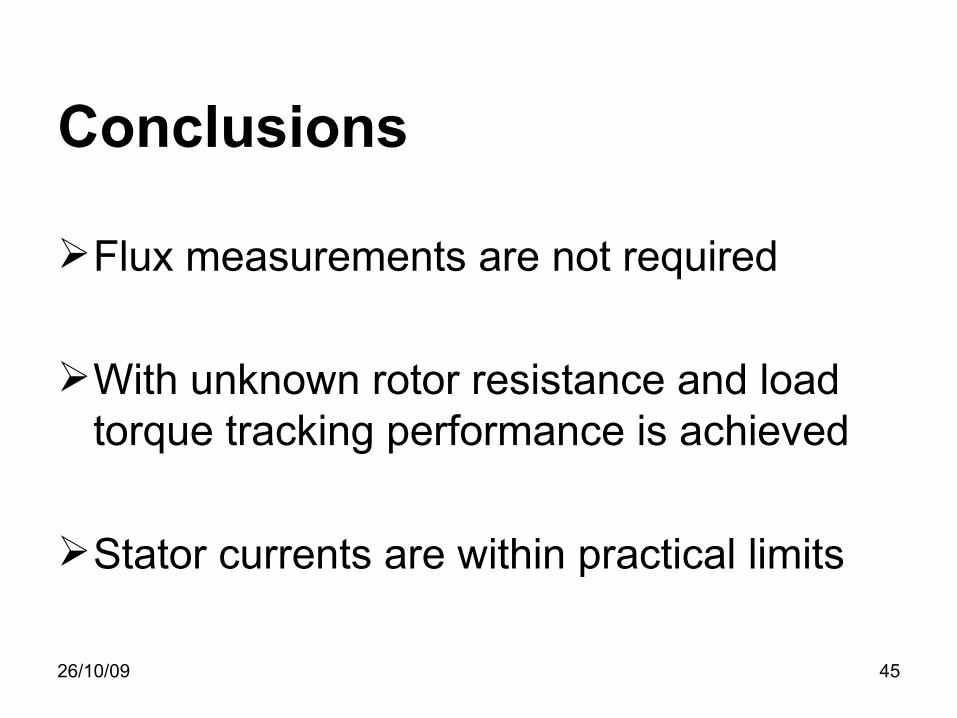
Conclusions

Flux measurements are not required

With unknown rotor resistance and load torque tracking performance is achieved

Stator currents are within practical limits

26/10/09 46

Sliding Mode ControlThe main advantage of Sliding Mode Control (SMC) is the robustness to modelling errors and unknown disturbances.

Traditional SMC was, however, limited by a

discontinuous control law.

There are techniques to limit and eliminate the high-frequency switching associated with traditional SMC.

Two SMC techniques utilizing a robot manipulator to eliminate the limitation of the discontinuous control law are presented.

26/10/09 47

SMC Design Methodology

• Design a sliding manifold or sliding surface in state space.

• Design a controller to reach the sliding surface in finite time.

• Design a control law to confine the desired state variables to the sliding manifold.

26/10/09 48

SMC Graphical Illustration

26/10/09 49

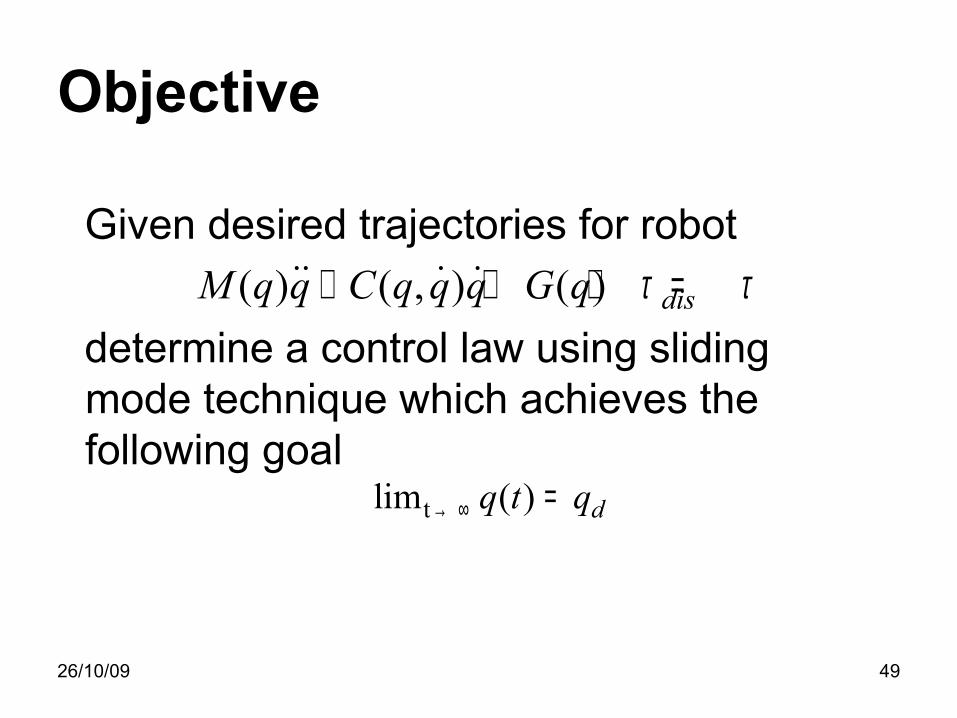
Objective

( ) ( , ) ( ) disM q q C q q q G q τ τ+ + + =˙̇ ˙ ˙

tlim ( ) dq t q→ ∞ =

Given desired trajectories for robot

determine a control law using sliding mode technique which achieves the following goal

26/10/09 50

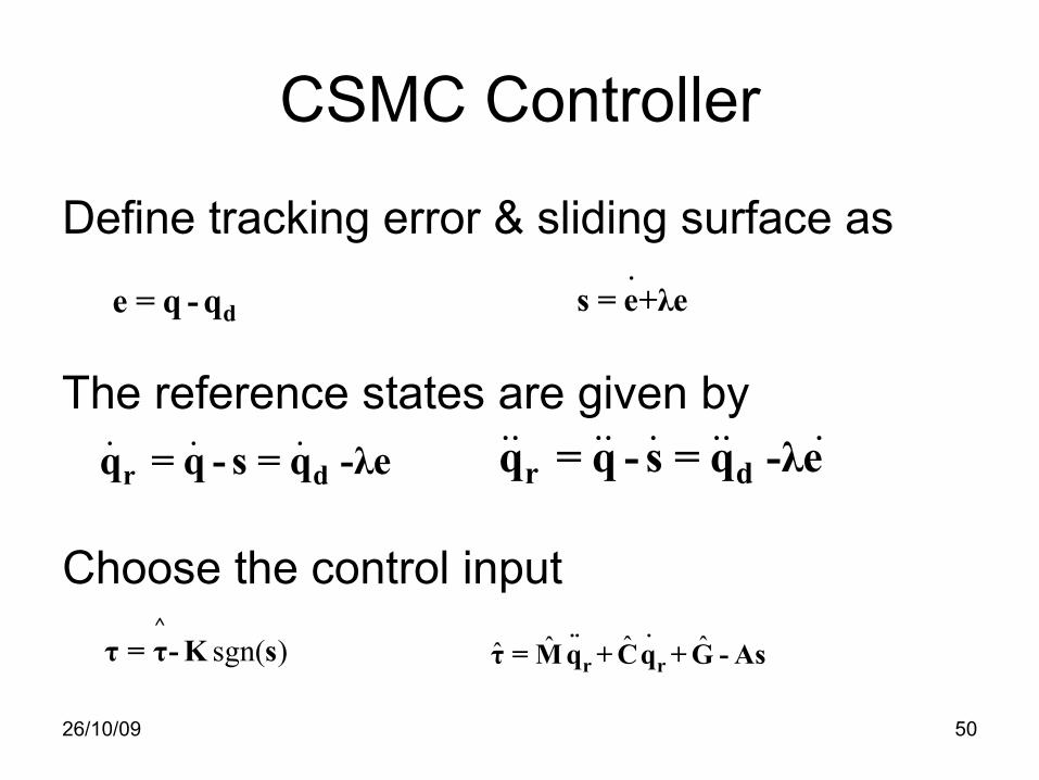
CSMC Controller

Define tracking error & sliding surface as

de = q - q.

s = e+λe

r dq = q - s = q -λe˙ ˙ ˙ r dq = q - s = q -λe˙̇ ˙̇ ˙ ˙̇ ˙

sgn( )^

τ = τ- K s ˆ ˆˆˆ.. .

r rτ = M q + Cq + G - As

Choose the control input

The reference states are given by

26/10/09 51

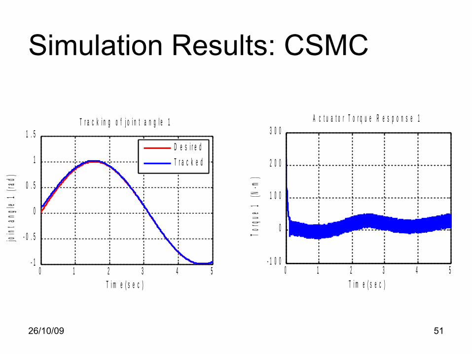
Simulation Results: CSMC

0 1 2 3 4 5- 1

- 0 . 5

0

0 . 5

1

1 . 5T r a c k i n g o f j o i n t a n g l e 1

T i m e ( s e c )

join

t ang

le 1

(rad

)

D e s i r e d

T r a c k e d

0 1 2 3 4 5- 1 0 0

0

1 0 0

2 0 0

3 0 0A c t u a t o r T o r q u e R e s p o n s e 1

T i m e ( s e c )

Torq

ue 1

(N-

m)

26/10/09 52

CSMC

0 1 2 3 4 5- 0 . 2

- 0 . 1

0

0 . 1

0 . 2T r a c k i n g e r r o r s o f j o i n t a n g l e s

T i m e ( s e c )

erro

rs o

f jo

int

angl

es (

rad) e r r o r o f j o i n t 1

e r r o r o f j o i n t 2

26/10/09 53

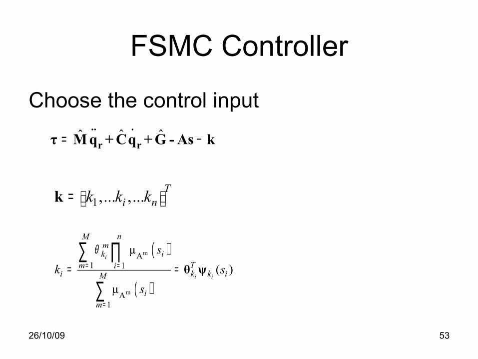
FSMC Controller

Choose the control input ˆ ˆˆ= −

.. .

r rτ M q + Cq + G - As k

1,... ,... Ti nk k k= k

( )

( )

m

m

A1 1

A1

µ( )

µ

i

i i

nMmk i

Tm ii k k iM

im

sk s

s

θ= =

=

= =∑ ∏

∑θ ψ

26/10/09 54

HOSMC Controller

• HOSMC eliminates chattering while retaining the main properties of FOSMC.

• It is characterized by a discontinuous control acting on higher order time derivatives of the sliding variable.

• Order of the sliding mode is the order of the first continuous total time derivative of the sliding variable.

26/10/09 55

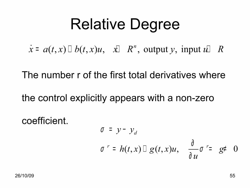
Relative Degree

( , ) ( , ) , 0

d

r r

y y

h t x g t x u gu

σ

σ σ

= −∂= + = ≠

∂

( , ) ( , ) , , output , input nx a t x b t x u x R y u R= + ∈ ∈˙

The number r of the first total derivatives where

the control explicitly appears with a non-zero

coefficient.

26/10/09 56

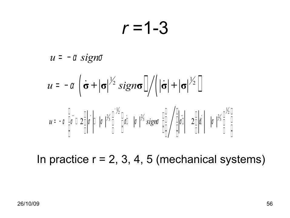
u signα σ= −

( ) ( )1 12 2u signα= − σ + σ σ σ + σ˙ ˙

1 12 2

2 2 23 3 3

.. . . .. .2 2u signα σ σ σ σ σ σ σ σ σ

− = − + + + + +

r =1-3

In practice r = 2, 3, 4, 5 (mechanical systems)

26/10/09 57

Define

dσ = e = q - q

ˆ sτ = τ + τ

( ) ( )1 12 2signα= −sτ σ + σ σ σ + σ˙ ˙

26/10/09 58

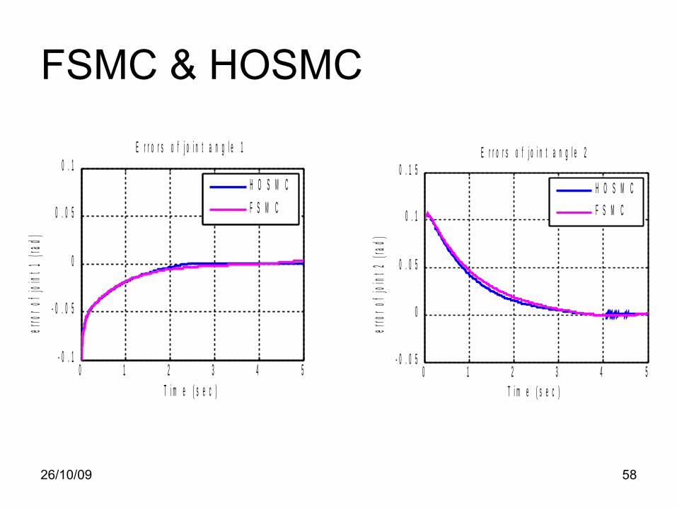
FSMC & HOSMC

0 1 2 3 4 5- 0 . 1

- 0 . 0 5

0

0 . 0 5

0 . 1E r r o r s o f j o i n t a n g l e 1

T i m e ( s e c )

erro

r of j

oint 1

(rad

)

H O S M C

F S M C

0 1 2 3 4 5- 0 . 0 5

0

0 . 0 5

0 . 1

0 . 1 5E r r o r s o f j o i n t a n g l e 2

T i m e ( s e c )er

ror o

f joi

nt 2

(rad

)

H O S M C

F S M C

26/10/09 59

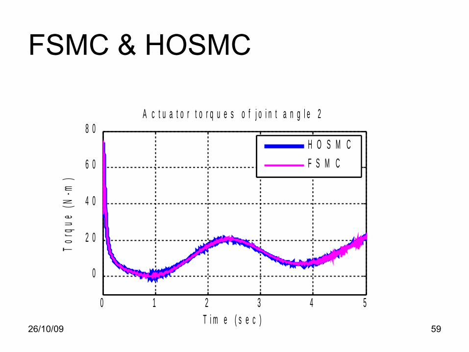
FSMC & HOSMC

0 1 2 3 4 5

0

2 0

4 0

6 0

8 0A c t u a t o r t o r q u e s o f j o i n t a n g l e 2

T i m e ( s e c )

Tor

que

(N-m

)

H O S M C

F S M C

26/10/09 60

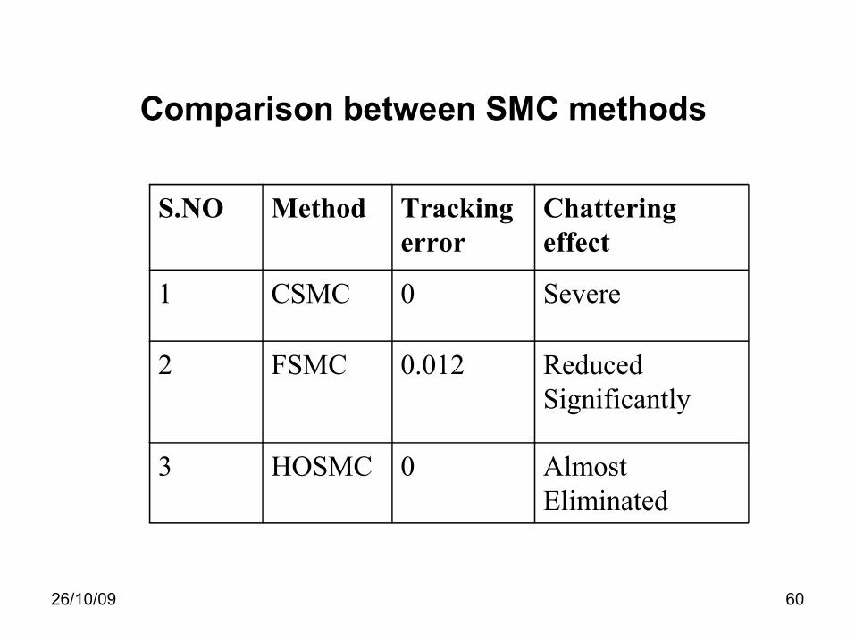
Comparison between SMC methods

S.NO Method Tracking error

Chattering effect

1 CSMC 0 Severe

2 FSMC 0.012 Reduced Significantly

3 HOSMC 0 Almost Eliminated

26/10/09 61

Summary Direct adaptive controller using NN/FLS for

companion form & strict feedback form nonlinear systems.

Controller structures are based on feedback linearization, backstepping and sliding mode based output feedback law.

The feedback control law which is a nonlinear function of system states is approximated using NN/FLS.

26/10/09 62

The tracking errors and weights of NN/FLS are uniformly ultimately bounded.

Efficacy of the proposed techniques is verified through simulation results.

Simulation results are verified on Induction motor & 2-link robot

26/10/09 63

Thank You