intelligent control of robots with mismatched dynamics...
TRANSCRIPT
Intelligent Control of Robots with Mismatched Dynamics and Mismatched Sensing
by
Wenjie Chen
A dissertation submitted in partial satisfaction of the
requirements for the degree of
Doctor of Philosophy
in
Engineering - Mechanical Engineering
in the
Graduate Division
of the
University of California, Berkeley
Committee in charge:
Professor Masayoshi Tomizuka, Chair
Professor J. Karl Hedrick
Professor Pieter Abbeel
Fall 2012

Intelligent Control of Robots with Mismatched Dynamics and Mismatched Sensing
Copyright 2012
by
Wenjie Chen
1
Abstract
Intelligent Control of Robots with Mismatched Dynamics and Mismatched Sensing
by
Wenjie Chen
Doctor of Philosophy in Engineering - Mechanical Engineering
University of California, Berkeley
Professor Masayoshi Tomizuka, Chair
Interest in industrial automation by robots has been continuously growing ever since the
first industrial robot was installed in 1961. This creates an increasing demand for robot per-
formance enhancement by means of intelligent control. Difficulties in meeting stringent per-
formance requirements, however, arise by some inherent characteristics of the robots, which
are: 1) mismatched dynamics (i.e., the control input and the system uncertainty/disturbance
are in different channels), and 2) mismatched sensing (i.e., the system lacks of direct sensing
of the desired output).
A typical example of mismatched systems is an industrial robot with joint elasticity, the
control objective of which is to obtain desired performances of the end-effector such as accu-
rate positioning and tracking. This kind of robot can be characterized as a two-mass system
with one mass being the motor side mass with control input and sensing and the other the load
side/end-effector mass without control input or sensing, respectively. In this dissertation, sev-
eral key technologies on intelligent control for this type of robot are introduced, including 1)
handling mismatched sensing by sensor fusion, 2) handling mismatched dynamics by real-time
control, and 3) handling mismatched dynamics by iterative learning control.
This dissertation develops several sensor fusion algorithms to estimate both the load side
and the end-effector states from limited sensing. The dynamic and kinematic models are
utilized with consideration to problems such as fictitious noises and computation requirement.
The well-developed sensor fusion schemes provide the essential desired information of the
system for control purposes. With the mismatched sensing problem solved by sensor fusion,
the control approaches to handle the mismatched dynamics are investigated in both the real-
time domain and the iteration domain. Considering the nature of the mismatched system as
a two-mass system, the real-time and iterative approaches are utilized in a hybrid two-stage
manner to deal with the mismatched dynamics. The developed algorithms for sensor fusion
and control provide not only the theoretical insights, but also the capability to address the
real-world problems especially in industrial automation. Experimental studies on a single-joint
research testbed and a commercial 6-DOF industrial robot manipulator have demonstrated the
superior performance of the proposed algorithms.

i
To my family
ii
Contents
Contents ii
List of Figures vii
List of Tables x
List of Common Symbols xi
1 Introduction 1
1.1 Background . . . . . . . . . . . . . . . . . . . . . . . . . . . . . . . . . . . . . . . . . . 1
1.2 Motivation and Contribution . . . . . . . . . . . . . . . . . . . . . . . . . . . . . . . . 2
1.2.1 Modeling Mismatched System . . . . . . . . . . . . . . . . . . . . . . . . . . 2
1.2.2 Handling Mismatched Sensing: Sensor Fusion Approaches . . . . . . . . . 3
1.2.3 Handling Mismatched Dynamics: Real-time Control Approaches . . . . . 4
1.2.4 Handling Mismatched Dynamics: Iterative Learning Control Approaches 5
1.3 Appearance of Research Contributions in Publications . . . . . . . . . . . . . . . . 6
1.4 Dissertation Outline . . . . . . . . . . . . . . . . . . . . . . . . . . . . . . . . . . . . . 7
2 Robots with Mismatched Dynamics and Mismatched Sensing 9
2.1 Introduction . . . . . . . . . . . . . . . . . . . . . . . . . . . . . . . . . . . . . . . . . . 9
2.2 Dynamic Modeling of Mismatched Robots . . . . . . . . . . . . . . . . . . . . . . . . 9
2.2.1 Mismatched System Model . . . . . . . . . . . . . . . . . . . . . . . . . . . . 9
2.2.2 Single-Joint Robot Model . . . . . . . . . . . . . . . . . . . . . . . . . . . . . 10
2.2.3 Multi-Joint Robot Model . . . . . . . . . . . . . . . . . . . . . . . . . . . . . . 17
2.3 Experimental Setup . . . . . . . . . . . . . . . . . . . . . . . . . . . . . . . . . . . . . . 21
2.3.1 Single-Joint Robot Experimental Setup . . . . . . . . . . . . . . . . . . . . . 21
2.3.2 Multi-Joint Robot Experimental Setup . . . . . . . . . . . . . . . . . . . . . . 23
2.4 Chapter Summary . . . . . . . . . . . . . . . . . . . . . . . . . . . . . . . . . . . . . . . 27
iii
I Handling Mismatched Sensing:Sensor Fusion Approaches 28
3 Load Side State Estimation in Single-Joint Robot 29
3.1 Introduction . . . . . . . . . . . . . . . . . . . . . . . . . . . . . . . . . . . . . . . . . . 29
3.2 Estimation Algorithms . . . . . . . . . . . . . . . . . . . . . . . . . . . . . . . . . . . . 30
3.2.1 Model for Measurement Dynamics . . . . . . . . . . . . . . . . . . . . . . . . 30
3.2.2 System Dynamic Model . . . . . . . . . . . . . . . . . . . . . . . . . . . . . . . 30
3.2.3 System Kinematic Model . . . . . . . . . . . . . . . . . . . . . . . . . . . . . . 31
3.2.4 Kalman Filtering . . . . . . . . . . . . . . . . . . . . . . . . . . . . . . . . . . . 33
3.2.5 Estimation of Noise Covariance . . . . . . . . . . . . . . . . . . . . . . . . . . 35
3.3 Experimental Study . . . . . . . . . . . . . . . . . . . . . . . . . . . . . . . . . . . . . . 36
3.3.1 Experimental Setup . . . . . . . . . . . . . . . . . . . . . . . . . . . . . . . . . 36
3.3.2 Load Side Estimation Experiments . . . . . . . . . . . . . . . . . . . . . . . . 37
3.4 Discussion . . . . . . . . . . . . . . . . . . . . . . . . . . . . . . . . . . . . . . . . . . . 43
3.5 Chapter Summary . . . . . . . . . . . . . . . . . . . . . . . . . . . . . . . . . . . . . . . 43
4 End-effector State Estimation in Multi-Joint Robot 45
4.1 Introduction . . . . . . . . . . . . . . . . . . . . . . . . . . . . . . . . . . . . . . . . . . 45
4.2 MD Kinematic Model . . . . . . . . . . . . . . . . . . . . . . . . . . . . . . . . . . . . . 46
4.2.1 MD Rigid Body Motion . . . . . . . . . . . . . . . . . . . . . . . . . . . . . . . 46
4.2.2 Sensor Measurement Dynamics . . . . . . . . . . . . . . . . . . . . . . . . . . 47
4.2.3 State-Space Model Representation . . . . . . . . . . . . . . . . . . . . . . . . 48
4.3 MD Kinematic Kalman Filter . . . . . . . . . . . . . . . . . . . . . . . . . . . . . . . . 49
4.3.1 Prediction by Inertia Sensor Measurement . . . . . . . . . . . . . . . . . . . 49
4.3.2 Propagation of Estimation Errors . . . . . . . . . . . . . . . . . . . . . . . . . 50
4.3.3 Correction by Vision Sensor Measurement . . . . . . . . . . . . . . . . . . . 51
4.4 Experimental Study . . . . . . . . . . . . . . . . . . . . . . . . . . . . . . . . . . . . . . 53
4.4.1 Sensor Fusion Using IMU & CompuGauge 3D . . . . . . . . . . . . . . . . . 53
4.4.2 Sensor Fusion Using IMU & PSD Camera . . . . . . . . . . . . . . . . . . . . 55
4.5 Chapter Summary . . . . . . . . . . . . . . . . . . . . . . . . . . . . . . . . . . . . . . . 60
5 Load Side Joint State Estimation in Multi-Joint Robot 62
5.1 Introduction . . . . . . . . . . . . . . . . . . . . . . . . . . . . . . . . . . . . . . . . . . 62
5.2 Robot Inverse Differential Kinematics . . . . . . . . . . . . . . . . . . . . . . . . . . . 63
5.2.1 Dynamic Model for Rough Estimates . . . . . . . . . . . . . . . . . . . . . . 63
5.2.2 Basic Differential Kinematics . . . . . . . . . . . . . . . . . . . . . . . . . . . 64
5.2.3 Optimization Based Inverse Differential Kinematics . . . . . . . . . . . . . 64
5.2.4 Final Optimization Solution . . . . . . . . . . . . . . . . . . . . . . . . . . . . 65
5.2.5 Practical Implementation Issues . . . . . . . . . . . . . . . . . . . . . . . . . 66
5.3 Kinematic Kalman Filter . . . . . . . . . . . . . . . . . . . . . . . . . . . . . . . . . . . 66
5.3.1 Decoupled Kinematic Kalman Filter . . . . . . . . . . . . . . . . . . . . . . . 66
iv
5.3.2 Parameter Estimation . . . . . . . . . . . . . . . . . . . . . . . . . . . . . . . . 68
5.4 Discussion of the Approach . . . . . . . . . . . . . . . . . . . . . . . . . . . . . . . . . 69
5.4.1 Computation Load . . . . . . . . . . . . . . . . . . . . . . . . . . . . . . . . . . 69
5.4.2 Extensions to Other Sensor Configurations . . . . . . . . . . . . . . . . . . . 70
5.5 Simulation & Experimental Study . . . . . . . . . . . . . . . . . . . . . . . . . . . . . 71
5.5.1 Test Setup . . . . . . . . . . . . . . . . . . . . . . . . . . . . . . . . . . . . . . . 71
5.5.2 Algorithm Settings . . . . . . . . . . . . . . . . . . . . . . . . . . . . . . . . . . 71
5.5.3 Simulation Results . . . . . . . . . . . . . . . . . . . . . . . . . . . . . . . . . . 72
5.5.4 Experimental Results . . . . . . . . . . . . . . . . . . . . . . . . . . . . . . . . 76
5.6 Chapter Summary . . . . . . . . . . . . . . . . . . . . . . . . . . . . . . . . . . . . . . . 79
II Handling Mismatched Dynamics:Real-time Control Approaches 80
6 Hybrid Adaptive Friction Compensation in Single-Joint Robot 81
6.1 Introduction . . . . . . . . . . . . . . . . . . . . . . . . . . . . . . . . . . . . . . . . . . 81
6.2 System Overview . . . . . . . . . . . . . . . . . . . . . . . . . . . . . . . . . . . . . . . 82
6.2.1 Single-Joint Indirect Drive Model . . . . . . . . . . . . . . . . . . . . . . . . 82
6.2.2 Modified Friction Model . . . . . . . . . . . . . . . . . . . . . . . . . . . . . . 82
6.2.3 Controller Structure . . . . . . . . . . . . . . . . . . . . . . . . . . . . . . . . . 84
6.3 Friction Compensation . . . . . . . . . . . . . . . . . . . . . . . . . . . . . . . . . . . . 85
6.3.1 Motor Side Friction Compensation . . . . . . . . . . . . . . . . . . . . . . . . 85
6.3.2 Load Side Friction Compensation . . . . . . . . . . . . . . . . . . . . . . . . 88
6.3.3 Hybrid Compensator Structure . . . . . . . . . . . . . . . . . . . . . . . . . . 89
6.4 Experimental Results . . . . . . . . . . . . . . . . . . . . . . . . . . . . . . . . . . . . . 89
6.4.1 Experimental Setup . . . . . . . . . . . . . . . . . . . . . . . . . . . . . . . . . 89
6.4.2 Motor Side Friction Compensation . . . . . . . . . . . . . . . . . . . . . . . . 90
6.4.3 Load Side Friction Compensation . . . . . . . . . . . . . . . . . . . . . . . . 93
6.5 Chapter Summary . . . . . . . . . . . . . . . . . . . . . . . . . . . . . . . . . . . . . . . 94
7 Motor Side Disturbance Rejection in Multi-Joint Robot 96
7.1 Introduction . . . . . . . . . . . . . . . . . . . . . . . . . . . . . . . . . . . . . . . . . . 96
7.2 Robot Model Study . . . . . . . . . . . . . . . . . . . . . . . . . . . . . . . . . . . . . . 97
7.2.1 Transfer Function Analysis . . . . . . . . . . . . . . . . . . . . . . . . . . . . . 97
7.2.2 Inertia Variation and Model Simplification . . . . . . . . . . . . . . . . . . . 98
7.3 Controller Design . . . . . . . . . . . . . . . . . . . . . . . . . . . . . . . . . . . . . . . 102
7.3.1 Baseline Controller Design . . . . . . . . . . . . . . . . . . . . . . . . . . . . . 102
7.3.2 Feedforward Controller Design . . . . . . . . . . . . . . . . . . . . . . . . . . 102
7.3.3 PID Controller Design . . . . . . . . . . . . . . . . . . . . . . . . . . . . . . . . 104
7.3.4 Disturbance Observer (DOB) Based Disturbance Rejection . . . . . . . . . 104
7.3.5 Adaptive Robust Controller (ARC) Based Disturbance Rejection . . . . . . 105

v
7.3.6 Transfer Function Analysis . . . . . . . . . . . . . . . . . . . . . . . . . . . . . 108
7.4 Experimental Study . . . . . . . . . . . . . . . . . . . . . . . . . . . . . . . . . . . . . . 111
7.4.1 Experimental Setup . . . . . . . . . . . . . . . . . . . . . . . . . . . . . . . . . 111
7.4.2 Experimental Results . . . . . . . . . . . . . . . . . . . . . . . . . . . . . . . . 111
7.5 Chapter Summary . . . . . . . . . . . . . . . . . . . . . . . . . . . . . . . . . . . . . . . 113
III Handling Mismatched Dynamics:Iterative Learning Control Approaches 118
8 Hybrid Two-Stage Model Based Iterative Learning Control Scheme for MIMO
Mismatched Linear Systems 119
8.1 Introduction . . . . . . . . . . . . . . . . . . . . . . . . . . . . . . . . . . . . . . . . . . 119
8.2 System Overview . . . . . . . . . . . . . . . . . . . . . . . . . . . . . . . . . . . . . . . 120
8.2.1 System Model . . . . . . . . . . . . . . . . . . . . . . . . . . . . . . . . . . . . 120
8.2.2 Basic Controller Structure . . . . . . . . . . . . . . . . . . . . . . . . . . . . . 121
8.3 Two-Stage ILC Scheme . . . . . . . . . . . . . . . . . . . . . . . . . . . . . . . . . . . . 122
8.3.1 ILC Basics . . . . . . . . . . . . . . . . . . . . . . . . . . . . . . . . . . . . . . . 122
8.3.2 ILC With Reference Update . . . . . . . . . . . . . . . . . . . . . . . . . . . . 123
8.3.3 ILC With Torque Update . . . . . . . . . . . . . . . . . . . . . . . . . . . . . . 125
8.3.4 Hybrid Scheme With Two-Stage ILC . . . . . . . . . . . . . . . . . . . . . . . 127
8.4 Experimental Study . . . . . . . . . . . . . . . . . . . . . . . . . . . . . . . . . . . . . . 128
8.4.1 Experimental Setup & Dynamic Model . . . . . . . . . . . . . . . . . . . . . 128
8.4.2 System Disturbance Characteristics . . . . . . . . . . . . . . . . . . . . . . . 128
8.4.3 Algorithm Setup . . . . . . . . . . . . . . . . . . . . . . . . . . . . . . . . . . . 129
8.4.4 Experimental Results . . . . . . . . . . . . . . . . . . . . . . . . . . . . . . . . 131
8.5 Chapter Summary . . . . . . . . . . . . . . . . . . . . . . . . . . . . . . . . . . . . . . . 133
9 Iterative Learning Control with Sensor Fusion: Application to Multi-Joint Robot 136
9.1 Introduction . . . . . . . . . . . . . . . . . . . . . . . . . . . . . . . . . . . . . . . . . . 136
9.2 System Overview . . . . . . . . . . . . . . . . . . . . . . . . . . . . . . . . . . . . . . . 137
9.2.1 Robot Dynamic Model . . . . . . . . . . . . . . . . . . . . . . . . . . . . . . . 137
9.2.2 Robot Controller Structure . . . . . . . . . . . . . . . . . . . . . . . . . . . . . 138
9.3 ILC Scheme with Sensor Fusion . . . . . . . . . . . . . . . . . . . . . . . . . . . . . . 139
9.3.1 Two ILC Stages . . . . . . . . . . . . . . . . . . . . . . . . . . . . . . . . . . . . 139
9.3.2 Hybrid Scheme For Two-Stage ILC . . . . . . . . . . . . . . . . . . . . . . . . 140
9.3.3 Robot Load Side State Estimation . . . . . . . . . . . . . . . . . . . . . . . . 141
9.4 Experimental Study . . . . . . . . . . . . . . . . . . . . . . . . . . . . . . . . . . . . . . 141
9.4.1 Test Setup . . . . . . . . . . . . . . . . . . . . . . . . . . . . . . . . . . . . . . . 141
9.4.2 Algorithm Setup . . . . . . . . . . . . . . . . . . . . . . . . . . . . . . . . . . . 141
9.4.3 Experimental Results . . . . . . . . . . . . . . . . . . . . . . . . . . . . . . . . 142
9.5 Chapter Summary . . . . . . . . . . . . . . . . . . . . . . . . . . . . . . . . . . . . . . . 144
vi
10 Concluding Remarks and Open Issues 145
10.1 Concluding Remarks . . . . . . . . . . . . . . . . . . . . . . . . . . . . . . . . . . . . . 145
10.2 Future Avenues of Research . . . . . . . . . . . . . . . . . . . . . . . . . . . . . . . . . 146
Bibliography 148
IV Appendix 156
A Robot System Setup 157
A.1 Robot Controller Hardware Configuration . . . . . . . . . . . . . . . . . . . . . . . . 157
A.2 Real-Time System . . . . . . . . . . . . . . . . . . . . . . . . . . . . . . . . . . . . . . . 158
A.3 Payload Design . . . . . . . . . . . . . . . . . . . . . . . . . . . . . . . . . . . . . . . . 159
A.4 Sensor Configurations . . . . . . . . . . . . . . . . . . . . . . . . . . . . . . . . . . . . 160
A.4.1 Accelerometer . . . . . . . . . . . . . . . . . . . . . . . . . . . . . . . . . . . . 160
A.4.2 Inertia Sensor Setup . . . . . . . . . . . . . . . . . . . . . . . . . . . . . . . . 161
A.4.3 PSD Camera . . . . . . . . . . . . . . . . . . . . . . . . . . . . . . . . . . . . . 163
A.4.4 CompuGauge 3D . . . . . . . . . . . . . . . . . . . . . . . . . . . . . . . . . . . 164
A.5 Robot Simulator & Experimentor . . . . . . . . . . . . . . . . . . . . . . . . . . . . . 164
A.5.1 Robot Simulator . . . . . . . . . . . . . . . . . . . . . . . . . . . . . . . . . . . 164
A.5.2 Robot Experimentor . . . . . . . . . . . . . . . . . . . . . . . . . . . . . . . . . 166
B System Identification 171
B.1 Linear Dynamics Identification of Multi-Joint Robot . . . . . . . . . . . . . . . . . . 171
B.1.1 Posture Selection . . . . . . . . . . . . . . . . . . . . . . . . . . . . . . . . . . 171
B.1.2 Identification Procedure . . . . . . . . . . . . . . . . . . . . . . . . . . . . . . 173
B.1.3 Closed Loop Identification . . . . . . . . . . . . . . . . . . . . . . . . . . . . . 175
B.2 Friction Identification . . . . . . . . . . . . . . . . . . . . . . . . . . . . . . . . . . . . 175
B.2.1 Friction Identification for Multi-Joint Robot . . . . . . . . . . . . . . . . . . 175
B.2.2 Friction Identification for Single-Joint Setup . . . . . . . . . . . . . . . . . . 181
C Covariance Estimation 182
C.1 Covariance Estimation in Chapter 3 . . . . . . . . . . . . . . . . . . . . . . . . . . . . 182
C.2 Parameter Estimation in Chapter 5 . . . . . . . . . . . . . . . . . . . . . . . . . . . . 184
C.2.1 Maximizing Expected Likelihood . . . . . . . . . . . . . . . . . . . . . . . . . 184
C.2.2 Off-line Solution: EM Algorithm . . . . . . . . . . . . . . . . . . . . . . . . . 186
C.2.3 Online Solution . . . . . . . . . . . . . . . . . . . . . . . . . . . . . . . . . . . 186

vii
List of Figures
1.1 The Structure Overview of the Dissertation . . . . . . . . . . . . . . . . . . . . . . . . . 8
2.1 Single-Joint Indirect-Drive Mechanism . . . . . . . . . . . . . . . . . . . . . . . . . . . . 11
2.2 Definition of the Transmission Error . . . . . . . . . . . . . . . . . . . . . . . . . . . . . . 17
2.3 Single-Joint Indirect Drive System Setup . . . . . . . . . . . . . . . . . . . . . . . . . . . 21
2.4 Accelerometer Installation . . . . . . . . . . . . . . . . . . . . . . . . . . . . . . . . . . . . 22
2.5 FANUC M-16iB Robot System . . . . . . . . . . . . . . . . . . . . . . . . . . . . . . . . . . 24
2.6 FANUC M-16iB Robot System Setup Scheme . . . . . . . . . . . . . . . . . . . . . . . . 25
2.7 Reference Configuration for FANUC M-16iB Robot . . . . . . . . . . . . . . . . . . . . . 25
2.8 Angle Conventions (left) and Attached Frames (right) . . . . . . . . . . . . . . . . . . 26
2.9 Home Position for FANUC M-16iB Robot . . . . . . . . . . . . . . . . . . . . . . . . . . . 26
3.1 Bode Plot ofθℓ(s)
λ0θm(s)for the System Setup in Fig. 2.3 . . . . . . . . . . . . . . . . . . . . 32
3.2 Structure of Dynamic Model Based Kalman Filter (DKF) . . . . . . . . . . . . . . . . . 34
3.3 Structure of Kinematic Model Based Kalman Filter (KKF) . . . . . . . . . . . . . . . . . 35
3.4 Chirp Input Signal Frequency . . . . . . . . . . . . . . . . . . . . . . . . . . . . . . . . . . 38
3.5 Estimation Errors of Load Side Position in Chirp Experiment (Without Covariance
Adaptation or Parametric Uncertainty) . . . . . . . . . . . . . . . . . . . . . . . . . . . . 38
3.6 Estimation Errors of Load Side Position in Chirp Experiment (With Covariance
Adaptation and Parametric Uncertainty) . . . . . . . . . . . . . . . . . . . . . . . . . . . 39
3.7 Covariance Estimation in Chirp Experiment . . . . . . . . . . . . . . . . . . . . . . . . . 40
3.8 Bias Estimation in Chirp Experiment . . . . . . . . . . . . . . . . . . . . . . . . . . . . . 41
3.9 Load Side Desired Trajectory . . . . . . . . . . . . . . . . . . . . . . . . . . . . . . . . . . 41
3.10 Estimation Errors of Load Side Position in Trajectory Experiment . . . . . . . . . . . . 42
3.11 Load Side Actual and Estimated Position Tracking Error . . . . . . . . . . . . . . . . . 42
4.1 Sensor Configuration and Coordinate System of FANUC M-16iB Robot End-effector 47
4.2 Basic Structure of MD-KKF Scheme . . . . . . . . . . . . . . . . . . . . . . . . . . . . . . 49
4.3 TCP Estimation for P2P Scanning Trajectory (with IMU & CompuGauge) . . . . . . . 54
4.4 Measurement Comparison Between PSD Camera and CompuGauge . . . . . . . . . . 56
4.5 TCP Estimation for Square Trajectory without Orientation Change . . . . . . . . . . . 57
4.6 TCP Estimation for Circle Trajectory without Orientation Change . . . . . . . . . . . . 58
viii
4.7 End-effector Path with Orientation Change . . . . . . . . . . . . . . . . . . . . . . . . . 59
4.8 Locations of Two PSD Markers and the TCP . . . . . . . . . . . . . . . . . . . . . . . . . 59
4.9 TCP Estimation for Curve Path with Orientation Change . . . . . . . . . . . . . . . . . 61
5.1 Adaptive Kinematic Kalman Filter Process . . . . . . . . . . . . . . . . . . . . . . . . . . 68
5.2 The Structure of Load Side State Estimation Approach . . . . . . . . . . . . . . . . . . 70
5.3 Y-Z Plane TCP Position Estimation (Experiment) . . . . . . . . . . . . . . . . . . . . . . 72
5.4 Load Side Joint Position Estimation Absolute Error (Simulation) . . . . . . . . . . . . 73
5.5 Load Side Joint Velocity Estimation Absolute Error (Simulation) . . . . . . . . . . . . 74
5.6 Load Side Joint Acceleration Estimation Absolute Error (Simulation) . . . . . . . . . 75
5.7 TCP Estimation on Y & Z Axes When Coming to a Stop (Experiment) . . . . . . . . . 77
5.8 TCP Estimation Error When Coming to a Stop (Experiment) . . . . . . . . . . . . . . . 78
6.1 Block Diagram of the Overall Control System . . . . . . . . . . . . . . . . . . . . . . . . 84
6.2 Hybrid Compensator Structure . . . . . . . . . . . . . . . . . . . . . . . . . . . . . . . . . 90
6.3 Desired Load Side Trajectory . . . . . . . . . . . . . . . . . . . . . . . . . . . . . . . . . . 91
6.4 Performance of the Motor Side Compensators . . . . . . . . . . . . . . . . . . . . . . . . 91
6.5 Friction Estimates by FB-A Observer . . . . . . . . . . . . . . . . . . . . . . . . . . . . . . 92
6.6 Friction Parameter Estimations (SI Units) . . . . . . . . . . . . . . . . . . . . . . . . . . 93
6.7 Performance of the Hybrid Compensator . . . . . . . . . . . . . . . . . . . . . . . . . . . 94
6.8 Load Side Friction Estimates . . . . . . . . . . . . . . . . . . . . . . . . . . . . . . . . . . 95
7.1 Frequency Responses of s2P i
∆ℓdℓand s2P i
ℓdfor Each Robot Joint . . . . . . . . . . . . . 99
7.2 Variations of Mn2 of the FANUC M-16iB Robot in the Work Space . . . . . . . . . . . . 100
7.3 Frequency Responses of Joint Models of the FANUC M-16iB Robot (Solid Color
Lines: Indirect Drive Model sP imu
; Black Marker Line: Simplified Model sP imusim
) . . . 101
7.4 Controller Structure of the Multi-Joint Robot . . . . . . . . . . . . . . . . . . . . . . . . 102
7.5 PID Controller Structure of the Multi-Joint Robot . . . . . . . . . . . . . . . . . . . . . 104
7.6 DOB Controller Structure of the Multi-Joint Robot . . . . . . . . . . . . . . . . . . . . . 105
7.7 ARC Controller Structure of the Multi-Joint Robot . . . . . . . . . . . . . . . . . . . . . 108
7.8 TCP Cartesian Space Trajectory Reference . . . . . . . . . . . . . . . . . . . . . . . . . . 112
7.9 TCP Cartesian Space Position Tracking Performance . . . . . . . . . . . . . . . . . . . . 114
7.10 Motor Side Position Tracking Error (in Load Side Scale) . . . . . . . . . . . . . . . . . 115
7.11 Motor Position Error Spectrum . . . . . . . . . . . . . . . . . . . . . . . . . . . . . . . . . 116
7.12 Torque Profile Comparison . . . . . . . . . . . . . . . . . . . . . . . . . . . . . . . . . . . 117
8.1 Control Structure with Reference & Torque Update . . . . . . . . . . . . . . . . . . . . 121
8.2 Load Side Disturbance Setup for Single-Joint System . . . . . . . . . . . . . . . . . . . 129
8.3 Load Side Desired Trajectory . . . . . . . . . . . . . . . . . . . . . . . . . . . . . . . . . . 130
8.4 Disturbance Effects on Load Side Position Tracking Error . . . . . . . . . . . . . . . . . 130
8.5 Frequency Responses of βr and βu with ±50% Parametric Uncertainties . . . . . . . 131
8.6 Performance Comparisons using Accurate Nominal Model (After 10 Iterations) . . . 132

ix
8.7 Error Convergence Comparisons using Nominal Model with 15% Parametric Un-
certainties (10 Iterations) . . . . . . . . . . . . . . . . . . . . . . . . . . . . . . . . . . . . 134
8.8 Performance Comparisons using Nominal Model with 15% Parametric Uncertain-
ties (After 10 Iterations) . . . . . . . . . . . . . . . . . . . . . . . . . . . . . . . . . . . . . 135
9.1 Robot Control Structure with Reference & Torque Update . . . . . . . . . . . . . . . . 138
9.2 TCP Position RMS Error Comparisons in Iteration Domain . . . . . . . . . . . . . . . . 142
9.3 IMU Acceleration RMS Error Comparisons in Iteration Domain . . . . . . . . . . . . . 143
9.4 TCP Position Error Comparisons in Time Domain . . . . . . . . . . . . . . . . . . . . . . 143
9.5 IMU Acceleration Error Comparisons in Time Domain . . . . . . . . . . . . . . . . . . . 144
A.1 FANUC M-16iB Robot System Setup Scheme . . . . . . . . . . . . . . . . . . . . . . . . 158
A.2 Payload Mounted on Joint 6 . . . . . . . . . . . . . . . . . . . . . . . . . . . . . . . . . . . 159
A.3 Payload Surface Straightness . . . . . . . . . . . . . . . . . . . . . . . . . . . . . . . . . . 160
A.4 Inertia Sensor Setup Configuration . . . . . . . . . . . . . . . . . . . . . . . . . . . . . . 162
A.5 Structure of the PSD Camera Prototype . . . . . . . . . . . . . . . . . . . . . . . . . . . . 163
A.6 Precision Levels for Measurement Planes at Different Distances . . . . . . . . . . . . . 163
A.7 M-16iB Robot Simulator & Experimentor . . . . . . . . . . . . . . . . . . . . . . . . . . 165
A.8 Testing Position Trajectory Comparison between Simulation and Experiment (Load
Side Scale) . . . . . . . . . . . . . . . . . . . . . . . . . . . . . . . . . . . . . . . . . . . . . 167
A.9 Motor Torque Comparison between Simulation and Experiment . . . . . . . . . . . . 168
A.10 Virtual Reality in Simulator vs. Actual Experiment (FANUC M-16iB) . . . . . . . . . . 169
A.11 Virtual Reality in Simulator vs. Actual Experiment (Single-Joint Setup) . . . . . . . . 170
B.1 FANUC M-16iB Robot Postures for System Identification . . . . . . . . . . . . . . . . . 172
B.2 System Identification Flow Chart for FANUC M-16iB Robot . . . . . . . . . . . . . . . 174
B.3 Static Friction Identification Result for FANUC M-16iB Robot with Payload . . . . . . 178
B.4 Static Friction Identification Result for FANUC M-16iB Robot without Payload . . . . 179
B.5 Static Friction Identification Result for Single-Joint Testbed . . . . . . . . . . . . . . . 181

x
List of Tables
2.1 Identified Parameters for the Single-Joint Robot . . . . . . . . . . . . . . . . . . . . . . 22
2.2 DH Parameters for FANUC M-16iB Robot . . . . . . . . . . . . . . . . . . . . . . . . . . . 26
3.1 The Noise Variance Used in Chirp Experiment (SI Units) . . . . . . . . . . . . . . . . . 37
4.1 Identified Variances for the IMU Measurements for Sensor Fusion Using IMU &
CompuGauge 3D . . . . . . . . . . . . . . . . . . . . . . . . . . . . . . . . . . . . . . . . . 53
4.2 Identified Variances for the IMU and PSD Camera Measurements for Sensor Fusion
using IMU & PSD Camera . . . . . . . . . . . . . . . . . . . . . . . . . . . . . . . . . . . . 56
5.1 TCP Estimation Errors When Coming to a Stop (Experiment) . . . . . . . . . . . . . . 79
6.1 Improvements Compared to the No-Comp. Case . . . . . . . . . . . . . . . . . . . . . . 92
7.1 The Comparison Between DOB and ARC . . . . . . . . . . . . . . . . . . . . . . . . . . . 111
A.1 Specification of the Payload . . . . . . . . . . . . . . . . . . . . . . . . . . . . . . . . . . . 160
A.2 Covariance of the Inertia Sensor Signals (in IMU Coordinates) . . . . . . . . . . . . . 162
B.1 Identified Friction Parameters for FANUC M-16iB Robot (SI Units) . . . . . . . . . . . 180
B.2 Identified Friction Parameters for Single-Joint Testbed (SI Units) . . . . . . . . . . . . 181

xi
List of Common Symbols
N Reduction ratio of the gear reducer (single-joint/multi-joint robot)
Pℓd Transfer function from the disturbance d to the load side position θℓ (or qℓ for multi-
joint robot)
Pℓu Transfer function from the torque u (or τm for multi-joint robot) to the load side
position θℓ (or qℓ for multi-joint robot)
Pmd Transfer function from the disturbance d to the motor side position θm (or qm for
multi-joint robot)
Pmu Transfer function from the torque u (or τm for multi-joint robot) to the motor side
position θm (or qm for multi-joint robot)
d Lumped (fictitious) disturbance (single-joint/multi-joint robot)
dℓ Load side lumped (fictitious) disturbance (single-joint/multi-joint robot)
dm Motor side lumped (fictitious) disturbance (single-joint/multi-joint robot)
θℓ Load side position (single-joint robot)
θℓd Load side desired position reference (single-joint robot)
θm Motor side position (single-joint robot)
θmd Motor side desired position reference (single-joint robot)
θ Reducer transmission error (single-joint robot)
Jℓ Load side inertia (single-joint robot)
Jm Motor side inertia (single-joint robot)
d f ℓ Load side external disturbance (single-joint robot)
d f m Motor side external disturbance (single-joint robot)
d j Joint reducer damping (single-joint robot)
dℓ Load side damping (single-joint robot)
dm Motor side damping (single-joint robot)
fh Friction in the gear reducer (single-joint robot)
fℓ Load side friction (including Coulomb friction and viscous damping) (single-joint
robot)

xii
fℓc Load side Coulomb friction (single-joint robot)
fm Motor side friction (including Coulomb friction and viscous damping) (single-joint
robot)
fmc Motor side Coulomb friction (single-joint robot)
k j Joint reducer stiffness (single-joint robot)
u Motor side torque (single-joint robot)
q State vector for multi-joint robot model
qℓ Load side position (multi-joint robot)
qℓd Load side desired position reference (multi-joint robot)
qm Motor side position (multi-joint robot)
qmd Motor side desired position reference (multi-joint robot)
q Reducer transmission error (multi-joint robot)
C(qℓ, qℓ) Coriolis and centrifugal force matrix (multi-joint robot)
G(qℓ) Gravity torque vector (multi-joint robot)
J(qℓ) Jacobian matrix mapping from the load side joint space to the end-effector Cartesian
space (multi-joint robot)
J(qℓ, qℓ) Time derivative of the Jacobian matrix J(qℓ) (multi-joint robot)
Mℓ(qℓ) Load side inertia matrix (multi-joint robot)
Mm Motor side inertia matrix (multi-joint robot)
τm Motor side torque vector (multi-joint robot)
D j Joint reducer damping matrix (multi-joint robot)
Dℓ Load side damping matrix (multi-joint robot)
Dm Motor side damping matrix (multi-joint robot)
fex t End-effector external contact force/torque vector (multi-joint robot)
Fℓc Load side Coulomb friction matrix (multi-joint robot)
Fmc Motor side Coulomb friction matrix (multi-joint robot)
K j Joint reducer stiffness matrix (multi-joint robot)
In An n× n identity matrix

xiii
Acknowledgments
My five years in Berkeley have been the greatest part in my life so far. I know that I could not
have reached to this stage without the precious help and support from many people. I hope
to recognize the wonderful moments with all these people as much as possible even though I
realize that it is not an easy job within this limited space.
First of all, I want to express my earnest gratitude and sincere respect to my research
advisor Professor Masayoshi Tomizuka. Professor Tomizuka has been a remarkably amazing
mentor not only in academic research but also in life experience throughout my Ph.D. student
career. The persistent encouragement, the profound knowledge, and the valuable suggestions
that he has provided to me have greatly shaped my Ph.D. study and beyond. His huge enthu-
siasm on the work, insightful vision for the student, and also enormous courage to face the
reality have set up a great example for me to follow. I would also like to thank Mrs. Miwako
Tomizuka for her kindness and care to my life.
I am also very grateful to Professor J. Karl Hedrick and Professor Pieter Abbeel for their
willingness to serve as my dissertation committee. Their kind support has motivated me to
further improve the quality of this dissertation.
I am also thankful to my undergraduate’s advisors, Professor Bin Yao, Professor Qingfeng
Wang, and Professor Linyi Gu, for their valuable guidance and precious opportunities that led
me to this academic area.
Special thanks go to FANUC Ltd, the sponsor for the work in this dissertation. I would
like to thank Dr. Seiuemon Inaba and Dr. Yoshiharu Inaba sincerely for their continuing
interest in this research and their encouragement. I also appreciate the valuable technical
discussions/communications with Dr. Kiyonori Inaba and Dr. Shinsuke Sakakibara that have
helped to enhance this dissertation with industrial perspective. I also appreciate Chiang Chen
Overseas Graduate Fellowship for its generous support during my first year Ph.D. study.
I have also greatly benefited from being a member of the Mechanical Systems Control
(MSC) Laboratory. I am very fortunate to interact with all the MSC talents in the last five
years. Special thanks go to Evan Chang-Siu (also Kaori Noguchi and cutie baby Kenta Siu). I
will not forget all those wonderful moments we shared together in study, research, and life.
They have truly helped me to adapt and shape my multi-cultural perspectives of the life. Also
I am greatly thankful to Kyoungchul Kong, who is like my big brother and has provided so
many precious experiences and suggestions to my research and life. I really appreciate his
encouragement and support for the great time and also difficult time I have gone through. I
hope we can both succeed in our dreams.
I would also like to thank Sumio Sugita who always knows how to make practical things
to work and helped me patiently with his expertise. I also appreciate the inspiring technical
discussions/collaborations on the FANUC project with Cheng-Huei (Nora) Han, Kiyonori In-
aba, Haifei Cheng, Chun-Chih Wang, Soo Jeon, Pedro Mora-Reynoso, Mike Chan, Cong Wang,
and Chung-Yen Lin. The collaborations with Jonathan Asensio on the neural network learning
and with Miguel Lagullon Garcia on the 3D animation were also enjoyable. I will not forget
the collaborations with Chi-Shen Tsai and Dae-Kyu Yun on the Hyundai project. The ongoing

xiv
collaborations with Joonbum Bae and Junkai Lu on the BMI project have also been delightful.
I would also like to thank all the other current and past colleagues at the MSC Lab: Shuwen
(Emma) Yu, Nancy Feng Dan Dong, Hoday Stearns, Qixing Zheng, Xuan Fan, Guoyuan Wu,
Sandipan Mishra, Takashi Nagata, Sanggyum Kim, Xu Chen, Yizhou Wang, Wenlong Zhang,
Kanjanapas (Oak) Kan, Raechel Tan, Pey Yuen Tao, Benjamin Fine, Yasuyuki Matzuda, Kiy-
otaka Kawashima, Atsushi Oshima, Atsuki Naka, Ahmed Hamdy El-shaer, Minghui Zheng,
Chen-Yu Chan, Omar Abdul-hadi, Robert Matthew, Hiroshi Niki, Ric Jacobs, and all others.
Also, I cannot forget all the other friends in Berkeley. Especially, I am thankful to Heng
Pan, Weiya Fang, Liang Pan, Ran Liu, Yudong Ma, and Zhichao Song for their warm-hearted
friendship. I will also always remember all the friends back in China, both from my hometown
and from my undergraduate college, with whom I always had a great time whenever I was
visiting.
Last and foremost, I would like to express my deepest love to my parents, Naihui Chen
and Ailing Chen, and my sister, Wenting Chen, for their unconditioned love, support, and
encouragement throughout my whole life. I am, and will also be greatly indebted to my
fiancee, Su Chen, for her enormous love, understanding, and dedication. You all are the
reasons of my life that have made me achieve so far, and I love you all.
1
Chapter 1
Introduction
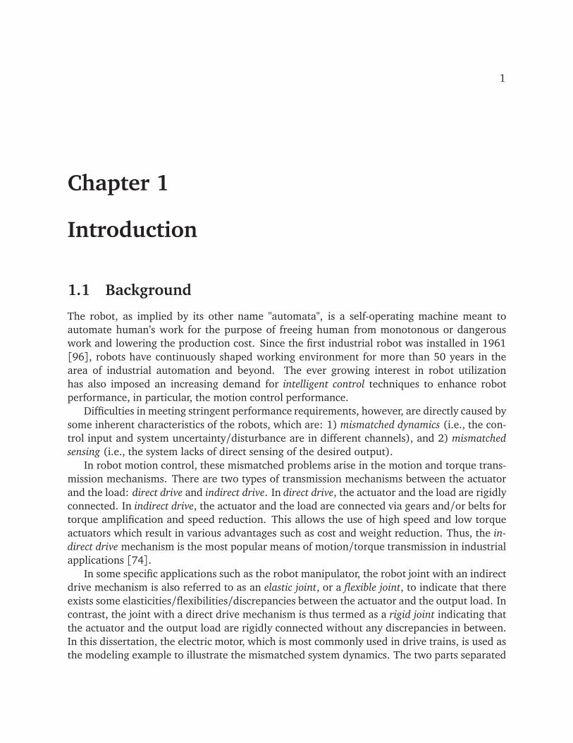
1.1 Background
The robot, as implied by its other name "automata", is a self-operating machine meant to
automate human’s work for the purpose of freeing human from monotonous or dangerous
work and lowering the production cost. Since the first industrial robot was installed in 1961
[96], robots have continuously shaped working environment for more than 50 years in the
area of industrial automation and beyond. The ever growing interest in robot utilization
has also imposed an increasing demand for intelligent control techniques to enhance robot
performance, in particular, the motion control performance.
Difficulties in meeting stringent performance requirements, however, are directly caused by
some inherent characteristics of the robots, which are: 1) mismatched dynamics (i.e., the con-
trol input and system uncertainty/disturbance are in different channels), and 2) mismatched
sensing (i.e., the system lacks of direct sensing of the desired output).
In robot motion control, these mismatched problems arise in the motion and torque trans-
mission mechanisms. There are two types of transmission mechanisms between the actuator
and the load: direct drive and indirect drive. In direct drive, the actuator and the load are rigidly
connected. In indirect drive, the actuator and the load are connected via gears and/or belts for
torque amplification and speed reduction. This allows the use of high speed and low torque
actuators which result in various advantages such as cost and weight reduction. Thus, the in-
direct drive mechanism is the most popular means of motion/torque transmission in industrial
applications [74].
In some specific applications such as the robot manipulator, the robot joint with an indirect
drive mechanism is also referred to as an elastic joint, or a flexible joint, to indicate that there
exists some elasticities/flexibilities/discrepancies between the actuator and the output load. In
contrast, the joint with a direct drive mechanism is thus termed as a rigid joint indicating that
the actuator and the output load are rigidly connected without any discrepancies in between.
In this dissertation, the electric motor, which is most commonly used in drive trains, is used as
the modeling example to illustrate the mismatched system dynamics. The two parts separated

CHAPTER 1. INTRODUCTION 2
by the indirect drive mechanism are termed as the motor side and the load side, respectively,
with the working tool (i.e., end-effector) rigidly attached to the last joint of the robot.
Therefore, in industrial robot applications, the ultimate objective is to achieve the desired
performance at the end-effector. For simplicity and efficiency in industrial control, this is
normally done by decentralized joint space control to achieve equivalent desired performance
on the load side [58, 74]. Load side sensing at the joints, however, is usually not available
due to cost and assembly issues. This leads to the mismatched sensing problem. On the
other hand, the control input is supplied only at the motor side where the actuator is located,
while the uncertainties and/or disturbances normally appear from the load side/end-effector.
Thus, the desired end-effector performance cannot be guaranteed with only good motor side
performance [19, 91]. This results in the mismatched dynamics problem.
The fundamental problem associated with these mismatches is that the desired variable
cannot be directly sensed or controlled. This sets severe challenges in meeting stringent per-
formance requirements. To solve this problem in a cost-effective and timely manner, a mecha-
tronic approach, which gives considerations to both mechanical hardware and servo software,
should be pursued [81]. Therefore, in this dissertation, the mismatched problems are properly
tackled from the perspectives of both estimation and control, with contributions to hardware
(sensor) configuration, dynamic modeling, algorithm developments, and real-world experi-
mentation.
1.2 Motivation and Contribution
1.2.1 Modeling Mismatched System
Mismatched systems take various forms in the physical realization. The actuator may be an
electric motor, a pneumatic actuator, a hydraulic piston, and so on. The transmission mech-
anism can be realized as various kinds of gear boxes, belt-pulley sets, and so on. In terms of
motion and torque transmissions, however, they all share the same characteristic, and hence
the indirect drive train/elastic joint is usually modeled as a system of two masses connected by
spring (and damper) [92, 97, 72].
Based on this unifying model, the dynamics of robots with mismatched dynamics and mis-
matched sensing is studied in Chapter 2. Different model representations such as equations of
motion, state space model, and transfer function model are formulated. The nonlinear dynam-
ics such as friction effects, transmission error, and external disturbances are also considered.
This unified model formulation provides the foundation for the synthesis of model based sen-
sor fusion and control algorithms. In addition, a novel approach is proposed to decouple
the highly nonlinear coupling dynamics for multi-joint robots. The decoupled linear form is
essential for decentralized estimation and control using linear system theory/techniques.
In addition to the theoretical work for dynamic modeling, an original multi-functional
Robot Simulator/Experimentor with high fidelity physical modeling is also developed. This
creates a practical and safe environment for both simulation and experimentation. To obtain

CHAPTER 1. INTRODUCTION 3
the high fidelity model, extensive system identification has been conducted for both a single-
joint research testbed and a commercial 6 degrees-of-freedom (DOF) industrial robot. The
results of system identification are also essential for the success of the sensor fusion and control
study in this dissertation.
1.2.2 Handling Mismatched Sensing: Sensor Fusion Approaches
As discussed above, precise load side measurements at the joints are usually not available due
to cost and assembly issues. Motor side encoders, in most cases, have been the only sensors
used for feedback control. Due to the joint flexibilities from gear mechanisms, kinematic
errors of the links, and so on, the information from motor side encoders does not precisely
characterize the load side/end-effector performance, which is of ultimate interest.
To tackle this mismatched sensing problem, several novel sensor fusion approaches are
developed to provide the desired estimates for the information of interest. More specifically,
the sensor fusion schemes are investigated in the following three major cases:
Load Side State Estimation in Single-Joint Robot
In Chapter 3, as an initial effort to tackle the complex mismatched sensing problem, the load
side state estimation for the single-joint indirect drive robot is investigated. To obtain the de-
sired sensing in a cost-effective manner, economic MEMS inertia sensors (e.g, gyroscopes and
accelerometers) instead of expensive encoders1, are utilized on the load side. Measurement
dynamics is incorporated into the model to deal with the sensor noises and biases. Kalman
filtering method is designed based on the extended dynamic/kinematic model for the fusion
of multiple sensor signals. The covariance adaptation for fictitious noises is also studied using
the maximum likelihood principle. The effectiveness of the proposed scheme is experimentally
demonstrated on a single-joint research testbed.
End-effector State Estimation in Multi-Joint Robot
The extension of the sensor fusion scheme from the single-joint case to the multi-joint case
is considerably challenging, due to the highly nonlinear dynamics/kinematics induced by the
multi-joint configuration. In Chapter 4, instead of the load side sensing on each joint, the in-
expensive MEMS inertia measurement unit (IMU) is adopted only on the end-effector, which
is more realistic for industrial applications. Also, in industrial operational space control tasks,
vision systems are commonly utilized. To mimic industrial vision system, a three-dimensional
position measurement system, CompuGauge 3D, is utilized to provide down-sampled mea-
surements for the tool center point (TCP) position. As a vision system alternative, an optical
sensor (PSD camera) based on a position sensitive detector (PSD) is developed2 to measure
1A representative cost comparison between the encoders and the MEMS inertia sensors can be found in [70].2The complete details of PSD camera development can be found in [94]. Some key features/specifications of
the setup are listed in Appendix A.4.3.
CHAPTER 1. INTRODUCTION 4
the end-effector position directly. The developed PSD camera features high precision and fast
response speed for position sensing at a low cost. The velocity and orientation information
inferred indirectly from the mimicked vision system/PSD camera measurements, however, is
still not satisfactory.
To better estimate the TCP position, velocity, and orientation in Cartesian space, the single-
joint sensor fusion scheme is extended to the multi-dimensional kinematic Kalman filter (MD-
KKF) for the multi-joint robot. The end-effector kinematic model is formulated based on multi-
dimensional rigid body motion and sensor measurement dynamics. The MD-KKF approach
proposed in [53] is revisited and extended in Chapter 4 with a newly phrased multi-rate
processing procedure and extensive experimental validation. Experimentation on a 6-DOF
industrial robot demonstrates the superior performance of the proposed method, especially for
the TCP velocity/orientation estimation. Two sensor configurations (i.e., IMU plus mimicked
vision camera by CompuGauge 3D, and IMU plus PSD camera) are experimentally tested.
Load Side Joint State Estimation in Multi-Joint Robot
End-effector state estimation of the multi-joint robot is not sufficient for industrial robot con-
trol, especially when decentralized joint space control is preferred. Hence, it is desired to di-
rectly estimate the load side joint states with limited available sensing. The resulting method
should be cost-effective and computationally light for industrial applications.
In Chapter 5, an innovative load side state estimation scheme is developed for the multi-
joint robot with joint elasticity. The low-cost sensor configuration is emphasized, i.e., motor
encoders and an economic end-effector MEMS sensor such as a 3-axial accelerometer. An
optimization based inverse differential kinematics algorithm is designed to obtain the load
side joint acceleration estimate. The joint position/velocity estimation problem is then con-
veniently decoupled into a simple second order kinematic Kalman filter (KKF) for each joint.
Maximum likelihood principle is utilized to adapt the covariances for the fictitious noises in
KKF. Both off-line and online solutions are derived. The light computation load of the scheme
is discussed. The scheme is also extended to other sensor configurations to show its wide ap-
plication potential. The effectiveness of the developed method is demonstrated through both
simulation and experimental study on a commercial 6-DOF industrial robot.
1.2.3 Handling Mismatched Dynamics: Real-time Control Approaches
The above sensor fusion schemes conveniently provide desired information for further actions
on the mismatched dynamics issue. The mismatched dynamics problem arises naturally in
robots with joint elasticity, where the control input and the uncertainties/disturbances are
unfortunately separated by the indirect drive mechanism. Thus, direct compensation for the
mismatched uncertainties/disturbances is extremely challenging. This dissertation develops
the following real-time feedback control approaches to handle this problem for the single-
joint robot as well as the multi-joint robot.
CHAPTER 1. INTRODUCTION 5
Hybrid Adaptive Friction Compensation in Single-Joint Robot
In Chapter 6, friction, one of the main mismatched disturbance factors that diminish control
performance, is investigated and compensated. The friction effects are properly compensated
by manipulating both the reference trajectory and the torque input. In the motor side torque
compensation, a novel adaptive friction observer is designed based on the modified LuGre
model to estimate the entire friction force reflected to the motor side. It is theoretically proved
that with additional assumptions, the designed motor side control law with adaptive observer
achieves perfect motor side tracking performance. To further improve the load side perfor-
mance, the motor side reference is modified by injecting the adaptive estimate of the load side
friction. A hybrid controller structure is developed to properly engage or disengage the load
side compensator based on the motor side performance. The effectiveness of the proposed
scheme is validated through experimentation on a single-joint research testbed.
Motor Side Disturbance Rejection in Multi-Joint Robot
Similar to sensor fusion, the extension of friction compensation from the single-joint case
to the multi-joint case is nontrivial due to the complex nonlinear coupling dynamics. Since
friction effects are usually highly coupled with other forms of disturbances, it makes more
sense to address the problem of estimating and rejecting disturbances rather than friction
compensation only.
As a first step for this study, Chapter 7 presents a decentralized motor side controller for
the multi-joint robot with joint elasticity. The transfer function analysis of the decoupled
model shows that, under ideal conditions in the low frequency range, the perfect disturbance
rejection on the motor side also results in the effective disturbance rejection on the load side.
Thus, the aim for this study becomes to improve the load side/end-effector performance by
rejecting the low frequency disturbance effects from the motor side. With that idea in mind,
motor side disturbance rejection is achieved by making the inner plant of the robot behave as
the simplified nominal model. A disturbance observer (DOB) and an adaptive robust controller
(ARC) are designed separately to accomplish this objective. A comparative study between the
DOB and ARC approaches is conducted through both the closed loop dynamics analysis and the
experimentation on a 6-DOF industrial robot. This study shows the significant contributions
that the two schemes bring to the control system. To further enhance high frequency load side
performance, direct load side disturbance rejection becomes necessary, which is a pending
future work.
1.2.4 Handling Mismatched Dynamics: Iterative Learning Control
Approaches
In industrial applications, robots are often repeatedly performing a single task under the same
operating conditions. Thus, in addition to the real-time approaches, it would be most bene-
CHAPTER 1. INTRODUCTION 6
ficial to further utilize this repeatable feature for better handling the mismatched dynamics.
This leads to the following iterative learning control (ILC) approach.
Hybrid Two-Stage Model Based Iterative Learning Control Scheme for MIMO
Mismatched Linear Systems
Chapter 8 presents a hybrid two-stage model based ILC scheme for a broad class of multi-
input-multi-output (MIMO) mismatched linear systems. Two model based ILC algorithms,
namely reference ILC and torque ILC, are designed for different injection locations in the
closed loop system. With the derivation of the tracking error/model following error dynamics,
the plant inversion learning filter is formulated with guaranteed error convergence for each
standalone ILC stage. Similar to the friction compensation in Chapter 6, an original ad hoc
hybrid scheme is proposed to enable the two ILC stages to work together properly. In this way,
higher bandwidth learning could be safely achieved by inner model matching in the presence
of mismatched dynamics. Besides the theoretical framework, the superior performance of the
proposed hybrid scheme over other benchmark controllers is experimentally demonstrated
on a single-joint research testbed with inherent and intentionally designed uncertainties and
disturbances.
Iterative Learning Control with Sensor Fusion: Application to Multi-Joint Robot
Chapter 9 presents the cumulative work of applying the well-developed ILC scheme and senor
fusion scheme to the multi-joint robot with mismatched dynamics and mismatched sensing.
The novel decoupled model formulation for the multi-joint robot dynamics enables the ap-
plication of the decentralized ILC scheme for MIMO mismatched linear systems. The minor
modification of the nominal model for learning process is discussed, which is essential for
successful practical implementation. New iteration varying gains for hybrid scheme are also
proposed to address the different behaviors in the multi-joint robot. The modifications are
well matched with the low-cost sensor configuration (i.e., motor encoders and end-effector
accelerometer) and the load side joint state estimation method. The exceptional performance
of the proposed algorithm is experimentally demonstrated in end-effector position tracking
and vibration reduction of a commercial 6-DOF industrial robot.3
1.3 Appearance of Research Contributions in Publications
The research contributions described above have appeared in various publications as follows:
3As the partial extension of the ILC work, a robot learning control based on neural network prediction has
been studied in [9] to generate the feedforward torque for a set of general motions. This provides significant flex-
ibilities to the real-world automation process, where with the help of neural network prediction, the production
line does not need to be stopped for learning a new trajectory. Thus it greatly improves the productivity.
CHAPTER 1. INTRODUCTION 7
• Handling mismatched sensing: sensor fusion approaches
The sensor fusion study for the single-joint robot (Chapter 3) was reported in [24],
while the multi-joint case was partially presented in [94] (Chapter 4, end-effector state
estimation) and [26] (Chapter 5, load side joint state estimation).
• Handling mismatched dynamics: real-time control approaches
The real-time friction compensation algorithm for the single-joint robot (Chapter 6) was
published in [19], while the publication for the disturbance rejection scheme for the
multi-joint robot (Chapter 7) is still in preparation.
• Handling mismatched dynamics: iterative learning control approaches
The ILC scheme for MIMO mismatched linear systems (Chapter 8) was published in
[23]. This ILC scheme together with the sensor fusion method applied to the multi-joint
robot (Chapter 9) will appear in [25]. Furthermore, the extension of this ILC work to
other general motions using neural network prediction will be presented in [9].
Moreover, most of the research studies performed in this dissertation were also docu-
mented in the research project reports [44, 43, 21, 22, 20] to FANUC Ltd. Some of the pro-
posed approaches (i.e., dynamic modeling, DOB, and ILC) were also applied to the Hyundai
Heavy Industry LCD substrate transfer robot in the simulation study, and the results were
reported in [103].
1.4 Dissertation Outline
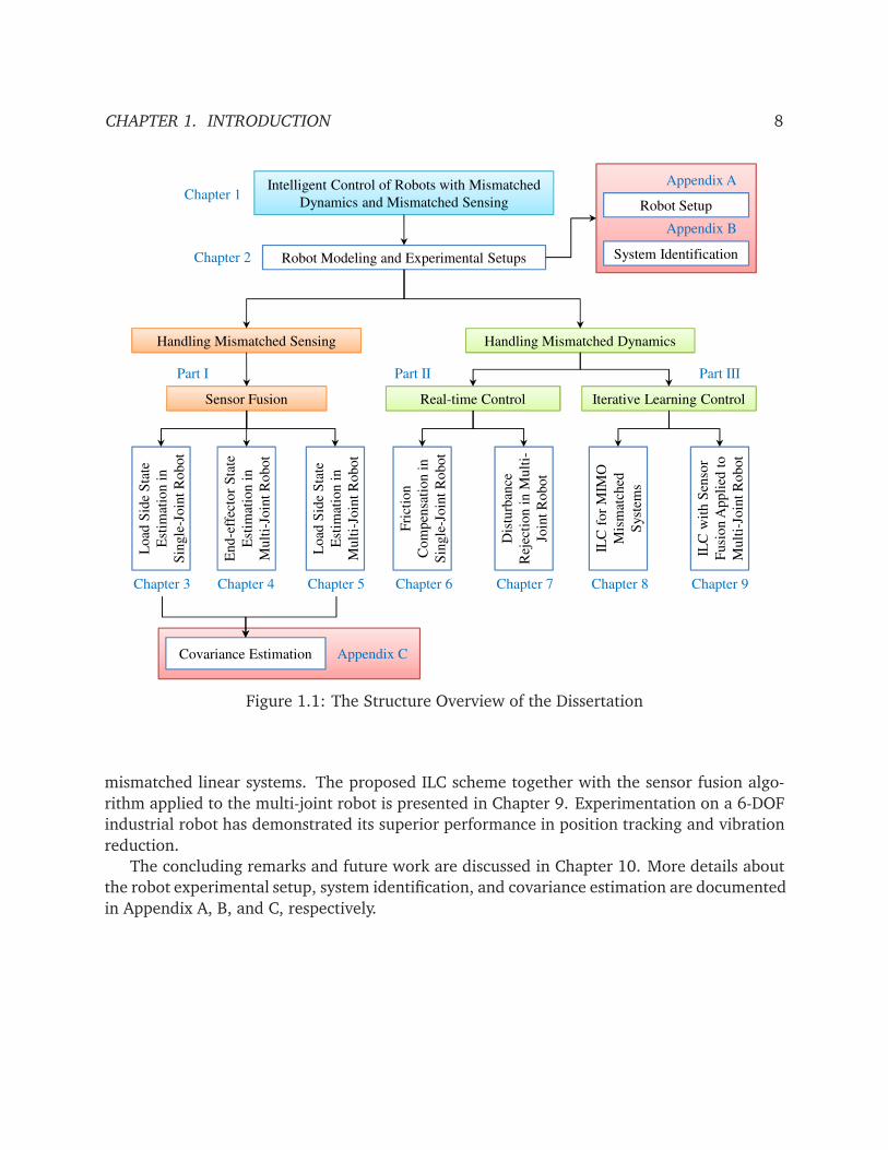
The structure of this dissertation is depicted in Fig. 1.1. More specifically, the remainder of
this dissertation is organized as follows:
Chapter 2 presents the dynamic modeling for robots with mismatched dynamics and mis-
matched sensing, as well as the experimental setups (i.e., the single-joint research testbed and
the commercial FANUC M-16iB robot system) used for algorithm validation.
The major contributions of the dissertation are then presented in three parts. In Part I, the
sensor fusion approaches for handling mismatched sensing are presented with three chapters
(i.e., Chapter 3 for sensor fusion in the single-joint robot, Chapter 4 for sensor fusion in the
multi-joint robot to estimate end-effector states, and Chapter 5 for sensor fusion in the multi-
joint robot to estimate load side joint states). The benefits of sensor fusion for load side/end-
effector state estimation are demonstrated.
Part II discusses the real-time control approaches for handling mismatched dynamics.
Chapter 6 proposes a hybrid adaptive friction compensation method for the single-joint robot,
and Chapter 7 presents the motor side disturbance rejection scheme for the multi-joint robot.
The load side/end-effector performance is significantly enhanced with the developed real-time
feedback approaches.
The iterative learning control approach for handling mismatched dynamics is given in
Part III. In Chapter 8, a hybrid two-stage model based ILC scheme is proposed for MIMO
CHAPTER 1. INTRODUCTION 8
Intelligent Control of Robots with Mismatched
Dynamics and Mismatched Sensing
Robot Modeling and Experimental Setups
Handling Mismatched Sensing Handling Mismatched Dynamics
Sensor Fusion Real-time Control Iterative Learning Control
Lo
ad S
ide
Sta
te
Est
imat
ion
in
Sin
gle
-Jo
int
Ro
bo
t
En
d-e
ffec
tor
Sta
te
Est
imat
ion
in
Mu
lti-
Join
t R
ob
ot
Lo
ad S
ide
Sta
te
Est
imat
ion
in
Mu
lti-
Join
t R
ob
ot
Fri
ctio
n
Co
mp
ensa
tio
n i
n
Sin
gle
-Jo
int
Ro
bo
t
Dis
turb
ance
Rej
ecti
on
in
Mu
lti-
Join
t R
ob
ot
ILC
fo
r M
IMO
Mis
mat
ched
Syst
ems
ILC
wit
h S
enso
r
Fu
sio
n A
pp
lied
to
Mu
lti-
Join
t R
ob
ot
Chapter 3
Part I Part II Part III
Chapter 4 Chapter 5 Chapter 6 Chapter 7 Chapter 8 Chapter 9
Chapter 2
Chapter 1Robot Setup
System Identification
Appendix A
Appendix B
Chapter 3 Chapter 4 Chapter 5 Chapter 6 Chapter 7 Chapter 8 Chapter 9
Covariance Estimation Appendix C
Figure 1.1: The Structure Overview of the Dissertation
mismatched linear systems. The proposed ILC scheme together with the sensor fusion algo-
rithm applied to the multi-joint robot is presented in Chapter 9. Experimentation on a 6-DOF
industrial robot has demonstrated its superior performance in position tracking and vibration
reduction.
The concluding remarks and future work are discussed in Chapter 10. More details about
the robot experimental setup, system identification, and covariance estimation are documented
in Appendix A, B, and C, respectively.
9
Chapter 2
Robots with Mismatched Dynamics and
Mismatched Sensing
2.1 Introduction
As discussed in Chapter 1, the mismatched dynamics and mismatched sensing are common
inherent issues in robots with indirect drive mechanisms. Despite various physical realizations
of the mismatched systems, they all share the same characteristic in terms of motion and
torque transmissions, and hence the indirect drive train is usually modeled as a system of two
masses connected by spring (and damper) [92, 97, 72]. To address the mismatched problems,
good dynamic modeling of such mismatched systems is required.
The rest of this chapter introduces the dynamic models and experimental setups of the mis-
matched systems that will be used throughout this dissertation. More specifically, Section 2.2.1
first presents the general form of the mismatched dynamical system. Section 2.2.2 formulates
the mathematical model of the single-joint indirect drive robot, which is expanded with the
consideration of friction effects and transmission error. Section 2.2.3 presents the mathemat-
ical model of the multi-joint robot with joint flexibilities. A single-joint research testbed and
a commercial 6-DOF industrial robot (i.e., FANUC M-16iB robot) in the Mechanical Systems
Control Laboratory at the University of California, Berkeley are then described in Section 2.3.
2.2 Dynamic Modeling of Mismatched Robots
2.2.1 Mismatched System Model
Consider a multi-input-multi-output (MIMO) mismatched system in the following continuous
time state space form

CHAPTER 2. ROBOTS WITH MISMATCHED DYNAMICS AND MISMATCHED SENSING 10
x(t) = Ax(t) + Buu(t) + Bdd(t) (2.1a)
y(t) =
qm(t)
qℓ(t)
=
Cm
Cℓ
x(t) +
Dmu
Dℓu
u(t)+
Dmd
Dℓd
d(t) (2.1b)
where x ∈ Rnx is the system state, u ∈ R
nu is the control input, d ∈ Rnd is the lumped distur-
bance, qm ∈ Rnm and qℓ ∈ R
nℓ are the two outputs of the plant. d is regarded as the mismatched
uncertainty/disturbance if it (or part of it) is applied to different channels from the control
input u (i.e., Bu 6= αBd ,∀α ∈ R). Another mismatched assumption is that, only part of the
outputs (i.e., qm) is measured for real-time feedback, even if the output of interest may be
qℓ. Furthermore, besides the unknown mismatched dynamics, it is assumed that parametric
uncertainties exist in the available nominal model.
This system can be reformulated into the following transfer function form
qm(s) = Pmu(s)u(s) + Pmd(s)d(s) (2.2a)
qℓ(s) = Pℓu(s)u(s) + Pℓd(s)d(s) (2.2b)
where s is the complex variable in the Laplace domain. Pmu, Pmd, Pℓu, and Pℓd are the transfer
functions from u or d to the corresponding output as follows
Pmu(s) = Cm(sInx− A)−1Bu + Dmu (2.3a)
Pℓu(s) = Cℓ(sInx− A)−1Bu + Dℓu (2.3b)
Pmd(s) = Cm(sInx− A)−1Bd + Dmd (2.3c)
Pℓd(s) = Cℓ(sInx− A)−1Bd + Dℓd (2.3d)
where Inxis an nx × nx identity matrix.
The above formulations (2.1) and (2.2) define the general form of the mismatched sys-
tem that is addressed in this dissertation. In the following sections, more detailed dynamic
modeling will be studied for the specific examples, i.e., robots with indirect drive trains/joint
flexibilities.
2.2.2 Single-Joint Robot Model
Dynamic Modeling of Indirect Drive Train
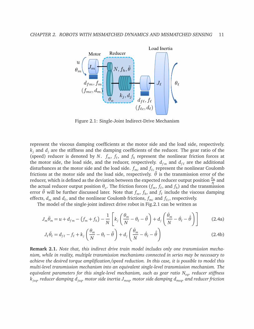
Figure 2.1 shows the schematic of a single-joint indirect drive mechanism. The subscripts
m and ℓ denote the motor side and the load side quantities1, respectively. θ represents the
angular position and J is the moment of inertia. u is the motor torque input. dm and dℓ1Recall that as discussed in Chapter 1, the electric motor is used as the modeling example for the actuator.
Thus, the two different parts separated by the indirect drive mechanism are termed as the motor side and the
load side, respectively.
CHAPTER 2. ROBOTS WITH MISMATCHED DYNAMICS AND MISMATCHED SENSING 11
u
Jm
dfm, fm
dfℓ, fℓkj , dj
N, fh, θ
ReducerLoad Inertia
θm
Motor
Jℓ θℓ
(fmc, dm)
(fℓc, dℓ)
θo
Figure 2.1: Single-Joint Indirect-Drive Mechanism
represent the viscous damping coefficients at the motor side and the load side, respectively.
k j and d j are the stiffness and the damping coefficients of the reducer. The gear ratio of the
(speed) reducer is denoted by N . fm, fℓ, and fh represent the nonlinear friction forces at
the motor side, the load side, and the reducer, respectively. d f m and d f ℓ are the additional
disturbances at the motor side and the load side. fmc and fℓc represent the nonlinear Coulomb
frictions at the motor side and the load side, respectively. θ is the transmission error of the
reducer, which is defined as the deviation between the expected reducer output positionθm
Nand
the actual reducer output position θo. The friction forces ( fm, fℓ, and fh) and the transmission
error θ will be further discussed later. Note that fm, fh, and fℓ include the viscous damping
effects, dm and dℓ, and the nonlinear Coulomb frictions, fmc and fℓc, respectively.
The model of the single-joint indirect drive robot in Fig.2.1 can be written as
Jmθm = u+ d f m−
fm+ fh
−
1
N
k j
θm
N− θℓ− θ
+ d j
θm
N− θℓ−
˙θ
(2.4a)
Jℓθℓ = d f ℓ− fℓ+ k j
θm
N− θℓ− θ
+ d j
θm
N− θℓ−
˙θ
(2.4b)
Remark 2.1. Note that, this indirect drive train model includes only one transmission mecha-
nism, while in reality, multiple transmission mechanisms connected in series may be necessary to
achieve the desired torque amplification/speed reduction. In this case, it is possible to model this
multi-level transmission mechanism into an equivalent single-level transmission mechanism. The
equivalent parameters for this single-level mechanism, such as gear ratio Neq, reducer stiffness
k jeq, reducer damping d jeq, motor side inertia Jmeq, motor side damping dmeq, and reducer friction
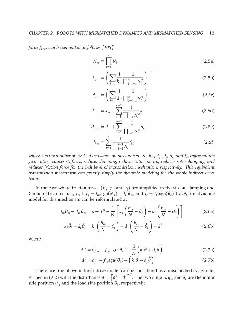
CHAPTER 2. ROBOTS WITH MISMATCHED DYNAMICS AND MISMATCHED SENSING 12
force fheq, can be computed as follows [103]
Neq =
n∏
i=1
Ni (2.5a)
k jeq =
n∑
i=1
1
k ji
1∏n
l=i+1N 2
l
!−1
(2.5b)
d jeq =
n∑
i=1
1
d ji
1∏n
l=i+1N 2
l
!−1
(2.5c)
Jmeq = Jm+
n−1∑
i=1
1∏i
l=1N 2
l
Ji (2.5d)
dmeq = dm+
n−1∑
i=1
1∏i
l=1N 2
l
di (2.5e)
fheq =
n∑
i=1
1∏i−1
l=1Nl
fhi (2.5f)
where n is the number of levels of transmission mechanism. Ni, k ji, d ji, Ji, di, and fhi represent the
gear ratio, reducer stiffness, reducer damping, reducer rotor inertia, reducer rotor damping, and
reducer friction force for the i-th level of transmission mechanism, respectively. This equivalent
transmission mechanism can greatly simply the dynamic modeling for the whole indirect drive
train.
In the case where friction forces ( fm, fh, and fℓ) are simplified to the viscous damping and
Coulomb frictions, i.e., fm+ fh = fmcsgn(θm) + dmθm, and fℓ = fℓcsgn(θℓ) + dℓθℓ, the dynamic
model for this mechanism can be reformulated as
Jmθm+ dmθm = u+ dm−1
N
k j
θm
N− θℓ
+ d j
θm
N− θℓ
(2.6a)
Jℓθℓ+ dℓθℓ = k j
θm
N− θℓ
+ d j
θm
N− θℓ
+ dℓ (2.6b)
where
dm = d f m− fmcsgn(θm) +1
N
k jθ + d j˙θ
(2.7a)
dℓ = d f ℓ− fℓcsgn(θℓ)−
k jθ + d j˙θ
(2.7b)
Therefore, the above indirect drive model can be considered as a mismatched system de-
scribed in (2.2) with the disturbance d =
dm dℓT
. The two outputs qm and qℓ are the motor
side position θm and the load side position θℓ, respectively.
CHAPTER 2. ROBOTS WITH MISMATCHED DYNAMICS AND MISMATCHED SENSING 13
Transfer Function Realizations
With the above modeling, the continuous time transfer functions from the inputs to the outputs
in (2.2) are derived as
Pmu(s) =Jℓs
2 + (d j + dℓ)s+ k j
JmJℓs4 + Jds3 + Jks2 + k j(dm+ dℓ/N
2)s(2.8a)
Pℓu(s) =d js+ k j
N
JmJℓs4 + Jds3 + Jks2 + k j(dm+ dℓ/N
2)s (2.8b)
Pmdm(s) =d js+ k j
N
JmJℓs4 + Jds3 + Jks2 + k j(dm+ dℓ/N
2)s (2.8c)
Pℓdℓ(s) =Jmis
2 + (d j/N2 + dm)s+ k j/N
2
JmJℓs4 + Jds3 + Jks2 + k j(dm+ dℓ/N
2)s(2.8d)
Pmd(s) =
Pmu(s) Pmdm(s)
, Pℓd(s) =
Pℓu(s) Pℓdℓ(s)
(2.8e)
where
Jd = Jm(d j + dℓ) + Jℓ
d j
N 2+ dm
(2.9a)
Jk = Jmk j +Jℓk j
N 2+ (d j + dℓ)dm+
d jdℓ
N 2(2.9b)
Furthermore, the transfer functions from the torque input u to the motor side velocity θm
and the load side acceleration θℓ can be found as
Gm(s) =θm(s)
u(s)= Pmu(s)s =
Jℓs2 +
d j + dℓ
s+ k j
JmJℓs3 + Jds2 + Jks+ k j
dm+dℓ
N2
(2.10a)
Gℓ(s) =θl(s)
u(s)= Pℓu(s)s
2 =d js
2 + k js
N
JmJℓs3 + Jds2 + Jks+ k j
dm+dℓ
N2
(2.10b)
In practice, the damping parameters dm, dℓ, and d j are often relatively small and neglected.
This simplifies the estimation of the plant poles and zeros. Based on this simplification, the
anti-resonant mode ωar and the resonant mode ωr for this open loop system are approxi-
mately [86]
ωar =
È
k j
Jℓ(rad/sec) (2.11a)
ωr =
È
k j
Jℓ+
k j
JmN 2(rad/sec) (2.11b)
CHAPTER 2. ROBOTS WITH MISMATCHED DYNAMICS AND MISMATCHED SENSING 14
State-Space Formulation
The continuous time state-space formulation of (2.6) can be written as
x(t) = Ac x(t) + Bucu(t) + Bdcd(t) (2.12)
where
x = [θm θm θℓ θℓ]T
d =
dm
dℓ
=
d f m− fmcsgn(θm) +1
N
k jθ + d j˙θ
d f ℓ− fℓcsgn(θℓ)−
k jθ + d j˙θ
Ac =
0 1 0 0−k j
N2Jm−
dm+d j/N2
Jm
k j
N Jm
d j
N Jm
0 0 0 1k j
N Jℓ
d j
N Jℓ
−k j
Jℓ−
d j+dℓ
Jℓ
Buc =h
0 1
Jm0 0
iT
Bdc =
0 1
Jm0 0
0 0 0 1
Jℓ
T
Linear Approximation
Note that all the nonlinear parts are grouped into the disturbance term d. While the actual
robot joint is inherently nonlinear, a good linear approximation can still preserve satisfactory
performance if either the nonlinear elements are negligible or if the linear parts are of most
interest. Additionally, the linear model allows the use of various linear analysis and control
synthesis methods. Thus, if the external disturbances (d f m and d f ℓ, which are usually negligi-
ble under normal operation condition), the transmission error θ , and nonlinear friction effects
are ignored, (2.6) can be rewritten as
Jmθm+ dmθm =−1
N
k j
θm
N− θℓ
+ d j
θm
N− θℓ
+ u (2.13a)
Jℓθℓ+ dℓθℓ = k j
θm
N− θℓ
+ d j
θm
N− θℓ
(2.13b)
and the state-space realization is accordingly
x(t) = Ac x(t) + Bucu(t) (2.14)
where the variables follow the same definition as in (2.12).
CHAPTER 2. ROBOTS WITH MISMATCHED DYNAMICS AND MISMATCHED SENSING 15
Friction Modeling
For the purpose of friction identification and compensation, the following nonlinear model
will be adopted without the consideration of the external disturbances d f m and d f ℓ.
Jmθm = −1
N
k j
θm
N− θℓ− θ
+ d j
θm
N− θℓ−
˙θ
+ u−
fm+ fh
(2.15a)
Jℓθℓ = k j
θm
N− θℓ− θ
+ d j
θm
N− θℓ−
˙θ
− fℓ (2.15b)
In this system, the energy is dissipated mainly by three friction forces: the motor bearing
friction, fm, the load output bearing friction, fℓ, and the reducer gear meshing friction, fh.
Although the gear meshing friction fh is dominant in a free load condition [76], the load side
friction fℓ can become more significant as the load side inertia increases.
The combination of system model with friction effects (2.15) gives
Jmθm+1
NJℓθℓ = u− F (2.16a)
F = fm+ fh+fℓ
N(2.16b)
where F can be explained as the entire friction force imposed on the whole system when
reflected to the motor side.
There are several reasons to model the entire friction force F in the viewpoint of the motor
side. First of all, it is easier to identify the friction on the motor side for industrial indirect
drives. Secondly, from the torque compensation point of view, the friction force is usually
compensated at the motor side where the actuator locates. Also it is not necessary to model
these friction forces separately, especially when they exhibit similar behaviors.
To describe the friction effects imposed on the motor side, this dissertation (especially
Chapter 6) employs the Lund-Grenoble (LuGre) model [15]. The LuGre model uses an internal
friction state, z, governed by
z = v −σ0|v|
g(v)z (2.17a)
g(v) = Fc +
Fs − Fc
e(−v2/v2
s ) (2.17b)
F = σ0z+σ1z +σ2v (2.17c)
where v is the relative velocity between two contacting surfaces on the motor side, i.e., v = θm.
σ0, σ1, and σ2 represent the micro-stiffness, micro-damping of the internal state z, and the
macro-damping of the velocity v, respectively. The function g(v) is chosen to capture the
Stribeck effect, where FC and FS are the levels of Coulomb friction and stiction force. vs is
the Stribeck velocity. The internal friction state z can be regarded as the deflection of bristles,
which represents the asperities between two contacting surfaces.
CHAPTER 2. ROBOTS WITH MISMATCHED DYNAMICS AND MISMATCHED SENSING 16
From (2.17), the entire friction force, F , can be written as:
F = KTΦ (2.18)
where K =
σ1 +σ2 σ0 σ0σ1
T, Φ =
h
v z −|v|
g(v)ziT
.
If only static friction is considered, i.e., z = 0, the LuGre model is simplified to
F(v) =h
Fc +
Fs − Fc
e(−v2/v2
s )i
sgn(v) +σ2v (2.19)
If further omitting the Stribeck effect, i.e., Fs = Fc, this model reduces to
F(v) = Fcsgn(v) +σ2v (2.20)
which is more commonly used in many practical applications due to its simplicity.
If the load side friction effects are not negligible, it is necessary to consider the load side
friction separately. Assuming that the load side friction shares the same characteristics as the
entire friction force F in (2.16b), a ratio rℓ can be introduced to derive the load side friction
fℓ from F , i.e.
fℓ = rℓF (2.21)
This assumption makes sense in most cases, especially when the motor is spinning in one
direction. The transient behavior during the velocity reversal might not strictly follow this
assumption. This velocity reversal case, however, is not of the interest in most applications
since the transient time is usually sufficiently short to be negligible.
Transmission Error Modeling
As stated above, there are various forms of transmission mechanisms in indirect drive trains
for speed reduction and torque amplification. In industrial robots, rotary vector (RV) reducers
and harmonic gears are the most popular means for this purpose due to their compact de-
sign and large torque capacity. However, they possess a periodic position error known as the
transmission error.
The transmission error θ is defined as the deviation between the theoretical output position
and the actual output position. It is given by the following equation (see Fig. 2.2)
θ =θm
N− θo (2.22)
where θm and θo are the motor position and reducer output position, respectively.
Due to mechanical imperfections such as gear assembly misalignments and dimensional
inaccuracies of the gear itself, the output oscillations may vary with different drives and oper-
ating conditions. It has been shown in the literature, however, that the dominant component
of the experimental transmission error waveforms is repeated (such as for every half turn
of the input shaft in harmonic drive) [39]. In other words, the ripple is periodic in nature

CHAPTER 2. ROBOTS WITH MISMATCHED DYNAMICS AND MISMATCHED SENSING 17
θ =θm
N− θo
1
N
θℓθoθm
_
+
Figure 2.2: Definition of the Transmission Error
and its fundamental frequency component corresponds to twice the rotation frequency of the
input shaft (in the case of harmonic drive). In addition to the fundamental frequency, high-
frequency error components are also observed but with relatively small amplitudes. Hence, θ
can be approximated with a simple sinusoid as follows
θ ≈ θdominant = Ate sin(ωo t +φ) (2.23)
where Ate is the amplitude of the transmission error which can be found in the reducer cat-
alogue. φ is the phase of the error and ωo is the frequency of the error (e.g., ωo = 2θm in
harmonic drive). The higher frequency components in the error are neglected here.
Note that the error exhibits in the system as a position error at the output of the motor
shaft. The dynamic model with this transmission error is formulated as in (2.4).
2.2.3 Multi-Joint Robot Model
Lagrangian Dynamics
The multi-joint robot with indirect drive trains considered in this dissertation is assumed to be
connected in serial. A typical example of this kind of system is the industrial serial robot ma-
nipulator with revolute/prismatic joints. The dynamics of such an n-joint robot manipulator
with gear compliance can be expressed as [92, 97, 72]
Mℓ(qℓ)qℓ+ C(qℓ, qℓ)qℓ+ G(qℓ) + Dℓqℓ+ Fℓcsgn(qℓ) + J(qℓ)T fex t
= KJ
N−1qm− qℓ− q
+ DJ
N−1qm− qℓ− ˙q
(2.24a)
Mmqm+ Dmqm+ Fmcsgn(qm) = τm− N−1
KJ
N−1qm− qℓ− q
+ DJ
N−1qm− qℓ− ˙q
(2.24b)
where qℓ ∈ Rn and qm ∈ R
n are the load side and the motor side position vectors, respectively.
q ∈ Rn is the transmission error vector resulted from the joint reducers. τm ∈ R
n is the motor
torque input vector. Mℓ(qℓ) ∈ Rn×n is the load side inertia matrix, C(qℓ, qℓ) ∈ R
n×n is the
Coriolis and centrifugal force matrix, and G(qℓ) ∈ Rn is the gravity torque vector. Mm, KJ , DJ ,
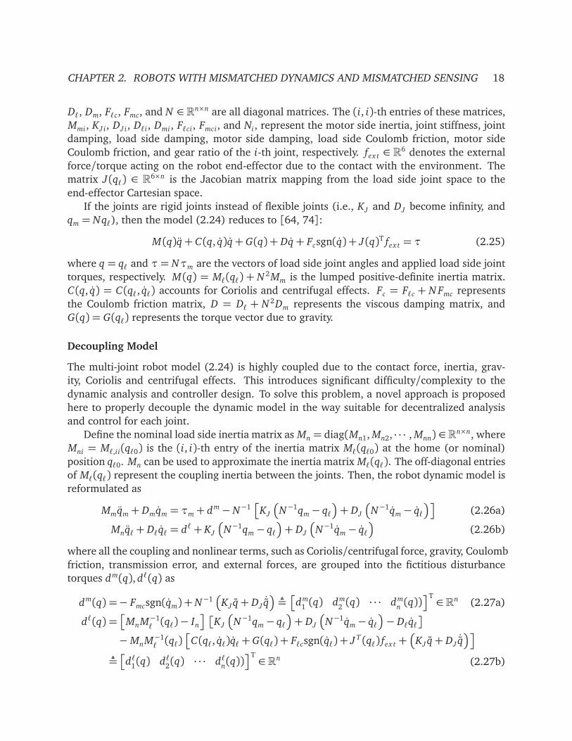
CHAPTER 2. ROBOTS WITH MISMATCHED DYNAMICS AND MISMATCHED SENSING 18
Dℓ, Dm, Fℓc, Fmc, and N ∈ Rn×n are all diagonal matrices. The (i, i)-th entries of these matrices,
Mmi, KJ i, DJ i, Dℓi, Dmi, Fℓci, Fmci, and Ni, represent the motor side inertia, joint stiffness, joint
damping, load side damping, motor side damping, load side Coulomb friction, motor side
Coulomb friction, and gear ratio of the i-th joint, respectively. fex t ∈ R6 denotes the external
force/torque acting on the robot end-effector due to the contact with the environment. The
matrix J(qℓ) ∈ R6×n is the Jacobian matrix mapping from the load side joint space to the
end-effector Cartesian space.
If the joints are rigid joints instead of flexible joints (i.e., KJ and DJ become infinity, and
qm = Nqℓ), then the model (2.24) reduces to [64, 74]:
M(q)q+ C(q, q)q+ G(q) + Dq+ Fcsgn(q) + J(q)T fex t = τ (2.25)
where q = qℓ and τ= Nτm are the vectors of load side joint angles and applied load side joint
torques, respectively. M(q) = Mℓ(qℓ) + N 2Mm is the lumped positive-definite inertia matrix.
C(q, q) = C(qℓ, qℓ) accounts for Coriolis and centrifugal effects. Fc = Fℓc + N Fmc represents
the Coulomb friction matrix, D = Dℓ + N 2Dm represents the viscous damping matrix, and
G(q) = G(qℓ) represents the torque vector due to gravity.
Decoupling Model
The multi-joint robot model (2.24) is highly coupled due to the contact force, inertia, grav-
ity, Coriolis and centrifugal effects. This introduces significant difficulty/complexity to the
dynamic analysis and controller design. To solve this problem, a novel approach is proposed
here to properly decouple the dynamic model in the way suitable for decentralized analysis
and control for each joint.
Define the nominal load side inertia matrix as Mn = diag(Mn1, Mn2, · · · , Mnn) ∈ Rn×n, where
Mni = Mℓ,ii(qℓ0) is the (i, i)-th entry of the inertia matrix Mℓ(qℓ0) at the home (or nominal)
position qℓ0. Mn can be used to approximate the inertia matrix Mℓ(qℓ). The off-diagonal entries
of Mℓ(qℓ) represent the coupling inertia between the joints. Then, the robot dynamic model is
reformulated as
Mmqm+ Dmqm = τm+ dm− N−1
KJ
N−1qm− qℓ
+ DJ
N−1qm− qℓ
(2.26a)
Mnqℓ+ Dℓqℓ = dℓ+ KJ
N−1qm− qℓ
+ DJ
N−1qm− qℓ
(2.26b)
where all the coupling and nonlinear terms, such as Coriolis/centrifugal force, gravity, Coulomb
friction, transmission error, and external forces, are grouped into the fictitious disturbance
torques dm(q), dℓ(q) as
dm(q) =− Fmcsgn(qm) + N−1
KJ q+ DJ˙q
¬
dm1(q) dm
2(q) · · · dm
n(q))
T∈ R
n (2.27a)
dℓ(q) =
MnM−1ℓ(qℓ)− In
KJ
N−1qm− qℓ
+ DJ
N−1qm− qℓ
− Dℓqℓ
−MnM−1ℓ(qℓ)
C(qℓ, qℓ)qℓ+ G(qℓ) + Fℓcsgn(qℓ) + J T (qℓ) fex t +
KJ q+ DJ˙q
¬
dℓ1(q) dℓ
2(q) · · · dℓ
n(q))
T∈ R
n (2.27b)

CHAPTER 2. ROBOTS WITH MISMATCHED DYNAMICS AND MISMATCHED SENSING 19
where In is an n× n identity matrix and q is defined as
q =
qT1
qT2· · · qT
n
T∈ R
4n (2.28a)
qi =
qmi qmi qℓi qℓiT∈ R
4, i = 1, 2, · · · , n (2.28b)
Thus, the robot can be considered as a MIMO system with 2n inputs and 2n outputs as
qm(s) = Pmu(s)τm(s) + Pmd(s)d(s) (2.29a)
qℓ(s) = Pℓu(s)τm(s) + Pℓd(s)d(s) (2.29b)
where the fictitious disturbance input d(t) is defined as
d(t) =d(q(t)) =
d1(q(t))T d2(q(t))
T · · · dn(q(t))TT∈ R
2n (2.30a)
di(t) =di(q(t)) =
dmi(q(t)) dℓ
i(q(t))
T∈ R
2, i = 1, 2, · · · , n (2.30b)
Similar to the single-joint case in Section 2.2.2, the continuous time transfer functions from
the inputs to the outputs for the i-th joint are derived from (2.26) as
P imu(s) =
Mnis2 + (DJ i + Dℓi)s+ KJ i
Mmi Mnis4 + Jdis
3 + Jkis2 + KJ i(Dmi + Dℓi/N
2i )s
(2.31a)
P iℓu(s) =
DJ is+ KJ i
Ni
Mmi Mnis4 + Jdis
3 + Jkis2 + KJ i(Dmi + Dℓi/N
2i )s (2.31b)
P i
mdℓ(s) =
DJ is+ KJ i
Ni
Mmi Mnis4 + Jdis
3 + Jkis2 + KJ i(Dmi + Dℓi/N
2i )s (2.31c)
P i
ℓdℓ(s) =
Mmis2 + (DJ i/N
2i+ Dmi)s+ KJ i/N
2i
Mmi Mnis4 + Jdis
3 + Jkis2 + KJ i(Dmi + Dℓi/N
2i )s
(2.31d)
P imd(s) =
P imu(s) P i
mdℓ(s)
, P iℓd(s) =
P iℓu(s) P i
ℓdℓ(s)
(2.31e)
where the subscript/superscript i denotes the joint index, and
Jdi =Mmi(DJ i + Dℓi) +Mni(DJ i
N 2i
+ Dmi) (2.32a)
Jki =MmiKJ i +MniKJ i
N 2i
+ (DJ i + Dℓi)Dmi +DJ iDℓi
N 2i
(2.32b)
Remark 2.2. Note that the robot dynamic model (2.26) is in a decoupled form since all the
variables are expressed in the diagonal matrix form or vector form. This model formulation
enables the way to design and analyze the robot controller in a decentralized fashion for each
individual joint.
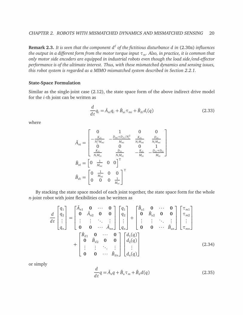
CHAPTER 2. ROBOTS WITH MISMATCHED DYNAMICS AND MISMATCHED SENSING 20
Remark 2.3. It is seen that the component dℓ of the fictitious disturbance d in (2.30a) influences
the output in a different form from the motor torque input τm. Also, in practice, it is common that
only motor side encoders are equipped in industrial robots even though the load side/end-effector
performance is of the ultimate interest. Thus, with these mismatched dynamics and sensing issues,
this robot system is regarded as a MIMO mismatched system described in Section 2.2.1.
State-Space Formulation
Similar as the single-joint case (2.12), the state space form of the above indirect drive model
for the i-th joint can be written as
d
d tqi = Aniqi + Buiτmi + Bdidi(q) (2.33)
where
Ani =
0 1 0 0
−KJ i
N2i Mmi
−Dmi+DJ i/N
2i
Mmi
KJ i
Ni Mmi
DJ i
Ni Mmi
0 0 0 1KJ i
Ni Mni
DJ i
Ni Mni−
KJ i
Mni−
DJ i+Dℓi
Mni
Bui =h
0 1
Mmi0 0
iT
Bdi =
0 1
Mmi0 0
0 0 0 1
Mni
T
By stacking the state space model of each joint together, the state space form for the whole
n-joint robot with joint flexibilities can be written as
d
d t
q1
q2...
qn
=
An1 0 · · · 0
0 An2 0 0...
.... . .
...
0 0 · · · Ann
q1
q2...
qn
+
Bu1 0 · · · 0
0 Bu2 0 0...
.... . .
...
0 0 · · · Bun
τm1
τm2...
τmn
+
Bd1 0 · · · 0
0 Bd2 0 0...
.... . .
...
0 0 · · · Bdn
d1(q)
d2(q)...
dn(q)
(2.34)
or simplyd
d tq = Anq+ Buτm+ Bd d(q) (2.35)
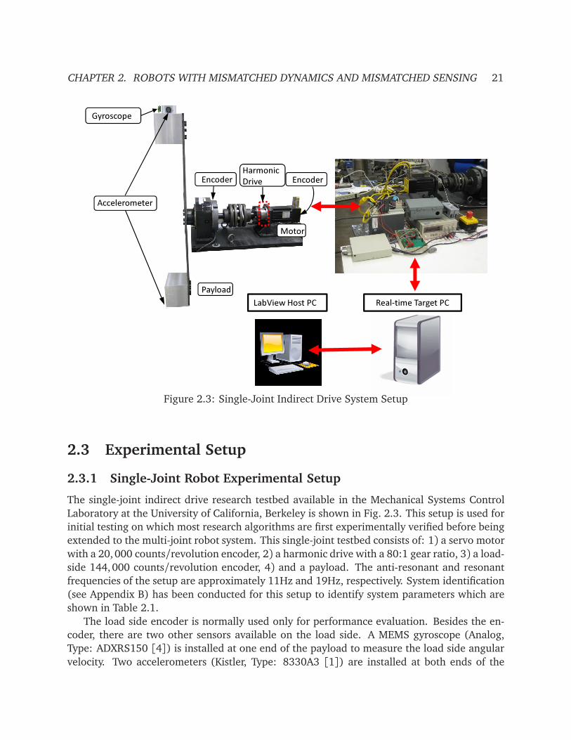
CHAPTER 2. ROBOTS WITH MISMATCHED DYNAMICS AND MISMATCHED SENSING 21
Figure 2.3: Single-Joint Indirect Drive System Setup
2.3 Experimental Setup
2.3.1 Single-Joint Robot Experimental Setup
The single-joint indirect drive research testbed available in the Mechanical Systems Control
Laboratory at the University of California, Berkeley is shown in Fig. 2.3. This setup is used for
initial testing on which most research algorithms are first experimentally verified before being
extended to the multi-joint robot system. This single-joint testbed consists of: 1) a servo motor
with a 20, 000 counts/revolution encoder, 2) a harmonic drive with a 80:1 gear ratio, 3) a load-
side 144, 000 counts/revolution encoder, 4) and a payload. The anti-resonant and resonant
frequencies of the setup are approximately 11Hz and 19Hz, respectively. System identification
(see Appendix B) has been conducted for this setup to identify system parameters which are
shown in Table 2.1.
The load side encoder is normally used only for performance evaluation. Besides the en-
coder, there are two other sensors available on the load side. A MEMS gyroscope (Analog,
Type: ADXRS150 [4]) is installed at one end of the payload to measure the load side angular
velocity. Two accelerometers (Kistler, Type: 8330A3 [1]) are installed at both ends of the
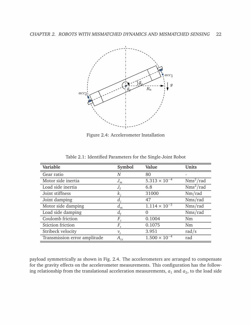
CHAPTER 2. ROBOTS WITH MISMATCHED DYNAMICS AND MISMATCHED SENSING 22
g
θℓRa
θℓ
acc1
acc2
Figure 2.4: Accelerometer Installation
Table 2.1: Identified Parameters for the Single-Joint Robot
Variable Symbol Value Units
Gear ratio N 80 -
Motor side inertia Jm 5.313× 10⁻⁴ Nms2/rad
Load side inertia Jℓ 6.8 Nms2/rad
Joint stiffness k j 31000 Nm/rad
Joint damping d j 47 Nms/rad
Motor side damping dm 1.114× 10⁻³ Nms/rad
Load side damping dℓ 0 Nms/rad
Coulomb friction Fc 0.1004 Nm
Stiction friction Fs 0.1075 Nm
Stribeck velocity vs 3.951 rad/s
Transmission error amplitude Ate 1.500× 10⁻⁴ rad
payload symmetrically as shown in Fig. 2.4. The accelerometers are arranged to compensate
for the gravity effects on the accelerometer measurements. This configuration has the follow-
ing relationship from the translational acceleration measurements, a1 and a2, to the load side

CHAPTER 2. ROBOTS WITH MISMATCHED DYNAMICS AND MISMATCHED SENSING 23
angular acceleration, θℓ, and the gravity, g
a1 = Raθℓ+ g cos θℓ (2.36a)
a2 = Raθℓ− g cos θℓ (2.36b)
where Ra is the distance from the rotation axis to the accelerometer measurement point, and
θℓ is the angle of the payload from the horizontal position. It is not necessary to measure the
angle θℓ, since the angular acceleration θℓ can be obtained as
θℓ =a1 + a2
2Ra
(2.37)
which is independent of the gravity effect.
Finally, the controller and sensor fusion algorithms are implemented in a LabVIEW real-
time target installed with LabVIEW Real-Time and FPGA modules. The sampling rate is se-
lected as 1kHz for all the research implementation on this setup.
2.3.2 Multi-Joint Robot Experimental Setup
The multi-joint robot experimental setup used at the University of California, Berkeley, cour-
tesy of FANUC, is the M-16iB/20 industrial robot as shown in Fig. 2.5. It is a six-axis, medium
size robot and can carry objects up to 20 kg at a maximum speed of 2000 mm/sec. It is mainly
used for the high-speed applications such as spot welding, material handling, sealing, and
water-jet cutting. The specification of this robot can be found in [59].
The hardware connection diagram of the experimental setup is illustrated in Fig. 2.6. The
M-16iB robot is equipped with built-in motor encoder for each joint. An "L" shape steel payload
of the weight of 18.37kg is attached at the last joint as the end-effector. An inertia measure-
ment unit (IMU) (Analog Devices, ADIS16400 [3]) consisting of a 3-axial accelerometer and
a 3-axial gyroscope is attached to the end-effector. The three-dimensional position measure-
ment system, CompuGauge 3D (repeatability of 0.02mm, accuracy of 0.15mm, resolution of
0.01mm [28]), is utilized to measure the end-effector tool center point (TCP) position. Fur-
thermore, a PSD camera of high precision and fast response has been developed to directly
sense the two-dimensional positions of the infrared markers attached on the robot end-effector
[94]. These sensors allow to obtain the end-effector information along with time information
for the purpose of performance improvement and evaluation.
The sampling rates of all the sensor signals as well as the real-time controller implemented
through MATLAB xPC Target are set to 1kHz. System identifications are conducted for each
individual joint at several different postures to obtain the nominal dynamic parameters in the
dynamic model (2.26). The details of the system identifications can be found in Appendix B.
The development of PSD camera is detailed in [94, 22]. All other parts (e.g., FANUC
robot controller, real-time system, payload design, inertia sensor setup, and Robot Simula-
tion/Experimentor) of the hardware setup are described in Appendix A and also reported in
[44, 43, 21, 50].
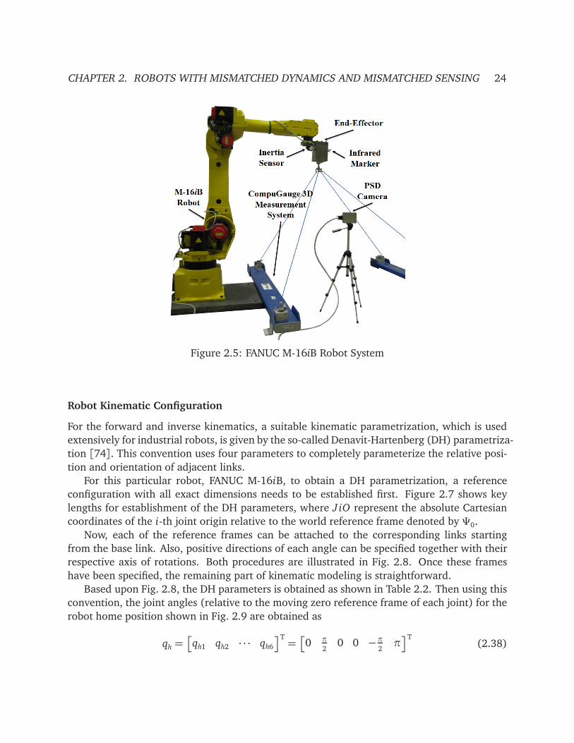
CHAPTER 2. ROBOTS WITH MISMATCHED DYNAMICS AND MISMATCHED SENSING 24
Figure 2.5: FANUC M-16iB Robot System
Robot Kinematic Configuration
For the forward and inverse kinematics, a suitable kinematic parametrization, which is used
extensively for industrial robots, is given by the so-called Denavit-Hartenberg (DH) parametriza-
tion [74]. This convention uses four parameters to completely parameterize the relative posi-
tion and orientation of adjacent links.
For this particular robot, FANUC M-16iB, to obtain a DH parametrization, a reference
configuration with all exact dimensions needs to be established first. Figure 2.7 shows key
lengths for establishment of the DH parameters, where J iO represent the absolute Cartesian
coordinates of the i-th joint origin relative to the world reference frame denoted by Ψ0.
Now, each of the reference frames can be attached to the corresponding links starting
from the base link. Also, positive directions of each angle can be specified together with their
respective axis of rotations. Both procedures are illustrated in Fig. 2.8. Once these frames
have been specified, the remaining part of kinematic modeling is straightforward.
Based upon Fig. 2.8, the DH parameters is obtained as shown in Table 2.2. Then using this
convention, the joint angles (relative to the moving zero reference frame of each joint) for the
robot home position shown in Fig. 2.9 are obtained as
qh =
qh1 qh2 · · · qh6
T=
0 π
20 0 −π
2πT
(2.38)

CHAPTER 2. ROBOTS WITH MISMATCHED DYNAMICS AND MISMATCHED SENSING 25
!" #"
$ % ""&#%!
'"##(
)
*%
'
'+,,
-)./
-
0-
'.
-
&#%!'"##(
)#""')12)',3/4 #"5 #)
Figure 2.6: FANUC M-16iB Robot System Setup Scheme
Figure 2.7: Reference Configuration for FANUC M-16iB Robot
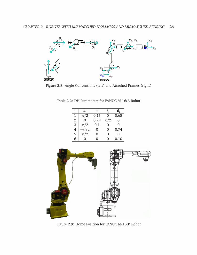
CHAPTER 2. ROBOTS WITH MISMATCHED DYNAMICS AND MISMATCHED SENSING 26
θ1
θ2
θ3
θ4
θ5θ6
x0
z0x1
z1
x2
z2
x3z3
x4, x5
z4z5
x6
z6
Ψ0
Ψ6
Figure 2.8: Angle Conventions (left) and Attached Frames (right)
Table 2.2: DH Parameters for FANUC M-16iB Robot
i αi ai θi di
1 π/2 0.15 0 0.65
2 0 0.77 π/2 0
3 π/2 0.1 0 0
4 −π/2 0 0 0.74
5 π/2 0 0 0
6 0 0 0 0.10
Figure 2.9: Home Position for FANUC M-16iB Robot

CHAPTER 2. ROBOTS WITH MISMATCHED DYNAMICS AND MISMATCHED SENSING 27
2.4 Chapter Summary
This chapter introduced the dynamic modeling and experimental setups for the robots with
mismatched dynamics and mismatched sensing. The unifying characteristic of such mis-
matched systems was described first. Then the dynamic modeling for the single-joint mis-
matched robot was studied with the consideration of friction and transmission error effects.
The multi-joint mismatched robot dynamics was subsequently investigated, and a novel ap-
proach was presented to decouple the multi-joint model and to formulate it into the standard
MIMO mismatched model form. The experimental setups (including single-joint and multi-
joint setups) that are used in this dissertation research were then introduced. The configura-
tion and implementation of the experimental setups are detailed in Appendix A.
28
Part I
Handling Mismatched Sensing:
Sensor Fusion Approaches

29
Chapter 3
Load Side State Estimation in Single-Joint
Robot
3.1 Introduction
As discussed in previous chapters, in robot applications, discrepancies between the available
measurements and the required information set difficulties in achieving good control perfor-
mance. Such phenomena are resulted from sensor dynamics as well as robot dynamics. Par-
ticularly, in robots with joint flexibilities, good motor side performance based on motor side
measurements does not guarantee good load side performance, which is a critical issue in prac-
tical applications. Precise load side position measurements (e.g., load side encoder), however,
are usually not available in industrial robots due to cost and assembly issues. To overcome this
problem, inexpensive MEMS sensors1 that are easy to mount may be considered. Considera-
tion should be given, however, to problems such as non-negligible biases, limited bandwidth,
and noises from low-cost sensors, which set restrictions on the direct utilization of sensor
signals. These problems may be circumvented by the proper fusion of multiple sensor signals.
In recent years, estimation algorithms using multi-sensor configurations have been studied.
Two robust estimation schemes incorporating the Kalman filter and disturbance observer for
robot dynamic models have been reported in [49, 71]. These methods require accurate system
parameters and thus are not reliable when subjected to model uncertainties. In [56, 51], it
has been suggested that a kinematic model based Kalman filter (KKF) can be formulated by
making use of accelerometers and position encoders. The model uncertainties are avoided
by using the kinematic relation between the position and the acceleration. These methods,
however, were developed mainly for one-mass systems or direct drives (i.e., without indirect
drive joint compliance), and the main purpose is velocity estimation while assuming the po-
sition information is measured. Also, noise covariance in these methods were used as design
parameters, which are not easy to select when multiple measurements are utilized.
In this chapter, this load side state estimation problem in the single-joint indirect drive
1A representative cost comparison between the encoders and the MEMS inertia sensors can be found in [70].

CHAPTER 3. LOAD SIDE STATE ESTIMATION IN SINGLE-JOINT ROBOT 30
robot is investigated. Measurement dynamics are introduced into the dynamic/kinematic
model to deal with sensor noises and biases. The estimation algorithm is formulated in Sec-
tion 3.2 based on the extended model to fuse the measurements from both the motor side and
the load side. Noise covariance adaptation issue is also addressed. The schemes are tested by
experiments in Section 3.3 and will be utilized in the friction compensation in Chapter 6.
3.2 Estimation Algorithms
3.2.1 Model for Measurement Dynamics
The bias and the noise in the sensor output can be described as
b (t) = nb (t) (3.1a)
xs (t) = x (t) + b (t) + ns (t) (3.1b)
where b is the bias of the sensor output varying with the fictitious noise nb. xs is the sensor
measurement for the actual physical quantity x with the measurement noise ns.
3.2.2 System Dynamic Model
Consider the linear model representation (2.14) of an indirect drive robot joint restated as
x(t) = Ac x(t) + Bucu(t) (3.2)
where
x = [θm θm θℓ θℓ]T
Ac =
0 1 0 0−k j
N2Jm−
dm+d j/N2
Jm
k j
N Jm
d j
N Jm
0 0 0 1k j
N Jℓ
d j
N Jℓ
−k j
Jℓ−
d j+dℓ
Jℓ
Buc =h
0 1
Jm0 0
iT
and all the variable definitions are the same as in Chapter 2.
If the load side is equipped with the gyroscope and the accelerometer, the system model
(3.2) with measurement dynamics is extended to
xm(t) = Amxm(t) +Bm,uus(t) +Bm,wwm(t) (3.3a)
ym(t) = Cmxm(t) + vm(t) (3.3b)

CHAPTER 3. LOAD SIDE STATE ESTIMATION IN SINGLE-JOINT ROBOT 31
where
xm =
xT ba bv
T∈ R
6×1, ym =
θm,s θℓ,s θℓ,sT∈ R
3×1
wm =
−nu nba nbv
T∈ R
3×1, vm =
nsm nvℓ naℓ
T∈ R
3×1
Am =
Ac 0
0 0
∈ R6×6, Bm,u =
Buc 0T∈ R6×1
Bm,w =
Buc 0
0 I2
∈ R6×3, Cm =
1 0 0 0 0 0
0 0 0 1 0 1
Ac4 1 0
∈ R
3×6
where Ac4 is the fourth row of the matrix Ac, and In is an n× n identity matrix. •s denotes
the sensor measurement of the actual physical quantity •. ba and bv represent the biases of
accelerometer and gyroscope outputs, respectively. nu, nba, and nbv are the noises of motor
torque output, u, accelerometer bias, ba, and gyroscope bias, bv , respectively. nsm, nvℓ, and naℓ
are the measurement noises of motor side position, θm, load side velocity, θℓ, and load side
acceleration, θℓ, respectively.
3.2.3 System Kinematic Model
The kinematic model from the acceleration to the position on the load side can be written as
d
d t
θℓ(t)
θℓ(t)
=
0 1
0 0
θℓ(t)
θℓ(t)
+
0
1
θℓ(t) (3.4)
The Kalman filter based on the kinematic model (3.4) is called the kinematic Kalman
filter (KKF) [56]. In KKF, the acceleration is used as an input to the filter, and the position
information is used to correct the estimation output. In the indirect drive robot joint, however,
precise load side position measurement (e.g., load side encoder) is usually not available, which
makes it difficult to directly utilize the KKF algorithm.
Here, a novel but intuitive method is proposed to approximate the load side position mea-
surement. Let Gm2l (s) be the transfer function from the motor side position θm to the load side
position θℓ, i.e.,
Gm2l (s) ¬θℓ (s)
θm (s)=
d js+ k j
N
Jℓs2 + (d j + dℓ)s+ k j
(3.5)
by the inherent system dynamics ((2.13) in Chapter 2). Thus, Gm2l (s) is approximately zero-
phase static gain at the low frequency region (Fig. 3.1), since the dynamic chain from θm
to θℓ is modeled by mass, gear, spring, and damper. This indicates that the low frequency
component of θℓ can be approximated by that of θm.
Pass θm and θℓ through a first order low-pass filter G f (s) =α
s+α, where α = β fb, fb is the
bandwidth of Gm2l(s), and β ∈ (0,∞) is a design parameter for the low-pass filter. Denote the

CHAPTER 3. LOAD SIDE STATE ESTIMATION IN SINGLE-JOINT ROBOT 32
100
101
102
103
−180
−135
−90
−45
0
Phase (
deg)
Bode Diagram
Frequency (Hz)
−60
−40
−20
0
20
System: untitled1Frequency (Hz): 16.5Magnitude (dB): −3.01
Magnitude (
dB
)
Figure 3.1: Bode Plot ofθℓ(s)
λ0θm(s)for the System Setup in Fig. 2.3
filter outputs as θmf and θℓ f , respectively. It follows that
θmf =−αθmf +αθm (3.6a)
θℓ f =−αθℓ f +αθℓ (3.6b)
The above analysis shows that, if β is chosen properly, the filter outputs will have the
following relation
θℓ f ≈ λ0θmf (3.7)
where λ0 is the DC gain of Gm2l (s) (e.g., λ0 =1
Nfor the system in Fig. 2.1). Generally, it is
desired that β ≤ 1 and thus α ≤ fb. If the low frequency components of θm and θℓ are highly
dominant, however, β can be chosen to be larger than 1 to increase the filter convergence rate.
The filter dynamics (3.6) and the measurement dynamics (3.1) can be added into the
system kinematic model (3.4), giving
xk(t) = Ak xk(t) +Bk,uθℓ,s(t) +Bk,wwk(t) (3.8a)
yk(t) = Ck xk(t) + vk(t) (3.8b)
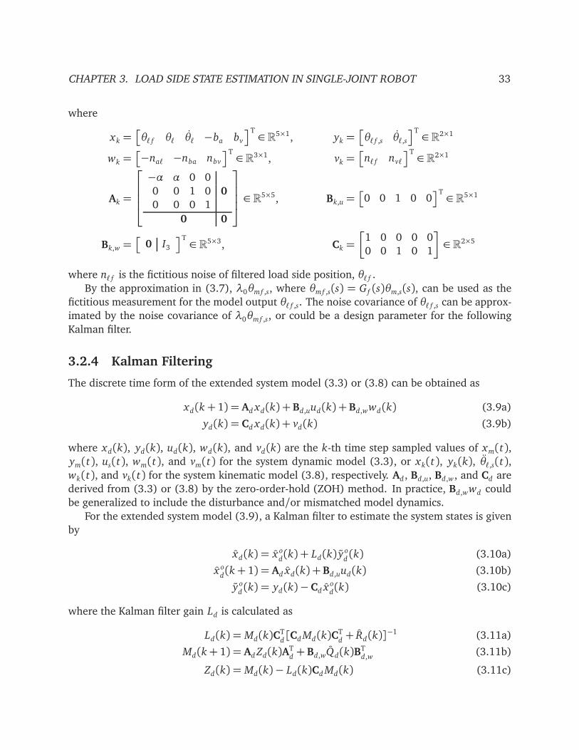
CHAPTER 3. LOAD SIDE STATE ESTIMATION IN SINGLE-JOINT ROBOT 33
where
xk =
θℓ f θℓ θℓ −ba bv
T∈ R
5×1, yk =
θℓ f ,s θℓ,sT∈ R2×1
wk =
−naℓ −nba nbv
T∈ R3×1, vk =
nℓ f nvℓ
T∈ R
2×1
Ak =
−α α 0 0
00 0 1 0
0 0 0 1
0 0
∈ R
5×5, Bk,u =
0 0 1 0 0T∈ R
5×1
Bk,w =
0 I3
T∈ R
5×3, Ck =
1 0 0 0 0
0 0 1 0 1
∈ R2×5
where nℓ f is the fictitious noise of filtered load side position, θℓ f .
By the approximation in (3.7), λ0θmf ,s, where θmf ,s(s) = G f (s)θm,s(s), can be used as the
fictitious measurement for the model output θℓ f ,s. The noise covariance of θℓ f ,s can be approx-
imated by the noise covariance of λ0θmf ,s, or could be a design parameter for the following
Kalman filter.
3.2.4 Kalman Filtering
The discrete time form of the extended system model (3.3) or (3.8) can be obtained as
xd(k+ 1) = Ad xd(k) +Bd,uud(k) +Bd,wwd(k) (3.9a)
yd(k) = Cd xd(k) + vd(k) (3.9b)
where xd(k), yd(k), ud(k), wd(k), and vd(k) are the k-th time step sampled values of xm(t),
ym(t), us(t), wm(t), and vm(t) for the system dynamic model (3.3), or xk(t), yk(k), θℓ,s(t),
wk(t), and vk(t) for the system kinematic model (3.8), respectively. Ad , Bd,u, Bd,w, and Cd are
derived from (3.3) or (3.8) by the zero-order-hold (ZOH) method. In practice, Bd,wwd could
be generalized to include the disturbance and/or mismatched model dynamics.
For the extended system model (3.9), a Kalman filter to estimate the system states is given
by
xd(k) = x od(k) + Ld(k) y
od(k) (3.10a)
x od(k+ 1) = Ad xd(k) +Bd,uud(k) (3.10b)
yod(k) = yd(k)−Cd x o
d(k) (3.10c)
where the Kalman filter gain Ld is calculated as
Ld(k) = Md(k)CTd[Cd Md(k)C
Td+ Rd(k)]
−1 (3.11a)
Md(k+ 1) = Ad Zd(k)ATd+ Bd,wQd(k)B
Td,w
(3.11b)
Zd(k) = Md(k)− Ld(k)Cd Md(k) (3.11c)
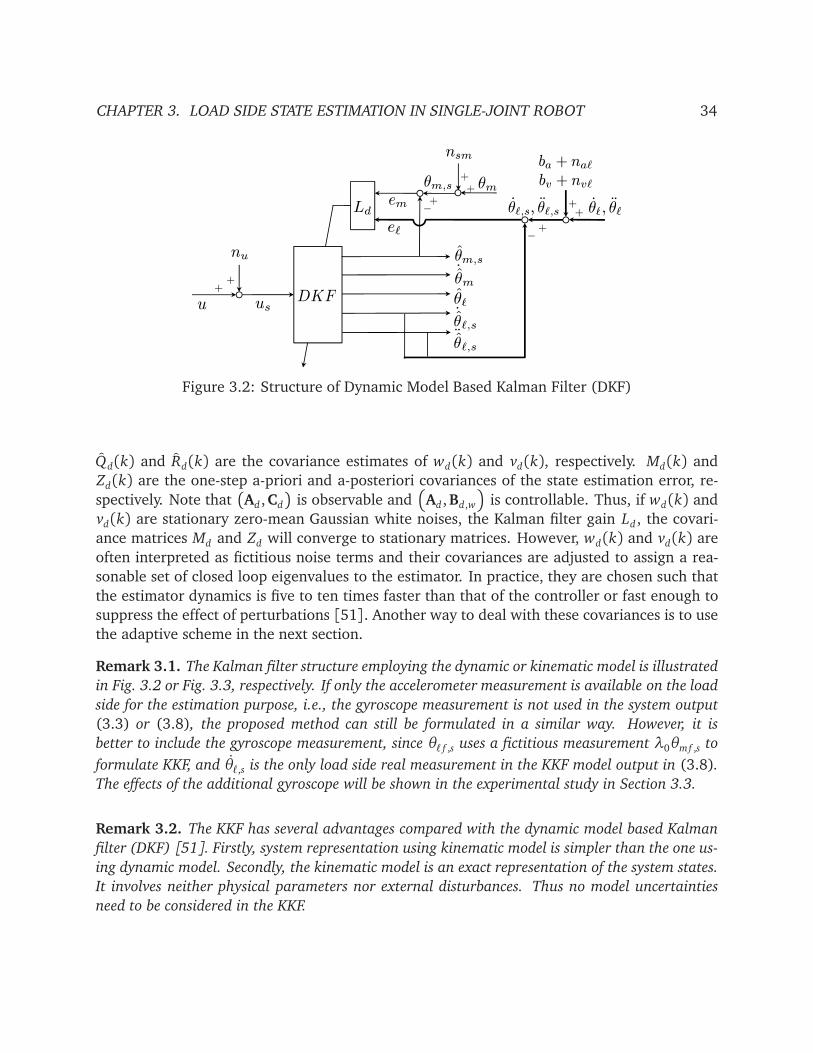
CHAPTER 3. LOAD SIDE STATE ESTIMATION IN SINGLE-JOINT ROBOT 34
++
nu
em
θm,s θm++
−
+
˙θm
θm,s
u
nsm
θℓ˙θℓ,s¨θℓ,s
θℓ,s, θℓ,s
bv + nvℓ
us
DKF
Ld
+
+ θℓ, θℓ+
eℓ−
ba + naℓ
Figure 3.2: Structure of Dynamic Model Based Kalman Filter (DKF)
Qd(k) and Rd(k) are the covariance estimates of wd(k) and vd(k), respectively. Md(k) and
Zd(k) are the one-step a-priori and a-posteriori covariances of the state estimation error, re-
spectively. Note thatAd ,Cd
is observable and
Ad ,Bd,w
is controllable. Thus, if wd(k) and
vd(k) are stationary zero-mean Gaussian white noises, the Kalman filter gain Ld , the covari-
ance matrices Md and Zd will converge to stationary matrices. However, wd(k) and vd(k) are
often interpreted as fictitious noise terms and their covariances are adjusted to assign a rea-
sonable set of closed loop eigenvalues to the estimator. In practice, they are chosen such that
the estimator dynamics is five to ten times faster than that of the controller or fast enough to
suppress the effect of perturbations [51]. Another way to deal with these covariances is to use
the adaptive scheme in the next section.
Remark 3.1. The Kalman filter structure employing the dynamic or kinematic model is illustrated
in Fig. 3.2 or Fig. 3.3, respectively. If only the accelerometer measurement is available on the load
side for the estimation purpose, i.e., the gyroscope measurement is not used in the system output
(3.3) or (3.8), the proposed method can still be formulated in a similar way. However, it is
better to include the gyroscope measurement, since θℓ f ,s uses a fictitious measurement λ0θmf ,s to
formulate KKF, and θℓ,s is the only load side real measurement in the KKF model output in (3.8).
The effects of the additional gyroscope will be shown in the experimental study in Section 3.3.
Remark 3.2. The KKF has several advantages compared with the dynamic model based Kalman
filter (DKF) [51]. Firstly, system representation using kinematic model is simpler than the one us-
ing dynamic model. Secondly, the kinematic model is an exact representation of the system states.
It involves neither physical parameters nor external disturbances. Thus no model uncertainties
need to be considered in the KKF.
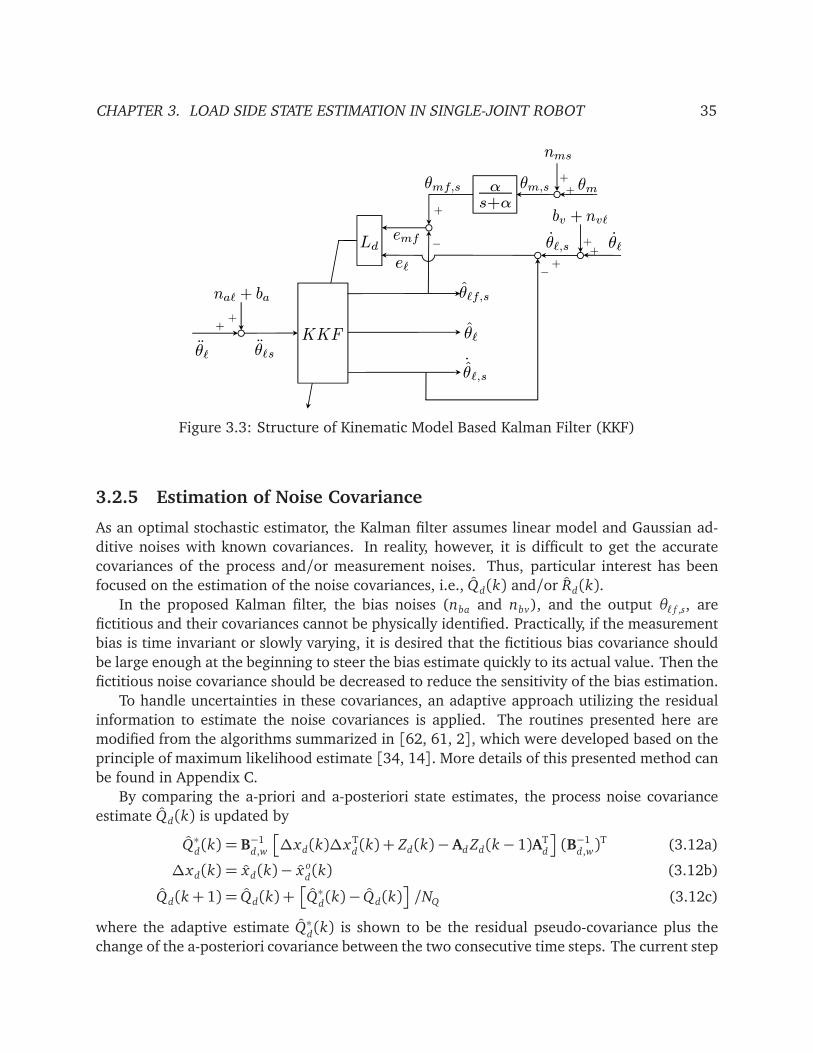
CHAPTER 3. LOAD SIDE STATE ESTIMATION IN SINGLE-JOINT ROBOT 35
++
nms
θm++
−
+
KKF
+
+emf
naℓ + ba
θℓ θℓs
θℓ
˙θℓ,s
θℓ,s θℓ
bv + nvℓ
Ld
θℓf,s
θmf,s
+
eℓ−
θm,sα
s+α
Figure 3.3: Structure of Kinematic Model Based Kalman Filter (KKF)
3.2.5 Estimation of Noise Covariance
As an optimal stochastic estimator, the Kalman filter assumes linear model and Gaussian ad-
ditive noises with known covariances. In reality, however, it is difficult to get the accurate
covariances of the process and/or measurement noises. Thus, particular interest has been
focused on the estimation of the noise covariances, i.e., Qd(k) and/or Rd(k).
In the proposed Kalman filter, the bias noises (nba and nbv), and the output θℓ f ,s, are
fictitious and their covariances cannot be physically identified. Practically, if the measurement
bias is time invariant or slowly varying, it is desired that the fictitious bias covariance should
be large enough at the beginning to steer the bias estimate quickly to its actual value. Then the
fictitious noise covariance should be decreased to reduce the sensitivity of the bias estimation.
To handle uncertainties in these covariances, an adaptive approach utilizing the residual
information to estimate the noise covariances is applied. The routines presented here are
modified from the algorithms summarized in [62, 61, 2], which were developed based on the
principle of maximum likelihood estimate [34, 14]. More details of this presented method can
be found in Appendix C.
By comparing the a-priori and a-posteriori state estimates, the process noise covariance
estimate Qd(k) is updated by
Q∗d(k) = B−1
d,w
∆xd(k)∆xTd(k) + Zd(k)−Ad Zd(k− 1)AT
d
(B−1d,w)T (3.12a)
∆xd(k) = xd(k)− x od(k) (3.12b)
Qd(k+ 1) = Qd(k) +
Q∗d(k)− Qd(k)
/NQ (3.12c)
where the adaptive estimate Q∗d(k) is shown to be the residual pseudo-covariance plus the
change of the a-posteriori covariance between the two consecutive time steps. The current step

CHAPTER 3. LOAD SIDE STATE ESTIMATION IN SINGLE-JOINT ROBOT 36
covariance estimate Qd(k) is then updated to this estimate Q∗d(k) in an exponential moving
average manner with NQ as the window size. Note that, if Bd,w is not invertible, B−1d,w
in (3.12a)
can be replaced by the following pseudo-inverse
B†
d,w=
BTd,w
Bd,w
−1BT
d,w, Bd,w is thin; (3.13a)
BTd,w
Bd,wBTd,w
−1, Bd,w is fat. (3.13b)
Similarly, the measurement noise covariance estimate, Rd(k), can be adaptively updated
by
R∗d(k) = ∆yd(k)∆yT
d(k) +Cd Zd(k)C
Td
(3.14a)
∆yd(k) = yd(k)−Cd xd(k) (3.14b)
Rd(k+ 1) = Rd(k) +
R∗d(k)− Rd(k)
/NR (3.14c)
where ∆yd(k) is not the innovation but the a-posteriori estimation error. The physical inter-
pretation of this solution is that the theoretical value of measurement noise covariance should
match with the estimation residual covariance (see Appendix C).
Remark 3.3. Note that, the above adaptation for the process (or measurement) noise covariance
estimate, Qd (or Rd), is the sub-optimal solution developed separately assuming that the actual
covariance Rd (or Qd) is known [61]. The two solutions can be used, with caution, to estimate
both covariances simultaneously, or can be implemented one after another in the serial way, or
can be confined to adapt Qd (or Rd) only.
Remark 3.4. The adaptive performance is sensitive to the window sizes of the moving average
filters. Thus, they should be carefully selected for each application. Sometimes it may be preferred
to use small window sizes at the beginning to speed up the covariance estimation process. After
the covariances are converged, the window sizes can be changed to a larger value to maintain
smooth estimation performance.
3.3 Experimental Study
3.3.1 Experimental Setup
The proposed method is implemented on a single-joint indirect drive robot setup shown in
Fig. 2.3 in Chapter 2.
The load side encoder is used only for performance evaluation, while the gyroscope and
the accelerometers are used for the estimation algorithm. The algorithm is implemented with
the sampling rate of 1kHz.
The noise of θm,s is bounded by the encoder resolution δθm,s. This gives the approximate
output noise variance var(nsm) = δθ2m,s/12 [51]. The noise variances for θℓ,s and θℓ,s can be

CHAPTER 3. LOAD SIDE STATE ESTIMATION IN SINGLE-JOINT ROBOT 37
Table 3.1: The Noise Variance Used in Chirp Experiment (SI Units)
nu nsm nℓ f ,s nvℓ naℓ nbv nba
10−4 8.2247× 10⁻⁹ 8.2247× 10⁻⁹ 2.5251× 10⁻⁵ 3.2841× 10⁻³ 10−5 10−2
obtained by zero-acceleration and zero-velocity experiments. The fictitious noise variances of
θℓ f ,s, us and the two measurement biases, i.e., var(nℓ f ,s), var(nu), var(nba), and var(nbv), can-
not be determined experimentally (no torque measurement is available in this experimental
setup), and thus could be used as design parameters or with covariance adaptation for the
estimation performance.
3.3.2 Load Side Estimation Experiments
The performance validation is conducted for the following five estimation configurations:
• DKF-AG: Dynamic model based Kalman filter with accelerometers and gyroscope
• DKF-A: Dynamic model based Kalman filter with accelerometers only
• KKF-AG: Kinematic model based Kalman filter with accelerometers and gyroscope
• KKF-A: Kinematic model based Kalman filter with accelerometers only
• Torsion: Use motor encoder output θm,s as the load side position directly. In this case the
load side position estimation error is given by the joint torsion δℓ,s =θm,s
N− θℓ,s.
Estimation without Covariance Adaption or Parametric Uncertainty: Open Loop
Frequency Rich Response
This experiment is to test the effectiveness of the above algorithm configurations in the open
loop frequency rich response. The motor torque command is a quadratic chirp signal with the
magnitude of 0.2Nm. The frequency range varies from 0.5Hz to 50Hz quadratically in 50sec
as shown in Fig. 3.4.
In this experiment, the algorithms are tested without covariance adaptation or parametric
uncertainty to see the general benefits of the load side sensors. The fixed noise variances used
in the algorithms are listed in Table 3.1. These variances are mostly the nominal variances
identified experimentally as described in Section 3.3.1, except for the ones of nℓ f ,s, nu, nba,
and nbv . Besides, β in the low-pass filter in KKF algorithms is selected to be 1, which gives
α = fb. The nominal dynamic parameter values from Table 2.1 in Chapter 2 are used in the
DKF-AG and DKF-A methods.
The estimation errors of the load side position by five estimation configurations are com-
pared in Fig. 3.5. In Fig. 3.5, the rms value on the right top of each sub-figure denotes the

CHAPTER 3. LOAD SIDE STATE ESTIMATION IN SINGLE-JOINT ROBOT 38
0 10 20 30 40 500
10
20
30
40
50
60
Fre
qu
en
cy (
Hz)
Time (sec)
Chirp Input Signal Frequency
Figure 3.4: Chirp Input Signal Frequency
0 5 10 15 20 25 30 35 40 45 50−2
0
2x 10
−3
rms=0.327 x10⁻³
rad
Tors
ion
0 5 10 15 20 25 30 35 40 45 50−2
0
2x 10
−3
rms=0.116 x10⁻³
rad
DK
F−
AG
0 5 10 15 20 25 30 35 40 45 50−2
0
2x 10
−3
rms=0.116 x10⁻³
rad
DK
F−
A
0 5 10 15 20 25 30 35 40 45 50−2
0
2x 10
−3
rms=0.105 x10⁻³
rad
KK
F−
AG
0 5 10 15 20 25 30 35 40 45 50−2
0
2x 10
−3
rms=0.181 x10⁻³
rad
KK
F−
A
Time (sec)
Unit: rad
Figure 3.5: Estimation Errors of Load Side Position in Chirp Experiment (Without Covariance
Adaptation or Parametric Uncertainty)
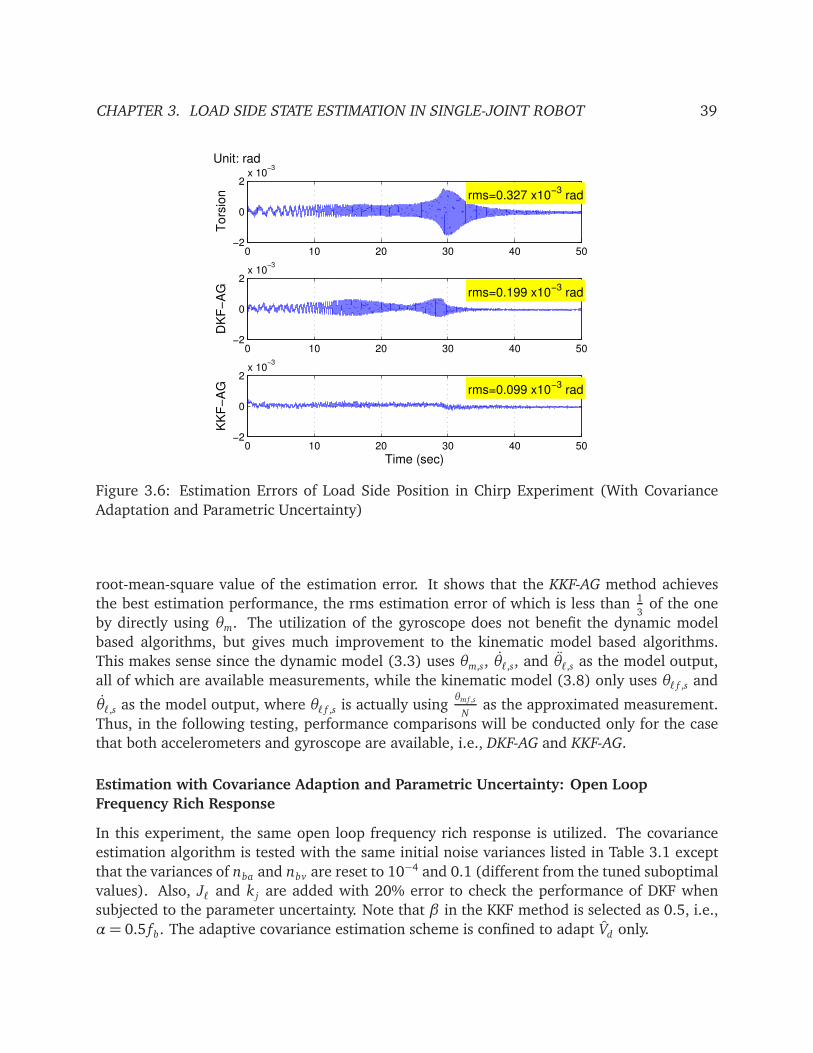
CHAPTER 3. LOAD SIDE STATE ESTIMATION IN SINGLE-JOINT ROBOT 39
0 10 20 30 40 50−2
0
2x 10
−3
rms=0.327 x10⁻³
rad
Tors
ion
0 10 20 30 40 50−2
0
2x 10
−3
rms=0.199 x10⁻³
rad
DK
F−
AG
0 10 20 30 40 50−2
0
2x 10
−3
rms=0.099 x10⁻³
rad
Time (sec)
KK
F−
AG
Unit: rad
Figure 3.6: Estimation Errors of Load Side Position in Chirp Experiment (With Covariance
Adaptation and Parametric Uncertainty)
root-mean-square value of the estimation error. It shows that the KKF-AG method achieves
the best estimation performance, the rms estimation error of which is less than 1
3of the one
by directly using θm. The utilization of the gyroscope does not benefit the dynamic model
based algorithms, but gives much improvement to the kinematic model based algorithms.
This makes sense since the dynamic model (3.3) uses θm,s, θℓ,s, and θℓ,s as the model output,
all of which are available measurements, while the kinematic model (3.8) only uses θℓ f ,s and
θℓ,s as the model output, where θℓ f ,s is actually usingθmf ,s
Nas the approximated measurement.
Thus, in the following testing, performance comparisons will be conducted only for the case
that both accelerometers and gyroscope are available, i.e., DKF-AG and KKF-AG.
Estimation with Covariance Adaption and Parametric Uncertainty: Open Loop
Frequency Rich Response
In this experiment, the same open loop frequency rich response is utilized. The covariance
estimation algorithm is tested with the same initial noise variances listed in Table 3.1 except
that the variances of nba and nbv are reset to 10−4 and 0.1 (different from the tuned suboptimal
values). Also, Jℓ and k j are added with 20% error to check the performance of DKF when
subjected to the parameter uncertainty. Note that β in the KKF method is selected as 0.5, i.e.,
α = 0.5 fb. The adaptive covariance estimation scheme is confined to adapt Vd only.

CHAPTER 3. LOAD SIDE STATE ESTIMATION IN SINGLE-JOINT ROBOT 40
0 5 10 15 20 25 30 35 40 45 50
0
2.5
5x 10
−3
DK
F−
AG
R(1
,1)
0 5 10 15 20 25 30 35 40 45 5005
1015
x 10−4
DK
F−
AG
R
(2,2
)
0 5 10 15 20 25 30 35 40 45 5005
1015
DK
F−
AG
R(3
,3)
0 5 10 15 20 25 30 35 40 45 500123
x 10−7
KK
F−
AG
R
(1,1
)
0 5 10 15 20 25 30 35 40 45 500
10
20x 10
−4
Time (sec)
KK
F−
AG
R
(2,2
)
Figure 3.7: Covariance Estimation in Chirp Experiment
Figure 3.6 shows that the KKF-AG method still achieves the best estimation performance,
where the estimation error is greatly reduced upon all the testing frequency range. The DKF-
AG method does not perform as good as KKF-AG, and it amplifies the estimation error at some
frequency range due to the parameter uncertainty.
The adapted Vd in both methods is shown in Fig. 3.7. As expected, to match the covari-
ance with the estimation results, Vd tends to increase when the estimation error is increasing
(especially around the resonant frequency 19Hz at about 30sec).
Figure 3.8 shows that both KKF-AG and DKF-AG are effective to estimate the biases of
gyroscope and accelerometer outputs. Thus, the bias effects in the utilization of sensor signals
are attenuated.
Estimation with Covariance Adaption and Parametric Uncertainty: Closed Loop
Trajectory Tracking
This experiment is to verify the effectiveness of the methods for specific tracking trajectory.
The desired load side trajectory is shown in Fig. 3.9, which is designed based on the fourth-
order smooth time optimal trajectory suggested in [55]. The feedback controller used here is
illustrated in Fig. 6.1 in Chapter 6 with basic PID and feedforward controller. All the covari-
ances and dynamic parameter values remain the same as those in the second chirp experiment
(Fig. 3.6) except for the window size NR used in the covariance adaptation scheme.

CHAPTER 3. LOAD SIDE STATE ESTIMATION IN SINGLE-JOINT ROBOT 41
0 10 20 30 40 50
0
5
10
15x 10
−3 Bias Estimation of Load Side Gyroscope
Time (sec)
Bia
s (
rad
/se
c)
0 10 20 30 40 50
0
0.02
0.04
0.06
Bias Estimation of Load Side Accelerometer
Time (sec)
Bia
s (
rad
/se
c2)
DKF−AG
KKF−AG
Identified Bias
DKF−AG
KKF−AG
Identified Bias
Figure 3.8: Bias Estimation in Chirp Experiment
0 5 10 15 20 25 300
0.5
1
Time (sec)
Po
sitio
n
(ra
d)
0 5 10 15 20 25 30−2
0
2
Time (sec)
Ve
locity
(ra
d/s
ec)
0 5 10 15 20 25 30−5
0
5
Time (sec)
Acce
lera
tio
n
(ra
d/s
ec
2)
Figure 3.9: Load Side Desired Trajectory

CHAPTER 3. LOAD SIDE STATE ESTIMATION IN SINGLE-JOINT ROBOT 42
0 5 10 15 20 25 30−1
0
1x 10
−3
rms=0.384 x10⁻³
radT
ors
ion
0 5 10 15 20 25 30−1
0
1x 10
−3
rms=0.215 x10⁻³
rad
DK
F−
AG
0 5 10 15 20 25 30−1
0
1x 10
−3
rms=0.166 x10⁻³
rad
Time (sec)
KK
F−
AG
Unit: rad
Figure 3.10: Estimation Errors of Load Side Position in Trajectory Experiment
0 5 10 15 20 25 30−8
−6
−4
−2
0
2
4
6
8x 10
−4
Time (sec)
Load S
ide P
ositio
n
Tra
ckin
g E
rror
Estim
ation (
rad)
Load Side Position Tracking Error Estimation
Using θm,s
Actual Error
KKF−AG
Figure 3.11: Load Side Actual and Estimated Position Tracking Error
CHAPTER 3. LOAD SIDE STATE ESTIMATION IN SINGLE-JOINT ROBOT 43
The result of this experiment is shown in Fig. 3.10, where KKF-AG still achieves the best
estimation performance. It is seen that the remaining estimation error by KKF-AG is oscillatory.
This is mainly due to the transmission error effect, since this effect is not considered in the
estimation algorithm. Figure 3.11 illustrates the actual and estimated tracking errors of the
load side position in this experiment. It shows that the tracking error estimated by KKF-AG
captures most trends of the actual tracking error. Therefore, the KKF-AG method is utilized in
the load side position tracking application, e.g., friction compensation in Chapter 6.
3.4 Discussion
Note that, the DKF and KKF methods are individually formulated based on separated models.
However, it may be beneficial to combine both the dynamic model and the kinematic model
for Kalman filter formulation. The following two ways may be used to achieve this objective.
First, in KKF, instead of simple first order low-pass filter G f (s) =α
s+α, the nominal dynamic
transfer functionθℓ (s)
θm (s)≈
d js+ k j
N
Jℓs2 + (d j + dℓ)s+ k j
can be used to obtain the load side position approximation from the motor side encoder mea-
surement, where • denotes the nominal value of •. The problem with this approach is that it
results in a higher order model formulation which introduces more complexity and computa-
tion load. Actually, it may not be favorable to use high order model since its high frequency
response will always be subject to large error due the model uncertainties. Furthermore, one
can note that nonlinear dynamic terms such as Coulomb friction and transmission error are
still not considered in this method due to the utilization of the linear transfer function.
The second way to approximate the load side position measurement is to use the dynamic
model (2.6a), which yields
θℓ,s =1
d js+ k j
k j
Nθm,s+
d j
Nθm,s− N
us + dm− Jmˆθm,s− dmθm,s
(3.15)
where θm,s and θm,s are obtained from motor encoder measurements. us can be either motor
torque command or measured by motor current. The desired trajectory θmd can be used
instead of ˆθm,s in (3.15) as approximation. By this approach, the nonlinear dynamic terms
have been taken into account as dm if good model knowledge of these terms is available. This
first order system formulation is relatively easy and efficient. Thus it will be adopted in the
load side state estimation method for multi-joint robot discussed in Chapter 5.
3.5 Chapter Summary
This chapter presented the load side state estimation algorithm for the single-joint indirect
drive robot based on a multi-sensor configuration. Kalman filtering method was formulated
CHAPTER 3. LOAD SIDE STATE ESTIMATION IN SINGLE-JOINT ROBOT 44
using the extended dynamic/kinematic model taking measurement dynamics (bias and noise)
into consideration. Noise covariance adaptation was studied. The effectiveness of the method
was verified experimentally on a single-joint indirect drive robot setup. The developed KKF
method will be applied to the friction compensation application in Chapter 6.

45
Chapter 4
End-effector State Estimation in
Multi-Joint Robot
4.1 Introduction
In Chapter 3 on load side state estimation, the kinematic Kalman filter (KKF) algorithm was
formulated for the single joint robot by fusing the measurements of load side inertial sen-
sors (accelerometer and gyroscope) with the measurement of the motor side encoder. In this
chapter, this KKF algorithm is extended to the multi-joint robot to estimate the end-effector
information.
In robot applications, the end-effector performance enhancement is the ultimate objective.
In general, position, velocity, and orientation information of the end-effector is all impor-
tant for motion control. Without consideration of cost and assembly issues, many different
kinds of end-effector senors could be utilized for such purpose, such as vision camera for po-
sition/pattern sensing, inertia sensor for acceleration and angular velocity sensing, and laser
tracker for position sensing. However, none of these sensors alone would be sufficient for
obtaining all the desired end-effector information. For example, the PSD camera (see Ap-
pendix A.4.3) developed in [94] has good capability on position sensing. Its measurement
alone, however, is not sufficient to support fine velocity or orientation estimation. Also, al-
most all sensors exhibit some kind of limitations, such as slow sampling rate for vision camera,
noneligible bias and noise in low-cost MEMS sensors. To address these issues, it is favorable
to investigate the multi-sensor fusion approach to complement each individual sensor’s limi-
tations.
Some previous work on the multi-sensor fusion for the multi-joint robot has been reported
in [53]. In [53], the idea of multi-dimensional kinematic Kalman filter (MD-KKF) algorithm
using the measurements of the vision camera and inertia sensors was proposed. The effec-
tiveness of the method was validated through experiments on a two-link direct-drive robot.
However, the technical potential of this approach cannot be fully validated on this simple
2-DOF planar robot.

CHAPTER 4. END-EFFECTOR STATE ESTIMATION IN MULTI-JOINT ROBOT 46
In this chapter, the idea of MD-KKF method is revisited and implemented on the 6-DOF
FANUC M-16iB robot system. In order to follow the idea of fusing vision sensor signals with
inertia sensor signals, the CompuGauge 3D measurement output is resampled and adjusted to
typical vision sensor specifications to simulate the vision sensor measurements. Furthermore,
another experimental study is conducted with the inertia senor and the newly developed PSD
camera, which is capable of end-effector position sensing with fast sampling rate and high
precision. Promising results on the tool center point (TCP) velocity/orientation estimation
have been demonstrated.
This chapter is organized as follows. A multi-dimensional (MD) kinematic model of the
robot end-effector is introduced first in Section 4.2. Then the idea of MD-KKF method is
revisited in Section 4.3. Finally, the experimental study of the method on the FANUC M-16iB
robot is presented in Section 4.4. The conclusion of this work is given in Section 4.5 at last.
4.2 MD Kinematic Model
4.2.1 MD Rigid Body Motion
For the MD-KKF scheme on the FANUC M-16iB robot system, consider the sensor configuration
and coordinate system shown in Fig. 4.1. The CompuGauge 3D measurement point is used to
simulate the virtual TCP, the absolute position of which is assumed to be measured by 3D vision
sensors. There are two infrared markers attached on the end-effector for the PSD camera
sensing (see [94] for more details). The inertia measurement unit (IMU) (3-axial gyroscope
and 3-axial accelerometer) is attached to a fixed point on the end-effector of the robot. For
convenience, denote the inertia sensor measurement point as the wrist. The coordinate frame
of the inertia sensor is aligned with the body coordinate frame of the end-effector, denoted by
(x b, y b, z b). The spatial (world) coordinate frame is represented as (x s, y s, zs). The desired
and the actual paths that TCP is following are shown as dash line and solid line in the figure,
respectively.
Based on the above coordinate system definition, the MD rigid body motion on the end-
effector can be described as
psT C P= vs
wr+R
ωb×
rbT C P/wr
(4.1a)
vswr= Rfb
wr+ gs (4.1b)
R= R
ωb×
(4.1c)
where psT C P
and vswr
are the position of the TCP and the velocity of the wrist in world coor-
dinates, (x s, y s, zs), respectively. R is the rotational matrix of the end-effector mapping from
the body coordinate frame to the world coordinate frame. ωb and fbwr
are the angular velocity
and the linear acceleration of the wrist in the body frame, (x b, y b, z b), respectively. Note that
the accelerometer includes the gravity effect gs =
0 0 gz
Tin the actual measurement.
Finally, rbT C P/wr
denotes the position vector of the TCP relative to the wrist in the body frame.

CHAPTER 4. END-EFFECTOR STATE ESTIMATION IN MULTI-JOINT ROBOT 47
Inertia
Sensors
Wrist
Desired PathTCP
Actual Path
xs
zs
ys
Os
xb
zb
yb
Ob
Infrared Markers
Figure 4.1: Sensor Configuration and Coordinate System of FANUC M-16iB Robot End-effector
Note that, [a×] ∈ R3×3 is the skew-symmetric matrix, equivalent to the cross product oper-
ation of the corresponding vector, i.e., for a,b ∈ R3, [a×]b ≡ a × b. More specifically, for
a=
a1 a2 a3
T,
[a×] =
0 −a3 a2
a3 0 −a1
−a2 a1 0
(4.2)
4.2.2 Sensor Measurement Dynamics
The inertia measurement unit (IMU), which consists of a set of MEMS sensors, has non-
negligible sensor biases and noises that need to be accounted for when utilizing the mea-
surement outputs. Also the vision sensors’ accuracy is also be subject to certain biases and
noises. This sensor measurement dynamics can be modeled as follows
bω = nbω(4.3a)
ωb =ωb + bω+ nω (4.3b)
b f = nb f(4.3c)
fbwr= fb
wr+ b f + n f (4.3d)
bp = nbp(4.3e)
psT C P= ps
T C P+ bp + np (4.3f)
where • is the real quantity to be measured and • is the corresponding measurement output.
b• is the bias of the measurement output •, which is modeled to be updated by the fictitious
noise nb•. n• is the noise of the measurement •.
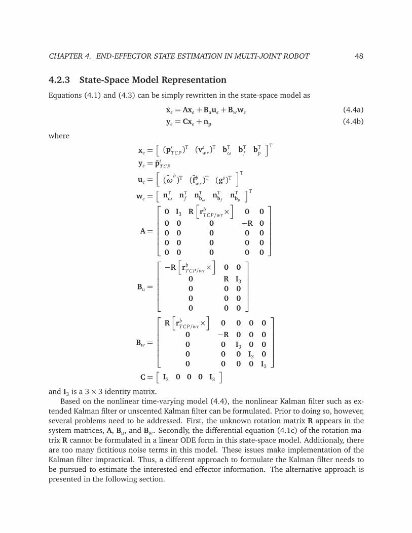
CHAPTER 4. END-EFFECTOR STATE ESTIMATION IN MULTI-JOINT ROBOT 48
4.2.3 State-Space Model Representation
Equations (4.1) and (4.3) can be simply rewritten in the state-space model as
xe = Axe +Buue +Bwwe (4.4a)
ye = Cxe + np (4.4b)
where
xe =
(psT C P)T (vs
wr)T bT
ωbT
fbT
p
T
ye = psT C P
ue =h
¯(ωb)T (fb
wr)T (gs)T
iT
we =
nTω
nTf
nTbω
nTb f
nTbp
T
A=
0 I3 Rh
rbT C P/wr
×i
0 0
0 0 0 −R 0
0 0 0 0 0
0 0 0 0 0
0 0 0 0 0
Bu =
−Rh
rbT C P/wr
×i
0 0
0 R I3
0 0 0
0 0 0
0 0 0
Bw =
Rh
rbT C P/wr
×i
0 0 0 0
0 −R 0 0 0
0 0 I3 0 0
0 0 0 I3 0
0 0 0 0 I3
C=
I3 0 0 0 I3
and I3 is a 3× 3 identity matrix.
Based on the nonlinear time-varying model (4.4), the nonlinear Kalman filter such as ex-
tended Kalman filter or unscented Kalman filter can be formulated. Prior to doing so, however,
several problems need to be addressed. First, the unknown rotation matrix R appears in the
system matrices, A, Bu, and Bw. Secondly, the differential equation (4.1c) of the rotation ma-
trix R cannot be formulated in a linear ODE form in this state-space model. Additionaly, there
are too many fictitious noise terms in this model. These issues make implementation of the
Kalman filter impractical. Thus, a different approach to formulate the Kalman filter needs to
be pursued to estimate the interested end-effector information. The alternative approach is
presented in the following section.

CHAPTER 4. END-EFFECTOR STATE ESTIMATION IN MULTI-JOINT ROBOT 49
End-effector Position
Measurements
Wrist Gyro. & Accl.
Measurements
MD-KKF based on
MD Kinematic
Model
TCP Estimation
Position
Velocity
Orientation
Camera
IMU
Figure 4.2: Basic Structure of MD-KKF Scheme
4.3 MD Kinematic Kalman Filter
The MD-KKF approach proposed in [53] is revisited and extended in this section. The basic
structure of this scheme is shown in Fig. 4.2. This scheme fuses the end-effector position
measurement from the camera device with the acceleration and angular velocity information
from the inertia sensors. The Kalman filter is formulated based on the MD kinematic model
(4.1) to estimate the TCP information.
To investigate the feasibility of the MD-KKF scheme, an assumption is made to simplify the
design process. Assume that the biases in the sensor measurements are time-invariant (or very
slowly time-varying), and they have been accurately identified and removed in the utilization
of the measurement outputs. As a result, the sensor bias terms (bω, b f , bp) are neglected.
Then the system model is simplified to focus on the basic MD rigid body motion in (4.1).
4.3.1 Prediction by Inertia Sensor Measurement
From (4.1), the open loop estimation of the continuous time states can be written as
˙psoT C P= vso
wr+ Ro
ωb×
rbT C P/wr
(4.6a)
˙vsowr= Ro fb
wr+ gs (4.6b)
˙Ro = Ro
ωb×
(4.6c)
where •o denotes the open loop estimate of the corresponding variable •.
The discrete time form of the open loop estimator (4.6) is then given by
Ro(k+ 1) = Ro(k)
I3+ Ts[ωb(k+ 1)×] +
T 2s
2[ωb(k+ 1)×]2
(4.7a)
pso
T C P(k+ 1)
vsowr(k+ 1)
=
I3 TsI3
0 I3
pso
T C P(k)
vsowr(k)
+ Ts
−Ro(k+ 1)[rbT C P/wr
×]Ts
2Ro(k+ 1)
0 Ro(k+ 1)
×
ωb(k+ 1)
fbwr(k+ 1)
+ Ts
Ts
2I3
I3
gs (4.7b)
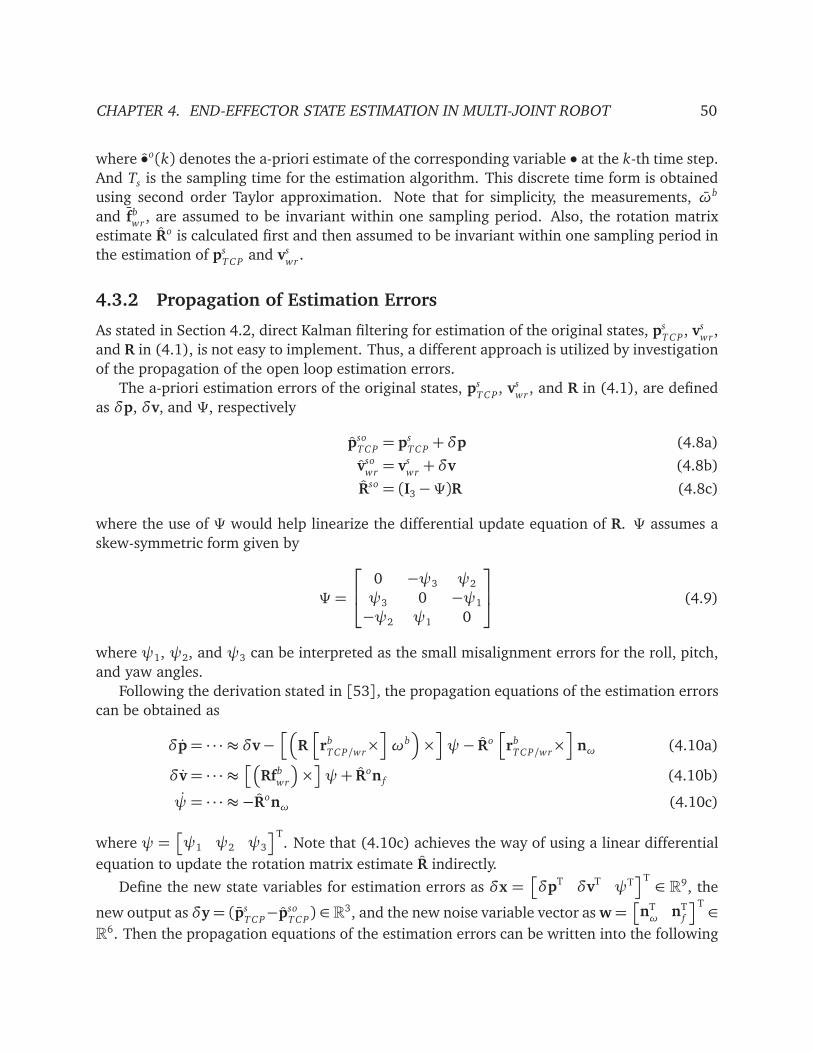
CHAPTER 4. END-EFFECTOR STATE ESTIMATION IN MULTI-JOINT ROBOT 50
where •o(k) denotes the a-priori estimate of the corresponding variable • at the k-th time step.
And Ts is the sampling time for the estimation algorithm. This discrete time form is obtained
using second order Taylor approximation. Note that for simplicity, the measurements, ωb
and fbwr
, are assumed to be invariant within one sampling period. Also, the rotation matrix
estimate Ro is calculated first and then assumed to be invariant within one sampling period in
the estimation of psT C P
and vswr
.
4.3.2 Propagation of Estimation Errors
As stated in Section 4.2, direct Kalman filtering for estimation of the original states, psT C P
, vswr
,
and R in (4.1), is not easy to implement. Thus, a different approach is utilized by investigation
of the propagation of the open loop estimation errors.
The a-priori estimation errors of the original states, psT C P
, vswr
, and R in (4.1), are defined
as δp, δv, and Ψ, respectively
psoT C P= ps
T C P+δp (4.8a)
vsowr= vs
wr+δv (4.8b)
Rso = (I3−Ψ)R (4.8c)
where the use of Ψ would help linearize the differential update equation of R. Ψ assumes a
skew-symmetric form given by
Ψ =
0 −ψ3 ψ2
ψ3 0 −ψ1
−ψ2 ψ1 0
(4.9)
where ψ1, ψ2, and ψ3 can be interpreted as the small misalignment errors for the roll, pitch,
and yaw angles.
Following the derivation stated in [53], the propagation equations of the estimation errors
can be obtained as
δp= · · · ≈ δv−h
Rh
rbT C P/wr
×i
ωb
×i
ψ− Roh
rbT C P/wr
×i
nω (4.10a)
δv= · · · ≈
Rfbwr
×
ψ+ Ron f (4.10b)
ψ= · · · ≈ −Ronω (4.10c)
where ψ =
ψ1 ψ2 ψ3
T. Note that (4.10c) achieves the way of using a linear differential
equation to update the rotation matrix estimate R indirectly.
Define the new state variables for estimation errors as δx =
δpT δvT ψTT∈ R
9, the
new output as δy= (psT C P−pso
T C P) ∈ R
3, and the new noise variable vector as w=
nTω
nTf
T∈
R6. Then the propagation equations of the estimation errors can be written into the following
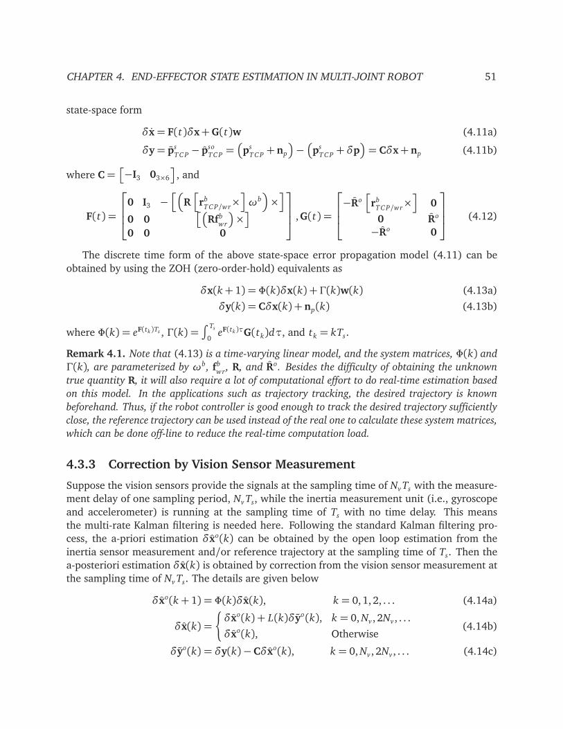
CHAPTER 4. END-EFFECTOR STATE ESTIMATION IN MULTI-JOINT ROBOT 51
state-space form
δx= F(t)δx+G(t)w (4.11a)
δy= psT C P− pso
T C P=
psT C P+ np
−
psT C P+δp
= Cδx+ np (4.11b)
where C=
−I3 03×6
, and
F(t) =
0 I3 −h
Rh
rbT C P/wr
×i
ωb
×i
0 0
Rfbwr
×
0 0 0
,G(t) =
−Roh
rbT C P/wr
×i
0
0 Ro
−Ro 0
(4.12)
The discrete time form of the above state-space error propagation model (4.11) can be
obtained by using the ZOH (zero-order-hold) equivalents as
δx(k+ 1) = Φ(k)δx(k) + Γ(k)w(k) (4.13a)
δy(k) = Cδx(k) + np(k) (4.13b)
where Φ(k) = eF(tk)Ts , Γ(k) =∫ Ts
0eF(tk)τG(tk)dτ, and tk = kTs.
Remark 4.1. Note that (4.13) is a time-varying linear model, and the system matrices, Φ(k) and
Γ(k), are parameterized by ωb, fbwr
, R, and Ro. Besides the difficulty of obtaining the unknown
true quantity R, it will also require a lot of computational effort to do real-time estimation based
on this model. In the applications such as trajectory tracking, the desired trajectory is known
beforehand. Thus, if the robot controller is good enough to track the desired trajectory sufficiently
close, the reference trajectory can be used instead of the real one to calculate these system matrices,
which can be done off-line to reduce the real-time computation load.
4.3.3 Correction by Vision Sensor Measurement
Suppose the vision sensors provide the signals at the sampling time of Nv Ts with the measure-
ment delay of one sampling period, Nv Ts, while the inertia measurement unit (i.e., gyroscope
and accelerometer) is running at the sampling time of Ts with no time delay. This means
the multi-rate Kalman filtering is needed here. Following the standard Kalman filtering pro-
cess, the a-priori estimation δxo(k) can be obtained by the open loop estimation from the
inertia sensor measurement and/or reference trajectory at the sampling time of Ts. Then the
a-posteriori estimation δx(k) is obtained by correction from the vision sensor measurement at
the sampling time of Nv Ts. The details are given below
δxo(k+ 1) = Φ(k)δx(k), k = 0, 1, 2, . . . (4.14a)
δx(k) =
¨
δxo(k) + L(k)δyo(k), k = 0, Nv , 2Nv , . . .
δxo(k), Otherwise(4.14b)
δyo(k) = δy(k)−Cδxo(k), k = 0, Nv , 2Nv , . . . (4.14c)

CHAPTER 4. END-EFFECTOR STATE ESTIMATION IN MULTI-JOINT ROBOT 52
where the Kalman filter gain L(k) is calculated by
L(k) = M(k)CT[CM(k)CT + V (k)]−1, k = 0, Nv , 2Nv , . . . (4.15a)
M(k+ 1) = Φ(k)Z(k)ΦT(k) + Γ(k)W (k)ΓT(k), k = 0, 1, 2, . . . (4.15b)
Z(k) =
¨
M(k)− L(k)CM(k), k = 0, Nv , 2Nv , . . .
M(k), Otherwise(4.15c)
where W (k) and V (k) are the covariance estimates of w(k) and np(k), respectively. M(k)
and Z(k) are the one-step a-priori and a-posteriori covariances of the state estimation error,
respectively. Note that due to the slow sampling rate of the vision sensor measurements, the
a-posteriori correction δyo(k) from the vision measurement and the Kalman filter gain L(k)
are calculated at the sampling time of Nv Ts.
Furthermore, with the measurement delay, the error propagation output δy(k) is actually
based on the vision measurement available at the (k + Nv)-th time step. More specifically,
when calculating the error propagation output δy(k), (4.11b) is modified to
δy(k) = psT C P(k+ Nv)− pso
T C P(k) = Cδx(k) + np(k), k = 0, Nv , 2Nv , . . . (4.16)
Thus, an Nv-time-step delay is required for the a-priori estimate to be corrected by the
vision sensor measurement, which doubles the computation load for the prediction step. For
example, to obtain the estimation from the Nv-th to the (2Nv − 1)-th time step, the following
procedure needs to be carried out:
1. For k = Nv , . . . , 2Nv − 1, the open-loop estimation is done using (4.14a) and the second
case of (4.14b).
2. At the 2Nv-th time step, the vision measurement for the Nv-th time step becomes avail-
able.
3. Equation (4.14c) and the first case of (4.14b) are used to recalculate the a-posteriori es-
timate δx(k) for k = Nv using the newly obtained 2Nv-th time step vision measurement.
4. Equation (4.14a) and the second case of (4.14b) are used again to recalculate the a-
posteriori estimate δx(k) for k = Nv + 1, . . . , 2Nv − 1.
Finally, denoting δx=
δpT δvT ψTT∈ R
9, the a-posteriori estimations of the position,
the velocity, and the rotation matrix are updated as follows
psT C P(k) = pso
T C P(k)−δp(k) (4.17a)
vswr(k) = vso
wr(k)−δv(k) (4.17b)
R(k) =
I3−
ψ(k)×−1
Ro(k) (4.17c)
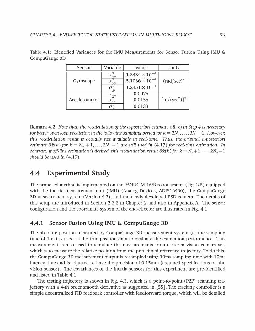
CHAPTER 4. END-EFFECTOR STATE ESTIMATION IN MULTI-JOINT ROBOT 53
Table 4.1: Identified Variances for the IMU Measurements for Sensor Fusion Using IMU &
CompuGauge 3D
Sensor Variable Value Units
Gyroscope
σ2x x
1.8434× 10−4
(rad/sec)2σ2
y y5.1036× 10−4
σ2zz
1.2451× 10⁻⁴
Accelerometer
σ2x x
0.0075
[m/(sec2)]2σ2y y
0.0155
σ2zz
0.0133
Remark 4.2. Note that, the recalculation of the a-posteriori estimate δx(k) in Step 4 is necessary
for better open loop prediction in the following sampling period for k = 2Nv , . . . , 3Nv−1. However,
this recalculation result is actually not available in real-time. Thus, the original a-posteriori
estimate δx(k) for k = Nv + 1, . . . , 2Nv − 1 are still used in (4.17) for real-time estimation. In
contrast, if off-line estimation is desired, this recalculation result δx(k) for k = Nv+1, . . . , 2Nv−1
should be used in (4.17).
4.4 Experimental Study
The proposed method is implemented on the FANUC M-16iB robot system (Fig. 2.5) equipped
with the inertia measurement unit (IMU) (Analog Devices, ADIS16400), the CompuGauge
3D measurement system (Version 4.3), and the newly developed PSD camera. The details of
this setup are introduced in Section 2.3.2 in Chapter 2 and also in Appendix A. The sensor
configuration and the coordinate system of the end-effector are illustrated in Fig. 4.1.
4.4.1 Sensor Fusion Using IMU & CompuGauge 3D
The absolute position measured by CompuGauge 3D measurement system (at the sampling
time of 1ms) is used as the true position data to evaluate the estimation performance. This
measurement is also used to simulate the measurements from a stereo vision camera set,
which is to measure the relative position from the predefined reference trajectory. To do this,
the CompuGauge 3D measurement output is resampled using 10ms sampling time with 10ms
latency time and is adjusted to have the precision of 0.15mm (assumed specifications for the
vision sensor). The covariances of the inertia sensors for this experiment are pre-identified
and listed in Table 4.1.
The testing trajectory is shown in Fig. 4.3, which is a point-to-point (P2P) scanning tra-
jectory with a 4-th order smooth derivative as suggested in [55]. The tracking controller is a
simple decentralized PID feedback controller with feedforward torque, which will be detailed

CHAPTER 4. END-EFFECTOR STATE ESTIMATION IN MULTI-JOINT ROBOT 54
2 2.2 2.4 2.6 2.8 3 3.2 3.4 3.6 3.8 40.85
0.9
0.95
1
1.05
Po
sitio
n
X (
m)
2 2.2 2.4 2.6 2.8 3 3.2 3.4 3.6 3.8 4
−0.3
−0.2
−0.1
0
Po
sitio
n
Y (
m)
2 2.2 2.4 2.6 2.8 3 3.2 3.4 3.6 3.8 4
0.8
1
1.2
Time (sec)
Po
sitio
n
Z (
m)
CG (Real)
MD−KKF
"Vision"
(a) TCP Position Estimation
2 2.2 2.4 2.6 2.8 3 3.2 3.4 3.6 3.8 4
−0.1
−0.05
0
0.05
Ve
locity X
(m
/se
c)
CG (Real)
MD−KKF
"Vision"
2 2.2 2.4 2.6 2.8 3 3.2 3.4 3.6 3.8 4−0.4
−0.2
0
Ve
locity Y
(m
/se
c)
2 2.2 2.4 2.6 2.8 3 3.2 3.4 3.6 3.8 4
−0.4
−0.2
0
Time (sec)
Ve
locity Z
(m
/se
c)
(b) TCP Velocity Estimation
2 2.5 3 3.53
3.2
3.4
Ro
ll X
(r
ad
)
2 2.5 3 3.5−1
0
1
Pitch
Y
(ra
d)
Encoder
MD−KKF
2 2.5 3 3.52.8
3
3.2
Time (sec)
Ya
w Z
(r
ad
)
(c) TCP Orientation Estimation
Figure 4.3: TCP Estimation for P2P Scanning Trajectory (with IMU & CompuGauge)

CHAPTER 4. END-EFFECTOR STATE ESTIMATION IN MULTI-JOINT ROBOT 55
in Chapter 7. The controller and the MD-KKF method are running at the sampling time of
1ms. The fictitious vision sensor provides the position measurement at the sampling time of
10ms with 10ms time delay, i.e., Nv = 10. The Kalman filter gain for each correction step is
calculated beforehand using the desired trajectory.
Figure 4.3a shows the TCP position estimation result. It can be seen that the estimated
TCP position (MD-KKF) captures the true position (CG(Real)) smoothly and closely, while the
fictitious vision measurement ("Vision") shows the time delay and slow sampling rate effects.
The TCP velocity and orientation estimation results are shown in Fig. 4.3b and Fig. 4.3c
respectively. The benefits of the MD-KKF method can be appreciated clearly from these two
figures. The velocity data (CG(Real)), generated by backward numerical differentiation of
the original CompuGauge measurement, is used as the true velocity data to evaluate the per-
formance. The velocity data generated similarly from the fictitious vision measurements ("Vi-
sion"), however, appears to be very noisy compared to the clean velocity estimation (MD-KKF).
The orientation estimation is illustrated by Roll-Pitch-Yaw Euler angle set [74]. Figure 4.3c
shows that the orientation estimation (MD-KKF) also closely follows the orientation data cal-
culated from the forward kinematics of the motor encoder data (Encoder), while the vision
sensor or CompuGauge 3D does not provide any orientation measurement.
4.4.2 Sensor Fusion Using IMU & PSD Camera
The PSD camera developed in [94] provides another mean of end-effector position sensing
with fast sampling rate and high precision. With this new TCP position sensing device, the MD-
KKF scheme is applied again to further validate the sensor fusion method for TCP information
estimation.
Note that, since the PSD camera achieves a high sampling rate, the drawbacks of the low
sampling rate and measurement delay in the normal vision camera system are no longer an
issue. Actually, the original PSD camera measurement is filtered and downsampled to get the
same sampling rate (i.e., 1kHz) as that of the IMU signals and the estimation algorithm. Thus,
in the MD-KKF algorithm, it is set that Nv = 1 without measurement delay.
Again, the absolute position measured by CompuGauge system is used as the true value
for performance evaluation. Note that, the developed PSD camera has good capability on
the position sensing (see Fig. 4.4). Thus, the main objective here is to obtain better TCP
velocity/orientation estimate rather than the TCP position estimate.
The covariances of the inertia sensor and PSD camera measurements are pre-identified for
each experiment and are listed in Table 4.2. The slight difference of the variances between dif-
ferent experiments are due to the time-varying property of the MEMS sensor for environmental
changes, and also the PSD calibration process for each experiment. The larger covariances of
PSD camera measurement for curve trajectory are due to the combination of measurements
for two markers (see second set of experiment later).
Note that the current setting (i.e., one camera and one/two markers) of PSD camera is
only capable of two-dimensional position sensing (at X-Z plane). Thus, in order to implement
the MD-KKF algorithm, a fictitious Y-axis position measurement is added into the final PSD
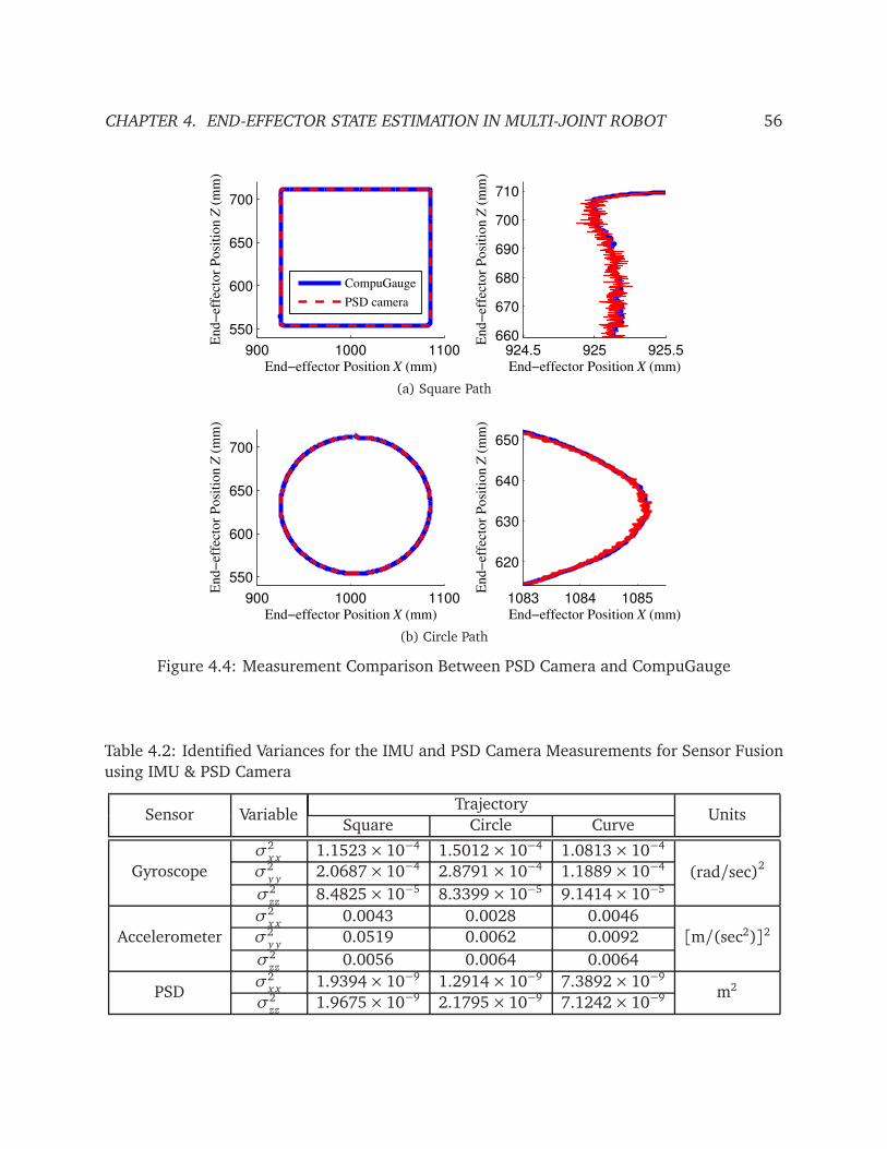
CHAPTER 4. END-EFFECTOR STATE ESTIMATION IN MULTI-JOINT ROBOT 56
900 1000 1100
550
600
650
700
End−effector Position X (mm)
End−
effe
ctor
Posi
tion Z
(m
m)
CompuGauge
PSD camera
924.5 925 925.5660
670
680
690
700
710
End−effector Position X (mm)
End−
effe
ctor
Posi
tion Z
(m
m)
(a) Square Path
900 1000 1100
550
600
650
700
End−effector Position X (mm)
End−
effe
ctor
Posi
tion Z
(m
m)
1083 1084 1085
620
630
640
650
End−effector Position X (mm)
End−
effe
ctor
Posi
tion Z
(m
m)
(b) Circle Path
Figure 4.4: Measurement Comparison Between PSD Camera and CompuGauge
Table 4.2: Identified Variances for the IMU and PSD Camera Measurements for Sensor Fusion
using IMU & PSD Camera
Sensor VariableTrajectory
UnitsSquare Circle Curve
Gyroscope
σ2x x
1.1523× 10−4 1.5012× 10⁻⁴ 1.0813× 10⁻⁴
(rad/sec)2σ2
y y2.0687× 10−4 2.8791× 10⁻⁴ 1.1889× 10⁻⁴
σ2zz
8.4825× 10⁻⁵ 8.3399× 10⁻⁵ 9.1414× 10⁻⁵
Accelerometer
σ2x x
0.0043 0.0028 0.0046
[m/(sec2)]2σ2y y
0.0519 0.0062 0.0092
σ2zz
0.0056 0.0064 0.0064
PSDσ2
x x1.9394× 10−9 1.2914× 10⁻⁹ 7.3892× 10⁻⁹
m2
σ2zz
1.9675× 10⁻⁹ 2.1795× 10⁻⁹ 7.1242× 10⁻⁹

CHAPTER 4. END-EFFECTOR STATE ESTIMATION IN MULTI-JOINT ROBOT 57
0 0.5 1 1.5 2 2.5 30.9
0.95
1
1.05
1.1
Po
sitio
n X
(m
)
0 0.5 1 1.5 2 2.5 3
0.55
0.6
0.65
0.7
0.75
Time (sec)
Po
sitio
n Z
(m
)PSD
CG (Real)
MD−KKF
(a) TCP Position Estimation
0 0.5 1 1.5 2 2.5 3−0.5
0
0.5
Ve
locity X
(m
/se
c)
0 0.5 1 1.5 2 2.5 3−0.5
0
0.5
Time (sec)
Ve
locity Z
(m
/se
c)
PSD
CG (Real)
MD−KKF
(b) TCP Velocity Estimation
Figure 4.5: TCP Estimation for Square Trajectory without Orientation Change
camera measurement. Without loss of generality, this Y-axis position measurement is set to
be simply the same constant value as in the robot home position. And the variance of this
fictitious measurement is set to be the same as X-axis measurement.
Two sets of experiments are conducted as follows.
Using IMU & PSD Camera (One Marker)
In the first set, one marker is installed on the end-effector, providing two-dimensional position
sensing without rotation measurement. The testing TCP trajectories are designed to be only
within the X-Z plane without orientation changes. Two testing TCP trajectories are shown in
Fig. 4.4. The first one is a 160mm×160mm square with a peak Cartesian speed of 300mm/sec.
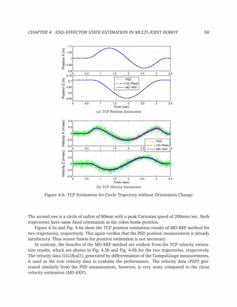
CHAPTER 4. END-EFFECTOR STATE ESTIMATION IN MULTI-JOINT ROBOT 58
0 0.5 1 1.5 2 2.5 3 3.50.9
0.95
1
1.05
1.1
Po
sitio
n X
(m
)
0 0.5 1 1.5 2 2.5 3 3.5
0.55
0.6
0.65
0.7
0.75
Time (sec)
Po
sitio
n Z
(m
)
PSD
CG (Real)
MD−KKF
(a) TCP Position Estimation
0 0.5 1 1.5 2 2.5 3 3.5−0.4
−0.2
0
0.2
0.4
Ve
locity X
(m
/se
c)
0 0.5 1 1.5 2 2.5 3 3.5−0.4
−0.2
0
0.2
0.4
Time (sec)
Ve
locity Z
(m
/se
c)
PSD
CG (Real)
MD−KKF
(b) TCP Velocity Estimation
Figure 4.6: TCP Estimation for Circle Trajectory without Orientation Change
The second one is a circle of radius of 80mm with a peak Cartesian speed of 200mm/sec. Both
trajectories have same fixed orientation as the robot home position.
Figure 4.5a and Fig. 4.6a show the TCP position estimation results of MD-KKF method for
two trajectories, respectively. This again verifies that the PSD position measurement is already
satisfactory. Thus sensor fusion for position estimation is not necessary.
In contrast, the benefits of the MD-KKF method are evident from the TCP velocity estima-
tion results, which are shown in Fig. 4.5b and Fig. 4.6b for the two trajectories, respectively.
The velocity data (CG(Real)), generated by differentiation of the CompuGauge measurements,
is used as the true velocity data to evaluate the performance. The velocity data (PSD) gen-
erated similarly from the PSD measurement, however, is very noisy compared to the clean
velocity estimation (MD-KKF).
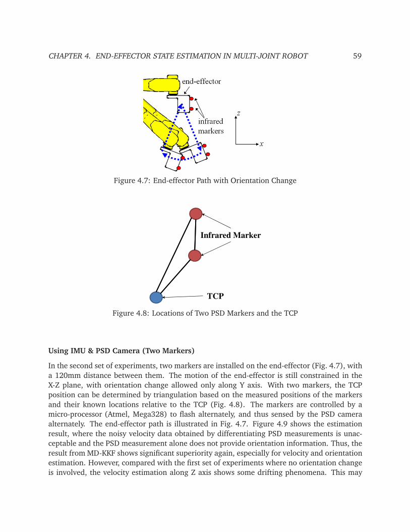
CHAPTER 4. END-EFFECTOR STATE ESTIMATION IN MULTI-JOINT ROBOT 59
Figure 4.7: End-effector Path with Orientation Change
Infrared Marker
TCP
Figure 4.8: Locations of Two PSD Markers and the TCP
Using IMU & PSD Camera (Two Markers)
In the second set of experiments, two markers are installed on the end-effector (Fig. 4.7), with
a 120mm distance between them. The motion of the end-effector is still constrained in the
X-Z plane, with orientation change allowed only along Y axis. With two markers, the TCP
position can be determined by triangulation based on the measured positions of the markers
and their known locations relative to the TCP (Fig. 4.8). The markers are controlled by a
micro-processor (Atmel, Mega328) to flash alternately, and thus sensed by the PSD camera
alternately. The end-effector path is illustrated in Fig. 4.7. Figure 4.9 shows the estimation
result, where the noisy velocity data obtained by differentiating PSD measurements is unac-
ceptable and the PSD measurement alone does not provide orientation information. Thus, the
result from MD-KKF shows significant superiority again, especially for velocity and orientation
estimation. However, compared with the first set of experiments where no orientation change
is involved, the velocity estimation along Z axis shows some drifting phenomena. This may

CHAPTER 4. END-EFFECTOR STATE ESTIMATION IN MULTI-JOINT ROBOT 60
be due to the calibration inaccuracy of the gyroscope. To address this, a more complex sensor
fusion algorithm with the consideration of sensor self-calibration may be necessary.
4.5 Chapter Summary
This chapter presented the study on the sensor fusion work for the purpose of end-effector
state estimation. An MD-KKF scheme for the multi-joint robot based on the work in [53]
was re-investigated. Some minor extensions were presented and the method was then imple-
mented on the 6-DOF FANUC M-16iB robot system with equipped inertia measurement unit,
CompuGauge 3D, and also newly developed PSD camera. The experimental results showed
that the proposed method was effective to estimate the TCP information using the fusion of
the sensor signals at two different sampling rates (e.g., inertia sensor signals and fictitious
vision sensor signals), and was especially beneficial for TCP velocity/orientation estimation.
However, this algorithm was formulated for the simplified case without consideration of sen-
sor biases. Thus, self-calibration technique of sensor signals to incorporate with the MD-KKF
scheme may be a key aspect if the estimation performance is to be further improved.

CHAPTER 4. END-EFFECTOR STATE ESTIMATION IN MULTI-JOINT ROBOT 61
11 11.5 12 12.5 13 13.5 14 14.5 150.8
0.9
1
1.1
Positio
n X
(m
)
11 11.5 12 12.5 13 13.5 14 14.5 15
0.65
0.7
0.75
Time (sec)
Positio
n Z
(m
)
PSD
CG (Real)
MD−KKF
(a) TCP Position Estimation
11 11.5 12 12.5 13 13.5 14 14.5 15−1
−0.5
0
0.5
Velo
city X
(m
/sec)
11 11.5 12 12.5 13 13.5 14 14.5 15−0.5
0
0.5
Time (sec)
Velo
city Z
(m/s
ec)
PSD
CG (Real)
MD−KKF
(b) TCP Velocity Estimation
11 11.5 12 12.5 13 13.5 14 14.5 15
3
3.5
Roll
X
(rad)
11 11.5 12 12.5 13 13.5 14 14.5 15−0.5
0
0.5
Pitch Y
(r
ad)
11 11.5 12 12.5 13 13.5 14 14.5 153
3.1
3.2
Time (sec)
Yaw
Z
(rad)
Encoder
MD−KKF
(c) TCP Orientation Estimation
Figure 4.9: TCP Estimation for Curve Path with Orientation Change

62
Chapter 5
Load Side Joint State Estimation in
Multi-Joint Robot
5.1 Introduction
As discussed in previous chapters, in robot applications, discrepancies between the available
and the desired measurements make it difficult to achieve good control performance. These
discrepancies are caused by both sensor and robot dynamics. Particularly, in robots with com-
plex joint dynamics (e.g., flexibilities, friction, etc.), end-effector performance cannot be guar-
anteed with motor side information alone. This mismatched sensing problem is a critical issue
for most practical robot applications where only motor side information is available.
In previous chapters, it has been proposed that this problem can be tackled by adopting
low-cost MEMS sensors, such as an accelerometer, for robot end-effector sensing. Since de-
coupled joint space position/velocity control is usually preferred in industrial robot control,
end-effector sensing with end-effector state estimation only is not ideal/sufficient. Therefore,
it would be most beneficial to be able to estimate the load side joint states from the end-
effector measurements.
In Chapter 3, a Kalman filter scheme using either dynamic model or kinematic model was
investigated for a single-joint robot with joint elasticity. The scheme fused the motor encoder
measurements with the load side inertia sensor signals to estimate the load side position. The
multi-dimensional kinematic Kalman filter (MD-KKF) proposed in [53] was reinvestigated in
Chapter 4 for multi-joint robot end-effector sensing. Several end-effector sensors (i.e., camera,
gyroscope, and accelerometer) were required. The approach, however, was not able to directly
achieve joint space estimation nor utilize available motor encoder information. In [69, 27],
joint angle estimation was achieved utilizing an accelerometer (and a gyroscope) for each joint
without the use of motor encoders. The achieved accuracy was only good for service robots
where millimeter-order errors are acceptable. In [48, 10, 90], the load side state estimation
problem was formulated as an extended Kalman filter (EKF) or particle filter (PF) problem.
Both filters utilized motor encoders and end-effector accelerometer. The computation load,

CHAPTER 5. LOAD SIDE JOINT STATE ESTIMATION IN MULTI-JOINT ROBOT 63
however, was nontrivial due to the complex dynamic model and the EKF/PF algorithms. Thus,
the methods were only intended for the applications such as iterative learning control, where
off-line computing is feasible.
In this chapter, a sensor fusion scheme, which is computationally light and suitable for
various applications, is proposed for the multi-joint robot with joint elasticity equipped with
an end-effector accelerometer. In Section 5.2, an optimization based inverse differential kine-
matics approach is designed to obtain the joint acceleration estimates. Section 5.3 continues
with the estimation scheme as a decoupled kinematic Kalman filter for each joint to estimate
the load side joint position and velocity. Expectation maximization (EM) ([73, 32, 38]) is
utilized for determining the unknown parameters off-line. An online solution is also proposed.
The computation load and extensions to other sensor configurations are discussed in Section
5.4. Section 5.5 presents the simulation and experimental study on the 6-DOF FANUC M-16iB
robot. The conclusion is given in Section 5.6 at last.
5.2 Robot Inverse Differential Kinematics
5.2.1 Dynamic Model for Rough Estimates
Consider a 6-DOF robot manipulator with n elastic joints (n ≥ 6). The dynamic model (2.24)
of this robot with gear compliance is restated as
Mℓ(qℓ)qℓ+ C(qℓ, qℓ)qℓ+ G(qℓ) + Dℓqℓ+ Fℓcsgn(qℓ) + J(qℓ)T fex t
= KJ
N−1qm− qℓ− q
+ DJ
N−1qm− qℓ− ˙q
(5.1)
Mmqm+ Dmqm+ Fmcsgn(qm) = τm− N−1
KJ
N−1qm− qℓ− q
+ DJ
N−1qm− qℓ− ˙q
(5.2)
where all the variable definitions are the same as in Chapter 2.
Due to the joint compliance dynamics, discrepancies exist between the motor side joint
position qm and the load side joint position qℓ (i.e., qm 6= qℓ in general). Normally, qm can be
measured by motor side encoders, while qℓ, which is of ultimate interest, is not measurable
due to the lack of load side sensor.
With (5.2), the load side joint position qℓ can be roughly estimated as
qoℓ= (DJs+ KJ)
−1h
KJ
N−1qm− ˆq
+ DJ
N−1qm−ˆq
− N
τm− Mmˆqm− Dmqm− Fmcsgn(qm)
i
(5.3)
where • denotes the nominal value of the dynamic parameter •. qm and qm are obtained from
motor encoder measurements, and τm can be either motor torque command or measured by
motor current. The desired trajectory qmd can be used instead of ˆqm in (5.3) as approximation.
The transmission error effects can be omitted for simplicity due to the lack of measurement,

CHAPTER 5. LOAD SIDE JOINT STATE ESTIMATION IN MULTI-JOINT ROBOT 64
i.e., ˆq = 0 and ˆq = 0. Furthermore, with Euler differentiation of qoℓ, the rough estimate of the
load side joint velocity, ˆqoℓ, is obtained.
Note that the rough estimate ˆqoℓ
could be acceptable but noisy. So the load side joint
acceleration estimate ˆqℓ cannot be obtained by direct differentiation of ˆqoℓ. Also, this rough
estimate by (5.3) is subject to the model uncertainty. Thus, it is necessary to adopt an end-
effector sensor such as accelerometer to supplement the lacking information.
5.2.2 Basic Differential Kinematics
Let ve =
pTeωT
e
T∈ R
6 denotes the end-effector Cartesian velocity vector composing of the
translational velocity pe and the angular velocityωe at the accelerometer mounting point. The
kinematic relation between the joint space and the Cartesian space can be described as [74]
ve = J(qℓ)qℓ (5.4)
And the acceleration relationship is obtained accordingly by taking the time derivative of both
sides of (5.4), which gives
ve = J(qℓ)qℓ+ J(qℓ, qℓ)qℓ (5.5)
In practice, even if equipped with an additional gyroscope, the measured angular velocity
will be contaminated with additive sensor noise. Thus, it is not a good idea to obtain the angu-
lar acceleration (last three rows of ve) by simply differentiating the gyroscope measurements.
So it is impractical to simply use (5.5) in the actual implementation.
Here, to set the problem further restrictive, assume that only three-dimensional transla-
tional acceleration measured by the end-effector accelerometer is available for control/sensor
fusion. Let J(qℓ) ∈ R3×n and ¯J(qℓ, qℓ) ∈ R
3×n denote the first three rows of the Jacobian
matrix, J(qℓ), and its time derivative, J(qℓ, qℓ), respectively. Then (5.5) reduces to
pe = J(qℓ)qℓ+¯J(qℓ, qℓ)qℓ (5.6)
This provides the base to fully retrieve the load side joint acceleration information from
the limited-dimensional end-effector measurements.
5.2.3 Optimization Based Inverse Differential Kinematics
Define the pseudo-inverse of J(qℓ) as
J†(qℓ) = J(qℓ)T
J(qℓ)J(qℓ)T−1
(5.7)
Then from (5.6), the load side joint acceleration estimate can be solved as the following
general solutions
ˆqℓ = J†(qℓ)h
pe −¯J(qℓ, qℓ)qℓ
i
+
In− J†(qℓ)J(qℓ)
ϕ (5.8)
CHAPTER 5. LOAD SIDE JOINT STATE ESTIMATION IN MULTI-JOINT ROBOT 65
where In is an n×n identity matrix and ϕ ∈ Rn is an arbitrary vector. The first term on the right
hand side, J†(qℓ)h
pe −¯J(qℓ, qℓ)qℓ
i
∈ Null⊥J(qℓ)
≡ Row
J(qℓ)
T, is the particular solution
which minimizes the norm of the solution ‖ ˆqℓ ‖. The second term,
In− J†(qℓ)J(qℓ)
ϕ, is
the projection of ϕ into NullJ(qℓ)
and is termed as homogeneous solution.
The choice of ϕ is thus important for selecting an appropriate estimate for the load side
joint acceleration. The redundancy of these infinite solutions makes it possible to enforce some
practical constraints.
Rewrite (5.6) as
J(qℓ)qℓ = pe −¯J(qℓ, qℓ)qℓ ⇒ Aˆqℓ = b (5.9)
which becomes a constraint for the satisfactory load side acceleration estimate ˆqℓ. Therefore,
the inverse differential kinematics problem can be reformulated as the following standard
optimization problem
minˆqℓ
f (ˆqℓ) s.t. Aˆqℓ = b (5.10)
where the imposed physical constraint is expressed as to minimize f (ˆqℓ).
5.2.4 Final Optimization Solution
With the rough estimate ˆqoℓ¬
∫ˆqoℓd t from the Euler differentiation of qo
ℓin (5.3), a least-
squares optimization problem can be formulated as
minˆqℓ
f (ˆqℓ) =1
2
∫
ˆqℓd t −
∫
ˆqoℓd t
2
2
s.t. Aˆqℓ = b (5.11)
This optimization problem over the whole time series would be impractical to solve especially
within the real-time environment. Instead, a point-wise optimization can be performed for
each time step to generate the sub-optimal solution. For each time step tk, let
ˆqoℓ,k=
∫ tk
0
ˆqoℓ(t)d t , ˆqℓ,k =
k∑
i=0
ˆqℓ,i∆t (5.12)
where the subscript k denotes the time index and ∆t is the sampling time. Then (5.11) is
relaxed to a convex optimization problem for each time step tk as
minˆqℓ,k
f (ˆqℓ,k) =1
2
ˆqℓ,k−∆ˆqℓ,k
2
2(5.13)
s.t. Akˆqℓ,k = bk
where
Ak = J(qℓ,k), bk = pe,k−¯J(qℓ,k, qℓ,k)qℓ,k (5.14)

CHAPTER 5. LOAD SIDE JOINT STATE ESTIMATION IN MULTI-JOINT ROBOT 66
and ∆ˆqℓ,k =ˆqoℓ,k−ˆqℓ,k−1
∆talso includes the accumulated acceleration estimation error not compen-
sated from previous steps. The resulting problem (5.13) has the global optimal closed form
solution (i.e., load side joint acceleration estimate) as
ˆqℓ,k = ATk
AkATk
−1bk +
h
In− ATk
AkATk
−1Ak
i
∆ˆqℓ,k (5.15)
which is in the form of the general solution (5.8).
5.2.5 Practical Implementation Issues
In practice, the acceleration measurement fa provided by the end-effector accelerometer is
the translational acceleration with additional gravity effect expressed in the accelerometer
coordinate frame. Thus, the end-effector translational acceleration pe in the world coordinates
is obtained as
pe = Ra(qℓ) fa + gs (5.16)
where Ra(qℓ) is the rotation matrix of the accelerometer coordinate frame with respect to the
world coordinate frame and gs =
0 0 −9.8T
m/sec2 is the gravity vector expressed in the
world coordinate frame.
Furthermore, since the measurements of qℓ and qℓ are generally not available, the rough
estimates qoℓ
and ˆqoℓ
are used instead in (5.14) and (5.16) to calculate J(qℓ),¯J(qℓ, qℓ)qℓ, and
Ra(qℓ).1 These adjustments for the calculation are reasonable under the fact that the tiny
discrepancies between the actual motion and the rough estimates normally do not make much
difference in the Jacobian matrices and the orientation matrix.
5.3 Kinematic Kalman Filter
5.3.1 Decoupled Kinematic Kalman Filter
As shown above, the load side rough approximations have been obtained as qoℓ
in (5.3) and ˆqℓin (5.15) for each joint. Thus, the estimation problem for the whole robot can be decoupled
into n kinematic Kalman filters (KKF) running in parallel, which are computationally efficient,
to refine the estimates for the load side joint position and velocity. The discrete time kinematic
1The calculations of the Jacobian J(qℓ) and its time derivative J(qℓ, qℓ) are detailed in [74, 12, 22]. The
calculation of the rotation matrix Ra(qℓ) can be found in [74].
CHAPTER 5. LOAD SIDE JOINT STATE ESTIMATION IN MULTI-JOINT ROBOT 67
model for the Kalman filter is written as
qℓ,k+1
qℓ,k+1
︸ ︷︷ ︸
xk+1
=
In ∆t In
0 In
︸ ︷︷ ︸
A
qℓ,kqℓ,k
︸ ︷︷ ︸
xk
+
1
2∆t2In
∆t In
︸ ︷︷ ︸
B
ˆqℓ,k︸︷︷︸
uk
+wk (5.17a)
qoℓ,k︸︷︷︸
yk
=
In 0
︸ ︷︷ ︸
C
qℓ,kqℓ,k
︸ ︷︷ ︸
xk
+vk (5.17b)
which is in the following standard form
xk+1 = Axk + Buk +wk (5.18a)
yk = C xk + vk (5.18b)
with the assumption that x1 s X1 = N ( x1, P1), wk s Wk = N (0,Q), vk s Vk = N (0, R),
1≤ k ≤ T , where T is the total number of time steps for the executing trajectory.
Then in the off-line case, the Kalman smoother using the following forward recursion and
backward recursion procedures [32] can be applied to estimate the state:
• Forward recursion
xk|k−1 = Axk−1|k−1+ Buk−1 (5.19a)
Pk|k−1 = APk−1|k−1AT+ Q (5.19b)
Kk = Pk|k−1CT(C Pk|k−1CT+ R)−1 (5.19c)
xk|k = xk|k−1+ Kk(yk − C xk|k−1) (5.19d)
Pk|k = Pk|k−1− KkC Pk|k−1 (5.19e)
P(k,k−1)|k = (In− KkC)APk−1|k−1 (5.19f)
• Backward recursion
Lk−1 = Pk−1|k−1ATP−1k|k−1
(5.20a)
xk−1|T = xk−1|k−1+ Lk−1( xk|T − xk|k−1) (5.20b)
Pk|T = Pk|k+ Lk(Pk+1|T − Pk+1|k)LTk
(5.20c)
P(k,k−1)|T = Pk|T P−1k|k
P(k,k−1)|k (5.20d)
where •k| j represents the conditional expectation of •k given the information up to the j-th
time step. Q and R are the estimates of Q and R. The online version of the Kalman filter is the
causal forward recursion part (5.19) only. Note that, Pk| j denotes the error covariance of xk| j,
while P(k,k−1)| j denotes the cross error covariance of xk| j and xk−1| j, i.e.
Pk| j = Eh
xk − xk| j
xk− xk| j
Ti
(5.21)
P(k,k−1)| j = Eh
xk − xk| j
xk−1− xk−1| j
Ti
(5.22)
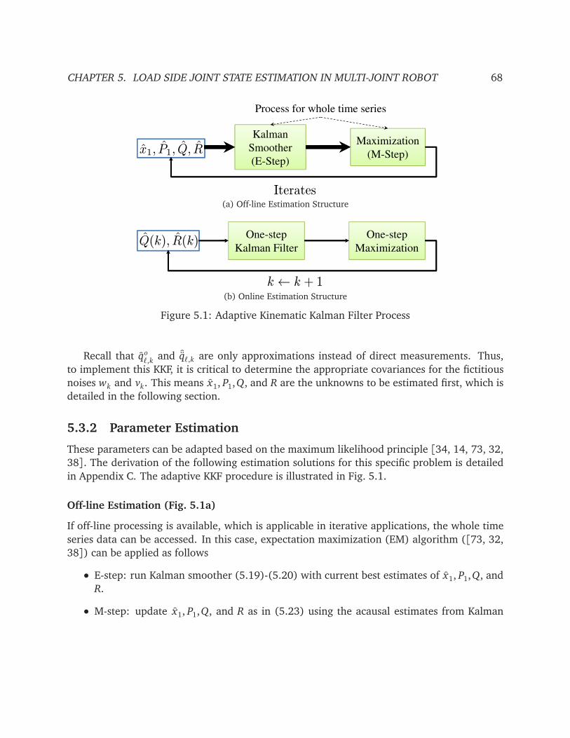
CHAPTER 5. LOAD SIDE JOINT STATE ESTIMATION IN MULTI-JOINT ROBOT 68
Kalman
Smoother
(E-Step)
Maximization
(M-Step)x1, P1, Q, R
Process for whole time series
Iterates
(a) Off-line Estimation Structure
One-step
Kalman Filter
One-step
MaximizationQ(k), R(k)
k ← k + 1
(b) Online Estimation Structure
Figure 5.1: Adaptive Kinematic Kalman Filter Process
Recall that qoℓ,k
and ˆqℓ,k are only approximations instead of direct measurements. Thus,
to implement this KKF, it is critical to determine the appropriate covariances for the fictitious
noises wk and vk. This means x1, P1,Q, and R are the unknowns to be estimated first, which is
detailed in the following section.
5.3.2 Parameter Estimation
These parameters can be adapted based on the maximum likelihood principle [34, 14, 73, 32,
38]. The derivation of the following estimation solutions for this specific problem is detailed
in Appendix C. The adaptive KKF procedure is illustrated in Fig. 5.1.
Off-line Estimation (Fig. 5.1a)
If off-line processing is available, which is applicable in iterative applications, the whole time
series data can be accessed. In this case, expectation maximization (EM) algorithm ([73, 32,
38]) can be applied as follows
• E-step: run Kalman smoother (5.19)-(5.20) with current best estimates of x1, P1,Q, and
R.
• M-step: update x1, P1,Q, and R as in (5.23) using the acausal estimates from Kalman
CHAPTER 5. LOAD SIDE JOINT STATE ESTIMATION IN MULTI-JOINT ROBOT 69
smoother (5.19)-(5.20).
x1 = x1|T P1 = P1|T (5.23a)
Q =1
T − 1
T∑
k=2
h
xk|T − Axk−1|T − Buk−1
xk|T − Axk−1|T − Buk−1
T
+ Pk|T − APT(k,k−1)|T
− P(k,k−1)|TAT + APk−1|TATi
(5.23b)
R=1
T
T∑
k=1
h
yk − C xk|T
yk − C xk|T
T+ C Pk|T CT
i
(5.23c)
• Return to E-step until the increment of the expected likelihood is within chosen thresh-
old.
Online Estimation (Fig. 5.1b)
If real-time computing is desired, only causal estimates from forward recursion (5.19) (i.e.,
Kalman filter) can be used. Furthermore, instead of estimating using the whole time series as
in (5.23), the covariances Q and R are adapted for each time step as
Qok+1=
xk|k− Axk−1|k−1− Buk−1
xk|k− Axk−1|k−1− Buk−1
T
+ Pk|k− APT(k,k−1)|k
− P(k,k−1)|kAT + APk−1|k−1AT (5.24a)
Rok+1=
yk − C xk|k
yk − C xk|k
T+ C Pk|kCT (5.24b)
In practice, to avoid drastic change to the covariances, exponential moving average can be
applied to control the adaptive rate for smooth estimation. This is done as
Qk+1 =
1−1
NQ
Qk+1
NQ
Qok+1
(5.25a)
Rk+1 =
1−1
NR
Rk +1
NR
Rok+1
(5.25b)
where NQ and NR are the window sizes for the moving average filters. Qk and Rk are the
estimated covariance matrices actually utilized in the online Kalman filter. Also, note that, the
initial conditions x1 and P1 is not adapted in this real-time case.
5.4 Discussion of the Approach
5.4.1 Computation Load
It should be noted that one of the great advantages of the proposed method over others is its
light computation load. As shown in Fig. 5.2, this approach mainly consists of two stages,

CHAPTER 5. LOAD SIDE JOINT STATE ESTIMATION IN MULTI-JOINT ROBOT 70
Motor Encoder
End-effector
Accelerometer
TCP
(Pos/Vel/Acc)
Estimates
Joint
(Pos/Vel/Acc)
Estimates
Optimization
Based Inverse
Kinematics
Decoupled
Adaptive
KKF
Joint
(Pos/Vel/Acc)
Rough Estimates
Forward
Kinematics
To Decouple Problem
Figure 5.2: The Structure of Load Side State Estimation Approach
optimization based inverse differential kinematics and KKF with parameter estimation. The
forward kinematics stage is additional if the tool center point (TCP) information is desired. At
the inverse differential kinematics stage, the main computation lies in (5.3), which is diagonal
matrix calculation due to the property of motor side model, and (5.15), where a 3× 3 matrix
inversion requires the most effort. The calculations of (5.14) and (5.16) are basically 3× 1
vector operations and 3 × 3 matrix multiplications. After this stage, the problem becomes
decoupled Kalman filter (or smoother) for each joint with the kinematic model of only 2 states,
1 input, and 1 output. The matrix inversion becomes scalar inversion for Kalman filter case
and 2×2 matrix inversion for smoother case, both of which are computationally simple. In the
parameter estimation, only 2×2 matrix multiplications and scalar operations are required. The
optional forward kinematics stage, which consists of n 4× 4 matrix multiplications, can also
be efficiently processed. Therefore, the overall computation load for the proposed approach
is sufficiently light for both online computing and off-line processing with limited onboard
industrial computation power.
5.4.2 Extensions to Other Sensor Configurations
The developed approach is designed for the case where motor encoders and the end-effector
accelerometer are available. It should be noted, however, that the extensions to other sensor
configurations can also be easily derived.
If motor encoders and the end-effector gyroscope are available, the optimization problem
(5.11) in the inverse differential kinematics stage can be modified to obtain the load side joint
velocity estimate as
minˆqℓ
f (ˆqℓ) =1
2
ˆqℓ− ˆq
oℓ
2
2s.t. J(qo
ℓ)ˆqℓ =ωe (5.26)
where J(qoℓ) ∈ R3×n denotes the last three rows of J(qo
ℓ). The Kalman filter (smoother) is then

CHAPTER 5. LOAD SIDE JOINT STATE ESTIMATION IN MULTI-JOINT ROBOT 71
simplified to be the one with a first order kinematic model
qℓ,k+1 = qℓ,k+∆t ˆqℓ,k+wk, qoℓ,k= qℓ,k+ vk (5.27)
Note that only qℓ and qℓ can be estimated due to the lack of accelerometer. However, if the
rotational vibration is the motion of interest to observe, this approach would be suitable.
Similarly, if the robot is only equipped with motor encoders and the end-effector position
sensor such as a vision camera, the inverse differential kinematics stage (5.15) becomes the
case to obtain the load side joint position estimate as
minqℓ
f (qℓ) =1
2
qℓ− qo
ℓ
2
2s.t. J(qo
ℓ)qℓ = pe (5.28)
This stage needs to be iterated with newly updated qoℓ← qℓ until the solution converges. The
Kalman filter (smoother) stage becomes unnecessary and the final approach is only suitable
for estimating the load side joint position qℓ.
5.5 Simulation & Experimental Study
5.5.1 Test Setup
The proposed method is implemented on the 6-joint FANUC M-16iB robot as shown in Fig. 2.5.
The motor encoders and the 3-axial end-effector accelerometer (Analog Devices, ADIS16400)
are utilized for the load side state estimation algorithm. The CompuGauge 3D system is uti-
lized to measure the end-effector tool center point (TCP) position as a ground truth for per-
formance validation. The sampling rates of all the sensor signals as well as the real-time
controller implemented through MATLAB xPC Target are set to 1kHz.
Furthermore, a robot simulator (see Appendix A.5) has been designed using MATLAB
Simulink & SimMechanics Toolbox based on robot dynamic and kinematic parameters as well
as the calibrated sensor parameters. Therefore, robot dynamic simulation is available with the
access of load side joint information for performance evaluation. The experimental validation,
however, can be conducted only in Cartesian space to compare with CompuGauge 3D and
accelerometer measurements.
5.5.2 Algorithm Settings
The testing TCP trajectory (Fig. 5.3) is a 10cm × 10cm square path on the Y-Z plane with fixed
orientation and maximum speed of 1m/sec. For this motion, all joints except Joint 4 need to
be moved. The estimation algorithm settings for comparisons are listed as follows:
1. KKF-Offline: Off-line estimation with EM and Kalman smoother. A 30Hz zero phase low-
pass filter is applied to the raw accelerometer measurements fa and the rough estimateˆqoℓ.

CHAPTER 5. LOAD SIDE JOINT STATE ESTIMATION IN MULTI-JOINT ROBOT 72
1.0982
1.0984
1.0986
xis
(m
)
0.0132 0.0134 0.0136 0.0138
1.1
1.11
1.12
1.13
1.14
1.15
1.16
1.17
1.18
1.19
Z A
xis
(m
)
Y Axis (m)-0.1 -0.08 -0.06 -0.04 -0.02 0 0.02
1.08
1.1
1.12
1.14
1.16
1.18
1.2
1.22
Y Axis (m)
Z A
xis
(m
)
Y-Z Plane Position Trajectory
KKF-Online
KKF-OnlineFix
KKF-Offline
CG3D
Motor
-0.08 -0.07 -0.06 -0.05 -0.04 -0.03 -0.02 -0.01 0 0.011.0976
1.0978
1.098
1.0982
Z A
xis
Y Axis (m)
Figure 5.3: Y-Z Plane TCP Position Estimation (Experiment)
2. KKF-Online: Online estimation with Kalman filter forward recursion only and online
covariance updating using window sizes NQ = NR = 500. A 100Hz causal low-pass filter
is applied to the raw signals. Note that this low-pass filter will introduce some phase
delay to the signals and thus the bandwidth is chosen as 100Hz as the trade off between
the phase delay effect and high frequency noise filtering.
3. KKF-OnlineFix: The same as KKF-Online except that the covariances Q and R are pre-
tuned in advance and fixed in the online KKF process.
4. CG3D: Real measurement and its differentiation from CompuGauge 3D system.
5. Motor: Using motor side information (i.e., simulated motor side position, velocity, and
acceleration in the simulation, or motor encoder signals in the experiment) directly as
load side information to estimate.
5.5.3 Simulation Results
The load side joint estimation errors calculated from the simulated load side information are
plotted using absolute values in Fig. 5.4, Fig. 5.5, and Fig. 5.6. It is shown that the proposed

CHAPTER 5. LOAD SIDE JOINT STATE ESTIMATION IN MULTI-JOINT ROBOT 73
2 3 4 50
1
2
3
4
5
6x 10
-4
Time (sec)
Ab
so
lute
Err
or
(ra
d)
Joint 1 Position
KKF-OnlineFix
KKF-Online
Motor
KKF-Offline
KKF-Offline / KKF-Online /
KKF-OnlineFix
Motor
0.5
1
1.5
2x 10
-3
Ab
so
lute
Err
or
(ra
d)
Joint 3 Position
KKF-Offline
KKF-Online /KKF-OnlineFix
Motor
2 3 4 50
2
4
6
8x 10
-4
Time (sec)A
bso
lute
Err
or
(ra
d)
Joint 2 Position
KKF-Online /KKF-OnlineFix
Motor
KKF-Offline
0.2
0.4
0.6
0.8
1
1.2x 10
-4
Ab
so
lute
Err
or
(ra
d)
Joint 4 Position
KKF-Offline /KKF-Online /
KKF-OnlineFix
Motor
2 3 4 50
Time (sec)
A
2 3 4 5
0
0.2
Time (sec)
A
2 3 4 50
1
2
3
4
5
6x 10
-4
Time (sec)
Ab
so
lute
Err
or
(ra
d)
Joint 5 Position
KKF-Offline /KKF-Online /
KKF-OnlineFix
Motor
2 3 4 50
0.5
1
1.5
2x 10
-3
Time (sec)
Ab
so
lute
Err
or
(ra
d)
Joint 6 Position
KKF-Offline /KKF-Online /
KKF-OnlineFix
Motor
Figure 5.4: Load Side Joint Position Estimation Absolute Error (Simulation)
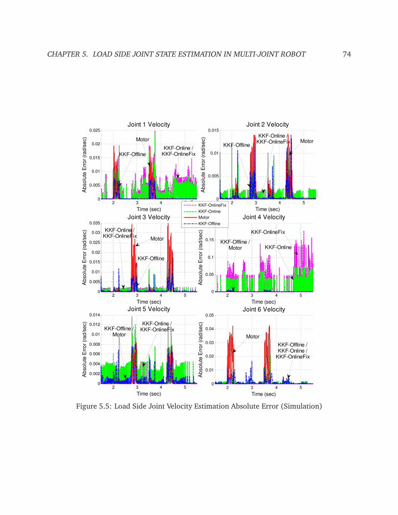
CHAPTER 5. LOAD SIDE JOINT STATE ESTIMATION IN MULTI-JOINT ROBOT 74
2 3 4 50
0.005
0.01
0.015
0.02
0.025
Time (sec)
Ab
so
lute
Err
or
(ra
d/s
ec)
Joint 1 Velocity
KKF-Online /KKF-OnlineFix
Motor
KKF-Offline
2 3 4 50
0.005
0.01
0.015
Time (sec)
Ab
so
lute
Err
or
(ra
d/s
ec)
Joint 2 Velocity
KKF-Offline
KKF-Online /KKF-OnlineFix Motor
0.01
0.015
0.02
0.025
0.03
0.035
bso
lute
Err
or
(ra
d/s
ec)
Joint 3 Velocity
KKF-Offline
KKF-Online /KKF-OnlineFix
Motor
0.05
0.1
0.15
0.2
bso
lute
Err
or
(ra
d/s
ec)
Joint 4 Velocity
KKF-Offline /Motor KKF-Online
KKF-OnlineFix
elocity KKF-OnlineFix
KKF-Online
Motor
KKF-Offline
2 3 4 50
0.005
Time (sec)
Ab
s
2 3 4 5
0
Time (sec)
Ab
s
2 3 4 50
0.002
0.004
0.006
0.008
0.01
0.012
0.014
Time (sec)
Ab
so
lute
Err
or
(ra
d/s
ec)
Joint 5 Velocity
KKF-Offline /Motor
KKF-Online /KKF-OnlineFix
2 3 4 50
0.01
0.02
0.03
0.04
0.05
Time (sec)
Ab
so
lute
Err
or
(ra
d/s
ec)
Joint 6 Velocity
KKF-Offline /KKF-Online /
KKF-OnlineFix
Motor
Figure 5.5: Load Side Joint Velocity Estimation Absolute Error (Simulation)

CHAPTER 5. LOAD SIDE JOINT STATE ESTIMATION IN MULTI-JOINT ROBOT 75
2 3 4 50
0.5
1
1.5
2
Time (sec)
Ab
so
lute
Err
or
(ra
d/s
ec2
)
Joint 1 Acceleration
KKF-OfflineKKF-Online /
KKF-OnlineFix
Motor
2 3 4 50
0.2
0.4
0.6
0.8
1
1.2
1.4
Time (sec)A
bso
lute
Err
or
(ra
d/s
ec2
)
Joint 2 Acceleration
KKF-Offline
KKF-Online /KKF-OnlineFix
Motor
0.5
1
1.5
2
2.5
bso
lute
Err
or
(ra
d/s
ec2
)
Joint 3 Acceleration
KKF-OfflineKKF-Online /
KKF-OnlineFix
Motor
1
2
3
4
bso
lute
Err
or
(ra
d/s
ec2
)
Joint 4 Acceleration
KKF-Offline
KKF-Online /KKF-OnlineFix
Motor
elocity KKF-OnlineFix
KKF-Online
Motor
KKF-Offline
2 3 4 50
0.5
Time (sec)
Ab
s
2 3 4 5
0
Time (sec)
Ab
s
2 3 4 50
1
2
3
4
Time (sec)
Ab
so
lute
Err
or
(ra
d/s
ec2
)
Joint 5 Acceleration
KKF-Offline
KKF-Online /KKF-OnlineFix
Motor
2 3 4 50
1
2
3
4
5
6
Time (sec)
Ab
so
lute
Err
or
(ra
d/s
ec2
)
Joint 6 Acceleration
KKF-Offline
Motor
KKF-Online /KKF-OnlineFix
Figure 5.6: Load Side Joint Acceleration Estimation Absolute Error (Simulation)

CHAPTER 5. LOAD SIDE JOINT STATE ESTIMATION IN MULTI-JOINT ROBOT 76
KKF schemes outperform the Motor setting significantly. Particularly in Fig. 5.4, for Joint 2,
3, and 5, where gravity effects are evident, the position estimation by Motor suffers from
noticeable offset error, while the KKF schemes successfully account for the gravity effects.
Among the KKF schemes, the online velocity and acceleration estimates (Fig. 5.5 and Fig. 5.6)
from KKF-Online and KKF-OnlineFix are not clean due to the high-bandwidth low-pass filter
applied to the raw signals, while KKF-Offline provides the best estimates among the all. Even
though for some particular instances, KKF-Online and KKF-OnlineFix may perform noisier than
Motor in simulation, it is still beneficial to use KKF-Online and KKF-OnlineFix since in reality
Motor does not provide velocity/acceleration measurements.
5.5.4 Experimental Results
The methods are also implemented on the actual experimental setup for Cartesian space com-
parisons. The load side joint state estimates are used in the forward kinematics to obtain the
Cartesian space estimates for comparisons. Figure 5.3 shows the estimated position trajectory
on the Y-Z plane. Again, it is clearly seen that all the KKF settings perform much better than
the Motor setting by capturing closer transient motion on Y Axis and with much less offset on
Z Axis.
The superior performance of the proposed schemes can be better appreciated for the resid-
ual vibration sensing when the robot comes to a stop as shown in Fig. 5.7 and Fig. 5.8. In
general, the Motor setting cannot capture the vibratory motion at the end-effector and the
resulting TCP acceleration estimation is very noisy, while the proposed KKF schemes are able
to do both very well with the fusion of end-effector accelerometer measurements. It is shown
in Fig. 5.7 that the proposed KKF estimates closely follow the CG3D measurements and the
Accelerometer measurements. In particular, during the stopping period (i.e., after 3.85sec for
Y Axis and after 3.05sec for Z Axis), the Motor estimates look static. The actual residual mo-
tion, however, is vibratory and can be successfully captured by the KKF estimates. Recall that,
the CompuGauge measurement and its differentiation (CG3D) are used as the ground truth
for position and velocity estimation performance evaluation. In the acceleration comparison,
however, the real accelerometer measurement (Accelerometer) is used instead of the noisy
CG3D data differentiation as the ground truth.
Another benefit of the proposed KKF schemes is that the velocity/acceleration estimates
are even cleaner than the CG3D setting which is obtained by direct differentiation from the
position measurement, even though there are also some minor noises present in the KKF-
Online and KKF-OnlineFix estimates.
The estimation errors2 for end-effector TCP position/velocity/acceleration when the robot
is coming to a stop are illustrated in Fig. 5.8. The above conclusions are confirmed again
in this figure. Among all the KKF settings, KKF-Offline performs the best due to its acausal
processing availability. KKF-Online and KKF-OnlineFix perform similarly, which indicates that
2This Cartesian space error is defined as the Euclidean distance between the estimated posi-
tion/velocity/acceleration and the actual ones.

CHAPTER 5. LOAD SIDE JOINT STATE ESTIMATION IN MULTI-JOINT ROBOT 77
0
0.02
0.04
0.06
Ve
locity (
m/s
ec)
Z Axis Velocity
MotorKKF-Offline
KKF-Online / KKF-OnlineFix
3 3.1 3.2 3.3 3.41.097
1.0975
1.098
1.0985
Time (sec)P
ositio
n (
m)
Z Axis Position
MotorKKF-Online
KKF-OnlineFixKKF-Offline
CG3D
-0.05
0
0.05
0.1
Ve
locity (
m/s
ec)
Y Axis Velocity
Motor
CG3D
KKF-Offline /KKF-Online /
3.8 3.9 4 4.1
0.0115
0.012
0.0125
0.013
0.0135
Time (sec)
Po
sitio
n (
m)
Y Axis Position
KKF-Online / KKF-OnlineFix
MotorCG3D
KKF-Offline
3.8 3.9 4 4.1-10
-5
0
5
10
Time (sec)
Acce
lera
tio
n (
m/s
ec2
)
Y Axis Acceleration
CG3D
KKF-Offline / KKF-Online /
KKF-Online Fix
Motor
Accelerometer
3 3.1 3.2 3.3 3.4-3
-2
-1
0
1
2
3
Time (sec)
Acce
lera
tio
n (
m/s
ec2
)
Z Axis Acceleration
CG3D Motor
Accelerometer / KKF-Offline / KKF-Online / KKF-OnlineFix
3 3.1 3.2 3.3 3.4
-0.02
Time (sec)
CG3D
3.8 3.9 4 4.1-0.1
Time (sec)
KKF-Online /KKF-OnlineFix
CG3D
Motor
KKF-OnlineFix
KKF-Online
KKF-Offline
Accelerometer
Figure 5.7: TCP Estimation on Y & Z Axes When Coming to a Stop (Experiment)

CHAPTER 5. LOAD SIDE JOINT STATE ESTIMATION IN MULTI-JOINT ROBOT 78
3.8 3.9 4 4.1 4.20
0.5
1
1.5
2
2.5
Time (sec)
Po
s E
rro
r (m
m)
Cartesian Position Error Comparisons
Motor
KKF−OnlineFix
KKF−Online
KKF−Offline
KKF−Offline /KKF−Online /
KKF−OnlineFix
Motor
(a) TCP Position Estimation Error
3.5 3.6 3.7 3.8 3.9 4 4.1 4.20
0.05
0.1
0.15
0.2
Time (sec)
Ve
l E
rro
r (m
/se
c)
Cartesian Velocity Error Comparisons
Motor
KKF−OnlineFix
KKF−Online
KKF−Offline
Motor
KKF−Offline /KKF−Online /
KKF−OnlineFix
(b) TCP Velocity Estimation Error
3.5 3.6 3.7 3.8 3.9 4 4.1 4.20
5
10
15
20
Time (sec)
Acc E
rro
r (m
/se
c2)
Cartesian Acceleration Error Comparisons
CG3D
Motor
KKF−OnlineFix
KKF−Online
KKF−Offline
Motor
KKF−Offline
KKF−Online /KKF−OnlineFix
CG3D
(c) TCP Acceleration Estimation Error
Figure 5.8: TCP Estimation Error When Coming to a Stop (Experiment)

CHAPTER 5. LOAD SIDE JOINT STATE ESTIMATION IN MULTI-JOINT ROBOT 79
Table 5.1: TCP Estimation Errors When Coming to a Stop (Experiment)
RMS Errors Pos. (mm) Vel. (mm/sec) Acc. (mm/sec2)
KKF-Offline 0.262 34.638 1641.400
KKF-Online 0.440 37.832 2729.828
KKF-OnlineFix 0.476 34.517 2729.347
Motor 0.758 67.652 4843.979
with properly pre-tuned covariances, the online computing can be further simplified without
sacrificing much performance. These conclusions can also be drawn from the root-mean-
square (RMS) estimation errors for position/velocity/acceleration as listed in Table 5.1, which
shows that the RMS estimation errors can be reduced by the proposed KKF schemes to about
half or even less of that of the Motor estimates.
5.6 Chapter Summary
This paper investigated the load side state estimation problem for the robots with mismatched
sensing, i.e., robots with joint elasticity. The problem was tackled by using a combination
of motor encoders and a low-cost end-effector sensor (e.g., an end-effector accelerometer).
The direct joint space estimation was achieved for the purpose of decentralized joint control.
With the equipped end-effector accelerometer, the load side joint acceleration was estimated
through an optimization based inverse differential kinematics algorithm. The problem was
then decoupled into n simple kinematic Kalman filters to estimate the load side joint position
and velocity. Both off-line and online solutions were presented for determining the fictitious
noise covariance. The proposed approach is computationally efficient for both off-line ap-
plications and online computing. Simulation and experimental study on a 6-DOF industrial
robot demonstrated the superior performance of the developed method and the necessity of
the end-effector sensing.

80
Part II
Handling Mismatched Dynamics:
Real-time Control Approaches

81
Chapter 6
Hybrid Adaptive Friction Compensation in
Single-Joint Robot
6.1 Introduction
As pointed out in Chapter 2, the mismatched dynamics and sensing problem is common among
the robots with indirect drive trains. These indirect drive trains, e.g., robotic joints that uti-
lize gear transmissions, are commonly used in industrial applications due to their high torque
capacity. The indirect drive transmissions, however, set challenges in high precision motion
control because of gear compliances as well as nonlinearities such as friction and torque hys-
teresis. Particularly, the nonlinear friction effects on the load side are difficult to compensate
for because: 1) the load side position measurement is often unavailable (i.e., mismatched sens-
ing), and 2) it is indirectly compensated for through the gear transmission (i.e., mismatched
dynamics). Since the load side performance is critical in practical applications, a method that
compensates for the load side friction as well as the motor side friction is necessary.
Over the past several decades, modeling and compensation of the friction effects have
been intensively studied from various viewpoints, including static/dynamic characterizations
and feedback/feedforward compensation schemes [8, 15, 82, 5]. For example, many model-
based friction compensation techniques have been developed to reject the friction effects by
adaptively [13, 33] or robustly [98] estimating the real friction. Also, typical approaches such
as the disturbance observer [66] or repetitive control [83, 85] have been used to compensate
for friction.
Most of these studies, however, validated their performance based on simple one-mass
systems or direct drives only. When a two-mass system or an indirect drive is considered,
the friction effects introduced from the load side remain as a challenge. For this reason,
friction characteristics in harmonic drive systems were studied in [76, 35]. The performance
and stability issues due to friction forces (e.g., limit cycles) were addressed in [52]. Some
compensation schemes were proposed to overcome the friction effects in harmonic drives.
Most of them, however, were still focused on the motor side compensation only [35, 31, 46]

CHAPTER 6. HYBRID ADAPTIVE FRICTION COMPENSATION IN SINGLE-JOINT ROBOT 82
or torque tracking control [77]. To improve the load side position tracking performance, the
position information of both the motor side and the load side was utilized in the controller
design [95, 79]. Such controllers, however, are difficult to implement in industrial robots,
which are usually not equipped with precise load side position sensors.
In this chapter, a hybrid adaptive two-stage friction compensation scheme for indirect drive
trains is developed in the absence of precise load side position measurements. The load side
state estimation method proposed in Chapter 3 is utilized in the compensation algorithm. The
proposed friction compensation method manipulates both the torque input and the reference
trajectory, which is controlled by a hybrid system scheme based on the tracking performance.
The proposed method is verified by the experimentation on a single-joint indirect drive setup.
6.2 System Overview
6.2.1 Single-Joint Indirect Drive Model
The schematic of a single-joint indirect drive mechanism was illustrated in Fig. 2.1 in Chapter
2. The equations of motion (2.15) for this system are restated as
Jmθm = u−
fm+ fh
−
1
N
k j
θm
N− θℓ− θ
+ d j
θm
N− θℓ−
˙θ
(6.1a)
Jℓθℓ =− fℓ+ k j
θm
N− θℓ− θ
+ d j
θm
N− θℓ−
˙θ
(6.1b)
where all the variables are as defined in Section 2.2.2. Note that the external disturbances d f m
and d f ℓ are omitted here since this chapter will focus on friction compensation rather than
compensation of external disturbances.
6.2.2 Modified Friction Model
As described in Section 2.2.2, the friction effect in the indirect drive train is characterized by
three friction forces, i.e., the motor side bearing friction, fm, the load side bearing friction, fℓ,
and the reducer gear meshing friction, fh.
The combination of system model (6.1) with friction effect gives
Jmθm+1
NJℓθℓ = u− F (6.2a)
F = fm+ fh+fℓ
N(6.2b)
where F represents the entire friction force imposed on the whole system when reflected to the
motor side. As suggested in Section 2.2.2, the load side friction fℓ could be roughly modeled
as a scaled quantity from the entire friction force F with rℓ as a scaling factor, i.e.
fℓ = rℓF (6.3)
CHAPTER 6. HYBRID ADAPTIVE FRICTION COMPENSATION IN SINGLE-JOINT ROBOT 83
To facilitate the development of the adaptive friction compensation algorithm, the LuGre
model (2.17), which was used in Section 2.2.2 to describe F , is further modified as
z = v −β0|v|
g(v)z (6.4a)
g(v) = Fc +
Fs − Fc
e(−v2/v2
s ) (6.4b)
F = σ0z+σ1z +σ2v (6.4c)
where all the variables except β0 in this modified model are as defined in Section 2.2.2. Here
in (6.4a), β0 is used to denote the nominal micro-stiffness σ0 of the internal state z (i.e., the
deflection of bristles between the two contacting surfaces). This differs from the standard
LuGre model (2.17), and the modification will be shown to simplify the friction compensation
algorithm.
From (6.4), the friction force, F , can be written as:
F = KTΦ (6.5)
where K =
σ1 +σ2 σ0 β0σ1
T, Φ =
h
v z −|v|
g(v)ziT
.
Notice that the modified LuGre model still preserves the following property of standard
LuGre model [15]:
Property 6.1. Fc ≤ g(v) ≤ Fs. If |z(0)| ≤Fs
β0, then |z(t)| ≤
Fs
β0, ∀t ≥ 0.
In reality, it can be assumed that the deflection of bristles starts at rest, i.e., z(0) = 0,
without loss of generality. Therefore, |z(t)| ≤Fs
β0
,∀t ≥ 0. This property will be used in the
subsequent controller design to ensure the bounded stability of the friction observer.
Remark 6.1. In practice, friction characteristics may vary due to the variations of the normal
contact forces, lubricant condition, temperature, material wear, and so on [13]. Variations in the
normal forces usually cause an impact on the values of only static parameters, i.e., FC , FS, vs, and
σ2, while the changes in lubricant condition, temperature and/or materials may affect both static
and dynamic parameters.
Remark 6.2. If only static friction is considered, i.e., z = 0, the modified LuGre model reduces to
F(v) =σ0
β0
h
Fc +
Fs − Fc
e(−v2/v2
s )i
sgn(v) +σ2v (6.6)
This indicates that, by fixing the nominal micro-stiffness, β0, the adaptation of real micro-stiffness,
σ0, effectively changes the level of static parameters, e.g., FC and FS in g(v). Thus, the adaptation
of σ0,σ1, and σ2 can account for most parameter variations in the modified friction model
regardless of the dynamics for internal state z. Based on this, K in (6.5), which consists of σ0,
σ1, and σ2, may be adapted in real-time with Φ as the regressor.

CHAPTER 6. HYBRID ADAPTIVE FRICTION COMPENSATION IN SINGLE-JOINT ROBOT 84
θℓd
θmd
F1
F2
Cfb
uff
u
−
+
θℓ
θm
+
+
ufb
θℓ
KKFθm, θℓ
P
FO
fℓ
F
Figure 6.1: Block Diagram of the Overall Control System
6.2.3 Controller Structure
Figure 6.1 shows the overall control structure of the single-joint indirect drive system, where P
denotes the system plant with the measurable outputs as the motor side position θm, load side
velocity θℓ, and load side acceleration θℓ. The controller structure consists of two feedforward
controllers, F1 and F2, one feedback controller, C f b, the state estimator, KKF , and the friction
observer, FO.
Here the state estimator KKF utilizes the kinematic Kalman filter (KKF-AG) method de-
veloped in Chapter 3 to estimate the load side position θℓ using gyroscope and accelerometer
measurements. The friction observer FO detailed in the following sections estimates the entire
friction F and the load side friction fℓ to be used in the feedforward controllers F1 and F2. The
feedforward controller, F2, is designed from (6.2a) as
u f f (t) = Jmθmd (t) +1
NJℓθℓd (t) + F (t) (6.7)
where F is the estimated entire friction force. θℓd is the desired load side acceleration. In the
case where the acceleration is measured by sensors (e.g., load side accelerometers), θℓd can
be replaced with θℓ. θmd is the motor side position reference generated by F1 from the desired
load side position, θℓd, i.e.
θmd (t) =N
k j
Jℓθℓd (t) + fℓ (t)
+ Nθℓd (t) (6.8)
where fℓ is the estimated load side friction. Equation (6.8) is derived from (6.1b) by neglecting
the transmission error θ and the joint damping d j, since k j
θm
N− θℓ
≫ d j
θm
N− θℓ
usually
holds within the system bandwidth.
The feedback controller, C f b, which consists of a proportional position control loop and a
proportional-integral (PI) velocity control loop, can be described as
C f b (s) =
kv +ki
s
s+ kp
(6.9)
CHAPTER 6. HYBRID ADAPTIVE FRICTION COMPENSATION IN SINGLE-JOINT ROBOT 85
where kp is the gain of the position loop, kv and ki are the gains of the velocity loop. The
above controller is discretized by the Euler method for implementation.
6.3 Friction Compensation
As shown in the controller structure (6.7)-(6.8), the proposed friction compensator consists of
two parts. The motor side friction compensation is designed in the feedforward controller F2
by injecting into the torque input u, and the load side friction effects are further compensated
for in the feedforward controller F1 by manipulating the motor side reference, θmd.
6.3.1 Motor Side Friction Compensation
Feedback Friction Compensation
Let em = θm−θmd be the motor side position tracking error. Define a first order sliding surface,
pm, as
pm = em+ ksem (6.10)
where ks is a positive constant. Thus em is small or converges to zero if pm is small or converges
to zero, sinceem(s)
pm(s)= 1
s+ksis asymptotically stable.
From (6.2a) and (6.10), the motor side error dynamics is derived as
Jm pm = u− F −1
NJℓθℓ− Jmθmd + Jmks em (6.11)
The controller structure (Fig. 6.1) yields the following control law
u(t) = u f f (t) + u f b(t)
=
Jmθmd(t) +1
NJℓθℓd(t) + F(t)
−
kvsm(t) +
∫ t
0
kism(τ)dτ
(6.12)
where sm(t) = em(t) + kpem(t) is the error term in the velocity loop.
By applying the adaptive control technique [75], an adaptive friction observer is designed
to obtain F(t), i.e.
F = KTΦ (6.13)
where Φ =
θm z0 −|θm|
g(θm)z1
T
. K , z0, and z1 are the estimates obtained from the following
CHAPTER 6. HYBRID ADAPTIVE FRICTION COMPENSATION IN SINGLE-JOINT ROBOT 86
update laws
˙K = −ΓΦpm (6.14a)
˙z0 = θm−β0
θm
g
θm
z0− γ3pm (6.14b)
˙z1 = θm−β0
θm
g
θm
z1+ γ4
θm
g
θm
pm (6.14c)
where Γ = diagγ0,γ1,γ2
, γ3, and γ4 are positive adaptation gains. Notice that the unmea-
surable internal friction state z is estimated by a dual-observer structure [78] with the two
state estimates, z0 and z1. Equations (6.14b) and (6.14c) result in the following observer error
dynamics
˙z0 =−β0
θm
g
θm
z0 + γ3pm (6.15a)
˙z1 =−β0
θm
g
θm
z1 − γ4
θm
g
θm
pm (6.15b)
where z0 = z − z0 and z1 = z − z1 are the estimation errors with regard to the same internal
state z. Note that the nominal static parameters (e.g., FC , FS, and vs) in g
θm
are to be
identified and the actual variations of these parameters can be effectively accounted for by the
adaptation of σ0 as mentioned above.
Stability Analysis
The following theorem proves the stability of the closed-loop system under additional assump-
tions as stated therein.
Theorem 6.1. For the system model described by (6.1)-(6.4), global asymptotic tracking perfor-
mance on the motor side can be achieved by the proposed controller in (6.7)-(6.9) and adaptive
friction observer in (6.13)-(6.14), if the integrator term of the PID controller C f b is suppressed,
i.e., ki = 0, and the real load side acceleration measurement, θℓ, is used instead of θℓd in (6.7).
Proof. Suppose that the PID controller gains are
kp =hks
Jmks + h, kv = Jmks + h (6.16)
where h is a positive constant. By the assumption in the theorem, ki = 0. Then the control law
in (6.12) can be rewritten as
u=
Jmθmd +1
NJℓθℓd + F
−Jmks em+ hpm
(6.17)

CHAPTER 6. HYBRID ADAPTIVE FRICTION COMPENSATION IN SINGLE-JOINT ROBOT 87
From (6.11) and (6.17), the control law results in the following closed loop dynamics
Jm pm =−hpm−Jℓ
N
θℓ− θℓd
−
F − F
=−hpm−Jℓ
Neℓ− KTΦ− KTΦ (6.18)
where eℓ = θℓ− θℓd is the load side acceleration tracking error, K = K − K and Φ = Φ− Φ are
the estimation errors.
Let a Lyapunov function candidate for the system be
V (pm, K , z0, z1) =1
2Jmp2
m+
1
2KTΓ−1K +
1
2γ3
k1z20+
1
2γ4
k2z21
(6.19)
where k1 = σ0 and k2 = β0σ1 are the last two entries in K .
In most applications, it is reasonable to assume that the actual friction parameters, K =
σ1 +σ2 σ0 β0σ1
T, are unknown but constant. It follows that K = 0 and ˙K = − ˙K .
Therefore, by differentiating V in (6.19) and substituting the update laws from (6.14), the
derivative of V is obtained as
V (pm, K , z0, z1) =−hp2m−
Jℓ
Npmeℓ−
k1
γ3
β0
θm
g
θm
z20−
k2
γ4
β0
θm
g
θm
z21
(6.20)
Recall that h is a positive constant. Thus, every term on the right hand side of (6.20),
except for the second term, is negative semi-definite. Moreover, if the load side acceleration is
measured by sensors (i.e., θℓd is replaced with θℓ to calculate u f f in (6.7)), the second term
becomes zero. It follows that
V (pm, K , z0, z1) = −hp2m−
k1
γ3
β0
θm
g
θm
z20−
k2
γ4
β0
θm
g
θm
z21≤ −hp2
m(6.21)
From Lyapunov stability theory [75], it is concluded that the motor side tracking error, pm,
the friction parameter estimation error, K , and the internal friction state estimation errors, z0
and z1, are globally uniformly bounded. Since the actual friction parameters K are assumed
to be constant during one trajectory task, and actual internal friction state, z, is bounded as
shown in Property 6.1, it follows that the estimates, K , z0, and z1, are globally uniformly
bounded as well. In addition, the actual motor side position and velocity, θm and θm, are
globally uniformly bounded, since pm is globally uniformly bounded, and the generated motor
side reference θmd is bounded by the characteristics of the feedforward controller, F1. With all
these bounded variables, it can be shown that V is also bounded. Then by Barbalat’s lemma,
(6.19) and (6.21) imply that V → 0 (i.e., pm → 0) as t → ∞. Therefore, the motor side
tracking error em =1
s+kspm asymptotically converges to zero.

CHAPTER 6. HYBRID ADAPTIVE FRICTION COMPENSATION IN SINGLE-JOINT ROBOT 88
Remark 6.3. The above theorem provides a sufficient condition to achieve global asymptotic
tracking performance on the motor side. Two assumptions were introduced to theoretically guar-
antee the stability of the proposed method. These assumptions, however, may be relaxed without
jeopardizing the closed loop stability of the system in practice. The relaxation is demonstrated in
the experiments with preserved integrator in C f b to maintain the basic feedback controller struc-
ture (i.e., ki 6= 0). Also, the desired reference θℓd is used in (6.7) instead of the real measurement
θℓ to decrease the dependence on the load side sensors.
Feedforward Friction Compensation
The above friction compensation scheme is in the feedback form, since the actual physical
measurements are used in the regressor estimate, Φ. When doing tracking control, feedfor-
ward control often improves the performance in the sense that it allows anti-causal terms in
the controller. It recovers the limitation of feedback controller due to the dynamic lag of the
plant [82]. Recall that the feedback controller must see an error first before it can take any
corrective action. In particular, this limitation adversely affects the performance by the quick
direction reversal of Coulomb friction force.
By replacing the measurements in the friction observer regressor Φ with corresponding
trajectory references, and excluding the motor side error term, pm, a feedforward version of
friction observer regressor, Φd , is obtained as
Φd =
θmd zd −|θmd|
g(θmd)zd
T
, ˙zd = θmd −β0
θmd
g
θmd
zd (6.22)
Thus, the dual estimations of internal friction state z are replaced by single desired (nominal)
internal state zd as in (6.22). In this feedforward form, the friction observer structure is
simplified by reducing the number of adaptive variables from 5 to 3, and the noises and
disturbances from feedback measurements are also avoided.
6.3.2 Load Side Friction Compensation
Due to the characteristics of indirect drives, perfect tracking performance on the motor side
does not guarantee perfect load side tracking performance. Since the load side performance
is often of the major concern in practical applications, friction compensation should also be
considered on the load side.
Recall that, in (6.3), the load side friction, fℓ, was modeled as a scaled quantity of the
entire friction force, F . Thus, once friction parameters are adapted successfully on the motor
side, the load side friction fℓ can be roughly estimated as
fℓ = rℓ F (6.23)
where F is the estimated entire friction force from the motor side compensator, and rℓ is the
estimated scaling factor obtained by the following update laws
˙rℓ =−γrℓF eℓ, eℓ = θℓ− θℓd (6.24)
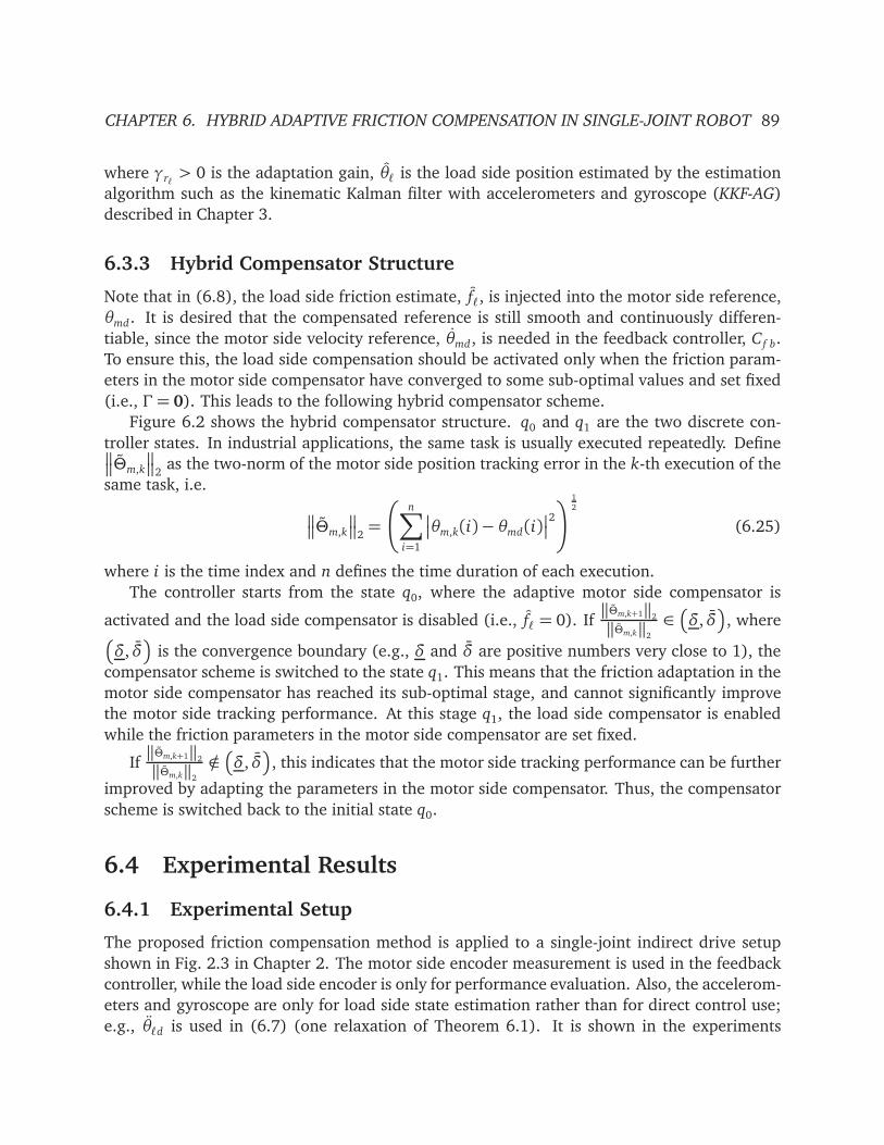
CHAPTER 6. HYBRID ADAPTIVE FRICTION COMPENSATION IN SINGLE-JOINT ROBOT 89
where γrℓ> 0 is the adaptation gain, θℓ is the load side position estimated by the estimation
algorithm such as the kinematic Kalman filter with accelerometers and gyroscope (KKF-AG)
described in Chapter 3.
6.3.3 Hybrid Compensator Structure
Note that in (6.8), the load side friction estimate, fℓ, is injected into the motor side reference,
θmd. It is desired that the compensated reference is still smooth and continuously differen-
tiable, since the motor side velocity reference, θmd, is needed in the feedback controller, C f b.
To ensure this, the load side compensation should be activated only when the friction param-
eters in the motor side compensator have converged to some sub-optimal values and set fixed
(i.e., Γ = 0). This leads to the following hybrid compensator scheme.
Figure 6.2 shows the hybrid compensator structure. q0 and q1 are the two discrete con-
troller states. In industrial applications, the same task is usually executed repeatedly. Define Θm,k
2as the two-norm of the motor side position tracking error in the k-th execution of the
same task, i.e.
Θm,k
2=
n∑
i=1
θm,k(i)− θmd(i)
2
! 1
2
(6.25)
where i is the time index and n defines the time duration of each execution.
The controller starts from the state q0, where the adaptive motor side compensator is
activated and the load side compensator is disabled (i.e., fℓ = 0). If‖Θm,k+1‖2
‖Θm,k‖2
∈
δ, δ
, where
δ, δ
is the convergence boundary (e.g., δ and δ are positive numbers very close to 1), the
compensator scheme is switched to the state q1. This means that the friction adaptation in the
motor side compensator has reached its sub-optimal stage, and cannot significantly improve
the motor side tracking performance. At this stage q1, the load side compensator is enabled
while the friction parameters in the motor side compensator are set fixed.
If‖Θm,k+1‖2
‖Θm,k‖2
/∈
δ, δ
, this indicates that the motor side tracking performance can be further
improved by adapting the parameters in the motor side compensator. Thus, the compensator
scheme is switched back to the initial state q0.
6.4 Experimental Results
6.4.1 Experimental Setup
The proposed friction compensation method is applied to a single-joint indirect drive setup
shown in Fig. 2.3 in Chapter 2. The motor side encoder measurement is used in the feedback
controller, while the load side encoder is only for performance evaluation. Also, the accelerom-
eters and gyroscope are only for load side state estimation rather than for direct control use;
e.g., θℓd is used in (6.7) (one relaxation of Theorem 6.1). It is shown in the experiments
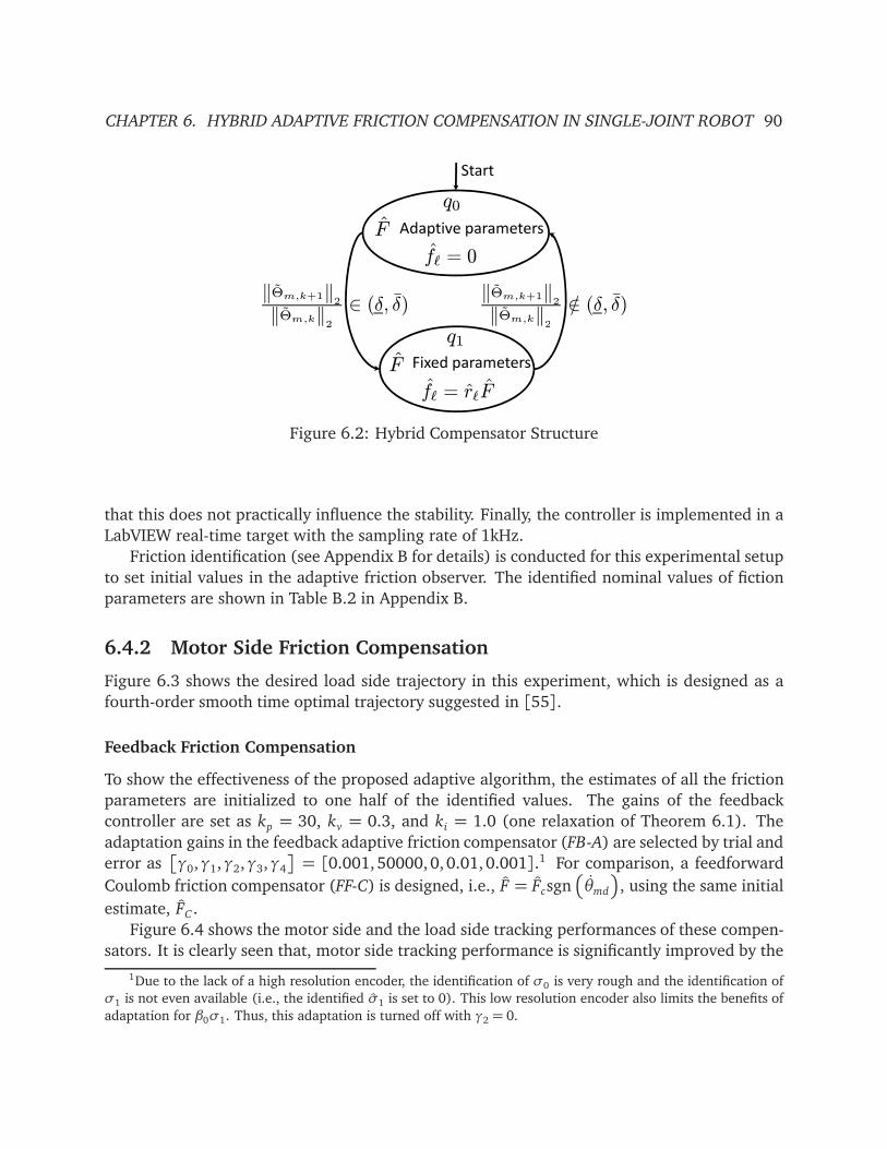
CHAPTER 6. HYBRID ADAPTIVE FRICTION COMPENSATION IN SINGLE-JOINT ROBOT 90
F
fℓ = 0
F
fℓ = rℓF
‖Θm,k+1‖2
‖Θm,k‖2
∈ (δ, δ)‖Θm,k+1‖
2
‖Θm,k‖2
/∈ (δ, δ)
q0
q1
Figure 6.2: Hybrid Compensator Structure
that this does not practically influence the stability. Finally, the controller is implemented in a
LabVIEW real-time target with the sampling rate of 1kHz.
Friction identification (see Appendix B for details) is conducted for this experimental setup
to set initial values in the adaptive friction observer. The identified nominal values of fiction
parameters are shown in Table B.2 in Appendix B.
6.4.2 Motor Side Friction Compensation
Figure 6.3 shows the desired load side trajectory in this experiment, which is designed as a
fourth-order smooth time optimal trajectory suggested in [55].
Feedback Friction Compensation
To show the effectiveness of the proposed adaptive algorithm, the estimates of all the friction
parameters are initialized to one half of the identified values. The gains of the feedback
controller are set as kp = 30, kv = 0.3, and ki = 1.0 (one relaxation of Theorem 6.1). The
adaptation gains in the feedback adaptive friction compensator (FB-A) are selected by trial and
error asγ0,γ1,γ2,γ3,γ4
= [0.001, 50000, 0, 0.01, 0.001].1 For comparison, a feedforward
Coulomb friction compensator (FF-C) is designed, i.e., F = Fcsgn
θmd
, using the same initial
estimate, FC .
Figure 6.4 shows the motor side and the load side tracking performances of these compen-
sators. It is clearly seen that, motor side tracking performance is significantly improved by the
1Due to the lack of a high resolution encoder, the identification of σ0 is very rough and the identification of
σ1 is not even available (i.e., the identified σ1 is set to 0). This low resolution encoder also limits the benefits of
adaptation for β0σ1. Thus, this adaptation is turned off with γ2 = 0.
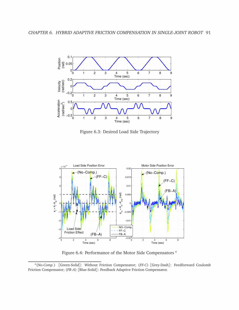
CHAPTER 6. HYBRID ADAPTIVE FRICTION COMPENSATION IN SINGLE-JOINT ROBOT 91
0 1 2 3 4 5 6 7 8 90
0.05
0.1
Time (sec)
Positio
n(r
ad)
0 1 2 3 4 5 6 7 8 9−0.2
0
0.2
Time (sec)
Velo
city
(rad/s
ec)
0 1 2 3 4 5 6 7 8 9−0.5
0
0.5
Time (sec)
Accele
ration
(rad/s
ec
2)
Figure 6.3: Desired Load Side Trajectory
0 2 4 6 8−4
−3
−2
−1
0
1
2
3
4x 10
−4 Load Side Position Error
Time (sec)
el =
θl−
θld
(ra
d)
0 2 4 6 8−0.02
−0.015
−0.01
−0.005
0
0.005
0.01
0.015
0.02
Motor Side Position Error
Time (sec)
em
= θ
m−
θm
d (
rad)
NO−Comp.
FF−C
FB−A
(No−Comp.)
(FF−C)(FF−C)
(FB−A)
(No−Comp.)
Load SideFriction Effect
(FB−A)
Figure 6.4: Performance of the Motor Side Compensators a
a(No-Comp.) [Green-Solid]: Without Friction Compensator; (FF-C) [Grey-Dash]: Feedforward Coulomb
Friction Compensator; (FB-A) [Blue-Solid]: Feedback Adaptive Friction Compensator.
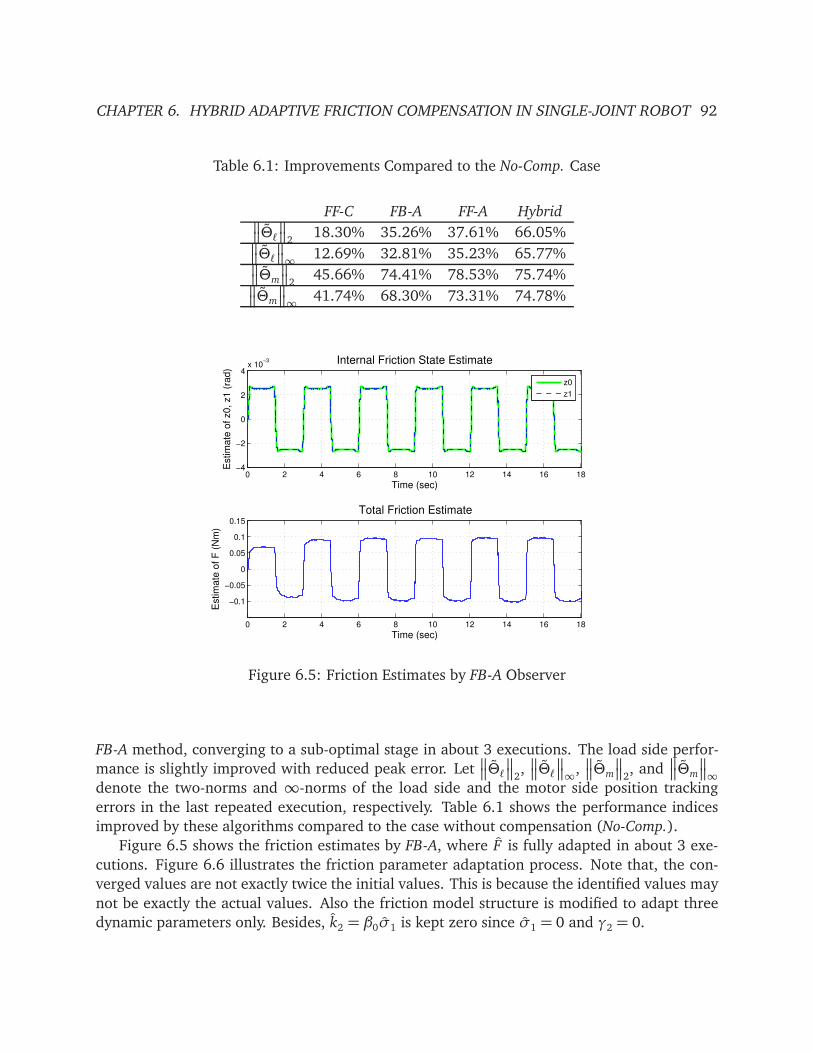
CHAPTER 6. HYBRID ADAPTIVE FRICTION COMPENSATION IN SINGLE-JOINT ROBOT 92
Table 6.1: Improvements Compared to the No-Comp. Case
FF-C FB-A FF-A Hybrid Θℓ
218.30% 35.26% 37.61% 66.05%
Θℓ ∞
12.69% 32.81% 35.23% 65.77% Θm
245.66% 74.41% 78.53% 75.74%
Θm
∞
41.74% 68.30% 73.31% 74.78%
0 2 4 6 8 10 12 14 16 18−4
−2
0
2
4x 10
−3 Internal Friction State Estimate
Time (sec)
Estim
ate
of
z0
, z1
(ra
d)
z0
z1
0 2 4 6 8 10 12 14 16 18
−0.1
−0.05
0
0.05
0.1
0.15
Total Friction Estimate
Time (sec)
Estim
ate
of
F (
Nm
)
Figure 6.5: Friction Estimates by FB-A Observer
FB-A method, converging to a sub-optimal stage in about 3 executions. The load side perfor-
mance is slightly improved with reduced peak error. Let Θℓ
2, Θℓ ∞
, Θm
2, and
Θm
∞
denote the two-norms and ∞-norms of the load side and the motor side position tracking
errors in the last repeated execution, respectively. Table 6.1 shows the performance indices
improved by these algorithms compared to the case without compensation (No-Comp.).
Figure 6.5 shows the friction estimates by FB-A, where F is fully adapted in about 3 exe-
cutions. Figure 6.6 illustrates the friction parameter adaptation process. Note that, the con-
verged values are not exactly twice the initial values. This is because the identified values may
not be exactly the actual values. Also the friction model structure is modified to adapt three
dynamic parameters only. Besides, k2 = β0σ1 is kept zero since σ1 = 0 and γ2 = 0.

CHAPTER 6. HYBRID ADAPTIVE FRICTION COMPENSATION IN SINGLE-JOINT ROBOT 93
0 2 4 6 8 10 12 14 16 185
8
11
12x 10
−4 Friction Parameter Estimations (SI)
Time (sec)
k0 =
σ1+
σ2
0 2 4 6 8 10 12 14 16 1815
20
25
30
35
40
Time (sec)
k1 =
σ0
Figure 6.6: Friction Parameter Estimations (SI Units)
Feedforward Friction Compensation
The modification of the proposed adaptive friction observer from the feedback form to the
feedforward form is also tested in the experiment. The same controller gains, kp, kv , and ki,
and adaptation gains, γ0, γ1, and γ2, from FB-A, are used in the feedforward compensator
(FF-A). Table 6.1 shows that FF-A slightly improves the performance of FB-A.
6.4.3 Load Side Friction Compensation
The motor side compensation result (e.g., Fig. 6.4) shows that, even if the motor side perfor-
mance is significantly improved, little improvement can be observed at the load side. Actually,
in Fig. 6.4, the oscillation in the load side position error is mainly due to the transmission
error θ , while the offset in the tracking error is due to the load side friction effects, which is
explained by (6.8). This suggests the necessity to implement the load side friction compensa-
tion.
In Chapter 3, it was shown that the tracking error offset rather than the transmission error
can be successfully estimated by the KKF-AG method. Therefore, this method is employed here
to estimate the load side position.
To show the effectiveness of the proposed load side compensation algorithm, rℓ was ini-
tialized to 1.0N where N is the reducer gear ratio. Figure 6.7 illustrates the performance of
friction compensator enabled on both the motor side and the load side (Hybrid), i.e., the state

CHAPTER 6. HYBRID ADAPTIVE FRICTION COMPENSATION IN SINGLE-JOINT ROBOT 94
0 2 4 6 8−4
−3
−2
−1
0
1
2
3
4x 10
−4 Load Side Position Error
Time (sec)
el =
θl−
θld
(ra
d)
0 2 4 6 8−0.02
−0.015
−0.01
−0.005
0
0.005
0.01
0.015
0.02Motor Side Position Error
Time (sec)
em
= θ
m−
θm
d (
rad
)
NO−Comp.
FF−A
Hybrid(No. Comp.)(No. Comp.)
(FF−A)
(Hybrid)(Hybrid)
(FF−A)
Figure 6.7: Performance of the Hybrid Compensator b
b(No-Comp.) [Green-Solid]: Without Friction Compensator; (FF-A) [Grey-Dash]: Feedforward Adaptive
Friction Compensator at Motor Side Only; (Hybrid) [Blue-Solid]: Hybrid Compensator at the State q1.
q1 in Fig. 6.2. It can be seen that the load side position error offset is significantly reduced
by the hybrid compensator scheme in less than 1 execution, while the motor side tracking
performance is maintained at about the same level. This is also confirmed by the performance
indices in Table 6.1. The convergence of the estimated friction ratio rℓ and the estimated load
side friction fℓ is illustrated in Fig. 6.8.
6.5 Chapter Summary
This chapter investigated the friction compensation in the single-joint indirect drive mecha-
nism by separating the problem into two parts, i.e., motor side and load side. The motor
side compensator employed the idea of an adaptive friction observer based on the modified
LuGre model, while the load side compensator was implemented by injecting the load side
friction estimate into the generated motor side reference. A hybrid compensator scheme was
proposed to deal with the switching between the two compensator algorithms. It has demon-
strated the necessity of load side friction compensation for enhancing load side performance.
Experimental results validated the effectiveness of the proposed scheme.

CHAPTER 6. HYBRID ADAPTIVE FRICTION COMPENSATION IN SINGLE-JOINT ROBOT 95
0 2 4 6 8 10 12 14 16 180
0.2
0.4
0.6
0.8
1Estimation of Friction Scaling Factor r
l
Time (sec)
Estim
ate
d r
l/N
0 2 4 6 8 10 12 14 16 18
−0.1
−0.05
0
0.05
0.1
Friction Estimations
Time (sec)
Estim
ate
d F
rictio
n (
Nm
)
Total Friction F
Load Side Friction fl/N
Figure 6.8: Load Side Friction Estimates
96
Chapter 7
Motor Side Disturbance Rejection in
Multi-Joint Robot
7.1 Introduction
In motion control applications, various disturbances, such as friction force, contact force, trans-
mission error, or model uncertainties, can severely deteriorate performance. Thus, effective
disturbance rejection is essential for the feedback controller to achieve high precision posi-
tion/force tracking. In indirect drive robot joints, however, disturbances operate in combina-
tion with compliant gears and also nonlinear robot dynamics, which makes it difficult to reject
them directly. Thus, it is desired to study the disturbance estimation and rejection taking the
indirect drive mechanism into consideration.
Chapter 6 presented the friction force compensation in the single-joint indirect drive robot.
A hybrid adaptive friction compensator was proposed and experimentally validated. In extend-
ing the single-joint results to the multi-joint case, one can note that friction compensation is
one form of disturbance rejection. Since friction effects are usually highly coupled with other
disturbances, it makes more sense to estimate and reject the lumped disturbance rather than
solely focus on friction compensation.
Therefore, in this chapter, the disturbance rejection schemes in the multi-joint indirect
drive robot are investigated. The ultimate objective is to improve the load side (or end-
effector) performance. The robot dynamics is studied in Section 7.2, which indicates that
low frequency motor side disturbance rejection can also result in effective low frequency dis-
turbance rejection on the load side. This leads to the general idea of low frequency motor side
disturbance rejection. With this idea in mind, a decentralized motor side controller for the in-
direct drive robot manipulator is presented in Section 7.3, where two disturbance cancellation
schemes, disturbance observer (DOB) and adaptive robust controller (ARC), are developed
separately to reject the low frequency disturbance from the motor side. The proposed schemes
are validated through the experimental study on the FANUC M-16iB robot system in Section
7.4.
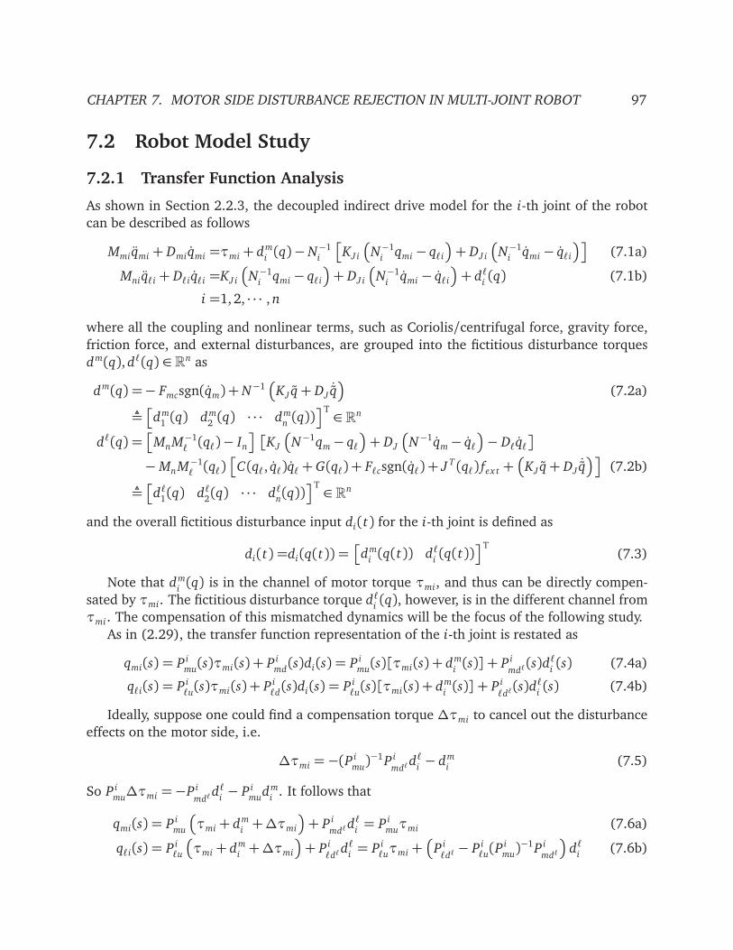
CHAPTER 7. MOTOR SIDE DISTURBANCE REJECTION IN MULTI-JOINT ROBOT 97
7.2 Robot Model Study
7.2.1 Transfer Function Analysis
As shown in Section 2.2.3, the decoupled indirect drive model for the i-th joint of the robot
can be described as follows
Mmiqmi + Dmiqmi =τmi + dmi(q)− N−1
i
KJ i
N−1i
qmi − qℓi
+ DJ i
N−1i
qmi − qℓi
(7.1a)
Mniqℓi + Dℓiqℓi =KJ i
N−1i
qmi − qℓi
+ DJ i
N−1i
qmi − qℓi
+ dℓi(q) (7.1b)
i =1, 2, · · · , n
where all the coupling and nonlinear terms, such as Coriolis/centrifugal force, gravity force,
friction force, and external disturbances, are grouped into the fictitious disturbance torques
dm(q), dℓ(q) ∈ Rn as
dm(q) =− Fmcsgn(qm) + N−1
KJ q+ DJ˙q
(7.2a)
¬
dm1(q) dm
2(q) · · · dm
n(q))
T∈ R
n
dℓ(q) =
MnM−1ℓ(qℓ)− In
KJ
N−1qm− qℓ
+ DJ
N−1qm− qℓ
− Dℓqℓ
−MnM−1ℓ(qℓ)
C(qℓ, qℓ)qℓ+ G(qℓ) + Fℓcsgn(qℓ) + J T (qℓ) fex t +
KJ q+ DJ˙q
(7.2b)
¬
dℓ1(q) dℓ
2(q) · · · dℓ
n(q))
T∈ R
n
and the overall fictitious disturbance input di(t) for the i-th joint is defined as
di(t) =di(q(t)) =
dmi(q(t)) dℓ
i(q(t))
T(7.3)
Note that dmi(q) is in the channel of motor torque τmi, and thus can be directly compen-
sated by τmi. The fictitious disturbance torque dℓi(q), however, is in the different channel from
τmi. The compensation of this mismatched dynamics will be the focus of the following study.
As in (2.29), the transfer function representation of the i-th joint is restated as
qmi(s) = P imu(s)τmi(s) + P i
md(s)di(s) = P i
mu(s)[τmi(s) + dm
i(s)] + P i
mdℓ(s)dℓ
i(s) (7.4a)
qℓi(s) = P iℓu(s)τmi(s) + P i
ℓd(s)di(s) = P i
ℓu(s)[τmi(s) + dm
i(s)] + P i
ℓdℓ(s)dℓ
i(s) (7.4b)
Ideally, suppose one could find a compensation torque ∆τmi to cancel out the disturbance
effects on the motor side, i.e.
∆τmi = −(Pimu)−1P i
mdℓdℓ
i− dm
i(7.5)
So P imu∆τmi =−P i
mdℓdℓ
i− P i
mudm
i. It follows that
qmi(s) = P imu
τmi + dmi+∆τmi
+ P i
mdℓdℓ
i= P i
muτmi (7.6a)
qℓi(s) = P iℓu
τmi + dmi+∆τmi
+ P i
ℓdℓdℓ
i= P i
ℓuτmi +
P i
ℓdℓ− P i
ℓu(P i
mu)−1P i
mdℓ
dℓi
(7.6b)

CHAPTER 7. MOTOR SIDE DISTURBANCE REJECTION IN MULTI-JOINT ROBOT 98
Denote
P i
∆ℓdℓ= P i
ℓu(P i
mu)−1P i
mdℓ
=Mni(DJ is+ KJ i)
2
N 2i s
MmiMnis3 + Jdis
2 + Jkis+ KJ i(Dmi + Dℓi/N2i )
Mnis2 + (DJ i + Dℓi)s+ KJ i
which has the following property
P i
∆ℓdℓ=
Mni
s(N 2i Dmi + Dℓi)
, s→ 0, (7.8a)
→ 0, s→∞. (7.8b)
From (2.31d), one can show that the transfer function P i
ℓdℓfrom the fictitious disturbance
input dℓi
to the load side position output qℓi has the similar property as (7.8a) when s → 0.
Figure 7.1 plots the frequency responses of the two transfer functions (i.e., s2P i
∆ℓdℓand s2P i
ℓdℓ)
for each joint of the FANUC M-16iB robot. It shows that the frequency responses of the two
transfer functions match each other very well up to the anti-resonant frequencies. This means
that, under ideal conditions, the perfect disturbance rejection on the motor side also results in
perfect disturbance rejection on the load side (i.e., P i
ℓdℓ− P i
ℓu(P i
mu)−1P i
mdℓin (7.6b) vanishes) in
the low frequency range. Thus, it is possible to improve the load side performance by adding
motor side disturbance rejection if the focus is in the low frequency region.
7.2.2 Inertia Variation and Model Simplification
Recall that Mn represents the diagonal terms of the load side inertia matrix Mℓ(qℓ), i.e., Mn =
diag(Mn1, Mn2, · · · , Mnn). From the simulation study of the FANUC M-16iB robot, it can be
shown that the load side inertia Mℓ(qℓ) varies significantly in the work space. For example,
Fig. 7.2 shows the variations of the second diagonal term Mn2 of the FANUC M-16iB robot
inertia matrix Mℓ(qℓ) in the work space, which ranges from about 30 kg· m2 to 90 kg· m2.
It is important to see how this inertia variation affects the frequency response of the indirect
drive model. Consider the simplification of the indirect drive model, e.g., assuming KJ i =
∞, DJ i =∞ (i.e., Niqℓi = qmi). The transfer function P imu
in (2.31a) from the motor torque τmi
to the motor side position qmi is thus simplified as
P imusim
=qmi(s)
τmi(s)=
1
s(Jis+ Di)(7.9)
where
Ji =Mni
N 2i
+Mmi, Di =Dℓi
N 2i
+ Dmi (7.10)
Figure 7.3 shows the frequency responses of the indirect drive model sP imu
(2.31a) and the
simplified model sP imusim
(7.9) together. The frequency response of the indirect drive model is

CHAPTER 7. MOTOR SIDE DISTURBANCE REJECTION IN MULTI-JOINT ROBOT 99
100
102
104
−270−180
−900
90180
Phase (
deg)
J1
Frequency (rad/sec)
−100
−50
0
Magnitude (
dB
)
10−2
100
102
104
−270−180
−900
90
Phase (
deg)
J2
Frequency (rad/sec)
−150
−100
−50
0
Magnitude (
dB
)
100
102
104
−270
−180
−90
0
90
Phase (
deg)
J3
−100
−50
0
Magnitude (
dB
)
10−2
100
102
104
−270
−180
−90
0
90
Phase (
deg)
J4
−150
−100
−50
0
Magnitude (
dB
)
100
102
104
Frequency (rad/sec)
10−2
100
102
104
Frequency (rad/sec)
−100
−50
0
Magnitude (
dB
)
100
102
104
−270
−180
−90
0
90
Phase (
deg)
J5
Frequency (rad/sec)
−100
−50
0
Magnitude (
dB
)
100
102
104
−180
−90
0
90
Phase (
deg)
J6
Frequency (rad/sec)P
∆ ld
Pld
s2P∆ℓdℓ
s2Pℓdℓ
Figure 7.1: Frequency Responses of s2P i
∆ℓdℓand s2P i
ℓdfor Each Robot Joint
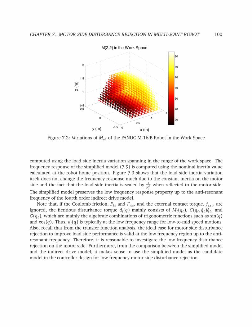
CHAPTER 7. MOTOR SIDE DISTURBANCE REJECTION IN MULTI-JOINT ROBOT 100
0
0.5
1
1.5
-0.5
0
0.50.5
1
1.5
2
x (m)
M(2,2) in the Work Space
y (m)
z (
m)
30
40
50
60
70
80
90
x (m)y (m)
Figure 7.2: Variations of Mn2 of the FANUC M-16iB Robot in the Work Space
computed using the load side inertia variation spanning in the range of the work space. The
frequency response of the simplified model (7.9) is computed using the nominal inertia value
calculated at the robot home position. Figure 7.3 shows that the load side inertia variation
itself does not change the frequency response much due to the constant inertia on the motor
side and the fact that the load side inertia is scaled by 1
N2i
when reflected to the motor side.
The simplified model preserves the low frequency response property up to the anti-resonant
frequency of the fourth order indirect drive model.
Note that, if the Coulomb friction, Fℓc and Fmc, and the external contact torque, fex t , are
ignored, the fictitious disturbance torque di(q) mainly consists of Mℓ(qℓ), C(qℓ, qℓ)qℓ, and
G(qℓ), which are mainly the algebraic combinations of trigonometric functions such as sin(q)
and cos(q). Thus, di(q) is typically at the low frequency range for low-to-mid speed motions.
Also, recall that from the transfer function analysis, the ideal case for motor side disturbance
rejection to improve load side performance is valid at the low frequency region up to the anti-
resonant frequency. Therefore, it is reasonable to investigate the low frequency disturbance
rejection on the motor side. Furthermore, from the comparison between the simplified model
and the indirect drive model, it makes sense to use the simplified model as the candidate
model in the controller design for low frequency motor side disturbance rejection.

CHAPTER 7. MOTOR SIDE DISTURBANCE REJECTION IN MULTI-JOINT ROBOT 101
-50
0
50
100
Magnitu
de (
dB
)
10-2
100
102
104
-90
-45
0
45
90
Phase (
deg)
Joint 1
Frequency (rad/sec)
-100
-50
0
50
100
Magnitu
de (
dB
)
10-2
100
102
104
-90
-45
0
45
90
Phase (
deg)
Joint 2
Frequency (rad/sec)
-40
-20
0
20
40
60
80
Magnitu
de (
dB
)
0
45
(deg)
Joint 3
-50
0
50
100
Magnitu
de (
dB
)
45
90
(deg)
Joint 4
Frequency (rad/sec) Frequency (rad/sec)
Magnitude (
dB
)
Magnitude (
dB
) (
deg)
(deg)
Magnitude (
dB
)
Magnitude (
dB
)P
hase (
deg)
Phase (
deg)
10-2
100
102
104
-90
-45Phase (
de
Frequency (rad/sec)
10-2
100
102
104
-90
-45
0
Phase (
de
Frequency (rad/sec)
-40
-20
0
20
40
60
80
Magnitu
de (
dB
)
10-2
100
102
104
-90
-45
0
45
Phase (
deg)
Joint 5
Frequency (rad/sec)
-40
-20
0
20
40
60
80
Magnitu
de (
dB
)
10-2
100
102
104
-90
-45
0
Phase (
deg)
Joint 6
Frequency (rad/sec)
Frequency (rad/sec) Frequency (rad/sec)
Frequency (rad/sec) Frequency (rad/sec)
Magnitude (
dB
)
Magnitude (
dB
)P
hase (
deg)
Phase (
deg)
Phase (
d
Phase (
d
Figure 7.3: Frequency Responses of Joint Models of the FANUC M-16iB Robot (Solid Color
Lines: Indirect Drive Model sP imu
; Black Marker Line: Simplified Model sP imusim
)
CHAPTER 7. MOTOR SIDE DISTURBANCE REJECTION IN MULTI-JOINT ROBOT 102
F1
F2
qℓdqmd
τff
qℓCpid
τm qm−
+
+ +
τpid
Cint
τint
+
Pa
d
Figure 7.4: Controller Structure of the Multi-Joint Robot
7.3 Controller Design
7.3.1 Baseline Controller Design
A basic decentralized controller is designed utilizing only motor side encoder signals for real-
time feedback. This is common practice in industrial robot control due to its simple structure
and efficient computation. The basic controller structure for the multi-joint robot is illustrated
in Fig. 7.4, which is similar to the single-joint case shown in Fig. 6.1.
In Fig. 7.4, Pa represents the actual multi-joint robot, which produces the load side position
output qℓ and the motor side position output qm. d is the fictitious disturbance torque defined
in (7.3). The overall controller structure consists of two feedforward controllers, F1 and F2,
and two feedback controllers, Cpid and Cint .
When performing a trajectory tracking task, the robot is typically given the tool center point
(TCP) trajectory in the Cartesian space, which is converted to the equivalent load side desired
trajectory by inverse kinematics. Then the motor side position reference qmd is generated
by the feedforward controller F1 from the load side position reference qℓd. The feedfoward
controller F2 generates the feedforward torque τ f f based on the available desired references,
qℓd and qmd. Cpid is a PID controller designed in the decentralized manner. Cint is the internal
feedback controller (e.g., disturbance observer (DOB) [66, 87] or adaptive robust controller
(ARC) [102, 99, 101, 100]) to reject the low frequency disturbances from the motor side.
In this controller structure, Cpid and Cint can be treated as the motor side controller, while
F1 (also part of F2) could be regarded as the load side controller to address the joint compliance
effects resulted from the indirect drive mechanism. The design for each controller part is
detailed in the following sections.
7.3.2 Feedforward Controller Design
In most cases, the feedback controllers are designed based on some simplified dynamic model,
i.e., the effects of some nonlinearities such as transmission elasticity, joint compliances, and
amplifier dynamics, are neglected. This implies that imposing large feedback gains to ob-

CHAPTER 7. MOTOR SIDE DISTURBANCE REJECTION IN MULTI-JOINT ROBOT 103
tain satisfactory performance may be impractical, since the existence of unmodeled dynamics
might degrade system performance and may eventually drive it to instability [74]. In other
words, the gains of the feedback controller should not be aggressively chosen because of the
unmodeled dynamics, and a well-tuned feedforward controller becomes essential for achiev-
ing good performance.
Good knowledge of the dynamic model is important in the feedforward controller design.
In this study, the Lagrangian model (2.24) is utilized, which leads to the following control law
for F1 and F2
τℓd = Mℓ(qℓd)qℓd + C(qℓd , qℓd)qℓd + G(qℓd) + JT(qℓd) fex t,d (7.11a)
qmd = N
qℓd + K−1Jτℓd
(7.11b)
τmd = Mmqmd + Dqmd + Fcsgn(qmd) (7.11c)
τ f f = τmd + N−1τℓd (7.11d)
where • is the nominal value of the matrix •. The actual computation of (7.11a) is performed
using recursive Newton-Euler method, which is computationally efficient.
Remark 7.1. Note that, due to the unmeasurable load side information, the friction parameter
identification is performed only on the motor side (see Appendix B for details). The identified
Coulomb friction, Fc = Fmc+N−1Fℓc, and viscous damping coefficient, D = Dm+N−2Dℓ, represent
the combined frictional effects of the motor side and the load side, and the feedforward friction
compensation is implemented only through the motor side.
Remark 7.2. To avoid the singularity of the signum function, an approximation for sgn(qmd) is
implemented as follows to have a smooth and continuous derivative
ˆsgn(qmd)≈1
π
atan(αqmd)− atan(−αqmd)
(7.12)
where α is the parameter to adjust the sharpness of the function shape around qmd = 0, i.e.,
ˆsgn(qmd)→ sgn(qmd) as α→∞.
The feedforward torque τ f f in (7.11d) can be divided into two parts, the linear part τln
corresponding to the simplified nominal model Pmusim, and the remaining nonlinear part τnl ,
i.e.
τln(qmd) = Jnqmd + Dnqmd (7.13a)
τnl = τ f f − τln (7.13b)
where the diagonal matrices Jn = Mm + N−2Mn ∈ Rn×n and Dn = D ∈ R
n×n are the nominal
linear inertia and nominal linear damping referencing to the motor side, respectively.

CHAPTER 7. MOTOR SIDE DISTURBANCE REJECTION IN MULTI-JOINT ROBOT 104
qmd
qmd
qm
+−
Kp Kv+
+
−
qm
Ki
s
τpid+
+
Cpid
Figure 7.5: PID Controller Structure of the Multi-Joint Robot
7.3.3 PID Controller Design
Similar to the single-joint case in Section 6.2.3, Fig. 7.5 illustrates the decoupled PID controller
structure of the multi-joint robot, which is described as
Cpid(s) =
Kv +Ki
s
Kp + s
(7.14a)
=
Ki + KvKp
+KiKp
s+ Kvs (7.14b)
where the diagonal matrix Kp ∈ Rn×n is the proportional gain of the position loop, the diagonal
matrices Kv ∈ Rn×n and Ki ∈ R
n×n are the proportional and integral gains of the velocity loop,
respectively.
Remark 7.3. As analyzed in previous sections, to compensate for the fictitious disturbance d(q),
the feedforward controller and the PID controller require a good knowledge of the robot dynamic
model to achieve high performance. In reality, however, it is normally impossible to obtain a
perfect and complete robot dynamic model. Hence, d(q) cannot be completely compensated for
and the resulting model discrepancy can be treated as a form of fictitious disturbance in the actual
plant.
To handle this problem, several approaches can be utilized, such as disturbance observer
(DOB) [66, 87] and adaptive robust controller (ARC) [102, 99, 101, 100], to reject the low fre-
quency disturbance from the motor side. By doing disturbance rejection, these two approaches
aim to make the shaded part (i.e., the inner plant) in Fig. 7.4 behave as the simplified nominal
model. Details of the two schemes are covered separately in the following sections.
7.3.4 Disturbance Observer (DOB) Based Disturbance Rejection
The disturbance observer regards any difference between the actual plant output and the nom-
inal model output as being caused by an equivalent disturbance applied to the nominal model
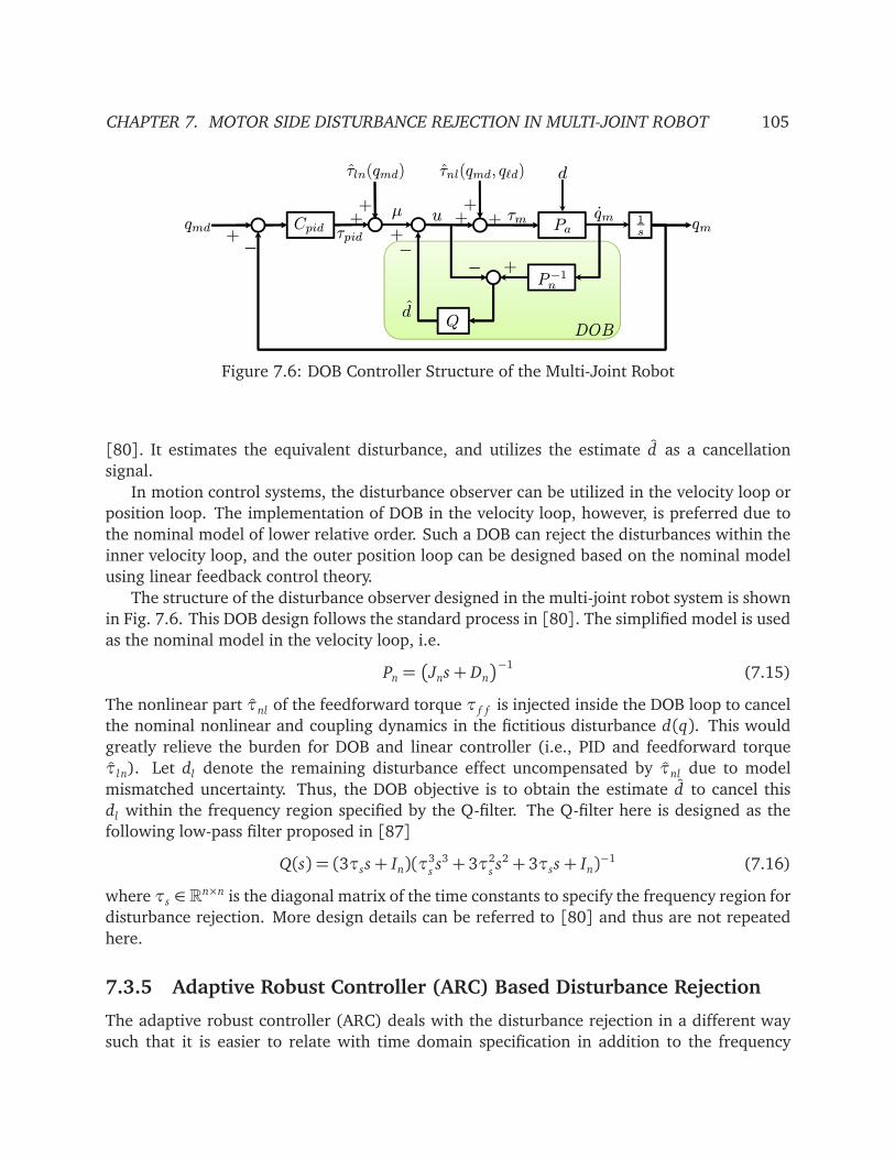
CHAPTER 7. MOTOR SIDE DISTURBANCE REJECTION IN MULTI-JOINT ROBOT 105
qmd qm+−
Pa++
qm+ 1
s
τnl(qmd, qℓd)
u
P−1
n
Cpid
τln(qmd)
τm
−
− +
d
DOBQ
++ µ
+τpid
d
Figure 7.6: DOB Controller Structure of the Multi-Joint Robot
[80]. It estimates the equivalent disturbance, and utilizes the estimate d as a cancellation
signal.
In motion control systems, the disturbance observer can be utilized in the velocity loop or
position loop. The implementation of DOB in the velocity loop, however, is preferred due to
the nominal model of lower relative order. Such a DOB can reject the disturbances within the
inner velocity loop, and the outer position loop can be designed based on the nominal model
using linear feedback control theory.
The structure of the disturbance observer designed in the multi-joint robot system is shown
in Fig. 7.6. This DOB design follows the standard process in [80]. The simplified model is used
as the nominal model in the velocity loop, i.e.
Pn =Jns+ Dn
−1(7.15)
The nonlinear part τnl of the feedforward torque τ f f is injected inside the DOB loop to cancel
the nominal nonlinear and coupling dynamics in the fictitious disturbance d(q). This would
greatly relieve the burden for DOB and linear controller (i.e., PID and feedforward torque
τln). Let dl denote the remaining disturbance effect uncompensated by τnl due to model
mismatched uncertainty. Thus, the DOB objective is to obtain the estimate d to cancel this
dl within the frequency region specified by the Q-filter. The Q-filter here is designed as the
following low-pass filter proposed in [87]
Q(s) = (3τss+ In)(τ3ss3 + 3τ2
ss2 + 3τss+ In)
−1 (7.16)
where τs ∈ Rn×n is the diagonal matrix of the time constants to specify the frequency region for
disturbance rejection. More design details can be referred to [80] and thus are not repeated
here.
7.3.5 Adaptive Robust Controller (ARC) Based Disturbance Rejection
The adaptive robust controller (ARC) deals with the disturbance rejection in a different way
such that it is easier to relate with time domain specification in addition to the frequency
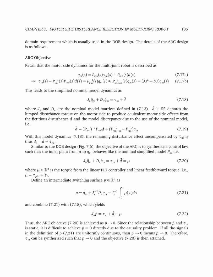
CHAPTER 7. MOTOR SIDE DISTURBANCE REJECTION IN MULTI-JOINT ROBOT 106
domain requirement which is usually used in the DOB design. The details of the ARC design
is as follows.
ARC Objective
Recall that the motor side dynamics for the multi-joint robot is described as
qm(s) = Pmu(s)τm(s) + Pmd(s)d(s) (7.17a)
⇒ τm(s) + P−1mu(s)Pmd(s)d(s) = P−1
mu(s)qm(s) ≈ P−1
musim(s)qm(s) = (Js2 + Ds)qm(s) (7.17b)
This leads to the simplified nominal model dynamics as
Jnqm+ Dnqm = τm+ d (7.18)
where Jn and Dn are the nominal model matrices defined in (7.13). d ∈ Rn denotes the
lumped disturbance torque on the motor side to produce equivalent motor side effects from
the fictitious disturbance d and the model discrepancy due to the use of the nominal model,
i.e.
d = (Pmu)−1Pmdd + (P−1
musim− P−1
mu)qm (7.19)
With this model dynamics (7.18), the remaining disturbance effect uncompensated by τnl is
thus dl = d + τnl .
Similar to the DOB design (Fig. 7.6), the objective of the ARC is to synthesize a control law
such that the inner plant from µ to qm behaves like the nominal simplified model Pn, i.e.
Jnqm+ Dnqm = τm+ d = µ (7.20)
where µ ∈ Rn is the torque from the linear PID controller and linear feedforward torque, i.e.,
µ= τpid + τln.
Define an intermediate switching surface p ∈ Rn as
p = qm+ J−1n
Dnqm− J−1n
∫ t
0
µ(τ)dτ (7.21)
and combine (7.21) with (7.18), which yields
Jn p = τm+ d −µ (7.22)
Thus, the ARC objective (7.20) is achieved as p→ 0. Since the relationship between p and τm
is static, it is difficult to achieve p = 0 directly due to the causality problem. If all the signals
in the definition of p (7.21) are uniformly continuous, then p → 0 means p → 0. Therefore,
τm can be synthesized such that p→ 0 and the objective (7.20) is then attained.

CHAPTER 7. MOTOR SIDE DISTURBANCE REJECTION IN MULTI-JOINT ROBOT 107
ARC Control Law
The proposed ARC control law is as follows
τm = us + u f , us =−Ks p, u f = µ+ τnl − dl (7.23)
where Ks ∈ Rn×n is a positive definite diagonal gain matrix. dl is the estimate of the un-
compensated fictitious disturbance dl . Furthermore, it is assumed that this uncompensated
disturbance dl is bounded, i.e., dl ∈ [dm, dM]. Comparing with the basic controller without
ARC, the additional control action introduced here is −Ksp− dl .
Substituting the control law (7.23) into the system dynamics (7.22), one can get
Jn p = −Ks p+µ+ τnl − dl + d −µ (7.24a)
= −Ks p+ dl − dl (7.24b)
⇒ Jn p+ Ksp = dl − dl (7.24c)
which is a first order stable system yielding
|p(∞)| ≤ K−1s|dl(∞)− dl(∞)| (7.25)
This indicates that p can be decreased by imposing a larger Ks. However, Ks is limited by the
system bandwidth and thus cannot be arbitrarily large. The other way to decrease p is by
decreasing |dl − dl |, which can be done by adaptively estimating dl .
The adaptation law to obtain the estimate dl is designed as
˙dl i = Pro j(Γi pi) =
0, if
¨dl i = dMi and pi > 0
dl i = dmi and pi < 0
Γi pi, otherwise
(7.26)
where Γ = diag(Γ1,Γ2, · · · ,Γn) ∈ Rn×n is a positive definite diagonal matrix, and •i denotes
the i-th entry of the vector •. It follows that
dl i ∈ [dmi, dMi], dl i(˙dl i −Γi pi)≤ 0, i = 1, 2, · · · , n (7.27)
Remark 7.4. With this adaptation law, if dl is not saturated, the dynamic equation (7.24c) with
regard to p becomes
Jn p+ Ks p+Γ
∫ t
0
pd t = dl (7.28)
and thus p(s)
dl(s)
P I D+ARC
= s(Jns2 + Kss+Γ)−1 (7.29)
where•
•
denotes the element-wise division of the numerator and denominator vectors and re-
sults in a diagonal matrix. Note that (7.29) is a second order system. Therefore, an appropriate
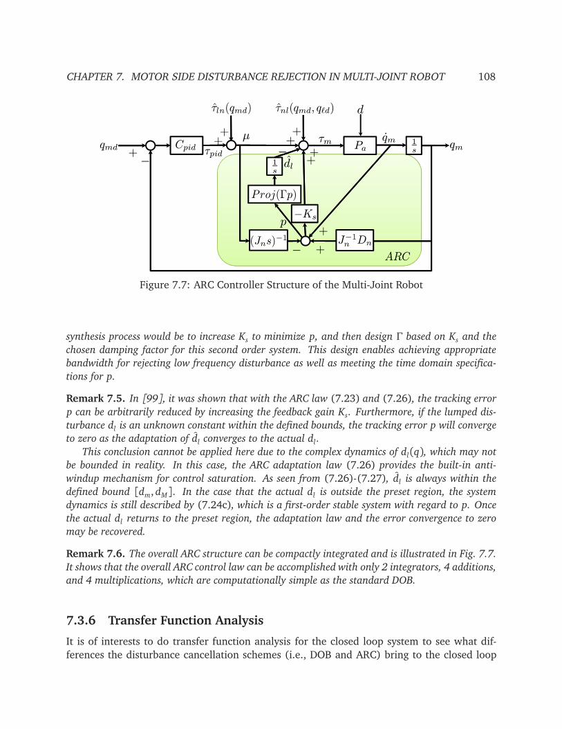
CHAPTER 7. MOTOR SIDE DISTURBANCE REJECTION IN MULTI-JOINT ROBOT 108
qmd qm+−
++
qm
+
τln(qmd)
1
s
++ µ
τpid
τnl(qmd, qℓd)
−Ks
Cpid
J−1
nDn(Jns)
−1
τmPa
Proj(Γp)
1
s
+
+−
−
+
ARC
dl
p
d
Figure 7.7: ARC Controller Structure of the Multi-Joint Robot
synthesis process would be to increase Ks to minimize p, and then design Γ based on Ks and the
chosen damping factor for this second order system. This design enables achieving appropriate
bandwidth for rejecting low frequency disturbance as well as meeting the time domain specifica-
tions for p.
Remark 7.5. In [99], it was shown that with the ARC law (7.23) and (7.26), the tracking error
p can be arbitrarily reduced by increasing the feedback gain Ks. Furthermore, if the lumped dis-
turbance dl is an unknown constant within the defined bounds, the tracking error p will converge
to zero as the adaptation of dl converges to the actual dl .
This conclusion cannot be applied here due to the complex dynamics of dl(q), which may not
be bounded in reality. In this case, the ARC adaptation law (7.26) provides the built-in anti-
windup mechanism for control saturation. As seen from (7.26)-(7.27), dl is always within the
defined bound [dm, dM]. In the case that the actual dl is outside the preset region, the system
dynamics is still described by (7.24c), which is a first-order stable system with regard to p. Once
the actual dl returns to the preset region, the adaptation law and the error convergence to zero
may be recovered.
Remark 7.6. The overall ARC structure can be compactly integrated and is illustrated in Fig. 7.7.
It shows that the overall ARC control law can be accomplished with only 2 integrators, 4 additions,
and 4 multiplications, which are computationally simple as the standard DOB.
7.3.6 Transfer Function Analysis
It is of interests to do transfer function analysis for the closed loop system to see what dif-
ferences the disturbance cancellation schemes (i.e., DOB and ARC) bring to the closed loop
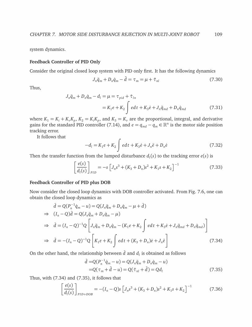
CHAPTER 7. MOTOR SIDE DISTURBANCE REJECTION IN MULTI-JOINT ROBOT 109
system dynamics.
Feedback Controller of PID Only
Consider the original closed loop system with PID only first. It has the following dynamics
Jnqm+ Dnqm− d = τm = µ+ τnl (7.30)
Thus,
Jnqm+ Dnqm− dl = µ = τpid + τln
= K1e+ K2
∫
ed t + K3 e+ Jnqmd + Dnqmd (7.31)
where K1 = Ki + KvKp, K2 = KiKp, and K3 = Kv are the proportional, integral, and derivative
gains for the standard PID controller (7.14), and e = qmd − qm ∈ Rn is the motor side position
tracking error.
It follows that
−dl = K1e+ K2
∫
ed t + K3 e+ Jne+ Dne (7.32)
Then the transfer function from the lumped disturbance dl(s) to the tracking error e(s) is
e(s)
dl(s)
P I D
= −s
Jns3 + (K3+ Dn)s2 + K1s+ K2
−1(7.33)
Feedback Controller of PID plus DOB
Now consider the closed loop dynamics with DOB controller activated. From Fig. 7.6, one can
obtain the closed loop dynamics as
d = Q(P−1n
qm− u) = Q(Jnqm+ Dnqm−µ+ d)
⇒ (In−Q)d = Q(Jnqm+ Dnqm−µ)
⇒ d = (In−Q)−1Q
Jnqm+ Dnqm− (K1e+ K2
∫
ed t + K3 e+ Jnqmd + Dnqmd)
⇒ d = −(In−Q)−1Q
K1e+ K2
∫
ed t + (K3+ Dn)e+ Jne
(7.34)
On the other hand, the relationship between d and dl is obtained as follows
d =Q(P−1n
qm− u) =Q(Jnqm+ Dnqm− u)
=Q(τm+ d − u) = Q(τnl + d) = Qdl (7.35)
Thus, with (7.34) and (7.35), it follows that
e(s)
dl(s)
P I D+DOB
=−(In −Q)s
Jns3 + (K3 + Dn)s2 + K1s+ K2
−1(7.36)
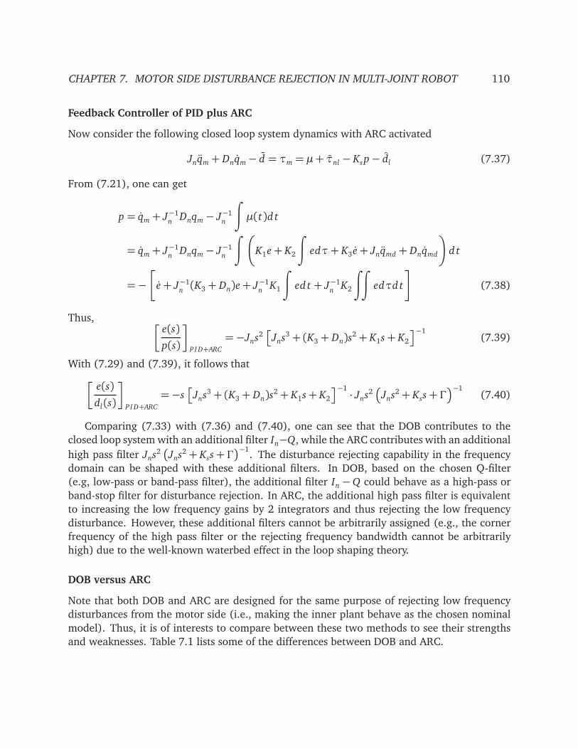
CHAPTER 7. MOTOR SIDE DISTURBANCE REJECTION IN MULTI-JOINT ROBOT 110
Feedback Controller of PID plus ARC
Now consider the following closed loop system dynamics with ARC activated
Jnqm+ Dnqm− d = τm = µ+ τnl − Ksp− dl (7.37)
From (7.21), one can get
p = qm+ J−1n
Dnqm− J−1n
∫
µ(t)d t
= qm+ J−1n
Dnqm− J−1n
∫
K1e+ K2
∫
edτ+ K3e+ Jnqmd + Dnqmd
d t
=−
e+ J−1n(K3 + Dn)e+ J−1
nK1
∫
ed t + J−1n
K2
∫∫
edτd t
(7.38)
Thus,
e(s)
p(s)
P I D+ARC
= −Jns2
Jns3 + (K3 + Dn)s2 + K1s+ K2
−1(7.39)
With (7.29) and (7.39), it follows that
e(s)
dl(s)
P I D+ARC
= −s
Jns3 + (K3+ Dn)s2 + K1s+ K2
−1· Jns2
Jns2 + Kss+Γ−1
(7.40)
Comparing (7.33) with (7.36) and (7.40), one can see that the DOB contributes to the
closed loop system with an additional filter In−Q, while the ARC contributes with an additional
high pass filter Jns2Jns2 + Kss+Γ
−1. The disturbance rejecting capability in the frequency
domain can be shaped with these additional filters. In DOB, based on the chosen Q-filter
(e.g, low-pass or band-pass filter), the additional filter In −Q could behave as a high-pass or
band-stop filter for disturbance rejection. In ARC, the additional high pass filter is equivalent
to increasing the low frequency gains by 2 integrators and thus rejecting the low frequency
disturbance. However, these additional filters cannot be arbitrarily assigned (e.g., the corner
frequency of the high pass filter or the rejecting frequency bandwidth cannot be arbitrarily
high) due to the well-known waterbed effect in the loop shaping theory.
DOB versus ARC
Note that both DOB and ARC are designed for the same purpose of rejecting low frequency
disturbances from the motor side (i.e., making the inner plant behave as the chosen nominal
model). Thus, it is of interests to compare between these two methods to see their strengths
and weaknesses. Table 7.1 lists some of the differences between DOB and ARC.
CHAPTER 7. MOTOR SIDE DISTURBANCE REJECTION IN MULTI-JOINT ROBOT 111
Table 7.1: The Comparison Between DOB and ARC
Aspects DOB ARC
Disturbance Rejection
Frequency Range
Frequency range specified
by Q-filter, e.g., low-pass or
band-pass filters
Low frequency disturbance
rejection
Design with Perfor-
mance Specification
Normally design in the fre-
quency domain rather than
the time domain
Could relate the design
with both time domain
and frequency domain
requirements
Controller Order Depends on the order of the
nominal inversed model and
Q-filter
Usually simple and low or-
der
Plant Uncertainty Q-filter bandwidth needs to
be conservative due to plant
uncertainty
Needs to make appropriate
assumption for plant uncer-
tainty bounds
Control Saturation Usually not considered Built-in anti-windup mecha-
nism for saturation
7.4 Experimental Study
7.4.1 Experimental Setup
The above disturbance rejection algorithms are validated on the FANUC M-16iB industrial
robot system shown in Section 2.3.2. In spite of the many sensors available on this experi-
mental setup, only motor side encoders are used for feedback control, while the CompuGauge
3D measurements are utilized only for performance evaluation. The real-time controllers are
implemented on the UCB-FANUC M-16iB Robot Experimentor through the xPC-Target system
with the sampling rate as 1kHz.
In the DOB and ARC implementations, the nominal linear inertia Jn and linear damping
Dn are chosen as the nominal values at the robot home position. The bandwidth of the Q-filter
in the DOB design is set to 1.5 times higher than the position loop bandwidth. In the ARC
design, Ks and Γ are designed such that the second order system (7.29) has a damping factor
of 1. The lumped fictitious disturbance bounds, dm and dM , are selected based on the motor
specifications and torque profiles from the feedforward torque calculation.
7.4.2 Experimental Results
The tool center point (TCP) testing trajectory (Fig. 7.8), which is a 4-th order smooth time
optimal trajectory [55], is designed to be a point-to-point scanning trajectory with a maximum

CHAPTER 7. MOTOR SIDE DISTURBANCE REJECTION IN MULTI-JOINT ROBOT 112
1.5 2 2.5 3 3.5 4 4.5 5 5.5 6
−0.2
0
0.2
0.4
0.6
0.8
1
1.2
1.4
1.6
Time (sec)
Positio
n (
m)
TCP Cartesian Space Position Trajectory
x
y
z
(a)
1.5 2 2.5 3 3.5 4 4.5 5 5.5 6−0.5
0
0.5
1
1.5
2
2.5
3
3.5
Time (sec)
Angle
(ra
d)
TCP Orientation Trajectory (Euler Angle ZYX/RPY)
Yaw (X)
Pitch (Y)
Roll (Z)
(b)
Figure 7.8: TCP Cartesian Space Trajectory Reference
CHAPTER 7. MOTOR SIDE DISTURBANCE REJECTION IN MULTI-JOINT ROBOT 113
Cartesian velocity of 800mm/sec, and a maximum Cartesian acceleration of 3000 mm/sec2.
Figure 7.9 and Fig. 7.10 illustrate the TCP Cartesian space position trajectory and the motor
side position errors, respectively. The performances of three controller designs are compared:
• the feedback controller with PID only (PID)
• the feedback controller with PID plus DOB (PID+DOB)
• the feedback controller with PID plus ARC (PID+ARC)
Figure 7.10 shows that both DOB and ARC can greatly improve the motor side tracking perfor-
mance. This improvement on the motor side also results in the significant improvement of the
load side/end-effector performance (Fig. 7.9), which is expected from the transfer function
analysis in Section 7.2.1. The frequency spectrum of the motor side position errors is illus-
trated in Fig. 7.11. It shows that the low frequency disturbance effects on the motor side has
been substantially reduced by the designed schemes.
Figure 7.12 compares the joint torque profiles for the three controller designs:
• the PID feedback torque (i.e., τpid in Fig. 7.4) in the setting PID
• the estimated disturbance torque (i.e., −d in Fig. 7.6) in the setting PID+DOB
• the ARC compensation torque (i.e., −Ks p− dl in Fig. 7.7) in the setting PID+ARC
Note that the compensation torques produced by the disturbance rejection methods (i.e., DOB
or ARC) match quite well with the PID torque in the setting PID. The large differences around
the middle and end points of the trajectory are due to the implementation setting that DOB
and ARC are basically disabled at the near-zero speed region for anti-windup. Overall, it
implies that the disturbance rejection schemes are essentially relieving the burden on the PID
controller. This means that even with conservative PID controller gains, good performance can
still be achieved with the help of disturbance rejection schemes.
7.5 Chapter Summary
This chapter presented the motor side disturbance rejection algorithms for the multi-joint
robot. The ultimate objective is to improve the load side (or end-effector) performance
through the disturbance rejection. As a prerequisite to achieving this goal, however, this
chapter focused on the design of motor side disturbance rejection controller. Two motor side
disturbance rejection schemes (i.e., DOB and ARC) were designed and compared. From the
robot model analysis and the experimental results, it demonstrated that the effects of the low
frequency motor side disturbance were greatly suppressed, and in addition, the load side/end-
effector performance was also significantly improved. In order to further achieve high band-
width load side performance, disturbance rejection scheme on the load side other than the
motor side is one of the future works.
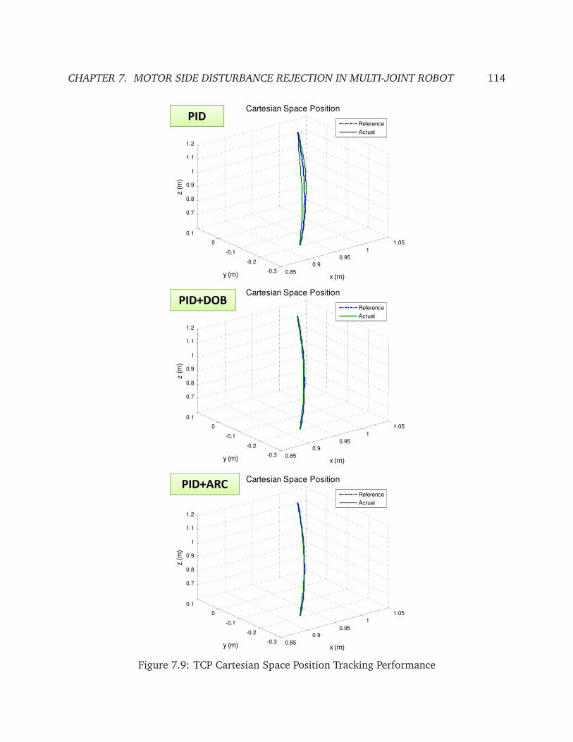
CHAPTER 7. MOTOR SIDE DISTURBANCE REJECTION IN MULTI-JOINT ROBOT 114
0.8
0.9
1
1.1
1.2
Cartesian Space Position
z (
m)
Reference
Actual
0.85
0.9
0.95
1
1.05
-0.3
-0.2
-0.1
0
0.1
0.7
0.8
0.9
1
1.1
1.2
x (m)
Cartesian Space Position
y (m)
z (
m)
Reference
Actual
0.85
0.9
0.95
1
1.05
-0.3
-0.2
-0.1
0
0.1
0.7
0.8
0.9
1
1.1
1.2
x (m)
Cartesian Space Position
y (m)
z (
m)
Reference
Actual
0.85
0.9
0.95
1
1.05
-0.3
-0.2
-0.1
0
0.1
0.7
x (m)y (m)
Figure 7.9: TCP Cartesian Space Position Tracking Performance
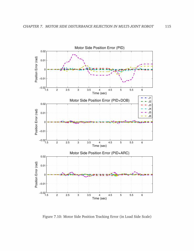
CHAPTER 7. MOTOR SIDE DISTURBANCE REJECTION IN MULTI-JOINT ROBOT 115
1.5 2 2.5 3 3.5 4 4.5 5 5.5 6−0.02
−0.01
0
0.01
0.02
Motor Side Position Error (PID)
Time (sec)
Po
sitio
n E
rro
r (r
ad
)
1.5 2 2.5 3 3.5 4 4.5 5 5.5 6−0.02
−0.01
0
0.01
0.02
Motor Side Position Error (PID+DOB)
Time (sec)
Po
sitio
n E
rro
r (r
ad
)
1.5 2 2.5 3 3.5 4 4.5 5 5.5 6−0.02
−0.01
0
0.01
0.02
Time (sec)
Po
sitio
n E
rro
r (r
ad
)
Motor Side Position Error (PID+ARC)
J1
J2
J3
J4
J5
J6
Figure 7.10: Motor Side Position Tracking Error (in Load Side Scale)

CHAPTER 7. MOTOR SIDE DISTURBANCE REJECTION IN MULTI-JOINT ROBOT 116
0 2 4 60
1
2
3
4
5
6
7
8
x 10−3 PID
Frequency (Hz)
|Mo
torP
osE
rrF
FT
|
0 2 4 60
1
2
3
4
5
6
7
8
x 10−3 PID+DOB
Frequency (Hz)
|Mo
torP
osE
rrF
FT
|Single−Sided Amplitude Spectrum of Motor Position Error
0 2 4 60
1
2
3
4
5
6
7
8
x 10−3 PID+ARC
Frequency (Hz)
|Mo
torP
osE
rrF
FT
|
J1
J2
J3
J4
J5
J6
Figure 7.11: Motor Position Error Spectrum
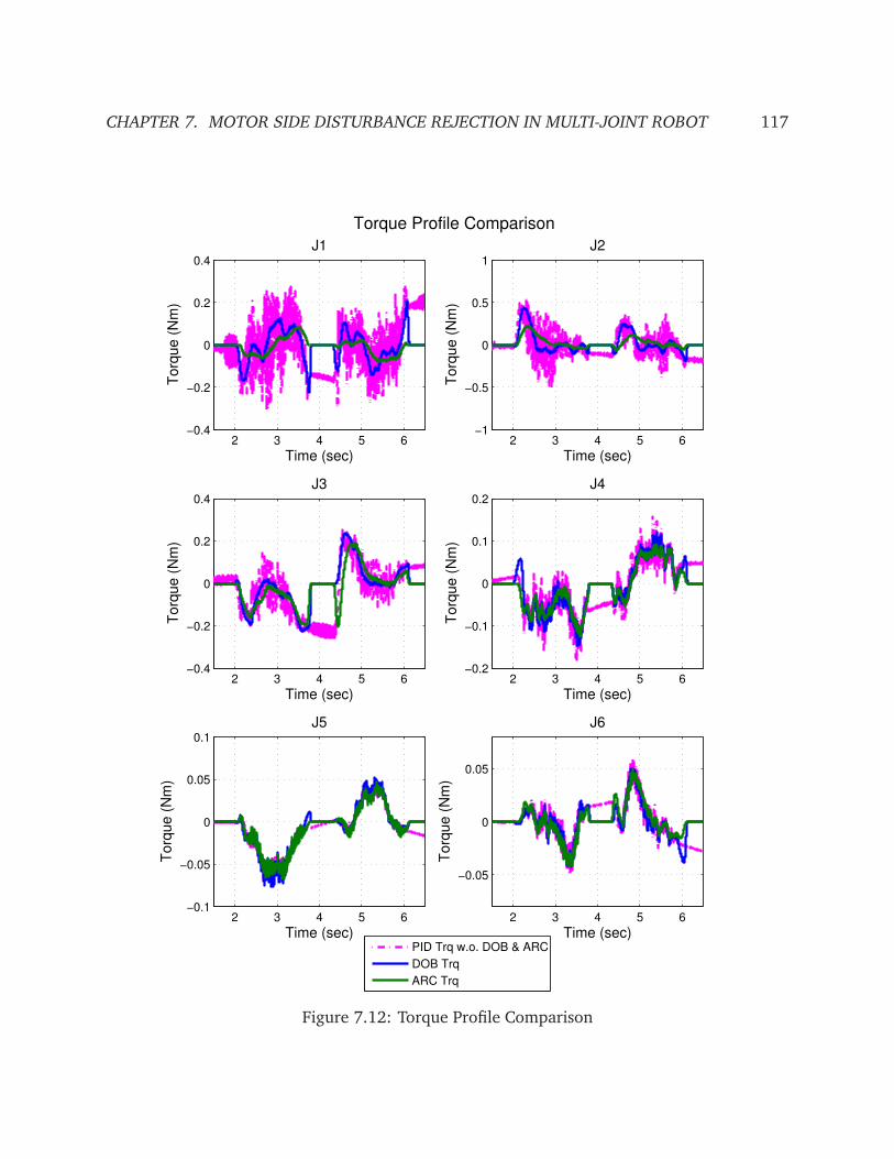
CHAPTER 7. MOTOR SIDE DISTURBANCE REJECTION IN MULTI-JOINT ROBOT 117
2 3 4 5 6−0.4
−0.2
0
0.2
0.4
Time (sec)
To
rqu
e (
Nm
)
J1
PID Trq w.o. DOB & ARC
DOB Trq
ARC Trq
2 3 4 5 6−1
−0.5
0
0.5
1
Time (sec)T
orq
ue
(N
m)
J2
2 3 4 5 6−0.4
−0.2
0
0.2
0.4
Time (sec)
To
rqu
e (
Nm
)
J3
2 3 4 5 6−0.2
−0.1
0
0.1
0.2
Time (sec)
To
rqu
e (
Nm
)
J4
2 3 4 5 6−0.1
−0.05
0
0.05
0.1
Time (sec)
To
rqu
e (
Nm
)
J5
Torque Profile Comparison
2 3 4 5 6
−0.05
0
0.05
Time (sec)
To
rqu
e (
Nm
)
J6
Figure 7.12: Torque Profile Comparison

118
Part III
Handling Mismatched Dynamics:
Iterative Learning Control Approaches
119
Chapter 8
Hybrid Two-Stage Model Based Iterative
Learning Control Scheme for MIMO
Mismatched Linear Systems
8.1 Introduction
Automated systems (e.g., robotic manipulators) used in industrial applications are often re-
quired to repeatedly perform a single task under the same operating conditions. If the system
repeatability is good, the trajectory tracking error will become repetitive from one run to an-
other. In this case, the iterative learning control (ILC) scheme is well suited to compensate for
the repeatable tracking error [11, 7].
ILC is a data-driven methodology which iteratively utilizes the data (e.g., error profile)
from previous trials to update the system inputs for the next iteration. Many versions of ILC
have been developed for various applications [11]. Most of them, however, are developed for
the fundamental case where the system has direct measurement of the interested output for
real-time feedback and does not have disturbances in the channels different from the control
input. Therefore, in mismatched systems where the above scenario does not hold, the perfor-
mance of the standard ILC is limited and in some cases may not be guaranteed to converge.
As discussed in Chapter 2, mismatched systems are common in practical applications, e.g.,
industrial robots with indirect-drive joint mechanisms (joints with elasticity). Several feedback
control approaches, such as integrator backstepping [45], dynamic surface control [47], and
adaptive robust control [100], have been developed specifically to handle mismatched system
behavior. Some efforts have been devoted to migrating these ideas to the field of ILC to deal
with the mismatched uncertainty iteratively while exploiting the advantage of noncasual off-
line processing.
Among those early works, a two-stage ILC approach was proposed in [63] for robots with
joint elasticity. Similar to backstepping, the real-time measured output (i.e., motor side state)
is utilized in [63] as a hypothetical input to control the output of interest (i.e., load side state).
CHAPTER 8. HYBRID TWO-STAGE MODEL BASED ITERATIVE LEARNING CONTROL
SCHEME FOR MIMO MISMATCHED LINEAR SYSTEMS 120
As shown later in this chapter, the convergence rate of this learning process may be adversely
affected and thus the use of a high bandwidth Q filter to learn high frequency error may com-
promise stability. Other studies such as [57, 89] also reported the compromise on the tracking
performance they had to make for a better learning convergence. This is especially the case
when the system exhibits mismatched uncertainties. Regarding this stability issue under un-
certainty, various robust approaches have been proposed [30, 67]. The resulting algorithms
are usually nontrivial and the performance is normally compromised for a conservative robust
controller. The scheme in [67] requires the plant resonances to be suppressed by feedback
compensation in order for the proposed method to improve the robustness to high-frequency
modeling errors. In [41], a model-based ILC approach was developed for robots with elas-
tic joints to learn the error component beyond the first resonant frequency. This approach,
however, requires an accurate piecewise-linear model to be identified for each trajectory in
advance, which limits its application.
This chapter proposes a hybrid two-stage model-based ILC approach for a class of MIMO
mismatched linear systems. The two-stage ILC is aimed to push the learning algorithm to
a higher bandwidth while maintaining the fast model-based convergence rate. The chapter
is organized as follows. The system model and the basic controller structure are introduced
first. Then two ILC schemes are designed independently, and are followed by an ad hoc hybrid
scheme to enable the two ILC schemes to execute simultaneously. The experimental study on
a single-joint indirect drive system is presented to validate the effectiveness of the proposed
scheme. The parametric uncertainty and mismatched dynamics such as various disturbances
at different locations of the system will be addressed. Finally, the conclusions of this work will
be given.
8.2 System Overview
8.2.1 System Model
The MIMO mismatched linear system (2.1) studied in this dissertation is restated here as
x(t) = Ax(t) + Buu(t) + Bdd(t) (8.1a)
y(t) =
qTm( j), qT
ℓ( j)T= C x(t) + Duu(t) + Ddd(t) (8.1b)
where x ∈ Rnx is the system state, u ∈ R
nu is the control input, d ∈ Rnd is the lumped distur-
bance, qm ∈ Rnm and qℓ ∈ R
nℓ are the two outputs of the plant. d is regarded as the mismatched
uncertainty/disturbance if it (or part of it) is applied to different channels from the control
input u (i.e., Bu 6= αBd ,∀α ∈ R). Another mismatched assumption is that, only part of the
outputs (i.e., qm) is measured for real-time feedback, even if the output of interest may be qℓ.
However, the measurement of qℓ may be available for iteration based off-line use. Further-
more, besides the unknown mismatched dynamics, it is assumed that parametric uncertainties
exist in the available nominal model.
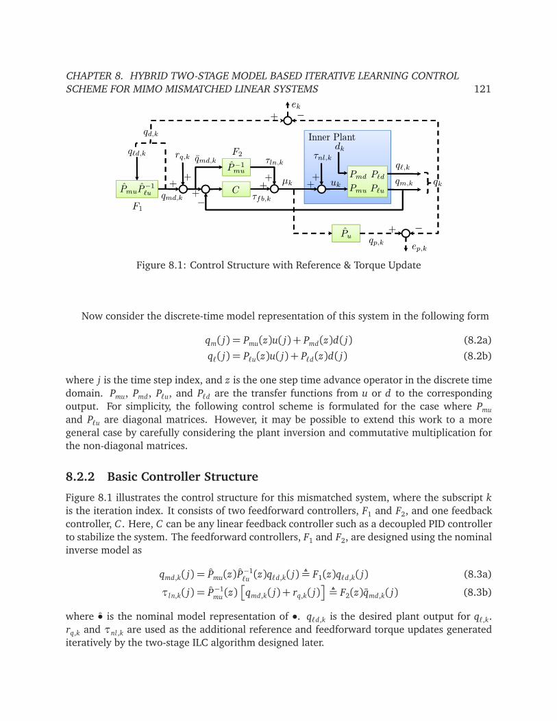
CHAPTER 8. HYBRID TWO-STAGE MODEL BASED ITERATIVE LEARNING CONTROL
SCHEME FOR MIMO MISMATCHED LINEAR SYSTEMS 121
+
−
C++ Pmd
Pmu Pℓu
Pℓd
qmd,k τfb,k
µk
dk
qℓ,k
qm,kPmuP
−1
ℓu
qℓd,k rq,k
++
++
τln,kτnl,k
Pu
P−1
mu
Inner Plant
qk
ek
uk
+ −
qd,k
+ −
ep,k
F1
F2qmd,k
qp,k
Figure 8.1: Control Structure with Reference & Torque Update
Now consider the discrete-time model representation of this system in the following form
qm( j) = Pmu(z)u( j) + Pmd(z)d( j) (8.2a)
qℓ( j) = Pℓu(z)u( j) + Pℓd(z)d( j) (8.2b)
where j is the time step index, and z is the one step time advance operator in the discrete time
domain. Pmu, Pmd, Pℓu, and Pℓd are the transfer functions from u or d to the corresponding
output. For simplicity, the following control scheme is formulated for the case where Pmu
and Pℓu are diagonal matrices. However, it may be possible to extend this work to a more
general case by carefully considering the plant inversion and commutative multiplication for
the non-diagonal matrices.
8.2.2 Basic Controller Structure
Figure 8.1 illustrates the control structure for this mismatched system, where the subscript k
is the iteration index. It consists of two feedforward controllers, F1 and F2, and one feedback
controller, C . Here, C can be any linear feedback controller such as a decoupled PID controller
to stabilize the system. The feedforward controllers, F1 and F2, are designed using the nominal
inverse model as
qmd,k( j) = Pmu(z)P−1ℓu(z)qℓd,k( j)¬ F1(z)qℓd,k( j) (8.3a)
τln,k( j) = P−1mu(z)
qmd,k( j) + rq,k( j)
¬ F2(z)qmd,k( j) (8.3b)
where • is the nominal model representation of •. qℓd,k is the desired plant output for qℓ,k.
rq,k and τnl ,k are used as the additional reference and feedforward torque updates generated
iteratively by the two-stage ILC algorithm designed later.

CHAPTER 8. HYBRID TWO-STAGE MODEL BASED ITERATIVE LEARNING CONTROL
SCHEME FOR MIMO MISMATCHED LINEAR SYSTEMS 122
8.3 Two-Stage ILC Scheme
8.3.1 ILC Basics
Here some basics of the general ILC scheme are reviewed first, which will be utilized in the
subsequent ILC scheme design. Consider the MIMO linear system with the error dynamics and
the ILC law in the following form
ek( j) = −Peu(z)uk( j) + r( j) (8.4a)
uk+1( j) = Q(z)
uk( j) + L(z)ek( j)
(8.4b)
where e is the error that the ILC scheme aims to reduce, r is the lumped repetitive reference
and/or disturbance input to the system, and u is the control input updated iteratively by the
ILC scheme using the filters L(z) and Q(z). Similar to [68, 11], the following convergence
property holds:
Theorem 8.1. The ILC system (8.4) is monotonically and exponentially convergent in the sense
that uk − u∞
p→ 0 and
ek − e∞
p→ 0 as k→∞, if
β = Q(z)
I − L(z)Peu(z)
p< 1 (8.5)
where β is the rate of convergence, I is the identity matrix with appropriate dimension, the p-
norm ‖ • ‖p =∑
i| •i |
p1/p
, and
u∞( j) =
I −Q(z) +Q(z)L(z)Peu(z)−1
Q(z)L(z)r( j) (8.6a)
e∞( j) =
I −Q(z) +Q(z)L(z)Peu(z)−1[I −Q(z)] r( j) (8.6b)
Proof. First, with (8.4), it is easy to see that
uk+1( j) =Q(z)
I − L(z)Peu(z)
uk( j) +Q(z)L(z)r( j) (8.7)
which yields
uk+1− u∞
p= Q(z)
I − L(z)Peu(z)
(uk − u∞)
p
≤ Q(z)
I − L(z)Peu(z)
p
uk − u∞
p(8.8)
Therefore, if Q(z)
I − L(z)Peu(z)
p< 1,
uk− u∞
p→ 0 as k → ∞. With (8.4a), similar
conclusion can be drawn for the convergence of ek. The converged steady states of u and
e are given in (8.6). Note that the inversion
I −Q(z)+Q(z)L(z)Peu(z)−1
exists because Q(z)[I − L(z)Peu(z)]
p< 1.
Equation (8.6b) shows that the steady state error e∞ vanishes with complete learning (i.e.,
Q(z) = I), which means the effects on e∞ from the repetitive input r will be fully compensated.

CHAPTER 8. HYBRID TWO-STAGE MODEL BASED ITERATIVE LEARNING CONTROL
SCHEME FOR MIMO MISMATCHED LINEAR SYSTEMS 123
The ILC law (8.4b) implies the Q filter can also be used to shape the learning ability in the
frequency domain. In order to achieve better performance, it is desired to push the bandwidth
of Q(z) to be as high as possible. Equation (8.5), however, indicates that the bandwidth of Q(z)
may have to be compromised to ensure monotonic convergence and to avoid poor transients
in the learning process. In practice, a low-pass filter Q(z) is typically employed to prevent the
effects of high frequency model uncertainties from entering the learning process [11]. Also,
Q(z) should be unity gain at low frequencies where complete learning is preferred to achieve
zero steady state error. Since the ILC scheme is an off-line iteration based method, acausal
filtering can be utilized to obtain a zero-phase learning response.1
Given a fixed Q filter, the optimal learning filter to achieve the fastest convergence is ob-
tained as
L∗(z) = argminL(z)
Q(z)
I − L(z)Peu(z)
p(8.9)
This leads to the plant inversion choice, i.e., L∗(z) = P−1eu(z). This model matching problem
can be solved with many optimization techniques, such as the H∞ synthesis [30], if the model
uncertainty bound is known. The designed Q(z) and L(z) need to be validated using (8.5) with
the knowledge of system model uncertainty. Without loss of generality, the optimal learning
filter in this chapter is simply chosen as L∗(z) = P−1eu(z).
8.3.2 ILC With Reference Update
Let Sp(z) =
I + C(z)Pmu(z)−1
denote the sensitivity function of the closed loop system in
Fig. 8.1. From (8.3a), qmd,k is related to qd,k (i.e., qℓd,k or qmd,k) as follows
qmd,k = Pmu P−1u
qd,k (8.10)
where Pu can be either Pmu or Pℓu depending on the choice of qd,k. The time index j for all
signals and the discrete time operator z for all transfer functions are omitted hereafter for
simplicity.
To reduce the tracking error ek = qd,k − qk, an ILC scheme with reference update can be
applied according to the following lemma.
Lemma 8.1. If the desired trajectory qd,k, the feedforward torque update τnl ,k, and the distur-
bance dk are repetitive for each iteration, the tracking error ek will be monotonically converging
1A typical way of designing a zero-phase low pass filter is Q(z) = Q1(z−1)Q1(z) where Q1(z) is a causal low-
pass filter with chosen cut-off frequency. In digital implementation (e.g., MATLAB "filtfilt" function), it means the
data series is filtered using Q1(z) in the forward direction and then filtered again in the backward direction. The
phase delay of the filtered data is canceled and the magnitude amplification is the square of the Q1(z)magnitude.
This Q filter is also usually used to make the non-proper plant inversion learning filter realizable. If Q1(z) or the
non-proper learning filter is an IIR filter, the initial condition of the filtered data needs to be taken care of as
suggested in [40].

CHAPTER 8. HYBRID TWO-STAGE MODEL BASED ITERATIVE LEARNING CONTROL
SCHEME FOR MIMO MISMATCHED LINEAR SYSTEMS 124
in the iteration domain by the following ILC scheme
rq,k+1 = Q r(rq,k+ L∗rek) (8.11)
L∗r= P−1
uPmu (8.12)
as long as the convergence rate β∗r
satisfies
β∗r=
Q r(I − P−1
uPuSpS−1
p)
∞< 1 (8.13)
Proof. The system output qk (i.e., qm,k or qℓ,k) can be derived as
qk = Puuk+ Pddk
= PuSp
(C + P−1mu)(qmd,k+ rq,k) +τnl ,k− C Pmddk
+ Pddk
= P−1mu
PuSpS−1p
rq,k+ PuSp
P−1u
S−1p
qd,k+τnl ,k− C Pmddk
+ Pddk (8.14)
where it has been assumed that Pmu, Pℓu, and C are diagonal matrices. Hence commutative
multiplication law applies hereafter. The corresponding tracking error ek is
ek = qd,k − qk =− P−1mu
PuSpS−1p
rq,k+ (I − PuSp P−1u
S−1p)qd,k
− PuSpτnl ,k+ (PuSpC Pmd − Pd)dk
¬− Peu,r rq,k+ rr,k (8.15)
Therefore, the tracking performance of the next iteration can be improved by the ILC scheme
with reference update (8.11) (namely reference ILC (L) or reference ILC (M) depending on
the choice of ek), if the desired trajectory qd,k, the feedforward torque update τnl ,k, and the dis-
turbance dk are repetitive for each iteration. From Theorem 8.1, the monotonic convergence
of this ILC scheme (8.11) can be guaranteed if βr =
Q r(1− Lr P−1
muPuSpS−1
p)
∞< 1. With the
nominal model inversion P−1eu,r= P−1
uPmu, the optimal learning filter and the convergence rate
are obtained as (8.12) and (8.13), respectively.
Remark 8.1. With complete learning (i.e., Q r = I), the tracking error e∞ vanishes when the
convergent condition (8.13) is met.
Remark 8.2. It is seen in (8.13) that, the model uncertainty will greatly affect the convergence
rate. In order to achieve fast convergence rate without compromising the bandwidth of Q r, it is
desired to reduce the model uncertainties. This can be done by obtaining a nominal model Pu more
accurately representing the actual physical plant, which requires significant system identification
effort and the resulting controller is generally too complex (highly nonlinear or high order).
In contrast, the same objective can be achieved by making the inner plant (blue shaded area in
Fig. 8.1) behave as the chosen nominal model Pu. In the next section, an ILC scheme with torque
update is introduced to accomplish this, i.e., making qk → Puµk, where µk = τln,k + τ f b,k is the
torque input to the inner plant.
CHAPTER 8. HYBRID TWO-STAGE MODEL BASED ITERATIVE LEARNING CONTROL
SCHEME FOR MIMO MISMATCHED LINEAR SYSTEMS 125
8.3.3 ILC With Torque Update
Define ep,k as the model following error between the nominal plant output (i.e., qp,k ¬ Puµk)
and the actual plant output qk (i.e., qℓ,k or qm,k). The ILC scheme to reduce this model follow-
ing error ep,k = qp,k− qk can be written as
τnl ,k+1 =Qu
τnl ,k+ Luep,k
(8.16)
where Pu is Pℓu or Pmu to match with the choice of qk. The corresponding ILC is termed as
torque ILC (L) or torque ILC (M).
Remark 8.3. It shows that τnl ,k is used to cancel out the effects on qk from model uncertainty
∆P ¬ Pu − Pu and mismatched disturbance dk. The ideal τ∗nl ,k
to achieve this objective can be
derived as
Puµk = Pu(µk +τ∗nl ,k) + Pddk ⇒ τ∗
nl ,k= −P−1
u(∆Pµk+ Pddk) (8.17)
In mismatched systems, the two objectives, following Pmu (i.e., torque ILC (M)) and following Pℓu(i.e., torque ILC (L)), cannot be attained simultaneously (i.e., τ∗
nl ,mk6= τ∗
nl ,ℓk), since P−1
muPmd 6=
P−1ℓu
Pℓd and P−1mu∆Pm 6= P−1
ℓu∆Pℓ in general. This means that at this stage it is desired to select the
nominal model to match with the chosen one in the reference ILC stage.
Convergence of Model Following Error
Lemma 8.2. If the desired trajectory qmd,k, the reference update rq,k, and the disturbance dk
remain the same for each iteration, the model following error ep,k will be monotonically converging
by the torque ILC scheme (8.16) if
Lu = L∗u= P−1
u(8.18)
β∗u=
Qu
I − Pu P−1u
Sp
∞< 1 (8.19)
Proof. The input-output equation of the nominal plant can be derived as
qp,k ¬ Puµk = PuSp
(C + P−1mu)(qmd,k+ rq,k)− C Pmuτnl ,k− C Pmddk
(8.20)
Then from (8.14) and (8.20), the model following error ep,k becomes
ep,k = qp,k − qk =− TuSpτnl ,k−∆PSp(C + P−1mu)(qmd,k+ rq,k)
+ (∆PSpC Pmd − Pd)dk
¬− Peu,uτnl ,k+ ru,k (8.21)
where Tu = PuC Pmu+ Pu.
Therefore, if the desired trajectory qmd,k, the reference update rq,k, and the disturbance
dk remain the same for each iteration, by Theorem 8.1, the torque ILC scheme (8.16) will be

CHAPTER 8. HYBRID TWO-STAGE MODEL BASED ITERATIVE LEARNING CONTROL
SCHEME FOR MIMO MISMATCHED LINEAR SYSTEMS 126
monotonically converging if βu =
Qu
I − LuTuSp
∞< 1. Using the nominal plant inversion
P−1eu,u= S−1
pT−1
u= P−1
u, the optimal choice of Lu and the convergence rate βu become (8.18)
and (8.19), respectively.
Remark 8.4. With complete learning (i.e., Qu = I), the inner plant behaves like the nominal
model as the model following error ep,∞→ 0 when the convergent condition (8.19) is met.
Convergence of Tracking Error
Lemma 8.3. If qd,k, rq,k, and dk do not vary from one iteration to another, then the tracking error
ek will converge monotonically with the rate of βe ≤ ‖PuT−1u‖∞βu as long as the model following
error ep,k converges and PuT−1u
is BIBO stable.
Proof. Using (8.15) and (8.21), the tracking error ek can be derived as
ek =PuT−1u
h
ep,k + PmuC
P−1u
Pmu Pu P−1mu− I
qd,k
−
P−1mu+ C
Purq,k+ C Pu
Pmd − Pd PmuP−1u
dk
i
(8.22)
Thus, the conclusion in the lemma is obtained.
Remark 8.5. For torque ILC (M) (i.e., Pu = Pmu and Pd = Pmd), P−1u
Pmu Pu P−1mu− I = 0 and
Pmd − Pd PmuP−1u= 0, which further reduces (8.22) to
ek = PuT−1u
ep,k− (P−1mu+ C)Purq,k
(8.23)
Thus if rq,k = 0 (i.e., the reference ILC is not activated), ek→ 0 as ep,k vanishes.
Remark 8.6. For torque ILC (L) (i.e., Pu = Pℓu and Pd = Pℓd), even if rq,k = 0 and ep,k vanishes,
ek → 0 is not necessarily true due to the mismatched behavior. The remaining tracking error e∞is
e∞ = PuT−1u
h
PmuC
P−1u
Pmu Pu P−1mu− I
qd,∞
−(P−1mu+ C)Purq,∞+ C Pu(Pmd − Pd PmuP−1
u)d∞
i
¬ −Peu,ur rq,∞+ rur,∞ (8.24)
This steady state tracking error e∞ can be further eliminated through the reference ILC using
L∗r= P−1
eu,ur= P−1
uPmu, and this matches with (8.12).
CHAPTER 8. HYBRID TWO-STAGE MODEL BASED ITERATIVE LEARNING CONTROL
SCHEME FOR MIMO MISMATCHED LINEAR SYSTEMS 127
8.3.4 Hybrid Scheme With Two-Stage ILC
In general, for the closed loop system with a satisfactory feedback controller, the sensitivity
function Sp will behave as a high-pass filter to mitigate the low frequency error. Therefore, in
the convergence condition (8.19), the low frequency model uncertainty is greatly suppressed
by Sp. This allows Qu to have higher bandwidth without worrying about the low frequency
uncertainty. Then with the effects of the torque ILC, the inner plant will behave like the
nominal model (i.e., qk → Puµk) up to the bandwidth of Qu. Within this frequency range, the
convergence condition of the reference ILC (8.13) will be simplified to
βr ≈
Q r
I − SpS−1p
∞< 1 (8.25)
which allows to push Q r to a higher bandwidth for better tracking performance.
Note that the repetitive assumption is used in the derivation of the aforementioned two ILC
schemes. When these two ILC schemes are activated simultaneously, the repetitive assumption
will be no longer valid (i.e., rq,k and τnl ,k are not repetitive from one iteration to another).
Therefore, an ad hoc hybrid scheme is designed to reduce the adverse interference of the two
ILC stages. Specifically, an iteration-varying gain is applied to each ILC stage as follows
τnl ,k+1 = Qu
τnl ,k+ γu,k Luep,k
(8.26)
rq,k+1 = Q r(rq,k+ γr,k Lr ek) (8.27)
where the two gains γu,k and γr,k can be tuned by trial and error, e.g., γu,k =min(4
∑
j ‖ep,k( j)‖2∑
j ‖ep,1( j)‖2, 1)
and γr,k = 1− 1
2γu,k. The basic idea behind is that the torque ILC needs to take more effects
whenever the model following error becomes larger in the previous iteration (i.e.,
∑
j ‖ep,k( j)‖2∑
j ‖ep,1( j)‖2
increases). In order for the torque ILC to perform better, the effects of the reference ILC is
accordingly attenuated with a decreased γr,k. In contrast, once the model following error is
sufficiently small (i.e., the inner plant behaves as the nominal model), the torque ILC becomes
not necessary and the reference ILC can be fully activated.
Remark 8.7. As shown in (8.23), for the application of tracking qm, the reference ILC is not
necessary and the torque ILC (M) with Pu = Pmu will be sufficient. In order to track qℓ, however,
the aforementioned hybrid two-stage ILC scheme with Pu = Pℓu will be necessary. And it is under-
stood that the nominal models used in two ILC stages should match with each other due to the
mismatched dynamics. In the experimental study, the algorithm validation will focus on the case
of tracking qℓ to test the effectiveness of the hybrid two-stage ILC scheme.
CHAPTER 8. HYBRID TWO-STAGE MODEL BASED ITERATIVE LEARNING CONTROL
SCHEME FOR MIMO MISMATCHED LINEAR SYSTEMS 128
8.4 Experimental Study
8.4.1 Experimental Setup & Dynamic Model
The proposed method is validated on a single-joint indirect drive robot shown in Fig. 2.3 in
Chapter 2. It is assumed that the load side encoder measurement is only available for iteration
based off-line use rather than for real-time feedback use. The gyroscope and accelerometer
measurements are not used in this ILC study. Finally, the algorithms are implemented using a
1kHz sampling rate through a LabVIEW real-time target.
Figure 2.1 in Chapter 2 illustrates the schematic of the single-joint indirect drive mecha-
nism. And the dynamic model (2.6) for this setup is restated as
Jmθm+ dmθm = u+ dm−1
N
k j
θm
N− θℓ
+ d j
θm
N− θℓ
(8.28a)
Jℓθℓ+ dℓθℓ = k j
θm
N− θℓ
+ d j
θm
N− θℓ
+ dℓ (8.28b)
where
dm = d f m− fmcsgn(θm) +1
N
k jθ + d j˙θ
(8.29a)
dℓ = d f ℓ− fℓcsgn(θℓ)−
k jθ + d j˙θ
(8.29b)
and all the variables are as defined in Chapter 2. Therefore, the above indirect drive model can
be considered as a mismatched system described in (8.2) with the disturbance d =
dm dℓT
.
The two outputs qm and qℓ are the motor side position θm and the load side position θℓ,
respectively. The continuous time transfer functions (i.e., Pmu, Pmd, Pℓu, and Pℓd) from the
inputs to the outputs were derived as (2.8) in Chapter 2.
8.4.2 System Disturbance Characteristics
Note that the disturbance d includes the Coulomb frictions (i.e., fmc and fℓc), external distur-
bances (i.e., d f m and d f ℓ), and the transmission error θ . It can be seen that d is repetitive if
qm and qℓ are repetitive.
In this setup, the identified Coulomb friction combined at the motor side (i.e., fmc +fℓc
N2 ) is
about 0.1004Nm (see Appendix B for more details). A fictitious torque is added in the motor
torque command to simulate the external disturbance d f m at the motor side. In the following
experiments, d f m is set as a 1Hz sinusoid starting from 3sec with an amplitude of 0.2Nm,
i.e., d f m = 0.2 sin(2π(t − 3))Nm. The repetitive external disturbance d f ℓ at the load side is
generated using the setup shown in Fig. 8.2. It is designed to have the extension springs apply
a maximum disturbance of approximately 20Nm at the load side when the payload hits the
ball and continues rotating for about 14 degrees.

CHAPTER 8. HYBRID TWO-STAGE MODEL BASED ITERATIVE LEARNING CONTROL
SCHEME FOR MIMO MISMATCHED LINEAR SYSTEMS 129
Load Side External
Disturbance Setup
≈ 0.2m ≈ 0.28m
≈ 500N/m
Figure 8.2: Load Side Disturbance Setup for Single-Joint System
The motor side feedback controller C designed for this setup has a resonant frequency
at about 11Hz for the velocity loop. This corresponds to about 1 rad/sec at the load side.
Recall that the dominant component of the transmission error in the harmonic drive has the
frequency ωo twice the motor side velocity θm (i.e., ωo = 2θm). Therefore, in order to amplify
the transmission error effects, the load side desired trajectory is designed to have a speed of
0.5 rad/sec for most time so that the resulting transmission error frequency will coincide with
the resonant frequency of the velocity loop . The resulting trajectory is shown in Fig. 8.3,
which was designed as a fourth-order smooth time optimal trajectory suggested in [55].
The effects of these different kinds of disturbances on the load side tracking performance
with the basic controller structure (i.e., C , F1, and F2 in Fig. 8.1) are illustrated in Fig. 8.4.
8.4.3 Algorithm Setup
Design the zero-phase acausal low-pass filters Q r and Qu as Q r(z) = Qu(z) = Q1(z−1)Q1(z),
where Q1(z) is a low-pass filter with a cut-off frequency of 30Hz, which is beyond the system
elastic anti-resonant and resonant frequencies. With this selection of Q r(z) and Qu(z), the
frequency responses of βr in (8.13) and βu in (8.19) with ±50% parametric uncertainties are
plotted in Fig. 8.5 to verify the monotonic stability condition.
Figure 8.5 shows that, using either motor side model or load side model, the magnitudes
of βr and βu are always below 0dB indicating βr < 1 and βu < 1. Therefore, the monotonic
stabilities (8.13) and (8.19) are ensured separately for both ILC schemes.
Now consider the old two-stage approach proposed in [63] as a benchmark controller. It
can be shown that, if using plant inversion learning filters, this old approach in [63] can be
reformulated similarly as the reference ILC (L) with Pu = Pℓu plus the torque ILC (M) with Pu =
Pmu in this chapter. This means that the two-stage ILC scheme is performed with mismatched
nominal models. As expected, this will not help to attenuate the model uncertainty but instead
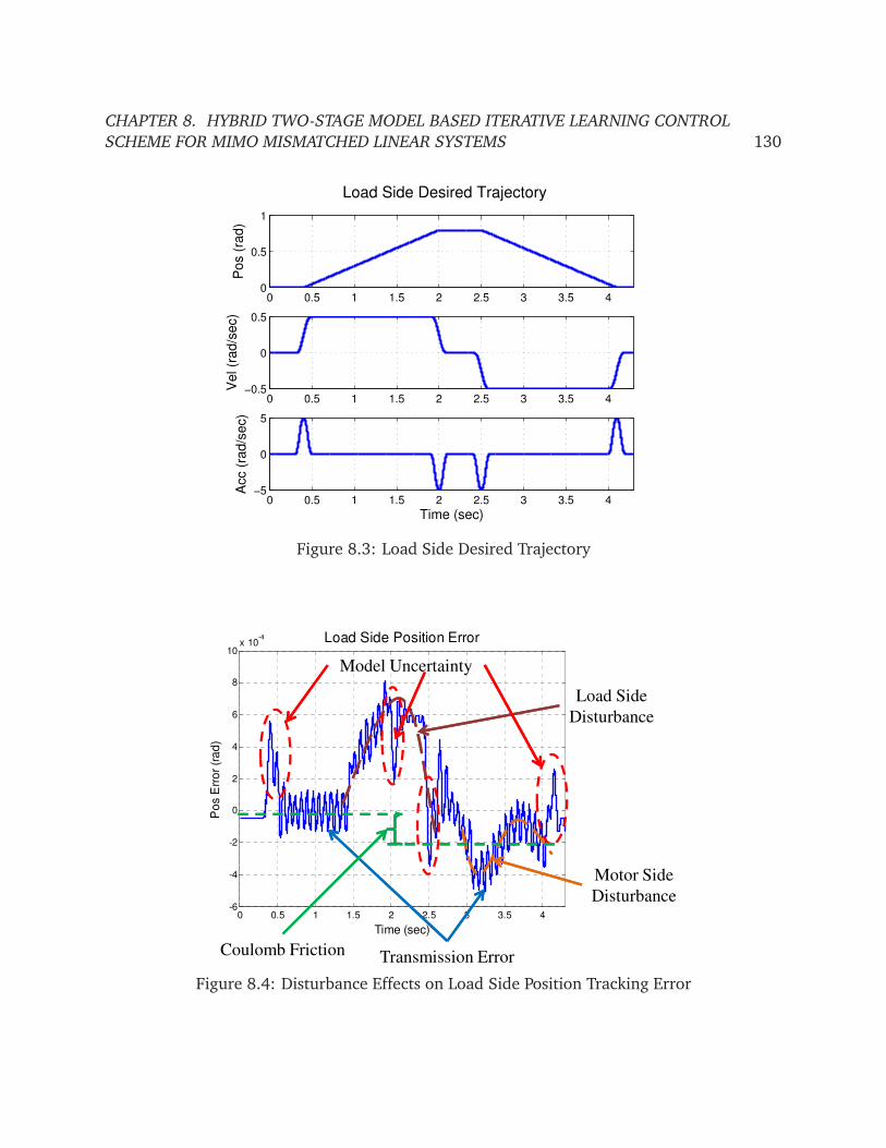
CHAPTER 8. HYBRID TWO-STAGE MODEL BASED ITERATIVE LEARNING CONTROL
SCHEME FOR MIMO MISMATCHED LINEAR SYSTEMS 130
0 0.5 1 1.5 2 2.5 3 3.5 40
0.5
1
Po
s (
rad
)
0 0.5 1 1.5 2 2.5 3 3.5 4−0.5
0
0.5
Ve
l (r
ad
/se
c)
Load Side Desired Trajectory
0 0.5 1 1.5 2 2.5 3 3.5 4−5
0
5
Acc (
rad/s
ec)
Time (sec)
Figure 8.3: Load Side Desired Trajectory
0 0.5 1 1.5 2 2.5 3 3.5 4-6
-4
-2
0
2
4
6
8
10x 10
-4
Po
s E
rro
r (r
ad
)
Time (sec)
Load Side Position Error
Load Side
Disturbance
Motor Side
Disturbance
Transmission Error
Model Uncertainty
Coulomb Friction
Figure 8.4: Disturbance Effects on Load Side Position Tracking Error
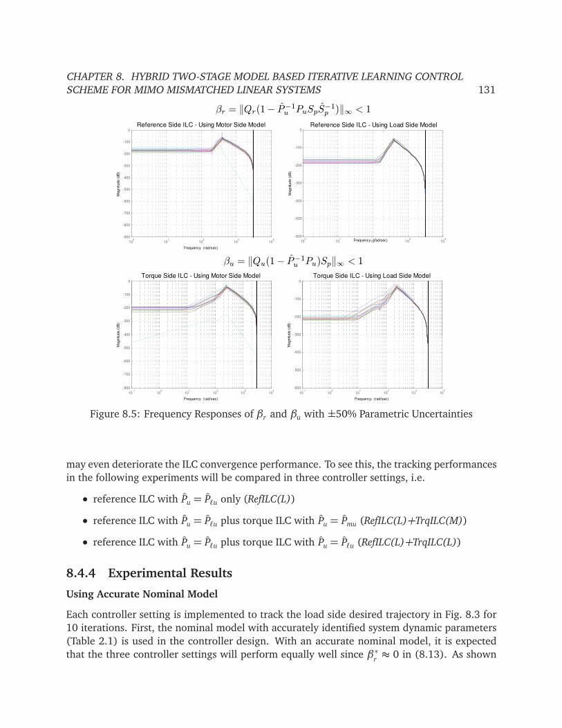
CHAPTER 8. HYBRID TWO-STAGE MODEL BASED ITERATIVE LEARNING CONTROL
SCHEME FOR MIMO MISMATCHED LINEAR SYSTEMS 131
100
101
102
103
104
-900
-800
-700
-600
-500
-400
-300
-200
-100
0
Magnitu
de (
dB
)
Reference Side ILC - Using Motor Side Model
Frequency (rad/sec)
-400
-300
-200
-100
0
itude (
dB
)
Torque Side ILC - Using Motor Side Model
-300
-200
-100
0
itude (
dB
)
Torque Side ILC - Using Load Side Model
100
101
102
103
104
-600
-500
-400
-300
-200
-100
0
Magnitu
de (
dB
)
Frequency (rad/sec)
βu = ‖Qu(1− P−1
uPu)Sp‖∞ < 1
βr = ‖Qr(1− P−1
uPuSpS
−1
p)‖∞ < 1
Reference Side ILC - Using Load Side Model
10-1
100
101
102
103
104
-800
-700
-600
-500
-400
Magnitu
Frequency (rad/sec)
10-1
100
101
102
103
104
-600
-500
-400
-300
Magnitu
Frequency (rad/sec)
Figure 8.5: Frequency Responses of βr and βu with ±50% Parametric Uncertainties
may even deteriorate the ILC convergence performance. To see this, the tracking performances
in the following experiments will be compared in three controller settings, i.e.
• reference ILC with Pu = Pℓu only (RefILC(L))
• reference ILC with Pu = Pℓu plus torque ILC with Pu = Pmu (RefILC(L)+TrqILC(M))
• reference ILC with Pu = Pℓu plus torque ILC with Pu = Pℓu (RefILC(L)+TrqILC(L))
8.4.4 Experimental Results
Using Accurate Nominal Model
Each controller setting is implemented to track the load side desired trajectory in Fig. 8.3 for
10 iterations. First, the nominal model with accurately identified system dynamic parameters
(Table 2.1) is used in the controller design. With an accurate nominal model, it is expected
that the three controller settings will perform equally well since β∗r≈ 0 in (8.13). As shown
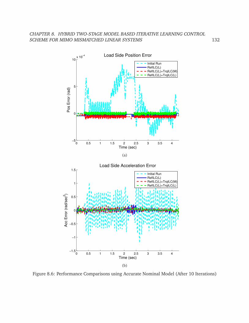
CHAPTER 8. HYBRID TWO-STAGE MODEL BASED ITERATIVE LEARNING CONTROL
SCHEME FOR MIMO MISMATCHED LINEAR SYSTEMS 132
0 0.5 1 1.5 2 2.5 3 3.5 4−5
0
5
10x 10
−4
Po
s E
rro
r (r
ad
)
Time (sec)
Load Side Position Error
Initial Run
RefILC(L)
RefILC(L)+TrqILC(M)
RefILC(L)+TrqILC(L)
(a)
0 0.5 1 1.5 2 2.5 3 3.5 4−1.5
−1
−0.5
0
0.5
1
1.5
Acc E
rro
r (r
ad
/se
c2)
Time (sec)
Load Side Acceleration Error
Initial Run
RefILC(L)
RefILC(L)+TrqILC(M)
RefILC(L)+TrqILC(L)
(b)
Figure 8.6: Performance Comparisons using Accurate Nominal Model (After 10 Iterations)
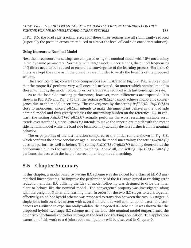
CHAPTER 8. HYBRID TWO-STAGE MODEL BASED ITERATIVE LEARNING CONTROL
SCHEME FOR MIMO MISMATCHED LINEAR SYSTEMS 133
in Fig. 8.6, the load side tracking errors for these three settings are all significantly reduced
(especially the position errors are reduced to almost the level of load side encoder resolution).
Using Inaccurate Nominal Model
Next the three controller settings are compared using the nominal model with 15% uncertainty
in the dynamic parameters. Normally, with larger model uncertainties, the cut off frequencies
of Q filters need to be reduced to ensure the convergence of the learning process. Here, the Q
filters are kept the same as in the previous case in order to verify the benefits of the proposed
scheme.
The error (∞-norm) convergence comparisons are illustrated in Fig. 8.7. Figure 8.7a shows
that the torque ILC performs very well once it is activated. No matter which nominal model is
chosen to follow, the model following errors are greatly reduced with fast convergence rate.
As to the load side tracking performance, however, more differences are expected. It is
shown in Fig. 8.7b and Fig. 8.7c that the setting RefILC(L) cannot achieve monotonic conver-
gence due to the model uncertainty. The convergence by the setting RefILC(L)+TrqILC(L) is
close to monotonic, since TrqILC(L) intends to make the inner plant behave as the load side
nominal model and thus greatly releases the uncertainty burden on the reference ILC. In con-
trast, the setting RefILC(L)+TrqILC(M) actually performs the worst resulting unstable error
trends over iterations, since TrqILC(M) intends to make the inner plant match with the motor
side nominal model while the load side behavior may actually deviate further from its nominal
behavior.
The error profiles of the last iteration compared to the initial run are shown in Fig. 8.8,
which confirms the above conclusion again. Due to the model uncertainty, the setting RefILC(L)
does not perform as well as before. The setting RefILC(L)+TrqILC(M) actually deteriorates the
performance due to the wrong model matching. Above all, the setting RefILC(L)+TrqILC(L)
performs the best with the help of correct inner loop model matching.
8.5 Chapter Summary
In this chapter, a model based two-stage ILC scheme was developed for a class of MIMO mis-
matched linear systems. To improve the performance of the ILC stage aimed at tracking error
reduction, another ILC utilizing the idea of model following was designed to drive the inner
plant to behave like the nominal model. The convergence property was investigated along
with the design of Q filter and learning filter. In order for the two ILC stages to work together
effectively, an ad hoc hybrid scheme was proposed to transition between the two ILC stages. A
single-joint indirect drive system with several inherent as well as intentional external distur-
bances was utilized to experimentally validate the proposed ILC scheme. It was shown that the
proposed hybrid two-stage ILC scheme using the load side nominal model outperformed the
other two benchmark controller settings in the load side tracking application. The application
extension of this work to a 6-joint robot manipulator will be discussed in Chapter 9.

CHAPTER 8. HYBRID TWO-STAGE MODEL BASED ITERATIVE LEARNING CONTROL
SCHEME FOR MIMO MISMATCHED LINEAR SYSTEMS 134
1 2 3 4 5 6 7 8 9 100
2
4
6
8
10
12
Pos E
rror
(rad)
Time (sec)
Model Following Error (Max)
RefILC(L)
RefILC(L)+TrqILC(M)
RefILC(L)+TrqILC(L)
(a)
1 2 3 4 5 6 7 8 9 100
0.2
0.4
0.6
0.8
1
1.2x 10
−3
Pos E
rror
(rad)
Time (sec)
Load Side Position Error (Max)
RefILC(L)
RefILC(L)+TrqILC(M)
RefILC(L)+TrqILC(L)
(b)
1 2 3 4 5 6 7 8 9 100.4
0.6
0.8
1
1.2
1.4
1.6
1.8
2
2.2
2.4
Acc E
rror
(rad/s
ec
2)
Time (sec)
Load Side Acceleration Error (Max)
RefILC(L)
RefILC(L)+TrqILC(M)
RefILC(L)+TrqILC(L)
(c)
Figure 8.7: Error Convergence Comparisons using Nominal Model with 15% Parametric Un-
certainties (10 Iterations)

CHAPTER 8. HYBRID TWO-STAGE MODEL BASED ITERATIVE LEARNING CONTROL
SCHEME FOR MIMO MISMATCHED LINEAR SYSTEMS 135
0 0.5 1 1.5 2 2.5 3 3.5 4−1.5
−1
−0.5
0
0.5
1
1.5x 10
−3
Po
s E
rro
r (r
ad
)
Time (sec)
Load Side Position Error
Initial Run
RefILC(L)
RefILC(L)+TrqILC(M)
RefILC(L)+TrqILC(L)
(a)
0 0.5 1 1.5 2 2.5 3 3.5 4−2
−1.5
−1
−0.5
0
0.5
1
1.5
2
2.5
Acc E
rro
r (r
ad
/se
c2)
Time (sec)
Load Side Acceleration Error
Initial Run
RefILC(L)
RefILC(L)+TrqILC(M)
RefILC(L)+TrqILC(L)
(b)
Figure 8.8: Performance Comparisons using Nominal Model with 15% Parametric Uncertain-
ties (After 10 Iterations)
136
Chapter 9
Iterative Learning Control with Sensor
Fusion: Application to Multi-Joint Robot
9.1 Introduction
As discussed in Chapter 2, the multi-joint robot with joint elasticity can be regarded as a typical
mismatched dynamic system. Chapter 8 proposed a hybrid two-stage model based ILC scheme,
where the reference trajectory and the feedforward torque input were both iteratively updated
to achieve high bandwidth performance while maintaining convergence property. This scheme
will be applied in this Chapter to deal with the mismatched system behaviors in the multi-joint
robot with joint elasticity.
While many literatures have suggested different kinds of iterative learning control (ILC)
schemes [11, 7], one of the essential factors for the algorithms to work effectively is to choose
and obtain the appropriate error information for the learning process.
For robots with joint compliance, the load side (end-effector) performance is of ultimate
interest, which cannot be guaranteed with motor side information alone [19, 91]. Chapter 8
and some early work [63, 57] on this topic considered only the single joint case or assumed
availability of load side joint measurements. In industrial robots, however, the load side joint
encoders are usually not available due to cost and assembly issue, thus creating a mismatched
sensing problem. Chapter 5 has shown that this problem can be tackled by adopting a low-cost
MEMS accelerometer to measure the end-effector vibration. The load side state estimation was
done using an optimization based inverse differential kinematics algorithm and an adaptive
kinematic Kalman filter (KKF) for each joint. The method is computationally light and will be
utilized in this chapter to provide desired load side joint state estimates.
Thus, in this chapter, the developed ILC scheme together with the sensor fusion method
will be applied to the multi-joint robot with joint elasticity, to demonstrate its superior perfor-
mance on the end-effector position tracking as well as the vibration reduction. This chapter
is organized as follows. The robot modeling and control structure are reviewed first. These
are followed by the application of the two-stage ILC scheme and the load side state estima-
CHAPTER 9. ITERATIVE LEARNING CONTROL WITH SENSOR FUSION: APPLICATION TO
MULTI-JOINT ROBOT 137
tion method, which is to retrieve the load side joint information from the measured Cartesian
space acceleration for implementation of the ILC scheme in the joint space. The experimental
study on the 6-DOF FANUC robot is presented to validate the effectiveness of the proposed
approach. Finally the conclusion is given.
9.2 System Overview
Consider an n-joint robot with gear compliance. The robot is equipped with motor side en-
coders to provide direct measurements of motor side joint positions and velocities for real-time
feedback. In addition, a three-dimensional accelerometer is mounted at the robot end-effector
to measure the end-effector acceleration in Cartesian space. Note that, if the computing re-
source and the sensor configuration allow, the end-effector sensor can also be used online.
This chapter, however, will address the conservative case where the end-effector sensor is for
off-line and training use only, which is usually preferred in industry due to the cost saving and
the limited real-time computational power.
9.2.1 Robot Dynamic Model
Following the variable definitions in Chapter 2, the decoupled robot dynamic model ((2.26)
in Chapter 2) can be restated as follows
Mmqm+ Dmqm = τm+ dm− N−1
KJ
N−1qm− qℓ
+ DJ
N−1qm− qℓ
(9.1a)
Mnqℓ+ Dℓqℓ = dℓ+ KJ
N−1qm− qℓ
+ DJ
N−1qm− qℓ
(9.1b)
where all the coupling and nonlinear terms, such as Coriolis/centrifugal force, gravity, Coulomb
frictions, transmission error, and external forces, are grouped into the fictitious disturbance
torques dm(q), dℓ(q) ∈ Rn as
dm(q) =− Fmcsgn(qm) + N−1
KJ q+ DJ˙q
(9.2a)
dℓ(q) =
MnM−1ℓ(qℓ)− In
KJ
N−1qm− qℓ
+ DJ
N−1qm− qℓ
− Dℓqℓ
−MnM−1ℓ(qℓ)
C(qℓ, qℓ)qℓ+ G(qℓ) + Fℓcsgn(qℓ) + J T (qℓ) fex t +
KJ q+ DJ˙q
(9.2b)
Thus, the robot can be considered as a MIMO system with 2n inputs and 2n outputs in the
following discrete-time form
qm( j) = Pmu(z)τm( j) + Pmd(z)d( j) (9.3a)
qℓ( j) = Pℓu(z)τm( j) + Pℓd(z)d( j) (9.3b)
where j is the time index, z is the one step time advance operator in the discrete time domain,
and the fictitious disturbance input d( j) is defined as (2.30a). The transfer functions (Pmu, Pℓu,
Pmd, and Pℓd) are derived as (2.31) in Chapter 2.

CHAPTER 9. ITERATIVE LEARNING CONTROL WITH SENSOR FUSION: APPLICATION TO
MULTI-JOINT ROBOT 138
+
−
C++ Pmd
Pmu Pℓu
Pℓd
qmd,k τfb,k
µk
dk
qℓ,k
qm,kPmuP
−1
ℓu
qℓd,k rq,k
++
++
τln,kτnl,k
Pu
P−1
mu
Inner Plant
qk
ek
τm,k
+ −
qd,k
+ −
ep,k
F1
F2qmd,k
qp,k
Figure 9.1: Robot Control Structure with Reference & Torque Update
9.2.2 Robot Controller Structure
It is seen that the robot dynamic model (9.1) is in a decoupled manner since all the variables
are expressed in the diagonal matrix form or vector form. Therefore, the robot controller can
be implemented in a decentralized form for each individual joint.
Note that the MIMO linear system representation (9.3) is obtained not through local lin-
earization but by considering the fictitious disturbance d as an input which includes the model
uncertainties and nonlinearities. The dℓ component of the fictitious disturbance d in (2.30a)
influences the output in a different way from the motor torque input τm. Thus this robot
system is regarded as a MIMO mismatched dynamic system.
The compensation of this fictitious disturbance d should be considered in the controller
design. To achieve this, the same controller structure (Fig. 9.1) developed in Chapter 8 can
be applied to this system. The variables in this controller structure follow the definitions in
Chapter 8. However, the initialization of two control updates (i.e., rq,k and τnl ,k) for the first
experiment iteration is designed as
rq,0 = NK−1J(τℓd − Mnqℓd − Dℓqℓd) (9.4a)
τnl ,0 = τ f f ,0− τln,0 (9.4b)
where
τℓd = Mℓ(qℓd)qℓd + C(qℓd , qℓd)qℓd + G(qℓd) + Dℓqℓd
+ Fℓcsgn(qℓd) + JT(qℓd) fex t,d (9.5a)
τmd,0 = Mm¯qmd,0+ Dm
¯qmd,0+ Fmcsgn(¯qmd,0) (9.5b)
τ f f ,0 = τmd,0+ N−1τℓd (9.5c)
CHAPTER 9. ITERATIVE LEARNING CONTROL WITH SENSOR FUSION: APPLICATION TO
MULTI-JOINT ROBOT 139
9.3 ILC Scheme with Sensor Fusion
To deal with the MIMO mismatched dynamic system described above, the hybrid two-stage
ILC scheme proposed in Chapter 8 is adopted here with specific consideration of the assumed
sensor configuration.
9.3.1 Two ILC Stages
For robot applications, the ultimate objective is to reduce the load side (end-effector) tracking
error. Here, to make the algorithm more general, define the tracking error as ek ¬ qd,k − qk.
When load side learning is desired and feasible with available information, the tracking error
is thus ek = eℓ,k ¬ qℓd,k − qℓ,k, with the corresponding transfer functions denoted as Pu = Pℓuand Pd = Pℓd . In contrast, if the load side information is not available for learning, only motor
side learning can be conducted with ek = em,k ¬ qmd,k − qm,k. Similarly, the corresponding
transfer functions would be Pu = Pmu and Pd = Pmd.
As derived in Chapter 8, the tracking performance of the next iteration can be improved
with the following reference update scheme using plant inversion learning filter
rq,k+1 = Q r(rq,k+ L∗rek) (9.6)
L∗r= P−1
eu,r= P−1
uPmu (9.7)
In order to achieve fast convergence rate without compromising the bandwidth of Q r, it is
desired to reduce the model uncertainties. This can be done by making the inner plant (blue
shaded area in Fig. 9.1) behave as the chosen nominal model Pu (e.g., making qk → Puµk).
Thus, another ILC stage with torque update based on the idea of model following is formulated
as
τnl ,k+1 = Qu
τnl ,k+ L∗uep,k
(9.8)
L∗u= P−1
eu,u= S−1
pT−1
u= P−1
u(9.9)
where ep,k ¬ qp,k − qk is the model following error between the nominal plant output (i.e.,
qp,k ¬ Puµk) and the actual plant output qk.
Similarly, depending on the available error information for learning process, this ILC stage
can be either load side learning (i.e., qk = qℓ,k, Pu = Pℓu, and Pd = Pℓd), or motor side learning
(i.e., qk = qm,k, Pu = Pmu, and Pd = Pmd). In practice, the plant inversion in (9.9) usually
encounters numerical difficulty since the relative order of Pℓu(s) or Pmu(s) is 3 or 2. Thus it
is more favorable to choose Pu(s) = Pℓu(s)s2 or Pu(s) = Pmu(s)s, both of which have lower
relative orders. The corresponding desired learning information for this new choice of Pu is
the load side acceleration qℓ,k or the motor side velocity qm,k, which is available with the as-
sumed sensor configuration (i.e., end-effector accelerometer and motor encoders). By similar
derivation, the torque ILC stage with these changes can still be obtained exactly the same as
(9.8)-(9.9), and achieves the same objective, i.e., making the inner plant behave as the chosen
CHAPTER 9. ITERATIVE LEARNING CONTROL WITH SENSOR FUSION: APPLICATION TO
MULTI-JOINT ROBOT 140
nominal model. Another benefit of this modification is that the torque ILC will be effective for
vibration suppression, while the reference ILC achieves the position error reduction. Thus, in
the practical implementation such as the following experimental study, these changes will be
applied to the torque ILC scheme to avoid numerical instability.
9.3.2 Hybrid Scheme For Two-Stage ILC
Recall that in Chapter 8, the repetitive assumption is used in the derivation of the aforemen-
tioned two ILC schemes. Here, the disturbance dk depends on the actual robot state q, and
is thus not repetitive. This can be relaxed in practice as follows: since the robot basic perfor-
mance should be already close to satisfactory, the tiny changes of q around desired state qd
in each iteration normally will not result in drastic change in dk. However, when these two
ILC stages are activated simultaneously, the repetitive assumption will be no longer valid (i.e.,
rq,k and τnl ,k are not repetitive from one iteration to another). Therefore, an ad hoc hybrid
scheme is designed to reduce the adverse interference of the two ILC stages. Specifically, an
iteration-varying gain is applied to each ILC stage as follows
τnl ,k+1 = Qu
τnl ,k+ γu,k L∗uep,k
(9.10)
rq,k+1 = Q r(rq,k+ γr,k L∗rek) (9.11)
where γu,k = diag(γ1u,k
, · · · ,γnu,k) and γr,k = diag(γ1
r,k, · · · ,γn
r,k). The two gains γi
u,kand γi
r,kfor
the i-th joint can be tuned by trial and error, e.g.
γiu,k=max
0.2, min
6
γiu,k−1
‖eip,k‖2
‖eip,k−1‖2
− 1
, 1
!!
(9.12a)
γir,k=
1− 0.8γiu,k
·min
2‖ei
k‖∞
‖ei0‖∞
, 1
(9.12b)
with the initialization as γiu,0= 1,γi
r,0= 0.2. The basic idea behind is that once the model
following error is becoming stable (i.e.,‖ei
p,k‖2
‖eip,k−1
‖2≈ 1, which means either the inner plant has
behaved as the nominal model or the torque ILC cannot make further improvement), the
torque ILC becomes less important and the reference ILC can be further activated with a
decreased γiu,k
and an increased γir,k
. In contrast, the torque ILC can take more effects and make
further improvement whenever the model following error is still drastically changing from the
previous iteration. In order for the torque ILC to perform better, the effects of the reference
ILC is accordingly attenuated with a decreased γir,k
. Furthermore, if the maximum tracking
error is sufficiently small (i.e.,‖ei
k‖∞
‖ei0‖∞≈ 0), the necessity of the reference ILC diminishes. Thus,
the gain γir,k
is accordingly decreased. However, to maintain the basic convergence rate, the
gain γiu,k
for the torque ILC is constrained to be within [0.2, 1] as indicated in (9.12).
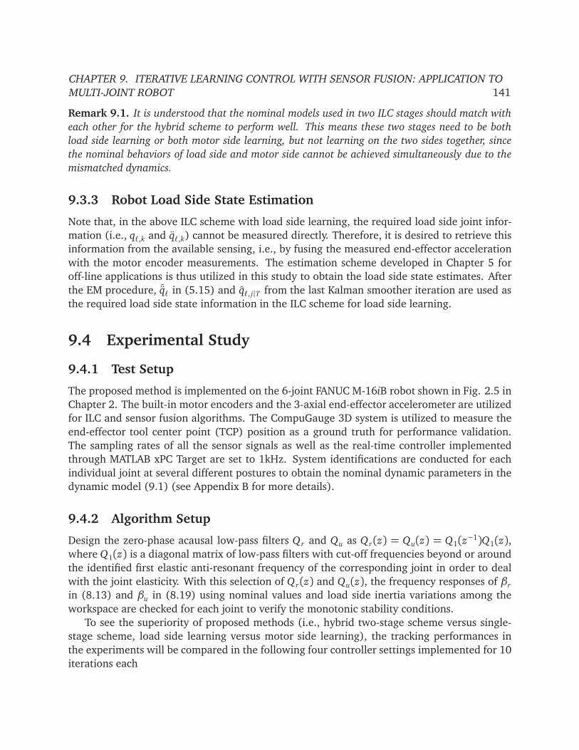
CHAPTER 9. ITERATIVE LEARNING CONTROL WITH SENSOR FUSION: APPLICATION TO
MULTI-JOINT ROBOT 141
Remark 9.1. It is understood that the nominal models used in two ILC stages should match with
each other for the hybrid scheme to perform well. This means these two stages need to be both
load side learning or both motor side learning, but not learning on the two sides together, since
the nominal behaviors of load side and motor side cannot be achieved simultaneously due to the
mismatched dynamics.
9.3.3 Robot Load Side State Estimation
Note that, in the above ILC scheme with load side learning, the required load side joint infor-
mation (i.e., qℓ,k and qℓ,k) cannot be measured directly. Therefore, it is desired to retrieve this
information from the available sensing, i.e., by fusing the measured end-effector acceleration
with the motor encoder measurements. The estimation scheme developed in Chapter 5 for
off-line applications is thus utilized in this study to obtain the load side state estimates. After
the EM procedure, ˆqℓ in (5.15) and qℓ, j|T from the last Kalman smoother iteration are used as
the required load side state information in the ILC scheme for load side learning.
9.4 Experimental Study
9.4.1 Test Setup
The proposed method is implemented on the 6-joint FANUC M-16iB robot shown in Fig. 2.5 in
Chapter 2. The built-in motor encoders and the 3-axial end-effector accelerometer are utilized
for ILC and sensor fusion algorithms. The CompuGauge 3D system is utilized to measure the
end-effector tool center point (TCP) position as a ground truth for performance validation.
The sampling rates of all the sensor signals as well as the real-time controller implemented
through MATLAB xPC Target are set to 1kHz. System identifications are conducted for each
individual joint at several different postures to obtain the nominal dynamic parameters in the
dynamic model (9.1) (see Appendix B for more details).
9.4.2 Algorithm Setup
Design the zero-phase acausal low-pass filters Q r and Qu as Q r(z) = Qu(z) = Q1(z−1)Q1(z),
where Q1(z) is a diagonal matrix of low-pass filters with cut-off frequencies beyond or around
the identified first elastic anti-resonant frequency of the corresponding joint in order to deal
with the joint elasticity. With this selection of Q r(z) and Qu(z), the frequency responses of βr
in (8.13) and βu in (8.19) using nominal values and load side inertia variations among the
workspace are checked for each joint to verify the monotonic stability conditions.
To see the superiority of proposed methods (i.e., hybrid two-stage scheme versus single-
stage scheme, load side learning versus motor side learning), the tracking performances in
the experiments will be compared in the following four controller settings implemented for 10
iterations each

CHAPTER 9. ITERATIVE LEARNING CONTROL WITH SENSOR FUSION: APPLICATION TO
MULTI-JOINT ROBOT 142
1 2 3 4 5 6 7 8 9 100.8
1
1.2
1.4
1.6
1.8
2
2.2
x 10−3
Iteration
RM
S E
rro
r (m
)
TCP Position RMS Error
RefILC(L)
TrqILC(L)
RefILC(M)+TrqILC(M)
RefILC(L)+TrqILC(L)
Figure 9.2: TCP Position RMS Error Comparisons in Iteration Domain
1. RefILC(L): Reference ILC only using load side learning, i.e., Pu(s) = Pℓu(s), γr,k ≡ 1, and
γu,k ≡ 0.
2. TrqILC(L): Torque ILC only using load side learning, i.e., Pu(s) = Pℓu(s)s2, γr,k ≡ 0, and
γu,k ≡ 1.
3. RefILC(L)+TrqILC(L): Reference ILC plus torque ILC using load side learning, i.e., Pu(s) =
Pℓu(s) for reference ILC and Pu(s) = Pℓu(s)s2 for torque ILC. γr,k and γu,k are updated as
in (9.12).
4. RefILC(M)+TrqILC(M): Reference ILC plus torque ILC using motor side learning, i.e.,
Pu(s) = Pmu(s) for reference ILC and Pu(s) = Pmu(s)s for torque ILC. γr,k and γu,k are
updated as in (9.12).
9.4.3 Experimental Results
The testing TCP trajectory is the same as the one (Fig. 5.3) in Chapter 5 for sensor fusion
method validation, which is a 10cm × 10cm square path on the Y-Z plane with fixed orienta-
tion, maximum velocity of 1m/sec, and maximum acceleration of 12.5m/sec2.
Figure 9.2 and Fig. 9.3 show the iteration domain root-mean-square (RMS) tracking error1
convergence profiles, while Fig. 9.4 and Fig. 9.5 show the time domain error profiles of the
initial run and the last runs of these controller settings.
It can be seen that the RefILC(L)+TrqILC(L) setting achieves the overall best performance
in position tracking and vibration reduction, even though there is non-monotonic transient
1The Cartesian space error here is defined as the Euclidean distance between the estimated posi-
tion/acceleration and the actual measured position/acceleration.
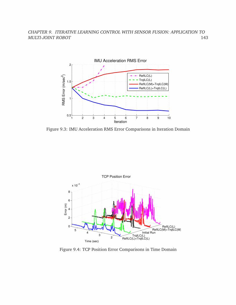
CHAPTER 9. ITERATIVE LEARNING CONTROL WITH SENSOR FUSION: APPLICATION TO
MULTI-JOINT ROBOT 143
1 2 3 4 5 6 7 8 9 100.5
1
1.5
2
Iteration
RM
S E
rror
(m/s
ec
2)
IMU Acceleration RMS Error
RefILC(L)
TrqILC(L)
RefILC(M)+TrqILC(M)
RefILC(L)+TrqILC(L)
Figure 9.3: IMU Acceleration RMS Error Comparisons in Iteration Domain
RefILC(L)+TrqILC(L)TrqILC(L)
Initial RunRefILC(M)+TrqILC(M)
RefILC(L)
23
45
0
2
4
6
8
x 10−3
TCP Position Error
Time (sec)
Err
or
(m)
Figure 9.4: TCP Position Error Comparisons in Time Domain

CHAPTER 9. ITERATIVE LEARNING CONTROL WITH SENSOR FUSION: APPLICATION TO
MULTI-JOINT ROBOT 144
RefILC(L)+TrqILC(L)TrqILC(L)
Initial RunRefILC(M)+TrqILC(M)
RefILC(L)
23
45
0
2
4
6
IMU Acceleration Error
Time (sec)
Err
or
(m/s
ec
2)
Figure 9.5: IMU Acceleration Error Comparisons in Time Domain
around the 5-th and 6-th iterations in the position error convergence due to the interference
between the two ILC stages. The RefILC(L) setting turns out to be unstable in the iteration
domain without the help of torque ILC to reduce model mismatched uncertainty. This implies
that the Q filter bandwidth (i.e., learning ability) for the RefILC(L) setting needs to be further
compromised. The TrqILC(L) setting looks monotonically convergent but with quite limited
improvement in error reductions (especially for moving periods), since the torque ILC aims
at modeling matching for the inner plant rather than directly addresses the load side tracking
error. The RefILC(M)+TrqILC(M) setting does not perform well either, since motor side model
can only be used for motor side learning, while the load side (end-effector) performance is
not guaranteed and may be even degraded due to the mismatched dynamics.
9.5 Chapter Summary
This chapter applied the model based ILC scheme developed in Chapter 8 to the multi-joint
robot with joint compliance for end-effector performance enhancement. The scheme itera-
tively updated the reference trajectory and the feedforward torque input in a two-stage man-
ner in order to achieve both high bandwidth performance and robust convergence. In order to
implement the decentralized ILC scheme in joint space, the load side state estimation method
developed in Chapter 5 was applied to retrieve the joint space information from the end-
effector measurements. The resulting ILC scheme and the load side state estimation method
were validated through the experimental study on a 6-DOF industrial robot. The study veri-
fied the benefits of sensor fusion utilizing end-effector measurements for learning process, and
the advantage of the hybrid two-stage ILC scheme to deal with the mismatched dynamics, in
end-effector position tracking and vibration mitigation.

145
Chapter 10
Concluding Remarks and Open Issues
10.1 Concluding Remarks
In the motion control of robots with joint flexibilities, the key inherent challenge is that the
robots exhibit mismatched dynamics and mismatched sensing. In other words, the desired vari-
able cannot be directly controlled or sensed.
This dissertation attempted to solve this fundamental problem through a mechatronic ap-
proach with contributions to hardware (sensor) configuration, dynamic modeling, algorithm
developments, and real-world experimentation. More specifically, the two mismatched prob-
lems were tackled from the perspectives of both estimation and control as follows:
Handling Mismatched Sensing: Sensor Fusion Approaches
This dissertation explored various sensor fusion schemes for handling mismatched sensing in
three fundamental cases:
• Load side joint state estimation in single-joint robot
• End-effector state estimation in multi-joint robot
• Load side joint state estimation in multi-joint robot
The sensor fusion algorithms for these three cases can meet most real-world needs in robots
with mismatched sensing. The sensor fusion schemes utilized dynamic and/or kinematic mod-
els. The study also examined various practical issues such as economic benefit, measurement
dynamics, model uncertainty, fictitious noise, and computation effort in one or more algorithm
designs. The designed algorithms and their validations through simulation and experimenta-
tion implicitly confirmed the following arguments
• It is undoubtedly beneficial to supplement robots with additional sensing on the load
side (for single-joint robots) or on the end-effector side (for multi-joint robots).
CHAPTER 10. CONCLUDING REMARKS AND OPEN ISSUES 146
• With proper sensor fusion, even low-cost and unprecise sensors can provide significant
performance enhancement.
• With careful customization, it is possible for the computation load of sensor fusion to be
considerably light. Especially, the developed load side state estimation scheme is suitable
for both off-line and online processing even with limited industrial computation power.
Handling Mismatched Dynamics: Control Approaches
This dissertation examined various control approaches for handling mismatched dynamics in
both the real-time domain (e.g., adaptive friction compensation, disturbance observer (DOB),
and adaptive robust controller (ARC)) and the iteration domain (e.g., iterative learning control
(ILC)). It was shown that compensation for the load side/end-effector uncertainty/disturbance
is necessary in addition to that for the motor side. However, if the focus is in the low frequency
range, then perfect motor side disturbance rejection also results in effective disturbance rejec-
tion on the load side/end-effector. The novel decoupled model formulation enabled the im-
plementation of the proposed controllers in the decentralized manner for multi-joint robots.
Considering the nature of the mismatched system as a two-mass system, the real-time and
iterative approaches were utilized in a hybrid two-stage manner to deal with the mismatched
dynamics. The algorithms manipulated both the motor side reference trajectory and the torque
input, in real-time or iteratively, using hybrid transition mechanisms to enable the two stages
to work together effectively. It was experimentally demonstrated that better load side/end-
effector performance (or higher bandwidth learning for the iterative approach) could be safely
achieved in this way in the presence of mismatched uncertainties/disturbances.
10.2 Future Avenues of Research
The results in this dissertation raise several issues as further research topics.
Sensor Fusion
The load side joint state estimation method (Chapter 5) is designed to satisfy industrial de-
mands for decentralized robot control. It can be, however, further improved by considering
more realistic factors. These issues include the sensor measurement dynamics (e.g., time-
varying biases and noises) and model uncertainty (e.g., dynamic and kinematic uncertainties).
These issues were considered in the single-joint sensor fusion study. The merit of the approach
may be properly extended to the multi-joint robot case.
Furthermore, similar to the multi-rate MD-KKF (for end-effector state estimation in Chap-
ter 4), the multi-rate extension can also be investigated for load side joint state estimation,
when sensors with different sampling rates are used.
CHAPTER 10. CONCLUDING REMARKS AND OPEN ISSUES 147
Control
The transfer function analysis and the experimentation in Chapter 7 demonstrated the signif-
icant improvement of the load side/end-effector performance by low frequency disturbance
rejection from the motor side. However, to further enhance high frequency load side perfor-
mance, the direct load side disturbance rejection becomes necessary. Disturbance rejections
on both the motor side and the load side need to be active for optimal performance. This
may be approached in a hybrid two-stage manner similar to the ILC scheme in Chapter 8 - 9.
The stability assurance for the designed real-time feedback algorithms will also be among the
future work.
The ILC scheme in Chapter 9 demonstrated its superior performance. Some ad hoc set-
tings, however, could be further investigated and replaced by a systematic control synthesis.
These settings include the optimal tuning of the two iteration-varying learning gains in (9.12)
for any given trajectory. The learning gain synthesis may be formulated as an optimization
problem with the cost function to properly describe the trade off between the two stages.
Nonlinear programming techniques may be employed to solve the optimization problem with
experimental data.
Other Applications
The sensor fusion methods (especially the load side joint state estimation) can also be applied
to applications such as the automatic controller tuning for load side/end-effector performance
enhancement. For example, the estimated load side joint states can be incorporated in the cost
functions in [93, 16] to address the load side/end-effector performance. The optimization
methods stated thereafter in [93, 16] can be then used to find the optimal controller gains.
Another important area that could be addressed is force/impedance sensing and estimation
at the load side/end-effector. With estimated load side/end-effector states, the information
of force/impedance may be properly observed. This extension would greatly broaden the
application area from position control to force/impedance control, or even beyond industrial
automation (such as service robots which require more human-robot interaction).

148
Bibliography
[1] Kistler (8330A3). http://www.kistler.com/mediaaccess/000-542e-07.06.pdf. Online. May
2009.
[2] Paul D. Abramson. “Simultaneous estimation of the state and noise statistics in linear
dynamical systems”. PhD thesis. Massachusetts Institute of Technology, 1968.
[3] Analog Devices (ADIS16400). http://www.analog.com/en/mems/imu/adis16400
/products/product.html. Online. July 2009.
[4] Analog Devices (ADXRS150). http://www.analog.com/en/mems-sensors/mems-
inertial-sensors/adxrs150/products/product.html. Online. July 2009.
[5] Friedhelm Altpeter. “Friction Modeling, Identification and Compensation”. PhD thesis.
Ecole Polytechnique Federale de Lausanne, 1999.
[6] MATLAB Simulink 3D Animation. http://www.mathworks.com/products/3d-animation.
Online. May 2012.
[7] Suguru Arimoto, Sadao Kawamura, and Fumio Miyazaki. “Bettering operation of Robots
by learning”. In: Journal of Robotic Systems 1.2 (1984), pp. 123–140.
[8] B Armstronghelouvry, Pierre Dupont, and Carlos Canudas De Wit. “A survey of models,
analysis tools and compensation methods for the control of machines with friction”.
In: Automatica 30.7 (1994), pp. 1083–1138.
[9] Jonathan Asensio, Wenjie Chen, and Masayoshi Tomizuka. “Robot Learning Control
Based on Neural Network Prediction”. In: Proceedings of the ASME Dynamic Systems
and Control Conference (DSCC). 2012.
[10] Patrik Axelsson, Rickard Karlsson, and Mikael Norrlöf. Bayesian State Estimation of a
Flexible Industrial Robot. Tech. rep. LiTH-ISY-R-3027. SE-581 83 Linkoping, Sweden:
Department of Electrical Engineering, Linkoping University, Oct. 2011.
[11] Douglas A Bristow and Marina Tharayil. “A survey of iterative learning control: A
learning-based method for high-performance tracking control”. In: IEEE Control Sys-
tems Magazine June (2006), pp. 96–114.
[12] H Bruyninckx and J Deschutter. “Symbolic differentiation of the velocity mapping for a
serial kinematic chain”. In: Mechanism and Machine Theory 31.2 (Feb. 1996), pp. 135–
148.

BIBLIOGRAPHY 149
[13] P Lischinsky C. Canudas de Wit. “Adaptive friction compensation with partially known
dynamic friction model”. In: International Journal of Adaptive Control and Signal Pro-
cessing 11.1 (1997), pp. 65–80.
[14] L Le Cam. “Maximum likelihood: an introduction”. In: Statistical Review/Revue Inter-
nationale de Statistique 58.2 (1990), pp. 153–171.
[15] C. Canudas de Wit, H. Olsson, K.J. Astrom, and P. Lischinsky. “A new model for control
of systems with friction”. In: IEEE Transactions on Automatic Control 40.3 (1995),
pp. 419–425.
[16] Michael Chan, Kyoungchul Kong, and Masayoshi Tomizuka. “Automatic Controller
Gain Tuning of a Multiple Joint Robot Based on Modified Extremum Seeking Control”.
In: Proceedings of the 18th IFAC World Congress. 2011, pp. 4131–4136.
[17] Wenjie Chen. UCB-FANUC M-16iB Robot Experimentor. Software. Version 4.2. Univer-
sity of California at Berkeley, 2012.
[18] Wenjie Chen. UCB-FANUC M-16iB Robot Simulator. Software. Version 4.2. University
of California at Berkeley, 2012.
[19] Wenjie Chen, Kyoungchul Kong, and Masayoshi Tomizuka. “Hybrid Adaptive Friction
Compensation of Indirect Drive Trains”. In: Proceedings of the 2009 ASME Dynamic
Systems and Control Conference (DSCC). 2009, pp. 313–320.
[20] Wenjie Chen, Pedro R. Mora, Mike Chan, Cong Wang, Chung-Yen Lin, and Masayoshi
Tomizuka. UCB-FANUC Project, Activity Report June 2011 - May 2012. Tech. rep. De-
partment of Mechanical Engineering, University of California, Berkeley, 2012.
[21] Wenjie Chen, Pedro Reynoso Mora, Mike Chan, Cheng-Huei Han, and Masayoshi
Tomizuka. UCB-FANUC Project Activity Report June 2009 - July 2010. Tech. rep. De-
partment of Mechanical Engineering, University of California at Berkeley, 2010.
[22] Wenjie Chen, Pedro Reynoso Mora, Mike Chan, Cong Wang, and Masayoshi Tomizuka.
UCB-FANUC Project, Activity Report June 2010 - May 2011. Tech. rep. Department of
Mechanical Engineering, University of California, Berkeley, 2011.
[23] Wenjie Chen and Masayoshi Tomizuka. “A Two-Stage Model Based Iterative Learning
Control Scheme for a Class of MIMO Mismatched Linear Systems”. In: Proceedings of
the ASME International Symposium on Flexible Automation (ISFA). 2012.
[24] Wenjie Chen and Masayoshi Tomizuka. “Estimation of load side position in indirect
drive robots by sensor fusion and kalman filtering”. In: Proceedings of American Control
Conference (ACC). 2010, pp. 6852–6857.
[25] Wenjie Chen and Masayoshi Tomizuka. “Iterative Learning Control with Sensor Fusion
for Robots with Mismatched Dynamics and Mismatched Sensing”. In: Proceedings of
the ASME Dynamic Systems and Control Conference (DSCC). 2012.

BIBLIOGRAPHY 150
[26] Wenjie Chen and Masayoshi Tomizuka. “Load Side State Estimation in Robot with
Joint Elasticity”. In: Proceedings of the IEEE/ASME International Conference on Ad-
vanced Intelligent Mechatronics (AIM). 2012.
[27] Peng Cheng and Bengt Oelmann. “Joint-Angle Measurement Using Accelerometers
and Gyroscopes – A Survey”. In: IEEE Transactions on Instrumentation and Measure-
ment 59.2 (2010), pp. 404–414.
[28] CompuGauge 3D. http://www.dynalog-us.com/solutions. Online. 2009.
[29] P.I. Corke. “A Robotics Toolbox for MATLAB”. In: IEEE Robotics and Automation Maga-
zine 3.1 (1996), pp. 24–32.
[30] D. De Roover and O.H. Bosgra. “Synthesis of robust multivariable iterative learning
controllers with application to a wafer stage motion system”. In: International Journal
of Control 73.10 (2000), pp. 968–979.
[31] R Dhaouadi. “Nonlinear friction compensation in harmonic drives with hysteresis”. In:
Proceedings of IEEE/ASME International Conference on Advanced Intelligent Mechatron-
ics (AIM). Vol. 1. 2003, pp. 278–283.
[32] V Digalakis, J.R. Rohlicek, and M Ostendorf. “ML estimation of a stochastic linear
system with the EM algorithm and its application to speech recognition”. In: IEEE
Transactions on Speech and Audio Processing 1.4 (1993), pp. 431–442.
[33] A Dixit and S Suryanarayanan. “Adaptive observers for servo systems with friction”.
In: Proceedings of IEEE International Conference on Control Applications (CCA). 2008,
pp. 960–965.
[34] RA Fisher. “Theory of statistical estimation”. In: Mathematical Proceedings of the Cam-
bridge 22 (1925), pp. 700–725.
[35] P.S. Gandhi, F.H. Ghorbel, and J. Dabney. “Modeling, identification, and compensation
of friction in harmonic drives”. In: Proceedings of the 41st IEEE Conference on Decision
and Control. Vol. 1. 2002, pp. 160–166.
[36] Miguel Lagullón García. “Robot Simulation based on the Integration of MatlabSimulink
and UGS Platforms”. MA thesis. University of California, Berkeley, and Polytechnic
University of Valencia, 2011.
[37] GE. http://www.geindustrial.com/products/brochures/Alphaiservospecs.pdf. Online. May
2009.
[38] Zoubin Ghahramani and Geoffrey E. Hinton. Parameter estimation for linear dynamical
systems. Tech. rep. CRG-TR-96-2. University of Toronto, 1996.
[39] Fathi H. Ghorbel, Prasanna S. Gandhi, and Friedhelm Alpeter. “On the Kinematic Error
in Harmonic Drive Gears”. In: Transactions of the ASME, Journal of Mechanical Design
123.1 (2001), pp. 90–97.
[40] F. Gustafsson. “Determining the initial states in forward-backward filtering”. In: IEEE
Transactions on Signal Processing 44.4 (Apr. 1996), pp. 988–992.

BIBLIOGRAPHY 151
[41] W.B.J. Hakvoort, R.G.K.M. Aarts, J. van Dijk, and J.B. Jonker. “Model-based iterative
learning control applied to an industrial robot with elasticity”. In: Proceedings of IEEE
Conference on Decision and Control. 2007, pp. 4185–4190.
[42] Cheng-huei Han. “High Precision Control of Indirect Drive Systems Based on End-
effector Sensor Information”. PhD thesis. University of California, Berkeley, 2009.
[43] Cheng-huei Han, Wenjie Chen, Pedro R. Mora, Mike Chan, and Masayoshi Tomizuka.
UCB-FANUC Project Activity Report June 2008 - July 2009. Tech. rep. Department of
Mechanical Engineering, University of California at Berkeley, 2009.
[44] Cheng-Huei Han, Chun-Chih Wang, Wenjie Chen, and Masayoshi Tomizuka. UCB-
FANUC Project Activity Report June 2007 - July 2008. Tech. rep. Department of Me-
chanical Engineering, University of California at Berkeley, 2008.
[45] Hassan K. Khalil. Nonlinear Systems. Prentice Hall, 2002.
[46] J P Hauschild, G. Heppler, and J. McPhee. “Friction compensation of harmonic drive
actuators”. In: Proceedings of the 6th International Conference on Dynamics and Control
of Systems and Structures in Space. v. 2004, pp. 683–692.
[47] J. K. Hedrick and P. P. Yip. “Multiple Sliding Surface Control: Theory and Application”.
In: Journal of Dynamic Systems, Measurement, and Control 122.4 (2000), pp. 586–593.
[48] Robert Henriksson, M. Norrlof, Stig Moberg, Erik Wernholt, and TB Schon. “Experi-
mental comparison of observers for tool position estimation of industrial robots”. In:
Proceedings of the 48th IEEE Conference on Decision and Control. 2009, pp. 8065–8070.
[49] Kim Heui-Wook and Sul Seung-Ki. “A new motor speed estimator using Kalman fil-
ter in low-speed range”. In: IEEE Transactions on Industrial Electronics 43.4 (1996),
pp. 498–504.
[50] Kiyonori Inaba. “Iterative learning control for industrial robots with end effector sens-
ing”. PhD thesis. University of California at Berkeley, 2009.
[51] Soo Jeon and Masayoshi Tomizuka. “Benefits of acceleration measurement in velocity
estimation and motion control”. In: Control Engineering Practice 15.3 (Mar. 2007),
pp. 325–332.
[52] Soo Jeon and Masayoshi Tomizuka. “Limit cycles due to friction forces in flexible joint
mechanisms”. In: Proceedings of IEEE/ASME International Conference on Advanced In-
telligent Mechatronics (AIM). 2005, pp. 723–728.
[53] Soo Jeon, Masayoshi Tomizuka, and Tetsuaki Katou. “Kinematic Kalman Filter (KKF)
for Robot End-Effector Sensing”. In: Journal of Dynamic Systems, Measurement, and
Control 131.2 (2009), pp. 21010–21018.
[54] National Instruments LabVIEW. http://www.ni.com/labview/. July 2012.
[55] Paul Lambrechts, Matthijs Boerlage, and Maarten Steinbuch. “Trajectory planning and
feedforward design for electromechanical motion systems”. In: Control Engineering
Practice 13.2 (2005), pp. 145–157.
BIBLIOGRAPHY 152
[56] D J Lee and Masayoshi Tomizuka. “State/Parameter/Disturbance Estimation with an
Accelerometer in Precision Motion Control of a Linear Motor”. In: Proceedings of the
ASME International Mechanical Engineering Congress and Exposition (IMECE). 2001.
[57] Alessandro De Luca and Giovanni Ulivi. “Iterative Learning Control of Robots with
Elastic Joints”. In: Proceedings of IEEE International Conference on Robotic and Automa-
tion (ICRA). Vol. 3. 1992, pp. 1920–1926.
[58] J. Y. S. Luh. “Conventional controller design for industrial robots - A tutorial”. In: IEEE
Transactions on Systems, Man, and Cybernetics 13 (1983), pp. 298–316.
[59] FANUC Ltd. (M-16iB). http://www.micromech.co.uk/dir_products/pdf/fanuc/
m_16ib_20_10l.pdf. Online. Apr. 2012.
[60] MATLAB. http://www.mathworks.com/products/index.html. Online. May 2012.
[61] Peter S Maybeck. Stochastic Models, Estimation, and Control. Vol. 2. New York: Aca-
demic Press, Inc., 1982.
[62] R. Mehra. “Approaches to adaptive filtering”. In: IEEE Transactions on Automatic Con-
trol 17.5 (1972), pp. 693–698.
[63] F Miyazaki, S Kawamura, M. Matsumori, and S. Arimoto. “Learning control scheme
for a class of robot systems with elasticity”. In: Proceedings of the 25th IEEE Conference
on Decision and Control, vol. 25. 1986, pp. 74–79.
[64] R.M. Murray, Z. Li, and S.S. Sastry. A Mathematical Introduction to ROBOTIC MANIPU-
LATION. 1st. CRC Press, 1994.
[65] Unigraphics Nx7. http://www.plm.automation.siemens.com/en_us/products/nx/. On-
line. June 2011.
[66] K Ohnishi. “A new servo method in mechatronics”. In: Transactions of Japanese Society
of Electrical Engineering 107-D (1987), pp. 83–86.
[67] DH Owens, JJ Hatonen, and S. Daley. “Robust monotone gradient based discrete time
iterative learning control”. In: International Journal of Robust and Nonlinear Control
19 (2009), pp. 634–661.
[68] Francois Padieu and Renjeng Su. “An H∞ approach to learning control systems”. In: In-
ternational Journal of Adaptive Control and Signal Processing 4.6 (Nov. 1990), pp. 465–
474.
[69] Morgan Quigley, Reuben Brewer, S.P. Soundararaj, Vijay Pradeep, Quoc Le, and A.Y.
Ng. “Low-cost accelerometers for robotic manipulator perception”. In: Proceedings of
IEEE/RSJ International Conference on Intelligent Robots and Systems (IROS). 2010,
pp. 6168–6174.
[70] P. Roan, N. Deshpande, Y. Wang, and B. Pitzer. “Manipulator state estimation with
low-cost accelerometers and gyroscopes”. In: Proceedings of IEEE/RSJ International
Conference on Intelligent Robots and Systems (IROS). 2012.

BIBLIOGRAPHY 153
[71] Kwon SangJoo, Chung Wan Kyun, and Youm Youngil. “A combined observer for ro-
bust state estimation and Kalman filtering”. In: Proceedings of the American Control
Conference (ACC). Vol. 3. 2003, 2459–2464 vol.3.
[72] Scholarpedia. http://www.scholarpedia.org/article/Robot_dynamics. Online. June 2009.
[73] R. H. Shumway and D. S. Stoffer. “An Approach To Time Series Smoothing and Fore-
casting Using the Em Algorithm”. In: Journal of Time Series Analysis 3.4 (July 1982),
pp. 253–264.
[74] B. Siciliano, L. Sciavicco, L. Villani, and G. Oriolo. Robotics: Modelling, Planning and
Control. 1st. Advanced Textbooks in Control and Signal Processing. Springer-Verlag,
2009.
[75] Jean-Jacques E Slotine and Weiping Li. Applied nonlinear control. Upper Saddle River,
NJ: Prentice-Hall, 1991.
[76] H D Taghirad and P R Belanger. “Modeling and Parameter Identification of Harmonic
Drive Systems”. In: Journal of Dynamic Systems, Measurement, and Control 120.4
(1998), pp. 439–444.
[77] H D Taghirad and P R Belanger. “Robust friction compensator for harmonic drive trans-
mission”. In: Proceedings of the IEEE International Conference on Control Applications.
Vol. 1. 1998, pp. 547–551.
[78] Yaolong Tan and I. Kanellakopoulos. “Adaptive nonlinear friction compensation with
parametric uncertainties”. In: Proceedings of the American Control Conference (ACC).
Vol. 4. 1999, pp. 2511–2515.
[79] T Tjahjowidodo, F Al-Bender, Hendrik Van Brussel, and Wim Symens. “Positioning
controller for mechanical systems with a mini harmonic drive servo actuator”. In:
Proceedings of IEEE/ASME international conference on Advanced intelligent mechatronics
(AIM). 2007, pp. 1–6.
[80] Masayoshi Tomizuka. Advanced Control Systems II. Class Notes for ME233, University
of California at Berkeley, Spring 2008.
[81] Masayoshi Tomizuka. “Mechatronics: from the 20th to 21st century”. In: Control engi-
neering practice 10 (2002), pp. 877–886.
[82] Masayoshi Tomizuka. “On the compensation of friction forces in precision motion con-
trol”. In: Proceedings of the Asia-Pacific Workshop on Advances in Motion Control. 1993,
pp. 69–74.
[83] Masayoshi Tomizuka, T.-C. Tsao, and K Chew. “Discrete-time domain analysis and syn-
thesis of repetitive controllers”. In: ASME Journal of Dynamic Systems, Measurement,
and Control 111 (1989), pp. 353–358.
[84] MATLAB SimMechanics Toolbox. http://www.mathworks.com/products/simmechanics/.
Online. May 2012.
BIBLIOGRAPHY 154
[85] E D Tung, G Anwar, and Masayoshi Tomizuka. “Low Velocity Friction Compensation
and Feedforward Solution Based on Repetitive Control”. In: Journal of Dynamic Sys-
tems, Measurement, and Control 115.2A (1993), pp. 279–284.
[86] S. Tungpataratanawong, K Ohnishi, and T. Miyazaki. “High performance robust mo-
tion control of industrial robot using parameter identification based on resonant fre-
quency”. In: Proceedings of the 30th Annual Conference of IEEE Industrial Electronics
Society (IECON) (2004), pp. 111–116.
[87] T. Umeno and Y. Hori. “Robust speed control of DC servomotors using modern two
degrees-of-freedom controller design”. In: IEEE Transactions on Industrial Electronics
38.5 (1991), pp. 363–368.
[88] Virtual Reality Modeling Language (VRML). http://en.wikipedia.org/wiki/VRML. On-
line. May 2012.
[89] Masayoshi Wada, Takashi Tsukahara, Kiichiro Tsuda, Fuji Electric, and Electronics De-
velopment Division. “Learning Control of Elastic Joint Robot and its Application to the
Industrial Robot Manipulator”. In: Proceedings of the IEEE International Conference on
Robotics and Automation (1993), pp. 417–422.
[90] J. Wallén, Svante Gunnarsson, Robert Henriksson, Stig Moberg, and M. Norrlof. “ILC
applied to a flexible two-link robot model using sensor-fusion-based estimates”. In:
Proceedings of the 48th IEEE Conference on Decision and Control (CDC). 1. 2009, pp. 458–
463.
[91] Johanna Wallén, Mikael Norrlöf, and Svante Gunnarsson. “Arm-side evaluation of
ILC applied to a six-degrees-of-freedom industrial robot”. In: Proceedings of 17th IFAC
World Congress. Seoul, Korea, July 2008, pp. 13450–13455.
[92] Chun-Chih Wang. “Motion Control of Indirect-drive Robots: Model Based Controller
Design and Performance Enhancement Based on Load-side Sensors”. PhD thesis. Uni-
versity of California at Berkeley, 2008.
[93] Chun-Chih Wang and Masayoshi Tomizuka. “Sensor-based controller tuning of indi-
rect drive trains”. In: Proceedings of the 10th IEEE International Workshop on Advanced
Motion Control (AMC). 2008, pp. 188–193.
[94] Cong Wang, Wenjie Chen, and Masayoshi Tomizuka. “Robot End-effector Sensing with
Position Sensitive Detector and Inertial Sensors”. In: Proceedings of the IEEE Interna-
tional Conference on Robot and Automation (ICRA). 2012, pp. 5252–5257.
[95] Zhu Wen-Hong and M. Doyon. “Adaptive control of harmonic drives”. In: Proceedings
of the 43rd IEEE Conference on Decision and Control (CDC) 3 (2004), pp. 2602–2608.
[96] Wikipedia. http://en.wikipedia.org/wiki/Robot. July 2012.
[97] Carlos Canudas de Wit, Georges Bastin, and Bruno Siciliano. Theory of Robot Control.
1st. Secaucus, NJ: Springer-Verlag New York, Inc., Jan. 1996.

BIBLIOGRAPHY 155
[98] Li Xu and Bin Yao. “Adaptive Robust Control of Mechanical Systems with Nonlinear
Dynamic Friction Compensation”. In: Proceedings of the American Control Conference.
Vol. 4. 2000, pp. 2595–2599.
[99] Bin Yao, M. Al-Majed, and Masayoshi Tomizuka. “High-performance robust motion
control of machine tools: an adaptive robust control approach and comparative ex-
periments”. In: IEEE/ASME Transactions on Mechatronics 2.2 (June 1997), pp. 63–76.
[100] Bin Yao and Masayoshi Tomizuka. “Adaptive robust control of MIMO nonlinear sys-
tems in semi-strict feedback forms”. In: Automatica 37.9 (2001), pp. 1305–1321.
[101] Bin Yao and Masayoshi Tomizuka. “Adaptive robust control of SISO nonlinear systems
in a semi-strict feedback form”. In: Automatica 33.5 (1997), pp. 893–900.
[102] Bin Yao and Masayoshi Tomizuka. “Smooth Robust Adaptive Sliding Mode Control of
Manipulators With Guaranteed Transient Performance”. In: Journal of Dynamic Sys-
tems, Measurement, and Control 118.4 (Dec. 1996), pp. 764–775.
[103] Daekyu Yun, Chi-Shen Tsai, Wenjie Chen, and Masayoshi Tomizuka. Development of
DesignAnalysis and Evaluation Technologies for Vibration Reduction of LCD Substrate
Transfer Robot. Tech. rep. University of California at Berkeley, Feb. 2012.

156
Part IV
Appendix

157
Appendix A
Robot System Setup
This appendix provides more details about the FANUC M-16iB robot system setup introduced
in Chapter 2. The hardware connection diagram of this system setup is re-illustrated in
Fig. A.1.
A.1 Robot Controller Hardware Configuration
The M-16iB robot controller by FANUC provides robot position and velocity feedback control.
Once the desired trajectory is determined, it is programmed in the controller, and followed by
the robot during operation. However, the structure of the commercial robot controller is fixed
and does not offer flexibility in the customization of the control algorithm. It is desired to
design and implement control algorithms using MATLAB [60] for the FANUC M-16iB robot for
research purpose. Therefore, a DSA (Digital Servo Adapter) is utilized to connect the real-time
target computer (see Section A.2) with the FANUC robot controller. The control algorithms
can be designed by MATLAB on the host computer.
By using DSA, the control signal (i.e., motor torque command) is determined by the control
algorithm running on the target computer, and is converted to the current command for the
FANUC robot controller to actuate the robot. Thus the feedback control algorithm in the
FANUC robot controller is no longer in action. However, the FANUC robot controller still
plays significant roles in current feedback control and brake control. The current feedback
loop is active in the FANUC robot controller to generate the motor current as desired. The
brake function is controlled with a DIO (Digital Input/Output) board installed on the target
computer (see Brake box in Fig. A.1). The robot driver used in the target PC controller turns
off the brake when the operation starts and turns on the brake after the operation ends. In
case of emergency (e.g., robot motion speed becomes too high), the FANUC robot controller
automatically activates the brake of the motors. The operator could also activate the brake
with the emergency button on the robot teaching pendant.

APPENDIX A. ROBOT SYSTEM SETUP 158
!" #"
$ % ""&#%!
'"##(
)
*%
'
'+,,
-)./
-
0-
'.
-
&#%!'"##(
)#""')12)',3/4 #"5 #)
Figure A.1: FANUC M-16iB Robot System Setup Scheme
A.2 Real-Time System
Commercialized programs, such as MATLAB [60] and LABVIEW [54] that include control
toolboxes, provide engineers with various advantages. In the robot system setup, MATLAB
installed on Windows platform together with xPC Target is utilized to design and implement
real-time control algorithms.
In real-time systems, the exact sampling period is required such that uncertainties in timing
caused by control equipments are minimized. Windows systems, however, do not guarantee
the exact sampling period due to unexpected interferences such as virus checking and event
logging and are not appropriate for the real-time operation.
To overcome these problems, two computers are used in the real-time control system setup.
The host computer is operated on Windows platform, and therefore allows users to easily
use MATLAB/Simulink to design control algorithms. In another computer called the target
computer, the system is operated based on the xPC Target system such that the real-time

APPENDIX A. ROBOT SYSTEM SETUP 159
x
z
yo
x
z
yO
Figure A.2: Payload Mounted on Joint 6
processing is guaranteed. Notice that the target computer has access of the motor position,
the motor velocity, and the motor current through HSSB (High-Speed Serial Bus).
The host and target computers are connected via Ethernet. Once a control algorithm is
designed on the host computer, it is compiled and downloaded to the target computer. When
the control algorithm is running on the target computer, the connection between the two
computers is automatically disconnected such that the real-time execution of the algorithm is
not interfered by the host computer.
A.3 Payload Design1
A payload is designed to attach to the last joint of the robot as the end-effector. Sensor
mounting issues such as the direction of measurement and the straightness of the mounting
surface are considered in the design. As shown in Fig. A.2, the payload is made of a steel
block and a steel plate, which weights about 18.37kg in total. This is close to the maximum
load weight (i.e., 20kg) of this robot in order to test the robot under this extreme condition. It
is mounted on the 6-th joint (J6) of the FANUC M-16iB/20 robot using pin and screw fixtures.
The facade of the plate and the bottom surface of the block can be used for mounting the
inertia measurement unit (IMU), vision sensor, the CompuGauge measuring tip, etc.
Since the accuracy of the sensor measurements highly depends on the flatness of mounting
surfaces, it is necessary to make the surfaces of the payload within certain straightness require-
ments. Figure A.3 shows the measured results of the payload after final machining. The final
specification of the payload is listed in Table A.1. The center point of the tip of J6 is regarded
1Payload design and machining was performed by Dr. Soo Jeon, a former Ph.D graduate, and Mr. Yasuyuki
Matsuda, a Visiting Industrial Fellow from NSK Corporation. The final refinement of the payload with regard to
the sensor mounting was performed by the author.

APPENDIX A. ROBOT SYSTEM SETUP 160
Figure A.3: Payload Surface Straightness
Table A.1: Specification of the Payload
Parameter Unit Value
Mass kg 18.37
Volume m3 2.333× 10⁻³
Center of Mass
xc, yc, zc
mm (68.135,−0.009,−97.564)
Moments of Inertia
Ix x Ix y Ixz
I y x I y y I yz
Izx Iz y Izz
kgm2
6.111× 10⁻² −2.667× 10⁻⁶ −1.486× 10⁻²
−2.667× 10⁻⁶ 8.727× 10⁻² 8.192× 10⁻⁶
−1.486× 10⁻² 8.192× 10⁻⁶ 6.625× 10⁻²
as the origin of the payload coordinates (the coordinates direction is shown in Fig. A.2 which
is the same as the world coordinates defined in Fig. 2.7). The moments of inertia are taken at
the center of mass and aligned with the payload coordinates, where I jk denotes the moment
of inertia along the k-axis when the object is rotated along the j-axis.
A.4 Sensor Configurations
A.4.1 Accelerometer
For system identification (see Appendix B for details) of each individual joint, an accelerometer
(Kistler, Type: 8330A3 [1]) is installed on the payload (Fig. A.2 - Fig. A.3) to measure the end-

APPENDIX A. ROBOT SYSTEM SETUP 161
effector state. It is mounted with a cube made of polypropylene to avoid the electrical noise
transferred through robot frames. For details of this sensor mounting and configuration, please
refer to the work in [44].
A.4.2 Inertia Sensor Setup
The above accelerometer is of high-sensitivity with good dynamic range. However, it is only
capable of single axis acceleration measurement. In this 6 degree-of-freedom (DOF) robot, it
is desired to have the sensor to measure the multi-dimensional information of the end-effector
for the general motion. Therefore, an inertia measurement unit (Analog Devices, ADIS16400
[3]) is adopted on the end-effector (i.e., payload) of the FANUC M-16iB robot. This sensor
functions as a 3-axial gyroscope, a 3-axial accelerometer, and a 3-axial magnetometer. The
addition of this sensor allows to explore the methodologies utilizing more information from
the end-effector. The specification of this sensor can be found in [3].
Data Acquisition
The acquisition of the inertia sensor signals in real-time turns out to be a non-trivial task
for the FANUC M-16iB system. The inertia sensor, ADIS16400, outputs the sensor signals in
Serial Peripheral Interface Bus (SPI) format, which cannot be directly read by the xPC target
system. To solve this issue, a driver to decode the SPI signals was programmed in an NI
FPGA board, which is set to auto load and auto run the driver when powered up. The inertia
sensor SPI output is fed into the NI FPGA board through an NI CB-68LP connector block.
The NI FPGA board decodes the SPI data input and then outputs all the sensor signals (i.e.,
3-axial gyroscope, 3-axial accelerometer, 3-axial magnetometer, and temperature) in analog
form through the NI CB-68LP connector block. These analog signals are directly read through
an NI SCB-68 connector block into an NI PCI-6023E DAQ board installed in the xPC Target
system. This data acquisition procedure is illustrated in Fig. A.4.
Noise Issue
A Cat-6 shielded network cable is utilized to transfer the signals from the inertia sensor on the
end-effector to the NI FPGA board. The cable is suitably attached to the robot and selected
to be long enough to match the robot workspace. The long cable, however, has a large re-
sistance and noise inductance, which might attenuate the sensor signals and also add noise
into them. Moreover, it is known that the PWM (Pulse-Width Modulation) signal used to drive
the motor causes large noises when the motor control is activated, which frequently changes
the magnitude and the sign of the signal. Particularly, the noise induced by the PWM sig-
nal shows repetitive peaks due to rapid changes in magnetic flux. To reduce the huge noise
influence on the sensor signals by PWM, a shielded cable and separated grounds have been
utilized. Furthermore, several ferrite beads are employed on the shielded cable to suppress
the high-frequency noise (especially the noise induced by PWM). The resulting sensor signals

APPENDIX A. ROBOT SYSTEM SETUP 162
Figure A.4: Inertia Sensor Setup Configuration
Table A.2: Covariance of the Inertia Sensor Signals (in IMU Coordinates)a
Sensor Value
Gyroscope Unit: (rad/sec)2
σ2x x
σ2x y
σ2xz
σ2y x
σ2y y
σ2yz
σ2zx
σ2z y
σ2zz
1.8434× 10⁻⁴ 4.9530× 10⁻⁶ −2.0275× 10⁻⁶
4.9530× 10⁻⁶ 5.1036× 10⁻⁴ −1.4175× 10⁻⁶
−2.0275× 10⁻⁶ −1.4175× 10⁻⁶ 1.2451× 10⁻⁴
Accelerometer Unit: (m/sec2)2
σ2x x
σ2x y
σ2xz
σ2y x
σ2y y
σ2yz
σ2zx
σ2z y
σ2zz
7.5071× 10⁻³ −1.1562× 10⁻³ 4.4898× 10⁻⁴
−1.1562× 10⁻³ 1.5481× 10⁻² −3.0192× 10⁻³
4.4898× 10⁻⁴ −3.0192× 10⁻³ 1.3316× 10⁻²
aThe covariance result may subject to change from one experiment to another experiment due to the time-
varying property of the MEMS sensor for environmental changes. The values shown here are from one set of
typical identification experiment and indicate the rough level of the covariance values for this IMU sensor.
are as clean as indicated on the sensor specification in [3]. This can be seen through the co-
variance of the sensor signals (e.g., gyroscope and accelerometer measurements) identified in
this system as shown in Table A.2.

APPENDIX A. ROBOT SYSTEM SETUP 163
Figure A.5: Structure of the PSD Camera Prototype
Figure A.6: Precision Levels for Measurement Planes at Different Distances
A.4.3 PSD Camera
The position sensitive detector (PSD), unlike CCD/CMOS image sensors which sense input
light in image form, senses only the position of a light spot. The PSD camera based on this
principle was developed in [94] to directly sense the two-dimensional positions of infrared
markers attached on the robot end-effector. The structure of the designed PSD camera proto-
type is illustrated in Fig. A.5.
This PSD camera features high precision sensing as described in Fig. A.6. For example, at
the distance of 0.5m, the PSD camera can achieve 0.15mm precision level for a measurement
area of 4502mm2, which is much better compared to the traditional vision camera. Further-
more, this PSD camera achieves a much faster response time at the level of microseconds and
can be sampled easily with a much higher sampling rate (e.g., up to 10kHz in this real-time
system setup). These advantages make it very suitable for the real-time feedback control in the
robot end-effector tracking application. The details of this camera development are reported
in [94].
APPENDIX A. ROBOT SYSTEM SETUP 164
A.4.4 CompuGauge 3D
The three-dimensional position measurement system, CompuGauge 3D, is utilized to measure
the end-effector tool center point (TCP) position as the ground truth for performance eval-
uation. This measurement setup features a repeatability of 0.02mm, accuracy of 0.15mm,
resolution of 0.01mm, measurement space of 1.5m×1.5m×1.5m, tracking rate of up to 5m/s,
and the sampling frequency of up to 1000Hz. The details of this setup can be found in its
operation manual [28].
A.5 Robot Simulator & Experimentor
A.5.1 Robot Simulator
In order to utilize the robot system more efficiently and confidently, a Robot Simulator (see
Fig. A.7a) [18] is developed to simulate proposed algorithms prior to implementing them on
the actual FANUC robot. Based on the parameters obtained from system identification (See
Appendix B), and also from FANUC Ltd., a basic M-16iB Robot Simulator is set up in MATLAB
using Simulink model with SimMechanics Toolbox [84] and Simulink 3D Animation Toolbox
[6] complemented by MATLAB script files. This Simulator is capable of simulating real robot
dynamic behaviors, performing trajectory planning tasks, and providing virtual reality robot
animation as well.
Convention Consistency
Note that conventions for the coordinate system and robot angle definitions used in this dis-
sertation are different from the ones used by FANUC engineers. Thus, special efforts have been
made to convert these conventions properly in the Simulator. To make conventions consistent
in the research study, all the conventions of the signals outside the robot model are restricted
to follow the standard conventions used in the MATLAB Robotic Toolbox [29]. These conven-
tions were illustrated in Section 2.3.2.
Controller Design
The basic controller used in the Robot Simulator is a decentralized PID feedback controller
with pre-calculated feedforward torques as described in Chapter 7. The decentralized PID
feedback controller is proportional control in position loop and proportional and integral con-
trol in velocity loop for each joint. The feedforward torques are calculated off-line using
the simplified multi-joint robot model (2.25) in Section 2.2.3 with nominal parameter values.
This calculation can be done efficiently using recursive Newton-Euler method such as the "rne"
function in the MATLAB Robotic Toolbox. This controller structure can be further customized
to add on more high level and/or more sophisticated controllers/estimators.
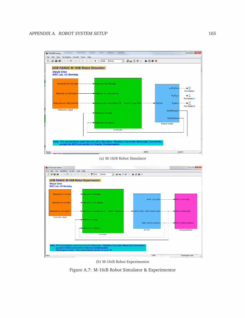
APPENDIX A. ROBOT SYSTEM SETUP 165
(a) M-16iB Robot Simulator
(b) M-16iB Robot Experimentor
Figure A.7: M-16iB Robot Simulator & Experimentor
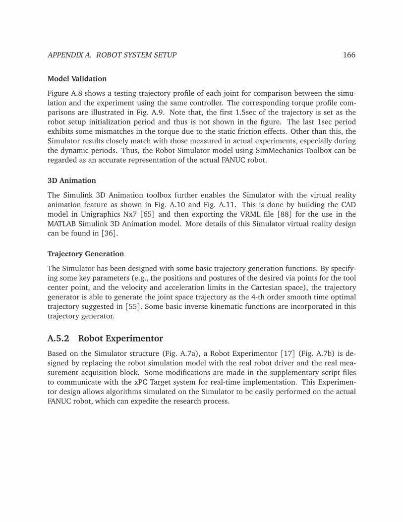
APPENDIX A. ROBOT SYSTEM SETUP 166
Model Validation
Figure A.8 shows a testing trajectory profile of each joint for comparison between the simu-
lation and the experiment using the same controller. The corresponding torque profile com-
parisons are illustrated in Fig. A.9. Note that, the first 1.5sec of the trajectory is set as the
robot setup initialization period and thus is not shown in the figure. The last 1sec period
exhibits some mismatches in the torque due to the static friction effects. Other than this, the
Simulator results closely match with those measured in actual experiments, especially during
the dynamic periods. Thus, the Robot Simulator model using SimMechanics Toolbox can be
regarded as an accurate representation of the actual FANUC robot.
3D Animation
The Simulink 3D Animation toolbox further enables the Simulator with the virtual reality
animation feature as shown in Fig. A.10 and Fig. A.11. This is done by building the CAD
model in Unigraphics Nx7 [65] and then exporting the VRML file [88] for the use in the
MATLAB Simulink 3D Animation model. More details of this Simulator virtual reality design
can be found in [36].
Trajectory Generation
The Simulator has been designed with some basic trajectory generation functions. By specify-
ing some key parameters (e.g., the positions and postures of the desired via points for the tool
center point, and the velocity and acceleration limits in the Cartesian space), the trajectory
generator is able to generate the joint space trajectory as the 4-th order smooth time optimal
trajectory suggested in [55]. Some basic inverse kinematic functions are incorporated in this
trajectory generator.
A.5.2 Robot Experimentor
Based on the Simulator structure (Fig. A.7a), a Robot Experimentor [17] (Fig. A.7b) is de-
signed by replacing the robot simulation model with the real robot driver and the real mea-
surement acquisition block. Some modifications are made in the supplementary script files
to communicate with the xPC Target system for real-time implementation. This Experimen-
tor design allows algorithms simulated on the Simulator to be easily performed on the actual
FANUC robot, which can expedite the research process.

APPENDIX A. ROBOT SYSTEM SETUP 167
2 3 4 5 6−0.3
−0.2
−0.1
0
0.1
Time (sec)
Po
sitio
n (
rad
)
Joint 1 Position
2 3 4 5 61.55
1.6
1.65
1.7
1.75
Time (sec)P
ositio
n (
rad
)
Joint 2 Position
2 3 4 5 6−1
−0.5
0
0.5
Time (sec)
Po
sitio
n (
rad
)
Joint 3 Position
2 3 4 5 6−1
−0.5
0
0.5
Time (sec)
Po
sitio
n (
rad
)Joint 4 Position
2 3 4 5 6−2
−1.5
−1
−0.5
0
Time (sec)
Po
sitio
n (
rad
)
Joint 5 Position
2 3 4 5 63
3.5
4
4.5
Time (sec)
Po
sitio
n (
rad
)
Joint 6 Position
Reference
Experiment
Simulation
Figure A.8: Testing Position Trajectory Comparison between Simulation and Experiment (Load
Side Scale)
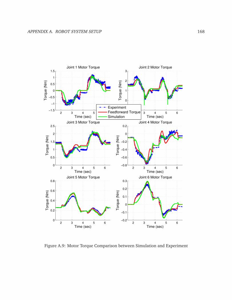
APPENDIX A. ROBOT SYSTEM SETUP 168
2 3 4 5 6−1.5
−1
−0.5
0
0.5
1
1.5
Time (sec)
Torq
ue (
Nm
)
Joint 1 Motor Torque
2 3 4 5 6−1
0
1
2
3
Time (sec)T
orq
ue (
Nm
)
Joint 2 Motor Torque
2 3 4 5 60
0.5
1
1.5
2
2.5
Time (sec)
Torq
ue (
Nm
)
Joint 3 Motor Torque
2 3 4 5 6−0.8
−0.6
−0.4
−0.2
0
0.2
Time (sec)
Torq
ue (
Nm
)
Joint 4 Motor Torque
2 3 4 5 60
0.2
0.4
0.6
0.8
Time (sec)
Torq
ue (
Nm
)
Joint 5 Motor Torque
2 3 4 5 6−0.2
−0.1
0
0.1
0.2
0.3
Time (sec)
Torq
ue (
Nm
)
Joint 6 Motor Torque
Experiment
Feedforward Torque
Simulation
Figure A.9: Motor Torque Comparison between Simulation and Experiment
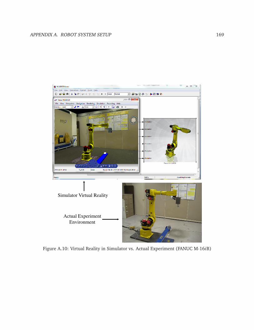
APPENDIX A. ROBOT SYSTEM SETUP 169
Simulator Virtual Reality
Actual Experiment
Environment
Figure A.10: Virtual Reality in Simulator vs. Actual Experiment (FANUC M-16iB)
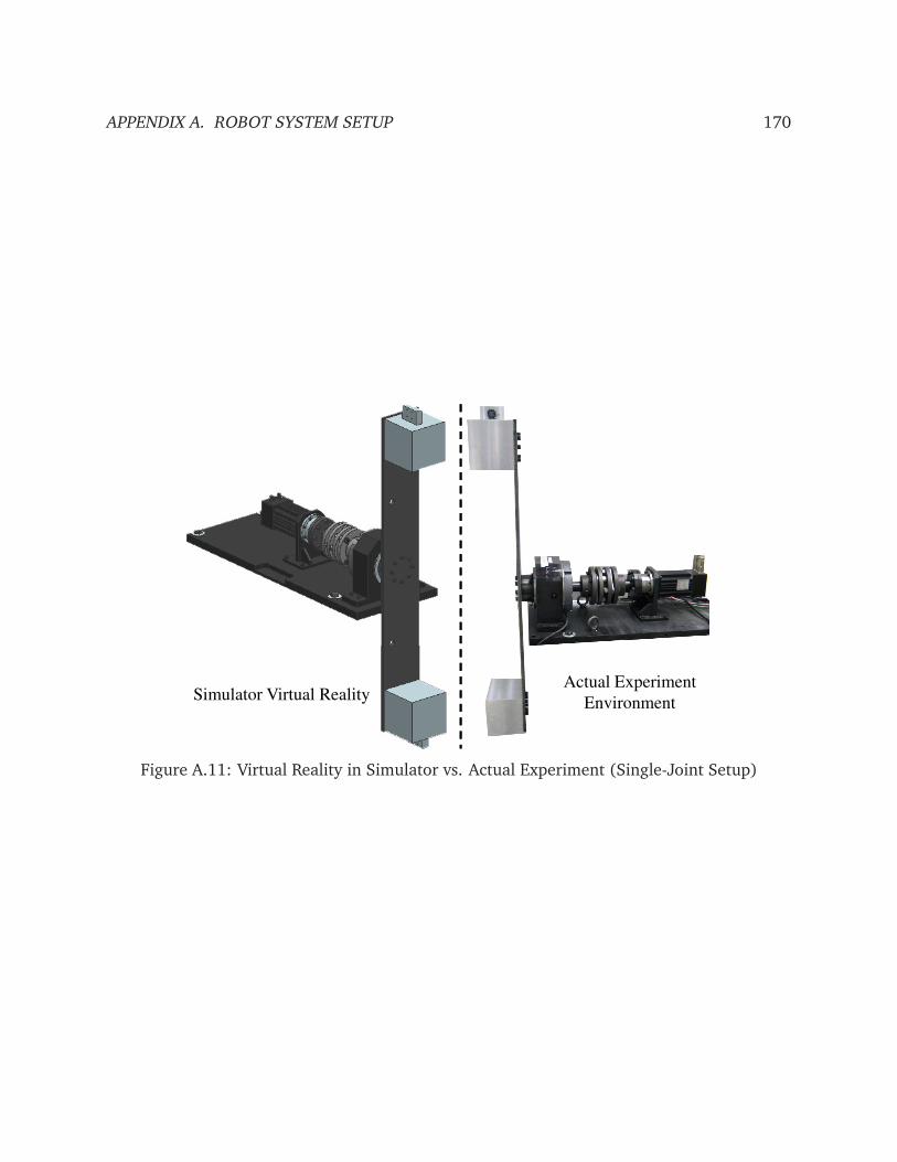
APPENDIX A. ROBOT SYSTEM SETUP 170
Simulator Virtual RealityActual Experiment
Environment
Figure A.11: Virtual Reality in Simulator vs. Actual Experiment (Single-Joint Setup)
171
Appendix B
System Identification 1
B.1 Linear Dynamics Identification of Multi-Joint Robot
Extensive system identification has been conducted for the single-joint indirect drive robot
(Fig. 2.3) as well as the multi-joint indirect drive robot (i.e., FANUC M-16iB robot shown in
Fig. 2.5). The linear two-mass model (2.13) was utilized to identify each joint’s linear dy-
namics. Key parameters (e.g., motor/load side inertia, joint stiffness, joint damping) in this
linear model were identified for each joint at their corresponding maximum-inertia posture.
The identification process was done through sine sweep and sine-by-sine excitation experi-
ments. The optimization based transfer function fitting was performed to identify the system
model. Furthermore, the multi-input-multi-output (MIMO) system identification considering
the system coupling dynamics was also investigated.
The identification approaches, experimental setup, data processing procedures, and results
of this linear dynamics identification are extensively documented in [43, 44, 42] and will not
be detailed here. However, as a glance of the identification procedure, some of the key points
in the linear system identification for the multi-joint robot are briefly summarized as follows.
B.1.1 Posture Selection
To ensure that the two-inertia model (2.13) is valid, the robot joint motions must be decoupled
from each other during the system identification process. As a result, the robot postures for
the system identification process are selected to produce the largest inertia with respect to the
moving joint while trying to reduce coupling motions among the joints. The robot postures for
the identification experiment of each joint are visually shown in Fig. B.1.
1The extensive experiments for the linear dynamics identification study (Section B.1) were performed as the
work by a group, which includes the author, Ms. Cheng-Huei Han, Mr. Michael Chan, and Mr. Pedro Reynoso
Mora, while the friction identification study in Section B.2 was conducted mainly by the author.

APPENDIX B. SYSTEM IDENTIFICATION 172
J1
J2
J4
J5
J3 J6
Figure B.1: FANUC M-16iB Robot Postures for System Identification
APPENDIX B. SYSTEM IDENTIFICATION 173
B.1.2 Identification Procedure
Figure B.2 shows the system identification procedure. Since the system is represented using
a linear time-invariant (LTI) model (2.13), LTI techniques and assumptions can be used to
perform system identification. The system’s response to a certain frequency can be obtained
by harmonically driving the system at that specific frequency (Fig. B.2(a)). The excitation
frequency can be varied such that the system dynamics are captured over a broad frequency
range.
Once the system output measurements are recorded, the frequency response is then calcu-
lated by finding the magnitude and the phase at each particular frequency (Fig. B.2(b)). After
a plot of the frequency response is obtained, a least-squares fit is used to empirically obtain the
system parameters. In the system identification process, the unknown parameters are: Jm, Jℓ,
dm, dℓ, d j, and k j. Note that the load side inertia, Jℓ, is the total inertia of the links connected
by the subsequent joints. The corresponding inertia/mass for each joint can also be roughly
calculated using the robot CAD model. On the other hand, Jm, dm, dℓ, d j, and k j obtained from
the identification experiments will be used directly as the joint parameters.
For identifying these parameters, a good initial estimate for each parameter is important.
The gear ratio N is exactly known from the gear catalogue. Based on available technical
documentation, a good estimate can also be established for Jm. By treating Jm and N as
knowns and neglecting damping, initial estimates are obtained for Jℓ and k j by using (2.11)
as
Jℓ =JmN 2(ω2
r−ω2
ar)
ω2ar
, k j = JmN 2(ω2r−ω2
ar) (B.1)
where ωar and ωr are read from the calculated frequency response plot (Fig. B.2(c)) as the
anti-resonance frequency and resonance frequency, respectively. The initial estimates for the
damping parameters dm, d j, and dℓ are obtained through a friction identification process in a
later section and also by some simplification assumptions (Fig. B.2(d)). With all these initial
estimates, the following constrained non-linear optimization is formulated to obtain more
accurate system parameter estimates (Fig. B.2(e))
minx
∑
ω ∈ Ω
G( x ,ω)− Gm(ω)
2
(B.2)
s.t. Ax ≤ b
where:
x =
Jm Jℓ dm dℓ d j k j
T
A∈Rn×6, b ∈ Rn×1
G( x ,ω) is the magnitude of the transfer function evaluated with the estimated parameter
vector, x , at frequency ω. Gm(ω) is the magnitude of the measured frequency response at
frequency ω. Ω is the set of frequencies at which measurements are taken. Matrix A and
vector b are selected to enforce n bounding constraints on the adjustable parameters.

APPENDIX B. SYSTEM IDENTIFICATION 174
1 0- 1
1 00
1 01
1 02
-8 0
-6 0
-4 0
-2 0
0
1 0- 1
1 00
1 01
1 02
-3 0 0
-2 0 0
-1 0 0
0
1 0 0
1 0- 1
1 00
1 01
1 02
-8 0
-6 0
-4 0
-2 0
0
1 0- 1
1 00
1 01
1 02
-3 0 0
-2 0 0
-1 0 0
0
1 0 0
Harmonically excite robot
Acquire data and calculate
frequency response
Locate the anti-resonant (ω)and resonant (ω) frequencies
Obtain initial estimates for J and k
J =JN(ω
− ω)
ω
k = JN(ω
− ω)
(a) (b)
Obtain initial estimatesfor d, d , and d
(discussed in a later section)
Velocity-Friction Map
-0.5 -0.4 -0.3 -0.2 -0.1 0 0.1 0.2 0.3 0.4 0.5-1.5
-1
-0.5
0
0.5
1
1.5
Motor Side Velocity Refer to the Load Side (rad/sec)
Fricti
on F
orc
e R
efe
r to
th
e M
oto
r S
ide (
Nm
)
Experimental Data
Fitted Curve
Obtain parameters with
nonlinear optimization
10-1
100
101
102
-20
0
20
40
Frequency(Hz)
Ma
gn
itud
e (
dB
)
From experiment
Curve fitting result
Transfer function w/ par. from FANUC
Disturbance Torque to Motor Side Velocity
10-1
100
101
102
-200
-100
0
100
Phas
e (
deg
)
(c)
(d) (e)
Figure B.2: System Identification Flow Chart for FANUC M-16iB Robot

APPENDIX B. SYSTEM IDENTIFICATION 175
B.1.3 Closed Loop Identification
Ideally, open loop system identification will produce the most accurate results. But due to
system instability from gravity effects, open loop identification is not possible for J2 and J3,
and closed loop identification is performed instead. Both open and closed loop identification
experiments, however, are initially performed for the remaining four joints to verify the fidelity
of the closed loop results. It is worth mentioning that for both open loop and closed loop
experiments, the joints not being actuated are held rigid by mechanical brakes.
Remark B.1. More details and results of this linear dynamics identification can be found in [43,
44, 42]. This linear dynamics identification provides an intuitive check of the parameters for a
more complex nonlinear model. The friction effect, which is one of the most important nonlinear
dynamics in the robot system, were also identified. The following section presents the systematic
procedure for friction identification in the single-joint system as well as the multi-joint robot
system.
B.2 Friction Identification
B.2.1 Friction Identification for Multi-Joint Robot
The friction model to describe the friction effects in the indirect drive mechanism is presented
in Section 2.2.2. Due to the lack of load side joint measurements, the friction identification
can only be conducted on the motor side (i.e., only the combined entire friction F = fm+ fh+fℓ
Nin (2.16b) can be identified). The LuGre model for this friction effect is restated here as
z = v −σ0|v|
g(v)z (B.3a)
g(v) = Fc +
Fs − Fc
e(−v2/v2
s ) (B.3b)
F = σ0z+σ1z +σ2v (B.3c)
where all the variables are as defined in Section 2.2.2. Thus, the purpose of friction identifi-
cation is to identify the six parameters in the LuGre model, i.e., FC , FS, vs, σ0, σ1, and σ2 for
each joint.
Static Friction Identification
For the motor side identification, consider the dynamic model for the robot with n rigid joints
(2.25). The friction identification experiment is conducted for each individual joint moving at
its chosen posture shown in Fig. B.1, while all the other joints are kept static by mechanical
brakes. For the particular joint to be identified (e.g., the i-th joint), rewrite (2.25) as
[M(q)q]i + [C(q, q)q]i + [G(q)]i + [N F(q)]i = [Nτm]i (B.4)
APPENDIX B. SYSTEM IDENTIFICATION 176
where [•]i denotes the i-th entry of the vector •. Note that, the case without contact force (i.e.,
fex t = 0) is considered here. The entire friction force reflecting on the motor side is denoted
as F(q). In this joint, the friction regime of gross motion between surfaces is characterized by
z = 0 and q = 0 [5]. Thus, M(q)q = 0, and the LuGre model (B.3) for the friction at the i-th
joint reduces to the static relation
Fi
qmi
=h
Fc +
Fs − Fc
e(−q2
mi/v2s )i
sgnqmi
+σ2qmi (B.5)
Furthermore, [C(q, q)q]i = 0 since only one joint is moving and the centrifugal/coriolis effects
induced by this moving joint to itself is 0. Then the robot model (B.4) reduces to
Fi(t) +Gi(t)
Ni
= τmi(t) (B.6)
For the joints J1, J4, J5, and J6 at their identification postures as in Fig. B.1, the gravity
force is not effective in the moving direction, i.e.
Gi(t) =0 (B.7a)
⇒ Fi(t) =τmi(t) (B.7b)
which means that the friction force Fi(t) can be directly identified by the measurement of
τmi(t).
For the joints J2 and J3, however, the gravity force is effective in the moving direction, i.e.,
Gi(t) 6= 0. Hence, the experiment is designed to run the joint moving in the same position
region at constant speeds in two directions. The motion dynamics in two directions can be
written as
Forward Direction: Ff
i (tf ) +
Gf
i (tf )
Ni
= τf
mi(tf ), 0≤ t f ≤ T (B.8a)
Backward Direction: F bi(t b) +
Gf
i (tb)
Ni
= τbmi(t b), 0 ≤ t b ≤ T (B.8b)
where T denotes the time duration for one direction movement.
Assuming that the friction characteristic is skew-symmetric for both directions, for t f+t b =
T , the following relationships can be obtained
Ff
i (tf ) = −F b
i(t b) (B.9a)
Gf
i (tf ) = G b
i(t b) (B.9b)
It follows that
Ff
i (tf ) =
1
2
τf
mi(tf )−τb
mi(t b)
(B.10a)
F bi(t b) =−
1
2
τf
mi(tf )−τb
mi(t b)
(B.10b)
APPENDIX B. SYSTEM IDENTIFICATION 177
The combination of (B.5) and (B.7b) or (B.5) and (B.10) properly describes the static
velocity-torque (friction force) characteristic, as shown in Fig. B.3 and Fig. B.4.
Each point in Fig. B.3 and Fig. B.4 is obtained by keeping the motor side velocity constant
for the same amount of distance in a closed-loop manner. The average value of the steady state
torque (friction force Fi
qmi
) at the corresponding velocity is recorded based on (B.7b) or
(B.10). The experiment is repeated at various velocities for the same path to obtain the whole
static velocity-torque map. The nonlinear least-squares method in the MATLAB Optimization
Toolbox is applied to obtain the static friction parameters, FC , FS, vs, and σ2, for the i-th joint.
The nonlinear programming problem is formulated as
minFc ,Fs ,vs,σ2
∑
qmi∈Ωmi
Fi
qmi
− Fi
qmi
2(B.11a)
s.t. Fi
qmi
=h
Fc +
Fs − Fc
e(−q2
mi/v2s )i
sgnqmi
+ σ2qmi (B.11b)
Fc ≥ 0, Fs ≥ Fc, vs ≥ 0, σ2 ≥ 0
where Ωmi is the set of all the testing motor side velocities for the i-th joint.
The identified parameters for each joint are listed in Table B.1. The friction identification
experiments are performed for two cases: with payload and without payload. The identifi-
cation results in Table B.1 show that the static friction parameters for both cases are almost
at the same level, which indicates that the payload of a 18.37kg weight does not have much
effect on friction at the identification postures. It concludes that the gear meshing friction
might be dominant in these joint mechanisms as stated in [76] and Section 2.2.2. Besides,
another possibility is that the load side inertia induced from the robot itself is more significant
than the payload, which is true especially for J1, J2, and J3.
Dynamic Friction Identification
As far as the author knows, no closed loop identification methods for the dynamic parameters,
σ0 and σ1 in the LuGre model (B.3), have been reported so far. Thus, the dynamic friction
identification can only be conducted for joints J1, J4, J5, and J6 in the open loop manner at
their identification postures.
It is shown in [5] that the dynamic parameters, σ0 and σ1, can be identified using an
ARX (Auto-Regressive with eXogenous input signal) or a BJ (Box Jenkins) model structure
with pre-sliding open loop motion data. The resolution of motor position data for the FANUC
M-16iB robot, however, limits the implementation of this method. It can be found in [37]
that the motor encoder used for each joint has the resolution of 1, 000, 000 counts/revolution.
Nevertheless, by the data processing in the DSA (Digital Servo Adapter), the output motor
position data has the resolution of only up to 10, 000 counts/revolution (i.e., 6.2832× 10⁻⁴
rad/count on the motor side). This resolution is not high enough to capture the dynamic
motion in the pre-sliding regime.
Thus, the method in [13] is employed here to obtain the rough estimate of σ0, using ramp
input response and step input response experimental data.

APPENDIX B. SYSTEM IDENTIFICATION 178
−0.5 −0.3 −0.1 0.1 0.3 0.5−1.5
−1
−0.5
0
0.5
1
1.5
Motor Side Velocity / Ratio (rad/sec)
Friction F
orc
e (
Nm
)
J1 Velocity−Friction Map
−0.5 −0.3 −0.1 0.1 0.3 0.5−1
−0.5
0
0.5
1
Motor Side Velocity / Ratio (rad/sec)
Friction F
orc
e (
Nm
)
J2 Velocity−Friction Map
−0.5 −0.3 −0.1 0.1 0.3 0.5−0.4
−0.2
0
0.2
0.4
Motor Side Velocity / Ratio (rad/sec)
Friction F
orc
e (
Nm
)
J3 Velocity−Friction Map
−0.5 −0.3 −0.1 0.1 0.3 0.5
−0.2
−0.1
0
0.1
0.2
0.3
Motor Side Velocity / Ratio (rad/sec)
Friction F
orc
e (
Nm
)
J4 Velocity−Friction Map
−0.5 −0.3 −0.1 0.1 0.3 0.5−0.1
−0.05
0
0.05
0.1
Motor Side Velocity / Ratio (rad/sec)
Friction F
orc
e (
Nm
)
J5 Velocity−Friction Map
−0.5 −0.3 −0.1 0.1 0.3 0.5
−0.1
−0.05
0
0.05
0.1
0.15
Motor Side Velocity / Ratio (rad/sec)
Friction F
orc
e (
Nm
)
J6 Velocity−Friction Map
Experimental Data
Fitted Curve
Figure B.3: Static Friction Identification Result for FANUC M-16iB Robot with Payload
During the stiction state of open loop motions with slowly varying input torque (smaller
than the breakaway torque), the velocity v and the dynamics of the internal state z might be
negligible. Thus, g(v) ≈ Fs and τmi ≈ Fi ≈ σ0z. Assuming that the experiment is performed

APPENDIX B. SYSTEM IDENTIFICATION 179
−0.5 −0.3 −0.1 0.1 0.3 0.5−1.5
−1
−0.5
0
0.5
1
1.5
Motor Side Velocity / Ratio (rad/sec)
Friction F
orc
e (
Nm
)
J1 Velocity−Friction Map
−0.5 −0.3 −0.1 0.1 0.3 0.5−1
−0.5
0
0.5
1
Motor Side Velocity / Ratio (rad/sec)
Friction F
orc
e (
Nm
)
J2 Velocity−Friction Map
−0.5 −0.3 −0.1 0.1 0.3 0.5−0.4
−0.2
0
0.2
0.4
Motor Side Velocity / Ratio (rad/sec)
Friction F
orc
e (
Nm
)
J3 Velocity−Friction Map
−0.5 −0.3 −0.1 0.1 0.3 0.5
−0.2
−0.1
0
0.1
0.2
0.3
Motor Side Velocity / Ratio (rad/sec)
Friction F
orc
e (
Nm
)
J4 Velocity−Friction Map
−0.5 −0.3 −0.1 0.1 0.3 0.5−0.1
−0.05
0
0.05
0.1
Motor Side Velocity / Ratio (rad/sec)
Friction F
orc
e (
Nm
)
J5 Velocity−Friction Map
−0.5 −0.3 −0.1 0.1 0.3 0.5
−0.1
−0.05
0
0.05
0.1
0.15
Motor Side Velocity / Ratio (rad/sec)
Friction F
orc
e (
Nm
)
J6 Velocity−Friction Map
Experimental Data
Fitted Curve
Figure B.4: Static Friction Identification Result for FANUC M-16iB Robot without Payload
from rest (i.e., z(0) = 0), then (B.3a) can be approximated as
z ≈ v −τmi|v|
Fs
, v = qmi (B.12)
If applying a ramp input torque τmi(t) = c t with small c > 0, z(t) can be explicitly obtained
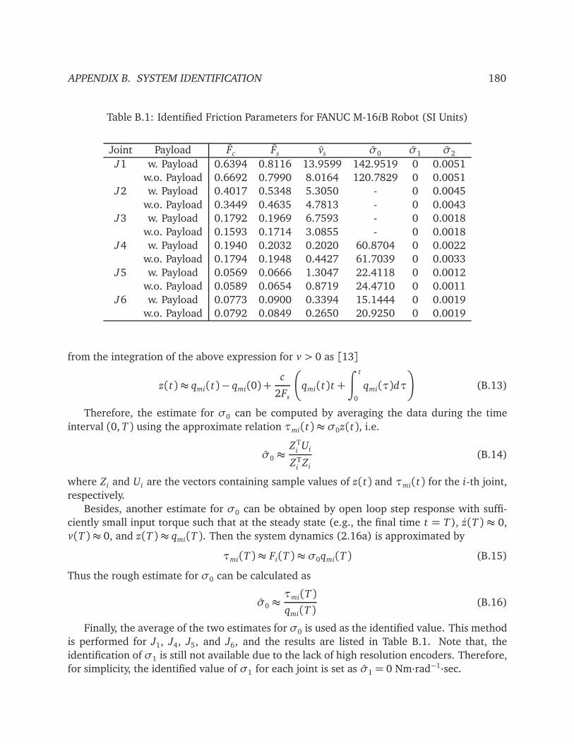
APPENDIX B. SYSTEM IDENTIFICATION 180
Table B.1: Identified Friction Parameters for FANUC M-16iB Robot (SI Units)
Joint Payload Fc Fs vs σ0 σ1 σ2
J1 w. Payload 0.6394 0.8116 13.9599 142.9519 0 0.0051
w.o. Payload 0.6692 0.7990 8.0164 120.7829 0 0.0051
J2 w. Payload 0.4017 0.5348 5.3050 - 0 0.0045
w.o. Payload 0.3449 0.4635 4.7813 - 0 0.0043
J3 w. Payload 0.1792 0.1969 6.7593 - 0 0.0018
w.o. Payload 0.1593 0.1714 3.0855 - 0 0.0018
J4 w. Payload 0.1940 0.2032 0.2020 60.8704 0 0.0022
w.o. Payload 0.1794 0.1948 0.4427 61.7039 0 0.0033
J5 w. Payload 0.0569 0.0666 1.3047 22.4118 0 0.0012
w.o. Payload 0.0589 0.0654 0.8719 24.4710 0 0.0011
J6 w. Payload 0.0773 0.0900 0.3394 15.1444 0 0.0019
w.o. Payload 0.0792 0.0849 0.2650 20.9250 0 0.0019
from the integration of the above expression for v > 0 as [13]
z(t)≈ qmi(t)− qmi(0) +c
2Fs
qmi(t)t +
∫ t
0
qmi(τ)dτ
(B.13)
Therefore, the estimate for σ0 can be computed by averaging the data during the time
interval (0, T ) using the approximate relation τmi(t)≈ σ0z(t), i.e.
σ0 ≈ZT
iUi
ZTi Zi
(B.14)
where Zi and Ui are the vectors containing sample values of z(t) and τmi(t) for the i-th joint,
respectively.
Besides, another estimate for σ0 can be obtained by open loop step response with suffi-
ciently small input torque such that at the steady state (e.g., the final time t = T), z(T ) ≈ 0,
v(T )≈ 0, and z(T )≈ qmi(T ). Then the system dynamics (2.16a) is approximated by
τmi(T )≈ Fi(T )≈ σ0qmi(T ) (B.15)
Thus the rough estimate for σ0 can be calculated as
σ0 ≈τmi(T )
qmi(T )(B.16)
Finally, the average of the two estimates for σ0 is used as the identified value. This method
is performed for J1, J4, J5, and J6, and the results are listed in Table B.1. Note that, the
identification of σ1 is still not available due to the lack of high resolution encoders. Therefore,
for simplicity, the identified value of σ1 for each joint is set as σ1 = 0 Nm·rad−1·sec.

APPENDIX B. SYSTEM IDENTIFICATION 181
−30 −20 −10 0 10 20 30
−0.1
−0.05
0
0.05
0.1
Motor Side Velocity (rad/sec)
Mo
tor
To
rqu
e C
om
ma
nd
(N
m)
Experiment
Curve Fit
Figure B.5: Static Friction Identification Result for Single-Joint Testbed
Table B.2: Identified Friction Parameters for Single-Joint Testbed (SI Units)
Fc Fs vs σ0 σ1 σ2
(Nm) (Nm) (rad/sec) (Nm·rad−1) (Nm·sec·rad−1) (Nm·sec·rad−1)
0.1004 0.1075 3.951 40 0 0.001114
B.2.2 Friction Identification for Single-Joint Setup
The same method is applied to the single-joint setup (Fig. 2.3) to identify the friction parame-
ters. The identified static velocity-torque (friction force) characteristic is illustrated in Fig. B.5,
while the identified static and dynamic parameter values are listed in Table B.2.
Note that the resolution of the motor encoder in this setup also limits the identification of
dynamic parameters. Thus, the method in [13] is employed here again to obtain the rough
estimate of σ0, using ramp and step input response data, which gives σ0 = 33.34(ramp) and
57.03(step) Nm·rad−1, respectively. The identification of σ1 is still not available due to the
lack of a high resolution encoder. For simplicity, the final estimates are set as σ0 = 40Nm·rad−1
and σ1 = 0Nm·rad−1·sec.
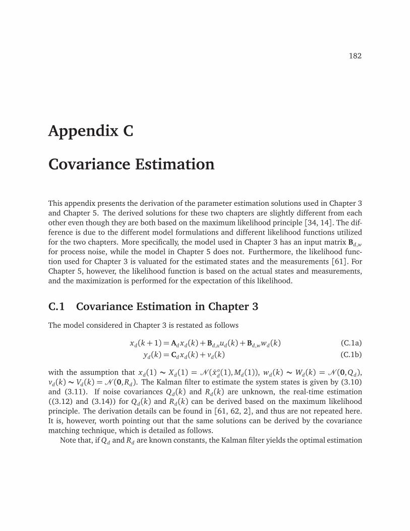
182
Appendix C
Covariance Estimation
This appendix presents the derivation of the parameter estimation solutions used in Chapter 3
and Chapter 5. The derived solutions for these two chapters are slightly different from each
other even though they are both based on the maximum likelihood principle [34, 14]. The dif-
ference is due to the different model formulations and different likelihood functions utilized
for the two chapters. More specifically, the model used in Chapter 3 has an input matrix Bd,w
for process noise, while the model in Chapter 5 does not. Furthermore, the likelihood func-
tion used for Chapter 3 is valuated for the estimated states and the measurements [61]. For
Chapter 5, however, the likelihood function is based on the actual states and measurements,
and the maximization is performed for the expectation of this likelihood.
C.1 Covariance Estimation in Chapter 3
The model considered in Chapter 3 is restated as follows
xd(k+ 1) = Ad xd(k) +Bd,uud(k) +Bd,wwd(k) (C.1a)
yd(k) = Cd xd(k) + vd(k) (C.1b)
with the assumption that xd(1) s Xd(1) = N ( xod(1), Md(1)), wd(k) s Wd(k) = N (0,Qd),
vd(k) s Vd(k) = N (0, Rd). The Kalman filter to estimate the system states is given by (3.10)
and (3.11). If noise covariances Qd(k) and Rd(k) are unknown, the real-time estimation
((3.12) and (3.14)) for Qd(k) and Rd(k) can be derived based on the maximum likelihood
principle. The derivation details can be found in [61, 62, 2], and thus are not repeated here.
It is, however, worth pointing out that the same solutions can be derived by the covariance
matching technique, which is detailed as follows.
Note that, if Qd and Rd are known constants, the Kalman filter yields the optimal estimation
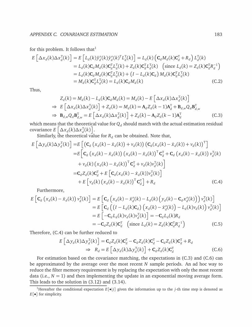
APPENDIX C. COVARIANCE ESTIMATION 183
for this problem. It follows that1
E
∆xd(k)∆xTd(k)
= E
Ld(k) yod(k) yo
d(k)T LT
d(k)
= Ld(k)
Cd Md(k)CTd+ Rd
LTd(k)
= Ld(k)Cd Md(k)CTdLT
d(k) + Zd(k)C
TdLT
d(k)
since Ld(k) = Zd(k)CTdR−1
d
= Ld(k)Cd Md(k)CTdLT
d(k) +
I − Ld(k)Cd
Md(k)C
TdLT
d(k)
= Md(k)CTdLT
d(k) = Ld(k)Cd Md(k) (C.2)
Thus,
Zd(k) = Md(k)− Ld(k)Cd Md(k) = Md(k)− E
∆xd(k)∆xTd(k)
⇒ E
∆xd(k)∆xTd(k)
+ Zd(k) = Md(k) = Ad Zd(k− 1)ATd+Bd,wQdBT
d,w
⇒ Bd,wQdBTd,w= E
∆xd(k)∆xTd(k)
+ Zd(k)−Ad Zd(k− 1)ATd
(C.3)
which means that the theoretical value for Qd should match with the actual estimation residual
covariance E
∆xd(k)∆xTd(k)
.
Similarly, the theoretical value for Rd can be obtained. Note that,
E
∆yd(k)∆yTd(k)
=E
Cd
xd(k)− xd(k)
+ vd(k)
Cd(xd(k)− xd(k)) + vd(k)
T
=Eh
Cd
xd(k)− xd(k)
xd(k)− xd(k)
TCT
d+Cd
xd(k)− xd(k)
vT
d(k)
+ vd(k)
xd(k)− xd(k)T
CTd+ vd(k)v
Td(k)i
=Cd Zd(k)CTd+ E
Cd(xd(k)− xd(k))vTd(k)
+ E
vd(k)
xd(k)− xd(k)T
CTd
+ Rd (C.4)
Furthermore,
E
Cd
xd(k)− xd(k)
vT
d(k)
= E
Cd
xd(k)− x od(k)− Ld(k)
yd(k)−Cd x od(k)
vTd(k)
= E
Cd
I − Ld(k)Cd
xd(k)− x od(k)
− Ld(k)vd(k)
vTd(k)
= E
−Cd Ld(k)vd(k)vTd(k)
=−Cd Ld(k)Rd
=−Cd Zd(k)CTd
since Ld(k) = Zd(k)CTdR−1
d
(C.5)
Therefore, (C.4) can be further reduced to
E
∆yd(k)∆yTd(k)
= Cd Zd(k)CTd−Cd Zd(k)C
Td−Cd Zd(k)C
Td+ Rd
⇒ Rd = E
∆yd(k)∆yTd(k)
+Cd Zd(k)CTd
(C.6)
For estimation based on the covariance matching, the expectations in (C.3) and (C.6) can
be approximated by the average over the most recent N sample periods. An ad hoc way to
reduce the filter memory requirement is by replacing the expectation with only the most recent
data (i.e., N = 1) and then implementing the update in an exponential moving average form.
This leads to the solution in (3.12) and (3.14).1Hereafter the conditional expectation E[•| j] given the information up to the j-th time step is denoted as
E[•] for simplicity.
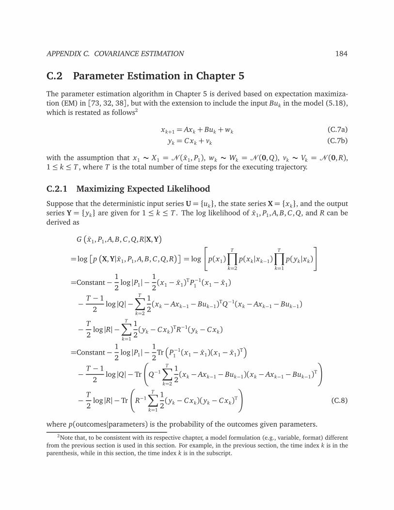
APPENDIX C. COVARIANCE ESTIMATION 184
C.2 Parameter Estimation in Chapter 5
The parameter estimation algorithm in Chapter 5 is derived based on expectation maximiza-
tion (EM) in [73, 32, 38], but with the extension to include the input Buk in the model (5.18),
which is restated as follows2
xk+1 = Axk + Buk +wk (C.7a)
yk = C xk + vk (C.7b)
with the assumption that x1 s X1 = N ( x1, P1), wk s Wk = N (0,Q), vk s Vk = N (0, R),
1≤ k ≤ T , where T is the total number of time steps for the executing trajectory.
C.2.1 Maximizing Expected Likelihood
Suppose that the deterministic input series U = uk, the state series X= xk, and the output
series Y = yk are given for 1 ≤ k ≤ T . The log likelihood of x1, P1, A, B, C ,Q, and R can be
derived as
G
x1, P1, A, B, C ,Q, R|X,Y
= log
pX,Y| x1, P1, A, B, C ,Q, R
= log
p(x1)
T∏
k=2
p(xk|xk−1)
T∏
k=1
p(yk|xk)
=Constant−1
2log |P1| −
1
2(x1− x1)
TP−11(x1− x1)
−T − 1
2log |Q| −
T∑
k=2
1
2(xk − Axk−1− Buk−1)
TQ−1(xk − Axk−1− Buk−1)
−T
2log |R| −
T∑
k=1
1
2(yk − C xk)
TR−1(yk − C xk)
=Constant−1
2log |P1| −
1
2Tr
P−11(x1− x1)(x1− x1)
T
−T − 1
2log |Q| − Tr
Q−1
T∑
k=2
1
2(xk − Axk−1− Buk−1)(xk − Axk−1− Buk−1)
T
!
−T
2log |R| − Tr
R−1
T∑
k=1
1
2(yk − C xk)(yk − C xk)
T
!
(C.8)
where p(outcomes|parameters) is the probability of the outcomes given parameters.
2Note that, to be consistent with its respective chapter, a model formulation (e.g., variable, format) different
from the previous section is used in this section. For example, in the previous section, the time index k is in the
parenthesis, while in this section, the time index k is in the subscript.

APPENDIX C. COVARIANCE ESTIMATION 185
Now the objective is to maximize this log likelihood, G
x1, P1, A, B, C ,Q, R|X,Y. Since the
actual states are normally unknown, the expected likelihood E[G
x1, P1, A, B, C ,Q, R|X,Y] is
used instead to perform maximization. With the first order condition∂ E[G(•)]
∂ (•)= 0, the resulting
estimates can be derived as
x1 = E[x1] P1 = E
(x1− x o1)(x1− x o
1)T
(C.9a)
A=
T∑
k=2
E
xk xTk−1− Bouk−1xT
k−1
! T∑
k=2
E
xk−1xTk−1
!−1
(C.9b)
B =
T∑
k=2
E
xkuTk−1− Ao xk−1uT
k−1
! T∑
k=2
E
uk−1uTk−1
!−1
(C.9c)
C =
T∑
k=1
E
yk xTk
! T∑
k=1
E
xk xTk
!−1
(C.9d)
Q =1
T − 1
T∑
k=2
E
(xk− Ao xk−1− Bouk−1)(xk − Ao xk−1− Bouk−1)T
!
(C.9e)
R=1
T
T∑
k=1
E
(yk − C o xk)(yk − C o xk)T
!
(C.9f)
where Ao, Bo, C o, and x o1
are the a-priori or initial estimates of A, B, C , and x1.

APPENDIX C. COVARIANCE ESTIMATION 186
C.2.2 Off-line Solution: EM Algorithm
The expected values used in (C.9) can be calculated by applying Kalman smoother (5.19)-
(5.20) for off-line processing. The resulting estimation solutions are derived as
x1 = x1|T P1 = P1|T (C.10a)
A=
T∑
k=2
xk|T xTk−1|T
+ P(k,k−1)|T − Bouk−1 xTk−1|T
!
T∑
k=2
xk−1|T xTk−1|T
+ Pk−1|T
!−1
(C.10b)
B =
T∑
k=2
xk|TuTk−1− Ao xk−1|TuT
k−1
! T∑
k=2
uk−1uTk−1
!−1
(C.10c)
C =
T∑
k=1
yk xTk|T
!
T∑
k=1
xk|T xTk|T+ Pk|T
!−1
(C.10d)
Q =1
T − 1
T∑
k=2
h
xk|T − Axk−1|T − Buk−1
xk|T − Axk−1|T − Buk−1
T
+ Pk|T − APT(k,k−1)|T
− P(k,k−1)|TAT+ APk−1|T ATi
(C.10e)
R=1
T
T∑
k=1
h
yk − C xk|T
yk − C xk|T
T+ C Pk|T CT
i
(C.10f)
The whole expectation maximization (EM) procedure ([73, 32, 38]) can be applied as
follows
• E-step: run Kalman smoother (5.19)-(5.20) with current best estimates of x1, P1, A, B, C ,Q,
and R.
• M-step: update x1, P1, A, B, C ,Q, and R as in (C.10) using the acausal estimates from
Kalman smoother (5.19)-(5.20).
• Return to E-step until the increment of the expected likelihood is within chosen thresh-
old.
C.2.3 Online Solution
If real-time computing is desired, only causal estimates from Kalman filter (5.19) can be used.
Thus, instead of estimating using the whole time series as in the off-line case, A, B, C ,Q, and R
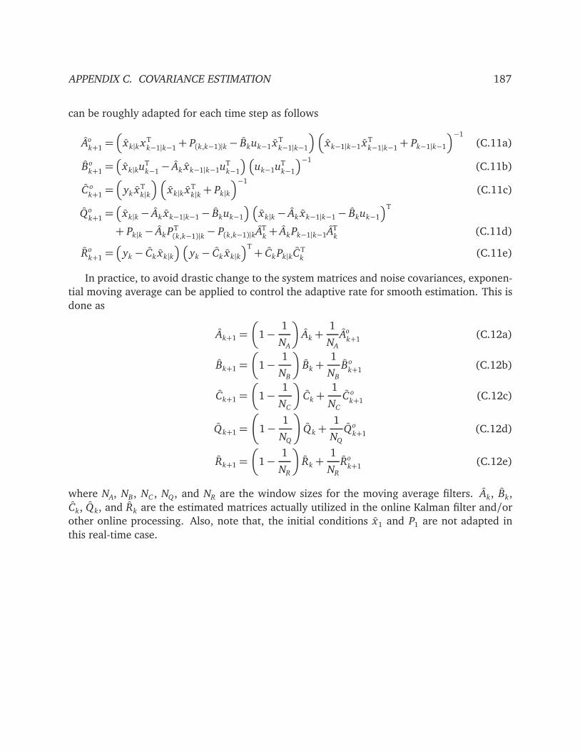
APPENDIX C. COVARIANCE ESTIMATION 187
can be roughly adapted for each time step as follows
Aok+1=
xk|k xTk−1|k−1
+ P(k,k−1)|k− Bkuk−1 xTk−1|k−1
xk−1|k−1 xTk−1|k−1
+ Pk−1|k−1
−1
(C.11a)
Bok+1=
xk|kuTk−1− Ak xk−1|k−1uT
k−1
uk−1uTk−1
−1(C.11b)
C ok+1=
yk xTk|k
xk|k xTk|k+ Pk|k
−1
(C.11c)
Qok+1=
xk|k− Ak xk−1|k−1− Bkuk−1
xk|k− Ak xk−1|k−1− Bkuk−1
T
+ Pk|k− AkPT(k,k−1)|k
− P(k,k−1)|kATk+ AkPk−1|k−1AT
k(C.11d)
Rok+1=
yk − Ck xk|k
yk − Ck xk|k
T+ Ck Pk|kCT
k(C.11e)
In practice, to avoid drastic change to the system matrices and noise covariances, exponen-
tial moving average can be applied to control the adaptive rate for smooth estimation. This is
done as
Ak+1 =
1−1
NA
Ak +1
NA
Aok+1
(C.12a)
Bk+1 =
1−1
NB
Bk +1
NB
Bok+1
(C.12b)
Ck+1 =
1−1
NC
Ck +1
NC
C ok+1
(C.12c)
Qk+1 =
1−1
NQ
Qk+1
NQ
Qok+1
(C.12d)
Rk+1 =
1−1
NR
Rk +1
NR
Rok+1
(C.12e)
where NA, NB, NC , NQ, and NR are the window sizes for the moving average filters. Ak, Bk,
Ck, Qk, and Rk are the estimated matrices actually utilized in the online Kalman filter and/or
other online processing. Also, note that, the initial conditions x1 and P1 are not adapted in
this real-time case.